

Compact Muon Solenoid
LHC, CERN
| CMS-EGM-20-001 ; CERN-EP-2022-028 | ||
| Reconstruction of decays to merged photons using end-to-end deep learning with domain continuation in the CMS detector | ||
| CMS Collaboration | ||
| 26 April 2022 | ||
| Phys. Rev. D 108 (2023) 052002 | ||
| Abstract: A novel technique based on machine learning is introduced to reconstruct the decays of highly Lorentz-boosted particles. Using an \textitend-to-end deep learning strategy, the technique bypasses existing rule-based particle reconstruction methods typically used in high energy physics analyses. It uses minimally processed detector data as input and directly outputs particle properties of interest. The new technique is demonstrated for the reconstruction of the invariant mass of particles decaying in the CMS detector. The decay of a hypothetical scalar particle $ \mathcal{A} $ into two photons, $ \mathcal{A}\to\gamma\gamma $, is chosen as a benchmark decay. Lorentz boosts $ \gamma_{\mathrm{L}} = $ 60--600 are considered, ranging from regimes where both photons are resolved to those where the photons are closely merged as one object. A training method using domain continuation is introduced, enabling the invariant mass reconstruction of unresolved photon pairs in a novel way. The new technique is validated using $ \pi^{0}\to\gamma\gamma $ decays in LHC collision data. | ||
| Links: e-print arXiv:2204.12313 [hep-ex] (PDF) ; CDS record ; inSPIRE record ; CADI line (restricted) ; | ||
| Figures | |
png pdf |
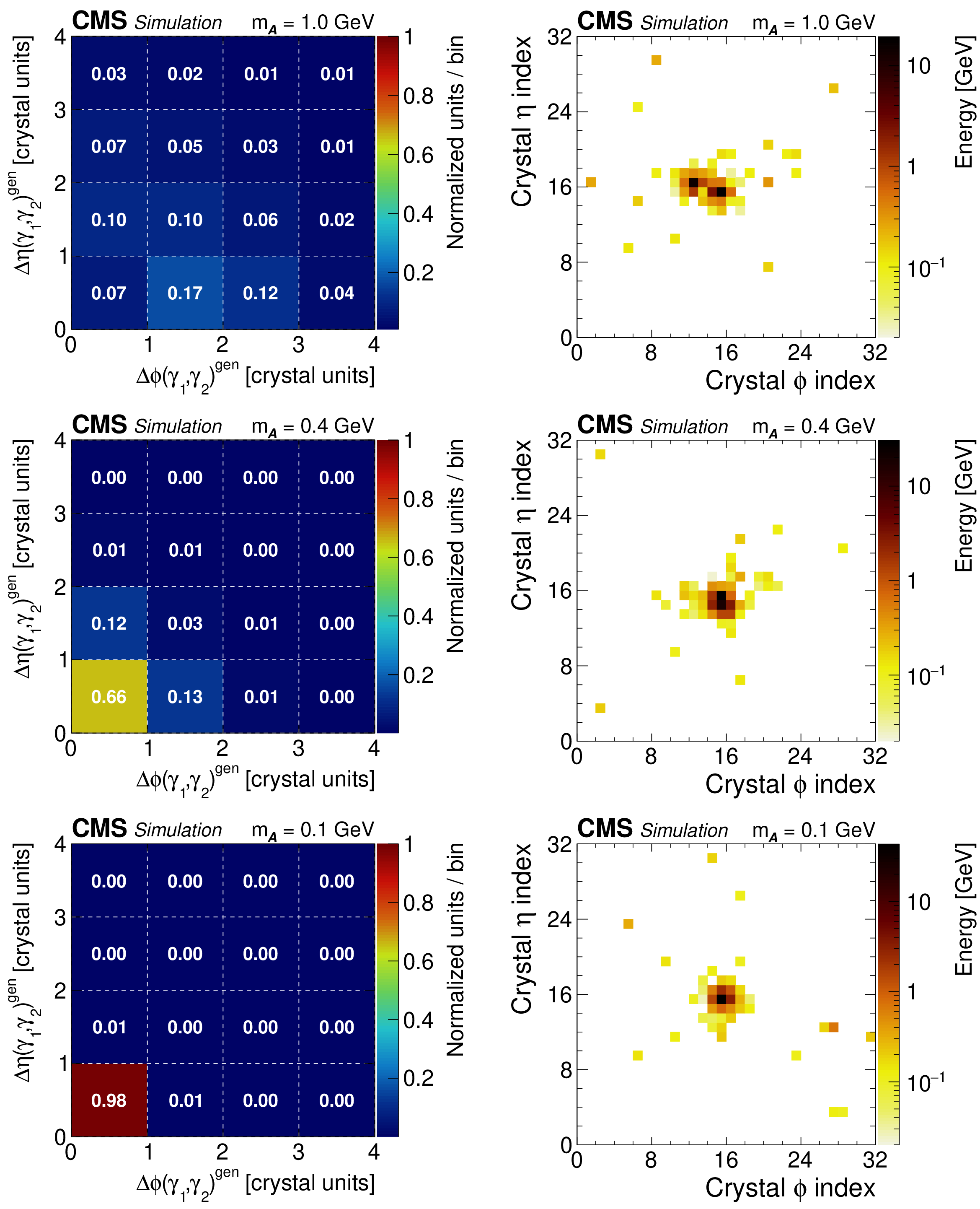
Figure 1:
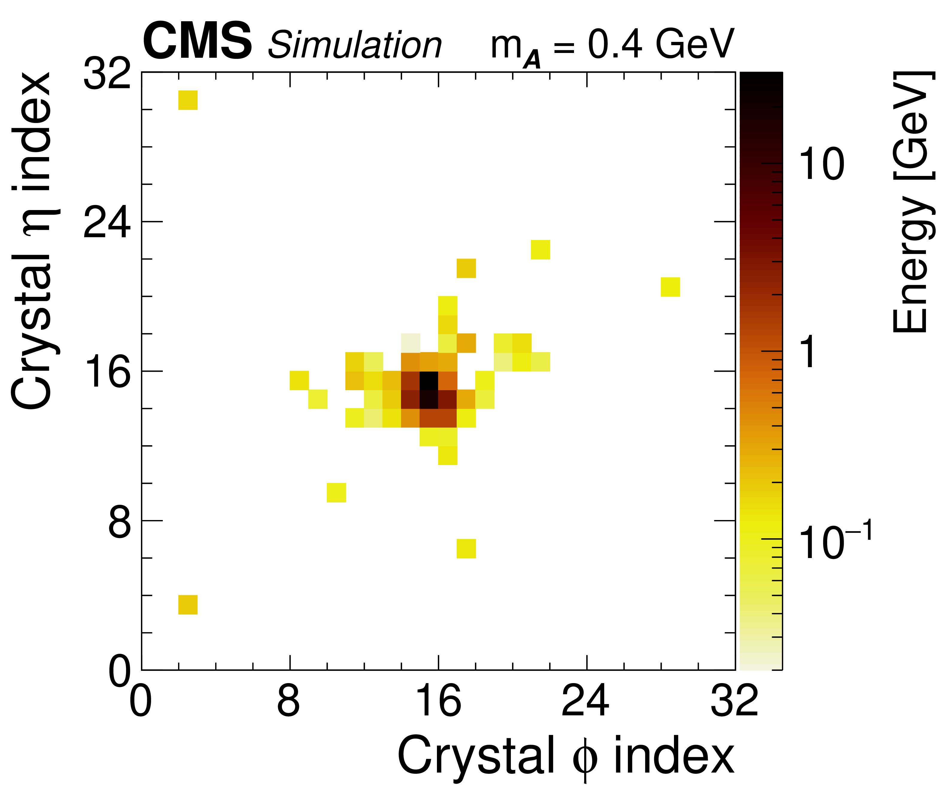
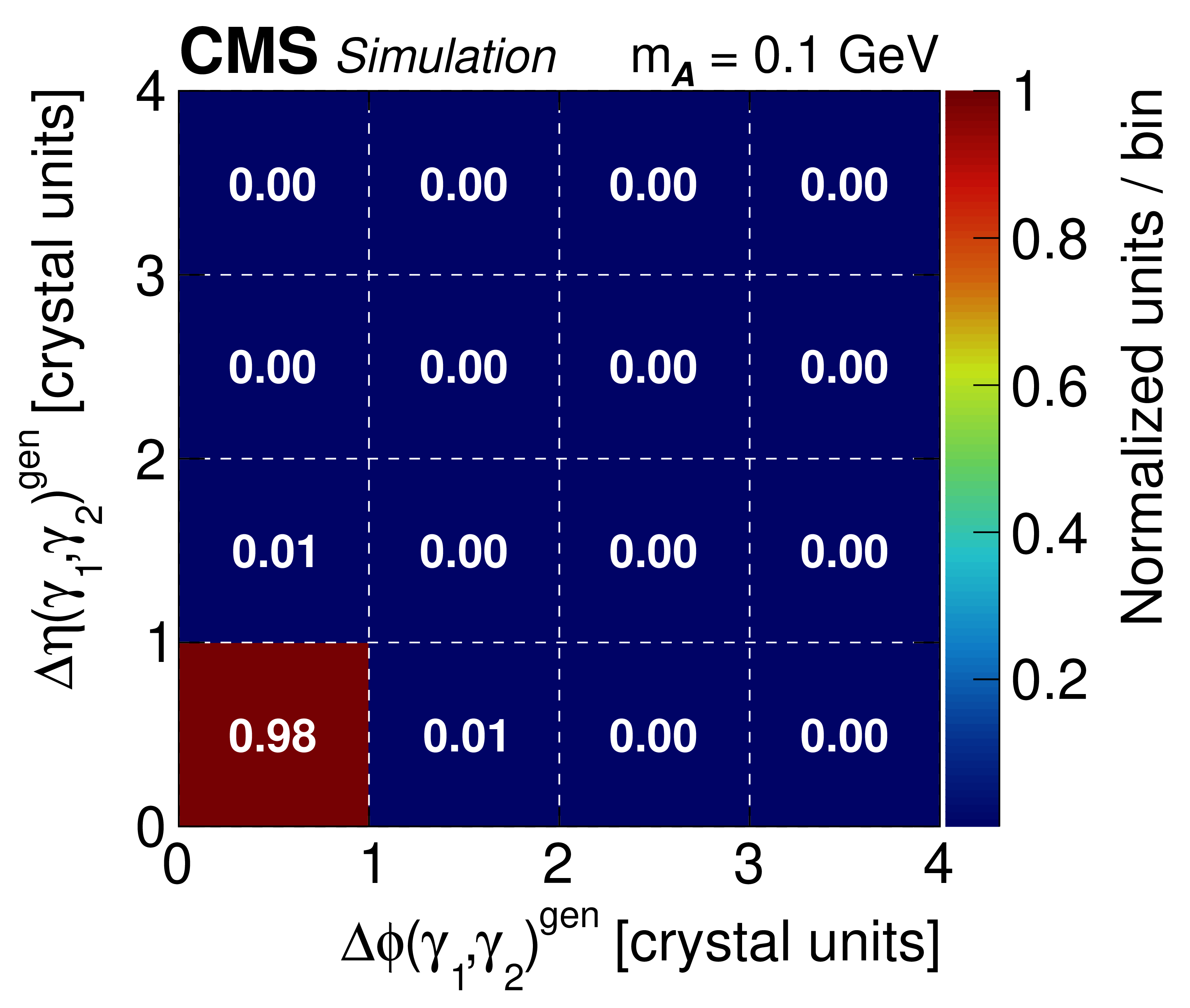
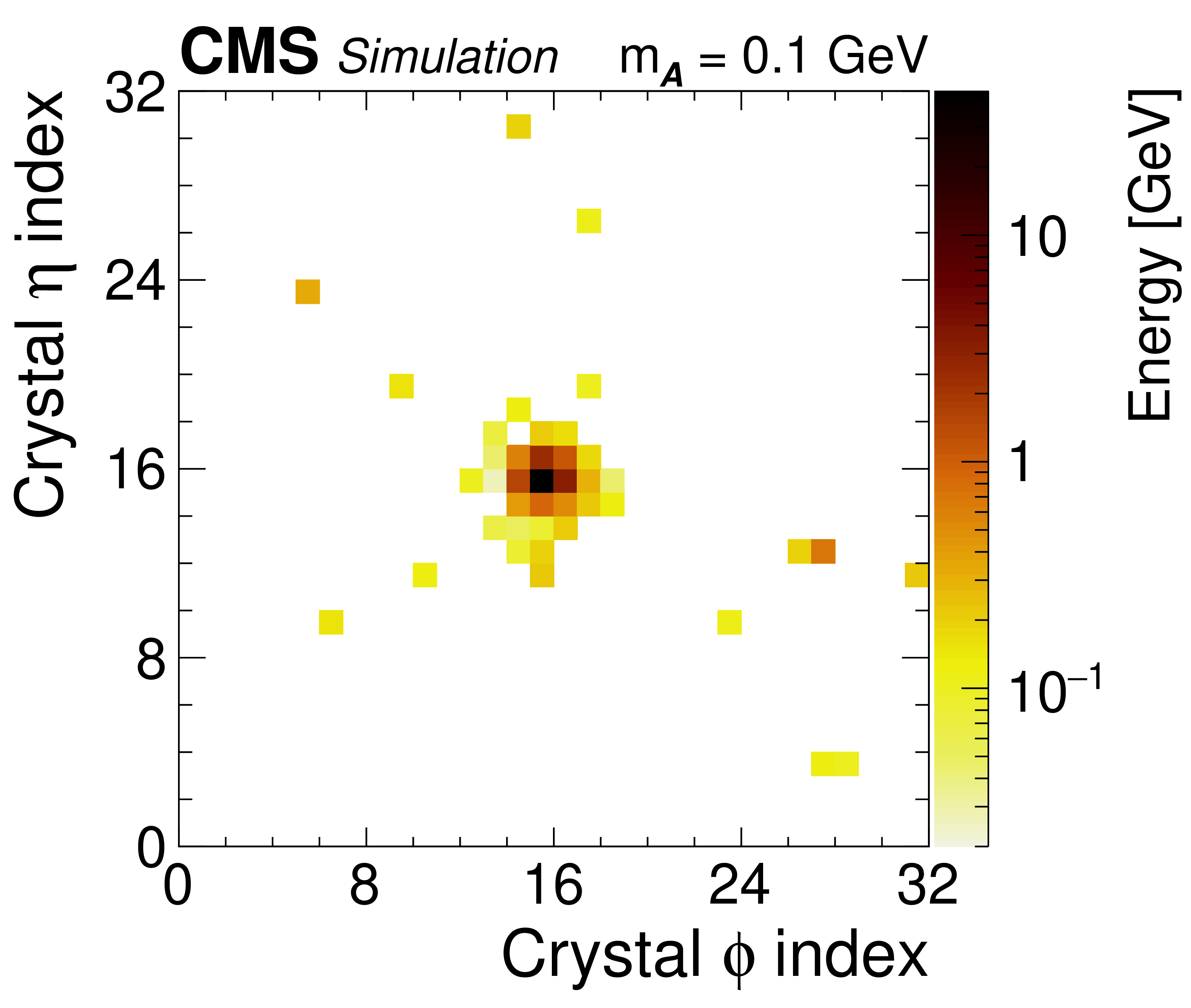
Simulation results for the decay chain $\mathrm{H} \to {\mathcal{A}} {\mathcal{A}} $, $ {\mathcal{A}} \to \gamma \gamma $ at various boosts: (upper plots) barely resolved, $m_{\mathcal{A}} = $ 1.0 GeV, $\gamma _{\mathrm {L}}= $ 50; (middle plots) shower merged, $m_{\mathcal{A}} = $ 0.4 GeV, $\gamma _{\mathrm {L}}= $ 150; and (lower plots) instrumentally merged, $m_{\mathcal{A}} = $ 0.1 GeV, $\gamma _{\mathrm {L}}= $ 625. The left column shows the normalized distribution of opening angles between the leading ($\gamma _1$) and subleading ($\gamma _2$) photons from the particle $ {\mathcal{A}} $ decay, expressed by the number of crystals in the $\eta $ direction, $\Delta \eta (\gamma _1, \gamma _2)^{\mathrm {gen}}$, versus the $\phi $ direction, $\Delta \phi (\gamma _1, \gamma _2)^{\mathrm {gen}}$. Note that the distributions include contributions outside of the plotted ranges and thus may not sum to unity within the displayed ranges. The right column displays the ECAL energy shower pattern for a single $ {\mathcal{A}} \to \gamma \gamma $ decay, plotted in relative ECAL crystal index coordinates and color-coded by energy. In all cases, only decays reconstructed as a single PF photon candidate passing selection criteria are used. |
png pdf |
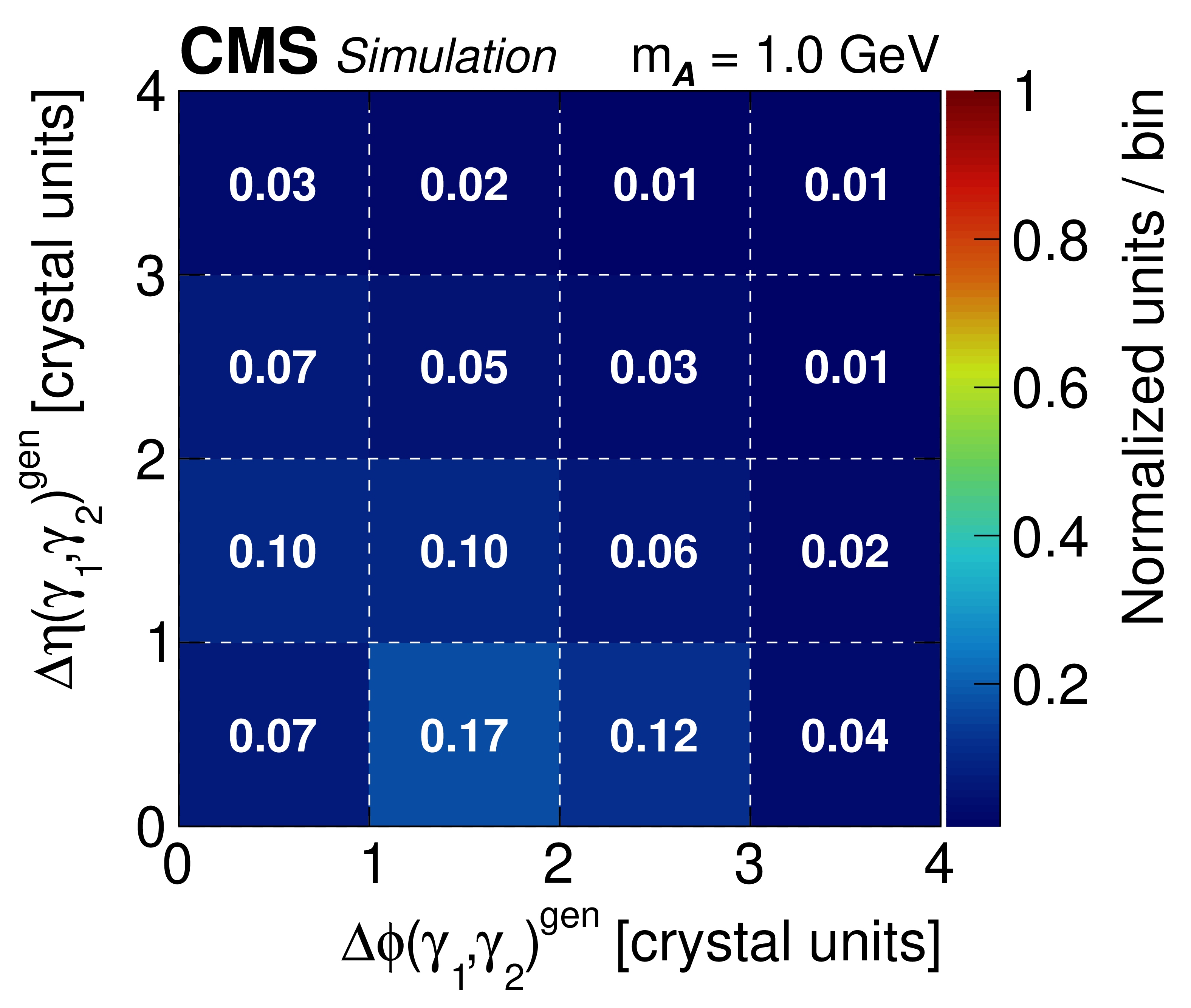
Figure 1-a:
Simulation results for the decay chain $\mathrm{H} \to {\mathcal{A}} {\mathcal{A}} $, $ {\mathcal{A}} \to \gamma \gamma $ at boost: barely resolved, $m_{\mathcal{A}} = $ 1.0 GeV, $\gamma _{\mathrm {L}}= $ 50. The plot shows the normalized distribution of opening angles between the leading ($\gamma _1$) and subleading ($\gamma _2$) photons from the particle $ {\mathcal{A}} $ decay, expressed by the number of crystals in the $\eta $ direction, $\Delta \eta (\gamma _1, \gamma _2)^{\mathrm {gen}}$, versus the $\phi $ direction, $\Delta \phi (\gamma _1, \gamma _2)^{\mathrm {gen}}$. Note that the distributions include contributions outside of the plotted ranges and thus may not sum to unity within the displayed ranges. Only decays reconstructed as a single PF photon candidate passing selection criteria are used. |
png pdf |
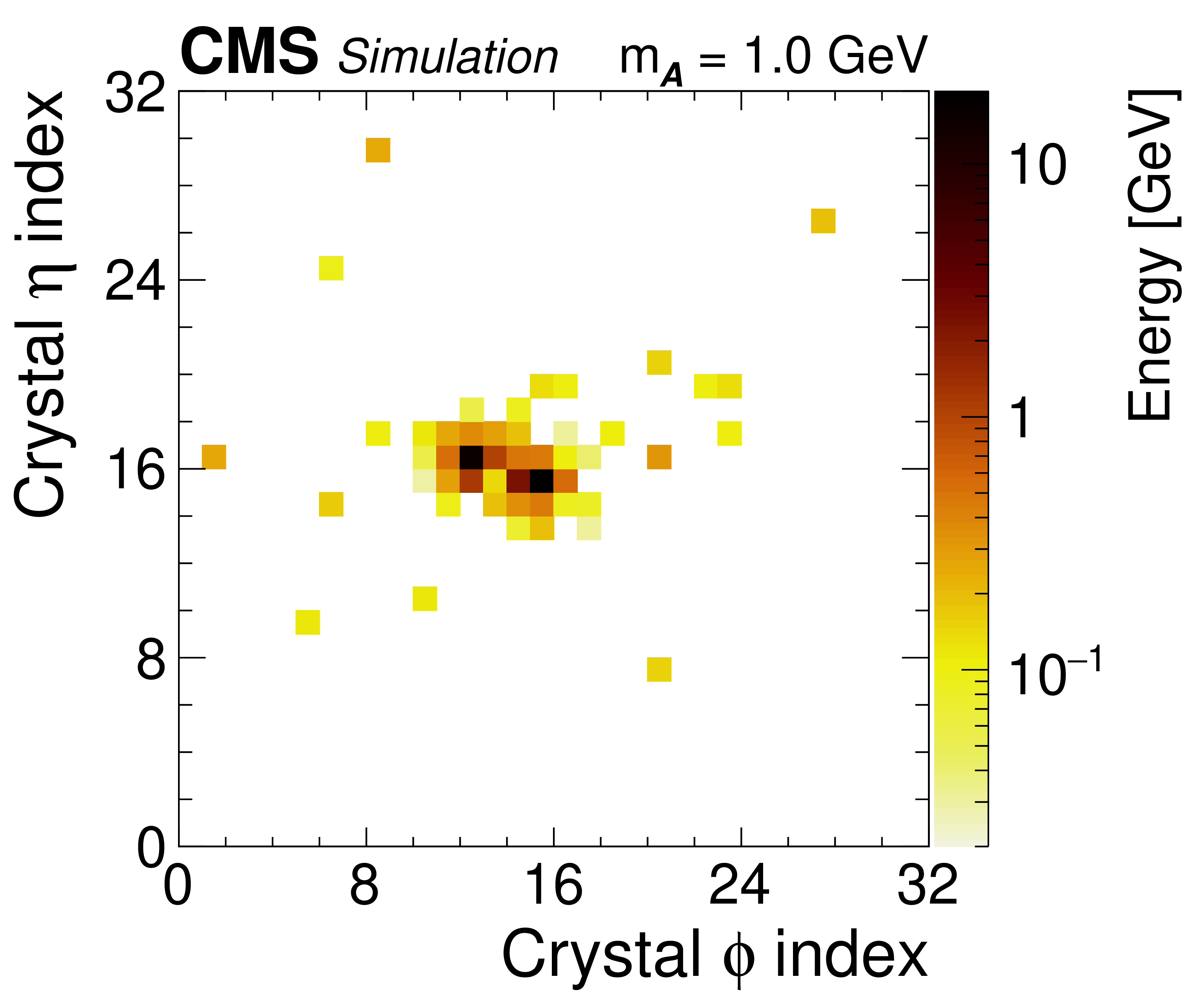
Figure 1-b:
Simulation results for the decay chain $\mathrm{H} \to {\mathcal{A}} {\mathcal{A}} $, $ {\mathcal{A}} \to \gamma \gamma $ for boost: barely resolved, $m_{\mathcal{A}} = $ 1.0 GeV, $\gamma _{\mathrm {L}}= $ 50. The plot displays the ECAL energy shower pattern for a single $ {\mathcal{A}} \to \gamma \gamma $ decay, plotted in relative ECAL crystal index coordinates and color-coded by energy. Only decays reconstructed as a single PF photon candidate passing selection criteria are used. |
png pdf |
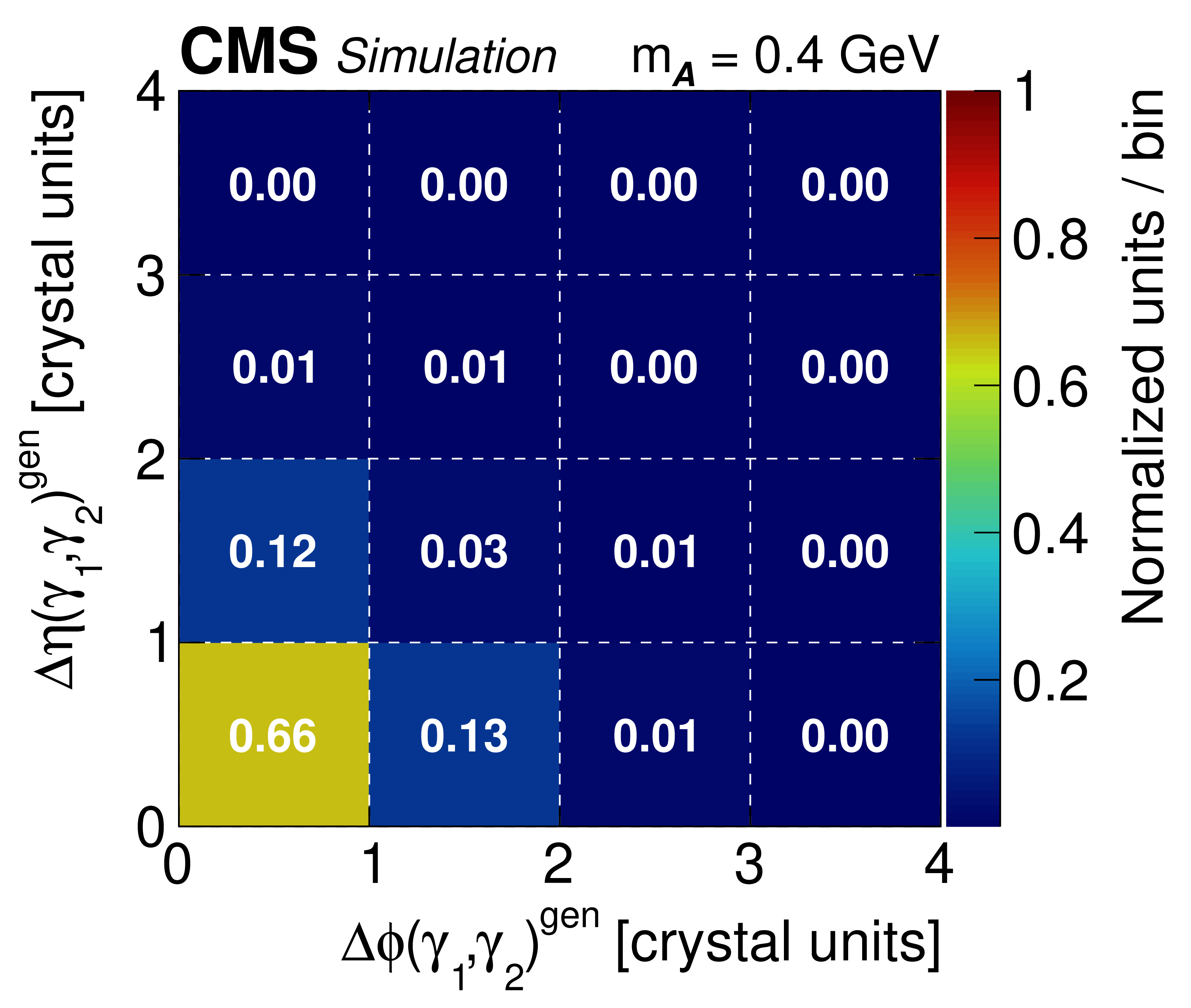
Figure 1-c:
Simulation results for the decay chain $\mathrm{H} \to {\mathcal{A}} {\mathcal{A}} $, $ {\mathcal{A}} \to \gamma \gamma $ for boost: shower merged, $m_{\mathcal{A}} = $ 0.4 GeV, $\gamma _{\mathrm {L}}= $ 150. The plot shows the normalized distribution of opening angles between the leading ($\gamma _1$) and subleading ($\gamma _2$) photons from the particle $ {\mathcal{A}} $ decay, expressed by the number of crystals in the $\eta $ direction, $\Delta \eta (\gamma _1, \gamma _2)^{\mathrm {gen}}$, versus the $\phi $ direction, $\Delta \phi (\gamma _1, \gamma _2)^{\mathrm {gen}}$. Note that the distributions include contributions outside of the plotted ranges and thus may not sum to unity within the displayed ranges. Only decays reconstructed as a single PF photon candidate passing selection criteria are used. |
png pdf |
Figure 1-d:
Simulation results for the decay chain $\mathrm{H} \to {\mathcal{A}} {\mathcal{A}} $, $ {\mathcal{A}} \to \gamma \gamma $ for boost: shower merged, $m_{\mathcal{A}} = $ 0.4 GeV, $\gamma _{\mathrm {L}}= $ 150. The plot displays the ECAL energy shower pattern for a single $ {\mathcal{A}} \to \gamma \gamma $ decay, plotted in relative ECAL crystal index coordinates and color-coded by energy. Only decays reconstructed as a single PF photon candidate passing selection criteria are used. |
png pdf |
Figure 1-e:
Simulation results for the decay chain $\mathrm{H} \to {\mathcal{A}} {\mathcal{A}} $, $ {\mathcal{A}} \to \gamma \gamma $ for boost: instrumentally merged, $m_{\mathcal{A}} = $ 0.1 GeV, $\gamma _{\mathrm {L}}= $ 625. The plot shows the normalized distribution of opening angles between the leading ($\gamma _1$) and subleading ($\gamma _2$) photons from the particle $ {\mathcal{A}} $ decay, expressed by the number of crystals in the $\eta $ direction, $\Delta \eta (\gamma _1, \gamma _2)^{\mathrm {gen}}$, versus the $\phi $ direction, $\Delta \phi (\gamma _1, \gamma _2)^{\mathrm {gen}}$. Note that the distributions include contributions outside of the plotted ranges and thus may not sum to unity within the displayed ranges. Only decays reconstructed as a single PF photon candidate passing selection criteria are used. |
png pdf |
Figure 1-f:
Simulation results for the decay chain $\mathrm{H} \to {\mathcal{A}} {\mathcal{A}} $, $ {\mathcal{A}} \to \gamma \gamma $ for boost: instrumentally merged, $m_{\mathcal{A}} = $ 0.1 GeV, $\gamma _{\mathrm {L}}= $ 625. The plot displays the ECAL energy shower pattern for a single $ {\mathcal{A}} \to \gamma \gamma $ decay, plotted in relative ECAL crystal index coordinates and color-coded by energy. Only decays reconstructed as a single PF photon candidate passing selection criteria are used. |
png pdf |
Figure 2:
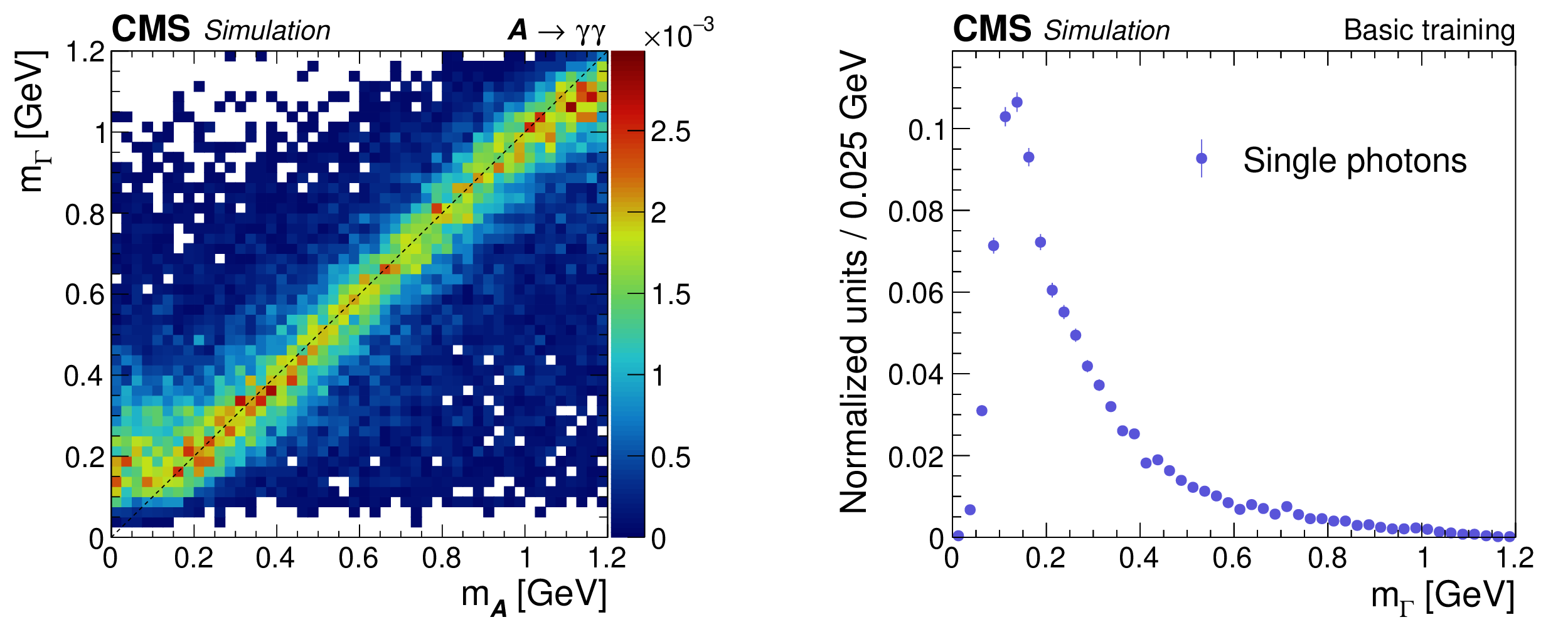
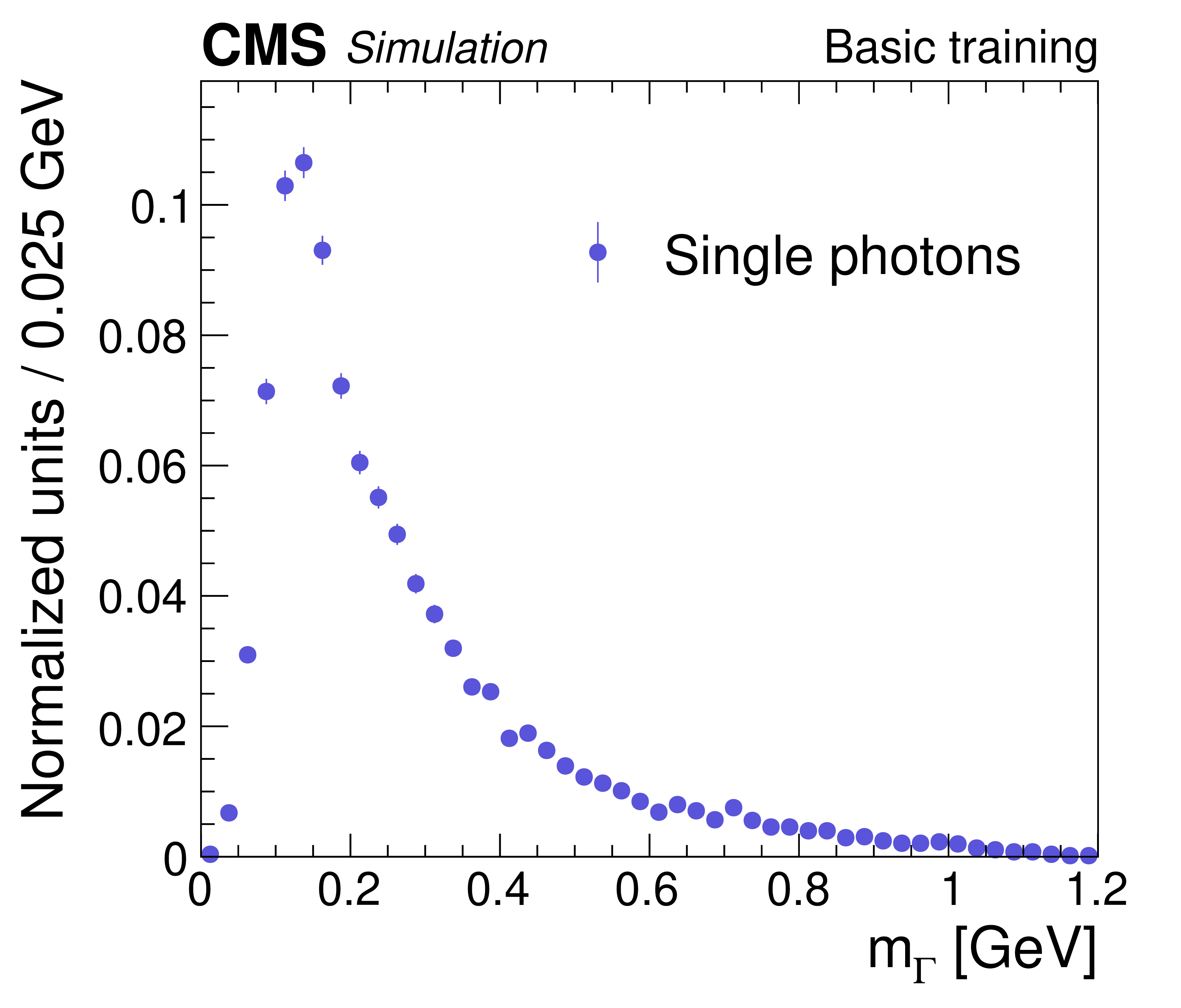
Left: The regressed mass $m_{\Gamma}$ vs. the generated $m_{\mathcal{A}}$ value for simulated $ {\mathcal{A}} \to \gamma \gamma $ decays generated uniformly in $({p_{\mathrm{T}}},\,m_{\mathcal{A}})$ before domain continuation is implemented. The regressed $m_{\Gamma}$ is normalized in 0.025 GeV vertical slices of the generated $m_{\mathcal{A}}$. The color scale to the right of the plot gives the normalized number of events per vertical slice in 0.025 GeV bins of $m_{\Gamma}$. Right: The regressed $m_{\Gamma}$ distribution for simulated single-photon samples only, before domain continuation, resulting in a distinct peak in the low-$m_{\Gamma}$ region. The distribution is normalized to unity with the vertical bars on the points indicating the statistical uncertainty. |

png pdf |
Figure 2-a:
The regressed mass $m_{\Gamma}$ vs. the generated $m_{\mathcal{A}}$ value for simulated $ {\mathcal{A}} \to \gamma \gamma $ decays generated uniformly in $({p_{\mathrm{T}}},\,m_{\mathcal{A}})$ before domain continuation is implemented. The regressed $m_{\Gamma}$ is normalized in 0.025 GeV vertical slices of the generated $m_{\mathcal{A}}$. The color scale to the right of the plot gives the normalized number of events per vertical slice in 0.025 GeV bins of $m_{\Gamma}$. |
png pdf |
Figure 2-b:
The regressed $m_{\Gamma}$ distribution for simulated single-photon samples only, before domain continuation, resulting in a distinct peak in the low-$m_{\Gamma}$ region. The distribution is normalized to unity with the vertical bars on the points indicating the statistical uncertainty. |
png pdf |
Figure 3:
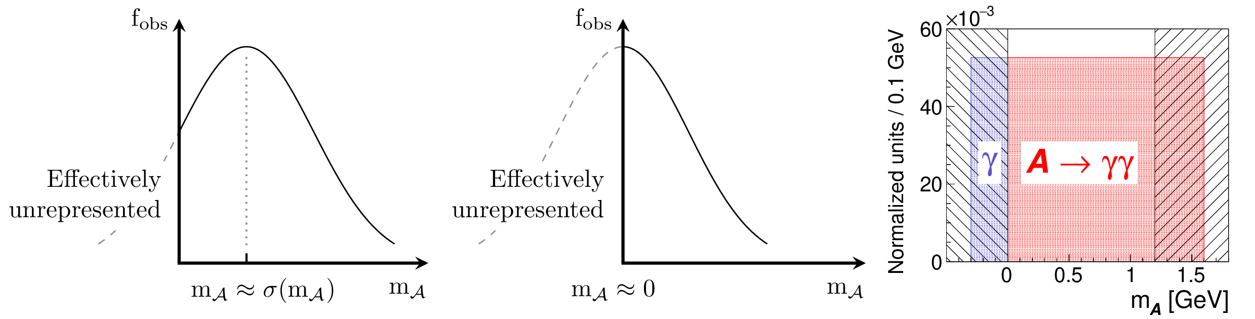
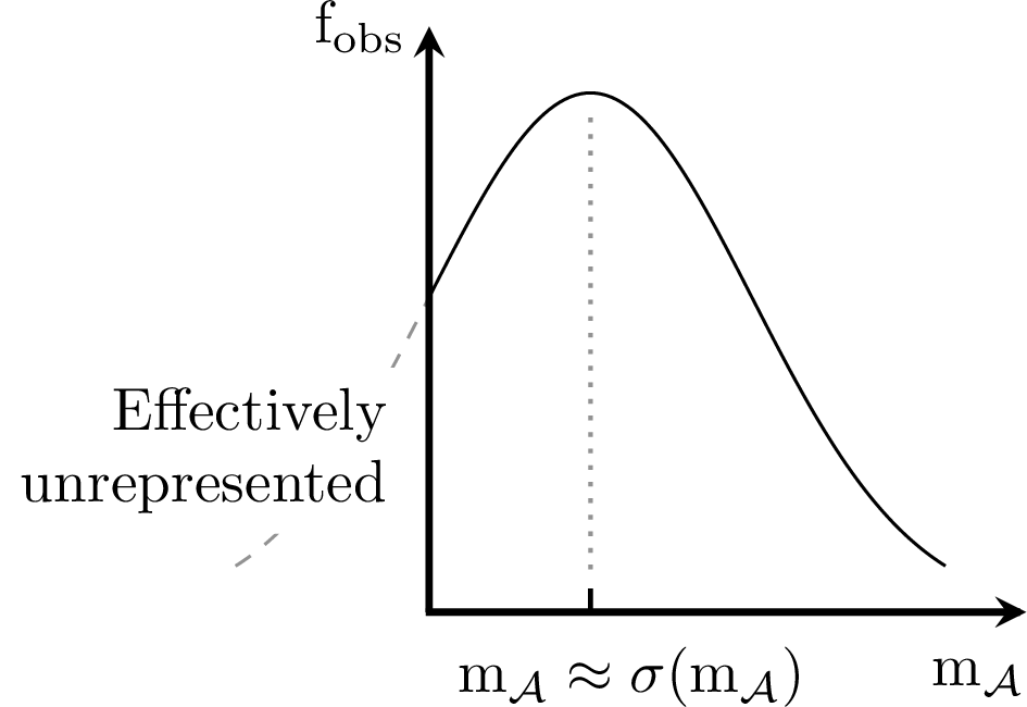
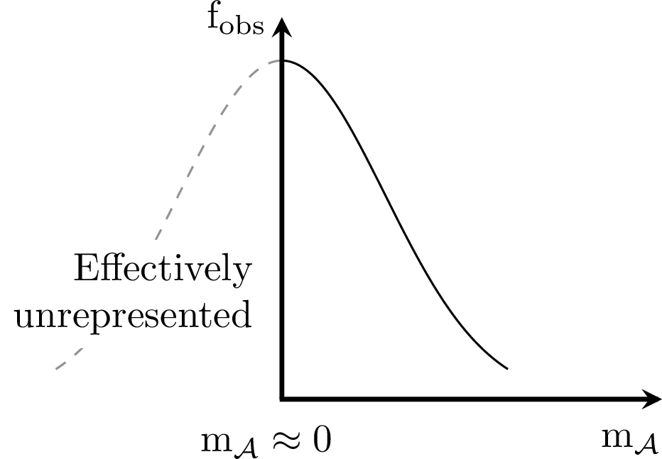
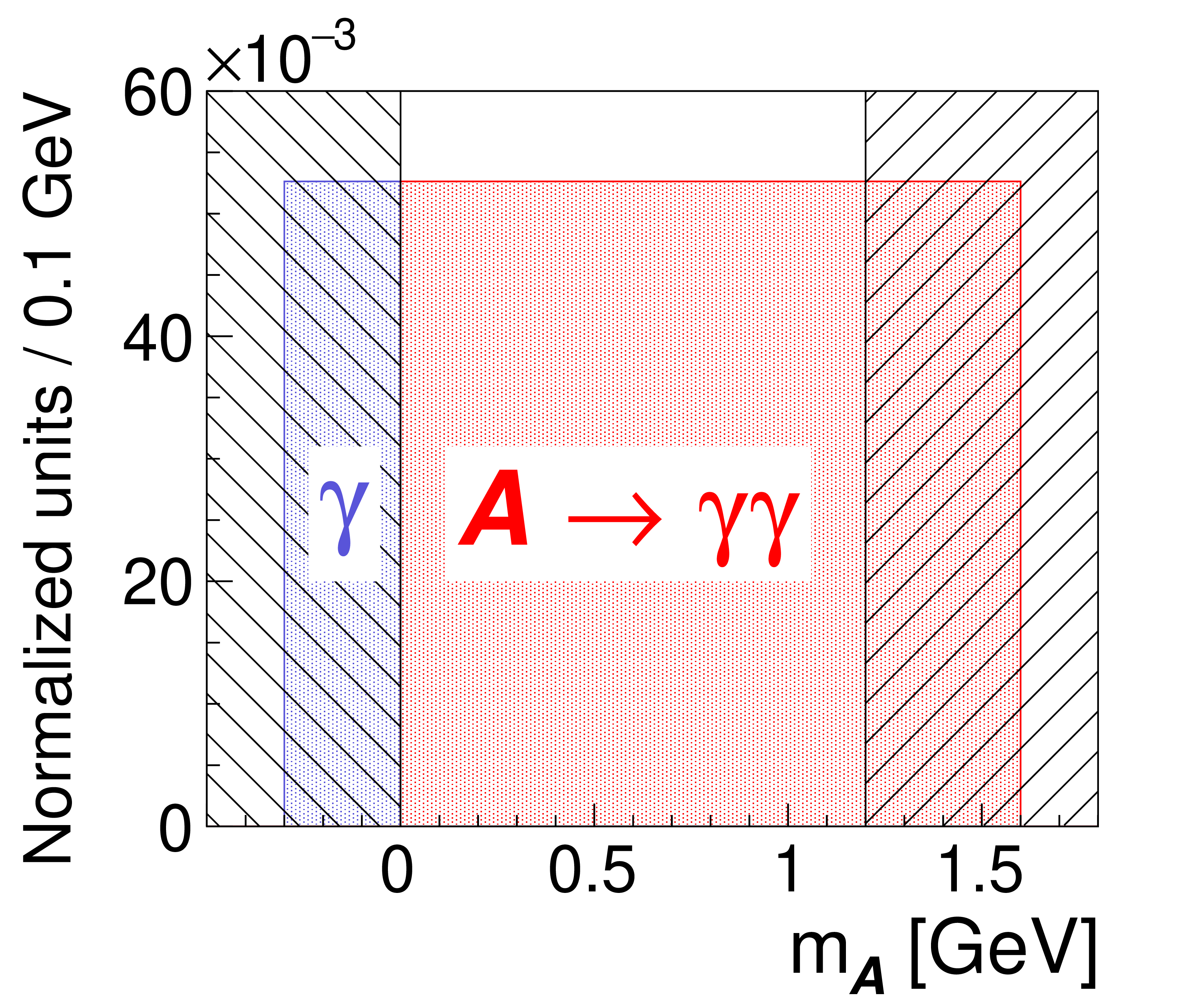
Pictorial representation of the $m_{\mathcal{A}}\to$ 0 boundary problem occurring when attempting to regress below the mass resolution. Left: The distribution of physically observable $ {\mathcal{A}} \to \gamma \gamma $ invariant masses ($f_{\text{obs}}$) vs. the generated $m_{\mathcal{A}}$. When $m_{\mathcal{A}}\approx \sigma (m_{\mathcal{A}})$, the left tail of the mass distribution becomes underrepresented in the training set. Middle: As $m_{\mathcal{A}}\to $ 0, only half of the mass distribution is represented. The regressor subsequently defaults to the last full mass distribution at $m_{\mathcal{A}}\approx \sigma (m_{\mathcal{A}})$. Right: With domain continuation, the generated mass distribution of the original training samples ($ {\mathcal{A}} \to \gamma \gamma $, red region) is augmented with topologically similar samples that are randomly assigned nonphysical masses ($\gamma $, blue region). This allows the regressor to see a full mass distribution over the entire region of interest (unhatched region). Predictions in the black hatched regions are discarded. |
png pdf |
Figure 3-a:
Pictorial representation of the $m_{\mathcal{A}}\to$ 0 boundary problem occurring when attempting to regress below the mass resolution. The distribution of physically observable $ {\mathcal{A}} \to \gamma \gamma $ invariant masses ($f_{\text{obs}}$) vs. the generated $m_{\mathcal{A}}$. When $m_{\mathcal{A}}\approx \sigma (m_{\mathcal{A}})$, the left tail of the mass distribution becomes underrepresented in the training set. |
png pdf |
Figure 3-b:
Pictorial representation of the $m_{\mathcal{A}}\to$ 0 boundary problem occurring when attempting to regress below the mass resolution. As $m_{\mathcal{A}}\to $ 0, only half of the mass distribution is represented. The regressor subsequently defaults to the last full mass distribution at $m_{\mathcal{A}}\approx \sigma (m_{\mathcal{A}})$. |
png pdf |
Figure 3-c:
Pictorial representation of the $m_{\mathcal{A}}\to$ 0 boundary problem occurring when attempting to regress below the mass resolution. With domain continuation, the generated mass distribution of the original training samples ($ {\mathcal{A}} \to \gamma \gamma $, red region) is augmented with topologically similar samples that are randomly assigned nonphysical masses ($\gamma $, blue region). This allows the regressor to see a full mass distribution over the entire region of interest (unhatched region). Predictions in the black hatched regions are discarded. |
png pdf |
Figure 4:
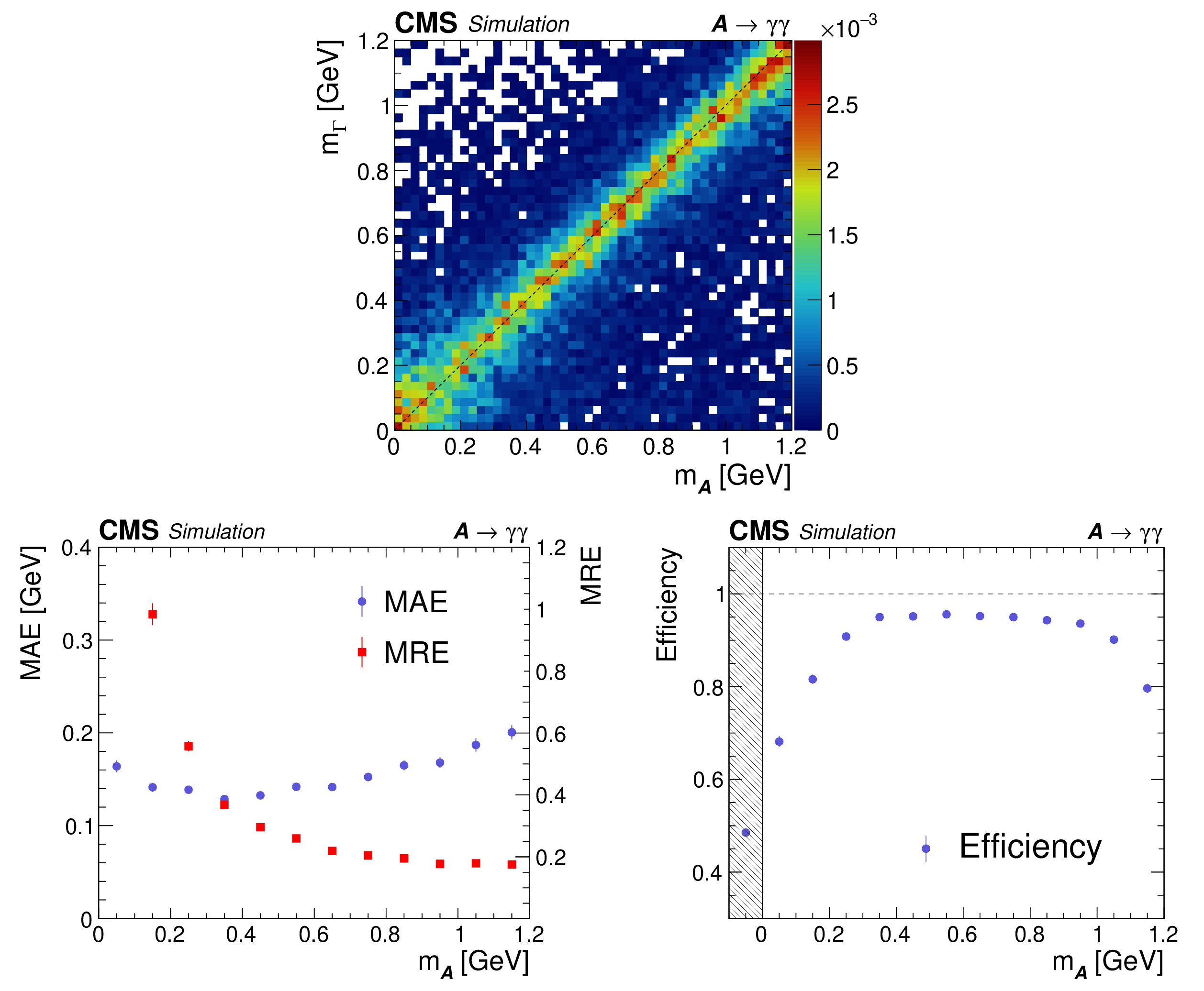
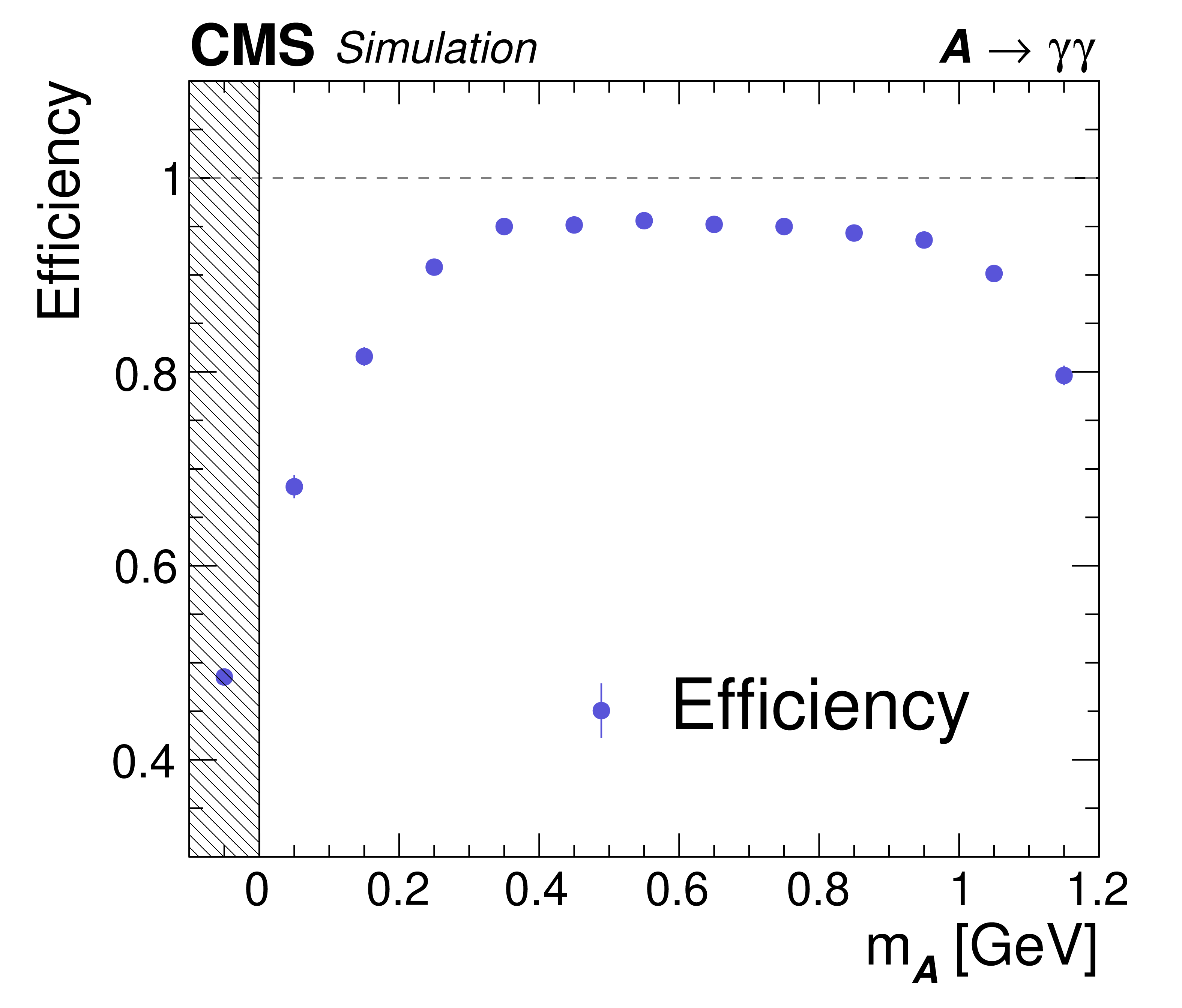
Mass regression performance for simulated $ {\mathcal{A}} \to \gamma \gamma $ samples generated uniformly in $({p_{\mathrm{T}}},m_{\mathcal{A}})$, corresponding to mean boosts in the range $\langle \gamma _{\mathrm {L}}\rangle =$ 600-50 for $m_{\mathcal{A}}=$ 0.1-1.2 GeV. Upper: Regressed $m_{\Gamma}$ vs. generated $m_{\mathcal{A}}$. The regressed $m_{\Gamma}$ is normalized in 0.025 GeV vertical slices of the generated $m_{\mathcal{A}}$. The color scale to the right of the plot gives the normalized number of events per vertical slice in 0.025 GeV bins of $m_{\Gamma}$. Lower left: The MAE (blue circles, use left scale) and MRE (red squares, use right scale) vs. the generated $m_{\mathcal{A}}$. For clarity, the MRE for $m_{\mathcal{A}} < $ 0.1 GeV is not shown since its value diverges as $m_{\mathcal{A}}\to $ 0. Lower right: The $m_{\mathcal{A}}$ regression efficiency as a function of the generated $m_{\mathcal{A}}$. The hatched region shows the efficiency for single photons. The vertical bars on the points show the statistical uncertainty in the simulated sample. |
png pdf |
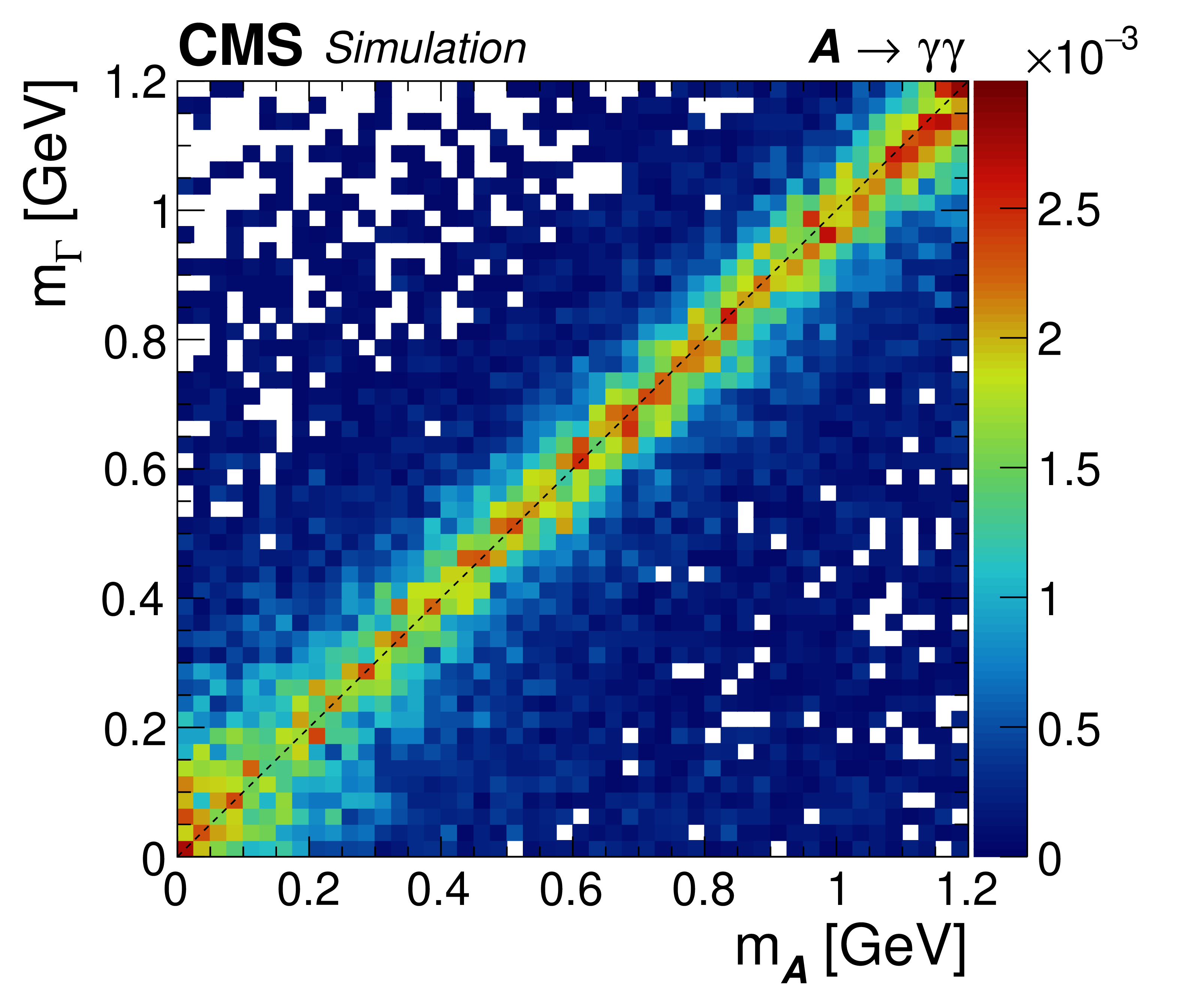
Figure 4-a:
Mass regression performance for simulated $ {\mathcal{A}} \to \gamma \gamma $ samples generated uniformly in $({p_{\mathrm{T}}},m_{\mathcal{A}})$, corresponding to mean boosts in the range $\langle \gamma _{\mathrm {L}}\rangle =$ 600-50 for $m_{\mathcal{A}}=$ 0.1-1.2 GeV: Regressed $m_{\Gamma}$ vs. generated $m_{\mathcal{A}}$. The regressed $m_{\Gamma}$ is normalized in 0.025 GeV vertical slices of the generated $m_{\mathcal{A}}$. The color scale to the right of the plot gives the normalized number of events per vertical slice in 0.025 GeV bins of $m_{\Gamma}$. |
png pdf |
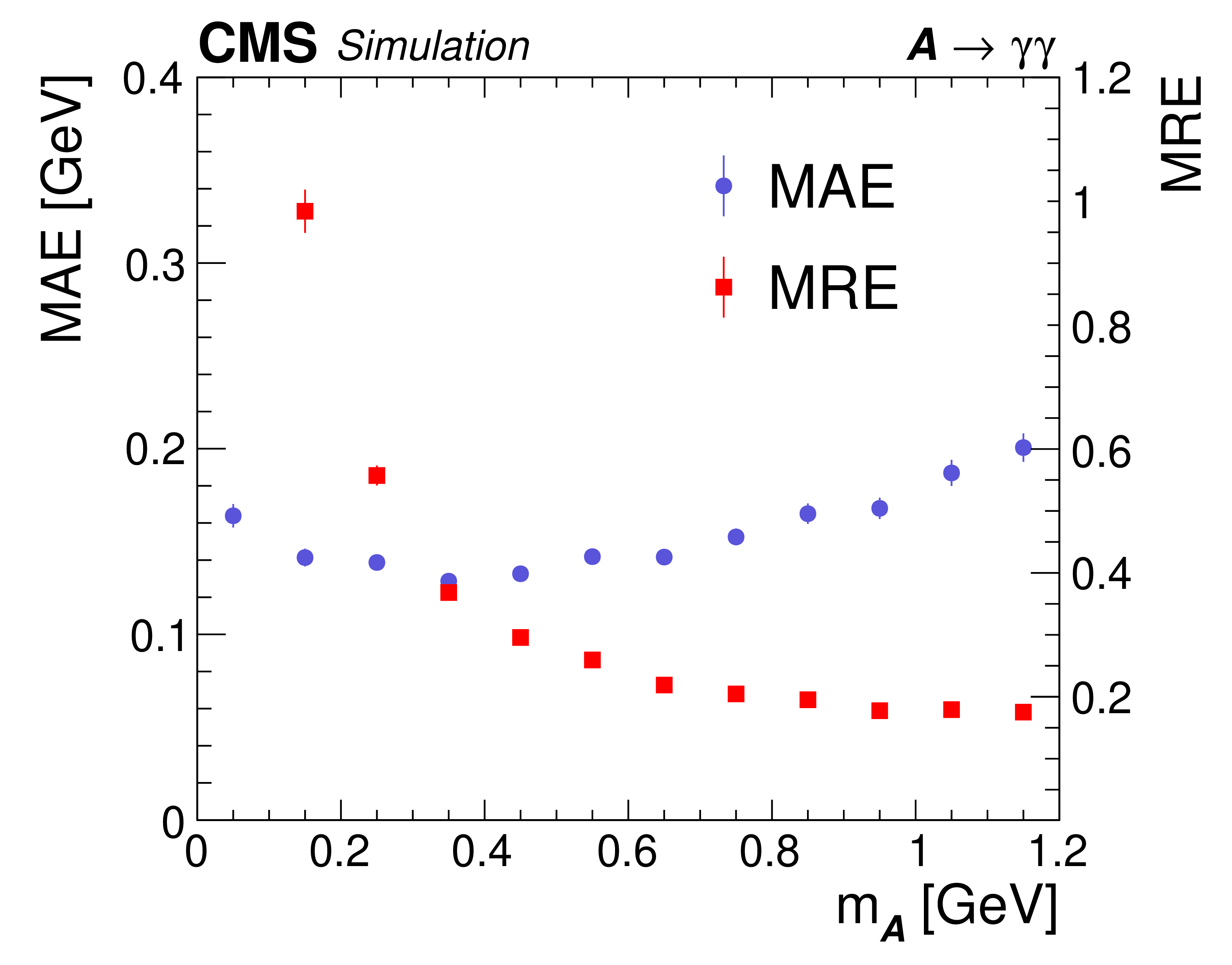
Figure 4-b:
Mass regression performance for simulated $ {\mathcal{A}} \to \gamma \gamma $ samples generated uniformly in $({p_{\mathrm{T}}},m_{\mathcal{A}})$, corresponding to mean boosts in the range $\langle \gamma _{\mathrm {L}}\rangle =$ 600-50 for $m_{\mathcal{A}}=$ 0.1-1.2 GeV: The MAE (blue circles, use left scale) and MRE (red squares, use right scale) vs. the generated $m_{\mathcal{A}}$. For clarity, the MRE for $m_{\mathcal{A}} < $ 0.1 GeV is not shown since its value diverges as $m_{\mathcal{A}}\to $ 0. |
png pdf |
Figure 4-c:
Mass regression performance for simulated $ {\mathcal{A}} \to \gamma \gamma $ samples generated uniformly in $({p_{\mathrm{T}}},m_{\mathcal{A}})$, corresponding to mean boosts in the range $\langle \gamma _{\mathrm {L}}\rangle =$ 600-50 for $m_{\mathcal{A}}=$ 0.1-1.2 GeV: The $m_{\mathcal{A}}$ regression efficiency as a function of the generated $m_{\mathcal{A}}$. The hatched region shows the efficiency for single photons. The vertical bars on the points show the statistical uncertainty in the simulated sample. |
png pdf |
Figure 5:
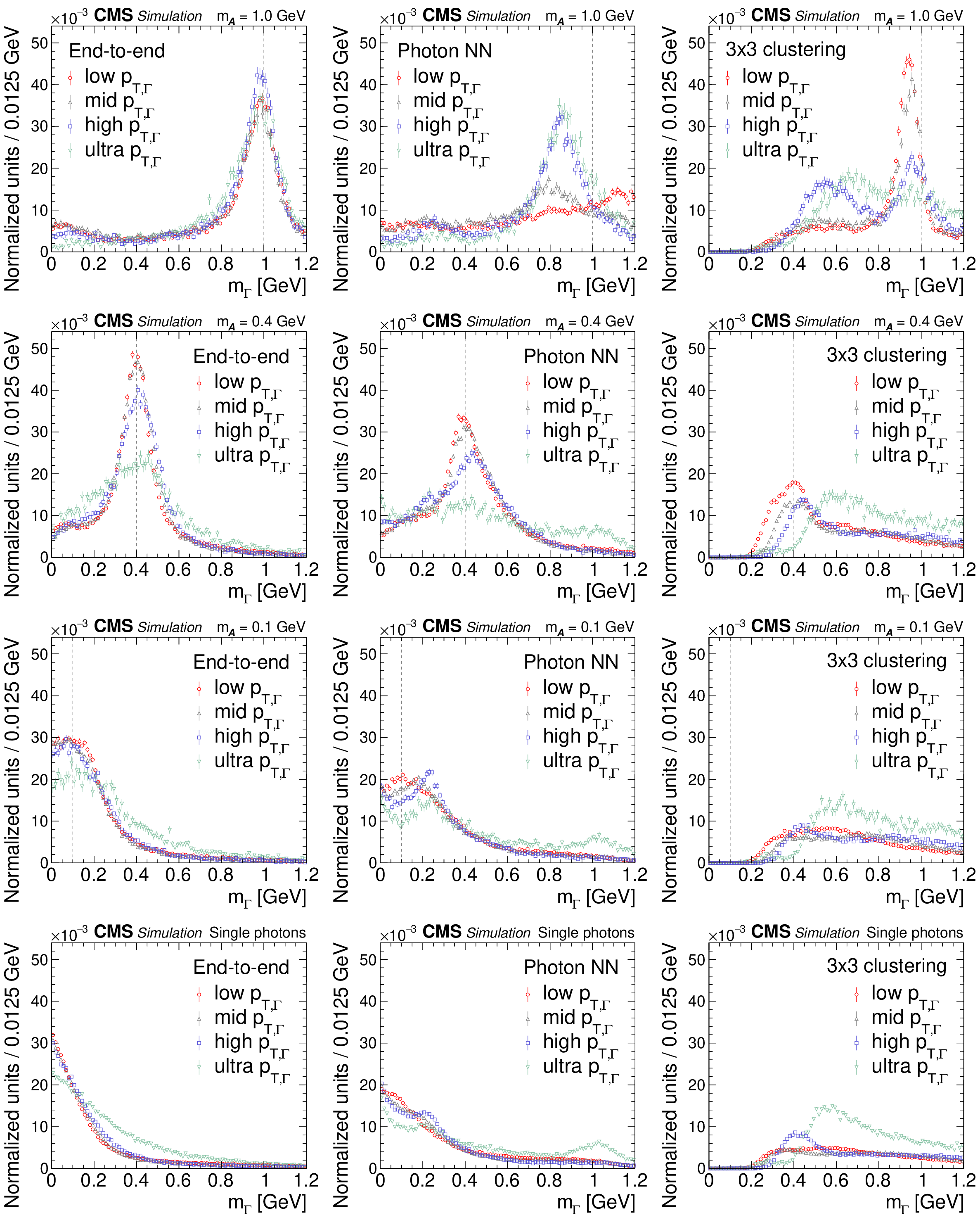
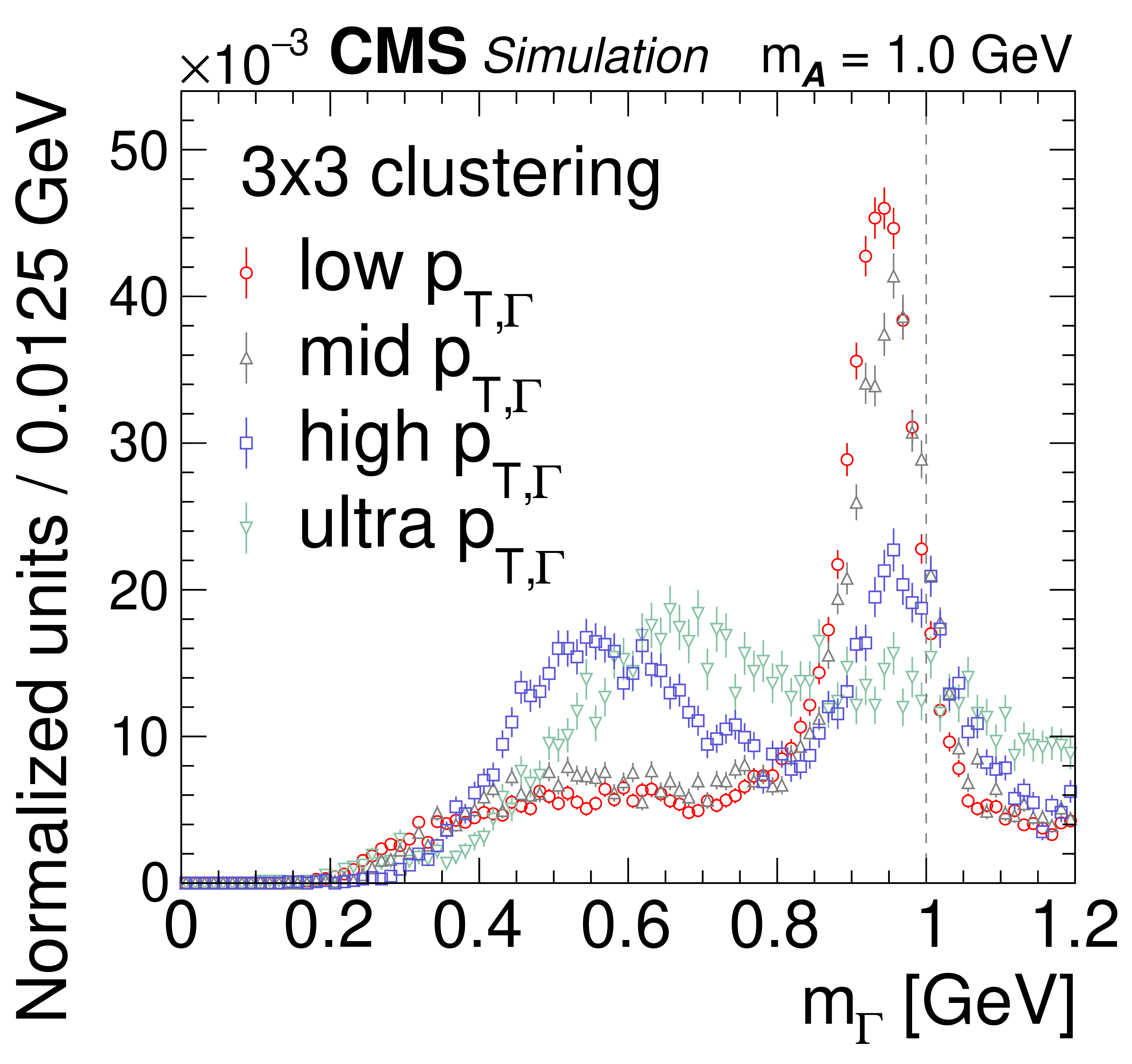
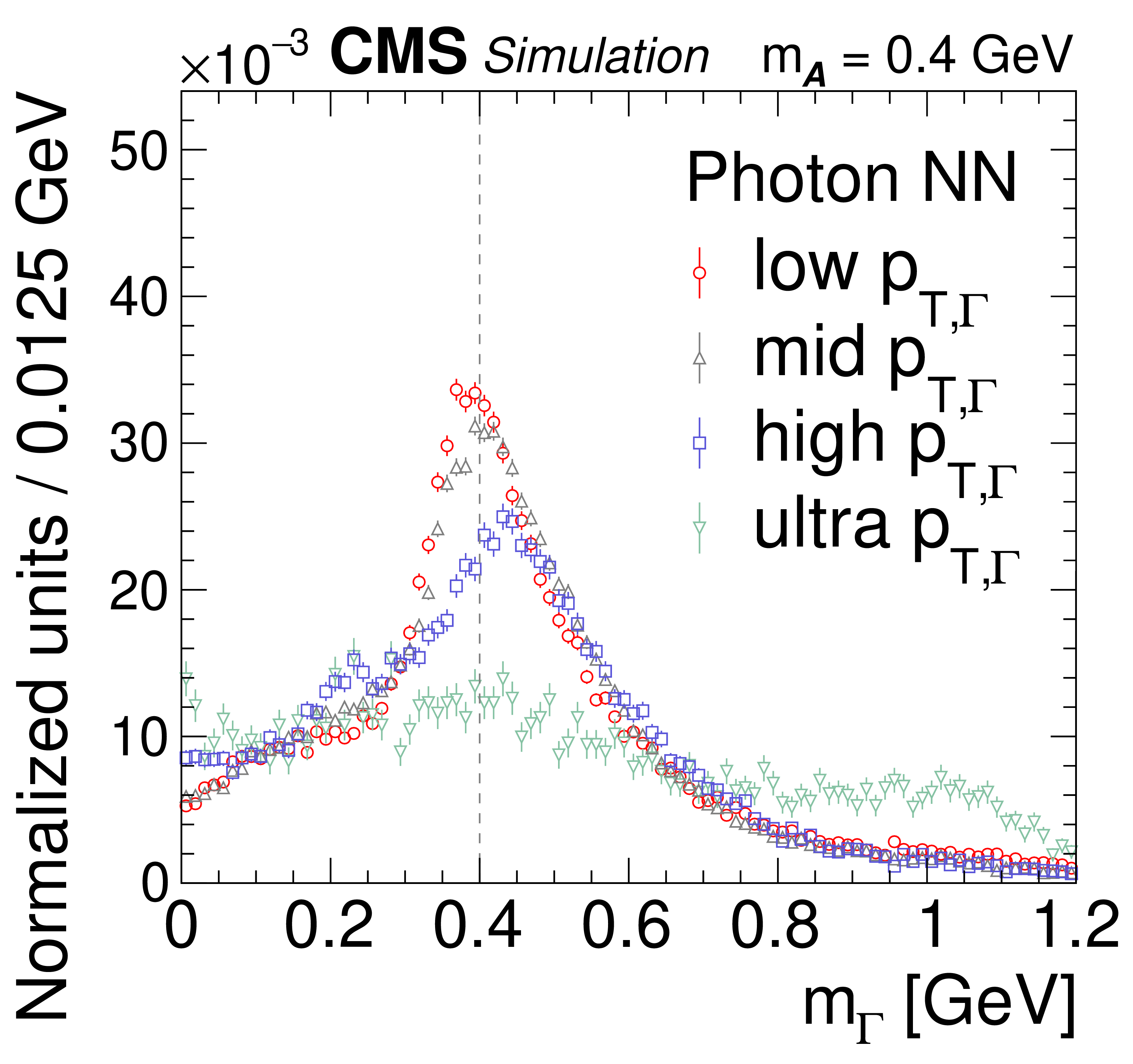
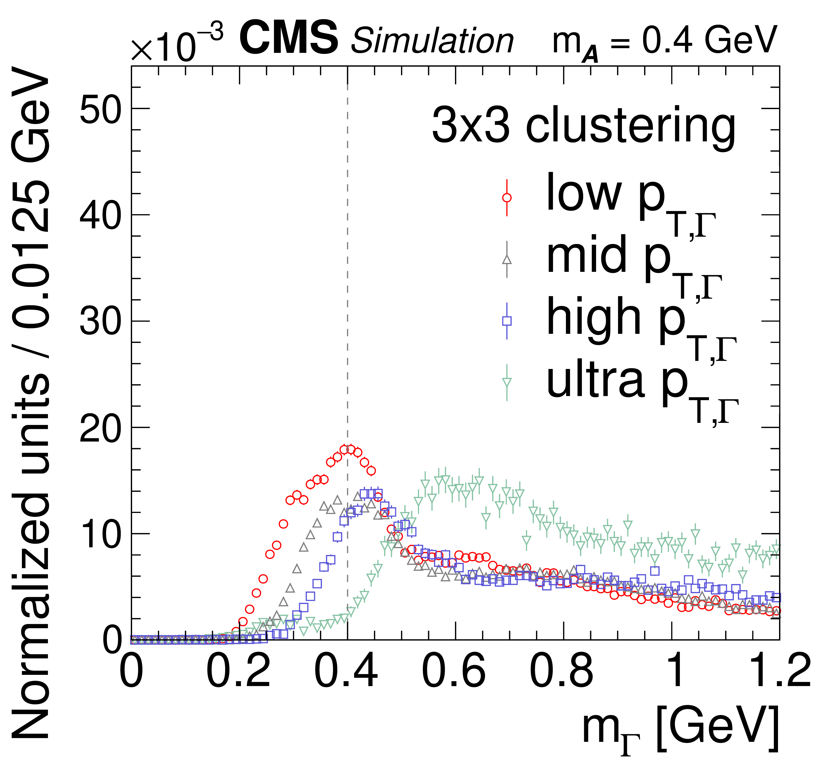
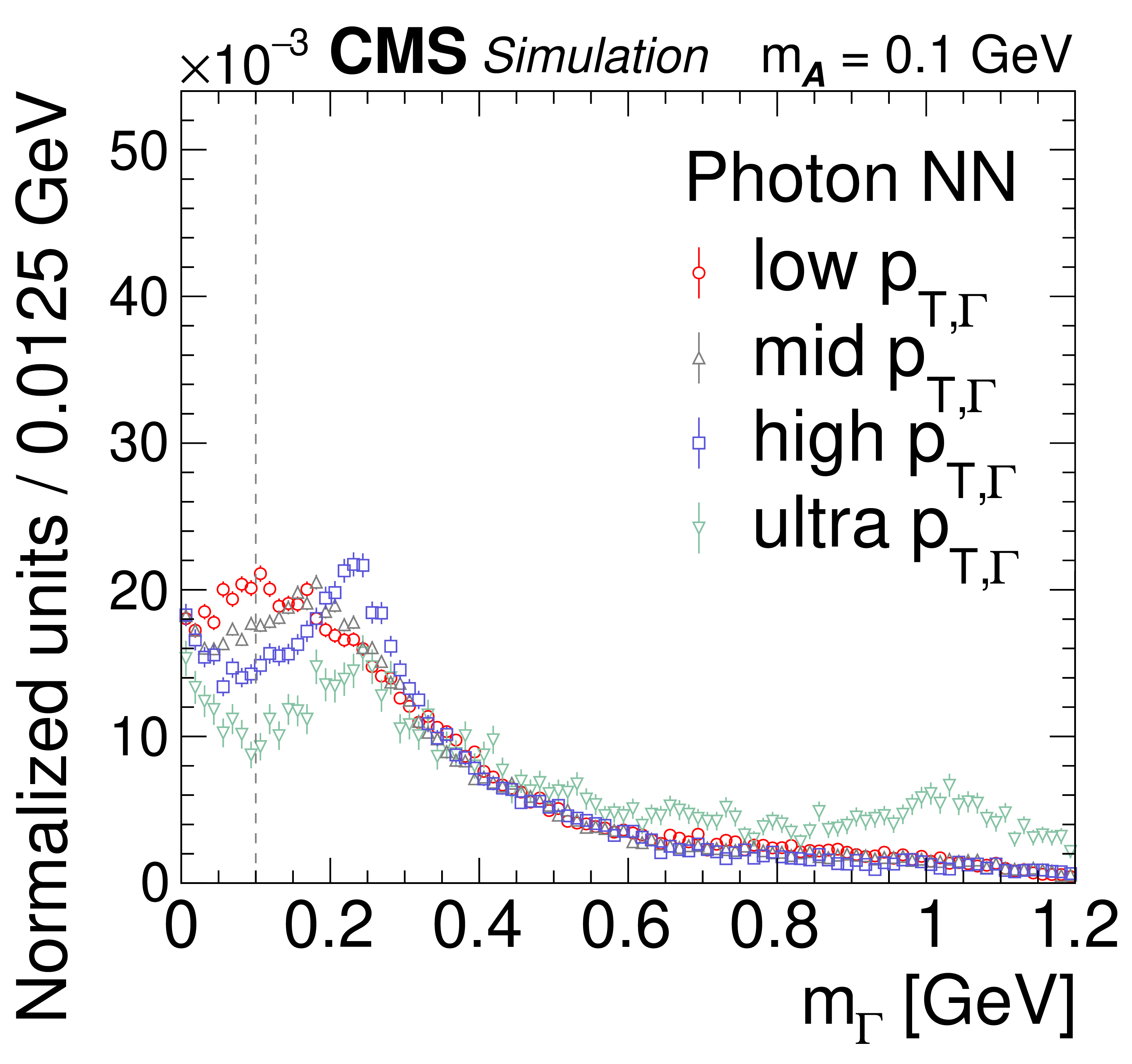
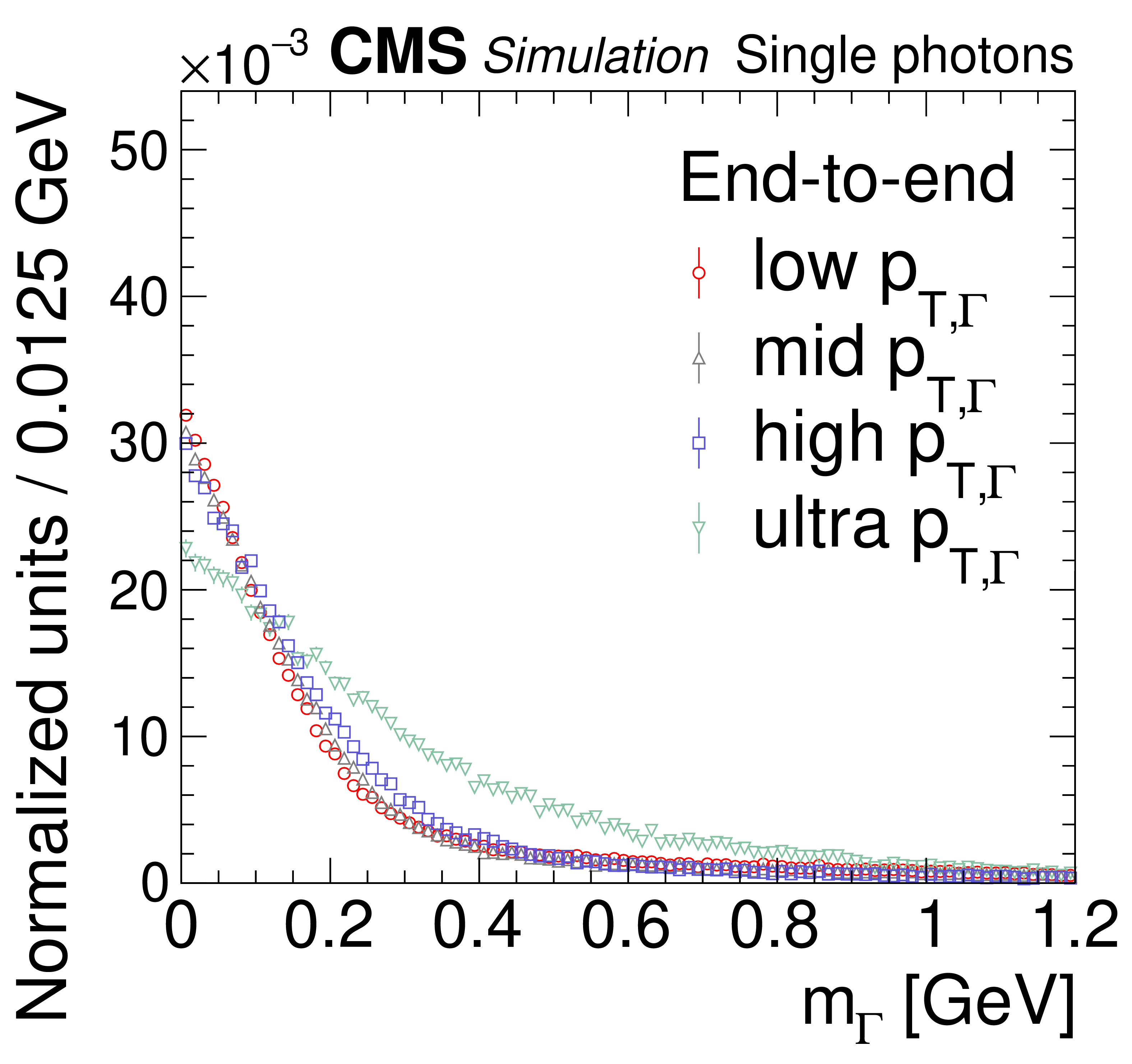
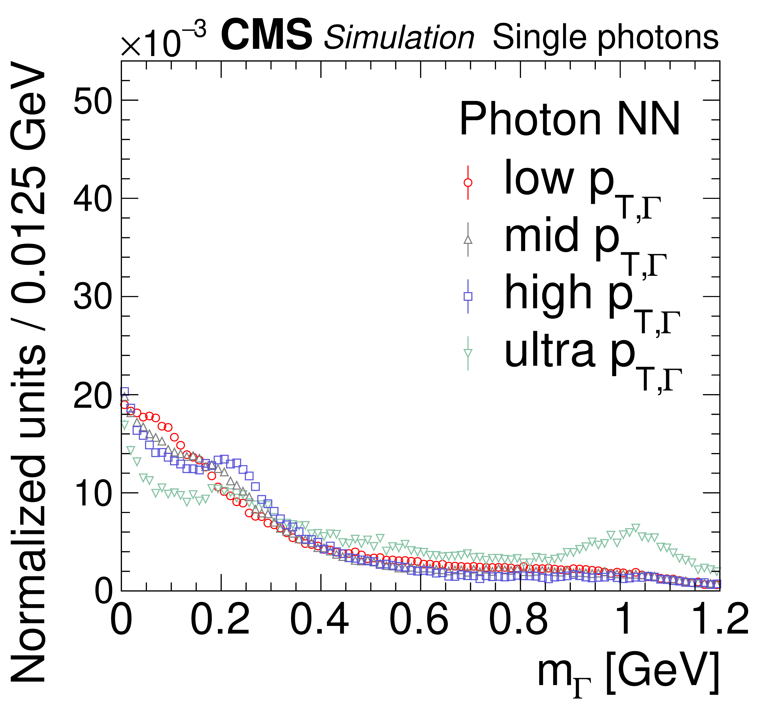
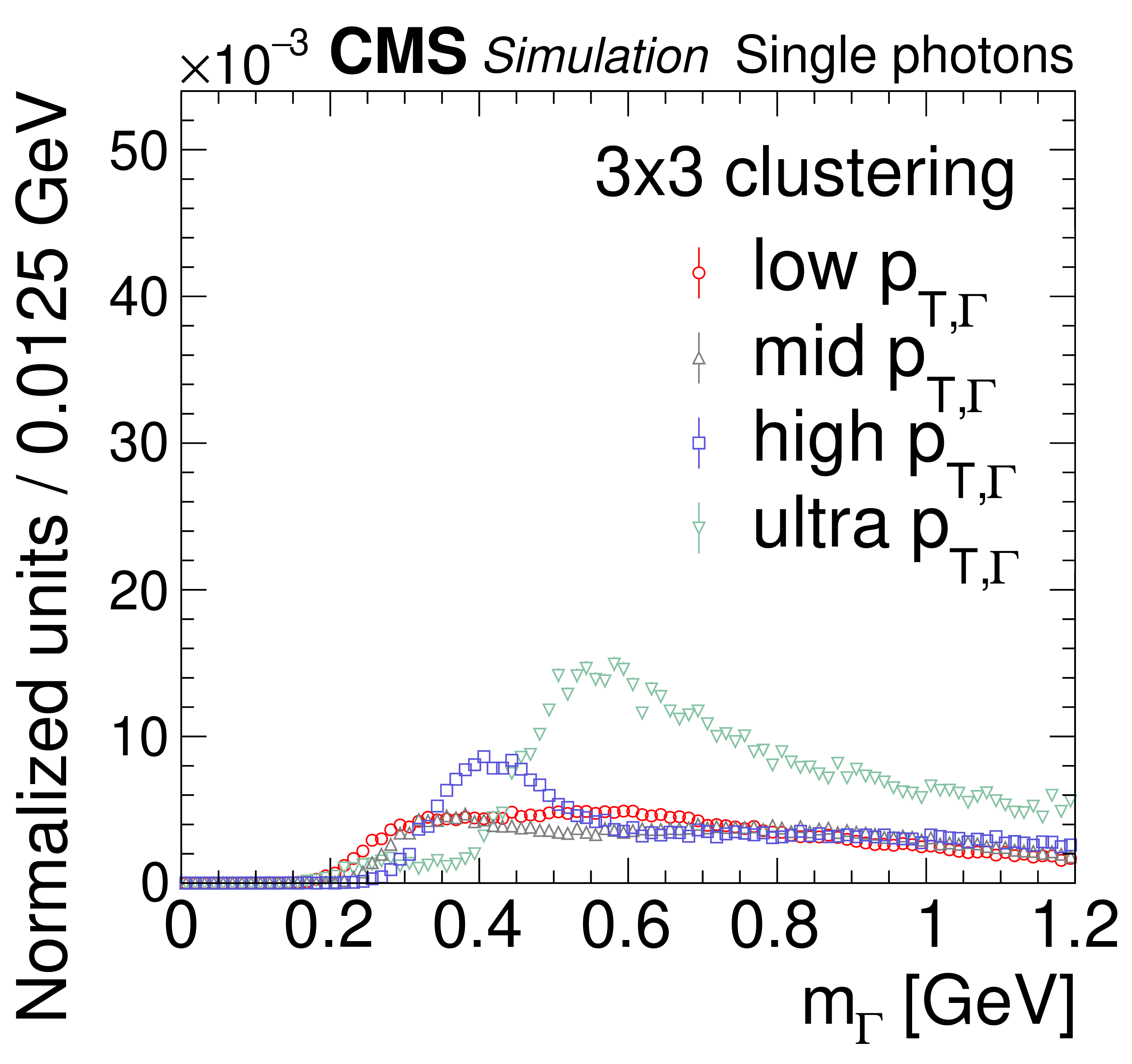
Reconstructed mass spectra for end-to-end (left column), photon NN (middle column), and 3$\times$3 algorithms (right column) for $ {\mathcal{A}} \to \gamma \gamma $ decays with $m_{\mathcal{A}} = $ 1.0 GeV (upper row), $m_{\mathcal{A}} = $ 0.4 GeV (second row), $m_{\mathcal{A}} = $ 0.1 GeV (third row), and for isolated single photons (lower row). The $ {\mathcal{A}} \to \gamma \gamma $ decays (single photons) are obtained from simulated $\mathrm{H} \to {\mathcal{A}} {\mathcal{A}} \to 4 \gamma $ ($\mathrm{H} \to \gamma \gamma $) events. For each panel, the mass spectra are separated by reconstructed $ {p_{\mathrm {T},\,\Gamma}} $ value into ranges of 30-55 GeV (red circles, low $ {p_{\mathrm {T},\,\Gamma}} $), 55-70 GeV (gray triangles, mid $ {p_{\mathrm {T},\,\Gamma}} $), 70-100 GeV (blue squares, high $ {p_{\mathrm {T},\,\Gamma}} $), and $ > $ 100 GeV (green inverted triangles, ultra $ {p_{\mathrm {T},\,\Gamma}} $). The vertical bars on the points give the statistical uncertainties. All the mass spectra are normalized to unity, including samples outside $m_{\mathcal{A}}$-ROI. The vertical dotted line shows the input $m_{\mathcal{A}}$ value. |
png pdf |
Figure 5-a:
Reconstructed mass spectra for the 3$\times$3 algorithm for $ {\mathcal{A}} \to \gamma \gamma $ decays with $m_{\mathcal{A}} = $ 1.0 GeV. The $ {\mathcal{A}} \to \gamma \gamma $ decays (single photons) are obtained from simulated $\mathrm{H} \to {\mathcal{A}} {\mathcal{A}} \to 4 \gamma $ ($\mathrm{H} \to \gamma \gamma $) events. The mass spectra are separated by reconstructed $ {p_{\mathrm {T},\,\Gamma}} $ value into ranges of 30-55 GeV (red circles, low $ {p_{\mathrm {T},\,\Gamma}} $), 55-70 GeV (gray triangles, mid $ {p_{\mathrm {T},\,\Gamma}} $), 70-100 GeV (blue squares, high $ {p_{\mathrm {T},\,\Gamma}} $), and $ > $ 100 GeV (green inverted triangles, ultra $ {p_{\mathrm {T},\,\Gamma}} $). The vertical bars on the points give the statistical uncertainties. All the mass spectra are normalized to unity, including samples outside $m_{\mathcal{A}}$-ROI. The vertical dotted line shows the input $m_{\mathcal{A}}$ value. |
png pdf |
Figure 5-b:
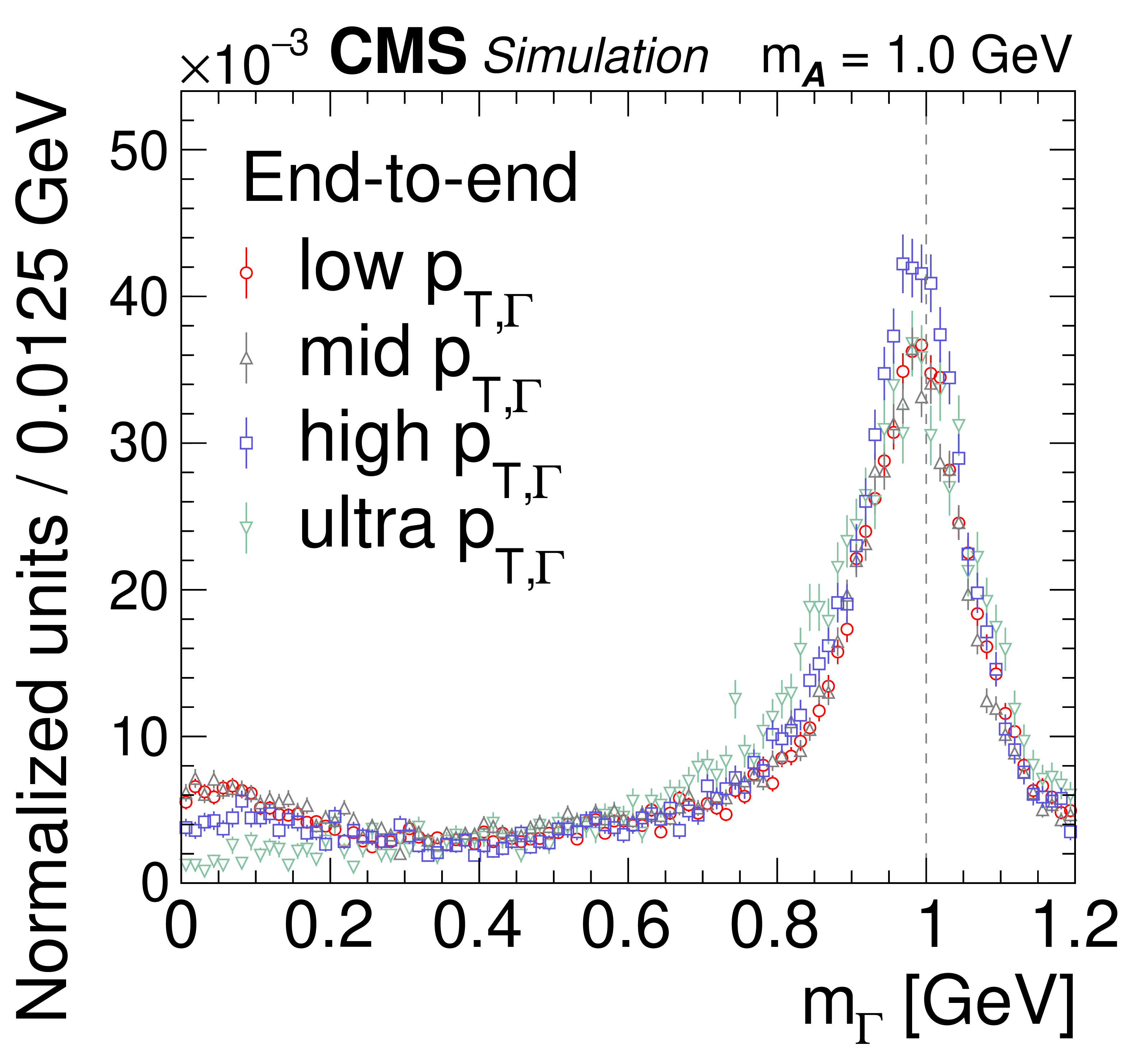
Reconstructed mass spectra for the end-to-end algorithm for $ {\mathcal{A}} \to \gamma \gamma $ decays with $m_{\mathcal{A}} = $ 1.0 GeV. The $ {\mathcal{A}} \to \gamma \gamma $ decays (single photons) are obtained from simulated $\mathrm{H} \to {\mathcal{A}} {\mathcal{A}} \to 4 \gamma $ ($\mathrm{H} \to \gamma \gamma $) events. The mass spectra are separated by reconstructed $ {p_{\mathrm {T},\,\Gamma}} $ value into ranges of 30-55 GeV (red circles, low $ {p_{\mathrm {T},\,\Gamma}} $), 55-70 GeV (gray triangles, mid $ {p_{\mathrm {T},\,\Gamma}} $), 70-100 GeV (blue squares, high $ {p_{\mathrm {T},\,\Gamma}} $), and $ > $ 100 GeV (green inverted triangles, ultra $ {p_{\mathrm {T},\,\Gamma}} $). The vertical bars on the points give the statistical uncertainties. All the mass spectra are normalized to unity, including samples outside $m_{\mathcal{A}}$-ROI. The vertical dotted line shows the input $m_{\mathcal{A}}$ value. |
png pdf |
Figure 5-c:
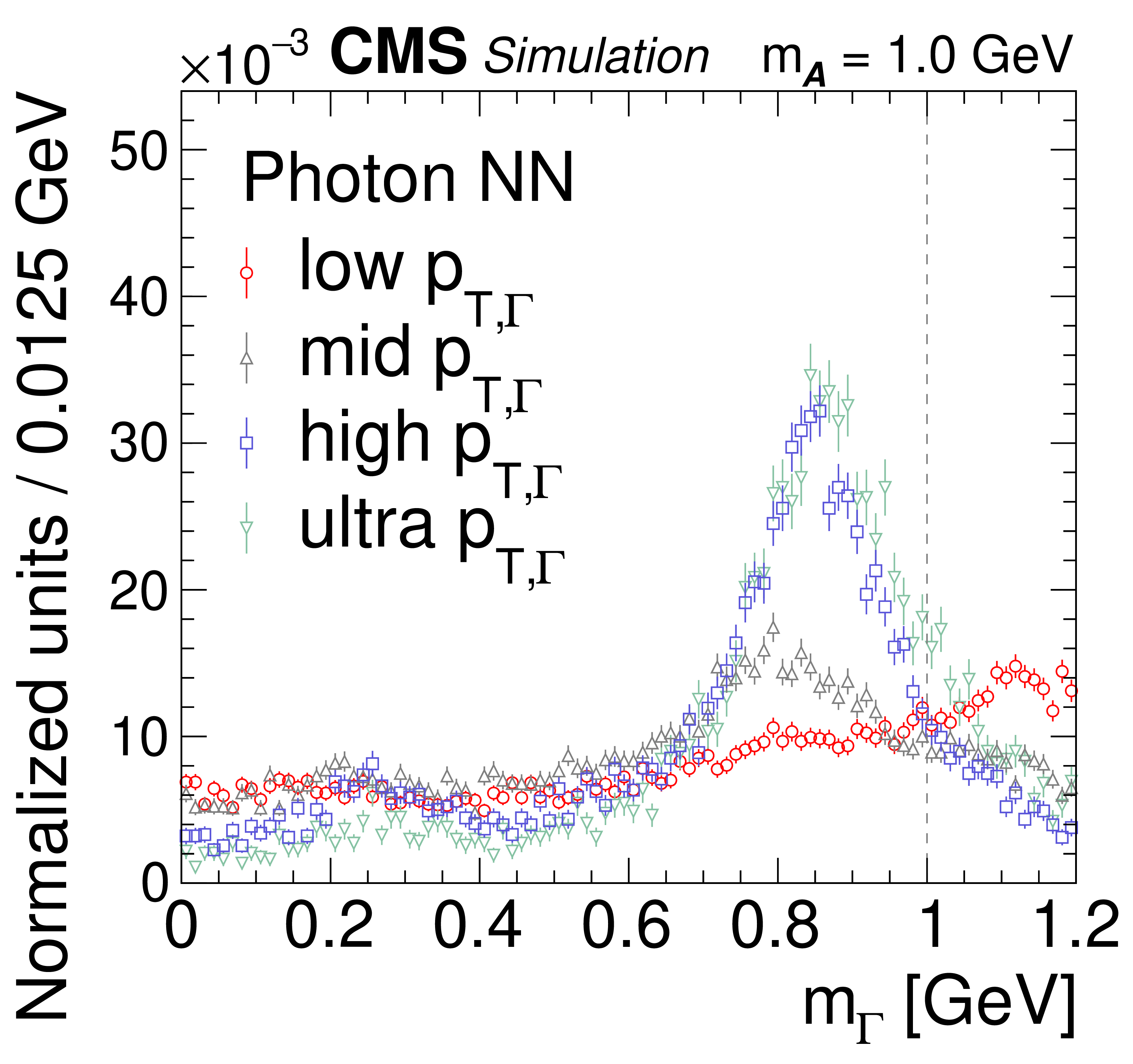
Reconstructed mass spectra for the photon NN algorithm for $ {\mathcal{A}} \to \gamma \gamma $ decays with $m_{\mathcal{A}} = $ 1.0 GeV. The $ {\mathcal{A}} \to \gamma \gamma $ decays (single photons) are obtained from simulated $\mathrm{H} \to {\mathcal{A}} {\mathcal{A}} \to 4 \gamma $ ($\mathrm{H} \to \gamma \gamma $) events. The mass spectra are separated by reconstructed $ {p_{\mathrm {T},\,\Gamma}} $ value into ranges of 30-55 GeV (red circles, low $ {p_{\mathrm {T},\,\Gamma}} $), 55-70 GeV (gray triangles, mid $ {p_{\mathrm {T},\,\Gamma}} $), 70-100 GeV (blue squares, high $ {p_{\mathrm {T},\,\Gamma}} $), and $ > $ 100 GeV (green inverted triangles, ultra $ {p_{\mathrm {T},\,\Gamma}} $). The vertical bars on the points give the statistical uncertainties. All the mass spectra are normalized to unity, including samples outside $m_{\mathcal{A}}$-ROI. The vertical dotted line shows the input $m_{\mathcal{A}}$ value. |

png pdf |
Figure 5-d:
Reconstructed mass spectra for the end-to-end algorithm for $ {\mathcal{A}} \to \gamma \gamma $ decays with $m_{\mathcal{A}} = $ 0.4 GeV. The $ {\mathcal{A}} \to \gamma \gamma $ decays (single photons) are obtained from simulated $\mathrm{H} \to {\mathcal{A}} {\mathcal{A}} \to 4 \gamma $ ($\mathrm{H} \to \gamma \gamma $) events. The mass spectra are separated by reconstructed $ {p_{\mathrm {T},\,\Gamma}} $ value into ranges of 30-55 GeV (red circles, low $ {p_{\mathrm {T},\,\Gamma}} $), 55-70 GeV (gray triangles, mid $ {p_{\mathrm {T},\,\Gamma}} $), 70-100 GeV (blue squares, high $ {p_{\mathrm {T},\,\Gamma}} $), and $ > $ 100 GeV (green inverted triangles, ultra $ {p_{\mathrm {T},\,\Gamma}} $). The vertical bars on the points give the statistical uncertainties. All the mass spectra are normalized to unity, including samples outside $m_{\mathcal{A}}$-ROI. The vertical dotted line shows the input $m_{\mathcal{A}}$ value. |
png pdf |
Figure 5-e:
Reconstructed mass spectra for the photon NN algorithm for $ {\mathcal{A}} \to \gamma \gamma $ decays with $m_{\mathcal{A}} = $ 0.4 GeV. The $ {\mathcal{A}} \to \gamma \gamma $ decays (single photons) are obtained from simulated $\mathrm{H} \to {\mathcal{A}} {\mathcal{A}} \to 4 \gamma $ ($\mathrm{H} \to \gamma \gamma $) events. The mass spectra are separated by reconstructed $ {p_{\mathrm {T},\,\Gamma}} $ value into ranges of 30-55 GeV (red circles, low $ {p_{\mathrm {T},\,\Gamma}} $), 55-70 GeV (gray triangles, mid $ {p_{\mathrm {T},\,\Gamma}} $), 70-100 GeV (blue squares, high $ {p_{\mathrm {T},\,\Gamma}} $), and $ > $ 100 GeV (green inverted triangles, ultra $ {p_{\mathrm {T},\,\Gamma}} $). The vertical bars on the points give the statistical uncertainties. All the mass spectra are normalized to unity, including samples outside $m_{\mathcal{A}}$-ROI. The vertical dotted line shows the input $m_{\mathcal{A}}$ value. |
png pdf |
Figure 5-f:
Reconstructed mass spectra for the 3$\times$3 algorithm for $ {\mathcal{A}} \to \gamma \gamma $ decays with $m_{\mathcal{A}} = $ 0.4 GeV. The $ {\mathcal{A}} \to \gamma \gamma $ decays (single photons) are obtained from simulated $\mathrm{H} \to {\mathcal{A}} {\mathcal{A}} \to 4 \gamma $ ($\mathrm{H} \to \gamma \gamma $) events. The mass spectra are separated by reconstructed $ {p_{\mathrm {T},\,\Gamma}} $ value into ranges of 30-55 GeV (red circles, low $ {p_{\mathrm {T},\,\Gamma}} $), 55-70 GeV (gray triangles, mid $ {p_{\mathrm {T},\,\Gamma}} $), 70-100 GeV (blue squares, high $ {p_{\mathrm {T},\,\Gamma}} $), and $ > $ 100 GeV (green inverted triangles, ultra $ {p_{\mathrm {T},\,\Gamma}} $). The vertical bars on the points give the statistical uncertainties. All the mass spectra are normalized to unity, including samples outside $m_{\mathcal{A}}$-ROI. The vertical dotted line shows the input $m_{\mathcal{A}}$ value. |

png pdf |
Figure 5-g:
Reconstructed mass spectra for the end-to-end algorithm for $ {\mathcal{A}} \to \gamma \gamma $ decays with $m_{\mathcal{A}} = $ 0.1 GeV. The $ {\mathcal{A}} \to \gamma \gamma $ decays (single photons) are obtained from simulated $\mathrm{H} \to {\mathcal{A}} {\mathcal{A}} \to 4 \gamma $ ($\mathrm{H} \to \gamma \gamma $) events. The mass spectra are separated by reconstructed $ {p_{\mathrm {T},\,\Gamma}} $ value into ranges of 30-55 GeV (red circles, low $ {p_{\mathrm {T},\,\Gamma}} $), 55-70 GeV (gray triangles, mid $ {p_{\mathrm {T},\,\Gamma}} $), 70-100 GeV (blue squares, high $ {p_{\mathrm {T},\,\Gamma}} $), and $ > $ 100 GeV (green inverted triangles, ultra $ {p_{\mathrm {T},\,\Gamma}} $). The vertical bars on the points give the statistical uncertainties. All the mass spectra are normalized to unity, including samples outside $m_{\mathcal{A}}$-ROI. The vertical dotted line shows the input $m_{\mathcal{A}}$ value. |
png pdf |
Figure 5-h:
Reconstructed mass spectra for the photon NN algorithm for $ {\mathcal{A}} \to \gamma \gamma $ decays with $m_{\mathcal{A}} = $ 0.1 GeV. The $ {\mathcal{A}} \to \gamma \gamma $ decays (single photons) are obtained from simulated $\mathrm{H} \to {\mathcal{A}} {\mathcal{A}} \to 4 \gamma $ ($\mathrm{H} \to \gamma \gamma $) events. The mass spectra are separated by reconstructed $ {p_{\mathrm {T},\,\Gamma}} $ value into ranges of 30-55 GeV (red circles, low $ {p_{\mathrm {T},\,\Gamma}} $), 55-70 GeV (gray triangles, mid $ {p_{\mathrm {T},\,\Gamma}} $), 70-100 GeV (blue squares, high $ {p_{\mathrm {T},\,\Gamma}} $), and $ > $ 100 GeV (green inverted triangles, ultra $ {p_{\mathrm {T},\,\Gamma}} $). The vertical bars on the points give the statistical uncertainties. All the mass spectra are normalized to unity, including samples outside $m_{\mathcal{A}}$-ROI. The vertical dotted line shows the input $m_{\mathcal{A}}$ value. |
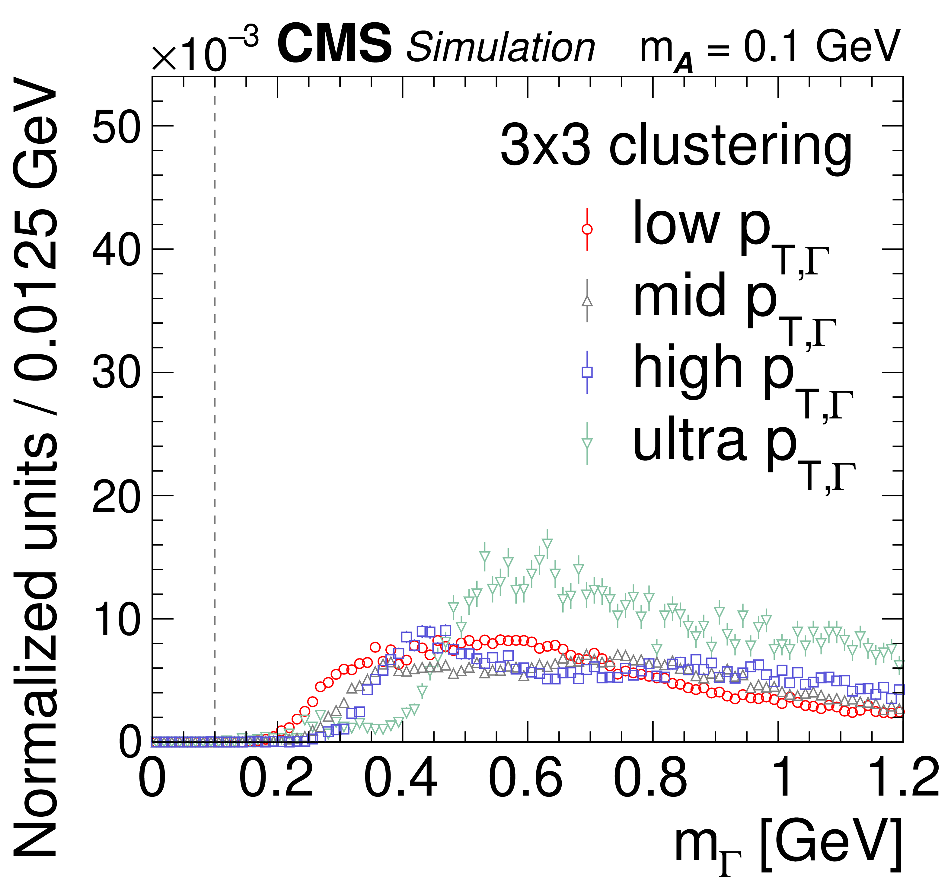
png pdf |
Figure 5-i:
Reconstructed mass spectra for the 3$\times$3 algorithm for $ {\mathcal{A}} \to \gamma \gamma $ decays with $m_{\mathcal{A}} = $ 0.1 GeV. The $ {\mathcal{A}} \to \gamma \gamma $ decays (single photons) are obtained from simulated $\mathrm{H} \to {\mathcal{A}} {\mathcal{A}} \to 4 \gamma $ ($\mathrm{H} \to \gamma \gamma $) events. The mass spectra are separated by reconstructed $ {p_{\mathrm {T},\,\Gamma}} $ value into ranges of 30-55 GeV (red circles, low $ {p_{\mathrm {T},\,\Gamma}} $), 55-70 GeV (gray triangles, mid $ {p_{\mathrm {T},\,\Gamma}} $), 70-100 GeV (blue squares, high $ {p_{\mathrm {T},\,\Gamma}} $), and $ > $ 100 GeV (green inverted triangles, ultra $ {p_{\mathrm {T},\,\Gamma}} $). The vertical bars on the points give the statistical uncertainties. All the mass spectra are normalized to unity, including samples outside $m_{\mathcal{A}}$-ROI. The vertical dotted line shows the input $m_{\mathcal{A}}$ value. |
png pdf |
Figure 5-j:
Reconstructed mass spectra for the end-to-end algorithm for $ {\mathcal{A}} \to \gamma \gamma $ decays for isolated single photons. The $ {\mathcal{A}} \to \gamma \gamma $ decays (single photons) are obtained from simulated $\mathrm{H} \to {\mathcal{A}} {\mathcal{A}} \to 4 \gamma $ ($\mathrm{H} \to \gamma \gamma $) events. The mass spectra are separated by reconstructed $ {p_{\mathrm {T},\,\Gamma}} $ value into ranges of 30-55 GeV (red circles, low $ {p_{\mathrm {T},\,\Gamma}} $), 55-70 GeV (gray triangles, mid $ {p_{\mathrm {T},\,\Gamma}} $), 70-100 GeV (blue squares, high $ {p_{\mathrm {T},\,\Gamma}} $), and $ > $ 100 GeV (green inverted triangles, ultra $ {p_{\mathrm {T},\,\Gamma}} $). The vertical bars on the points give the statistical uncertainties. All the mass spectra are normalized to unity. |
png pdf |
Figure 5-k:
Reconstructed mass spectra for the photon NN algorithm for $ {\mathcal{A}} \to \gamma \gamma $ decays for isolated single photons. The $ {\mathcal{A}} \to \gamma \gamma $ decays (single photons) are obtained from simulated $\mathrm{H} \to {\mathcal{A}} {\mathcal{A}} \to 4 \gamma $ ($\mathrm{H} \to \gamma \gamma $) events. The mass spectra are separated by reconstructed $ {p_{\mathrm {T},\,\Gamma}} $ value into ranges of 30-55 GeV (red circles, low $ {p_{\mathrm {T},\,\Gamma}} $), 55-70 GeV (gray triangles, mid $ {p_{\mathrm {T},\,\Gamma}} $), 70-100 GeV (blue squares, high $ {p_{\mathrm {T},\,\Gamma}} $), and $ > $ 100 GeV (green inverted triangles, ultra $ {p_{\mathrm {T},\,\Gamma}} $). The vertical bars on the points give the statistical uncertainties. All the mass spectra are normalized to unity. |
png pdf |
Figure 5-l:
Reconstructed mass spectra for the 3$\times$3 algorithm for $ {\mathcal{A}} \to \gamma \gamma $ decays for isolated single photons. The $ {\mathcal{A}} \to \gamma \gamma $ decays (single photons) are obtained from simulated $\mathrm{H} \to {\mathcal{A}} {\mathcal{A}} \to 4 \gamma $ ($\mathrm{H} \to \gamma \gamma $) events. The mass spectra are separated by reconstructed $ {p_{\mathrm {T},\,\Gamma}} $ value into ranges of 30-55 GeV (red circles, low $ {p_{\mathrm {T},\,\Gamma}} $), 55-70 GeV (gray triangles, mid $ {p_{\mathrm {T},\,\Gamma}} $), 70-100 GeV (blue squares, high $ {p_{\mathrm {T},\,\Gamma}} $), and $ > $ 100 GeV (green inverted triangles, ultra $ {p_{\mathrm {T},\,\Gamma}} $). The vertical bars on the points give the statistical uncertainties. All the mass spectra are normalized to unity. |

png pdf |
Figure 6:
Reconstructed mass $m_{\Gamma}$ for end-to-end (red circles), photon NN (blue squares), and 3$\times$3 (gray triangles) algorithms for hadronic jets from data enriched with $\pi^{0} \to \gamma \gamma $ decays. All distributions are normalized to the same number of events, including those outside $m_{\mathcal{A}}$-ROI. The statistical uncertainties in the distributions are negligible. |
png pdf |
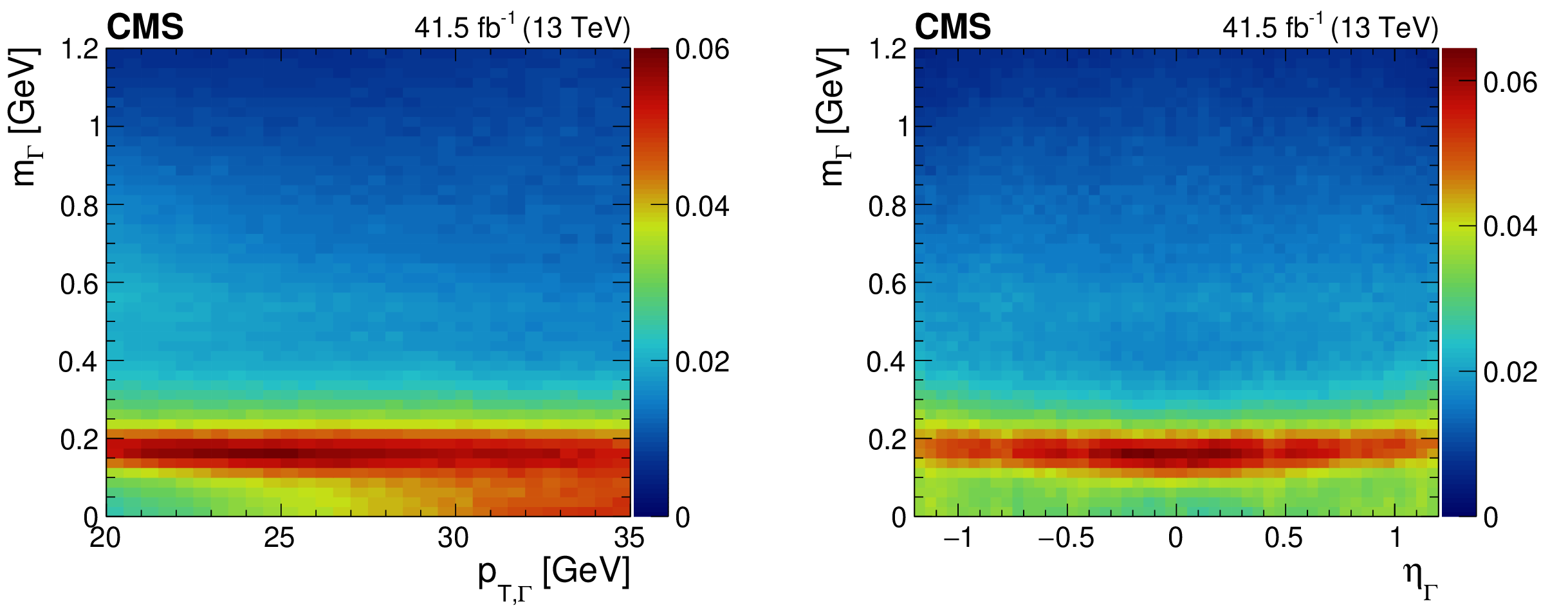
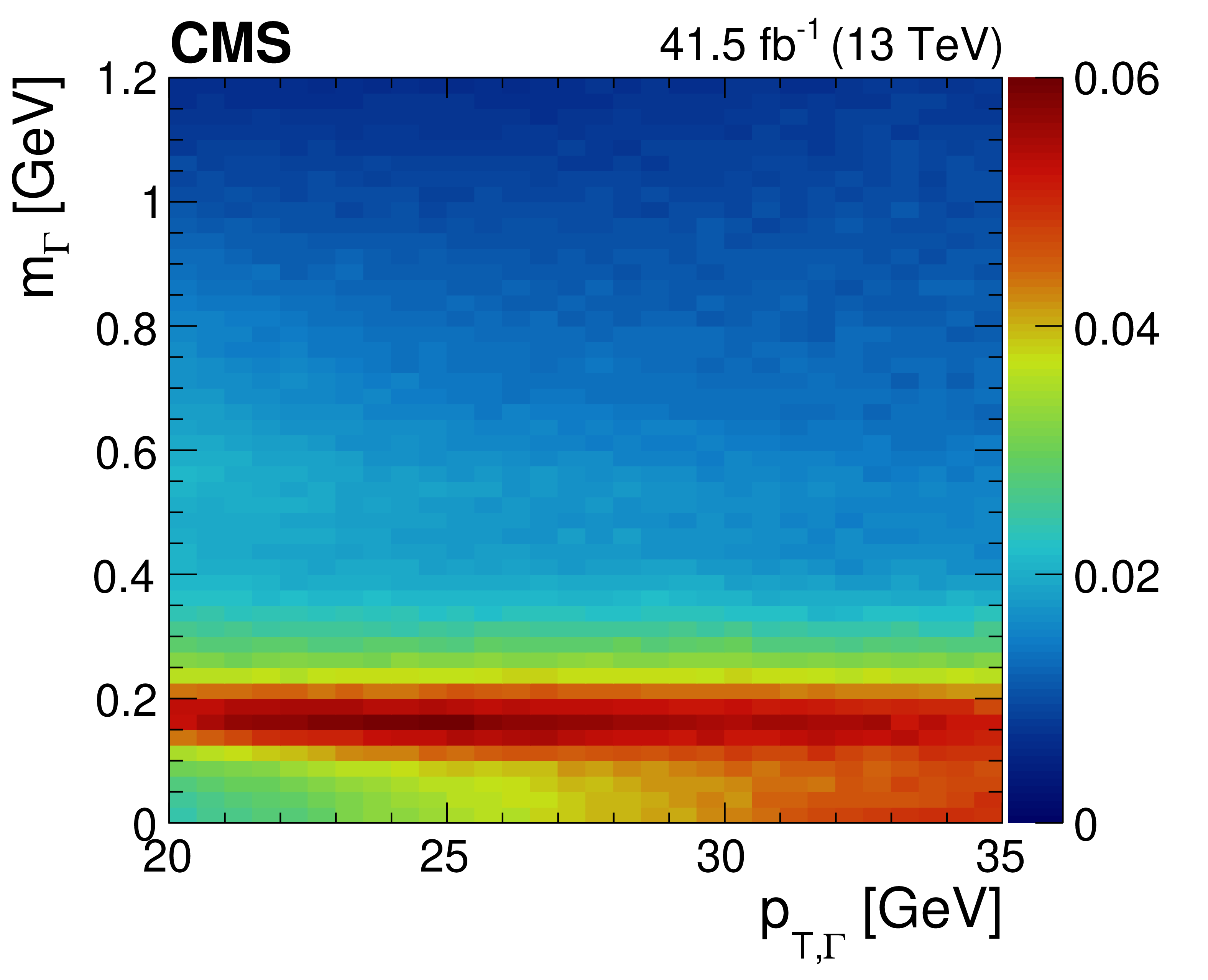
Figure 7:
Regressed mass from $\pi^{0} \to \gamma \gamma $ data events vs. $ {p_{\mathrm {T},\,\Gamma}} $ (left) and $\eta _{\Gamma}$ (right). For both plots, the regressed mass distributions are normalized in vertical slices of the accompanying kinematic quantity to highlight the intrinsic dependence on the quantity. The relative contribution over each vertical slice is given by the color scale to the right of each plot. |
png pdf |
Figure 7-a:
Regressed mass from $\pi^{0} \to \gamma \gamma $ data events vs. $ {p_{\mathrm {T},\,\Gamma}} $. The regressed mass distributions are normalized in vertical slices of the accompanying kinematic quantity to highlight the intrinsic dependence on the quantity. The relative contribution over each vertical slice is given by the color scale to the right of the plot. |
png pdf |
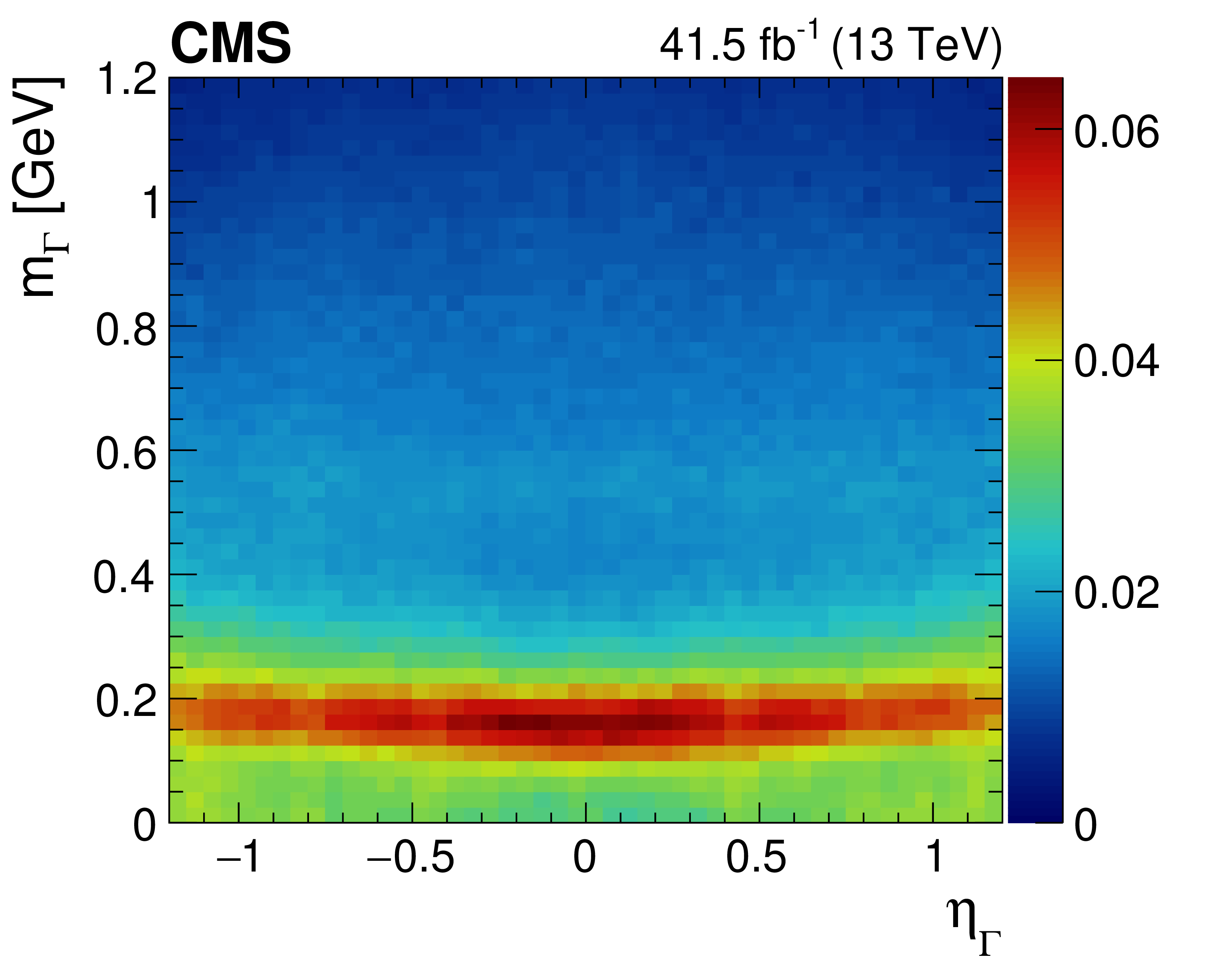
Figure 7-b:
Regressed mass from $\pi^{0} \to \gamma \gamma $ data events vs. $\eta _{\Gamma}$. The regressed mass distributions are normalized in vertical slices of the accompanying kinematic quantity to highlight the intrinsic dependence on the quantity. The relative contribution over each vertical slice is given by the color scale to the right of the plot. |
png pdf |
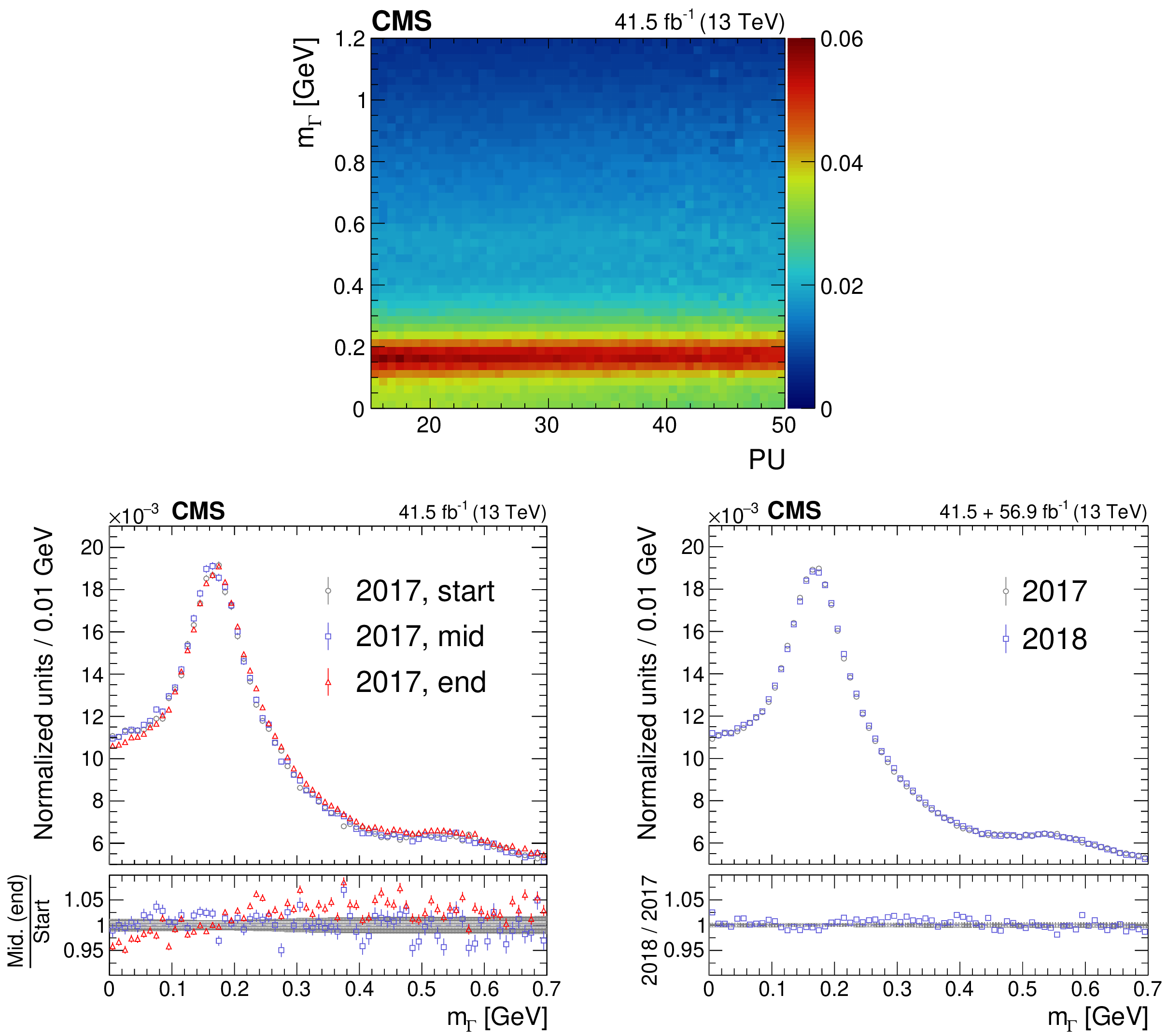
Figure 8:
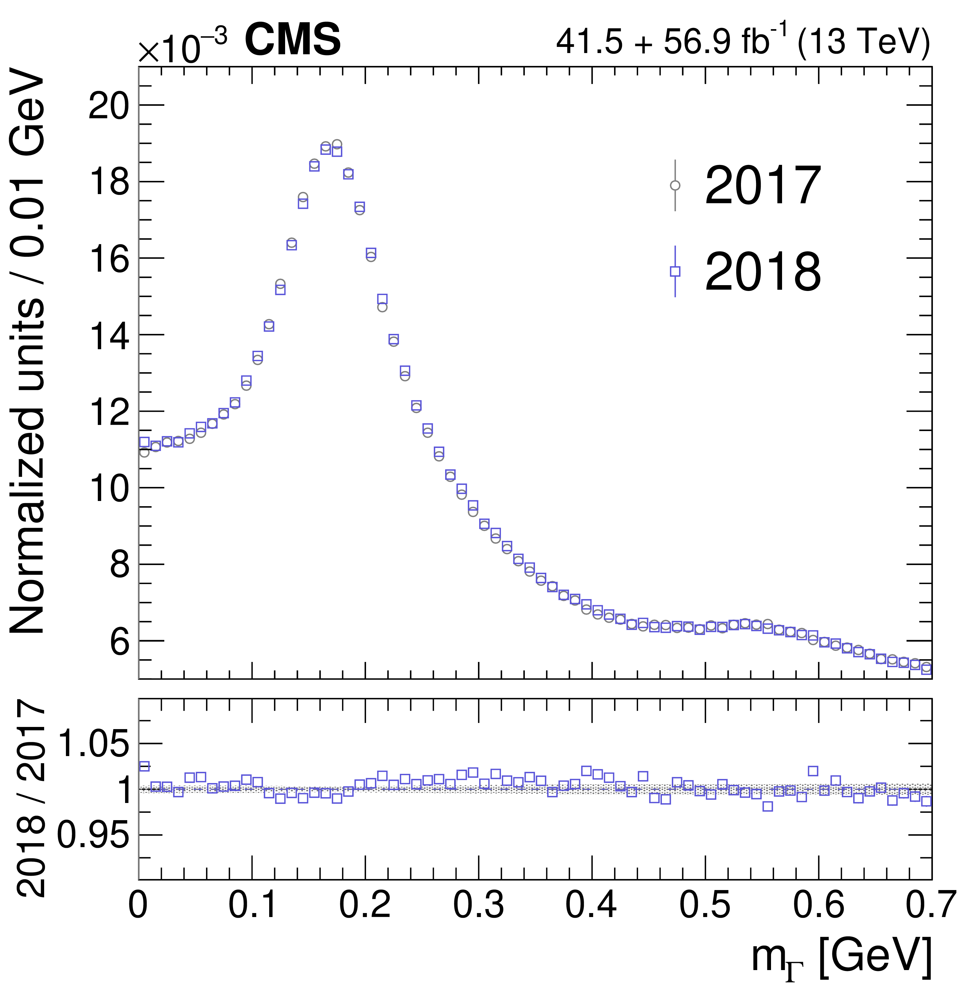
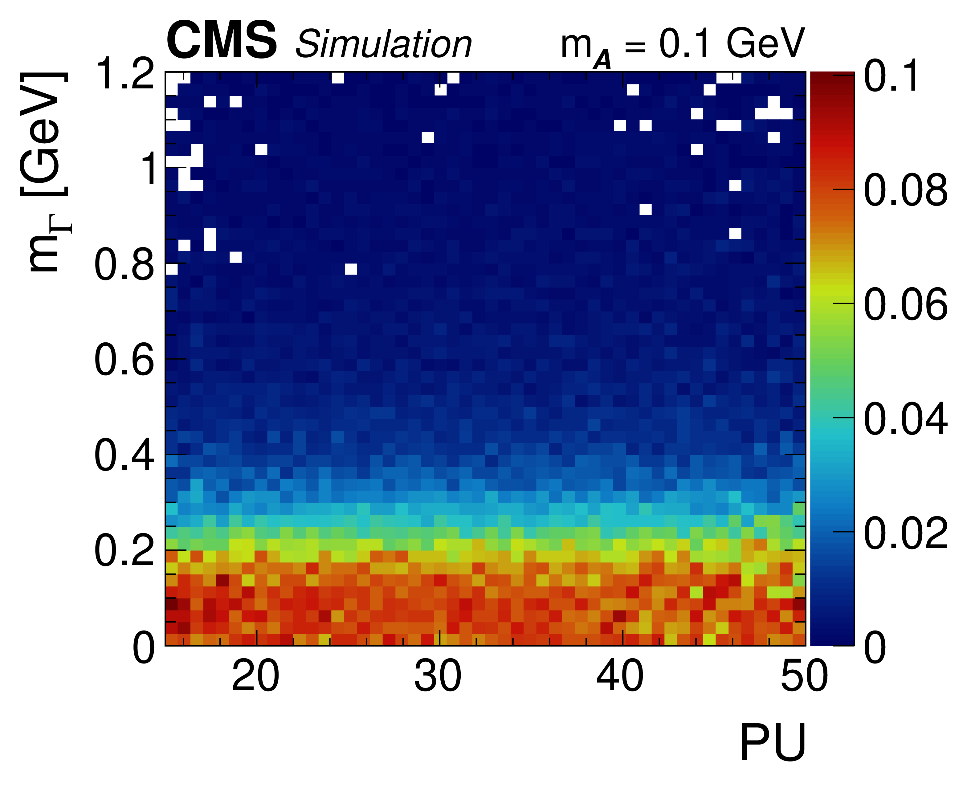
Upper: Two-dimensional plot of the regressed mass for $\pi^{0} \to \gamma \gamma $ data events vs. the amount of pileup (PU). The mass distribution is normalized in vertical slices of the amount of pileup. The relative contribution over each vertical slice is given by the color scale to the right of the plot. Lower left: The regressed mass distributions for the start (gray circles), middle (blue squares), and end (red triangles) of the 2017 data-taking period. Lower right: The regressed mass distributions for the 2017 (gray circles) and 2018 (blue squares) data-taking periods. The lower two plots are normalized to unity and the vertical bars on the points show the statistical uncertainties. The lower panel for the lower left plot gives the ratio of distributions for the middle to the start (blue squares) and the end to the start (red triangles) of the 2017 data-taking period. The lower panel for the lower right plot gives the ratio (blue squares) for the 2018 and 2017 data-taking periods. The vertical bars on the points in both lower panels show the statistical uncertainties in the numerator quantity, and the gray bands give the similar uncertainty in the denominator quantity. |

png pdf |
Figure 8-a:
Two-dimensional plot of the regressed mass for $\pi^{0} \to \gamma \gamma $ data events vs. the amount of pileup (PU). The mass distribution is normalized in vertical slices of the amount of pileup. The relative contribution over each vertical slice is given by the color scale to the right of the plot. |

png pdf |
Figure 8-b:
The regressed mass distributions for the 2017 (gray circles) and 2018 (blue squares) data-taking periods. The plots are normalized to unity and the vertical bars on the points show the statistical uncertainties. The lower panel gives the ratio of distributions for the middle to the start (blue squares) and the end to the start (red triangles) of the 2017 data-taking period. The vertical bars on the points show the statistical uncertainties in the numerator quantity, and the gray band gives the similar uncertainty in the denominator quantity. |
png pdf |
Figure 8-c:
The regressed mass distributions for the 2017 (gray circles) and 2018 (blue squares) data-taking periods. The plots are normalized to unity and the vertical bars on the points show the statistical uncertainties. The lower panel gives the ratio (blue squares) for the 2018 and 2017 data-taking periods. The vertical bars on the points show the statistical uncertainties in the numerator quantity, and the gray band gives the similar uncertainty in the denominator quantity. |

png pdf |
Figure 9:
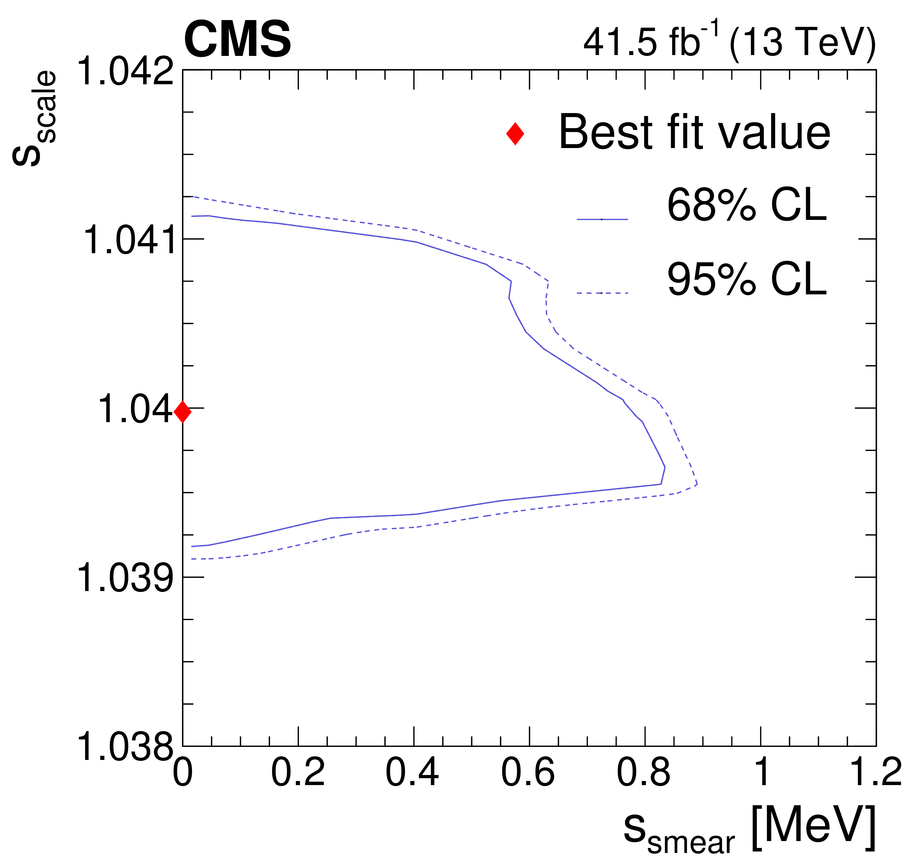
The agreement in the regressed $m_{\Gamma}$ spectrum between electrons in data versus simulation. Left: Contours of 68% (solid line) and 95% (dotted line) confidence level (CL) in the $\chi ^2$ test statistic as a function of the ($s_{\mathrm {scale}}$, $s_{\mathrm {smear}}$) hypothesis. The best fit point ($s_{\mathrm {scale}}=$ 1.040, $s_{\mathrm {smear}} = $ 0 MeV) is indicated by the red diamond. Right: The regressed mass distributions in data (points) and the best fit Monte Carlo (MC) simulation (blue region) for electrons from $\mathrm{Z} \to \mathrm{e^{+}} \mathrm{e^{-}} $ events. The difference between the simulated distribution under the null scale and smearing hypothesis versus the best fit hypothesis (Syst) is plotted as a green band. Each of the distributions are normalized to unity, including samples outside $m_{\mathcal{A}}$-ROI. Statistical uncertainties in the data distribution are negligible. The lower panel shows the ratio of the data to the simulation under the best fit hypothesis (points). The statistical uncertainties in the latter are plotted as a blue band. The ratio of the simulated distribution for the null to the best fit hypothesis is displayed as a green band. |
png pdf |
Figure 9-a:
The agreement in the regressed $m_{\Gamma}$ spectrum between electrons in data versus simulation: Contours of 68% (solid line) and 95% (dotted line) confidence level (CL) in the $\chi ^2$ test statistic as a function of the ($s_{\mathrm {scale}}$, $s_{\mathrm {smear}}$) hypothesis. The best fit point ($s_{\mathrm {scale}}=$ 1.040, $s_{\mathrm {smear}} = $ 0 MeV) is indicated by the red diamond. |

png pdf |
Figure 9-b:
The regressed mass distributions in data (points) and the best fit Monte Carlo (MC) simulation (blue region) for electrons from $\mathrm{Z} \to \mathrm{e^{+}} \mathrm{e^{-}} $ events. The difference between the simulated distribution under the null scale and smearing hypothesis versus the best fit hypothesis (Syst) is plotted as a green band. Each of the distributions are normalized to unity, including samples outside $m_{\mathcal{A}}$-ROI. Statistical uncertainties in the data distribution are negligible. The lower panel shows the ratio of the data to the simulation under the best fit hypothesis (points). The statistical uncertainties in the latter are plotted as a blue band. The ratio of the simulated distribution for the null to the best fit hypothesis is displayed as a green band. |
png pdf |
Figure A1:
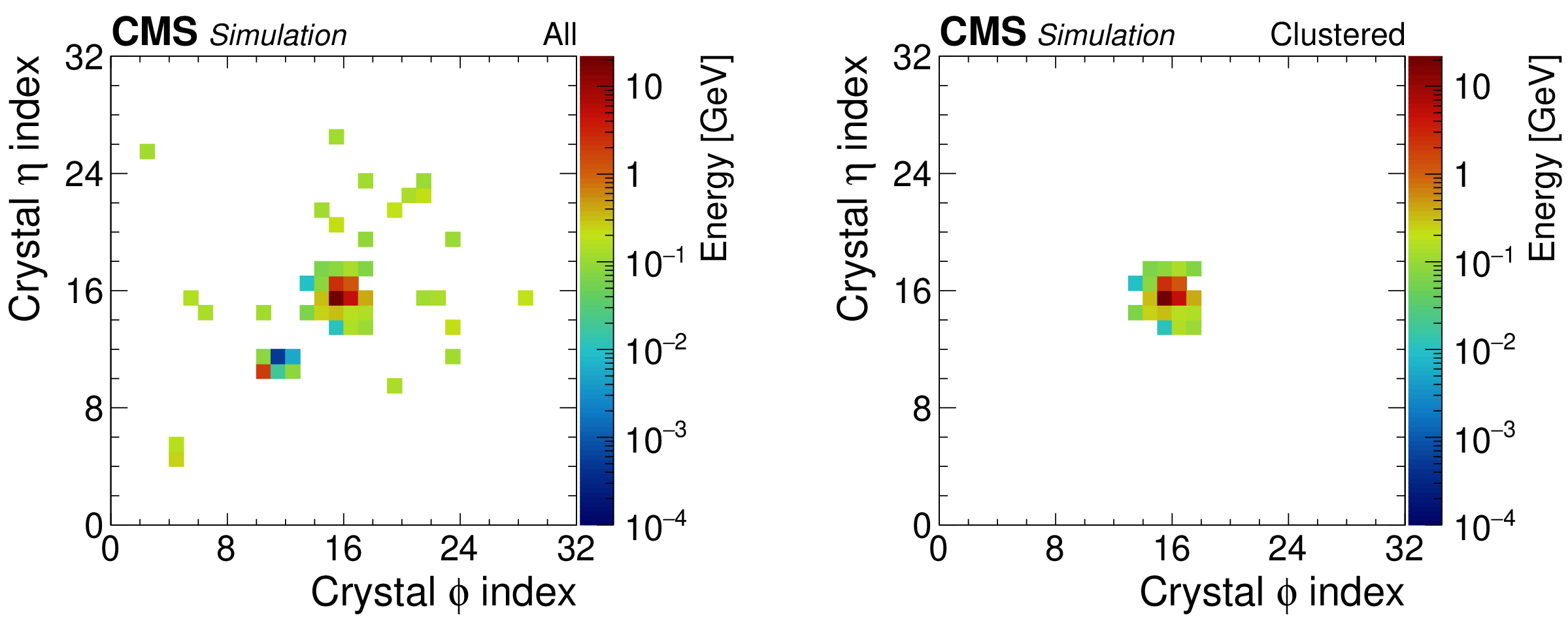
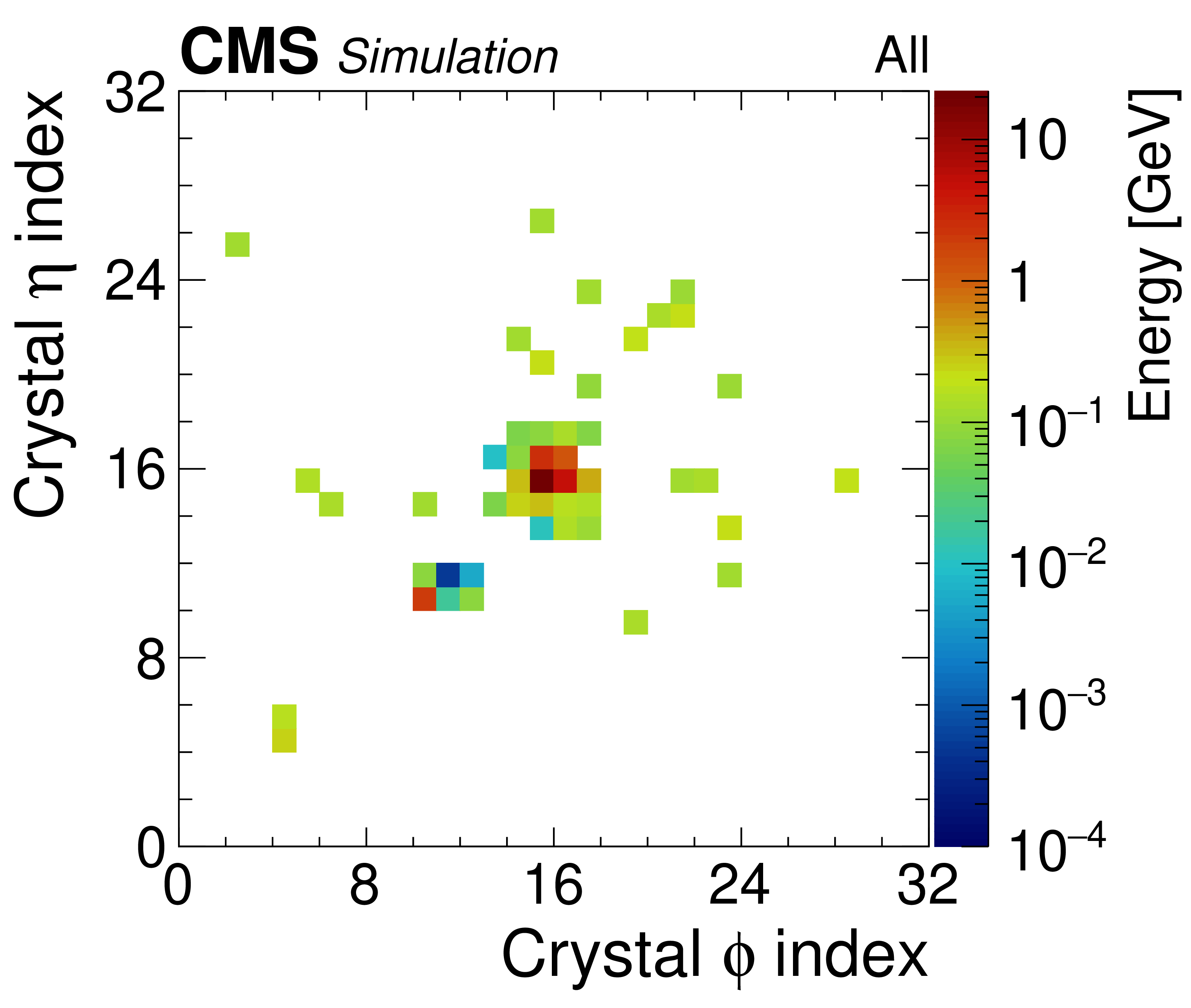
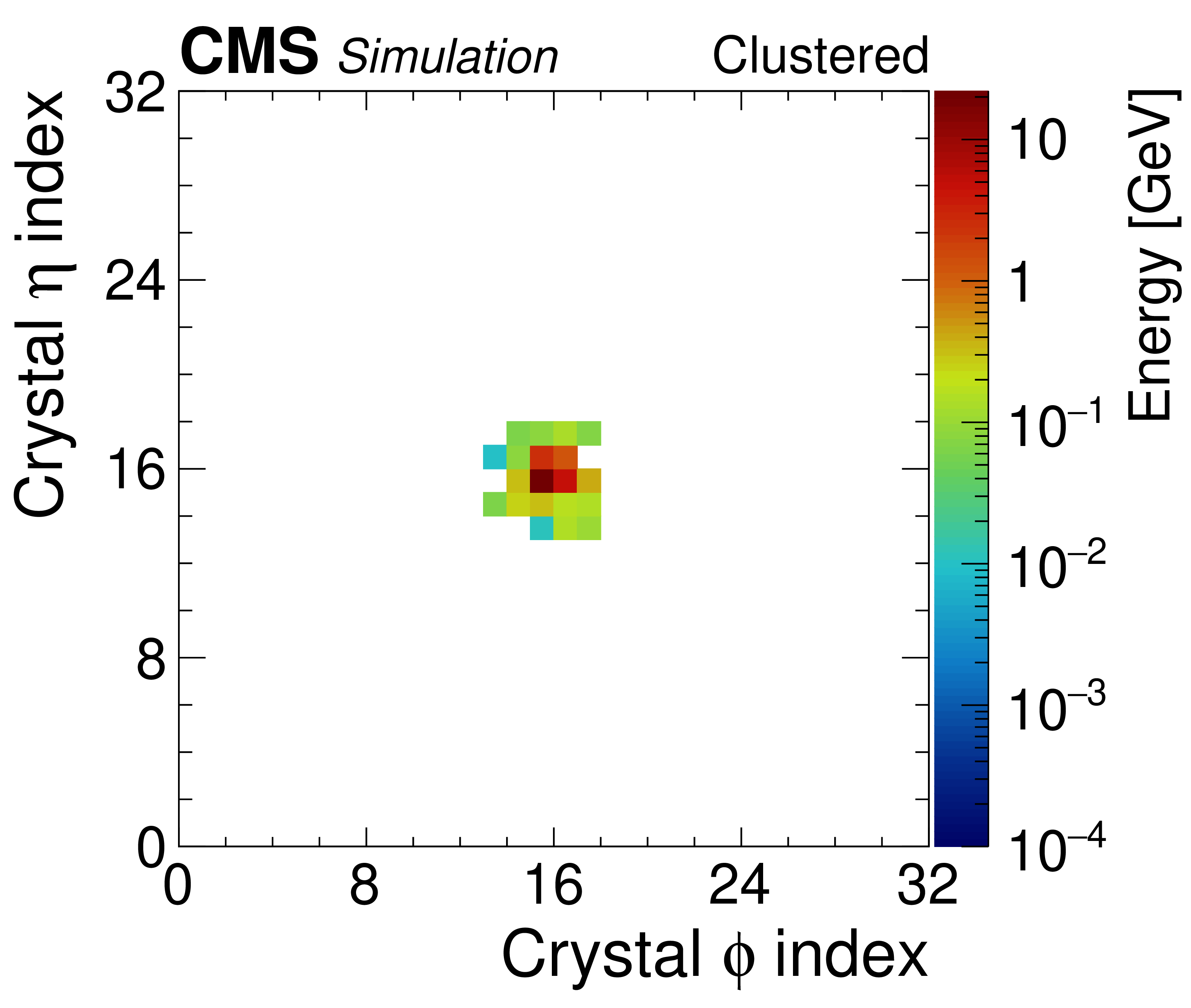
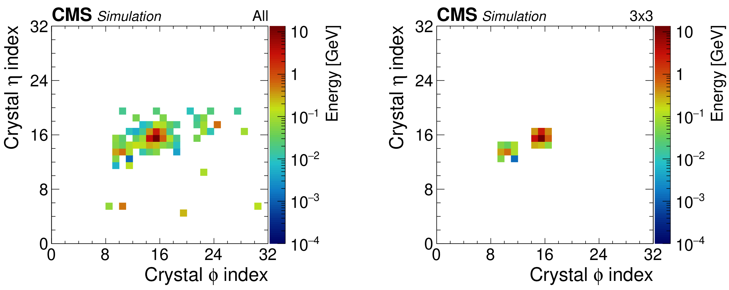
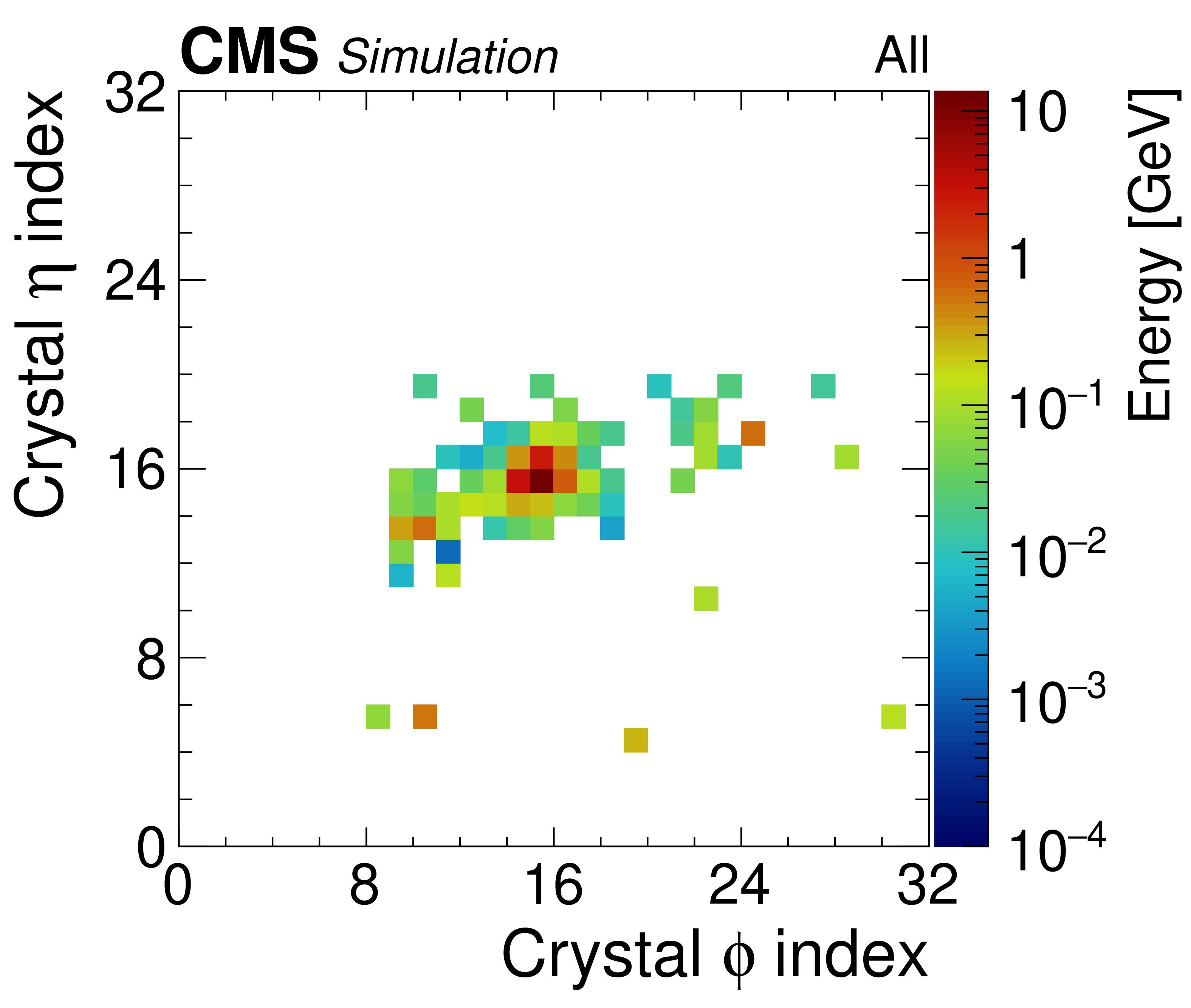
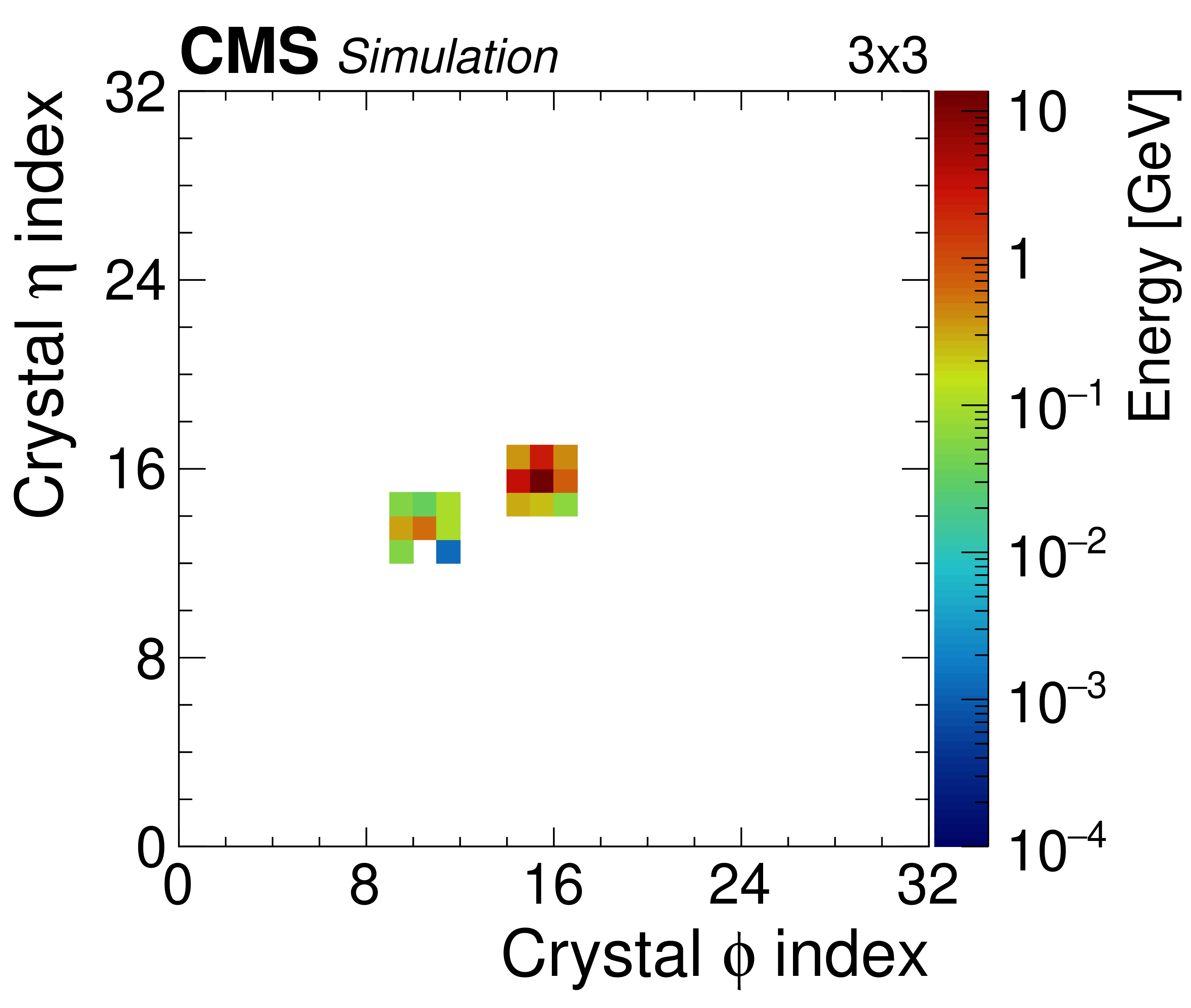
A typical $ {\mathcal{A}} \to \gamma \gamma $ decay using minimally processed (left) and clustered (right) data. The energy distributions are plotted in relative ECAL crystal index coordinates of the pseudorapidity $\eta $ versus the azimuthal angle $\phi $ and color coded by energy. |
png pdf |
Figure A1-a:
A typical $ {\mathcal{A}} \to \gamma \gamma $ decay using minimally processed data. The energy distributions are plotted in relative ECAL crystal index coordinates of the pseudorapidity $\eta $ versus the azimuthal angle $\phi $ and color coded by energy. |
png pdf |
Figure A1-b:
A typical $ {\mathcal{A}} \to \gamma \gamma $ decay using clustered data. The energy distributions are plotted in relative ECAL crystal index coordinates of the pseudorapidity $\eta $ versus the azimuthal angle $\phi $ and color coded by energy. |

png pdf |
Figure A2:
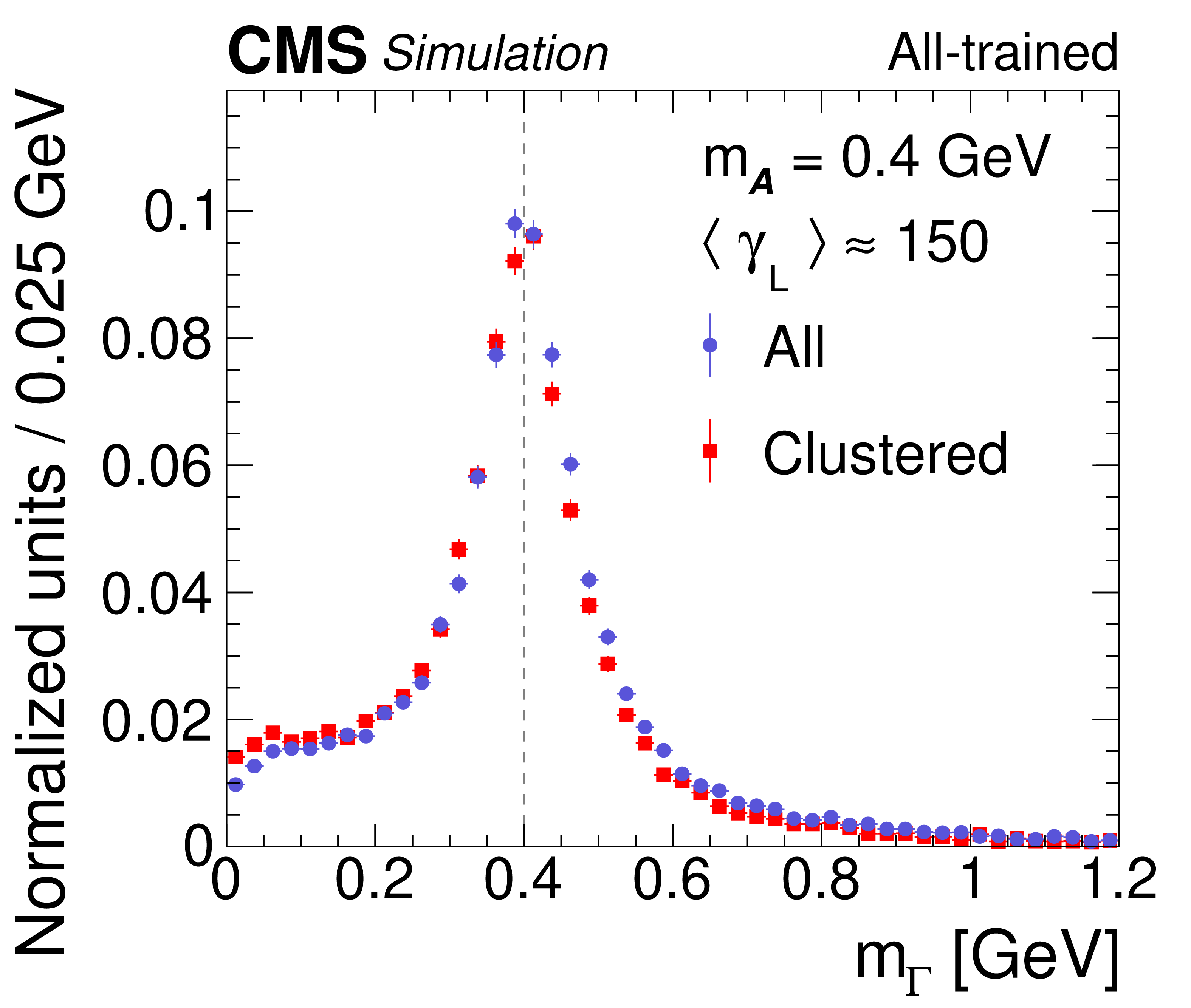
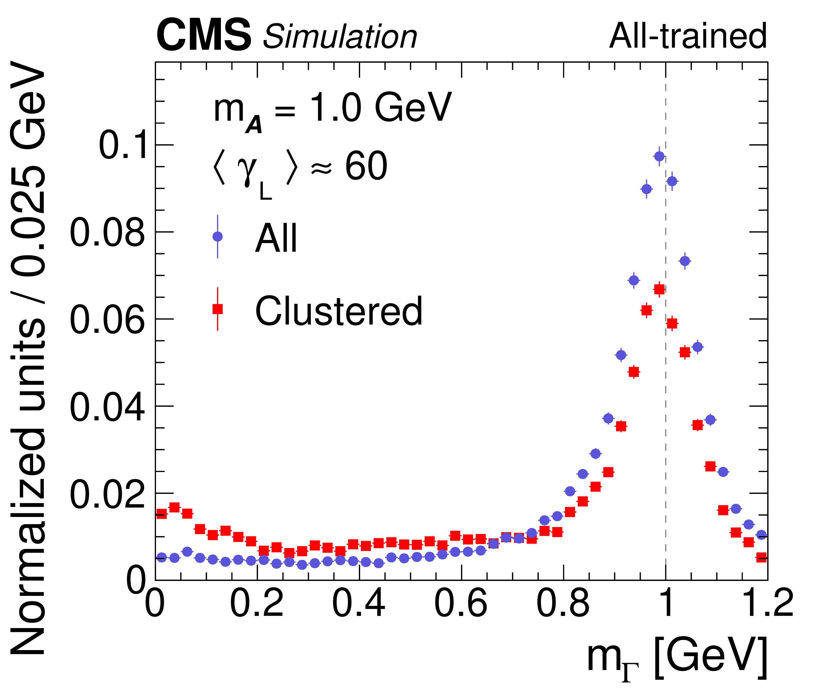
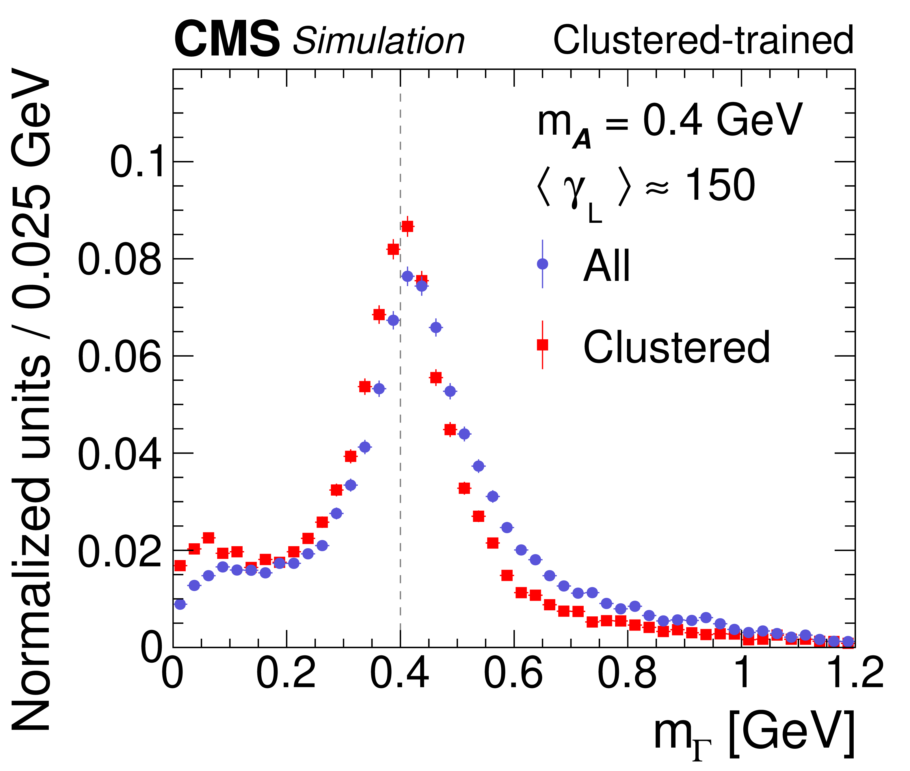
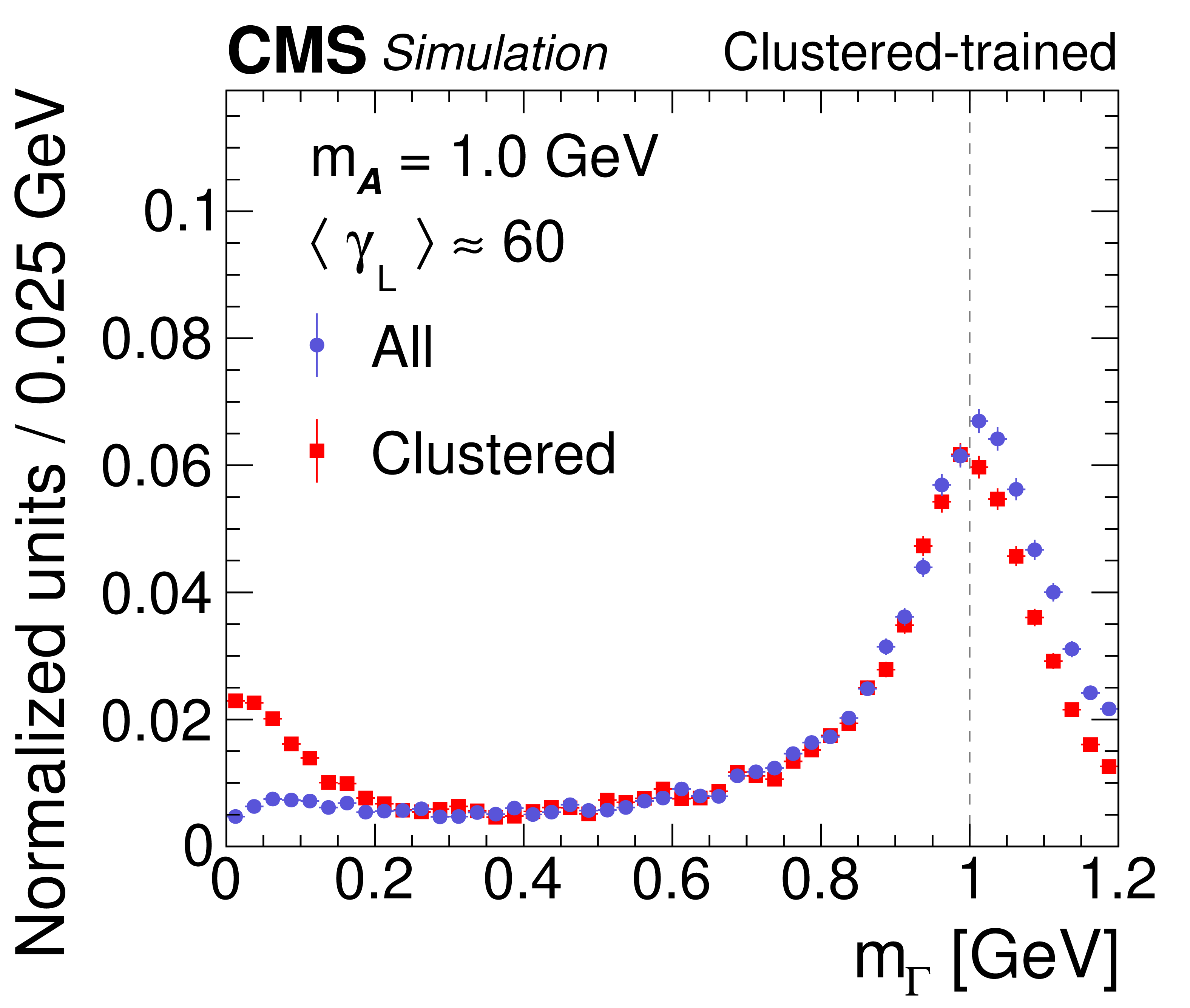
Regressed mass spectra for the mass regressor trained on minimally processed data (upper) versus clustered data (lower) at shower-merged boosts (left) and barely resolved boosts (right). For each scenario, the mass regressor is run on the same set of $ {\mathcal{A}} \to \gamma \gamma $ decays, composed either of minimally processed (blue circles, all) or clustered (red squares, clustered) data. The vertical bars on the points give the statistical uncertainties and the vertical dotted line shows the input $m_{{\mathcal{A}}}$ value. |
png pdf |
Figure A2-a:
Regressed mass spectra for the mass regressor trained on minimally processed data at shower-merged boosts. The mass regressor is run on the set of $ {\mathcal{A}} \to \gamma \gamma $ decays that is composed either of minimally processed (blue circles, all) or clustered (red squares, clustered) data. The vertical bars on the points give the statistical uncertainties and the vertical dotted line shows the input $m_{{\mathcal{A}}}$ value. |
png pdf |
Figure A2-b:
Regressed mass spectra for the mass regressor trained on minimally processed data at barely resolved boosts. The mass regressor is run on the set of $ {\mathcal{A}} \to \gamma \gamma $ decays that is composed either of minimally processed (blue circles, all) or clustered (red squares, clustered) data. The vertical bars on the points give the statistical uncertainties and the vertical dotted line shows the input $m_{{\mathcal{A}}}$ value. |
png pdf |
Figure A2-c:
Regressed mass spectra for the mass regressor trained on clustered data at shower-merged boosts. The mass regressor is run on the set of $ {\mathcal{A}} \to \gamma \gamma $ decays that is composed either of minimally processed (blue circles, all) or clustered (red squares, clustered) data. The vertical bars on the points give the statistical uncertainties and the vertical dotted line shows the input $m_{{\mathcal{A}}}$ value. |
png pdf |
Figure A2-d:
Regressed mass spectra for the mass regressor trained on clustered data at barely resolved boosts. The mass regressor is run on the set of $ {\mathcal{A}} \to \gamma \gamma $ decays that is composed either of minimally processed (blue circles, all) or clustered (red squares, clustered) data. The vertical bars on the points give the statistical uncertainties and the vertical dotted line shows the input $m_{{\mathcal{A}}}$ value. |
png pdf |
Figure A3:
A typical hadronic jet sample reconstructed by the 3${\times}$3 algorithm with a mass near the $\eta $ meson peak, using minimally processed (all, left) and 3${\times}$3 clustered (3${\times}$3, right) data. The energy distributions are plotted in relative ECAL crystal index coordinates of the azimuthal angle $\phi $ versus the pseudorapidity $\eta $ and color coded by energy. |
png pdf |
Figure A3-a:
A typical hadronic jet sample reconstructed by the 3${\times}$3 algorithm with a mass near the $\eta $ meson peak, using minimally processed (all) data. The energy distributions are plotted in relative ECAL crystal index coordinates of the azimuthal angle $\phi $ versus the pseudorapidity $\eta $ and color coded by energy. |
png pdf |
Figure A3-b:
A typical hadronic jet sample reconstructed by the 3${\times}$3 algorithm with a mass near the $\eta $ meson peak, using 3${\times}$3 clustered (3${\times}$3) data. The energy distributions are plotted in relative ECAL crystal index coordinates of the azimuthal angle $\phi $ versus the pseudorapidity $\eta $ and color coded by energy. |
png pdf |
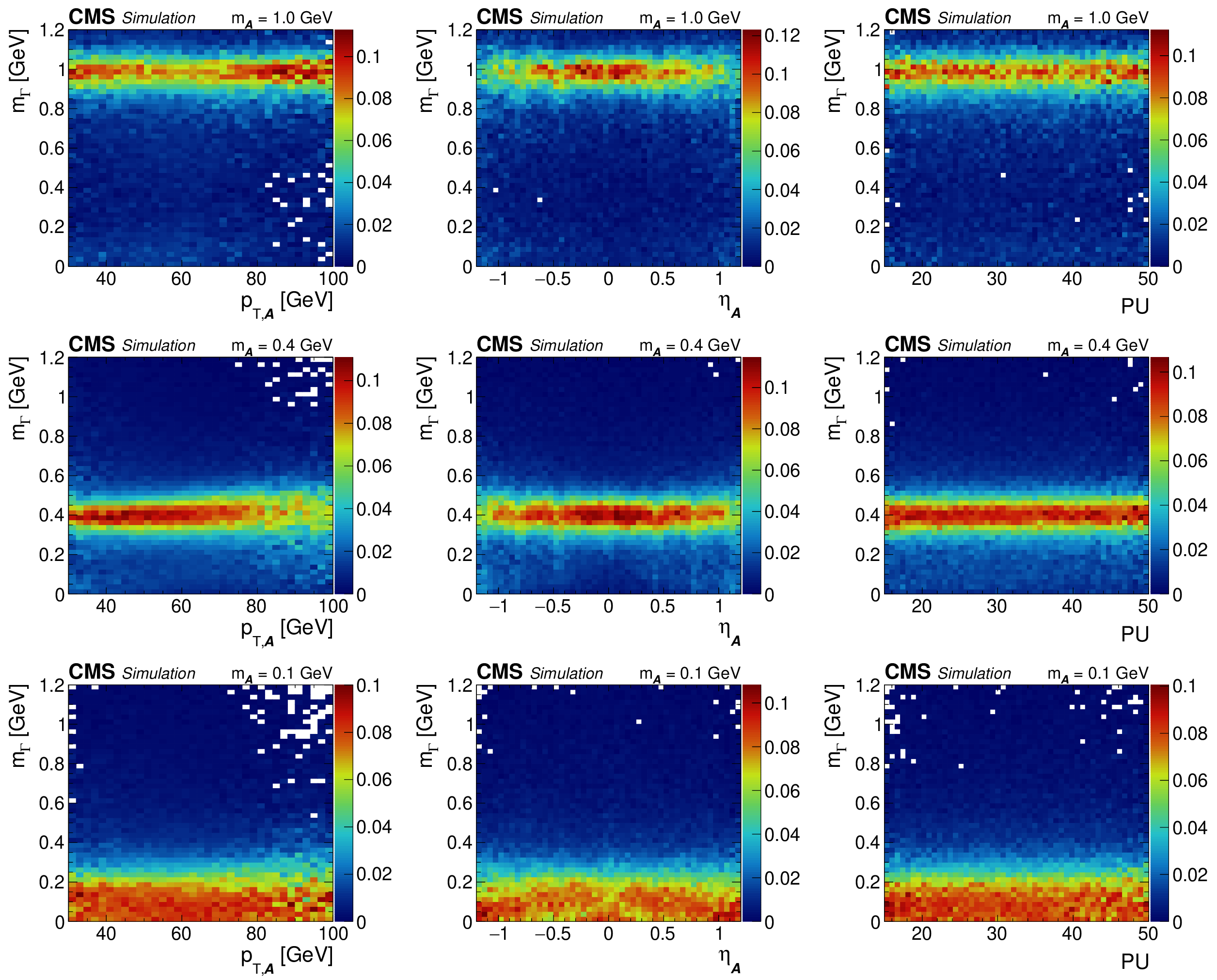
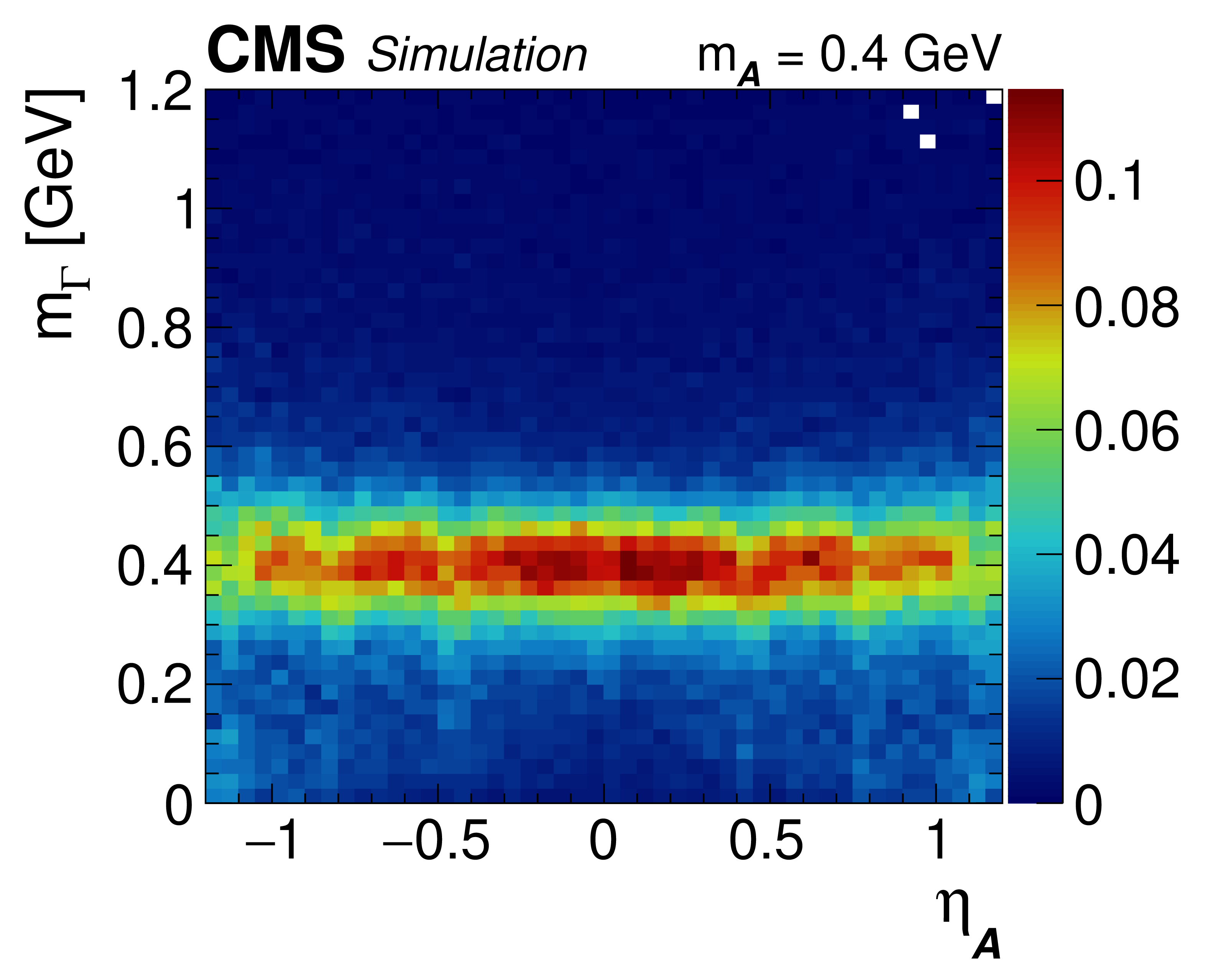
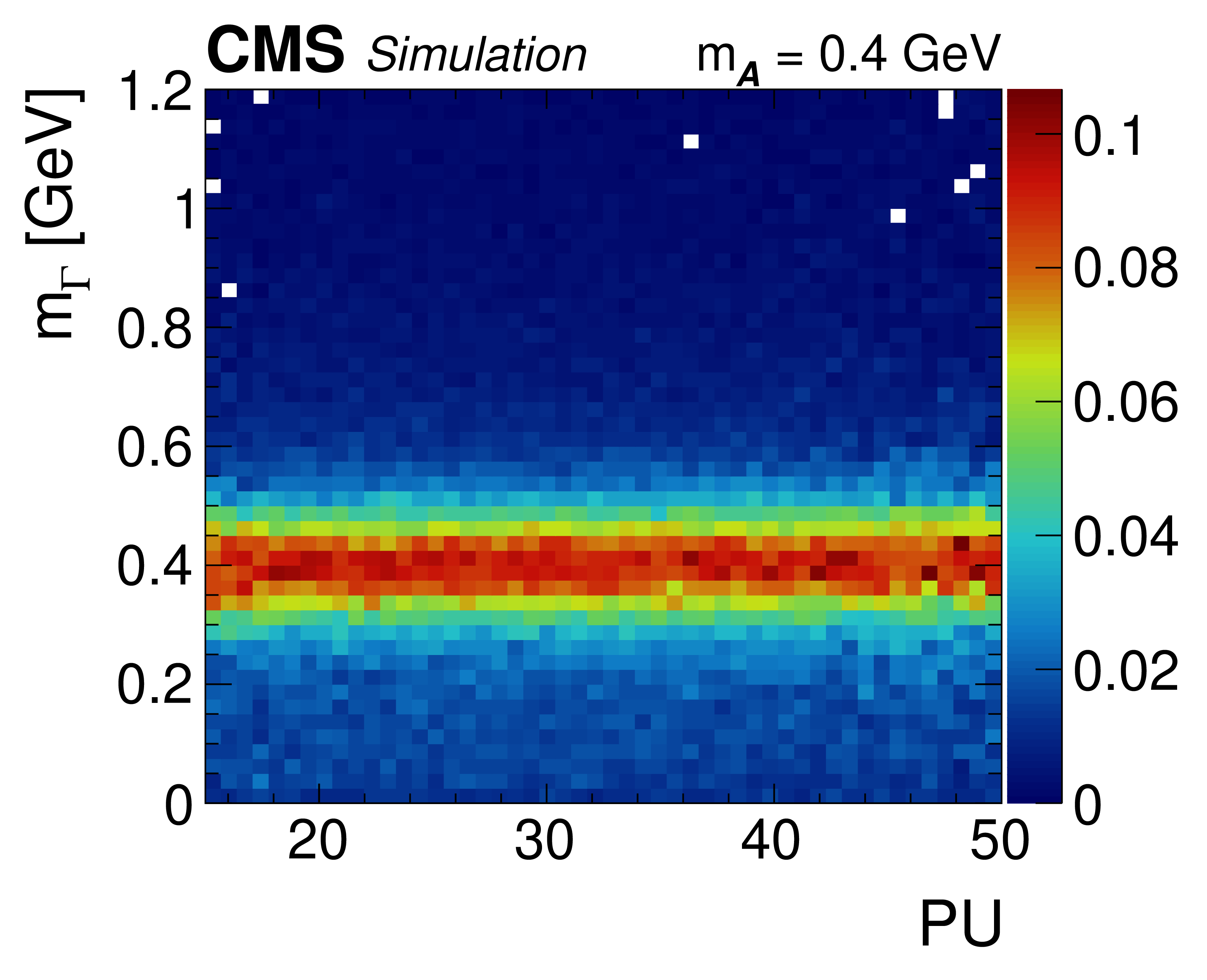
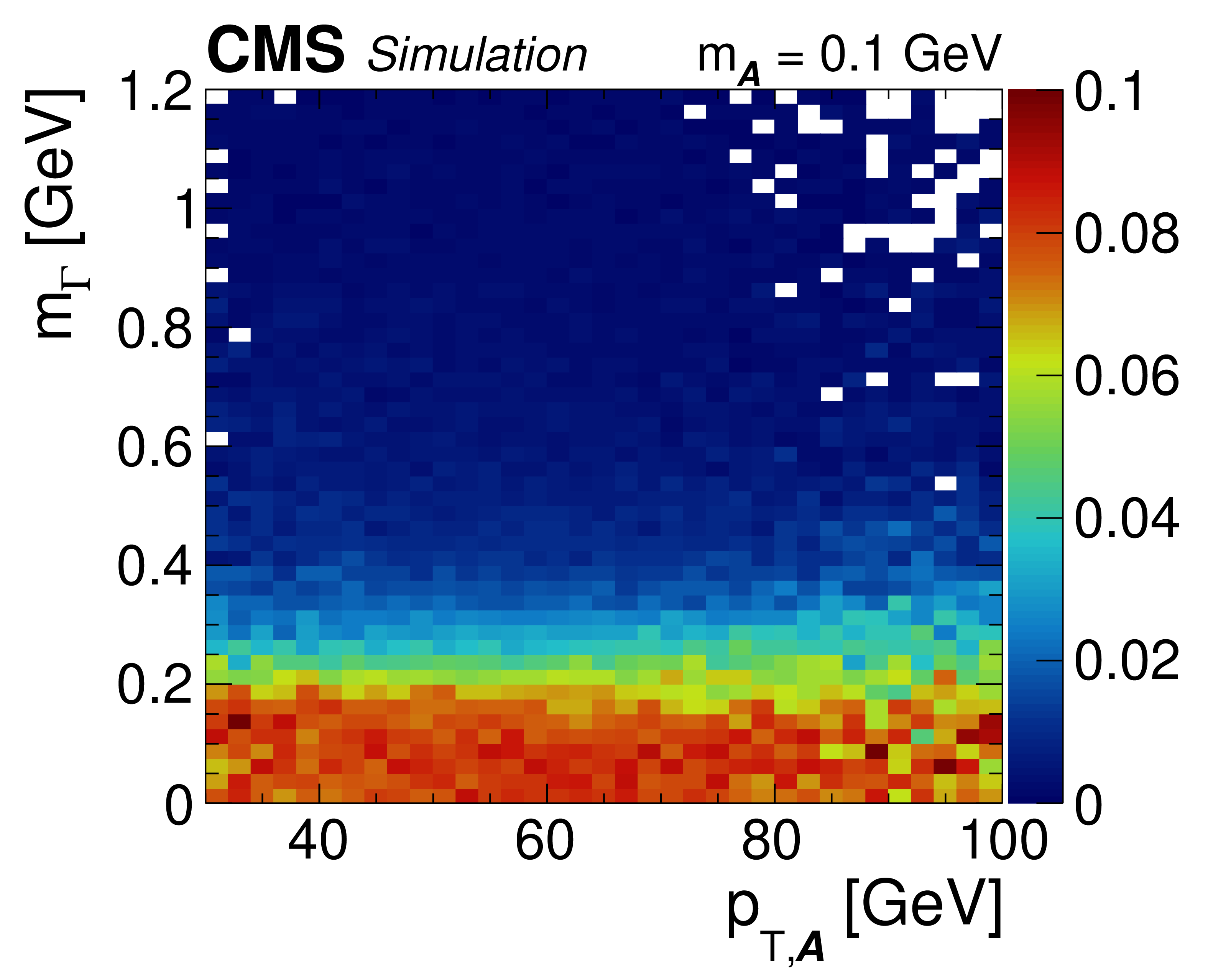
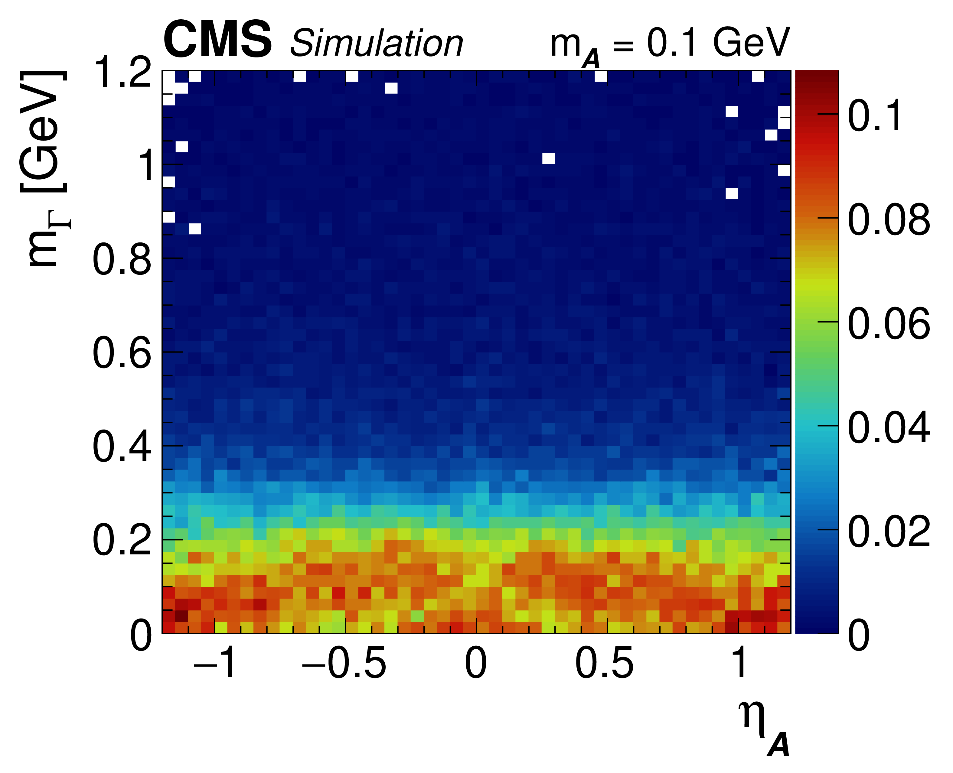
Figure A4:
Regressed mass spectra vs. generated $ {p_{\mathrm {T,\, {\mathcal{A}}}}} $ (left), generated $ {\eta _{{\mathcal{A}}}} $ (center), and amount of pileup (right), for $ {\mathcal{A}} \to \gamma \gamma $ decays that are barely resolved (upper), shower merged (middle), or instrumentally merged (lower). The $ {\mathcal{A}} \to \gamma \gamma $ decays are obtained from simulated $\mathrm{H} \to {\mathcal{A}} {\mathcal{A}} \to 4 \gamma $ events. In all plots, the regressed mass distribution is normalized in vertical slices of the quantity of interest. The relative contribution over each vertical slice is given by the color scale to the right of each plot. |
png pdf |
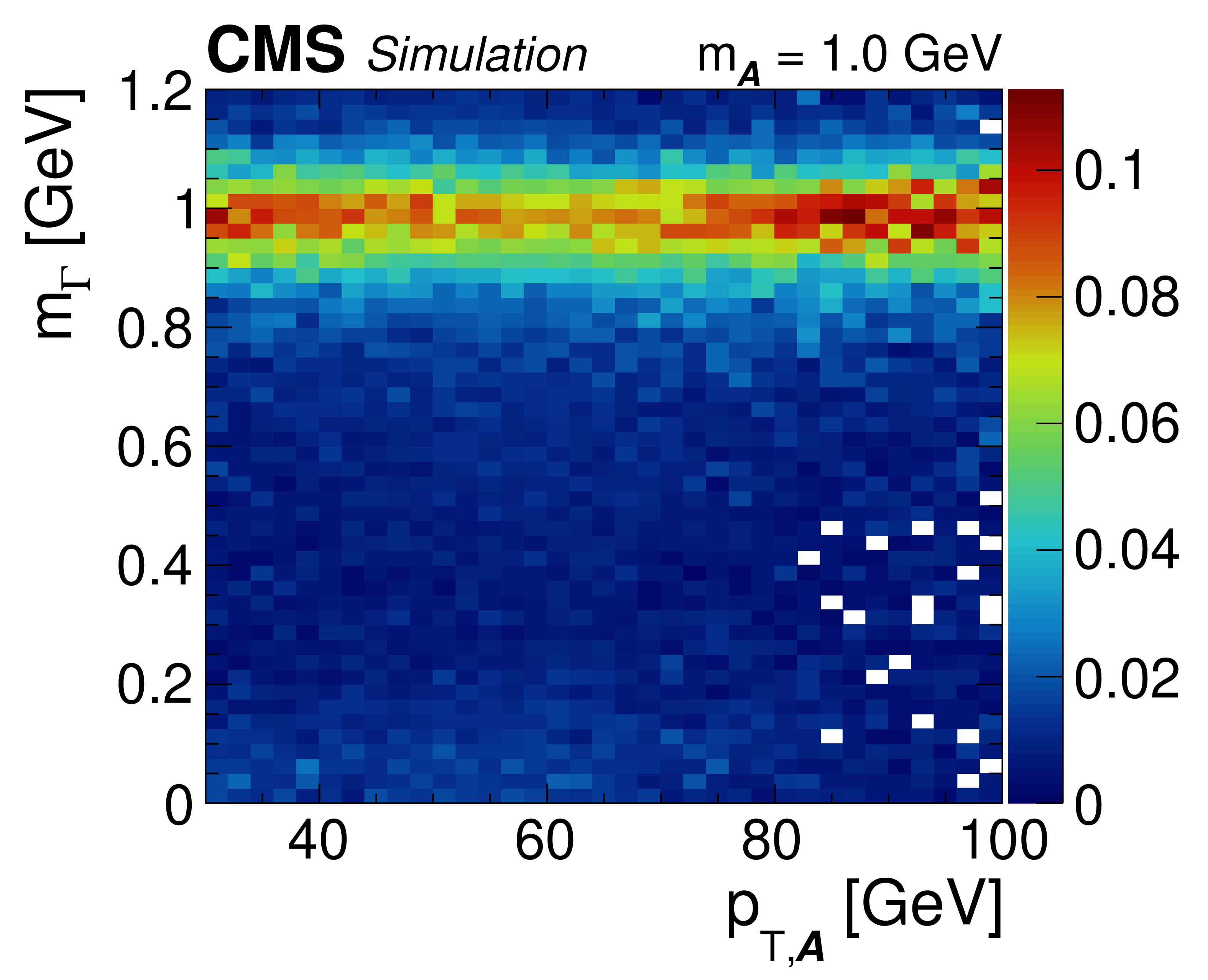
Figure A4-a:
Regressed mass spectra vs. generated $ {p_{\mathrm {T,\, {\mathcal{A}}}}} $ for $ {\mathcal{A}} \to \gamma \gamma $ decays that are barely resolved. The $ {\mathcal{A}} \to \gamma \gamma $ decays are obtained from simulated $\mathrm{H} \to {\mathcal{A}} {\mathcal{A}} \to 4 \gamma $ events. The regressed mass distribution is normalized in vertical slices of the quantity of interest. The relative contribution over each vertical slice is given by the color scale to the right of the plot. |
png pdf |
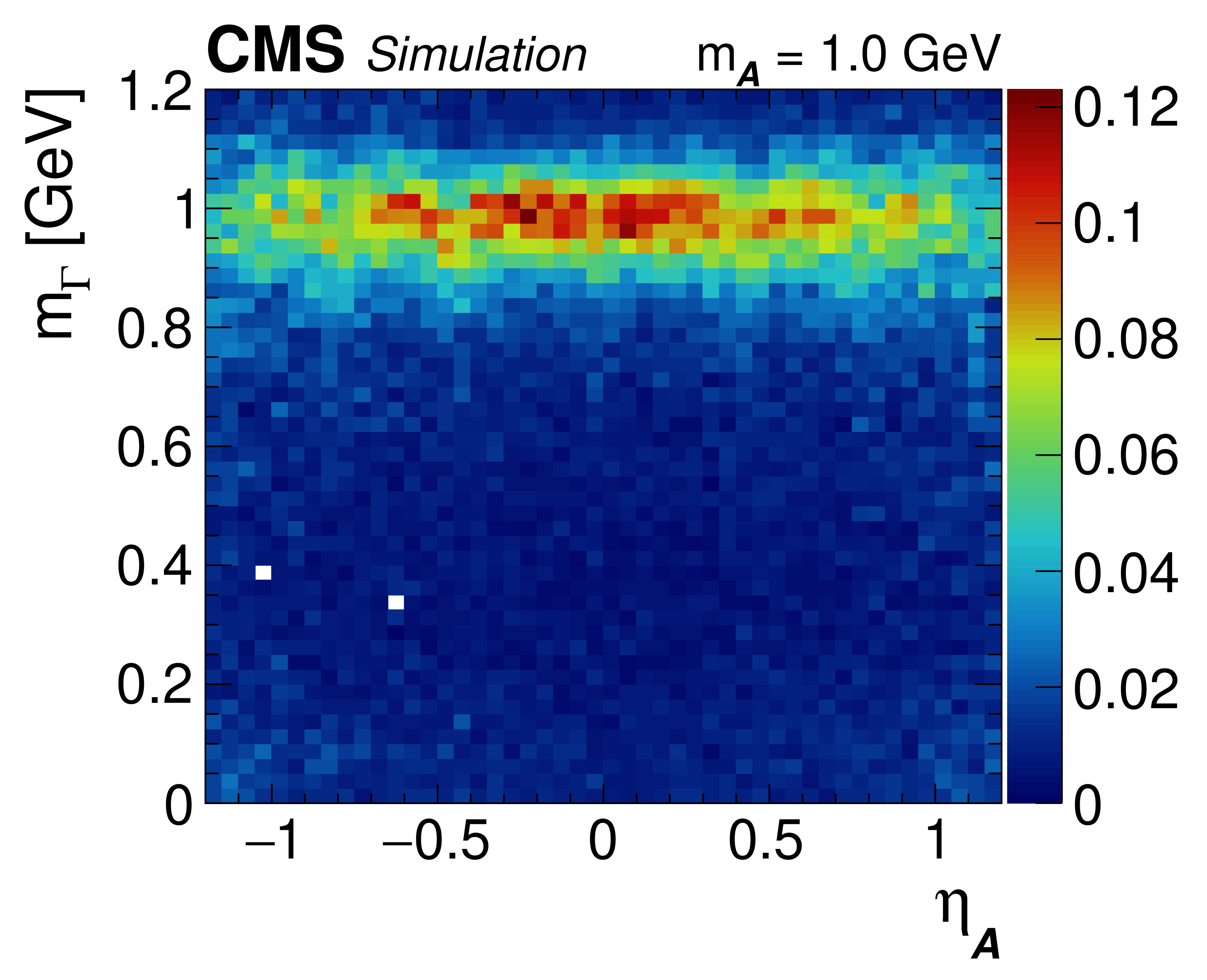
Figure A4-b:
Regressed mass spectra vs. generated $ {\eta _{{\mathcal{A}}}} $ for $ {\mathcal{A}} \to \gamma \gamma $ decays that are shower merged. The $ {\mathcal{A}} \to \gamma \gamma $ decays are obtained from simulated $\mathrm{H} \to {\mathcal{A}} {\mathcal{A}} \to 4 \gamma $ events. The regressed mass distribution is normalized in vertical slices of the quantity of interest. The relative contribution over each vertical slice is given by the color scale to the right of the plot. |

png pdf |
Figure A4-c:
Regressed mass spectra vs. amount of pileup for $ {\mathcal{A}} \to \gamma \gamma $ decays that are instrumentally merged. The $ {\mathcal{A}} \to \gamma \gamma $ decays are obtained from simulated $\mathrm{H} \to {\mathcal{A}} {\mathcal{A}} \to 4 \gamma $ events. The regressed mass distribution is normalized in vertical slices of the quantity of interest. The relative contribution over each vertical slice is given by the color scale to the right of the plot. |
png pdf |
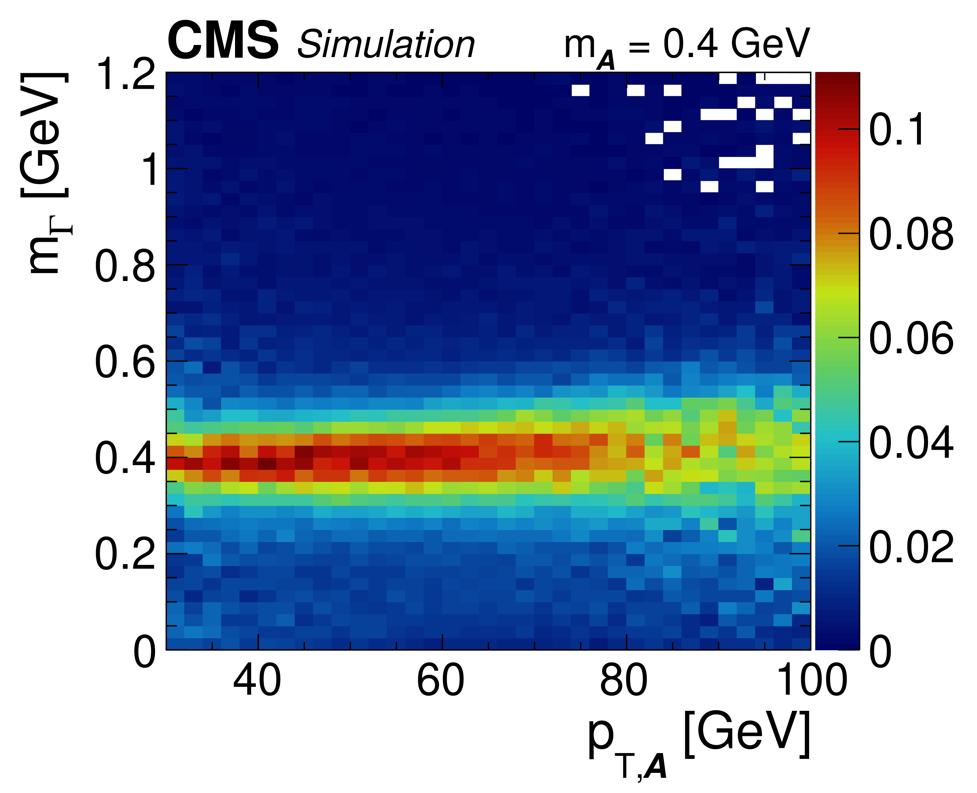
Figure A4-d:
Regressed mass spectra vs. generated $ {p_{\mathrm {T,\, {\mathcal{A}}}}} $ for $ {\mathcal{A}} \to \gamma \gamma $ decays that are barely resolved. The $ {\mathcal{A}} \to \gamma \gamma $ decays are obtained from simulated $\mathrm{H} \to {\mathcal{A}} {\mathcal{A}} \to 4 \gamma $ events. The regressed mass distribution is normalized in vertical slices of the quantity of interest. The relative contribution over each vertical slice is given by the color scale to the right of the plot. |
png pdf |
Figure A4-e:
Regressed mass spectra vs. generated $ {\eta _{{\mathcal{A}}}} $ for $ {\mathcal{A}} \to \gamma \gamma $ decays that are shower merged. The $ {\mathcal{A}} \to \gamma \gamma $ decays are obtained from simulated $\mathrm{H} \to {\mathcal{A}} {\mathcal{A}} \to 4 \gamma $ events. The regressed mass distribution is normalized in vertical slices of the quantity of interest. The relative contribution over each vertical slice is given by the color scale to the right of the plot. |
png pdf |
Figure A4-f:
Regressed mass spectra vs. amount of pileup for $ {\mathcal{A}} \to \gamma \gamma $ decays that are instrumentally merged. The $ {\mathcal{A}} \to \gamma \gamma $ decays are obtained from simulated $\mathrm{H} \to {\mathcal{A}} {\mathcal{A}} \to 4 \gamma $ events. The regressed mass distribution is normalized in vertical slices of the quantity of interest. The relative contribution over each vertical slice is given by the color scale to the right of the plot. |
png pdf |
Figure A4-g:
Regressed mass spectra vs. generated $ {p_{\mathrm {T,\, {\mathcal{A}}}}} $ for $ {\mathcal{A}} \to \gamma \gamma $ decays that are barely resolved. The $ {\mathcal{A}} \to \gamma \gamma $ decays are obtained from simulated $\mathrm{H} \to {\mathcal{A}} {\mathcal{A}} \to 4 \gamma $ events. The regressed mass distribution is normalized in vertical slices of the quantity of interest. The relative contribution over each vertical slice is given by the color scale to the right of the plot. |
png pdf |
Figure A4-h:
Regressed mass spectra vs. generated $ {\eta _{{\mathcal{A}}}} $ for $ {\mathcal{A}} \to \gamma \gamma $ decays that are shower merged. The $ {\mathcal{A}} \to \gamma \gamma $ decays are obtained from simulated $\mathrm{H} \to {\mathcal{A}} {\mathcal{A}} \to 4 \gamma $ events. The regressed mass distribution is normalized in vertical slices of the quantity of interest. The relative contribution over each vertical slice is given by the color scale to the right of the plot. |
png pdf |
Figure A4-i:
Regressed mass spectra vs. amount of pileup for $ {\mathcal{A}} \to \gamma \gamma $ decays that are instrumentally merged. The $ {\mathcal{A}} \to \gamma \gamma $ decays are obtained from simulated $\mathrm{H} \to {\mathcal{A}} {\mathcal{A}} \to 4 \gamma $ events. The regressed mass distribution is normalized in vertical slices of the quantity of interest. The relative contribution over each vertical slice is given by the color scale to the right of the plot. |
| Summary |
| A novel end-to-end particle reconstruction technique is introduced that is able to serve as a general strategy for reconstructing decays of boosted particles. The method involves the use of deep learning algorithms that do not rely on particle-flow objects, but are trained directly on minimally processed detector-level data to reconstruct particle properties of interest. Using simulated $ \mathcal{A}\to\gamma\gamma $ decays in the CMS electromagnetic calorimeter, where $ \mathcal{A} $ is a hypothetical scalar particle, the technique is used to reconstruct the diphoton invariant mass over a wide range of photon-merging scales, corresponding to Lorentz boosts $ \gamma_{\mathrm{L}}= $ 60--600. Furthermore, when domain continuation is incorporated in the training, the most challenging parts of the $ \mathcal{A}\to\gamma\gamma $ phase space ($ \gamma_{\mathrm{L}} > $ 150) are made accessible. The resulting end-to-end mass regressor, in addition to being a highly sensitive tool, also has a robust response. Based on studies using simulated samples and collision data, a stable mass response is observed in various kinematic, beam, and detector conditions. Studies are under way to employ the end-to-end mass regressor in $ \pi^{0}\to\gamma\gamma $ reconstruction and in searches for new physics, such as $ \mathrm{H}/\mathrm{X} \to \mathcal{A}\mathcal{A} \to 4\gamma $, where H is the Higgs boson and X is some new heavy resonance. Furthermore, although demonstrated for the specific case of mass reconstruction of a boosted particle decaying to photons, the end-to-end deep learning technique can be used for arbitrary decay modes by including additional subdetector information. The technique is not restricted to mass reconstruction; other particle properties, particularly those that are currently resolution constrained, such as the lifetime of particles in long-lived decays, stand to benefit significantly. It can potentially be used instead of particle-flow techniques to reconstruct the four-momenta of resolved decays. Sensitivity gains in these cases, however, are likely to be more modest, and must be balanced against the challenges of accessing the wider event content of the CMS datasets. The technique of training via domain continuation can be exploited independently of the end-to-end method. Indeed, it is applied to the training of the photon neural network used as a benchmark. The application of this technique is not specific to high energy physics. It should be applicable in any machine learning regression task that seeks to regress a quantity near a boundary, physical or otherwise, that is close in scale to its resolution. When end-to-end particle reconstruction is combined with domain continuation, diphoton showers that are completely unresolved can now be reconstructed. This is a regime inaccessible to existing reconstruction techniques, and it is the first time a technique has been developed to achieve this important goal. |
| References | ||||
| 1 | A. Abdesselam et al. | Boosted objects: a probe of beyond the standard model physics | EPJC 71 (2011) 1661 | 1012.5412 |
| 2 | CMS Collaboration | Particle-flow reconstruction and global event description with the CMS detector | JINST 12 (2017) P10003 | CMS-PRF-14-001 1706.04965 |
| 3 | ATLAS Collaboration | Jet reconstruction and performance using particle flow with the ATLAS detector | EPJC 77 (2017) 466 | 1703.10485 |
| 4 | CMS Collaboration | Measurement of the jet mass distribution and top quark mass in hadronic decays of boosted top quarks in pp collisions at $ \sqrt{s} = $ 13 TeV | PRL 124 (2020) 202001 | CMS-TOP-19-005 1911.03800 |
| 5 | CMS Collaboration | Inclusive search for a highly boosted Higgs boson decaying to a bottom quark-antiquark pair | PRL 120 (2018) 071802 | CMS-HIG-17-010 1709.05543 |
| 6 | ATLAS Collaboration | Measurements of $ \mathrm{t\bar{t}} $ differential cross-sections of highly boosted top quarks decaying to all-hadronic final states in pp collisions at $ \sqrt{s}= $ 13 TeV using the ATLAS detector | PRD 98 (2018) 012003 | 1801.02052 |
| 7 | ATLAS Collaboration | Identification of boosted Higgs bosons decaying into $ \mathrm{b} $-quark pairs with the ATLAS detector at 13 TeV | EPJC 79 (2019) 836 | 1906.11005 |
| 8 | CMS Collaboration | Performance of photon reconstruction and identification with the CMS detector in proton-proton collisions at $ \sqrt{s} = $ 8 TeV | JINST 10 (2015) P08010 | CMS-EGM-14-001 1502.02702 |
| 9 | D. Curtin et al. | Exotic decays of the 125 GeV Higgs boson | PRD 90 (2014) 075004 | 1312.4992 |
| 10 | N. Toro and I. Yavin | Multiphotons and photon jets from new heavy vector bosons | PRD 86 (2012) 055005 | 1202.6377 |
| 11 | M. Bauer, M. Neubert, and A. Thamm | Collider probes of axion-like particles | JHEP 12 (2017) 044 | 1708.00443 |
| 12 | B. A. Dobrescu, G. Landsberg, and K. T. Matchev | Higgs boson decays to $ \mathrm{CP} $-odd scalars at the Fermilab Tevatron and beyond | PRD 63 (2001) 075003 | hep-ph/0005308 |
| 13 | CMS Collaboration | Observation of the diphoton decay of the Higgs boson and measurement of its properties | EPJC 74 (2014) 3076 | CMS-HIG-13-001 1407.0558 |
| 14 | CMS Collaboration | Combined measurements of Higgs boson couplings in proton-proton collisions at $ \sqrt{s}= $ 13 TeV | EPJC 79 (2019) 421 | CMS-HIG-17-031 1809.10733 |
| 15 | M. Andrews, M. Paulini, S. Gleyzer, and B. Poczos | End-to-end physics event classification with CMS open data: applying image-based deep learning to detector data for the direct classification of collision events at the LHC | Comput. Softw. Big Sci. 4 (2020) 6 | 1807.11916 |
| 16 | CMS Collaboration | Pileup mitigation at CMS in 13 TeV data | JINST 15 (2020) P09018 | CMS-JME-18-001 2003.00503 |
| 17 | CMS Collaboration | The CMS experiment at the CERN LHC | JINST 3 (2008) S08004 | CMS-00-001 |
| 18 | G. Kasieczka, T. Plehn, M. Russell, and T. Schell | Deep-learning top taggers or the end of QCD? | JHEP 05 (2017) 006 | 1701.08784 |
| 19 | ATLAS Collaboration | Performance of top-quark and $ \mathrm{W} $-boson tagging with ATLAS in Run 2 of the LHC | EPJC 79 (2019) 375 | 1808.07858 |
| 20 | X. Ju and B. Nachman | Supervised jet clustering with graph neural networks for Lorentz boosted bosons | PRD 102 (2020) 075014 | 2008.06064 |
| 21 | P. T. Komiske, E. M. Metodiev, and J. Thaler | Energy flow networks: deep sets for particle jets | JHEP 01 (2019) 121 | 1810.05165 |
| 22 | H. Qu and L. Gouskos | ParticleNet: jet tagging via particle clouds | PRD 101 (2020) 056019 | 1902.08570 |
| 23 | CMS Collaboration | Identification of heavy-flavour jets with the CMS detector in pp collisions at 13 TeV | JINST 13 (2017) P05011 | CMS-BTV-16-002 1712.07158 |
| 24 | CMS Collaboration | A deep neural network for simultaneous estimation of $ \mathrm{b} $ quark energy and resolution | Comput. Softw. Big Sci. 4 (2020) 10 | CMS-HIG-18-027 1912.06046 |
| 25 | CMS Collaboration | A deep neural network to search for new long-lived particles decaying to jets | Mach. Learn. Sci. Tech. 1 (2020) 035012 | CMS-EXO-19-011 1912.12238 |
| 26 | A. Butter, G. Kasieczka, T. Plehn, and M. Russell | Deep-learned top tagging with a Lorentz layer | SciPost Phys. 5 (2018) 028 | 1707.08966 |
| 27 | G. Louppe, K. Cho, C. Becot, and K. Cranmer | QCD-aware recursive neural networks for jet physics | JHEP 01 (2019) 057 | 1702.00748 |
| 28 | A. Krizhevsky, I. Sutskever, and G. E. Hinton | ImageNet classification with deep convolutional neural networks | Commun. ACM 60 (2017) 84 | |
| 29 | A. Esteva et al. | Dermatologist-level classification of skin cancer with deep neural networks | Nature 542 (2017) 115 | |
| 30 | D. Silver et al. | A general reinforcement learning algorithm that masters chess, shogi, and Go through self-play | Science 362 (2018) 1140 | 1712.01815 |
| 31 | A. W. Senior et al. | Improved protein structure prediction using potentials from deep learning | Nature 577 (2020) 706 | |
| 32 | A. Aurisano et al. | A convolutional neural network neutrino event classifier | JINST 11 (2016) P09001 | 1604.01444 |
| 33 | MicroBooNE Collaboration | Deep neural network for pixel-level electromagnetic particle identification in the MicroBooNE liquid argon time projection chamber | PRD 99 (2019) 092001 | 1808.07269 |
| 34 | L. Uboldi et al. | Extracting low energy signals from raw LArTPC waveforms using deep learning techniques -- a proof of concept | NIMA 1028 (2022) 166371 | 2106.09911 |
| 35 | M. Andrews et al. | End-to-end jet classification of quarks and gluons with the CMS open data | NIMA 977 (2020) 164304 | 1902.08276 |
| 36 | L. De Oliveira, B. Nachman, and M. Paganini | Electromagnetic showers beyond shower shapes | NIMA 951 (2020) 162879 | 1806.05667 |
| 37 | X. Ju et al. | Graph neural networks for particle reconstruction in high energy physics detectors | 33rd Ann. Conf. Neural Information Processing Systems (2020) | 2003.11603 |
| 38 | S. R. Qasim, J. Kieseler, Y. Iiyama, and M. Pierini | Learning representations of irregular particle-detector geometry with distance-weighted graph networks | EPJC 79 (2019) 608 | 1902.07987 |
| 39 | M. Andrews, M. Paulini, S. Gleyzer, and B. Poczos | End-to-End event classification of high-energy physics data | J. Phys. Conf. Ser. 1085 (2018) 042022 | |
| 40 | CMS Collaboration | The CMS trigger system | JINST 12 (2017) P01020 | CMS-TRG-12-001 1609.02366 |
| 41 | CMS Collaboration | Measurement of the inclusive $ \mathrm{W} $ and $ \mathrm{Z} $ production cross sections in pp collisions at $ \sqrt{s}= $ 7 TeV | JHEP 10 (2011) 132 | CMS-EWK-10-005 1107.4789 |
| 42 | K. He, X. Zhang, S. Ren, and J. Sun | Deep residual learning for image recognition | 2016 IEEE Conf. Computer Vision and Pattern Recognition (2016) | 1512.03385 |
| 43 | D. P. Kingma and J. Ba | Adam: a method for stochastic optimization | 3rd Int. Conf. for Learning Representations (2015) | 1412.6980 |
| 44 | The ATLAS Collaboration, The CMS Collaboration, The LHC Higgs Combination Group | Procedure for the LHC Higgs boson search combination in Summer 2011 | CMS-NOTE-2011-005 | |
| 45 | GlueX Collaboration | Search for photoproduction of axion-like particles at GlueX | 2109.13439 | |
|
|
Compact Muon Solenoid LHC, CERN |
|

|

|

|

|

|