

Compact Muon Solenoid
LHC, CERN
| CMS-JME-18-001 ; CERN-EP-2020-017 | ||
| Pileup mitigation at CMS in 13 TeV data | ||
| CMS Collaboration | ||
| 1 March 2020 | ||
| JINST 15 (2020) P09018 | ||
| Abstract: With increasing instantaneous luminosity at the LHC come additional reconstruction challenges. At high luminosity, many collisions occur simultaneously within one proton-proton bunch crossing. The isolation of an interesting collision from the additional "pileup'' collisions is needed for effective physics performance. In the CMS Collaboration, several techniques capable of mitigating the impact of these pileup collisions have been developed. Such methods include charged-hadron subtraction, pileup jet identification, isospin-based neutral particle "$\delta\beta$'' correction, and, most recently, pileup per particle identification. This paper surveys the performance of these techniques for jet and missing transverse momentum reconstruction, as well as muon isolation. The analysis makes use of data corresponding to 35.9 fb$^{-1}$ collected with the CMS experiment in 2016 at a center-of-mass energy of 13 TeV. The performance of each algorithm is discussed for up to 70 simultaneous collisions per bunch crossing. Significant improvements are found in the identification of pileup jets, the jet energy, mass, and angular resolution, missing transverse momentum resolution, and muon isolation when using pileup per particle identification. | ||
| Links: e-print arXiv:2003.00503 [hep-ex] (PDF) ; CDS record ; inSPIRE record ; CADI line (restricted) ; | ||
| Figures | |
png pdf |
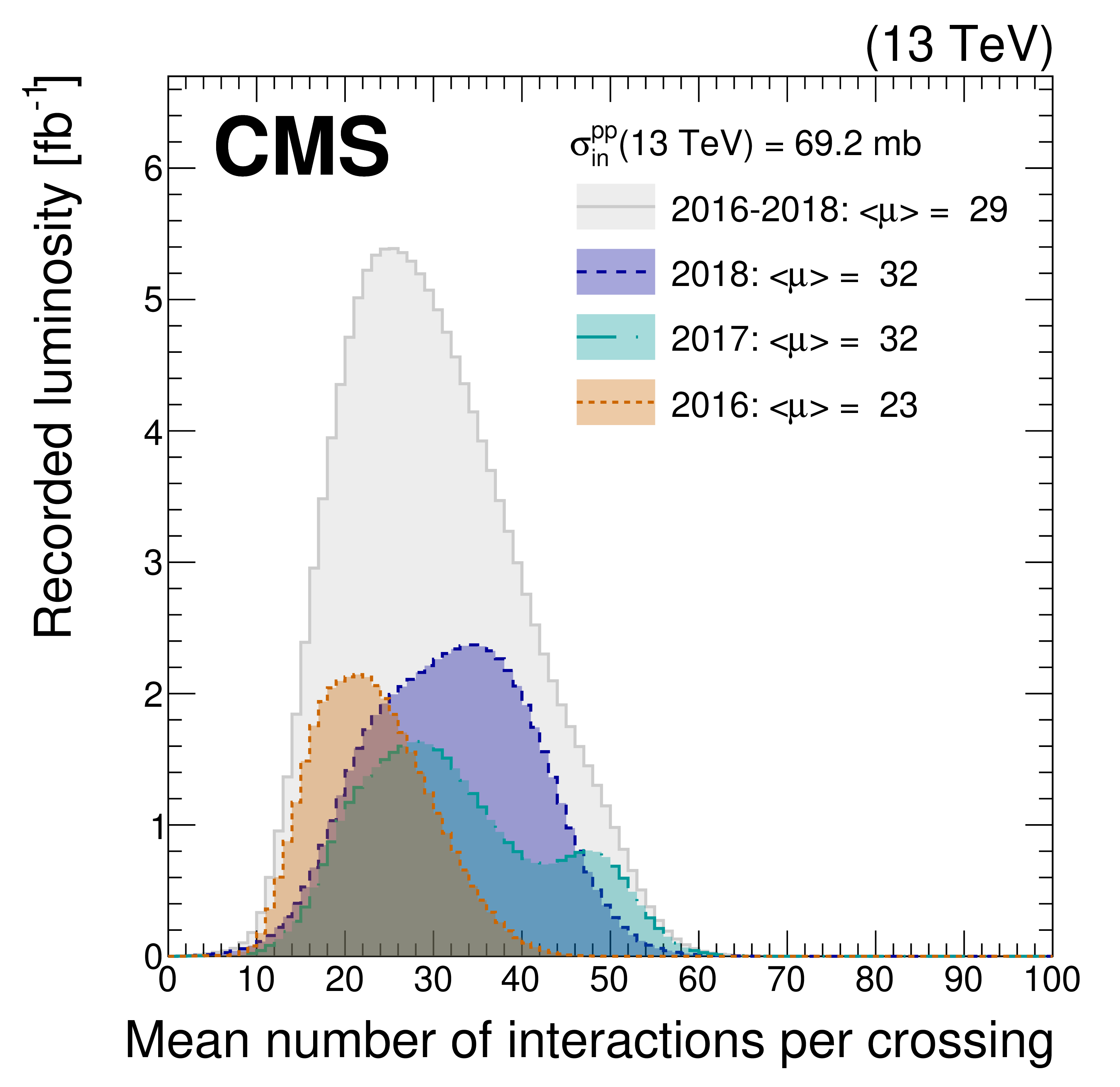
Figure 1:
Distribution of the mean number of inelastic interactions per crossing (pileup) in data for pp collisions in 2016 (dotted orange line), 2017 (dotted dashed light blue line), 2018 (dashed navy blue line), and integrated over 2016-2018 (solid grey line). A minimum bias cross section of 69.2 mb is chosen. The mean number per bunch crossing and year of inelastic interactions is provided in the legend. |

png pdf |
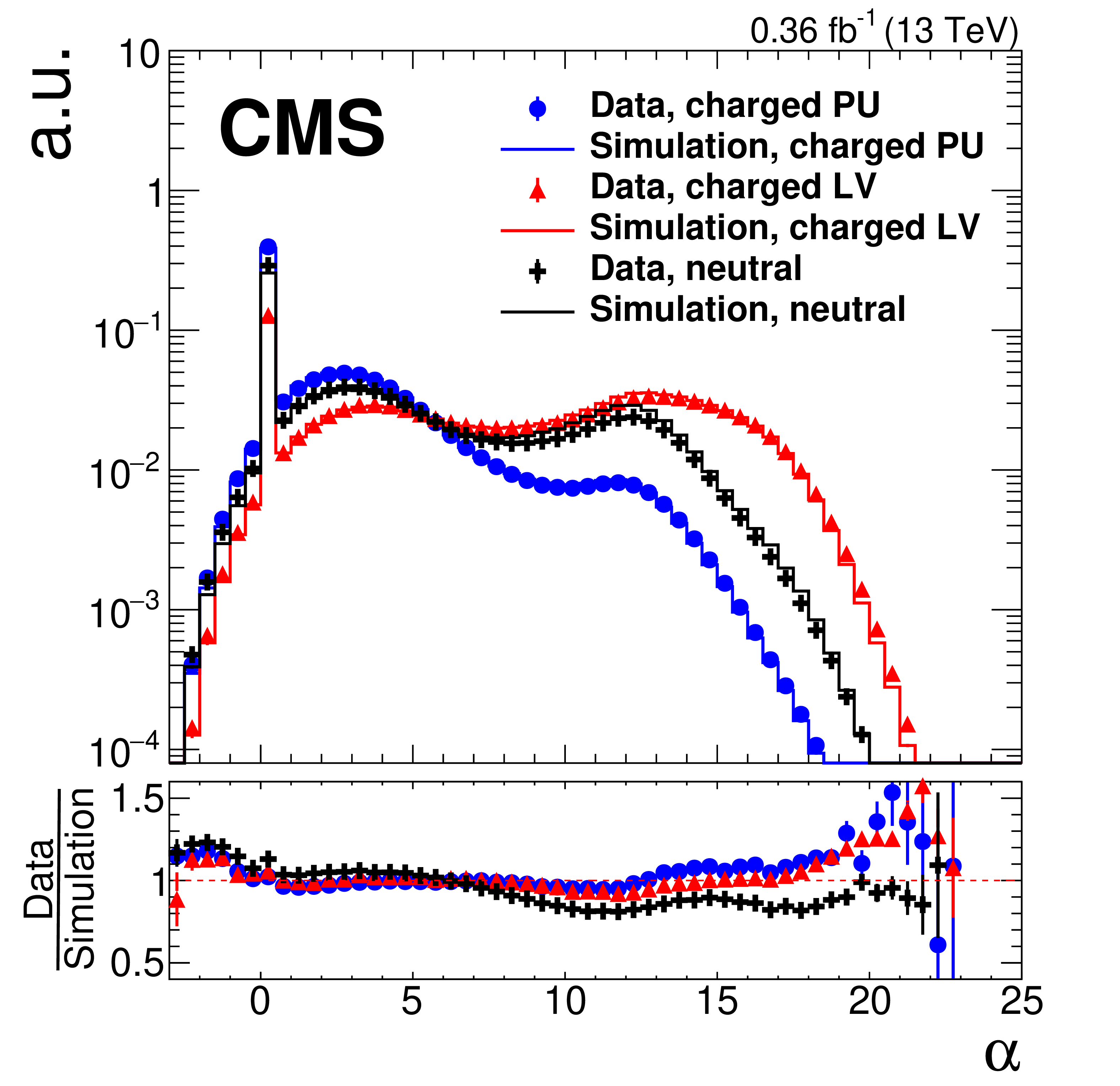
Figure 2:
Data-to-simulation comparison for three different variables of the PUPPI algorithm. The markers show a subset of the data taken in 2016, while the solid lines are QCD multijet simulations. The lower panel of each plot shows the ratio of data to simulation. Only statistical uncertainties are displayed. Each distribution is normalized to unity. The upper plot shows the $\alpha $ distribution for charged particles associated with the LV (red triangles), charged particles associated with PU vertices (blue circles), and neutral particles (black crosses) for $ {| \eta |} > $ 2.5. The lower left plot shows the signed $\chi ^{2}=(\alpha - \overline {\alpha}_{{\text {PU}}}) {| \alpha - \overline {\alpha}_{{\text {PU}}} |}/(\alpha _{{\text {PU}}}^{{\text {RMS}}})^{2}$ for charged particles associated with PU vertices. The lower right plot shows the PUPPI weight distribution for neutral particles. This distribution is normalized to unity only taking into account particles with weights greater than 0.01, i.e., those that are not rejected by the PUPPI algorithm. The error bars correspond to the statistical uncertainty. |
png pdf |
Figure 2-a:
Data-to-simulation comparison for three different variables of the PUPPI algorithm. The markers show a subset of the data taken in 2016, while the solid lines are QCD multijet simulations. The lower panel of each plot shows the ratio of data to simulation. Only statistical uncertainties are displayed. Each distribution is normalized to unity. The upper plot shows the $\alpha $ distribution for charged particles associated with the LV (red triangles), charged particles associated with PU vertices (blue circles), and neutral particles (black crosses) for $ {| \eta |} > $ 2.5. The lower left plot shows the signed $\chi ^{2}=(\alpha - \overline {\alpha}_{{\text {PU}}}) {| \alpha - \overline {\alpha}_{{\text {PU}}} |}/(\alpha _{{\text {PU}}}^{{\text {RMS}}})^{2}$ for charged particles associated with PU vertices. The lower right plot shows the PUPPI weight distribution for neutral particles. This distribution is normalized to unity only taking into account particles with weights greater than 0.01, i.e., those that are not rejected by the PUPPI algorithm. The error bars correspond to the statistical uncertainty. |

png pdf |
Figure 2-b:
Data-to-simulation comparison for three different variables of the PUPPI algorithm. The markers show a subset of the data taken in 2016, while the solid lines are QCD multijet simulations. The lower panel of each plot shows the ratio of data to simulation. Only statistical uncertainties are displayed. Each distribution is normalized to unity. The upper plot shows the $\alpha $ distribution for charged particles associated with the LV (red triangles), charged particles associated with PU vertices (blue circles), and neutral particles (black crosses) for $ {| \eta |} > $ 2.5. The lower left plot shows the signed $\chi ^{2}=(\alpha - \overline {\alpha}_{{\text {PU}}}) {| \alpha - \overline {\alpha}_{{\text {PU}}} |}/(\alpha _{{\text {PU}}}^{{\text {RMS}}})^{2}$ for charged particles associated with PU vertices. The lower right plot shows the PUPPI weight distribution for neutral particles. This distribution is normalized to unity only taking into account particles with weights greater than 0.01, i.e., those that are not rejected by the PUPPI algorithm. The error bars correspond to the statistical uncertainty. |

png pdf |
Figure 2-c:
Data-to-simulation comparison for three different variables of the PUPPI algorithm. The markers show a subset of the data taken in 2016, while the solid lines are QCD multijet simulations. The lower panel of each plot shows the ratio of data to simulation. Only statistical uncertainties are displayed. Each distribution is normalized to unity. The upper plot shows the $\alpha $ distribution for charged particles associated with the LV (red triangles), charged particles associated with PU vertices (blue circles), and neutral particles (black crosses) for $ {| \eta |} > $ 2.5. The lower left plot shows the signed $\chi ^{2}=(\alpha - \overline {\alpha}_{{\text {PU}}}) {| \alpha - \overline {\alpha}_{{\text {PU}}} |}/(\alpha _{{\text {PU}}}^{{\text {RMS}}})^{2}$ for charged particles associated with PU vertices. The lower right plot shows the PUPPI weight distribution for neutral particles. This distribution is normalized to unity only taking into account particles with weights greater than 0.01, i.e., those that are not rejected by the PUPPI algorithm. The error bars correspond to the statistical uncertainty. |
png pdf |
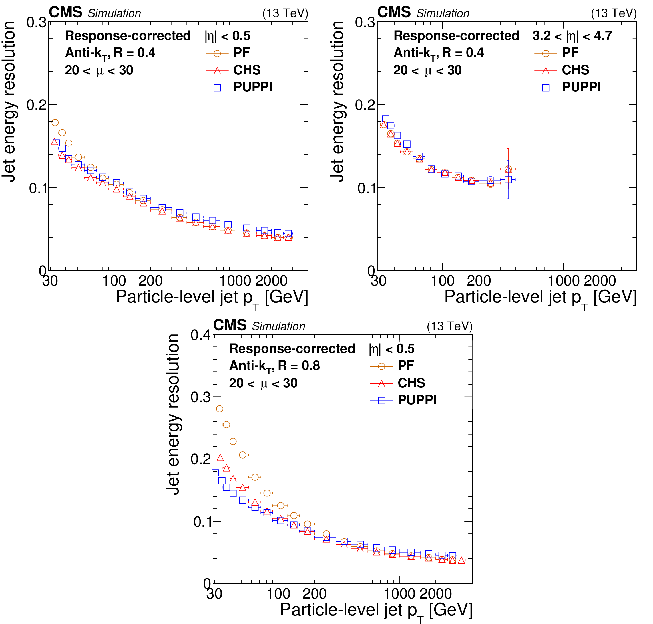
Figure 3:
Jet energy resolution as a function of the particle-level jet ${p_{\mathrm {T}}}$ for PF jets (orange circles), PF jets with CHS applied (red triangles), and PF jets with PUPPI applied (blue squares) in QCD multijet simulation. The number of interactions is required to be between 20 and 30. The resolution is shown for AK4 jets with $ {| \eta |} < $ 0.5 (upper left) and 3.2 $ < {| \eta |} < 4.7$ (upper right), as well as for AK8 jets with $ {| \eta |} < $ 0.5 (lower). The error bars correspond to the statistical uncertainty in the simulation. |

png pdf |
Figure 3-a:
Jet energy resolution as a function of the particle-level jet ${p_{\mathrm {T}}}$ for PF jets (orange circles), PF jets with CHS applied (red triangles), and PF jets with PUPPI applied (blue squares) in QCD multijet simulation. The number of interactions is required to be between 20 and 30. The resolution is shown for AK4 jets with $ {| \eta |} < $ 0.5 (upper left) and 3.2 $ < {| \eta |} < 4.7$ (upper right), as well as for AK8 jets with $ {| \eta |} < $ 0.5 (lower). The error bars correspond to the statistical uncertainty in the simulation. |

png pdf |
Figure 3-b:
Jet energy resolution as a function of the particle-level jet ${p_{\mathrm {T}}}$ for PF jets (orange circles), PF jets with CHS applied (red triangles), and PF jets with PUPPI applied (blue squares) in QCD multijet simulation. The number of interactions is required to be between 20 and 30. The resolution is shown for AK4 jets with $ {| \eta |} < $ 0.5 (upper left) and 3.2 $ < {| \eta |} < 4.7$ (upper right), as well as for AK8 jets with $ {| \eta |} < $ 0.5 (lower). The error bars correspond to the statistical uncertainty in the simulation. |
png pdf |
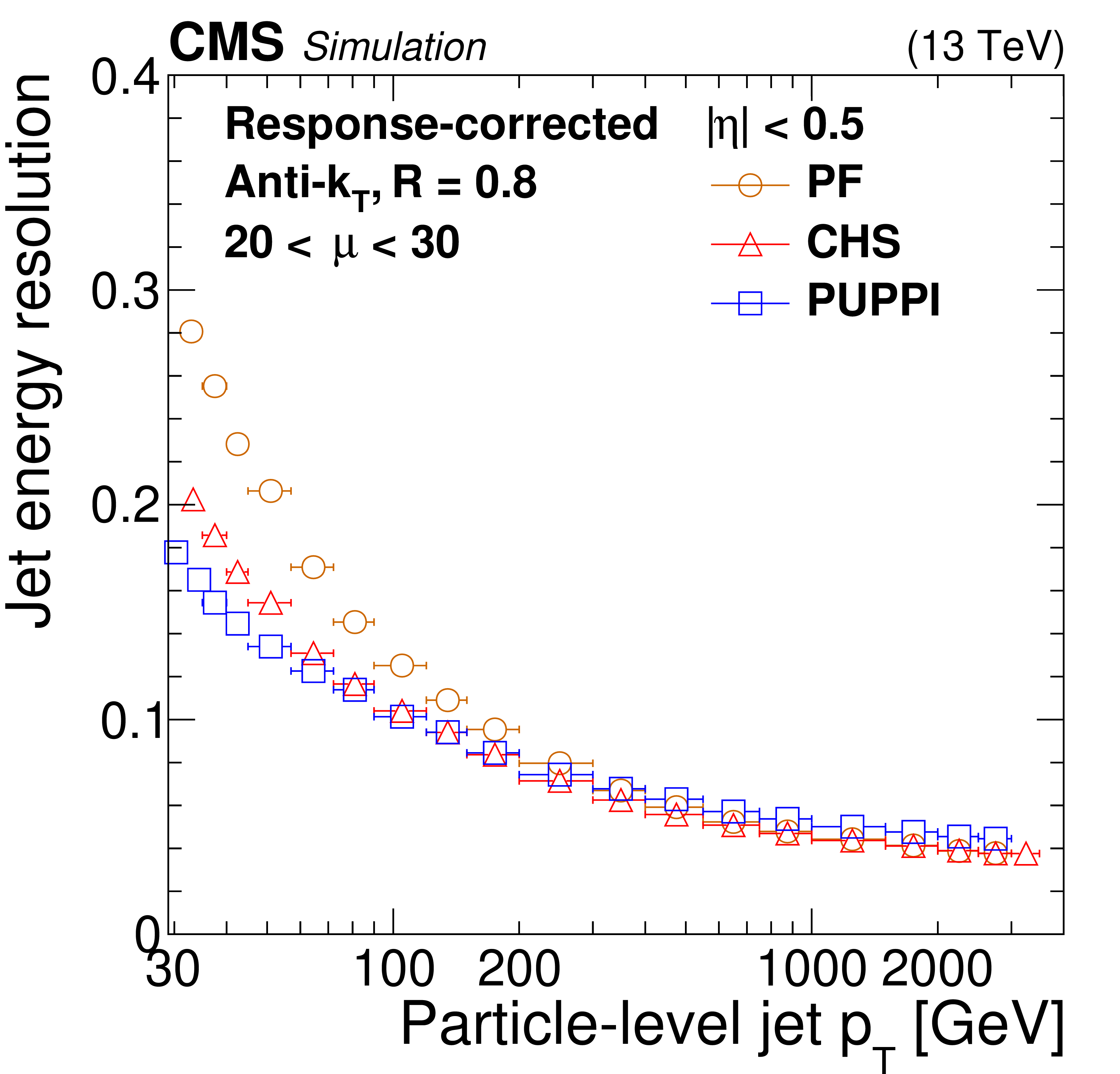
Figure 3-c:
Jet energy resolution as a function of the particle-level jet ${p_{\mathrm {T}}}$ for PF jets (orange circles), PF jets with CHS applied (red triangles), and PF jets with PUPPI applied (blue squares) in QCD multijet simulation. The number of interactions is required to be between 20 and 30. The resolution is shown for AK4 jets with $ {| \eta |} < $ 0.5 (upper left) and 3.2 $ < {| \eta |} < 4.7$ (upper right), as well as for AK8 jets with $ {| \eta |} < $ 0.5 (lower). The error bars correspond to the statistical uncertainty in the simulation. |
png pdf |
Figure 4:
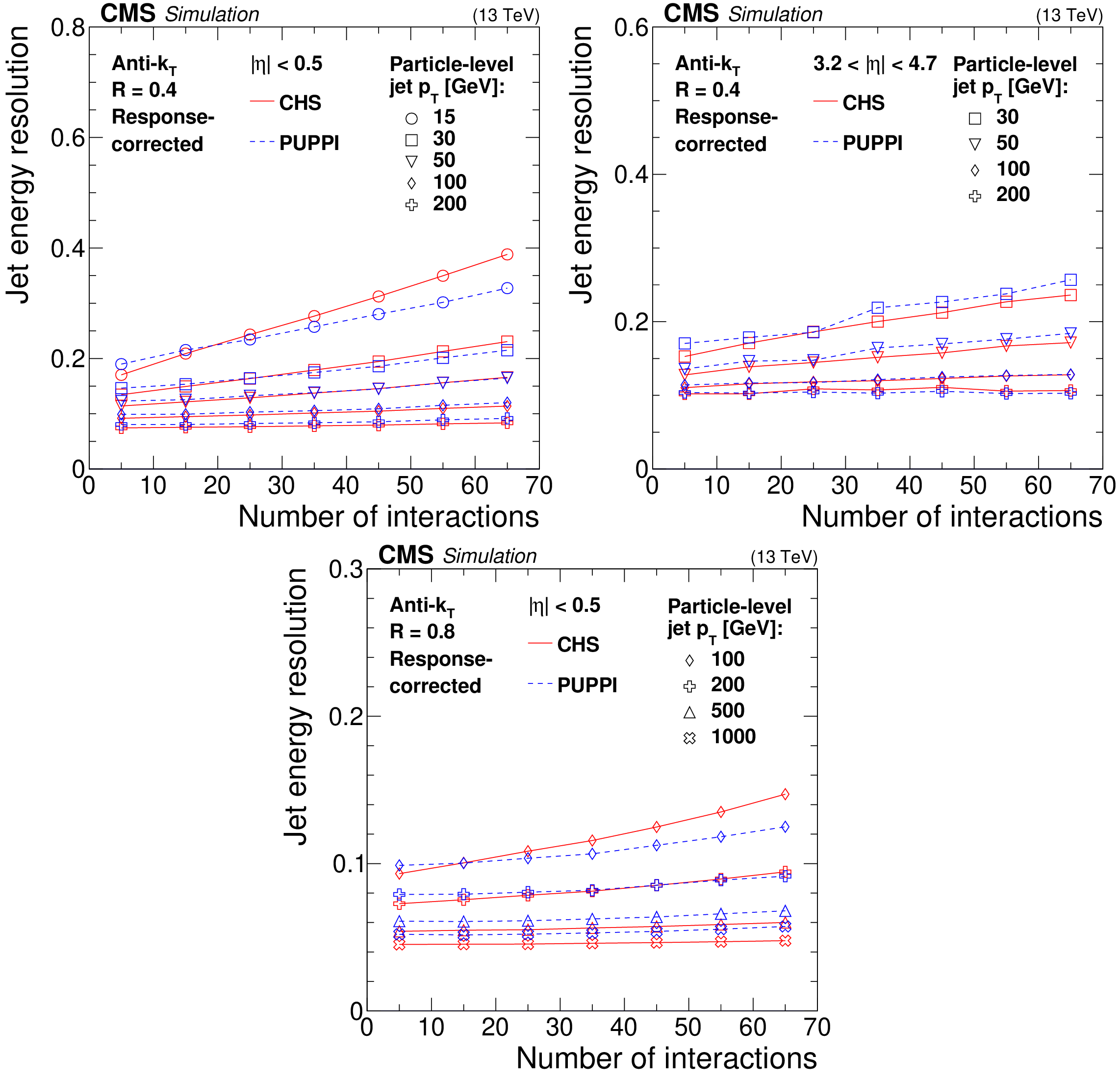
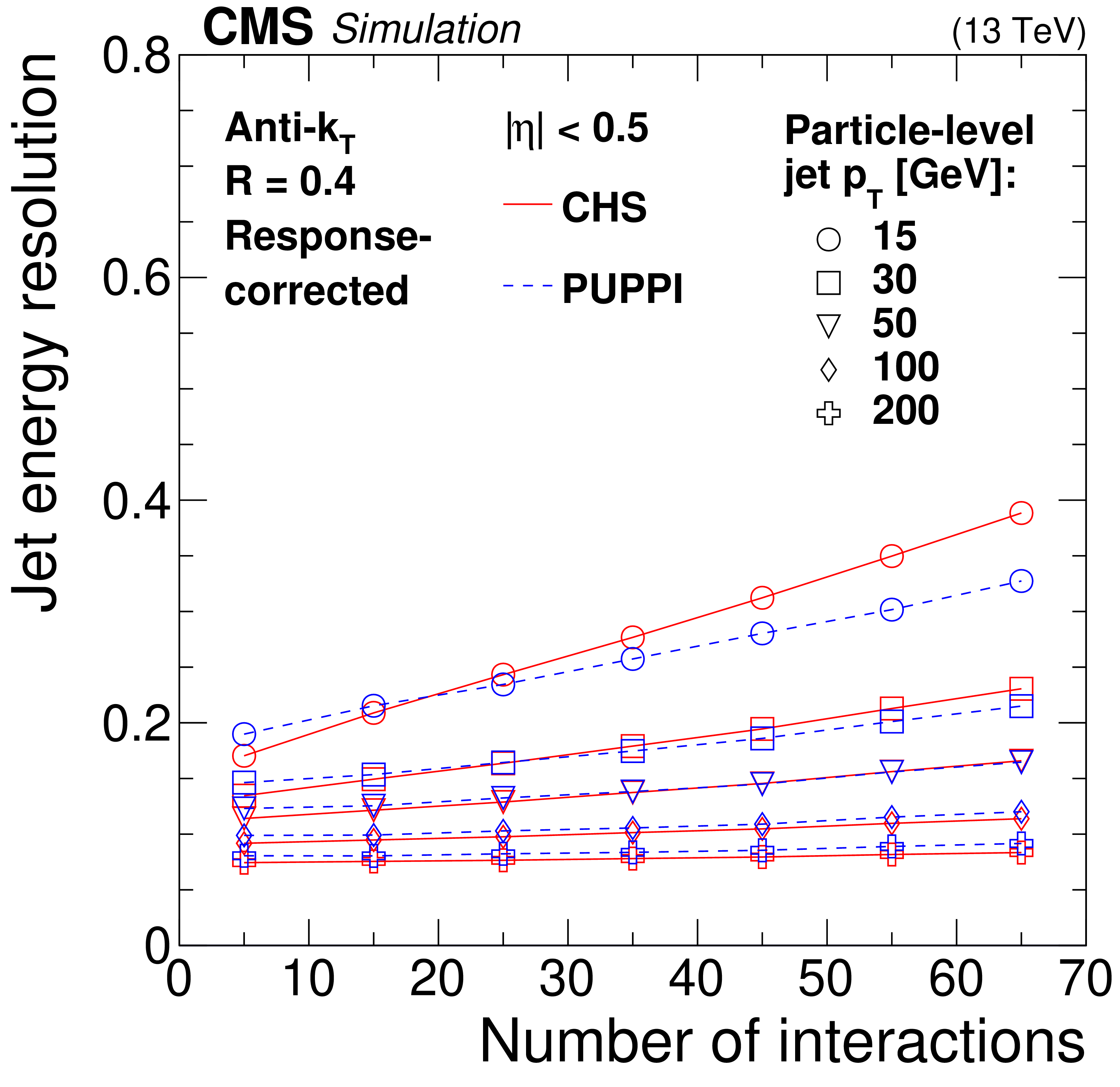
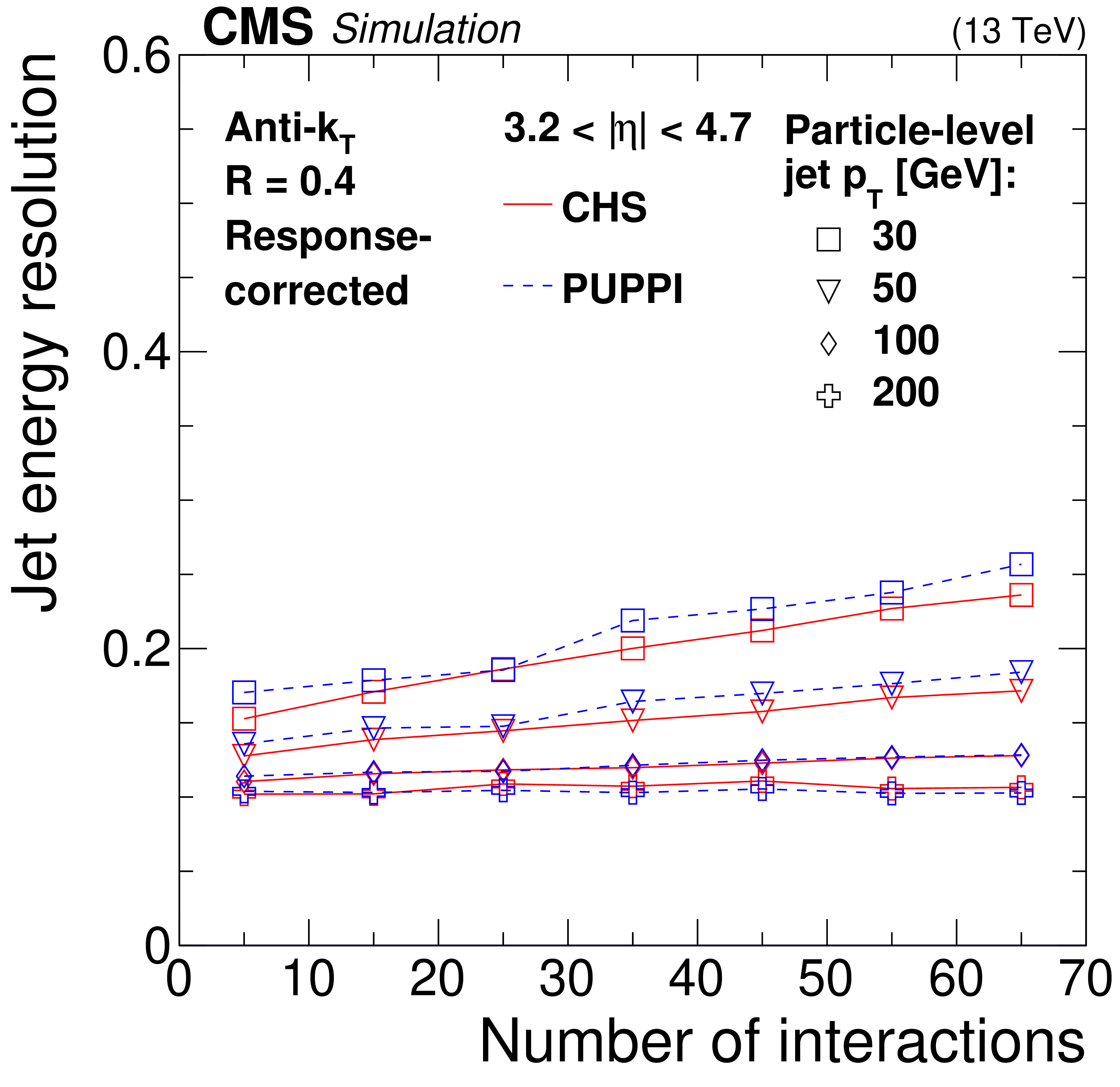
Jet energy resolution as a function of the number of interactions for jets with CHS (solid red line) and with PUPPI (dashed blue line) algorithms applied in QCD multijet simulation for different jet ${p_{\mathrm {T}}}$ values (different markers). The resolution is shown for AK4 jets with $ {| \eta |} < $ 0.5 (upper left) and 3.2 $ < {| \eta |} < 4.7$ (upper right), as well as for AK8 jets with $ {| \eta |} < $ 0.5 (lower). The error bars correspond to the statistical uncertainty in the simulation. |
png pdf |
Figure 4-a:
Jet energy resolution as a function of the number of interactions for jets with CHS (solid red line) and with PUPPI (dashed blue line) algorithms applied in QCD multijet simulation for different jet ${p_{\mathrm {T}}}$ values (different markers). The resolution is shown for AK4 jets with $ {| \eta |} < $ 0.5 (upper left) and 3.2 $ < {| \eta |} < 4.7$ (upper right), as well as for AK8 jets with $ {| \eta |} < $ 0.5 (lower). The error bars correspond to the statistical uncertainty in the simulation. |
png pdf |
Figure 4-b:
Jet energy resolution as a function of the number of interactions for jets with CHS (solid red line) and with PUPPI (dashed blue line) algorithms applied in QCD multijet simulation for different jet ${p_{\mathrm {T}}}$ values (different markers). The resolution is shown for AK4 jets with $ {| \eta |} < $ 0.5 (upper left) and 3.2 $ < {| \eta |} < 4.7$ (upper right), as well as for AK8 jets with $ {| \eta |} < $ 0.5 (lower). The error bars correspond to the statistical uncertainty in the simulation. |

png pdf |
Figure 4-c:
Jet energy resolution as a function of the number of interactions for jets with CHS (solid red line) and with PUPPI (dashed blue line) algorithms applied in QCD multijet simulation for different jet ${p_{\mathrm {T}}}$ values (different markers). The resolution is shown for AK4 jets with $ {| \eta |} < $ 0.5 (upper left) and 3.2 $ < {| \eta |} < 4.7$ (upper right), as well as for AK8 jets with $ {| \eta |} < $ 0.5 (lower). The error bars correspond to the statistical uncertainty in the simulation. |
png pdf |
Figure 5:
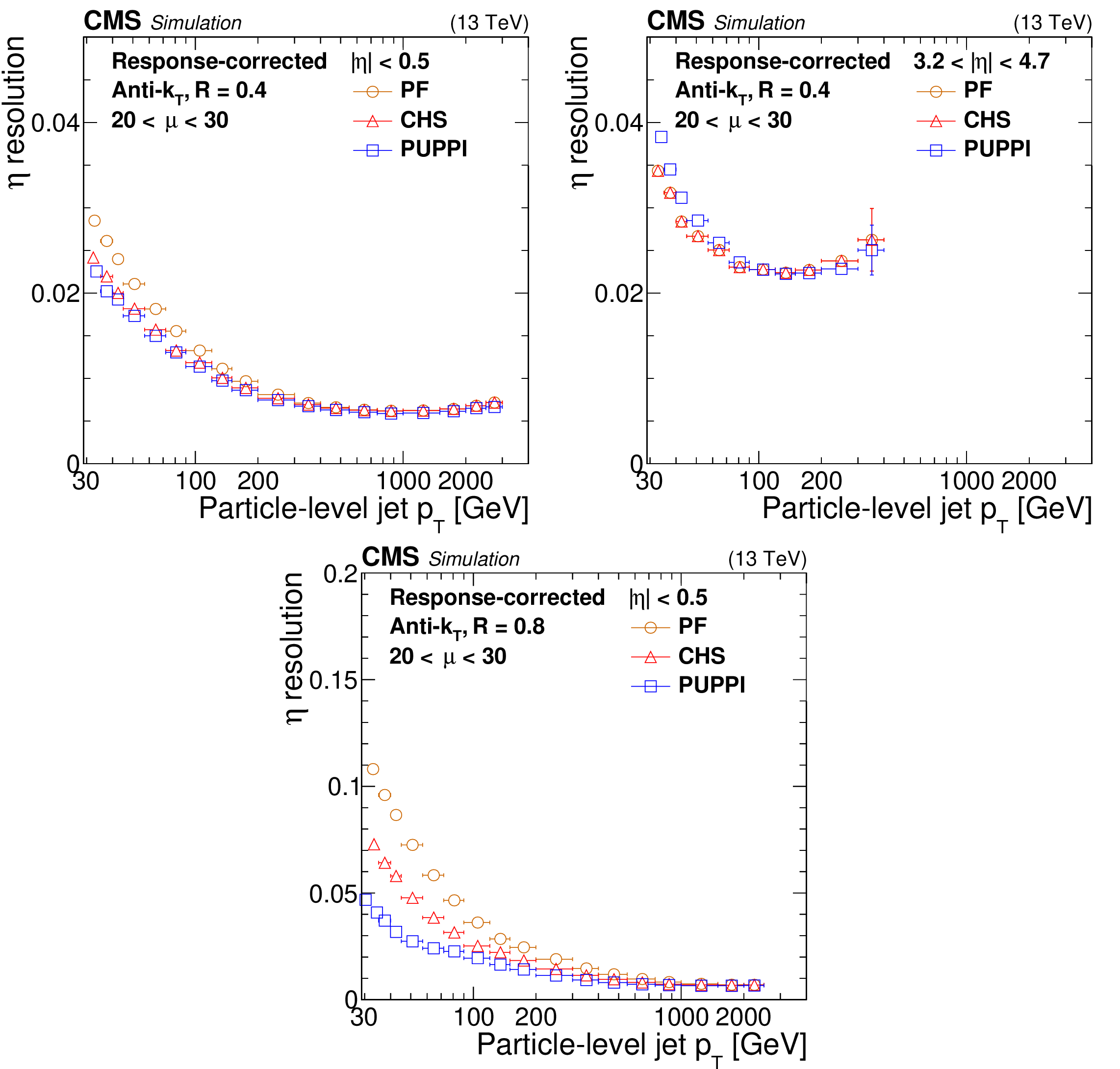
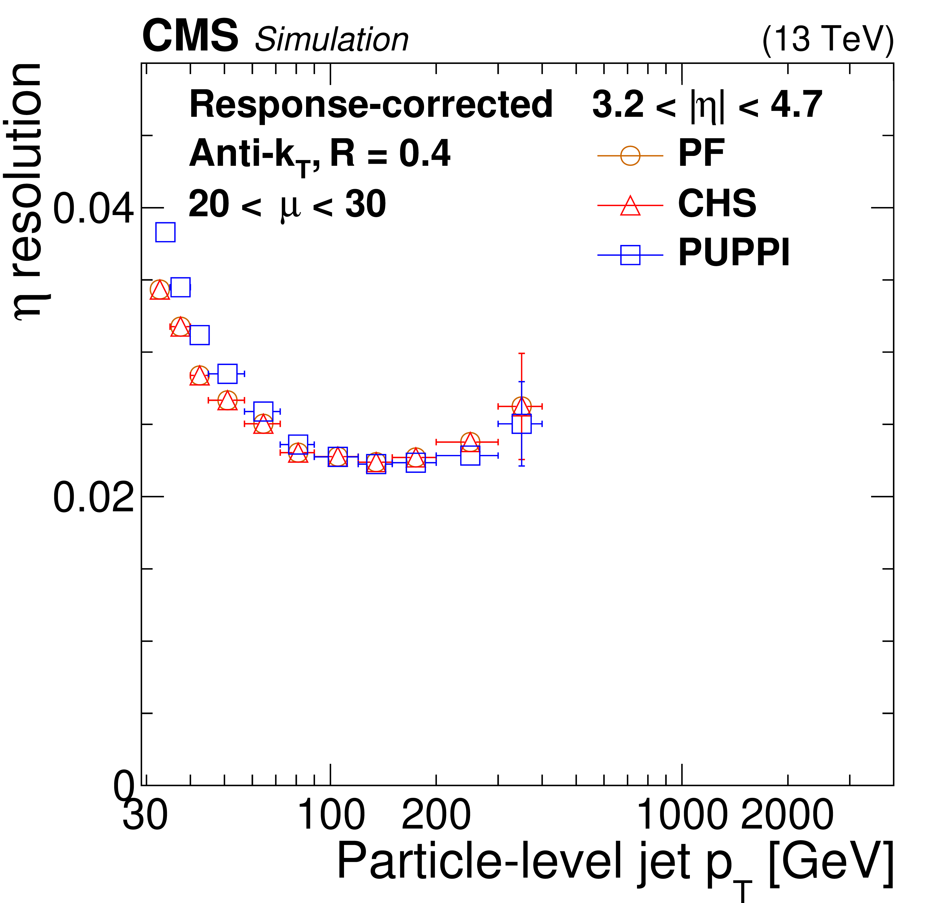
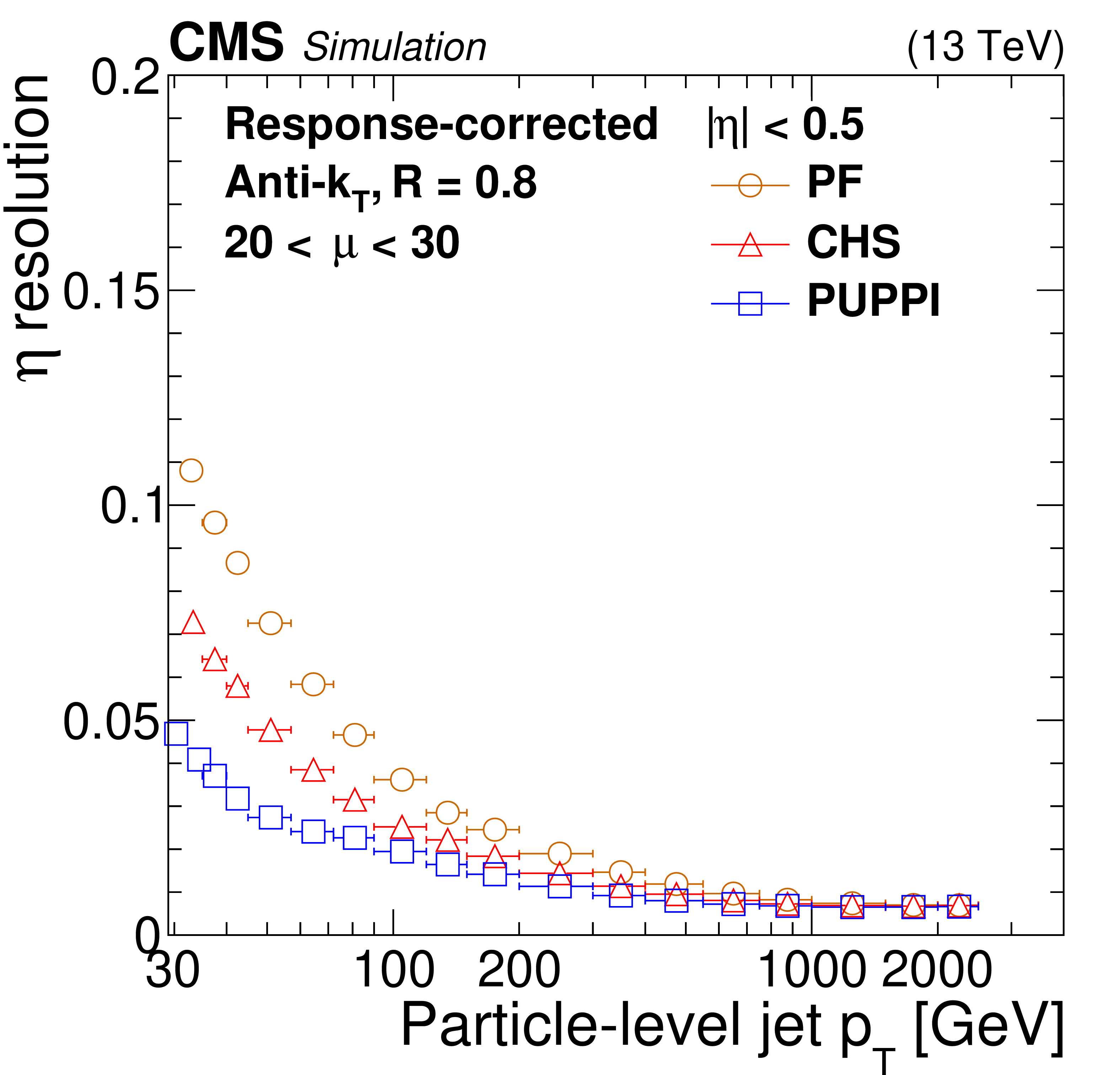
Jet $\eta $ resolution as a function of particle-level jet ${p_{\mathrm {T}}}$ for PF jets (orange circles), PF jets with CHS applied (red triangles), and PF jets with PUPPI applied (blue squares) in QCD multijet simulation. The number of interactions is required to be between 20 and 30. The resolution is shown for AK4 jets with $ {| \eta |} < $ 0.5 (upper left) and 3.2 $ < {| \eta |} < 4.7$ (upper right) as well as for AK8 jets with $ {| \eta |} < $ 0.5 (lower). The error bars correspond to the statistical uncertainty in the simulation. |

png pdf |
Figure 5-a:
Jet $\eta $ resolution as a function of particle-level jet ${p_{\mathrm {T}}}$ for PF jets (orange circles), PF jets with CHS applied (red triangles), and PF jets with PUPPI applied (blue squares) in QCD multijet simulation. The number of interactions is required to be between 20 and 30. The resolution is shown for AK4 jets with $ {| \eta |} < $ 0.5 (upper left) and 3.2 $ < {| \eta |} < 4.7$ (upper right) as well as for AK8 jets with $ {| \eta |} < $ 0.5 (lower). The error bars correspond to the statistical uncertainty in the simulation. |
png pdf |
Figure 5-b:
Jet $\eta $ resolution as a function of particle-level jet ${p_{\mathrm {T}}}$ for PF jets (orange circles), PF jets with CHS applied (red triangles), and PF jets with PUPPI applied (blue squares) in QCD multijet simulation. The number of interactions is required to be between 20 and 30. The resolution is shown for AK4 jets with $ {| \eta |} < $ 0.5 (upper left) and 3.2 $ < {| \eta |} < 4.7$ (upper right) as well as for AK8 jets with $ {| \eta |} < $ 0.5 (lower). The error bars correspond to the statistical uncertainty in the simulation. |
png pdf |
Figure 5-c:
Jet $\eta $ resolution as a function of particle-level jet ${p_{\mathrm {T}}}$ for PF jets (orange circles), PF jets with CHS applied (red triangles), and PF jets with PUPPI applied (blue squares) in QCD multijet simulation. The number of interactions is required to be between 20 and 30. The resolution is shown for AK4 jets with $ {| \eta |} < $ 0.5 (upper left) and 3.2 $ < {| \eta |} < 4.7$ (upper right) as well as for AK8 jets with $ {| \eta |} < $ 0.5 (lower). The error bars correspond to the statistical uncertainty in the simulation. |

png pdf |
Figure 6:
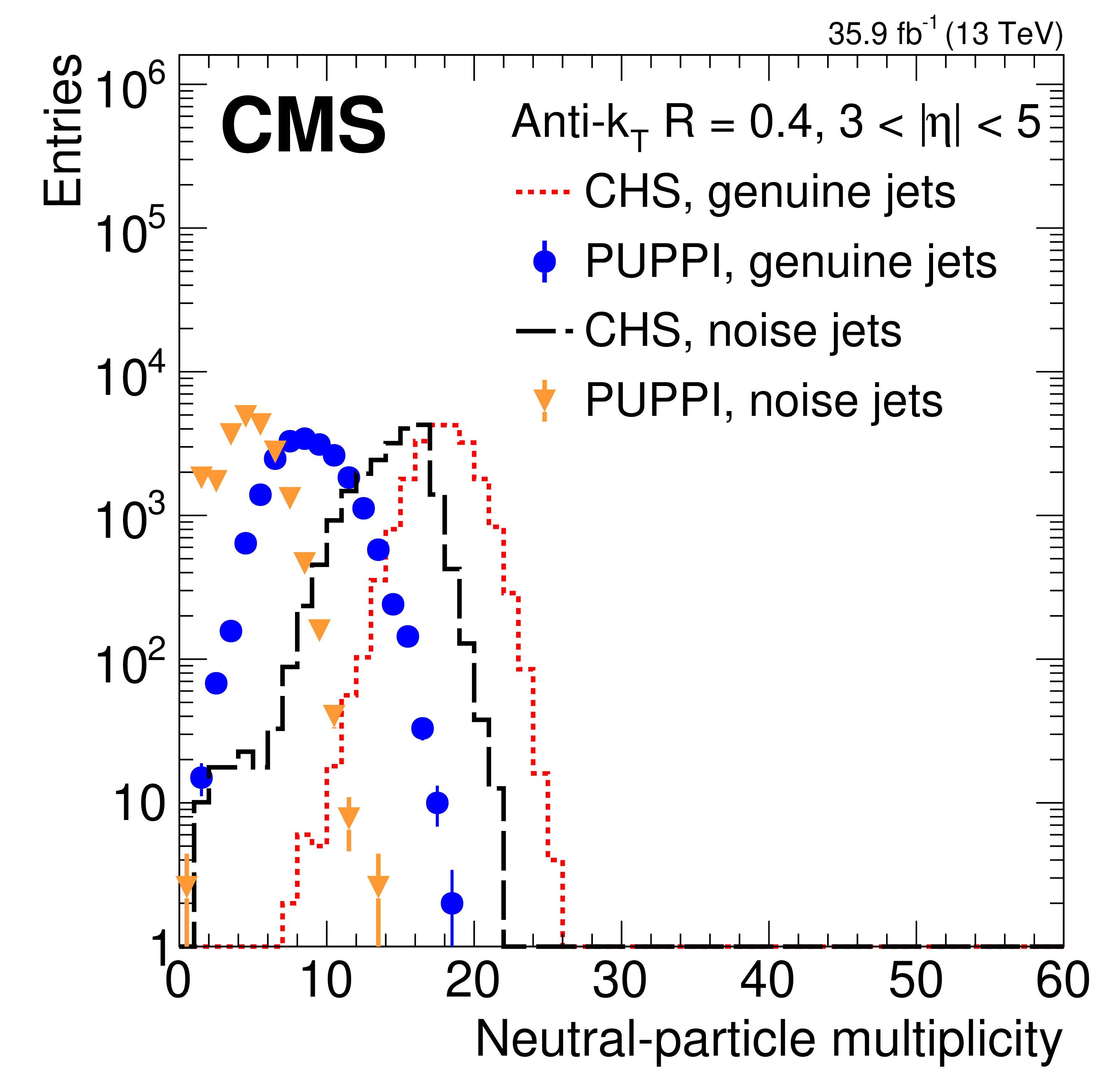
The charged- and neutral-particle multiplicities for CHS and PUPPI in a dijet (genuine jets) and minimum bias (noise jets) selection in data. The multiplicities are shown for AK4 jets using CHS reconstructed real jets (red dashed), CHS reconstructed noise jets (black long dashed), PUPPI reconstructed genuine jets (blue circles), and PUPPI reconstructed noise jets (orange triangles). The upper plots show the charged (left) and neutral particle multiplicities (right) for jets with $ {| \eta |} < $ 0.5. The lower left plot shows the neutral particle multiplicity for jets with 3 $ < {| \eta |} < 5$. The lower right plot shows the neutral particle multiplicity of AK4 jets with $ {| \eta |} < $ 0.5 in a dijet selection in data using CHS and PUPPI for 15-20 and 35-50 interactions. The error bars correspond to the statistical uncertainty. |

png pdf |
Figure 6-a:
The charged- and neutral-particle multiplicities for CHS and PUPPI in a dijet (genuine jets) and minimum bias (noise jets) selection in data. The multiplicities are shown for AK4 jets using CHS reconstructed real jets (red dashed), CHS reconstructed noise jets (black long dashed), PUPPI reconstructed genuine jets (blue circles), and PUPPI reconstructed noise jets (orange triangles). The upper plots show the charged (left) and neutral particle multiplicities (right) for jets with $ {| \eta |} < $ 0.5. The lower left plot shows the neutral particle multiplicity for jets with 3 $ < {| \eta |} < 5$. The lower right plot shows the neutral particle multiplicity of AK4 jets with $ {| \eta |} < $ 0.5 in a dijet selection in data using CHS and PUPPI for 15-20 and 35-50 interactions. The error bars correspond to the statistical uncertainty. |

png pdf |
Figure 6-b:
The charged- and neutral-particle multiplicities for CHS and PUPPI in a dijet (genuine jets) and minimum bias (noise jets) selection in data. The multiplicities are shown for AK4 jets using CHS reconstructed real jets (red dashed), CHS reconstructed noise jets (black long dashed), PUPPI reconstructed genuine jets (blue circles), and PUPPI reconstructed noise jets (orange triangles). The upper plots show the charged (left) and neutral particle multiplicities (right) for jets with $ {| \eta |} < $ 0.5. The lower left plot shows the neutral particle multiplicity for jets with 3 $ < {| \eta |} < 5$. The lower right plot shows the neutral particle multiplicity of AK4 jets with $ {| \eta |} < $ 0.5 in a dijet selection in data using CHS and PUPPI for 15-20 and 35-50 interactions. The error bars correspond to the statistical uncertainty. |
png pdf |
Figure 6-c:
The charged- and neutral-particle multiplicities for CHS and PUPPI in a dijet (genuine jets) and minimum bias (noise jets) selection in data. The multiplicities are shown for AK4 jets using CHS reconstructed real jets (red dashed), CHS reconstructed noise jets (black long dashed), PUPPI reconstructed genuine jets (blue circles), and PUPPI reconstructed noise jets (orange triangles). The upper plots show the charged (left) and neutral particle multiplicities (right) for jets with $ {| \eta |} < $ 0.5. The lower left plot shows the neutral particle multiplicity for jets with 3 $ < {| \eta |} < 5$. The lower right plot shows the neutral particle multiplicity of AK4 jets with $ {| \eta |} < $ 0.5 in a dijet selection in data using CHS and PUPPI for 15-20 and 35-50 interactions. The error bars correspond to the statistical uncertainty. |

png pdf |
Figure 6-d:
The charged- and neutral-particle multiplicities for CHS and PUPPI in a dijet (genuine jets) and minimum bias (noise jets) selection in data. The multiplicities are shown for AK4 jets using CHS reconstructed real jets (red dashed), CHS reconstructed noise jets (black long dashed), PUPPI reconstructed genuine jets (blue circles), and PUPPI reconstructed noise jets (orange triangles). The upper plots show the charged (left) and neutral particle multiplicities (right) for jets with $ {| \eta |} < $ 0.5. The lower left plot shows the neutral particle multiplicity for jets with 3 $ < {| \eta |} < 5$. The lower right plot shows the neutral particle multiplicity of AK4 jets with $ {| \eta |} < $ 0.5 in a dijet selection in data using CHS and PUPPI for 15-20 and 35-50 interactions. The error bars correspond to the statistical uncertainty. |

png pdf |
Figure 7:
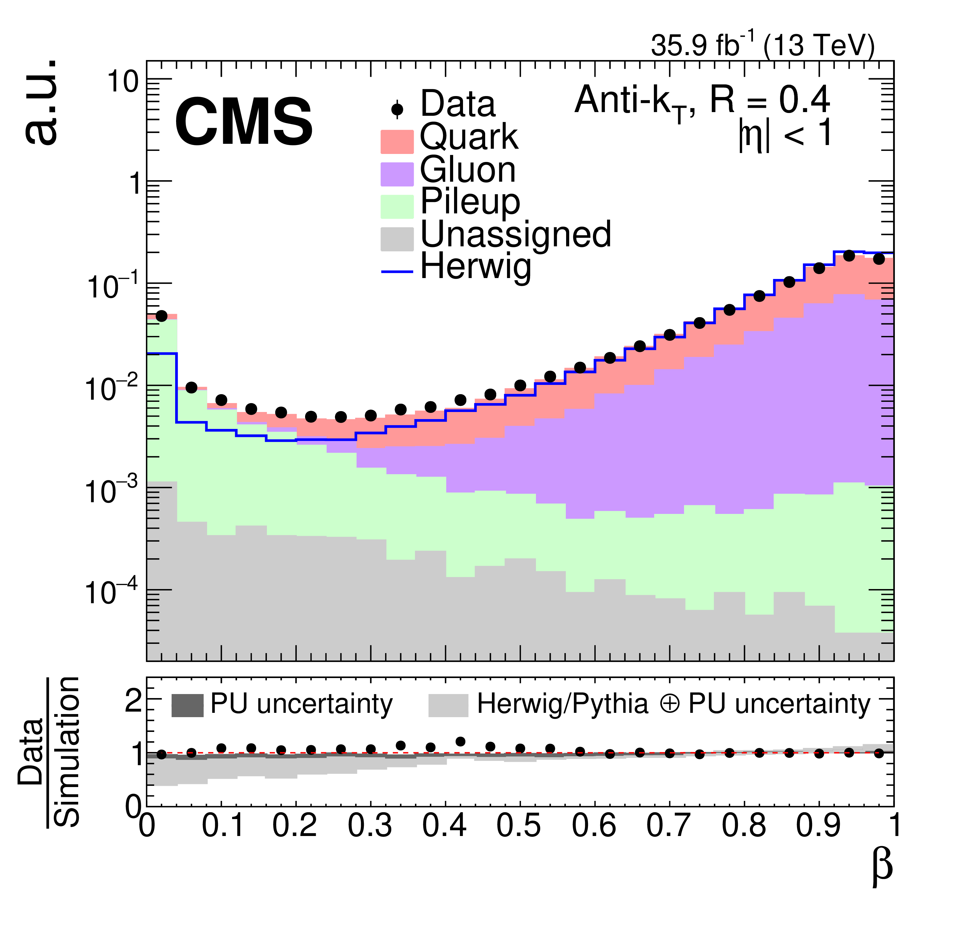
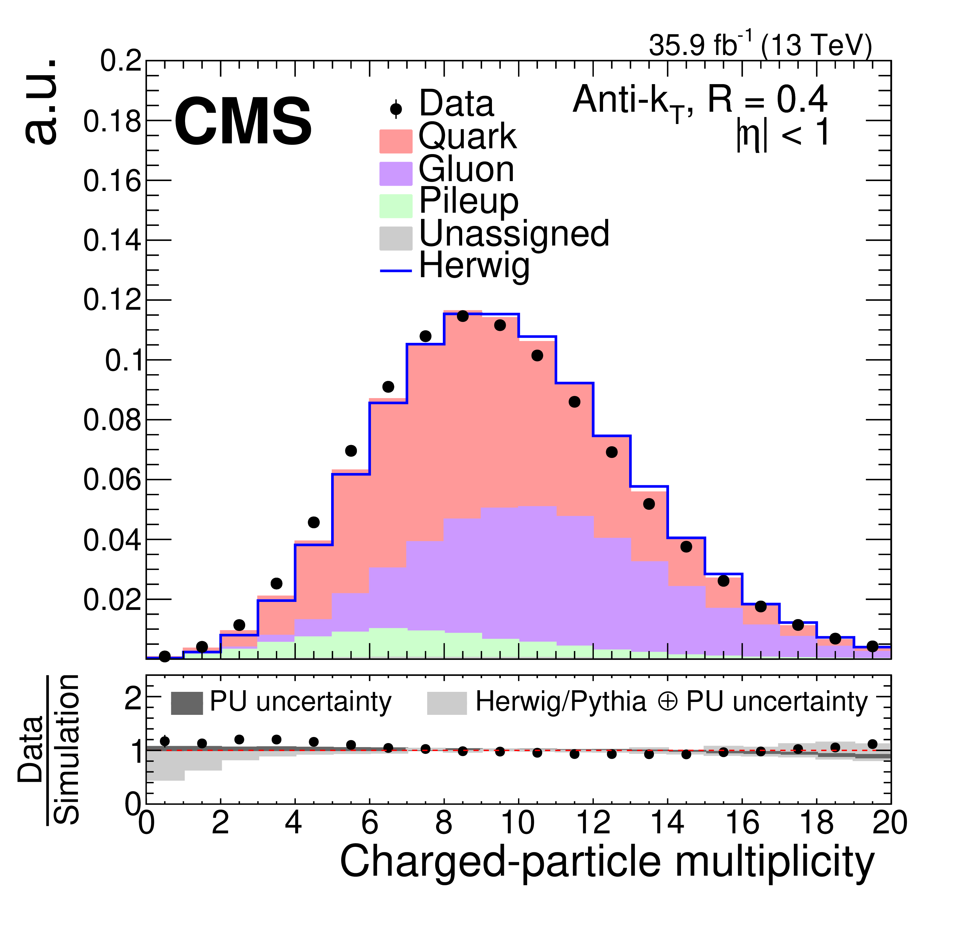
Data-to-simulation comparison for two input variables to the PU jet ID calculation: $\beta $ (left) and charged-particle multiplicity (right). Black markers represent the data while the colored areas are Z+jets simulation events. The simulation sample is split into jets originating from quarks (red), gluons (purple), PU (green), and jets that could not be assigned (gray). The distributions are normalized to unity. The shape of a sample showered with HERWIG++ is superimposed and included in the total uncertainty band in the ratio panel (light gray). Also included in the ratio panel is the PU rate uncertainty (dark gray). |
png pdf |
Figure 7-a:
Data-to-simulation comparison for two input variables to the PU jet ID calculation: $\beta $ (left) and charged-particle multiplicity (right). Black markers represent the data while the colored areas are Z+jets simulation events. The simulation sample is split into jets originating from quarks (red), gluons (purple), PU (green), and jets that could not be assigned (gray). The distributions are normalized to unity. The shape of a sample showered with HERWIG++ is superimposed and included in the total uncertainty band in the ratio panel (light gray). Also included in the ratio panel is the PU rate uncertainty (dark gray). |
png pdf |
Figure 7-b:
Data-to-simulation comparison for two input variables to the PU jet ID calculation: $\beta $ (left) and charged-particle multiplicity (right). Black markers represent the data while the colored areas are Z+jets simulation events. The simulation sample is split into jets originating from quarks (red), gluons (purple), PU (green), and jets that could not be assigned (gray). The distributions are normalized to unity. The shape of a sample showered with HERWIG++ is superimposed and included in the total uncertainty band in the ratio panel (light gray). Also included in the ratio panel is the PU rate uncertainty (dark gray). |

png pdf |
Figure 8:
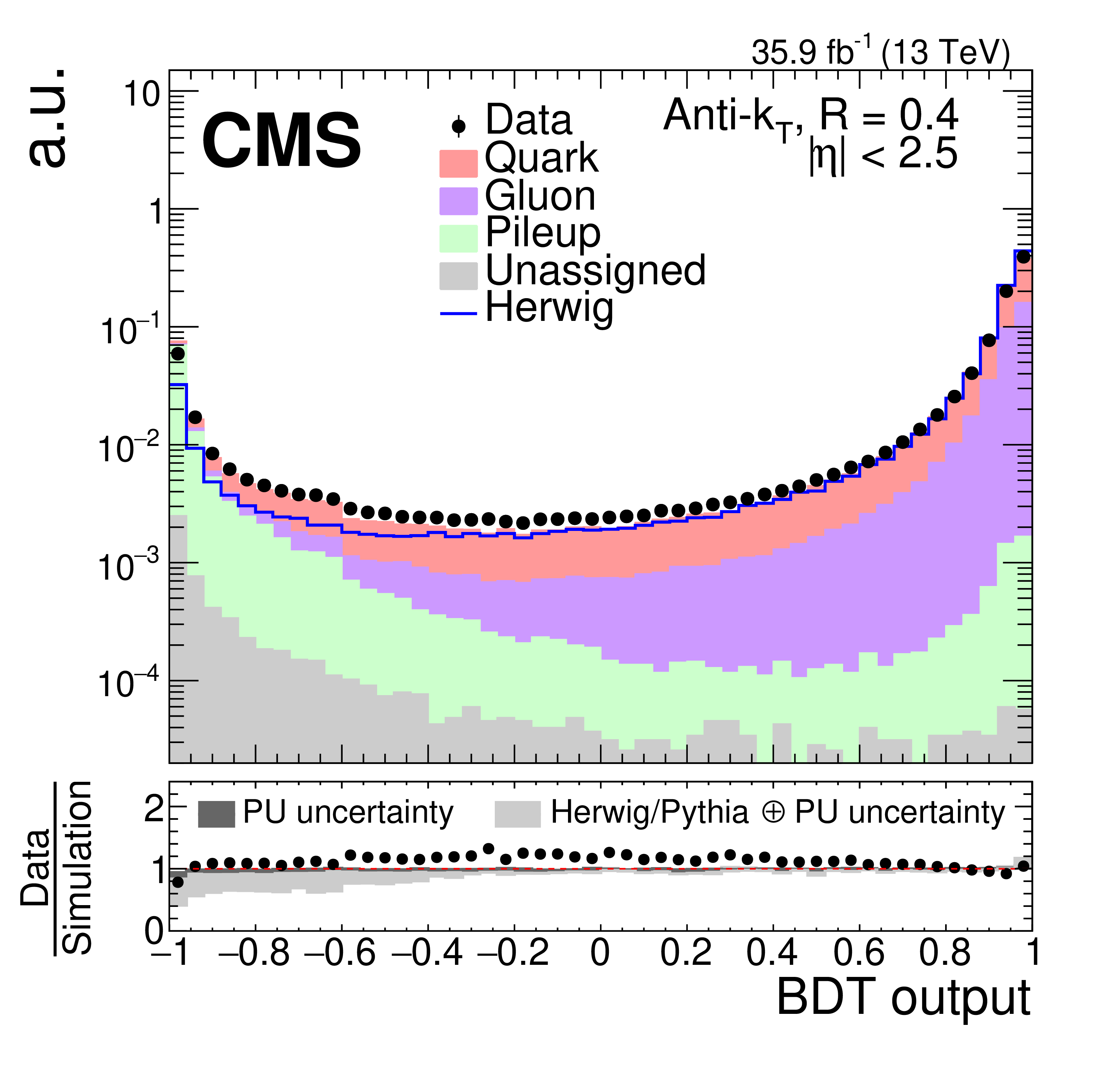
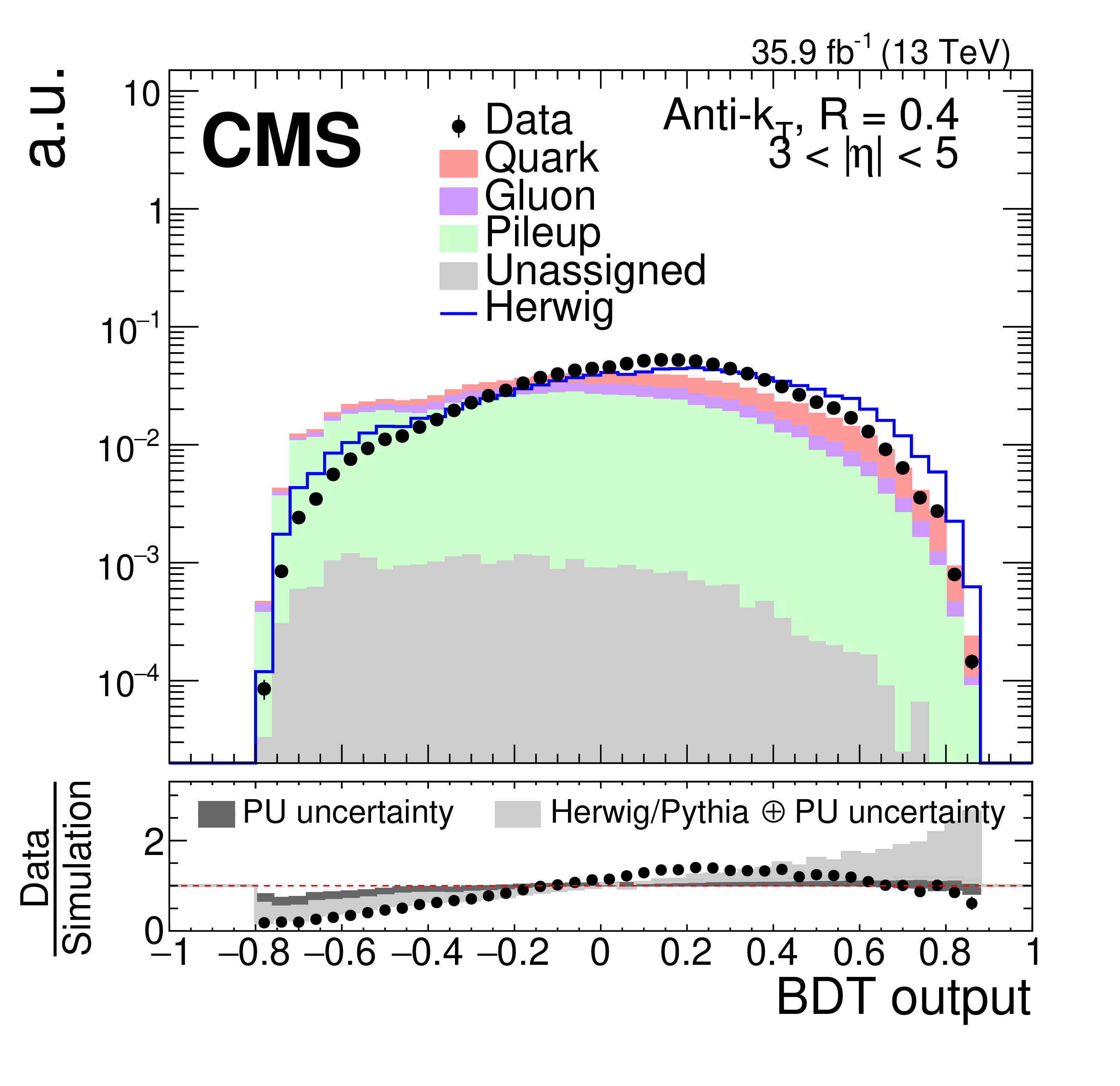
Data-to-simulation comparison of the PU jet ID boosted decision tree (BDT) output for AK4 jets with 30 $ < {p_{\mathrm {T}}} < $ 50 GeV for the detector region within the tracker volume (left) and 3 $ < {| \eta |} < 5$ (right). Black markers represent the data while the colored areas are Z+jets simulation events. The simulation sample is split into jets originating from quarks (red), gluons (purple), PU (green), and jets that could not be assigned (gray). The distributions are normalized to unity. The shape of a sample showered with HERWIG++ is superimposed and included in the total uncertainty band in the ratio panel (light gray). Also included in the ratio panel is the PU rate uncertainty (dark gray). |
png pdf |
Figure 8-a:
Data-to-simulation comparison of the PU jet ID boosted decision tree (BDT) output for AK4 jets with 30 $ < {p_{\mathrm {T}}} < $ 50 GeV for the detector region within the tracker volume (left) and 3 $ < {| \eta |} < 5$ (right). Black markers represent the data while the colored areas are Z+jets simulation events. The simulation sample is split into jets originating from quarks (red), gluons (purple), PU (green), and jets that could not be assigned (gray). The distributions are normalized to unity. The shape of a sample showered with HERWIG++ is superimposed and included in the total uncertainty band in the ratio panel (light gray). Also included in the ratio panel is the PU rate uncertainty (dark gray). |
png pdf |
Figure 8-b:
Data-to-simulation comparison of the PU jet ID boosted decision tree (BDT) output for AK4 jets with 30 $ < {p_{\mathrm {T}}} < $ 50 GeV for the detector region within the tracker volume (left) and 3 $ < {| \eta |} < 5$ (right). Black markers represent the data while the colored areas are Z+jets simulation events. The simulation sample is split into jets originating from quarks (red), gluons (purple), PU (green), and jets that could not be assigned (gray). The distributions are normalized to unity. The shape of a sample showered with HERWIG++ is superimposed and included in the total uncertainty band in the ratio panel (light gray). Also included in the ratio panel is the PU rate uncertainty (dark gray). |
png pdf |
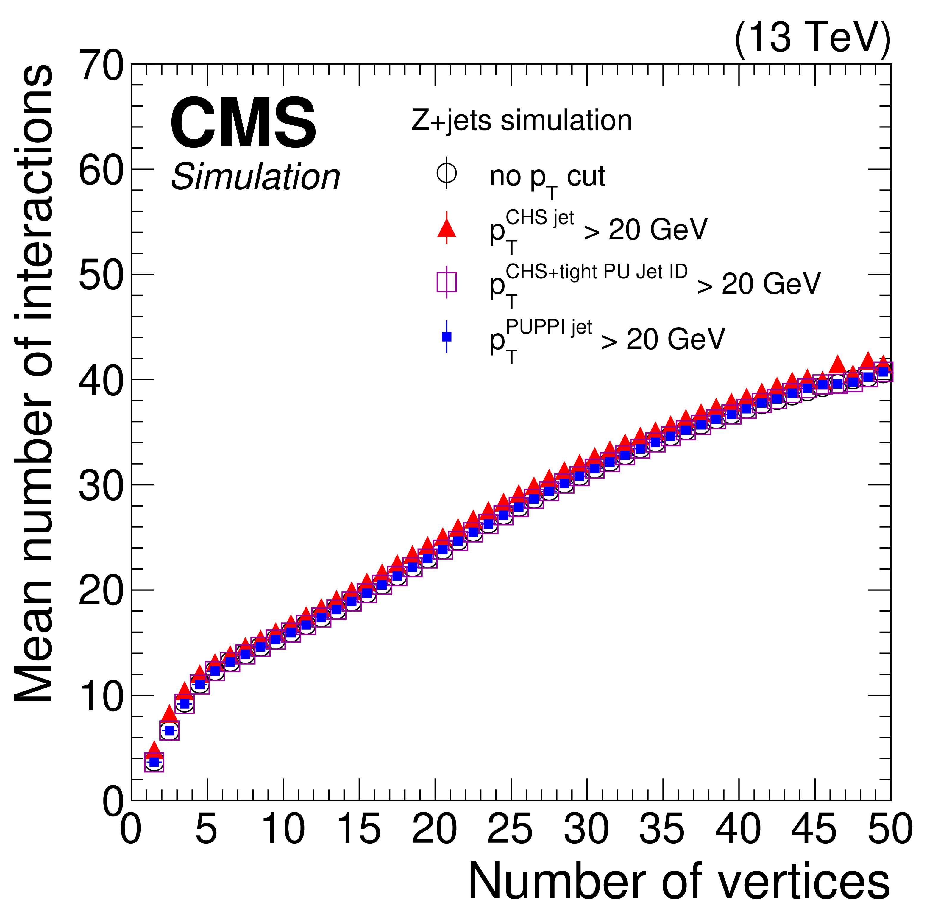
Figure 9:
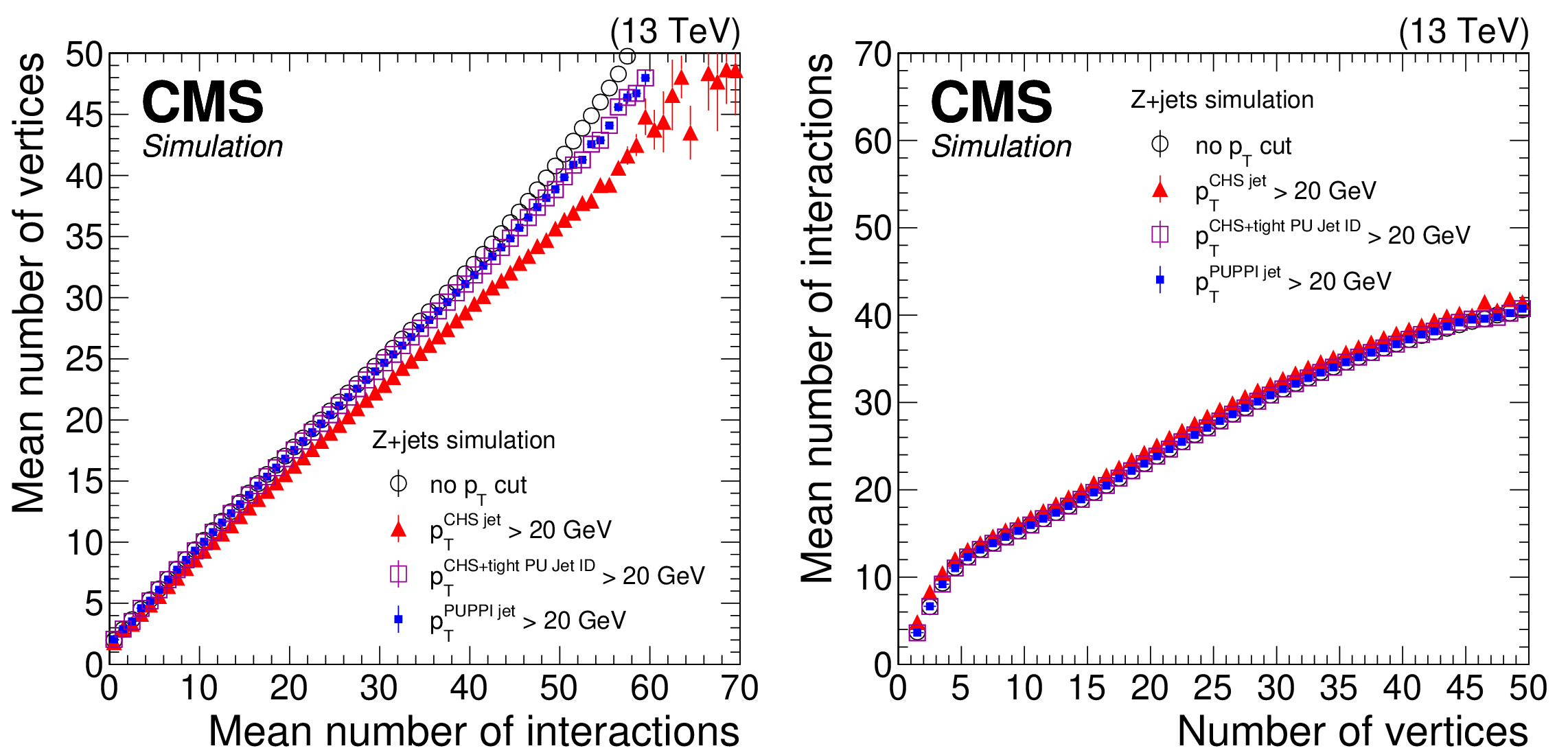
Left: distribution of mean number of reconstructed vertices as a function of the mean number of interactions in Z+jets simulation. Right: distribution of the mean number of interactions as a function of the number of vertices in Z+jets simulation. The black open circles show the behavior without applying any event selection, while for the other markers a selection on jets of $ {p_{\mathrm {T}}} > $ 20 GeV is applied using the CHS (full red triangles), CHS+tight PU jet ID (violet open squares), and PUPPI (full blue squares) algorithms. The error bars correspond to the statistical uncertainty in the simulation. |

png pdf |
Figure 9-a:
Left: distribution of mean number of reconstructed vertices as a function of the mean number of interactions in Z+jets simulation. Right: distribution of the mean number of interactions as a function of the number of vertices in Z+jets simulation. The black open circles show the behavior without applying any event selection, while for the other markers a selection on jets of $ {p_{\mathrm {T}}} > $ 20 GeV is applied using the CHS (full red triangles), CHS+tight PU jet ID (violet open squares), and PUPPI (full blue squares) algorithms. The error bars correspond to the statistical uncertainty in the simulation. |
png pdf |
Figure 9-b:
Left: distribution of mean number of reconstructed vertices as a function of the mean number of interactions in Z+jets simulation. Right: distribution of the mean number of interactions as a function of the number of vertices in Z+jets simulation. The black open circles show the behavior without applying any event selection, while for the other markers a selection on jets of $ {p_{\mathrm {T}}} > $ 20 GeV is applied using the CHS (full red triangles), CHS+tight PU jet ID (violet open squares), and PUPPI (full blue squares) algorithms. The error bars correspond to the statistical uncertainty in the simulation. |
png pdf |
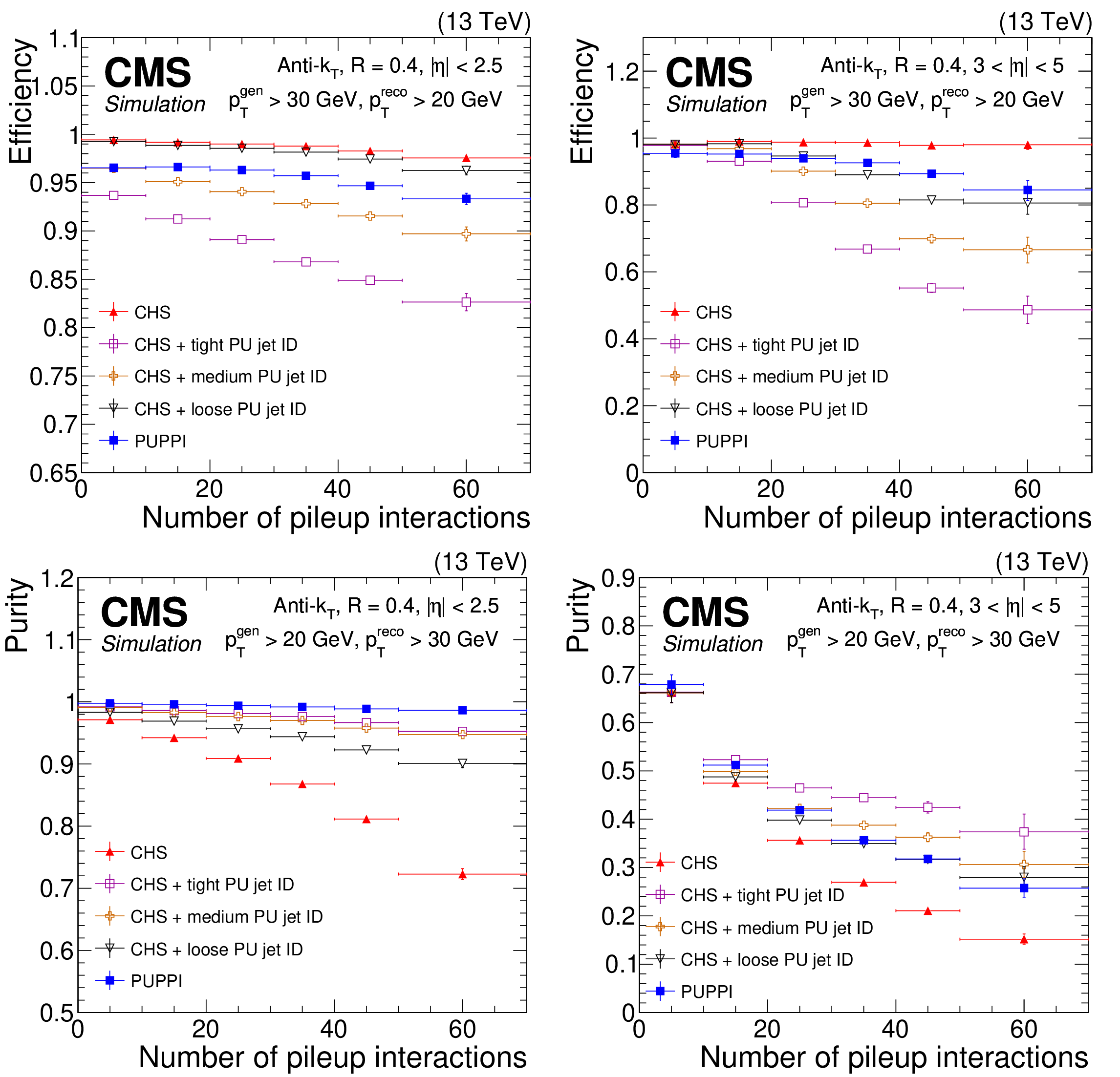
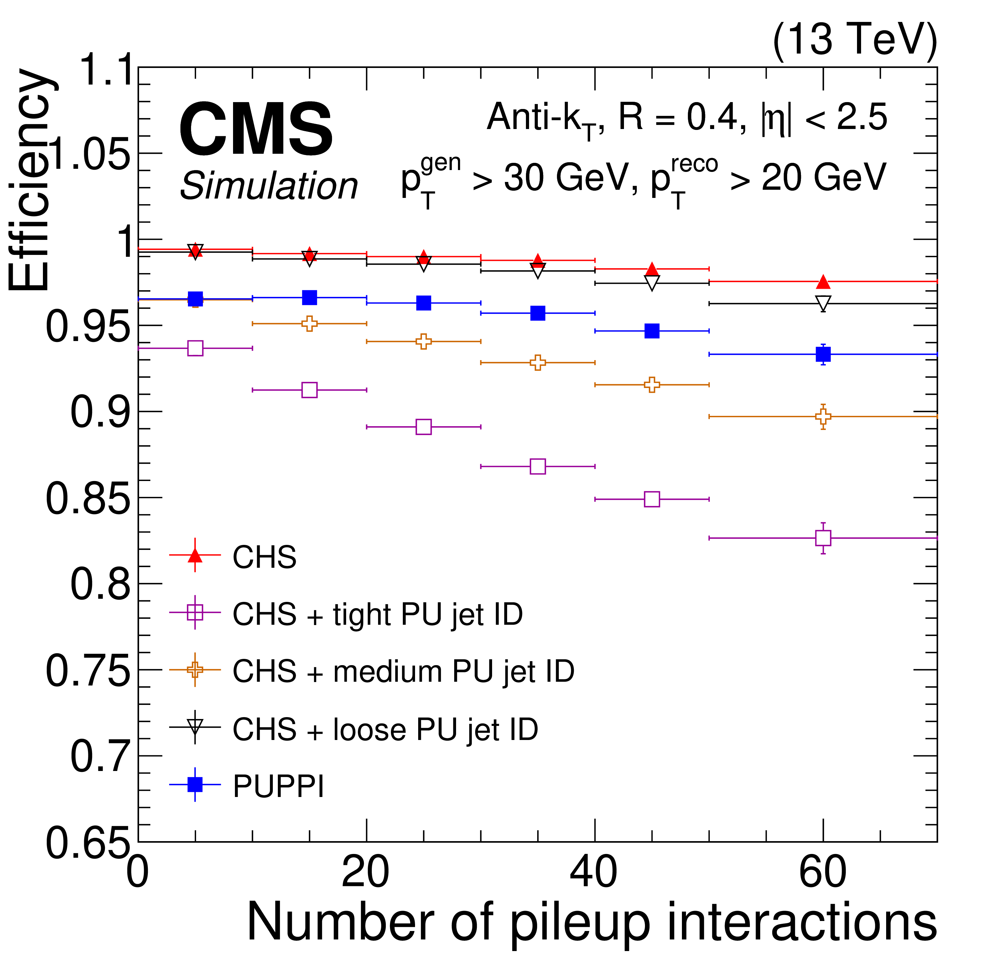
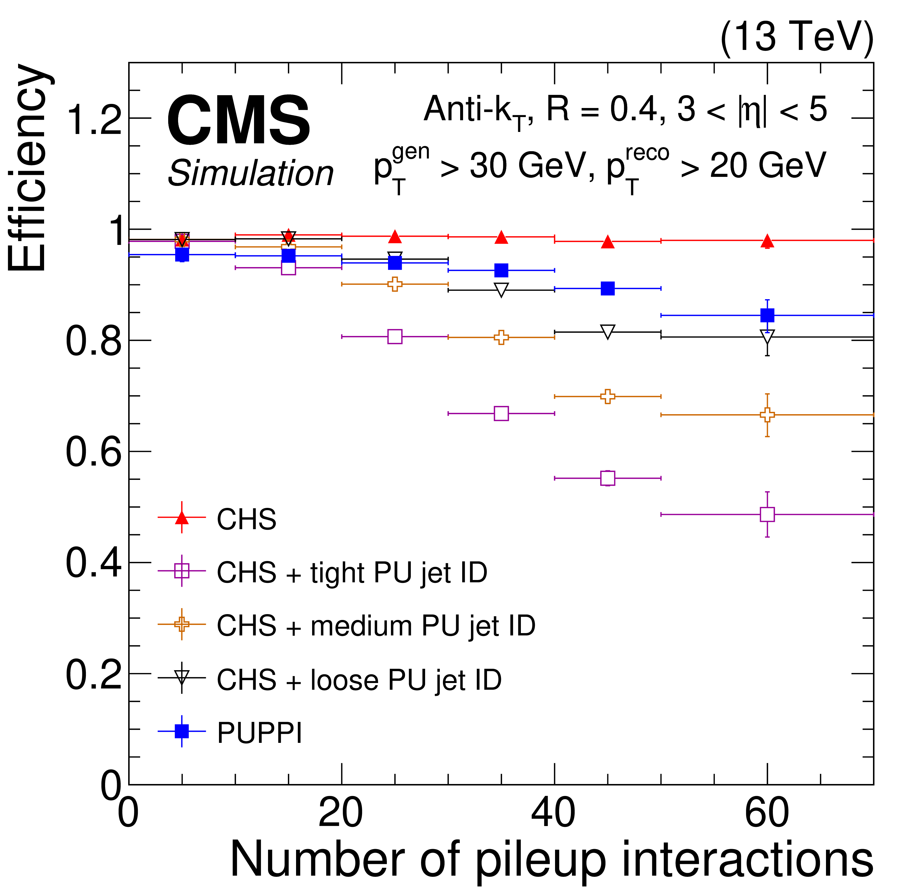
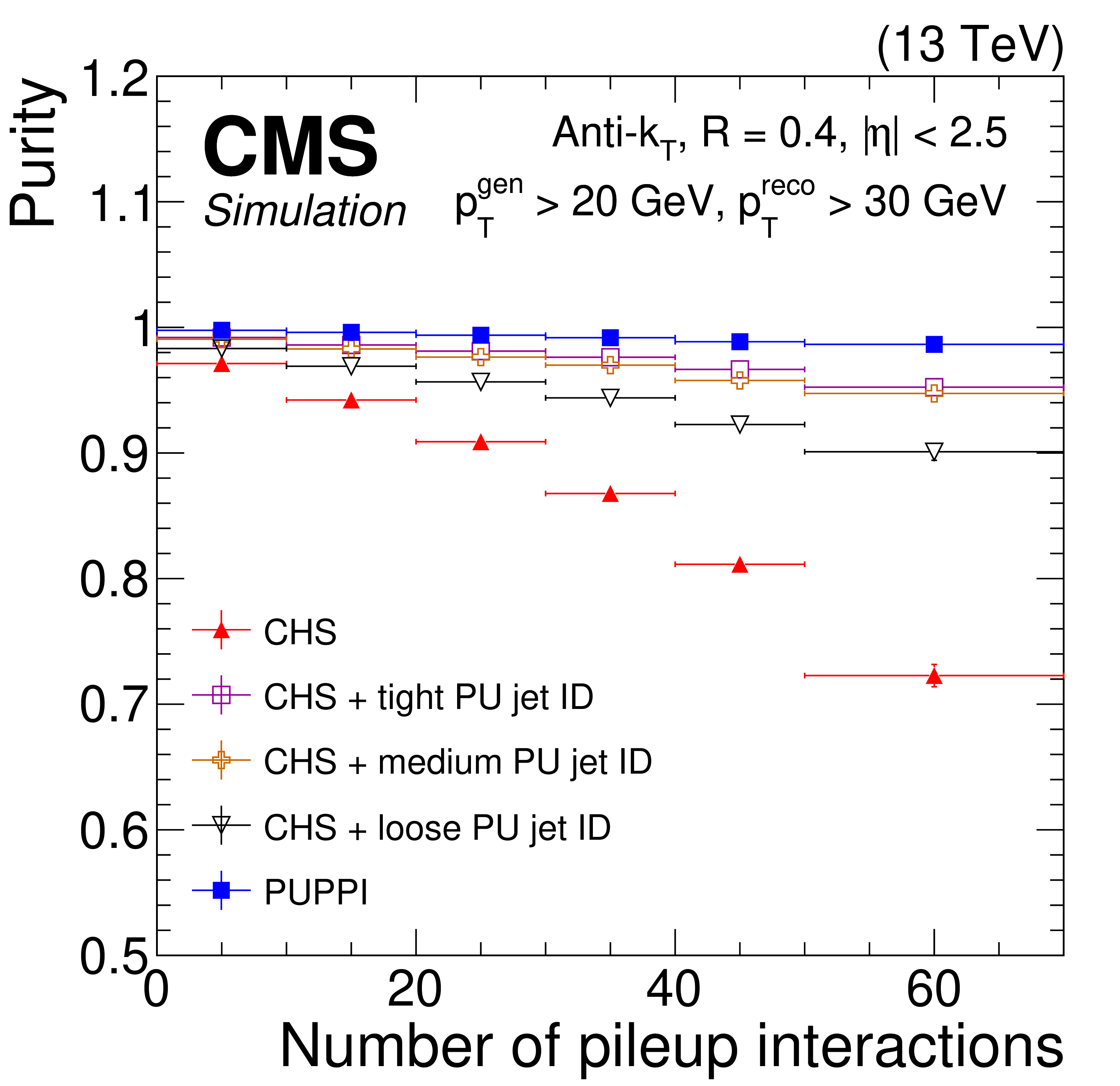
Figure 10:
The LV jet efficiency (upper) and purity (lower) in Z+jets simulation as a function of the number of interactions for PUPPI (blue closed squares), CHS (red closed triangles), CHS+tight PU jet ID (magenta open squares), CHS+medium PU jet ID (orange crosses), and CHS+loose PU jet ID (black triangles). Plots are shown for AK4 jets $ {p_{\mathrm {T}}} > $ 20 GeV, and (left) $ {| \eta |} > $ 2.5 and (right) $ {| \eta |} > 3$. The LV jet efficiency is defined as the number of matched reconstruction-level jets with $ {p_{\mathrm {T}}} > $ 20 GeV divided by the number of particle-level jets with $ {p_{\mathrm {T}}} > $ 30 GeV that originate from the main interaction. For the lower plots, the purity is defined as the number of matched particle-level jets with $ {p_{\mathrm {T}}} > $ 20 GeV divided by the number of reconstructed jets that have $ {p_{\mathrm {T}}} > $ 30 GeV. The error bars correspond to the statistical uncertainty in the simulation. |
png pdf |
Figure 10-a:
The LV jet efficiency (upper) and purity (lower) in Z+jets simulation as a function of the number of interactions for PUPPI (blue closed squares), CHS (red closed triangles), CHS+tight PU jet ID (magenta open squares), CHS+medium PU jet ID (orange crosses), and CHS+loose PU jet ID (black triangles). Plots are shown for AK4 jets $ {p_{\mathrm {T}}} > $ 20 GeV, and (left) $ {| \eta |} > $ 2.5 and (right) $ {| \eta |} > 3$. The LV jet efficiency is defined as the number of matched reconstruction-level jets with $ {p_{\mathrm {T}}} > $ 20 GeV divided by the number of particle-level jets with $ {p_{\mathrm {T}}} > $ 30 GeV that originate from the main interaction. For the lower plots, the purity is defined as the number of matched particle-level jets with $ {p_{\mathrm {T}}} > $ 20 GeV divided by the number of reconstructed jets that have $ {p_{\mathrm {T}}} > $ 30 GeV. The error bars correspond to the statistical uncertainty in the simulation. |
png pdf |
Figure 10-b:
The LV jet efficiency (upper) and purity (lower) in Z+jets simulation as a function of the number of interactions for PUPPI (blue closed squares), CHS (red closed triangles), CHS+tight PU jet ID (magenta open squares), CHS+medium PU jet ID (orange crosses), and CHS+loose PU jet ID (black triangles). Plots are shown for AK4 jets $ {p_{\mathrm {T}}} > $ 20 GeV, and (left) $ {| \eta |} > $ 2.5 and (right) $ {| \eta |} > 3$. The LV jet efficiency is defined as the number of matched reconstruction-level jets with $ {p_{\mathrm {T}}} > $ 20 GeV divided by the number of particle-level jets with $ {p_{\mathrm {T}}} > $ 30 GeV that originate from the main interaction. For the lower plots, the purity is defined as the number of matched particle-level jets with $ {p_{\mathrm {T}}} > $ 20 GeV divided by the number of reconstructed jets that have $ {p_{\mathrm {T}}} > $ 30 GeV. The error bars correspond to the statistical uncertainty in the simulation. |
png pdf |
Figure 10-c:
The LV jet efficiency (upper) and purity (lower) in Z+jets simulation as a function of the number of interactions for PUPPI (blue closed squares), CHS (red closed triangles), CHS+tight PU jet ID (magenta open squares), CHS+medium PU jet ID (orange crosses), and CHS+loose PU jet ID (black triangles). Plots are shown for AK4 jets $ {p_{\mathrm {T}}} > $ 20 GeV, and (left) $ {| \eta |} > $ 2.5 and (right) $ {| \eta |} > 3$. The LV jet efficiency is defined as the number of matched reconstruction-level jets with $ {p_{\mathrm {T}}} > $ 20 GeV divided by the number of particle-level jets with $ {p_{\mathrm {T}}} > $ 30 GeV that originate from the main interaction. For the lower plots, the purity is defined as the number of matched particle-level jets with $ {p_{\mathrm {T}}} > $ 20 GeV divided by the number of reconstructed jets that have $ {p_{\mathrm {T}}} > $ 30 GeV. The error bars correspond to the statistical uncertainty in the simulation. |

png pdf |
Figure 10-d:
The LV jet efficiency (upper) and purity (lower) in Z+jets simulation as a function of the number of interactions for PUPPI (blue closed squares), CHS (red closed triangles), CHS+tight PU jet ID (magenta open squares), CHS+medium PU jet ID (orange crosses), and CHS+loose PU jet ID (black triangles). Plots are shown for AK4 jets $ {p_{\mathrm {T}}} > $ 20 GeV, and (left) $ {| \eta |} > $ 2.5 and (right) $ {| \eta |} > 3$. The LV jet efficiency is defined as the number of matched reconstruction-level jets with $ {p_{\mathrm {T}}} > $ 20 GeV divided by the number of particle-level jets with $ {p_{\mathrm {T}}} > $ 30 GeV that originate from the main interaction. For the lower plots, the purity is defined as the number of matched particle-level jets with $ {p_{\mathrm {T}}} > $ 20 GeV divided by the number of reconstructed jets that have $ {p_{\mathrm {T}}} > $ 30 GeV. The error bars correspond to the statistical uncertainty in the simulation. |
png pdf |
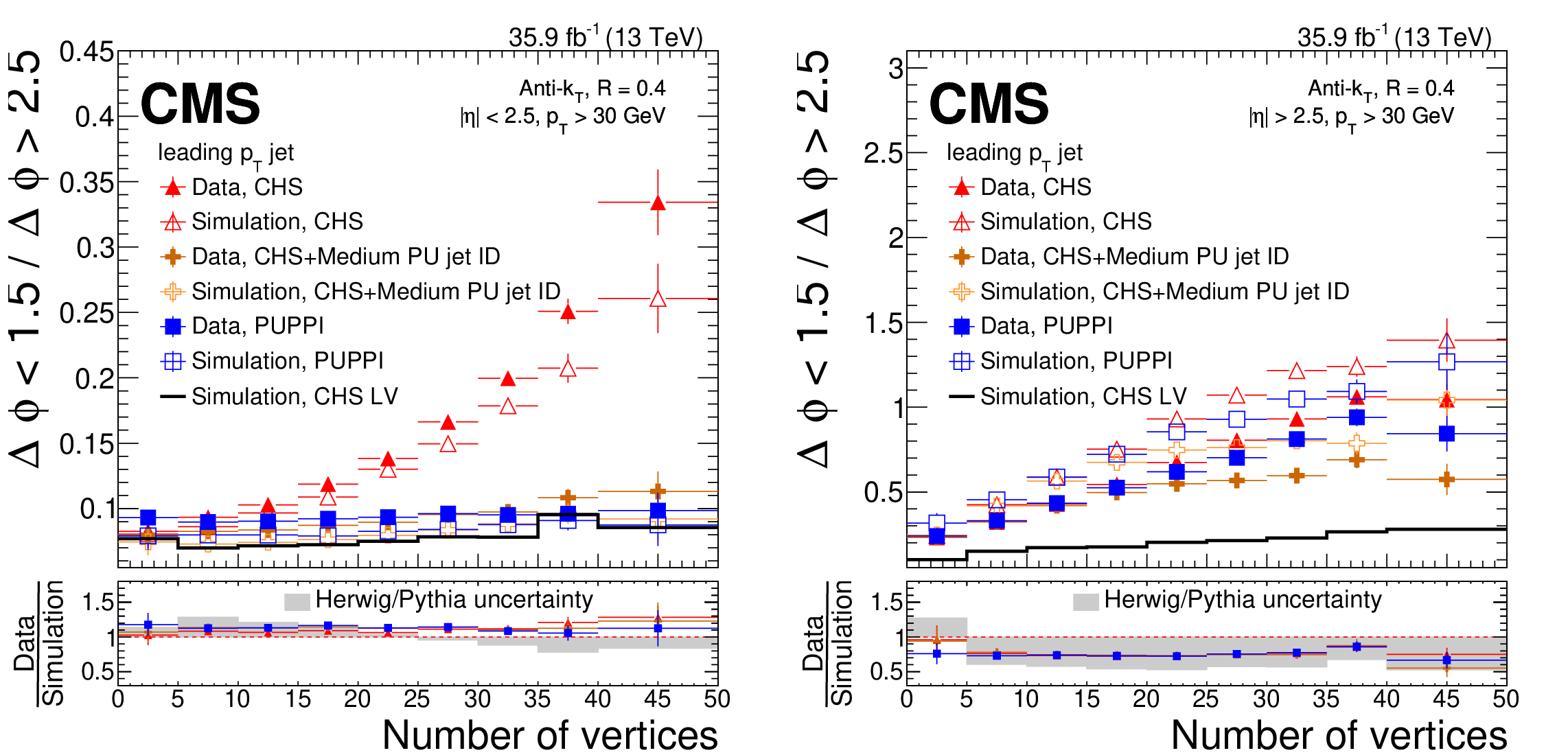
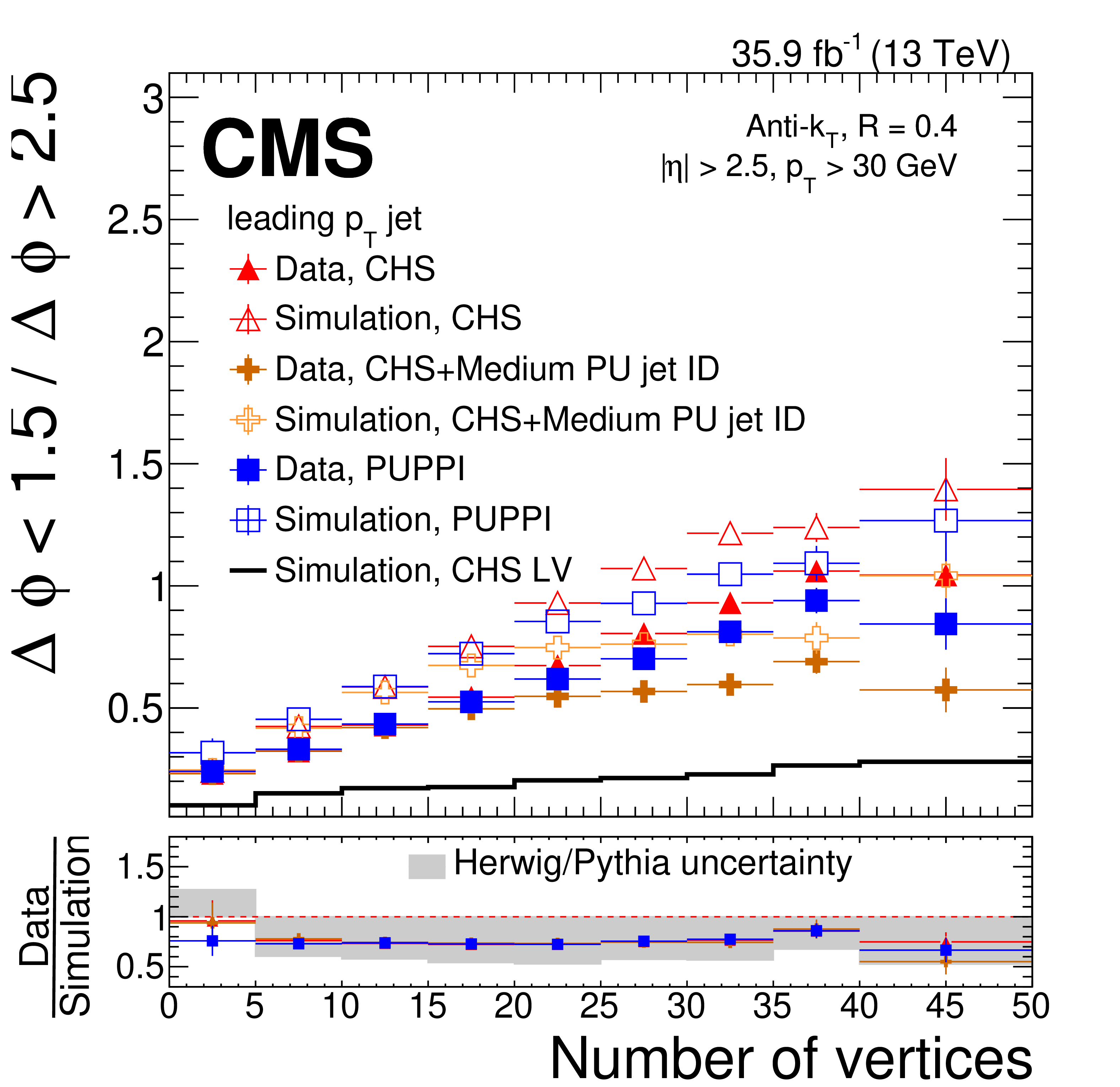
Figure 11:
Rate of jets in the PU-enriched region divided by the rate of jets in the LV-enriched region as a function of the number of vertices for CHS jets (red triangles), CHS jets with medium PU jet ID applied (orange crosses) and PUPPI jets (blue squares) in Z+jets simulation (open markers), and data (full markers). The plots show the ratio for events with $ {| \eta |} > $ 2.5 (left) and $ {| \eta |} > $ 2.5 (right). The lower panels show the data-to-simulation ratio along with a gray band corresponding to the one-sided uncertainty that is the difference between simulated Z+jets events showered with the {pythia} parton shower to those showered with the HERWIG++ parton shower. |

png pdf |
Figure 11-a:
Rate of jets in the PU-enriched region divided by the rate of jets in the LV-enriched region as a function of the number of vertices for CHS jets (red triangles), CHS jets with medium PU jet ID applied (orange crosses) and PUPPI jets (blue squares) in Z+jets simulation (open markers), and data (full markers). The plots show the ratio for events with $ {| \eta |} > $ 2.5 (left) and $ {| \eta |} > $ 2.5 (right). The lower panels show the data-to-simulation ratio along with a gray band corresponding to the one-sided uncertainty that is the difference between simulated Z+jets events showered with the {pythia} parton shower to those showered with the HERWIG++ parton shower. |
png pdf |
Figure 11-b:
Rate of jets in the PU-enriched region divided by the rate of jets in the LV-enriched region as a function of the number of vertices for CHS jets (red triangles), CHS jets with medium PU jet ID applied (orange crosses) and PUPPI jets (blue squares) in Z+jets simulation (open markers), and data (full markers). The plots show the ratio for events with $ {| \eta |} > $ 2.5 (left) and $ {| \eta |} > $ 2.5 (right). The lower panels show the data-to-simulation ratio along with a gray band corresponding to the one-sided uncertainty that is the difference between simulated Z+jets events showered with the {pythia} parton shower to those showered with the HERWIG++ parton shower. |
png pdf |
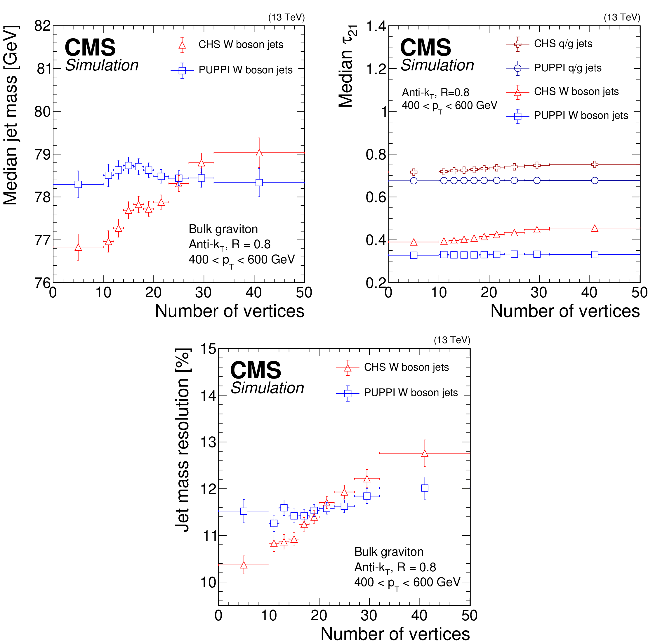
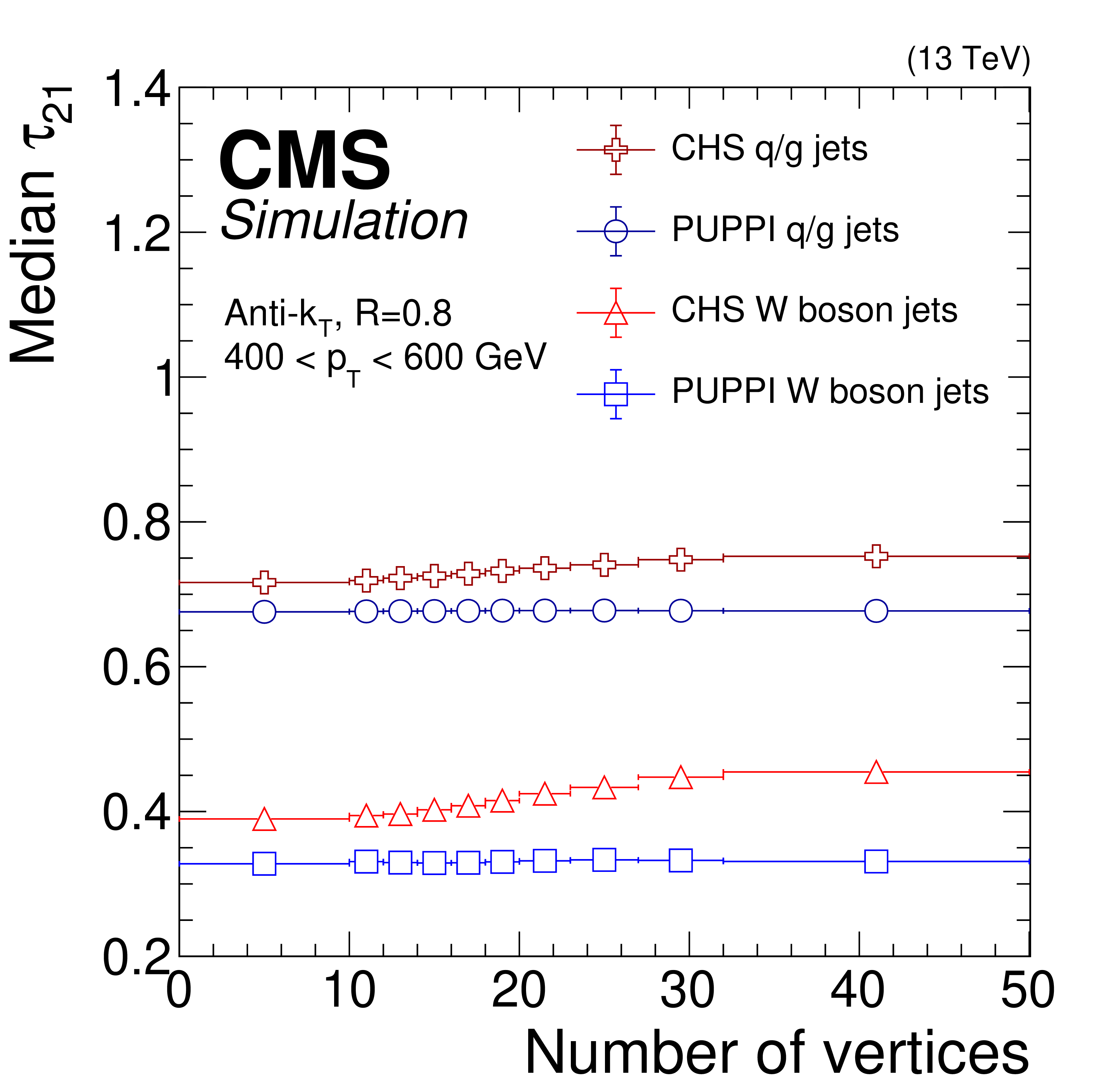
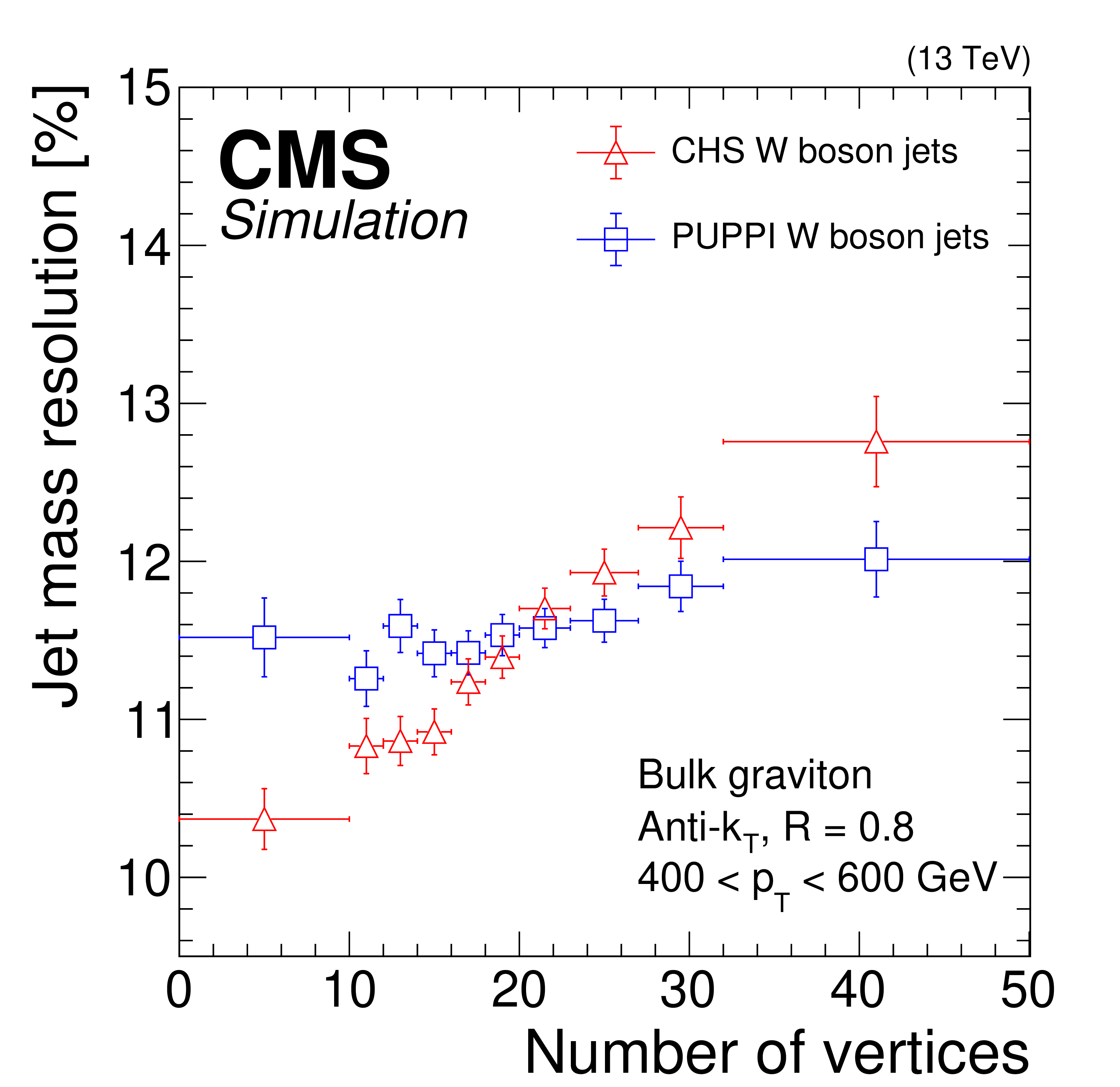
Figure 12:
Median soft drop jet mass (upper left), median $\tau _{21}$ (upper right), and soft drop jet mass resolution (lower) for AK8 jets from boosted W bosons with 400 $ < {p_{\mathrm {T}}} < $ 600 GeV for CHS (red triangles) and PUPPI (blue squares) jets in a bulk graviton decaying to WW signal sample, as a function of the number of vertices. The error bars correspond to the statistical uncertainty in the simulation. |

png pdf |
Figure 12-a:
Median soft drop jet mass (upper left), median $\tau _{21}$ (upper right), and soft drop jet mass resolution (lower) for AK8 jets from boosted W bosons with 400 $ < {p_{\mathrm {T}}} < $ 600 GeV for CHS (red triangles) and PUPPI (blue squares) jets in a bulk graviton decaying to WW signal sample, as a function of the number of vertices. The error bars correspond to the statistical uncertainty in the simulation. |
png pdf |
Figure 12-b:
Median soft drop jet mass (upper left), median $\tau _{21}$ (upper right), and soft drop jet mass resolution (lower) for AK8 jets from boosted W bosons with 400 $ < {p_{\mathrm {T}}} < $ 600 GeV for CHS (red triangles) and PUPPI (blue squares) jets in a bulk graviton decaying to WW signal sample, as a function of the number of vertices. The error bars correspond to the statistical uncertainty in the simulation. |
png pdf |
Figure 12-c:
Median soft drop jet mass (upper left), median $\tau _{21}$ (upper right), and soft drop jet mass resolution (lower) for AK8 jets from boosted W bosons with 400 $ < {p_{\mathrm {T}}} < $ 600 GeV for CHS (red triangles) and PUPPI (blue squares) jets in a bulk graviton decaying to WW signal sample, as a function of the number of vertices. The error bars correspond to the statistical uncertainty in the simulation. |
png pdf |
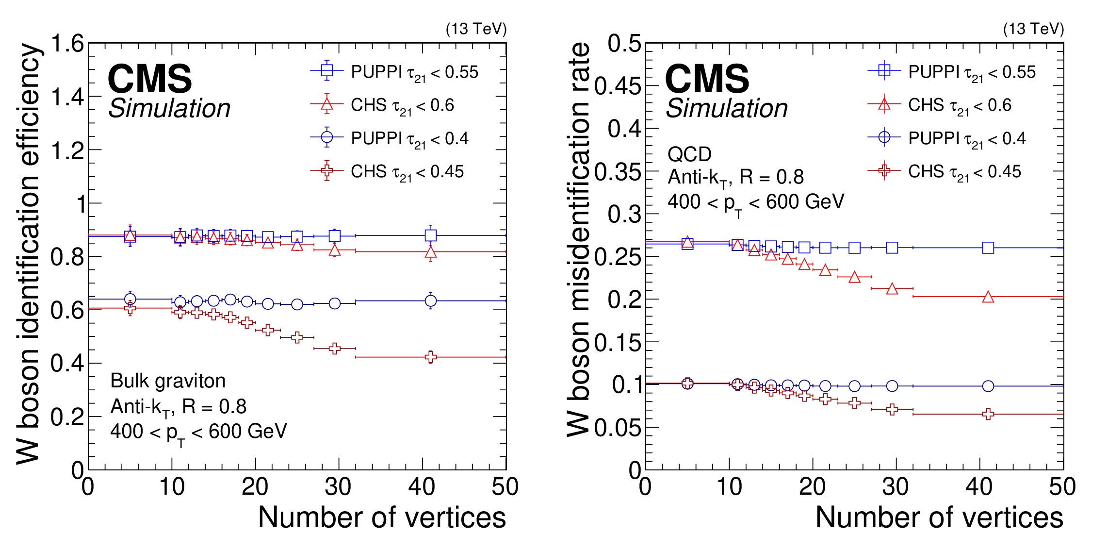
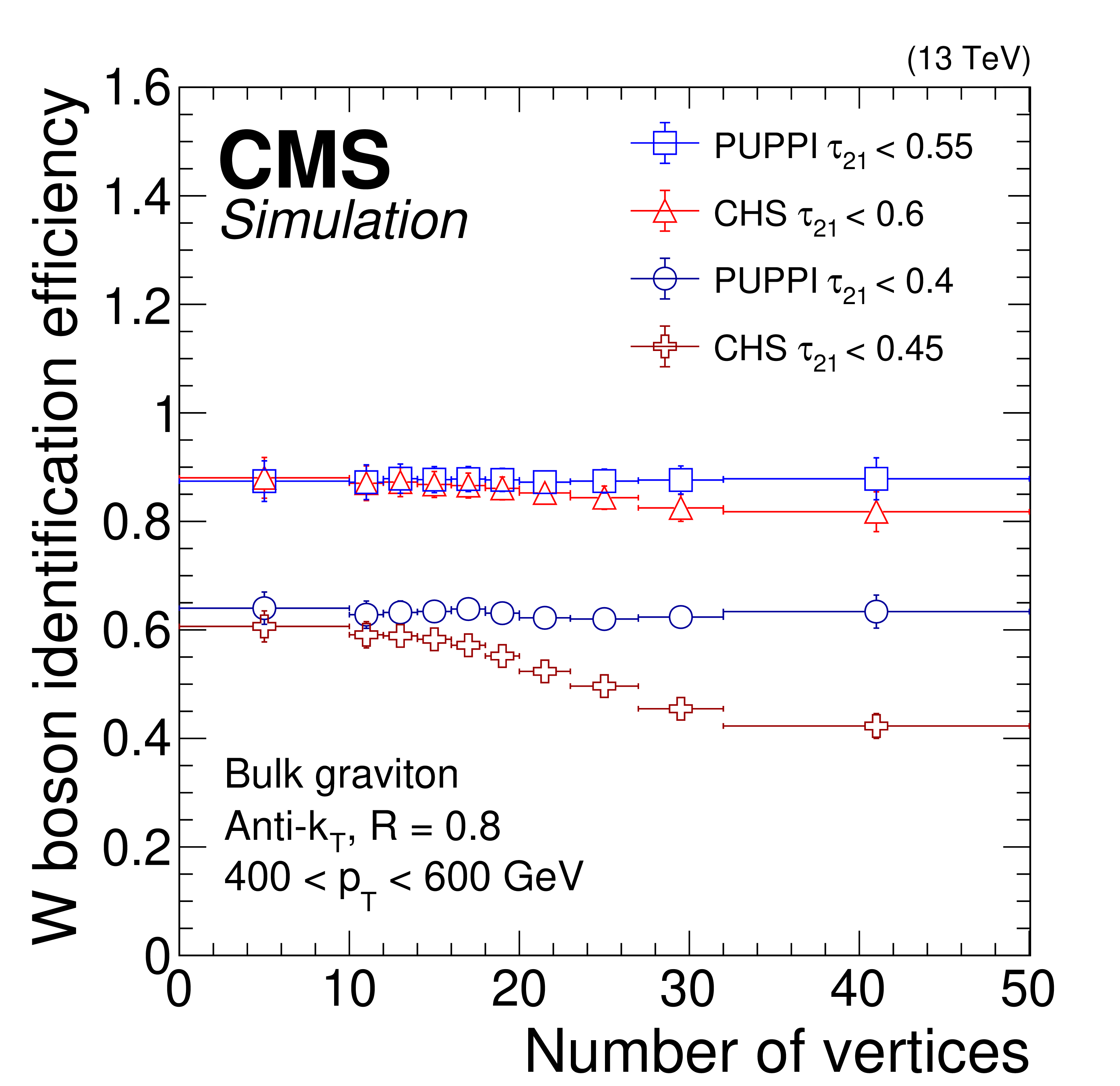
Figure 13:
W boson identification performance using a selection on $\tau _{21}$ for CHS (red triangles and dark red crosses) and PUPPI (blue squares and circles) AK8 jets as a function of the number of vertices for loose and tight selections, respectively. Shown on the left is the W boson identification efficiency evaluated in simulation for a bulk graviton decaying to a WW boson pair and on the right the misidentification rate evaluated with QCD multijet simulation. The error bars correspond to the statistical uncertainty in the simulation. |
png pdf |
Figure 13-a:
W boson identification performance using a selection on $\tau _{21}$ for CHS (red triangles and dark red crosses) and PUPPI (blue squares and circles) AK8 jets as a function of the number of vertices for loose and tight selections, respectively. Shown on the left is the W boson identification efficiency evaluated in simulation for a bulk graviton decaying to a WW boson pair and on the right the misidentification rate evaluated with QCD multijet simulation. The error bars correspond to the statistical uncertainty in the simulation. |

png pdf |
Figure 13-b:
W boson identification performance using a selection on $\tau _{21}$ for CHS (red triangles and dark red crosses) and PUPPI (blue squares and circles) AK8 jets as a function of the number of vertices for loose and tight selections, respectively. Shown on the left is the W boson identification efficiency evaluated in simulation for a bulk graviton decaying to a WW boson pair and on the right the misidentification rate evaluated with QCD multijet simulation. The error bars correspond to the statistical uncertainty in the simulation. |

png pdf |
Figure 14:
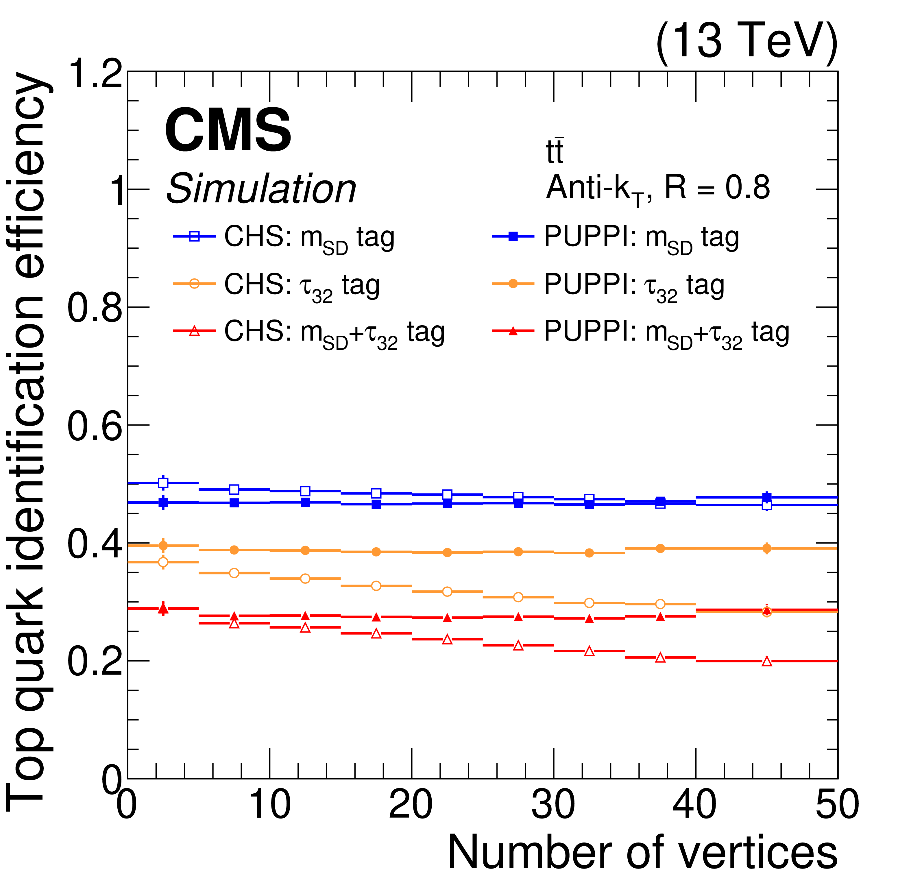
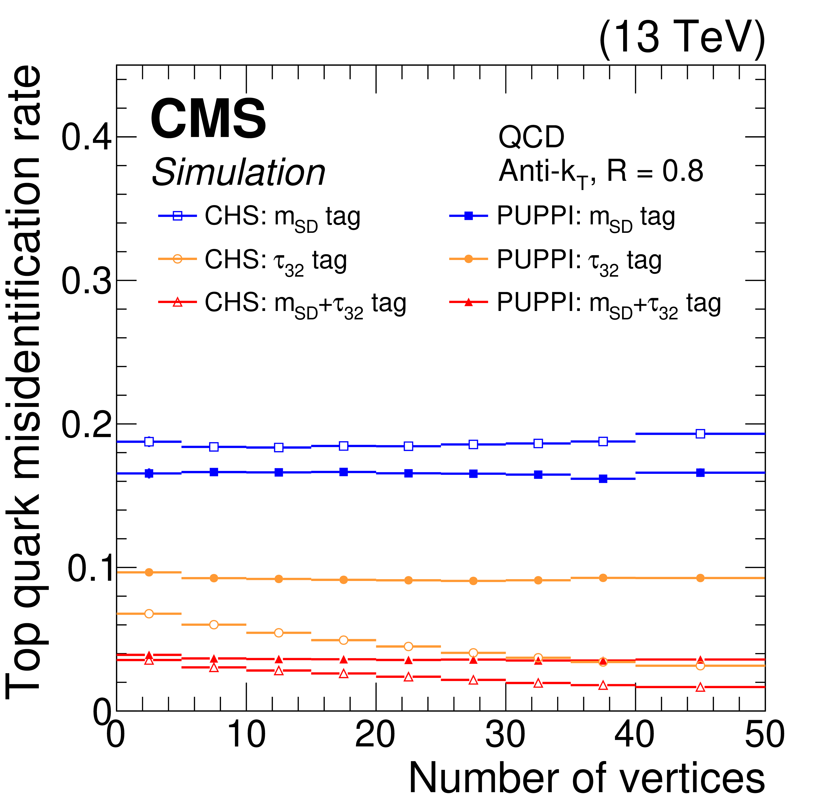
Top quark identification efficiency (left) and misidentification rate (right) as a function of the number of vertices for CHS (open symbols) and PUPPI (closed symbols) jets, using different combinations of substructure variables: soft drop mass cut between 105 and 210 GeV (blue rectangles), $\tau _{32} < 0.54$ (orange circles), and both requirements together (red triangles). The error bars correspond to the statistical uncertainty in the simulation. |
png pdf |
Figure 14-a:
Top quark identification efficiency (left) and misidentification rate (right) as a function of the number of vertices for CHS (open symbols) and PUPPI (closed symbols) jets, using different combinations of substructure variables: soft drop mass cut between 105 and 210 GeV (blue rectangles), $\tau _{32} < 0.54$ (orange circles), and both requirements together (red triangles). The error bars correspond to the statistical uncertainty in the simulation. |
png pdf |
Figure 14-b:
Top quark identification efficiency (left) and misidentification rate (right) as a function of the number of vertices for CHS (open symbols) and PUPPI (closed symbols) jets, using different combinations of substructure variables: soft drop mass cut between 105 and 210 GeV (blue rectangles), $\tau _{32} < 0.54$ (orange circles), and both requirements together (red triangles). The error bars correspond to the statistical uncertainty in the simulation. |

png pdf |
Figure 15:
The hadronic recoil response ($-< u_{\parallel} > /< q_{\mathrm {T}} > $) of the Z boson computed for PUPPI and PF ${{p_{\mathrm {T}}} ^\text {miss}}$, as a function of $q_\mathrm {T}$ in ${\mathrm{Z} \to \mathrm{ee}}$ events in collision data. The lower panel shows the data-to-simulation ratio. A gray shaded band is added in the lower panel showing the systematic uncertainties resulting from jet energy scale and jet energy resolution variations, and variations in the unclustered energy added in quadrature. |

png pdf |
Figure 16:
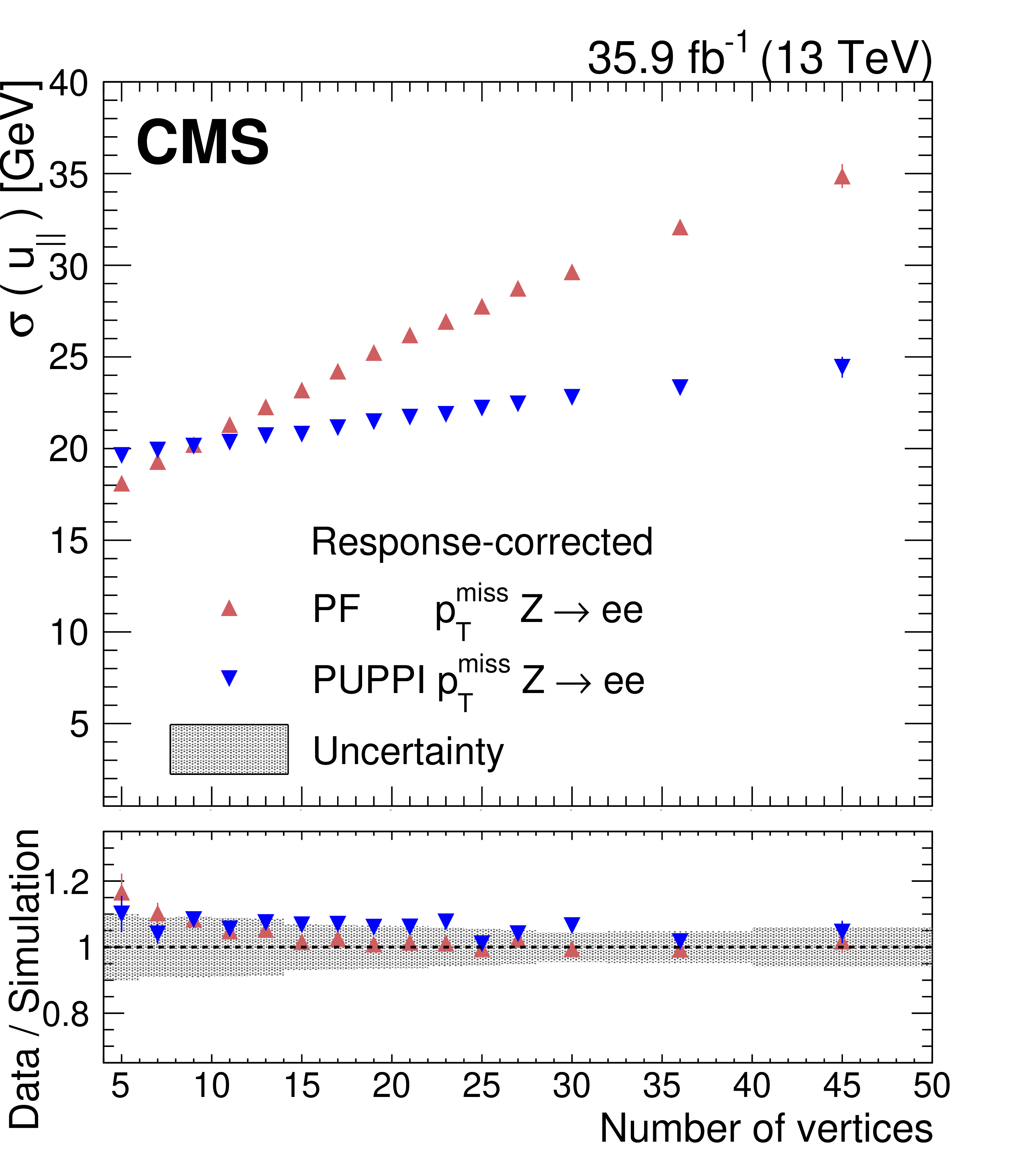
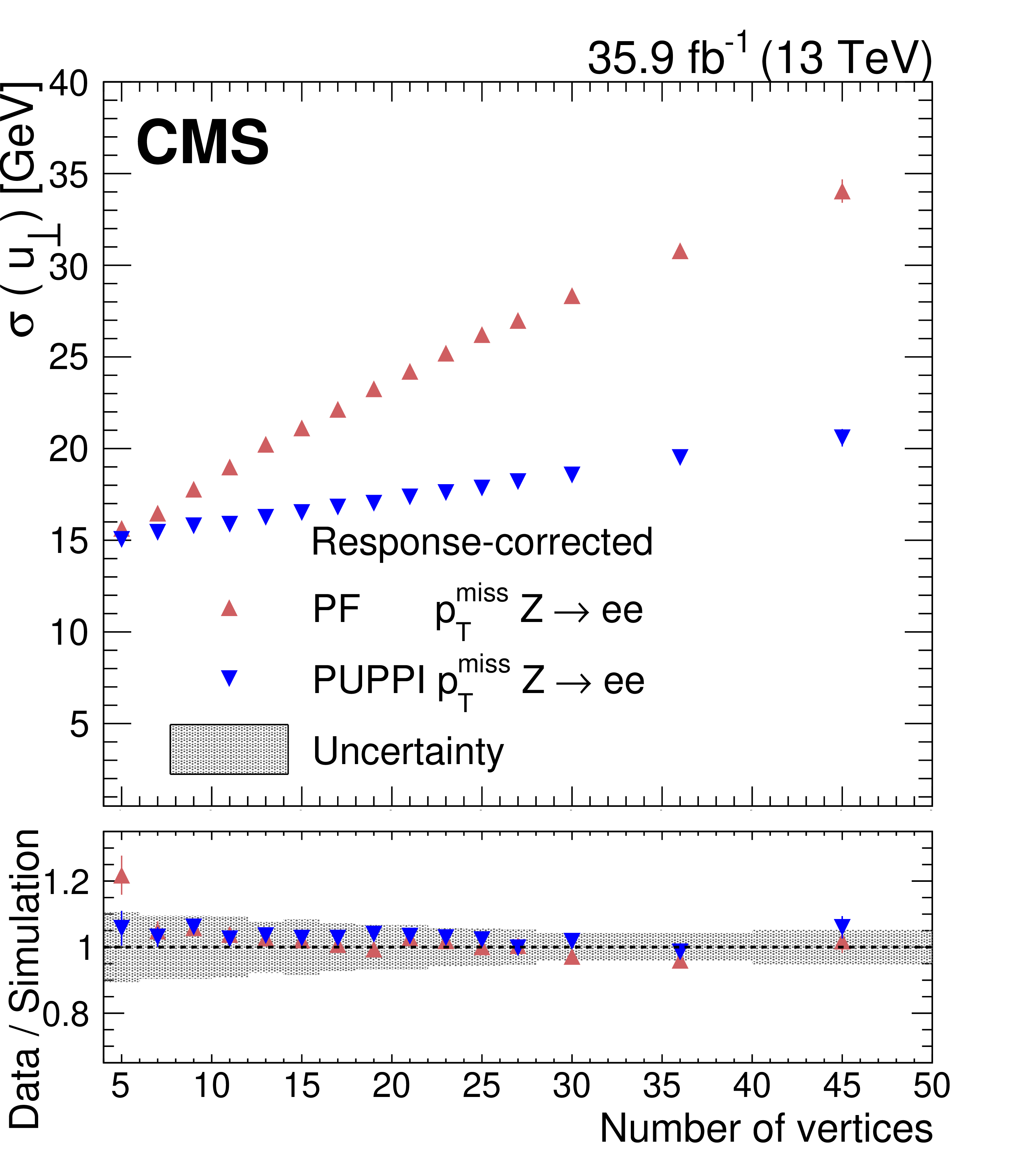
The hadronic recoil components ${u_{||}}$ (left) and ${u_{\perp}}$ (right) for PUPPI and PF ${{p_{\mathrm {T}}} ^\text {miss}}$ resolution as a function of the number of vertices in ${\mathrm{Z} \to \mathrm{ee}}$ events in collision data. The lower panel shows the data-to-simulation ratio. A gray shaded band is added in the lower panel showing the systematic uncertainties resulting from jet energy scale and jet energy resolution variations, and variations in the unclustered energy added in quadrature. |
png pdf |
Figure 16-a:
The hadronic recoil components ${u_{||}}$ (left) and ${u_{\perp}}$ (right) for PUPPI and PF ${{p_{\mathrm {T}}} ^\text {miss}}$ resolution as a function of the number of vertices in ${\mathrm{Z} \to \mathrm{ee}}$ events in collision data. The lower panel shows the data-to-simulation ratio. A gray shaded band is added in the lower panel showing the systematic uncertainties resulting from jet energy scale and jet energy resolution variations, and variations in the unclustered energy added in quadrature. |
png pdf |
Figure 16-b:
The hadronic recoil components ${u_{||}}$ (left) and ${u_{\perp}}$ (right) for PUPPI and PF ${{p_{\mathrm {T}}} ^\text {miss}}$ resolution as a function of the number of vertices in ${\mathrm{Z} \to \mathrm{ee}}$ events in collision data. The lower panel shows the data-to-simulation ratio. A gray shaded band is added in the lower panel showing the systematic uncertainties resulting from jet energy scale and jet energy resolution variations, and variations in the unclustered energy added in quadrature. |

png pdf |
Figure 17:
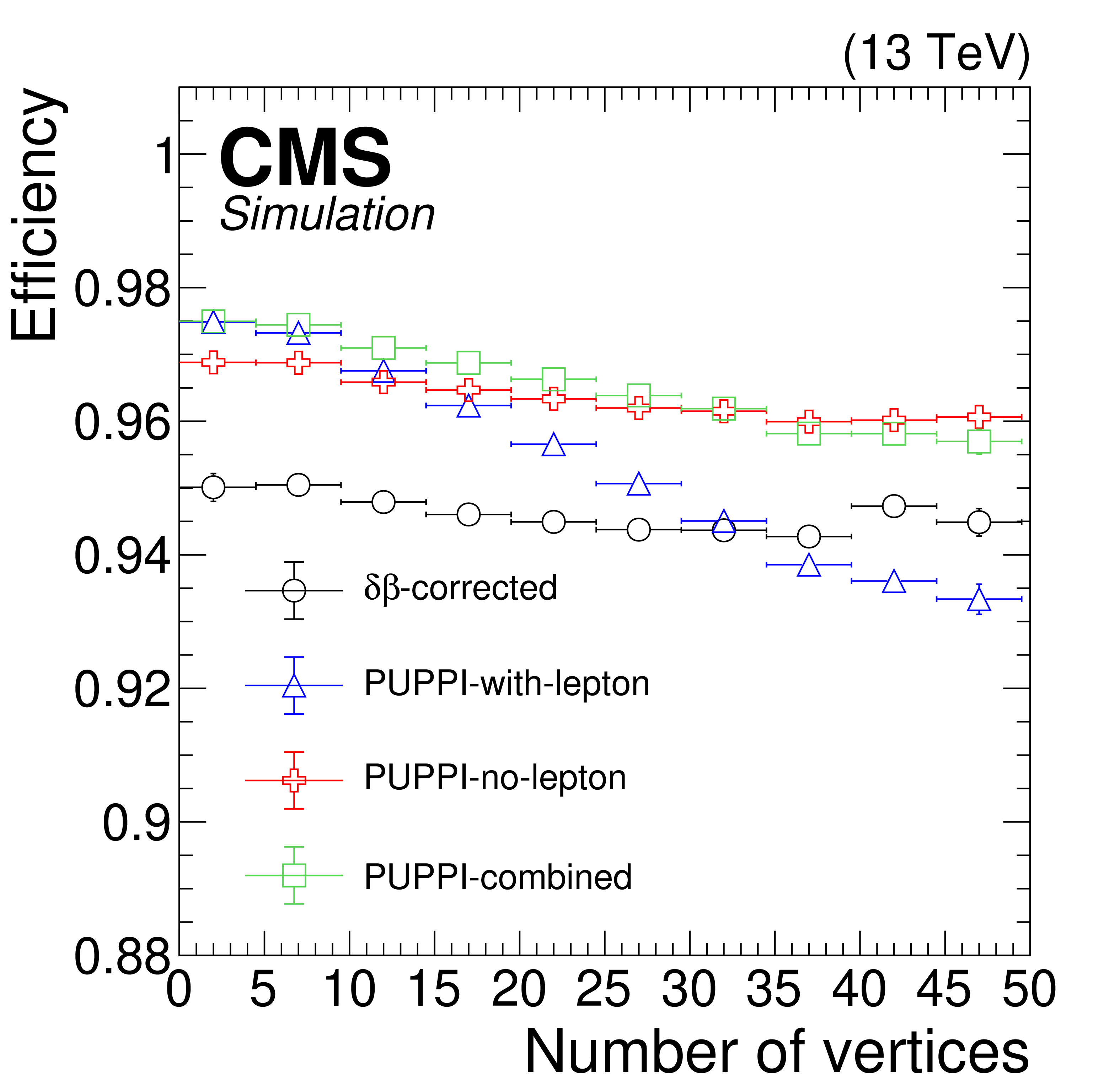
The identification efficiency for prompt muons in simulated Z+jets events (left) and the misidentification rate for nonprompt muons in QCD multijet simulated events (right) for the different definitions of the isolation: ${\delta \beta \text {-corrected}}$ isolation (black circles), PUPPI-with-lepton (blue triangles), PUPPI-no-lepton (red crosses), PUPPI-combined (green squares), as a function of the number of vertices. The threshold of each isolation is set to yield a 12% misidentification rate for reconstructed muons in QCD multijet simulation. The error bars correspond to the statistical uncertainty in the simulation. |
png pdf |
Figure 17-a:
The identification efficiency for prompt muons in simulated Z+jets events (left) and the misidentification rate for nonprompt muons in QCD multijet simulated events (right) for the different definitions of the isolation: ${\delta \beta \text {-corrected}}$ isolation (black circles), PUPPI-with-lepton (blue triangles), PUPPI-no-lepton (red crosses), PUPPI-combined (green squares), as a function of the number of vertices. The threshold of each isolation is set to yield a 12% misidentification rate for reconstructed muons in QCD multijet simulation. The error bars correspond to the statistical uncertainty in the simulation. |

png pdf |
Figure 17-b:
The identification efficiency for prompt muons in simulated Z+jets events (left) and the misidentification rate for nonprompt muons in QCD multijet simulated events (right) for the different definitions of the isolation: ${\delta \beta \text {-corrected}}$ isolation (black circles), PUPPI-with-lepton (blue triangles), PUPPI-no-lepton (red crosses), PUPPI-combined (green squares), as a function of the number of vertices. The threshold of each isolation is set to yield a 12% misidentification rate for reconstructed muons in QCD multijet simulation. The error bars correspond to the statistical uncertainty in the simulation. |
png pdf |
Figure 18:
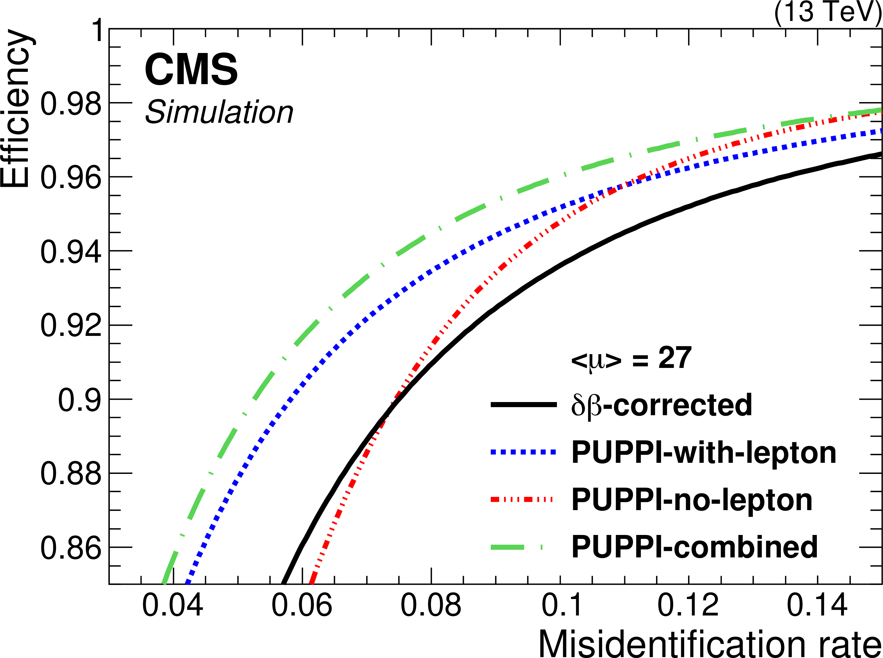
The identification efficiency for prompt muons in simulated Z+jets events as a function of the misidentification rate for nonprompt muons in QCD multijet simulated events for the different definitions of the isolation: ${\delta \beta \text {-corrected}}$ isolation (black solid line), PUPPI-with-lepton (blue dashed line), PUPPI-no-lepton (red mixed dashed), PUPPI-combined (green long mixed dashed). The average number of interactions is 27. |

png pdf |
Figure 19:
Mean relative isolation for PUPPI-with-lepton (left) and PUPPI-no-lepton (right) in data compared to Z+jets simulation. The relative isolation is split into separate charged hadron (Ch, green squares), neutral hadron (Nh, blue circles), photon (Ph, red crosses) components, and combined (black triangles). Data and simulation are shown using full and open markers, respectively. The lower panels show the data-to-simulation ratio of each component. The error bars correspond to the statistical uncertainty. |

png pdf |
Figure 19-a:
Mean relative isolation for PUPPI-with-lepton (left) and PUPPI-no-lepton (right) in data compared to Z+jets simulation. The relative isolation is split into separate charged hadron (Ch, green squares), neutral hadron (Nh, blue circles), photon (Ph, red crosses) components, and combined (black triangles). Data and simulation are shown using full and open markers, respectively. The lower panels show the data-to-simulation ratio of each component. The error bars correspond to the statistical uncertainty. |

png pdf |
Figure 19-b:
Mean relative isolation for PUPPI-with-lepton (left) and PUPPI-no-lepton (right) in data compared to Z+jets simulation. The relative isolation is split into separate charged hadron (Ch, green squares), neutral hadron (Nh, blue circles), photon (Ph, red crosses) components, and combined (black triangles). Data and simulation are shown using full and open markers, respectively. The lower panels show the data-to-simulation ratio of each component. The error bars correspond to the statistical uncertainty. |

png pdf |
Figure 20:
The identification efficiency for prompt muon isolation selection in ${\mathrm{Z} \to \mu\mu}$ events in data compared to Z+jets simulation, as a function of the number of vertices for PUPPI-combined (green circles) and ${\delta \beta \text {-corrected}}$ isolation (black squares). Data and simulation are shown using full and open markers, respectively. The lower panel shows the data-to-simulation ratio. The error bars correspond to the statistical uncertainty. |

png pdf |
Figure 21:
The misidentification rate defined as the number of events with a third isolated muon divided by the total number of events with a third muon in ${\mathrm{Z} \to \mu\mu}$ data for PUPPI-combined (blue closed circles) and ${\delta \beta \text {-corrected}}$ isolation (red open circles). The lower panel shows the ratio of PUPPI-combined and ${\delta \beta \text {-corrected}}$ isolation, taking the correlation of their uncertainties into account. |
| Tables | |

png pdf |
Table 1:
The tunable parameters of PUPPI optimized for application in 2016 data analysis. The transfer factors used to extrapolate the $\overline {\alpha}_{{\text {PU}}}$ and $\alpha _{{\text {PU}}}^{\text {RMS}}$ to $ {| \eta |} > $ 2.5 are denoted TF. |

png pdf |
Table 2:
Jet ID criteria for CHS and PUPPI jets yielding a genuine jet efficiency of 99% in different regions of $ {| \eta |}$. |
png pdf |
Table 3:
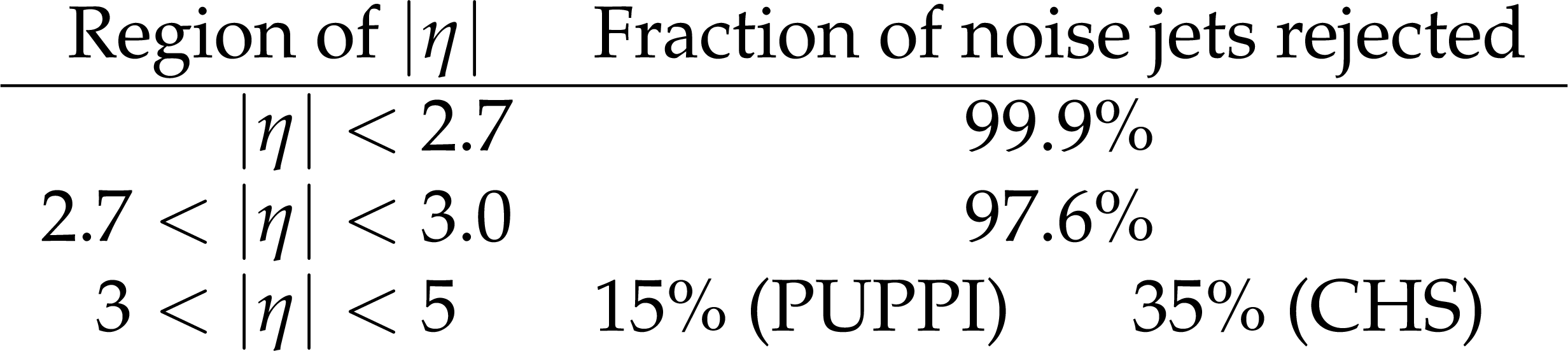
Fraction of noise jets rejected when applying jet ID criteria to PUPPI and CHS jets yielding a genuine jet efficiency of 99% in different regions of $ {| \eta |}$. |

png pdf |
Table 4:
List of variables used in the PU jet ID for CHS jets. |

png pdf |
Table 5:
Data-to-simulation scale factors for the jet mass scale, jet mass resolution, and the $\tau _{21}$ selection efficiency for the CHS and PUPPI algorithms. |
| Summary |
| The impact of pileup (PU) mitigation techniques on object reconstruction performance in the CMS experiment has been presented. The main techniques under study are charged-hadron subtraction (CHS) and pileup per particle identification (PUPPI), which both exploit particle-level information. The performance of these techniques is evaluated in the context of the reconstruction of jets and missing transverse momentum (${p_{\mathrm{T}}}^{\text{miss}}$), lepton isolation, and the calculation of jet substructure observables for boosted object tagging. The CHS and PUPPI algorithms are further compared with other algorithmic approaches that act on jet, ${p_{\mathrm{T}}}^{\text{miss}}$, and lepton objects. While CHS rejects charged particles associated with PU vertices, PUPPI applies a more stringent selection to charged particles and rescales the four-momentum of neutral particles according to their probability to originate from the leading vertex. Both techniques reduce the dependence on PU interactions across all objects. A stronger reduction is achieved with PUPPI, especially for events with more than 30 interactions. The PUPPI algorithm provides the best performance for jet mass and substructure observables, ${p_{\mathrm{T}}}^{\text{miss}}$ resolution, and rejection of misidentified muons. With respect to jet-momentum resolution and PU jet rejection, the preferred algorithm depends on the physics process under study: the PUPPI algorithm provides a better jet momentum resolution for jets with ${p_{\mathrm{T}}} < $ 100 GeV, whereas CHS does so for ${p_{\mathrm{T}}} > $ 100 GeV. The highest rejection rate for jets originating purely from PU is obtained when using a dedicated PU jet identification in addition to CHS. However, when a looser working point for the PU jet identification is chosen such that its efficiency for selecting jets coming from the leading vertex is similar to that of PUPPI, both provide a similar rejection power. The PU suppression techniques studied in this paper are proven to maintain reasonable object performance up to 70 interactions. Their use will be crucial for future running of the LHC, where even more challenging PU conditions up to 200 interactions per bunch crossing are expected. |
| References | ||||
| 1 | CMS Collaboration | CMS luminosity measurements for the 2016 data taking period | CMS-PAS-LUM-17-001 | CMS-PAS-LUM-17-001 |
| 2 | CMS Collaboration | Particle-flow reconstruction and global event description with the CMS detector | JINST 12 (2017) P10003 | CMS-PRF-14-001 1706.04965 |
| 3 | M. Cacciari, G. P. Salam, and G. Soyez | The catchment area of jets | JHEP 04 (2008) 005 | 0802.1188 |
| 4 | M. Cacciari and G. P. Salam | Pileup subtraction using jet areas | PLB 659 (2008) 119 | 0707.1378 |
| 5 | CMS Collaboration | Jet energy scale and resolution in the CMS experiment in pp collisions at 8 TeV | JINST 12 (2017) P02014 | CMS-JME-13-004 1607.03663 |
| 6 | CMS Collaboration | Jet algorithms performance in 13 TeV data | CMS-PAS-JME-16-003 | CMS-PAS-JME-16-003 |
| 7 | D. Bertolini, P. Harris, M. Low, and N. Tran | Pileup per particle identification | JHEP 10 (2014) 059 | 1407.6013 |
| 8 | CMS Collaboration | Description and performance of track and primary-vertex reconstruction with the CMS tracker | JINST 9 (2014) P10009 | CMS-TRK-11-001 1405.6569 |
| 9 | CMS Collaboration | The CMS experiment at the CERN LHC | JINST 3 (2008) S08004 | CMS-00-001 |
| 10 | CMS Collaboration | The CMS trigger system | JINST 12 (2017) P01020 | CMS-TRG-12-001 1609.02366 |
| 11 | CMS Collaboration | Measurement of the inclusive production cross sections for forward jets and for dijet events with one forward and one central jet in $ {\mathrm{p}}{\mathrm{p}} $ collisions at $ \sqrt{s}= $ 7 TeV | JHEP 06 (2012) 036 | CMS-FWD-11-002 1202.0704 |
| 12 | CMS Collaboration | Measurement of the inelastic $ {\mathrm{p}}{\mathrm{p}} $ cross section at $ \sqrt{s} = $ 7 TeV | CMS-PAS-QCD-11-002 | |
| 13 | T. Sjöstrand et al. | An introduction to PYTHIA 8.2 | CPC 191 (2015) 159 | 1410.3012 |
| 14 | B. Andersson, G. Gustafson, G. Ingelman, and T. Sjostrand | Parton fragmentation and string dynamics | PR 97 (1983) 31 | |
| 15 | T. Sjostrand | The merging of jets | PLB 142 (1984) 420 | |
| 16 | J. Alwall et al. | The automated computation of tree-level and next-to-leading order differential cross sections, and their matching to parton shower simulations | JHEP 07 (2014) 079 | 1405.0301 |
| 17 | P. Nason | A new method for combining NLO QCD with shower Monte Carlo algorithms | JHEP 11 (2004) 040 | hep-ph/0409146 |
| 18 | S. Frixione, P. Nason, and C. Oleari | Matching NLO QCD computations with parton shower simulations: the POWHEG method | JHEP 11 (2007) 070 | 0709.2092 |
| 19 | S. Alioli, P. Nason, C. Oleari, and E. Re | A general framework for implementing NLO calculations in shower Monte Carlo programs: the POWHEG BOX | JHEP 06 (2010) 043 | 1002.2581 |
| 20 | K. Agashe, H. Davoudiasl, G. Perez, and A. Soni | Warped gravitons at the LHC and beyond | PRD 76 (2007) 036006 | hep-ph/0701186 |
| 21 | A. L. Fitzpatrick, J. Kaplan, L. Randall, and L.-T. Wang | Searching for the Kaluza-Klein graviton in bulk RS models | JHEP 09 (2007) 013 | hep-ph/0701150 |
| 22 | O. Antipin, D. Atwood, and A. Soni | Search for RS gravitons via W(L)W(L) decays | PLB 666 (2008) 155 | 0711.3175 |
| 23 | M. Bahr et al. | Herwig++ physics and manual | EPJC 58 (2008) 639 | 0803.0883 |
| 24 | J. Bellm et al. | Herwig++ 2.7 release note | 1310.6877 | |
| 25 | M. H. Seymour and A. Siodmok | Constraining MPI models using $ \sigma_{eff} $ and recent Tevatron and LHC underlying event data | JHEP 10 (2013) 113 | 1307.5015 |
| 26 | NNPDF Collaboration | Parton distributions for the LHC Run II | JHEP 04 (2015) 040 | 1410.8849 |
| 27 | P. Skands, S. Carrazza, and J. Rojo | Tuning PYTHIA 8.1: the Monash 2013 tune | EPJC 74 (2014) 3024 | 1404.5630 |
| 28 | CMS Collaboration | Event generator tunes obtained from underlying event and multiparton scattering measurements | EPJC 76 (2016) 155 | CMS-GEN-14-001 1512.00815 |
| 29 | CMS Collaboration | Investigations of the impact of the parton shower tuning in $ PYTHIA $ 8 in the modelling of $ \mathrm{t\overline{t}} $ at $ \sqrt{s}= $ 8 and 13 TeV | CMS-PAS-TOP-16-021 | CMS-PAS-TOP-16-021 |
| 30 | GEANT4 Collaboration | GEANT4--a simulation toolkit | NIMA 506 (2003) 250 | |
| 31 | M. Cacciari, G. P. Salam, and G. Soyez | The anti-$ {k_{\mathrm{T}}} $ jet clustering algorithm | JHEP 04 (2008) 063 | 0802.1189 |
| 32 | M. Cacciari, G. P. Salam, and G. Soyez | FastJet user manual | EPJC 72 (2012) 1896 | 1111.6097 |
| 33 | CMS Collaboration | 2017 tracking performance plots | CDS | |
| 34 | CMS Collaboration | Identification techniques for highly boosted W bosons that decay into hadrons | JHEP 12 (2014) 017 | CMS-JME-13-006 1410.4227 |
| 35 | CMS Collaboration | Machine learning-based identification of highly Lorentz-boosted hadronically decaying particles at the CMS experiment | CMS-PAS-JME-18-002 | CMS-PAS-JME-18-002 |
| 36 | A. J. Larkoski, S. Marzani, G. Soyez, and J. Thaler | Soft drop | JHEP 05 (2014) 146 | 1402.2657 |
| 37 | M. Dasgupta, A. Fregoso, S. Marzani, and G. P. Salam | Towards an understanding of jet substructure | JHEP 09 (2013) 029 | 1307.0007 |
| 38 | Y. L. Dokshitzer, G. D. Leder, S. Moretti, and B. R. Webber | Better jet clustering algorithms | JHEP 08 (1997) 001 | hep-ph/9707323 |
| 39 | J. Thaler and K. Van Tilburg | Maximizing boosted top identification by minimizing $ N $-subjettiness | JHEP 02 (2012) 093 | 1108.2701 |
| 40 | CMS Collaboration | Performance of missing transverse momentum reconstruction in proton-proton collisions at $ \sqrt{s} = $ 13 TeV using the CMS detector | JINST 14 (2019) P07004 | CMS-JME-17-001 1903.06078 |
| 41 | CMS Collaboration | Performance of the CMS muon detector and muon reconstruction with proton-proton collisions at $ \sqrt{s}= $ 13 TeV | JINST 13 (2018) P06015 | CMS-MUO-16-001 1804.04528 |
| 42 | CMS Collaboration | Performance of CMS muon reconstruction in pp collision events at $ \sqrt{s}= $ 7 TeV | JINST 7 (2012) P10002 | CMS-MUO-10-004 1206.4071 |
|
|
Compact Muon Solenoid LHC, CERN |
|

|

|

|

|

|