

Compact Muon Solenoid
LHC, CERN
| CMS-HIG-17-031 ; CERN-EP-2018-263 | ||
| Combined measurements of Higgs boson couplings in proton-proton collisions at $\sqrt{s} = $ 13 TeV | ||
| CMS Collaboration | ||
| 27 September 2018 | ||
| Eur. Phys. J. C 79 (2019) 421 | ||
| Abstract: Combined measurements of the production and decay rates of the Higgs boson, as well as its couplings to vector bosons and fermions, are presented. The analysis uses the LHC proton-proton collision data set recorded with the CMS detector in 2016 at $\sqrt{s} = $ 13 TeV, corresponding to an integrated luminosity of 35.9 fb$^{-1}$ . The combination is based on analyses targeting the five main Higgs boson production mechanisms (gluon fusion, vector boson fusion, and associated production with a W or Z boson, or a top quark-antiquark pair) and the following decay modes: $\mathrm{H}\to\gamma\gamma$, $\mathrm{Z}\mathrm{Z}$, $\mathrm{W}\mathrm{W}$, $\tau\tau$, $\mathrm{b}\mathrm{b}$, and $\mu \mu $. Searches for invisible Higgs boson decays are also considered. The best-fit ratio of the signal yield to the standard model expectation is measured to be $\mu= $ 1.17 $\pm$ 0.10, assuming a Higgs boson mass of 125.09 GeV. Additional results are given for parametrizations with varying assumptions on the scaling behavior of the different production and decay modes, including generic ones based on ratios of cross sections and branching fractions or coupling modifiers. The results are compatible with the standard model predictions in all parametrizations considered. In addition, constraints are placed on various two Higgs doublet models. | ||
| Links: e-print arXiv:1809.10733 [hep-ex] (PDF) ; CDS record ; inSPIRE record ; CADI line (restricted) ; | ||
| Figures & Tables | Summary | Additional Figures | References | CMS Publications |
|---|
| Figures | |
png pdf |
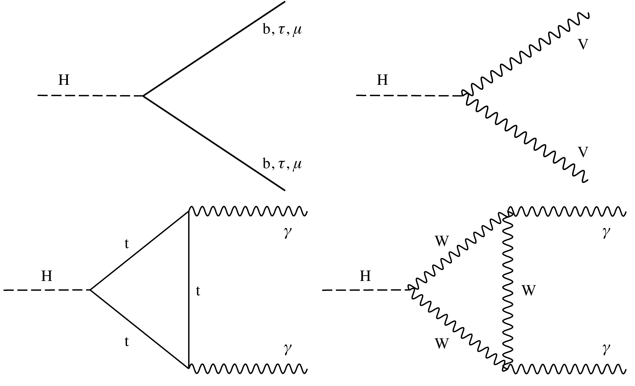
Figure 1:
Examples of leading-order Feynman diagrams for Higgs boson decays in the $\mathrm{H \to b\bar{b} }$, $\mathrm{H \to \tau\tau }$, and $\mathrm{H \to \mu\mu }$ (upper left); $\mathrm{H \to ZZ }$ and $\mathrm{H \to WW }$ (upper right); and $\mathrm{H \to \gamma\gamma }$ (lower) channels. |

png pdf |
Figure 1-a:
Example of leading-order Feynman diagram for Higgs boson decays in the $\mathrm{H \to b\bar{b} }$, $\mathrm{H \to \tau\tau }$, and $\mathrm{H \to \mu\mu }$ channels. |
png pdf |
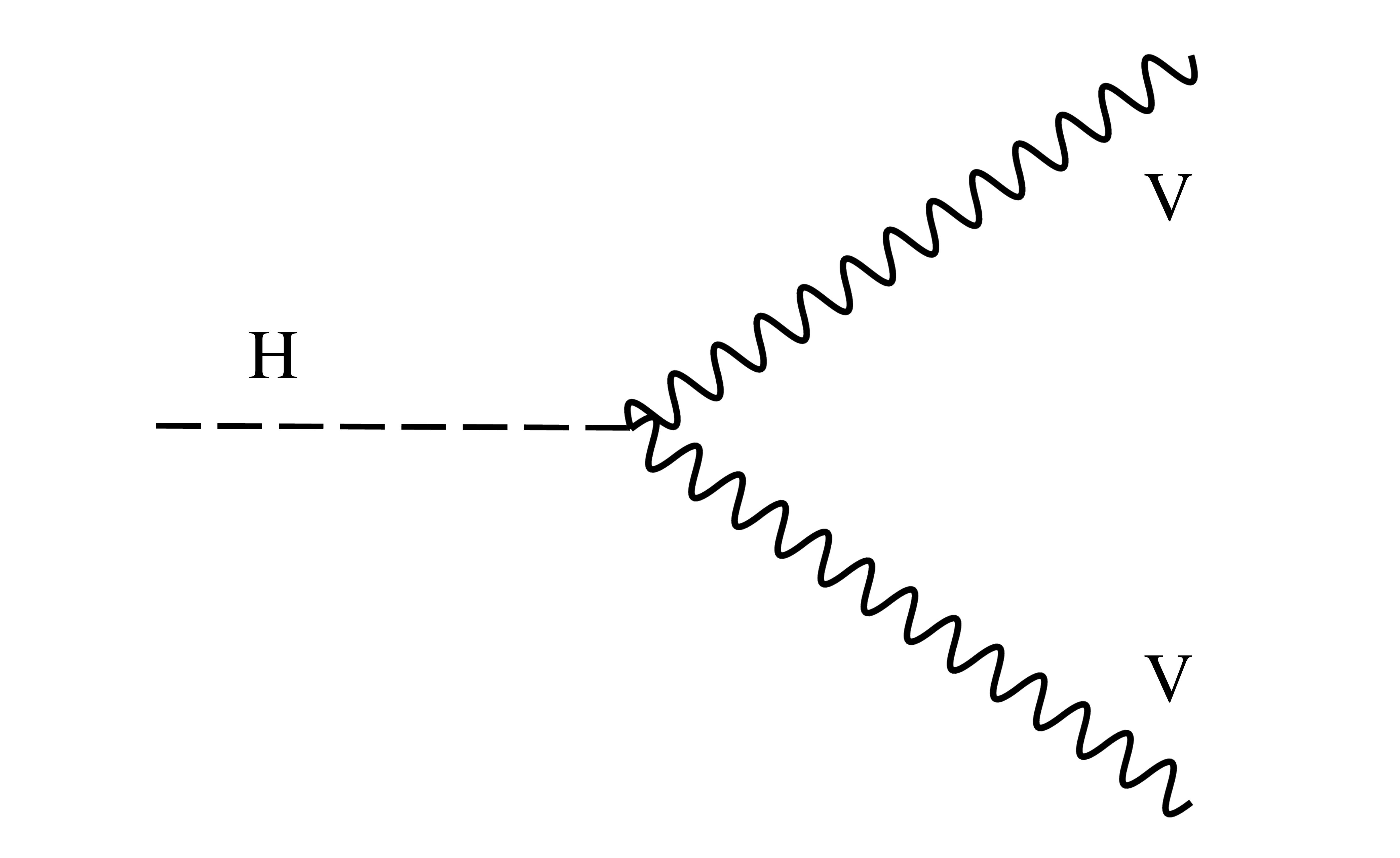
Figure 1-b:
Example of leading-order Feynman diagram for Higgs boson decays in the $\mathrm{H \to ZZ }$ and $\mathrm{H \to WW }$ channels. |
png pdf |
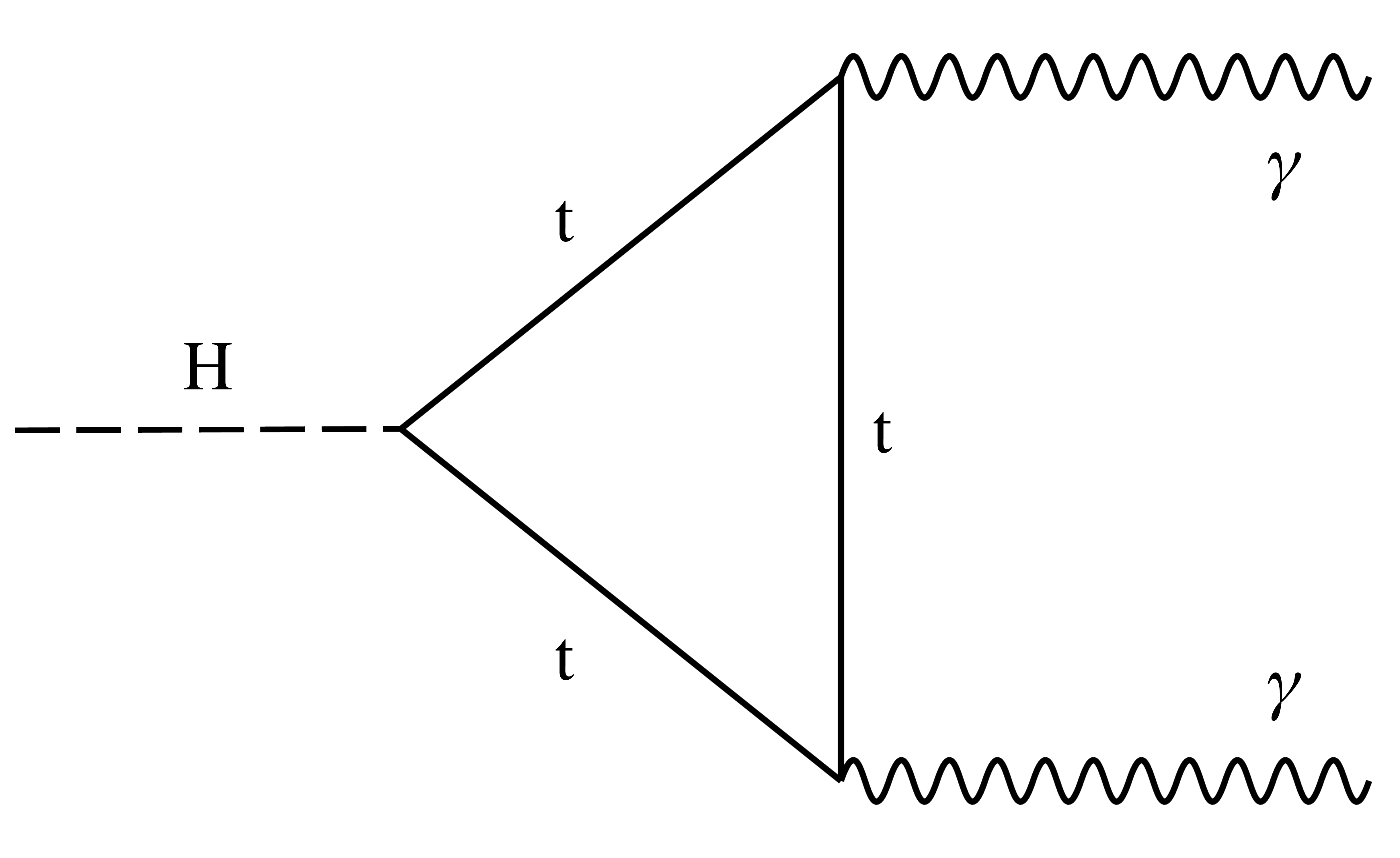
Figure 1-c:
Example of leading-order Feynman diagram for Higgs boson decays in the $\mathrm{H \to \gamma\gamma }$ channel. |

png pdf |
Figure 1-d:
Example of leading-order Feynman diagram for Higgs boson decays in the $\mathrm{H \to \gamma\gamma }$ channel. |
png pdf |
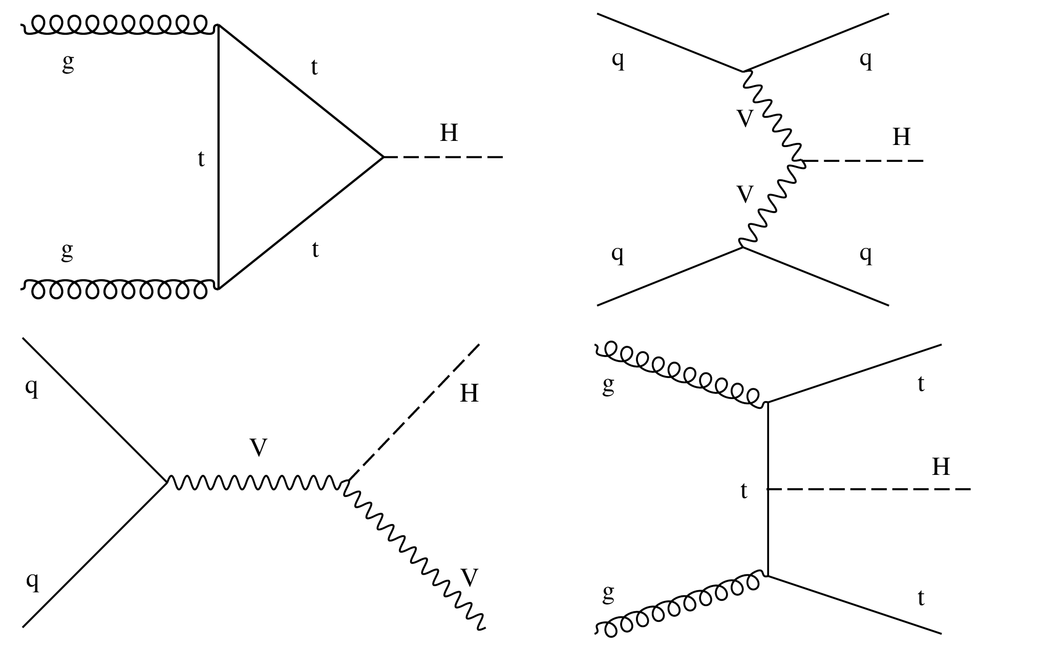
Figure 2:
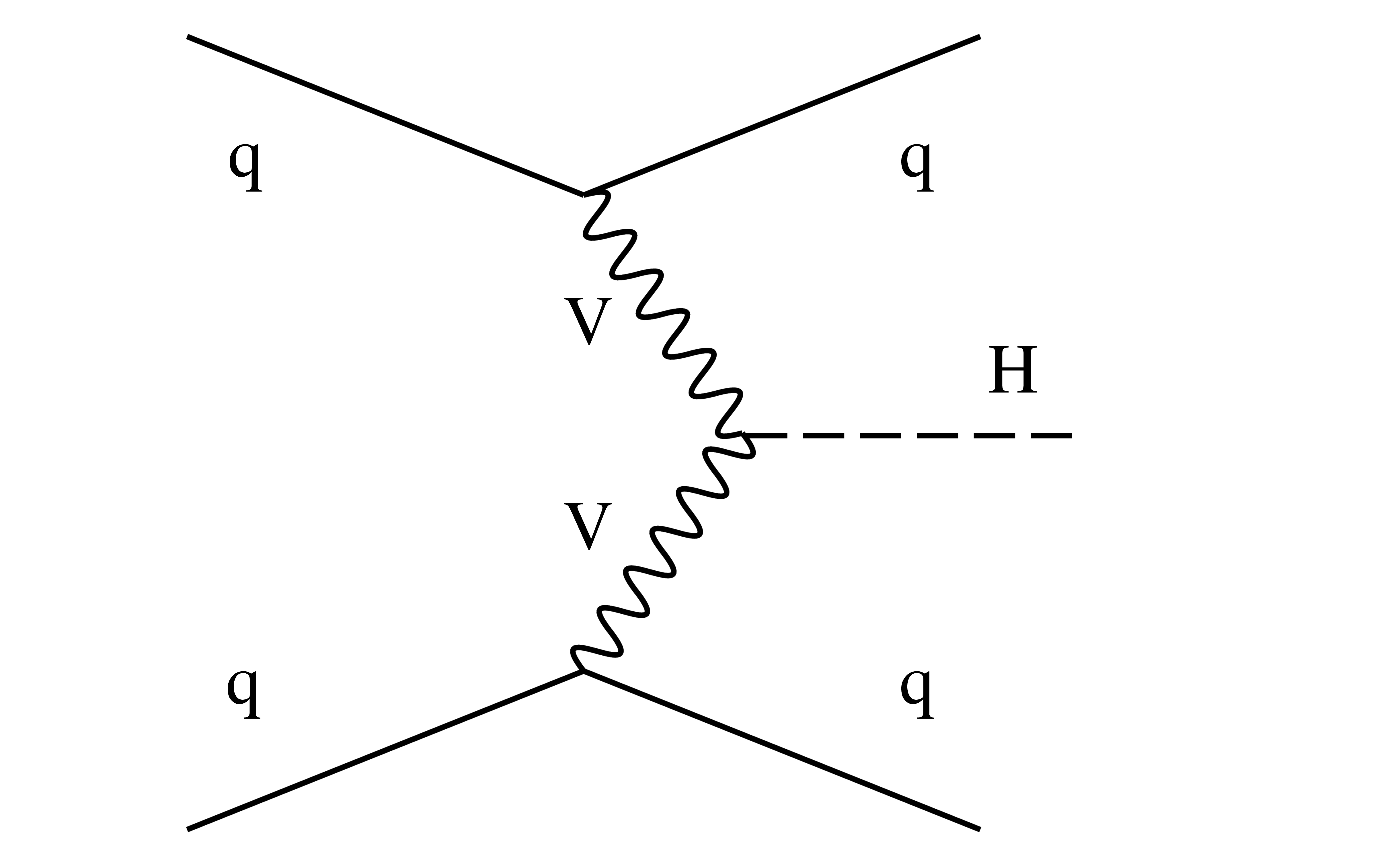
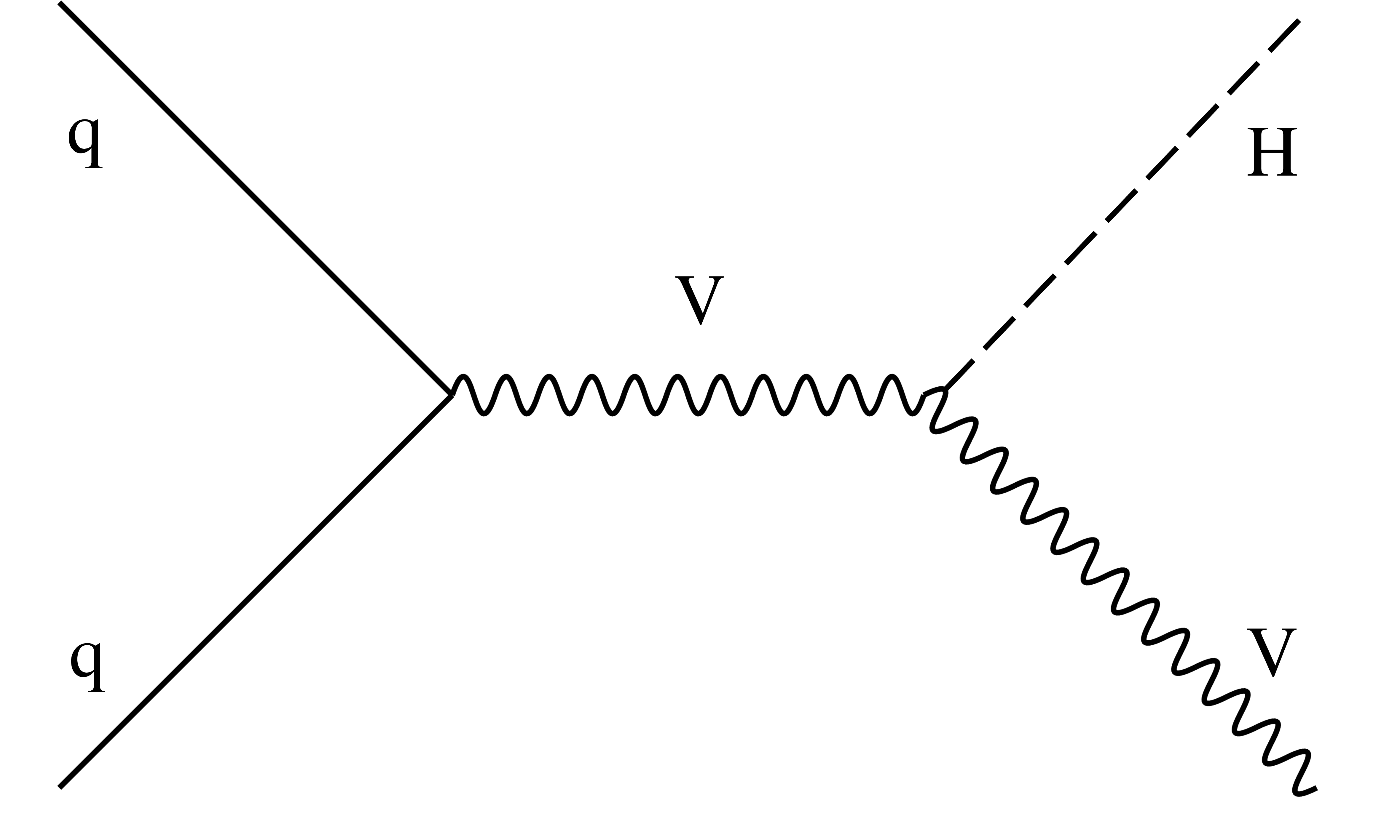
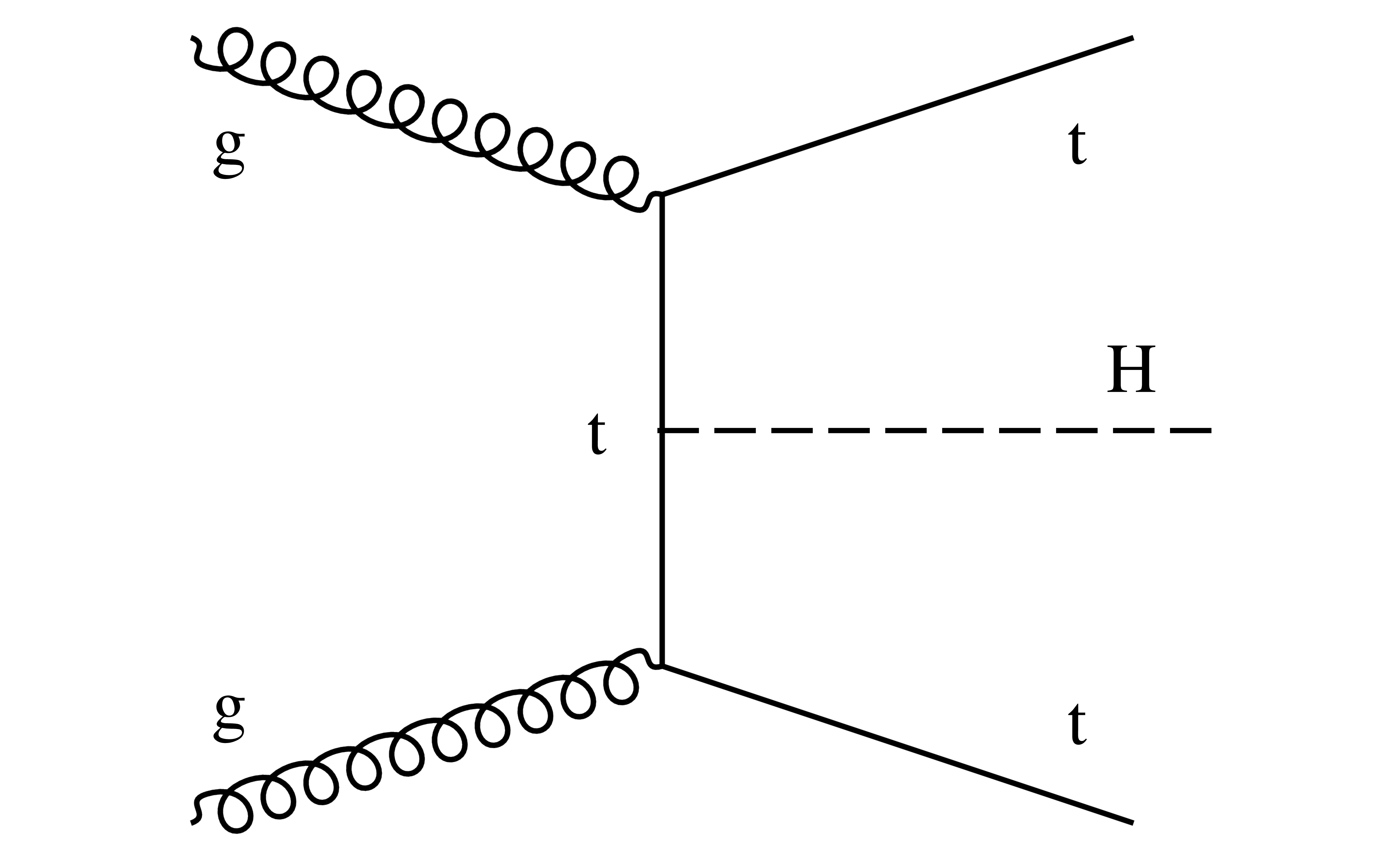
Examples of leading-order Feynman diagrams for the ggH (upper left), VBF (upper right), VH (lower left), and ttH (lower right) production modes. |

png pdf |
Figure 2-a:
Example of leading-order Feynman diagram for the ggH production mode. |
png pdf |
Figure 2-b:
Example of leading-order Feynman diagram for the VBF production mode. |
png pdf |
Figure 2-c:
Example of leading-order Feynman diagram for the VH production mode. |
png pdf |
Figure 2-d:
Example of leading-order Feynman diagram for the ttH production mode. |
png pdf |
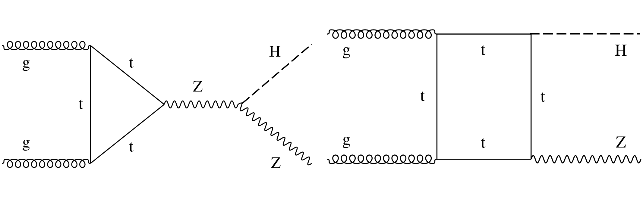
Figure 3:
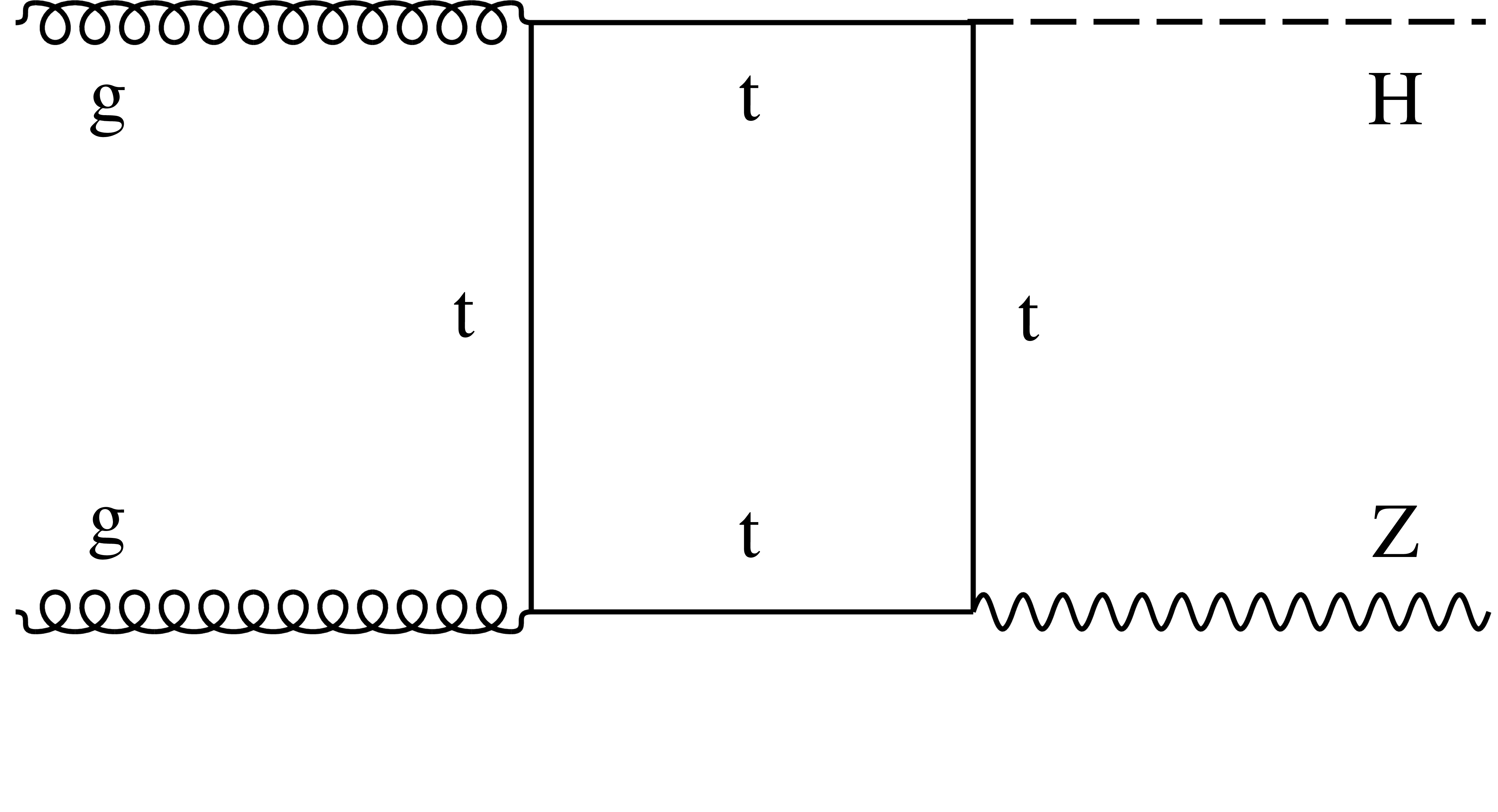
Examples of leading-order Feynman diagrams for the $ {\mathrm {g}} {\mathrm {g}} \to {{\mathrm {Z}} {\mathrm {H}}} $ production mode. |

png pdf |
Figure 3-a:
Example of leading-order Feynman diagram for the $ {\mathrm {g}} {\mathrm {g}} \to {{\mathrm {Z}} {\mathrm {H}}} $ production mode. |
png pdf |
Figure 3-b:
Example of leading-order Feynman diagram for the $ {\mathrm {g}} {\mathrm {g}} \to {{\mathrm {Z}} {\mathrm {H}}} $ production mode. |
png pdf |
Figure 4:
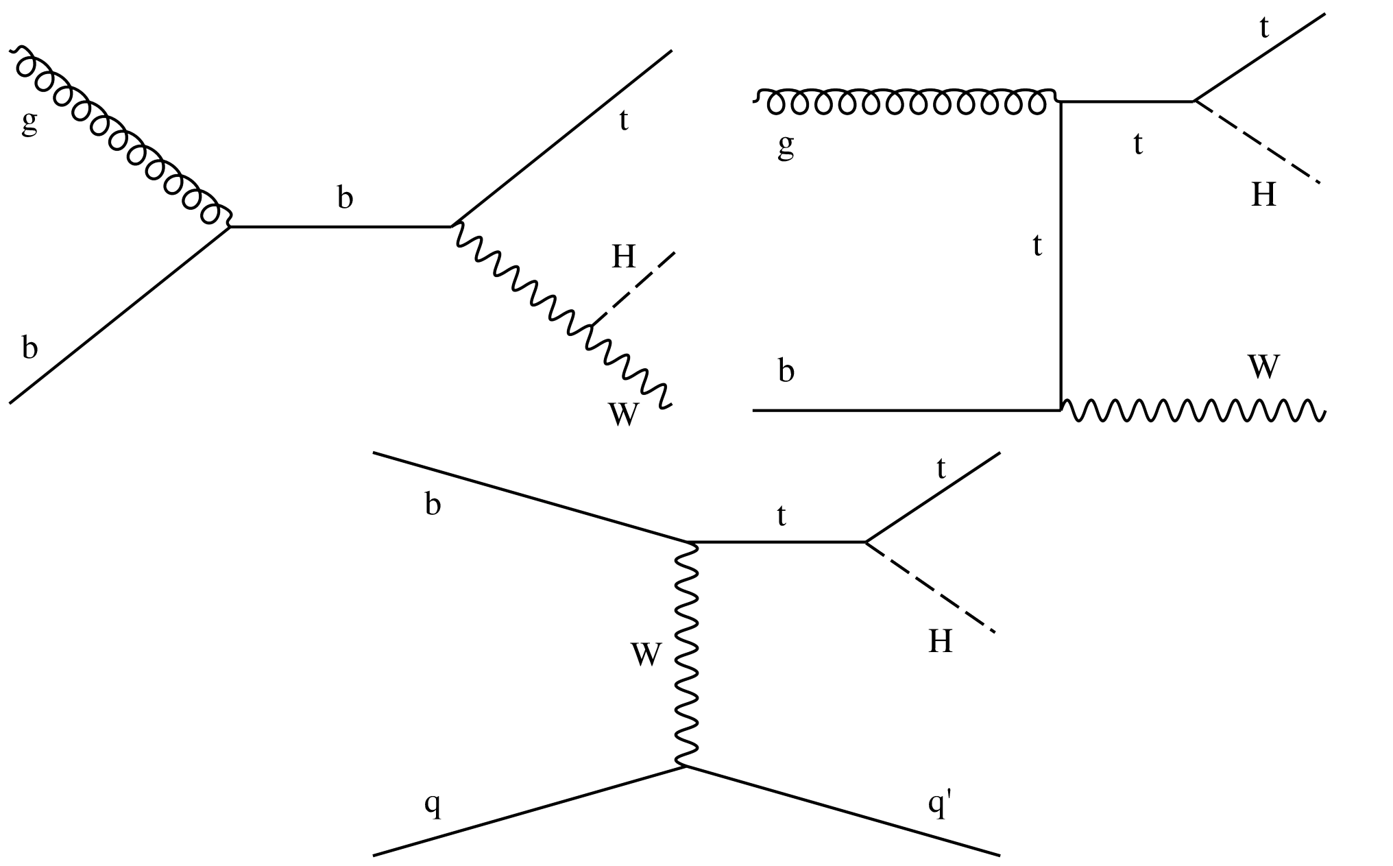
Examples of leading-order Feynman diagrams for ${{\mathrm {t}} {\mathrm {H}}}$ production via the ${{\mathrm {t}} {\mathrm {H}} {\mathrm {W}}}$ (upper left and right) and ${{\mathrm {t}} {\mathrm {H}} {\mathrm {q}}}$ (lower) modes. |
png pdf |
Figure 4-a:
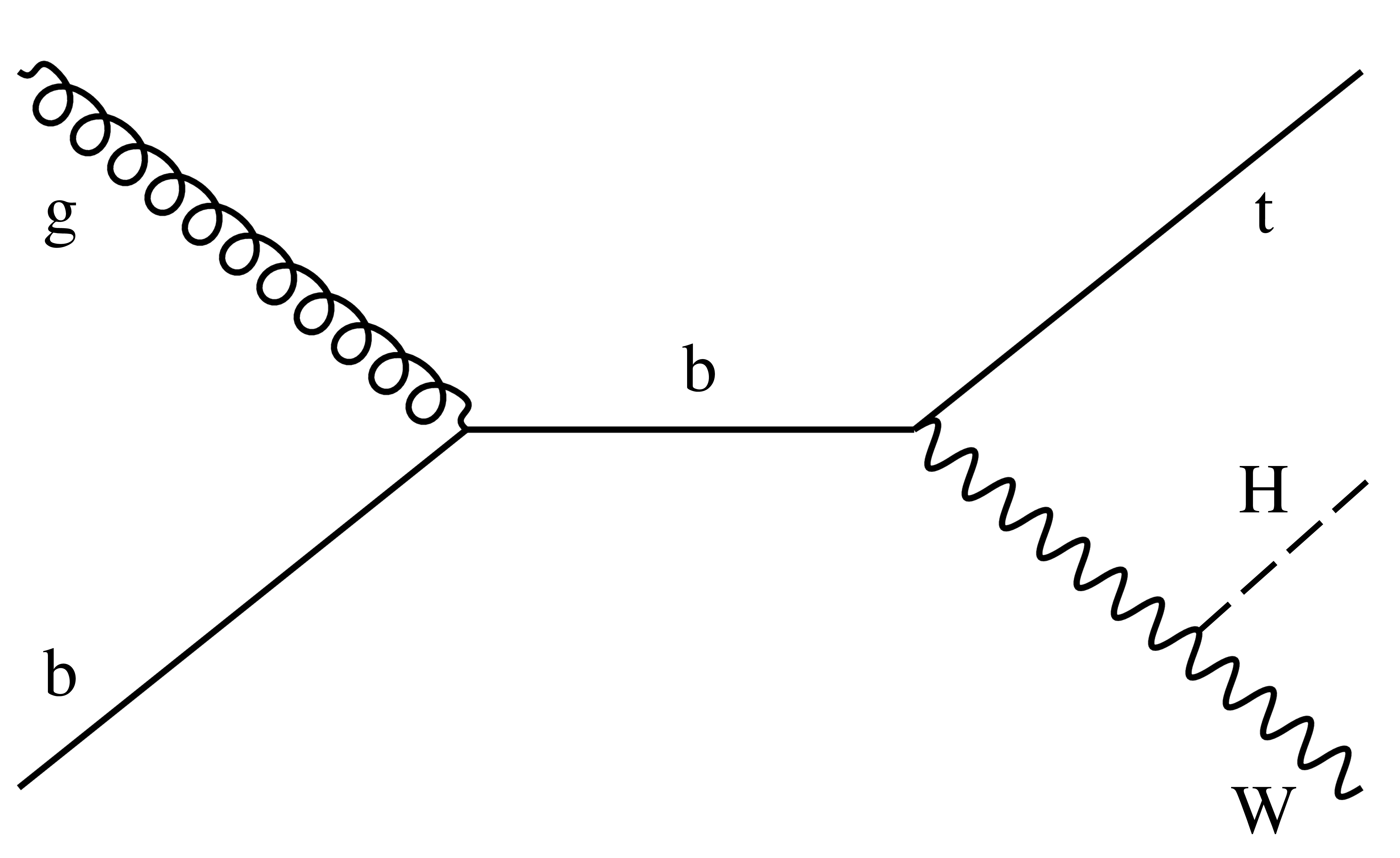
Example of leading-order Feynman diagram for ${{\mathrm {t}} {\mathrm {H}}}$ production via the ${{\mathrm {t}} {\mathrm {H}} {\mathrm {W}}}$ mode. |

png pdf |
Figure 4-b:
Example of leading-order Feynman diagram for ${{\mathrm {t}} {\mathrm {H}}}$ production via the ${{\mathrm {t}} {\mathrm {H}} {\mathrm {W}}}$ mode. |

png pdf |
Figure 4-c:
Example of leading-order Feynman diagram for ${{\mathrm {t}} {\mathrm {H}}}$ production via the ${{\mathrm {t}} {\mathrm {H}} {\mathrm {q}}}$ mode. |
png pdf |
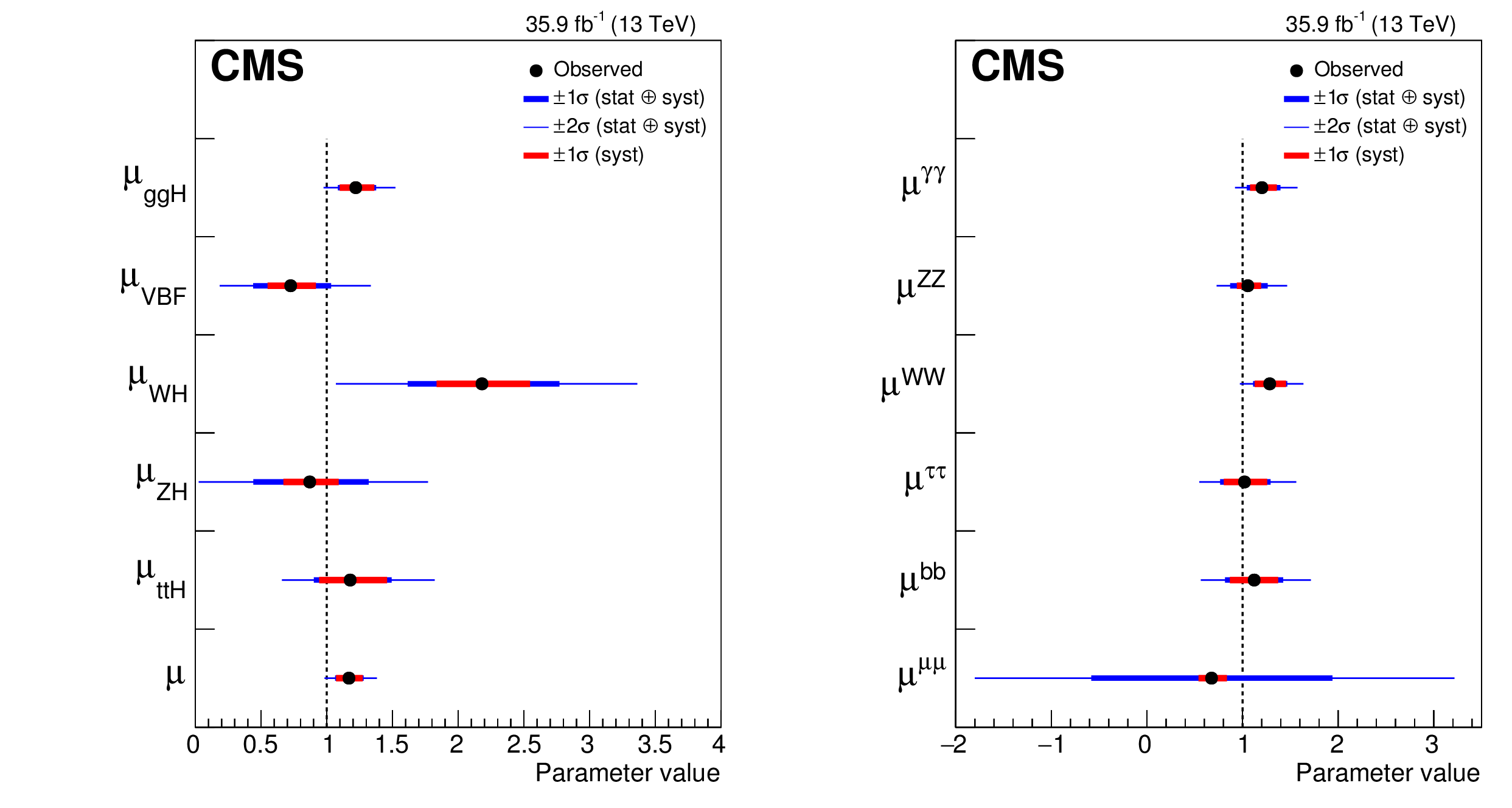
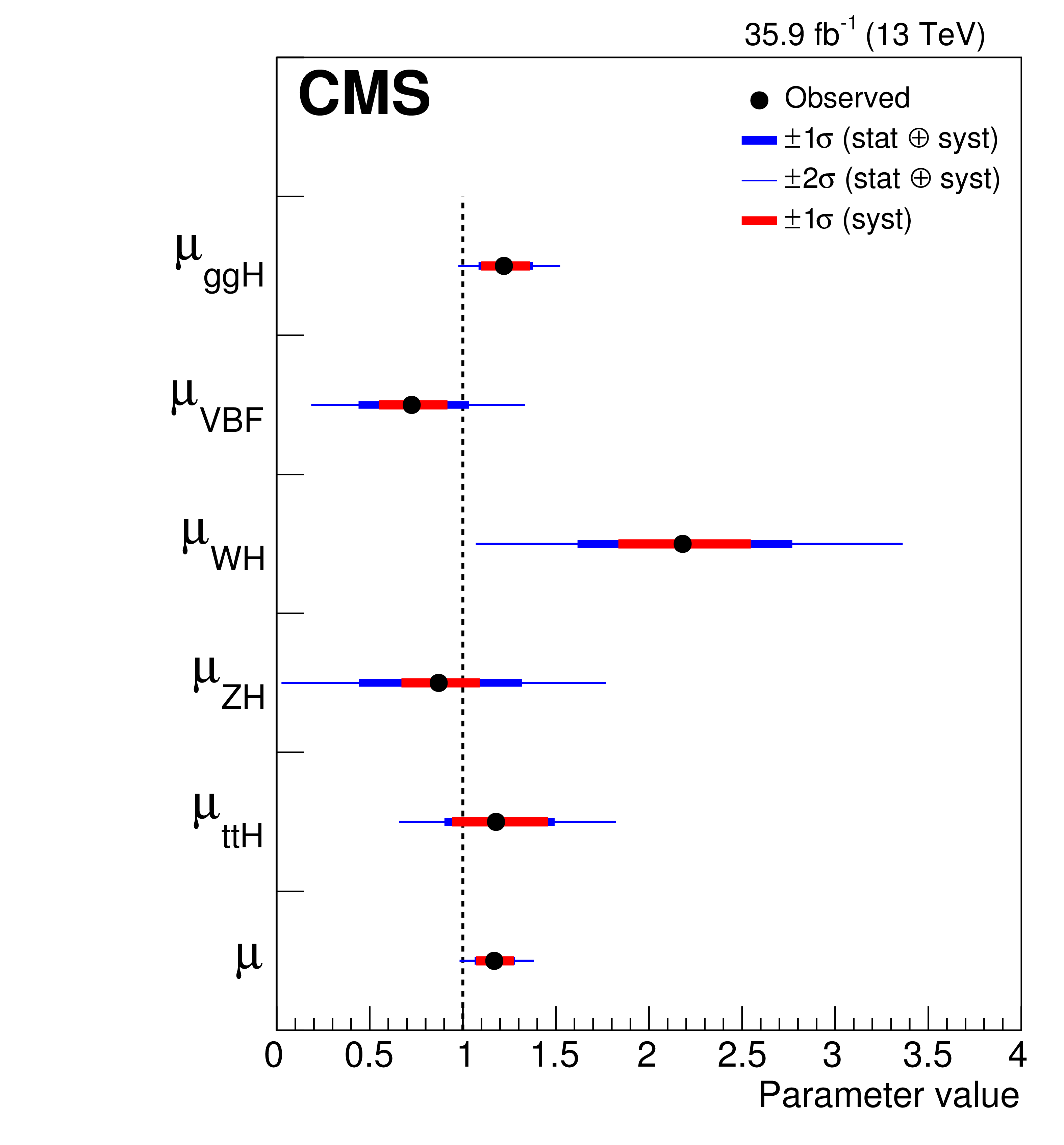
Figure 5:
Summary plot of the fit to the per-production mode (left) and per-decay mode (right) signal strength modifiers. The thick and thin horizontal bars indicate the $ {\pm} 1 \sigma $ and $ {\pm} 2 \sigma $ uncertainties, respectively. Also shown are the $ {\pm} 1 \sigma $ systematic components of the uncertainties. The last point in the per-production mode summary plot is taken from a separate fit and indicates the result of the combined overall signal strength $\mu $. |
png pdf |
Figure 5-a:
Summary plot of the fit to the per-production mode signal strength modifiers. The thick and thin horizontal bars indicate the $ {\pm} 1 \sigma $ and $ {\pm} 2 \sigma $ uncertainties, respectively. Also shown are the $ {\pm} 1 \sigma $ systematic components of the uncertainties. The last point is taken from a separate fit and indicates the result of the combined overall signal strength $\mu $. |
png pdf |
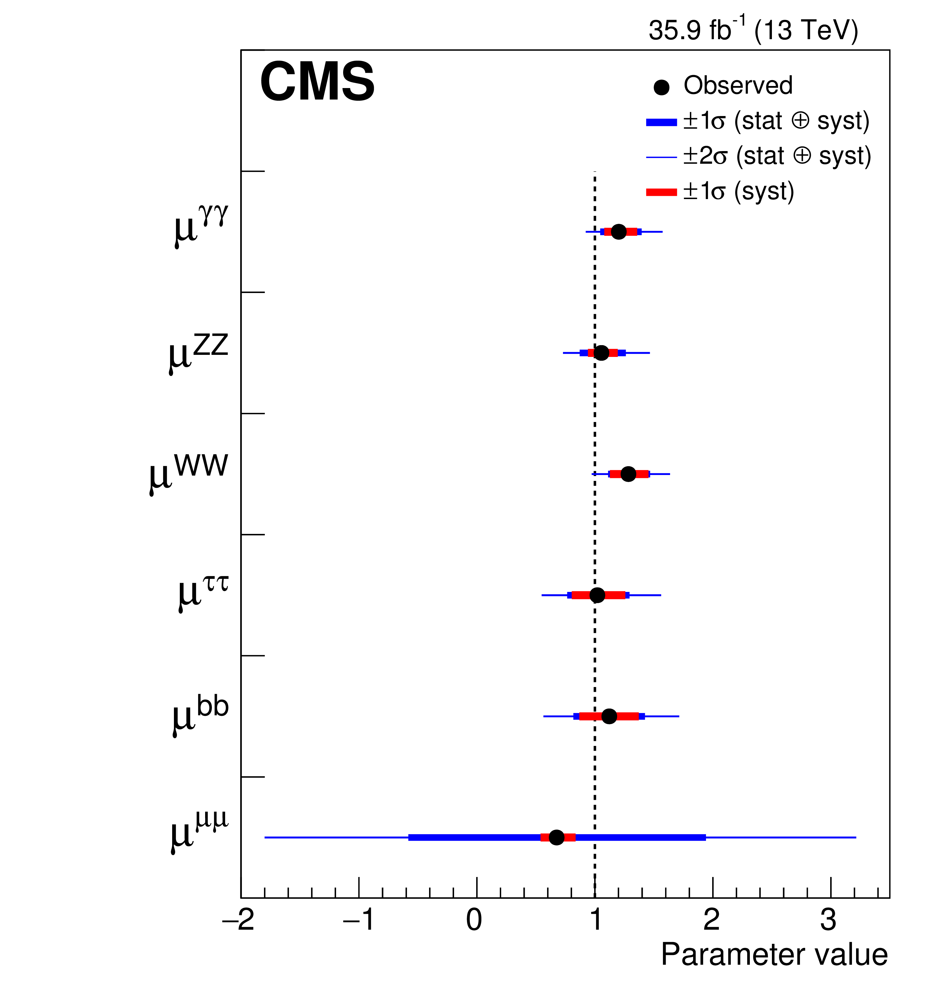
Figure 5-b:
Summary plot of the fit to the per-decay mode signal strength modifiers. The thick and thin horizontal bars indicate the $ {\pm} 1 \sigma $ and $ {\pm} 2 \sigma $ uncertainties, respectively. Also shown are the $ {\pm} 1 \sigma $ systematic components of the uncertainties. |
png pdf |
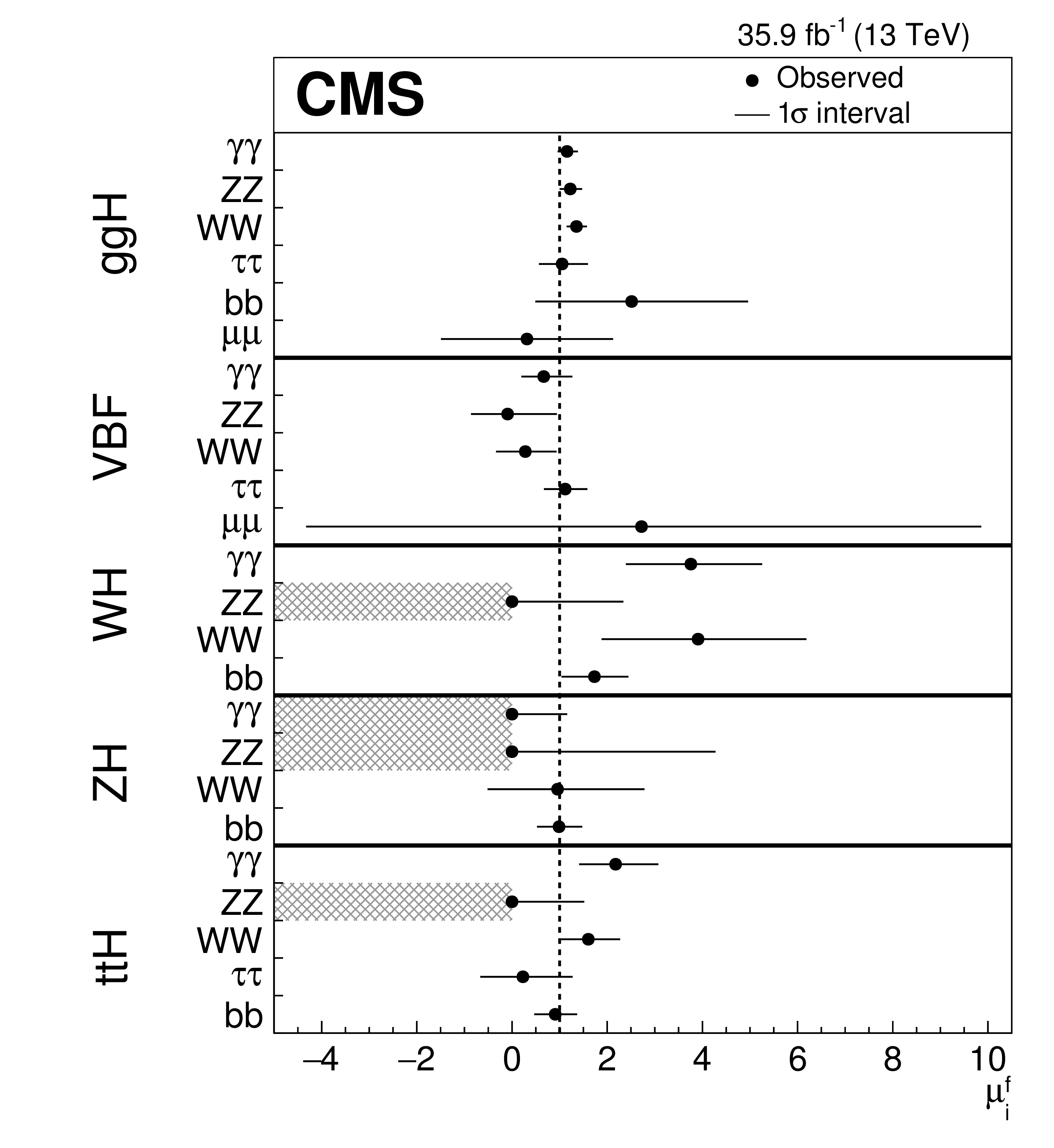
Figure 6:
Summary plot of the fit to the production-decay signal strength products $\mu _{i}^{f}=\mu _{i} \mu ^{f}$. The points indicate the best fit values while the horizontal bars indicate the $1\sigma $ CL intervals. The hatched areas indicate signal strengths that are restricted to nonnegative values as described in the text. |
png pdf |
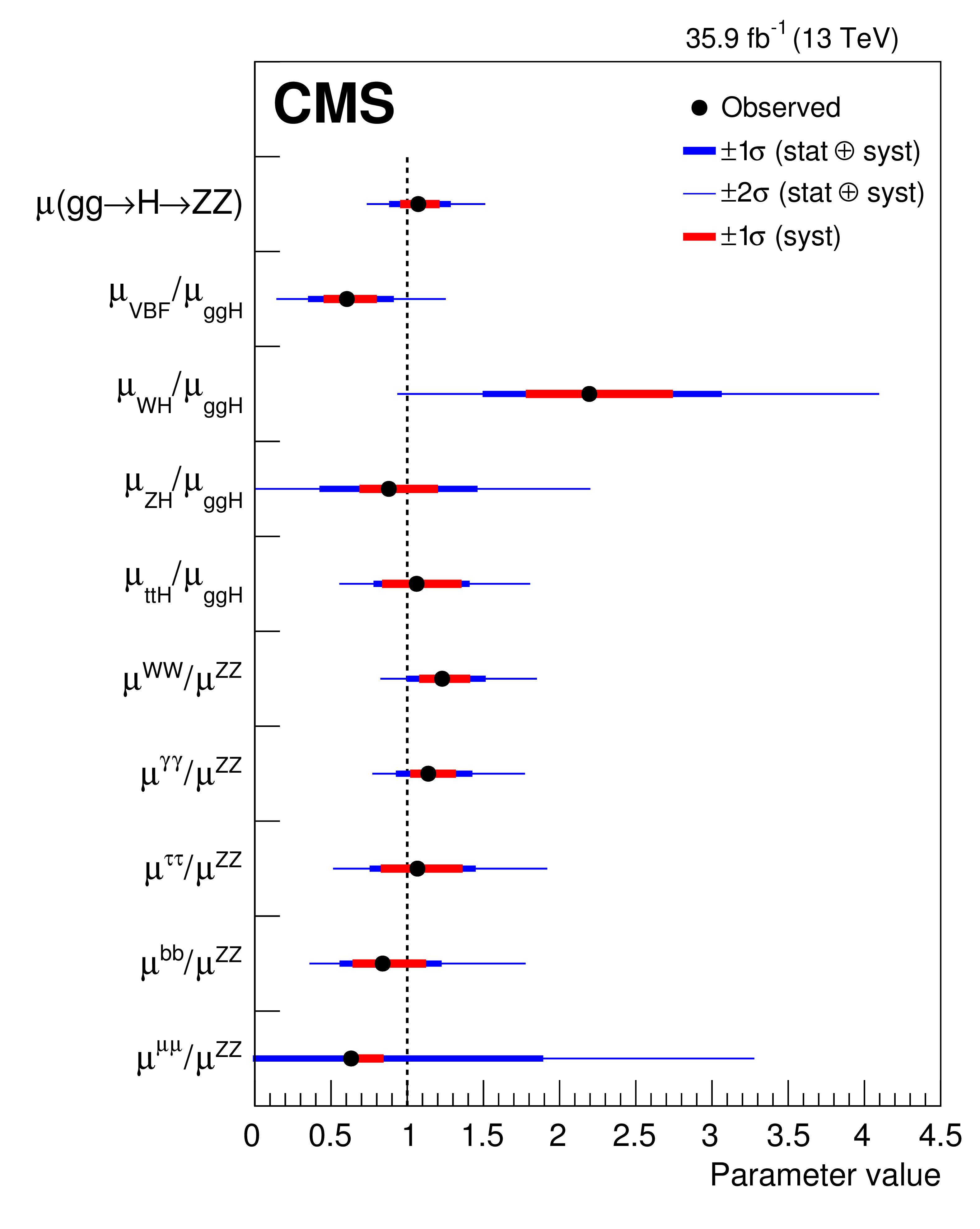
Figure 7:
Summary of the cross section and branching fraction ratio model. The thick and thin horizontal bars indicate the $ {\pm} 1 \sigma $ and $ {\pm} 2 \sigma $ uncertainties, respectively. Also shown are the $ {\pm} 1 \sigma $ systematic components of the uncertainties. |
png pdf |
Figure 8:
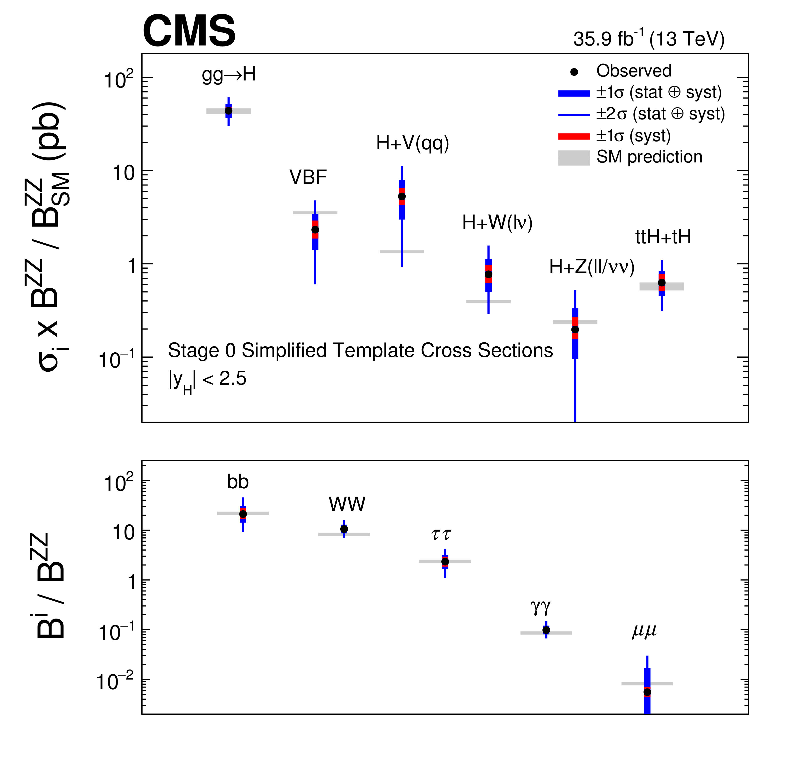
Summary of the stage 0 model, ratios of cross sections and branching fractions. The points indicate the best fit values, while the error bars show the $ {\pm} 1 \sigma $ and $ {\pm} 2 \sigma $ uncertainties. The $ {\pm} 1 \sigma $ uncertainties on the measurements considering only the contributions from the systematic uncertainties are also shown. The uncertainties in the SM predictions are indicated. |
png pdf |
Figure 9:
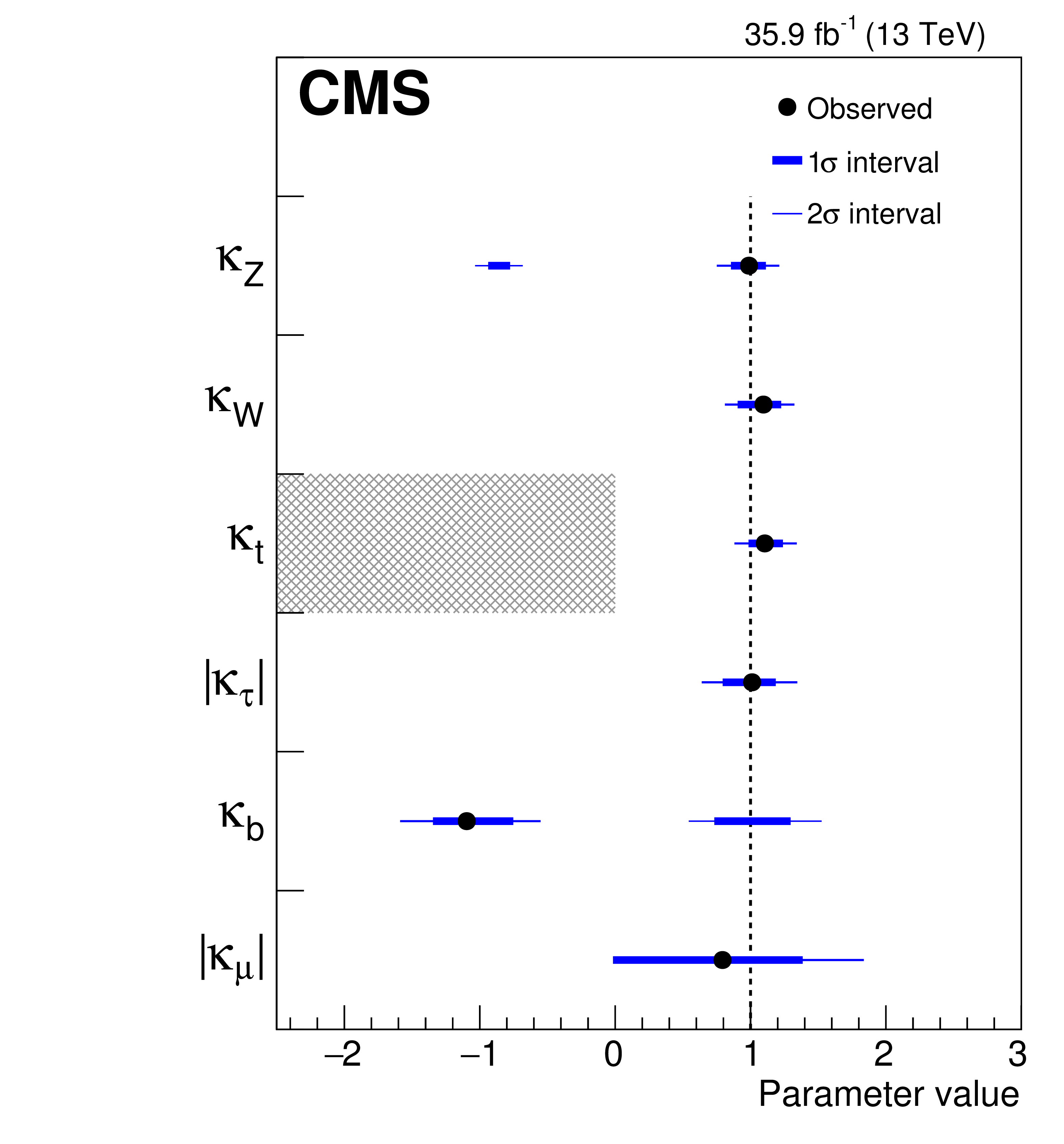
Summary of the $\kappa $-framework model assuming resolved loops and $ {{\mathcal {B}} _{\mathrm {BSM}}} =$ 0. The points indicate the best fit values while the thick and thin horizontal bars show the $1\sigma $ and $2\sigma $ CL intervals, respectively. In this model, the ggH and ${{\mathrm {H}} \to {{\gamma} {\gamma}}}$ loops are resolved in terms of the remaining coupling modifiers. For this model, both positive and negative values of $\kappa _{{\mathrm {W}}}$, $\kappa _{{\mathrm {Z}}}$, and $\kappa _{{\mathrm {b}}}$ are considered. Negative values of $\kappa _{{\mathrm {W}}}$ in this model are disfavored by more than $2\sigma $. |
png pdf |
Figure 10:
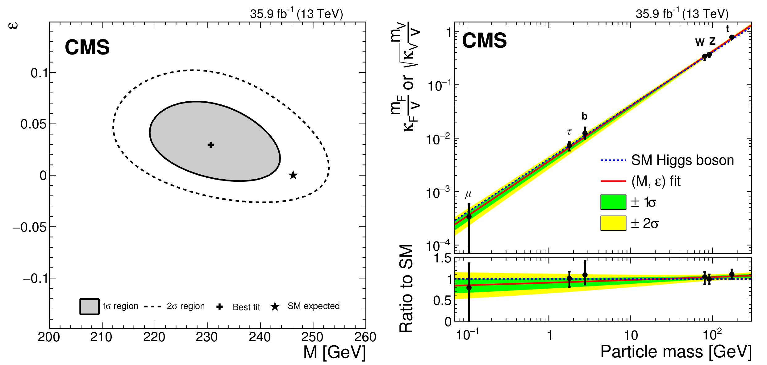
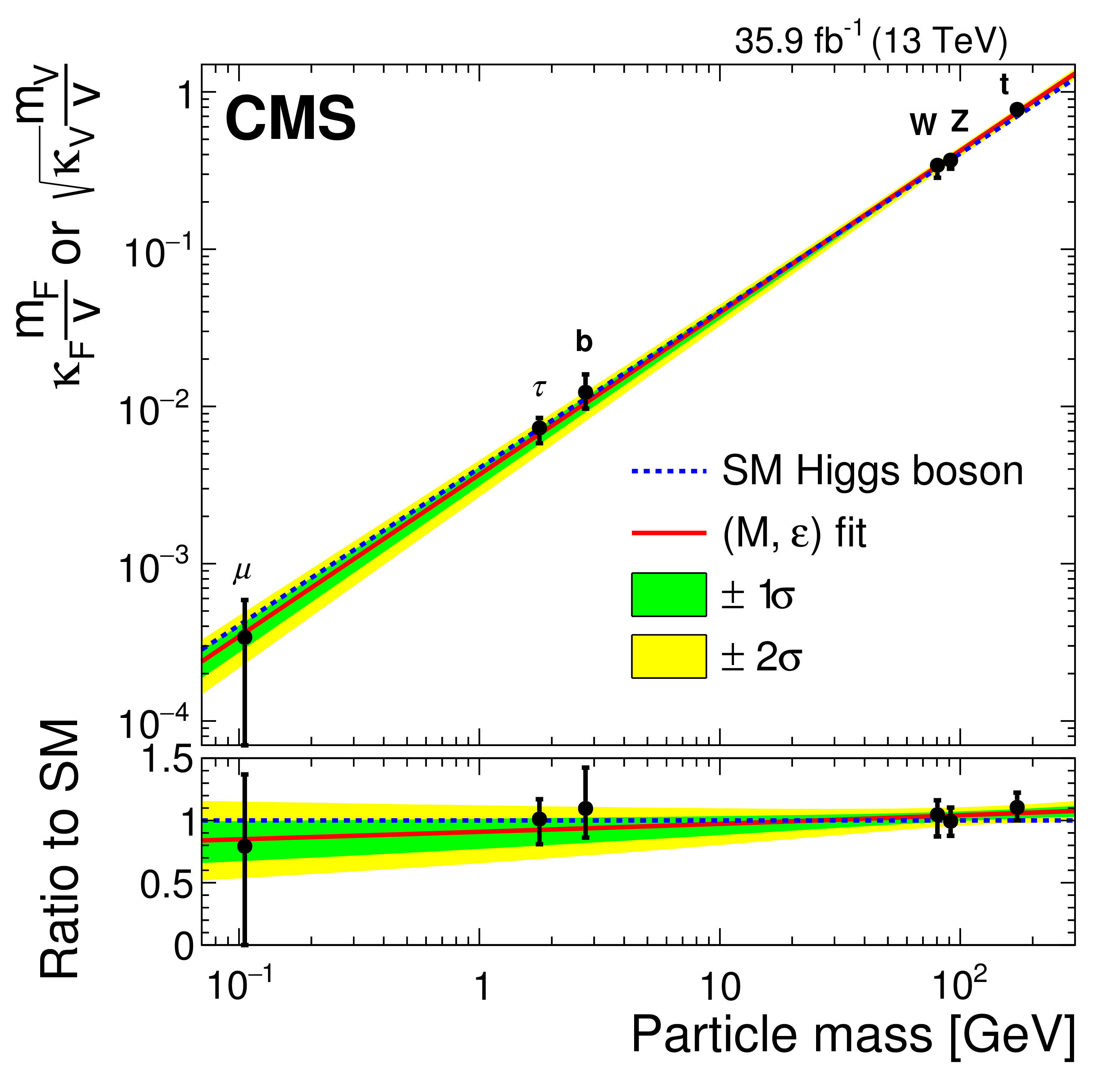
Likelihood scan in the $M{\text{-}}\epsilon$ plane (left). The best fit point and the 1$\sigma$ and 2$\sigma$ CL regions are shown, along with the SM prediction. Result of the phenomenological $(M,\,\epsilon)$ fit overlayed with the resolved $\kappa$-framework model (right). |
png pdf |
Figure 10-a:
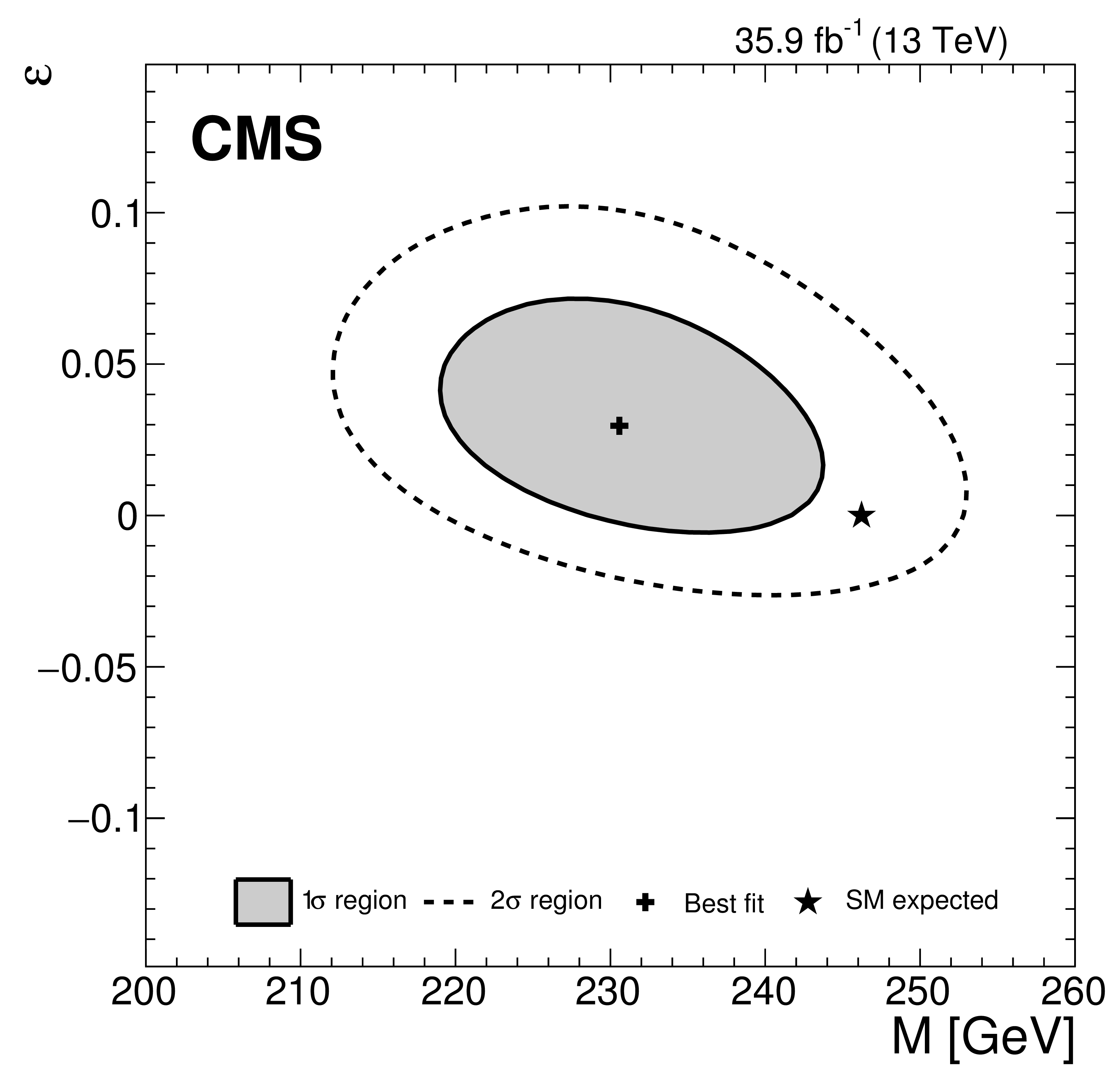
Likelihood scan in the $M{\text{-}}\epsilon$ plane. The best fit point and the 1$\sigma$ and 2$\sigma$ CL regions are shown, along with the SM prediction. |
png pdf |
Figure 10-b:
Result of the phenomenological $(M,\,\epsilon)$ fit overlayed with the resolved $\kappa$-framework model. |

png pdf |
Figure 11:
Summary plots for the $\kappa $-framework model in which the ggH and ${{\mathrm {H}} \to {{\gamma} {\gamma}}}$ loops are scaled with effective couplings. The points indicate the best fit values while the thick and thin horizontal bars show the $1\sigma $ and $2\sigma $ CL intervals, respectively. In the left figure the constraint $ {{\mathcal {B}} _{\mathrm {BSM}}} =$ 0 is imposed, and both positive and negative values of $\kappa _{{\mathrm {W}}}$ and $\kappa _{{\mathrm {Z}}}$ are considered. In the right figure a constraint $ {| \kappa _{{\mathrm {W}}} |},\, {| \kappa _{{\mathrm {Z}}} |}\le $ 1 is imposed (same sign of $\kappa _{{\mathrm {W}}}$ and $\kappa _{{\mathrm {Z}}}$), while $ {{\mathcal {B}} _{\mathrm {inv}}} > $ 0 and $ {{\mathcal {B}} _{\mathrm {undet}}} > $ 0 are free parameters. |

png pdf |
Figure 11-a:
Summary plot for the $\kappa $-framework model in which the ggH and ${{\mathrm {H}} \to {{\gamma} {\gamma}}}$ loops are scaled with effective couplings. The points indicate the best fit values while the thick and thin horizontal bars show the $1\sigma $ and $2\sigma $ CL intervals, respectively. In the figure the constraint $ {{\mathcal {B}} _{\mathrm {BSM}}} =$ 0 is imposed, and both positive and negative values of $\kappa _{{\mathrm {W}}}$ and $\kappa _{{\mathrm {Z}}}$ are considered. |
png pdf |
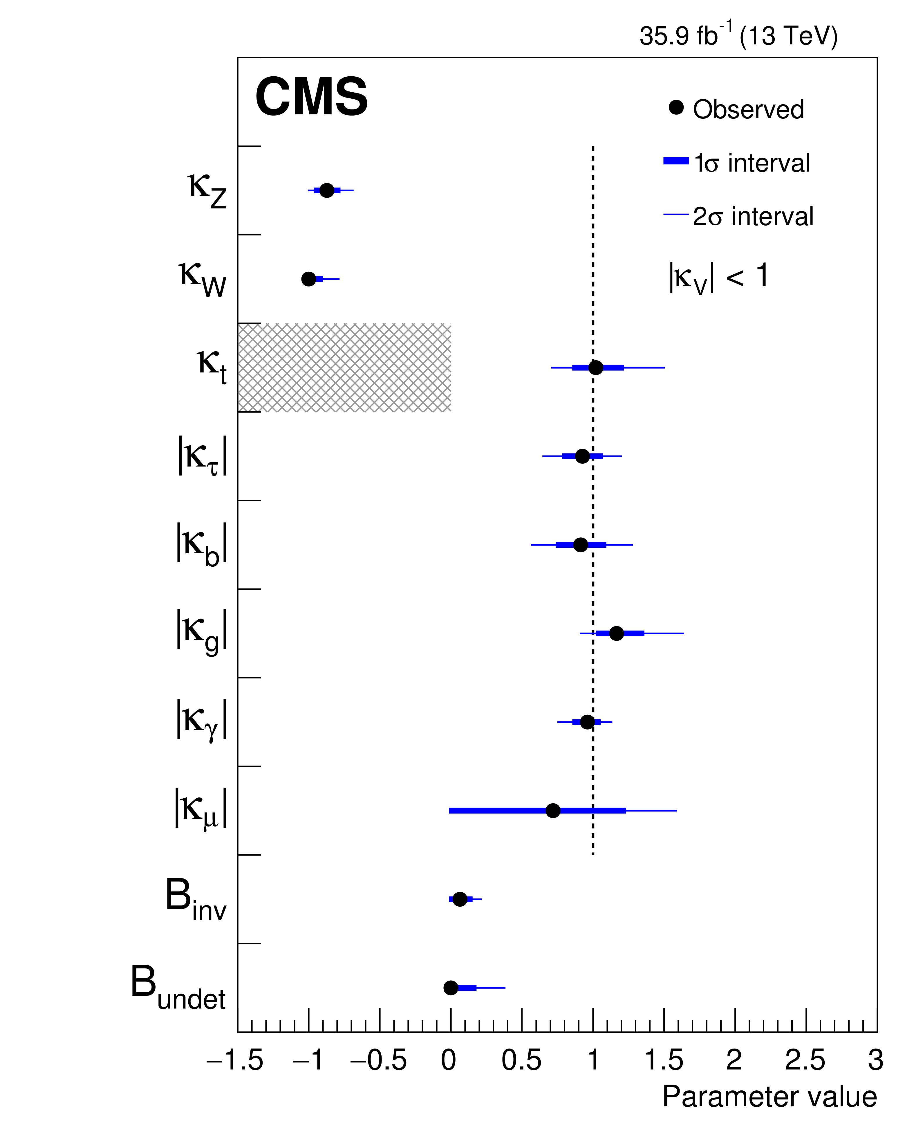
Figure 11-b:
Summary plot for the $\kappa $-framework model in which the ggH and ${{\mathrm {H}} \to {{\gamma} {\gamma}}}$ loops are scaled with effective couplings. The points indicate the best fit values while the thick and thin horizontal bars show the $1\sigma $ and $2\sigma $ CL intervals, respectively. In the figure a constraint $ {| \kappa _{{\mathrm {W}}} |},\, {| \kappa _{{\mathrm {Z}}} |}\le $ 1 is imposed (same sign of $\kappa _{{\mathrm {W}}}$ and $\kappa _{{\mathrm {Z}}}$), while $ {{\mathcal {B}} _{\mathrm {inv}}} > $ 0 and $ {{\mathcal {B}} _{\mathrm {undet}}} > $ 0 are free parameters. |
png pdf |
Figure 12:
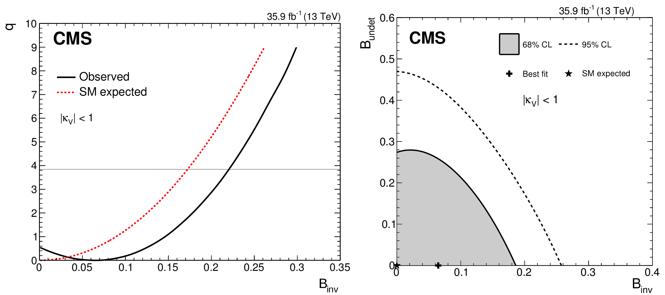
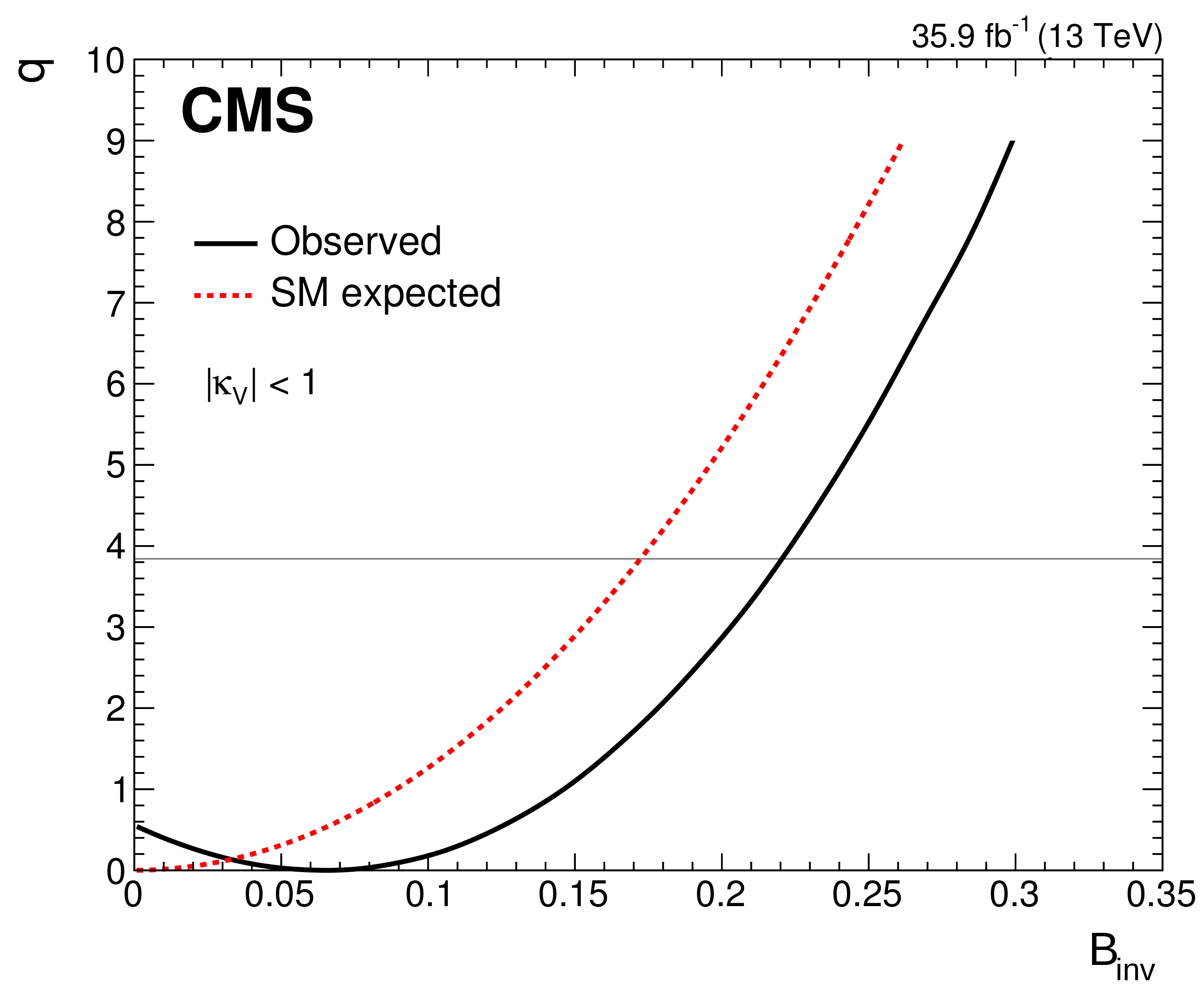
Results within the generic $\kappa $-framework model with effective loops and with the constraint $ {| \kappa _{{\mathrm {W}}} |},\, {| \kappa _{{\mathrm {Z}}} |}\le $ 1 (same sign of $\kappa _{{\mathrm {W}}}$ and $\kappa _{{\mathrm {Z}}}$), and with $ {{\mathcal {B}} _{\mathrm {inv}}} > $ 0 and $ {{\mathcal {B}} _{\mathrm {undet}}} > $ 0 as free parameters. Scan of the test statistic $q$ as a function of $ {{\mathcal {B}} _{\mathrm {inv}}} $ (left), and 68 and 95% CL regions for $ {{\mathcal {B}} _{\mathrm {inv}}} $ vs. $ {{\mathcal {B}} _{\mathrm {undet}}} $ (right). The scan of the test statistic $q$ as a function of $ {{\mathcal {B}} _{\mathrm {inv}}} $ expected assuming the SM is also shown in the left figure. |
png pdf |
Figure 12-a:
Results within the generic $\kappa $-framework model with effective loops and with the constraint $ {| \kappa _{{\mathrm {W}}} |},\, {| \kappa _{{\mathrm {Z}}} |}\le $ 1 (same sign of $\kappa _{{\mathrm {W}}}$ and $\kappa _{{\mathrm {Z}}}$), and with $ {{\mathcal {B}} _{\mathrm {inv}}} > $ 0 and $ {{\mathcal {B}} _{\mathrm {undet}}} > $ 0 as free parameters. Scan of the test statistic $q$ as a function of $ {{\mathcal {B}} _{\mathrm {inv}}} $. The scan of the test statistic $q$ as a function of $ {{\mathcal {B}} _{\mathrm {inv}}} $ expected assuming the SM is also shown. |

png pdf |
Figure 12-b:
Results within the generic $\kappa $-framework model with effective loops and with the constraint $ {| \kappa _{{\mathrm {W}}} |},\, {| \kappa _{{\mathrm {Z}}} |}\le $ 1 (same sign of $\kappa _{{\mathrm {W}}}$ and $\kappa _{{\mathrm {Z}}}$), and with $ {{\mathcal {B}} _{\mathrm {inv}}} > $ 0 and $ {{\mathcal {B}} _{\mathrm {undet}}} > $ 0 as free parameters. 68 and 95% CL regions for $ {{\mathcal {B}} _{\mathrm {inv}}} $ vs. $ {{\mathcal {B}} _{\mathrm {undet}}} $. |
png pdf |
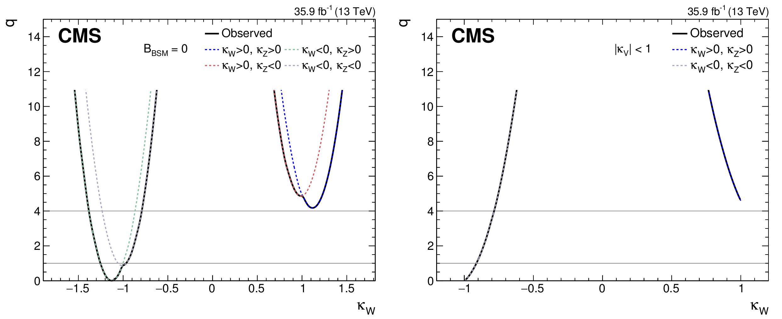
Figure 13:
Scan of the test statistic $q$ as a function of $\kappa _{{\mathrm {W}}}$ in the generic $\kappa $ model assuming $ {{\mathcal {B}} _{\mathrm {BSM}}} =$ 0 (left) and allowing $ {{\mathcal {B}} _{\mathrm {inv}}} $ and $ {{\mathcal {B}} _{\mathrm {undet}}} $ to float (right). The different colored lines indicate the value of $q$ for different combinations of signs for $\kappa _{{\mathrm {W}}}$ and $\kappa _{{\mathrm {Z}}}$. The solid black line shows the minimum value of $q(\kappa _{{\mathrm {W}}})$ in each case and is used to determine the best fit point and the $1\sigma $ and $2\sigma $ CL regions. The scan in the right figure is truncated because of the constraints of $ {| \kappa _{{\mathrm {W}}} |}\le $ 1 and $ {| \kappa _{{\mathrm {Z}}} |}\le $ 1, which are imposed in this model. |

png pdf |
Figure 13-a:
Scan of the test statistic $q$ as a function of $\kappa _{{\mathrm {W}}}$ in the generic $\kappa $ model assuming $ {{\mathcal {B}} _{\mathrm {BSM}}} =$ 0. The different colored lines indicate the value of $q$ for different combinations of signs for $\kappa _{{\mathrm {W}}}$ and $\kappa _{{\mathrm {Z}}}$. The solid black line shows the minimum value of $q(\kappa _{{\mathrm {W}}})$ in each case and is used to determine the best fit point and the $1\sigma $ and $2\sigma $ CL regions. |
png pdf |
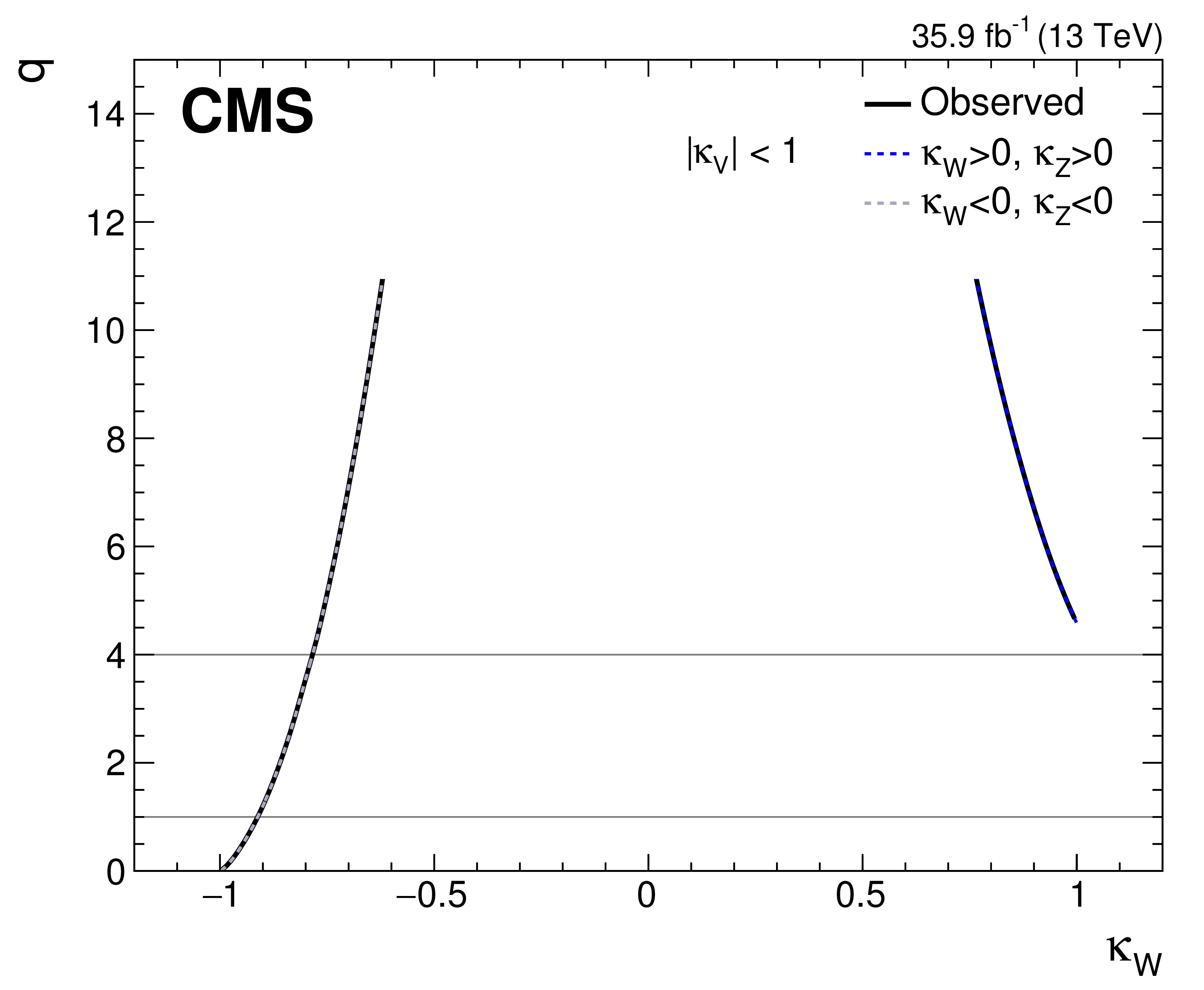
Figure 13-b:
Scan of the test statistic $q$ as a function of $\kappa _{{\mathrm {W}}}$ in the generic $\kappa $ model allowing $ {{\mathcal {B}} _{\mathrm {inv}}} $ and $ {{\mathcal {B}} _{\mathrm {undet}}} $ to float. The different colored lines indicate the value of $q$ for different combinations of signs for $\kappa _{{\mathrm {W}}}$ and $\kappa _{{\mathrm {Z}}}$. The solid black line shows the minimum value of $q(\kappa _{{\mathrm {W}}})$ in each case and is used to determine the best fit point and the $1\sigma $ and $2\sigma $ CL regions. The scan is truncated because of the constraints of $ {| \kappa _{{\mathrm {W}}} |}\le $ 1 and $ {| \kappa _{{\mathrm {Z}}} |}\le $ 1, which are imposed in this model. |
png pdf |
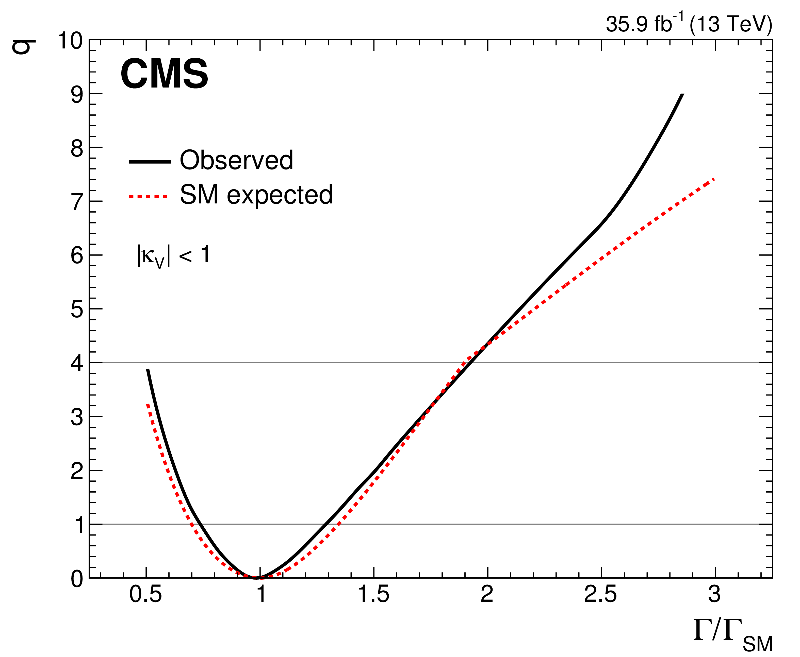
Figure 14:
The scan of the test statistic $q$ as a function of $\Gamma _{{\mathrm {H}}}/\Gamma _{{\mathrm {H}}}^{\mathrm {SM}}$ obtained by reinterpreting the model allowing for BSM decays of the Higgs boson. The expected scan of $q$ as a function of $\Gamma _{{\mathrm {H}}}/\Gamma _{{\mathrm {H}}}^{\mathrm {SM}}$ assuming the SM is also shown. |
png pdf |
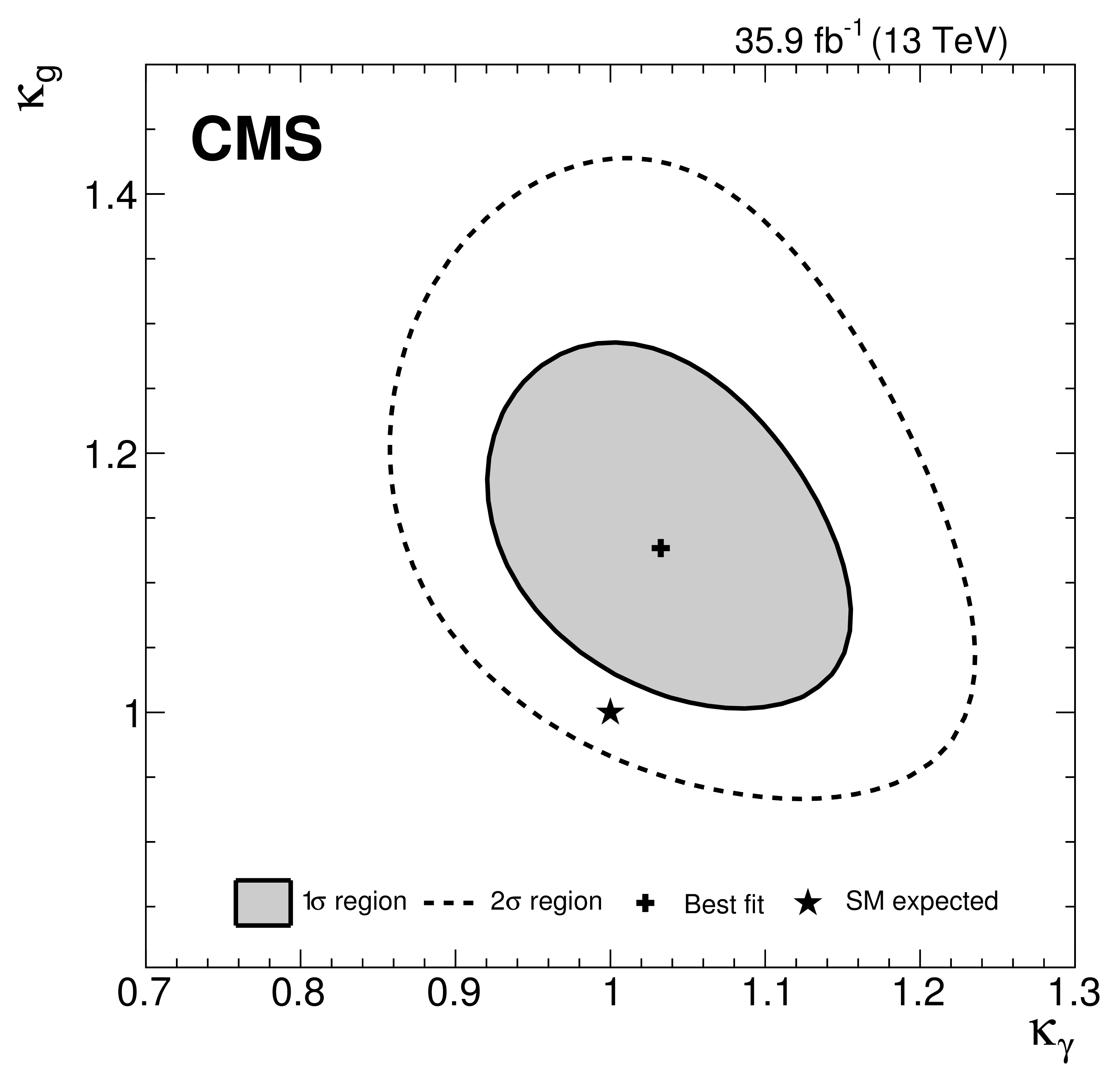
Figure 15:
The $1\sigma $ and $2\sigma $ CL regions in the $\kappa _{{\mathrm {g}}}$ vs. $\kappa _{{\gamma}}$ parameter space for the model assuming the only BSM contributions to the Higgs boson couplings appear in the loop-induced processes or in BSM Higgs decays. |
png pdf |
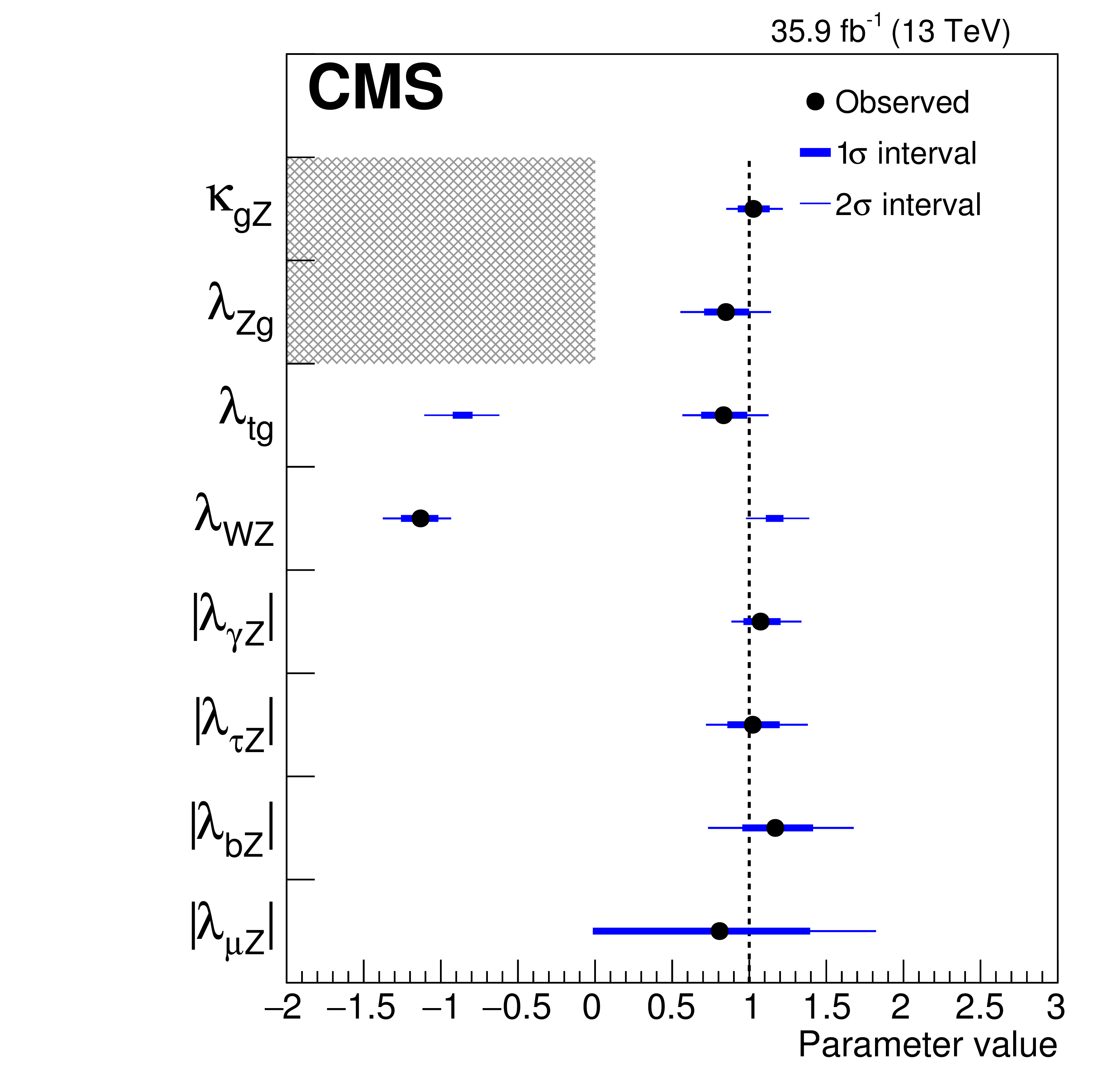
Figure 16:
Summary of the model with coupling ratios and effective couplings for the ggH and ${{\mathrm {H}} \to {{\gamma} {\gamma}}}$ loops. The points indicate the best fit values while the thick and thin horizontal bars show the $1\sigma $ and $2\sigma $ CL intervals, respectively. For this model, both positive and negative values of $\lambda _{{\mathrm {W}} {\mathrm {Z}}}$ and $\lambda _{{\mathrm {t}} {\mathrm {g}}}$ are considered. |
png pdf |
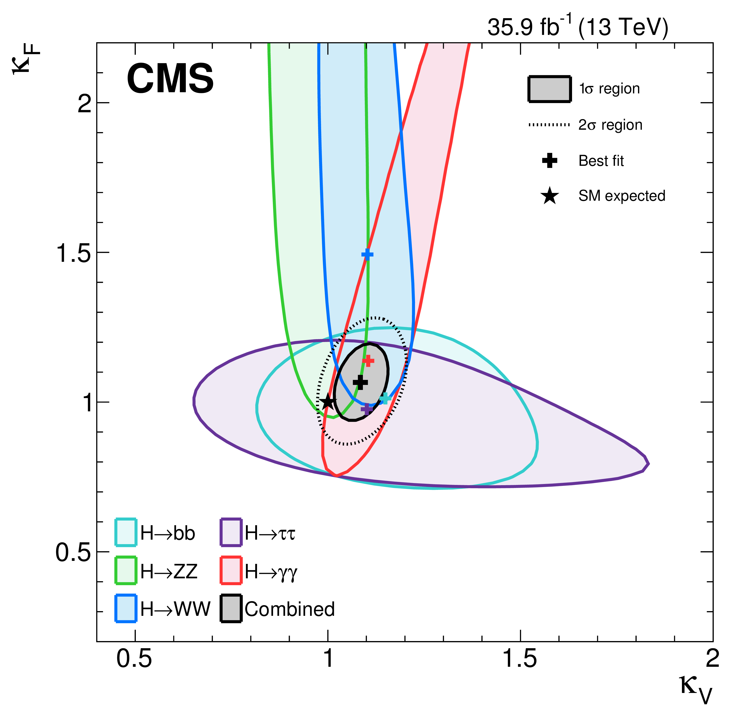
Figure 17:
The $1\sigma $ and $2\sigma $ CL regions in the $\kappa _{\mathrm {F}}$ vs. $\kappa _{\mathrm {V}}$ parameter space for the model assuming a common scaling of all the vector boson and fermion couplings. |
png pdf |
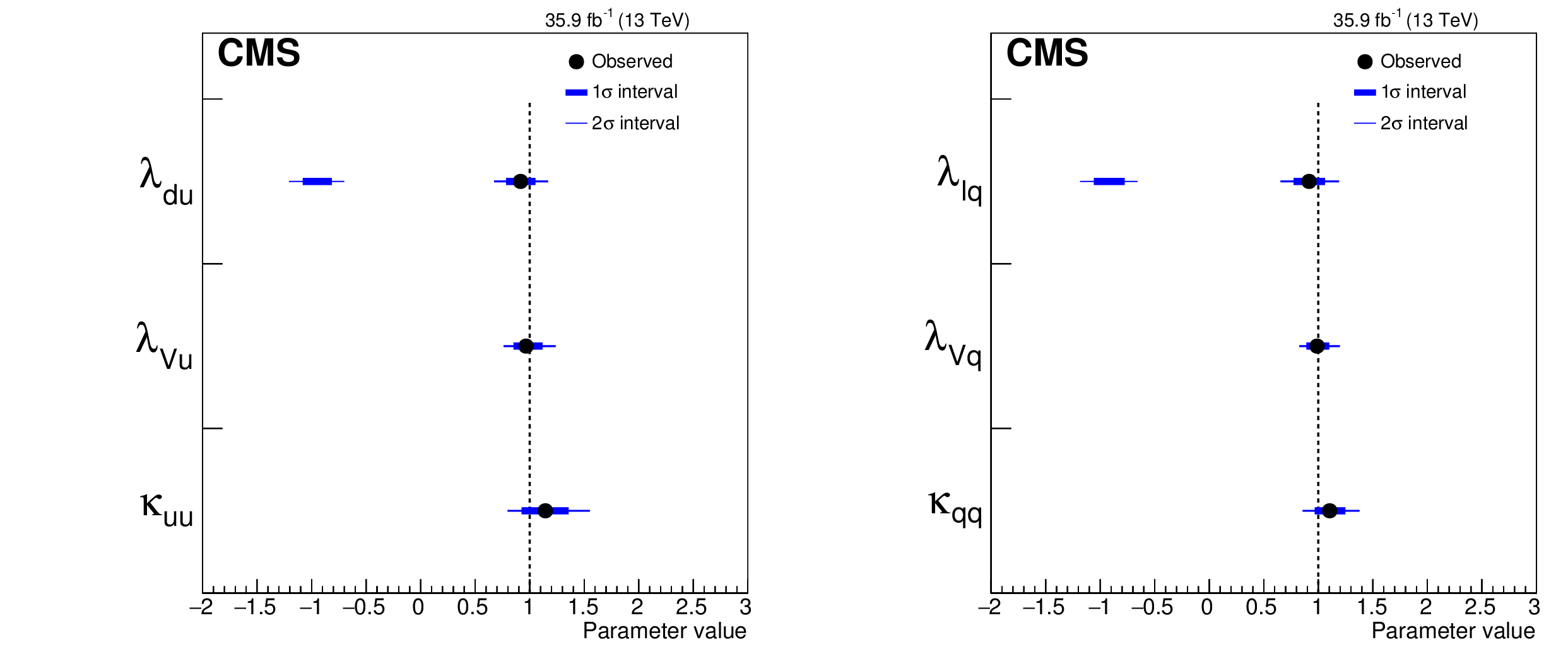
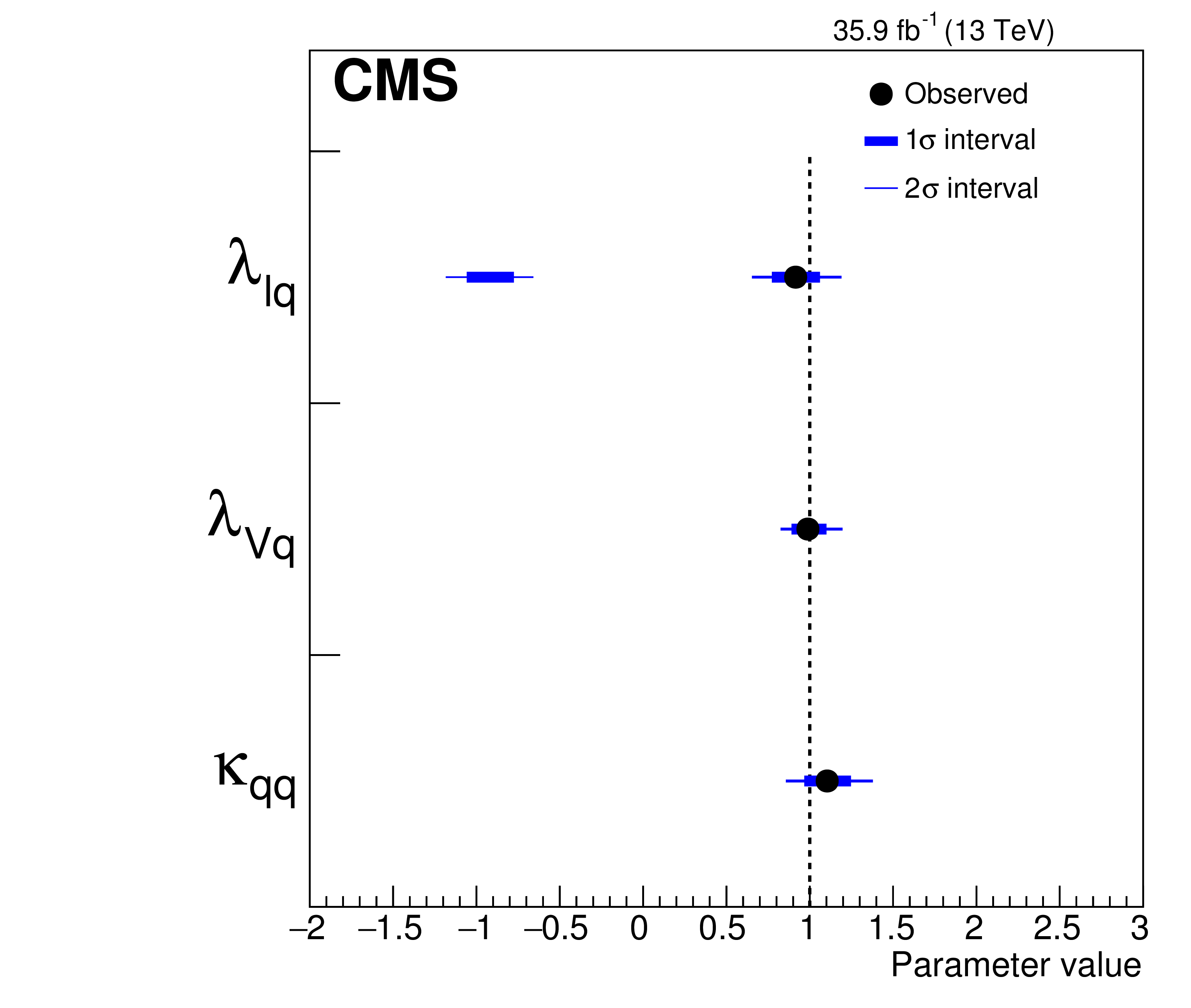
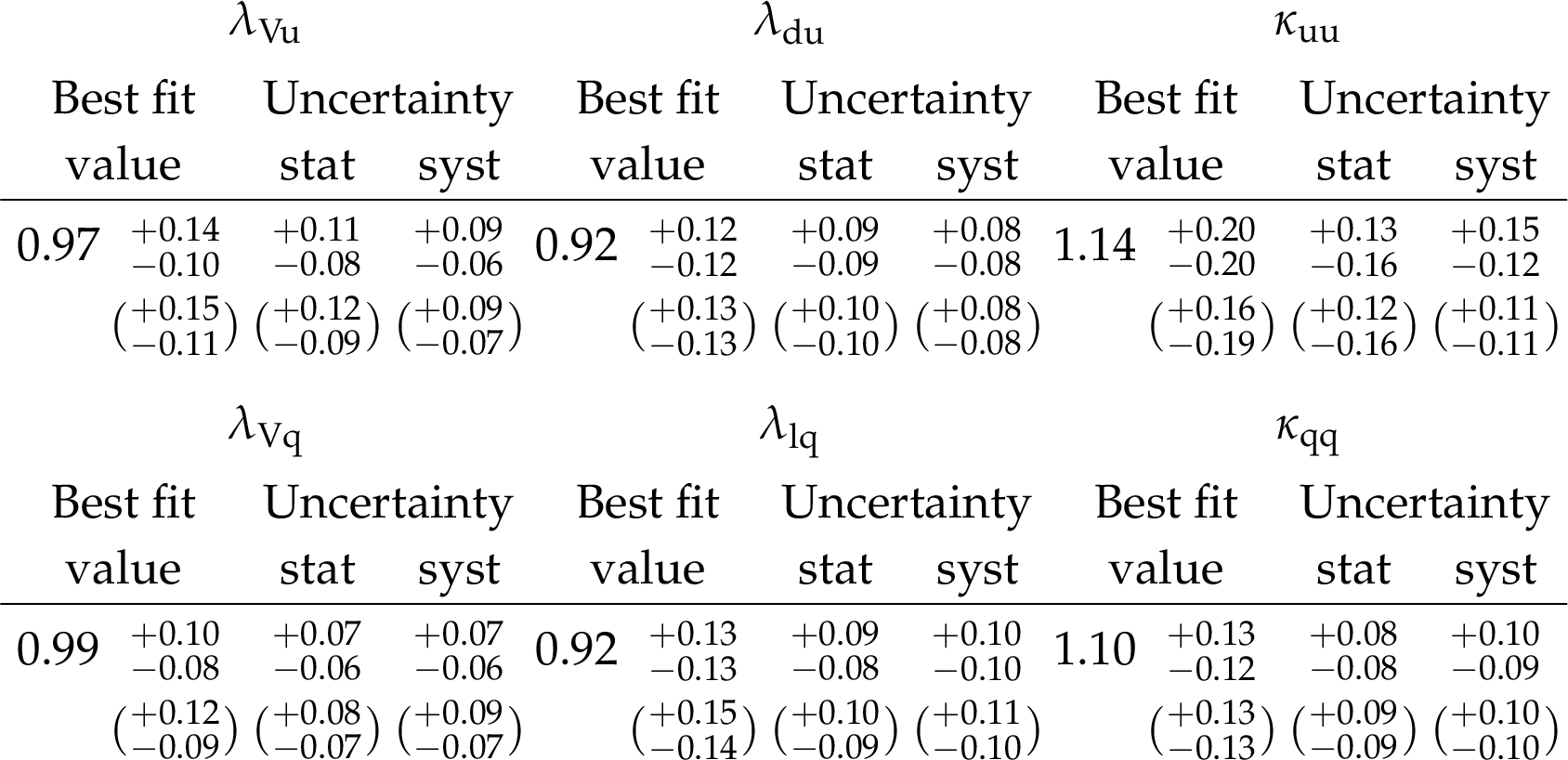
Figure 18:
Summary plots of the 3-parameter models comparing up- and down-type fermions, and floating the ratio of the vector coupling to the up-type coupling (left) and comparing lepton and quark couplings (right). The points indicate the best fit values while the thick and thin horizontal bars show the $1\sigma $ and $2\sigma $ CL intervals, respectively. Both positive and negative values of $\lambda _{{\mathrm {d}} {\mathrm {u}}}$, $\lambda _{\mathrm {V} {\mathrm {u}}}$, $\lambda _{\text {l} {\mathrm {q}}}$, and $\lambda _{\mathrm {V} {\mathrm {q}}}$ are considered. |
png pdf |
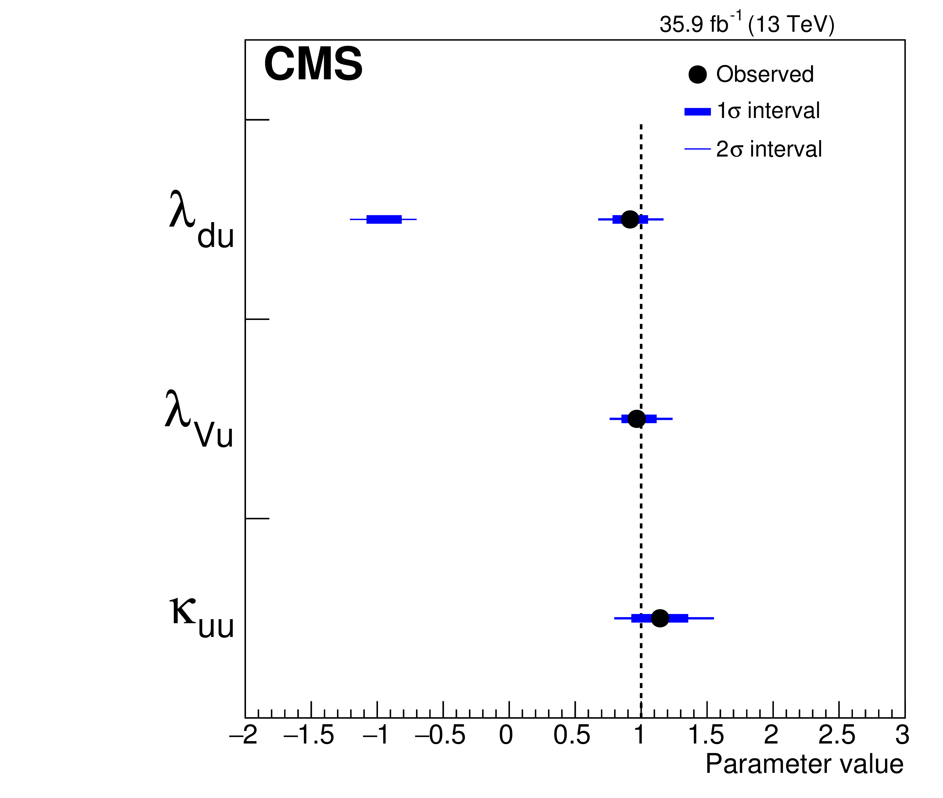
Figure 18-a:
Summary plot of the 3-parameter model comparing up- and down-type fermions, and floating the ratio of the vector coupling to the up-type coupling. The points indicate the best fit values while the thick and thin horizontal bars show the $1\sigma $ and $2\sigma $ CL intervals, respectively. Positive and negative values of $\lambda _{{\mathrm {d}} {\mathrm {u}}}$ and $\lambda _{\mathrm {V} {\mathrm {u}}}$ are considered. |
png pdf |
Figure 18-b:
Summary plot of the 3-parameter models comparing lepton and quark couplings. The points indicate the best fit values while the thick and thin horizontal bars show the $1\sigma $ and $2\sigma $ CL intervals, respectively. Positive and negative values of $\lambda _{\text {l} {\mathrm {q}}}$ and $\lambda _{\mathrm {V} {\mathrm {q}}}$ are considered. |
png pdf |
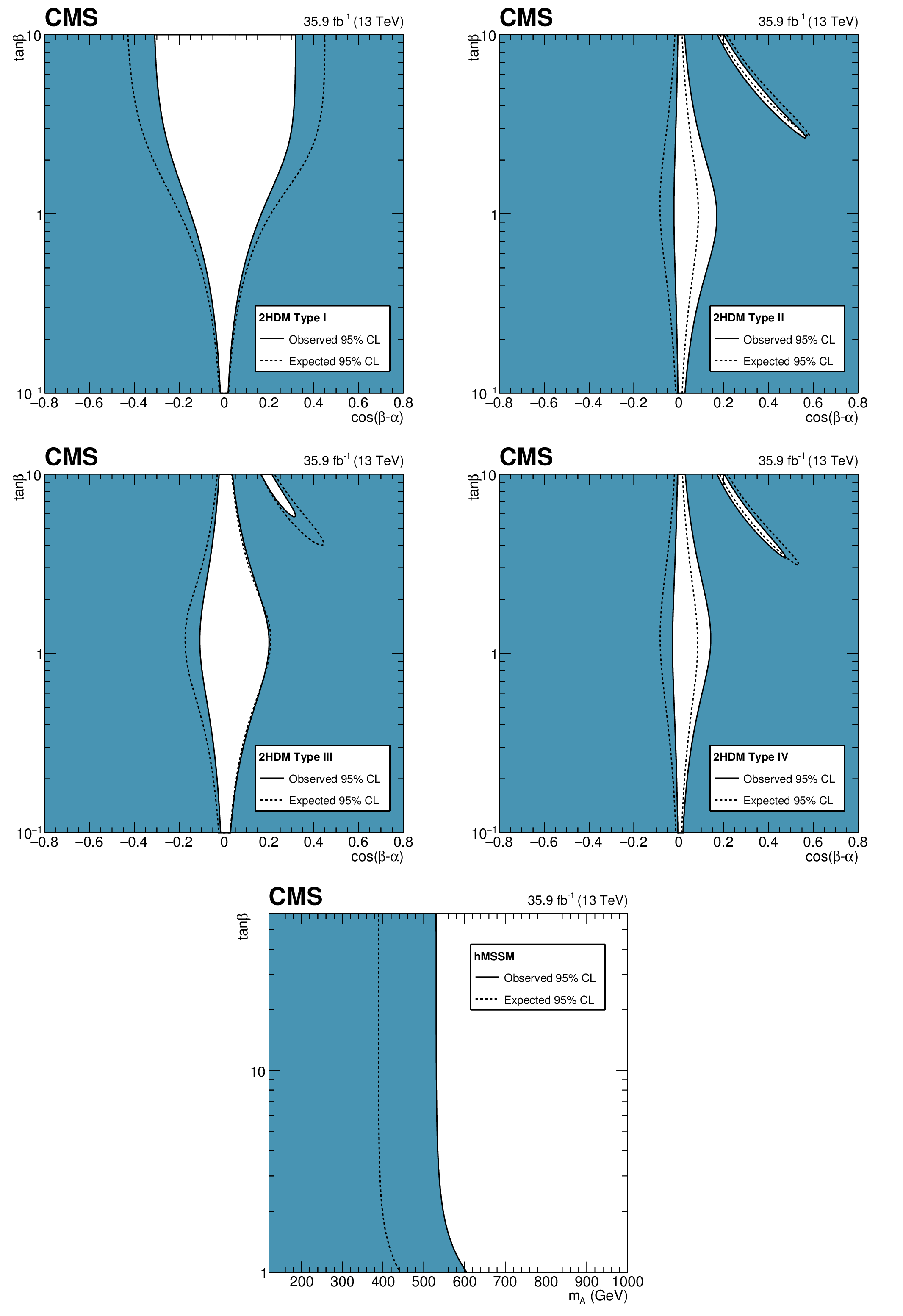
Figure 19:
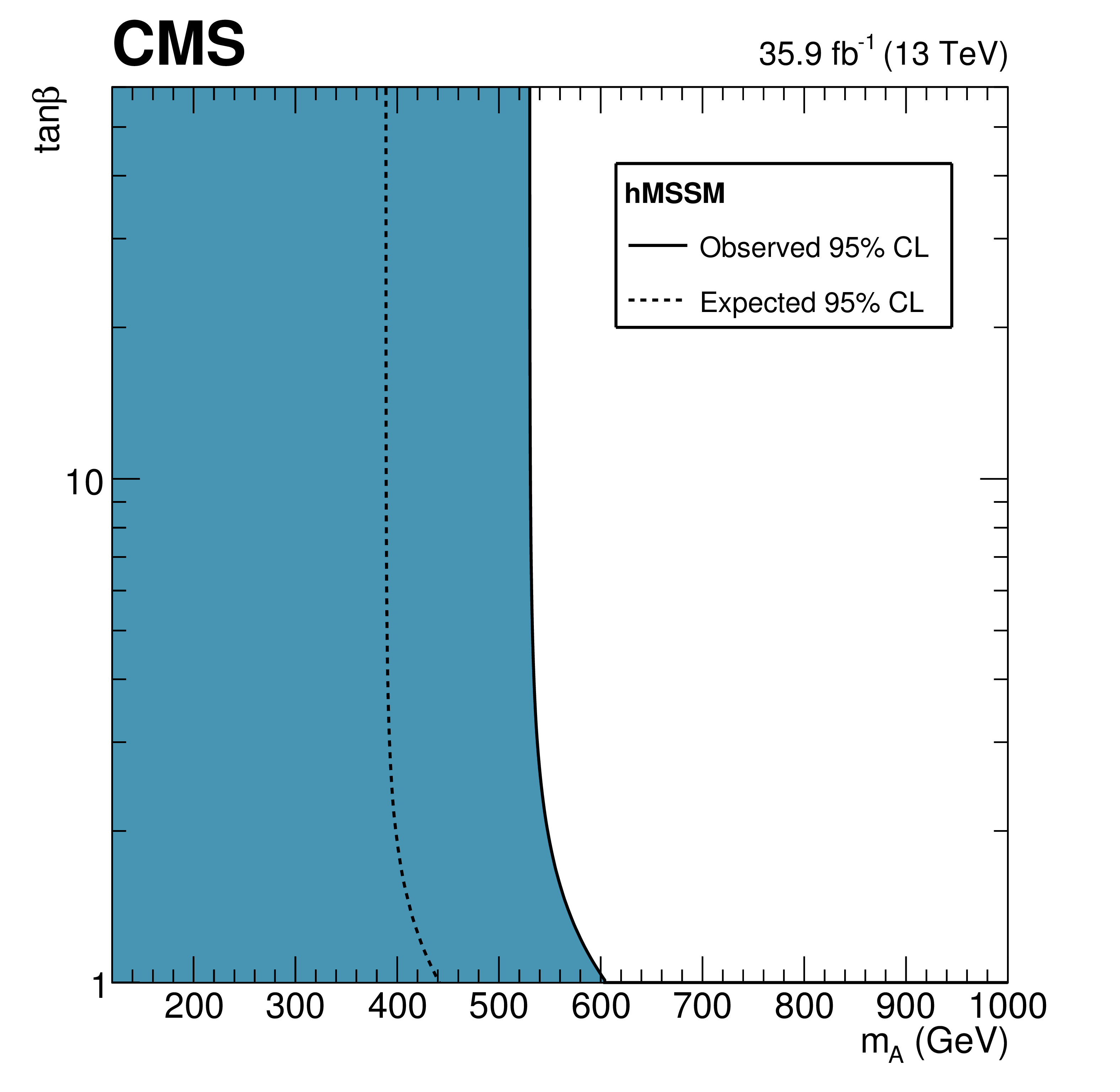
Constraints in the $\cos({\beta -\alpha})$ vs. $\tan\beta $ plane for the Types I, II, III, and IV 2HDM, and constraints in the $m_ {\mathrm {A}} $ vs. $\tan\beta $ plane for the hMSSM. The white regions, bounded by the solid black lines, in each plane represent the regions of the parameter space that are allowed at the 95% CL, given the data observed. The dashed lines indicate the boundaries of the allowed regions expected for the SM Higgs boson. |
png pdf |
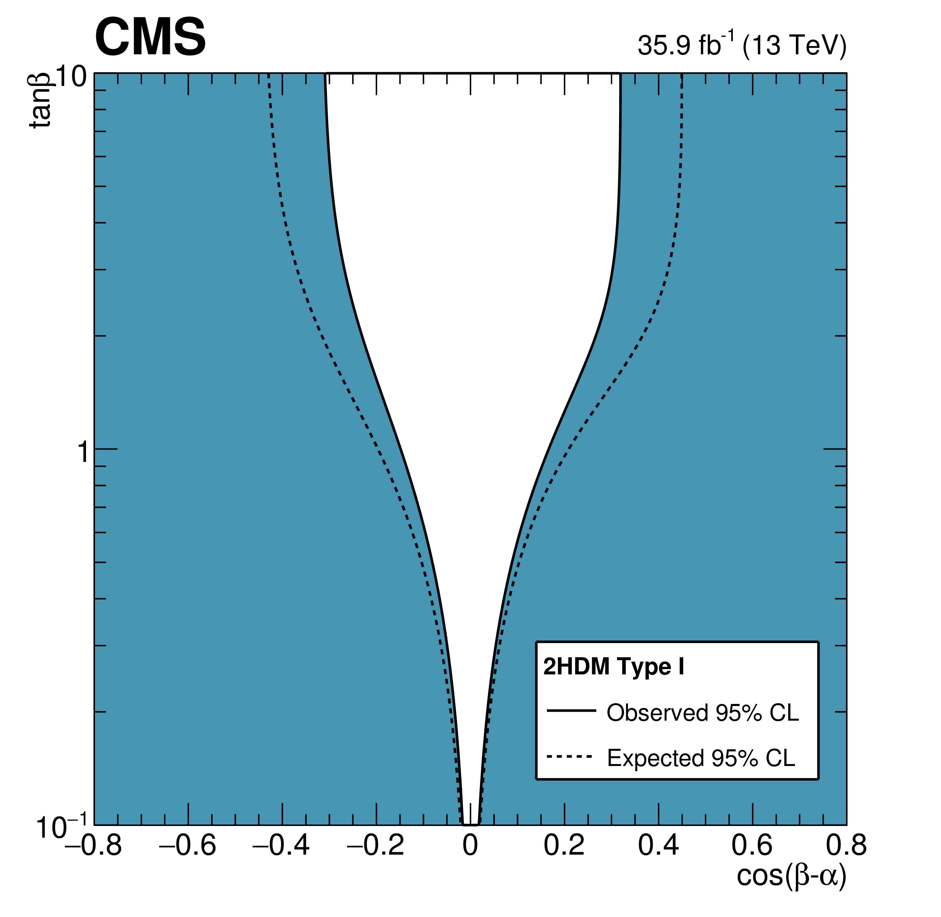
Figure 19-a:
Constraints in the $\cos({\beta -\alpha})$ vs. $\tan\beta $ plane for the Types I 2HDM. The white regions, bounded by the solid black lines, in each plane represent the regions of the parameter space that are allowed at the 95% CL, given the data observed. The dashed lines indicate the boundaries of the allowed regions expected for the SM Higgs boson. |

png pdf |
Figure 19-b:
Constraints in the $\cos({\beta -\alpha})$ vs. $\tan\beta $ plane for the Types II 2HDM. The white regions, bounded by the solid black lines, in each plane represent the regions of the parameter space that are allowed at the 95% CL, given the data observed. The dashed lines indicate the boundaries of the allowed regions expected for the SM Higgs boson. |
png pdf |
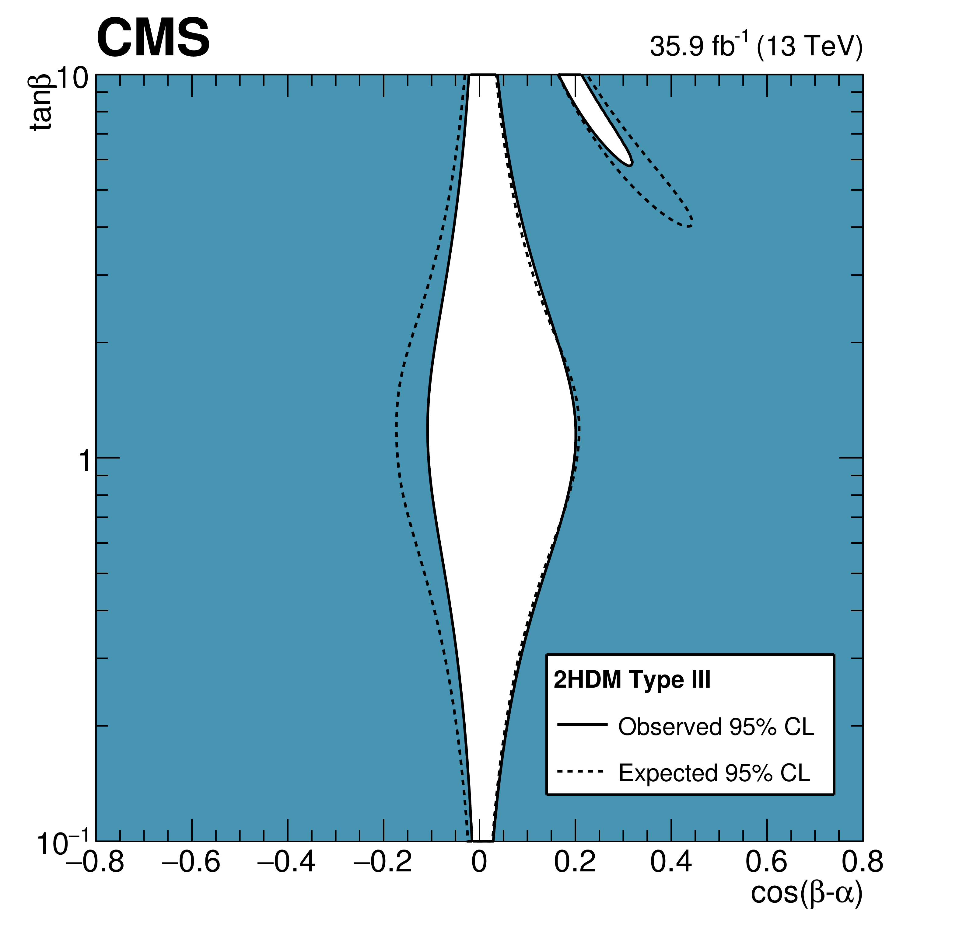
Figure 19-c:
Constraints in the $\cos({\beta -\alpha})$ vs. $\tan\beta $ plane for the Types III 2HDM. The white regions, bounded by the solid black lines, in each plane represent the regions of the parameter space that are allowed at the 95% CL, given the data observed. The dashed lines indicate the boundaries of the allowed regions expected for the SM Higgs boson. |

png pdf |
Figure 19-d:
Constraints in the $\cos({\beta -\alpha})$ vs. $\tan\beta $ plane for the Types IV 2HDM. The white regions, bounded by the solid black lines, in each plane represent the regions of the parameter space that are allowed at the 95% CL, given the data observed. The dashed lines indicate the boundaries of the allowed regions expected for the SM Higgs boson. |
png pdf |
Figure 19-e:
Constraints in the $m_ {\mathrm {A}} $ vs. $\tan\beta $ plane for the hMSSM. The white regions, bounded by the solid black lines, in each plane represent the regions of the parameter space that are allowed at the 95% CL, given the data observed. The dashed lines indicate the boundaries of the allowed regions expected for the SM Higgs boson. |
| Tables | |
png pdf |
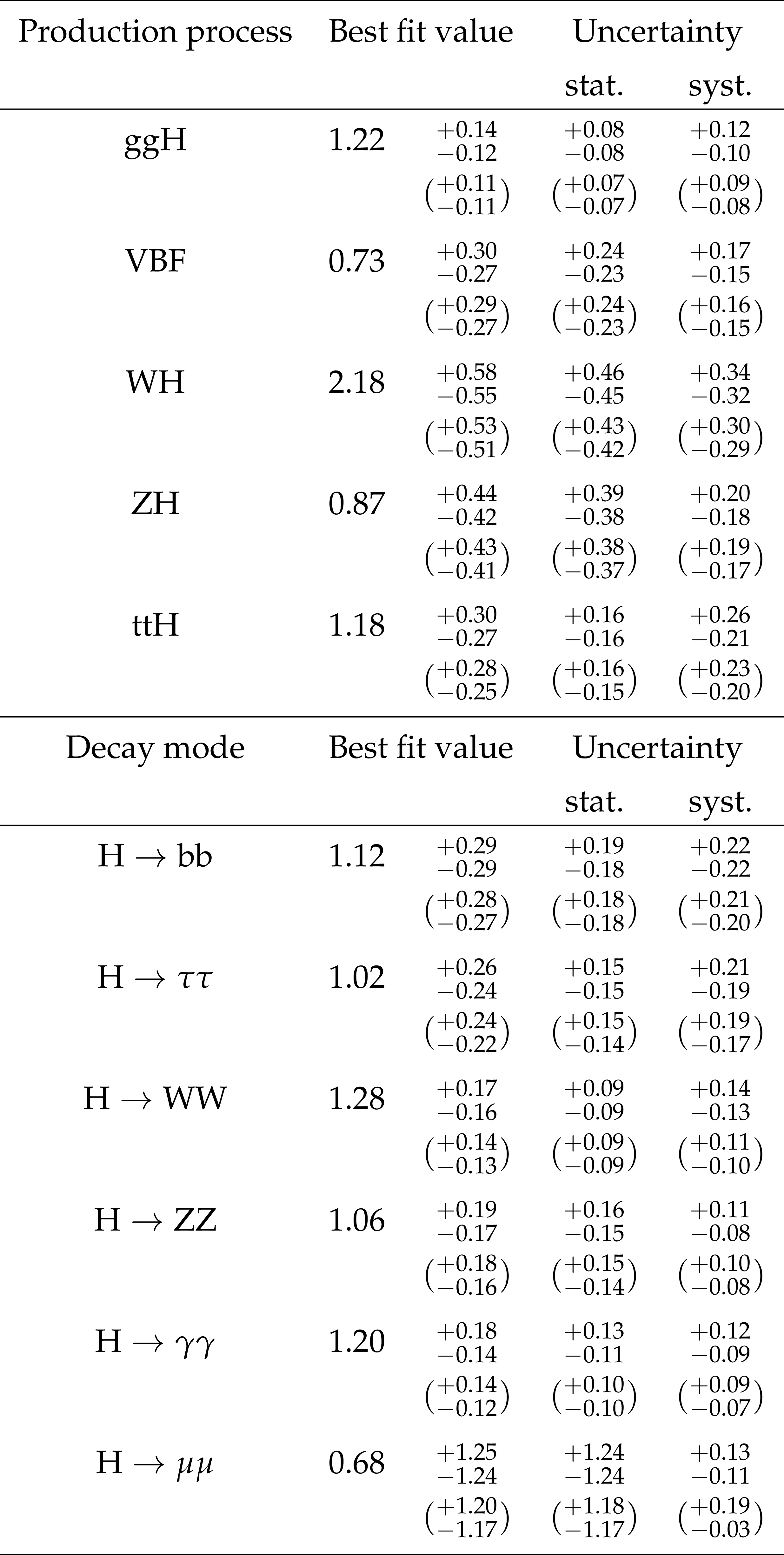
Table 2:
Best fit values and $ {\pm} 1 \sigma $ uncertainties for the parameters of the parametrizations with per-production mode and per-decay mode signal strength modifiers. The expected uncertainties are given in brackets. |
png pdf |
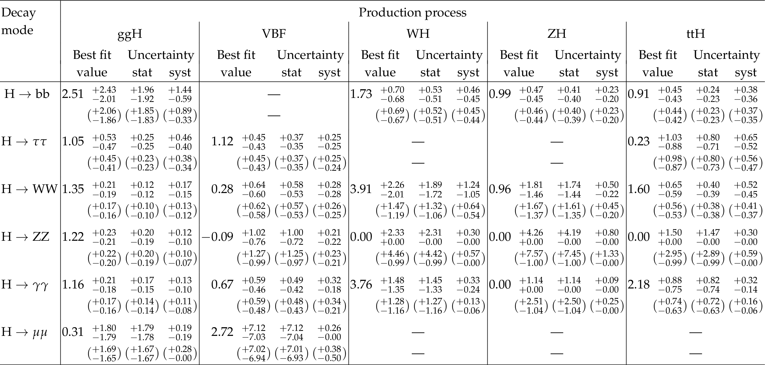
Table 3:
Best fit values and $ {\pm} 1 \sigma $ uncertainties for the parameters of the model with one signal strength parameter for each production and decay mode combination. The entries in the table represent the parameter $\mu _{i}^{f}=\mu _{i} \mu ^{f}$, where $i$ is indicated by the column and $f$ by the row. The expected uncertainties are given in brackets. Some of the signal strengths are restricted to nonnegative values, as described in the text. |
png pdf |
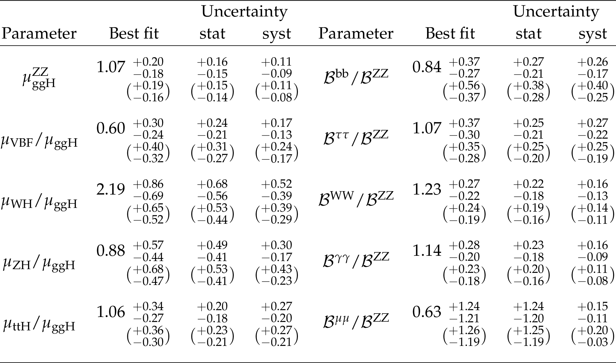
Table 4:
Best fit values and $ {\pm} 1 \sigma $ uncertainties for the parameters of the cross section and branching fraction ratio model. The expected uncertainties are given in brackets. |

png pdf |
Table 5:
Best fit values and $ {\pm} 1 \sigma $ uncertainties for the parameters of the stage 0 simplified template cross section model. The values are all normalized to the SM predictions. The expected uncertainties are given in brackets. |
png pdf |
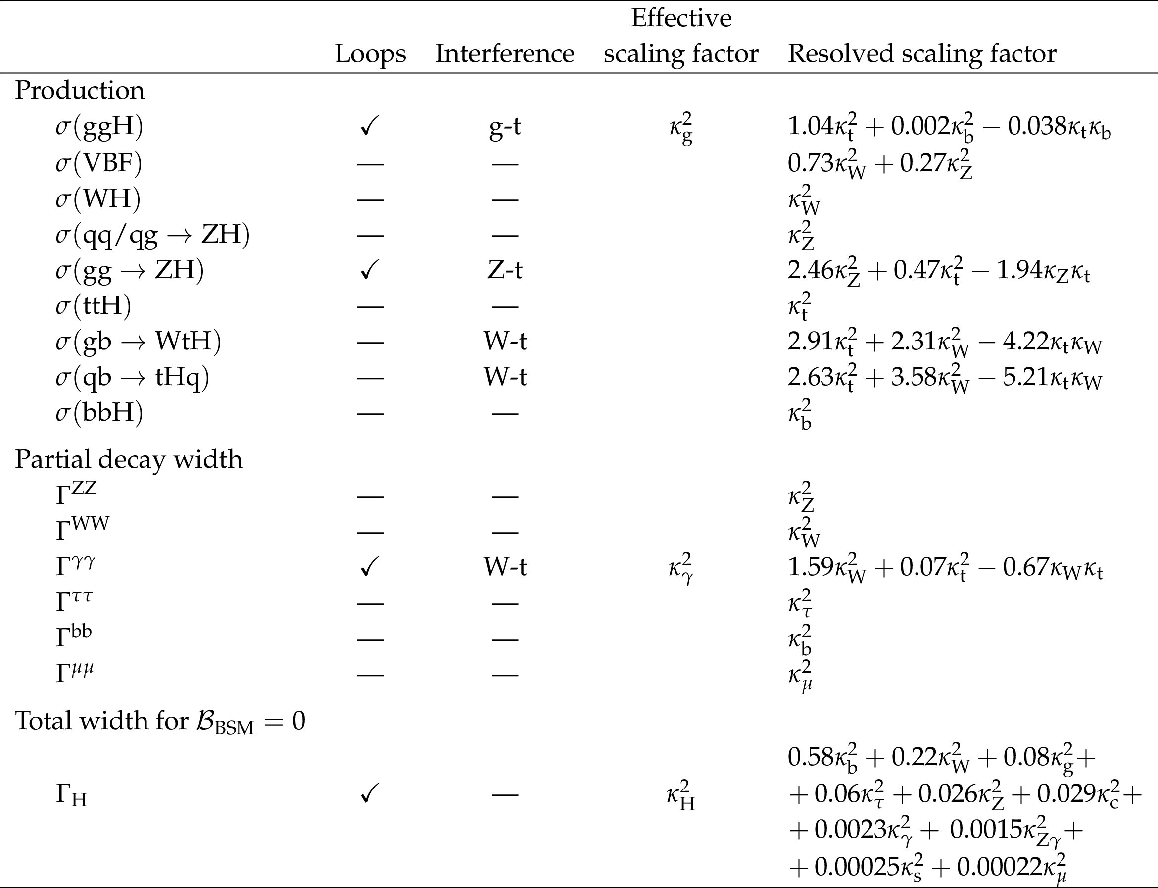
Table 6:
Normalization scaling factors for all relevant production cross sections and decay partial widths. For the $\kappa $ parameters representing loop processes, the resolved scaling in terms of the fundamental SM couplings is also given. |
png pdf |
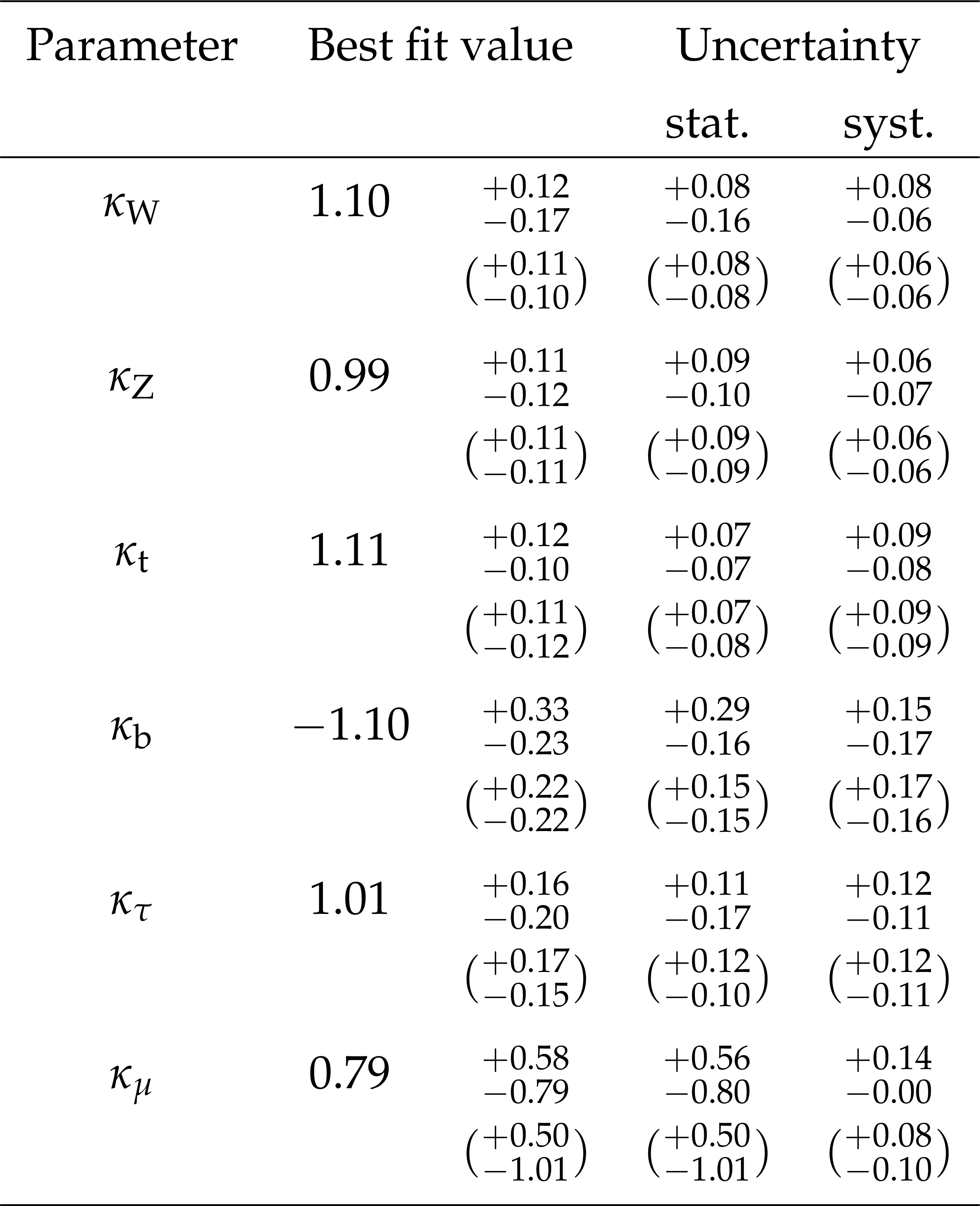
Table 7:
Best fit values and $ {\pm} 1 \sigma $ uncertainties for the parameters of the $\kappa $ model in which the loop processes are resolved. The expected uncertainties are given in brackets. |

png pdf |
Table 8:
Best fit values and $ {\pm} 1 \sigma $ uncertainties for the parameters of the $\kappa $-framework model with effective loops. The expected uncertainties are given in brackets. |
png pdf |
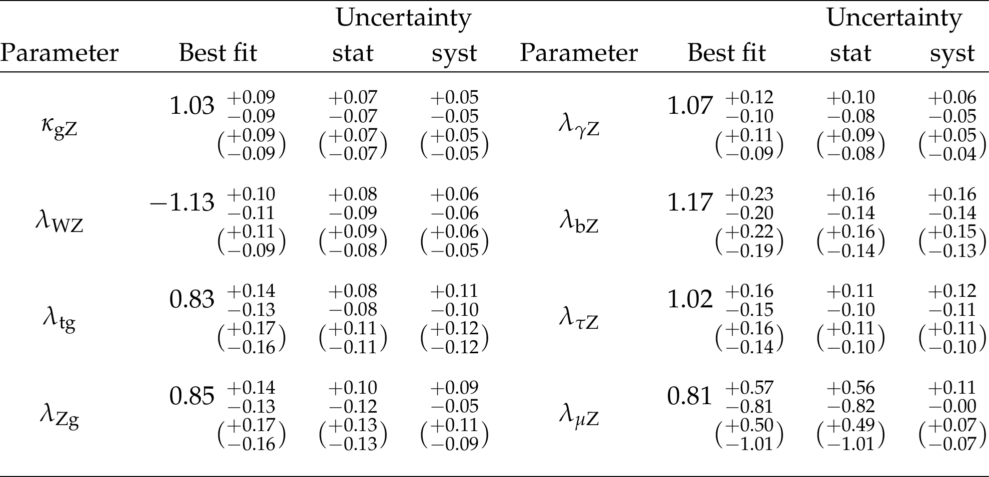
Table 9:
Best fit values and $ {\pm} 1 \sigma $ uncertainties for the parameters of the coupling modifier ratio model. The expected uncertainties are given in brackets. |
png pdf |
Table 10:
Best fit values and $ {\pm} 1 \sigma $ uncertainties for the parameters of the $\kappa _{\mathrm {V}},\kappa _{\mathrm {F}}$ model. The expected uncertainties are given in brackets. |
png pdf |
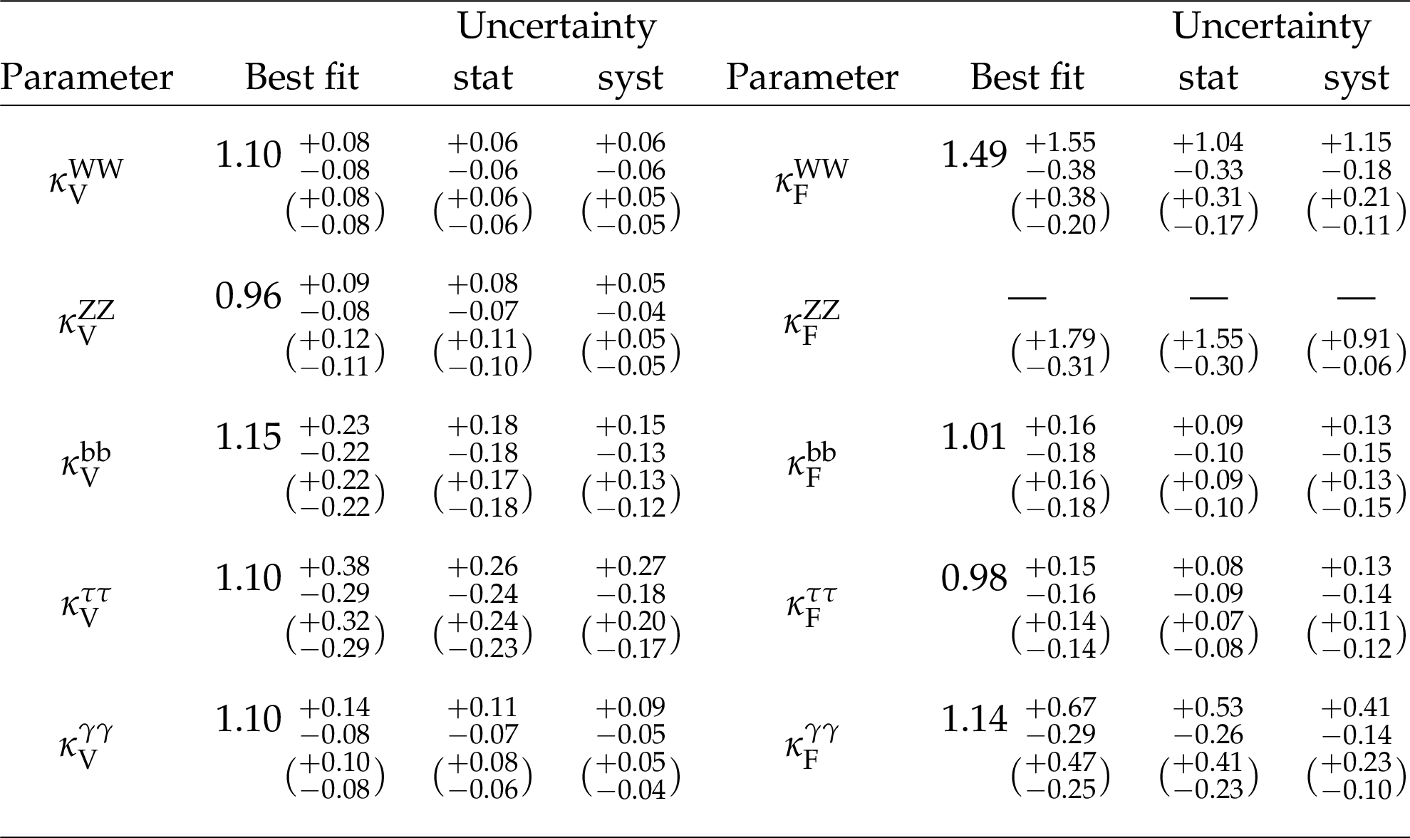
Table 11:
Best fit values and $ {\pm} 1 \sigma $ uncertainties for the parameters of the two benchmark models with resolved loops to test the symmetry of fermion couplings. The expected uncertainties are given in brackets. |

png pdf |
Table 12:
Compatibility of the fit results with the SM prediction under various signal parametrizations. The value of $q$ at the values of the POIs for which the SM expectation is obtained ($q_{\text {SM}}$) is shown along with the corresponding $p$-value, with respect to the SM, assuming $q$ is distributed according to a $\chi ^{2}$ function with the specified number of degrees of freedom (DOF). |
png pdf |
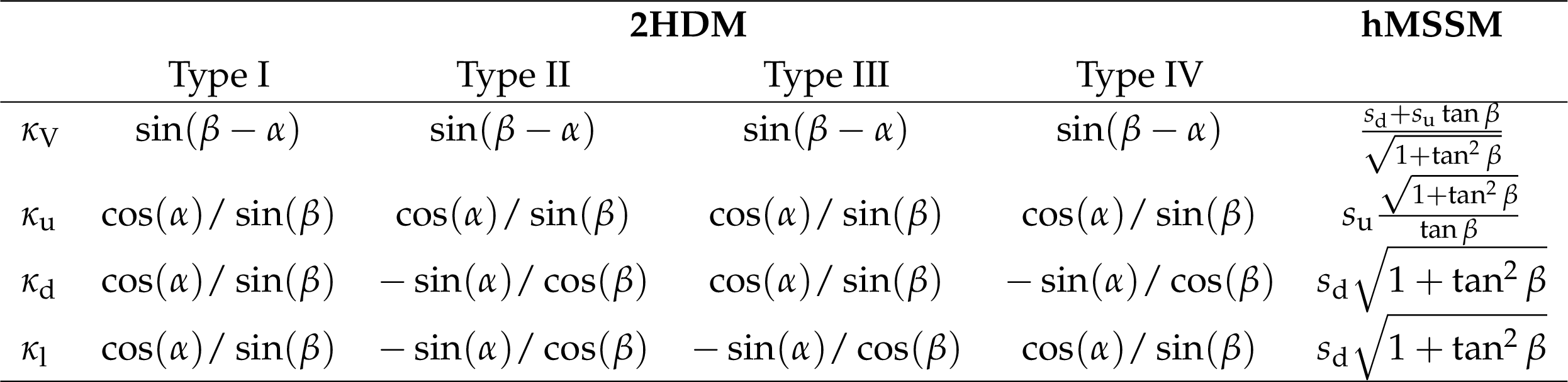
Table 13:
Modifications to the couplings of the Higgs bosons to up-type ($\kappa _{{\mathrm {u}}}$) and down-type ($\kappa _{{\mathrm {d}}}$) fermions, and vector bosons ($\kappa _{\mathrm {V}}$), with respect to the SM expectation, in 2HDM and for the hMSSM. The coupling modifications for the hMSSM are completed by the expressions for $s_{{\mathrm {u}}}$ and $s_{{\mathrm {d}}}$, as given by Eqs. (8) and (9). |
| Summary |
|
A set of combined measurements of Higgs boson production and decay rates has been presented, along with the consequential constraints placed on its couplings to standard model (SM) particles, and on the parameter spaces of several beyond the standard model (BSM) scenarios. The combination is based on analyses targeting the gluon fusion and vector boson fusion production modes, and associated production with a vector boson or a pair of top quarks. The analyses included in the combination target Higgs boson decay in the $\mathrm{H} \to \mathrm{Z}\mathrm{Z},\,\mathrm{W}\mathrm{W},\,{\gamma\gamma} ,\,{\tau\tau} $, ${\mathrm{b}\mathrm{b}} $, and $ {\mu \mu } $ channels, using 13 TeV proton-proton collision data collected in 2016 and corresponding to an integrated luminosity of 35.9 fb$^{-1}$. Additionally, searches for invisible Higgs boson decays are included to increase the sensitivity to potential interactions with BSM particles. Measurements of the Higgs boson production cross section times branching fraction in each of the channels are presented, along with a generic parametrization in terms of ratios of production cross sections and branching fractions, which makes no assumptions about the Higgs boson total width. The combined signal yield relative to the SM prediction has been measured as 1.17 $\pm$ 0.10 at $m_{\mathrm{H}} = $ 125.09 GeV. An improvement in the measured precision of the gluon fusion production rate of around $\sim$50% is achieved compared to previous ATLAS and CMS measurements. Additionally, a set of fiducial Higgs boson cross sections, in the context of the simplified template cross section framework, is presented for the first time from a combination of six decay channels. Furthermore, interpretations are provided in the context of a leading-order coupling modifier framework, including variants for which effective couplings to the photon and gluon are introduced. All of the results presented are compatible with the SM prediction. The invisible (undetected) branching fraction of the Higgs boson is constrained to be less than 22 (38%) at 95% Confidence Level. The results are additionally interpreted in two BSM models, the minimal supersymmetric model and the generic two Higgs doublet model. The constraints placed on the parameter spaces of these models are complementary to those that can be obtained from direct searches for additional Higgs bosons. |
| Additional Figures | |
png pdf |
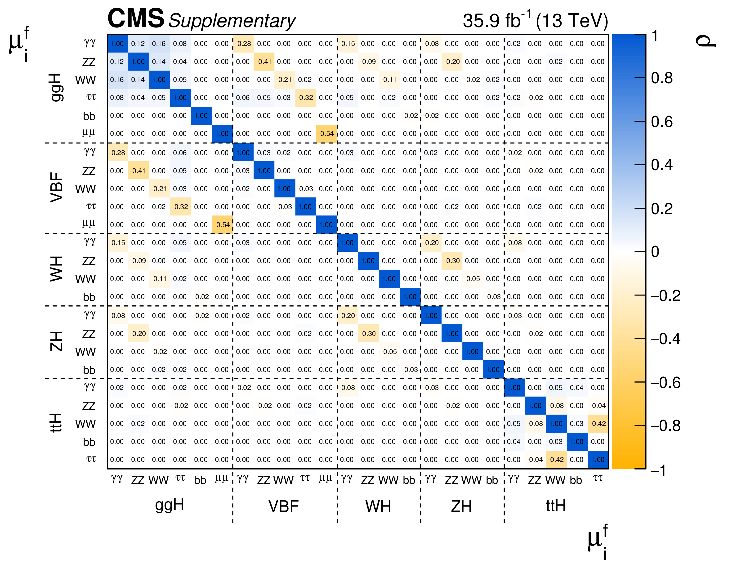
Additional Figure 1:
The correlation coefficients ($\rho $) obtained from the fit to data for the model with one signal strength parameter for each production and decay mode combination $\mu _{i}^{f}$. The production modes $i$ include gluon fusion (ggH), vector boson fusion (VBF), associated production with a vector boson (WH, ZH) and associated production with a pair of top quarks (ttH). The decay modes $f$ include ZZ, WW, $\gamma \gamma $, $\tau \tau $, bb and $ {{\mu}} {{\mu}}$. |

png pdf |
Additional Figure 2:
The correlation coefficients ($\rho $) obtained from the fit to data for the stage 0 simplified template cross section model. Six of the parameters represent the fiducial cross sections $\sigma _{{{\mathrm {g}} {\mathrm {g}} {\mathrm {H}}}}$, $\sigma _{{\mathrm {VBF}}}$, $\sigma _{{\mathrm {H}} +\rm {V}({\mathrm {q}} {\mathrm {q}})}$, $\sigma _{{\mathrm {H}} + {\mathrm {W}}(\ell \nu)}$, $\sigma _{{\mathrm {H}} +{{\mathrm {Z}}(\ell \ell /\nu \nu)}}$ and $\sigma _{{{\mathrm {t}} {\mathrm {t}} {\mathrm {H}}}}$ multiplied by the branching fraction $\mathcal {B}^{{\mathrm {Z}} {\mathrm {Z}}}$. The remaining five parameters represent the branching fractions for WW, $\gamma \gamma $, $\tau \tau $, $ {{\mathrm {b}} {\mathrm {b}}} $ and $ {{\mu}} {{\mu}}$ divided by $\mathcal {B}^{{\mathrm {Z}} {\mathrm {Z}}}$. |
| References | ||||
| 1 | S. L. Glashow | Partial-symmetries of weak interactions | NP 22 (1961) 579 | |
| 2 | S. Weinberg | A model of leptons | PRL 19 (1967) 1264 | |
| 3 | A. Salam | Weak and electromagnetic interactions | in Elementary particle physics: relativistic groups and analyticity, N. Svartholm, ed., p. 367 Almqvist \& Wiskell, 1968Proceedings of the 8th Nobel symposium | |
| 4 | G. 't Hooft and M. J. G. Veltman | Regularization and renormalization of gauge fields | NPB 44 (1972) 189 | |
| 5 | F. Englert and R. Brout | Broken symmetry and the mass of gauge vector mesons | PRL 13 (1964) 321 | |
| 6 | P. W. Higgs | Broken symmetries, massless particles and gauge fields | PL12 (1964) 132 | |
| 7 | P. W. Higgs | Broken symmetries and the masses of gauge bosons | PRL 13 (1964) 508 | |
| 8 | G. S. Guralnik, C. R. Hagen, and T. W. B. Kibble | Global conservation laws and massless particles | PRL 13 (1964) 585 | |
| 9 | P. W. Higgs | Spontaneous symmetry breakdown without massless bosons | PR145 (1966) 1156 | |
| 10 | T. W. B. Kibble | Symmetry breaking in non-Abelian gauge theories | PR155 (1967) 1554 | |
| 11 | Y. Nambu and G. Jona-Lasinio | Dynamical model of elementary particles based on an analogy with superconductivity. I | PR122 (1961) 345 | |
| 12 | ATLAS Collaboration | Observation of a new particle in the search for the standard model Higgs boson with the ATLAS detector at the LHC | PLB 716 (2012) 1 | 1207.7214 |
| 13 | CMS Collaboration | Observation of a new boson at a mass of 125 GeV with the CMS experiment at the LHC | PLB 716 (2012) 30 | CMS-HIG-12-028 1207.7235 |
| 14 | CMS Collaboration | Observation of a new boson with mass near 125 GeV in pp collisions at $ \sqrt{s} = $ 7 and 8 TeV | JHEP 06 (2013) 81 | CMS-HIG-12-036 1303.4571 |
| 15 | K. G. Wilson | Renormalization group and strong interactions | PRD 3 (1971) 1818 | |
| 16 | E. Gildener | Gauge-symmetry hierarchies | PRD 14 (1976) 1667 | |
| 17 | S. Weinberg | Gauge hierarchies | PLB 82 (1979) 387 | |
| 18 | G. 't Hooft | Naturalness, chiral symmetry, and spontaneous chiral symmetry breaking | NATO Sci. Ser. B 59 (1980) 135 | |
| 19 | L. Susskind | Dynamics of spontaneous symmetry breaking in the Weinberg-Salam theory | PRD 20 (1979) 2619 | |
| 20 | S. Dimopoulos and H. Georgi | Softly broken supersymmetry and SU(5) | NPB 193 (1981) 150 | |
| 21 | E. Witten | Dynamical breaking of supersymmetry | NPB 188 (1981) 513 | |
| 22 | N. Arkani-Hamed, S. Dimopoulos, and G. Dvali | The hierarchy problem and new dimensions at a millimeter | PLB 429 (1998) 263 | hep-ph/9803315 |
| 23 | L. Randall and R. Sundrum | Large mass hierarchy from a small extra dimension | PRL 83 (1999) 3370 | hep-ph/9905221 |
| 24 | N. Arkani-Hamed, A. G. Cohen, and H. Georgi | Electroweak symmetry breaking from dimensional deconstruction | PLB 513 (2001) 232 | hep-ph/0105239 |
| 25 | G. B\'elanger et al. | The MSSM invisible Higgs in the light of dark matter and g-2 | PLB 519 (2001) 93 | hep-ph/0106275 |
| 26 | G. F. Giudice, R. Rattazzi, and J. D. Wells | Graviscalars from higher-dimensional metrics and curvature-Higgs mixing | NPB 595 (2001) 250 | hep-ph/0002178 |
| 27 | D. Dominici and J. F. Gunion | Invisible Higgs decays from Higgs-graviscalar mixing | PRD 80 (2009) 115006 | 0902.1512 |
| 28 | C. Bonilla, J. C. Rom\ ao, and J. W. F. Valle | Neutrino mass and invisible Higgs decays at the LHC | PRD 91 (2015) 113015 | 1502.01649 |
| 29 | C. Anastasiou et al. | Higgs boson gluon-fusion production in QCD at three loops | PRL 114 (2015) 212001 | 1503.06056 |
| 30 | C. Anastasiou et al. | High precision determination of the gluon fusion Higgs boson cross-section at the LHC | JHEP 05 (2016) 58 | 1602.00695 |
| 31 | M. Ciccolini, A. Denner, and S. Dittmaier | Strong and electroweak corrections to the production of a Higgs boson+2 jets via weak interactions at the Large Hadron Collider | PRL 99 (2007) 161803 | 0707.0381 |
| 32 | M. Ciccolini, A. Denner, and S. Dittmaier | Electroweak and QCD corrections to Higgs production via vector-boson fusion at the LHC | PRD 77 (2008) 013002 | 0710.4749 |
| 33 | P. Bolzoni, F. Maltoni, S.-O. Moch, and M. Zaro | Higgs production via vector-boson fusion at NNLO in QCD | PRL 105 (2010) 011801 | 1003.4451 |
| 34 | P. Bolzoni, F. Maltoni, S.-O. Moch, and M. Zaro | Vector boson fusion at next-to-next-to-leading order in QCD: Standard model Higgs boson and beyond | PRD 85 (2012) 035002 | 1109.3717 |
| 35 | O. Brein, A. Djouadi, and R. Harlander | NNLO QCD corrections to the Higgs-strahlung processes at hadron colliders | PLB 579 (2004) 149 | hep-ph/0307206 |
| 36 | M. L. Ciccolini, S. Dittmaier, and M. Kramer | Electroweak radiative corrections to associated $ WH $ and $ ZH $ production at hadron colliders | PRD 68 (2003) 073003 | hep-ph/0306234 |
| 37 | W. Beenakker et al. | Higgs radiation off top quarks at the Tevatron and the LHC | PRL 87 (2001) 201805 | hep-ph/0107081 |
| 38 | W. Beenakker et al. | NLO QCD corrections to $ \mathrm{t\bar{t}} $ H production in hadron collisions. | NPB 653 (2003) 151 | hep-ph/0211352 |
| 39 | S. Dawson, L. H. Orr, L. Reina, and D. Wackeroth | Associated top quark Higgs boson production at the LHC | PRD 67 (2003) 071503 | hep-ph/0211438 |
| 40 | S. Dawson et al. | Associated Higgs production with top quarks at the Large Hadron Collider: NLO QCD corrections | PRD 68 (2003) 034022 | hep-ph/0305087 |
| 41 | Z. Yu et al. | QCD NLO and EW NLO corrections to $ t\bar{t}H $ production with top quark decays at hadron collider | PLB 738 (2014) 1 | 1407.1110 |
| 42 | S. S. Frixione et al. | Weak corrections to Higgs hadroproduction in association with a top-quark pair | JHEP 09 (2014) 65 | 1407.0823 |
| 43 | F. Demartin, F. Maltoni, K. Mawatari, and M. Zaro | Higgs production in association with a single top quark at the LHC | EPJC 75 (2015) 267 | 1504.0611 |
| 44 | F. Demartin et al. | tWH associated production at the LHC | EPJC 77 (2017) 34 | 1607.05862 |
| 45 | A. Denner et al. | Standard model Higgs-boson branching ratios with uncertainties | EPJC 71 (2011) 1753 | 1107.5909 |
| 46 | A. Djouadi, J. Kalinowski, and M. Spira | HDECAY: A Program for Higgs boson decays in the standard model and its supersymmetric extension | CPC 108 (1998) 56 | hep-ph/9704448 |
| 47 | A. Djouadi, J. Kalinowski, M. Muhlleitner, and M. Spira | An update of the program HDECAY | in The Les Houches 2009 workshop on TeV colliders: The tools and Monte Carlo working group summary report 2010 | 1003.1643 |
| 48 | A. Bredenstein, A. Denner, S. Dittmaier, and M. M. Weber | Precise predictions for the Higgs-boson decay H $ \rightarrow $ WW/ZZ $ \rightarrow $ 4 leptons | PRD 74 (2006) 013004 | hep-ph/0604011 |
| 49 | A. Bredenstein, A. Denner, S. Dittmaier, and M. M. Weber | Radiative corrections to the semileptonic and hadronic Higgs-boson decays H $ \rightarrow $WW/ZZ$ \rightarrow $ 4 fermions | JHEP 02 (2007) 80 | hep-ph/0611234 |
| 50 | S. Boselli et al. | Higgs boson decay into four leptons at NLOPS electroweak accuracy | JHEP 06 (2015) 23 | 1503.07394 |
| 51 | S. Actis, G. Passarino, C. Sturm, and S. Uccirati | NNLO computational techniques: the cases $ H \to \gamma \gamma $ and $ H \to g g $ | NPB 811 (2009) 182 | 0809.3667 |
| 52 | LHC Higgs Cross Section Working Group | Handbook of LHC Higgs cross sections: 4. Deciphering the nature of the Higgs sector | 1610.07922 | |
| 53 | ATLAS Collaboration | Measurements of the Higgs boson production and decay rates and coupling strengths using $ pp $ collision data at $ \sqrt{s} = $ 7 and 8 TeV in the ATLAS experiment | EPJC 76 (2016) 6 | 1507.04548 |
| 54 | CMS Collaboration | Precise determination of the mass of the Higgs boson and tests of compatibility of its couplings with the standard model predictions using proton collisions at 7 and 8 TeV | EPJC 75 (2015) 212 | CMS-HIG-14-009 1412.8662 |
| 55 | ATLAS and CMS Collaborations | Measurements of the Higgs boson production and decay rates and constraints on its couplings from a combined ATLAS and CMS analysis of the LHC $ pp $ collision data at $ \sqrt{s} = $ 7 and 8 TeV | JHEP 08 (2016) 45 | 1606.02266 |
| 56 | CMS Collaboration | The CMS experiment at the CERN LHC | JINST 3 (2008) S08004 | CMS-00-001 |
| 57 | CMS Collaboration | Measurements of Higgs boson properties in the diphoton decay channel in proton-proton collisions at $ \sqrt{s}= $ 13 TeV | \emphSubmitted to JHEP | CMS-HIG-16-040 1804.02716 |
| 58 | B. P. Roe et al. | Boosted decision trees as an alternative to artificial neural networks for particle identification | NIMA 543 (2005) 577 | physics/0408124 |
| 59 | P. D. Dauncey, M. Kenzie, N. Wardle, and G. J. Davies | Handling uncertainties in background shapes: the discrete profiling method | JINST 10 (2015) P04015 | 1408.6865 |
| 60 | CMS Collaboration | Measurements of properties of the Higgs boson decaying into the four-lepton final state in pp collisions at $ \sqrt{s}= $ 13 ~TeV | JHEP 11 (2017) 47 | CMS-HIG-16-041 1706.09936 |
| 61 | CMS Collaboration | Measurements of properties of the Higgs boson decaying to a W boson pair in pp collisions at $ \sqrt{s}= $ 13 TeV | Submitted to PLB | CMS-HIG-16-042 1806.05246 |
| 62 | CMS Collaboration | Observation of the Higgs boson decay to a pair of $ \tau $ leptons with the CMS detector | PLB 779 (2018) 283 | CMS-HIG-16-043 1708.00373 |
| 63 | CMS Collaboration | Evidence for the Higgs boson decay to a bottom quark-antiquark pair | PLB 780 (2018) 501 | CMS-HIG-16-044 1709.07497 |
| 64 | T. Aaltonen et al. | Improved $ b $-jet Energy Correction for $ H \to b\bar{b} $ Searches at CDF | 1107.3026 | |
| 65 | CMS Collaboration | Search for the associated production of a Higgs boson with a single top quark in proton-proton collisions at $ \sqrt{s} = $ 8 TeV | JHEP 06 (2016) 177 | CMS-HIG-14-027 1509.08159 |
| 66 | ATLAS Collaboration | Search for the $ \mathrm{b}\overline{\mathrm{b}} $ decay of the Standard Model Higgs boson in associated (W/Z)H production with the ATLAS detector | JHEP 01 (2015) 69 | 1409.6212 |
| 67 | CMS Collaboration | Identification of b-quark jets with the CMS experiment | JINST 8 (2013) P04013 | |
| 68 | CMS Collaboration | Identification of heavy-flavour jets with the CMS detector in pp collisions at 13 TeV | JINST (2017) P05011 | CMS-BTV-16-002 1712.07158 |
| 69 | CMS Collaboration | Inclusive search for a highly boosted Higgs boson decaying to a bottom quark-antiquark pair | PRL 120 (2018) 071802 | CMS-HIG-17-010 1709.05543 |
| 70 | M. Cacciari, G. P. Salam, and G. Soyez | The anti-$ {k_{\mathrm{T}}} $ jet clustering algorithm | JHEP 04 (2008) 63 | 0802.1189 |
| 71 | M. Cacciari, G. P. Salam, and G. Soyez | FastJet user manual | EPJC 72 (2012) 1896 | 1111.6097 |
| 72 | M. Dasgupta, A. Fregoso, S. Marzani, and G. P. Salam | Towards an understanding of jet substructure | JHEP 09 (2013) 29 | 1307.0007 |
| 73 | A. J. Larkoski, S. Marzani, G. Soyez, and J. Thaler | Soft drop | JHEP 05 (2014) 146 | 1402.2657 |
| 74 | CMS Collaboration | Identification of double-$ \mathrm{b} $ quark jets in boosted event topologies | CMS-PAS-BTV-15-002 | CMS-PAS-BTV-15-002 |
| 75 | CMS Collaboration | Observation of $ \mathrm{t\bar{t}H} $ production | PRL 120 (2018) 231801 | CMS-HIG-17-035 1804.02610 |
| 76 | CMS Collaboration | Evidence for associated production of a Higgs boson with a top quark pair in final states with electrons, muons, and hadronically decaying $ \tau $ leptons at $ \sqrt{s} = $ 13 TeV | JHEP 08 (2018) 066 | CMS-HIG-17-018 1803.05485 |
| 77 | CMS Collaboration | Search for $ \mathrm{t\overline{t}} $H production in the H$ \mathrm{b\overline{b}} $ decay channel with leptonic $ \mathrm{t\overline{t}} $ decays in proton-proton collisions at $ \sqrt{s}= $ 13 TeV | Submitted to JHEP | CMS-HIG-17-026 1804.03682 |
| 78 | CMS Collaboration | Search for $ \mathrm{t}\overline{\mathrm{t}} $H production in the all-jet final state in proton-proton collisions at $ \sqrt{s}= $ 13 TeV | Submitted to JHEP | CMS-HIG-17-022 1803.06986 |
| 79 | J. Schmidhuber | Deep learning in neural networks: An overview | Neural Networks 61 (2015) 85 | |
| 80 | T. J. Hastie, R. J. Tibshirani, and J. H. Friedman | The elements of statistical learning: data mining, inference, and prediction | Springer series in statistics. Springer, New York, NY, 2nd edition edition | |
| 81 | P. C. Bhat | Multivariate analysis methods in particle physics | Annu. Rev. Nucl. Part. Sci. 61 (2011) 281 | |
| 82 | P. Speckmayer, A. Hocker, J. Stelzer, and H. Voss | The toolkit for multivariate data analysis, TMVA 4 | J. Phys. Conf. Ser. 219 (2010) 032057 | |
| 83 | K. Kondo | Dynamical likelihood method for reconstruction of events with missing momentum. 1: Method and toy models | J. Phys. Soc. Jpn. 57 (1988) 4126 | |
| 84 | D0 Collaboration | A precision measurement of the mass of the top quark | Nature 429 (2004) 638 | hep-ex/0406031 |
| 85 | CMS Collaboration | Performance of quark/gluon discrimination in 8 TeV pp data | CMS-PAS-JME-13-002 | CMS-PAS-JME-13-002 |
| 86 | CMS Collaboration | Performance of quark/gluon discrimination in 13 TeV data | CDS | |
| 87 | CMS Collaboration | Search for the Higgs boson decaying to two muons in proton-proton collisions at $ \sqrt{s}= $ 13 TeV | Submitted to PRLett | CMS-HIG-17-019 1807.06325 |
| 88 | R. E. Shrock and M. Suzuki | Invisible decays of Higgs bosons | PLB 110 (1982) 250 | |
| 89 | CMS Collaboration | Search for invisible decays of a Higgs boson produced through vector boson fusion in proton-proton collisions at $ \sqrt{s}= $ 13 TeV | Submitted to PLB | CMS-HIG-17-023 1809.05937 |
| 90 | CMS Collaboration | Search for new physics in events with a leptonically decaying Z boson and a large transverse momentum imbalance in proton-proton collisions at $ \sqrt{s}= $ 13 TeV | EPJC 78 (2017) 291 | CMS-EXO-16-052 1711.00431 |
| 91 | CMS Collaboration | Search for new physics in final states with an energetic jet or a hadronically decaying W or Z boson and transverse momentum imbalance at $ \sqrt{s}= $ 13 TeV | PRD 97 (2018) 092005 | CMS-EXO-16-048 1712.02345 |
| 92 | E. Bagnaschi, G. Degrassi, P. Slavich, and A. Vicini | Higgs production via gluon fusion in the POWHEG approach in the SM and in the MSSM | JHEP 02 (2012) 88 | 1111.2854 |
| 93 | P. Nason | A New method for combining NLO QCD with shower Monte Carlo algorithms | JHEP 11 (2004) 040 | hep-ph/0409146 |
| 94 | S. Frixione, P. Nason, and C. Oleari | Matching NLO QCD computations with parton shower simulations: the $ POWHEG $ method | JHEP 11 (2007) 070 | 0709.2092 |
| 95 | S. Alioli, P. Nason, C. Oleari, and E. Re | A general framework for implementing NLO calculations in shower Monte Carlo programs: the POWHEG BOX | JHEP 06 (2010) 043 | 1002.2581 |
| 96 | J. Alwall et al. | The automated computation of tree-level and next-to-leading order differential cross sections, and their matching to parton shower simulations | JHEP 07 (2014) 079 | 1405.0301 |
| 97 | R. Frederix and S. Frixione | Merging meets matching in MC@NLO | JHEP 12 (2012) 61 | 1209.6215 |
| 98 | K. Hamilton, P. Nason, E. Re, and G. Zanderighi | NNLOPS simulation of Higgs boson production | JHEP 10 (2013) 222 | 1309.0017 |
| 99 | K. Hamilton, P. Nason, and G. Zanderighi | Finite quark-mass effects in the NNLOPS POWHEG+MiNLO Higgs generator | 1501.04637 | |
| 100 | R. Barlow and C. Beeston | Fitting using finite Monte Carlo samples | Comp. Phys. Comms. 77 (1993) 219 | |
| 101 | J. S. Conway | Incorporating nuisance parameters in likelihoods for multisource spectra | 1103.0354 | |
| 102 | The ATLAS Collaboration, The CMS Collaboration, The LHC Higgs Combination Group | Procedure for the LHC Higgs boson search combination in Summer 2011 | CMS-NOTE-2011-005 | |
| 103 | CMS Collaboration | Combined results of searches for the standard model Higgs boson in pp collisions at $ \sqrt{s} = $ 7 TeV | PLB 710 (2012) 26 | CMS-HIG-11-032 1202.1488 |
| 104 | W. Verkerke and D. P. Kirkby | The RooFit toolkit for data modeling | in 13$^\textth$ International Conference for Computing in High Energy and Nuclear Physics (CHEP03) 2003 CHEP-2003-MOLT007 | physics/0306116 |
| 105 | L. Moneta et al. | The RooStats project | in 13th International Workshop on Advanced Computing and Analysis Techniques in Physics Research (ACAT2010) SISSA, 2010 PoS(ACAT2010)057 | 1009.1003 |
| 106 | G. Cowan, K. Cranmer, E. Gross, and O. Vitells | Asymptotic formulae for likelihood-based tests of new physics | EPJC 71 (2011) 1554 | 1007.1727 |
| 107 | ATLAS and CMS Collaborations | Combined Measurement of the Higgs Boson Mass in $ pp $ Collisions at $ \sqrt{s}= $ 7 and 8 TeV with the ATLAS and CMS Experiments | PRL 114 (2015) 191803 | 1503.07589 |
| 108 | CMS Collaboration | CMS luminosity measurements for the 2016 data taking period | CMS-PAS-LUM-17-001 | CMS-PAS-LUM-17-001 |
| 109 | E. Boos, V. Bunichev, M. Dubinin, and Y. Kurihara | Higgs boson signal at complete tree level in the SM extension by dimension-six operators | PRD 89 (2014) 035001 | 1309.5410 |
| 110 | LHC Higgs Cross Section Working Group | Handbook of LHC Higgs Cross Sections: 3. Higgs Properties | 1307.1347 | |
| 111 | C. Englert, M. McCullough, and M. Spannowsky | Gluon-initiated associated production boosts Higgs physics | PRD 89 (2014) 013013 | 1310.4828 |
| 112 | K. Hagiwara, R. Szalapski, and D. Zeppenfeld | Anomalous Higgs boson production and decay | PLB 318 (1993) 155 | hep-ph/9308347 |
| 113 | C. Arzt, M. B. Einhorn, and J. Wudka | Patterns of deviation from the standard model | NPB 433 (1995) 41 | hep-ph/9405214 |
| 114 | D. Zeppenfeld, R. Kinnunen, A. Nikitenko, and E. Richter-Was | Measuring Higgs boson couplings at the CERN LHC | PRD 62 (2000) 013009 | hep-ph/0002036 |
| 115 | V. Barger et al. | Effects of genuine dimension-six Higgs operators | PRD 67 (2003) 115001 | hep-ph/0301097 |
| 116 | M. Duhrssen et al. | Extracting Higgs boson couplings from CERN LHC data | PRD 70 (2004) 113009 | hep-ph/0406323 |
| 117 | A. Manohar and M. Wise | Modifications to the properties of the Higgs boson | PLB 636 (2006) 107 | hep-ph/0601212 |
| 118 | I. Low, R. Rattazzi, and A. Vichi | Theoretical constraints on the Higgs effective couplings | JHEP 04 (2010) 126 | 0907.5413 |
| 119 | J. Ellis and T. You | Global analysis of experimental constraints on a possible Higgs-like particle with mass ~125 GeV | JHEP 06 (2012) 140 | 1204.0464 |
| 120 | T. Corbett, O. J. P. Eboli, J. Gonzalez-Fraile, and M. C. Gonzalez-Garcia | Constraining anomalous Higgs boson interactions | PRD 86 (2012) 075013 | 1207.1344 |
| 121 | G. Passarino | NLO inspired effective Lagrangians for Higgs physics | NPB 868 (2013) 416 | 1209.5538 |
| 122 | M. Klute et al. | Measuring Higgs couplings from LHC data | PRL 109 (2012) 101801 | 1205.2699 |
| 123 | R. Contino et al. | Effective Lagrangian for a light Higgs-like scalar | JHEP 07 (2013) 35 | 1303.3876 |
| 124 | W.-F. Chang, W.-P. Pan, and F. Xu | Effective gauge-Higgs operators analysis of new physics associated with the Higgs boson | PRD 88 (2013) 033004 | 1303.7035 |
| 125 | P. P. Giardino et al. | The universal Higgs fit | JHEP 05 (2014) 46 | 1303.3570 |
| 126 | M. Ghezzi, R. Gomez-Ambrosio, G. Passarino, and S. Uccirati | NLO Higgs effective field theory and $ \kappa $-framework | JHEP 07 (2015) 175 | 1505.03706 |
| 127 | J. Ellis and T. You | Global analysis of the Higgs candidate with mass $ \sim $ 125 GeV | JHEP 09 (2012) 123 | 1207.1693 |
| 128 | J. Ellis and T. You | Updated global analysis of Higgs couplings | JHEP 06 (2013) 103 | 1303.3879 |
| 129 | Particle Data Group | Review of particle physics | CPC 40 (2016) 100001 | |
| 130 | G. C. Branco et al. | Theory and phenomenology of two-Higgs-doublet models | PR 516 (2012) 1 | 1106.0034 |
| 131 | J. F. Gunion and H. E. Haber | CP-conserving two-Higgs-doublet model: The approach to the decoupling limit | PRD 67 (2003) 075019 | hep-ph/0207010 |
| 132 | L. Maiani, A. D. Polosa, and V. Riquer | Bounds to the Higgs sector masses in minimal supersymmetry from LHC data | PLB 724 (2013) 274 | 1305.2172 |
| 133 | A. Djouadi | The Anatomy of electroweak symmetry breaking Tome II. The Higgs bosons in the minimal supersymmetric model | PR 459 (2008) 1 | hep-ph/0503173 |
| 134 | J. F. Gunion and H. E. Haber | Higgs bosons in supersymmetric models (I) | NPB 272 (1986) 1 | |
| 135 | H. E. Haber and G. L. Kane | The search for supersymmetry: Probing physics beyond the standard model | PR 117 (1985) 75 | |
| 136 | H. P. Nilles | Supersymmetry, supergravity and particle physics | PR 110 (1984) 1 | |
| 137 | A. Djouadi et al. | The post-Higgs MSSM scenario: habemus MSSM? | EPJC 73 (2013) 2650 | 1307.5205 |
| 138 | A. Djouadi et al. | Fully covering the MSSM Higgs sector at the LHC | JHEP 06 (2015) 168 | 1502.05653 |
| 139 | ATLAS Collaboration | Constraints on new phenomena via Higgs boson couplings and invisible decays with the ATLAS detector | JHEP 11 (2015) 206 | 1509.00672 |
| 140 | M. Carena et al. | MSSM Higgs boson searches at the LHC: benchmark scenarios after the discovery of a Higgs-like particle | EPJC 73 (2013) 2552 | 1302.7033 |
| 141 | ATLAS Collaboration | Search for heavy resonances decaying into $ WW $ in the $ e\nu\mu\nu $ final state in $ pp $ collisions at $ \sqrt{s}= $ 13 TeV with the ATLAS detector | EPJC 78 (2018) 24 | 1710.01123 |
| 142 | ATLAS Collaboration | Search for additional heavy neutral Higgs and gauge bosons in the ditau final state produced in 36 fb$ ^{-1} $ of pp collisions at $ \sqrt{s} = $ 13 TeV with the ATLAS detector | JHEP 01 (2018) 55 | 1709.07242 |
| 143 | ATLAS Collaboration | Search for charged Higgs bosons produced in association with a top quark and decaying via $ H^{\pm} \rightarrow \tau\nu $ using $ pp $ collision data recorded at $ \sqrt{s} = $ 13 TeV by the ATLAS detector | PLB 759 (2016) 555 | 1603.09203 |
| 144 | CMS Collaboration | Search for neutral MSSM Higgs bosons decaying to a pair of tau leptons in pp collisions | JHEP 10 (2014) 160 | CMS-HIG-13-021 1408.3316 |
| 145 | CMS Collaboration | Search for a standard-model-like Higgs boson with a mass in the range 145 to 1000 GeV at the LHC | EPJC 73 (2013) 2469 | CMS-HIG-12-034 1304.0213 |
|
|
Compact Muon Solenoid LHC, CERN |
|

|

|

|

|

|