

Compact Muon Solenoid
LHC, CERN
| CMS-EXO-19-009 ; CERN-EP-2023-003 | ||
| A search for new physics in central exclusive production using the missing mass technique with the CMS detector and the CMS-TOTEM precision proton spectrometer | ||
| CMS and TOTEM Collaborations | ||
| 8 March 2023 | ||
| Accepted for publication in Eur. Phys. J. C | ||
| Abstract: A generic search is presented for the associated production of a Z boson or a photon with an additional unspecified massive particle X, $ \mathrm{p}\mathrm{p}\to \mathrm{p}\mathrm{p} +\mathrm{Z}/\gamma+\mathrm{X} $, in proton-tagged events from proton-proton collisions at $ \sqrt{s}= $ 13 TeV, recorded in 2017 with the CMS detector and the CMS-TOTEM precision proton spectrometer. The missing mass spectrum is analysed in the 600-1600 GeV range and a fit is performed to search for possible deviations from the background expectation. No significant excess in data with respect to the background predictions has been observed. Model-independent upper limits on the visible production cross section of $ \mathrm{p}\mathrm{p}\to \mathrm{p}\mathrm{p} +\mathrm{Z}/\gamma+\mathrm{X} $ are set. | ||
| Links: e-print arXiv:2303.04596 [hep-ex] (PDF) ; CDS record ; inSPIRE record ; HepData record ; CADI line (restricted) ; | ||
| Figures | |
png pdf |
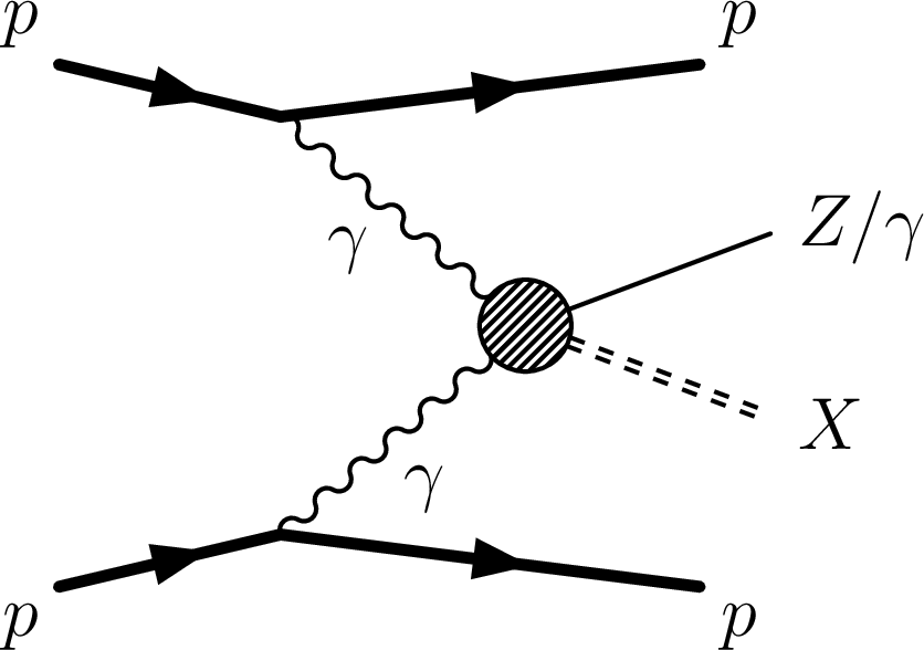
Figure 1:
Schematic diagram of the photon-photon production of a Z boson or a photon with an additional, unknown particle X, giving rise to $ m_{\mathrm{miss}} = m_{\mathrm{X}} $. The production mechanism does not have to proceed through photon exchange. Other colourless exchange mechanisms (e.g. double pomeron [11]) are also allowed. For high-mass central exclusive production, electroweak processes are expected to dominate, and QCD-based colourless exchanges are expected to be suppressed. |
png pdf |
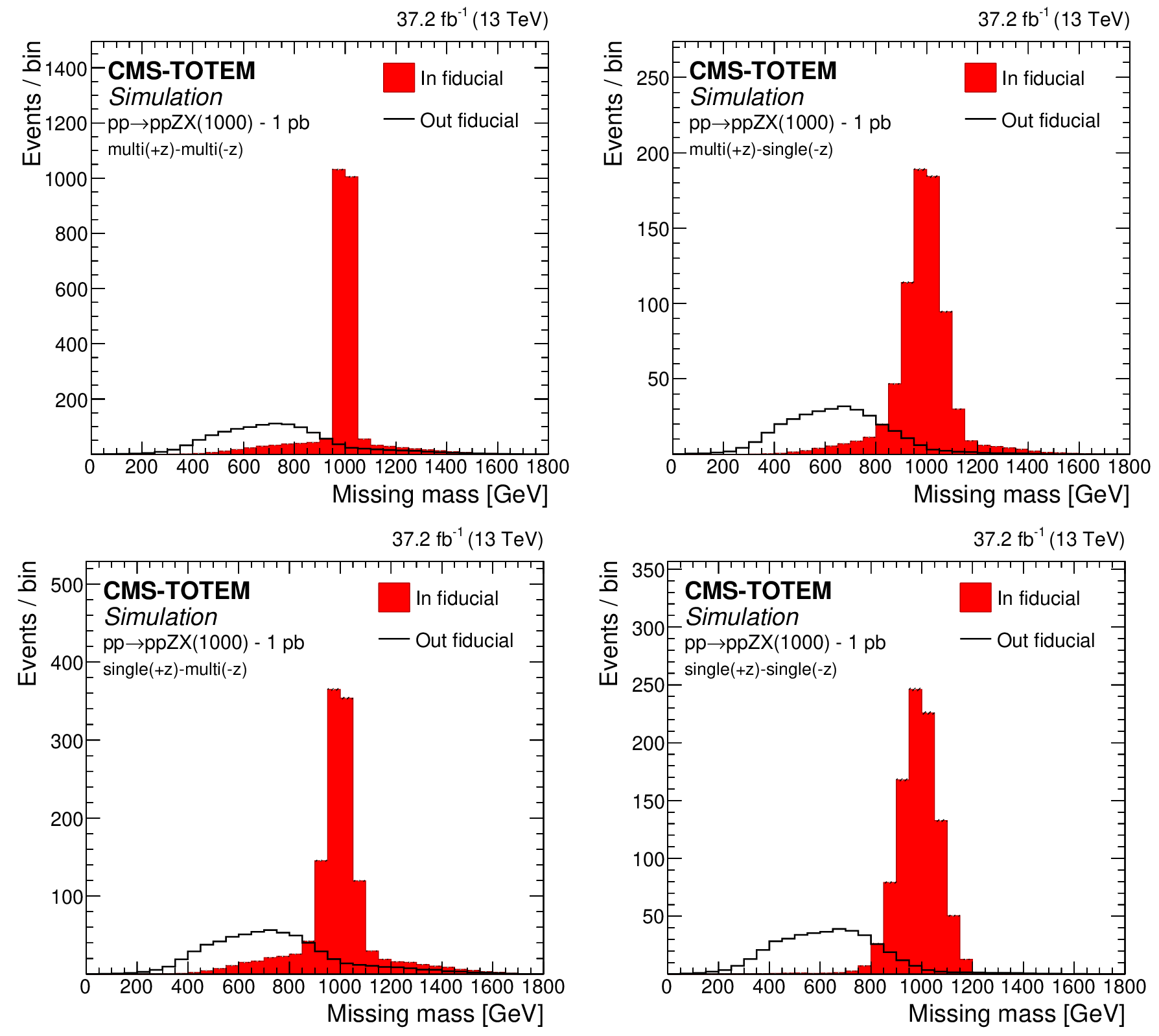
Figure 2:
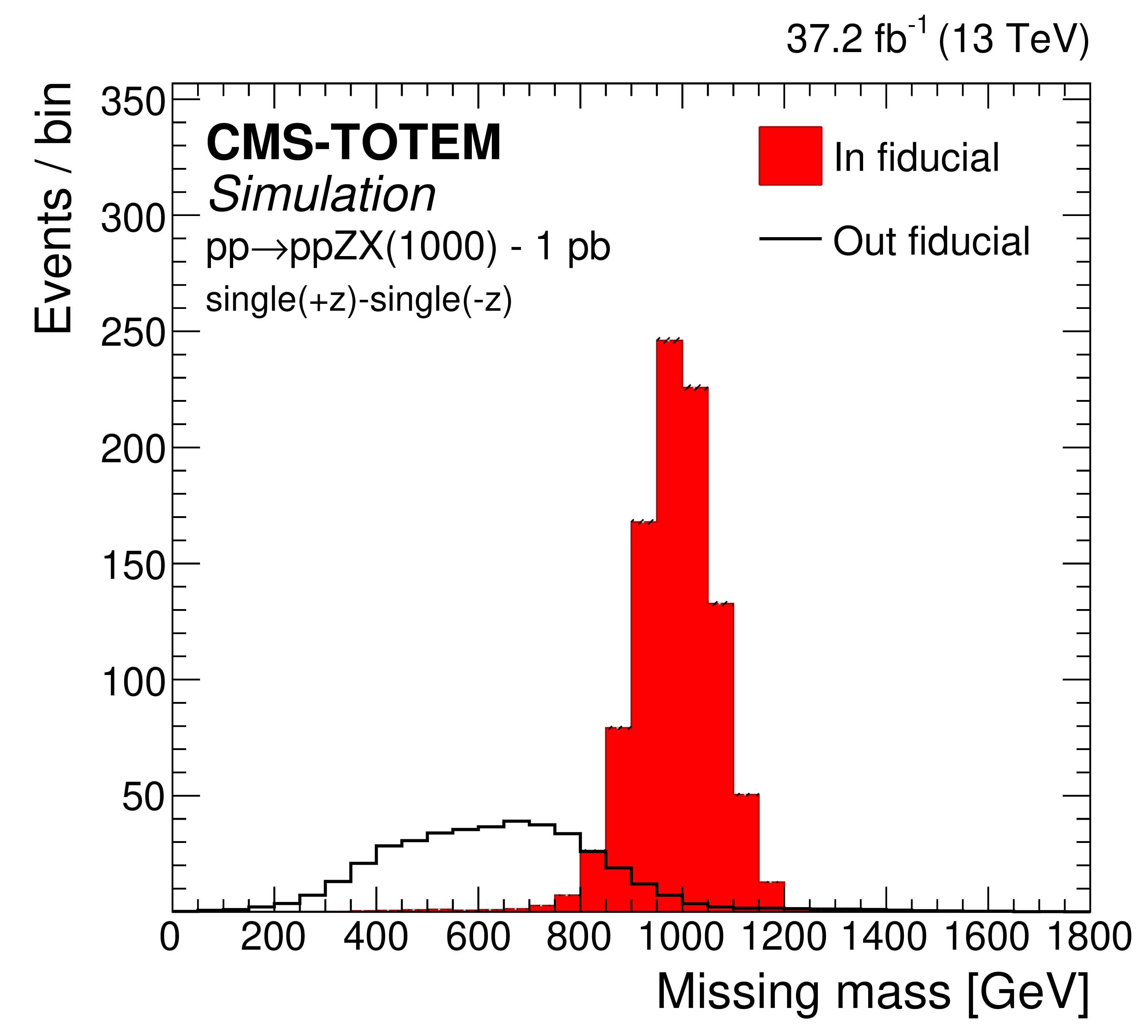
Comparison of the $ m_{\mathrm{miss}} $ shapes for the simulated $ \mathrm{p}\mathrm{p}\to \mathrm{p}\mathrm{p}\mathrm{Z}\mathrm{X} $ signal events within the fiducial region and those outside it, after including the effect of PU protons as described in the text, for a generated $ m_{\mathrm{X}} $ mass of 1000 GeV. A fiducial cross section of 1 pb is used to normalize the simulation. From left to right and top to bottom, the distributions are shown for the different proton reconstruction categories: multi($ +z $)-multi($ -z $), multi($ +z $)-single($ -z $), single($ +z $)-multi($ -z $) and single($ +z $)-single($ -z $). |
png pdf |
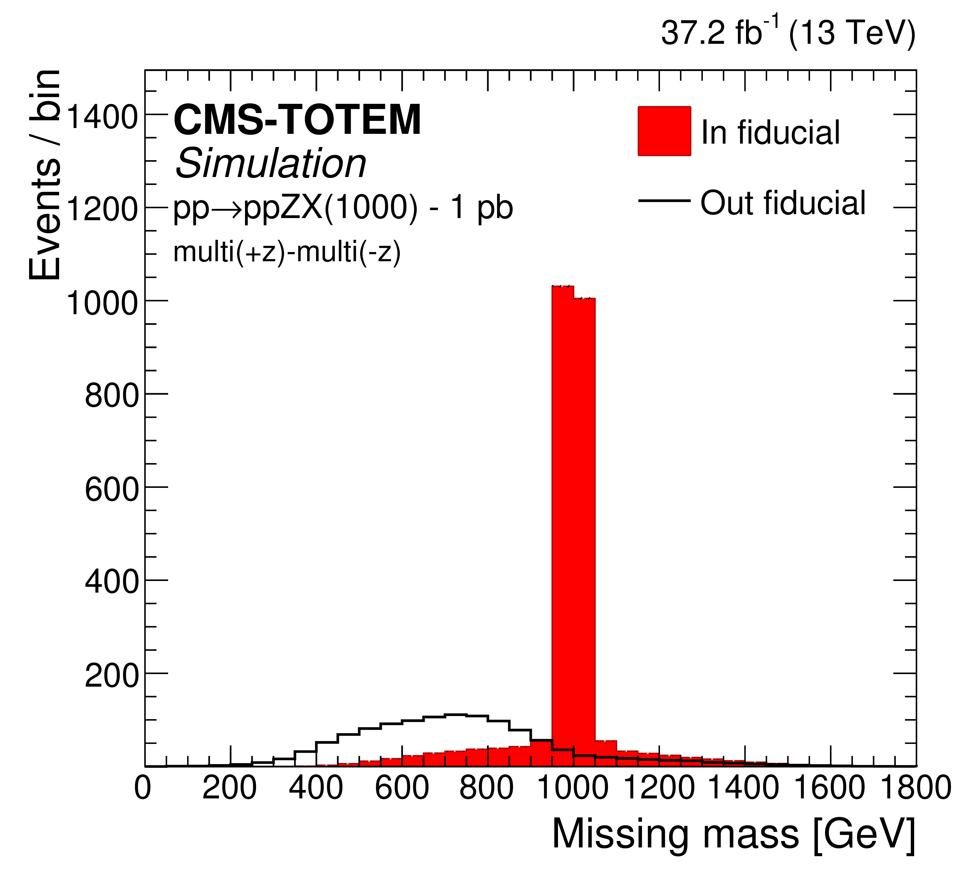
Figure 2-a:
Comparison of the $ m_{\mathrm{miss}} $ shapes for the simulated $ \mathrm{p}\mathrm{p}\to \mathrm{p}\mathrm{p}\mathrm{Z}\mathrm{X} $ signal events within the fiducial region and those outside it, after including the effect of PU protons as described in the text, for a generated $ m_{\mathrm{X}} $ mass of 1000 GeV. A fiducial cross section of 1 pb is used to normalize the simulation. From left to right and top to bottom, the distributions are shown for the different proton reconstruction categories: multi($ +z $)-multi($ -z $), multi($ +z $)-single($ -z $), single($ +z $)-multi($ -z $) and single($ +z $)-single($ -z $). |
png pdf |
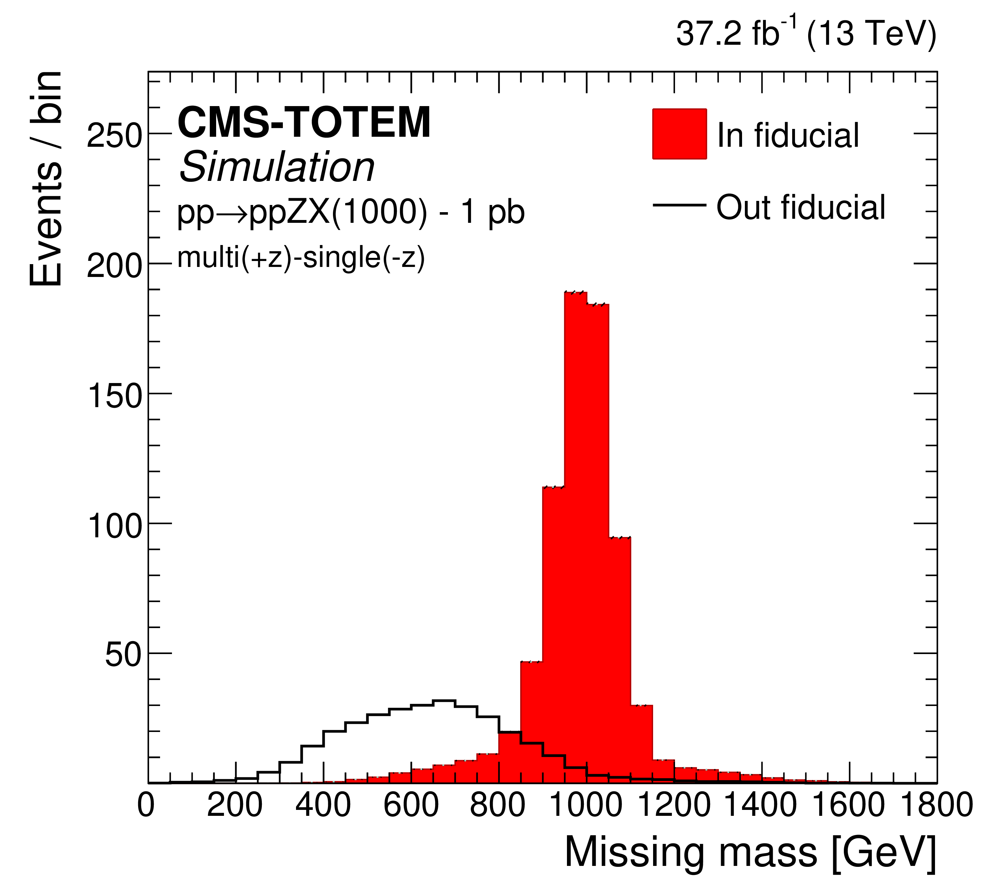
Figure 2-b:
Comparison of the $ m_{\mathrm{miss}} $ shapes for the simulated $ \mathrm{p}\mathrm{p}\to \mathrm{p}\mathrm{p}\mathrm{Z}\mathrm{X} $ signal events within the fiducial region and those outside it, after including the effect of PU protons as described in the text, for a generated $ m_{\mathrm{X}} $ mass of 1000 GeV. A fiducial cross section of 1 pb is used to normalize the simulation. From left to right and top to bottom, the distributions are shown for the different proton reconstruction categories: multi($ +z $)-multi($ -z $), multi($ +z $)-single($ -z $), single($ +z $)-multi($ -z $) and single($ +z $)-single($ -z $). |

png pdf |
Figure 2-c:
Comparison of the $ m_{\mathrm{miss}} $ shapes for the simulated $ \mathrm{p}\mathrm{p}\to \mathrm{p}\mathrm{p}\mathrm{Z}\mathrm{X} $ signal events within the fiducial region and those outside it, after including the effect of PU protons as described in the text, for a generated $ m_{\mathrm{X}} $ mass of 1000 GeV. A fiducial cross section of 1 pb is used to normalize the simulation. From left to right and top to bottom, the distributions are shown for the different proton reconstruction categories: multi($ +z $)-multi($ -z $), multi($ +z $)-single($ -z $), single($ +z $)-multi($ -z $) and single($ +z $)-single($ -z $). |
png pdf |
Figure 2-d:
Comparison of the $ m_{\mathrm{miss}} $ shapes for the simulated $ \mathrm{p}\mathrm{p}\to \mathrm{p}\mathrm{p}\mathrm{Z}\mathrm{X} $ signal events within the fiducial region and those outside it, after including the effect of PU protons as described in the text, for a generated $ m_{\mathrm{X}} $ mass of 1000 GeV. A fiducial cross section of 1 pb is used to normalize the simulation. From left to right and top to bottom, the distributions are shown for the different proton reconstruction categories: multi($ +z $)-multi($ -z $), multi($ +z $)-single($ -z $), single($ +z $)-multi($ -z $) and single($ +z $)-single($ -z $). |
png pdf |
Figure 3:
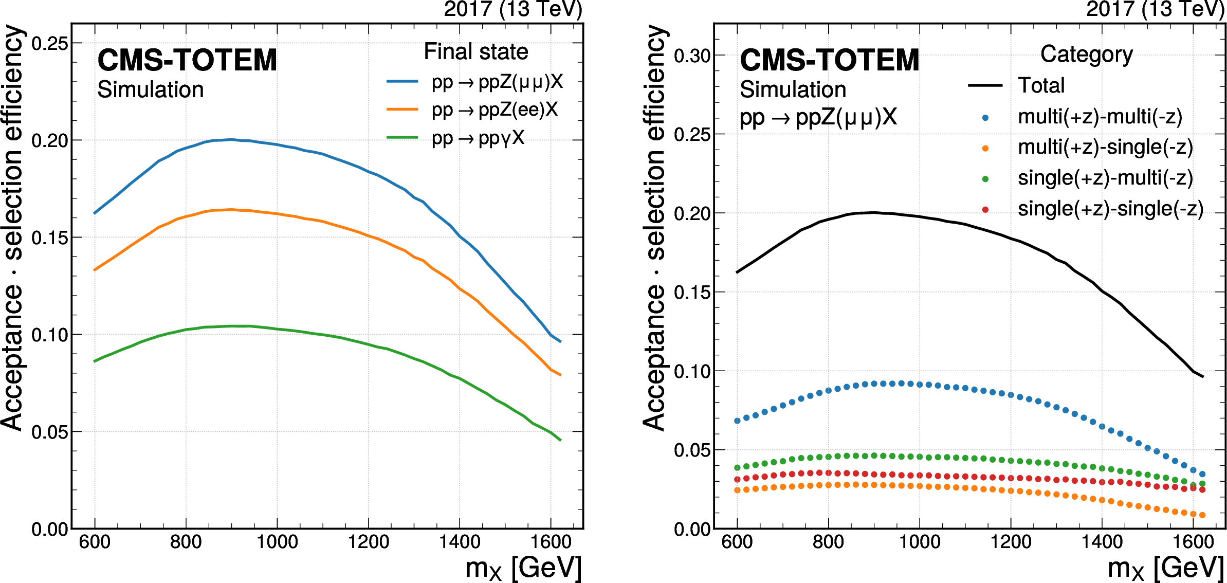
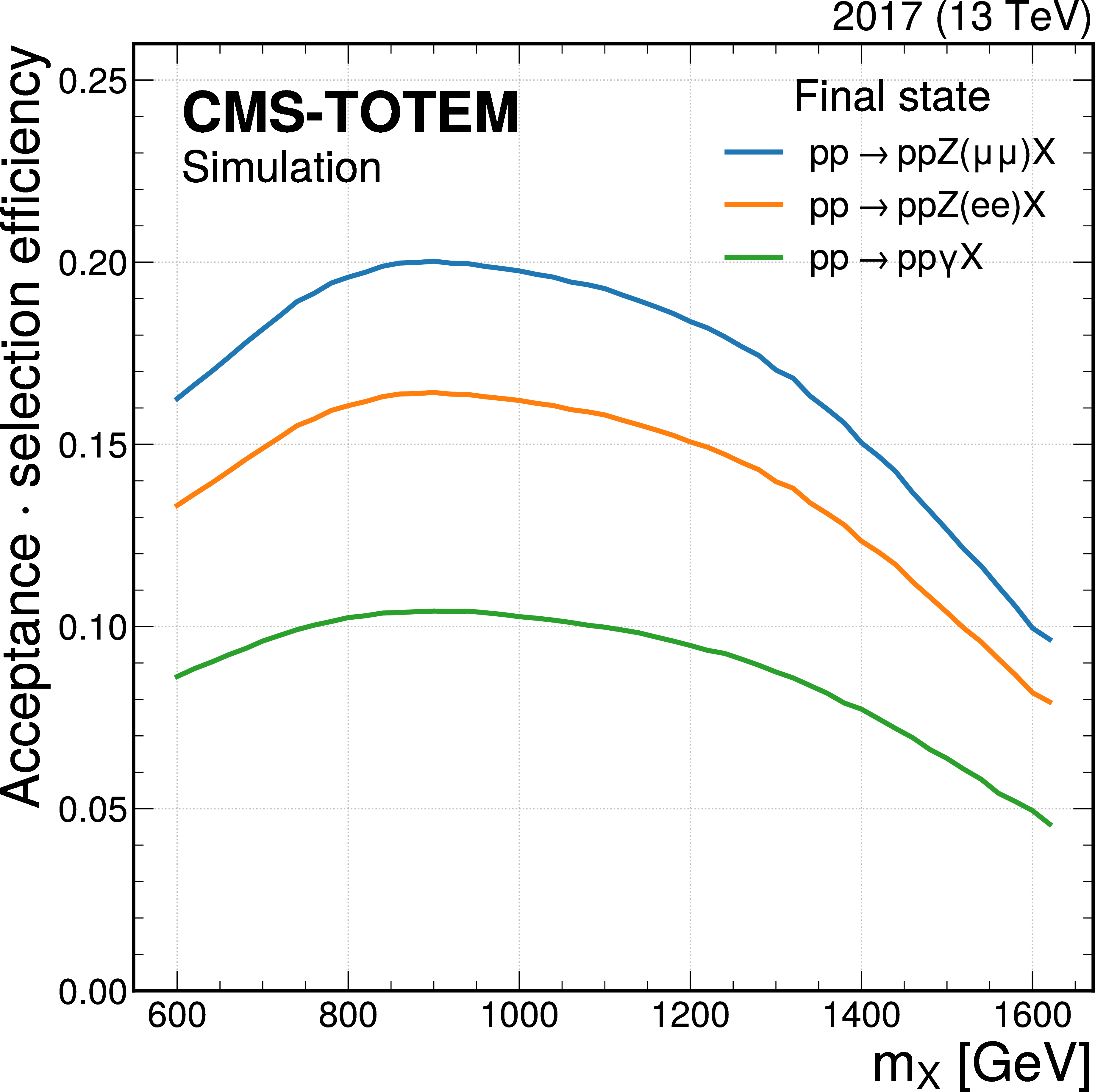
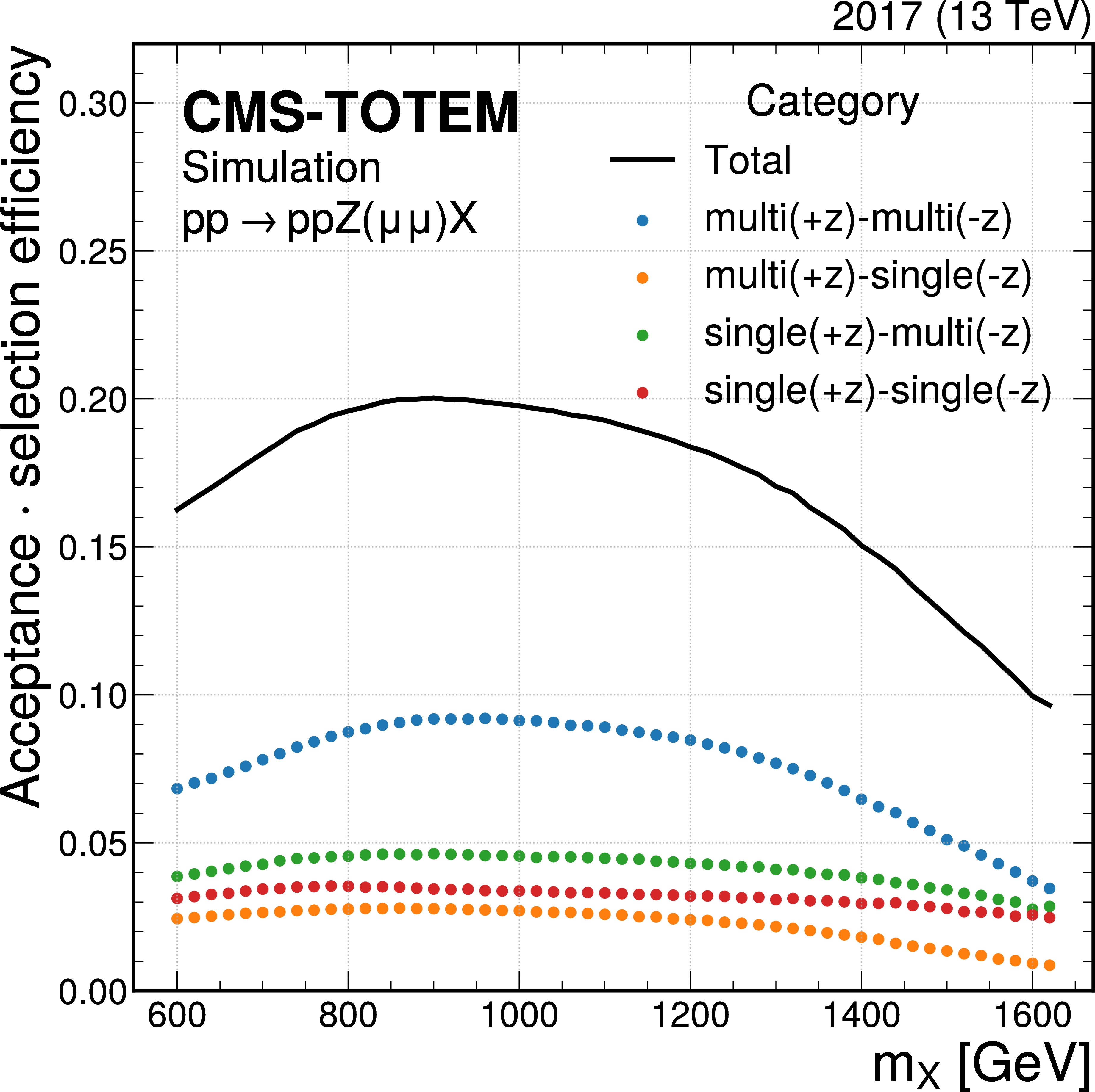
Product of the acceptance and the combined reconstruction and identification efficiency, as a function of $ m_{\mathrm{X}} $, for events generated inside the fiducial volume defined in Table 1. The curves shown in the left panel display the different final states, while the ones in the right panel show the contributions from the different proton reconstruction categories in the $ \mathrm{Z}\to\mu\mu $ analysis: multi($ +z $)-multi($ -z $), multi($ +z $)-single($ -z $), single($ +z $)-multi($ -z $) and single($ +z $)-single($ -z $). The definitions of the fiducial region and of the signal model used to estimate the acceptance are provided in the text. |
png pdf |
Figure 3-a:
Product of the acceptance and the combined reconstruction and identification efficiency, as a function of $ m_{\mathrm{X}} $, for events generated inside the fiducial volume defined in Table 1. The curves shown in the left panel display the different final states, while the ones in the right panel show the contributions from the different proton reconstruction categories in the $ \mathrm{Z}\to\mu\mu $ analysis: multi($ +z $)-multi($ -z $), multi($ +z $)-single($ -z $), single($ +z $)-multi($ -z $) and single($ +z $)-single($ -z $). The definitions of the fiducial region and of the signal model used to estimate the acceptance are provided in the text. |
png pdf |
Figure 3-b:
Product of the acceptance and the combined reconstruction and identification efficiency, as a function of $ m_{\mathrm{X}} $, for events generated inside the fiducial volume defined in Table 1. The curves shown in the left panel display the different final states, while the ones in the right panel show the contributions from the different proton reconstruction categories in the $ \mathrm{Z}\to\mu\mu $ analysis: multi($ +z $)-multi($ -z $), multi($ +z $)-single($ -z $), single($ +z $)-multi($ -z $) and single($ +z $)-single($ -z $). The definitions of the fiducial region and of the signal model used to estimate the acceptance are provided in the text. |
png pdf |
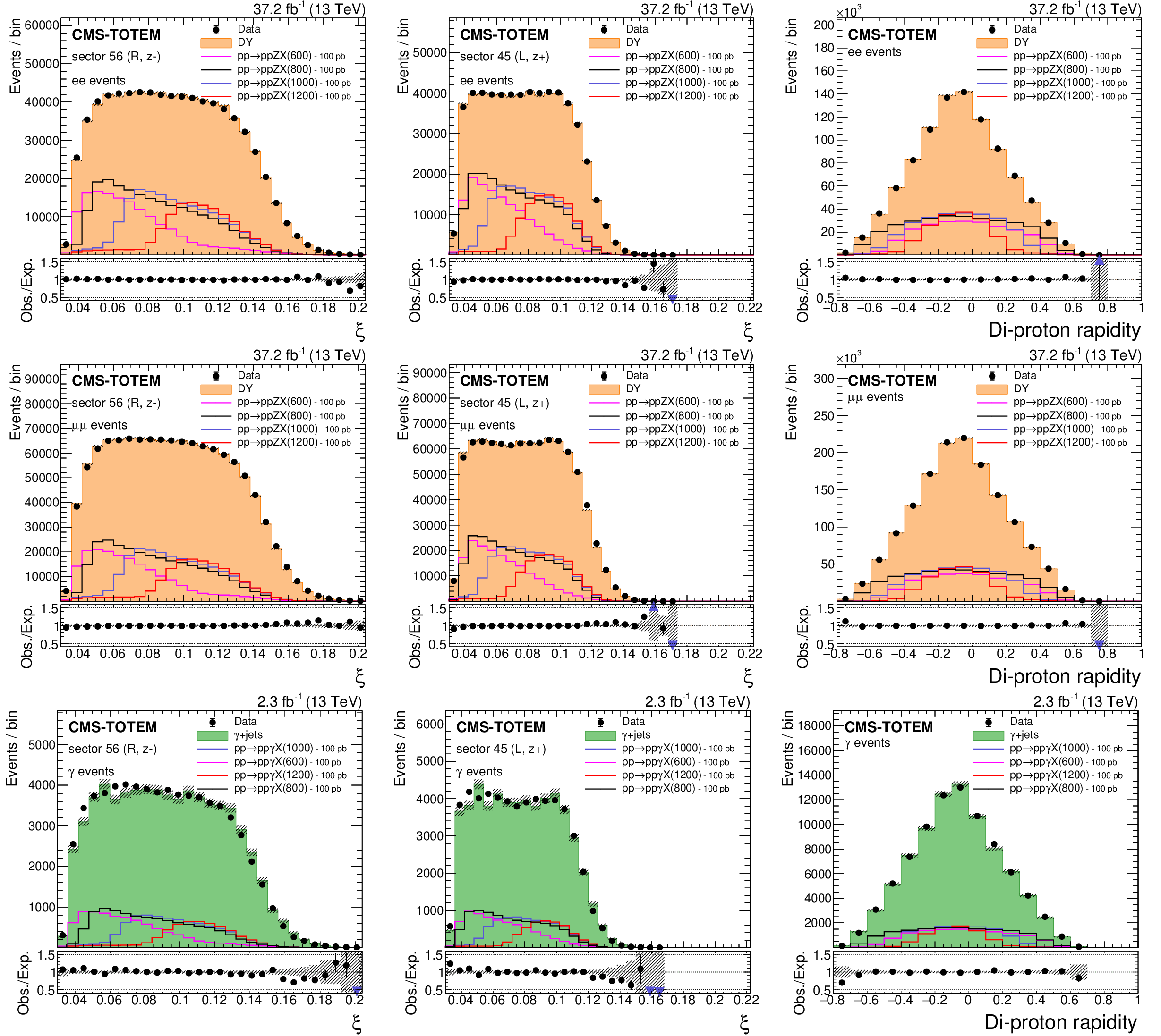
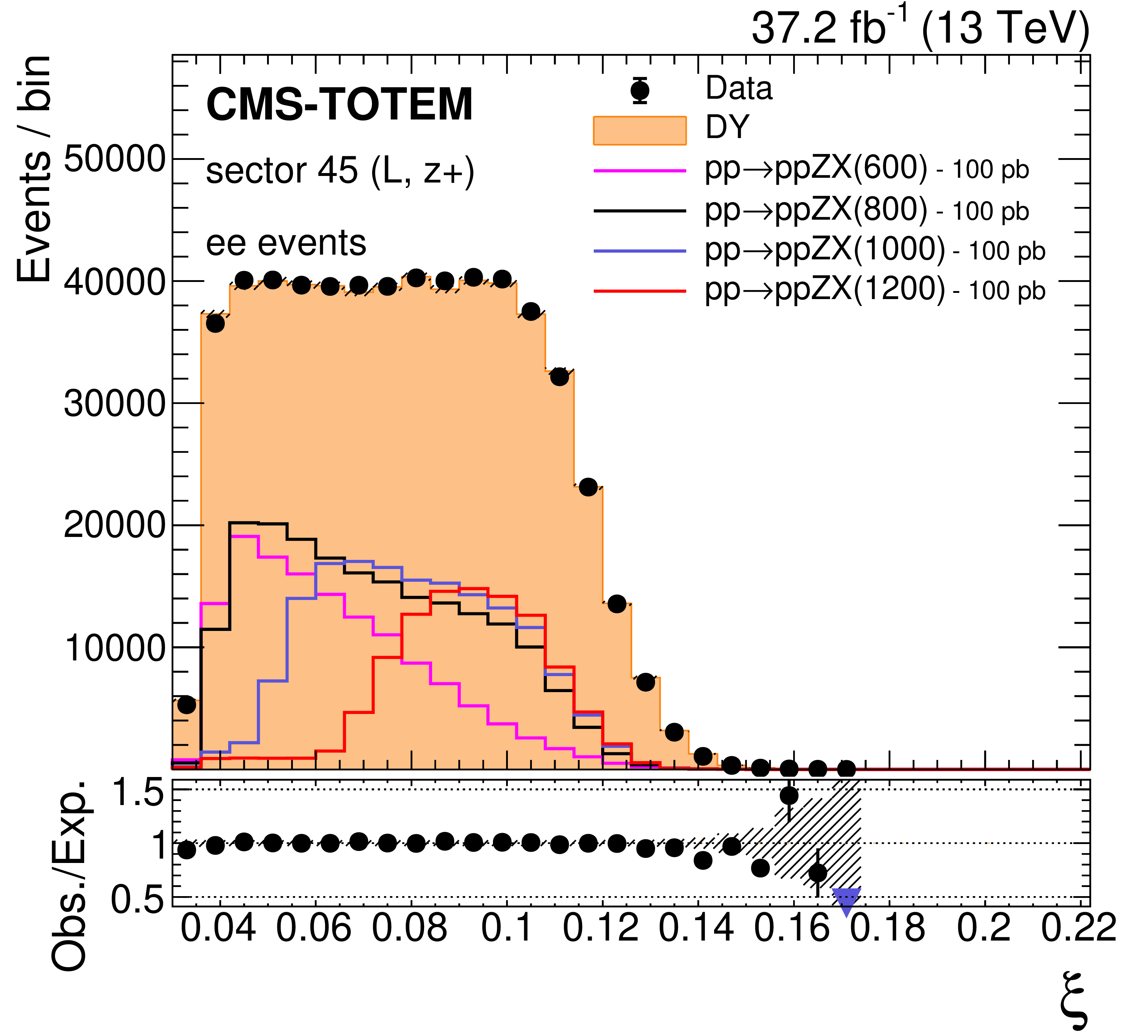
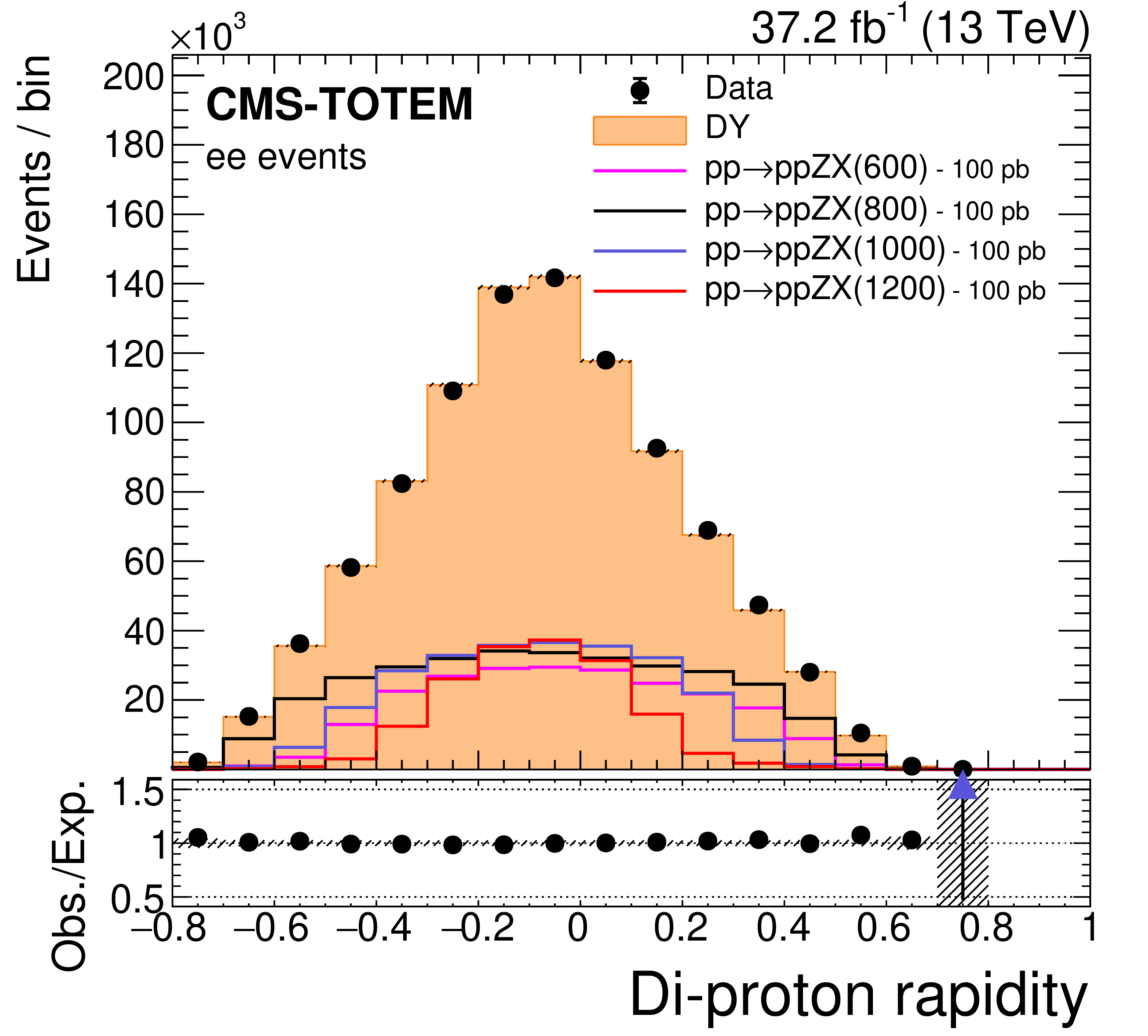
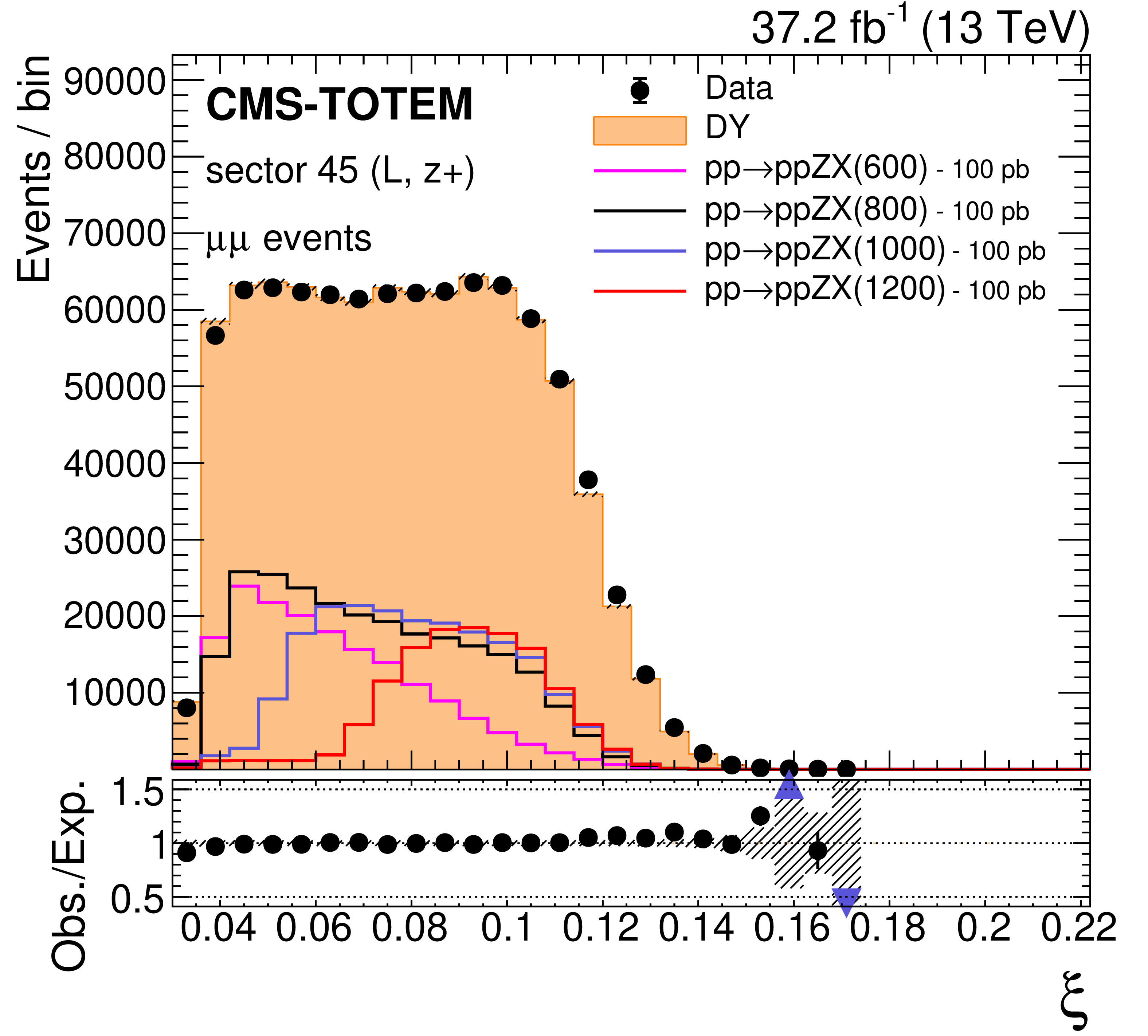
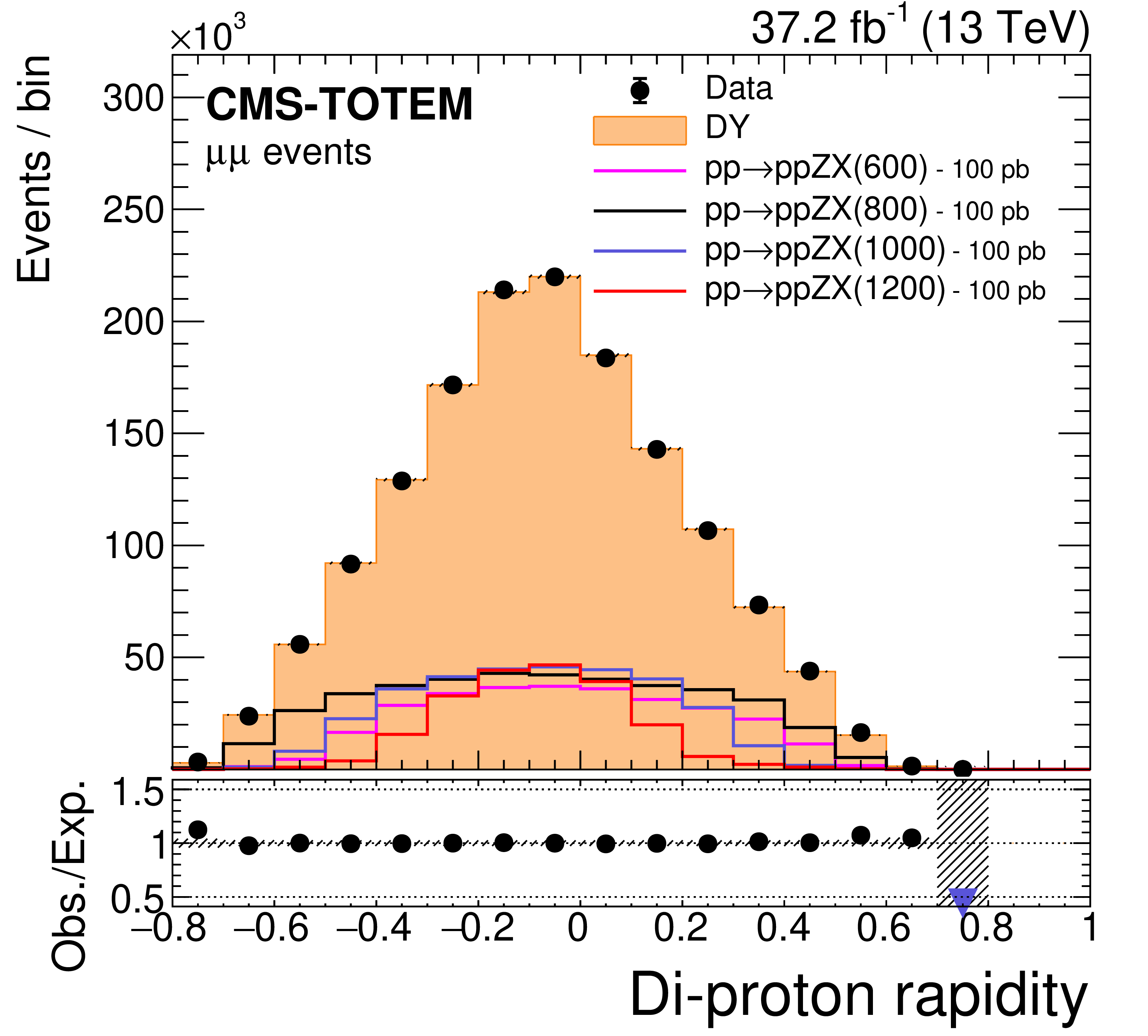
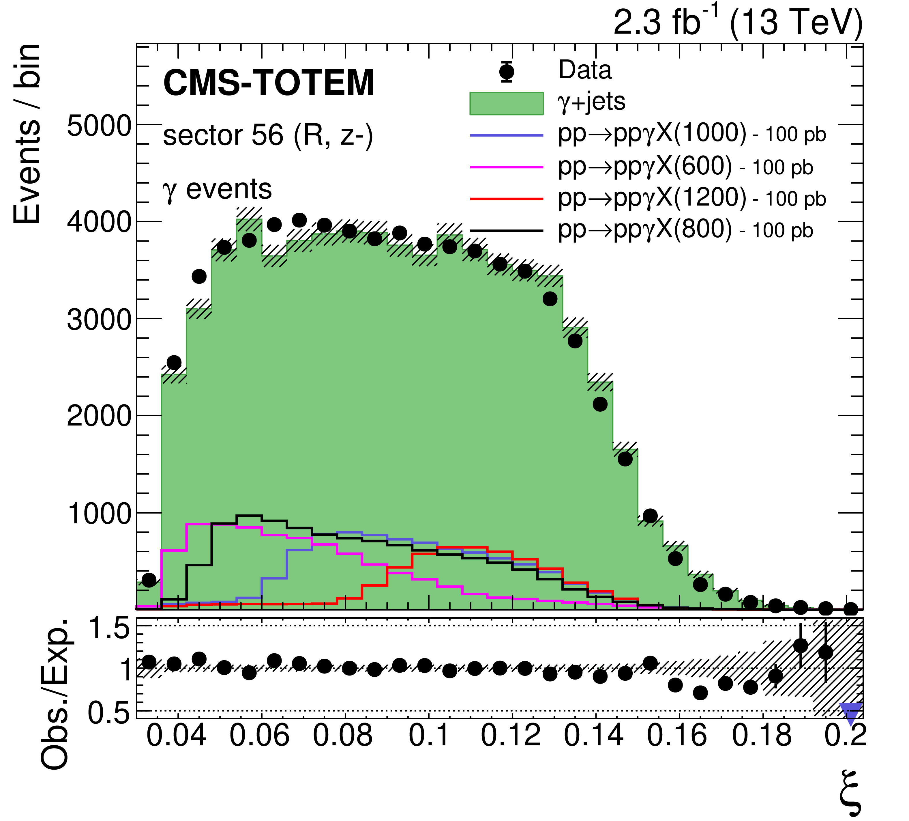
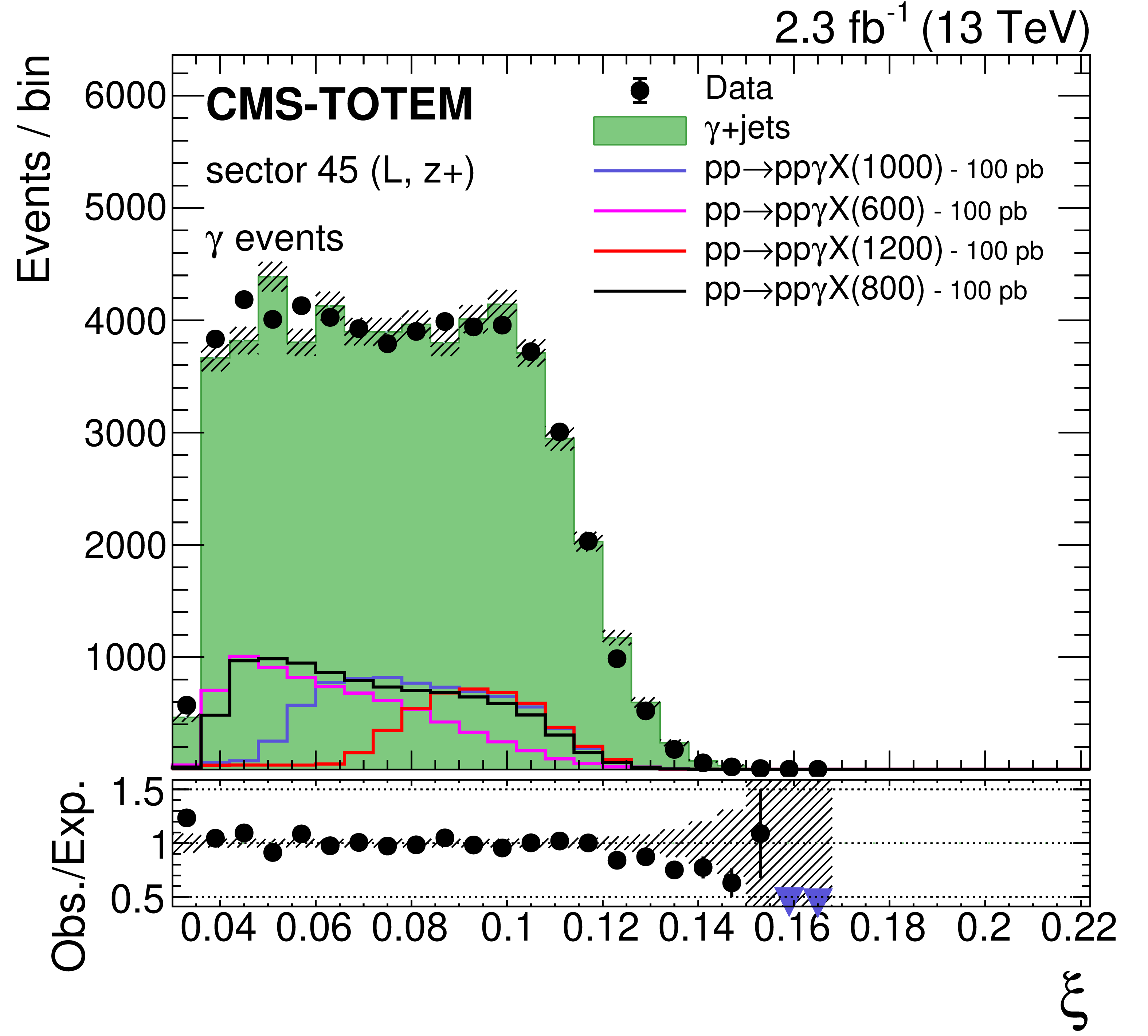
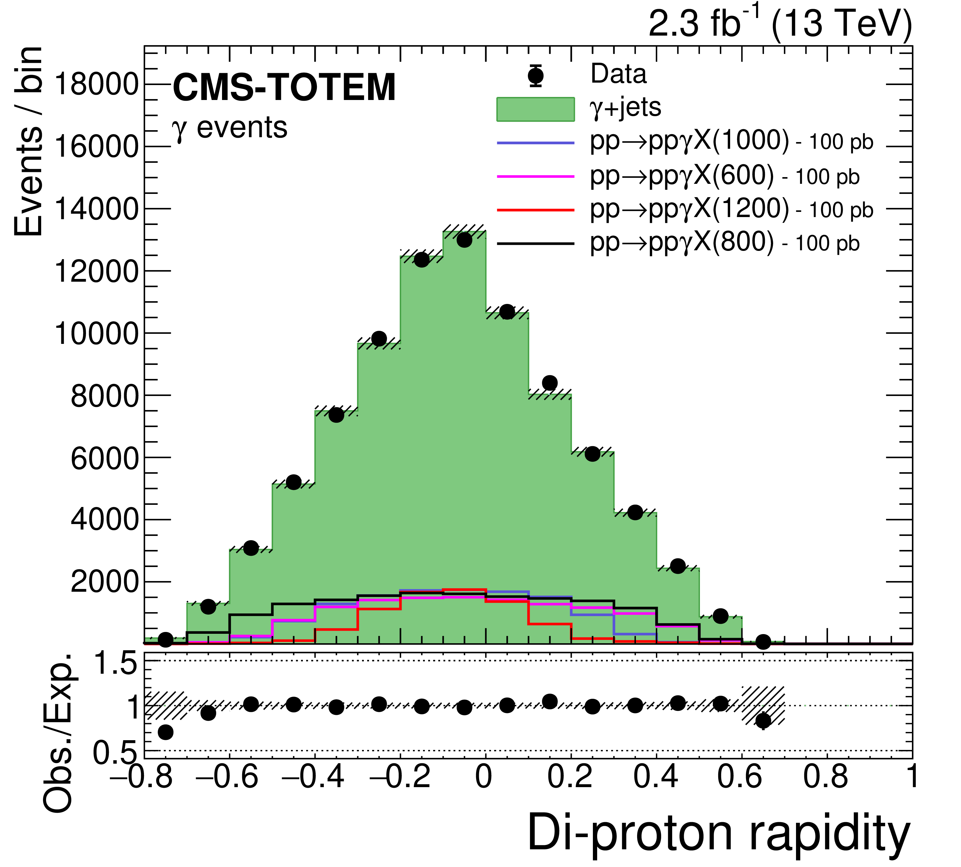
Figure 4:
Distributions of the reconstructed proton $ \xi $ in the negative arm (left), positive arm (middle), and the corresponding di-proton rapidity (right) from the proton mixing procedure with simulated MC events are compared to data, in the upper panels in each plot. Processes other than the ones displayed in the figures are estimated to have negligible residual contributions. The lower panels display the ratio between the data and the background model, with the arrows indicating values lying outside the displayed range. The hatched band illustrates the statistical uncertainty of the background model. The $ \mathrm{e}\mathrm{e} $, $ \mu\mu $, and photon final states are shown from top to bottom. The $ \mathrm{e}\mathrm{e} $ and $ \mu\mu $ events are displayed without the Z boson $ p_{\mathrm{T}} $ requirement. For illustration, the simulated signal distributions are superimposed for various choices of $ m_{\mathrm{X}} $, normalised to a generated fiducial cross section of 100 pb. |

png pdf |
Figure 4-a:
Distributions of the reconstructed proton $ \xi $ in the negative arm (left), positive arm (middle), and the corresponding di-proton rapidity (right) from the proton mixing procedure with simulated MC events are compared to data, in the upper panels in each plot. Processes other than the ones displayed in the figures are estimated to have negligible residual contributions. The lower panels display the ratio between the data and the background model, with the arrows indicating values lying outside the displayed range. The hatched band illustrates the statistical uncertainty of the background model. The $ \mathrm{e}\mathrm{e} $, $ \mu\mu $, and photon final states are shown from top to bottom. The $ \mathrm{e}\mathrm{e} $ and $ \mu\mu $ events are displayed without the Z boson $ p_{\mathrm{T}} $ requirement. For illustration, the simulated signal distributions are superimposed for various choices of $ m_{\mathrm{X}} $, normalised to a generated fiducial cross section of 100 pb. |
png pdf |
Figure 4-b:
Distributions of the reconstructed proton $ \xi $ in the negative arm (left), positive arm (middle), and the corresponding di-proton rapidity (right) from the proton mixing procedure with simulated MC events are compared to data, in the upper panels in each plot. Processes other than the ones displayed in the figures are estimated to have negligible residual contributions. The lower panels display the ratio between the data and the background model, with the arrows indicating values lying outside the displayed range. The hatched band illustrates the statistical uncertainty of the background model. The $ \mathrm{e}\mathrm{e} $, $ \mu\mu $, and photon final states are shown from top to bottom. The $ \mathrm{e}\mathrm{e} $ and $ \mu\mu $ events are displayed without the Z boson $ p_{\mathrm{T}} $ requirement. For illustration, the simulated signal distributions are superimposed for various choices of $ m_{\mathrm{X}} $, normalised to a generated fiducial cross section of 100 pb. |
png pdf |
Figure 4-c:
Distributions of the reconstructed proton $ \xi $ in the negative arm (left), positive arm (middle), and the corresponding di-proton rapidity (right) from the proton mixing procedure with simulated MC events are compared to data, in the upper panels in each plot. Processes other than the ones displayed in the figures are estimated to have negligible residual contributions. The lower panels display the ratio between the data and the background model, with the arrows indicating values lying outside the displayed range. The hatched band illustrates the statistical uncertainty of the background model. The $ \mathrm{e}\mathrm{e} $, $ \mu\mu $, and photon final states are shown from top to bottom. The $ \mathrm{e}\mathrm{e} $ and $ \mu\mu $ events are displayed without the Z boson $ p_{\mathrm{T}} $ requirement. For illustration, the simulated signal distributions are superimposed for various choices of $ m_{\mathrm{X}} $, normalised to a generated fiducial cross section of 100 pb. |

png pdf |
Figure 4-d:
Distributions of the reconstructed proton $ \xi $ in the negative arm (left), positive arm (middle), and the corresponding di-proton rapidity (right) from the proton mixing procedure with simulated MC events are compared to data, in the upper panels in each plot. Processes other than the ones displayed in the figures are estimated to have negligible residual contributions. The lower panels display the ratio between the data and the background model, with the arrows indicating values lying outside the displayed range. The hatched band illustrates the statistical uncertainty of the background model. The $ \mathrm{e}\mathrm{e} $, $ \mu\mu $, and photon final states are shown from top to bottom. The $ \mathrm{e}\mathrm{e} $ and $ \mu\mu $ events are displayed without the Z boson $ p_{\mathrm{T}} $ requirement. For illustration, the simulated signal distributions are superimposed for various choices of $ m_{\mathrm{X}} $, normalised to a generated fiducial cross section of 100 pb. |
png pdf |
Figure 4-e:
Distributions of the reconstructed proton $ \xi $ in the negative arm (left), positive arm (middle), and the corresponding di-proton rapidity (right) from the proton mixing procedure with simulated MC events are compared to data, in the upper panels in each plot. Processes other than the ones displayed in the figures are estimated to have negligible residual contributions. The lower panels display the ratio between the data and the background model, with the arrows indicating values lying outside the displayed range. The hatched band illustrates the statistical uncertainty of the background model. The $ \mathrm{e}\mathrm{e} $, $ \mu\mu $, and photon final states are shown from top to bottom. The $ \mathrm{e}\mathrm{e} $ and $ \mu\mu $ events are displayed without the Z boson $ p_{\mathrm{T}} $ requirement. For illustration, the simulated signal distributions are superimposed for various choices of $ m_{\mathrm{X}} $, normalised to a generated fiducial cross section of 100 pb. |
png pdf |
Figure 4-f:
Distributions of the reconstructed proton $ \xi $ in the negative arm (left), positive arm (middle), and the corresponding di-proton rapidity (right) from the proton mixing procedure with simulated MC events are compared to data, in the upper panels in each plot. Processes other than the ones displayed in the figures are estimated to have negligible residual contributions. The lower panels display the ratio between the data and the background model, with the arrows indicating values lying outside the displayed range. The hatched band illustrates the statistical uncertainty of the background model. The $ \mathrm{e}\mathrm{e} $, $ \mu\mu $, and photon final states are shown from top to bottom. The $ \mathrm{e}\mathrm{e} $ and $ \mu\mu $ events are displayed without the Z boson $ p_{\mathrm{T}} $ requirement. For illustration, the simulated signal distributions are superimposed for various choices of $ m_{\mathrm{X}} $, normalised to a generated fiducial cross section of 100 pb. |
png pdf |
Figure 4-g:
Distributions of the reconstructed proton $ \xi $ in the negative arm (left), positive arm (middle), and the corresponding di-proton rapidity (right) from the proton mixing procedure with simulated MC events are compared to data, in the upper panels in each plot. Processes other than the ones displayed in the figures are estimated to have negligible residual contributions. The lower panels display the ratio between the data and the background model, with the arrows indicating values lying outside the displayed range. The hatched band illustrates the statistical uncertainty of the background model. The $ \mathrm{e}\mathrm{e} $, $ \mu\mu $, and photon final states are shown from top to bottom. The $ \mathrm{e}\mathrm{e} $ and $ \mu\mu $ events are displayed without the Z boson $ p_{\mathrm{T}} $ requirement. For illustration, the simulated signal distributions are superimposed for various choices of $ m_{\mathrm{X}} $, normalised to a generated fiducial cross section of 100 pb. |
png pdf |
Figure 4-h:
Distributions of the reconstructed proton $ \xi $ in the negative arm (left), positive arm (middle), and the corresponding di-proton rapidity (right) from the proton mixing procedure with simulated MC events are compared to data, in the upper panels in each plot. Processes other than the ones displayed in the figures are estimated to have negligible residual contributions. The lower panels display the ratio between the data and the background model, with the arrows indicating values lying outside the displayed range. The hatched band illustrates the statistical uncertainty of the background model. The $ \mathrm{e}\mathrm{e} $, $ \mu\mu $, and photon final states are shown from top to bottom. The $ \mathrm{e}\mathrm{e} $ and $ \mu\mu $ events are displayed without the Z boson $ p_{\mathrm{T}} $ requirement. For illustration, the simulated signal distributions are superimposed for various choices of $ m_{\mathrm{X}} $, normalised to a generated fiducial cross section of 100 pb. |
png pdf |
Figure 4-i:
Distributions of the reconstructed proton $ \xi $ in the negative arm (left), positive arm (middle), and the corresponding di-proton rapidity (right) from the proton mixing procedure with simulated MC events are compared to data, in the upper panels in each plot. Processes other than the ones displayed in the figures are estimated to have negligible residual contributions. The lower panels display the ratio between the data and the background model, with the arrows indicating values lying outside the displayed range. The hatched band illustrates the statistical uncertainty of the background model. The $ \mathrm{e}\mathrm{e} $, $ \mu\mu $, and photon final states are shown from top to bottom. The $ \mathrm{e}\mathrm{e} $ and $ \mu\mu $ events are displayed without the Z boson $ p_{\mathrm{T}} $ requirement. For illustration, the simulated signal distributions are superimposed for various choices of $ m_{\mathrm{X}} $, normalised to a generated fiducial cross section of 100 pb. |
png pdf |
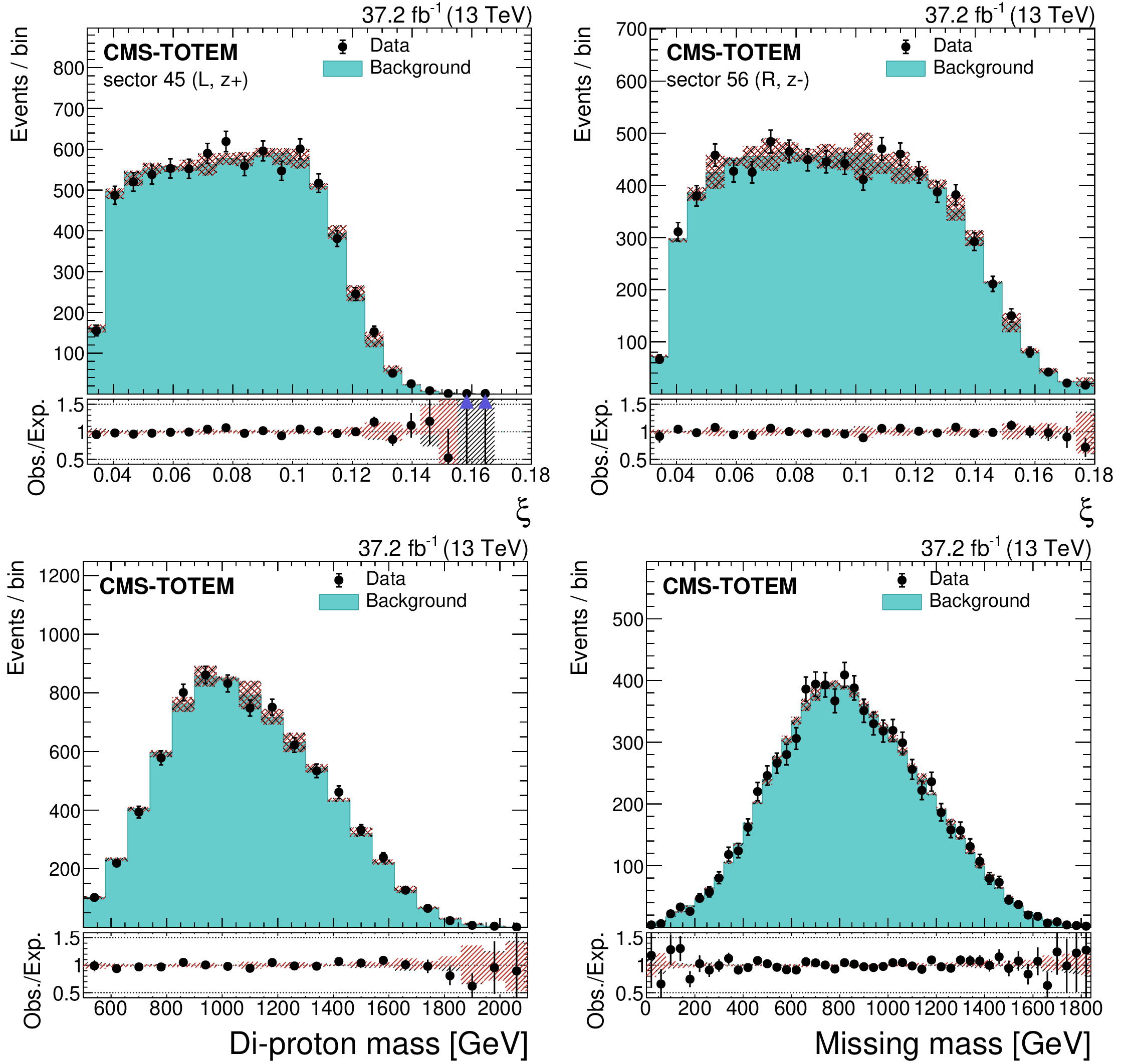
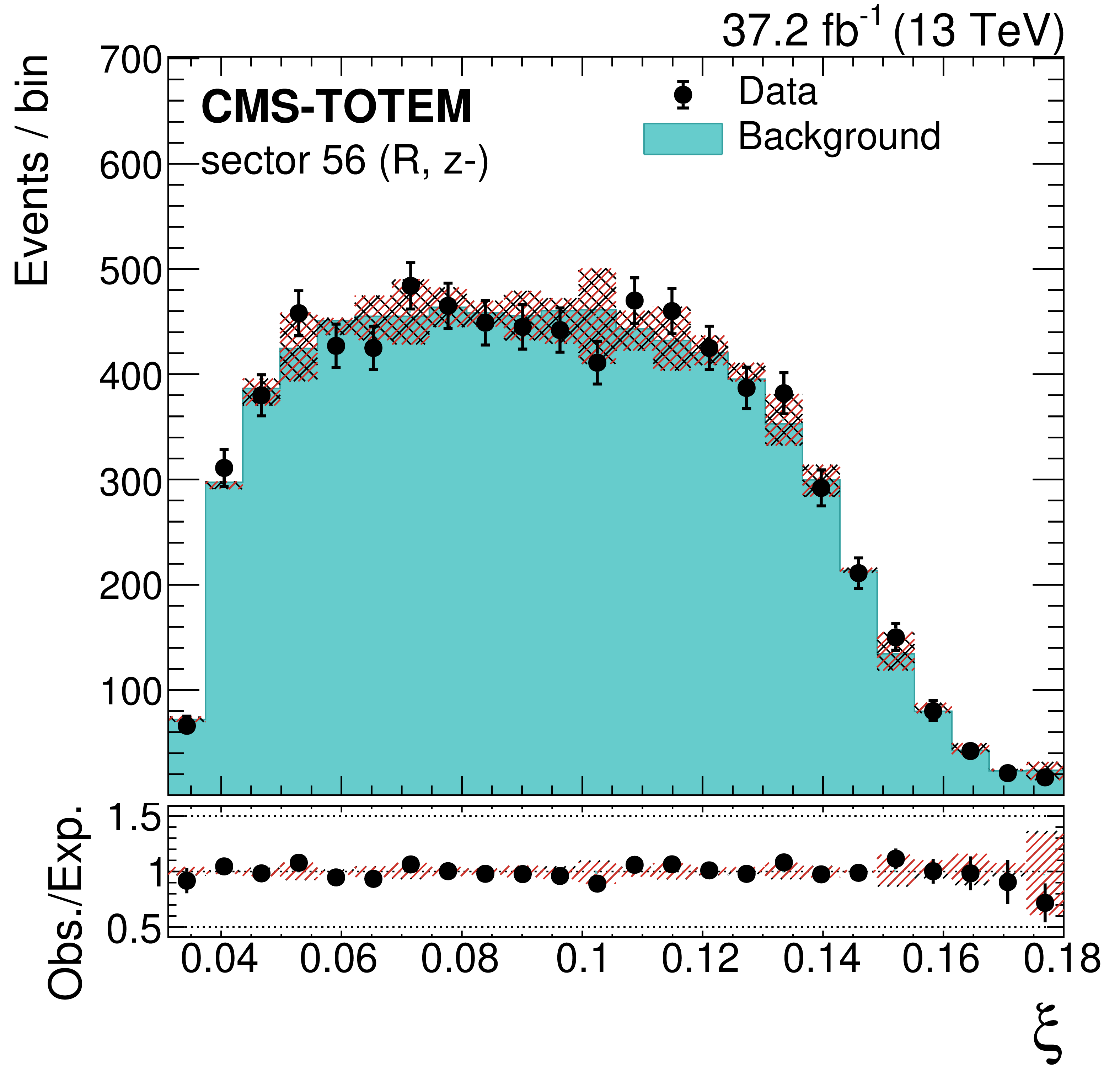
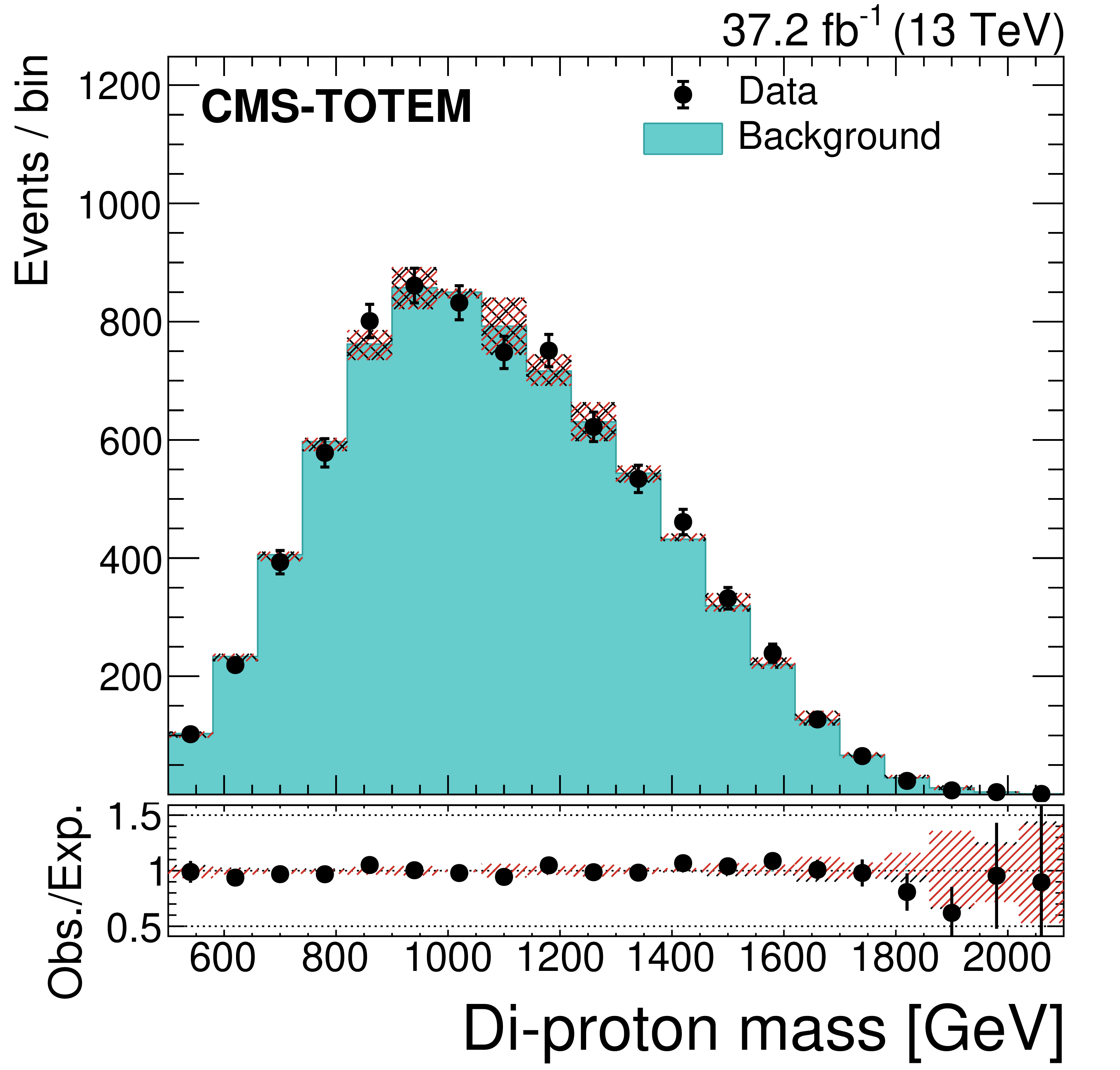
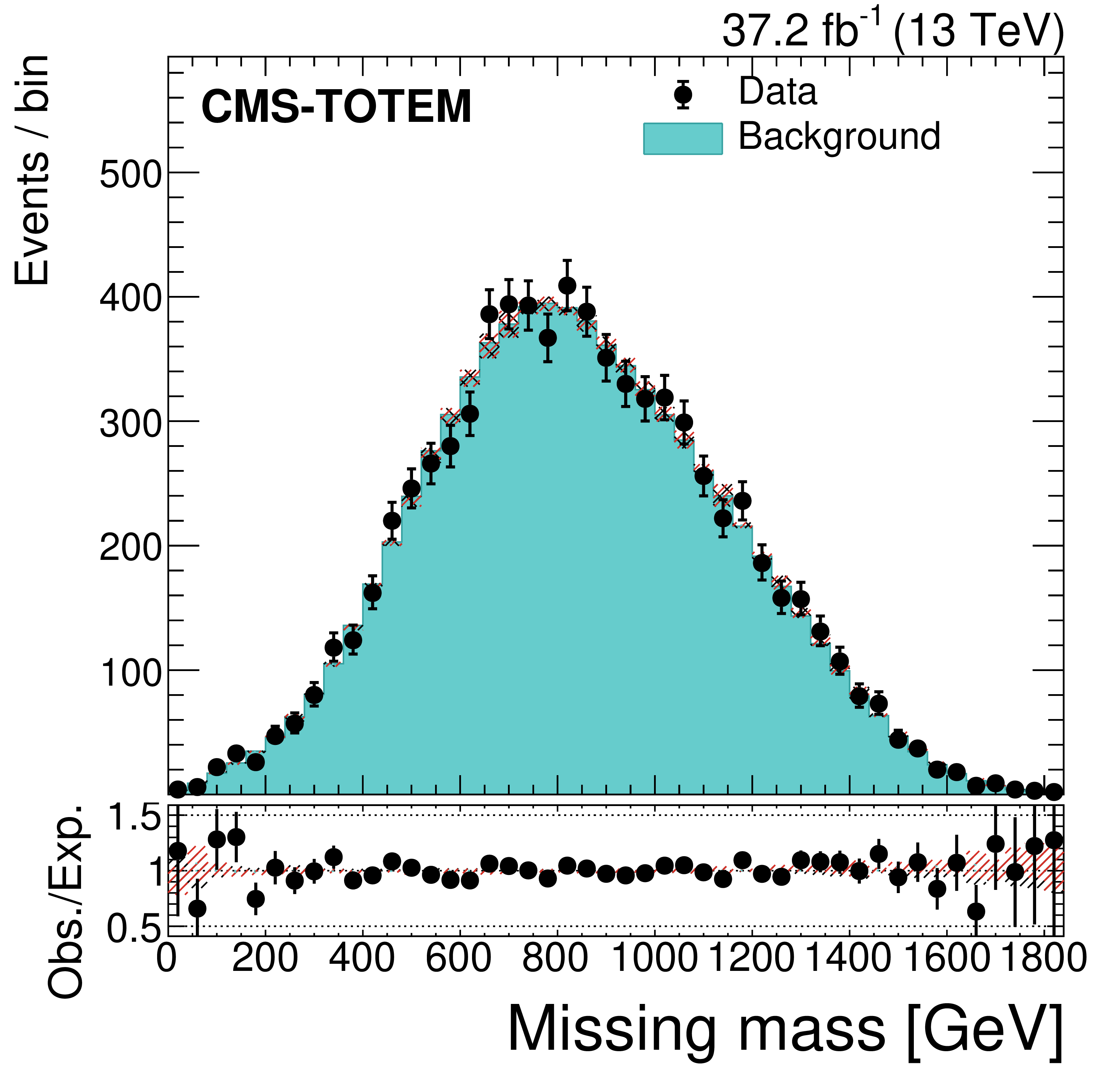
Figure 5:
Validation of the background modelling method, using the $ \mathrm{e}\mu $ control sample. Selected $ \mathrm{e}\mu $ events are mixed with protons from $ \mathrm{Z}\to\mu\mu $ events with $ p_{\mathrm{T}}(\mathrm{Z}) < $ 10 GeV to simulate the combinatorial background shape, while the data points are unaltered $ \mathrm{e}\mu $ events. The proton $ \xi $ distributions for both CT-PPS arms (upper row), those of the di-proton invariant mass (lower left), and of $ m_{\mathrm{miss}} $ (lower right) are shown. The lower panel in each plot displays the ratio between the data and the background model, with the arrows indicating values lying outside the displayed range. The gray uncertainty band around the background prediction represents the contribution from the limited sample size. The red uncertainty band represents the effect of adding in quadrature the differences with the alternative mixing approaches described in the text. |

png pdf |
Figure 5-a:
Validation of the background modelling method, using the $ \mathrm{e}\mu $ control sample. Selected $ \mathrm{e}\mu $ events are mixed with protons from $ \mathrm{Z}\to\mu\mu $ events with $ p_{\mathrm{T}}(\mathrm{Z}) < $ 10 GeV to simulate the combinatorial background shape, while the data points are unaltered $ \mathrm{e}\mu $ events. The proton $ \xi $ distributions for both CT-PPS arms (upper row), those of the di-proton invariant mass (lower left), and of $ m_{\mathrm{miss}} $ (lower right) are shown. The lower panel in each plot displays the ratio between the data and the background model, with the arrows indicating values lying outside the displayed range. The gray uncertainty band around the background prediction represents the contribution from the limited sample size. The red uncertainty band represents the effect of adding in quadrature the differences with the alternative mixing approaches described in the text. |
png pdf |
Figure 5-b:
Validation of the background modelling method, using the $ \mathrm{e}\mu $ control sample. Selected $ \mathrm{e}\mu $ events are mixed with protons from $ \mathrm{Z}\to\mu\mu $ events with $ p_{\mathrm{T}}(\mathrm{Z}) < $ 10 GeV to simulate the combinatorial background shape, while the data points are unaltered $ \mathrm{e}\mu $ events. The proton $ \xi $ distributions for both CT-PPS arms (upper row), those of the di-proton invariant mass (lower left), and of $ m_{\mathrm{miss}} $ (lower right) are shown. The lower panel in each plot displays the ratio between the data and the background model, with the arrows indicating values lying outside the displayed range. The gray uncertainty band around the background prediction represents the contribution from the limited sample size. The red uncertainty band represents the effect of adding in quadrature the differences with the alternative mixing approaches described in the text. |
png pdf |
Figure 5-c:
Validation of the background modelling method, using the $ \mathrm{e}\mu $ control sample. Selected $ \mathrm{e}\mu $ events are mixed with protons from $ \mathrm{Z}\to\mu\mu $ events with $ p_{\mathrm{T}}(\mathrm{Z}) < $ 10 GeV to simulate the combinatorial background shape, while the data points are unaltered $ \mathrm{e}\mu $ events. The proton $ \xi $ distributions for both CT-PPS arms (upper row), those of the di-proton invariant mass (lower left), and of $ m_{\mathrm{miss}} $ (lower right) are shown. The lower panel in each plot displays the ratio between the data and the background model, with the arrows indicating values lying outside the displayed range. The gray uncertainty band around the background prediction represents the contribution from the limited sample size. The red uncertainty band represents the effect of adding in quadrature the differences with the alternative mixing approaches described in the text. |
png pdf |
Figure 5-d:
Validation of the background modelling method, using the $ \mathrm{e}\mu $ control sample. Selected $ \mathrm{e}\mu $ events are mixed with protons from $ \mathrm{Z}\to\mu\mu $ events with $ p_{\mathrm{T}}(\mathrm{Z}) < $ 10 GeV to simulate the combinatorial background shape, while the data points are unaltered $ \mathrm{e}\mu $ events. The proton $ \xi $ distributions for both CT-PPS arms (upper row), those of the di-proton invariant mass (lower left), and of $ m_{\mathrm{miss}} $ (lower right) are shown. The lower panel in each plot displays the ratio between the data and the background model, with the arrows indicating values lying outside the displayed range. The gray uncertainty band around the background prediction represents the contribution from the limited sample size. The red uncertainty band represents the effect of adding in quadrature the differences with the alternative mixing approaches described in the text. |

png pdf |
Figure 6:
$ m_{\mathrm{miss}} $ distributions in the $ \mathrm{Z}\to \mathrm{e}\mathrm{e} $ final state. The distributions are shown for protons reconstructed with (from left to right) the multi-multi, multi-single, single-multi and single-single methods, respectively. The background distributions are shown after the fit. The lower panels display the ratio between the data and the background model, with the arrows indicating values lying outside the displayed range. The expectations for a signal with $ m_{\mathrm{X}} = $ 1000 GeV are superimposed and normalised to 1 pb. |
png pdf |
Figure 7:
$ m_{\mathrm{miss}} $ distributions in the $ \mathrm{Z}\to\mu\mu $ final state. The distributions are shown for protons reconstructed with (from left to right) the multi-multi, multi-single, single-multi and single-single methods, respectively. The background distributions are shown after the fit. The lower panels display the ratio between the data and the background model, with the arrows indicating values lying outside the displayed range. The expectations for a signal with $ m_{\mathrm{X}} = $ 1000 GeV are superimposed and normalised to 1 pb. |

png pdf |
Figure 8:
$ m_{\mathrm{miss}} $ distributions in the $ \gamma $ final state. The distributions are shown for protons reconstructed with (from left to right) the multi-multi, multi-single, single-multi and single-single methods, respectively. The background distributions are shown after the fit. The lower panels display the ratio between the data and the background model, with the arrows indicating values lying outside the displayed range. The expectations for a signal with $ m_{\mathrm{X}} = $ 1000 GeV are superimposed and normalised to 10 pb. |
png pdf |
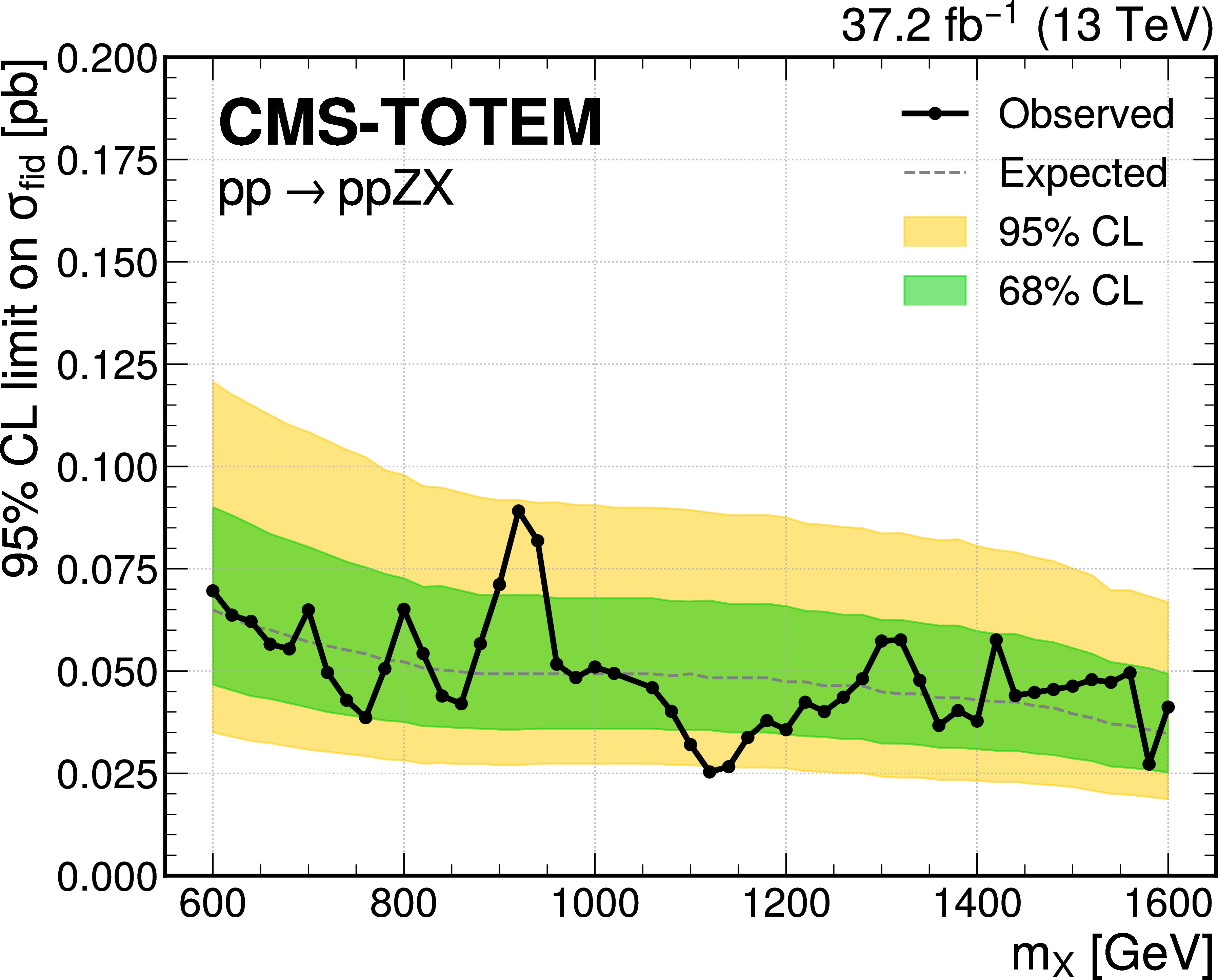
Figure 9:
Upper limits on the $ \mathrm{p}\mathrm{p}\to \mathrm{p}\mathrm{p}\mathrm{Z}/\gamma+\mathrm{X} $ cross section at 95% CL, as a function of $ m_{\mathrm{X}} $. The 68 and 95% central intervals of the expected limits are represented by the dark green and light yellow bands, respectively, while the observed limit is superimposed as a curve. The upper plots correspond to the $ \mathrm{Z}\to \mathrm{e}\mathrm{e} $ and $ \mathrm{Z}\to\mu\mu $ final states, while the lower plots correspond to the combined Z and $ \gamma $ analyses. |
png pdf |
Figure 9-a:
Upper limits on the $ \mathrm{p}\mathrm{p}\to \mathrm{p}\mathrm{p}\mathrm{Z}/\gamma+\mathrm{X} $ cross section at 95% CL, as a function of $ m_{\mathrm{X}} $. The 68 and 95% central intervals of the expected limits are represented by the dark green and light yellow bands, respectively, while the observed limit is superimposed as a curve. The upper plots correspond to the $ \mathrm{Z}\to \mathrm{e}\mathrm{e} $ and $ \mathrm{Z}\to\mu\mu $ final states, while the lower plots correspond to the combined Z and $ \gamma $ analyses. |
png pdf |
Figure 9-b:
Upper limits on the $ \mathrm{p}\mathrm{p}\to \mathrm{p}\mathrm{p}\mathrm{Z}/\gamma+\mathrm{X} $ cross section at 95% CL, as a function of $ m_{\mathrm{X}} $. The 68 and 95% central intervals of the expected limits are represented by the dark green and light yellow bands, respectively, while the observed limit is superimposed as a curve. The upper plots correspond to the $ \mathrm{Z}\to \mathrm{e}\mathrm{e} $ and $ \mathrm{Z}\to\mu\mu $ final states, while the lower plots correspond to the combined Z and $ \gamma $ analyses. |
png pdf |
Figure 9-c:
Upper limits on the $ \mathrm{p}\mathrm{p}\to \mathrm{p}\mathrm{p}\mathrm{Z}/\gamma+\mathrm{X} $ cross section at 95% CL, as a function of $ m_{\mathrm{X}} $. The 68 and 95% central intervals of the expected limits are represented by the dark green and light yellow bands, respectively, while the observed limit is superimposed as a curve. The upper plots correspond to the $ \mathrm{Z}\to \mathrm{e}\mathrm{e} $ and $ \mathrm{Z}\to\mu\mu $ final states, while the lower plots correspond to the combined Z and $ \gamma $ analyses. |

png pdf |
Figure 9-d:
Upper limits on the $ \mathrm{p}\mathrm{p}\to \mathrm{p}\mathrm{p}\mathrm{Z}/\gamma+\mathrm{X} $ cross section at 95% CL, as a function of $ m_{\mathrm{X}} $. The 68 and 95% central intervals of the expected limits are represented by the dark green and light yellow bands, respectively, while the observed limit is superimposed as a curve. The upper plots correspond to the $ \mathrm{Z}\to \mathrm{e}\mathrm{e} $ and $ \mathrm{Z}\to\mu\mu $ final states, while the lower plots correspond to the combined Z and $ \gamma $ analyses. |
| Tables | |

png pdf |
Table 1:
Combined CMS+CT-PPS fiducial volume selection criteria in the Z and $ \gamma $ analyses. The leading- and subleading-$ p_{\mathrm{T}} $ leptons, where $ p_{\mathrm{T}} $ is transverse momentum, are labelled as $ \ell_1 $ and $ \ell_2 $, respectively. The Z boson mass is noted as $ m_{\mathrm{Z}} $. |
| Summary |
| A search is presented for anomalous central exclusive $ \mathrm{Z}/\gamma+\mathrm{X} $ production using proton-proton (pp) data samples corresponding to an integrated luminosity up to 37.2 fb$^{-1}$ recorded in 2017 by the CMS detector and the CMS-TOTEM precision proton spectrometer (CT-PPS). A hypothetical X resonance is searched for in the mass region between 0.6 and 1.6 TeV, with selections optimised for the best expected significance. Benefitting from the excellent mass resolution of 2% offered by the combination of the CMS central detector and CT-PPS, for the first time at the CERN Large Hadron Collider (LHC), the missing mass distribution is used to perform a model-independent search. Upper limits on the visible cross section of the $ \mathrm{p}\mathrm{p}\to \mathrm{p}\mathrm{p} \mathrm{Z}/\gamma+\mathrm{X} $ process are set in a fiducial volume, using a generic model, in the absence of significant deviations in data with respect to the background predictions. Upper limits in the 0.025-0.089 pb range are obtained for $ \sigma(\mathrm{p}\mathrm{p}\to \mathrm{p}\mathrm{p}\mathrm{Z}\mathrm{X}) $ and 0.47-1.75 pb for $ \sigma(\mathrm{p}\mathrm{p}\to \mathrm{p}\mathrm{p}\gamma\mathrm{X}) $. With these results we demonstrate the feasibility of the missing mass approach for searches at the LHC. |
| References | ||||
| 1 | ATLAS Collaboration | A strategy for a general search for new phenomena using data-derived signal regions and its application within the ATLAS experiment | EPJC 79 (2019) 120 | 1807.07447 |
| 2 | CMS Collaboration | MUSiC: a model-unspecific search for new physics in proton-proton collisions at $ \sqrt{s}= $ 13 TeV | EPJC 81 (2021) 629 | CMS-EXO-19-008 2010.02984 |
| 3 | ATLAS Collaboration | Search for new phenomena in three- or four-lepton events in pp collisions at $ \sqrt{s} = 13\,\text {TeV} $ with the ATLAS detector | PLB 824 (2022) 136832 | 2107.00404 |
| 4 | G. Karagiorgi et al. | Machine learning in the search for new fundamental physics | 2112.03769 | |
| 5 | W. Buchmüller and D. Wyler | Effective lagrangian analysis of new interactions and flavor conservation | NPB 268 (1986) 621 | |
| 6 | B. Grzadkowski, M. Iskrzynski, M. Misiak, and J. Rosiek | Dimension-six terms in the standard model lagrangian | JHEP 10 (2010) 085 | 1008.4884 |
| 7 | J. Ellis et al. | Top, Higgs, diboson and electroweak fit to the standard model effective field theory | JHEP 04 (2021) 279 | 2012.02779 |
| 8 | SMEFiT Collaboration | Combined SMEFT interpretation of higgs, diboson, and top quark data from the LHC | JHEP 11 (2021) 089 | 2105.00006 |
| 9 | E. Chapon, C. Royon, and O. Kepka | Anomalous quartic WW$ \gamma\gamma $, ZZ$ \gamma\gamma $, and trilinear WW$ \gamma $ couplings in two-photon processes at high luminosity at the LHC | PRD 81 (2010) 074003 | 0912.5161 |
| 10 | V. A. Khoze, A. D. Martin, and M. G. Ryskin | Prospects for new physics observations in diffractive processes at the LHC and Tevatron | EPJC 23 (2002) 311 | hep-ph/0111078 |
| 11 | P. D. B. Collins | An Introduction to Regge Theory and High-Energy Physics | Cambridge Univ. Press, . , ISBN~978-0-521-1-8, 2009 link |
|
| 12 | CMS Collaboration | The CMS experiment at the CERN LHC | JINST 3 (2008) S08004 | |
| 13 | CMS and TOTEM Collaborations | CMS-TOTEM precision proton spectrometer | Technical Report CERN-LHCC-2014-021, TOTEM-TDR-003, CMS-TDR-13, 2014 | |
| 14 | CMS Collaboration | HEPData record for this analysis | link | |
| 15 | CMS Collaboration | Performance of the CMS Level-1 trigger in proton-proton collisions at $ \sqrt{s} = $ 13 TeV | JINST 15 (2020) P10017 | CMS-TRG-17-001 2006.10165 |
| 16 | CMS Collaboration | The CMS trigger system | JINST 12 (2017) P01020 | CMS-TRG-12-001 1609.02366 |
| 17 | TOTEM Collaboration | The TOTEM experiment at the CERN Large Hadron Collider | JINST 3 (2008) S08007 | |
| 18 | CMS and TOTEM Collaboration | Proton reconstruction with the CMS-TOTEM precision proton spectrometer | Submitted to JINST, 2022 | 2210.05854 |
| 19 | CMS Collaboration | Proton reconstruction with the precision proton spectrometer (PPS) in run 2 | CMS Detector Performance Summary CMS-DP-2020-047, CERN, 2020 CDS |
|
| 20 | CMS Collaboration | Efficiency of the Si-strips sensors used in the precision proton spectrometer: radiation damage | CMS Detector Performance Summary CMS-DP-2019-035, CERN, 2019 CDS |
|
| 21 | CMS Collaboration | Efficiency of the pixel sensors used in the precision proton spectrometer: radiation damage | CMS Detector Performance Summary CMS-DP-2019-036, CERN, 2019 CDS |
|
| 22 | CMS and TOTEM Collaborations | Observation of proton-tagged, central (semi)exclusive production of high-mass lepton pairs in pp collisions at 13 TeV with the CMS-TOTEM precision proton spectrometer | JHEP 07 (2018) 153 | 1803.04496 |
| 23 | V. M. Budnev, I. F. Ginzburg, G. V. Meledin, and V. G. Serbo | The two photon particle production mechanism. Physical problems. Applications. Equivalent photon approximation | Phys. Rept. 15 (1975) 181 | |
| 24 | S. Agostinelli et al. | Geant4 - a simulation toolkit | NIM A 506 (2003) 250 | |
| 25 | R. Frederix and S. Frixione | Merging meets matching in MC@NLO | JHEP 12 (2012) 061 | 1209.6215 |
| 26 | J. Alwall et al. | Comparative study of various algorithms for the merging of parton showers and matrix elements in hadronic collisions | EPJC 53 (2008) 473 | 0706.2569 |
| 27 | E. Re | Single-top Wt-channel production matched with parton showers using the POWHEG method | EPJC 71 (2011) 1547 | 1009.2450 |
| 28 | S. Frixione, P. Nason, and G. Ridolfi | A positive-weight next-to-leading-order monte carlo for heavy flavour hadroproduction | JHEP 09 (2007) 126 | 0707.3088 |
| 29 | T. Sjöstrand et al. | An introduction to PYTHIA 8.2 | Comput. Phys. Commun. 191 (2015) 159 | 1410.3012 |
| 30 | M. Arneodo and M. Diehl | Diffraction for non-believers | HERA and the LHC: A Workshop on the Implications of HERA and LHC Physics, CERN, 2004 | hep-ph/0511047 |
| 31 | B. E. Cox and J. R. Forshaw | POMWIG: HERWIG for diffractive interactions | Comput. Phys. Commun. 144 (2002) 104 | hep-ph/0010303 |
| 32 | CMS Collaboration | Particle-flow reconstruction and global event description with the CMS detector | JINST 12 (2017) P10003 | CMS-PRF-14-001 1706.04965 |
| 33 | CMS Collaboration | Electron and photon reconstruction and identification with the CMS experiment at the CERN LHC | JINST 16 (2021) P05014 | CMS-EGM-17-001 2012.06888 |
| 34 | CMS Collaboration | Performance of the reconstruction and identification of high-momentum muons in proton-proton collisions at $ \sqrt{s} = $ 13 TeV | JINST 15 (2020) P0 | CMS-MUO-17-001 1912.03516 |
| 35 | L. Moneta et al. | The RooStats project | 13$^\text{th}$ International Workshop on Advanced Computing and Analysis Techniques in Physics Research (ACAT). SISSA, 2010 | 1009.1003 |
| 36 | B. Todd, L. Ponce, A. Apollonio, and D. J. Walsh | LHC availability 2017: technical stop 2 to end of standard proton physics | Accelerators and Technology Sector Notes CERN-ACC-NOTE-2017-0062, CERN, 2017 | |
| 37 | CMS Collaboration | CMS luminosity measurement for the 2017 data-taking period at $ \sqrt{s} = $ 13 TeV | CMS Physics Analysis Summary , CERN, 2018 CMS-PAS-LUM-17-004 |
CMS-PAS-LUM-17-004 |
| 38 | R. J. Barlow and C. Beeston | Fitting using finite Monte Carlo samples | Comput. Phys. Commun. 77 (1993) 219 | |
| 39 | T. Junk | Confidence level computation for combining searches with small statistics | NIM A 434 (1999) 435 | hep-ex/9902006 |
| 40 | A. L. Read | Presentation of search results: the CL$ _{\rm s} $ technique | JPG 28 (2002) 2693 | |
| 41 | ATLAS and CMS Collaborations, and LHC Higgs Combination Group | Procedure for the LHC Higgs boson search combination in summer 2011 | Technical Report CMS-NOTE-2011-005, ATL-PHYS-PUB-2011-011, 2011 | |
| 42 | G. Cowan, K. Cranmer, E. Gross, and O. Vitells | Asymptotic formulae for likelihood-based tests of new physics | EPJC 71 (2011) 1554 | 1007.1727 |
| 43 | E. Gross and O. Vitells | Trial factors for the look elsewhere effect in high energy physics | EPJC 70 (2010) 525 | 1005.1891 |
|
|
Compact Muon Solenoid LHC, CERN |
|

|

|

|

|

|