

Compact Muon Solenoid
LHC, CERN
| CMS-MUO-17-001 ; CERN-EP-2019-238 | ||
| Performance of the reconstruction and identification of high-momentum muons in proton-proton collisions at $\sqrt{s} = $ 13 TeV | ||
| CMS Collaboration | ||
| 7 December 2019 | ||
| JINST 15 (2020) P02027 | ||
| Abstract: The CMS detector at the LHC has recorded events from proton-proton collisions, with muon momenta reaching up to 1.8 TeV in the collected dimuon samples. These high-momentum muons allow direct access to new regimes in physics beyond the standard model. Because the physics and reconstruction of these muons are different from those of their lower-momentum counterparts, this paper presents for the first time dedicated studies of efficiencies, momentum assignment, resolution, scale, and showering of very high momentum muons produced at the LHC. These studies are performed using the 2016 and 2017 data sets of proton-proton collisions at $\sqrt{s} = $ 13 TeV with integrated luminosities of 36.3 and 42.1 fb$^{-1}$, respectively. | ||
| Links: e-print arXiv:1912.03516 [hep-ex] (PDF) ; CDS record ; inSPIRE record ; CADI line (restricted) ; | ||
| Figures | |
png pdf |
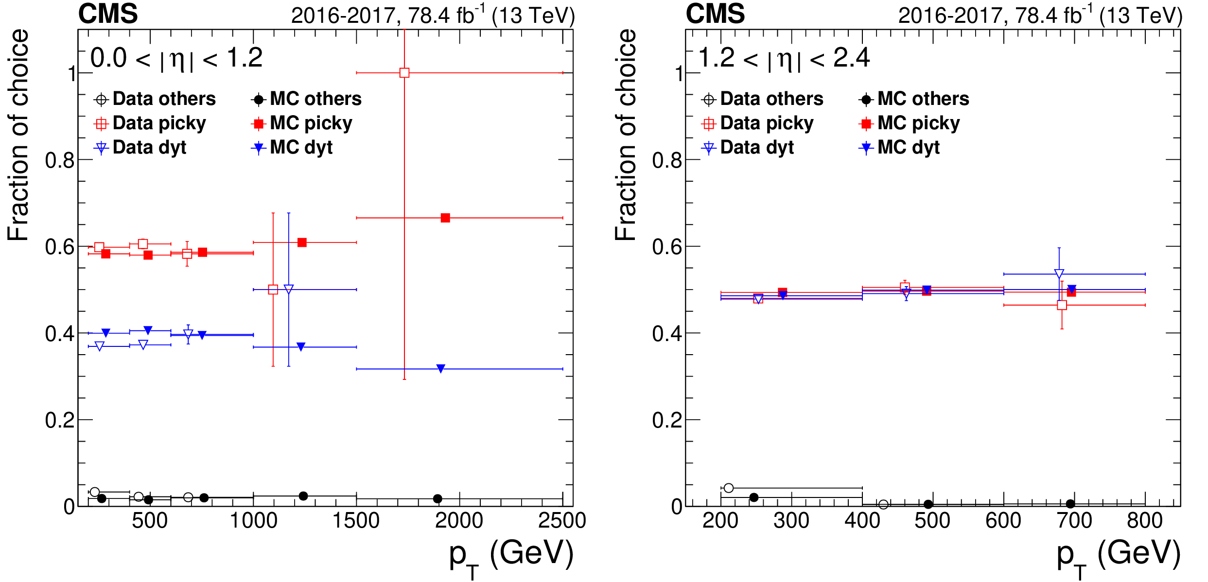
Figure 1:
Fraction of choices of different refit algorithms chosen by TuneP, comparing 2016+2017 data and DY simulation for five $ {p_{\mathrm {T}}} $ ranges and for two $\eta $ categories: (left) barrel with $ {| \eta |} < $ 1.2 and (right) endcap with 1.2 $ < {| \eta |} < $ 2.4. The central value in each bin is obtained from the average of the distribution within the bin. |

png pdf |
Figure 1-a:
Fraction of choices of different refit algorithms chosen by TuneP, comparing 2016+2017 data and DY simulation for five $ {p_{\mathrm {T}}} $ ranges in the $\eta $ category: barrel with $ {| \eta |} < $ 1.2. The central value in each bin is obtained from the average of the distribution within the bin. |
png pdf |
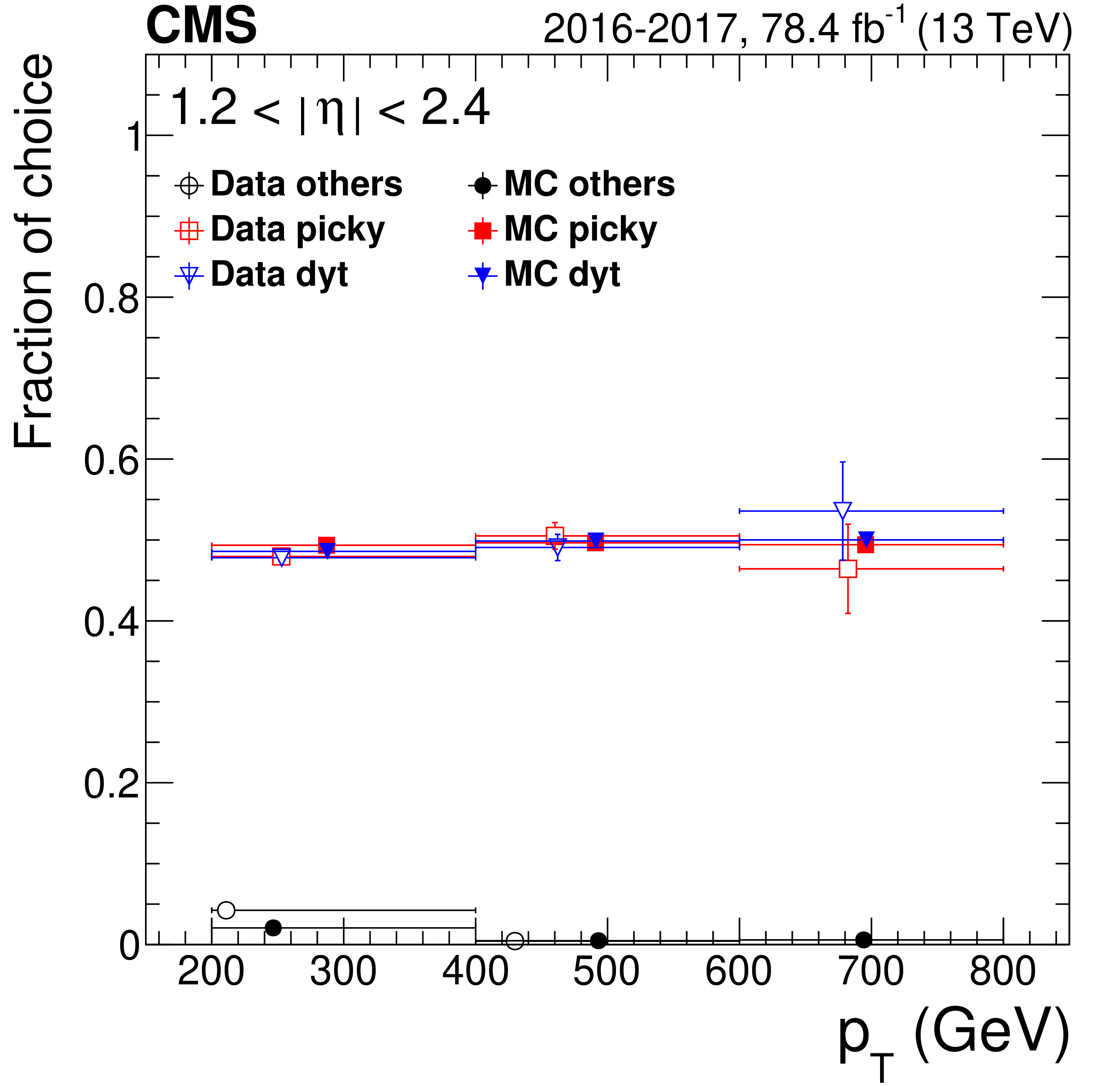
Figure 1-b:
Fraction of choices of different refit algorithms chosen by TuneP, comparing 2016+2017 data and DY simulation for five $ {p_{\mathrm {T}}} $ ranges in the $\eta $ category: endcap with 1.2 $ < {| \eta |} < $ 2.4. The central value in each bin is obtained from the average of the distribution within the bin. |
png pdf |
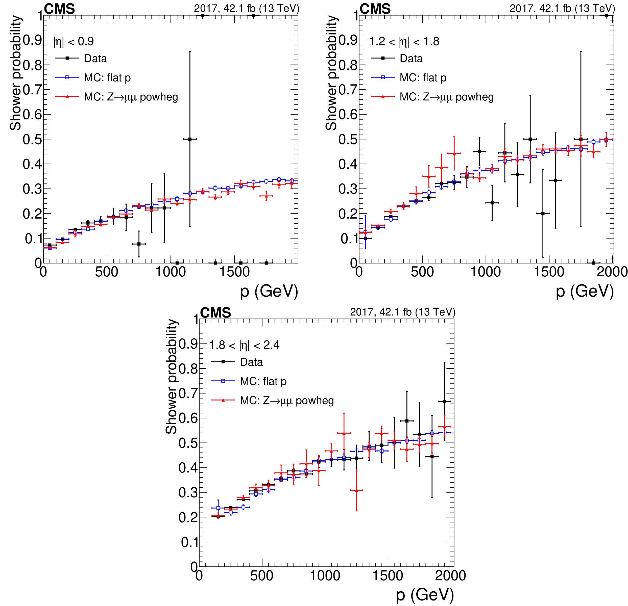
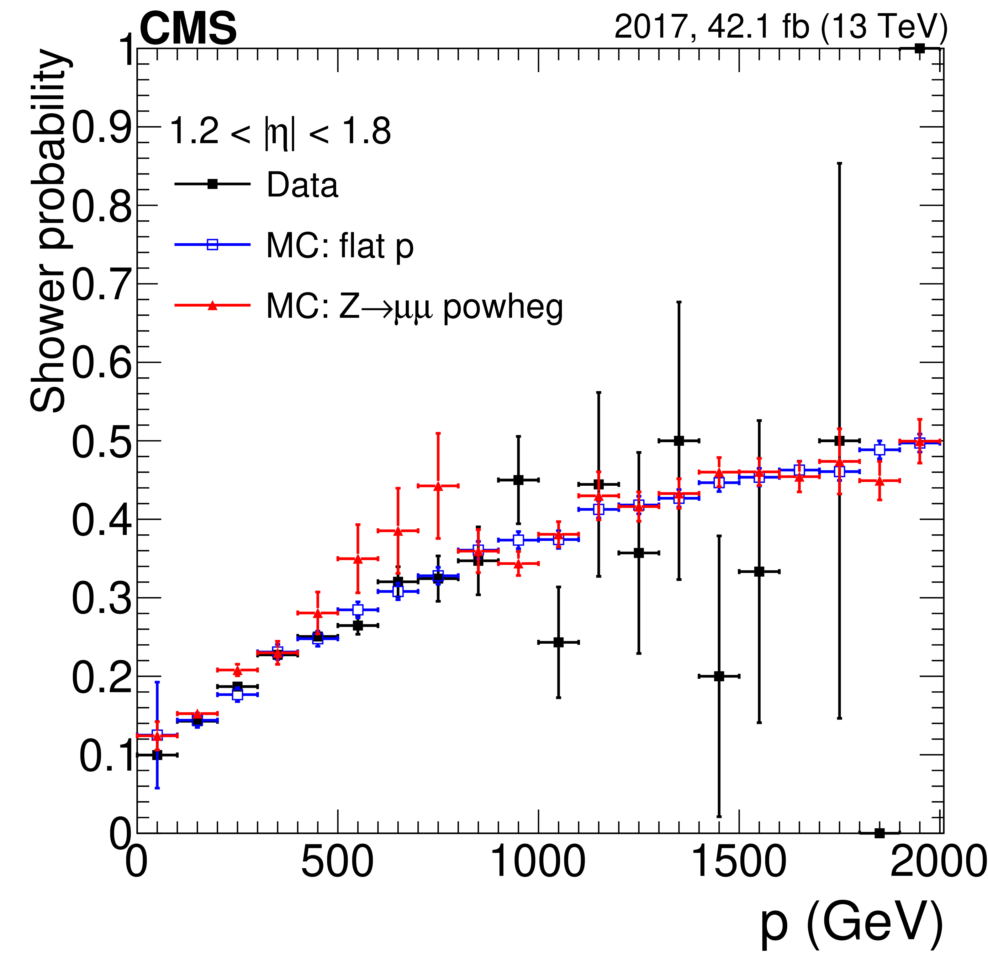
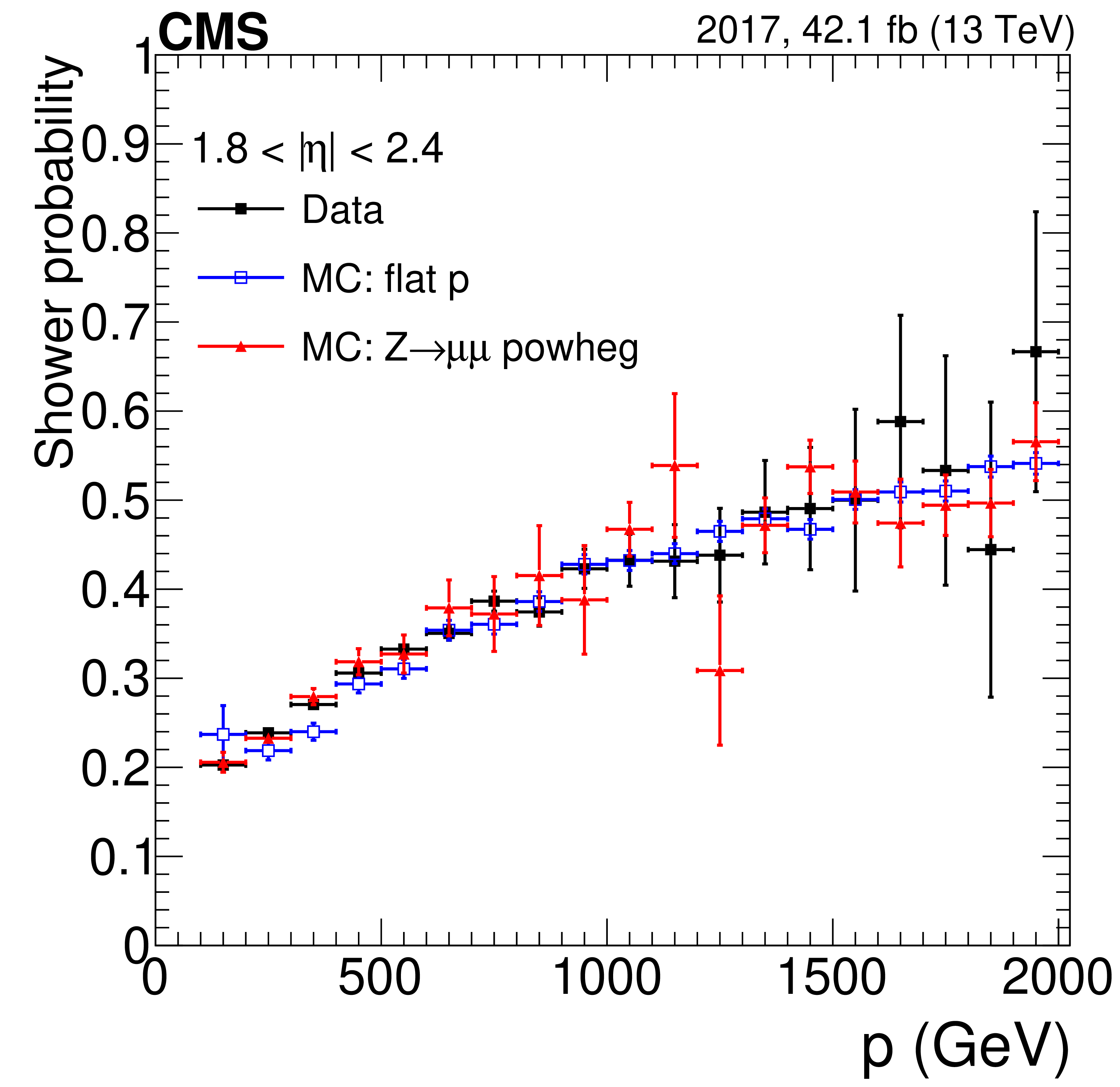
Figure 2:
The probability $ {P_{\text {shower}}} (p)$ to tag at least one shower in any of the four stations, as a function of the incoming muon momentum, for (upper left) DTs; (upper right) CSCs with muon $ {| \eta |} < $ 1.8; and (lower) CSCs with muon $ {| \eta |} > $ 1.8. Results are evaluated for the shower tagging definition requiring $ {N_{\text {seg}}} \ge $ 2. Different colors refer to: data (black), DY simulation (red), and single muons simulated with a uniform $p$ distribution (blue). |
png pdf |
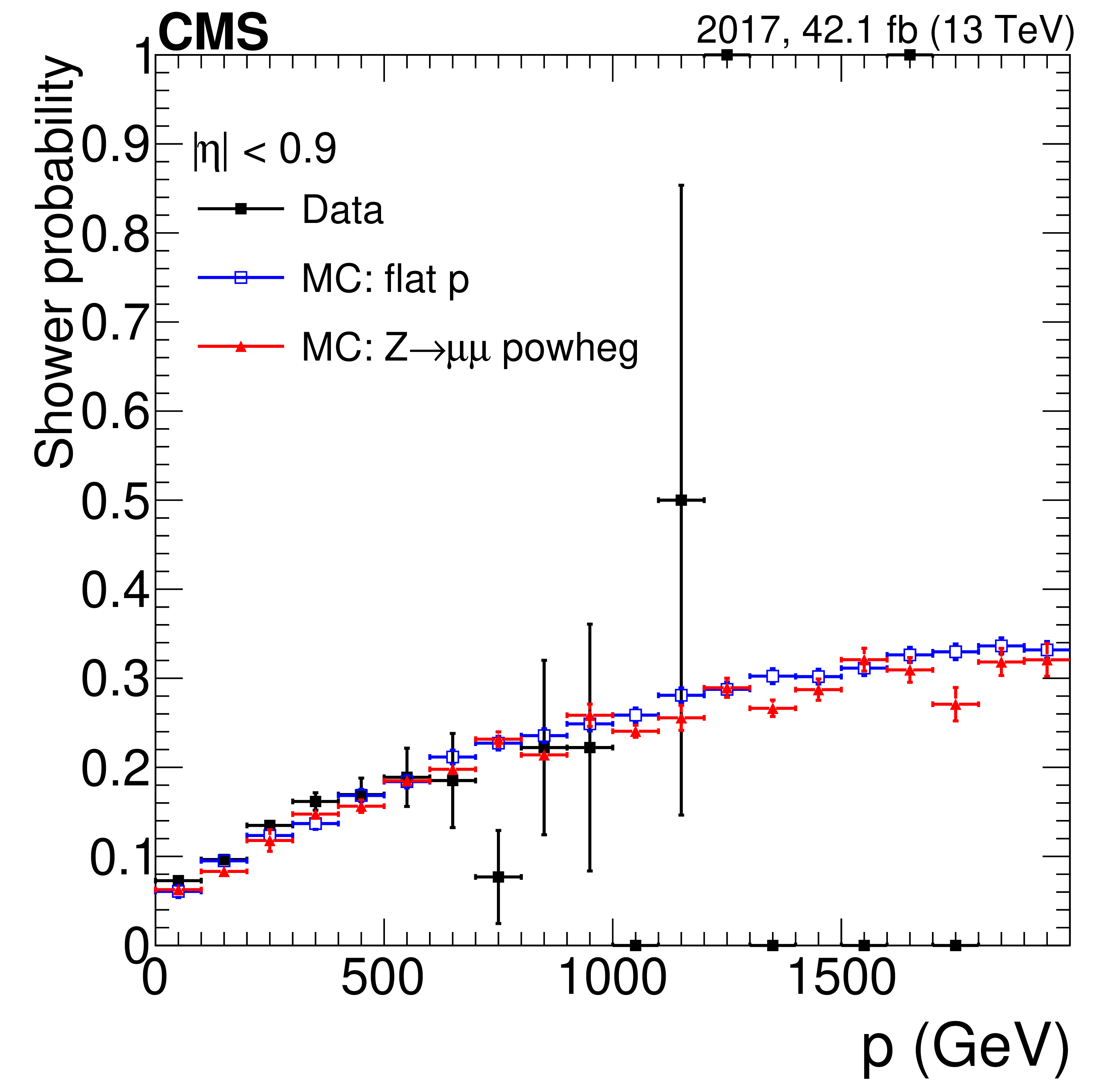
Figure 2-a:
The probability $ {P_{\text {shower}}} (p)$ to tag at least one shower in any of the four stations, as a function of the incoming muon momentum, for DTs. Results are evaluated for the shower tagging definition requiring $ {N_{\text {seg}}} \ge $ 2. Different colors refer to: data (black), DY simulation (red), and single muons simulated with a uniform $p$ distribution (blue). |
png pdf |
Figure 2-b:
The probability $ {P_{\text {shower}}} (p)$ to tag at least one shower in any of the four stations, as a function of the incoming muon momentum, for CSCs with muon $ {| \eta |} < $ 1.8. Results are evaluated for the shower tagging definition requiring $ {N_{\text {seg}}} \ge $ 2. Different colors refer to: data (black), DY simulation (red), and single muons simulated with a uniform $p$ distribution (blue). |
png pdf |
Figure 2-c:
The probability $ {P_{\text {shower}}} (p)$ to tag at least one shower in any of the four stations, as a function of the incoming muon momentum, for CSCs with muon $ {| \eta |} > $ 1.8. Results are evaluated for the shower tagging definition requiring $ {N_{\text {seg}}} \ge $ 2. Different colors refer to: data (black), DY simulation (red), and single muons simulated with a uniform $p$ distribution (blue). |
png pdf |
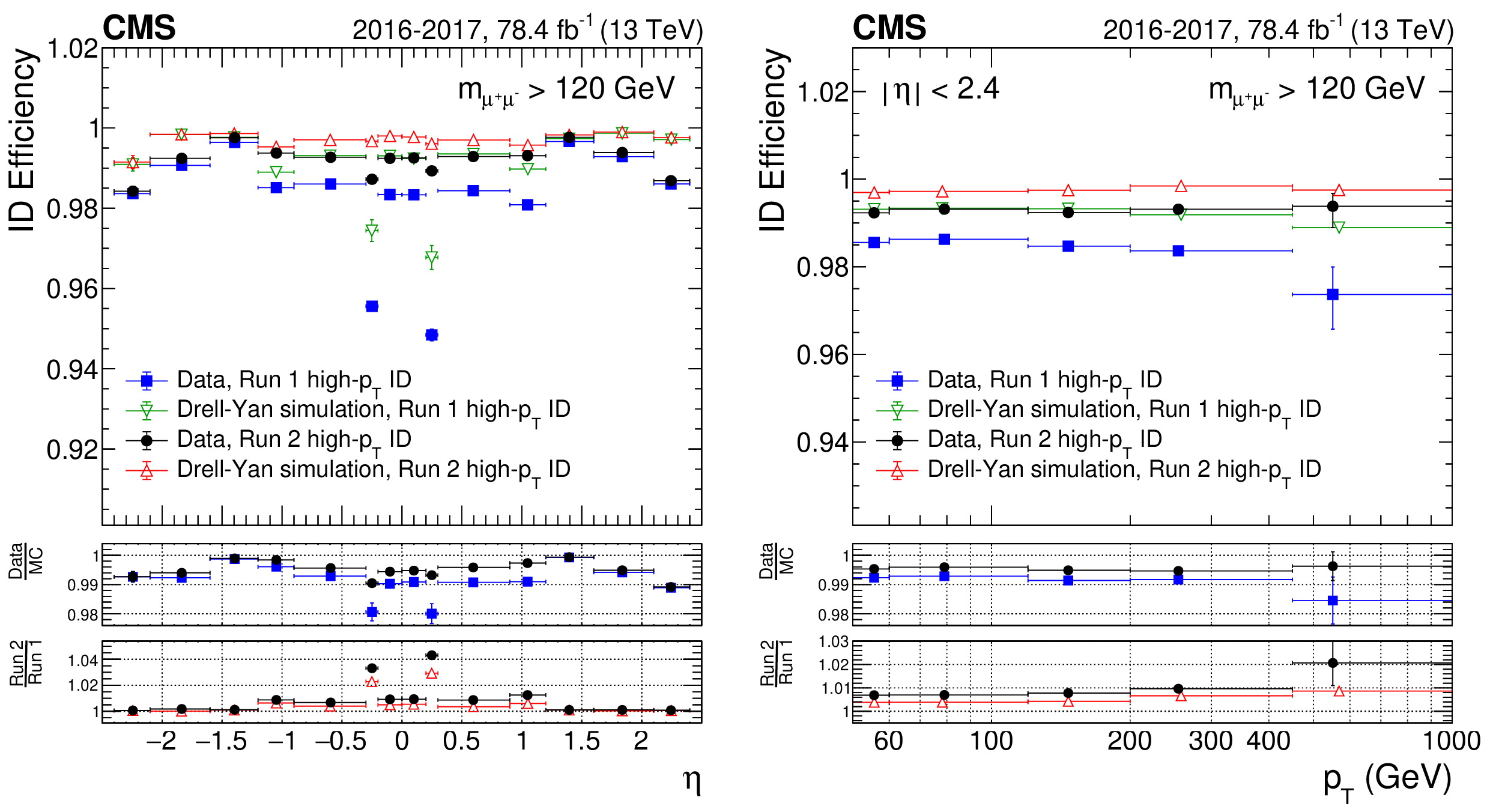
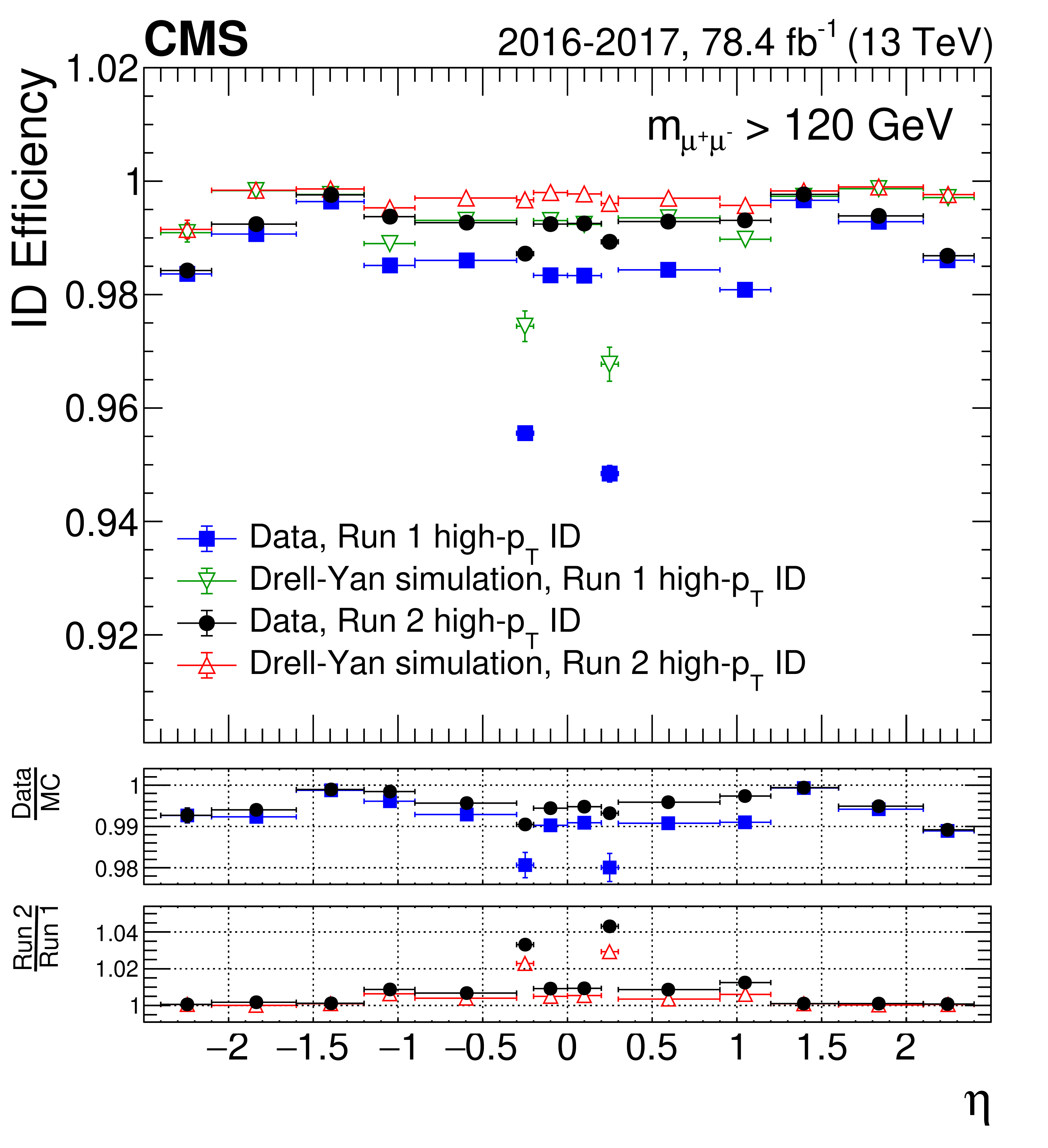
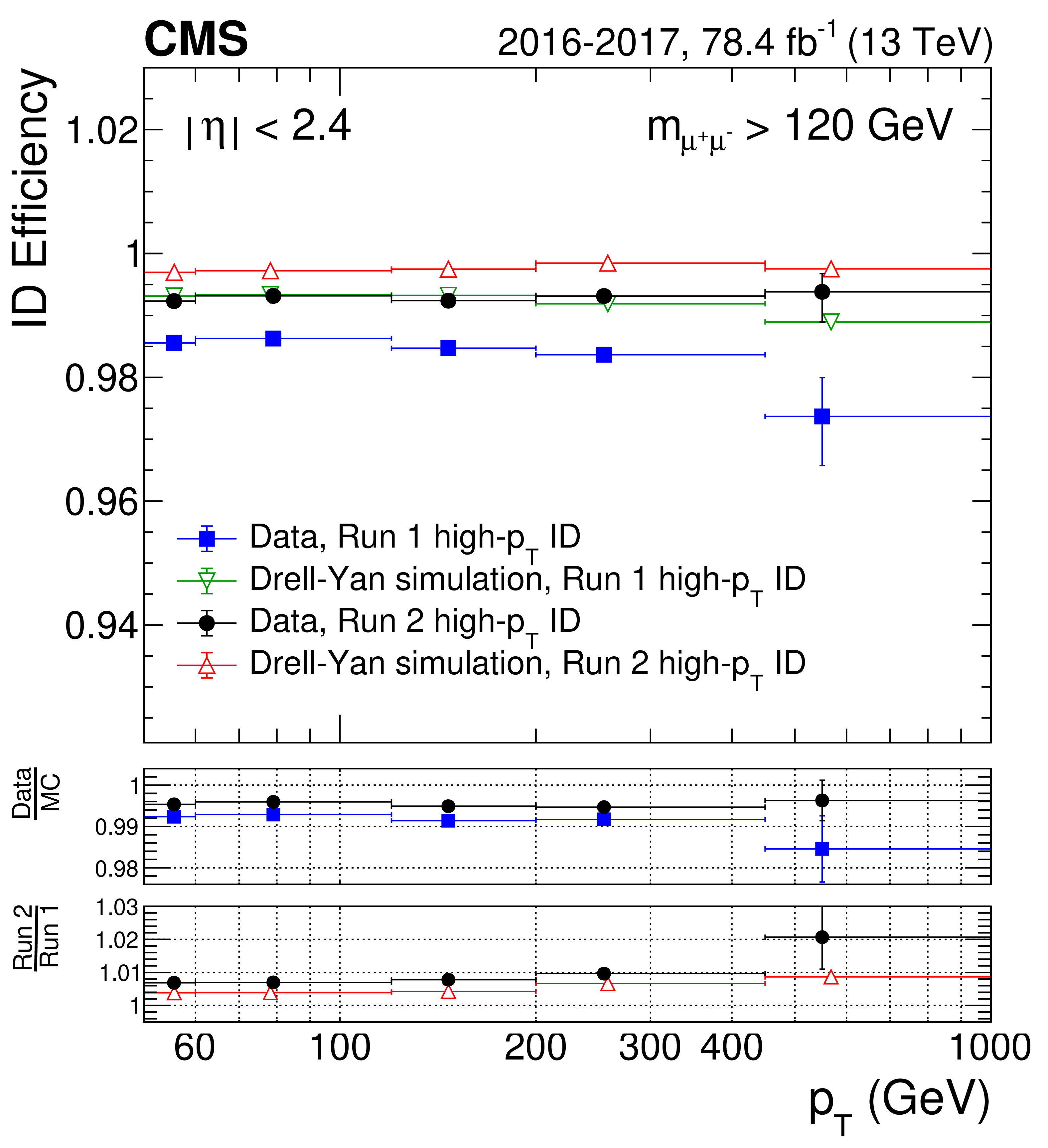
Figure 3:
Comparison between the efficiency of Run 2 and Run 1 high-$ {p_{\mathrm {T}}}$ ID, as a function of (left) $\eta $ and (right) ${p_{\mathrm {T}}}$. The efficiencies are obtained from dimuon events with a mass greater than 120 GeV to further select the high-mass DY process. The top panel shows the data to simulation efficiency ratio obtained for the Run 1 (blue squares) and for the Run 2 high-$ {p_{\mathrm {T}}}$ ID (black circles). The bottom panel shows the Run 2 to Run 1 high-$ {p_{\mathrm {T}}}$ ID efficiency ratio obtained from the data (black circles) and from simulation (red triangles). The central value in each bin is obtained from the average of the distribution within the bin. |
png pdf |
Figure 3-a:
Comparison between the efficiency of Run 2 and Run 1 high-$ {p_{\mathrm {T}}}$ ID, as a function of $\eta $. The efficiencies are obtained from dimuon events with a mass greater than 120 GeV to further select the high-mass DY process. The top panel shows the data to simulation efficiency ratio obtained for the Run 1 (blue squares) and for the Run 2 high-$ {p_{\mathrm {T}}}$ ID (black circles). The bottom panel shows the Run 2 to Run 1 high-$ {p_{\mathrm {T}}}$ ID efficiency ratio obtained from the data (black circles) and from simulation (red triangles). The central value in each bin is obtained from the average of the distribution within the bin. |
png pdf |
Figure 3-b:
Comparison between the efficiency of Run 2 and Run 1 high-$ {p_{\mathrm {T}}}$ ID, as a function of ${p_{\mathrm {T}}}$. The efficiencies are obtained from dimuon events with a mass greater than 120 GeV to further select the high-mass DY process. The top panel shows the data to simulation efficiency ratio obtained for the Run 1 (blue squares) and for the Run 2 high-$ {p_{\mathrm {T}}}$ ID (black circles). The bottom panel shows the Run 2 to Run 1 high-$ {p_{\mathrm {T}}}$ ID efficiency ratio obtained from the data (black circles) and from simulation (red triangles). The central value in each bin is obtained from the average of the distribution within the bin. |
png pdf |
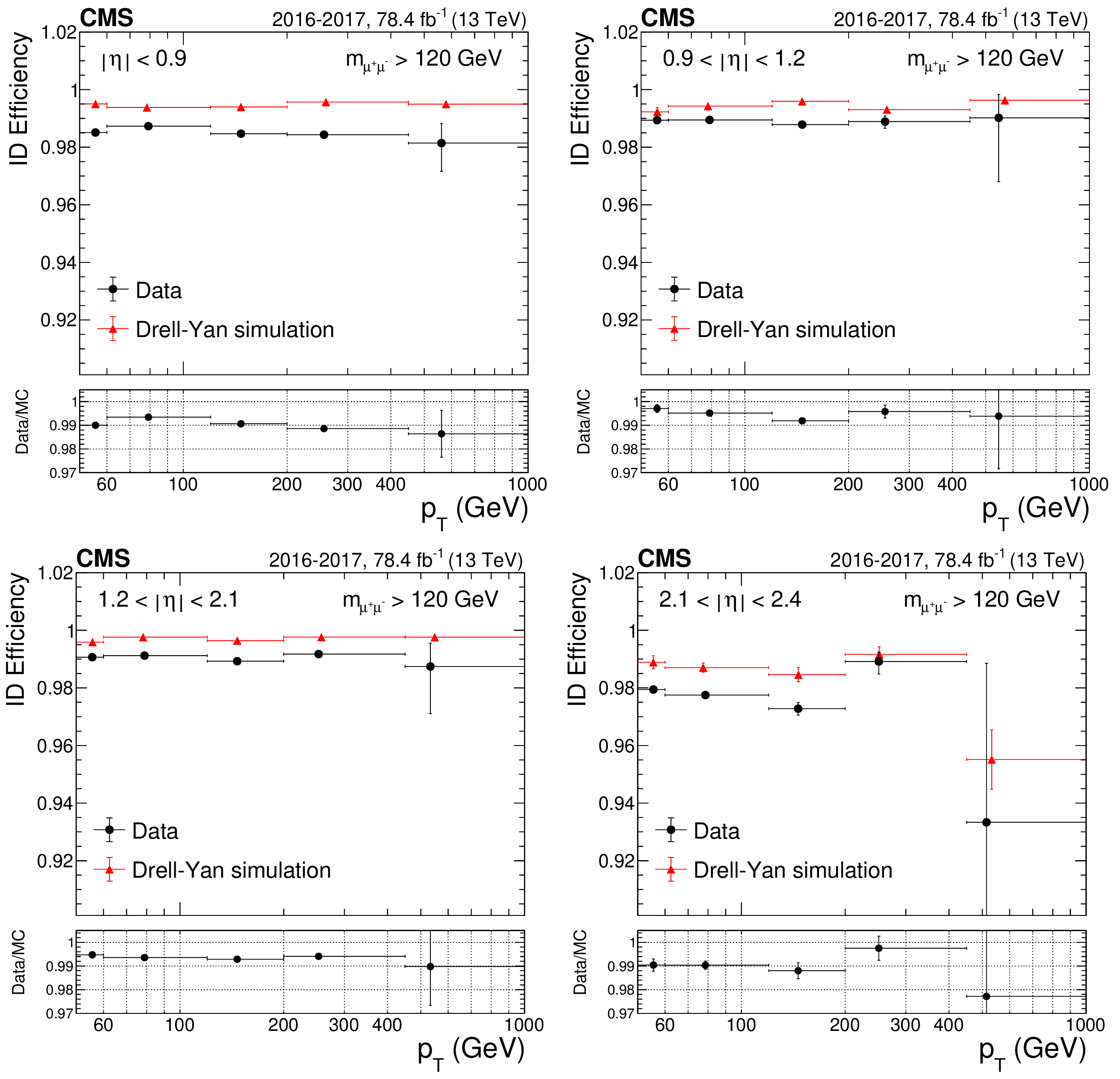
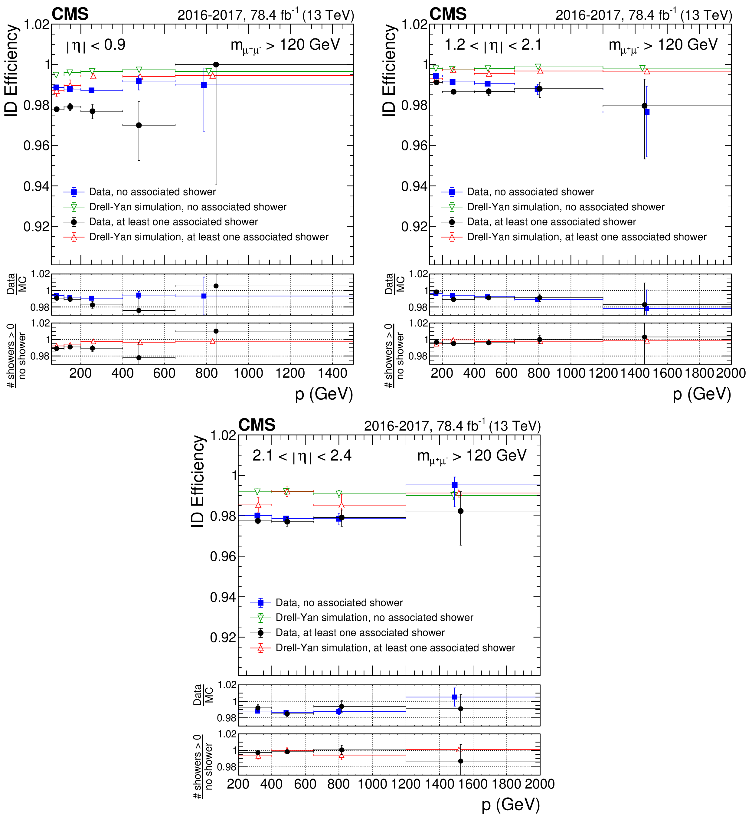
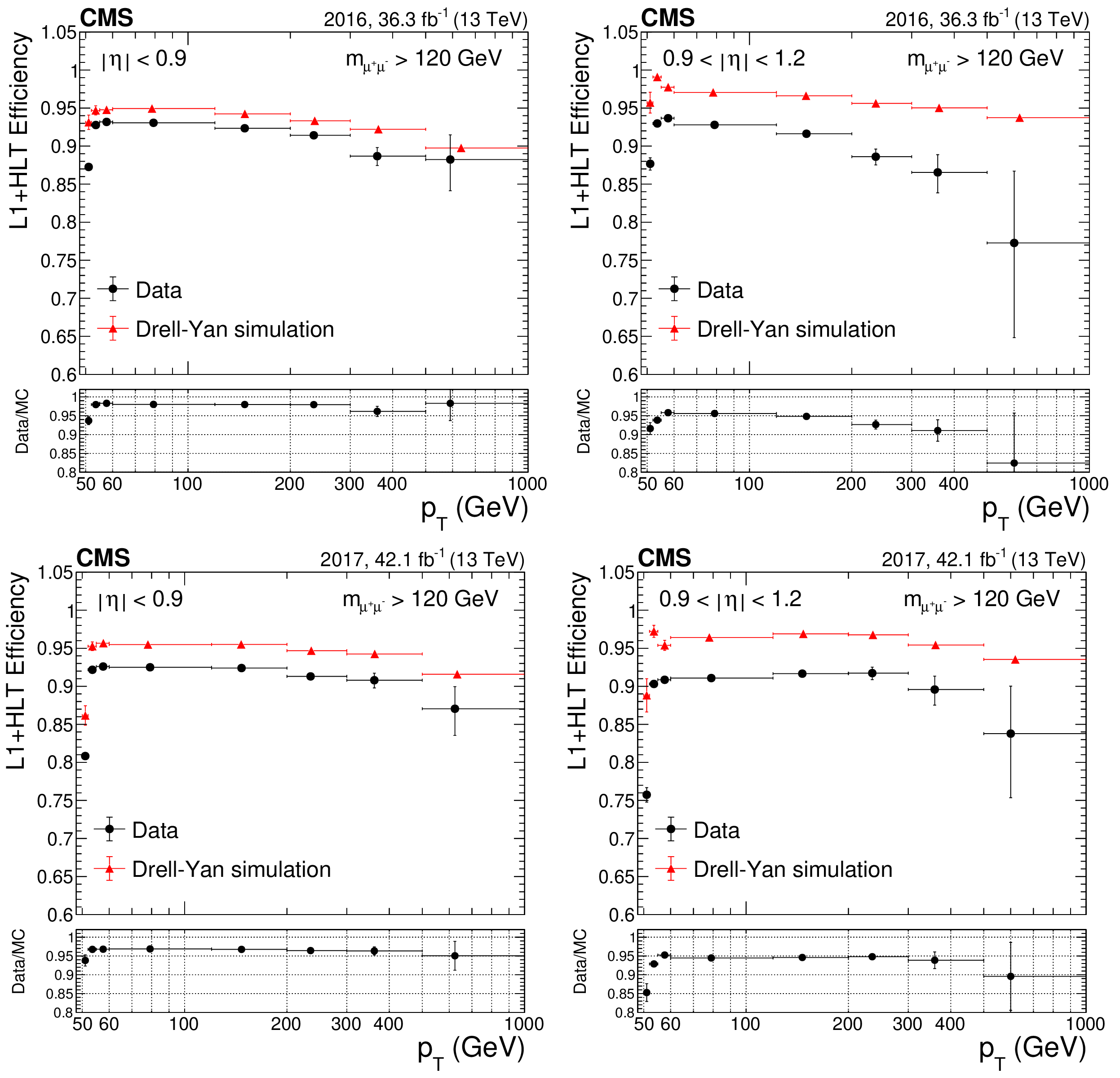
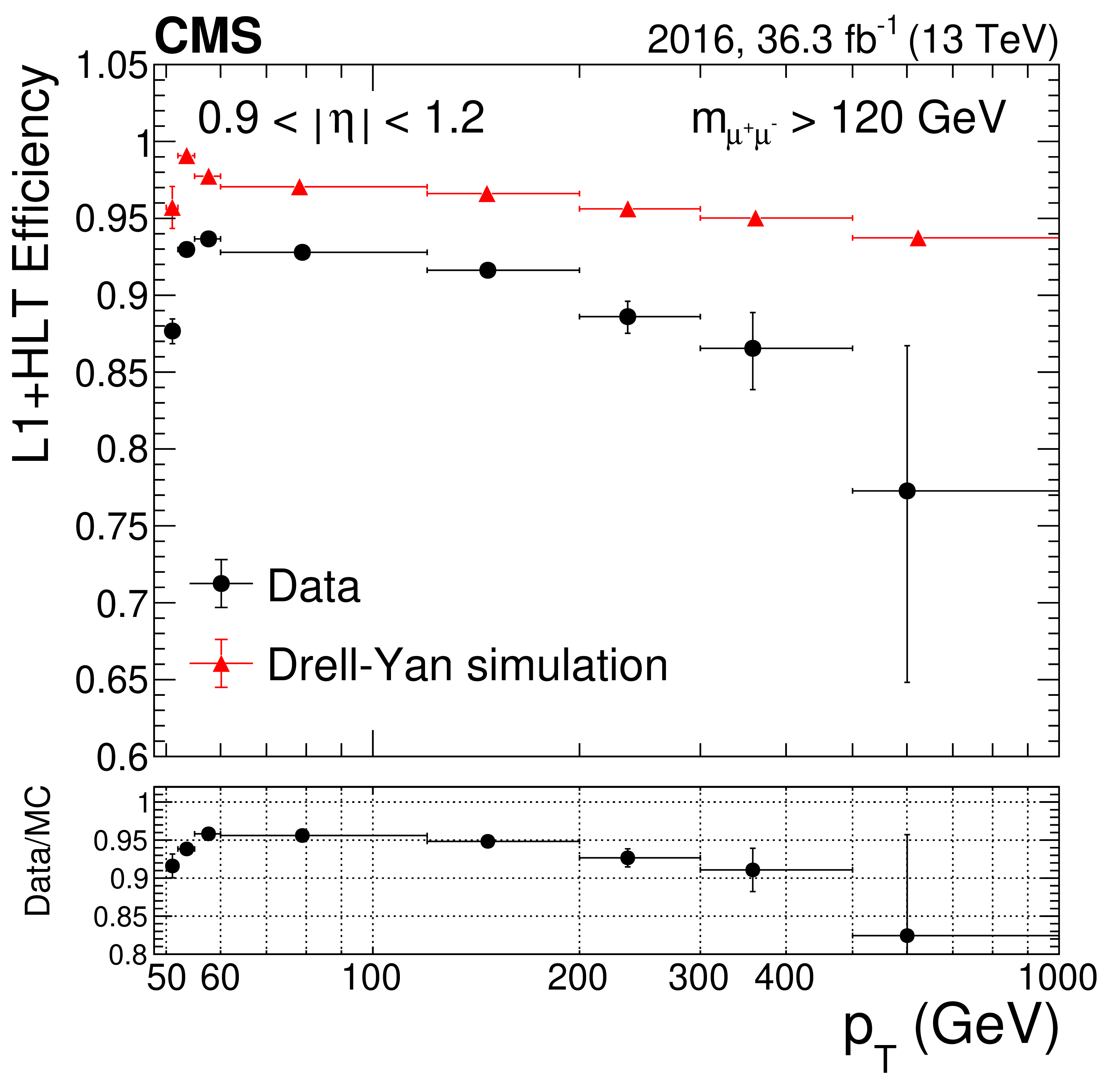
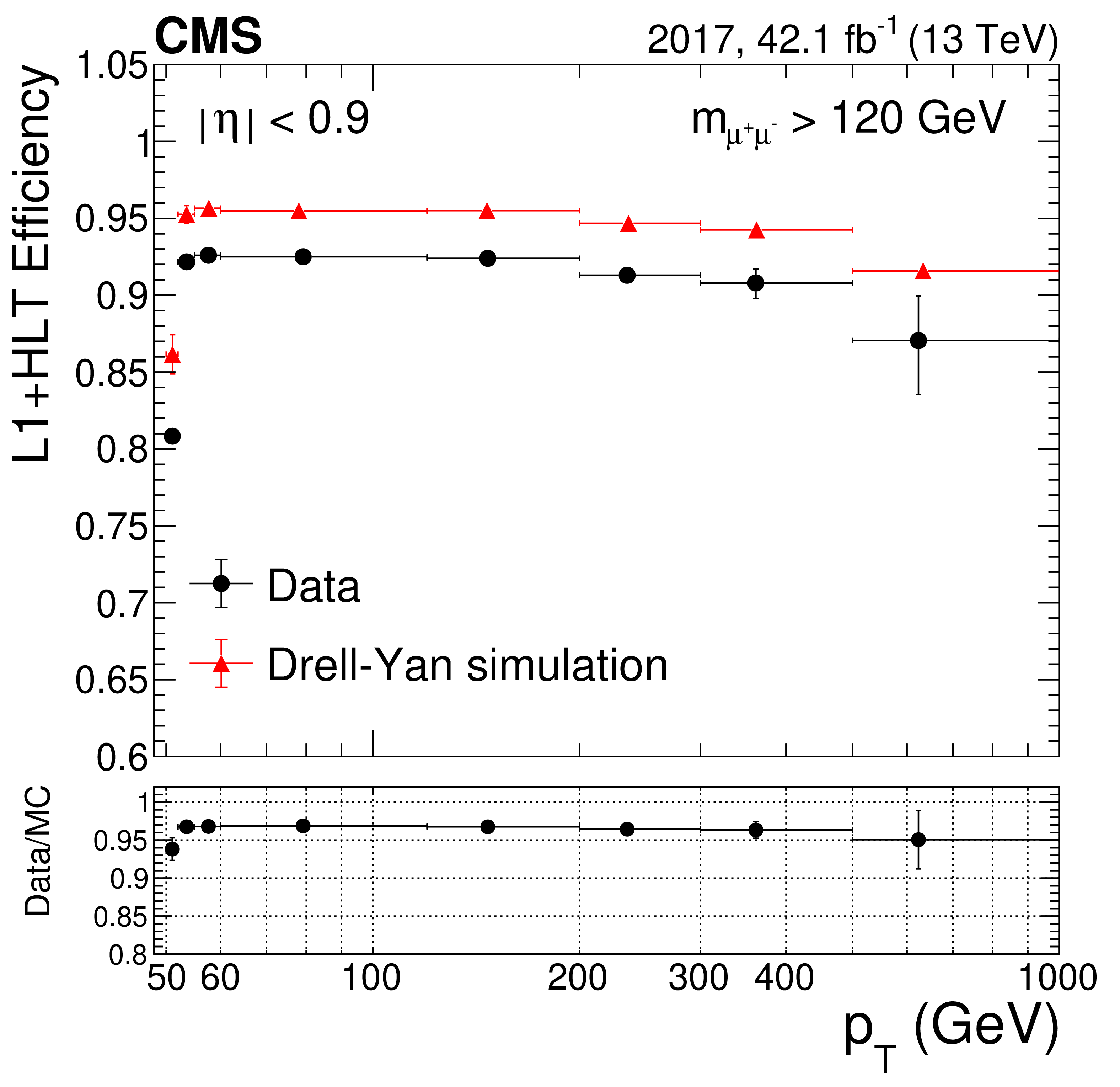
Figure 4:
High-$ {p_{\mathrm {T}}}$ ID efficiency for 2016 and 2017 data, and corresponding DY simulation, as a function of ${p_{\mathrm {T}}}$ for (upper left) $ {| \eta |} < $ 0.9, (upper right) 0.9 $ < {| \eta |} < $ 1.2, (lower left) 1.2 $ < {| \eta |} < $ 2.1, and (lower right) 2.1 $ < {| \eta |} < $ 2.4. The black circles represent data; the red triangles represent DY simulation. The data-to-simulation ratio, also called the data-to-simulation scale factor (SF), is displayed in the lower panels. The central value in each bin is obtained from the average of the distribution within the bin. |
png pdf |
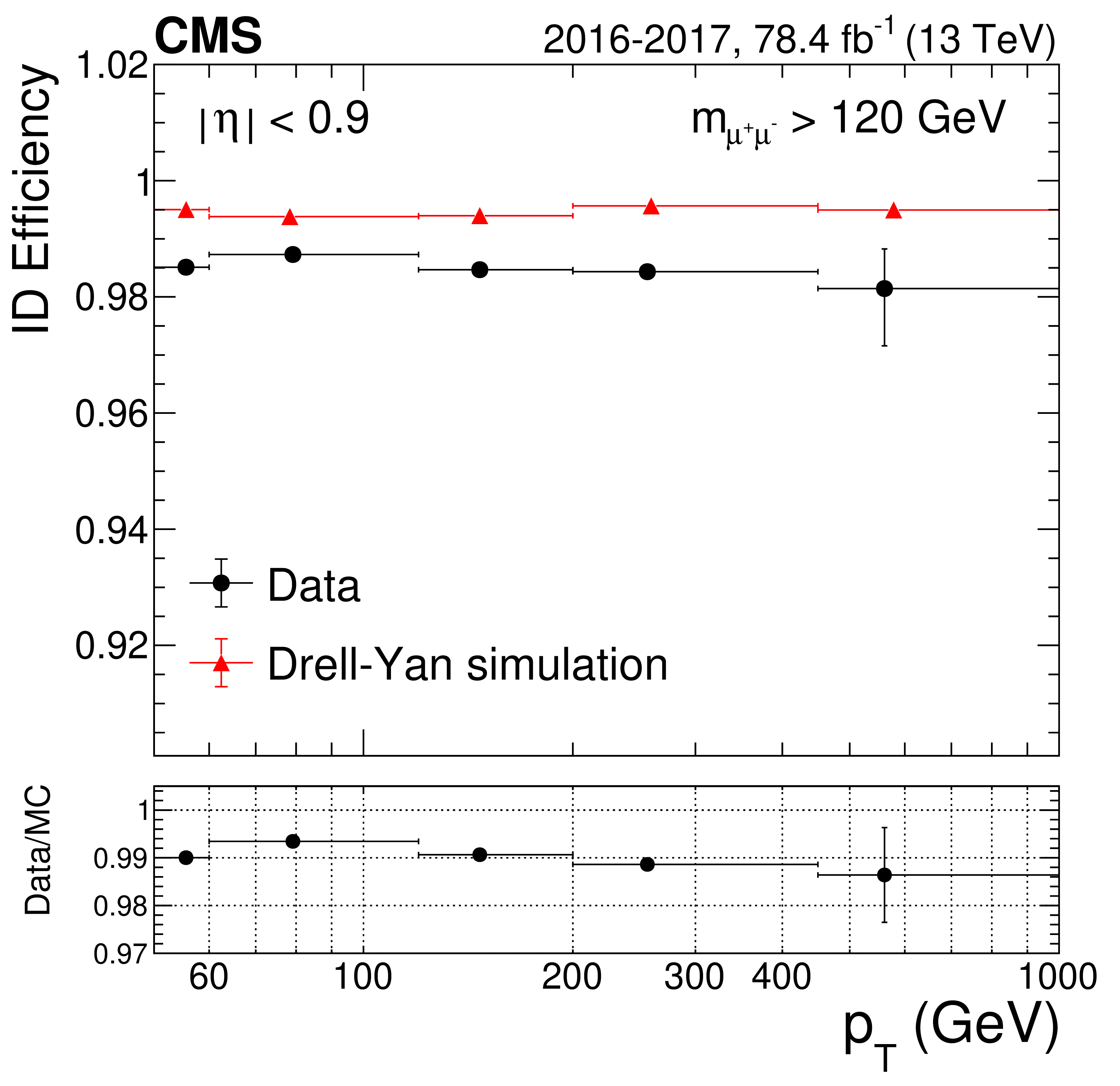
Figure 4-a:
High-$ {p_{\mathrm {T}}}$ ID efficiency for 2016 and 2017 data, and corresponding DY simulation, as a function of ${p_{\mathrm {T}}}$ for $ {| \eta |} < $ 0.9. The black circles represent data; the red triangles represent DY simulation. The data-to-simulation ratio, also called the data-to-simulation scale factor (SF), is displayed in the lower panels. The central value in each bin is obtained from the average of the distribution within the bin. |
png pdf |
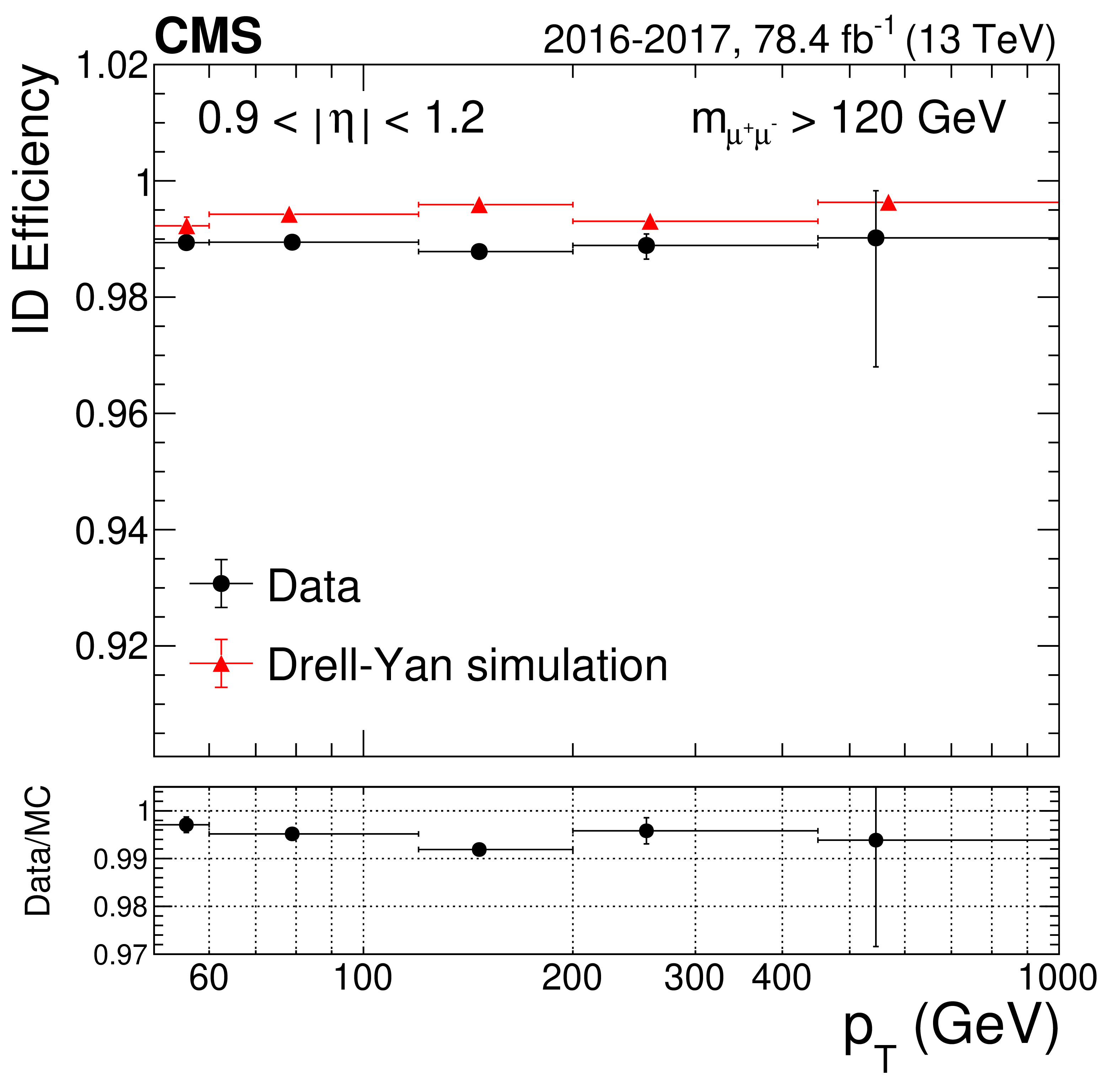
Figure 4-b:
High-$ {p_{\mathrm {T}}}$ ID efficiency for 2016 and 2017 data, and corresponding DY simulation, as a function of ${p_{\mathrm {T}}}$ for 0.9 $ < {| \eta |} < $ 1.2. The black circles represent data; the red triangles represent DY simulation. The data-to-simulation ratio, also called the data-to-simulation scale factor (SF), is displayed in the lower panels. The central value in each bin is obtained from the average of the distribution within the bin. |
png pdf |
Figure 4-c:
High-$ {p_{\mathrm {T}}}$ ID efficiency for 2016 and 2017 data, and corresponding DY simulation, as a function of ${p_{\mathrm {T}}}$ for 1.2 $ < {| \eta |} < $ 2.1. The black circles represent data; the red triangles represent DY simulation. The data-to-simulation ratio, also called the data-to-simulation scale factor (SF), is displayed in the lower panels. The central value in each bin is obtained from the average of the distribution within the bin. |

png pdf |
Figure 4-d:
High-$ {p_{\mathrm {T}}}$ ID efficiency for 2016 and 2017 data, and corresponding DY simulation, as a function of ${p_{\mathrm {T}}}$ for 2.1 $ < {| \eta |} < $ 2.4. The black circles represent data; the red triangles represent DY simulation. The data-to-simulation ratio, also called the data-to-simulation scale factor (SF), is displayed in the lower panels. The central value in each bin is obtained from the average of the distribution within the bin. |
png pdf |
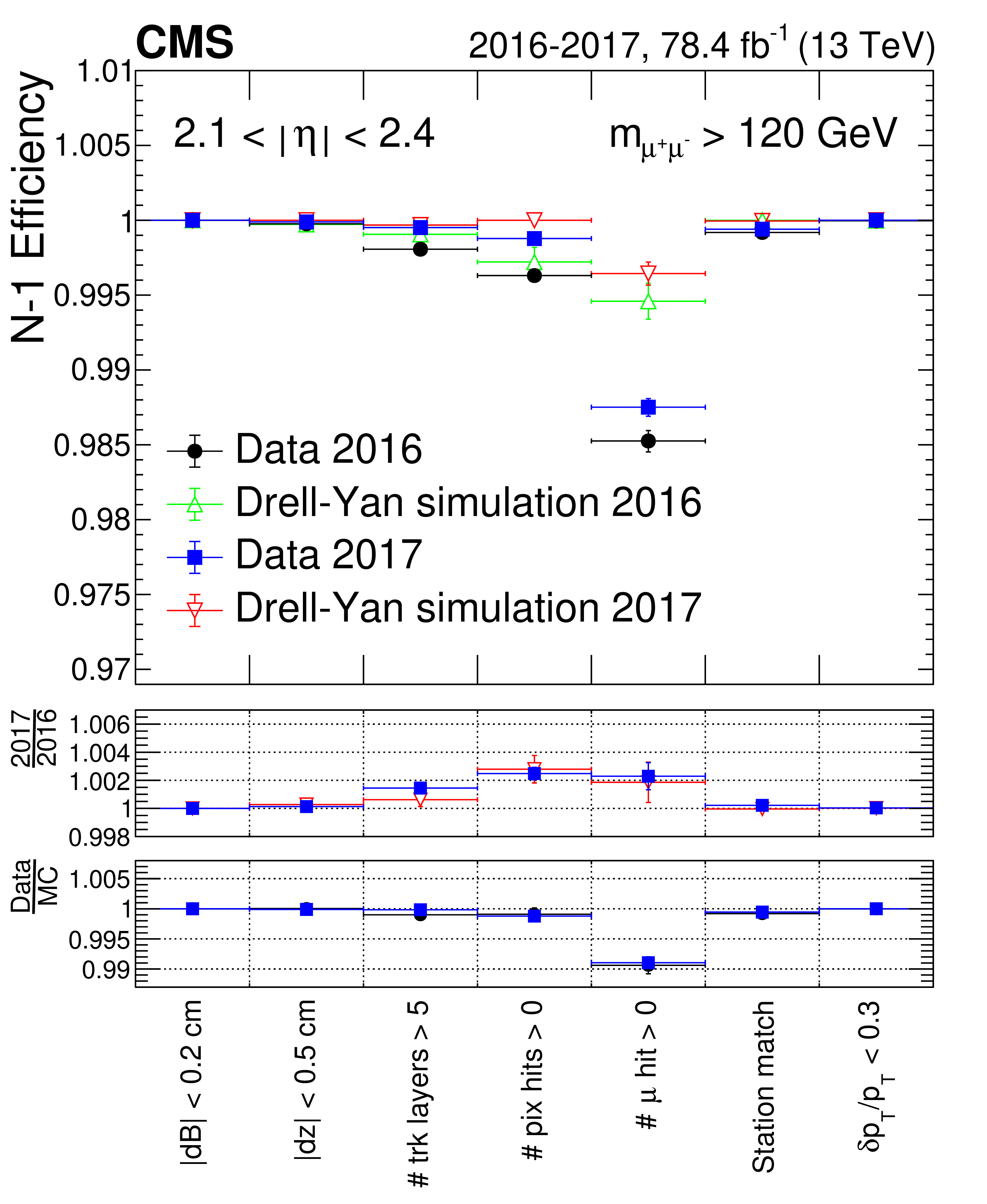
Figure 5:
The $N-1$ efficiencies, for $ {p_{\mathrm {T}}} > $ 53 GeV and binned in $\eta $, comparison between 2016 and 2017 data sets and for the corresponding DY simulations, for (upper left) $ {| \eta |} < $ 0.9, (upper right) 0.9 $ < {| \eta |} < $ 1.2, (lower left) 1.2 $ < {| \eta |} < $ 2.1, and (lower right) 2.1 $ < {| \eta |} < $ 2.4. The black circles represent 2016 data; the blue squares represent 2017 data. The lower panels display the ratio of $N-1$ efficiencies obtained for each of the criteria, between 2017 and 2016 data sets, and between data and their corresponding simulations for both years. |

png pdf |
Figure 5-a:
The $N-1$ efficiencies, for $ {p_{\mathrm {T}}} > $ 53 GeV and binned in $\eta $, comparison between 2016 and 2017 data sets and for the corresponding DY simulations, for $ {| \eta |} < $ 0.9. The black circles represent 2016 data; the blue squares represent 2017 data. The lower panels display the ratio of $N-1$ efficiencies obtained for each of the criteria, between 2017 and 2016 data sets, and between data and their corresponding simulations for both years. |
png pdf |
Figure 5-b:
The $N-1$ efficiencies, for $ {p_{\mathrm {T}}} > $ 53 GeV and binned in $\eta $, comparison between 2016 and 2017 data sets and for the corresponding DY simulations, for 0.9 $ < {| \eta |} < $ 1.2. The black circles represent 2016 data; the blue squares represent 2017 data. The lower panels display the ratio of $N-1$ efficiencies obtained for each of the criteria, between 2017 and 2016 data sets, and between data and their corresponding simulations for both years. |
png pdf |
Figure 5-c:
The $N-1$ efficiencies, for $ {p_{\mathrm {T}}} > $ 53 GeV and binned in $\eta $, comparison between 2016 and 2017 data sets and for the corresponding DY simulations, for 1.2 $ < {| \eta |} < $ 2.1. The black circles represent 2016 data; the blue squares represent 2017 data. The lower panels display the ratio of $N-1$ efficiencies obtained for each of the criteria, between 2017 and 2016 data sets, and between data and their corresponding simulations for both years. |
png pdf |
Figure 5-d:
The $N-1$ efficiencies, for $ {p_{\mathrm {T}}} > $ 53 GeV and binned in $\eta $, comparison between 2016 and 2017 data sets and for the corresponding DY simulations, for 2.1 $ < {| \eta |} < $ 2.4. The black circles represent 2016 data; the blue squares represent 2017 data. The lower panels display the ratio of $N-1$ efficiencies obtained for each of the criteria, between 2017 and 2016 data sets, and between data and their corresponding simulations for both years. |
png pdf |
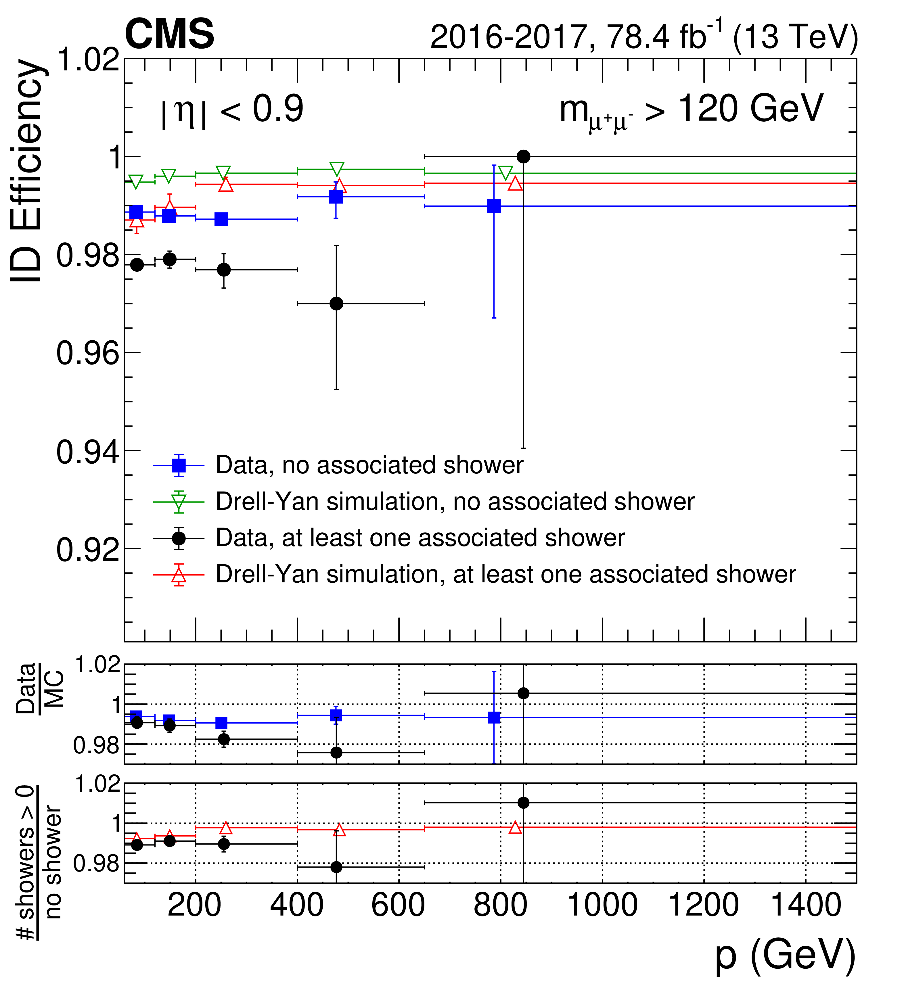
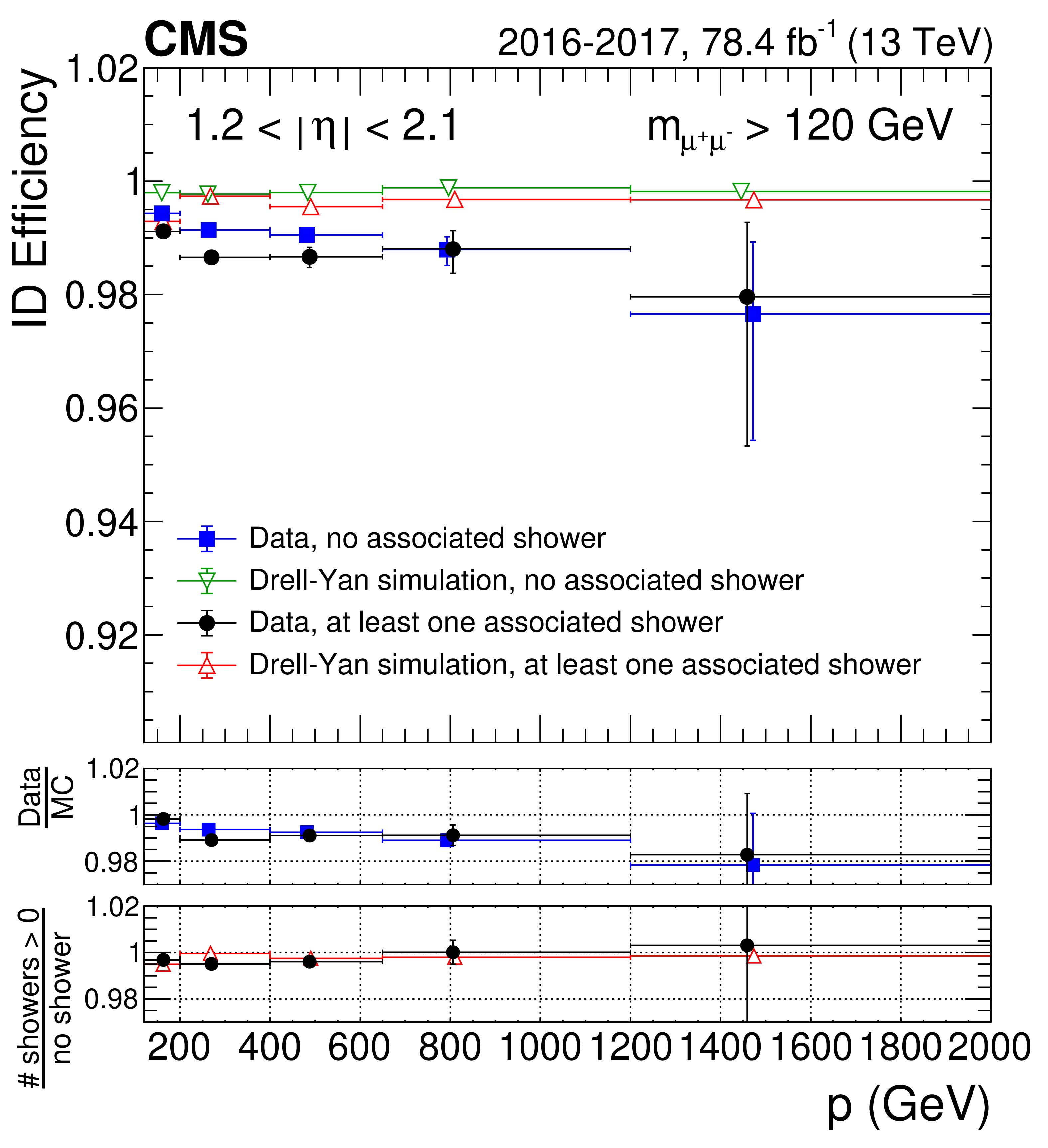
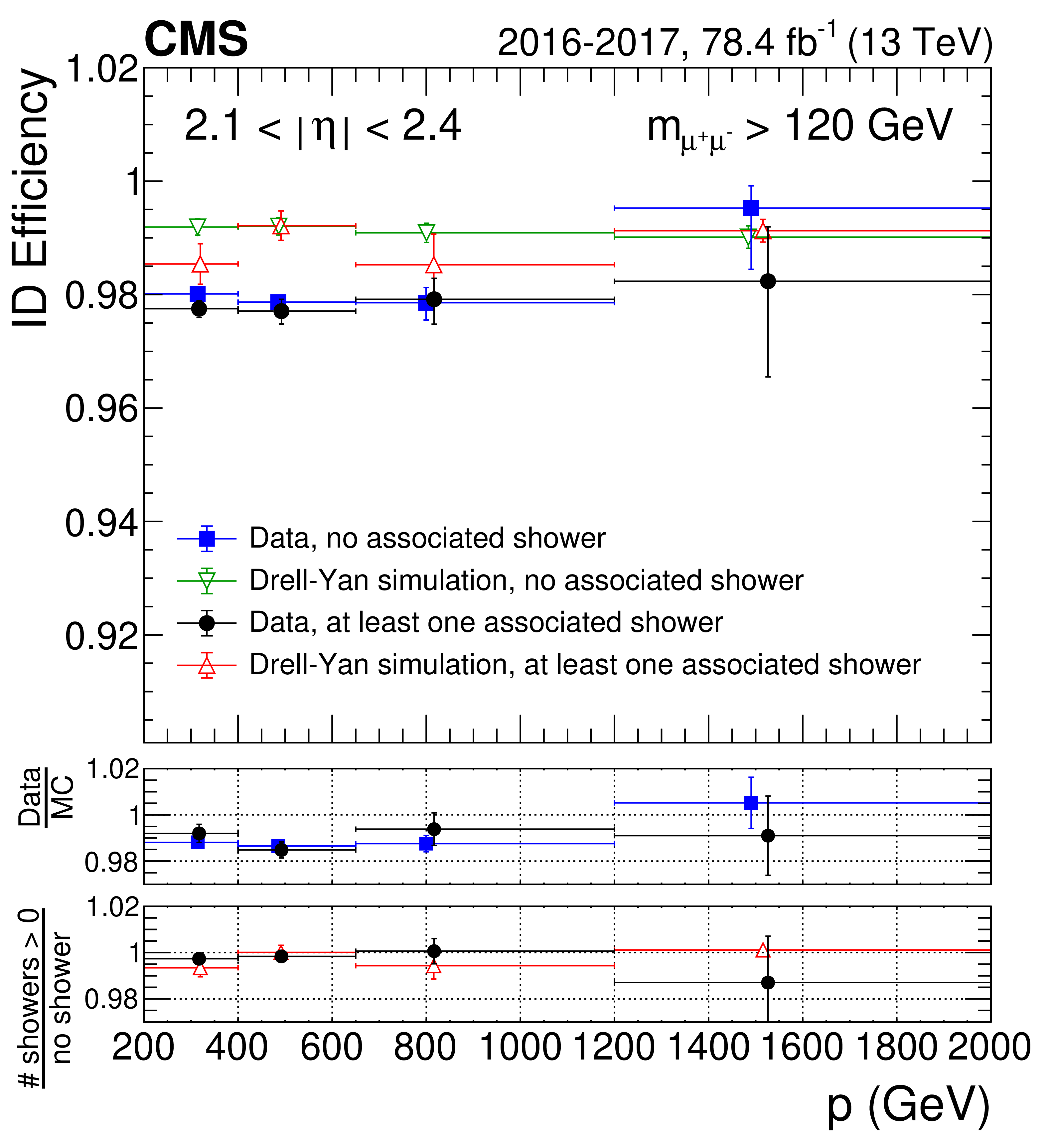
Figure 6:
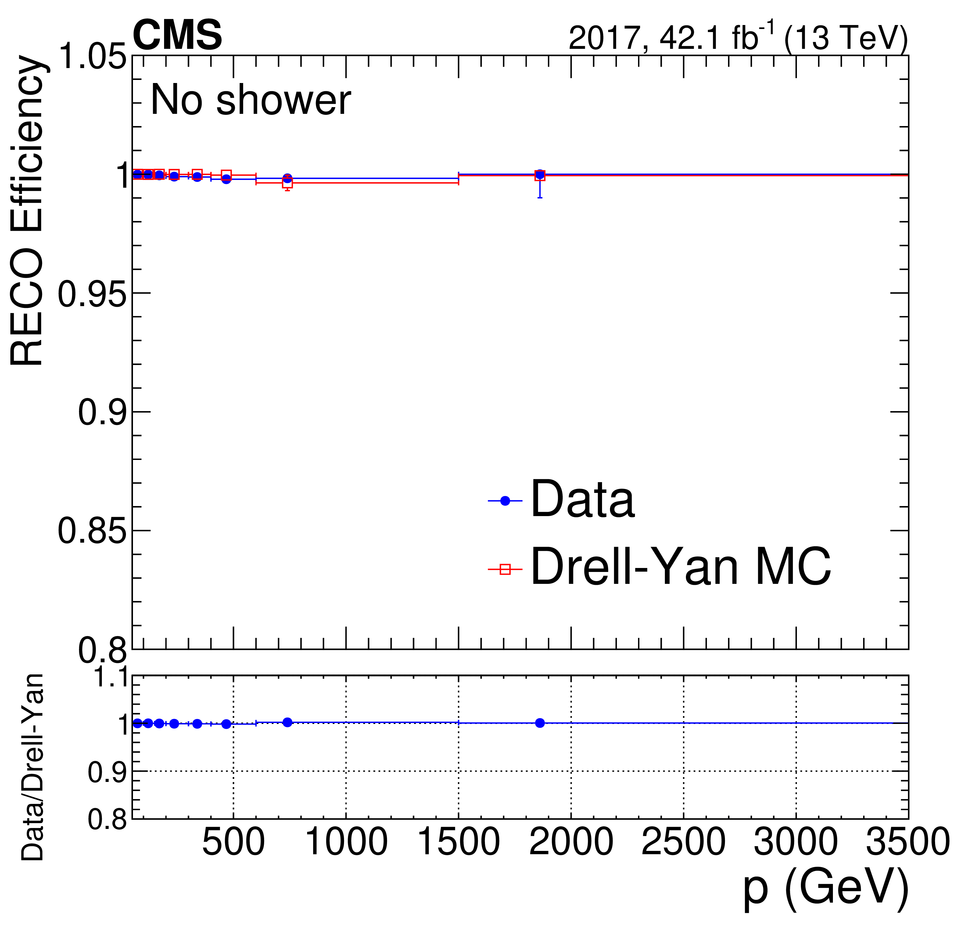
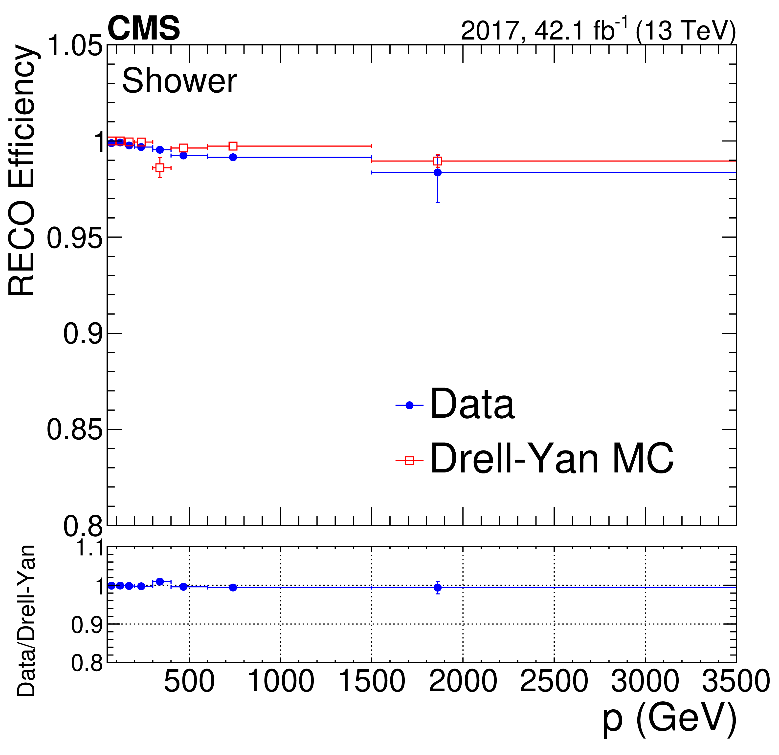
High-$ {p_{\mathrm {T}}}$ ID efficiency for 2016+2017 data, and corresponding DY simulation, as a function of $p$ for (upper left) $ {| \eta |} < $ 0.9, (upper right) 1.2 $ < {| \eta |} < $ 2.1, and (lower) 2.1 $ < {| \eta |} < $ 2.4. The blue squares show efficiency for muons in data with no showers tagged; the green inverted triangles show the same for muons in DY simulation. The black circles correspond to muons in data with at least one shower tag, while the red triangles are the same for muons in DY simulation. The central value in each bin is obtained from the average of the distribution within the bin. |
png pdf |
Figure 6-a:
High-$ {p_{\mathrm {T}}}$ ID efficiency for 2016+2017 data, and corresponding DY simulation, as a function of $p$ for $ {| \eta |} < $ 0.9. The blue squares show efficiency for muons in data with no showers tagged; the green inverted triangles show the same for muons in DY simulation. The black circles correspond to muons in data with at least one shower tag, while the red triangles are the same for muons in DY simulation. The central value in each bin is obtained from the average of the distribution within the bin. |
png pdf |
Figure 6-b:
High-$ {p_{\mathrm {T}}}$ ID efficiency for 2016+2017 data, and corresponding DY simulation, as a function of $p$ for 1.2 $ < {| \eta |} < $ 2.1. The blue squares show efficiency for muons in data with no showers tagged; the green inverted triangles show the same for muons in DY simulation. The black circles correspond to muons in data with at least one shower tag, while the red triangles are the same for muons in DY simulation. The central value in each bin is obtained from the average of the distribution within the bin. |
png pdf |
Figure 6-c:
High-$ {p_{\mathrm {T}}}$ ID efficiency for 2016+2017 data, and corresponding DY simulation, as a function of $p$ for 2.1 $ < {| \eta |} < $ 2.4. The blue squares show efficiency for muons in data with no showers tagged; the green inverted triangles show the same for muons in DY simulation. The black circles correspond to muons in data with at least one shower tag, while the red triangles are the same for muons in DY simulation. The central value in each bin is obtained from the average of the distribution within the bin. |

png pdf |
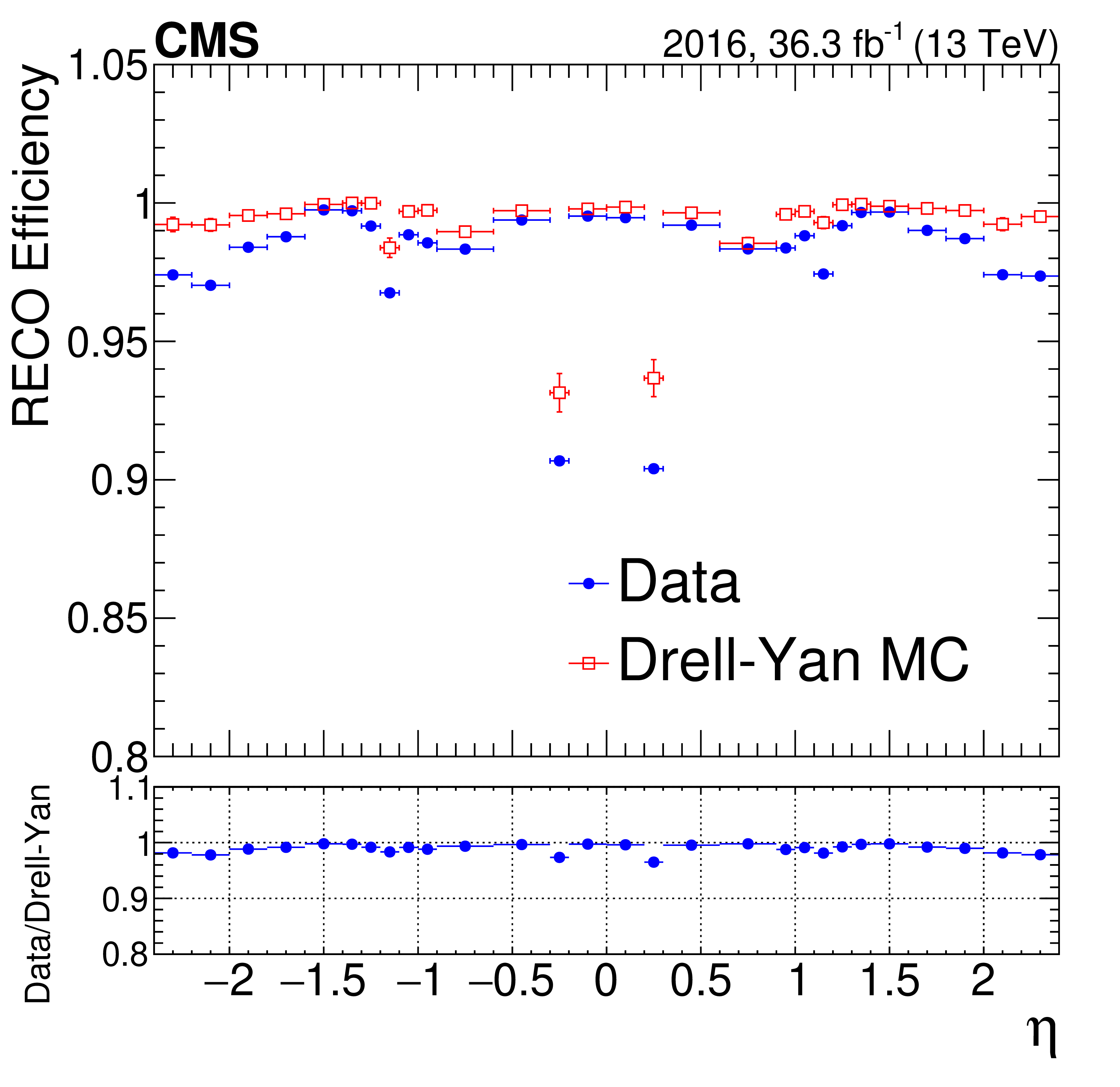
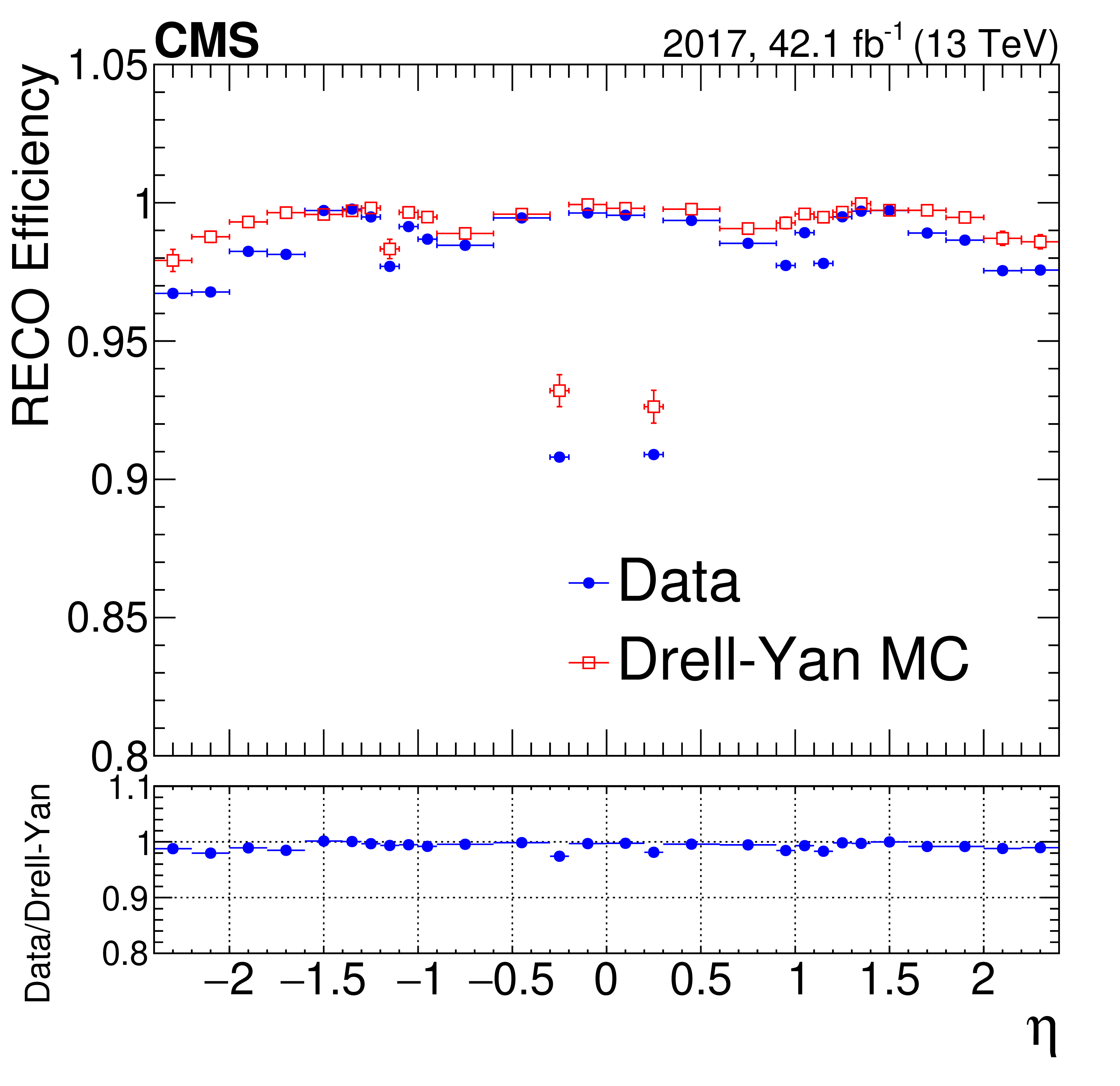
Figure 7:
Standalone muon reconstruction efficiency as a function of muon $\eta $ for the (left) 2016 and (right) 2017 data sets. The blue points represent the data, while the red empty squares represent the simulation. |
png pdf |
Figure 7-a:
Standalone muon reconstruction efficiency as a function of muon $\eta $ for the 2016 data set. The blue points represent the data, while the red empty squares represent the simulation. |
png pdf |
Figure 7-b:
Standalone muon reconstruction efficiency as a function of muon $\eta $ for the 2017 data set. The blue points represent the data, while the red empty squares represent the simulation. |

png pdf |
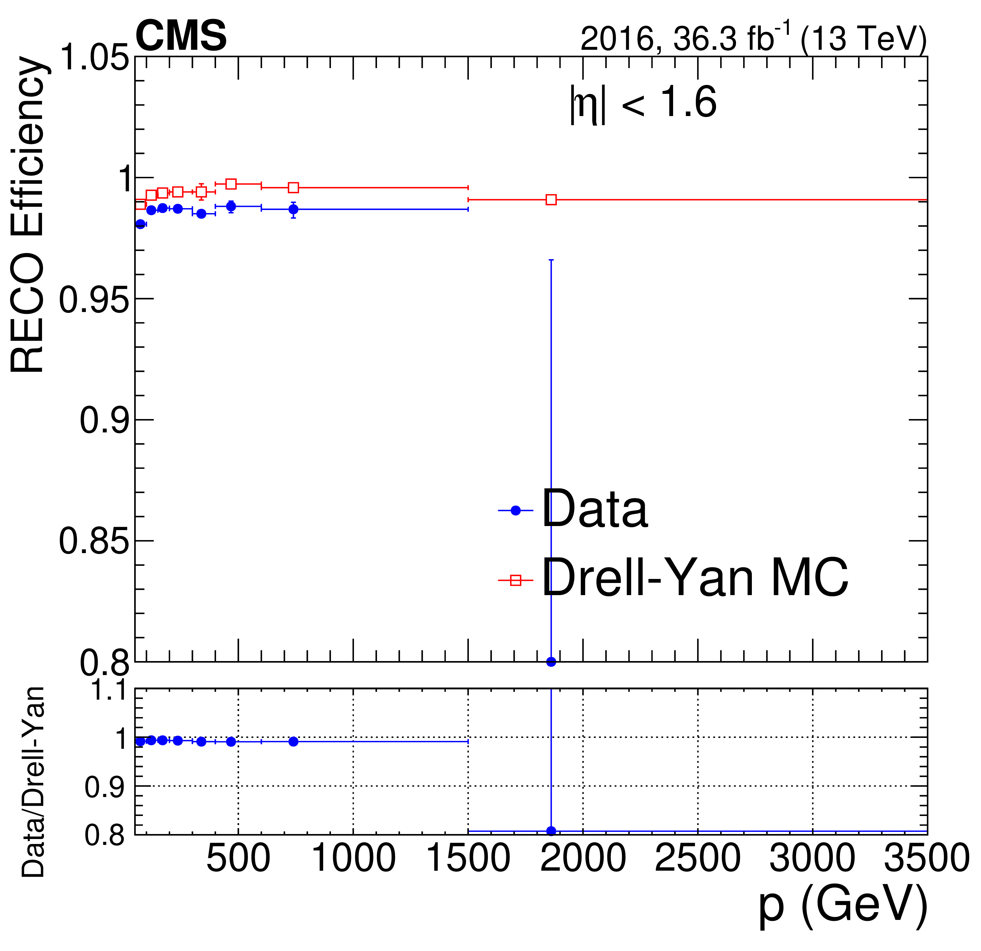
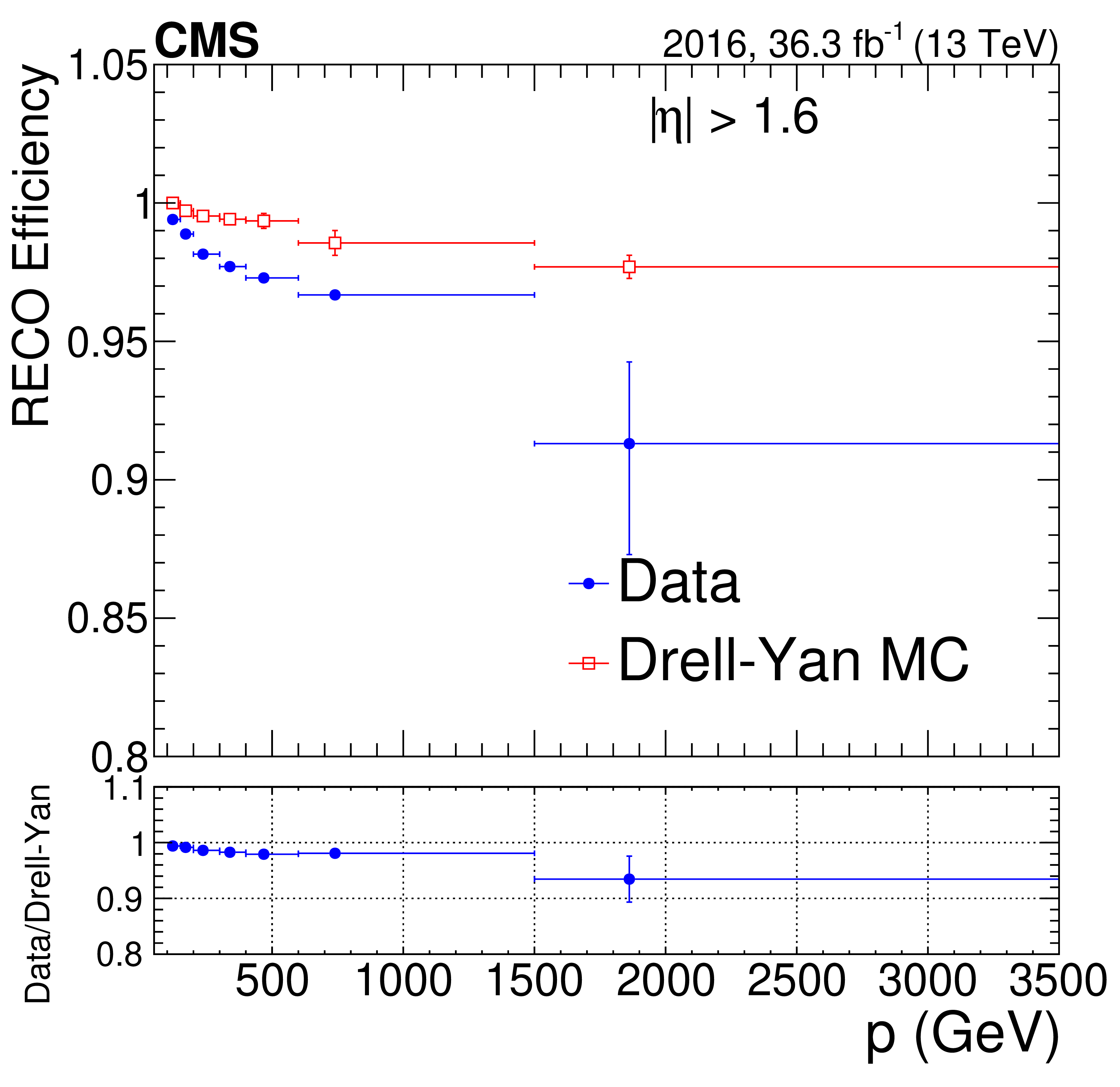
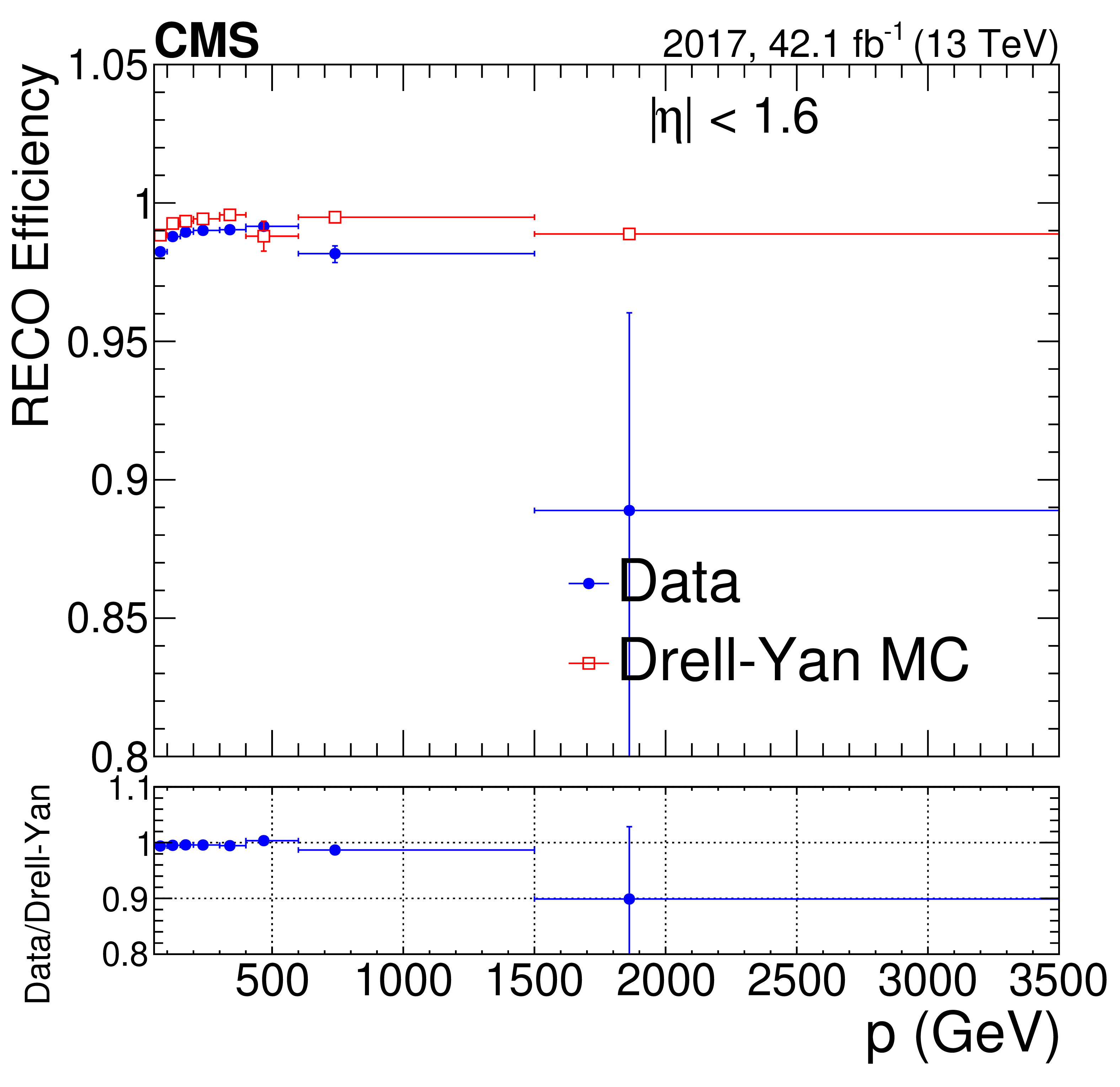
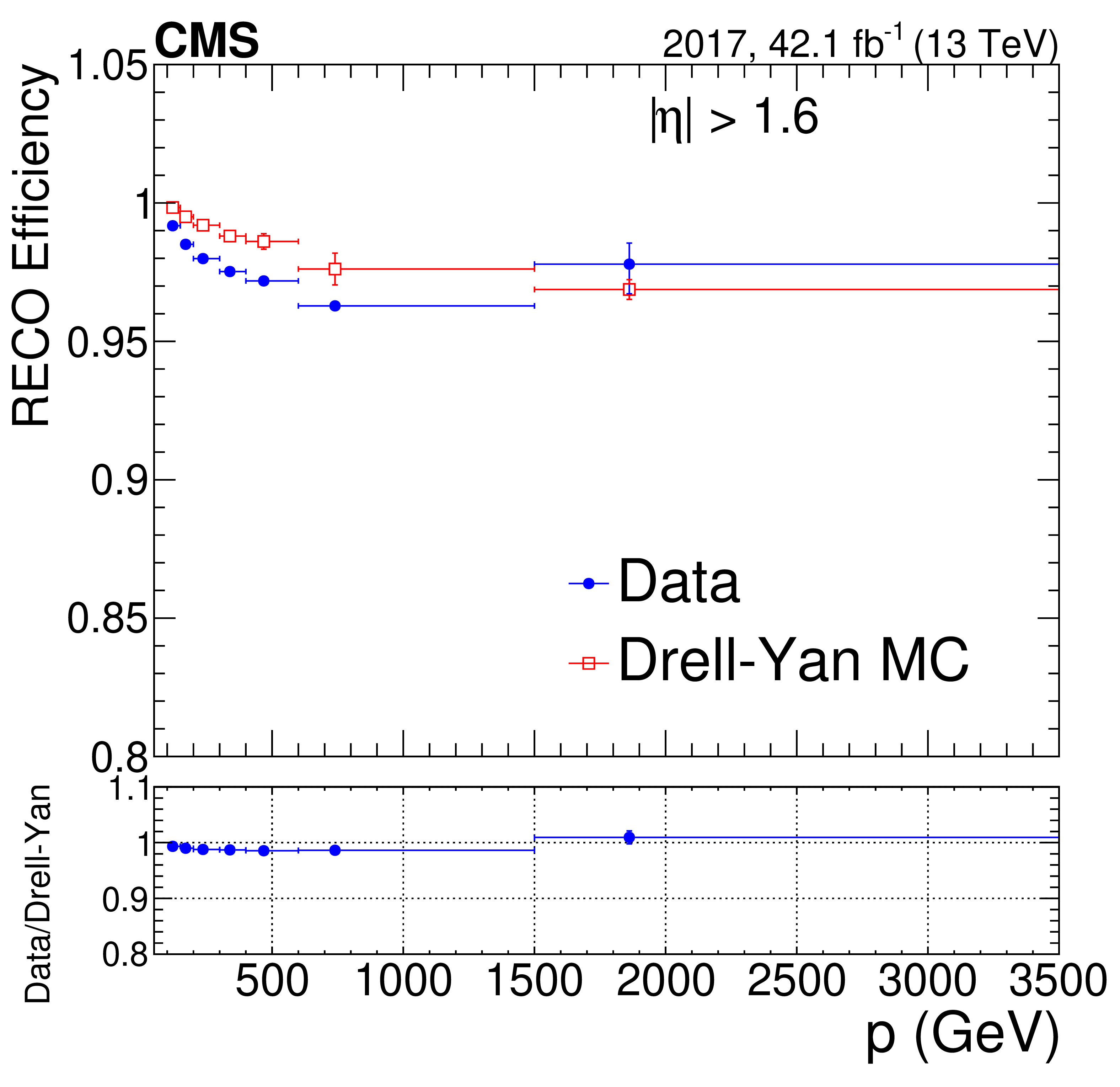
Figure 8:
Standalone muon reconstruction efficiency as a function of muon momentum in two different $ {| \eta |}$ regions: (left) $ {| \eta |} < $ 1.6, and (right) forward endcaps from, 1.6 $ < {| \eta |} < $ 2.4. The upper row shows the 2016 results, with blue points representing data and red empty squares representing simulation. The lower row shows the 2017 results. The lower panels of the plots show the ratio of data to simulation. The central value in each bin is obtained from the average of the distribution within the bin. |
png pdf |
Figure 8-a:
Standalone muon reconstruction efficiency as a function of muon momentum in the $ {| \eta |}$ region $ {| \eta |} < $ 1.6. The upper row shows the 2016 results, with blue points representing data and red empty squares representing simulation. The lower row shows the 2017 results. The lower panel of the plot shows the ratio of data to simulation. The central value in each bin is obtained from the average of the distribution within the bin. |
png pdf |
Figure 8-b:
Standalone muon reconstruction efficiency as a function of muon momentum in the $ {| \eta |}$ region 1.6 $ < {| \eta |} < $ 2.4. The upper row shows the 2016 results, with blue points representing data and red empty squares representing simulation. The lower row shows the 2017 results. The lower panel of the plot shows the ratio of data to simulation. The central value in each bin is obtained from the average of the distribution within the bin. |
png pdf |
Figure 8-c:
Standalone muon reconstruction efficiency as a function of muon momentum in two different $ {| \eta |}$ regions: (left) $ {| \eta |} < $ 1.6, and (right) forward endcaps from, 1.6 $ < {| \eta |} < $ 2.4. The upper row shows the 2016 results, with blue points representing data and red empty squares representing simulation. The lower row shows the 2017 results. The lower panels of the plots show the ratio of data to simulation. The central value in each bin is obtained from the average of the distribution within the bin. |
png pdf |
Figure 8-d:
Standalone muon reconstruction efficiency as a function of muon momentum in two different $ {| \eta |}$ regions: (left) $ {| \eta |} < $ 1.6, and (right) forward endcaps from, 1.6 $ < {| \eta |} < $ 2.4. The upper row shows the 2016 results, with blue points representing data and red empty squares representing simulation. The lower row shows the 2017 results. The lower panels of the plots show the ratio of data to simulation. The central value in each bin is obtained from the average of the distribution within the bin. |
png pdf |
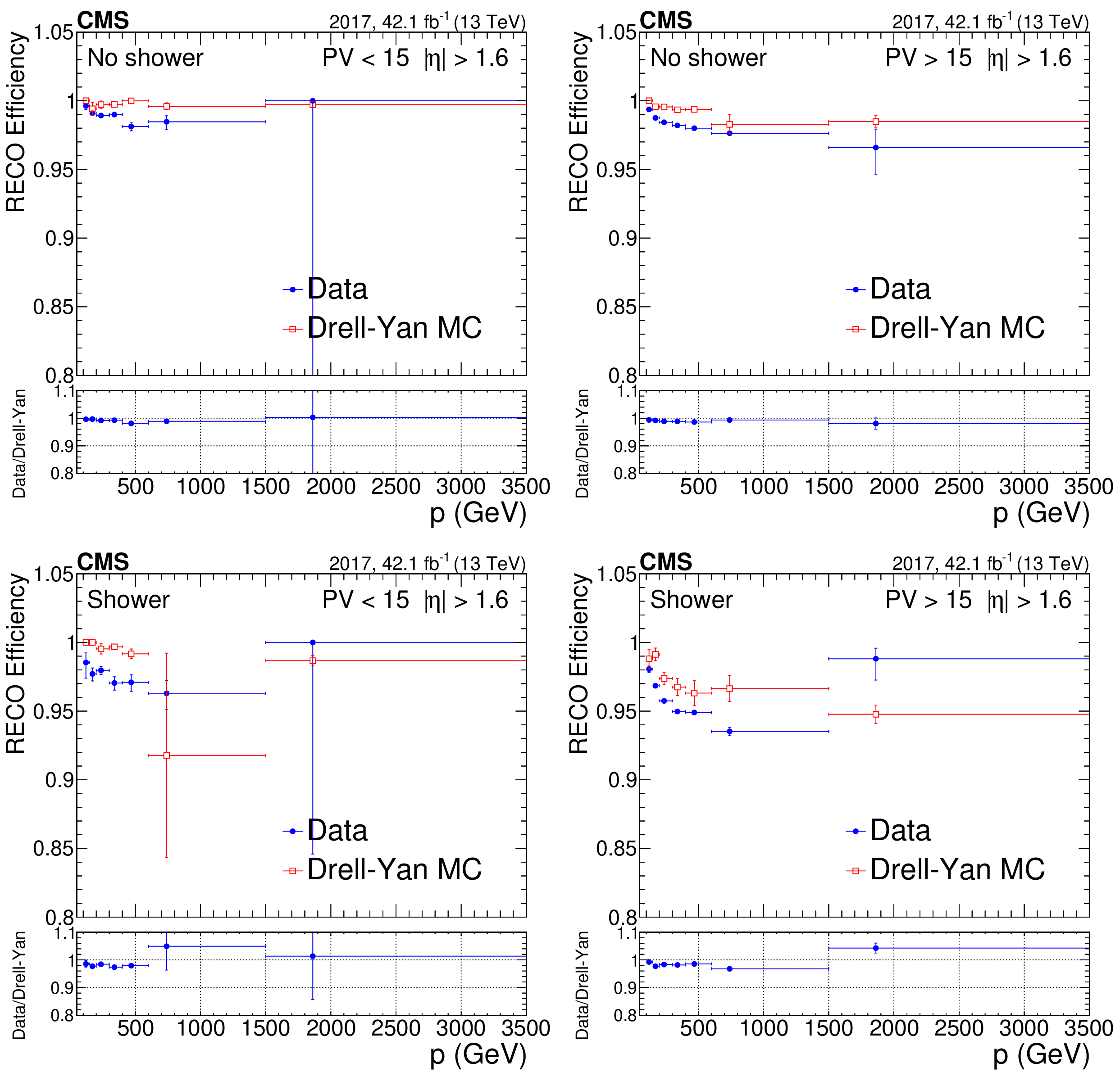
Figure 9:
Standalone muon reconstruction efficiency as a function of muon $p$ for muons with 1.6 $ < {| \eta |} < $ 2.4. The left plots are for low pileup (up to 15 vertices) while the right plots are for higher pileup. The upper plots are obtained with events without any showers; the lower ones contain events with at least one shower. The blue points represent data and the red empty squares represent simulation. The lower panels of the plots show the ratio of data to simulation. The central value in each bin is obtained from the average of the distribution within the bin. |
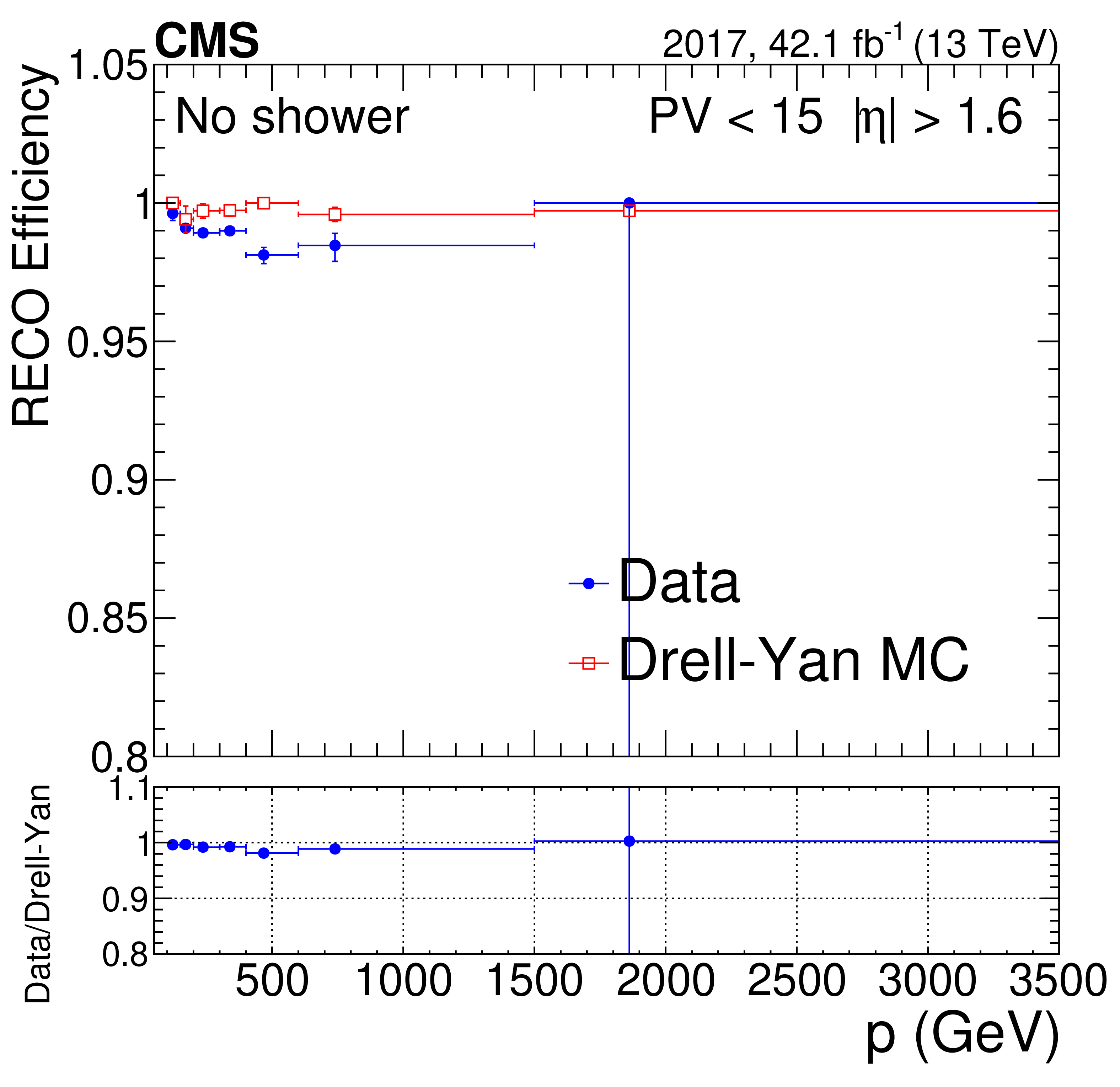
png pdf |
Figure 9-a:
Standalone muon reconstruction efficiency as a function of muon $p$ for muons with 1.6 $ < {| \eta |} < $ 2.4 for low pileup (up to 15 vertices). The plot is obtained with events without any showers. The blue points represent data and the red empty squares represent simulation. The lower panel of the plot shows the ratio of data to simulation. The central value in each bin is obtained from the average of the distribution within the bin. |
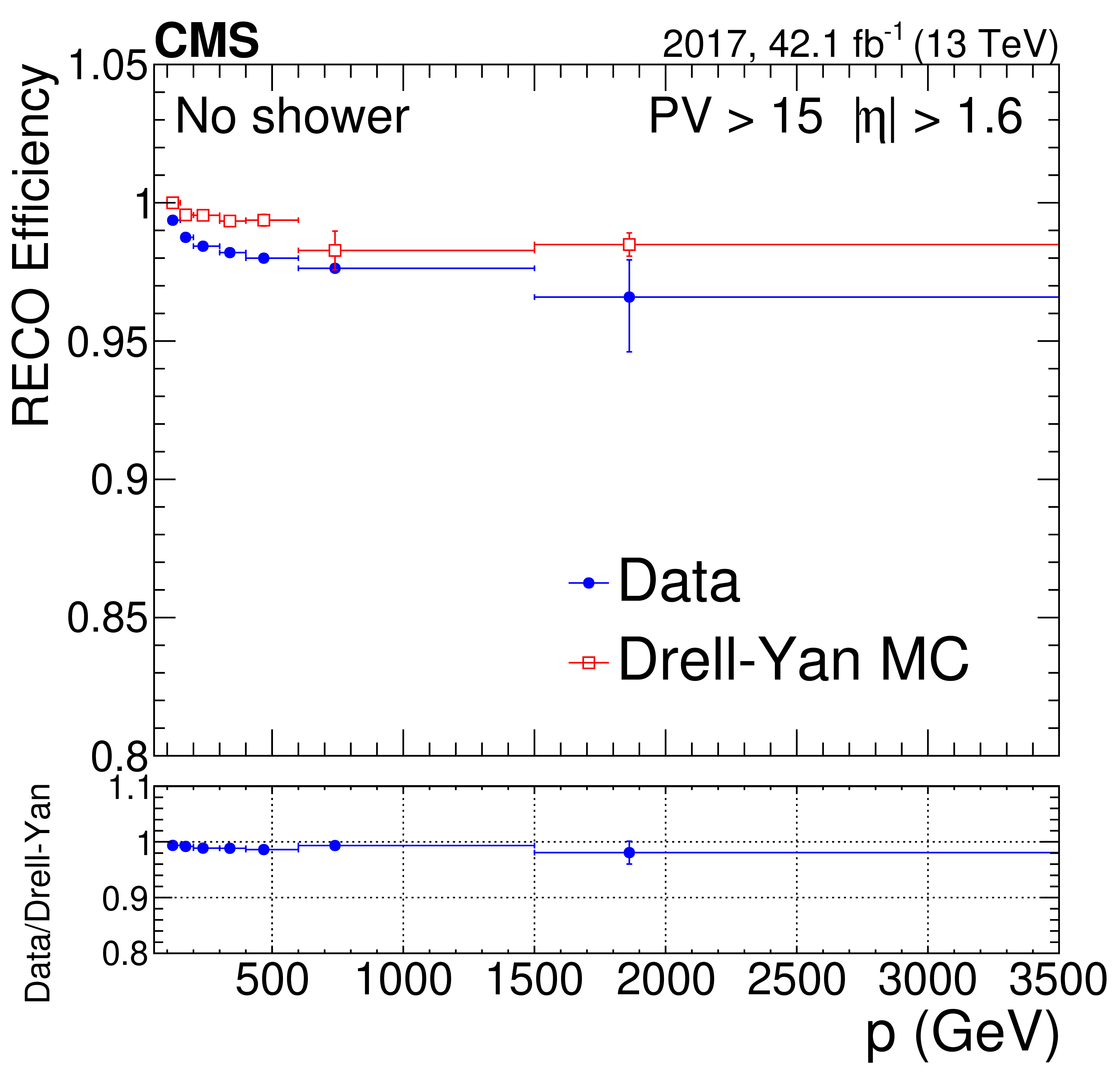
png pdf |
Figure 9-b:
Standalone muon reconstruction efficiency as a function of muon $p$ for muons with 1.6 $ < {| \eta |} < $ 2.4 for high pileup (higher than 15 vertices). The plot is obtained with events without any showers. The blue points represent data and the red empty squares represent simulation. The lower panel of the plot shows the ratio of data to simulation. The central value in each bin is obtained from the average of the distribution within the bin. |
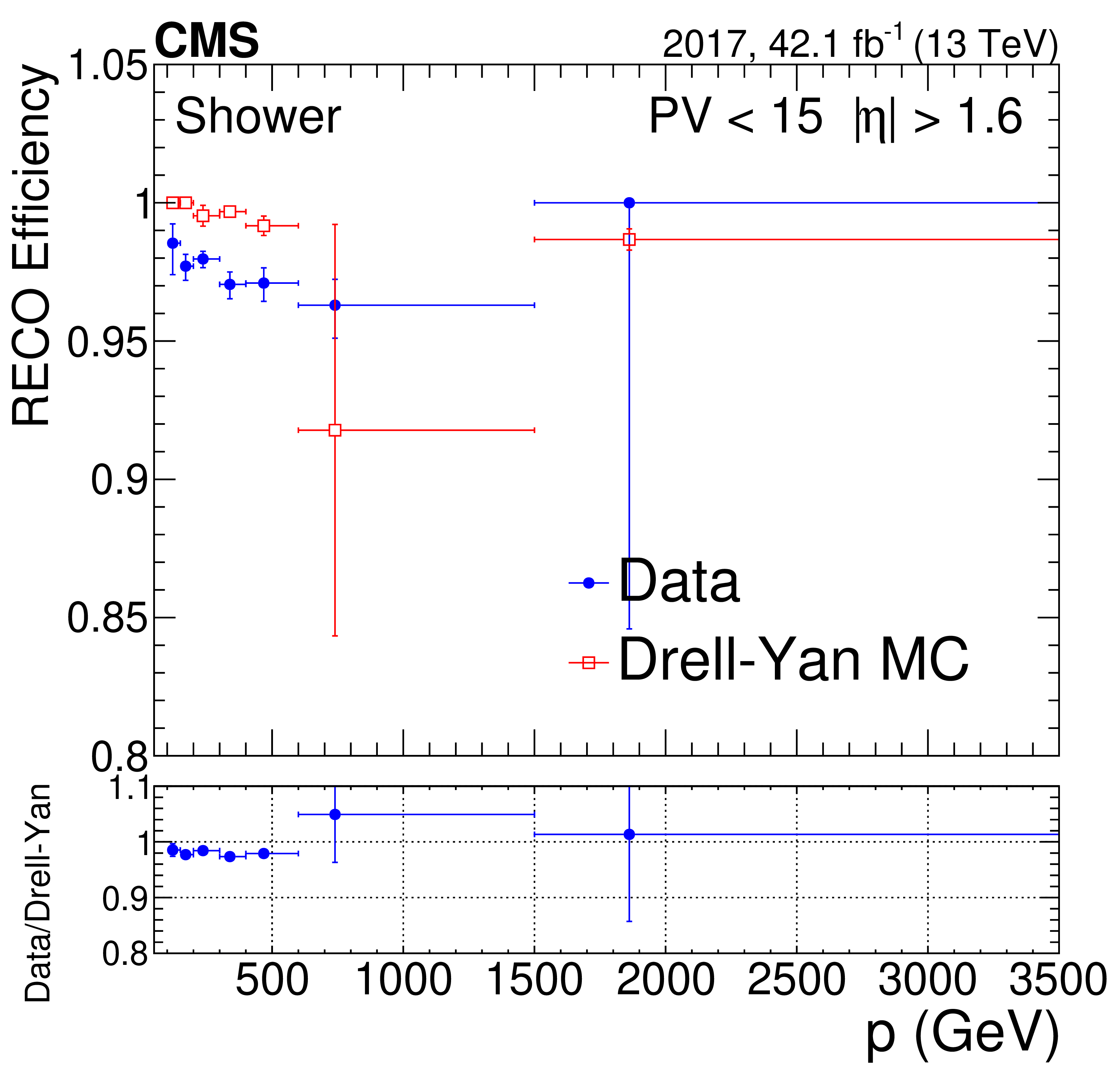
png pdf |
Figure 9-c:
Standalone muon reconstruction efficiency as a function of muon $p$ for muons with 1.6 $ < {| \eta |} < $ 2.4 for low pileup (up to 15 vertices). The plot contains events with at least one shower. The blue points represent data and the red empty squares represent simulation. The lower panel of the plot shows the ratio of data to simulation. The central value in each bin is obtained from the average of the distribution within the bin. |
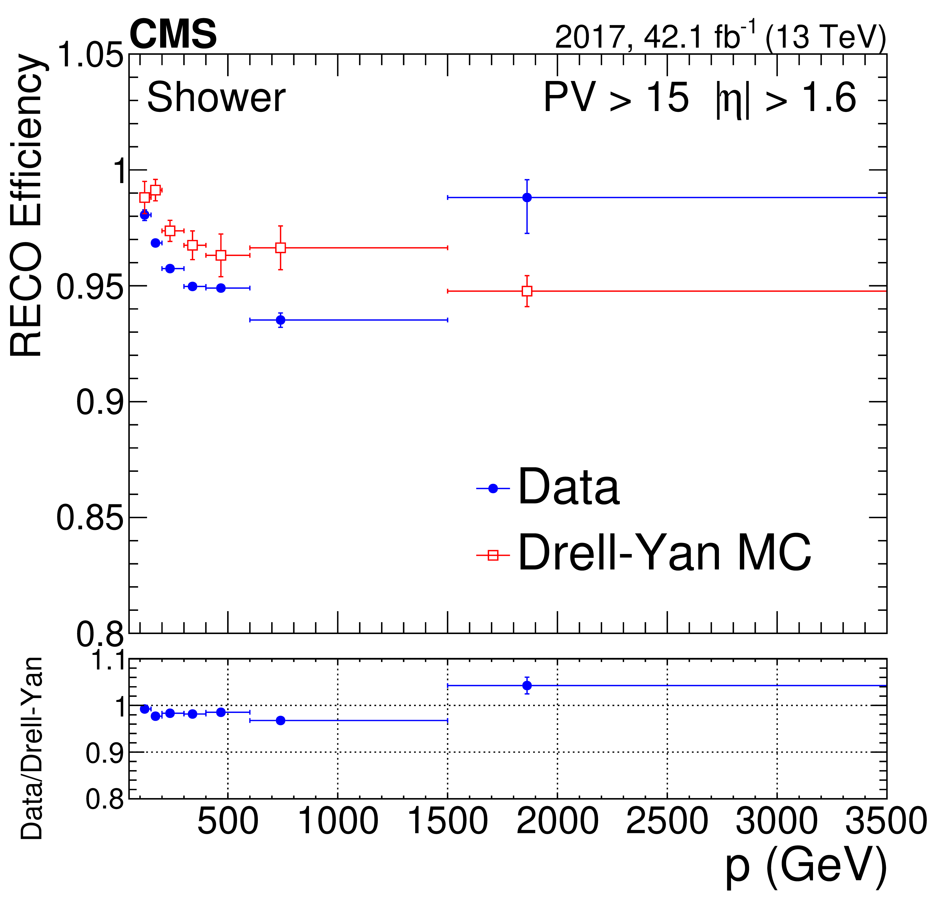
png pdf |
Figure 9-d:
Standalone muon reconstruction efficiency as a function of muon $p$ for muons with 1.6 $ < {| \eta |} < $ 2.4 for high pileup (higher than 15 vertices). The plot contains events with at least one shower. The blue points represent data and the red empty squares represent simulation. The lower panel of the plot shows the ratio of data to simulation. The central value in each bin is obtained from the average of the distribution within the bin. |

png pdf |
Figure 10:
Global muon reconstruction efficiency as a function of muon momentum. The left plot is obtained with events without any showers, while the right one contains events with at least one shower. The blue points represent data and the red empty squares represent simulation. The lower panels of the plots show the ratio of data to simulation. The central value in each bin is obtained from the average of the distribution within the bin. |
png pdf |
Figure 10-a:
Global muon reconstruction efficiency as a function of muon momentum. The plot is obtained with events without any showers. The blue points represent data and the red empty squares represent simulation. The lower panel shows the ratio of data to simulation. The central value in each bin is obtained from the average of the distribution within the bin. |
png pdf |
Figure 10-b:
Global muon reconstruction efficiency as a function of muon momentum. The plot contains events with at least one shower. The blue points represent data and the red empty squares represent simulation. The lower panel shows the ratio of data to simulation. The central value in each bin is obtained from the average of the distribution within the bin. |
png pdf |
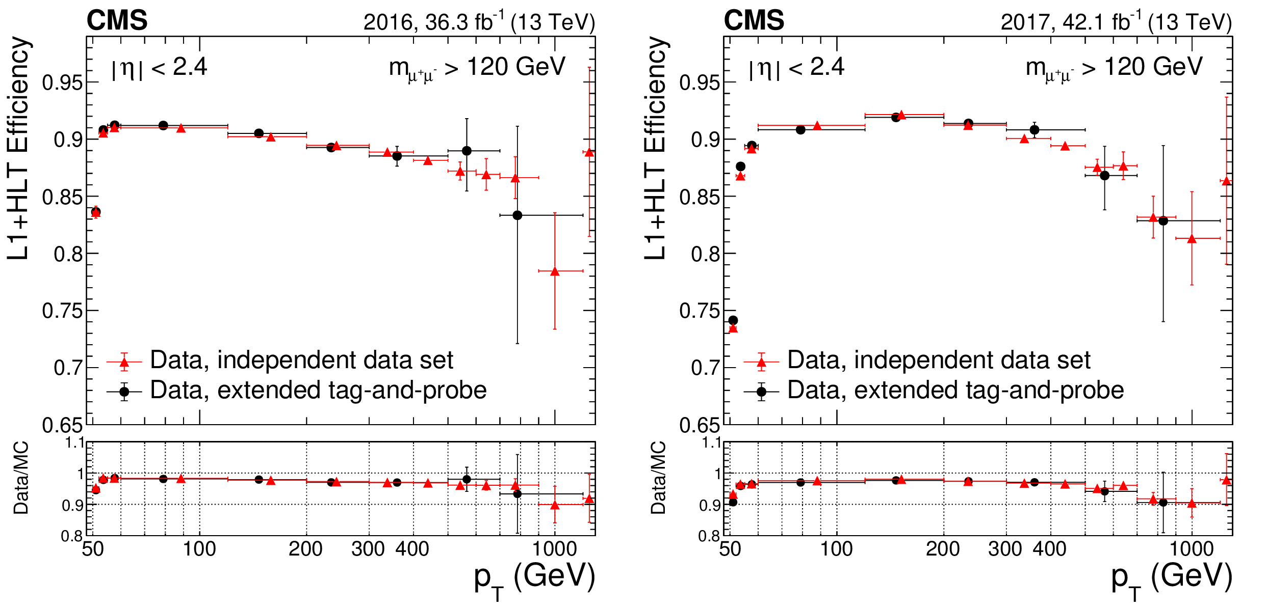
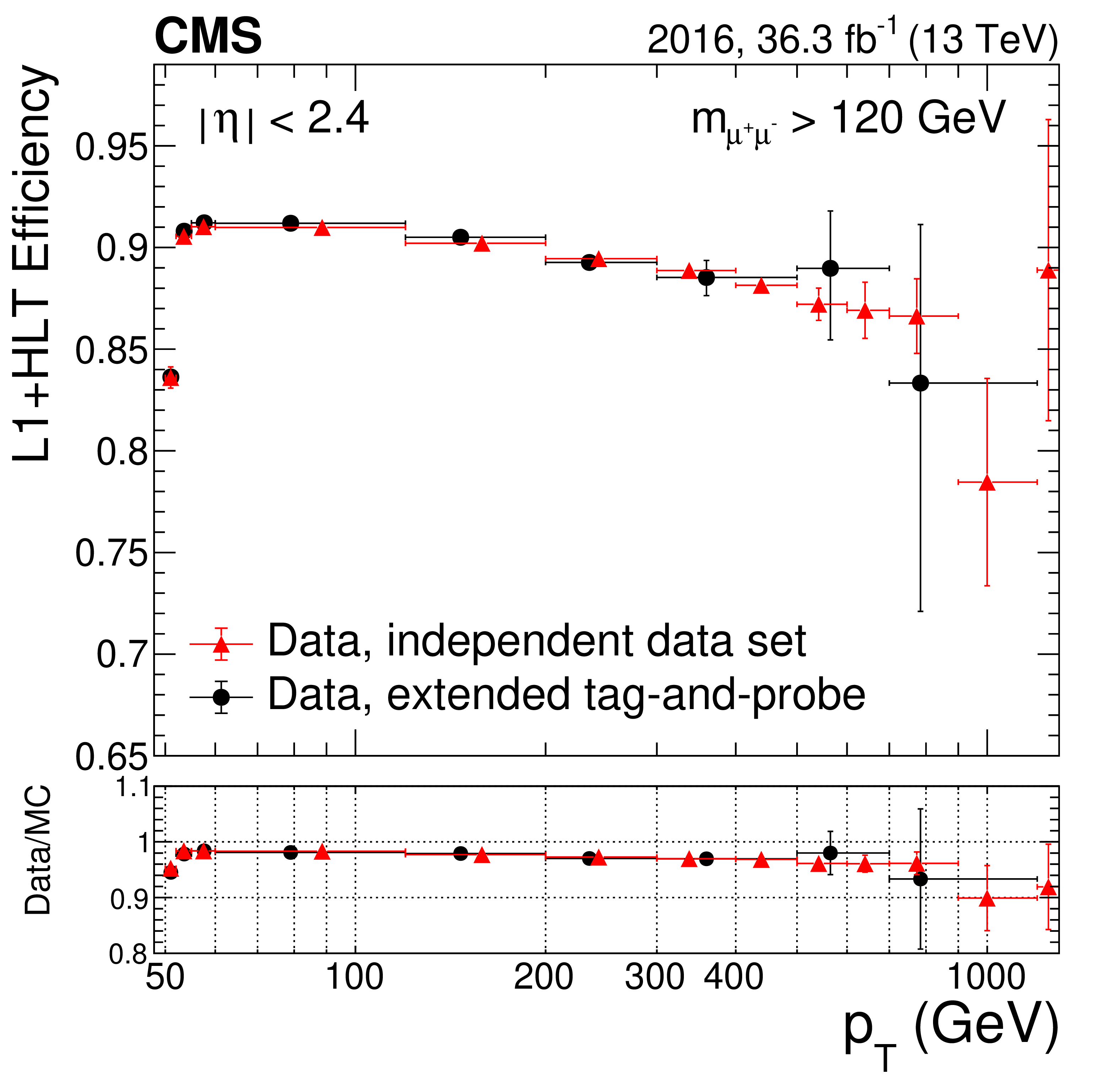
Figure 11:
The combined HLT+L1 efficiency with respect to the offline selection, and the ratio of data to simulation for different methods, as functions of ${p_{\mathrm {T}}}$, for (left) 2016 data and (right) 2017 data. The red triangles are measured using an independent data set collected with a ${{p_{\mathrm {T}}} ^\text {miss}}$ trigger; the black circles are measured by the extended tag-and-probe method in which selected events have $m_{\mu \mu} > $ 120 GeV. The central value in each bin is obtained from the average of the distribution within the bin. |
png pdf |
Figure 11-a:
The combined HLT+L1 efficiency with respect to the offline selection, and the ratio of data to simulation for different methods, as functions of ${p_{\mathrm {T}}}$, for (left) 2016 data and (right) 2017 data. The red triangles are measured using an independent data set collected with a ${{p_{\mathrm {T}}} ^\text {miss}}$ trigger; the black circles are measured by the extended tag-and-probe method in which selected events have $m_{\mu \mu} > $ 120 GeV. The central value in each bin is obtained from the average of the distribution within the bin. |
png pdf |
Figure 11-b:
The combined HLT+L1 efficiency with respect to the offline selection, and the ratio of data to simulation for different methods, as functions of ${p_{\mathrm {T}}}$, for (left) 2016 data and (right) 2017 data. The red triangles are measured using an independent data set collected with a ${{p_{\mathrm {T}}} ^\text {miss}}$ trigger; the black circles are measured by the extended tag-and-probe method in which selected events have $m_{\mu \mu} > $ 120 GeV. The central value in each bin is obtained from the average of the distribution within the bin. |
png pdf |
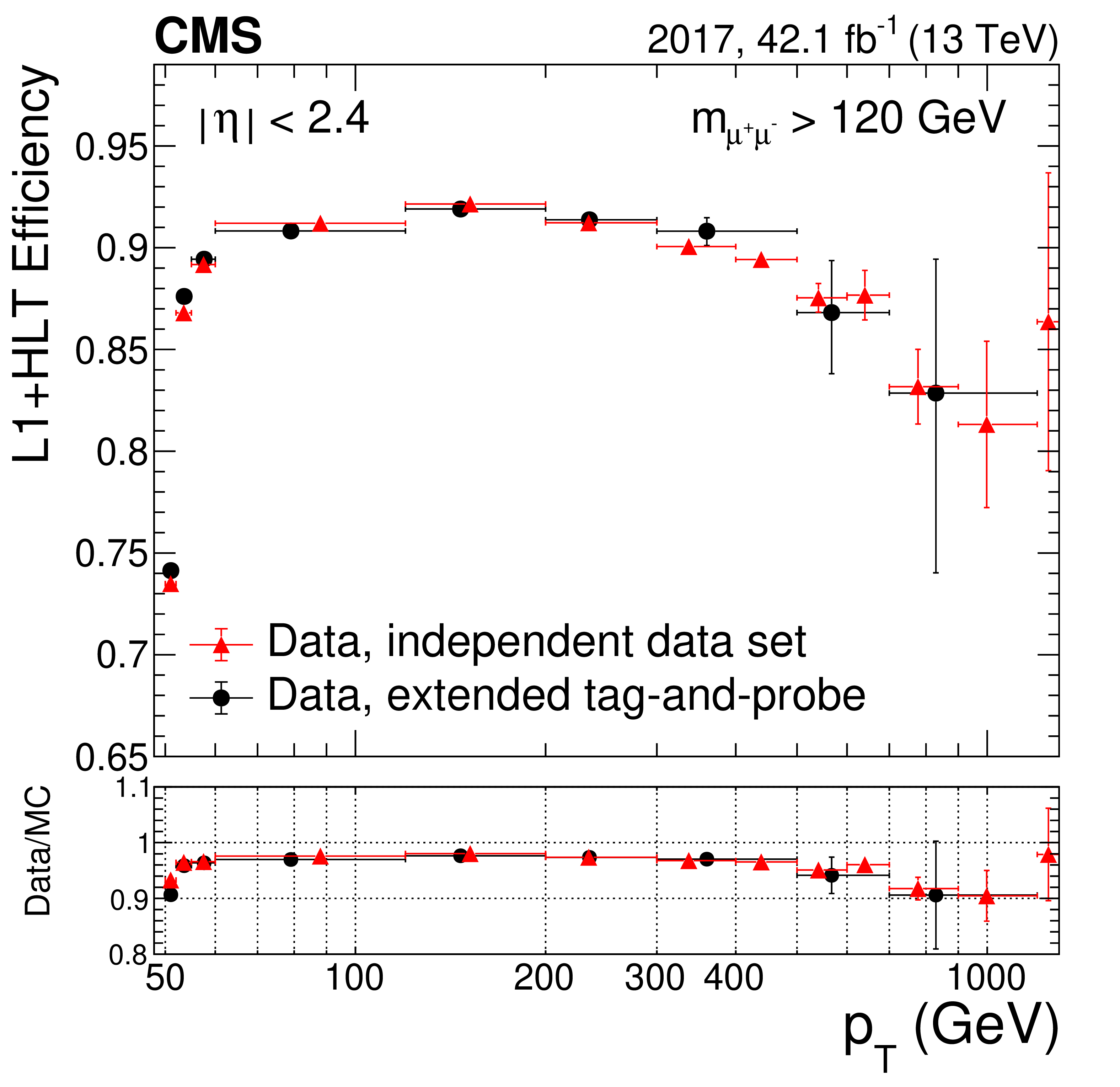
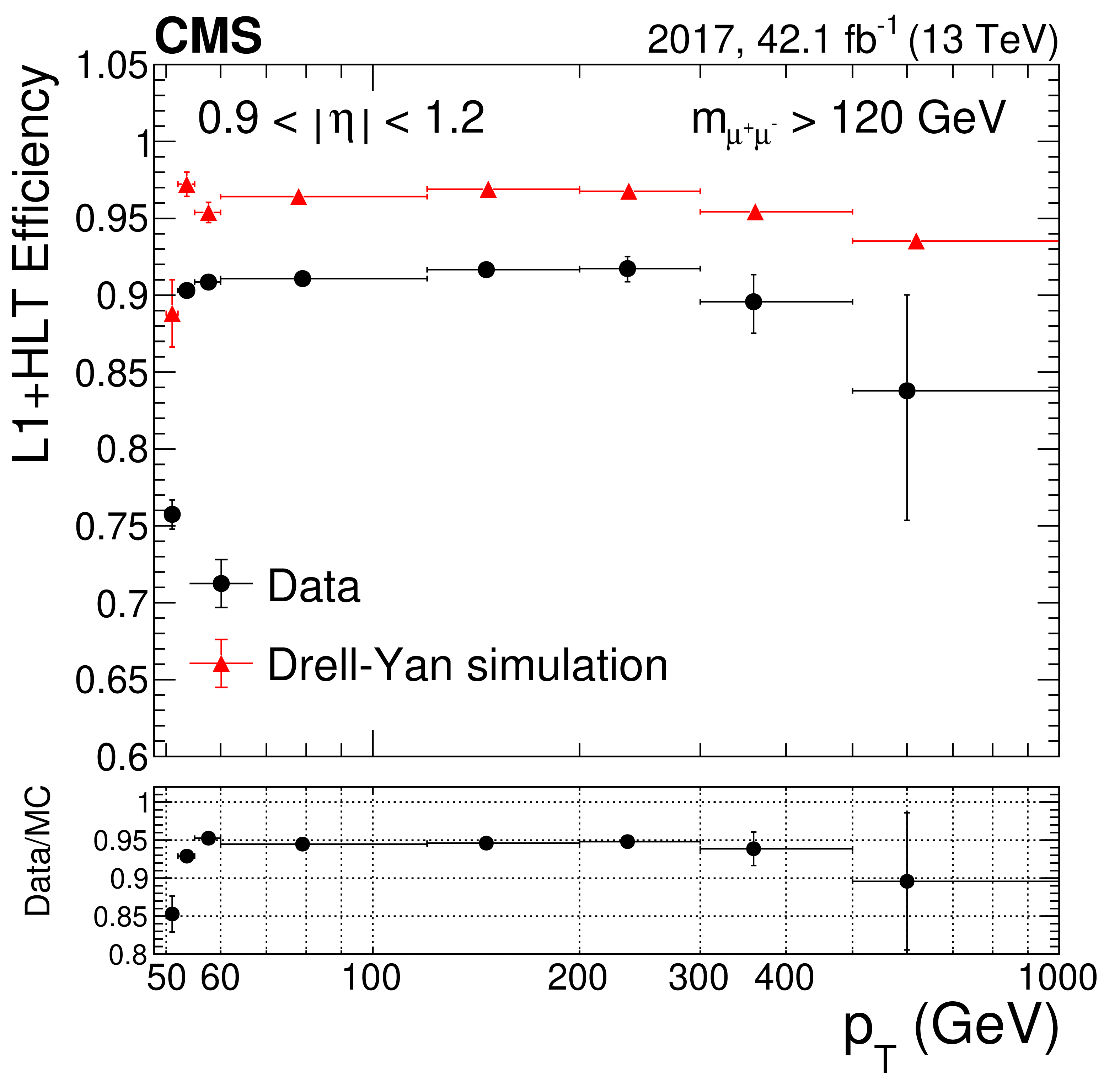
Figure 12:
The combined HLT+L1 efficiency with respect to the offline selection, and the ratio of data to simulation, as a function of ${p_{\mathrm {T}}}$, for (upper) 2016 data and (lower) 2017 data and simulation. The left plots are for the barrel region and the right plots are for the overlap region. The red triangles represent the simulation while the black dots are the data. The lower panels display the ratio of efficiencies in data and simulation. The central value in each bin is obtained from the average of the distribution within the bin. |

png pdf |
Figure 12-a:
The combined HLT+L1 efficiency with respect to the offline selection, and the ratio of data to simulation, as a function of ${p_{\mathrm {T}}}$, for 2016 data and simulation. The plot is for the barrel region. The red triangles represent the simulation while the black dots are the data. The lower panel displays the ratio of efficiencies in data and simulation. The central value in each bin is obtained from the average of the distribution within the bin. |
png pdf |
Figure 12-b:
The combined HLT+L1 efficiency with respect to the offline selection, and the ratio of data to simulation, as a function of ${p_{\mathrm {T}}}$, for 2016 data and simulation. The plot is for the overlap region. The red triangles represent the simulation while the black dots are the data. The lower panel displays the ratio of efficiencies in data and simulation. The central value in each bin is obtained from the average of the distribution within the bin. |
png pdf |
Figure 12-c:
The combined HLT+L1 efficiency with respect to the offline selection, and the ratio of data to simulation, as a function of ${p_{\mathrm {T}}}$, for 2017 data and simulation. The plot is for the barrel region. The red triangles represent the simulation while the black dots are the data. The lower panel displays the ratio of efficiencies in data and simulation. The central value in each bin is obtained from the average of the distribution within the bin. |
png pdf |
Figure 12-d:
The combined HLT+L1 efficiency with respect to the offline selection, and the ratio of data to simulation, as a function of ${p_{\mathrm {T}}}$, for 2017 data and simulation. The plot is for the overlap region. The red triangles represent the simulation while the black dots are the data. The lower panel displays the ratio of efficiencies in data and simulation. The central value in each bin is obtained from the average of the distribution within the bin. |
png pdf |
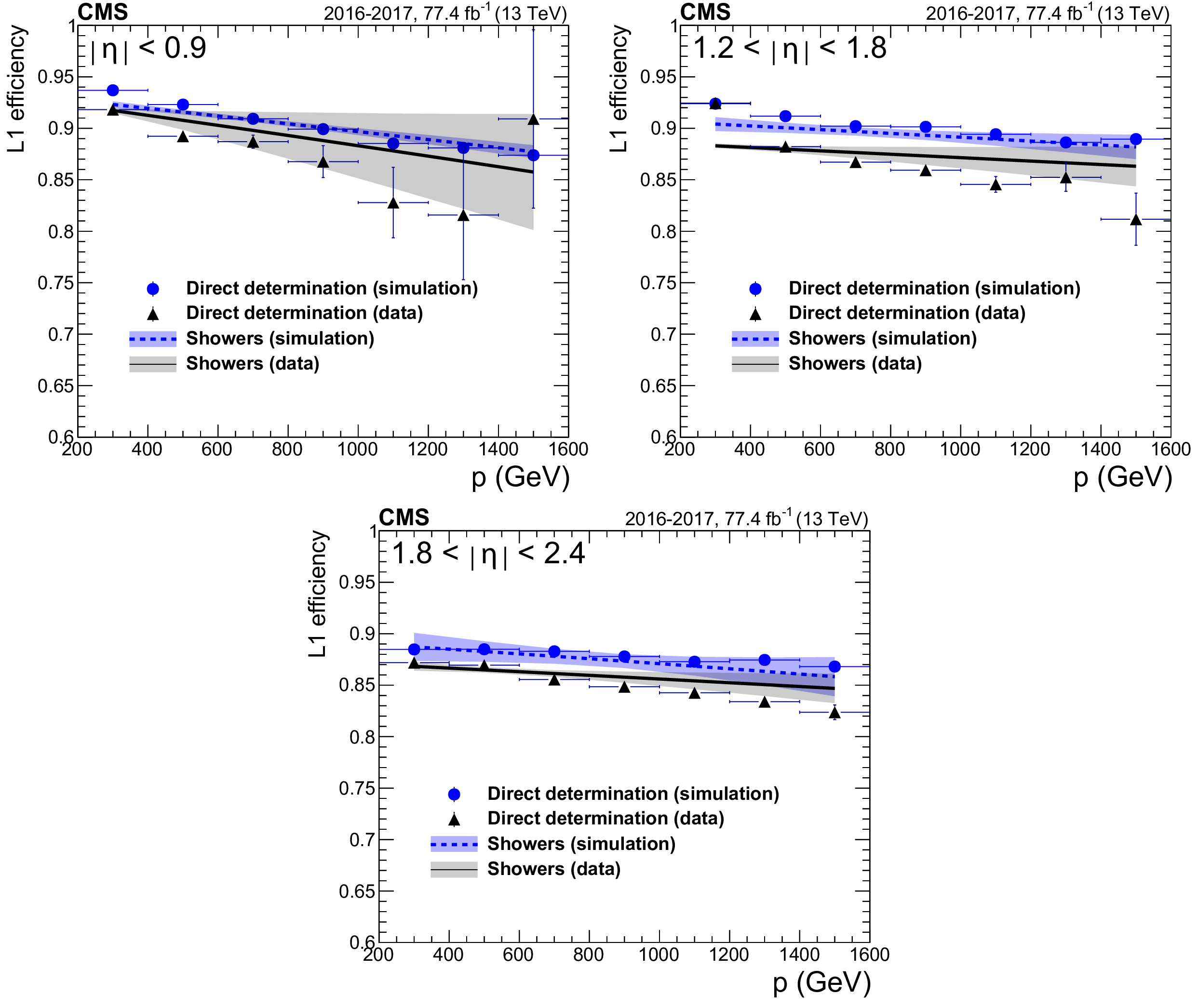
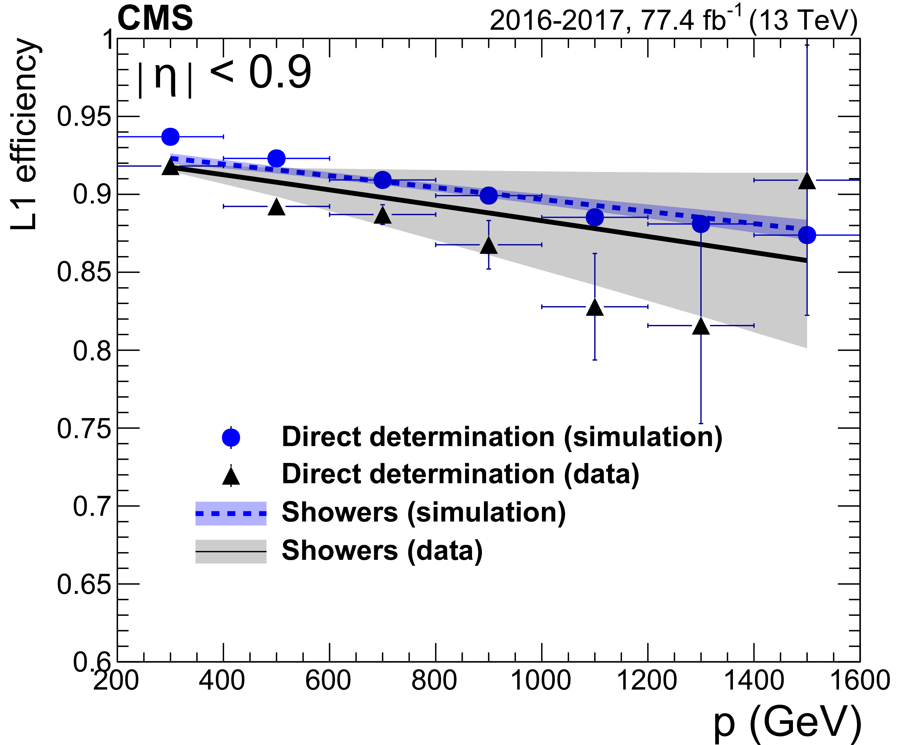
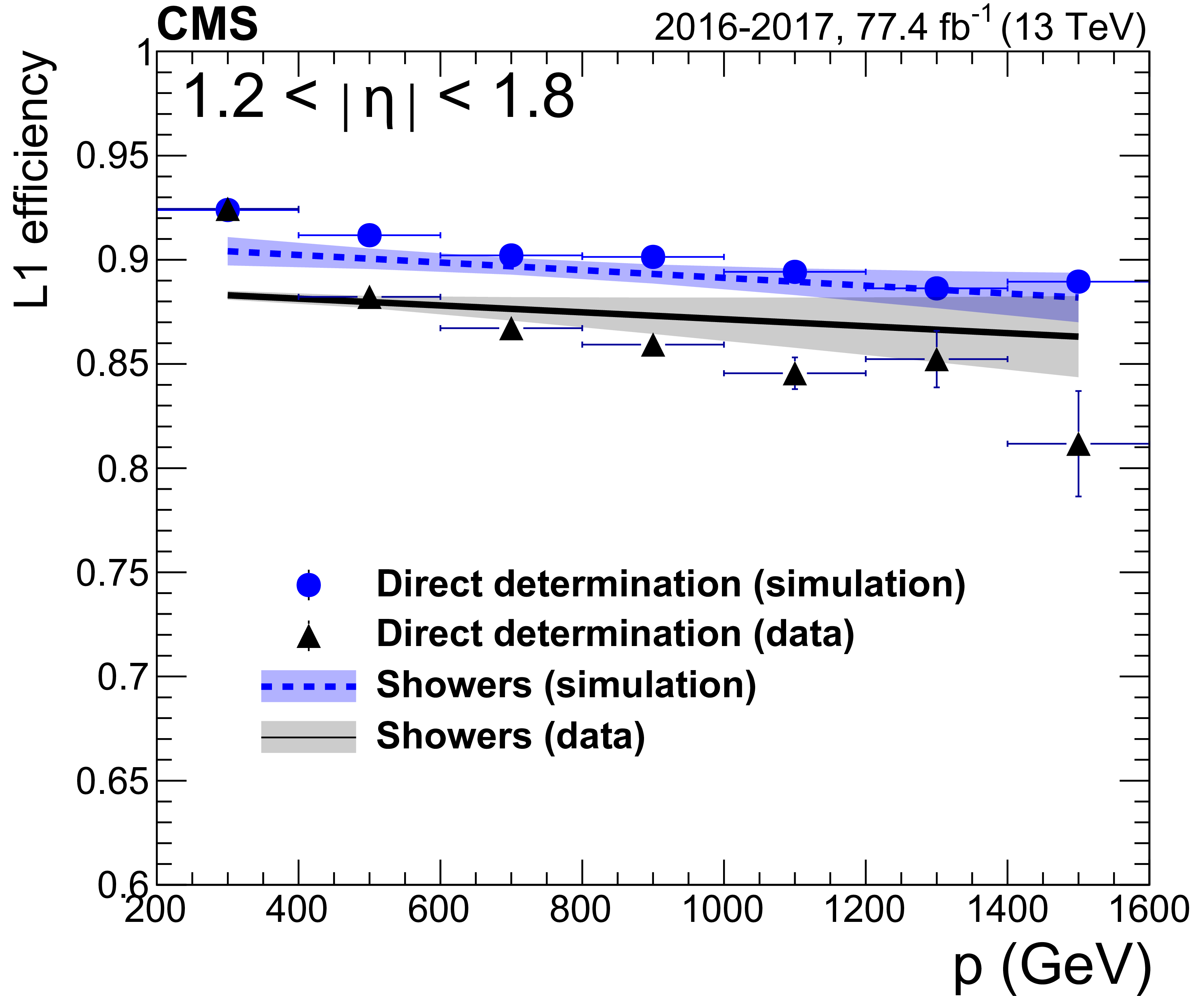
Figure 13:
The L1 efficiency in three $\eta $ regions: (upper left) barrel; (upper right) for muon with 1.2 $ < {| \eta |} < $ 1.8; and (lower) endcap with muon $ {| \eta |} > $ 1.8. The plots show a comparison between directly determining the efficiency from simulation (blue dots) and with data (black triangles) with respect to calculating it from shower multiplicity, both in 2016+2017 combined data (black line) and 2017 simulation (dashed blue line). The shaded bands include the statistical uncertainties of the measurements and the systematic uncertainty of the showering probability determination. |
png pdf |
Figure 13-a:
The L1 efficiency in the barrel region. The plot shows a comparison between directly determining the efficiency from simulation (blue dots) and with data (black triangles) with respect to calculating it from shower multiplicity, both in 2016+2017 combined data (black line) and 2017 simulation (dashed blue line). The shaded bands include the statistical uncertainties of the measurements and the systematic uncertainty of the showering probability determination. |
png pdf |
Figure 13-b:
The L1 efficiency for muon with 1.2 $ < {| \eta |} < $ 1.8. The plot shows a comparison between directly determining the efficiency from simulation (blue dots) and with data (black triangles) with respect to calculating it from shower multiplicity, both in 2016+2017 combined data (black line) and 2017 simulation (dashed blue line). The shaded bands include the statistical uncertainties of the measurements and the systematic uncertainty of the showering probability determination. |
png pdf |
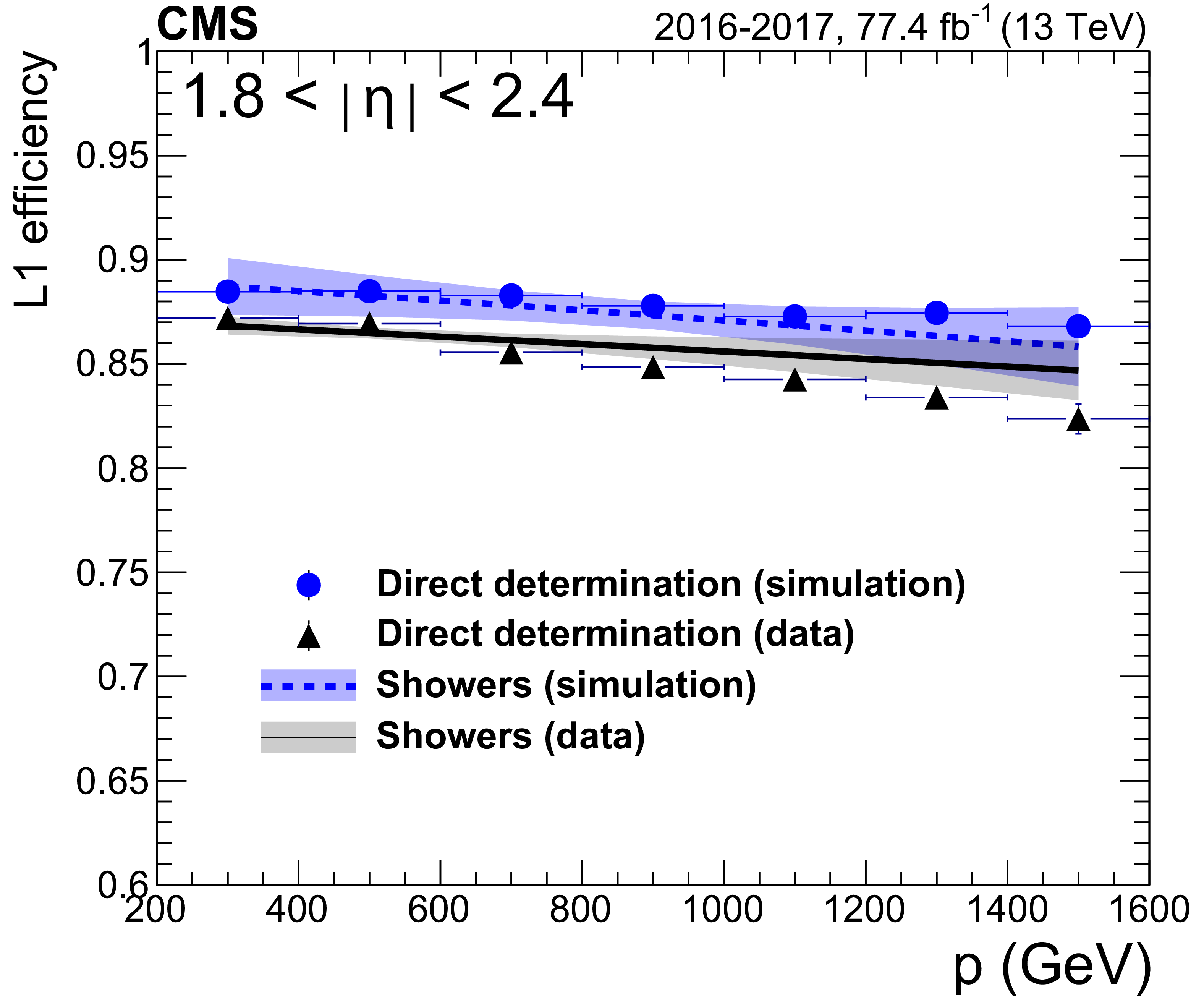
Figure 13-c:
The L1 efficiency in the endcap with muon $ {| \eta |} > $ 1.8. The plot shows a comparison between directly determining the efficiency from simulation (blue dots) and with data (black triangles) with respect to calculating it from shower multiplicity, both in 2016+2017 combined data (black line) and 2017 simulation (dashed blue line). The shaded bands include the statistical uncertainties of the measurements and the systematic uncertainty of the showering probability determination. |
png pdf |
Figure 14:
Muon momentum resolution (standard deviation $\sigma $ of the fit of the core distributions to a Gaussian function) in (left) the barrel region $ {| \eta |} < $ 0.9 and (right) the endcap region 1.2 $ < {| \eta |} < $ 2.4, for the TuneP algorithm, as a function of muon momentum, for the various misalignment scenarios with and without APEs. A comparison with the ideal scenario is also given. The performance of the tracker-only fit is shown for comparison. |
png pdf |
Figure 14-a:
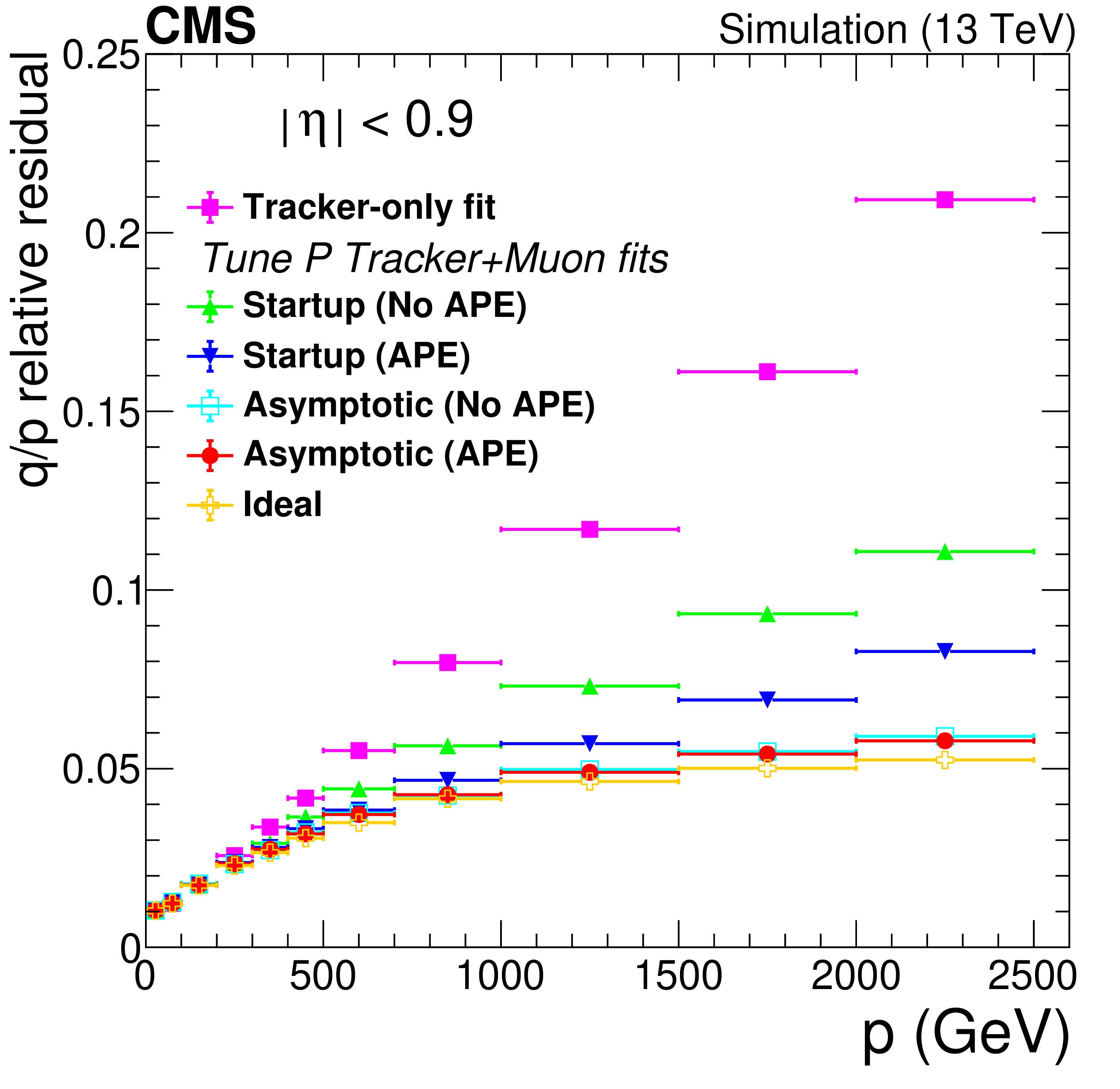
Muon momentum resolution (standard deviation $\sigma $ of the fit of the core distributions to a Gaussian function) in the barrel region $ {| \eta |} < $ 0.9, for the TuneP algorithm, as a function of muon momentum, for the various misalignment scenarios with and without APEs. A comparison with the ideal scenario is also given. The performance of the tracker-only fit is shown for comparison. |
png pdf |
Figure 14-b:
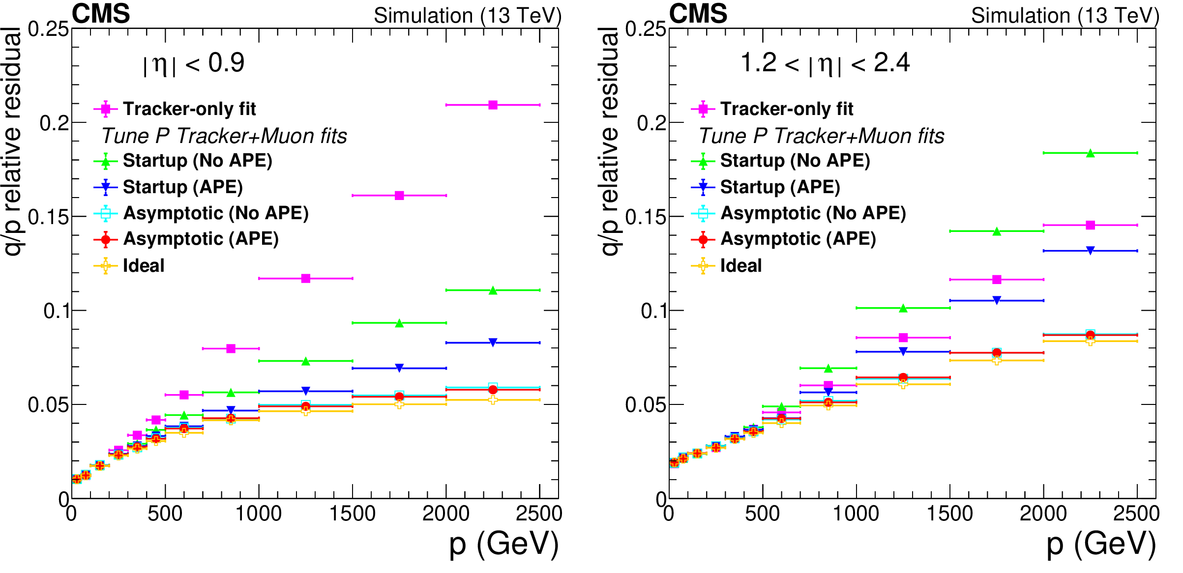
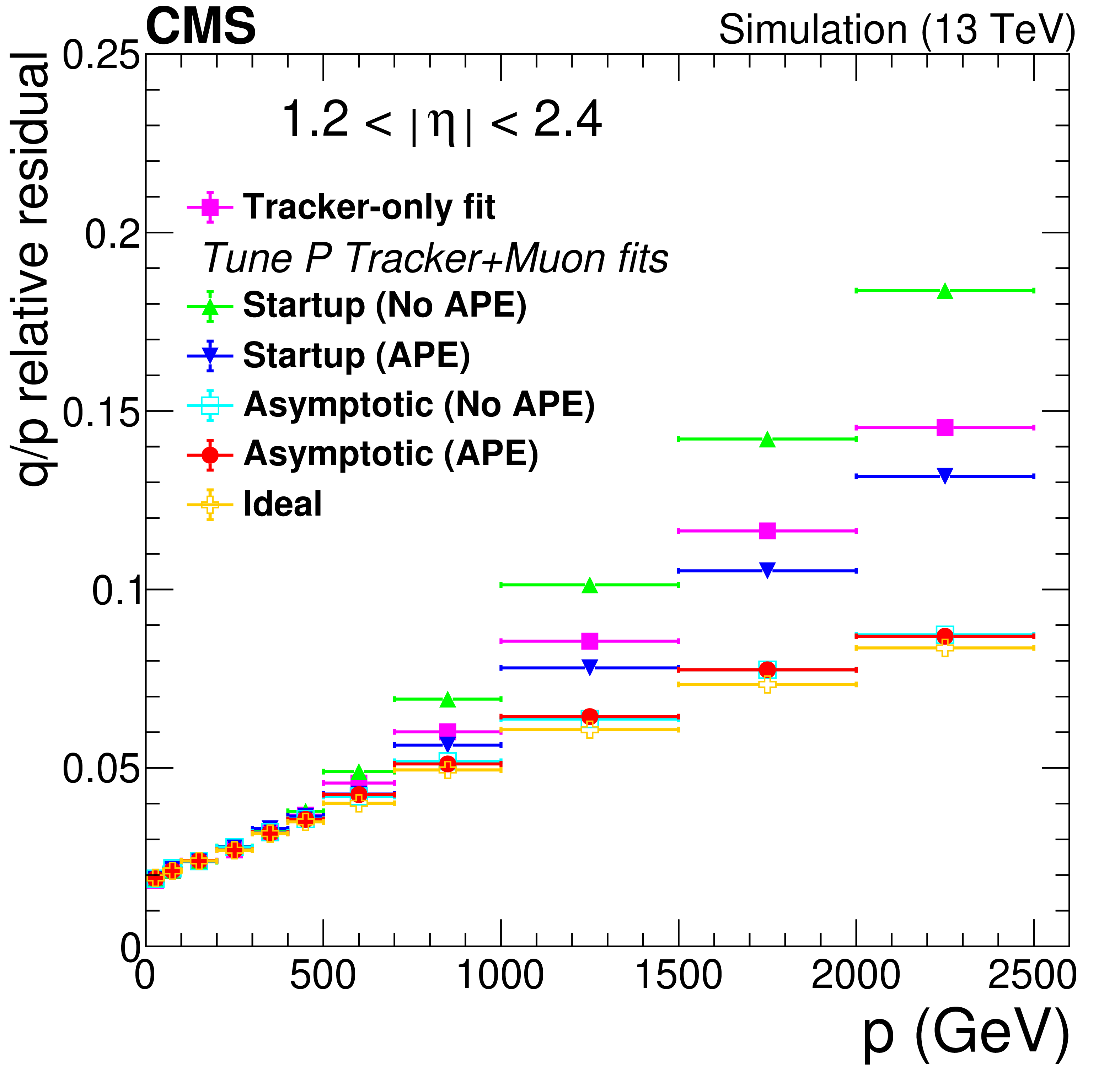
Muon momentum resolution (standard deviation $\sigma $ of the fit of the core distributions to a Gaussian function) for the TuneP algorithm, as a function of muon momentum, for the various misalignment scenarios with and without APEs. A comparison with the ideal scenario is also given. The performance of the tracker-only fit is shown for comparison. |
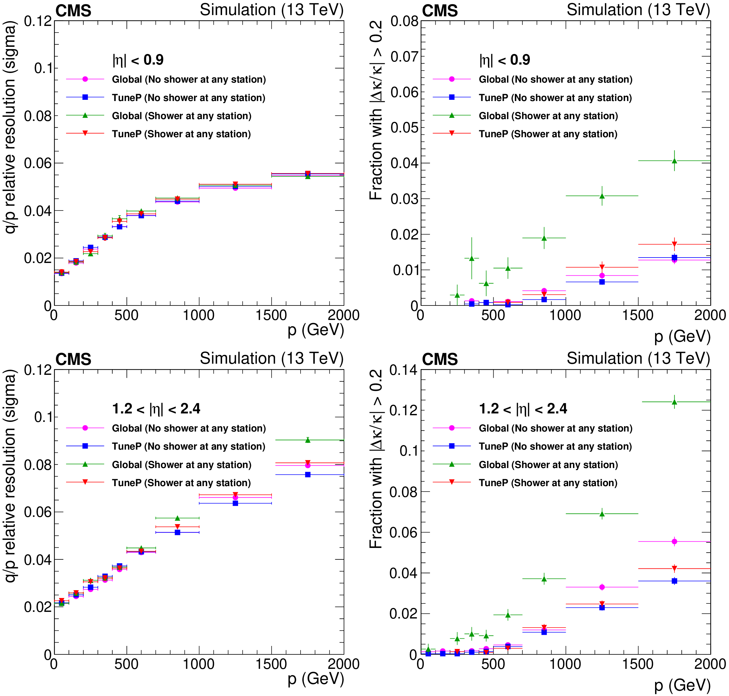
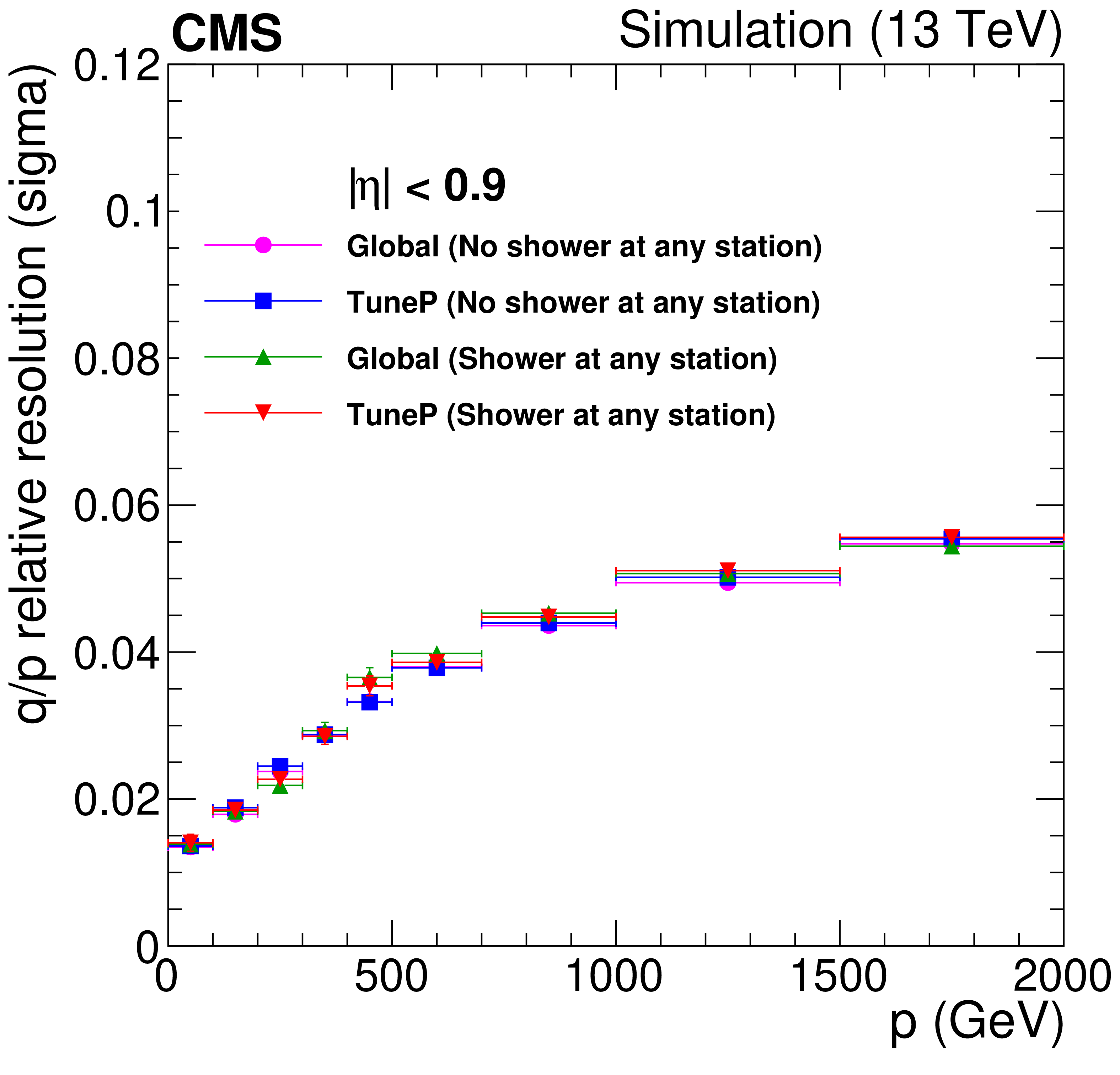
png pdf |
Figure 15:
Comparison of the TuneP and global reconstruction algorithms for simulated muons in the (upper) barrel and (lower) endcap, for the cases with and without the presence of tagged showers in any muon station. The left plots show the momentum resolution (Gaussian $\sigma $); the right plots show the tail fraction with $ {| \delta k /k |} > $ 20%, as a function of muon momentum. |
png pdf |
Figure 15-a:
Comparison of the TuneP and global reconstruction algorithms for simulated muons in the barrel, for the cases with and without the presence of tagged showers in any muon station. The plot shows the momentum resolution (Gaussian $\sigma $), as a function of muon momentum. |
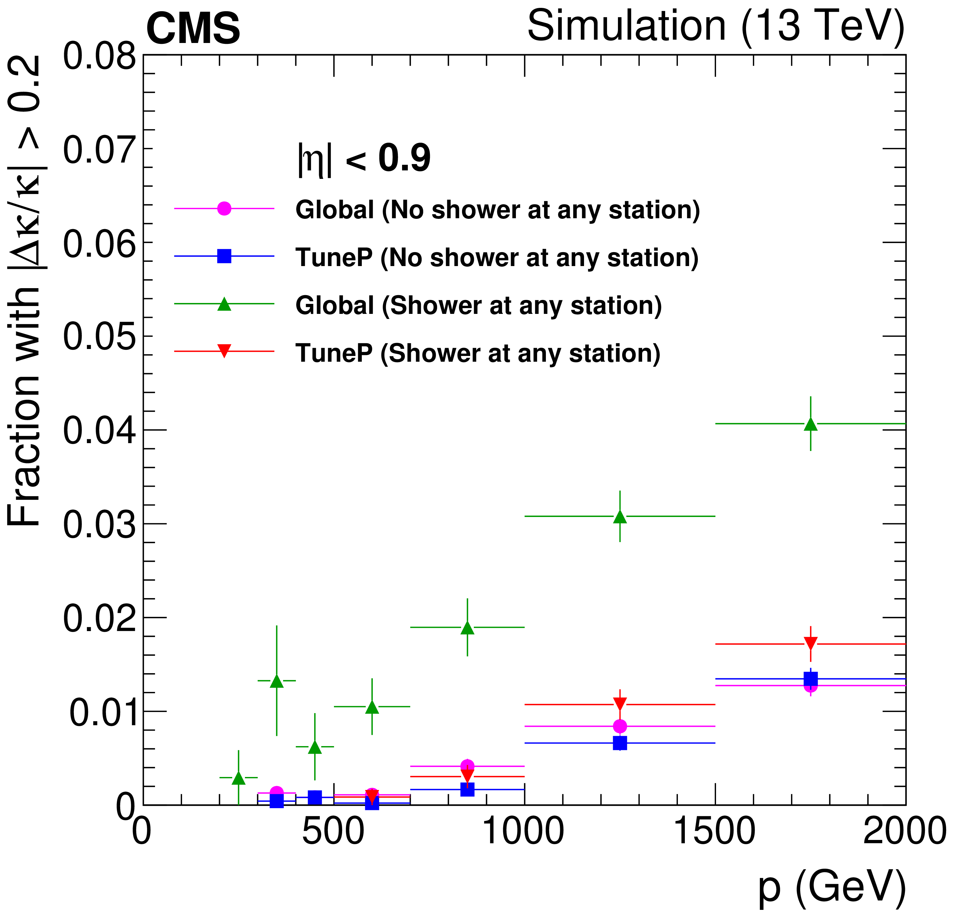
png pdf |
Figure 15-b:
Comparison of the TuneP and global reconstruction algorithms for simulated muons in the barrel, for the cases with and without the presence of tagged showers in any muon station. The plot shows the momentum resolution (Gaussian $\sigma $), as a function of muon momentum. |

png pdf |
Figure 15-c:
Comparison of the TuneP and global reconstruction algorithms for simulated muons in the endcap, for the cases with and without the presence of tagged showers in any muon station. The plot shows the tail fraction with $ {| \delta k /k |} > $ 20%, as a function of muon momentum. |
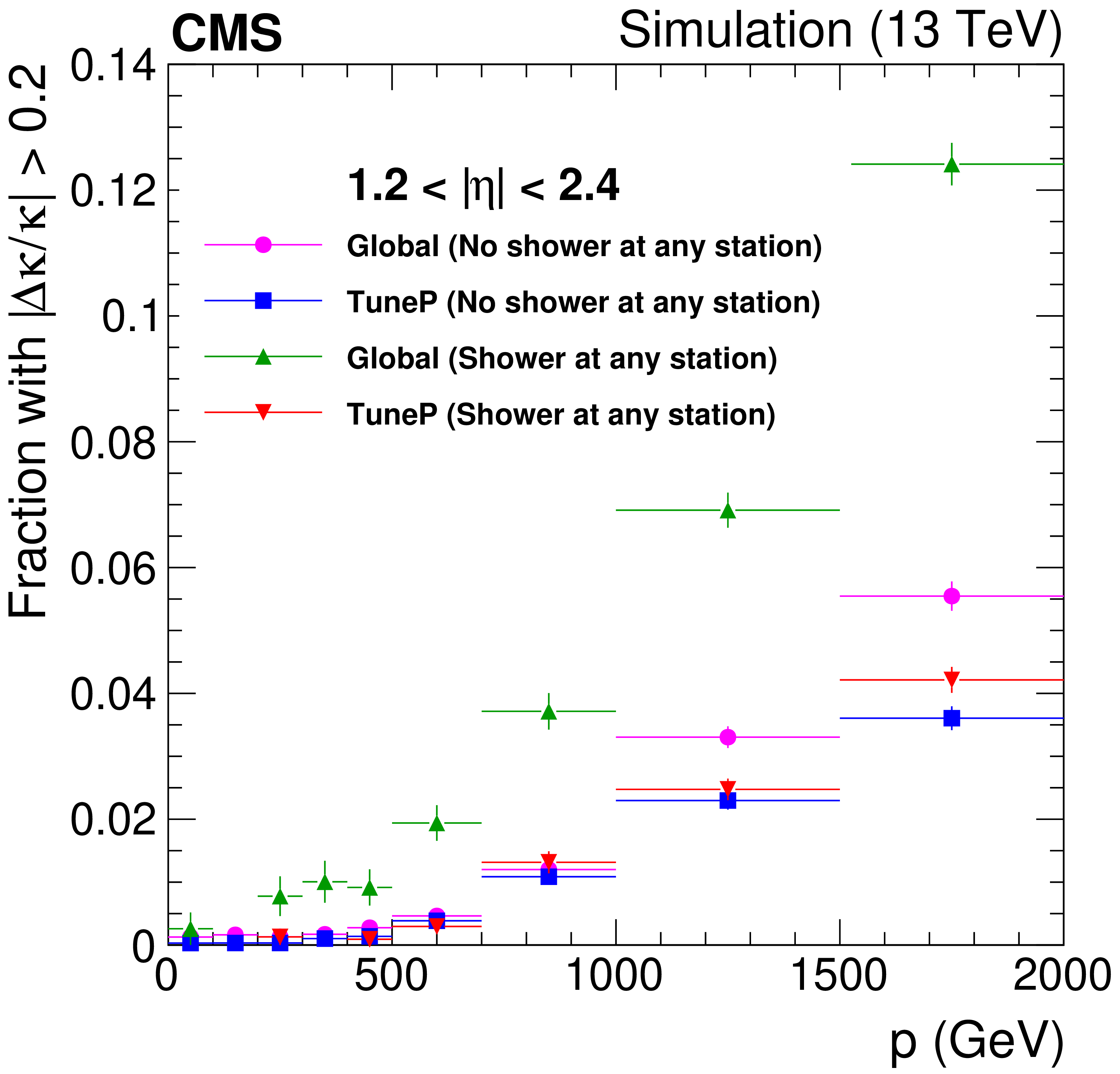
png pdf |
Figure 15-d:
Comparison of the TuneP and global reconstruction algorithms for simulated muons in the endcap, for the cases with and without the presence of tagged showers in any muon station. The plot shows the tail fraction with $ {| \delta k /k |} > $ 20%, as a function of muon momentum. |
png pdf |
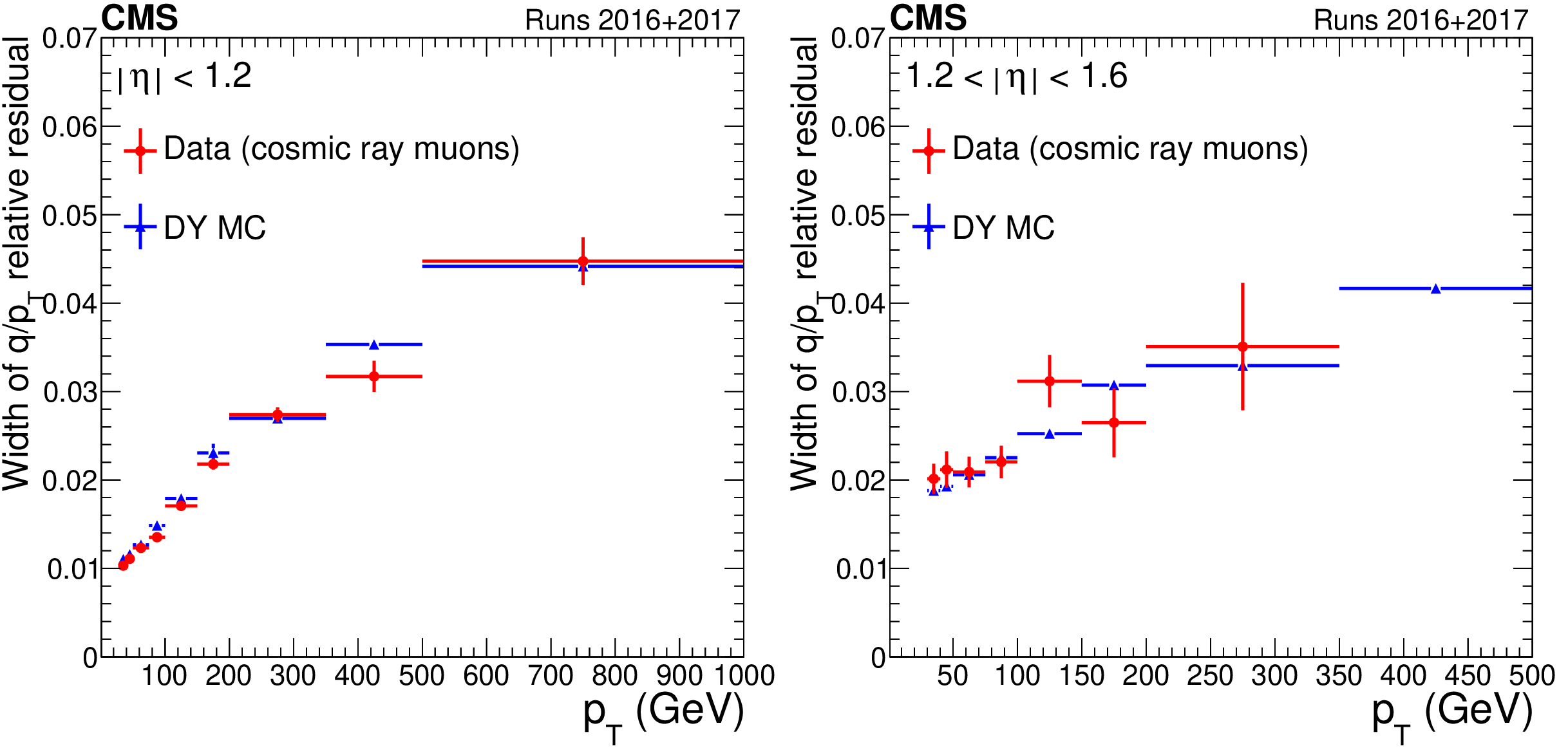
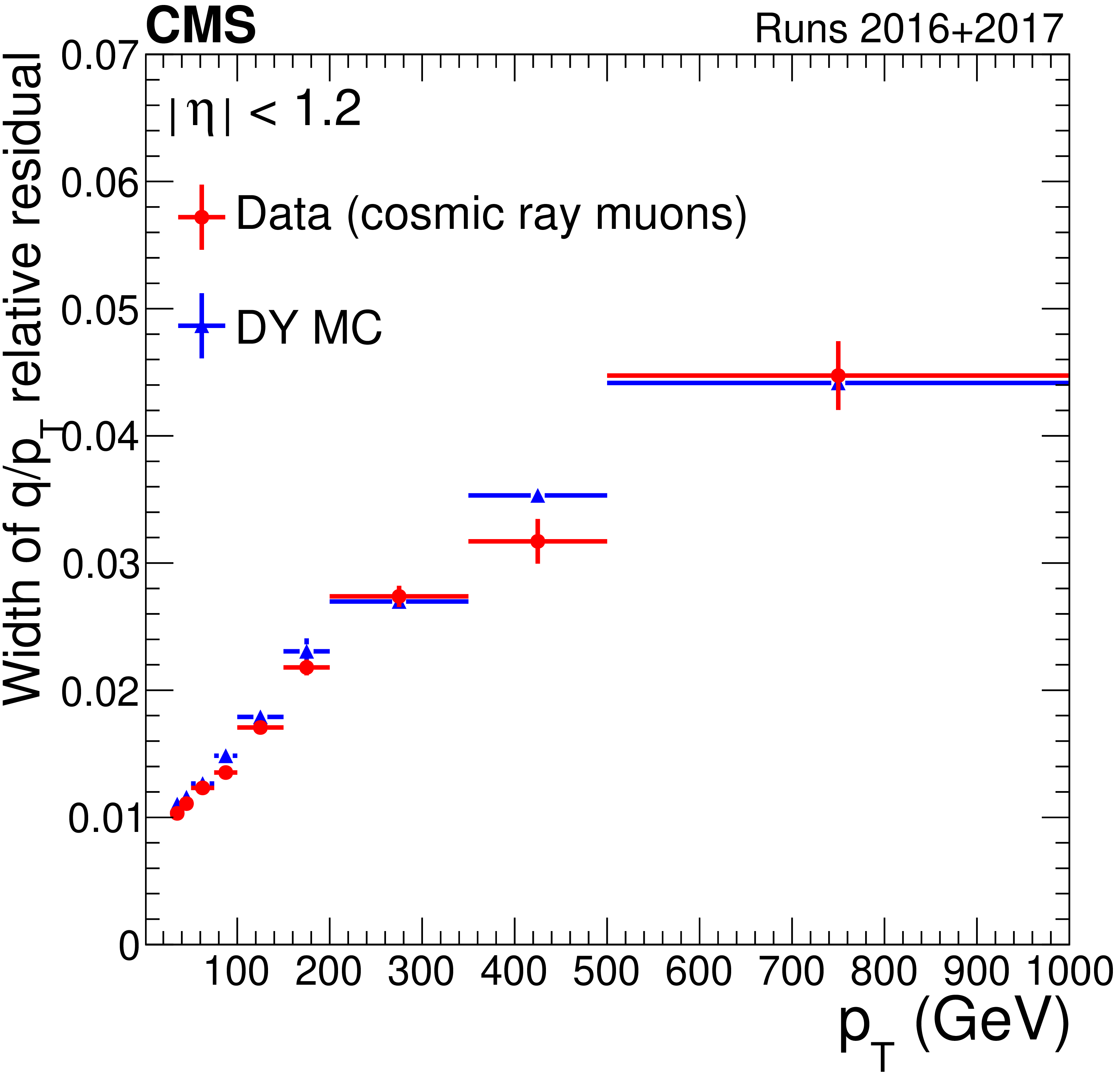
Figure 16:
Gaussian $\sigma $ of fits to $q/ {p_{\mathrm {T}}} $ relative residuals for TuneP cosmic ray muons collected in 2016 and 2017 for (left) the barrel ($ {| \eta |} < $ 1.2) and (right) the endcap (1.2 $ < {| \eta |} < $ 1.6) regions, compared to the resolution extracted from DY simulation. |
png pdf |
Figure 16-a:
Gaussian $\sigma $ of fits to $q/ {p_{\mathrm {T}}} $ relative residuals for TuneP cosmic ray muons collected in 2016 and 2017 for the barrel ($ {| \eta |} < $ 1.2) region, compared to the resolution extracted from DY simulation. |
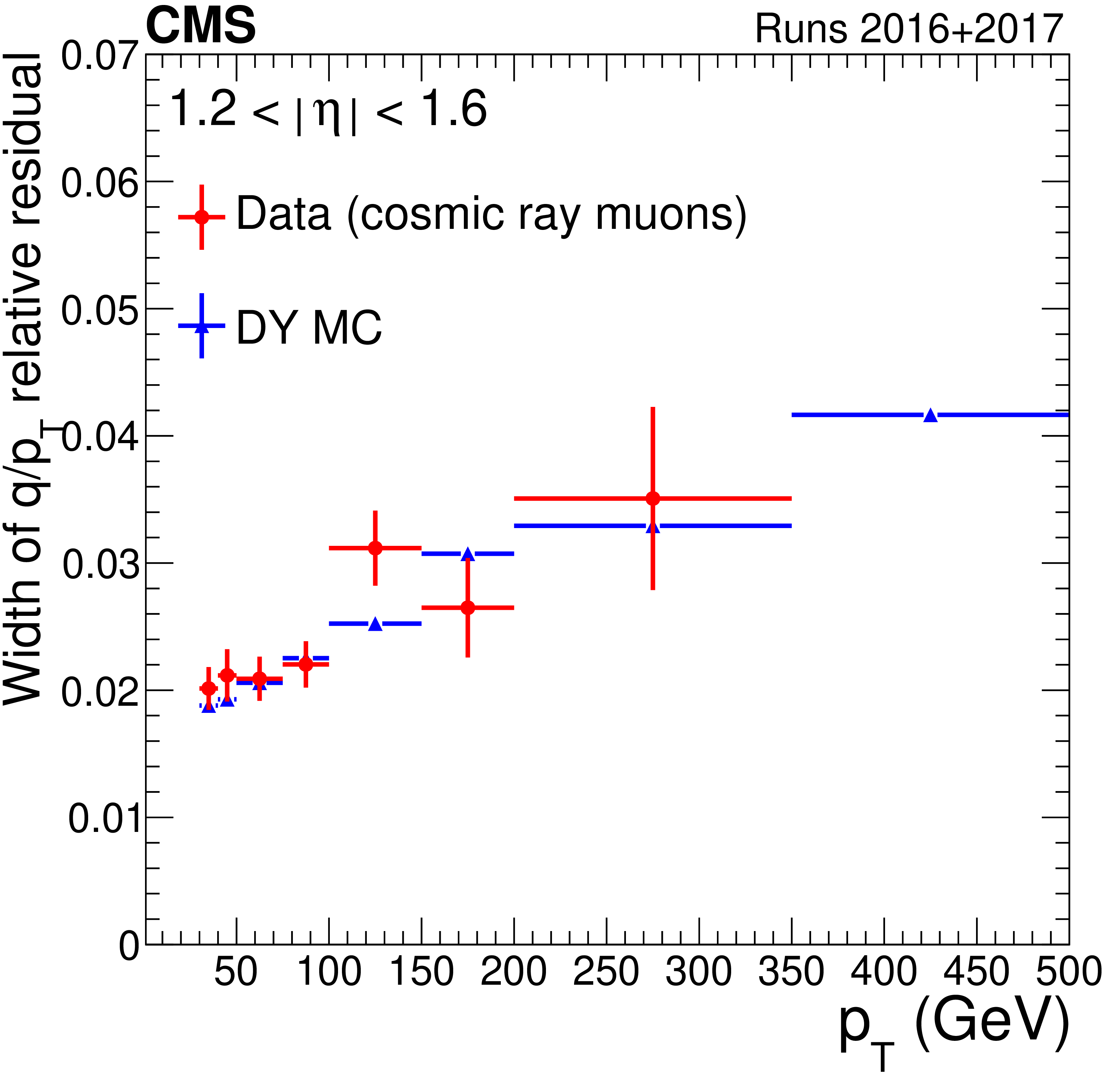
png pdf |
Figure 16-b:
Gaussian $\sigma $ of fits to $q/ {p_{\mathrm {T}}} $ relative residuals for TuneP cosmic ray muons collected in 2016 and 2017 for the endcap (1.2 $ < {| \eta |} < $ 1.6) region, compared to the resolution extracted from DY simulation. |

png pdf |
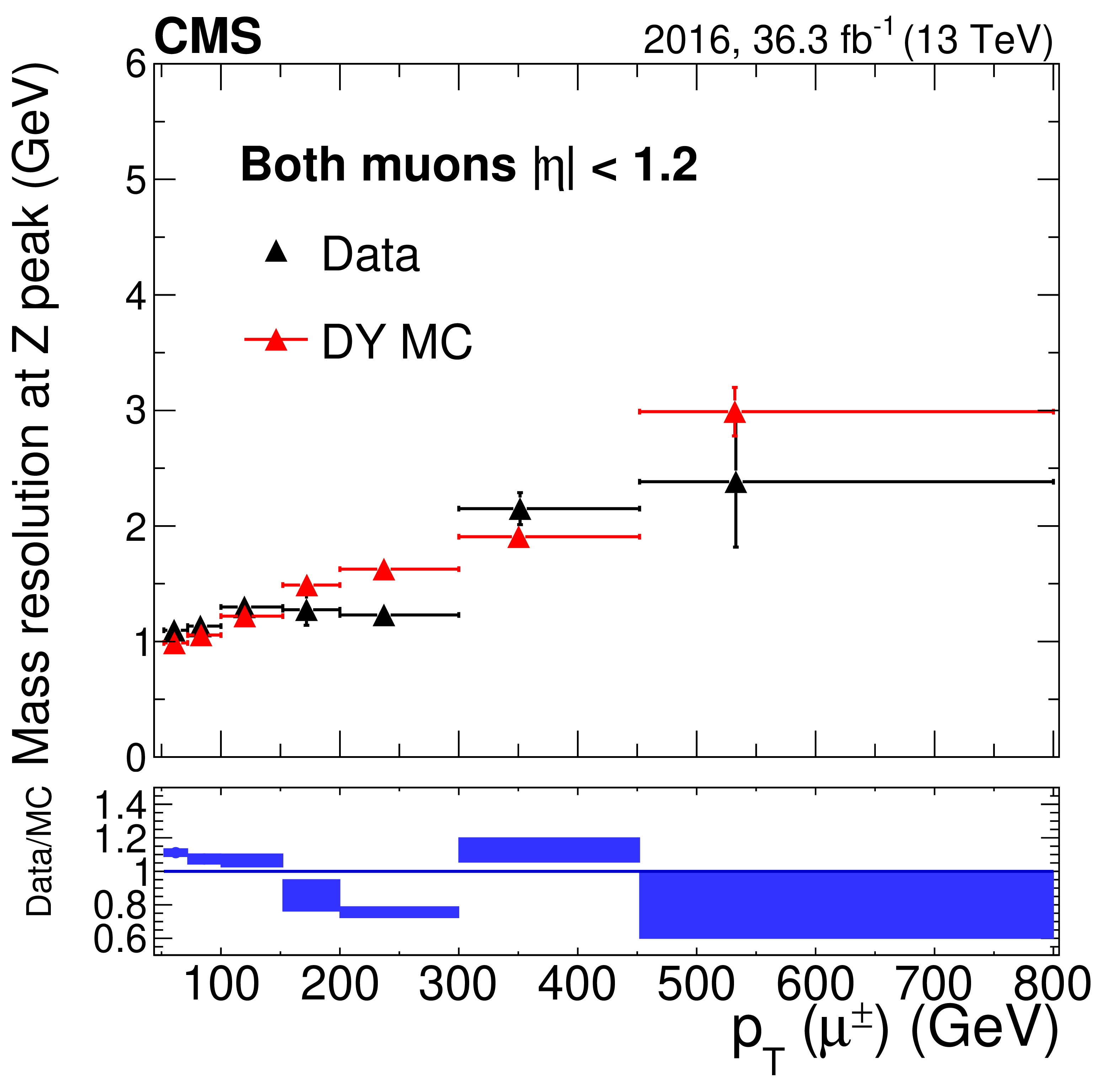
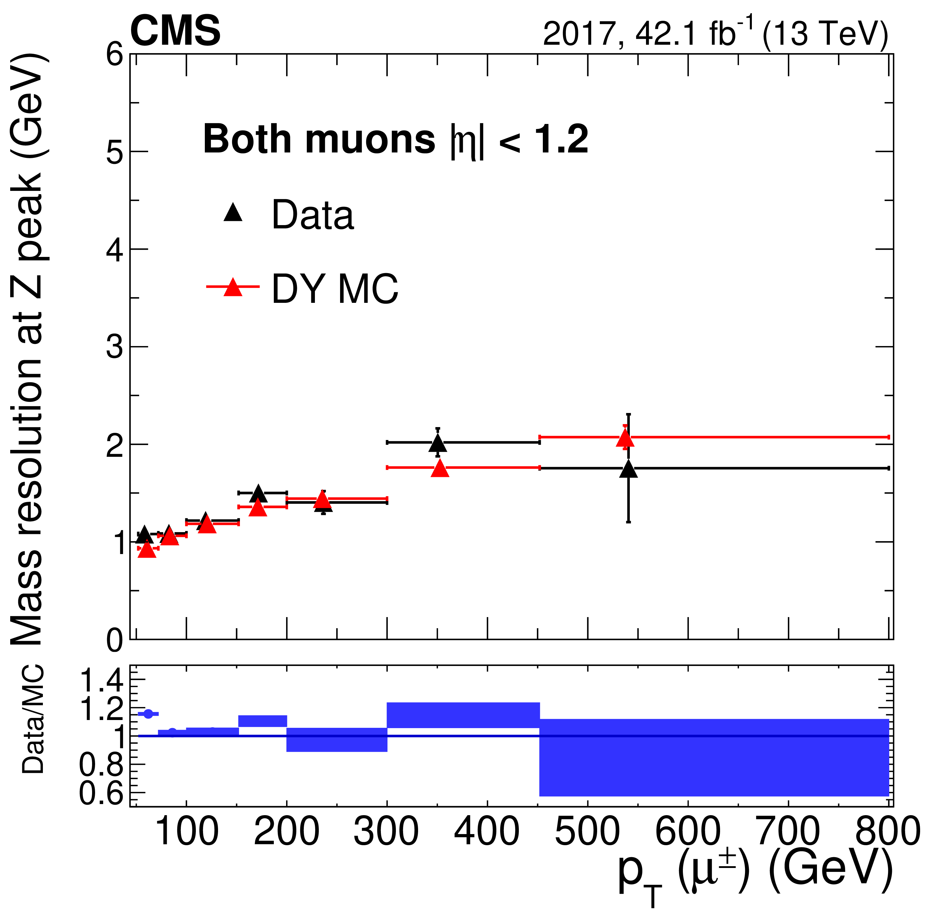
Figure 17:
Dimuon mass resolution (Gaussian $\sigma $), as a function of muon TuneP ${p_{\mathrm {T}}}$ in the BB category. Each dimuon event is counted twice since each muon ($\mu ^+$ and $\mu ^-$) in the event is filling the histograms. Results for (left) 2016 and (right) 2017 are shown. Data are shown in black while the resolution obtained from simulation is shown in red. The lower panels of the plots show the ratio of data to simulation; the blue boxes represent the statistical uncertainties. The central value in each bin is obtained from the average of the distribution within the bin. |
png pdf |
Figure 17-a:
Dimuon mass resolution (Gaussian $\sigma $), as a function of muon TuneP ${p_{\mathrm {T}}}$ in the BB category. Each dimuon event is counted twice since each muon ($\mu ^+$ and $\mu ^-$) in the event is filling the histograms. Results for 2016 are shown. Data are shown in black while the resolution obtained from simulation is shown in red. The lower panel shows the ratio of data to simulation; the blue boxes represent the statistical uncertainties. The central value in each bin is obtained from the average of the distribution within the bin. |
png pdf |
Figure 17-b:
Dimuon mass resolution (Gaussian $\sigma $), as a function of muon TuneP ${p_{\mathrm {T}}}$ in the BB category. Each dimuon event is counted twice since each muon ($\mu ^+$ and $\mu ^-$) in the event is filling the histograms. Results for 2017 are shown. Data are shown in black while the resolution obtained from simulation is shown in red. The lower panel shows the ratio of data to simulation; the blue boxes represent the statistical uncertainties. The central value in each bin is obtained from the average of the distribution within the bin. |
png pdf |
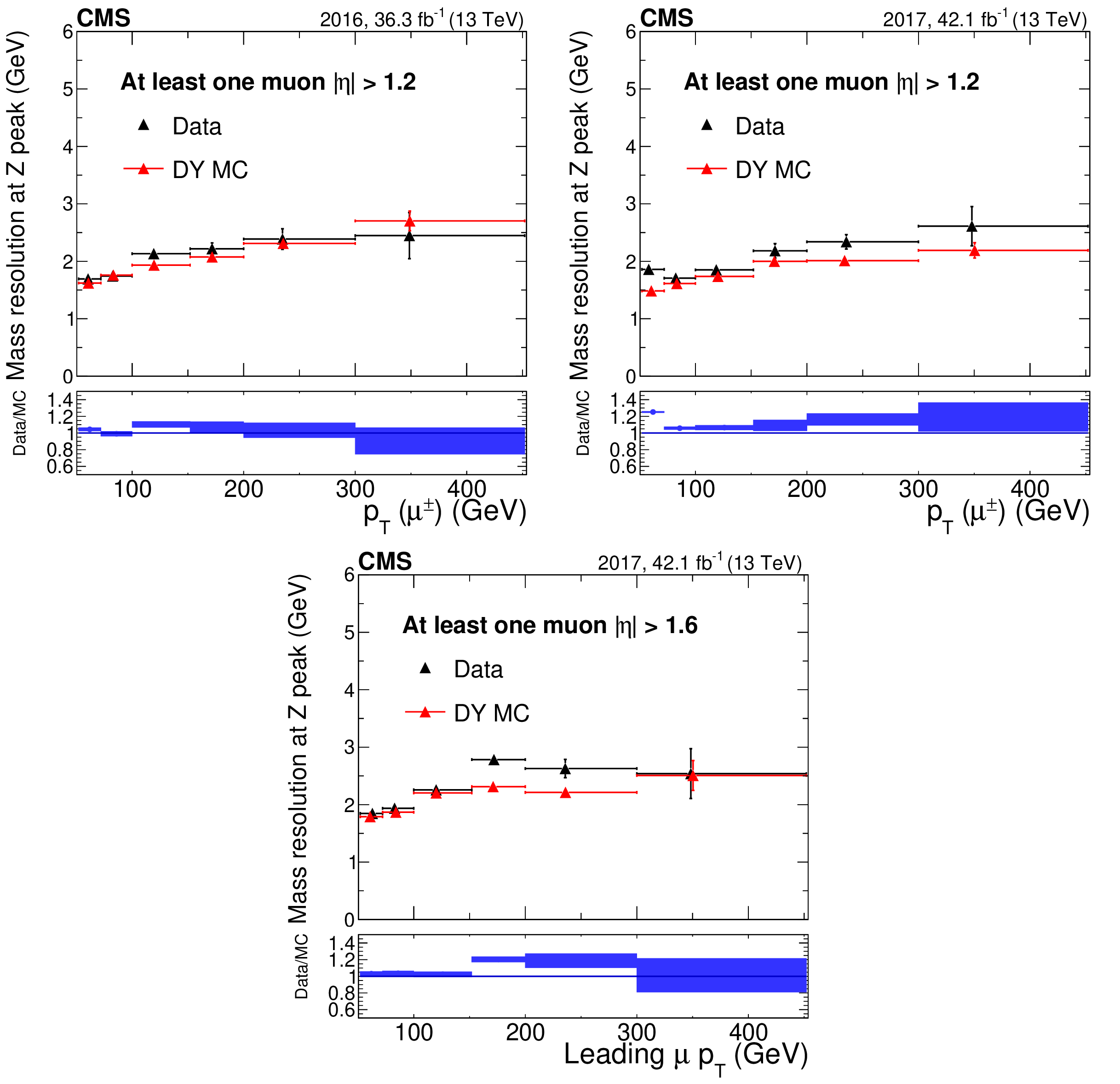
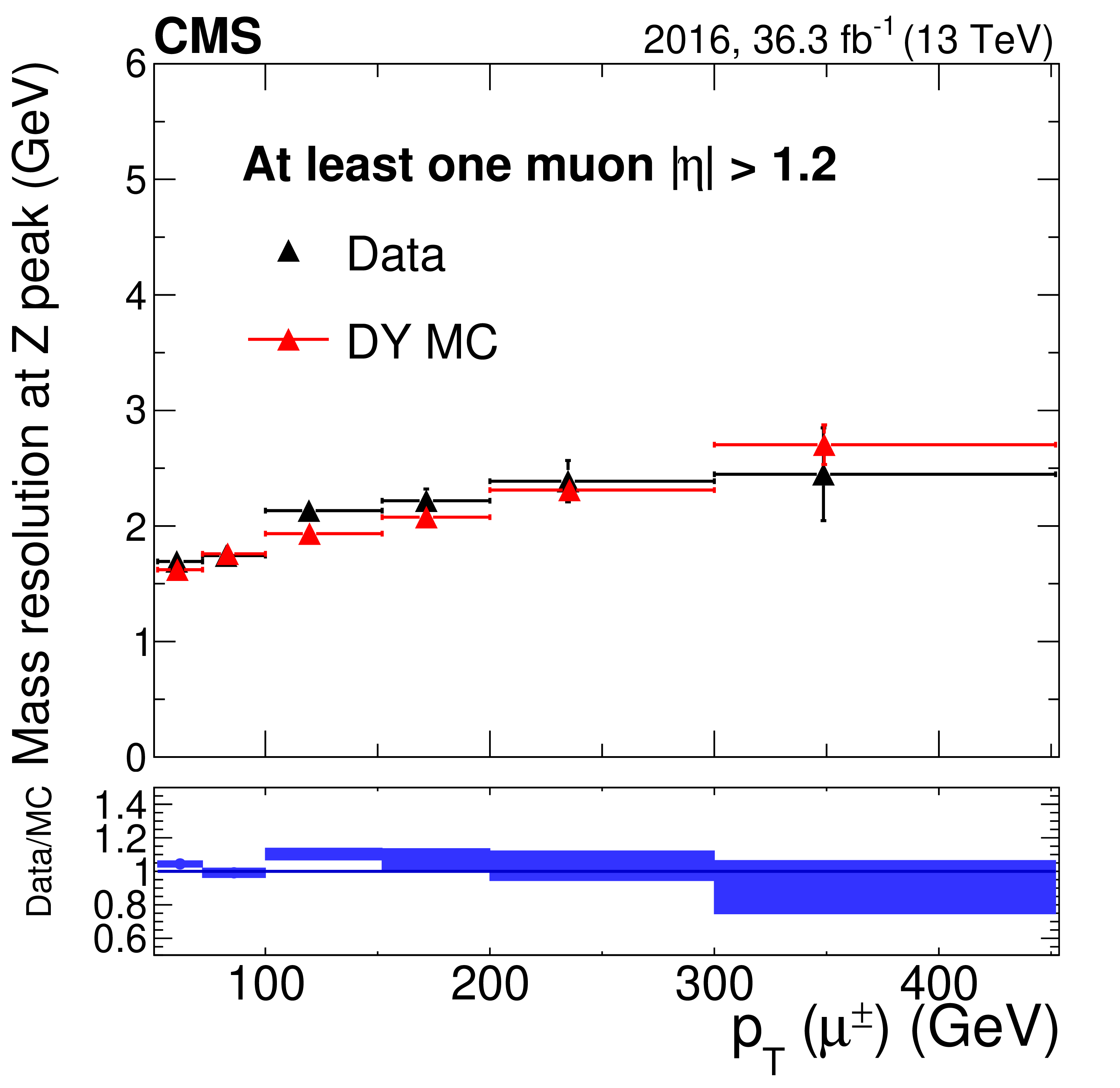
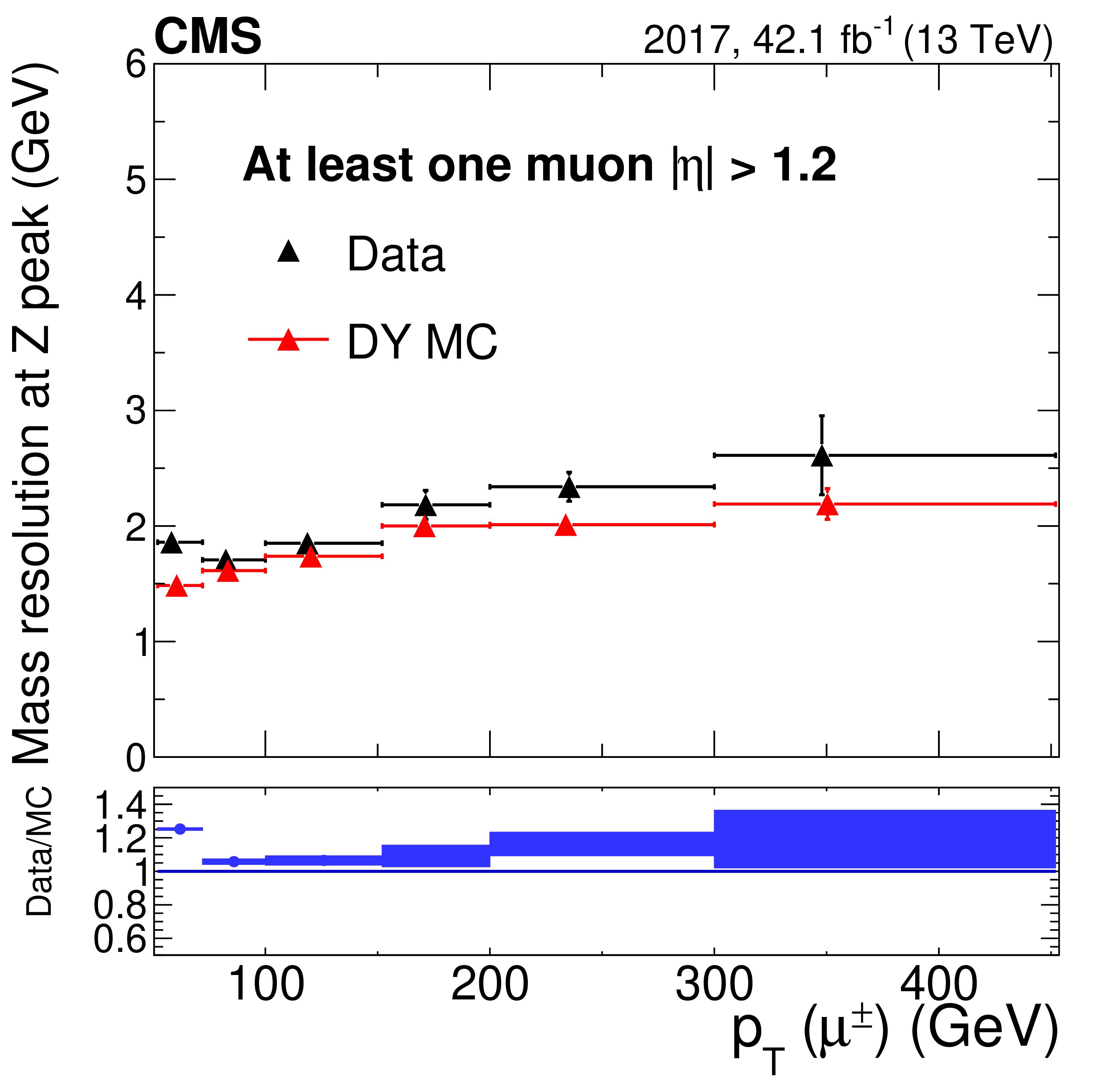
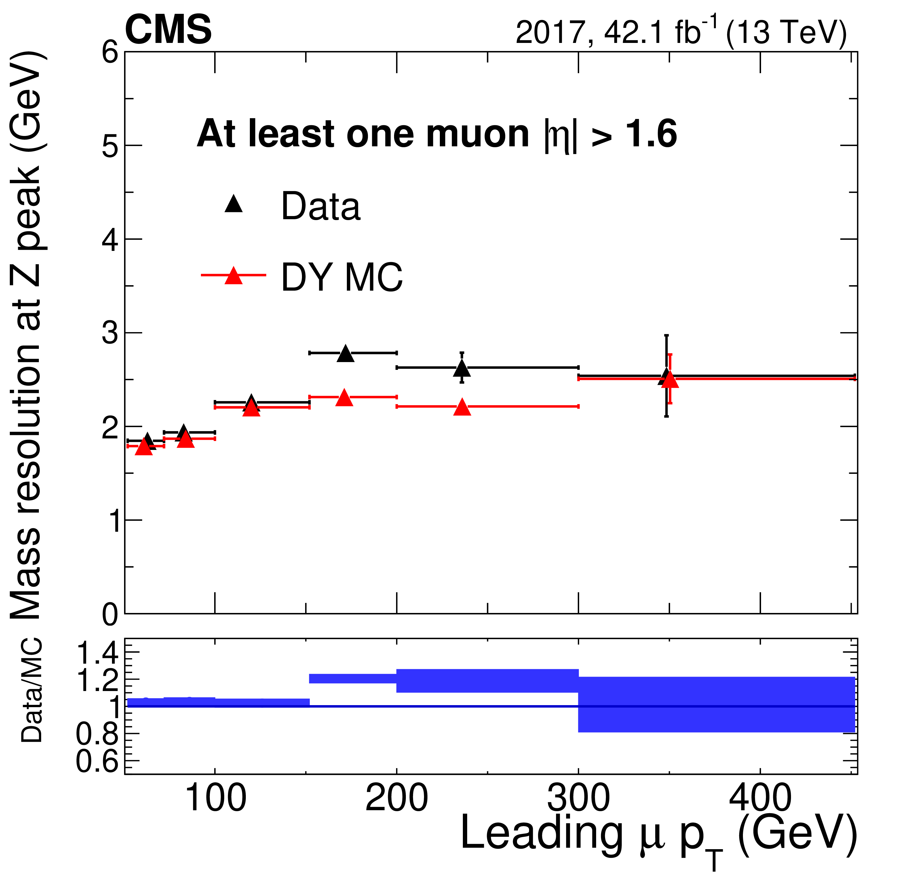
Figure 18:
Dimuon mass resolution (Gaussian $\sigma $), as a function of muon TuneP ${p_{\mathrm {T}}}$ in the BE+EE category. Each dimuon event is counted twice since each muon ($\mu ^+$ and $\mu ^-$) in the event is filling the histograms. Results for (upper left) 2016 and (upper right) 2017 are shown. The lower plot is for 2017 data where the BE+EE category is defined with at least one of the two muons with $ {| \eta |} > $ 1.6. Data are shown in black while the resolution obtained from simulation is shown in red. The central value in each bin is obtained from the average of the distribution within the bin. |
png pdf |
Figure 18-a:
Dimuon mass resolution (Gaussian $\sigma $), as a function of muon TuneP ${p_{\mathrm {T}}}$ in the BE+EE category. Each dimuon event is counted twice since each muon ($\mu ^+$ and $\mu ^-$) in the event is filling the histograms. Results for 2016 are shown. Data are shown in black while the resolution obtained from simulation is shown in red. The central value in each bin is obtained from the average of the distribution within the bin. |
png pdf |
Figure 18-b:
Dimuon mass resolution (Gaussian $\sigma $), as a function of muon TuneP ${p_{\mathrm {T}}}$ in the BE+EE category. Each dimuon event is counted twice since each muon ($\mu ^+$ and $\mu ^-$) in the event is filling the histograms. Results for 2017 are shown. Data are shown in black while the resolution obtained from simulation is shown in red. The central value in each bin is obtained from the average of the distribution within the bin. |
png pdf |
Figure 18-c:
Dimuon mass resolution (Gaussian $\sigma $), as a function of muon TuneP ${p_{\mathrm {T}}}$ in the BE+EE category. Each dimuon event is counted twice since each muon ($\mu ^+$ and $\mu ^-$) in the event is filling the histograms. The plot is for 2017 data where the BE+EE category is defined with at least one of the two muons with $ {| \eta |} > $ 1.6. Data are shown in black while the resolution obtained from simulation is shown in red. The central value in each bin is obtained from the average of the distribution within the bin. |

png pdf |
Figure 19:
Data to simulation comparison of the curvature distribution in $\mathrm{Z} \to \mu ^+\mu ^-$ events, for 2017 data with muon $ {p_{\mathrm {T}}} > $ 200 GeV. |
png pdf |
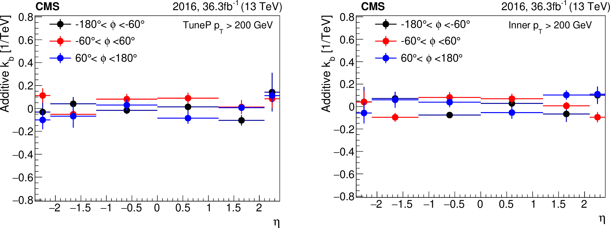
Figure 20:
Measurement of the scale bias for muons above 200 GeV with 2016 data. On the left the ${p_{\mathrm {T}}}$ corresponds to TuneP, while on the right it corresponds to the tracker-only assignment. |
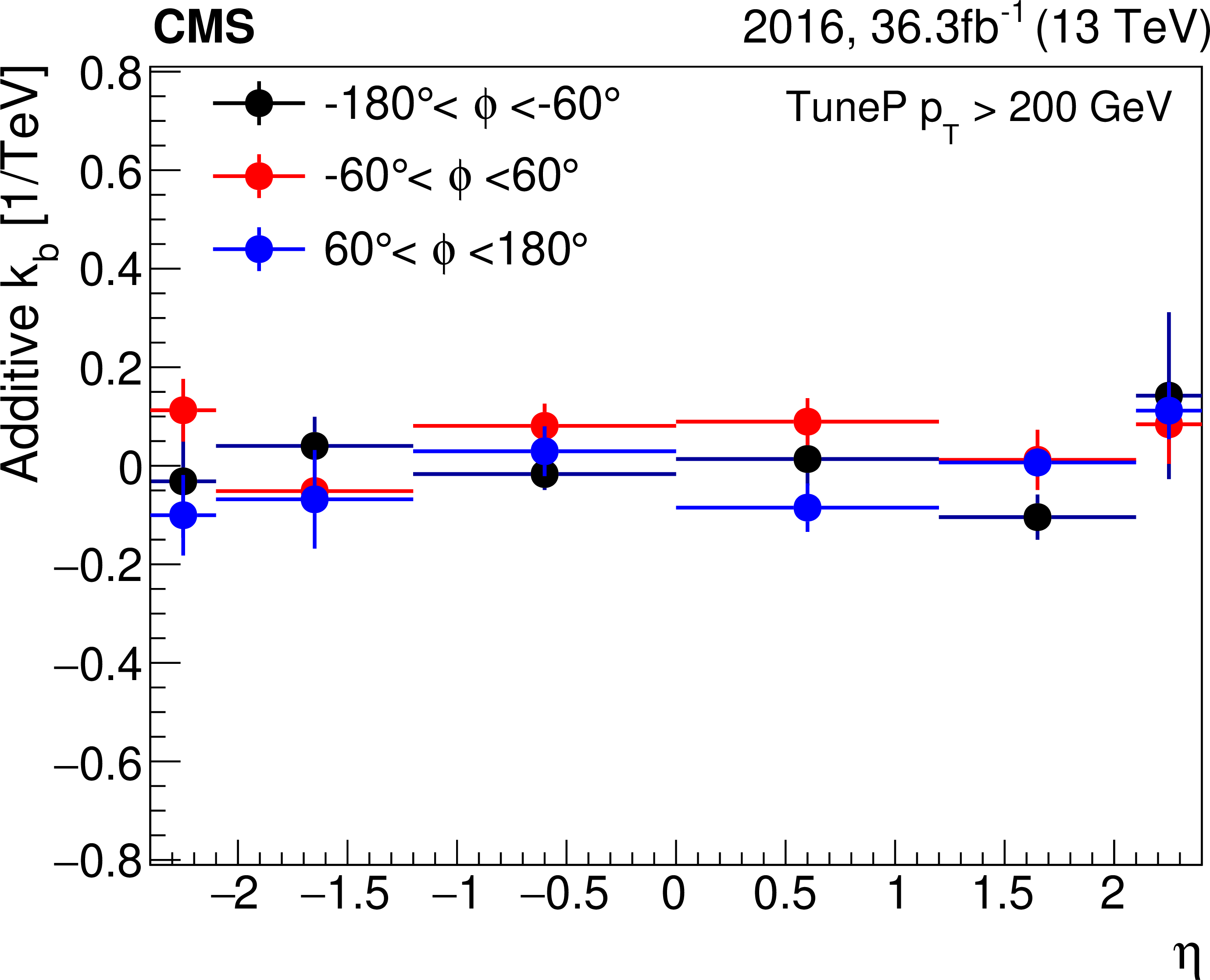
png pdf |
Figure 20-a:
Measurement of the scale bias for muons above 200 GeV with 2016 data. The ${p_{\mathrm {T}}}$ corresponds to TuneP. |
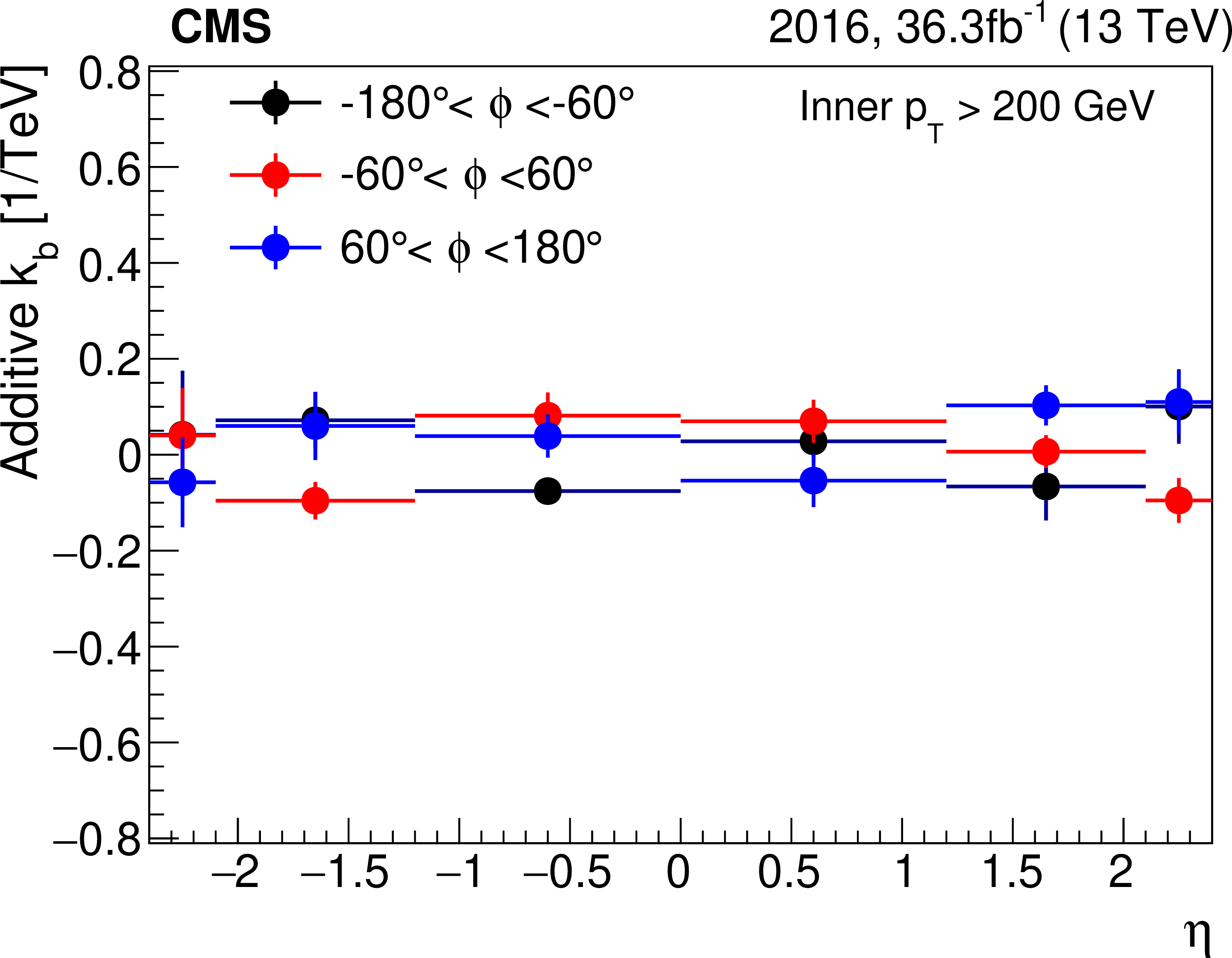
png pdf |
Figure 20-b:
Measurement of the scale bias for muons above 200 GeV with 2016 data. The ${p_{\mathrm {T}}}$ corresponds to the tracker-only assignment. |

png pdf |
Figure 21:
Measurement of the scale bias for muons above 200 GeV with 2017 data. On the left the ${p_{\mathrm {T}}}$ corresponds to the TuneP, while on the right it corresponds to the tracker-only assignment. |

png pdf |
Figure 21-a:
Measurement of the scale bias for muons above 200 GeV with 2017 data. The ${p_{\mathrm {T}}}$ corresponds to the TuneP. |
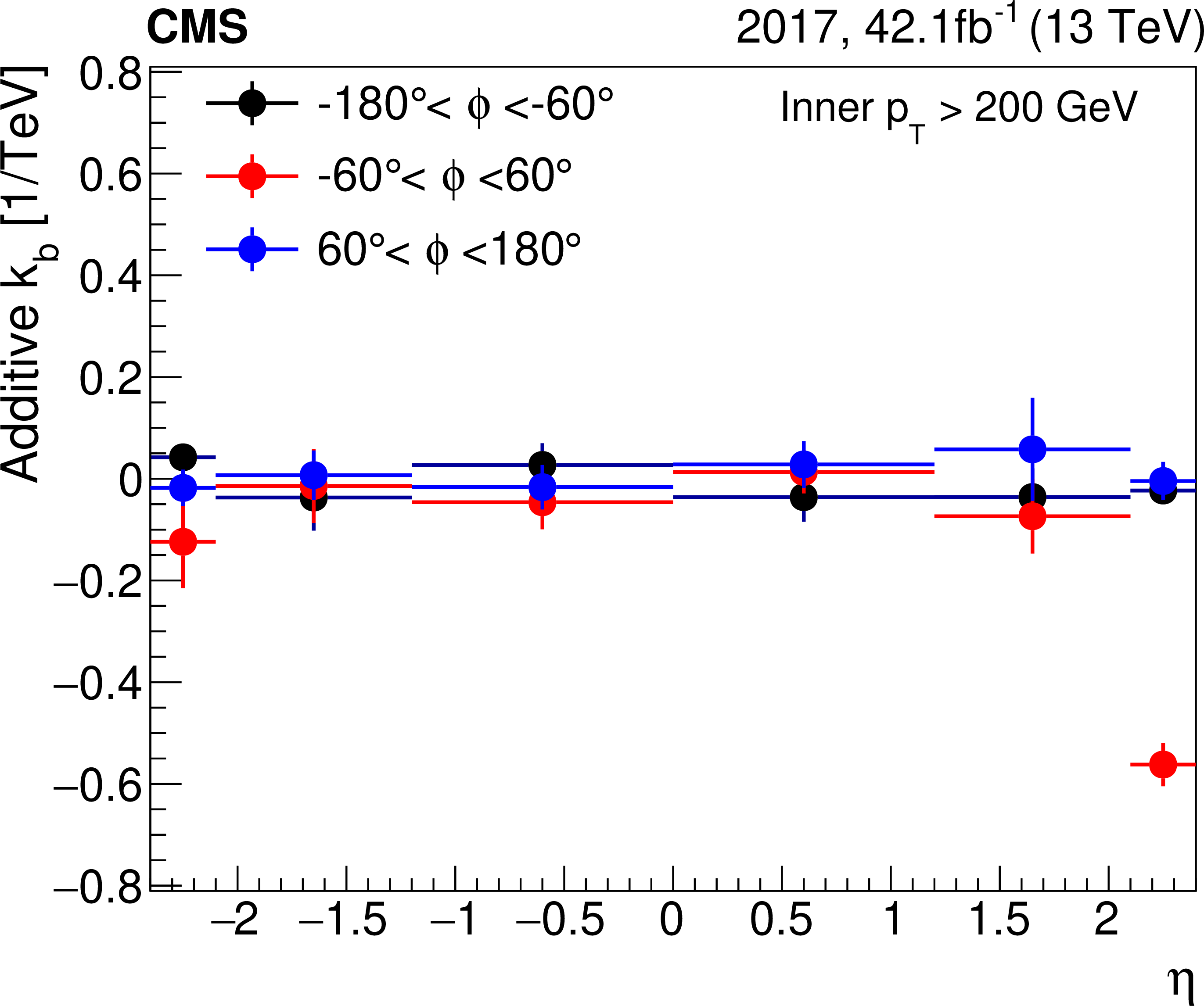
png pdf |
Figure 21-b:
Measurement of the scale bias for muons above 200 GeV with 2017 data. The ${p_{\mathrm {T}}}$ corresponds to the tracker-only assignment. |
| Tables | |

png pdf |
Table 1:
The L1 trigger efficiency for barrel and endcap muons measured as a function of the number of showers in the muon stations. The endcap was split into near ($ {| \eta |} < $ 1.8) and far ($ {| \eta |} > $ 1.8) sections. |
| Summary |
| The performance of muon reconstruction, identification, trigger, and momentum assignment has been studied in a sample enriched in high-momentum muons using proton-proton collisions at $\sqrt{s} = $ 13 TeV, collected by the CMS experiment at the LHC in 2016-2017, and corresponding to the integrated luminosity of 78.4 fb$^{-1}$. Depending on the longitudinal component of the momentum, muons with transverse momentum ${p_{\mathrm{T}}} > $ 200 GeV can have radiative energy losses in steel that are no longer negligible compared to ionization energy losses. Dedicated methods have been developed to study the performance impact of the detector alignment and electromagnetic showers along the muon track. Overall, the measurements are described accurately by the simulation and their reach in momentum is limited by the statistical uncertainties. The largest discrepancy between data and simulation is found at the trigger level with a 10% efficiency difference for muons with ${p_{\mathrm{T}}}$ around 1 TeV. Representative figures of merit that illustrate the muon performance at high momentum are listed below. |
| References | ||||
| 1 | A. Leike | The phenomenology of extra neutral gauge bosons | PR 317 (1999) 143 | hep-ph/9805494 |
| 2 | P. Langacker | The physics of heavy $ Z^\prime $ gauge bosons | Rev. Mod. Phys. 81 (2009) 1199 | 0801.1345 |
| 3 | K. Hsieh, K. Schmitz, J.-H. Yu, and C. P. Yuan | Global analysis of general SU(2) x SU(2) x U(1) models with precision data | PRD 82 (2010) 035011 | 1003.3482 |
| 4 | CMS Collaboration | The performance of the CMS muon detector in proton-proton collisions at $ \sqrt{s}= $ 7 ~TeV at the LHC | JINST 8 (2013) P11002 | CMS-MUO-11-001 1306.6905 |
| 5 | CMS Collaboration | Performance of CMS muon reconstruction in pp collision events at $ \sqrt{s}= $ 7 TeV | JINST 7 (2012) P10002 | CMS-MUO-10-004 1206.4071 |
| 6 | CMS Collaboration | Performance of the CMS muon detector and muon reconstruction with proton-proton collisions at $ \sqrt{s}= $ 13 TeV | JINST 13 (2018) P06015 | CMS-MUO-16-001 1804.04528 |
| 7 | CMS Collaboration | The CMS trigger system | JINST 12 (2017) P01020 | CMS-TRG-12-001 1609.02366 |
| 8 | CMS Collaboration | The CMS experiment at the CERN LHC | JINST 3 (2008) S08004 | CMS-00-001 |
| 9 | P. Nason | A new method for combining NLO QCD with shower Monte Carlo algorithms | JHEP 11 (2004) 040 | hep-ph/0409146 |
| 10 | S. Frixione, P. Nason, and C. Oleari | Matching NLO QCD computations with parton shower simulations: the POWHEG method | JHEP 11 (2007) 070 | 0709.2092 |
| 11 | S. Alioli, P. Nason, C. Oleari, and E. Re | A general framework for implementing NLO calculations in shower Monte Carlo programs: the POWHEG BOX | JHEP 06 (2010) 043 | 1002.2581 |
| 12 | J. Alwall et al. | The automated computation of tree-level and next-to-leading order differential cross sections, and their matching to parton shower simulations | JHEP 07 (2014) 079 | 1405.0301 |
| 13 | T. Sjostrand et al. | An introduction to PYTHIA 8.2 | CPC 191 (2015) 159 | 1410.3012 |
| 14 | M. Czakon and A. Mitov | Top++: A program for the calculation of the top-pair cross-section at hadron colliders | CPC 185 (2014) 2930 | 1112.5675 |
| 15 | CMS Collaboration | Underlying event tunes and double parton scattering | CMS-PAS-GEN-14-001 | |
| 16 | CMS Collaboration | Extraction and validation of a new set of CMS PYTHIA8 tunes from underlying-event measurements | CMS-GEN-17-001 1903.12179 |
|
| 17 | NNPDF Collaboration | Parton distributions for the LHC Run II | JHEP 04 (2015) 040 | 1410.8849 |
| 18 | NNPDF Collaboration | Parton distributions from high-precision collider data | EPJC 77 (2017) 663 | 1706.00428 |
| 19 | GEANT4 Collaboration | GEANT4--a simulation toolkit | NIMA 506 (2003) 250 | |
| 20 | Particle Data Group, M. Tanabashi et al. | Review of particle physics | PRD 98 (2018) 030001 | |
| 21 | CMS Collaboration | Search for high-mass resonances in dilepton final states in proton-proton collisions at $ \sqrt{s}= $ 13 TeV | JHEP 06 (2018) 120 | CMS-EXO-16-047 1803.06292 |
| 22 | W. Adam, B. Mangano, T. Speer, and T. Todorov | Track reconstruction in the CMS tracker | CMS-NOTE-2006-041 | |
| 23 | R. Fruhwirth | Application of Kalman filtering to track and vertex fitting | NIMA 262 (1987) 444 | |
| 24 | CMS Collaboration | Search for physics beyond the standard model in dilepton mass spectra in proton-proton collisions at $ \sqrt{s}= $ 8 TeV | JHEP 04 (2015) 025 | CMS-EXO-12-061 1412.6302 |
| 25 | CMS Collaboration | Description and performance of track and primary-vertex reconstruction with the CMS tracker | JINST 9 (2014) P10009 | CMS-TRK-11-001 1405.6569 |
| 26 | CMS Collaboration | Alignment of the CMS silicon tracker during commissioning with cosmic rays | JINST 5 (2010) T03009 | CMS-CFT-09-003 0910.2505 |
| 27 | CMS Collaboration | Alignment of the CMS tracker with LHC and cosmic ray data | JINST 9 (2014) P06009 | CMS-TRK-11-002 1403.2286 |
| 28 | CMS Collaboration | Performance of muon reconstruction including alignment position errors for 2016 collision data | CDS | |
| 29 | CMS Collaboration | Alignment of the CMS muon system with cosmic-ray and beam-halo muons | JINST 5 (2010) T03020 | CMS-CFT-09-016 0911.4022 |
| 30 | CMS Collaboration | Performance of CMS muon reconstruction in cosmic-ray events | JINST 5 (2010) T03022 | CMS-CFT-09-014 0911.4994 |
| 31 | LVD Collaboration | Measurement of cosmic muon charge ratio with the Large Volume Detector | 1311.6995 | |
| 32 | M. J. Oreglia | A study of the reactions $\psi' \to \gamma\gamma \psi$ | PhD thesis, Stanford University, 1980 SLAC Report SLAC-R-236, see A | |
| 33 | J. Gaiser | Charmonium Spectroscopy From Radiative Decays of the $\mathrm{J}/\psi$ | PhD thesis, SLAC | |
| 34 | A. Bodek et al. | Extracting muon momentum scale corrections for hadron collider experiments | EPJC 72 (2012) 2194 | 1208.3710 |
|
|
Compact Muon Solenoid LHC, CERN |
|

|

|

|

|

|