

Compact Muon Solenoid
LHC, CERN
| CMS-HIG-16-040 ; CERN-EP-2018-060 | ||
| Measurements of Higgs boson properties in the diphoton decay channel in proton-proton collisions at $\sqrt{s} = $ 13 TeV | ||
| CMS Collaboration | ||
| 8 April 2018 | ||
| JHEP 11 (2018) 185 | ||
| Abstract: Measurements of Higgs boson properties in the ${\mathrm{H}\to\gamma\gamma}$ decay channel are reported. The analysis is based on data collected by the CMS experiment in proton-proton collisions at $\sqrt{s} = $ 13 TeV during the 2016 LHC running period, corresponding to an integrated luminosity of 35.6 fb$^{-1}$. Allowing the Higgs mass to float, the measurement yields a signal strength relative to the standard model prediction of 1.18$^{+0.17}_{-0.14}$ = 1.18$^{+0.12}_{-0.11}$ (stat) $^{+0.09}_{-0.07}$ (syst) $^{+0.07}_{-0.06}$ (theo), which is largely insensitive to the exact Higgs mass around 125 GeV. Signal strengths associated with the different Higgs boson production mechanisms, couplings to bosons and fermions, and effective couplings to photons and gluons are also measured. | ||
| Links: e-print arXiv:1804.02716 [hep-ex] (PDF) ; CDS record ; inSPIRE record ; CADI line (restricted) ; | ||
| Figures & Tables | Summary | Additional Figures | References | CMS Publications |
|---|
| Figures | |
png pdf |
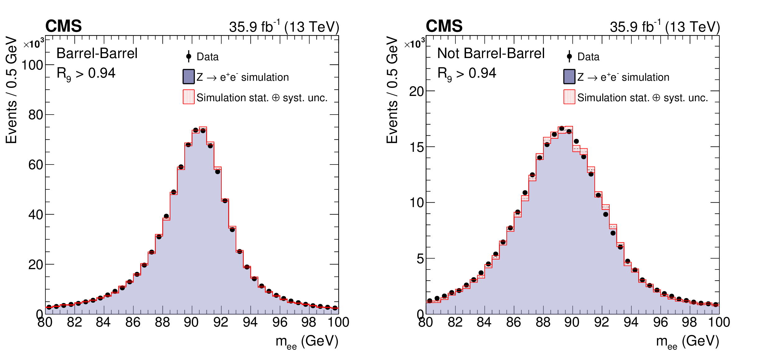
Figure 1:
Comparison of the dielectron invariant mass distributions in data and simulation (after energy smearing) for $ \mathrm{Z} \to \mathrm{e}^+ \mathrm {e}^- $ events where electrons are reconstructed as photons. The comparison is shown requiring $ R_9 > $ 0.94 for both "photons'' and for (left) events with both photons in the barrel, and (right) the remaining events. The simulated distributions are normalized to the integral of the data distribution in the range 87 $ < m_{\mathrm{ee}} < $ 93 GeV to highlight the agreement in the bulk of the distributions. |
png pdf |
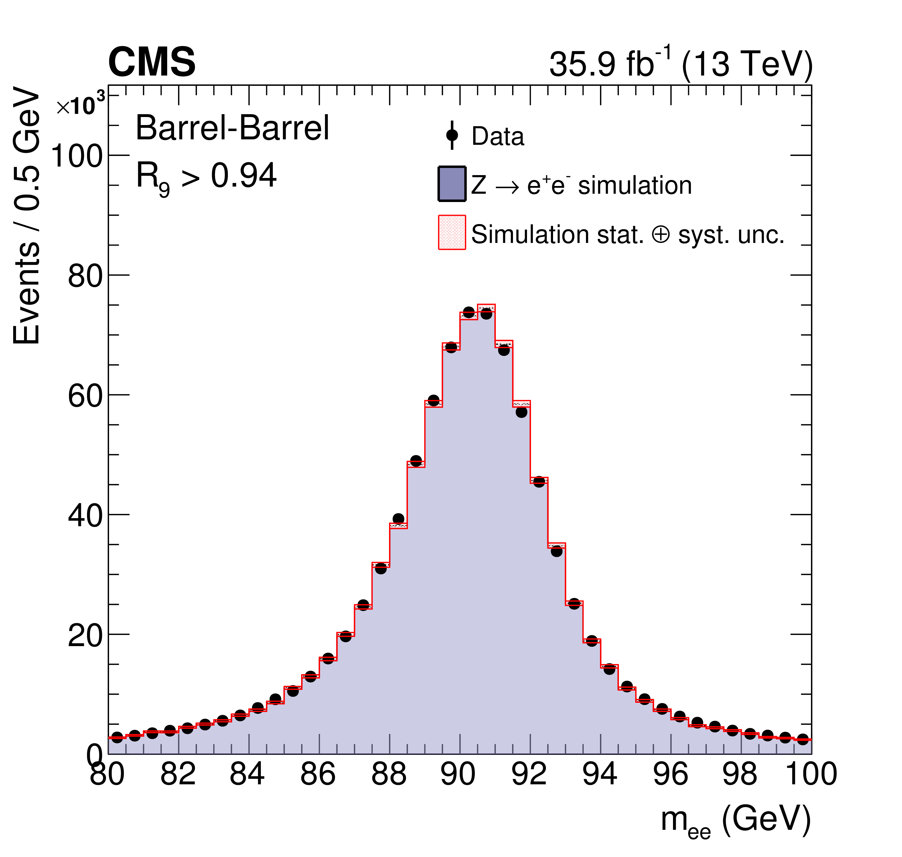
Figure 1-a:
Comparison of the dielectron invariant mass distributions in data and simulation (after energy smearing) for $ \mathrm{Z} \to \mathrm{e}^+ \mathrm {e}^- $ events where electrons are reconstructed as photons. The comparison is shown requiring $ R_9 > $ 0.94 for both "photons'' and for events with both photons in the barrel. The simulated distributions are normalized to the integral of the data distribution in the range 87 $ < m_{\mathrm{ee}} < $ 93 GeV to highlight the agreement in the bulk of the distributions. |
png pdf |
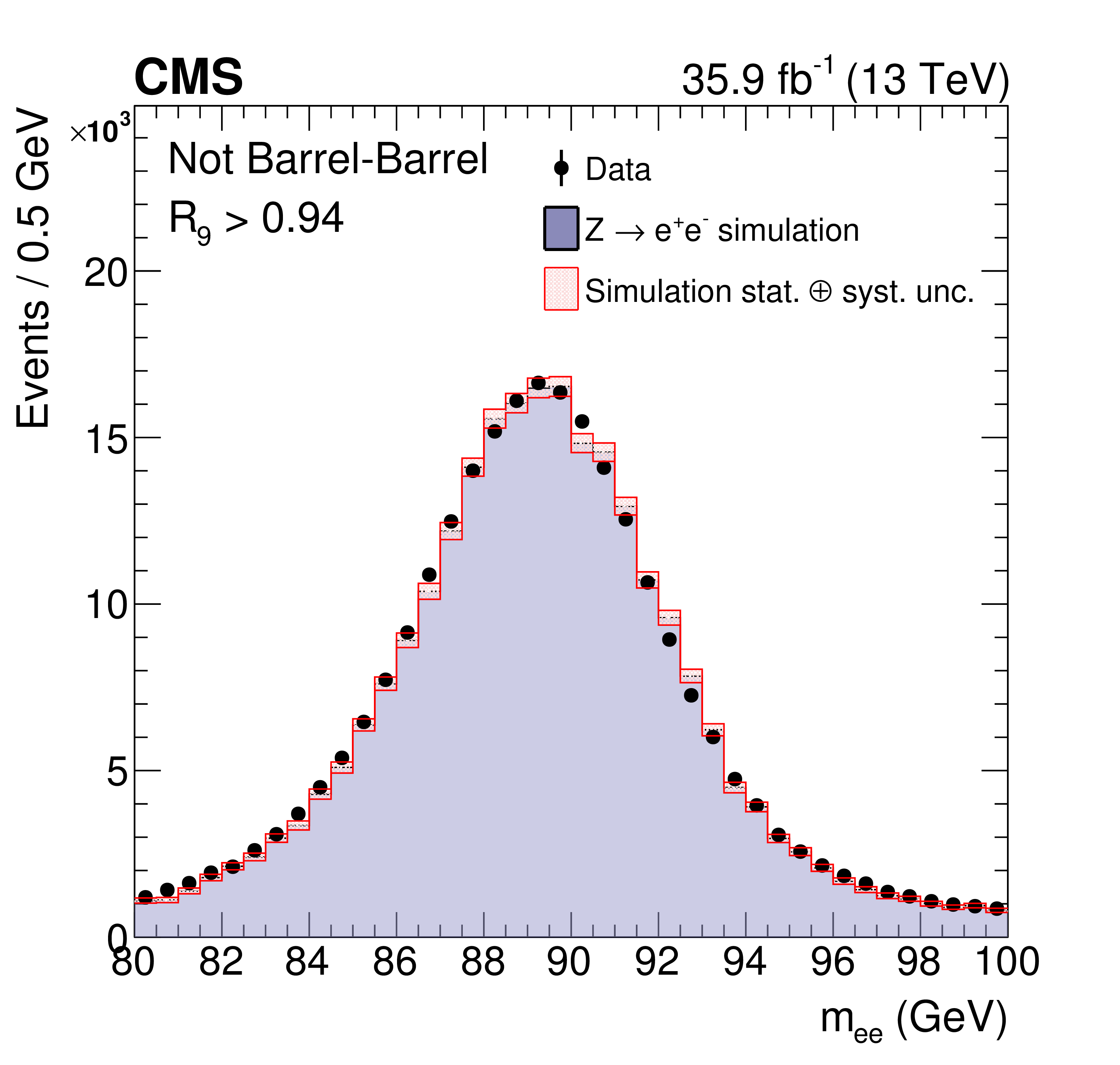
Figure 1-b:
Comparison of the dielectron invariant mass distributions in data and simulation (after energy smearing) for $ \mathrm{Z} \to \mathrm{e}^+ \mathrm {e}^- $ events where electrons are reconstructed as photons. The comparison is shown requiring $ R_9 > $ 0.94 for both "photons'' and for events with at least one photon not in the barrel. The simulated distributions are normalized to the integral of the data distribution in the range 87 $ < m_{\mathrm{ee}} < $ 93 GeV to highlight the agreement in the bulk of the distributions. |
png pdf |
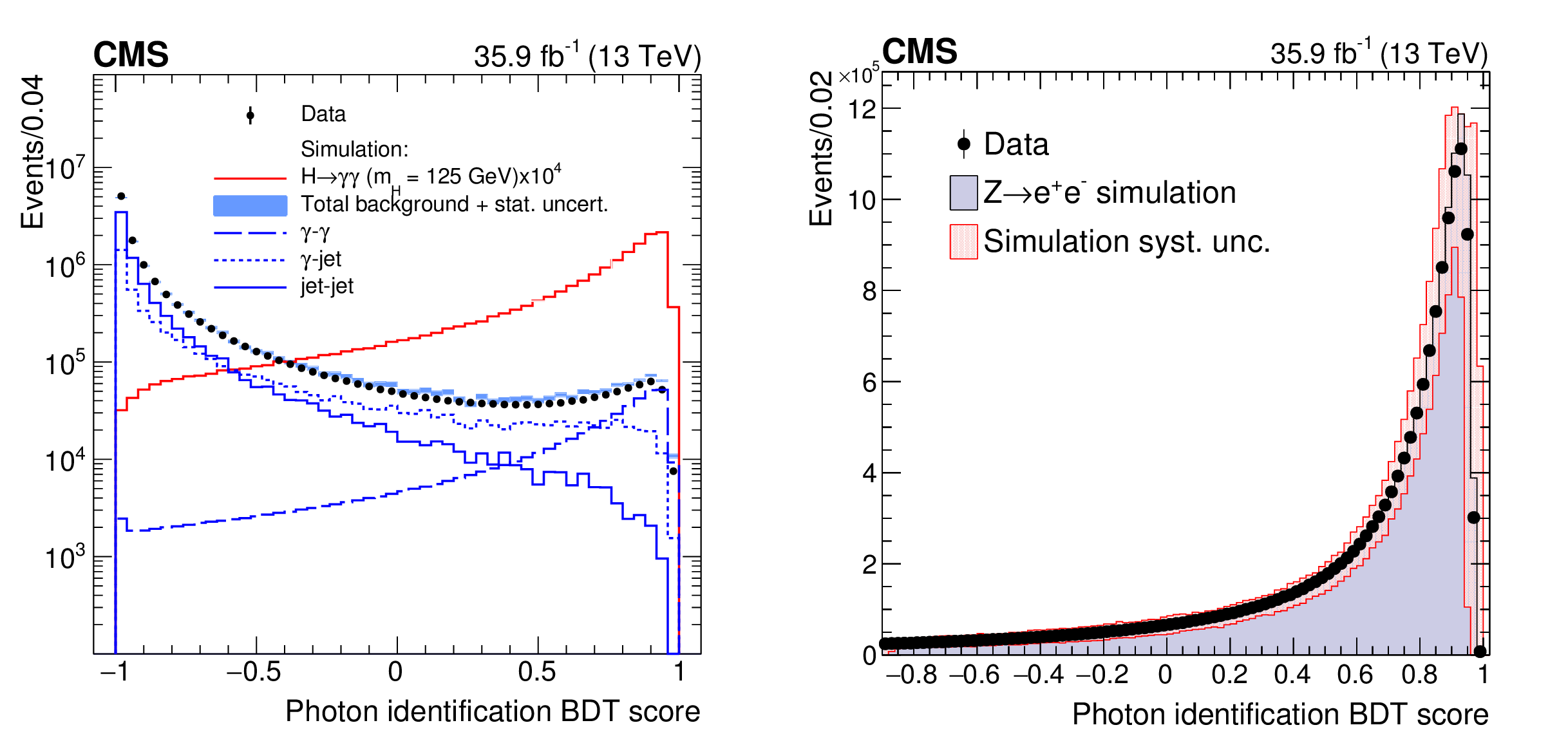
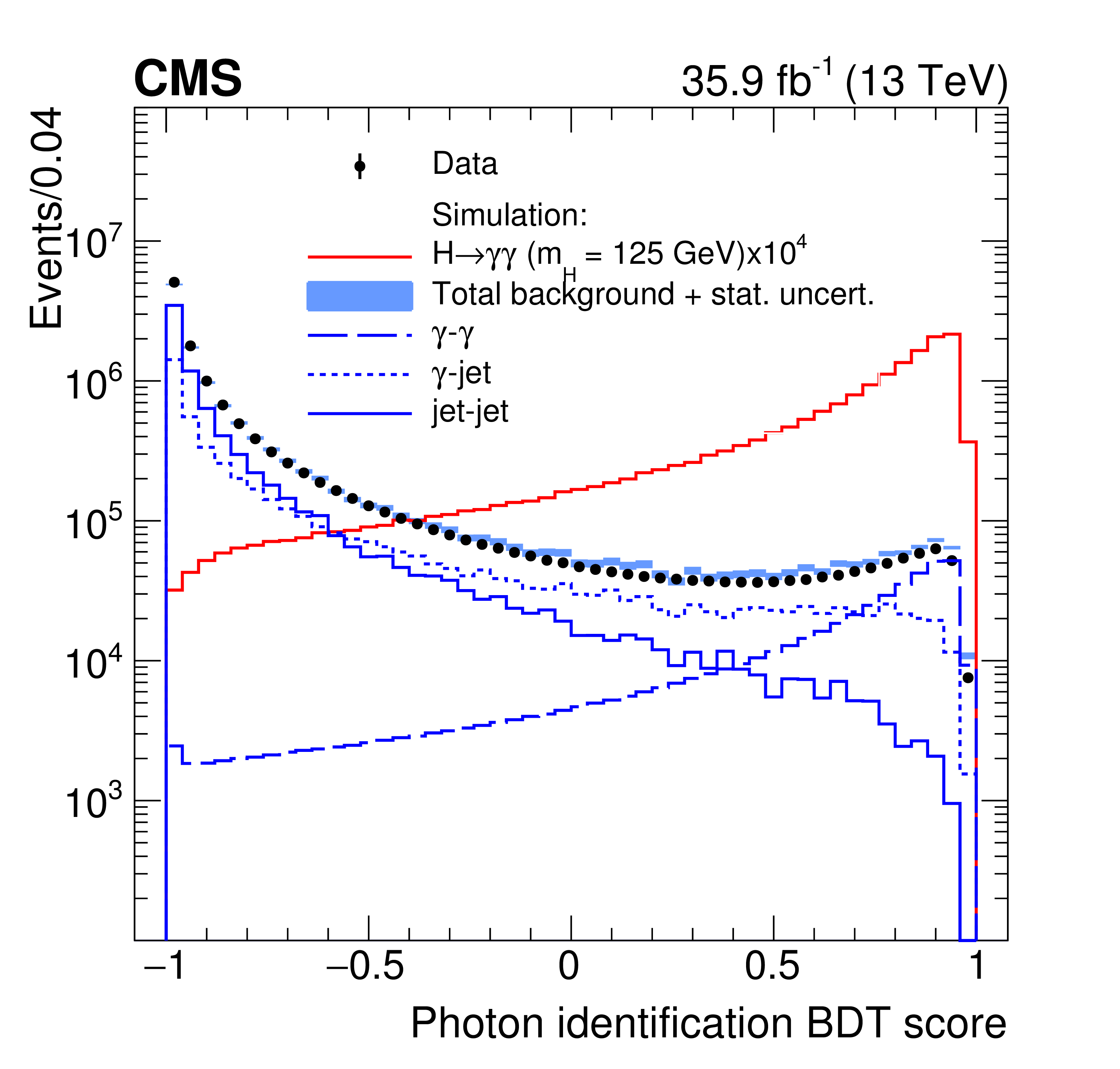
Figure 2:
(Left) Distribution of the photon identification BDT score of the lowest scoring photon of diphoton pairs with an invariant mass in the range 100 $ < {{{m}}_{{\gamma} {\gamma}}} < $ 180 GeV, for events passing the preselection in the 13 TeV data set (points), and for simulated background events (blue histogram). Histograms are also shown for different components of the simulated background. The sum of all background distributions is scaled up to data. The red histogram corresponds to simulated Higgs boson signal events. (Right) Distribution of the photon identification BDT score for $ \mathrm{Z} \to \mathrm{e}^+ \mathrm {e}^- $ events in data and simulation, where the electrons are reconstructed as photons. The systematic uncertainty applied to the shape from simulation (hashed region) is also shown. |
png pdf |
Figure 2-a:
Distribution of the photon identification BDT score of the lowest scoring photon of diphoton pairs with an invariant mass in the range 100 $ < {{{m}}_{{\gamma} {\gamma}}} < $ 180 GeV, for events passing the preselection in the 13 TeV data set (points), and for simulated background events (blue histogram). Histograms are also shown for different components of the simulated background. The sum of all background distributions is scaled up to data. The red histogram corresponds to simulated Higgs boson signal events. |
png pdf |
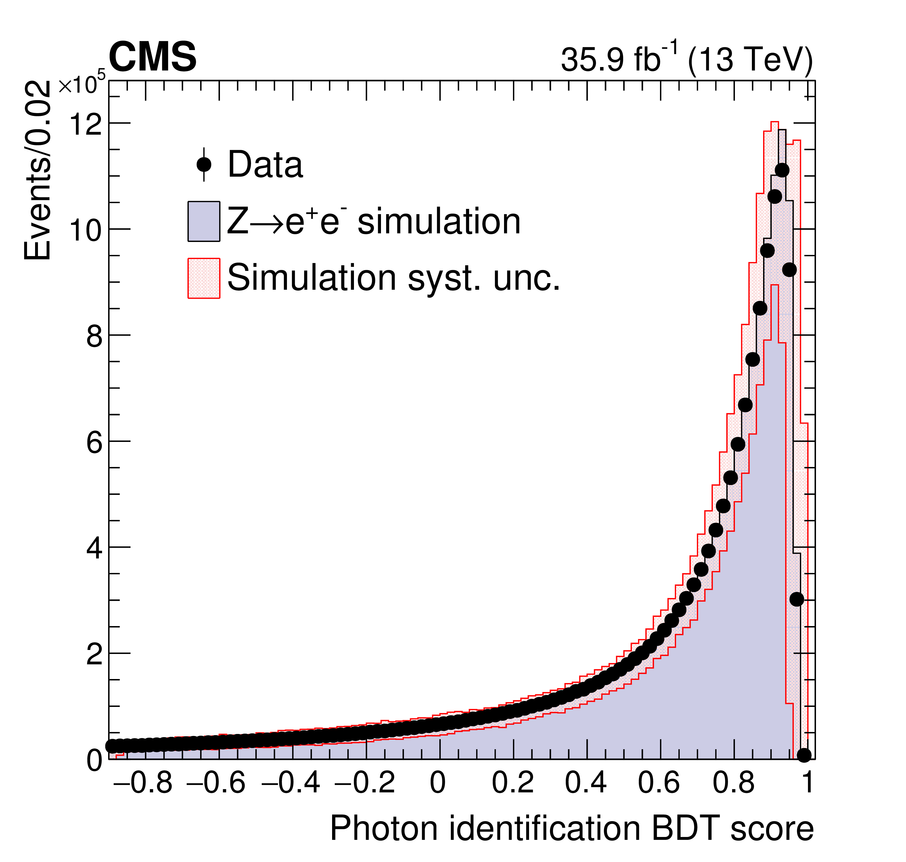
Figure 2-b:
Distribution of the photon identification BDT score for $ \mathrm{Z} \to \mathrm{e}^+ \mathrm {e}^- $ events in data and simulation, where the electrons are reconstructed as photons. The systematic uncertainty applied to the shape from simulation (hashed region) is also shown. |

png pdf |
Figure 3:
Validation of the $ {\mathrm{H}\to \gamma \gamma}$ vertex identification algorithm on $ \mathrm{Z} \to {{{\mu ^+}} {{\mu ^-}}} $ events omitting the muon tracks. Simulated events are weighted to match the distributions of pileup and location of primary vertices in data. |
png pdf |
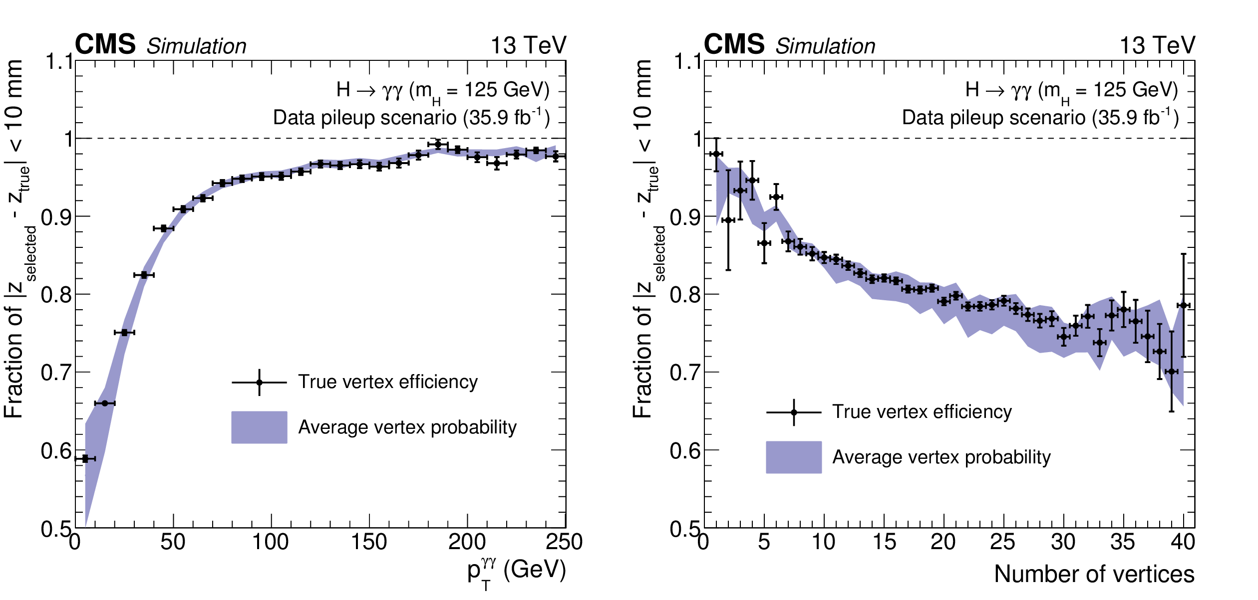
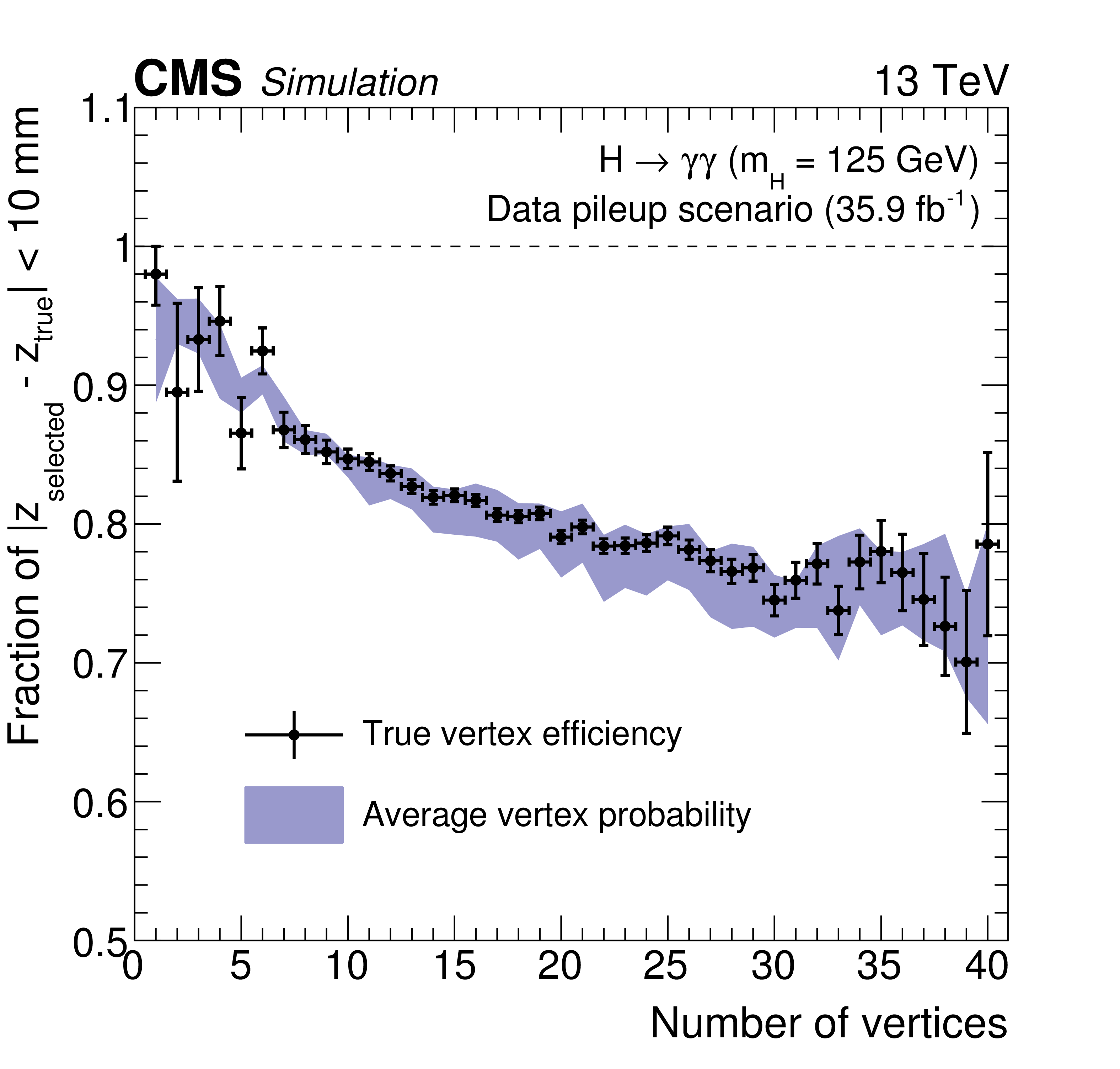
Figure 4:
Comparison of the true vertex identification efficiency and the average estimated vertex probability as a function of the reconstructed diphoton $ p_{\mathrm{T}} $ (left) and of the number of primary vertices (right) in simulated $ {\mathrm{H}\to \gamma \gamma}$ events with $m_{\mathrm{H}} = $ 125 GeV. Events are weighted according to the cross sections of the different production modes and to match the distributions of pileup and location of primary vertices in data. |
png pdf |
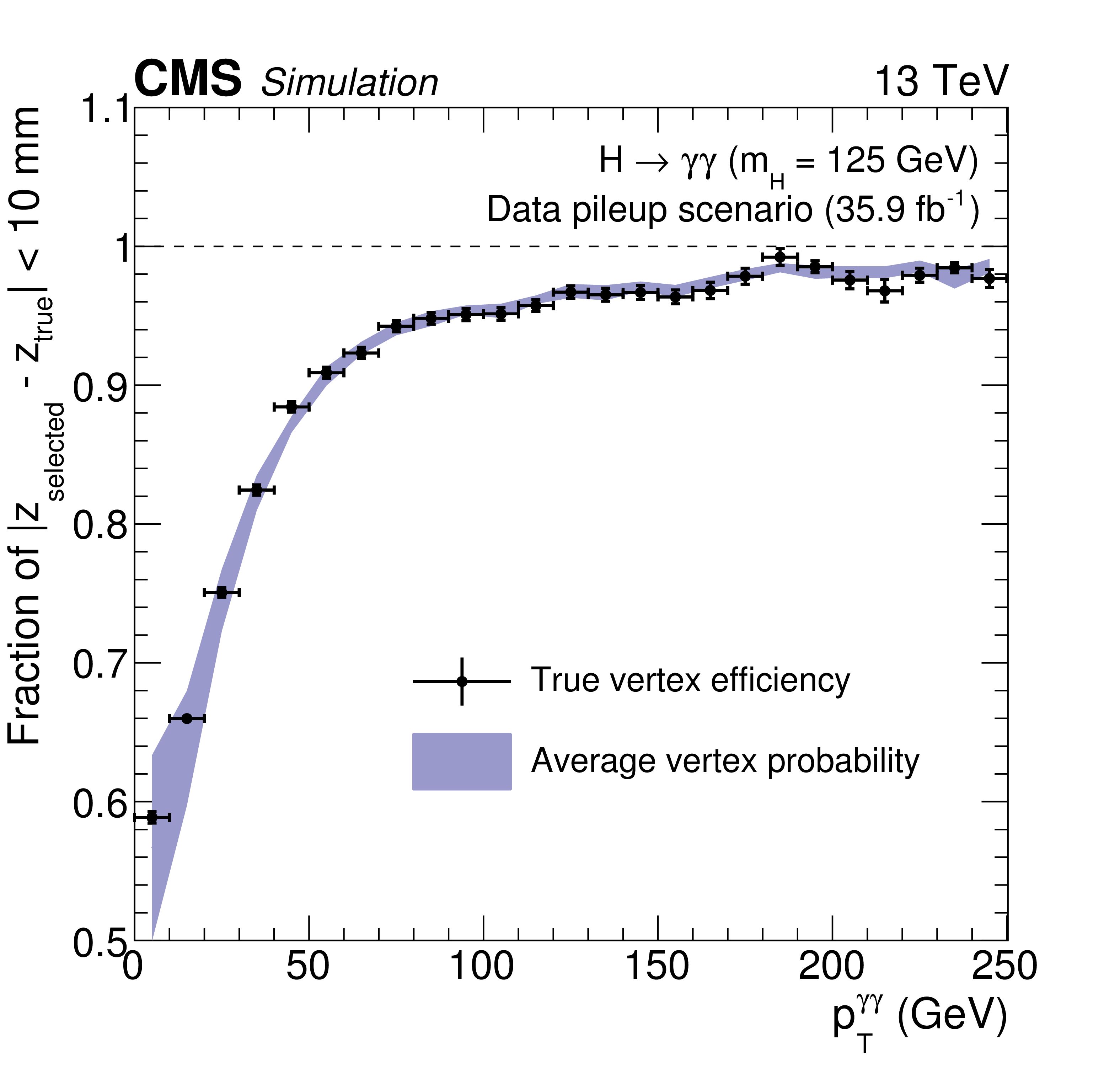
Figure 4-a:
Comparison of the true vertex identification efficiency and the average estimated vertex probability as a function of the reconstructed diphoton $ p_{\mathrm{T}} $ in simulated $ {\mathrm{H}\to \gamma \gamma}$ events with $m_{\mathrm{H}} = $ 125 GeV. Events are weighted according to the cross sections of the different production modes and to match the distributions of pileup and location of primary vertices in data. |
png pdf |
Figure 4-b:
Comparison of the true vertex identification efficiency and the average estimated vertex probability as a function of the number of primary vertices in simulated $ {\mathrm{H}\to \gamma \gamma}$ events with $m_{\mathrm{H}} = $ 125 GeV. Events are weighted according to the cross sections of the different production modes and to match the distributions of pileup and location of primary vertices in data. |
png pdf |
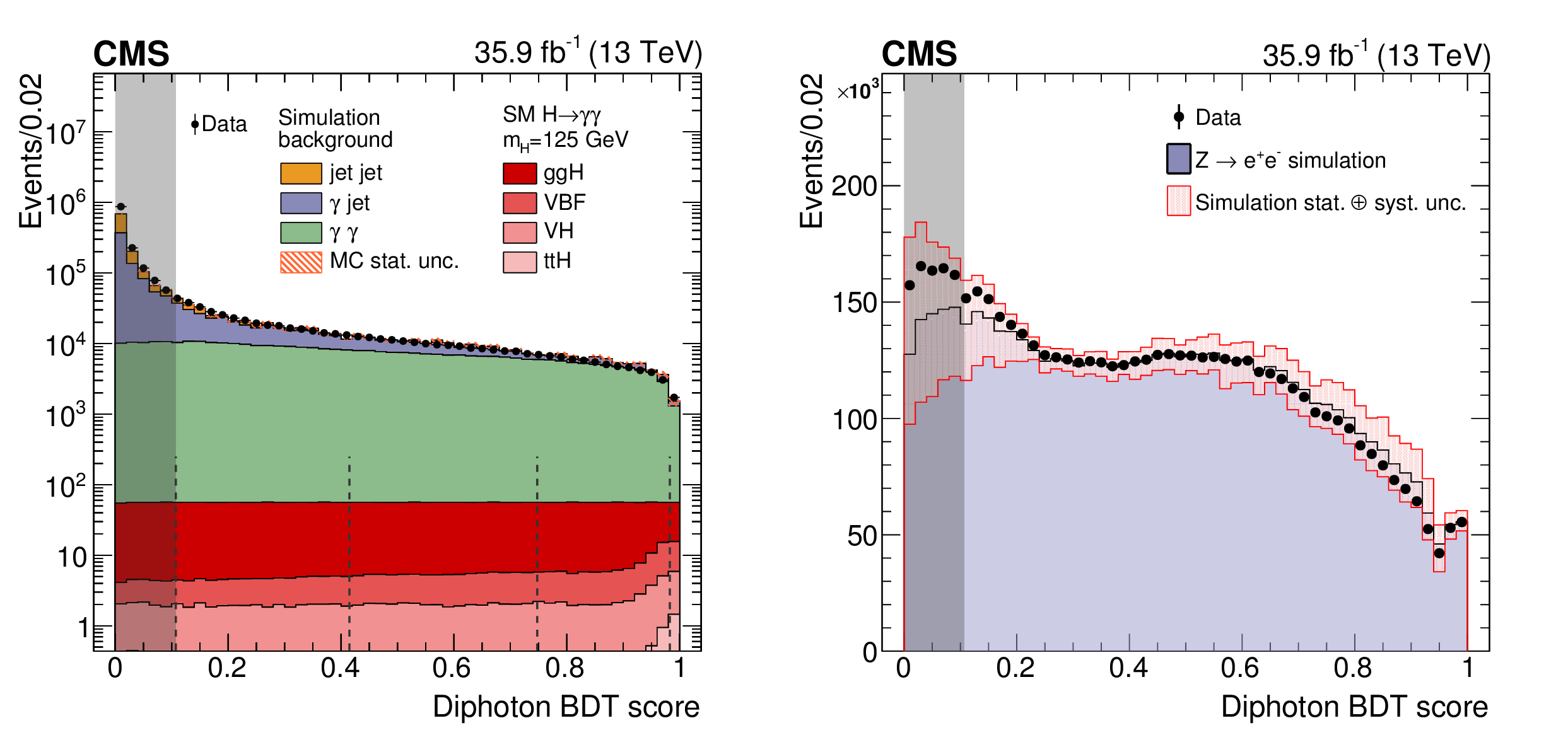
Figure 5:
(Left) Transformed score distribution from the diphoton multivariate classifier for events with two photons satisfying the preselection requirements in data (points), simulated signal (red shades), and simulated background (coloured histograms). Both signal and background are stacked together. The vertical dashed lines show the boundaries of the untagged categories, the grey shade indicates events discarded from the analysis. (Right) Score distribution of the diphoton multivariate classifier in $ {{\mathrm{Z} \to \mathrm{e}^+ \mathrm {e}^-}} $ events where the electrons are reconstructed as photons. The points show the distribution for data, the histogram shows the distribution for simulated Drell-Yan events. The pink band indicates the statistical and systematic uncertainties in simulation. The grey shade indicates events discarded from the analysis. |
png pdf |
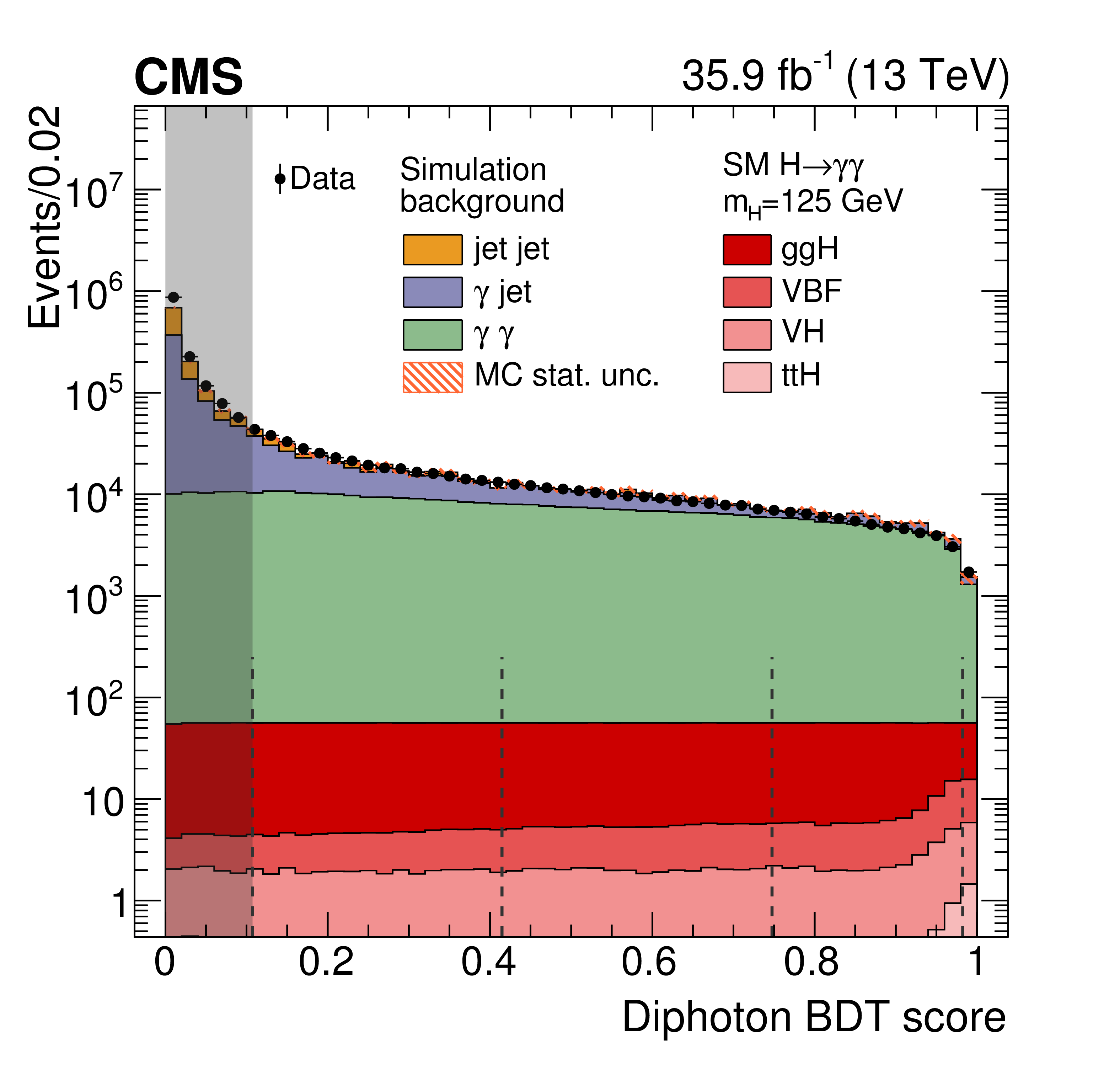
Figure 5-a:
Transformed score distribution from the diphoton multivariate classifier for events with two photons satisfying the preselection requirements in data (points), simulated signal (red shades), and simulated background (coloured histograms). Both signal and background are stacked together. The vertical dashed lines show the boundaries of the untagged categories, the grey shade indicates events discarded from the analysis. |
png pdf |
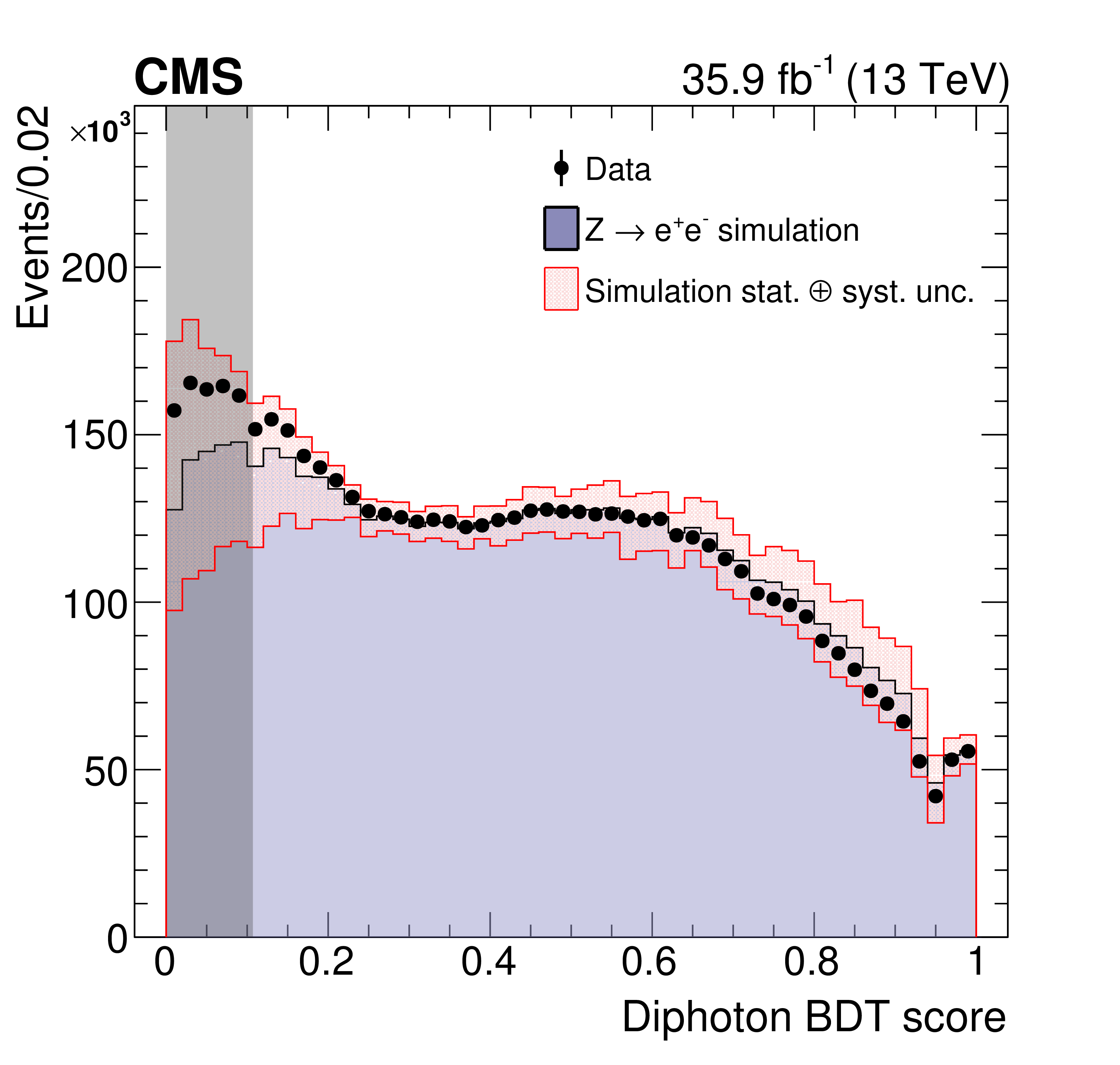
Figure 5-b:
Score distribution of the diphoton multivariate classifier in $ {{\mathrm{Z} \to \mathrm{e}^+ \mathrm {e}^-}} $ events where the electrons are reconstructed as photons. The points show the distribution for data, the histogram shows the distribution for simulated Drell-Yan events. The pink band indicates the statistical and systematic uncertainties in simulation. The grey shade indicates events discarded from the analysis. |
png pdf |
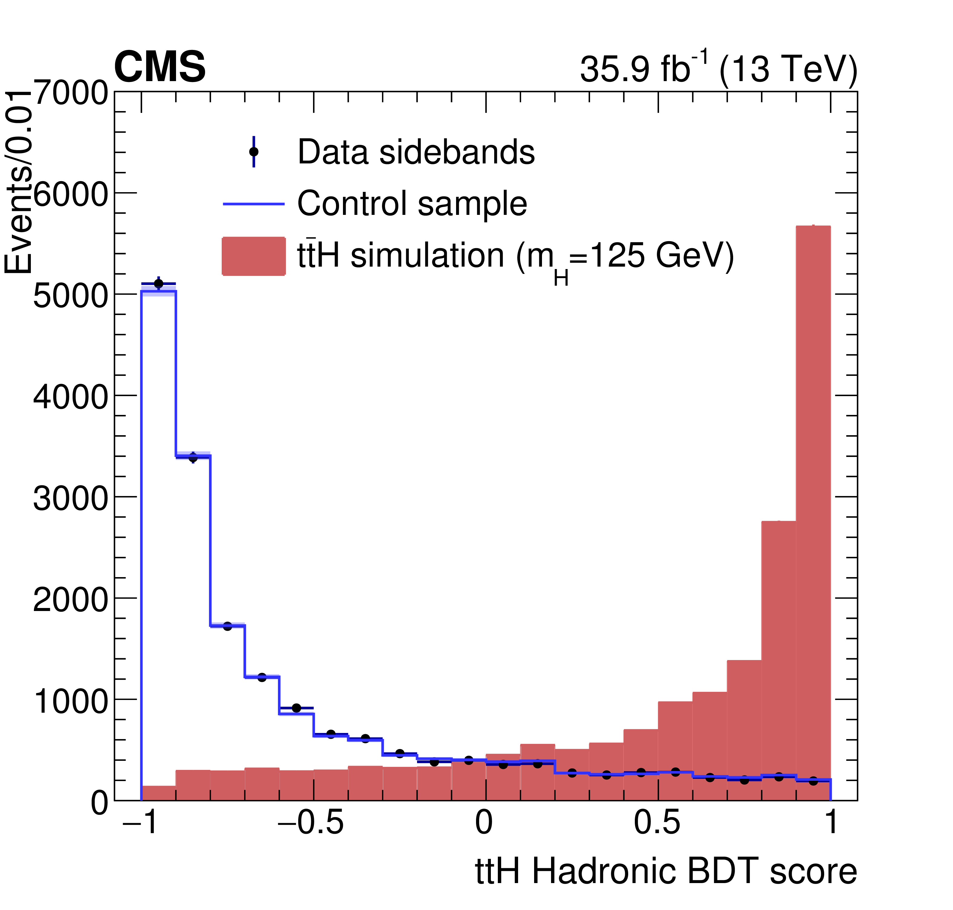
Figure 6:
Score distribution of the jet multivariate discriminant used to enhance jet tagging in the ttH multijet category. The points show the distribution for data in the signal region sidebands, $ {{{m}}_{{\gamma} {\gamma}}} < $ 115 GeV or $ {{{m}}_{{\gamma} {\gamma}}} > $ 135 GeV; the histogram shows the distribution for events in the data control sample; the filled histogram shows the distribution for simulated signal events. The distributions in the simulated and control samples are scaled as to match the integral of that from the data sidebands. |
png pdf |
Figure 7:
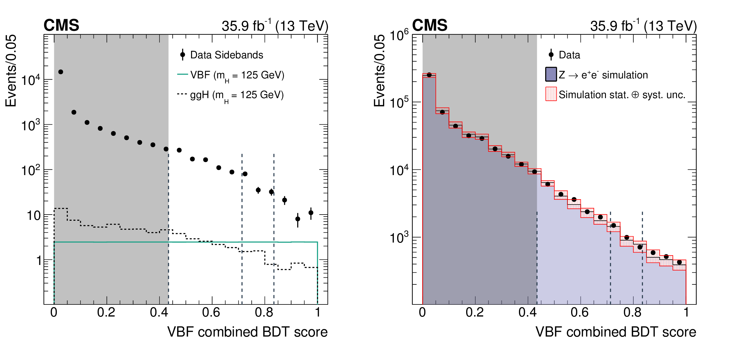
Score distribution from the VBF combined BDT for (left) ggH and VBF signal distributions, compared to background taken from data in the mass sideband regions, and (right) $ {{\mathrm{Z} \to \mathrm{e}^+ \mathrm {e}^-}} $ + jets events. On the left, the signal region selection is applied to the simulated ggH and VBF events; these are compared to points representing the background, as determined from data using the signal region selection in mass sidebands. On the right, the signal selection is applied to electrons reconstructed as photons, with points showing the distribution for data and the histogram showing the distribution for simulated Drell-Yan events, including statistical and systematic uncertainties (pink band). In both plots, dotted lines delimit the three VBF categories, while the grey region is discarded from the analysis. |
png pdf |
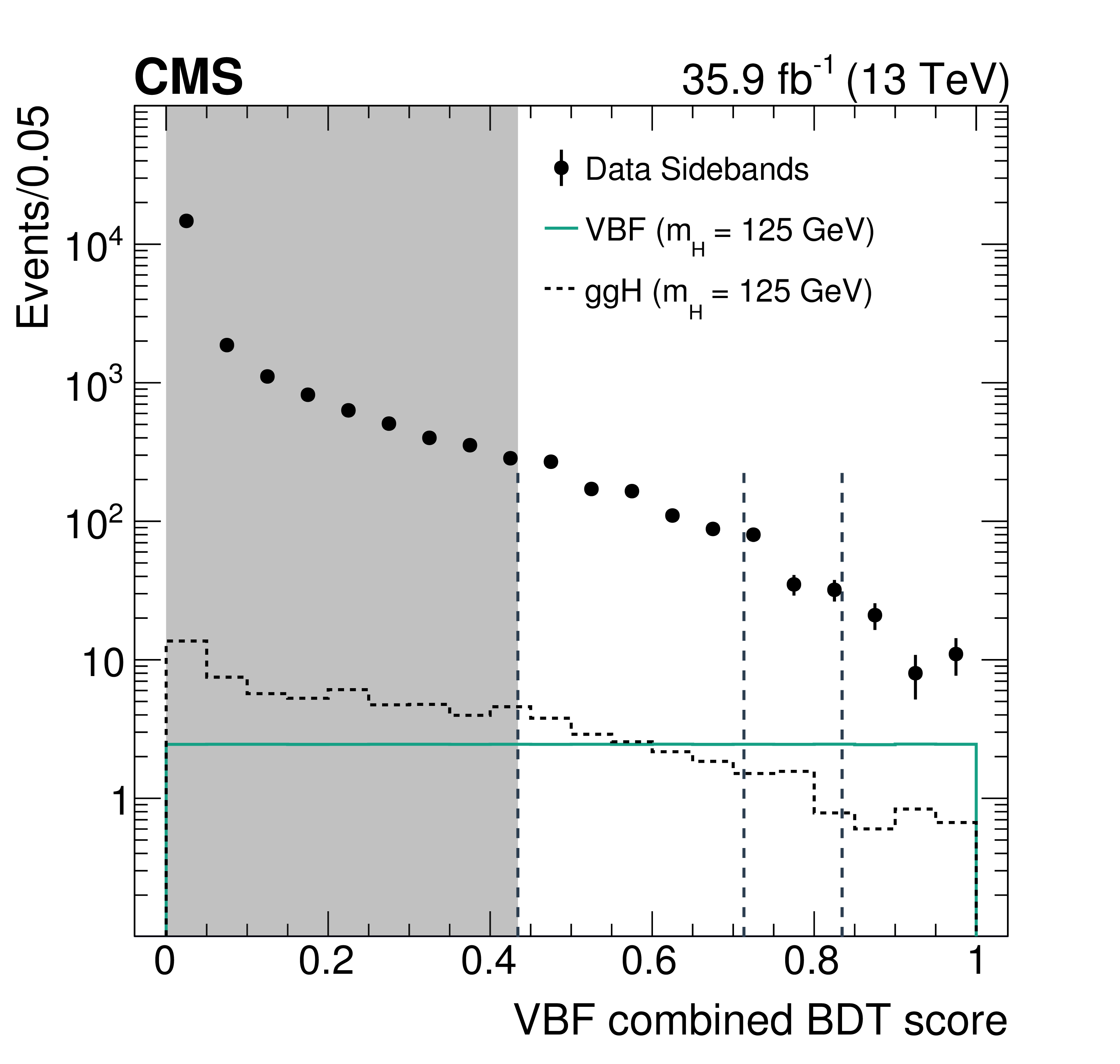
Figure 7-a:
Score distribution from the VBF combined BDT for ggH and VBF signal distributions, compared to background taken from data in the mass sideband regions.The signal region selection is applied to the simulated ggH and VBF events; these are compared to points representing the background, as determined from data using the signal region selection in mass sidebands. Dotted lines delimit the three VBF categories, while the grey region is discarded from the analysis. |
png pdf |
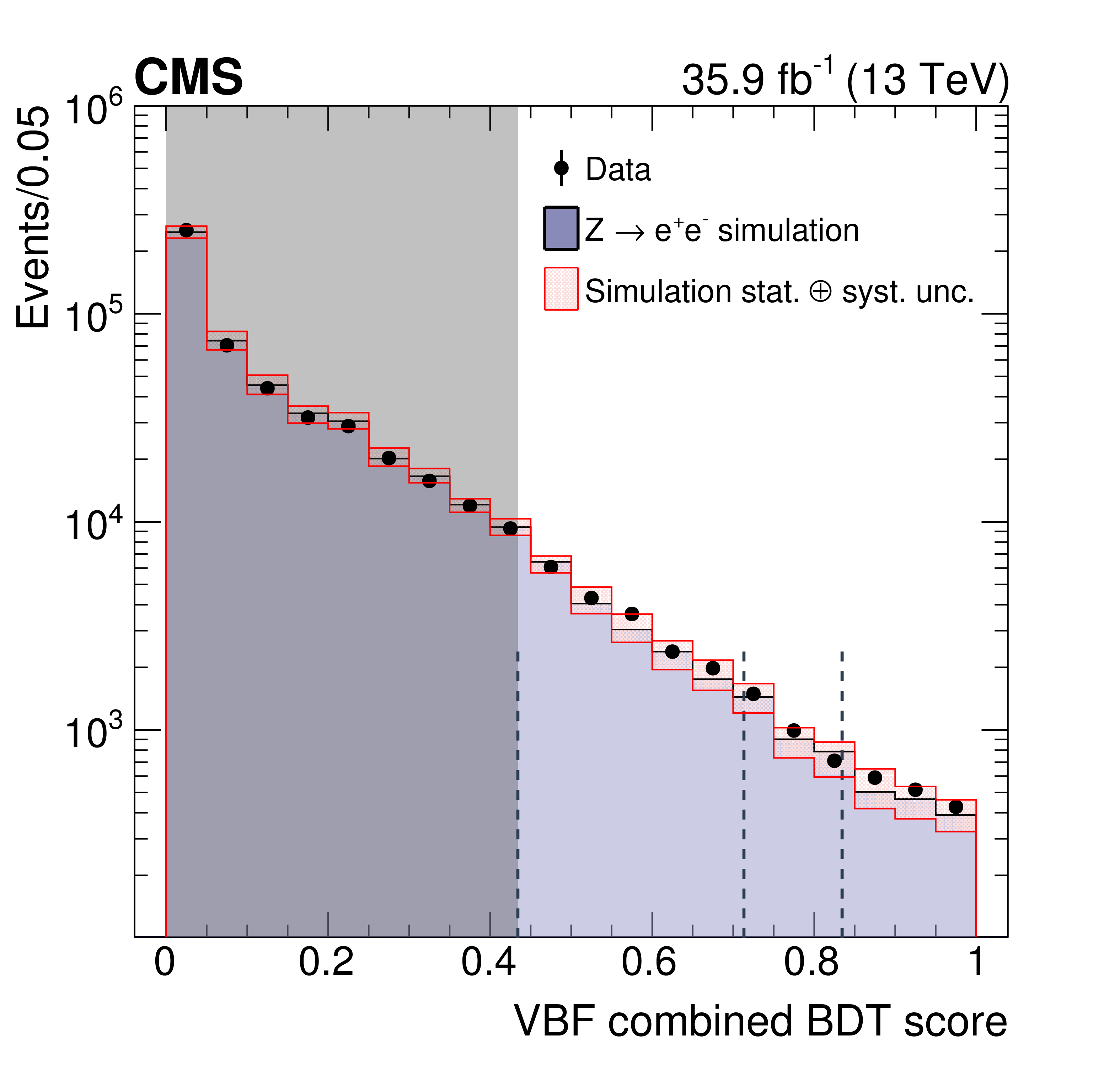
Figure 7-b:
Score distribution from the VBF combined BDT for $ {{\mathrm{Z} \to \mathrm{e}^+ \mathrm {e}^-}} $ + jets events. The signal selection is applied to electrons reconstructed as photons, with points showing the distribution for data and the histogram showing the distribution for simulated Drell-Yan events, including statistical and systematic uncertainties (pink band). Dotted lines delimit the three VBF categories, while the grey region is discarded from the analysis. |
png pdf |
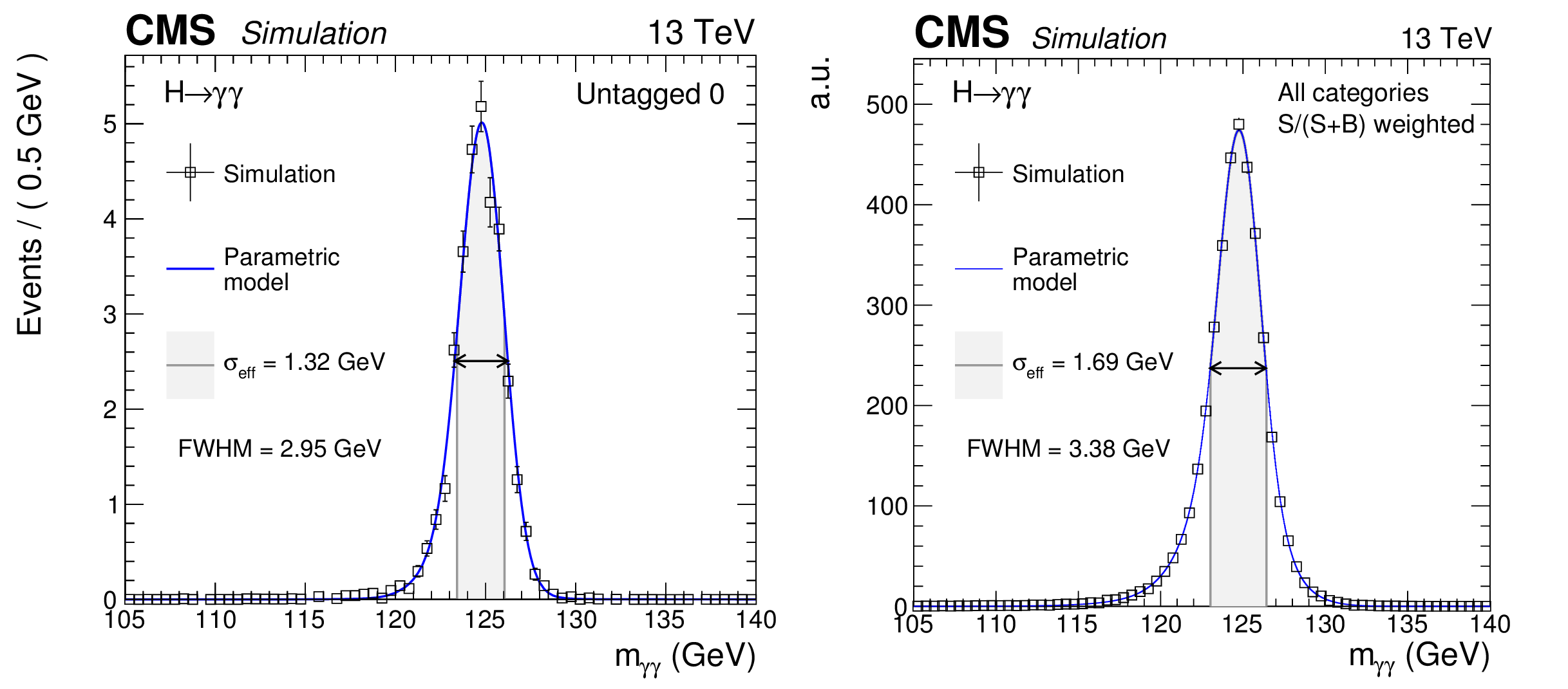
Figure 8:
Parametrized signal shape for the best resolution category (left) and for all categories combined together and weighted by the S/(S+B) ratio (right) for a simulated $ {\mathrm{H}\to \gamma \gamma}$ signal sample with $ {{m}}_{\mathrm{H}} = $ 125 GeV. The open squares represent weighted simulated events and the blue lines are the corresponding models. Also shown are the $\sigma _{\text {eff}}$ value (half the width of the narrowest interval containing 68.3% of the invariant mass distribution) and the corresponding interval as a grey band, and the full width at half maximum (FWHM) and the corresponding interval as a double arrow. |

png pdf |
Figure 8-a:
Parametrized signal shape for the best resolution category for a simulated $ {\mathrm{H}\to \gamma \gamma}$ signal sample with $ {{m}}_{\mathrm{H}} = $ 125 GeV. |
png pdf |
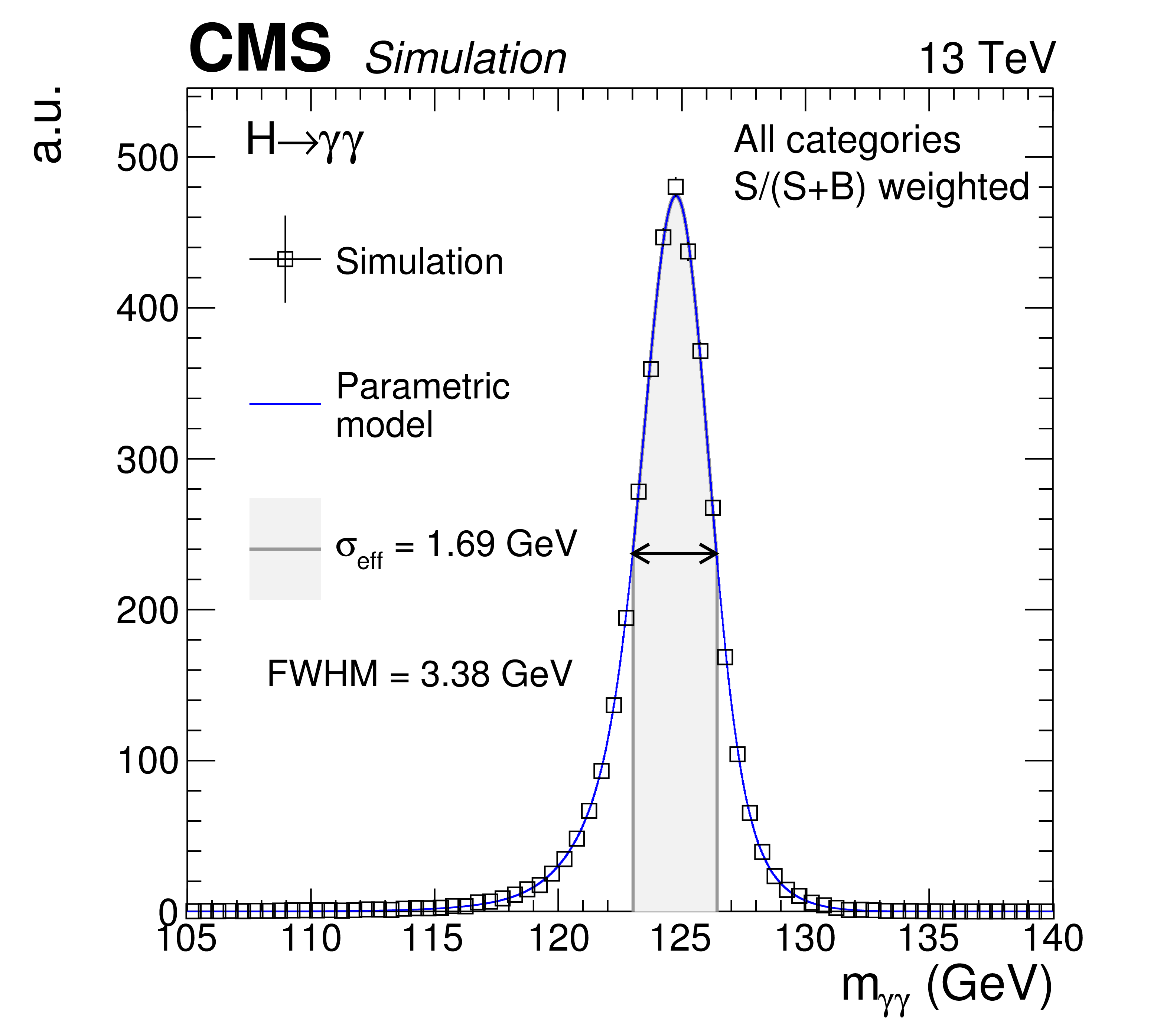
Figure 8-b:
Parametrized signal shape for all categories combined together and weighted by the S/(S+B) ratio for a simulated $ {\mathrm{H}\to \gamma \gamma}$ signal sample with $ {{m}}_{\mathrm{H}} = $ 125 GeV. The open squares represent weighted simulated events and the blue lines are the corresponding models. Also shown are the $\sigma _{\text {eff}}$ value (half the width of the narrowest interval containing 68.3% of the invariant mass distribution) and the corresponding interval as a grey band, and the full width at half maximum (FWHM) and the corresponding interval as a double arrow. |
png pdf |
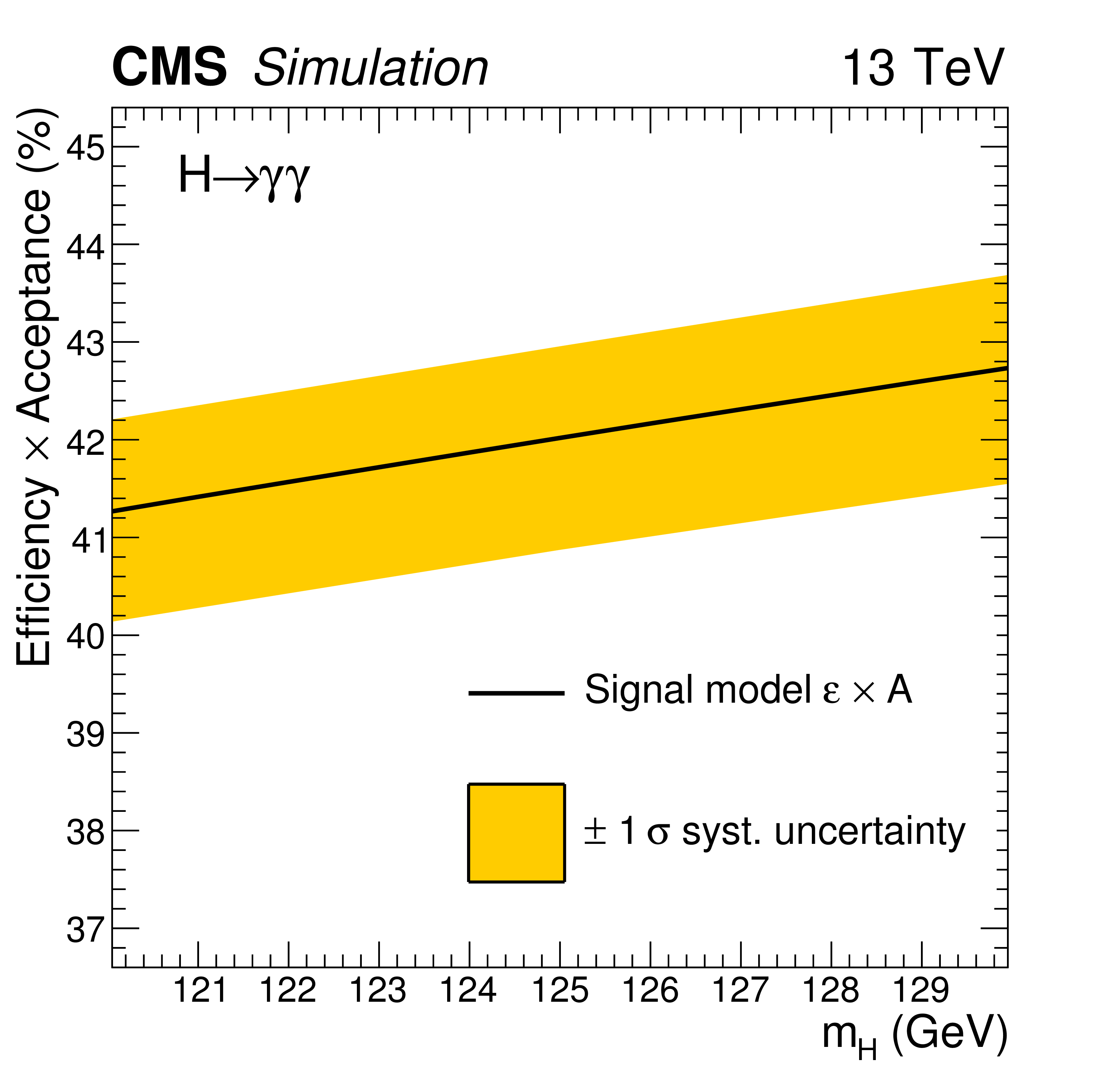
Figure 9:
The product of efficiency and acceptance of the signal model as a function of $ {{{m}}_{\mathrm{H}}} $ for all categories combined. The black line represents the yield from the signal model. The yellow band indicates the effect of the $\pm $1 standard deviation of the systematic uncertainties for trigger, photon identification and selection, photon energy scale and modelling of the photon energy resolution, and vertex identification (described in Section xxxxx). |
png pdf |
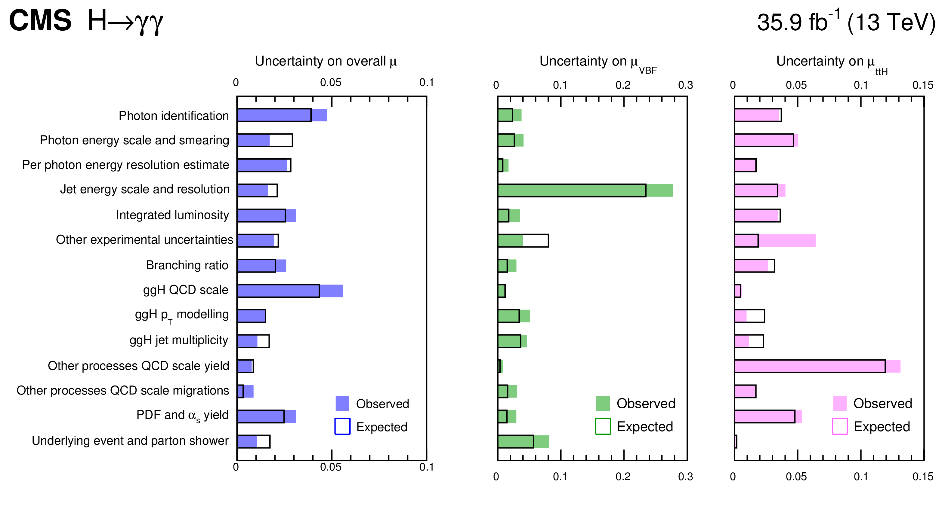
Figure 10:
Summary of the impact of the different systematic uncertainties on the overall signal strength modifier and on the signal strength modifiers for the VBF and ttH production processes. The observed (expected) results are shown by the solid (empty) bars. |
png pdf |
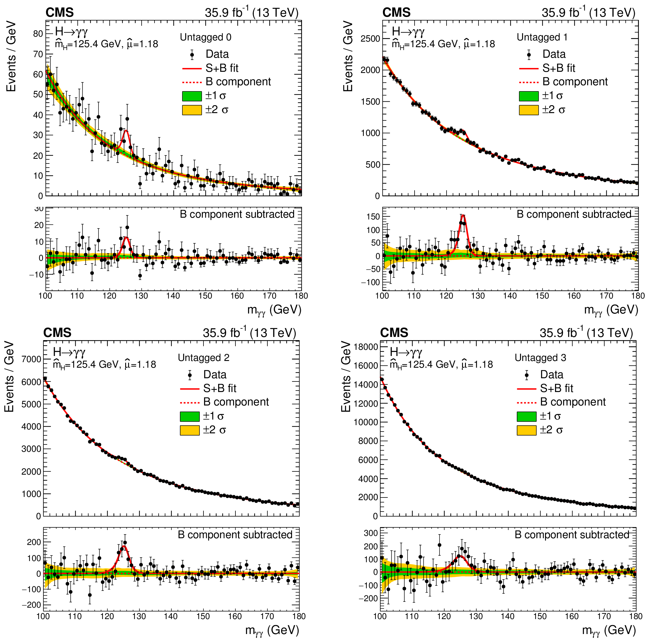
Figure 11:
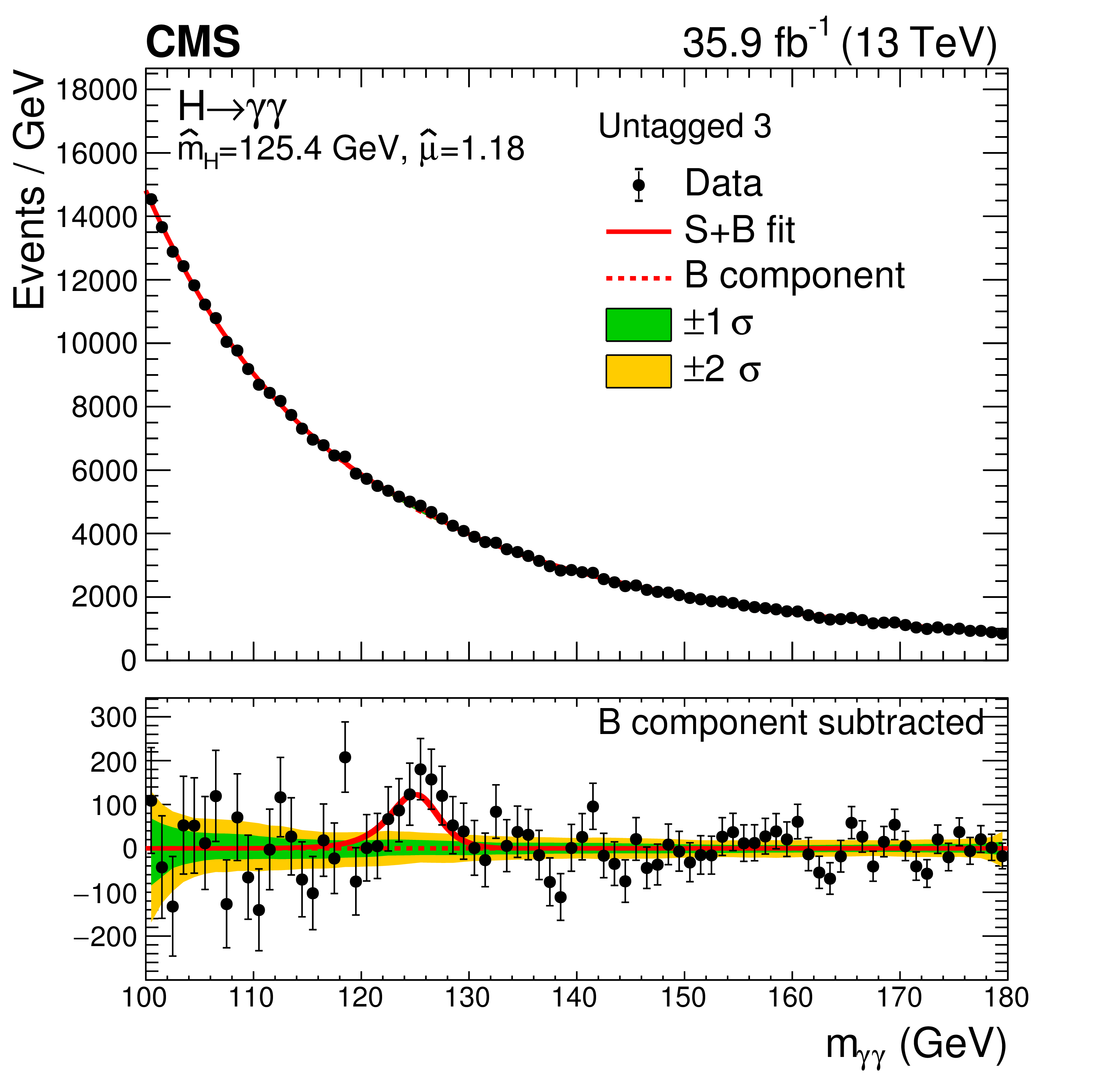
Data and signal-plus-background model fits in the four untagged categories are shown. The one (green) and two (yellow) standard deviation bands include the uncertainties in the background component of the fit. The lower panel in each plot shows the residuals after the background subtraction. |
png pdf |
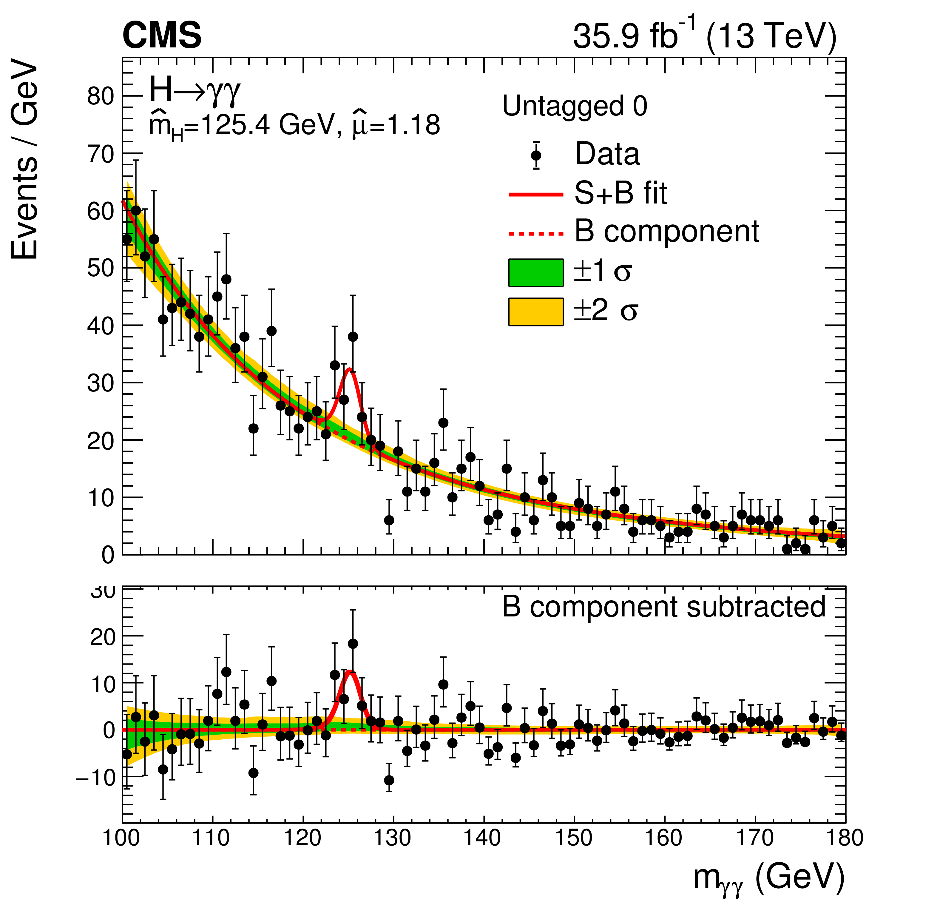
Figure 11-a:
Data and signal-plus-background model fits in the untagged 0 are shown. The one (green) and two (yellow) standard deviation bands include the uncertainties in the background component of the fit. The lower panel in each plot shows the residuals after the background subtraction. |
png pdf |
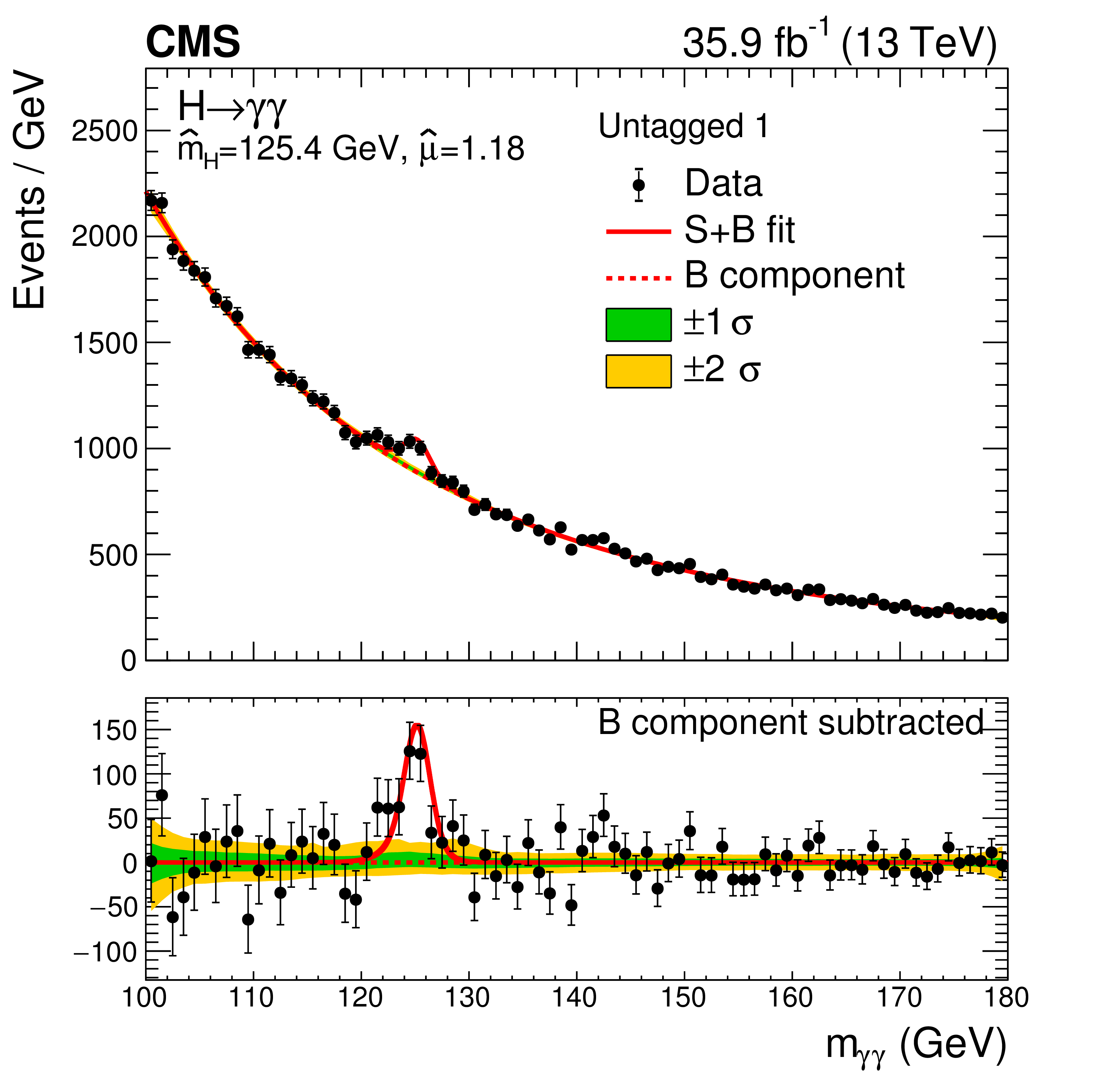
Figure 11-b:
Data and signal-plus-background model fits in the untagged 1 are shown. The one (green) and two (yellow) standard deviation bands include the uncertainties in the background component of the fit. The lower panel in each plot shows the residuals after the background subtraction. |
png pdf |
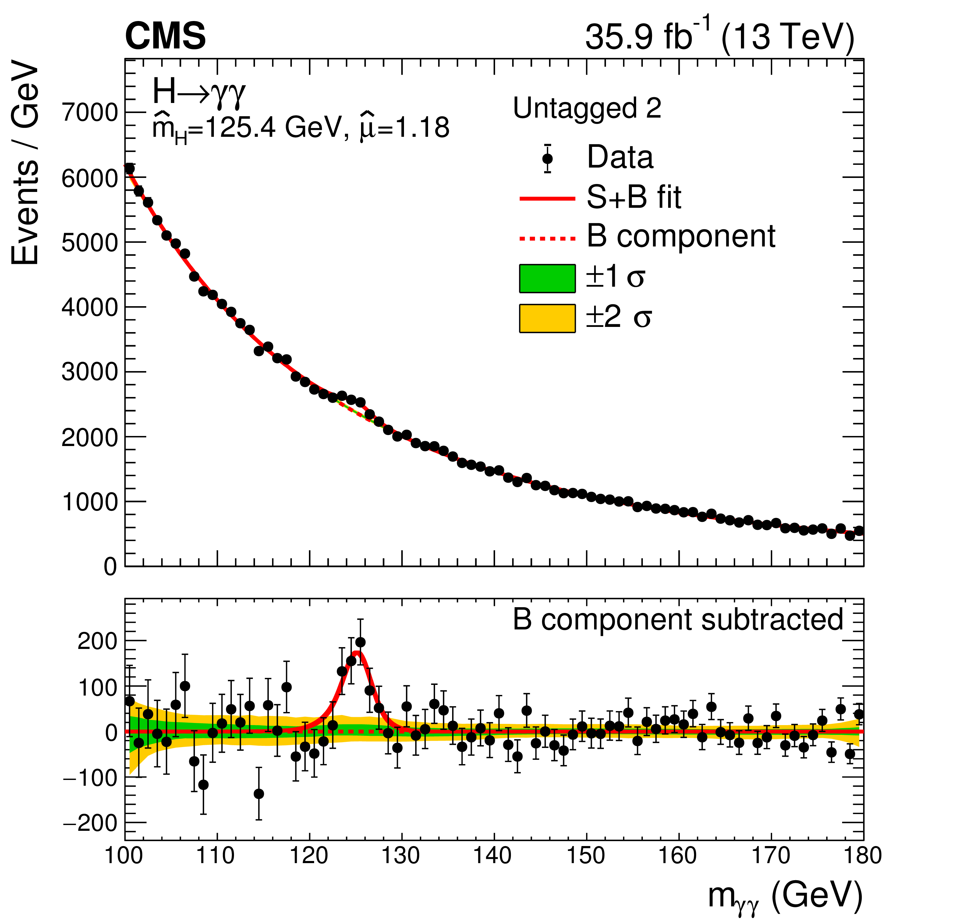
Figure 11-c:
Data and signal-plus-background model fits in the untagged 2 are shown. The one (green) and two (yellow) standard deviation bands include the uncertainties in the background component of the fit. The lower panel in each plot shows the residuals after the background subtraction. |
png pdf |
Figure 11-d:
Data and signal-plus-background model fits in the untagged 3 are shown. The one (green) and two (yellow) standard deviation bands include the uncertainties in the background component of the fit. The lower panel in each plot shows the residuals after the background subtraction. |
png pdf |
Figure 12:
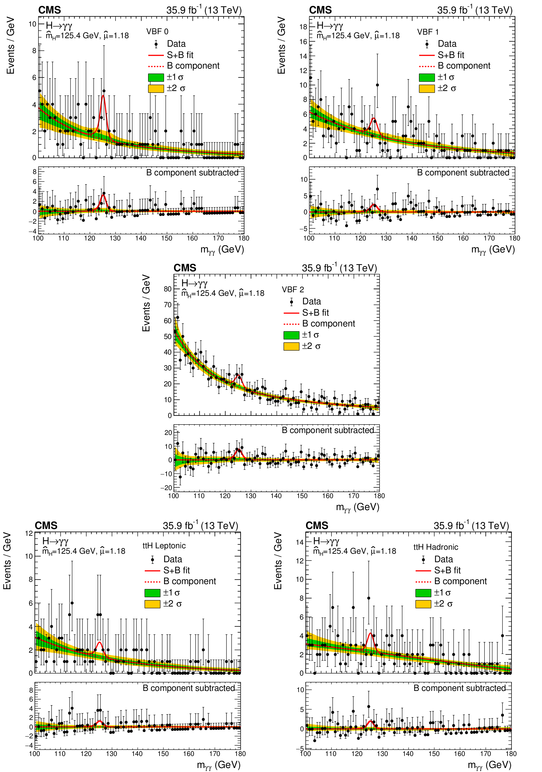
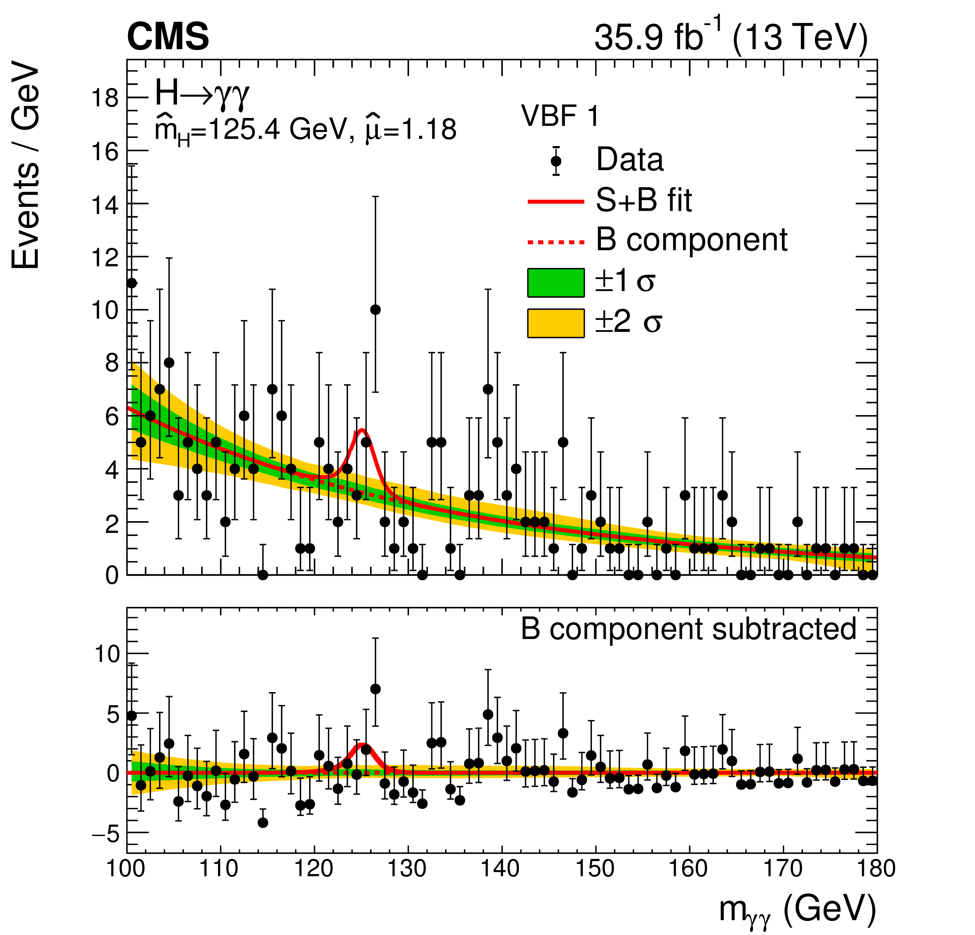
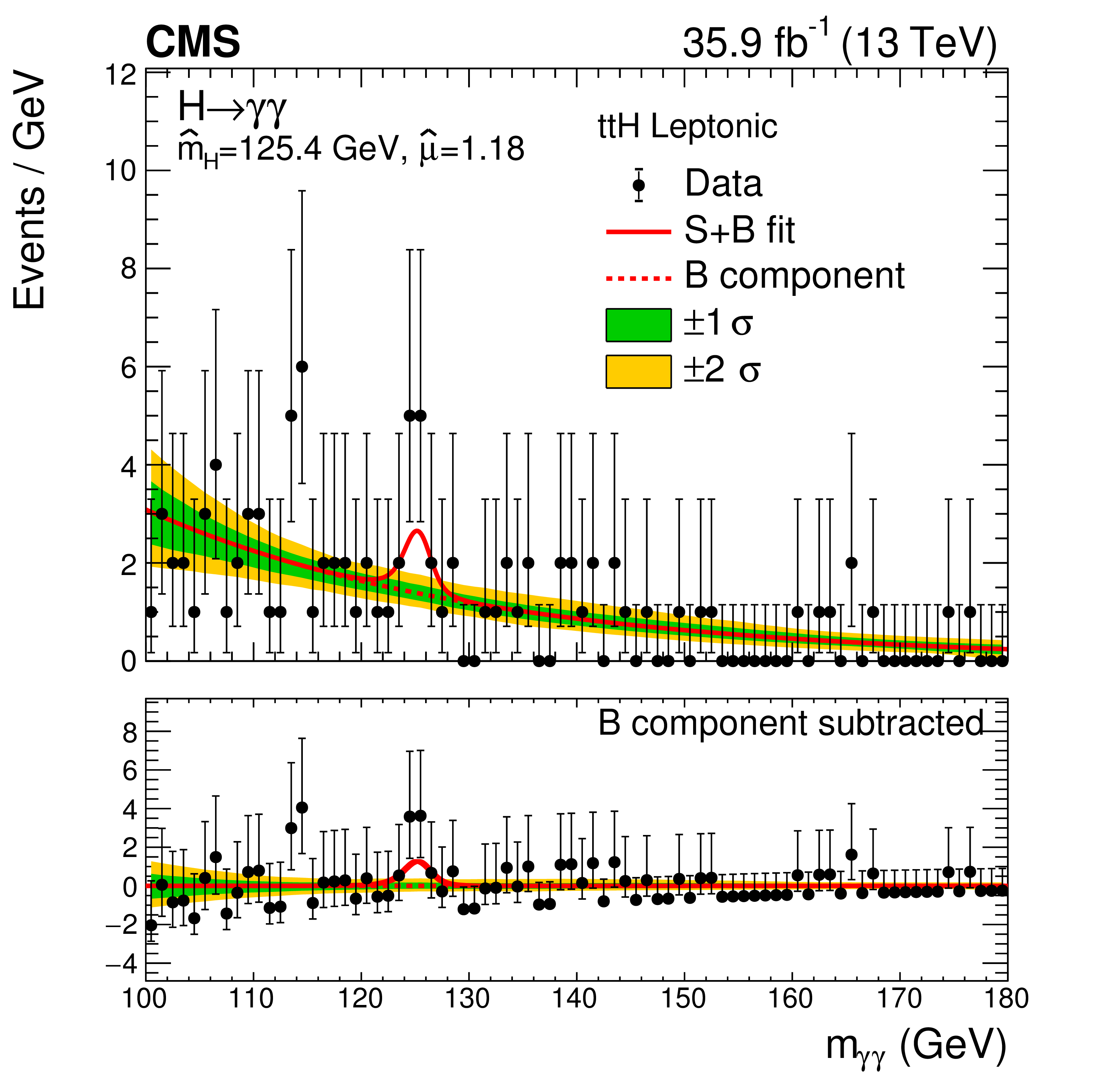
Data and signal-plus-background model fits in VBF and ttH categories are shown. The one (green) and two (yellow) standard deviation bands include the uncertainties in the background component of the fit. The lower panel in each plot shows the residuals after the background subtraction. |

png pdf |
Figure 12-a:
Data and signal-plus-background model fits in the VBF 0 category are shown. The one (green) and two (yellow) standard deviation bands include the uncertainties in the background component of the fit. The lower panel in each plot shows the residuals after the background subtraction. |
png pdf |
Figure 12-b:
Data and signal-plus-background model fits in the VBF 1 category are shown. The one (green) and two (yellow) standard deviation bands include the uncertainties in the background component of the fit. The lower panel in each plot shows the residuals after the background subtraction. |

png pdf |
Figure 12-c:
Data and signal-plus-background model fits in the VBF 2 category are shown. The one (green) and two (yellow) standard deviation bands include the uncertainties in the background component of the fit. The lower panel in each plot shows the residuals after the background subtraction. |
png pdf |
Figure 12-d:
Data and signal-plus-background model fits in the ttH Leptonic category are shown. The one (green) and two (yellow) standard deviation bands include the uncertainties in the background component of the fit. The lower panel in each plot shows the residuals after the background subtraction. |
png pdf |
Figure 12-e:
Data and signal-plus-background model fits in the ttH Hadronic category are shown. The one (green) and two (yellow) standard deviation bands include the uncertainties in the background component of the fit. The lower panel in each plot shows the residuals after the background subtraction. |
png pdf |
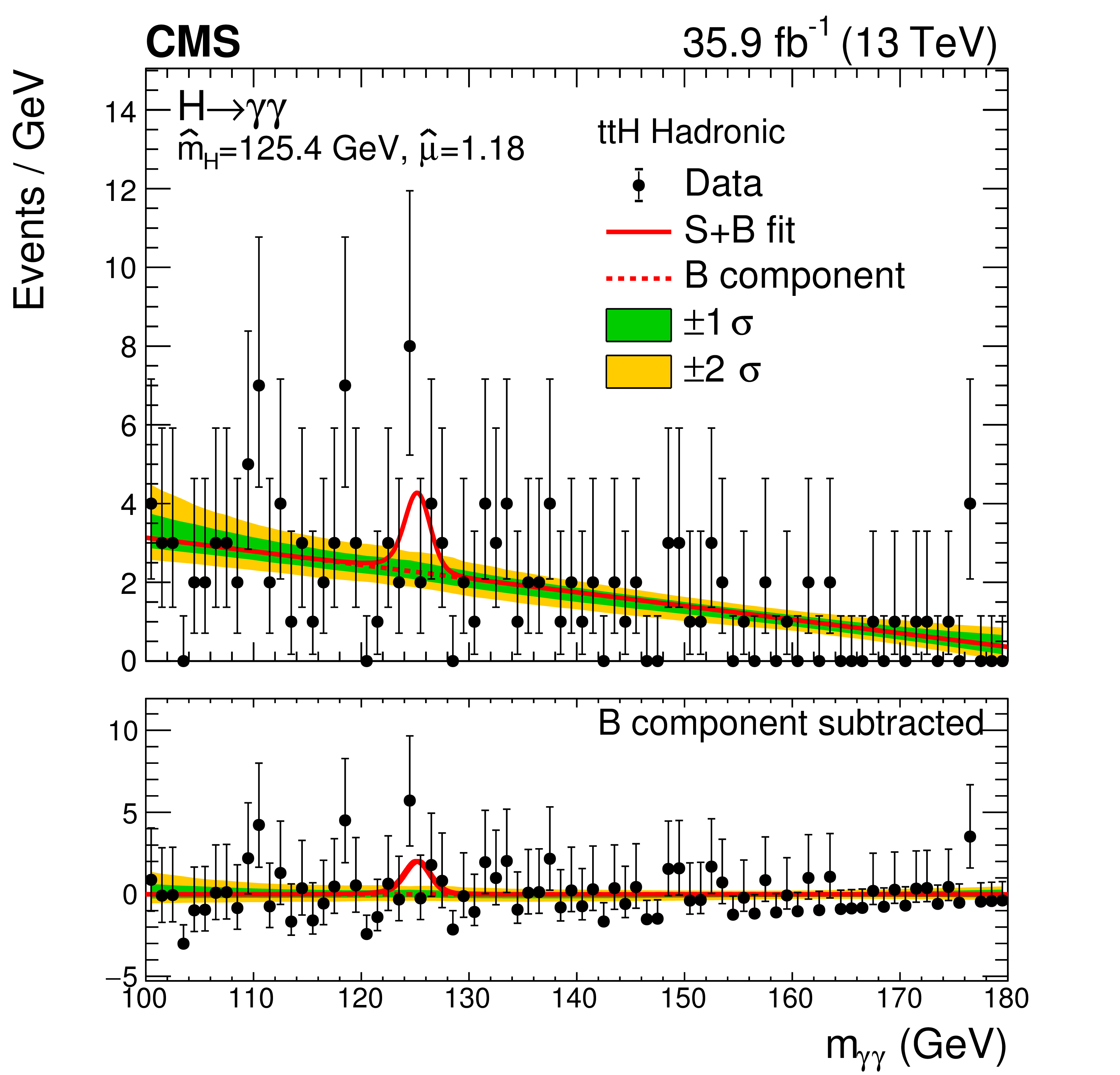
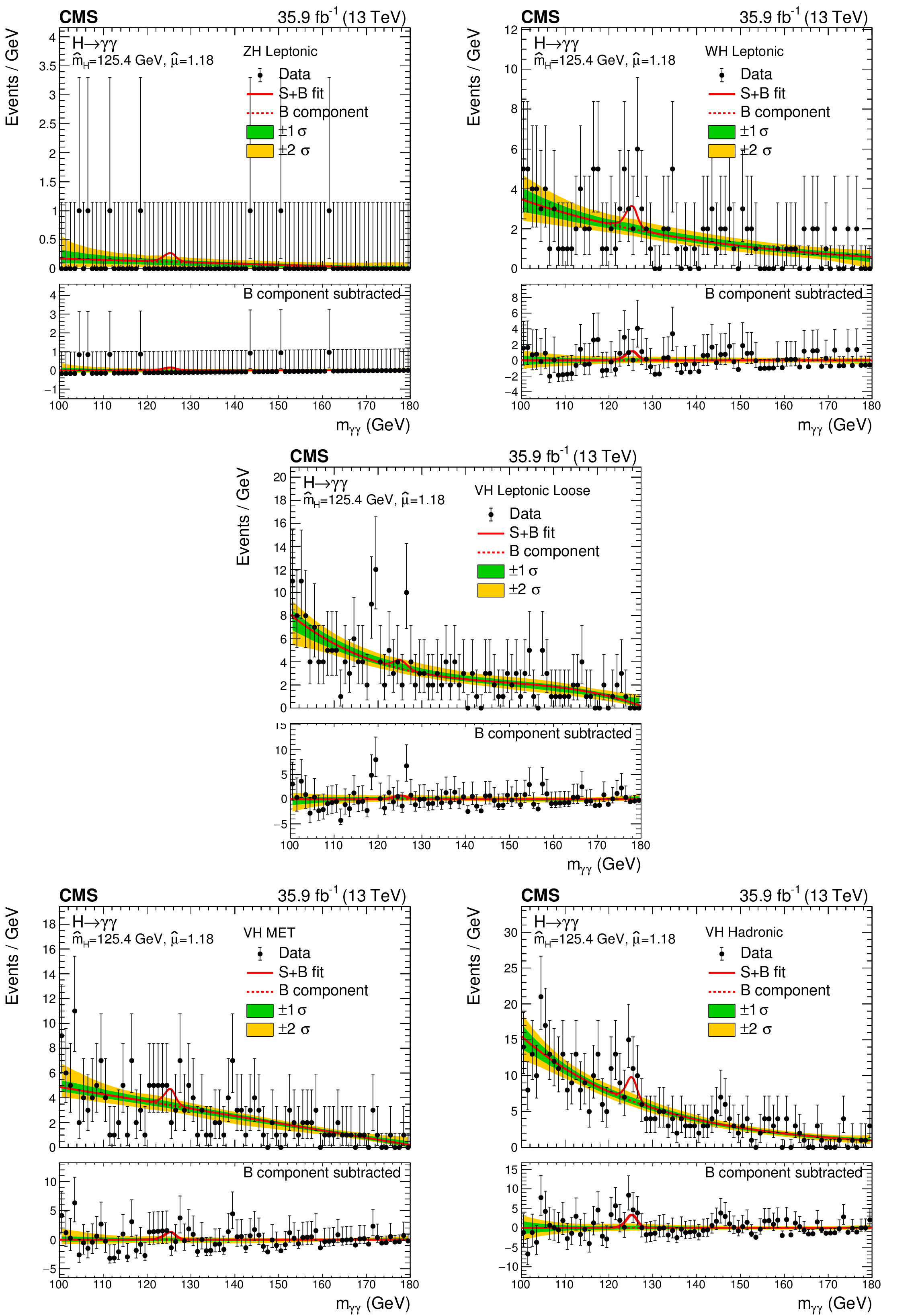
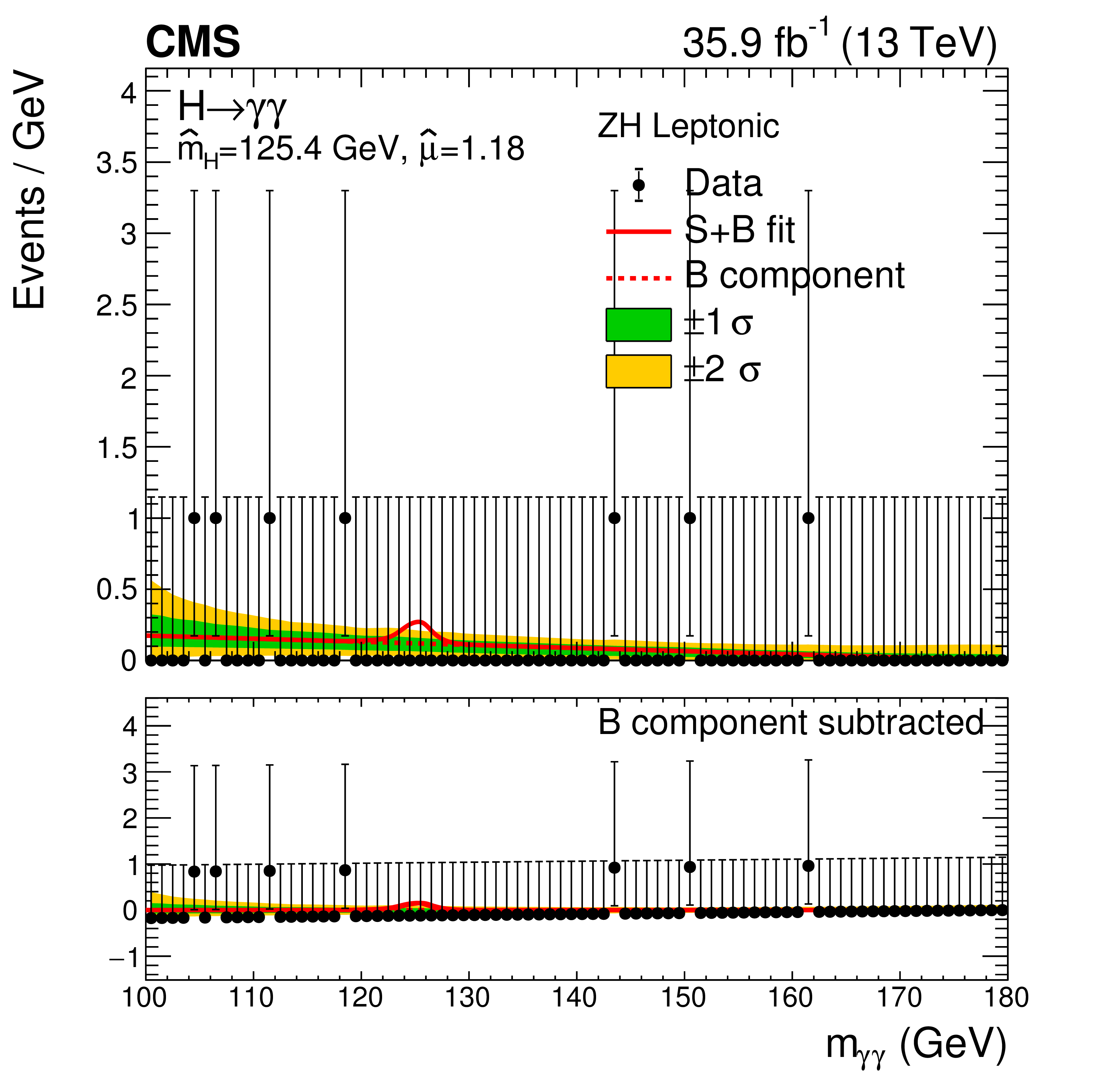
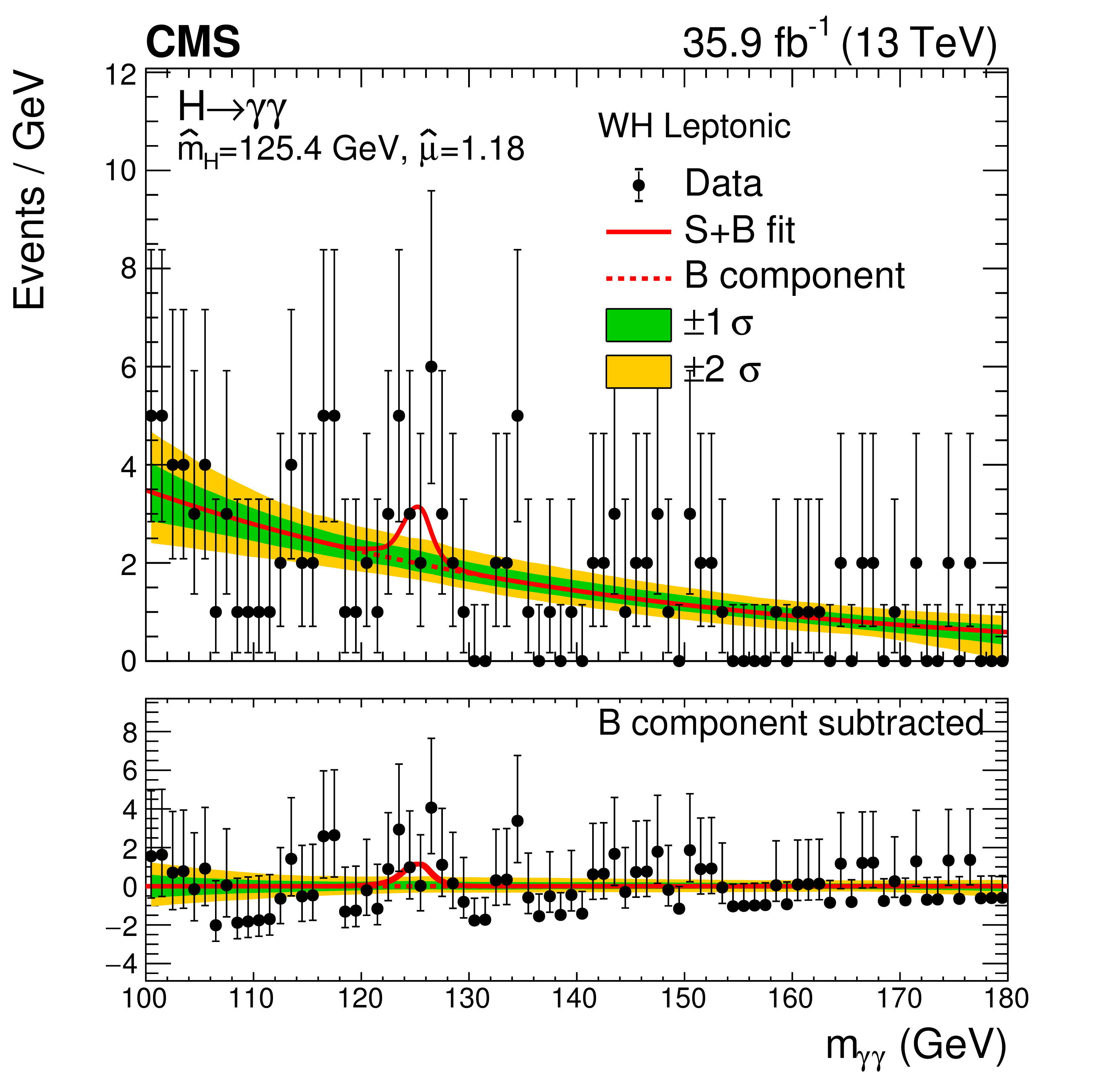
Figure 13:
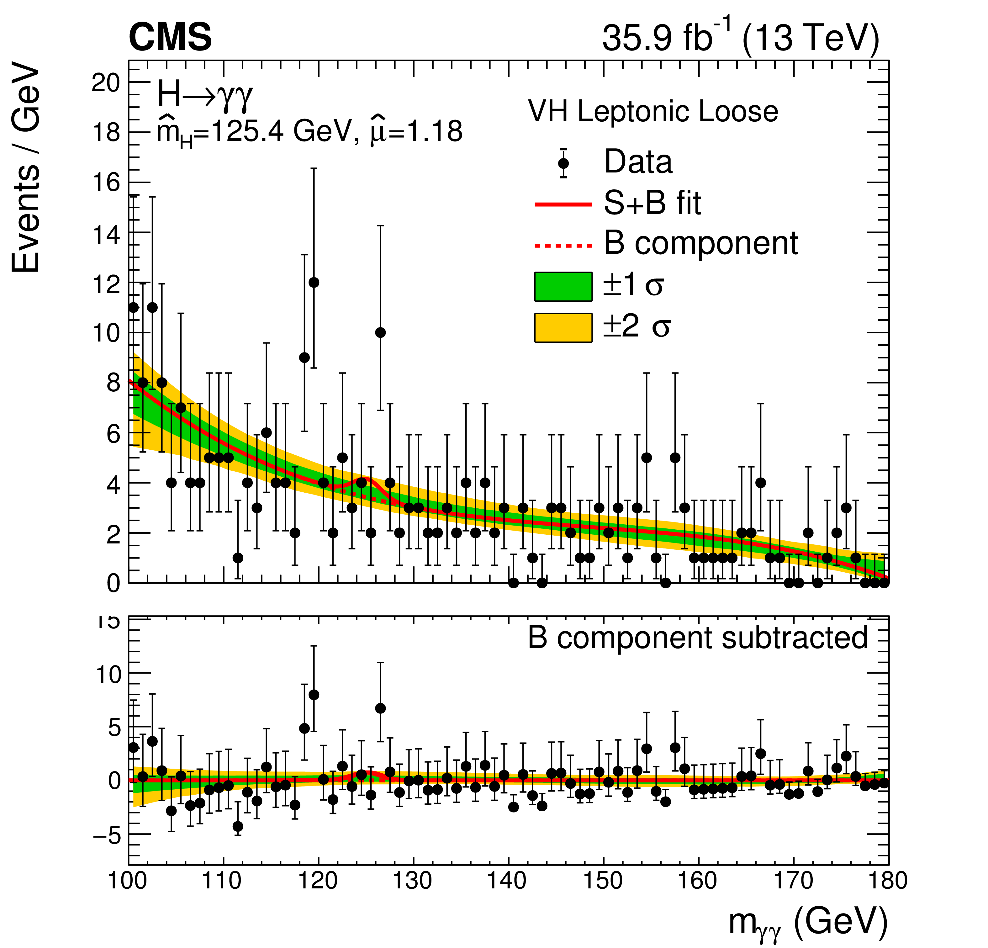
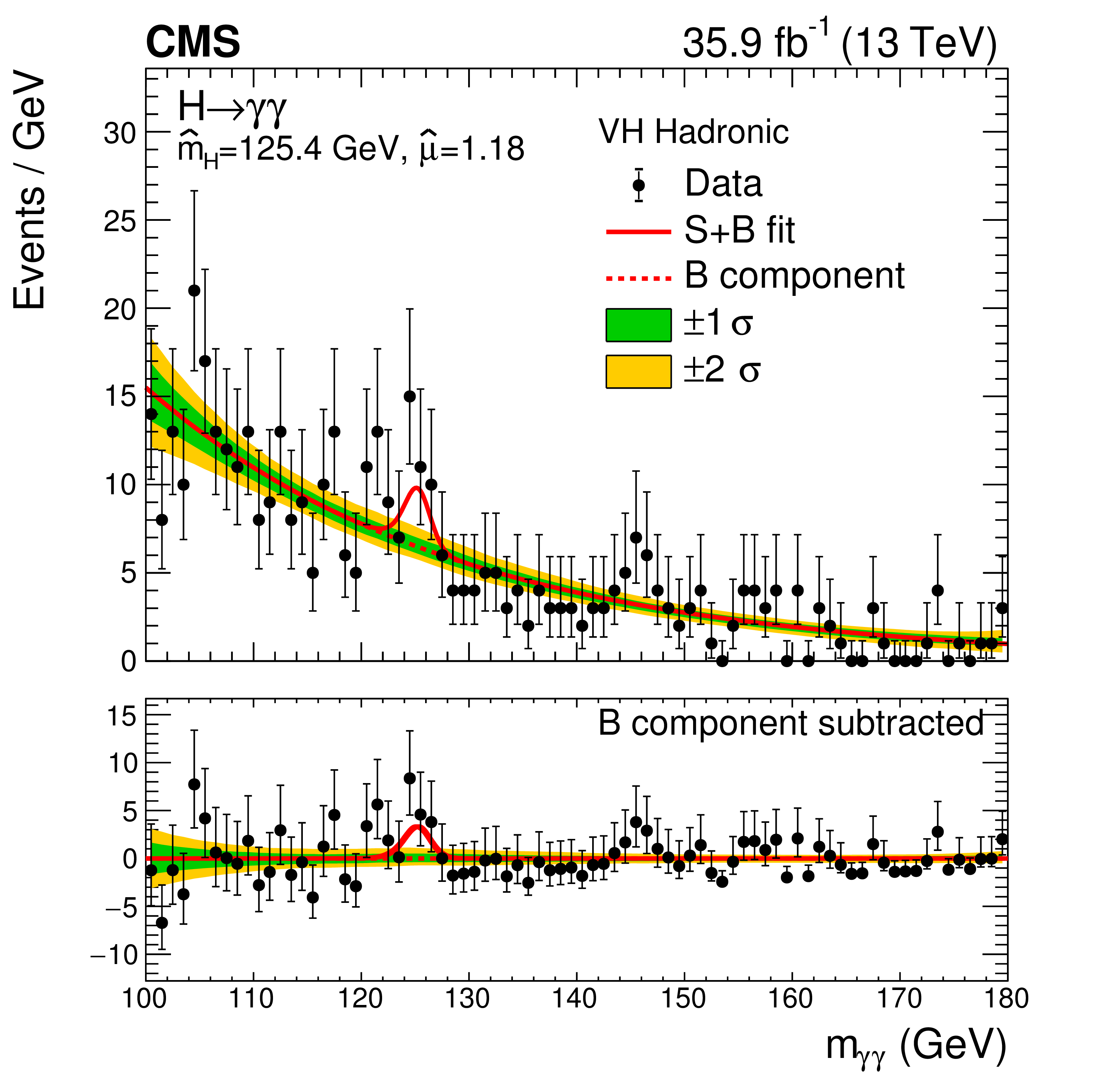
Data and signal-plus-background model fits in VH categories are shown. The one (green) and two (yellow) standard deviation bands include the uncertainties in the background component of the fit. The lower panel in each plot shows the residuals after the background subtraction. |
png pdf |
Figure 13-a:
Data and signal-plus-background model fits in the ZH Leptonic category are shown. The one (green) and two (yellow) standard deviation bands include the uncertainties in the background component of the fit. The lower panel in each plot shows the residuals after the background subtraction. |
png pdf |
Figure 13-b:
Data and signal-plus-background model fits in the WH Leptonic category are shown. The one (green) and two (yellow) standard deviation bands include the uncertainties in the background component of the fit. The lower panel in each plot shows the residuals after the background subtraction. |
png pdf |
Figure 13-c:
Data and signal-plus-background model fits in the VH Leptonic Loose category are shown. The one (green) and two (yellow) standard deviation bands include the uncertainties in the background component of the fit. The lower panel in each plot shows the residuals after the background subtraction. |

png pdf |
Figure 13-d:
Data and signal-plus-background model fits in the VH MET category are shown. The one (green) and two (yellow) standard deviation bands include the uncertainties in the background component of the fit. The lower panel in each plot shows the residuals after the background subtraction. |
png pdf |
Figure 13-e:
Data and signal-plus-background model fits in the VH Hadronic category are shown. The one (green) and two (yellow) standard deviation bands include the uncertainties in the background component of the fit. The lower panel in each plot shows the residuals after the background subtraction. |
png pdf |
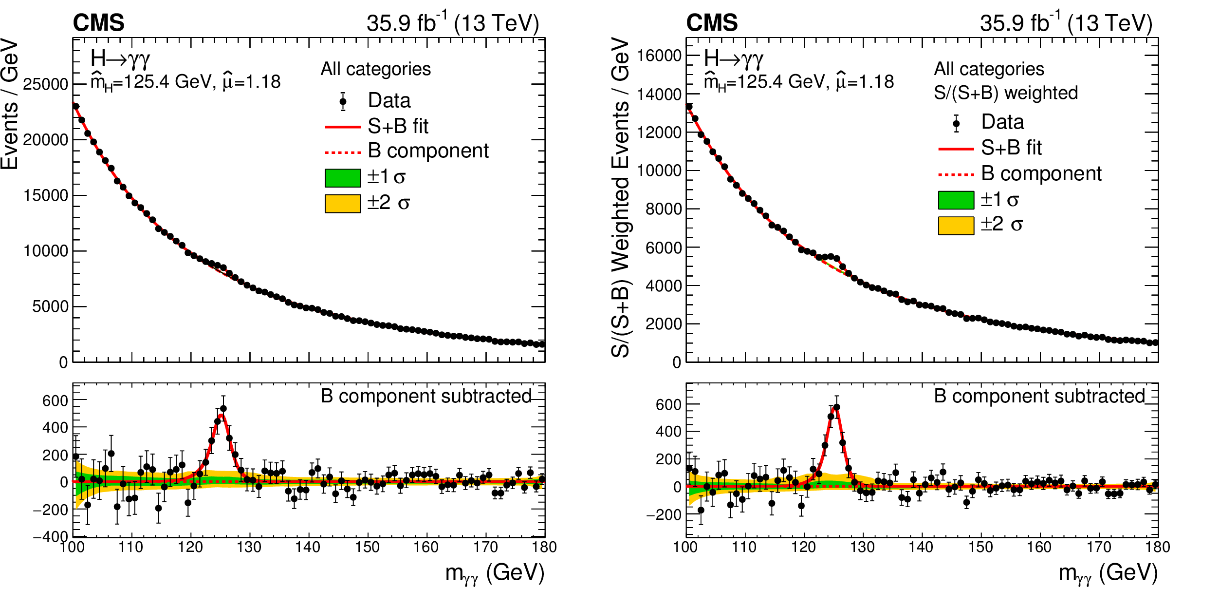
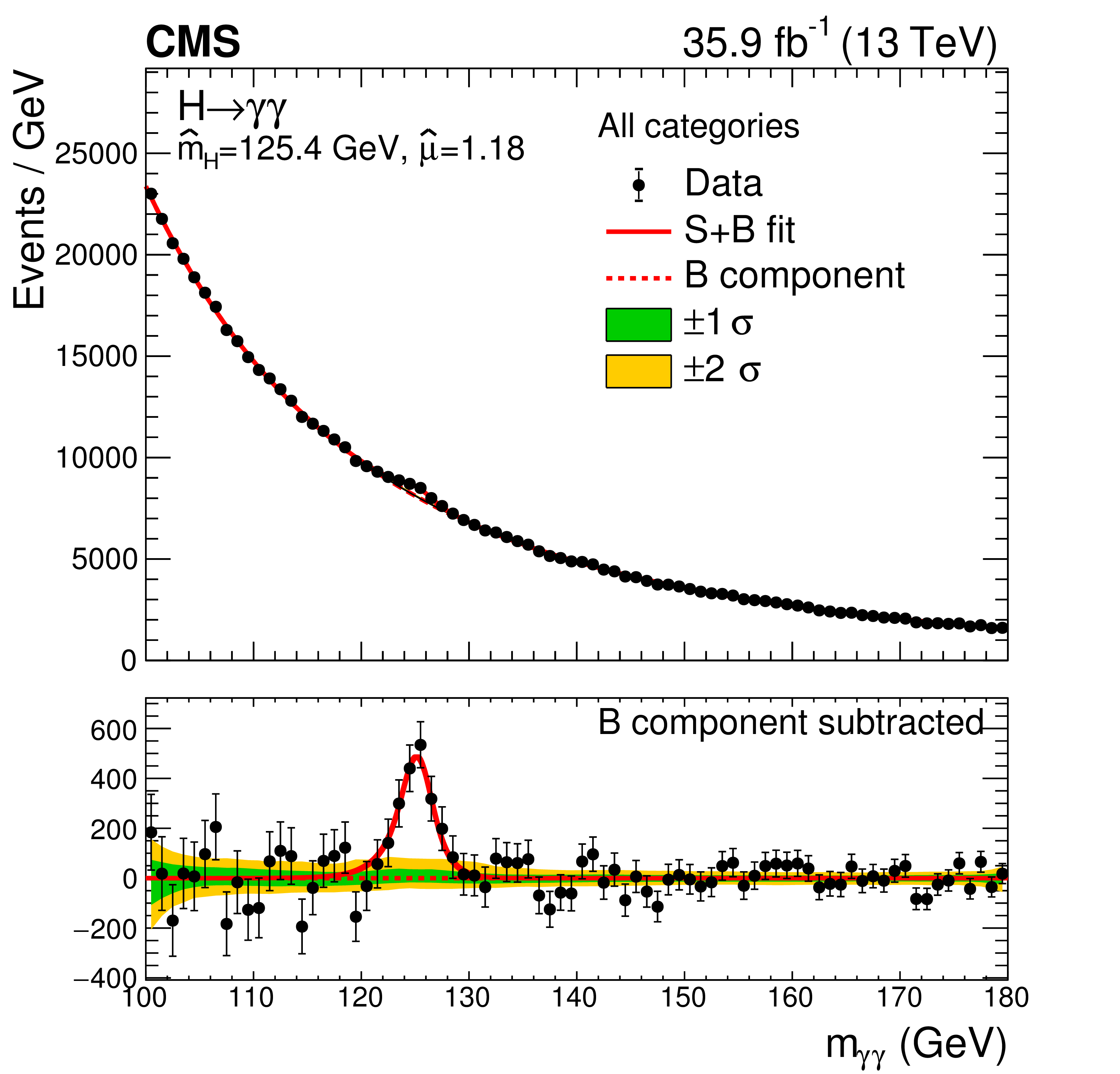
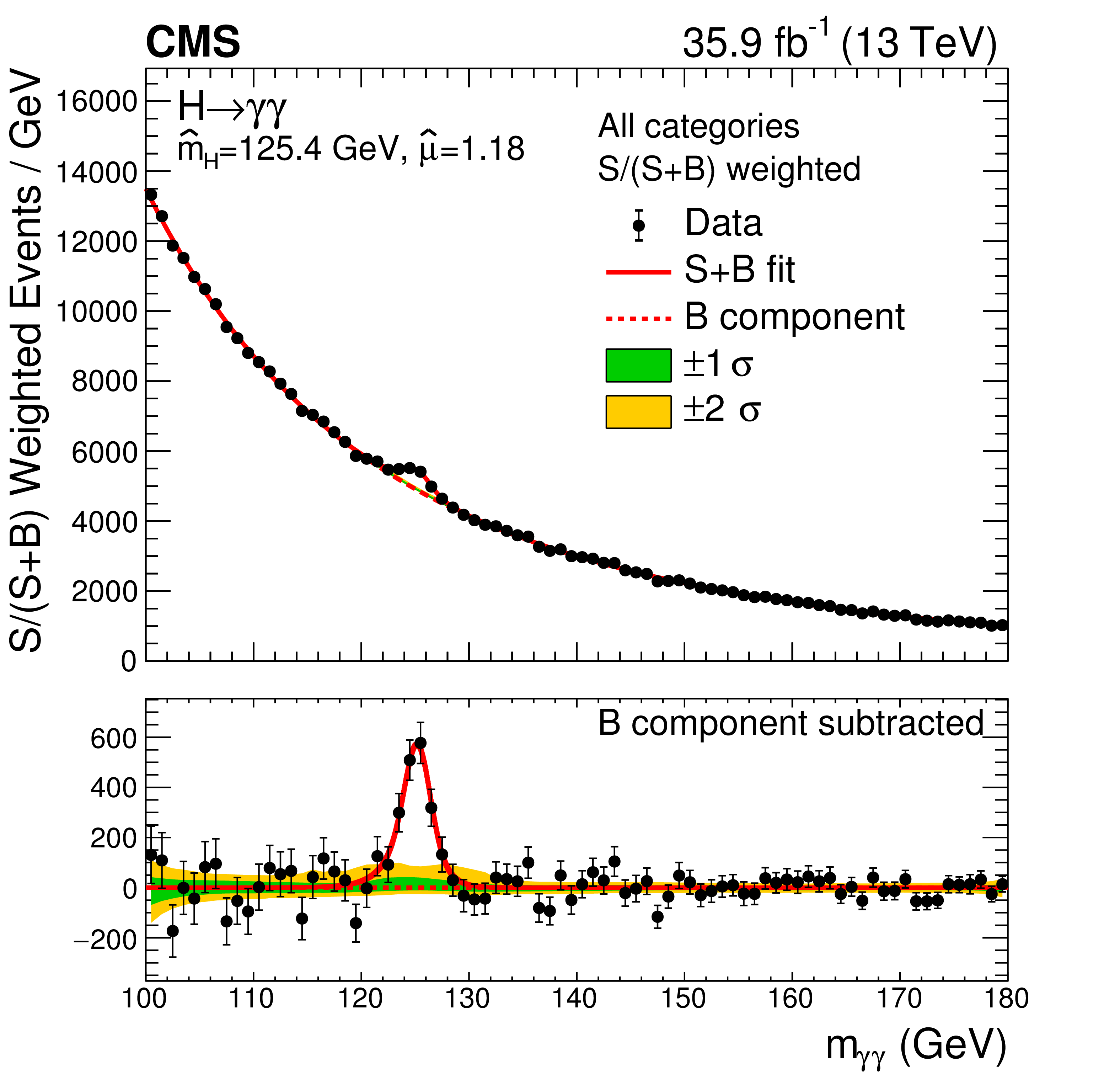
Figure 14:
Data and signal-plus-background model fits for all categories summed (left) and where the categories are summed weighted by their sensitivity (right). The one (green) and two (yellow) standard deviation bands include the uncertainties in the background component of the fit. The lower panel in each plot show the residuals after the background subtraction. |
png pdf |
Figure 14-a:
Data and signal-plus-background model fits for all categories summed. The one (green) and two (yellow) standard deviation bands include the uncertainties in the background component of the fit. The lower panel in each plot show the residuals after the background subtraction. |
png pdf |
Figure 14-b:
Data and signal-plus-background model fits where the categories are summed weighted by their sensitivity. The one (green) and two (yellow) standard deviation bands include the uncertainties in the background component of the fit. The lower panel in each plot show the residuals after the background subtraction. |

png pdf |
Figure 15:
Expected fraction of signal events per production mode in the different categories. For each category, the $\sigma _{\text {eff}}$ and $\sigma _{\text {HM}}$ of the signal model, as described in the text, are given. The ratio of the number of signal events (S) to the number of signal-plus-background events (S+B) is shown on the right hand side. |
png pdf |
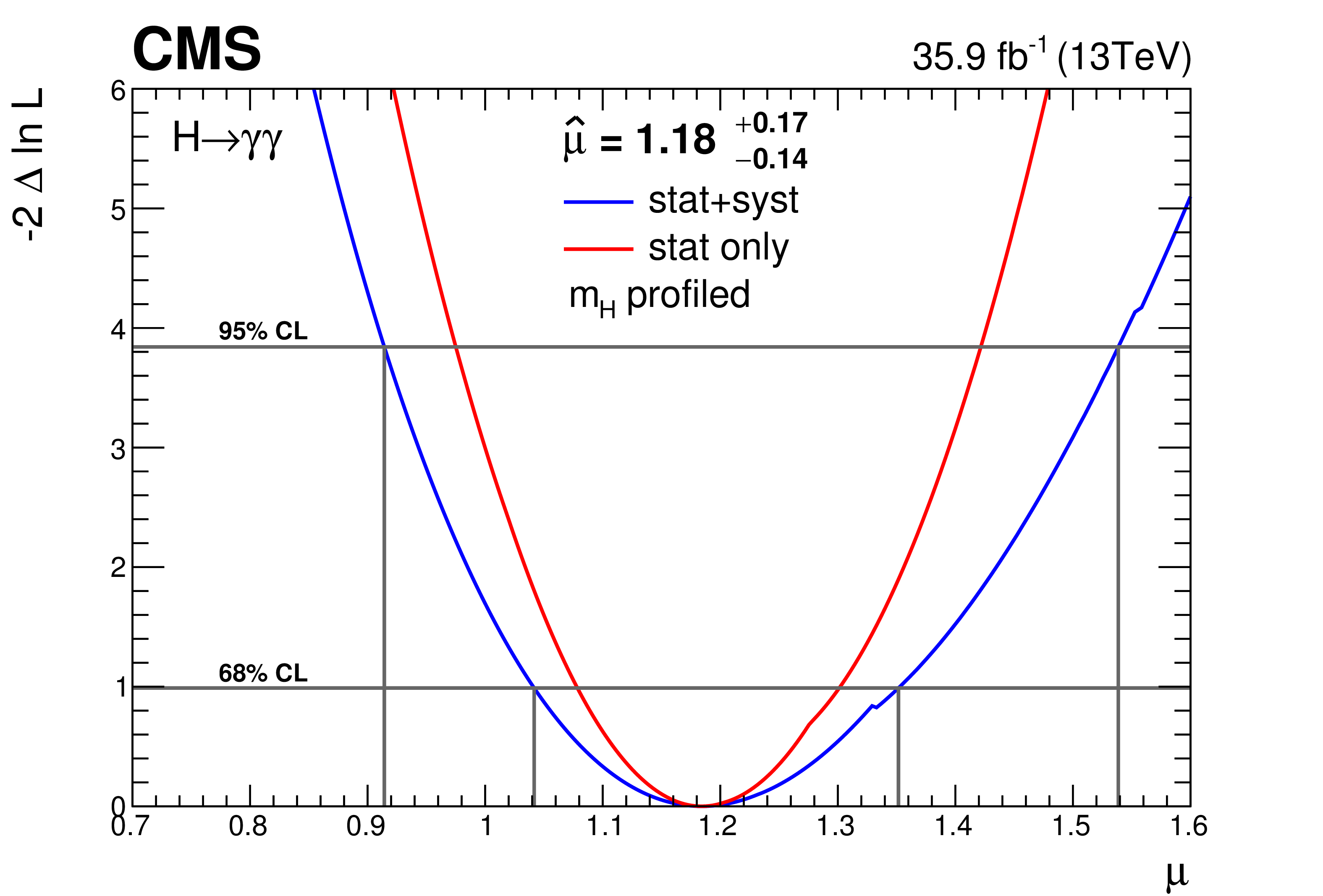
Figure 16:
The likelihood scan for the signal strength modifier where the value of the SM Higgs boson mass is profiled in the fit. |
png pdf |
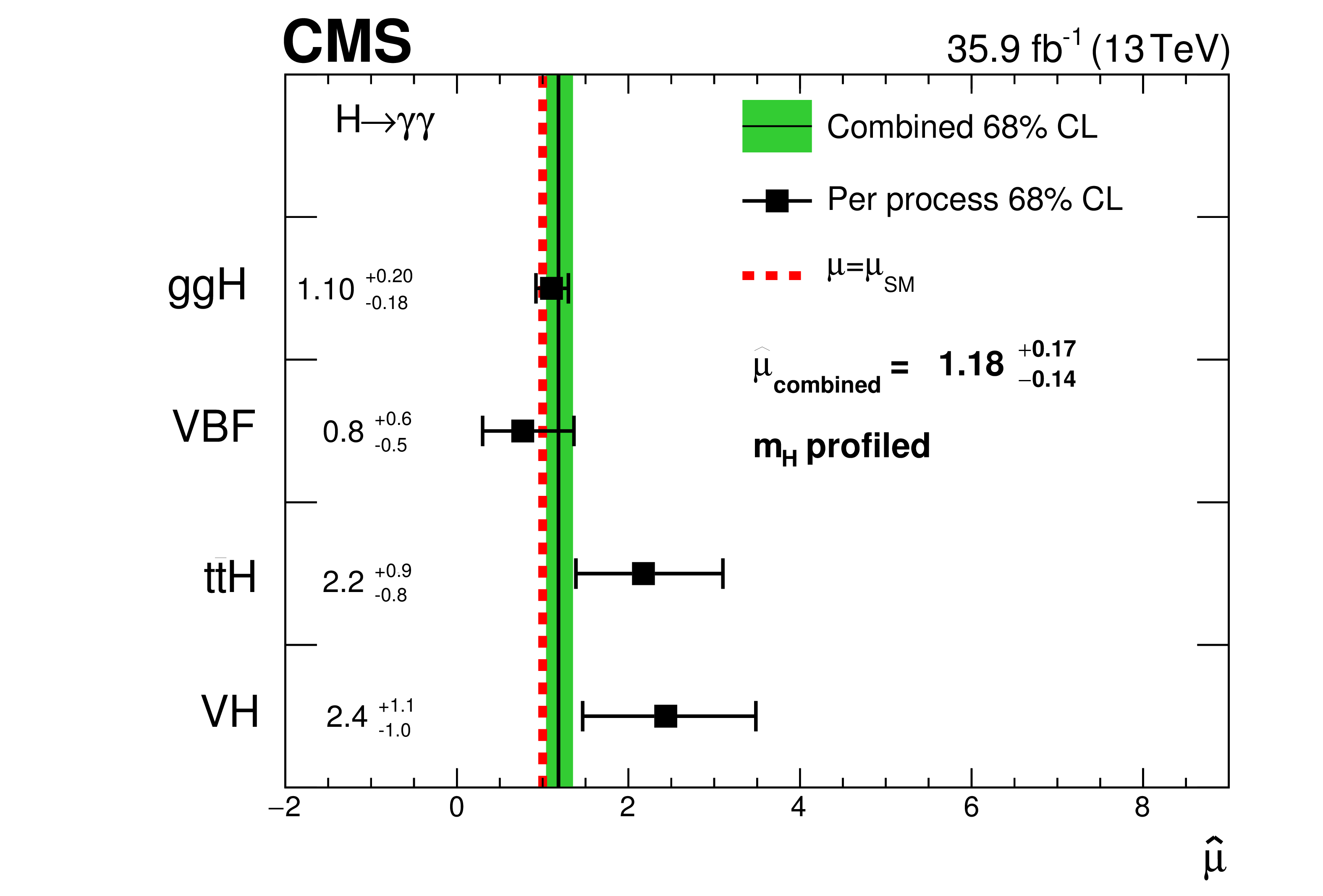
Figure 17:
Signal strength modifiers measured for each process (black points), with the SM Higgs boson mass profiled, compared to the overall signal strength modifier (green band) and to the SM expectation (dashed red line). |
png pdf |
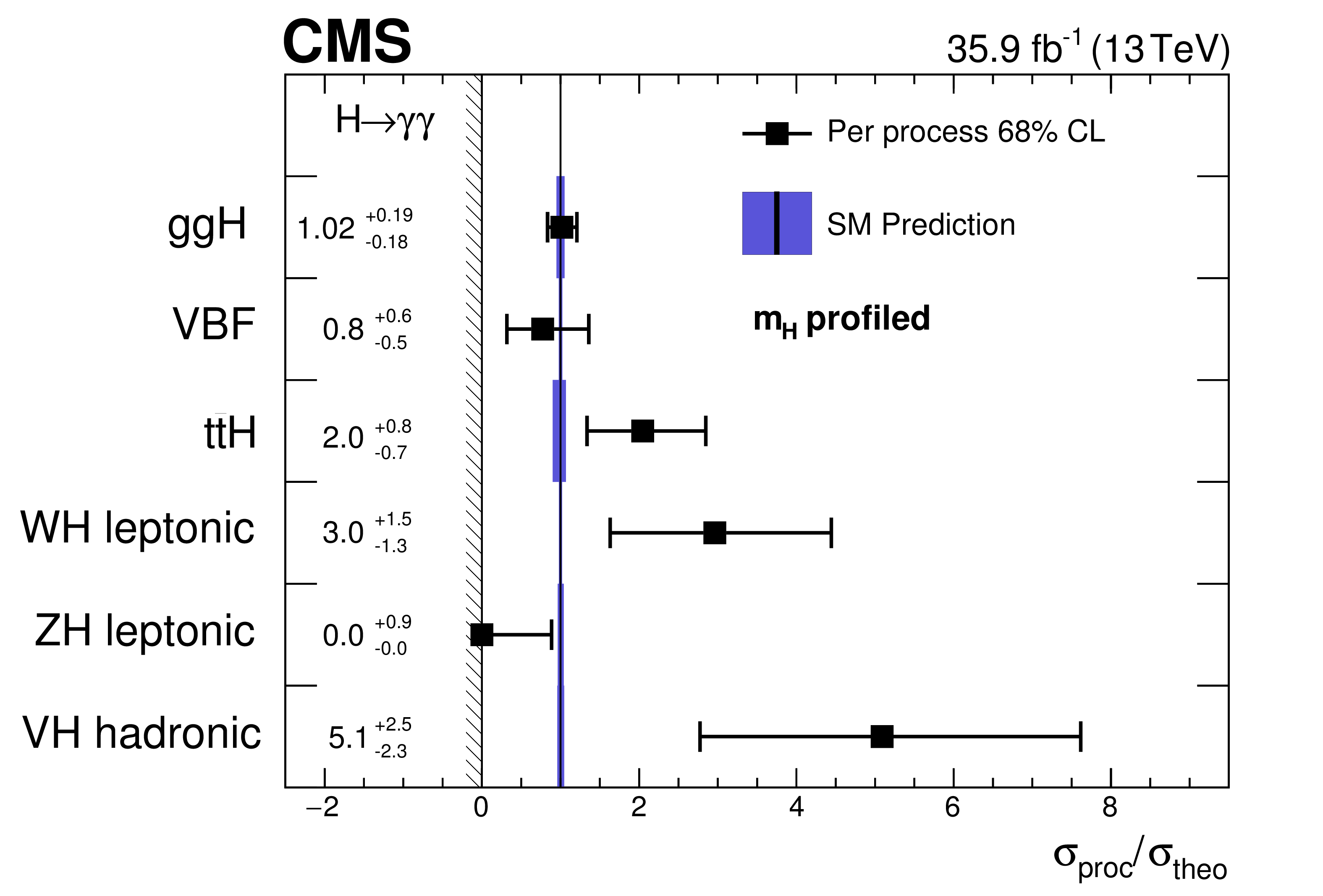
Figure 18:
Cross section ratios measured for each process (black points) in the Higgs simplified template cross section framework [32], with the SM Higgs boson mass profiled, compared to the SM expectations and their uncertainties (blue band). The signal strength modifiers are constrained to be nonnegative, as indicated by the vertical line and hashed pattern at zero. |
png pdf |
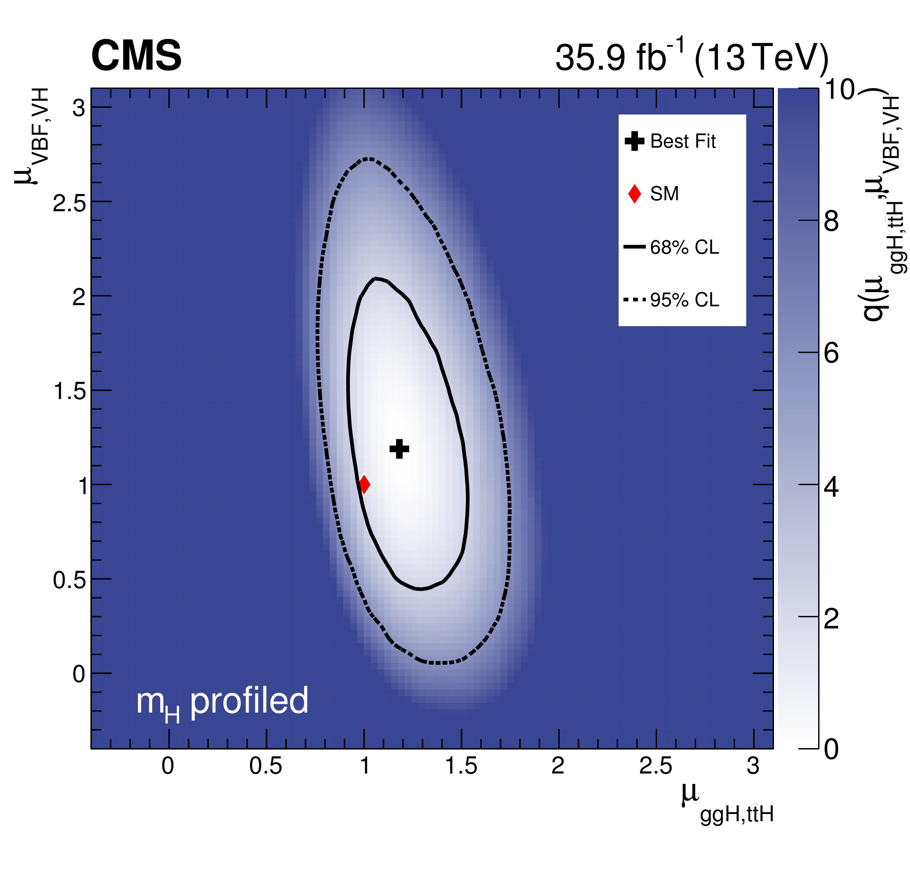
Figure 19:
The two-dimensional best fit (black cross) of the signal strength modifiers for fermionic (ggH, ttH) and bosonic (VBF, ZH, WH) production modes compared to the SM expectation (red diamond). The Higgs boson mass is profiled in the fit. The solid (dashed) line represents the 68 (95)% confidence region. |
png pdf |
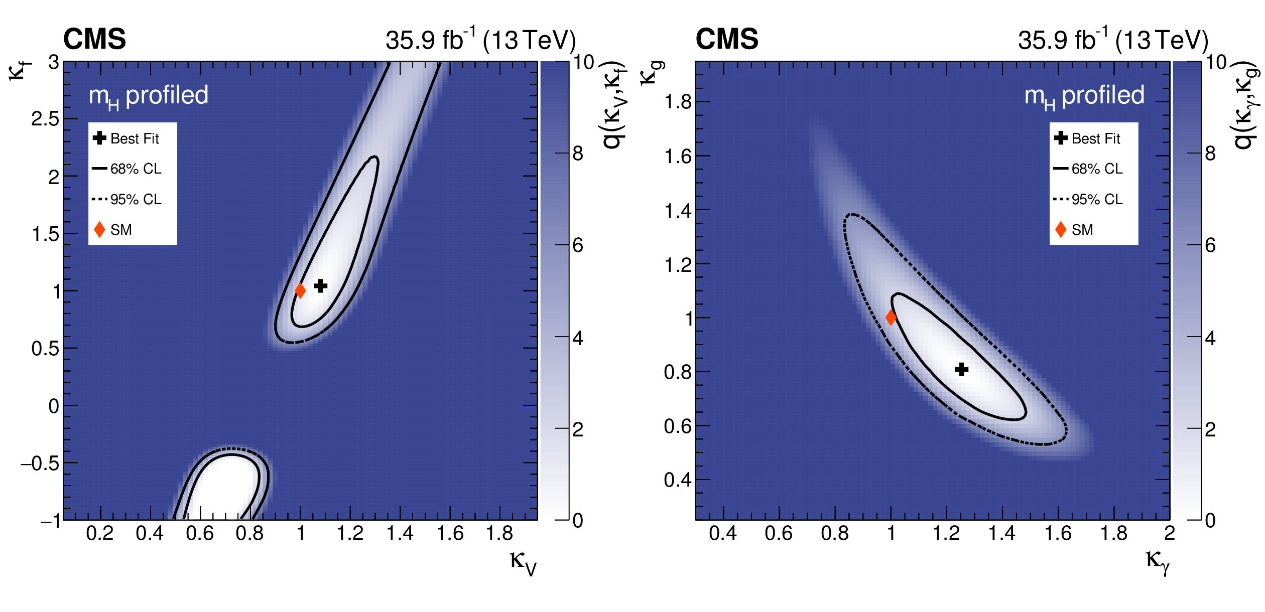
Figure 20:
Two-dimensional likelihood scans of $ {\kappa _{\mathrm{f}}}$ versus $ {\kappa _{\mathrm{V}}}$ (left) and $ {\kappa _{\mathrm{g}}}$ versus $ {\kappa _{{\gamma}}}$ (right). All four variables are expressed relative to the SM expectations. The mass of the Higgs boson is profiled in the fits. The crosses indicate the best fit values, the diamonds indicate the standard model expectations. The colour maps indicate the value of the test statistic $q$ as described in the text. |
png pdf |
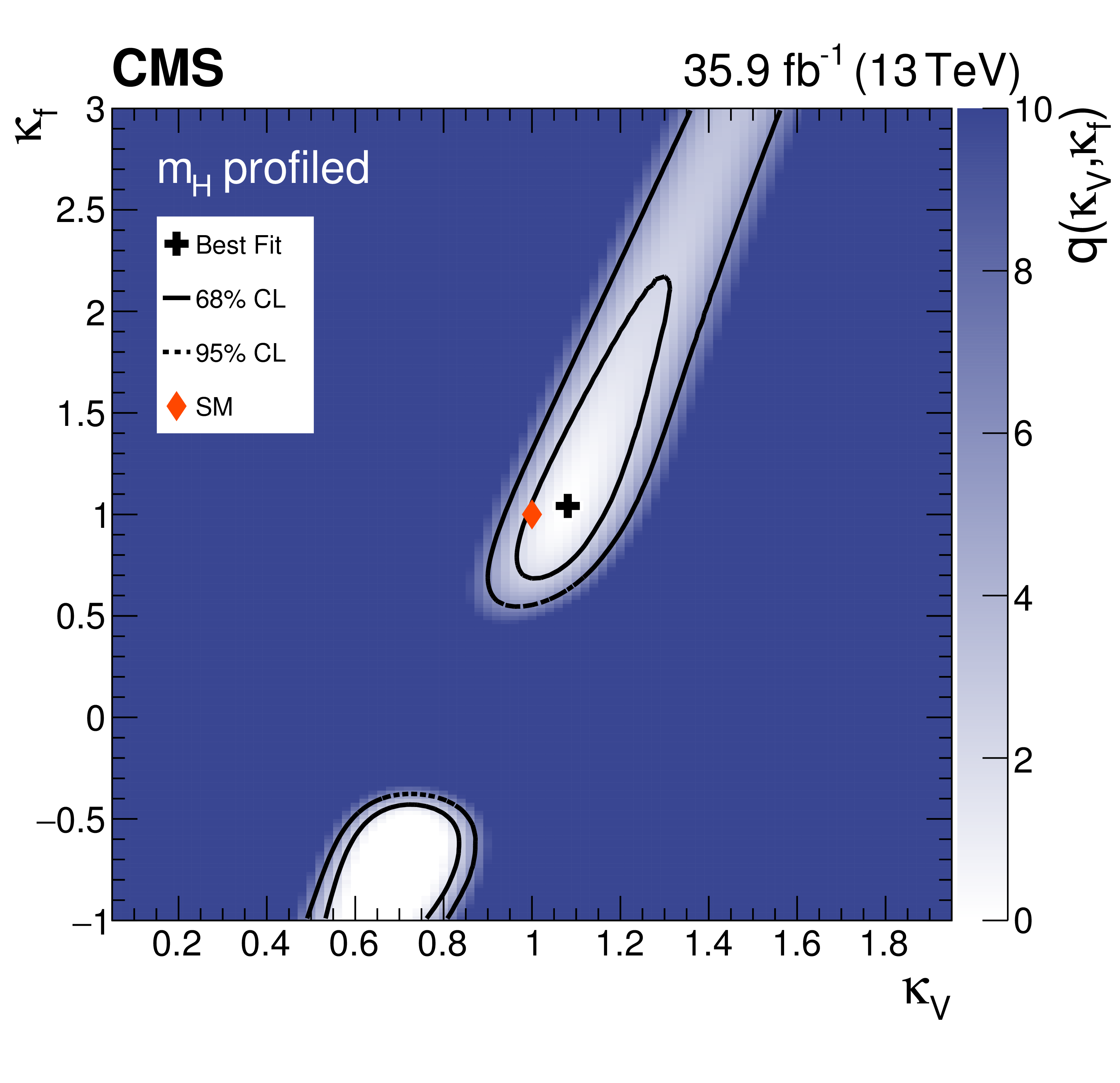
Figure 20-a:
Two-dimensional likelihood scans of $ {\kappa _{\mathrm{f}}}$ versus $ {\kappa _{\mathrm{V}}}$. Variables are expressed relative to the SM expectations. The mass of the Higgs boson is profiled in the fits. The cross indicates the best fit value, the diamond indicates the standard model expectation. The colour maps indicate the value of the test statistic $q$ as described in the text. |
png pdf |
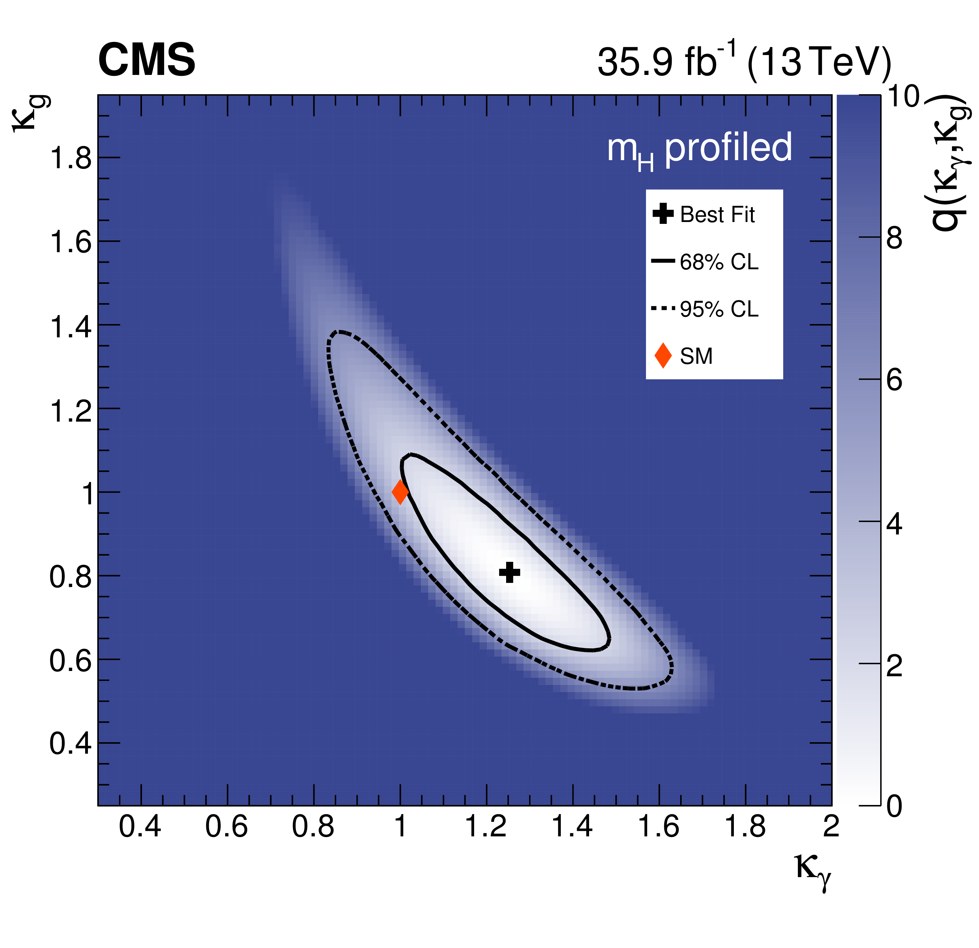
Figure 20-b:
Two-dimensional likelihood scans of $ {\kappa _{\mathrm{g}}}$ versus $ {\kappa _{{\gamma}}}$. Variables are expressed relative to the SM expectations. The mass of the Higgs boson is profiled in the fits. The cross indicates the best fit value, the diamond indicates the standard model expectation. The colour maps indicate the value of the test statistic $q$ as described in the text. |
| Tables | |
png pdf |
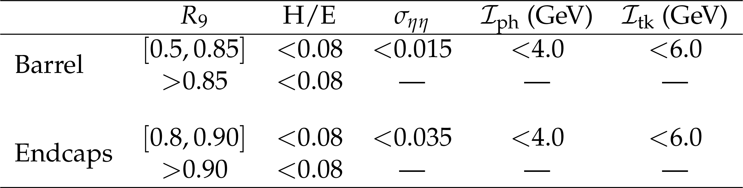
Table 1:
Schema of the photon preselection requirements. |

png pdf |
Table 2:
Photon preselection efficiencies as measured in four photon categories, obtained with tag-and-probe techniques using $ {{\mathrm{Z} \to \mathrm{e}^+ \mathrm {e}^-}} $ and $ \mathrm{Z} \to {{{\mu ^+}} {{\mu ^-}}} {\gamma}$ events. The quoted uncertainties include the statistical and systematic components. |

png pdf |
Table 3:
The expected number of signal events per category and the percentage breakdown per production mode in that category. The $\sigma _{\text {eff}}$, computed as the smallest interval containing 68.3% of the invariant mass distribution, and $\sigma _{\text {HM}}$, computed as the width of the distribution at half of its highest point divided by 2.35, are also shown as an estimate of the $ {{{m}}_{{\gamma} {\gamma}}} $ resolution in that category. The expected number of background events per GeV around 125 GeV is also listed. |
| Summary |
| We report measurements of the production cross section and couplings of the Higgs boson using its diphoton decay: the overall signal strength modifier; the signal strength modifier for each production mode separately; cross section ratios for the stage 0 simplified template cross section framework; the best fit rates in the $\mu_{\mathrm{VBF},\,\mathrm{VH} }$-$\mu_{\mathrm{ggH},\,\mathrm{ttH} }$ plane with VBF and VH production, and ggH and ttH production, varied together; and the best fit coupling modifiers in the ${\kappa_{\mathrm{f}}}$-${\kappa_{\mathrm{V}}}$ and ${\kappa_{\mathrm{g}}}$-${\kappa_{\gamma}}$ planes. The analysis is based on proton-proton collision data collected at $\sqrt{s} = $ 13 TeV by the CMS experiment at the LHC in 2016, corresponding to an integrated luminosity of 35.9 fb$^{-1}$. The best fit signal strength modifier obtained after profiling ${{{m}}_{\mathrm{H}}} $ is ${\widehat{\mu}} = $ 1.18$^{+0.12}_{-0.11}$ (stat) $^{+0.09}_{-0.07}$ (syst) $^{+0.07}_{-0.06}$ (theo). The best fit values in the $\mu_{\mathrm{VBF},\,\mathrm{VH} }$-$\mu_{\mathrm{ggH},\,\mathrm{ttH} }$ plane are ${\widehat{\mu}}_{\mathrm{ggH},\,\mathrm{ttH} } = $ 1.19$^{+0.22}_{-0.18}$ and ${\widehat{\mu}}_{\mathrm{VBF},\,\mathrm{VH} }=$ 1.21$^{+0.58}_{-0.51}$. When $\mu_{ttH }$ is considered separately, the best fit value is ${\widehat{\mu}}_{ttH } = $ 2.2$^{+0.9}_{-0.8}$, corresponding to a $p$-value of 0.074% with respect to the absence of ttH production. Stage 0 simplified template cross sections are compatible with the standard model. |
| Additional Figures | |
png pdf |
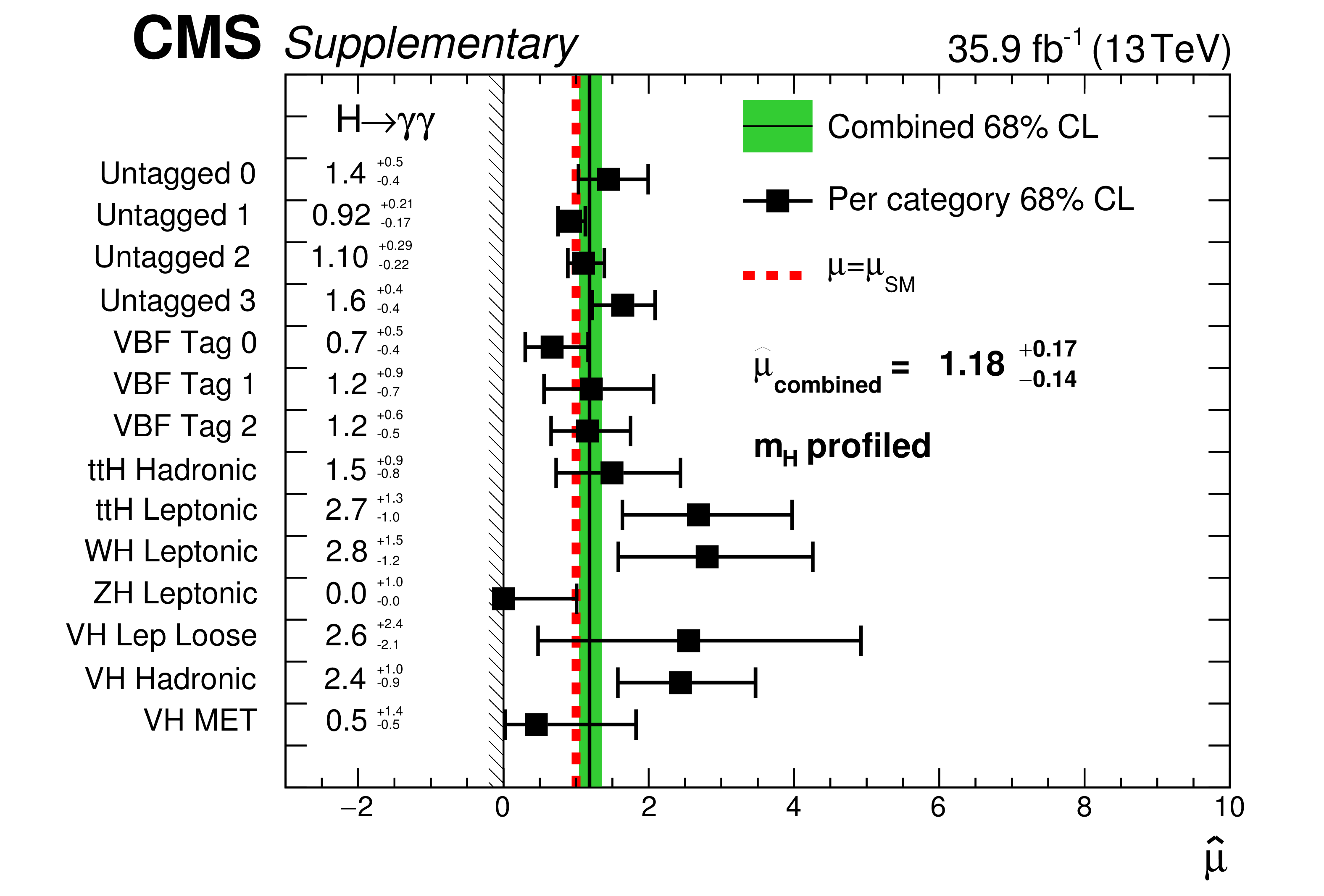
Additional Figure 1:
Signal strength modifiers measured for each category (black points), with the SM Higgs boson mass profiled, compared to the overall signal strength modifier (green band) and to the SM expectation (dashed red line). The signal strength modifiers are constrained to be nonnegative, as indicated by the vertical line and hashed pattern at zero. |
png pdf |
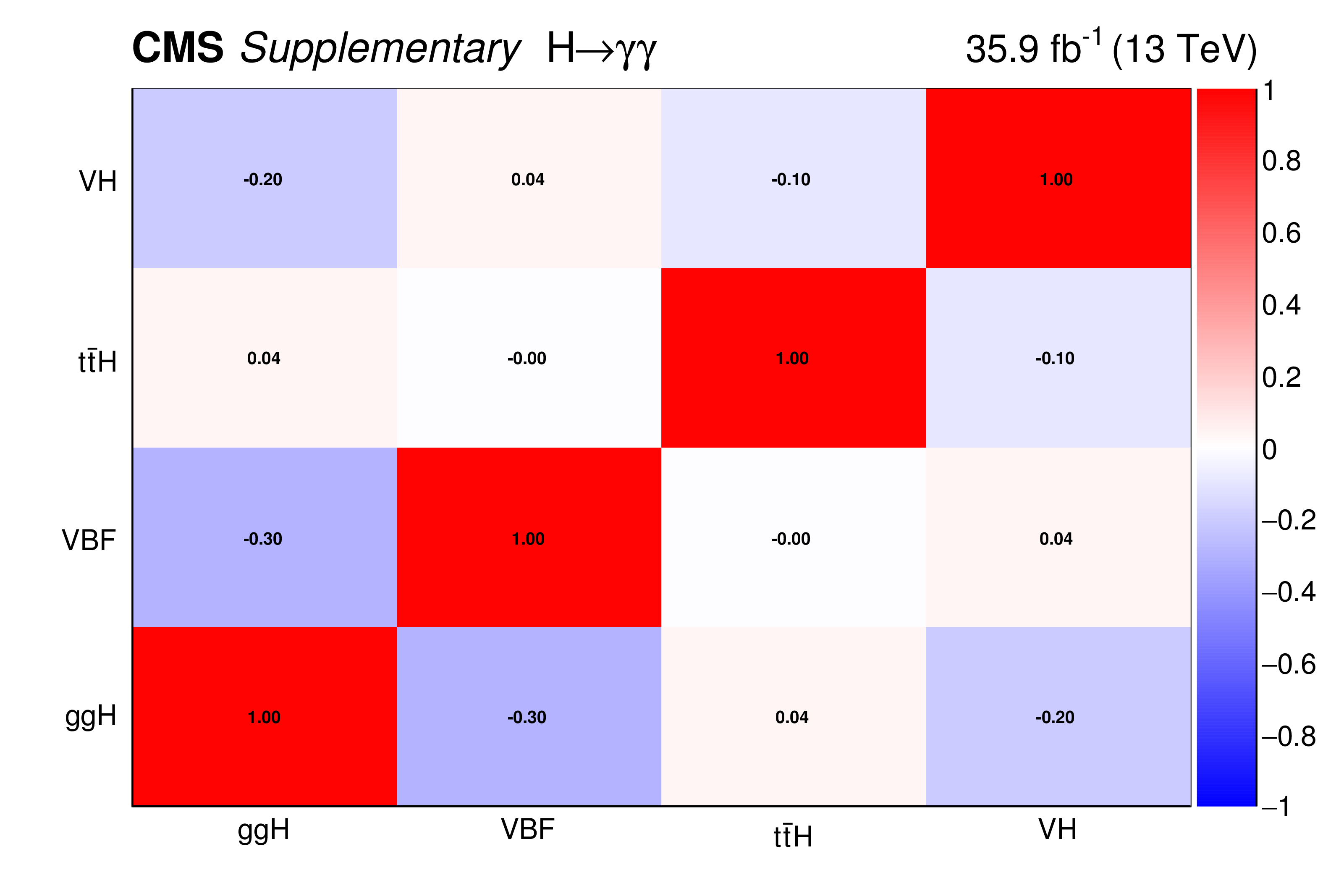
Additional Figure 2:
Observed correlations in a fit to the signal strength modifier for each production mode. The size of the correlation is indicated by the colour scale. |

png pdf |
Additional Figure 3:
Observed correlations in a fit to the ratios of the observed cross sections to the SM prediction in the stage 0 of the simplified template cross section framework. The size of the correlation is indicated by the colour scale. |
| References | ||||
| 1 | S. L. Glashow | Partial-symmetries of weak interactions | NP 22 (1961) 579 | |
| 2 | S. Weinberg | A model of leptons | PRL 19 (1967) 1264 | |
| 3 | A. Salam | Weak and electromagnetic interactions | in Elementary particle physics: relativistic groups and analyticity, N. Svartholm, ed., p. 367 Almquvist \& Wiskell, 1968 Proceedings of the eighth Nobel symposium | |
| 4 | ATLAS Collaboration | Observation of a new particle in the search for the standard model Higgs boson with the ATLAS detector at the LHC | PLB 716 (2012) 1 | 1207.7214 |
| 5 | CMS Collaboration | Observation of a new boson at a mass of 125 GeV with the CMS experiment at the LHC | PLB 716 (2012) 30 | CMS-HIG-12-028 1207.7235 |
| 6 | CMS Collaboration | Observation of a new boson with mass near 125 GeV in pp collisions at $ \sqrt{s} = $ 7 and 8 TeV | JHEP 06 (2013) 081 | CMS-HIG-12-036 1303.4571 |
| 7 | ATLAS and CMS Collaborations | Combined measurement of the Higgs boson mass in pp collisions at $ \sqrt{s}= $ 7 and 8 TeV with the ATLAS and CMS experiments | PRL 114 (2015) 191803 | 1503.07589 |
| 8 | ATLAS and CMS Collaborations | Measurements of the Higgs boson production and decay rates and constraints on its couplings from a combined ATLAS and CMS analysis of the LHC pp collision data at $ \sqrt{s}= $ 7 and 8 TeV | JHEP 08 (2016) 045 | 1606.02266 |
| 9 | F. Englert and R. Brout | Broken symmetry and the mass of gauge vector mesons | PRL 13 (1964) 321 | |
| 10 | P. W. Higgs | Broken symmetries, massless particles and gauge fields | PL12 (1964) 132 | |
| 11 | P. W. Higgs | Broken symmetries and the masses of gauge bosons | PRL 13 (1964) 508 | |
| 12 | G. S. Guralnik, C. R. Hagen, and T. W. B. Kibble | Global conservation laws and massless particles | PRL 13 (1964) 585 | |
| 13 | P. W. Higgs | Spontaneous symmetry breakdown without massless bosons | PR145 (1966) 1156 | |
| 14 | T. W. B. Kibble | Symmetry breaking in non-Abelian gauge theories | PR155 (1967) 1554 | |
| 15 | CMS Collaboration | Observation of the diphoton decay of the Higgs boson and measurement of its properties | EPJC 74 (2014) 3076 | CMS-HIG-13-001 1407.0558 |
| 16 | ATLAS Collaboration | Measurement of Higgs boson production in the diphoton decay channel in pp collisions at center-of-mass energies of 7 and 8 TeV with the ATLAS detector | PRD 90 (2014) 112015 | 1408.7084 |
| 17 | LHC Higgs Cross Section Working Group | Handbook of LHC Higgs Cross Sections: 3. Higgs Properties | CERN-2013-004, CERN | 1307.1347 |
| 18 | CMS Collaboration | Energy calibration and resolution of the CMS electromagnetic calorimeter in pp collisions at $ \sqrt{s} = $ 7 TeV | JINST 8 (2013) P09009 | CMS-EGM-11-001 1306.2016 |
| 19 | CMS Collaboration | Particle-flow reconstruction and global event description with the CMS detector | JINST 12 (2017) P10003 | CMS-PRF-14-001 1706.04965 |
| 20 | M. Cacciari, G. P. Salam, and G. Soyez | The anti-$ {k_{\mathrm{T}}} $ jet clustering algorithm | JHEP 04 (2008) 063 | 0802.1189 |
| 21 | CMS Collaboration | Jet energy scale and resolution in the CMS experiment in pp collisions at 8 TeV | JINST 12 (2017) P02014 | CMS-JME-13-004 1607.03663 |
| 22 | CMS Collaboration | Identification of b-quark jets with the CMS experiment | JINST 8 (2013) P04013 | CMS-BTV-12-001 1211.4462 |
| 23 | CMS Collaboration | Identification of heavy-flavour jets with the CMS detector in pp collisions at 13 TeV | Submitted to JINST | CMS-BTV-16-002 1712.07158 |
| 24 | CMS Collaboration | The CMS experiment at the CERN LHC | JINST 3 (2008) S08004 | CMS-00-001 |
| 25 | CMS Collaboration | Measurement of the inclusive $ \mathrm{W} $ and $ \mathrm{Z} $ production cross sections in pp collisions at $ \sqrt{s}= $ 7 TeV with the CMS experiment | JHEP 10 (2011) 132 | CMS-EWK-10-005 1107.4789 |
| 26 | J. Alwall et al. | The automated computation of tree-level and next-to-leading order differential cross sections, and their matching to parton shower simulations | JHEP 07 (2014) 079 | 1405.0301 |
| 27 | R. Frederix and S. Frixione | Merging meets matching in MC@NLO | JHEP 12 (2012) 061 | 1209.6215 |
| 28 | T. Sjostrand, S. Mrenna, and P. Z. Skands | A brief introduction to PYTHIA 8.1 | CPC 178 (2008) 852 | 0710.3820 |
| 29 | CMS Collaboration | Event generator tunes obtained from underlying event and multiparton scattering measurements | EPJC 76 (2016) 155 | CMS-GEN-14-001 1512.00815 |
| 30 | K. Hamilton, P. Nason, E. Re, and G. Zanderighi | NNLOPS simulation of Higgs boson production | JHEP 10 (2013) 222 | 1309.0017 |
| 31 | NNPDF Collaboration | Parton distributions for the LHC Run II | JHEP 04 (2015) 040 | 1410.8849 |
| 32 | LHC Higgs Cross Section Working Group | Handbook of LHC Higgs cross sections: 4. Deciphering the nature of the Higgs sector | CERN-2017-002-M, CERN | 1610.07922 |
| 33 | T. Gleisberg, S. Hoeche, F. Krauss, M. Schonherr, S. Schumann, F. Siegert, and J. Winter | Event generation with SHERPA 1.1 | JHEP 02 (2009) 007 | 0811.4622 |
| 34 | GEANT4 Collaboration | GEANT4---a simulation toolkit | NIMA 506 (2003) 250 | |
| 35 | CMS Collaboration | Performance of photon reconstruction and identification with the CMS detector in proton-proton collisions at $ \sqrt{s} = $ 8 TeV | JINST 10 (2015) P08010 | CMS-EGM-14-001 1502.02702 |
| 36 | M. Cacciari, G. P. Salam, and G. Soyez | FastJet user manual | EPJC 72 (2012) 1896 | 1111.6097 |
| 37 | CMS Collaboration | Electron and photon performance using data collected by CMS at $ \sqrt{s} = $ 13 TeV and 25 ns | CDS | |
| 38 | P. D. Dauncey, M. Kenzie, N. Wardle, and G. J. Davies | Handling uncertainties in background shapes: the discrete profiling method | JINST 10 (2015) P04015 | 1408.6865 |
| 39 | R. A. Fisher | On the Interpretation of $ \chi^{2} $ from Contingency Tables, and the Calculation of p | J. Royal Stat. Soc 85 (1922) 87 | |
| 40 | J. Butterworth et al. | PDF4LHC recommendations for LHC Run II | JPG 43 (2016) 023001 | 1510.03865 |
| 41 | S. Carrazza et al. | An unbiased Hessian representation for Monte Carlo PDFs | EPJC 75 (2015) 369 | 1505.06736 |
| 42 | CMS Collaboration | Measurements of $ \mathrm{t\overline{t}} $ cross sections in association with $ \rm b $ jets and inclusive jets and their ratio using dilepton final states in pp collisions at $ \sqrt{s} = $ 13 TeV | PLB 776 (2018) 355 | CMS-TOP-16-010 1705.10141 |
| 43 | I. W. Stewart, F. J. Tackmann, J. R. Walsh, and S. Zuberi | Jet $ p_t $ resummation in Higgs production at NNLL' + NNLO | PRD 89 (2014) 054001 | 1307.1808 |
| 44 | X. Liu and F. Petriello | Reducing theoretical uncertainties for exclusive Higgs-boson plus one-jet production at the LHC | PRD 87 (2013) 094027 | 1303.4405 |
| 45 | R. Boughezal, X. Liu, F. Petriello, F. J. Tackmann, and J. R. Walsh | Combining resummed Higgs predictions across jet bins | PRD 89 (2014) 074044 | 1312.4535 |
| 46 | J. M. Campbell and R. K. Ellis | MCFM for the Tevatron and the LHC | NPPS 205-206 (2010) 10 | 1007.3492 |
| 47 | I. W. Stewart and F. J. Tackmann | Theory uncertainties for Higgs and other searches using jet bins | PRD 85 (2012) 034011 | 1107.2117 |
| 48 | S. Gangal and F. J. Tackmann | Next-to-leading-order uncertainties in Higgs+2 jets from gluon fusion | PRD 87 (2013) 093008 | 1302.5437 |
| 49 | S. M. Seltzer and M. J. Berger | Transmission and reflection of electrons by foils | NIM119 (1974) 157 | |
| 50 | CMS Collaboration | Performance of missing energy reconstruction in 13 TeV pp collision data using the CMS detector | CMS-PAS-JME-16-004 | CMS-PAS-JME-16-004 |
| 51 | CMS Collaboration | CMS luminosity measurements for the 2016 data taking period | CMS-PAS-LUM-17-001 | CMS-PAS-LUM-17-001 |
| 52 | ATLAS and CMS Collaborations, LHC Higgs Combination Group | Procedure for the LHC Higgs boson search combination in summer 2011 | CMS/ATLAS joint note ATL-PHYS-PUB-2011-11, CMS NOTE 2011/005 | |
| 53 | T. Junk | Confidence level computation for combining searches with small statistics | NIMA 434 (1999) 435 | hep-ex/9902006 |
| 54 | A. L. Read | Presentation of search results: The cl$ {_{\mathrm{s}}} $ technique | JPG 28 (2002) 2693 | |
| 55 | G. Cowan, K. Cranmer, E. Gross, and O. Vitells | Asymptotic formulae for likelihood-based tests of new physics | EPJC 71 (2011) 1 | 1007.1727 |
|
|
Compact Muon Solenoid LHC, CERN |
|

|

|

|

|

|