

Compact Muon Solenoid
LHC, CERN
| CMS-HIG-17-011 ; CERN-EP-2017-143 | ||
| Constraints on anomalous Higgs boson couplings using production and decay information in the four-lepton final state | ||
| CMS Collaboration | ||
| 3 July 2017 | ||
| Phys. Lett. B 775 (2017) 1 | ||
| Abstract: A search is performed for anomalous interactions of the recently discovered Higgs boson using matrix element techniques with the information from its decay to four leptons and from associated Higgs boson production with two quark jets in either vector boson fusion or associated production with a vector boson. The data were recorded by the CMS experiment at the LHC at a center-of-mass energy of 13 TeV and correspond to an integrated luminosity of 38.6 fb$^{-1}$. These data are combined with the data collected at center-of-mass energies of 7 and 8 TeV, corresponding to integrated luminosities of 5.1 and 19.7 fb$^{-1}$, respectively. All observations are consistent with the expectations for the standard model Higgs boson. | ||
| Links: e-print arXiv:1707.00541 [hep-ex] (PDF) ; CDS record ; inSPIRE record ; HepData record ; CADI line (restricted) ; | ||
| Figures & Tables | Summary | Additional Figures & Material | References | CMS Publications |
|---|
| Figures | |

png pdf |
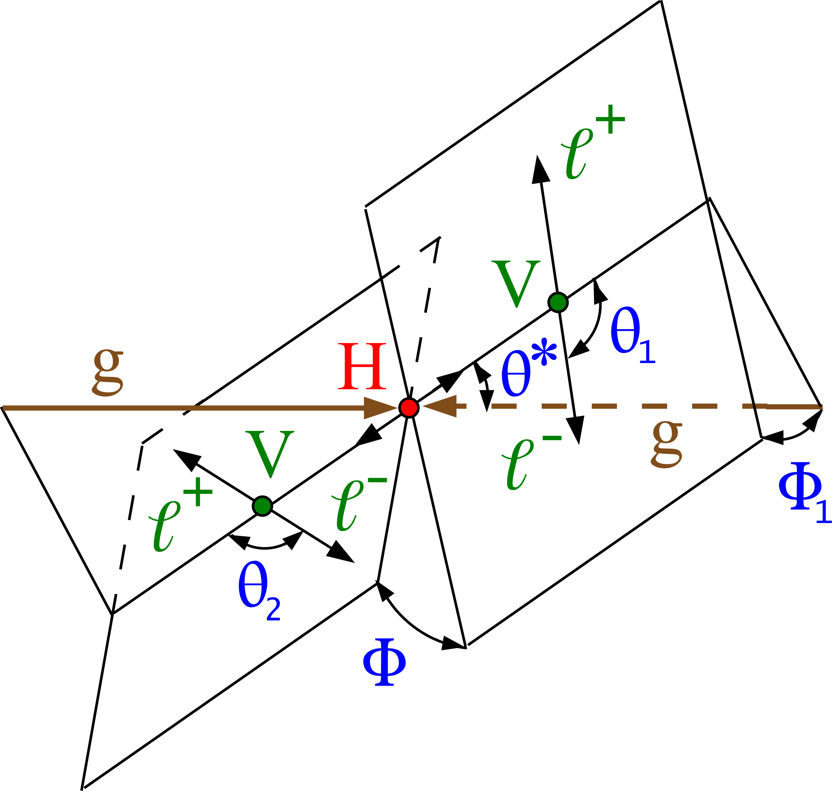
Figure 1:
Illustration of H boson production and decay in three topologies: gluon fusion $\mathrm{g} \mathrm{g} \to \mathrm{ H } \to {\mathrm {V}} {\mathrm {V}} \to 4\ell $ (left); vector boson fusion $ {\mathrm{ q } \mathrm{ q } } \to {\mathrm {V}} {\mathrm {V}} ( {\mathrm{ q } \mathrm{ q } } ) \to \mathrm{ H } ( {\mathrm{ q } \mathrm{ q } } ) \to {\mathrm {V}} {\mathrm {V}} ( {\mathrm{ q } \mathrm{ q } } )$ (middle); and associated production $ {\mathrm{ q } \mathrm{ q } } \to {\mathrm {V}} \to {\mathrm {V}} \mathrm{ H } \to ( {\mathrm {ff}} )\mathrm{ H } \to ( {\mathrm {ff}} ) {\mathrm {V}} {\mathrm {V}} $ (right). In the latter two cases, the production and decay $\mathrm{ H } \to {\mathrm {V}} {\mathrm {V}} $ may be followed by the same four-lepton decay shown in the first case. The five angles shown in blue and the invariant masses of the two vector bosons shown in green fully characterize either the production or the decay chain. The angles are defined in either the H or V boson rest frames [26,33]. |
png pdf |
Figure 1-a:
Illustration of H boson production and decay in the gluon fusion topology, $\mathrm{g} \mathrm{g} \to \mathrm{ H } \to {\mathrm {V}} {\mathrm {V}} \to 4\ell $. The five angles shown in blue and the invariant masses of the two vector bosons shown in green fully characterize either the production or the decay chain. The angles are defined in either the H or V boson rest frames [26,33]. |
png pdf |
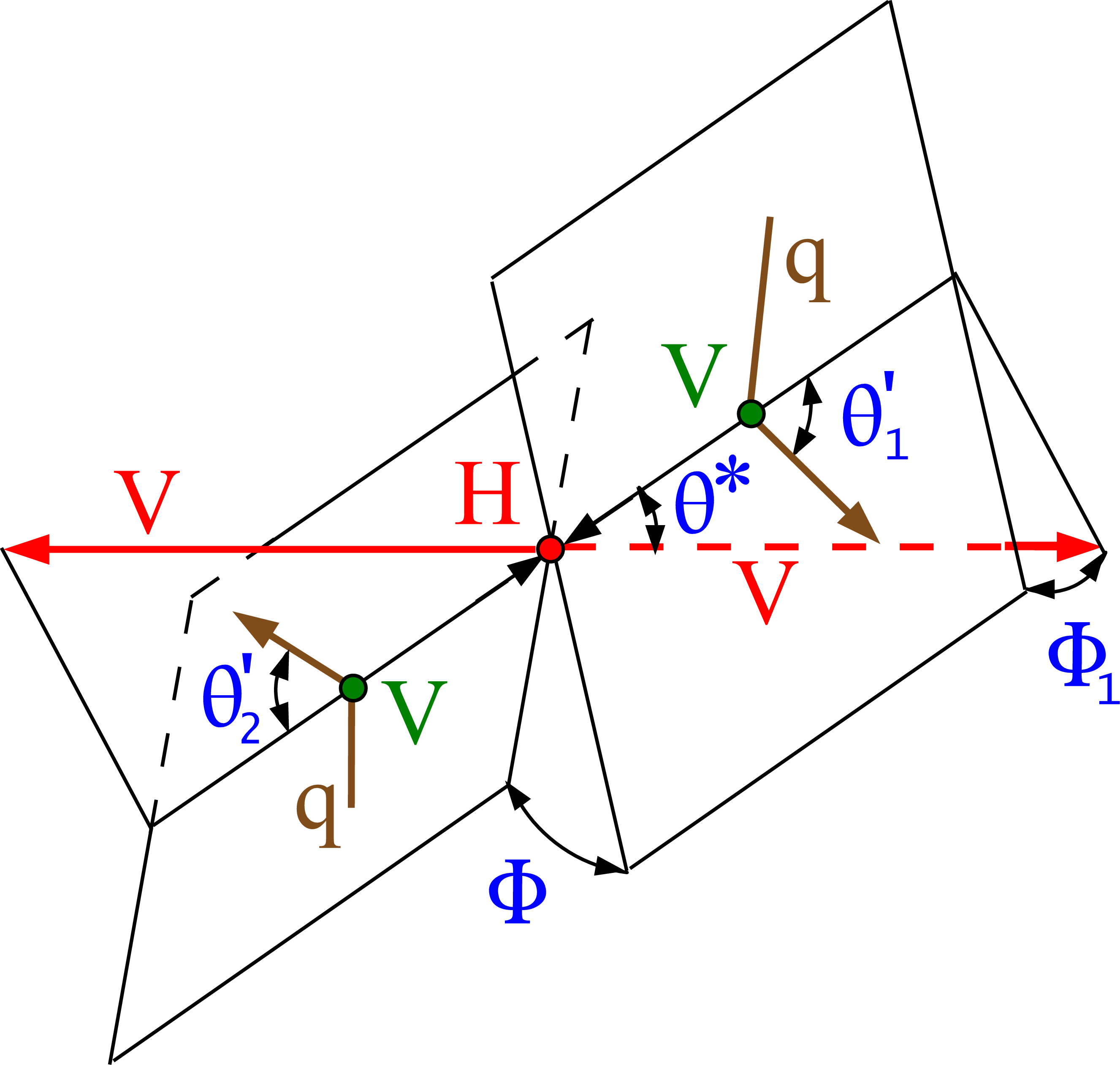
Figure 1-b:
Illustration of H boson production and decay in the vector boson fusion topology $ {\mathrm{ q } \mathrm{ q } } \to {\mathrm {V}} {\mathrm {V}} ( {\mathrm{ q } \mathrm{ q } } ) \to \mathrm{ H } ( {\mathrm{ q } \mathrm{ q } } ) \to {\mathrm {V}} {\mathrm {V}} ( {\mathrm{ q } \mathrm{ q } } )$. The production and decay $\mathrm{ H } \to {\mathrm {V}} {\mathrm {V}} $ may be followed by the same four-lepton decay shown in Fig. 1-a. The five angles shown in blue and the invariant masses of the two vector bosons shown in green fully characterize either the production or the decay chain. The angles are defined in either the H or V boson rest frames [26,33]. |
png pdf |
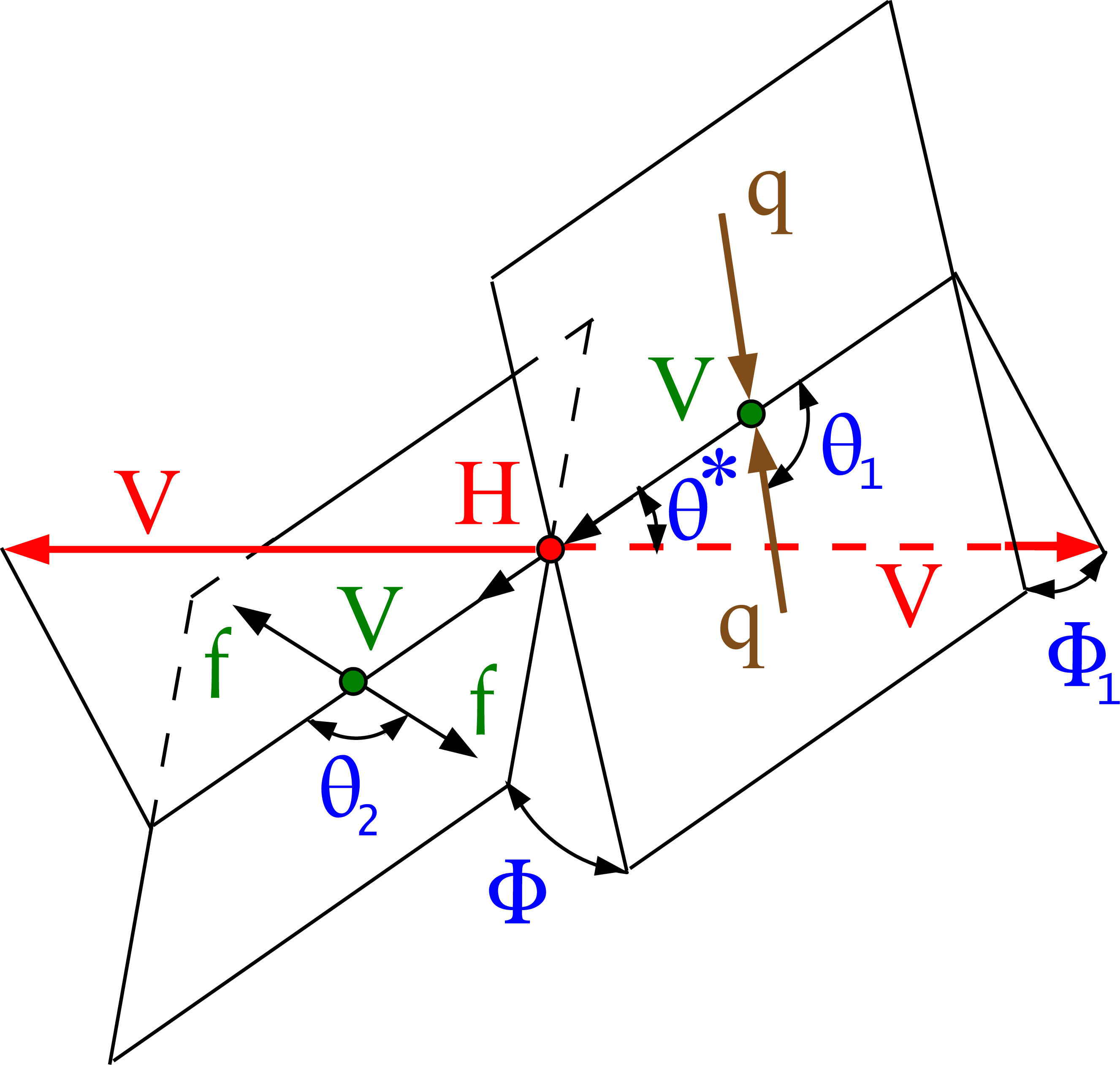
Figure 1-c:
Illustration of H boson production and decay in the associated production topology $ {\mathrm{ q } \mathrm{ q } } \to {\mathrm {V}} \to {\mathrm {V}} \mathrm{ H } \to ( {\mathrm {ff}} )\mathrm{ H } \to ( {\mathrm {ff}} ) {\mathrm {V}} {\mathrm {V}} $. The production and decay $\mathrm{ H } \to {\mathrm {V}} {\mathrm {V}} $ may be followed by the same four-lepton decay shown in Fig. 1-a. The five angles shown in blue and the invariant masses of the two vector bosons shown in green fully characterize either the production or the decay chain. The angles are defined in either the H or V boson rest frames [26,33]. |
png pdf |
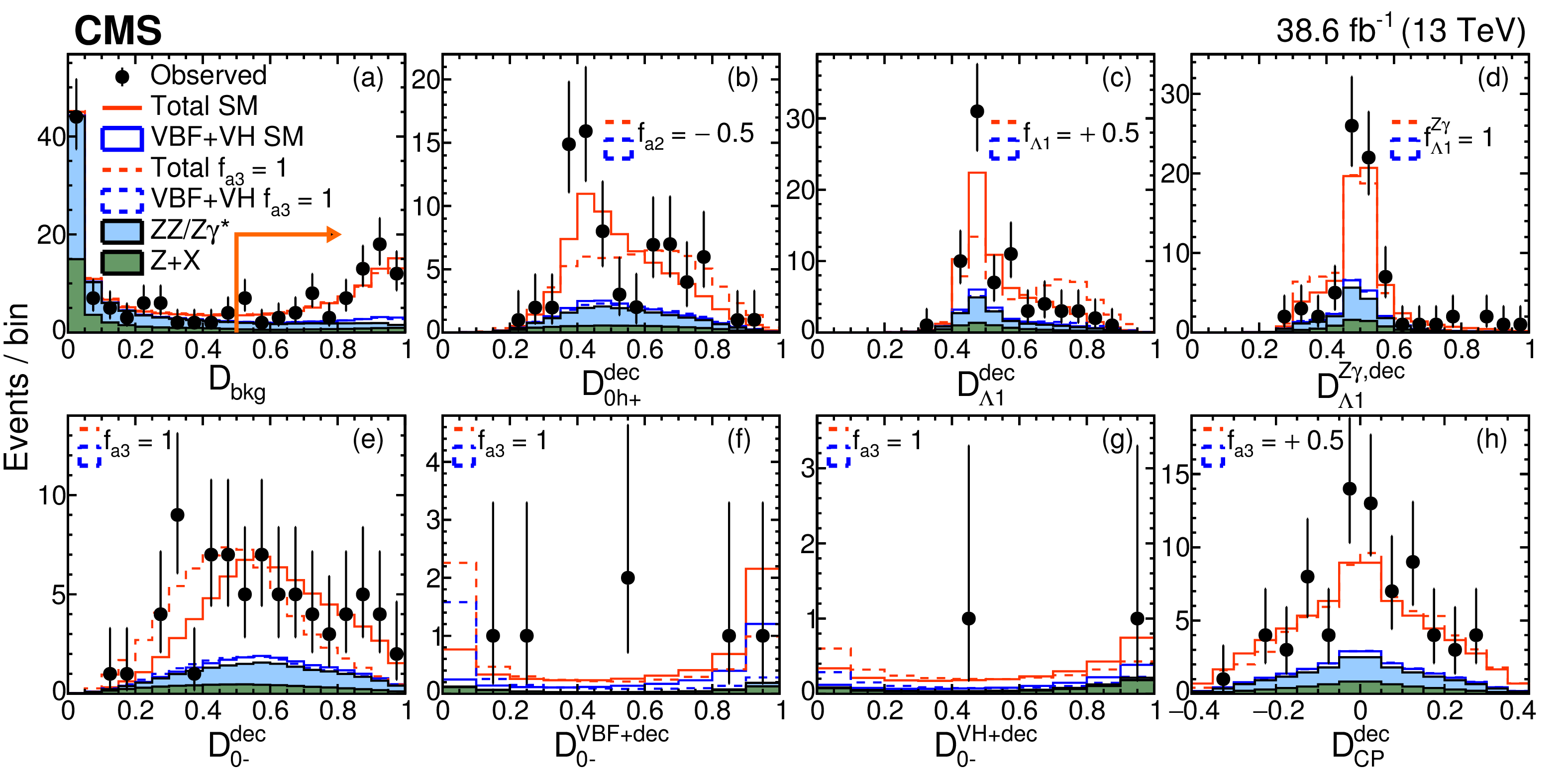
Figure 2:
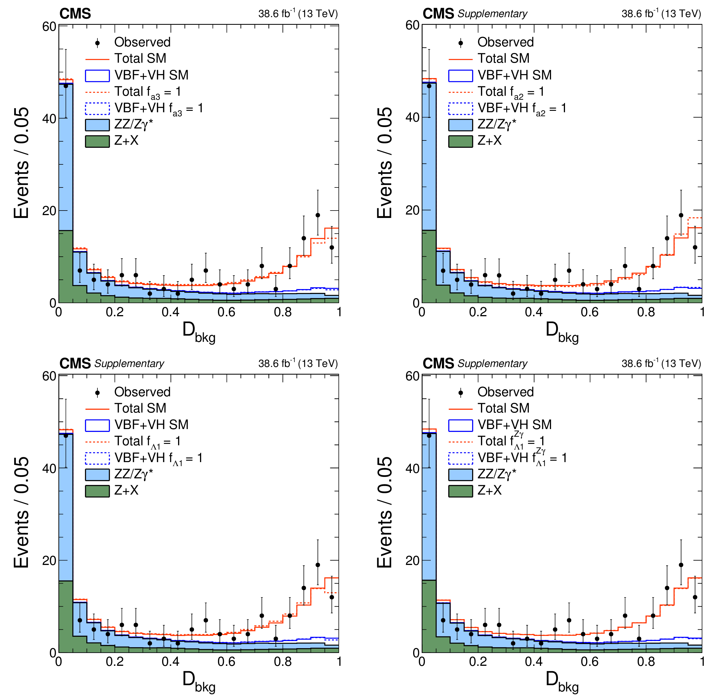
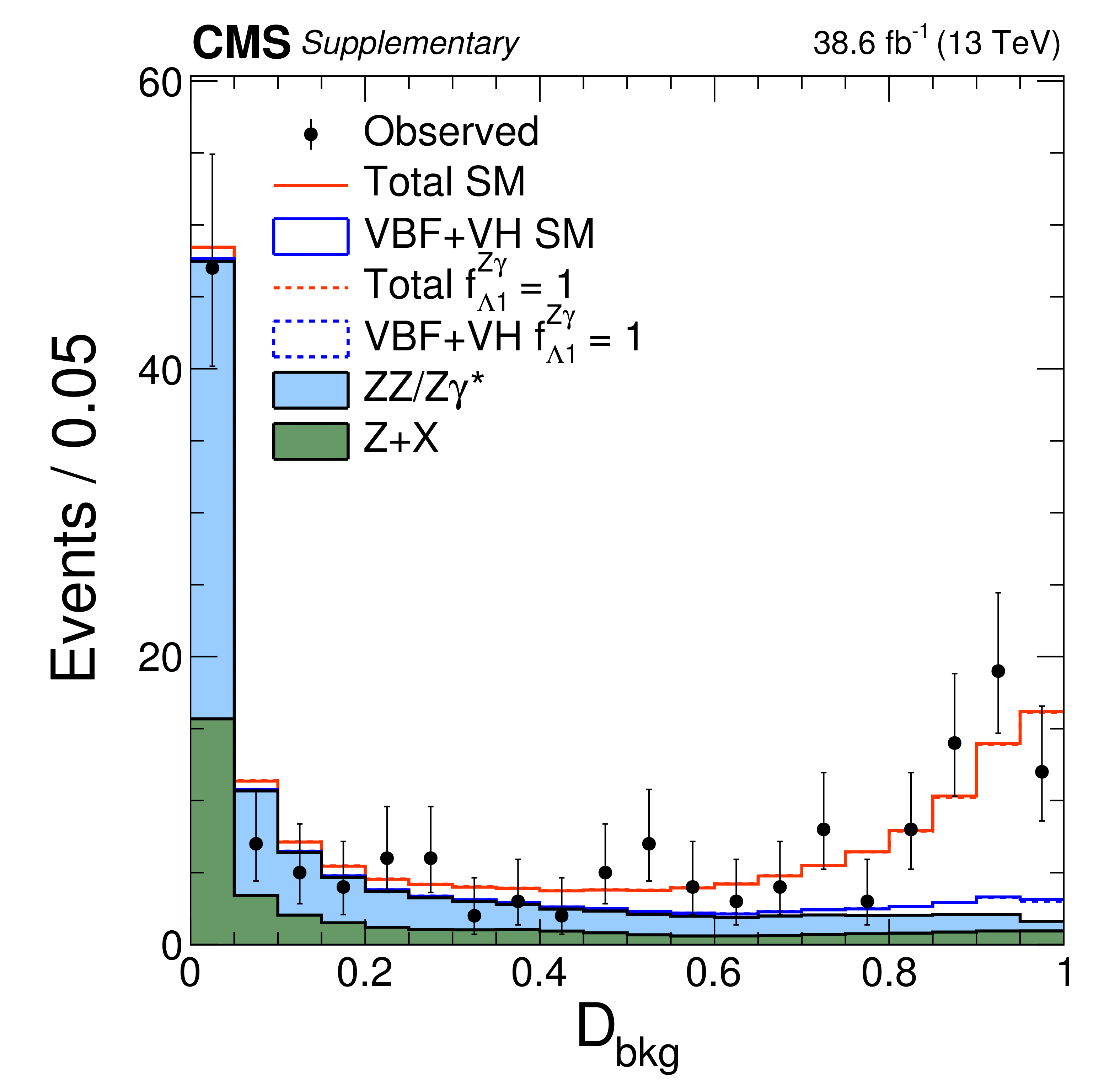
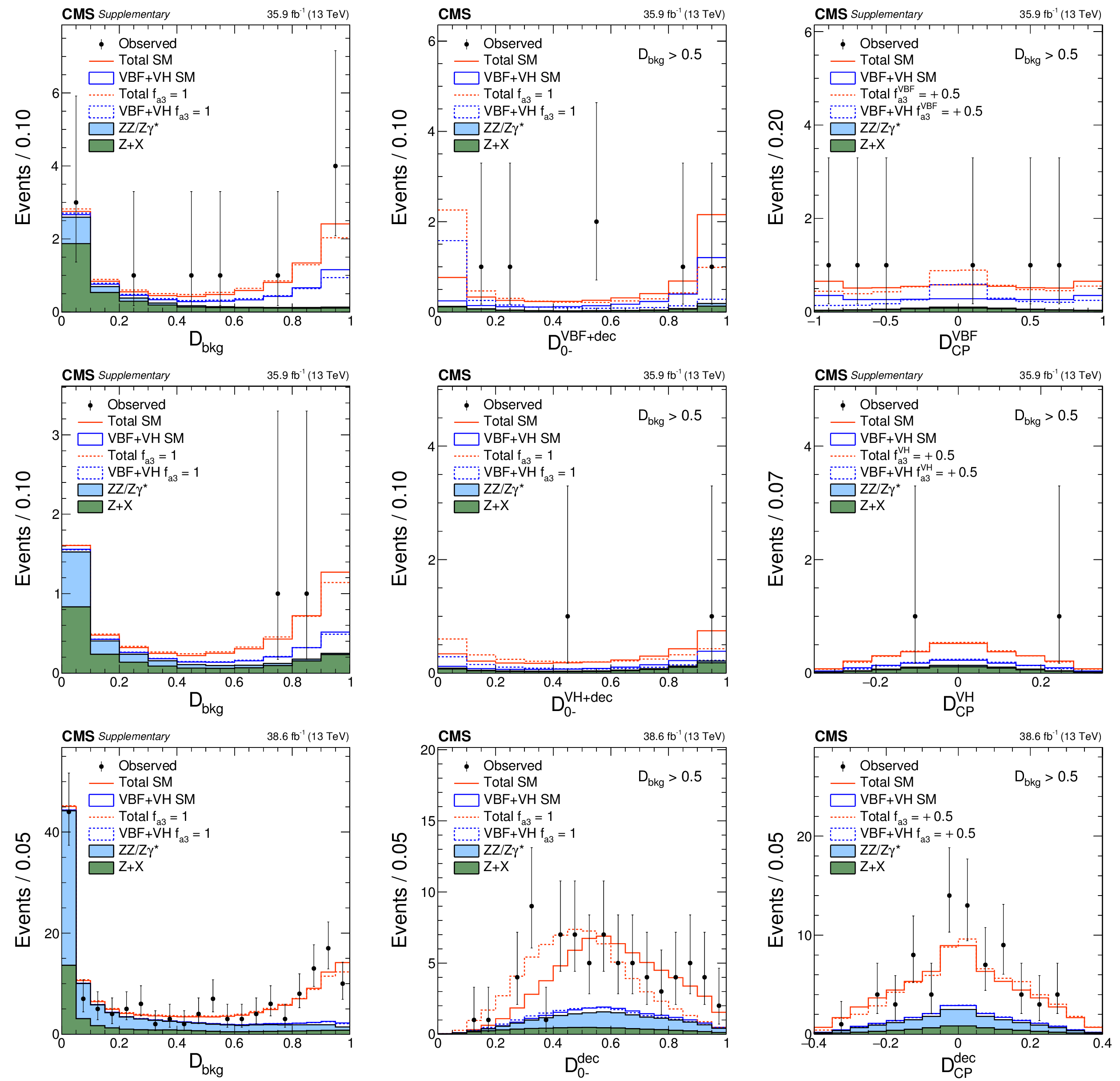
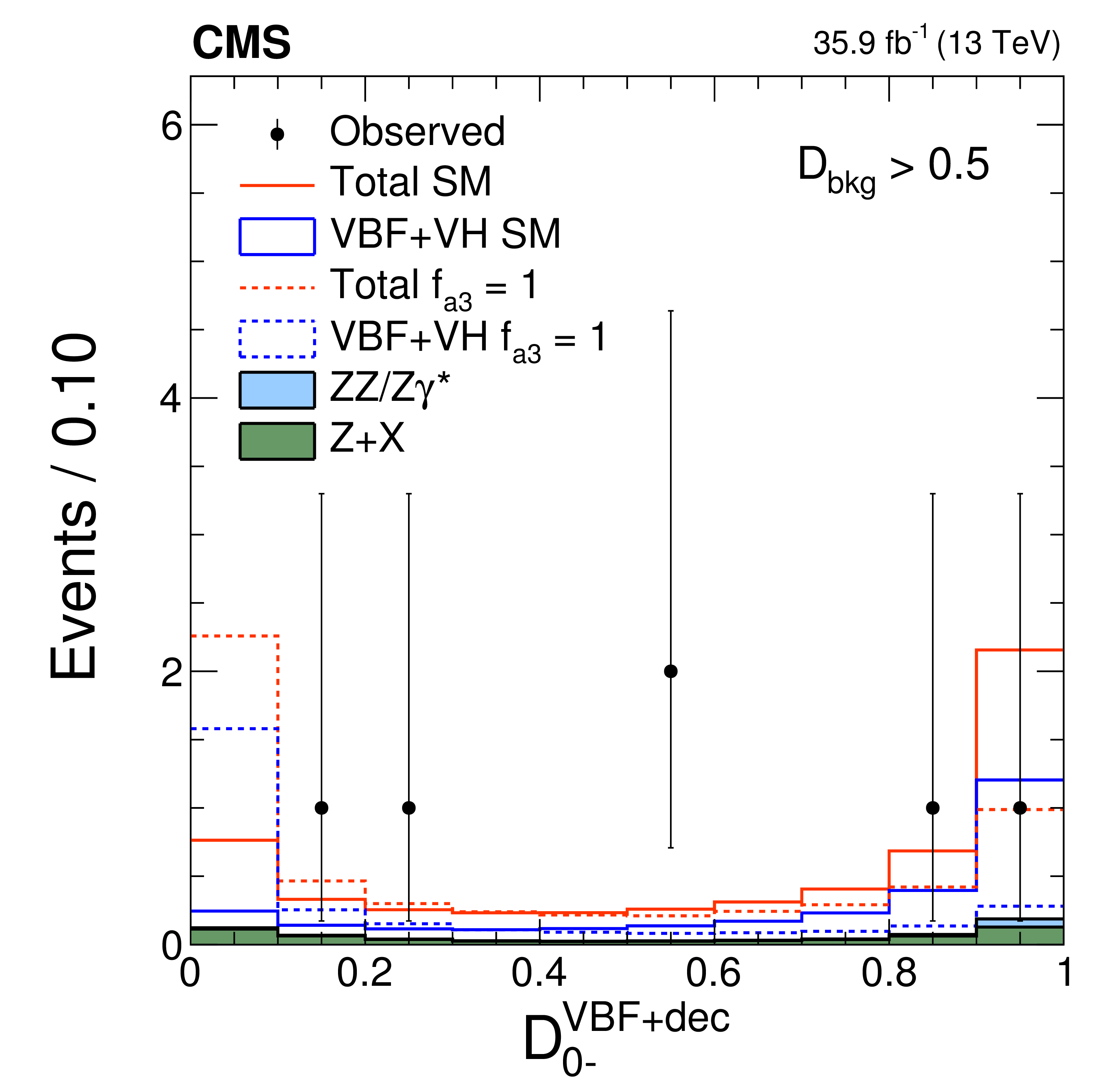
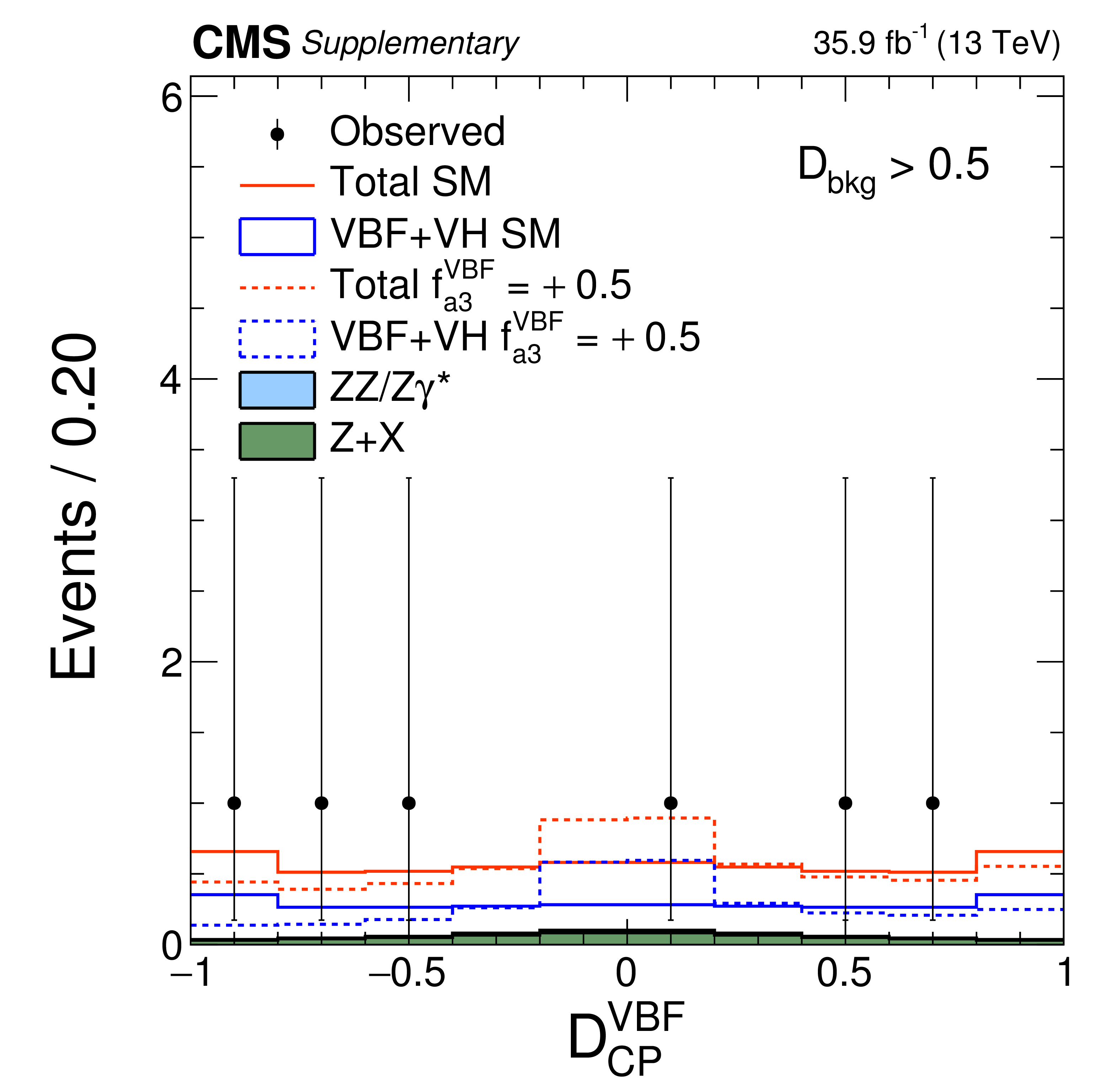
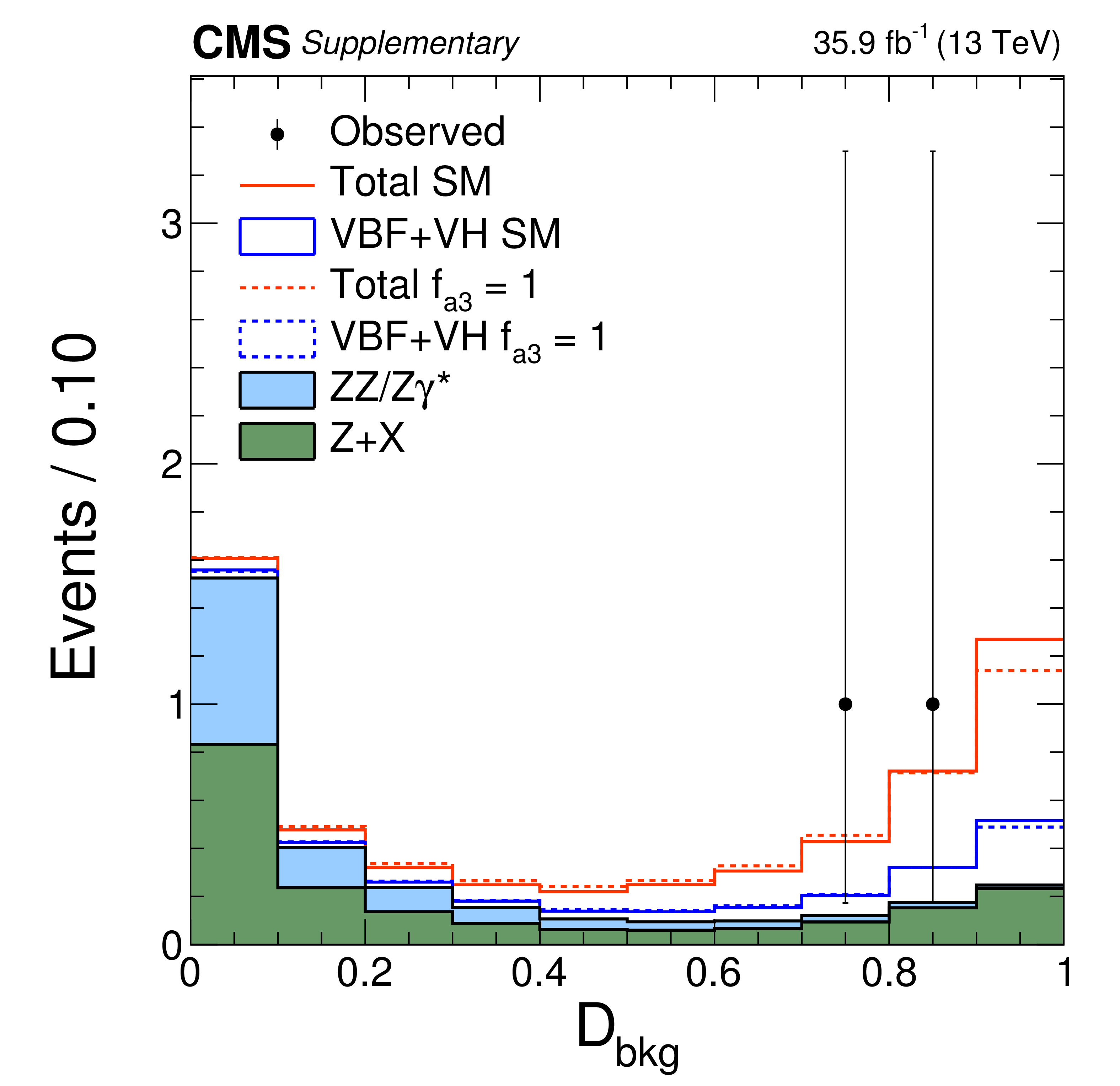
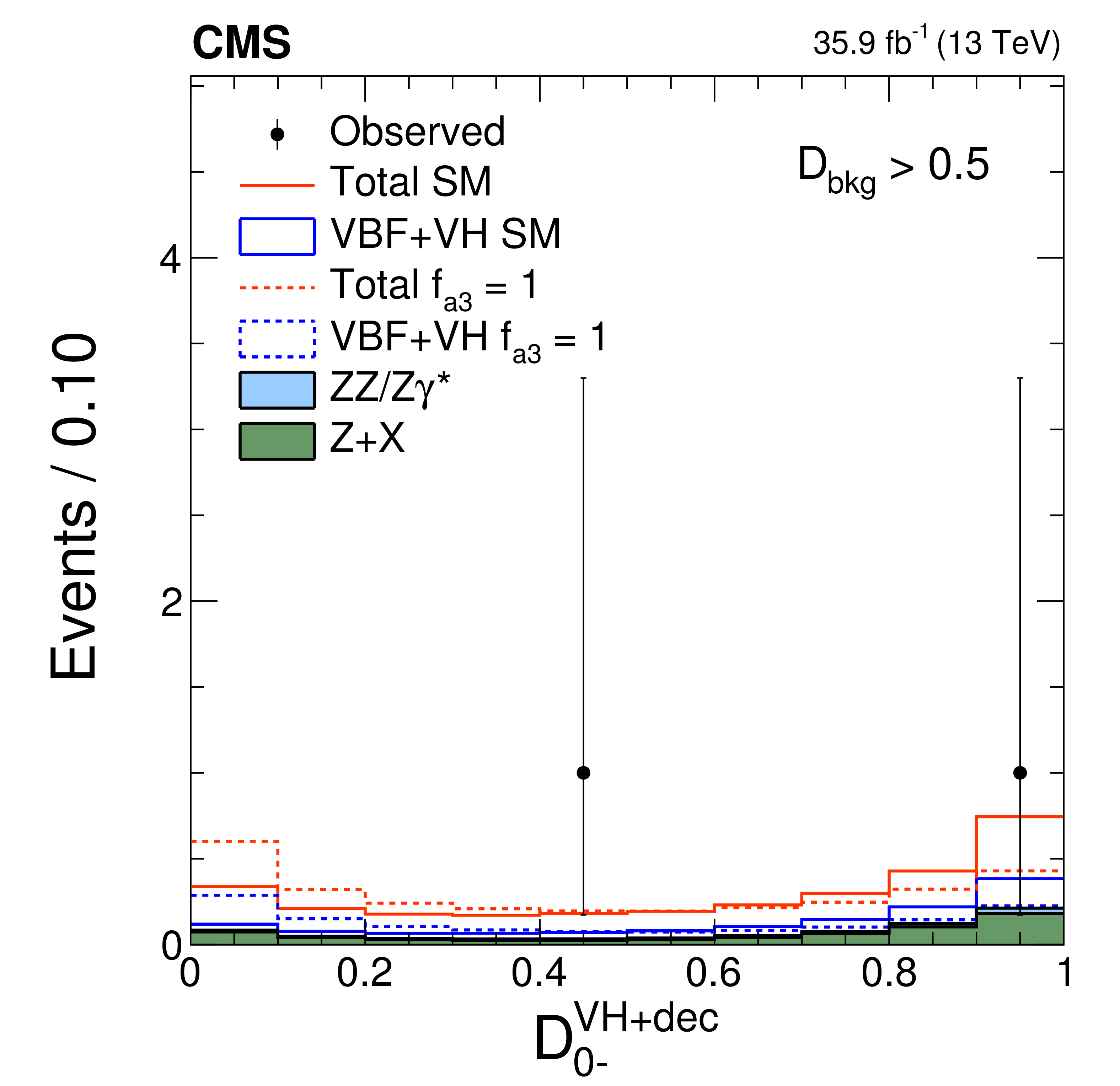
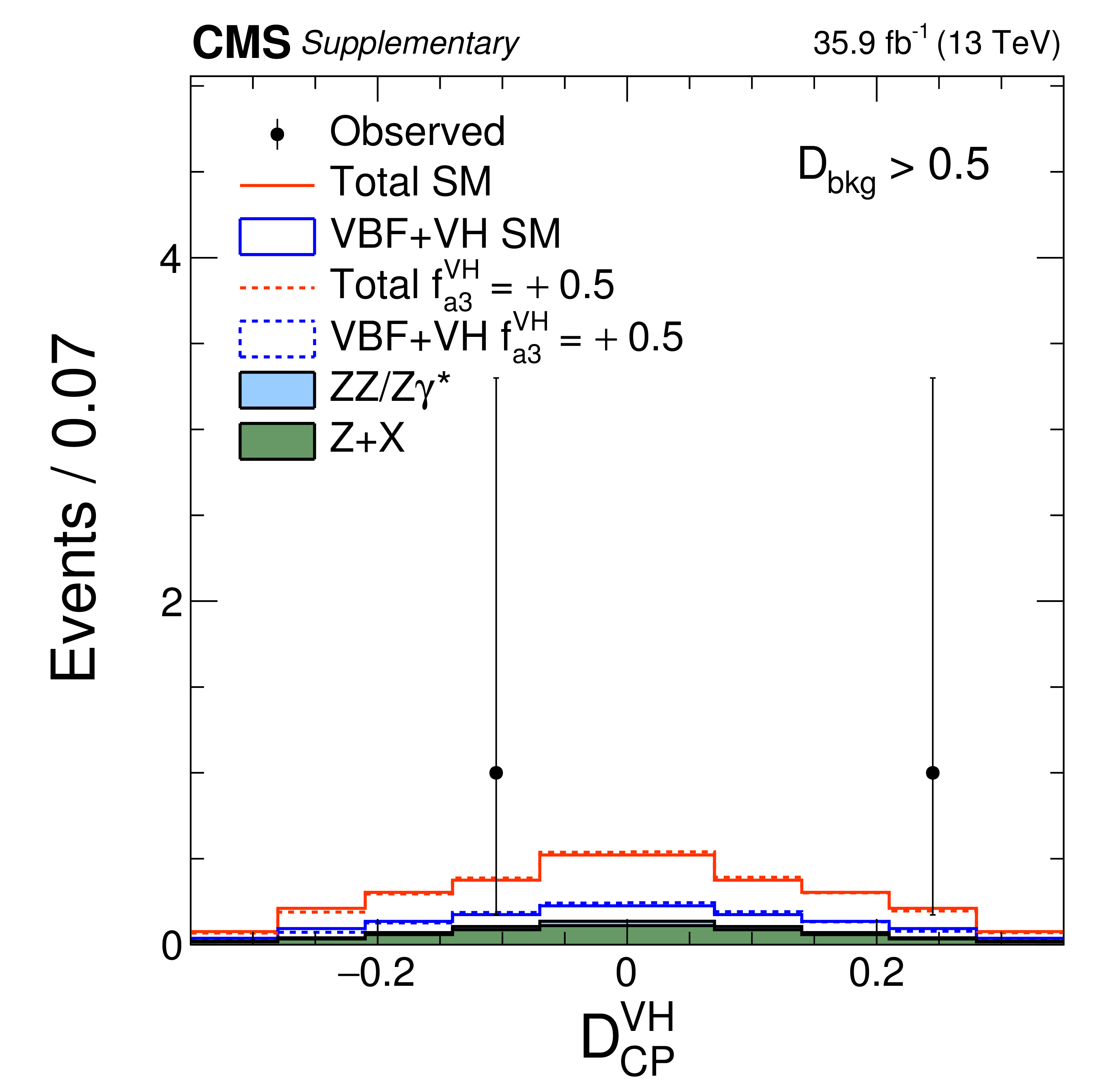
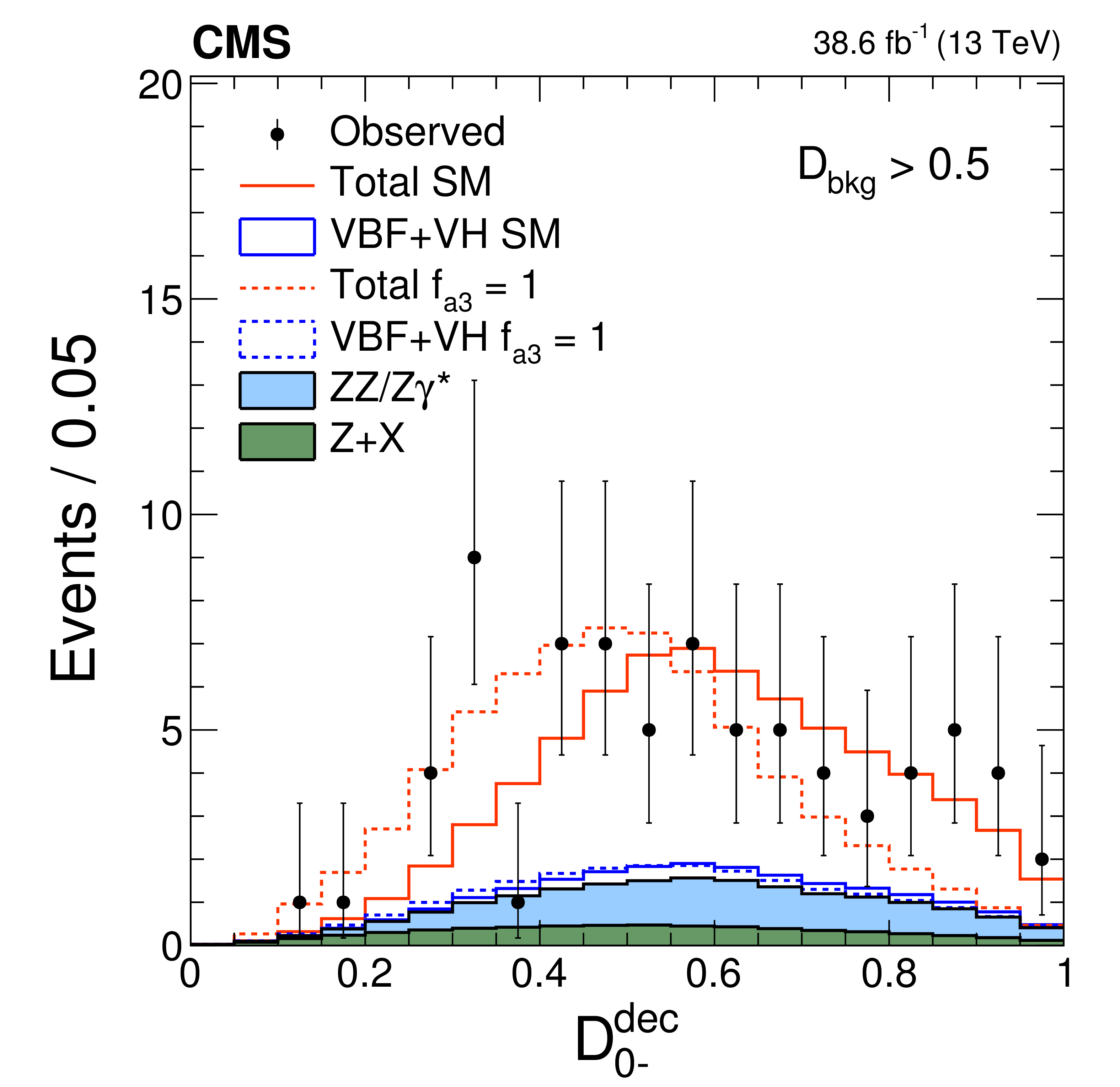
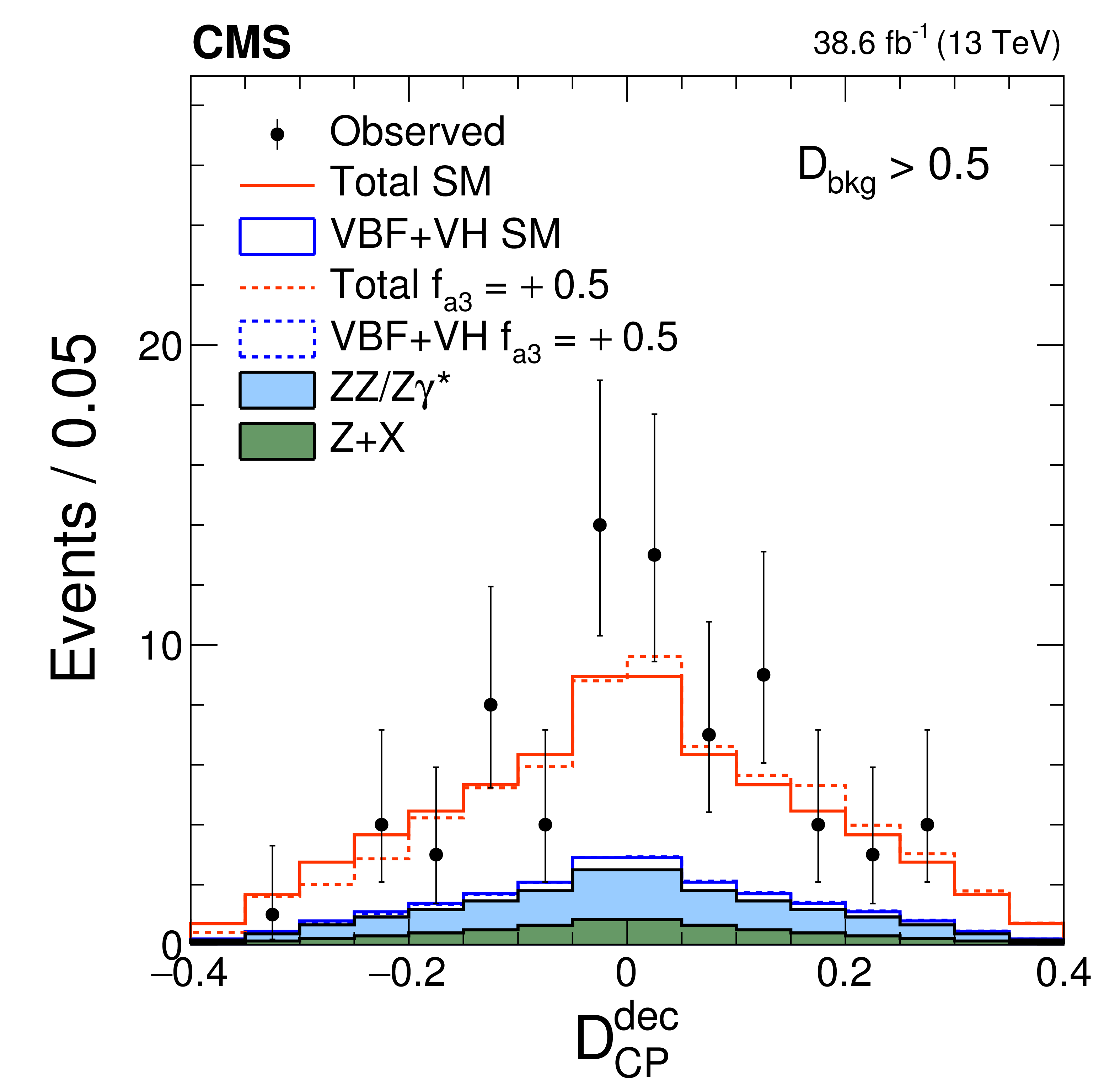
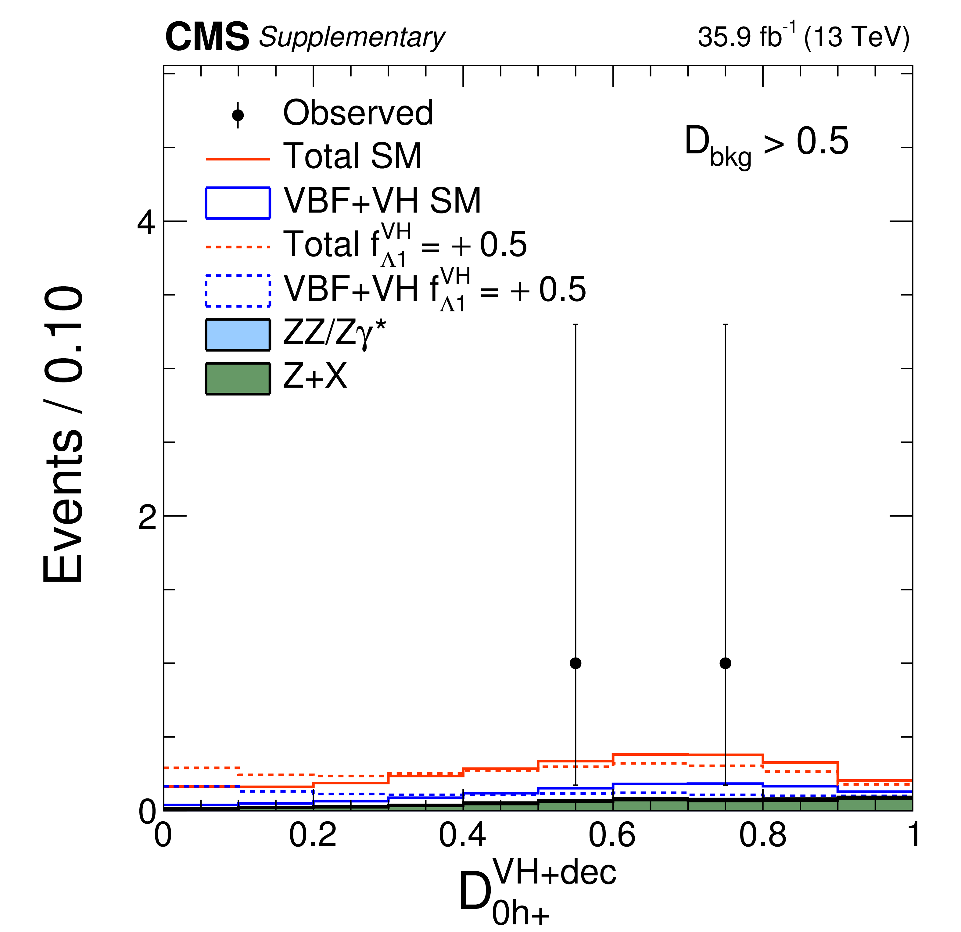
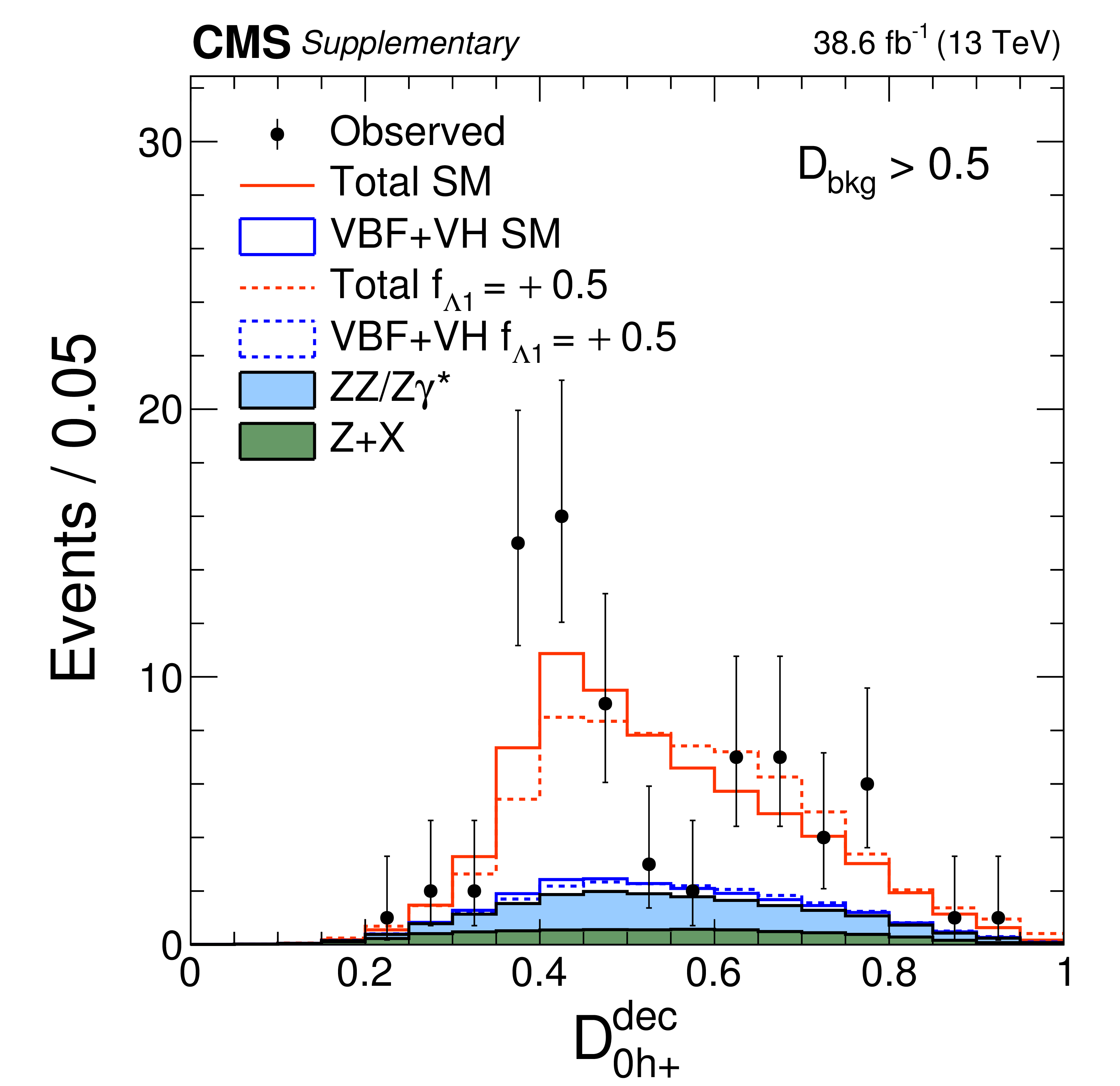
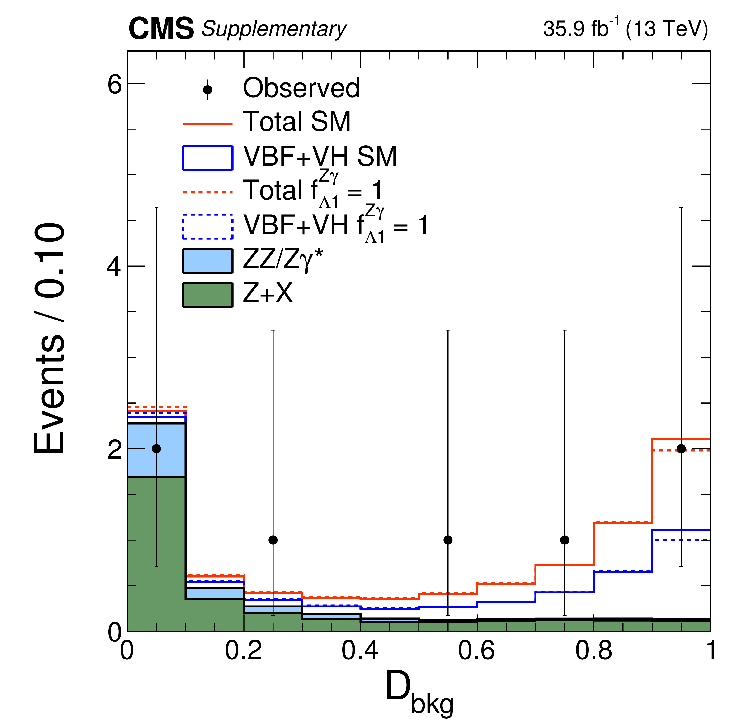
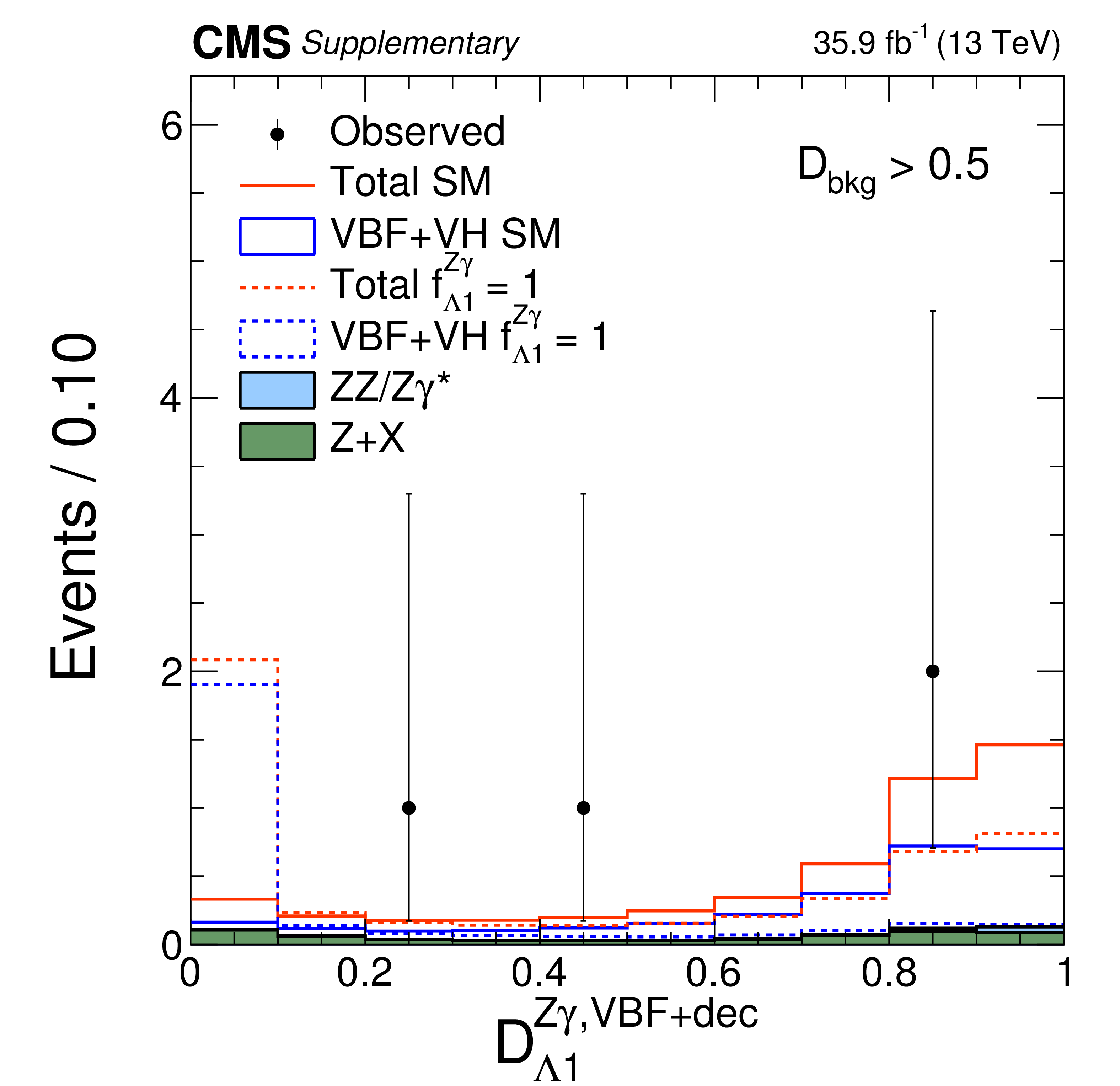
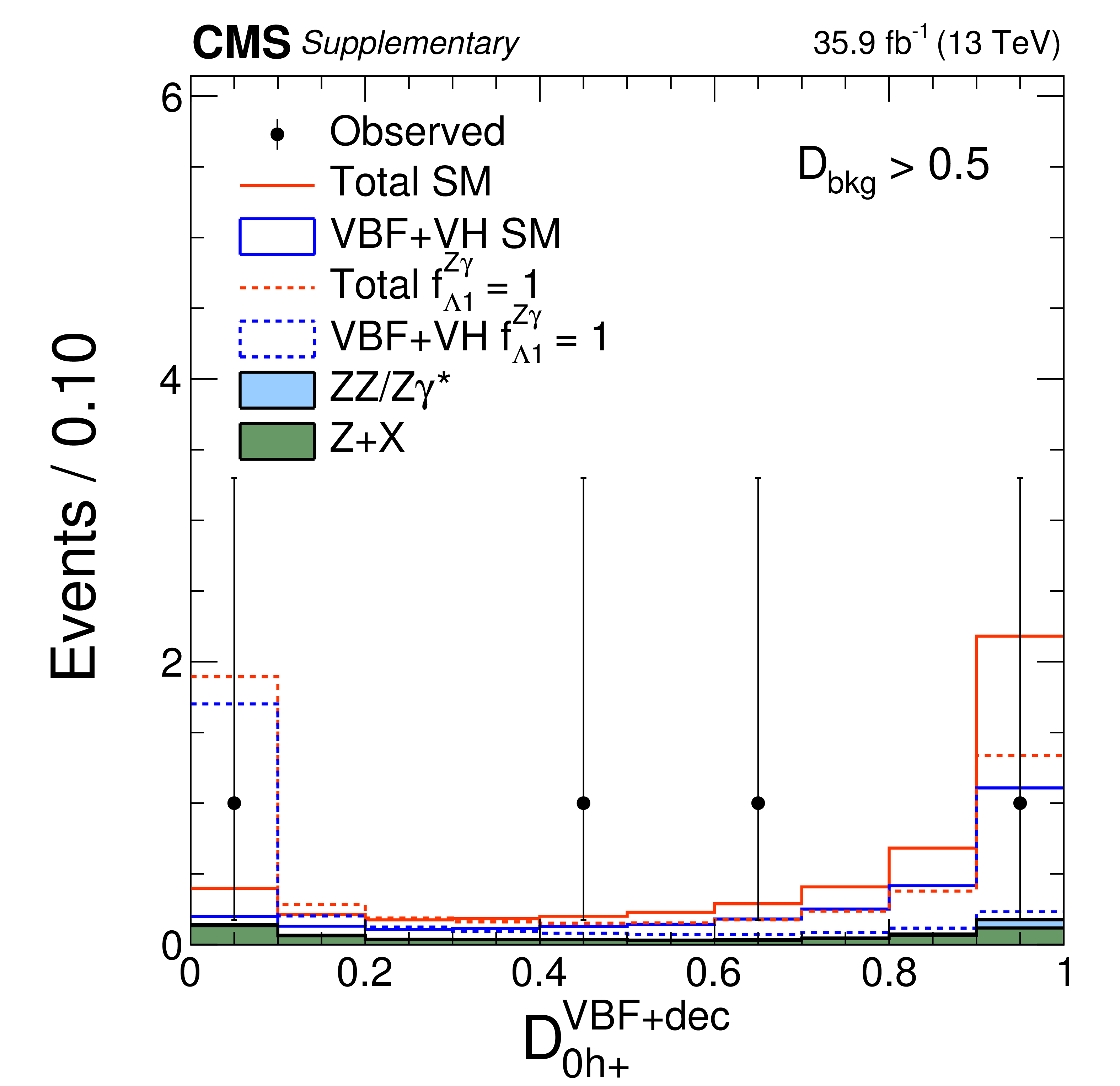
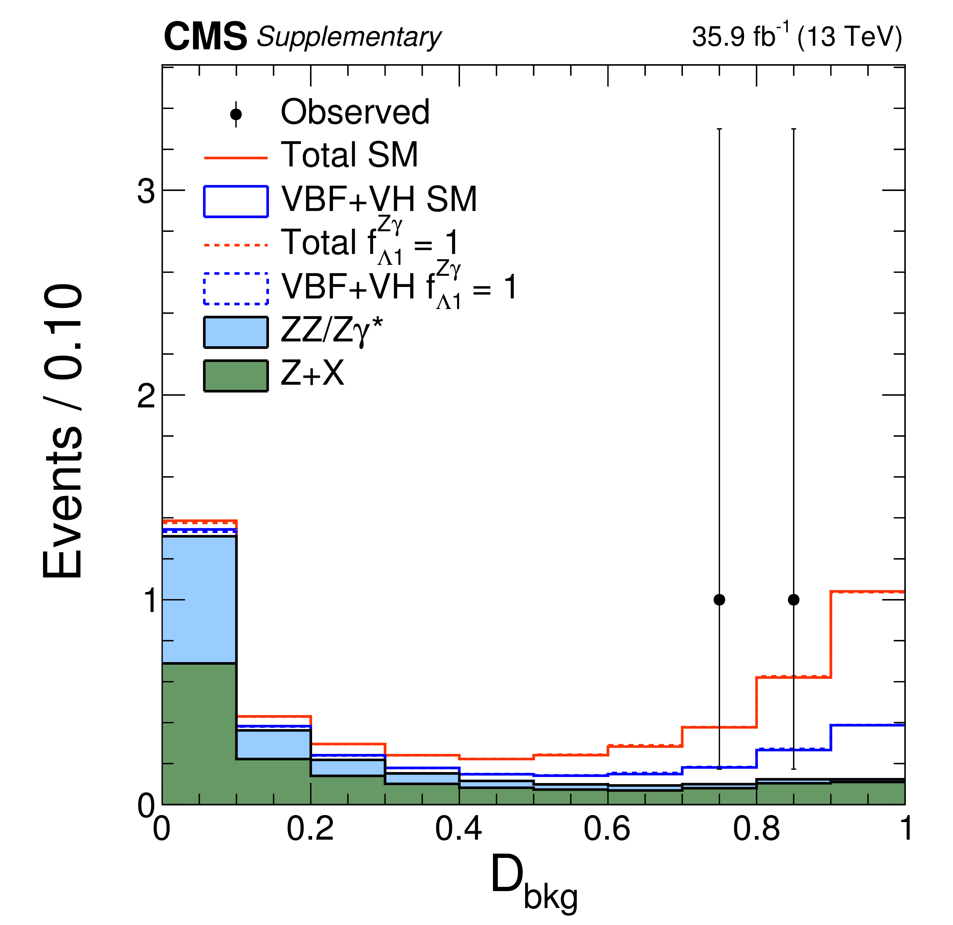
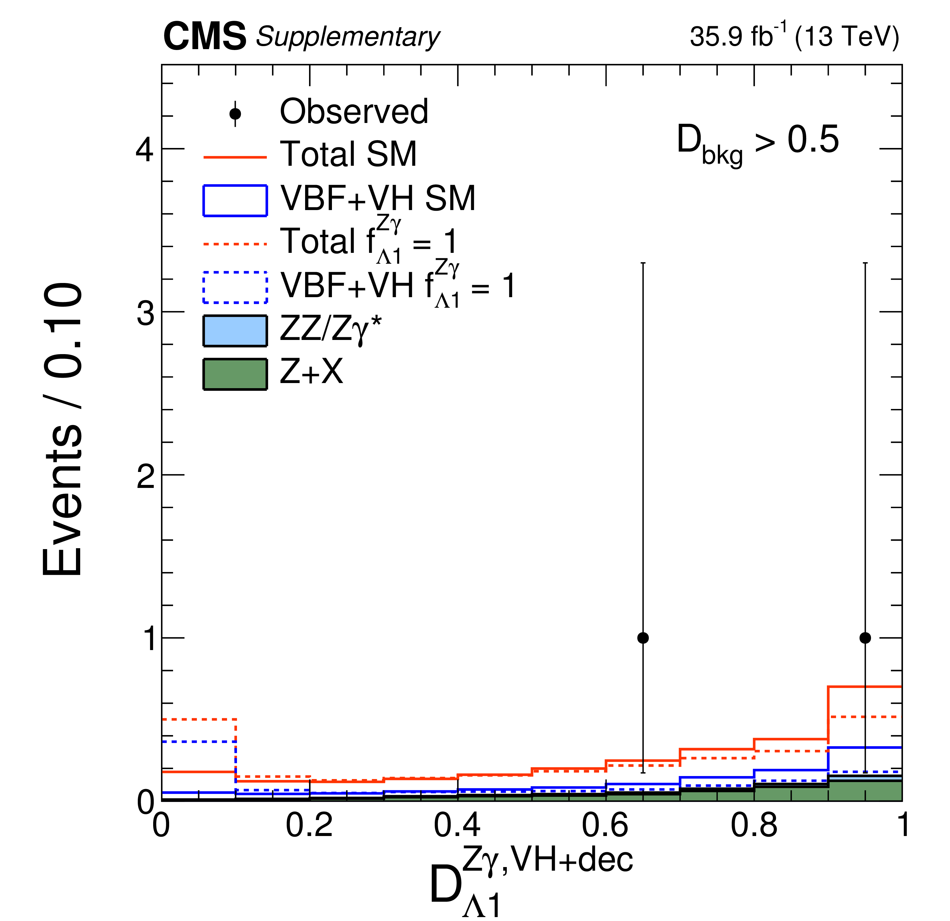
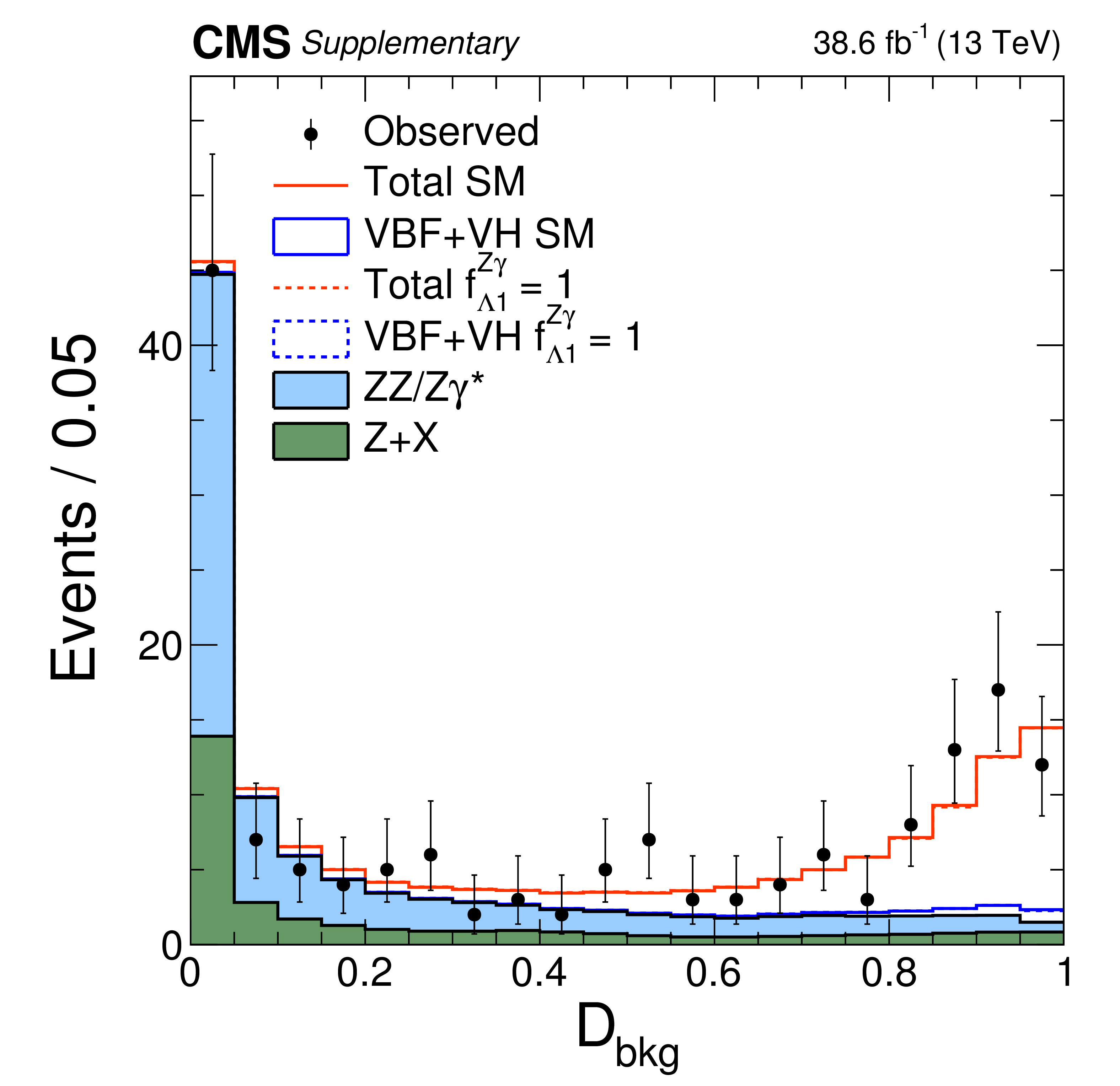
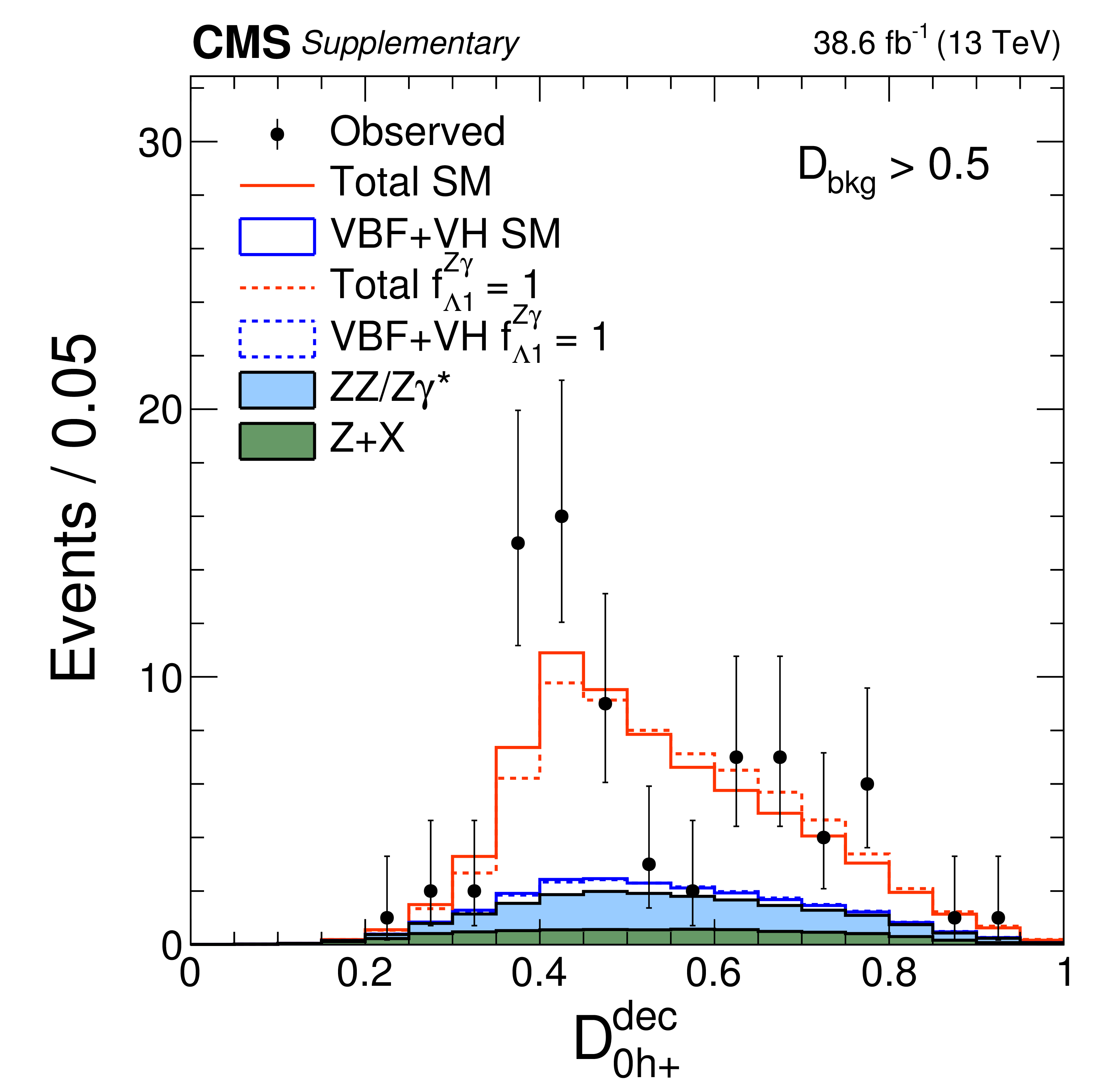
Distributions of $\mathcal {D}_\text {bkg}$ (a) for all events in Run 2; $\mathcal {D}_{0h+}$ (b), $\mathcal {D}_{\Lambda 1}$ (c) , $\mathcal {D}_{\Lambda 1}^{{\mathrm{ Z } } \gamma }$ (d), $\mathcal {D}_{0-}$ (e), and $\mathcal {D}_{CP}$ (h) for the untagged and 2015 events; $\mathcal {D}_{0-}$ in the VBF-jet (f) and $ {\mathrm {V}} \mathrm{ H } $-jet (g) categories. The arrow in (a) indicates the requirement $\mathcal {D}_\text {bkg}>0.5$, used to suppress background on all other plots. Points with error bars show data and histograms show expectations for background and signal, as indicated in the legend in (a). The dashed lines show expectations for BSM hypotheses, as indicated in the individual legends. |
png pdf |
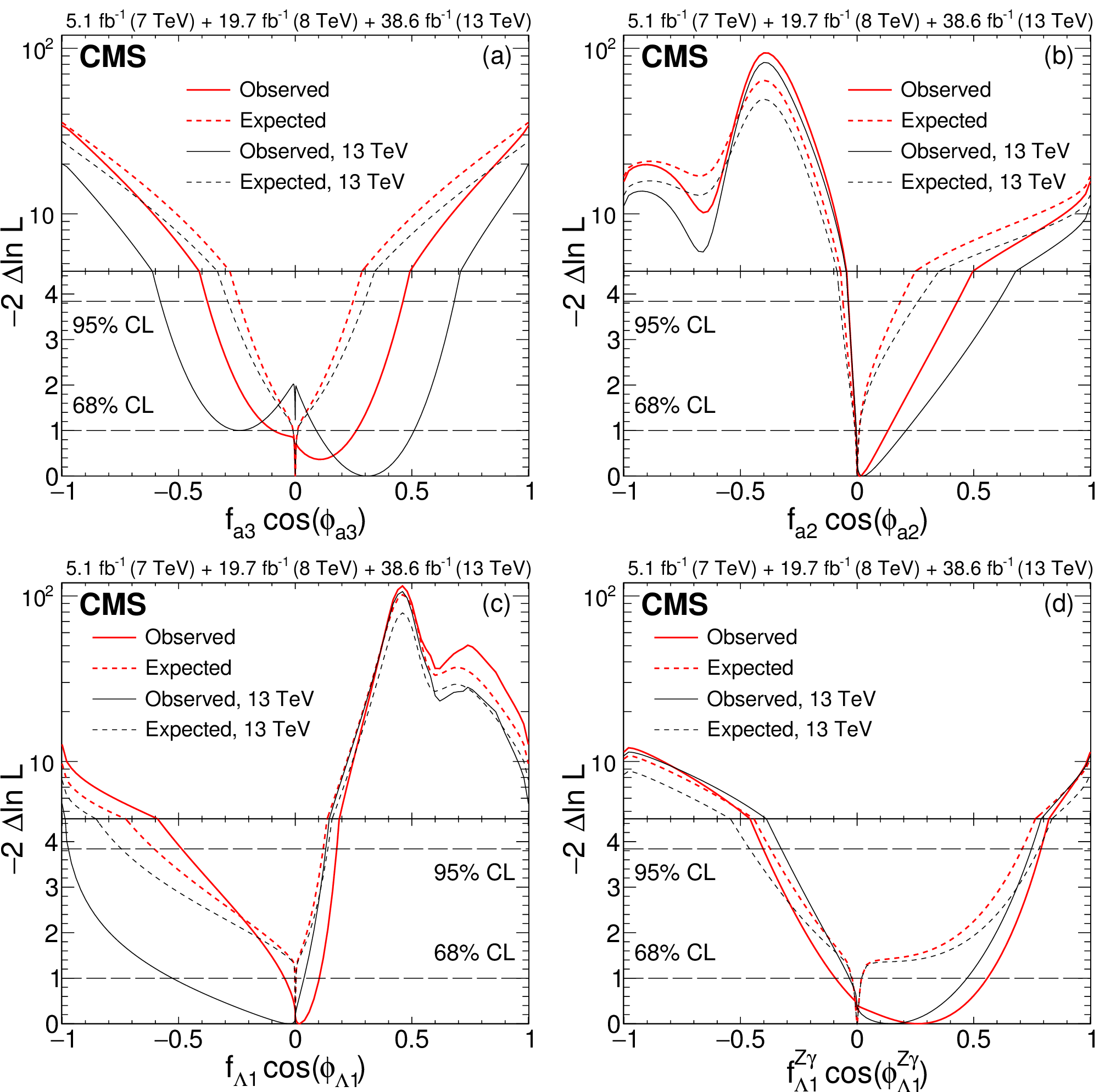
Figure 3:
Observed (solid) and expected (dashed) likelihood scans of $f_{a3}\cos(\phi _{a3})$ (a), $f_{a2}\cos(\phi _{a2})$ (b), $f_{\Lambda 1}\cos(\phi _{\Lambda 1})$ (c), and $f_{\Lambda 1}^{{\mathrm{ Z } } \gamma }\cos(\phi _{\Lambda 1}^{{\mathrm{ Z } } \gamma })$ (d). Results of the Run 2 only and the combined Run 1 and Run 2 analyses are shown. |
png pdf |
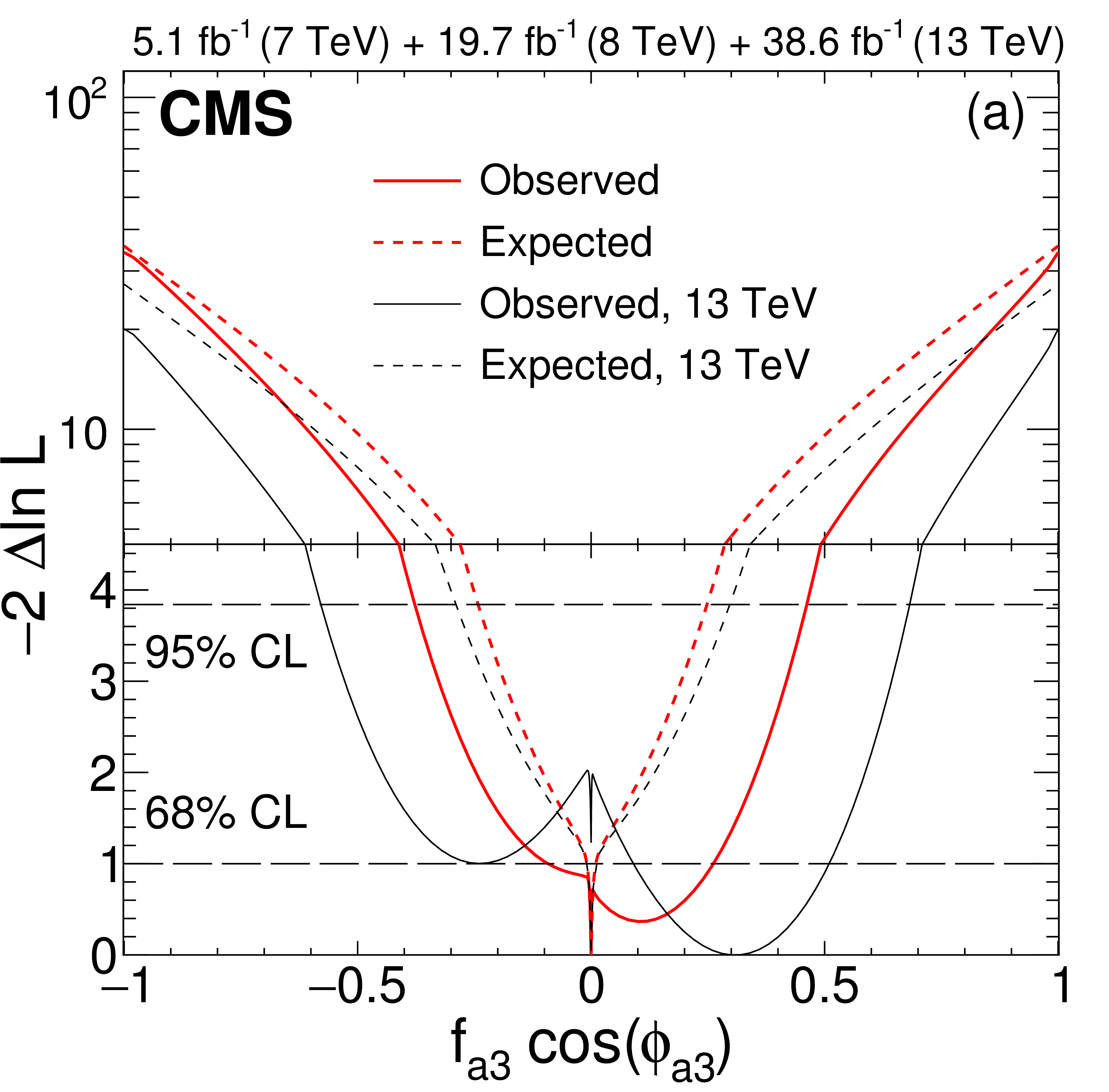
Figure 3-a:
Observed (solid) and expected (dashed) likelihood scans of $f_{a3}\cos(\phi _{a3})$. Results of the Run 2 only and the combined Run 1 and Run 2 analyses are shown. |
png pdf |
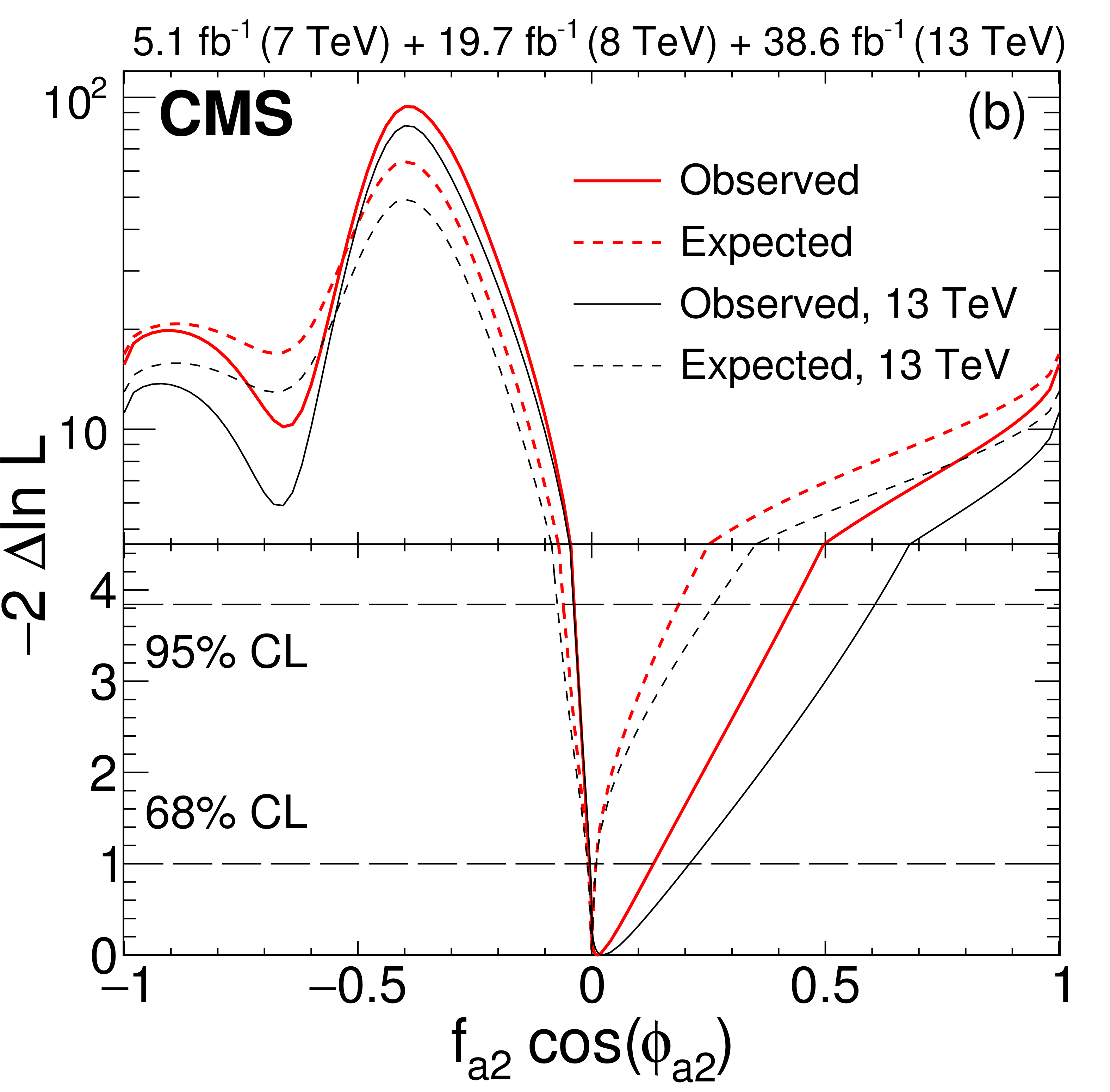
Figure 3-b:
Observed (solid) and expected (dashed) likelihood scans of $f_{a2}\cos(\phi _{a2})$. Results of the Run 2 only and the combined Run 1 and Run 2 analyses are shown. |

png pdf |
Figure 3-c:
Observed (solid) and expected (dashed) likelihood scans of $f_{\Lambda 1}\cos(\phi _{\Lambda 1})$. Results of the Run 2 only and the combined Run 1 and Run 2 analyses are shown. |
png pdf |
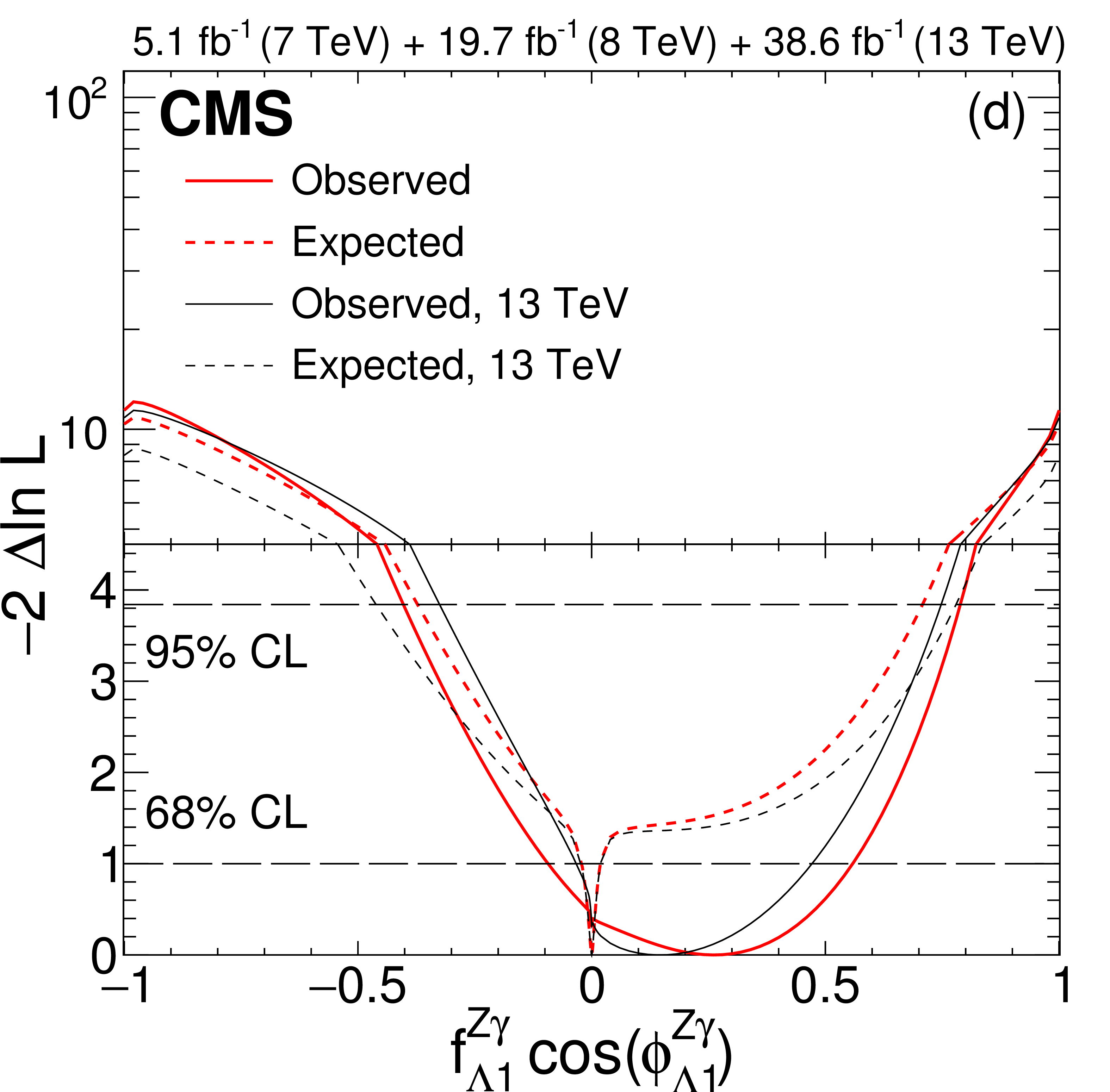
Figure 3-d:
Observed (solid) and expected (dashed) likelihood scans of $f_{\Lambda 1}^{{\mathrm{ Z } } \gamma }\cos(\phi _{\Lambda 1}^{{\mathrm{ Z } } \gamma })$. Results of the Run 2 only and the combined Run 1 and Run 2 analyses are shown. |
| Tables | |
png pdf |
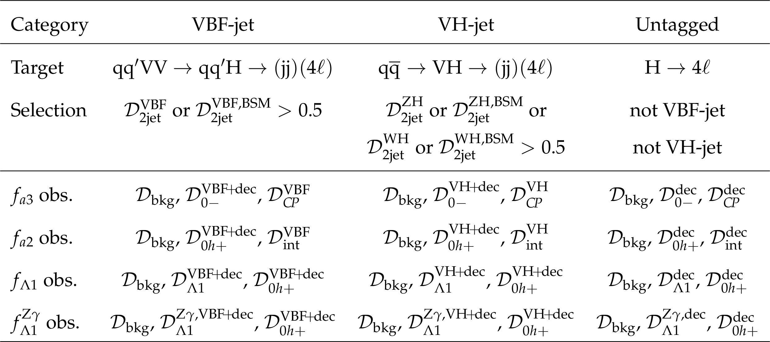
Table 1:
Summary of the three production categories in the analysis of 2016 data. The discriminants $\mathcal {D}$ are calculated from Eqs.(4) and (5), as discussed in more detail in the text. For each analysis, the appropriate BSM model is considered in the definition of the categories: $f_{a3}=1$, $f_{a2}=1$, $f_{\Lambda 1}=1$, or $f^{{\mathrm{ Z } } \gamma }_{\Lambda 1}=1$. Three observables (abbreviated as obs.) are listed for each analysis and for each category. They are described in more detail later in the text. |
png pdf |
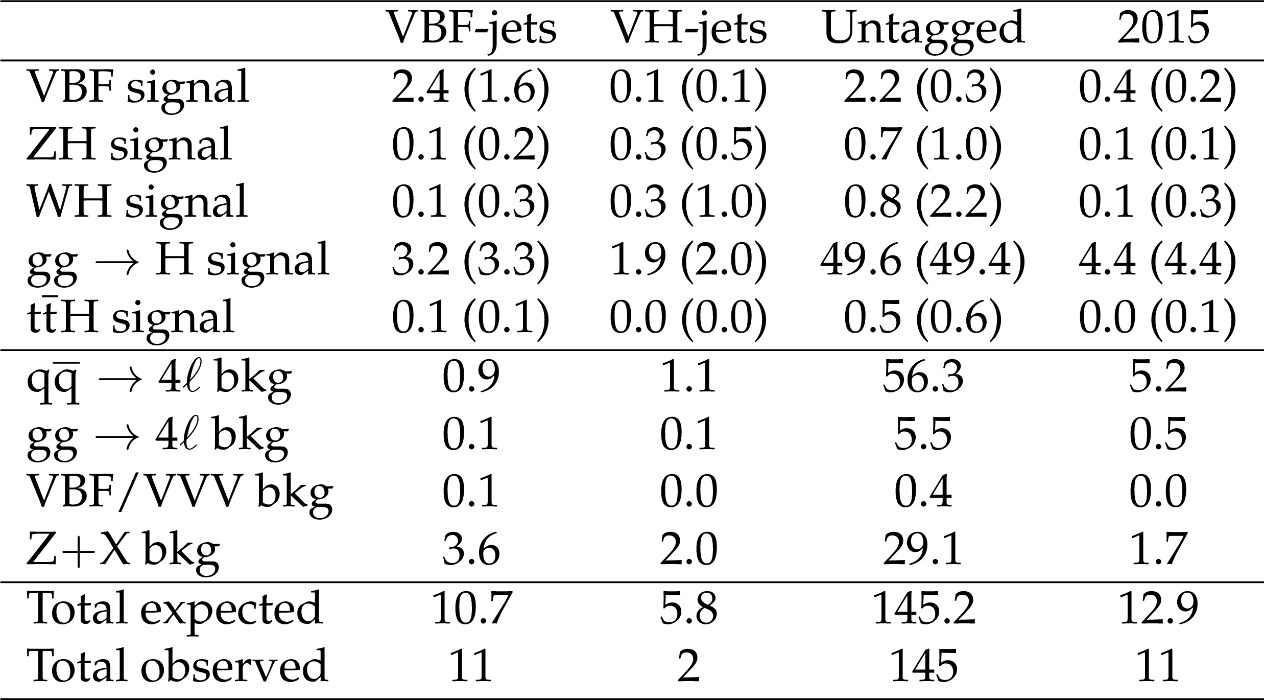
Table 2:
The numbers of events expected for the SM (or $f_{a3}=1$, in parentheses) for different signal and background modes and the total observed numbers of events across the three $f_{a3}$ categories in 2016 and 2015 data. |
png pdf |
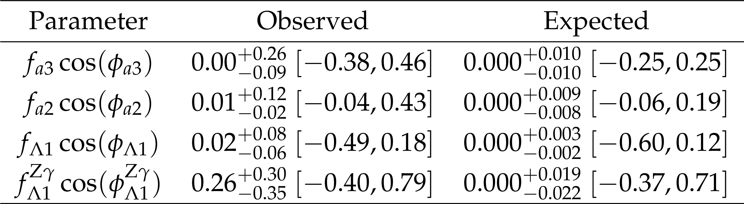
Table 3:
Summary of allowed 68%CL (central values with uncertainties) and 95%CL (in square brackets) intervals on anomalous coupling parameters obtained from the combined Run 1 and Run 2 data analysis. |
| Summary |
| We study anomalous interactions of the H boson using novel techniques with a matrix element likelihood approach to simultaneously analyze the $\mathrm{ H }\to4\ell$ decay and associated production with two quark jets. Three categories of events are analyzed, targeting events produced in vector boson fusion, with an associated vector boson, and in gluon fusion, respectively. The data collected at a center-of-mass energy of 13 TeV in Run\,2 of the LHC are combined with the Run\,1 data, collected at 7 and 8 TeV. No deviations from the standard model are observed and constraints are set on the four anomalous $\mathrm{ H }{\mathrm{V}} {\mathrm{V}} $ contributions, including the CP-violation parameter $f_{a3}$, summarized in Table 3. |
| Additional Figures | |
png pdf |
Additional Figure 1:
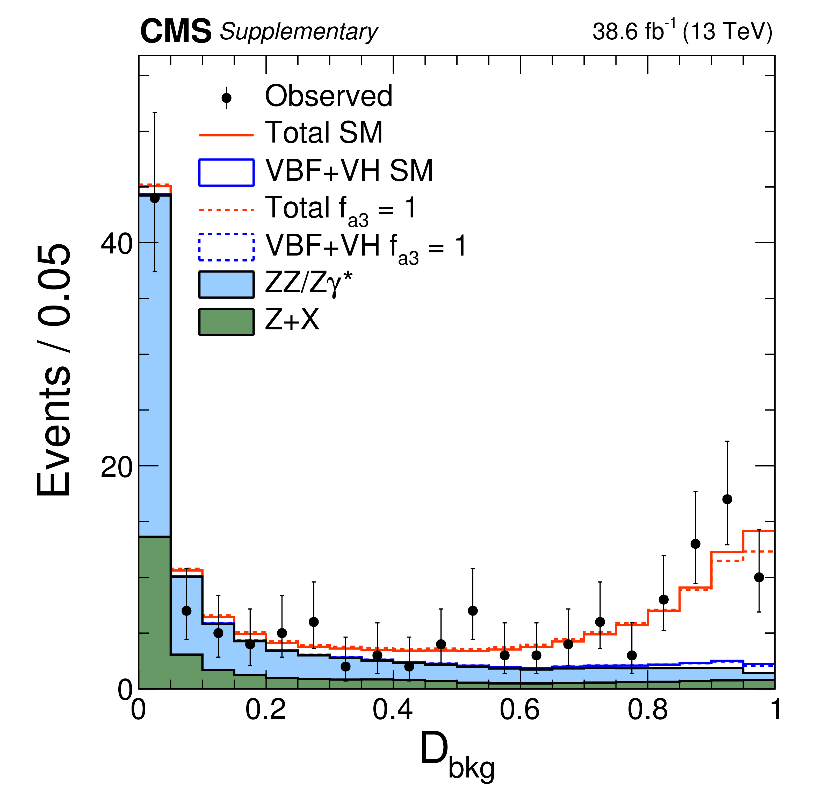
Distributions of the $\mathcal {D}_{\rm bkg}$ kinematic discriminant in the $f_{a3}$ (a), $f_{a2}$ (b), $f_{\Lambda 1}$ (c), and $f_{\Lambda 1}^{{\mathrm{ Z } } \gamma }$ (d) analyses. The distributions are summed over all three categories. Points with error bars show data and histograms show expectations for background and SM or BSM signal as indicated in the legend. |

png pdf |
Additional Figure 1-a:
Distributions of the $\mathcal {D}_{\rm bkg}$ kinematic discriminant in the $f_{a3}$ analysis. The distributions are summed over all three categories. Points with error bars show data and histograms show expectations for background and SM or BSM signal as indicated in the legend. |

png pdf |
Additional Figure 1-b:
Distributions of the $\mathcal {D}_{\rm bkg}$ kinematic discriminant in the $f_{a2}$ analysis. The distributions are summed over all three categories. Points with error bars show data and histograms show expectations for background and SM or BSM signal as indicated in the legend. |

png pdf |
Additional Figure 1-c:
Distributions of the $\mathcal {D}_{\rm bkg}$ kinematic discriminant in the $f_{\Lambda 1}$ analysis. The distributions are summed over all three categories. Points with error bars show data and histograms show expectations for background and SM or BSM signal as indicated in the legend. |
png pdf |
Additional Figure 1-d:
Distributions of the $\mathcal {D}_{\rm bkg}$ kinematic discriminant in the $f_{\Lambda 1}^{{\mathrm{ Z } } \gamma }$ analysis. The distributions are summed over all three categories. Points with error bars show data and histograms show expectations for background and SM or BSM signal as indicated in the legend. |
png pdf |
Additional Figure 2:
Distributions of kinematic discriminants in the $f_{a3}$ analysis: $\mathcal {D}_{\rm bkg}$ (a), (d), (g), $\mathcal {D}_{0-}$ (b), (e), (h), and $\mathcal {D}_{CP}$ (c), (f), (i). The decay or production information used in the $\mathcal {D}_{0-}$ and $\mathcal {D}_{CP}$ discriminants is reflected in the superscript label and depends on the tagging category. $f_{a3}^\text {VBF}$ and $f_{a3}^{\mathrm {V} \mathrm{ H } }$ are defined using Eq.(2) by analogy with $f_{a3}$, but using the cross sections for the VBF and VH processes, respectively. Three tagging categories are shown: VBF-jets (a)-(c), VH-jets (d)-(f), and untagged (g)-(i). Points with error bars show data and histograms show expectations for background and SM or BSM signal as indicated in the legend. |

png pdf |
Additional Figure 2-a:
Distribution of the $\mathcal {D}_{\rm bkg}$ kinematic discriminant in the $f_{a3}$ analysis, in the VBF-jets tagging category. Points with error bars show data and histograms show expectations for background and SM or BSM signal as indicated in the legend. |
png pdf |
Additional Figure 2-b:
Distribution of the $\mathcal {D}_{0-}$ kinematic discriminant in the $f_{a3}$ analysis, in the VBF-jets tagging category. Points with error bars show data and histograms show expectations for background and SM or BSM signal as indicated in the legend. |
png pdf |
Additional Figure 2-c:
Distribution of the $\mathcal {D}_{CP}$ kinematic discriminant in the $f_{a3}$ analysis, in the VBF-jets tagging category. Points with error bars show data and histograms show expectations for background and SM or BSM signal as indicated in the legend. |
png pdf |
Additional Figure 2-d:
Distribution of the $\mathcal {D}_{\rm bkg}$ kinematic discriminant in the $f_{a3}$ analysis, in the VH-jets tagging category. Points with error bars show data and histograms show expectations for background and SM or BSM signal as indicated in the legend. |
png pdf |
Additional Figure 2-e:
Distribution of the $\mathcal {D}_{0-}$ kinematic discriminant in the $f_{a3}$ analysis, in the VH-jets tagging category. Points with error bars show data and histograms show expectations for background and SM or BSM signal as indicated in the legend. |
png pdf |
Additional Figure 2-f:
Distribution of the $\mathcal {D}_{CP}$ kinematic discriminant in the $f_{a3}$ analysis, in the VH-jets tagging category. Points with error bars show data and histograms show expectations for background and SM or BSM signal as indicated in the legend. |
png pdf |
Additional Figure 2-g:
Distribution of the $\mathcal {D}_{\rm bkg}$ kinematic discriminant in the $f_{a3}$ analysis, in the untagged tagging category. Points with error bars show data and histograms show expectations for background and SM or BSM signal as indicated in the legend. |
png pdf |
Additional Figure 2-h:
Distribution of the $\mathcal {D}_{0-}$ kinematic discriminant in the $f_{a3}$ analysis, in the untagged tagging category. Points with error bars show data and histograms show expectations for background and SM or BSM signal as indicated in the legend. |
png pdf |
Additional Figure 2-i:
Distribution of the $\mathcal {D}_{CP}$ kinematic discriminant in the $f_{a3}$ analysis, in the untagged tagging category. Points with error bars show data and histograms show expectations for background and SM or BSM signal as indicated in the legend. |
png pdf |
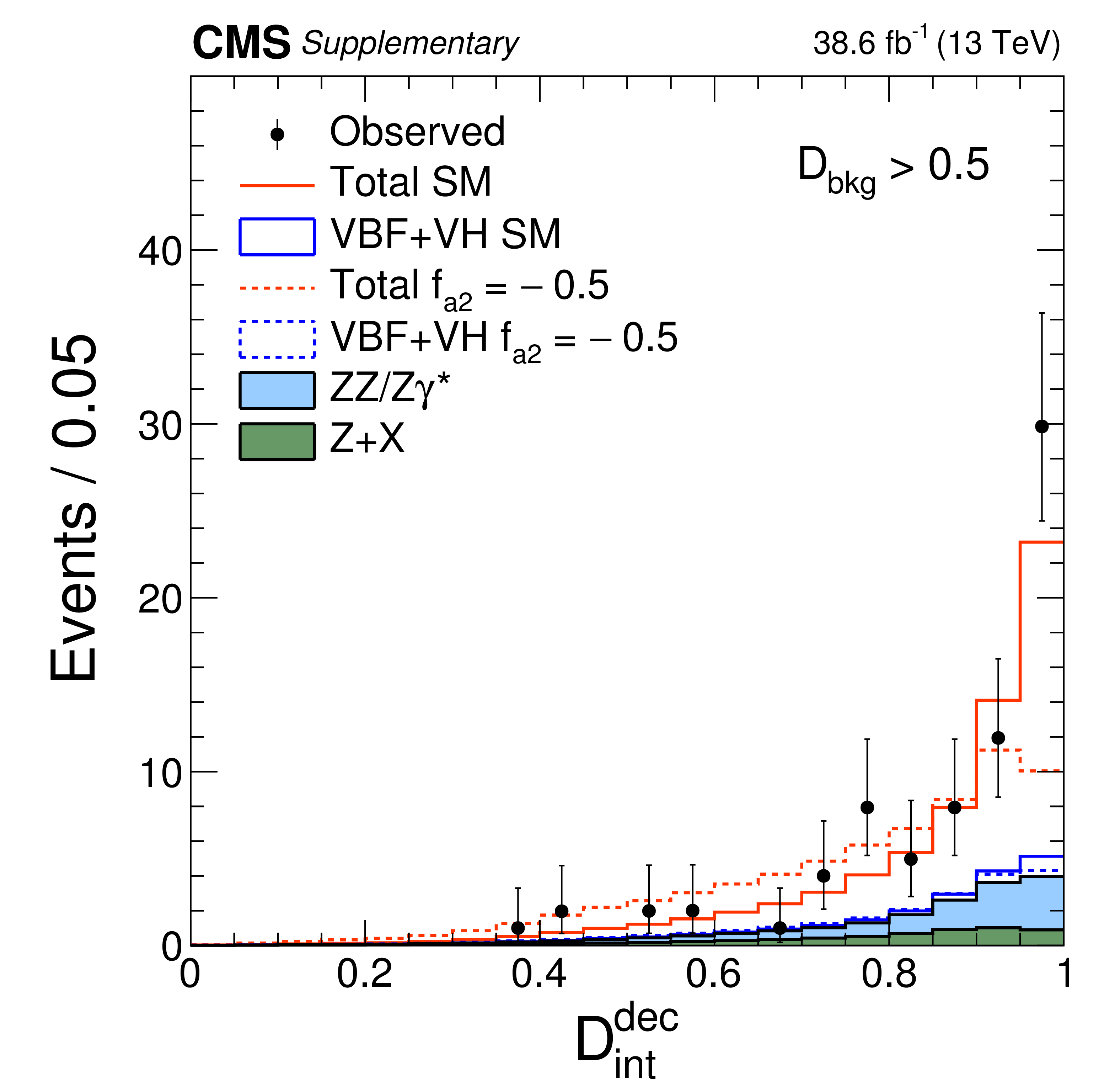
Additional Figure 3:
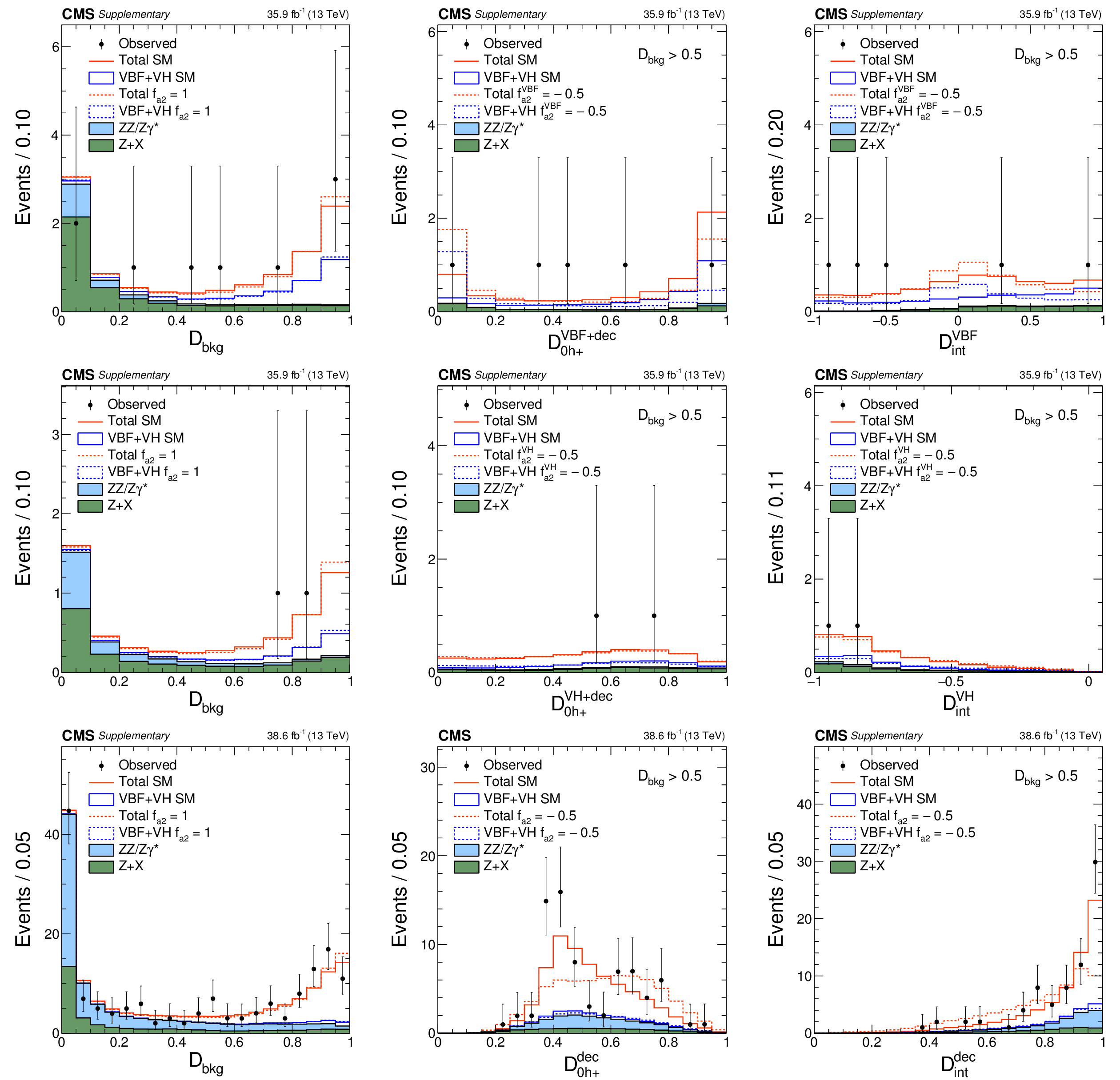
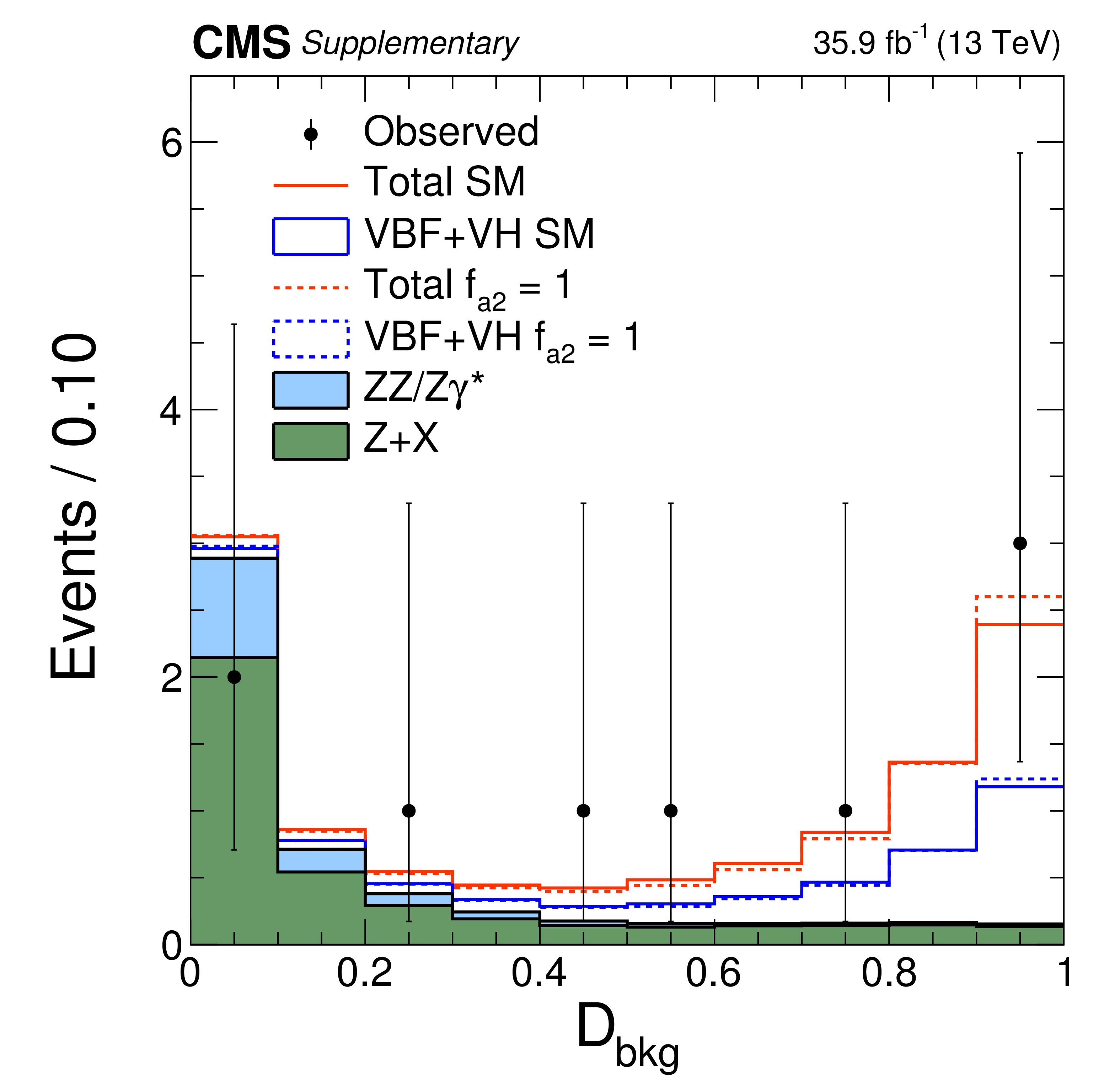
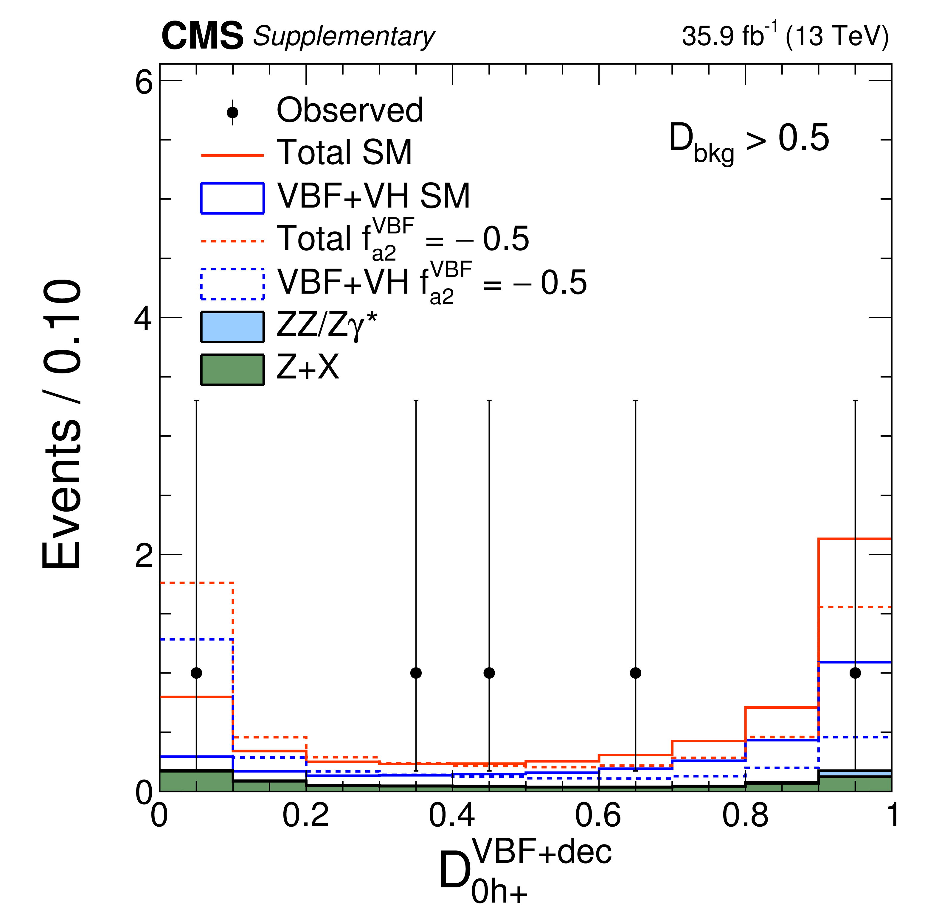
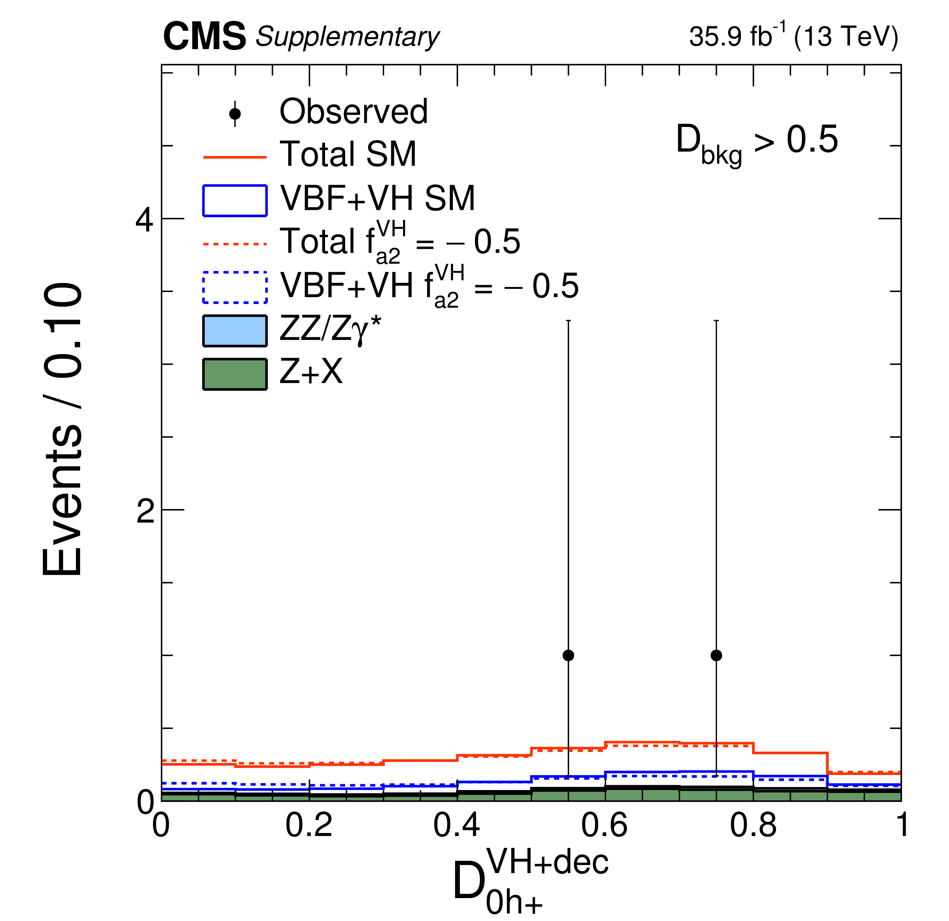
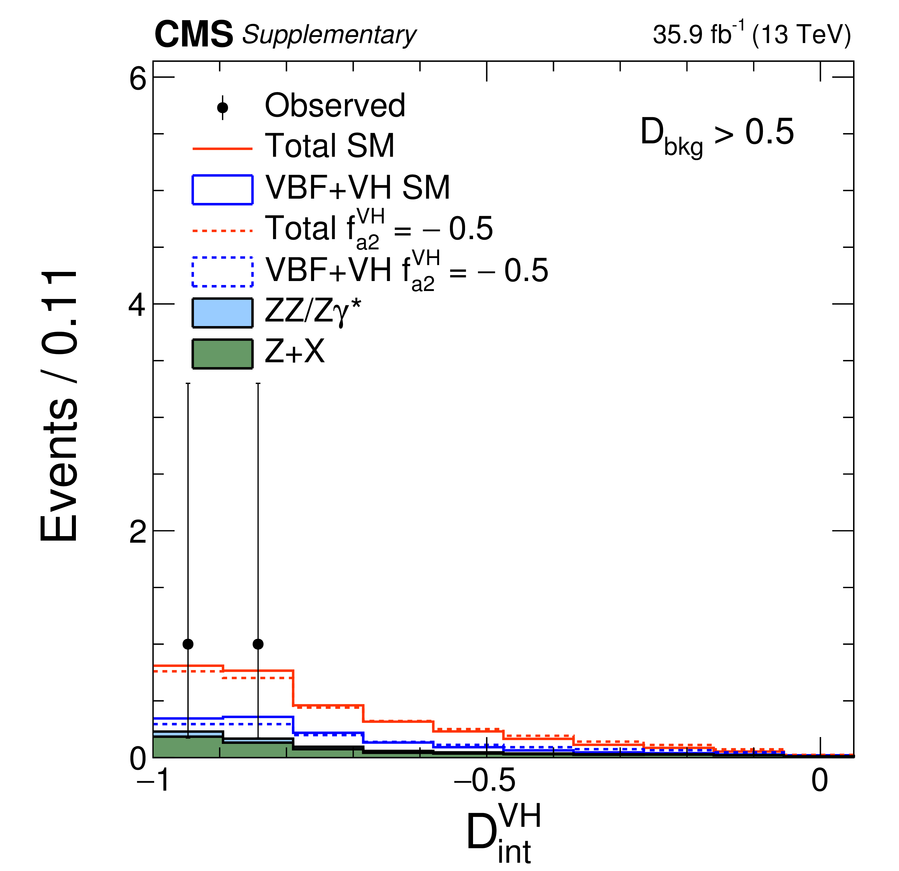
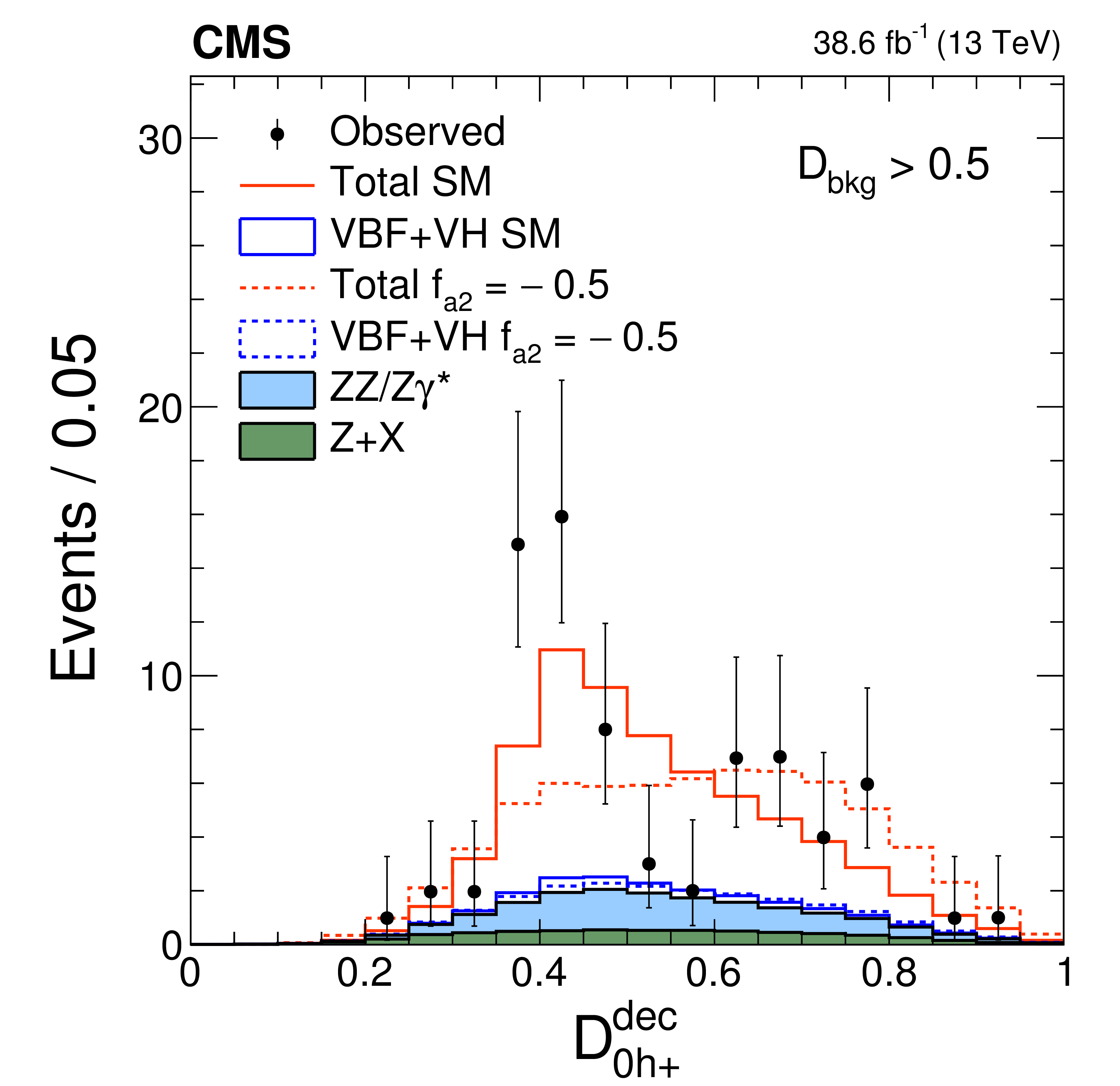
Distributions of kinematic discriminants in the $f_{a2}$ analysis: $\mathcal {D}_{\rm bkg}$ (a), (d), (g), $\mathcal {D}_{0h+}$ (b), (e), (h) and $\mathcal {D}_\text {int}$ (c), (f), (i). The decay or production information used in the $\mathcal {D}_{0h+}$ and $\mathcal {D}_\text {int}$ discriminants is reflected in the superscript label and depends on the tagging category. $f_{a2}^\text {VBF}$ and $f_{a2}^{\mathrm {V} \mathrm{ H } }$ are defined using Eq.(2) by analogy with $f_{a2}$, but using the cross sections for the VBF and VH processes, respectively. Three tagging categories are shown: VBF-jets (a)-(c), VH-jets (d)-(f), and untagged (g)-(i). Points with error bars show data and histograms show expectations for background and SM or BSM signal as indicated in the legend. |
png pdf |
Additional Figure 3-a:
Distribution of the $\mathcal {D}_{\rm bkg}$ kinematic discriminants in the $f_{a2}$ analysis, in the VBF-jets tagging category. Points with error bars show data and histograms show expectations for background and SM or BSM signal as indicated in the legend. |
png pdf |
Additional Figure 3-b:
Distribution of the $\mathcal {D}_{0h+}$ kinematic discriminants in the $f_{a2}$ analysis, in the VBF-jets tagging category. Points with error bars show data and histograms show expectations for background and SM or BSM signal as indicated in the legend. |

png pdf |
Additional Figure 3-c:
Distribution of the $\mathcal {D}_\text {int}$ kinematic discriminants in the $f_{a2}$ analysis, in the VBF-jets tagging category. Points with error bars show data and histograms show expectations for background and SM or BSM signal as indicated in the legend. |

png pdf |
Additional Figure 3-d:
Distribution of the $\mathcal {D}_{\rm bkg}$ kinematic discriminants in the $f_{a2}$ analysis, in the VH-jets tagging category. Points with error bars show data and histograms show expectations for background and SM or BSM signal as indicated in the legend. |
png pdf |
Additional Figure 3-e:
Distribution of the $\mathcal {D}_{0h+}$ kinematic discriminants in the $f_{a2}$ analysis, in the VH-jets tagging category. Points with error bars show data and histograms show expectations for background and SM or BSM signal as indicated in the legend. |
png pdf |
Additional Figure 3-f:
Distribution of the $\mathcal {D}_\text {int}$ kinematic discriminants in the $f_{a2}$ analysis, in the VH-jets tagging category. Points with error bars show data and histograms show expectations for background and SM or BSM signal as indicated in the legend. |

png pdf |
Additional Figure 3-g:
Distribution of the $\mathcal {D}_{\rm bkg}$ kinematic discriminants in the $f_{a2}$ analysis, in the untagged tagging category. Points with error bars show data and histograms show expectations for background and SM or BSM signal as indicated in the legend. |
png pdf |
Additional Figure 3-h:
Distribution of the $\mathcal {D}_{0h+}$ kinematic discriminants in the $f_{a2}$ analysis, in the untagged tagging category. Points with error bars show data and histograms show expectations for background and SM or BSM signal as indicated in the legend. |
png pdf |
Additional Figure 3-i:
Distribution of the $\mathcal {D}_\text {int}$ kinematic discriminants in the $f_{a2}$ analysis, in the untagged tagging category. Points with error bars show data and histograms show expectations for background and SM or BSM signal as indicated in the legend. |
png pdf |
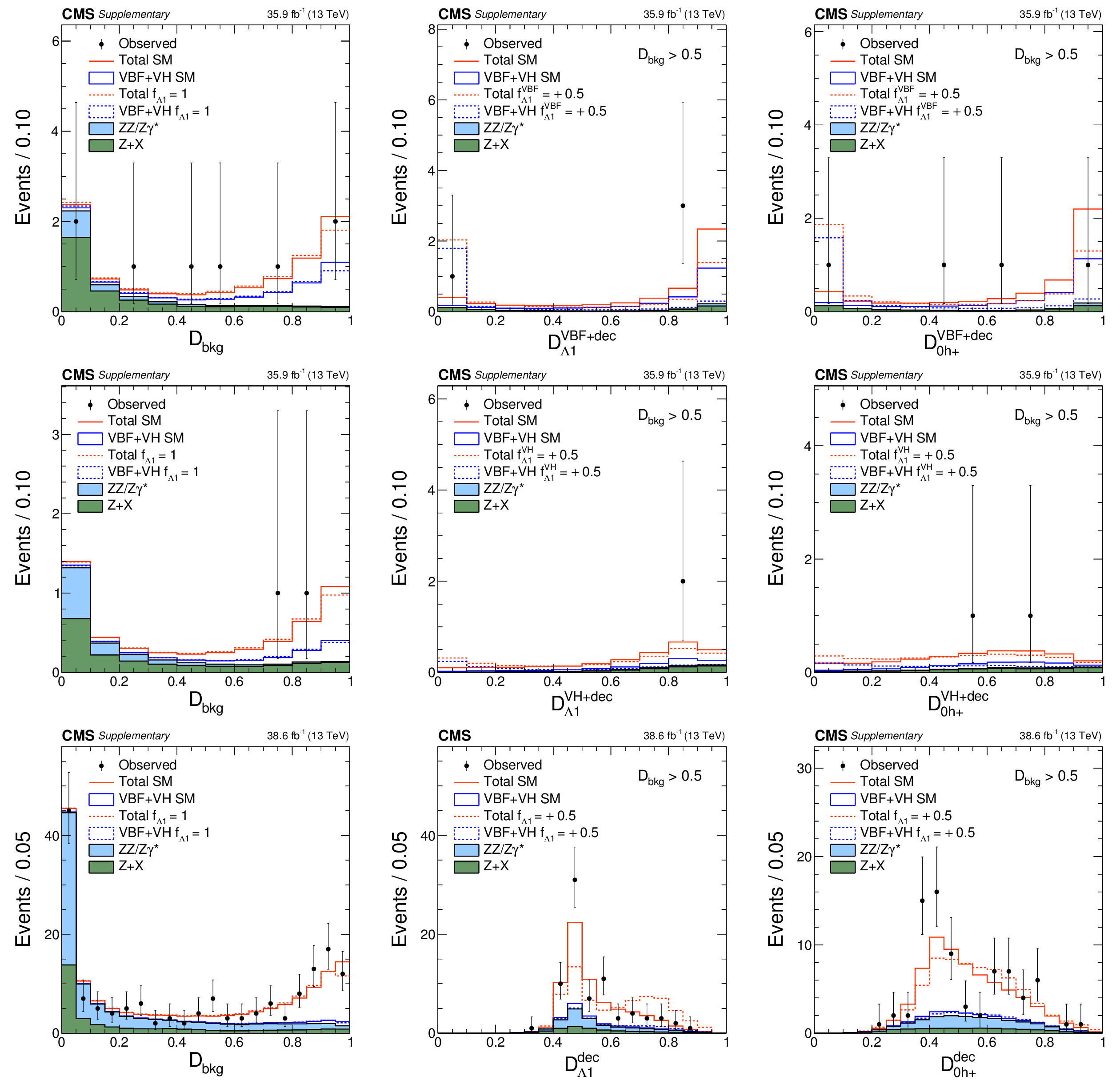
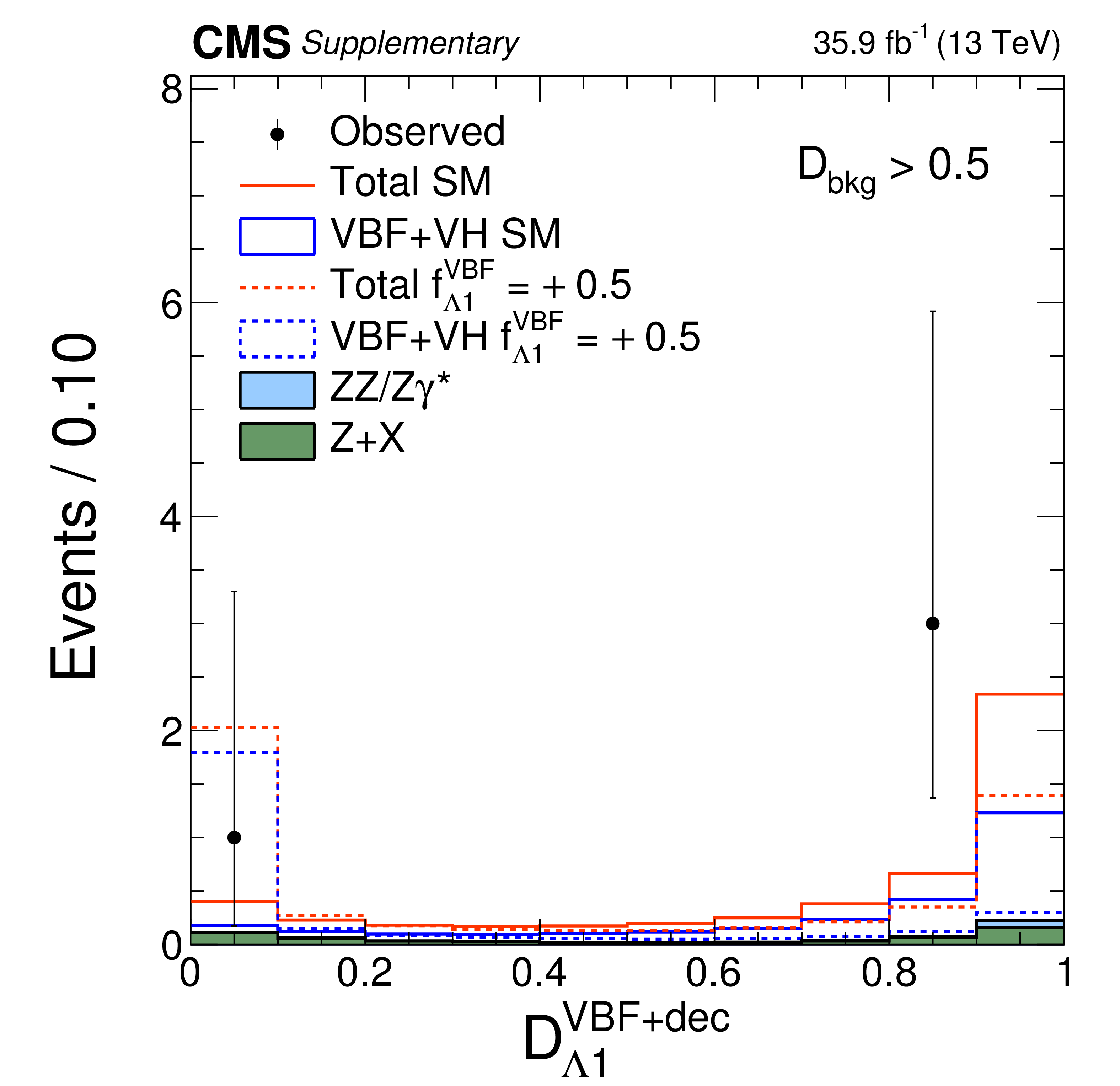
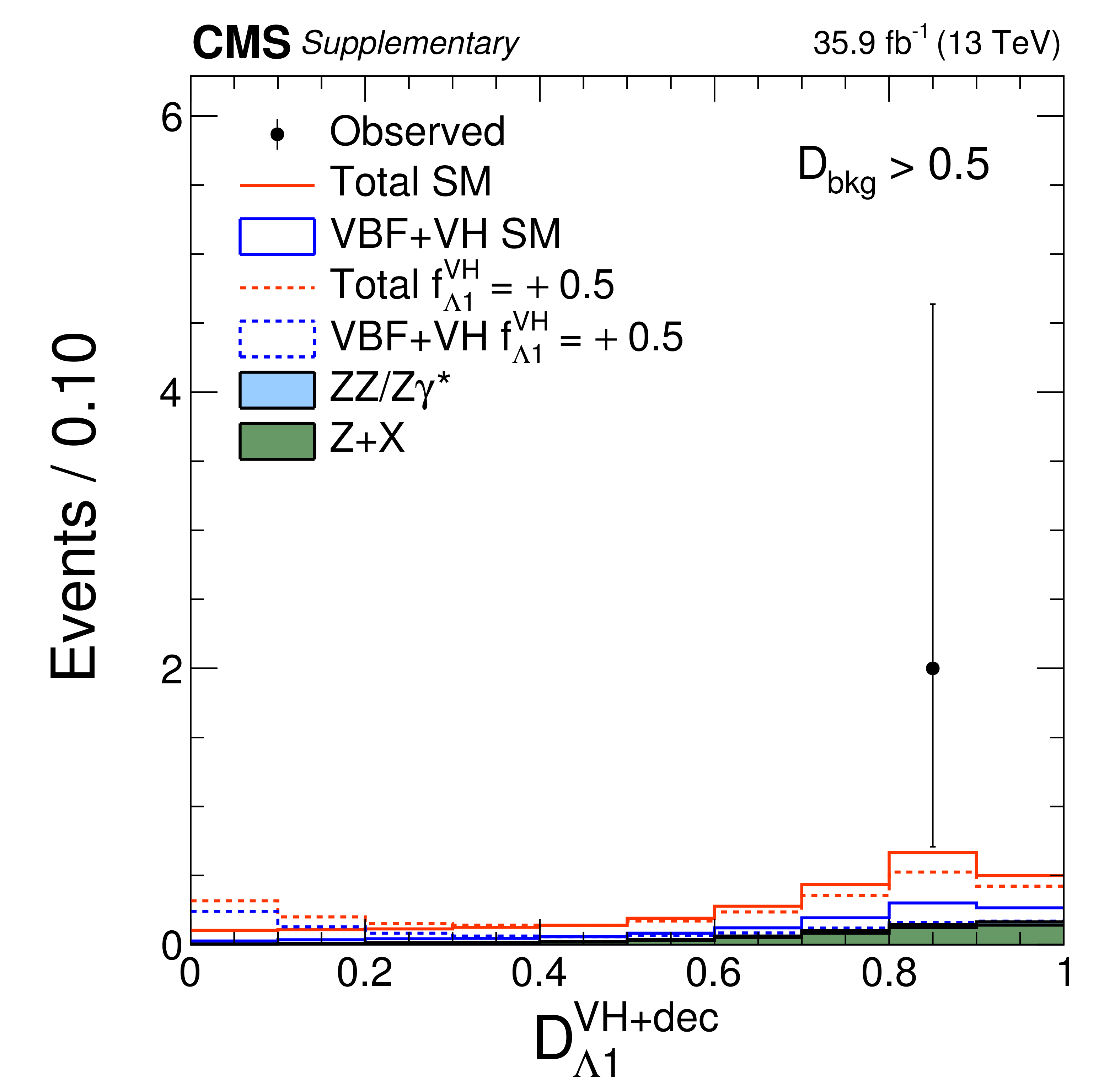
Additional Figure 4:
Distributions of kinematic discriminants in the $f_{\Lambda 1}$ analysis: $\mathcal {D}_{\rm bkg}$ (a), (d), (g), $\mathcal {D}_{\Lambda 1}$ (b), (e), (h). and $\mathcal {D}_{0h+}$ (c), (f), (i). The decay or production information used in the $\mathcal {D}_{\Lambda 1}$ and $\mathcal {D}_{0h+}$ discriminants is reflected in the superscript label and depends on the tagging category. $f_{\Lambda 1}^\text {VBF}$ and $f_{\Lambda 1}^{\mathrm {V} \mathrm{ H } }$ are defined using Eq.(2) by analogy with $f_{\Lambda 1}$, but using the cross sections for the VBF and VH processes, respectively. Three tagging categories are shown: VBF-jets (a)-(c), VH-jets (d)-(f), and untagged (g)-(i). Points with error bars show data and histograms show expectations for background and SM or BSM signal as indicated in the legend. |

png pdf |
Additional Figure 4-a:
Distribution of the $\mathcal {D}_{\rm bkg}$ kinematic discriminant in the $f_{\Lambda 1}$ analysis, in the VBF-jets tagging category. Points with error bars show data and histograms show expectations for background and SM or BSM signal as indicated in the legend. |
png pdf |
Additional Figure 4-b:
Distribution of the $\mathcal {D}_{\Lambda 1}$ kinematic discriminant in the $f_{\Lambda 1}$ analysis, in the VBF-jets tagging category. Points with error bars show data and histograms show expectations for background and SM or BSM signal as indicated in the legend. |

png pdf |
Additional Figure 4-c:
Distribution of the $\mathcal {D}_{0h+}$ kinematic discriminant in the $f_{\Lambda 1}$ analysis, in the VBF-jets tagging category. Points with error bars show data and histograms show expectations for background and SM or BSM signal as indicated in the legend. |

png pdf |
Additional Figure 4-d:
Distribution of the $\mathcal {D}_{\rm bkg}$ kinematic discriminant in the $f_{\Lambda 1}$ analysis, in the VH-jets tagging category. Points with error bars show data and histograms show expectations for background and SM or BSM signal as indicated in the legend. |
png pdf |
Additional Figure 4-e:
Distribution of the $\mathcal {D}_{\Lambda 1}$ kinematic discriminant in the $f_{\Lambda 1}$ analysis, in the VH-jets tagging category. Points with error bars show data and histograms show expectations for background and SM or BSM signal as indicated in the legend. |
png pdf |
Additional Figure 4-f:
Distribution of the $\mathcal {D}_{0h+}$ kinematic discriminant in the $f_{\Lambda 1}$ analysis, in the VH-jets tagging category. Points with error bars show data and histograms show expectations for background and SM or BSM signal as indicated in the legend. |

png pdf |
Additional Figure 4-g:
Distribution of the $\mathcal {D}_{\rm bkg}$ kinematic discriminant in the $f_{\Lambda 1}$ analysis, in the untagged tagging category. Points with error bars show data and histograms show expectations for background and SM or BSM signal as indicated in the legend. |

png pdf |
Additional Figure 4-h:
Distribution of the $\mathcal {D}_{\Lambda 1}$ kinematic discriminant in the $f_{\Lambda 1}$ analysis, in the untagged tagging category. Points with error bars show data and histograms show expectations for background and SM or BSM signal as indicated in the legend. |
png pdf |
Additional Figure 4-i:
Distribution of the $\mathcal {D}_{0h+}$ kinematic discriminant in the $f_{\Lambda 1}$ analysis, in the untagged tagging category. Points with error bars show data and histograms show expectations for background and SM or BSM signal as indicated in the legend. |

png pdf |
Additional Figure 5:
Distributions of kinematic discriminants in the $f_{\Lambda 1}^{{\mathrm{ Z } } \gamma }$ analysis: $\mathcal {D}_{\rm bkg}$ (a), (d), (g), $\mathcal {D}_{\Lambda 1}^{{\mathrm{ Z } } \gamma }$ (b), (e), (h), and $\mathcal {D}_{0h+}$ (c), (f), (i). The decay or production information used in the $\mathcal {D}_{\Lambda 1}^{{\mathrm{ Z } } \gamma }$ and $\mathcal {D}_{0h+}$ discriminants is reflected in the superscript label and depends on the tagging category. Three tagging categories are shown: VBF-jets (a)-(c), VH-jets (d)-(f), and untagged (g)-(i). Points with error bars show data and histograms show expectations for background and SM or BSM signal as indicated in the legend. |
png pdf |
Additional Figure 5-a:
Distribution of the $\mathcal {D}_{\rm bkg}$ kinematic discriminant in the $f_{\Lambda 1}^{{\mathrm{ Z } } \gamma }$ analysis, in the VBF-jets tagging category. Points with error bars show data and histograms show expectations for background and SM or BSM signal as indicated in the legend. |
png pdf |
Additional Figure 5-b:
Distribution of the $\mathcal {D}_{\Lambda 1}^{{\mathrm{ Z } } \gamma }$ kinematic discriminant in the $f_{\Lambda 1}^{{\mathrm{ Z } } \gamma }$ analysis, in the VBF-jets tagging category. Points with error bars show data and histograms show expectations for background and SM or BSM signal as indicated in the legend. |
png pdf |
Additional Figure 5-c:
Distribution of the $\mathcal {D}_{0h+}$ kinematic discriminant in the $f_{\Lambda 1}^{{\mathrm{ Z } } \gamma }$ analysis, in the VBF-jets tagging category. Points with error bars show data and histograms show expectations for background and SM or BSM signal as indicated in the legend. |
png pdf |
Additional Figure 5-d:
Distribution of the $\mathcal {D}_{\rm bkg}$ kinematic discriminant in the $f_{\Lambda 1}^{{\mathrm{ Z } } \gamma }$ analysis, in the VH-jets tagging category. Points with error bars show data and histograms show expectations for background and SM or BSM signal as indicated in the legend. |
png pdf |
Additional Figure 5-e:
Distribution of the $\mathcal {D}_{\Lambda 1}^{{\mathrm{ Z } } \gamma }$ kinematic discriminant in the $f_{\Lambda 1}^{{\mathrm{ Z } } \gamma }$ analysis, in the VH-jets tagging category. Points with error bars show data and histograms show expectations for background and SM or BSM signal as indicated in the legend. |

png pdf |
Additional Figure 5-f:
Distribution of the $\mathcal {D}_{0h+}$ kinematic discriminant in the $f_{\Lambda 1}^{{\mathrm{ Z } } \gamma }$ analysis, in the VH-jets tagging category. Points with error bars show data and histograms show expectations for background and SM or BSM signal as indicated in the legend. |
png pdf |
Additional Figure 5-g:
Distribution of the $\mathcal {D}_{\rm bkg}$ kinematic discriminant in the $f_{\Lambda 1}^{{\mathrm{ Z } } \gamma }$ analysis, in the untagged tagging category. Points with error bars show data and histograms show expectations for background and SM or BSM signal as indicated in the legend. |

png pdf |
Additional Figure 5-h:
Distribution of the $\mathcal {D}_{\Lambda 1}^{{\mathrm{ Z } } \gamma }$ kinematic discriminant in the $f_{\Lambda 1}^{{\mathrm{ Z } } \gamma }$ analysis, in the untagged tagging category. Points with error bars show data and histograms show expectations for background and SM or BSM signal as indicated in the legend. |
png pdf |
Additional Figure 5-i:
Distribution of the $\mathcal {D}_{0h+}$ kinematic discriminant in the $f_{\Lambda 1}^{{\mathrm{ Z } } \gamma }$ analysis, in the untagged tagging category. Points with error bars show data and histograms show expectations for background and SM or BSM signal as indicated in the legend. |
png pdf |
Additional Figure 6:
Animated distributions of the $\mathcal {D}_{\rm bkg}$ kinematic discriminant in the $f_{a3}$ (a), $f_{a2}$ (b), $f_{\Lambda 1}$ (c), and $f_{\Lambda 1}^{{\mathrm{ Z } } \gamma }$ (d) analyses. The distributions are summed over all three categories. Points with error bars show data and histograms show expectations for background and SM or BSM signal as indicated in the legend. The animations scan $f_{ai}$ to illustrate how the expected signal distributions change as a function of $f_{ai}$. For each value of $f_{ai}$, the signal strengths for Higgs production through couplings to fermions $\mu _f$ and bosons $\mu _V$ are set to their best-fit values. The values of $f_{ai}$, $f_{ai}^\text {VBF}$, and $f_{ai}^{\mathrm {V} \mathrm{ H } }$ are recorded on the plots, along with the negative log likelihood. $f_{ai}^\text {VBF}$ and $f_{ai}^{\mathrm {V} \mathrm{ H } }$ are defined using Eq.(2) by analogy with $f_{ai}$, but using the cross sections for the VBF and VH processes, respectively. |

png pdf |
Additional Figure 12:
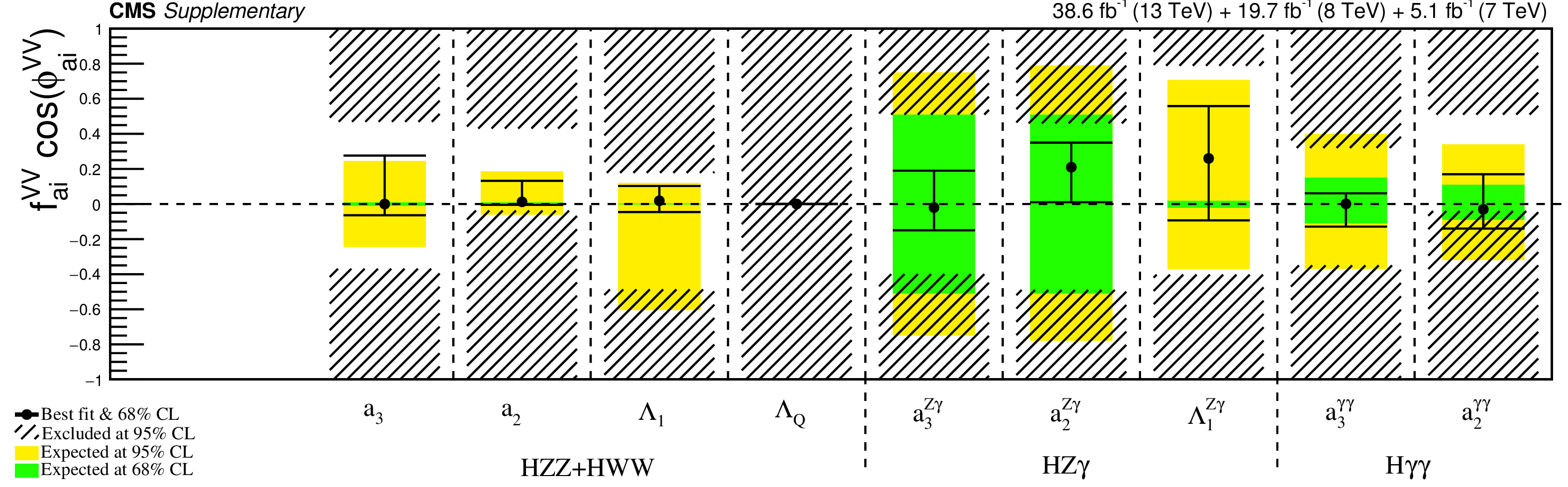
Summary of allowed confidence level intervals on anomalous coupling parameters in HVV interactions under the assumption that all the coupling ratios are real ($\phi _{ai}^{\mathrm {V} \mathrm {V} }=0$ or $\pi $). The HZZ+HWW coupling limits assume that $a_{i}^{{\mathrm{ Z } } {\mathrm{ Z } } }=a_{i}^{\mathrm{ W } \mathrm{ W } }$, and the $f_{\Lambda Q}$ limits assume that the Higgs boson width is $4.1 MeV $. The expected 68% and 95% CL regions are shown as green and yellow bands. The observed constraints at 68% and 95% CL are shown as points with errors and the excluded hatched regions. The limits on $f_{a2,3}^{{\mathrm{ Z } } \gamma ,\gamma \gamma }$ are from Ref. [13], and the limits on $f_{\Lambda Q}$ are from Ref. [15]. |
| Additional Material: Animated Distributions |
| Additional Figure 6: Animated distributions of the $\mathcal {D}_{\rm bkg}$ kinematic discriminant in the $f_{a3}$ (a), $f_{a2}$ (b), $f_{\Lambda 1}$ (c), and $f_{\Lambda 1}^{{\mathrm{ Z } } \gamma }$ (d) analyses. The distributions are summed over all three categories. Points with error bars show data and histograms show expectations for background and SM or BSM signal as indicated in the legend. The animations scan $f_{ai}$ to illustrate how the expected signal distributions change as a function of $f_{ai}$. For each value of $f_{ai}$, the signal strengths for Higgs production through couplings to fermions $\mu _f$ and bosons $\mu _V$ are set to their best-fit values. The values of $f_{ai}$, $f_{ai}^\text {VBF}$, and $f_{ai}^{\mathrm {V} \mathrm{ H } }$ are recorded on the plots, along with the negative log likelihood. $f_{ai}^\text {VBF}$ and $f_{ai}^{\mathrm {V} \mathrm{ H } }$ are defined using Eq.(2) by analogy with $f_{ai}$, but using the cross sections for the VBF and VH processes, respectively. | |
animated gif |
Additional Figure 6-a:
Animated distribution of the $\mathcal {D}_{\rm bkg}$ kinematic discriminant in the $f_{a3}$ analysis. The distribution is summed over all three categories. Points with error bars show data and histograms show expectations for background and SM or BSM signal as indicated in the legend. |

animated gif |
Additional Figure 6-b:
Animated distribution of the $\mathcal {D}_{\rm bkg}$ kinematic discriminant in the $f_{a2}$ analysis. The distribution is summed over all three categories. Points with error bars show data and histograms show expectations for background and SM or BSM signal as indicated in the legend. |
animated gif |
Additional Figure 6-c:
Animated distribution of the $\mathcal {D}_{\rm bkg}$ kinematic discriminant in the $f_{\Lambda 1}$ analysis. The distribution is summed over all three categories. Points with error bars show data and histograms show expectations for background and SM or BSM signal as indicated in the legend. |
animated gif |
Additional Figure 6-d:
Animated distribution of the $\mathcal {D}_{\rm bkg}$ kinematic discriminant in the $f_{\Lambda 1}^{{\mathrm{ Z } } \gamma }$ analysis. The distribution is summed over all three categories. Points with error bars show data and histograms show expectations for background and SM or BSM signal as indicated in the legend. |
| Additional Figure 7: Animated distributions of kinematic discriminants in the $f_{a3}$ analysis: $\mathcal {D}_{\rm bkg}$ (a), (d), (g), $\mathcal {D}_{0-}$ (b), (e), (h), and $\mathcal {D}_{CP}$ (c), (f), (i). The decay or production information used in the $\mathcal {D}_{0-}$ and $\mathcal {D}_{CP}$ discriminants is reflected in the superscript label and depends on the tagging category. Three tagging categories are shown: VBF-jets (a)-(c), VH-jets (d)-(f), and untagged (g)-(i). Points with error bars show data and histograms show expectations for background and signal as indicated in the legend. The animations scan $f_{a3}$ to illustrate how the expected signal distributions change as a function of $f_{a3}$. For each value of $f_{a3}$, the signal strengths for Higgs production through couplings to fermions $\mu _f$ and bosons $\mu _V$ are set to their best-fit values. The values of $f_{a3}$, $f_{a3}^\text {VBF}$, and $f_{a3}^{\mathrm {V} \mathrm{ H } }$ are recorded on the plots, along with the negative log likelihood. $f_{a3}^\text {VBF}$ and $f_{a3}^{\mathrm {V} \mathrm{ H } }$ are defined using Eq.(2) by analogy with $f_{a3}$, but using the cross sections for the VBF and VH processes, respectively. | |

animated gif |
Additional Figure 7-a:
Animated distributions of the $\mathcal {D}_{\rm bkg}$ kinematic discriminant in the $f_{a3}$ analysis, in the VBF-jets tagging category. Points with error bars show data and histograms show expectations for background and signal as indicated in the legend. |
animated gif |
Additional Figure 7-b:
Animated distributions of the $\mathcal {D}_{0-}$ kinematic discriminant in the $f_{a3}$ analysis, in the VBF-jets tagging category. The decay or production information usedis reflected in the superscript label and depends on the tagging category. Points with error bars show data and histograms show expectations for background and signal as indicated in the legend. |
animated gif |
Additional Figure 7-c:
Animated distributions of the $\mathcal {D}_{CP}$ kinematic discriminant in the $f_{a3}$ analysis, in the VBF-jets tagging category. The decay or production information used is reflected in the superscript label and depends on the tagging category. Points with error bars show data and histograms show expectations for background and signal as indicated in the legend. |
animated gif |
Additional Figure 7-d:
Animated distributions of the $\mathcal {D}_{\rm bkg}$ kinematic discriminant in the $f_{a3}$ analysis, in the VH-jets tagging category. Points with error bars show data and histograms show expectations for background and signal as indicated in the legend. |

animated gif |
Additional Figure 7-e:
Animated distributions of the $\mathcal {D}_{0-}$ kinematic discriminant in the $f_{a3}$ analysis, in the VH-jets tagging category. The decay or production information used is reflected in the superscript label and depends on the tagging category. Points with error bars show data and histograms show expectations for background and signal as indicated in the legend. |
animated gif |
Additional Figure 7-f:
Animated distributions of the $\mathcal {D}_{CP}$ kinematic discriminant in the $f_{a3}$ analysis, in the VH-jets tagging category. The decay or production information used is reflected in the superscript label and depends on the tagging category. Points with error bars show data and histograms show expectations for background and signal as indicated in the legend. |
animated gif |
Additional Figure 7-g:
Animated distributions of the $\mathcal {D}_{\rm bkg}$ kinematic discriminant in the $f_{a3}$ analysis, in the untagged tagging category. Points with error bars show data and histograms show expectations for background and signal as indicated in the legend. |
animated gif |
Additional Figure 7-h:
Animated distributions of the $\mathcal {D}_{0-}$ kinematic discriminant in the $f_{a3}$ analysis, in the untagged tagging category. The decay or production information used is reflected in the superscript label and depends on the tagging category. Points with error bars show data and histograms show expectations for background and signal as indicated in the legend. |
animated gif |
Additional Figure 7-i:
Animated distributions of the $\mathcal {D}_{CP}$ kinematic discriminant in the $f_{a3}$ analysis, in the untagged tagging category. Points with error bars show data and histograms show expectations for background and signal as indicated in the legend. |
| Additional Figure 8: Animated distributions of kinematic discriminants in the $f_{a2}$ analysis: $\mathcal {D}_{\rm bkg}$ (a), (d), (g), $\mathcal {D}_{0h+}$ (b), (e), (h), and $\mathcal {D}_\text {int}$ (c), (f), (i). The decay or production information used in the $\mathcal {D}_{0h+}$ and $\mathcal {D}_\text {int}$ discriminants is reflected in the superscript label and depends on the tagging category. Three tagging categories are shown: VBF-jets (a)-(c), VH-jets (d)-(f), and untagged (g)-(i). Points with error bars show data and histograms show expectations for background and signal as indicated in the legend. The animations scan $f_{a2}$ to illustrate how the expected signal distributions change as a function of $f_{a2}$. For each value of $f_{a2}$, the signal strengths for Higgs production through couplings to fermions $\mu _f$ and bosons $\mu _V$ are set to their best-fit values. The values of $f_{a2}$, $f_{a2}^\text {VBF}$, and $f_{a2}^{\mathrm {V} \mathrm{ H } }$ are recorded on the plots, along with the negative log likelihood. $f_{a2}^\text {VBF}$ and $f_{a2}^{\mathrm {V} \mathrm{ H } }$ are defined using Eq.(2) by analogy with $f_{a2}$, but using the cross sections for the VBF and VH processes, respectively. | |
animated gif |
Additional Figure 8-a:
Animated distributions of the $\mathcal {D}_{\rm bkg}$ kinematic discriminant in the $f_{a2}$ analysis, in the VBF-jets tagging category. Points with error bars show data and histograms show expectations for background and signal as indicated in the legend. |
animated gif |
Additional Figure 8-b:
Animated distributions of the $\mathcal {D}_{0h+}$ kinematic discriminant in the $f_{a2}$ analysis, in the VBF-jets tagging category. The decay or production information used is reflected in the superscript label and depends on the tagging category. Points with error bars show data and histograms show expectations for background and signal as indicated in the legend. |
animated gif |
Additional Figure 8-c:
Animated distributions of the $\mathcal {D}_\text {int}$ kinematic discriminant in the $f_{a2}$ analysis, in the VBF-jets tagging category. The decay or production information used is reflected in the superscript label and depends on the tagging category. Points with error bars show data and histograms show expectations for background and signal as indicated in the legend. |
animated gif |
Additional Figure 8-d:
Animated distributions of the $\mathcal {D}_{\rm bkg}$ kinematic discriminant in the $f_{a2}$ analysis, in the VH-jets tagging category. Points with error bars show data and histograms show expectations for background and signal as indicated in the legend. |
animated gif |
Additional Figure 8-e:
Animated distributions of the $\mathcal {D}_{0h+}$ kinematic discriminant in the $f_{a2}$ analysis, in the VH-jets tagging category. The decay or production information used is reflected in the superscript label and depends on the tagging category. Points with error bars show data and histograms show expectations for background and signal as indicated in the legend. |
animated gif |
Additional Figure 8-f:
Animated distributions of the $\mathcal {D}_\text {int}$ kinematic discriminant in the $f_{a2}$ analysis, in the VH-jets tagging category. The decay or production information used is reflected in the superscript label and depends on the tagging category. Points with error bars show data and histograms show expectations for background and signal as indicated in the legend. |
animated gif |
Additional Figure 8-g:
Animated distributions of the $\mathcal {D}_{\rm bkg}$ kinematic discriminant in the $f_{a2}$ analysis, in the untagged tagging category. Points with error bars show data and histograms show expectations for background and signal as indicated in the legend. |
animated gif |
Additional Figure 8-h:
Animated distributions of the $\mathcal {D}_{0h+}$ kinematic discriminant in the $f_{a2}$ analysis, in the untagged tagging category. The decay or production information used is reflected in the superscript label and depends on the tagging category. Points with error bars show data and histograms show expectations for background and signal as indicated in the legend. |

animated gif |
Additional Figure 8-i:
Animated distributions of the $\mathcal {D}_\text {int}$ kinematic discriminant in the $f_{a2}$ analysis, in the untagged tagging category. The decay or production information used is reflected in the superscript label and depends on the tagging category. Points with error bars show data and histograms show expectations for background and signal as indicated in the legend. |
| Additional Figure 9: Animated distributions of kinematic discriminants in the $f_{\Lambda 1}$ analysis: $\mathcal {D}_{\rm bkg}$ (a), (d), (g), $\mathcal {D}_{\Lambda 1}$ (b), (e), (h), and $\mathcal {D}_{0h+}$ (c), (f), (i). The decay or production information used in the $\mathcal {D}_{\Lambda 1}$ and $\mathcal {D}_{0h+}$ discriminants is reflected in the superscript label and depends on the tagging category. Three tagging categories are shown: VBF-jets (a)-(c), VH-jets (d)-(f), and untagged (g)-(i). Points with error bars show data and histograms show expectations for background and signal as indicated in the legend. The animations scan $f_{\Lambda 1}$ to illustrate how the expected signal distributions change as a function of $f_{\Lambda 1}$. For each value of $f_{\Lambda 1}$, the signal strengths for Higgs production through couplings to fermions $\mu _f$ and bosons $\mu _V$ are set to their best-fit values. The values of $f_{\Lambda 1}$, $f_{\Lambda 1}^\text {VBF}$, and $f_{\Lambda 1}^{\mathrm {V} \mathrm{ H } }$ are recorded on the plots, along with the negative log likelihood. $f_{\Lambda 1}^\text {VBF}$ and $f_{\Lambda 1}^{\mathrm {V} \mathrm{ H } }$ are defined using Eq.(2) by analogy with $f_{\Lambda 1}$, but using the cross sections for the VBF and VH processes, respectively. | |

animated gif |
Additional Figure 9-a:
Animated distributions of the $\mathcal {D}_{\rm bkg}$ kinematic discriminant in the $f_{\Lambda 1}$ analysis, in the VBF-jets tagging category. Points with error bars show data and histograms show expectations for background and signal as indicated in the legend. |

animated gif |
Additional Figure 9-b:
Animated distributions of the $\mathcal {D}_{\Lambda 1}$ kinematic discriminant in the $f_{\Lambda 1}$ analysis, in the VBF-jets tagging category.The decay or production information used is reflected in the superscript label and depends on the tagging category. Points with error bars show data and histograms show expectations for background and signal as indicated in the legend. |
animated gif |
Additional Figure 9-c:
Animated distributions of the $\mathcal {D}_{0h+}$ kinematic discriminant in the $f_{\Lambda 1}$ analysis, in the VBF-jets tagging category.The decay or production information used is reflected in the superscript label and depends on the tagging category. Points with error bars show data and histograms show expectations for background and signal as indicated in the legend. |
animated gif |
Additional Figure 9-d:
Animated distributions of the $\mathcal {D}_{\rm bkg}$ kinematic discriminant in the $f_{\Lambda 1}$ analysis, in the VH-jets tagging category. Points with error bars show data and histograms show expectations for background and signal as indicated in the legend. |
animated gif |
Additional Figure 9-e:
Animated distributions of the $\mathcal {D}_{\Lambda 1}$ kinematic discriminant in the $f_{\Lambda 1}$ analysis, in the VH-jets tagging category.The decay or production information used is reflected in the superscript label and depends on the tagging category. Points with error bars show data and histograms show expectations for background and signal as indicated in the legend. |

animated gif |
Additional Figure 9-f:
Animated distributions of the $\mathcal {D}_{0h+}$ kinematic discriminant in the $f_{\Lambda 1}$ analysis, in the VH-jets tagging category.The decay or production information used is reflected in the superscript label and depends on the tagging category. Points with error bars show data and histograms show expectations for background and signal as indicated in the legend. |

animated gif |
Additional Figure 9-g:
Animated distributions of the $\mathcal {D}_{\rm bkg}$ kinematic discriminant in the $f_{\Lambda 1}$ analysis, in the untagged tagging category. Points with error bars show data and histograms show expectations for background and signal as indicated in the legend. |
animated gif |
Additional Figure 9-h:
Animated distributions of the $\mathcal {D}_{\Lambda 1}$ kinematic discriminant in the $f_{\Lambda 1}$ analysis, in the untagged tagging category.The decay or production information used is reflected in the superscript label and depends on the tagging category. Points with error bars show data and histograms show expectations for background and signal as indicated in the legend. |

animated gif |
Additional Figure 9-i:
Animated distributions of the $\mathcal {D}_{0h+}$ kinematic discriminant in the $f_{\Lambda 1}$ analysis, in the untagged tagging category.The decay or production information used is reflected in the superscript label and depends on the tagging category. Points with error bars show data and histograms show expectations for background and signal as indicated in the legend. |
| Additional Figure 10: Animated distributions of kinematic discriminants in the $f_{\Lambda 1}^{{\mathrm{ Z } } \gamma }$ analysis: $\mathcal {D}_{\rm bkg}$ (a), (d), (g), $\mathcal {D}_{\Lambda 1}^{{\mathrm{ Z } } \gamma }$ (b), (e), (h), and $\mathcal {D}_{0h+}$ (c), (f), (i). The decay or production information used in the $\mathcal {D}_{\Lambda 1}^{{\mathrm{ Z } } \gamma }$ and $\mathcal {D}_{0h+}$ discriminants is reflected in the superscript label and depends on the tagging category. Three tagging categories are shown: VBF-jets (a)-(c), VH-jets (d)-(f), and untagged (g)-(i). Points with error bars show data and histograms show expectations for background and signal as indicated in the legend. The animations scan $f_{\Lambda 1}^{{\mathrm{ Z } } \gamma }$ to illustrate how the expected signal distributions change as a function of $f_{\Lambda 1}^{{\mathrm{ Z } } \gamma }$. For each value of $f_{\Lambda 1}^{{\mathrm{ Z } } \gamma }$, the signal strengths for Higgs production through couplings to fermions $\mu _f$ and bosons $\mu _V$ are set to their best-fit values. The values of $f_{\Lambda 1}^{{\mathrm{ Z } } \gamma }$, $f_{\Lambda 1}^{{\mathrm{ Z } } \gamma , \text {VBF}}$, and $f_{\Lambda 1}^{{\mathrm{ Z } } \gamma , \mathrm {V} \mathrm{ H } }$ are recorded on the plots, along with the negative log likelihood. $f_{\Lambda 1}^{{\mathrm{ Z } } \gamma , \text {VBF}}$ and $f_{\Lambda 1}^{{\mathrm{ Z } } \gamma , \mathrm {V} \mathrm{ H } }$ are defined using Eq.(2) by analogy with $f_{\Lambda 1}^{{\mathrm{ Z } } \gamma }$, but using the cross sections for the VBF and VH processes, respectively. | |
animated gif |
Additional Figure 10-a:
Animated distributions of the $\mathcal {D}_{\rm bkg}$ kinematic discriminant in the $f_{\Lambda 1}^{{\mathrm{ Z } } \gamma }$ analysis, in the VBF-jets tagging category. Points with error bars show data and histograms show expectations for background and signal as indicated in the legend. |
animated gif |
Additional Figure 10-b:
Animated distributions of the $\mathcal {D}_{\Lambda 1}^{{\mathrm{ Z } } \gamma }$s kinematic discriminant in the $f_{\Lambda 1}^{{\mathrm{ Z } } \gamma }$ analysis, in the VBF-jets tagging category. The decay or production information used is reflected in the superscript label and depends on the tagging category. Points with error bars show data and histograms show expectations for background and signal as indicated in the legend. |
animated gif |
Additional Figure 10-c:
Animated distributions of the $\mathcal {D}_{0h+}$ kinematic discriminant in the $f_{\Lambda 1}^{{\mathrm{ Z } } \gamma }$ analysis, in the VBF-jets tagging category. The decay or production information used is reflected in the superscript label and depends on the tagging category. Points with error bars show data and histograms show expectations for background and signal as indicated in the legend. |

animated gif |
Additional Figure 10-d:
Animated distributions of the $\mathcal {D}_{\rm bkg}$ kinematic discriminant in the $f_{\Lambda 1}^{{\mathrm{ Z } } \gamma }$ analysis, in the VH-jets tagging category. Points with error bars show data and histograms show expectations for background and signal as indicated in the legend. |
animated gif |
Additional Figure 10-e:
Animated distributions of the $\mathcal {D}_{\Lambda 1}^{{\mathrm{ Z } } \gamma }$s kinematic discriminant in the $f_{\Lambda 1}^{{\mathrm{ Z } } \gamma }$ analysis, in the VH-jets tagging category. The decay or production information used is reflected in the superscript label and depends on the tagging category. Points with error bars show data and histograms show expectations for background and signal as indicated in the legend. |
animated gif |
Additional Figure 10-f:
Animated distributions of the $\mathcal {D}_{0h+}$ kinematic discriminant in the $f_{\Lambda 1}^{{\mathrm{ Z } } \gamma }$ analysis, in the VH-jets tagging category. The decay or production information used is reflected in the superscript label and depends on the tagging category. Points with error bars show data and histograms show expectations for background and signal as indicated in the legend. |
animated gif |
Additional Figure 10-g:
Animated distributions of the $\mathcal {D}_{\rm bkg}$ kinematic discriminant in the $f_{\Lambda 1}^{{\mathrm{ Z } } \gamma }$ analysis, in the untagged tagging category. Points with error bars show data and histograms show expectations for background and signal as indicated in the legend. |
animated gif |
Additional Figure 10-h:
Animated distributions of the $\mathcal {D}_{\Lambda 1}^{{\mathrm{ Z } } \gamma }$s kinematic discriminant in the $f_{\Lambda 1}^{{\mathrm{ Z } } \gamma }$ analysis, in the untagged tagging category. The decay or production information used is reflected in the superscript label and depends on the tagging category. Points with error bars show data and histograms show expectations for background and signal as indicated in the legend. |
animated gif |
Additional Figure 10-i:
Animated distributions of the $\mathcal {D}_{0h+}$ kinematic discriminant in the $f_{\Lambda 1}^{{\mathrm{ Z } } \gamma }$ analysis, in the untagged tagging category. The decay or production information used is reflected in the superscript label and depends on the tagging category. Points with error bars show data and histograms show expectations for background and signal as indicated in the legend. |
| Additional Figure 11: Observed (solid) and expected (dashed) likelihood scans of $f_{a3}\cos(\phi _{a3})$ (a), $f_{a2}\cos(\phi _{a2})$ (b), $f_{\Lambda 1}\cos(\phi _{\Lambda 1})$ (c), and $f_{\Lambda 1}^{{\mathrm{ Z } } \gamma }\cos(\phi _{\Lambda 1}^{{\mathrm{ Z } } \gamma })$ (d). Results of the Run 2 only and the combined Run 1 and Run 2 analyses are shown. The marker follows the observed likelihood scan for the combined Run 1 and Run 2 analysis at the same speed as the animated discriminant distributions. The plots can be played simultaneously in order to better follow the animated distributions. | |

animated gif |
Additional Figure 11-a:
Observed (solid) and expected (dashed) likelihood scans of $f_{a3}\cos(\phi _{a3})$. Results of the Run 2 only and the combined Run 1 and Run 2 analyses are shown. The marker follows the observed likelihood scan for the combined Run 1 and Run 2 analysis at the same speed as the animated discriminant distributions. |

animated gif |
Additional Figure 11-b:
Observed (solid) and expected (dashed) likelihood scans of $f_{a2}\cos(\phi _{a2})$. Results of the Run 2 only and the combined Run 1 and Run 2 analyses are shown. The marker follows the observed likelihood scan for the combined Run 1 and Run 2 analysis at the same speed as the animated discriminant distributions. |
animated gif |
Additional Figure 11-c:
Observed (solid) and expected (dashed) likelihood scans of $f_{\Lambda 1}\cos(\phi _{\Lambda 1})$. Results of the Run 2 only and the combined Run 1 and Run 2 analyses are shown. The marker follows the observed likelihood scan for the combined Run 1 and Run 2 analysis at the same speed as the animated discriminant distributions. |
animated gif |
Additional Figure 11-d:
Observed (solid) and expected (dashed) likelihood scans of $f_{\Lambda 1}^{{\mathrm{ Z } } \gamma }\cos(\phi _{\Lambda 1}^{{\mathrm{ Z } } \gamma })$. Results of the Run 2 only and the combined Run 1 and Run 2 analyses are shown. The marker follows the observed likelihood scan for the combined Run 1 and Run 2 analysis at the same speed as the animated discriminant distributions. |
| References | ||||
| 1 | ATLAS Collaboration | Observation of a new particle in the search for the Standard Model Higgs boson with the ATLAS detector at the LHC | PLB 716 (2012) 1 | 1207.7214 |
| 2 | CMS Collaboration | Observation of a new boson at a mass of 125 GeV with the CMS experiment at the LHC | PLB 716 (2012) 30 | CMS-HIG-12-028 1207.7235 |
| 3 | CMS Collaboration | Observation of a new boson with mass near 125 GeV in pp collisions at $ \sqrt{s} = $ 7 and 8 TeV | JHEP 06 (2013) 081 | CMS-HIG-12-036 1303.4571 |
| 4 | S. L. Glashow | Partial-symmetries of weak interactions | Nucl. Phys. 22 (1961) 579 | |
| 5 | F. Englert and R. Brout | Broken Symmetry and the Mass of Gauge Vector Mesons | PRL 13 (1964) 321 | |
| 6 | P. W. Higgs | Broken symmetries, massless particles and gauge fields | PL12 (1964) 132 | |
| 7 | P. W. Higgs | Broken symmetries and the masses of gauge bosons | PRL 13 (1964) 508 | |
| 8 | G. S. Guralnik, C. R. Hagen, and T. W. B. Kibble | Global conservation laws and massless particles | PRL 13 (1964) 585 | |
| 9 | S. Weinberg | A model of leptons | PRL 19 (1967) 1264 | |
| 10 | A. Salam | Weak and electromagnetic interactions | in Elementary particle physics: relativistic groups and analyticity,1968, Proceedings of the eighth Nobel symposium | |
| 11 | CMS Collaboration | On the mass and spin-parity of the Higgs boson candidate via its decays to Z boson pairs | PRL 110 (2013) 081803 | CMS-HIG-12-041 1212.6639 |
| 12 | CMS Collaboration | Measurement of the properties of a Higgs boson in the four-lepton final state | PRD 89 (2014) 092007 | CMS-HIG-13-002 1312.5353 |
| 13 | CMS Collaboration | Constraints on the spin-parity and anomalous HVV couplings of the Higgs boson in proton collisions at 7 and 8 TeV | PRD 92 (2015) 012004 | CMS-HIG-14-018 1411.3441 |
| 14 | CMS Collaboration | Combined search for anomalous pseudoscalar HVV couplings in VH(H $ \to \text{b}\bar{\text{b}} $) production and H $ \to $ VV decay | PLB 759 (2016) 672 | CMS-HIG-14-035 1602.04305 |
| 15 | CMS Collaboration | Limits on the Higgs boson lifetime and width from its decay to four charged leptons | PRD 92 (2015) 072010 | CMS-HIG-14-036 1507.06656 |
| 16 | ATLAS Collaboration | Evidence for the spin-0 nature of the Higgs boson using ATLAS data | PLB 726 (2013) 120 | 1307.1432 |
| 17 | ATLAS Collaboration | Study of the spin and parity of the Higgs boson in diboson decays with the ATLAS detector | EPJC 75 (2015) 476 | 1506.05669 |
| 18 | ATLAS Collaboration | Test of CP invariance in vector-boson fusion production of the Higgs boson using the Optimal Observable method in the ditau decay channel with the ATLAS detector | EPJC 76 (2016) 658 | 1602.04516 |
| 19 | C. A. Nelson | Correlation between decay planes in higgs boson decays into W pair (into Z pair) | PRD 37 (1988) 1220 | |
| 20 | A. Soni and R. M. Xu | Probing CP violation via Higgs decays to four leptons | PRD 48 (1993) 5259 | hep-ph/9301225 |
| 21 | T. Plehn, D. L. Rainwater, and D. Zeppenfeld | Determining the structure of Higgs couplings at the LHC | PRL 88 (2002) 051801 | hep-ph/0105325 |
| 22 | S. Y. Choi, D. J. Miller, M. M. M uhlleitner, and P. M. Zerwas | Identifying the Higgs spin and parity in decays to Z pairs | PLB 553 (2003) 61 | hep-ph/0210077 |
| 23 | C. P. Buszello, I. Fleck, P. Marquard, and J. J. van der Bij | Prospective analysis of spin- and CP-sensitive variables in $ \mathrm{H} \to \mathrm{Z}\mathrm{Z} \to l_1^+ l_1^- l_2^+ l_2^- $ at the LHC | EPJC 32 (2004) 209 | hep-ph/0212396 |
| 24 | R. M. Godbole, D. J. Miller, and M. M. M uhlleitner | Aspects of CP violation in the HZZ coupling at the LHC | JHEP 12 (2007) 031 | 0708.0458 |
| 25 | K. Hagiwara, Q. Li, and K. Mawatari | Jet angular correlation in vector-boson fusion processes at hadron colliders | JHEP 07 (2009) 101 | 0905.4314 |
| 26 | Y. Gao et al. | Spin determination of single-produced resonances at hadron colliders | PRD 81 (2010) 075022 | 1001.3396 |
| 27 | A. De R\' ujula et al. | Higgs look-alikes at the LHC | PRD 82 (2010) 013003 | 1001.5300 |
| 28 | N. D. Christensen, T. Han, and Y. Li | Testing CP Violation in ZZH Interactions at the LHC | PLB 693 (2010) 28 | 1005.5393 |
| 29 | S. Bolognesi et al. | Spin and parity of a single-produced resonance at the LHC | PRD 86 (2012) 095031 | 1208.4018 |
| 30 | J. Ellis, D. S. Hwang, V. Sanz, and T. You | A fast track towards the `Higgs' spin and parity | JHEP 11 (2012) 134 | 1208.6002 |
| 31 | Y. Chen, N. Tran, and R. Vega-Morales | Scrutinizing the Higgs signal and background in the $ 2e2\mu $ golden channel | JHEP 01 (2013) 182 | 1211.1959 |
| 32 | P. Artoisenet et al. | A framework for Higgs characterisation | JHEP 11 (2013) 043 | 1306.6464 |
| 33 | I. Anderson et al. | Constraining anomalous HVV interactions at proton and lepton colliders | PRD 89 (2014) 035007 | 1309.4819 |
| 34 | M. Chen et al. | Role of interference in unraveling the ZZ couplings of the newly discovered boson at the LHC | PRD 89 (2014) 034002 | 1310.1397 |
| 35 | M. Gonzalez-Alonso, A. Greljo, G. Isidori, and D. Marzocca | Pseudo-observables in Higgs decays | EPJC 75 (2015) 128 | 1412.6038 |
| 36 | A. Greljo, G. Isidori, J. M. Lindert, and D. Marzocca | Pseudo-observables in electroweak Higgs production | EPJC 76 (2016) 158 | 1512.06135 |
| 37 | L. D. Landau | On the angular momentum of a two-photon system | Dokl. Akad. Nauk 60 (1948) 207 | |
| 38 | C. N. Yang | Selection rules for the dematerialization of a particle into two photons | PR77 (1950) 242 | |
| 39 | D. de Florian et al. | Handbook of LHC Higgs cross sections: 4. deciphering the nature of the Higgs sector | technical report | 1610.07922 |
| 40 | CMS Collaboration | The CMS experiment at the CERN LHC | JINST 3 (2008) S08004 | CMS-00-001 |
| 41 | A. V. Gritsan, R. Rontsch, M. Schulze, and M. Xiao | Constraining anomalous Higgs boson couplings to the heavy flavor fermions using matrix element techniques | PRD 94 (2016) 055023 | 1606.03107 |
| 42 | S. Frixione, P. Nason, and C. Oleari | Matching NLO QCD computations with Parton Shower simulations: the POWHEG method | JHEP 11 (2007) 070 | 0709.2092 |
| 43 | E. Bagnaschi, G. Degrassi, P. Slavich, and A. Vicini | Higgs production via gluon fusion in the POWHEG approach in the SM and in the MSSM | JHEP 02 (2012) 088 | 1111.2854 |
| 44 | P. Nason and C. Oleari | NLO Higgs boson production via vector-boson fusion matched with shower in POWHEG | JHEP 02 (2010) 037 | 0911.5299 |
| 45 | J. M. Campbell and R. K. Ellis | MCFM for the Tevatron and the LHC | NPPS 205 (2010) 10 | 1007.3492 |
| 46 | J. M. Campbell, R. K. Ellis, and C. Williams | Vector boson pair production at the LHC | JHEP 07 (2011) 018 | 1105.0020 |
| 47 | J. M. Campbell, R. K. Ellis, and C. Williams | Bounding the Higgs width at the LHC using full analytic results for $ \mathrm{g}\mathrm{g}\to \mathrm{e^-}\mathrm{e^+} \mu^- \mu^+ $ | JHEP 04 (2014) 060 | 1311.3589 |
| 48 | CMS Collaboration | Constraints on the Higgs boson width from off-shell production and decay to Z-boson pairs | PLB 736 (2014) 64 | CMS-HIG-14-002 1405.3455 |
| 49 | A. Ballestrero et al. | PHANTOM: a Monte Carlo event generator for six parton final states at high energy colliders | CPC 180 (2009) 401 | 0801.3359 |
| 50 | NNPDF Collaboration | Unbiased global determination of parton distributions and their uncertainties at NNLO and at LO | Nucl. Phys. B 855 (2012) 153 | 1107.2652 |
| 51 | T. Sjostrand et al. | An introduction to PYTHIA 8.2 | CPC 191 (2015) 159 | 1410.3012 |
| 52 | CMS Collaboration | Event generator tunes obtained from underlying event and multiparton scattering measurements | EPJC 76 (2016) 155 | CMS-GEN-14-001 1512.00815 |
| 53 | GEANT4 Collaboration | GEANT4---a simulation toolkit | NIMA 506 (2003) 250 | |
| 54 | CMS Collaboration | Measurements of properties of the Higgs boson decaying into the four-lepton final state in pp collisions at $ \sqrt{s}= $ 13 TeV | Submitted to JHEP | 1706.09936 |
| 55 | CMS Collaboration | Particle-flow reconstruction and global event description with the CMS detector | Submitted to JINST | CMS-PRF-14-001 1706.04965 |
| 56 | M. Cacciari, G. P. Salam, and G. Soyez | The anti-$ k_t $ jet clustering algorithm | JHEP 04 (2008) 063 | 0802.1189 |
| 57 | M. Cacciari, G. P. Salam, and G. Soyez | FastJet user manual | EPJC 72 (2012) 1896 | 1111.6097 |
|
|
Compact Muon Solenoid LHC, CERN |
|

|

|

|

|

|