Compact Muon Solenoid
LHC, CERN

Visit us: CMS Public Website, CMS Physics ; Contact us: CMS Publications Committee

CMS-HIG-17-028 ; CERN-EP-2018-304

Measurement and interpretation of differential cross sections for Higgs boson production at $\sqrt{s}=$ 13 TeV

CMS Collaboration

16 December 2018

Phys. Lett. B 792 (2019) 369

Abstract: Differential Higgs boson (H) production cross sections are sensitive probes for physics beyond the standard model. New physics may contribute in the gluon-gluon fusion loop, the dominant Higgs boson production mechanism at the LHC, and manifest itself through deviations from the distributions predicted by the standard model. Combined spectra for the $\mathrm{H}\to\gamma\gamma$, $\mathrm{H}\to\mathrm{Z}\mathrm{Z}$, and $\mathrm{H}\to\mathrm{b\bar{b}}$ decay channels and the inclusive Higgs boson production cross section are presented, based on proton-proton collision data recorded with the CMS detector at $\sqrt{s}=$ 13 TeV corresponding to an integrated luminosity of 35.9 fb$^{-1}$. The transverse momentum spectrum is used to place limits on the Higgs boson couplings to the top, bottom, and charm quarks, as well as its direct coupling to the gluon field. No significant deviations from the standard model are observed in any differential distribution. The measured total cross section is 61.1 $\pm$ 6.0 (stat) $\pm$ 3.7 (syst) pb, and the precision of the measurement of the differential cross section of the Higgs boson transverse momentum is improved by about 15% with respect to the $\mathrm{H}\to\gamma\gamma$ channel alone.

Links: e-print arXiv:1812.06504 [hep-ex] (PDF) ; CDS record ; inSPIRE record ; HepData record ; CADI line (restricted) ;

Figures
png pdf	Figure 1: Scan of the total cross section $\sigma _\text {tot}$ (left) and of the ratio of branching fractions $ {\mathcal {B}_{{{\gamma}} {{\gamma}}}} / {\mathcal {B}_{{{\mathrm {Z}}} {{\mathrm {Z}}}}} $ (right), based on a combination of the $ {{{\mathrm {H}}} \to {{\gamma}} {{\gamma}}} $ and $ {{{\mathrm {H}}} \to {{\mathrm {Z}}} {{\mathrm {Z}}}} $ analyses. The markers indicate the one standard deviation confidence interval. CYRM-2017-002 refers to Ref. [55].
png pdf	Figure 1-a: Scan of the total cross section $\sigma _\text {tot}$, based on a combination of the $ {{{\mathrm {H}}} \to {{\gamma}} {{\gamma}}} $ and $ {{{\mathrm {H}}} \to {{\mathrm {Z}}} {{\mathrm {Z}}}} $ analyses. The markers indicate the one standard deviation confidence interval. CYRM-2017-002 refers to Ref. [55].
png pdf	Figure 1-b: Ratio of branching fractions $ {\mathcal {B}_{{{\gamma}} {{\gamma}}}} / {\mathcal {B}_{{{\mathrm {Z}}} {{\mathrm {Z}}}}} $, based on a combination of the $ {{{\mathrm {H}}} \to {{\gamma}} {{\gamma}}} $ and $ {{{\mathrm {H}}} \to {{\mathrm {Z}}} {{\mathrm {Z}}}} $ analyses. The markers indicate the one standard deviation confidence interval. CYRM-2017-002 refers to Ref. [55].
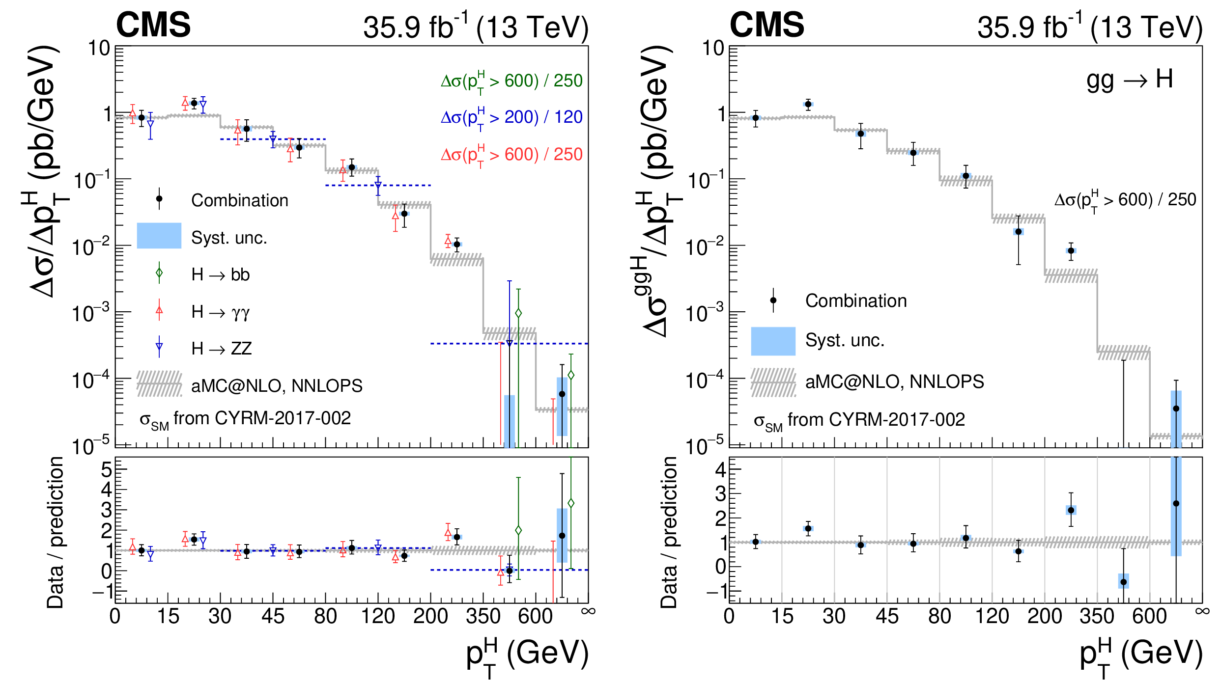
png pdf	Figure 2: Measurement of the total differential cross section (left) and the differential cross section of gluon fusion (right) as a function of $ {{p_{\mathrm {T}}} ^ {{\mathrm {H}}}} $. The combined spectrum is shown as black points with error bars indicating a 1 standard deviation uncertainty. The systematic component of the uncertainty is shown by a blue band. The spectra for the $ {{{\mathrm {H}}} \to {{\gamma}} {{\gamma}}} $, $ {{{\mathrm {H}}} \to {{\mathrm {Z}}} {{\mathrm {Z}}}} $, and $ {{{\mathrm {H}}} \to {{\mathrm {b}} {\overline {\mathrm {b}}}}} $ channels are shown in red, blue, and green, respectively. The dotted horizontal lines in the $ {{{\mathrm {H}}} \to {{\mathrm {Z}}} {{\mathrm {Z}}}} $ channel indicate the coarser binning of this measurement. The rightmost bins of the distributions are overflow bins; the normalizations of the cross sections in these bins are indicated in the figure. CYRM-2017-002 refers to Ref. [55].
png pdf	Figure 2-a: Measurement of the total differential cross section as a function of $ {{p_{\mathrm {T}}} ^ {{\mathrm {H}}}} $. The combined spectrum is shown as black points with error bars indicating a 1 standard deviation uncertainty. The systematic component of the uncertainty is shown by a blue band. The spectra for the $ {{{\mathrm {H}}} \to {{\gamma}} {{\gamma}}} $, $ {{{\mathrm {H}}} \to {{\mathrm {Z}}} {{\mathrm {Z}}}} $, and $ {{{\mathrm {H}}} \to {{\mathrm {b}} {\overline {\mathrm {b}}}}} $ channels are shown in red, blue, and green, respectively. The dotted horizontal lines in the $ {{{\mathrm {H}}} \to {{\mathrm {Z}}} {{\mathrm {Z}}}} $ channel indicate the coarser binning of this measurement. The rightmost bins of the distributions are overflow bins; the normalizations of the cross sections in these bins are indicated in the figure. CYRM-2017-002 refers to Ref. [55].
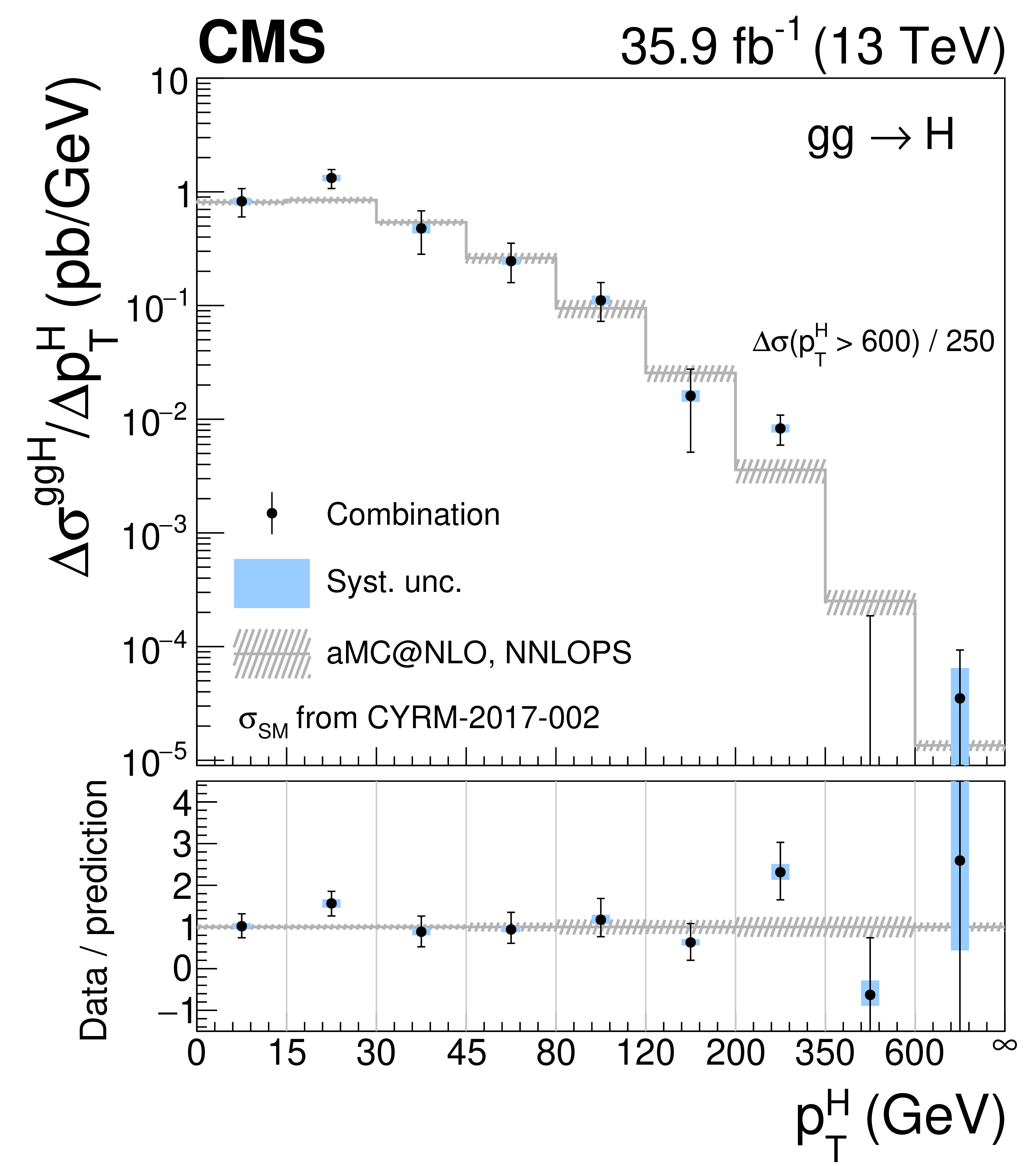
png pdf	Figure 2-b: Measurement of the differential cross section of gluon fusion as a function of $ {{p_{\mathrm {T}}} ^ {{\mathrm {H}}}} $. The combined spectrum is shown as black points with error bars indicating a 1 standard deviation uncertainty. The systematic component of the uncertainty is shown by a blue band. The spectra for the $ {{{\mathrm {H}}} \to {{\gamma}} {{\gamma}}} $, $ {{{\mathrm {H}}} \to {{\mathrm {Z}}} {{\mathrm {Z}}}} $, and $ {{{\mathrm {H}}} \to {{\mathrm {b}} {\overline {\mathrm {b}}}}} $ channels are shown in red, blue, and green, respectively. The dotted horizontal lines in the $ {{{\mathrm {H}}} \to {{\mathrm {Z}}} {{\mathrm {Z}}}} $ channel indicate the coarser binning of this measurement. The rightmost bins of the distributions are overflow bins; the normalizations of the cross sections in these bins are indicated in the figure. CYRM-2017-002 refers to Ref. [55].
png pdf	Figure 3: Measurement of the differential cross section as a function of $ {N_\text {jets}} $. The combined spectrum is shown as black points with error bars indicating a 1 standard deviation uncertainty. The systematic component of the uncertainty is shown by a blue band. The spectra for the $ {{{\mathrm {H}}} \to {{\gamma}} {{\gamma}}} $ and $ {{{\mathrm {H}}} \to {{\mathrm {Z}}} {{\mathrm {Z}}}} $ channels are shown in red and blue, respectively. The dotted horizontal lines in the $ {{{\mathrm {H}}} \to {{\mathrm {Z}}} {{\mathrm {Z}}}} $ channel indicate the coarser binning of this measurement. CYRM-2017-002 refers to Ref. [55].
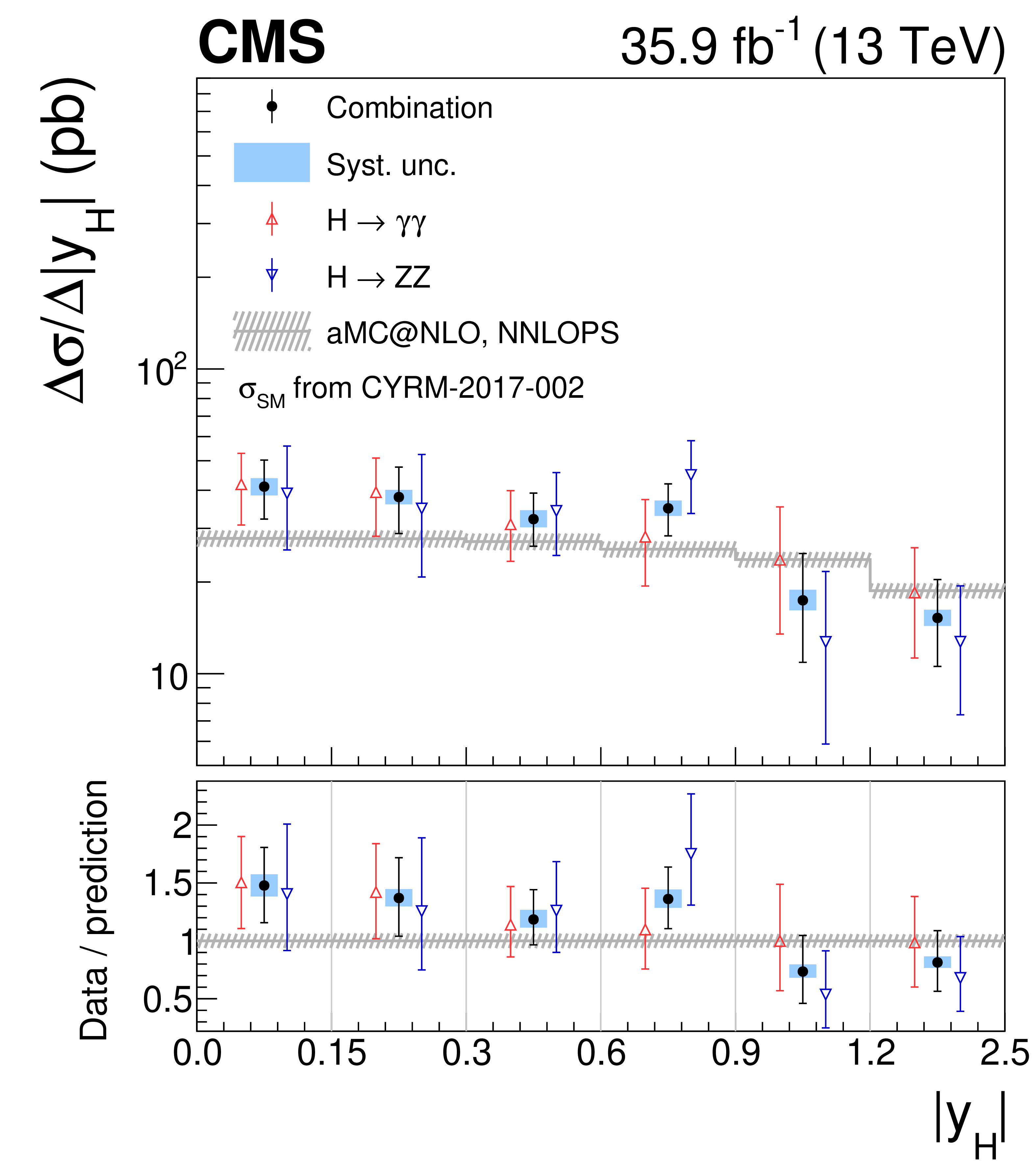
png pdf	Figure 4: Measurement of the differential cross section as a function of $ {{| y_ {{\mathrm {H}}} |}} $. The combined spectrum is shown as black points with error bars indicating a 1 standard deviation uncertainty. The systematic component of the uncertainty is shown by a blue band. The spectra for the $ {{{\mathrm {H}}} \to {{\gamma}} {{\gamma}}} $ and $ {{{\mathrm {H}}} \to {{\mathrm {Z}}} {{\mathrm {Z}}}} $ channels are shown in red and blue, respectively. CYRM-2017-002 refers to Ref. [55].
png pdf	Figure 5: Measurement of the differential cross section as a function of $ {{p_{\mathrm {T}}} ^\text {jet}} $. The combined spectrum is shown as black points with error bars indicating a 1 standard deviation uncertainty. The systematic component of the uncertainty is shown by a blue band. The spectra for the $ {{{\mathrm {H}}} \to {{\gamma}} {{\gamma}}} $ and $ {{{\mathrm {H}}} \to {{\mathrm {Z}}} {{\mathrm {Z}}}} $ channels are shown in red and blue, respectively. The dotted horizontal lines in the $ {{{\mathrm {H}}} \to {{\mathrm {Z}}} {{\mathrm {Z}}}} $ channel indicate the coarser binning of this measurement. The rightmost bin of the distribution is an overflow bin; the normalization of the cross section in that bin is indicated in the figure. CYRM-2017-002 refers to Ref. [55].
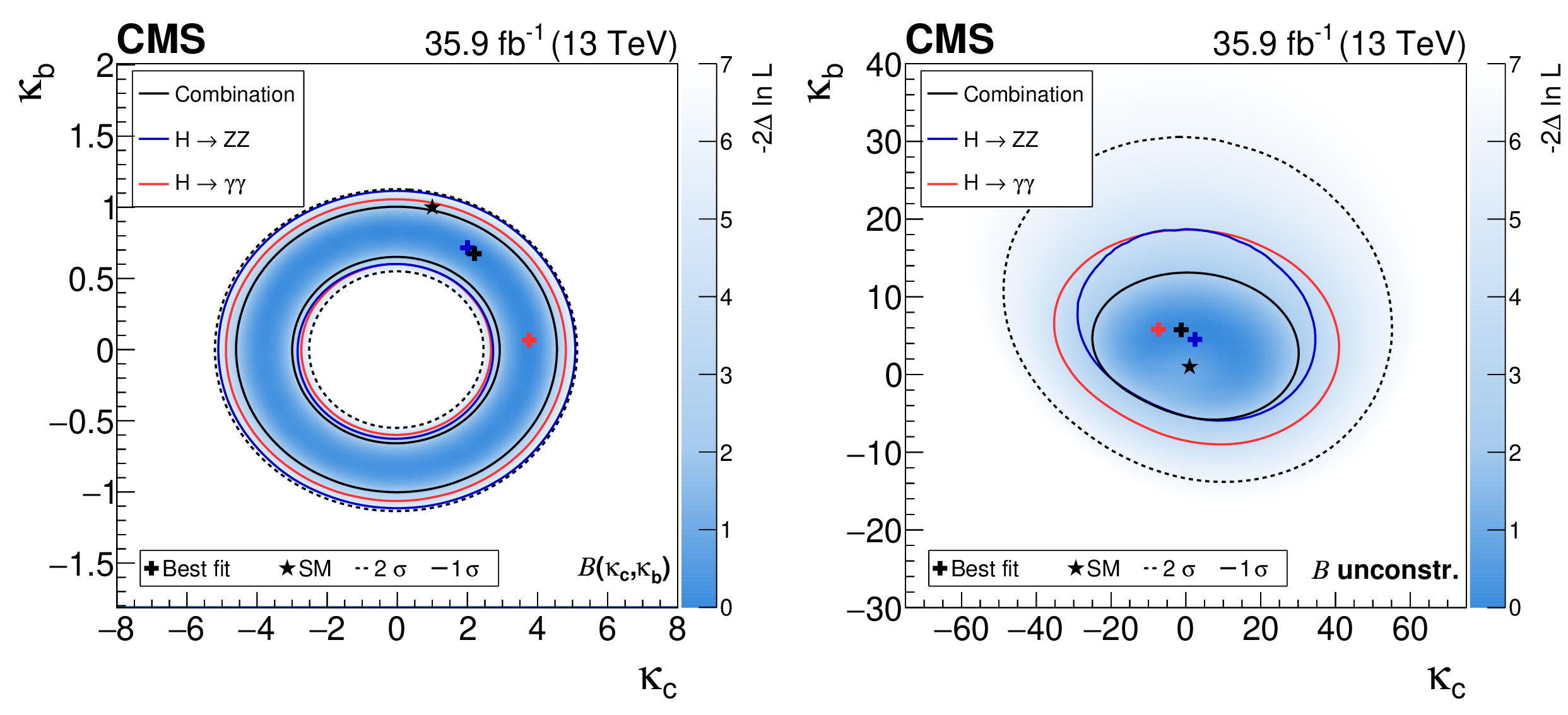
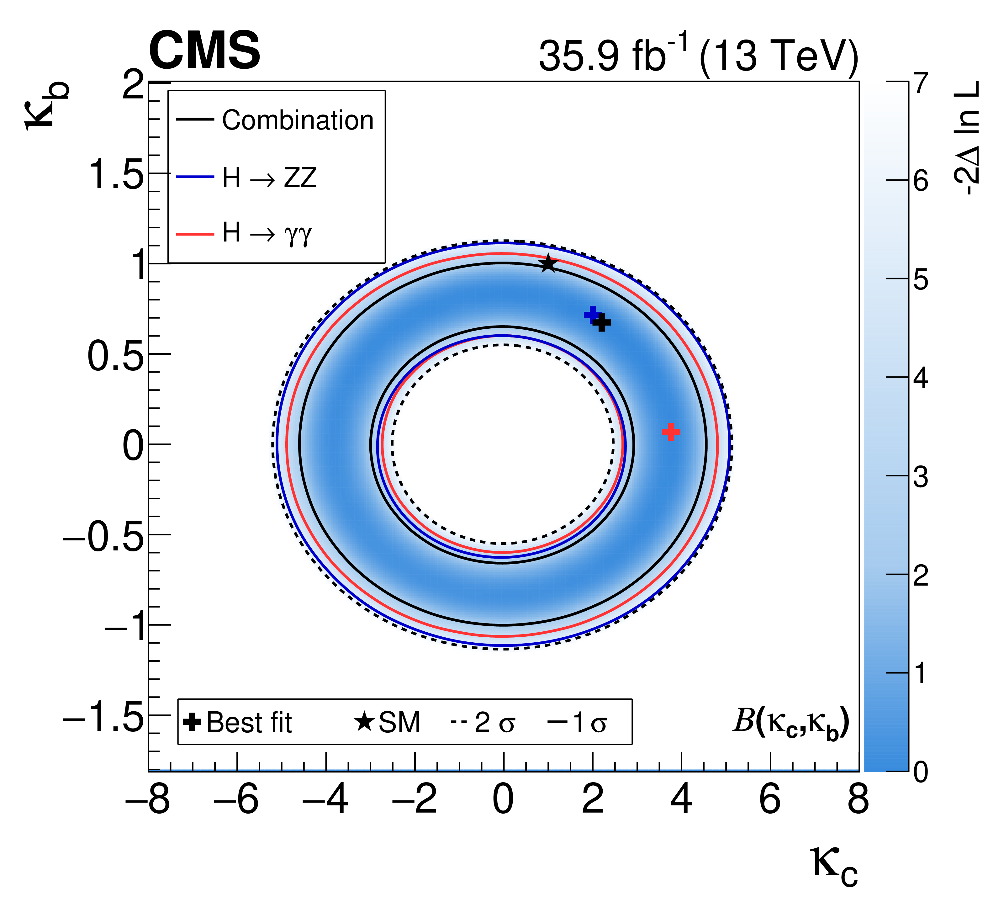
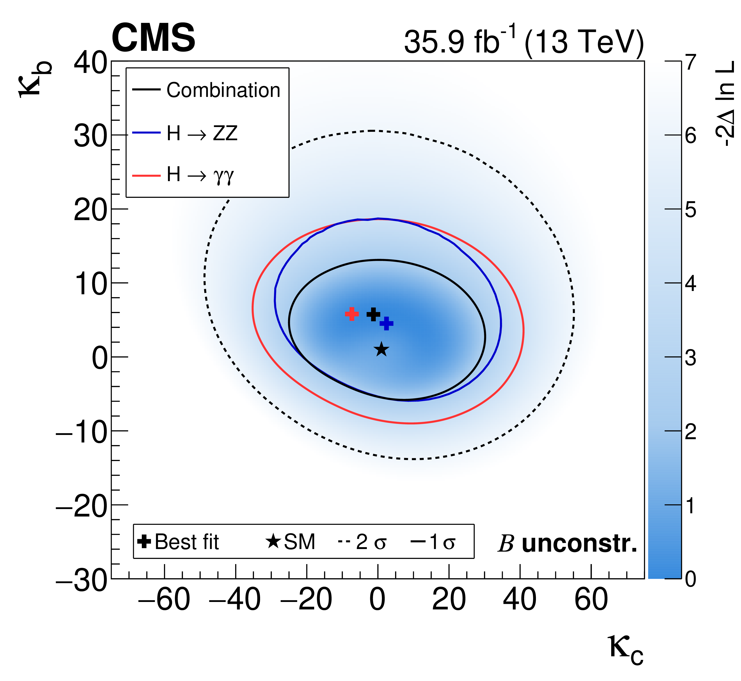
png pdf	Figure 6: Simultaneous fit to data for $ {\kappa _{{{\mathrm {b}}}}} $ and $ {\kappa _{{{\mathrm {c}}}}} $, assuming a coupling dependence of the branching fractions (left) and the branching fractions implemented as nuisance parameters with no prior constraint (right). The one standard deviation contour is drawn for the combination ($ {{{\mathrm {H}}} \to {{\gamma}} {{\gamma}}} $ and $ {{{\mathrm {H}}} \to {{\mathrm {Z}}} {{\mathrm {Z}}}} $), the $ {{{\mathrm {H}}} \to {{\gamma}} {{\gamma}}} $ channel, and the $ {{{\mathrm {H}}} \to {{\mathrm {Z}}} {{\mathrm {Z}}}} $ channel in black, red, and blue, respectively. For the combination the two standard deviation contour is drawn as a black dashed line, and the shading indicates the negative log-likelihood, with the scale shown on the right hand side of the plots.
png pdf	Figure 6-a: Simultaneous fit to data for $ {\kappa _{{{\mathrm {b}}}}} $ and $ {\kappa _{{{\mathrm {c}}}}} $, assuming a coupling dependence of the branching fractions. The one standard deviation contour is drawn for the combination ($ {{{\mathrm {H}}} \to {{\gamma}} {{\gamma}}} $ and $ {{{\mathrm {H}}} \to {{\mathrm {Z}}} {{\mathrm {Z}}}} $), the $ {{{\mathrm {H}}} \to {{\gamma}} {{\gamma}}} $ channel, and the $ {{{\mathrm {H}}} \to {{\mathrm {Z}}} {{\mathrm {Z}}}} $ channel in black, red, and blue, respectively. For the combination the two standard deviation contour is drawn as a black dashed line, and the shading indicates the negative log-likelihood, with the scale shown on the right hand side of the plots.
png pdf	Figure 6-b: Simultaneous fit to data for $ {\kappa _{{{\mathrm {b}}}}} $ and $ {\kappa _{{{\mathrm {c}}}}} $, with branching fractions implemented as nuisance parameters with no prior constraint. The one standard deviation contour is drawn for the combination ($ {{{\mathrm {H}}} \to {{\gamma}} {{\gamma}}} $ and $ {{{\mathrm {H}}} \to {{\mathrm {Z}}} {{\mathrm {Z}}}} $), the $ {{{\mathrm {H}}} \to {{\gamma}} {{\gamma}}} $ channel, and the $ {{{\mathrm {H}}} \to {{\mathrm {Z}}} {{\mathrm {Z}}}} $ channel in black, red, and blue, respectively. For the combination the two standard deviation contour is drawn as a black dashed line, and the shading indicates the negative log-likelihood, with the scale shown on the right hand side of the plots.
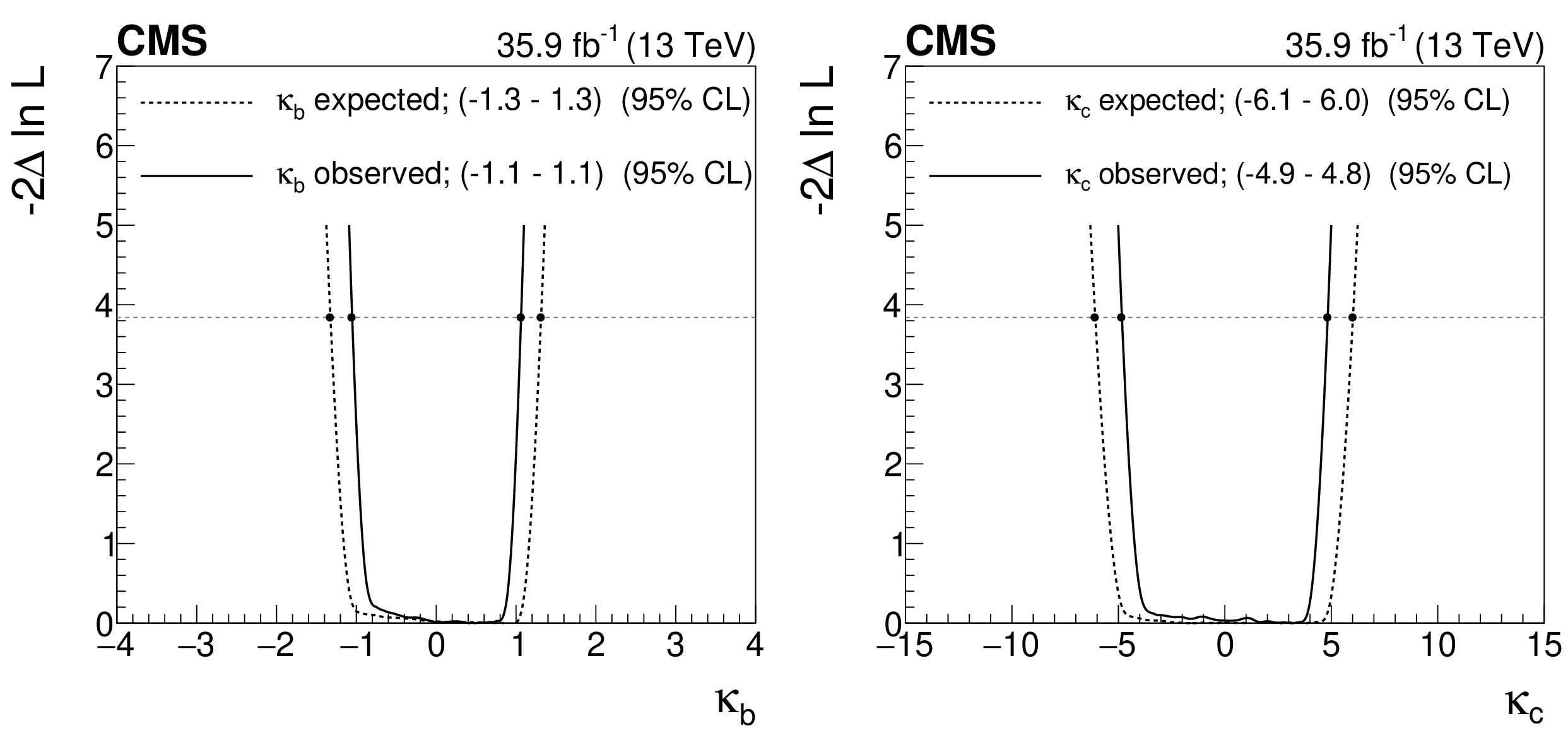
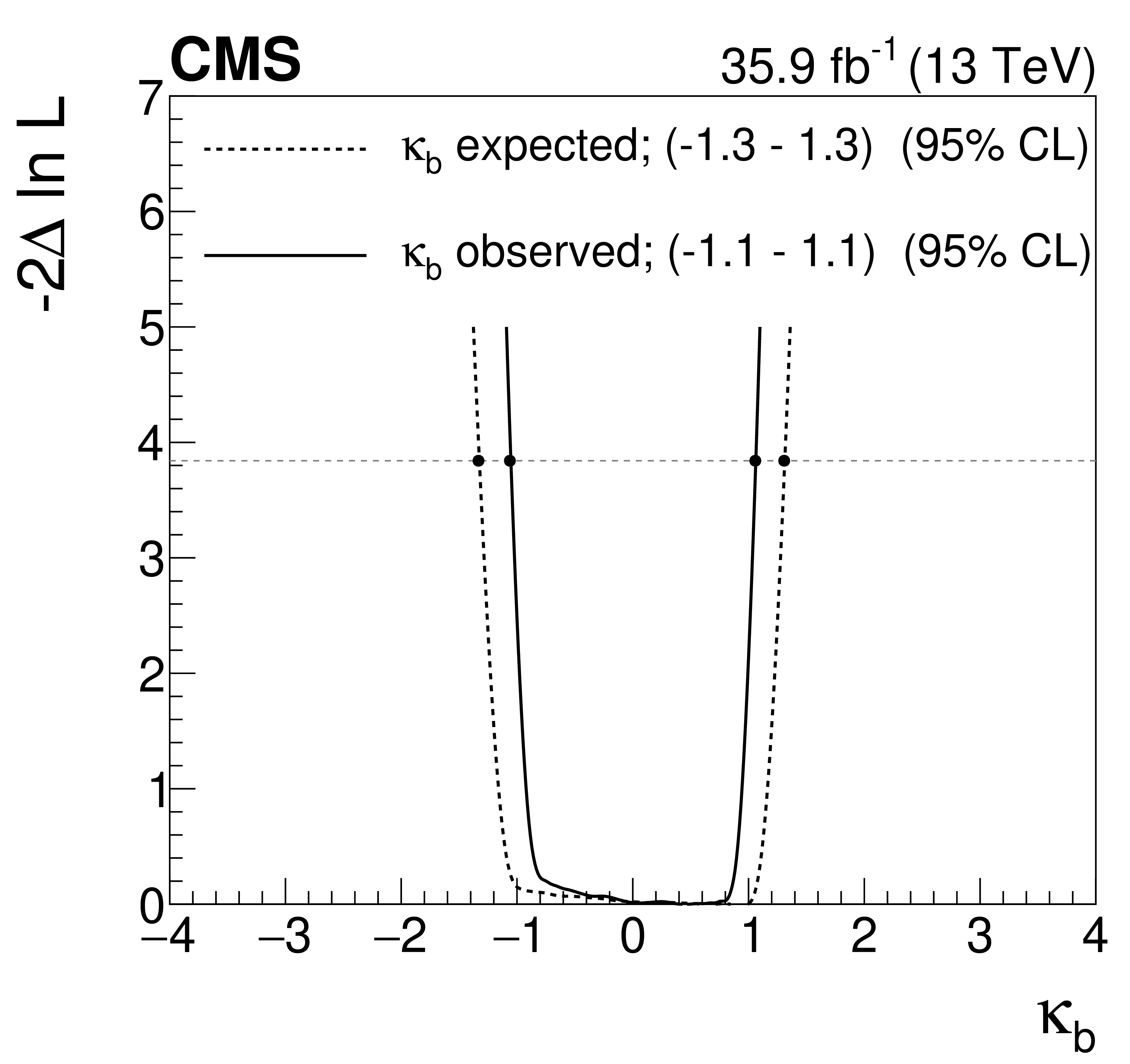
png pdf	Figure 7: Likelihood scan of $ {\kappa _{{{\mathrm {b}}}}} $ while profiling $ {\kappa _{{{\mathrm {c}}}}} $ (left), and of $ {\kappa _{{{\mathrm {c}}}}} $ while profiling $ {\kappa _{{{\mathrm {b}}}}} $ (right). The filled markers indicate the limits at 95% CL. The branching fractions are considered dependent on the values of the couplings.
png pdf	Figure 7-a: Likelihood scan of $ {\kappa _{{{\mathrm {b}}}}} $ while profiling $ {\kappa _{{{\mathrm {c}}}}} $. The filled markers indicate the limits at 95% CL. The branching fractions are considered dependent on the values of the couplings.
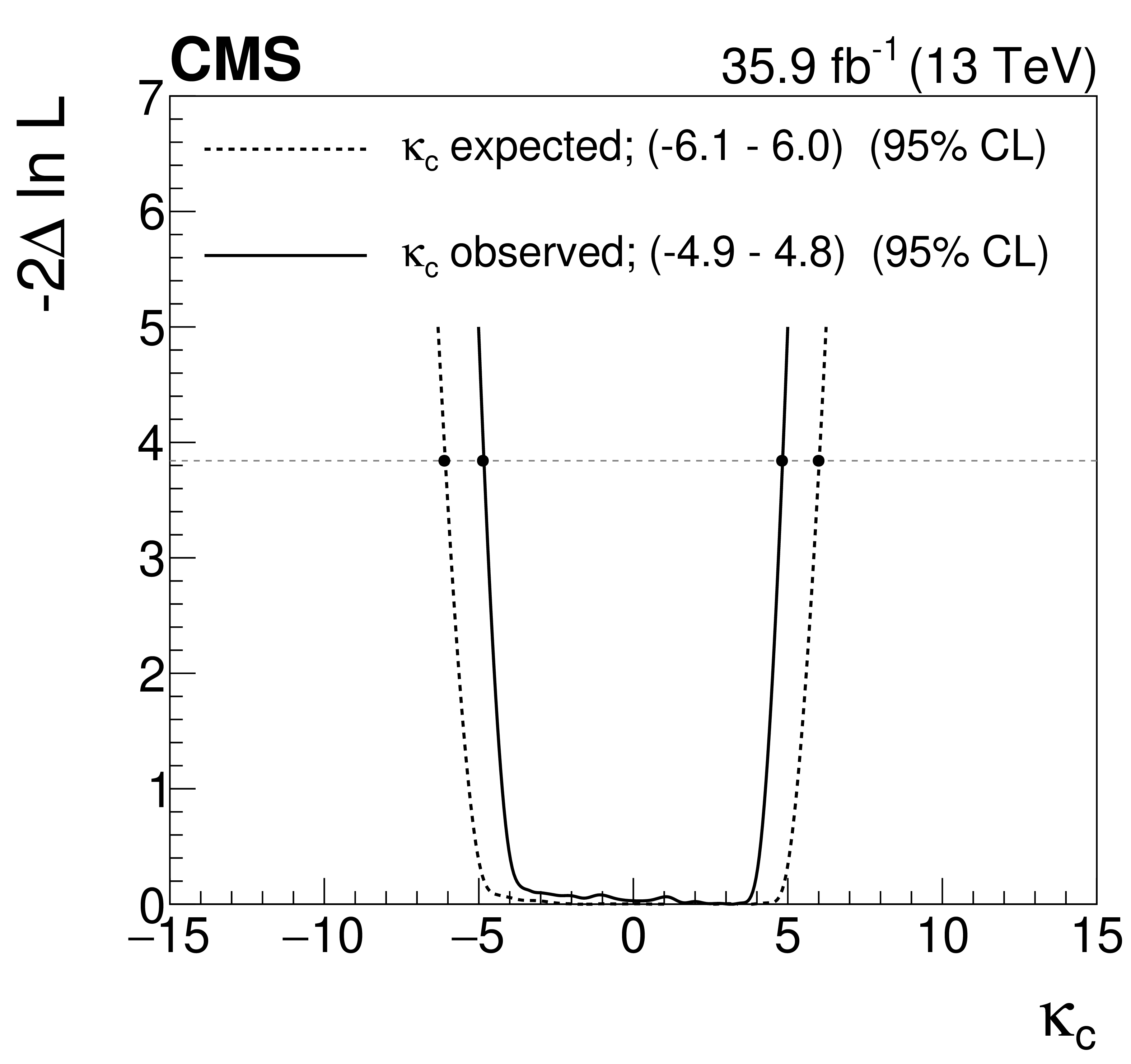
png pdf	Figure 7-b: Likelihood scan of $ {\kappa _{{{\mathrm {c}}}}} $ while profiling $ {\kappa _{{{\mathrm {b}}}}} $. The filled markers indicate the limits at 95% CL. The branching fractions are considered dependent on the values of the couplings.
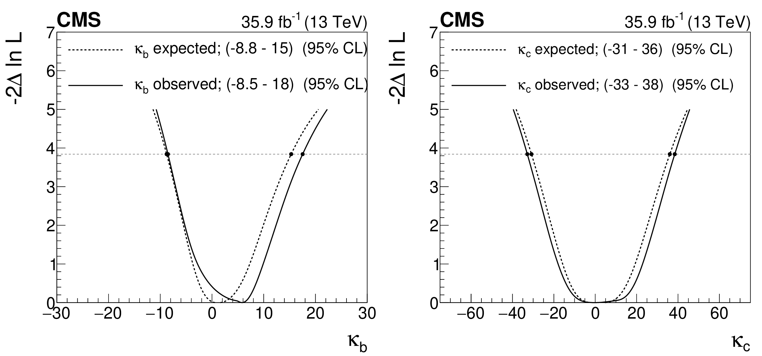
png pdf	Figure 8: Likelihood scan of $ {\kappa _{{{\mathrm {b}}}}} $ while profiling $ {\kappa _{{{\mathrm {c}}}}} $ (left), and of $ {\kappa _{{{\mathrm {c}}}}} $ while profiling $ {\kappa _{{{\mathrm {b}}}}} $ (right). The filled markers indicate the limits at 95% CL. The branching fractions are implemented as nuisance parameters with no prior constraint.
png pdf	Figure 8-a: Likelihood scan of $ {\kappa _{{{\mathrm {b}}}}} $ while profiling $ {\kappa _{{{\mathrm {c}}}}} $. The filled markers indicate the limits at 95% CL. The branching fractions are implemented as nuisance parameters with no prior constraint.
png pdf	Figure 8-b: Likelihood scan of $ {\kappa _{{{\mathrm {c}}}}} $ while profiling $ {\kappa _{{{\mathrm {b}}}}} $. The filled markers indicate the limits at 95% CL. The branching fractions are implemented as nuisance parameters with no prior constraint.
png pdf	Figure 9: Simultaneous fit to data for $ {\kappa _{{{\mathrm {t}}}}} $ and $ {c_ {\mathrm {g}}} $, assuming a coupling dependence of the branching fractions (left) and the branching fractions implemented as nuisance parameters with no prior constraint (right). The one standard deviation contour is drawn for the combination ($ {{{\mathrm {H}}} \to {{\gamma}} {{\gamma}}} $, $ {{{\mathrm {H}}} \to {{\mathrm {Z}}} {{\mathrm {Z}}}} $, and $ {{{\mathrm {H}}} \to {{\mathrm {b}} {\overline {\mathrm {b}}}}} $), the $ {{{\mathrm {H}}} \to {{\gamma}} {{\gamma}}} $ channel, and the $ {{{\mathrm {H}}} \to {{\mathrm {Z}}} {{\mathrm {Z}}}} $ channel in black, red, and blue, respectively. For the combination the two standard deviation contour is drawn as a black dashed line, and the shading indicates the negative log-likelihood, with the scale shown on the right hand side of the plots.
png pdf	Figure 9-a: Simultaneous fit to data for $ {\kappa _{{{\mathrm {t}}}}} $ and $ {c_ {\mathrm {g}}} $, assuming a coupling dependence of the branching fractions. The one standard deviation contour is drawn for the combination ($ {{{\mathrm {H}}} \to {{\gamma}} {{\gamma}}} $, $ {{{\mathrm {H}}} \to {{\mathrm {Z}}} {{\mathrm {Z}}}} $, and $ {{{\mathrm {H}}} \to {{\mathrm {b}} {\overline {\mathrm {b}}}}} $), the $ {{{\mathrm {H}}} \to {{\gamma}} {{\gamma}}} $ channel, and the $ {{{\mathrm {H}}} \to {{\mathrm {Z}}} {{\mathrm {Z}}}} $ channel in black, red, and blue, respectively. For the combination the two standard deviation contour is drawn as a black dashed line, and the shading indicates the negative log-likelihood, with the scale shown on the right hand side of the plots.
png pdf	Figure 9-b: Simultaneous fit to data for $ {\kappa _{{{\mathrm {t}}}}} $ and $ {c_ {\mathrm {g}}} $, with branching fractions implemented as nuisance parameters with no prior constraint. The one standard deviation contour is drawn for the combination ($ {{{\mathrm {H}}} \to {{\gamma}} {{\gamma}}} $, $ {{{\mathrm {H}}} \to {{\mathrm {Z}}} {{\mathrm {Z}}}} $, and $ {{{\mathrm {H}}} \to {{\mathrm {b}} {\overline {\mathrm {b}}}}} $), the $ {{{\mathrm {H}}} \to {{\gamma}} {{\gamma}}} $ channel, and the $ {{{\mathrm {H}}} \to {{\mathrm {Z}}} {{\mathrm {Z}}}} $ channel in black, red, and blue, respectively. For the combination the two standard deviation contour is drawn as a black dashed line, and the shading indicates the negative log-likelihood, with the scale shown on the right hand side of the plots.
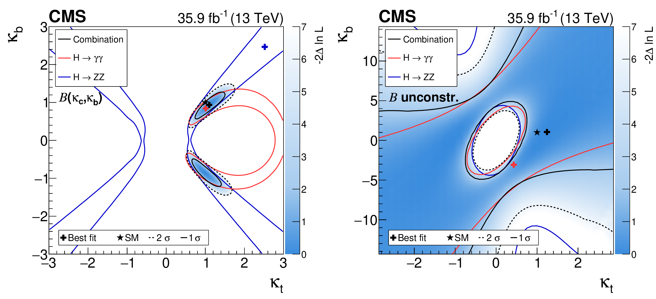
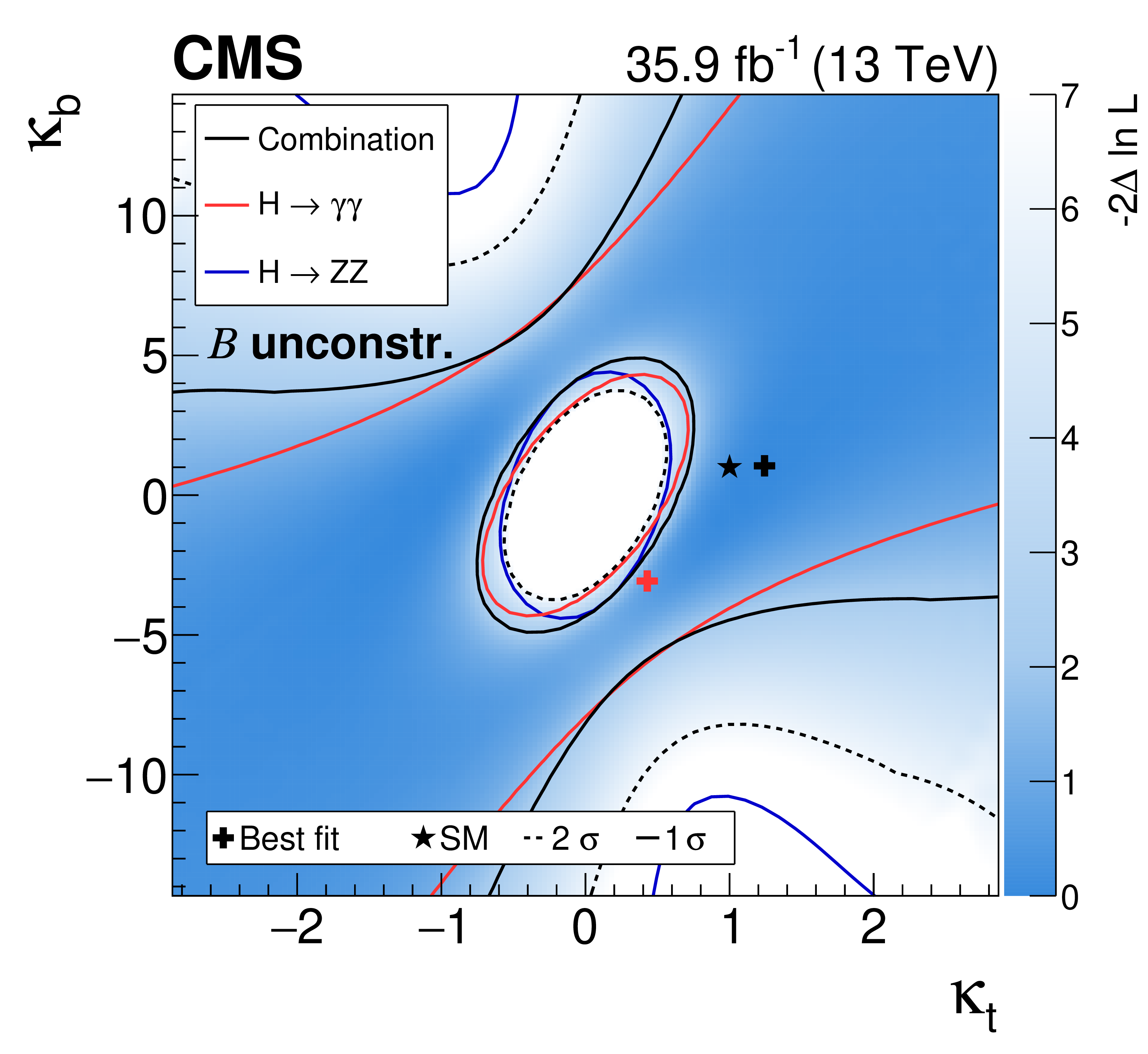
png pdf	Figure 10: Simultaneous fit to data for $ {\kappa _{{{\mathrm {t}}}}} $ and $ {\kappa _{{{\mathrm {b}}}}} $, assuming a coupling dependence of the branching fractions (left) and the branching fractions implemented as nuisance parameters with no prior constraint (right). The one standard deviation contour is drawn for the combination ($ {{{\mathrm {H}}} \to {{\gamma}} {{\gamma}}} $, $ {{{\mathrm {H}}} \to {{\mathrm {Z}}} {{\mathrm {Z}}}} $, and $ {{{\mathrm {H}}} \to {{\mathrm {b}} {\overline {\mathrm {b}}}}} $), the $ {{{\mathrm {H}}} \to {{\gamma}} {{\gamma}}} $ channel, and the $ {{{\mathrm {H}}} \to {{\mathrm {Z}}} {{\mathrm {Z}}}} $ channel in black, red, and blue, respectively. For the combination the two standard deviation contour is drawn as a black dashed line, and the shading indicates the negative log-likelihood, with the scale shown on the right hand side of the plots.
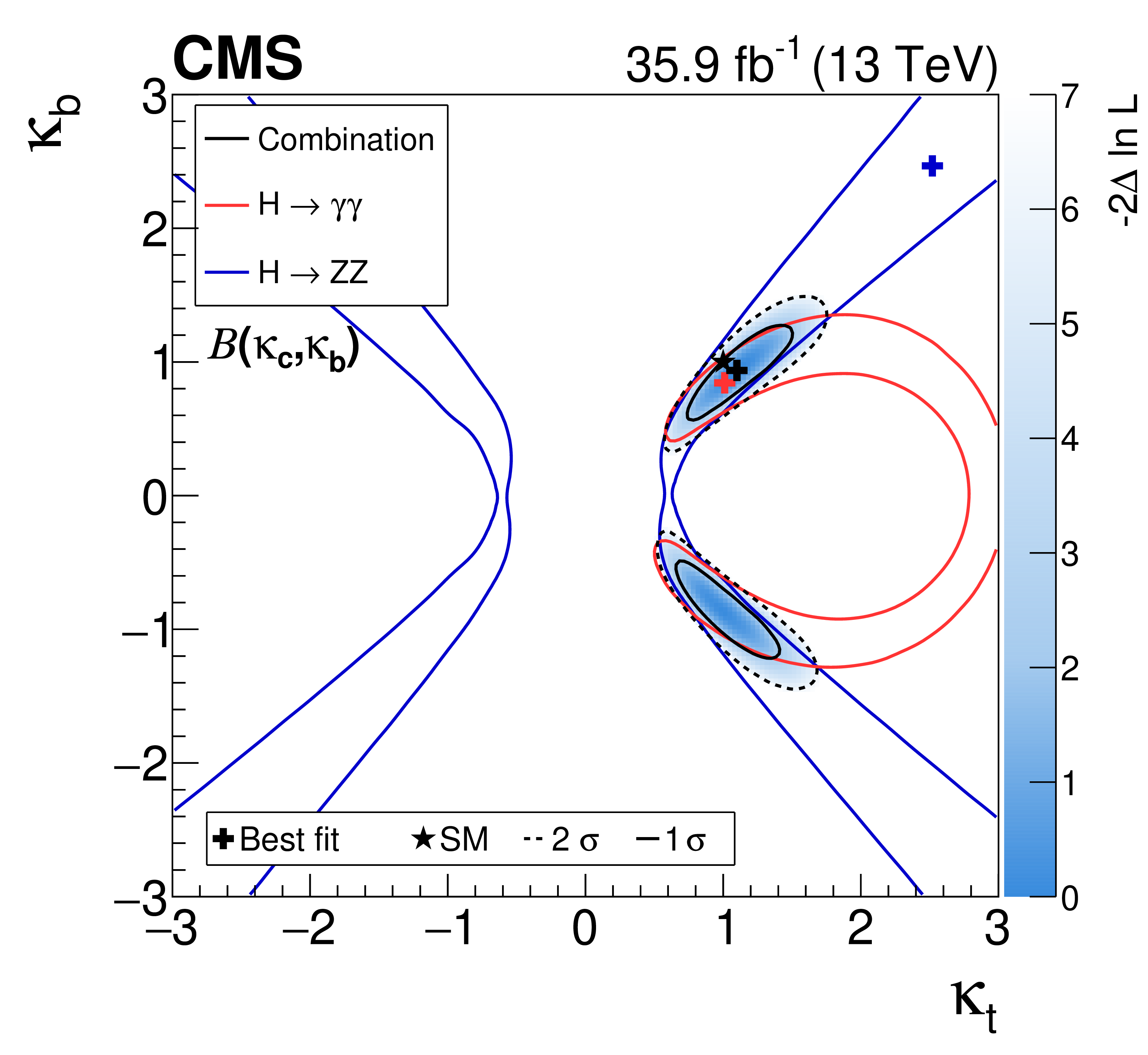
png pdf	Figure 10-a: Simultaneous fit to data for $ {\kappa _{{{\mathrm {t}}}}} $ and $ {\kappa _{{{\mathrm {b}}}}} $, assuming a coupling dependence of the branching fractions. The one standard deviation contour is drawn for the combination ($ {{{\mathrm {H}}} \to {{\gamma}} {{\gamma}}} $, $ {{{\mathrm {H}}} \to {{\mathrm {Z}}} {{\mathrm {Z}}}} $, and $ {{{\mathrm {H}}} \to {{\mathrm {b}} {\overline {\mathrm {b}}}}} $), the $ {{{\mathrm {H}}} \to {{\gamma}} {{\gamma}}} $ channel, and the $ {{{\mathrm {H}}} \to {{\mathrm {Z}}} {{\mathrm {Z}}}} $ channel in black, red, and blue, respectively. For the combination the two standard deviation contour is drawn as a black dashed line, and the shading indicates the negative log-likelihood, with the scale shown on the right hand side of the plots.
png pdf	Figure 10-b: Simultaneous fit to data for $ {\kappa _{{{\mathrm {t}}}}} $ and $ {\kappa _{{{\mathrm {b}}}}} $, with branching fractions implemented as nuisance parameters with no prior constraint. The one standard deviation contour is drawn for the combination ($ {{{\mathrm {H}}} \to {{\gamma}} {{\gamma}}} $, $ {{{\mathrm {H}}} \to {{\mathrm {Z}}} {{\mathrm {Z}}}} $, and $ {{{\mathrm {H}}} \to {{\mathrm {b}} {\overline {\mathrm {b}}}}} $), the $ {{{\mathrm {H}}} \to {{\gamma}} {{\gamma}}} $ channel, and the $ {{{\mathrm {H}}} \to {{\mathrm {Z}}} {{\mathrm {Z}}}} $ channel in black, red, and blue, respectively. For the combination the two standard deviation contour is drawn as a black dashed line, and the shading indicates the negative log-likelihood, with the scale shown on the right hand side of the plots.
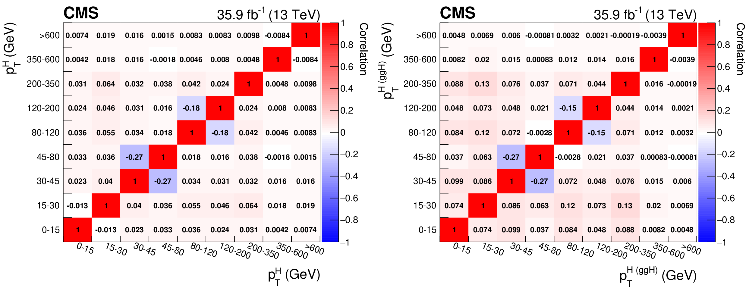
png pdf	Figure 11: Bin-to-bin correlation matrix of the $ {{p_{\mathrm {T}}} ^ {{\mathrm {H}}}} $ spectrum (left) and of the $ {{p_{\mathrm {T}}} ^ {{\mathrm {H}}}} $ spectrum of gluon fusion ($ {{\mathrm {g}} {\mathrm {g}} {{\mathrm {H}}}} $), where the non-$ {{\mathrm {g}} {\mathrm {g}} {{\mathrm {H}}}}$ contributions are fixed to the SM expectation (right).
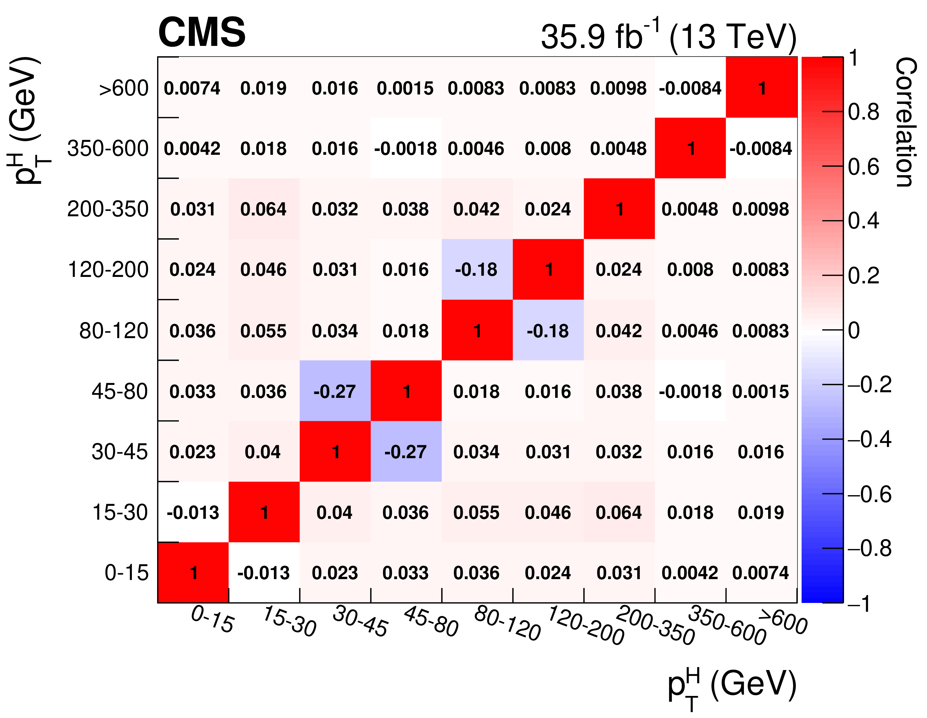
png pdf	Figure 11-a: Bin-to-bin correlation matrix of the $ {{p_{\mathrm {T}}} ^ {{\mathrm {H}}}} $ spectrum.
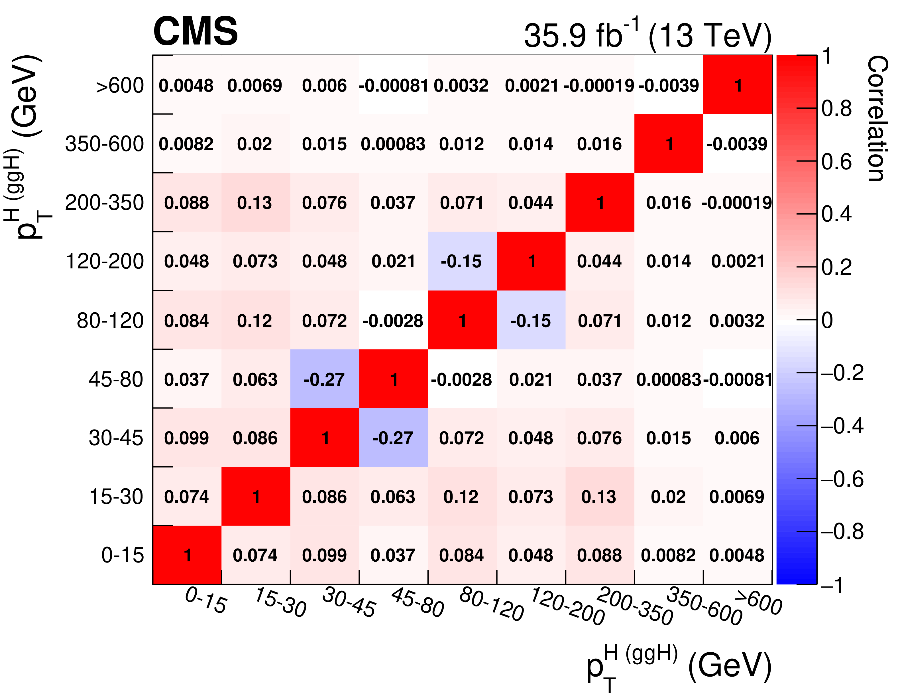
png pdf	Figure 11-b: The $ {{p_{\mathrm {T}}} ^ {{\mathrm {H}}}} $ spectrum of gluon fusion ($ {{\mathrm {g}} {\mathrm {g}} {{\mathrm {H}}}} $), where the non-$ {{\mathrm {g}} {\mathrm {g}} {{\mathrm {H}}}}$ contributions are fixed to the SM expectation.
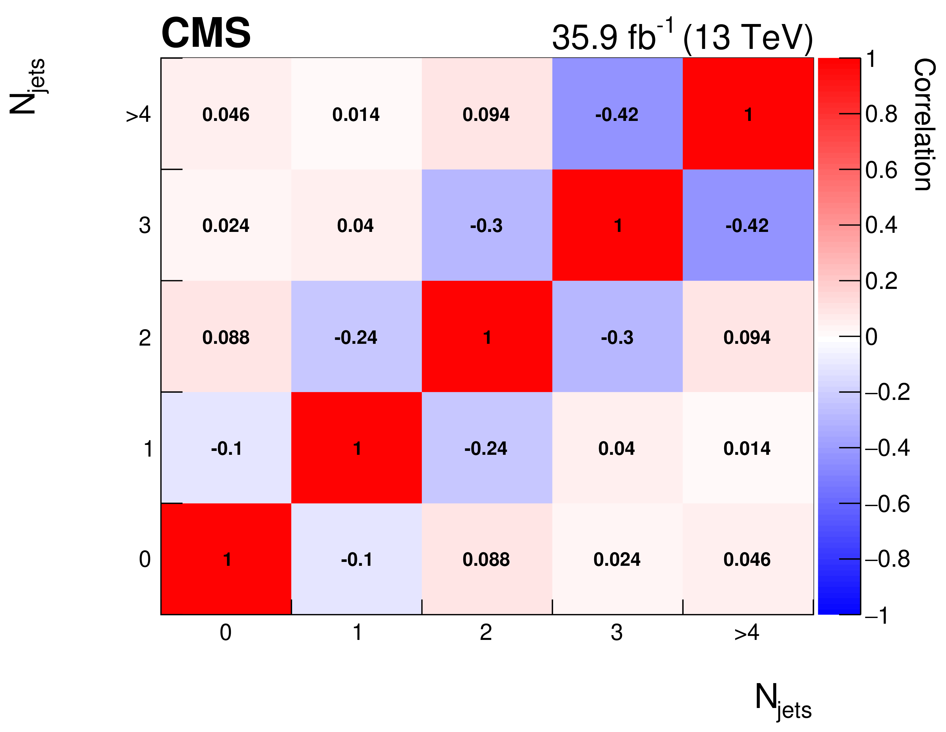
png pdf	Figure 12: Bin-to-bin correlation matrix of the $ {N_\text {jets}} $ spectrum.
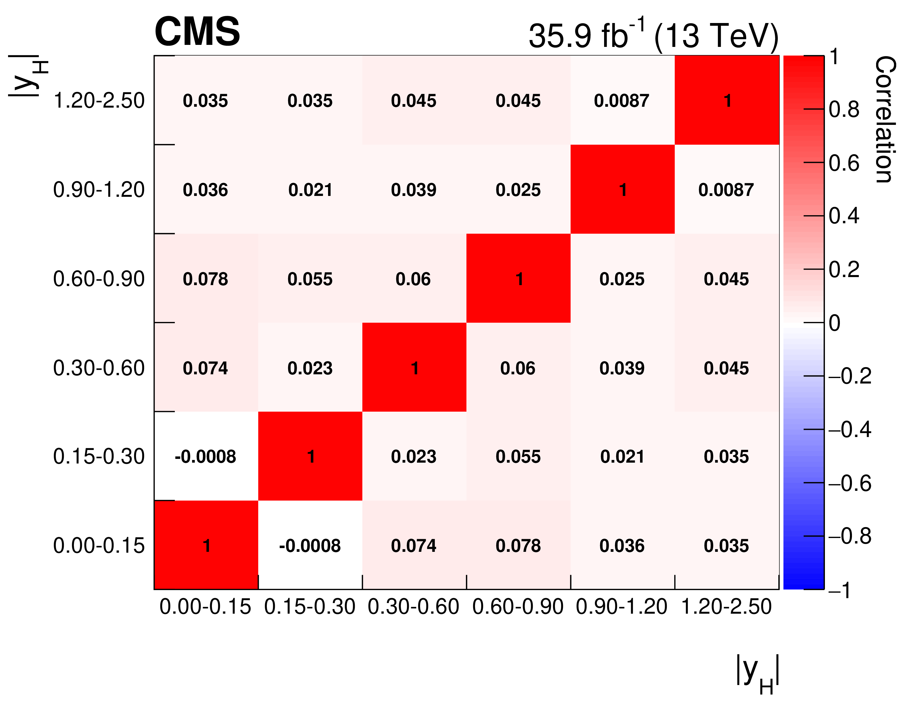
png pdf	Figure 13: Bin-to-bin correlation matrix of the $ {{| y_ {{\mathrm {H}}} |}} $ spectrum.
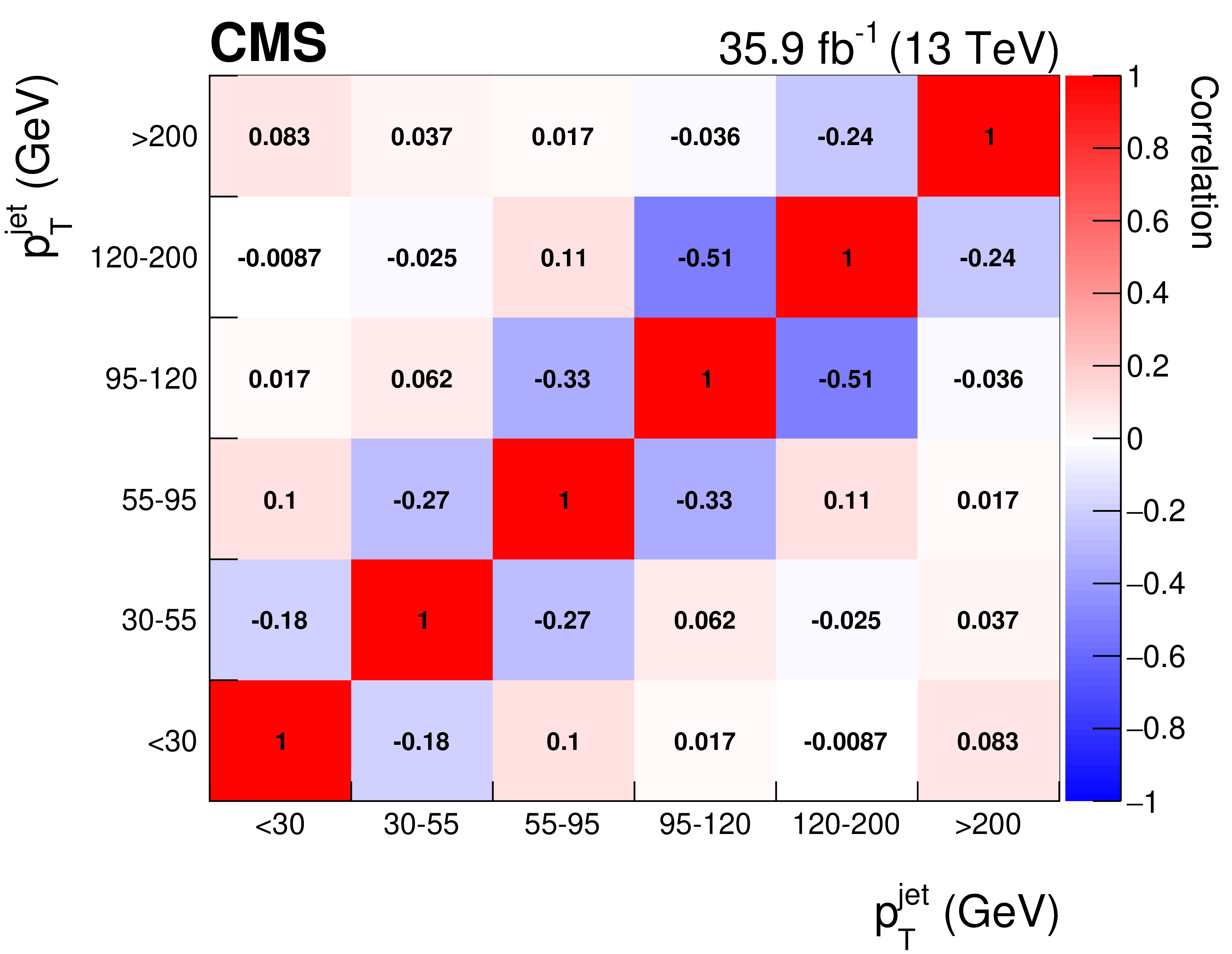
png pdf	Figure 14: Bin-to-bin correlation matrix of the $ {{p_{\mathrm {T}}} ^\text {jet}} $ spectrum.

Tables
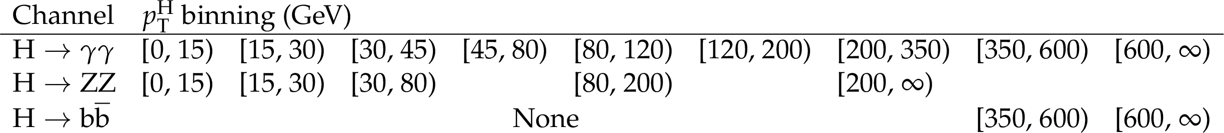
png pdf	Table 1: The reconstruction-level binning for $ {{p_{\mathrm {T}}} ^ {{\mathrm {H}}}} $ for the $ {{{\mathrm {H}}} \to {{\gamma}} {{\gamma}}} $, $ {{{\mathrm {H}}} \to {{\mathrm {Z}}} {{\mathrm {Z}}}} $, and $ {{{\mathrm {H}}} \to {{\mathrm {b}} {\overline {\mathrm {b}}}}} $ channels. This binning coincides with the binning of the unfolded cross sections in which the individual results are reported.
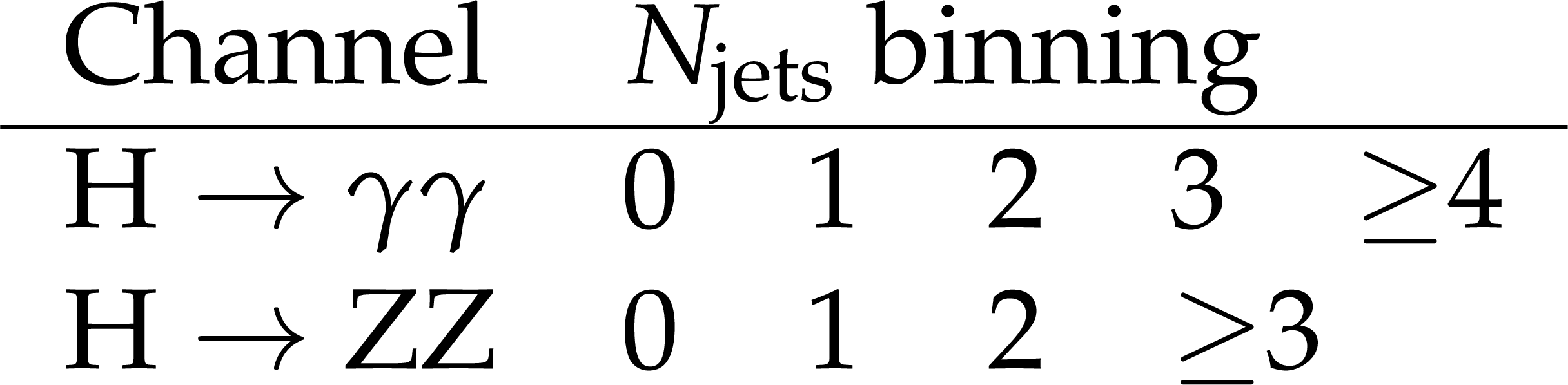
png pdf	Table 2: The binning for $ {N_\text {jets}} $ for the $ {{{\mathrm {H}}} \to {{\gamma}} {{\gamma}}} $ and the $ {{{\mathrm {H}}} \to {{\mathrm {Z}}} {{\mathrm {Z}}}} $ channels. This binning coincides with the binning of the unfolded cross sections in which the individual results are reported.
png pdf	Table 3: The binning for $ {{| y_ {{\mathrm {H}}} |}} $ for the $ {{{\mathrm {H}}} \to {{\gamma}} {{\gamma}}} $ and the $ {{{\mathrm {H}}} \to {{\mathrm {Z}}} {{\mathrm {Z}}}} $ channels. This binning coincides with the binning of the unfolded cross sections in which the individual results are reported.
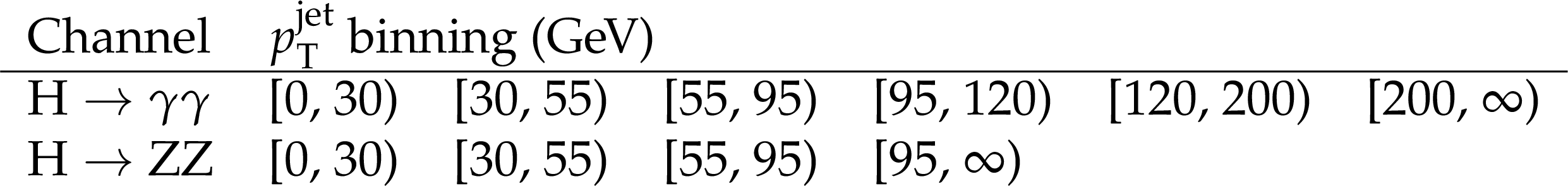
png pdf	Table 4: The binning for $ {{p_{\mathrm {T}}} ^\text {jet}} $ for the $ {{{\mathrm {H}}} \to {{\gamma}} {{\gamma}}} $ and the $ {{{\mathrm {H}}} \to {{\mathrm {Z}}} {{\mathrm {Z}}}} $ channels. This binning coincides with the binning of the unfolded cross sections in which the individual results are reported.
png pdf	Table 5: Uncertainties in the predicted $ {{p_{\mathrm {T}}} ^ {{\mathrm {H}}}} $ spectra related to variations of theory parameters for the $ {\kappa _{{{\mathrm {b}}}}} $ and $ {\kappa _{{{\mathrm {c}}}}} $ case.
png pdf	Table 6: Uncertainties in the predicted $ {{p_{\mathrm {T}}} ^ {{\mathrm {H}}}} $ spectra related to variations of theory parameters for the $ {\kappa _{{{\mathrm {t}}}}} $, $ {c_ {\mathrm {g}}} $, and $ {\kappa _{{{\mathrm {b}}}}} $ case.
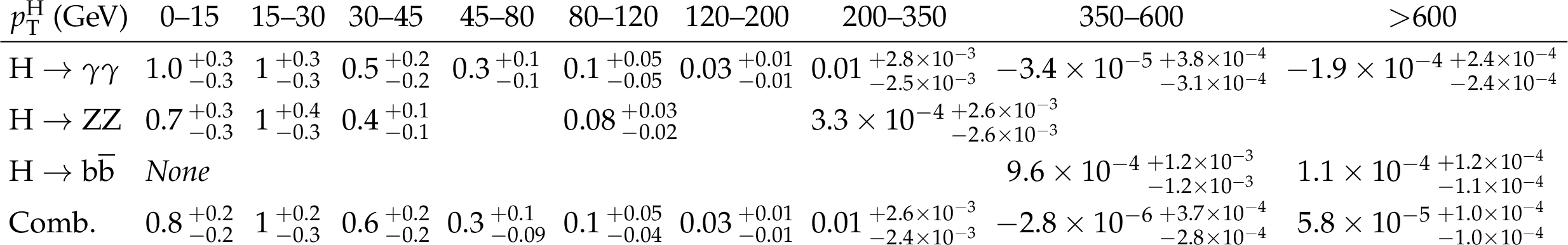
png pdf	Table 7: Differential cross sections (pb/GeV) for the observable $ {{p_{\mathrm {T}}} ^ {{\mathrm {H}}}} $.
png pdf	Table 8: Differential cross sections of gluon fusion ($ {{\mathrm {g}} {\mathrm {g}} {{\mathrm {H}}}} $) (pb/GeV) for the observable $ {{p_{\mathrm {T}}} ^ {{\mathrm {H}}}} $, with non-$ {{\mathrm {g}} {\mathrm {g}} {{\mathrm {H}}}}$ production modes fixed to their SM prediction.
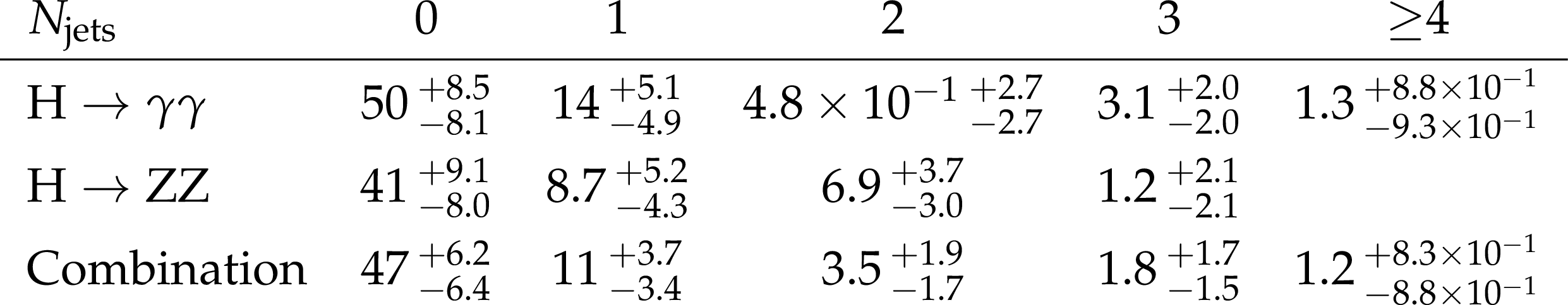
png pdf	Table 9: Differential cross sections (pb) for the observable $ {N_\text {jets}} $.
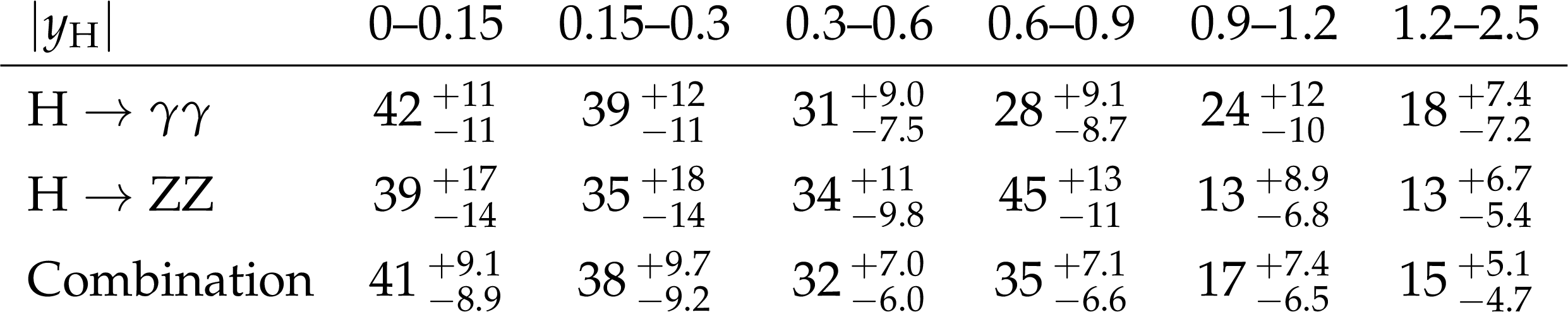
png pdf	Table 10: Differential cross sections (pb) for the observable $ {{| y_ {{\mathrm {H}}} |}} $.
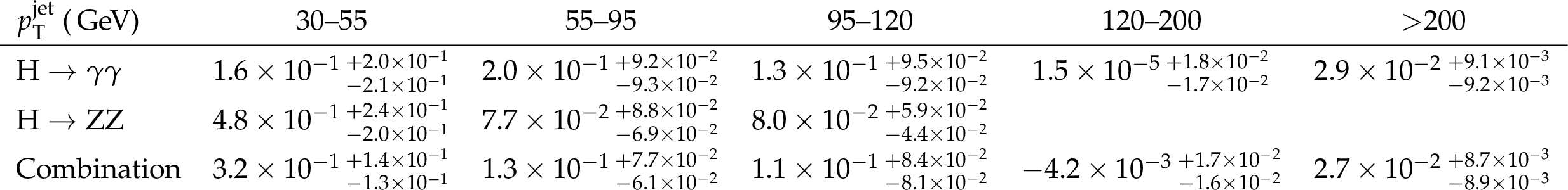
png pdf	Table 11: Differential cross sections (pb/GeV) for the observable $ {{p_{\mathrm {T}}} ^\text {jet}} $.

Summary

A combination of differential cross sections for the Higgs boson transverse momentum $p_{\mathrm{T}}^{\mathrm{H}}$, the number of jets, the rapidity of the Higgs boson, and the ${p_{\mathrm{T}}}$ of the leading jet has been presented, using proton-proton collision data collected at $\sqrt{s}=$ 13 TeV with the CMS detector, corresponding to an integrated luminosity of 35.9 fb$^{-1}$. The spectra obtained are based on data from the ${{\mathrm{H}} \to{\gamma} {\gamma} } $, $\mathrm{H}\to\mathrm{Z}\mathrm{Z}$, and ${{\mathrm{H}} \to\mathrm{b\bar{b}}} $ decay channels. The precision of the combined measurement of the differential cross section of $p_{\mathrm{T}}^{\mathrm{H}}$ is improved by about 15% with respect to the ${{\mathrm{H}} \to{\gamma} {\gamma} } $ channel alone. The improvement is larger in the low-$p_{\mathrm{T}}^{\mathrm{H}}$ region than in the high-$p_{\mathrm{T}}^{\mathrm{H}}$ tails. No significant deviations from the standard model are observed in any differential distribution. Additionally, the total cross section for Higgs boson production based on a combination of the ${{\mathrm{H}} \to{\gamma} {\gamma} } $ and $\mathrm{H}\to\mathrm{Z}\mathrm{Z}$ channels is measured to be 61.1 $\pm$ 6.0 (stat) $\pm$ 3.7 (syst) pb. The spectra obtained are interpreted in the $\kappa$-framework [30], in which simultaneous variations of ${\kappa_{{\mathrm{b}} }} $ and ${\kappa_{{\mathrm{c}} }} $, ${\kappa_{{\mathrm{t}} }} $ and ${\kappa_{{\mathrm{b}} }} $, and ${\kappa_{{\mathrm{t}} }} $ and the anomalous direct coupling to the gluon field ${c_\mathrm{g}} $ are fitted to the $p_{\mathrm{T}}^{\mathrm{H}}$ spectra. The limits obtained for the individual couplings are $-1.1 < {\kappa_{{\mathrm{b}} }} < 1.1$ and $-4.9 < {\kappa_{{\mathrm{c}} }} < 4.8$ at 95% confidence level, assuming the branching fractions scale with the Higgs boson couplings following the standard model prediction. For the charm coupling ${\kappa_{{\mathrm{c}} }} $ in particular, these bounds are comparable with those obtained from direct searches with charm quarks in the final state.

References
1	P. W. Higgs	Broken symmetries and the masses of gauge bosons	PRL 13 (1964) 508
2	F. Englert and R. Brout	Broken symmetry and the mass of gauge vector mesons	PRL 13 (1964) 321
3	G. S. Guralnik, C. R. Hagen, and T. W. B. Kibble	Global conservation laws and massless particles	PRL 13 (1964) 585
4	ATLAS Collaboration	Observation of a new particle in the search for the standard model Higgs boson with the ATLAS detector at the LHC	PLB 716 (2012) 1	1207.7214
5	CMS Collaboration	Observation of a new boson at a mass of 125 GeV with the CMS experiment at the LHC	PLB 716 (2012) 30	CMS-HIG-12-028 1207.7235
6	CMS Collaboration	Observation of a new boson with mass near 125 GeV in pp collisions at $ \sqrt{s} = $ 7 and 8 TeV	JHEP 06 (2013) 081	CMS-HIG-12-036 1303.4571
7	ATLAS and CMS Collaborations	Measurements of the Higgs boson production and decay rates and constraints on its couplings from a combined ATLAS and CMS analysis of the LHC pp collision data at $ \sqrt{s} = $ 7 and 8 TeV	JHEP 08 (2016) 045	1606.02266
8	ATLAS and CMS Collaborations	Combined measurement of the Higgs boson mass in pp collisions at $ \sqrt{s} = $ 7 and 8 TeV with the ATLAS and CMS experiments	PRL 114 (2015) 191803	1503.07589
9	CMS Collaboration	Combined measurements of Higgs boson couplings in proton-proton collisions at $ \sqrt{s}= $ 13 TeV	Submitted to EPJC	CMS-HIG-17-031 1809.10733
10	S. Dimopoulos and H. Georgi	Softly broken supersymmetry and SU(5)	NPB 193 (1981) 150
11	E. Witten	Dynamical breaking of supersymmetry	NPB 188 (1981) 513
12	F. Bishara, U. Haisch, P. F. Monni, and E. Re	Constraining light-quark Yukawa couplings from Higgs distributions	PRL 118 (2017) 121801	1606.09253
13	ATLAS Collaboration	Search for Higgs and Z boson decays to J/$ \psi\gamma $ and $ \Upsilon(nS)\gamma $ with the ATLAS detector	PRL 114 (2015) 121801	1501.03276
14	M. Konig and M. Neubert	Exclusive radiative Higgs decays as probes of light-quark Yukawa couplings	JHEP 08 (2015) 012	1505.03870
15	ATLAS Collaboration	Search for the decay of the Higgs boson to charm quarks with the ATLAS experiment	PRL 120 (2018) 211802	1802.04329
16	ATLAS Collaboration	Measurements of fiducial and differential cross sections for Higgs boson production in the diphoton decay channel at $ \sqrt{s} = $ 8 TeV with ATLAS	JHEP 09 (2014) 112	1407.4222
17	CMS Collaboration	Measurement of differential cross sections for Higgs boson production in the diphoton decay channel in pp collisions at $ \sqrt{s} = $ 8 TeV	EPJC 76 (2016) 13	CMS-HIG-14-016 1508.07819
18	ATLAS Collaboration	Fiducial and differential cross sections of Higgs boson production measured in the four-lepton decay channel in pp collisions at $ \sqrt{s} = $ 8 TeV with the ATLAS detector	PLB 738 (2014) 234	1408.3226
19	CMS Collaboration	Measurement of differential and integrated fiducial cross sections for Higgs boson production in the four-lepton decay channel in pp collisions at $ \sqrt{s} = $ 7 and 8 TeV	JHEP 04 (2016) 005	CMS-HIG-14-028 1512.08377
20	ATLAS Collaboration	Measurement of fiducial differential cross sections of gluon-fusion production of Higgs bosons decaying to $ \mathrm{WW}^{*} \rightarrow e\nu\mu\nu $ with the ATLAS detector at $ \sqrt{s} = $ 8 TeV	JHEP 08 (2016) 104	1604.02997
21	CMS Collaboration	Measurement of the transverse momentum spectrum of the Higgs boson produced in pp collisions at $ \sqrt{s} = $ 8 TeV using $ \mathrm{H} \to \mathrm{WW} $ decays	JHEP 03 (2017) 032	CMS-HIG-15-010 1606.01522
22	ATLAS Collaboration	Measurements of Higgs boson properties in the diphoton decay channel with 36 $ \text{fb}^{-1} $ of pp collision data at $ \sqrt{s} = $ 13 TeV with the ATLAS detector	Submitted to PRD	1802.04146
23	CMS Collaboration	Measurement of inclusive and differential Higgs boson production cross sections in the diphoton decay channel in proton-proton collisions at $ \sqrt{s}= $ 13 TeV	Submitted to JHEP	CMS-HIG-17-025 1807.03825
24	ATLAS Collaboration	Measurement of inclusive and differential cross sections in the $ \mathrm{H} \rightarrow \mathrm{ZZ}^* \rightarrow 4\ell $ decay channel in pp collisions at $ \sqrt{s} = $ 13 TeV with the ATLAS detector	JHEP 10 (2017) 132	1708.02810
25	CMS Collaboration	Measurements of properties of the Higgs boson decaying into the four-lepton final state in pp collisions at $ \sqrt{s} = $ 13 TeV	JHEP 11 (2017) 047	CMS-HIG-16-041 1706.09936
26	ATLAS Collaboration	Combined measurement of differential and total cross sections in the $ \mathrm{H} \rightarrow \gamma \gamma $ and the $ \mathrm{H} \rightarrow \mathrm{ZZ}^* \rightarrow 4\ell $ decay channels at $ \sqrt{s} = $ 13 TeV with the ATLAS detector	Submitted to PLB	1805.10197
27	CMS Collaboration	Inclusive search for a highly boosted Higgs boson decaying to a bottom quark-antiquark pair	PRL 120 (2018) 071802	CMS-HIG-17-010 1709.05543
28	M. Grazzini, A. Ilnicka, M. Spira, and M. Wiesemann	Effective field theory for Higgs properties parametrisation: The transverse momentum spectrum case	in Proceedings, 52nd Rencontres de Moriond on QCD and High Energy Interactions: La Thuile, Italy, March 25-April 1, 2017, p. 23 2017	1705.05143
29	M. Grazzini, A. Ilnicka, M. Spira, and M. Wiesemann	Modeling BSM effects on the Higgs transverse-momentum spectrum in an EFT approach	JHEP 03 (2017) 115	1612.00283
30	LHC Higgs Cross Section Working Group	Handbook of LHC Higgs cross sections: 3. Higgs properties	CERN (2013)	1307.1347
31	A. Banfi, P. F. Monni, and G. Zanderighi	Quark masses in Higgs production with a jet veto	JHEP 01 (2014) 097	1308.4634
32	G. Bozzi, S. Catani, D. de Florian, and M. Grazzini	The $ q_\text{T} $ spectrum of the Higgs boson at the LHC in QCD perturbation theory	PLB 564 (2003) 65	hep-ph/0302104
33	T. Becher and M. Neubert	Drell-Yan production at small $ q_\text{T} $, transverse parton distributions and the collinear anomaly	EPJC 71 (2011) 1665	1007.4005
34	P. F. Monni, E. Re, and P. Torrielli	Higgs transverse-momentum resummation in direct space	PRL 116 (2016) 242001	1604.02191
35	CMS Collaboration	The CMS experiment at the CERN LHC	JINST 3 (2008) S08004	CMS-00-001
36	J. Alwall et al.	The automated computation of tree-level and next-to-leading order differential cross sections, and their matching to parton shower simulations	JHEP 07 (2014) 079	1405.0301
37	T. Sjostrand et al.	An introduction to PYTHIA 8.2	CPC 191 (2015) 159	1410.3012
38	P. Skands, S. Carrazza, and J. Rojo	Tuning PYTHIA 8.1: the Monash 2013 tune	EPJC 74 (2014) 3024	1404.5630
39	R. Frederix and S. Frixione	Merging meets matching in MC@NLO	JHEP 12 (2012) 061	1209.6215
40	K. Hamilton, P. Nason, and G. Zanderighi	MINLO: Multi-scale improved NLO	JHEP 10 (2012) 155	1206.3572
41	A. Kardos, P. Nason, and C. Oleari	Three-jet production in POWHEG	JHEP 04 (2014) 043	1402.4001
42	NNPDF Collaboration	Parton distributions for the LHC Run II	JHEP 04 (2015) 040	1410.8849
43	CMS Collaboration	Particle-flow reconstruction and global event description with the CMS detector	JINST 12 (2017) P10003	CMS-PRF-14-001 1706.04965
44	M. Cacciari, G. P. Salam, and G. Soyez	The anti-$ {k_{\mathrm{T}}} $ jet clustering algorithm	JHEP 04 (2008) 063	0802.1189
45	M. Dasgupta, A. Fregoso, S. Marzani, and G. P. Salam	Towards an understanding of jet substructure	JHEP 09 (2013) 029	1307.0007
46	A. J. Larkoski, S. Marzani, G. Soyez, and J. Thaler	Soft drop	JHEP 05 (2014) 146	1402.2657
47	J. Dolen et al.	Thinking outside the ROCs: Designing decorrelated taggers (DDT) for jet substructure	JHEP 05 (2016) 156	1603.00027
48	I. Moult, L. Necib, and J. Thaler	New angles on energy correlation functions	JHEP 12 (2016) 153	1609.07483
49	A. J. Larkoski, G. P. Salam, and J. Thaler	Energy correlation functions for jet substructure	JHEP 06 (2013) 108	1305.0007
50	J. Thaler and K. Van Tilburg	Identifying boosted objects with N-subjettiness	JHEP 03 (2011) 015	1011.2268
51	CMS Collaboration	Identification of heavy-flavour jets with the CMS detector in pp collisions at 13 TeV	JINST 13 (2018) P05011	CMS-BTV-16-002 1712.07158
52	P. C. Hansen	The L-curve and its use in the numerical treatment of inverse problems	in Computational Inverse Problems in Electrocardiology, p. 119 Southampton: WIT Press
53	G. Cowan, K. Cranmer, E. Gross, and O. Vitells	Asymptotic formulae for likelihood-based tests of new physics	EPJC 71 (2011) 1554	1007.1727
54	The ATLAS Collaboration, The CMS Collaboration, The LHC Higgs Combination Group	Procedure for the LHC Higgs boson search combination in Summer 2011	CMS-NOTE-2011-005
55	LHC Higgs Cross Section Working Group	Handbook of LHC Higgs cross sections: 4. Deciphering the nature of the Higgs sector	CERN (2016)	1610.07922

Compact Muon Solenoid LHC, CERN

© Copyright CERN for the benefit of the CMS Collaboration