

Compact Muon Solenoid
LHC, CERN
| CMS-TOP-17-009 ; CERN-EP-2017-262 | ||
| Search for standard model production of four top quarks with same-sign and multilepton final states in proton-proton collisions at $\sqrt{s} = $ 13 TeV | ||
| CMS Collaboration | ||
| 30 October 2017 | ||
| Eur. Phys. J. C 78 (2018) 140 | ||
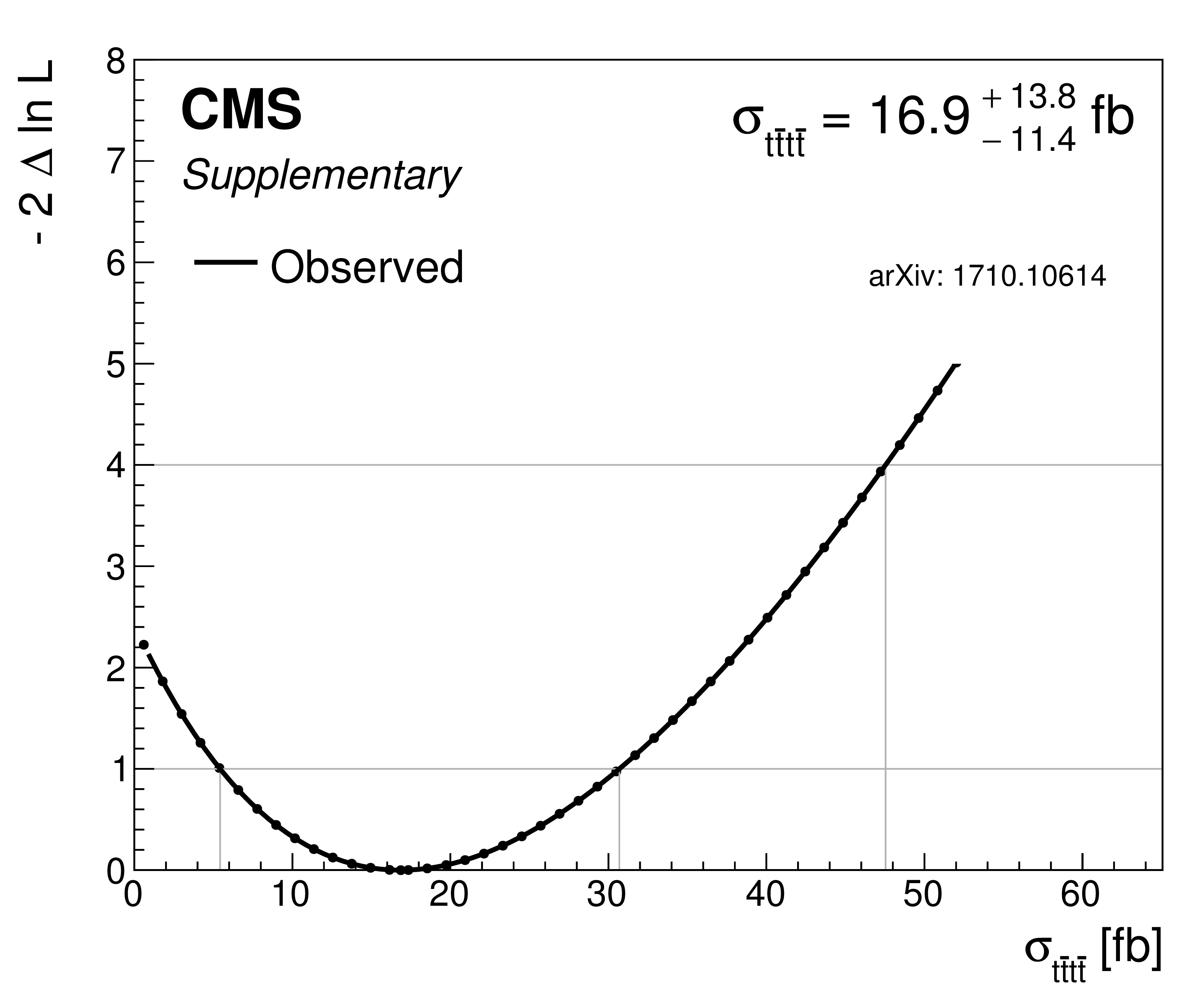
| Abstract: A search for standard model production of four top quarks (${\mathrm{t\bar{t}}\mathrm{t\bar{t}}} $) is reported using events containing at least three leptons (e, $\mu$) or a same-sign lepton pair. The events are produced in proton-proton collisions at a center-of-mass energy of 13 TeV at the LHC, and the data sample, recorded in 2016, corresponds to an integrated luminosity of 35.9 fb$^{-1}$. Jet multiplicity and flavor are used to enhance signal sensitivity, and dedicated control regions are used to constrain the dominant backgrounds. The observed and expected signal significances are, respectively, 1.6 and 1.0 standard deviations, and the ${\mathrm{t\bar{t}}\mathrm{t\bar{t}}} $ cross section is measured to be 16.9$^{+13.8}_{-11.4}$ fb, in agreement with next-to-leading-order standard model predictions. These results are also used to constrain the Yukawa coupling between the top quark and the Higgs boson to be less than 2.1 times its expected standard model value at 95% confidence level. | ||
| Links: e-print arXiv:1710.10614 [hep-ex] (PDF) ; CDS record ; inSPIRE record ; CADI line (restricted) ; | ||
| Figures & Tables | Summary | Additional Figures & Material | References | CMS Publications |
|---|
| Figures | |

png pdf |
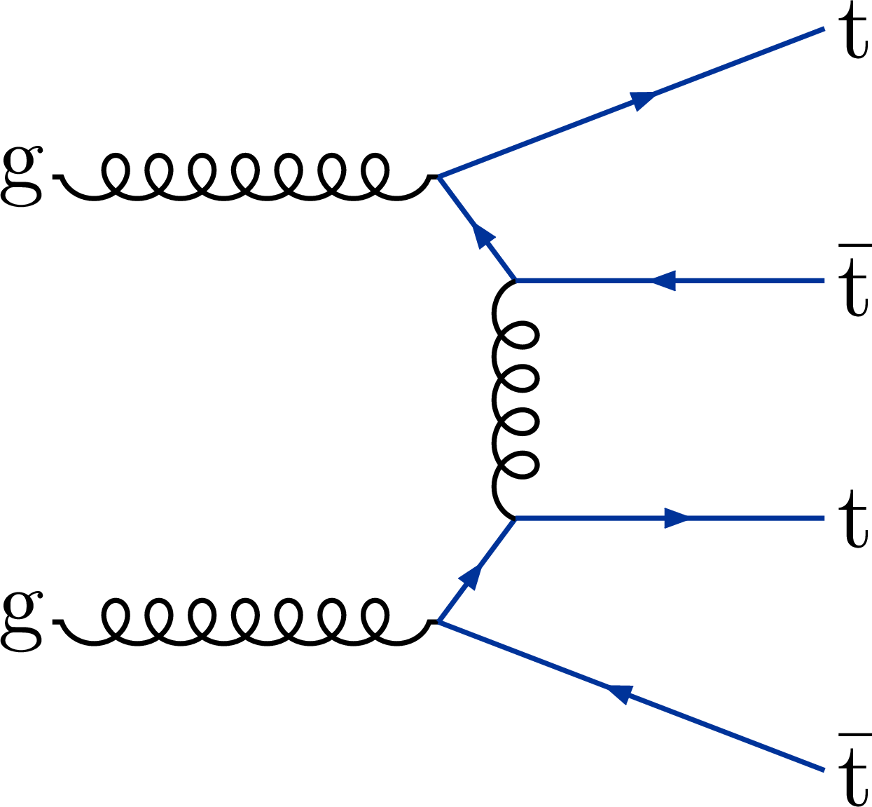
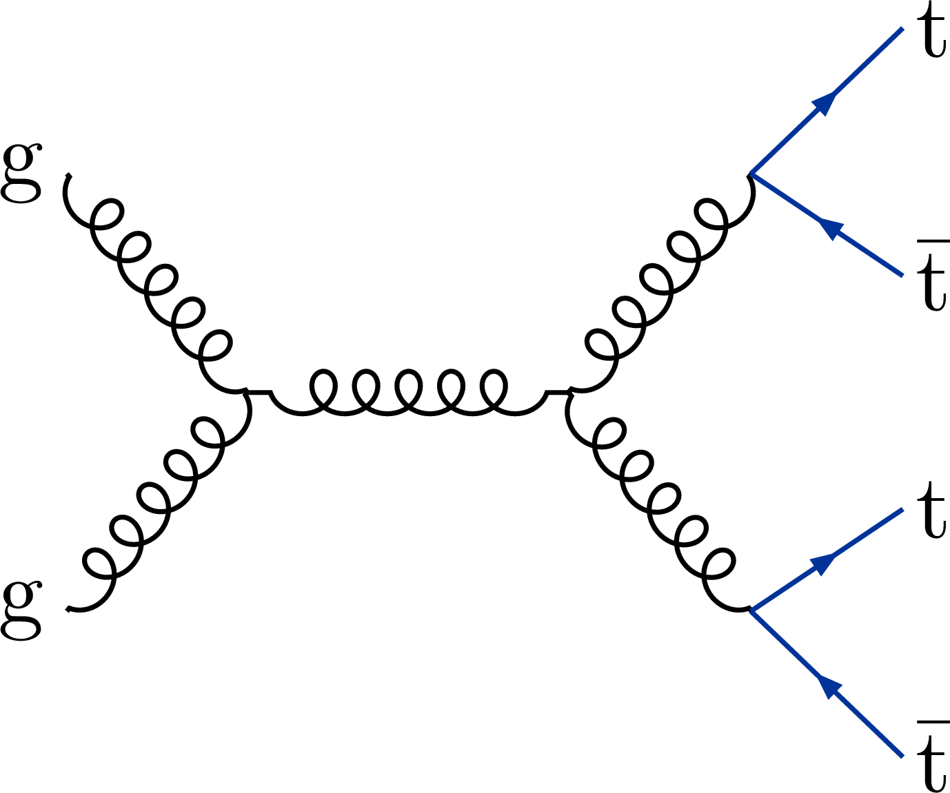
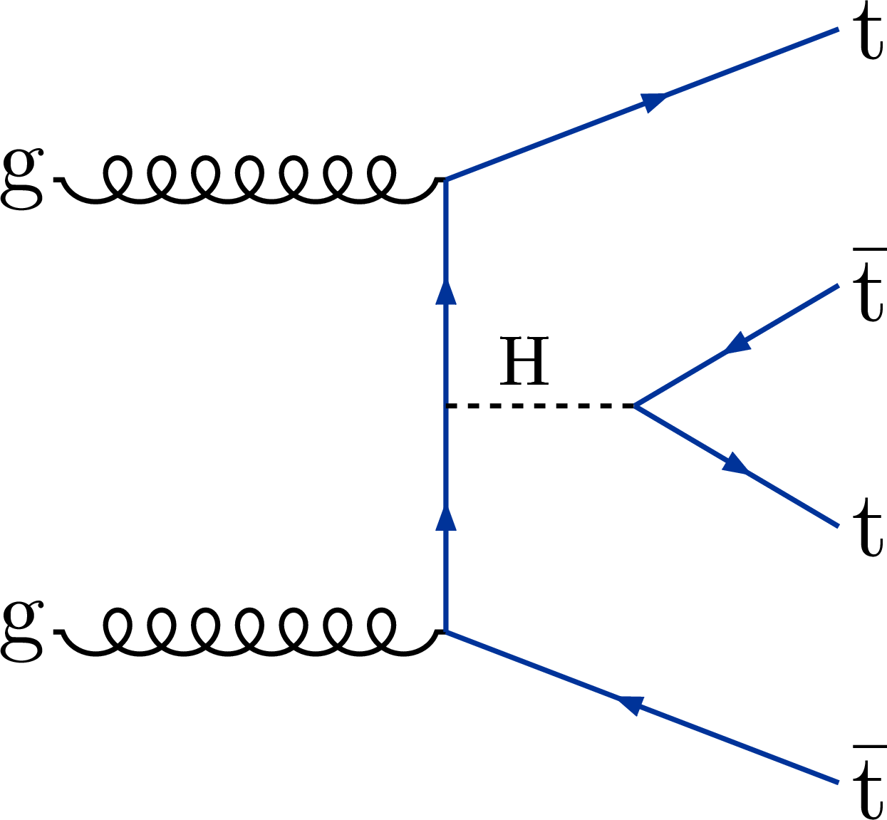
Figure 1:
Representative Feynman diagrams for ${{\mathrm{t} {}\mathrm{\bar{t}}} {\mathrm{t} {}\mathrm{\bar{t}}}} $ production at LO in the SM. |
png pdf |
Figure 1-a:
One representative Feynman diagram for ${{\mathrm{t} {}\mathrm{\bar{t}}} {\mathrm{t} {}\mathrm{\bar{t}}}} $ production at LO in the SM. |
png pdf |
Figure 1-b:
One representative Feynman diagram for ${{\mathrm{t} {}\mathrm{\bar{t}}} {\mathrm{t} {}\mathrm{\bar{t}}}} $ production at LO in the SM. |
png pdf |
Figure 1-c:
One representative Feynman diagram for ${{\mathrm{t} {}\mathrm{\bar{t}}} {\mathrm{t} {}\mathrm{\bar{t}}}} $ production at LO in the SM. |
png pdf |
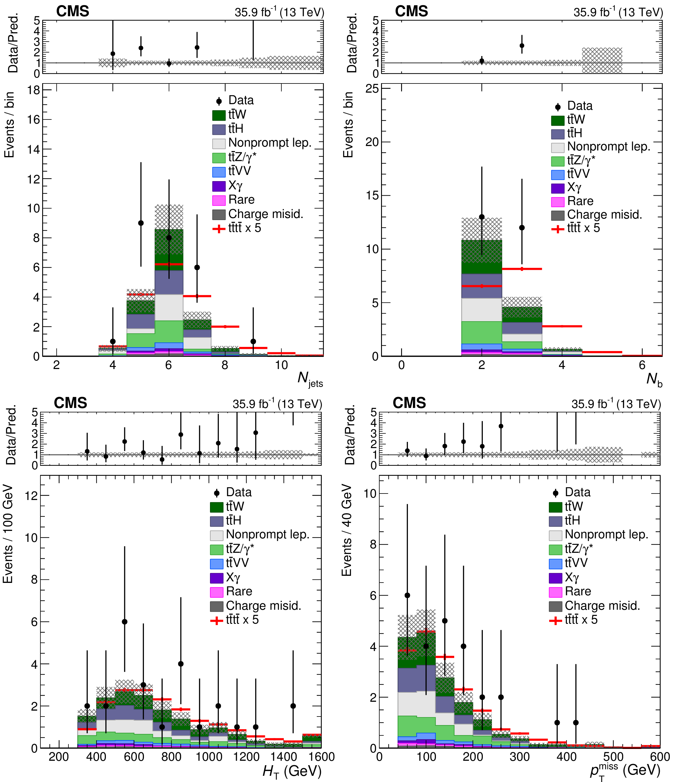
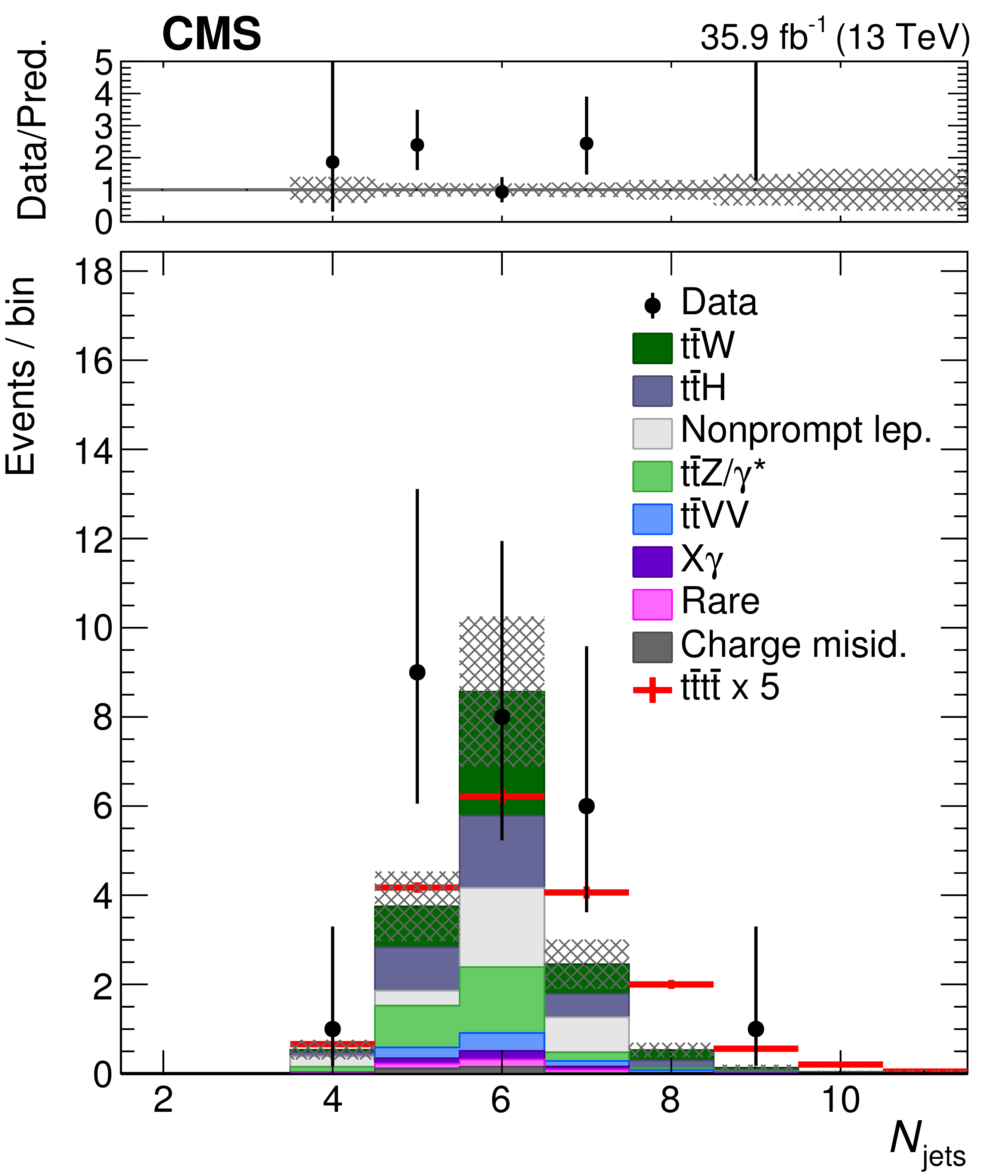
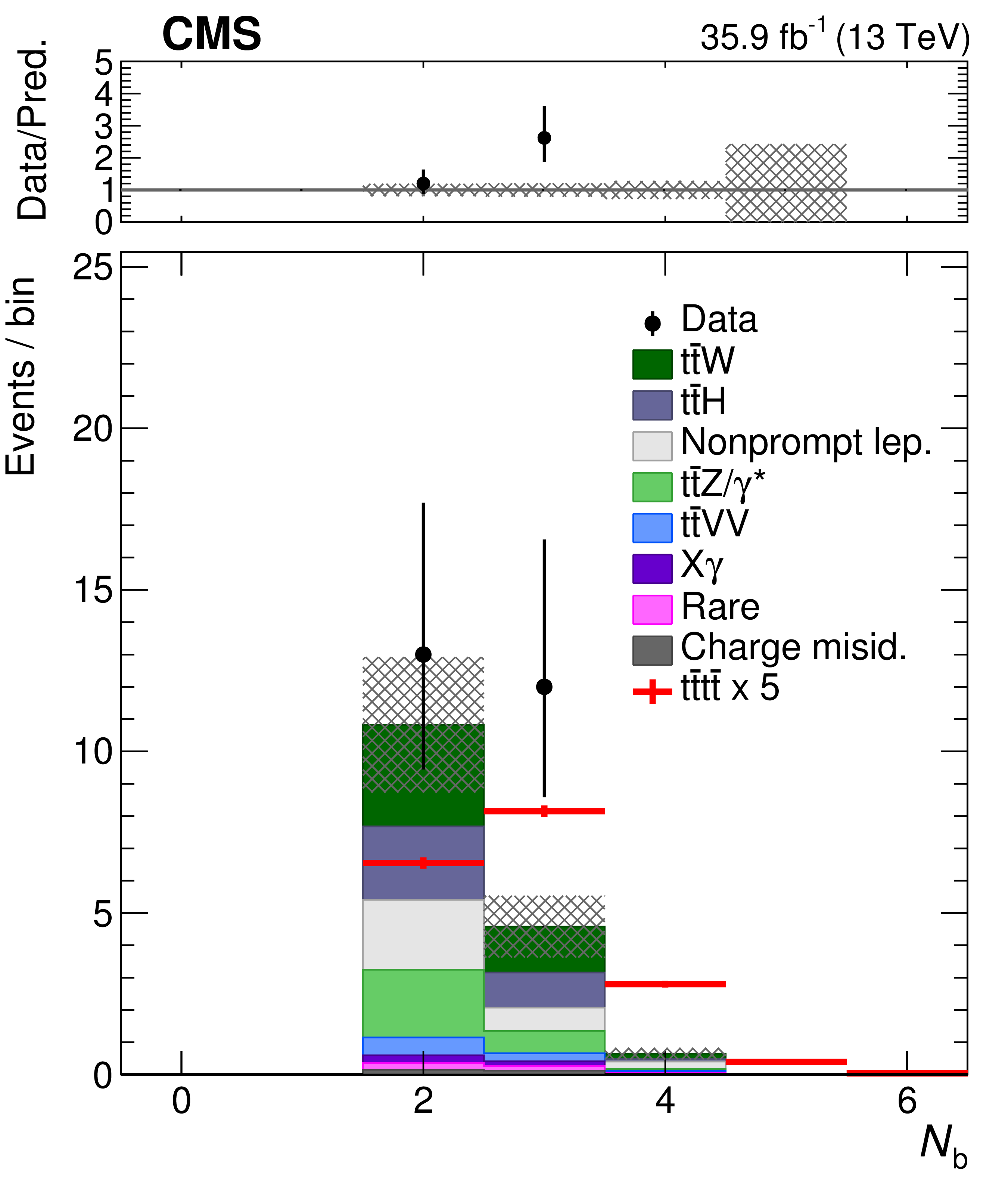
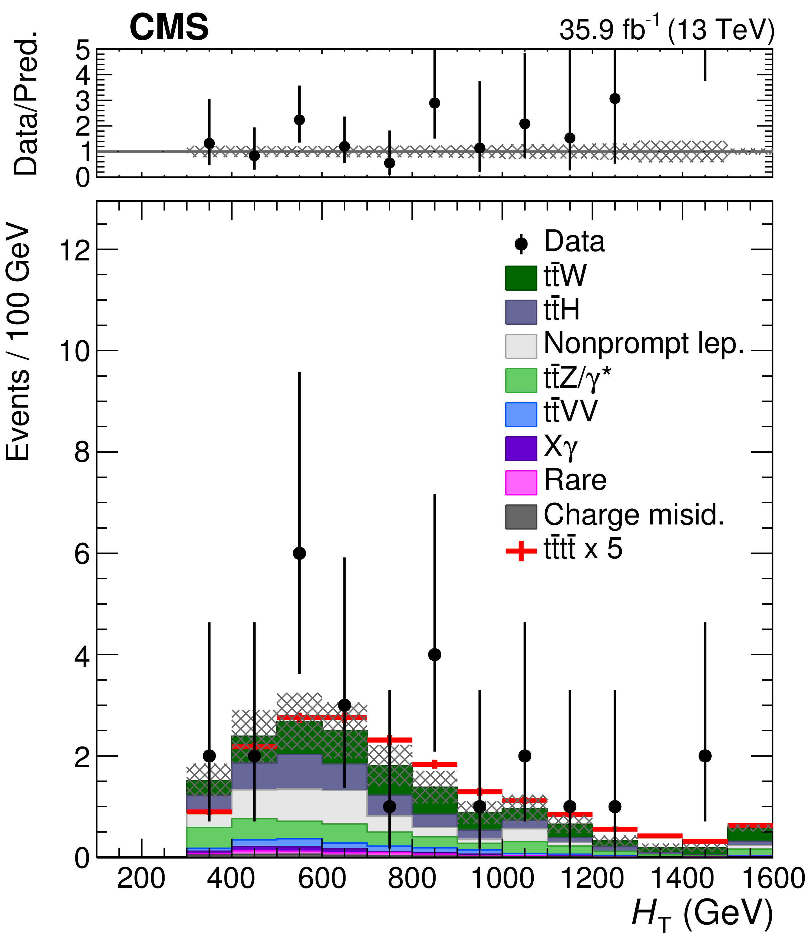
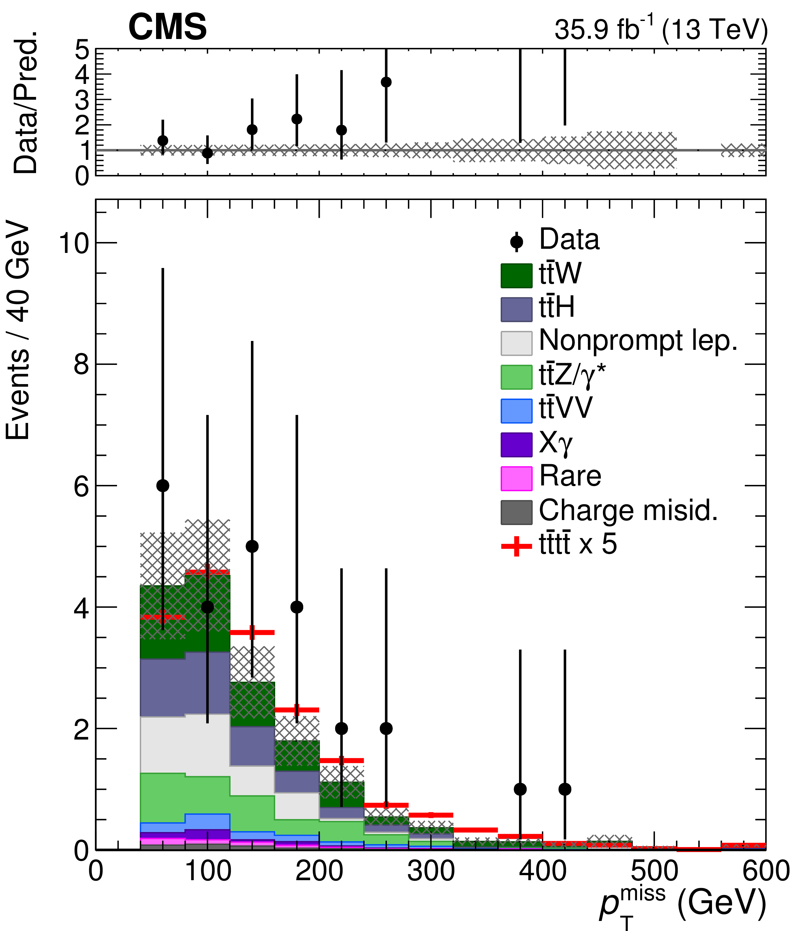
Figure 2:
Distributions in ${N_\text {jets}}$ (upper left), ${N_\text {b}}$ (upper right), ${H_{\mathrm {T}}}$ (lower left), and ${{p_{\mathrm {T}}} ^\text {miss}}$ (lower right) in the signal regions (SR1-8), before fitting to data, where the last bins include the overflows. The hatched areas represent the total uncertainties in the SM background predictions, while the solid lines represent the ${{\mathrm{t} {}\mathrm{\bar{t}}} {\mathrm{t} {}\mathrm{\bar{t}}}}$ signal, scaled up by a factor of 5, assuming the SM cross section from Ref. [17]. The upper panels show the ratios of the observed event yield to the total background prediction. Bins without a data point have no observed events. |
png pdf |
Figure 2-a:
Distribution in ${N_\text {jets}}$ in the signal regions (SR1-8), before fitting to data, where the last bins include the overflows. The hatched areas represent the total uncertainties in the SM background predictions, while the solid lines represent the ${{\mathrm{t} {}\mathrm{\bar{t}}} {\mathrm{t} {}\mathrm{\bar{t}}}}$ signal, scaled up by a factor of 5, assuming the SM cross section from Ref. [17]. The upper panel shows the ratios of the observed event yield to the total background prediction. Bins without a data point have no observed events. |
png pdf |
Figure 2-b:
Distribution in ${N_\text {b}}$ in the signal regions (SR1-8), before fitting to data, where the last bins include the overflows. The hatched areas represent the total uncertainties in the SM background predictions, while the solid lines represent the ${{\mathrm{t} {}\mathrm{\bar{t}}} {\mathrm{t} {}\mathrm{\bar{t}}}}$ signal, scaled up by a factor of 5, assuming the SM cross section from Ref. [17]. The upper panel shows the ratios of the observed event yield to the total background prediction. Bins without a data point have no observed events. |
png pdf |
Figure 2-c:
Distribution in ${H_{\mathrm {T}}}$ in the signal regions (SR1-8), before fitting to data, where the last bins include the overflows. The hatched areas represent the total uncertainties in the SM background predictions, while the solid lines represent the ${{\mathrm{t} {}\mathrm{\bar{t}}} {\mathrm{t} {}\mathrm{\bar{t}}}}$ signal, scaled up by a factor of 5, assuming the SM cross section from Ref. [17]. The upper panel shows the ratios of the observed event yield to the total background prediction. Bins without a data point have no observed events. |
png pdf |
Figure 2-d:
Distribution in ${{p_{\mathrm {T}}} ^\text {miss}}$ in the signal regions (SR1-8), before fitting to data, where the last bins include the overflows. The hatched areas represent the total uncertainties in the SM background predictions, while the solid lines represent the ${{\mathrm{t} {}\mathrm{\bar{t}}} {\mathrm{t} {}\mathrm{\bar{t}}}}$ signal, scaled up by a factor of 5, assuming the SM cross section from Ref. [17]. The upper panel shows the ratios of the observed event yield to the total background prediction. Bins without a data point have no observed events. |
png pdf |
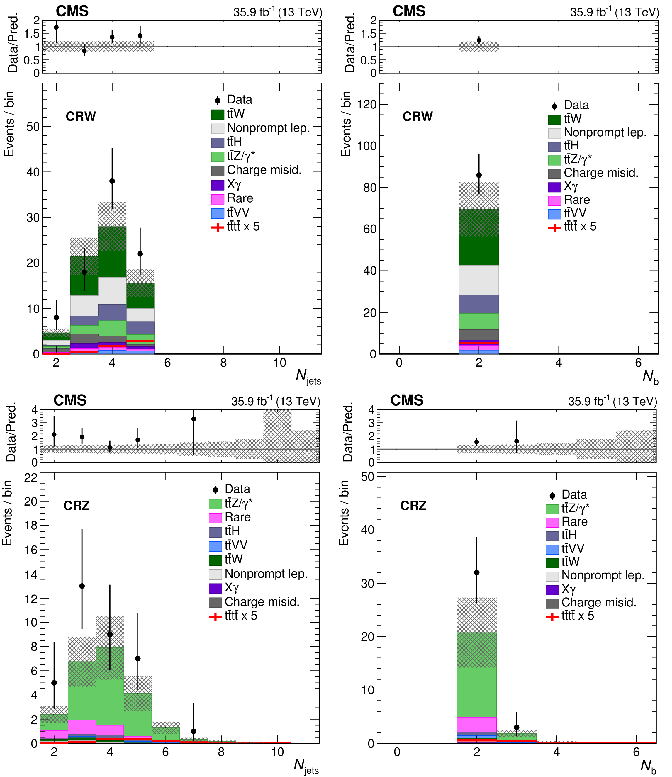
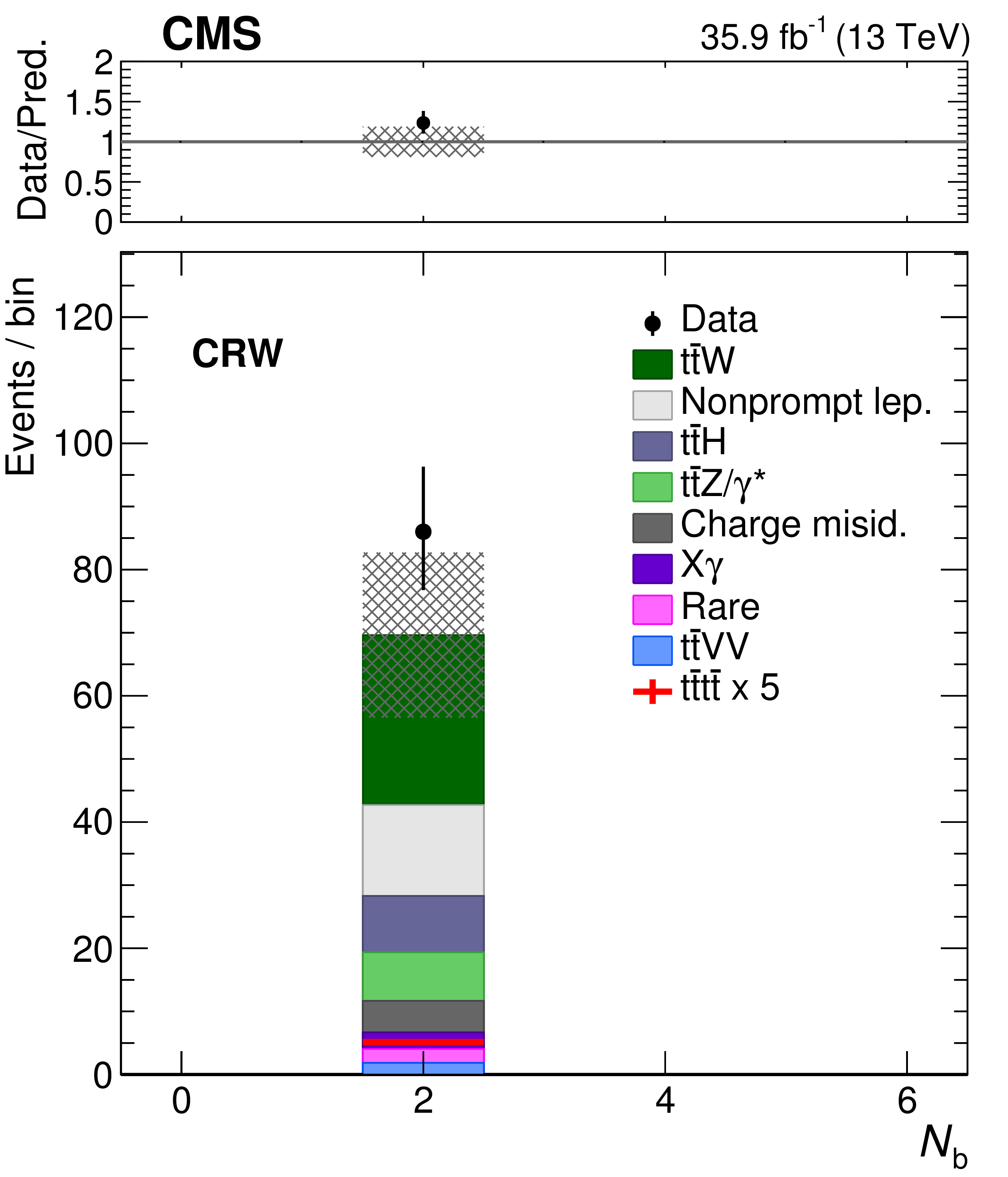
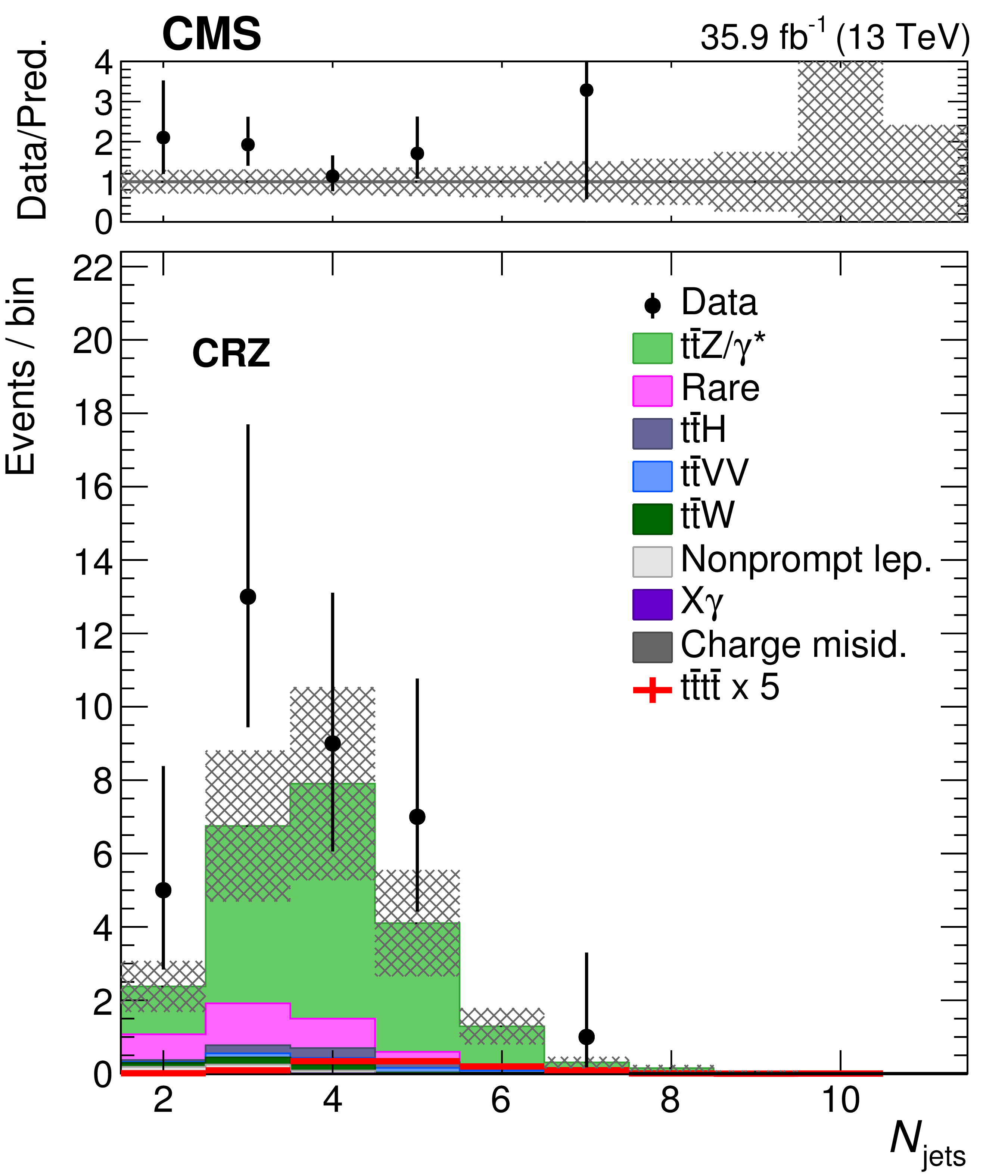
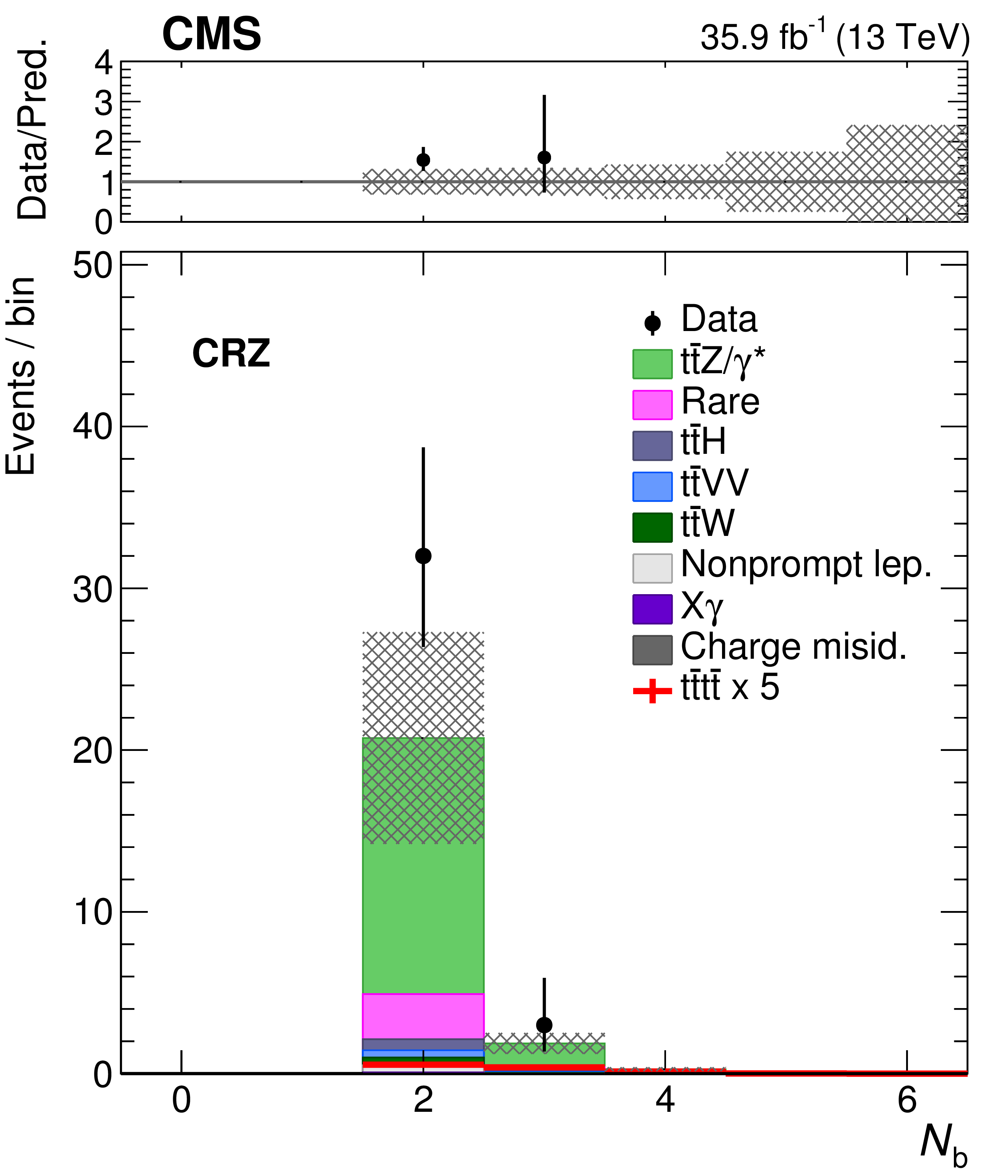
Figure 3:
Distributions in ${N_\text {jets}}$ and ${N_\text {b}}$ in ${{\mathrm{t} {}\mathrm{\bar{t}}} \mathrm{W}} $ (upper) and ${{\mathrm{t} {}\mathrm{\bar{t}}} \mathrm{Z}}$ (lower) control regions, before fitting to data. The hatched area represents the uncertainty in the SM background prediction, while the solid line represents the ${{\mathrm{t} {}\mathrm{\bar{t}}} {\mathrm{t} {}\mathrm{\bar{t}}}}$ signal, scaled up by a factor of 5, assuming the SM cross section from Ref. [17]. The upper panels show the ratios of the observed event yield to the total background prediction. Bins without a data point have no observed events. |

png pdf |
Figure 3-a:
Distribution in ${N_\text {jets}}$ in the ${{\mathrm{t} {}\mathrm{\bar{t}}} \mathrm{W}} $ control region, before fitting to data. The hatched area represents the uncertainty in the SM background prediction, while the solid line represents the ${{\mathrm{t} {}\mathrm{\bar{t}}} {\mathrm{t} {}\mathrm{\bar{t}}}}$ signal, scaled up by a factor of 5, assuming the SM cross section from Ref. [17]. The upper panel shows the ratios of the observed event yield to the total background prediction. Bins without a data point have no observed events. |
png pdf |
Figure 3-b:
Distribution in ${N_\text {b}}$ in the ${{\mathrm{t} {}\mathrm{\bar{t}}} \mathrm{Z}}$ control region, before fitting to data. The hatched area represents the uncertainty in the SM background prediction, while the solid line represents the ${{\mathrm{t} {}\mathrm{\bar{t}}} {\mathrm{t} {}\mathrm{\bar{t}}}}$ signal, scaled up by a factor of 5, assuming the SM cross section from Ref. [17]. The upper panel shows the ratios of the observed event yield to the total background prediction. Bins without a data point have no observed events. |
png pdf |
Figure 3-c:
Distribution in ${N_\text {jets}}$ in the ${{\mathrm{t} {}\mathrm{\bar{t}}} \mathrm{W}} $ control region, before fitting to data. The hatched area represents the uncertainty in the SM background prediction, while the solid line represents the ${{\mathrm{t} {}\mathrm{\bar{t}}} {\mathrm{t} {}\mathrm{\bar{t}}}}$ signal, scaled up by a factor of 5, assuming the SM cross section from Ref. [17]. The upper panel shows the ratios of the observed event yield to the total background prediction. Bins without a data point have no observed events. |
png pdf |
Figure 3-d:
Distribution in ${N_\text {b}}$ in the ${{\mathrm{t} {}\mathrm{\bar{t}}} \mathrm{Z}}$ control region, before fitting to data. The hatched area represents the uncertainty in the SM background prediction, while the solid line represents the ${{\mathrm{t} {}\mathrm{\bar{t}}} {\mathrm{t} {}\mathrm{\bar{t}}}}$ signal, scaled up by a factor of 5, assuming the SM cross section from Ref. [17]. The upper panel shows the ratios of the observed event yield to the total background prediction. Bins without a data point have no observed events. |

png pdf |
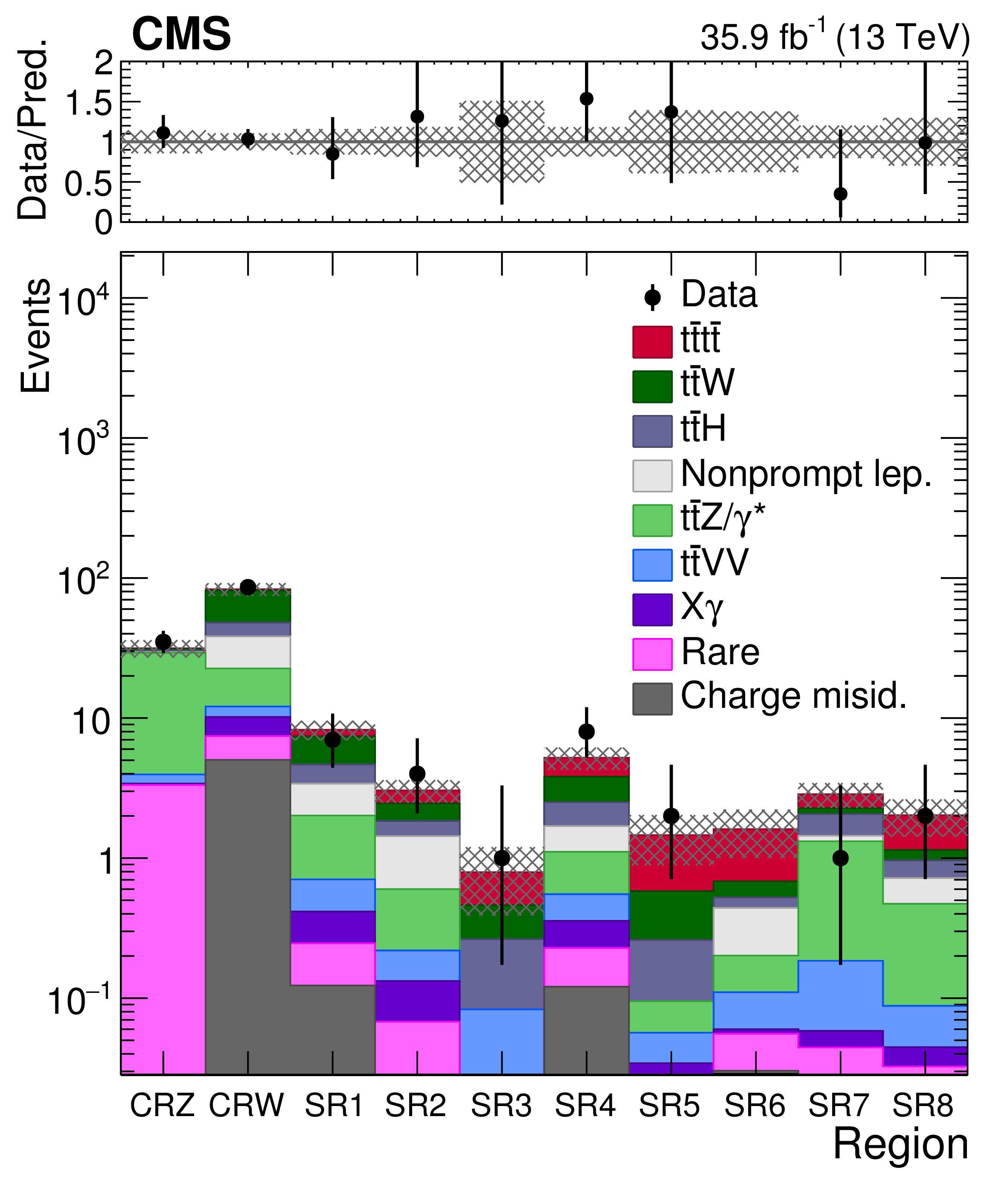
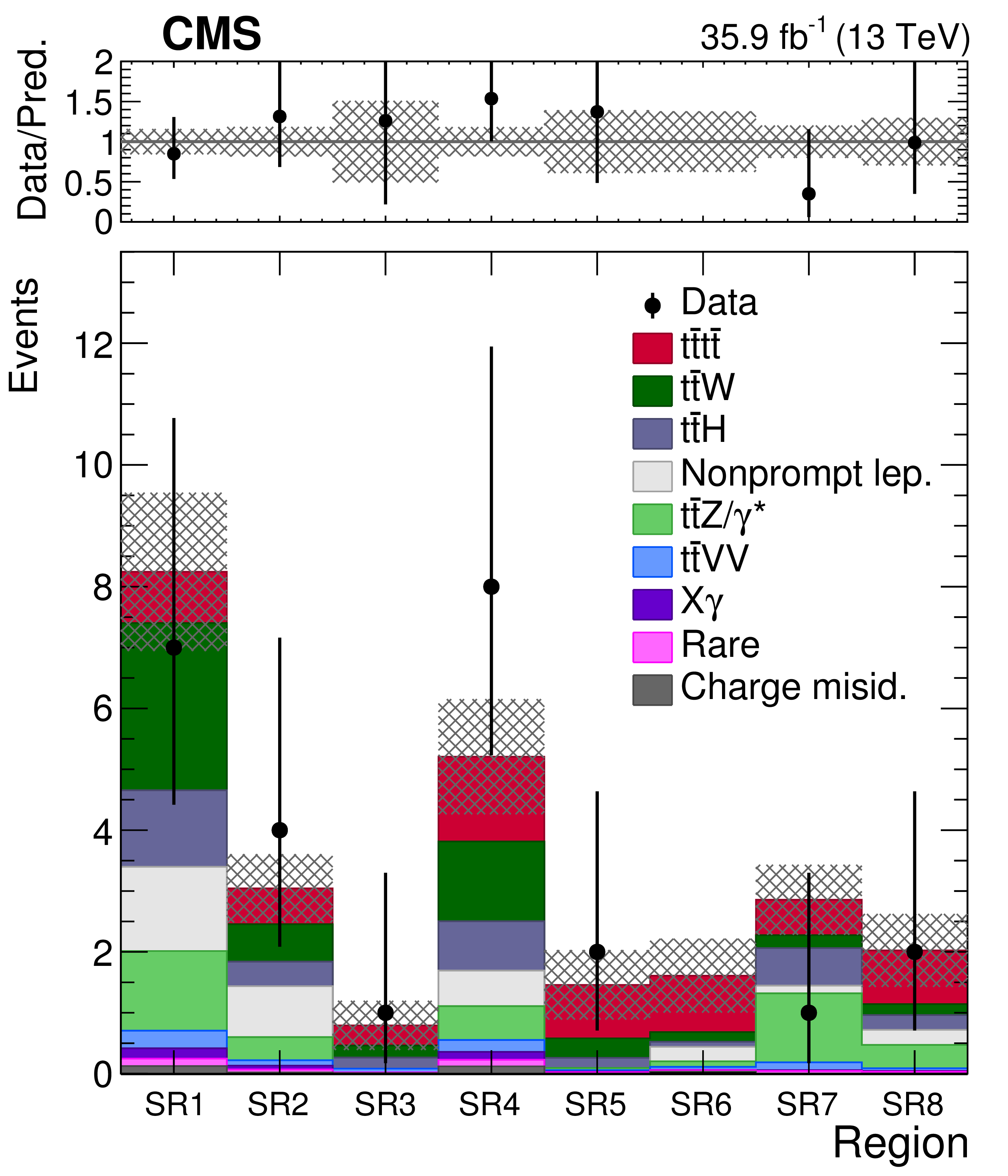
Figure 4:
Observed yields in the control and signal regions (left, in log scale), and signal regions only (right, in linear scale), compared to the post-fit predictions for signal and background processes. The hatched areas represent the total uncertainties in the signal and background predictions. The upper panels show the ratios of the observed event yield and the total prediction of signal and background. |
png pdf |
Figure 4-a:
Observed yields in the control and signal regions (in log scale), compared to the post-fit predictions for signal and background processes. The hatched areas represent the total uncertainties in the signal and background predictions. The upper panel shows the ratios of the observed event yield and the total prediction of signal and background. |
png pdf |
Figure 4-b:
Observed yields in the signal regions only (in linear scale), compared to the post-fit predictions for signal and background processes. The hatched areas represent the total uncertainties in the signal and background predictions. The upper panel shows the ratios of the observed event yield and the total prediction of signal and background. |

png pdf |
Figure 5:
The predicted SM value of ${\sigma ({\mathrm{p}} {\mathrm{p}} \to {{\mathrm{t} {}\mathrm{\bar{t}}} {\mathrm{t} {}\mathrm{\bar{t}}}}}) $ [16], calculated at LO with an NLO/LO $K$-factor of 1.27, as a function of $ {< y_{\mathrm{t}}/y_{\mathrm{t}}^{\mathrm {SM}} >}$ (dashed line), compared with the observed value of ${\sigma ({\mathrm{p}} {\mathrm{p}} \to {{\mathrm{t} {}\mathrm{\bar{t}}} {\mathrm{t} {}\mathrm{\bar{t}}}}})$ (solid line), and with the observed 95% CL upper limit (hatched line). |
| Tables | |

png pdf |
Table 1:
Kinematic requirements for leptons and jets. |
png pdf |
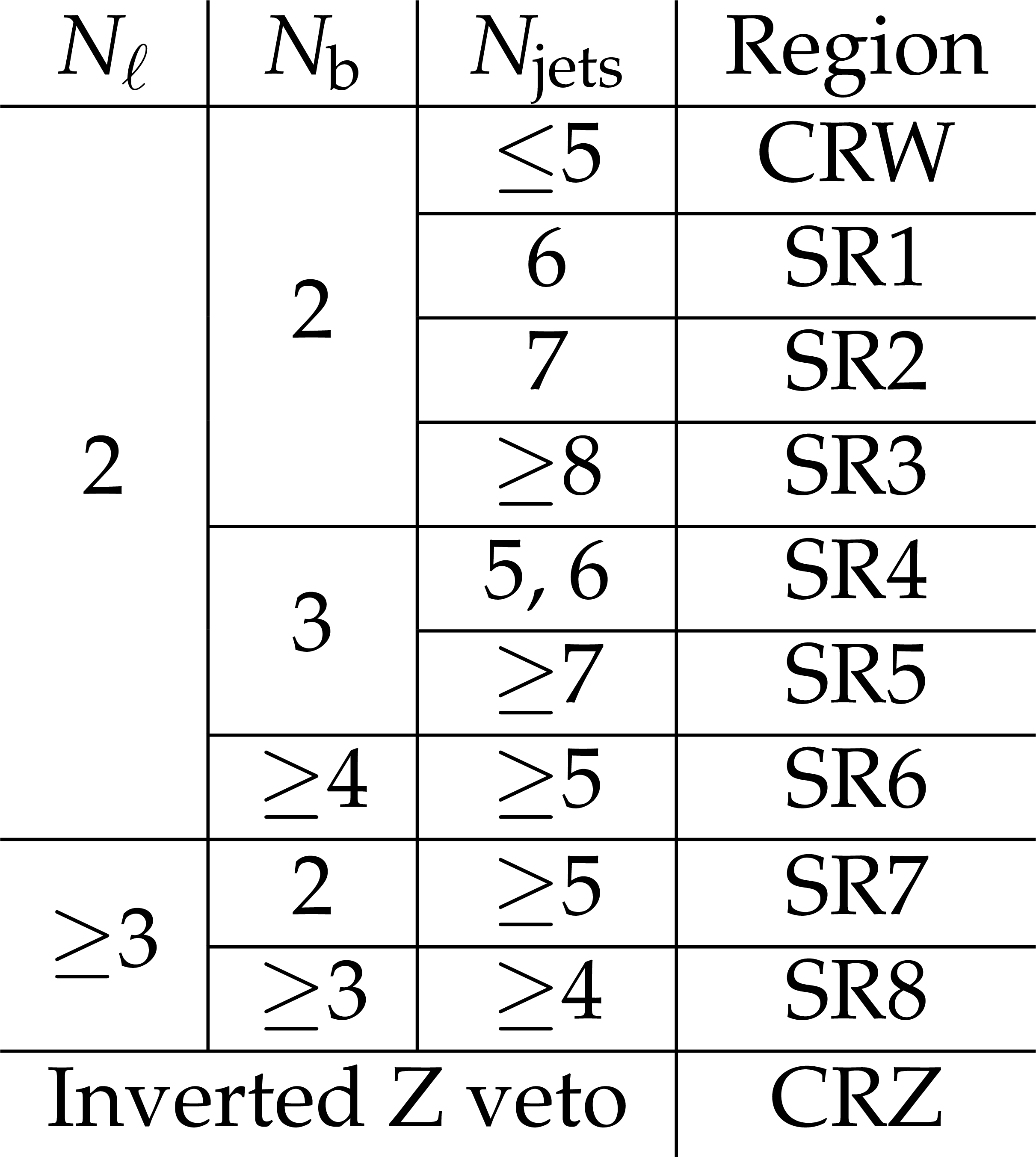
Table 2:
Definitions of the eight SRs and the two control regions for ${{\mathrm{t} {}\mathrm{\bar{t}}} \mathrm{W}}$ (CRW) and ${{\mathrm{t} {}\mathrm{\bar{t}}} \mathrm{Z}}$ (CRZ). |
png pdf |
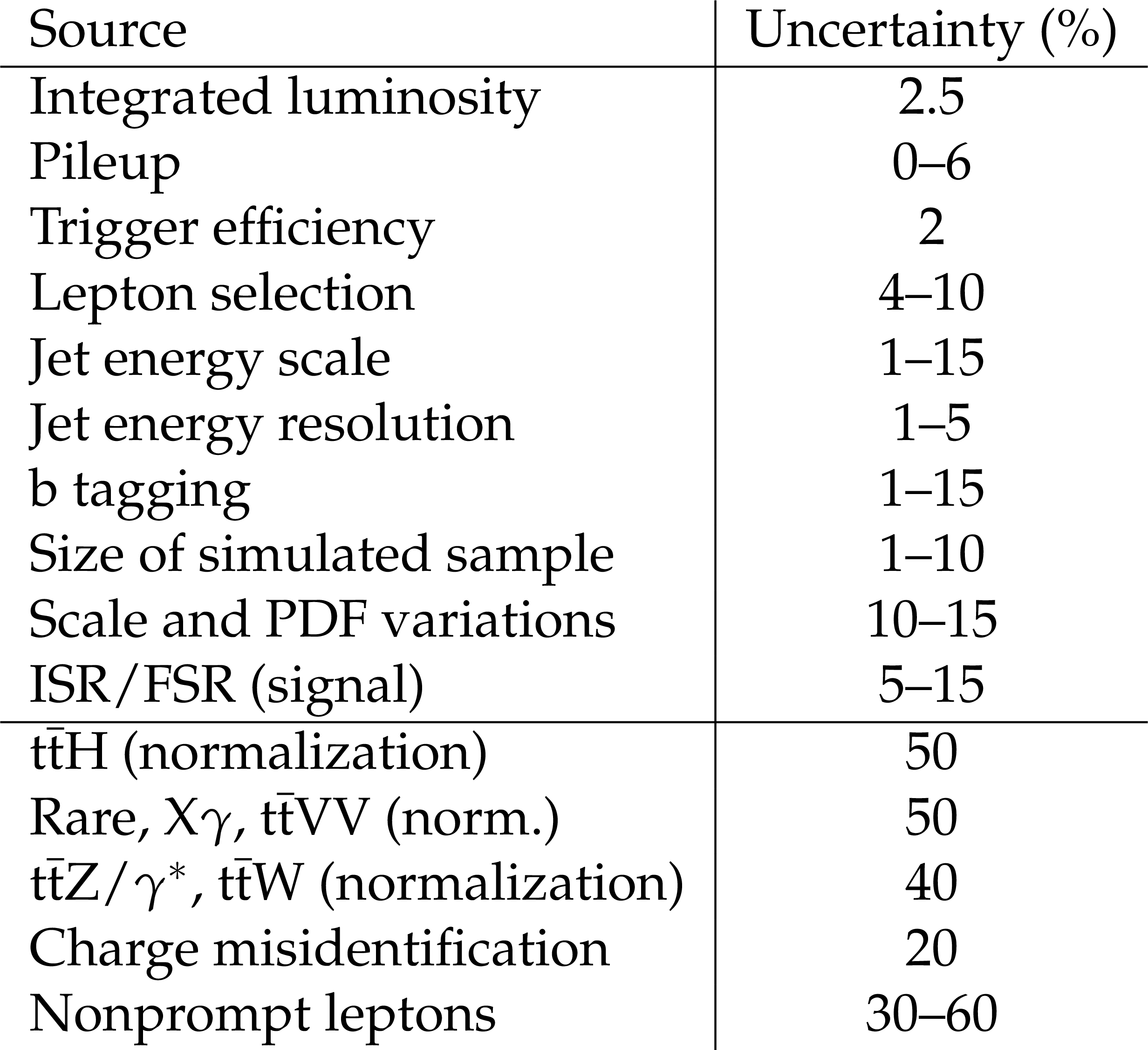
Table 3:
Summary of the sources of uncertainty and their effect on signal and background yields. The first group lists experimental and theoretical uncertainties in simulated signal and background processes. The second group lists normalization uncertainties in the estimated backgrounds. |
png pdf |
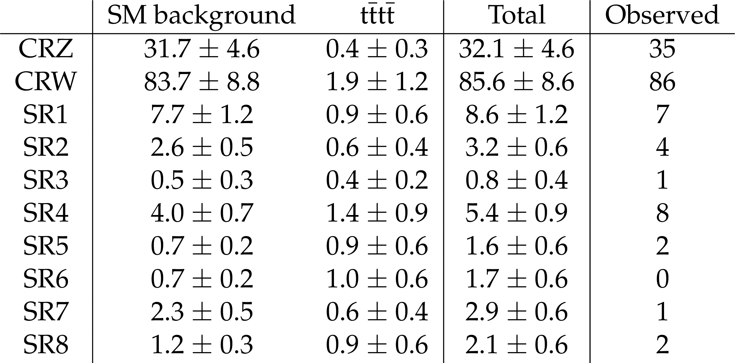
Table 4:
The post-fit background, signal, and total yields with their total uncertainties and the observed number of events in the control and signal regions in data. |
| Summary |
| The results of a search for standard model (SM) production of ${\mathrm{t\bar{t}}\mathrm{t\bar{t}}} $ at the LHC have been presented, using data from $\sqrt{s} = $ 13 TeV proton-proton collisions corresponding to an integrated luminosity of 35.9 fb$^{-1}$, collected with the CMS detector in 2016. The analysis strategy uses same-sign dilepton as well as three- (or more) lepton events, relying on jet multiplicity and jet flavor to define search regions that are used to probe the ${\mathrm{t\bar{t}}\mathrm{t\bar{t}}} $ process. Combining these regions yields a significance of 1.6 standard deviations relative to the background-only hypothesis, and a measured value for the ${\mathrm{t\bar{t}}\mathrm{t\bar{t}}} $ cross section of 16.9$^{+13.8}_{-11.4}$ fb, in agreement with the standard model predictions. The results are also re-interpreted to constrain the ratio of the top quark Yukawa coupling to its SM value, $ | y_{\mathrm{t}}/y_{\mathrm{t}}^{\mathrm{SM}} | < $ 2.1 at 95% confidence level. |
| Additional Figures | |
png pdf |
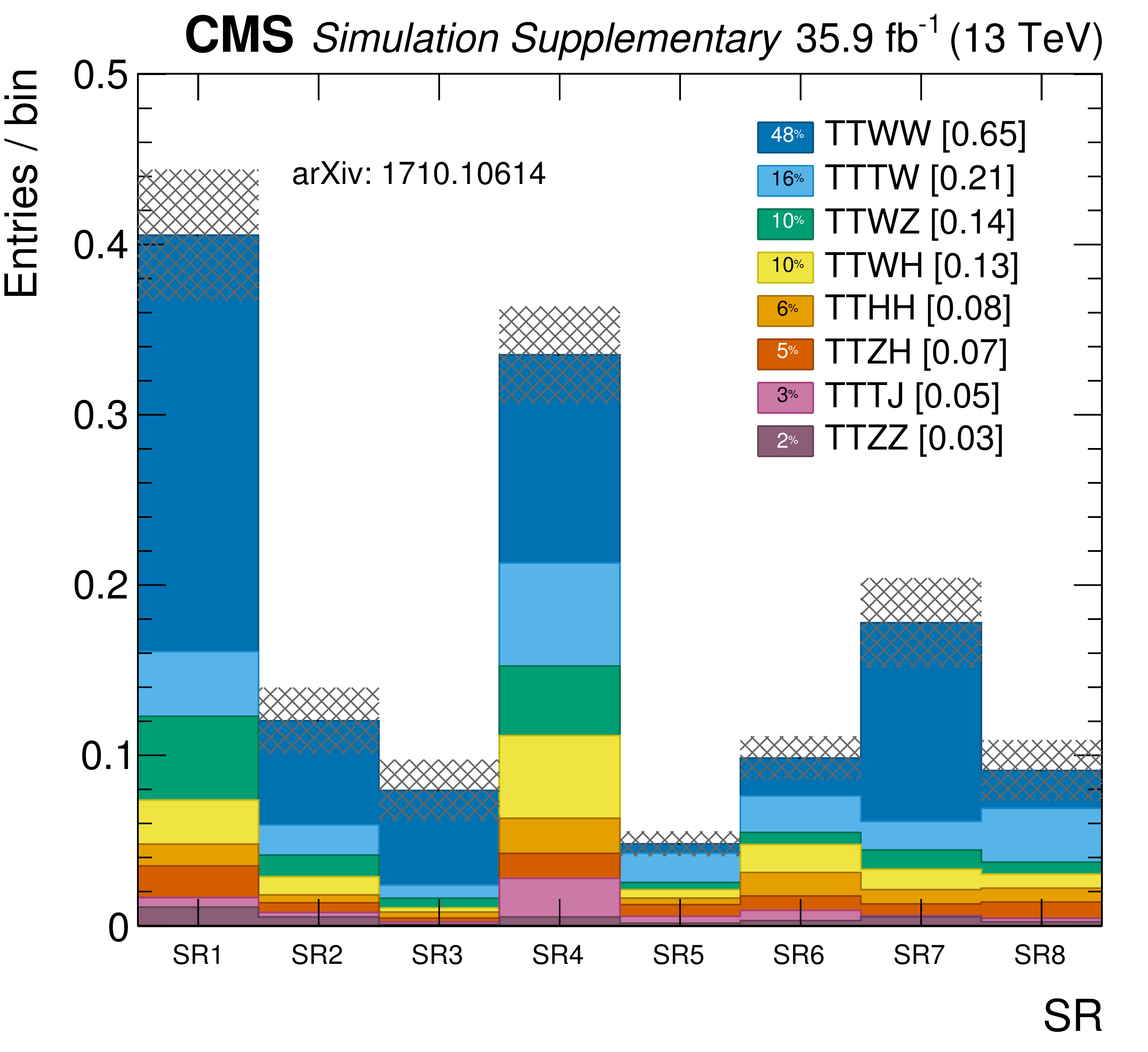
Additional Figure 1:
Detailed signal region yields for the "${\mathrm{t} {}\mathrm{\bar{t}}} \mathrm {VV}$'' backgrounds. The numbers in the legend boxes represent the relative fraction of each component and the hatched area represents the total uncertainty in the background prediction. |

png pdf |
Additional Figure 2:
True flavor of b-tagged jets in ${{\mathrm{t} {}\mathrm{\bar{t}}} \mathrm{W}}$ events with two or more b-tagged jets. |
png pdf |
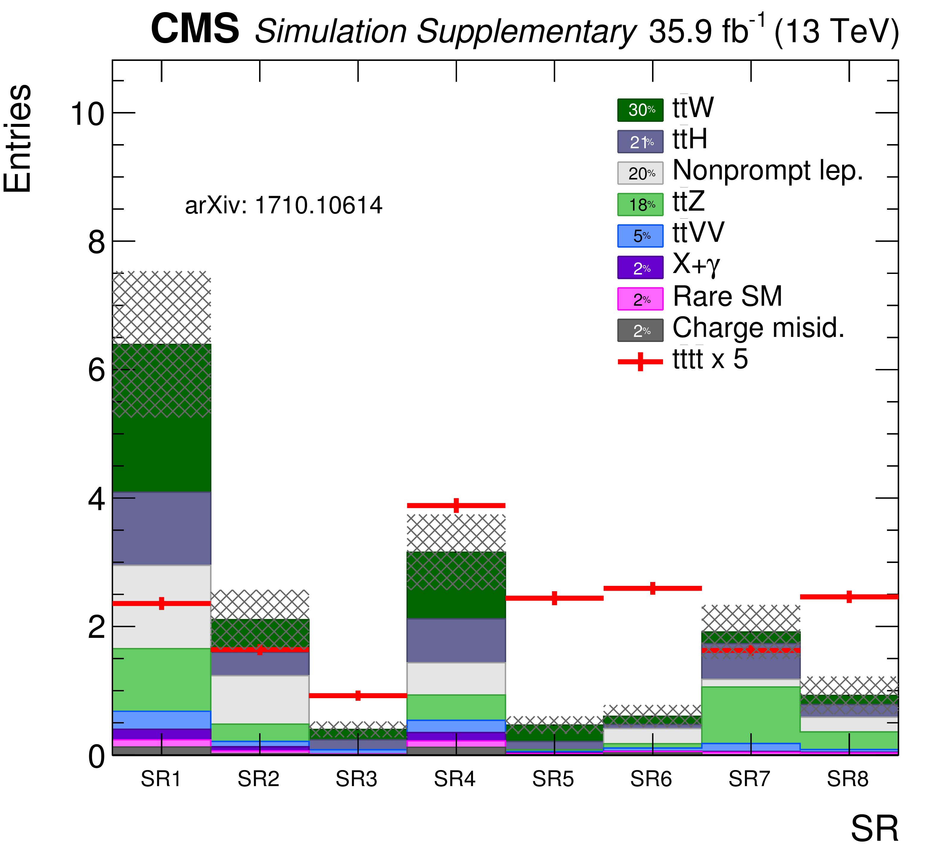
Additional Figure 3:
Signal and background predicted yields in the signal regions before the maximum-likelihood fit (pre-fit). The numbers in the legend boxes represent the relative fraction of each component and the hatched area represents the total uncertainty in the background prediction. |

png pdf |
Additional Figure 4:
Data compared to predicted signal and background yields in the signal regions before the maximum-likelihood fit (pre-fit). The numbers in the legend boxes represent the relative fraction of each component and the hatched area represents the total uncertainty in the background prediction. |
png pdf |
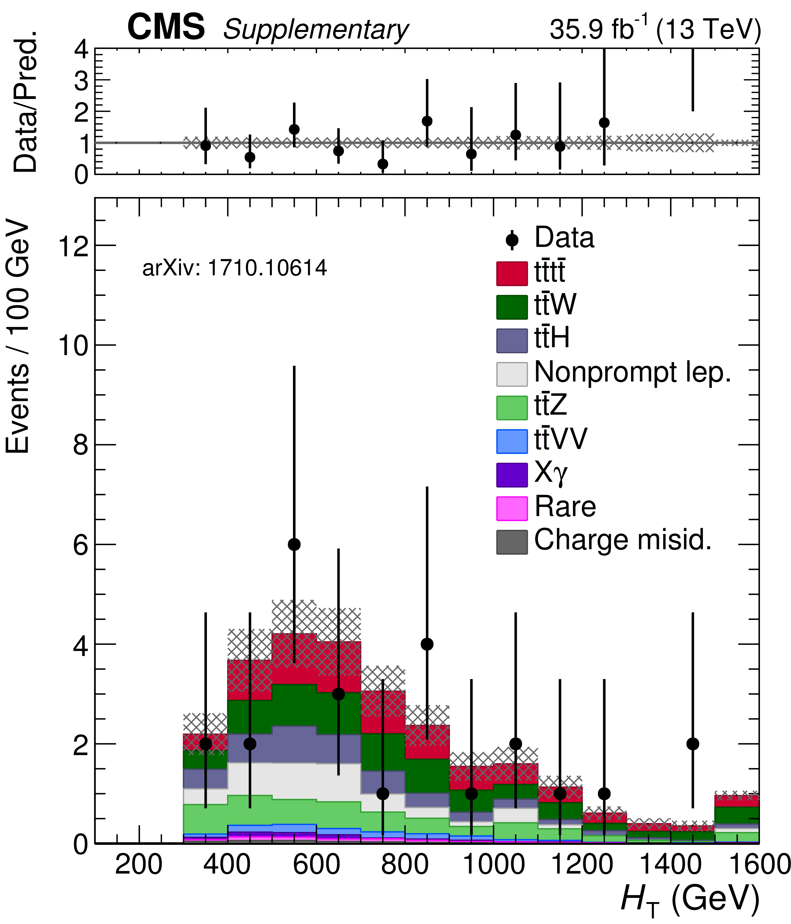
Additional Figure 5:
Distribution in ${H_{\mathrm {T}}} $ in the signal regions (SR 1-8) after fitting to data (post-fit), where the last bin includes the overflow. The hatched area represents the total uncertainty in the SM background prediction, and the signal is stacked. The upper panel shows the ratio of he observed event yield to the total prediction. Bins without a data point have no observed events. |
png pdf |
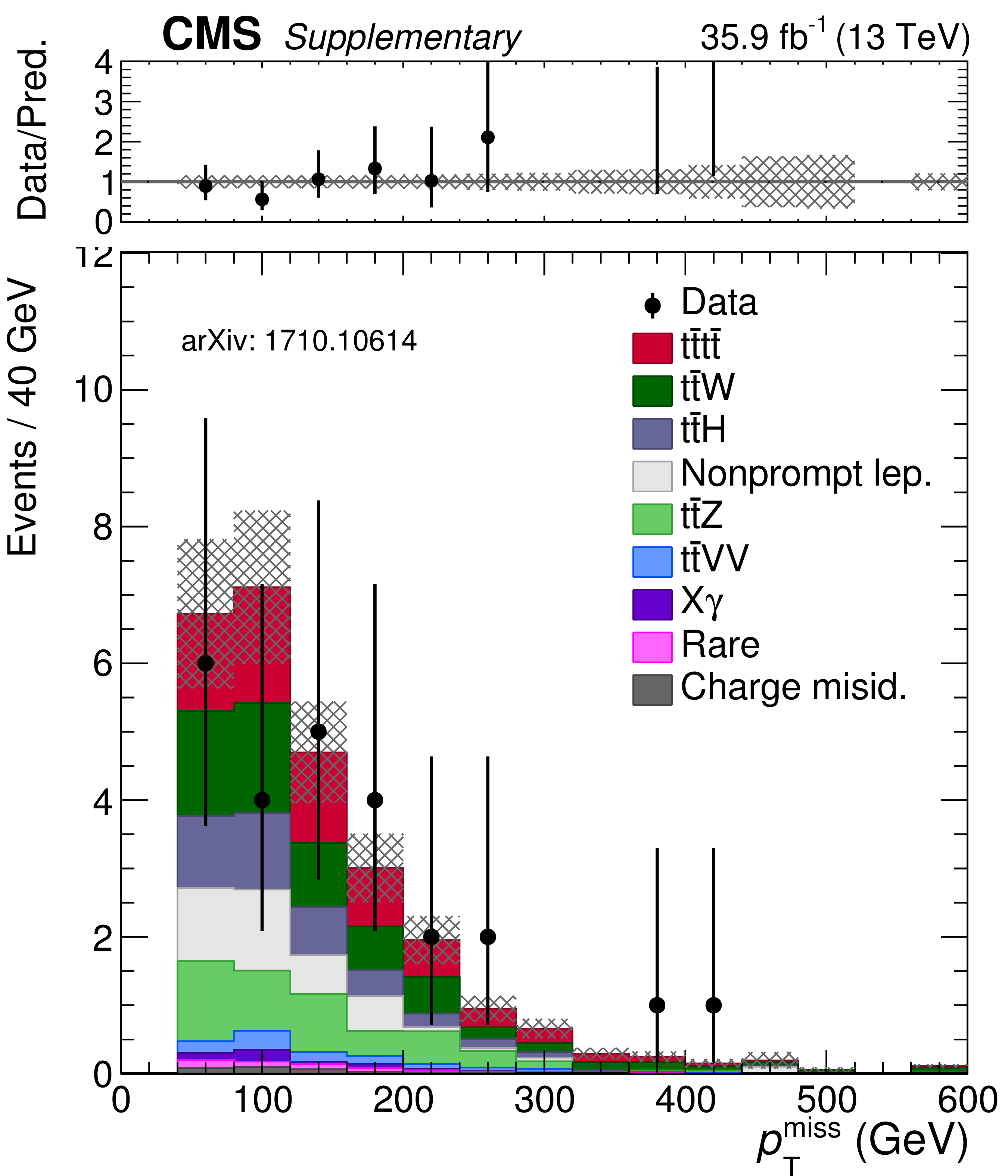
Additional Figure 6:
Distribution in missing transverse momentum in the signal regions (SR 1-8) after fitting to data (post-fit), where the last bin includes the overflow. The hatched area represents the total uncertainty in the SM background prediction, and the signal is stacked. The upper panel shows the ratio of he observed event yield to the total prediction. Bins without a data point have no observed events. |
png pdf |
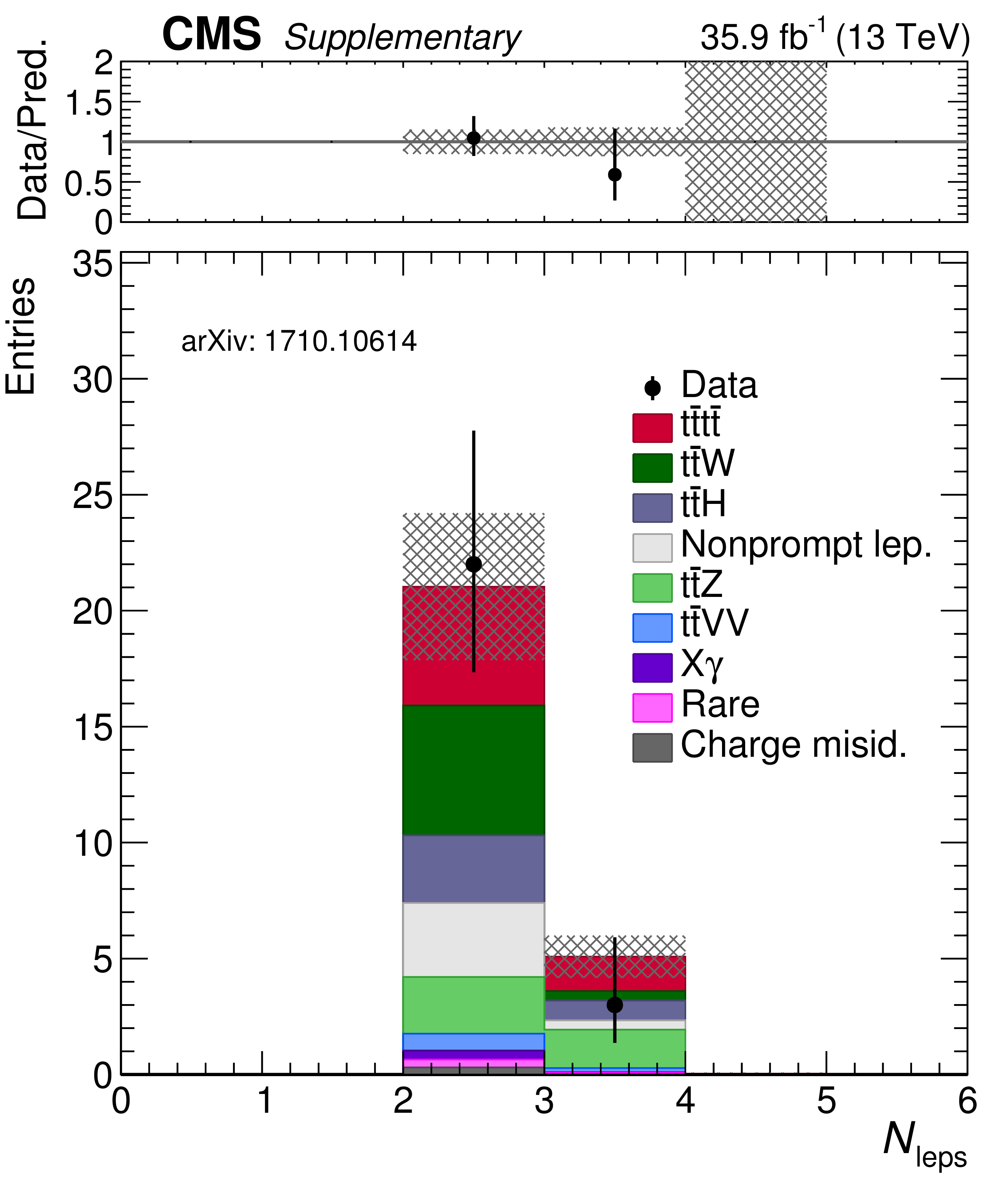
Additional Figure 7:
Distribution in number of leptons in the signal regions (SR 1-8) after fitting to data (post-fit), where the last bin includes the overflow. The hatched area represents the total uncertainty in the SM background prediction, and the signal is stacked. The upper panel shows the ratio of he observed event yield to the total prediction. Bins without a data point have no observed events. |

png pdf |
Additional Figure 8:
Distribution in number of jets in the signal regions (SR 1-8) after fitting to data (post-fit), where the last bin includes the overflow. The hatched area represents the total uncertainty in the SM background prediction, and the signal is stacked. The upper panel shows the ratio of he observed event yield to the total prediction. Bins without a data point have no observed events. |

png pdf |
Additional Figure 9:
Distribution in number of b-tagged jets in the signal regions (SR 1-8) after fitting to data (post-fit), where the last bin includes the overflow. The hatched area represents the total uncertainty in the SM background prediction, and the signal is stacked. The upper panel shows the ratio of he observed event yield to the total prediction. Bins without a data point have no observed events. |

png pdf |
Additional Figure 10:
Distribution in lepton flavor in the signal regions (SR 1-8) after fitting to data (post-fit), where the last bin includes the overflow. The hatched area represents the total uncertainty in the SM background prediction, and the signal is stacked. The upper panel shows the ratio of he observed event yield to the total prediction. Bins without a data point have no observed events. |
png pdf |
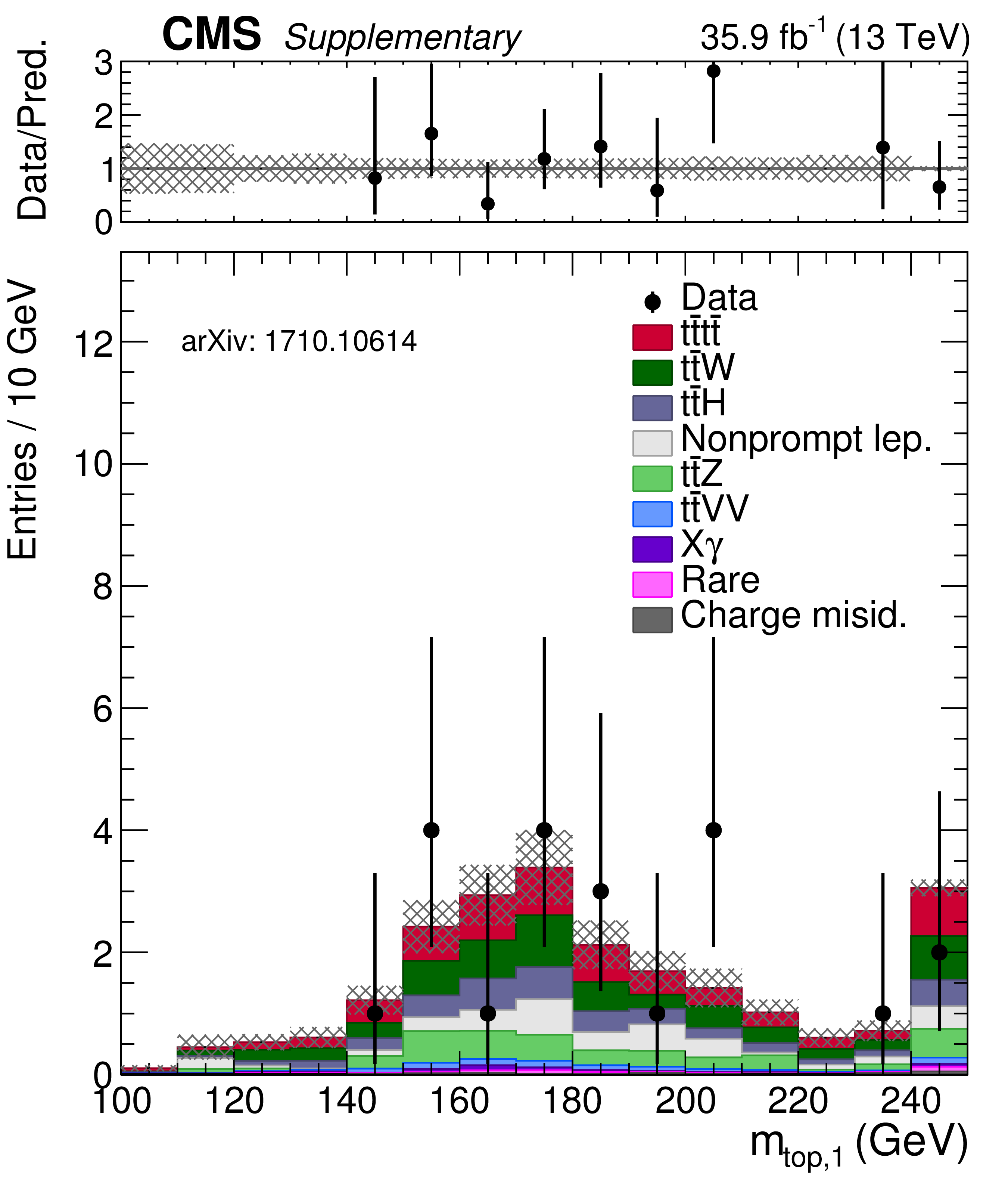
Additional Figure 11:
Distribution in the mass of the leading hadronic top quark candidate, based on $\chi ^2$ compatibility of three jets, of which one b-tagged, with a top quark and a W boson. The mass is shown in the signal regions (SR 1-8) after fitting to data (post-fit), where the last bin includes the overflow. The hatched area represents the total uncertainty in the SM background prediction, and the signal is stacked. The upper panel shows the ratio of he observed event yield to the total prediction. Bins without a data point have no observed events. |
png pdf |
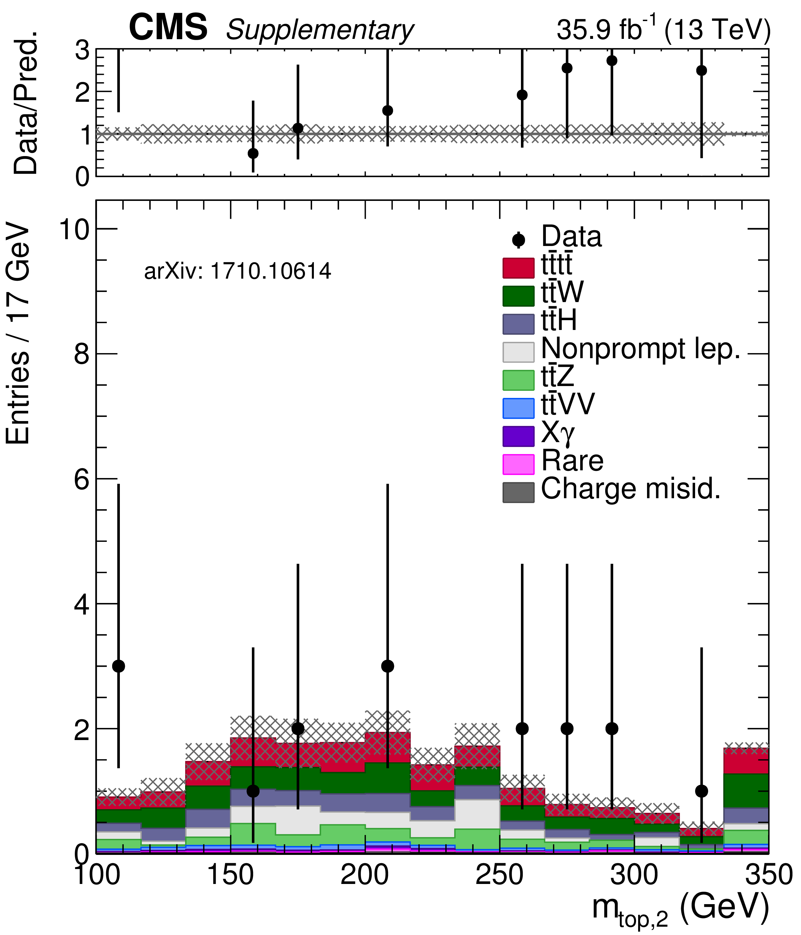
Additional Figure 12:
Distribution in the mass of the second leading hadronic top quark candidate, based on $\chi ^2$ compatibility of three jets, of which one b-tagged, with a top quark and a W boson. The mass is shown in the signal regions (SR 1-8) after fitting to data (post-fit), where the last bin includes the overflow. The hatched area represents the total uncertainty in the SM background prediction, and the signal is stacked. The upper panel shows the ratio of he observed event yield to the total prediction. Bins without a data point have no observed events. |
png pdf |
Additional Figure 13:
Likelihood scan corresponding to the cross-section measurement. |
| Additional Material: Data Cards |
|
MadGraph (MG5_aMC_v2.2.2) cards used to make the four top signal can be found at: param card, run card, proc card, and madspin card. The corresponding Pythia 8.212 parameters for this sample are listed here. |
| References | ||||
| 1 | P. Ramond | Dual theory for free fermions | PRD 3 (1971) 2415 | |
| 2 | Y. A. Gol'fand and E. P. Likhtman | Extension of the algebra of Poincar$ \'e $ group generators and violation of P invariance | JEPTL 13 (1971)323 | |
| 3 | A. Neveu and J. H. Schwarz | Factorizable dual model of pions | NPB 31 (1971) 86 | |
| 4 | D. V. Volkov and V. P. Akulov | Possible universal neutrino interaction | JEPTL 16 (1972)438 | |
| 5 | J. Wess and B. Zumino | A lagrangian model invariant under supergauge transformations | PLB 49 (1974) 52 | |
| 6 | J. Wess and B. Zumino | Supergauge transformations in four-dimensions | NPB 70 (1974) 39 | |
| 7 | P. Fayet | Supergauge invariant extension of the Higgs mechanism and a model for the electron and its neutrino | NPB 90 (1975) 104 | |
| 8 | H. P. Nilles | Supersymmetry, supergravity and particle physics | PR 110 (1984) 1 | |
| 9 | S. P. Martin | A supersymmetry primer | in Perspectives on Supersymmetry II, G. L. Kane, ed., p. 1 World Scientific, 2010 Adv. Ser. Direct. High Energy Phys., vol. 21 | |
| 10 | G. R. Farrar and P. Fayet | Phenomenology of the production, decay, and detection of new hadronic states associated with supersymmetry | PLB 76 (1978) 575 | |
| 11 | T. Plehn and T. M. P. Tait | Seeking sgluons | JPG 36 (2009) 075001 | 0810.3919 |
| 12 | S. Calvet, B. Fuks, P. Gris, and L. Valery | Searching for sgluons in multitop events at a center-of-mass energy of 8 TeV | JHEP 04 (2013) 043 | 1212.3360 |
| 13 | D. Dicus, A. Stange, and S. Willenbrock | Higgs decay to top quarks at hadron colliders | PLB 333 (1994) 126 | hep-ph/9404359 |
| 14 | N. Craig et al. | The hunt for the rest of the Higgs bosons | JHEP 06 (2015) 137 | 1504.04630 |
| 15 | N. Craig et al. | Heavy Higgs bosons at low $ \tan \beta $: from the LHC to 100 TeV | JHEP 01 (2017) 018 | 1605.08744 |
| 16 | Q.-H. Cao, S.-L. Chen, and Y. Liu | Probing Higgs width and top quark Yukawa coupling from $ {\rm t\bar{t}H} $ and $ {\rm t\bar{t}t\bar{t}} $ productions | PRD 95 (2017) 053004 | 1602.01934 |
| 17 | J. Alwall et al. | The automated computation of tree-level and next-to-leading order differential cross sections, and their matching to parton shower simulations | JHEP 07 (2014) 079 | 1405.0301 |
| 18 | G. Bevilacqua and M. Worek | Constraining BSM physics at the LHC: Four top final states with NLO accuracy in perturbative QCD | JHEP 07 (2012) 111 | 1206.3064 |
| 19 | Particle Data Group, C. Patrignani et al. | Review of Particle Physics | CPC 40 (2016) 100001 | |
| 20 | CMS Collaboration | Search for standard model production of four top quarks in the lepton+jets channel in pp collisions at $ \sqrt{s} = $ 8 TeV | JHEP 11 (2014) 154 | CMS-TOP-13-012 1409.7339 |
| 21 | ATLAS Collaboration | Search for production of vector-like quark pairs and of four top quarks in the lepton-plus-jets final state in pp collisions at $ \sqrt{s}= $ 8 TeV with the ATLAS detector | JHEP 08 (2015) 105 | 1505.04306 |
| 22 | CMS Collaboration | Search for standard model production of four top quarks in proton-proton collisions at $ \sqrt{s} = $ 13 TeV | PLB 772 (2017) 336 | CMS-TOP-16-016 1702.06164 |
| 23 | CMS Collaboration | Search for physics beyond the standard model in events with two leptons of same sign, missing transverse momentum, and jets in proton-proton collisions at $ \sqrt{s}= $ 13 TeV | EPJC 77 (2017) 578 | CMS-SUS-16-035 1704.07323 |
| 24 | ATLAS Collaboration | Analysis of events with $ b $-jets and a pair of leptons of the same charge in $ pp $ collisions at $ \sqrt{s}= $ 8 TeV with the ATLAS detector | JHEP 10 (2015) 150 | 1504.04605 |
| 25 | T. Melia, P. Nason, R. Rontsch, and G. Zanderighi | W$ ^+ $W$ ^- $, WZ and ZZ production in the POWHEG BOX | JHEP 11 (2011) 078 | 1107.5051 |
| 26 | P. Nason and G. Zanderighi | $ \mathrm{W}^+ \mathrm{W}^- $ , $ \mathrm{W} \mathrm{Z} $ and $ \mathrm{Z} \mathrm{Z} $ production in the POWHEG BOX V2 | EPJC 74 (2014) 2702 | 1311.1365 |
| 27 | D. de Florian et al. | Handbook of LHC Higgs cross sections: 4. deciphering the nature of the Higgs sector | CERN-2017-002-M | 1610.07922 |
| 28 | NNPDF Collaboration | Parton distributions for the LHC Run II | JHEP 04 (2015) 040 | 1410.8849 |
| 29 | T. Sjostrand, S. Mrenna, and P. Z. Skands | A brief introduction to PYTHIA 8.1 | CPC 178 (2008) 852 | 0710.3820 |
| 30 | J. Alwall et al. | Comparative study of various algorithms for the merging of parton showers and matrix elements in hadronic collisions | EPJC 53 (2008) 473 | 0706.2569 |
| 31 | R. Frederix and S. Frixione | Merging meets matching in MC@NLO | JHEP 12 (2012) 061 | 1209.6215 |
| 32 | GEANT4 Collaboration | $ GEANT4\ $ ---$ \ $ a simulation toolkit | NIMA 506 (2003) 250 | |
| 33 | CMS Collaboration | Measurements of $ t\bar{t} $ cross sections in association with $ b $ jets and inclusive jets and their ratio using dilepton final states in pp collisions at $ \sqrt{s} = $ 13 TeV | PLB 776 (2018) 355--378 | CMS-TOP-16-010 1705.10141 |
| 34 | CMS Collaboration | The CMS experiment at the CERN LHC | JINST 3 (2008) S08004 | CMS-00-001 |
| 35 | CMS Collaboration | The CMS trigger system | JINST 12 (2017) P01020 | CMS-TRG-12-001 1609.02366 |
| 36 | CMS Collaboration | Particle-flow reconstruction and global event description with the cms detector | JINST 12 (2017) P10003 | CMS-PRF-14-001 1706.04965 |
| 37 | CMS Collaboration | Performance of electron reconstruction and selection with the CMS detector in proton-proton collisions at $ \sqrt{s} = $ 8 TeV | JINST 10 (2015) P06005 | CMS-EGM-13-001 1502.02701 |
| 38 | CMS Collaboration | Performance of CMS muon reconstruction in pp collision events at $ \sqrt{s}= $ 7 TeV | JINST 7 (2012) P10002 | CMS-MUO-10-004 1206.4071 |
| 39 | M. Cacciari, G. P. Salam, and G. Soyez | The anti-$ k_t $ jet clustering algorithm | JHEP 04 (2008) 063 | 0802.1189 |
| 40 | M. Cacciari, G. P. Salam, and G. Soyez | FastJet user manual | EPJC 72 (2012) 1896 | 1111.6097 |
| 41 | CMS Collaboration | Determination of jet energy calibration and transverse momentum resolution in CMS | JINST 6 (2011) P11002 | CMS-JME-10-011 1107.4277 |
| 42 | CMS Collaboration | Jet energy scale and resolution in the CMS experiment in pp collisions at 8 TeV | JINST 12 (2016) P02014 | CMS-JME-13-004 1607.03663 |
| 43 | CMS Collaboration | Heavy flavor identification at CMS with deep neural networks | CDS | |
| 44 | CMS Collaboration | Performance of missing energy reconstruction in 13 TeV pp collision data using the CMS detector | CMS-PAS-JME-16-004 | CMS-PAS-JME-16-004 |
| 45 | CMS Collaboration | Search for new physics in same-sign dilepton events in proton-proton collisions at $ \sqrt{s} = $ 13 TeV | EPJC 76 (2016) 439 | CMS-SUS-15-008 1605.03171 |
| 46 | CMS Collaboration | CMS luminosity measurements for the 2016 data taking period | CMS-PAS-LUM-17-001 | CMS-PAS-LUM-17-001 |
| 47 | CMS Collaboration | Identification of b quark jets at the CMS experiment in the LHC Run2 | CMS-PAS-BTV-15-001 | CMS-PAS-BTV-15-001 |
| 48 | M. Botje et al. | The PDF4LHC Working Group Interim Recommendations | 1101.0538 | |
| 49 | S. Alekhin et al. | The PDF4LHC Working Group Interim Report | 1101.0536 | |
| 50 | CMS Collaboration | Search for Higgs boson production in association with top quarks in multilepton final states at $ \sqrt{s} = $ 13 TeV | CMS-PAS-HIG-17-004 | CMS-PAS-HIG-17-004 |
| 51 | ATLAS and CMS Collaborations | Procedure for the LHC Higgs boson search combination in summer 2011 | ATL-PHYS-PUB-2011-011, CMS NOTE-2011/005 | |
| 52 | CMS Collaboration | Precise determination of the mass of the Higgs boson and tests of compatibility of its couplings with the standard model predictions using proton collisions at 7 and 8 TeV | EPJC 75 (2015) 212 | CMS-HIG-14-009 1412.8662 |
| 53 | G. Cowan, K. Cranmer, E. Gross, and O. Vitells | Asymptotic formulae for likelihood-based tests of new physics | EPJC 71 (2011) 1554 | 1007.1727 |
| 54 | T. Junk | Confidence level computation for combining searches with small statistics | NIMA 434 (1999) 435 | hep-ex/9902006 |
| 55 | A. L. Read | Presentation of search results: the $ CL_s $ technique | in Durham IPPP Workshop: Advanced Statistical Techniques in Particle Physics, p. 2693 Durham, UK, March, 2002 [JPG 28 (2002) 2693] | |
|
|
Compact Muon Solenoid LHC, CERN |
|

|

|

|

|

|