

Compact Muon Solenoid
LHC, CERN
| CMS-TRK-20-001 ; CERN-EP-2021-203 | ||
| Strategies and performance of the CMS silicon tracker alignment during LHC Run 2 | ||
| CMS Collaboration | ||
| 17 November 2021 | ||
| Nucl. Instrum. Methods A 1037 (2022) 166795 | ||
| Abstract: The strategies for and the performance of the CMS silicon tracking system alignment during the 2015-2018 data-taking period of the LHC are described. The alignment procedures during and after data taking are explained. Alignment scenarios are also derived for use in the simulation of the detector response. Systematic effects, related to intrinsic symmetries of the alignment task or to external constraints, are discussed and illustrated for different scenarios. | ||
| Links: e-print arXiv:2111.08757 [hep-ex] (PDF) ; CDS record ; inSPIRE record ; CADI line (restricted) ; | ||
| Figures | |

png pdf |
Figure 1:
Sketch showing the transverse view of a silicon module working in a magnetic field B, with the backplane of the module located at the bottom. Here, $x'$ and $z'$ are the local coordinates of the module. The grey lines in the shaded rectangle indicate the direction of the Lorentz drift, forming an angle $\theta _\text {LA}$ with the $z'$ axis. The blue line represents a charged particle traversing the module with incident angle $\theta _\text {trk}$, and the magenta shaded area represents the volume in which charge carriers released by the ionization drift towards the electrodes at the top of the module. The blue-cyan (orange-red) dot represents the reconstructed hit if the Lorentz drift is (is not) included in the reconstruction. An example of a reconstructed charge cluster is shown by the vertical magenta bars above the module. |
png pdf |
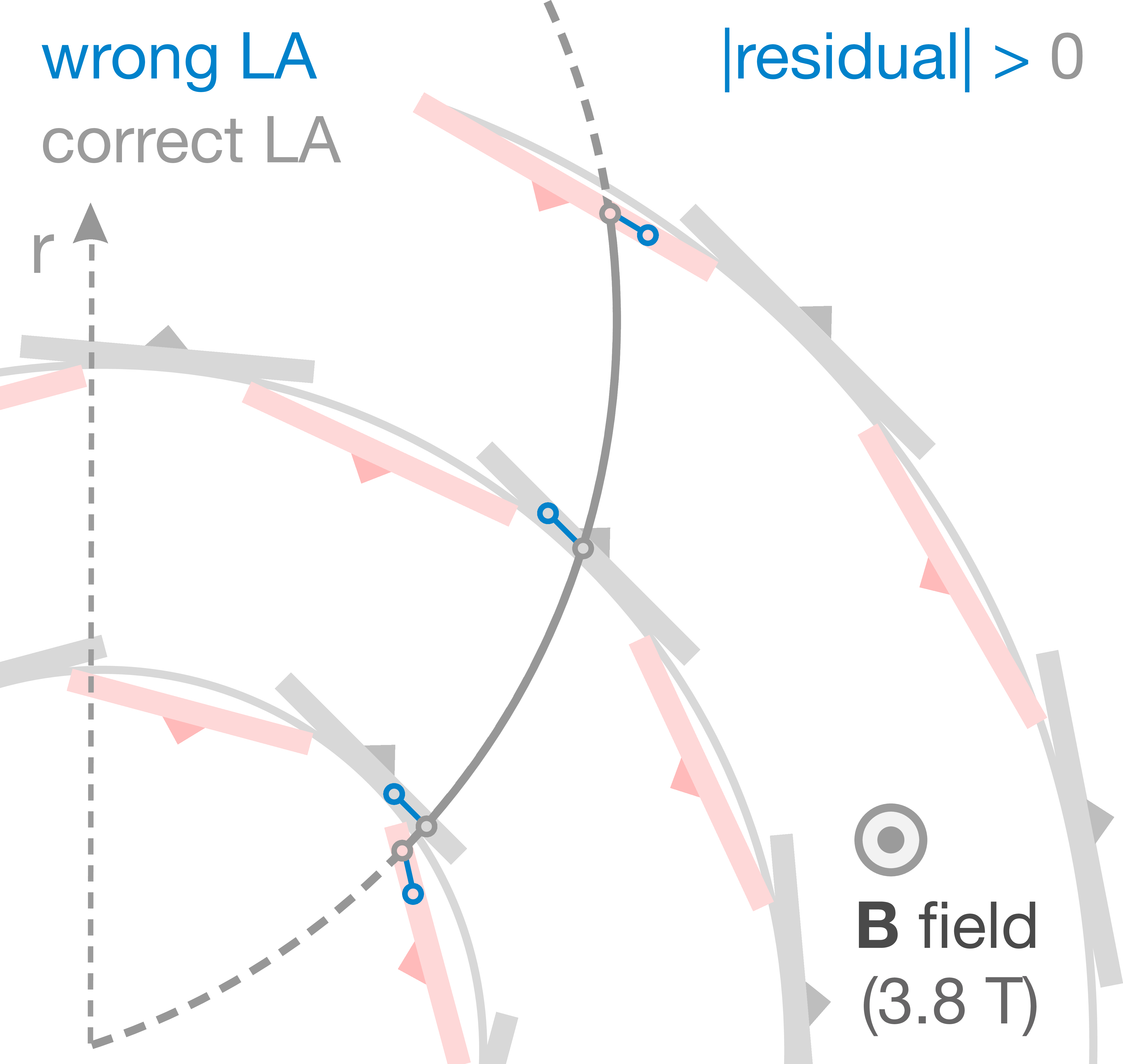
Figure 2:
Sketch showing the transverse view of the Phase-0 barrel pixel subdetector, made of successive layers of silicon modules. The alternating orientation of the modules within each layer is indicated by the triangles. The blue (grey) circles represent the reconstructed hit positions using incorrect (correct) Lorentz angles in the presence of a magnetic field B. The grey curve corresponds to a track built from the hits that were reconstructed with the correct Lorentz angles. Hits reconstructed with incorrect Lorentz angles are displaced in a direction defined by the orientation of the module, increasing the residual distance between the hits and the track. |

png pdf |
Figure 3:
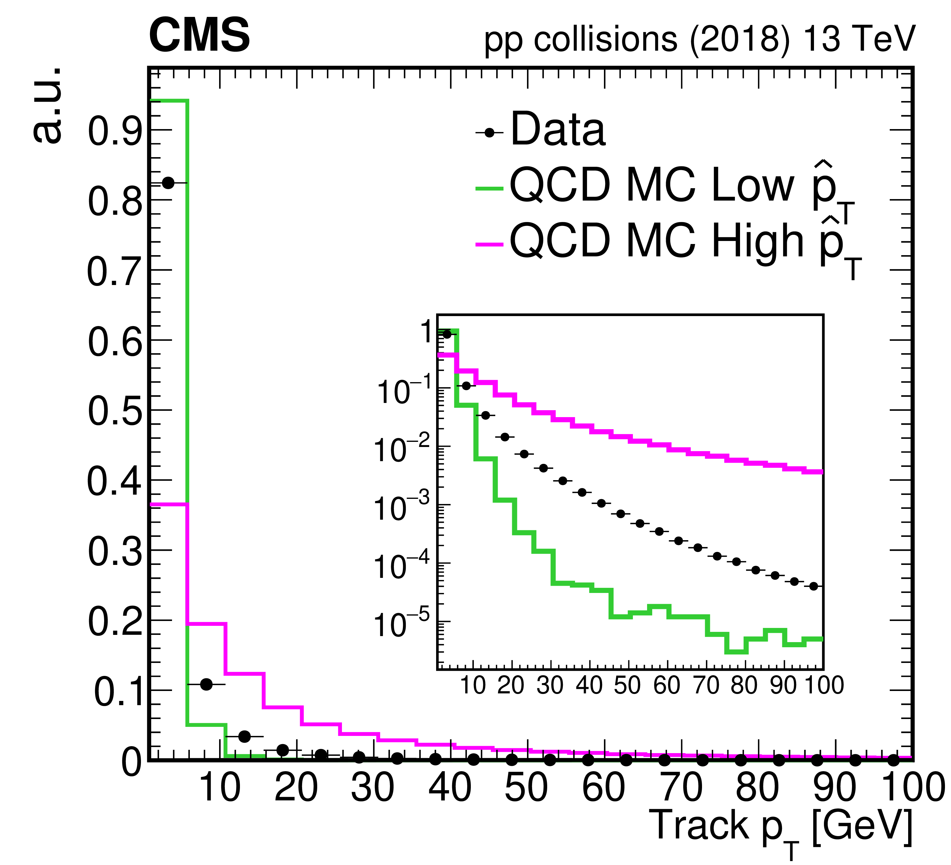
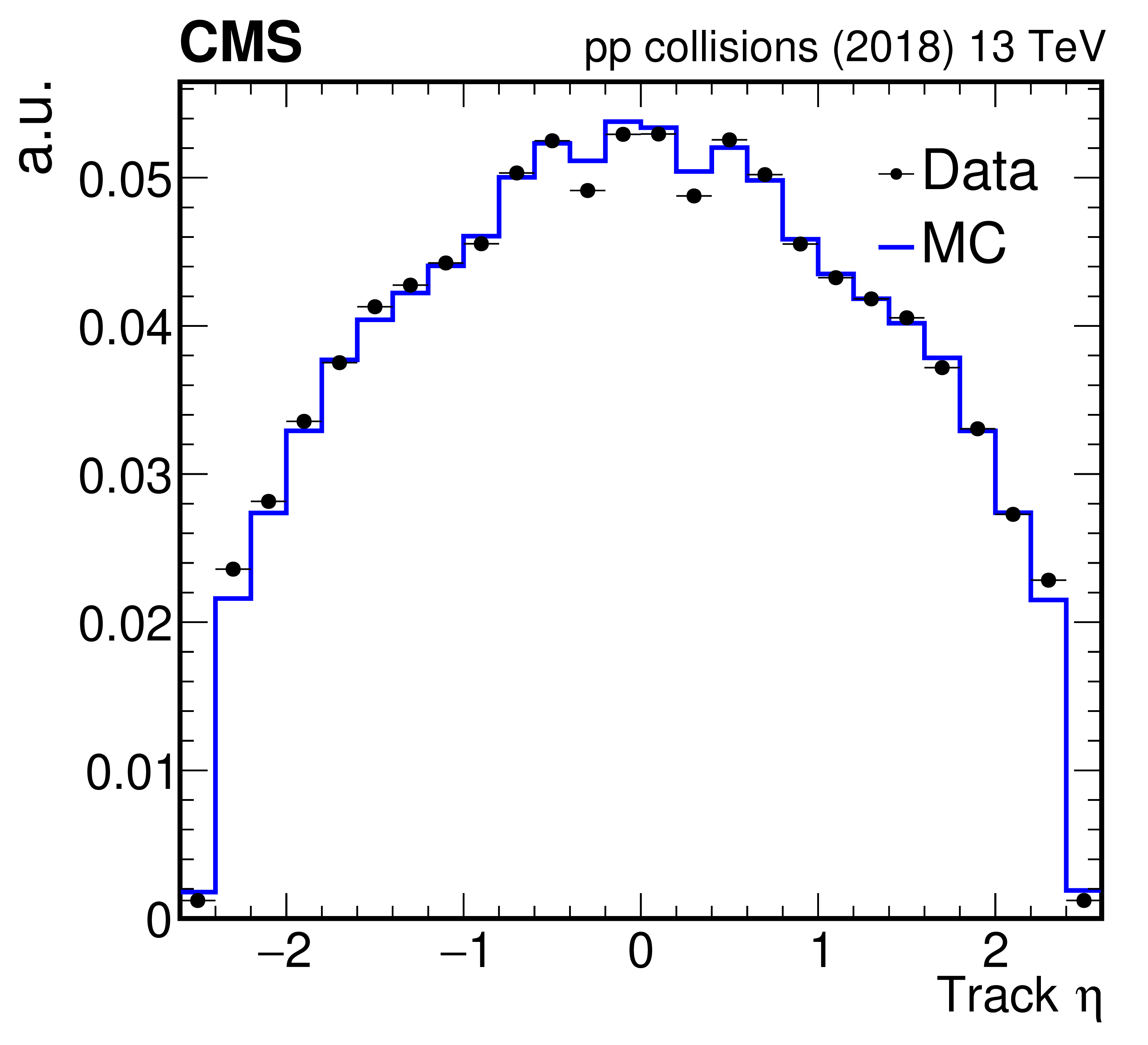
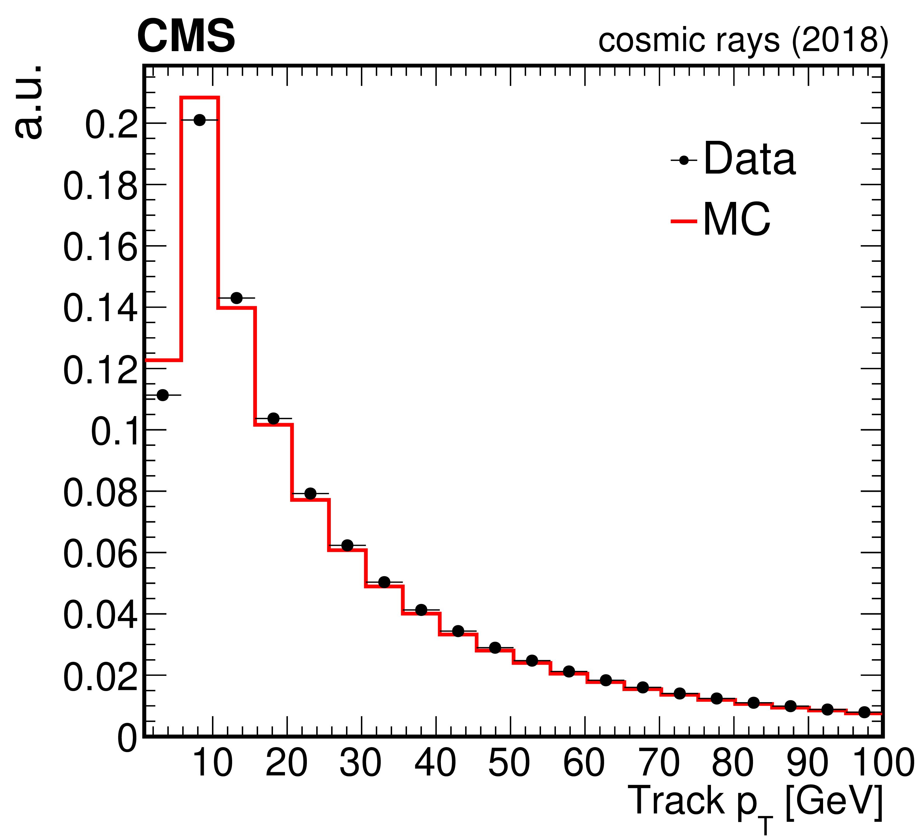
Normalized track ${p_{\mathrm {T}}}$ (left) and $\eta $ (right) distributions for the inclusive L1 trigger (top), $\mathrm{Z} \to \mu \mu $ (middle), and interfill cosmic ray muon (bottom) data sets in arbitrary units. Data collected with the CMS detector in 2018 and used for the final alignment in that year (solid black circles) are compared with the simulation (solid coloured lines). Distributions in data are obtained from a sample of 11$\times $10$^6$, 55$\times $10$^6$, and 3.4$\times $10$^6$ tracks for the inclusive L1 trigger, $\mathrm{Z} \to \mu \mu $, and cosmic ray muon data sets, respectively. For the inclusive L1 trigger data set, data are compared with two sets of simulated QCD events with different ranges of transverse momentum transfers $ {\hat{p}_\mathrm {T}} $. The green line corresponds to $ {\hat{p}_\mathrm {T}} $ between 15 and 30 GeV, whereas the magenta line corresponds to $ {\hat{p}_\mathrm {T}} $ between 1000 and 1400 GeV. The inset in the ${p_{\mathrm {T}}}$ distribution of the inclusive L1 trigger data set (top left) shows the same distribution with a logarithmic scale for the $y$ axis. No correction for the limited modelling of the trigger efficiency in the simulation has been applied for the $\mathrm{Z} \to \mu \mu $ data set. The statistical uncertainty is smaller than the symbol size and therefore imperceptible. |
png pdf |
Figure 3-a:
Normalized track ${p_{\mathrm {T}}}$ distribution for the inclusive L1 trigger data set in arbitrary units. Data collected with the CMS detector in 2018 and used for the final alignment in that year (solid black circles) are compared with the simulation (solid coloured lines). The distribution in data are obtained from a sample of 11$\times $10$^6$ tracks. Data are compared with two sets of simulated QCD events with different ranges of transverse momentum transfers $ {\hat{p}_\mathrm {T}} $. The green line corresponds to $ {\hat{p}_\mathrm {T}} $ between 15 and 30 GeV, whereas the magenta line corresponds to $ {\hat{p}_\mathrm {T}} $ between 1000 and 1400 GeV. The inset in the ${p_{\mathrm {T}}}$ distribution shows the same distribution with a logarithmic scale for the $y$ axis. The statistical uncertainty is smaller than the symbol size and therefore imperceptible. |

png pdf |
Figure 3-b:
Normalized track $\eta $ distribution for the inclusive L1 trigger data set in arbitrary units. Data collected with the CMS detector in 2018 and used for the final alignment in that year (solid black circles) are compared with the simulation (solid coloured lines). The distribution in data are obtained from a sample of 11$\times $10$^6$ tracks. Data are compared with two sets of simulated QCD events with different ranges of transverse momentum transfers $ {\hat{p}_\mathrm {T}} $. The green line corresponds to $ {\hat{p}_\mathrm {T}} $ between 15 and 30 GeV, whereas the magenta line corresponds to $ {\hat{p}_\mathrm {T}} $ between 1000 and 1400 GeV. The inset in the ${p_{\mathrm {T}}}$ distribution shows the same distribution with a logarithmic scale for the $y$ axis. The statistical uncertainty is smaller than the symbol size and therefore imperceptible. |

png pdf |
Figure 3-c:
Normalized track ${p_{\mathrm {T}}}$ distribution for the $\mathrm{Z} \to \mu \mu $ data set in arbitrary units. Data collected with the CMS detector in 2018 and used for the final alignment in that year (solid black circles) are compared with the simulation (solid coloured lines). The distribution in data are obtained from a sample of 55$\times $10$^6$ tracks. No correction for the limited modelling of the trigger efficiency in the simulation has been applied. The statistical uncertainty is smaller than the symbol size and therefore imperceptible. |
png pdf |
Figure 3-d:
Normalized track $\eta $ distribution for the $\mathrm{Z} \to \mu \mu $ data set in arbitrary units. Data collected with the CMS detector in 2018 and used for the final alignment in that year (solid black circles) are compared with the simulation (solid coloured lines). The distribution in data are obtained from a sample of 55$\times $10$^6$ tracks. No correction for the limited modelling of the trigger efficiency in the simulation has been applied. The statistical uncertainty is smaller than the symbol size and therefore imperceptible. |
png pdf |
Figure 3-e:
Normalized track ${p_{\mathrm {T}}}$ distribution for the interfill cosmic ray muon data set in arbitrary units. Data collected with the CMS detector in 2018 and used for the final alignment in that year (solid black circles) are compared with the simulation (solid coloured lines). The distribution in data are obtained from a sample of 3.4$\times $10$^6$ tracks. The statistical uncertainty is smaller than the symbol size and therefore imperceptible. |
png pdf |
Figure 3-f:
Normalized track $\eta $ distribution for the interfill cosmic ray muon data set in arbitrary units. Data collected with the CMS detector in 2018 and used for the final alignment in that year (solid black circles) are compared with the simulation (solid coloured lines). The distribution in data are obtained from a sample of 3.4$\times $10$^6$ tracks. The statistical uncertainty is smaller than the symbol size and therefore imperceptible. |
png pdf |
Figure 4:
Average event rates of cosmic ray muon data recorded with the CMS tracker during the years 2016, 2017, and 2018, obtained as explained in the text. The statistical uncertainty in the measured rates is negligible and is not shown in the figure. |

png pdf |
Figure 5:
Diagram demonstrating distortions of the tracker geometry that may not affect the consistency of a reconstructed collision track with the measured hits (left), but introduce a kink when reconstructing the two halves of a cosmic ray muon track (right), leading to an inconsistency. This illustrates the telescope effect from Table 1. |

png pdf |
Figure 6:
Diagram demonstrating the overlap regions of two representative modules $A$ and $B$. In the upper diagram, the predicted track impact points (green circles) and the actual hits with charge depositions (red and blue circles) do not coincide because of a wrong prediction of the module positions. In the lower diagram, the actual module positions are shown for the geometry with radial expansion, and the predicted impact points and hits coincide. Uncertainties due to track propagation are ignored in this illustration, but are greatly reduced in the difference of residuals as discussed in the text. The green dashed circles in the lower diagram indicate predicted impact points from the nominal geometry in the upper diagram. |

png pdf |
Figure 7:
Diagram demonstrating the overlap regions of three representative modules $A$, $B$, and $C$ in the first layer of the barrel pixel detector. The $y$-$z$ view (left) and $y$-$x$ view (right) are shown for the same modules. The overlap hits are indicated with the blue (inner) and red (outer) crosses and appear in tracks with hits in two consecutive modules in the same layer of the detector. The black cross represents the interaction point. The overlap between modules $A$ and $B$ constrains the distance between modules in the $\phi $ direction, whereas the overlap between modules $A$ and $C$ constrains the distance between modules in the $z$ direction. |
png pdf |
Figure 8:
Diagrams demonstrating distortions of the tracker geometry in the $r$-$z$ view (left) and in the $x$-$y$ view (right) with the reconstructed muon pair from a $\mathrm{Z} \to \mu \mu $ decay. The invariant mass of the pair of muons deviates from the expected value and becomes a function of the track parameters. This illustrates the twist effect from Table 1. |

png pdf |
Figure 9:
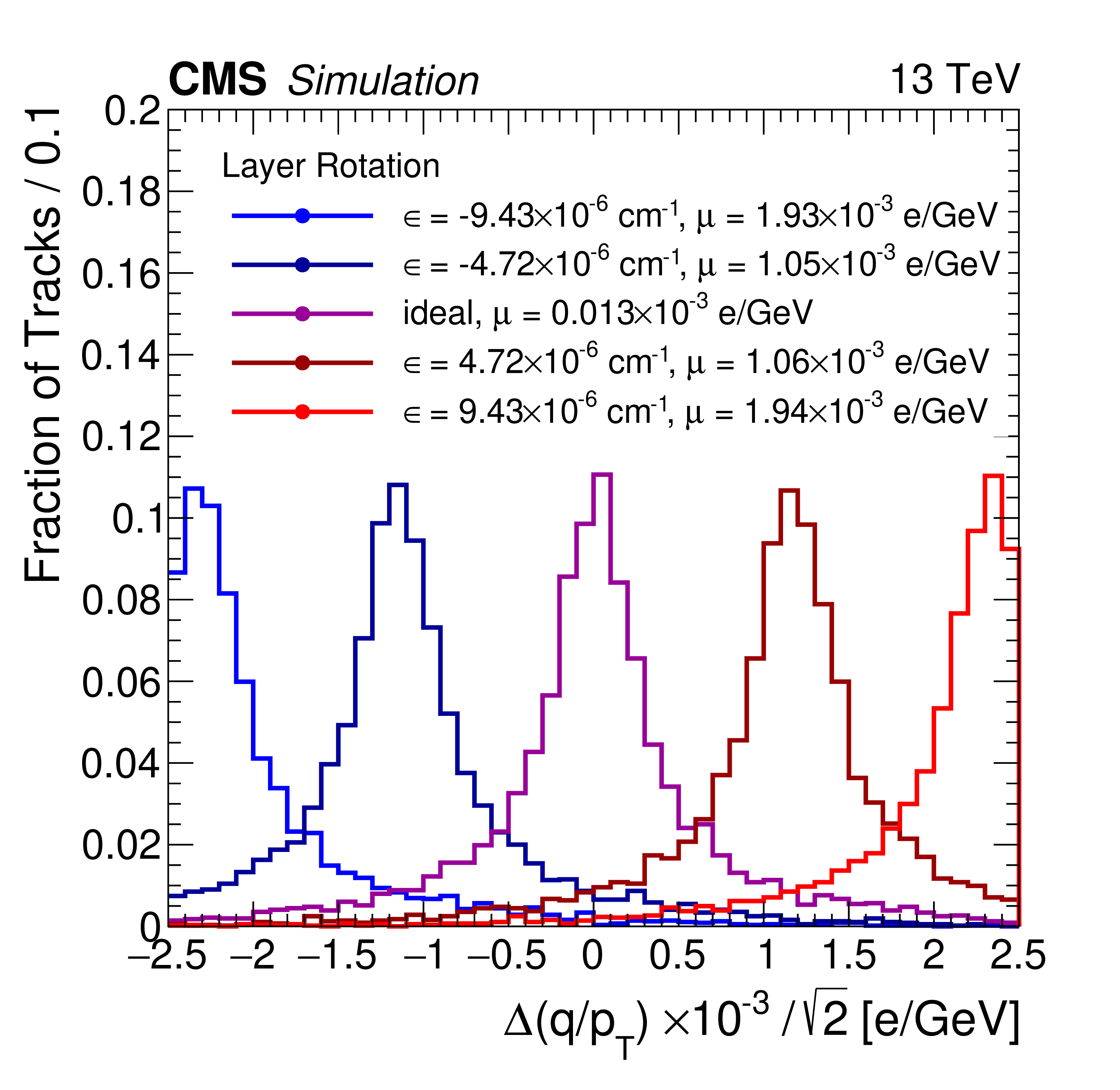
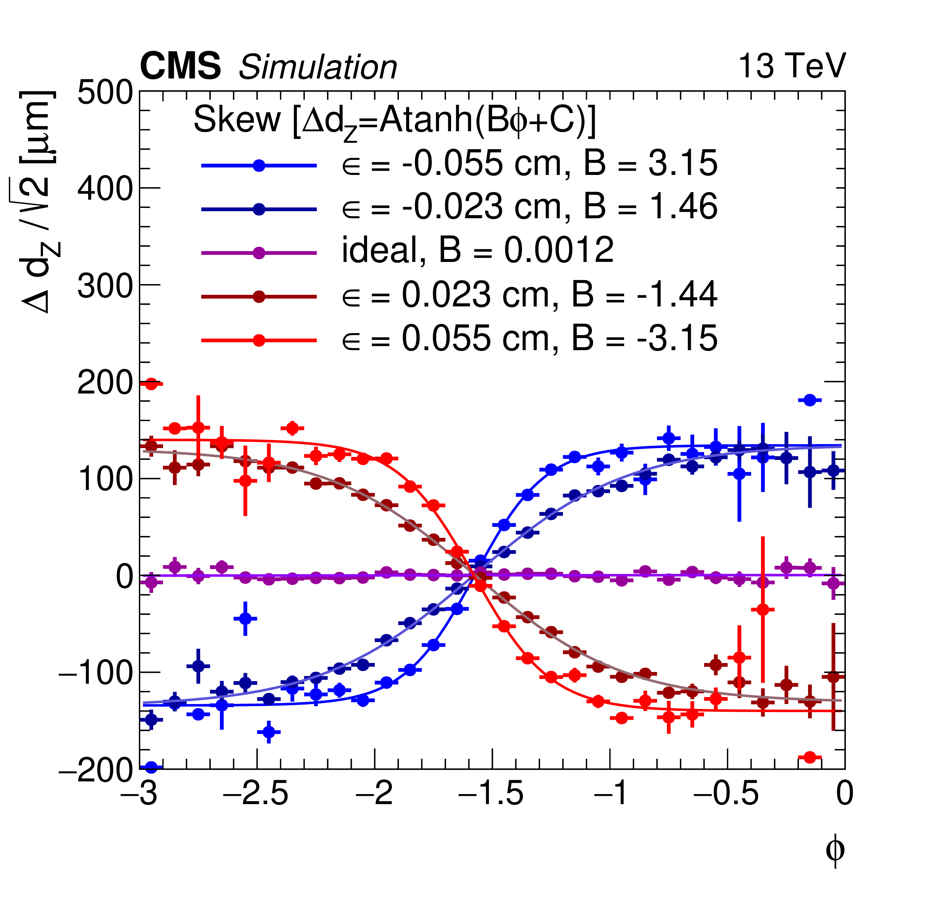
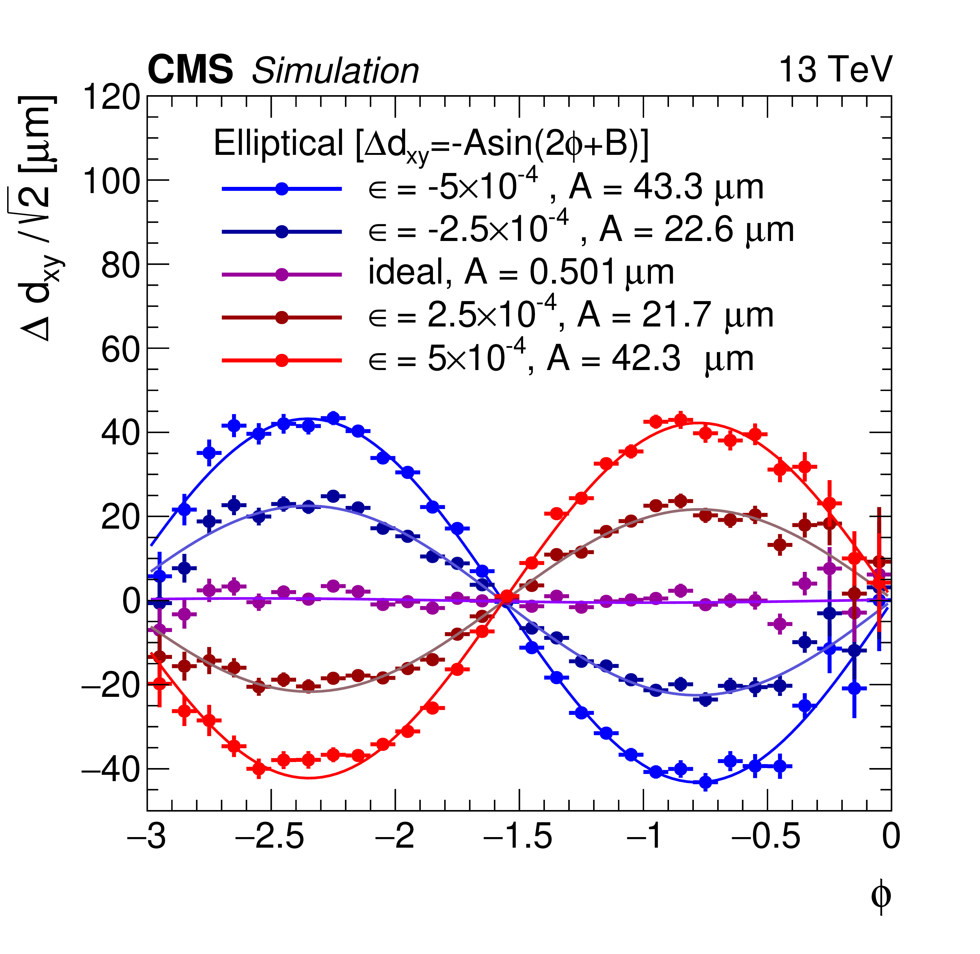
Validation of the nine basic systematic distortions summarized in Table 1 using reconstructed MC simulations with five variations of the misalignment parameter $\epsilon $ in each case. The ideal geometry in MC simulation corresponds to $\epsilon =$ 0. The horizontal lines show the uncertainty on the average of a measurement in a given bin. The most sensitive validation out of cosmic ray muon track, overlap, or dimuon validation is employed in each case, as discussed in more detail in the text and as indicated in Table 1. In the bottom row, the formulae indicate the functional form of the fit used to extract the parameter quoted in the legend, which can be used to quantify the distortion. The convention for the sign of $\epsilon $ is discussed in the text and corresponds to a distortion in the geometry used for the reconstruction of MC events. This is opposite to the sign of the distortion if it were to be introduced in simulation of the detector components traversed by the charged particles. |

png pdf |
Figure 9-a:
Validation of one of the nine basic systematic distortions summarized in Table 1 (z-Expansion) using reconstructed MC simulations with five variations of the misalignment parameter $\epsilon $ in each case. The ideal geometry in MC simulation corresponds to $\epsilon =$ 0. The horizontal lines show the uncertainty on the average of a measurement in a given bin. The most sensitive validation out of cosmic ray muon track, overlap, or dimuon validation is employed in each case, as discussed in more detail in the text and as indicated in Table 1. In the bottom row, the formulae indicate the functional form of the fit used to extract the parameter quoted in the legend, which can be used to quantify the distortion. The convention for the sign of $\epsilon $ is discussed in the text and corresponds to a distortion in the geometry used for the reconstruction of MC events. This is opposite to the sign of the distortion if it were to be introduced in simulation of the detector components traversed by the charged particles. |

png pdf |
Figure 9-b:
Validation of one of the nine basic systematic distortions summarized in Table 1 (Radial) using reconstructed MC simulations with five variations of the misalignment parameter $\epsilon $ in each case. The ideal geometry in MC simulation corresponds to $\epsilon =$ 0. The horizontal lines show the uncertainty on the average of a measurement in a given bin. The most sensitive validation out of cosmic ray muon track, overlap, or dimuon validation is employed in each case, as discussed in more detail in the text and as indicated in Table 1. In the bottom row, the formulae indicate the functional form of the fit used to extract the parameter quoted in the legend, which can be used to quantify the distortion. The convention for the sign of $\epsilon $ is discussed in the text and corresponds to a distortion in the geometry used for the reconstruction of MC events. This is opposite to the sign of the distortion if it were to be introduced in simulation of the detector components traversed by the charged particles. |
png pdf |
Figure 9-c:
Validation of one of the nine basic systematic distortions summarized in Table 1 (Twist) using reconstructed MC simulations with five variations of the misalignment parameter $\epsilon $ in each case. The ideal geometry in MC simulation corresponds to $\epsilon =$ 0. The horizontal lines show the uncertainty on the average of a measurement in a given bin. The most sensitive validation out of cosmic ray muon track, overlap, or dimuon validation is employed in each case, as discussed in more detail in the text and as indicated in Table 1. In the bottom row, the formulae indicate the functional form of the fit used to extract the parameter quoted in the legend, which can be used to quantify the distortion. The convention for the sign of $\epsilon $ is discussed in the text and corresponds to a distortion in the geometry used for the reconstruction of MC events. This is opposite to the sign of the distortion if it were to be introduced in simulation of the detector components traversed by the charged particles. |

png pdf |
Figure 9-d:
Validation of one of the nine basic systematic distortions summarized in Table 1 (Telescope) using reconstructed MC simulations with five variations of the misalignment parameter $\epsilon $ in each case. The ideal geometry in MC simulation corresponds to $\epsilon =$ 0. The horizontal lines show the uncertainty on the average of a measurement in a given bin. The most sensitive validation out of cosmic ray muon track, overlap, or dimuon validation is employed in each case, as discussed in more detail in the text and as indicated in Table 1. In the bottom row, the formulae indicate the functional form of the fit used to extract the parameter quoted in the legend, which can be used to quantify the distortion. The convention for the sign of $\epsilon $ is discussed in the text and corresponds to a distortion in the geometry used for the reconstruction of MC events. This is opposite to the sign of the distortion if it were to be introduced in simulation of the detector components traversed by the charged particles. |

png pdf |
Figure 9-e:
Validation of one of the nine basic systematic distortions summarized in Table 1 (Bowing) using reconstructed MC simulations with five variations of the misalignment parameter $\epsilon $ in each case. The ideal geometry in MC simulation corresponds to $\epsilon =$ 0. The horizontal lines show the uncertainty on the average of a measurement in a given bin. The most sensitive validation out of cosmic ray muon track, overlap, or dimuon validation is employed in each case, as discussed in more detail in the text and as indicated in Table 1. In the bottom row, the formulae indicate the functional form of the fit used to extract the parameter quoted in the legend, which can be used to quantify the distortion. The convention for the sign of $\epsilon $ is discussed in the text and corresponds to a distortion in the geometry used for the reconstruction of MC events. This is opposite to the sign of the distortion if it were to be introduced in simulation of the detector components traversed by the charged particles. |
png pdf |
Figure 9-f:
Validation of one of the nine basic systematic distortions summarized in Table 1 (Layer Rotation) using reconstructed MC simulations with five variations of the misalignment parameter $\epsilon $ in each case. The ideal geometry in MC simulation corresponds to $\epsilon =$ 0. The horizontal lines show the uncertainty on the average of a measurement in a given bin. The most sensitive validation out of cosmic ray muon track, overlap, or dimuon validation is employed in each case, as discussed in more detail in the text and as indicated in Table 1. In the bottom row, the formulae indicate the functional form of the fit used to extract the parameter quoted in the legend, which can be used to quantify the distortion. The convention for the sign of $\epsilon $ is discussed in the text and corresponds to a distortion in the geometry used for the reconstruction of MC events. This is opposite to the sign of the distortion if it were to be introduced in simulation of the detector components traversed by the charged particles. |
png pdf |
Figure 9-g:
Validation of one of the nine basic systematic distortions summarized in Table 1 (Skew) using reconstructed MC simulations with five variations of the misalignment parameter $\epsilon $ in each case. The ideal geometry in MC simulation corresponds to $\epsilon =$ 0. The horizontal lines show the uncertainty on the average of a measurement in a given bin. The most sensitive validation out of cosmic ray muon track, overlap, or dimuon validation is employed in each case, as discussed in more detail in the text and as indicated in Table 1. In the bottom row, the formulae indicate the functional form of the fit used to extract the parameter quoted in the legend, which can be used to quantify the distortion. The convention for the sign of $\epsilon $ is discussed in the text and corresponds to a distortion in the geometry used for the reconstruction of MC events. This is opposite to the sign of the distortion if it were to be introduced in simulation of the detector components traversed by the charged particles. |
png pdf |
Figure 9-h:
Validation of one of the nine basic systematic distortions summarized in Table 1 (Elliptical) using reconstructed MC simulations with five variations of the misalignment parameter $\epsilon $ in each case. The ideal geometry in MC simulation corresponds to $\epsilon =$ 0. The horizontal lines show the uncertainty on the average of a measurement in a given bin. The most sensitive validation out of cosmic ray muon track, overlap, or dimuon validation is employed in each case, as discussed in more detail in the text and as indicated in Table 1. In the bottom row, the formulae indicate the functional form of the fit used to extract the parameter quoted in the legend, which can be used to quantify the distortion. The convention for the sign of $\epsilon $ is discussed in the text and corresponds to a distortion in the geometry used for the reconstruction of MC events. This is opposite to the sign of the distortion if it were to be introduced in simulation of the detector components traversed by the charged particles. |

png pdf |
Figure 9-i:
Validation of one of the nine basic systematic distortions summarized in Table 1 (Sagitta) using reconstructed MC simulations with five variations of the misalignment parameter $\epsilon $ in each case. The ideal geometry in MC simulation corresponds to $\epsilon =$ 0. The horizontal lines show the uncertainty on the average of a measurement in a given bin. The most sensitive validation out of cosmic ray muon track, overlap, or dimuon validation is employed in each case, as discussed in more detail in the text and as indicated in Table 1. In the bottom row, the formulae indicate the functional form of the fit used to extract the parameter quoted in the legend, which can be used to quantify the distortion. The convention for the sign of $\epsilon $ is discussed in the text and corresponds to a distortion in the geometry used for the reconstruction of MC events. This is opposite to the sign of the distortion if it were to be introduced in simulation of the detector components traversed by the charged particles. |

png pdf |
Figure 10:
Diagram of the {HipPy} algorithm design with the sequence for event, track, and hit selection, including application of the weight factors and constraints. Not all features were used in the Run 2 alignment procedure, as described in the text. The algorithm operates in iterative mode, indicated with the arrows. |

png pdf |
Figure 11:
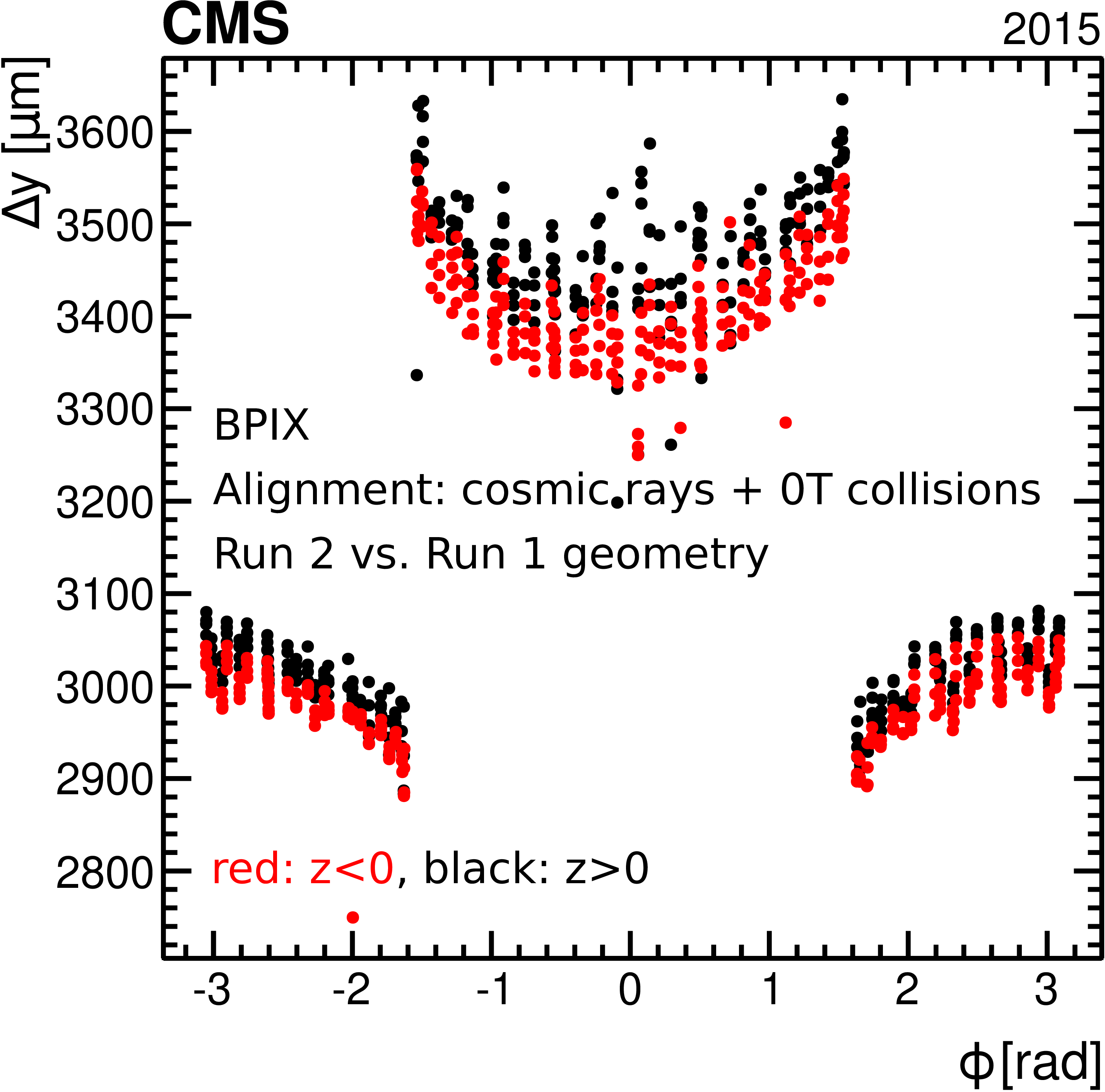
Comparison of the positions of the modules in the first IOV of Run 2 and the last IOV of Run 1 in the BPIX (left) and FPIX (right) detectors, determined using cosmic data collected with 0 T and 3.8 T magnetic field in the solenoid and collision data at 0 T [30]. The differences in position $\Delta y$ (Run 2 $-$ Run 1) and $\Delta z$ (Run 2 $-$ Run 1) of the sensor modules are shown as a function of $\phi $ in global coordinates. Modules on the $-z$ side are shown in red, modules on the $+z$ side are shown in black. |
png pdf |
Figure 11-a:
Comparison of the positions of the modules in the first IOV of Run 2 and the last IOV of Run 1 in the BPIX detector, determined using cosmic data collected with 0 T and 3.8 T magnetic field in the solenoid and collision data at 0 T [30]. The differences in position $\Delta y$ (Run 2 $-$ Run 1) of the sensor modules are shown as a function of $\phi $ in global coordinates. Modules on the $-z$ side are shown in red, modules on the $+z$ side are shown in black. |

png pdf |
Figure 11-b:
Comparison of the positions of the modules in the first IOV of Run 2 and the last IOV of Run 1 in the FPIX detector, determined using cosmic data collected with 0 T and 3.8 T magnetic field in the solenoid and collision data at 0 T [30]. The differences in position $\Delta z$ (Run 2 $-$ Run 1) of the sensor modules are shown as a function of $\phi $ in global coordinates. Modules on the $-z$ side are shown in red, modules on the $+z$ side are shown in black. |

png pdf |
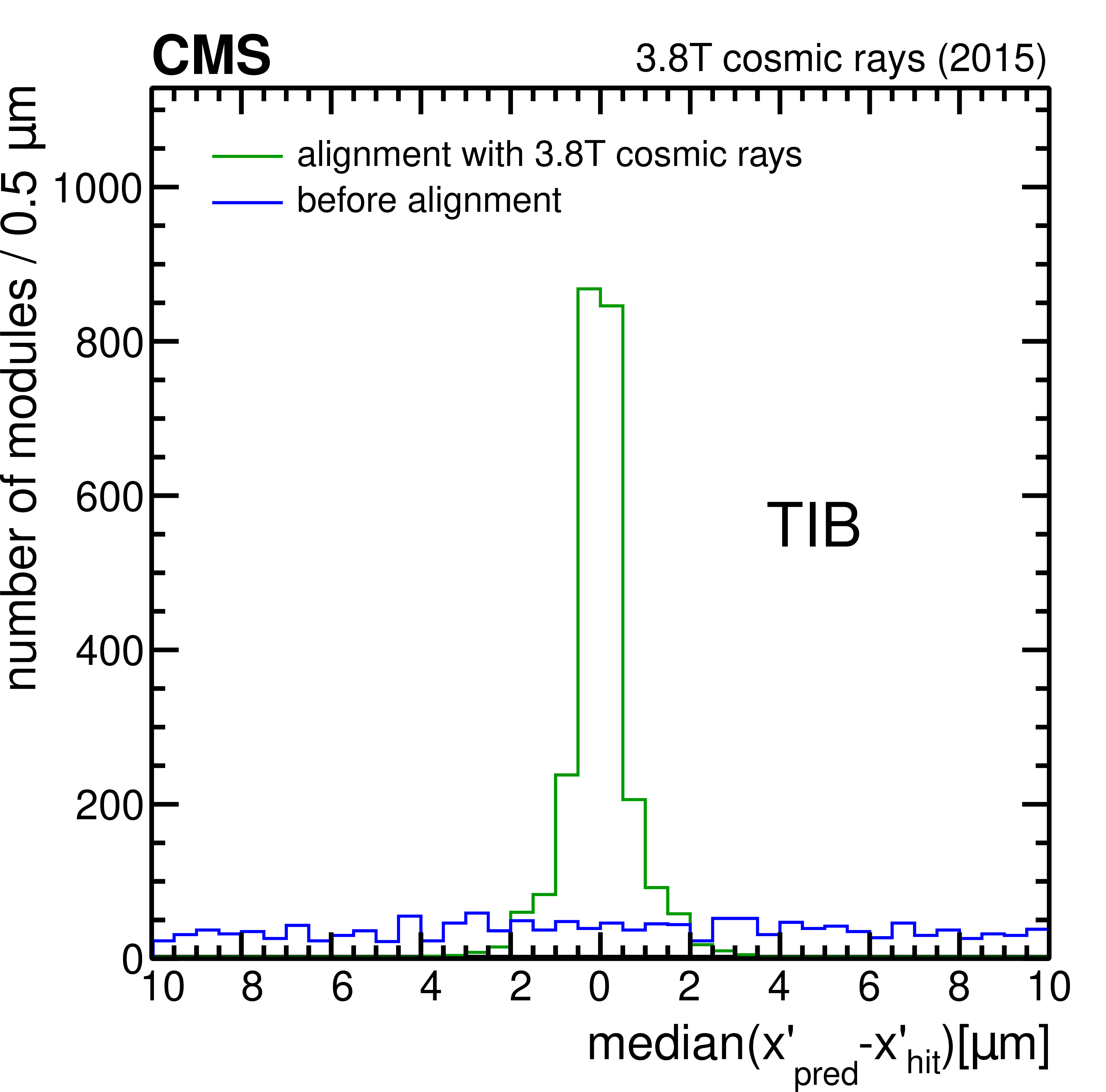
Figure 12:
DMRs for the local $x$ coordinate in the BPIX (left) and TIB (right), evaluated using 2$\times $10$^6$ cosmic ray muon tracks collected at 3.8 T (top) and 1.8$\times $10$^6$ tracks from collision data at 0 T (bottom). The alignment constants used to fit the tracks were determined successively from cosmic data at 3.8 T (green line) and, after the magnet was switched off, from 0 T cosmics and collision data (black line) as described in the text. Because of the detector movements caused by the change in the magnetic field, the alignment constants derived with 3.8 T data (green line) are not optimal for the track fits in the 0 T data (bottom row). The blue line shows the DMR computed assuming the Run 1 geometry, which is no longer valid for Run 2 data. |

png pdf |
Figure 12-a:
DMRs for the local $x$ coordinate in the BPIX, evaluated using 2$\times $10$^6$ cosmic ray muon tracks collected at 3.8 T. The alignment constants used to fit the tracks were determined from cosmic data at 3.8 T (green line). The blue line shows the DMR computed assuming the Run 1 geometry, which is no longer valid for Run 2 data. |
png pdf |
Figure 12-b:
DMRs for the local $x$ coordinate in the TIB, evaluated using 2$\times $10$^6$ cosmic ray muon tracks collected at 3.8 T. The alignment constants used to fit the tracks were determined from cosmic data at 3.8 T (green line). The blue line shows the DMR computed assuming the Run 1 geometry, which is no longer valid for Run 2 data. |

png pdf |
Figure 12-c:
DMRs for the local $x$ coordinate in the BPIX, evaluated using 1.8$\times $10$^6$ tracks from collision data at 0 T. The alignment constants used to fit the tracks were determined successively from cosmic data at 3.8 T (green line) and, after the magnet was switched off, from 0 T cosmics and collision data (black line) as described in the text. Because of the detector movements caused by the change in the magnetic field, the alignment constants derived with 3.8 T data (green line) are not optimal for the track fits in the 0 T data. The blue line shows the DMR computed assuming the Run 1 geometry, which is no longer valid for Run 2 data. |

png pdf |
Figure 12-d:
DMRs for the local $x$ coordinate in the TIB, evaluated using 1.8$\times $10$^6$ tracks from collision data at 0 T. The alignment constants used to fit the tracks were determined successively from cosmic data at 3.8 T (green line) and, after the magnet was switched off, from 0 T cosmics and collision data (black line) as described in the text. Because of the detector movements caused by the change in the magnetic field, the alignment constants derived with 3.8 T data (green line) are not optimal for the track fits in the 0 T data. The blue line shows the DMR computed assuming the Run 1 geometry, which is no longer valid for Run 2 data. |
png pdf |
Figure 13:
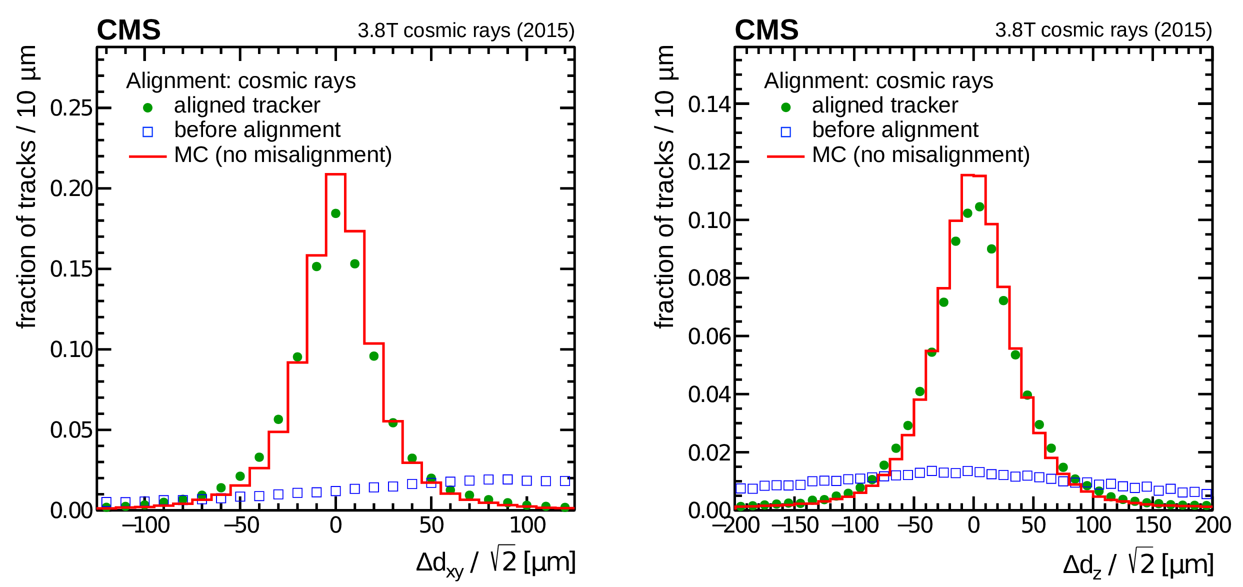
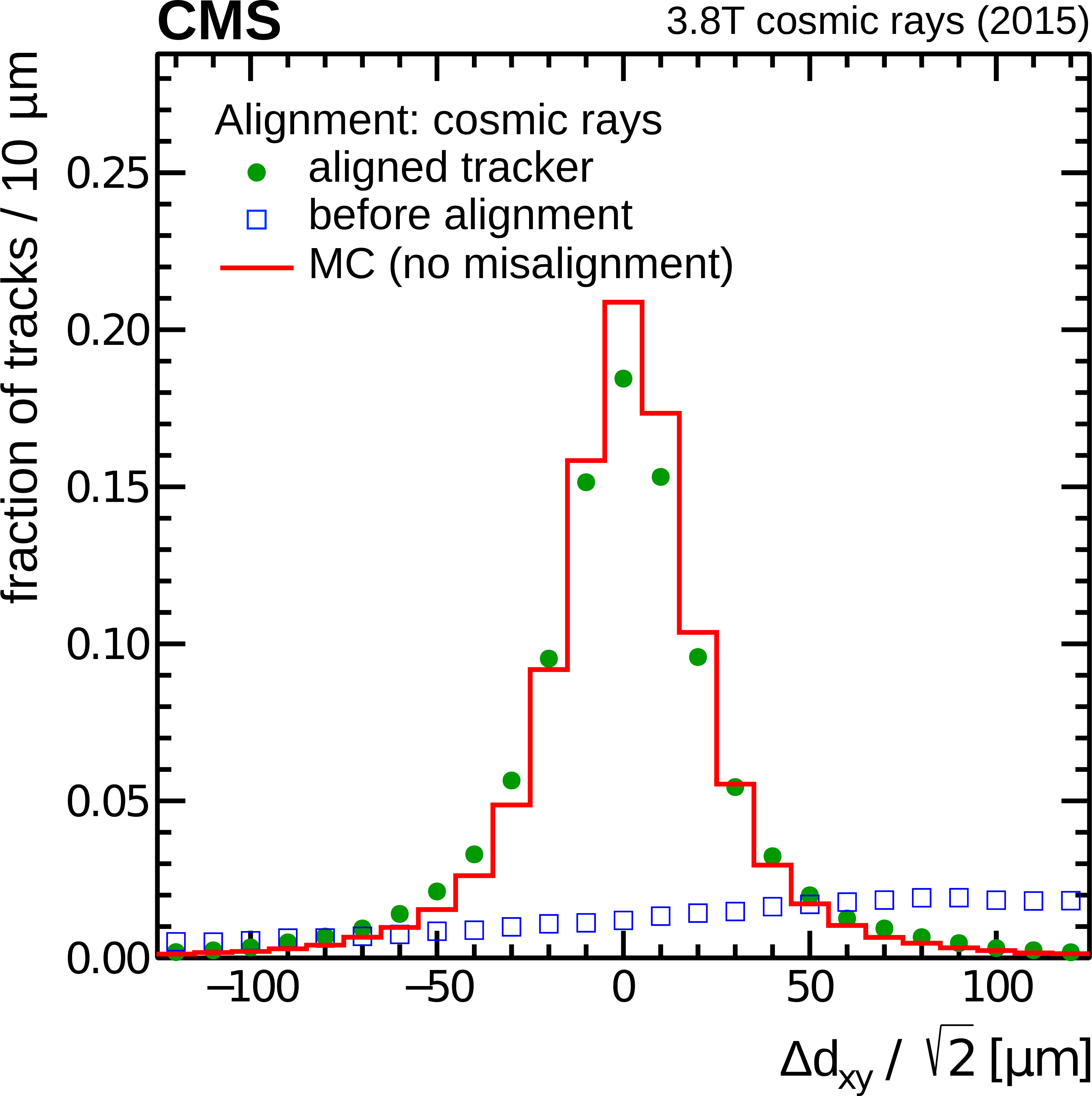
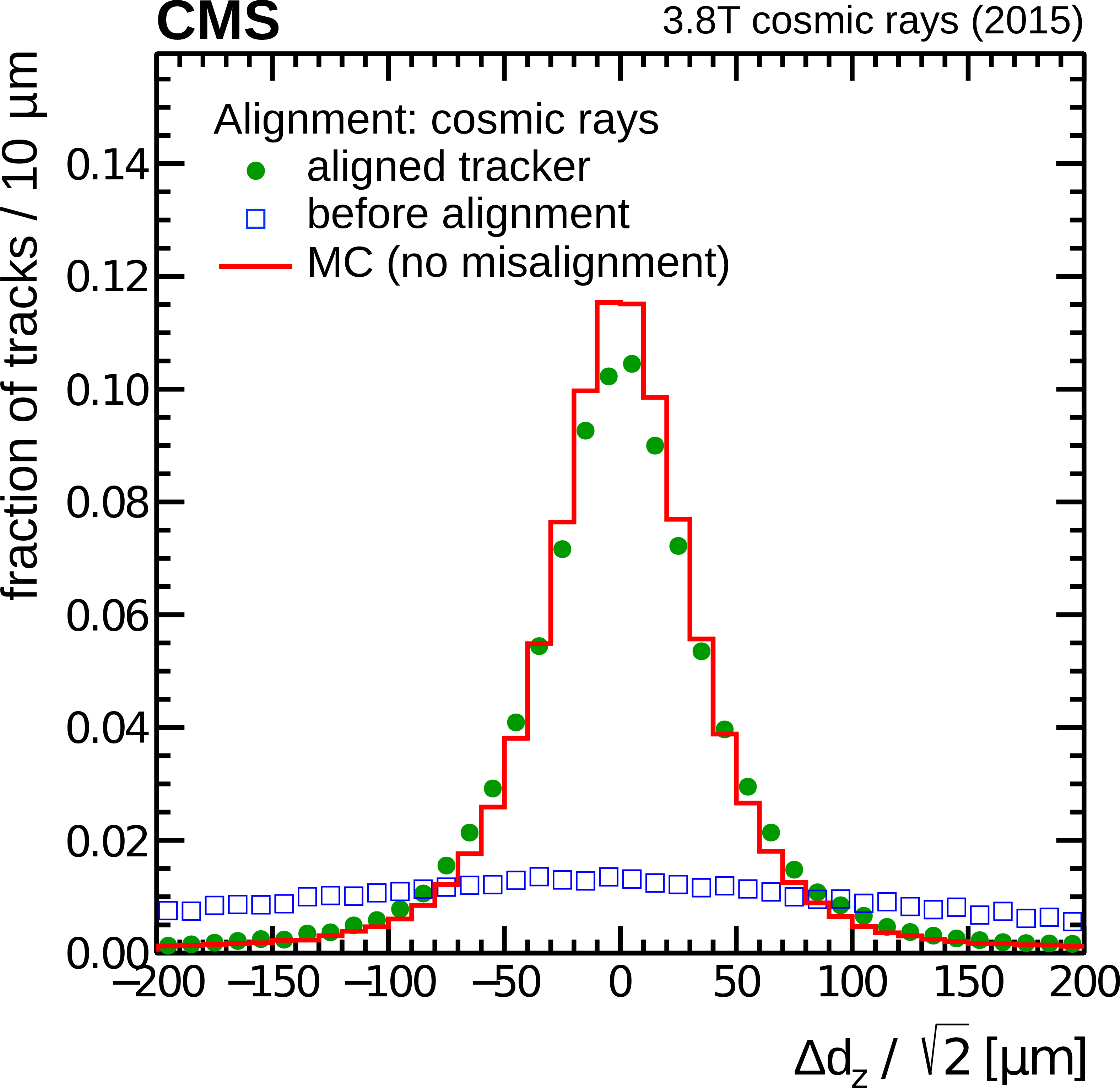
Distribution of the difference between two halves of a cosmic ray muon track, scaled by a factor $\sqrt {2}$ to account for the two independent measurements. The track is split at the point of closest approach to the interaction region, in the $x$-$y$ (left) and $z$ (right) distance between the track and the origin. The tracks are fit using the alignment constants determined with cosmics at 0 T and 3.8 T (green circles) and using the Run 1 geometry (blue squares), which is no longer valid for Run 2 data. Vertical error bars represent the statistical uncertainty due to the limited number of tracks; they are smaller than the marker size. For comparison, the case of perfect alignment and calibration obtained from simulated events is shown (red line) [30]. |
png pdf |
Figure 13-a:
Distribution of the difference between two halves of a cosmic ray muon track, scaled by a factor $\sqrt {2}$ to account for the two independent measurements. The track is split at the point of closest approach to the interaction region, in the $x$-$y$ distance between the track and the origin. The tracks are fit using the alignment constants determined with cosmics at 0 T and 3.8 T (green circles) and using the Run 1 geometry (blue squares), which is no longer valid for Run 2 data. Vertical error bars represent the statistical uncertainty due to the limited number of tracks; they are smaller than the marker size. For comparison, the case of perfect alignment and calibration obtained from simulated events is shown (red line) [30]. |
png pdf |
Figure 13-b:
Distribution of the difference between two halves of a cosmic ray muon track, scaled by a factor $\sqrt {2}$ to account for the two independent measurements. The track is split at the point of closest approach to the interaction region, in the $z$ distance between the track and the origin. The tracks are fit using the alignment constants determined with cosmics at 0 T and 3.8 T (green circles) and using the Run 1 geometry (blue squares), which is no longer valid for Run 2 data. Vertical error bars represent the statistical uncertainty due to the limited number of tracks; they are smaller than the marker size. For comparison, the case of perfect alignment and calibration obtained from simulated events is shown (red line) [30]. |
png pdf |
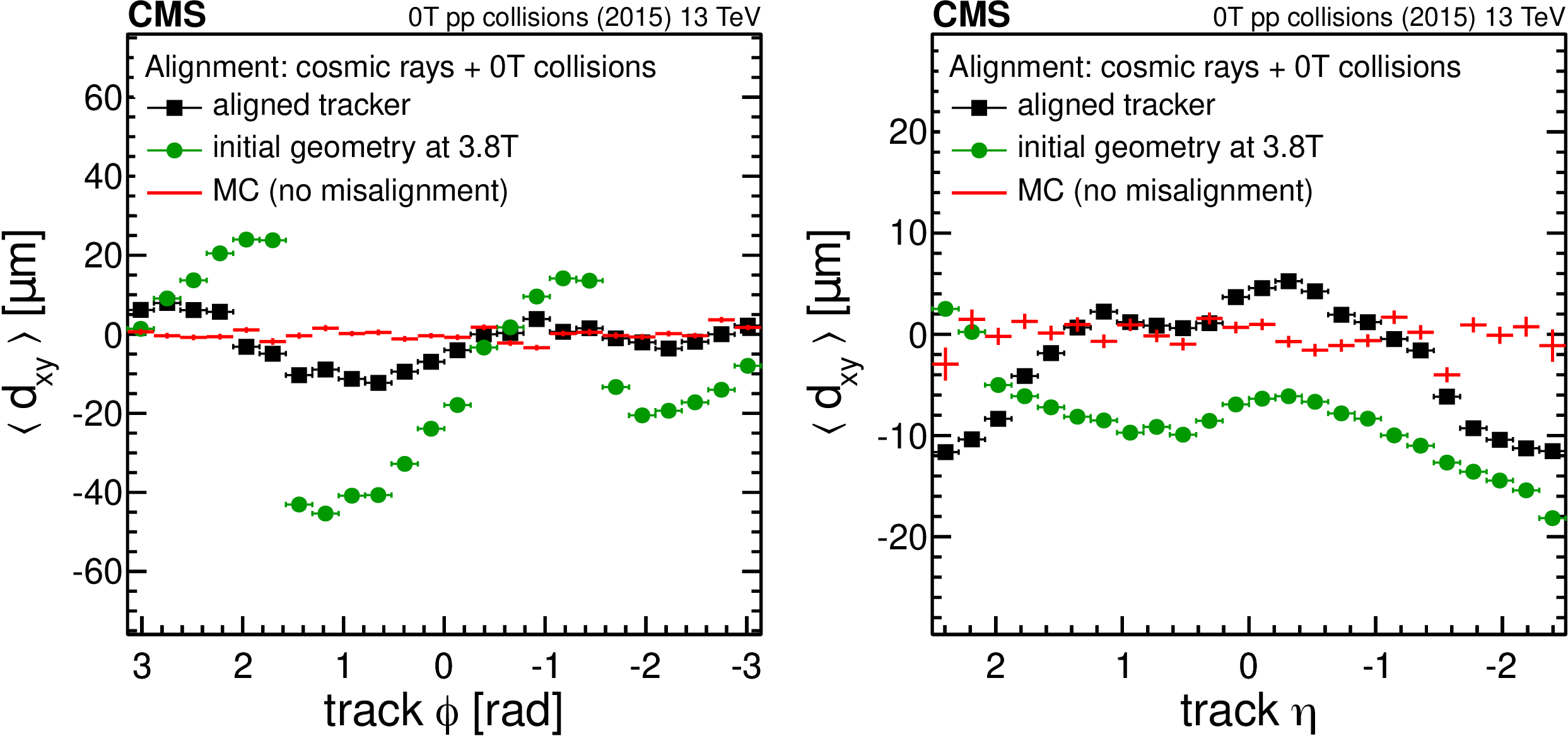
Figure 14:
Mean distance in the transverse plane of the track at its closest approach to a refit unbiased PV as a function of the track $\phi $ (left) and $\eta $ (right), measured in approximately 5.5$\times $10$^6$ collision events collected at 0 T magnetic field. Two different alignments are used to fit the tracks: the alignment constants obtained during the commissioning phase with cosmic ray muon tracks at 3.8 T prior to collision data taking (green circles) and the alignment constants determined subsequently with 0 T collision data (black squares). For comparison, the case of perfect alignment and calibration obtained from simulated data is shown (red line). Vertical error bars represent the statistical uncertainty due to the limited number of tracks; for the data, they are smaller than the size of the markers [30]. |
png pdf |
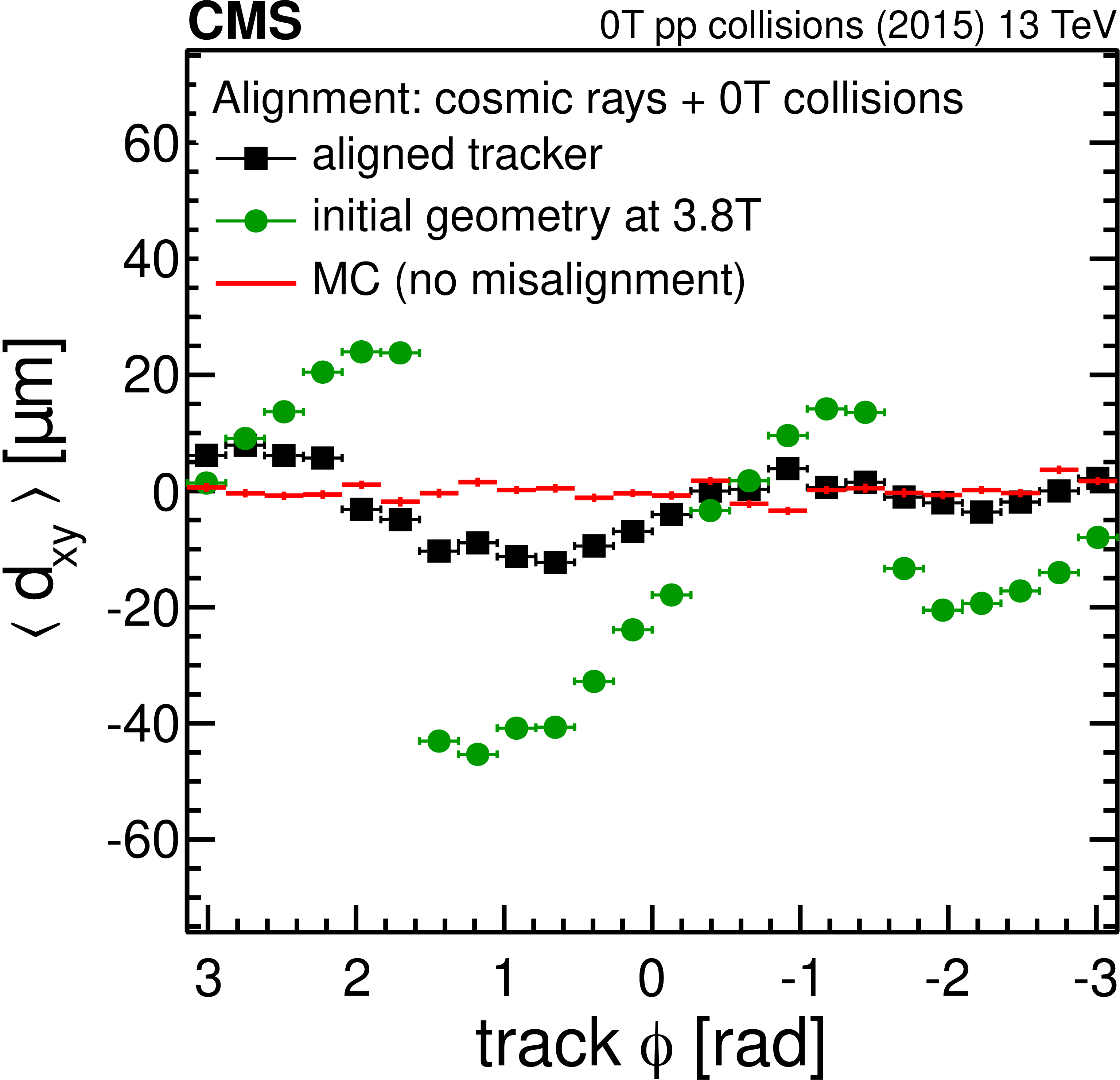
Figure 14-a:
Mean distance in the transverse plane of the track at its closest approach to a refit unbiased PV as a function of the track $\phi $, measured in approximately 5.5$\times $10$^6$ collision events collected at 0 T magnetic field. Two different alignments are used to fit the tracks: the alignment constants obtained during the commissioning phase with cosmic ray muon tracks at 3.8 T prior to collision data taking (green circles) and the alignment constants determined subsequently with 0 T collision data (black squares). For comparison, the case of perfect alignment and calibration obtained from simulated data is shown (red line). Vertical error bars represent the statistical uncertainty due to the limited number of tracks; for the data, they are smaller than the size of the markers [30]. |
png pdf |
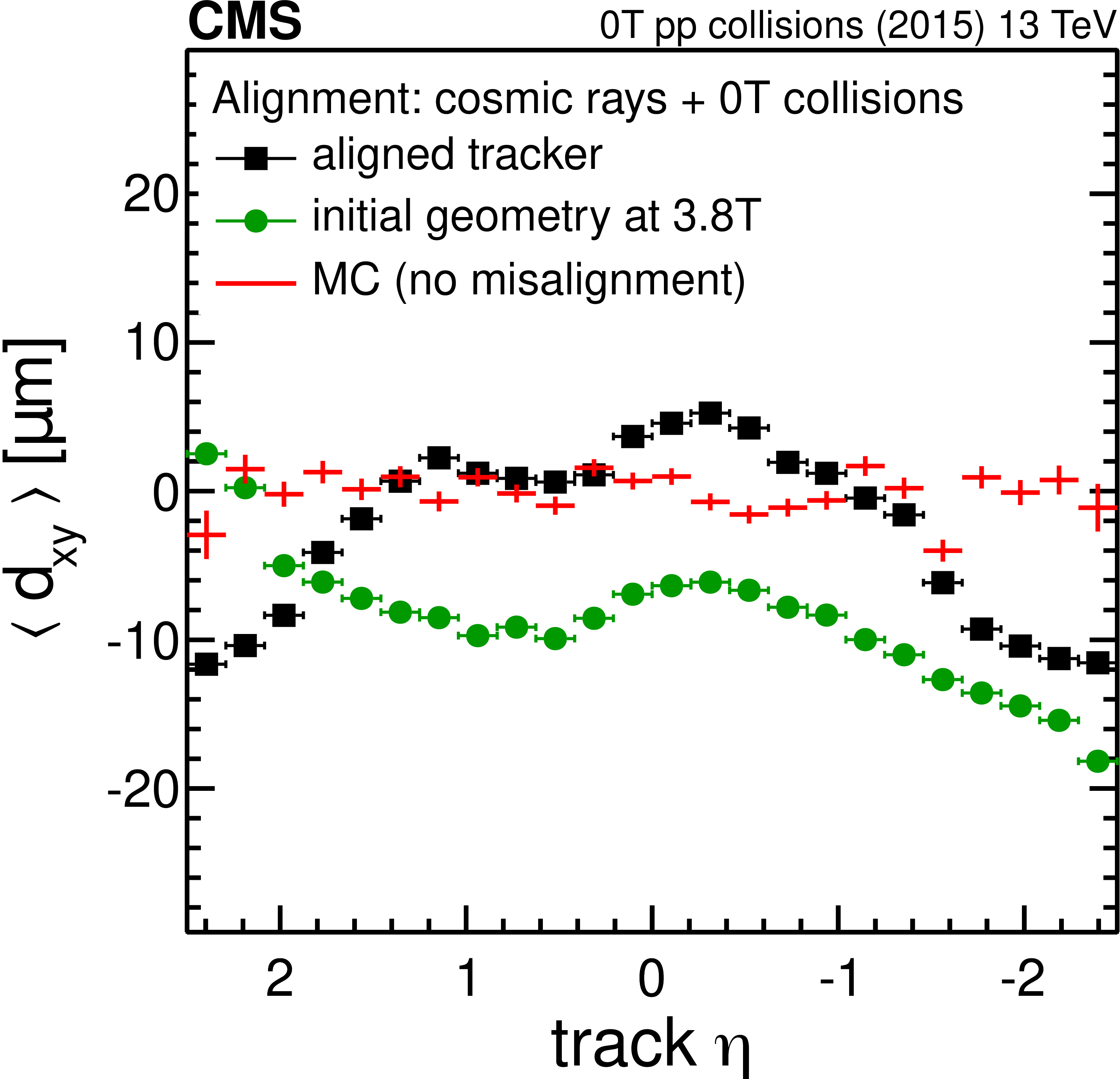
Figure 14-b:
Mean distance in the transverse plane of the track at its closest approach to a refit unbiased PV as a function of the track $\eta $, measured in approximately 5.5$\times $10$^6$ collision events collected at 0 T magnetic field. Two different alignments are used to fit the tracks: the alignment constants obtained during the commissioning phase with cosmic ray muon tracks at 3.8 T prior to collision data taking (green circles) and the alignment constants determined subsequently with 0 T collision data (black squares). For comparison, the case of perfect alignment and calibration obtained from simulated data is shown (red line). Vertical error bars represent the statistical uncertainty due to the limited number of tracks; for the data, they are smaller than the size of the markers [30]. |

png pdf |
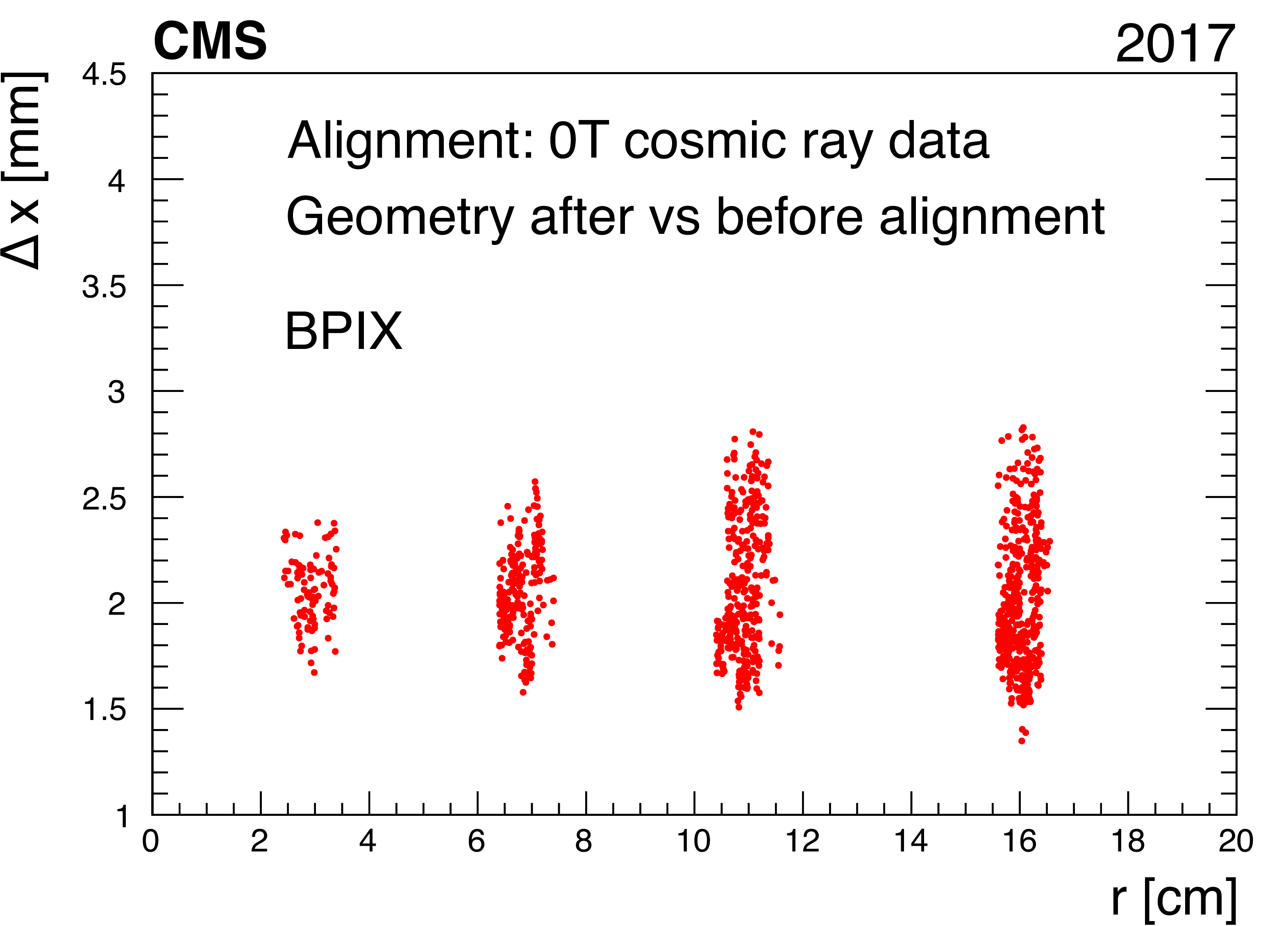
Figure 15:
Corrections after the first high-level structures alignment of the pixel detector in 2017, for the three FPIX disks (left) and the four BPIX layers (right). Shown are the differences of the module positions after the module-level alignment of the pixel detector, with respect to the ones considered before performing any alignment, as a function of the design positions. The alignments were performed with 0 T cosmic ray muon tracks. |

png pdf |
Figure 15-a:
Corrections after the first high-level structures alignment of the pixel detector in 2017, for the three FPIX disks. Shown are the differences of the module positions after the module-level alignment of the pixel detector, with respect to the ones considered before performing any alignment, as a function of the design positions. The alignments were performed with 0 T cosmic ray muon tracks. |
png pdf |
Figure 15-b:
Corrections after the first high-level structures alignment of the pixel detector in 2017, for the four BPIX layers. Shown are the differences of the module positions after the module-level alignment of the pixel detector, with respect to the ones considered before performing any alignment, as a function of the design positions. The alignments were performed with 0 T cosmic ray muon tracks. |
png pdf |
Figure 16:
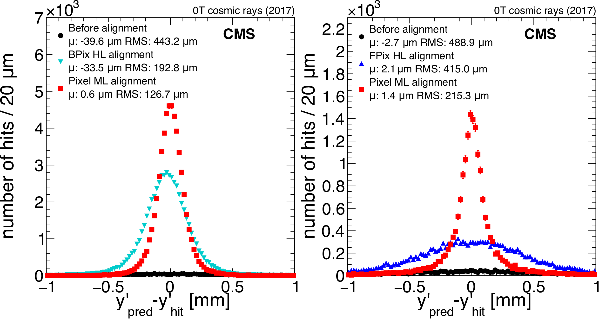
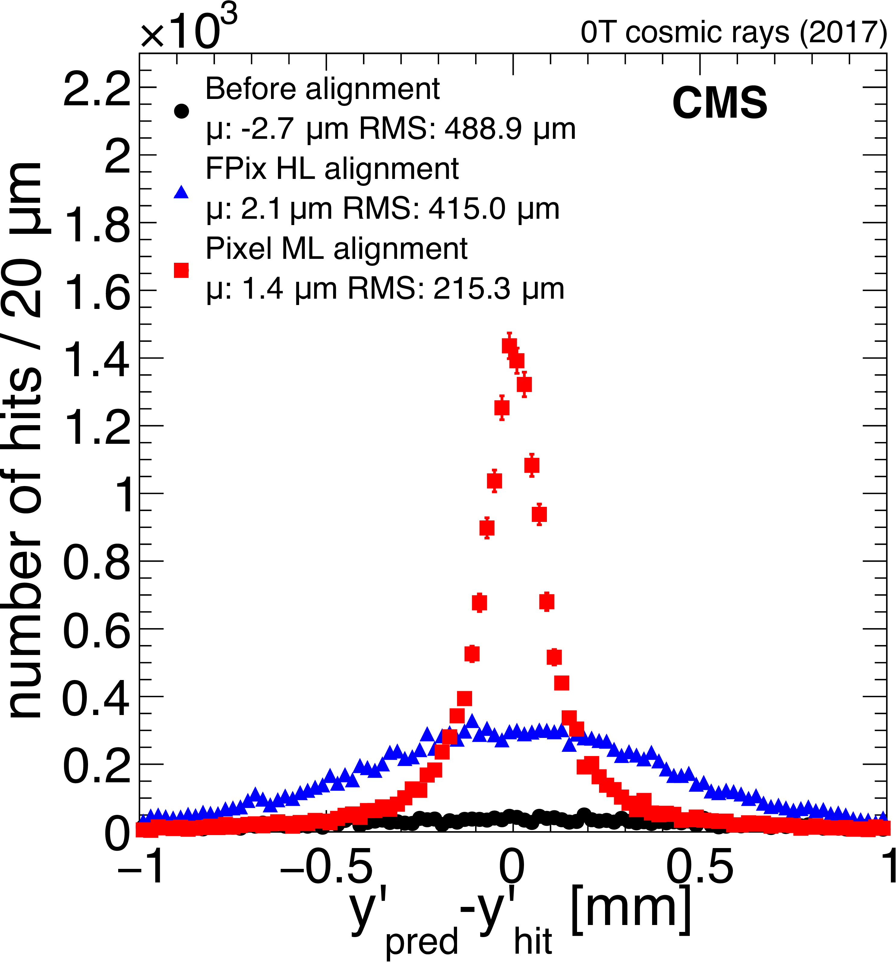
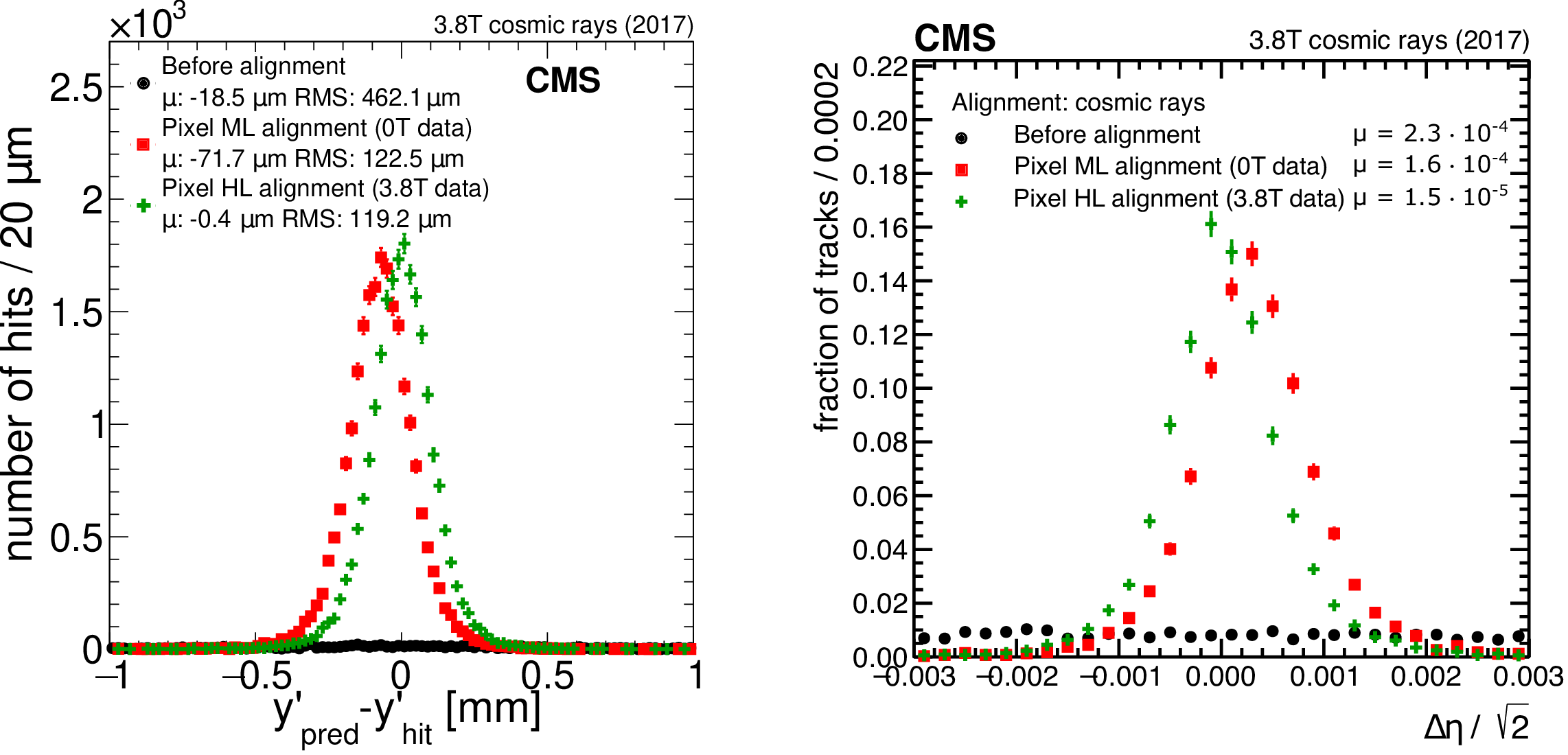
Unbiased track-hit residuals in the BPIX (left) and FPIX (right), in the local $y$ ($y'$) coordinate. The distributions are shown for the different alignment iterations that were performed: the black circles indicate the geometry assumed before performing any alignment fit, the blue and cyan triangles show the high-level (HL) structures alignment of the barrel and forward pixel detectors, and the red squares represent the module-level (ML) alignment of the pixel detector. The mean ($\mu $) and RMS of the distributions are given in the legend. Vertical error bars represent the statistical uncertainty; they are smaller than the marker size in most of the cases. |

png pdf |
Figure 16-a:
Unbiased track-hit residuals in the BPIX, in the local $y$ ($y'$) coordinate. The distributions are shown for the different alignment iterations that were performed: the black circles indicate the geometry assumed before performing any alignment fit, the blue and cyan triangles show the high-level (HL) structures alignment of the barrel and forward pixel detectors, and the red squares represent the module-level (ML) alignment of the pixel detector. The mean ($\mu $) and RMS of the distributions are given in the legend. Vertical error bars represent the statistical uncertainty; they are smaller than the marker size in most of the cases. |
png pdf |
Figure 16-b:
Unbiased track-hit residuals in the FPIX, in the local $y$ ($y'$) coordinate. The distributions are shown for the different alignment iterations that were performed: the black circles indicate the geometry assumed before performing any alignment fit, the blue and cyan triangles show the high-level (HL) structures alignment of the barrel and forward pixel detectors, and the red squares represent the module-level (ML) alignment of the pixel detector. The mean ($\mu $) and RMS of the distributions are given in the legend. Vertical error bars represent the statistical uncertainty; they are smaller than the marker size in most of the cases. |
png pdf |
Figure 17:
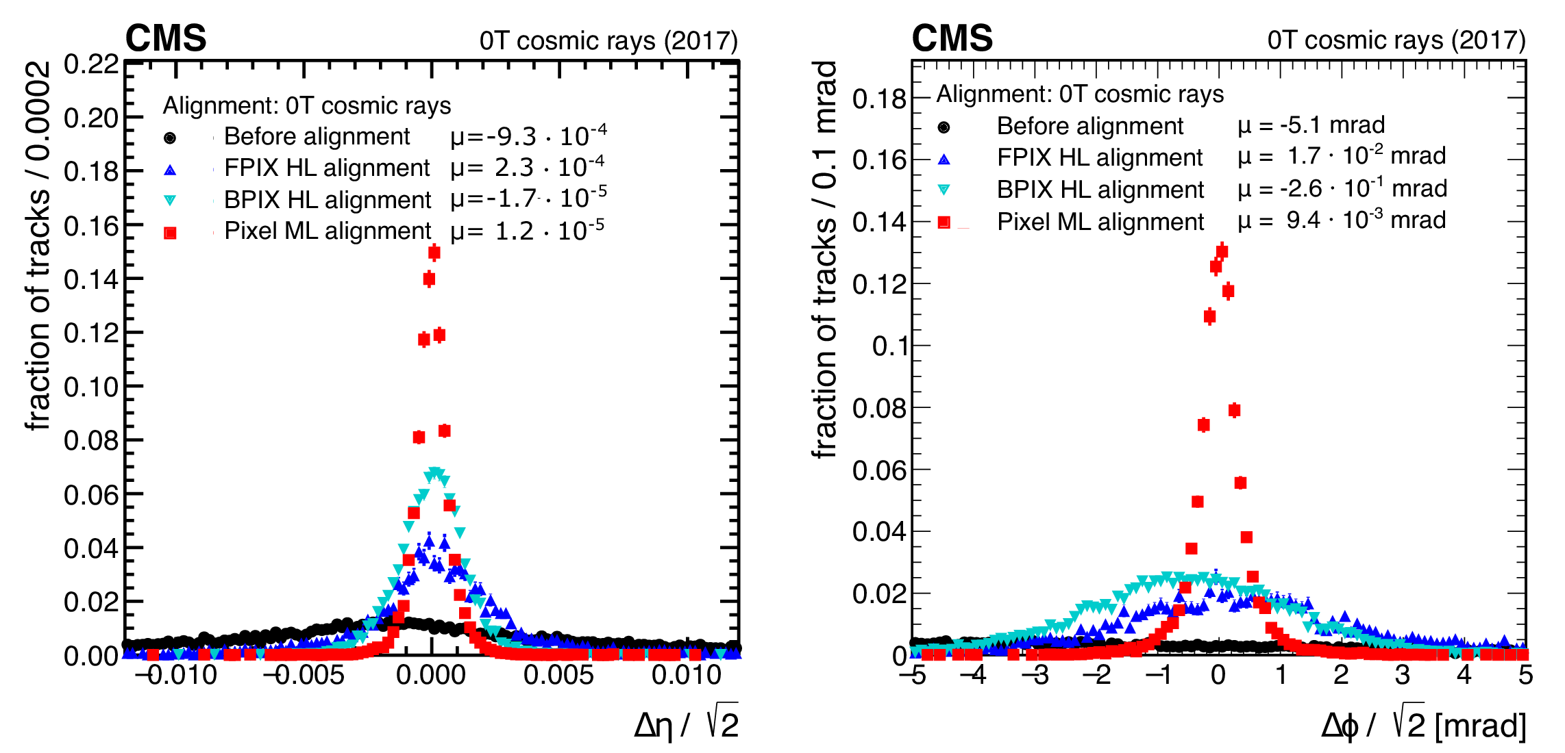
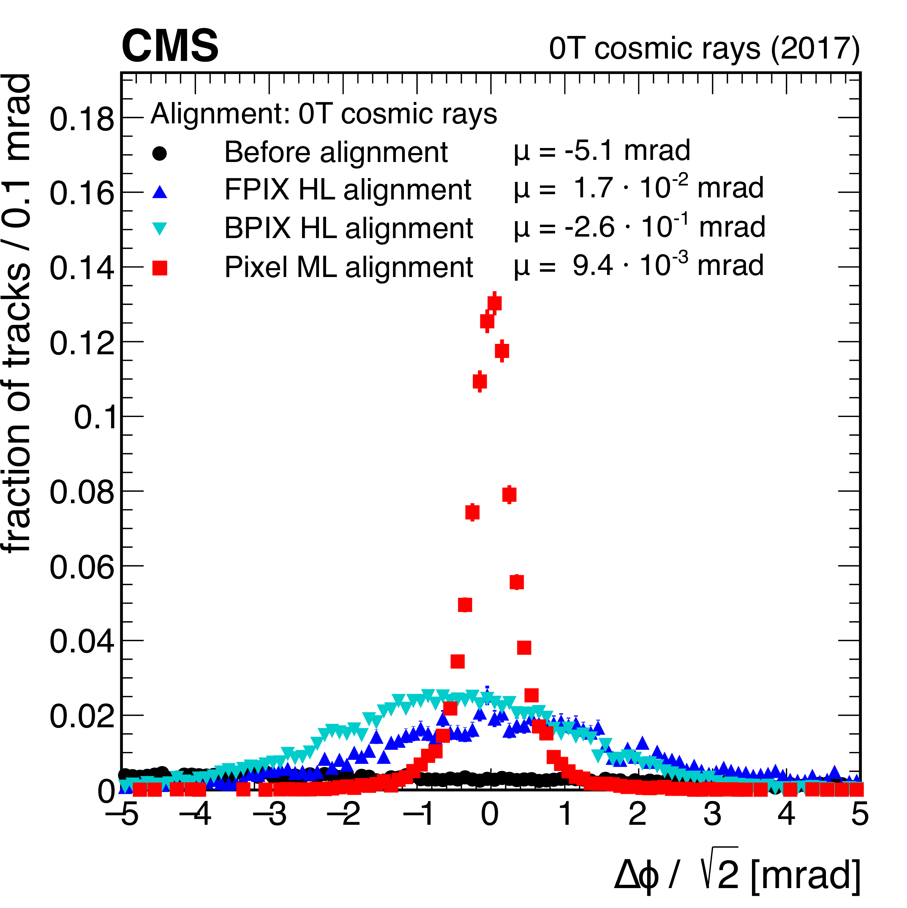
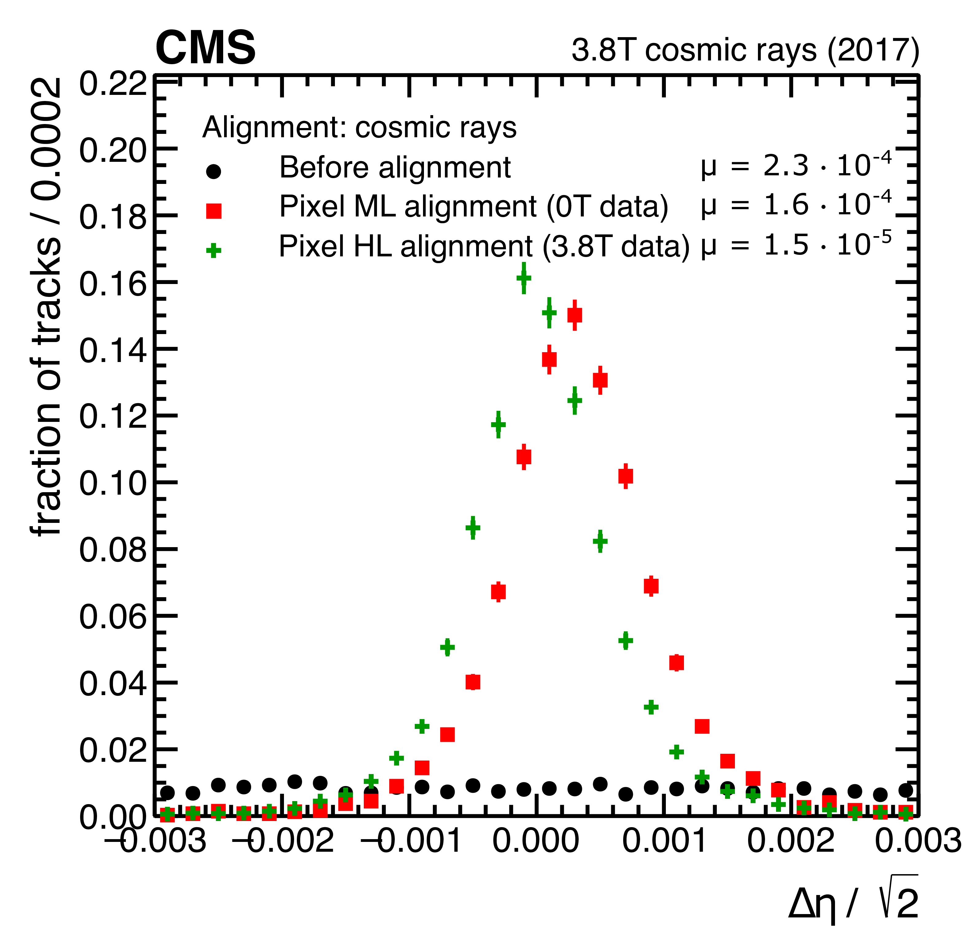
Distributions of the difference in reconstructed parameters between the two halves of a cosmic ray muon track, split at the point of closest approach to the interaction region: track $\eta $ (left) and $\phi $ (right) from a dataset recorded at 0 T. The difference is scaled by a factor $\sqrt {2}$ to account for the two independent measurements. The black circles show the geometry assumed before performing any alignment, the triangles show the FPIX and BPIX high-level (HL) structures alignment, and the red squares represent the module-level (ML) alignment of the pixel detector. The mean of the distributions ($\mu $) is given in the legend. Vertical error bars represent the statistical uncertainty; they are smaller than the marker size in most of the cases. |

png pdf |
Figure 17-a:
Distributions of the difference in reconstructed parameters between the two halves of a cosmic ray muon track, split at the point of closest approach to the interaction region: track $\eta $ from a dataset recorded at 0 T. The difference is scaled by a factor $\sqrt {2}$ to account for the two independent measurements. The black circles show the geometry assumed before performing any alignment, the triangles show the FPIX and BPIX high-level (HL) structures alignment, and the red squares represent the module-level (ML) alignment of the pixel detector. The mean of the distributions ($\mu $) is given in the legend. Vertical error bars represent the statistical uncertainty; they are smaller than the marker size in most of the cases. |
png pdf |
Figure 17-b:
Distributions of the difference in reconstructed parameters between the two halves of a cosmic ray muon track, split at the point of closest approach to the interaction region: track $\phi $ from a dataset recorded at 0 T. The difference is scaled by a factor $\sqrt {2}$ to account for the two independent measurements. The black circles show the geometry assumed before performing any alignment, the triangles show the FPIX and BPIX high-level (HL) structures alignment, and the red squares represent the module-level (ML) alignment of the pixel detector. The mean of the distributions ($\mu $) is given in the legend. Vertical error bars represent the statistical uncertainty; they are smaller than the marker size in most of the cases. |
png pdf |
Figure 18:
Performance of the 2017 CRAFT alignment fit (green crosses) compared with the geometry obtained after the alignment fit with 0 T cosmic ray muon tracks (red squares), and with the assumed geometry before performing any alignment (black circles). As an example, the track-hit residual distributions in the local $y$ coordinate for the BPIX (left) and the difference in track $\eta $ from the cosmic ray muon track split validation (right) are shown. The mean ($\mu $) of the distributions is given in the legend. For the track-hit residual distributions, also the RMS is indicated. Vertical error bars represent the statistical uncertainty; they are smaller than the marker size in most of the cases. |

png pdf |
Figure 18-a:
Performance of the 2017 CRAFT alignment fit (green crosses) compared with the geometry obtained after the alignment fit with 0 T cosmic ray muon tracks (red squares), and with the assumed geometry before performing any alignment (black circles). As an example, the track-hit residual distributions in the local $y$ coordinate for the BPIX are is shown. The mean ($\mu $) of the distributions is given in the legend. Also the RMS is indicated. Vertical error bars represent the statistical uncertainty; they are smaller than the marker size in most of the cases. |
png pdf |
Figure 18-b:
Performance of the 2017 CRAFT alignment fit (green crosses) compared with the geometry obtained after the alignment fit with 0 T cosmic ray muon tracks (red squares), and with the assumed geometry before performing any alignment (black circles). As an example, the difference in track $\eta $ from the cosmic ray muon track split validation are shown. The mean ($\mu $) of the distributions is given in the legend. Vertical error bars represent the statistical uncertainty; they are smaller than the marker size in most of the cases. |
png pdf |
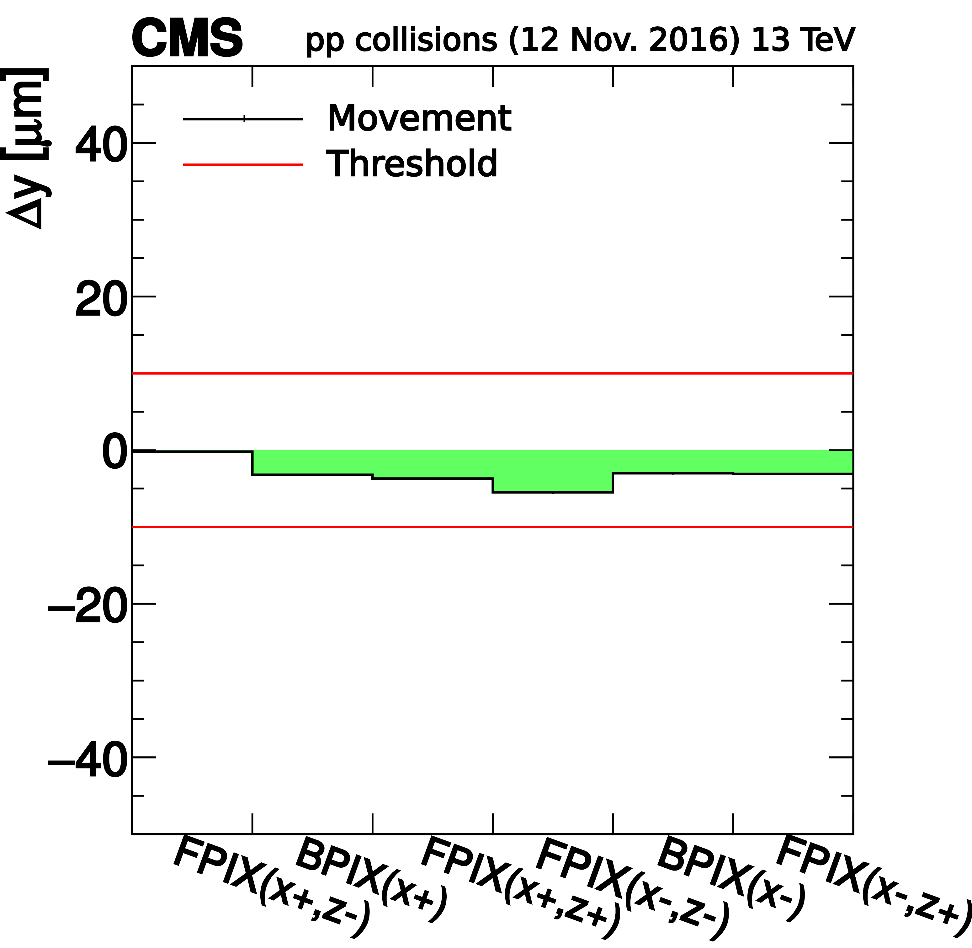
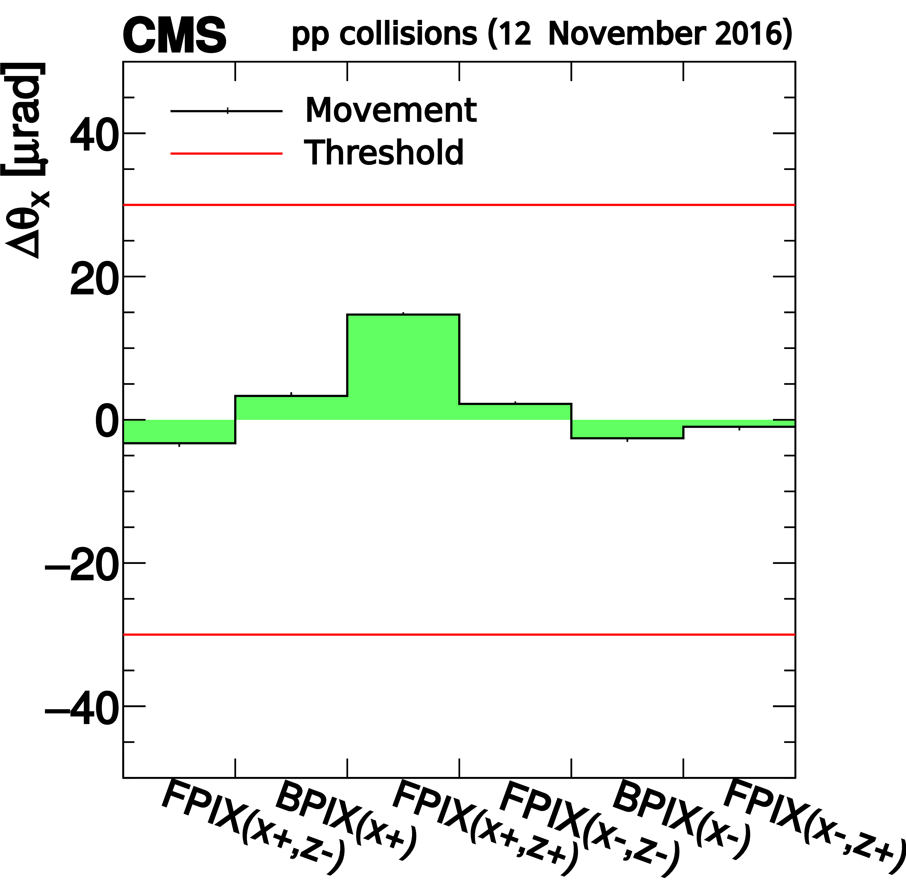
Figure 19:
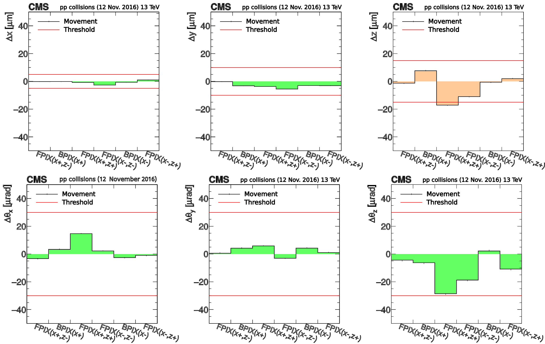
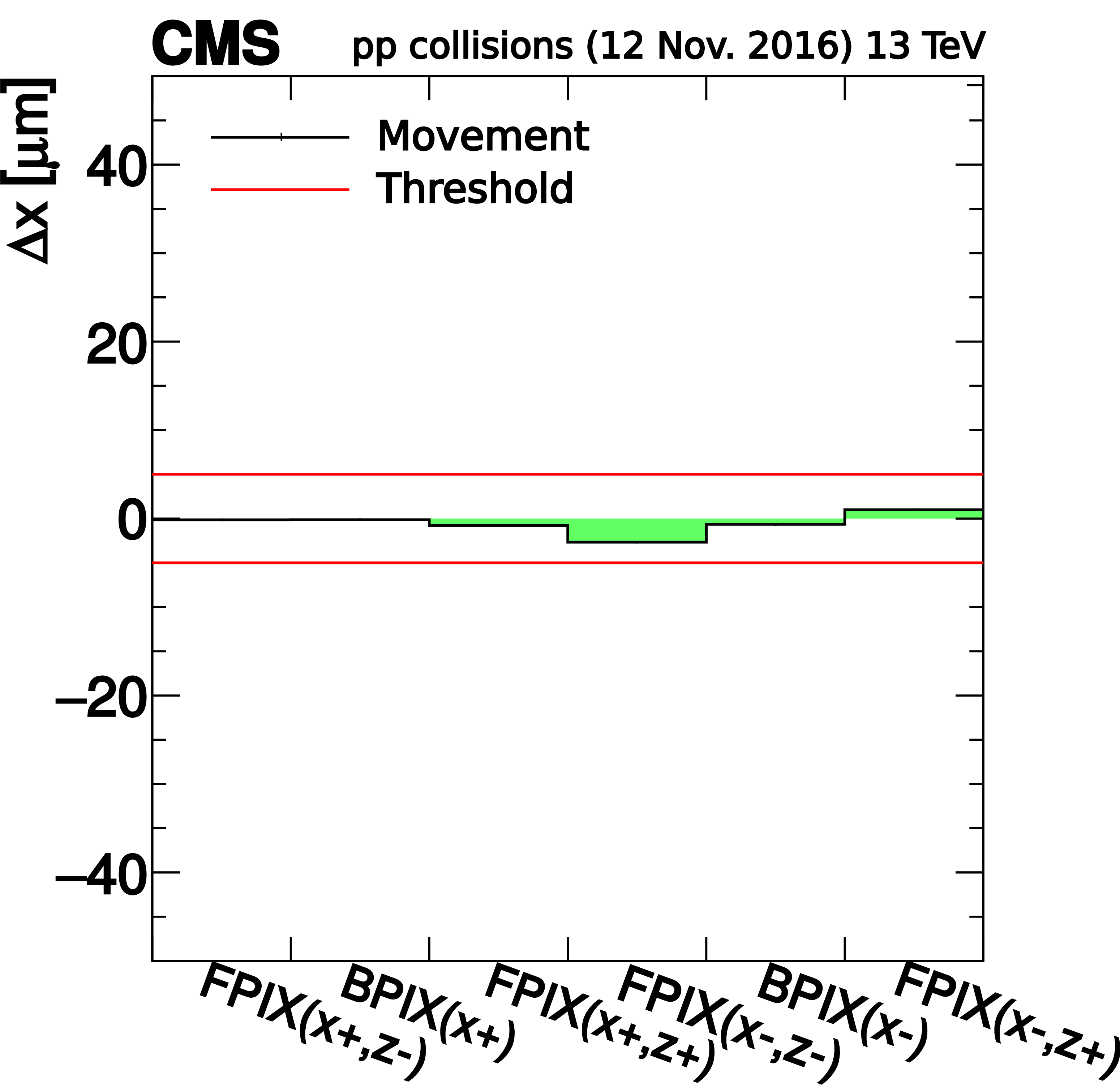
Observed movements of the six high-level structures in the pixel detector from the alignment procedure in the PCL for one arbitrary run in 2016. The two horizontal red lines in each of the figures show the threshold for triggering the deployment of a new set of alignment constants. The error bars represent the statistical uncertainties of the measurements. The orange bars in the figure showing the movement in the $z$ direction indicate that a sufficient movement to deploy a new set of alignment constants was observed. |
png pdf |
Figure 19-a:
Observed movements of one of the six high-level structures in the pixel detector ($\Delta x $) from the alignment procedure in the PCL for one arbitrary run in 2016. The two horizontal red lines ishow the threshold for triggering the deployment of a new set of alignment constants. The error bars represent the statistical uncertainties of the measurements. |
png pdf |
Figure 19-b:
Observed movements of one of the six high-level structures in the pixel detector ($\Delta y $) from the alignment procedure in the PCL for one arbitrary run in 2016. The two horizontal red lines ishow the threshold for triggering the deployment of a new set of alignment constants. The error bars represent the statistical uncertainties of the measurements. |

png pdf |
Figure 19-c:
Observed movements of one of the six high-level structures in the pixel detector ($\Delta z $) from the alignment procedure in the PCL for one arbitrary run in 2016. The two horizontal red lines ishow the threshold for triggering the deployment of a new set of alignment constants. The error bars represent the statistical uncertainties of the measurements. The orange bars indicate that a sufficient movement to deploy a new set of alignment constants was observed. |
png pdf |
Figure 19-d:
Observed movements of one of the six high-level structures in the pixel detector ($\Delta \theta_x$) from the alignment procedure in the PCL for one arbitrary run in 2016. The two horizontal red lines ishow the threshold for triggering the deployment of a new set of alignment constants. The error bars represent the statistical uncertainties of the measurements. |

png pdf |
Figure 19-e:
Observed movements of one of the six high-level structures in the pixel detector ($\Delta \theta_y$) from the alignment procedure in the PCL for one arbitrary run in 2016. The two horizontal red lines ishow the threshold for triggering the deployment of a new set of alignment constants. The error bars represent the statistical uncertainties of the measurements. |

png pdf |
Figure 19-f:
Observed movements of one of the six high-level structures in the pixel detector ($\Delta \theta_z$) from the alignment procedure in the PCL for one arbitrary run in 2016. The two horizontal red lines ishow the threshold for triggering the deployment of a new set of alignment constants. The error bars represent the statistical uncertainties of the measurements. |
png pdf |
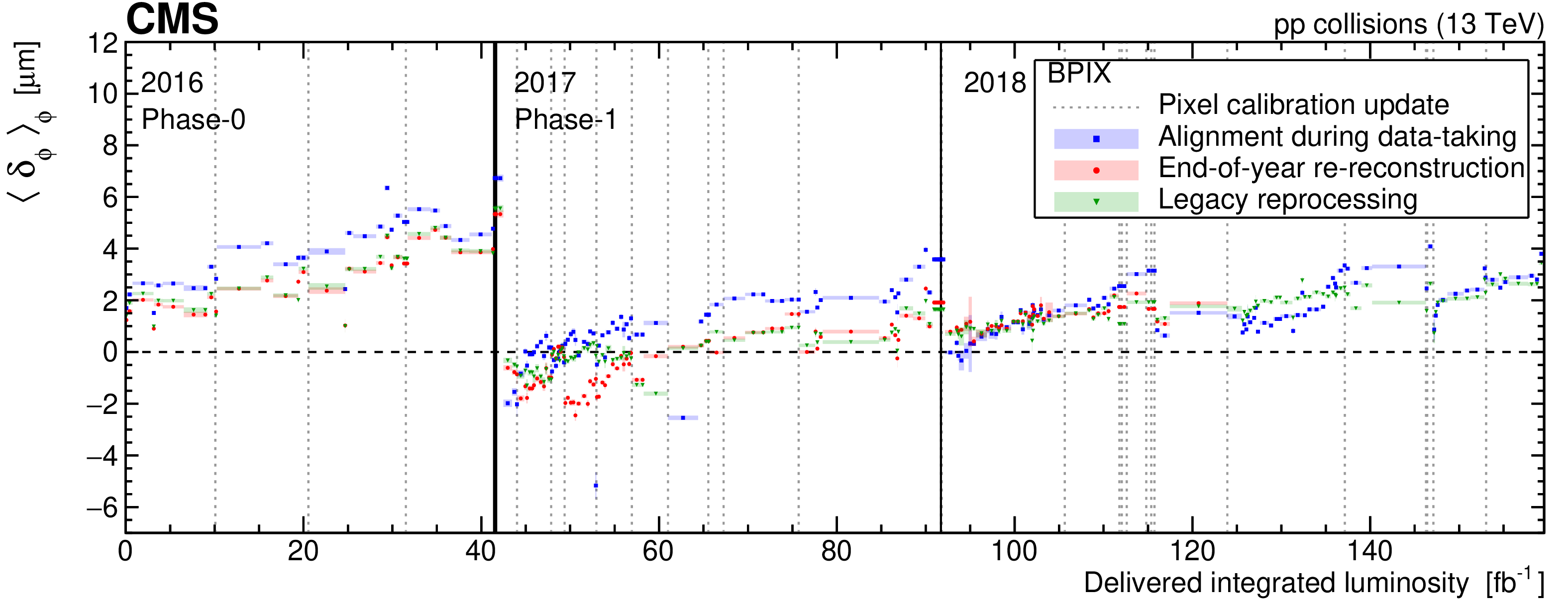
Figure 20:
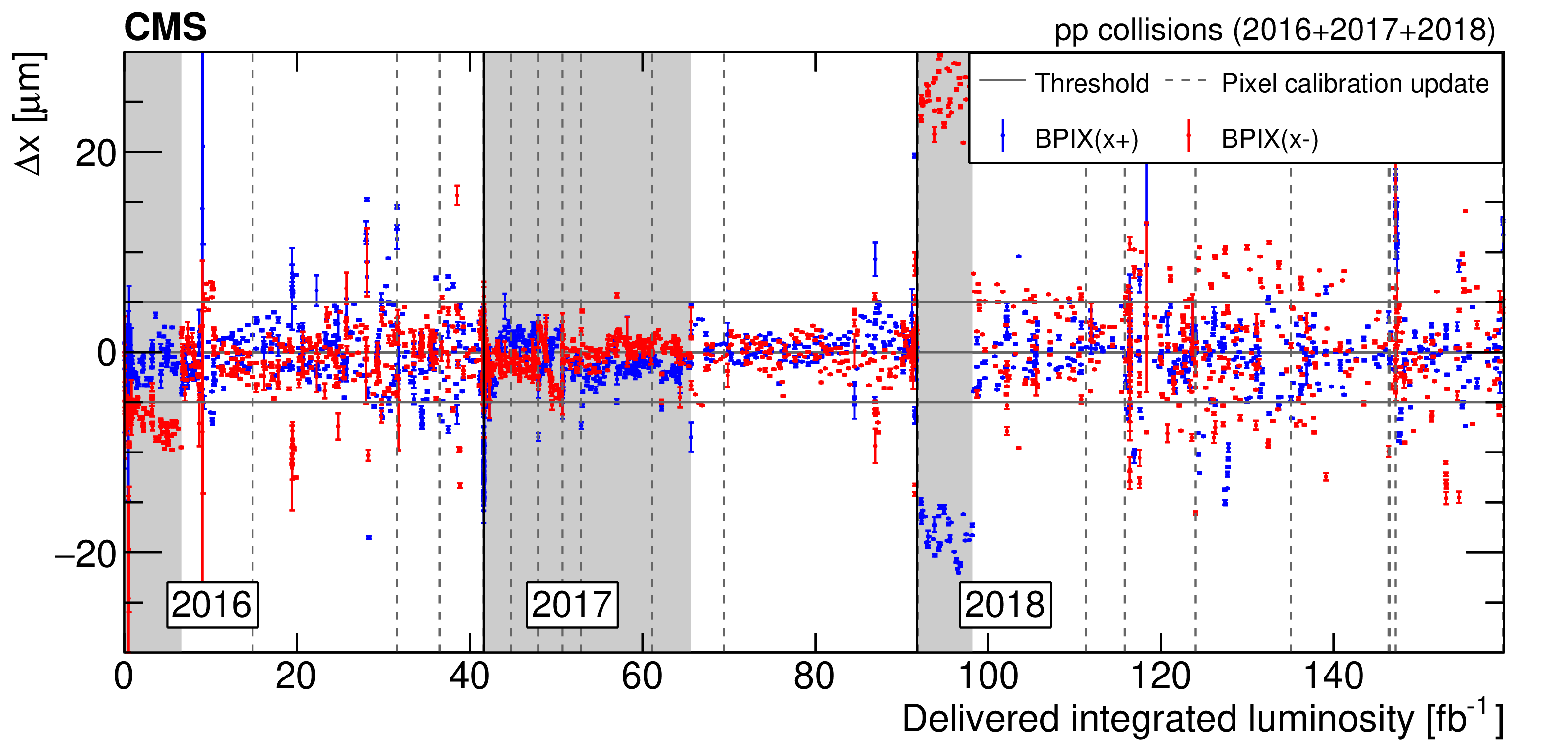
Observed movements in the $x$ direction of the two BPIX half cylinders, as functions of the delivered integrated luminosity, from the alignment procedure in the PCL. Each point corresponds to a single run. The vertical bars on each point represent the statistical uncertainty of the measurement. The vertical black solid lines indicate the first processed runs for the 2016, 2017, and 2018 data-taking periods, respectively. The vertical dashed lines illustrate updates of the pixel detector calibration. The two horizontal lines show the threshold for triggering the deployment of a new set of alignment constants. The grey bands at the beginning of each year indicate runs where the automated alignment updates were not active. |
png pdf |
Figure 21:
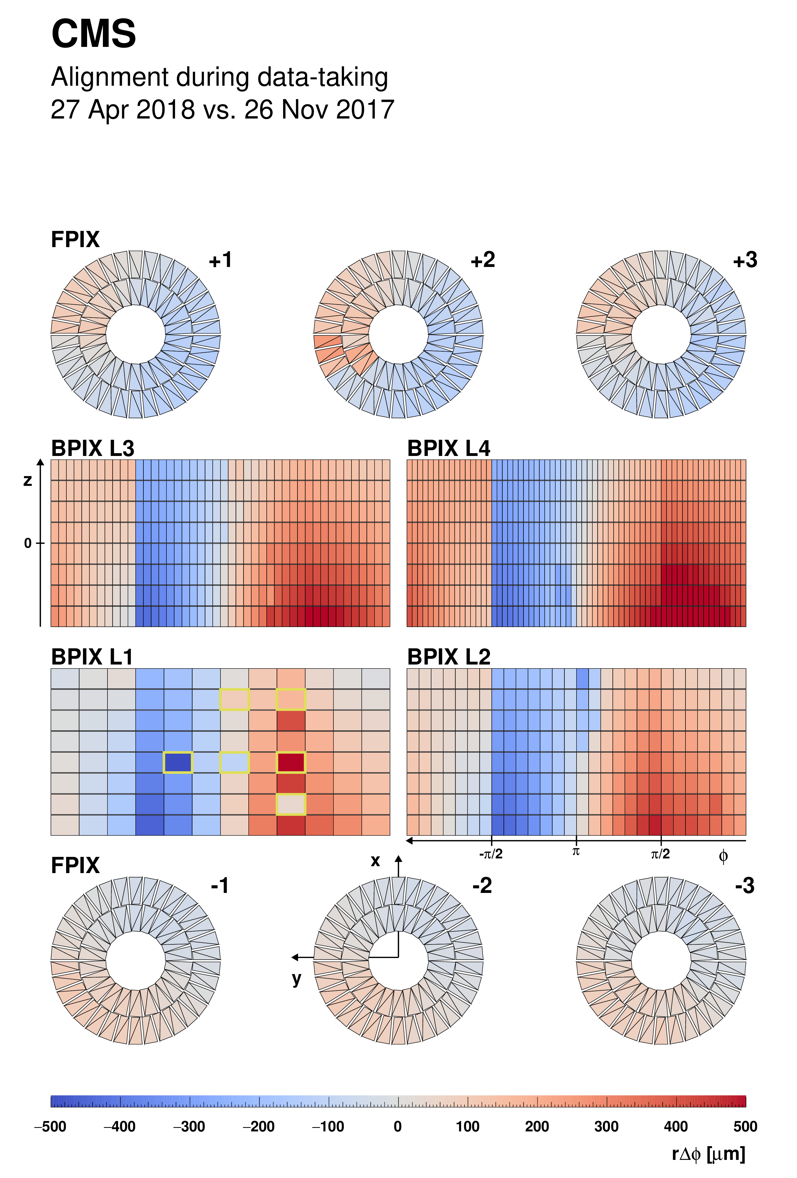
The value of the product $r\Delta \phi $ for each module in the pixel detector, comparing the alignment parameters of the alignment during data taking on 26 November 2017 and on 27 April 2018. These runs correspond to the last run of 2017 and the first run of 2018 after commissioning. During this transition, several modules of layer 1 of the BPIX were replaced (indicated in yellow frames), which explains the large movements with respect to their neighbouring modules. For each of the detector components, $r$ and $\phi $ correspond to the global coordinate, and $\Delta \phi $ is the shift in $\phi $ across the two alignments resulting in the physical shift $r\Delta \phi $ in the detector. |

png pdf |
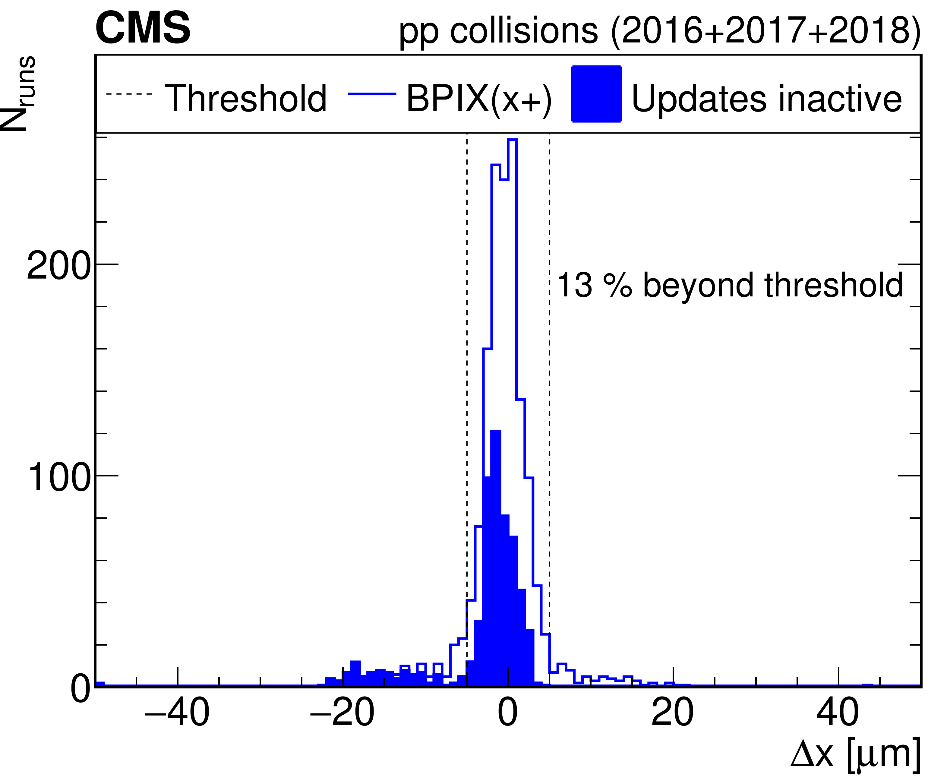
Figure 22:
Observed movements in the $x$ direction of the two BPIX half cylinders from the PCL alignment. The two vertical lines show the threshold for a new alignment to be triggered. The filled entries correspond to runs at the start of each year, where the automated updates of the alignment were not active. The percentage of the runs for which a new alignment was triggered by the movement in the $x$ direction is displayed below the legend in both figures. In the calculation of this percentage, the filled entries are not included. |
png pdf |
Figure 22-a:
Observed movements in the $x$ direction of the $x+$ BPIX half cylinder from the PCL alignment. The two vertical lines show the threshold for a new alignment to be triggered. The filled entries correspond to runs at the start of each year, where the automated updates of the alignment were not active. The percentage of the runs for which a new alignment was triggered by the movement in the $x$ direction is displayed below the legend in both figures. In the calculation of this percentage, the filled entries are not included. |

png pdf |
Figure 22-b:
Observed movements in the $x$ direction of the $x-$ BPIX half cylinder from the PCL alignment. The two vertical lines show the threshold for a new alignment to be triggered. The filled entries correspond to runs at the start of each year, where the automated updates of the alignment were not active. The percentage of the runs for which a new alignment was triggered by the movement in the $x$ direction is displayed below the legend in both figures. In the calculation of this percentage, the filled entries are not included. |
png pdf |
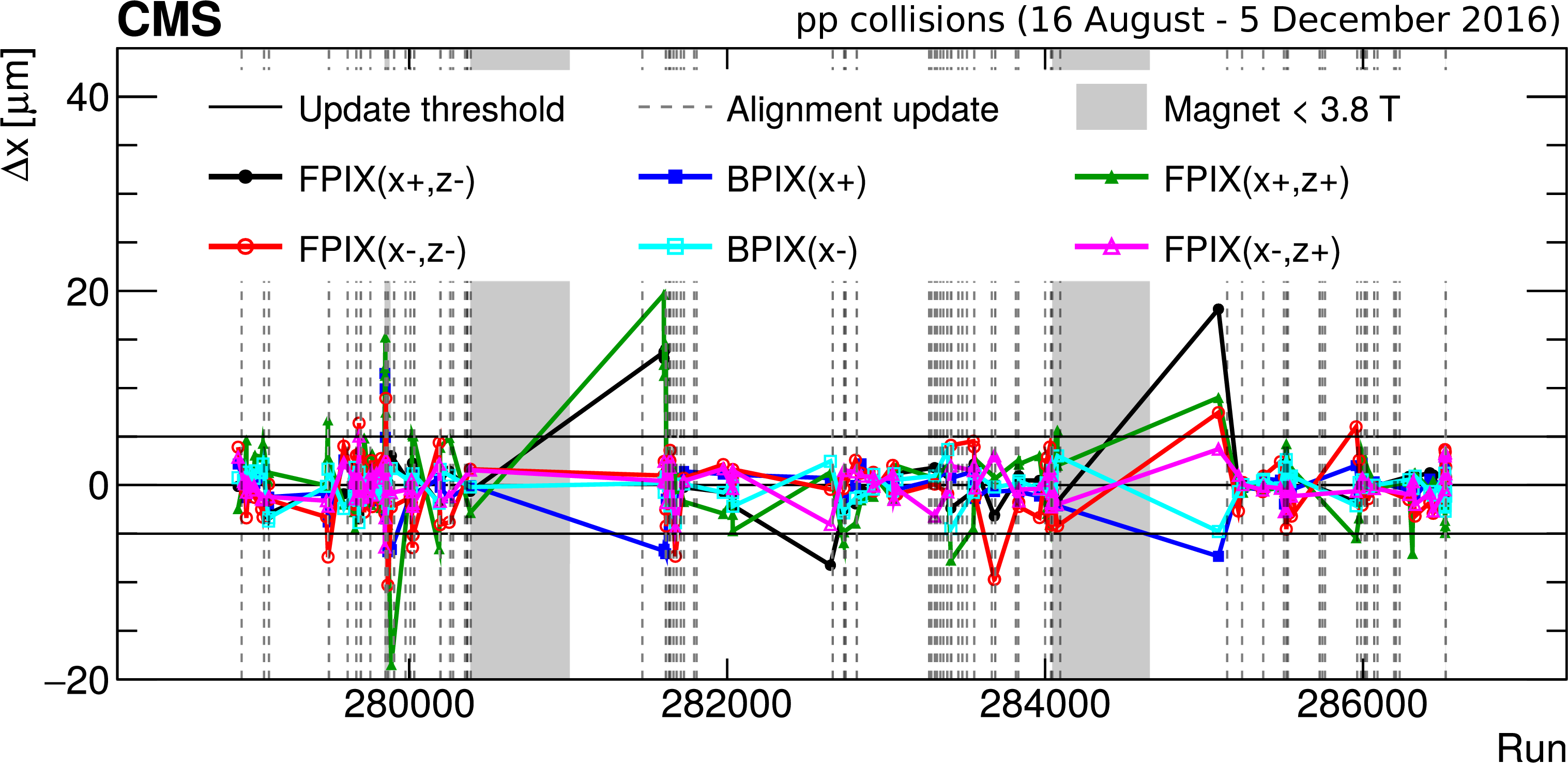
Figure 23:
Observed movements in the $x$ direction of the six high-level structures, as functions of the run number from the alignment procedure in the PCL for the data-taking period between 16 August and 5 December 2016. Each point corresponds to a run that triggered an update of the alignment parameters caused by a sufficient change in one of the three positions or rotations. The movements are shown without uncertainties. The vertical dashed lines illustrate the deployments of new sets of alignment constants. The two horizontal lines show the threshold for a new alignment to be triggered. The grey shaded regions indicate runs during which the magnet was not at 3.8 T (magnet cycle). After each of the two magnet cycles a large movement is observed for the very first run after the cycle. |
png pdf |
Figure 24:
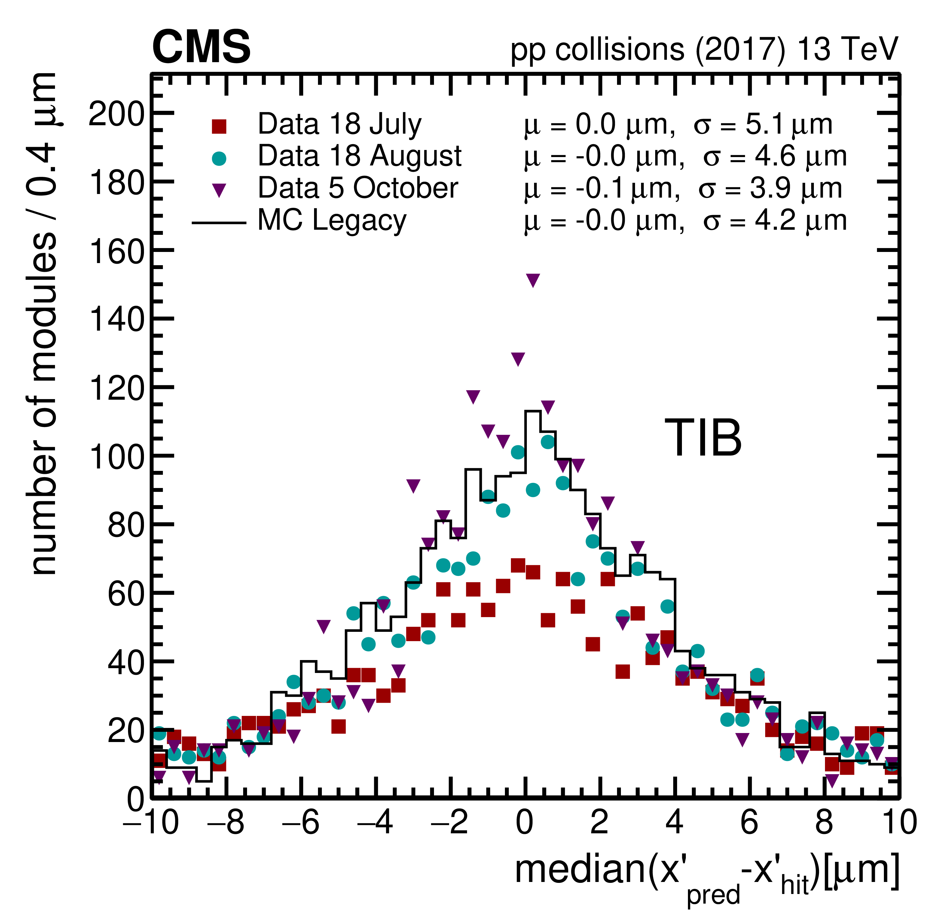
Distributions of per-module median track-hit residuals in the local $x$ ($x'$) coordinate, for two subdetectors (BPIX and TOB), produced with the single-muon data set. The distributions are averaged over all IOVs, where each IOV is weighted with the corresponding delivered integrated luminosity. The DMRs are shown for three different geometries in data. They are compared with the realistic MC scenario (black line) and the design MC scenario (magenta) evaluated in simulated isolated-muon events. The quoted means $\mu $ and standard deviations $\sigma $ are the parameters of a Gaussian fit to the distributions. |
png pdf |
Figure 24-a:
Distributions of per-module median track-hit residuals in the local $x$ ($x'$) coordinate, for the BPIX subdetector, produced with the single-muon data set. The distributions are averaged over all IOVs, where each IOV is weighted with the corresponding delivered integrated luminosity. The DMRs are shown for three different geometries in data. They are compared with the realistic MC scenario (black line) and the design MC scenario (magenta) evaluated in simulated isolated-muon events. The quoted means $\mu $ and standard deviations $\sigma $ are the parameters of a Gaussian fit to the distributions. |
png pdf |
Figure 24-b:
Distributions of per-module median track-hit residuals in the local $x$ ($x'$) coordinate, for the TOB subdetector, produced with the single-muon data set. The distributions are averaged over all IOVs, where each IOV is weighted with the corresponding delivered integrated luminosity. The DMRs are shown for three different geometries in data. They are compared with the realistic MC scenario (black line) and the design MC scenario (magenta) evaluated in simulated isolated-muon events. The quoted means $\mu $ and standard deviations $\sigma $ are the parameters of a Gaussian fit to the distributions. |
png pdf |
Figure 25:
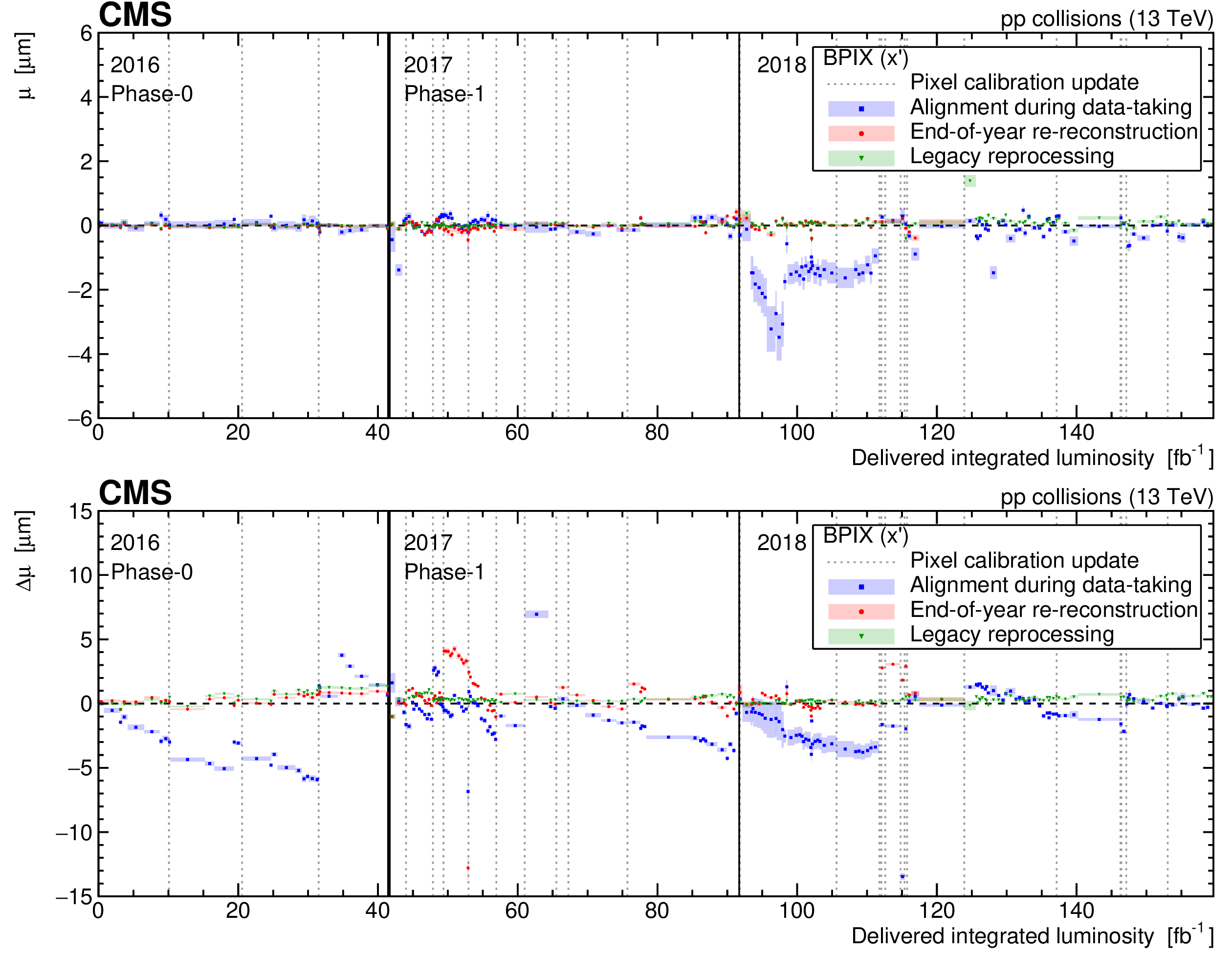
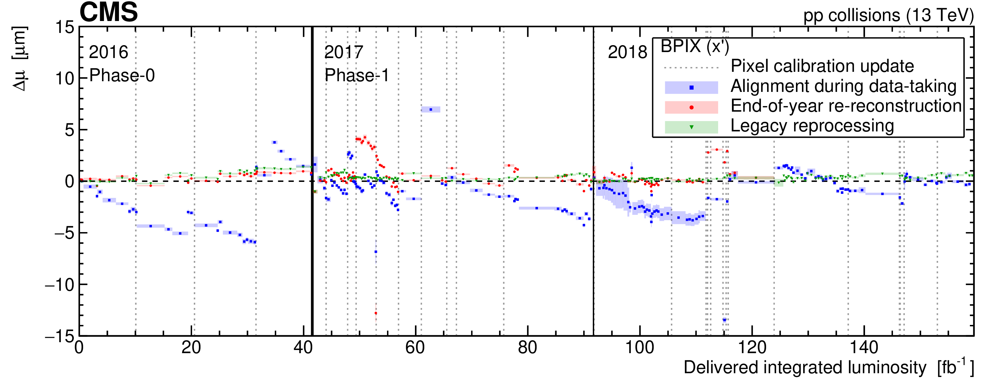
The DMR trends for the years 2016-2018, as functions of the delivered integrated luminosity, evaluated with a sample of data recorded by the inclusive L1 trigger. The upper figure shows the mean value of the distribution of median residuals for the local $x$ ($x'$) coordinate in the BPIX detector. The lower figure shows the difference between the mean values $\Delta \mu $ obtained separately for the modules with the electric field pointing radially inwards or outwards. This quantity is also shown in the $x'$ coordinate. The shaded band indicates one standard deviation from the Gaussian fit of the corresponding DMR. |

png pdf |
Figure 25-a:
The DMR trends for the years 2016-2018, as functions of the delivered integrated luminosity, evaluated with a sample of data recorded by the inclusive L1 trigger. The figure shows the mean value of the distribution of median residuals for the local $x$ ($x'$) coordinate in the BPIX detector. The shaded band indicates one standard deviation from the Gaussian fit of the corresponding DMR. |
png pdf |
Figure 25-b:
The DMR trends for the years 2016-2018, as functions of the delivered integrated luminosity, evaluated with a sample of data recorded by the inclusive L1 trigger. The figure shows the difference between the mean values $\Delta \mu $ obtained separately for the modules with the electric field pointing radially inwards or outwards. This quantity is shown in the $x'$ coordinate. The shaded band indicates one standard deviation from the Gaussian fit of the corresponding DMR. |
png pdf |
Figure 26:
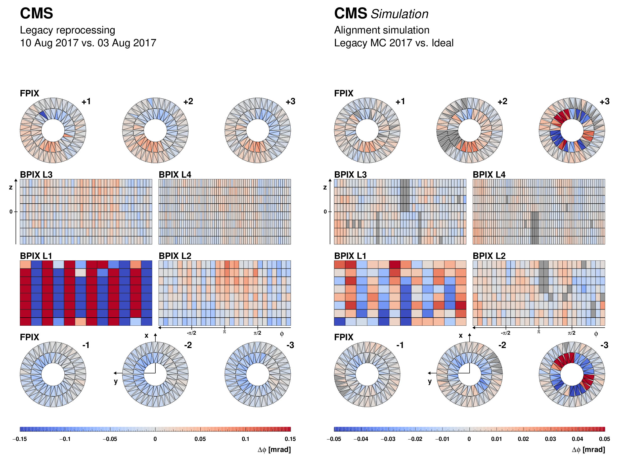
The value of $\Delta \phi $ for each module in the pixel detector, comparing the alignment parameters of the legacy reprocessing on 3 and 10 August 2017 (left) and comparing the alignment based on MC simulation for 2017 and the ideal detector (right). For each of the detector components, $\phi $ corresponds to the global coordinate. The colours denote the value of the $\Delta \phi $ movement, as shown by the bar at the bottom. These values are capped between $-$0.15 and 0.15 mrad for the alignments in data (left) and between $-$0.05 and 0.05 mrad for simulation (right). In the figure on the right, modules that were inactive in the simulation are indicated in dark grey. The alternating pattern visible in layer 1 of the BPIX is caused by radiation damage that is absorbed in the modules between local calibration updates of the pixel modules. Due to the opposite orientations of the neighbouring ladders, an alternating pattern is created. Radiation damage is more severe in the first layer which is closer to the interaction point, making the pattern more visible. |

png pdf |
Figure 26-a:
The value of $\Delta \phi $ for each module in the pixel detector, comparing the alignment parameters of the legacy reprocessing on 3 and 10 August 2017. For each of the detector components, $\phi $ corresponds to the global coordinate. The colours denote the value of the $\Delta \phi $ movement, as shown by the bar at the bottom. These values are capped between $-$0.15 and 0.15 mrad for the alignments in data. In the figure on the right, modules that were inactive in the simulation are indicated in dark grey. The alternating pattern visible in layer 1 of the BPIX is caused by radiation damage that is absorbed in the modules between local calibration updates of the pixel modules. Due to the opposite orientations of the neighbouring ladders, an alternating pattern is created. Radiation damage is more severe in the first layer which is closer to the interaction point, making the pattern more visible. |

png pdf |
Figure 26-b:
The value of $\Delta \phi $ for each module in the pixel detector, comparing the alignment based on MC simulation for 2017 and the ideal detector (right). For each of the detector components, $\phi $ corresponds to the global coordinate. The colours denote the value of the $\Delta \phi $ movement, as shown by the bar at the bottom. These values are capped between $-$0.05 and 0.05 mrad for simulation. The alternating pattern visible in layer 1 of the BPIX is caused by radiation damage that is absorbed in the modules between local calibration updates of the pixel modules. Due to the opposite orientations of the neighbouring ladders, an alternating pattern is created. Radiation damage is more severe in the first layer which is closer to the interaction point, making the pattern more visible. |
png pdf |
Figure 27:
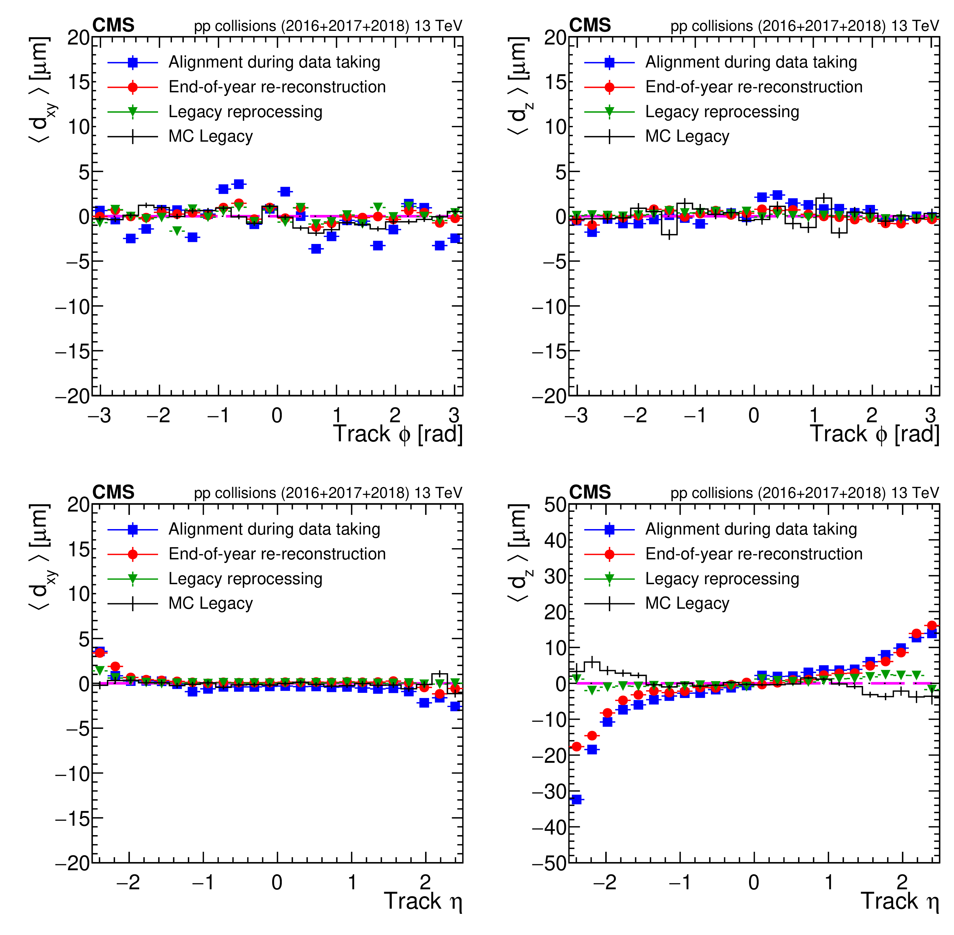
Mean track-vertex impact parameter in the transverse plane $ {d_{xy}}$ (left) and in the longitudinal plane $ {d_z}$ (right), as a function of track $\phi $ (top) and $\eta $ (bottom). The impact parameters are obtained by recalculating the vertex position after removal of the track under scrutiny and considering the impact parameter of this removed track. Only tracks with $ {p_{\mathrm {T}}} > $ 3 GeV are considered. These distributions are averaged over all runs of 2016, 2017, and 2018 after scaling them with the corresponding delivered integrated luminosity for each run. Three alignment geometries in data are compared with the realistic MC alignment scenario evaluated in a sample of simulated inclusive L1 trigger events (black points) scaled to the corresponding luminosity delivered in 2016, 2017, and 2018. The error bars represent the statistical uncertainties due to the limited number of tracks. In case of data points statistical uncertainties are smaller than size of the displayed markers. |

png pdf |
Figure 28:
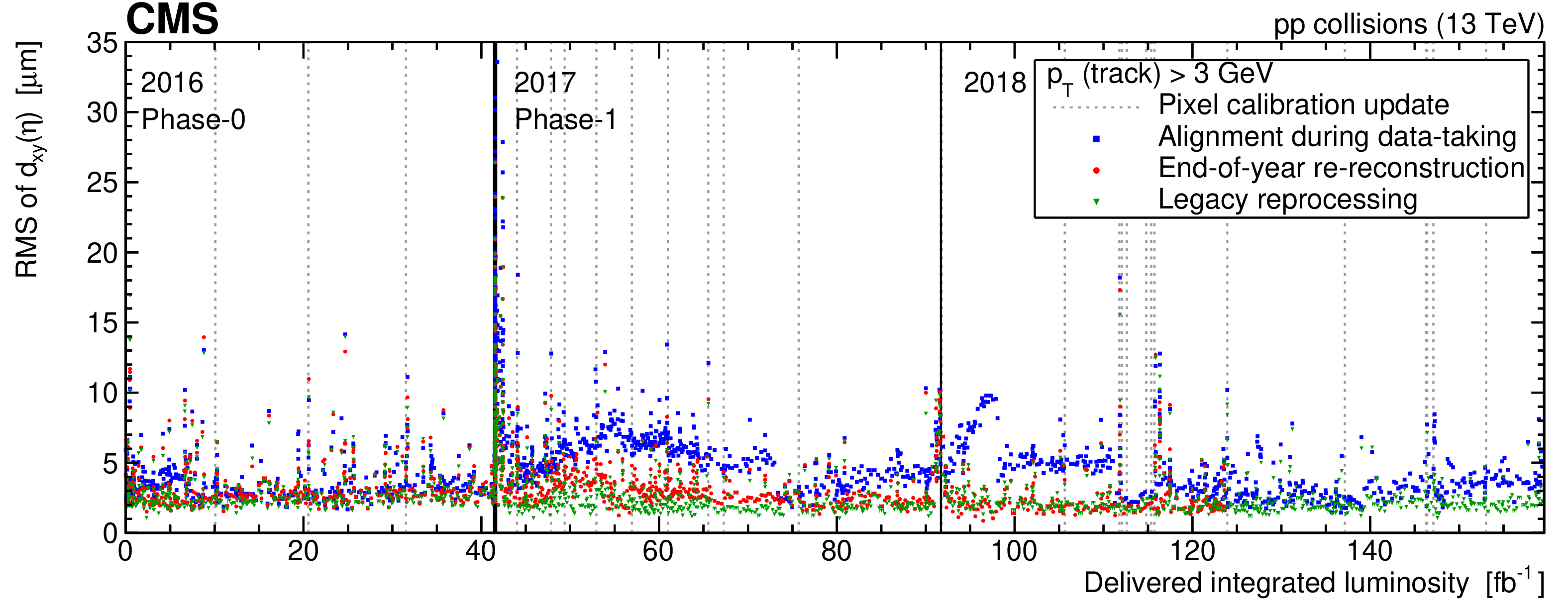
Impact parameter trends in the transverse plane $ {d_{xy}}$ as a function of the delivered integrated luminosity. Only tracks with $ {p_{\mathrm {T}}} > $ 3 GeV are considered. The upper figure shows the average $ {d_{xy}}$; the lower figure shows its RMS in bins of the track $\eta $. |

png pdf |
Figure 28-a:
Impact parameter trends in the transverse plane $ {d_{xy}}$ as a function of the delivered integrated luminosity. Only tracks with $ {p_{\mathrm {T}}} > $ 3 GeV are considered. The figure shows the average $ {d_{xy}}$; |
png pdf |
Figure 28-b:
Impact parameter trends in the transverse plane $ {d_{xy}}$ as a function of the delivered integrated luminosity. Only tracks with $ {p_{\mathrm {T}}} > $ 3 GeV are considered. The figure shows the RMS of the average $ {d_{xy}}$ in bins of the track $\eta $. |

png pdf |
Figure 29:
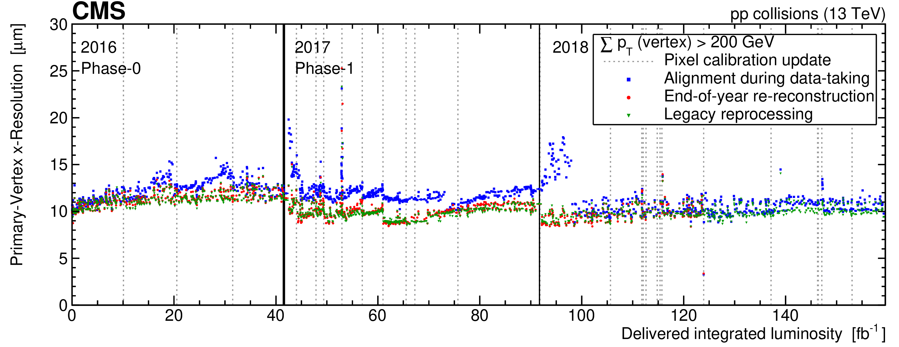
Primary vertex resolution in the $x$ (top) and $z$ (bottom) directions, calculated using refitted vertices with $\Sigma {p_{\mathrm {T}}} > $ 200 GeV ($x$) and $\Sigma {p_{\mathrm {T}}} > $ 400 GeV ($z$) in pp collisions. The vertical black lines indicate the first processed runs for the 2016, 2017, and 2018 data-taking periods. The vertical dotted lines indicate changes in the pixel tracker calibration. |
png pdf |
Figure 29-a:
Primary vertex resolution in the $x$ direction, calculated using refitted vertices with $\Sigma {p_{\mathrm {T}}} > $ 200 GeV ($x$) in pp collisions. The vertical black lines indicate the first processed runs for the 2016, 2017, and 2018 data-taking periods. The vertical dotted lines indicate changes in the pixel tracker calibration. |

png pdf |
Figure 29-b:
Primary vertex resolution in the $z$ direction, calculated using refitted vertices with $\Sigma {p_{\mathrm {T}}} > $ 400 GeV ($z$) in pp collisions. The vertical black lines indicate the first processed runs for the 2016, 2017, and 2018 data-taking periods. The vertical dotted lines indicate changes in the pixel tracker calibration. |

png pdf |
Figure 30:
Reconstructed Z boson mass as a function of the difference in $\eta $ between the positively and negatively charged muons, calculated from the full sample of dimuon events in the years 2016, 2017, and 2018. The error bars show the standard deviation of the invariant Z boson mass as retrieved from a fit of dimuon mass distribution to a Breit-Wigner convolved with a Crystal Ball function. |
png pdf |
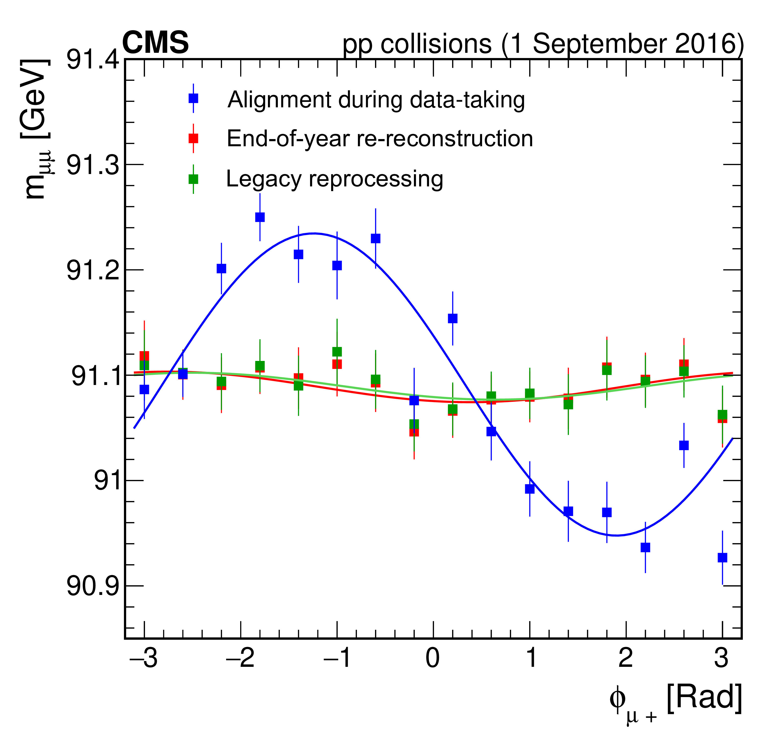
Figure 31:
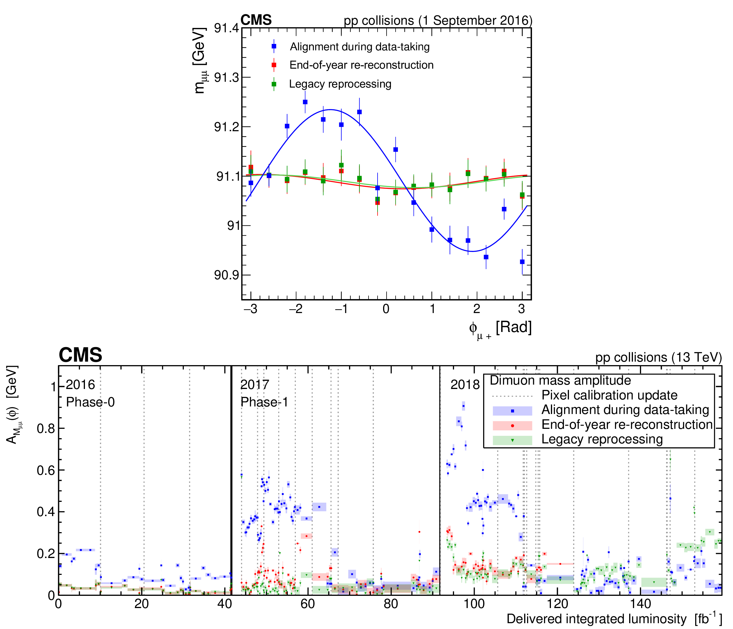
The upper figure shows the invariant mass of the dimuon system, as a function of the azimuthal angle of the positively charged track for a single IOV. The lower figure shows the amplitude $A$, obtained by fitting the invariant mass of the dimuon system versus $ {\phi _{\mu _+}}$ with a function of the form $A \cos{\left (\phi + \phi _{0}\right)} + b$ as a function of the delivered integrated luminosity. The vertical bars on the points in the upper figure show the uncertainty in the average $ {m_{\mu \mu}}$ of a given $ {\phi _{\mu _+}}$ bin. The shaded bands in the lower figure show the uncertainty in the fitted parameters calculated by a $\chi ^2$ regression. |
png pdf |
Figure 31-a:
The figure shows the invariant mass of the dimuon system, as a function of the azimuthal angle of the positively charged track for a single IOV. The vertical bars on the points show the uncertainty in the average $ {m_{\mu \mu}}$ of a given $ {\phi _{\mu _+}}$ bin. |

png pdf |
Figure 31-b:
The figure shows the amplitude $A$, obtained by fitting the invariant mass of the dimuon system versus $ {\phi _{\mu _+}}$ with a function of the form $A \cos{\left (\phi + \phi _{0}\right)} + b$ as a function of the delivered integrated luminosity. The shaded bands show the uncertainty in the fitted parameters calculated by a $\chi ^2$ regression. |
png pdf |
Figure 32:
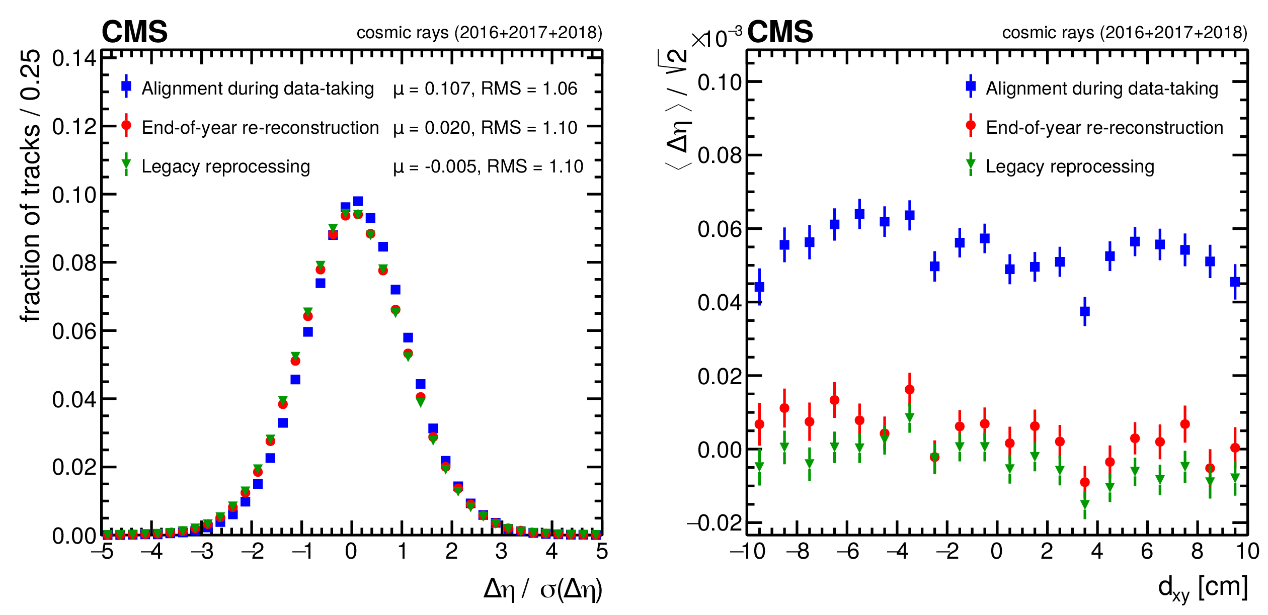
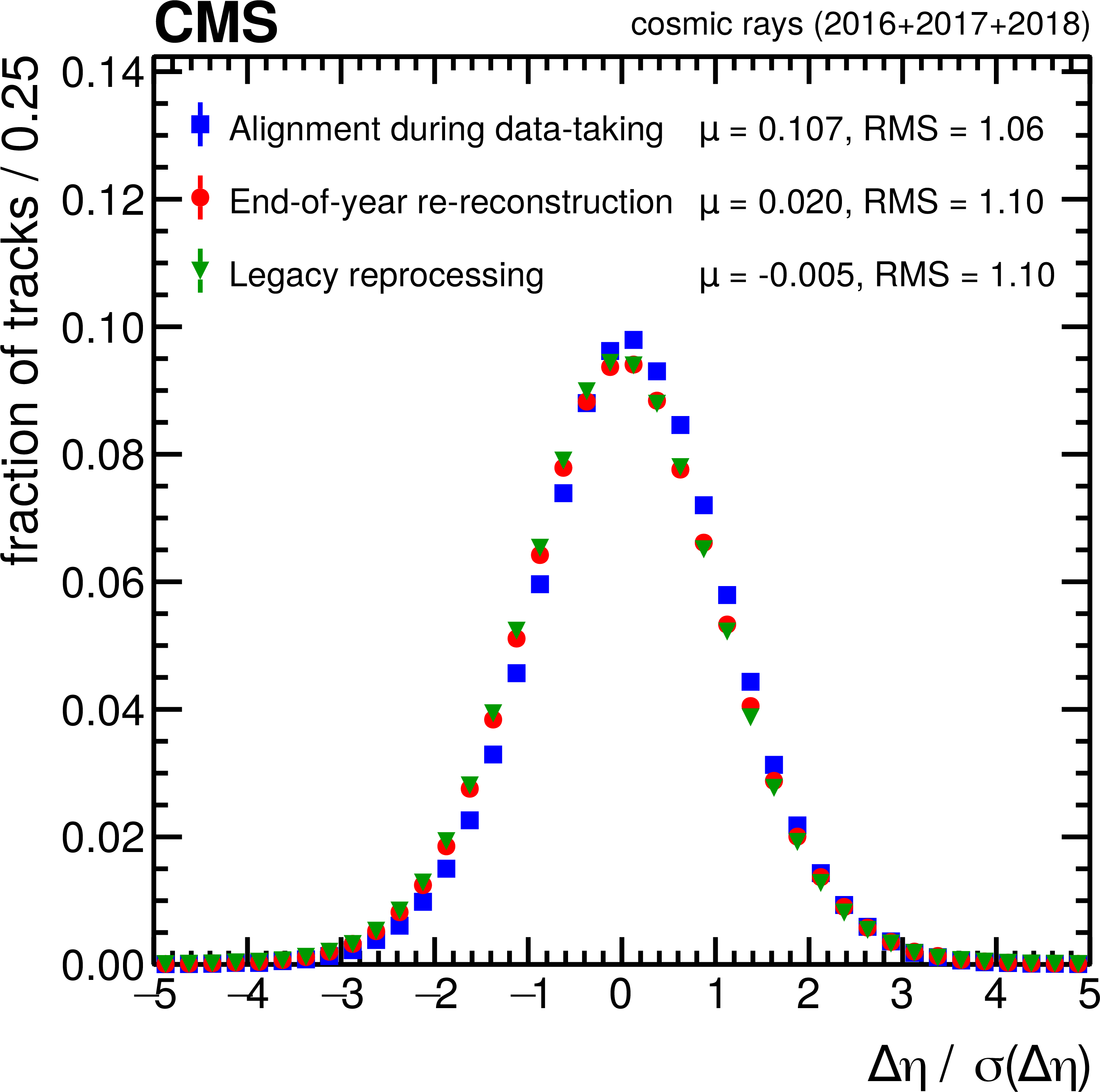
Performance results for cosmic ray muon tracks recorded during commissioning and interfill runs at 3.8 T during 2016, 2017, and 2018. The top and bottom halves of the cosmic ray track are reconstructed independently and the track parameters are compared at the point of closest approach to the interaction region. The mean and RMS of the distribution of $\Delta \eta $ relative to its uncertainty are shown in the figure on the left. The mean $\eta $ difference between the two tracks is presented as a function of $ {d_{xy}}$ on the right, scaled down by $\sqrt {2}$ to account for the two independent measurements. The error bars show the statistical uncertainty related to the limited number of tracks. |
png pdf |
Figure 32-a:
Performance results for cosmic ray muon tracks recorded during commissioning and interfill runs at 3.8 T during 2016, 2017, and 2018. The top and bottom halves of the cosmic ray track are reconstructed independently and the track parameters are compared at the point of closest approach to the interaction region. The mean and RMS of the distribution of $\Delta \eta $ relative to its uncertainty are shown. The error bars show the statistical uncertainty related to the limited number of tracks. |

png pdf |
Figure 32-b:
Performance results for cosmic ray muon tracks recorded during commissioning and interfill runs at 3.8 T during 2016, 2017, and 2018. The top and bottom halves of the cosmic ray track are reconstructed independently and the track parameters are compared at the point of closest approach to the interaction region. The mean $\eta $ difference between the two tracks is presented as a function of $ {d_{xy}}$, scaled down by $\sqrt {2}$ to account for the two independent measurements. The error bars show the statistical uncertainty related to the limited number of tracks. |
png pdf |
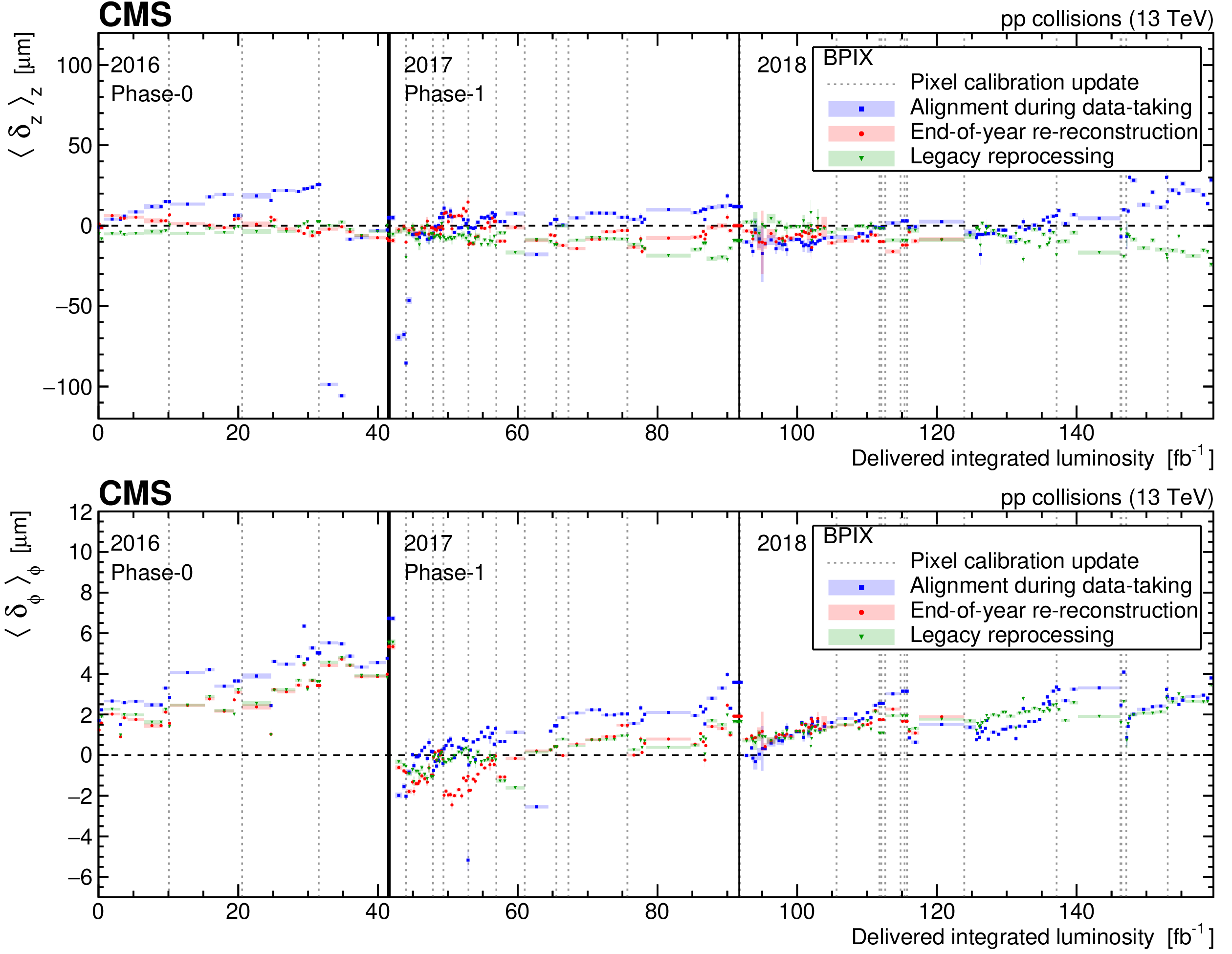
Figure 33:
The upper (lower) figure shows the mean difference in $z$ ($\phi $) residuals for modules overlapping in the $z$ ($\phi $) direction in the BPIX, $< \Delta \delta _z > $ ($< \Delta (r\delta _\phi) > $), as a function of the delivered integrated luminosity. The error bars show the statistical uncertainty in the mean of distribution of the residuals. These residuals are calculated using a sample of data recorded with the inclusive L1 trigger. |

png pdf |
Figure 33-a:
The figure shows the mean difference in $z$ residuals for modules overlapping in the $z$ direction in the BPIX, $< \Delta \delta _z > $, as a function of the delivered integrated luminosity. The error bars show the statistical uncertainty in the mean of distribution of the residuals. These residuals are calculated using a sample of data recorded with the inclusive L1 trigger. |
png pdf |
Figure 33-b:
The figure shows the mean difference in $\phi $ residuals for modules overlapping in the $\phi $ direction in the BPIX, $< \Delta (r\delta _\phi) > $, as a function of the delivered integrated luminosity. The error bars show the statistical uncertainty in the mean of distribution of the residuals. These residuals are calculated using a sample of data recorded with the inclusive L1 trigger. |
png pdf |
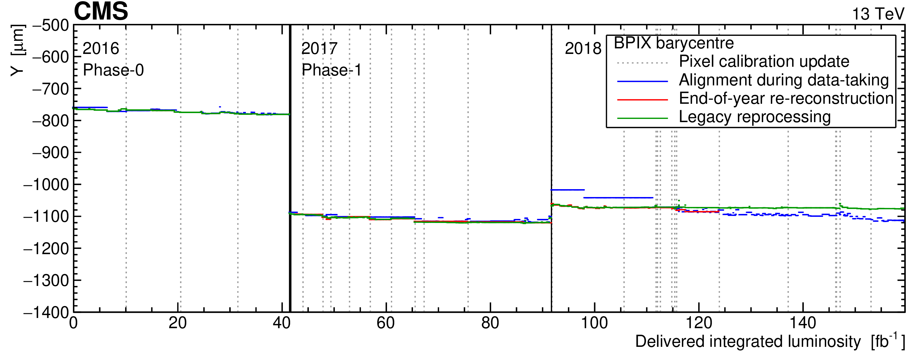
Figure 34:
The global $y$ coordinate of the barycentre position of the barrel pixel detector as a function of the delivered integrated luminosity, determined as the centre-of-gravity of the modules in the barrel pixel detector only. |

png pdf |
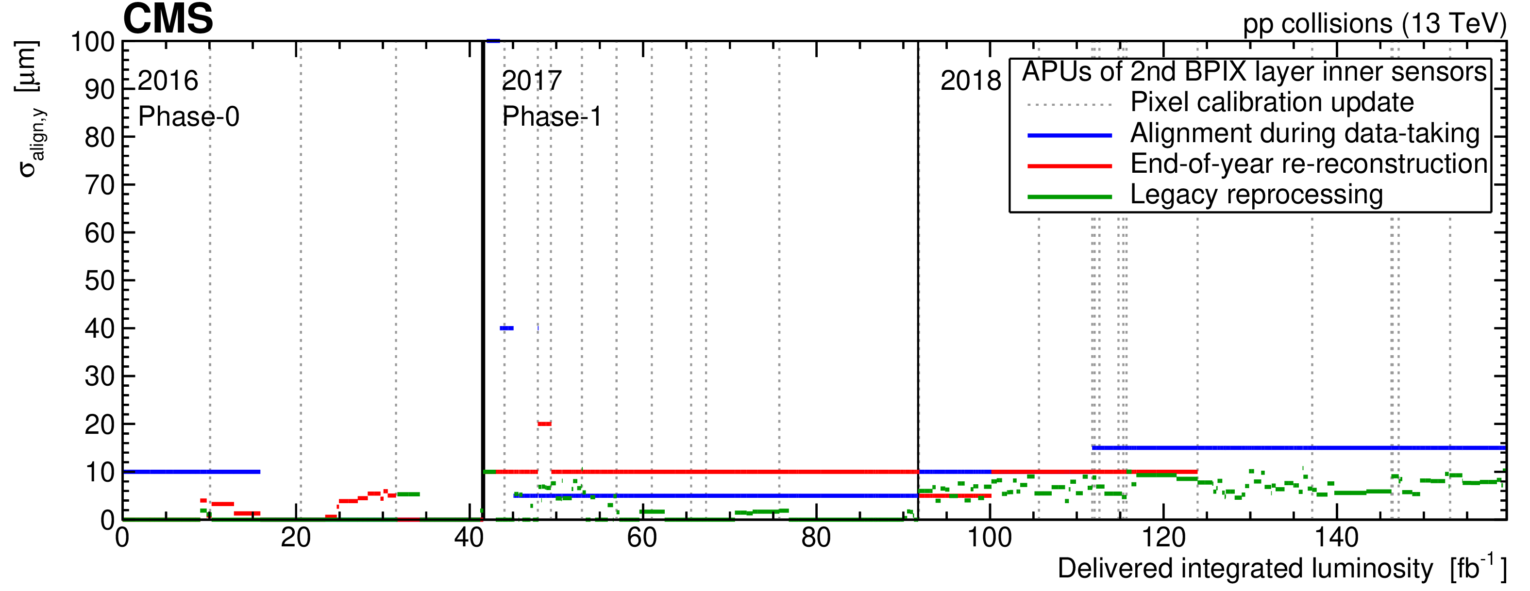
Figure 35:
The contribution from the misalignment of the sensors to the total hit resolution for the inner ladders of the first (top) and second (bottom) BPIX layers in the local $y$ coordinate as a function of the delivered integrated luminosity. For the legacy reprocessing, the measurements were performed with a higher granularity than in the other two cases. |

png pdf |
Figure 35-a:
The contribution from the misalignment of the sensors to the total hit resolution for the inner ladders of the first BPIX layer in the local $y$ coordinate as a function of the delivered integrated luminosity. For the legacy reprocessing, the measurements were performed with a higher granularity than in the other two cases. |
png pdf |
Figure 35-b:
The contribution from the misalignment of the sensors to the total hit resolution for the inner ladders of the second BPIX layer in the local $y$ coordinate as a function of the delivered integrated luminosity. For the legacy reprocessing, the measurements were performed with a higher granularity than in the other two cases. |

png pdf |
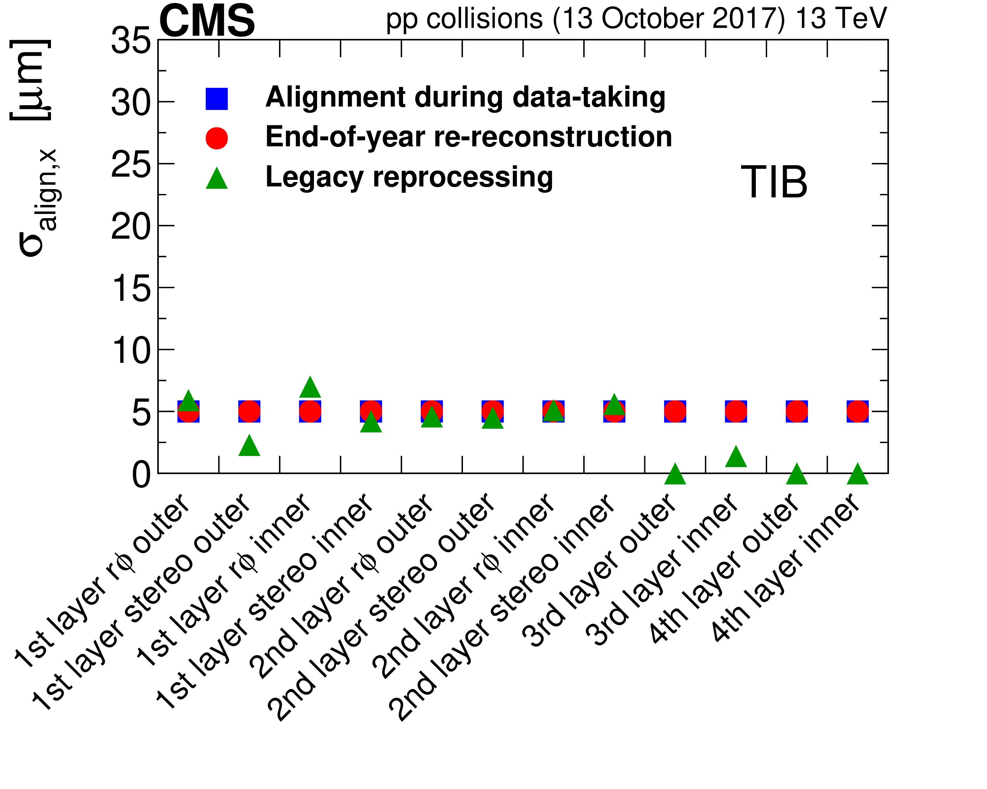
Figure 36:
The contribution from the misalignment of the sensors to the total hit resolution in the local $x$ coordinate for the tracker pixel detector (left) and the inner barrel region of the strip detector (right). These contributions are shown separately for the different module categories that characterize the hierarchical structure of each subdetector. |

png pdf |
Figure 36-a:
The contribution from the misalignment of the sensors to the total hit resolution in the local $x$ coordinate for the tracker pixel detector. These contributions are shown separately for the different module categories that characterize the hierarchical structure of each subdetector. |
png pdf |
Figure 36-b:
The contribution from the misalignment of the sensors to the total hit resolution in the local $x$ coordinate the inner barrel region of the strip detector. These contributions are shown separately for the different module categories that characterize the hierarchical structure of each subdetector. |

png pdf |
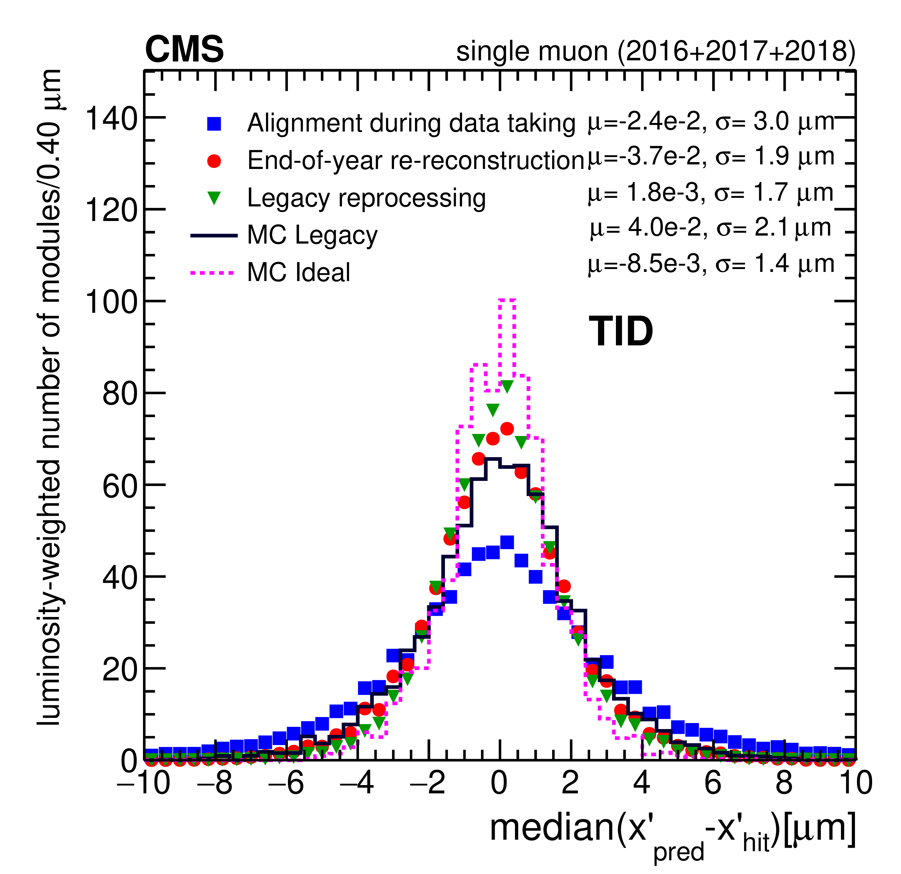
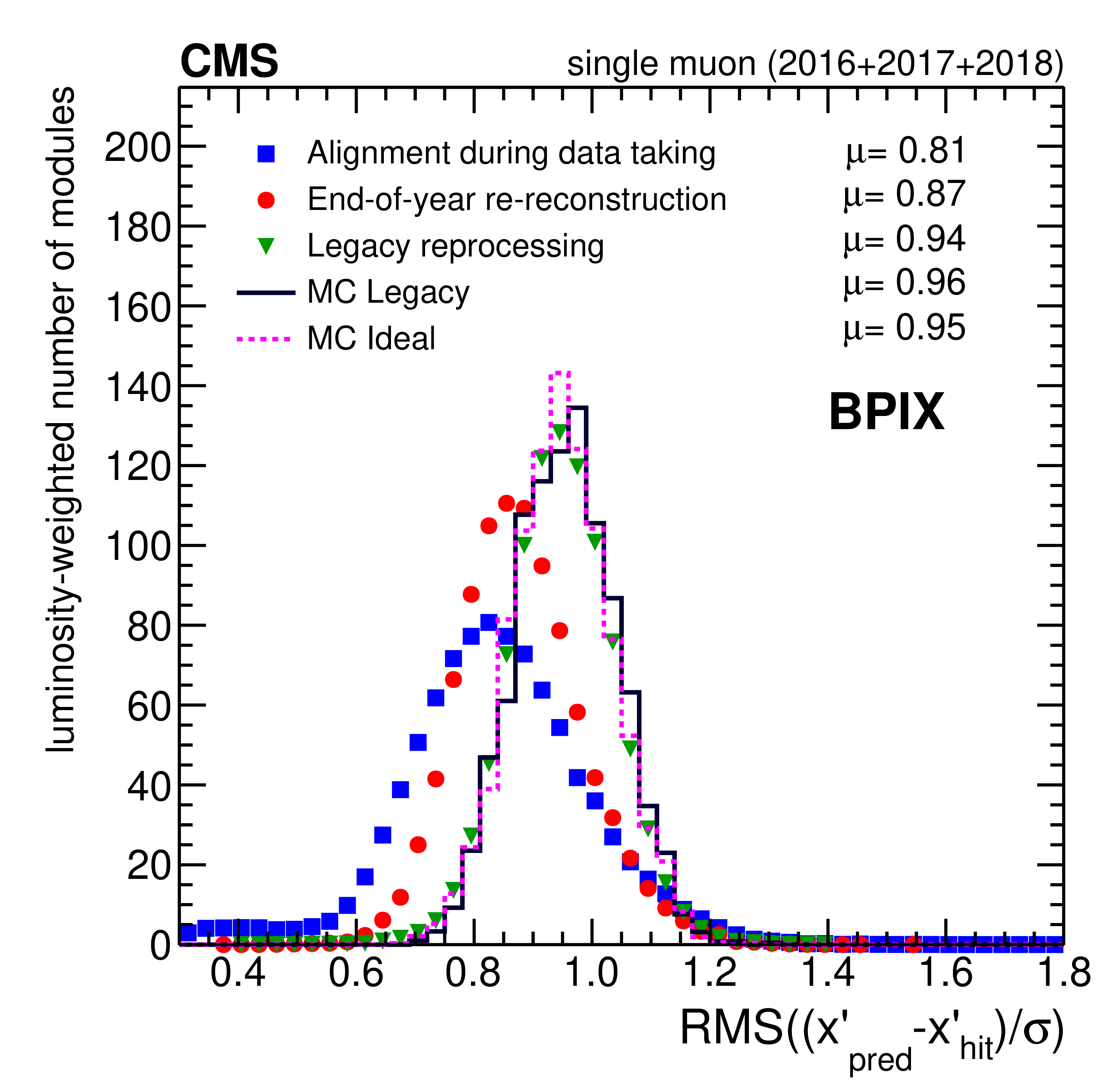
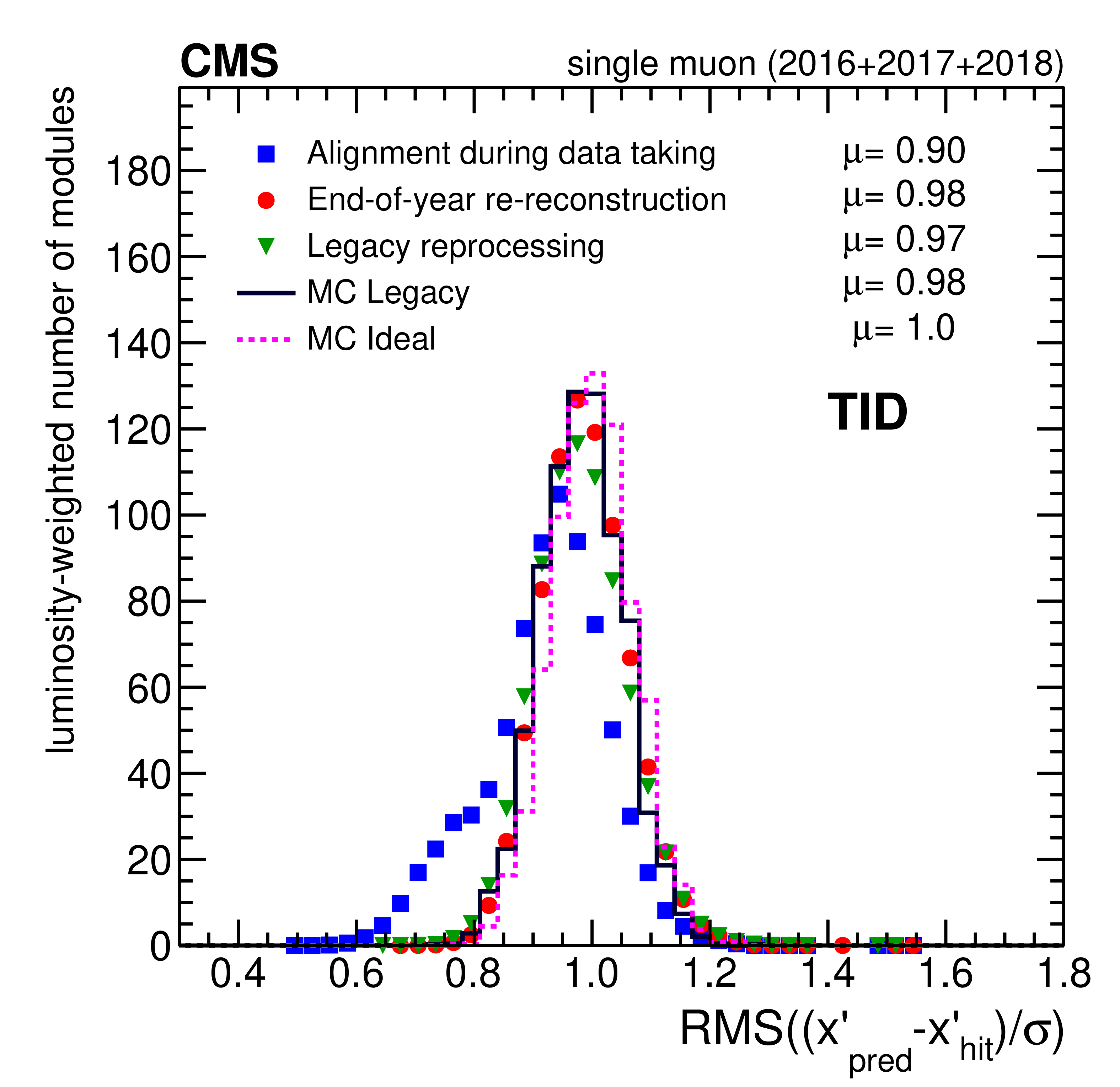
Figure 37:
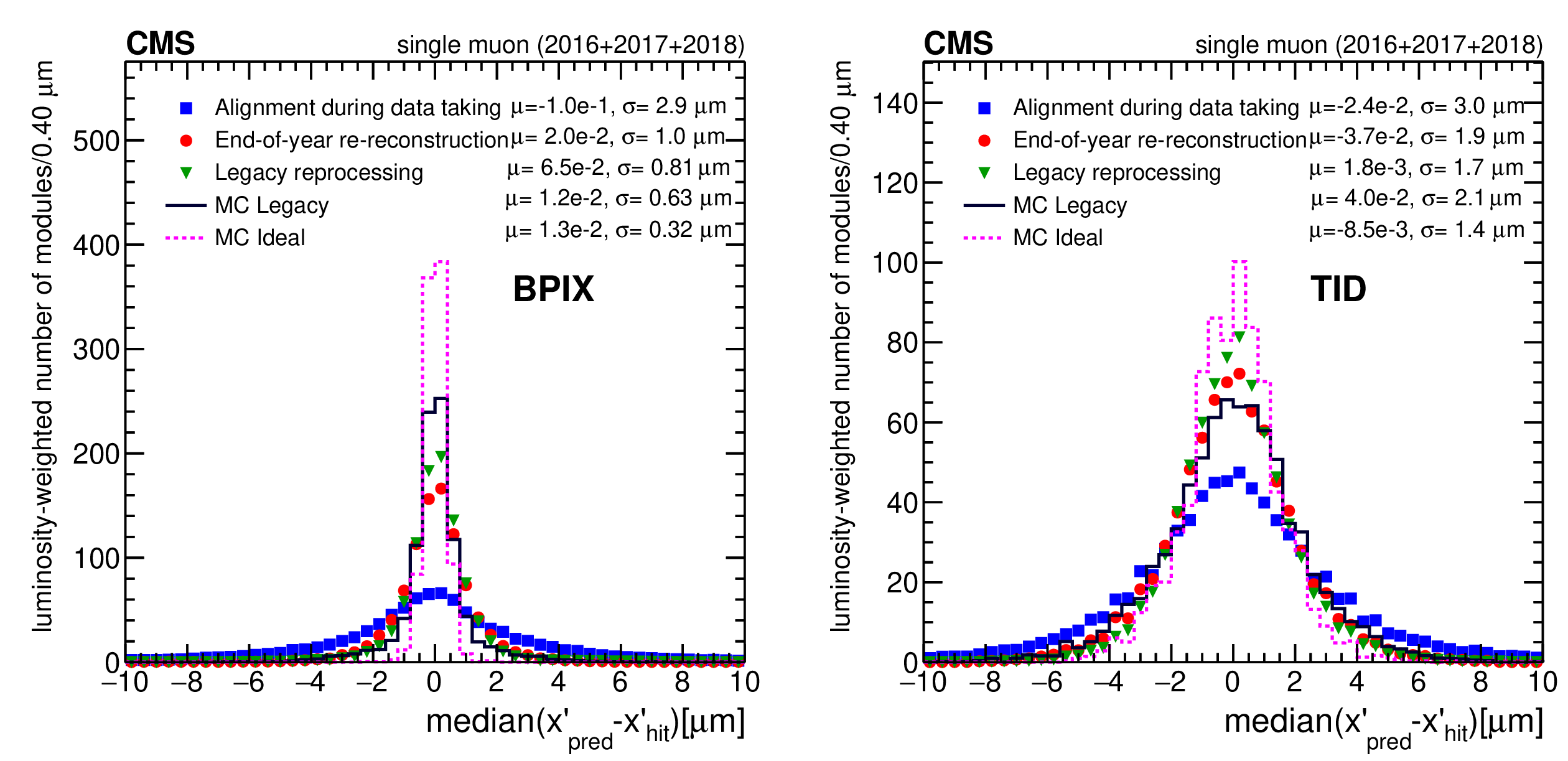
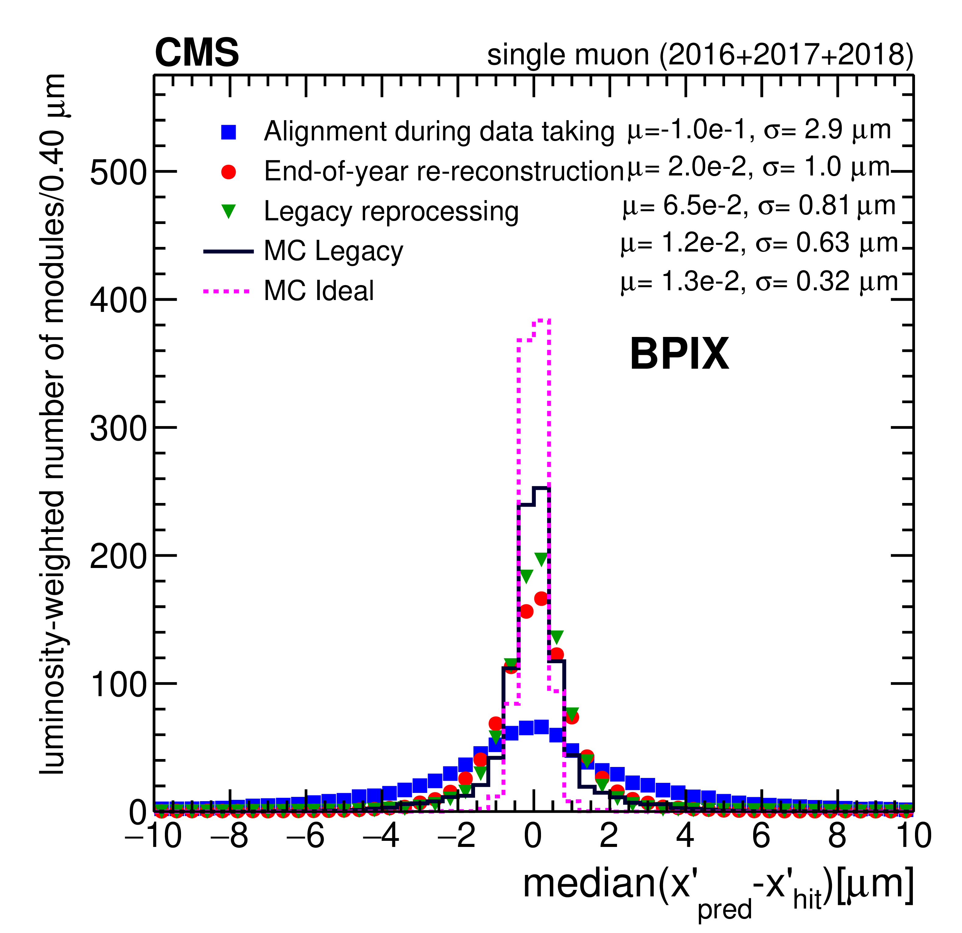
The distribution of the RMS of the normalized residuals in the local $x$ coordinate ($x'$) for modules in the BPIX (left) and in the TID (right). The distributions evaluated in data are averaged over all IOVs, weighted by the integrated luminosity delivered in each IOV. The distributions in data are compared with an MC scenario with realistic alignment conditions for the legacy reprocessing and an MC scenario with ideal alignment conditions. An improvement is visible in the legacy reprocessing compared with the other two alignments shown; this is quantified by the quoted means $\mu $ of the distributions. |
png pdf |
Figure 37-a:
The distribution of the RMS of the normalized residuals in the local $x$ coordinate ($x'$) for modules in the BPIX. The distributions evaluated in data are averaged over all IOVs, weighted by the integrated luminosity delivered in each IOV. The distributions in data are compared with an MC scenario with realistic alignment conditions for the legacy reprocessing and an MC scenario with ideal alignment conditions. An improvement is visible in the legacy reprocessing compared with the other two alignments shown; this is quantified by the quoted means $\mu $ of the distributions. |
png pdf |
Figure 37-b:
The distribution of the RMS of the normalized residuals in the local $x$ coordinate ($x'$) for modules in the TID. The distributions evaluated in data are averaged over all IOVs, weighted by the integrated luminosity delivered in each IOV. The distributions in data are compared with an MC scenario with realistic alignment conditions for the legacy reprocessing and an MC scenario with ideal alignment conditions. An improvement is visible in the legacy reprocessing compared with the other two alignments shown; this is quantified by the quoted means $\mu $ of the distributions. |

png pdf |
Figure 38:
Difference of module positions in the global $z$ coordinate as obtained in the 2018 MC alignment fit with respect to the ideal positions. The modules are given a colour corresponding to the value of $\Delta z$ according to the colour bar on the bottom. Modules that were inactive during the simulation are indicated in dark grey. A pattern typical for the $z$ expansion distortion can be observed in the TEC, with a maximum magnitude of approximately 200 m. The effect of this systematic misalignment on the alignment performance is expected to be small. |
png pdf |
Figure 39:
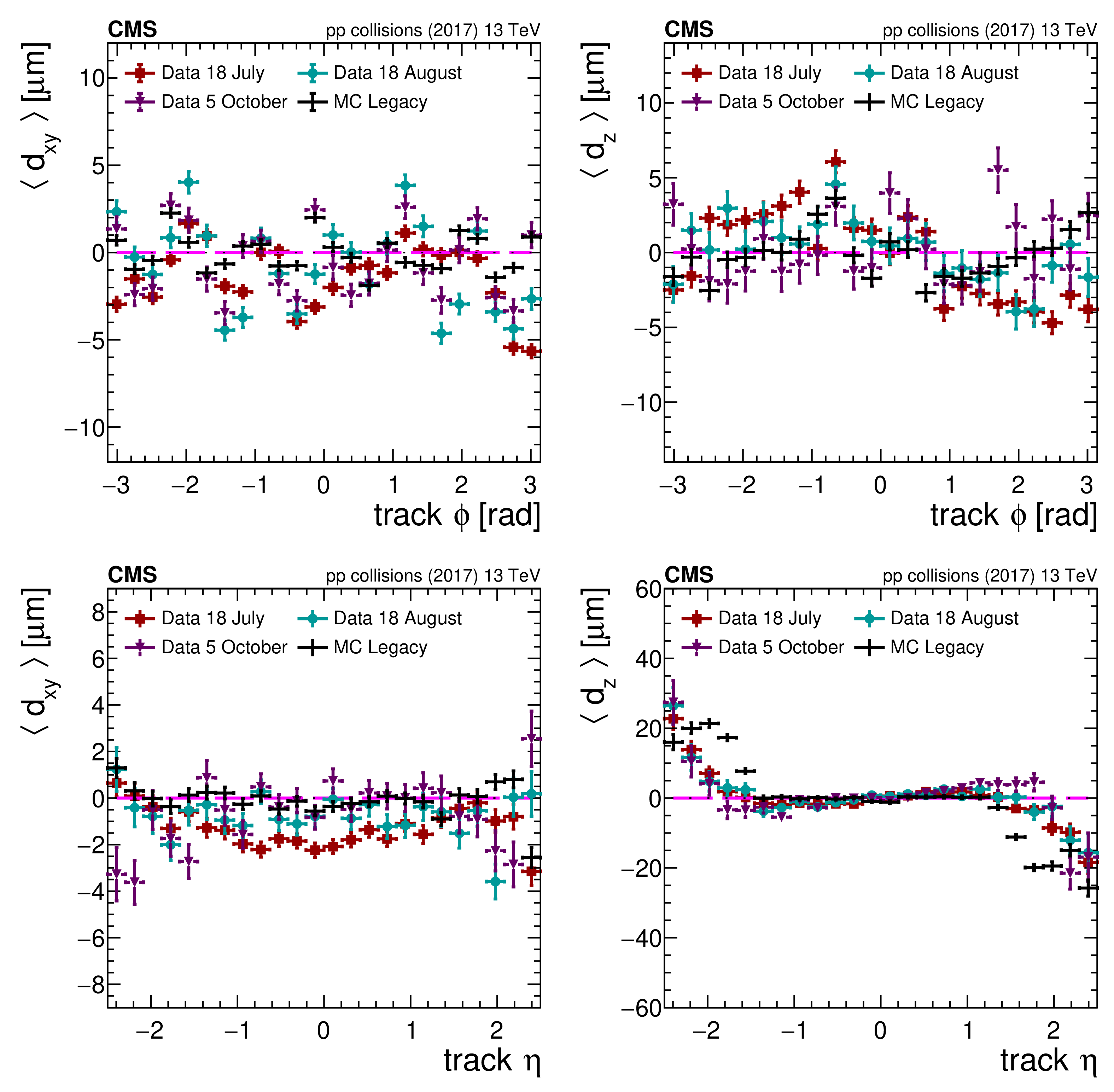
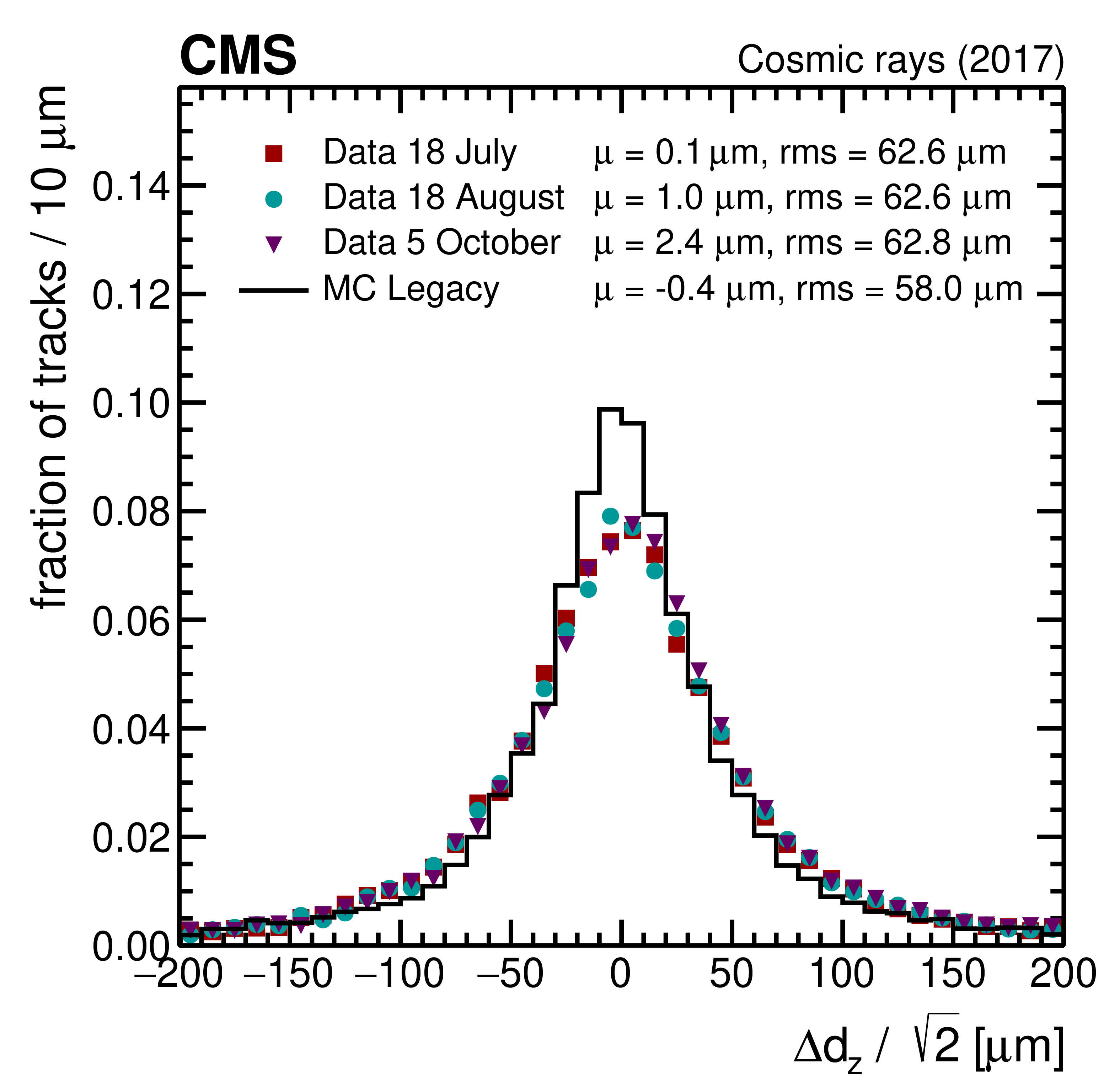
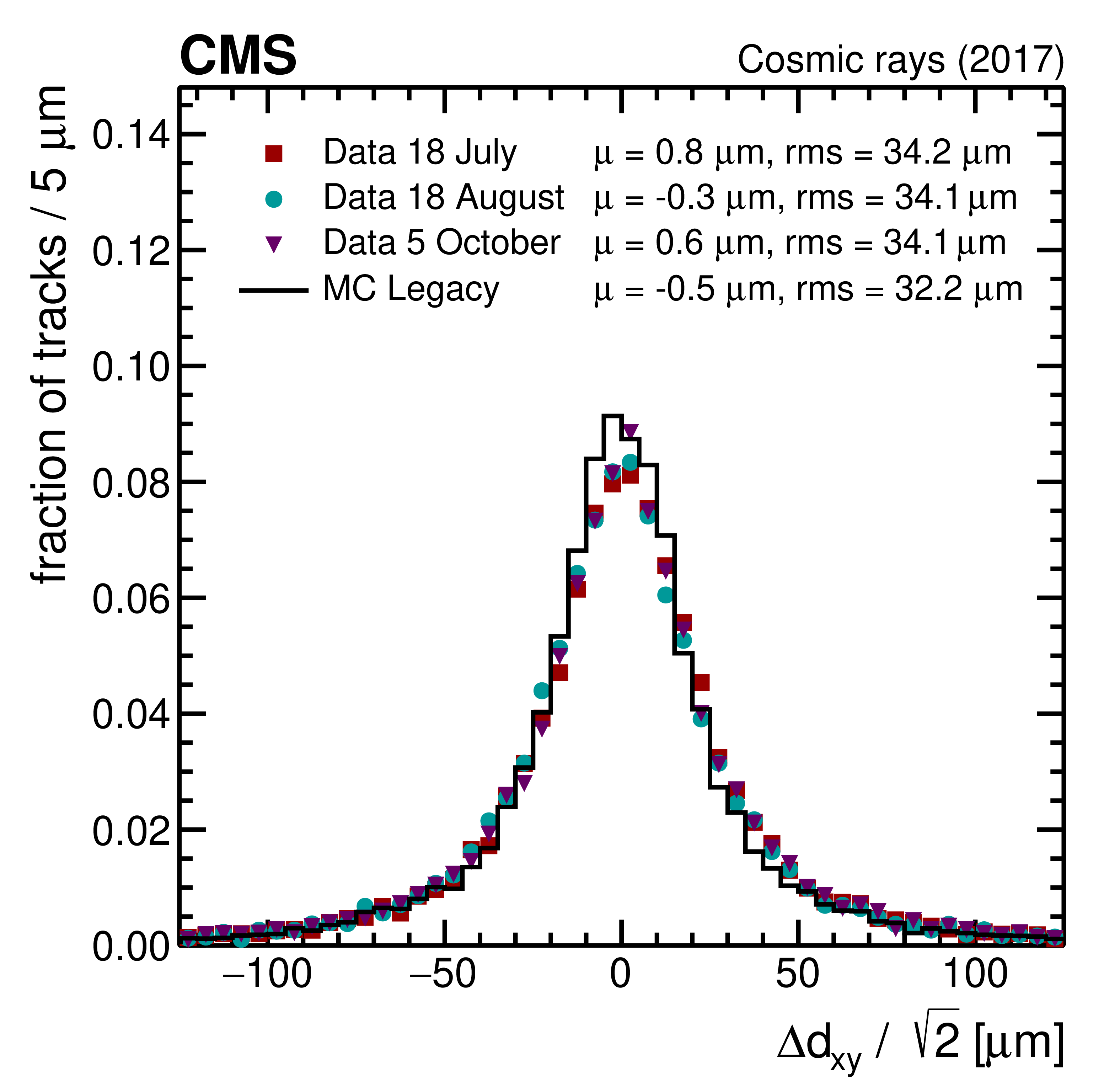
Distribution of the mean impact parameter in the transverse plane (left) and in the longitudinal plane (right) as a function of the track $\phi $ (top) and $\eta $ (bottom) for 2017. The derived MC scenario is compared with three representative IOVs from the year 2017 in data (18 July, 18 August, 5 October) to assess its validity as the final geometry. The error bars show the statistical uncertainty related to the limited number of tracks. |

png pdf |
Figure 40:
The DMRs in the local $x$ coordinate for different components of the tracker system. The derived MC scenario is compared with three representative IOVs from the year 2017 in data (18 July, 18 August, 5 October) to assess its validity as the final geometry. |

png pdf |
Figure 40-a:
The DMRs in the local $x$ coordinate for the BPIX. The derived MC scenario is compared with three representative IOVs from the year 2017 in data (18 July, 18 August, 5 October) to assess its validity as the final geometry. |

png pdf |
Figure 40-b:
The DMRs in the local $x$ coordinate for the FPIX. The derived MC scenario is compared with three representative IOVs from the year 2017 in data (18 July, 18 August, 5 October) to assess its validity as the final geometry. |
png pdf |
Figure 40-c:
The DMRs in the local $x$ coordinate for the TIB. The derived MC scenario is compared with three representative IOVs from the year 2017 in data (18 July, 18 August, 5 October) to assess its validity as the final geometry. |

png pdf |
Figure 40-d:
The DMRs in the local $x$ coordinate for the TEC. The derived MC scenario is compared with three representative IOVs from the year 2017 in data (18 July, 18 August, 5 October) to assess its validity as the final geometry. |

png pdf |
Figure 41:
Difference in the impact parameters in the longitudinal (left) and transverse (right) plane as evaluated in the cosmic ray muon track splitting validation. The derived MC scenario is compared with three representative IOVs from the year 2017 in data (18 July, 18 August, 5 October) to assess its validity as the final geometry. |
png pdf |
Figure 41-a:
Difference in the impact parameters in the longitudinal plane as evaluated in the cosmic ray muon track splitting validation. The derived MC scenario is compared with three representative IOVs from the year 2017 in data (18 July, 18 August, 5 October) to assess its validity as the final geometry. |
png pdf |
Figure 41-b:
Difference in the impact parameters in the transverse plane as evaluated in the cosmic ray muon track splitting validation. The derived MC scenario is compared with three representative IOVs from the year 2017 in data (18 July, 18 August, 5 October) to assess its validity as the final geometry. |
png pdf |
Figure 42:
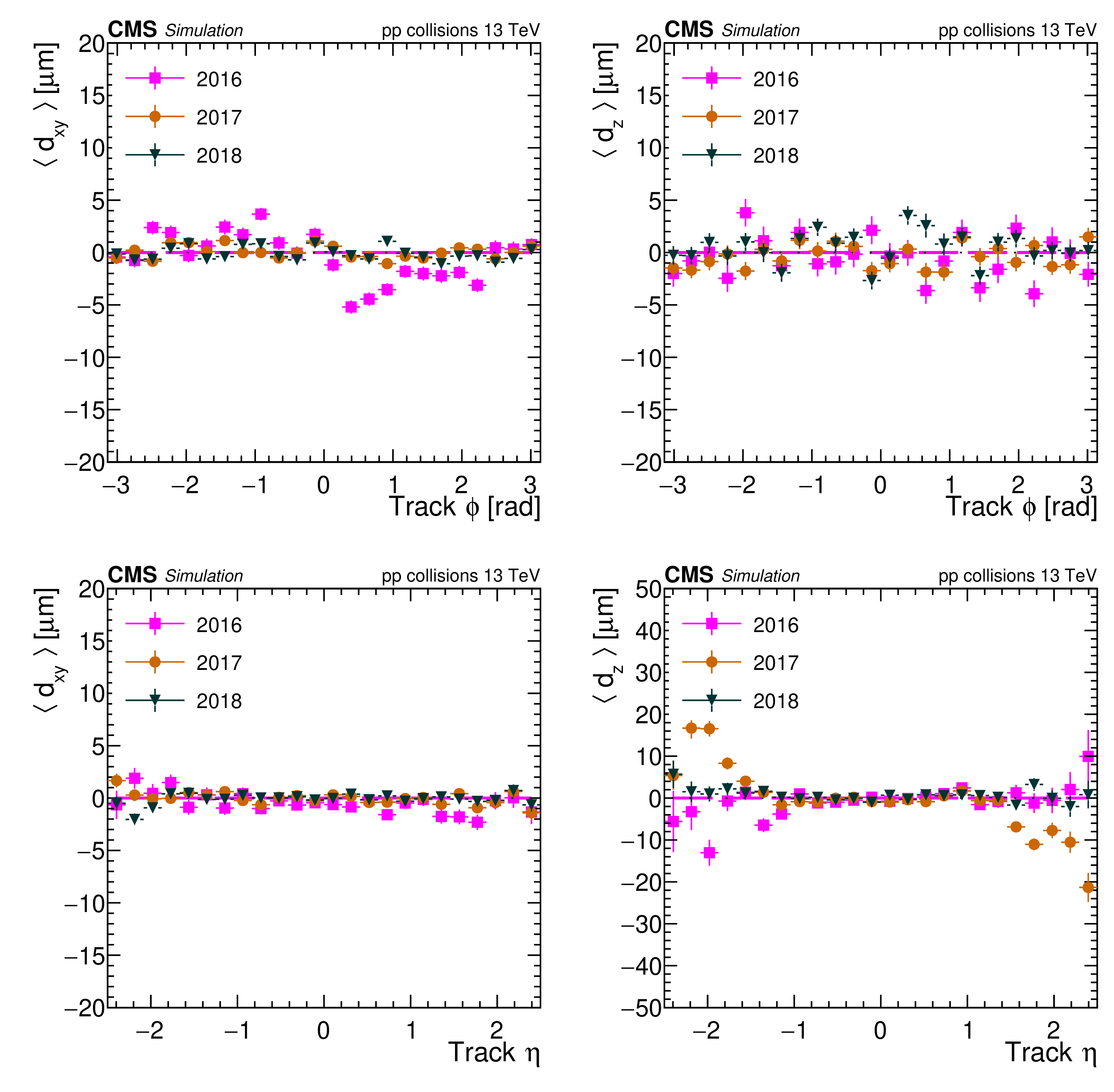
Mean track-vertex impact parameter in the transverse plane (left) and in the longitudinal plane (right), as a function of the track $\phi $ (top) and $\eta $ (bottom). A comparison of the results with the alignment constants derived in the Run 2 legacy MC scenario for 2016, 2017, and 2018 separately is shown. The error bars show the statistical uncertainty related to the limited number of tracks. |
png pdf |
Figure 43:
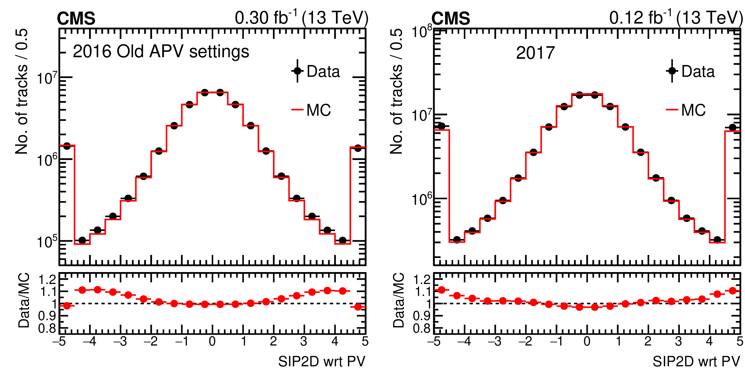
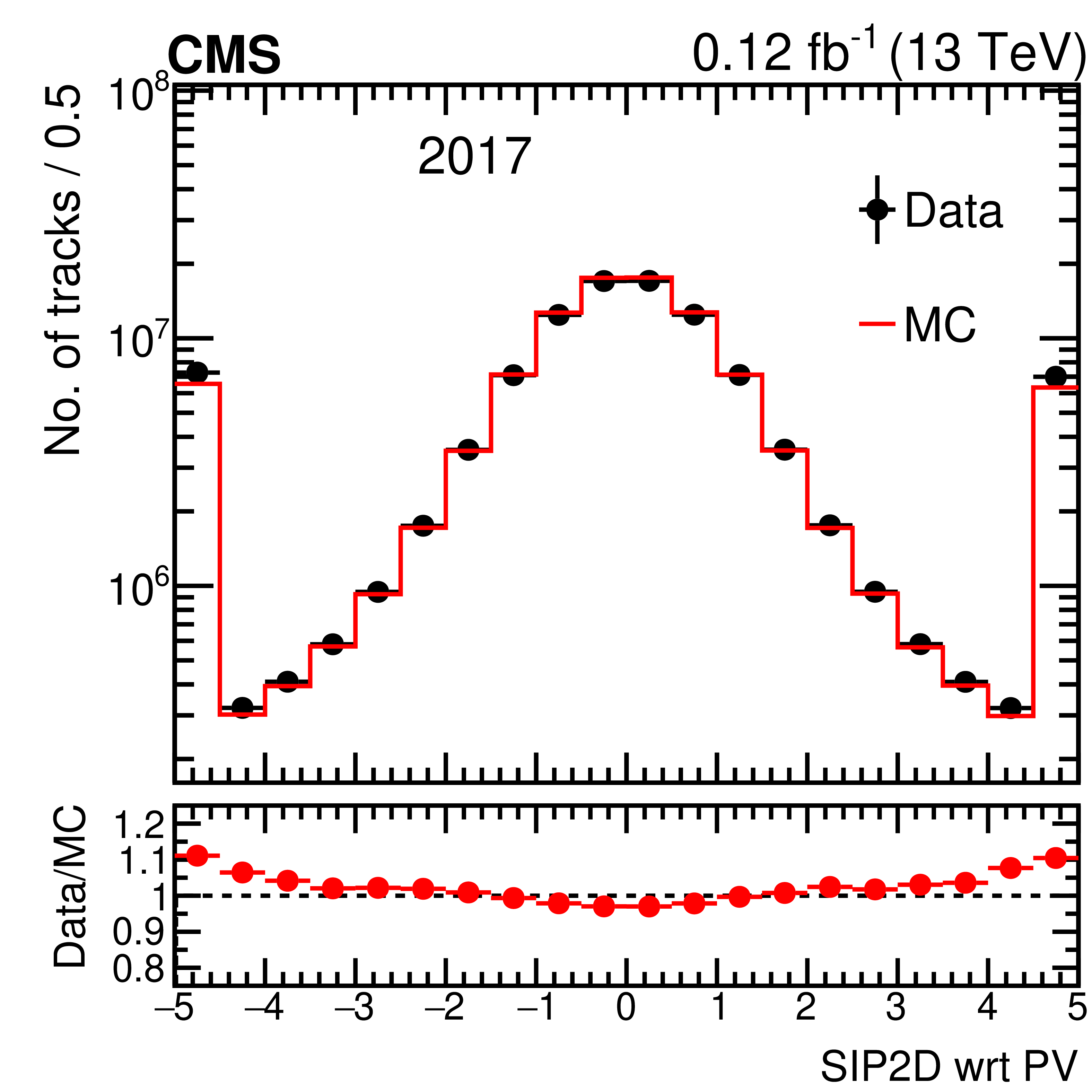
Distribution of the two-dimensional track impact parameter significance (SIP2D) with respect to the PV. Data collected in 2016 (left) and 2017 (right) are compared with the corresponding MC simulation. For 2016, the simulation with old APV settings is shown. For both data and simulation, the first and last bin include the underflow and overflow, respectively. Vertical error bars represent the statistical uncertainty due to the limited number of tracks; they are smaller than the marker size in both years. |

png pdf |
Figure 43-a:
Distribution of the two-dimensional track impact parameter significance (SIP2D) with respect to the PV. Data collected in 2016 are compared with the corresponding MC simulation. The simulation with old APV settings is shown. For both data and simulation, the first and last bin include the underflow and overflow, respectively. Vertical error bars represent the statistical uncertainty due to the limited number of tracks; they are smaller than the marker size. |
png pdf |
Figure 43-b:
Distribution of the two-dimensional track impact parameter significance (SIP2D) with respect to the PV. Data collected in 2017 are compared with the corresponding MC simulation. For both data and simulation, the first and last bin include the underflow and overflow, respectively. Vertical error bars represent the statistical uncertainty due to the limited number of tracks; they are smaller than the marker size. |
png pdf |
Figure 44:
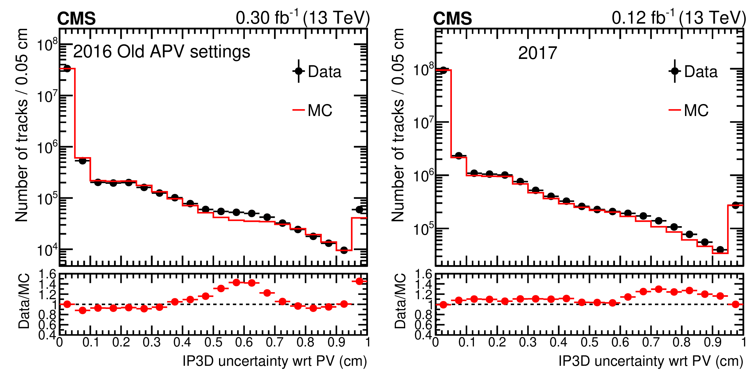
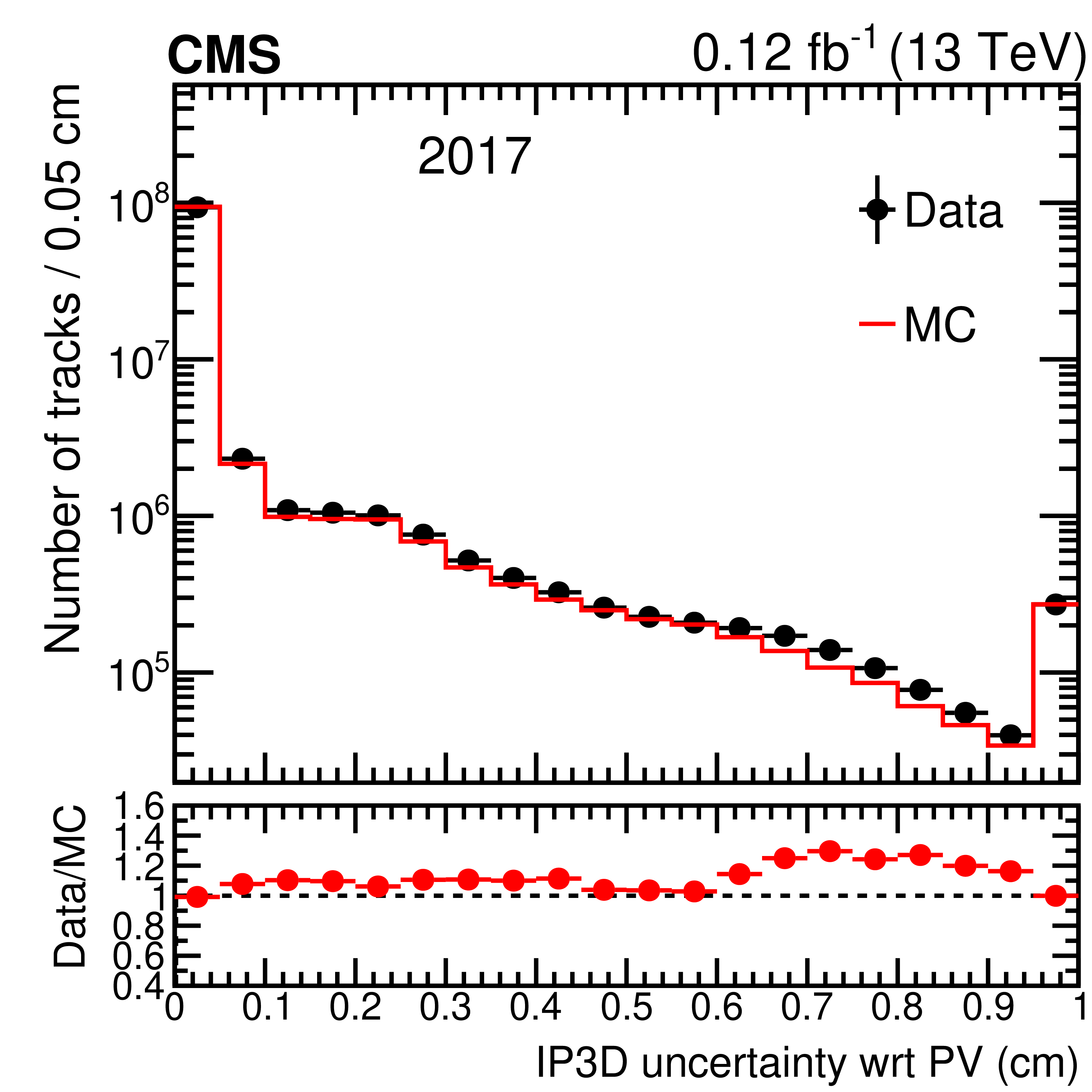
The distribution of the uncertainty in measuring the three-dimensional track impact parameter (IP3D), with respect to the PV. Data collected in 2016 (left) and 2017 (right) are compared with the corresponding MC simulation. For 2016, the simulation with old APV settings is shown. For both data and simulation, the last bin includes the overflow. Vertical error bars represent the statistical uncertainty due to the limited number of tracks; they are smaller than the marker size in both years. |

png pdf |
Figure 44-a:
The distribution of the uncertainty in measuring the three-dimensional track impact parameter (IP3D), with respect to the PV. Data collected in 2016 are compared with the corresponding MC simulation. The simulation with old APV settings is shown. For both data and simulation, the last bin includes the overflow. Vertical error bars represent the statistical uncertainty due to the limited number of tracks; they are smaller than the marker size. |
png pdf |
Figure 44-b:
The distribution of the uncertainty in measuring the three-dimensional track impact parameter (IP3D), with respect to the PV. Data collected in 2017 are compared with the corresponding MC simulation. For both data and simulation, the last bin includes the overflow. Vertical error bars represent the statistical uncertainty due to the limited number of tracks; they are smaller than the marker size. |

png pdf |
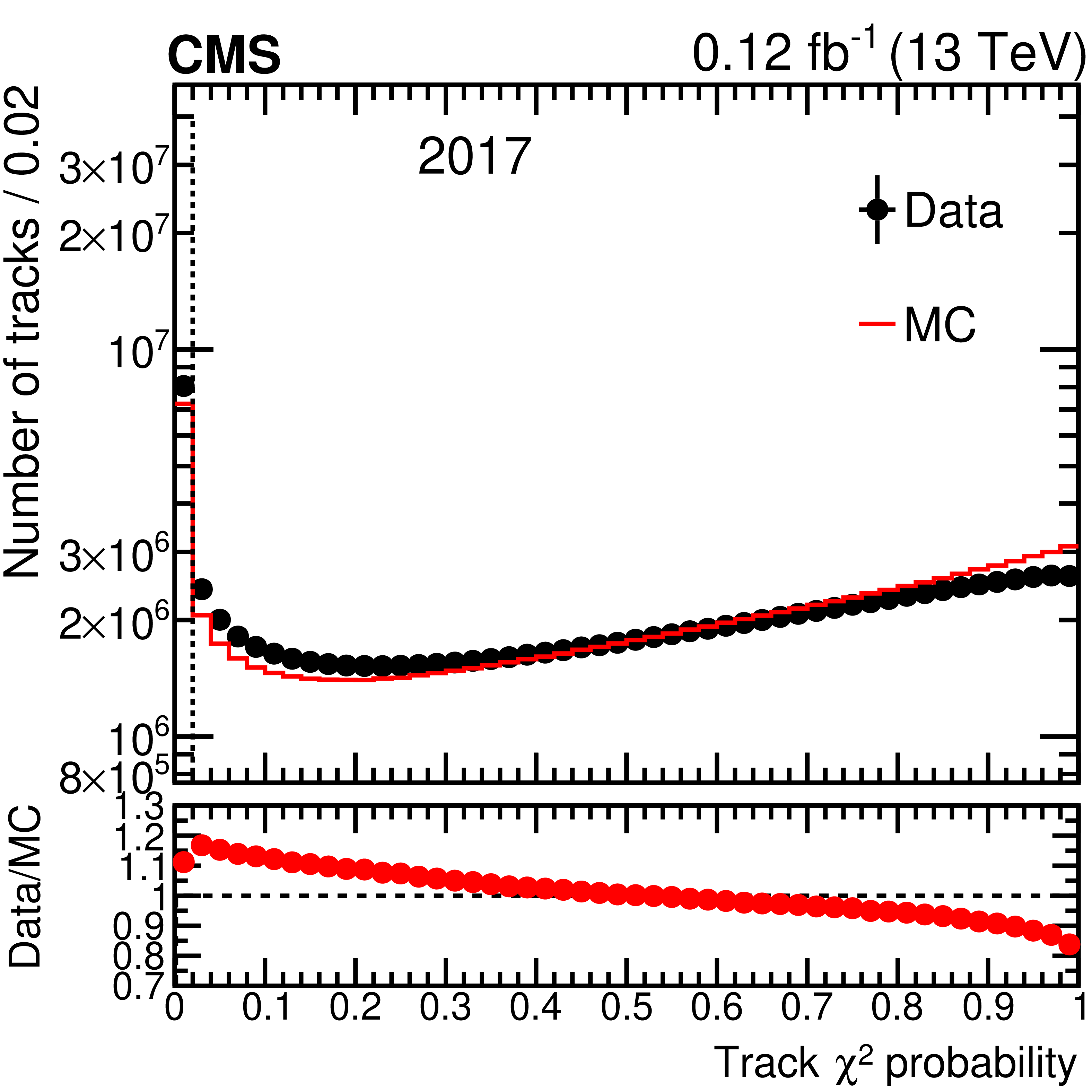
Figure 45:
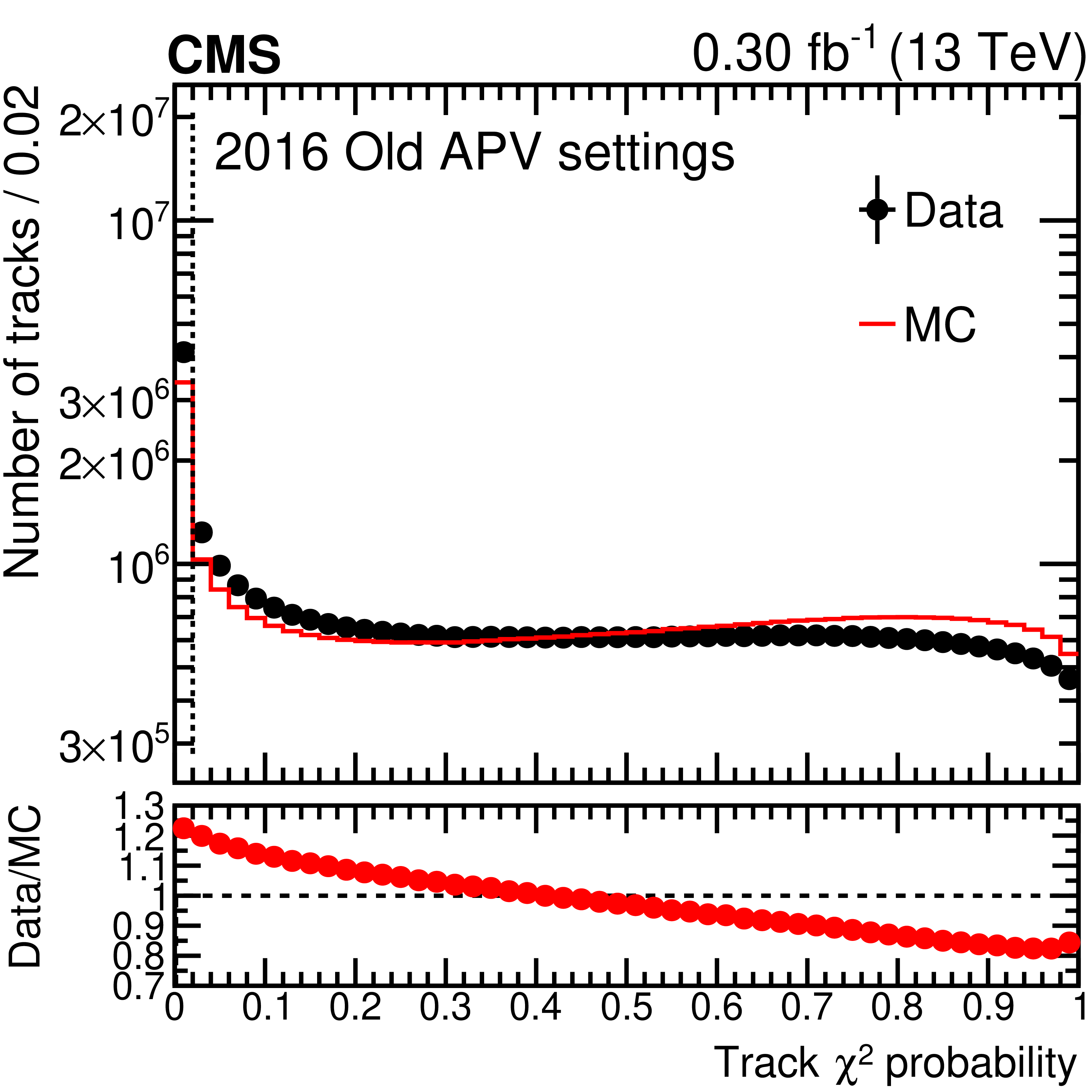
Distribution of the track $\chi ^{2}$ probability for the number of degrees of freedom in the track fit. Data collected in 2016 (left) and 2017 (right) are compared with the corresponding MC simulation. For 2016, the simulation with old APV settings is shown. Vertical error bars represent the statistical uncertainty due to the limited number of tracks; they are smaller than the marker size in both years. |
png pdf |
Figure 45-a:
Distribution of the track $\chi ^{2}$ probability for the number of degrees of freedom in the track fit. Data collected in 2016 are compared with the corresponding MC simulation. The simulation with old APV settings is shown. Vertical error bars represent the statistical uncertainty due to the limited number of tracks; they are smaller than the marker size. |
png pdf |
Figure 45-b:
Distribution of the track $\chi ^{2}$ probability for the number of degrees of freedom in the track fit. Data collected in 2017 are compared with the corresponding MC simulation. Vertical error bars represent the statistical uncertainty due to the limited number of tracks; they are smaller than the marker size. |
| Tables | |

png pdf |
Table 1:
The nine basic systematic distortions in the cylindrical system, with the names of each systematic misalignment, the function by which the misalignment is generated, and a validation type sensitive to the misalignment. The parameter $z_0=$ 271.846 cm is half of the length of the CMS tracker, and $\phi _0$ is an arbitrary constant phase. |
png pdf |
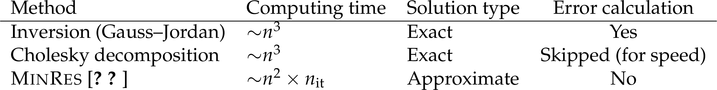
Table 2:
List of the main solution methods implemented in {millepede} -II. The computation time is given as a function of the number of parameters $n$ and the number of internal iterations $n_\text {it}$ if applicable. The type of solution delivered by the algorithm is also shown. |

png pdf |
Table 3:
Examples of Pede wall time (time taken from start of the program to end) for some larger alignment campaigns on a dedicated test machine (Intel Xeon E5-2667 @ 3.2 GHz, 256 GB memory @ 51 GB/s). |
png pdf |
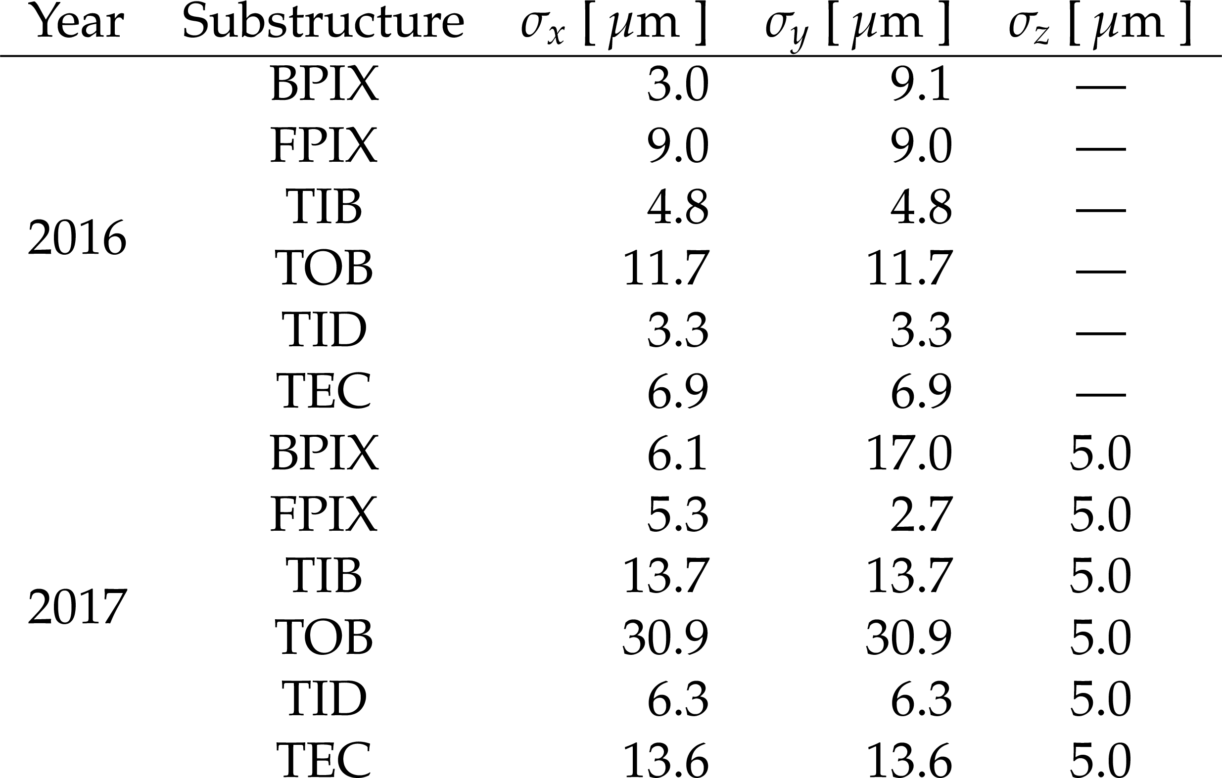
Table 4:
Magnitude of the Gaussian smearing applied to the design geometry to derive the starting geometry for the 2016 and 2017 legacy MC alignments. The adopted values in both years are reported for each substructure and by coordinate. |
| Summary |
|
In this paper, the strategies for and the performance of the alignment of the CMS central tracker during the data-taking period from 2015 to 2018 have been described. The alignment was determined from a global track fit, where the module parameters were released in addition to the track parameters. Two algorithms based on slightly different approaches were used to perform the minimization of this problem with a large number of parameters, namely HipPy and MILLEPEDE-II. Improvements of the software introduced for Run 2 were discussed. Different strategies were applied depending on the number of parameters to determine: at the beginning of the year and with the very limited amount of data available, the modules of the pixel tracker were aligned with respect to the strip tracker; during the year, an automated alignment procedure was performed for each run, correcting for movements of the mechanical structures of the pixel tracker with respect to the strip tracker; finally, in the middle or at the end of the year, once a large amount of data had been recorded (including e.g., a sufficient number of muon tracks from Z boson decays), all modules of the strip and pixel trackers were aligned in a single fit accounting for time dependence. The last strategy leads to the highest precision of all and is preferred for the event reconstruction in the context of physics analyses. Systematic distortions arising from the ageing of the detector, from internal symmetries of the minimization problem or from external constraints, were monitored using specific distributions. Examples of such distributions are the dimuon invariant mass as a function of the kinematical properties of the outgoing muons and the difference of the mean of the distribution of the median of the residuals for modules pointing in opposite directions. In general, the increased level of radiation compared with data collected before 2012 required an updated strategy. As part of the reprocessing of the data recorded during the period from 2016 to 2018 after the end of data taking, the alignment parameters were determined with a higher precision than for the end-of-year reconstruction. This was made possible by artificially moving the ladders and panels in the pixel trackers to absorb the gradually accumulating systematic shift induced by the ageing of the modules and by defining finer intervals of validity. In addition to the alignment of the modules in real data, scenarios for use in simulation were also derived, aiming to resemble the statistical performance and the systematic effects. A scenario was provided for each year separately, without time dependence in the alignment fit. Various comparisons of the performance in data and in simulation have been presented, especially in the context of the reprocessing of the data recorded between 2016 and 2018 after the end of data taking. |
| References | ||||
| 1 | CMS Collaboration | Alignment of the CMS silicon tracker during commissioning with cosmic rays | JINST 5 (2010) T03009 | CMS-CFT-09-003 0910.2505 |
| 2 | CMS Collaboration | Alignment of the CMS tracker with LHC and cosmic ray data | JINST 9 (2014) P06009 | CMS-TRK-11-002 1403.2286 |
| 3 | CMS Collaboration | CMS technical design report for the pixel detector upgrade | cms technical design report | |
| 4 | W. Adam et al. | The CMS phase-1 pixel detector upgrade | JINST 16 (2021) P02027 | 2012.14304 |
| 5 | CMS Collaboration | Performance of the CMS Level-1 trigger in proton-proton collisions at $ \sqrt{s} = $ 13 TeV | JINST 15 (2020) P10017 | CMS-TRG-17-001 2006.10165 |
| 6 | CMS Collaboration | The CMS trigger system | JINST 12 (2017) P01020 | CMS-TRG-12-001 1609.02366 |
| 7 | CMS Collaboration | Description and performance of track and primary-vertex reconstruction with the CMS tracker | JINST 9 (2014) P10009 | CMS-TRK-11-001 1405.6569 |
| 8 | CMS Collaboration | Track impact parameter resolution for the full pseudo rapidity coverage in the 2017 dataset with the CMS phase-1 pixel detector | CDS | |
| 9 | CMS Collaboration | The CMS experiment at the CERN LHC | JINST 3 (2008) S08004 | CMS-00-001 |
| 10 | V. Blobel and C. Kleinwort | A new method for the high precision alignment of track detectors | in Conference on Advanced Statistical Techniques in Particle Physics 2002 | hep-ex/0208021 |
| 11 | T. Sjostrand, S. Mrenna, and P. Skands | PYTHIA 6.4 physics and manual | JHEP 05 (2006) 026 | hep-ph/0603175 |
| 12 | T. Sjostrand et al. | An introduction to PYTHIA 8.2 | CPC 191 (2015) 159 | 1410.3012 |
| 13 | CMS Collaboration | Extraction and validation of a new set of CMS PYTHIA 8 tunes from underlying-event measurements | EPJC 80 (2020) 4 | CMS-GEN-17-001 1903.12179 |
| 14 | J. Alwall et al. | The automated computation of tree-level and next-to-leading order differential cross sections, and their matching to parton shower simulations | JHEP 07 (2014) 079 | 1405.0301 |
| 15 | P. Biallass and T. Hebbeker | Parametrization of the cosmic muon flux for the generator CMSCGEN | 0907.5514 | |
| 16 | P. Lenzi, C. Genta, and B. Mangano | Track reconstruction of real cosmic muon events with CMS tracker detector | in International Conference on Computing in High Energy and Nuclear Physics (CHEP '07) 2008 [J. Phys. Conf. Ser. 119, 032030] | |
| 17 | CMS Collaboration | Precision measurement of the structure of the CMS inner tracking system using nuclear interactions | JINST 13 (2018) P10034 | CMS-TRK-17-001 1807.03289 |
| 18 | CMS Collaboration | Alignment of the CMS silicon strip tracker during stand-alone commissioning | JINST 4 (2009) T07001 | 0904.1220 |
| 19 | Helmholtz Alliance | Terascale alliance website | link | |
| 20 | V. Blobel | Software alignment for tracking detectors | NIMA 566 (2006) 5 | |
| 21 | T. Bilka et al. | Alignment and calibration of the Belle II detector | in 23rd International Conference on Computing in High Energy and Nuclear Physics (CHEP 2018) | |
| 22 | R. Fruhwirth | Application of Kalman filtering to track and vertex fitting | NIMA 262 (1987) 444 | |
| 23 | W. D. Hulsbergen | The global covariance matrix of tracks fitted with a Kalman filter and an application in detector alignment | NIMA 600 (2009) 471 | |
| 24 | J. Amoraal et al. | Application of vertex and mass constraints in track-based alignment | NIMA 712 (2013) 48 | 1207.4756 |
| 25 | C. Kleinwort | General broken lines as advanced track fitting method | NIMA 673 (2012) 107 | 1201.4320 |
| 26 | Helmholtz Alliance | Gbl website | link | |
| 27 | S.-C. T. Choi, C. C. Paige, and M. A. Saunders | MINRES-QLP: A Krylov subspace method for indefinite or singular symmetric systems | SIAM J. Sci. Comput. 33 (2011) 1810 | 1003.4042 |
| 28 | S.-C. T. Choi and M. A. Saunders | Algorithm 937: MINRES-QLP for symmetric and Hermitian linear equations and least-squares problems | ACM Trans. Math. Soft. (TOMS) 40 (2014) 1 | 1301.2707 |
| 29 | V. Karimaki, A. Heikkinen, T. Lampen, and T. Linden | Sensor alignment by tracks | in 13th International Conference on Computing in High-Enery and Nuclear Physics (CHEP 2003) | physics/0306034 |
| 30 | CMS Collaboration | The HIP algorithm for track based alignment and its application to the CMS pixel detector | CDS | |
| 31 | D. N. Brown, A. V. Gritsan, Z. J. Guo, and D. Roberts | Local alignment of the BABAR silicon vertex tracking detector | NIMA 603 (2009) 467 | 0809.3823 |
| 32 | M. Schroder | Alignment of the upgraded CMS pixel detector | in 11th International Hiroshima Symposium on the Development and Application of Semiconductor Tracking Detectors (HSTD11) in conjunction with 2nd Workshop on SOI Pixel Detectors (SOIPIX2017) | |
| 33 | CMS Collaboration | Alignment of the CMS tracking-detector with first 2015 cosmic-ray and collision data | CDS | |
| 34 | K. Rose | Deterministic annealing for clustering, compression, classification, regression, and related optimization problems | Proceedings of the IEEE 86 (1998) 2210 | |
| 35 | G. Cerminara and B. van Besien | Automated workflows for critical time-dependent calibrations at the CMS experiment | in 21st International Conference on Computing in High Energy and Nuclear Physics (CHEP2015) | |
| 36 | CMS Collaboration, E. Butz | Operation and performance of the CMS outer tracker | in The 26th International Workshop on Vertex Detectors (Vertex 2017) | |
| 37 | M. French et al. | Design and results from the APV25, a deep sub-micron CMOS front-end chip for the CMS tracker | NIMA 466 (2001) 359 | |
| 38 | CMS Collaboration | Simulation of the silicon strip tracker pre-amplifier in early 2016 data | CDS | |
|
|
Compact Muon Solenoid LHC, CERN |
|

|

|

|

|

|