

Compact Muon Solenoid
LHC, CERN
| CMS-TRK-17-001 ; CERN-EP-2018-144 | ||
| Precision measurement of the structure of the CMS inner tracking system using nuclear interactions | ||
| CMS Collaboration | ||
| 9 July 2018 | ||
| JINST 13 (2018) P10034 | ||
| Abstract: The structure of the CMS inner tracking system has been studied using nuclear interactions of hadrons striking its material. Data from proton-proton collisions at a center-of-mass energy of 13 TeV recorded in 2015 at the LHC are used to reconstruct millions of secondary vertices from these nuclear interactions. Precise positions of the beam pipe and the inner tracking system elements, such as the pixel detector support tube, and barrel pixel detector inner shield and support rails, are determined using these vertices. These measurements are important for detector simulations, detector upgrades, and to identify any changes in the positions of inactive elements. | ||
| Links: e-print arXiv:1807.03289 [physics.ins-det] (PDF) ; CDS record ; inSPIRE record ; CADI line (restricted) ; | ||
| Figures | |
png pdf |
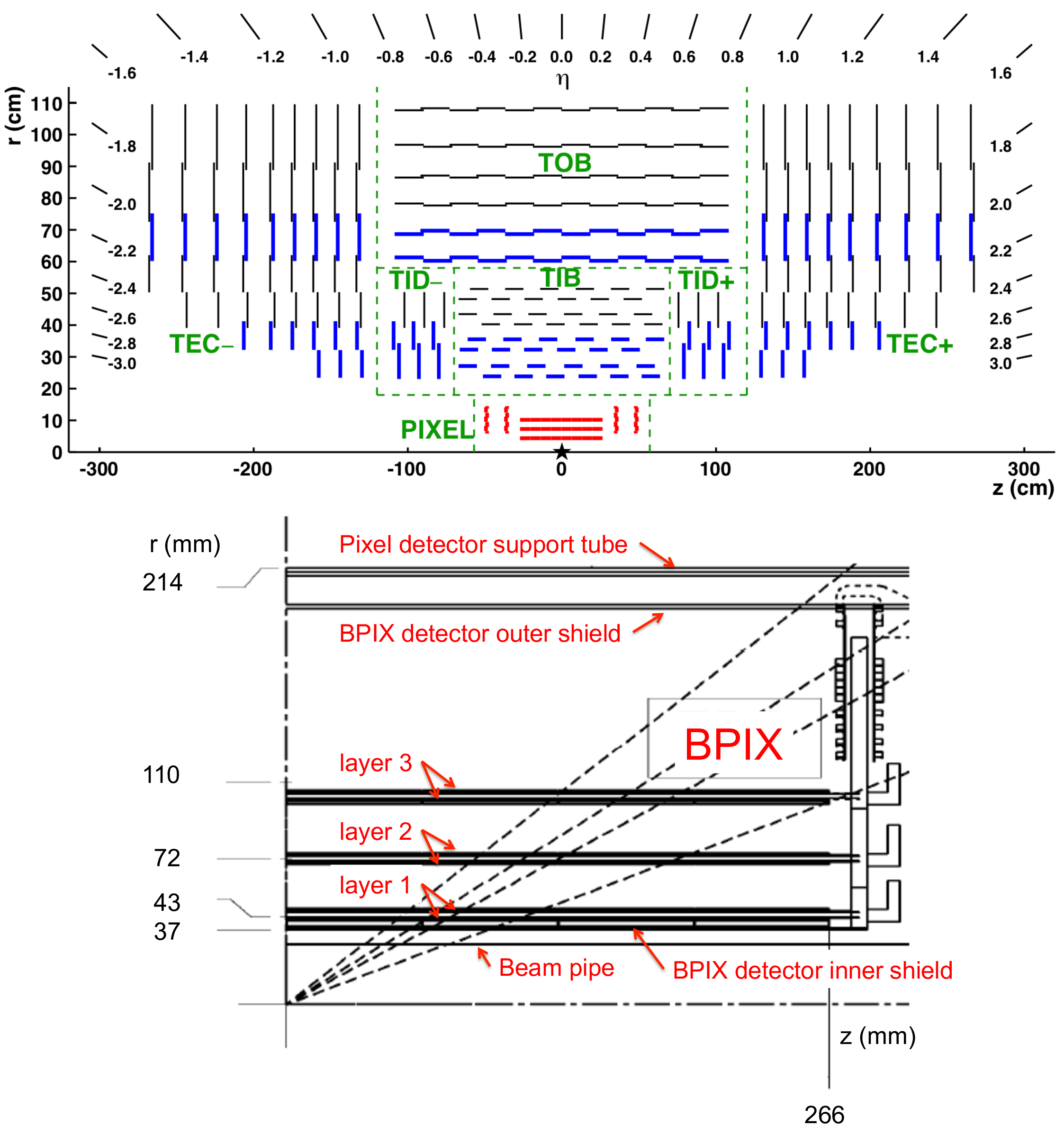
Figure 1:
(upper) Schematic view of the CMS tracker detector [1], and (lower) closeup view of the region around the original BPIX detector with labels identifying pixel detector support tube, BPIX detector outer and inner shields, three BPIX detector layers, and beam pipe. |
png pdf |
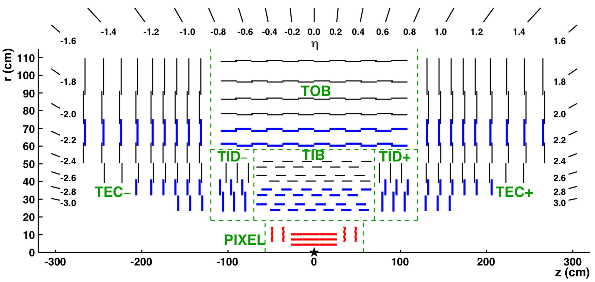
Figure 1-a:
Schematic view of the CMS tracker detector [1]. |
png pdf |
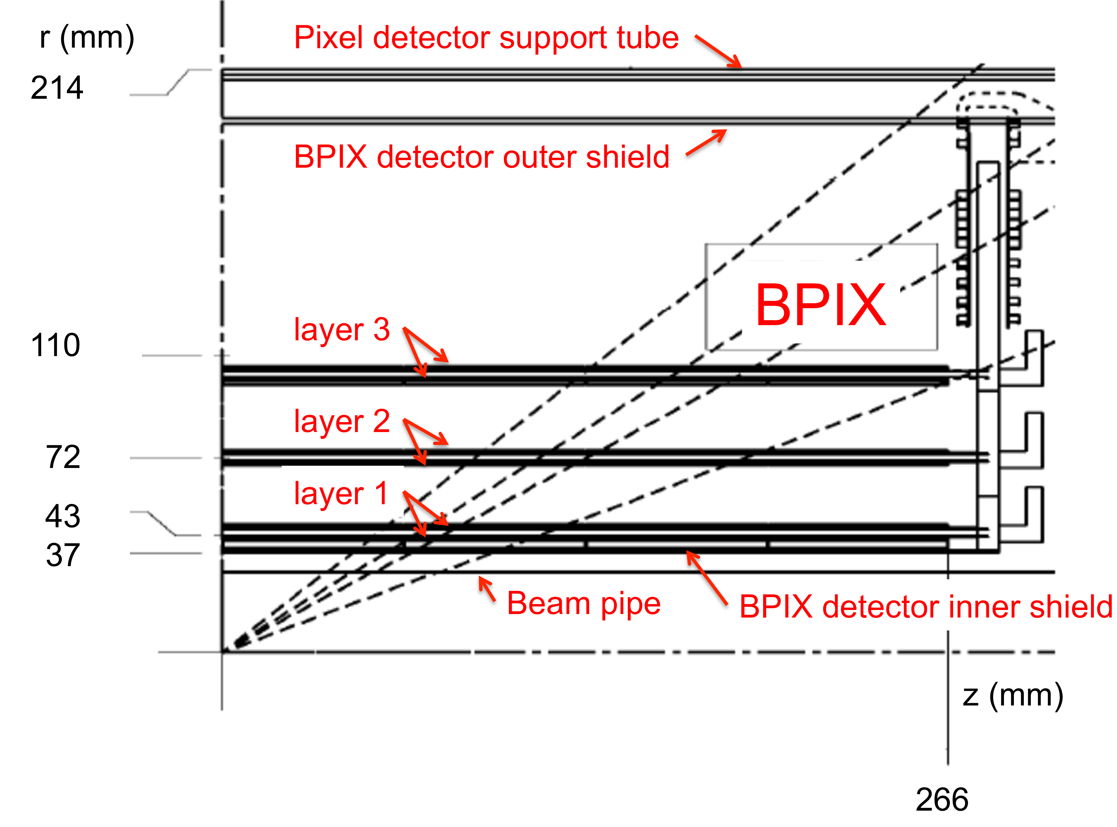
Figure 1-b:
Closeup view of the region around the original BPIX detector with labels identifying pixel detector support tube, BPIX detector outer and inner shields, three BPIX detector layers, and beam pipe. |

png pdf |
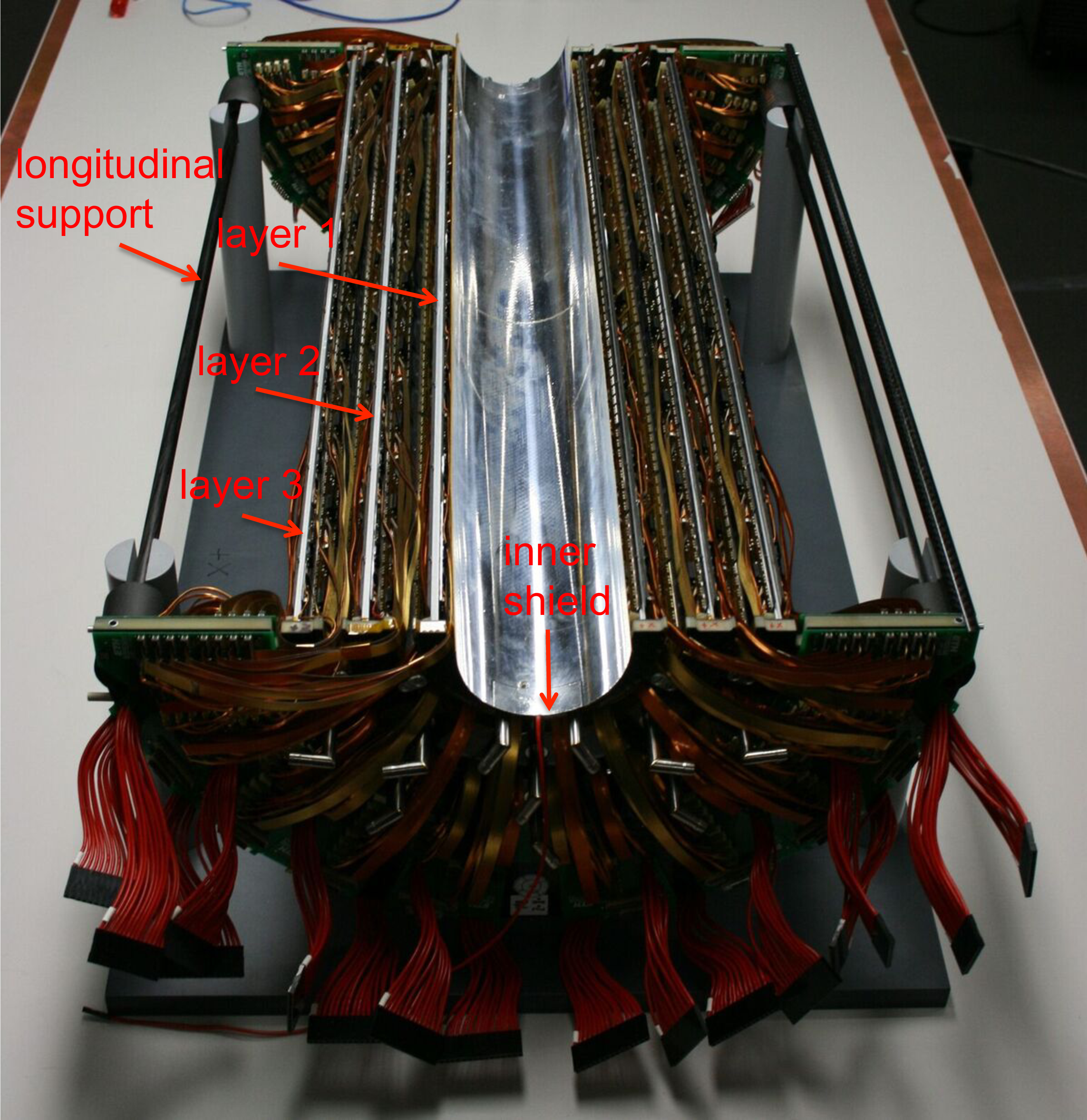
Figure 2:
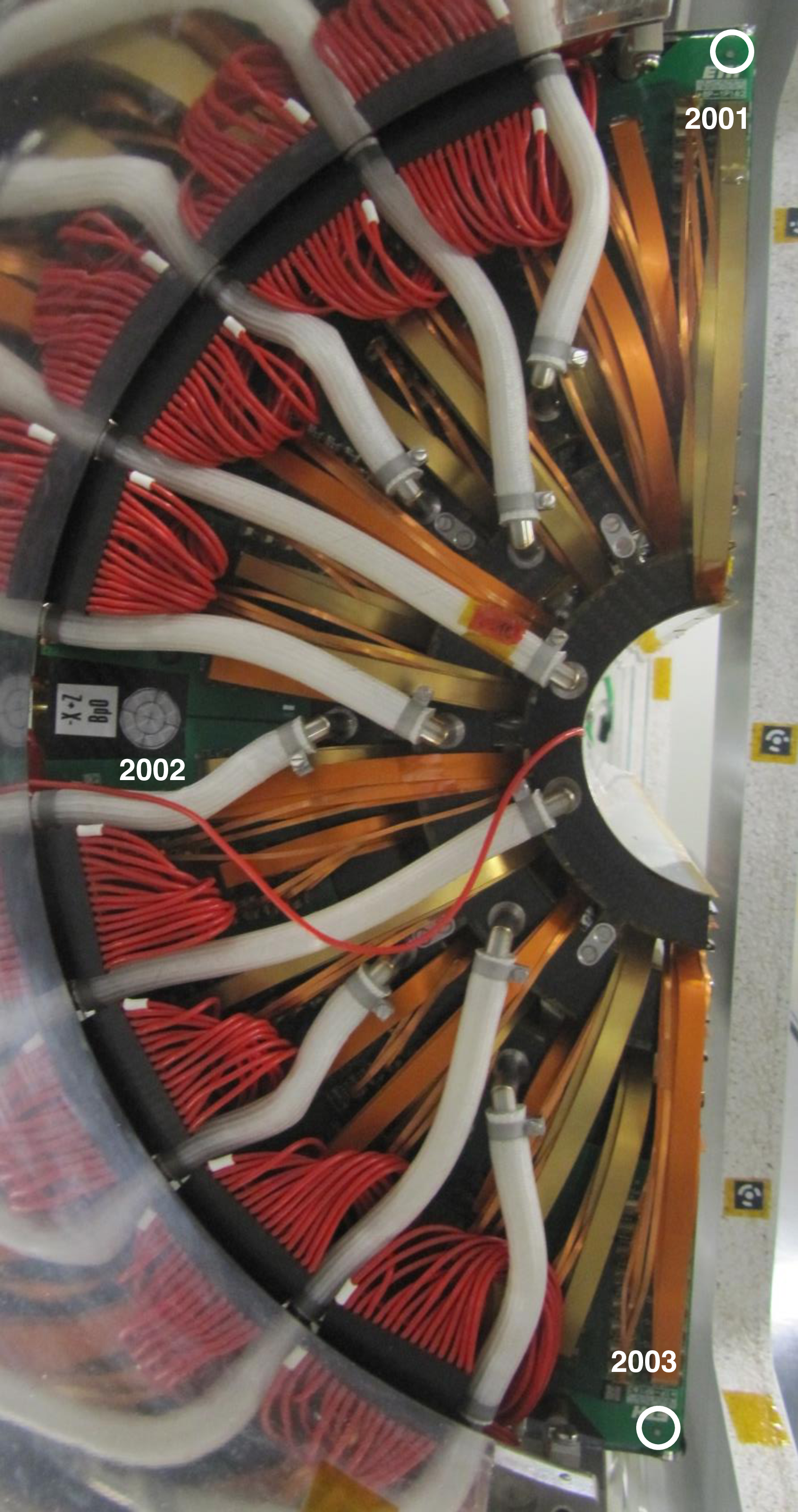
(left) Photograph of one half of the BPIX detector showing longitudinal support, three layers, and inner shield. (right) Photograph showing an end of the BPIX detector while standing on the installation cassette. Optical targets, indicated by the numbers 2001, 2002, and 2003, are used to locate the BPIX detector within the CMS cavern. Photographs by Antje Behrens, CERN. |
png pdf |
Figure 2-a:
Photograph of one half of the BPIX detector showing longitudinal support, three layers, and inner shield. |
png pdf |
Figure 2-b:
Photograph showing an end of the BPIX detector while standing on the installation cassette. Optical targets, indicated by the numbers 2001, 2002, and 2003, are used to locate the BPIX detector within the CMS cavern. Photographs by Antje Behrens, CERN. |
png pdf |
Figure 3:
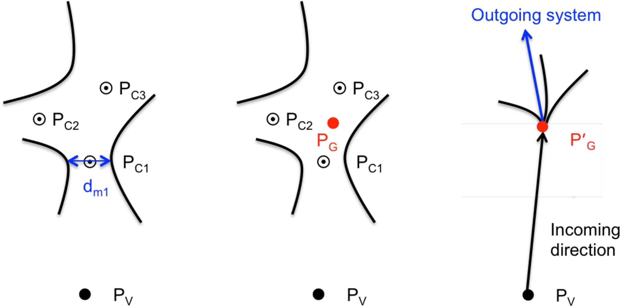
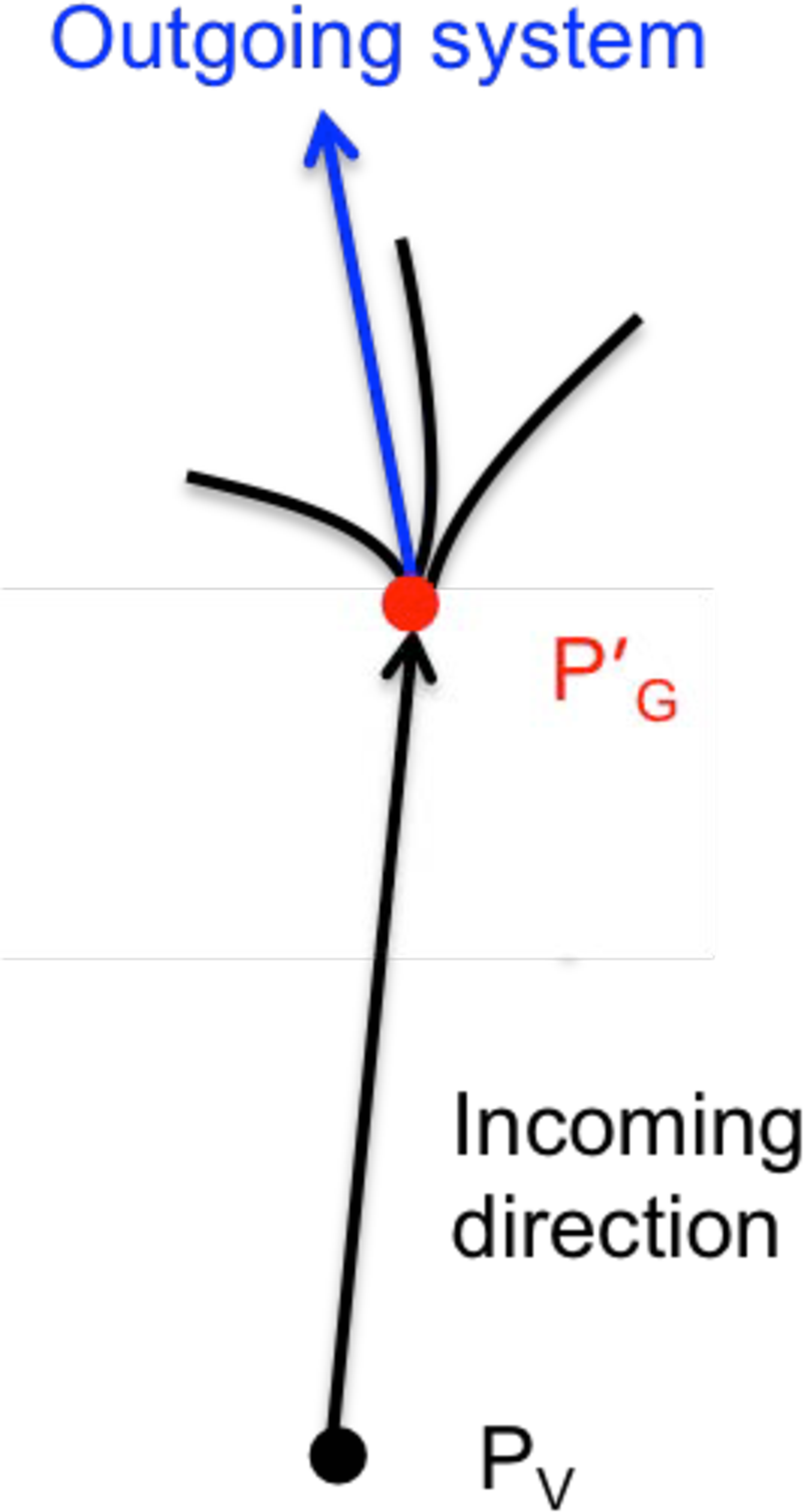
Schematic view of NI vertex reconstruction: (left) a cluster of $ {P_{\mathrm {C}}} $ positions ($ {P_{\mathrm {C}}} $, $ {P_{\mathrm {C2}}} $, and $ {P_{\mathrm {C3}}} $) with the distance of closest approach $ {d_{\mathrm {m}}} $ (labeled $d_{\mathrm {m1}}$), shown for $ {P_{\mathrm {C}}} $; (center) the algorithm uses the three $ {P_{\mathrm {C}}} $ points to identify an aggregate position $ {P_{\mathrm {G}}} $; (right) after refitting the track helices, the best vertex $ {P_{\mathrm {G}}'} $ is found with indicated incoming direction from the primary vertex position, $ {P_{\mathrm {V}}} $, and outgoing system. Black curves correspond to reconstructed charged particle tracks. |
png pdf |
Figure 3-a:
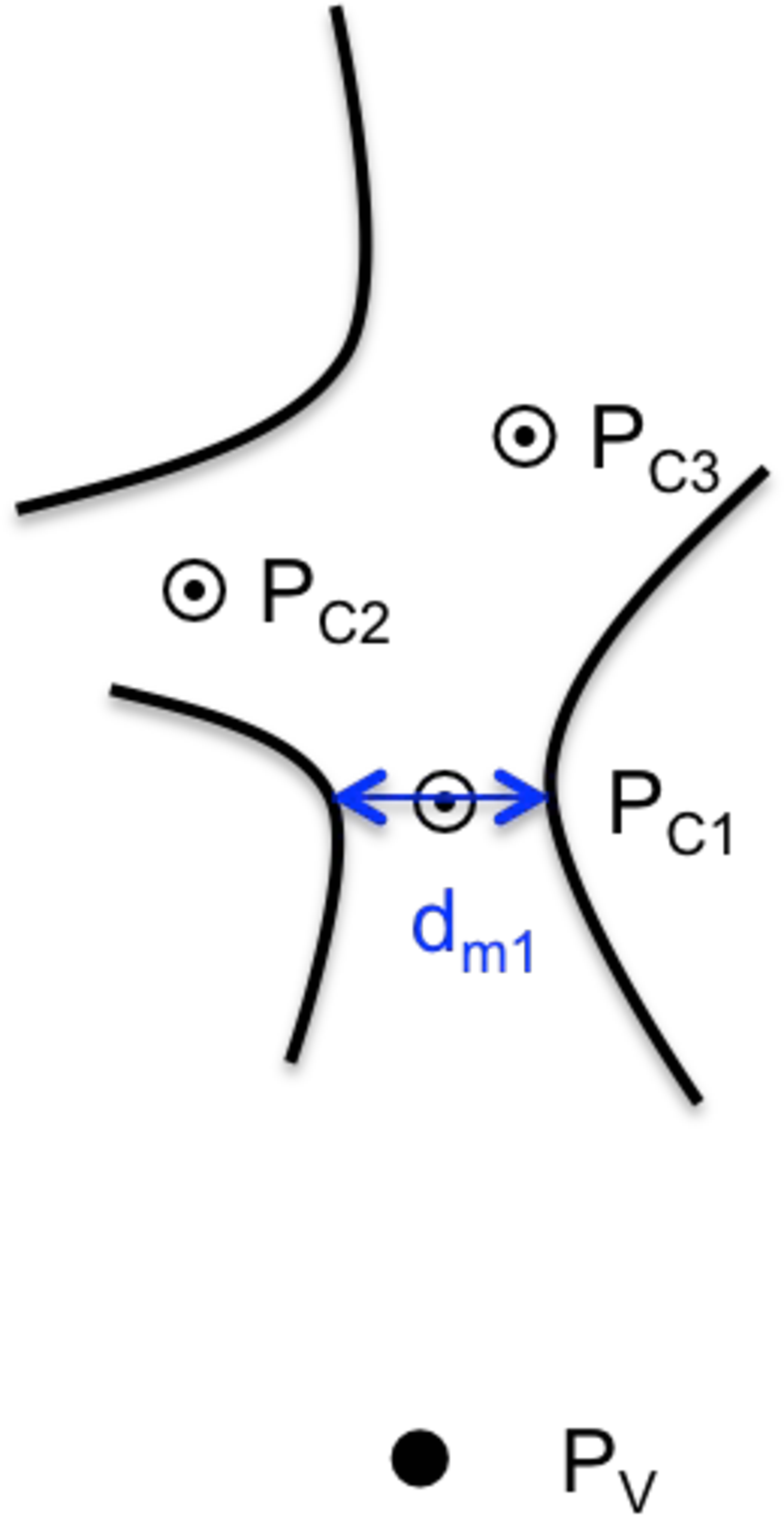
Schematic view of NI vertex reconstruction: a cluster of $ {P_{\mathrm {C}}} $ positions ($ {P_{\mathrm {C}}} $, $ {P_{\mathrm {C2}}} $, and $ {P_{\mathrm {C3}}} $) with the distance of closest approach $ {d_{\mathrm {m}}} $ (labeled $d_{\mathrm {m1}}$), shown for $ {P_{\mathrm {C}}} $; Black curves correspond to reconstructed charged particle tracks. |
png pdf |
Figure 3-b:
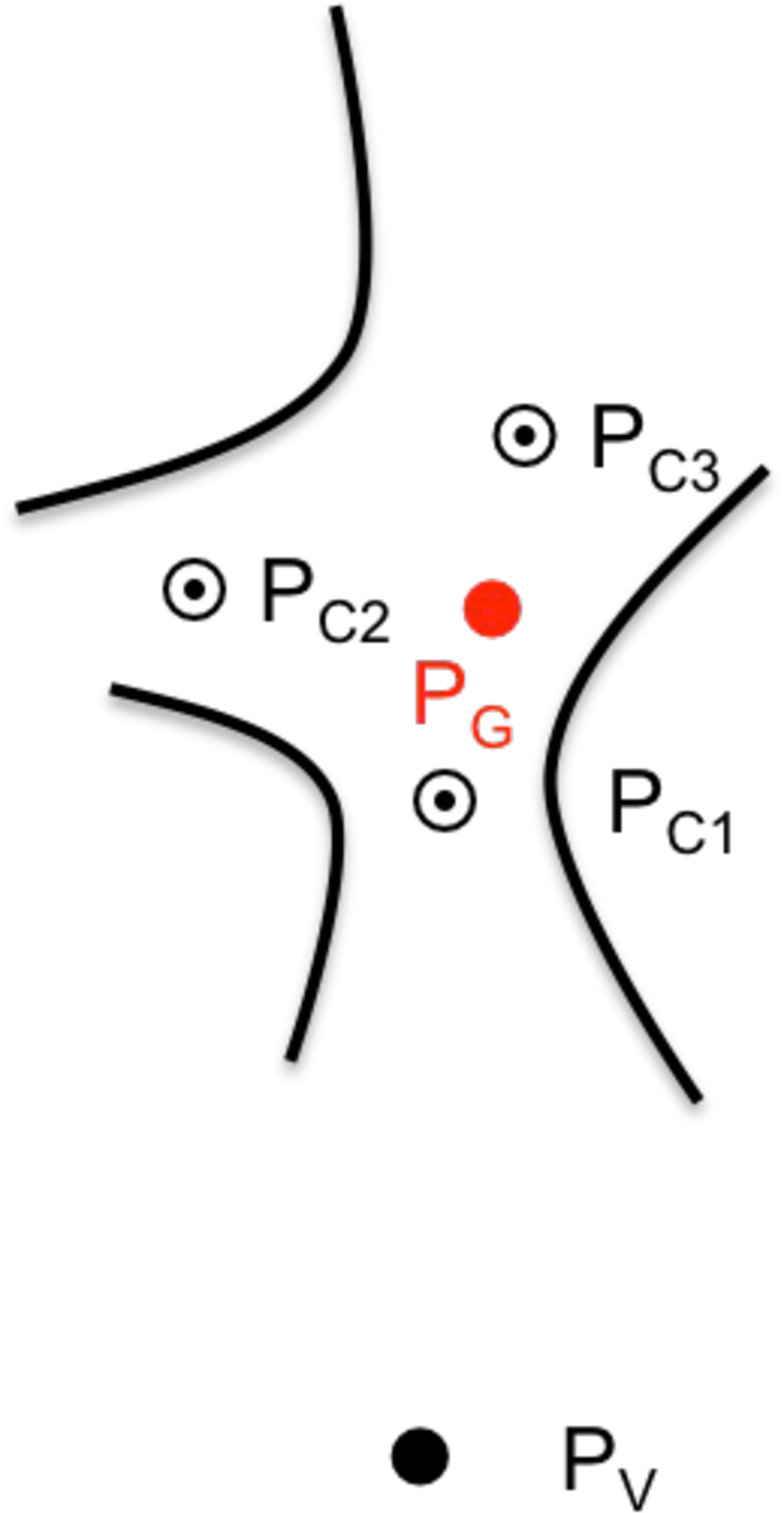
Schematic view of NI vertex reconstruction: the algorithm uses the three $ {P_{\mathrm {C}}} $ points to identify an aggregate position $ {P_{\mathrm {G}}} $; Black curves correspond to reconstructed charged particle tracks. |
png pdf |
Figure 3-c:
Schematic view of NI vertex reconstruction: after refitting the track helices, the best vertex $ {P_{\mathrm {G}}'} $ is found with indicated incoming direction from the primary vertex position, $ {P_{\mathrm {V}}} $, and outgoing system. Black curves correspond to reconstructed charged particle tracks. |
png pdf |
Figure 4:
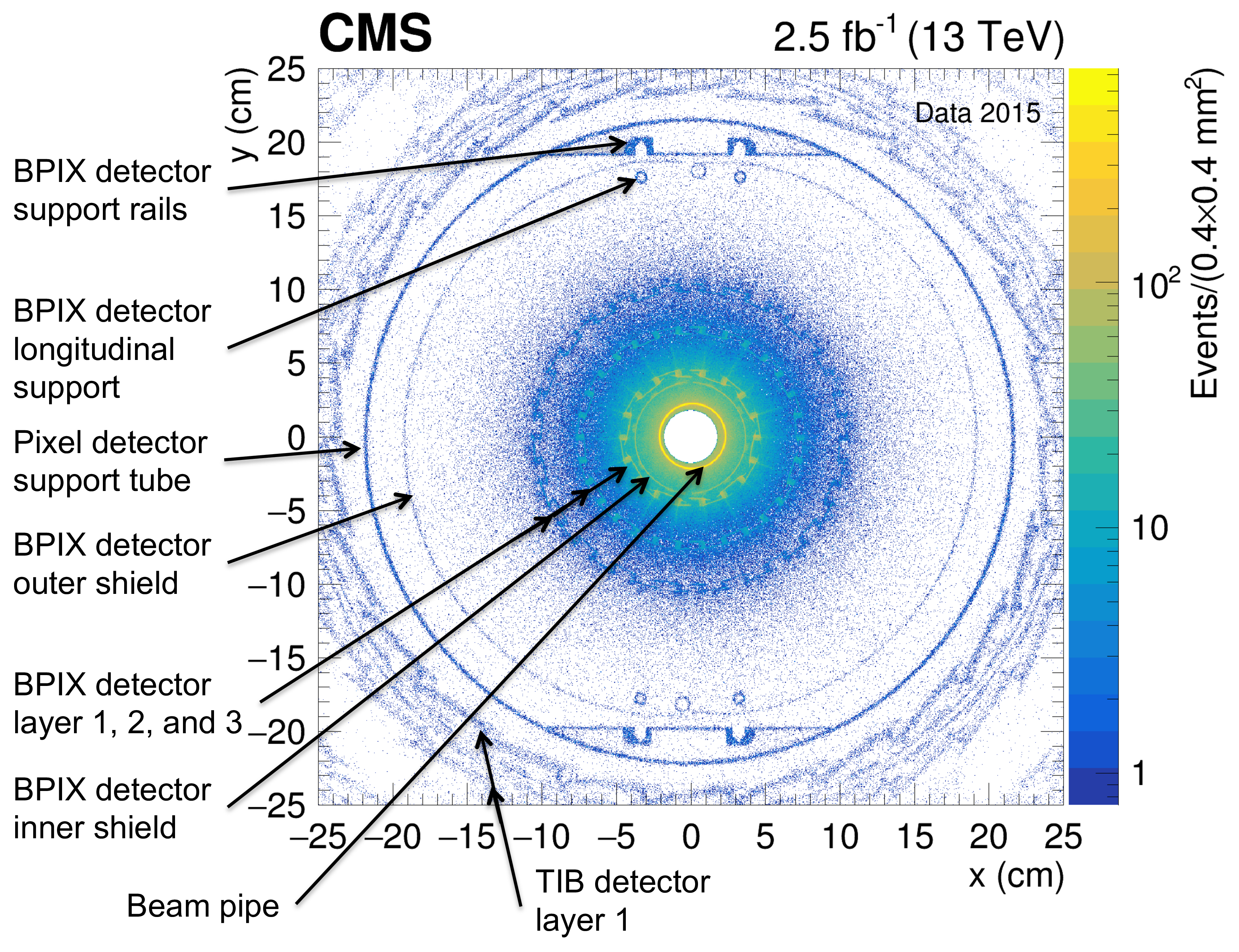
Hadrography of the tracker detector in the $x$-$y$ plane in the barrel region ($ | z | < $ 25 cm). The density of NI vertices is indicated by the color scale. The signatures of the beam pipe, the BPIX detector with its support, and the first layer of the TIB detector can be observed above the background of misreconstructed NIs. |
png pdf |
Figure 5:
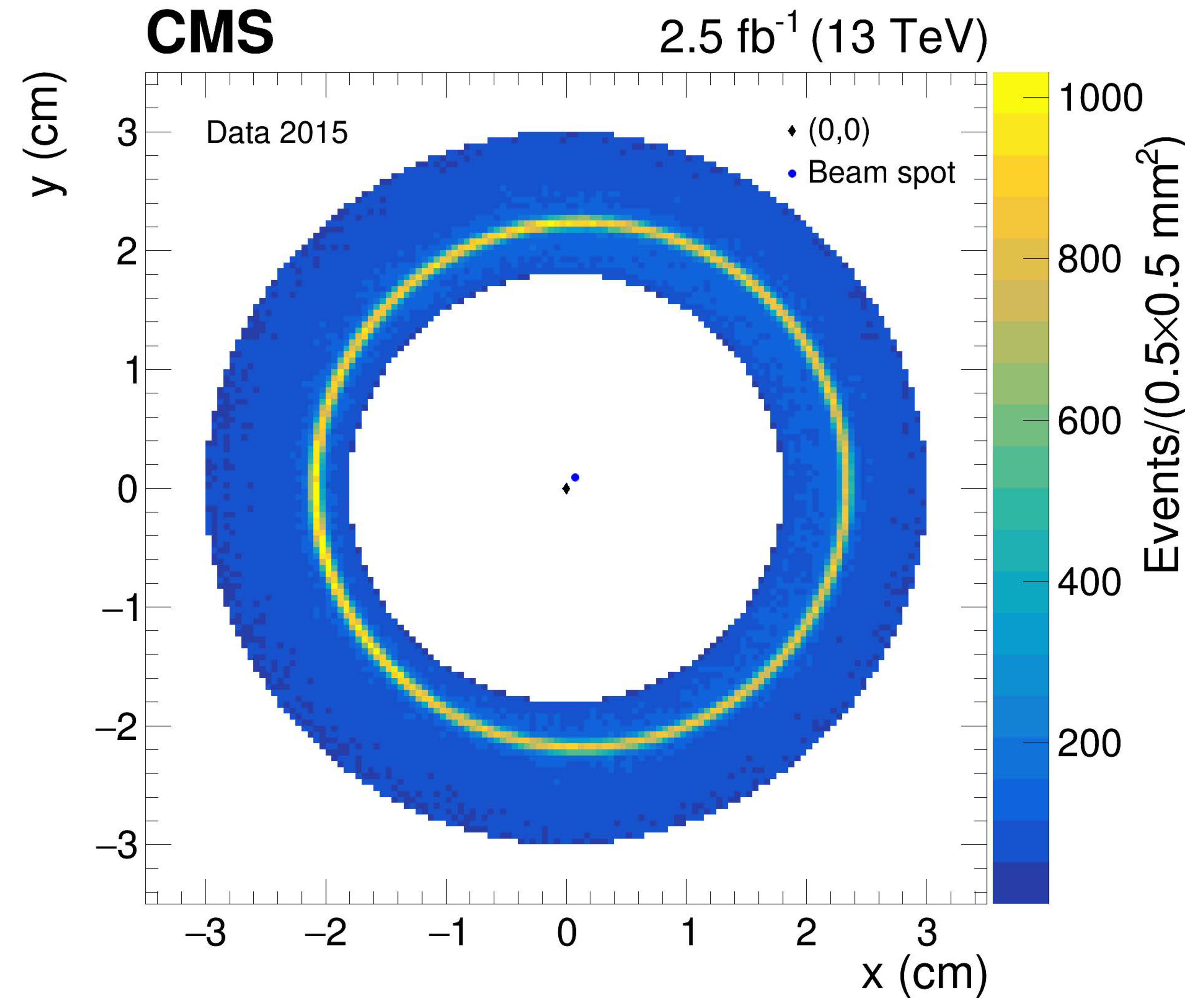
The beam pipe region viewed in the $x$-$y$ plane for $ | z | < $ 25 cm before background subtraction. The density of NI vertices is indicated by the color scale. $(0,0)$ is the origin of the CMS offline coordinate system, which is discussed in Section 7.1. The blue point in the center of the distribution corresponds to the average beam spot position of $ {x_{\text {bs}}} = $ 0.8 mm and $ {y_{\text {bs}}} = $ 0.9 mm in 2015. |
png pdf |
Figure 6:
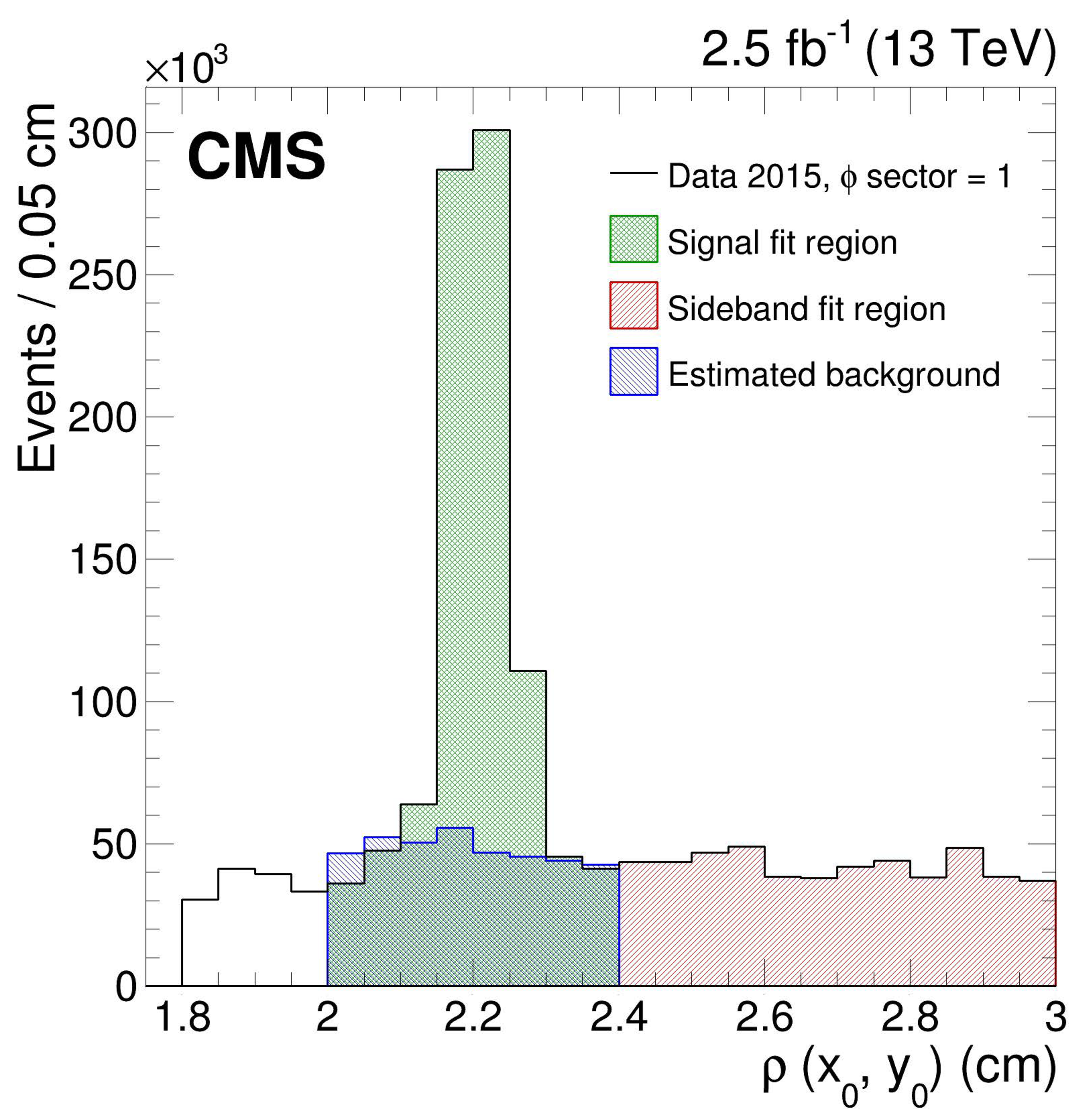
The density of NI vertices versus ${\rho ({x_{0}}, {y_{0}})}$ for a $\phi $ slice of the beam pipe located near $\phi = $ 0 (black line) for $ | z | < $ 25 cm before background subtraction. The green hatched area corresponds to the signal region, the red hatched area corresponds to the sideband region used to fit the background, and the blue hatched area corresponds to the estimated background in the signal region. |
png pdf |
Figure 7:
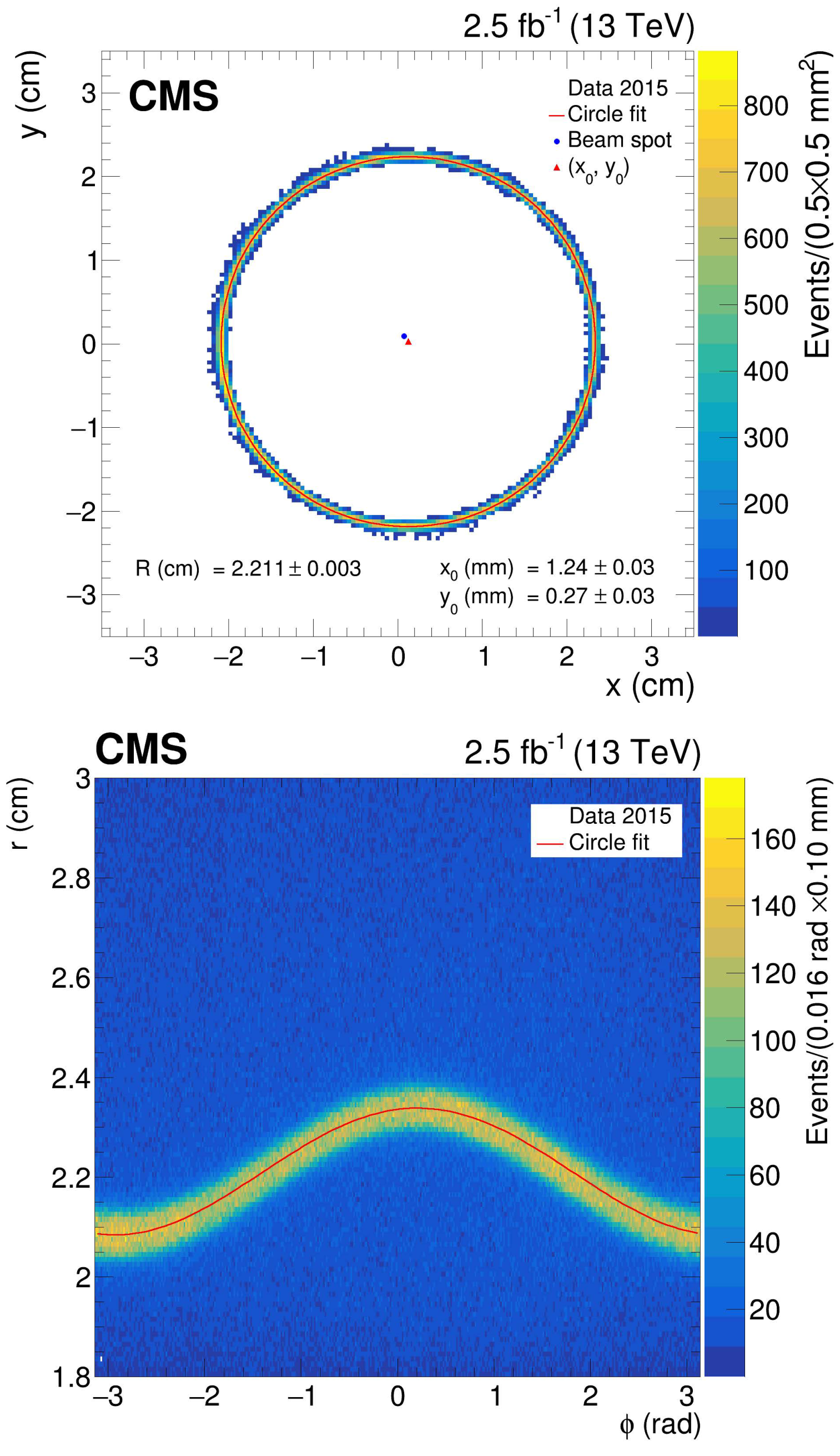
The beam pipe region with the fitted values for a circle of radius {R} and center $({x_{0}}, {y_{0}})$ for $ | z | < $ 25 cm. The $x$-$y$ plane after background subtraction (upper), and the $r$-$\phi $ coordinates before background subtraction (lower), are shown. The density of NI vertices is indicated by the color scale. The red line shows the fitted circle. The blue point in the center of the $x$-$y$ plane corresponds to the average beam spot position of $ {x_{\text {bs}}} =$ 0.8 mm and $ {y_{\text {bs}}} =$ 0.9 mm in 2015. |
png pdf |
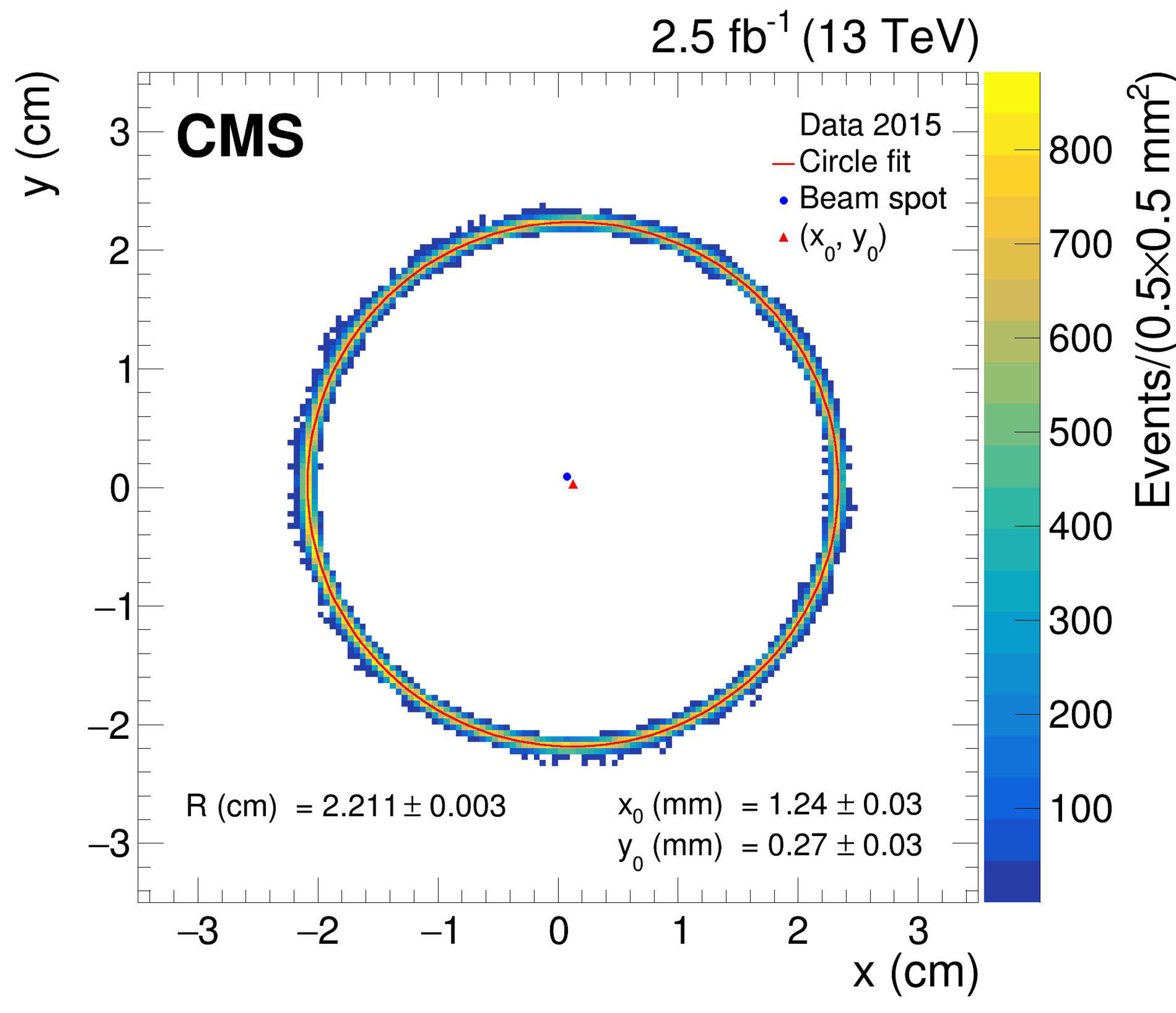
Figure 7-a:
The beam pipe region with the fitted values for a circle of radius {R} and center $({x_{0}}, {y_{0}})$ for $ | z | < $ 25 cm. The $x$-$y$ plane after background subtraction is shown. The density of NI vertices is indicated by the color scale. The red line shows the fitted circle. The blue point in the center of the $x$-$y$ plane corresponds to the average beam spot position of $ {x_{\text {bs}}} =$ 0.8 mm and $ {y_{\text {bs}}} =$ 0.9 mm in 2015. |

png pdf |
Figure 7-b:
The beam pipe region with the fitted values for a circle of radius {R} and center $({x_{0}}, {y_{0}})$ for $ | z | < $ 25 cm. The $r$-$\phi $ coordinates before background subtraction is shown. The density of NI vertices is indicated by the color scale. The red line shows the fitted circle. The blue point in the center of the $x$-$y$ plane corresponds to the average beam spot position of $ {x_{\text {bs}}} =$ 0.8 mm and $ {y_{\text {bs}}} =$ 0.9 mm in 2015. |
png pdf |
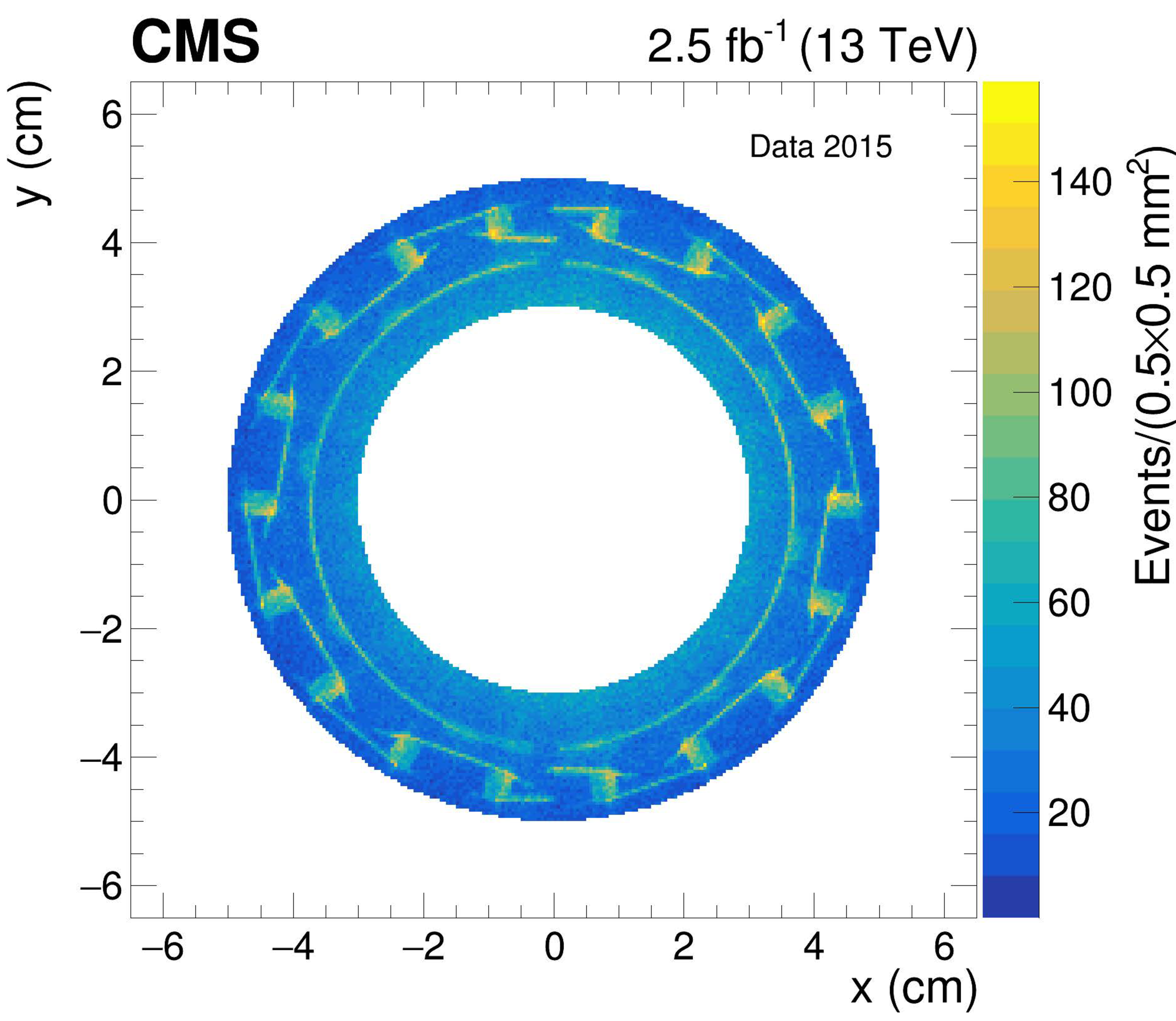
Figure 8:
The BPIX detector inner shield region viewed in the $x$-$y$ plane for $ | z | < $ 25 cm before background subtraction and removal of the $\phi $ regions with additional structures. The density of NI vertices is indicated by the color scale. The inner shield itself is the visible circle of radius $r = $ 3.8 cm. Modules in the first BPIX detector layer are visible at larger radius. The small bumps that can be seen around the shield correspond to cables connected to the first BPIX detector layer. |
png pdf |
Figure 9:
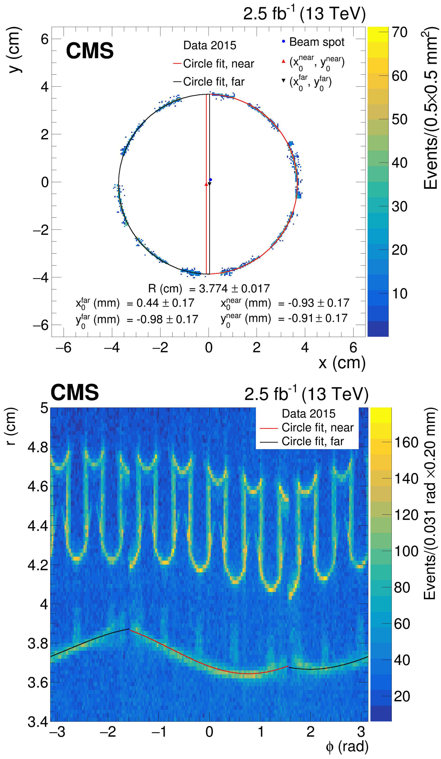
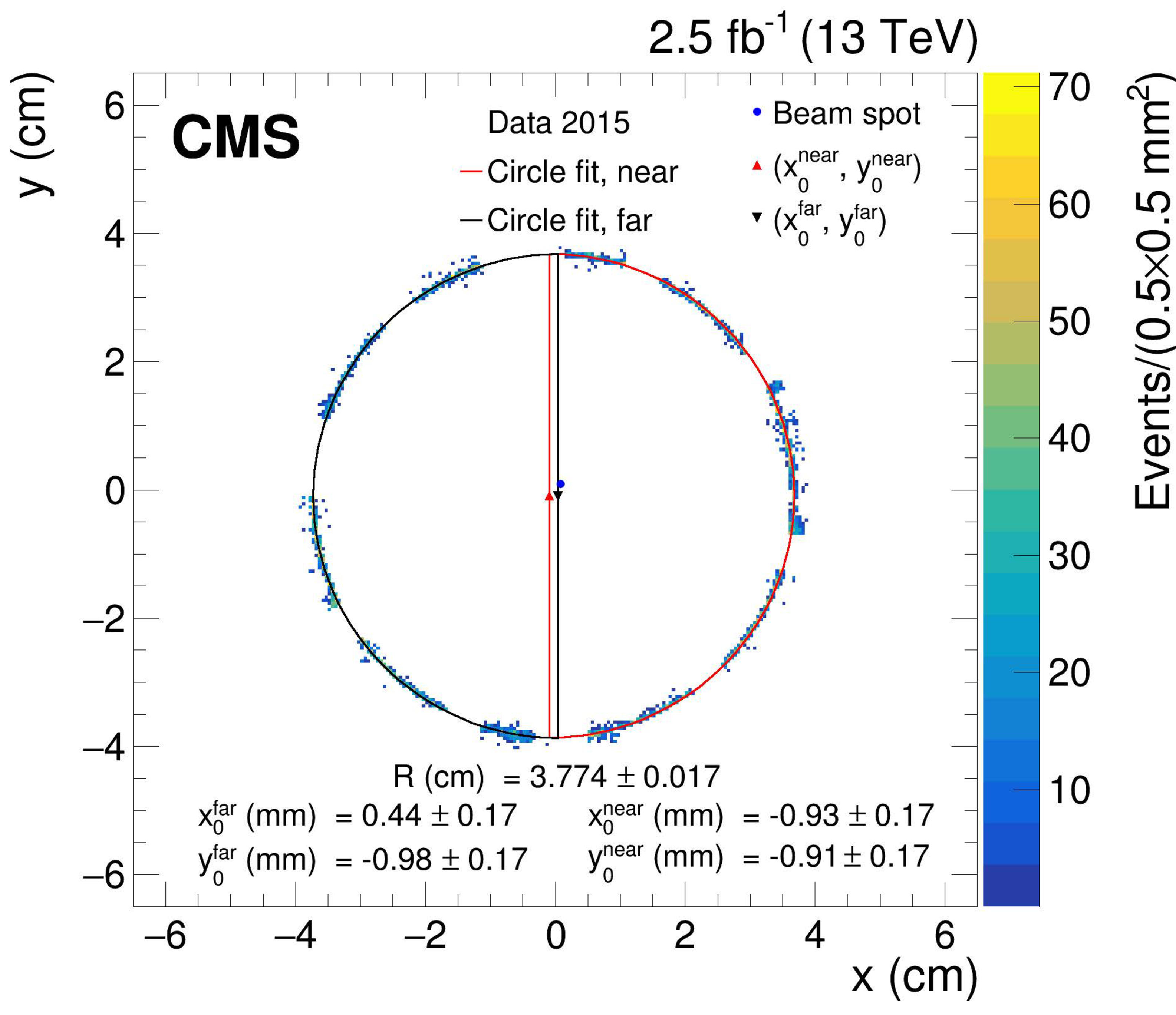
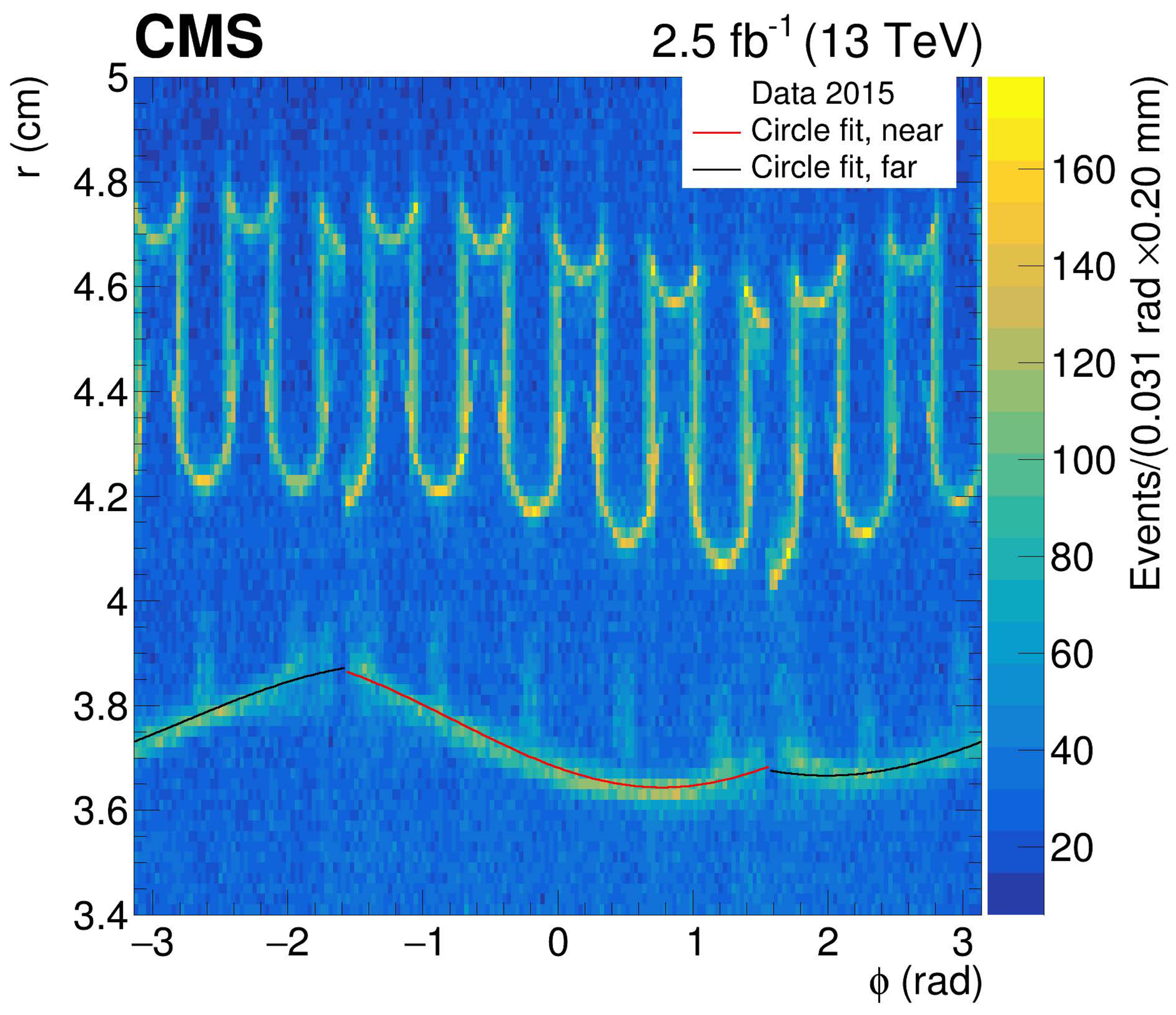
The BPIX detector inner shield with the fitted values for two half-circles of common radius R and centers $({{x_{0}} ^{\text {far}}}, {{y_{0}} ^{\text {far}}})$ and $({{x_{0}} ^{\text {near}}}, {{y_{0}} ^{\text {near}}})$ for $ | z | < $ 25 cm. The $x$-$y$ plane after background subtraction (upper), and the $r$-$\phi $ coordinates before background subtraction (lower), are shown. The density of NI vertices is indicated by the color scale. The red and black lines at around $r = $ 3.8 cm show the fitted half-circles on the far and near sides, respectively. The blue point at the center of the $x$-$y$ plane corresponds to the average beam spot position of $ {x_{\text {bs}}} =$ 0.8 mm and $ {y_{\text {bs}}} =$ 0.9 mm in 2015. Modules in the first BPIX detector layer are visible (lower) at larger radius. |
png pdf |
Figure 9-a:
The BPIX detector inner shield with the fitted values for two half-circles of common radius R and centers $({{x_{0}} ^{\text {far}}}, {{y_{0}} ^{\text {far}}})$ and $({{x_{0}} ^{\text {near}}}, {{y_{0}} ^{\text {near}}})$ for $ | z | < $ 25 cm. The $x$-$y$ plane after background subtraction is shown. The density of NI vertices is indicated by the color scale. The red and black lines at around $r = $ 3.8 cm show the fitted half-circles on the far and near sides, respectively. The blue point at the center of the $x$-$y$ plane corresponds to the average beam spot position of $ {x_{\text {bs}}} =$ 0.8 mm and $ {y_{\text {bs}}} =$ 0.9 mm in 2015. |
png pdf |
Figure 9-b:
The BPIX detector inner shield with the fitted values for two half-circles of common radius R and centers $({{x_{0}} ^{\text {far}}}, {{y_{0}} ^{\text {far}}})$ and $({{x_{0}} ^{\text {near}}}, {{y_{0}} ^{\text {near}}})$ for $ | z | < $ 25 cm. The $r$-$\phi $ coordinates before background subtraction is shown. The density of NI vertices is indicated by the color scale. The red and black lines at around $r = $ 3.8 cm show the fitted half-circles on the far and near sides, respectively. Modules in the first BPIX detector layer are visible at larger radius. |
png pdf |
Figure 10:
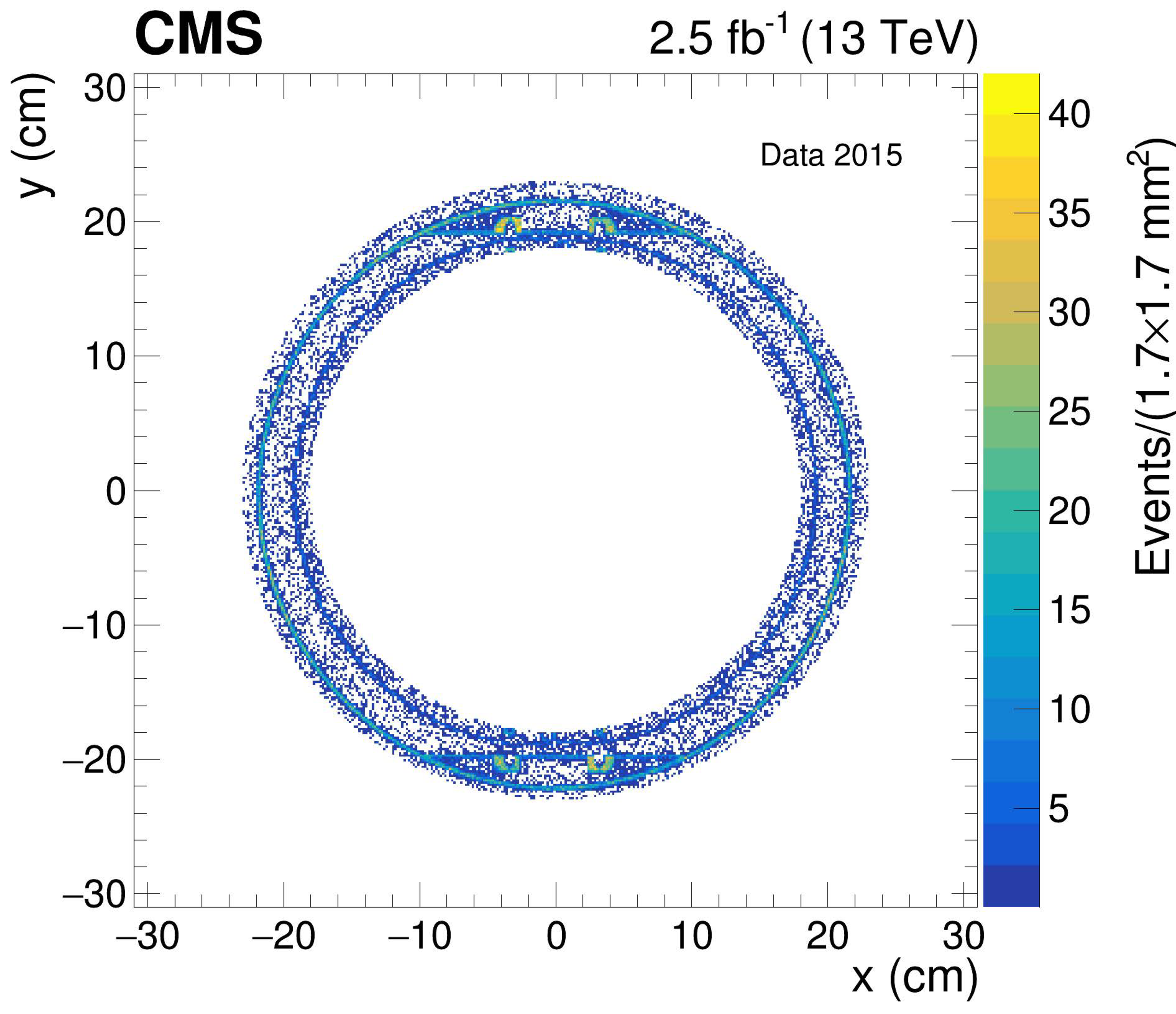
The region of the pixel detector support tube viewed in the $x$-$y$ plane for $ | z | < $ 25 cm before background subtraction and removal of the $\phi $ regions with additional structures. The density of NI vertices is indicated by the color scale. Two circular structures are visible. The circle with the smaller radius corresponds to the BPIX detector outer shield, while the one with the larger radius is the pixel detector support tube (also visible in Fig. 4. |
png pdf |
Figure 11:
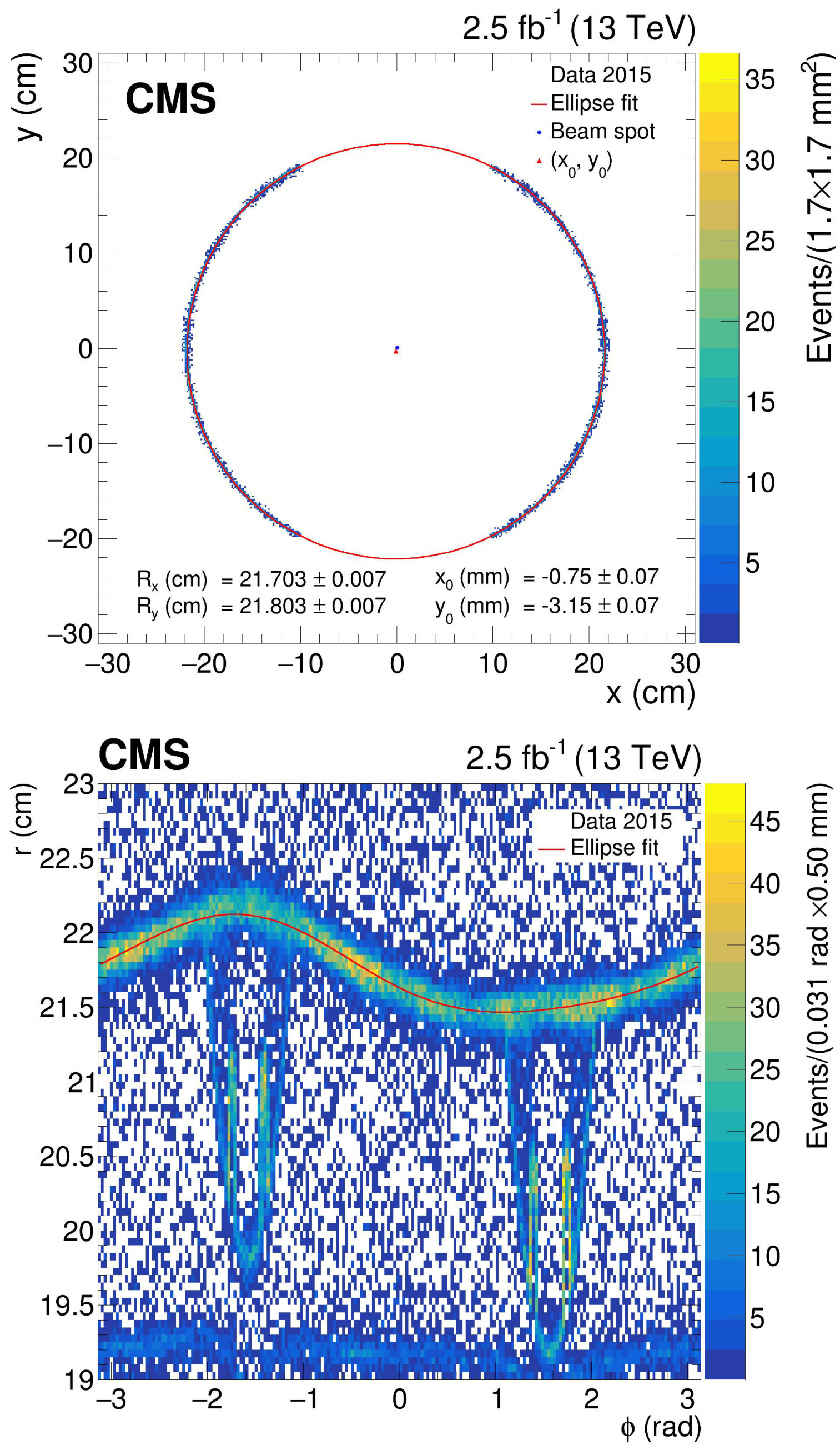
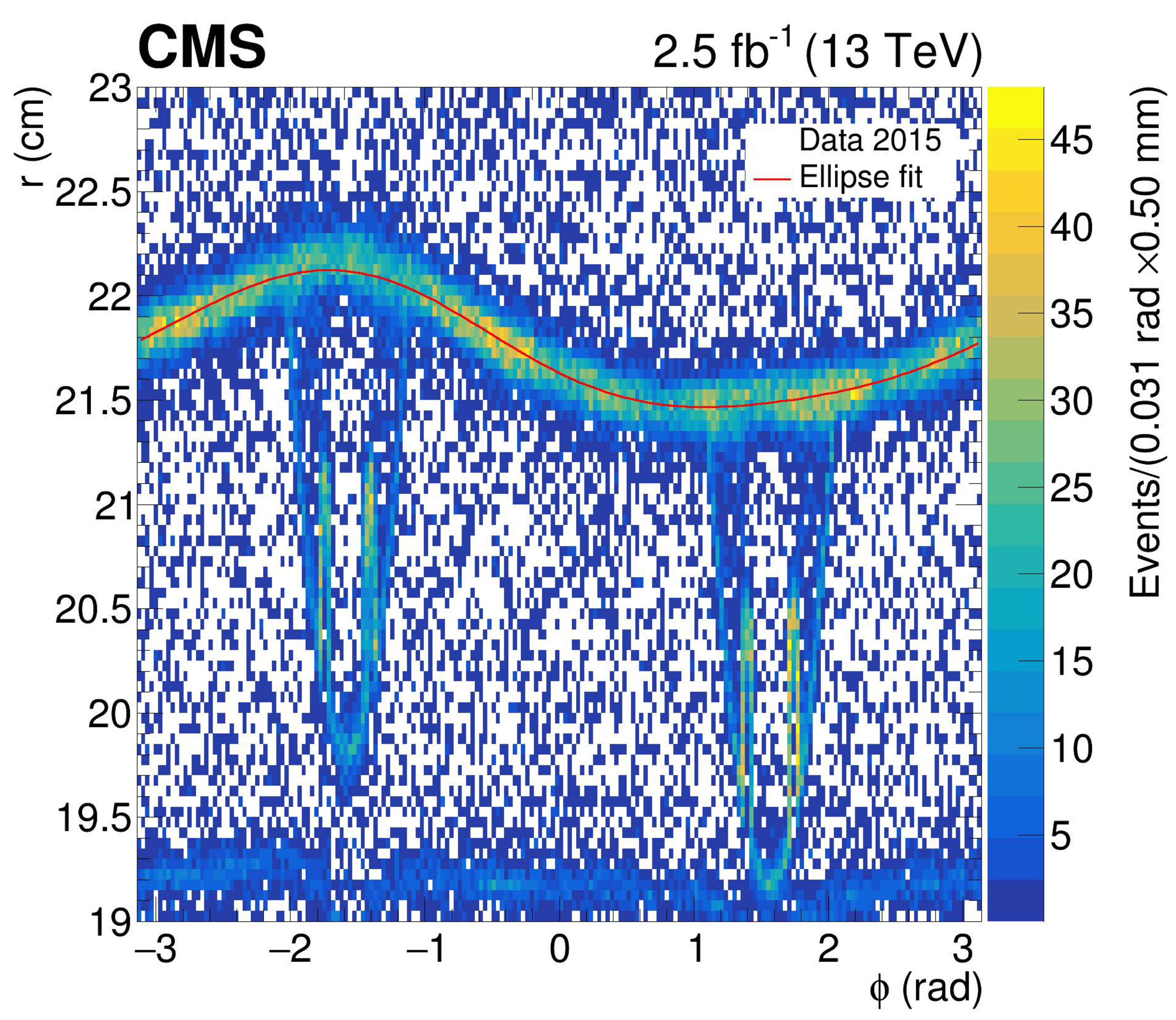
The pixel detector support tube with the fitted values for an ellipse with semi-minor axis $ {R_{\mathrm {x}}} $, semi-major axis $ {R_{\mathrm {y}}} $, and center $({x_{0}}, {y_{0}})$ for $ | z | < $ 25 cm. The $x$-$y$ plane after background subtraction (upper), and the $r$-$\phi $ coordinates before background subtraction (lower), are shown. The density of NI vertices is indicated by the color scale. The red line shows the fitted ellipse. The blue point in the center of the $x$-$y$ plane corresponds to the average beam spot position of $ {x_{\text {bs}}} =$ 0.8 mm and $ {y_{\text {bs}}} =$ 0.9 mm in 2015. |

png pdf |
Figure 11-a:
The pixel detector support tube with the fitted values for an ellipse with semi-minor axis $ {R_{\mathrm {x}}} $, semi-major axis $ {R_{\mathrm {y}}} $, and center $({x_{0}}, {y_{0}})$ for $ | z | < $ 25 cm. The $x$-$y$ plane after background subtraction is shown. The density of NI vertices is indicated by the color scale. The red line shows the fitted ellipse. The blue point in the center of the $x$-$y$ plane corresponds to the average beam spot position of $ {x_{\text {bs}}} =$ 0.8 mm and $ {y_{\text {bs}}} =$ 0.9 mm in 2015. |
png pdf |
Figure 11-b:
The pixel detector support tube with the fitted values for an ellipse with semi-minor axis $ {R_{\mathrm {x}}} $, semi-major axis $ {R_{\mathrm {y}}} $, and center $({x_{0}}, {y_{0}})$ for $ | z | < $ 25 cm. The $r$-$\phi $ coordinates before background subtraction (lower) is shown. The density of NI vertices is indicated by the color scale. The red line shows the fitted ellipse. |
png pdf |
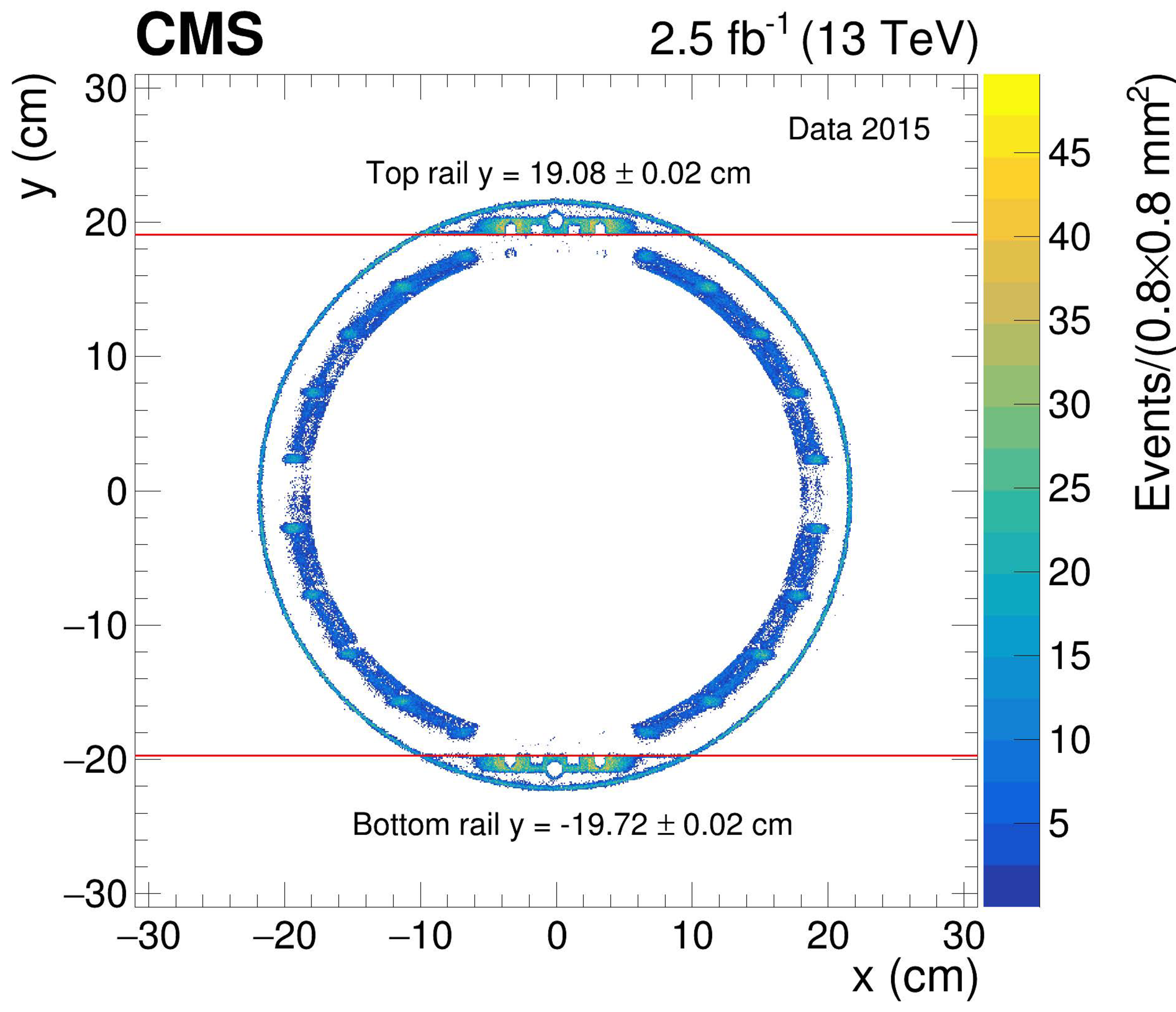
Figure 12:
The BPIX detector support rails after background subtraction in the $x$-$y$ plane for the combined tracker detector barrel and endcap regions. Horizontal red lines correspond to the fit of the BPIX detector support rails. The density of NI vertices is indicated by the color scale. |
| Tables | |
png pdf |
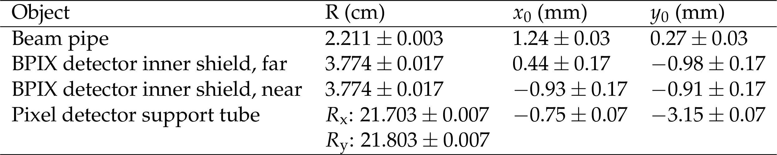
Table 1:
Results of the fit to the beam pipe with a circle, the BPIX detector inner shield with two half-circles, and the pixel detector support tube with an ellipse. Only systematic uncertainties are provided, since the statistical uncertainties are negligible. |

png pdf |
Table 2:
Results of the fitted $y$ coordinate of the bottom and top BPIX detector support rails with a horizontal line. Only systematic uncertainties are provided, since the statistical uncertainties are negligible. |
png pdf |
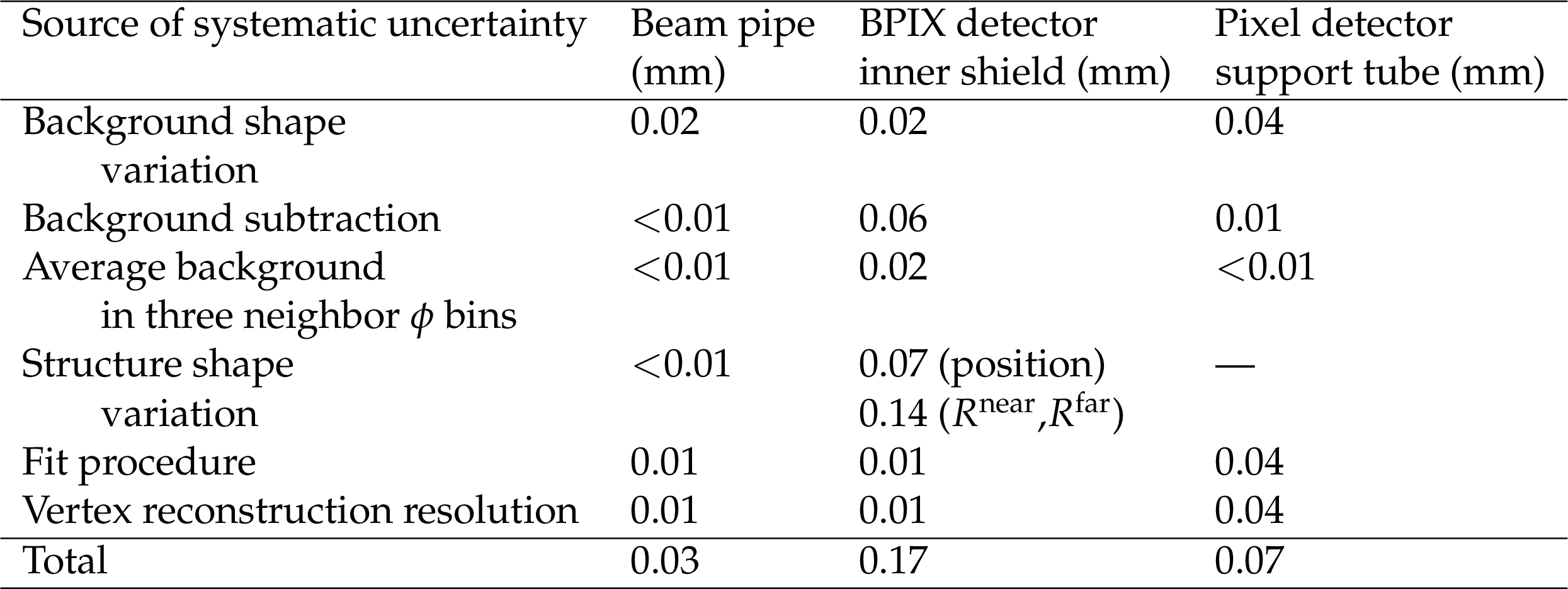
Table 3:
Systematic uncertainties in the position and radius measurements of three passive detector elements. |
png pdf |
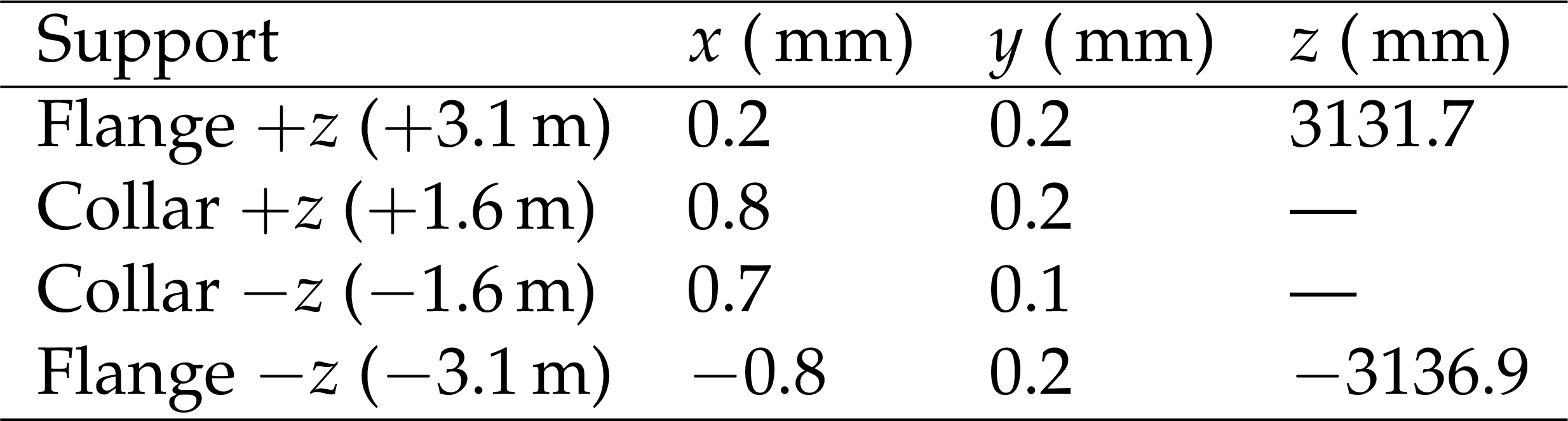
Table 4:
Results from the survey of the CMS central beam pipe positions on January 12, 2015. |
| Summary |
| Nuclear interactions have a reputation of being undesirable events that degrade the quality of the reconstruction of charged and neutral hadrons. In this analysis, it has been demonstrated that they can be used to produce a high-precision map of the material inside the tracker. Using a data set that corresponds to an integrated luminosity of 2.5 fb$^{-1}$ of proton-proton collisions at a center-of-mass energy of 13 TeV, a large sample of secondary hadronic interactions was collected. After background subtraction, the positions of the secondary vertices were used to determine the locations of passive material with a precision of the order of 100 $\mu$m. The positions of the beam pipe and the inner tracker structures (pixel detector support tube, and BPIX inner shield and support rails) were determined with a precision that depends on the structure under study. No significant position bias was identified through the technique, and statistical uncertainties were negligible. The positions of the structures under consideration were probed with a precision better than the typical installation tolerances and are found to be compatible with previous survey measurements. |
| References | ||||
| 1 | CMS Collaboration | The CMS experiment at the CERN LHC | JINST 3 (2008) S08004 | CMS-00-001 |
| 2 | CMS Collaboration | Search for long-lived charged particles in proton-proton collisions at $ \sqrt{s} = $ 13 TeV | PRD 94 (2016) 112004 | CMS-EXO-15-010 1609.08382 |
| 3 | CMS Collaboration | Search for new long-lived particles at $ \sqrt{s} = $ 13 TeV | PLB 780 (2018) 432 | CMS-EXO-16-003 1711.09120 |
| 4 | CMS Collaboration | Identification of heavy-flavour jets with the CMS detector in pp collisions at 13 TeV | JINST 13 (2018) P05011 | CMS-BTV-16-002 1712.07158 |
| 5 | GEANT4 Collaboration | $ GEANT4--a $ simulation toolkit | NIMA 506 (2003) 250 | |
| 6 | J. Allison et al. | $ GEANT4 $ developments and applications | IEEE Trans. Nucl. Sci. 53 (2006) 270 | |
| 7 | CMS Collaboration | Altered scenarios of the CMS tracker material for systematic uncertainties studies | CDS | |
| 8 | CMS Collaboration | Studies of tracker material | CMS-PAS-TRK-10-003 | |
| 9 | CMS Collaboration | Performance of photon reconstruction and identification with the CMS detector in proton-proton collisions at $ \sqrt{s} = $ 8 TeV | JINST 10 (2015) P08010 | CMS-EGM-14-001 1502.02702 |
| 10 | CMS Collaboration | CMS technical design report for the pixel detector upgrade | technical report, CERN | |
| 11 | ATLAS Collaboration | A study of the material in the ATLAS inner detector using secondary hadronic interactions | JINST 7 (2012) P01013 | 1110.6191 |
| 12 | ATLAS Collaboration | A measurement of material in the ATLAS tracker using secondary hadronic interactions in 7 TeV pp collisions | JINST 11 (2016) P11020 | 1609.04305 |
| 13 | CMS Collaboration | Alignment of the CMS tracker with LHC and cosmic ray data | JINST 9 (2014) P06009 | CMS-TRK-11-002 1403.2286 |
| 14 | T. Sjostrand, S. Mrenna, and P. Z. Skands | A brief introduction to $ PYTHIA $ 8.1 | CPC 178 (2008) 852 | 0710.3820 |
| 15 | T. Sjostrand et al. | An introduction to $ PYTHIA $ 8.2 | CPC 191 (2015) 159 | 1410.3012 |
| 16 | CMS Collaboration | Event generator tunes obtained from underlying event and multiparton scattering measurements | EPJC 76 (2016) 155 | CMS-GEN-14-001 1512.00815 |
| 17 | CMS Collaboration | The CMS trigger system | JINST 12 (2017) P01020 | CMS-TRG-12-001 1609.02366 |
| 18 | CMS Tracker Collaboration, R. Ranieri | The simulation of the CMS silicon tracker | in Proceedings, 2007 IEEE Nuclear Science Symposium and Medical Imaging Conference (NSS/MIC): Honolulu, Hawaii, p. 2434 2007 | |
| 19 | CMS Collaboration | Description and performance of track and primary-vertex reconstruction with the CMS tracker | JINST 9 (2014) P10009 | CMS-TRK-11-001 1405.6569 |
| 20 | CMS Collaboration | Particle-flow reconstruction and global event description with the CMS detector | JINST 12 (2017) P10003 | CMS-PRF-14-001 1706.04965 |
| 21 | CMS Collaboration | Tracking POG plot results on 2015 data | CDS | |
| 22 | M. Gallilee et al. | LHC detector vacuum system consolidation for long shutdown 1 (LS1) in 2013-2014 | in Proceedings, 3rd International Conference on Particle accelerator (IPAC 2012): New Orleans, USA, p. 25552012 | |
|
|
Compact Muon Solenoid LHC, CERN |
|

|

|

|

|

|