

Compact Muon Solenoid
LHC, CERN
| CMS-PAS-FTR-18-015 | ||
| Projection of differential $\mathrm{t\bar{t}}$ production cross section measurements in the e/$\mu$+jets channels in pp collisions at the HL-LHC | ||
| CMS Collaboration | ||
| December 2018 | ||
| Abstract: A study of the resolved reconstruction of top quark pairs in the e/$\mu$+jets channels and a projection of differential $\mathrm{t\bar{t}}$ cross section measurements at the HL-LHC with an integrated luminosity of 3 ab$^{-1}$ at 14 TeV are presented. The analysis techniques are based on previous measurements of differential $\mathrm{t\bar{t}}$ cross sections at 13 TeV. It is shown that such a measurement is feasible at the HL-LHC despite the expected large number of pileup interactions. The precision of the differential cross section will profit from the enormous amount of data and the extended $\eta$-range of the Phase-2 CMS detector. The results are used to estimate the improvement of constraints on parton distribution functions. | ||
| Links: CDS record (PDF) ; inSPIRE record ; CADI line (restricted) ; | ||
| Figures | |

png pdf |
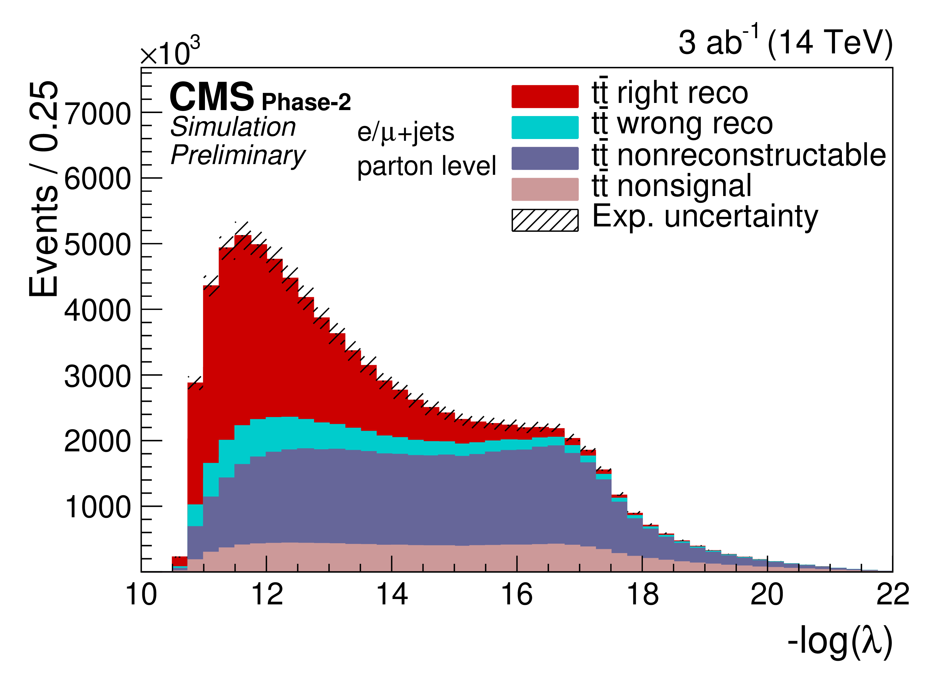
Figure 1:
Distributions of $\lambda $ and the reconstructed $ {m_ {\mathrm {t}}} $ of the hadronically decaying top quarks are shown for the Phase-2 simulation. |
png pdf |
Figure 1-a:
Distributions of $\lambda $ and the reconstructed $ {m_ {\mathrm {t}}} $ of the hadronically decaying top quarks are shown for the Phase-2 simulation. |

png pdf |
Figure 1-b:
Distributions of $\lambda $ and the reconstructed $ {m_ {\mathrm {t}}} $ of the hadronically decaying top quarks are shown for the Phase-2 simulation. |
png pdf |
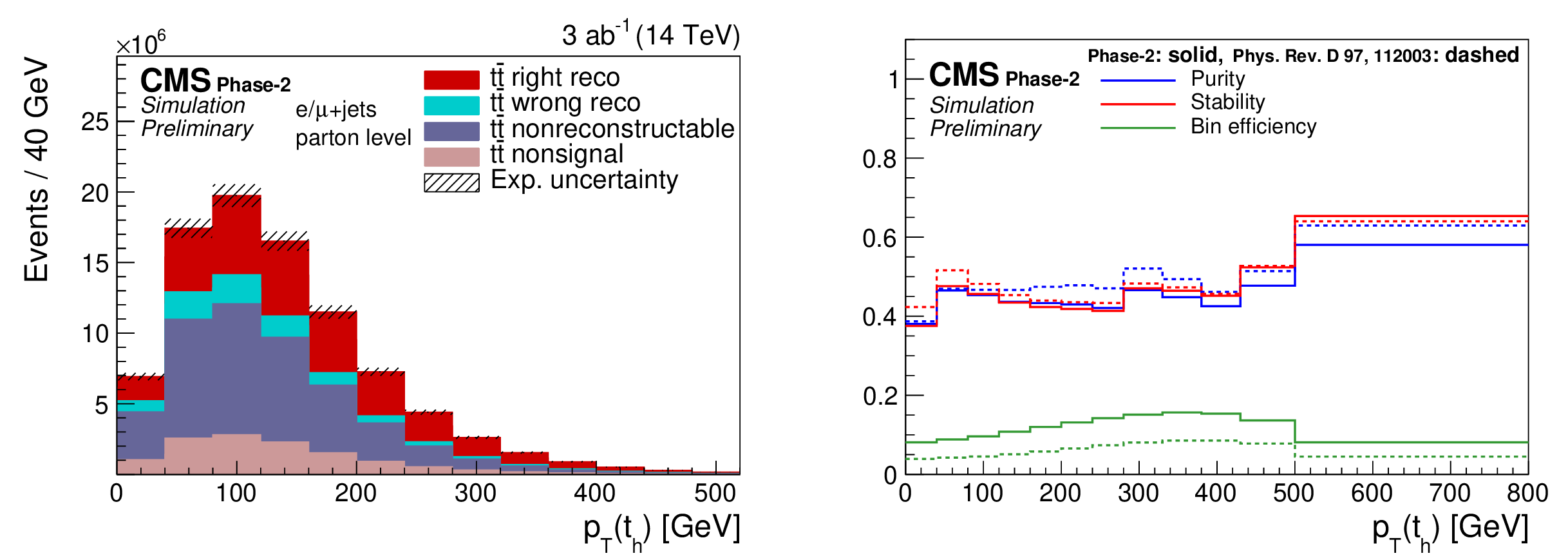
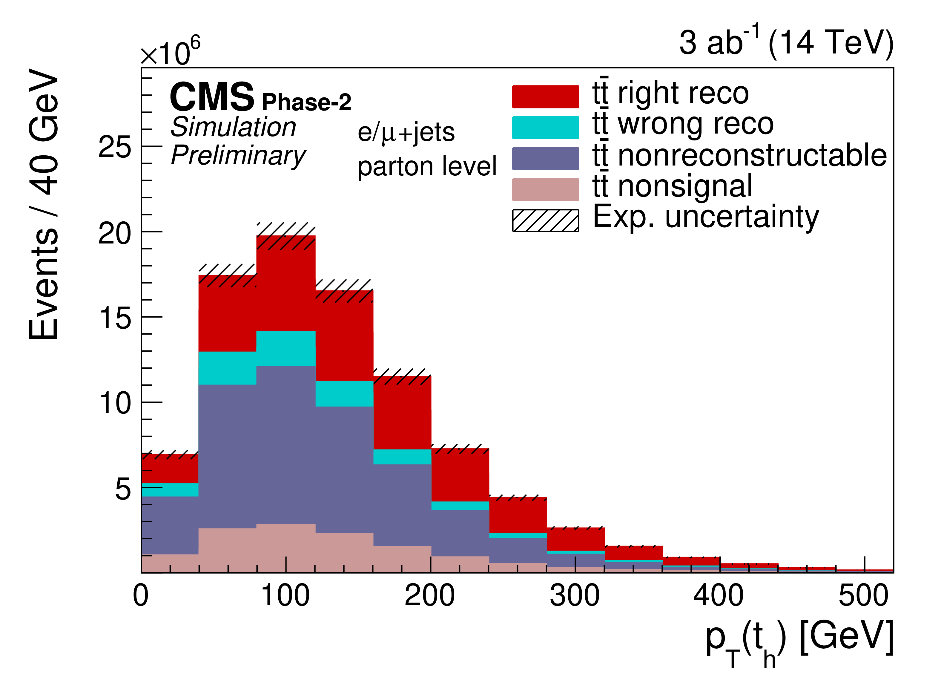
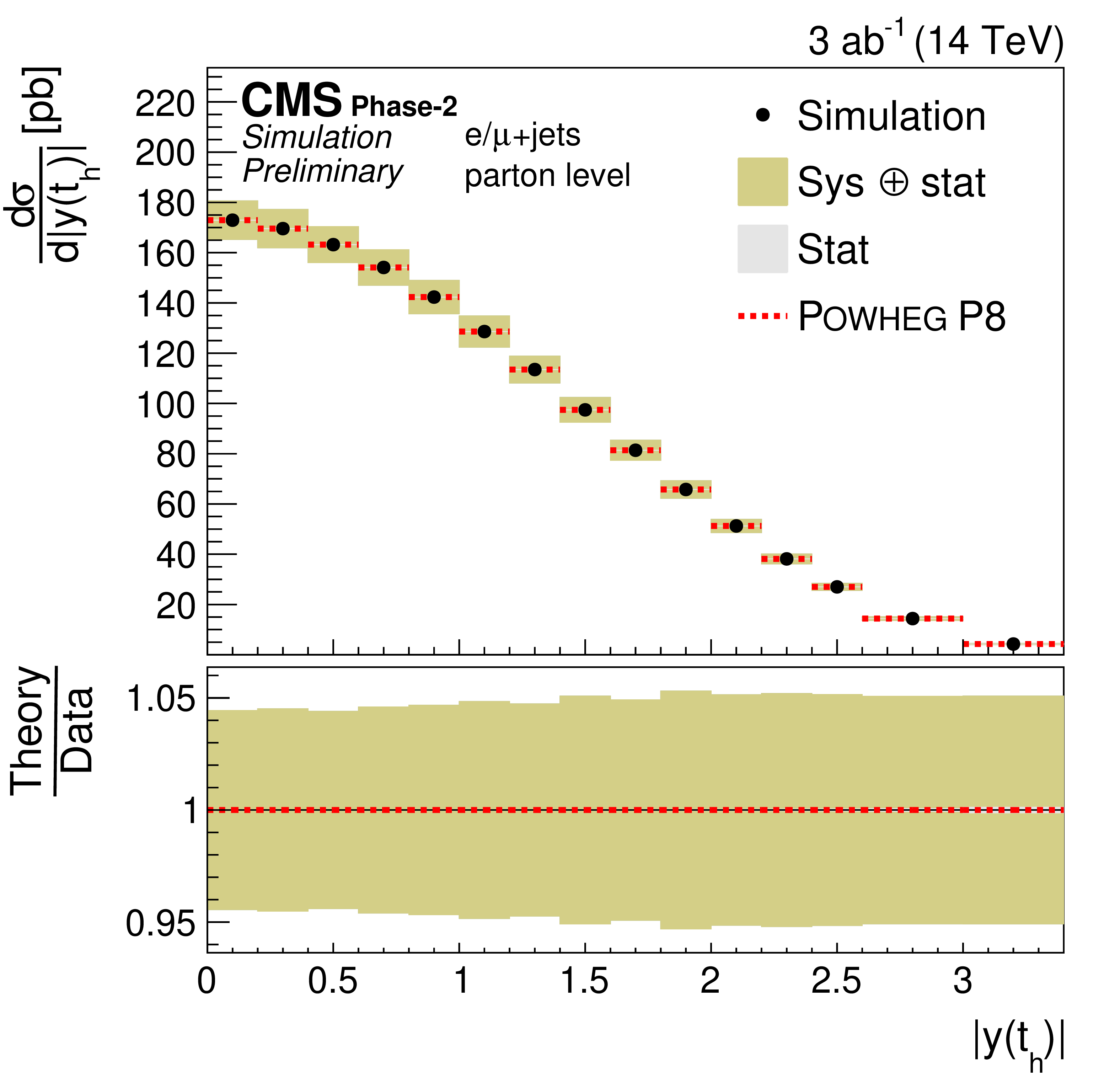
Figure 2:
Expected signal yields (left) and properties of the migration matrix (right) for the measurement of $ {p_{\mathrm {T}}} ({{\mathrm {t}} _\mathrm {h}})$. For comparison the properties are also shown for the 2016 analysis [2]. |
png pdf |
Figure 2-a:
Expected signal yields (left) and properties of the migration matrix (right) for the measurement of $ {p_{\mathrm {T}}} ({{\mathrm {t}} _\mathrm {h}})$. For comparison the properties are also shown for the 2016 analysis [2]. |

png pdf |
Figure 2-b:
Expected signal yields (left) and properties of the migration matrix (right) for the measurement of $ {p_{\mathrm {T}}} ({{\mathrm {t}} _\mathrm {h}})$. For comparison the properties are also shown for the 2016 analysis [2]. |
png pdf |
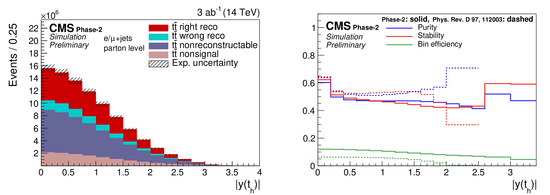
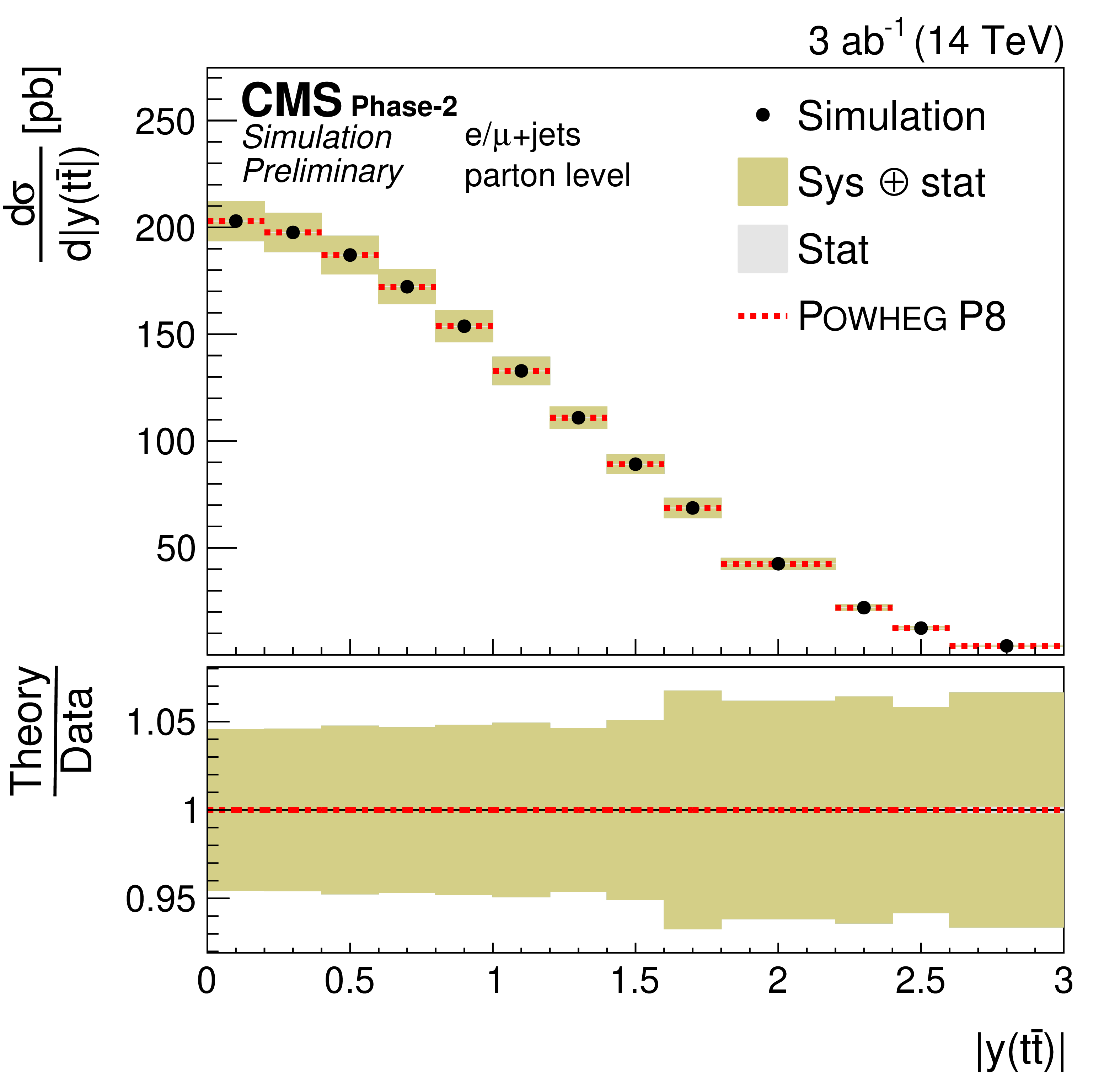
Figure 3:
Expected signal yields (left) and properties of the migration matrix (right) for the measurement of $ {| y({{\mathrm {t}} _\mathrm {h}}) |}$. For comparison the properties are also shown for the 2016 analysis [2]. |

png pdf |
Figure 3-a:
Expected signal yields (left) and properties of the migration matrix (right) for the measurement of $ {| y({{\mathrm {t}} _\mathrm {h}}) |}$. For comparison the properties are also shown for the 2016 analysis [2]. |

png pdf |
Figure 3-b:
Expected signal yields (left) and properties of the migration matrix (right) for the measurement of $ {| y({{\mathrm {t}} _\mathrm {h}}) |}$. For comparison the properties are also shown for the 2016 analysis [2]. |
png pdf |
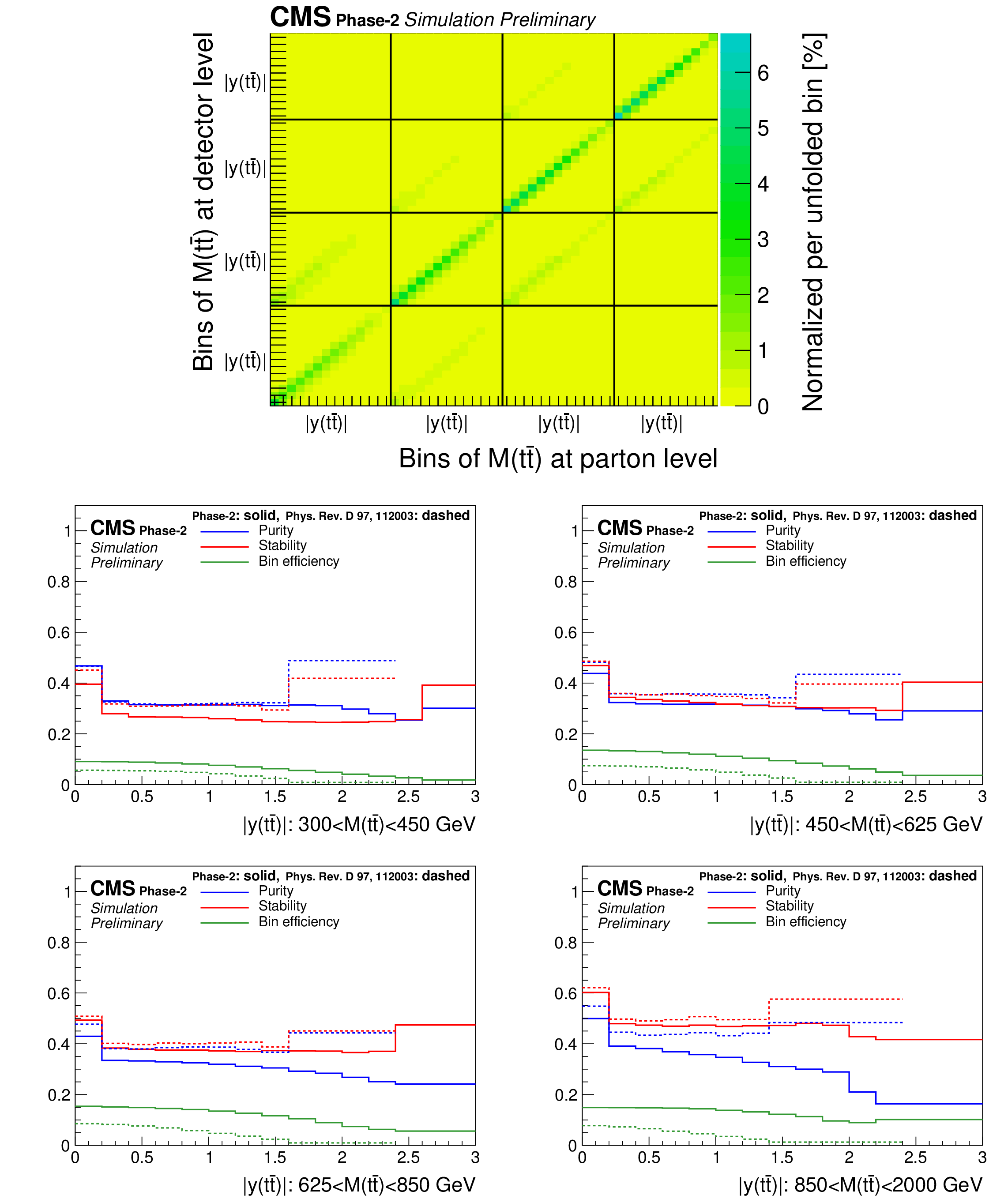
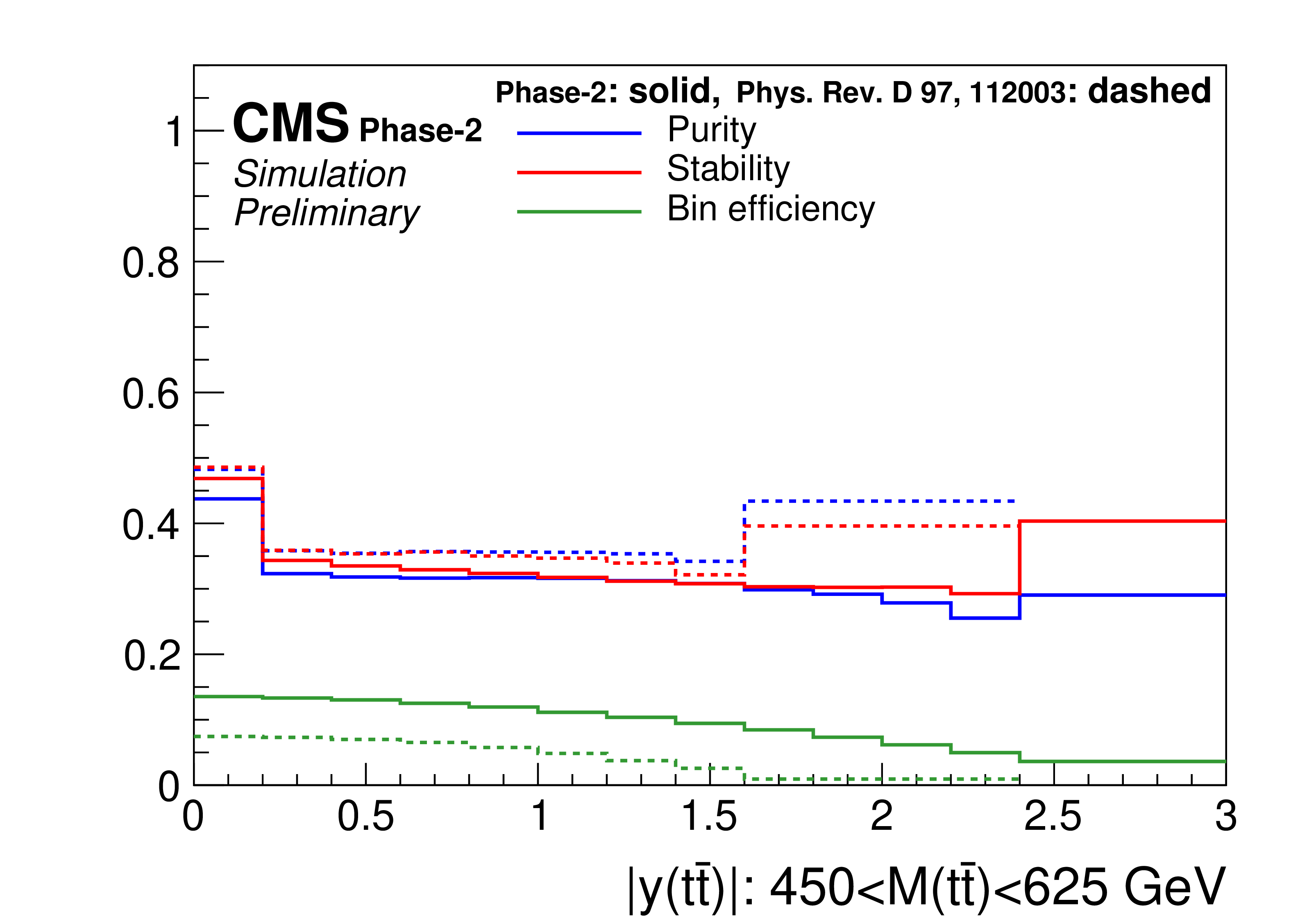
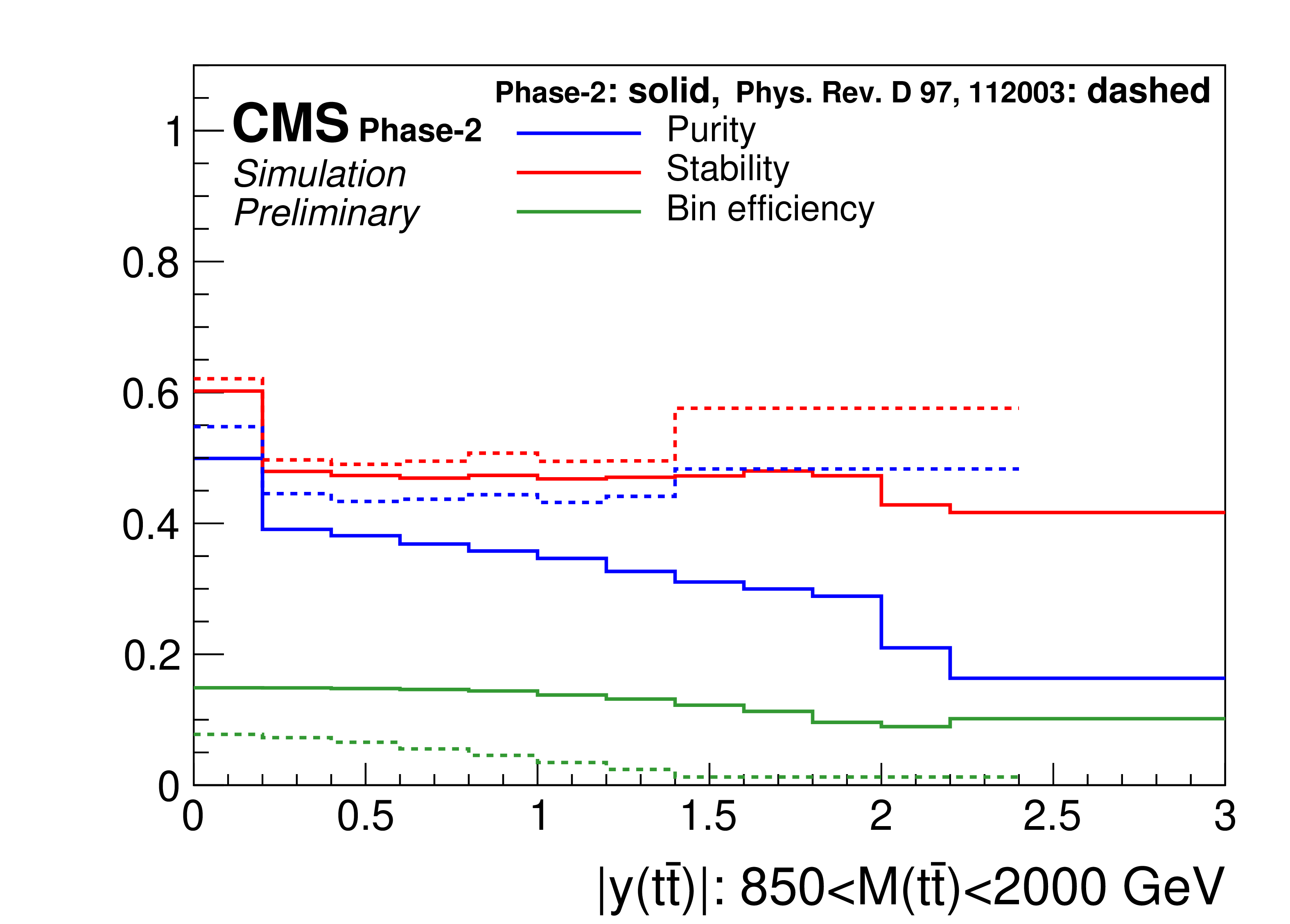
Figure 4:
Migration matrix (upper) and its properties (middle, lower) for the double-differential measurements as a function of $M({{\mathrm {t}\overline {\mathrm {t}}}})$ vs. $ {| y({{\mathrm {t}\overline {\mathrm {t}}}}) |}$. There are four $ {| y({{\mathrm {t}\overline {\mathrm {t}}}}) |}$ distributions for different regions of $M({{\mathrm {t}\overline {\mathrm {t}}}})$. The large off-diagonal structures in the migration matrix correspond to migrations among $M({{\mathrm {t}\overline {\mathrm {t}}}})$ regions. For comparison the properties are also shown for the 2016 analysis [2]. |

png pdf |
Figure 4-a:
Migration matrix (upper) and its properties (middle, lower) for the double-differential measurements as a function of $M({{\mathrm {t}\overline {\mathrm {t}}}})$ vs. $ {| y({{\mathrm {t}\overline {\mathrm {t}}}}) |}$. There are four $ {| y({{\mathrm {t}\overline {\mathrm {t}}}}) |}$ distributions for different regions of $M({{\mathrm {t}\overline {\mathrm {t}}}})$. The large off-diagonal structures in the migration matrix correspond to migrations among $M({{\mathrm {t}\overline {\mathrm {t}}}})$ regions. For comparison the properties are also shown for the 2016 analysis [2]. |

png pdf |
Figure 4-b:
Migration matrix (upper) and its properties (middle, lower) for the double-differential measurements as a function of $M({{\mathrm {t}\overline {\mathrm {t}}}})$ vs. $ {| y({{\mathrm {t}\overline {\mathrm {t}}}}) |}$. There are four $ {| y({{\mathrm {t}\overline {\mathrm {t}}}}) |}$ distributions for different regions of $M({{\mathrm {t}\overline {\mathrm {t}}}})$. The large off-diagonal structures in the migration matrix correspond to migrations among $M({{\mathrm {t}\overline {\mathrm {t}}}})$ regions. For comparison the properties are also shown for the 2016 analysis [2]. |
png pdf |
Figure 4-c:
Migration matrix (upper) and its properties (middle, lower) for the double-differential measurements as a function of $M({{\mathrm {t}\overline {\mathrm {t}}}})$ vs. $ {| y({{\mathrm {t}\overline {\mathrm {t}}}}) |}$. There are four $ {| y({{\mathrm {t}\overline {\mathrm {t}}}}) |}$ distributions for different regions of $M({{\mathrm {t}\overline {\mathrm {t}}}})$. The large off-diagonal structures in the migration matrix correspond to migrations among $M({{\mathrm {t}\overline {\mathrm {t}}}})$ regions. For comparison the properties are also shown for the 2016 analysis [2]. |

png pdf |
Figure 4-d:
Migration matrix (upper) and its properties (middle, lower) for the double-differential measurements as a function of $M({{\mathrm {t}\overline {\mathrm {t}}}})$ vs. $ {| y({{\mathrm {t}\overline {\mathrm {t}}}}) |}$. There are four $ {| y({{\mathrm {t}\overline {\mathrm {t}}}}) |}$ distributions for different regions of $M({{\mathrm {t}\overline {\mathrm {t}}}})$. The large off-diagonal structures in the migration matrix correspond to migrations among $M({{\mathrm {t}\overline {\mathrm {t}}}})$ regions. For comparison the properties are also shown for the 2016 analysis [2]. |
png pdf |
Figure 4-e:
Migration matrix (upper) and its properties (middle, lower) for the double-differential measurements as a function of $M({{\mathrm {t}\overline {\mathrm {t}}}})$ vs. $ {| y({{\mathrm {t}\overline {\mathrm {t}}}}) |}$. There are four $ {| y({{\mathrm {t}\overline {\mathrm {t}}}}) |}$ distributions for different regions of $M({{\mathrm {t}\overline {\mathrm {t}}}})$. The large off-diagonal structures in the migration matrix correspond to migrations among $M({{\mathrm {t}\overline {\mathrm {t}}}})$ regions. For comparison the properties are also shown for the 2016 analysis [2]. |

png pdf |
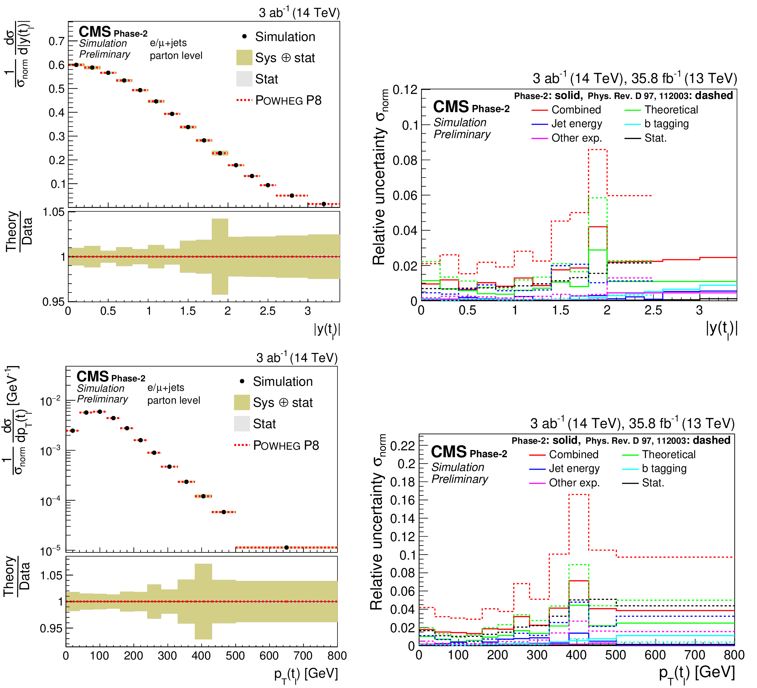
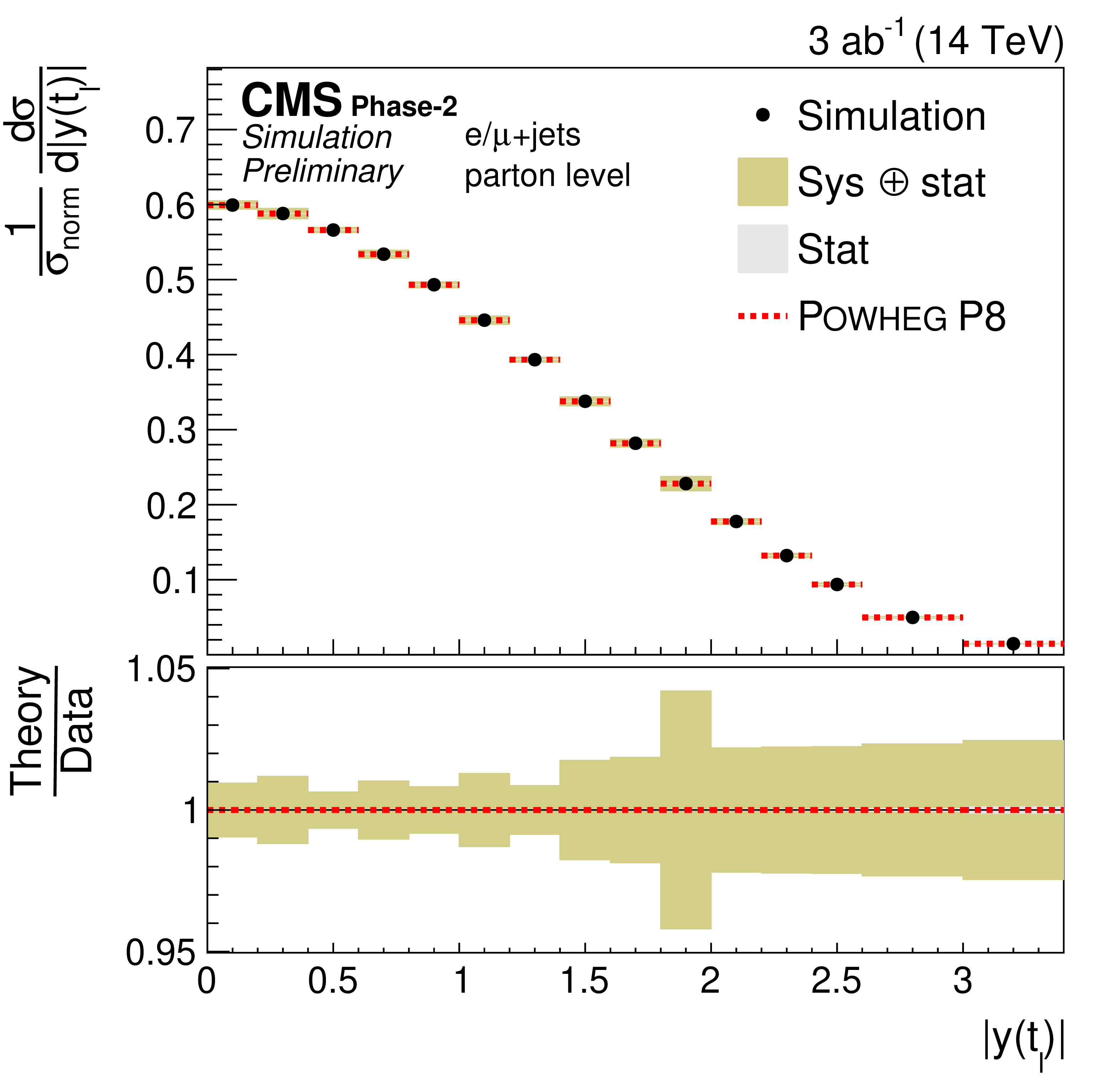
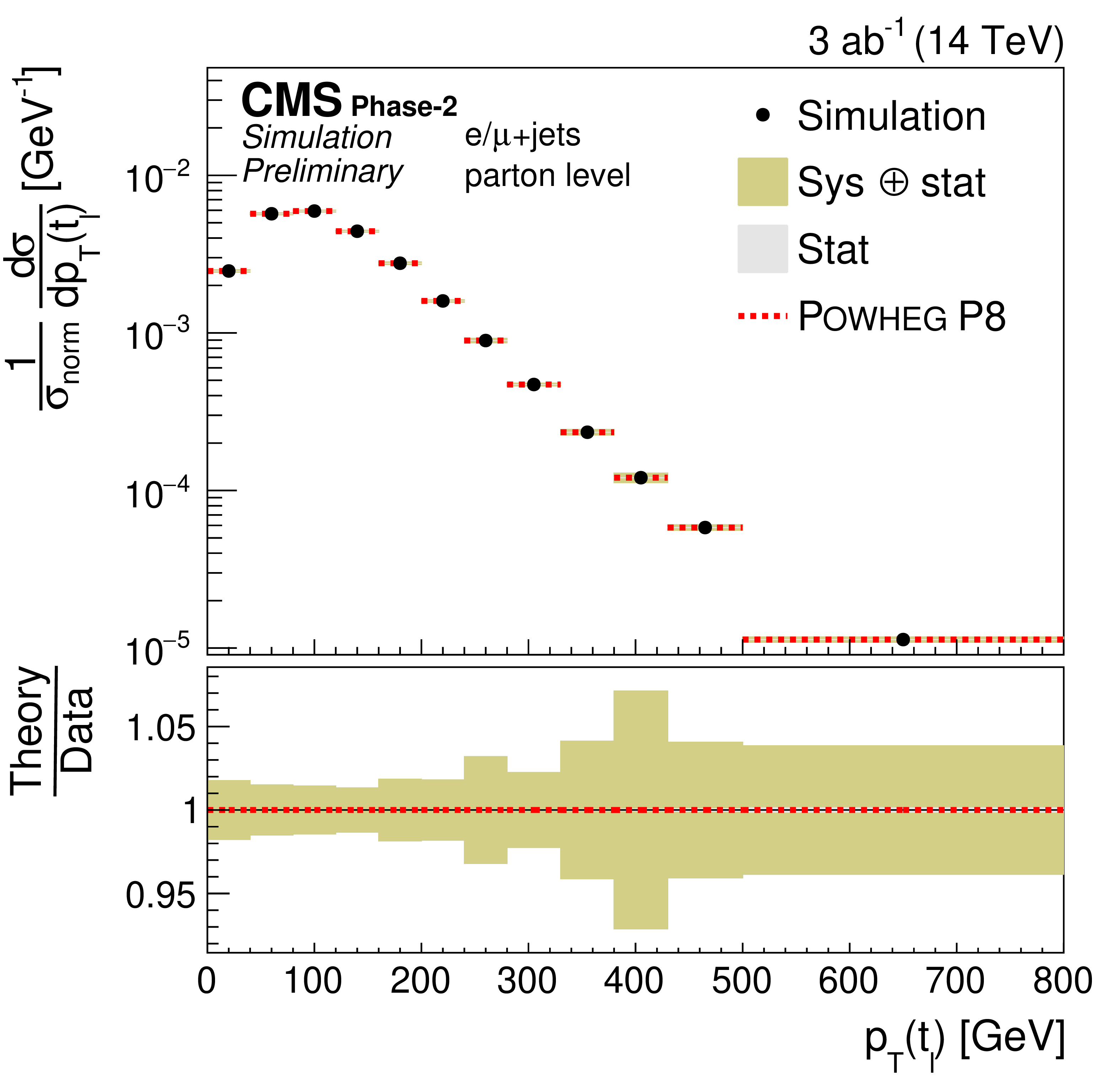
Figure 5:
Differential cross sections (left) as a function of $ {p_{\mathrm {T}}} ({{\mathrm {t}} _\mathrm {h}})$ (upper) and $ {| y({{\mathrm {t}} _\mathrm {h}}) |}$ (lower). The corresponding relative uncertainties (right) in the Phase-2 projections are compared to the uncertainties in the 2016 measurements [2]. |

png pdf |
Figure 5-a:
Differential cross sections (left) as a function of $ {p_{\mathrm {T}}} ({{\mathrm {t}} _\mathrm {h}})$ (upper) and $ {| y({{\mathrm {t}} _\mathrm {h}}) |}$ (lower). The corresponding relative uncertainties (right) in the Phase-2 projections are compared to the uncertainties in the 2016 measurements [2]. |

png pdf |
Figure 5-b:
Differential cross sections (left) as a function of $ {p_{\mathrm {T}}} ({{\mathrm {t}} _\mathrm {h}})$ (upper) and $ {| y({{\mathrm {t}} _\mathrm {h}}) |}$ (lower). The corresponding relative uncertainties (right) in the Phase-2 projections are compared to the uncertainties in the 2016 measurements [2]. |
png pdf |
Figure 5-c:
Differential cross sections (left) as a function of $ {p_{\mathrm {T}}} ({{\mathrm {t}} _\mathrm {h}})$ (upper) and $ {| y({{\mathrm {t}} _\mathrm {h}}) |}$ (lower). The corresponding relative uncertainties (right) in the Phase-2 projections are compared to the uncertainties in the 2016 measurements [2]. |
png pdf |
Figure 5-d:
Differential cross sections (left) as a function of $ {p_{\mathrm {T}}} ({{\mathrm {t}} _\mathrm {h}})$ (upper) and $ {| y({{\mathrm {t}} _\mathrm {h}}) |}$ (lower). The corresponding relative uncertainties (right) in the Phase-2 projections are compared to the uncertainties in the 2016 measurements [2]. |

png pdf |
Figure 6:
Differential cross sections (left) as a function of $ {p_{\mathrm {T}}} ({{\mathrm {t}} _\ell})$ (upper) and $ {| y({{\mathrm {t}} _\ell}) |}$ (lower). The corresponding relative uncertainties (right) in the Phase-2 projections are compared to the uncertainties in the 2016 measurements [2]. |
png pdf |
Figure 6-a:
Differential cross sections (left) as a function of $ {p_{\mathrm {T}}} ({{\mathrm {t}} _\ell})$ (upper) and $ {| y({{\mathrm {t}} _\ell}) |}$ (lower). The corresponding relative uncertainties (right) in the Phase-2 projections are compared to the uncertainties in the 2016 measurements [2]. |

png pdf |
Figure 6-b:
Differential cross sections (left) as a function of $ {p_{\mathrm {T}}} ({{\mathrm {t}} _\ell})$ (upper) and $ {| y({{\mathrm {t}} _\ell}) |}$ (lower). The corresponding relative uncertainties (right) in the Phase-2 projections are compared to the uncertainties in the 2016 measurements [2]. |

png pdf |
Figure 6-c:
Differential cross sections (left) as a function of $ {p_{\mathrm {T}}} ({{\mathrm {t}} _\ell})$ (upper) and $ {| y({{\mathrm {t}} _\ell}) |}$ (lower). The corresponding relative uncertainties (right) in the Phase-2 projections are compared to the uncertainties in the 2016 measurements [2]. |
png pdf |
Figure 6-d:
Differential cross sections (left) as a function of $ {p_{\mathrm {T}}} ({{\mathrm {t}} _\ell})$ (upper) and $ {| y({{\mathrm {t}} _\ell}) |}$ (lower). The corresponding relative uncertainties (right) in the Phase-2 projections are compared to the uncertainties in the 2016 measurements [2]. |
png pdf |
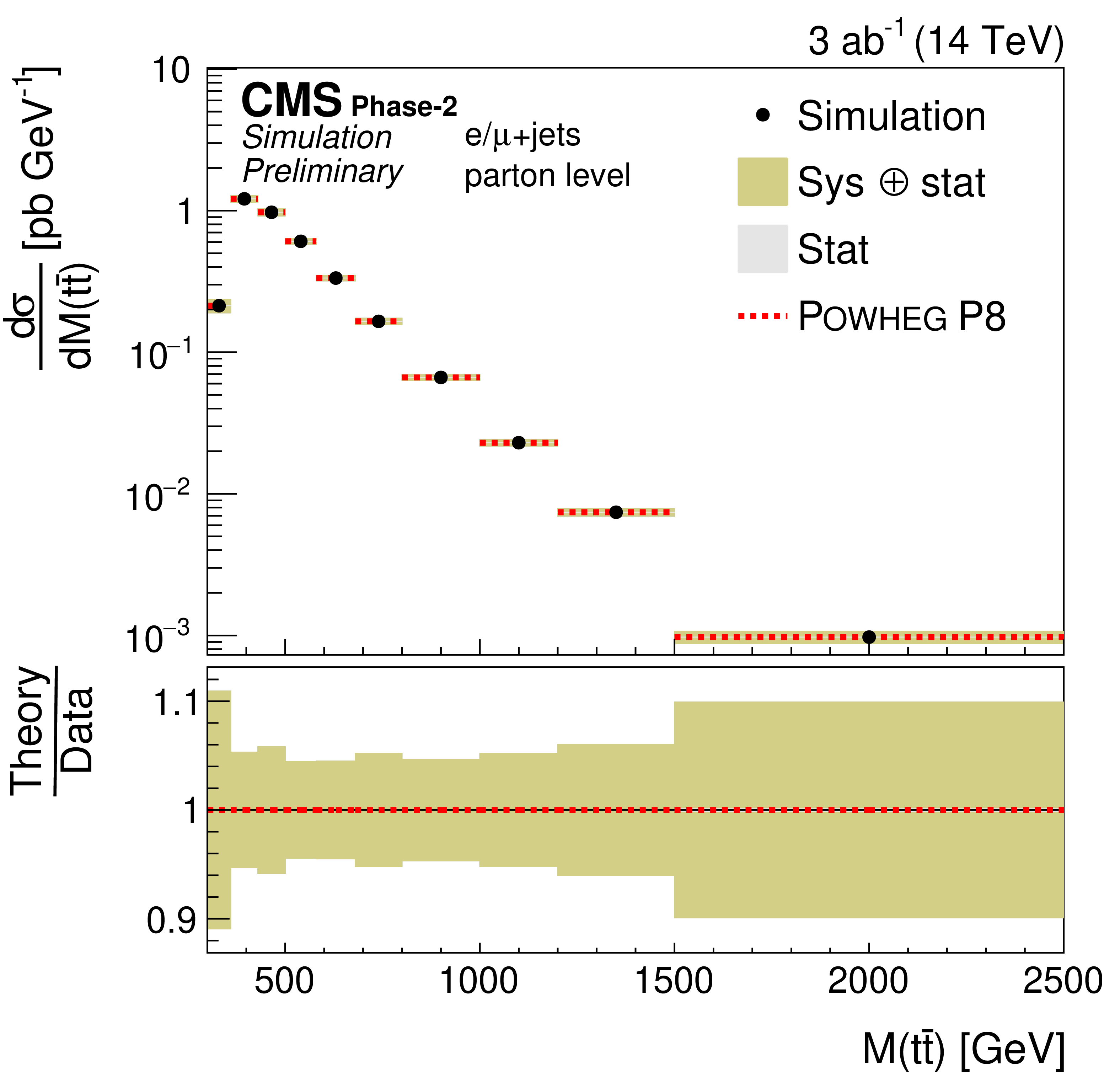
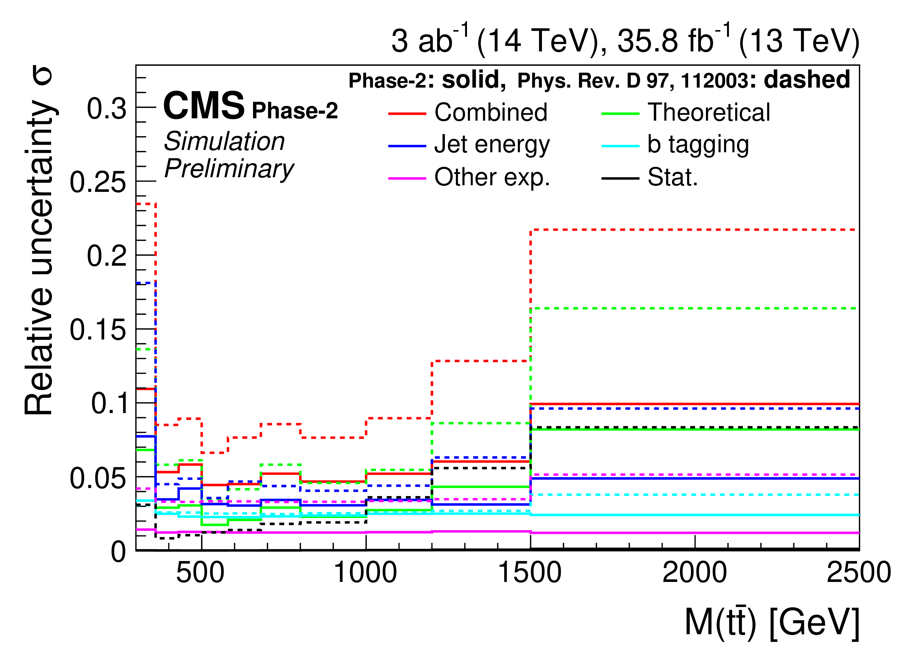
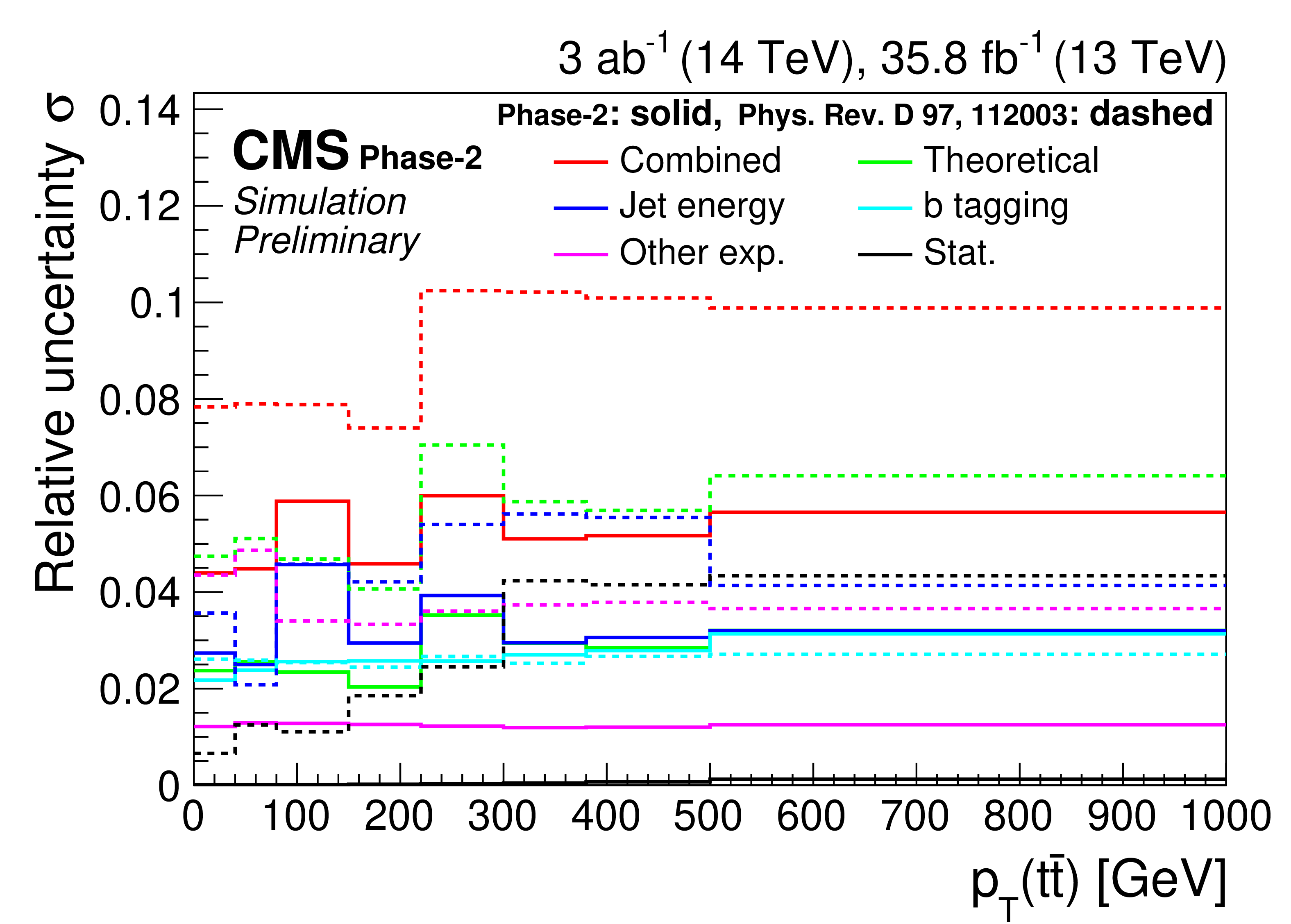
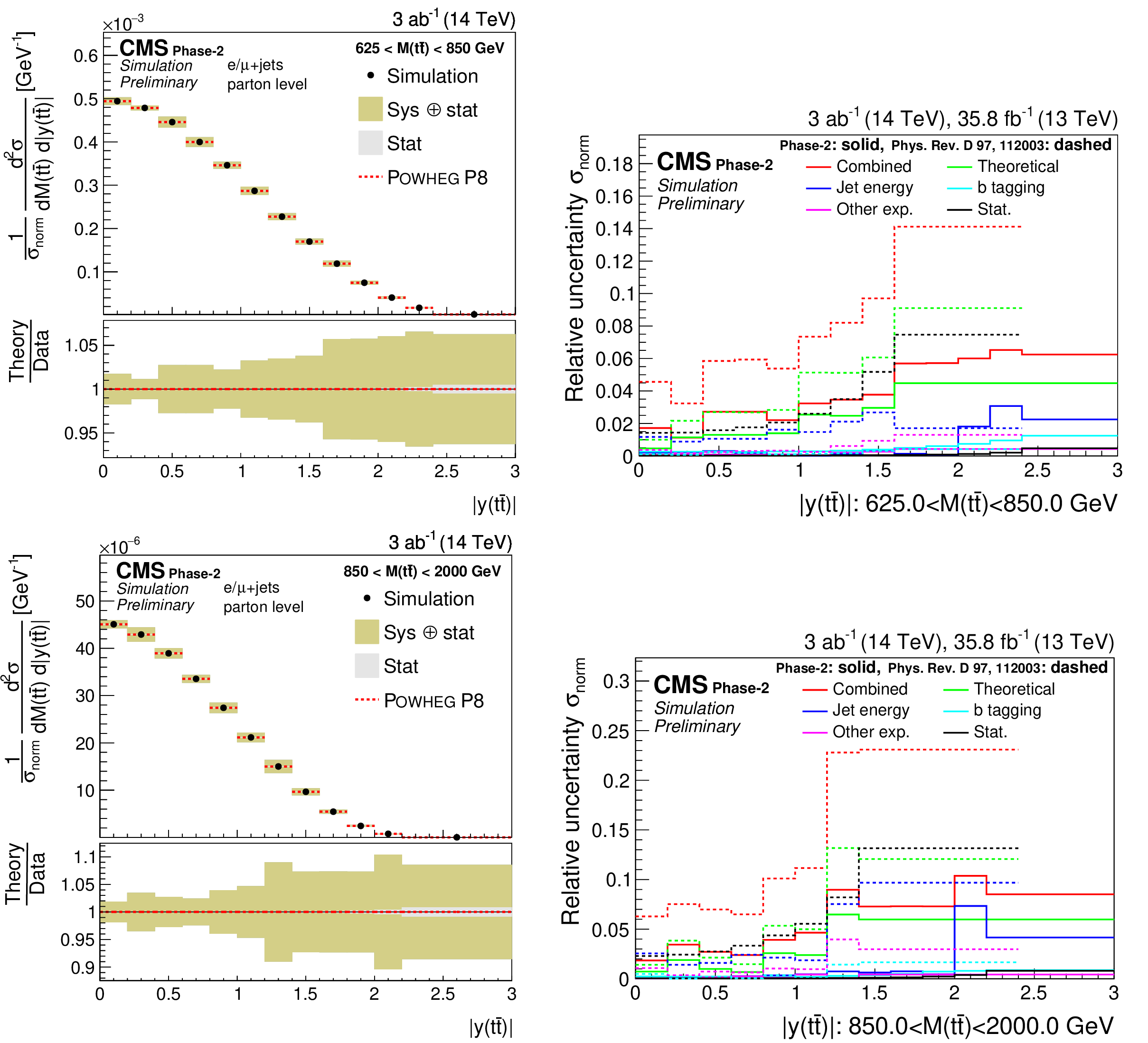
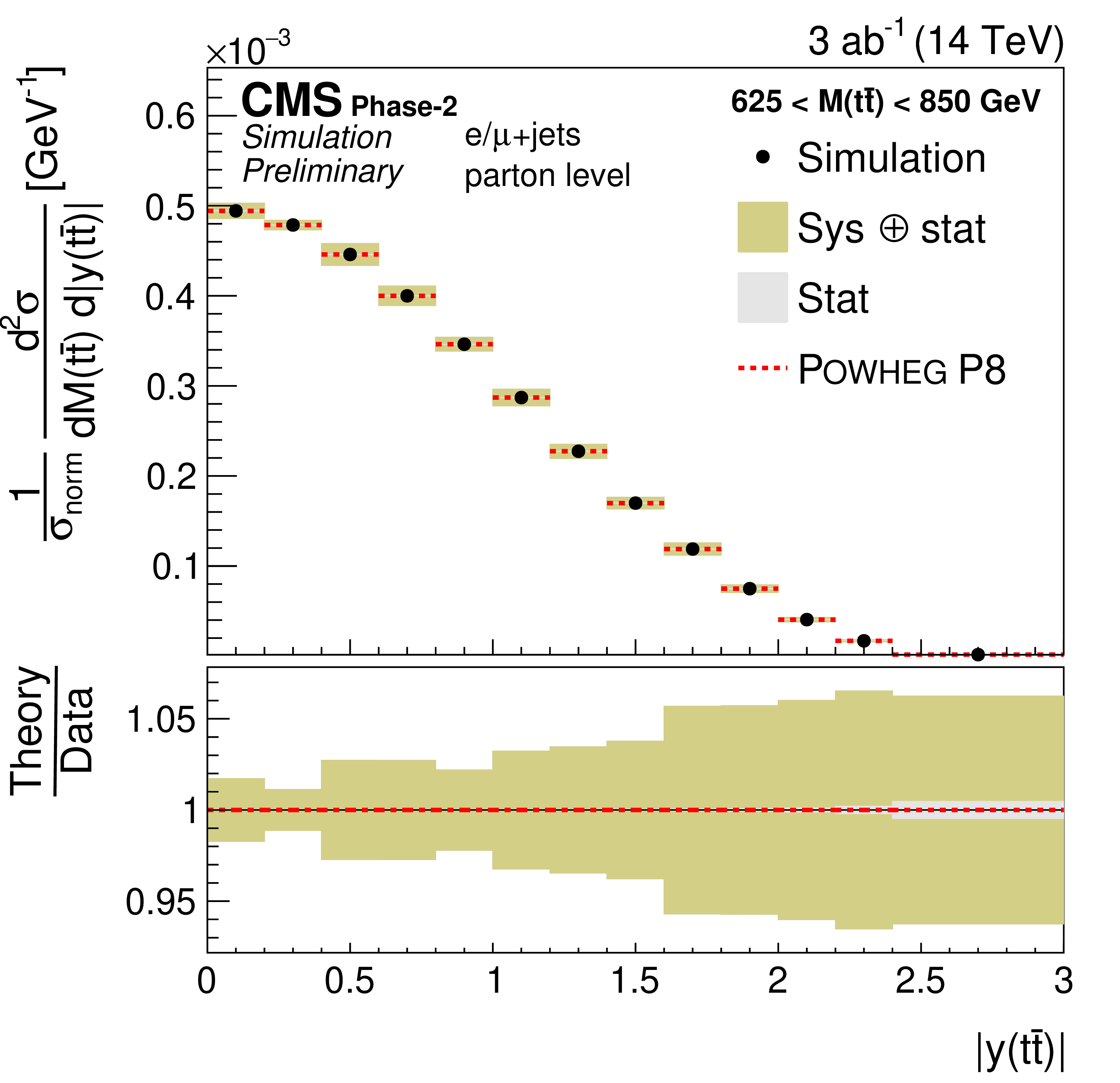
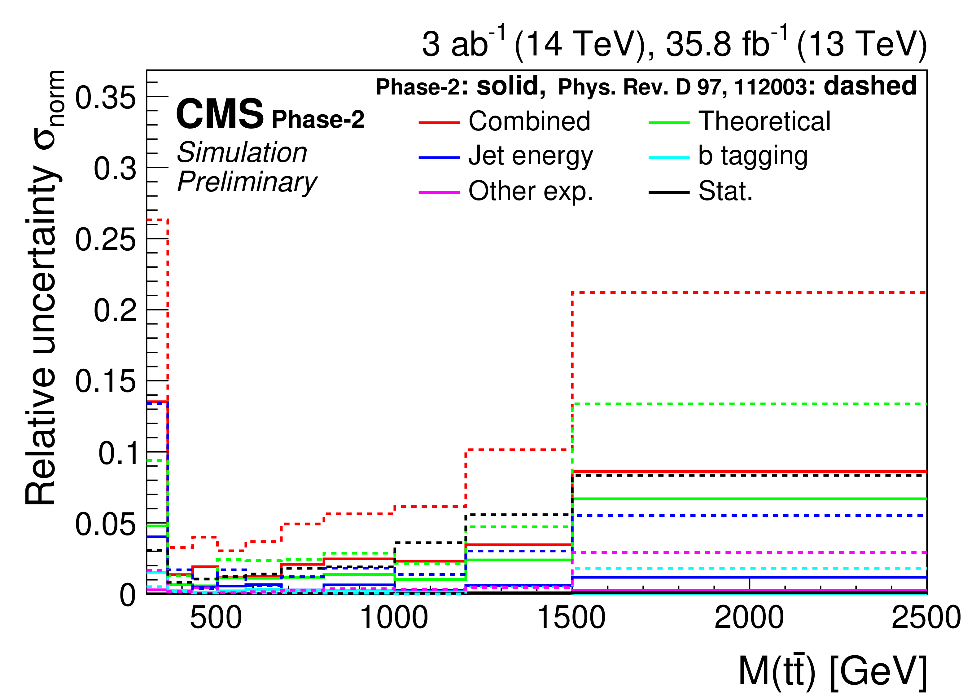
Figure 7:
Differential cross sections (left) as a function of $M({{\mathrm {t}\overline {\mathrm {t}}}})$ (upper), $ {p_{\mathrm {T}}} ({{\mathrm {t}\overline {\mathrm {t}}}})$ (middle), and $ {| y({{\mathrm {t}\overline {\mathrm {t}}}}) |}$ (lower). The corresponding relative uncertainties (right) in the Phase-2 projections are compared to the uncertainties in the 2016 measurements [2]. |
png pdf |
Figure 7-a:
Differential cross sections (left) as a function of $M({{\mathrm {t}\overline {\mathrm {t}}}})$ (upper), $ {p_{\mathrm {T}}} ({{\mathrm {t}\overline {\mathrm {t}}}})$ (middle), and $ {| y({{\mathrm {t}\overline {\mathrm {t}}}}) |}$ (lower). The corresponding relative uncertainties (right) in the Phase-2 projections are compared to the uncertainties in the 2016 measurements [2]. |
png pdf |
Figure 7-b:
Differential cross sections (left) as a function of $M({{\mathrm {t}\overline {\mathrm {t}}}})$ (upper), $ {p_{\mathrm {T}}} ({{\mathrm {t}\overline {\mathrm {t}}}})$ (middle), and $ {| y({{\mathrm {t}\overline {\mathrm {t}}}}) |}$ (lower). The corresponding relative uncertainties (right) in the Phase-2 projections are compared to the uncertainties in the 2016 measurements [2]. |

png pdf |
Figure 7-c:
Differential cross sections (left) as a function of $M({{\mathrm {t}\overline {\mathrm {t}}}})$ (upper), $ {p_{\mathrm {T}}} ({{\mathrm {t}\overline {\mathrm {t}}}})$ (middle), and $ {| y({{\mathrm {t}\overline {\mathrm {t}}}}) |}$ (lower). The corresponding relative uncertainties (right) in the Phase-2 projections are compared to the uncertainties in the 2016 measurements [2]. |
png pdf |
Figure 7-d:
Differential cross sections (left) as a function of $M({{\mathrm {t}\overline {\mathrm {t}}}})$ (upper), $ {p_{\mathrm {T}}} ({{\mathrm {t}\overline {\mathrm {t}}}})$ (middle), and $ {| y({{\mathrm {t}\overline {\mathrm {t}}}}) |}$ (lower). The corresponding relative uncertainties (right) in the Phase-2 projections are compared to the uncertainties in the 2016 measurements [2]. |
png pdf |
Figure 7-e:
Differential cross sections (left) as a function of $M({{\mathrm {t}\overline {\mathrm {t}}}})$ (upper), $ {p_{\mathrm {T}}} ({{\mathrm {t}\overline {\mathrm {t}}}})$ (middle), and $ {| y({{\mathrm {t}\overline {\mathrm {t}}}}) |}$ (lower). The corresponding relative uncertainties (right) in the Phase-2 projections are compared to the uncertainties in the 2016 measurements [2]. |

png pdf |
Figure 7-f:
Differential cross sections (left) as a function of $M({{\mathrm {t}\overline {\mathrm {t}}}})$ (upper), $ {p_{\mathrm {T}}} ({{\mathrm {t}\overline {\mathrm {t}}}})$ (middle), and $ {| y({{\mathrm {t}\overline {\mathrm {t}}}}) |}$ (lower). The corresponding relative uncertainties (right) in the Phase-2 projections are compared to the uncertainties in the 2016 measurements [2]. |

png pdf |
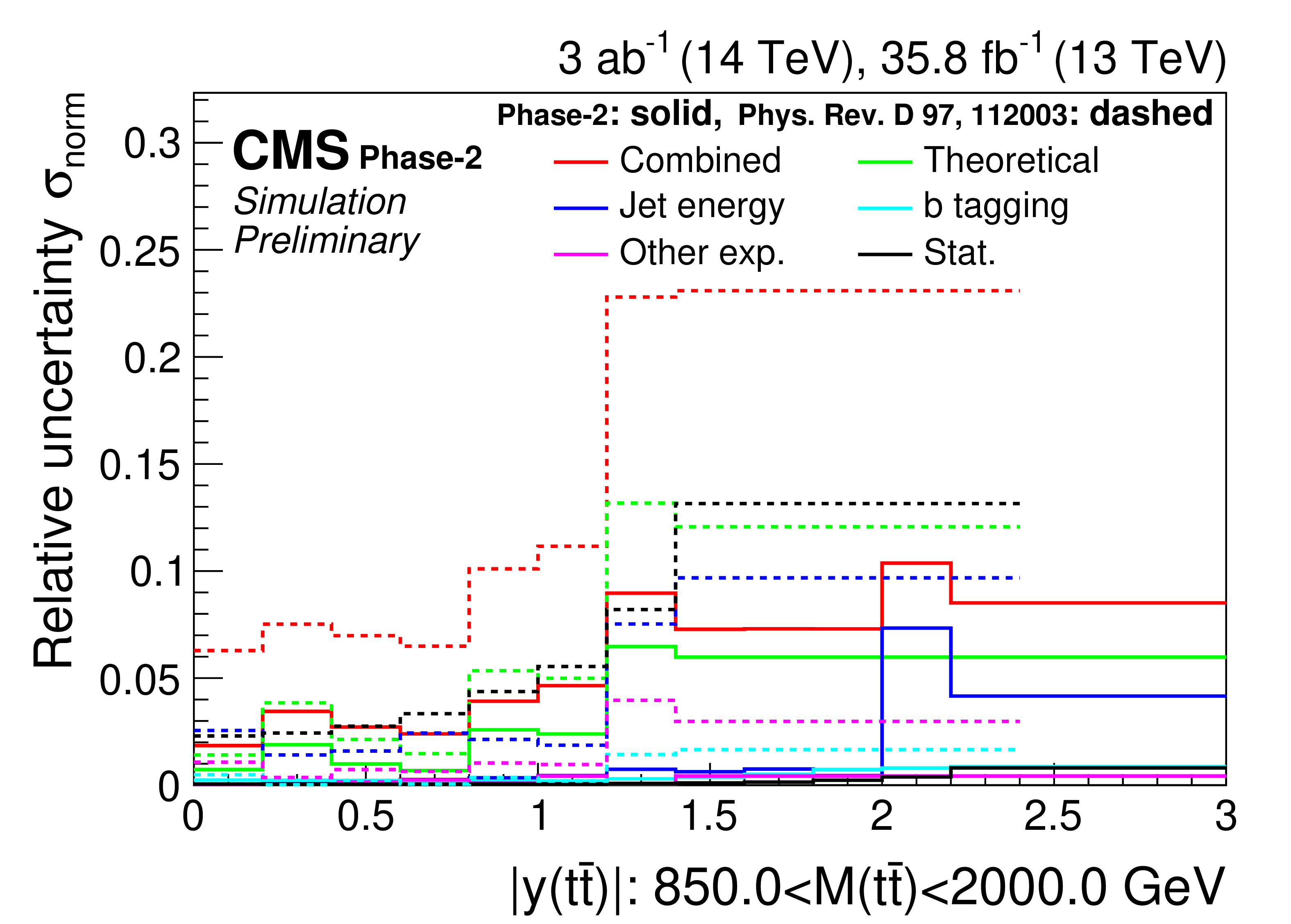
Figure 8:
Projections of the normalized double-differential cross section as a function of $M({{\mathrm {t}\overline {\mathrm {t}}}})$ vs. $ {| y({{\mathrm {t}\overline {\mathrm {t}}}}) |}$ (left). The corresponding relative uncertainties (right) in the Phase-2 projections are compared to the uncertainties in the 2016 measurements [2]. |
png pdf |
Figure 8-a:
Projections of the normalized double-differential cross section as a function of $M({{\mathrm {t}\overline {\mathrm {t}}}})$ vs. $ {| y({{\mathrm {t}\overline {\mathrm {t}}}}) |}$ (left). The corresponding relative uncertainties (right) in the Phase-2 projections are compared to the uncertainties in the 2016 measurements [2]. |
png pdf |
Figure 8-b:
Projections of the normalized double-differential cross section as a function of $M({{\mathrm {t}\overline {\mathrm {t}}}})$ vs. $ {| y({{\mathrm {t}\overline {\mathrm {t}}}}) |}$ (left). The corresponding relative uncertainties (right) in the Phase-2 projections are compared to the uncertainties in the 2016 measurements [2]. |
png pdf |
Figure 8-c:
Projections of the normalized double-differential cross section as a function of $M({{\mathrm {t}\overline {\mathrm {t}}}})$ vs. $ {| y({{\mathrm {t}\overline {\mathrm {t}}}}) |}$ (left). The corresponding relative uncertainties (right) in the Phase-2 projections are compared to the uncertainties in the 2016 measurements [2]. |
png pdf |
Figure 8-d:
Projections of the normalized double-differential cross section as a function of $M({{\mathrm {t}\overline {\mathrm {t}}}})$ vs. $ {| y({{\mathrm {t}\overline {\mathrm {t}}}}) |}$ (left). The corresponding relative uncertainties (right) in the Phase-2 projections are compared to the uncertainties in the 2016 measurements [2]. |
png pdf |
Figure 9:
Projections of the normalized double-differential cross section as a function of $M({{\mathrm {t}\overline {\mathrm {t}}}})$ vs. $ {| y({{\mathrm {t}\overline {\mathrm {t}}}}) |}$ (left). The corresponding relative uncertainties (right) in the Phase-2 projections are compared to the uncertainties in the 2016 measurements [2]. |
png pdf |
Figure 9-a:
Projections of the normalized double-differential cross section as a function of $M({{\mathrm {t}\overline {\mathrm {t}}}})$ vs. $ {| y({{\mathrm {t}\overline {\mathrm {t}}}}) |}$ (left). The corresponding relative uncertainties (right) in the Phase-2 projections are compared to the uncertainties in the 2016 measurements [2]. |

png pdf |
Figure 9-b:
Projections of the normalized double-differential cross section as a function of $M({{\mathrm {t}\overline {\mathrm {t}}}})$ vs. $ {| y({{\mathrm {t}\overline {\mathrm {t}}}}) |}$ (left). The corresponding relative uncertainties (right) in the Phase-2 projections are compared to the uncertainties in the 2016 measurements [2]. |

png pdf |
Figure 9-c:
Projections of the normalized double-differential cross section as a function of $M({{\mathrm {t}\overline {\mathrm {t}}}})$ vs. $ {| y({{\mathrm {t}\overline {\mathrm {t}}}}) |}$ (left). The corresponding relative uncertainties (right) in the Phase-2 projections are compared to the uncertainties in the 2016 measurements [2]. |
png pdf |
Figure 9-d:
Projections of the normalized double-differential cross section as a function of $M({{\mathrm {t}\overline {\mathrm {t}}}})$ vs. $ {| y({{\mathrm {t}\overline {\mathrm {t}}}}) |}$ (left). The corresponding relative uncertainties (right) in the Phase-2 projections are compared to the uncertainties in the 2016 measurements [2]. |
png pdf |
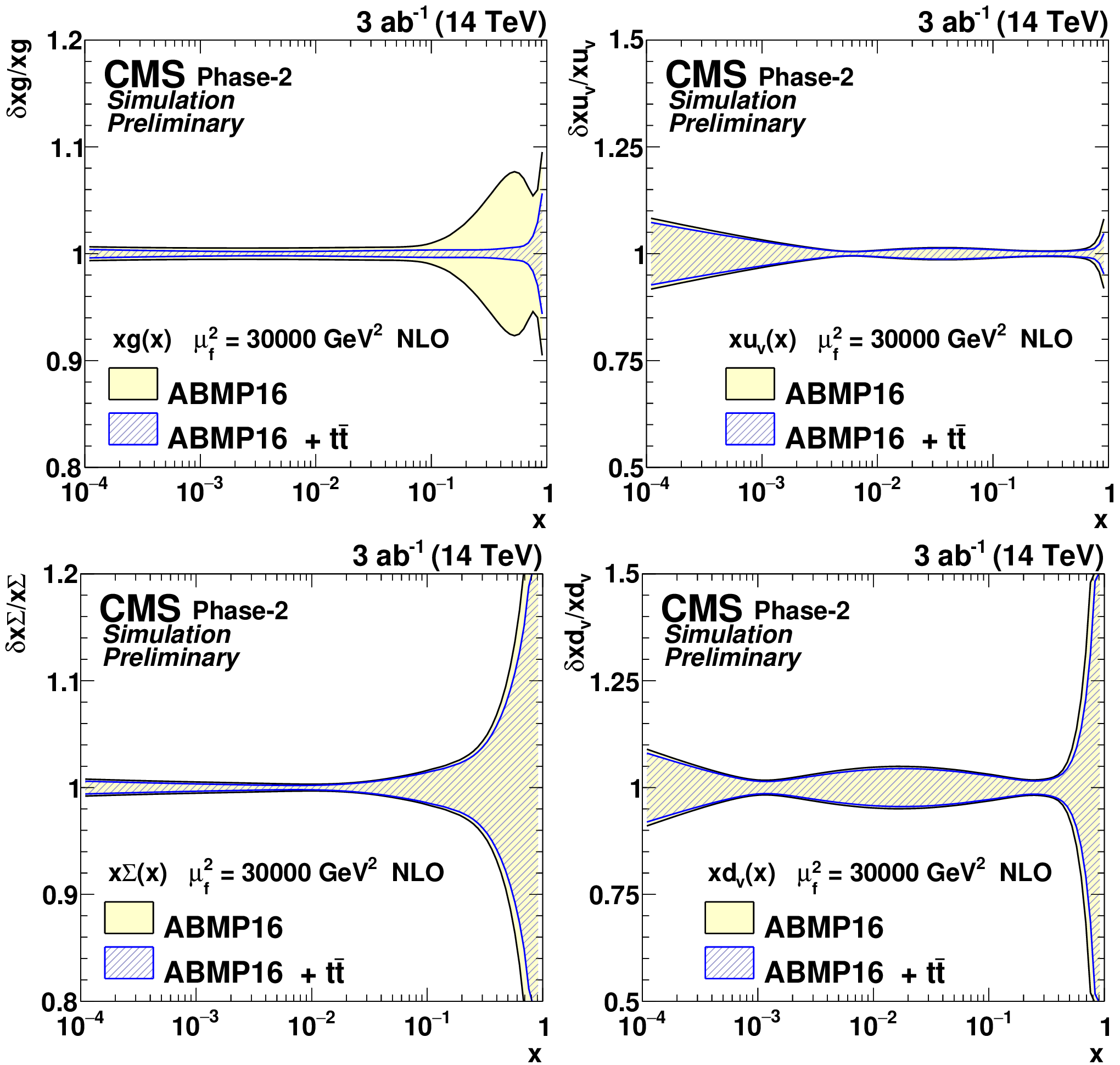
Figure 10:
The relative gluon (upper left), u valence quark (upper right), sea quark (lower left), and d valence quark (lower right) uncertainties of the original and profiled ABMP16 PDF set. |

png pdf |
Figure 10-a:
The relative gluon (upper left), u valence quark (upper right), sea quark (lower left), and d valence quark (lower right) uncertainties of the original and profiled ABMP16 PDF set. |

png pdf |
Figure 10-b:
The relative gluon (upper left), u valence quark (upper right), sea quark (lower left), and d valence quark (lower right) uncertainties of the original and profiled ABMP16 PDF set. |
png pdf |
Figure 10-c:
The relative gluon (upper left), u valence quark (upper right), sea quark (lower left), and d valence quark (lower right) uncertainties of the original and profiled ABMP16 PDF set. |

png pdf |
Figure 10-d:
The relative gluon (upper left), u valence quark (upper right), sea quark (lower left), and d valence quark (lower right) uncertainties of the original and profiled ABMP16 PDF set. |

png pdf |
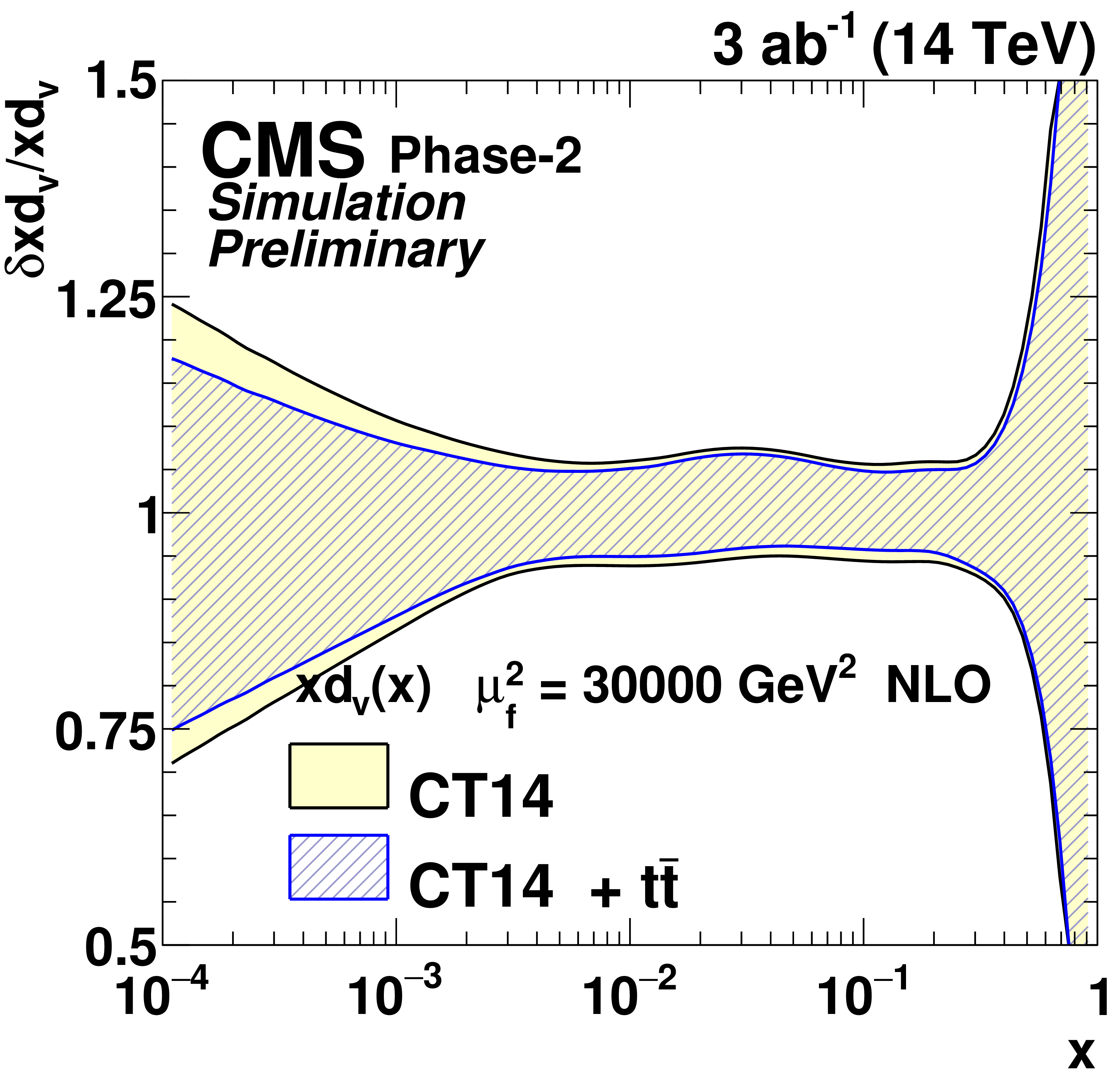
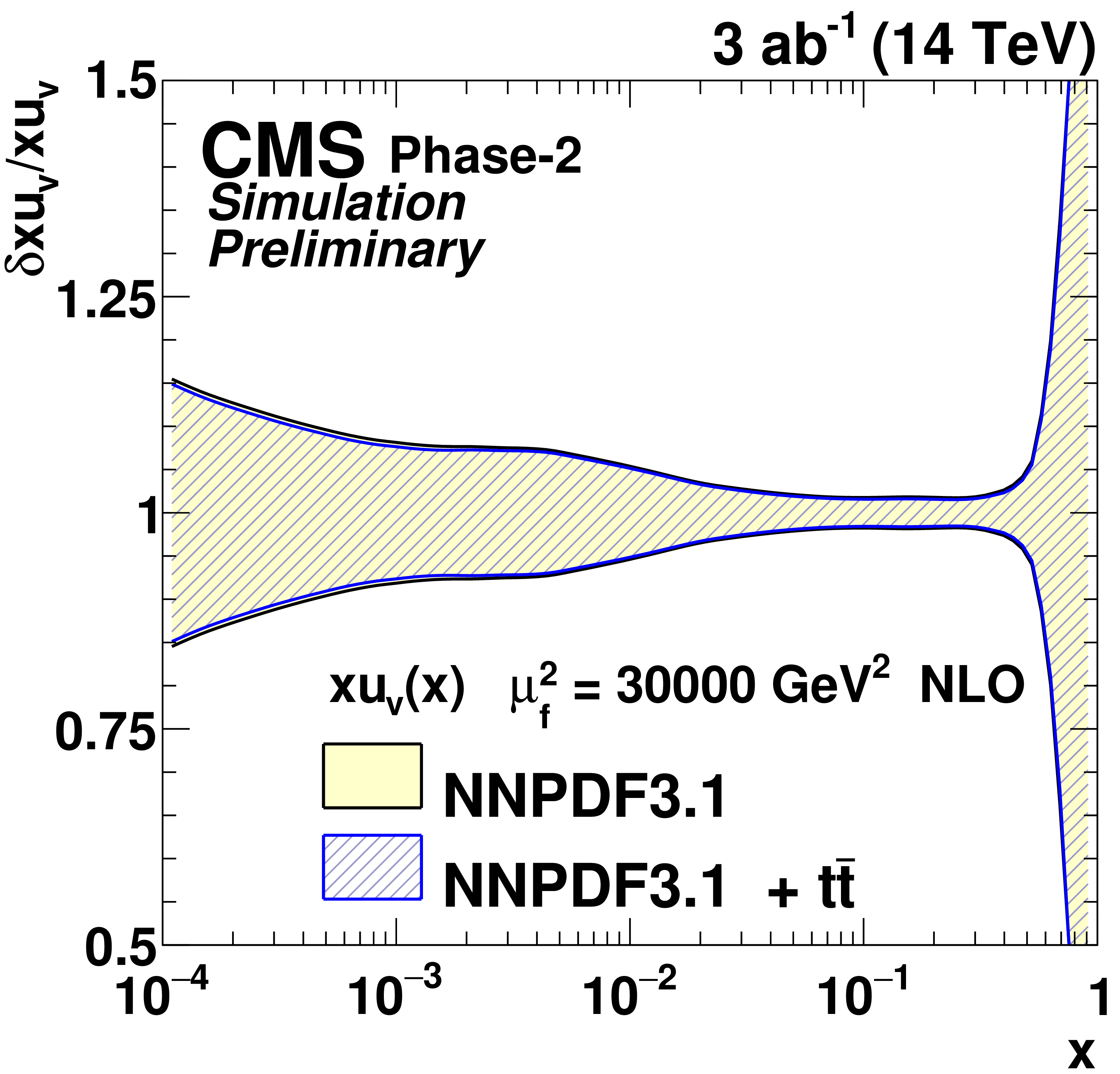
Figure 11:
The relative gluon (upper left), u valence quark (upper right), sea quark (lower left), and d valence quark (lower right) uncertainties of the original and profiled CT14 PDF set. |

png pdf |
Figure 11-a:
The relative gluon (upper left), u valence quark (upper right), sea quark (lower left), and d valence quark (lower right) uncertainties of the original and profiled CT14 PDF set. |

png pdf |
Figure 11-b:
The relative gluon (upper left), u valence quark (upper right), sea quark (lower left), and d valence quark (lower right) uncertainties of the original and profiled CT14 PDF set. |

png pdf |
Figure 11-c:
The relative gluon (upper left), u valence quark (upper right), sea quark (lower left), and d valence quark (lower right) uncertainties of the original and profiled CT14 PDF set. |
png pdf |
Figure 11-d:
The relative gluon (upper left), u valence quark (upper right), sea quark (lower left), and d valence quark (lower right) uncertainties of the original and profiled CT14 PDF set. |

png pdf |
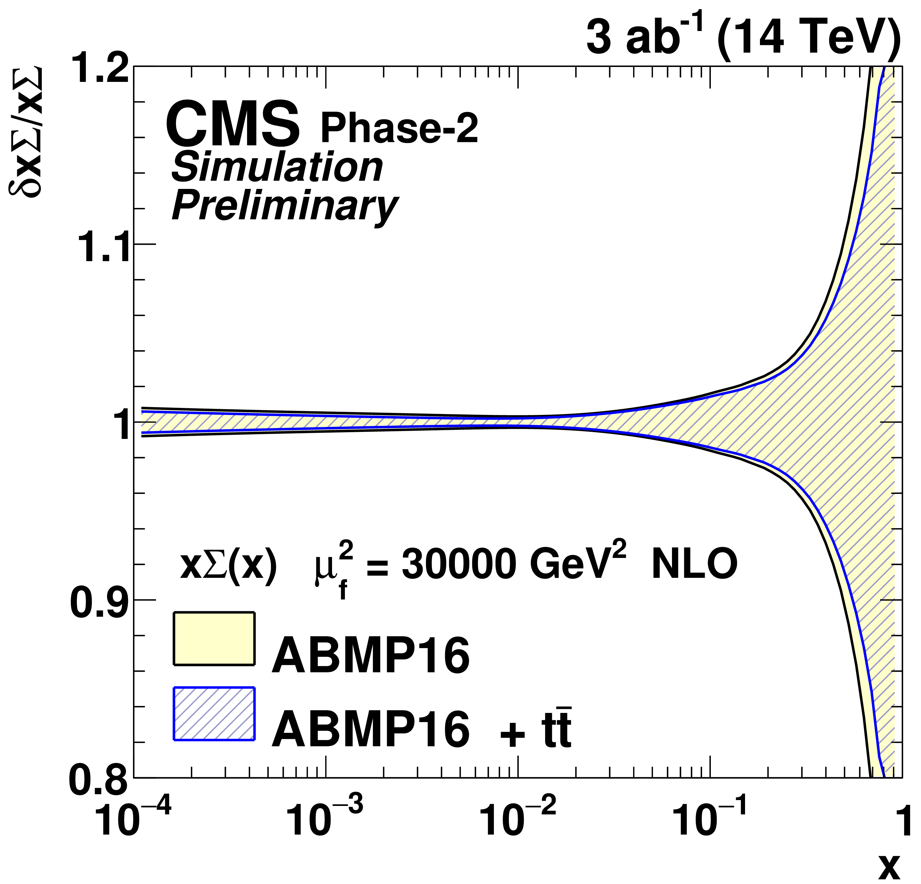
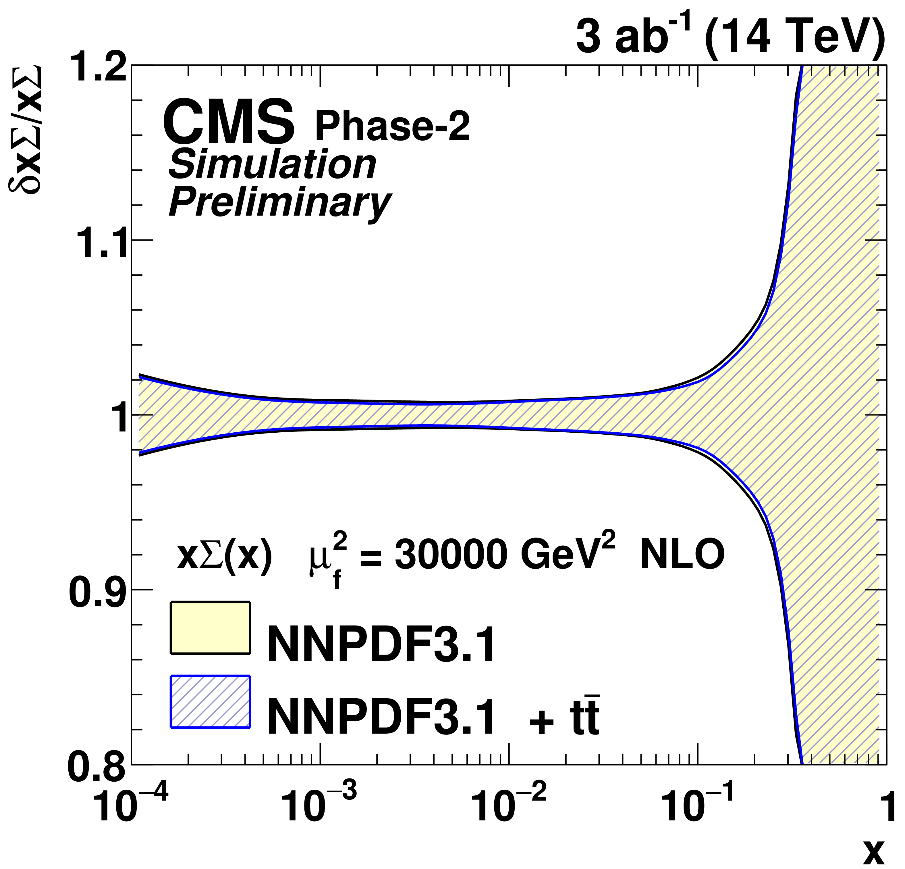
Figure 12:
The relative gluon (upper left), u valence quark (upper right), sea quark (lower left), and d valence quark (lower right) uncertainties of the original and profiled NNPDF3.1 PDF set. |

png pdf |
Figure 12-a:
The relative gluon (upper left), u valence quark (upper right), sea quark (lower left), and d valence quark (lower right) uncertainties of the original and profiled NNPDF3.1 PDF set. |
png pdf |
Figure 12-b:
The relative gluon (upper left), u valence quark (upper right), sea quark (lower left), and d valence quark (lower right) uncertainties of the original and profiled NNPDF3.1 PDF set. |
png pdf |
Figure 12-c:
The relative gluon (upper left), u valence quark (upper right), sea quark (lower left), and d valence quark (lower right) uncertainties of the original and profiled NNPDF3.1 PDF set. |

png pdf |
Figure 12-d:
The relative gluon (upper left), u valence quark (upper right), sea quark (lower left), and d valence quark (lower right) uncertainties of the original and profiled NNPDF3.1 PDF set. |

png pdf |
Figure 13:
Expected event yields (left) and properties of the migration matrix (right) for the measurement of $ {p_{\mathrm {T}}} ({{\mathrm {t}} _\ell})$. For comparison the properties are also shown for the 2016 analysis [2]. |
png pdf |
Figure 13-a:
Expected event yields (left) and properties of the migration matrix (right) for the measurement of $ {p_{\mathrm {T}}} ({{\mathrm {t}} _\ell})$. For comparison the properties are also shown for the 2016 analysis [2]. |
png pdf |
Figure 13-b:
Expected event yields (left) and properties of the migration matrix (right) for the measurement of $ {p_{\mathrm {T}}} ({{\mathrm {t}} _\ell})$. For comparison the properties are also shown for the 2016 analysis [2]. |

png pdf |
Figure 14:
Expected event yields (left) and properties of the migration matrix (right) for the measurement of $ {| y({{\mathrm {t}} _\ell}) |}$. For comparison the properties are also shown for the 2016 analysis [2]. |
png pdf |
Figure 14-a:
Expected event yields (left) and properties of the migration matrix (right) for the measurement of $ {| y({{\mathrm {t}} _\ell}) |}$. For comparison the properties are also shown for the 2016 analysis [2]. |
png pdf |
Figure 14-b:
Expected event yields (left) and properties of the migration matrix (right) for the measurement of $ {| y({{\mathrm {t}} _\ell}) |}$. For comparison the properties are also shown for the 2016 analysis [2]. |

png pdf |
Figure 15:
Expected event yields (left) and properties of the migration matrix (right) for the measurement of $M({{\mathrm {t}\overline {\mathrm {t}}}})$. For comparison the properties are also shown for the 2016 analysis [2]. |
png pdf |
Figure 15-a:
Expected event yields (left) and properties of the migration matrix (right) for the measurement of $M({{\mathrm {t}\overline {\mathrm {t}}}})$. For comparison the properties are also shown for the 2016 analysis [2]. |
png pdf |
Figure 15-b:
Expected event yields (left) and properties of the migration matrix (right) for the measurement of $M({{\mathrm {t}\overline {\mathrm {t}}}})$. For comparison the properties are also shown for the 2016 analysis [2]. |
png pdf |
Figure 16:
Expected event yields (left) and properties of the migration matrix (right) for the measurement of $ {p_{\mathrm {T}}} ({{\mathrm {t}\overline {\mathrm {t}}}})$. For comparison the properties are also shown for the 2016 analysis [2]. |
png pdf |
Figure 16-a:
Expected event yields (left) and properties of the migration matrix (right) for the measurement of $ {p_{\mathrm {T}}} ({{\mathrm {t}\overline {\mathrm {t}}}})$. For comparison the properties are also shown for the 2016 analysis [2]. |

png pdf |
Figure 16-b:
Expected event yields (left) and properties of the migration matrix (right) for the measurement of $ {p_{\mathrm {T}}} ({{\mathrm {t}\overline {\mathrm {t}}}})$. For comparison the properties are also shown for the 2016 analysis [2]. |

png pdf |
Figure 17:
Expected event yields (left) and properties of the migration matrix (right) for the measurement of $ {| y({{\mathrm {t}\overline {\mathrm {t}}}}) |}$. For comparison the properties are also shown for the 2016 analysis [2]. |

png pdf |
Figure 17-a:
Expected event yields (left) and properties of the migration matrix (right) for the measurement of $ {| y({{\mathrm {t}\overline {\mathrm {t}}}}) |}$. For comparison the properties are also shown for the 2016 analysis [2]. |
png pdf |
Figure 17-b:
Expected event yields (left) and properties of the migration matrix (right) for the measurement of $ {| y({{\mathrm {t}\overline {\mathrm {t}}}}) |}$. For comparison the properties are also shown for the 2016 analysis [2]. |

png pdf |
Figure 18:
Normalized differential cross sections (left) as a function of $ {p_{\mathrm {T}}} ({{\mathrm {t}} _\mathrm {h}})$ (upper) and $ {| y({{\mathrm {t}} _\mathrm {h}}) |}$ (lower). The corresponding relative uncertainties (right) in the Phase-2 projections are compared to the uncertainties in the 2016 measurements [2]. |
png pdf |
Figure 18-a:
Normalized differential cross sections (left) as a function of $ {p_{\mathrm {T}}} ({{\mathrm {t}} _\mathrm {h}})$ (upper) and $ {| y({{\mathrm {t}} _\mathrm {h}}) |}$ (lower). The corresponding relative uncertainties (right) in the Phase-2 projections are compared to the uncertainties in the 2016 measurements [2]. |
png pdf |
Figure 18-b:
Normalized differential cross sections (left) as a function of $ {p_{\mathrm {T}}} ({{\mathrm {t}} _\mathrm {h}})$ (upper) and $ {| y({{\mathrm {t}} _\mathrm {h}}) |}$ (lower). The corresponding relative uncertainties (right) in the Phase-2 projections are compared to the uncertainties in the 2016 measurements [2]. |

png pdf |
Figure 18-c:
Normalized differential cross sections (left) as a function of $ {p_{\mathrm {T}}} ({{\mathrm {t}} _\mathrm {h}})$ (upper) and $ {| y({{\mathrm {t}} _\mathrm {h}}) |}$ (lower). The corresponding relative uncertainties (right) in the Phase-2 projections are compared to the uncertainties in the 2016 measurements [2]. |
png pdf |
Figure 18-d:
Normalized differential cross sections (left) as a function of $ {p_{\mathrm {T}}} ({{\mathrm {t}} _\mathrm {h}})$ (upper) and $ {| y({{\mathrm {t}} _\mathrm {h}}) |}$ (lower). The corresponding relative uncertainties (right) in the Phase-2 projections are compared to the uncertainties in the 2016 measurements [2]. |
png pdf |
Figure 19:
Normalized differential cross section as a function of $ {p_{\mathrm {T}}} ({{\mathrm {t}} _\ell})$ (upper) and $ {| y({{\mathrm {t}} _\ell}) |}$ (lower). The corresponding relative uncertainties (right) in the Phase-2 projections are compared to the uncertainties in the 2016 measurements [2]. |
png pdf |
Figure 19-a:
Normalized differential cross section as a function of $ {p_{\mathrm {T}}} ({{\mathrm {t}} _\ell})$ (upper) and $ {| y({{\mathrm {t}} _\ell}) |}$ (lower). The corresponding relative uncertainties (right) in the Phase-2 projections are compared to the uncertainties in the 2016 measurements [2]. |

png pdf |
Figure 19-b:
Normalized differential cross section as a function of $ {p_{\mathrm {T}}} ({{\mathrm {t}} _\ell})$ (upper) and $ {| y({{\mathrm {t}} _\ell}) |}$ (lower). The corresponding relative uncertainties (right) in the Phase-2 projections are compared to the uncertainties in the 2016 measurements [2]. |
png pdf |
Figure 19-c:
Normalized differential cross section as a function of $ {p_{\mathrm {T}}} ({{\mathrm {t}} _\ell})$ (upper) and $ {| y({{\mathrm {t}} _\ell}) |}$ (lower). The corresponding relative uncertainties (right) in the Phase-2 projections are compared to the uncertainties in the 2016 measurements [2]. |

png pdf |
Figure 19-d:
Normalized differential cross section as a function of $ {p_{\mathrm {T}}} ({{\mathrm {t}} _\ell})$ (upper) and $ {| y({{\mathrm {t}} _\ell}) |}$ (lower). The corresponding relative uncertainties (right) in the Phase-2 projections are compared to the uncertainties in the 2016 measurements [2]. |

png pdf |
Figure 20:
Normalized differential cross section as a function of $M({{\mathrm {t}\overline {\mathrm {t}}}})$ (upper), $ {p_{\mathrm {T}}} ({{\mathrm {t}\overline {\mathrm {t}}}})$ (middle), and $ {| y({{\mathrm {t}\overline {\mathrm {t}}}}) |}$ (lower). The corresponding relative uncertainties (right) in the Phase-2 projections are compared to the uncertainties in the 2016 measurements [2]. |

png pdf |
Figure 20-a:
Normalized differential cross section as a function of $M({{\mathrm {t}\overline {\mathrm {t}}}})$ (upper), $ {p_{\mathrm {T}}} ({{\mathrm {t}\overline {\mathrm {t}}}})$ (middle), and $ {| y({{\mathrm {t}\overline {\mathrm {t}}}}) |}$ (lower). The corresponding relative uncertainties (right) in the Phase-2 projections are compared to the uncertainties in the 2016 measurements [2]. |
png pdf |
Figure 20-b:
Normalized differential cross section as a function of $M({{\mathrm {t}\overline {\mathrm {t}}}})$ (upper), $ {p_{\mathrm {T}}} ({{\mathrm {t}\overline {\mathrm {t}}}})$ (middle), and $ {| y({{\mathrm {t}\overline {\mathrm {t}}}}) |}$ (lower). The corresponding relative uncertainties (right) in the Phase-2 projections are compared to the uncertainties in the 2016 measurements [2]. |

png pdf |
Figure 20-c:
Normalized differential cross section as a function of $M({{\mathrm {t}\overline {\mathrm {t}}}})$ (upper), $ {p_{\mathrm {T}}} ({{\mathrm {t}\overline {\mathrm {t}}}})$ (middle), and $ {| y({{\mathrm {t}\overline {\mathrm {t}}}}) |}$ (lower). The corresponding relative uncertainties (right) in the Phase-2 projections are compared to the uncertainties in the 2016 measurements [2]. |

png pdf |
Figure 20-d:
Normalized differential cross section as a function of $M({{\mathrm {t}\overline {\mathrm {t}}}})$ (upper), $ {p_{\mathrm {T}}} ({{\mathrm {t}\overline {\mathrm {t}}}})$ (middle), and $ {| y({{\mathrm {t}\overline {\mathrm {t}}}}) |}$ (lower). The corresponding relative uncertainties (right) in the Phase-2 projections are compared to the uncertainties in the 2016 measurements [2]. |

png pdf |
Figure 20-e:
Normalized differential cross section as a function of $M({{\mathrm {t}\overline {\mathrm {t}}}})$ (upper), $ {p_{\mathrm {T}}} ({{\mathrm {t}\overline {\mathrm {t}}}})$ (middle), and $ {| y({{\mathrm {t}\overline {\mathrm {t}}}}) |}$ (lower). The corresponding relative uncertainties (right) in the Phase-2 projections are compared to the uncertainties in the 2016 measurements [2]. |

png pdf |
Figure 20-f:
Normalized differential cross section as a function of $M({{\mathrm {t}\overline {\mathrm {t}}}})$ (upper), $ {p_{\mathrm {T}}} ({{\mathrm {t}\overline {\mathrm {t}}}})$ (middle), and $ {| y({{\mathrm {t}\overline {\mathrm {t}}}}) |}$ (lower). The corresponding relative uncertainties (right) in the Phase-2 projections are compared to the uncertainties in the 2016 measurements [2]. |

png pdf |
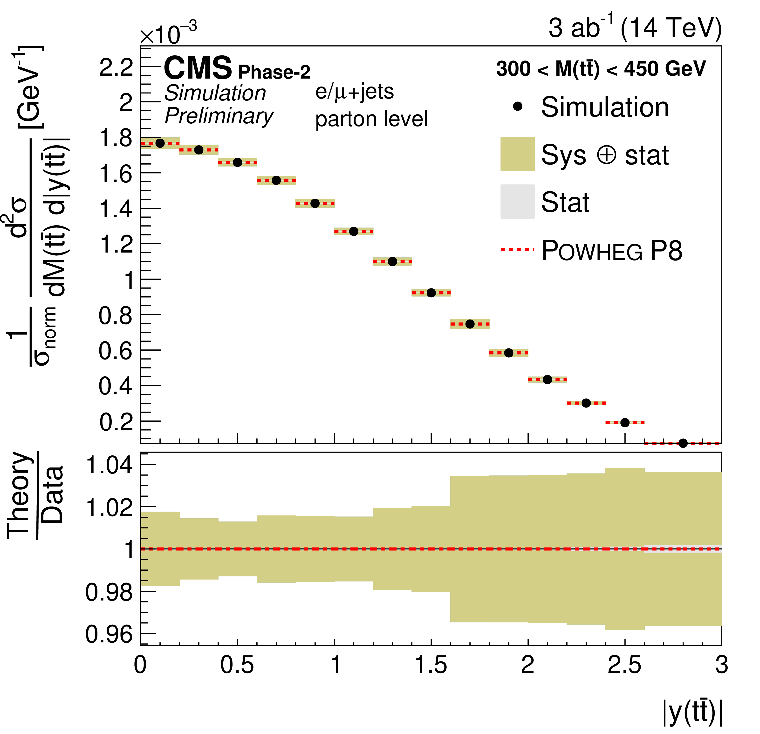
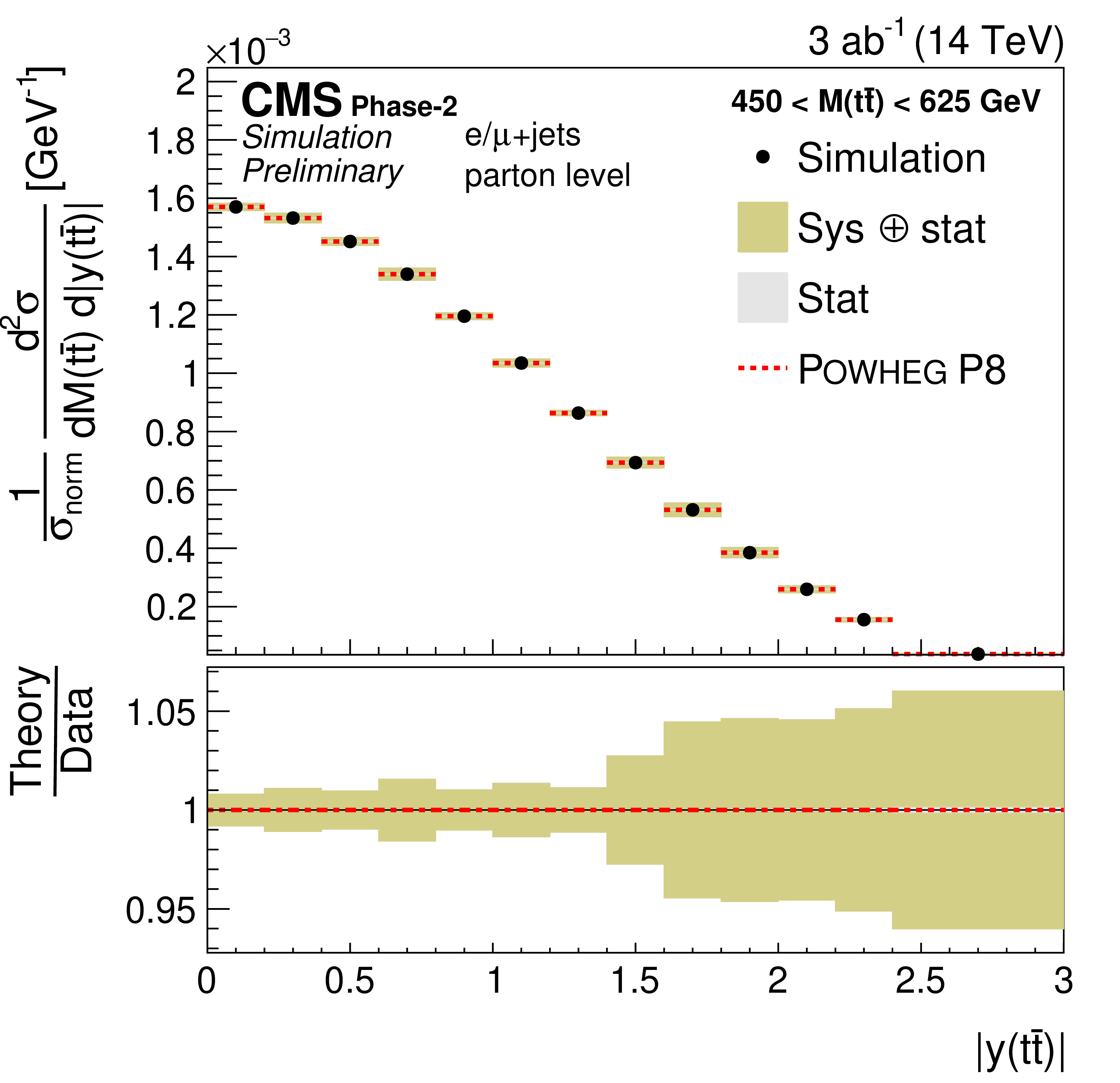
Figure 21:
Projections of the double-differential cross section as a function of $M({{\mathrm {t}\overline {\mathrm {t}}}})$ vs. $ {| y({{\mathrm {t}\overline {\mathrm {t}}}}) |}$ (left). The corresponding relative uncertainties (right) in the Phase-2 projections are compared to the uncertainties in the 2016 measurements [2]. |
png pdf |
Figure 21-a:
Projections of the double-differential cross section as a function of $M({{\mathrm {t}\overline {\mathrm {t}}}})$ vs. $ {| y({{\mathrm {t}\overline {\mathrm {t}}}}) |}$ (left). The corresponding relative uncertainties (right) in the Phase-2 projections are compared to the uncertainties in the 2016 measurements [2]. |
png pdf |
Figure 21-b:
Projections of the double-differential cross section as a function of $M({{\mathrm {t}\overline {\mathrm {t}}}})$ vs. $ {| y({{\mathrm {t}\overline {\mathrm {t}}}}) |}$ (left). The corresponding relative uncertainties (right) in the Phase-2 projections are compared to the uncertainties in the 2016 measurements [2]. |

png pdf |
Figure 21-c:
Projections of the double-differential cross section as a function of $M({{\mathrm {t}\overline {\mathrm {t}}}})$ vs. $ {| y({{\mathrm {t}\overline {\mathrm {t}}}}) |}$ (left). The corresponding relative uncertainties (right) in the Phase-2 projections are compared to the uncertainties in the 2016 measurements [2]. |

png pdf |
Figure 21-d:
Projections of the double-differential cross section as a function of $M({{\mathrm {t}\overline {\mathrm {t}}}})$ vs. $ {| y({{\mathrm {t}\overline {\mathrm {t}}}}) |}$ (left). The corresponding relative uncertainties (right) in the Phase-2 projections are compared to the uncertainties in the 2016 measurements [2]. |

png pdf |
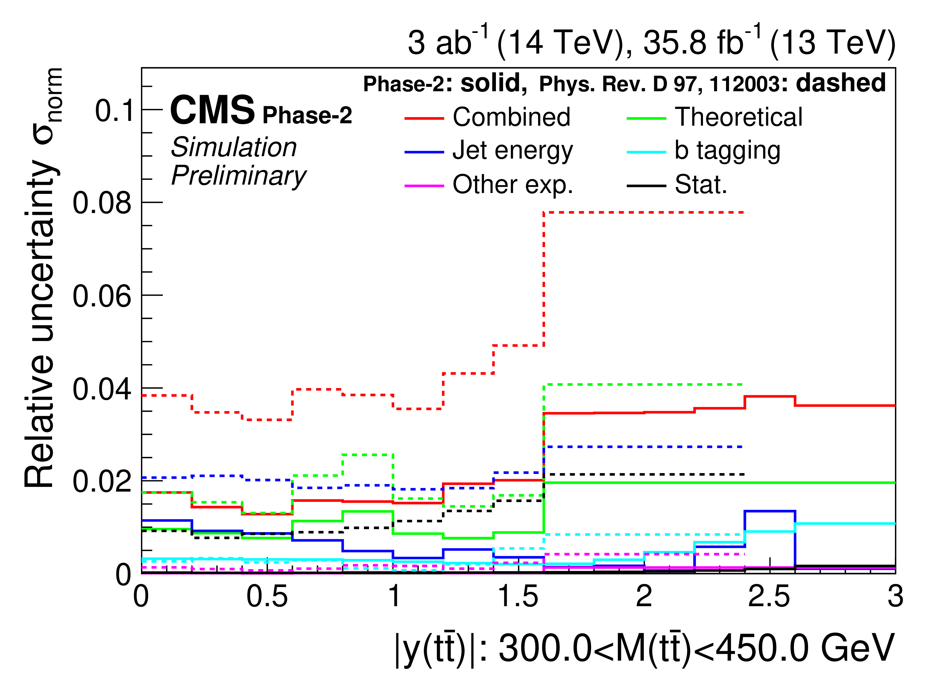
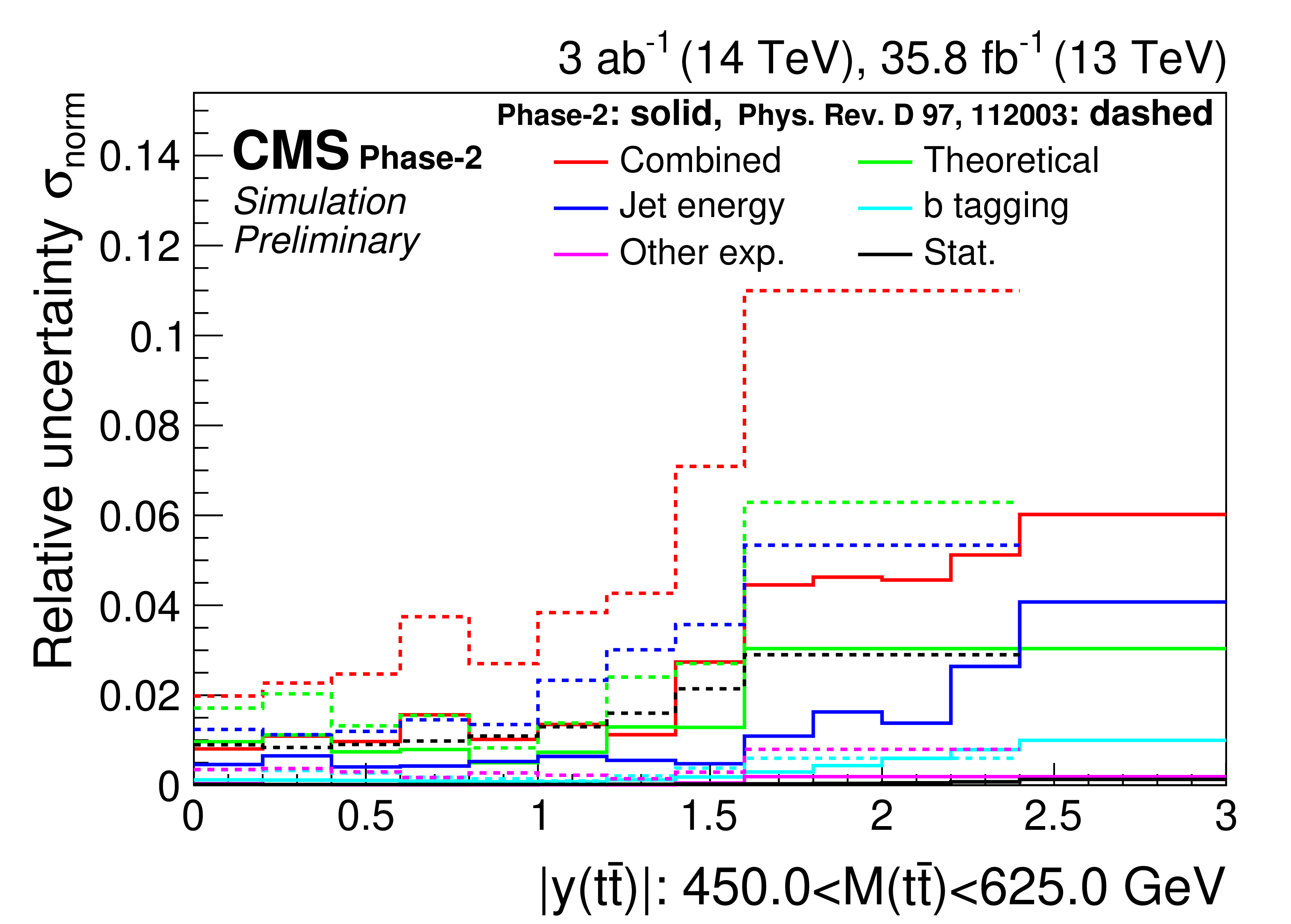
Figure 22:
Projections of the double-differential cross section as a function of $M({{\mathrm {t}\overline {\mathrm {t}}}})$ vs. $ {| y({{\mathrm {t}\overline {\mathrm {t}}}}) |}$ (left). The corresponding relative uncertainties (right) in the Phase-2 projections are compared to the uncertainties in the 2016 measurements [2]. |

png pdf |
Figure 22-a:
Projections of the double-differential cross section as a function of $M({{\mathrm {t}\overline {\mathrm {t}}}})$ vs. $ {| y({{\mathrm {t}\overline {\mathrm {t}}}}) |}$ (left). The corresponding relative uncertainties (right) in the Phase-2 projections are compared to the uncertainties in the 2016 measurements [2]. |

png pdf |
Figure 22-b:
Projections of the double-differential cross section as a function of $M({{\mathrm {t}\overline {\mathrm {t}}}})$ vs. $ {| y({{\mathrm {t}\overline {\mathrm {t}}}}) |}$ (left). The corresponding relative uncertainties (right) in the Phase-2 projections are compared to the uncertainties in the 2016 measurements [2]. |

png pdf |
Figure 22-c:
Projections of the double-differential cross section as a function of $M({{\mathrm {t}\overline {\mathrm {t}}}})$ vs. $ {| y({{\mathrm {t}\overline {\mathrm {t}}}}) |}$ (left). The corresponding relative uncertainties (right) in the Phase-2 projections are compared to the uncertainties in the 2016 measurements [2]. |

png pdf |
Figure 22-d:
Projections of the double-differential cross section as a function of $M({{\mathrm {t}\overline {\mathrm {t}}}})$ vs. $ {| y({{\mathrm {t}\overline {\mathrm {t}}}}) |}$ (left). The corresponding relative uncertainties (right) in the Phase-2 projections are compared to the uncertainties in the 2016 measurements [2]. |
| Summary |
| A projection of differential $\mathrm{t\bar{t}}$ cross section measurements at the HL-LHC has been shown. Using pileup mitigation techniques like PUPPI these measurements become feasible in an environment of 200 pileup events. The high amount of data and the extended $\eta$-range of the Phase-2 detector allow for fine-binned measurements in phase-space regions -- especially at high rapidity -- that are not accessible in current measurements. The most significant reduction of uncertainty is expected because of an improved jet energy calibration and a reduced uncertainty in the b jet identification. It is demonstrated that the projected differential $\mathrm{t\bar{t}}$ cross sections have a strong impact on the gluon distribution in the proton. Overall, this measurement will profit from both, the improved Phase-2 CMS detector and the high amount of data expected at the HL-LHC. |
| References | ||||
| 1 | CMS Collaboration | Measurement of differential cross sections for top quark pair production using the lepton+jets final state in proton-proton collisions at 13 TeV | PRD 95 (2017) 092001 | CMS-TOP-16-008 1610.04191 |
| 2 | CMS Collaboration | Measurement of differential cross sections for the production of top quark pairs and of additional jets in lepton+jets events from pp collisions at $ \sqrt{s} = $ 13 TeV | PRD 97 (2018) 112003 | CMS-TOP-17-002 1803.08856 |
| 3 | D. Bertolini, P. Harris, M. Low, and N. Tran | Pileup Per Particle Identification | JHEP (2014) 059 | 1407.6013 |
| 4 | CMS Collaboration | The CMS experiment at the CERN LHC | JINST 3 (2008) S08004 | CMS-00-001 |
| 5 | CMS Collaboration | The phase-2 upgrade of the cms tracker | CDS | |
| 6 | CMS Collaboration | The phase-2 upgrade of the cms barrel calorimeters technical design report | CDS | |
| 7 | CMS Collaboration | The phase-2 upgrade of the cms endcap calorimeter | CDS | |
| 8 | CMS Collaboration | The phase-2 upgrade of the cms muon detectors | CDS | |
| 9 | P. Nason | A new method for combining NLO QCD with shower Monte Carlo algorithms | JHEP 11 (2004) 040 | hep-ph/0409146 |
| 10 | S. Frixione, P. Nason, and C. Oleari | Matching NLO QCD computations with parton shower simulations: the POWHEG method | JHEP 11 (2007) 070 | 0709.2092 |
| 11 | S. Alioli, P. Nason, C. Oleari, and E. Re | A general framework for implementing NLO calculations in shower Monte Carlo programs: the POWHEG BOX | JHEP 06 (2010) 043 | 1002.2581 |
| 12 | J. M. Campbell, R. K. Ellis, P. Nason, and E. Re | Top-pair production and decay at NLO matched with parton showers | JHEP 04 (2015) 114 | 1412.1828 |
| 13 | T. Sjostrand, S. Mrenna, and P. Skands | PYTHIA 6.4 physics and manual | JHEP 05 (2006) 026 | hep-ph/0603175 |
| 14 | T. Sjostrand, S. Mrenna, and P. Skands | A brief introduction to PYTHIA 8.1 | CPC 178 (2008) 852 | 0710.3820 |
| 15 | P. Skands, S. Carrazza, and J. Rojo | Tuning PYTHIA 8.1: the Monash 2013 tune | EPJC 74 (2014) 3024 | 1404.5630 |
| 16 | CMS Collaboration | Investigations of the impact of the parton shower tuning in PYTHIA 8 in the modelling of $ \mathrm{t\overline{t}} $ at $ \sqrt{s}= $ 8 and 13 TeV | CMS-PAS-TOP-16-021 | CMS-PAS-TOP-16-021 |
| 17 | M. Czakon and A. Mitov | Top++: A program for the calculation of the top-pair cross-section at hadron colliders | CPC 185 (2014) 2930 | 1112.5675 |
| 18 | M. Selvaggi | DELPHES 3: A modular framework for fast-simulation of generic collider experiments | J. Phys. Conf. Ser. 523 (2014) 012033 | |
| 19 | CMS Collaboration | Identification of heavy-flavour jets with the CMS detector in pp collisions at 13 TeV | JINST 13 (2018) 05011 | CMS-BTV-16-002 1712.07158 |
| 20 | CMS Collaboration | Particle-flow reconstruction and global event description with the CMS detector | JINST 12 (2017) P10003 | CMS-PRF-14-001 1706.04965 |
| 21 | M. Cacciari, G. P. Salam, and G. Soyez | FastJet user manual | EPJC 72 (2012) 1896 | 1111.6097 |
| 22 | B. A. Betchart, R. Demina, and A. Harel | Analytic solutions for neutrino momenta in decay of top quarks | NIMA 736 (2014) 169 | 1305.1878 |
| 23 | G. D'Agostini | A multidimensional unfolding method based on Bayes' theorem | NIMA 362 (1995) 487 | |
| 24 | CMS Collaboration | CMS Luminosity measurement for the 2016 data taking period | CMS-PAS-LUM-17-001 | CMS-PAS-LUM-17-001 |
| 25 | CMS Collaboration | Performance of CMS muon reconstruction in pp collision events at $ \sqrt{s} = $ 7 TeV | JINST 7 (2012) P10002 | CMS-MUO-10-004 1206.4071 |
| 26 | CMS Collaboration | Performance of electron reconstruction and selection with the CMS detector in proton-proton collisions at $ \sqrt{s} = $ 8 TeV | JINST 10 (2015) P06005 | CMS-EGM-13-001 1502.02701 |
| 27 | CMS Collaboration | Jet energy scale and resolution in the CMS experiment in pp collisions at 8 TeV | JINST 12 (2017) P02014 | CMS-JME-13-004 1607.03663 |
| 28 | H. Paukkunen and P. Zurita | PDF reweighting in the Hessian matrix approach | arXiv:1402.6623 | |
| 29 | S. Alekhin, J. Blumlein, and S. Moch | NLO PDFs from the ABMP16 fit | 1803.07537 | |
| 30 | S. Dulat et al. | New parton distribution functions from a global analysis of quantum chromodynamics | PRD 93 (2016) 033006 | 1506.07443 |
| 31 | NNPDF Collaboration | Parton distributions from high-precision collider data | EPJC77 (2017), no. 10, 663 | 1706.00428 |
| 32 | A. Buckley et al. | LHAPDF6: parton density access in the LHC precision era | EPJC 75 (2015) 132 | 1412.7420 |
| 33 | CMS Collaboration | Measurement of double-differential cross sections for top quark pair production in pp collisions at $ \sqrt{s} = $ 8 TeV and impact on parton distribution functions | EPJC 77 (2017) 459 | CMS-TOP-14-013 1703.01630 |
| 34 | S. Alekhin et al. | HERAFitter | EPJC 75 (2015) 304 | 1410.4412 |
| 35 | J. Alwall et al. | The automated computation of tree-level and next-to-leading order differential cross sections, and their matching to parton shower simulations | JHEP 07 (2014) 079 | 1405.0301 |
| 36 | V. Bertone et al. | aMCfast: automation of fast NLO computations for PDF fits | JHEP 08 (2014) 166 | 1406.7693 |
| 37 | T. Carli et al. | A posteriori inclusion of parton density functions in NLO QCD final-state calculations at hadron colliders: The APPLGRID project | EPJC 66 (2010) 503 | 0911.2985 |
|
|
Compact Muon Solenoid LHC, CERN |
|

|

|

|

|

|