

Compact Muon Solenoid
LHC, CERN
| CMS-PAS-HIG-16-028 | ||
| Search for non-resonant Higgs boson pair production in the $\mathrm{b\overline{b}}\tau^+\tau^-$ final state using 2016 data | ||
| CMS Collaboration | ||
| August 2016 | ||
| Abstract: A search for non-resonant Higgs boson pair production in the $\mathrm{b\overline{b}}\tau^+\tau^-$ final state is presented. The search is performed using three $\tau\tau$ final states, $e\tau_{\rm h}, \mu\tau_{\rm h}$, and $\tau_{\rm h}\tau_{\rm h}$, where $e$ and $\mu$ indicate a $\tau$ lepton decaying to lighter leptons and $\tau_{\rm h}$ indicates a $\tau$ decay involving hadrons. The analysis uses proton-proton collision data collected in 2016 at 13 TeV and corresponding to an integrated luminosity of 12.9 fb$^{-1}$. | ||
| Links: CDS record (PDF) ; inSPIRE record ; CADI line (restricted) ; | ||
| Figures & Tables | Summary | Additional Figures | References | CMS Publications |
|---|
| Figures | |
png pdf |
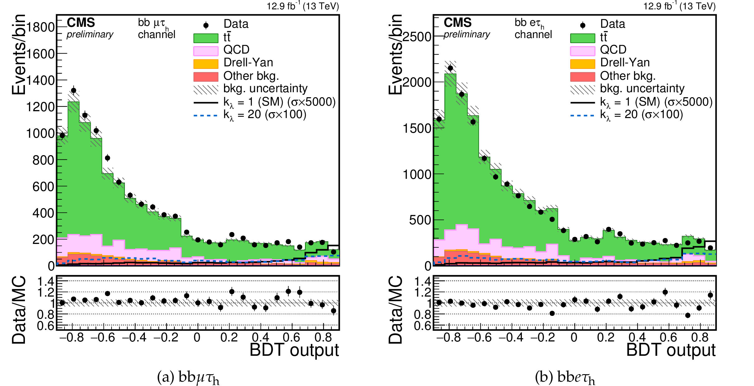
Figure 1:
Output of the BDT discriminator in the bb$\mu \tau _{\rm h}$ channel (a) and bb$e\tau _{\rm h}$ channel (b). Points with error bars represent the data and shaded histograms represent the backgrounds. The black unshaded histogram is the signal expectation for the SM ($k_\lambda = \lambda _{hhh}/\lambda ^{SM}_{hhh} =$ 1) and the blue dashed unshaded histogram is the signal expectation for $k_\lambda = $ 20. The SM production cross section is scaled by a factor 5000 and the $k_\lambda =$ 20 production cross section is scaled by a factor 100. Signal and background histograms are not stacked. The lower panel shows the ratio of the observed data to the MC prediction. |
png pdf |
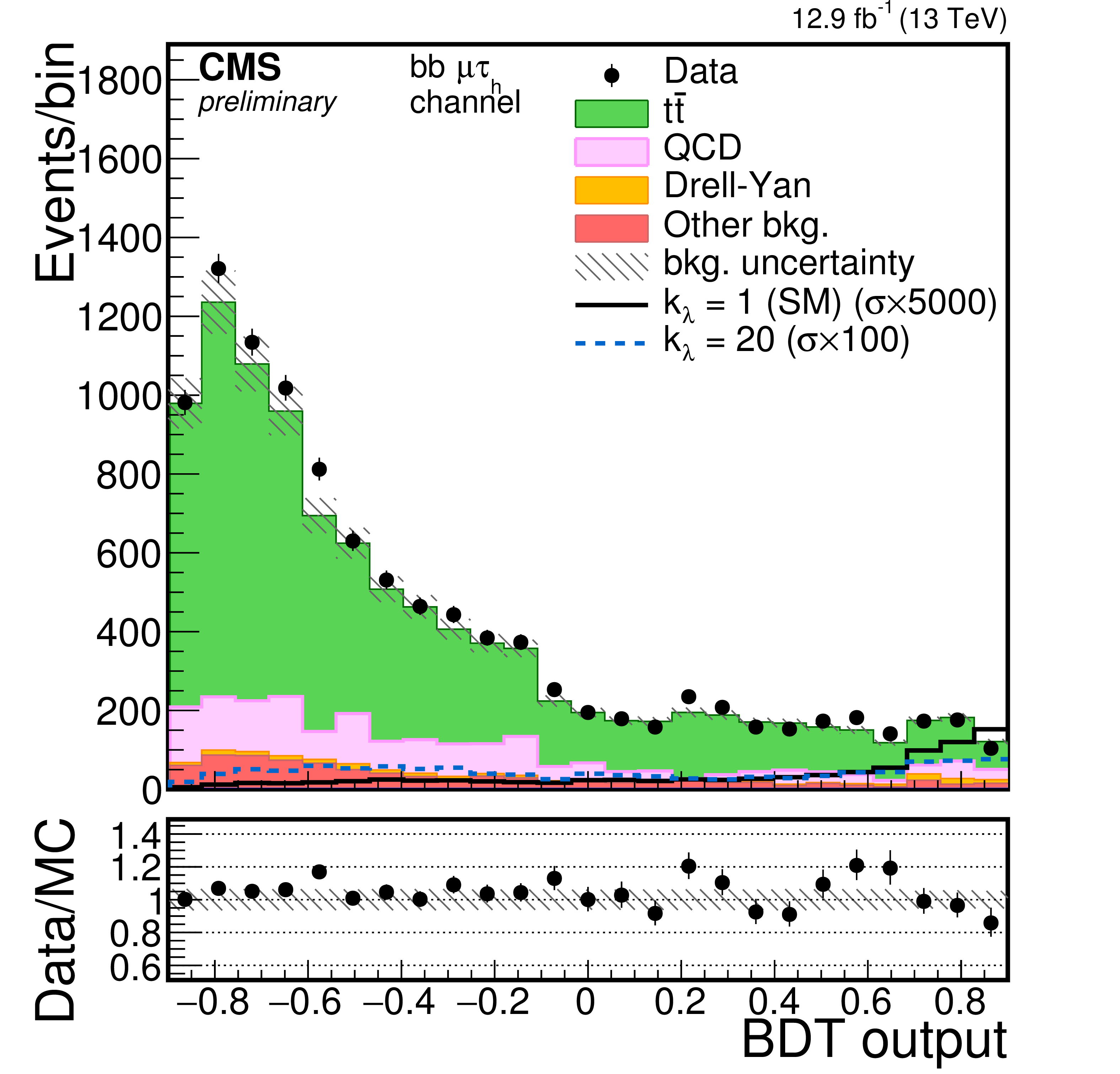
Figure 1-a:
Output of the BDT discriminator in the bb$\mu \tau _{\rm h}$ channel. Points with error bars represent the data and shaded histograms represent the backgrounds. The black unshaded histogram is the signal expectation for the SM ($k_\lambda = \lambda _{hhh}/\lambda ^{SM}_{hhh} =$ 1) and the blue dashed unshaded histogram is the signal expectation for $k_\lambda = $ 20. The SM production cross section is scaled by a factor 5000 and the $k_\lambda =$ 20 production cross section is scaled by a factor 100. Signal and background histograms are not stacked. The lower panel shows the ratio of the observed data to the MC prediction. |
png pdf |
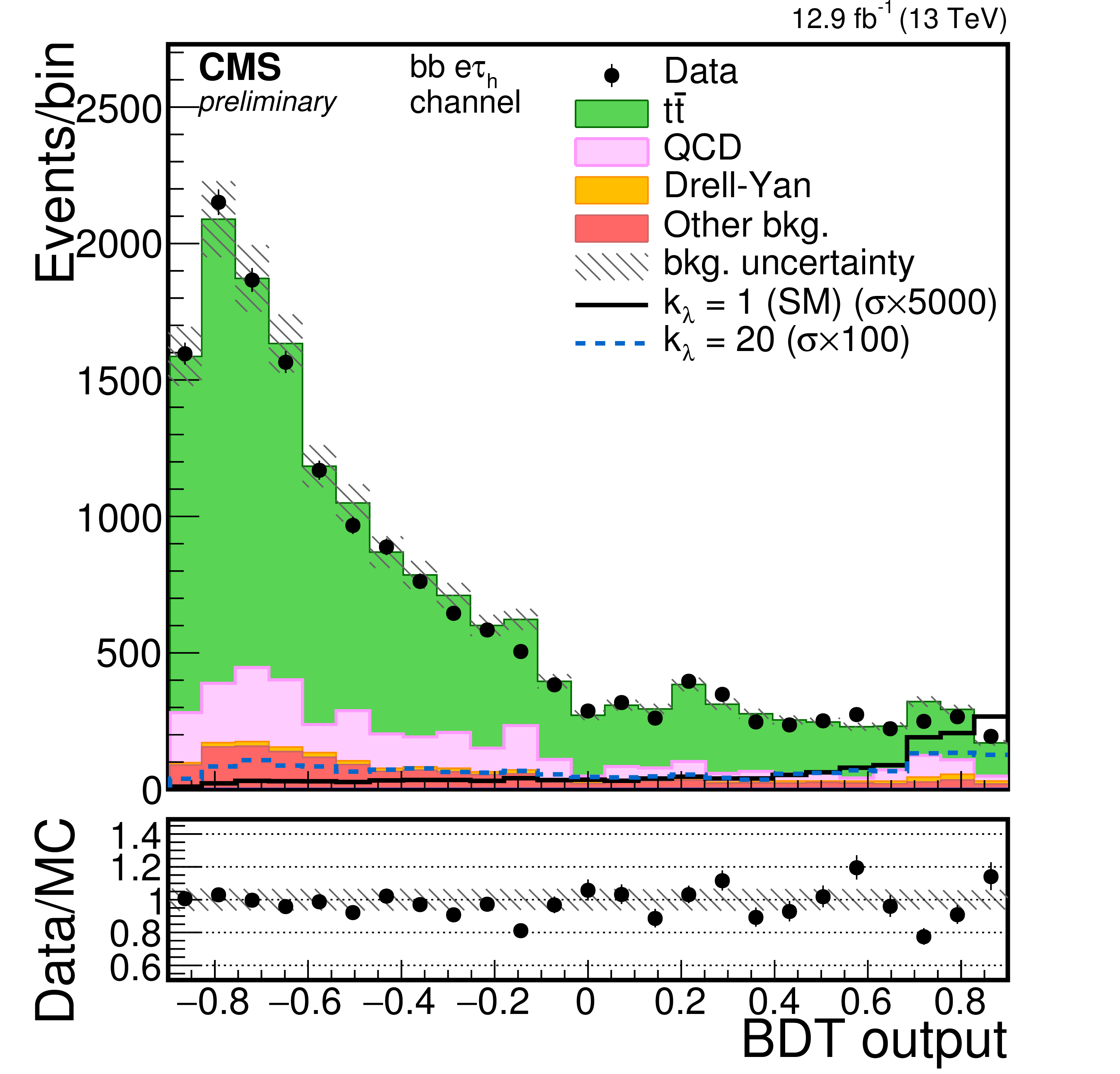
Figure 1-b:
Output of the BDT discriminator in the bb$e\tau _{\rm h}$ channel. Points with error bars represent the data and shaded histograms represent the backgrounds. The black unshaded histogram is the signal expectation for the SM ($k_\lambda = \lambda _{hhh}/\lambda ^{SM}_{hhh} =$ 1) and the blue dashed unshaded histogram is the signal expectation for $k_\lambda = $ 20. The SM production cross section is scaled by a factor 5000 and the $k_\lambda =$ 20 production cross section is scaled by a factor 100. Signal and background histograms are not stacked. The lower panel shows the ratio of the observed data to the MC prediction. |

png pdf |
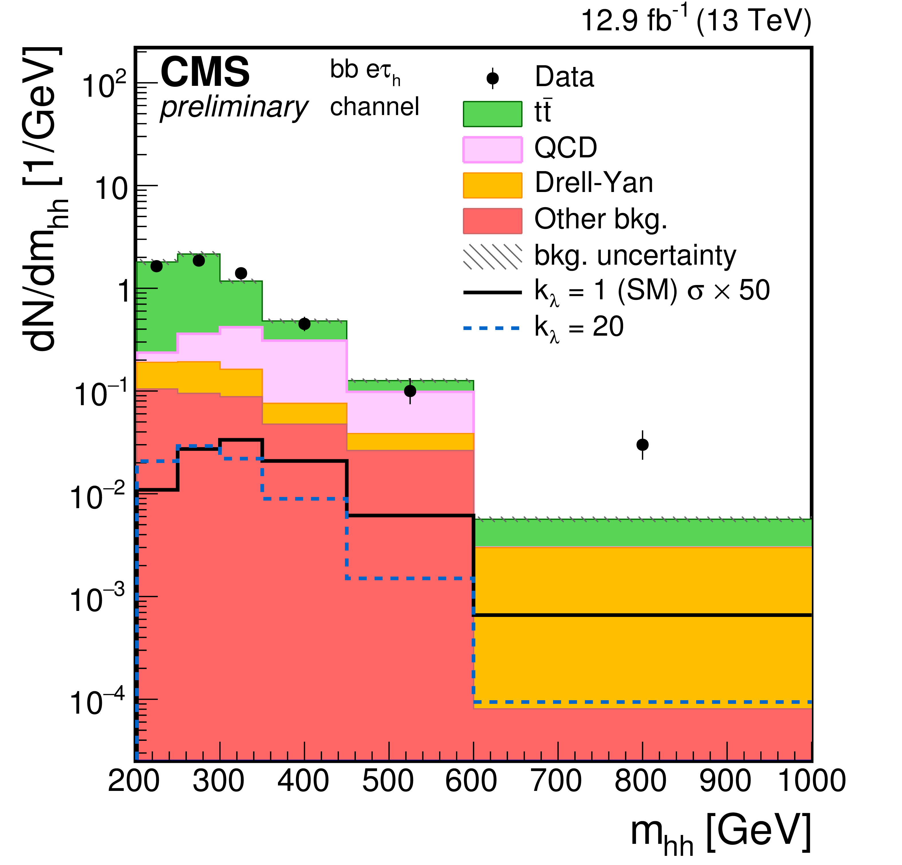
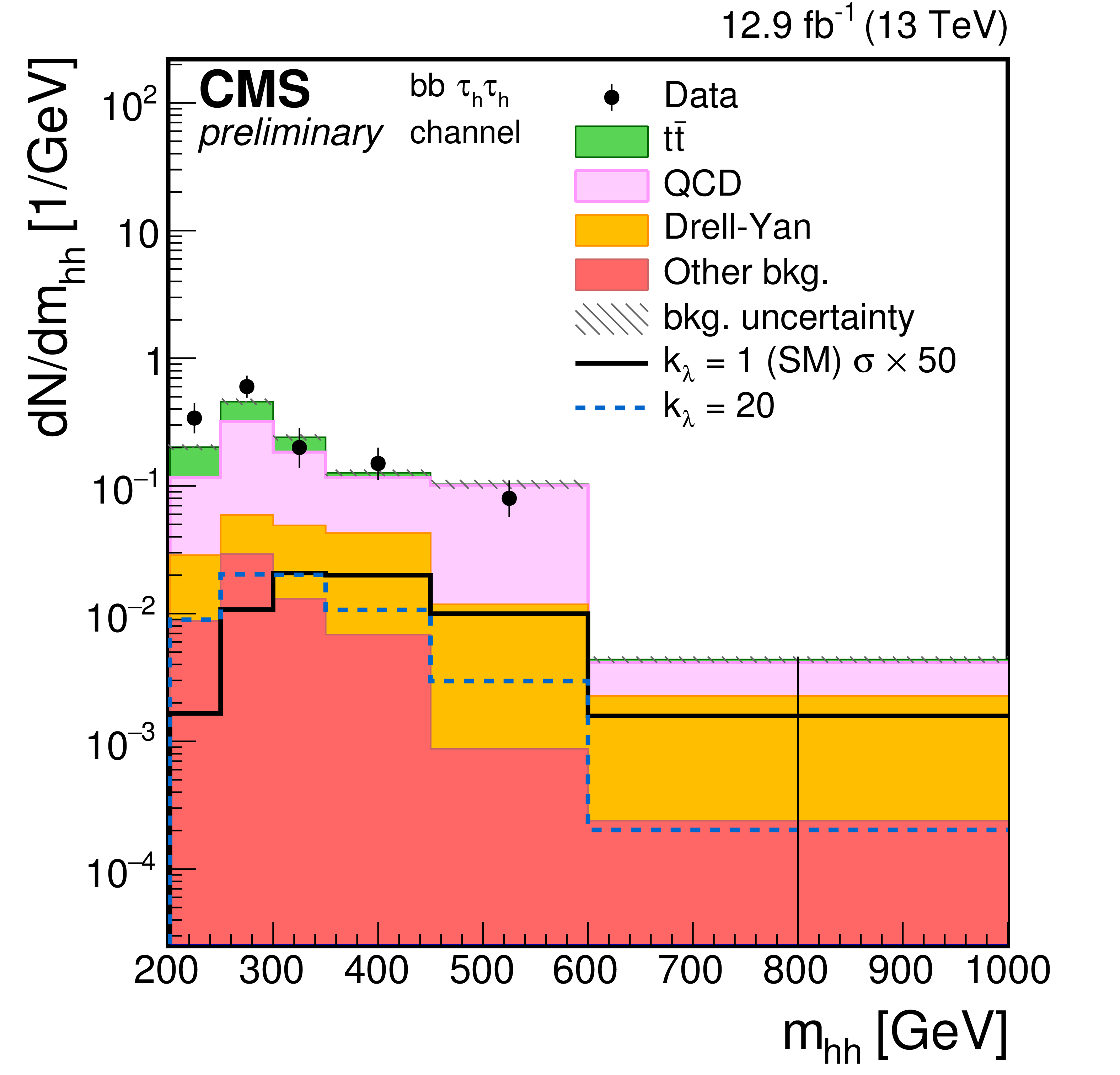
Figure 2:
Distributions of the reconstructed visible four-body mass (${\rm m_{hh}}$) after applying the event selection. The plots are shown for (a) bb$\mu \tau _{\rm h}$ , (b) bb$e\tau _{\rm h}$ , and (c) bb$e\tau _{\rm h}$ channels. Points with error bars represent the data, shaded histograms represent the backgrounds, the black unshaded histogram is the signal expectation for the SM ($\lambda _{\rm hhh}/\lambda ^{SM}_{\rm hhh}=1$), and the blue dotted unshaded histogram is the signal expectation for $\lambda _{\rm hhh}/\lambda ^{\rm SM}_{\rm hhh}=20$. The SM production cross section is scaled by a factor 50. Event yields in each bin are divided by the bin width. Expected background contributions are shown for the values of nuisance parameters (systematic uncertainties) obtained after fitting the background hypothesis to the data. Signal and background histograms are not stacked. |
png pdf |
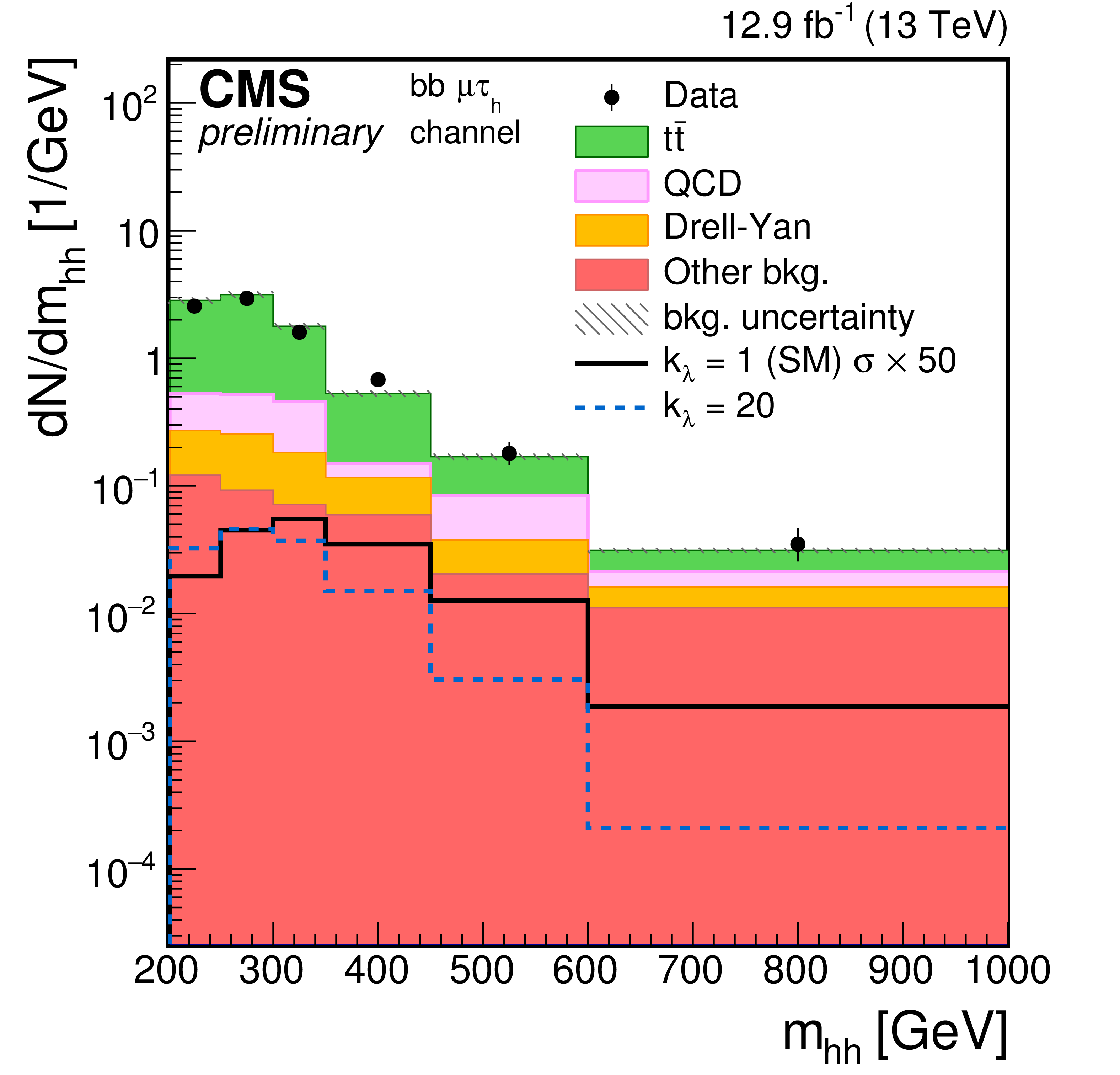
Figure 2-a:
Distribution of the reconstructed visible four-body mass (${\rm m_{hh}}$) after applying the event selection for the bb$\mu \tau _{\rm h}$ channel. Points with error bars represent the data, shaded histograms represent the backgrounds, the black unshaded histogram is the signal expectation for the SM ($\lambda _{\rm hhh}/\lambda ^{SM}_{\rm hhh}=1$), and the blue dotted unshaded histogram is the signal expectation for $\lambda _{\rm hhh}/\lambda ^{\rm SM}_{\rm hhh}= $ 20. The SM production cross section is scaled by a factor 50. Event yields in each bin are divided by the bin width. Expected background contributions are shown for the values of nuisance parameters (systematic uncertainties) obtained after fitting the background hypothesis to the data. Signal and background histograms are not stacked. |
png pdf |
Figure 2-b:
Distribution of the reconstructed visible four-body mass (${\rm m_{hh}}$) after applying the event selection for the bb$e\tau _{\rm h}$ channel. Points with error bars represent the data, shaded histograms represent the backgrounds, the black unshaded histogram is the signal expectation for the SM ($\lambda _{\rm hhh}/\lambda ^{SM}_{\rm hhh}=1$), and the blue dotted unshaded histogram is the signal expectation for $\lambda _{\rm hhh}/\lambda ^{\rm SM}_{\rm hhh}= $ 20. The SM production cross section is scaled by a factor 50. Event yields in each bin are divided by the bin width. Expected background contributions are shown for the values of nuisance parameters (systematic uncertainties) obtained after fitting the background hypothesis to the data. Signal and background histograms are not stacked. |
png pdf |
Figure 2-c:
Distribution of the reconstructed visible four-body mass (${\rm m_{hh}}$) after applying the event selection for the bb$e\tau _{\rm h}$ channel. Points with error bars represent the data, shaded histograms represent the backgrounds, the black unshaded histogram is the signal expectation for the SM ($\lambda _{\rm hhh}/\lambda ^{SM}_{\rm hhh}=1$), and the blue dotted unshaded histogram is the signal expectation for $\lambda _{\rm hhh}/\lambda ^{\rm SM}_{\rm hhh}= $ 20. The SM production cross section is scaled by a factor 50. Event yields in each bin are divided by the bin width. Expected background contributions are shown for the values of nuisance parameters (systematic uncertainties) obtained after fitting the background hypothesis to the data. Signal and background histograms are not stacked. |
png pdf |
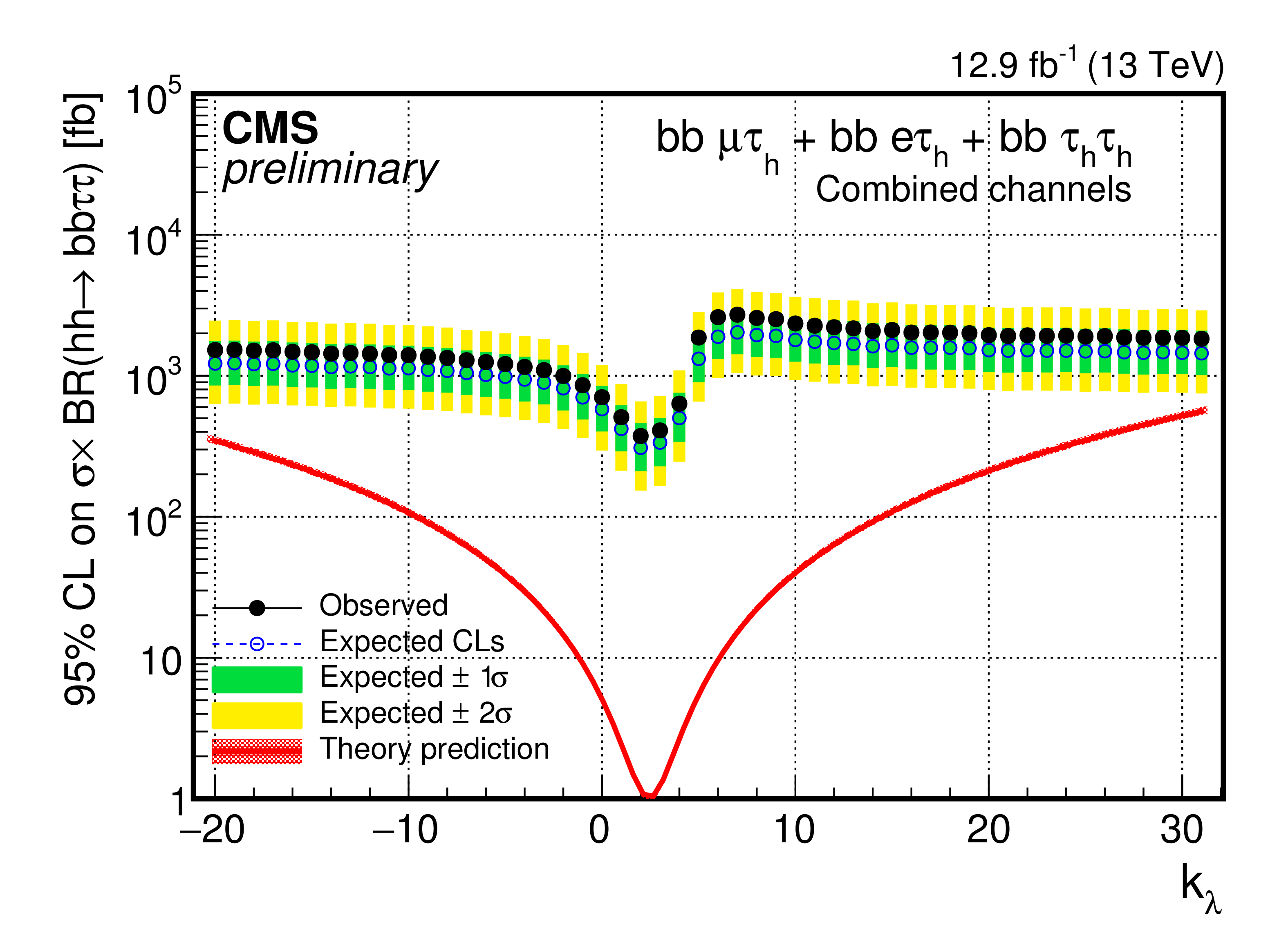
Figure 3:
Observed and expected 95% CL upper limits on cross section times branching ratio as a function of the ratio of the anomalous trilinear coupling to the SM trilinear coupling (${k_\lambda = \lambda _{\rm hhh}/\lambda ^{SM}_{\rm hhh}}$) combining all the final states. The red band shows the theoretical cross section expectation and its systematic uncertainty |
| Tables | |
png pdf |
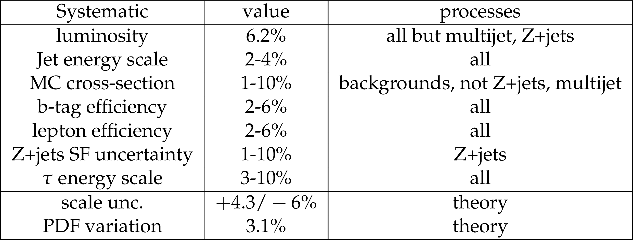
Table 1:
Systematic uncertainties affecting the normalization of the different processes. |

png pdf |
Table 2:
Observed and expected event yields in different event final states. Quoted uncertainties represent the combination of statistical plus systematic uncertainties. |
| Summary |
| The search for non-resonant Higgs boson pair production in the bb$\tau\tau$ final state with a collected luminosity of 12.9 fb$^{-1}$ at $\sqrt{s} = $ 13 TeV is presented. The search is performed using the three most sensitive decay channels of the $\tau$ leptons, $e\tau_{\rm h}$, $\mu\tau_{\rm h}$, and $\tau_{\rm h}\tau_{\rm h}$, where $\tau_{\rm h}$ indicates a tau decay involving hadrons. For non-resonant Higgs boson pair production at $k_\lambda = $ 1 the observed (expected) 95% CL upper limit on $\sigma({\rm pp \to hh \to bb}\tau\tau)$ amounts to 508 (420) fb. This value corresponds to approximately 200 (170) times the SM prediction. |
| Additional Figures | |
png pdf |
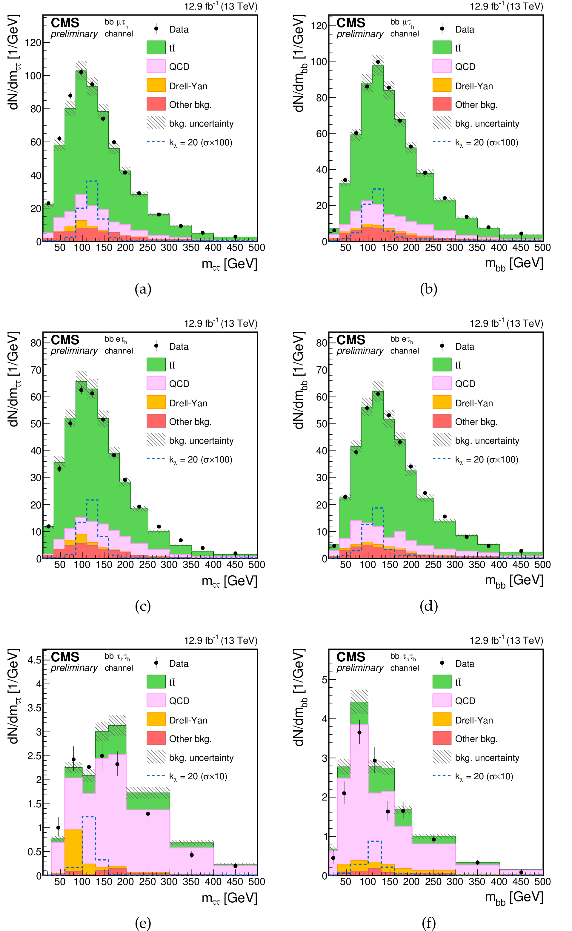
Additional Figure 1:
(a)-(c)-(e) distributions of the invariant mass of the $\tau \tau $ pair reconstructed using the SVfit algorithm and (b)-(d)-(f) distributions of the invariant mass of the bb pair. $\tau \tau $ and bb candidates selections are applied but no selection on the invariant mass is requested. (a)-(b) bb$\mu \tau _h$ channel, (c)-(d) bb${\rm e}\tau _h$ channel, and (e)-(f) bb$\tau _h\tau _h$ channel. Points with error bars represent the data and shaded histograms represent the backgrounds. The dashed blue line is the signal expectation for ${\rm k}_{\lambda } = 20$ and is scaled by a factor 100 for the bb$\mu \tau _h$ and bb${\rm e}\tau _h$ channels and by a factor 10 for the bb$\tau _h\tau _h$ channel. Signal and background histograms are not stacked. |
png pdf |
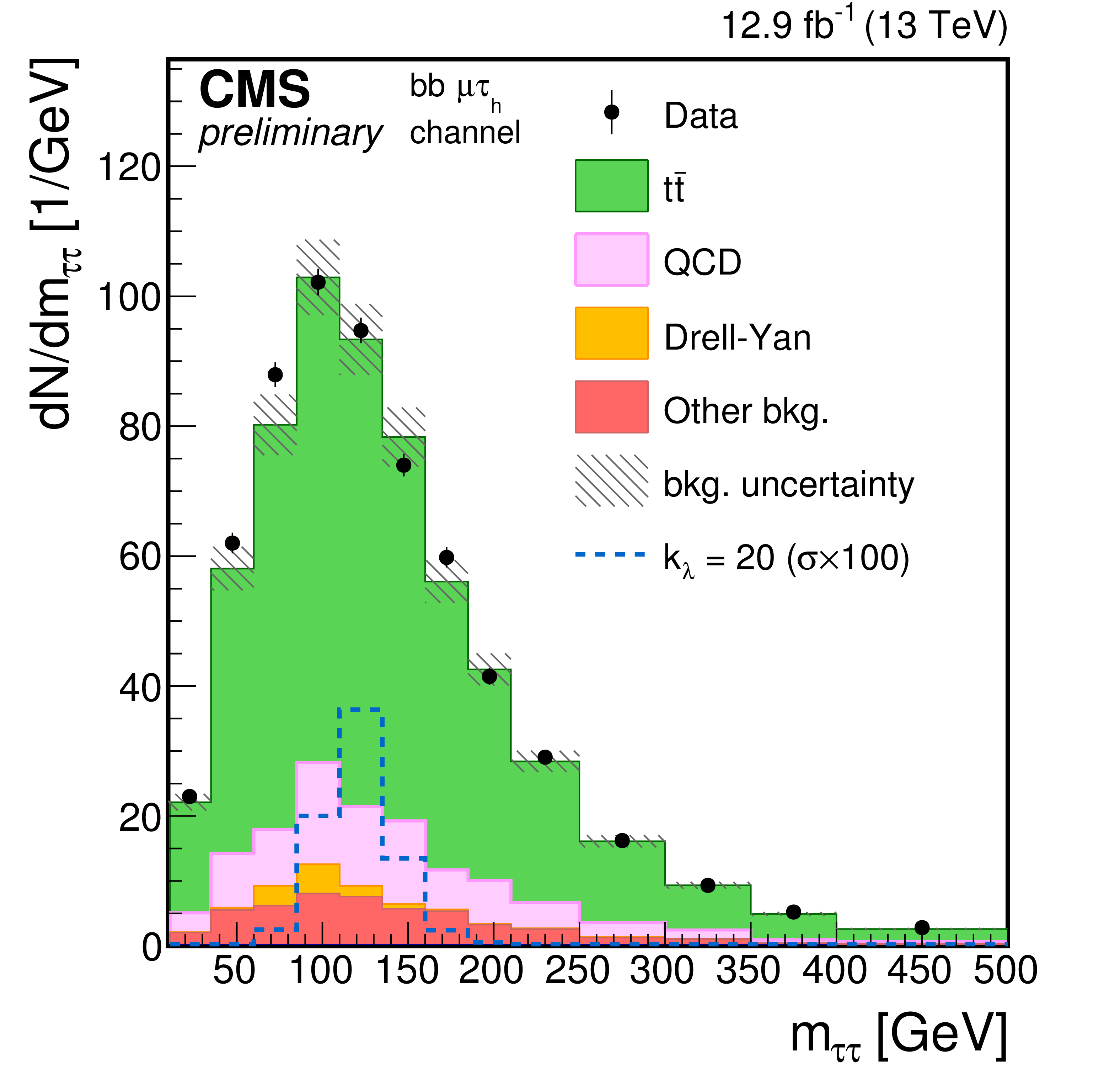
Additional Figure 1-a:
Distribution of the invariant mass of the $\tau \tau $ pair reconstructed using the SVfit algorithm: bb$\mu \tau _h$ channel. $\tau \tau $ and bb candidates selections are applied but no selection on the invariant mass is requested. Points with error bars represent the data and shaded histograms represent the backgrounds. The dashed blue line is the signal expectation for ${\rm k}_{\lambda } = 20$ and is scaled by a factor 100 for the bb$\mu \tau _h$ and bb${\rm e}\tau _h$ channels and by a factor 10 for the bb$\tau _h\tau _h$ channel. Signal and background histograms are not stacked. |
png pdf |
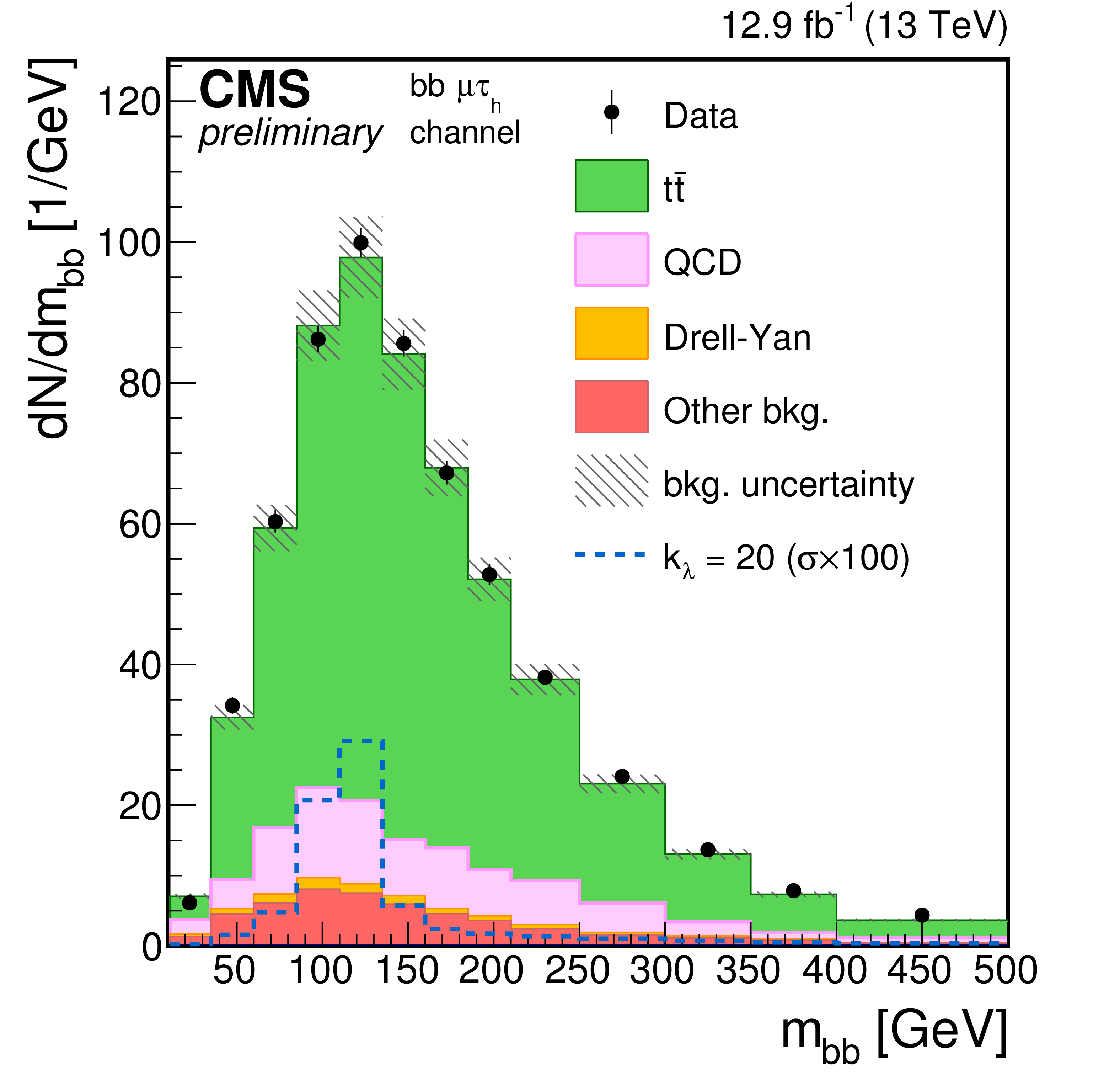
Additional Figure 1-b:
Distribution of the invariant mass of the bb pair: bb$\mu \tau _h$ channel. $\tau \tau $ and bb candidates selections are applied but no selection on the invariant mass is requested. Points with error bars represent the data and shaded histograms represent the backgrounds. The dashed blue line is the signal expectation for ${\rm k}_{\lambda } = 20$ and is scaled by a factor 100 for the bb$\mu \tau _h$ and bb${\rm e}\tau _h$ channels and by a factor 10 for the bb$\tau _h\tau _h$ channel. Signal and background histograms are not stacked. |

png pdf |
Additional Figure 1-c:
Distribution of the invariant mass of the $\tau \tau $ pair reconstructed using the SVfit algorithm: bb${\rm e}\tau _h$ channel. $\tau \tau $ and bb candidates selections are applied but no selection on the invariant mass is requested. Points with error bars represent the data and shaded histograms represent the backgrounds. The dashed blue line is the signal expectation for ${\rm k}_{\lambda } = 20$ and is scaled by a factor 100 for the bb$\mu \tau _h$ and bb${\rm e}\tau _h$ channels and by a factor 10 for the bb$\tau _h\tau _h$ channel. Signal and background histograms are not stacked. |
png pdf |
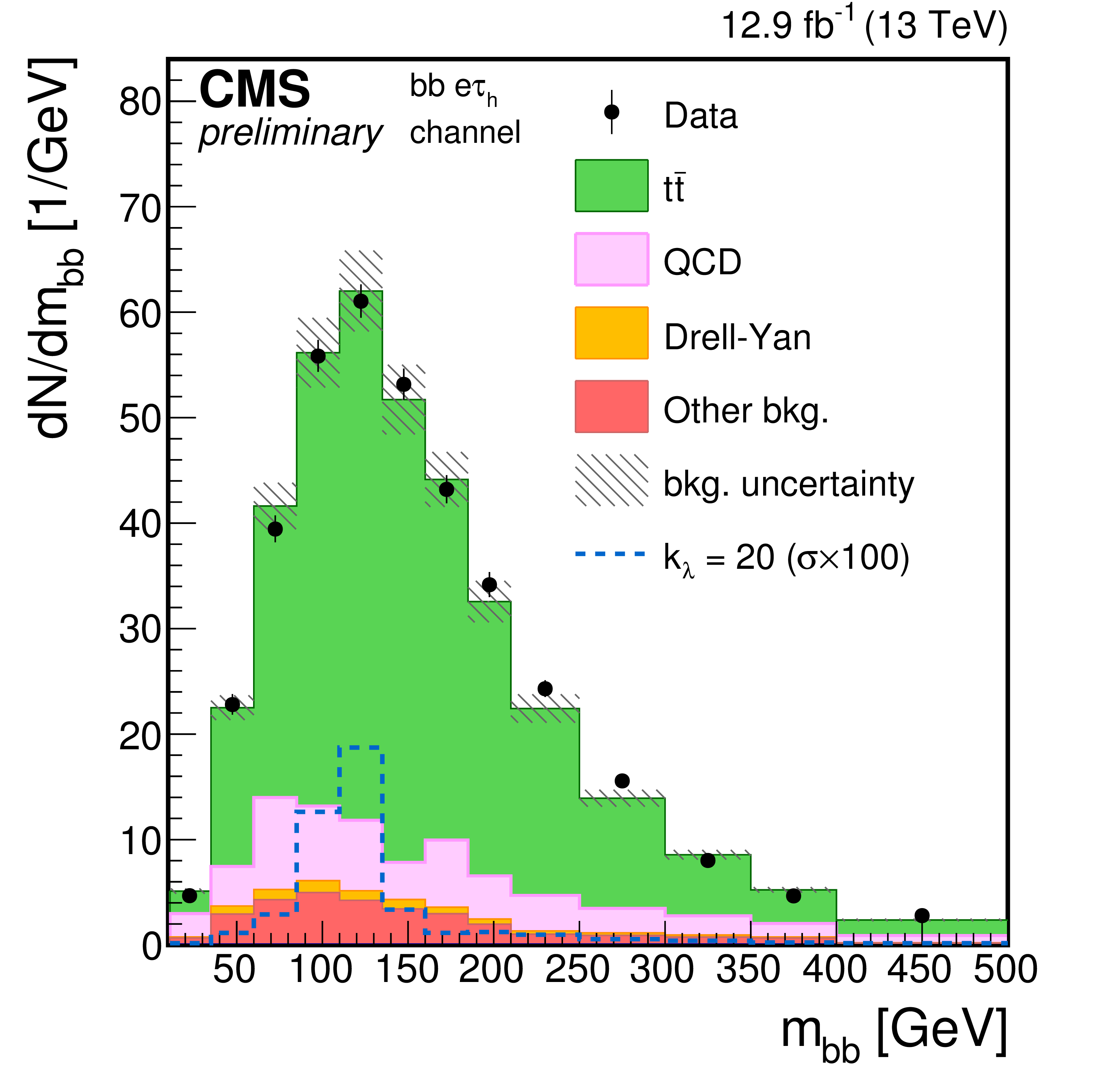
Additional Figure 1-d:
Distribution of the invariant mass of the bb pair: bb${\rm e}\tau _h$ channel. $\tau \tau $ and bb candidates selections are applied but no selection on the invariant mass is requested. Points with error bars represent the data and shaded histograms represent the backgrounds. The dashed blue line is the signal expectation for ${\rm k}_{\lambda } = 20$ and is scaled by a factor 100 for the bb$\mu \tau _h$ and bb${\rm e}\tau _h$ channels and by a factor 10 for the bb$\tau _h\tau _h$ channel. Signal and background histograms are not stacked. |
png pdf |
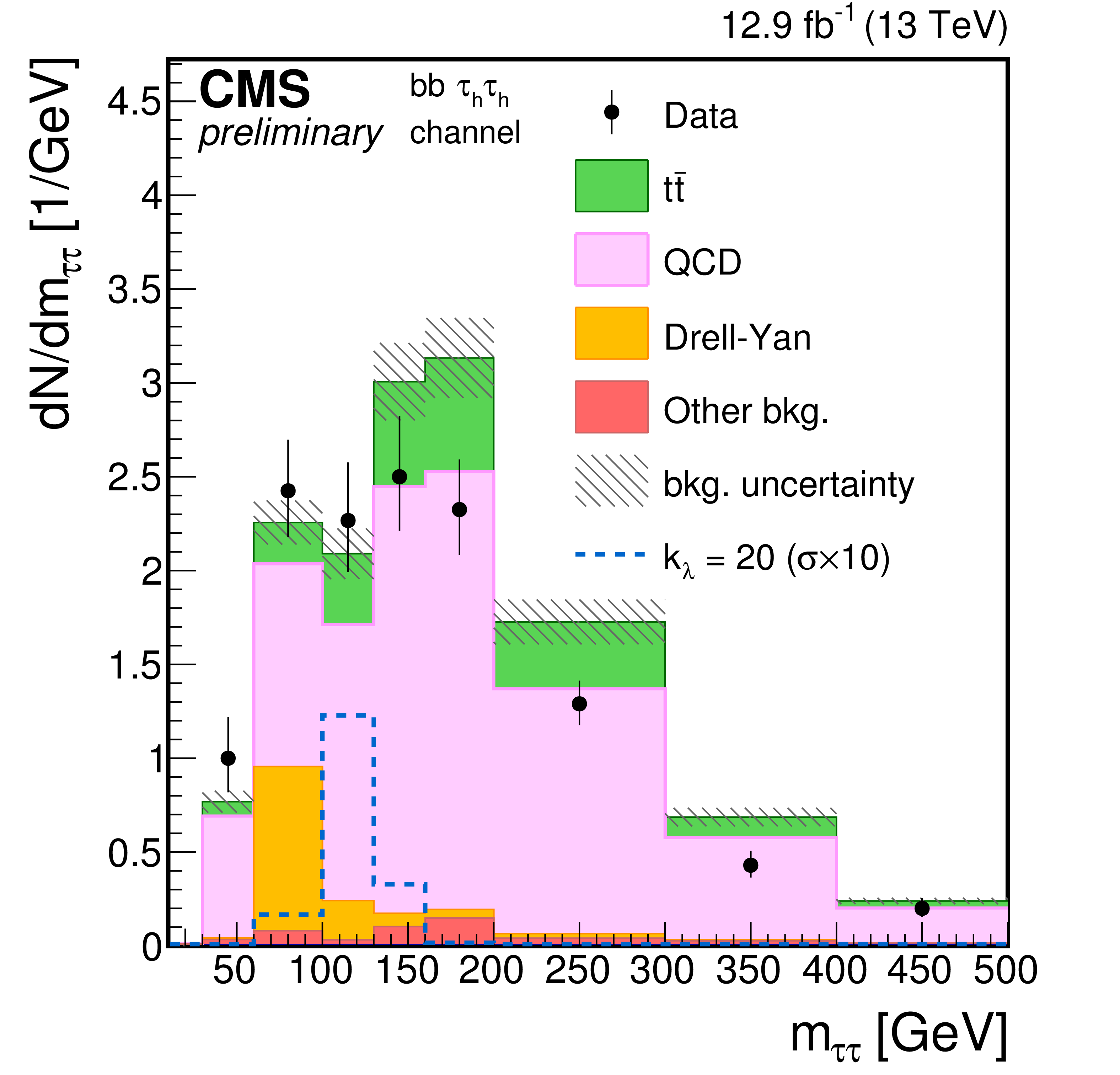
Additional Figure 1-e:
Distribution of the invariant mass of the $\tau \tau $ pair reconstructed using the SVfit algorithm: bb$\tau _h\tau _h$ channel. $\tau \tau $ and bb candidates selections are applied but no selection on the invariant mass is requested. Points with error bars represent the data and shaded histograms represent the backgrounds. The dashed blue line is the signal expectation for ${\rm k}_{\lambda } = 20$ and is scaled by a factor 100 for the bb$\mu \tau _h$ and bb${\rm e}\tau _h$ channels and by a factor 10 for the bb$\tau _h\tau _h$ channel. Signal and background histograms are not stacked. |

png pdf |
Additional Figure 1-f:
Distribution of the invariant mass of the bb pair: bb$\tau _h\tau _h$ channel. $\tau \tau $ and bb candidates selections are applied but no selection on the invariant mass is requested. Points with error bars represent the data and shaded histograms represent the backgrounds. The dashed blue line is the signal expectation for ${\rm k}_{\lambda } = 20$ and is scaled by a factor 100 for the bb$\mu \tau _h$ and bb${\rm e}\tau _h$ channels and by a factor 10 for the bb$\tau _h\tau _h$ channel. Signal and background histograms are not stacked. |

png pdf |
Additional Figure 2:
Distribution of the input variables of the BDT discriminant. (a) : $\Delta \varphi ({\rm h}_{\rm bb},h_{\tau \tau })$, (b) : $\Delta \varphi ({\rm h}_{\tau \tau }, {E_{\mathrm {T}}^{\text {miss}}} )$, (c) : $\Delta \varphi ({\rm h}_{\rm bb}, {E_{\mathrm {T}}^{\text {miss}}} )$, (d) : $\Delta R(\mu ,\tau _{\rm h})$, and (e) : $\Delta R({\rm b},{\rm b})$ . The distributions are shown for the bb$\mu \tau _{\rm h}$ channel after the candidate selection and before the application of the invariant mass requirement. Points with error bars represent the data and shaded histograms represent the backgrounds. The dashed blue line is the signal expectation for ${\rm k}_{\lambda } = 20$ and the solid black line is the signal expectation for ${\rm k}_{\lambda } = 1$, and they are scaled respectively by a factor 100 and 5000. Signal and background histograms are not stacked. The bottom panel shows the ratio of the observed data to the simulation prediction. |
png pdf |
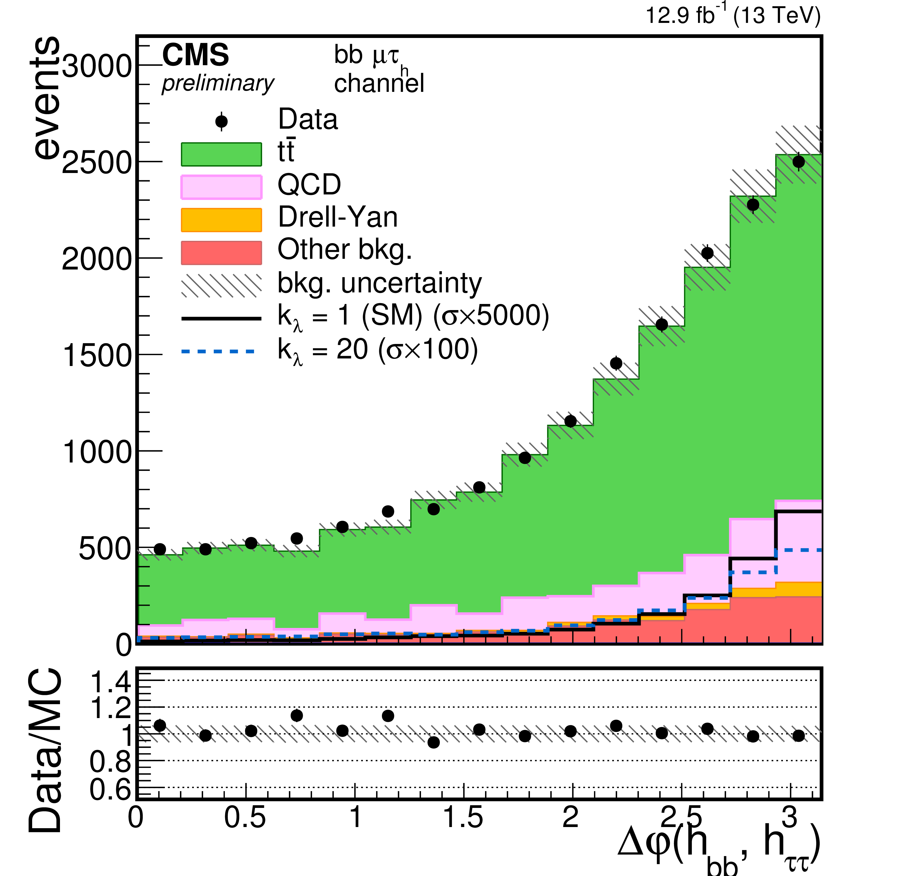
Additional Figure 2-a:
Distribution of the $\Delta \varphi ({\rm h}_{\rm bb},h_{\tau \tau })$ input variable of the BDT discriminant. The distributions are shown for the bb$\mu \tau _{\rm h}$ channel after the candidate selection and before the application of the invariant mass requirement. Points with error bars represent the data and shaded histograms represent the backgrounds. The dashed blue line is the signal expectation for ${\rm k}_{\lambda } = 20$ and the solid black line is the signal expectation for ${\rm k}_{\lambda } = 1$, and they are scaled respectively by a factor 100 and 5000. Signal and background histograms are not stacked. The bottom panel shows the ratio of the observed data to the simulation prediction. |
png pdf |
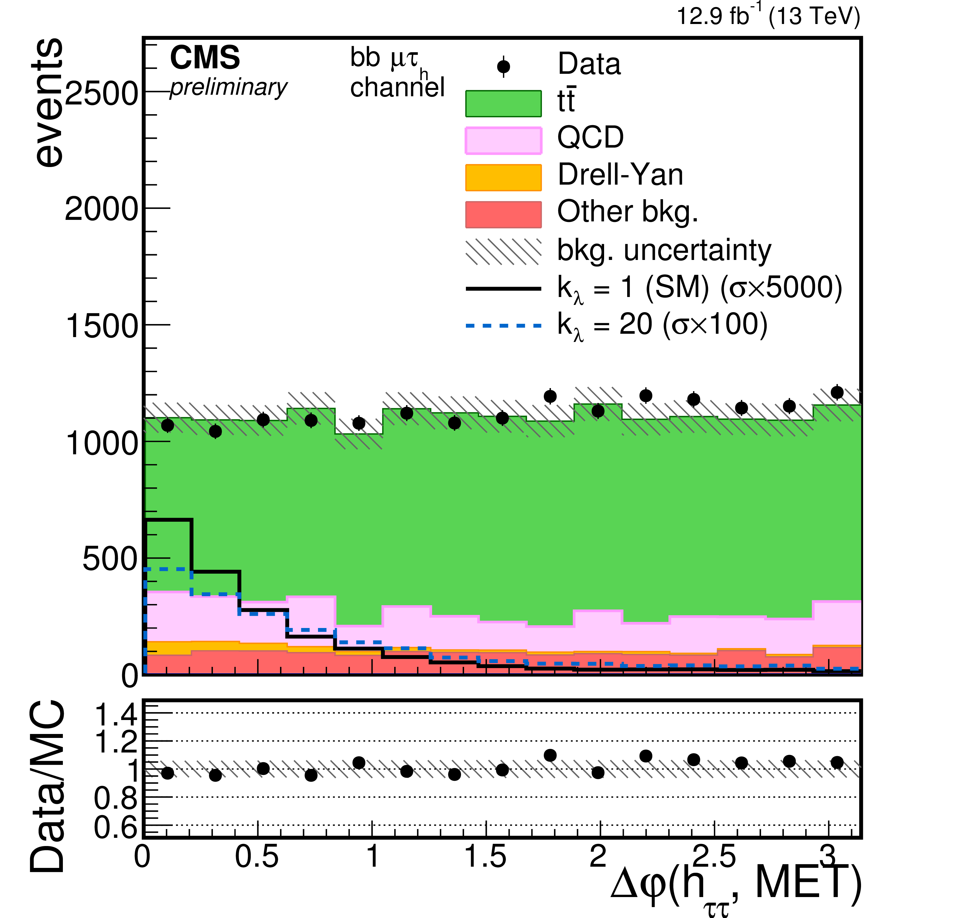
Additional Figure 2-b:
Distribution of the $\Delta \varphi ({\rm h}_{\tau \tau }, {E_{\mathrm {T}}^{\text {miss}}} )$ input variable of the BDT discriminant. The distributions are shown for the bb$\mu \tau _{\rm h}$ channel after the candidate selection and before the application of the invariant mass requirement. Points with error bars represent the data and shaded histograms represent the backgrounds. The dashed blue line is the signal expectation for ${\rm k}_{\lambda } = 20$ and the solid black line is the signal expectation for ${\rm k}_{\lambda } = 1$, and they are scaled respectively by a factor 100 and 5000. Signal and background histograms are not stacked. The bottom panel shows the ratio of the observed data to the simulation prediction. |
png pdf |
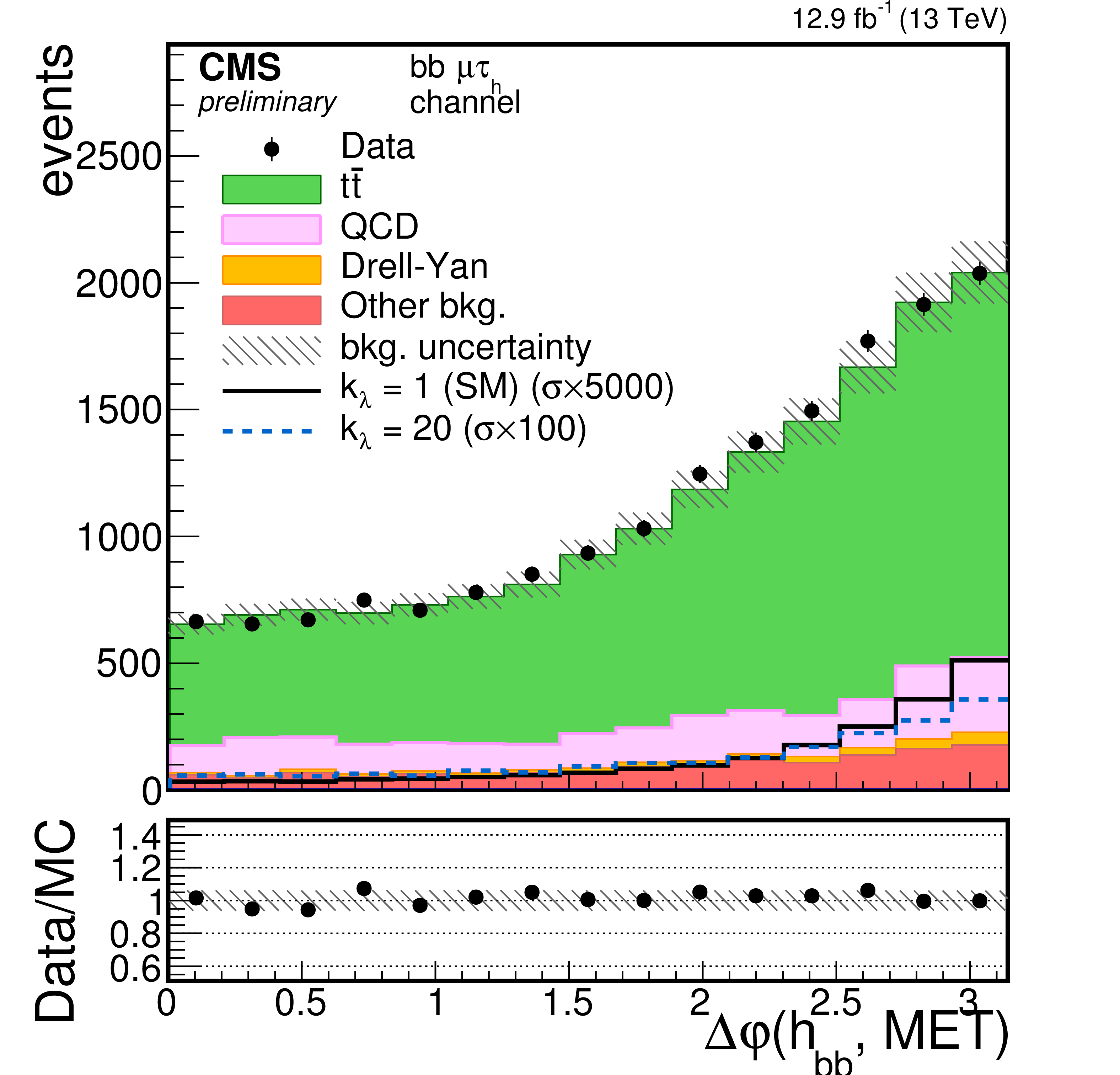
Additional Figure 2-c:
Distribution of the $\Delta \varphi ({\rm h}_{\rm bb}, {E_{\mathrm {T}}^{\text {miss}}} )$ input variable of the BDT discriminant. The distributions are shown for the bb$\mu \tau _{\rm h}$ channel after the candidate selection and before the application of the invariant mass requirement. Points with error bars represent the data and shaded histograms represent the backgrounds. The dashed blue line is the signal expectation for ${\rm k}_{\lambda } = 20$ and the solid black line is the signal expectation for ${\rm k}_{\lambda } = 1$, and they are scaled respectively by a factor 100 and 5000. Signal and background histograms are not stacked. The bottom panel shows the ratio of the observed data to the simulation prediction. |

png pdf |
Additional Figure 2-d:
Distribution of the $\Delta R(\mu ,\tau _{\rm h})$ input variable of the BDT discriminant. The distributions are shown for the bb$\mu \tau _{\rm h}$ channel after the candidate selection and before the application of the invariant mass requirement. Points with error bars represent the data and shaded histograms represent the backgrounds. The dashed blue line is the signal expectation for ${\rm k}_{\lambda } = 20$ and the solid black line is the signal expectation for ${\rm k}_{\lambda } = 1$, and they are scaled respectively by a factor 100 and 5000. Signal and background histograms are not stacked. The bottom panel shows the ratio of the observed data to the simulation prediction. |
png pdf |
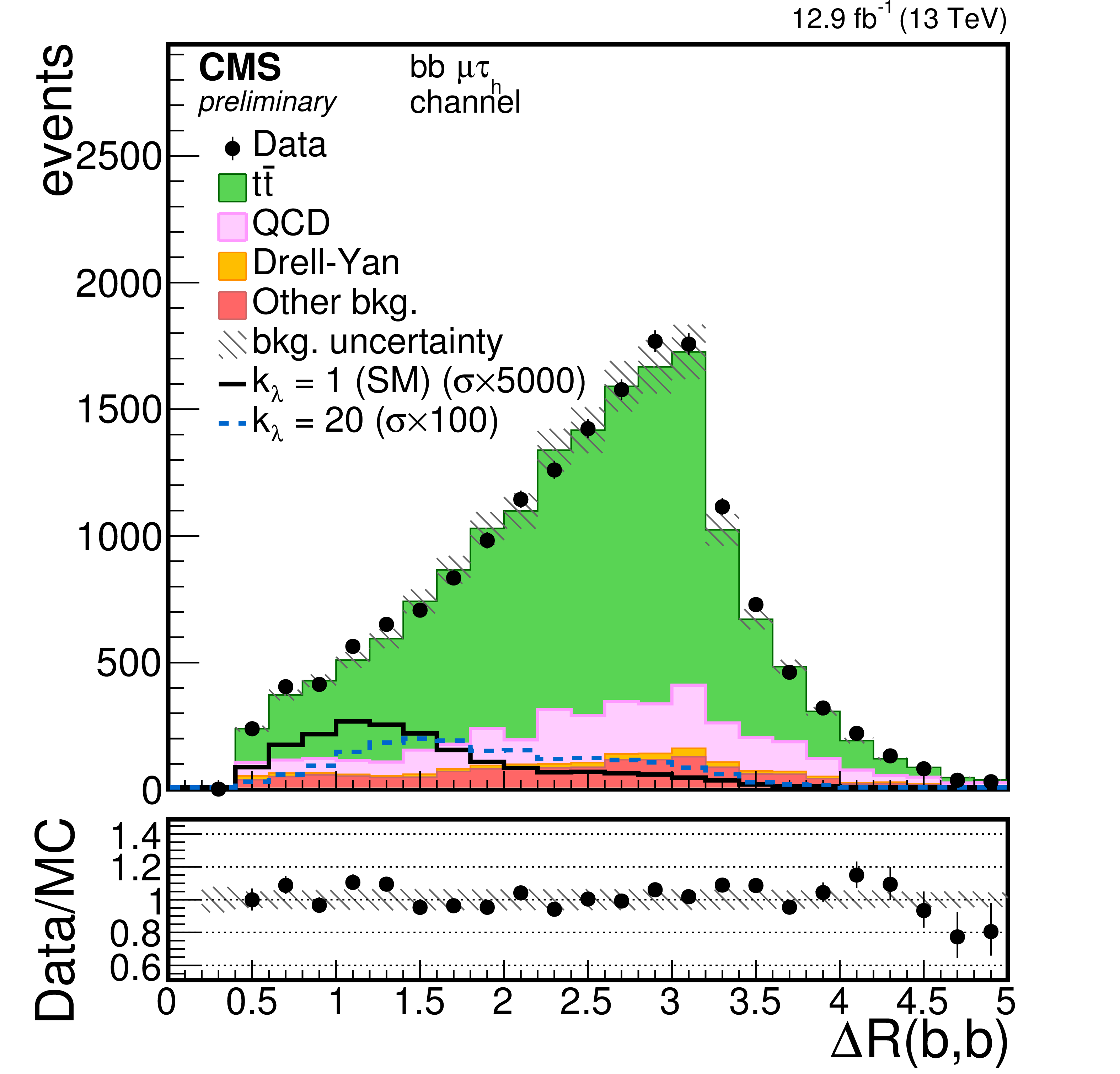
Additional Figure 2-e:
Distribution of the $\Delta R({\rm b},{\rm b})$ input variable of the BDT discriminant. The distributions are shown for the bb$\mu \tau _{\rm h}$ channel after the candidate selection and before the application of the invariant mass requirement. Points with error bars represent the data and shaded histograms represent the backgrounds. The dashed blue line is the signal expectation for ${\rm k}_{\lambda } = 20$ and the solid black line is the signal expectation for ${\rm k}_{\lambda } = 1$, and they are scaled respectively by a factor 100 and 5000. Signal and background histograms are not stacked. The bottom panel shows the ratio of the observed data to the simulation prediction. |
png pdf |
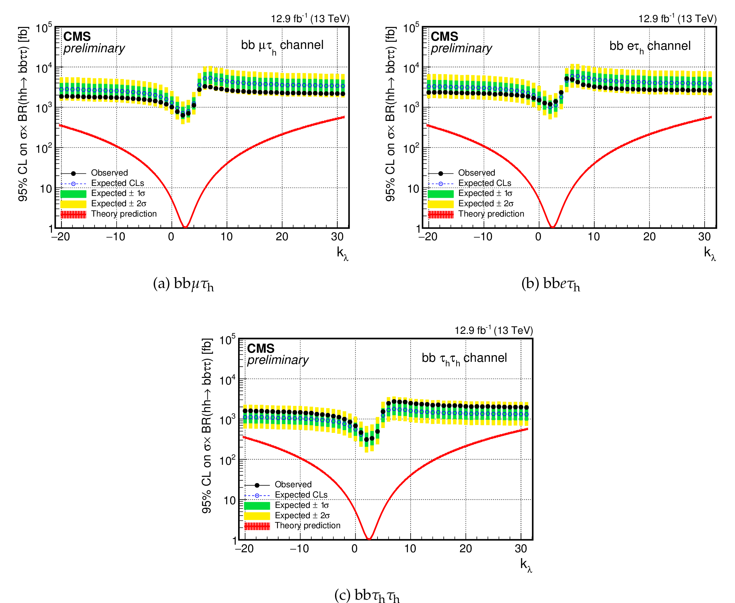
Additional Figure 3:
Observed and expected 95% CL upper limits on the hh cross section times bb$\tau \tau $ branching ratio as a function of the ratio of the anomalous trilinear Higgs boson coupling to the SM trilinear Higgs boson coupling (${\rm k}_\lambda = \lambda _{\rm hhh}/\lambda ^{\rm SM}_{\rm hhh}$). The plots are shown for (a) bb$\mu \tau _{\rm h}$ , (b) bb$e\tau _{\rm h}$ , and (c) bb$\tau _{\rm h}\tau _{\rm h}$ channels. The red band shows the theoretical cross section expectation and its systematic uncertainty. |

png pdf |
Additional Figure 3-a:
Observed and expected 95% CL upper limits on the hh cross section times bb$\tau \tau $ branching ratio as a function of the ratio of the anomalous trilinear Higgs boson coupling to the SM trilinear Higgs boson coupling (${\rm k}_\lambda = \lambda _{\rm hhh}/\lambda ^{\rm SM}_{\rm hhh}$), for the bb$\mu \tau _{\rm h}$ channel. The red band shows the theoretical cross section expectation and its systematic uncertainty. |
png pdf |
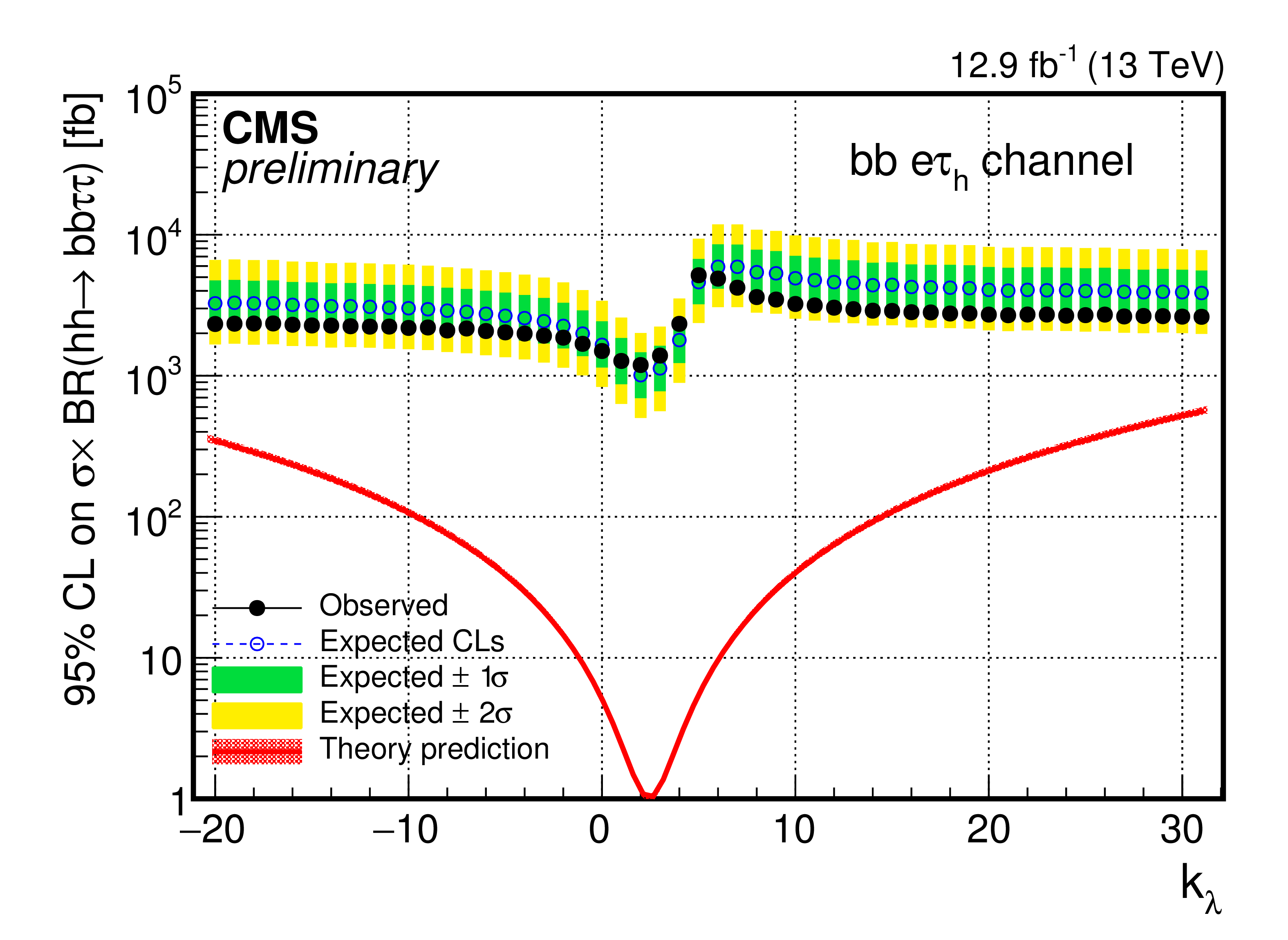
Additional Figure 3-b:
Observed and expected 95% CL upper limits on the hh cross section times bb$\tau \tau $ branching ratio as a function of the ratio of the anomalous trilinear Higgs boson coupling to the SM trilinear Higgs boson coupling (${\rm k}_\lambda = \lambda _{\rm hhh}/\lambda ^{\rm SM}_{\rm hhh}$), for the bb$e\tau _{\rm h}$ channel. The red band shows the theoretical cross section expectation and its systematic uncertainty. |
png pdf |
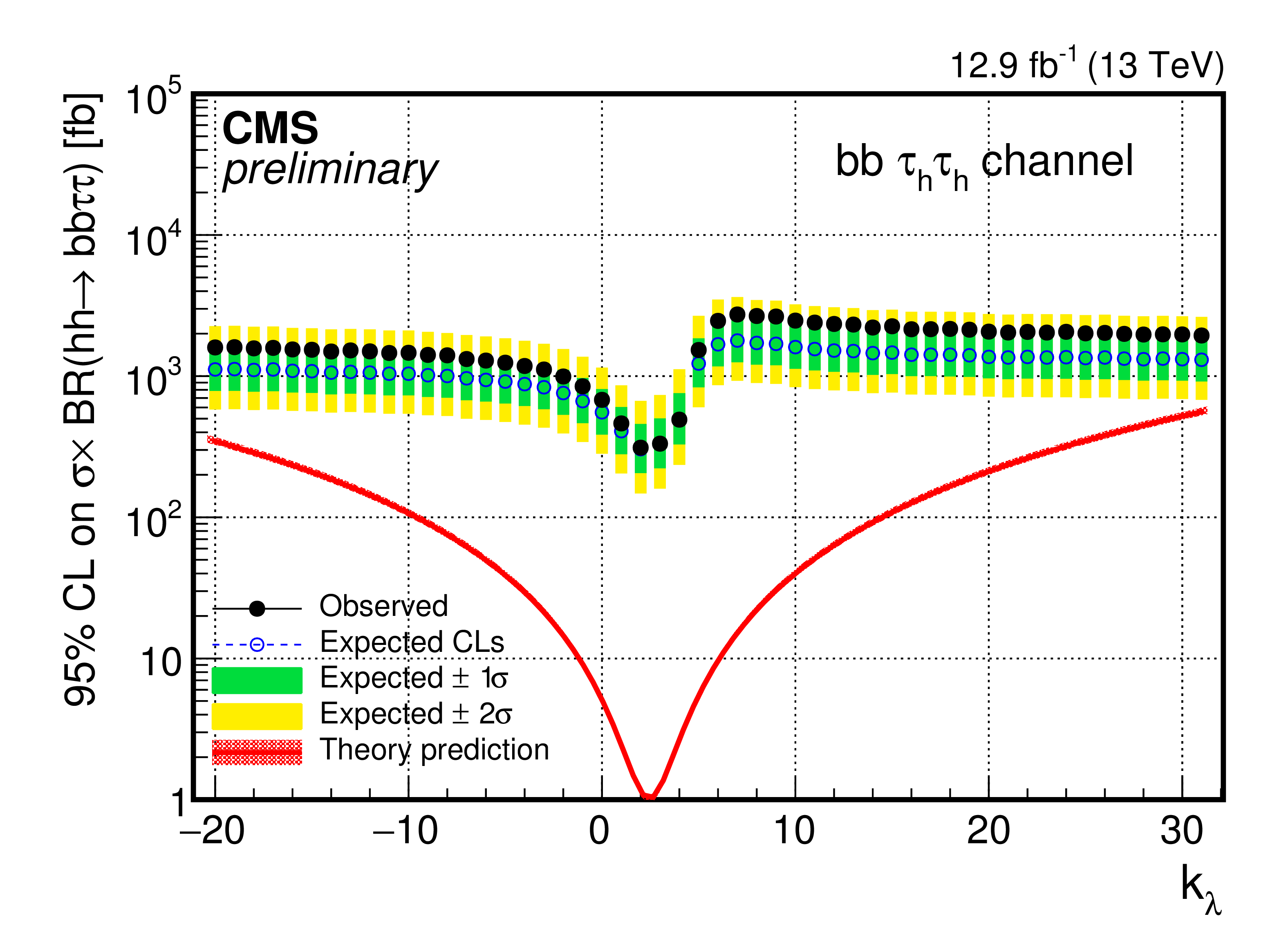
Additional Figure 3-c:
Observed and expected 95% CL upper limits on the hh cross section times bb$\tau \tau $ branching ratio as a function of the ratio of the anomalous trilinear Higgs boson coupling to the SM trilinear Higgs boson coupling (${\rm k}_\lambda = \lambda _{\rm hhh}/\lambda ^{\rm SM}_{\rm hhh}$), for the bb$\tau _{\rm h}\tau _{\rm h}$ channel. The red band shows the theoretical cross section expectation and its systematic uncertainty. |
png pdf |
Additional Figure 4:
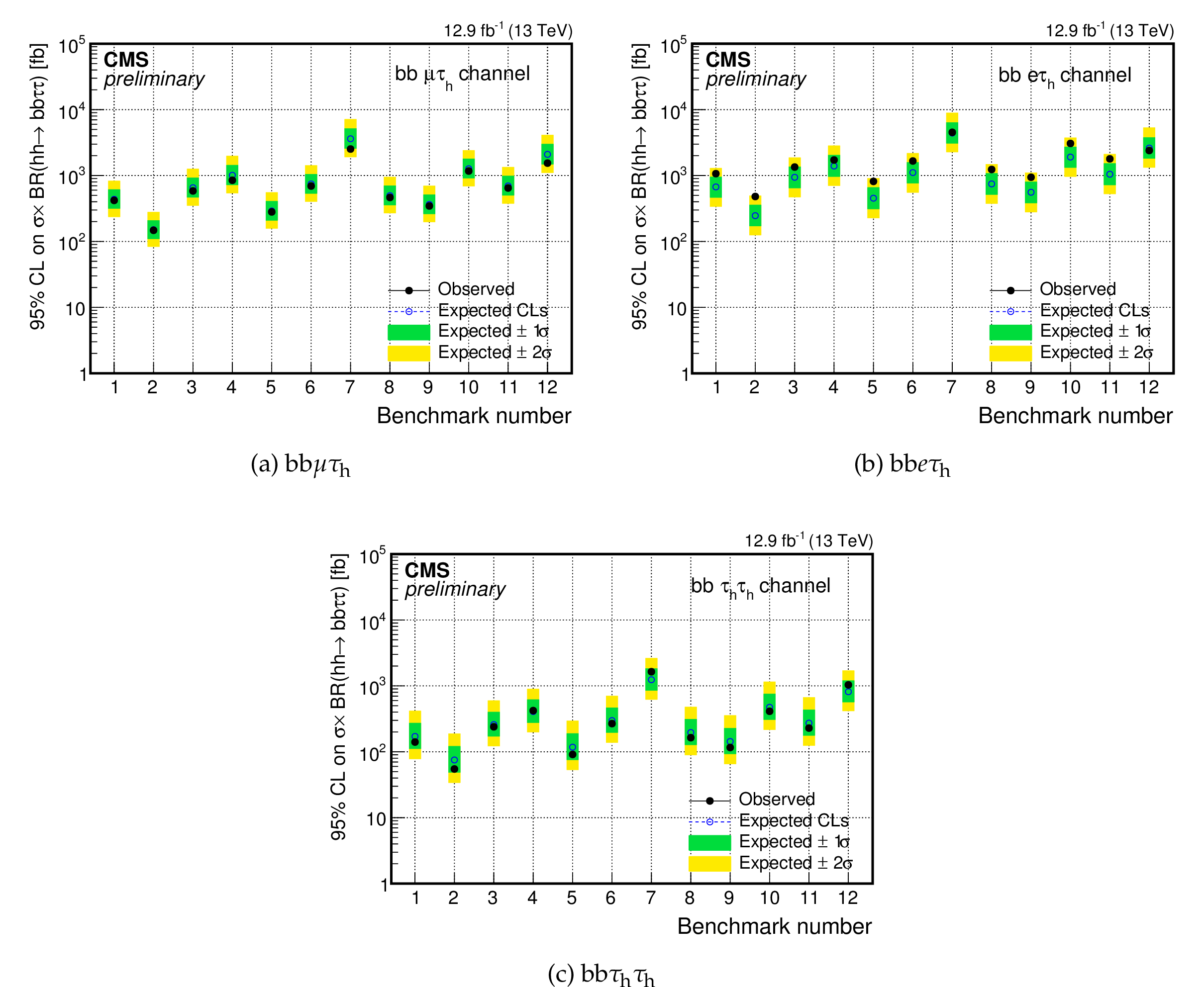
Observed and expected 95% CL upper limits on the hh cross section times bb$\tau \tau $ branching ratio for the 12 shape benchmarks. The plots are shown for (a) bb$\mu \tau _{\rm h}$ , (b) bb$e\tau _{\rm h}$ , and (c) bb$\tau _{\rm h}\tau _{\rm h}$ channels. |
png pdf |
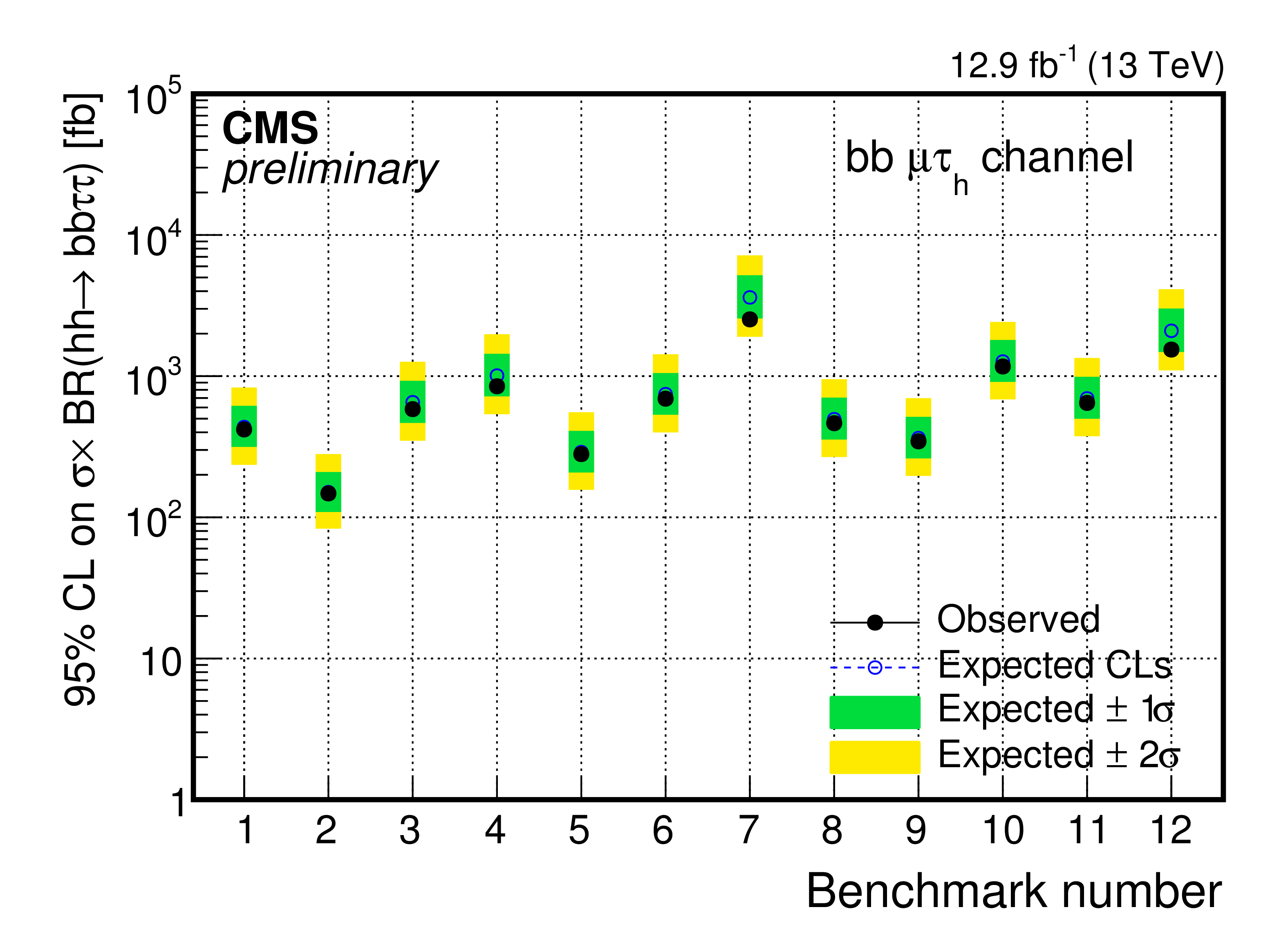
Additional Figure 4-a:
Observed and expected 95% CL upper limits on the hh cross section times bb$\tau \tau $ branching ratio for the 12 shape benchmarks, for the bb$\mu \tau _{\rm h}$ channel. |

png pdf |
Additional Figure 4-b:
Observed and expected 95% CL upper limits on the hh cross section times bb$\tau \tau $ branching ratio for the 12 shape benchmarks, for the bb$e\tau _{\rm h}$ channel. |

png pdf |
Additional Figure 4-c:
Observed and expected 95% CL upper limits on the hh cross section times bb$\tau \tau $ branching ratio for the 12 shape benchmarks, for the bb$\tau _{\rm h}\tau _{\rm h}$ channel. |
png pdf |
Additional Figure 5:
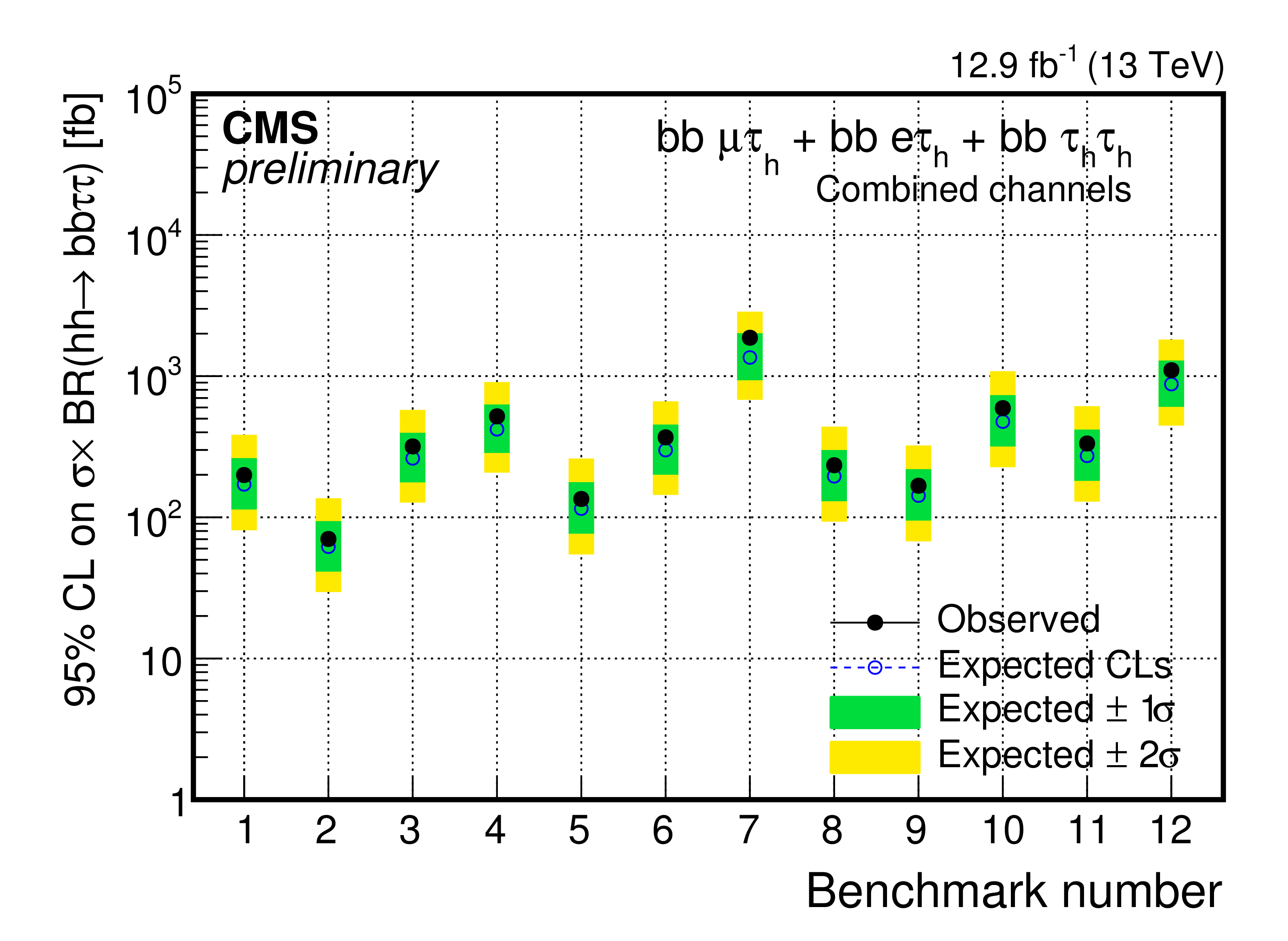
Observed and expected 95% CL upper limits on cross section times branching ratio for the 12 shape benchmarks combining all the final states. |
png pdf |
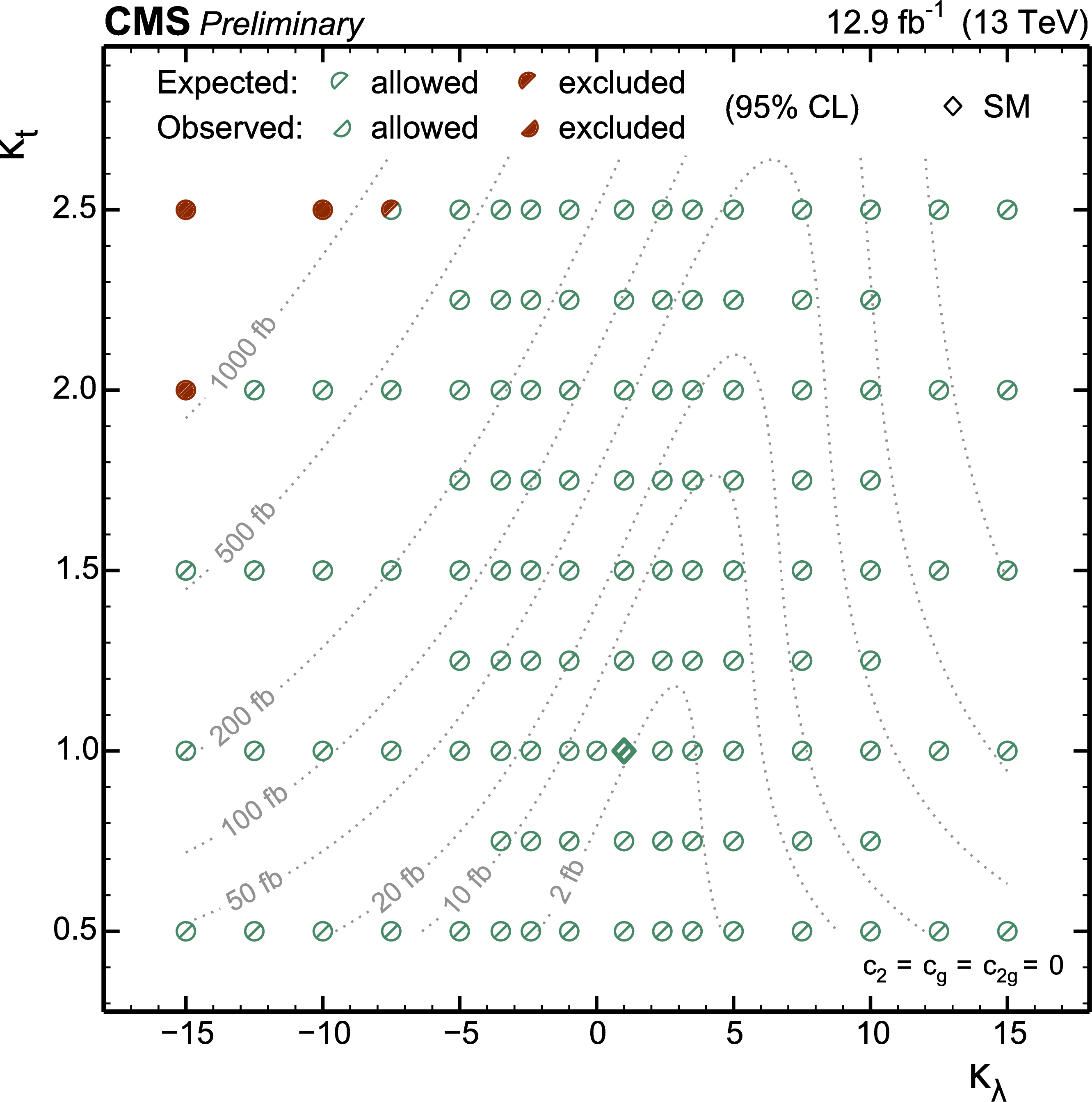
Additional Figure 6:
Exclusion of Higgs boson pair production in the EFT parametrization as a function of the coupling modifiers ${\rm k}_{\lambda }$ and ${\rm k}_{\rm t}$, fixing the other EFT parameters to ${c_g = c_{2g} = c_2 = 0}$. Each marker denotes a point in the bidimensional (${\rm k}_{\lambda },{\rm k}_{\rm t}$) plane for which the corresponding prediction has been tested with the available data. Open green semicircles denote points compatible with the current data while red full semicircles denote points excluded with the current data. The two halves of the circles denote the expected and observed exclusion as reported in the plot legend. The diamond shaped marker refers to the prediction of the SM. The dotted lines indicate trajectories in the plane with equal Higgs boson pair production cross section and are labeled with the corresponding value of $\sigma ({\rm gg\rightarrow hh}) \times {\rm BR} ({\rm hh}\rightarrow {\rm bb}\tau \tau )$. |
| References | ||||
| 1 | ATLAS Collaboration | Observation of a new particle in the search for the Standard Model Higgs boson with the ATLAS detector at the LHC | Physics Letters B 716 (2012), no. 1, 1 -- 29 | |
| 2 | CMS Collaboration | Observation of a new boson at a mass of 125 GeV with the CMS experiment at the LHC | Physics Letters B 716 (2012), no. 1, 30 -- 61 | |
| 3 | ATLAS, CMS Collaboration | Combined Measurement of the Higgs Boson Mass in $ pp $ Collisions at $ \sqrt{s}=7 $ and 8 TeV with the ATLAS and CMS Experiments | PRL 114 (2015) 191803 | 1503.07589 |
| 4 | CMS Collaboration | Measurements of the Higgs boson production and decay rates and constraints on its couplings from a combined ATLAS and CMS analysis of the LHC pp collision data at $ \sqrt{s} $ = 7 and 8 TeV | CMS-PAS-HIG-15-002 | CMS-PAS-HIG-15-002 |
| 5 | S. Dawson, A. Ismail, and I. Low | What's in the loop? The anatomy of double Higgs production | PRD91 (2015), no. 11, 115008 | 1504.05596 |
| 6 | CMS Collaboration | Search for resonant Higgs boson pair production in the $ \mathrm{b\overline{b}}\tau^+\tau^- $ final state | ||
| 7 | ATLAS Collaboration | Searches for Higgs boson pair production in the $ hh\to bb\tau\tau, \gamma\gamma WW^*, \gamma\gamma bb, bbbb $ channels with the ATLAS detector | PRD92 (2015) 092004 | 1509.04670 |
| 8 | CMS Collaboration | Model independent search for Higgs boson pair production in the $ \mathrm{b\overline{b}}\tau^+\tau^- $ final state | CMS-PAS-HIG-15-013 | CMS-PAS-HIG-15-013 |
| 9 | CMS Collaboration Collaboration | Search for non-resonant Higgs boson pair production in the $ \mathrm{b\overline{b}}\tau^+\tau^- $ final state | ||
| 10 | CMS Collaboration | The CMS experiment at the CERN LHC | JINST 3 (2008) S08004 | CMS-00-001 |
| 11 | J. Alwall et al. | The automated computation of tree-level and next-to-leading order differential cross sections, and their matching to parton shower simulations | JHEP 07 (2014) 079 | 1405.0301 |
| 12 | A. Carvalho Antunes De Oliveira et al. | Analytical parametrization and shape classification of anomalous HH production in EFT approach | LHCHXSWG report LHCHXSWG-2016-001, CERN, Geneva, Jul | |
| 13 | B. Mellado Garcia, P. Musella, M. Grazzini, and R. Harlander | CERN Report 4: Part I Standard Model Predictions | CERN Report LHCHXSWG-DRAFT-INT-2016-008, May | |
| 14 | S. Dawson, S. Dittmaier, and M. Spira | Neutral Higgs boson pair production at hadron colliders: QCD corrections | PRD58 (1998) 115012 | hep-ph/9805244 |
| 15 | D. de Florian and J. Mazzitelli | Higgs Boson Pair Production at Next-to-Next-to-Leading Order in QCD | PRL 111 (2013) 201801 | 1309.6594 |
| 16 | D. de Florian and J. Mazzitelli | Higgs pair production at next-to-next-to-leading logarithmic accuracy at the LHC | JHEP 09 (2015) 053 | 1505.07122 |
| 17 | S. Borowka et al. | Higgs boson pair production in gluon fusion at NLO with full top-quark mass dependence | 1604.06447 | |
| 18 | J. Butterworth et al. | PDF4LHC recommendations for LHC Run II | 1510.03865 | |
| 19 | A. Carvalho et al. | Higgs Pair Production: Choosing Benchmarks With Cluster Analysis | JHEP 04 (2016) 126 | 1507.02245 |
| 20 | S. Alioli, P. Nason, C. Oleari, and E. Re | NLO single-top production matched with shower in POWHEG: s- and t-channel contributions | JHEP 09 (2009) 111, , [Erratum: JHEP02,011(2010)] | 0907.4076 |
| 21 | J. M. Campbell, R. K. Ellis, P. Nason, and E. Re | Top-pair production and decay at NLO matched with parton showers | JHEP 04 (2015) 114 | 1412.1828 |
| 22 | M. Czakon and A. Mitov | Top++: A Program for the Calculation of the Top-Pair Cross-Section at Hadron Colliders | CPC 185 (2014) 2930 | 1112.5675 |
| 23 | T. Sjostrand, S. Mrenna, and P. Z. Skands | A Brief Introduction to PYTHIA 8.1 | CPC 178 (2008) 852--867 | 0710.3820 |
| 24 | CMS Collaboration | Particle--flow event reconstruction in CMS and performance for jets, taus, and $ E_{\mathrm{T}}^{\text{miss}} $ | CDS | |
| 25 | CMS Collaboration | Commissioning of the particle-flow event reconstruction with the first LHC collisions recorded in the CMS detector | CDS | |
| 26 | K. Rose | Deterministic annealing for clustering, compression, classification, regression and related optimisation problems | in Proceedings of the IEEE, volume 86, p. 86 1998 | |
| 27 | W. Waltenberger, R. Fr\"uhwirth, and P. Vanlaer | Adaptive vertex fitting | JPG 34 (2007) N343 | |
| 28 | CMS Collaboration | Performance of electron reconstruction and selection with the CMS detector in proton-proton collisions at $ \sqrt{s} $ = 8 TeV | JINST 10 (2015), no. 06, P06005 | CMS-EGM-13-001 1502.02701 |
| 29 | A. Hocker et al. | TMVA - Toolkit for Multivariate Data Analysis | PoS ACAT (2007) 040 | physics/0703039 |
| 30 | CMS Collaboration | Performance of CMS muon reconstruction in $ pp $ collision events at $ \sqrt{s}=7 $ TeV | JINST 7 (2012) P10002 | CMS-MUO-10-004 1206.4071 |
| 31 | M. Cacciari, G. P. Salam, and G. Soyez | The anti-$ k_t $ jet clustering algorithm | JHEP 04 (2008) 063 | 0802.1189 |
| 32 | M. Cacciari, G. P. Salam, and G. Soyez | FastJet user manual | EPJC 72 (2012) 1896 | 1111.6097 |
| 33 | CMS Collaboration | Algorithms for b Jet identification in CMS | CDS | |
| 34 | CMS Collaboration | Performance of tau-lepton reconstruction and identification in CMS | JINST 7 (2012) P01001 | CMS-TAU-11-001 1109.6034 |
| 35 | CMS Collaboration | Reconstruction and identification of $ \tau $ lepton decays to hadrons and $ \nu_\tau $ at CMS | CMS-TAU-14-001 1510.07488 |
|
| 36 | L. Bianchini, J. Conway, E. K. Friis, and C. Veelken | Reconstruction of the Higgs mass in H to tautau Events by Dynamical Likelihood techniques | Journal of Physics: Conference Series 513 (2014), no. 2, 022035 | |
| 37 | CMS Collaboration | Measurement of the inclusive and differential tt production cross sections in lepton + jets final states at 13 TeV | CMS-PAS-TOP-15-005 | CMS-PAS-TOP-15-005 |
| 38 | CMS Collaboration | Performance of reconstruction and identification of tau leptons in their decays to hadrons and tau neutrino in LHC Run-2 | CMS-PAS-TAU-16-002 | CMS-PAS-TAU-16-002 |
|
|
Compact Muon Solenoid LHC, CERN |
|

|

|

|

|

|