

Compact Muon Solenoid
LHC, CERN
| CMS-PAS-HIG-16-037 | ||
| Search for a neutral MSSM Higgs boson decaying into $\tau\tau$ with 12.9 fb$^{-1}$ of data at $\sqrt{s}= $ 13 TeV | ||
| CMS Collaboration | ||
| November 2016 | ||
| Abstract: A search for a neutral Higgs boson is presented, using the decay into two tau leptons. The analysis uses 12.9 fb$^{-1}$ of pp collision data collected by CMS in 2016, at a centre of mass energy of 13 TeV. The results are interpreted in the context of the minimal supersymmetric standard model. No excess above the expectation from the standard model is found and upper limits are set on the production cross sections times branching fraction for masses between 90 and 3200 GeV. Regions of phase space of two different benchmark scenarios are also excluded. | ||
| Links: CDS record (PDF) ; inSPIRE record ; CADI line (restricted) ; | ||
| Figures & Tables | Summary | Additional Figures & Material | References | CMS Publications |
|---|
| Figures | |
png pdf |
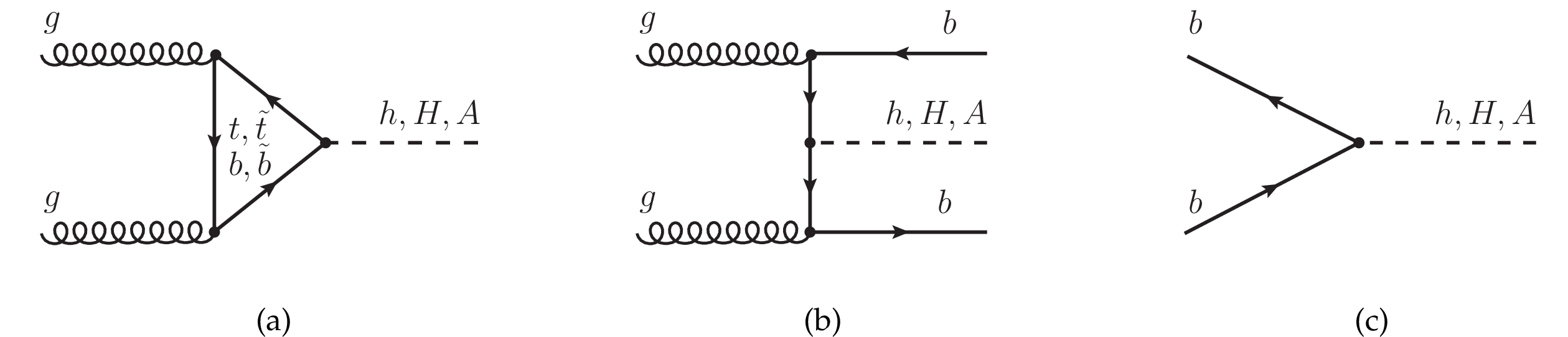
Figure 1:
Leading order diagrams of the a) gluon fusion and b) four-flavour and c) five-flavour schemes for the b associated production of the Higgs boson in the MSSM. |
png pdf |
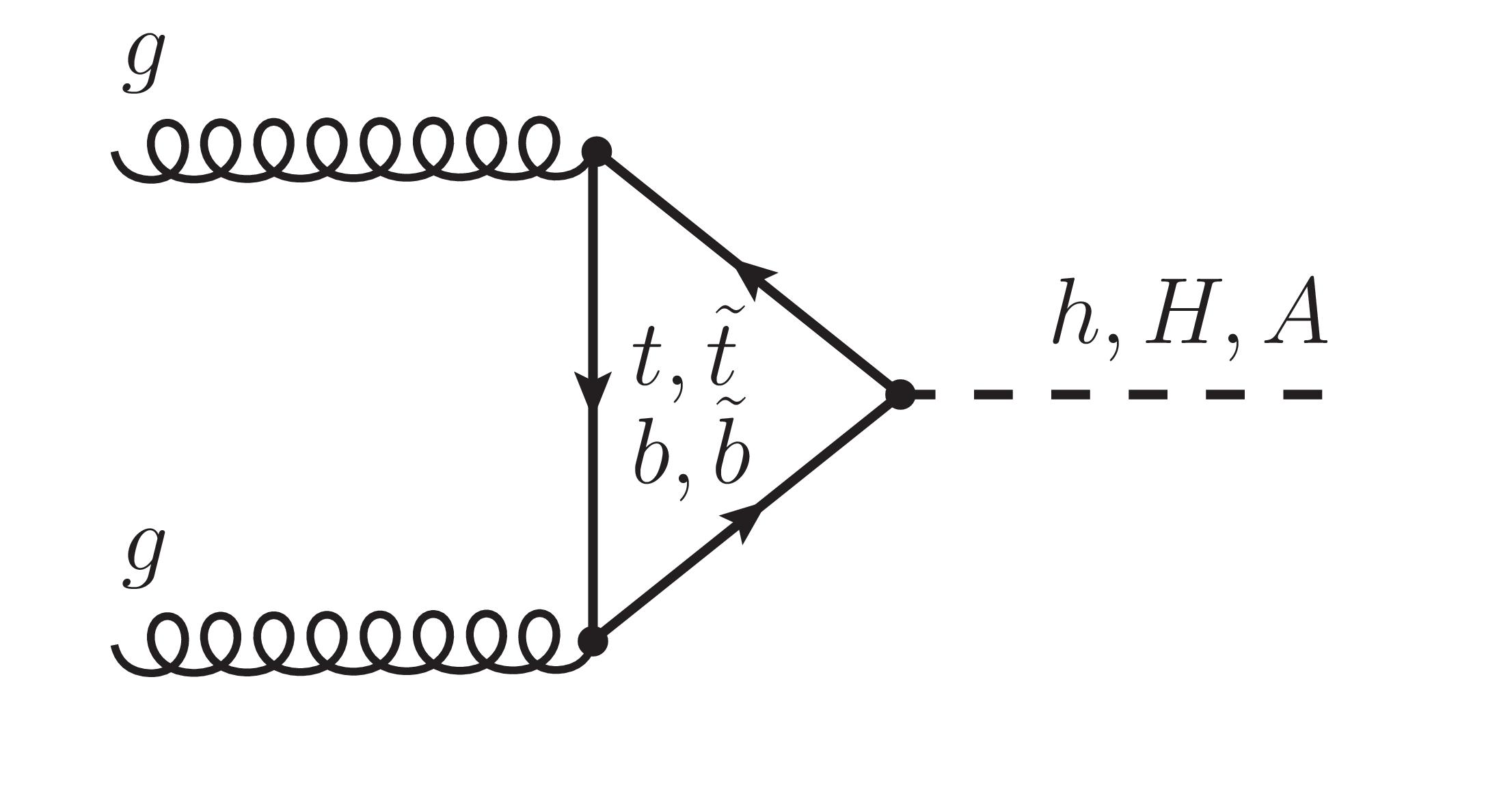
Figure 1-a:
Leading order diagram of the gluon fusion for the production of the Higgs boson in the MSSM. |

png pdf |
Figure 1-b:
Leading order diagram of the four-flavour scheme for the b associated production of the Higgs boson in the MSSM. |

png pdf |
Figure 1-c:
Leading order diagram of the five-flavour scheme for the b associated production of the Higgs boson in the MSSM. |

png pdf |
Figure 2:
Distribution of the transverse mass variable for events in the $\mu \tau _{\rm {h}}$ channel. The yields of all backgrounds are scaled following the final fit described in section 7, except for the W+jets background which is normalized using the high $m_{\mathrm{T}}$ region as indicated (see text). The ``Bkg. uncertainty'' band represents the systematic uncertainty on the background yield as determined in this fit in combination with the statistical uncertainty in each bin. The signal region is defined by $m_{\mathrm{T}} < $ 40 GeV as indicated, while the equivalent cut in the $\mathrm{ e } \tau _{\rm {h}}$ channel is $m_{\mathrm{T}} < $ 50 GeV. |

png pdf |
Figure 3:
Distribution of the $D_{\zeta }$ variable for events in the $\mathrm{ e } \mu $ channel. The yields of all backgrounds are scaled following the final fit described in section 7. The ``Bkg. uncertainty'' band represents the systematic uncertainty on the background yield as determined in this fit in combination with the statistical uncertainty in each bin. The signal region is defined by $D_{\zeta } > -$20 GeV as indicated. |
png pdf |
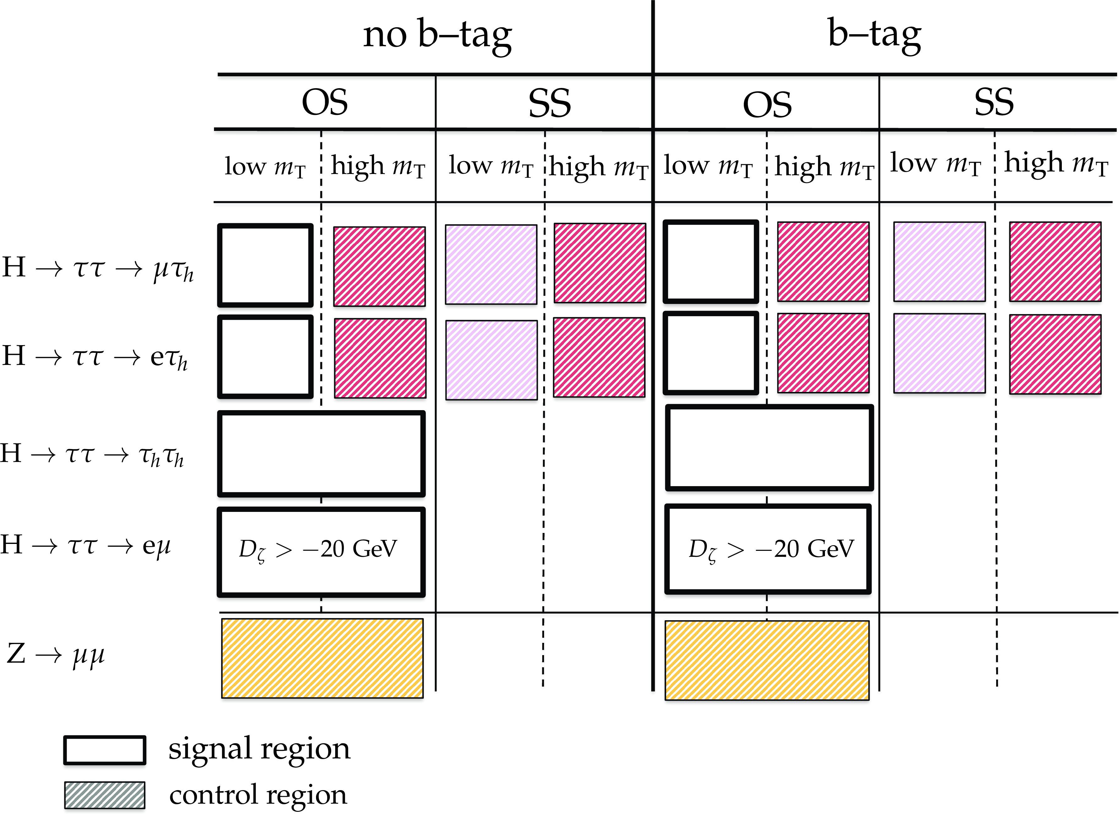
Figure 4:
Illustration of the full set of signal and control regions which are included in the final fit for this analysis described in section 7. In the case of the control regions, the colour indicates which background is most constrained by the region. |

png pdf |
Figure 5:
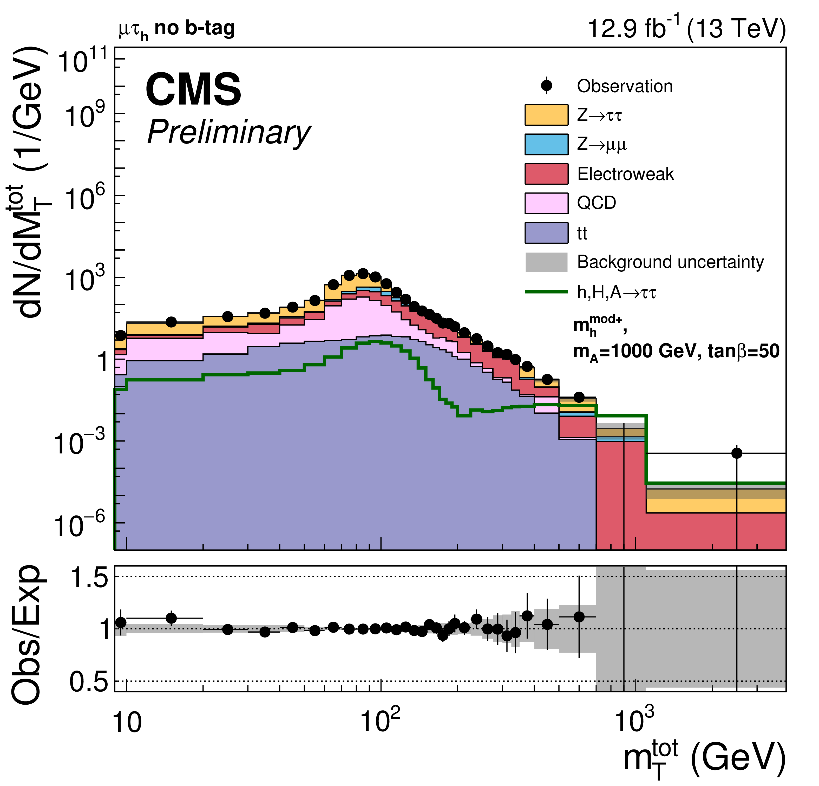
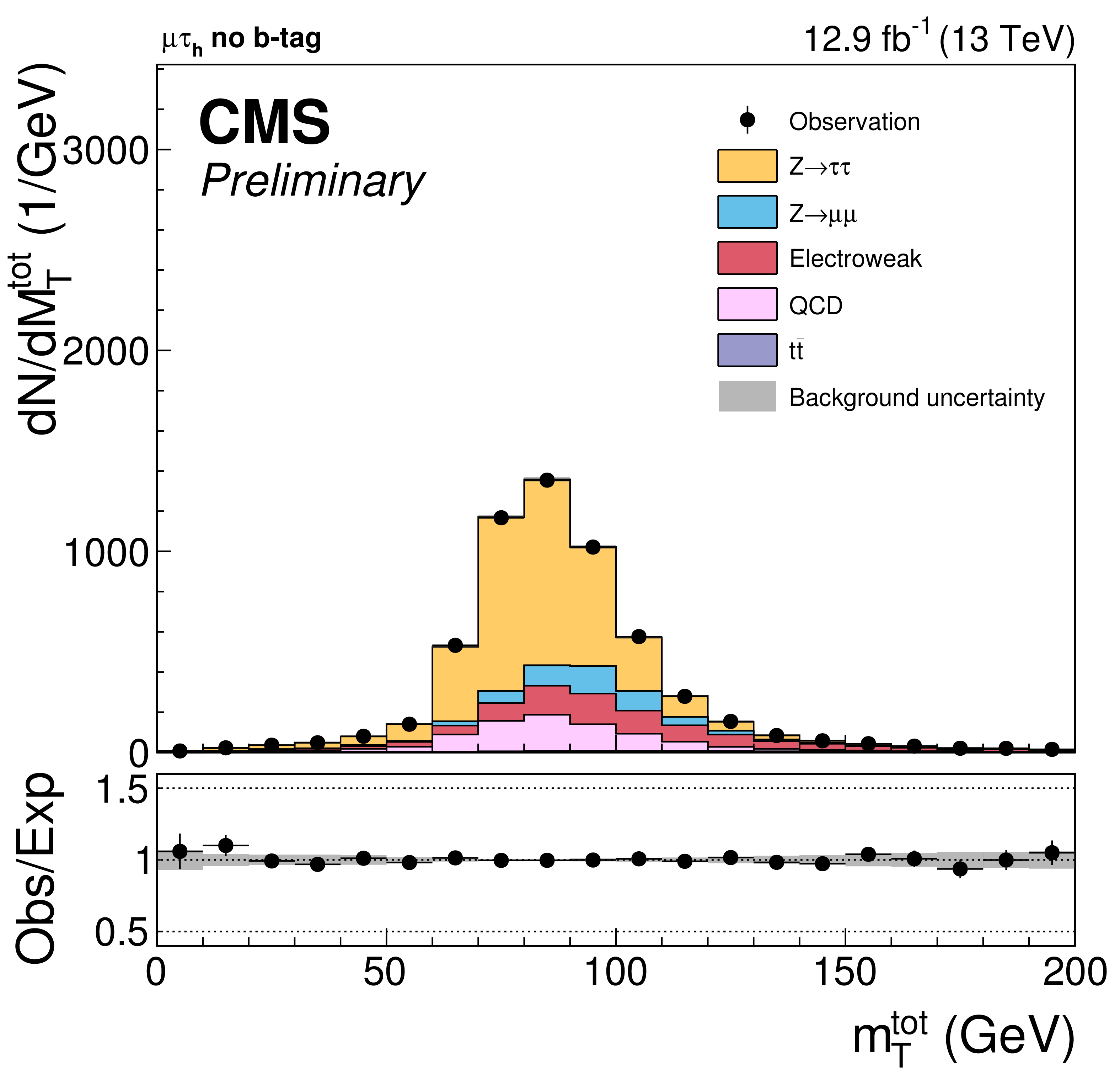
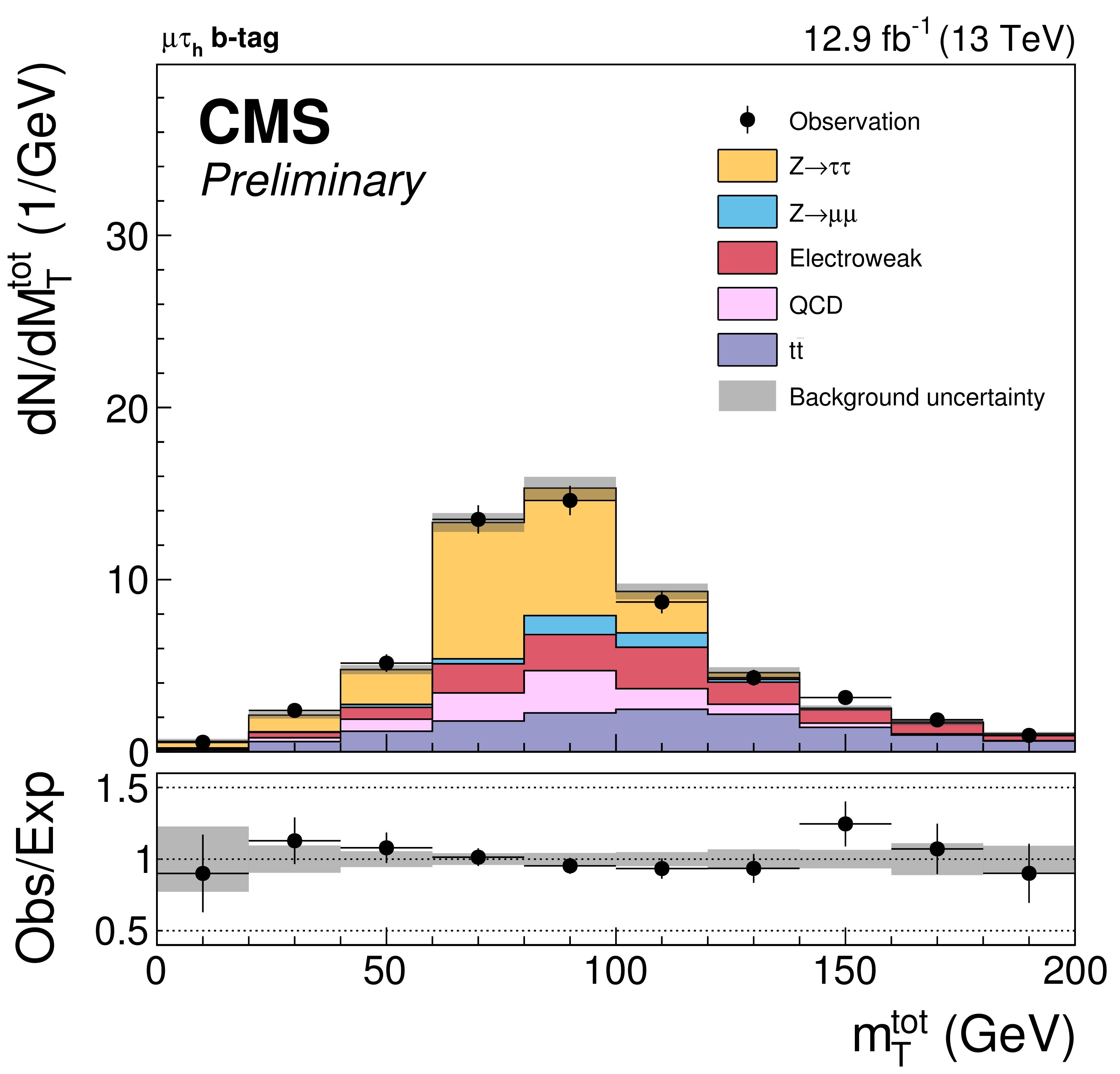
Post-fit plot of the total transverse mass distribution in (a) the no b-tag category and (b) the b-tag category of the $\mu \tau_{\mathrm{h}}$ channel |
png pdf |
Figure 5-a:
Post-fit plot of the total transverse mass distribution in the no b-tag category of the $\mu \tau_{\mathrm{h}}$ channel |

png pdf |
Figure 5-b:
Post-fit plot of the total transverse mass distribution in the b-tag category of the $\mu \tau_{\mathrm{h}}$ channel |
png pdf |
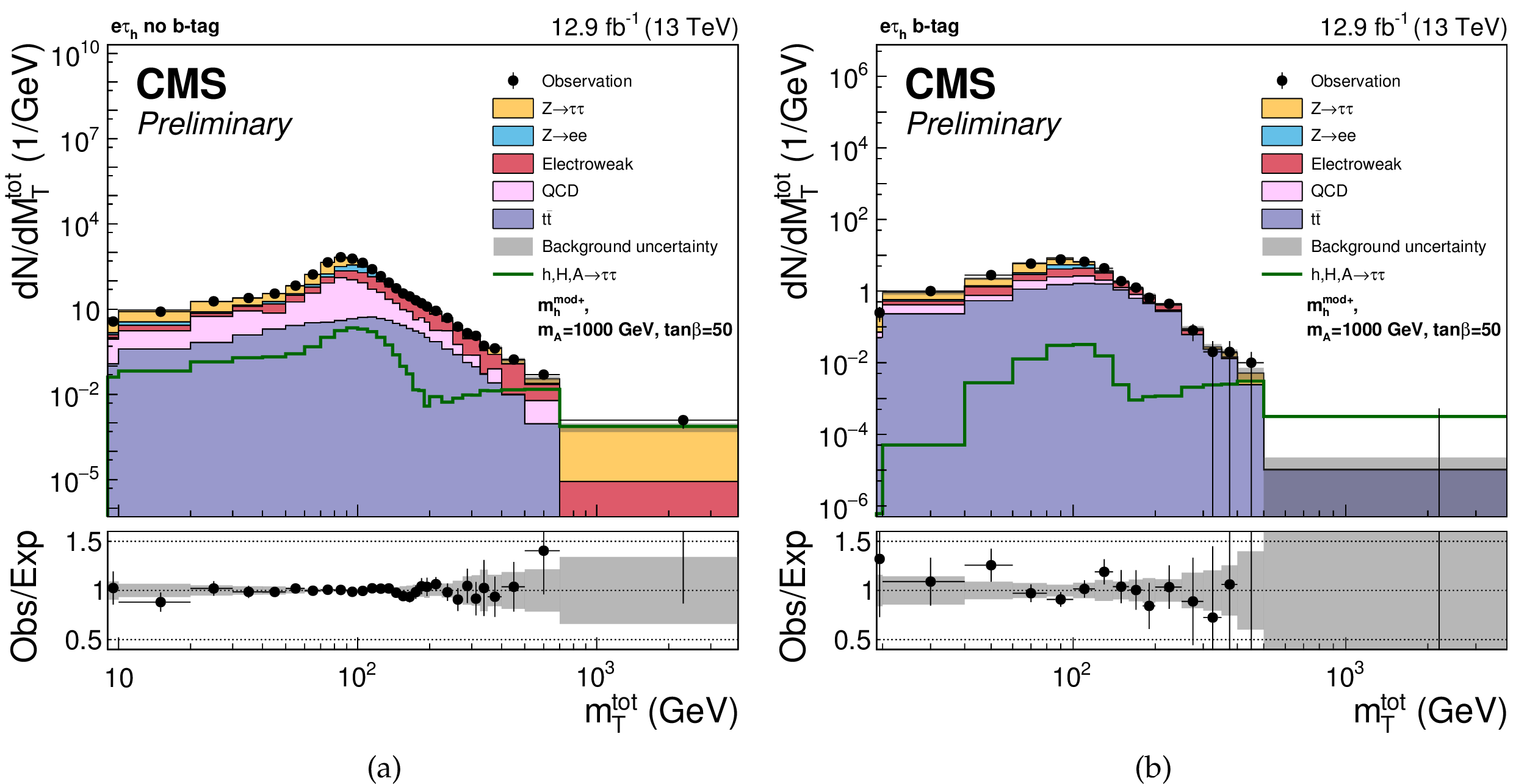
Figure 6:
Post-fit plot of the total transverse mass distribution in (a) the no b-tag category and (b) the b-tag category of the $\mathrm{e}\tau_{\mathrm{h}}$ channel |
png pdf |
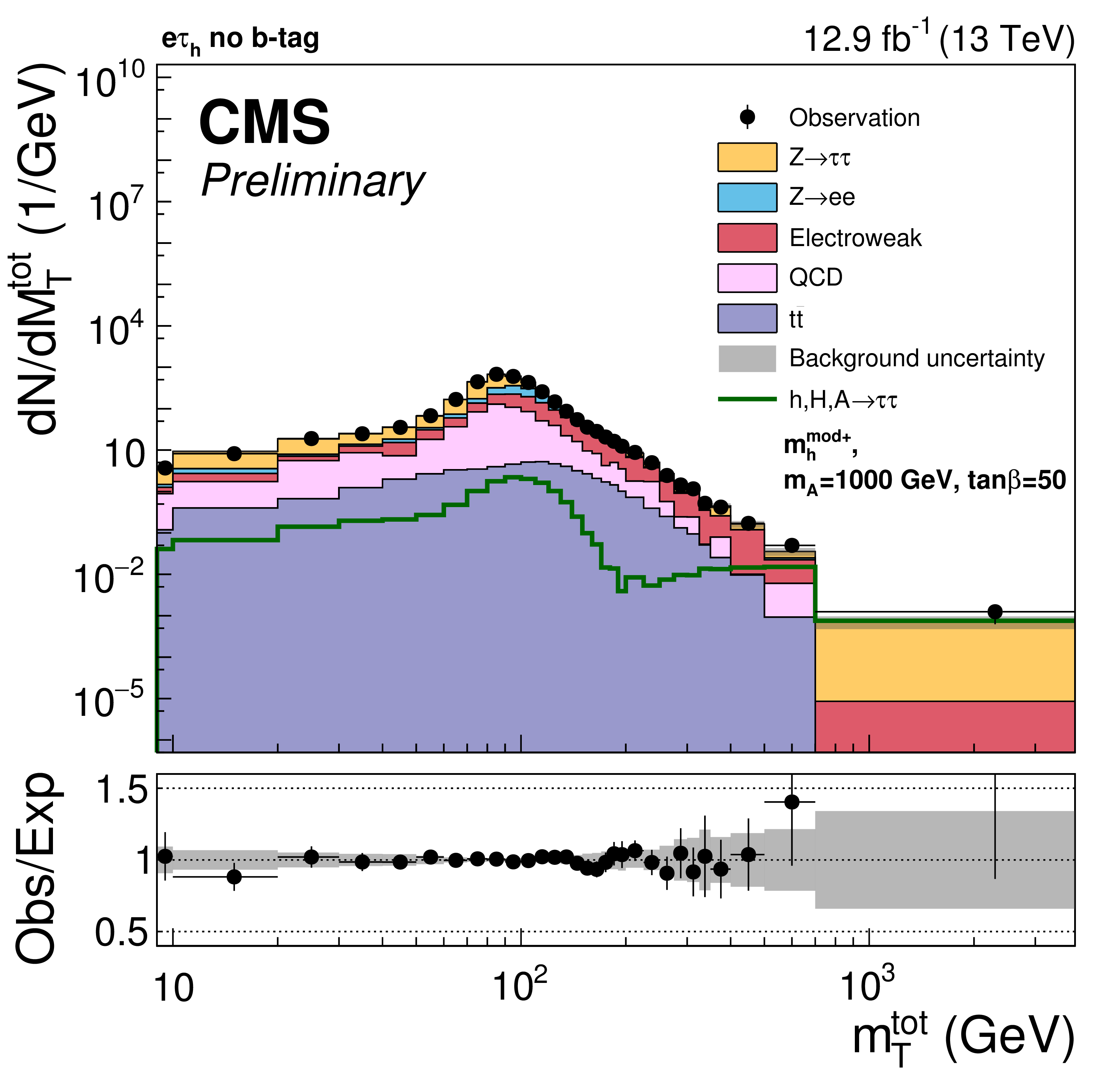
Figure 6-a:
Post-fit plot of the total transverse mass distribution in the no b-tag category the $\mathrm{e}\tau_{\mathrm{h}}$ channel |

png pdf |
Figure 6-b:
Post-fit plot of the total transverse mass distribution in the b-tag category of the $\mathrm{e}\tau_{\mathrm{h}}$ channel |

png pdf |
Figure 7:
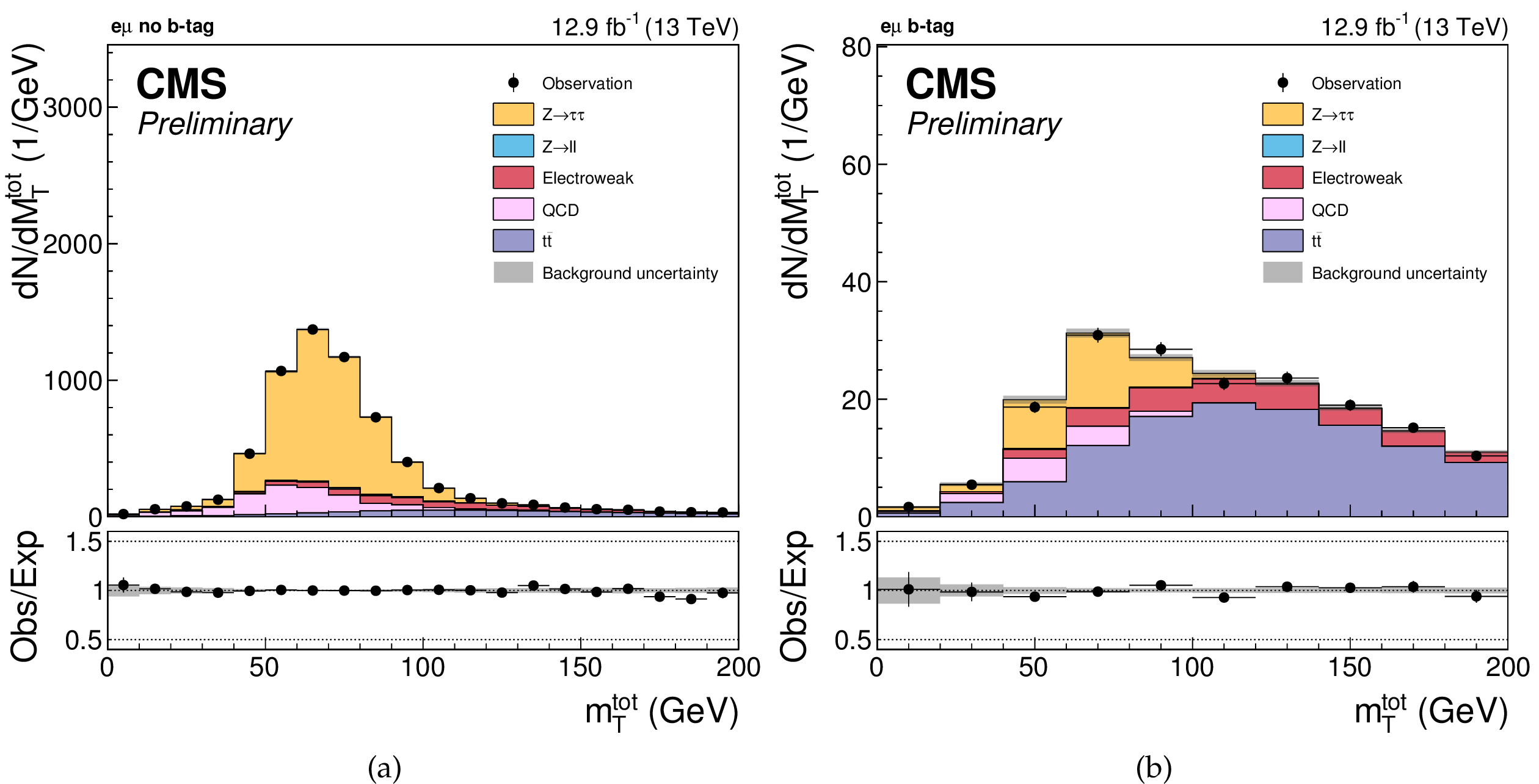
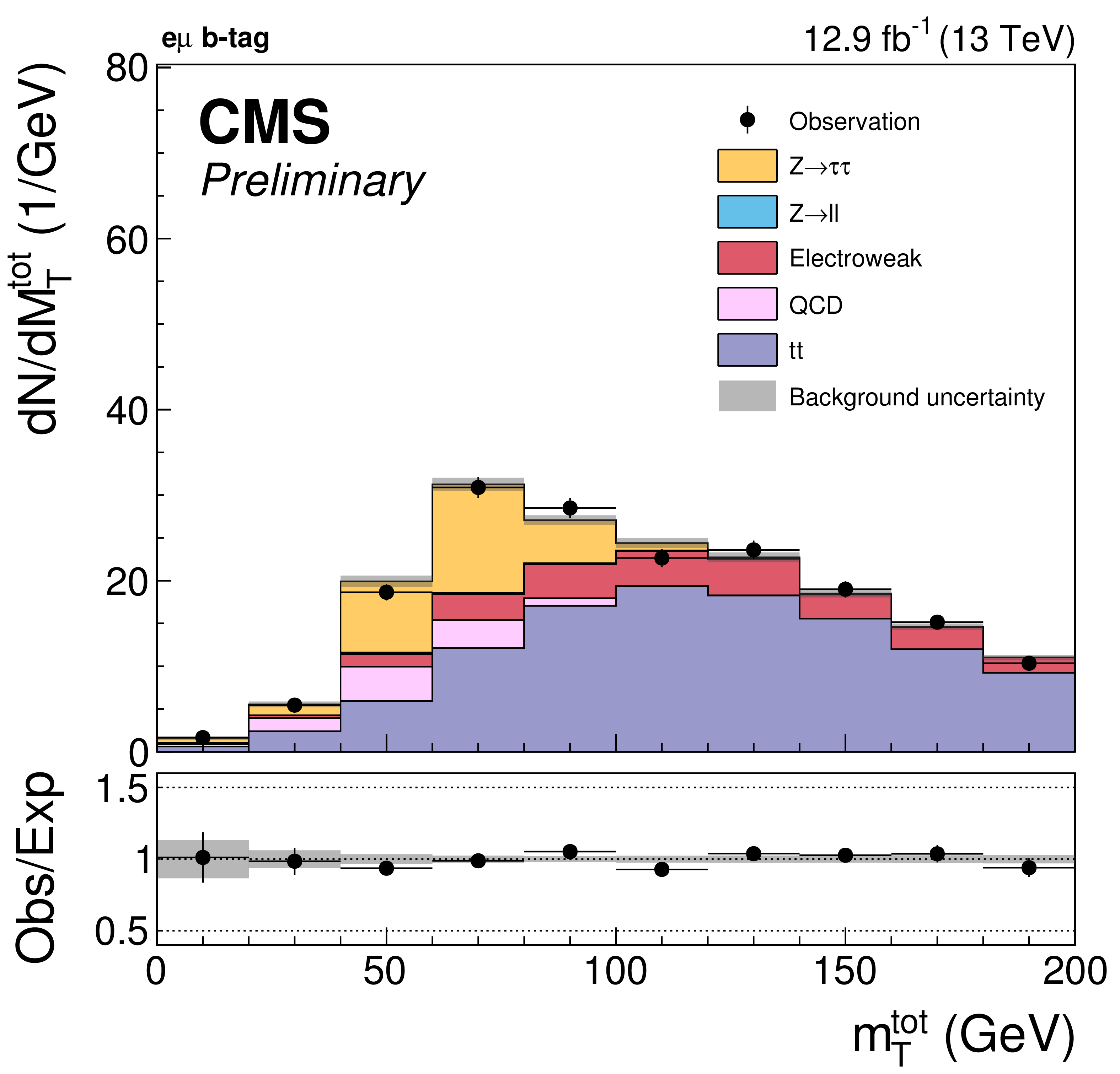
Post-fit plot of the total transverse mass distribution in (a) the no b-tag category and (b) the b-tag category of the $\mathrm{e}\mu $ channel |

png pdf |
Figure 7-a:
Post-fit plot of the total transverse mass distribution in the no b-tag category of the $\mathrm{e}\mu $ channel |

png pdf |
Figure 7-b:
Post-fit plot of the total transverse mass distribution in the b-tag category of the $\mathrm{e}\mu $ channel |
png pdf |
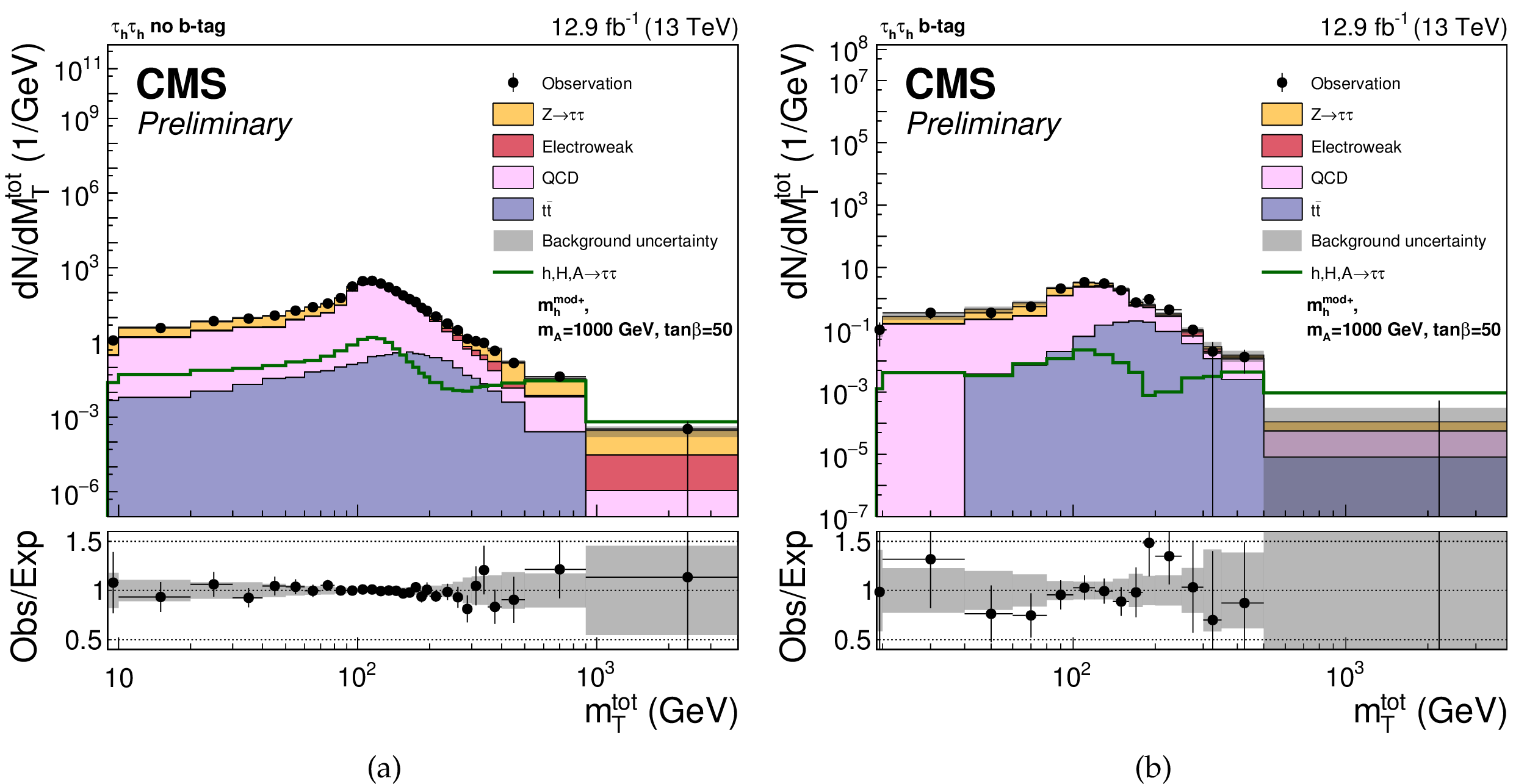
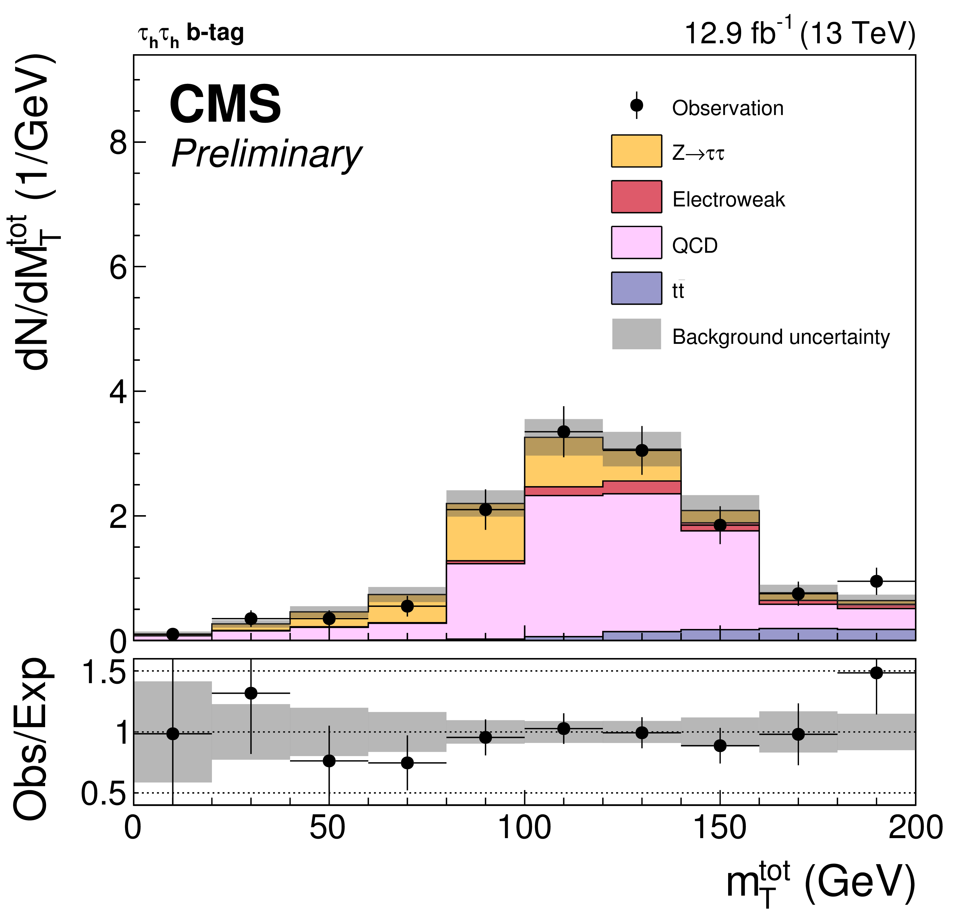
Figure 8:
Post-fit plot of the total transverse mass distribution in (a) the no b-tag category and (b) the b-tag category of the $\tau _{\rm {h}}\tau _{\rm {h}}$ channel |
png pdf |
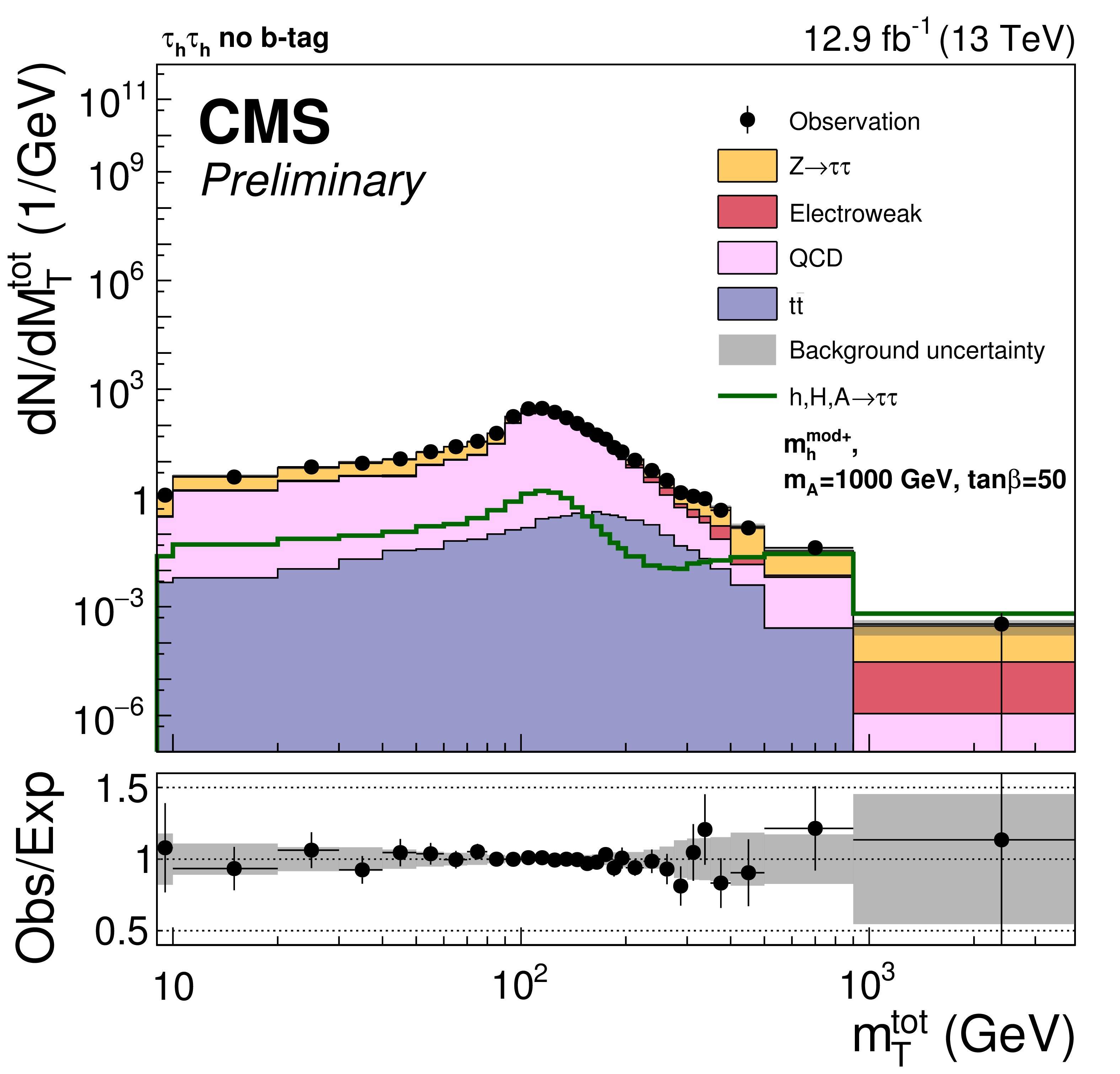
Figure 8-a:
Post-fit plot of the total transverse mass distribution in the no b-tag category of the $\tau _{\rm {h}}\tau _{\rm {h}}$ channel |

png pdf |
Figure 8-b:
Post-fit plot of the total transverse mass distribution in the b-tag category of the $\tau _{\rm {h}}\tau _{\rm {h}}$ channel |

png pdf |
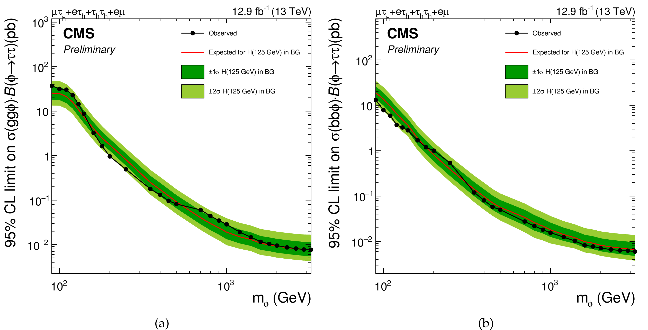
Figure 9:
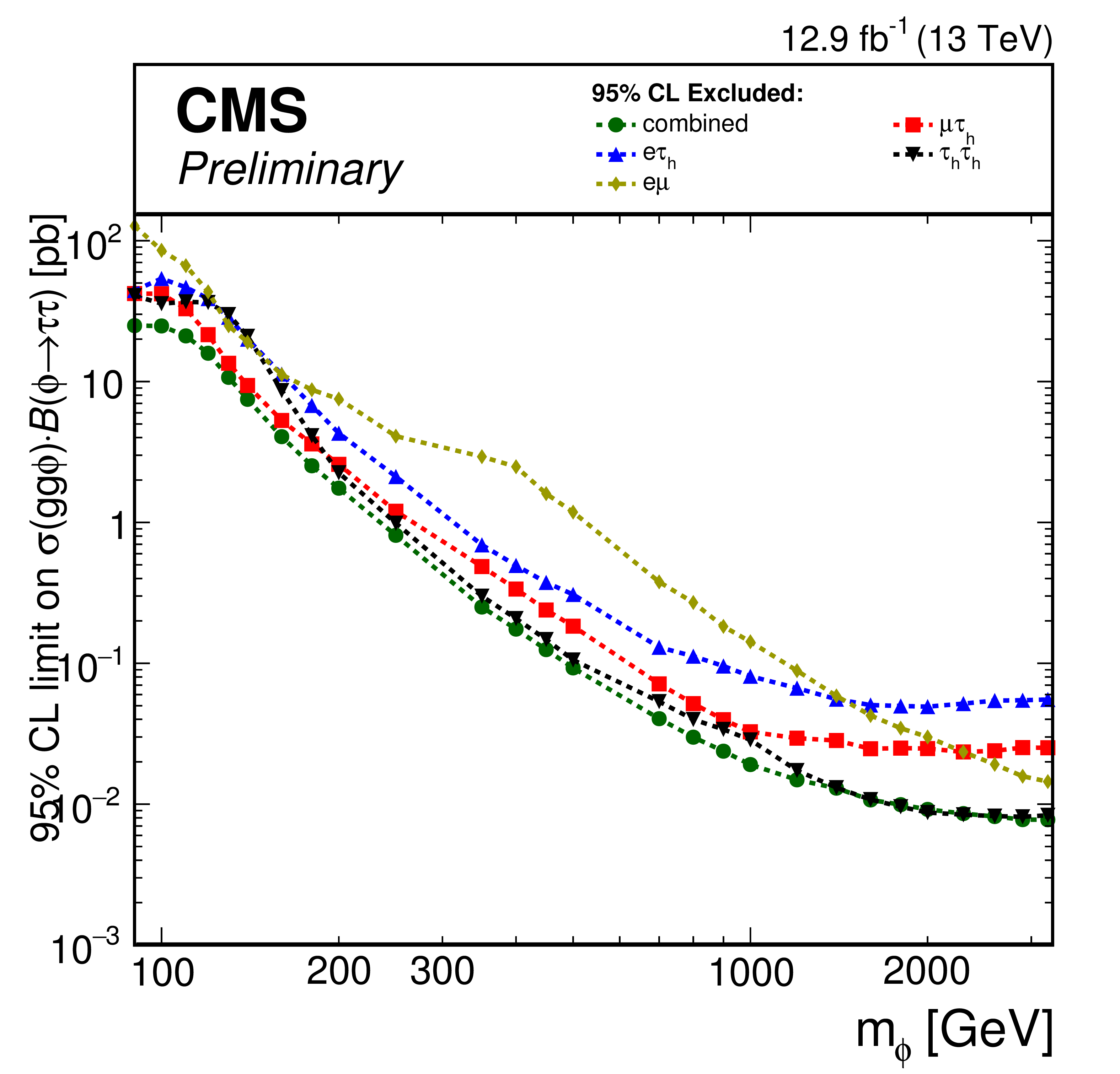
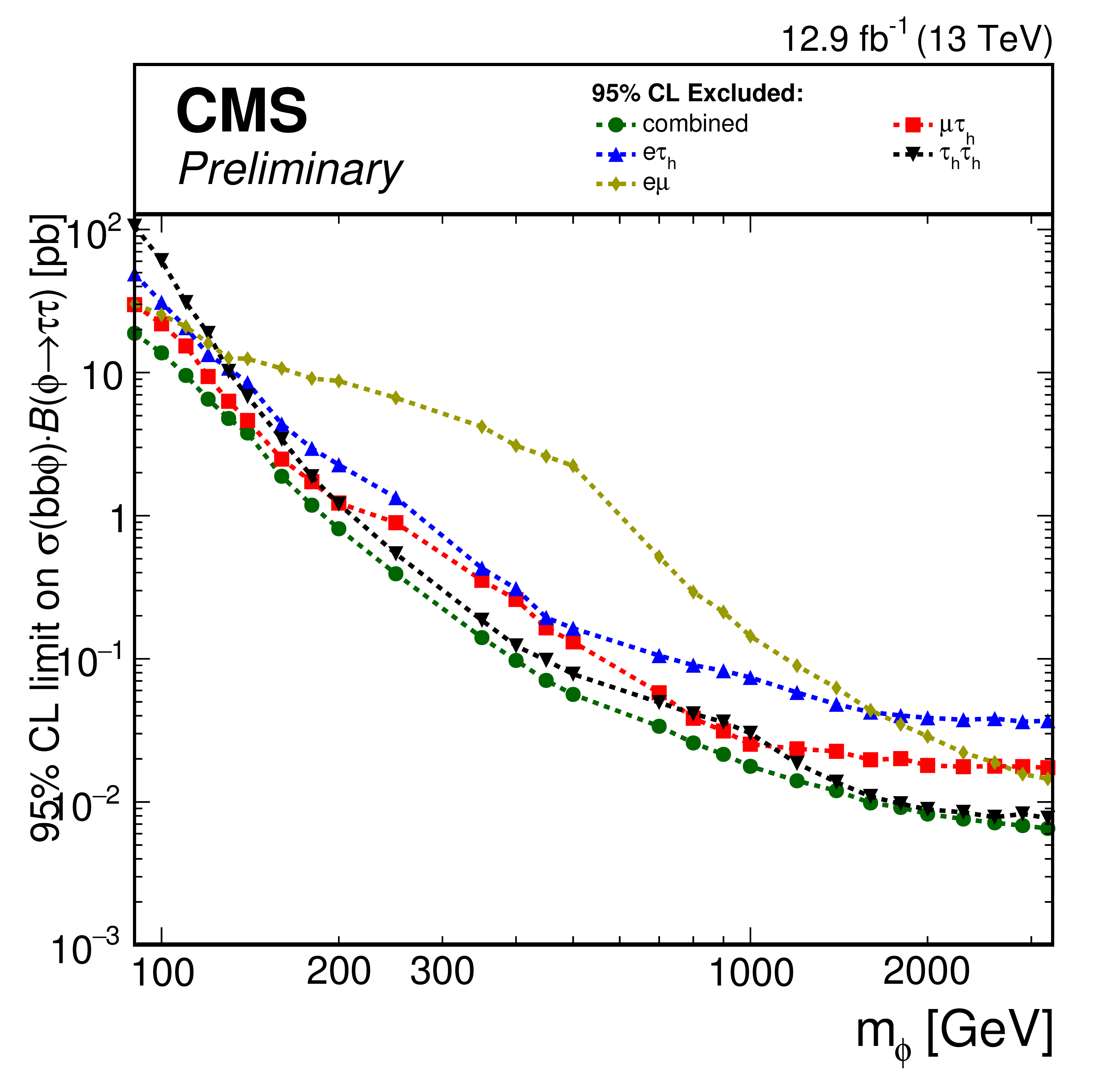
Expected and observed limits on cross-section times branching fraction for a) the gluon fusion process (gg$\phi $) and b) the b-associated production process (bb$\phi $), resulting from the combination of all four channels. The narrow width approximation is used for the signal. |

png pdf |
Figure 9-a:
Expected and observed limits on cross-section times branching fraction for the gluon fusion process (gg$\phi $), resulting from the combination of all four channels. The narrow width approximation is used for the signal. |

png pdf |
Figure 9-b:
Expected and observed limits on cross-section times branching fraction for the b-associated production process (bb$\phi $), resulting from the combination of all four channels. The narrow width approximation is used for the signal. |

png pdf |
Figure 10:
Comparison between the expected limits on cross-section times branching fraction for a) the gluon fusion process (gg$\phi $) and b) the b-associated production process (bb$\phi $) in each final state channel. |
png pdf |
Figure 10-a:
Comparison between the expected limits on cross-section times branching fraction for the gluon fusion process (gg$\phi $) in each final state channel. |
png pdf |
Figure 10-b:
Comparison between the expected limits on cross-section times branching fraction for the b-associated production process (bb$\phi $) in each final state channel. |

png pdf |
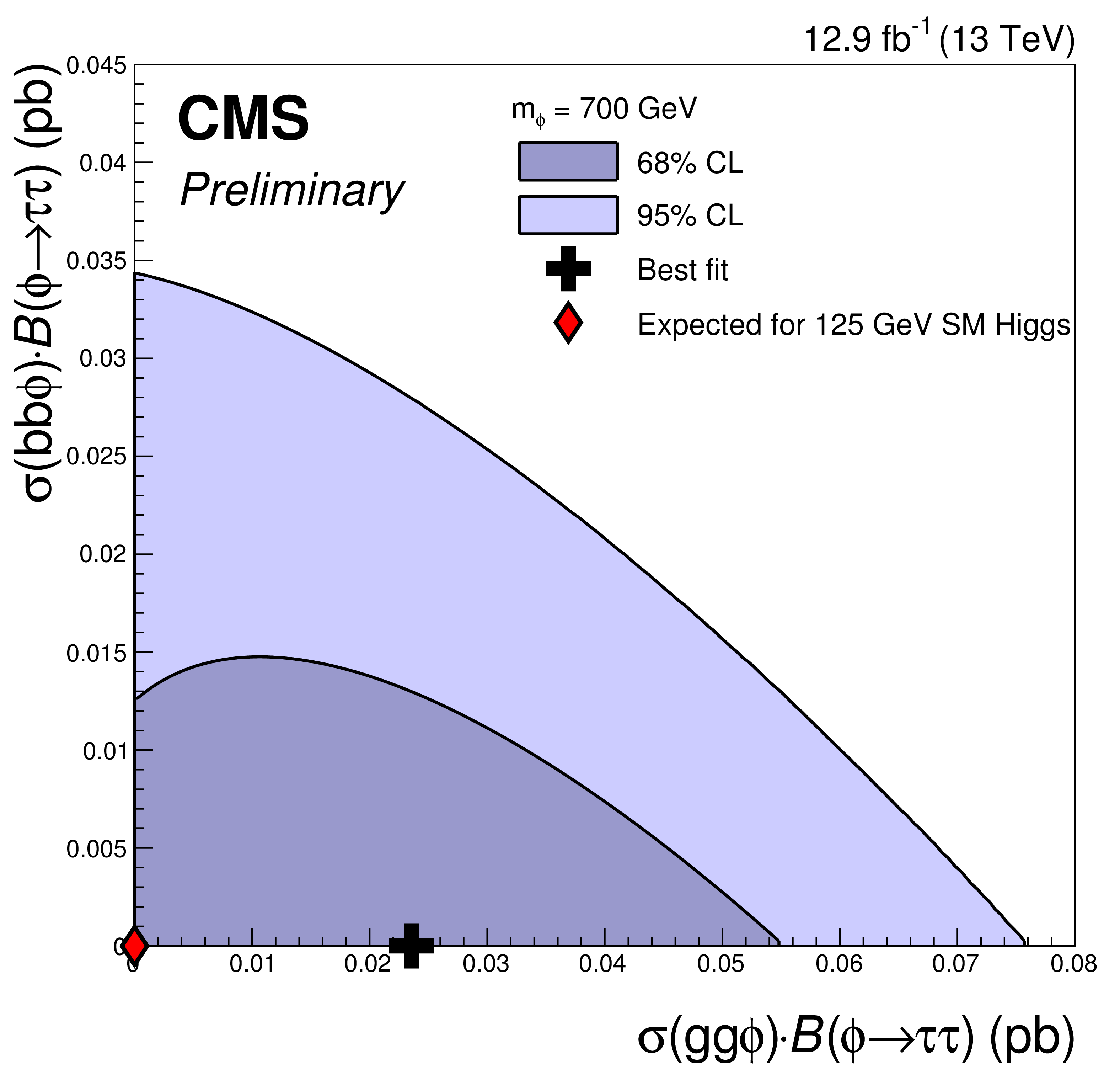
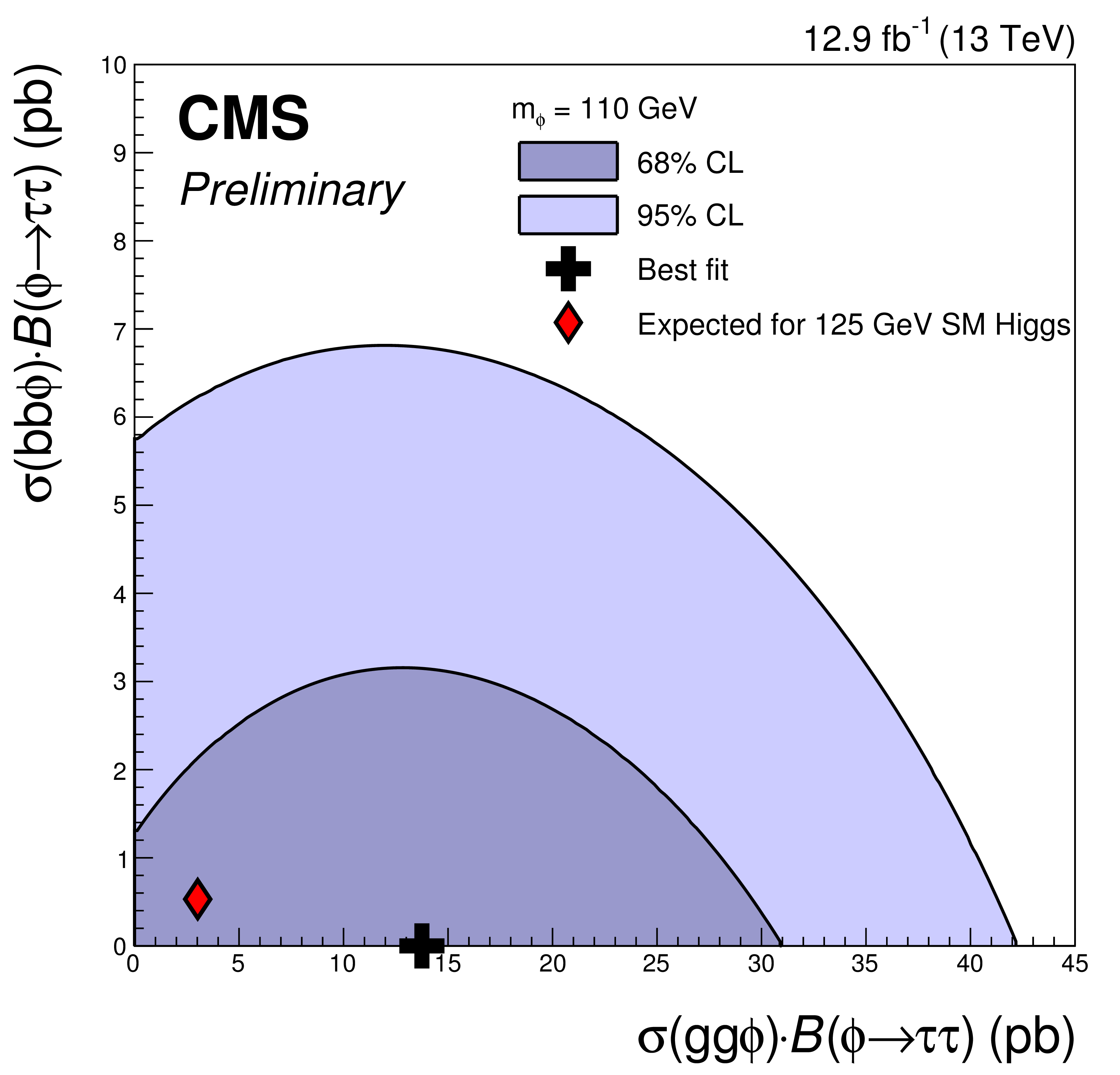
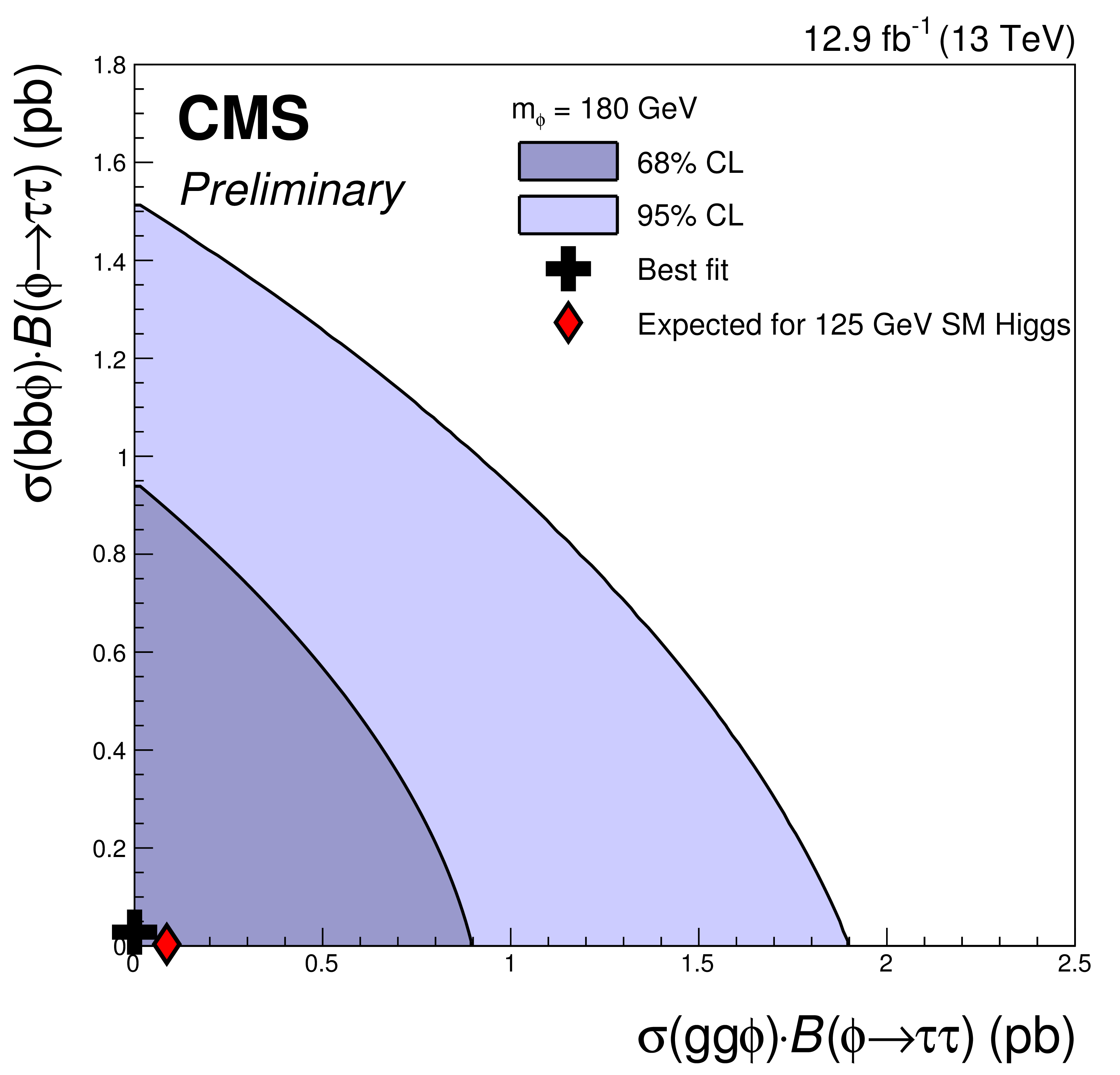
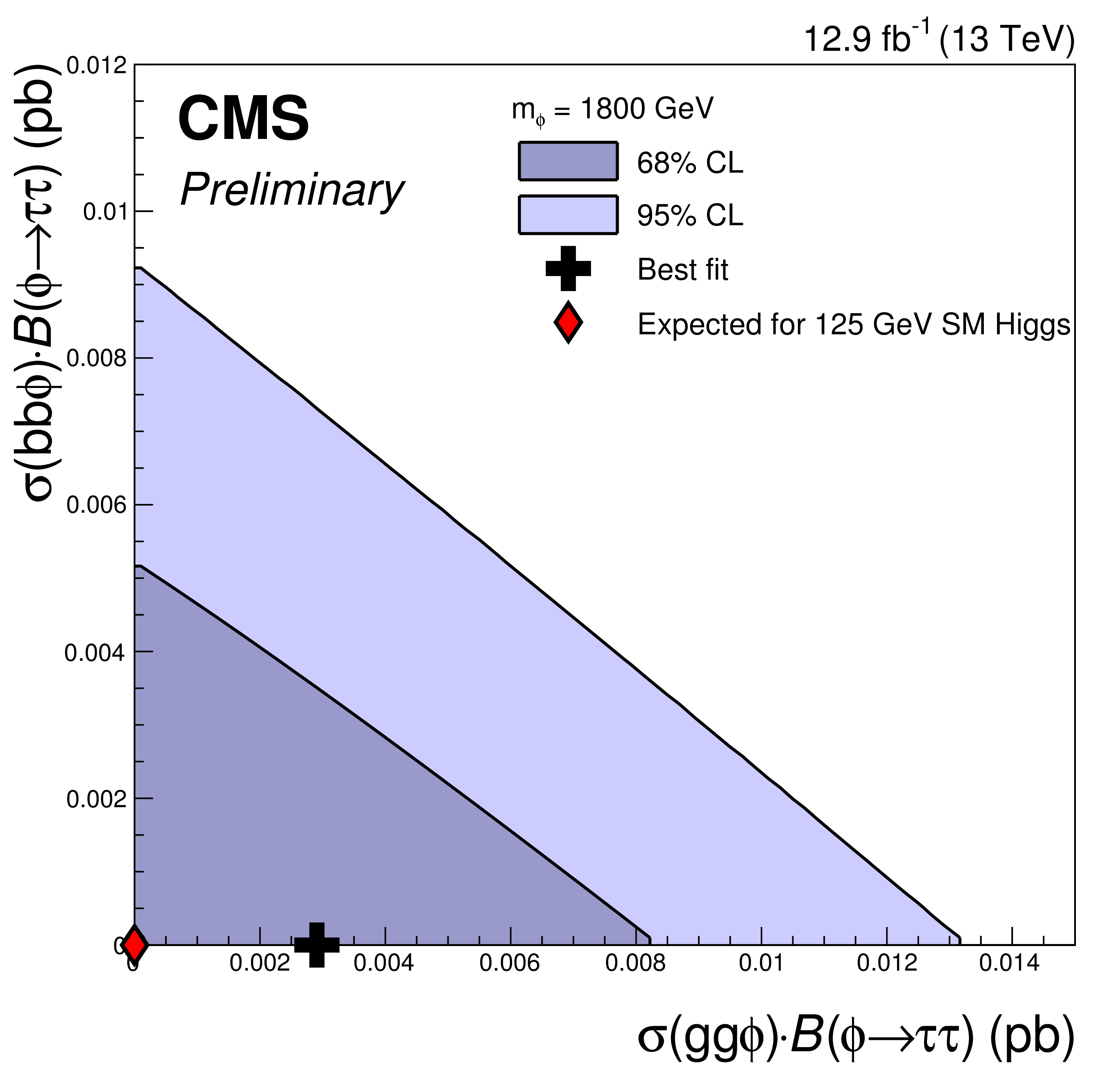
Figure 11:
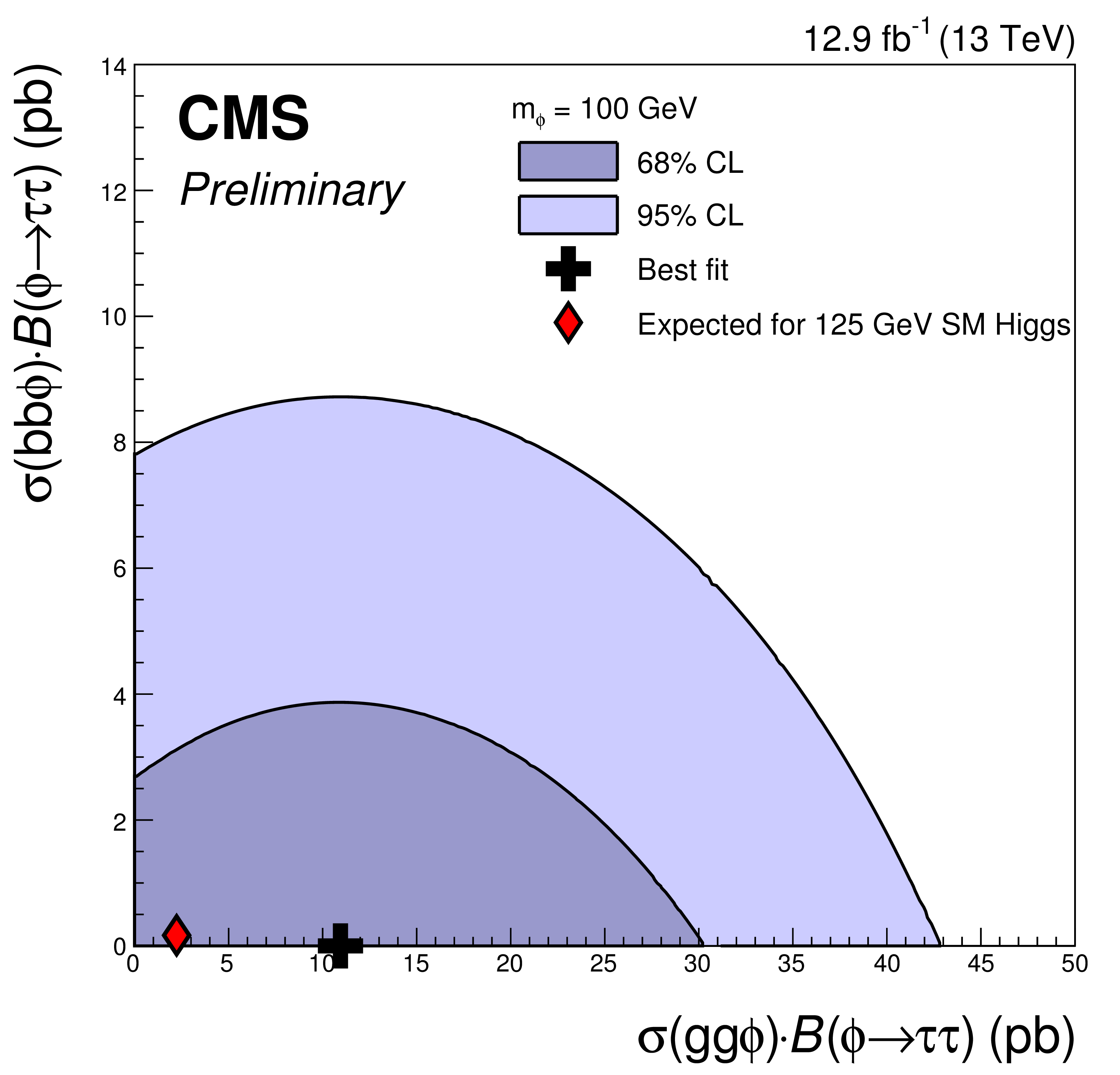
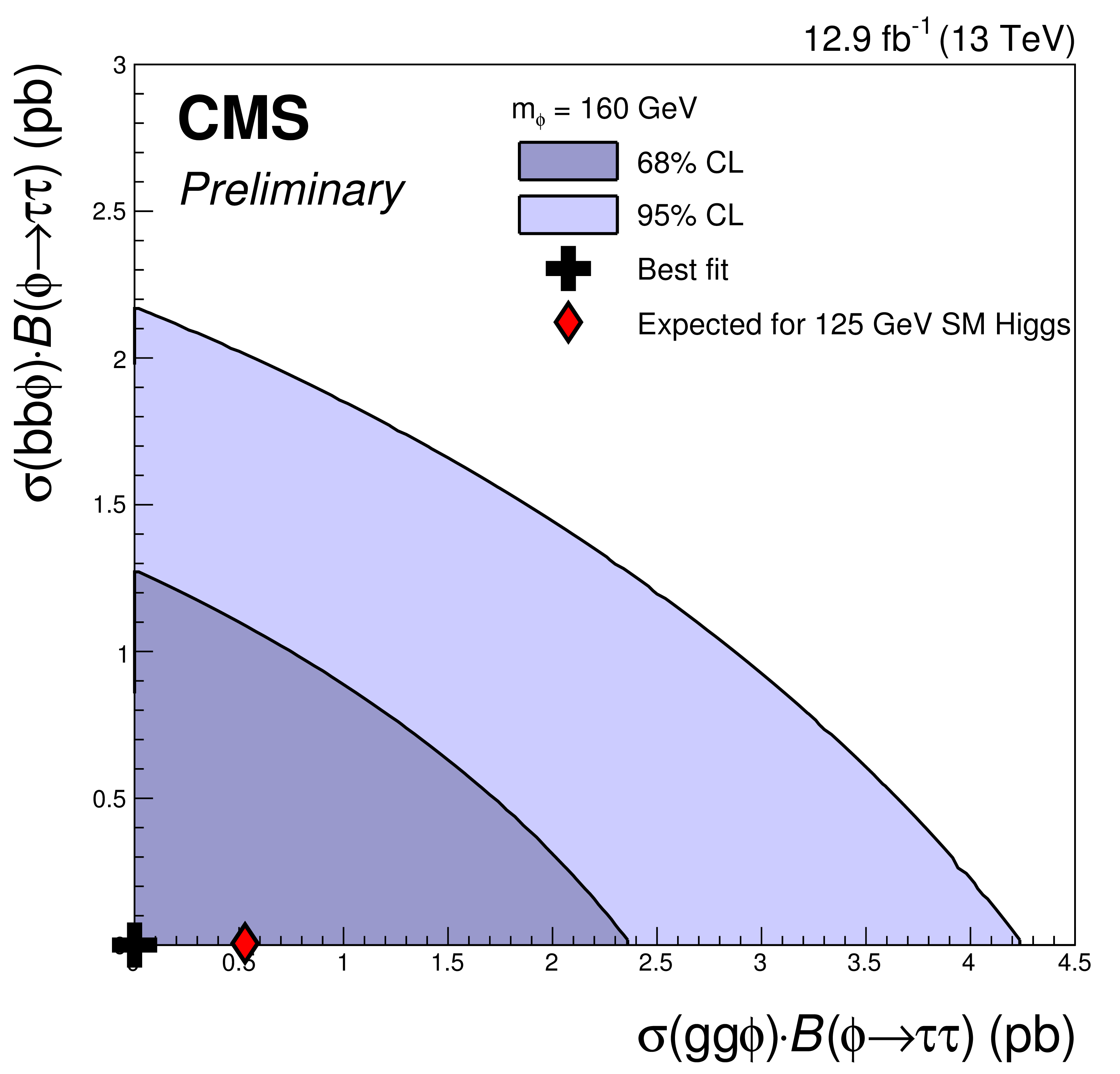
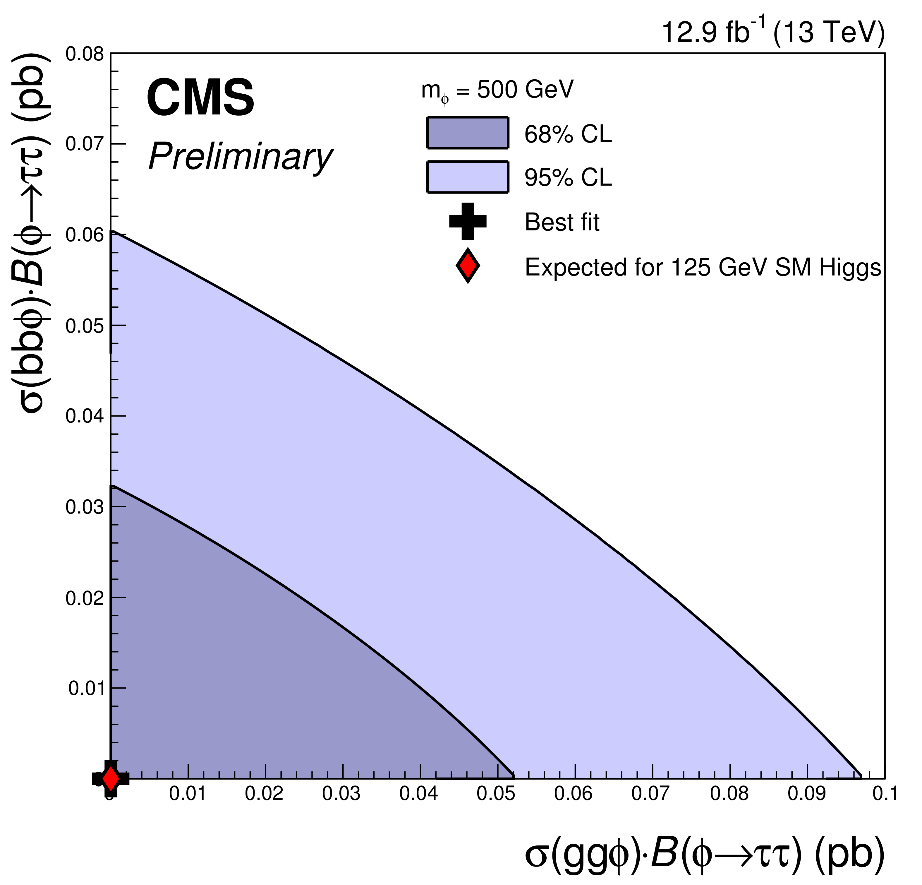
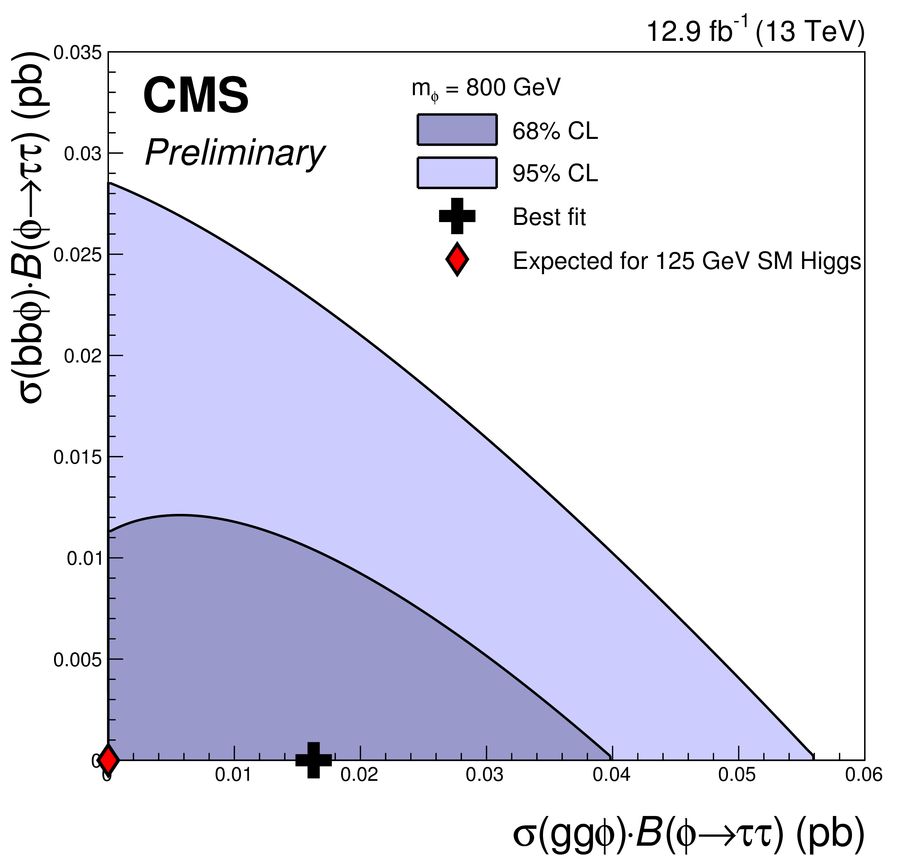
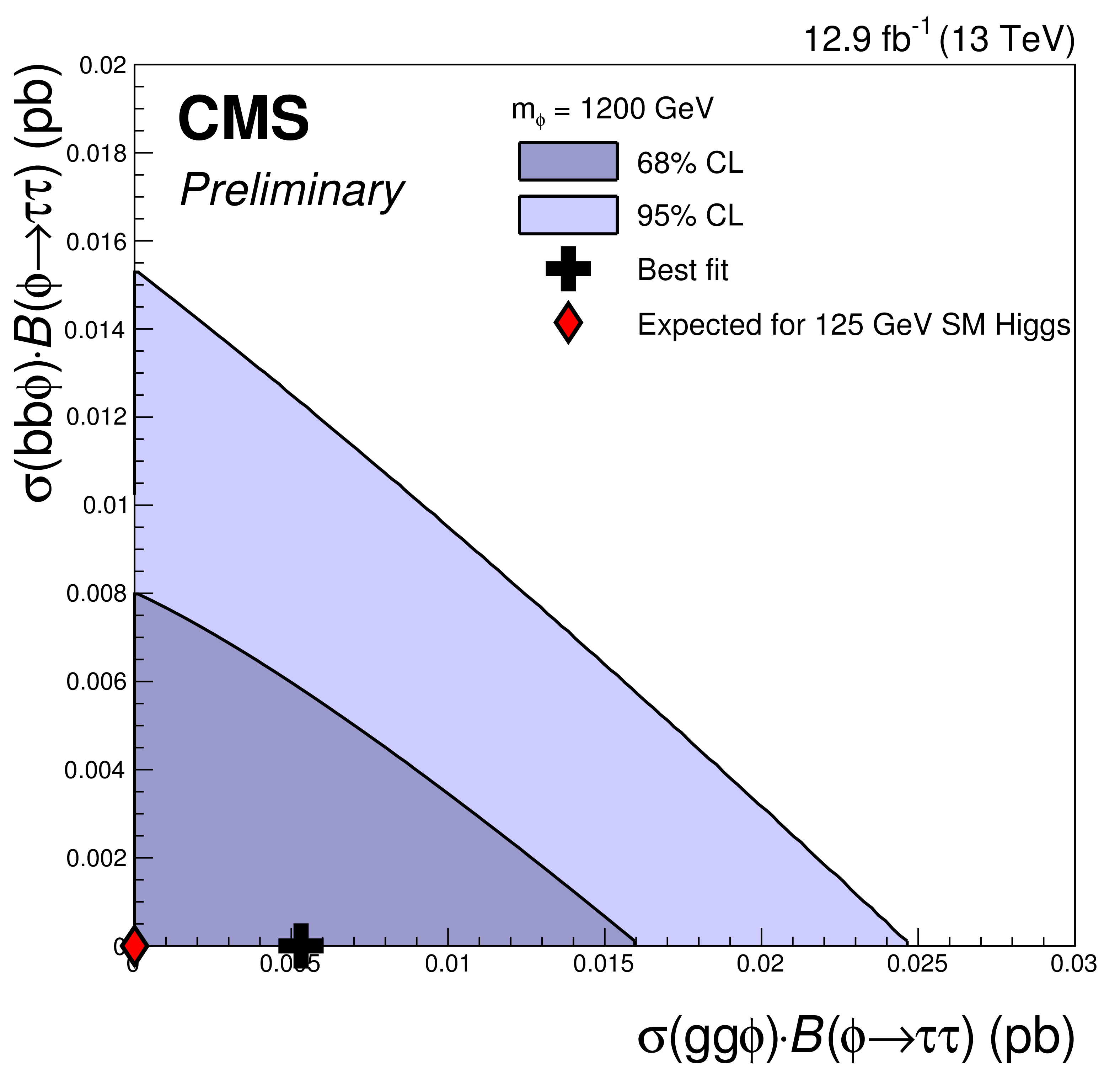
2D likelihood scan of cross-section time branching fraction for gg$\phi $ vs bb$\phi $ production processes, for selected Higgs boson masses between 100 GeV and 3200 GeV. The best fit point (black cross) and the 1 and 2 sigma contours are shown for the observed data. Also shown is the best fit value for an Asimov dataset containing background plus the SM Higgs with mass 125 GeV (red diamond). |
png pdf |
Figure 11-a:
2D likelihood scan of cross-section time branching fraction for gg$\phi $ vs bb$\phi $ production processes, for Higgs boson mass 100 GeV. The best fit point (black cross) and the 1 and 2 sigma contours are shown for the observed data. Also shown is the best fit value for an Asimov dataset containing background plus the SM Higgs with mass 125 GeV (red diamond). |

png pdf |
Figure 11-b:
2D likelihood scan of cross-section time branching fraction for gg$\phi $ vs bb$\phi $ production processes, for Higgs boson mass 125 GeV. The best fit point (black cross) and the 1 and 2 sigma contours are shown for the observed data. Also shown is the best fit value for an Asimov dataset containing background plus the SM Higgs with mass 125 GeV (red diamond). |

png pdf |
Figure 11-c:
2D likelihood scan of cross-section time branching fraction for gg$\phi $ vs bb$\phi $ production processes, for Higgs boson mass 140 GeV. The best fit point (black cross) and the 1 and 2 sigma contours are shown for the observed data. Also shown is the best fit value for an Asimov dataset containing background plus the SM Higgs with mass 125 GeV (red diamond). |
png pdf |
Figure 11-d:
2D likelihood scan of cross-section time branching fraction for gg$\phi $ vs bb$\phi $ production processes, for Higgs boson mass 160 GeV. The best fit point (black cross) and the 1 and 2 sigma contours are shown for the observed data. Also shown is the best fit value for an Asimov dataset containing background plus the SM Higgs with mass 125 GeV (red diamond). |

png pdf |
Figure 11-e:
2D likelihood scan of cross-section time branching fraction for gg$\phi $ vs bb$\phi $ production processes, for Higgs boson mass 200 GeV. The best fit point (black cross) and the 1 and 2 sigma contours are shown for the observed data. Also shown is the best fit value for an Asimov dataset containing background plus the SM Higgs with mass 125 GeV (red diamond). |

png pdf |
Figure 11-f:
2D likelihood scan of cross-section time branching fraction for gg$\phi $ vs bb$\phi $ production processes, for Higgs boson mass 350 GeV. The best fit point (black cross) and the 1 and 2 sigma contours are shown for the observed data. Also shown is the best fit value for an Asimov dataset containing background plus the SM Higgs with mass 125 GeV (red diamond). |
png pdf |
Figure 11-g:
2D likelihood scan of cross-section time branching fraction for gg$\phi $ vs bb$\phi $ production processes, for Higgs boson mass 700 GeV. The best fit point (black cross) and the 1 and 2 sigma contours are shown for the observed data. Also shown is the best fit value for an Asimov dataset containing background plus the SM Higgs with mass 125 GeV (red diamond). |
png pdf |
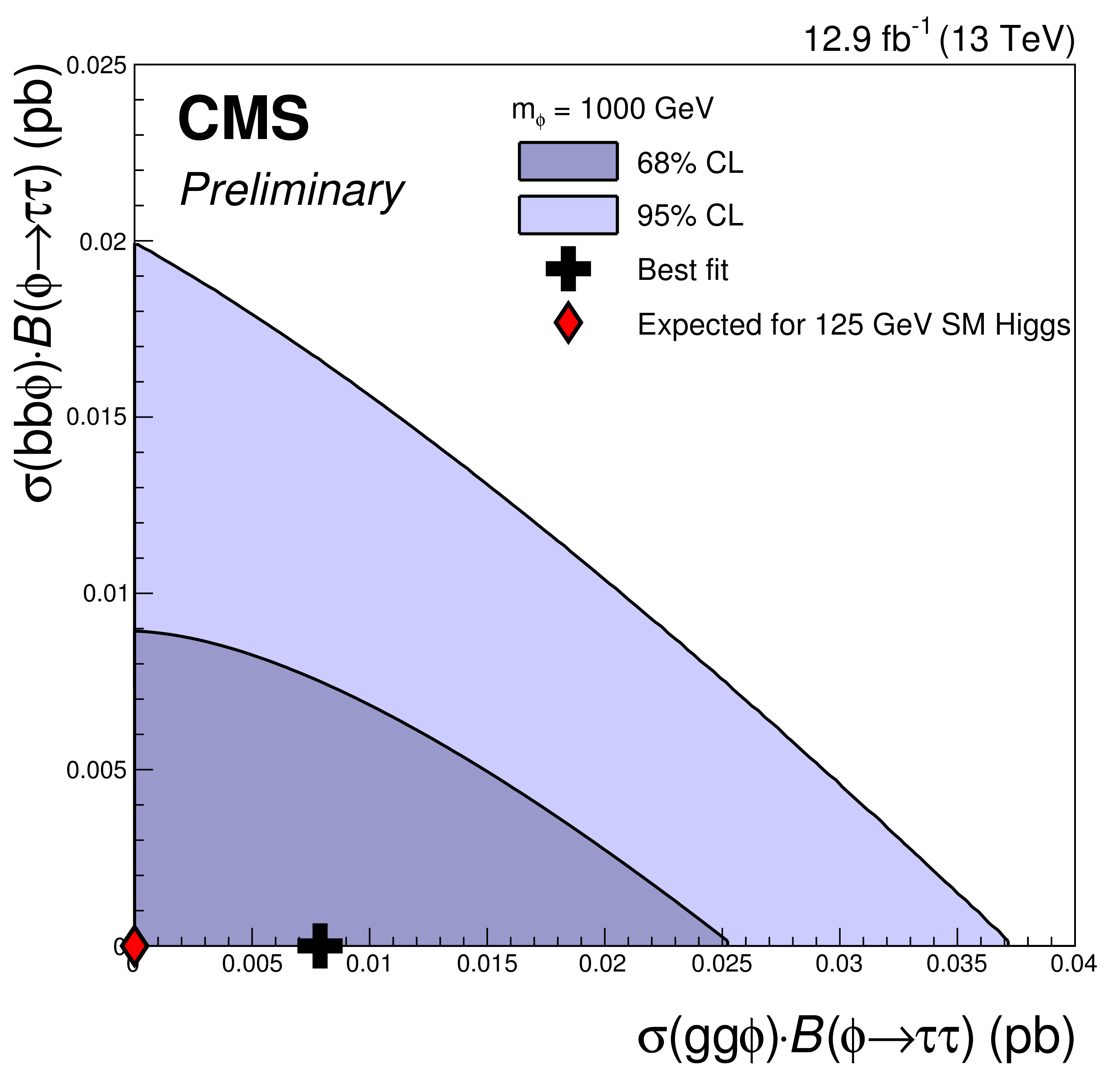
Figure 11-h:
2D likelihood scan of cross-section time branching fraction for gg$\phi $ vs bb$\phi $ production processes, for Higgs boson mass 1000 GeV. The best fit point (black cross) and the 1 and 2 sigma contours are shown for the observed data. Also shown is the best fit value for an Asimov dataset containing background plus the SM Higgs with mass 125 GeV (red diamond). |

png pdf |
Figure 11-i:
2D likelihood scan of cross-section time branching fraction for gg$\phi $ vs bb$\phi $ production processes, for Higgs boson mass 1600 GeV. The best fit point (black cross) and the 1 and 2 sigma contours are shown for the observed data. Also shown is the best fit value for an Asimov dataset containing background plus the SM Higgs with mass 125 GeV (red diamond). |
png pdf |
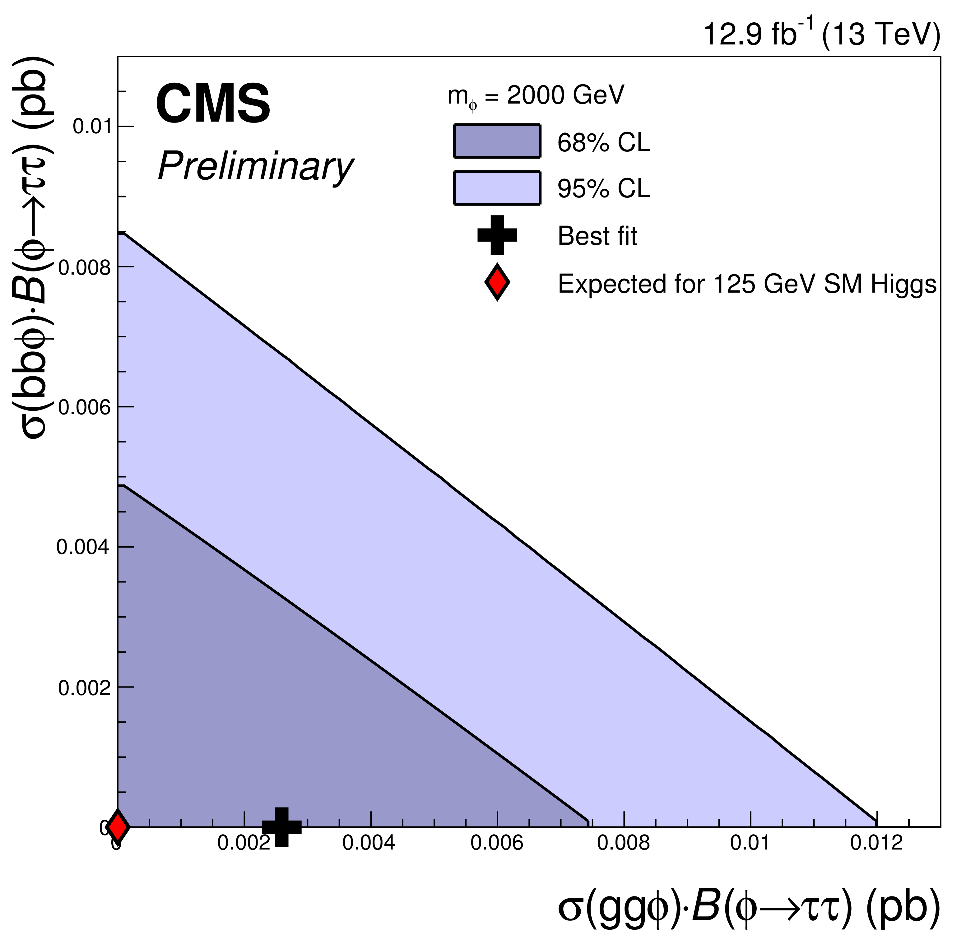
Figure 11-j:
2D likelihood scan of cross-section time branching fraction for gg$\phi $ vs bb$\phi $ production processes, for Higgs boson mass 2000 GeV. The best fit point (black cross) and the 1 and 2 sigma contours are shown for the observed data. Also shown is the best fit value for an Asimov dataset containing background plus the SM Higgs with mass 125 GeV (red diamond). |
png pdf |
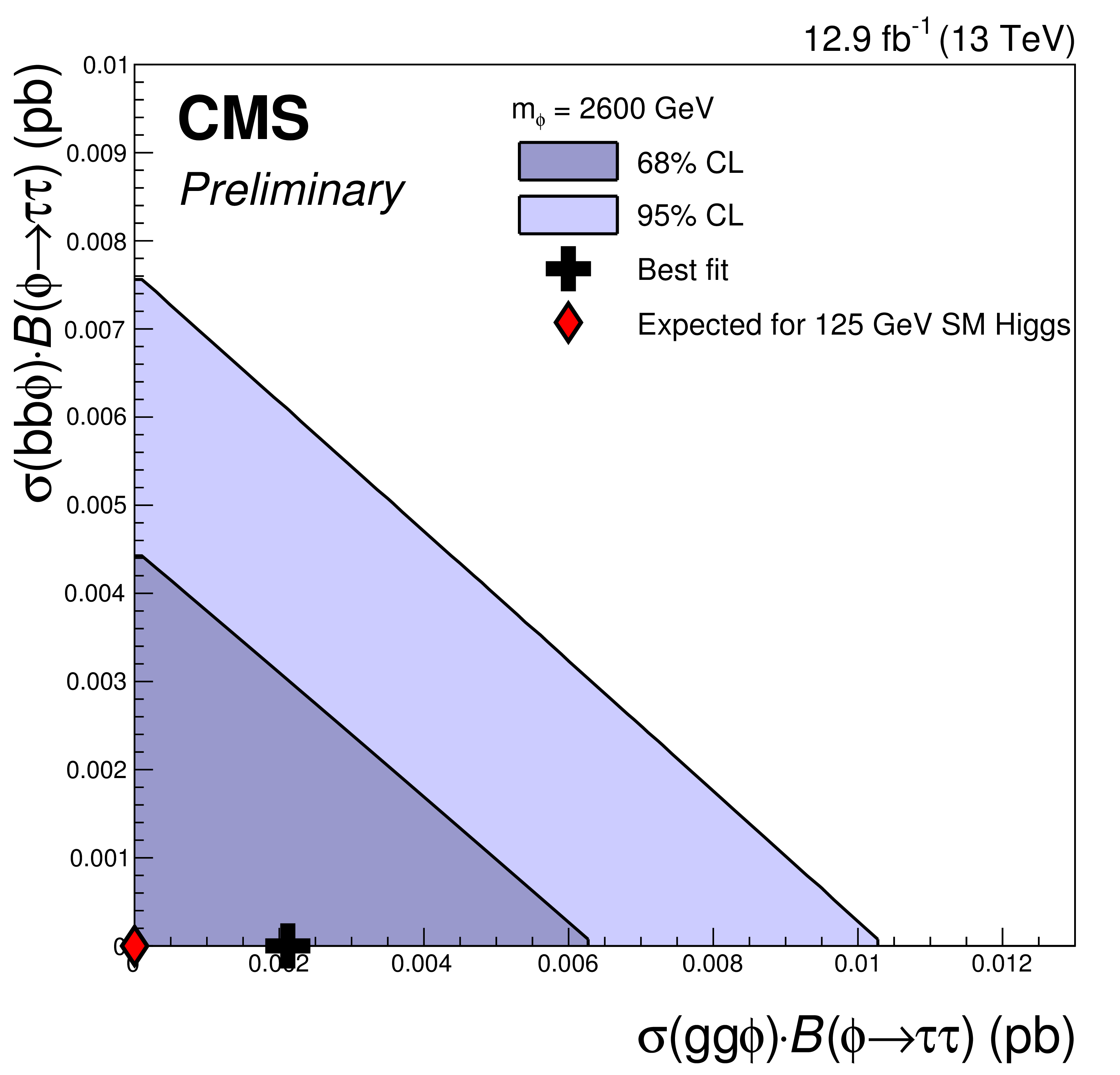
Figure 11-k:
2D likelihood scan of cross-section time branching fraction for gg$\phi $ vs bb$\phi $ production processes, for Higgs boson mass 2600 GeV. The best fit point (black cross) and the 1 and 2 sigma contours are shown for the observed data. Also shown is the best fit value for an Asimov dataset containing background plus the SM Higgs with mass 125 GeV (red diamond). |

png pdf |
Figure 11-l:
2D likelihood scan of cross-section time branching fraction for gg$\phi $ vs bb$\phi $ production processes, for Higgs boson mass 3200 GeV. The best fit point (black cross) and the 1 and 2 sigma contours are shown for the observed data. Also shown is the best fit value for an Asimov dataset containing background plus the SM Higgs with mass 125 GeV (red diamond). |

png pdf |
Figure 12:
Model dependent exclusion limits in the $m_{ {\mathrm {A}} }$-$\tan \beta $ plane, combining all channels, for a) the $m_{\phi}^{\text {mod+}}$ and b) hMSSM scenarios. In a) the red contour indicates the region which does not yield a Higgs boson consistent with a mass of 125 GeV within the theoretical uncertainties of $\pm$3 GeV. |

png pdf |
Figure 12-a:
Model dependent exclusion limits in the $m_{ {\mathrm {A}} }$-$\tan \beta $ plane, combining all channels, for the $m_{\phi}^{\text {mod+}}$ scenario. The red contour indicates the region which does not yield a Higgs boson consistent with a mass of 125 GeV within the theoretical uncertainties of $\pm$3 GeV. |

png pdf |
Figure 12-b:
Model dependent exclusion limits in the $m_{ {\mathrm {A}} }$-$\tan \beta $ plane, combining all channels, for the hMSSM scenario. |
| Tables | |

png pdf |
Table 1:
Summary of the lepton selections in each channel. |
| Summary |
| A search for neutral Higgs bosons of the MSSM decaying into the $\tau\tau$ final state has been presented, using the $\mu\tau_{\mathrm{h}}$, $\mathrm{ e }\tau_{\mathrm{h}}$, $\tau_{\mathrm{h}}\tau_{\mathrm{h}}$ and $\mathrm{ e }\mu$ final states. The dataset corresponds to an integrated luminosity of 12.9 fb$^{-1}$, recorded by the CMS detector at 13 TeV centre-of-mass energy in 2016. No evidence for a signal has been found and exclusion limits on the production cross section times branching fraction for the gluon fusion and b-associated production processes are presented. The results are also interpreted in the context of two MSSM benchmark scenarios, where exclusions are set as a function of $m_{\mathrm{A}}$ and $\tan \beta$. |
| Additional Figures | |

png pdf |
Additional Figure 1:
Post-fit plot of the transverse mass distribution in (a) the no b-tag category and (b) the b-tag category of the $\mu \tau _{\mathrm{h}}$ channel, showing the low mass region. Note that the signal prediction isn't shown, since it is only visible compared with background in the high mass region. |
png pdf |
Additional Figure 1-a:
Post-fit plot of the transverse mass distribution in the no b-tag category of the $\mu \tau _{\mathrm{h}}$ channel, showing the low mass region. Note that the signal prediction isn't shown, since it is only visible compared with background in the high mass region. |
png pdf |
Additional Figure 1-b:
Post-fit plot of the transverse mass distribution in the b-tag category of the $\mu \tau _{\mathrm{h}}$ channel, showing the low mass region. Note that the signal prediction isn't shown, since it is only visible compared with background in the high mass region. |

png pdf |
Additional Figure 2:
Post-fit plot of the transverse mass distribution in (a) the no b-tag category and (b) the b-tag category of the $e\tau _{\mathrm{h}}$ channel, showing the low mass region. Note that the signal prediction isn't shown, since it is only visible compared with background in the high mass region. |

png pdf |
Additional Figure 2-a:
Post-fit plot of the transverse mass distribution in the no b-tag category of the $e\tau _{\mathrm{h}}$ channel, showing the low mass region. Note that the signal prediction isn't shown, since it is only visible compared with background in the high mass region. |

png pdf |
Additional Figure 2-b:
Post-fit plot of the transverse mass distribution in the b-tag category of the $e\tau _{\mathrm{h}}$ channel, showing the low mass region. Note that the signal prediction isn't shown, since it is only visible compared with background in the high mass region. |
png pdf |
Additional Figure 3:
Post-fit plot of the transverse mass distribution in (a) the no b-tag category and (b) the b-tag category of the $\mathrm{e}\mu$ channel, showing the low mass region. Note that the signal prediction isn't shown, since it is only visible compared with background in the high mass region. |

png pdf |
Additional Figure 3-a:
Post-fit plot of the transverse mass distribution in the no b-tag category of the $\mathrm{e}\mu$ channel, showing the low mass region. Note that the signal prediction isn't shown, since it is only visible compared with background in the high mass region. |
png pdf |
Additional Figure 3-b:
Post-fit plot of the transverse mass distribution in the no b-tag category of the $\mathrm{e}\mu$ channel, showing the low mass region. Note that the signal prediction isn't shown, since it is only visible compared with background in the high mass region. |

png pdf |
Additional Figure 4:
Post-fit plot of the transverse mass distribution in (a) the no b-tag category and (b) the b-tag category of the $\tau _{\rm {h}}\tau _{\rm {h}}$ channel, showing the low mass region. Note that the signal prediction isn't shown, since it is only visible compared with background in the high mass region. |

png pdf |
Additional Figure 4-a:
Post-fit plot of the transverse mass distribution in the no b-tag category of the $\tau _{\rm {h}}\tau _{\rm {h}}$ channel, showing the low mass region. Note that the signal prediction isn't shown, since it is only visible compared with background in the high mass region. |
png pdf |
Additional Figure 4-b:
Post-fit plot of the transverse mass distribution in the b-tag category of the $\tau _{\rm {h}}\tau _{\rm {h}}$ channel, showing the low mass region. Note that the signal prediction isn't shown, since it is only visible compared with background in the high mass region. |
png pdf |
Additional Figure 5:
Expected and observed limits on cross-section times branching fraction for a) the gluon fusion process (gg$\phi $) and b) the b-associated production process (bb$\phi $), resulting from the combination of all four channels. In this version of the plots the SM Higgs of 125 GeV is included in the background only expectation. |

png pdf |
Additional Figure 5-a:
Expected and observed limits on cross-section times branching fraction for the gluon fusion process (gg$\phi $), resulting from the combination of all four channels. In this version of the plots the SM Higgs of 125 GeV is included in the background only expectation. |

png pdf |
Additional Figure 5-b:
Expected and observed limits on cross-section times branching fraction for the b-associated production process (bb$\phi $), resulting from the combination of all four channels. In this version of the plots the SM Higgs of 125 GeV is included in the background only expectation. |

png pdf |
Additional Figure 6:
2D likelihood scan of cross-section time branching fraction for $gg\phi $ vs $bb\phi $ production processes, for Higgs boson masses between 90 GeV and 1200 GeV. The best fit point (black cross) and the 1 and 2 sigma contours are shown for the observed data. Also shown is the best fit value for an Asimov dataset containing background plus the SM Higgs with mass 125 GeV (red diamond). |

png pdf |
Additional Figure 6-a:
2D likelihood scan of cross-section time branching fraction for $gg\phi $ vs $bb\phi $ production processes, for Higgs boson masses between 90 GeV and 1200 GeV. The best fit point (black cross) and the 1 and 2 sigma contours are shown for the observed data. Also shown is the best fit value for an Asimov dataset containing background plus the SM Higgs with mass 125 GeV (red diamond). |
png pdf |
Additional Figure 6-b:
2D likelihood scan of cross-section time branching fraction for $gg\phi $ vs $bb\phi $ production processes, for Higgs boson masses between 90 GeV and 1200 GeV. The best fit point (black cross) and the 1 and 2 sigma contours are shown for the observed data. Also shown is the best fit value for an Asimov dataset containing background plus the SM Higgs with mass 125 GeV (red diamond). |

png pdf |
Additional Figure 6-c:
2D likelihood scan of cross-section time branching fraction for $gg\phi $ vs $bb\phi $ production processes, for Higgs boson masses between 90 GeV and 1200 GeV. The best fit point (black cross) and the 1 and 2 sigma contours are shown for the observed data. Also shown is the best fit value for an Asimov dataset containing background plus the SM Higgs with mass 125 GeV (red diamond). |

png pdf |
Additional Figure 6-d:
2D likelihood scan of cross-section time branching fraction for $gg\phi $ vs $bb\phi $ production processes, for Higgs boson masses between 90 GeV and 1200 GeV. The best fit point (black cross) and the 1 and 2 sigma contours are shown for the observed data. Also shown is the best fit value for an Asimov dataset containing background plus the SM Higgs with mass 125 GeV (red diamond). |
png pdf |
Additional Figure 6-e:
2D likelihood scan of cross-section time branching fraction for $gg\phi $ vs $bb\phi $ production processes, for Higgs boson masses between 90 GeV and 1200 GeV. The best fit point (black cross) and the 1 and 2 sigma contours are shown for the observed data. Also shown is the best fit value for an Asimov dataset containing background plus the SM Higgs with mass 125 GeV (red diamond). |

png pdf |
Additional Figure 6-f:
2D likelihood scan of cross-section time branching fraction for $gg\phi $ vs $bb\phi $ production processes, for Higgs boson masses between 90 GeV and 1200 GeV. The best fit point (black cross) and the 1 and 2 sigma contours are shown for the observed data. Also shown is the best fit value for an Asimov dataset containing background plus the SM Higgs with mass 125 GeV (red diamond). |

png pdf |
Additional Figure 6-g:
2D likelihood scan of cross-section time branching fraction for $gg\phi $ vs $bb\phi $ production processes, for Higgs boson masses between 90 GeV and 1200 GeV. The best fit point (black cross) and the 1 and 2 sigma contours are shown for the observed data. Also shown is the best fit value for an Asimov dataset containing background plus the SM Higgs with mass 125 GeV (red diamond). |

png pdf |
Additional Figure 6-h:
2D likelihood scan of cross-section time branching fraction for $gg\phi $ vs $bb\phi $ production processes, for Higgs boson masses between 90 GeV and 1200 GeV. The best fit point (black cross) and the 1 and 2 sigma contours are shown for the observed data. Also shown is the best fit value for an Asimov dataset containing background plus the SM Higgs with mass 125 GeV (red diamond). |
png pdf |
Additional Figure 6-i:
2D likelihood scan of cross-section time branching fraction for $gg\phi $ vs $bb\phi $ production processes, for Higgs boson masses between 90 GeV and 1200 GeV. The best fit point (black cross) and the 1 and 2 sigma contours are shown for the observed data. Also shown is the best fit value for an Asimov dataset containing background plus the SM Higgs with mass 125 GeV (red diamond). |
png pdf |
Additional Figure 6-j:
2D likelihood scan of cross-section time branching fraction for $gg\phi $ vs $bb\phi $ production processes, for Higgs boson masses between 90 GeV and 1200 GeV. The best fit point (black cross) and the 1 and 2 sigma contours are shown for the observed data. Also shown is the best fit value for an Asimov dataset containing background plus the SM Higgs with mass 125 GeV (red diamond). |

png pdf |
Additional Figure 6-k:
2D likelihood scan of cross-section time branching fraction for $gg\phi $ vs $bb\phi $ production processes, for Higgs boson masses between 90 GeV and 1200 GeV. The best fit point (black cross) and the 1 and 2 sigma contours are shown for the observed data. Also shown is the best fit value for an Asimov dataset containing background plus the SM Higgs with mass 125 GeV (red diamond). |
png pdf |
Additional Figure 6-l:
2D likelihood scan of cross-section time branching fraction for $gg\phi $ vs $bb\phi $ production processes, for Higgs boson masses between 90 GeV and 1200 GeV. The best fit point (black cross) and the 1 and 2 sigma contours are shown for the observed data. Also shown is the best fit value for an Asimov dataset containing background plus the SM Higgs with mass 125 GeV (red diamond). |
png pdf |
Additional Figure 7:
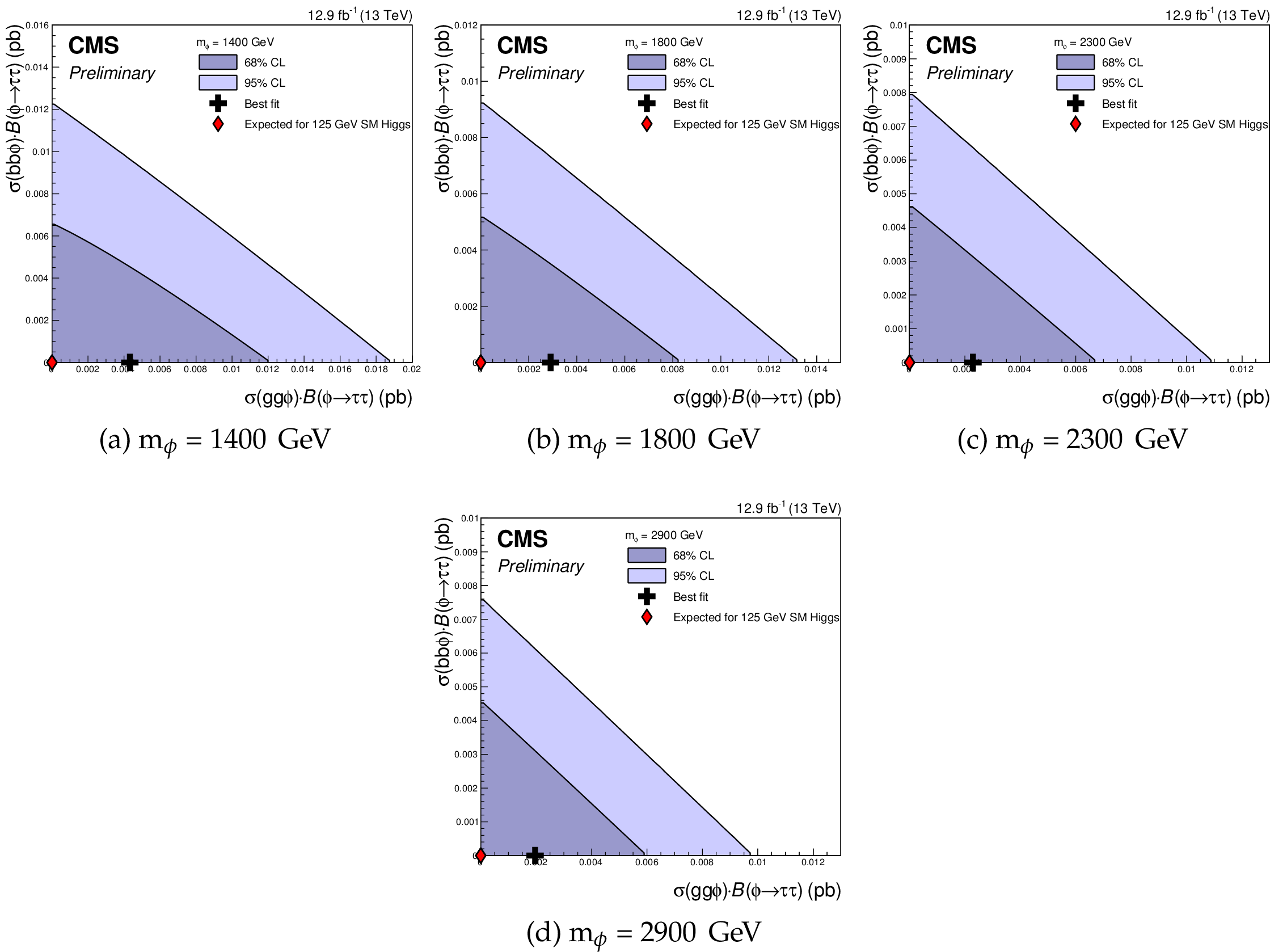
2D likelihood scan of cross-section time branching fraction for $gg\phi $ vs $bb\phi $ production processes, for Higgs boson masses between 1400 GeV and 2900 GeV. The best fit point (black cross) and the 1 and 2 sigma contours are shown for the observed data. Also shown is the best fit value for an Asimov dataset containing background plus the SM Higgs with mass 125 GeV (red diamond). |

png pdf |
Additional Figure 7-a:
2D likelihood scan of cross-section time branching fraction for $gg\phi $ vs $bb\phi $ production processes, for Higgs boson masses between 1400 GeV and 2900 GeV. The best fit point (black cross) and the 1 and 2 sigma contours are shown for the observed data. Also shown is the best fit value for an Asimov dataset containing background plus the SM Higgs with mass 125 GeV (red diamond). |
png pdf |
Additional Figure 7-b:
2D likelihood scan of cross-section time branching fraction for $gg\phi $ vs $bb\phi $ production processes, for Higgs boson masses between 1400 GeV and 2900 GeV. The best fit point (black cross) and the 1 and 2 sigma contours are shown for the observed data. Also shown is the best fit value for an Asimov dataset containing background plus the SM Higgs with mass 125 GeV (red diamond). |

png pdf |
Additional Figure 7-c:
2D likelihood scan of cross-section time branching fraction for $gg\phi $ vs $bb\phi $ production processes, for Higgs boson masses between 1400 GeV and 2900 GeV. The best fit point (black cross) and the 1 and 2 sigma contours are shown for the observed data. Also shown is the best fit value for an Asimov dataset containing background plus the SM Higgs with mass 125 GeV (red diamond). |

png pdf |
Additional Figure 7-d:
2D likelihood scan of cross-section time branching fraction for $gg\phi $ vs $bb\phi $ production processes, for Higgs boson masses between 1400 GeV and 2900 GeV. The best fit point (black cross) and the 1 and 2 sigma contours are shown for the observed data. Also shown is the best fit value for an Asimov dataset containing background plus the SM Higgs with mass 125 GeV (red diamond). |

png pdf |
Additional Figure 8:
Model dependent exclusion limits in the $m_{ {\mathrm {A}} }$-$\tan\beta $ plane, combining all channels, for the $m_{\text{h}}^{\text {mod+}}$ scenario. The red contour indicates the region which does not yield a Higgs boson consistent with a mass of 125 GeV within the theoretical uncertainties of $\pm$3 GeV. The blue lines indicate the expected (dashed) and observed (solid) exclusions obtained from the most recent Run 1 CMS search for $\phi \to \tau \tau $ [1]. |
| Additional Material | |
| Numerical values of ggH and bbH cross section times BR scans (2D database) |
Please read the file for instructions: README
Likelihood scan in 2D plane:
Notes
|
| References | ||||
| 1 | ATLAS Collaboration | Observation of a new particle in the search for the Standard Model Higgs boson with the ATLAS detector at the LHC | PLB 716 (2012) 1--29 | 1207.7214 |
| 2 | CMS Collaboration | Observation of a new boson at a mass of 125 GeV with the CMS experiment at the LHC | PLB 716 (2012) 30--61 | CMS-HIG-12-028 1207.7235 |
| 3 | F. Englert and R. Brout | Broken Symmetry and the Mass of Gauge Vector Mesons | PRL 13 (1964) 321 | |
| 4 | P. W. Higgs | Broken symmetries, massless particles and gauge fields | PL12 (1964) 132 | |
| 5 | P. W. Higgs | Broken Symmetries and the Masses of Gauge Bosons | PRL 13 (1964) 508 | |
| 6 | G. S. Guralnik, C. R. Hagen, and T. W. B. Kibble | Global Conservation Laws and Massless Particles | PRL 13 (1964) 585 | |
| 7 | P. W. Higgs | Spontaneous Symmetry Breakdown without Massless Bosons | PR145 (1966) 1156 | |
| 8 | T. W. B. Kibble | Symmetry breaking in non-Abelian gauge theories | PR155 (1967) 1554 | |
| 9 | ATLAS, CMS Collaboration | Combined Measurement of the Higgs Boson Mass in $ pp $ Collisions at $ \sqrt{s}=$ 7 and 8 TeV with the ATLAS and CMS Experiments | PRL 114 (2015) 191803 | 1503.07589 |
| 10 | ATLAS, CMS Collaboration | Measurements of the Higgs boson production and decay rates and constraints on its couplings from a combined ATLAS and CMS analysis of the LHC pp collision data at $ \sqrt{s}=$ 7 and 8 TeV | JHEP 08 (2016) 045 | 1606.02266 |
| 11 | ATLAS Collaboration | Study of the spin and parity of the Higgs boson in diboson decays with the ATLAS detector | EPJC. 75 (2015), no. 10, 476 | 1506.05669 |
| 12 | CMS Collaboration | Constraints on the spin-parity and anomalous HVV couplings of the Higgs boson in proton collisions at 7 and 8 TeV | PRD 92 (2015), no. 1, 012004 | CMS-HIG-14-018 1411.3441 |
| 13 | A. Djouadi | The Anatomy of electro-weak symmetry breaking. II. The Higgs bosons in the minimal supersymmetric model | PR 459 (2008) 1--241 | hep-ph/0503173 |
| 14 | G. C. Branco et al. | Theory and phenomenology of two-Higgs-doublet models | PR 516 (2012) 1--102 | 1106.0034 |
| 15 | Y. A. Golfand and E. P. Likhtman | Extension of the Algebra of Poincare Group Generators and Violation of p Invariance | JEPTL 13 (1971)323 | |
| 16 | J. Wess and B. Zumino | Supergauge transformations in four dimensions | Nucl. Phys. B. 70 (1974) 39 | |
| 17 | M. Carena et al. | MSSM Higgs Boson Searches at the LHC: Benchmark Scenarios after the Discovery of a Higgs-like Particle | EPJC. 73 (2013), no. 9 | 1302.7033 |
| 18 | E. Bagnaschi et al. | Benchmark scenarios for low $ \tan \beta $ in the MSSM | Technical Report LHCHXSWG-2015-002, CERN, Geneva, Aug | |
| 19 | CMS Collaboration | Search for neutral MSSM Higgs bosons decaying to a pair of tau leptons in pp collisions | JHEP 10 (2014) 160 | CMS-HIG-13-021 1408.3316 |
| 20 | CMS Collaboration | Search for additional neutral Higgs bosons decaying to a pair of tau leptons in pp collisions at $ \sqrt{s} =$ 7 and 8 TeV | CMS-PAS-HIG-14-029 | CMS-PAS-HIG-14-029 |
| 21 | ATLAS Collaboration | Search for neutral Higgs bosons of the minimal supersymmetric standard model in pp collisions at $ \sqrt{s} =$ 8 TeV with the ATLAS detector | JHEP \bf 11 (2014) 056 | 1409.6064 |
| 22 | CMS Collaboration | Search for a neutral MSSM Higgs boson decaying into $ \tau \tau $ at 13 TeV | CMS-PAS-HIG-16-006 | CMS-PAS-HIG-16-006 |
| 23 | ATLAS Collaboration | Search for Minimal Supersymmetric Standard Model Higgs bosons $ H/A $ and for a $ Z^{\prime} $ boson in the $ \tau \tau $ final state produced in $ pp $ collisions at $ \sqrt{s}= $ 13 TeV with the ATLAS Detector | EPJC. 76 (2016), no. 11, 585 | 1608.00890 |
| 24 | ATLAS Collaboration | Search for Minimal Supersymmetric Standard Model Higgs Bosons $ H/A $ in the $ \tau\tau $ final state in up to 13.3 fb$ ^{-1} $ of pp collisions at $ \sqrt{s} $= 13 TeV with the ATLAS Detector | ATLAS Conference Note ATLAS-CONF-2016-085 | |
| 25 | CMS Collaboration | The CMS experiment at the CERN LHC | JINST 3 (2008) S08004 | CMS-00-001 |
| 26 | CMS Collaboration | Particle--Flow Event Reconstruction in CMS and Performance for Jets, Taus, and $ E_{\mathrm{T}}^{\text{miss}} $ | CDS | |
| 27 | CMS Collaboration | Commissioning of the Particle-flow Event Reconstruction with the first LHC collisions recorded in the CMS detector | CDS | |
| 28 | K. Rose | Deterministic annealing for clustering, compression, classification, regression, and related optimization problems | Proceedings of the IEEE 86 (Nov, 1998) 2210--2239 | |
| 29 | CMS Collaboration | Performance of electron reconstruction and selection with the CMS detector in proton-proton collisions at $ \sqrt{s} = $ 8 TeV | JINST 10 (2015) P06005 | CMS-EGM-13-001 1502.02701 |
| 30 | H. Voss, A. H\"ocker, J. Stelzer, and F. Tegenfeldt | TMVA, the Toolkit for Multivariate Data Analysis with ROOT | in XIth International Workshop on Advanced Computing and Analysis Techniques in Physics Research (ACAT), p. 40 2007 | physics/0703039 |
| 31 | CMS Collaboration | Performance of CMS muon reconstruction in $ \mathrm{ p }\mathrm{ p } $ collision events at $ \sqrt{s}= $ 7 TeV | JINST 7 (2012) P10002 | CMS-MUO-10-004 1206.4071 |
| 32 | M. Cacciari, G. P. Salam, and G. Soyez | FastJet user manual | EPJC. 72 (2012) 1896 | 1111.6097 |
| 33 | M. Cacciari and G. P. Salam | Dispelling the $ N^{3} $ myth for the $ k_t $ jet-finder | PLB 641 (2006) 57 | hep-ph/0512210 |
| 34 | CMS Collaboration | Identification of b-quark jets with the CMS experiment | JINST 8 (2013) P04013 | CMS-BTV-12-001 1211.4462 |
| 35 | CMS Collaboration | Performance of reconstruction and identification of tau leptons in their decays to hadrons and tau neutrino in LHC Run-2 | CMS-PAS-TAU-16-002 | CMS-PAS-TAU-16-002 |
| 36 | CMS Collaboration | Reconstruction and identification of $\tau$ lepton decays to hadrons and $\mu_{\tau}$ at CMS | JINST 11 (2016), no. 01, P01019 | CMS-TAU-14-001 1510.07488 |
| 37 | CMS Collaboration | Performance of the CMS missing transverse momentum reconstruction in pp data at $ \sqrt{s} =$ 8 TeV | JINST 10 (2015) P02006 | CMS-JME-13-003 1411.0511 |
| 38 | T. Sjostrand, S. Mrenna, and P. Z. Skands | A Brief Introduction to PYTHIA 8.1 | CPC 178 (2008) 852--867 | 0710.3820 |
| 39 | J. Alwall et al. | The automated computation of tree-level and next-to-leading order differential cross sections, and their matching to parton shower simulations | JHEP 07 (2014) 079 | 1405.0301 |
| 40 | S. Alioli, P. Nason, C. Oleari, and E. Re | NLO single-top production matched with shower in POWHEG: s- and t-channel contributions | JHEP 09 (2009) 111, , [Erratum: JHEP02,011(2010)] | 0907.4076 |
| 41 | CMS Collaboration | Measurement of differential top-quark pair production cross sections in the lepton+jets channel in pp collisions at 8 TeV | CDS | |
| 42 | CMS Collaboration | Measurement of the differential cross section for top quark pair production in pp collisions at $ \sqrt{s} = $ 8 TeV | EPJC. 75 (2015), no. 11, 542 | CMS-TOP-12-028 1505.04480 |
| 43 | CMS Collaboration | Measurements of inclusive $ \mathrm{ W } $ and $ \mathrm{ Z } $ cross sections in $ \mathrm{ p }\mathrm{ p } $ collisions at $ \sqrt{s}= $ 7 TeV | JHEP 01 (2011) 080 | CMS-EWK-10-002 1012.2466 |
| 44 | CMS Collaboration | CMS Luminosity Measurement for the 2015 Data Taking Period | CMS-PAS-LUM-15-001 | CMS-PAS-LUM-15-001 |
| 45 | A. D. Martin, W. J. Stirling, R. S. Thorne, and G. Watt | Parton distributions for the LHC | EPJC. 63 (2009) 189--285 | 0901.0002 |
| 46 | A. D. Martin, W. J. Stirling, R. S. Thorne, and G. Watt | Uncertainties on alpha(S) in global PDF analyses and implications for predicted hadronic cross sections | EPJC. 64 (2009) 653--680 | 0905.3531 |
| 47 | The LHC Higgs Cross Section Working Group Collaboration | Handbook of LHC Higgs Cross Sections: 4. Deciphering the Nature of the Higgs Sector | 1610.07922 | |
| 48 | L. Moneta et al. | The RooStats Project | PoS ACAT2010 (2010) 057 | 1009.1003 |
| 49 | LHC Higgs Cross Section Working Group Collaboration | Handbook of LHC Higgs Cross Sections: 3. Higgs Properties | 1307.1347 | |
| 50 | R. V. Harlander, S. Liebler, and H. Mantler | SusHi: A program for the calculation of Higgs production in gluon fusion and bottom-quark annihilation in the Standard Model and the MSSM | CPC 184 (2013) 1605--1617 | 1212.3249 |
| 51 | M. Spira, A. Djouadi, D. Graudenz, and P. M. Zerwas | Higgs boson production at the LHC | Nucl. Phys. B. 453 (1995) 17--82 | hep-ph/9504378 |
| 52 | R. V. Harlander and M. Steinhauser | Supersymmetric Higgs production in gluon fusion at next-to-leading order | JHEP 09 (2004) 066 | hep-ph/0409010 |
| 53 | R. Harlander and P. Kant | Higgs production and decay: Analytic results at next-to-leading order QCD | JHEP 12 (2005) 015 | hep-ph/0509189 |
| 54 | G. Degrassi and P. Slavich | NLO QCD bottom corrections to Higgs boson production in the MSSM | JHEP 11 (2010) 044 | 1007.3465 |
| 55 | G. Degrassi, S. Di Vita, and P. Slavich | NLO QCD corrections to pseudoscalar Higgs production in the MSSM | JHEP 08 (2011) 128 | 1107.0914 |
| 56 | G. Degrassi, S. Di Vita, and P. Slavich | On the NLO QCD Corrections to the Production of the Heaviest Neutral Higgs Scalar in the MSSM | EPJC. 72 (2012) 2032 | 1204.1016 |
| 57 | R. V. Harlander and W. B. Kilgore | Next-to-next-to-leading order Higgs production at hadron colliders | PRL 88 (2002) 201801 | hep-ph/0201206 |
| 58 | C. Anastasiou and K. Melnikov | Higgs boson production at hadron colliders in NNLO QCD | Nucl. Phys. B. 646 (2002) 220--256 | hep-ph/0207004 |
| 59 | V. Ravindran, J. Smith, and W. L. van Neerven | NNLO corrections to the total cross-section for Higgs boson production in hadron hadron collisions | Nucl. Phys. B. 665 (2003) 325--366 | hep-ph/0302135 |
| 60 | R. V. Harlander and W. B. Kilgore | Production of a pseudoscalar Higgs boson at hadron colliders at next-to-next-to leading order | JHEP 10 (2002) 017 | hep-ph/0208096 |
| 61 | C. Anastasiou and K. Melnikov | Pseudoscalar Higgs boson production at hadron colliders in NNLO QCD | PRD. 67 (2003) 037501 | hep-ph/0208115 |
| 62 | U. Aglietti, R. Bonciani, G. Degrassi, and A. Vicini | Two loop light fermion contribution to Higgs production and decays | PLB. 595 (2004) 432--441 | hep-ph/0404071 |
| 63 | R. Bonciani, G. Degrassi, and A. Vicini | On the Generalized Harmonic Polylogarithms of One Complex Variable | CPC 182 (2011) 1253--1264 | 1007.1891 |
| 64 | S. Dittmaier, M. Kramer, 1, and M. Spira | Higgs radiation off bottom quarks at the Tevatron and the CERN LHC | PRD 70 (2004) 074010 | hep-ph/0309204 |
| 65 | S. Dawson, C. B. Jackson, L. Reina, and D. Wackeroth | Exclusive Higgs boson production with bottom quarks at hadron colliders | PRD 69 (Apr, 2004) 074027 | |
| 66 | R. V. Harlander and W. B. Kilgore | Higgs boson production in bottom quark fusion at next-to-next-to-leading order | PRD 68 (Jul, 2003) 013001 | |
| 67 | R. Harlander, M. Kramer, and M. Schumacher | Bottom-quark associated Higgs-boson production: reconciling the four- and five-flavour scheme approach | 1112.3478 | |
| 68 | S. Heinemeyer, W. Hollik, and G. Weiglein | FeynHiggs: A Program for the calculation of the masses of the neutral CP even Higgs bosons in the MSSM | CPC 124 (2000) 76--89 | hep-ph/9812320 |
| 69 | S. Heinemeyer, W. Hollik, and G. Weiglein | The Masses of the neutral CP - even Higgs bosons in the MSSM: Accurate analysis at the two loop level | EPJC. 9 (1999) 343--366 | hep-ph/9812472 |
| 70 | G. Degrassi et al. | Towards high precision predictions for the MSSM Higgs sector | EPJC. 28 (2003) 133--143 | hep-ph/0212020 |
| 71 | M. Frank et al. | The Higgs Boson Masses and Mixings of the Complex MSSM in the Feynman-Diagrammatic Approach | JHEP 02 (2007) 047 | hep-ph/0611326 |
| 72 | T. Hahn et al. | High-Precision Predictions for the Light CP -Even Higgs Boson Mass of the Minimal Supersymmetric Standard Model | PRL 112 (2014), no. 14, 141801 | 1312.4937 |
| 73 | A. Djouadi, J. Kalinowski, and M. Spira | HDECAY: A Program for Higgs boson decays in the standard model and its supersymmetric extension | CPC 108 (1998) 56--74 | hep-ph/9704448 |
|
|
Compact Muon Solenoid LHC, CERN |
|

|

|

|

|

|