

Compact Muon Solenoid
LHC, CERN
| CMS-EXO-16-051 ; CERN-EP-2017-299 | ||
| Search for dark matter in events with energetic, hadronically decaying top quarks and missing transverse momentum at $\sqrt{s} = $ 13 TeV | ||
| CMS Collaboration | ||
| 25 January 2018 | ||
| JHEP 06 (2018) 027 | ||
| Abstract: A search for dark matter is conducted in events with large missing transverse momentum and a hadronically decaying, Lorentz-boosted top quark. This study is performed using proton-proton collisions at a center-of-mass energy of 13 TeV, in data recorded by the CMS detector in 2016 at the LHC, corresponding to an integrated luminosity of 36 fb$^{-1}$. New substructure techniques, including the novel use of energy correlation functions, are utilized to identify the decay products of the top quark. With no significant deviations observed from predictions of the standard model, limits are placed on the production of new heavy bosons coupling to dark matter particles. For a scenario with purely vector-like or purely axial-vector-like flavor changing neutral currents, mediator masses between 0.20 and 1.75 TeV are excluded at 95% confidence level, given a sufficiently small dark matter mass. Scalar resonances decaying into a top quark and a dark matter fermion are excluded for masses below 3.4 TeV, assuming a dark matter mass of 100 GeV. | ||
| Links: e-print arXiv:1801.08427 [hep-ex] (PDF) ; CDS record ; inSPIRE record ; CADI line (restricted) ; | ||
| Figures | |

png pdf |
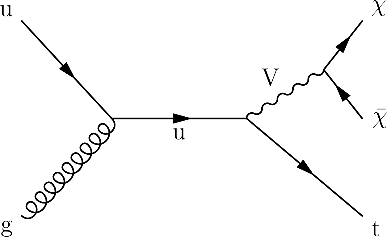
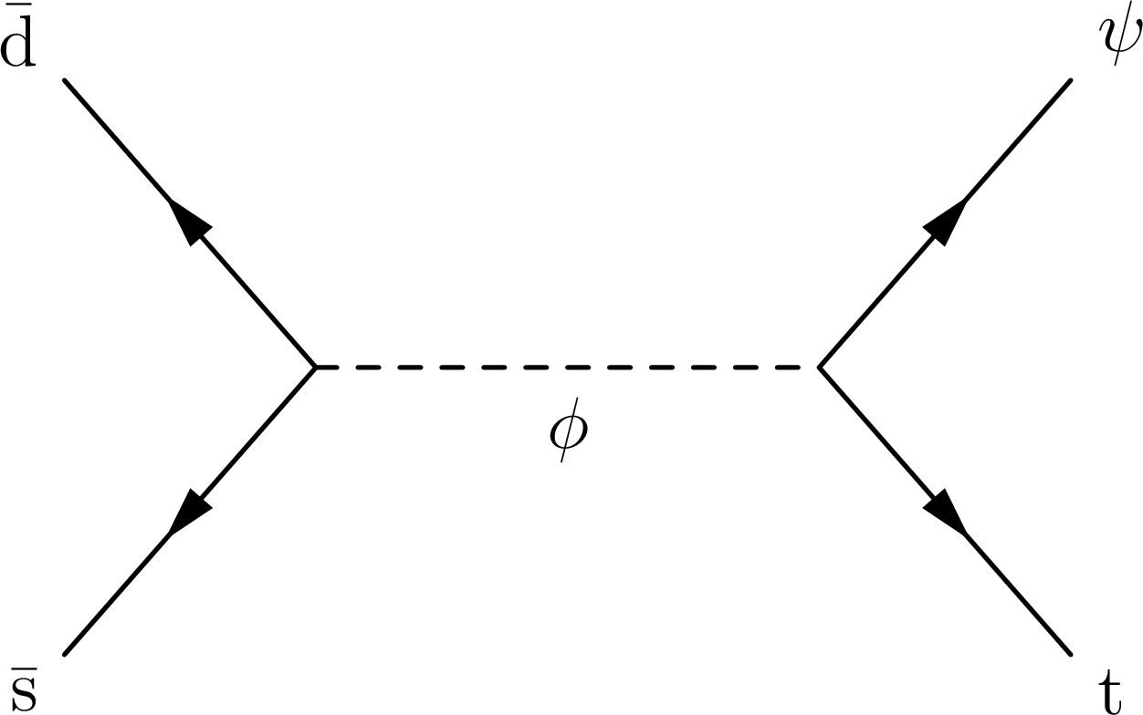
Figure 1:
Example Feynman diagrams of monotop production via a flavor-changing neutral current V (left) and a charged, heavy scalar resonance $\phi $ (right). |
png pdf |
Figure 1-a:
Example Feynman diagram of monotop production via a flavor-changing neutral current V. |
png pdf |
Figure 1-b:
Example Feynman diagram of monotop production via a charged, heavy scalar resonance $\phi $. |
png pdf |
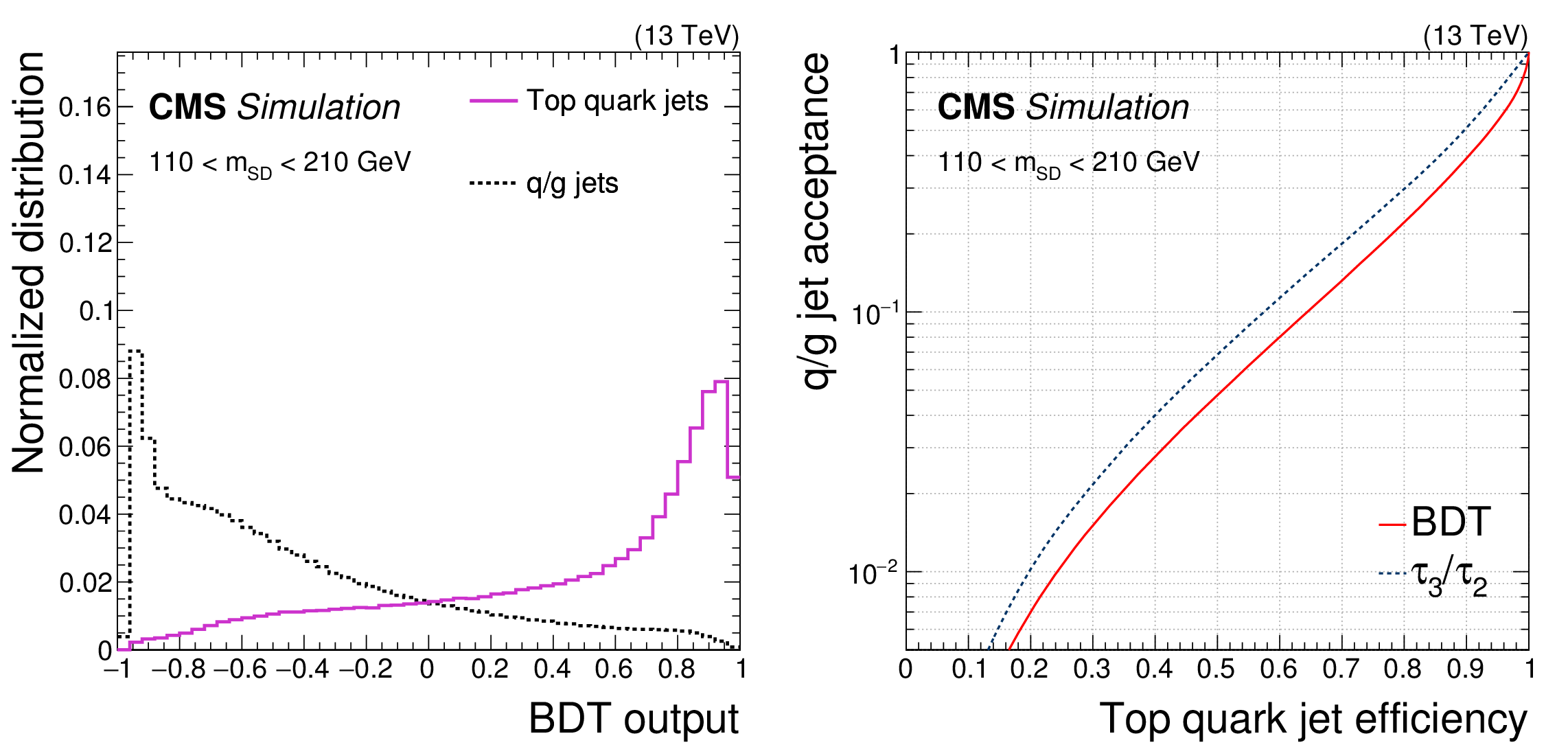
Figure 2:
Performance of BDT tagging of top quark and q/g jets. The left figure shows the BDT output in both types of jets. The right figure shows the rate of misidentifying a q/g jet as a function of the efficiency of selecting top jets. In both figures, the $ {p_{\mathrm {T}}} $ spectra of jets are weighted to be uniform, and the $m_\mathrm {SD}$ is required to be in the range of 110-210 GeV. |

png pdf |
Figure 2-a:
Performance of BDT tagging of top quark and q/g jets. The figure shows the BDT output in both types of jets. The $ {p_{\mathrm {T}}} $ spectra of jets are weighted to be uniform, and the $m_\mathrm {SD}$ is required to be in the range of 110-210 GeV. |

png pdf |
Figure 2-b:
Performance of BDT tagging of top quark and q/g jets. The figure shows the rate of misidentifying a q/g jet as a function of the efficiency of selecting top jets. The $ {p_{\mathrm {T}}} $ spectra of jets are weighted to be uniform, and the $m_\mathrm {SD}$ is required to be in the range of 110-210 GeV. |

png pdf |
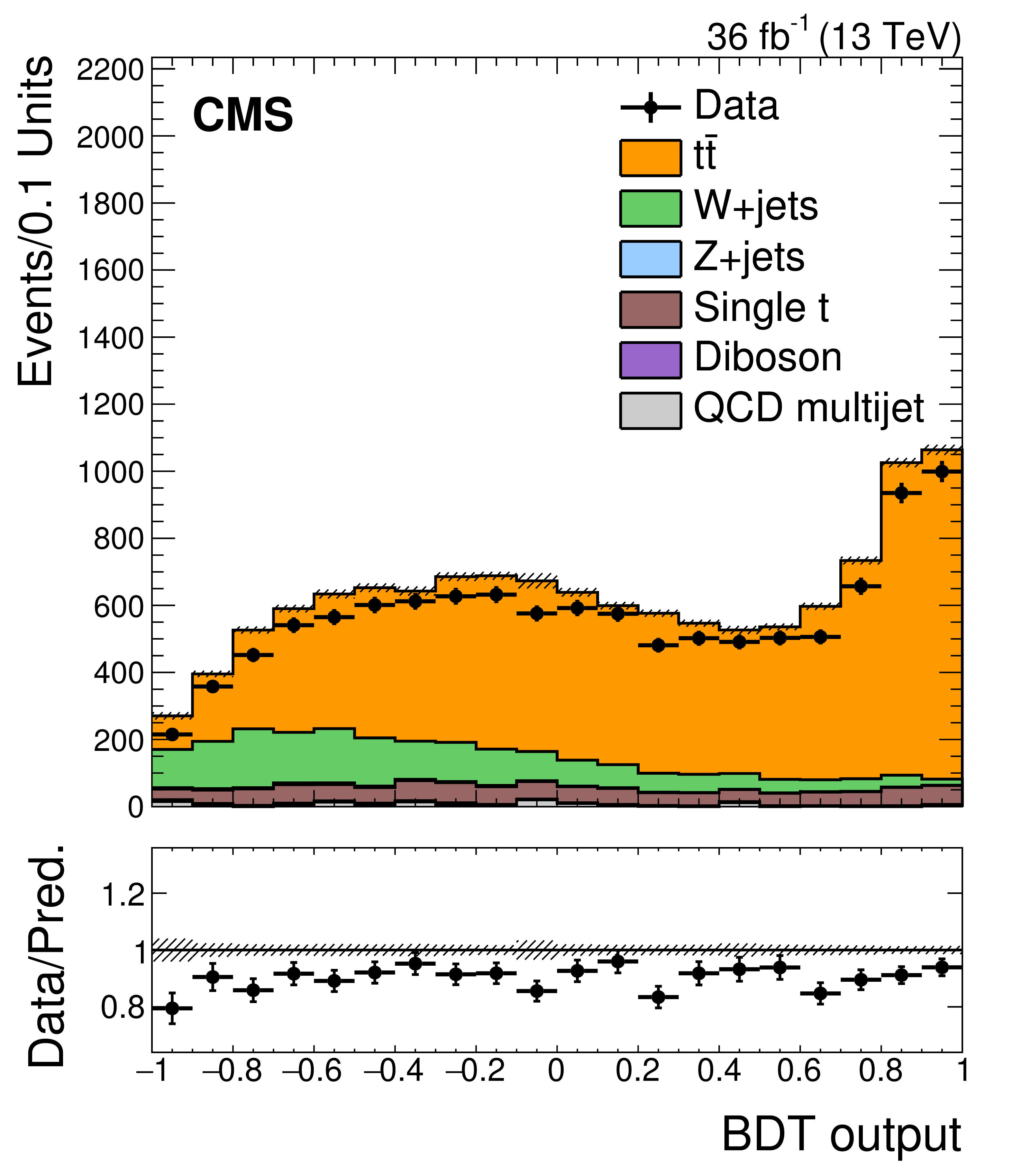
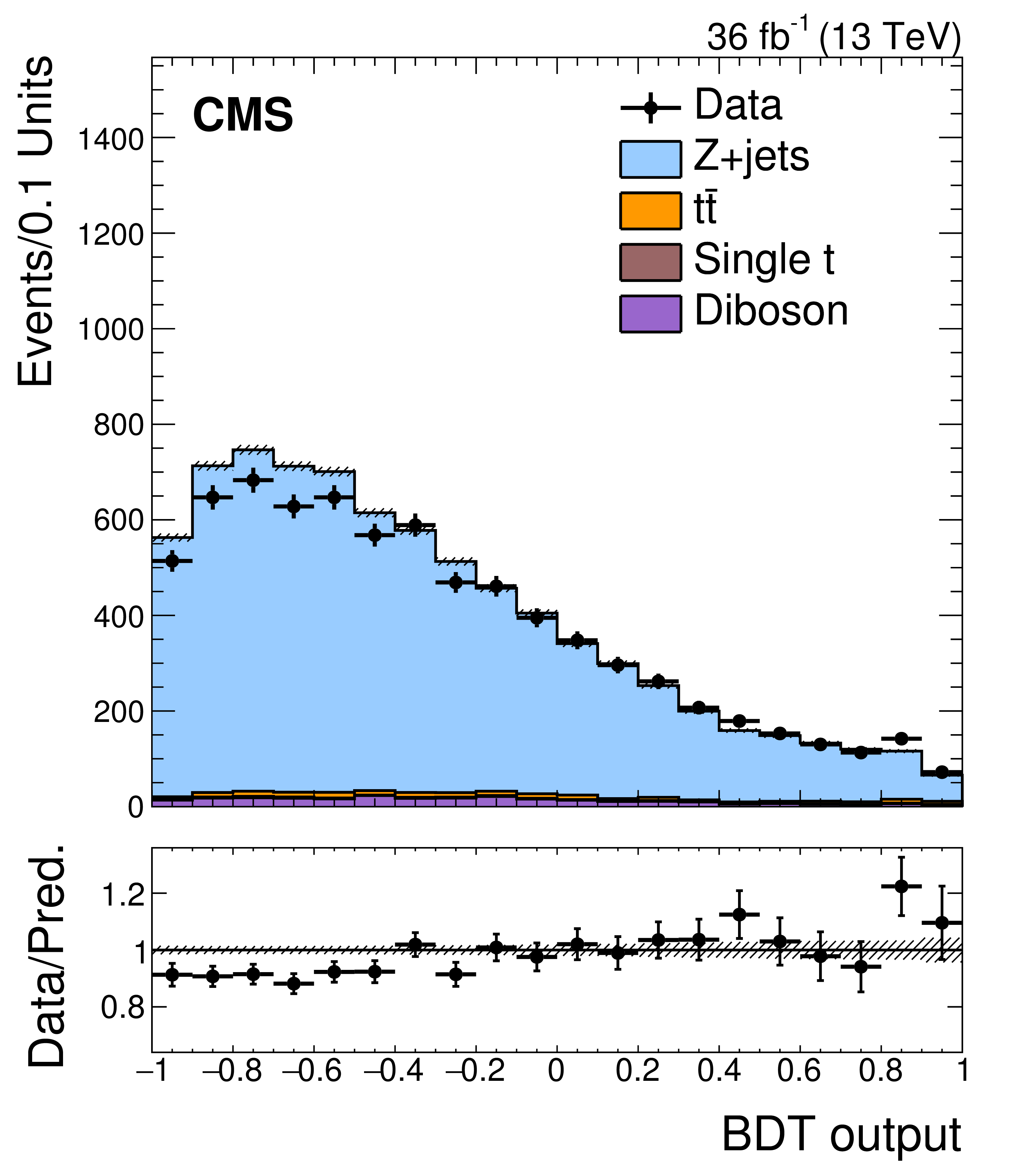
Figure 3:
Comparison of the BDT response in data and in simulation, in samples enriched in top-quark jets (left) and q/g jets (right). The lower panel of each plot shows the ratio of the observed data to the SM prediction in each bin. The shaded bands represent the statistical uncertainties in the simulation. |
png pdf |
Figure 3-a:
Comparison of the BDT response in data and in simulation, in samples enriched in top-quark jets. The lower panel shows the ratio of the observed data to the SM prediction in each bin. The shaded band represents the statistical uncertainties in the simulation. |
png pdf |
Figure 3-b:
Comparison of the BDT response in data and in simulation, in samples enriched in q/g jets. The lower panel shows the ratio of the observed data to the SM prediction in each bin. The shaded band represents the statistical uncertainties in the simulation. |
png pdf |
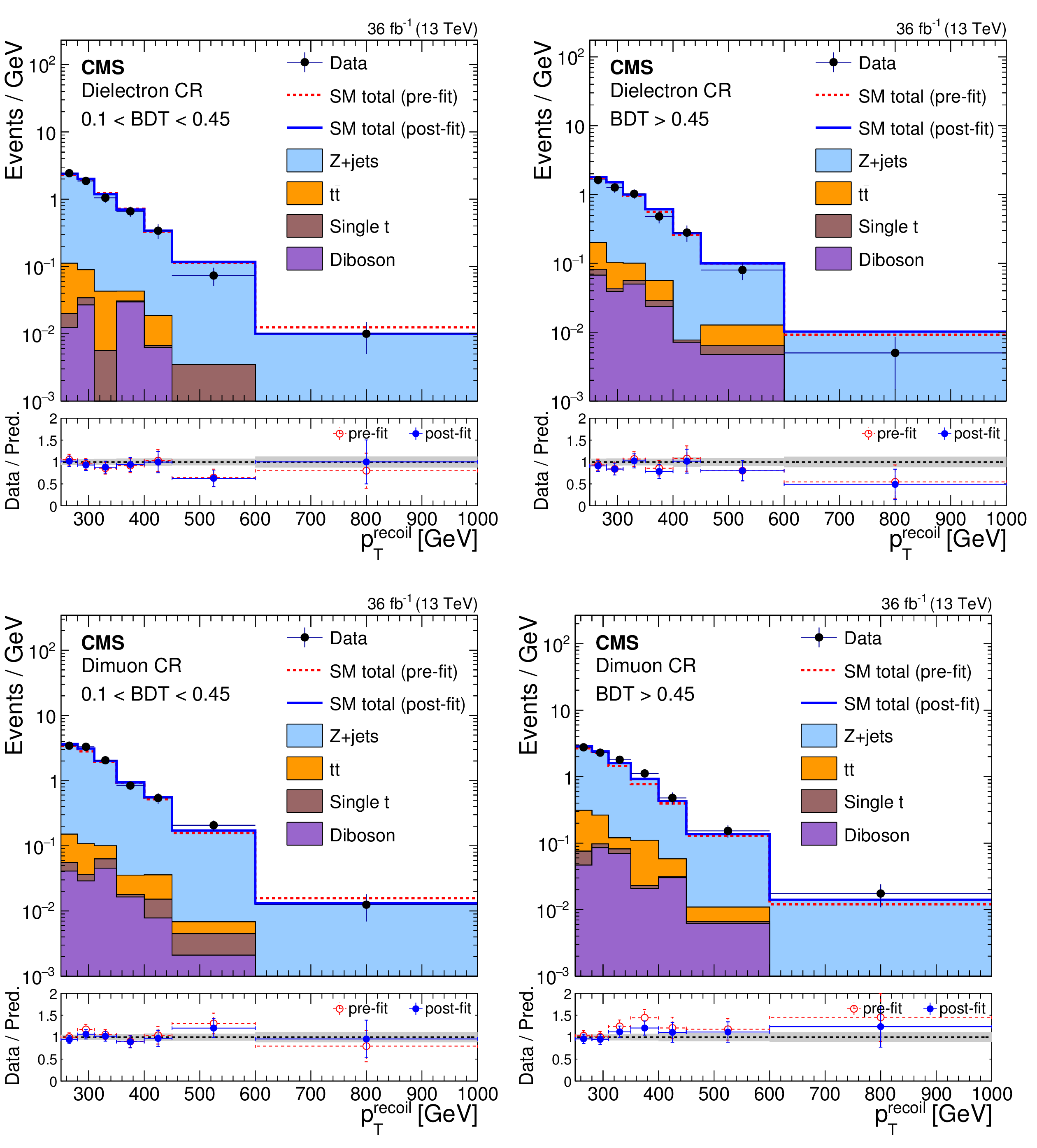
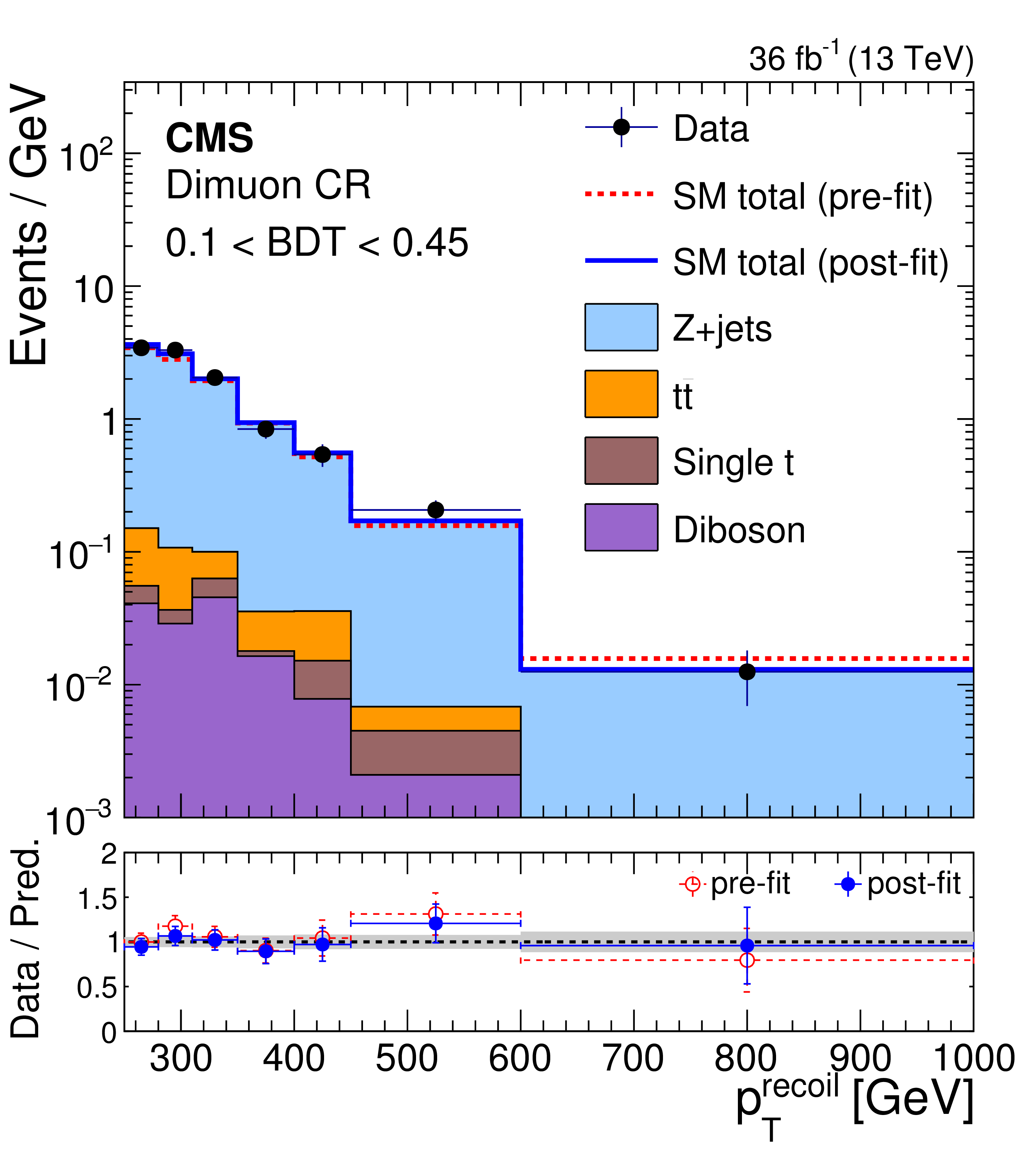
Figure 4:
Comparison between data and SM predictions in the dilepton control regions before and after performing the simultaneous fit to the different control regions and signal region. Each bin shows the event yields divided by the width of the bin. The upper row of figures corresponds to the dielectron control region, and the lower row to the dimuon control region. The left (right) column of figures corresponds to the loose (tight) category of the control regions. The blue solid line represents the sum of the SM contributions normalized to their fitted yields. The red dashed line represents the sum of the SM contributions normalized to the prediction. The stacked histograms show the individual fitted SM contributions. The lower panel of each figure shows the ratio of data to fitted prediction. The gray band on the ratio indicates the one standard deviation uncertainty on the prediction after propagating all the systematic uncertainties and their correlations in the fit. |
png pdf |
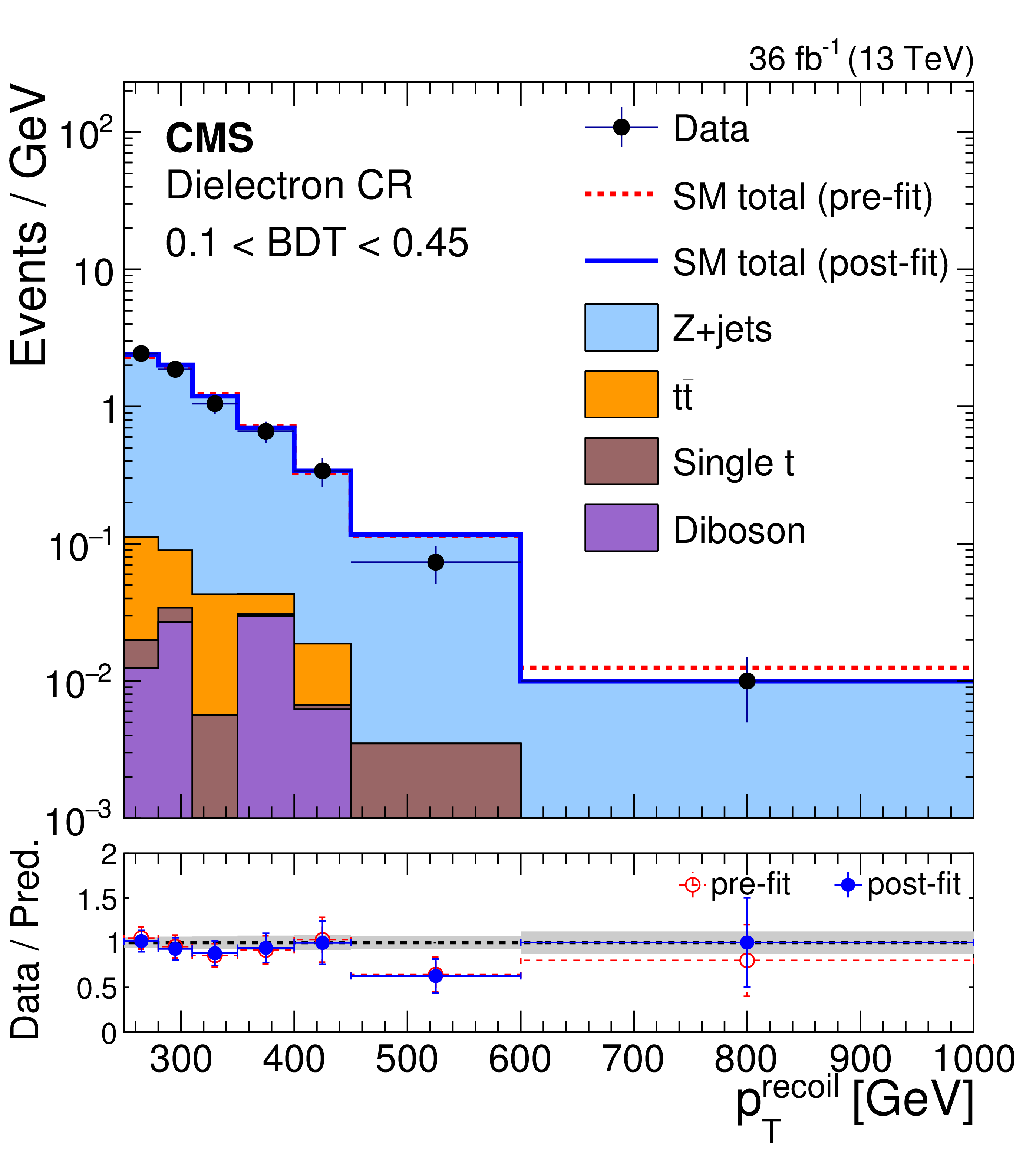
Figure 4-a:
Comparison between data and SM predictions in the dilepton control regions before and after performing the simultaneous fit to the different control regions and signal region. Each bin shows the event yields divided by the width of the bin. The figure corresponds to the dielectron control region and the loose category of the control regions. The blue solid line represents the sum of the SM contributions normalized to their fitted yields. The red dashed line represents the sum of the SM contributions normalized to the prediction. The stacked histograms show the individual fitted SM contributions. The lower panel shows the ratio of data to fitted prediction. The gray band on the ratio indicates the one standard deviation uncertainty on the prediction after propagating all the systematic uncertainties and their correlations in the fit. |
png pdf |
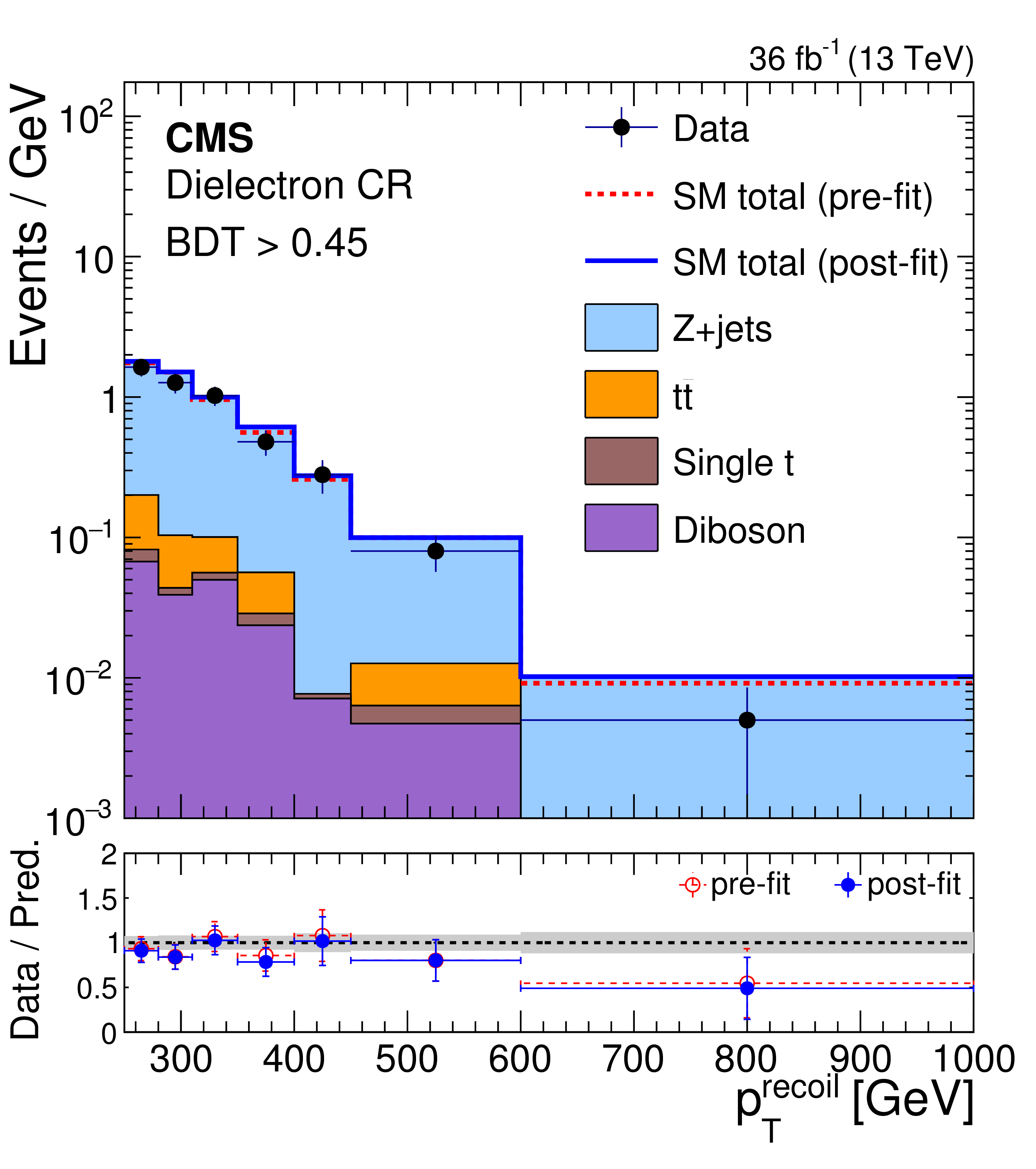
Figure 4-b:
Comparison between data and SM predictions in the dilepton control regions before and after performing the simultaneous fit to the different control regions and signal region. Each bin shows the event yields divided by the width of the bin. The figure corresponds to the dielectron control region and the tight category of the control regions. The blue solid line represents the sum of the SM contributions normalized to their fitted yields. The red dashed line represents the sum of the SM contributions normalized to the prediction. The stacked histograms show the individual fitted SM contributions. The lower panel shows the ratio of data to fitted prediction. The gray band on the ratio indicates the one standard deviation uncertainty on the prediction after propagating all the systematic uncertainties and their correlations in the fit. |
png pdf |
Figure 4-c:
Comparison between data and SM predictions in the dilepton control regions before and after performing the simultaneous fit to the different control regions and signal region. Each bin shows the event yields divided by the width of the bin. The figure corresponds to the dimuon control region and the loose category of the control regions. The blue solid line represents the sum of the SM contributions normalized to their fitted yields. The red dashed line represents the sum of the SM contributions normalized to the prediction. The stacked histograms show the individual fitted SM contributions. The lower panel shows the ratio of data to fitted prediction. The gray band on the ratio indicates the one standard deviation uncertainty on the prediction after propagating all the systematic uncertainties and their correlations in the fit. |

png pdf |
Figure 4-d:
Comparison between data and SM predictions in the dilepton control regions before and after performing the simultaneous fit to the different control regions and signal region. Each bin shows the event yields divided by the width of the bin. The figure corresponds to the dimuon control region and the tight category of the control regions. The blue solid line represents the sum of the SM contributions normalized to their fitted yields. The red dashed line represents the sum of the SM contributions normalized to the prediction. The stacked histograms show the individual fitted SM contributions. The lower panel shows the ratio of data to fitted prediction. The gray band on the ratio indicates the one standard deviation uncertainty on the prediction after propagating all the systematic uncertainties and their correlations in the fit. |

png pdf |
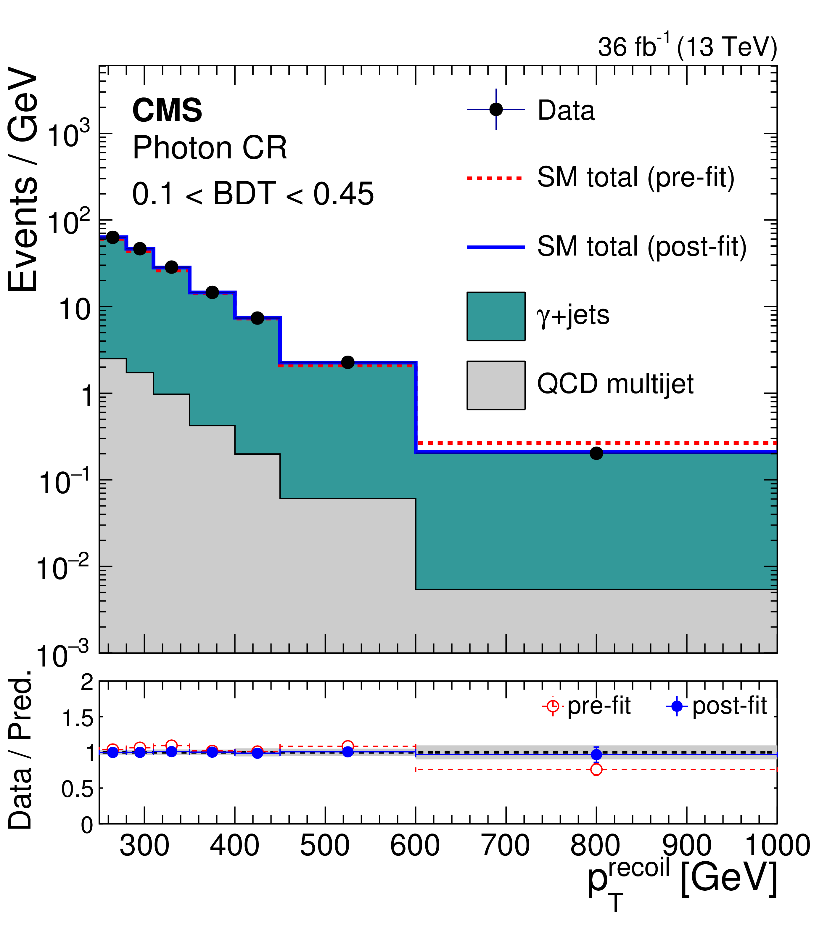
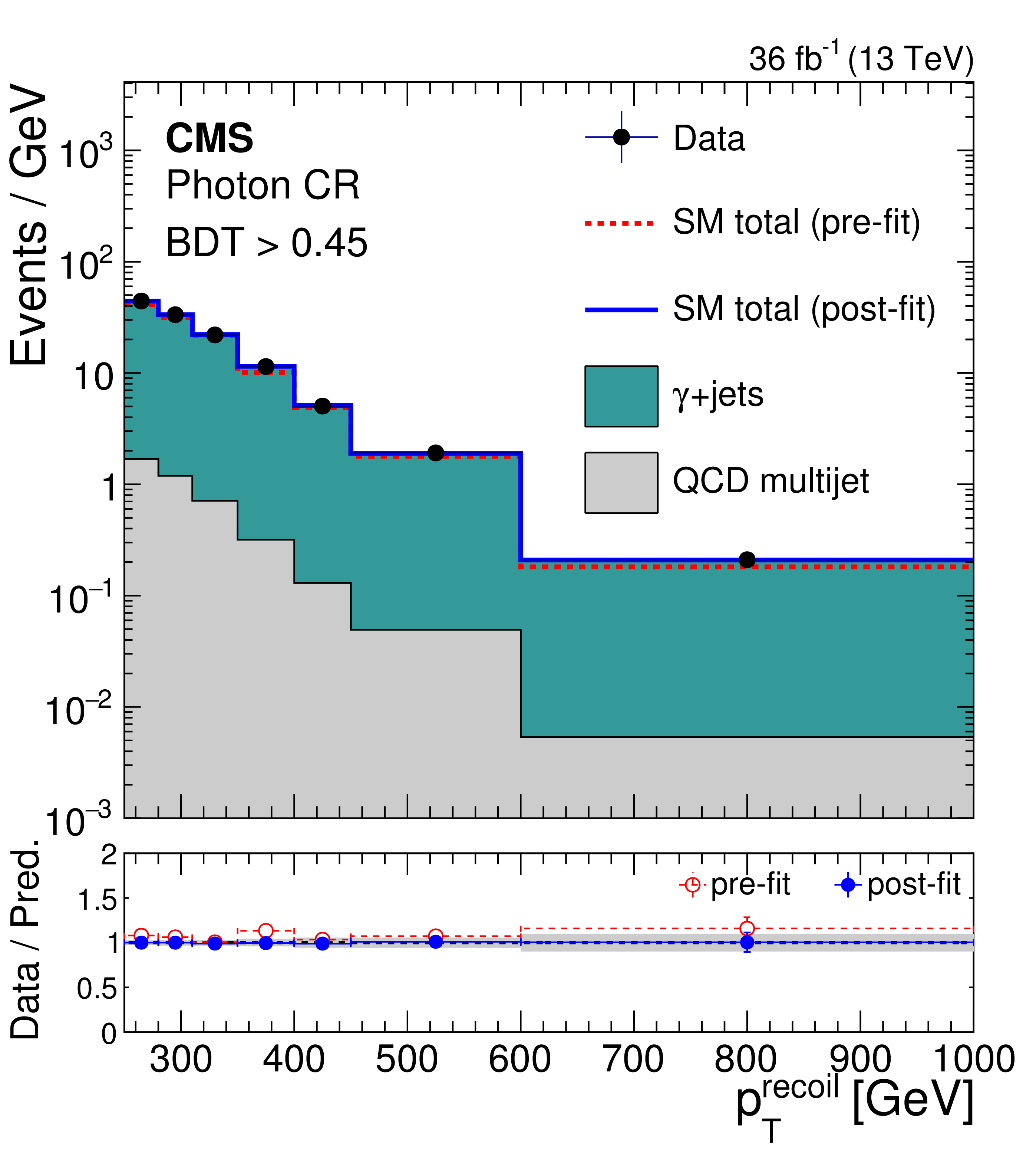
Figure 5:
Comparison between data and SM predictions in the photon control regions before and after performing the simultaneous fit to the different control regions and signal region. Each bin shows the event yields divided by the width of the bin. The left (right) figure corresponds to the loose (tight) category of the control region. The blue solid line represents the sum of the SM contributions normalized to their fitted yields. The red dashed line represents the sum of the SM contributions normalized to the prediction. The stacked histograms show the individual fitted SM contributions. The lower panel of each figure shows the ratio of data to fitted prediction. The gray band on the ratio indicates the one standard deviation uncertainty on the prediction after propagating all the systematic uncertainties and their correlations in the fit. |
png pdf |
Figure 5-a:
Comparison between data and SM predictions in the photon control regions before and after performing the simultaneous fit to the different control regions and signal region. Each bin shows the event yields divided by the width of the bin. The figure corresponds to the loose category of the control region. The blue solid line represents the sum of the SM contributions normalized to their fitted yields. The red dashed line represents the sum of the SM contributions normalized to the prediction. The stacked histograms show the individual fitted SM contributions. The lower panel shows the ratio of data to fitted prediction. The gray band on the ratio indicates the one standard deviation uncertainty on the prediction after propagating all the systematic uncertainties and their correlations in the fit. |
png pdf |
Figure 5-b:
Comparison between data and SM predictions in the photon control regions before and after performing the simultaneous fit to the different control regions and signal region. Each bin shows the event yields divided by the width of the bin. The figure corresponds to the tight category of the control region. The blue solid line represents the sum of the SM contributions normalized to their fitted yields. The red dashed line represents the sum of the SM contributions normalized to the prediction. The stacked histograms show the individual fitted SM contributions. The lower panel shows the ratio of data to fitted prediction. The gray band on the ratio indicates the one standard deviation uncertainty on the prediction after propagating all the systematic uncertainties and their correlations in the fit. |

png pdf |
Figure 6:
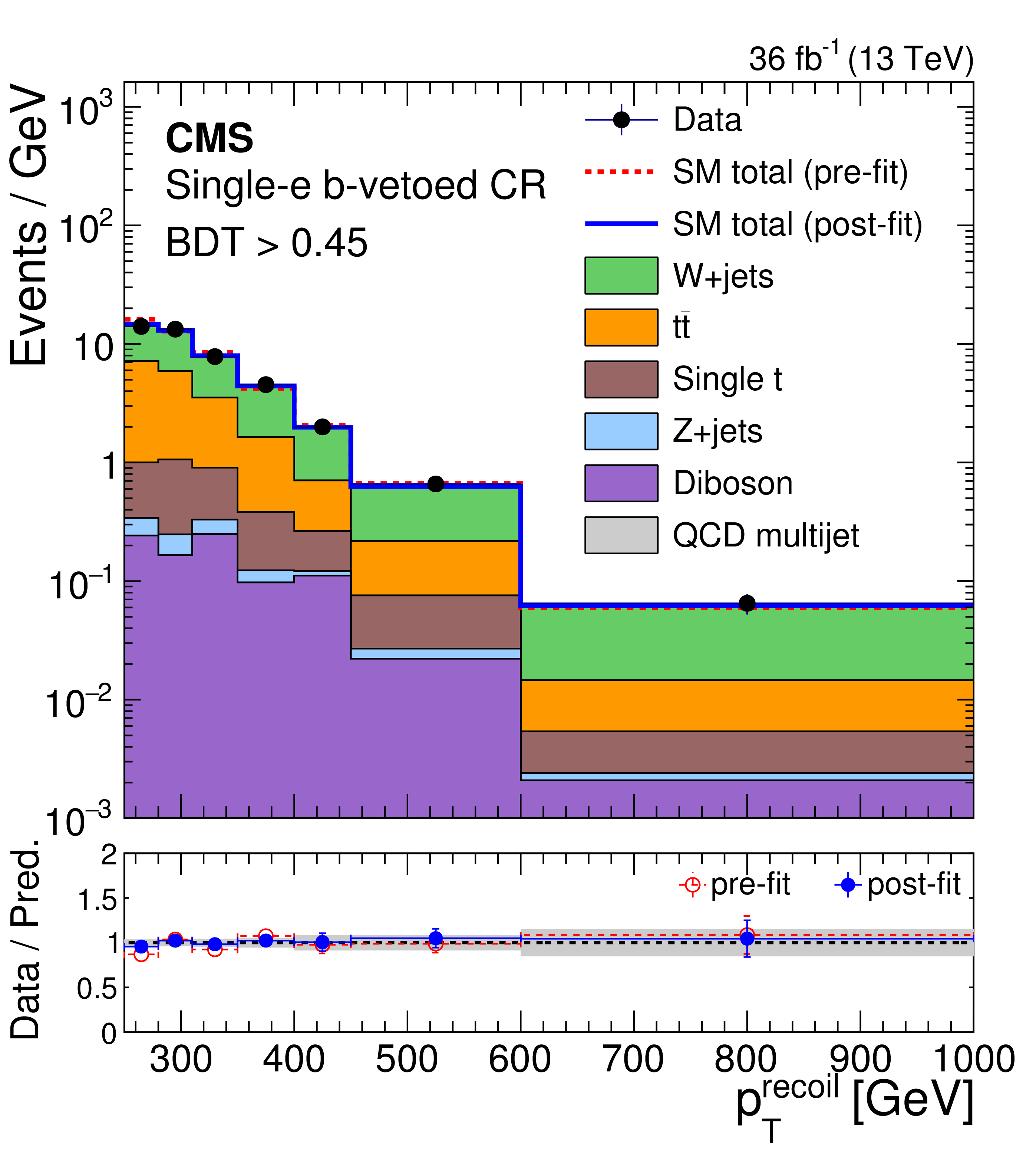
Comparison between data and SM predictions in the b-vetoed single lepton control regions before and after performing the simultaneous fit to the different control regions and signal region. Each bin shows the event yields divided by the width of the bin. The upper row of figures corresponds to the single electron b-vetoed control region, and lower row to the single muon b-vetoed control region. The left (right) column of figures corresponds to the loose (tight) category of the control regions. The blue solid line represents the sum of the SM contributions normalized to their fitted yields. The red dashed line represents the sum of the SM contributions normalized to the prediction. The stacked histograms show the individual fitted SM contributions. The lower panel of each figure shows the ratio of data to fitted prediction. The gray band on the ratio indicates the one standard deviation uncertainty on the prediction after propagating all the systematic uncertainties and their correlations in the fit. |

png pdf |
Figure 6-a:
Comparison between data and SM predictions in the b-vetoed single lepton control regions before and after performing the simultaneous fit to the different control regions and signal region. Each bin shows the event yields divided by the width of the bin. The figure corresponds to the single electron b-vetoed control region, and corresponds to the loose category of the control regions. The blue solid line represents the sum of the SM contributions normalized to their fitted yields. The red dashed line represents the sum of the SM contributions normalized to the prediction. The stacked histograms show the individual fitted SM contributions. The lower panel shows the ratio of data to fitted prediction. The gray band on the ratio indicates the one standard deviation uncertainty on the prediction after propagating all the systematic uncertainties and their correlations in the fit. |
png pdf |
Figure 6-b:
Comparison between data and SM predictions in the b-vetoed single lepton control regions before and after performing the simultaneous fit to the different control regions and signal region. Each bin shows the event yields divided by the width of the bin. The figure corresponds to the single electron b-vetoed control region, and corresponds to the tight category of the control regions. The blue solid line represents the sum of the SM contributions normalized to their fitted yields. The red dashed line represents the sum of the SM contributions normalized to the prediction. The stacked histograms show the individual fitted SM contributions. The lower panel shows the ratio of data to fitted prediction. The gray band on the ratio indicates the one standard deviation uncertainty on the prediction after propagating all the systematic uncertainties and their correlations in the fit. |
png pdf |
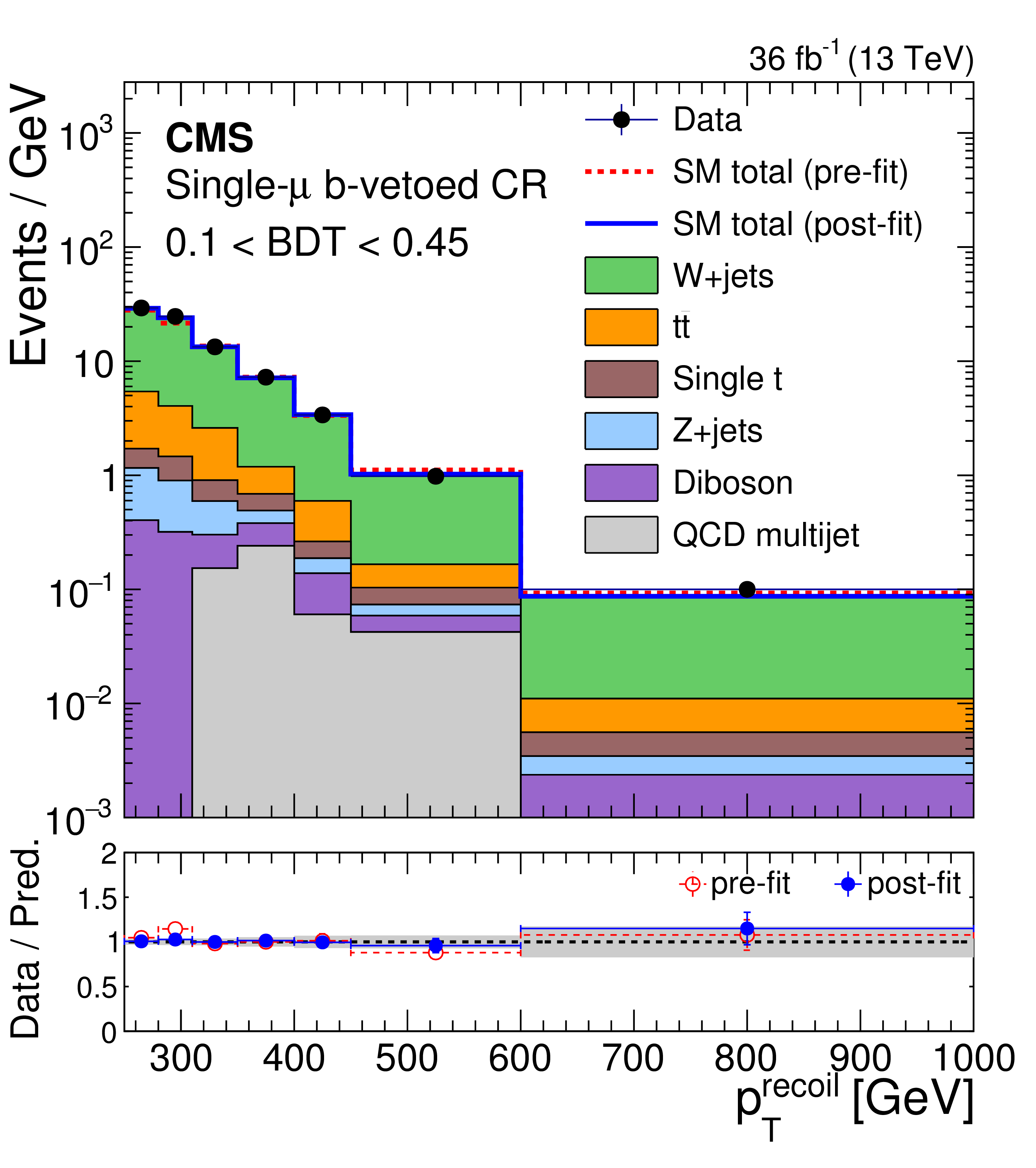
Figure 6-c:
Comparison between data and SM predictions in the b-vetoed single lepton control regions before and after performing the simultaneous fit to the different control regions and signal region. Each bin shows the event yields divided by the width of the bin. The figure corresponds to the single muon b-vetoed control region, and corresponds to the loose category of the control regions. The blue solid line represents the sum of the SM contributions normalized to their fitted yields. The red dashed line represents the sum of the SM contributions normalized to the prediction. The stacked histograms show the individual fitted SM contributions. The lower panel shows the ratio of data to fitted prediction. The gray band on the ratio indicates the one standard deviation uncertainty on the prediction after propagating all the systematic uncertainties and their correlations in the fit. |
png pdf |
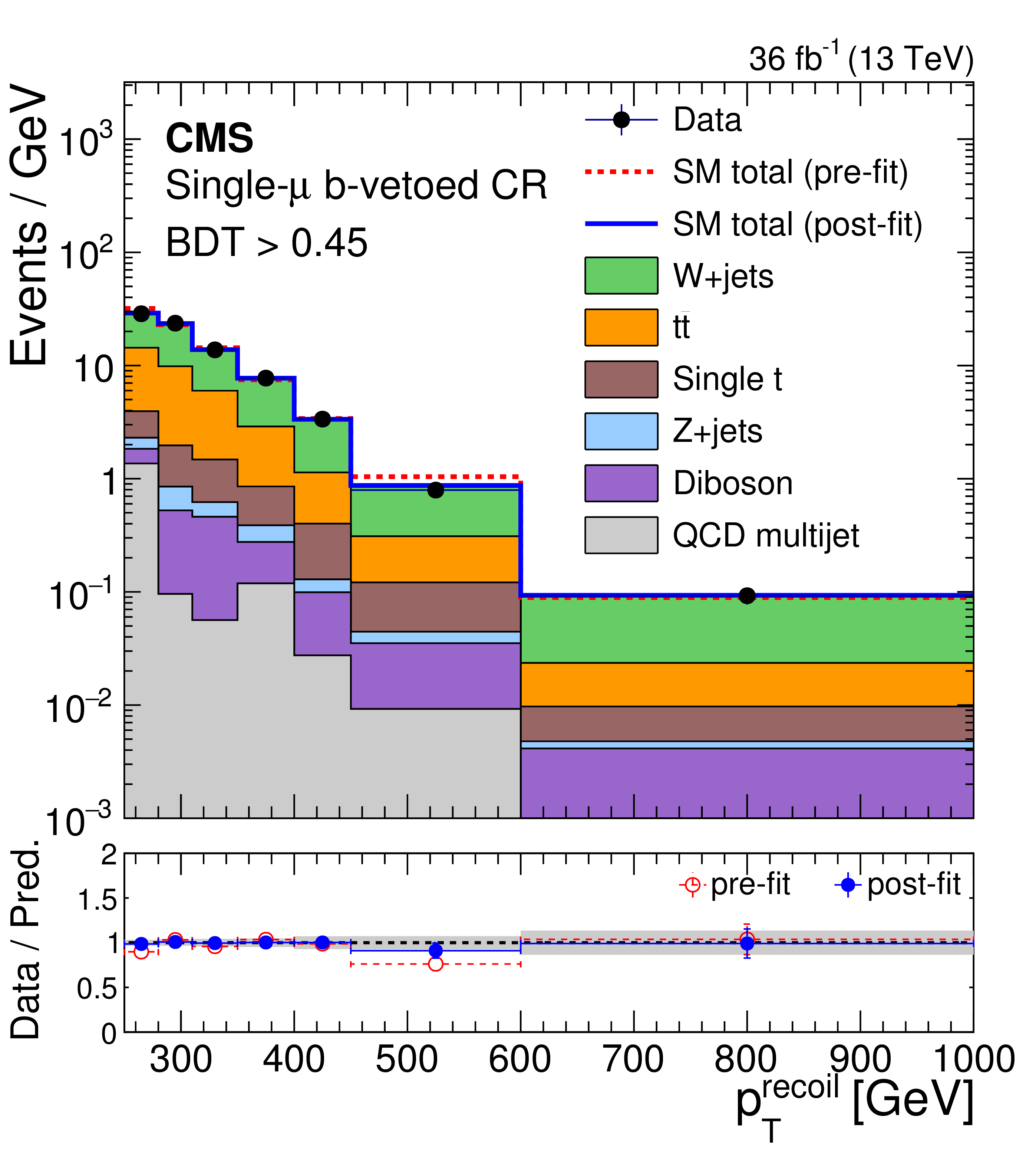
Figure 6-d:
Comparison between data and SM predictions in the b-vetoed single lepton control regions before and after performing the simultaneous fit to the different control regions and signal region. Each bin shows the event yields divided by the width of the bin. The figure corresponds to the single muon b-vetoed control region, and corresponds to the tight category of the control regions. The blue solid line represents the sum of the SM contributions normalized to their fitted yields. The red dashed line represents the sum of the SM contributions normalized to the prediction. The stacked histograms show the individual fitted SM contributions. The lower panel shows the ratio of data to fitted prediction. The gray band on the ratio indicates the one standard deviation uncertainty on the prediction after propagating all the systematic uncertainties and their correlations in the fit. |
png pdf |
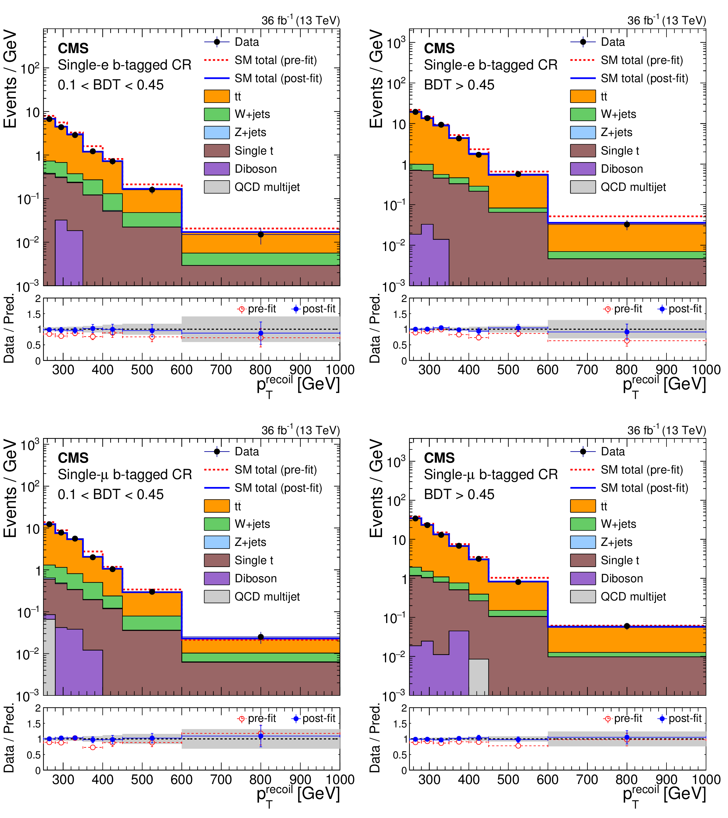
Figure 7:
Comparison between data and SM predictions in the b-tagged single lepton control regions before and after performing the simultaneous fit to the different control regions and signal region. Each bin shows the event yields divided by the width of the bin. The upper row of figures corresponds to the single electron b-tagged control region, and lower row to the single muon b-tagged control region. The left (right) column of figures corresponds to the loose (tight) category of the control regions. The blue solid line represents the sum of the SM contributions normalized to their fitted yields. The red dashed line represents the sum of the SM contributions normalized to the prediction. The stacked histograms show the individual fitted SM contributions. The lower panel of each figure shows the ratio of data to fitted prediction. The gray band on the ratio indicates the one standard deviation uncertainty on the prediction after propagating all the systematic uncertainties and their correlations in the fit. |

png pdf |
Figure 7-a:
Comparison between data and SM predictions in the b-tagged single lepton control regions before and after performing the simultaneous fit to the different control regions and signal region. Each bin shows the event yields divided by the width of the bin. The figure corresponds to the single electron b-tagged control region, and corresponds to the loose category of the control regions. The blue solid line represents the sum of the SM contributions normalized to their fitted yields. The red dashed line represents the sum of the SM contributions normalized to the prediction. The stacked histograms show the individual fitted SM contributions. The lower panel shows the ratio of data to fitted prediction. The gray band on the ratio indicates the one standard deviation uncertainty on the prediction after propagating all the systematic uncertainties and their correlations in the fit. |

png pdf |
Figure 7-b:
Comparison between data and SM predictions in the b-tagged single lepton control regions before and after performing the simultaneous fit to the different control regions and signal region. Each bin shows the event yields divided by the width of the bin. The figure corresponds to the single electron b-tagged control region, and corresponds to the tight category of the control regions. The blue solid line represents the sum of the SM contributions normalized to their fitted yields. The red dashed line represents the sum of the SM contributions normalized to the prediction. The stacked histograms show the individual fitted SM contributions. The lower panel shows the ratio of data to fitted prediction. The gray band on the ratio indicates the one standard deviation uncertainty on the prediction after propagating all the systematic uncertainties and their correlations in the fit. |

png pdf |
Figure 7-c:
Comparison between data and SM predictions in the b-tagged single lepton control regions before and after performing the simultaneous fit to the different control regions and signal region. Each bin shows the event yields divided by the width of the bin. The figure corresponds to the single muon b-tagged control region, and corresponds to the loose category of the control regions. The blue solid line represents the sum of the SM contributions normalized to their fitted yields. The red dashed line represents the sum of the SM contributions normalized to the prediction. The stacked histograms show the individual fitted SM contributions. The lower panel shows the ratio of data to fitted prediction. The gray band on the ratio indicates the one standard deviation uncertainty on the prediction after propagating all the systematic uncertainties and their correlations in the fit. |

png pdf |
Figure 7-d:
Comparison between data and SM predictions in the b-tagged single lepton control regions before and after performing the simultaneous fit to the different control regions and signal region. Each bin shows the event yields divided by the width of the bin. The figure corresponds to the single muon b-tagged control region, and corresponds to the tight category of the control regions. The blue solid line represents the sum of the SM contributions normalized to their fitted yields. The red dashed line represents the sum of the SM contributions normalized to the prediction. The stacked histograms show the individual fitted SM contributions. The lower panel shows the ratio of data to fitted prediction. The gray band on the ratio indicates the one standard deviation uncertainty on the prediction after propagating all the systematic uncertainties and their correlations in the fit. |
png pdf |
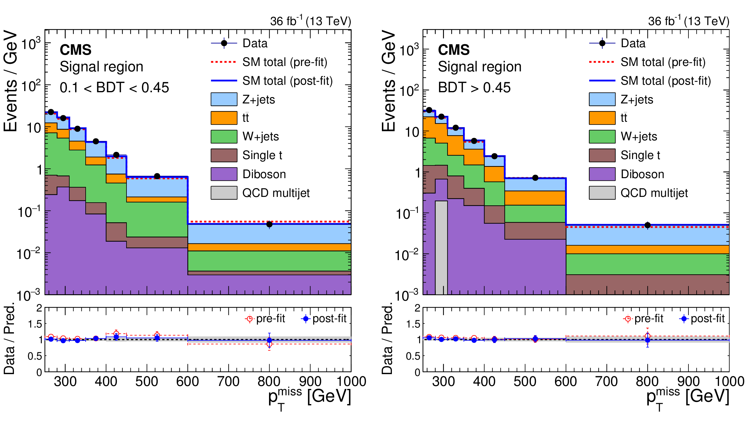
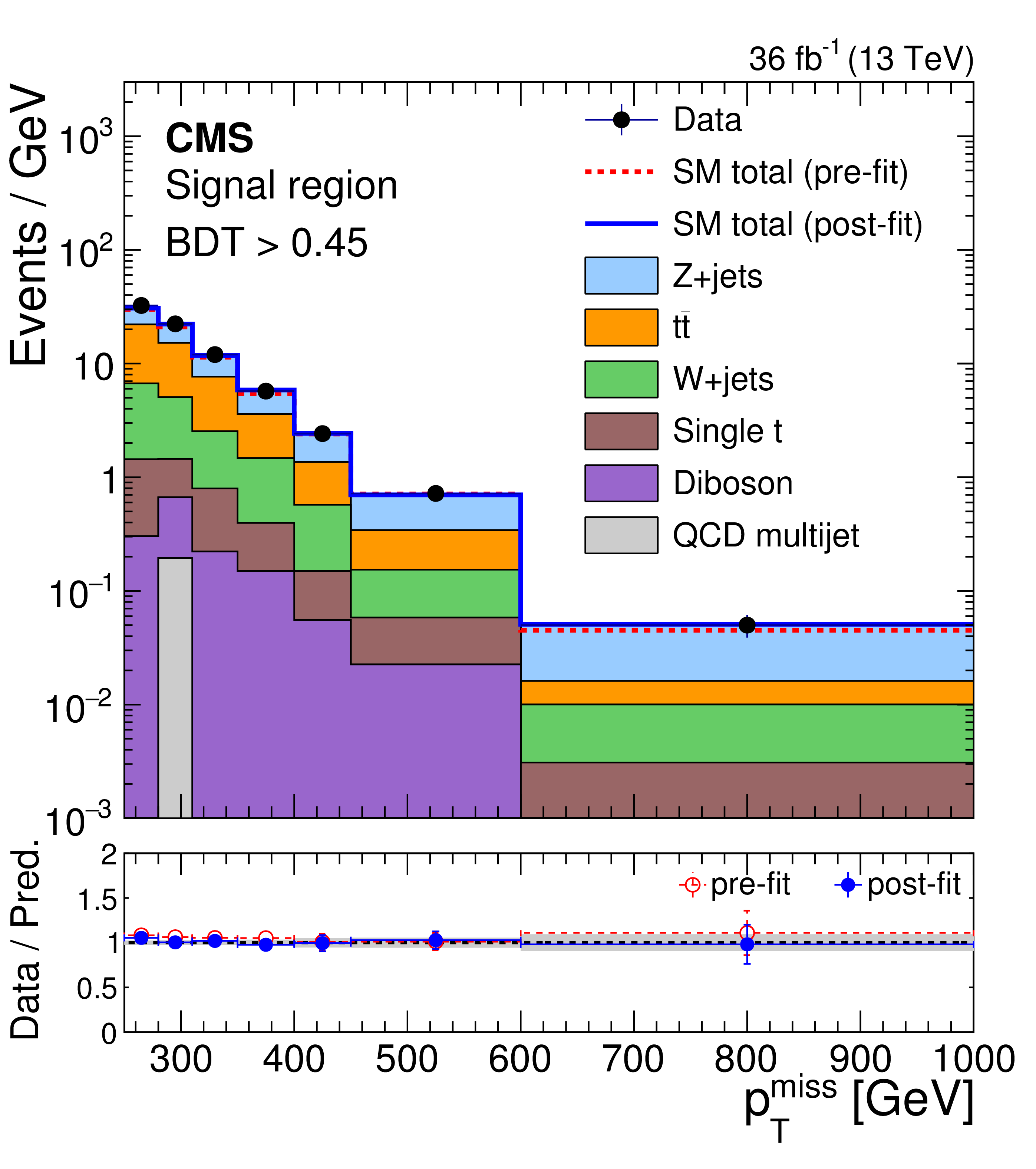
Figure 8:
Distribution of $ {{p_{\mathrm {T}}} ^\text {miss}} $ from SM backgrounds and data in the signal region after simultaneously fitting the signal region and all control regions. Each bin shows the event yields divided by the width of the bin. The left (right) figure corresponds to the loose (tight) category of the signal region. The stacked histograms show the individual fitted SM background contributions. The blue solid line represents the sum of the SM background contributions normalized to their fitted yields. The red dashed line represents the sum of the SM background contributions normalized to the prediction. The lower panel of each figure shows the ratio of data to fitted prediction. The gray band on the ratio indicates the one standard deviation uncertainty on the prediction after propagating all the systematic uncertainties and their correlations in the fit. |

png pdf |
Figure 8-a:
Distribution of $ {{p_{\mathrm {T}}} ^\text {miss}} $ from SM backgrounds and data in the signal region after simultaneously fitting the signal region and all control regions. Each bin shows the event yields divided by the width of the bin. The figure corresponds to the loose category of the signal region. The stacked histograms show the individual fitted SM background contributions. The blue solid line represents the sum of the SM background contributions normalized to their fitted yields. The red dashed line represents the sum of the SM background contributions normalized to the prediction. The lower panel shows the ratio of data to fitted prediction. The gray band on the ratio indicates the one standard deviation uncertainty on the prediction after propagating all the systematic uncertainties and their correlations in the fit. |
png pdf |
Figure 8-b:
Distribution of $ {{p_{\mathrm {T}}} ^\text {miss}} $ from SM backgrounds and data in the signal region after simultaneously fitting the signal region and all control regions. Each bin shows the event yields divided by the width of the bin. The figure corresponds to the tight category of the signal region. The stacked histograms show the individual fitted SM background contributions. The blue solid line represents the sum of the SM background contributions normalized to their fitted yields. The red dashed line represents the sum of the SM background contributions normalized to the prediction. The lower panel shows the ratio of data to fitted prediction. The gray band on the ratio indicates the one standard deviation uncertainty on the prediction after propagating all the systematic uncertainties and their correlations in the fit. |

png pdf |
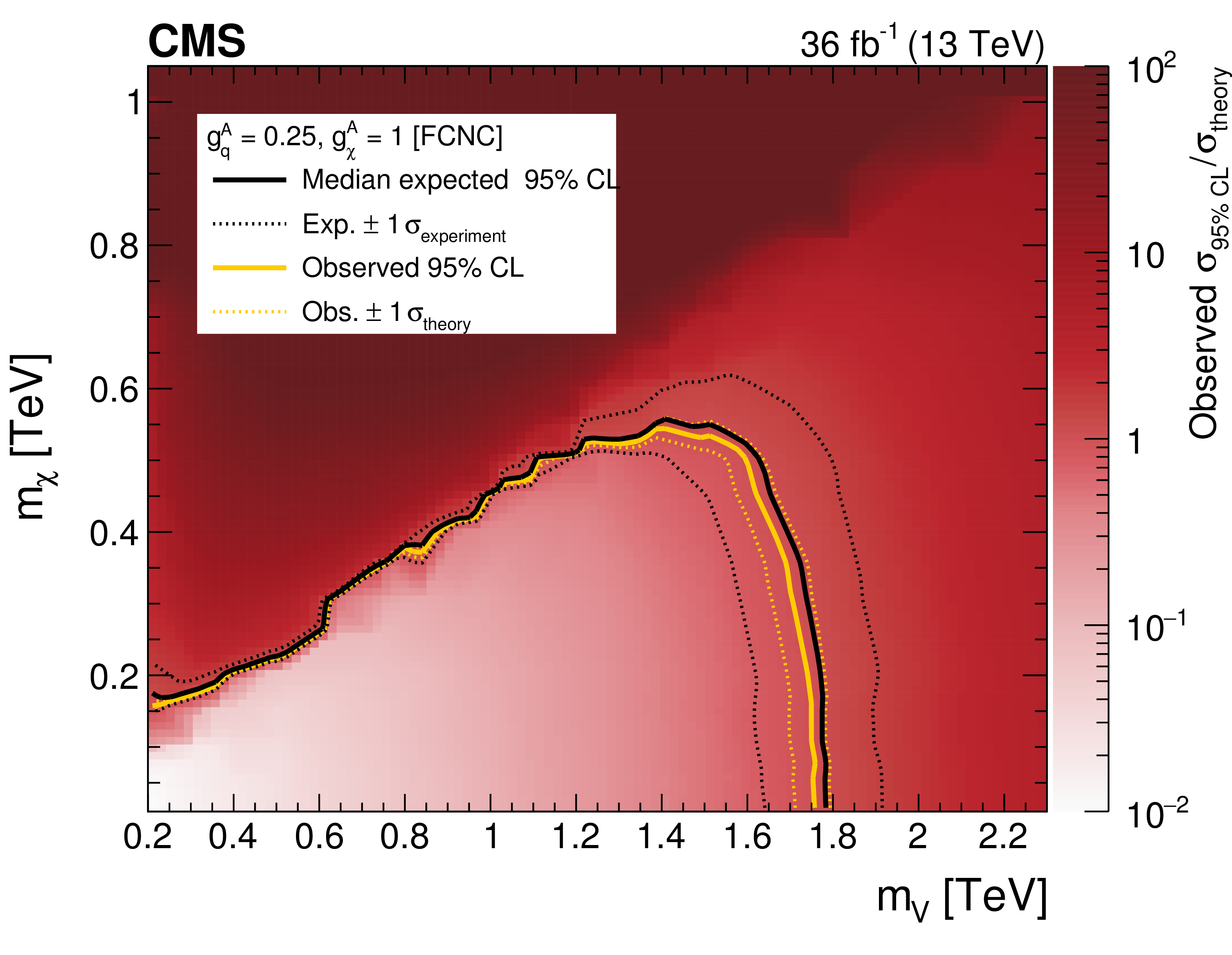
Figure 9:
Results for the FCNC interpretation presented in the two-dimensional plane spanned by the mediator and DM masses. The mediator is assumed to have purely vector couplings to quarks and DM particles. The observed exclusion range (gold solid line) is shown. The gold dashed lines show the cases in which the predicted cross section is shifted by the assigned theoretical uncertainty. The expected exclusion range is indicated by a black solid line, demonstrating the search sensitivity of the analysis. The experimental uncertainties are shown in black dashed lines. |
png pdf |
Figure 10:
Results for the FCNC interpretation presented in the two-dimensional plane spanned by the mediator and DM masses. The mediator is assumed to have purely axial couplings to quarks and DM particles. The observed exclusion range (gold solid line) is shown. The gold dashed lines show the cases in which the predicted cross section is shifted by the assigned theoretical uncertainty. The expected exclusion range is indicated by a black solid line, demonstrating the search sensitivity of the analysis. The experimental uncertainties are shown in black dashed lines. |

png pdf |
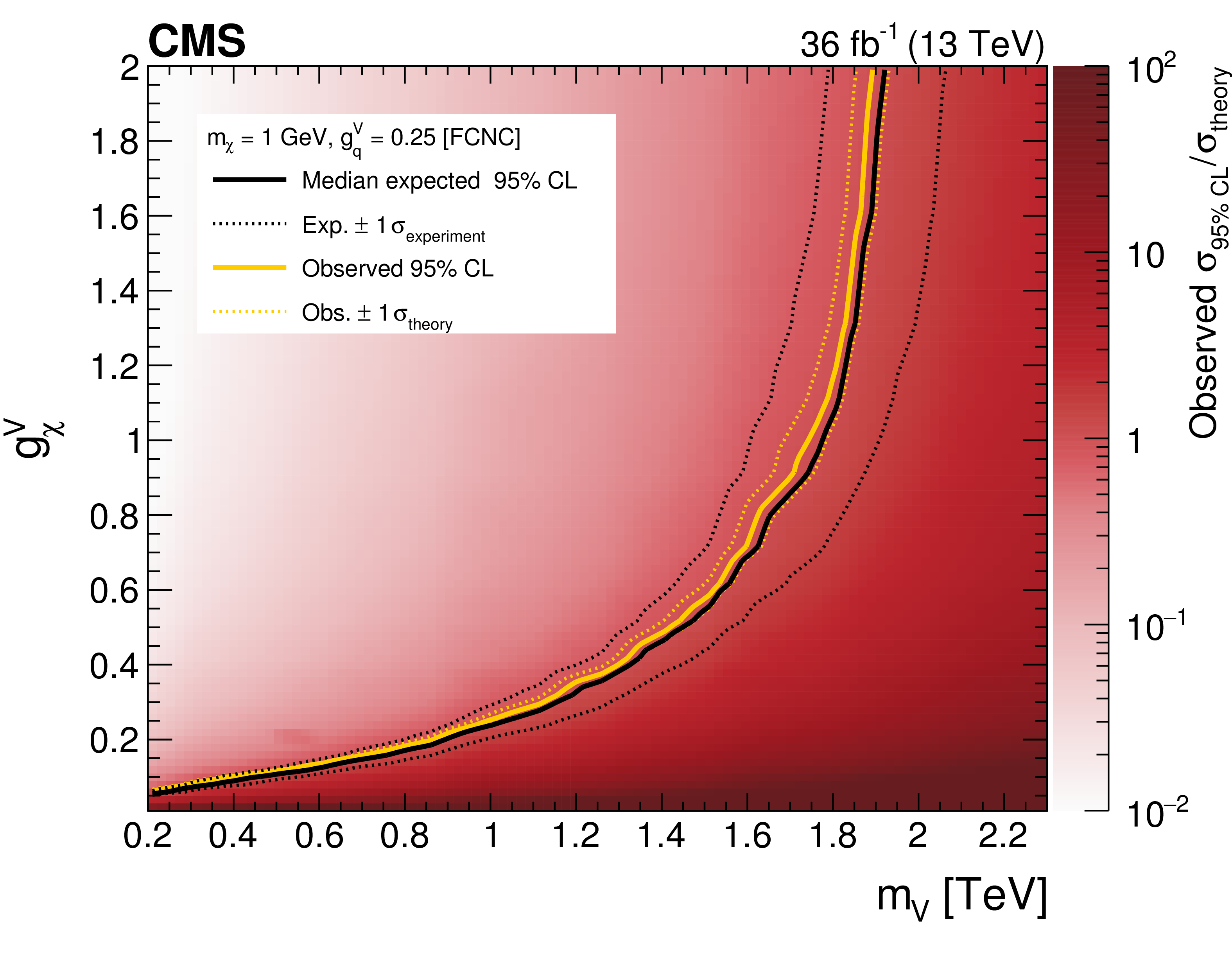
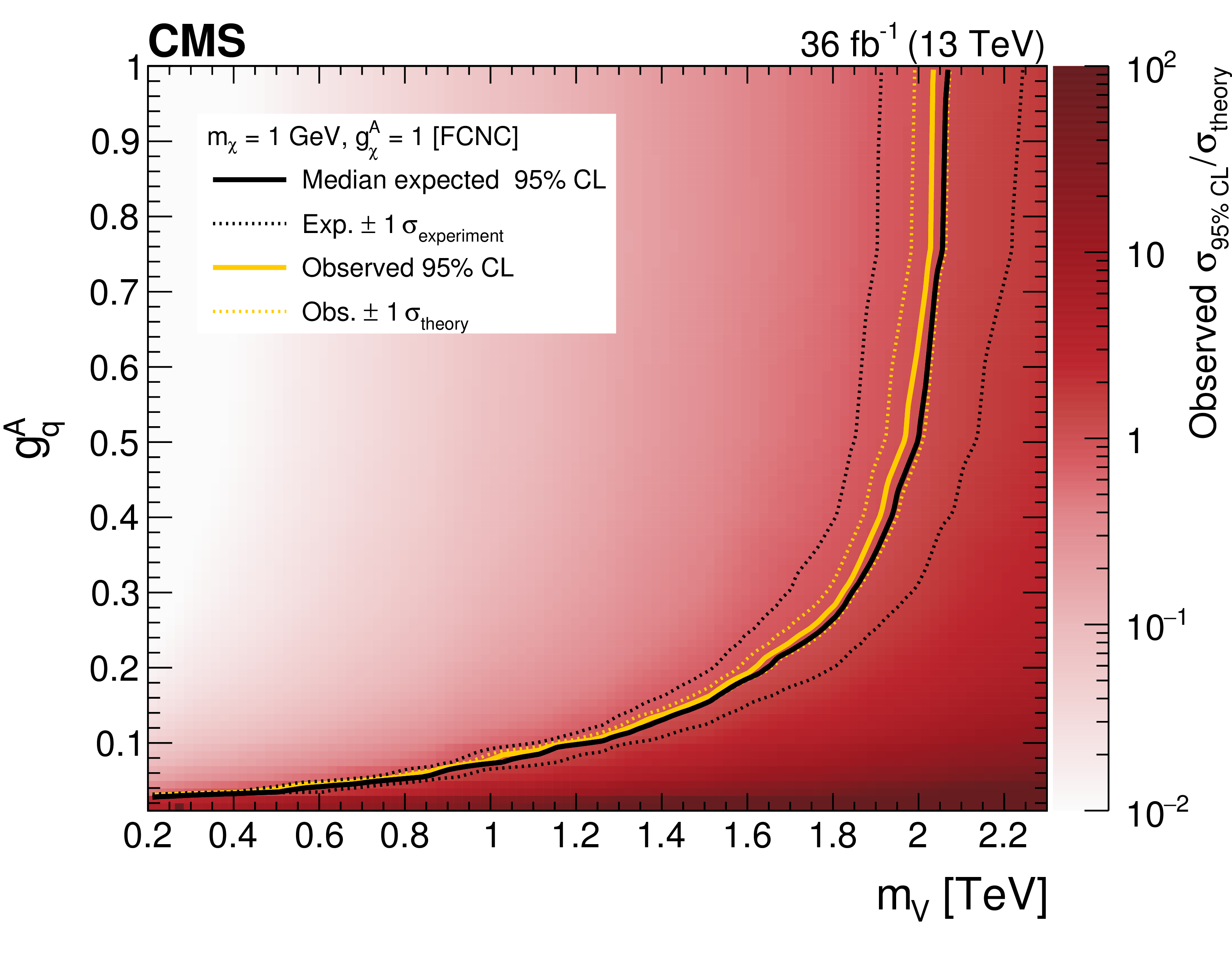
Figure 11:
Results for the FCNC interpretation presented in the two-dimensional plane spanned by the mediator mass and the coupling between the mediator and DM (upper) or quarks (lower). The mediator is assumed to have purely vector couplings. The observed exclusion range (gold solid line) is shown. The gold dashed lines show the cases in which the predicted cross section is shifted by the assigned theoretical uncertainty. The expected exclusion range is indicated by a black solid line, demonstrating the search sensitivity of the analysis. The experimental uncertainties are shown in black dashed lines. |
png pdf |
Figure 11-a:
Results for the FCNC interpretation presented in the two-dimensional plane spanned by the mediator mass and the coupling between the mediator and DM. The mediator is assumed to have purely vector couplings. The observed exclusion range (gold solid line) is shown. The gold dashed lines show the cases in which the predicted cross section is shifted by the assigned theoretical uncertainty. The expected exclusion range is indicated by a black solid line, demonstrating the search sensitivity of the analysis. The experimental uncertainties are shown in black dashed lines. |

png pdf |
Figure 11-b:
Results for the FCNC interpretation presented in the two-dimensional plane spanned by the mediator mass and the coupling between the mediator and quarks. The mediator is assumed to have purely vector couplings. The observed exclusion range (gold solid line) is shown. The gold dashed lines show the cases in which the predicted cross section is shifted by the assigned theoretical uncertainty. The expected exclusion range is indicated by a black solid line, demonstrating the search sensitivity of the analysis. The experimental uncertainties are shown in black dashed lines. |
png pdf |
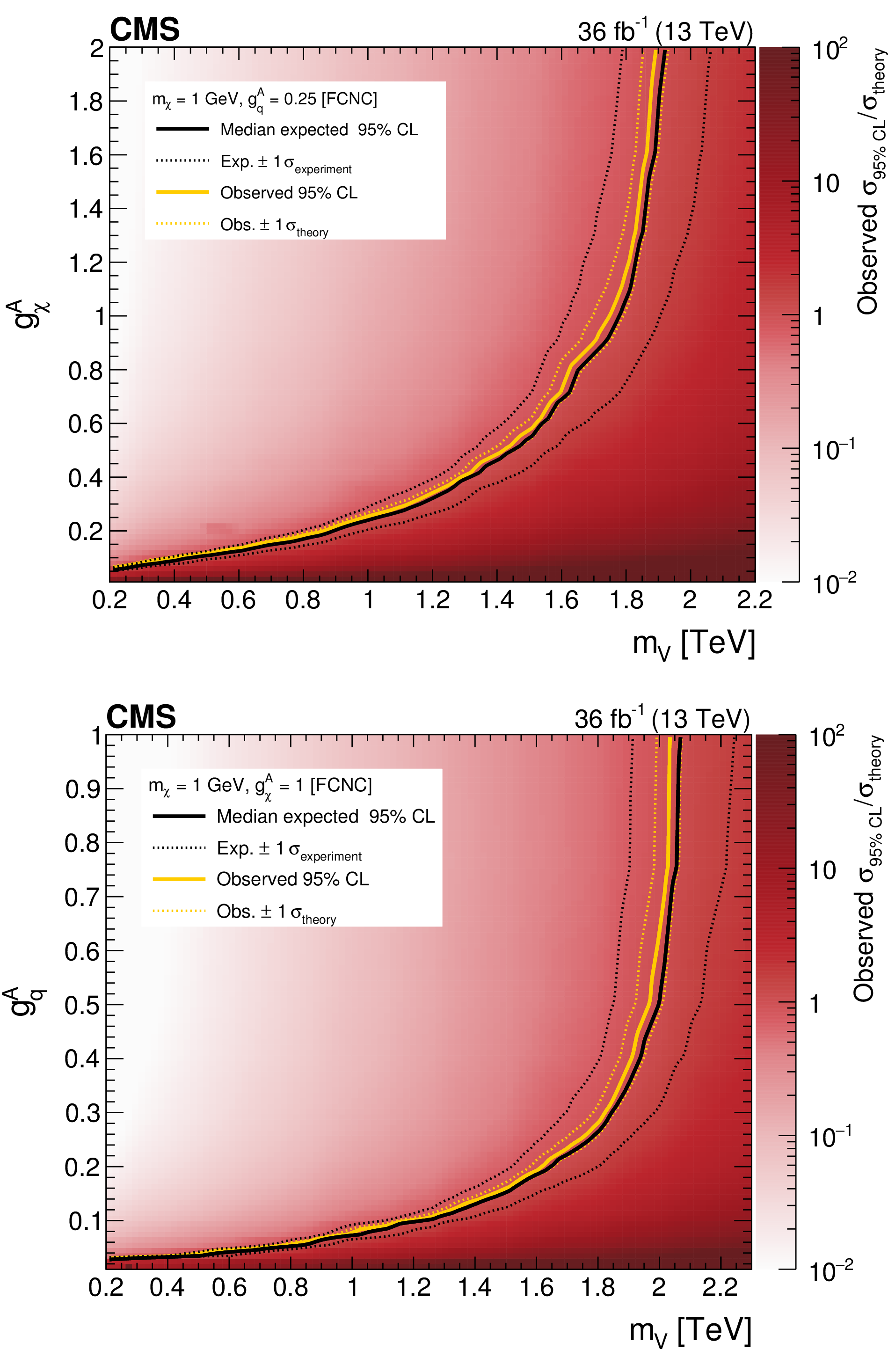
Figure 12:
Results for the FCNC interpretation presented in the two-dimensional plane spanned by the mediator mass and the coupling between the mediator and DM (upper) or quarks (lower). The mediator is assumed to have purely axial couplings. The observed exclusion range (gold solid line) is shown. The gold dashed lines show the cases in which the predicted cross section is shifted by the assigned theoretical uncertainty. The expected exclusion range is indicated by a black solid line, demonstrating the search sensitivity of the analysis. The experimental uncertainties are shown in black dashed lines. |

png pdf |
Figure 12-a:
Results for the FCNC interpretation presented in the two-dimensional plane spanned by the mediator mass and the coupling between the mediator and DM. The mediator is assumed to have purely axial couplings. The observed exclusion range (gold solid line) is shown. The gold dashed lines show the cases in which the predicted cross section is shifted by the assigned theoretical uncertainty. The expected exclusion range is indicated by a black solid line, demonstrating the search sensitivity of the analysis. The experimental uncertainties are shown in black dashed lines. |
png pdf |
Figure 12-b:
Results for the FCNC interpretation presented in the two-dimensional plane spanned by the mediator mass and the coupling between the mediator and quarks. The mediator is assumed to have purely axial couplings. The observed exclusion range (gold solid line) is shown. The gold dashed lines show the cases in which the predicted cross section is shifted by the assigned theoretical uncertainty. The expected exclusion range is indicated by a black solid line, demonstrating the search sensitivity of the analysis. The experimental uncertainties are shown in black dashed lines. |

png pdf |
Figure 13:
Upper limits at 95% CL on the mass of the scalar particle $\phi $ in the resonant model, assuming fixed $a_\mathrm {q} = b_\mathrm {q} = $ 0.1 and $a_\psi = b_\psi = $ 0.2. The green and yellow bands represent one and two standard deviations of experimental uncertainties, respectively. The red hatched band represents the signal cross section uncertainty as a function of $m_\phi $. |

png pdf |
Figure A1:
Inclusive distribution of the transverse momentum of the mediator boson V in the FCNC monotop production mechanism, both at leading-order (LO) and next-to-leading order (NLO) accuracy in QCD, assuming couplings of $g_\mathrm {q}^ {\mathrm {V}}= $ 0.25 and $g_\chi ^ {\mathrm {V}}= $ 1 and masses of 1.75 TeV and 1 GeV for V and the fermionic DM particle $\chi $, respectively. Shaded bands around the central predictions correspond to independent variations of the nominal factorization and renormalization scale $H_\mathrm {T}/2$ by factors of 2 and $1/2$. While the NLO case exhibits a softer spectrum for $ {p_{\mathrm {T}}} ^\mathrm {V}$ than the LO computation, which should result in a relatively softer $ {{p_{\mathrm {T}}} ^\text {miss}} $, the inclusive cross section increases by about 25% (from 24.8 fb at LO to 31.4 fb at NLO). |

png pdf |
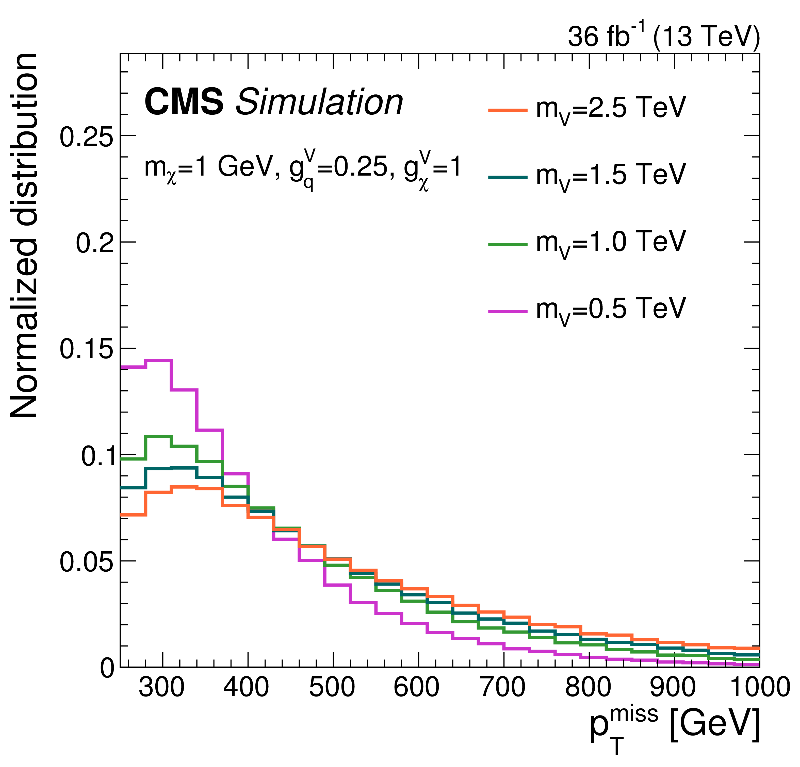
Figure A2:
Distribution of ${{p_{\mathrm {T}}} ^\text {miss}}$ in monotop signal models. On the left is shown the FCNC model for various values of $m_ {\mathrm {V}}$; on the right is the scalar resonance model for various values of $m_\phi $. |
png pdf |
Figure A2-a:
Distribution of ${{p_{\mathrm {T}}} ^\text {miss}}$ in monotop signal models. Is shown the FCNC model for various values of $m_ {\mathrm {V}}$. |

png pdf |
Figure A2-b:
Distribution of ${{p_{\mathrm {T}}} ^\text {miss}}$ in monotop signal models. Is shown the scalar resonance model for various values of $m_\phi $. |

png pdf |
Figure A3:
Distribution of $ {{p_{\mathrm {T}}} ^\text {miss}} $ from SM backgrounds and data in the loose category of the signal region after fitting the control regions only. Each bin shows the event yields divided by the width of the bin. The stacked histograms show the individual SM background distributions after the fit is performed. The lower panel of the figure shows the ratio of data to fitted prediction. The gray band on the ratio indicates the one standard deviation uncertainty on the prediction after propagating all the systematic uncertainties and their correlations in the fit. |

png pdf |
Figure A4:
Distribution of $ {{p_{\mathrm {T}}} ^\text {miss}} $ from SM backgrounds and data in the tight category of the signal region after fitting the control regions only. Each bin shows the event yields divided by the width of the bin. The stacked histograms show the individual SM background distributions after the fit is performed. The lower panel of the figure shows the ratio of data to fitted prediction. The gray band on the ratio indicates the one standard deviation uncertainty on the prediction after propagating all the systematic uncertainties and their correlations in the fit. |

png pdf |
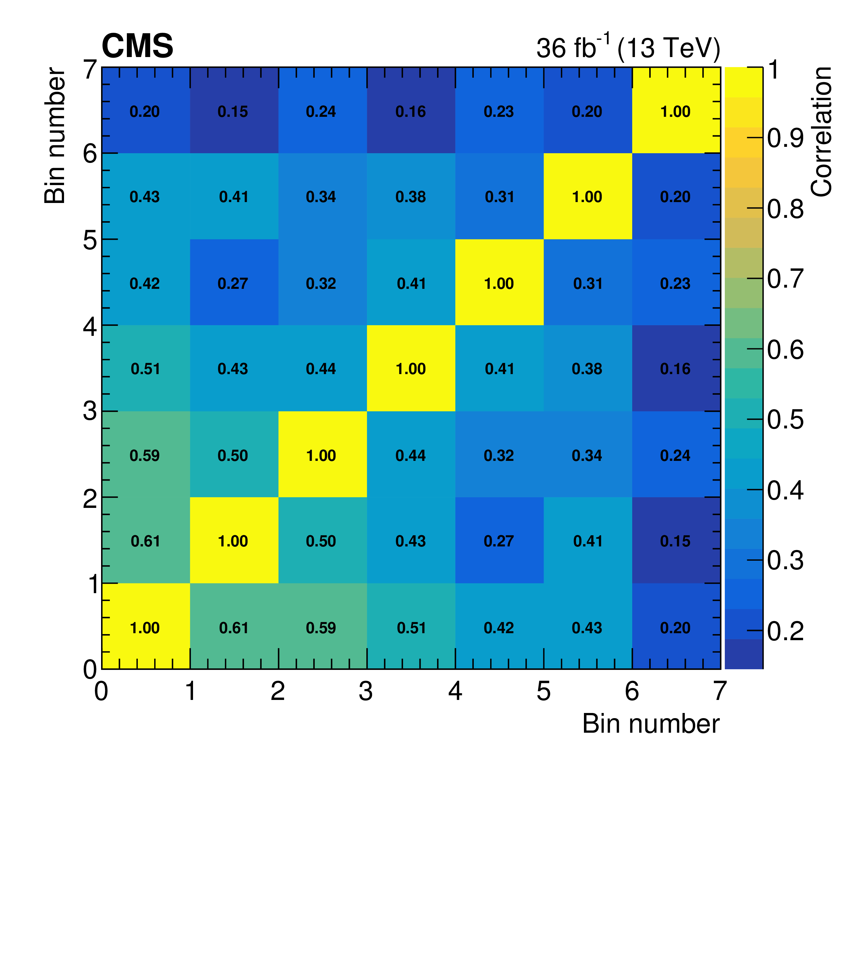
Figure A5:
Correlations between background predictions in each of the bins of the loose signal region, after performing the fit in only the control regions. |
png pdf |
Figure A6:
Correlations between background predictions in each of the bins of the tight signal region, after having performed the fit in only the control regions. |

png pdf |
Figure A7:
The maximum excluded mediator mass at 95% CL as a function of vector couplings to DM and quarks. This plot fixes $m_\chi = $ 1 GeV and $g_\chi ^\mathrm {A} = g_\mathrm {q}^\mathrm {A}= $ 0. Masses up to 2.5 TeV are excluded given sufficiently large coupling choices. |
| Tables | |
png pdf |
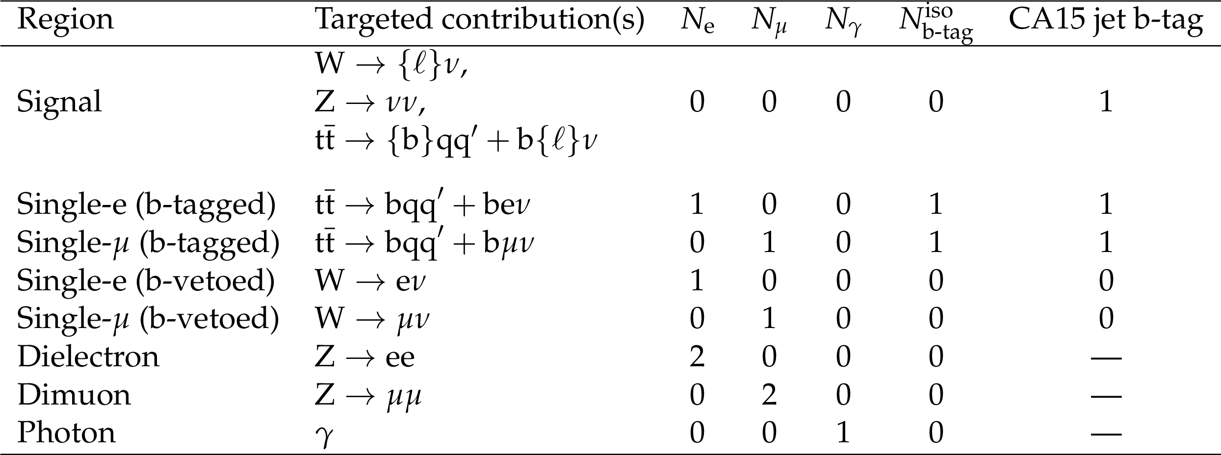
Table 1:
Summary of the selection criteria used in the SR and CRs. Symbols $\{\mathrm {b}\}$ and $\{\ell \}$ refer to cases where the b quark or lepton are not identified. $N_ {\mathrm {e}}$, $N_\mu $, and $N_\gamma $ refer to the number of selected electrons, muons, and photons, respectively. The number of b-tagged isolated jets is denoted with $N_{\text {b-tag}}^\text {iso}$. |

png pdf |
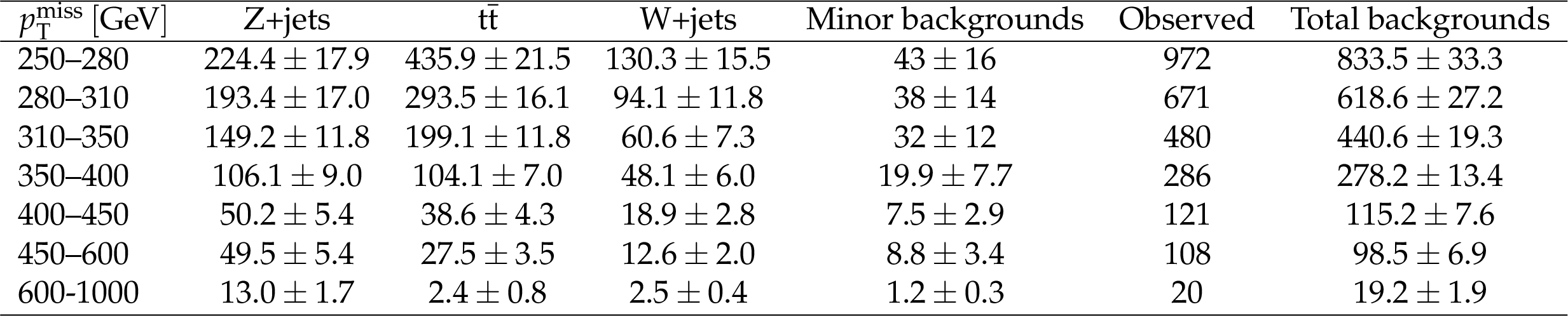
Table A1:
Predicted SM backgrounds and yields in data in each bin of the loose signal region, after performing the fit in the control regions only. "Minor backgrounds'' refers to the diboson, single t, and QCD multijet backgrounds. |
png pdf |
Table A2:
Predicted SM backgrounds and yields in data in each bin of the tight signal region, after performing the fit in the control regions only. "Minor backgrounds'' refers to the diboson, single t, and QCD multijet backgrounds. |
| Summary |
|
A search is reported for dark matter events with large transverse momentum imbalance and a hadronically decaying top quark. New t-tagging techniques are presented and utilized to identify jets from the Lorentz-boosted top quark. The data are found to be in agreement with the standard model prediction for the expected background. Results are interpreted in terms of limits on the production cross section of dark matter (DM) particles via a flavor-changing neutral current interaction or via the decay of a colored scalar resonance. Other experimental searches [60] probe the production of DM via neutral currents, under the assumption that flavor is conserved. This analysis augments these searches by considering DM production in scenarios that violate flavor conservation. Assuming $ m_\chi = $ 1 GeV, $ g^{\mathrm{V}}_\mathrm{u}= $ 0.25, and $ g^{\mathrm{V}}_{\chi}= $ 1, spin-1 mediators with masses 0.2 $ < m_{\mathrm{V}} < $ 1.75 TeV in the FCNC model are excluded at the 95% confidence level. Scalar resonances decaying to DM and a top quark are excluded in the range 1.5 $ < m_\phi < $ 3.4 TeV, assuming $m_\psi = $ 100 GeV. |
| References | ||||
| 1 | G. Bertone, D. Hooper, and J. Silk | Particle dark matter: evidence, candidates and constraints | Physics Reports 405 (2005) 279 | |
| 2 | J. L. Feng | Dark matter candidates from particle physics and methods of detection | Ann. Rev. Astron. Astrophys. 48 (2010) 495 | 1003.0904 |
| 3 | T. A. Porter, R. P. Johnson, and P. W. Graham | Dark matter searches with astroparticle data | Ann. Rev. Astron. Astrophys. 49 (2011) 15 | 1104.2836 |
| 4 | LUX Collaboration | The Large Underground Xenon (LUX) experiment | NIMA 704 (2013) 111 | 1211.3788 |
| 5 | AMS Collaboration | Electron and positron fluxes in primary cosmic rays measured with the alpha magnetic spectrometer on the international space station | PRL 113 (2014) 121102 | |
| 6 | J. Andrea, B. Fuks, and F. Maltoni | Monotops at the LHC | PRD 84 (2011) 074025 | 1106.6199 |
| 7 | CDF Collaboration | Search for a dark matter candidate produced in association with a single top quark in $ p\overline{p} $ collisions at $ \sqrt{s}= $ 1.96 TeV | PRL 108 (2012) 201802 | 1202.5653 |
| 8 | CMS Collaboration | Search for monotop signatures in proton-proton collisions at $ \sqrt{s}= $ 8 TeV | PRL 114 (2015) 101801 | CMS-B2G-12-022 1410.1149 |
| 9 | ATLAS Collaboration | Search for invisible particles produced in association with single-top-quarks in proton-proton collisions at $ \sqrt{s}=8\text{}\text{}\mathrm{TeV} $ with the ATLAS detector | EPJC 75 (2015) 79 | 1410.5404 |
| 10 | J.-L. Agram et al. | Monotop phenomenology at the Large Hadron Collider | PRD 89 (2014) 014028 | 1311.6478 |
| 11 | I. Boucheneb, G. Cacciapaglia, A. Deandrea, and B. Fuks | Revisiting monotop production at the LHC | JHEP 01 (2015) 017 | 1407.7529 |
| 12 | CMS Collaboration | The CMS experiment at the CERN LHC | JINST 3 (2008) S08004 | CMS-00-001 |
| 13 | CMS Collaboration | Particle-flow reconstruction and global event description with the CMS detector | JINST 12 (2017) P10003 | CMS-PRF-14-001 1706.04965 |
| 14 | J. Alwall et al. | The automated computation of tree-level and next-to-leading order differential cross sections, and their matching to parton shower simulations | JHEP 07 (2014) 079 | 1405.0301 |
| 15 | P. Nason | A new method for combining NLO QCD with shower Monte Carlo algorithms | JHEP 11 (2004) 040 | hep-ph/0409146 |
| 16 | S. Frixione, P. Nason, and C. Oleari | Matching NLO QCD computations with parton shower simulations: the $ POWHEG $ method | JHEP 11 (2007) 070 | 0709.2092 |
| 17 | S. Alioli, P. Nason, C. Oleari, and E. Re | A general framework for implementing NLO calculations in shower Monte Carlo programs: the $ POWHEG $ BOX | JHEP 06 (2010) 043 | 1002.2581 |
| 18 | T. Sjostrand et al. | An introduction to PYTHIA 8.2 | CPC 191 (2015) 159 | 1410.3012 |
| 19 | J. Alwall et al. | Comparative study of various algorithms for the merging of parton showers and matrix elements in hadronic collisions | EPJC 53 (2008) 473 | 0706.2569 |
| 20 | R. Frederix and S. Frixione | Merging meets matching in MC@NLO | JHEP 12 (2012) 061 | 1209.6215 |
| 21 | J. H. Kuhn, A. Kulesza, S. Pozzorini, and M. Schulze | Electroweak corrections to hadronic photon production at large transverse momenta | JHEP 03 (2006) 059 | hep-ph/0508253 |
| 22 | S. Kallweit et al. | NLO QCD+EW automation and precise predictions for V+multijet production | in 50th Rencontres de Moriond on QCD and High Energy Interactions La Thuile, Italy, March 21-28, 2015 2015 | 1505.05704 |
| 23 | S. Kallweit et al. | NLO QCD+EW predictions for V + jets including off-shell vector-boson decays and multijet merging | JHEP 04 (2016) 021 | 1511.08692 |
| 24 | CMS Collaboration | Event generator tunes obtained from underlying event and multiparton scattering measurements | EPJC 76 (2016) 155 | CMS-GEN-14-001 1512.00815 |
| 25 | P. Skands, S. Carrazza, and J. Rojo | Tuning PYTHIA 8.1: the Monash 2013 tune | EPJC 74 (2014) 3024 | 1404.5630 |
| 26 | NNPDF Collaboration | Parton distributions for the LHC Run II | JHEP 04 (2015) 040 | 1410.8849 |
| 27 | GEANT4 Collaboration | GEANT4---a simulation toolkit | NIMA 506 (2003) 250 | |
| 28 | CMS Collaboration | CMS luminosity measurements for the 2016 data taking period | CMS-PAS-LUM-17-001 | CMS-PAS-LUM-17-001 |
| 29 | Y. L. Dokshitzer, G. D. Leder, S. Moretti, and B. R. Webber | Better jet clustering algorithms | JHEP 08 (1997) 001 | hep-ph/9707323 |
| 30 | D. Bertolini, P. Harris, M. Low, and N. Tran | Pileup per particle identification | JHEP 10 (2014) 59 | |
| 31 | CMS Collaboration | Jet energy scale and resolution in the CMS experiment in pp collisions at 8 TeV | JINST 12 (2017) P02014 | CMS-JME-13-004 1607.03663 |
| 32 | A. J. Larkoski, S. Marzani, G. Soyez, and J. Thaler | Soft drop | JHEP 05 (2014) 146 | 1402.2657 |
| 33 | CMS Collaboration | Identification of b-quark jets with the CMS experiment | JINST 8 (2012) P04013 | |
| 34 | CMS Collaboration | Identification of b quark jets at the CMS Experiment in the LHC Run 2 | CMS-PAS-BTV-15-001 | CMS-PAS-BTV-15-001 |
| 35 | H. Voss, A. Hocker, J. Stelzer, and F. Tegenfeldt | TMVA, the toolkit for multivariate data analysis with ROOT | in XIth International Workshop on Advanced Computing and Analysis Techniques in Physics Research (ACAT), p. 40 2007 | physics/0703039 |
| 36 | J. Thaler and K. Tilburg | Identifying boosted objects with $ N $-subjettiness | JHEP 03 (2011) 015 | 1011.2268 |
| 37 | C. Anders et al. | Benchmarking an even better top tagger algorithm | PRD 89 (2014) 074047 | 1312.1504 |
| 38 | A. J. Larkoski, G. P. Salam, and J. Thaler | Energy correlation functions for jet substructure | JHEP 06 (2013) 108 | 1305.0007 |
| 39 | I. Moult, L. Necib, and J. Thaler | New angles on energy correlation functions | JHEP 12 (2016) 153 | 1609.07483 |
| 40 | M. Cacciari, G. P. Salam, and G. Soyez | The anti-$ k_t $ jet clustering algorithm | JHEP 04 (2008) 063 | 0802.1189 |
| 41 | CMS Collaboration | Performance of electron reconstruction and selection with the CMS detector in proton-proton collisions at $ \sqrt{s}= $ 8 TeV | JINST 10 (2015) P06005 | CMS-EGM-13-001 1502.02701 |
| 42 | CMS Collaboration | Performance of photon reconstruction and identification with the CMS detector in proton-proton collisions at $ \sqrt{s} = $ 8 TeV | JINST 10 (2015) P08010 | CMS-EGM-14-001 1502.02702 |
| 43 | A. Denner, S. Dittmaier, T. Kasprzik, and A. Muck | Electroweak corrections to W + jet hadroproduction including leptonic W-boson decays | JHEP 08 (2009) 075 | 0906.1656 |
| 44 | A. Denner, S. Dittmaier, T. Kasprzik, and A. Muck | Electroweak corrections to dilepton + jet production at hadron colliders | JHEP 06 (2011) 069 | 1103.0914 |
| 45 | A. Denner, S. Dittmaier, T. Kasprzik, and A. Muck | Electroweak corrections to monojet production at the LHC | EPJC 73 (2013) 2297 | 1211.5078 |
| 46 | J. H. Kuhn, A. Kulesza, S. Pozzorini, and M. Schulze | Logarithmic electroweak corrections to hadronic Z+1 jet production at large transverse momentum | PLB 609 (2005) 277 | hep-ph/0408308 |
| 47 | J. H. Kuhn, A. Kulesza, S. Pozzorini, and M. Schulze | One-loop weak corrections to hadronic production of Z bosons at large transverse momenta | NPB 727 (2005) 368 | hep-ph/0507178 |
| 48 | J. H. Kuhn, A. Kulesza, S. Pozzorini, and M. Schulze | Electroweak corrections to hadronic production of W bosons at large transverse momenta | NPB 797 (2008) 27 | 0708.0476 |
| 49 | CMS Collaboration | Differential cross section measurements for the production of a W boson in association with jets in proton-proton collisions at $ \sqrt s= $ 7 TeV | PLB 741 (2015) 12 | CMS-SMP-12-023 1406.7533 |
| 50 | CMS Collaboration | Measurement of the production cross section for a W boson and two b jets in pp collisions at $ \sqrt{s} = $ 7 TeV | PLB 735 (2014) 204 | CMS-SMP-12-026 1312.6608 |
| 51 | CMS Collaboration | Measurements of jet multiplicity and differential production cross sections of $ Z + $ jets events in proton-proton collisions at $ \sqrt{s} = $ 7 TeV | PRD 91 (2015) 052008 | CMS-SMP-12-017 1408.3104 |
| 52 | CMS Collaboration | Measurement of the production cross sections for a Z boson and one or more b jets in pp collisions at sqrt(s) = 7 TeV | JHEP 06 (2014) 120 | CMS-SMP-13-004 1402.1521 |
| 53 | CMS Collaboration | Observation of the associated production of a single top quark and a $ W $ boson in $ pp $ collisions at $ \sqrt s = $ 8 TeV | PRL 112 (2014) 231802 | CMS-TOP-12-040 1401.2942 |
| 54 | CMS Collaboration | Measurement of the ZZ production cross section and Z $ \to \ell^+\ell^-\ell'^+\ell'^- $ branching fraction in pp collisions at $ \sqrt s = $ 13 TeV | PLB 763 (2016) 280 | CMS-SMP-16-001 1607.08834 |
| 55 | CMS Collaboration | Measurement of the WZ production cross section in pp collisions at $ \sqrt s = $ 13 TeV | PLB 766 (2017) 268 | CMS-SMP-16-002 1607.06943 |
| 56 | CMS Collaboration | Performance of the CMS missing transverse momentum reconstruction in pp data at $ \sqrt{s} = $ 8 TeV | JINST 10 (2015) P02006 | CMS-JME-13-003 1411.0511 |
| 57 | G. Cowan, K. Cranmer, E. Gross, and O. Vitells | Asymptotic formulae for likelihood-based tests of new physics | EPJC 71 (2011) 1554 | 1007.1727 |
| 58 | T. Junk | Confidence level computation for combining searches with small statistics | NIMA 434 (1999) 435 | |
| 59 | A. L. Read | Presentation of search results: the $ CL_s $ technique | in Durham IPPP Workshop: Advanced Statistical Techniques in Particle Physics, p. 2693 Durham, UK, March, 2002 [JPG 28 (2002) 2693] | |
| 60 | CMS Collaboration | Search for dark matter produced with an energetic jet or a hadronically decaying W or Z boson at $ \sqrt{s}= $ 13 TeV | JHEP 07 (2017) 014 | CMS-EXO-16-037 1703.01651 |
|
|
Compact Muon Solenoid LHC, CERN |
|

|

|

|

|

|