

Compact Muon Solenoid
LHC, CERN
| CMS-HIG-17-029 ; CERN-EP-2018-078 | ||
| Search for an exotic decay of the Higgs boson to a pair of light pseudoscalars in the final state of two muons and two $\tau$ leptons in proton-proton collisions at $\sqrt{s} = $ 13 TeV | ||
| CMS Collaboration | ||
| 13 May 2018 | ||
| JHEP 11 (2018) 018 | ||
| Abstract: A search for exotic Higgs boson decays to light pseudoscalars in the final state of two muons and two $\tau$ leptons is performed using proton-proton collision data recorded by the CMS experiment at the LHC at a center-of-mass energy of 13 TeV in 2016, corresponding to an integrated luminosity of 35.9 fb$^{-1}$. Masses of the pseudoscalar boson between 15.0 and 62.5 GeV are probed, and no significant excess of data is observed above the prediction of the standard model. Upper limits are set on the branching fraction of the Higgs boson to two light pseudoscalar bosons in different types of two-Higgs-doublet models extended with a complex scalar singlet. | ||
| Links: e-print arXiv:1805.04865 [hep-ex] (PDF) ; CDS record ; inSPIRE record ; HepData record ; CADI line (restricted) ; | ||
| Figures | |
png pdf |
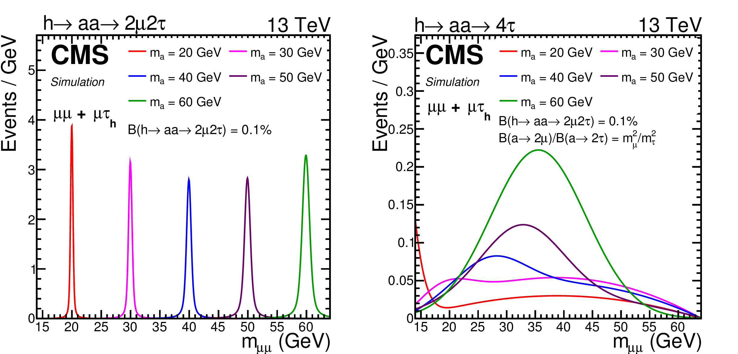
Figure 1:
Parameterized dimuon invariant mass distributions of the $ \mathrm{h} \to \mathrm{aa}\to 2 {\mu} 2{{\tau}} $ (left) and $ {\mathrm{h} \to \mathrm{aa}\to 4{{\tau}}} $ (right) signal processes simulated at different $ {m_{\mathrm{a}}} $ values in the $ {{\mu}} {{\mu}}+ {{\mu}} {{\tau} _{\mathrm{h}}} $ final state. The normalization corresponds to the number of expected signal events after the selection for an integrated luminosity of 35.9 fb$^{-1}$, assuming the production cross section of the Higgs boson predicted in the SM, $\mathcal{B}({\mathrm{h} \to \mathrm{aa}\to 2 {\mu} 2{{\tau}}})=0.1%$, and the relation in Eq. (1) to scale the $ {\mathrm{h} \to \mathrm{aa}\to 4{{\tau}}} $ contribution. |
png pdf |
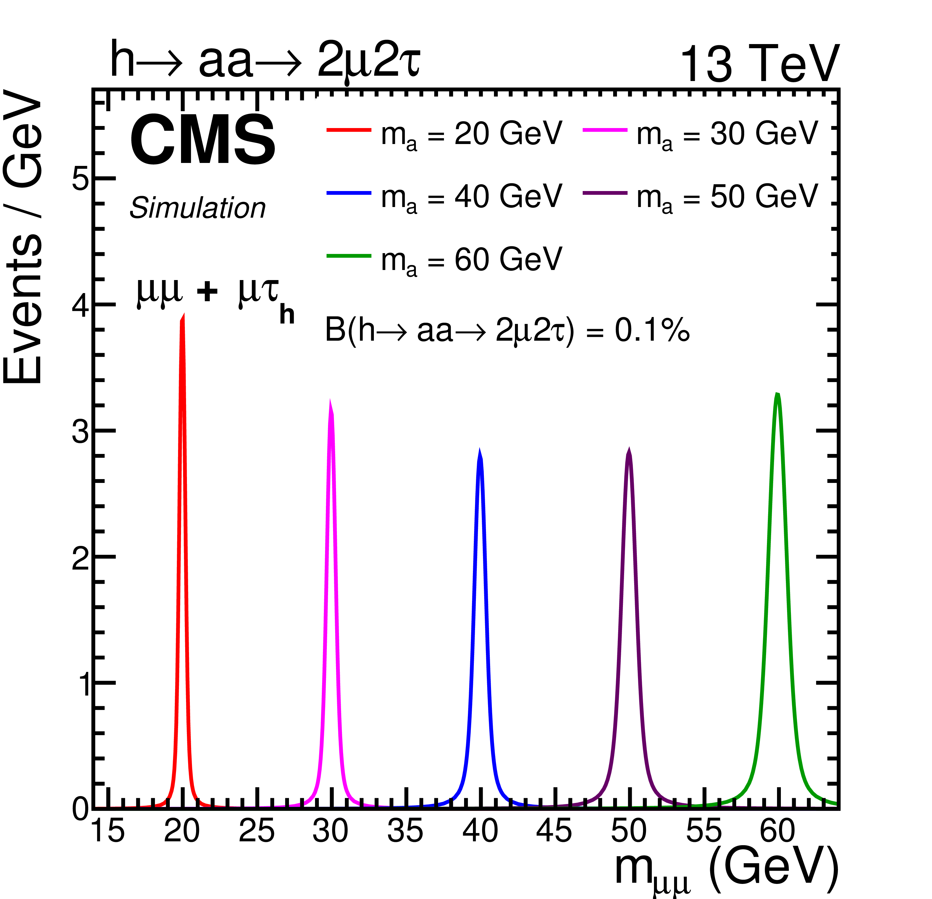
Figure 1-a:
Parameterized dimuon invariant mass distribution of the $ \mathrm{h} \to \mathrm{aa}\to 2 {\mu} 2{{\tau}} $ signal process simulated at different $ {m_{\mathrm{a}}} $ values in the $ {{\mu}} {{\mu}}+ {{\mu}} {{\tau} _{\mathrm{h}}} $ final state. The normalization corresponds to the number of expected signal events after the selection for an integrated luminosity of 35.9 fb$^{-1}$, assuming the production cross section of the Higgs boson predicted in the SM, $\mathcal{B}({\mathrm{h} \to \mathrm{aa}\to 2 {\mu} 2{{\tau}}})=0.1%$. |

png pdf |
Figure 1-b:
Parameterized dimuon invariant mass distribution of the $ {\mathrm{h} \to \mathrm{aa}\to 4{{\tau}}} $ signal process simulated at different $ {m_{\mathrm{a}}} $ values in the $ {{\mu}} {{\mu}}+ {{\mu}} {{\tau} _{\mathrm{h}}} $ final state. The normalization corresponds to the number of expected signal events after the selection for an integrated luminosity of 35.9 fb$^{-1}$, assuming the production cross section of the Higgs boson predicted in the SM, $\mathcal{B}({\mathrm{h} \to \mathrm{aa}\to 2 {\mu} 2{{\tau}}})=0.1%$, and the relation in Eq. (1) to scale the $ {\mathrm{h} \to \mathrm{aa}\to 4{{\tau}}} $ contribution. |
png pdf |
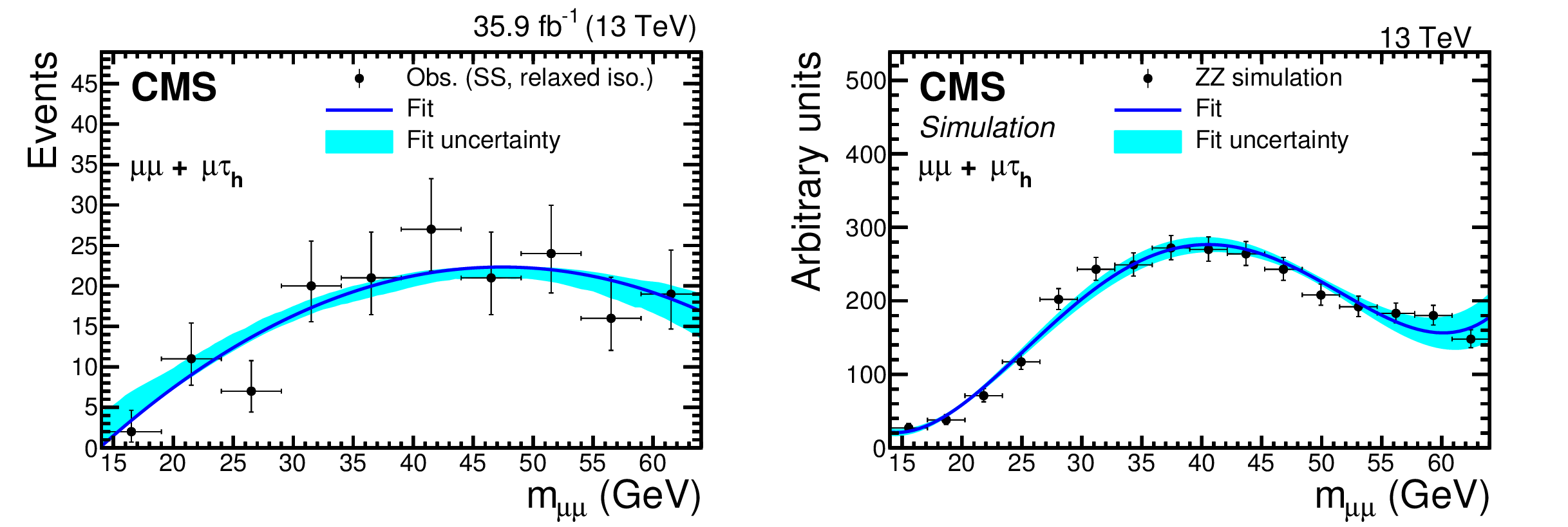
Figure 2:
Parameterization of the shape of the background with misidentified $ {\tau}$ leptons (left) and $ {{m_{\mathrm{Z}}}} $ pair production background (right) in the $ {{\mu}} {{\mu}}+ {{\mu}} {{\tau} _{\mathrm{h}}} $ final state. The points for the $ {{m_{\mathrm{Z}}}} {{m_{\mathrm{Z}}}} $ background represent events selected in simulation, whereas they correspond to observed data events in the SS region with relaxed isolation for the background with misidentified $ {\tau}$ leptons. |

png pdf |
Figure 2-a:
Parameterization of the shape of the background with misidentified $ {\tau}$ leptons in the $ {{\mu}} {{\mu}}+ {{\mu}} {{\tau} _{\mathrm{h}}} $ final state. The points correspond to observed data events in the SS region with relaxed isolation. |

png pdf |
Figure 2-b:
Parameterization of the shape of the background with $ {{m_{\mathrm{Z}}}} $ pair production background in the $ {{\mu}} {{\mu}}+ {{\mu}} {{\tau} _{\mathrm{h}}} $ final state. The points represent events selected in simulation. |
png pdf |
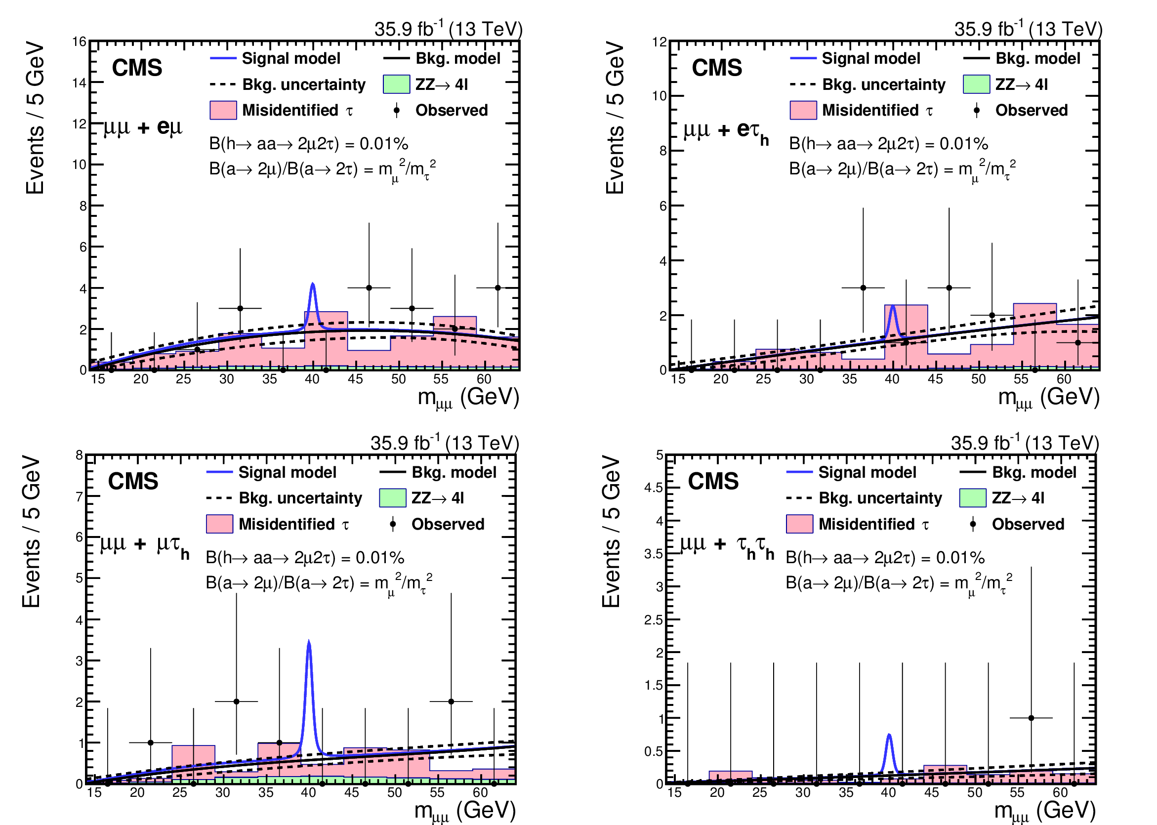
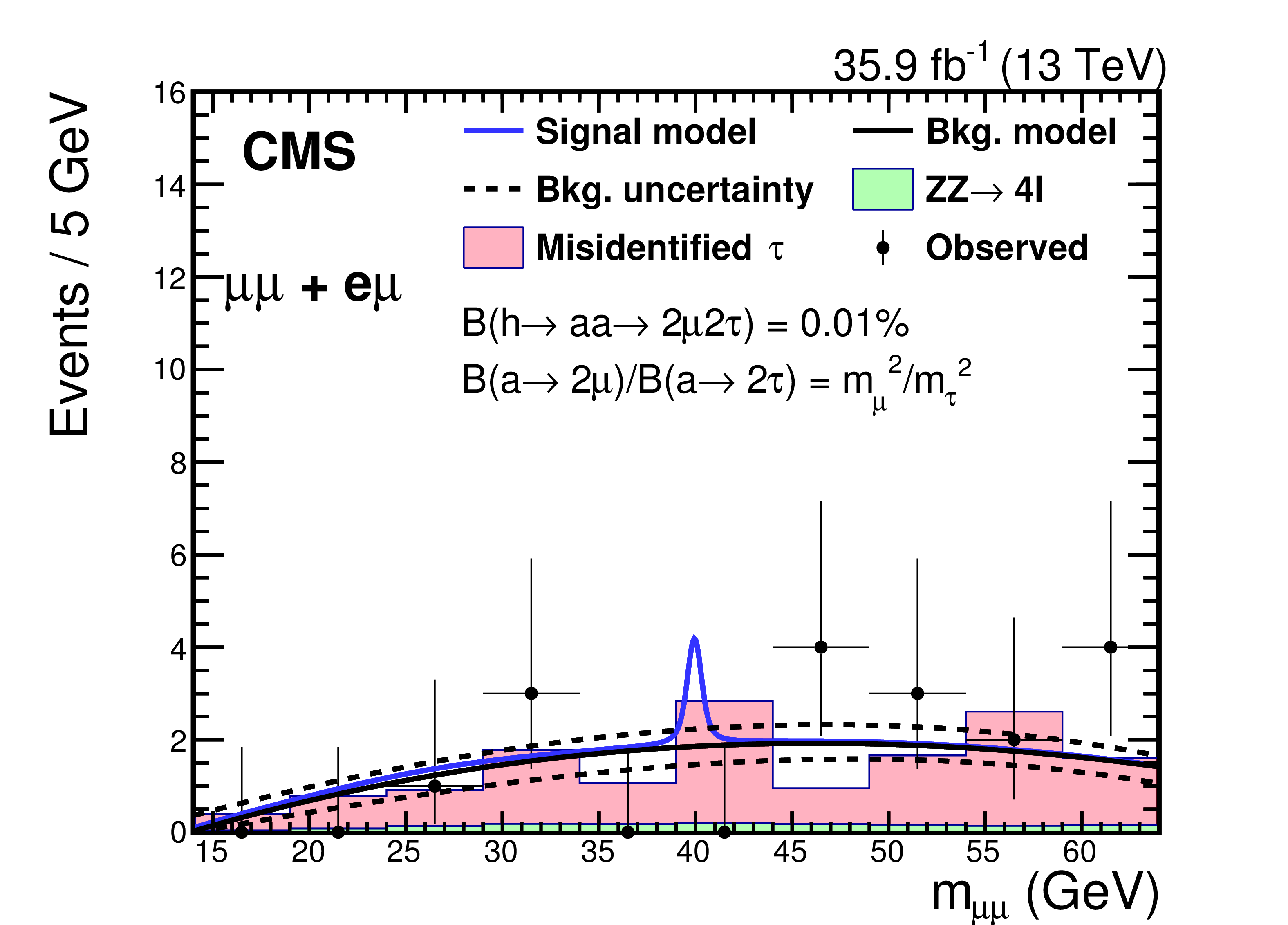
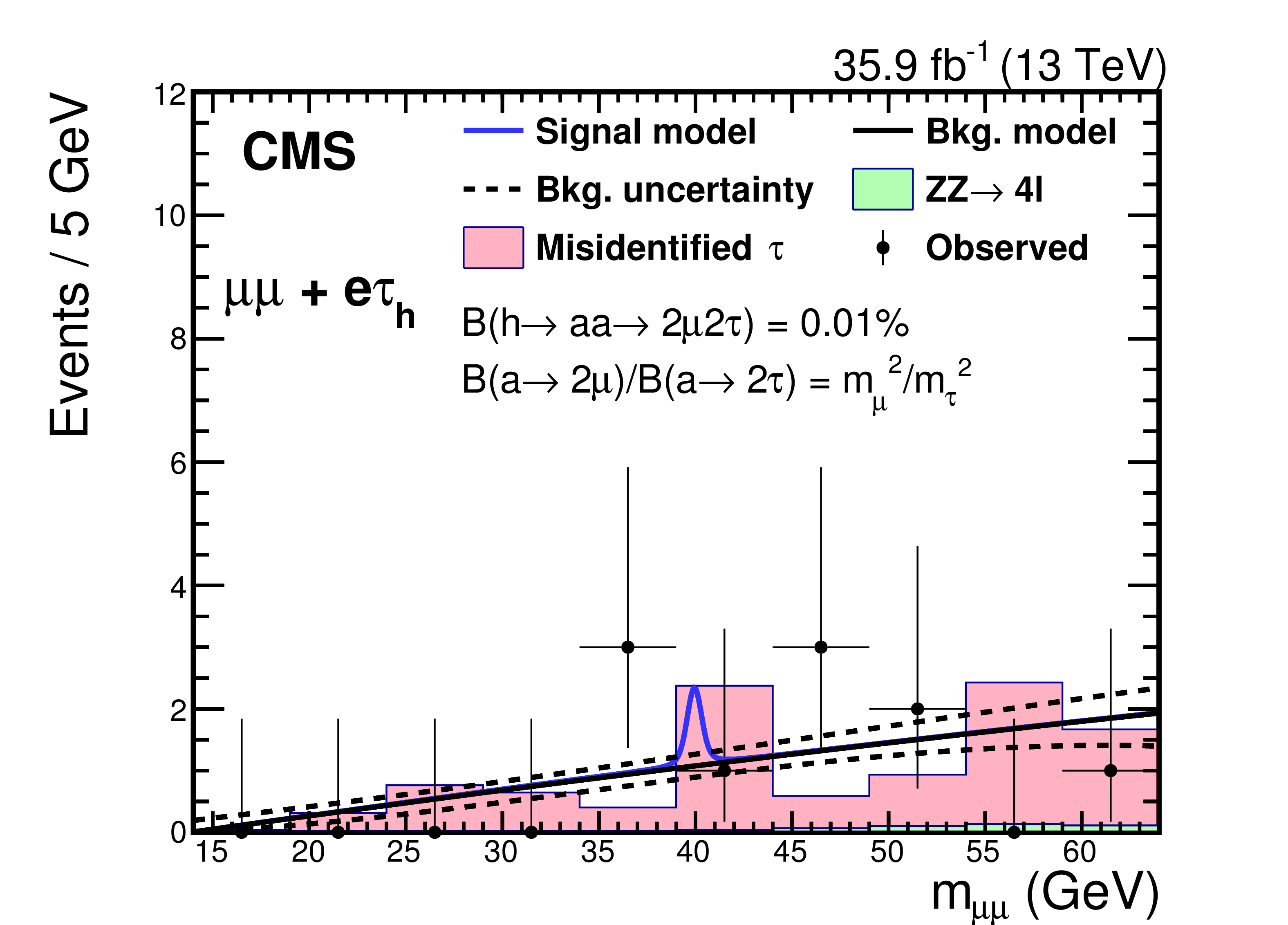
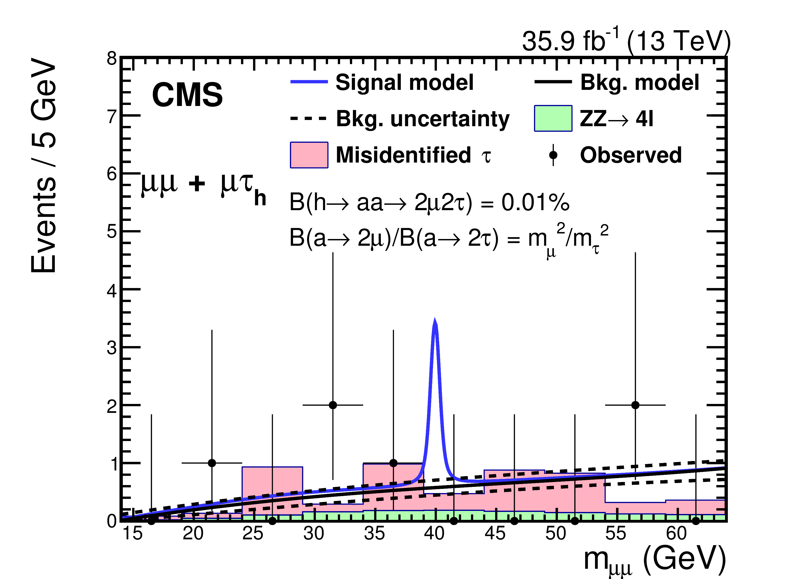
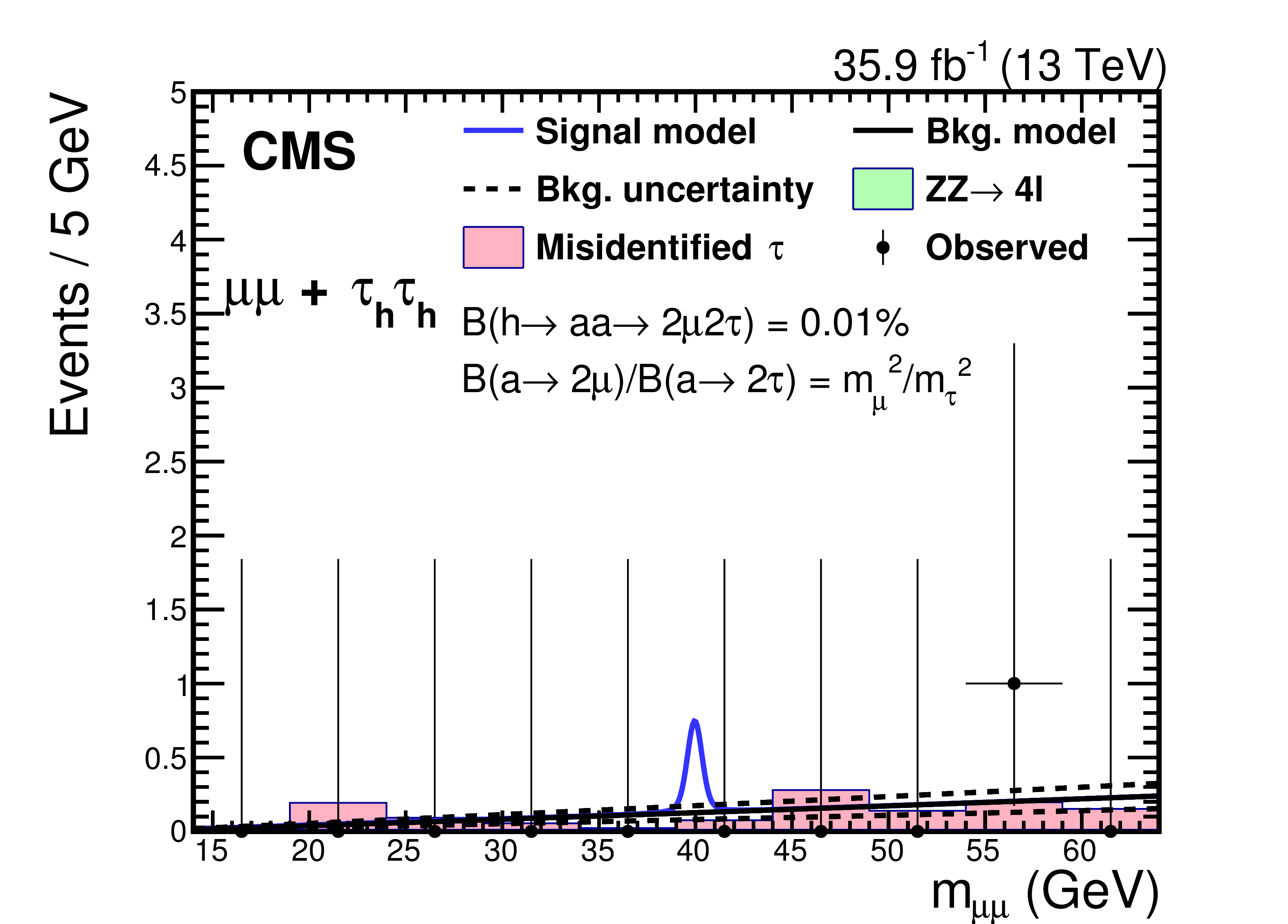
Figure 3:
Dimuon mass distributions in the $ {{\mu}} {{\mu}}+ {\mathrm{e}} {{\mu}}$ (upper left), $ {{\mu}} {{\mu}}+ {\mathrm{e}} {{\tau} _{\mathrm{h}}} $ (upper right), $ {{\mu}} {{\mu}}+ {{\mu}} {{\tau} _{\mathrm{h}}} $ (lower left), and $ {{\mu}} {{\mu}}+ {{\tau} _{\mathrm{h}}} {{\tau} _{\mathrm{h}}} $ (lower right) final states. The total background estimate and its uncertainty are given by the black lines. The histograms for the two background components are shown for illustrative purposes only as the background models are extracted from unbinned fits. The signal model is drawn in blue above the background model: it includes both $ {\mathrm{h} \to \mathrm{aa}\to 2 {\mu} 2{{\tau}}} $ and $ {\mathrm{h} \to \mathrm{aa}\to 4{{\tau}}} $, and is normalized using $\mathcal{B}({\mathrm{h} \to \mathrm{aa}\to 2 {\mu} 2{{\tau}}}) = $ 0.01%, assuming the relation in Eq. (1) to determine the relative proportion of these processes. The production cross section of the Higgs boson predicted in the SM is assumed. |
png pdf |
Figure 3-a:
Dimuon mass distribution in the $ {{\mu}} {{\mu}}+ {\mathrm{e}} {{\mu}}$ final state. The total background estimate and its uncertainty are given by the black lines. The histograms for the two background components are shown for illustrative purposes only as the background models are extracted from unbinned fits. The signal model is drawn in blue above the background model: it includes both $ {\mathrm{h} \to \mathrm{aa}\to 2 {\mu} 2{{\tau}}} $ and $ {\mathrm{h} \to \mathrm{aa}\to 4{{\tau}}} $, and is normalized using $\mathcal{B}({\mathrm{h} \to \mathrm{aa}\to 2 {\mu} 2{{\tau}}}) = $ 0.01%, assuming the relation in Eq. (1) to determine the relative proportion of these processes. The production cross section of the Higgs boson predicted in the SM is assumed. |
png pdf |
Figure 3-b:
Dimuon mass distribution in the $ {{\mu}} {{\mu}}+ {\mathrm{e}} {{\tau} _{\mathrm{h}}} $ final state. The total background estimate and its uncertainty are given by the black lines. The histograms for the two background components are shown for illustrative purposes only as the background models are extracted from unbinned fits. The signal model is drawn in blue above the background model: it includes both $ {\mathrm{h} \to \mathrm{aa}\to 2 {\mu} 2{{\tau}}} $ and $ {\mathrm{h} \to \mathrm{aa}\to 4{{\tau}}} $, and is normalized using $\mathcal{B}({\mathrm{h} \to \mathrm{aa}\to 2 {\mu} 2{{\tau}}}) = $ 0.01%, assuming the relation in Eq. (1) to determine the relative proportion of these processes. The production cross section of the Higgs boson predicted in the SM is assumed. |
png pdf |
Figure 3-c:
Dimuon mass distribution in the $ {{\mu}} {{\mu}}+ {{\mu}} {{\tau} _{\mathrm{h}}} $ final state. The total background estimate and its uncertainty are given by the black lines. The histograms for the two background components are shown for illustrative purposes only as the background models are extracted from unbinned fits. The signal model is drawn in blue above the background model: it includes both $ {\mathrm{h} \to \mathrm{aa}\to 2 {\mu} 2{{\tau}}} $ and $ {\mathrm{h} \to \mathrm{aa}\to 4{{\tau}}} $, and is normalized using $\mathcal{B}({\mathrm{h} \to \mathrm{aa}\to 2 {\mu} 2{{\tau}}}) = $ 0.01%, assuming the relation in Eq. (1) to determine the relative proportion of these processes. The production cross section of the Higgs boson predicted in the SM is assumed. |
png pdf |
Figure 3-d:
Dimuon mass distribution in the $ {{\mu}} {{\mu}}+ {{\tau} _{\mathrm{h}}} {{\tau} _{\mathrm{h}}} $ final state. The total background estimate and its uncertainty are given by the black lines. The histograms for the two background components are shown for illustrative purposes only as the background models are extracted from unbinned fits. The signal model is drawn in blue above the background model: it includes both $ {\mathrm{h} \to \mathrm{aa}\to 2 {\mu} 2{{\tau}}} $ and $ {\mathrm{h} \to \mathrm{aa}\to 4{{\tau}}} $, and is normalized using $\mathcal{B}({\mathrm{h} \to \mathrm{aa}\to 2 {\mu} 2{{\tau}}}) = $ 0.01%, assuming the relation in Eq. (1) to determine the relative proportion of these processes. The production cross section of the Higgs boson predicted in the SM is assumed. |
png pdf |
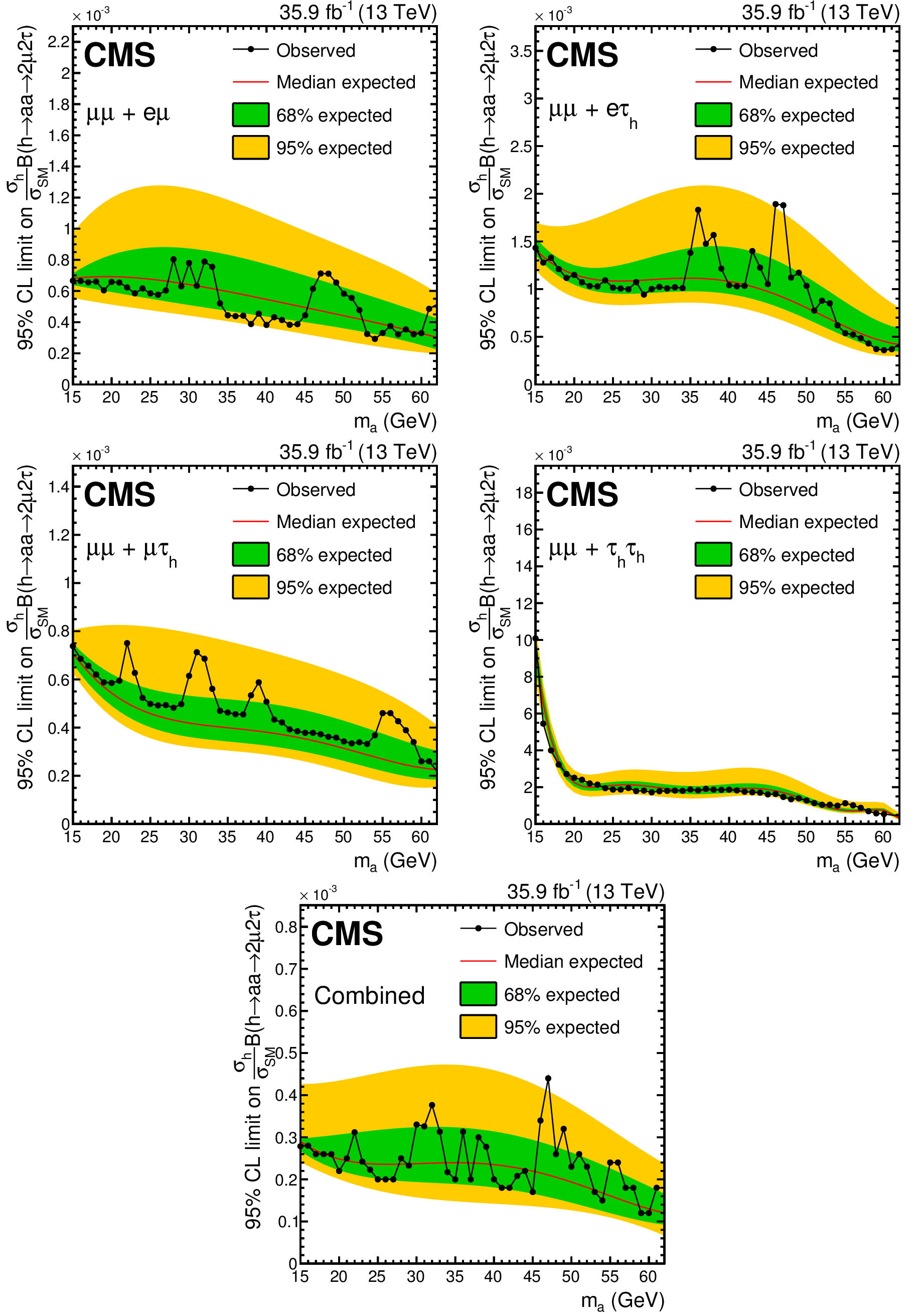
Figure 4:
Upper limits at 95% CL on $(\sigma _ {{\mathrm{h}}} /\sigma _{\textrm {SM}})\mathcal{B}({\mathrm{h} \to \mathrm{aa}\to 2 {\mu} 2{{\tau}}})$, in the $ {{\mu}} {{\mu}}+ {\mathrm{e}} {{\mu}}$ (upper left), $ {{\mu}} {{\mu}}+ {\mathrm{e}} {{\tau} _{\mathrm{h}}} $ (upper right), $ {{\mu}} {{\mu}}+ {{\mu}} {{\tau} _{\mathrm{h}}} $ (middle left), $ {{\mu}} {{\mu}}+ {{\tau} _{\mathrm{h}}} {{\tau} _{\mathrm{h}}} $ (middle right) final states, and for the combination of these final states (lower). The $ {\mathrm{h} \to \mathrm{aa}\to 4{{\tau}}} $ process is considered as a part of the signal, and is scaled with respect to the $ {\mathrm{h} \to \mathrm{aa}\to 2 {\mu} 2{{\tau}}} $ signal using Eq. (1). |
png pdf |
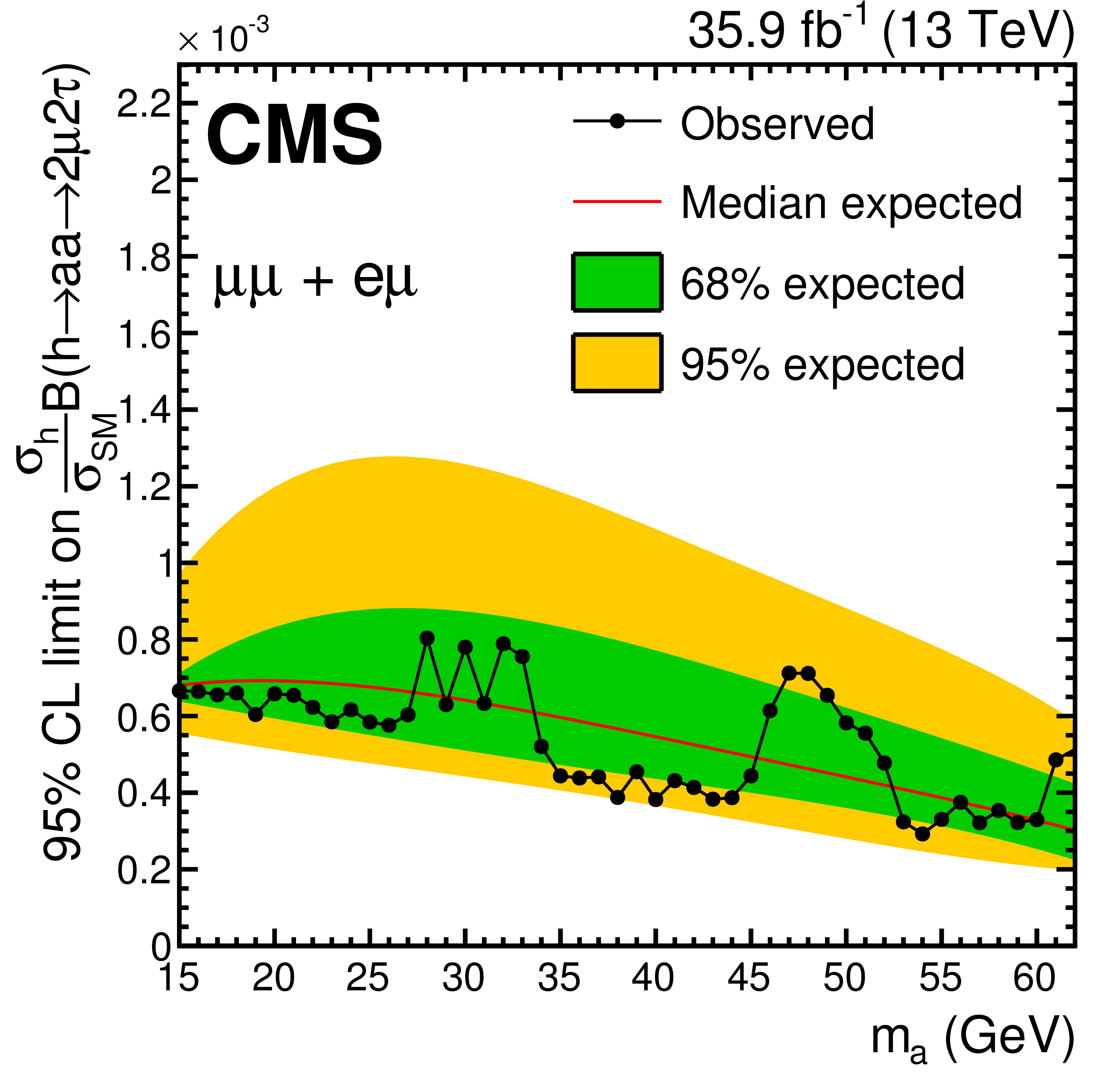
Figure 4-a:
Upper limits at 95% CL on $(\sigma _ {{\mathrm{h}}} /\sigma _{\textrm {SM}})\mathcal{B}({\mathrm{h} \to \mathrm{aa}\to 2 {\mu} 2{{\tau}}})$, in the $ {{\mu}} {{\mu}}+ {\mathrm{e}} {{\mu}}$ final state. The $ {\mathrm{h} \to \mathrm{aa}\to 4{{\tau}}} $ process is considered as a part of the signal, and is scaled with respect to the $ {\mathrm{h} \to \mathrm{aa}\to 2 {\mu} 2{{\tau}}} $ signal using Eq. (1). |
png pdf |
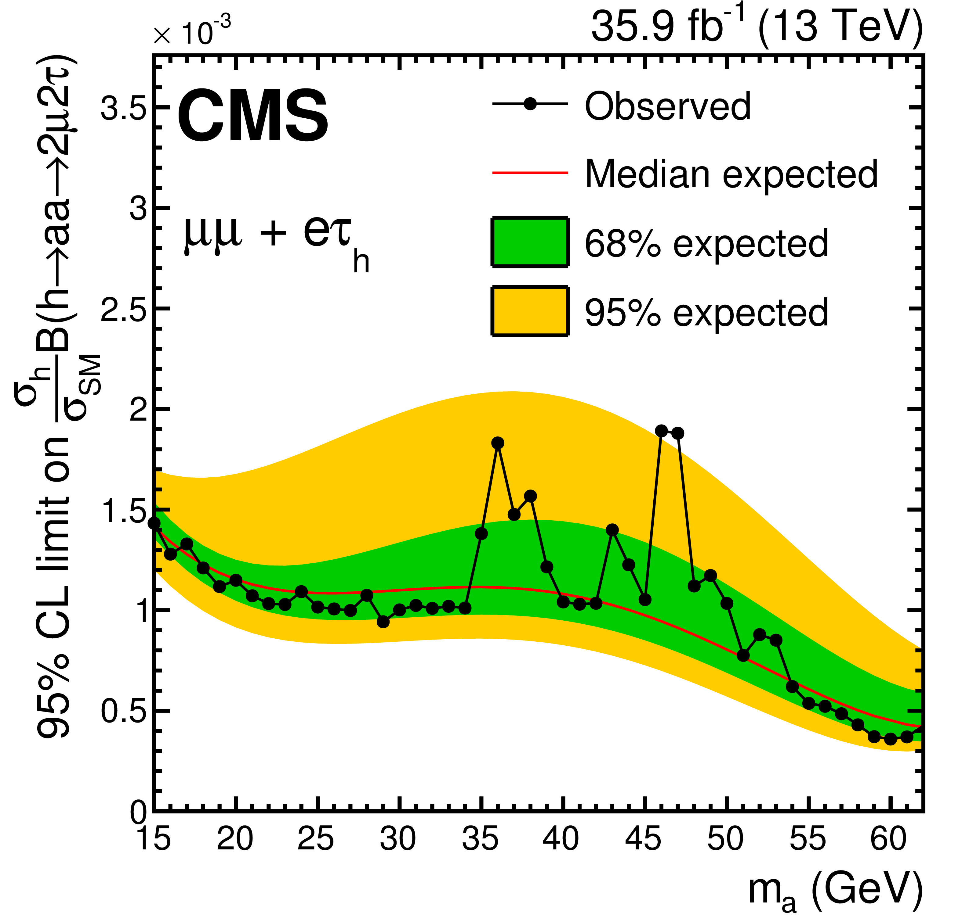
Figure 4-b:
Upper limits at 95% CL on $(\sigma _ {{\mathrm{h}}} /\sigma _{\textrm {SM}})\mathcal{B}({\mathrm{h} \to \mathrm{aa}\to 2 {\mu} 2{{\tau}}})$, in the $ {{\mu}} {{\mu}}+ {\mathrm{e}} {{\tau} _{\mathrm{h}}} $ final state. The $ {\mathrm{h} \to \mathrm{aa}\to 4{{\tau}}} $ process is considered as a part of the signal, and is scaled with respect to the $ {\mathrm{h} \to \mathrm{aa}\to 2 {\mu} 2{{\tau}}} $ signal using Eq. (1). |
png pdf |
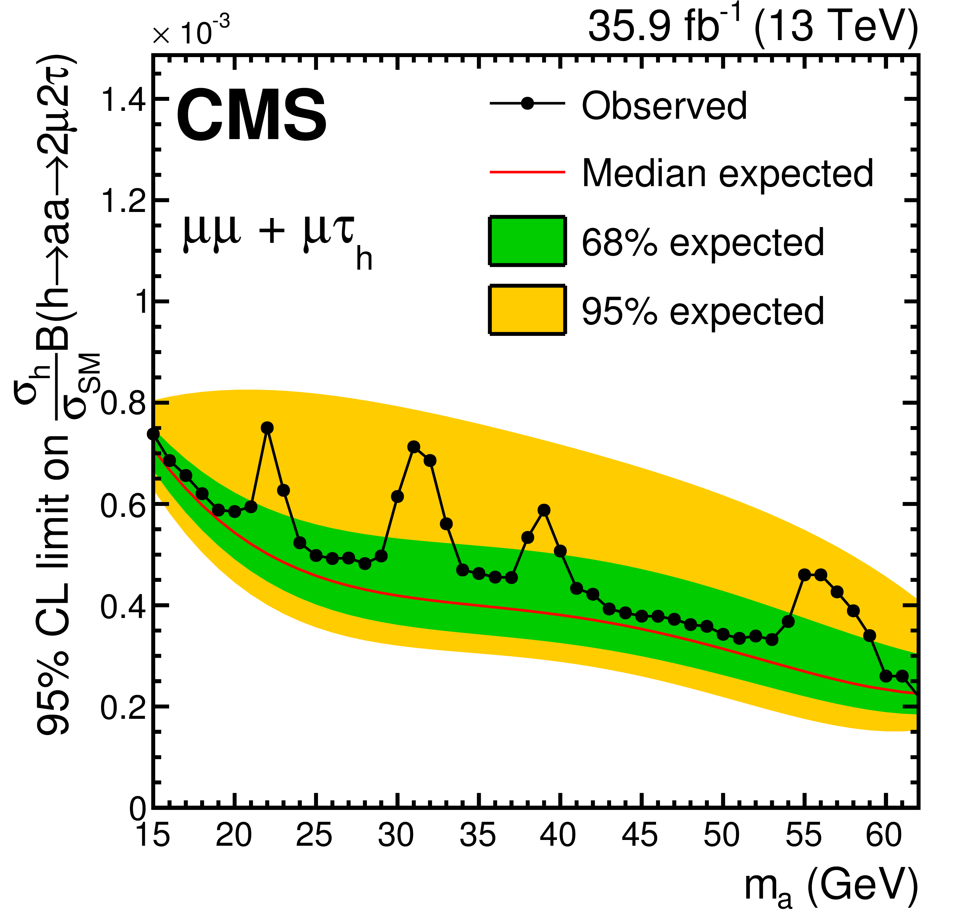
Figure 4-c:
Upper limits at 95% CL on $(\sigma _ {{\mathrm{h}}} /\sigma _{\textrm {SM}})\mathcal{B}({\mathrm{h} \to \mathrm{aa}\to 2 {\mu} 2{{\tau}}})$, in the $ {{\mu}} {{\mu}}+ {{\mu}} {{\tau} _{\mathrm{h}}} $ final state. The $ {\mathrm{h} \to \mathrm{aa}\to 4{{\tau}}} $ process is considered as a part of the signal, and is scaled with respect to the $ {\mathrm{h} \to \mathrm{aa}\to 2 {\mu} 2{{\tau}}} $ signal using Eq. (1). |
png pdf |
Figure 4-d:
Upper limits at 95% CL on $(\sigma _ {{\mathrm{h}}} /\sigma _{\textrm {SM}})\mathcal{B}({\mathrm{h} \to \mathrm{aa}\to 2 {\mu} 2{{\tau}}})$, in the $ {{\mu}} {{\mu}}+ {{\tau} _{\mathrm{h}}} {{\tau} _{\mathrm{h}}} $ final state. The $ {\mathrm{h} \to \mathrm{aa}\to 4{{\tau}}} $ process is considered as a part of the signal, and is scaled with respect to the $ {\mathrm{h} \to \mathrm{aa}\to 2 {\mu} 2{{\tau}}} $ signal using Eq. (1). |

png pdf |
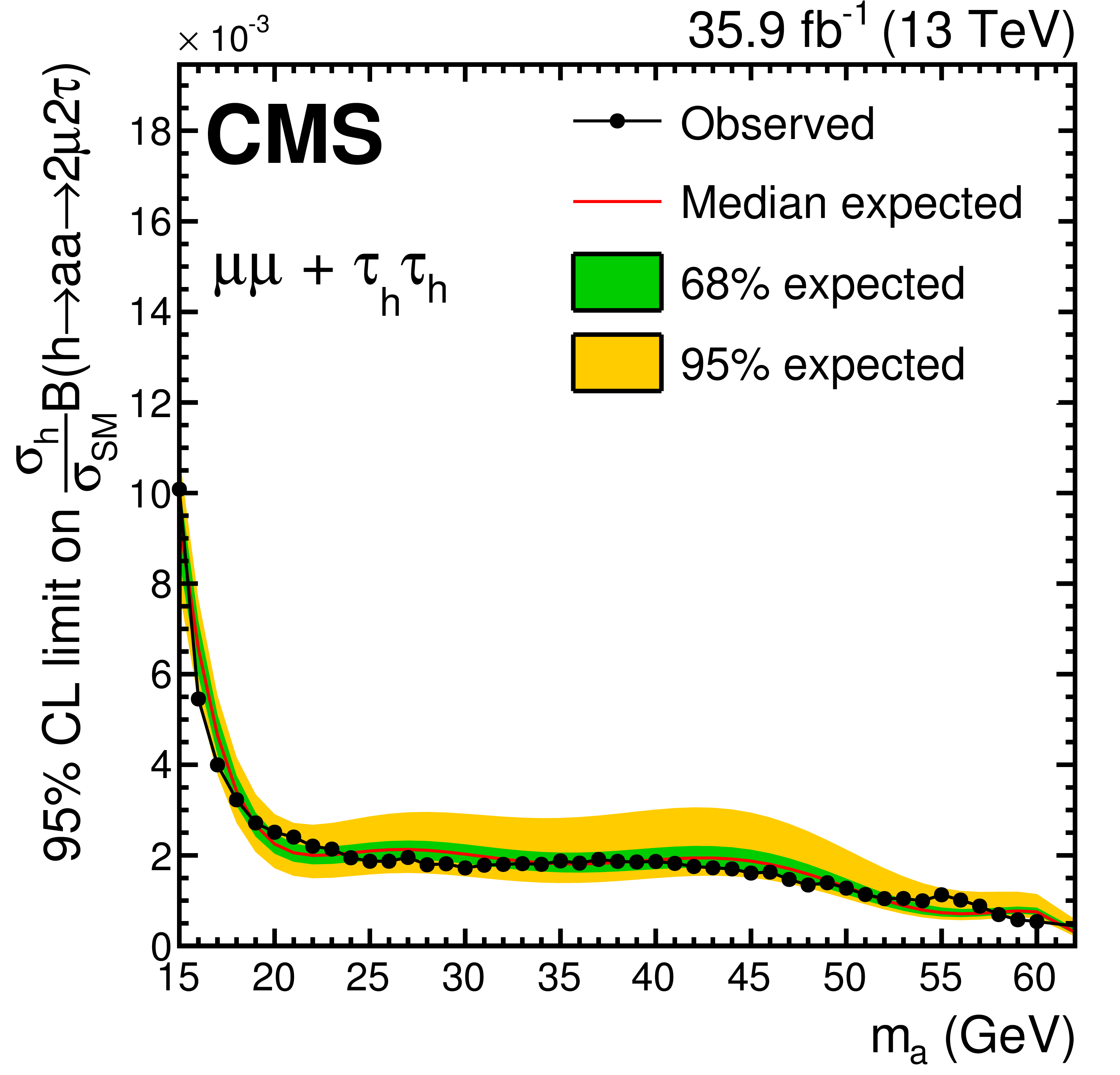
Figure 4-e:
Upper limits at 95% CL on $(\sigma _ {{\mathrm{h}}} /\sigma _{\textrm {SM}})\mathcal{B}({\mathrm{h} \to \mathrm{aa}\to 2 {\mu} 2{{\tau}}})$, for the combination of $ {{\mu}} {{\mu}}+ {\mathrm{e}} {{\mu}}$, $ {{\mu}} {{\mu}}+ {\mathrm{e}} {{\tau} _{\mathrm{h}}} $, $ {{\mu}} {{\mu}}+ {{\mu}} {{\tau} _{\mathrm{h}}} $, and $ {{\mu}} {{\mu}}+ {{\tau} _{\mathrm{h}}} {{\tau} _{\mathrm{h}}} $ final states. The $ {\mathrm{h} \to \mathrm{aa}\to 4{{\tau}}} $ process is considered as a part of the signal, and is scaled with respect to the $ {\mathrm{h} \to \mathrm{aa}\to 2 {\mu} 2{{\tau}}} $ signal using Eq. (1). |
png pdf |
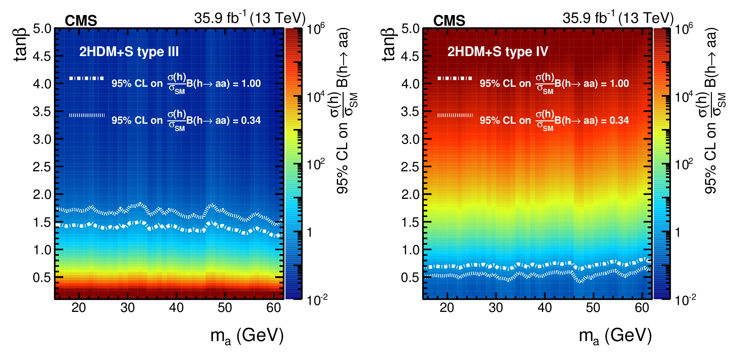
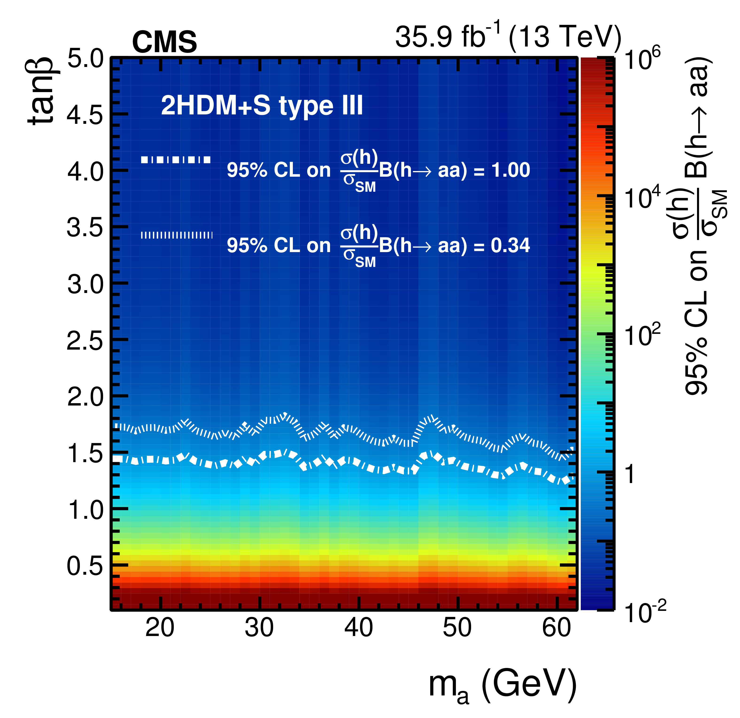
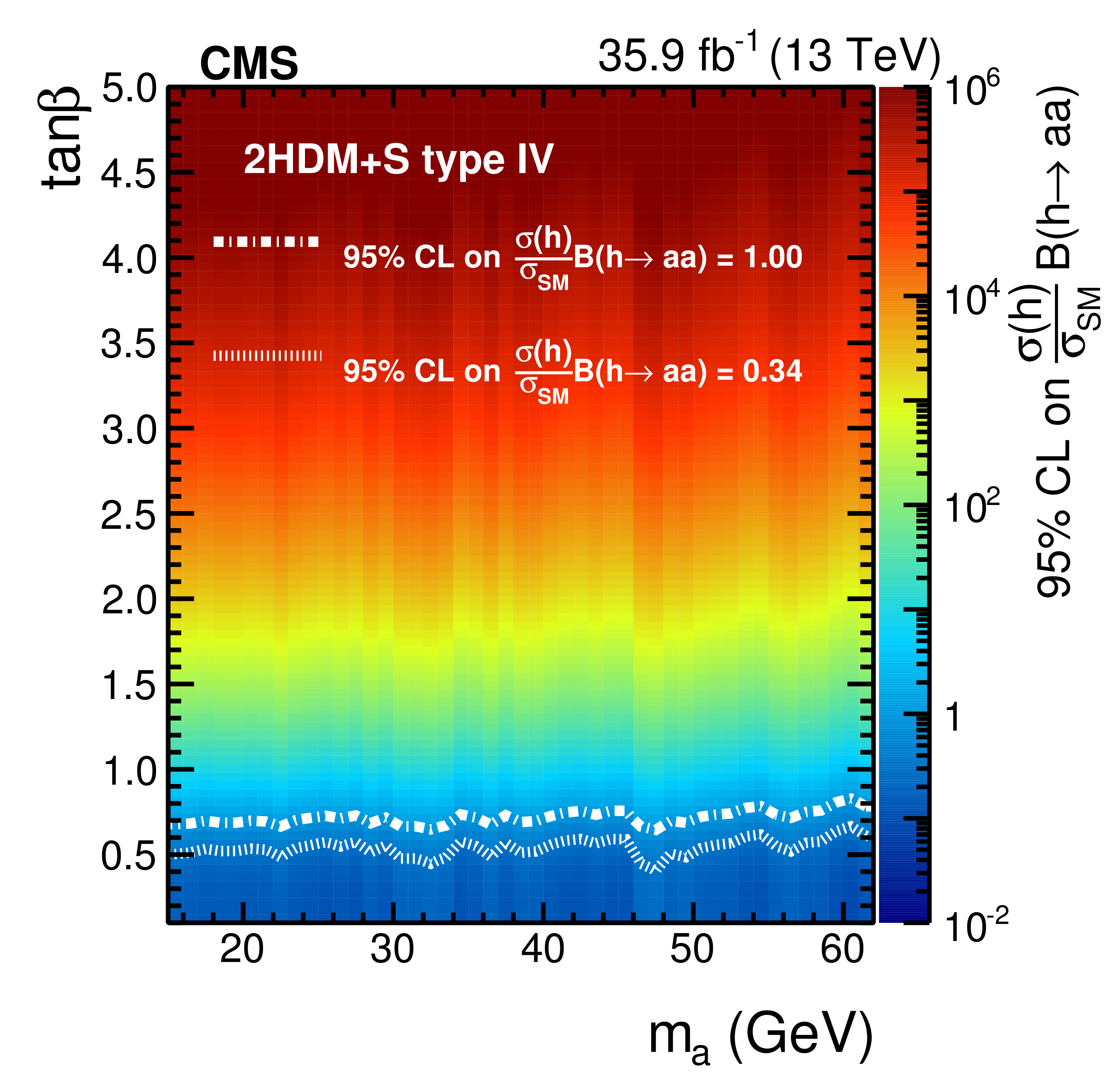
Figure 5:
Observed limits on $(\sigma _{{{\mathrm{h}}}}/\sigma _{ \mathrm{SM}})\mathcal{B}({{\mathrm{h}}} \to \mathrm{aa})$ in 2HDM+S type III (left) and type IV (right). The contour lines shown for $\mathcal{B}({{\mathrm{h}}} \to \mathrm{aa})= $ 1.0 and 0.34 correspond to the colour scale indicated on the right vertical scale. The number 0.34 corresponds to the limit on the branching fraction of the Higgs boson to beyond-the-SM particles at 95% CL obtained with data collected at center-of-mass energies of 7 and 8 TeV by the CMS and ATLAS experiments [10]. |
png pdf |
Figure 5-a:
Observed limits on $(\sigma _{{{\mathrm{h}}}}/\sigma _{ \mathrm{SM}})\mathcal{B}({{\mathrm{h}}} \to \mathrm{aa})$ in 2HDM+S type III. The contour lines shown for $\mathcal{B}({{\mathrm{h}}} \to \mathrm{aa})= $ 1.0 and 0.34 correspond to the colour scale indicated on the right vertical scale. The number 0.34 corresponds to the limit on the branching fraction of the Higgs boson to beyond-the-SM particles at 95% CL obtained with data collected at center-of-mass energies of 7 and 8 TeV by the CMS and ATLAS experiments [10]. |
png pdf |
Figure 5-b:
Observed limits on $(\sigma _{{{\mathrm{h}}}}/\sigma _{ \mathrm{SM}})\mathcal{B}({{\mathrm{h}}} \to \mathrm{aa})$ in 2HDM+S type IV. The contour lines shown for $\mathcal{B}({{\mathrm{h}}} \to \mathrm{aa})= $ 1.0 and 0.34 correspond to the colour scale indicated on the right vertical scale. The number 0.34 corresponds to the limit on the branching fraction of the Higgs boson to beyond-the-SM particles at 95% CL obtained with data collected at center-of-mass energies of 7 and 8 TeV by the CMS and ATLAS experiments [10]. |
| Tables | |
png pdf |
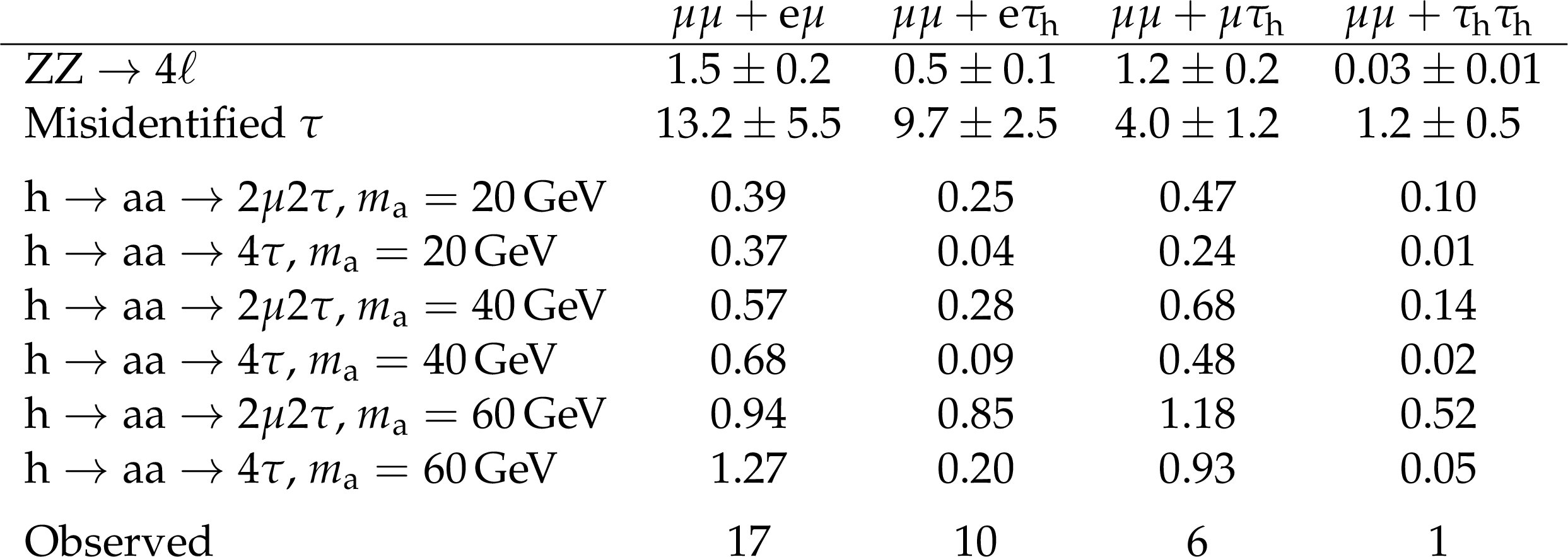
Table 1:
Yields of the signal and background processes in the four final states, as well as the number of observed events in each final state, in the dimuon mass range between 14 and 64 GeV. The signal yields are given for $\mathcal{B}({\mathrm{h} \to \mathrm{aa}\to 2 {\mu} 2{{\tau}}}) = $ 0.01%. The $ {\mathrm{h} \to \mathrm{aa}\to 4{{\tau}}} $ signal is scaled assuming the couplings of the pseudoscalar boson proportional to the squared lepton mass, as in Eq. (1). The production cross section of the Higgs boson predicted in the SM is assumed. The uncertainties combine the statistical and systematic sources. |
| Summary |
| A search for an exotic decay of the Higgs boson to a pair of light pseudoscalars in the final state of two muons and two $\tau$ leptons has been performed using data collected by the CMS experiment in 2016 at a center-of-mass energy of 13 TeV, and corresponding to an integrated luminosity of 35.9 fb$^{-1}$. The results are extracted from an unbinned fit of the dimuon mass spectrum. Limits are set at 95% confidence level on the branching fraction $\mathcal{B}(\mathcal{h}\to\mathrm{a}\mathrm{a}\to2\mu2\tau)$ for the masses of the light pseudoscalar between 15.0 and 62.5 GeV, and are as low as $1.2\times 10^{-4}$ for a mass of 60 GeV assuming the SM production cross section for the Higgs boson. These are the most stringent limits obtained in the final state of two muons and two $\tau$ leptons for the masses above 15 GeV, improving previous limits [14,20] by more than a factor two. They provide the tightest constraints in this mass range on exotic Higgs boson decays in scenarios where the decays of pseudoscalar bosons to leptons are enhanced. |
| References | ||||
| 1 | ATLAS Collaboration | Observation of a new particle in the search for the standard model Higgs boson with the ATLAS detector at the LHC | PLB 716 (2012) 1 | 1207.7214 |
| 2 | CMS Collaboration | Observation of a new boson at a mass of 125 GeV with the CMS experiment at the LHC | PLB 716 (2012) 30 | CMS-HIG-12-028 1207.7235 |
| 3 | CMS Collaboration | Observation of a new boson with mass near 125 GeV in pp collisions at $ \sqrt{s}= $ 7 and 8 TeV | JHEP 06 (2013) 081 | CMS-HIG-12-036 1303.4571 |
| 4 | F. Englert and R. Brout | Broken symmetry and the mass of gauge vector mesons | PRL 13 (1964) 321 | |
| 5 | P. W. Higgs | Broken symmetries, massless particles and gauge fields | PL12 (1964) 132 | |
| 6 | P. W. Higgs | Broken symmetries and the masses of gauge bosons | PRL 13 (1964) 508 | |
| 7 | G. S. Guralnik, C. R. Hagen, and T. W. B. Kibble | Global conservation laws and massless particles | PRL 13 (1964) 585 | |
| 8 | P. W. Higgs | Spontaneous symmetry breakdown without massless bosons | PR145 (1966) 1156 | |
| 9 | T. W. B. Kibble | Symmetry breaking in non-Abelian gauge theories | PR155 (1967) 1554 | |
| 10 | ATLAS and CMS Collaborations | Measurements of the Higgs boson production and decay rates and constraints on its couplings from a combined ATLAS and CMS analysis of the LHC pp collision data at $ \sqrt{s}= $ 7 and 8 TeV | JHEP 08 (2016) 045 | 1606.02266 |
| 11 | D. Curtin et al. | Exotic decays of the 125 GeV Higgs boson | PRD 90 (2014) 075004 | 1312.4992 |
| 12 | U. Ellwanger, C. Hugonie, and A. M. Teixeira | The next-to-minimal supersymmetric standard model | PR 496 (2010) 1 | 0910.1785 |
| 13 | M. Maniatis | The next-to-minimal supersymmetric extension of the standard model reviewed | Int. J. Mod. Phys. A 25 (2010) 3505 | 0906.0777 |
| 14 | CMS Collaboration | Search for light bosons in decays of the 125 GeV Higgs boson in proton-proton collisions at $ \sqrt{s}= $ 8 TeV | JHEP 10 (2017) 076 | CMS-HIG-16-015 1701.02032 |
| 15 | CMS Collaboration | Search for a very light NMSSM Higgs boson produced in decays of the 125 GeV scalar boson and decaying into $ \tau $ leptons in pp collisions at $ \sqrt{s}= $ 8 TeV | JHEP 01 (2016) 079 | CMS-HIG-14-019 1510.06534 |
| 16 | CMS Collaboration | A search for pair production of new light bosons decaying into muons | PLB 752 (2016) 146 | CMS-HIG-13-010 1506.00424 |
| 17 | ATLAS Collaboration | Search for the Higgs boson produced in association with a W boson and decaying to four $ b $-quarks via two spin-zero particles in pp collisions at 13 TeV with the ATLAS detector | EPJC 76 (2016) 605 | 1606.08391 |
| 18 | ATLAS Collaboration | Search for new light gauge bosons in Higgs boson decays to four-lepton final states in pp collisions at $ \sqrt{s}= $ 8 TeV with the ATLAS detector at the LHC | PRD 92 (2015) 092001 | 1505.07645 |
| 19 | ATLAS Collaboration | Search for new phenomena in events with at least three photons collected in pp collisions at $ \sqrt{s}= $ 8 TeV with the ATLAS detector | EPJC 76 (2016) 210 | 1509.05051 |
| 20 | ATLAS Collaboration | Search for Higgs bosons decaying to $ aa $ in the $ \mu\mu\tau\tau $ final state in pp collisions at $ \sqrt{s}= $ 8 TeV with the ATLAS experiment | PRD 92 (2015) 052002 | 1505.01609 |
| 21 | CMS Collaboration | The CMS trigger system | JINST 12 (2017) P01020 | CMS-TRG-12-001 1609.02366 |
| 22 | CMS Collaboration | The CMS experiment at the CERN LHC | JINST 3 (2008) S08004 | CMS-00-001 |
| 23 | J. Alwall et al. | The automated computation of tree-level and next-to-leading order differential cross sections, and their matching to parton shower simulations | JHEP 07 (2014) 079 | 1405.0301 |
| 24 | J. Alwall et al. | Comparative study of various algorithms for the merging of parton showers and matrix elements in hadronic collisions | EPJC 53 (2008) 473 | 0706.2569 |
| 25 | T. Sjostrand et al. | An introduction to PYTHIA 8.2 | CPC 191 (2015) 159 | 1410.3012 |
| 26 | CMS Collaboration | Event generator tunes obtained from underlying event and multiparton scattering measurements | EPJC 76 (2016) 155 | CMS-GEN-14-001 1512.00815 |
| 27 | S. Alioli, P. Nason, C. Oleari, and E. Re | NLO vector-boson production matched with shower in POWHEG | JHEP 07 (2008) 060 | 0805.4802 |
| 28 | P. Nason | A new method for combining NLO QCD with shower Monte Carlo algorithms | JHEP 11 (2004) 040 | hep-ph/0409146 |
| 29 | S. Frixione, P. Nason, and C. Oleari | Matching NLO QCD computations with parton shower simulations: the POWHEG method | JHEP 11 (2007) 070 | 0709.2092 |
| 30 | J. M. Campbell and R. K. Ellis | MCFM for the Tevatron and the LHC | NPPS 205 (2010) 10 | 1007.3492 |
| 31 | NNPDF Collaboration | Parton distributions for the LHC Run II | JHEP 04 (2015) 040 | 1410.8849 |
| 32 | M. Grazzini, S. Kallweit, and D. Rathlev | ZZ production at the LHC: Fiducial cross sections and distributions in NNLO QCD | PLB 750 (2015) 407 | 1507.06257 |
| 33 | GEANT4 Collaboration | GEANT4--a simulation toolkit | NIMA 506 (2003) 250 | |
| 34 | CMS Collaboration | Particle-flow reconstruction and global event description with the CMS detector | JINST 12 (2017) P10003 | CMS-PRF-14-001 1706.04965 |
| 35 | M. Cacciari, G. P. Salam, and G. Soyez | The anti-$ {k_{\mathrm{T}}} $ jet clustering algorithm | JHEP 04 (2008) 063 | 0802.1189 |
| 36 | M. Cacciari, G. P. Salam, and G. Soyez | FastJet user manual | EPJC 72 (2012) 1896 | 1111.6097 |
| 37 | CMS Collaboration | Performance of electron reconstruction and selection with the CMS detector in proton-proton collisions at $ \sqrt{s}= $ 8 TeV | JINST 10 (2015) P06005 | CMS-EGM-13-001 1502.02701 |
| 38 | CMS Collaboration | Performance of CMS muon reconstruction in pp collision events at $ \sqrt{s}= $ 7 TeV | JINST 7 (2012) P10002 | CMS-MUO-10-004 1206.4071 |
| 39 | M. Cacciari and G. P. Salam | Dispelling the $ N^{3} $ myth for the $ k_t $ jet-finder | PLB 641 (2006) 57 | hep-ph/0512210 |
| 40 | CMS Collaboration | Identification of heavy-flavour jets with the CMS detector in pp collisions at 13 TeV | JINST (2017) | CMS-BTV-16-002 1712.07158 |
| 41 | CMS Collaboration | Reconstruction and identification of $ \tau $ lepton decays to hadrons and $ \nu_\tau $ at CMS | JINST 11 (2016) P01019 | CMS-TAU-14-001 1510.07488 |
| 42 | CMS Collaboration | Performance of reconstruction and identification of tau leptons in their decays to hadrons and tau neutrino in LHC Run-2 | CMS-PAS-TAU-16-002 | CMS-PAS-TAU-16-002 |
| 43 | R. A. Fisher | On the interpretation of $ \chi^2 $ from contingency tables, and the calculation of p | J. Roy. Stat. Soc. 85 (1922) 87 | |
| 44 | CMS Collaboration | CMS luminosity measurements for the 2016 data taking period | CMS-PAS-LUM-17-001 | CMS-PAS-LUM-17-001 |
| 45 | The ATLAS Collaboration, The CMS Collaboration, The LHC Higgs Combination Group | Procedure for the LHC Higgs boson search combination in Summer 2011 | CMS-NOTE-2011-005 | |
| 46 | CMS Collaboration | Combined results of searches for the standard model Higgs boson in pp collisions at $ \sqrt{s}= $ 7 TeV | PLB 710 (2012) 26 | CMS-HIG-11-032 1202.1488 |
| 47 | T. Junk | Confidence level computation for combining searches with small statistics | NIMA 434 (1999) 435 | hep-ex/9902006 |
| 48 | A. L. Read | Presentation of search results: the $ CL_s $ technique | in Durham IPPP Workshop: Advanced Statistical Techniques in Particle Physics, p. 2693 Durham, UK, March, 2002 [JPG 28 (2002) 2693] | |
| 49 | A. Djouadi | The anatomy of electro-weak symmetry breaking. I: the Higgs boson in the standard model | Phys. Rep. 457 (2008) 1 | hep-ph/0503172 |
|
|
Compact Muon Solenoid LHC, CERN |
|

|

|

|

|

|