

Compact Muon Solenoid
LHC, CERN
| CMS-PRF-18-001 ; CERN-EP-2019-179 | ||
| Calibration of the CMS hadron calorimeters using proton-proton collision data at $\sqrt{s} = $ 13 TeV | ||
| CMS Collaboration | ||
| 30 September 2019 | ||
| JINST 15 (2020) P05002 | ||
| Abstract: Methods are presented for calibrating the hadron calorimeter system of the CMS detector at the LHC. The hadron calorimeters of the CMS experiment are sampling calorimeters of brass and scintillator, and are in the form of one central detector and two endcaps. These calorimeters cover pseudorapidities $| \eta | < $ 3 and are positioned inside a solenoidal magnet. An outer calorimeter, outside the magnet coil, covers $| \eta | < $ 1.26, and a steel and quartz-fiber Cherenkov forward calorimeter extends the coverage to $| \eta | < $ 5.2. The initial calibration of the calorimeters was based on results from test beams, augmented with the use of radioactive sources and lasers. The calibration was improved substantially using proton-proton collision data collected at $\sqrt{s} = $ 7, 8, and 13 TeV, as well as cosmic ray muon data collected during the periods when the LHC beams were not present. The present calibration is performed using the early 13 TeV data collected during 2016 corresponding to an integrated luminosity of 35.9 fb$^{-1}$. The intercalibration of channels exploits the approximate uniformity of energy deposit over the azimuthal angle. The absolute energy scale of the central and endcap calorimeters is set using isolated charged hadrons. The energy scale for the electromagnetic portion of the forward calorimeters is set using $ {\mathrm{Z} \to \mathrm{e^{+}e^{-}} } $ data. The energy scale of the outer calorimeters has been determined with test beam data and is confirmed through data with high transverse momentum jets. In this paper, we present the details of the calibration methods and accuracy. | ||
| Links: e-print arXiv:1910.00079 [hep-ex] (PDF) ; CDS record ; inSPIRE record ; CADI line (restricted) ; | ||
| Figures | |
png pdf |
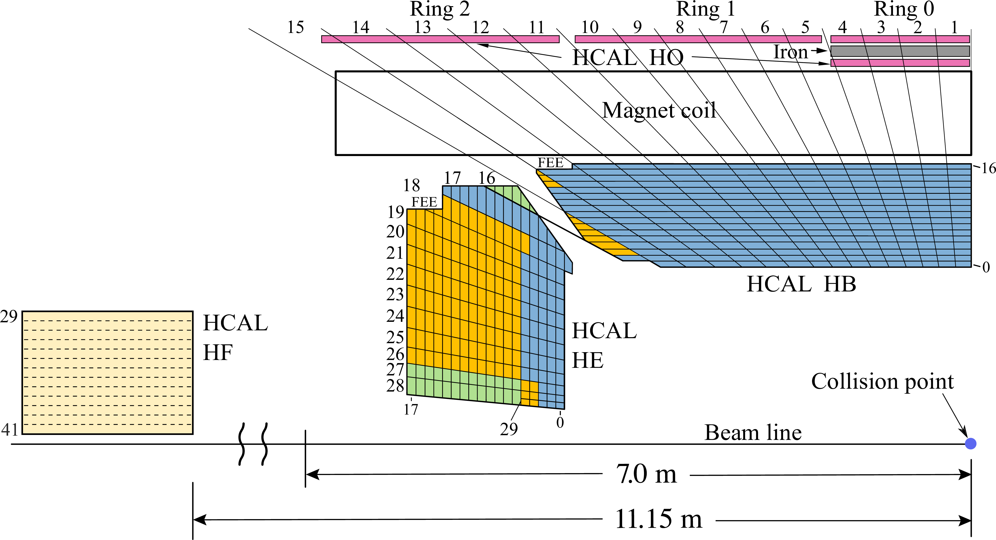
Figure 1:
A schematic view of one quarter of the CMS HCAL during 2016 LHC operation, showing the positions of its four major components: the hadron barrel (HB), the hadron endcap (HE), the hadron outer (HO), and the hadron forward (HF) calorimeters. The layers marked in blue are grouped together as $\text {depth} = $ 1, while the ones in yellow, green, and magenta are combined as depths 2, 3, and 4, respectively. |
png pdf |
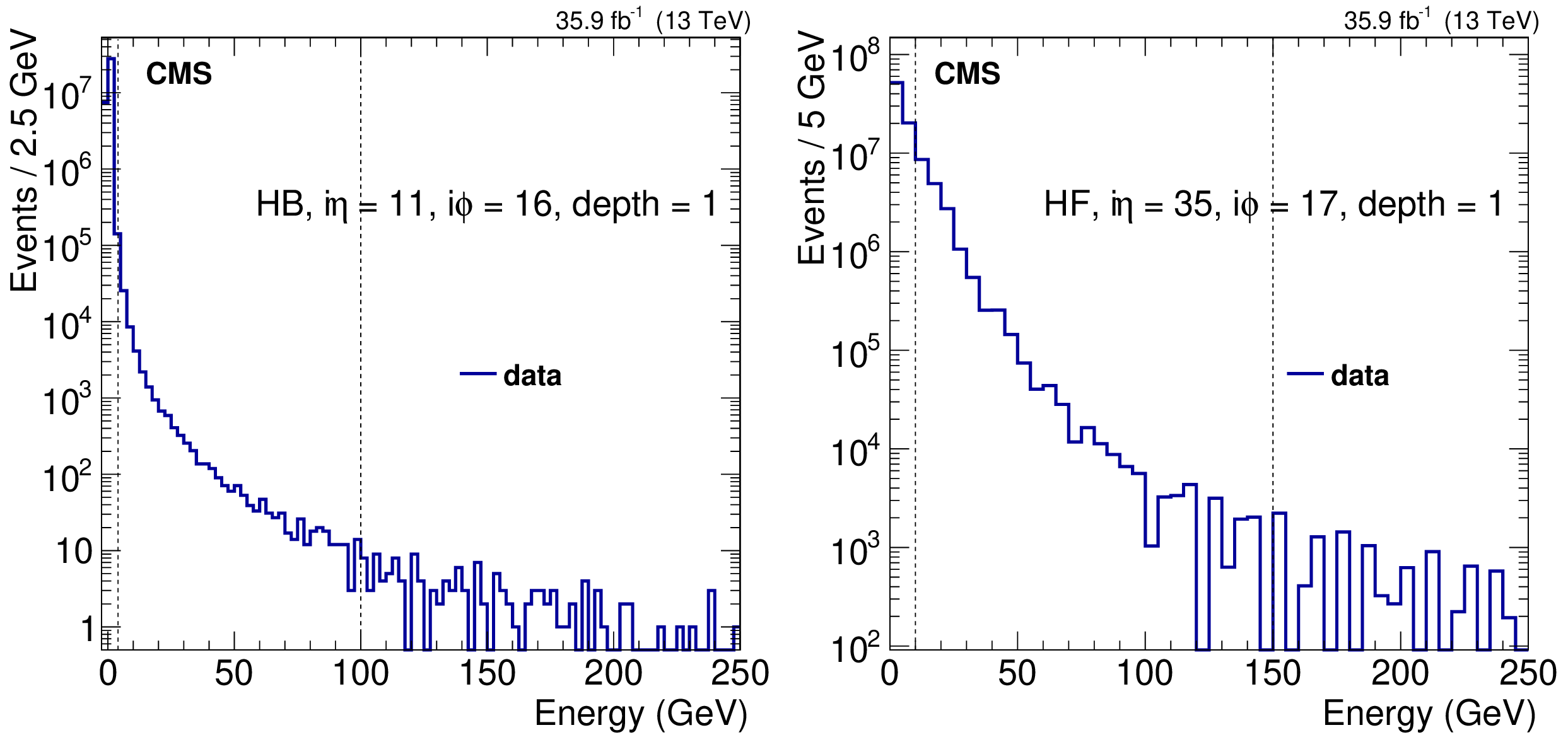
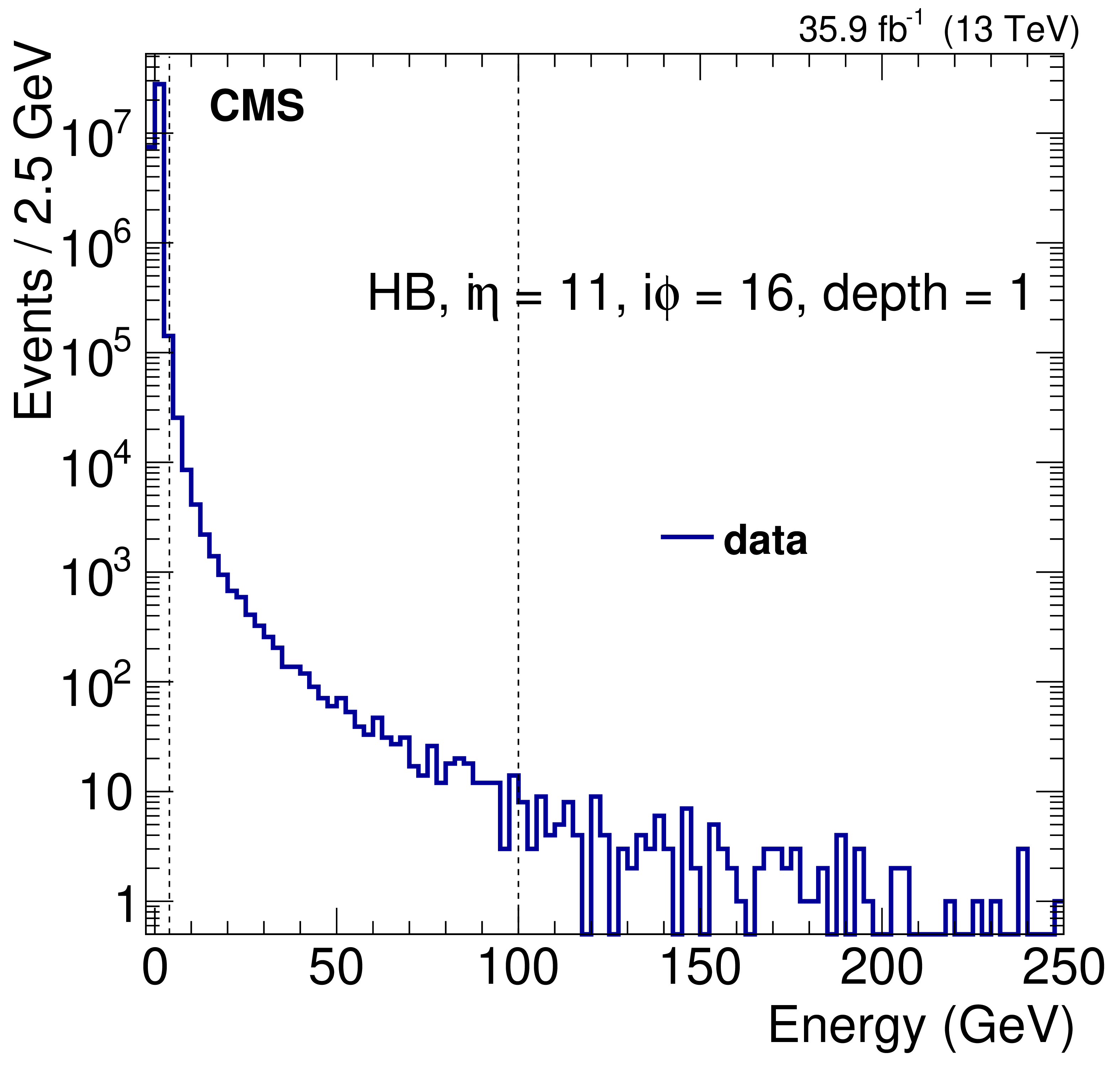
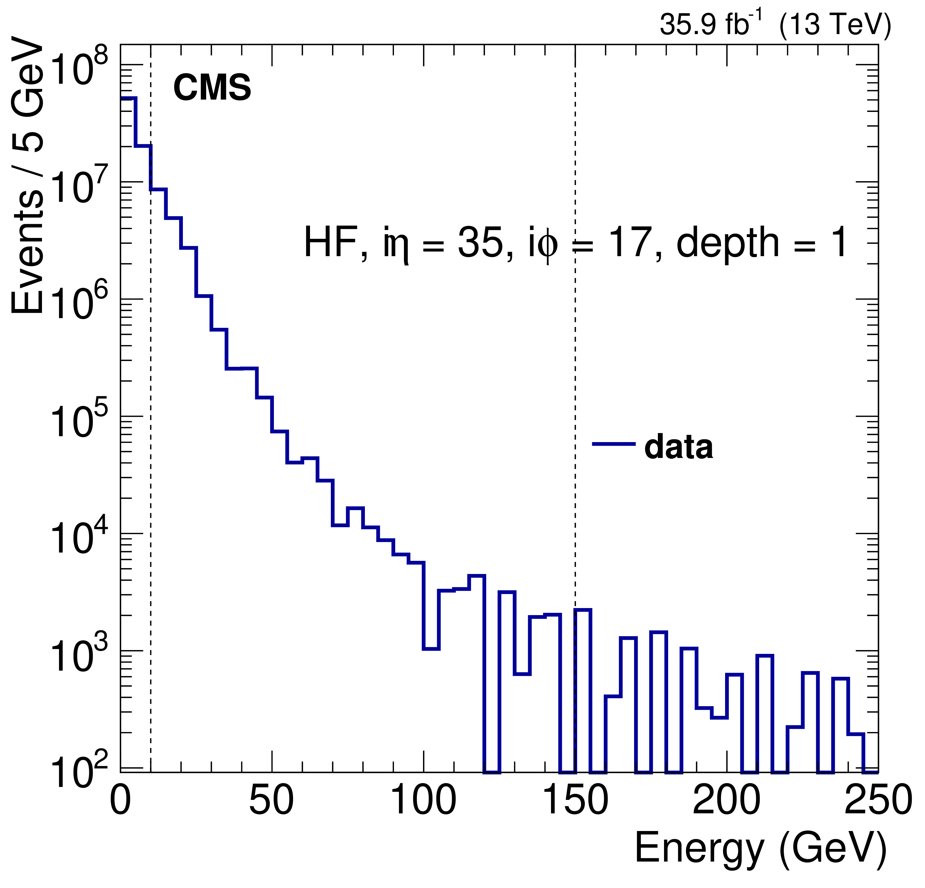
Figure 2:
Energy spectra used as an input to the iterative method of equalizing the $\phi $ response of one typical $ {i\eta} $ ring for an HB (left) and HF (right) calorimeter channel. Energy thresholds on the deposits used for the energy estimation are shown with dashed lines. The legends show the HCAL channel index in $ {i\eta} $, $ {i\phi} $, and depth segmentation units. |
png pdf |
Figure 2-a:
Energy spectrum used as an input to the iterative method of equalizing the $\phi $ response of one typical $ {i\eta} $ ring for an HB calorimeter channel. The energy threshold on the deposits used for the energy estimation is shown with a dashed line. The legend shows the HCAL channel index in $ {i\eta} $, $ {i\phi} $, and depth segmentation units. |
png pdf |
Figure 2-b:
Energy spectrum used as an input to the iterative method of equalizing the $\phi $ response of one typical $ {i\eta} $ ring for an HF calorimeter channel. The energy threshold on the deposits used for the energy estimation is shown with a dashed line. The legend shows the HCAL channel index in $ {i\eta} $, $ {i\phi} $, and depth segmentation units. |
png pdf |
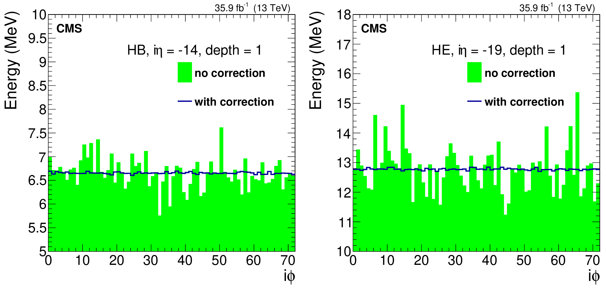
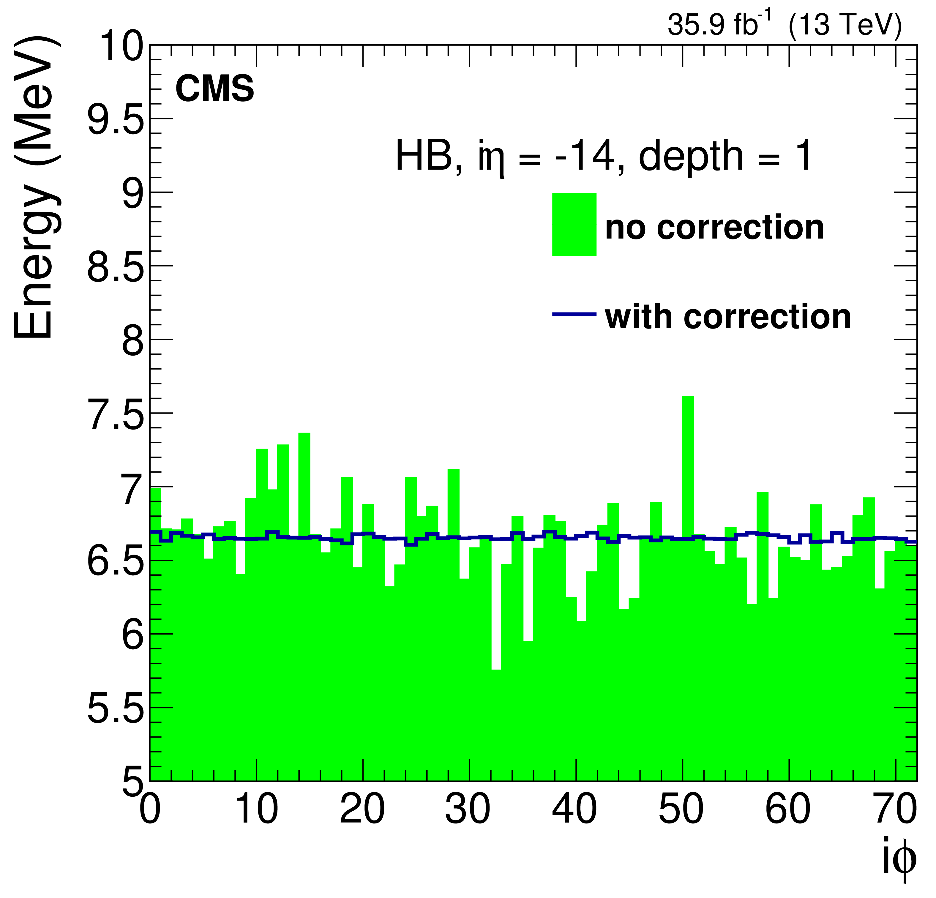
Figure 3:
Mean cell energy $< {E_\text {tot}} > $ for the iterative method measured before (solid histogram) and after (open histogram) correction as a function of $ {i\phi} $ for a typical $ {i\eta} $ ring of the HB ($ {i\eta} = -$14, $\text {depth} = $ 1, left) and of the HE ($ {i\eta} = -$19, $\text {depth} = $ 1, right) calorimeters. Data triggered using electrons, photons, and muon are used in this calibration procedure. |
png pdf |
Figure 3-a:
Mean cell energy $< {E_\text {tot}} > $ for the iterative method measured before (solid histogram) and after (open histogram) correction as a function of $ {i\phi} $ for a typical $ {i\eta} $ ring of the HB ($ {i\eta} = -$14, $\text {depth} = $ 1) calorimeter. Data triggered using electrons, photons, and muon are used in this calibration procedure. |

png pdf |
Figure 3-b:
Mean cell energy $< {E_\text {tot}} > $ for the iterative method measured before (solid histogram) and after (open histogram) correction as a function of $ {i\phi} $ for a typical $ {i\eta} $ ring of the HE ($ {i\eta} = -$19, $\text {depth} = $ 1) calorimeter. Data triggered using electrons, photons, and muon are used in this calibration procedure. |
png pdf |
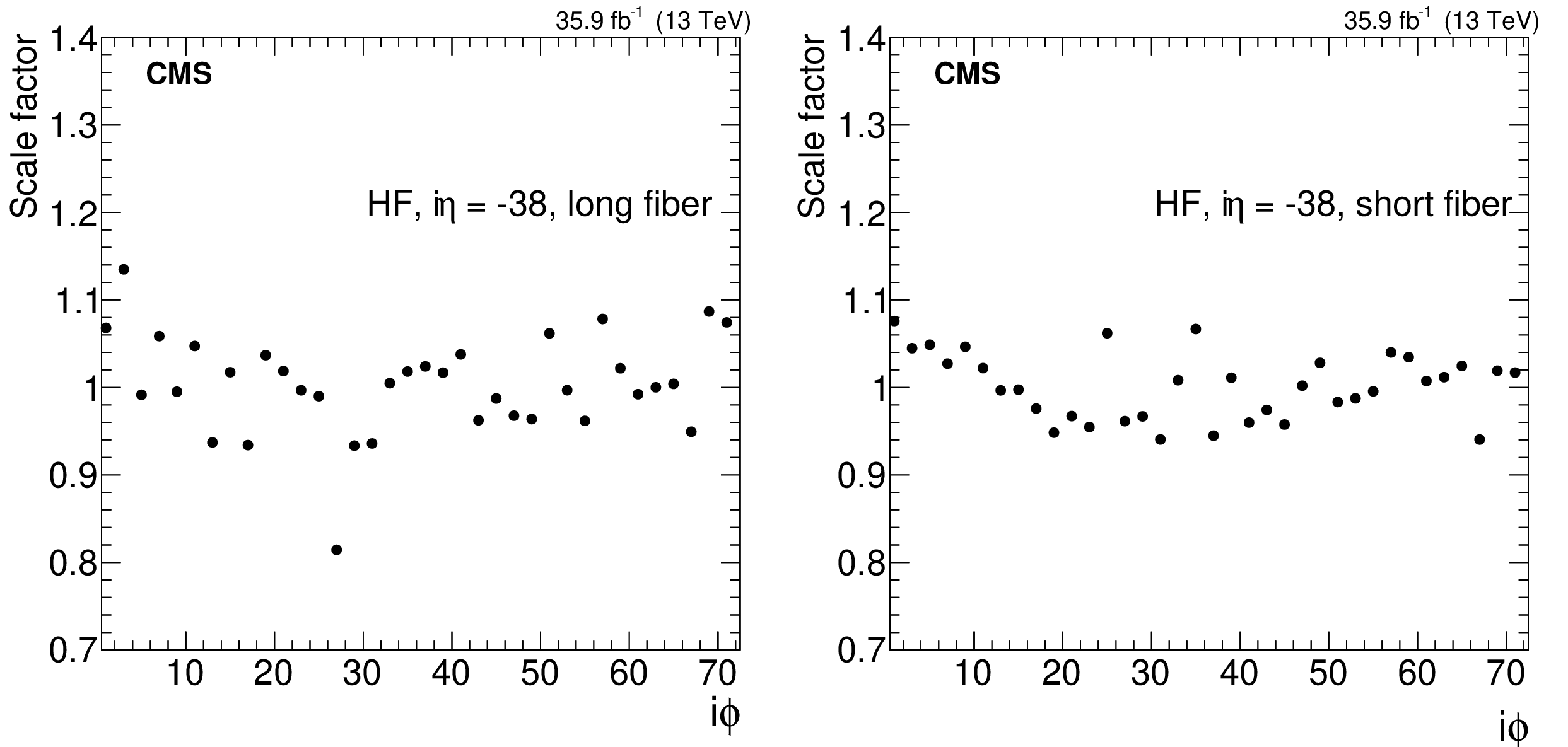
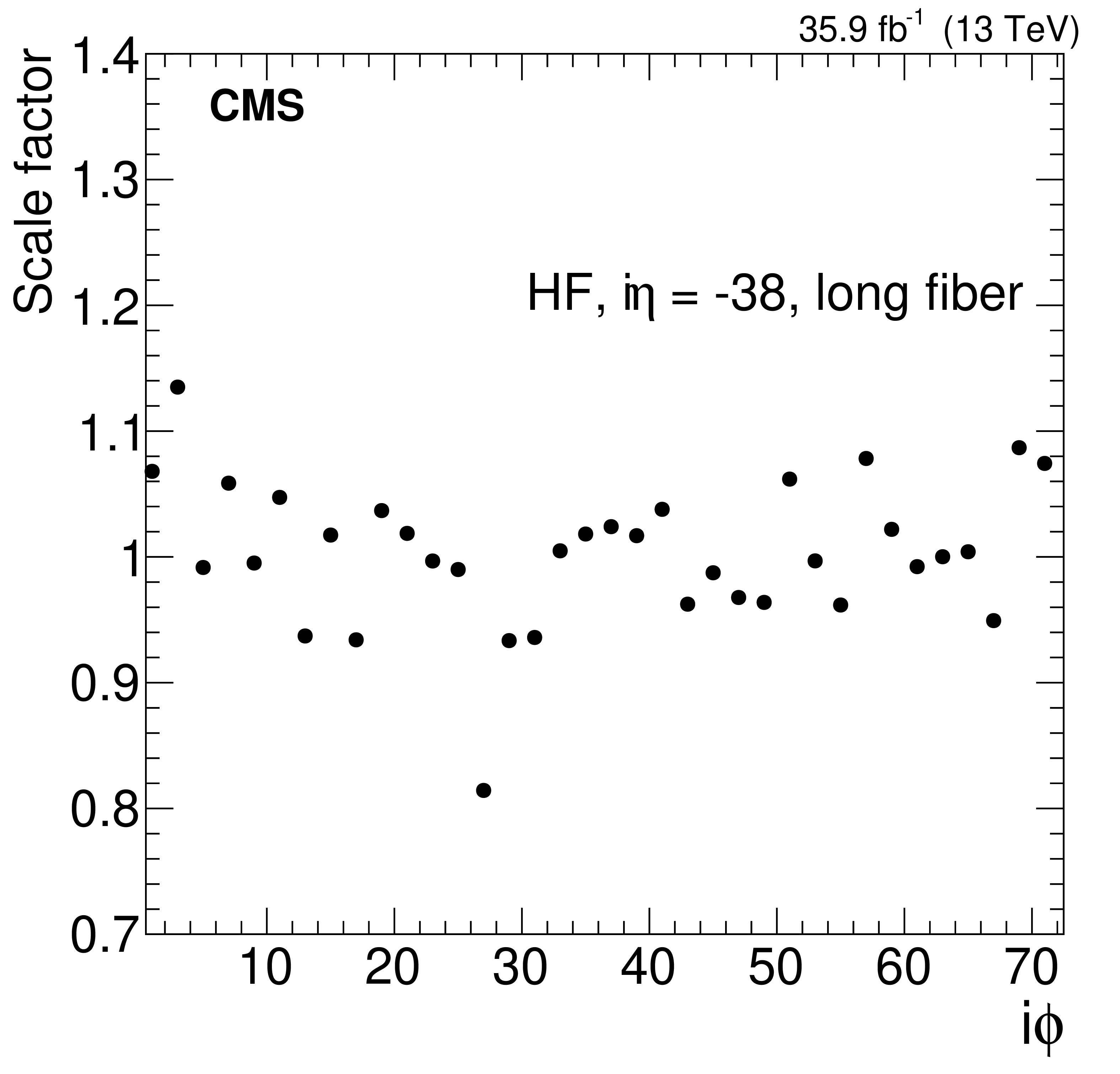
Figure 4:
Calibration scale factor obtained using the method of moments with the first moment of the energy distribution for long (left) and short (right) fibers for two typical HF channels with $ {i\eta} = -$38, as a function of $ {i\phi} $. Only statistical uncertainties in the measurements are shown in these plots. |
png pdf |
Figure 4-a:
Calibration scale factor obtained using the method of moments with the first moment of the energy distribution for a long fiber HF channel with $ {i\eta} = -$38, as a function of $ {i\phi} $. Only statistical uncertainties in the measurements are shown in these plots. |
png pdf |
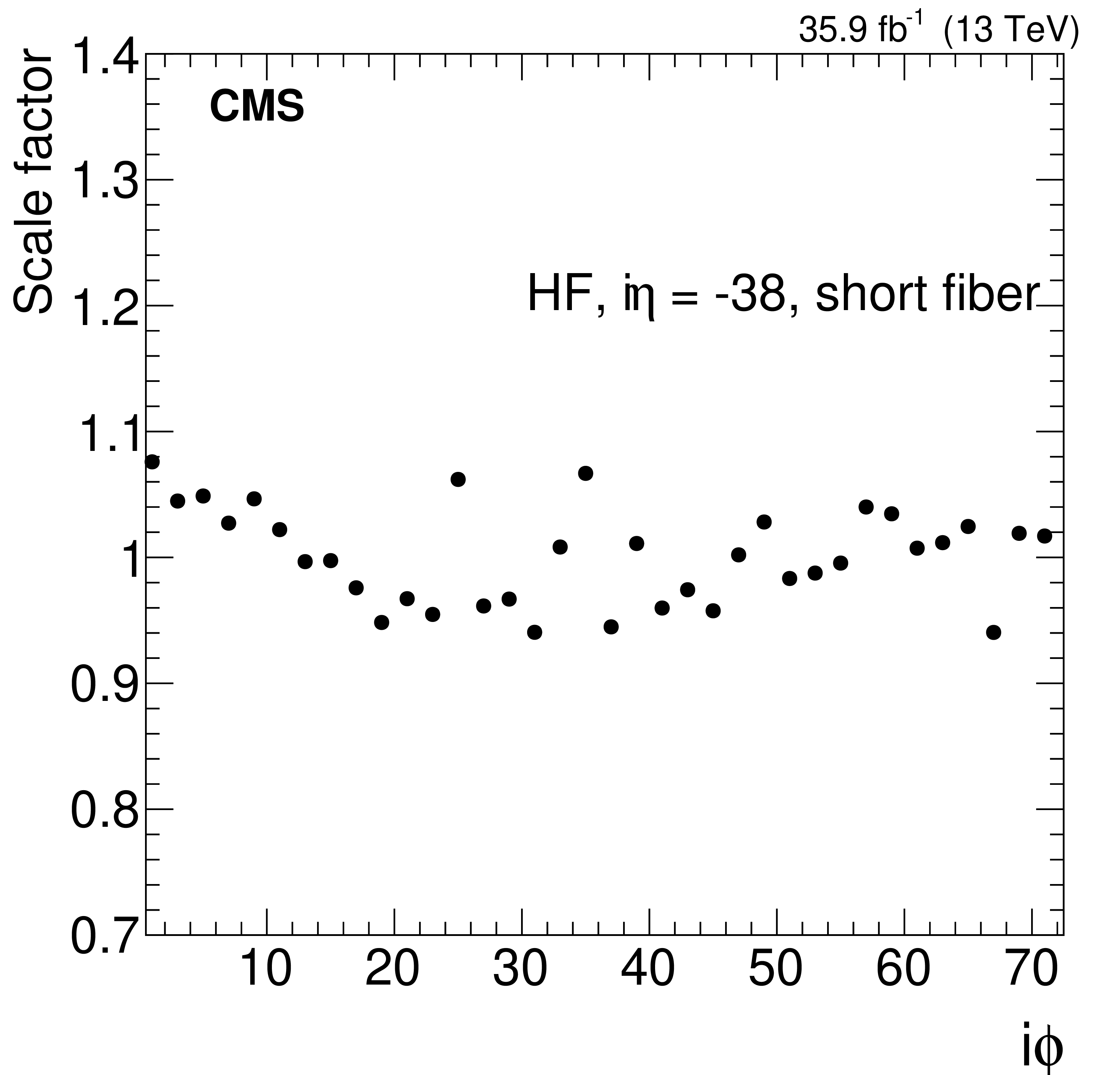
Figure 4-b:
Calibration scale factor obtained using the method of moments with the first moment of the energy distribution for a short fiber HF channel with $ {i\eta} = -$38, as a function of $ {i\phi} $. Only statistical uncertainties in the measurements are shown in these plots. |
png pdf |
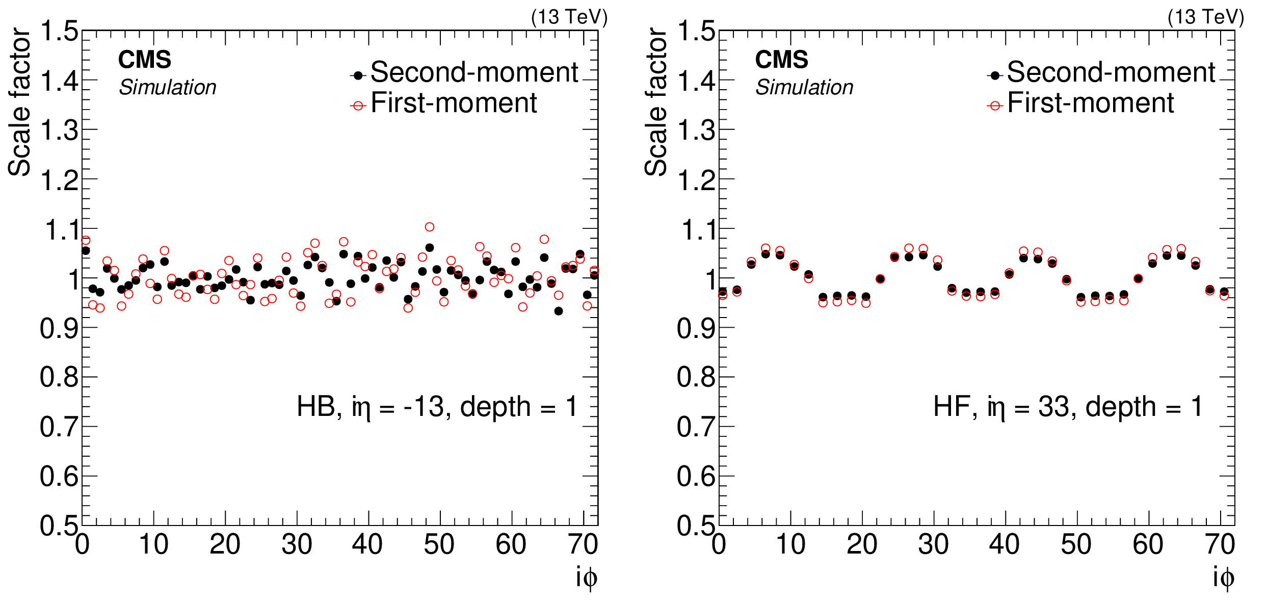
Figure 5:
Derived calibration scale factors that equalize the $\phi $ response in a simulated sample of minimum bias events for a channel in the HB ($ {i\eta} = -$13, $\text {depth} = $ 1, left) and HF ($ {i\eta} = $33, $\text {depth} = $ 1, right), as a function of $ {i\phi} $ using two different methods: of first and of second moment. |
png pdf |
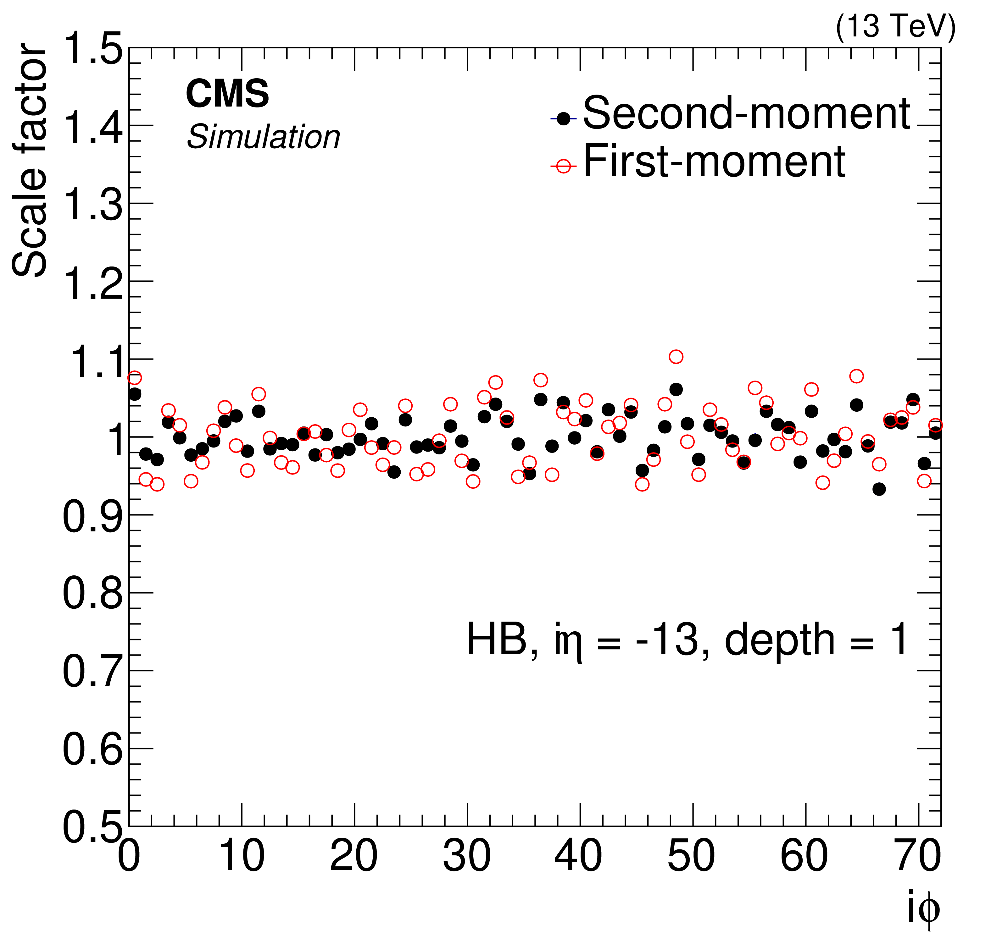
Figure 5-a:
Derived calibration scale factors that equalize the $\phi $ response in a simulated sample of minimum bias events for a channel in the HB ($ {i\eta} = -$13, $\text {depth} = $ 1), as a function of $ {i\phi} $ using two different methods: of first and of second moment. |
png pdf |
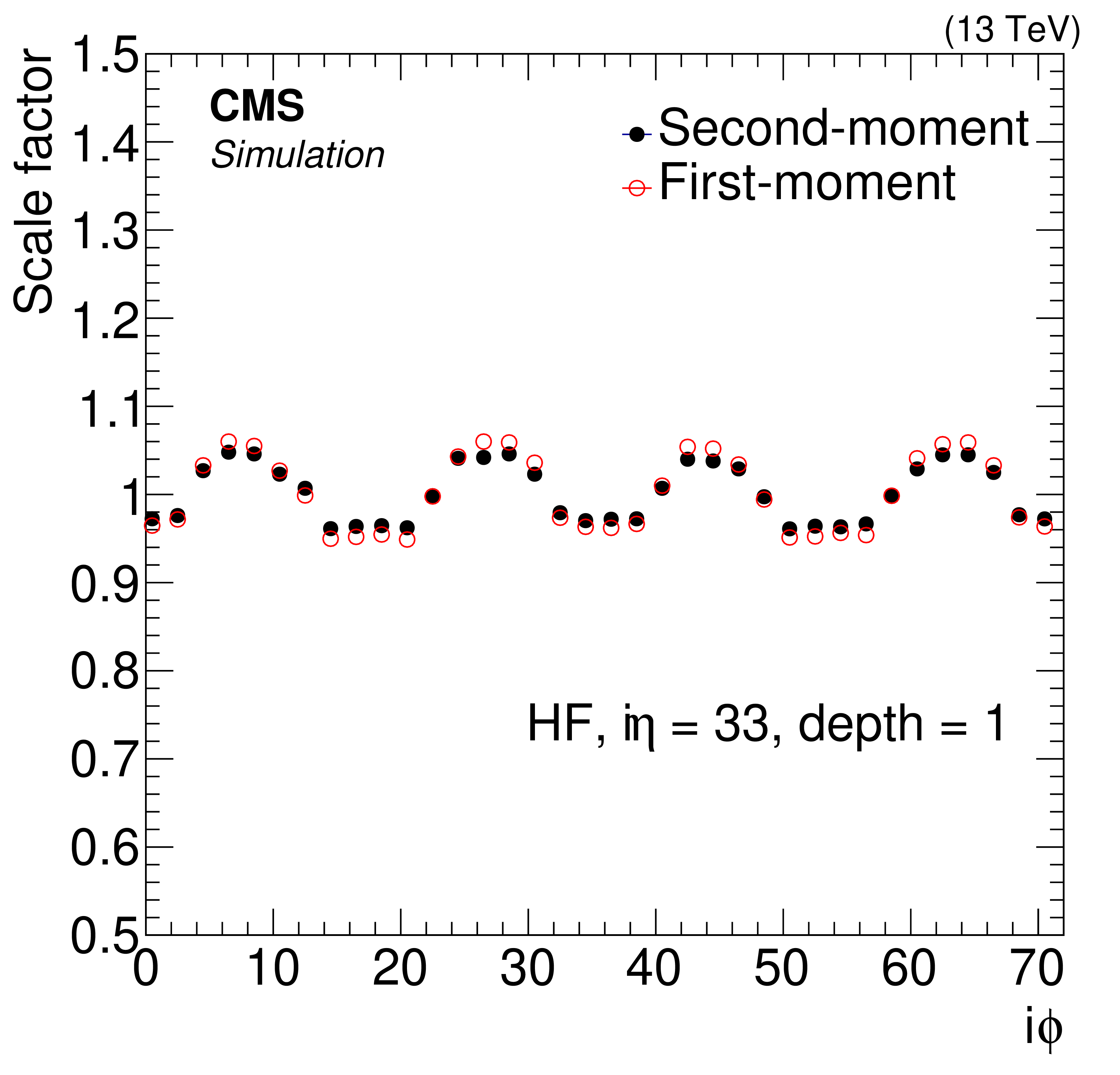
Figure 5-b:
Derived calibration scale factors that equalize the $\phi $ response in a simulated sample of minimum bias events for a channel in the HF ($ {i\eta} = $33, $\text {depth} = $ 1), as a function of $ {i\phi} $ using two different methods: of first and of second moment. |
png pdf |
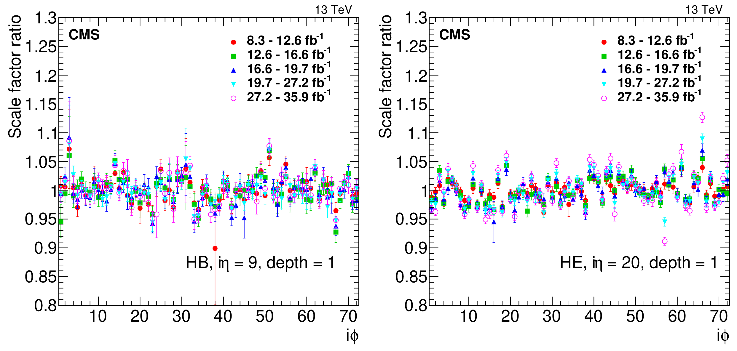
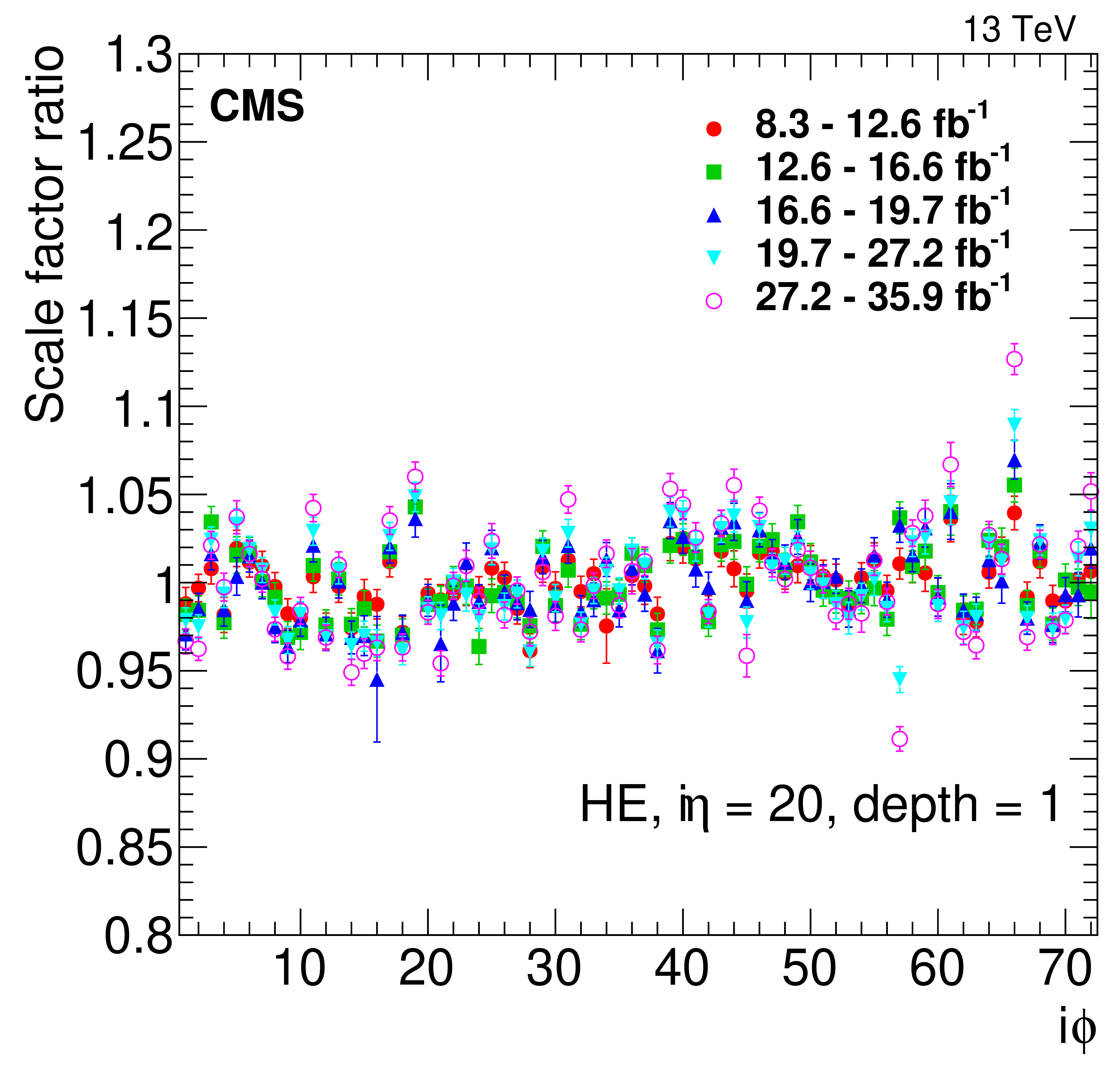
Figure 6:
Ratio of the calibration scale factors for a typical HB ($ {i\eta} = $ 9, $\text {depth} = $ 1, left) and HE ($ {i\eta} = 20$, $\text {depth} = $ 1, right) channels as a function of $ {i\phi} $, in different data taking periods, to that obtained in a sample corresponding to the first 8.3 fb$^{-1}$ of integrated luminosity accumulated during the run, for five data taking periods during 2016. Only statistical uncertainties in the scale factors are shown. |

png pdf |
Figure 6-a:
Ratio of the calibration scale factors for a typical HB ($ {i\eta} = $ 9, $\text {depth} = $ 1) channel as a function of $ {i\phi} $, in different data taking periods, to that obtained in a sample corresponding to the first 8.3 fb$^{-1}$ of integrated luminosity accumulated during the run, for five data taking periods during 2016. Only statistical uncertainties in the scale factors are shown. |
png pdf |
Figure 6-b:
Ratio of the calibration scale factors for a typical HE ($ {i\eta} = 20$, $\text {depth} = $ 1) channel as a function of $ {i\phi} $, in different data taking periods, to that obtained in a sample corresponding to the first 8.3 fb$^{-1}$ of integrated luminosity accumulated during the run, for five data taking periods during 2016. Only statistical uncertainties in the scale factors are shown. |
png pdf |
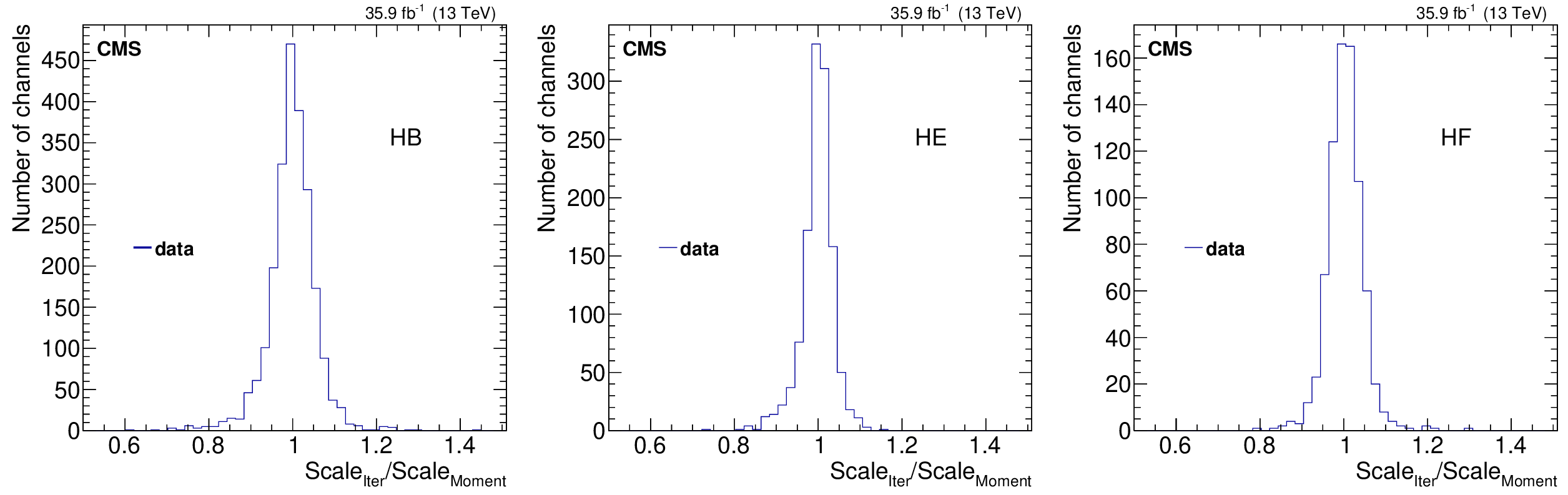
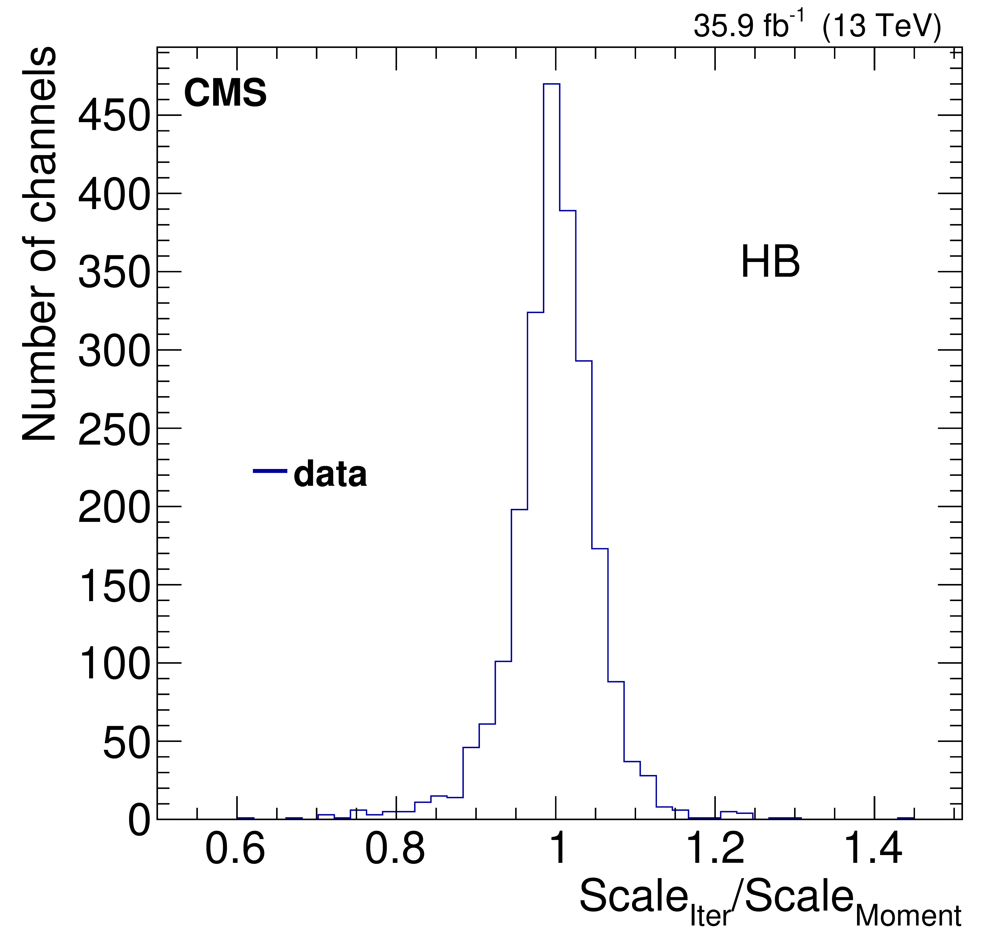
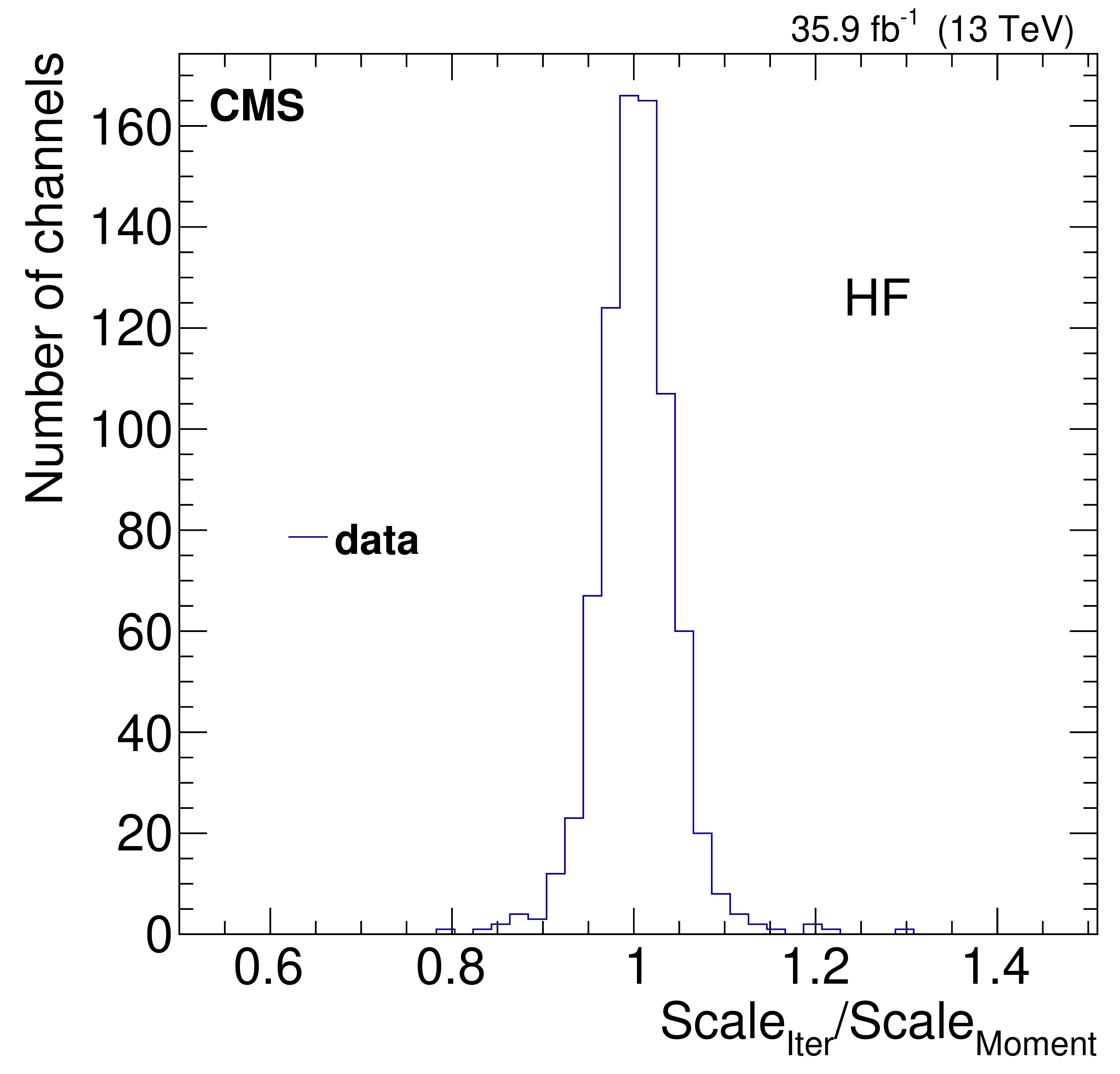
Figure 7:
The ratio of $\phi $ intercalibration scale factors obtained with the method of moments to that obtained with the iterative method for HB (left), HE (center), and HF (right). |
png pdf |
Figure 7-a:
The ratio of $\phi $ intercalibration scale factors obtained with the method of moments to that obtained with the iterative method for HB. |
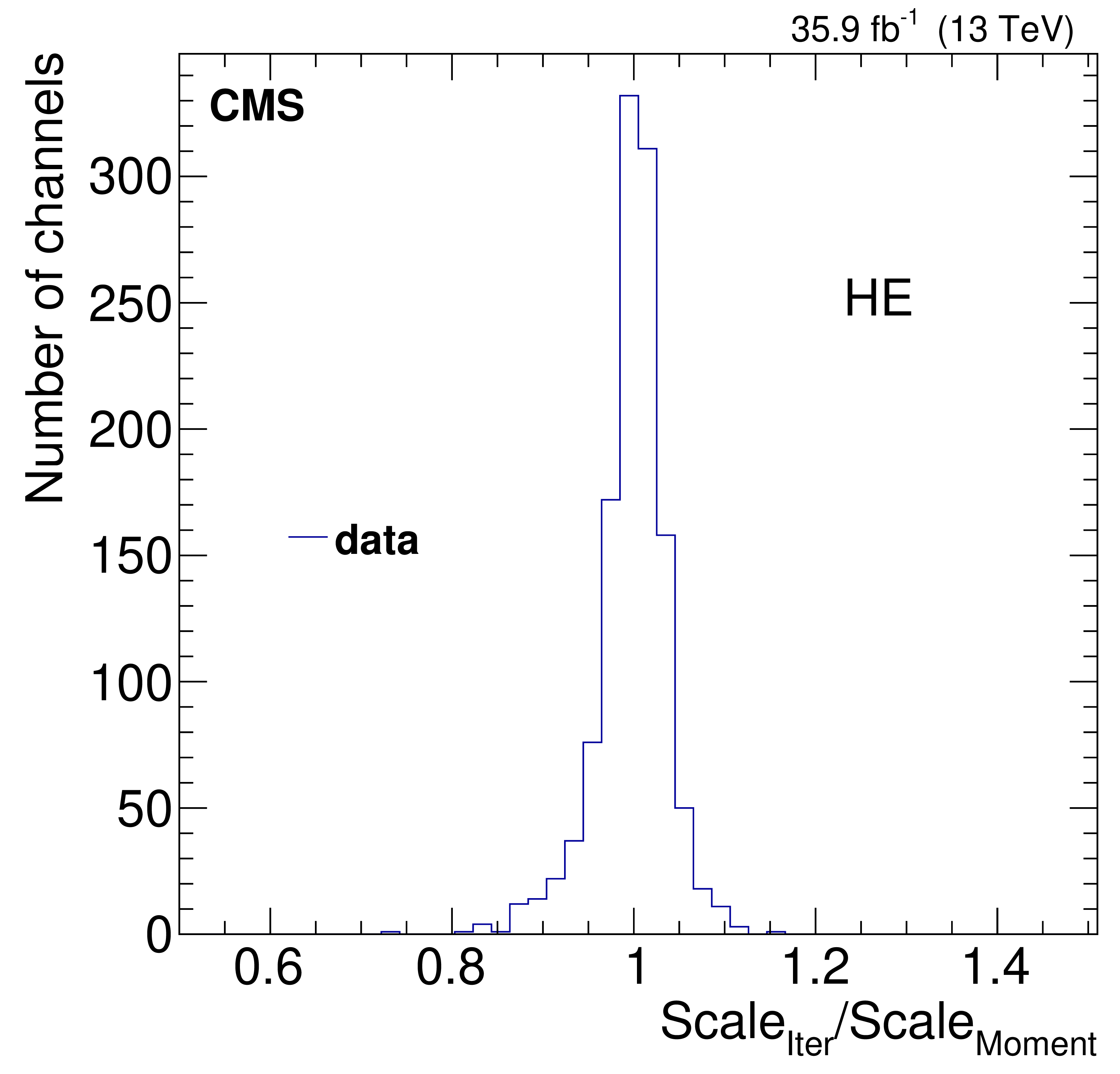
png pdf |
Figure 7-b:
The ratio of $\phi $ intercalibration scale factors obtained with the method of moments to that obtained with the iterative method for HE. |
png pdf |
Figure 7-c:
The ratio of $\phi $ intercalibration scale factors obtained with the method of moments to that obtained with the iterative method for HF. |
png pdf |
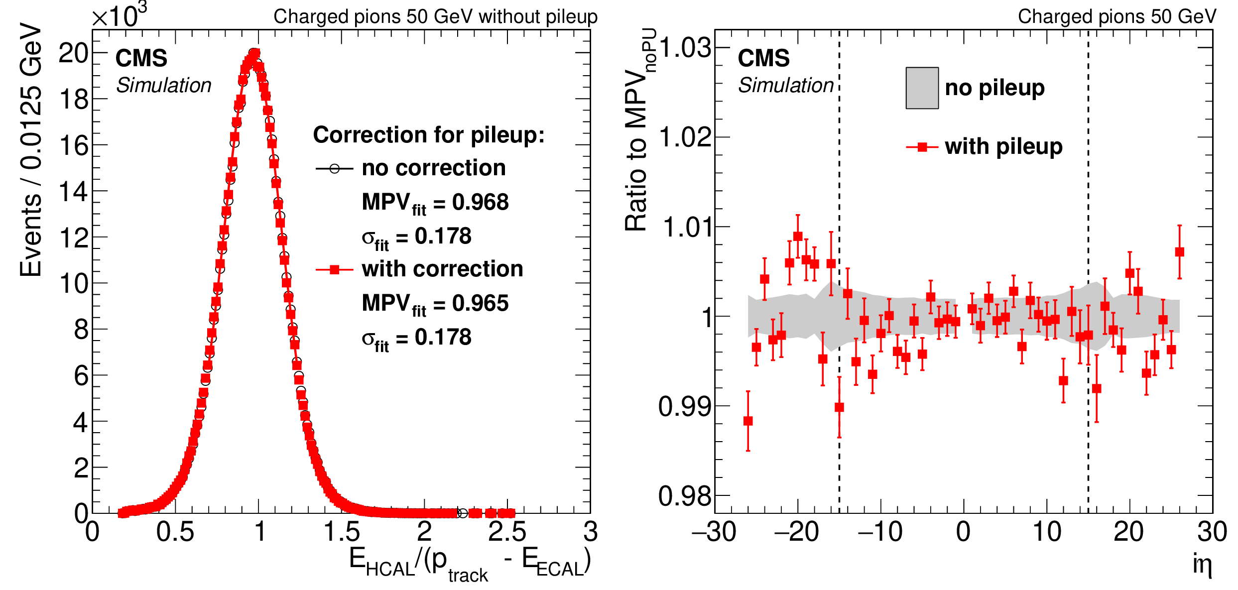
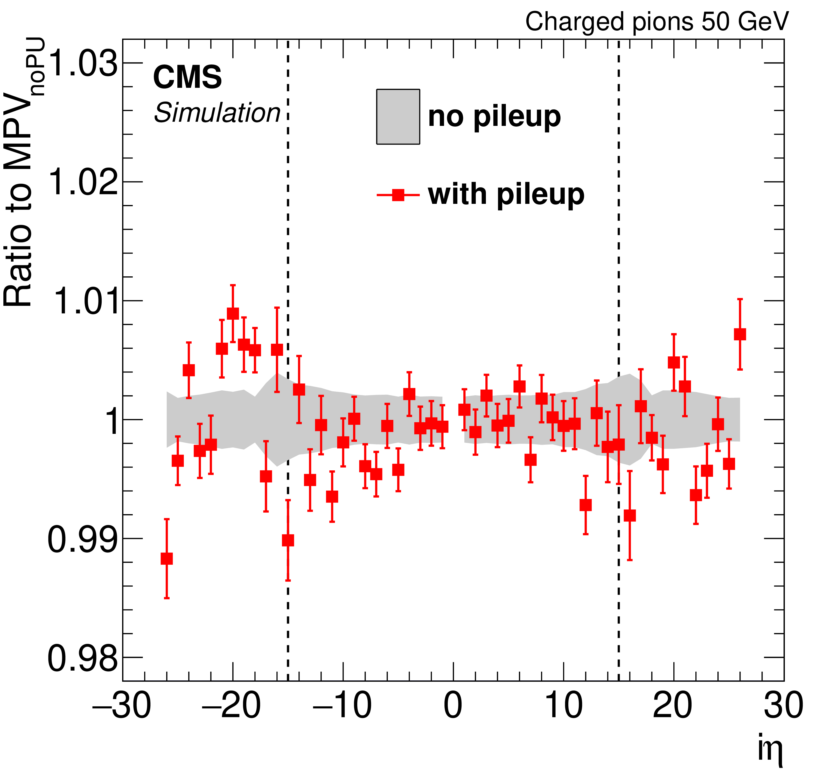
Figure 8:
left : Distribution of the energy response in a simulated sample of single isolated high-$ {p_{\mathrm {T}}} $ pions without pileup when the corrections for pileup have (red squares) or have not (black circles) been applied. The plot also shows the results of Gaussian fits. right : The ratio of the mode of the response distribution for a simulated pion sample with pileup, with loose charged-particle isolation, and the correction for pileup applied (red squares) to the mode from the sample without pileup. The uncertainties in the mode without pileup are shown with the gray band. Only statistical uncertainties are included. The dashed vertical lines show the boundaries between the barrel and the endcaps. |

png pdf |
Figure 8-a:
Distribution of the energy response in a simulated sample of single isolated high-$ {p_{\mathrm {T}}} $ pions without pileup when the corrections for pileup have (red squares) or have not (black circles) been applied. The plot also shows the results of Gaussian fits. |
png pdf |
Figure 8-b:
The ratio of the mode of the response distribution for a simulated pion sample with pileup, with loose charged-particle isolation, and the correction for pileup applied (red squares) to the mode from the sample without pileup. The uncertainties in the mode without pileup are shown with the gray band. Only statistical uncertainties are included. The dashed vertical lines show the boundaries between the barrel and the endcaps. |

png pdf |
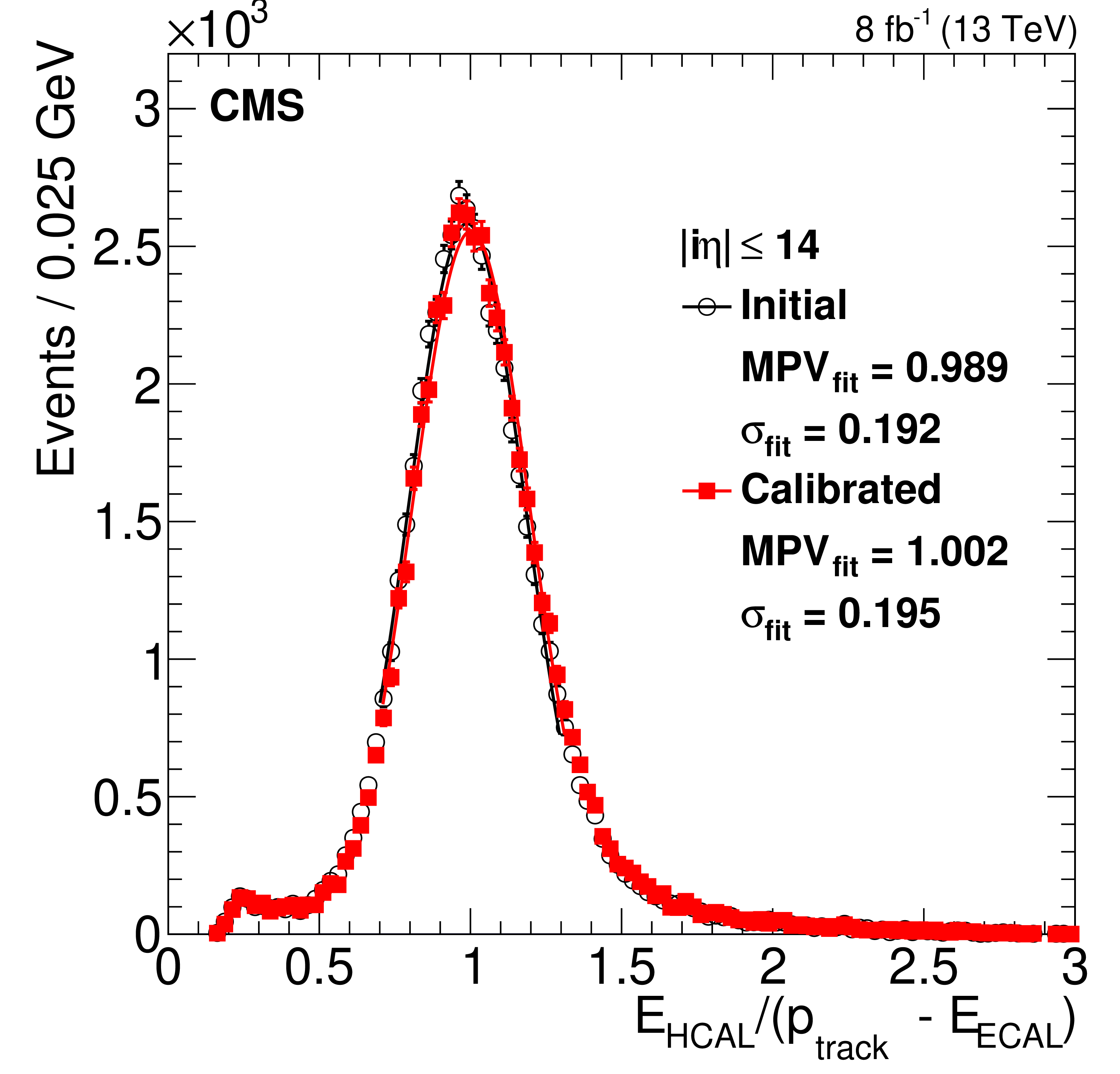
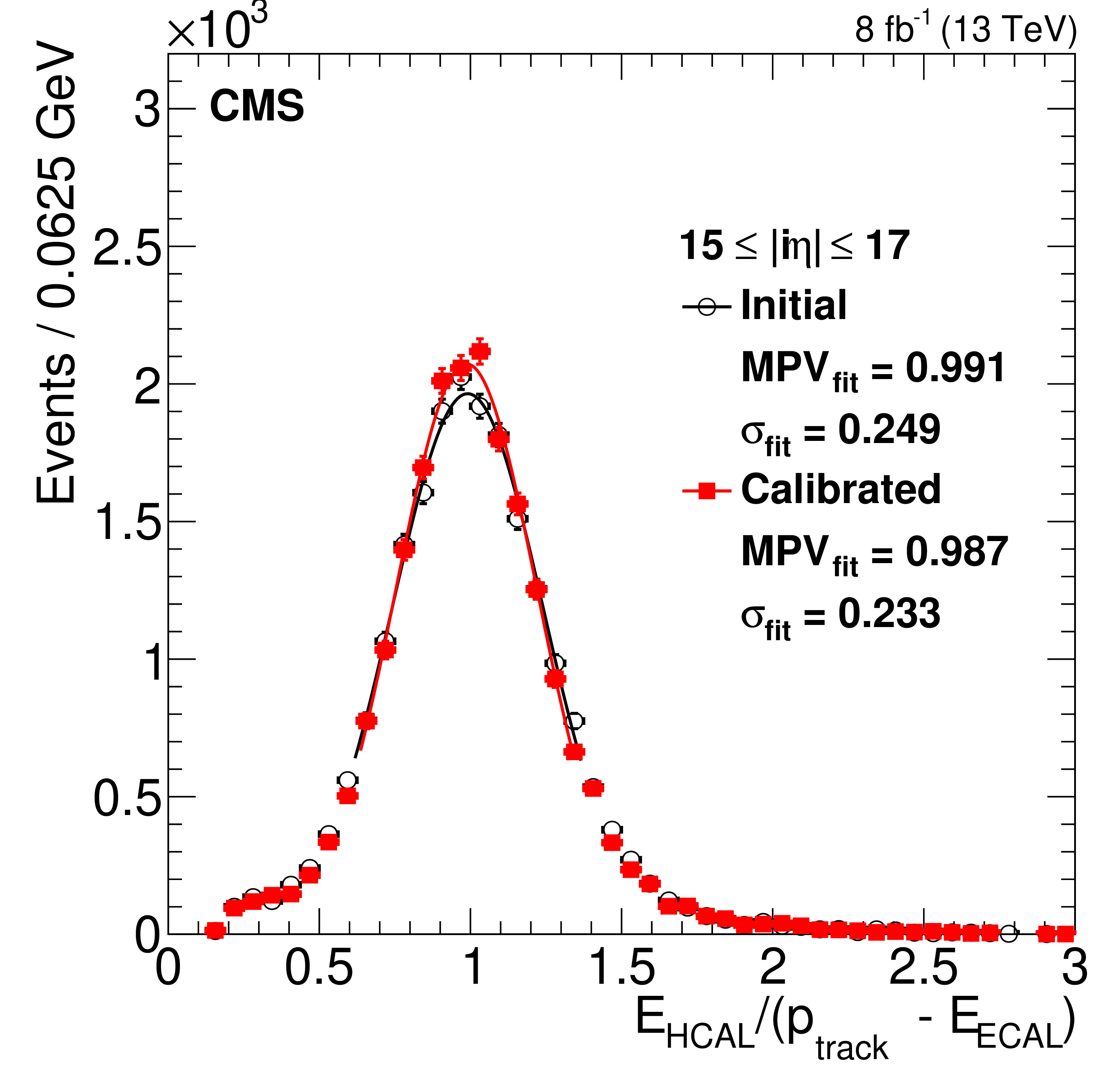
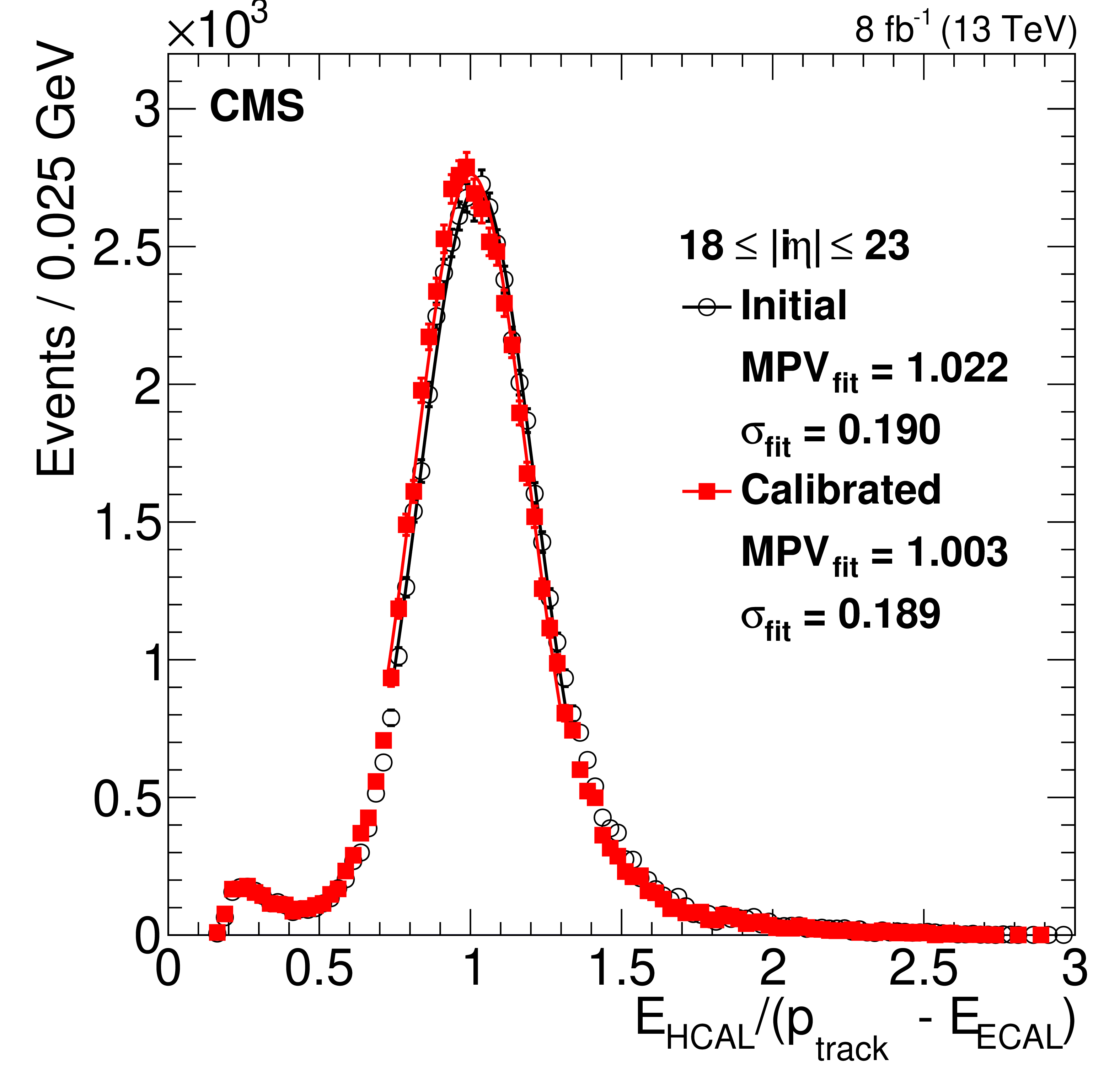
Figure 9:
Response distributions for pions from 2016 data in three different $\eta $ regions, $ {| \eta |} \leq $ 1.22 (left), 1.22 $ \leq {| \eta |} \leq $ 1.48 (middle), and 1.48 $ \leq {| \eta |} \leq $ 2.04 (right), with loose charged-particle isolation criterion: initial (black circles) and after convergence (red squares). Only statistical uncertainties are shown on the data points. |
png pdf |
Figure 9-a:
Response distribution for pions from 2016 data for $ {| \eta |} \leq $ 1.22, with loose charged-particle isolation criterion: initial (black circles) and after convergence (red squares). Only statistical uncertainties are shown on the data points. |
png pdf |
Figure 9-b:
Response distribution for pions from 2016 data for 1.22 $ \leq {| \eta |} \leq $ 1.48, with loose charged-particle isolation criterion: initial (black circles) and after convergence (red squares). Only statistical uncertainties are shown on the data points. |
png pdf |
Figure 9-c:
Response distribution for pions from 2016 data for 1.48 $ \leq {| \eta |} \leq $ 2.04, with loose charged-particle isolation criterion: initial (black circles) and after convergence (red squares). Only statistical uncertainties are shown on the data points. |
png pdf |
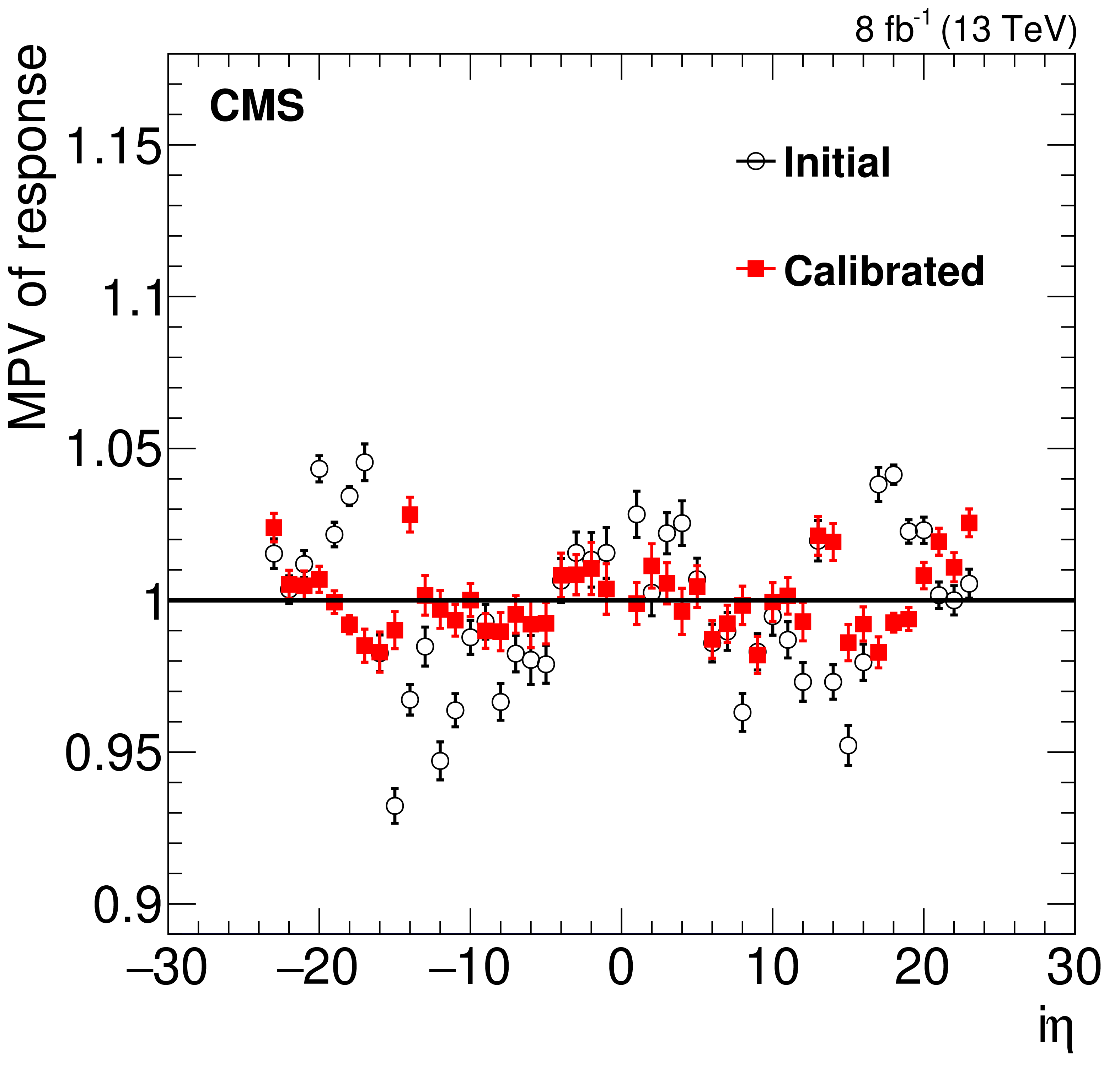
Figure 10:
Modes of the response with their statistical uncertainties versus $ {i\eta} $ from the 2016 data sample before (black circles) and after convergence (red squares). The loose charged-particle isolation constraint is applied. |
png pdf |
Figure 11:
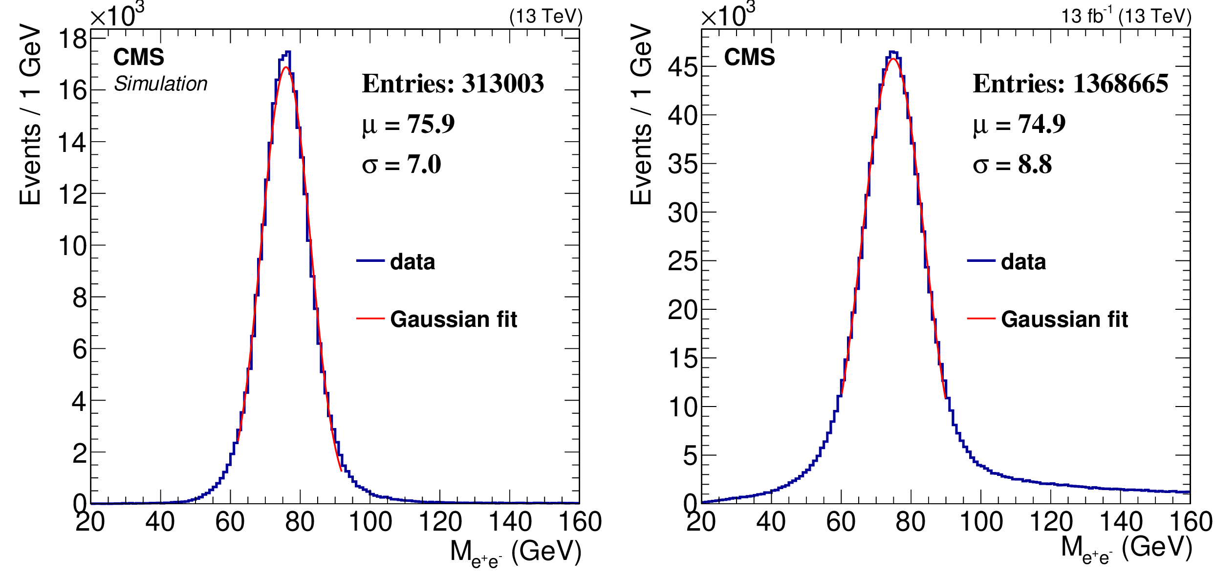
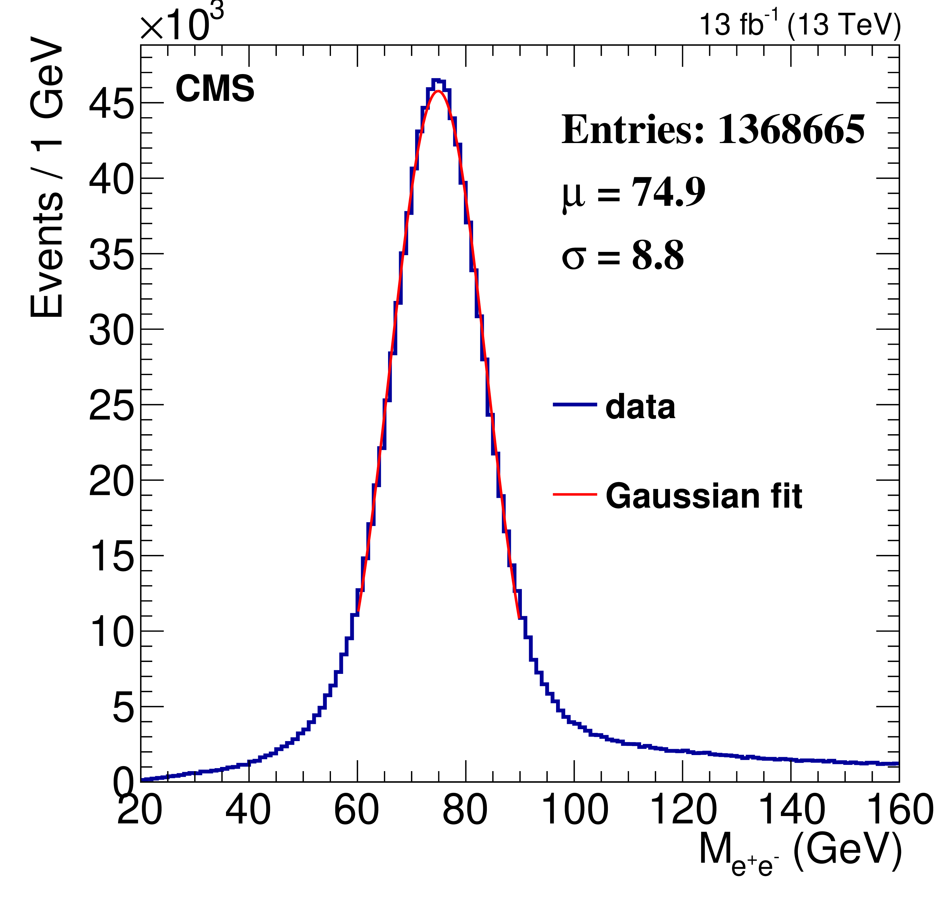
Invariant mass of the two electrons in candidate $ {\mathrm{Z} \to \mathrm{e^{+}e^{-}} } $ events for simulation (left), and for 2016 data (right). One candidate is required to be in the ECAL, the other one in the HF. The mean ($\mu $) and the width ($\sigma $) of the Gaussian fits are shown on the plots with their uncertainty. The quality of the fits is sufficient to extract the mean and the width to the necessary accuracies. |
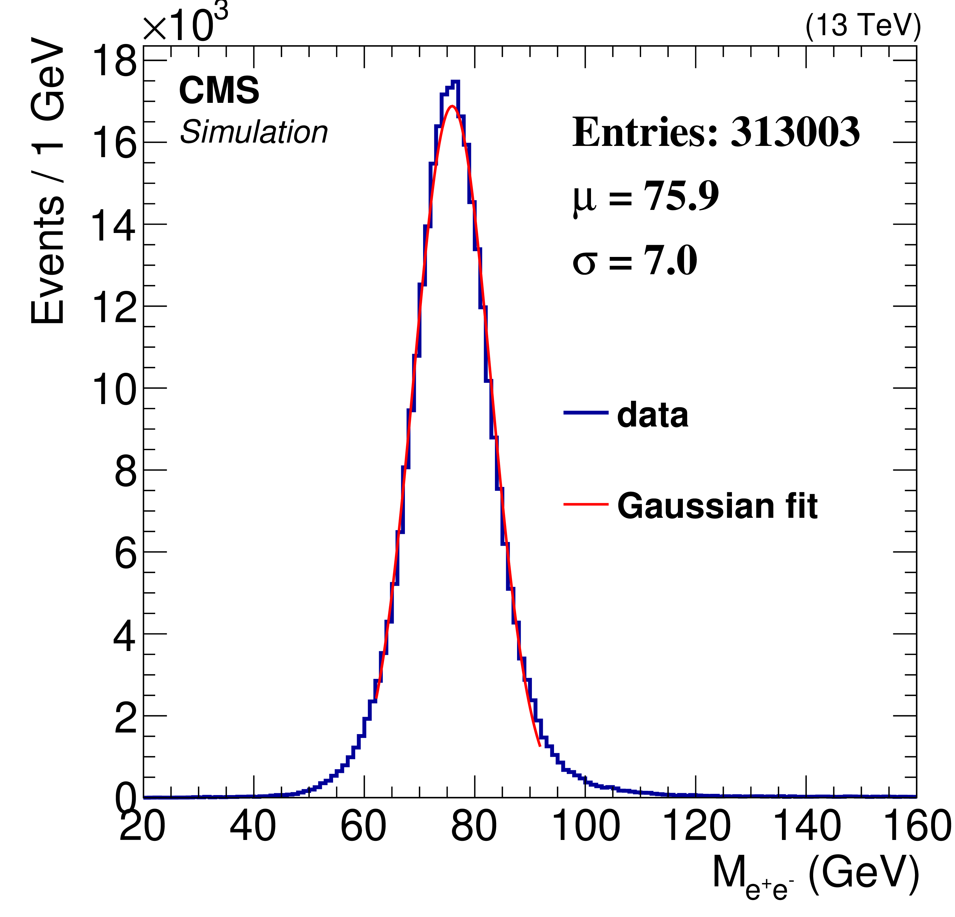
png pdf |
Figure 11-a:
Invariant mass of the two electrons in candidate $ {\mathrm{Z} \to \mathrm{e^{+}e^{-}} } $ events for simulation. One candidate is required to be in the ECAL, the other one in the HF. The mean ($\mu $) and the width ($\sigma $) of the Gaussian fits are shown on the plots with their uncertainty. The quality of the fits is sufficient to extract the mean and the width to the necessary accuracies. |
png pdf |
Figure 11-b:
Invariant mass of the two electrons in candidate $ {\mathrm{Z} \to \mathrm{e^{+}e^{-}} } $ events for 2016 data. One candidate is required to be in the ECAL, the other one in the HF. The mean ($\mu $) and the width ($\sigma $) of the Gaussian fits are shown on the plots with their uncertainty. The quality of the fits is sufficient to extract the mean and the width to the necessary accuracies. |
png pdf |
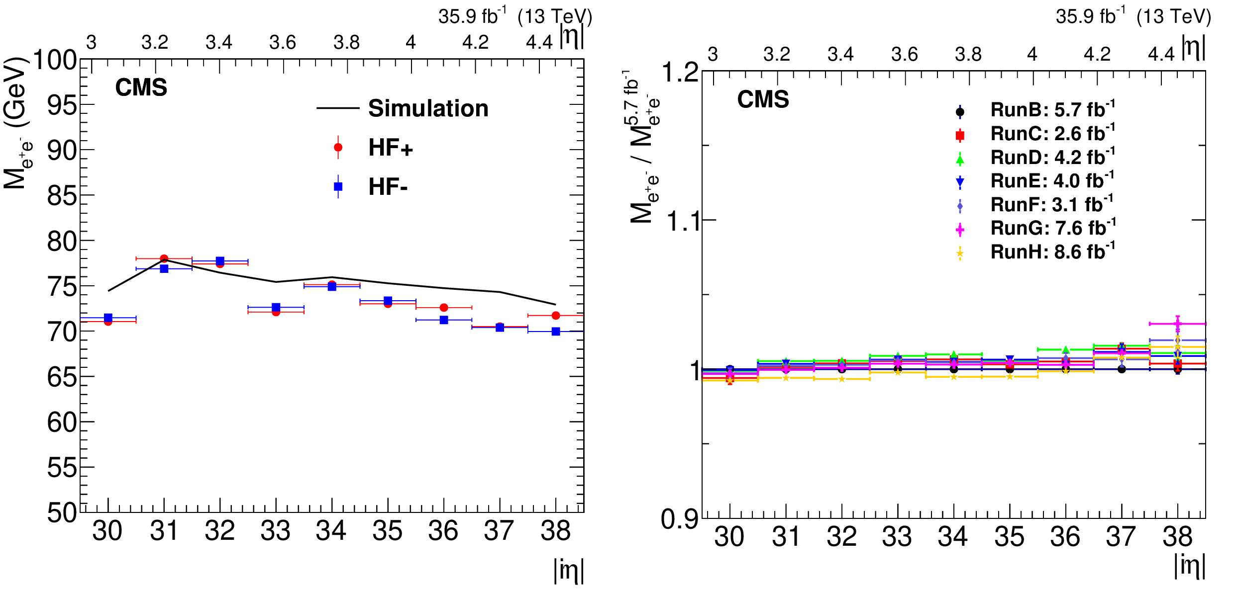
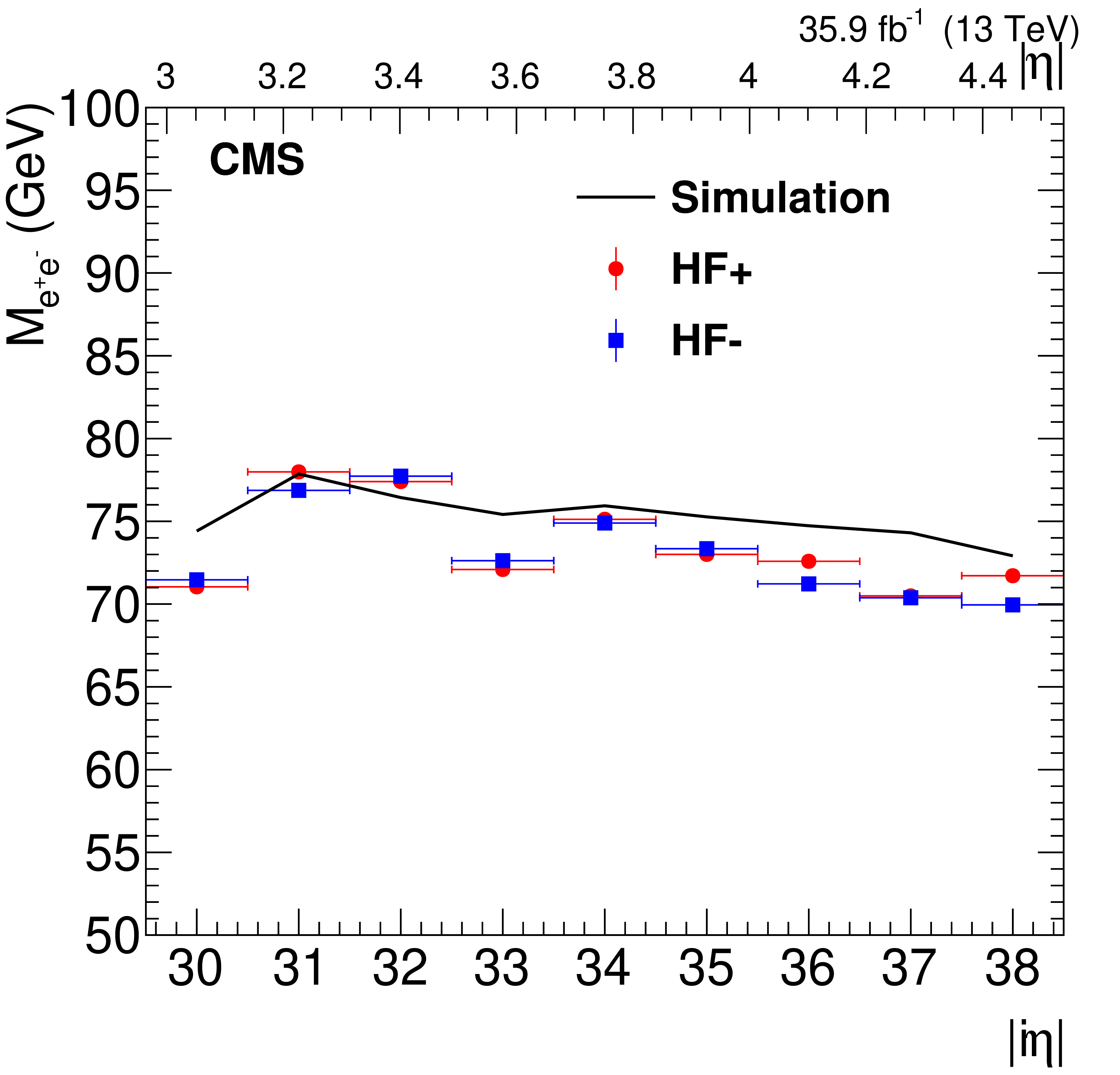
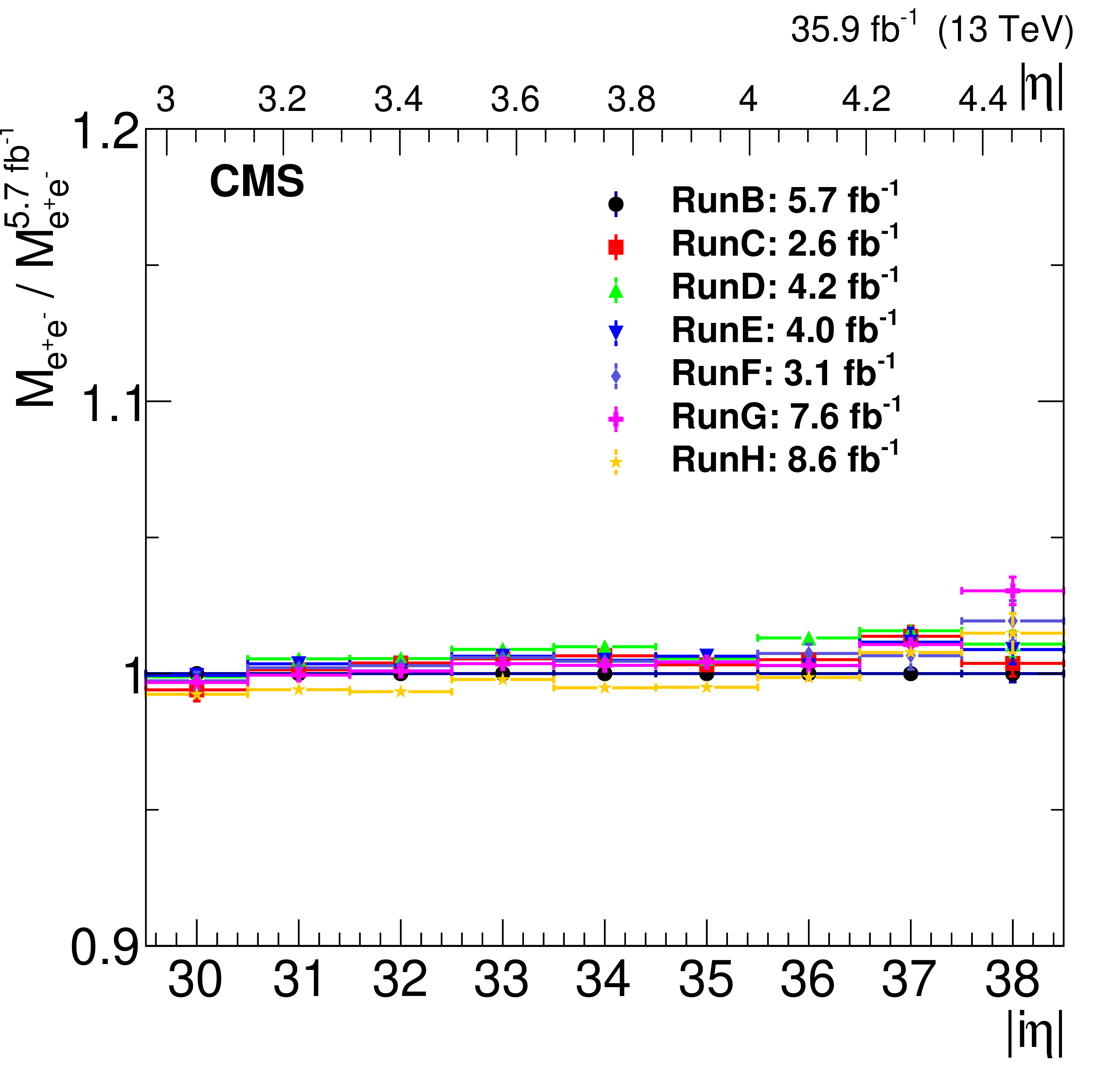
Figure 12:
(left) The results of the fits of the dielectron invariant mass to a Gaussian function for different $\eta $ values of the HF electron candidates obtained in simulation (black line, combined HF$+$ and HF$-$) and 2016 data, split by HF$+$ and HF$-$ (red and blue, respectively). (right) The results of the fits of the dielectron invariant mass to a Gaussian function for different pseudorapidity $\eta $ values of the HF electron candidates obtained in data corresponding to different run ranges. The dielectron mass in the denominator comes from the first run range corresponding to 5.7 fb$^{-1}$. Errors on the data points are statistical only. |
png pdf |
Figure 12-a:
The results of the fits of the dielectron invariant mass to a Gaussian function for different $\eta $ values of the HF electron candidates obtained in simulation (black line, combined HF$+$ and HF$-$) and 2016 data, split by HF$+$ and HF$-$ (red and blue, respectively). |
png pdf |
Figure 12-b:
The results of the fits of the dielectron invariant mass to a Gaussian function for different pseudorapidity $\eta $ values of the HF electron candidates obtained in data corresponding to different run ranges. The dielectron mass in the denominator comes from the first run range corresponding to 5.7 fb$^{-1}$. Errors on the data points are statistical only. |
png pdf |
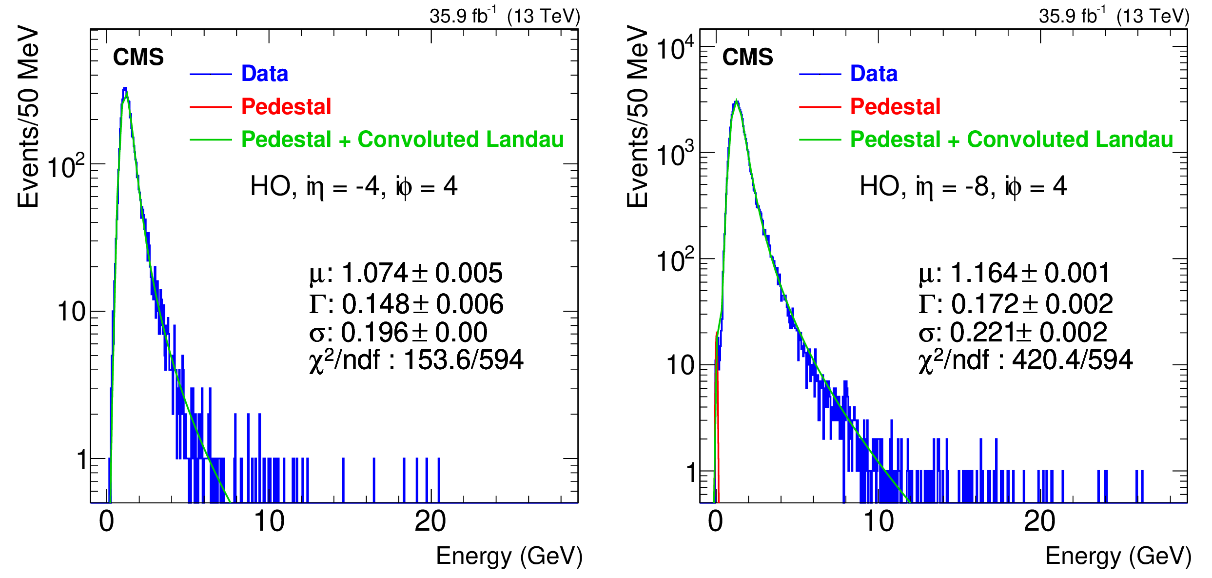
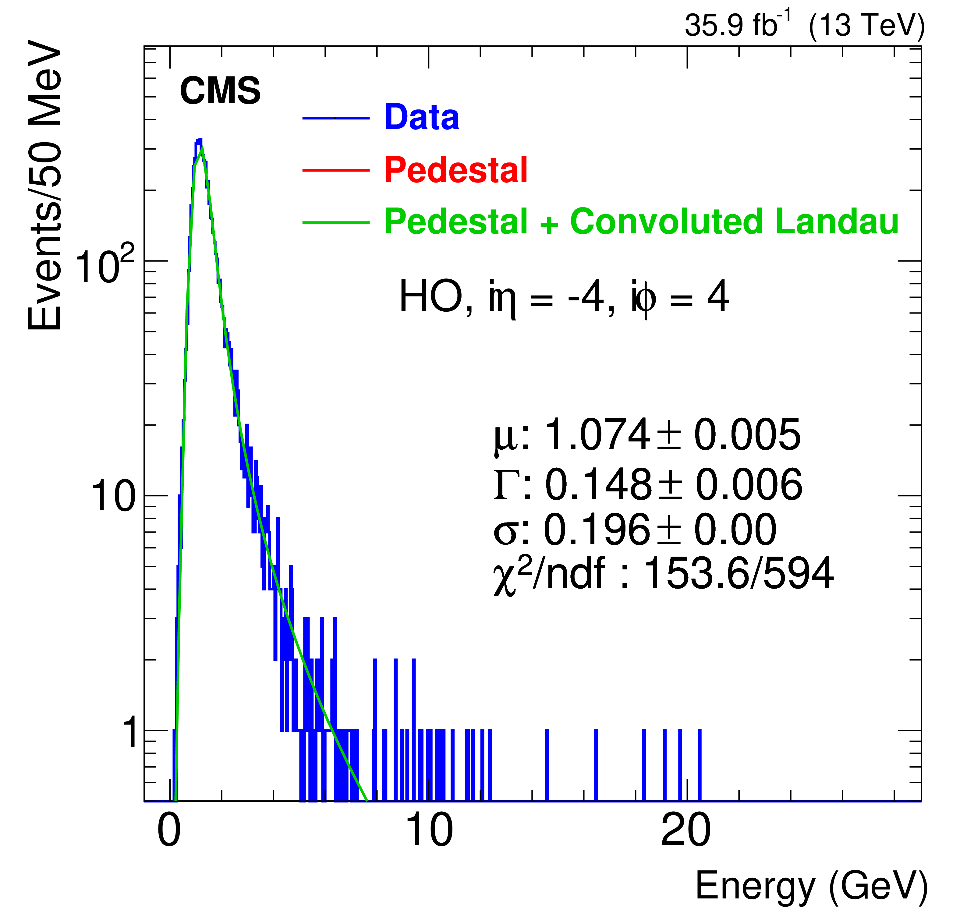
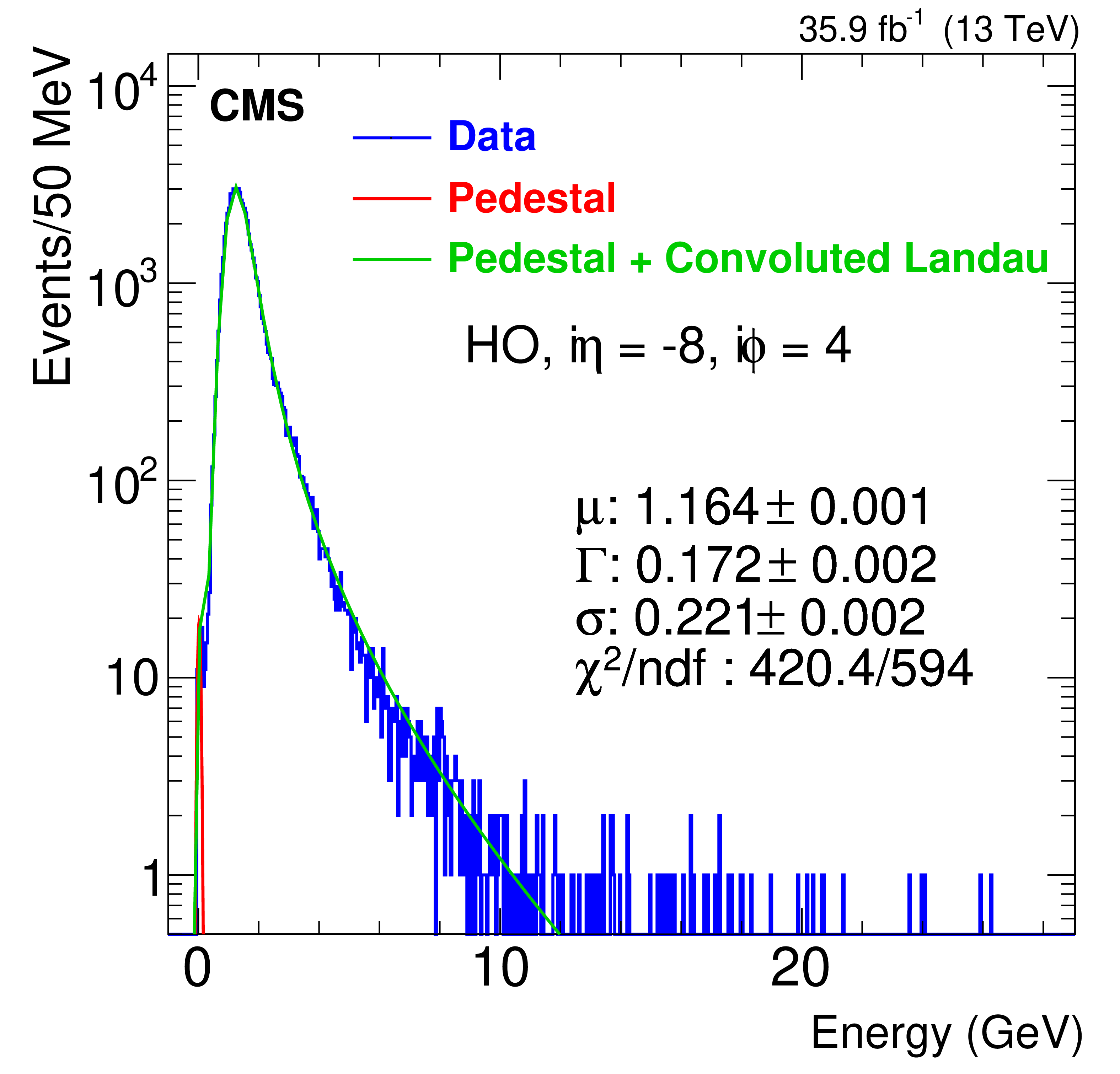
Figure 13:
Energy distributions for HO towers impacted by a high-$ {p_{\mathrm {T}}}$ muon for the central ring ($ {i\eta} = -$4, $ {i\phi} = $ 4, left) and for a side ring ($ {i\eta} = -$8, $ {i\phi} = $ 4, right), fitted with a combination of a Gaussian function for the pedestal region (shown as red lines) and a convolution of a Gaussian and a Landau function for the signal region (the combined fits are shown as the green lines). The parameters $\mu $, $\Gamma $ and $\sigma $ are the most probable values and widths of the Landau and the Gaussian functions, and ndf is number of degrees of freedom in the fit. |
png pdf |
Figure 13-a:
Energy distributions for HO towers impacted by a high-$ {p_{\mathrm {T}}}$ muon for the central ring ($ {i\eta} = -$4, $ {i\phi} = $ 4), fitted with a combination of a Gaussian function for the pedestal region (shown as red lines) and a convolution of a Gaussian and a Landau function for the signal region (the combined fits are shown as the green lines). The parameters $\mu $, $\Gamma $ and $\sigma $ are the most probable values and widths of the Landau and the Gaussian functions, and ndf is number of degrees of freedom in the fit. |
png pdf |
Figure 13-b:
Energy distributions for HO towers impacted by a high-$ {p_{\mathrm {T}}}$ muon for a side ring ($ {i\eta} = -$8, $ {i\phi} = $ 4), fitted with a combination of a Gaussian function for the pedestal region (shown as red lines) and a convolution of a Gaussian and a Landau function for the signal region (the combined fits are shown as the green lines). The parameters $\mu $, $\Gamma $ and $\sigma $ are the most probable values and widths of the Landau and the Gaussian functions, and ndf is number of degrees of freedom in the fit. |
png pdf |
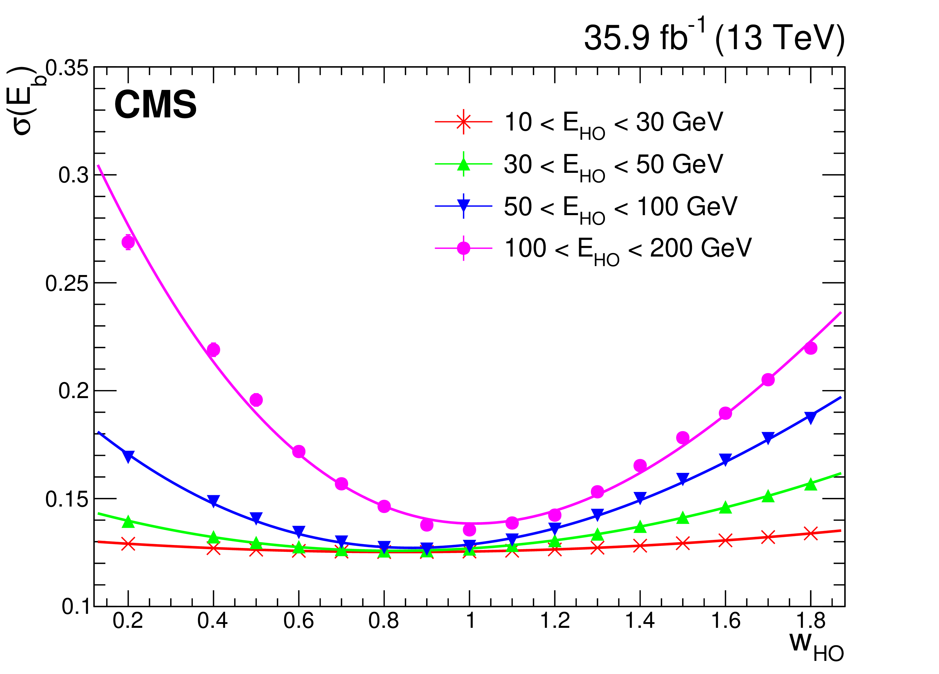
Figure 14:
The Gaussian width of the relative difference of $ {p_{\mathrm {T}}} $ of the two jets in dijet events as a function of HO weight factor in different ranges of energy contained in the HO cluster of the jet carrying the highest HO energy, when that jet is in ring 0. The smooth curves are results from fits to asymmetric parabolic function (Eq. xxxxx) through the points. Uncertainties are statistical only. |
| Summary |
|
The CMS experiment utilizes a variety of data to calibrate the energy measurements obtained from its hadron calorimeter systems. The strategy utilizes different approaches since the calorimeter subdetectors make use of multiple technologies, have different radiation environments, and probe a large range of particle energies. The calibration is generally performed in two steps: the azimuthal ($\phi$) intercalibration of the channels, followed by the determination of an absolute energy scale. In the barrel, endcap, and forward calorimeters, the $\phi$ symmetry of minimum bias events is used to carry out an interdetector calibration, whereas the hadron outer calorimeter utilizes reconstructed muons for this purpose. The absolute energy calibration of the barrel and endcap calorimeters is based on isolated charged hadrons with momenta between 40 and 60 GeV, whereas the calibration of the forward calorimeter relies on ${\mathrm{Z} \to \mathrm{e^{+}e^{-}} } $ events. The nonlinearity in the energy measurement of hadrons is addressed during the particle-flow reconstruction by using the predicted dependence on transverse momentum and pseudorapidity from a GEANT4-based simulation. Residual nonlinearities that affect the energy scale of reconstructed jets are reduced during the calibration of the jet energy scale. The calibration of the hadron outer calorimeter relies on the energy balance in dijet events. The methods use proton-proton collision data at $\sqrt{s} = $ 13 TeV collected with the CMS detector in 2016, and corresponding to integrated luminosities up to 35.9 fb$^{-1}$. The results are applied to the final reconstruction of events collected during that period. The systematic uncertainties in these measurements are dominated by systematic uncertainties in the amount of material between the interaction point and the detectors, including their dependence on azimuthal angle, and by the systematic uncertainties from the simulation of the effect of noise on the readout signal. These techniques lead to the final calibration precision of less than 3%. |
| References | ||||
| 1 | CMS Collaboration | Measurement of the top quark mass using proton-proton data at $ \sqrt{s} = $ 7 and 8 TeV | PRD 93 (2016) 072004 | CMS-TOP-14-022 1509.04044 |
| 2 | CMS Collaboration | Measurement of the top quark mass in the all-jets final state at $ \sqrt{s} = $ 13 tev and combination with the lepton+jets channel | EPJC 79 (2019) 313 | CMS-TOP-17-008 1812.10534 |
| 3 | ATLAS Collaboration | Measurement of the W-boson mass in pp collisions at $ \sqrt{s} = $ 7 TeV with the ATLAS detector | EPJC 78 (2018) 110 | 1701.07240 |
| 4 | CMS Collaboration | Search for dark matter, extra dimensions, and unparticles in monojet events in proton-proton collisions at $ \sqrt{s} = $ 8 tev | EPJC 75 (2015) 235 | CMS-EXO-12-048 1408.3583 |
| 5 | ATLAS Tile Calorimeter System Collaboration | The laser calibration of the ATLAS tile calorimeter during the LHC run 1 | JINST 11 (2016) T10005 | 1608.02791 |
| 6 | ATLAS Collaboration | A measurement of the calorimeter response to single hadrons and determination of the jet energy scale uncertainty using LHC Run-1 pp-collision data with the ATLAS detector | EPJC 77 (2017) 26 | 1607.08842 |
| 7 | CMS HCAL Collaboration | Studies of the response of the prototype CMS hadron calorimeter, including magnetic field effects, to pion, electron, and muon beams | NIMA 457 (2001) 75 | hep-ex/0007045 |
| 8 | CMS HCAL Collaboration | Design, performance, and calibration of the CMS hadron-outer calorimeter | EPJC 57 (2008) 653 | |
| 9 | CMS HCAL/ECAL Collaboration | The CMS barrel calorimeter response to particle beams from 2 to 350 GeV/$ c $ | EPJC 60 (2009) 359 | |
| 10 | ATLAS Liquid Argon EMEC/HEC Collaboration | Hadronic calibration of the ATLAS liquid argon end-cap calorimeter in the pseudorapidity region 1.6 $ < |\eta| < 1.8 $ in beam tests | NIMA 531 (2004) 481 | physics/0407009 |
| 11 | CMS Collaboration | CMS hadron calorimeter technical design report | CDS | |
| 12 | CMS Collaboration | The CMS experiment at the CERN LHC | JINST 3 (2008) S08004 | CMS-00-001 |
| 13 | CMS HCAL Collaboration | Design, performance, and calibration of CMS hadron-barrel calorimeter wedges | EPJC 55 (2008) 159 | |
| 14 | CMS HCAL Collaboration | Design, performance and calibration of the CMS forward calorimeter wedges | EPJC 53 (2008) 139 | |
| 15 | E. Hazen et al. | Radioactive source calibration technique for the CMS hadron calorimeter | NIMA 511 (2003) 311 | |
| 16 | CMS Collaboration | Performance of the CMS hadron calorimeter with cosmic ray muons and LHC beam data | JINST 5 (2010) T03012 | CMS-CFT-09-009 0911.4991 |
| 17 | CMS Collaboration | Particle-flow reconstruction and global event description with the CMS detector | JINST 12 (2017) P10003 | CMS-PRF-14-001 1706.04965 |
| 18 | GEANT4 Collaboration | $ GEANT4-a $ simulation toolkit | NIMA 506 (2003) 250 | |
| 19 | CMS Collaboration | Jet energy scale and resolution in the CMS experiment in pp collisions at 8 TeV | JINST 12 (2017) P02014 | CMS-JME-13-004 1607.03663 |
| 20 | CMS Collaboration | Performance of photon reconstruction and identification with the CMS detector in proton-proton collisions at $ \sqrt{s} = $ 8 TeV | JINST 10 (2015) P08010 | CMS-EGM-14-001 1502.02702 |
| 21 | CMS Collaboration | Description and performance of track and primary-vertex reconstruction with the CMS tracker | JINST 9 (2014) P10009 | CMS-TRK-11-001 1405.6569 |
| 22 | CMS Collaboration | The CMS trigger system | JINST 12 (2017) P01020 | CMS-TRG-12-001 1609.02366 |
| 23 | P. Cushman, A. Heering, and A. Ronzhin | Custom HPD readout for the CMS HCAL | NIMA 442 (2000) 289 | |
| 24 | T. M. Shaw et al. | Front end readout electronics for the CMS hadron calorimeter | in Nuclear Science Symposium Conference Record, 2002 IEEE, p. 194 2002 | |
| 25 | CMS HCAL Collaboration | Dose rate effects in the radiation damage of the plastic scintillators of the CMS hadron endcap calorimeter | JINST 11 (2016) T10004 | 1608.07267 |
| 26 | R. A. Shukla et al. | Microscopic characterisation of photo detectors from CMS hadron calorimeter | Rev. Sci. Instrum. 90 (2019) 023303 | 1806.09887 |
| 27 | M. Cacciari, G. P. Salam, and G. Soyez | The anti-$ {k_{\mathrm{T}}} $ jet clustering algorithm | JHEP 04 (2008) 063 | 0802.1189 |
| 28 | M. Cacciari, G. P. Salam, and G. Soyez | FastJet user manual | EPJC 72 (2012) 1896 | 1111.6097 |
| 29 | T. Sjostrand et al. | An introduction to Pythia 8.2 | CPC 191 (2015) 159 | 1410.3012 |
| 30 | J. Alwall et al. | The automated computation of tree-level and next-to-leading order differential cross sections, and their matching to parton shower simulations | JHEP 07 (2014) 079 | 1405.0301 |
| 31 | NNPDF Collaboration | Parton distributions for the LHC Run II | JHEP 04 (2015) 040 | 1410.8849 |
| 32 | CMS Collaboration | Event generator tunes obtained from underlying event and multiparton scattering measurements | EPJC 76 (2016) 155 | CMS-GEN-14-001 1512.00815 |
| 33 | CMS Collaboration | Performance of electron reconstruction and selection with the CMS detector in proton-proton collisions at $ \sqrt{s}= $ 8 TeV | JINST 10 (2015) P06005 | CMS-EGM-13-001 1502.02701 |
| 34 | Particle Data Group | Review of particle physics | PRD 98 (2018) 030001 | |
| 35 | CMS Collaboration | Performance of CMS muon reconstruction in pp collision events at $ \sqrt{s} = $ 7 TeV | JINST 7 (2012) P10002 | CMS-MUO-10-004 1206.4071 |
|
|
Compact Muon Solenoid LHC, CERN |
|

|

|

|

|

|