

Compact Muon Solenoid
LHC, CERN
| CMS-PRF-22-001 ; CERN-EP-2023-093 | ||
| Performance of the local reconstruction algorithms for the CMS hadron calorimeter with Run 2 data | ||
| CMS Collaboration | ||
| 17 June 2023 | ||
| JINST 18 (2023) P11017 | ||
| Abstract: A description is presented of the algorithms used to reconstruct energy deposited in the CMS hadron calorimeter during Run 2 (2015--2018) of the LHC. During Run 2, the characteristic bunch-crossing spacing for proton-proton collisions was 25 ns, which resulted in overlapping signals from adjacent crossings. The energy corresponding to a particular bunch crossing of interest is estimated using the known pulse shapes of energy depositions in the calorimeter, which are measured as functions of both energy and time. A variety of algorithms were developed to mitigate the effects of adjacent bunch crossings on local energy reconstruction in the hadron calorimeter in Run 2, and their performance is compared. | ||
| Links: e-print arXiv:2306.10355 [hep-ex] (PDF) ; CDS record ; inSPIRE record ; CADI line (restricted) ; | ||
| Figures | |
png pdf |
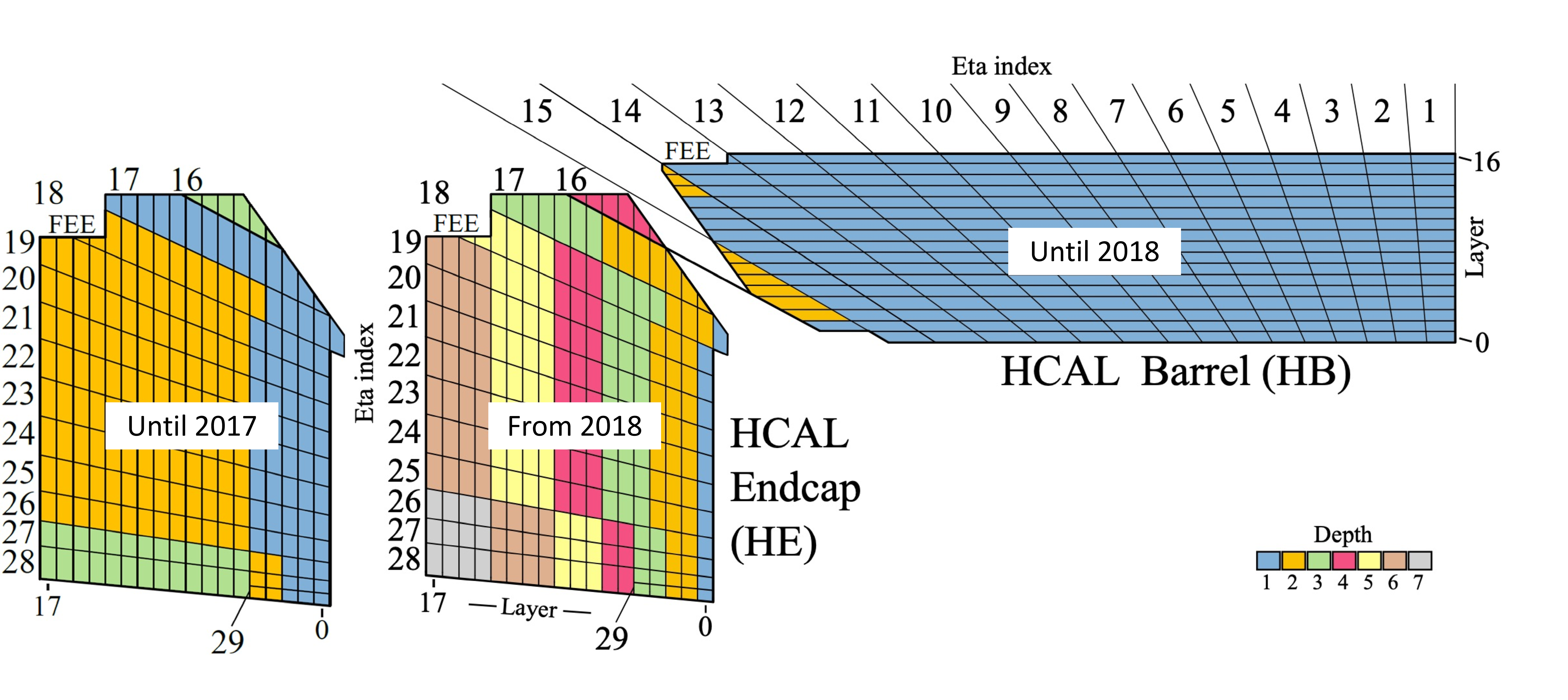
Figure 1:
A cross sectional view of the HB and HE in the $ r-z $ plane. The i.e.,ta coordinates are labeled, and the depth segmentation is coded in different colors. The number of depths of the HE was increased before the 2018 data-taking period. The location of the front-end electronics (labeled ``FEE'') is also shown. |
png pdf |
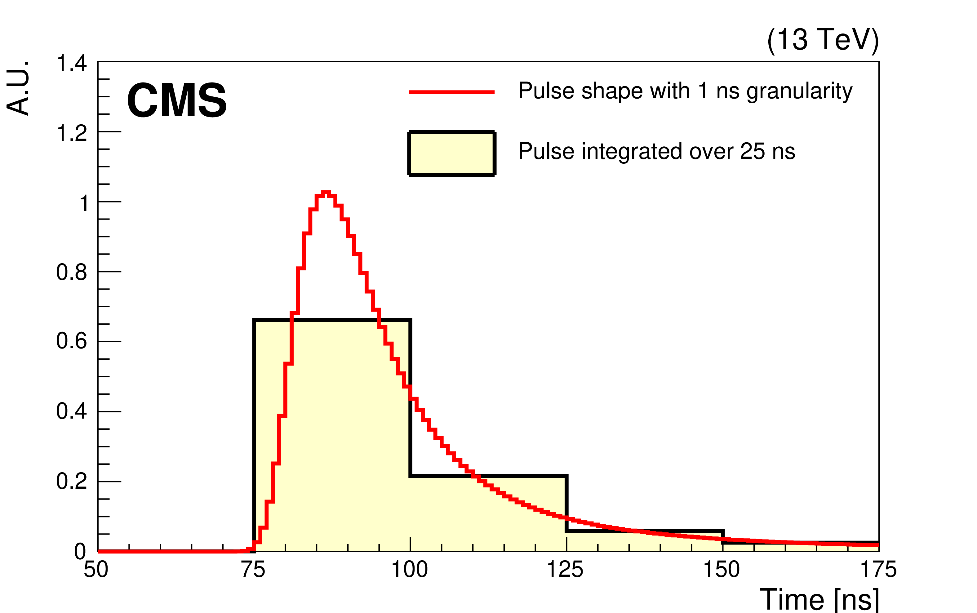
Figure 2:
Average pulse shape for high-energy depositions for a channel in the HE. The red solid line is the pulse shape used in reconstruction algorithms with 1 ns granularity. The yellow filled histogram is constructed from the red shape by integrating over each 25 ns TS. The SOI corresponds to the TS from 75 to 100 ns. |
png pdf |
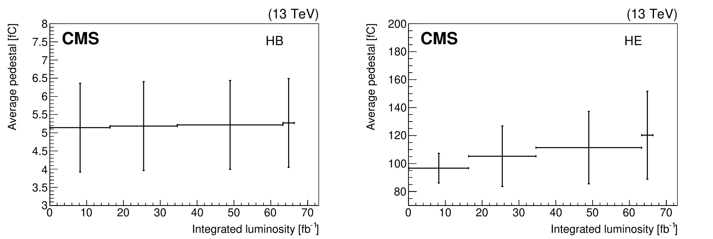
Figure 3:
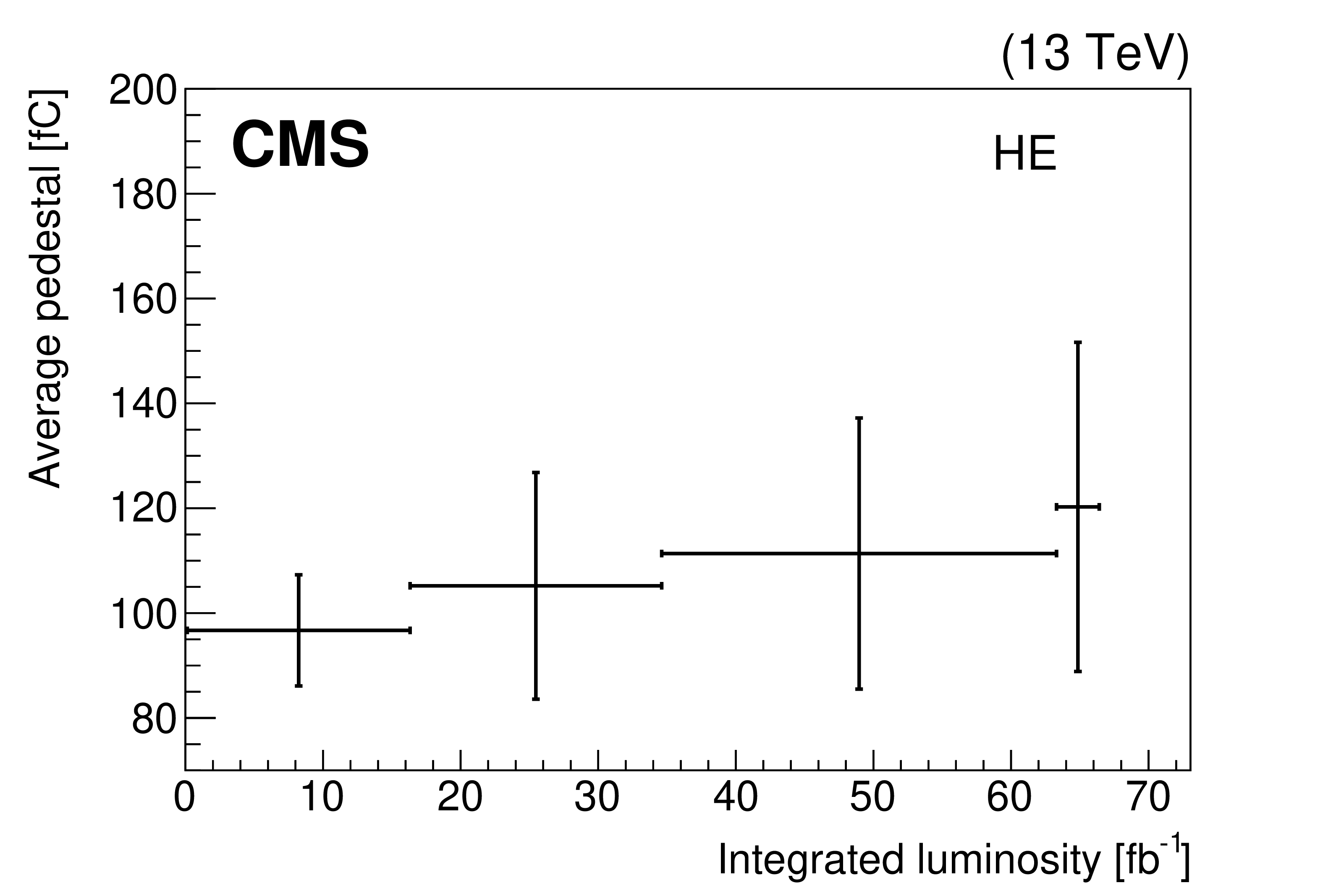
The average value of the pedestal, as a function of the integrated luminosity, since the start of 2018 data taking for the HB (left) and HE (right). Each horizontal line denotes the time range where the corresponding pedestal measurement is used in the energy reconstruction, and the error bars indicate the average standard deviation of the pedestal. |
png pdf |
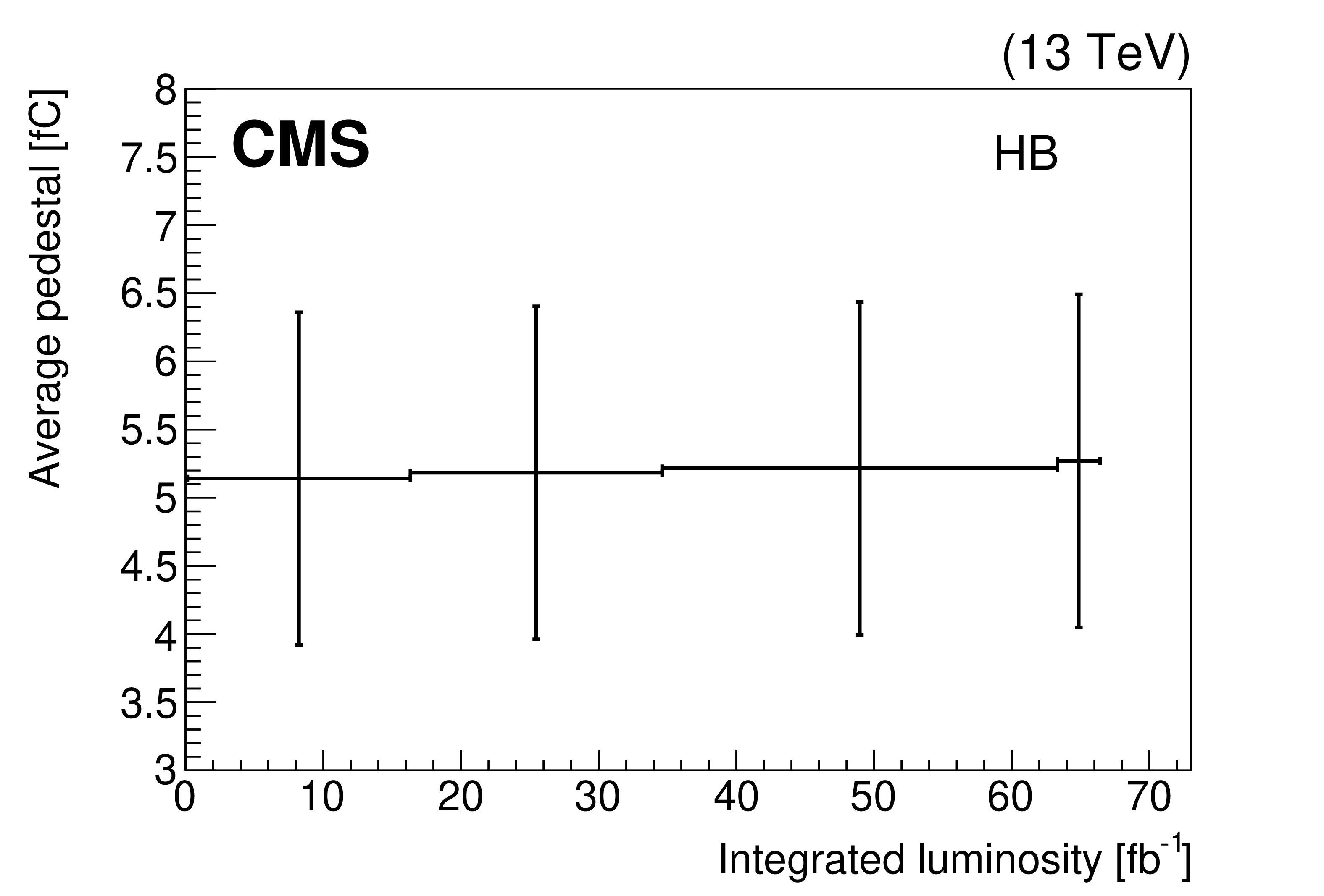
Figure 3-a:
The average value of the pedestal, as a function of the integrated luminosity, since the start of 2018 data taking for the HB. Each horizontal line denotes the time range where the corresponding pedestal measurement is used in the energy reconstruction, and the error bars indicate the average standard deviation of the pedestal. |
png pdf |
Figure 3-b:
The average value of the pedestal, as a function of the integrated luminosity, since the start of 2018 data taking for the HE. Each horizontal line denotes the time range where the corresponding pedestal measurement is used in the energy reconstruction, and the error bars indicate the average standard deviation of the pedestal. |

png pdf |
Figure 4:
An illustration of the M3 algorithm. Only three TSs from $ \text{SOI}{-1} $ to $ \text{SOI}{+1} $, indicated with dash lines, are used in the reconstruction. Pulse-shape templates for $ \text{SOI}{-1} $, SOI, and $ \text{SOI}{+1} $ are shown in blue, yellow, and pink, respectively. The gray shading shows the baseline. |

png pdf |
Figure 5:
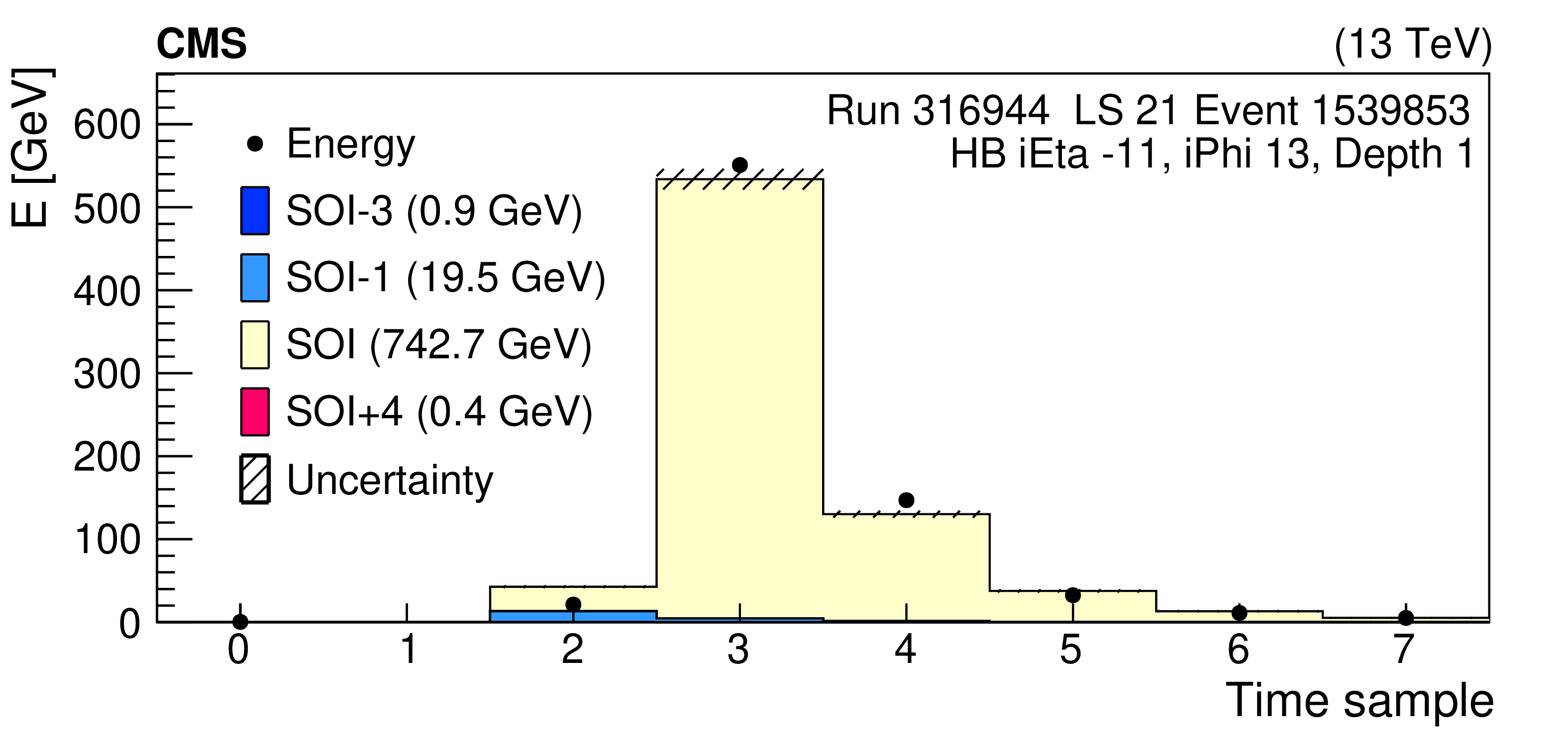
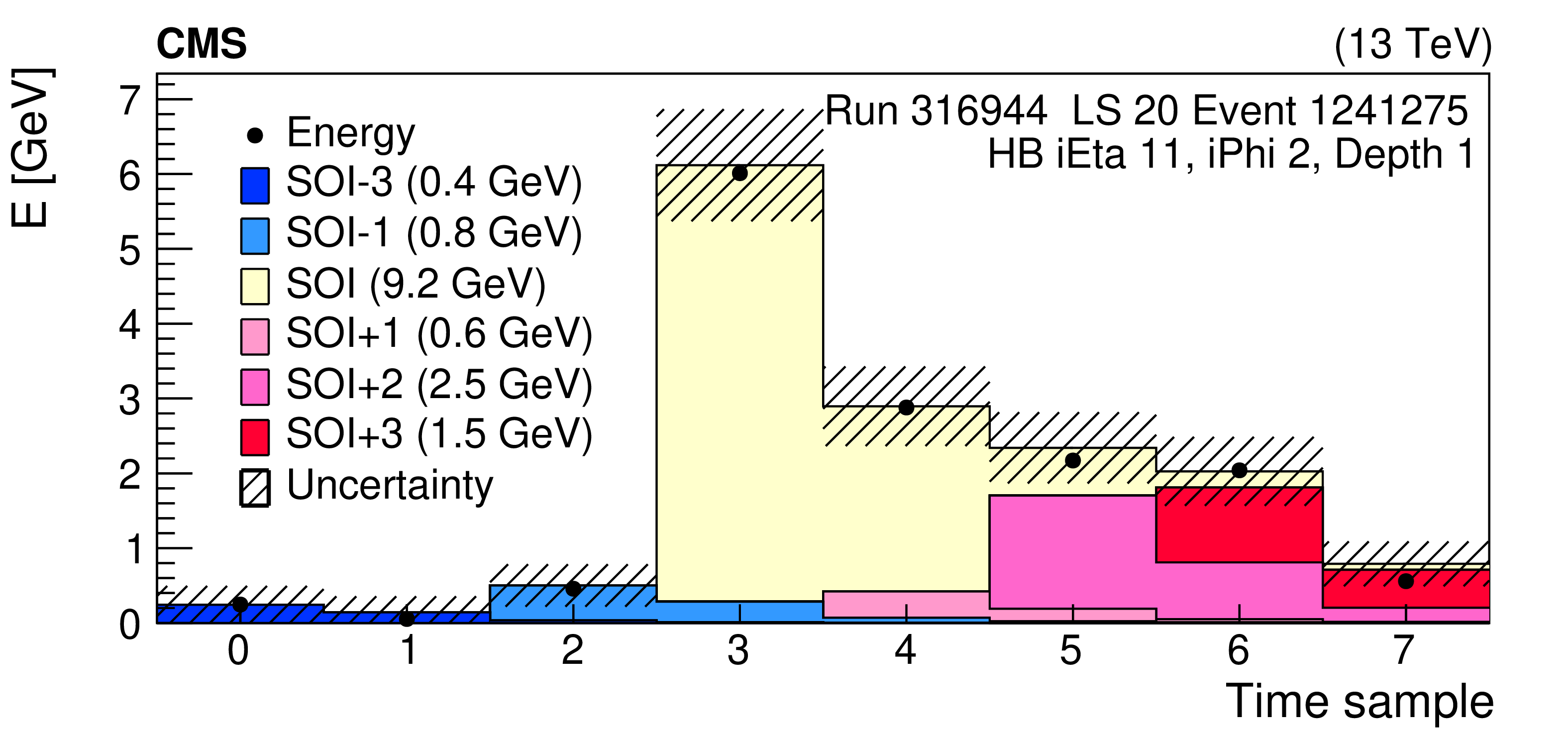
Representative fit results from MAHI for high-energy (left) and low-energy (right) pulses, in the HB (upper) and the HE (lower). The recorded pedestal-subtracted charge in the QIE (converted to units of energy) is given by the points, while the filled histograms represent the fitted values for the various pulse shapes. The sum of the fitted energy for each pulse, labeled by its position relative to the SOI, is presented in the legend. The combined uncertainty from the pedestal, photostatistics, and QIE quantization is shown by the hatched areas. |
png pdf |
Figure 5-a:
Representative fit results from MAHI for high-energy pulses, in the HB. The recorded pedestal-subtracted charge in the QIE (converted to units of energy) is given by the points, while the filled histograms represent the fitted values for the various pulse shapes. The sum of the fitted energy for each pulse, labeled by its position relative to the SOI, is presented in the legend. The combined uncertainty from the pedestal, photostatistics, and QIE quantization is shown by the hatched areas. |
png pdf |
Figure 5-b:
Representative fit results from MAHI for low-energy pulses, in the HB. The recorded pedestal-subtracted charge in the QIE (converted to units of energy) is given by the points, while the filled histograms represent the fitted values for the various pulse shapes. The sum of the fitted energy for each pulse, labeled by its position relative to the SOI, is presented in the legend. The combined uncertainty from the pedestal, photostatistics, and QIE quantization is shown by the hatched areas. |

png pdf |
Figure 5-c:
Representative fit results from MAHI for high-energy pulses, in the HE. The recorded pedestal-subtracted charge in the QIE (converted to units of energy) is given by the points, while the filled histograms represent the fitted values for the various pulse shapes. The sum of the fitted energy for each pulse, labeled by its position relative to the SOI, is presented in the legend. The combined uncertainty from the pedestal, photostatistics, and QIE quantization is shown by the hatched areas. |

png pdf |
Figure 5-d:
Representative fit results from MAHI for low-energy pulses, in the HE. The recorded pedestal-subtracted charge in the QIE (converted to units of energy) is given by the points, while the filled histograms represent the fitted values for the various pulse shapes. The sum of the fitted energy for each pulse, labeled by its position relative to the SOI, is presented in the legend. The combined uncertainty from the pedestal, photostatistics, and QIE quantization is shown by the hatched areas. |
png pdf |
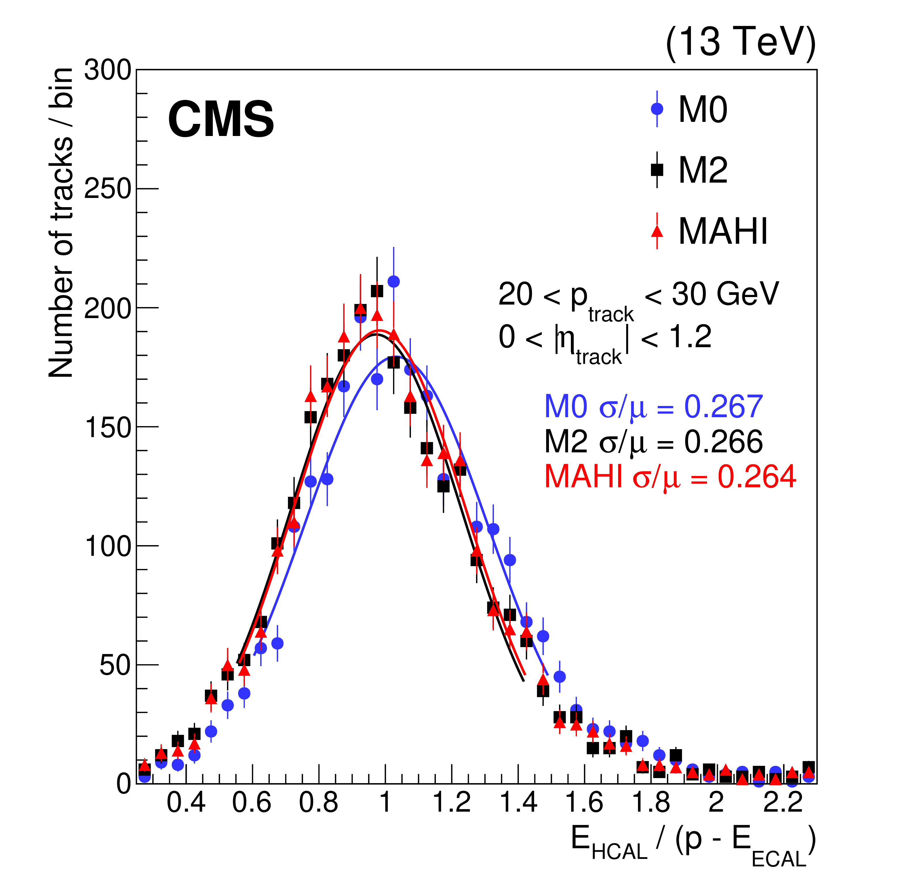
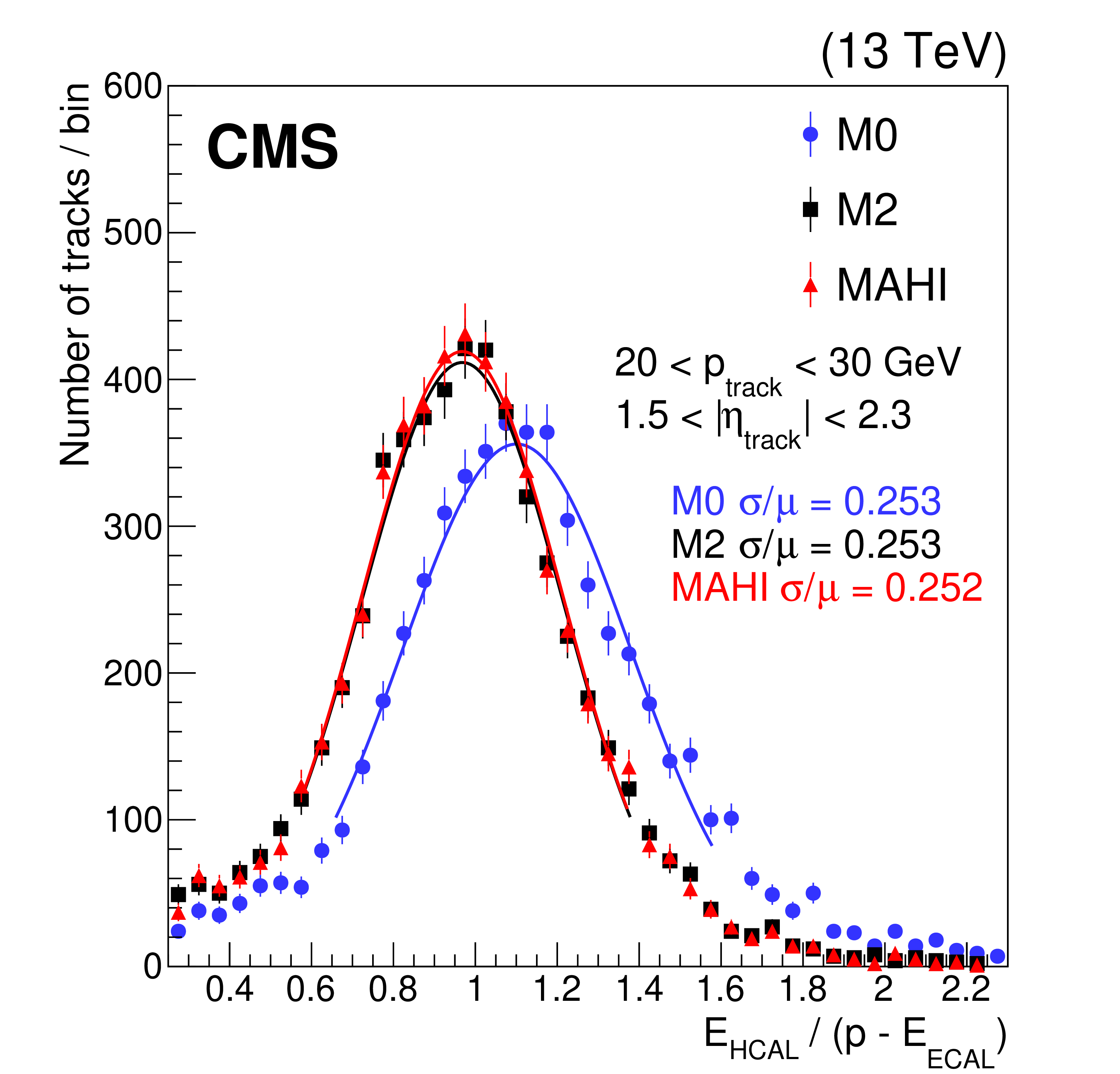
Figure 6:
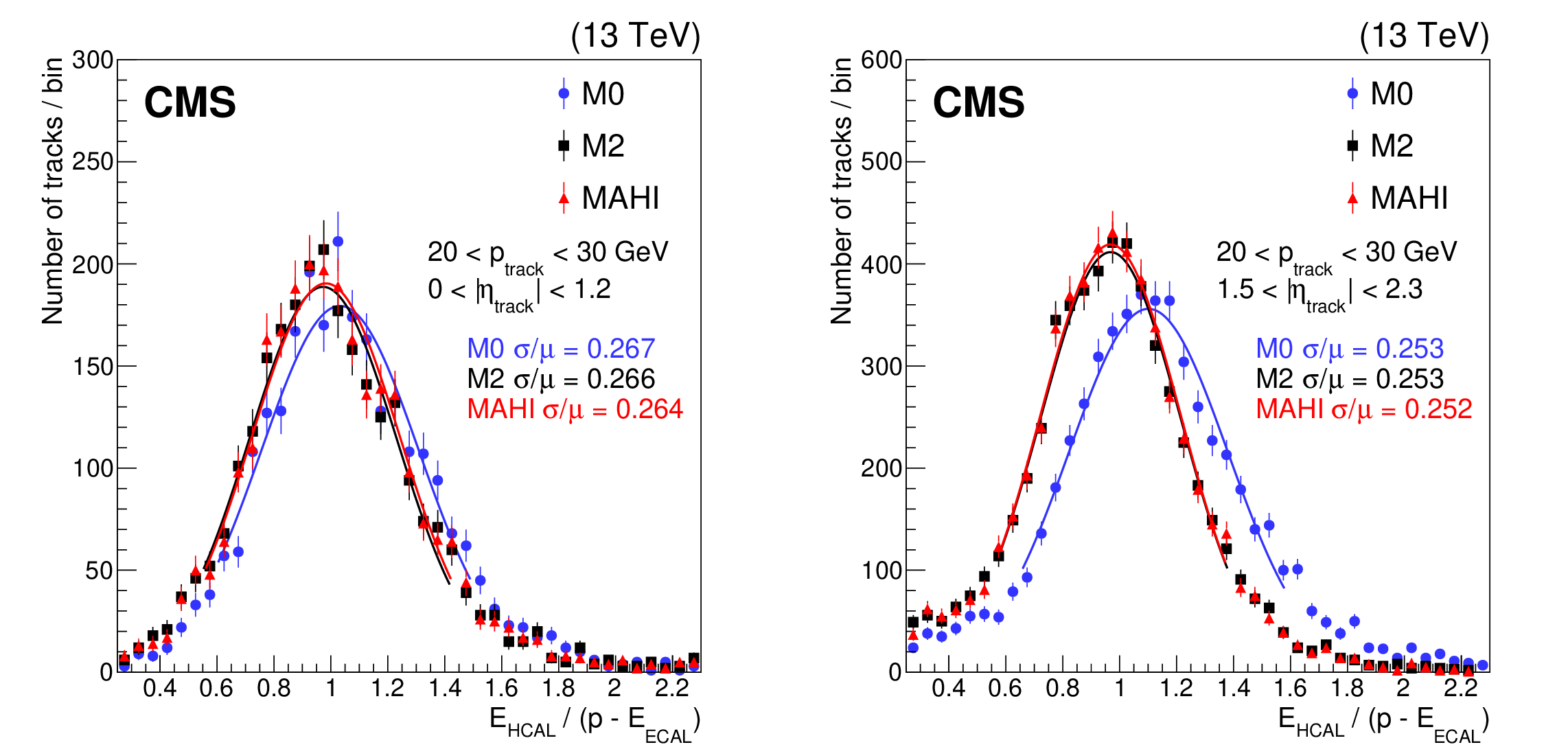
The HCAL energy response of M0, M2, and MAHI, measured in an electron/photon-triggered data set using isolated tracks with 20 $ < p_\text{track} < $ 30 GeV and either $ |\eta_\text{track}| < $ 1.2 (left) or 1.5 $ < |\eta_\text{track}| < $ 2.3 (right). The vertical bars show the statistical uncertainty in the number of tracks in each bin. The measured energy resolution for each method in this sample is comparable. |
png pdf |
Figure 6-a:
The HCAL energy response of M0, M2, and MAHI, measured in an electron/photon-triggered data set using isolated tracks with 20 $ < p_\text{track} < $ 30 GeV and $ |\eta_\text{track}| < $ 1.2. The vertical bars show the statistical uncertainty in the number of tracks in each bin. The measured energy resolution for each method in this sample is comparable. |
png pdf |
Figure 6-b:
The HCAL energy response of M0, M2, and MAHI, measured in an electron/photon-triggered data set using isolated tracks with 20 $ < p_\text{track} < $ 30 GeV and 1.5 $ < |\eta_\text{track}| < $ 2.3. The vertical bars show the statistical uncertainty in the number of tracks in each bin. The measured energy resolution for each method in this sample is comparable. |
png pdf |
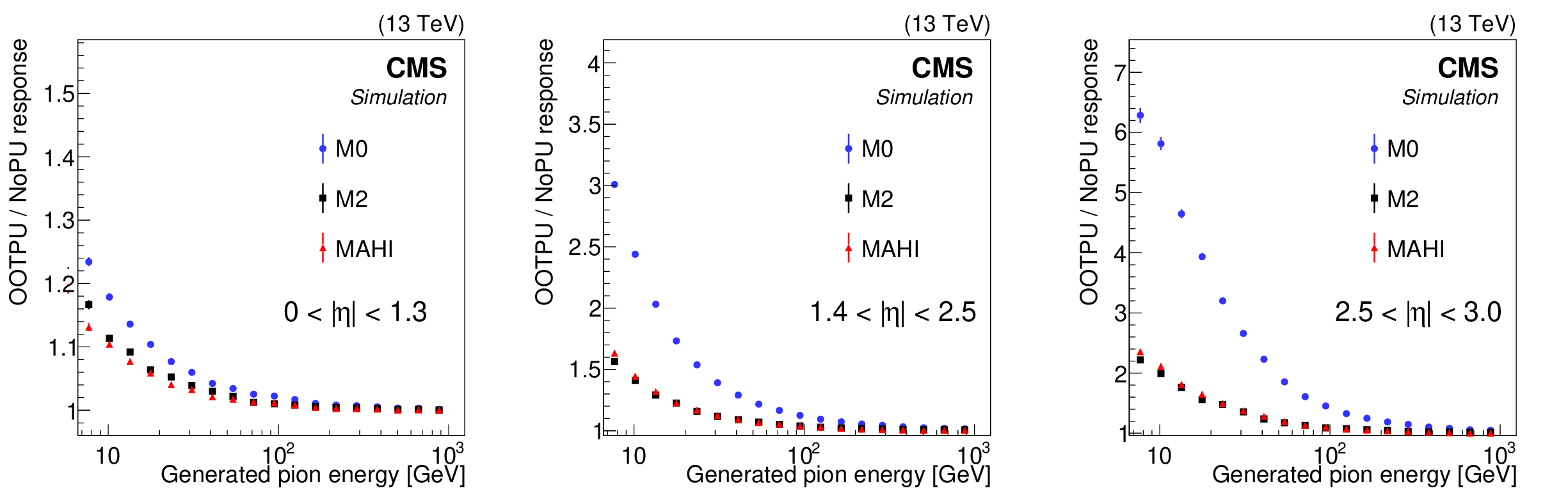
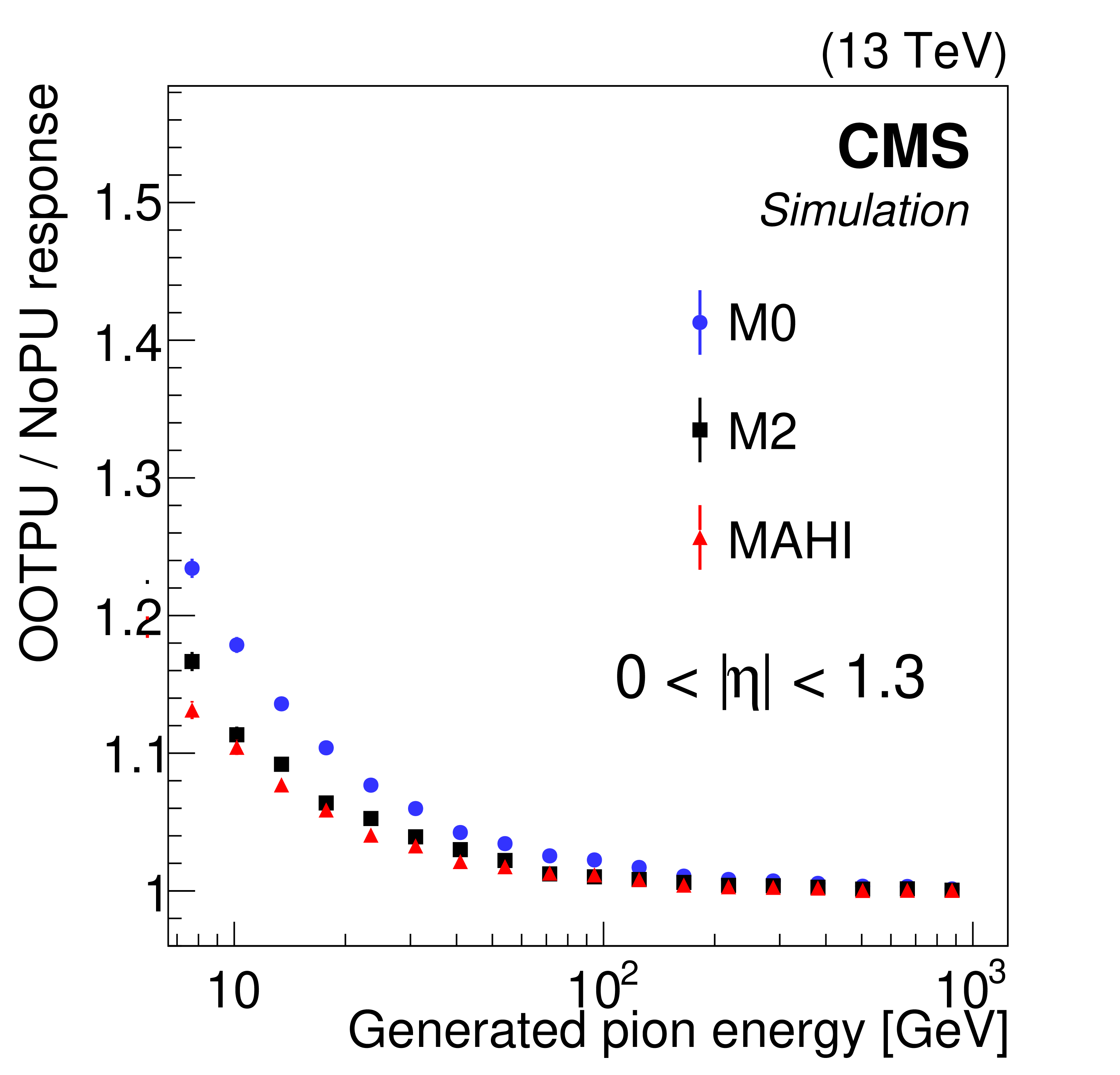
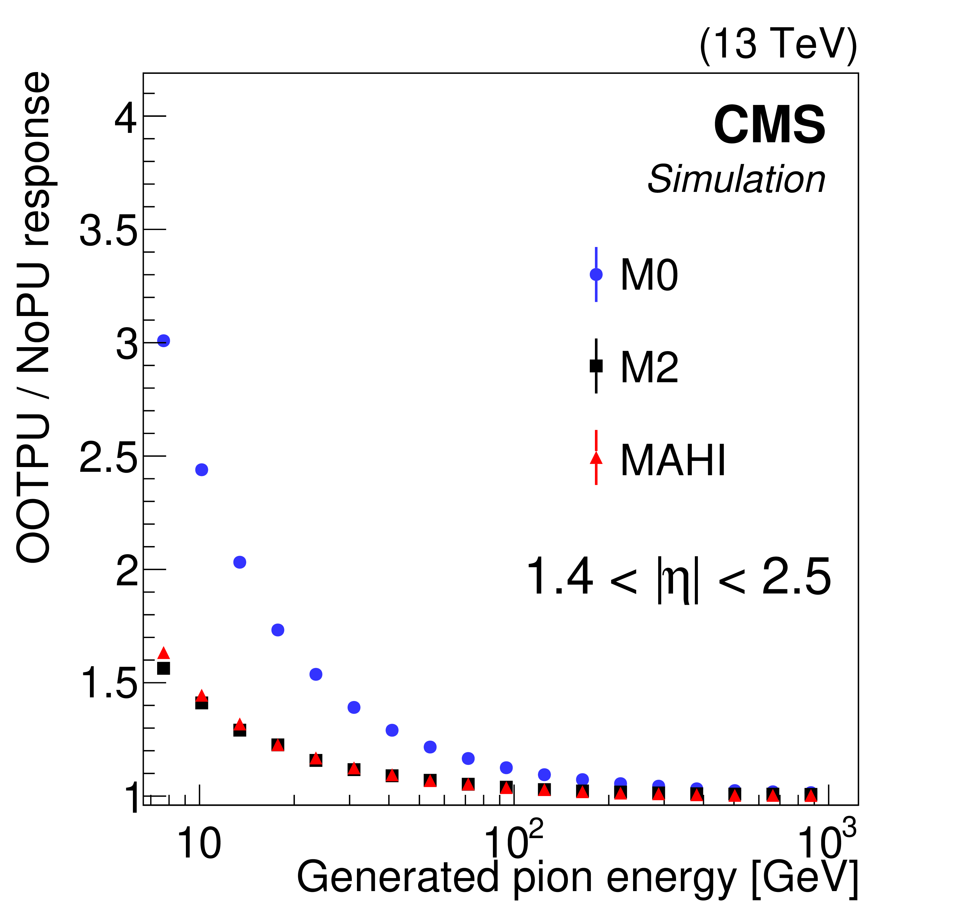
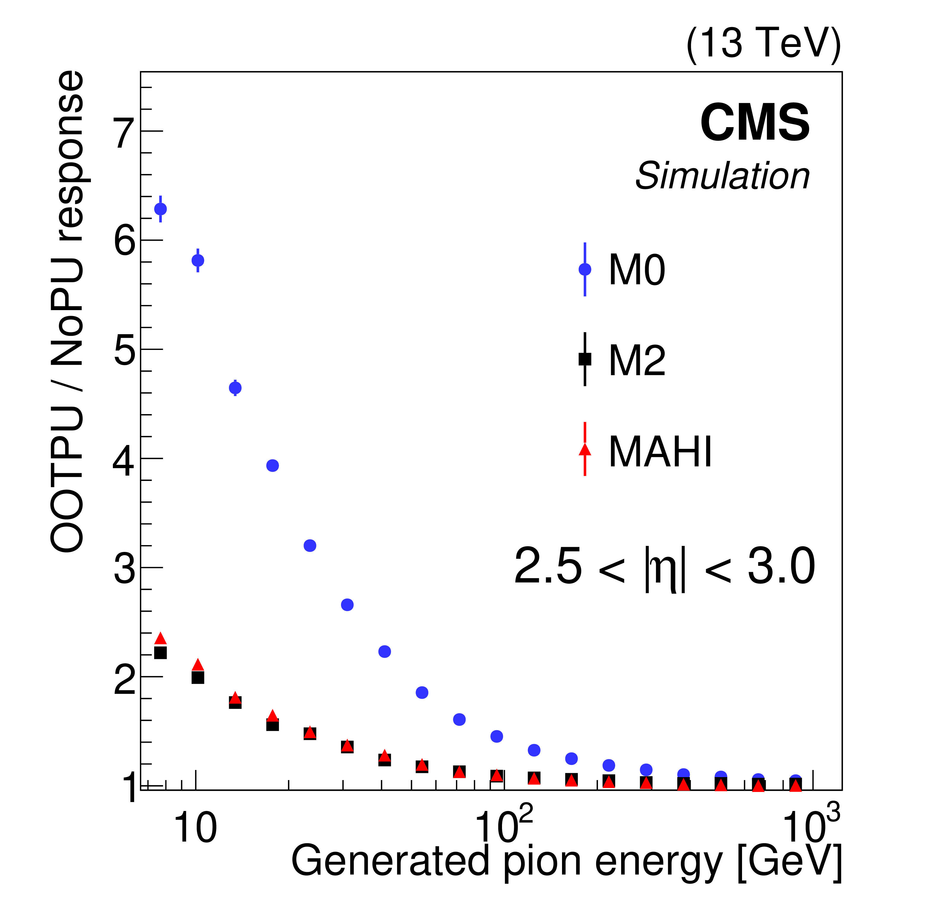
Figure 7:
Ratios of responses to simulated charged pions between a sample with OOTPU included to a sample with no pileup, as functions of the generated pion energy. The left plot shows the response for pions in the HB ($ |\eta| < $ 1.3), whereas the middle and right plots show the response for pions in the HE (1.4 $ < |\eta| < $ 2.5 and 2.5 $ < |\eta| < $ 3.0). |
png pdf |
Figure 7-a:
Ratios of responses to simulated charged pions between a sample with OOTPU included to a sample with no pileup, as functions of the generated pion energy. The plot shows the response for pions in the HB ($ |\eta| < $ 1.3). |
png pdf |
Figure 7-b:
Ratios of responses to simulated charged pions between a sample with OOTPU included to a sample with no pileup, as functions of the generated pion energy. The plot shows the response for pions in the HE (1.4 $ < |\eta| < $ 2.5). |
png pdf |
Figure 7-c:
Ratios of responses to simulated charged pions between a sample with OOTPU included to a sample with no pileup, as functions of the generated pion energy. The plot shows the response for pions in the HE (2.5 $ < |\eta| < $ 3.0). |
png pdf |
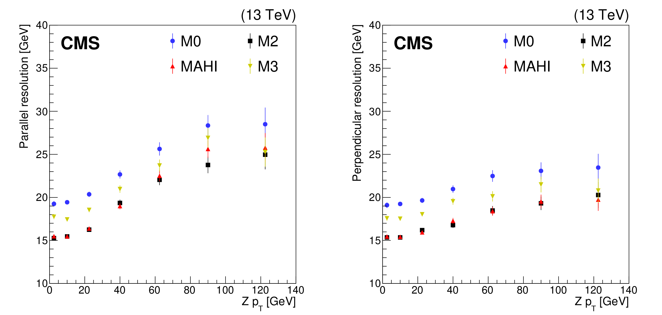
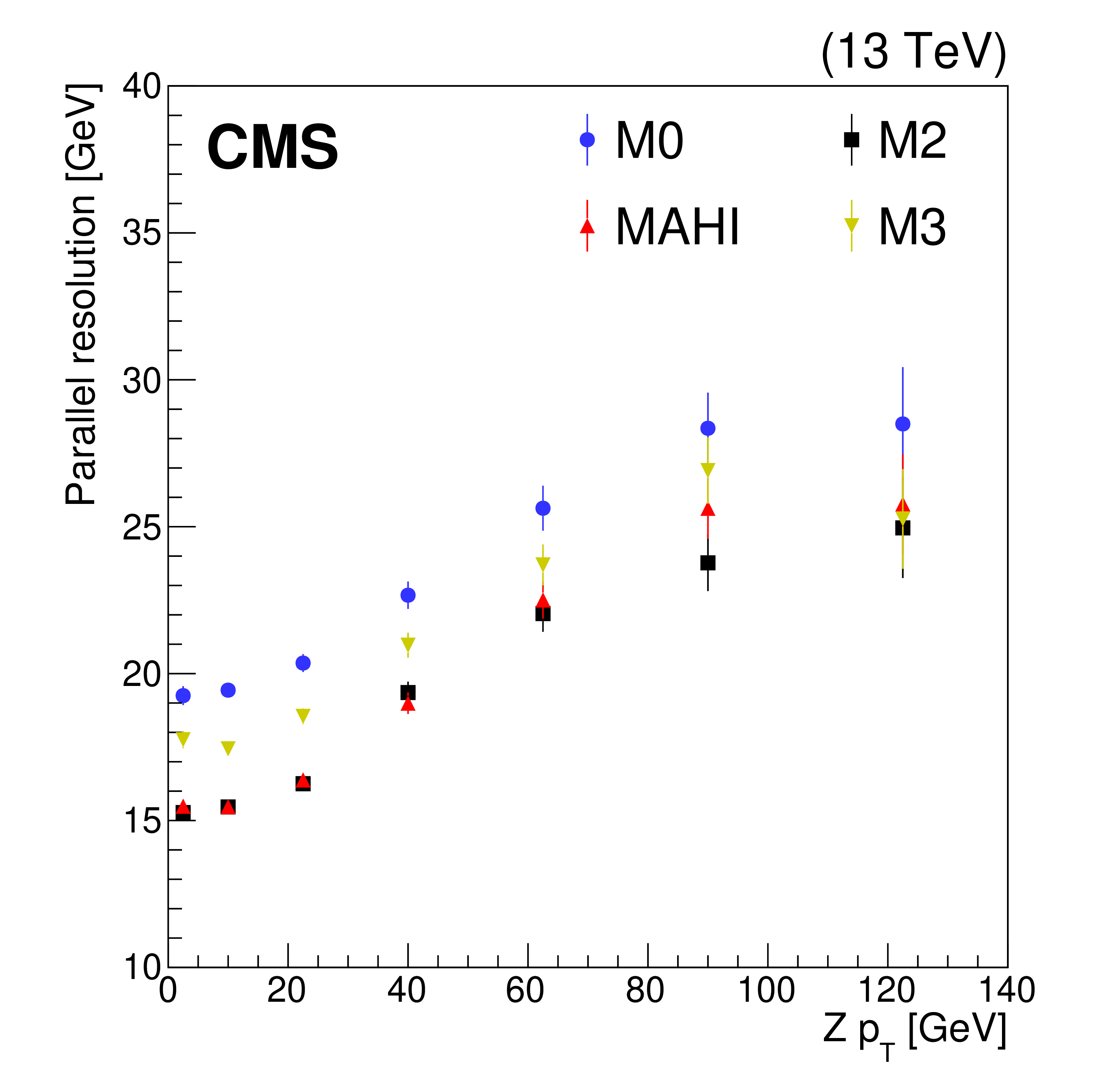
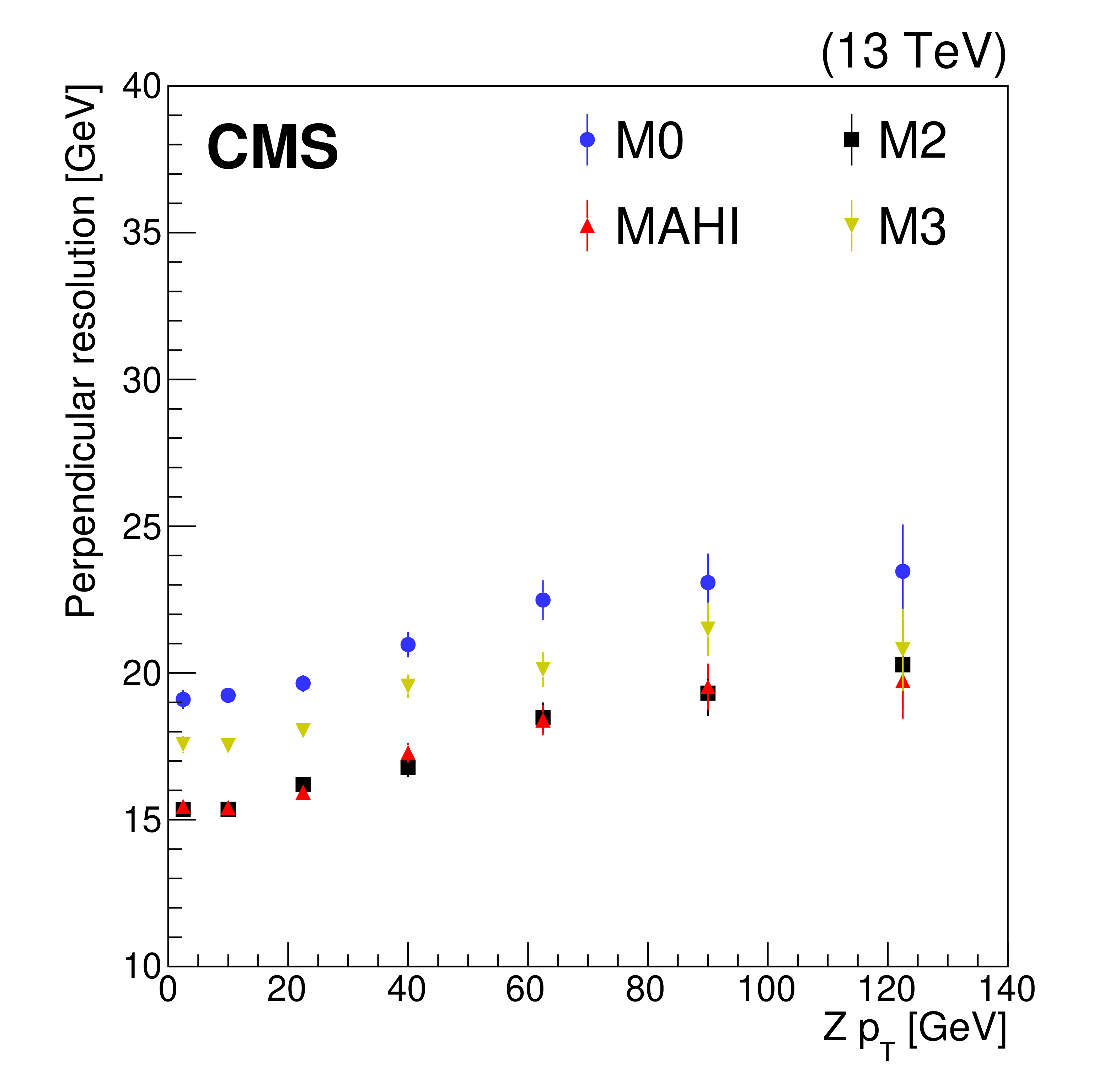
Figure 8:
$ p_{\mathrm{T}}^\text{miss} $ resolutions as a function of the Z boson $ p_{\mathrm{T}} $, measured in a data set triggered by two muons. The left (right) plot is the resolution of the component parallel (perpendicular) to the Z boson's $ p_{\mathrm{T}} $. Error bars reflect statistical uncertainties. |
png pdf |
Figure 8-a:
$ p_{\mathrm{T}}^\text{miss} $ resolutions as a function of the Z boson $ p_{\mathrm{T}} $, measured in a data set triggered by two muons. The plot is the resolution of the component parallel to the Z boson's $ p_{\mathrm{T}} $. Error bars reflect statistical uncertainties. |
png pdf |
Figure 8-b:
$ p_{\mathrm{T}}^\text{miss} $ resolutions as a function of the Z boson $ p_{\mathrm{T}} $, measured in a data set triggered by two muons. The plot is the resolution of the component perpendicular to the Z boson's $ p_{\mathrm{T}} $. Error bars reflect statistical uncertainties. |
png pdf |
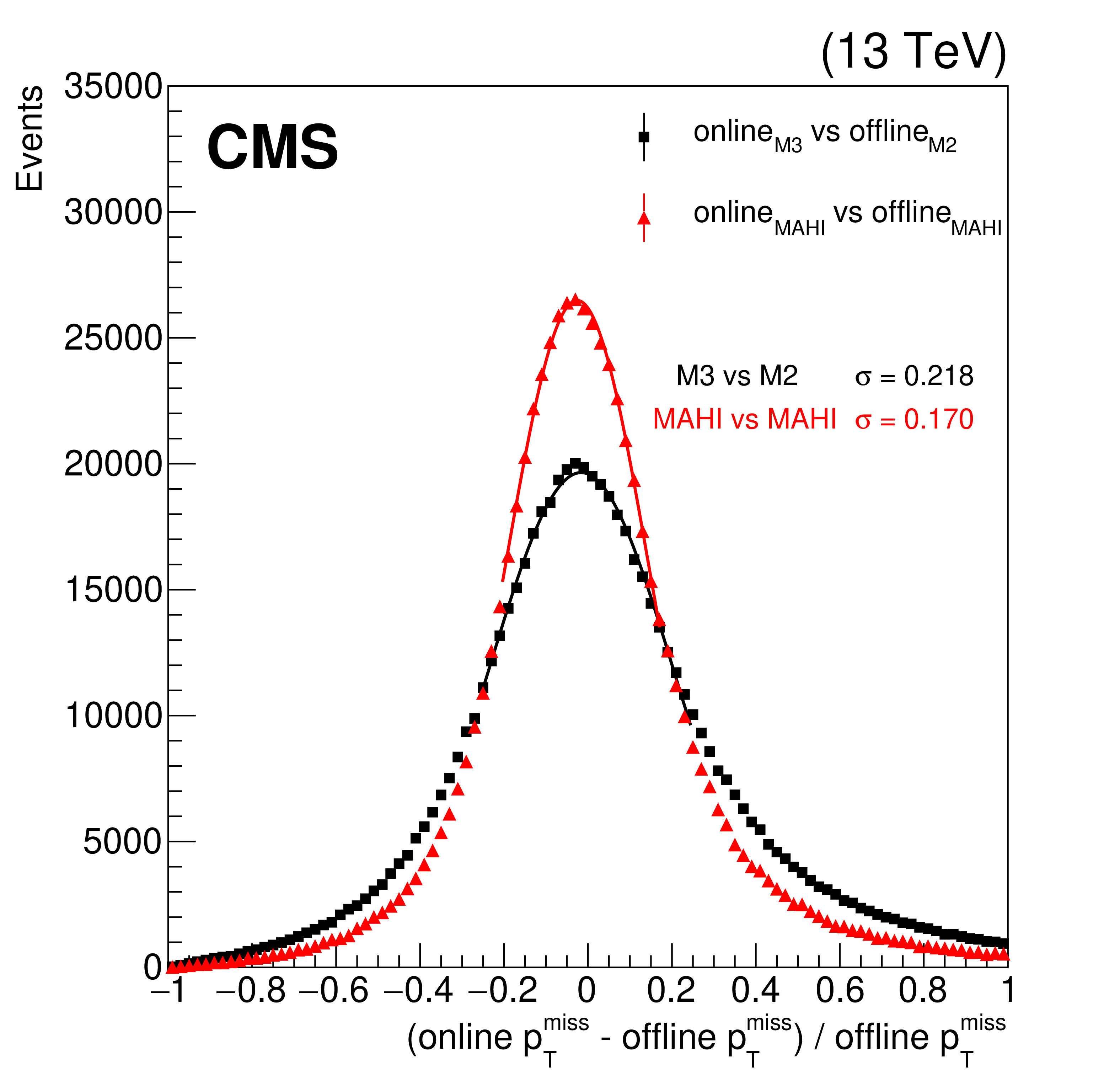
Figure 9:
Relative difference of $ p_{\mathrm{T}}^\text{miss} $ in muon-triggered events between the online and offline reconstructions. Black: (online }$ p_{\mathrm{T}}^\text{miss} $(\text{M3) $ - \text{offline }p_{\mathrm{T}}^\text{miss} $ (M2) $) / \text{offline }p_{\mathrm{T}}^\text{miss} $ (M2). Red: (online }$ p_{\mathrm{T}}^\text{miss} $(\text{MAHI) $ - \text{offline }p_{\mathrm{T}}^\text{miss} $ (MAHI) $) / \text{offline }p_{\mathrm{T}}^\text{miss} $ (MAHI). The differences are fit to a Gaussian distribution and the fitted value of the standard deviation is shown. |
| Summary |
| Four local energy reconstruction algorithms for the CMS hadron calorimeter (HCAL) have been presented in this paper and their performance compared. When the bunch-crossing spacing is at least 50 ns, Method 0 performs well; however, a pulse-shape fitting algorithm must be used when the spacing is only 25 ns. The performance of Method 2 is strong under conditions of high out-of-time pileup, but its long reconstruction time makes it unusable in the high-level trigger. The use of a different algorithm, such as Method 3, to accommodate the time constraints of online reconstruction is possible, but the deleterious effects of mismatched algorithms make this solution undesirable. ``Minimization at HCAL, Iteratively'' is a pulse-shape fitting algorithm that readily suppresses out-of-time pileup and has good intrinsic energy resolution, and is also sufficiently fast to run in the high-level trigger. Hence, it was the preferred local energy reconstruction algorithm for HCAL by the end of Run 2. |
| References | ||||
| 1 | CMS Collaboration | The CMS experiment at the CERN LHC | JINST 3 (2008) S08004 | |
| 2 | CMS Collaboration | Precision luminosity measurement in proton-proton collisions at $ \sqrt{s}= $ 13 TeV in 2015 and 2016 at CMS | EPJC 81 (2021) 800 | CMS-LUM-17-003 2104.01927 |
| 3 | CMS Collaboration | The CMS trigger system | JINST 12 (2017) P01020 | CMS-TRG-12-001 1609.02366 |
| 4 | CMS Collaboration | Identification and filtering of uncharacteristic noise in the CMS hadron calorimeter | JINST 5 (2010) T03014 | CMS-CFT-09-019 0911.4881 |
| 5 | CMS Collaboration | CMS technical design report for the Phase 1 upgrade of the hadron calorimeter | CMS Technical Design Report CERN-LHCC-2012-015 / CMS-TDR-010, 2012 CDS |
|
| 6 | S. Gundacker and A. Heering | The silicon photomultiplier: fundamentals and applications of a modern solid-state photon detector | Phys. Med. Biol. 65 (2020) 17TR01 | |
| 7 | T. Zimmerman and J. Hoff | The design of a charge-integrating modified floating-point ADC chip | IEEE J. Solid-, 2004 State Circ. 39 (2004) 895 |
|
| 8 | CMS HCAL Collaboration | Design, performance, and calibration of CMS hadron-barrel calorimeter wedges | EPJC 55 (2008) 159 | |
| 9 | CMS Collaboration | Reconstruction of signal amplitudes in the CMS electromagnetic calorimeter in the presence of overlapping proton-proton interactions | JINST 15 (2020) P10002 | CMS-EGM-18-001 2006.14359 |
| 10 | CMS Collaboration | Performance of CMS hadron calorimeter timing and synchronization using test beam, cosmic ray, and LHC beam data | JINST 5 (2010) T03013 | CMS-CFT-09-018 0911.4877 |
| 11 | CMS Collaboration | Search for long-lived particles using displaced jets in proton-proton collisions at $ \sqrt{s} = $ 13 TeV | PRD 104 (2021) 012015 | CMS-EXO-19-021 2012.01581 |
| 12 | CMS Collaboration | Search for long-lived particles using nonprompt jets and missing transverse momentum with proton-proton collisions at $ \sqrt{s} = $ 13 TeV | PLB 797 (2019) 134876 | CMS-EXO-19-001 1906.06441 |
| 13 | CMS Collaboration | Search for long-lived particles with displaced vertices in multijet events in proton-proton collisions at $ \sqrt{s}= $ 13 TeV | PRD 98 (2018) 092011 | CMS-EXO-17-018 1808.03078 |
| 14 | F. James and M. Roos | Minuit---a system for function minimization and analysis of the parameter errors and correlations | Comput. Phys. Commun. 10 (1975) 343 | |
| 15 | J. Cantarella and M. Piatek | Tsnnls: A solver for large sparse least squares problems with non-negative variables | cs/0408029 | |
| 16 | CMS Collaboration | Calibration of the CMS hadron calorimeters using proton-proton collision data at $ \sqrt{s} = $ 13 TeV | JINST 15 (2020) P05002 | CMS-PRF-18-001 1910.00079 |
| 17 | T. Sjöstrand et al. | An introduction to PYTHIA 8.2 | Comput. Phys. Commun. 191 (2015) 159 | 1410.3012 |
| 18 | GEANT4 Collaboration | GEANT 4---a simulation toolkit | NIM A 506 (2003) 250 | |
| 19 | CMS Collaboration | Performance of missing transverse momentum reconstruction in proton-proton collisions at $ \sqrt{s} = $ 13 TeV using the CMS detector | JINST 14 (2019) P07004 | CMS-JME-17-001 1903.06078 |
|
|
Compact Muon Solenoid LHC, CERN |
|

|

|

|

|

|