

Compact Muon Solenoid
LHC, CERN
| CMS-SUS-16-033 ; CERN-EP-2017-072 | ||
| Search for supersymmetry in multijet events with missing transverse momentum in proton-proton collisions at 13 TeV | ||
| CMS Collaboration | ||
| 25 April 2017 | ||
| Phys. Rev. D 96 (2017) 032003 | ||
| Abstract: A search for supersymmetry is presented based on multijet events with large missing transverse momentum produced in proton-proton collisions at a center-of-mass energy of $ \sqrt{s} = $ 13 TeV. The data, corresponding to an integrated luminosity of 35.9 fb$^{-1}$, were collected with the CMS detector at the CERN LHC in 2016. The analysis utilizes four-dimensional exclusive search regions defined in terms of the number of jets, the number of tagged bottom quark jets, the scalar sum of jet transverse momenta, and the magnitude of the vector sum of jet transverse momenta. No evidence for a significant excess of events is observed relative to the expectation from the standard model. Limits on the cross sections for the pair production of gluinos and squarks are derived in the context of simplified models. Assuming the lightest supersymmetric particle to be a weakly interacting neutralino, 95% confidence level lower limits on the gluino mass as large as 1800 to 1960 GeV are derived, and on the squark mass as large as 960 to 1390 GeV, depending on the production and decay scenario. | ||
| Links: e-print arXiv:1704.07781 [hep-ex] (PDF) ; CDS record ; inSPIRE record ; HepData record ; CADI line (restricted) ; | ||
| Figures & Tables | Summary | Additional Figures & Tables | References | CMS Publications |
|---|
|
Additional information on efficiencies needed for reinterpretation of these results are available here.
Additional technical material for CMS speakers can be found here |
| Figures | |
png pdf |
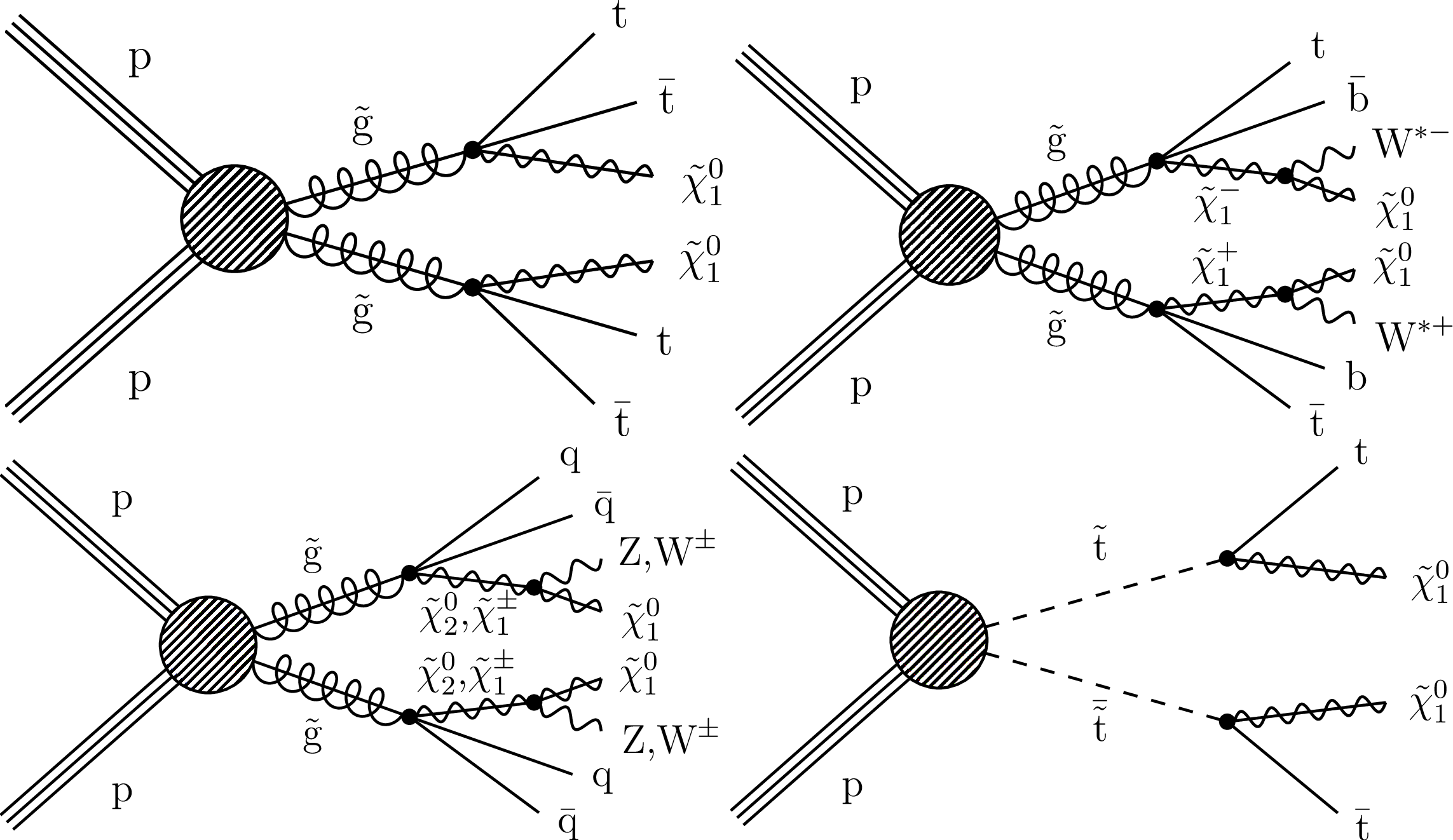
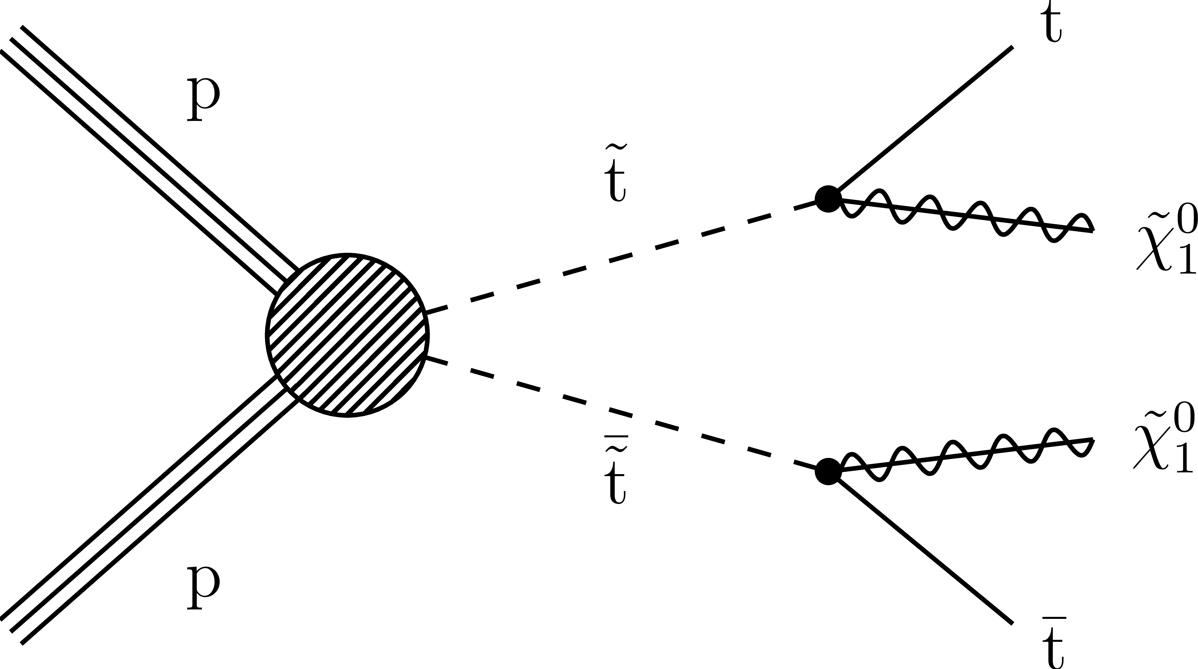
Figure 1:
Example Feynman diagrams for the simplified model signal scenarios considered in this study: the (upper left) T1tttt, (upper right) T1tbtb, (lower left) T5qqqqVV, and (lower right) T2tt scenarios. In the T5qqqqVV model, the flavors of the quark ${\mathrm{ q } }$ and antiquark ${\mathrm{ \bar{q} } }$ differ from each other if the gluino $ \tilde{g} $ decays as $\tilde{g} \to \mathrm{ q } \mathrm{ \bar{q} } \tilde{ \chi }^{\pm} _1$, where $\tilde{ \chi }^{\pm} _1$ is the lightest chargino. |
png pdf |
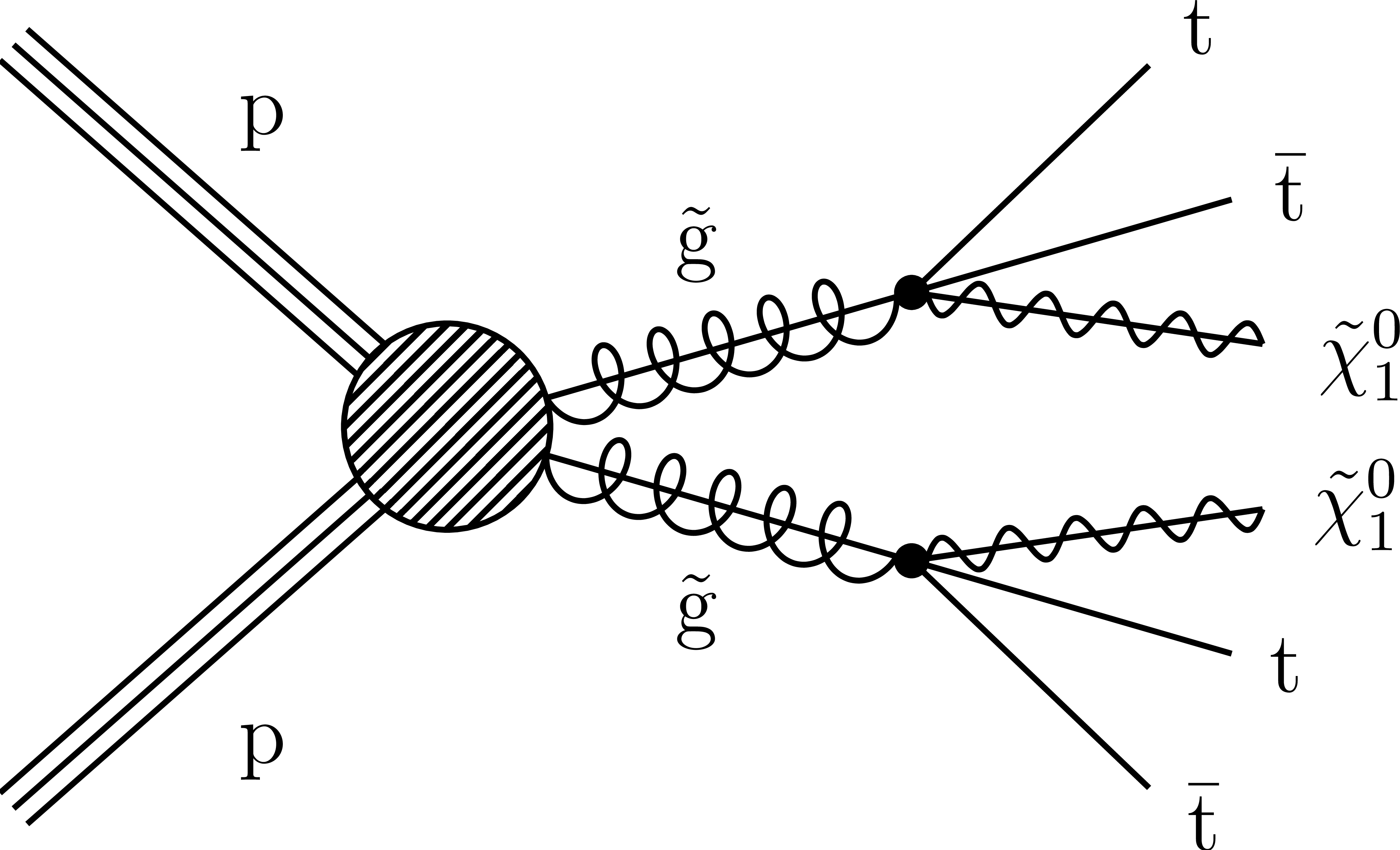
Figure 1-a:
Example Feynman diagrams for the simplified model signal scenarios considered in this study: the (upper left) T1tttt, (upper right) T1tbtb, (lower left) T5qqqqVV, and (lower right) T2tt scenarios. In the T5qqqqVV model, the flavors of the quark ${\mathrm{ q } }$ and antiquark ${\mathrm{ \bar{q} } }$ differ from each other if the gluino $ \tilde{g} $ decays as $\tilde{g} \to \mathrm{ q } \mathrm{ \bar{q} } \tilde{ \chi }^{\pm} _1$, where $\tilde{ \chi }^{\pm} _1$ is the lightest chargino. |
png pdf |
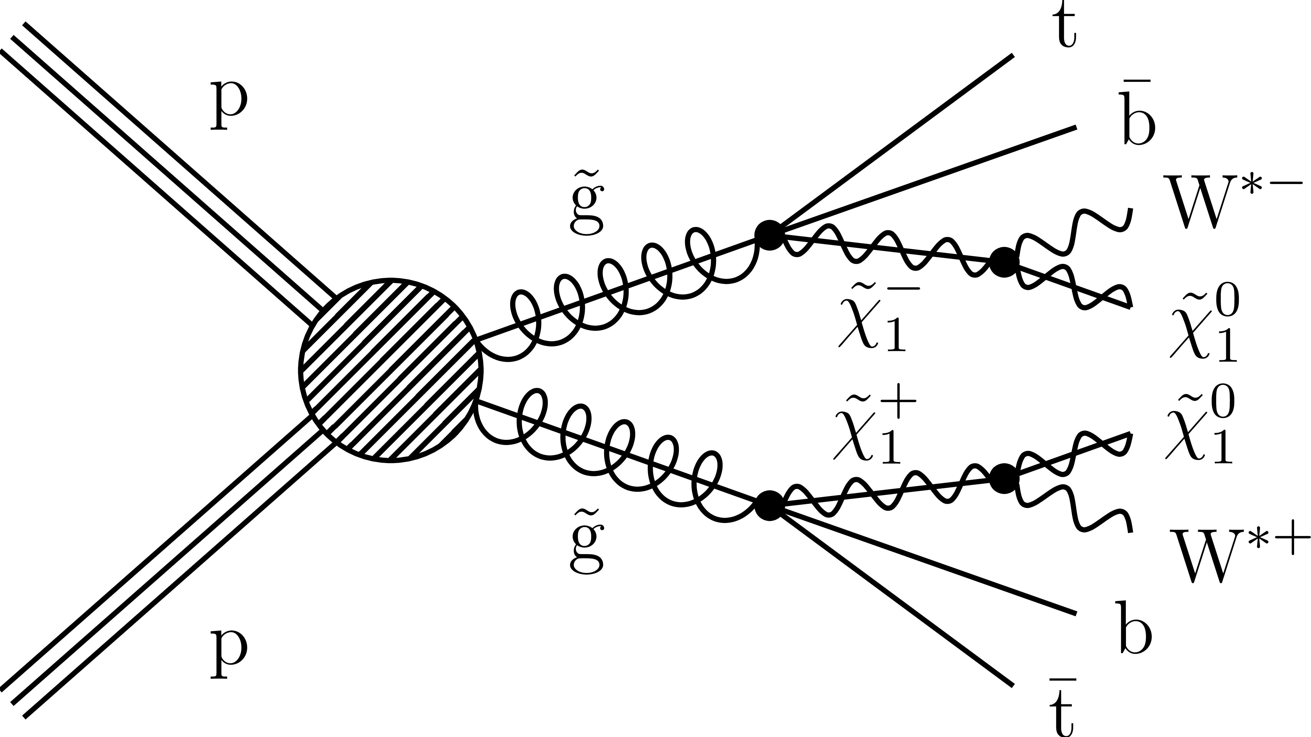
Figure 1-b:
Example Feynman diagrams for the simplified model signal scenarios considered in this study: the (upper left) T1tttt, (upper right) T1tbtb, (lower left) T5qqqqVV, and (lower right) T2tt scenarios. In the T5qqqqVV model, the flavors of the quark ${\mathrm{ q } }$ and antiquark ${\mathrm{ \bar{q} } }$ differ from each other if the gluino $ \tilde{g} $ decays as $\tilde{g} \to \mathrm{ q } \mathrm{ \bar{q} } \tilde{ \chi }^{\pm} _1$, where $\tilde{ \chi }^{\pm} _1$ is the lightest chargino. |
png pdf |
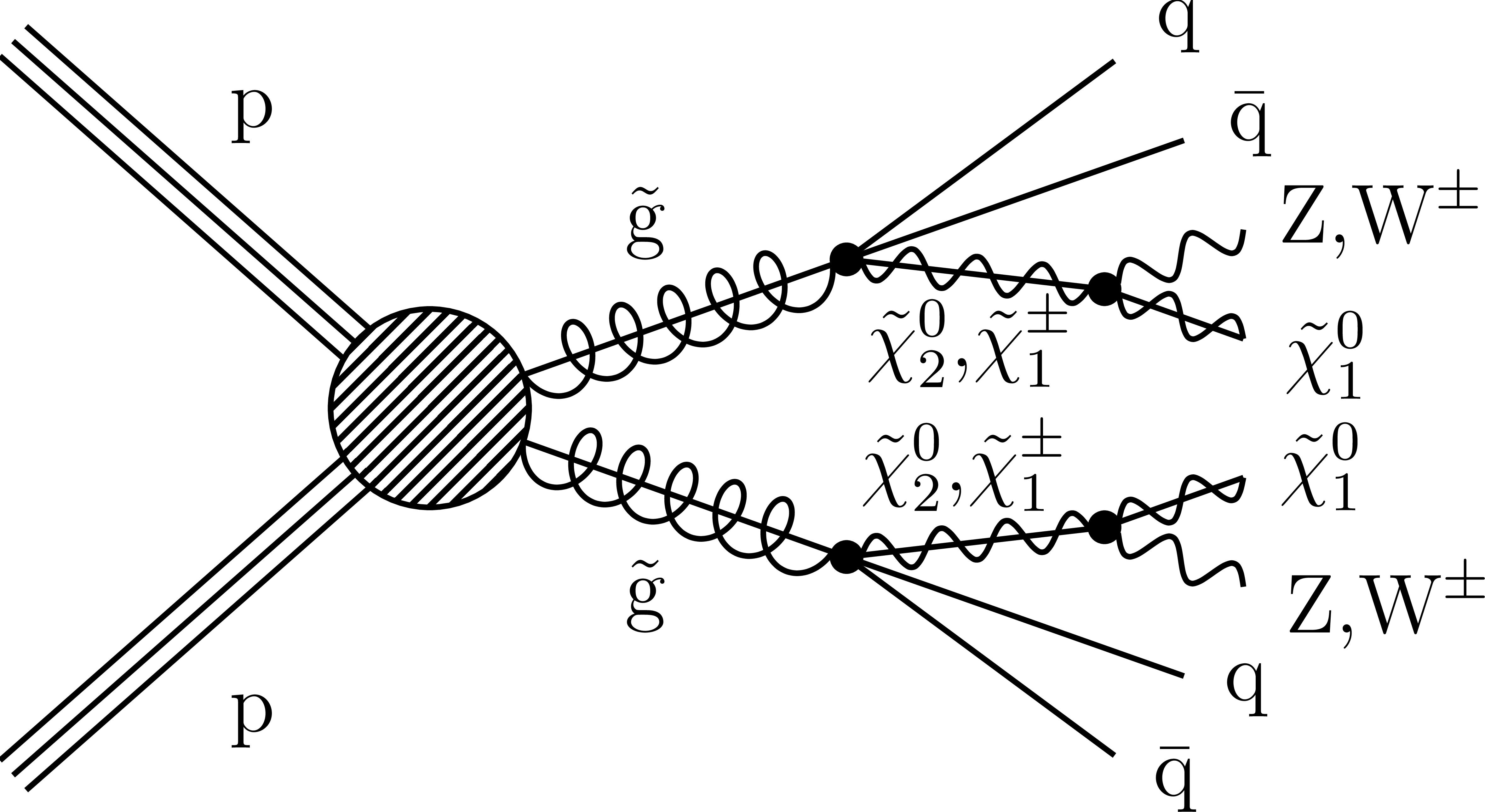
Figure 1-c:
Example Feynman diagrams for the simplified model signal scenarios considered in this study: the (upper left) T1tttt, (upper right) T1tbtb, (lower left) T5qqqqVV, and (lower right) T2tt scenarios. In the T5qqqqVV model, the flavors of the quark ${\mathrm{ q } }$ and antiquark ${\mathrm{ \bar{q} } }$ differ from each other if the gluino $ \tilde{g} $ decays as $\tilde{g} \to \mathrm{ q } \mathrm{ \bar{q} } \tilde{ \chi }^{\pm} _1$, where $\tilde{ \chi }^{\pm} _1$ is the lightest chargino. |
png pdf |
Figure 1-d:
Example Feynman diagrams for the simplified model signal scenarios considered in this study: the (upper left) T1tttt, (upper right) T1tbtb, (lower left) T5qqqqVV, and (lower right) T2tt scenarios. In the T5qqqqVV model, the flavors of the quark ${\mathrm{ q } }$ and antiquark ${\mathrm{ \bar{q} } }$ differ from each other if the gluino $ \tilde{g} $ decays as $\tilde{g} \to \mathrm{ q } \mathrm{ \bar{q} } \tilde{ \chi }^{\pm} _1$, where $\tilde{ \chi }^{\pm} _1$ is the lightest chargino. |

png pdf |
Figure 2:
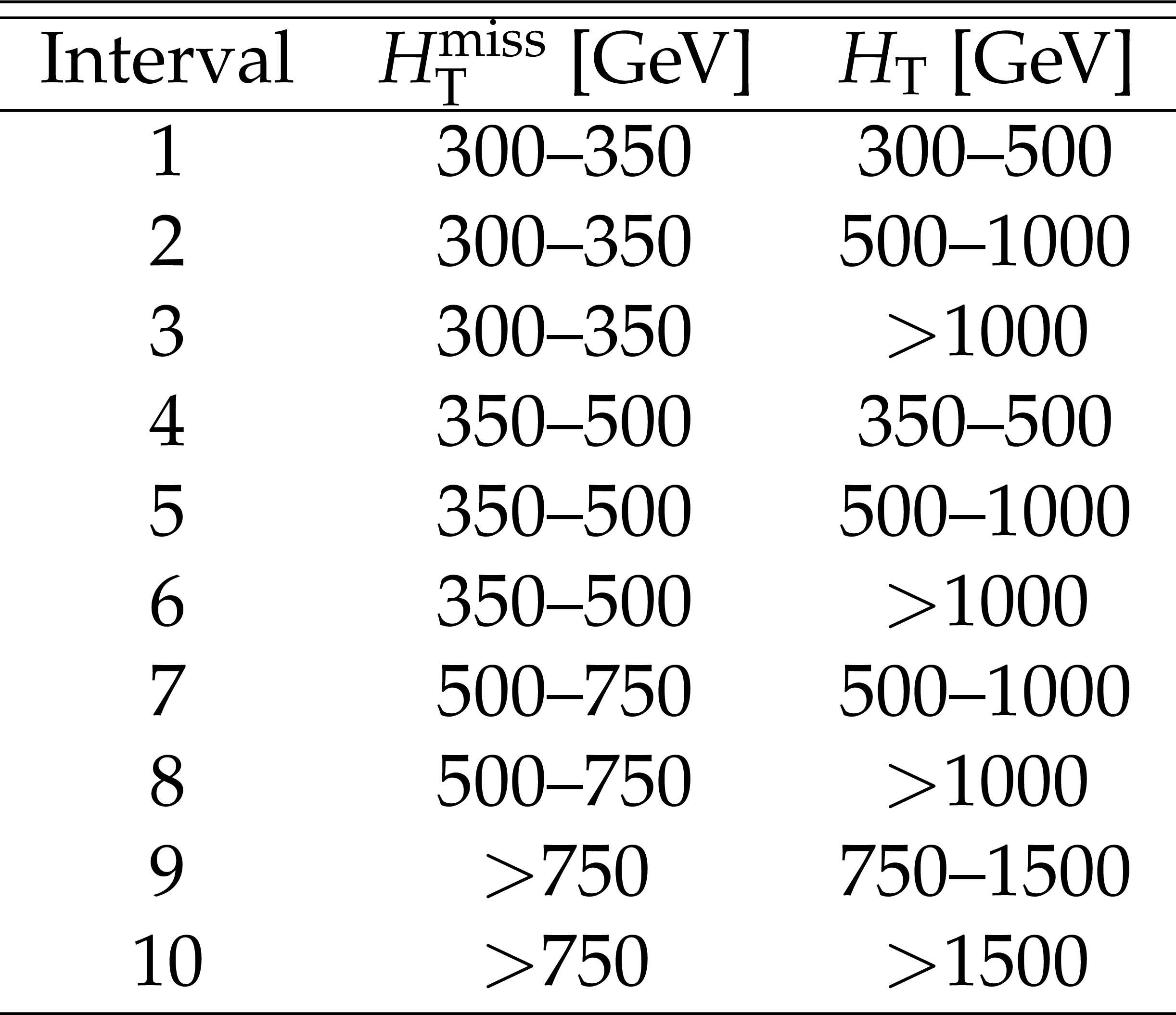
Schematic illustration of the 10 kinematic search intervals in the $ {H_{\text {T}}^{\text {miss}}} $ versus $ {H_{\mathrm {T}}} $ plane. Intervals 1 and 4 are discarded for $ {N_{\text {jet}}} \geq $ 7. The intervals labeled C1, C2, and C3 are control regions used to evaluate the QCD background. The rightmost and topmost bins are unbounded, extending to $ {H_{\mathrm {T}}} =\infty $ and $ {H_{\text {T}}^{\text {miss}}} =\infty $, respectively. |
png pdf |
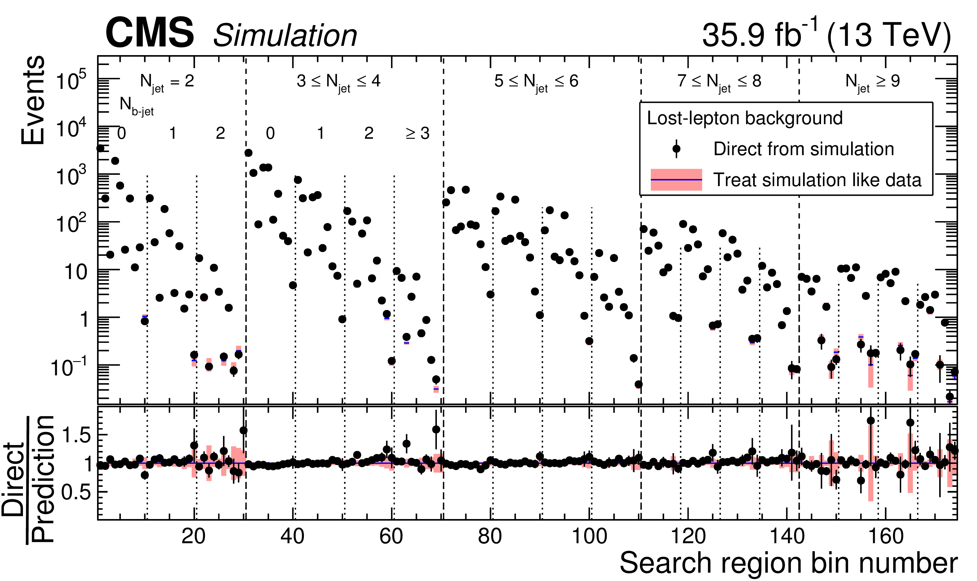
Figure 3:
The lost-lepton background in the 174 search regions of the analysis as determined directly from $ {\mathrm{ t } {}\mathrm{ \bar{t} } } $, single top quark, W+jets, diboson, and rare-event simulation (points, with statistical uncertainties) and as predicted by applying the lost-lepton background determination procedure to simulated electron and muon control samples (histograms, with statistical uncertainties). The results in the lower panel are obtained through bin-by-bin division of the results in the upper panel, including the uncertainties, by the central values of the "predicted'' results. The 10 results (8 results for $ {N_{\text {jet}}} \geq 7$) within each region delineated by vertical dashed lines correspond sequentially to the 10 (8) kinematic intervals of $ {H_{\mathrm {T}}} $ and $ {H_{\text {T}}^{\text {miss}}} $ indicated in Table 1 and Fig. 2. |

png pdf |
Figure 4:
The background from hadronically decaying $\tau $ leptons in the 174 search regions of the analysis as determined directly from $ {\mathrm{ t } {}\mathrm{ \bar{t} } } $, single top quark, and W+jets simulation (points, with statistical uncertainties) and as predicted by applying the hadronically decaying $\tau $ lepton background determination procedure to a simulated muon control sample (histograms, with statistical uncertainties). The results in the lower panel are obtained through bin-by-bin division of the results in the upper panel, including the uncertainties, by the central values of the "predicted'' results. The labeling of the bin numbers is the same as in Fig. 3. |
png pdf |
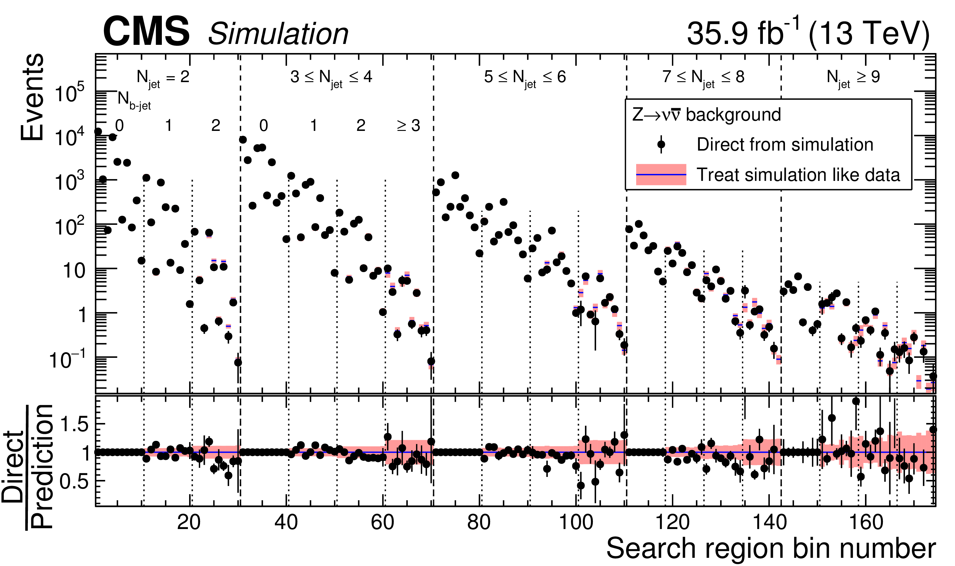
Figure 5:
The ${\mathrm{ Z } \to \nu \bar{\nu} }$ background in the 174 search regions of the analysis as determined directly from Z($\to \nu \bar{\nu} $)+jets simulation (points, with statistical uncertainties), and as predicted by applying the ${\mathrm{ Z } \to \nu \bar{\nu} }$ background determination procedure to statistically independent Z($\to \ell ^{+} \ell ^{-} $)+jets simulated event samples (histogram, with shaded regions indicating the quadrature sum of the systematic uncertainty associated with the assumption that $\mathcal {F}_{j,b}$ is independent of $ {H_{\mathrm {T}}} $ and $ {H_{\text {T}}^{\text {miss}}} $, and the statistical uncertainty). For bins corresponding to $ {N_{{\mathrm{ b } }\text {-jet}}} =$ 0, the agreement is exact by construction. The results in the lower panel are obtained through bin-by-bin division of the results in the upper panel, including the uncertainties, by the central values of the "predicted'' results. The labeling of the bin numbers is the same as in Fig. 3. |
png pdf |
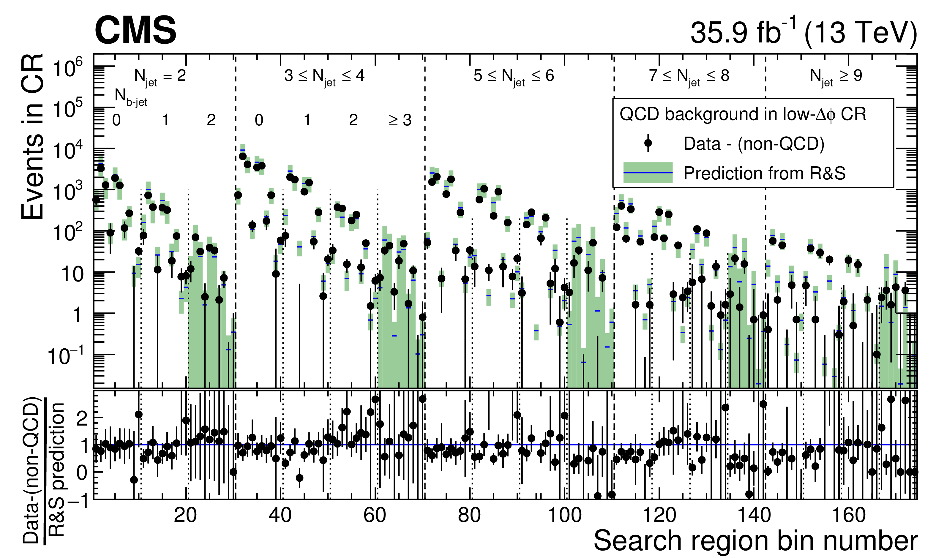
Figure 6:
The QCD background in the low-$ {\Delta \phi }$ control region (CR) as predicted by the rebalance-and-smear (R&S ) method (histograms, with statistical and systematic uncertainties added in quadrature), compared to the corresponding data from which the expected contributions of top quark, W+jets, and Z+jets events have been subtracted (points, with statistical uncertainties). The lower panel shows the ratio of the measured to the predicted results and its propagated uncertainty. The labeling of the bin numbers is the same as in Fig. 3. |
png pdf |
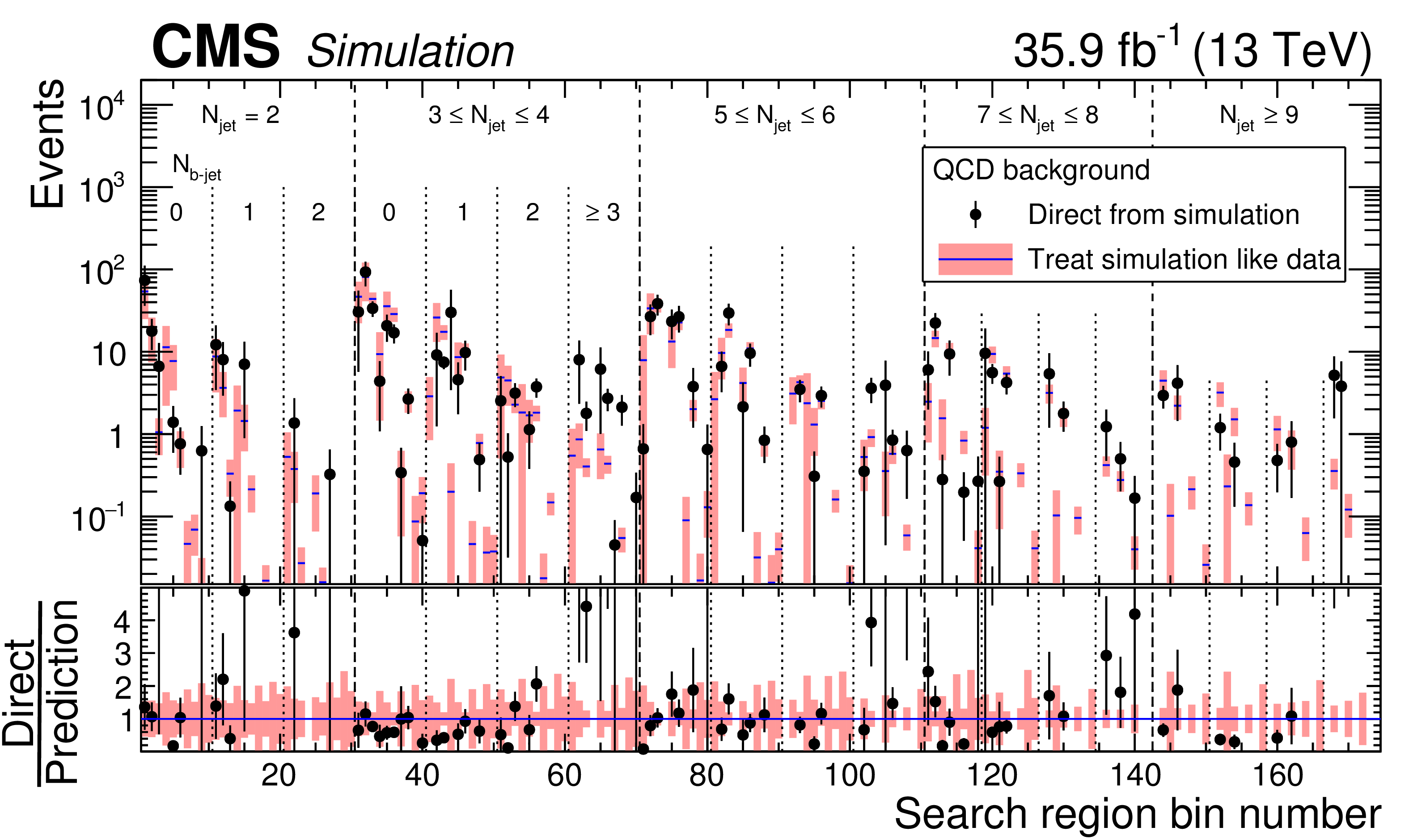
Figure 7:
The QCD background in the 174 search regions of the analysis as determined directly from QCD simulation (points, with statistical uncertainties) and as predicted by applying the low-$ {\Delta \phi }$ extrapolation QCD background determination procedure to simulated event samples (histograms, with statistical and systematic uncertainties added in quadrature). Bins without a point have no simulated QCD events in the search region, while bins without a histogram have no simulated QCD events in the corresponding control region. The results in the lower panel are obtained through bin-by-bin division of the results in the upper panel, including the uncertainties, by the central values of the "predicted'' results. No result is given in the lower panel if the value of the prediction is zero. The labeling of the bin numbers is the same as in Fig. 3. |
png pdf |
Figure 8:
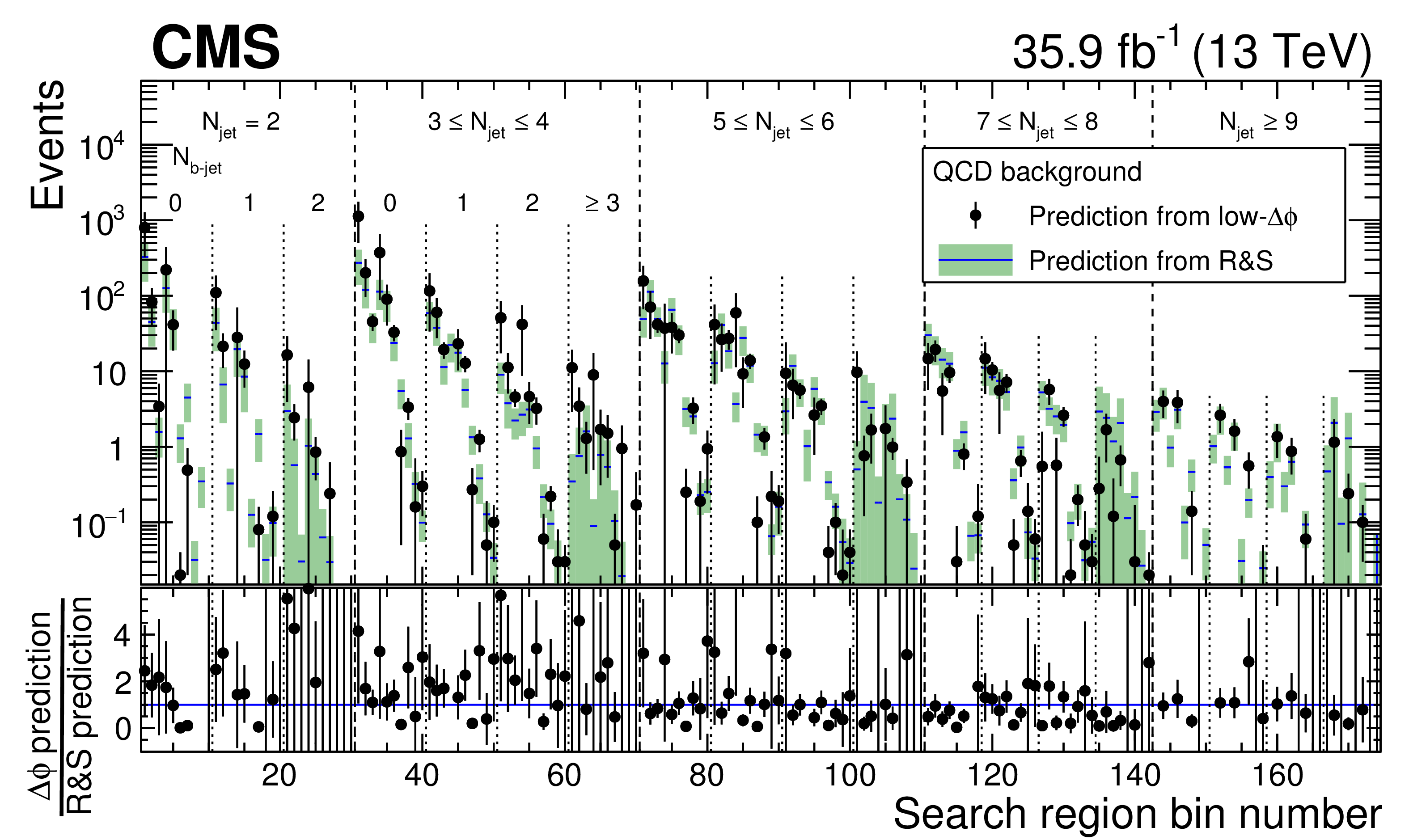
Comparison between the predictions for the number of QCD events in the 174 search regions of the analysis as determined from the rebalance-and-smear (R&S, histograms) and low-$ {\Delta \phi }$ extrapolation (points) methods. For both methods, the error bars indicate the combined statistical and systematic uncertainties. The lower panel shows the ratio of the low-$ {\Delta \phi }$ extrapolation to the R&S results and its propagated uncertainty. The labeling of the bin numbers is the same as in Fig. 3. |
png pdf root |
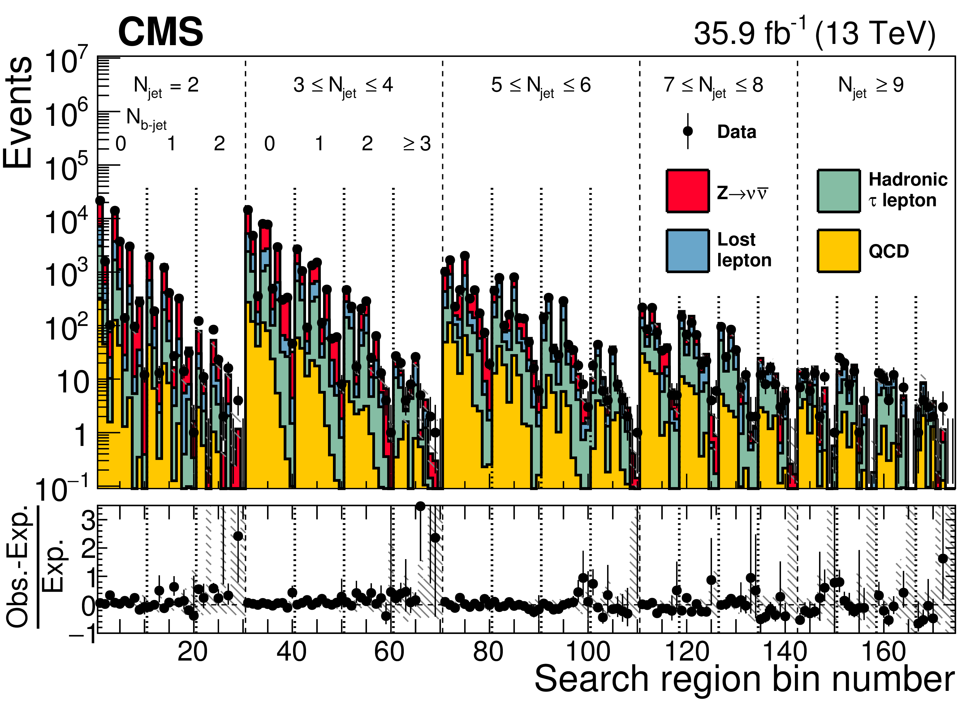
Figure 9:
The observed numbers of events and prefit SM background predictions in the 174 search regions of the analysis, where "prefit'' means there is no constraint from the likelihood fit. Numerical values are given in Tables B.1-B.5. The hatching indicates the total uncertainty in the background predictions. The lower panel displays the fractional differences between the data and SM predictions. The labeling of the bin numbers is the same as in Fig. 3. |

png pdf |
Figure 10:
The observed numbers of events and prefit SM background predictions in the 12 aggregate search regions, with fractional differences displayed in the lower panel, where "prefit'' means there is no constraint from the likelihood fit. The hatching indicates the total uncertainty in the background predictions. The numerical values are given in Table B.6. |
png pdf |
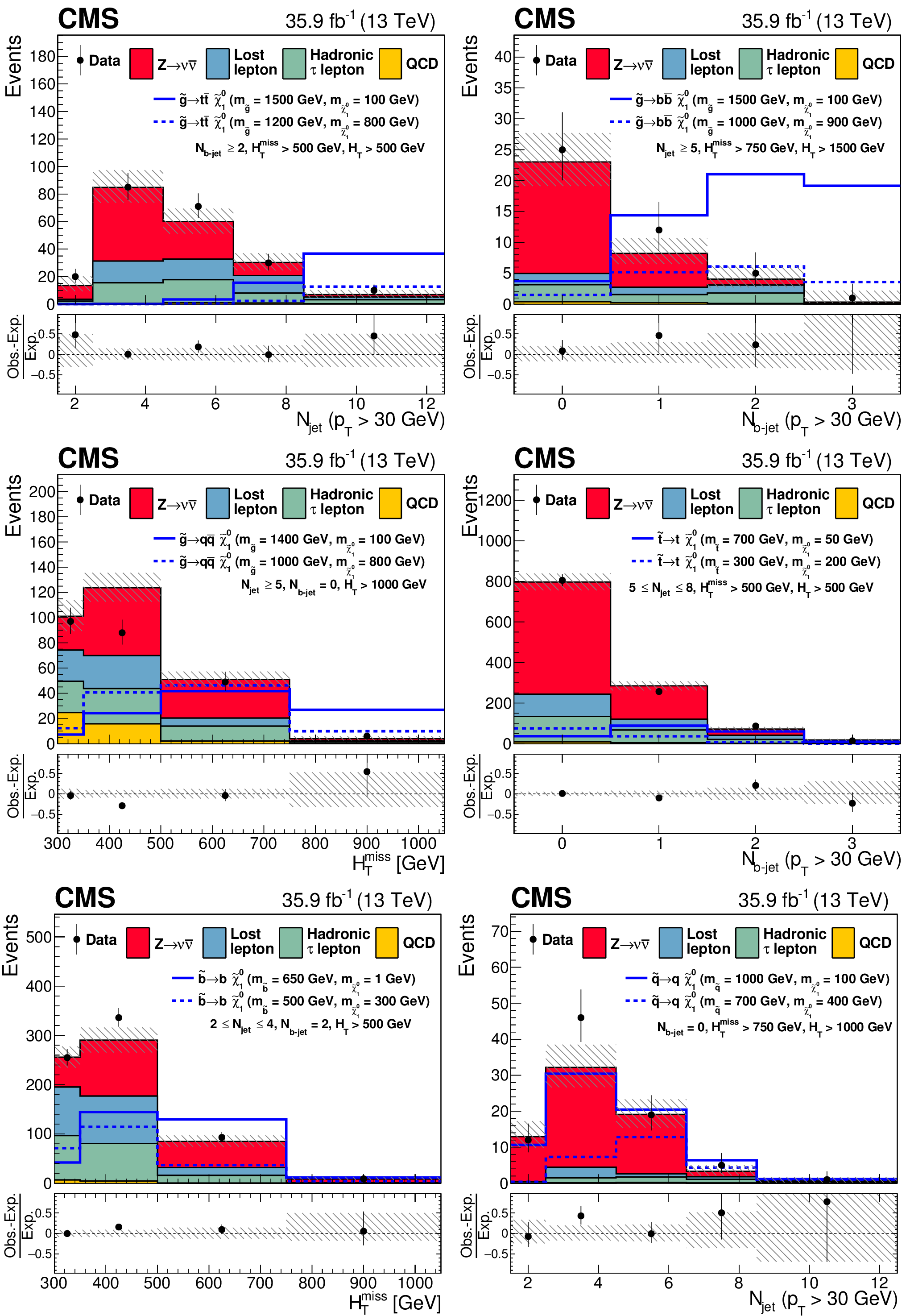
Figure 11:
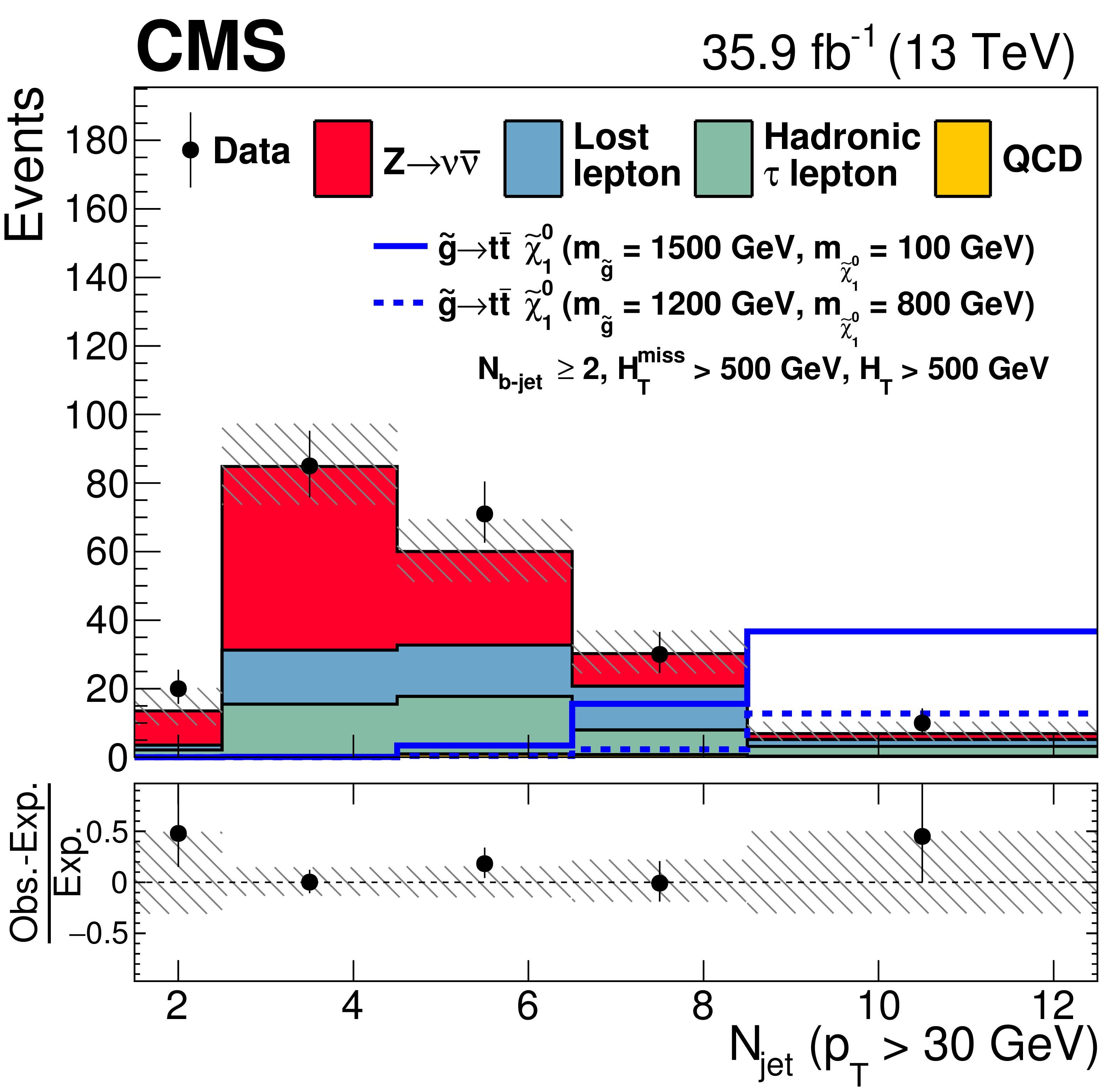
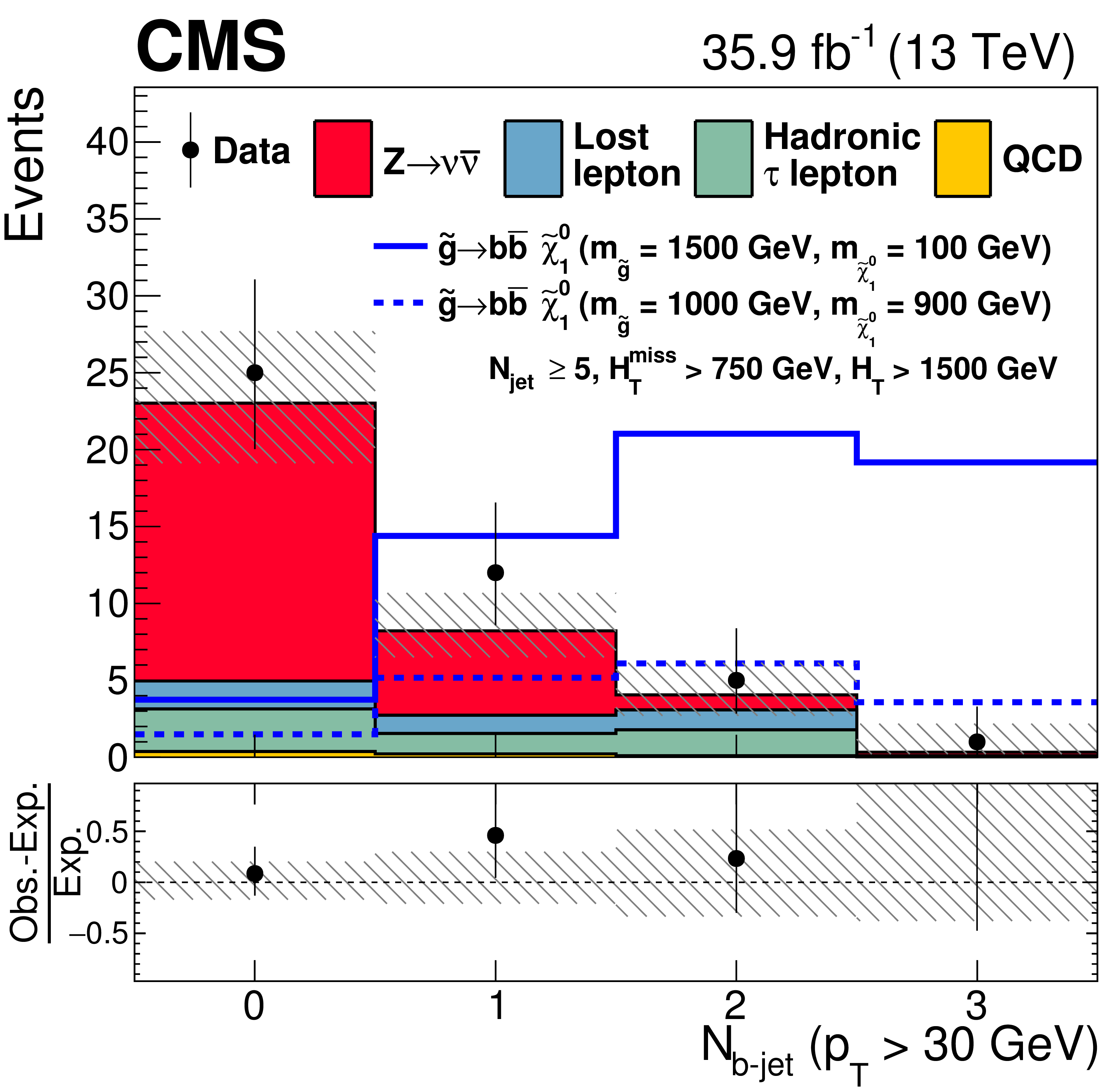
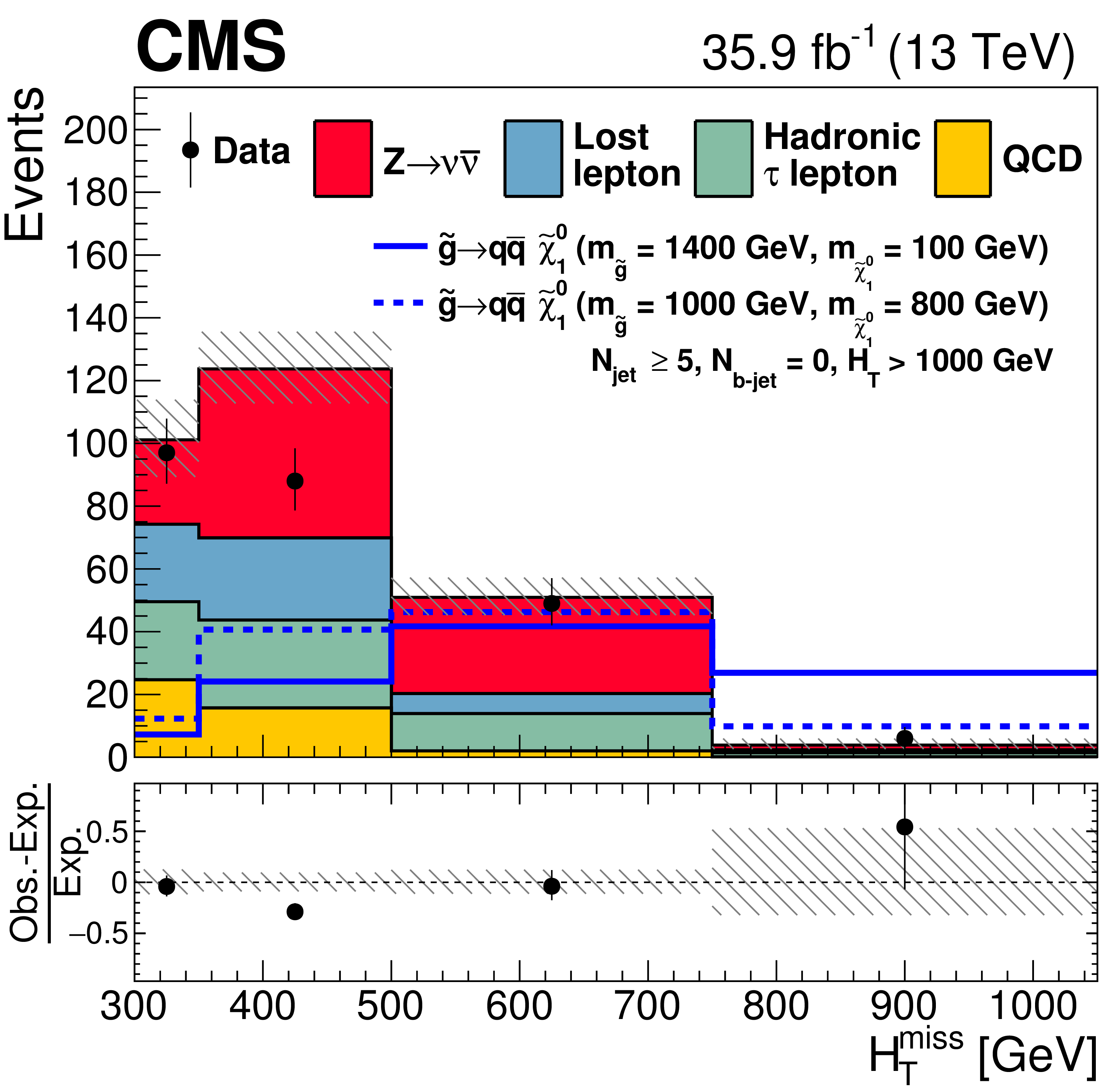
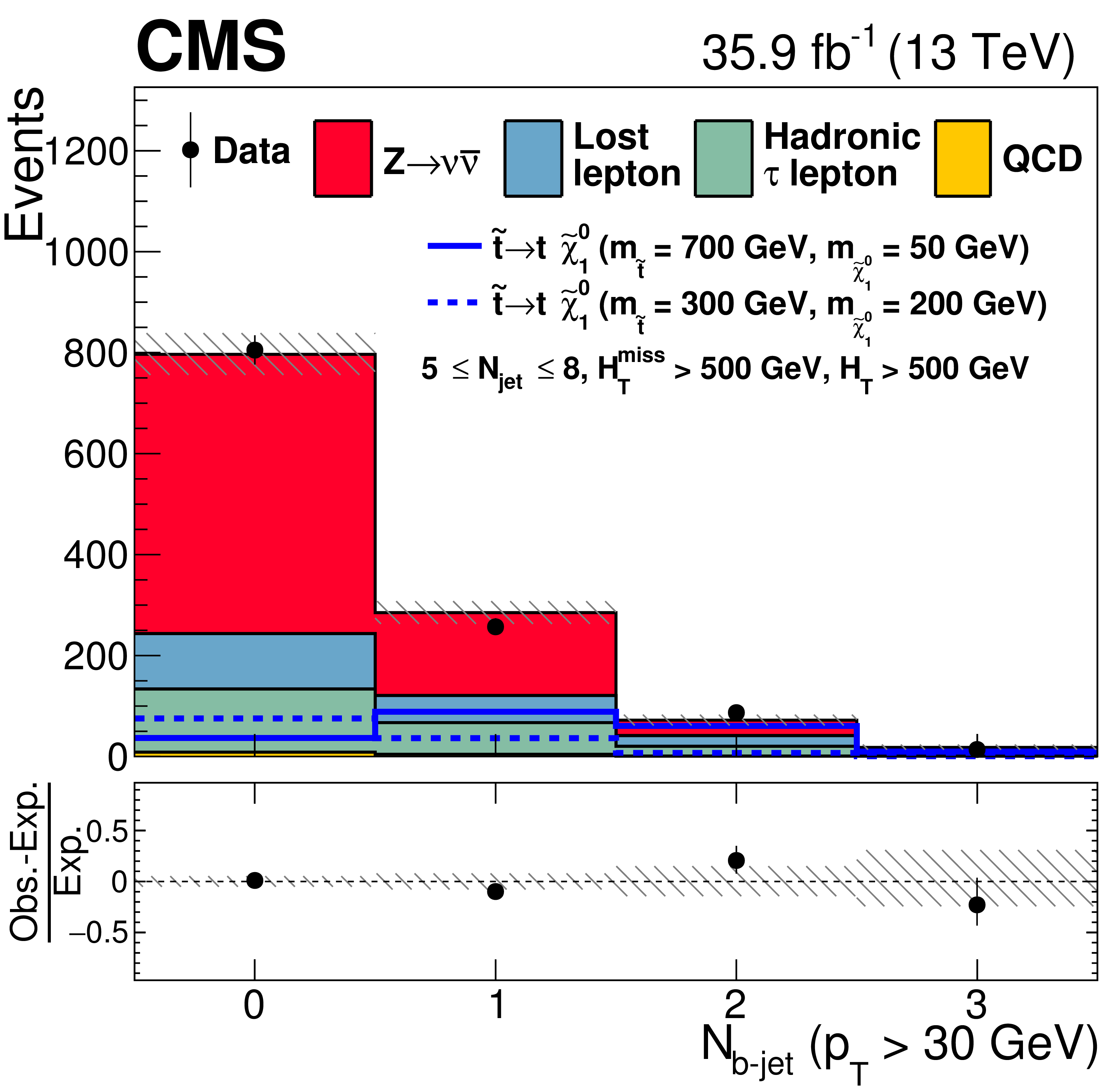
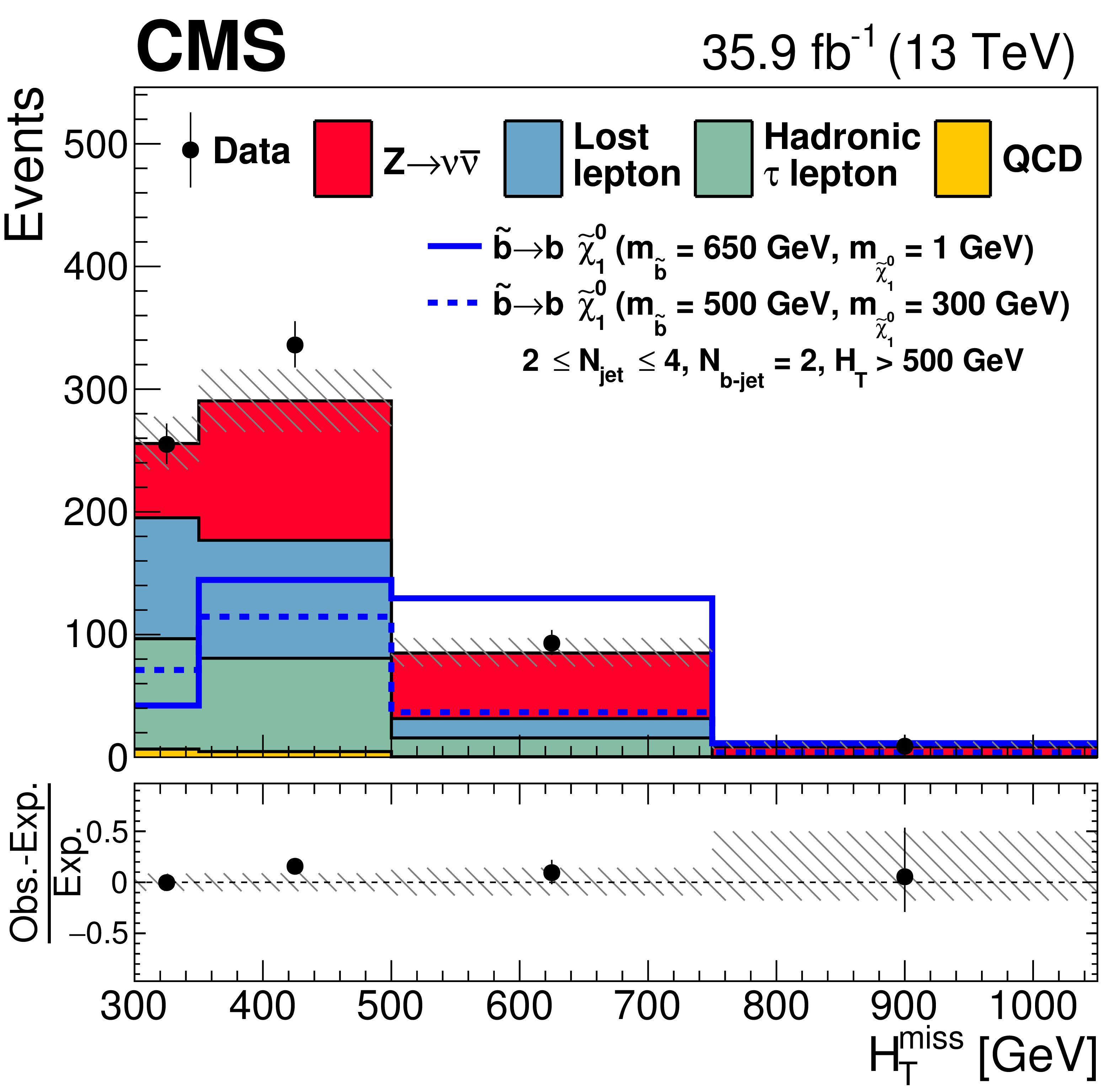
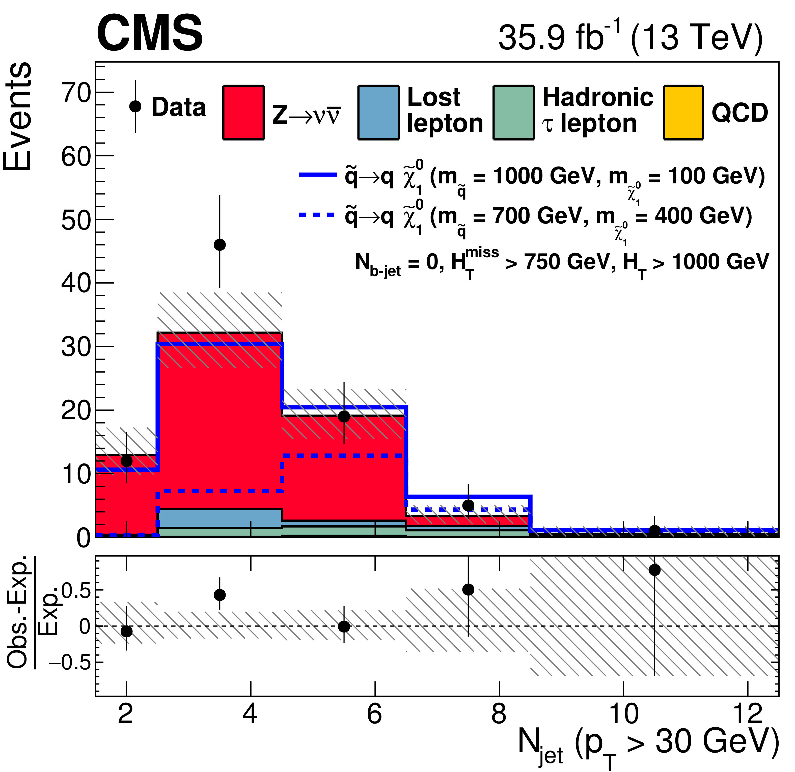
The observed numbers of events and SM background predictions for regions in the search region parameter space particularly sensitive to the production of events in the (upper left) T1tttt, (upper right) T1bbbb, (middle left) T1qqqq, (middle right) T2tt, (lower left) T2bb, and (lower right) T2qq scenarios. The selection requirements are given in the figure legends. The hatched regions indicate the total uncertainties in the background predictions. The (unstacked) results for two example signal scenarios are shown in each instance, one with $ {\Delta m} \gg $ 0 and the other with $ {\Delta m} \approx $ 0, where ${\Delta m}$ is the difference between the gluino or squark mass and the sum of the masses of the particles into which it decays. |
png pdf |
Figure 11-a:
The observed numbers of events and SM background predictions for regions in the search region parameter space particularly sensitive to the production of events in the (upper left) T1tttt, (upper right) T1bbbb, (middle left) T1qqqq, (middle right) T2tt, (lower left) T2bb, and (lower right) T2qq scenarios. The selection requirements are given in the figure legends. The hatched regions indicate the total uncertainties in the background predictions. The (unstacked) results for two example signal scenarios are shown in each instance, one with $ {\Delta m} \gg $ 0 and the other with $ {\Delta m} \approx $ 0, where ${\Delta m}$ is the difference between the gluino or squark mass and the sum of the masses of the particles into which it decays. |
png pdf |
Figure 11-b:
The observed numbers of events and SM background predictions for regions in the search region parameter space particularly sensitive to the production of events in the (upper left) T1tttt, (upper right) T1bbbb, (middle left) T1qqqq, (middle right) T2tt, (lower left) T2bb, and (lower right) T2qq scenarios. The selection requirements are given in the figure legends. The hatched regions indicate the total uncertainties in the background predictions. The (unstacked) results for two example signal scenarios are shown in each instance, one with $ {\Delta m} \gg $ 0 and the other with $ {\Delta m} \approx $ 0, where ${\Delta m}$ is the difference between the gluino or squark mass and the sum of the masses of the particles into which it decays. |
png pdf |
Figure 11-c:
The observed numbers of events and SM background predictions for regions in the search region parameter space particularly sensitive to the production of events in the (upper left) T1tttt, (upper right) T1bbbb, (middle left) T1qqqq, (middle right) T2tt, (lower left) T2bb, and (lower right) T2qq scenarios. The selection requirements are given in the figure legends. The hatched regions indicate the total uncertainties in the background predictions. The (unstacked) results for two example signal scenarios are shown in each instance, one with $ {\Delta m} \gg $ 0 and the other with $ {\Delta m} \approx $ 0, where ${\Delta m}$ is the difference between the gluino or squark mass and the sum of the masses of the particles into which it decays. |
png pdf |
Figure 11-d:
The observed numbers of events and SM background predictions for regions in the search region parameter space particularly sensitive to the production of events in the (upper left) T1tttt, (upper right) T1bbbb, (middle left) T1qqqq, (middle right) T2tt, (lower left) T2bb, and (lower right) T2qq scenarios. The selection requirements are given in the figure legends. The hatched regions indicate the total uncertainties in the background predictions. The (unstacked) results for two example signal scenarios are shown in each instance, one with $ {\Delta m} \gg $ 0 and the other with $ {\Delta m} \approx $ 0, where ${\Delta m}$ is the difference between the gluino or squark mass and the sum of the masses of the particles into which it decays. |
png pdf |
Figure 11-e:
The observed numbers of events and SM background predictions for regions in the search region parameter space particularly sensitive to the production of events in the (upper left) T1tttt, (upper right) T1bbbb, (middle left) T1qqqq, (middle right) T2tt, (lower left) T2bb, and (lower right) T2qq scenarios. The selection requirements are given in the figure legends. The hatched regions indicate the total uncertainties in the background predictions. The (unstacked) results for two example signal scenarios are shown in each instance, one with $ {\Delta m} \gg $ 0 and the other with $ {\Delta m} \approx $ 0, where ${\Delta m}$ is the difference between the gluino or squark mass and the sum of the masses of the particles into which it decays. |
png pdf |
Figure 11-f:
The observed numbers of events and SM background predictions for regions in the search region parameter space particularly sensitive to the production of events in the (upper left) T1tttt, (upper right) T1bbbb, (middle left) T1qqqq, (middle right) T2tt, (lower left) T2bb, and (lower right) T2qq scenarios. The selection requirements are given in the figure legends. The hatched regions indicate the total uncertainties in the background predictions. The (unstacked) results for two example signal scenarios are shown in each instance, one with $ {\Delta m} \gg $ 0 and the other with $ {\Delta m} \approx $ 0, where ${\Delta m}$ is the difference between the gluino or squark mass and the sum of the masses of the particles into which it decays. |
png pdf |
Figure 12:
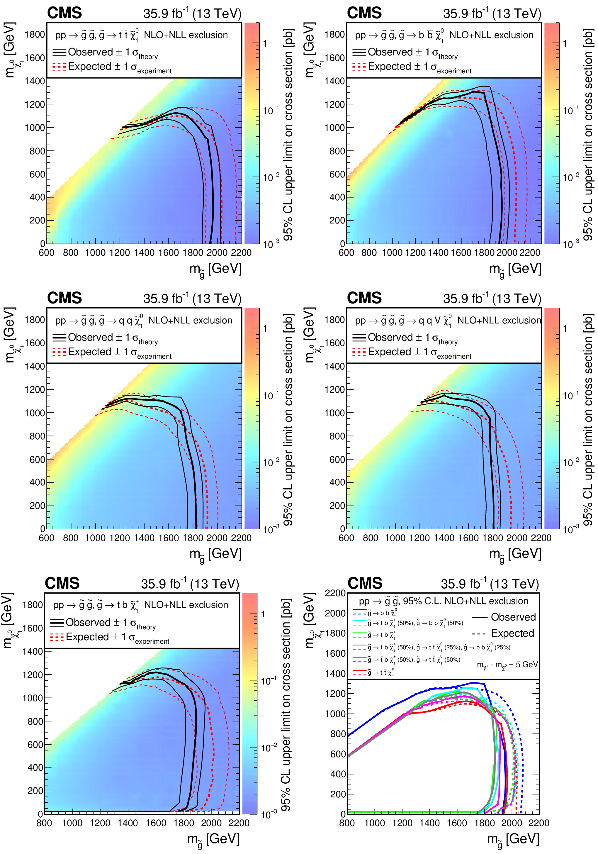
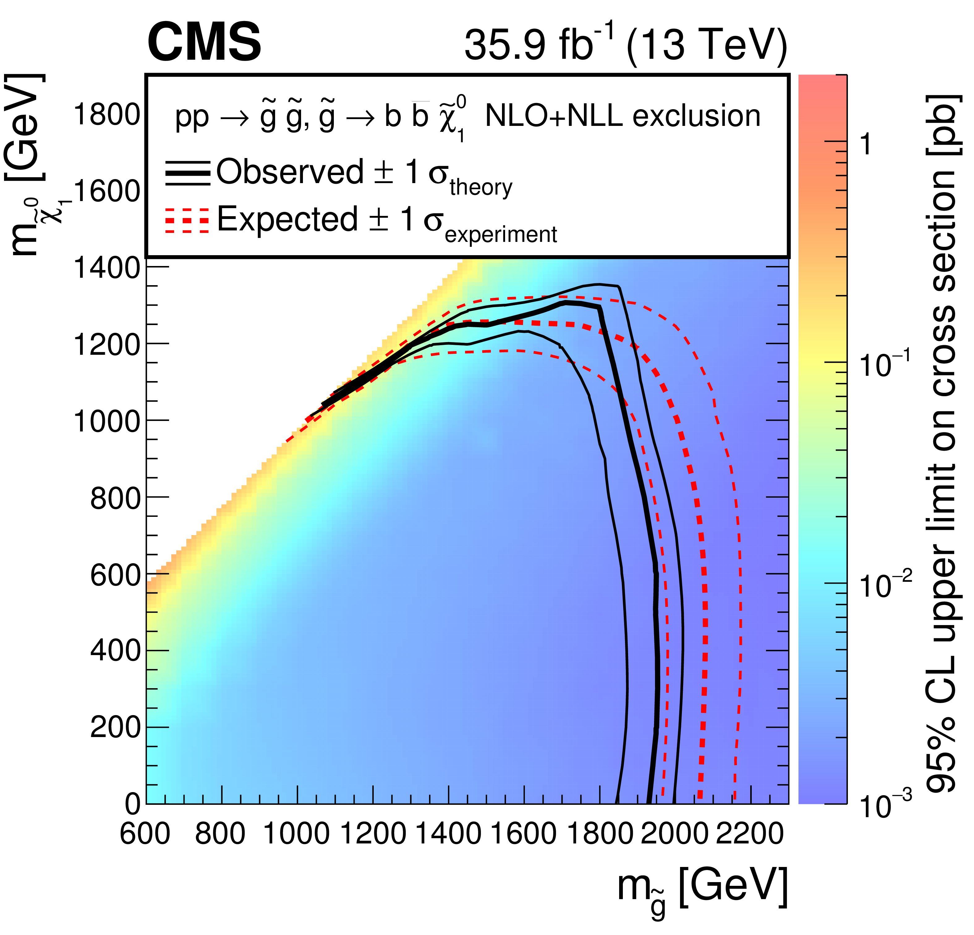
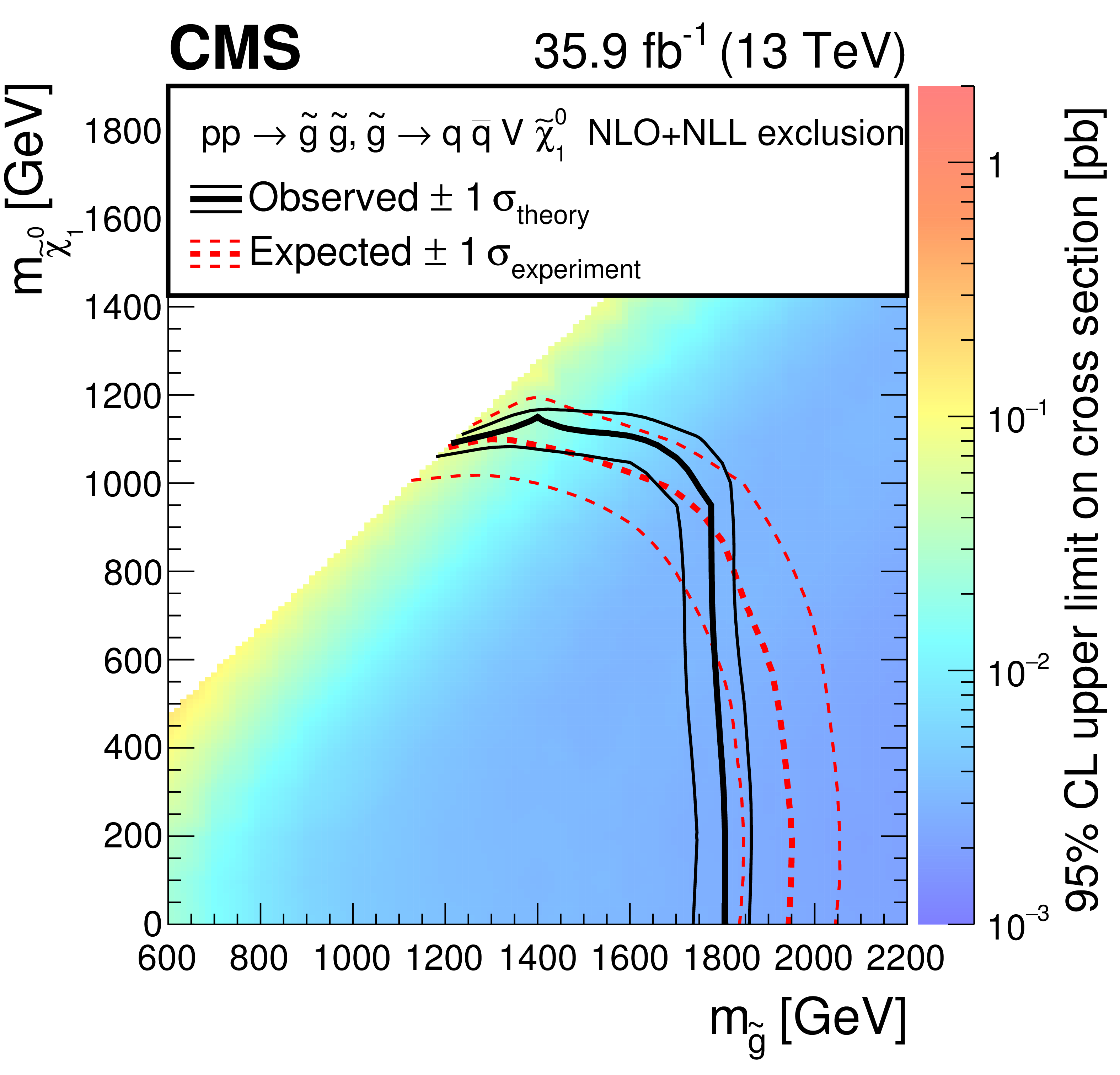
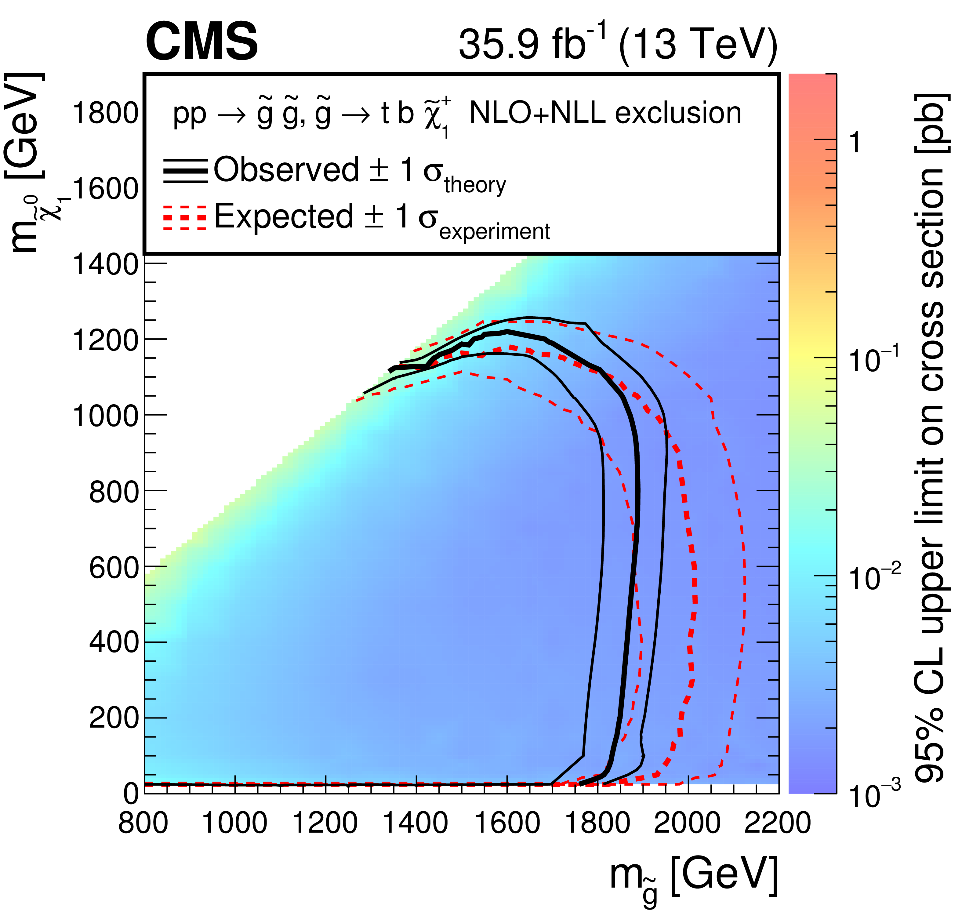
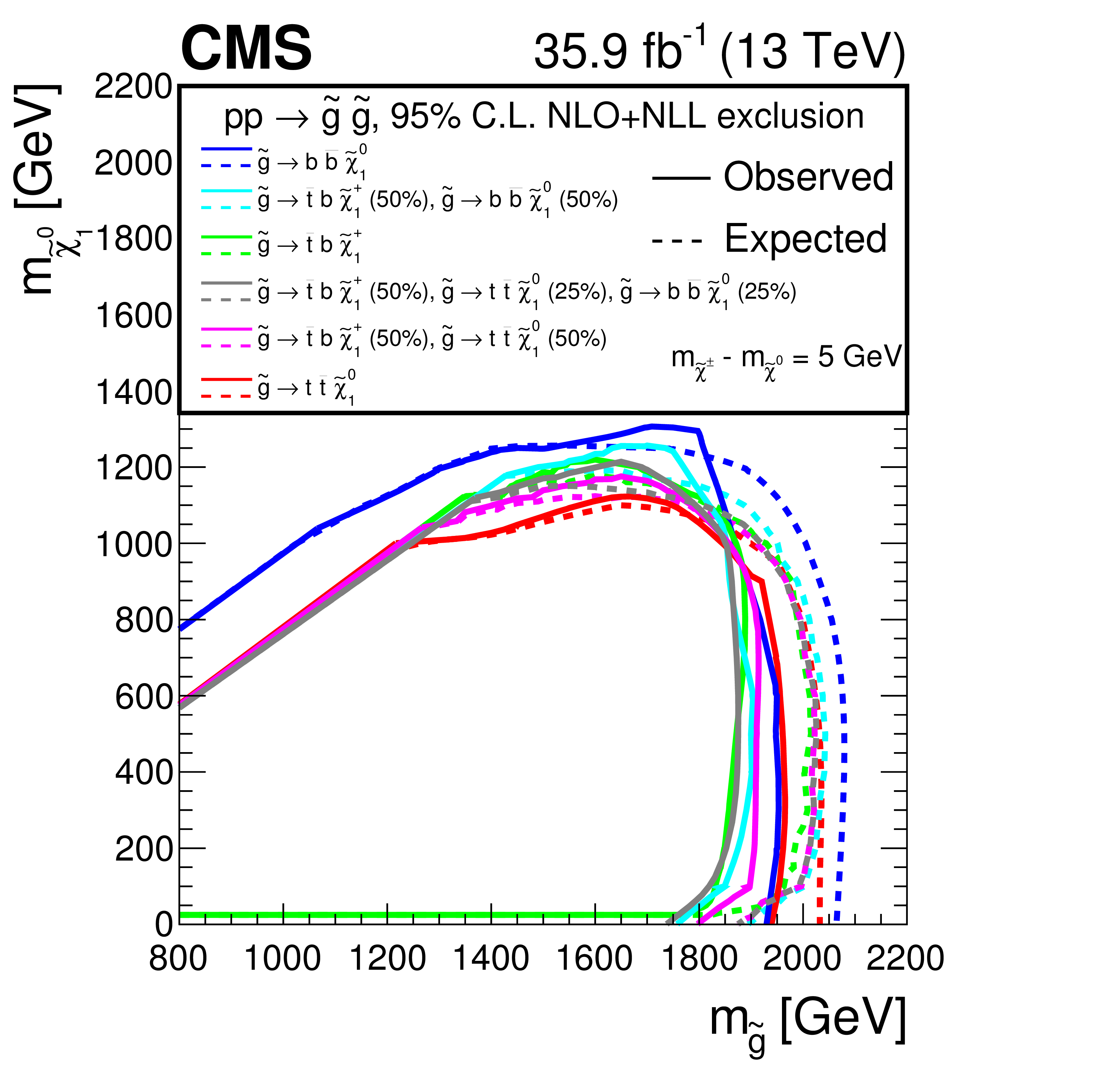
The 95% CL upper limits on the production cross sections for the (upper left) T1tttt, (upper right) T1bbbb, (middle left) T1qqqq, (middle right) T5qqqqVV, and (lower left) T1tbtb simplified models, shown as a function of the gluino and LSP masses ${m_{ \tilde{g} } }$ and ${m_{\tilde{ \chi }^0_1}}$. The solid (black) curves show the observed exclusion contours assuming the NLO+NLL cross sections [61,62,63,64,65], with the corresponding $\pm $1standard deviation uncertainties [80]. The dashed (red) curves present the expected limits with $\pm $1 standard deviation experimental uncertainties. (Lower right) The corresponding 95% NLO+NLL exclusion curves for the mixed models of gluino decays to heavy squarks. For the T1tbtb model, the results are restricted to $ {m_{\tilde{ \chi }^0_1}} >$ 25 GeV for the reason stated in the text. |
png pdf root |
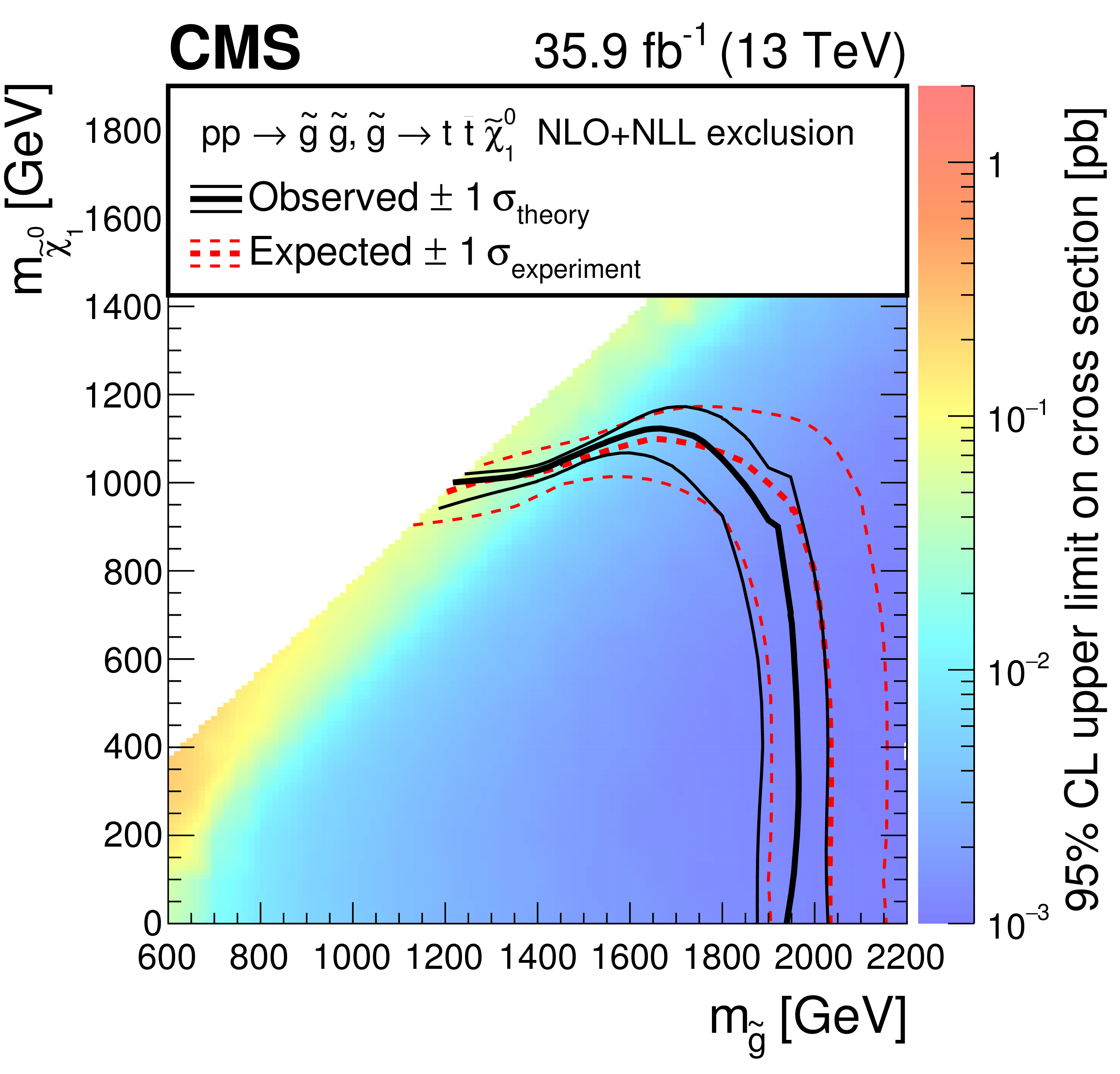
Figure 12-a:
The 95% CL upper limits on the production cross sections for the T1tttt simplified model, shown as a function of the gluino and LSP masses ${m_{ \tilde{g} } }$ and ${m_{\tilde{ \chi }^0_1}}$. The solid (black) curves show the observed exclusion contours assuming the NLO+NLL cross sections, with the corresponding $\pm $1standard deviation uncertainties. The dashed (red) curves present the expected limits with $\pm $1 standard deviation experimental uncertainties. |
png pdf root |
Figure 12-b:
The 95% CL upper limits on the production cross sections for the T1bbbb simplified model, shown as a function of the gluino and LSP masses ${m_{ \tilde{g} } }$ and ${m_{\tilde{ \chi }^0_1}}$. The solid (black) curves show the observed exclusion contours assuming the NLO+NLL cross sections, with the corresponding $\pm $1standard deviation uncertainties. The dashed (red) curves present the expected limits with $\pm $1 standard deviation experimental uncertainties. |

png pdf root |
Figure 12-c:
The 95% CL upper limits on the production cross sections for the T1qqqq simplified model, shown as a function of the gluino and LSP masses ${m_{ \tilde{g} } }$ and ${m_{\tilde{ \chi }^0_1}}$. The solid (black) curves show the observed exclusion contours assuming the NLO+NLL cross sections, with the corresponding $\pm $1standard deviation uncertainties. The dashed (red) curves present the expected limits with $\pm $1 standard deviation experimental uncertainties. |
png pdf root |
Figure 12-d:
The 95% CL upper limits on the production cross sections for the T5qqqqVV simplified model, shown as a function of the gluino and LSP masses ${m_{ \tilde{g} } }$ and ${m_{\tilde{ \chi }^0_1}}$. The solid (black) curves show the observed exclusion contours assuming the NLO+NLL cross sections, with the corresponding $\pm $1standard deviation uncertainties. The dashed (red) curves present the expected limits with $\pm $1 standard deviation experimental uncertainties. |
png pdf root |
Figure 12-e:
The 95% CL upper limits on the production cross sections for the T1tbtb simplified model, shown as a function of the gluino and LSP masses ${m_{ \tilde{g} } }$ and ${m_{\tilde{ \chi }^0_1}}$. The solid (black) curves show the observed exclusion contours assuming the NLO+NLL cross sections, with the corresponding $\pm $1standard deviation uncertainties. The dashed (red) curves present the expected limits with $\pm $1 standard deviation experimental uncertainties. The results are restricted to $ {m_{\tilde{ \chi }^0_1}} >$ 25 GeV for the reason stated in the text. |
png pdf |
Figure 12-f:
The corresponding 95% NLO+NLL exclusion curves for the mixed models of gluino decays to heavy squarks. |

png pdf |
Figure 13:
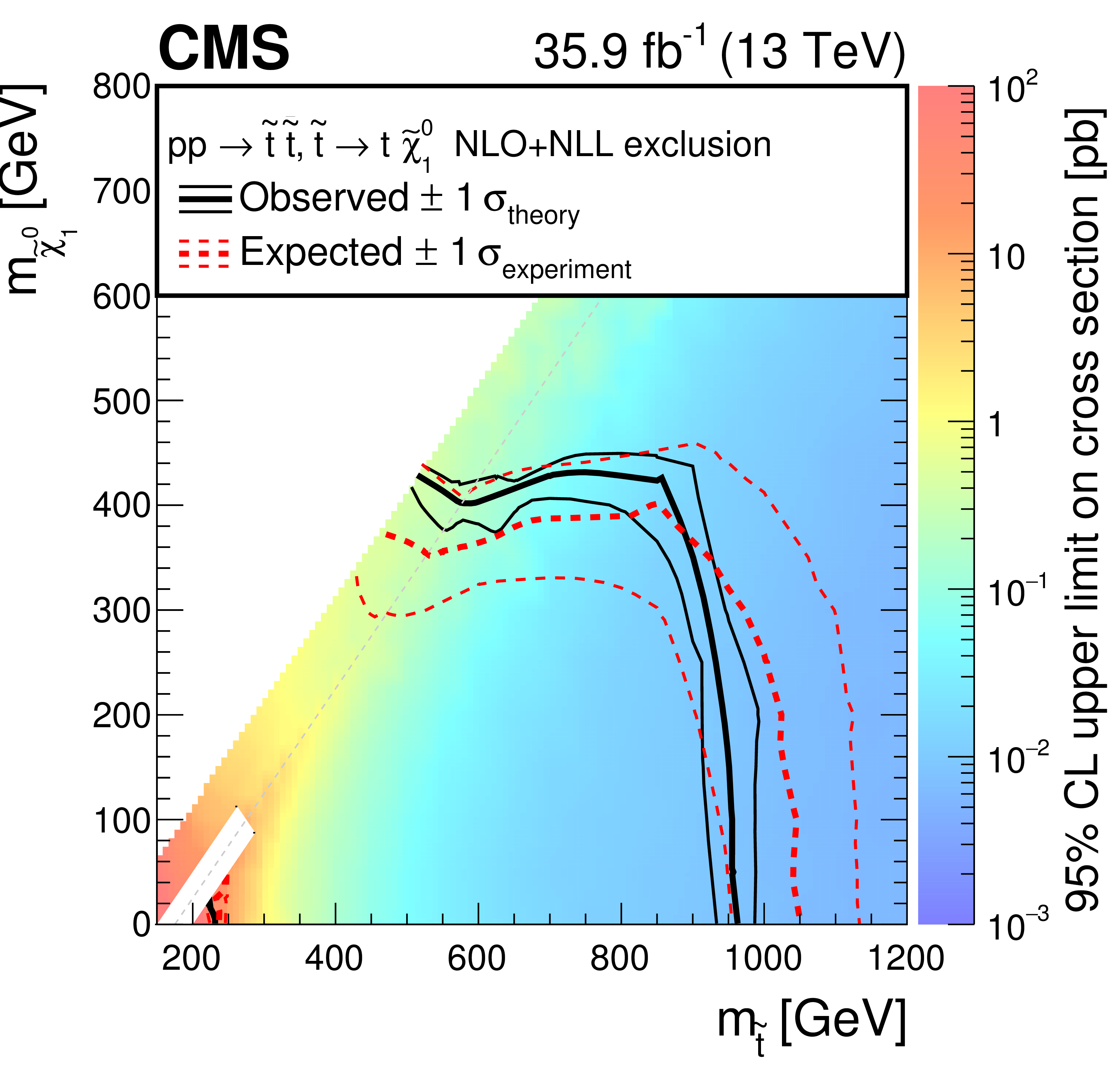
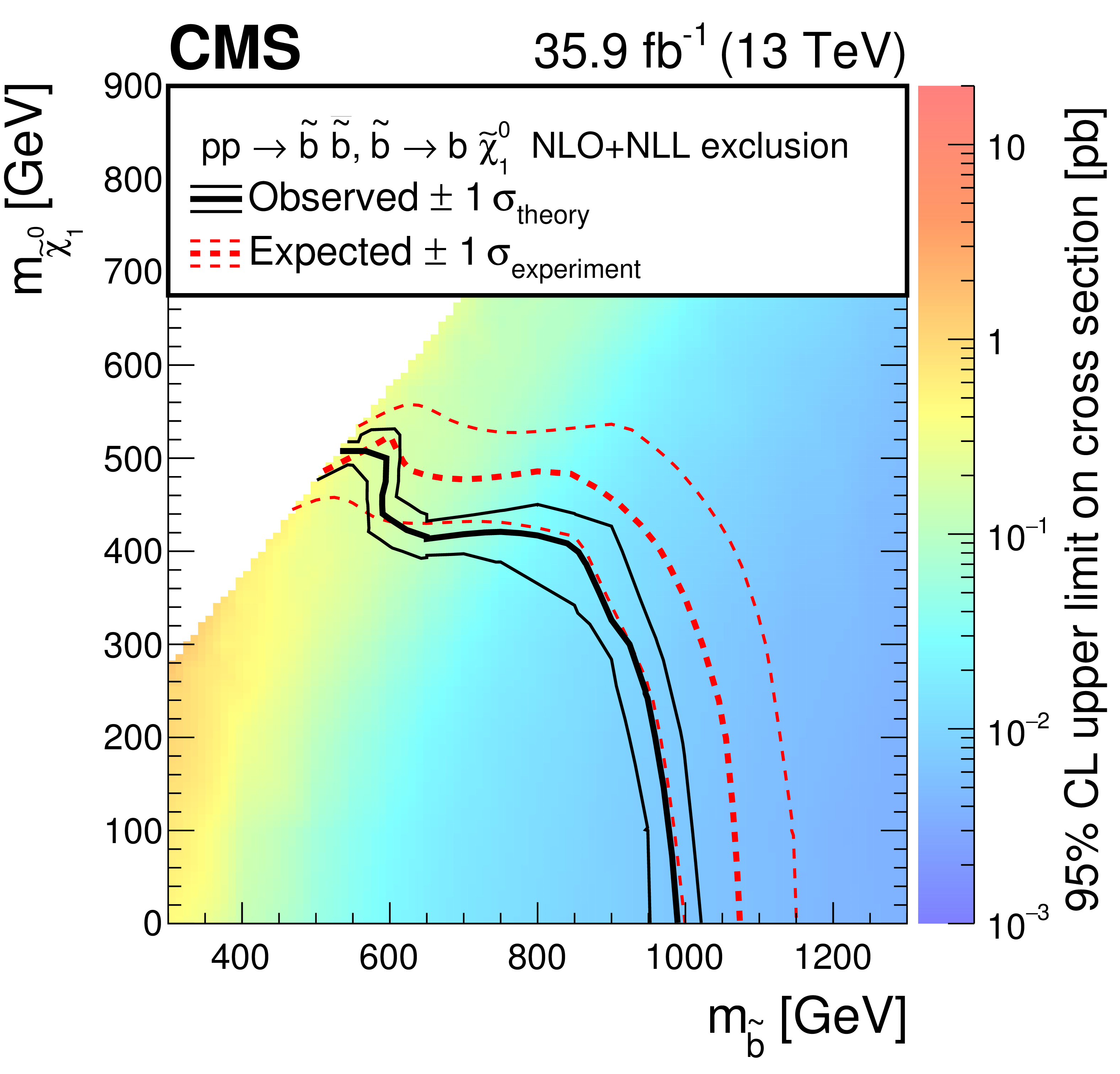
The 95% CL upper limits on the production cross section for the (upper left) T2tt, (upper right) T2bb, and (lower) T2qq simplified models, shown as a function of the squark and LSP masses ${m_{\tilde{ \mathrm{q} } }}$ and ${m_{\tilde{ \chi }^0_1}} $. The diagonal dotted line shown for the T2tt model corresponds to $ {m_{\tilde{ \mathrm{q} } }} - {m_{\tilde{ \chi }^0_1}} = {m_{\text {top}}} $. Note that for the T2tt model we do not present cross section upper limits in the unshaded diagonal region at low ${m_{\tilde{ \chi }^0_1}}$ for the reasons discussed in the text, and that there is a small region corresponding to $ {m_{\tilde{ \mathrm{ t } } }} \lesssim $ 230 GeV and $ {m_{\tilde{ \chi }^0_1}} \lesssim $ 20 GeV that is not included in the NLO+NLL exclusion region. The results labeled "one light $\tilde{ \mathrm{q} } $'' for the T2qq model are discussed in the text. The meaning of the curves is described in the Fig. 12 caption. |
png pdf root |
Figure 13-a:
The 95% CL upper limits on the production cross section for the T2tt simplified model, shown as a function of the squark and LSP masses ${m_{\tilde{ \mathrm{q} } }}$ and ${m_{\tilde{ \chi }^0_1}} $. The diagonal dotted line shown corresponds to $ {m_{\tilde{ \mathrm{q} } }} - {m_{\tilde{ \chi }^0_1}} = {m_{\text {top}}} $. Note that we do not present cross section upper limits in the unshaded diagonal region at low ${m_{\tilde{ \chi }^0_1}}$ for the reasons discussed in the text, and that there is a small region corresponding to $ {m_{\tilde{ \mathrm{ t } } }} \lesssim $ 230 GeV and $ {m_{\tilde{ \chi }^0_1}} \lesssim $ 20 GeV that is not included in the NLO+NLL exclusion region. The meaning of the curves is described in the Fig. 12 caption. |
png pdf root |
Figure 13-b:
The 95% CL upper limits on the production cross section for the T2bb simplified model, shown as a function of the squark and LSP masses ${m_{\tilde{ \mathrm{q} } }}$ and ${m_{\tilde{ \chi }^0_1}} $. The meaning of the curves is described in the Fig. 12 caption. |

png pdf root |
Figure 13-c:
The 95% CL upper limits on the production cross section for the T2qq simplified model, shown as a function of the squark and LSP masses ${m_{\tilde{ \mathrm{q} } }}$ and ${m_{\tilde{ \chi }^0_1}} $. The results labeled "one light $\tilde{ \mathrm{q} } $'' are discussed in the text. The meaning of the curves is described in the Fig. 12 caption. |
| Tables | |
png pdf |
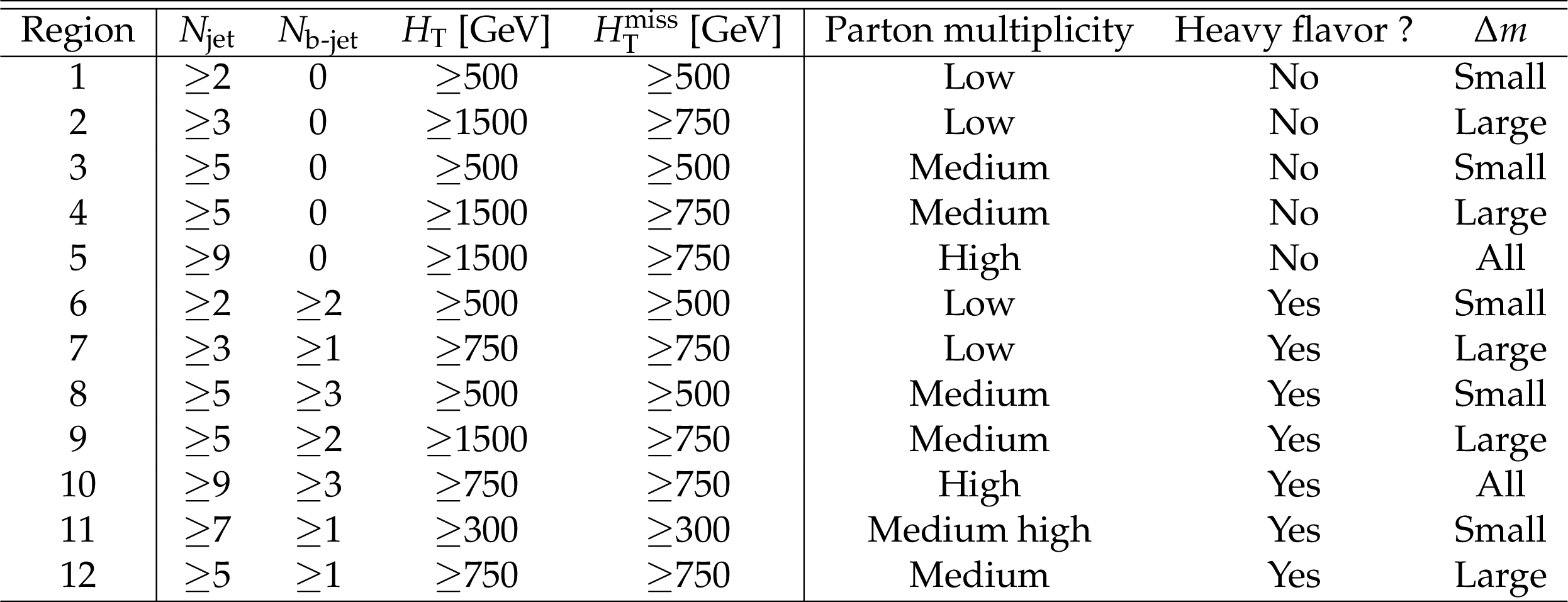
Table 1:
Definition of the search intervals in the $ {H_{\text {T}}^{\text {miss}}} $ and $ {H_{\mathrm {T}}} $ variables. Intervals 1 and 4 are discarded for $ {N_{\text {jet}}} \geq $ 7. |
png pdf |
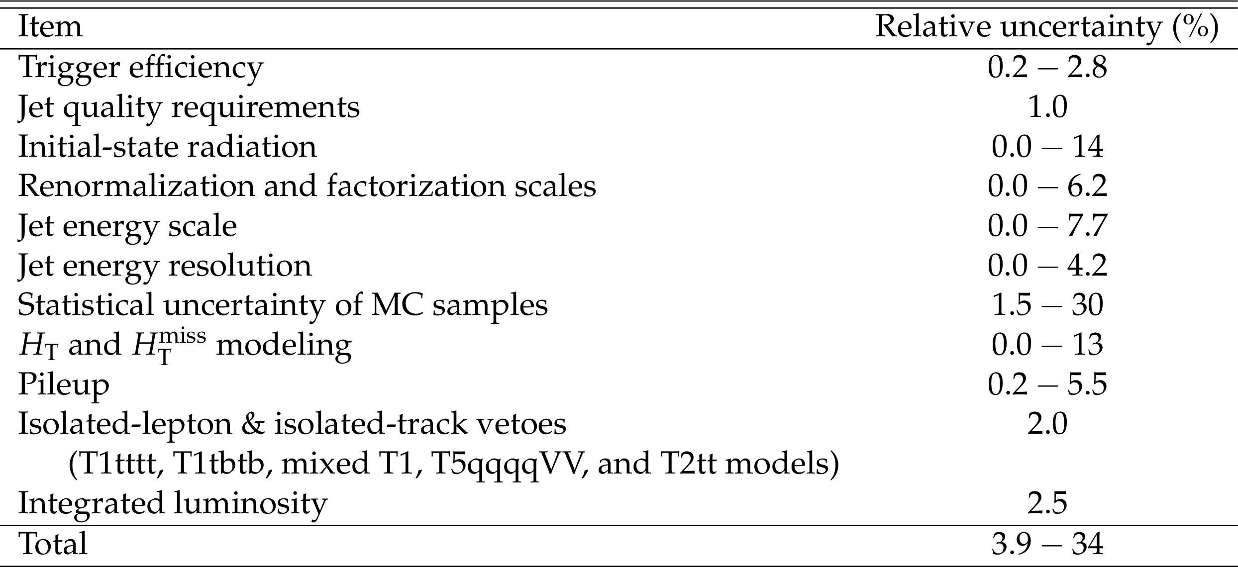
Table 2:
Systematic uncertainties in the yield of signal events, averaged over all search regions. The variations correspond to different signal models and choices for the SUSY particle masses. Results reported as 0.0 correspond to values less than 0.05%. "Mixed T1'' refers to the mixed models of gluino decays to heavy squarks described in the introduction. |
png pdf |
Table 3:
Definition of the aggregate search regions. Note that the cross-hatched region in Fig. 2, corresponding to large $ {H_{\text {T}}^{\text {miss}}} $ relative to $ {H_{\mathrm {T}}} $, is excluded from the definition of the aggregate regions. |
png pdf |
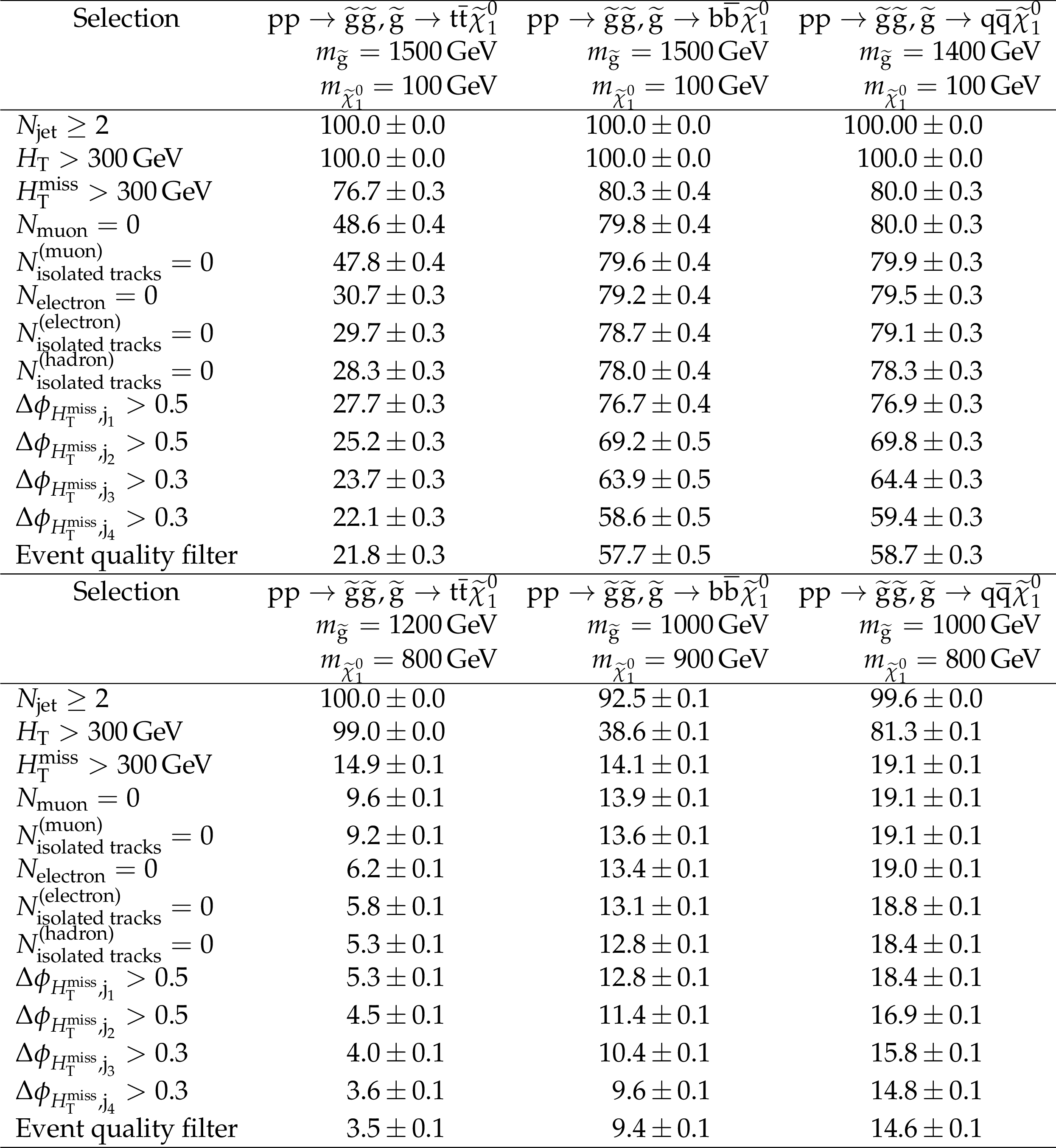
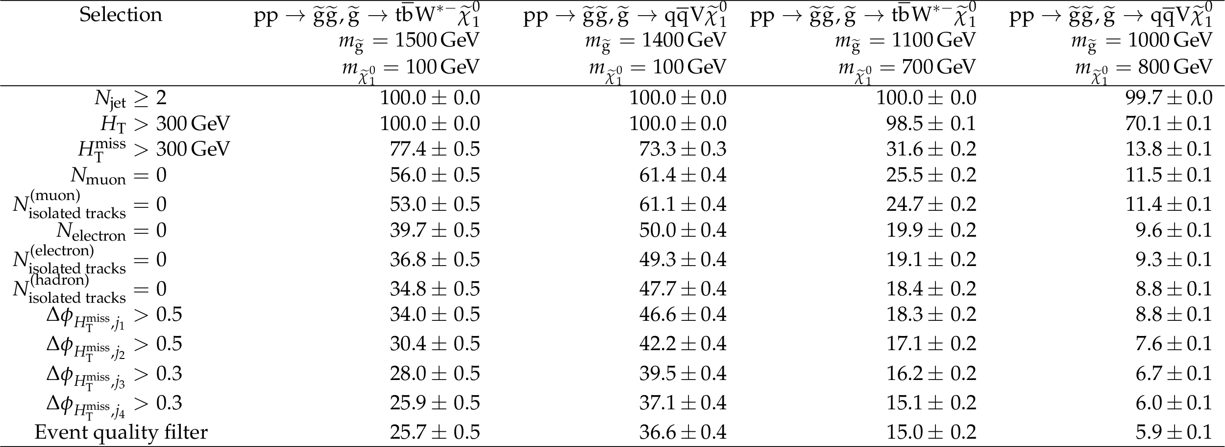
Table A1:
Absolute cumulative efficiencies in % for each step of the event selection process for representative models of gluino pair production. The uncertainties are statistical. Uncertainties reported as 0.0 correspond to values less than 0.05%. |

png pdf |
Table A2:
Absolute cumulative efficiencies in % for each step of the event selection process for representative models of squark pair production. The uncertainties are statistical. Uncertainties reported as 0.0 correspond to values less than 0.05%. |

png pdf |
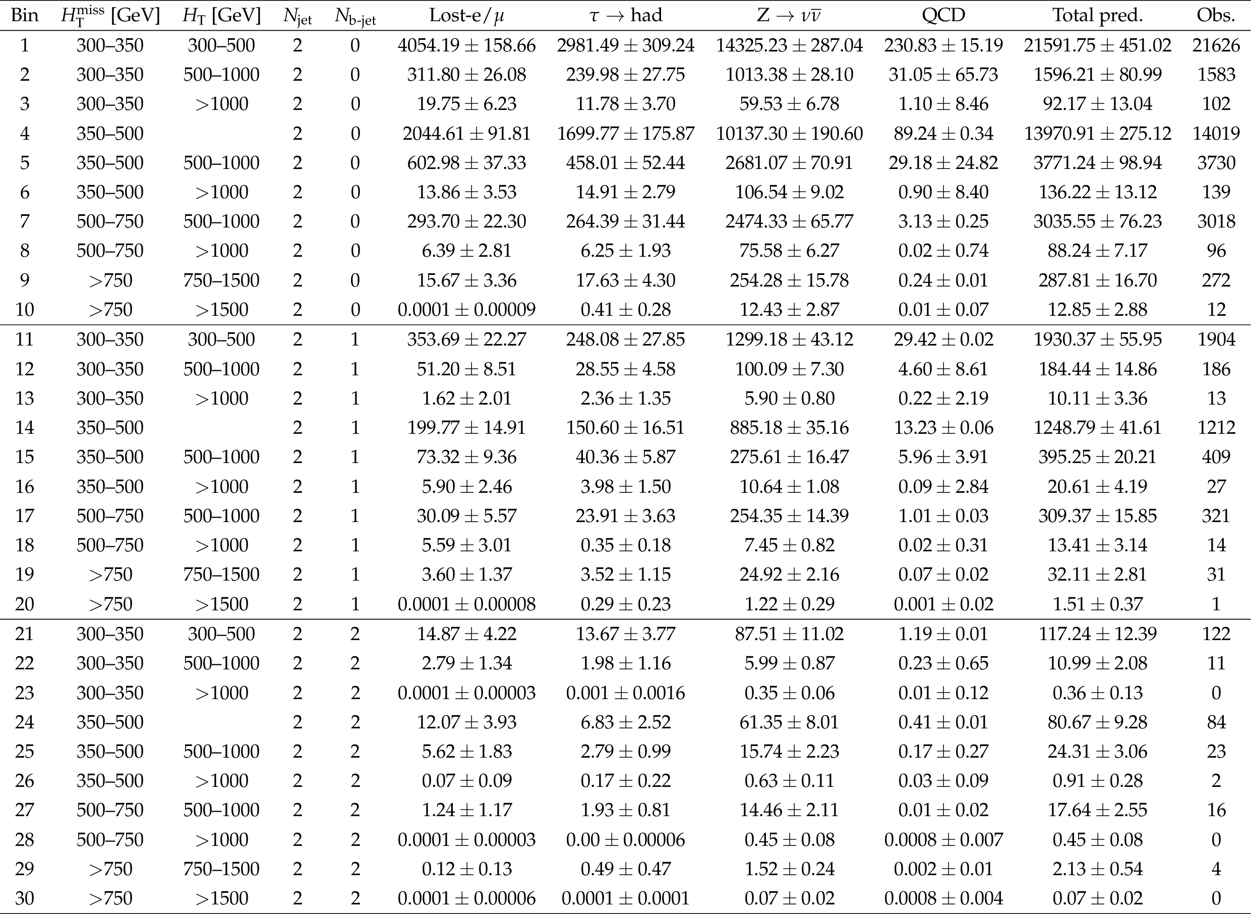
Table B1:
Observed numbers of events and prefit background predictions in the $ N_{\text{jets}} = $ 2 search regions. The first uncertainty is statistical and second systematic. |
png pdf |
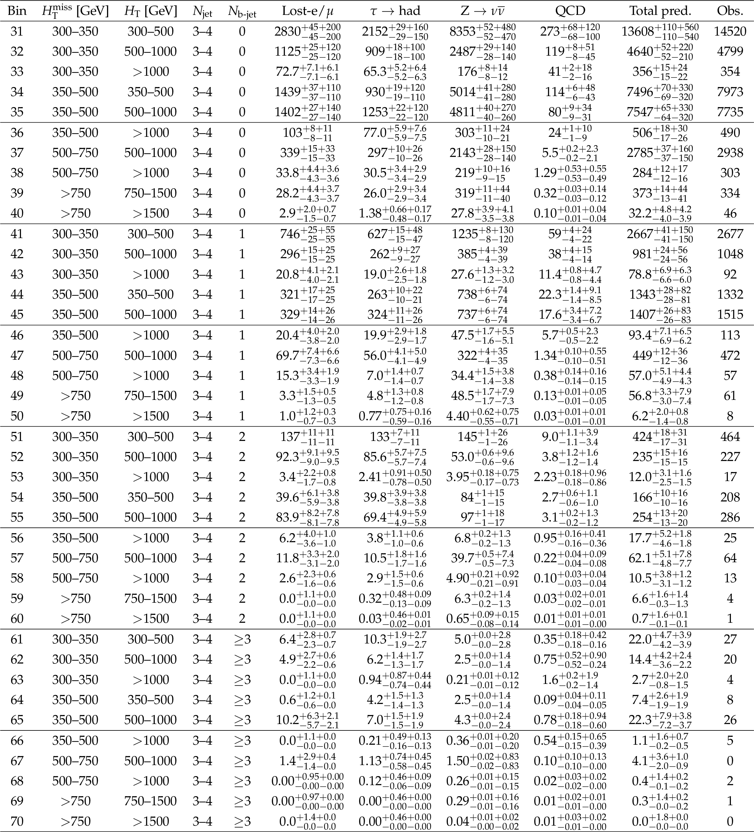
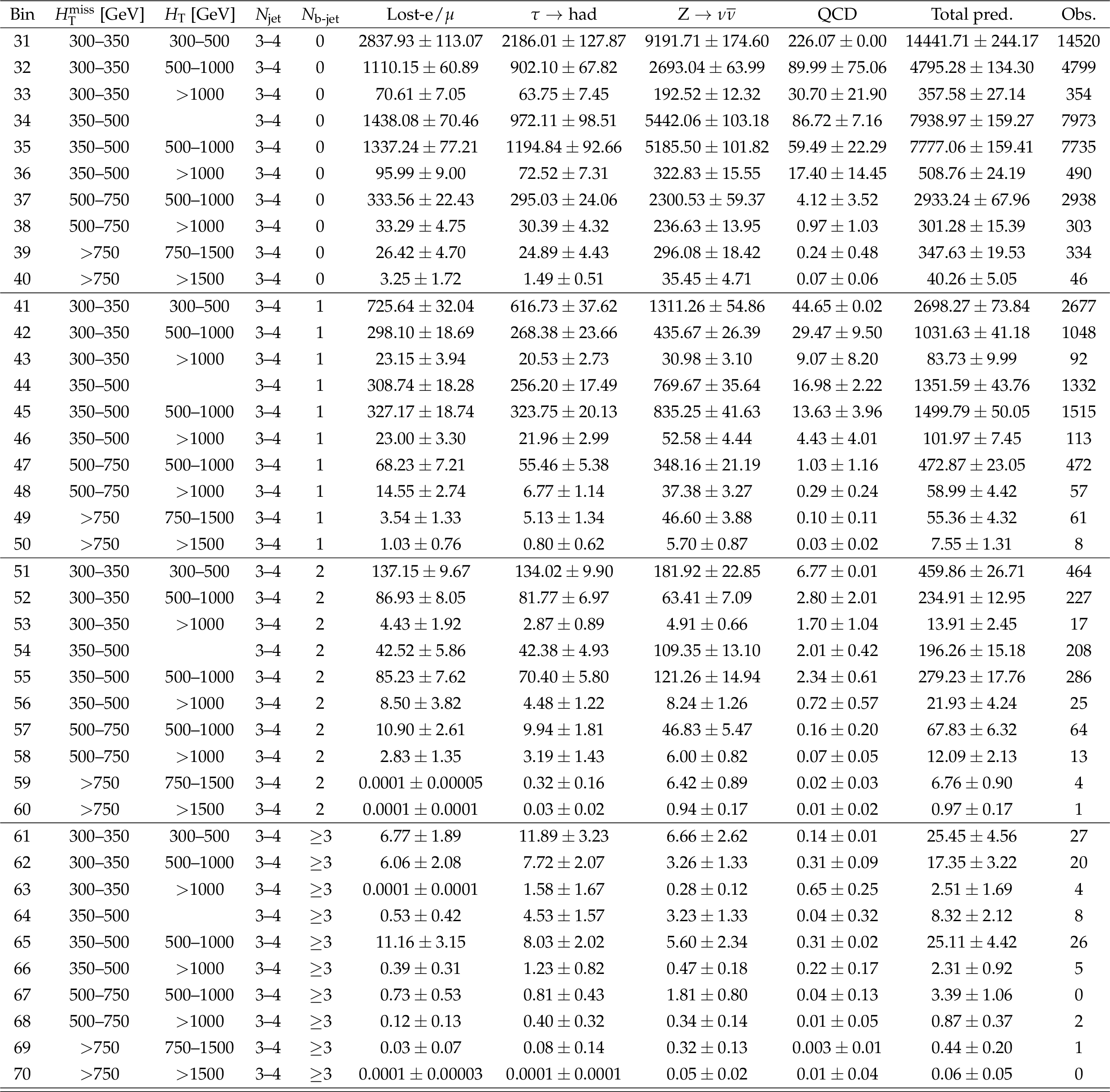
Table B2:
Observed numbers of events and prefit background predictions in the 3 $ \leq {N_{\text {jet}}} \leq $ 4 search regions. The first uncertainty is statistical and second systematic. |
png pdf |
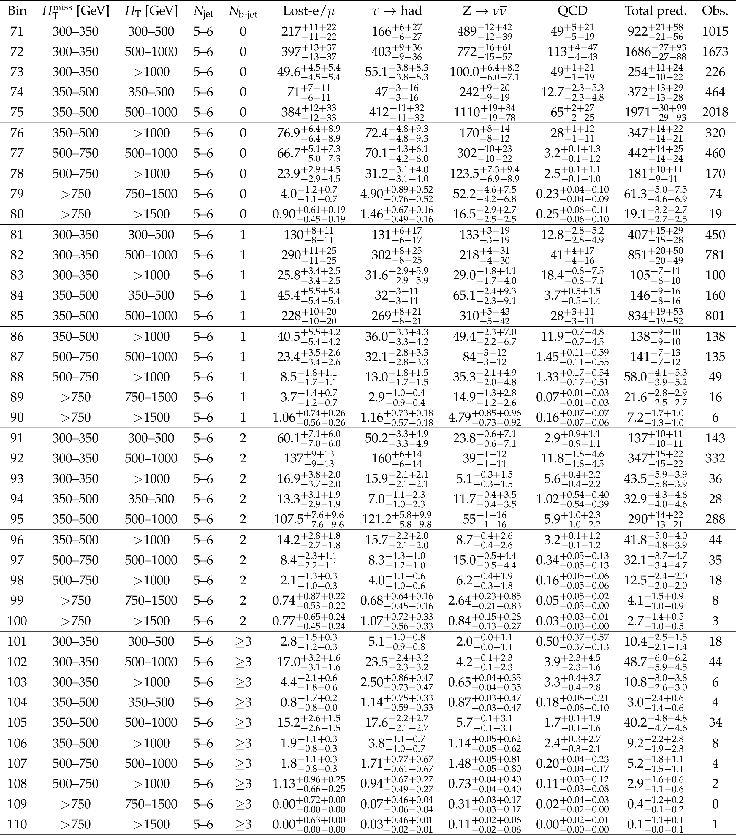
Table B3:
Observed numbers of events and prefit background predictions in the 5 $ \leq N_{\text{jets}} \leq $ 6 search regions. The first uncertainty is statistical and second systematic. |

png pdf |
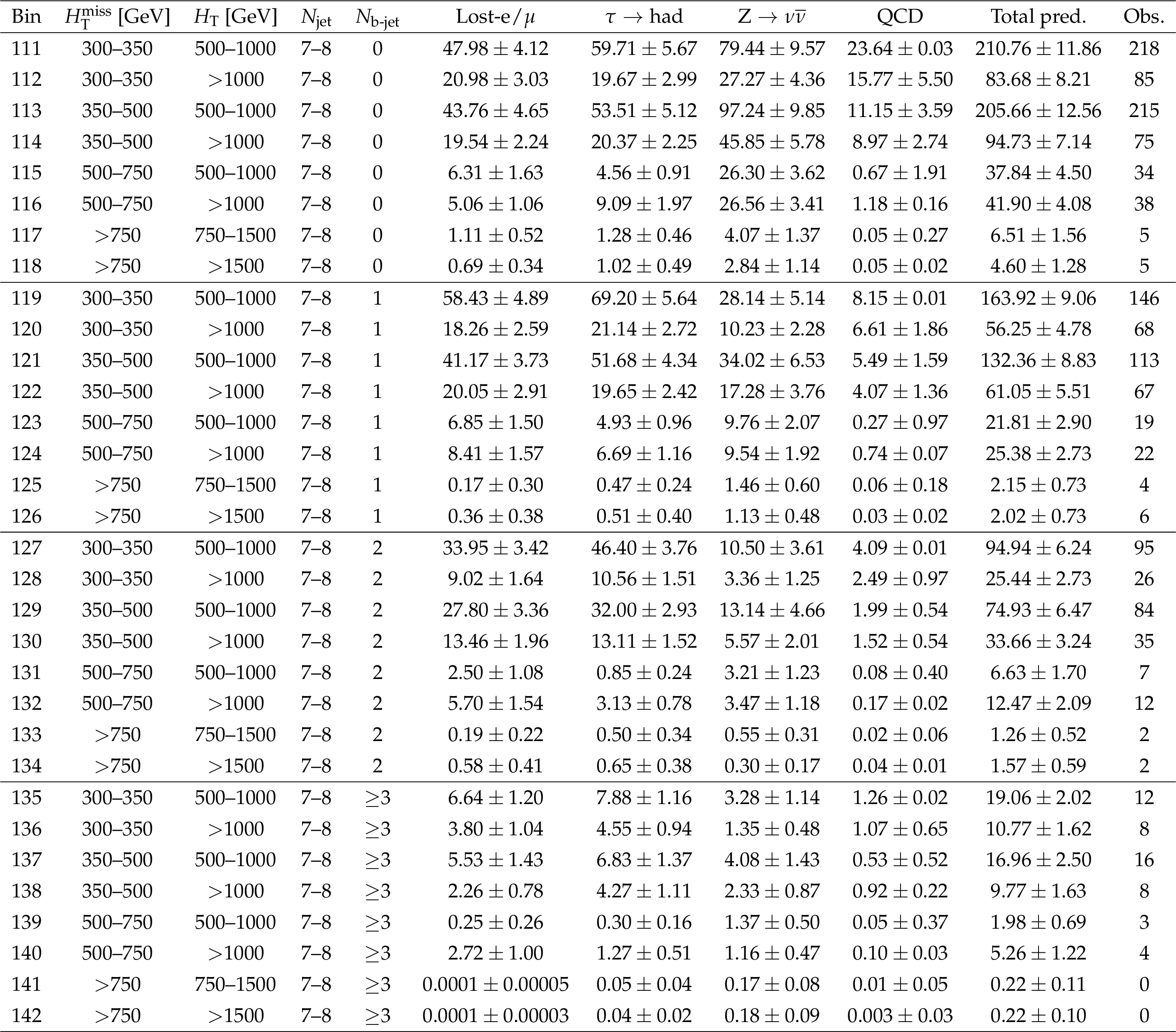
Table B4:
Observed numbers of events and prefit background predictions in the 7 $ \leq N_{\text{jets}} \leq $ 8 search regions. The first uncertainty is statistical and second systematic. |
png pdf |
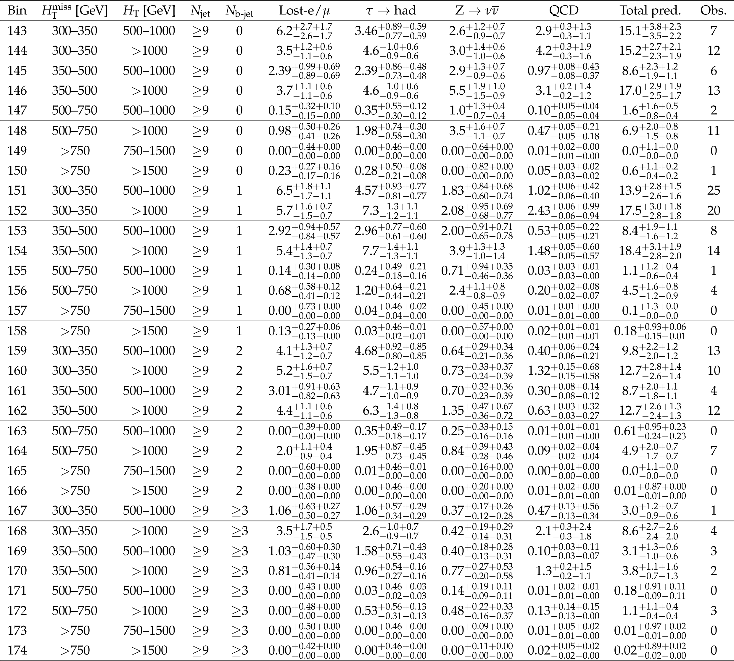
Table B5:
Observed numbers of events and prefit background predictions in the $ N_{\text{jets}} \geq $ 9 search regions. The first uncertainty is statistical and second systematic. |
png pdf |
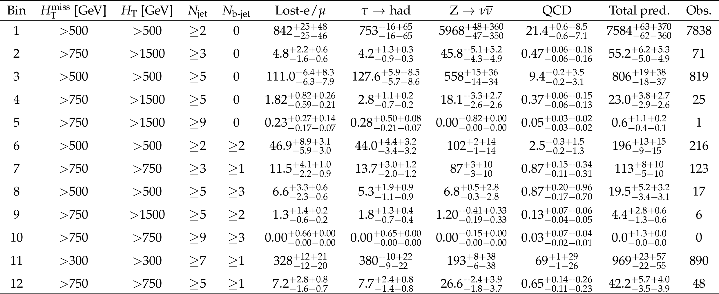
Table B6:
Observed numbers of events and prefit background predictions in the aggregate search regions. The first uncertainty is statistical and second systematic. |
| Summary |
|
A search for gluino and squark pair production is presented based on a sample of proton-proton collisions collected at a center-of-mass energy of 13 TeV with the CMS detector. The search is performed in the multijet channel, i.e., the visible reconstructed final state consists solely of jets. The data correspond to an integrated luminosity of 35.9 fb$^{-1}$. Events are required to have at least two jets, $H_{\mathrm{T}}> $ 300 GeV, and ${H_{\text{T}}^{\text{miss}}} > $ 300 GeV, where $H_{\mathrm{T}}$ is the scalar sum of jet transverse momenta $ p_{\mathrm{T}} $. The ${H_{\text{T}}^{\text{miss}}} $ variable, used as a measure of missing transverse momentum, is the magnitude of the vector $ p_{\mathrm{T}}$ sum of jets. Jets are required to have $p_{\mathrm{T}}> $ 30 GeV and to appear in the pseudorapidity range $| \eta | < $ 2.4. The data are examined in 174 exclusive four-dimensional search regions defined by the number of jets, the number of tagged bottom quark jets, $ H_{\mathrm{T}} $, and ${H_{\text{T}}^{\text{miss}}} $. Background from standard model processes is evaluated using control samples in the data. We also provide results for 12 aggregated search regions, to simplify use of our data by others. The estimates of the standard model background are found to agree with the observed numbers of events for all regions. The results are interpreted in the context of simplified models. We consider models in which pair-produced gluinos each decay to a $\mathrm{ t \bar{t} }$ pair and an undetected, stable, lightest-supersymmetric-particle (LSP) neutralino ${\tilde{\chi}^0_1}$ (T1tttt model); to a $\mathrm{ b \bar{b} }$ pair and the ${\tilde{\chi}^0_1}$ (T1bbbb model); to a light-flavored $ \mathrm{ q \bar{q} } $ pair and the ${\tilde{\chi}^0_1}$ (T1qqqq model); to a light-flavored quark and antiquark and either the second-lightest neutralino $ \tilde{ \chi }^0_2 $ or the lightest chargino $\tilde{ \chi }^{\pm}_1$, followed by decay of the $ \tilde{ \chi }^0_2 $ ($\tilde{ \chi }^{\pm}_1$) to the $\tilde{\chi}^0_1$ and an on- or off-shell ${\mathrm{ Z }}$ ({$\mathrm{ W }^\pm$}) boson (T5qqqqVV model); or to $\mathrm{ \bar{t} }\mathrm{ b }\tilde{ \chi }^{+}_1$ or $\mathrm{ t }\mathrm{ \bar{b} }\tilde{ \chi }^{-}_1$, followed by the decay of the $\tilde{ \chi }^{\pm}_1$ to the ${\tilde{\chi}^0_1}$ and an off-shell W boson (T1tbtb model). To provide more model independence, we also consider mixed scenarios in which a gluino can decay to $\mathrm{ t \bar{t} }\tilde{\chi}^0_1$, $\mathrm{ b \bar{b} }\tilde{\chi}^0_1$, $\mathrm{ \bar{t} }\mathrm{ b }\tilde{ \chi }^{+}_1$, or $\mathrm{ t }\mathrm{ \bar{b} }\tilde{ \chi }^{-}_1$ with various probabilities. Beyond the models for gluino production, we examine models for direct squark pair production. We consider scenarios in which each squark decays to a top quark and the ${\tilde{\chi}^0_1}$ (T2tt model); to a bottom quark and the ${\tilde{\chi}^0_1}$ (T2bb model); or to a light-flavored (u, d, s, c) quark and the ${\tilde{\chi}^0_1}$ (T2qq model). We derive upper limits at 95% confidence level on the model cross sections as a function of the gluino and LSP masses, or of the squark and LSP masses. Using the predicted cross sections with next-to-leading-order plus next-to-leading-logarithm accuracy as a reference, 95% confidence level lower limits on the gluino mass as large as 1800 to 1960 GeV are derived, depending on the scenario. The corresponding limits on the mass of directly produced squarks range from 960 to 1390 GeV. These results extend those from previous searches. |
| Additional Figures | |
png pdf |
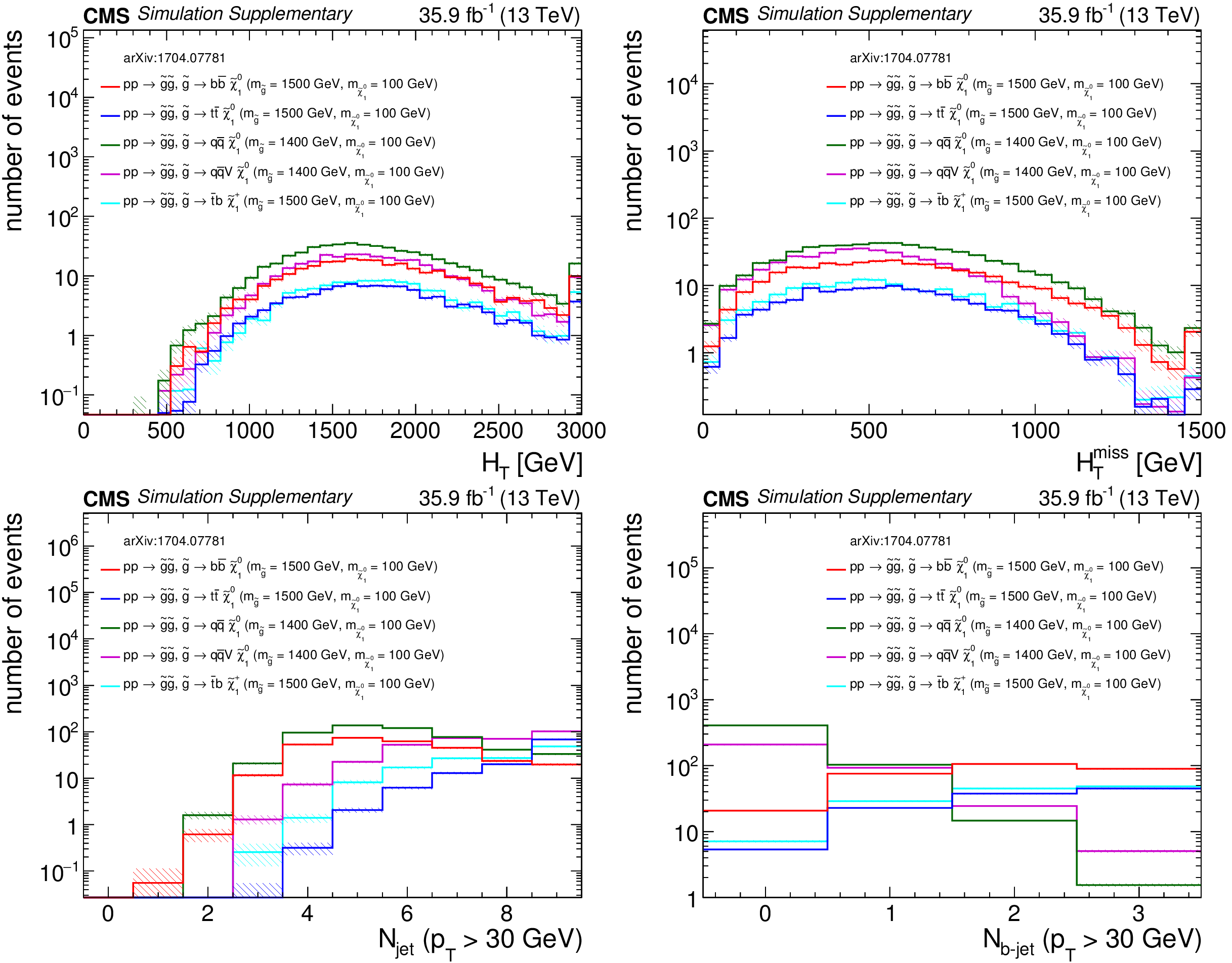
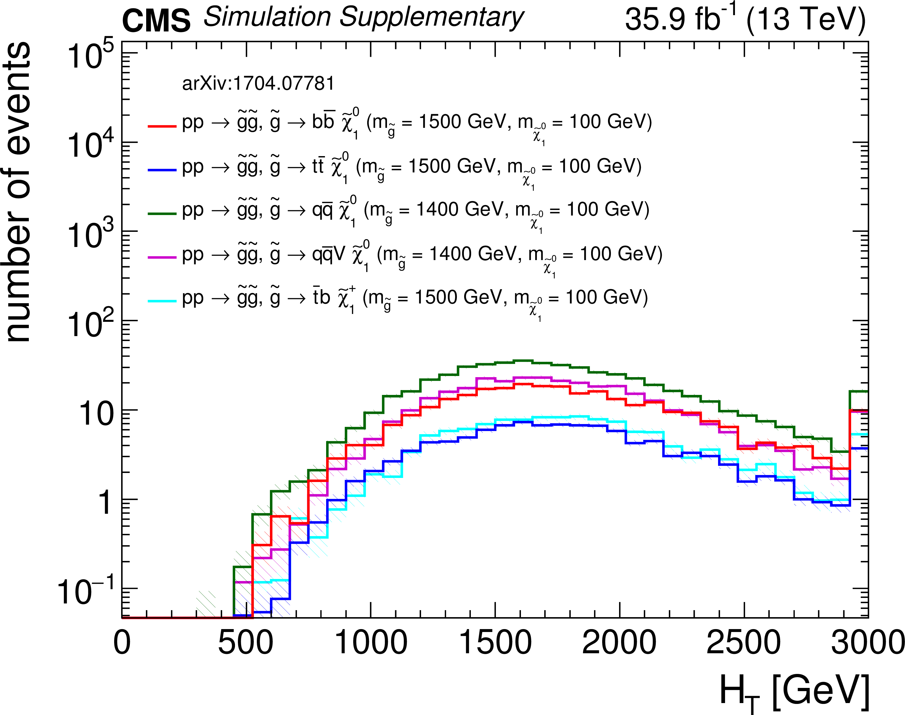
Additional Figure 1:
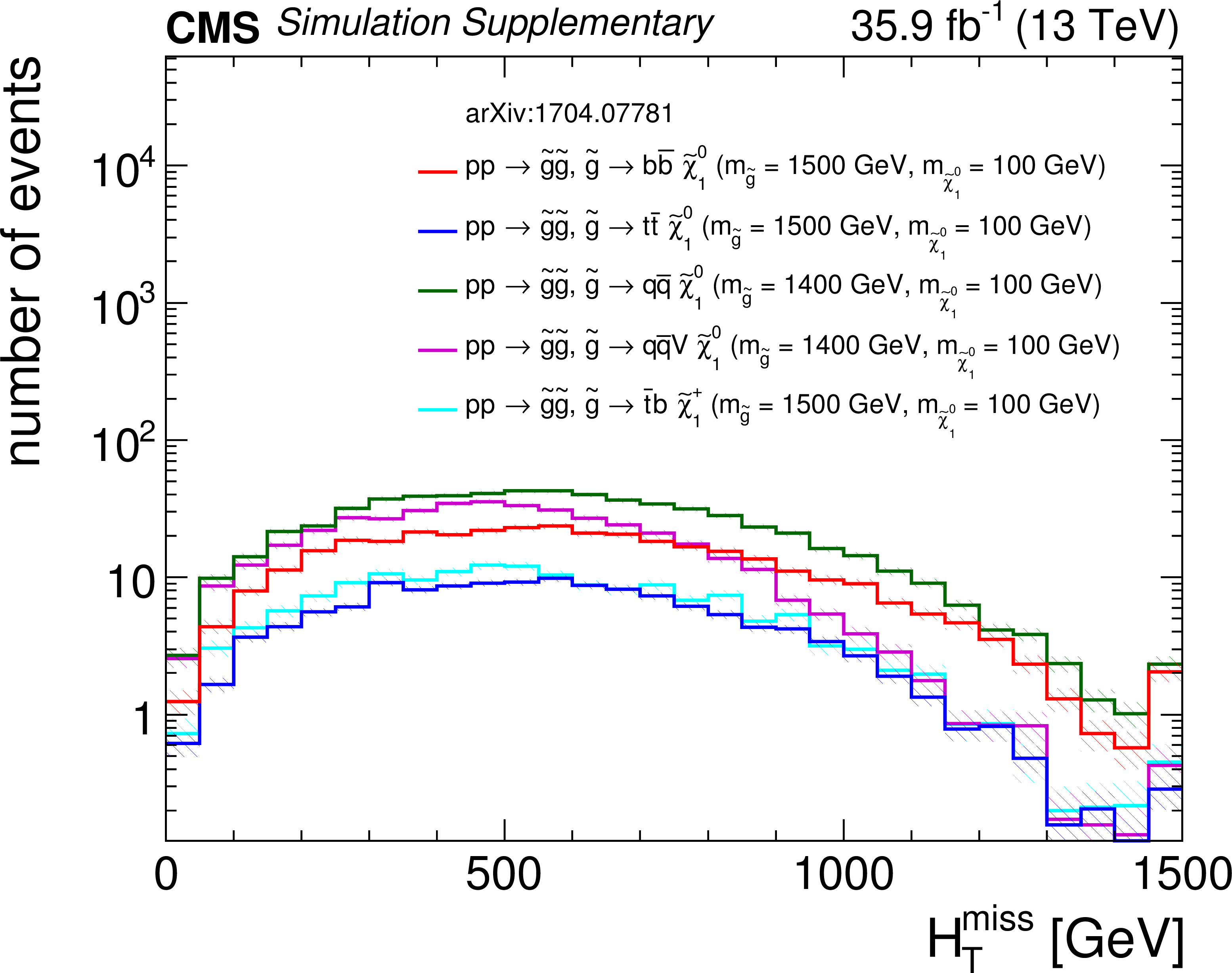
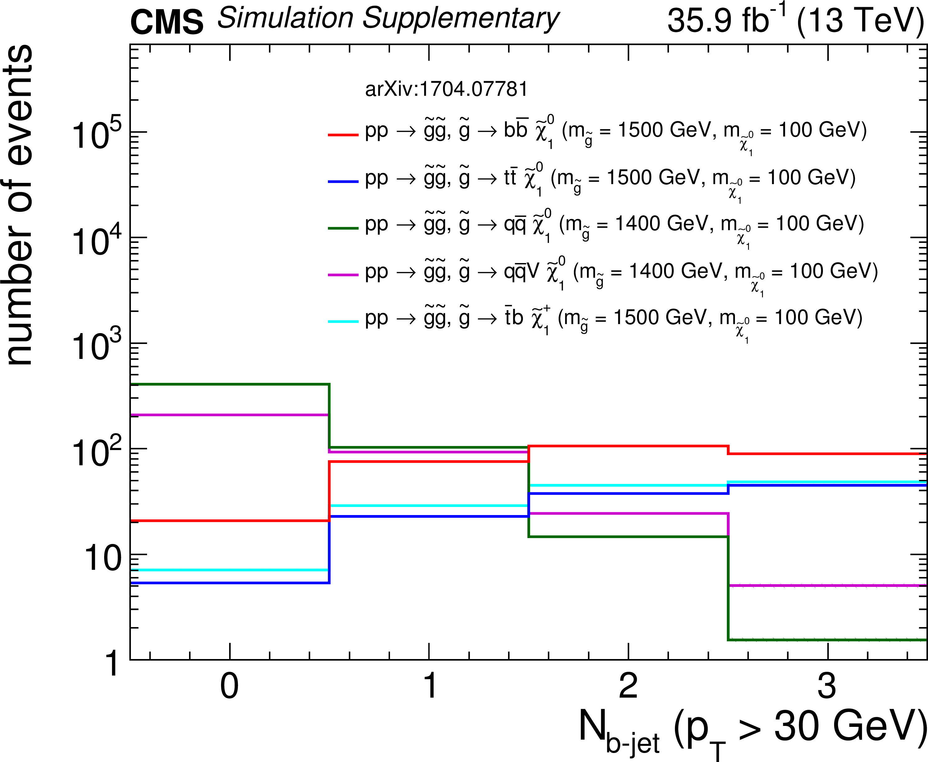
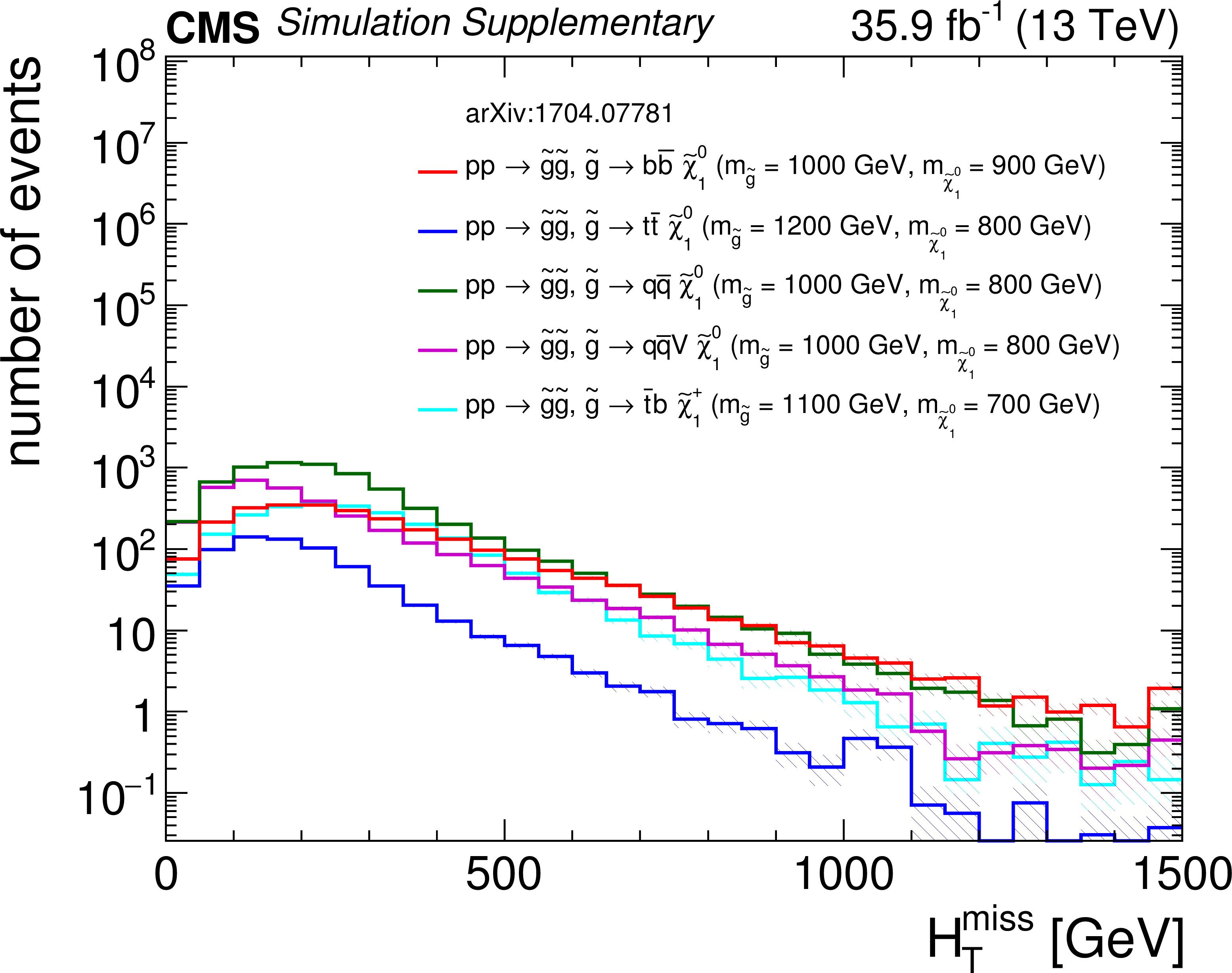
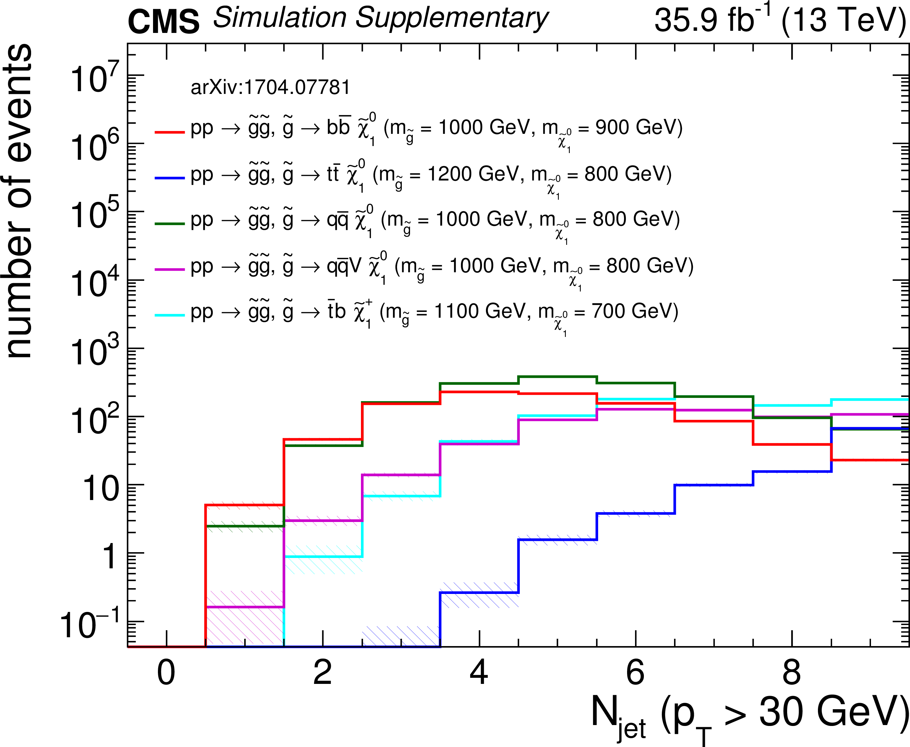
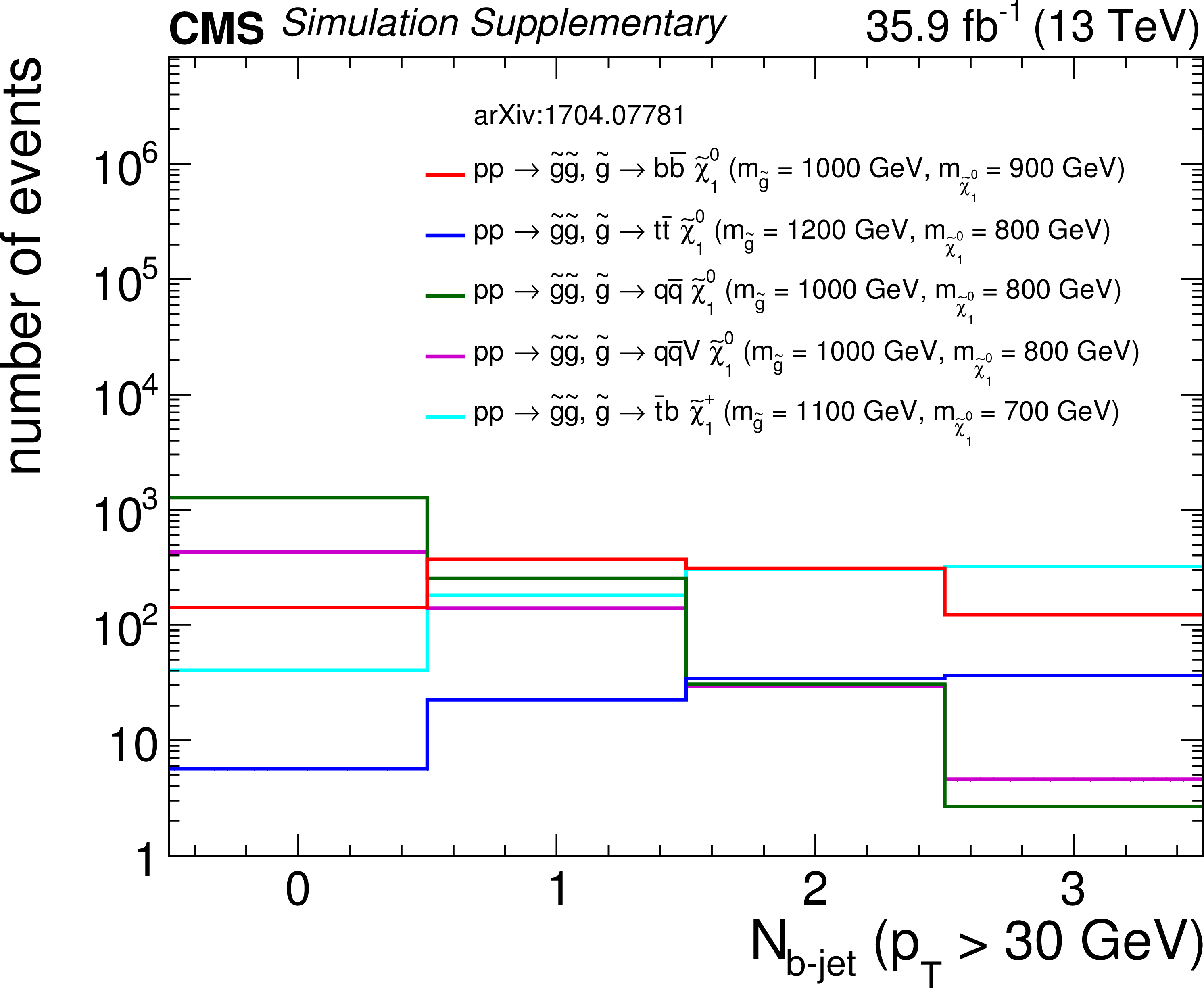
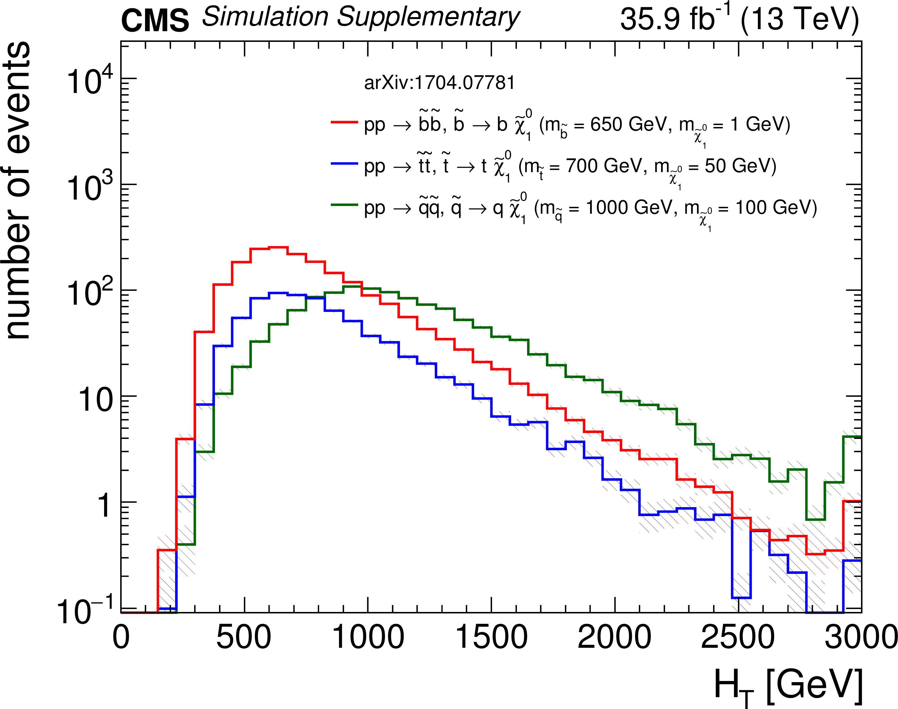
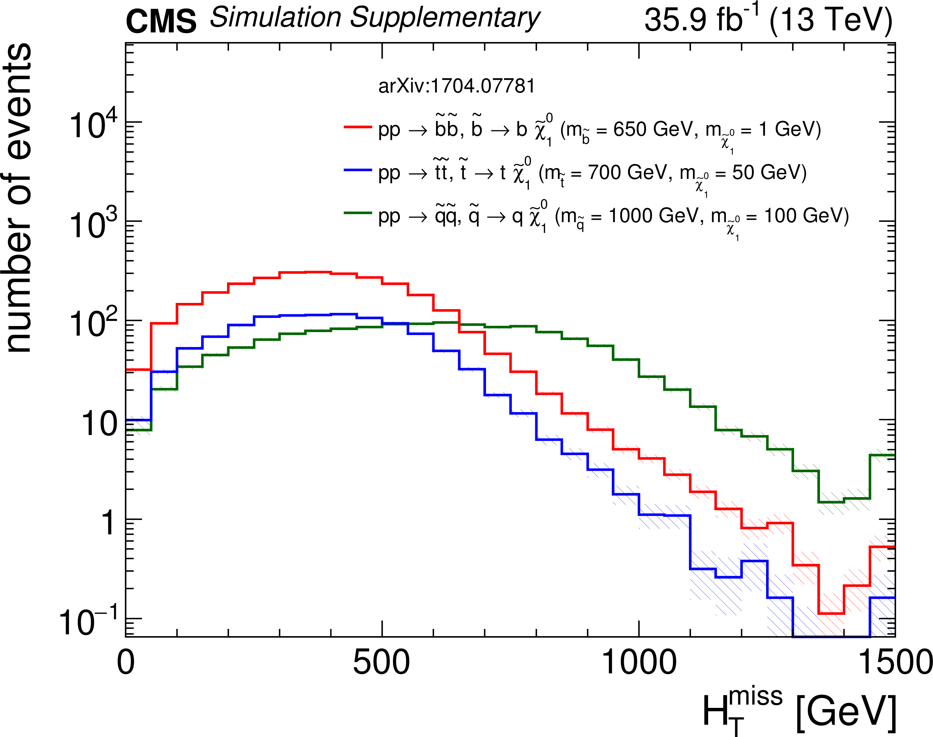
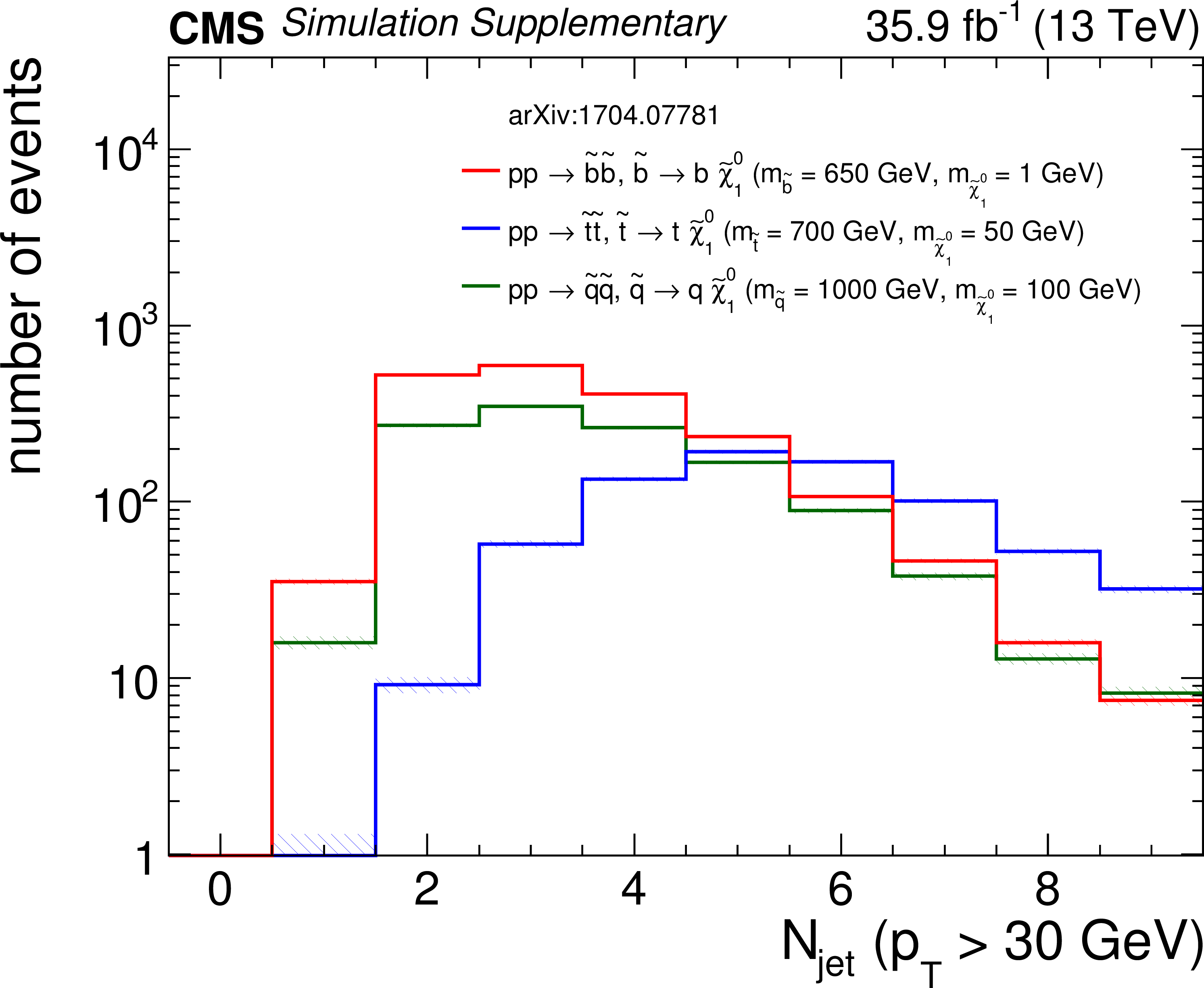
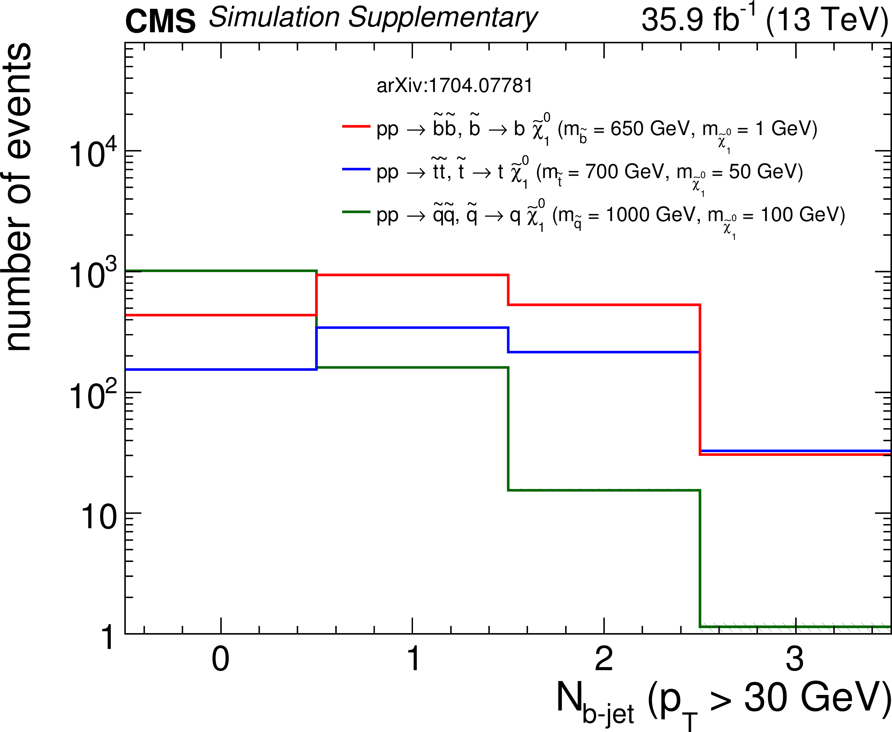
Distributions of (a) $H_{\rm T}$, (b) $H_{\rm T}^{\rm miss}$, (c) the number of jets, and (d) the number of b-tagged jets from five representative gluino pair production signal models with ${m_{\tilde{ \mathrm{g} } } \gg m_{\tilde{\chi}^0_1 }}$ after the baseline selection. Each plot ignores the baseline requirement (if any) for its respective variable. The last bin in each plot contains the overflow events. Only statistical uncertainties are shown. |
png pdf root |
Additional Figure 1-a:
Distribution of $H_{\rm T}$ from five representative gluino pair production signal models with ${m_{\tilde{ \mathrm{g} } } \gg m_{\tilde{\chi}^0_1 }}$ after the baseline selection. Each plot ignores the baseline requirement (if any) for its respective variable. The last bin contains the overflow events. Only statistical uncertainties are shown. |
png pdf root |
Additional Figure 1-b:
Distribution of $H_{\rm T}^{\rm miss}$ from five representative gluino pair production signal models with ${m_{\tilde{ \mathrm{g} } } \gg m_{\tilde{\chi}^0_1 }}$ after the baseline selection. Each plot ignores the baseline requirement (if any) for its respective variable. The last bin contains the overflow events. Only statistical uncertainties are shown. |

png pdf root |
Additional Figure 1-c:
Distribution of the number of jets from five representative gluino pair production signal models with ${m_{\tilde{ \mathrm{g} } } \gg m_{\tilde{\chi}^0_1 }}$ after the baseline selection. Each plot ignores the baseline requirement (if any) for its respective variable. The last bin contains the overflow events. Only statistical uncertainties are shown. |
png pdf root |
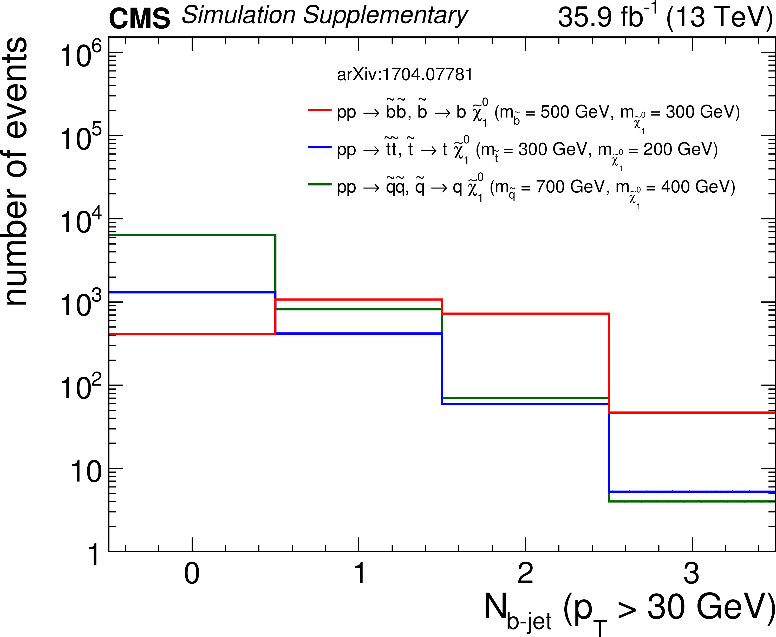
Additional Figure 1-d:
Distributions of the number of b-tagged jets from five representative gluino pair production signal models with ${m_{\tilde{ \mathrm{g} } } \gg m_{\tilde{\chi}^0_1 }}$ after the baseline selection. Each plot ignores the baseline requirement (if any) for its respective variable. The last bin contains the overflow events. Only statistical uncertainties are shown. |
png pdf |
Additional Figure 2:
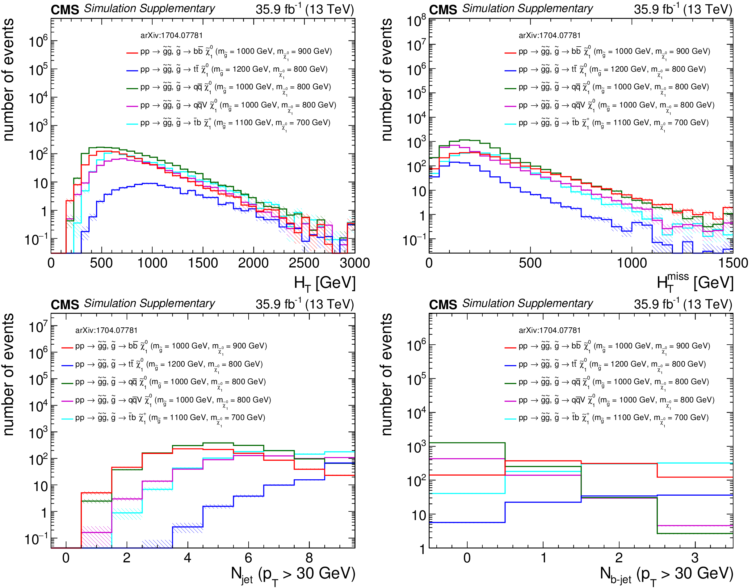
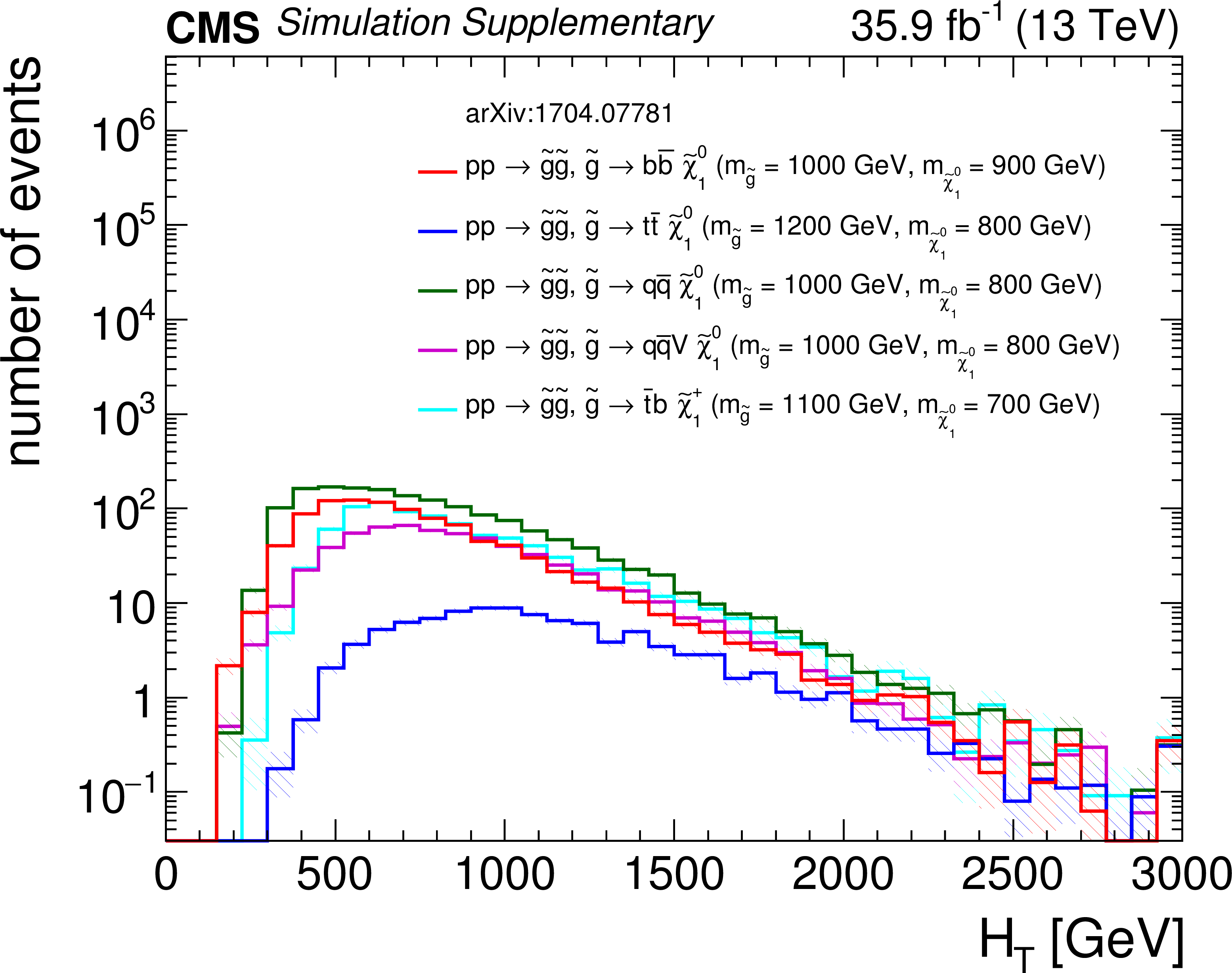
Distributions of (a) $H_{\rm T}$, (b) $H_{\rm T}^{\rm miss}$, (c) the number of jets, and (d) the number of b-tagged jets from five representative gluino pair production signal models with ${m_{\tilde{ \mathrm{g} } } \sim m_{\tilde{\chi}^0_1 }}$ after the baseline selection. Each plot ignores the baseline requirement (if any) for its respective variable. The last bin in each plot contains the overflow events. Only statistical uncertainties are shown. |
png pdf root |
Additional Figure 2-a:
Distribution of $H_{\rm T}$ from five representative gluino pair production signal models with ${m_{\tilde{ \mathrm{g} } } \sim m_{\tilde{\chi}^0_1 }}$ after the baseline selection. Each plot ignores the baseline requirement (if any) for its respective variable. The last bin contains the overflow events. Only statistical uncertainties are shown. |
png pdf root |
Additional Figure 2-b:
Distribution of $H_{\rm T}^{\rm miss}$ from five representative gluino pair production signal models with ${m_{\tilde{ \mathrm{g} } } \sim m_{\tilde{\chi}^0_1 }}$ after the baseline selection. Each plot ignores the baseline requirement (if any) for its respective variable. The last bin contains the overflow events. Only statistical uncertainties are shown. |
png pdf root |
Additional Figure 2-c:
Distribution of the number of jets from five representative gluino pair production signal models with ${m_{\tilde{ \mathrm{g} } } \sim m_{\tilde{\chi}^0_1 }}$ after the baseline selection. Each plot ignores the baseline requirement (if any) for its respective variable. The last bin contains the overflow events. Only statistical uncertainties are shown. |
png pdf root |
Additional Figure 2-d:
Distribution of the number of b-tagged jets from five representative gluino pair production signal models with ${m_{\tilde{ \mathrm{g} } } \sim m_{\tilde{\chi}^0_1 }}$ after the baseline selection. Each plot ignores the baseline requirement (if any) for its respective variable. The last bin contains the overflow events. Only statistical uncertainties are shown. |
png pdf |
Additional Figure 3:
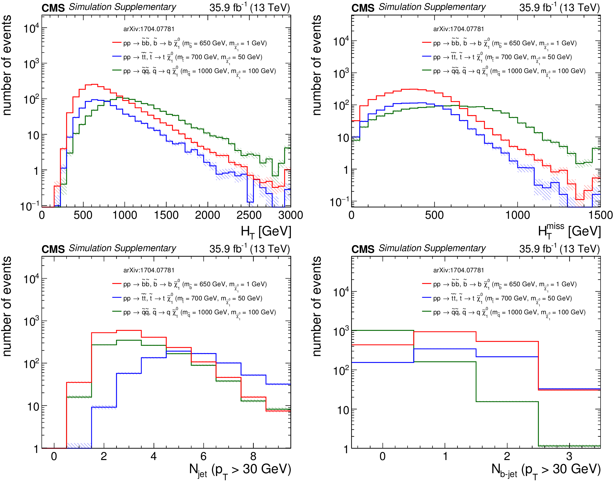
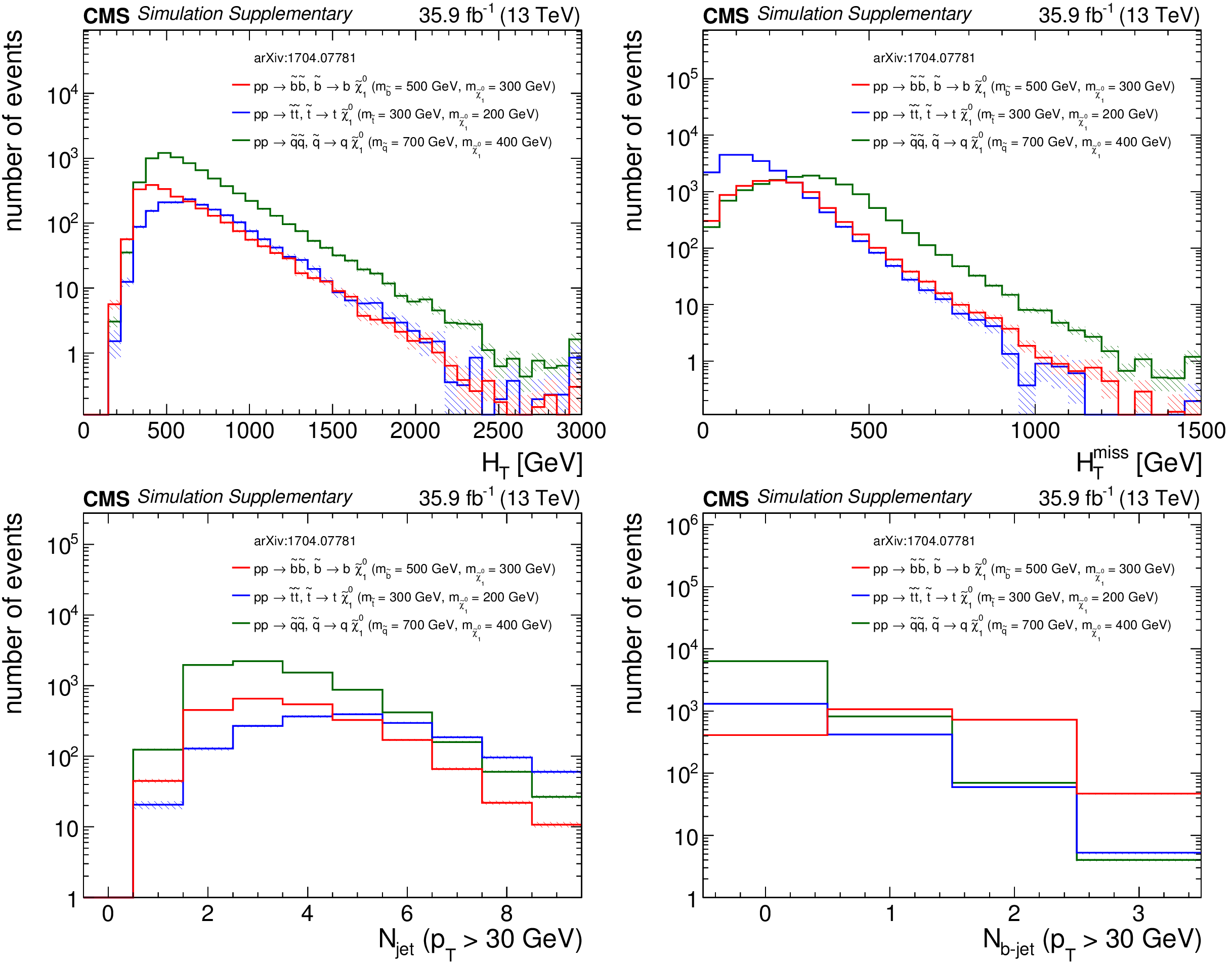
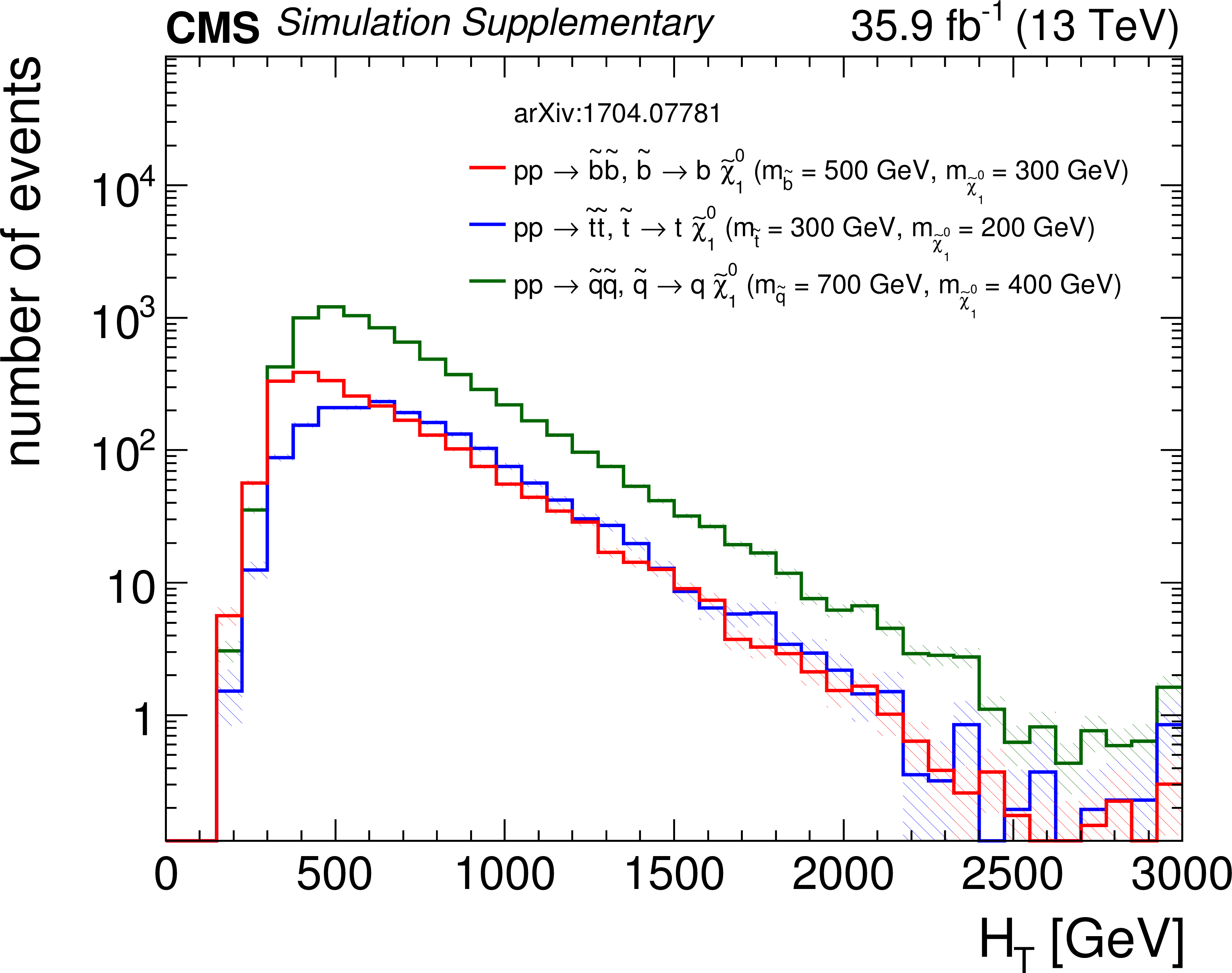
Distributions of (a) $H_{\rm T}$, (b) $H_{\rm T}^{\rm miss}$, (c) the number of jets, and (d) the number of b-tagged jets from three representative squark pair production signal models with ${m_{\tilde{ \mathrm{q} } } \gg m_{\tilde{\chi}^0_1 }}$ after the baseline selection. Each plot ignores the baseline requirement (if any) for its respective variable. The last bin in each plot contains the overflow events. Only statistical uncertainties are shown. |
png pdf root |
Additional Figure 3-a:
Distribution of $H_{\rm T}$ from three representative squark pair production signal models with ${m_{\tilde{ \mathrm{q} } } \gg m_{\tilde{\chi}^0_1 }}$ after the baseline selection. The plot ignores the baseline requirement. The last bin contains the overflow events. Only statistical uncertainties are shown. |
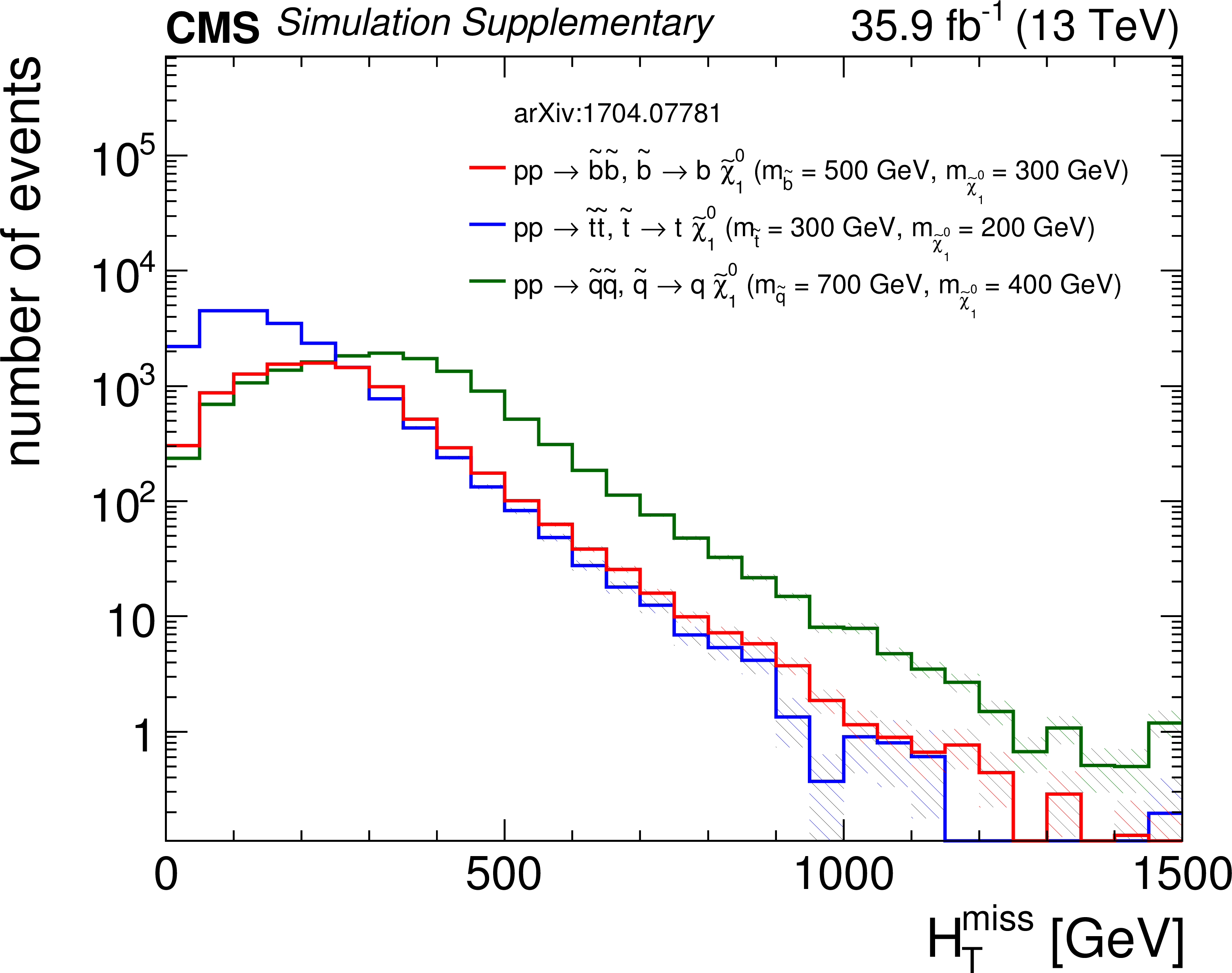
png pdf root |
Additional Figure 3-b:
Distribution of $H_{\rm T}^{\rm miss}$ from three representative squark pair production signal models with ${m_{\tilde{ \mathrm{q} } } \gg m_{\tilde{\chi}^0_1 }}$ after the baseline selection. The plot ignores the baseline requirement. The last bin contains the overflow events. Only statistical uncertainties are shown. |
png pdf root |
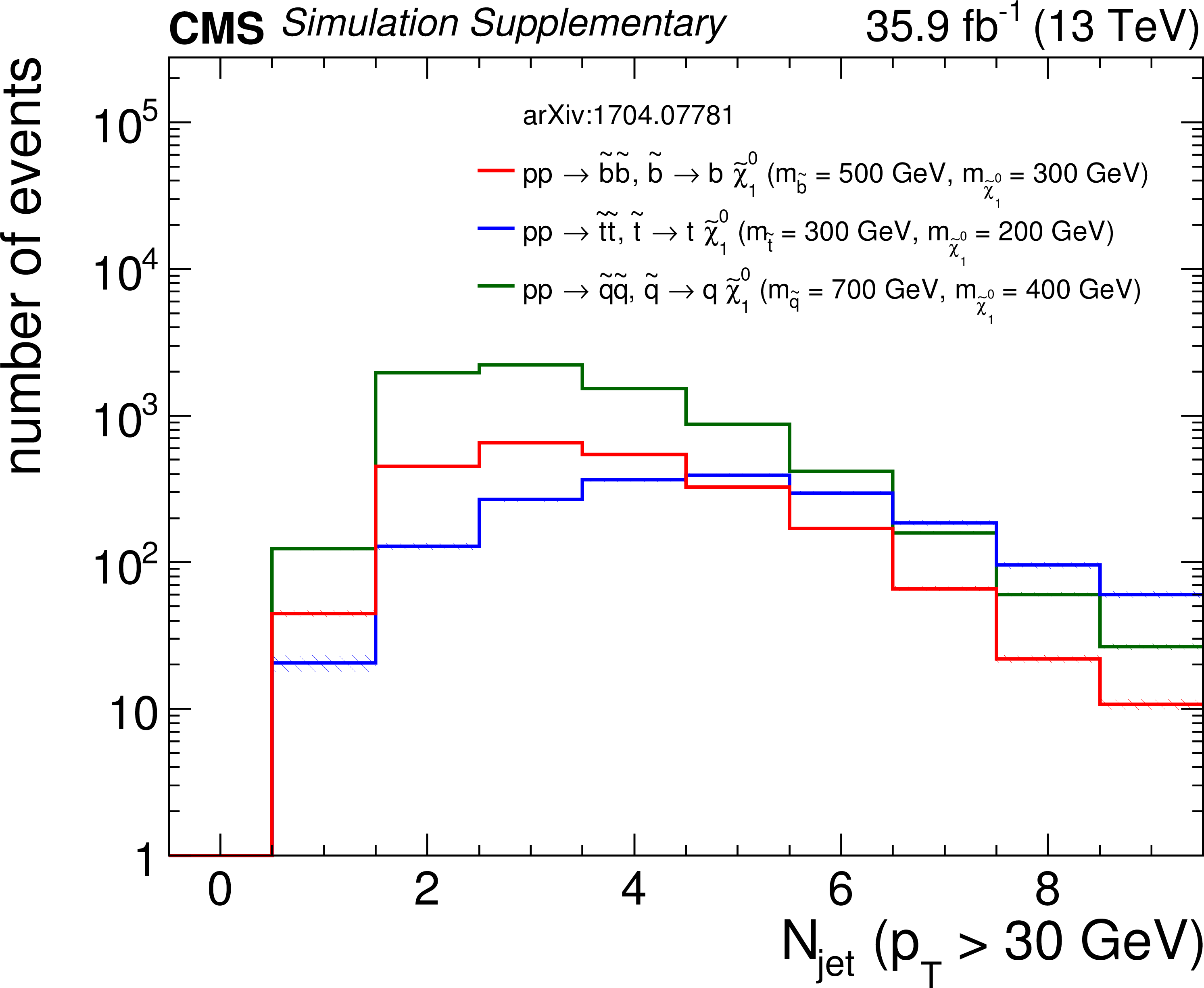
Additional Figure 3-c:
Distribution of the number of jets from three representative squark pair production signal models with ${m_{\tilde{ \mathrm{q} } } \gg m_{\tilde{\chi}^0_1 }}$ after the baseline selection. The plot ignores the baseline requirement. The last bin contains the overflow events. Only statistical uncertainties are shown. |
png pdf root |
Additional Figure 3-d:
Distribution of the number of b-tagged jets from three representative squark pair production signal models with ${m_{\tilde{ \mathrm{q} } } \gg m_{\tilde{\chi}^0_1 }}$ after the baseline selection. The plot ignores the baseline requirement. The last bin contains the overflow events. Only statistical uncertainties are shown. |
png pdf |
Additional Figure 4:
Distributions of (a) $H_{\rm T}$, (b) $H_{\rm T}^{\rm miss}$, (c) the number of jets, and (d) the number of b-tagged jets from three representative squark pair production signal models with ${m_{\tilde{ \mathrm{q} } } \sim m_{\tilde{\chi}^0_1 }}$ after the baseline selection. Each plot ignores the baseline requirement (if any) for its respective variable. The last bin in each plot contains the overflow events. Only statistical uncertainties are shown. |
png pdf root |
Additional Figure 4-a:
Distribution of $H_{\rm T}$ from three representative squark pair production signal models with ${m_{\tilde{ \mathrm{q} } } \sim m_{\tilde{\chi}^0_1 }}$ after the baseline selection. The plot ignores the baseline requirement. The last bin in each plot contains the overflow events. Only statistical uncertainties are shown. |
png pdf root |
Additional Figure 4-b:
Distribution of $H_{\rm T}^{\rm miss}$ from three representative squark pair production signal models with ${m_{\tilde{ \mathrm{q} } } \sim m_{\tilde{\chi}^0_1 }}$ after the baseline selection. The plot ignores the baseline requirement. The last bin in each plot contains the overflow events. Only statistical uncertainties are shown. |
png pdf root |
Additional Figure 4-c:
Distribution of the number of jets from three representative squark pair production signal models with ${m_{\tilde{ \mathrm{q} } } \sim m_{\tilde{\chi}^0_1 }}$ after the baseline selection. The plot ignores the baseline requirement. The last bin in each plot contains the overflow events. Only statistical uncertainties are shown. |
png pdf root |
Additional Figure 4-d:
Distribution of the number of b-tagged jets from three representative squark pair production signal models with ${m_{\tilde{ \mathrm{q} } } \sim m_{\tilde{\chi}^0_1 }}$ after the baseline selection. The plot ignores the baseline requirement. The last bin in each plot contains the overflow events. Only statistical uncertainties are shown. |
png pdf |
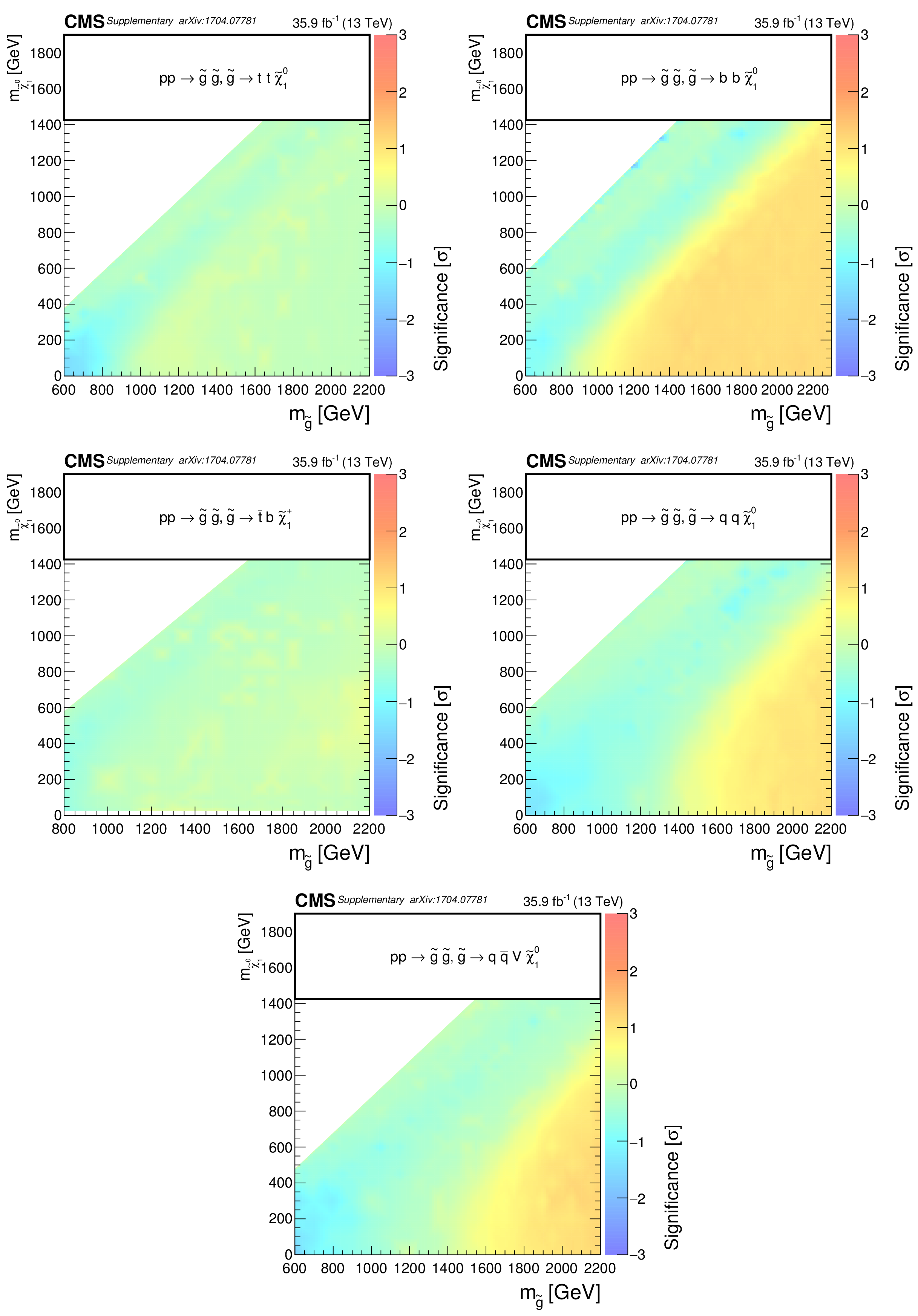
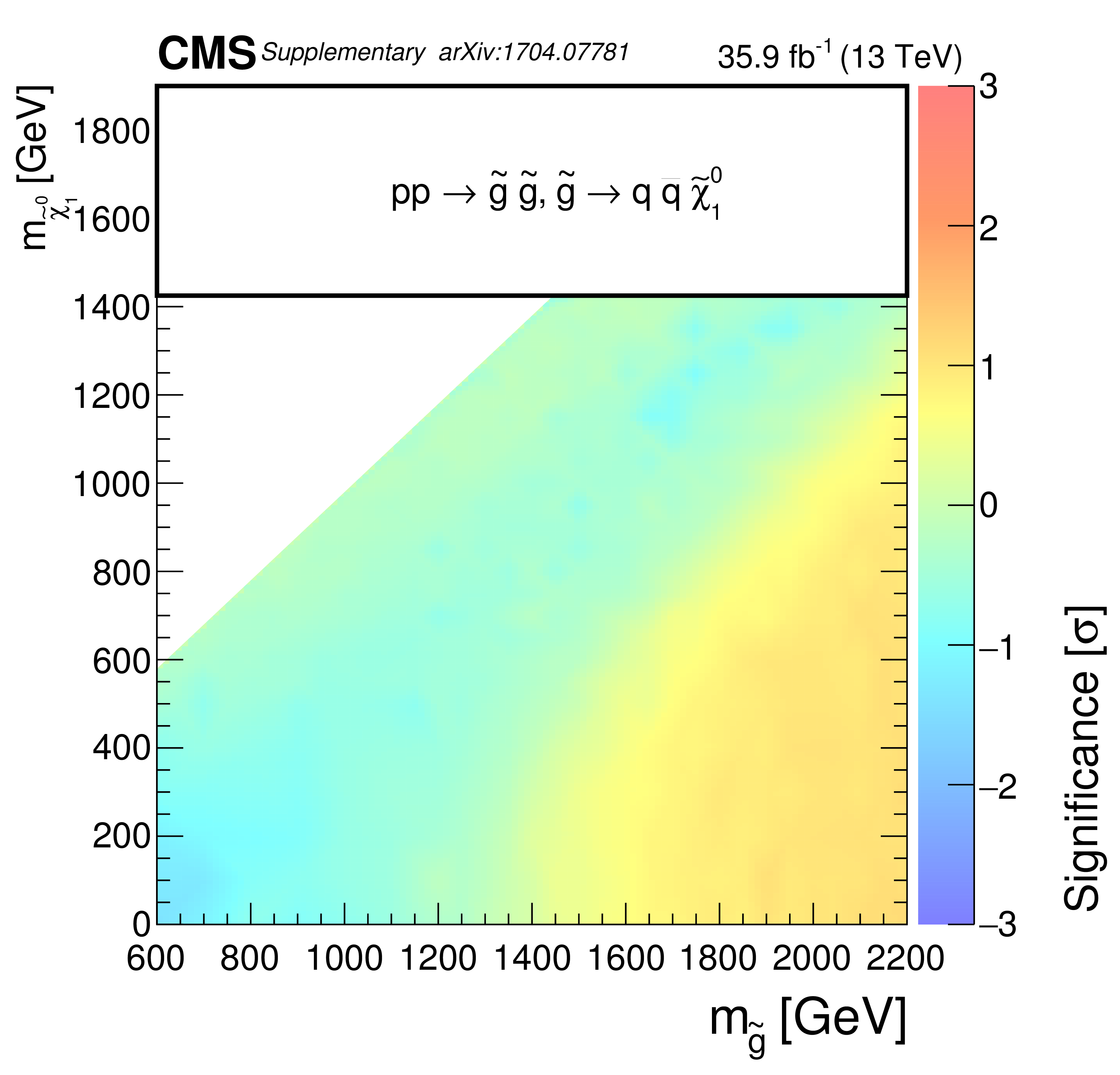
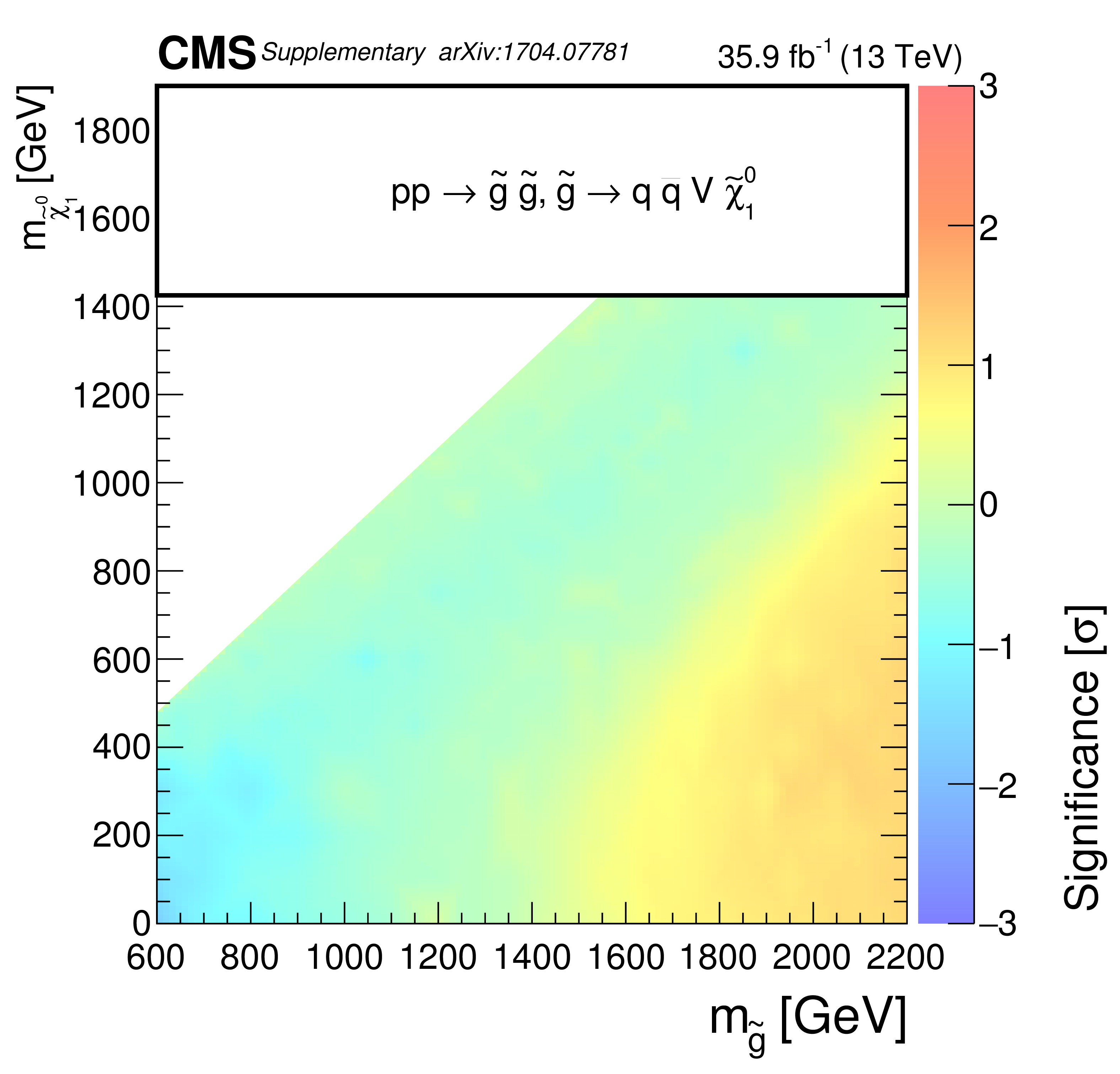
Additional Figure 5:
SMS model significance for gluino models. |
png pdf root |
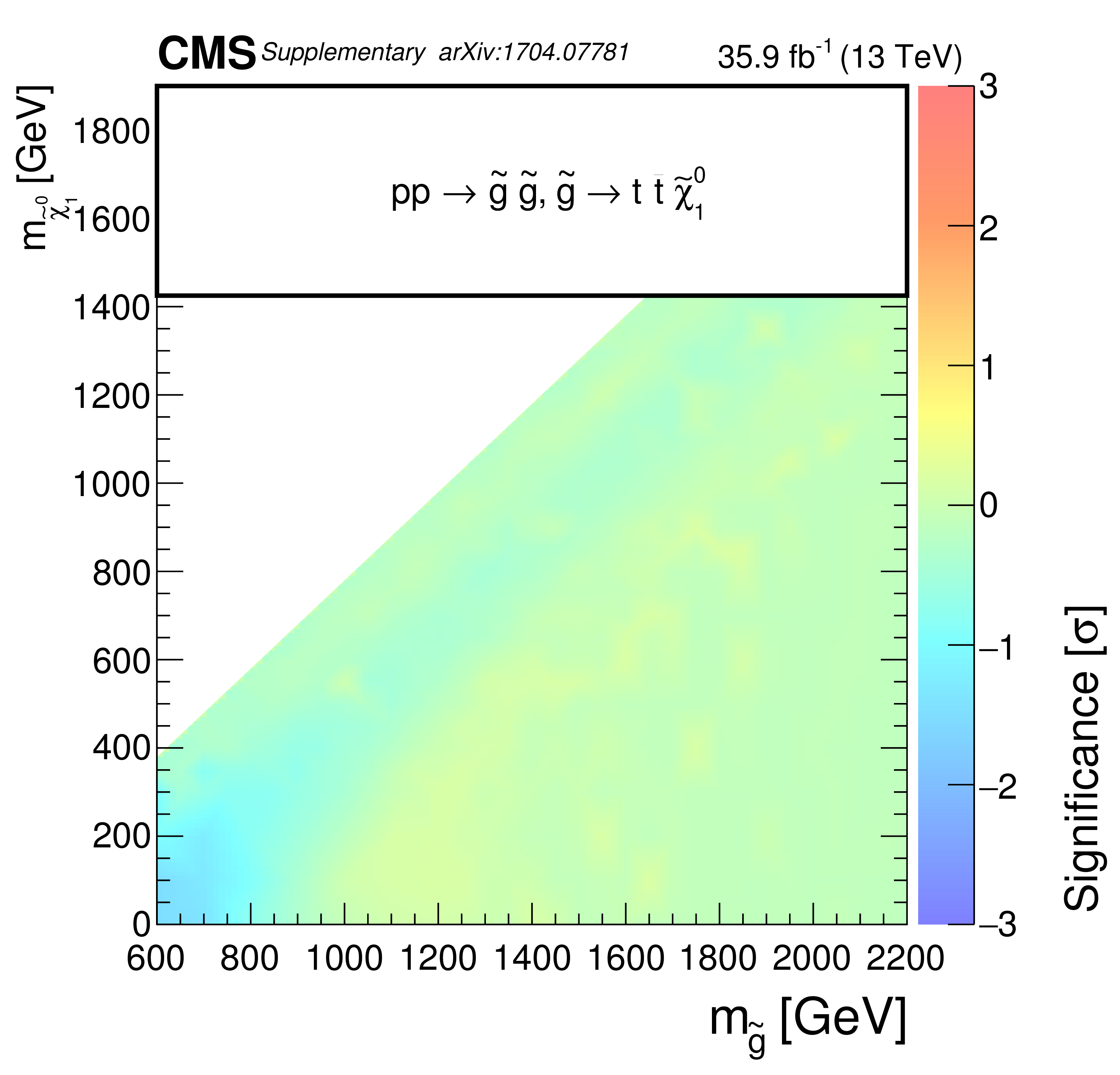
Additional Figure 5-a:
SMS model significance for the $ \mathrm{pp} \to \tilde{g} \tilde{g},\, \tilde{g} \to \mathrm{t} \mathrm{\bar{t}} \tilde{\chi}^0_1 $ gluino model. |

png pdf root |
Additional Figure 5-b:
SMS model significance for the $ \mathrm{pp} \to \tilde{g} \tilde{g},\, \tilde{g} \to \mathrm{b} \mathrm{\bar{b}} \tilde{\chi}^0_1 $ gluino model. |
png pdf root |
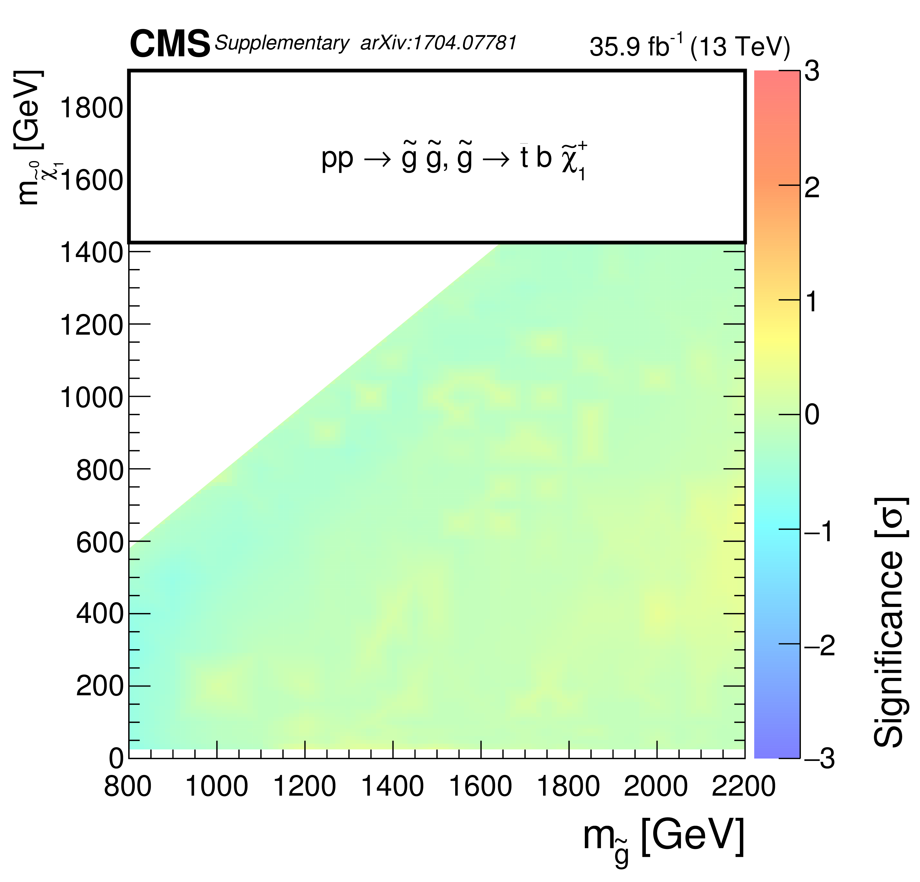
Additional Figure 5-c:
SMS model significance for the $ \mathrm{pp} \to \tilde{g} \tilde{g},\, \tilde{g} \to \mathrm{\bar{t}} \mathrm{b} \tilde{\chi}^+_1 $ gluino model. |
png pdf root |
Additional Figure 5-d:
SMS model significance for the $ \mathrm{pp} \to \tilde{g} \tilde{g},\, \tilde{g} \to \mathrm{q} \mathrm{\bar{q}} \tilde{\chi}^0_1 $ gluino model. |
png pdf root |
Additional Figure 5-e:
SMS model significance for the $ \mathrm{pp} \to \tilde{g} \tilde{g},\, \tilde{g} \to \mathrm{q} \mathrm{\bar{q}} \mathrm{V} \tilde{\chi}^0_1 $ gluino model. |
png pdf |
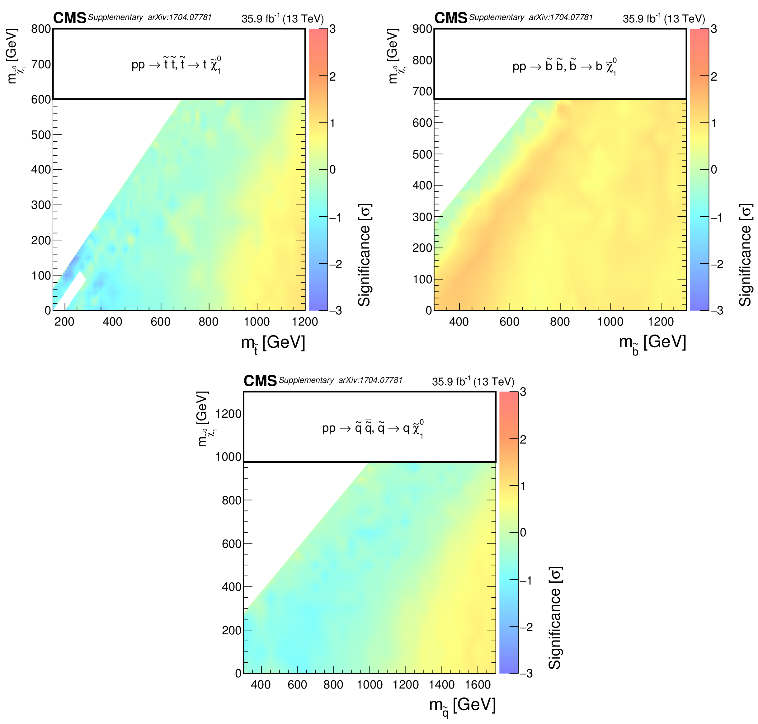
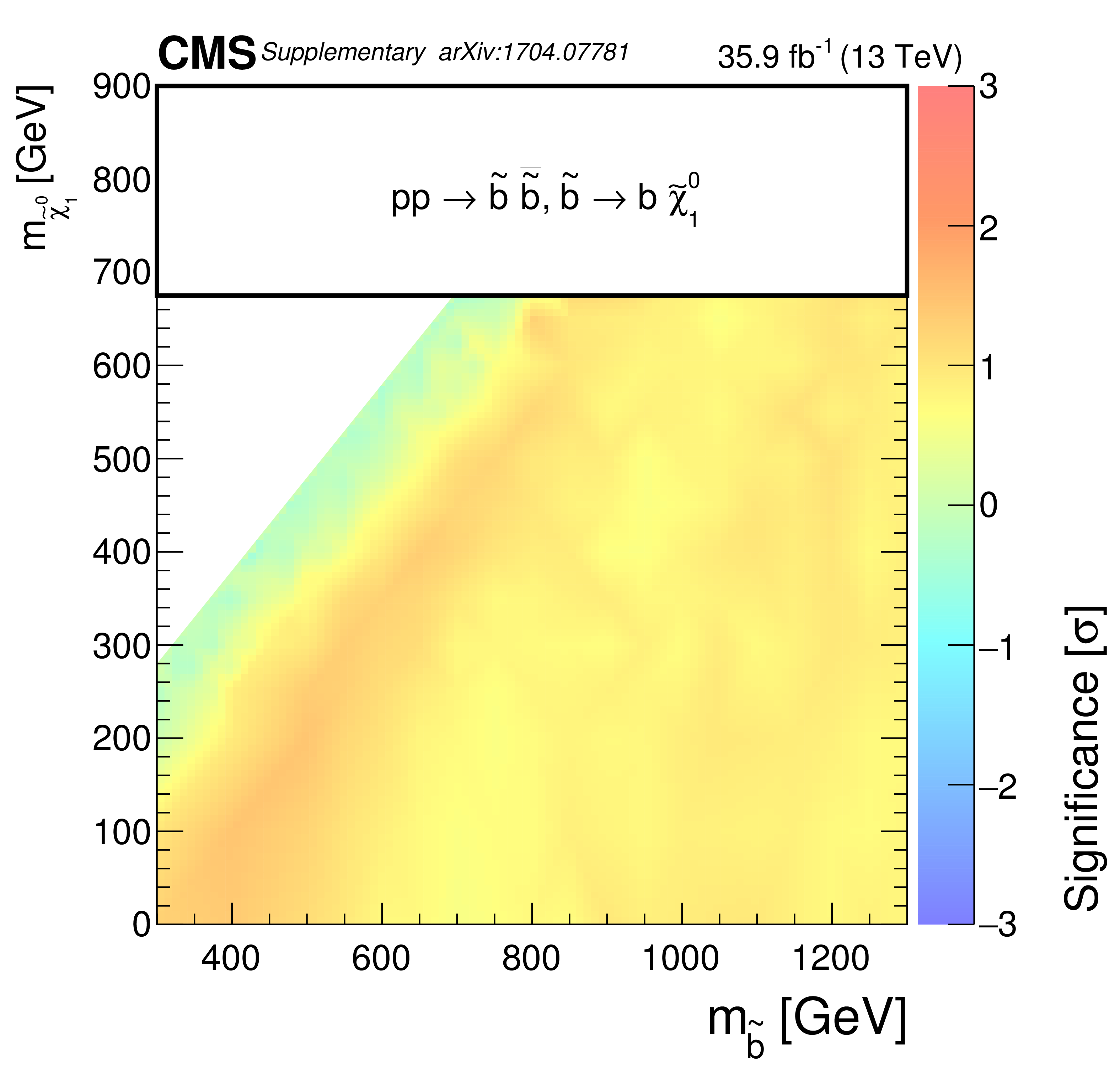
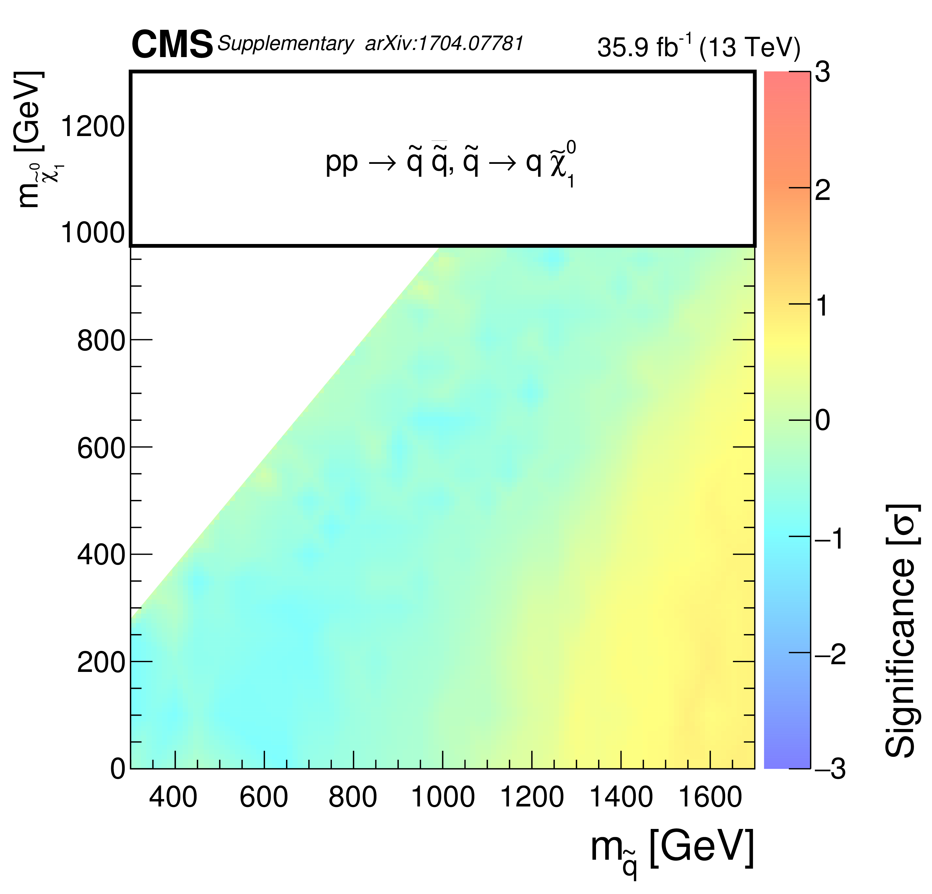
Additional Figure 6:
SMS model significance for squark models. |
png pdf root |
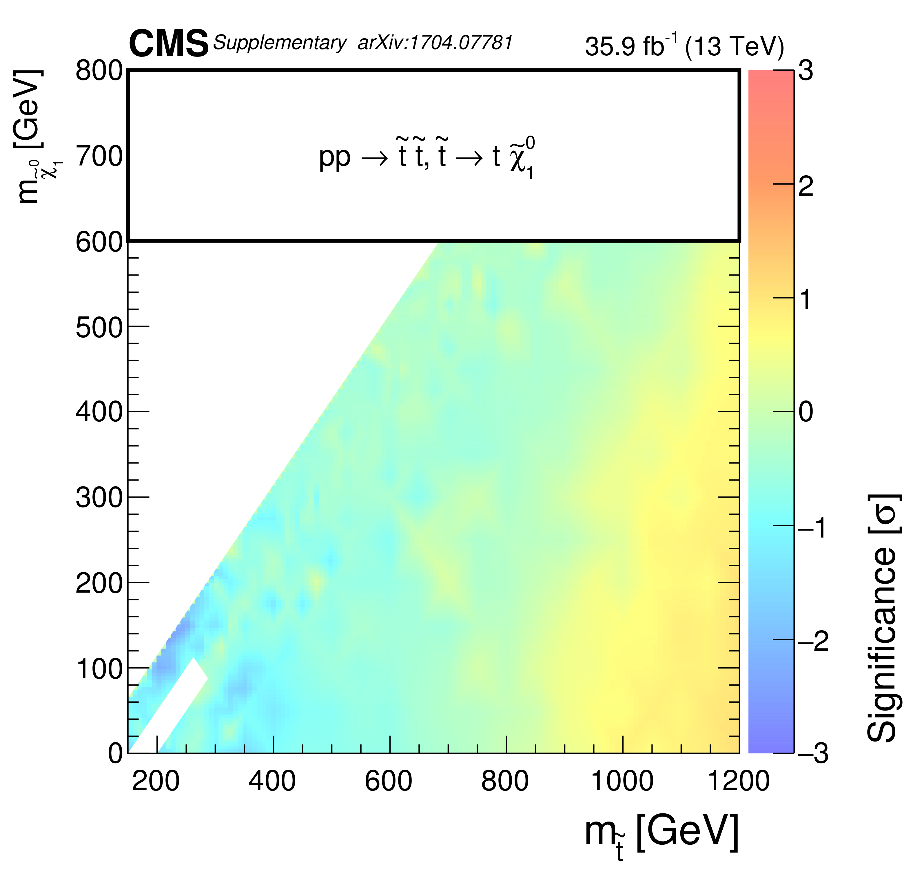
Additional Figure 6-a:
SMS model significance for the $ \mathrm{pp} \to \tilde{\mathrm{t}} \overline{\tilde{\mathrm{t}}},\, \tilde{\mathrm{t}} \to \mathrm{t} \tilde{\chi}^0_1 $ squark model. |
png pdf root |
Additional Figure 6-b:
SMS model significance for the $ \mathrm{pp} \to \tilde{\mathrm{b}}\overline{\tilde{\mathrm{b}}},\, \tilde{\mathrm{b}} \to \mathrm{b} \tilde{\chi}^0_1 $ squark model. |
png pdf root |
Additional Figure 6-c:
SMS model significance for the $ \mathrm{pp} \to \tilde{\mathrm{q}} \overline{\tilde{\mathrm{q}}},\, \tilde{\mathrm{q}} \to \mathrm{q} \tilde{\chi}^0_1 $ squark model. |
png pdf |
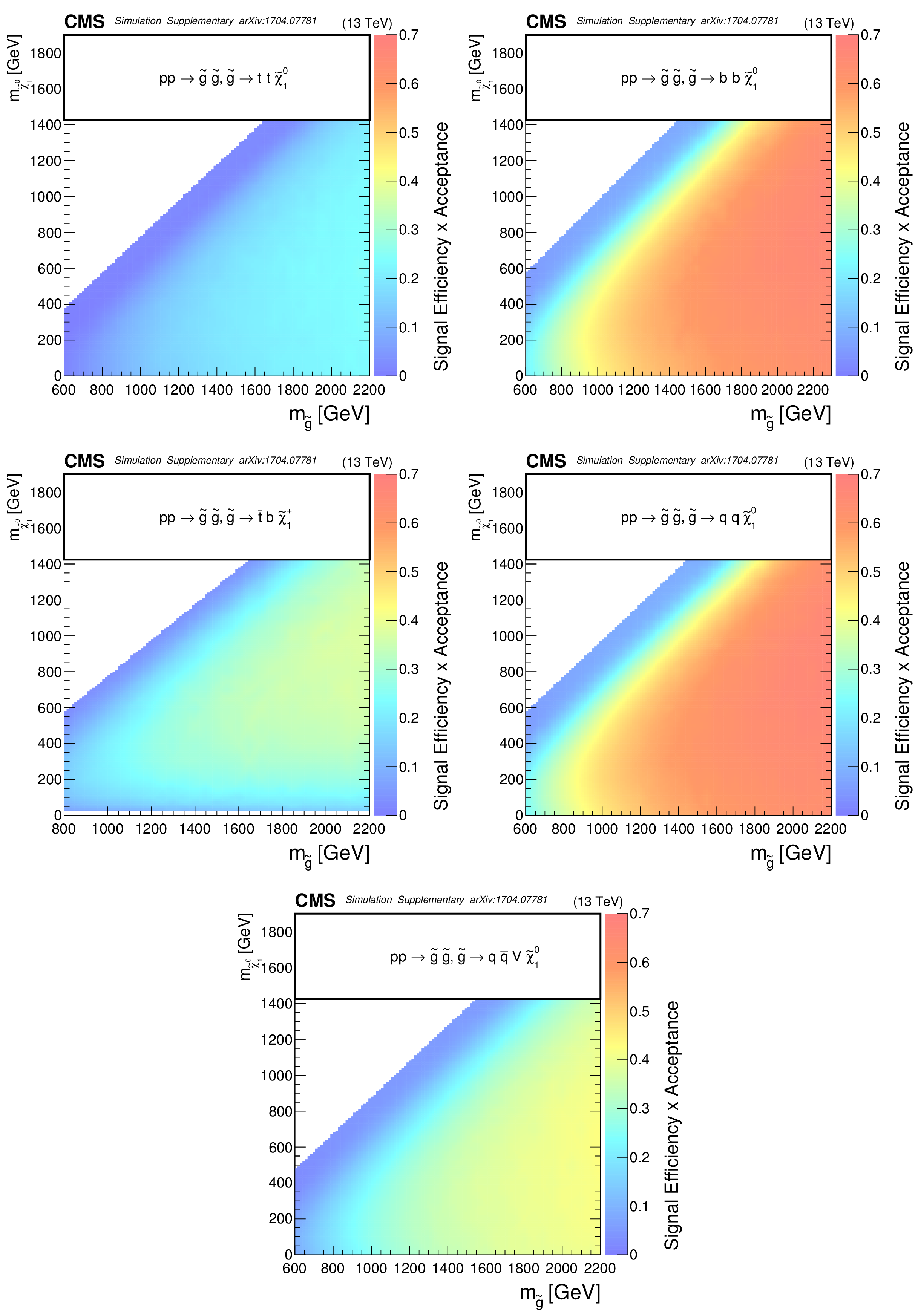
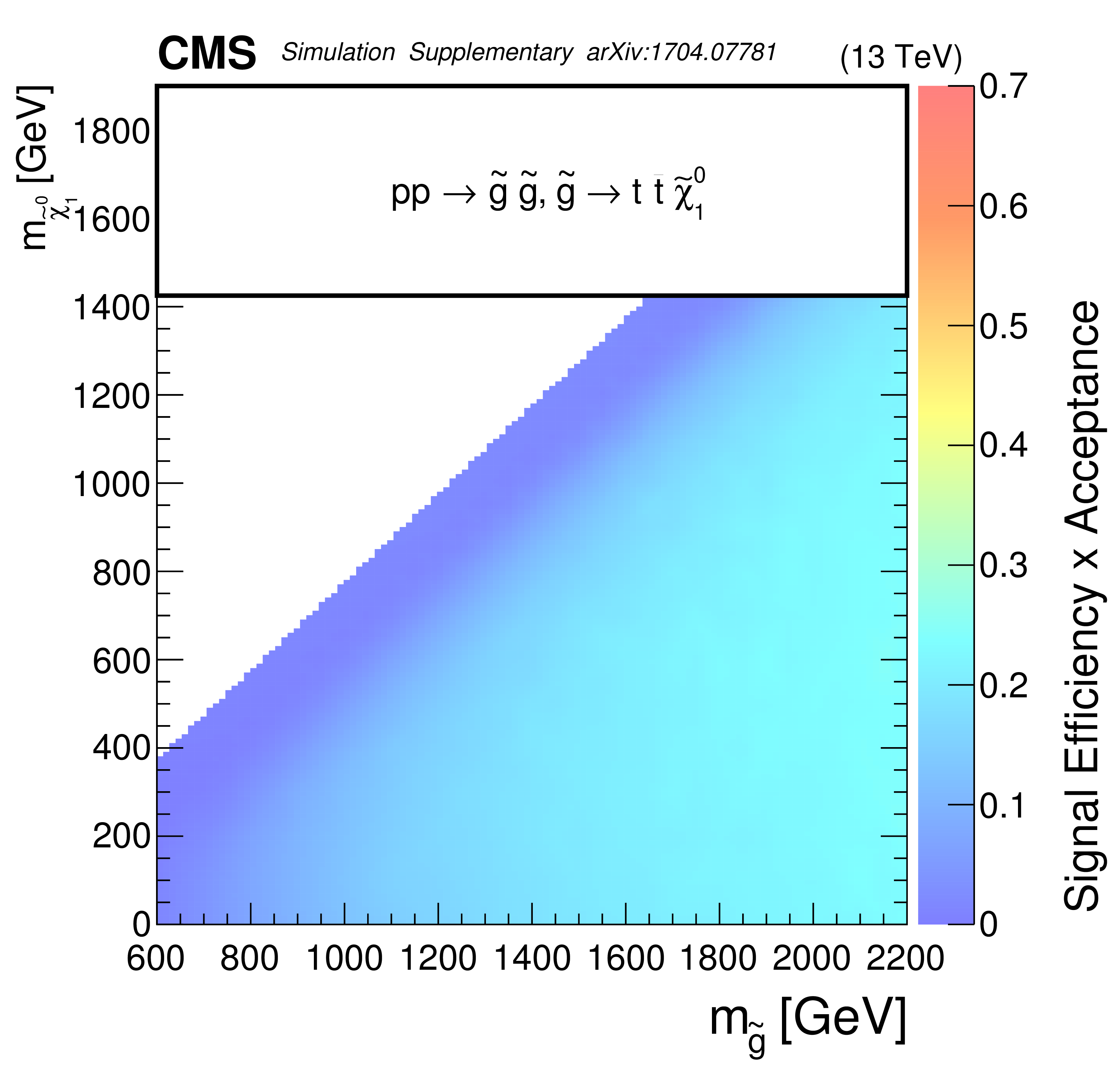
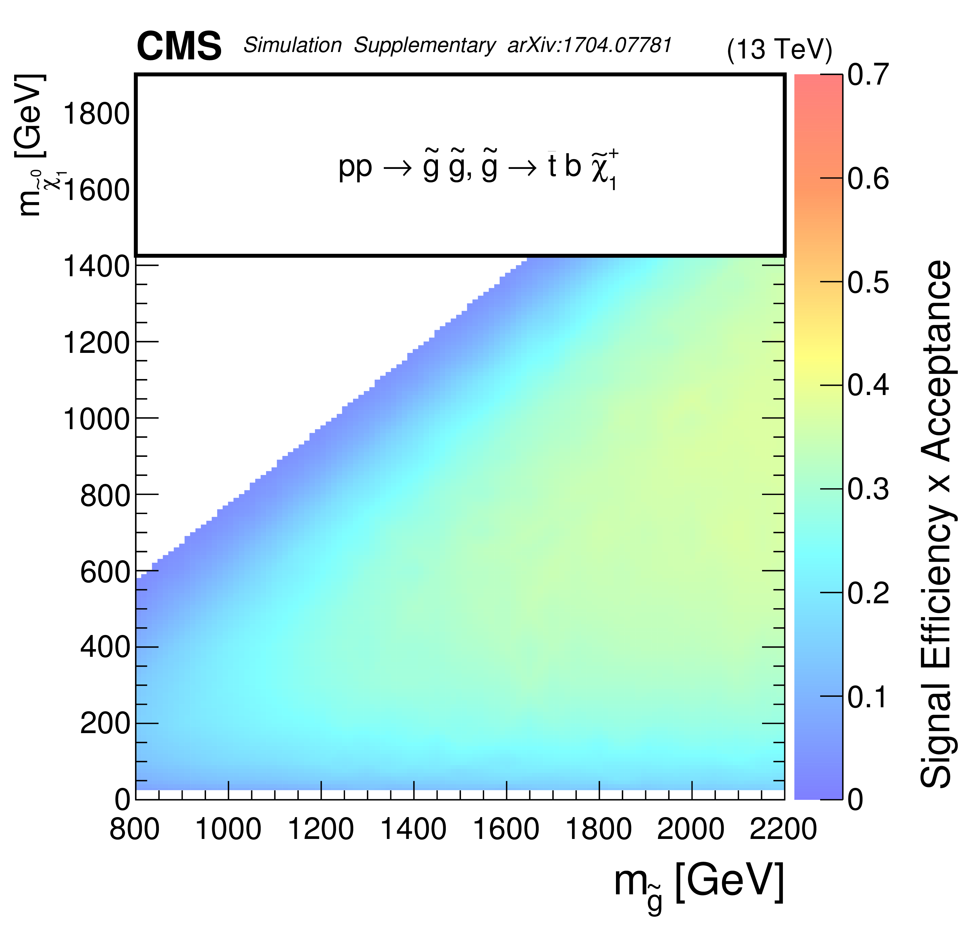
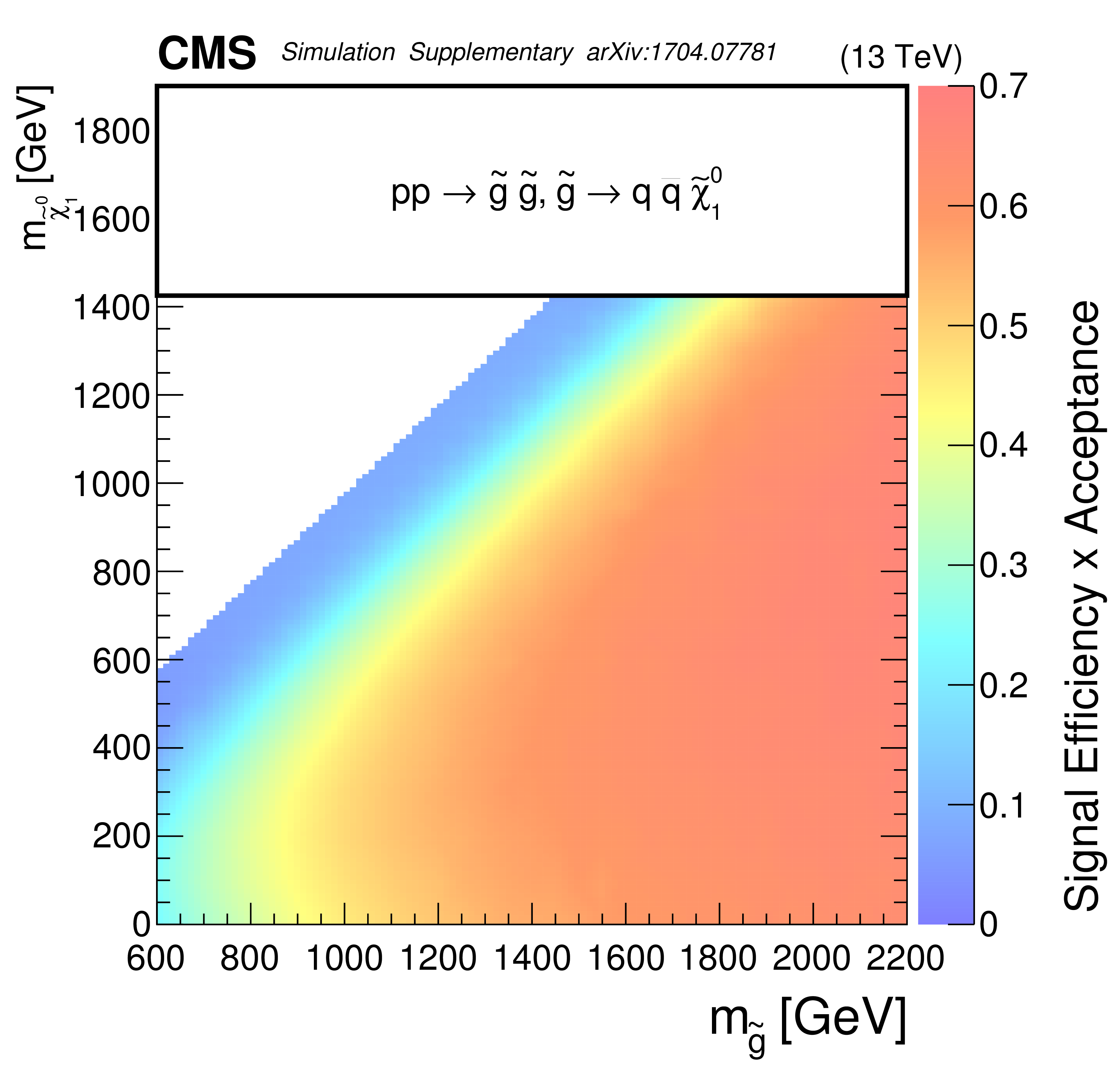
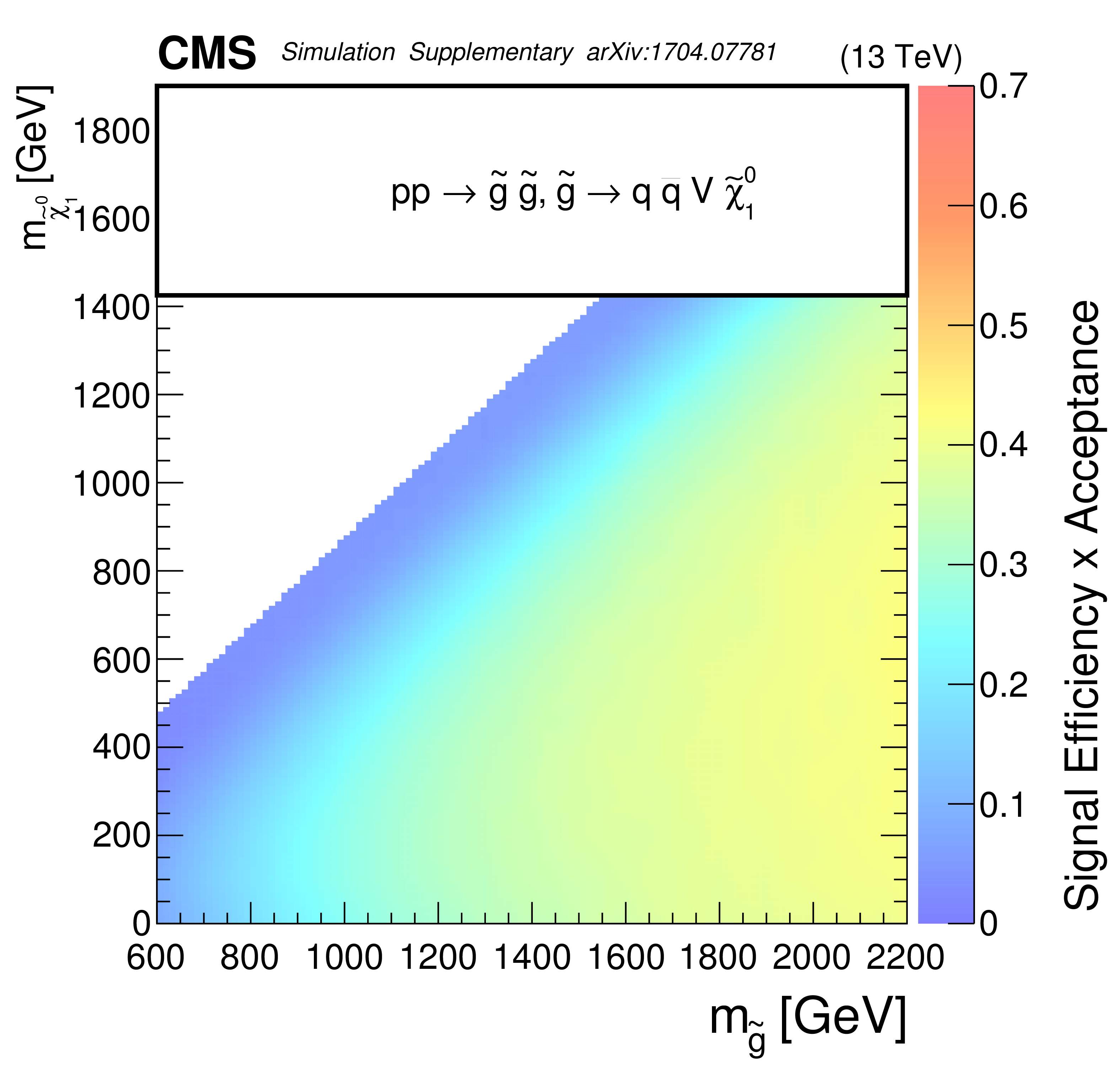
Additional Figure 7:
SMS model signal efficiency for gluino models. |
png pdf root |
Additional Figure 7-a:
SMS model signal efficiency for the $ \mathrm{pp} \to \tilde{g} \tilde{g},\, \tilde{g} \to \mathrm{t} \mathrm{\bar{t}} \tilde{\chi}^0_1 $ gluino model. |

png pdf root |
Additional Figure 7-b:
SMS model signal efficiency for the $ \mathrm{pp} \to \tilde{g} \tilde{g},\, \tilde{g} \to \mathrm{b} \mathrm{\bar{b}} \tilde{\chi}^0_1 $ gluino model. |
png pdf root |
Additional Figure 7-c:
SMS model signal efficiency for the $ \mathrm{pp} \to \tilde{g} \tilde{g},\, \tilde{g} \to \mathrm{\bar{t}} \mathrm{b} \tilde{\chi}^+_1 $ gluino model. |
png pdf root |
Additional Figure 7-d:
SMS model signal efficiency for the $ \mathrm{pp} \to \tilde{g} \tilde{g},\, \tilde{g} \to \mathrm{q} \mathrm{\bar{q}} \tilde{\chi}^0_1 $ gluino model. |
png pdf root |
Additional Figure 7-e:
SMS model signal efficiency for the $ \mathrm{pp} \to \tilde{g} \tilde{g},\, \tilde{g} \to \mathrm{q} \mathrm{\bar{q}} \mathrm{V} \tilde{\chi}^0_1 $ gluino model. |
png pdf |
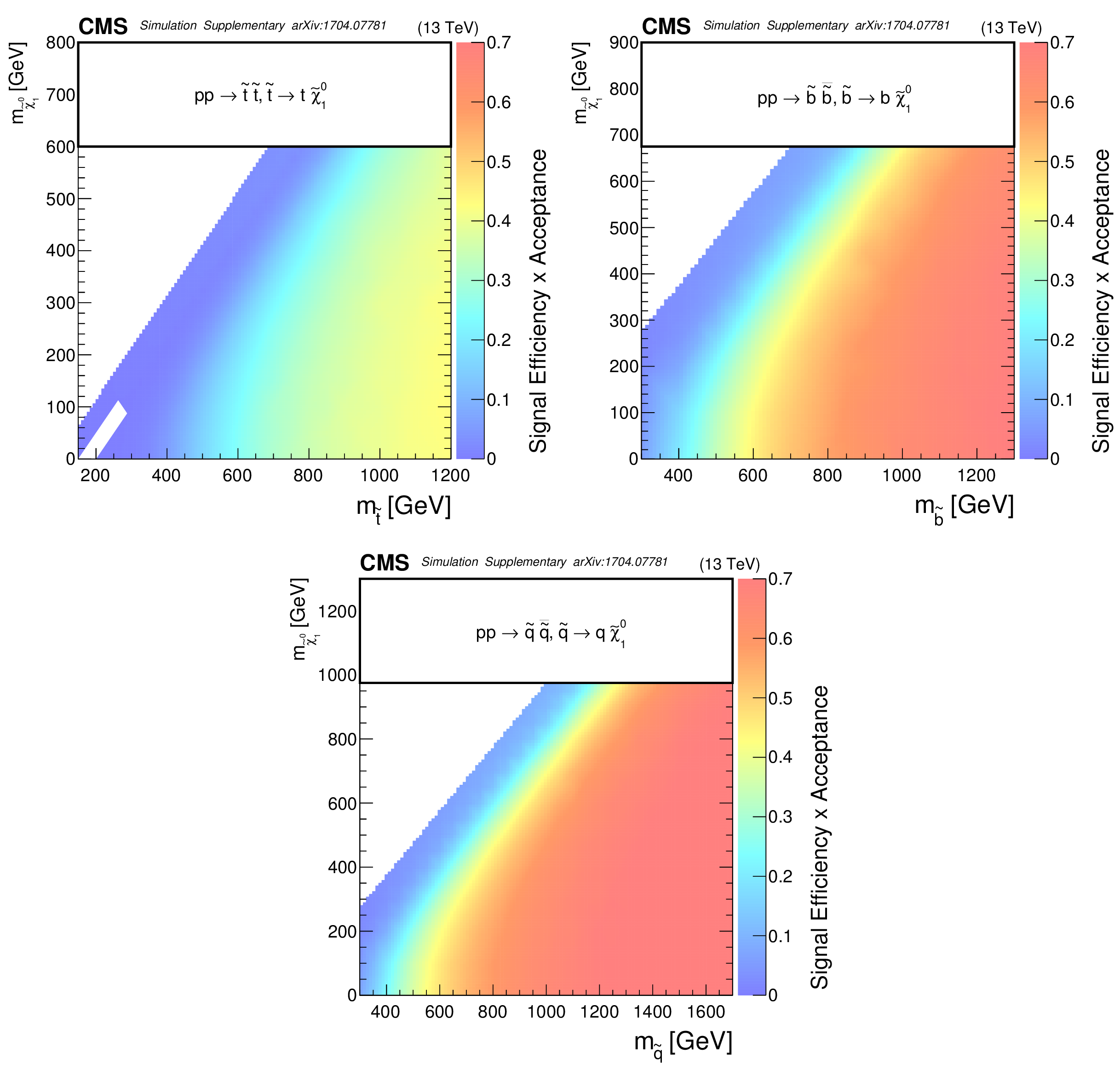
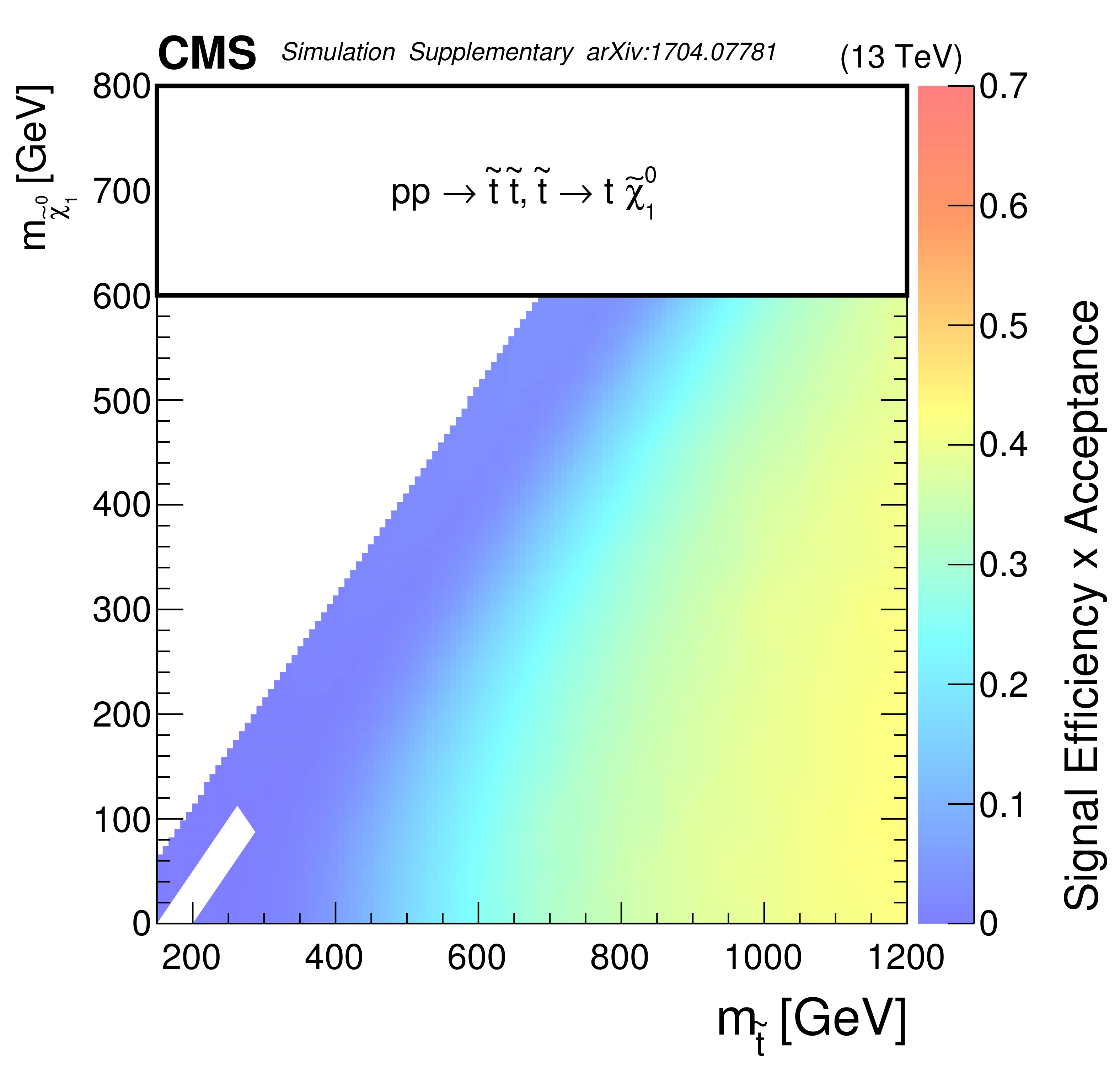
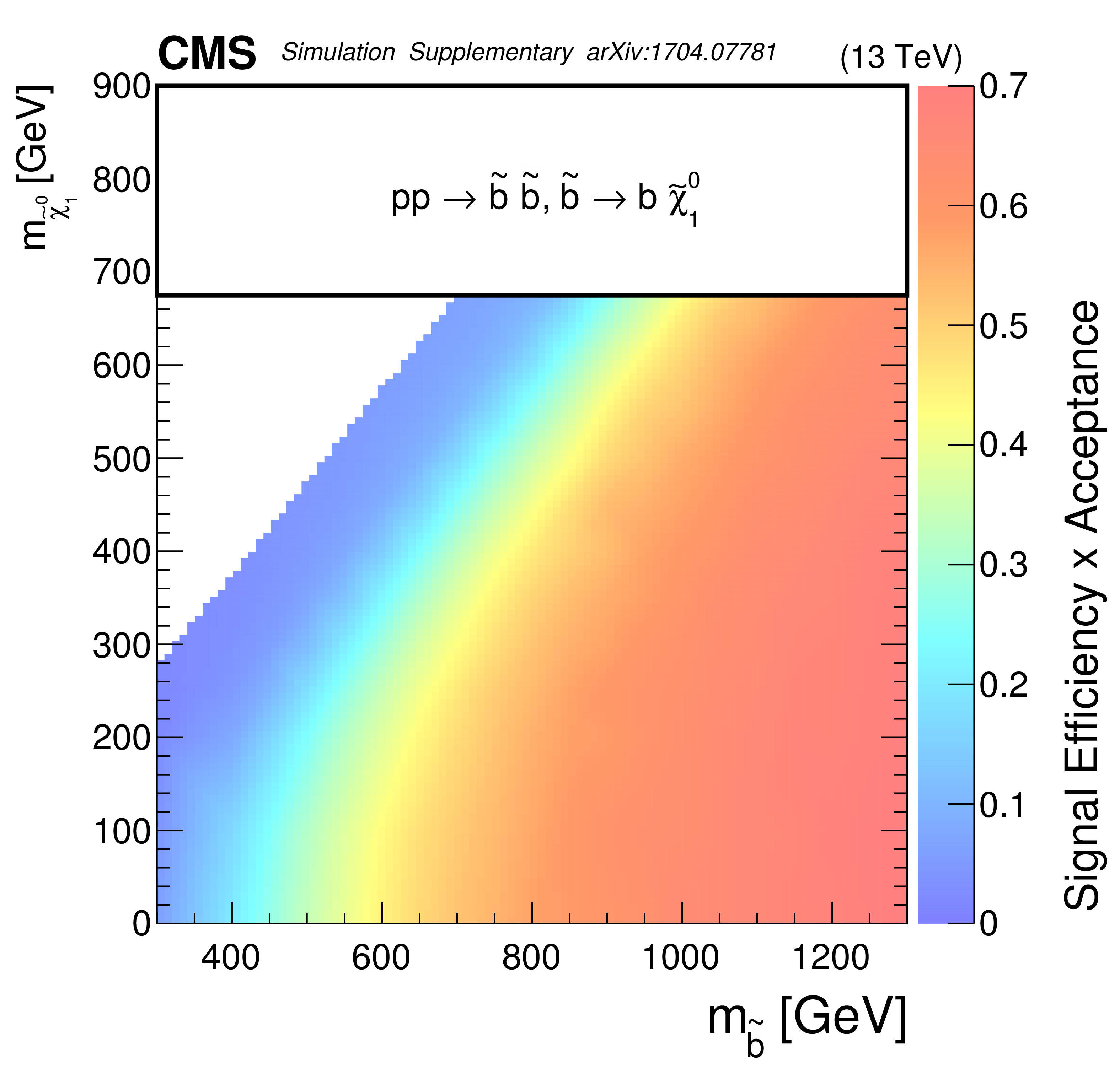
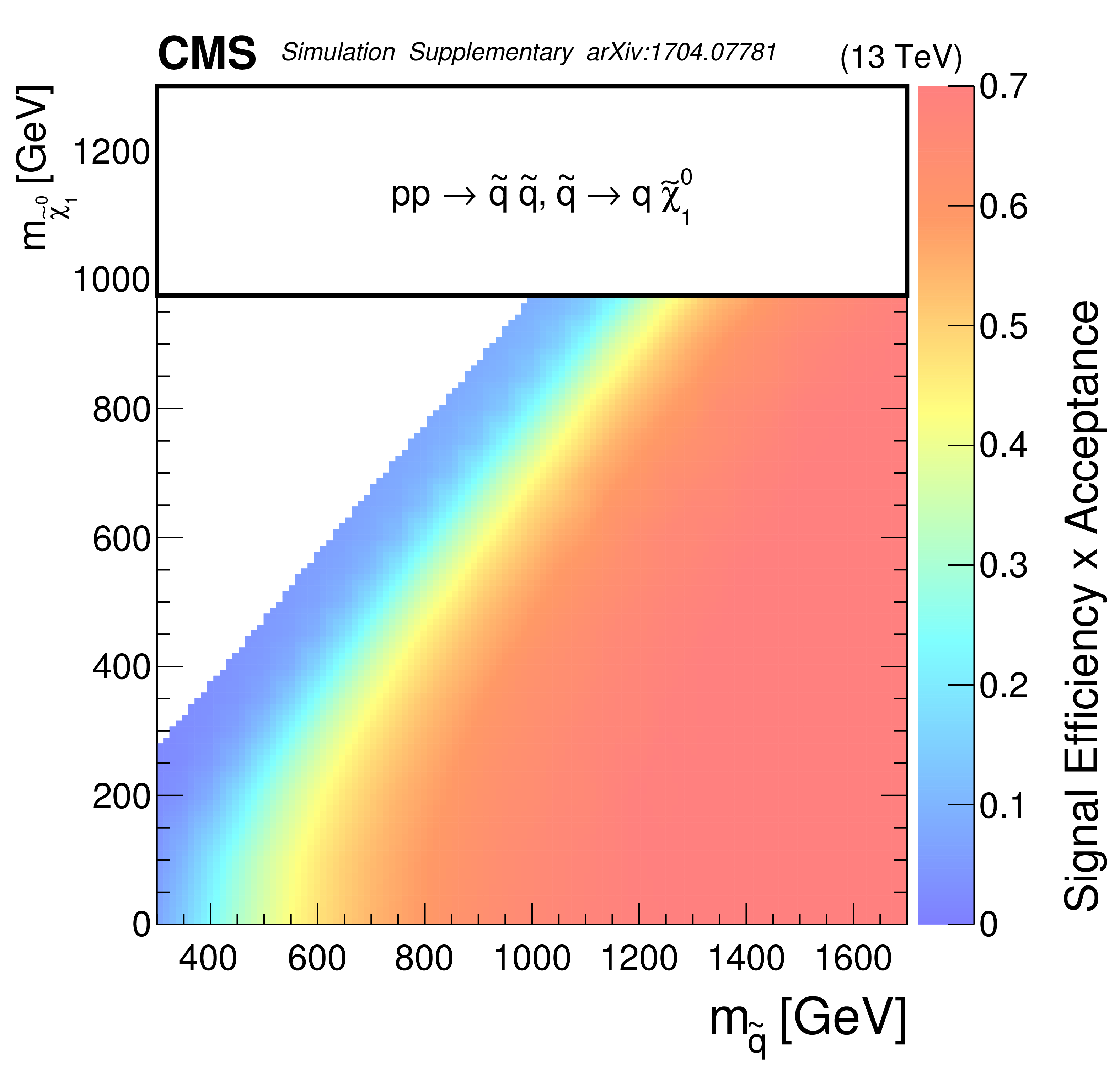
Additional Figure 8:
SMS model signal efficiency for squark models. |
png pdf root |
Additional Figure 8-a:
SMS model signal efficiency for the $ \mathrm{pp} \to \tilde{\mathrm{t}} \overline{\tilde{\mathrm{t}}},\, \tilde{\mathrm{t}} \to \mathrm{t} \tilde{\chi}^0_1 $ squark model. |
png pdf root |
Additional Figure 8-b:
SMS model signal efficiency for the $ \mathrm{pp} \to \tilde{\mathrm{b}}\overline{\tilde{\mathrm{b}}},\, \tilde{\mathrm{b}} \to \mathrm{b} \tilde{\chi}^0_1 $ squark model. |
png pdf root |
Additional Figure 8-c:
SMS model signal efficiency for the $ \mathrm{pp} \to \tilde{\mathrm{q}} \overline{\tilde{\mathrm{q}}},\, \tilde{\mathrm{q}} \to \mathrm{q} \tilde{\chi}^0_1 $ squark model. |
png pdf root |
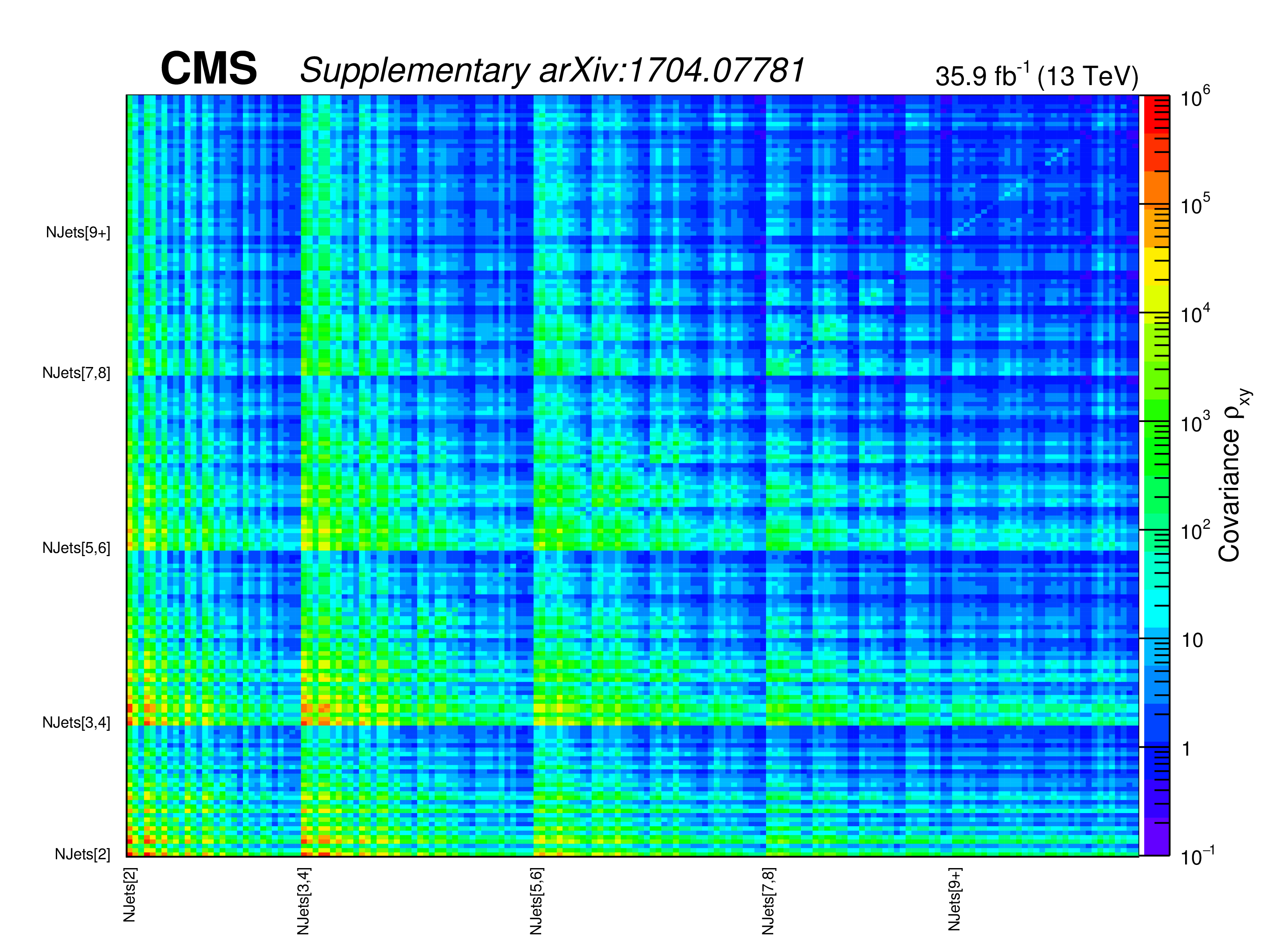
Additional Figure 9:
Pre-fit background covariance matrix. |
| Additional Tables | |
png pdf |
Additional Table 1:
Observed numbers of events and post-fit backgrounds in the $ {N_{\text {jet}}} = $ 2 search regions. |
png pdf |
Additional Table 2:
Observed numbers of events and post-fit backgrounds in the 3 $ \geq {N_{\text {jet}}} \geq $ 4 search regions. |

png pdf |
Additional Table 3:
Observed numbers of events and post-fit backgrounds in the 5 $ \geq {N_{\text {jet}}} \geq $ 6 search regions. |
png pdf |
Additional Table 4:
Observed numbers of events and post-fit backgrounds in the 7 $ \geq {N_{\text {jet}}} \geq $ 8 search regions. |

png pdf |
Additional Table 5:
Observed numbers of events and post-fit backgrounds in the $ {N_{\text {jet}}} \geq $ 9 search regions. |
png pdf |
Additional Table 6:
Absolute cumulative efficiencies in % for additional representative models of gluino pair production. The uncertainties are statistical. Uncertainties reported as 0.0 correspond to values less than 0.05%. |
png pdf |
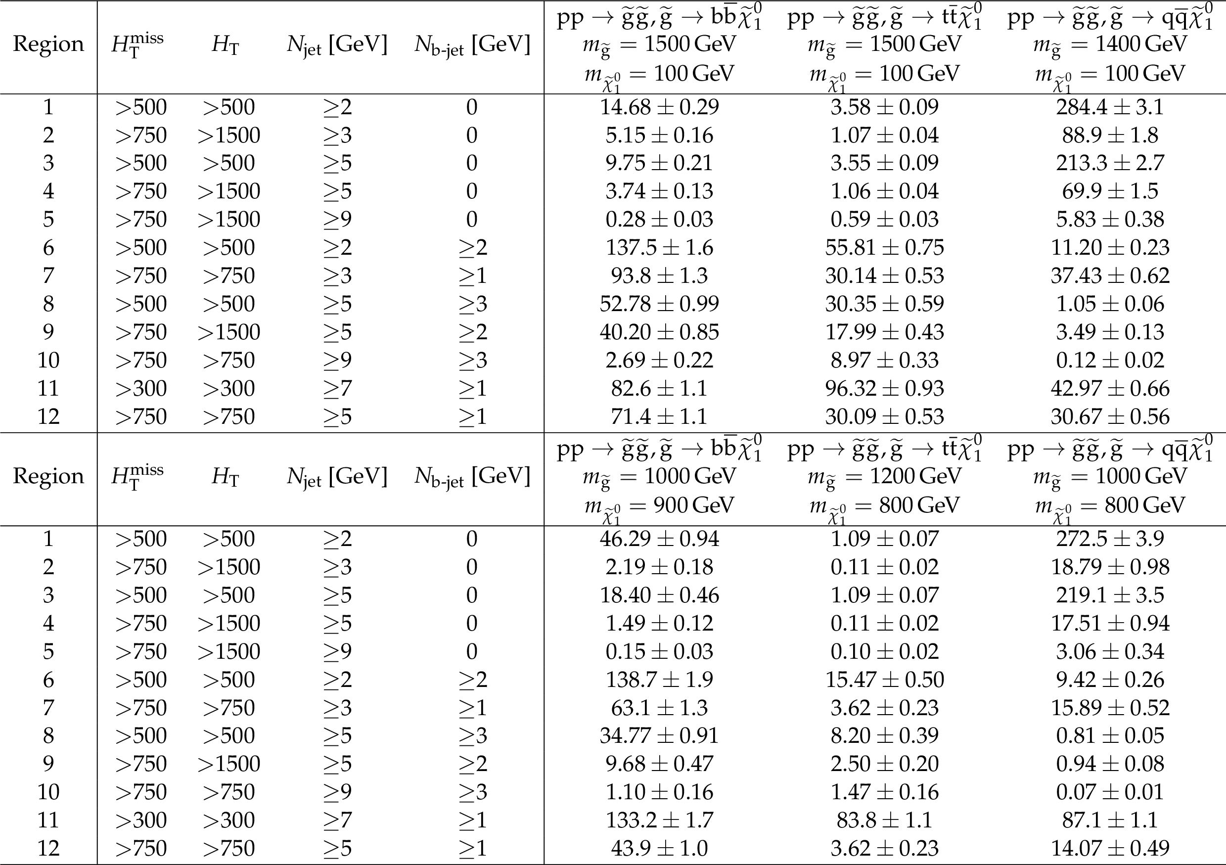
Additional Table 7:
Expected number of signal events in 35.9 fb$^{-1}$ of data for representative gluino pair production models in the aggregate search regions. Only statistical uncertainties are shown. |
png pdf |
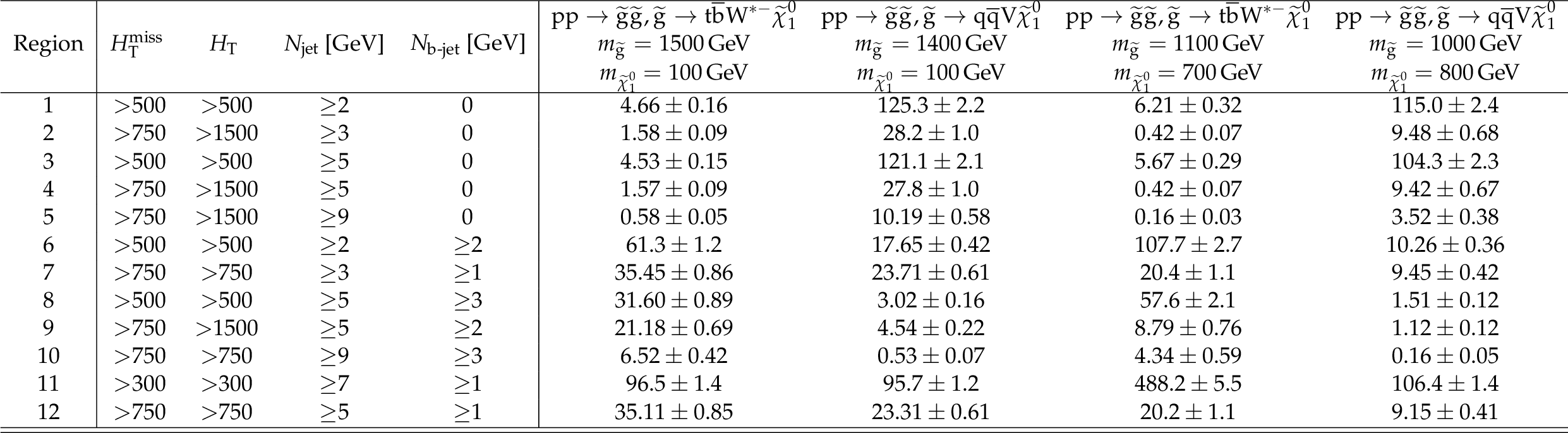
Additional Table 8:
Expected number of signal events in 35.9 fb$^{-1}$ of data for additional representative gluino pair production models in the aggregate search regions. Only statistical uncertainties are shown. |
png pdf |
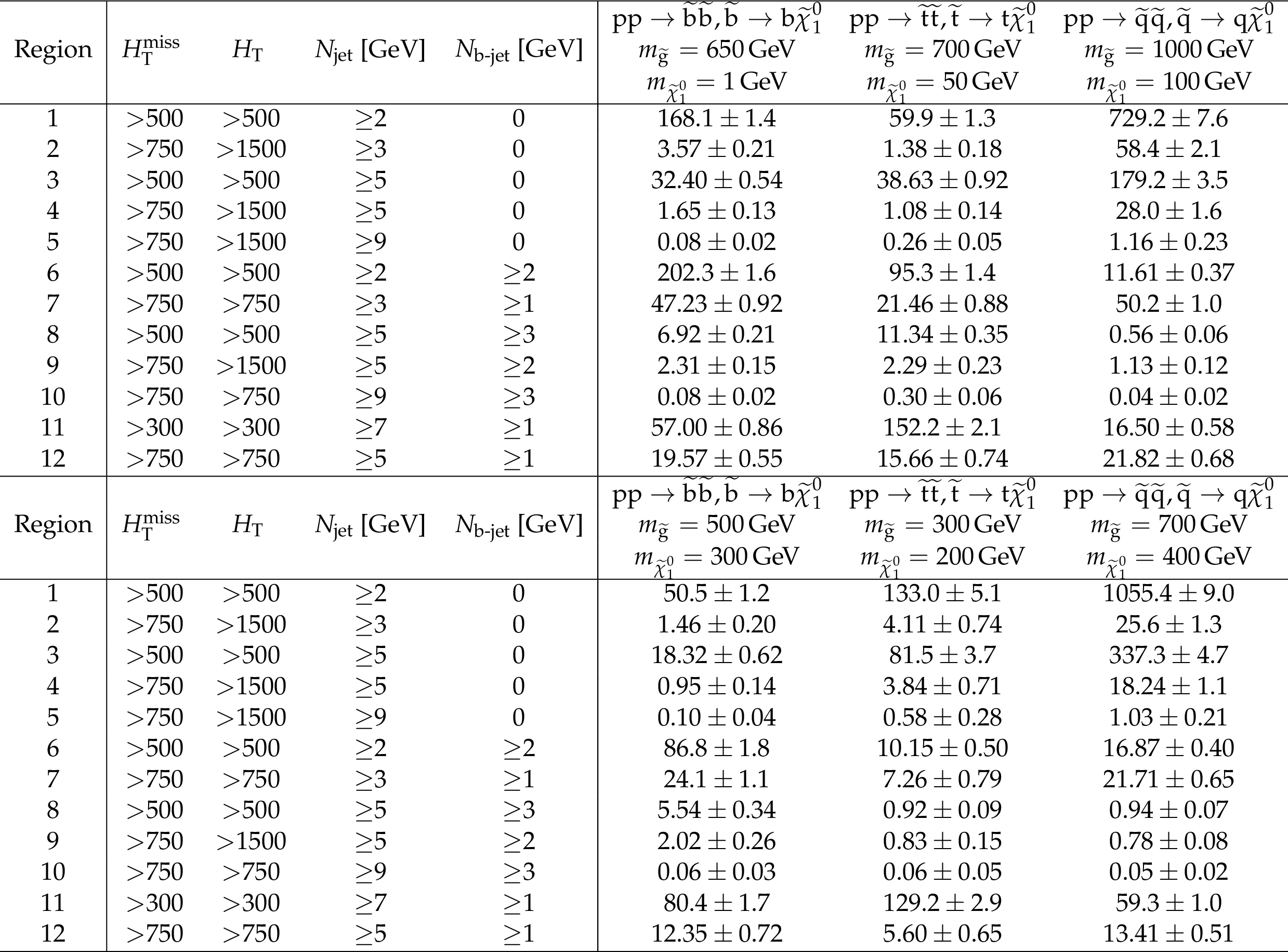
Additional Table 9:
Expected number of signal events in 35.9 fb$^{-1}$ of data for representative squark pair production models in the aggregate search regions. Only statistical uncertainties are shown. |
|
The values in the pre-fit background tables can be found in ROOT format here.
The values in the post-fit background tables can be found in ROOT format here. |
| References | ||||
| 1 | R. Barbieri and G. F. Giudice | Upper bounds on supersymmetric particle masses | NPB 306 (1988) 63 | |
| 2 | ATLAS and CMS Collaborations | Combined measurement of the Higgs boson mass in $ pp $ collisions at $ \sqrt{s}= $ 7 and 8 TeV with the ATLAS and CMS experiments | PRL 114 (2015) 191803 | 1503.07589 |
| 3 | P. Ramond | Dual theory for free fermions | PRD 3 (1971) 2415 | |
| 4 | Y. A. Golfand and E. P. Likhtman | Extension of the algebra of Poincare group generators and violation of P invariance | JEPTL 13 (1971)323 | |
| 5 | A. Neveu and J. H. Schwarz | Factorizable dual model of pions | NPB 31 (1971) 86 | |
| 6 | D. V. Volkov and V. P. Akulov | Possible universal neutrino interaction | JEPTL 16 (1972)438 | |
| 7 | J. Wess and B. Zumino | A Lagrangian model invariant under supergauge transformations | PLB 49 (1974) 52 | |
| 8 | J. Wess and B. Zumino | Supergauge transformations in four dimensions | NPB 70 (1974) 39 | |
| 9 | P. Fayet | Supergauge invariant extension of the Higgs mechanism and a model for the electron and its neutrino | NPB 90 (1975) 104 | |
| 10 | H. P. Nilles | Supersymmetry, supergravity and particle physics | Phys. Rep. 110 (1984) 1 | |
| 11 | S. Dimopoulos and G. F. Giudice | Naturalness constraints in supersymmetric theories with nonuniversal soft terms | PLB 357 (1995) 573 | hep-ph/9507282 |
| 12 | R. Barbieri and D. Pappadopulo | S-particles at their naturalness limits | JHEP 10 (2009) 061 | 0906.4546 |
| 13 | M. Papucci, J. T. Ruderman, and A. Weiler | Natural SUSY endures | JHEP 09 (2012) 035 | 1110.6926 |
| 14 | G. R. Farrar and P. Fayet | Phenomenology of the production, decay, and detection of new hadronic states associated with supersymmetry | PLB 76 (1978) 575 | |
| 15 | ATLAS Collaboration | Search for pair production of gluinos decaying via stop and sbottom in events with $ b $-jets and large missing transverse momentum in $ pp $ collisions at $ \sqrt{s} = $ 13 TeV with the ATLAS detector | PRD 94 (2016) 032003 | 1605.09318 |
| 16 | ATLAS Collaboration | Search for squarks and gluinos in final states with jets and missing transverse momentum at $ \sqrt{s} = $ 13 TeV with the ATLAS detector | EPJC 76 (2016) 392 | 1605.03814 |
| 17 | CMS Collaboration | Search for supersymmetry in the multijet and missing transverse momentum final state in pp collisions at 13 TeV | PLB 758 (2016) 152 | CMS-SUS-15-002 1602.06581 |
| 18 | CMS Collaboration | Search for new physics with the M$ _{\text{T2}} $ variable in all-jets final states produced in pp collisions at $ \sqrt{s}= $ 13 TeV | JHEP 10 (2016) 006 | CMS-SUS-15-003 1603.04053 |
| 19 | CMS Collaboration | Inclusive search for supersymmetry using razor variables in $ pp $ collisions at $ \sqrt{s}= $ 13 TeV | PRD 95 (2017) 012003 | CMS-SUS-15-004 1609.07658 |
| 20 | CMS Collaboration | A search for new phenomena in pp collisions at $ \sqrt{s}= $ 13 TeV in final states with missing transverse momentum and at least one jet using the $ {\alpha_{\text{T}}} $ variable | EPJC 77 (2017) 294 | CMS-SUS-15-005 1611.00338 |
| 21 | CMS Collaboration | Search for new physics with jets and missing transverse momentum in pp collisions at $ \sqrt{s}= $ 7 TeV | JHEP 08 (2011) 155 | CMS-SUS-10-005 1106.4503 |
| 22 | CMS Collaboration | Search for new physics in the multijet and missing transverse momentum final state in proton-proton collisions at $ \sqrt{s}= $ 8 TeV | JHEP 06 (2014) 055 | CMS-SUS-13-012 1402.4770 |
| 23 | N. Arkani-Hamed et al. | MARMOSET: The path from LHC data to the new standard model via on-shell effective theories | hep-ph/0703088 | |
| 24 | J. Alwall, P. C. Schuster, and N. Toro | Simplified models for a first characterization of new physics at the LHC | PRD 79 (2009) 075020 | 0810.3921 |
| 25 | J. Alwall, M.-P. Le, M. Lisanti, and J. G. Wacker | Model-independent jets plus missing energy searches | PRD 79 (2009) 015005 | 0809.3264 |
| 26 | D. Alves et al. | Simplified models for LHC new physics searches | JPG 39 (2012) 105005 | 1105.2838 |
| 27 | CMS Collaboration | Interpretation of searches for supersymmetry with simplified models | PRD 88 (2013) 052017 | CMS-SUS-11-016 1301.2175 |
| 28 | CMS Collaboration | The CMS experiment at the CERN LHC | JINST 3 (2008) S08004 | CMS-00-001 |
| 29 | CMS Collaboration | The CMS trigger system | JINST 12 (2017) P01020 | CMS-TRG-12-001 1609.02366 |
| 30 | CMS Collaboration | Particle-flow reconstruction and global event description with the CMS detector | Submitted to \it JINST | CMS-PRF-14-001 1706.04965 |
| 31 | CMS Collaboration | Performance of electron reconstruction and selection with the CMS detector in proton-proton collisions at $ \sqrt{s} = $ 8 TeV | JINST 10 (2015) P06005 | CMS-EGM-13-001 1502.02701 |
| 32 | CMS Collaboration | The performance of the CMS muon detector in proton-proton collisions at $ \sqrt{s} = $ 7 TeV at the LHC | JINST 8 (2013) P11002 | CMS-MUO-11-001 1306.6905 |
| 33 | M. Cacciari, G. P. Salam, and G. Soyez | The anti-$ k_t $ jet clustering algorithm | JHEP 04 (2008) 063 | 0802.1189 |
| 34 | M. Cacciari, G. P. Salam, and G. Soyez | FastJet user manual | EPJC 72 (2012) 1896 | 1111.6097 |
| 35 | M. Cacciari and G. P. Salam | Pileup subtraction using jet areas | PLB 659 (2008) 119 | 0707.1378 |
| 36 | K. Rehermann and B. Tweedie | Efficient identification of boosted semileptonic top quarks at the LHC | JHEP 03 (2011) 059 | 1007.2221 |
| 37 | CMS Collaboration | Jet performance in pp collisions at $ \sqrt{s}= $ 7 TeV | CDS | |
| 38 | CMS Collaboration | Jet energy scale and resolution in the CMS experiment in pp collisions at 8 TeV | JINST 12 (2017) P02014 | CMS-JME-13-004 1607.03663 |
| 39 | CMS Collaboration | Identification of b quark jets at the CMS experiment in the LHC Run-2 | CMS-PAS-BTV-15-001 | CMS-PAS-BTV-15-001 |
| 40 | UA1 Collaboration | Experimental observation of isolated large transverse energy electrons with associated missing energy at $ \sqrt{s}= $ 540 GeV | PLB 122 (1983) 103 | |
| 41 | CMS Collaboration | Performance of missing energy reconstruction in 13 TeV pp collision data using the CMS detector | CMS-PAS-JME-16-004 | CMS-PAS-JME-16-004 |
| 42 | J. Alwall et al. | The automated computation of tree-level and next-to-leading order differential cross sections, and their matching to parton shower simulations | JHEP 07 (2014) 079 | 1405.0301 |
| 43 | J. Alwall et al. | Comparative study of various algorithms for the merging of parton showers and matrix elements in hadronic collisions | EPJC 53 (2008) 473 | 0706.2569 |
| 44 | R. Frederix and S. Frixione | Merging meets matching in MC@NLO | JHEP 12 (2012) 061 | 1209.6215 |
| 45 | P. Nason | A new method for combining NLO QCD with shower Monte Carlo algorithms | JHEP 11 (2004) 040 | hep-ph/0409146 |
| 46 | S. Frixione, P. Nason, and C. Oleari | Matching NLO QCD computations with Parton Shower simulations: the POWHEG method | JHEP 11 (2007) 070 | 0709.2092 |
| 47 | S. Alioli, P. Nason, C. Oleari, and E. Re | A general framework for implementing NLO calculations in shower Monte Carlo programs: the POWHEG BOX | JHEP 06 (2010) 043 | 1002.2581 |
| 48 | S. Alioli, P. Nason, C. Oleari, and E. Re | NLO single-top production matched with shower in POWHEG: $ s $- and $ t $-channel contributions | JHEP 09 (2009) 111 | 0907.4076 |
| 49 | E. Re | Single-top $ Wt $-channel production matched with parton showers using the POWHEG method | EPJC 71 (2011) 1547 | 1009.2450 |
| 50 | GEANT4 Collaboration | GEANT4---a simulation toolkit | NIMA 506 (2003) 250 | |
| 51 | T. Melia, P. Nason, R. Rontsch, and G. Zanderighi | W$ ^+ $W$ ^- $, WZ and ZZ production in the POWHEG BOX | JHEP 11 (2011) 078 | 1107.5051 |
| 52 | M. Beneke, P. Falgari, S. Klein, and C. Schwinn | Hadronic top-quark pair production with NNLL threshold resummation | NPB 855 (2012) 695 | 1109.1536 |
| 53 | M. Cacciari et al. | Top-pair production at hadron colliders with next-to-next-to-leading logarithmic soft-gluon resummation | PLB 710 (2012) 612 | 1111.5869 |
| 54 | P. Barnreuther, M. Czakon, and A. Mitov | Percent-level-precision physics at the Tevatron: Next-to-next-to-leading order QCD corrections to $ q\bar{q}\to t\bar{t} + X $ | PRL 109 (2012) 132001 | 1204.5201 |
| 55 | M. Czakon and A. Mitov | NNLO corrections to top-pair production at hadron colliders: the all-fermionic scattering channels | JHEP 12 (2012) 054 | 1207.0236 |
| 56 | M. Czakon and A. Mitov | NNLO corrections to top pair production at hadron colliders: the quark-gluon reaction | JHEP 01 (2013) 080 | 1210.6832 |
| 57 | M. Czakon, P. Fiedler, and A. Mitov | Total top-quark pair-production cross section at hadron colliders through $ O(\alpha_S^4) $ | PRL 110 (2013) 252004 | 1303.6254 |
| 58 | R. Gavin, Y. Li, F. Petriello, and S. Quackenbush | W Physics at the LHC with FEWZ 2.1 | CPC 184 (2013) 208 | 1201.5896 |
| 59 | R. Gavin, Y. Li, F. Petriello, and S. Quackenbush | FEWZ 2.0: A code for hadronic Z production at next-to-next-to-leading order | CPC 182 (2011) 2388 | 1011.3540 |
| 60 | W. Beenakker, R. Hopker, M. Spira, and P. M. Zerwas | Squark and gluino production at hadron colliders | NPB 492 (1997) 51 | hep-ph/9610490 |
| 61 | A. Kulesza and L. Motyka | Threshold resummation for squark-antisquark and gluino-pair production at the LHC | PRL 102 (2009) 111802 | 0807.2405 |
| 62 | A. Kulesza and L. Motyka | Soft gluon resummation for the production of gluino-gluino and squark-antisquark pairs at the LHC | PRD 80 (2009) 095004 | 0905.4749 |
| 63 | W. Beenakker et al. | Soft-gluon resummation for squark and gluino hadroproduction | JHEP 12 (2009) 041 | 0909.4418 |
| 64 | W. Beenakker et al. | Squark and gluino hadroproduction | Int. J. Mod. Phys. A 26 (2011) 2637 | 1105.1110 |
| 65 | T. Sjostrand et al. | An introduction to PYTHIA 8.2 | CPC 191 (2015) 159 | 1410.3012 |
| 66 | CMS Collaboration | Fast simulation of the CMS detector | J. Phys. Conf. Ser. 219 (2010) 032053 | |
| 67 | CMS Collaboration | Comparison of the fast simulation of CMS with the first LHC data | CDS | |
| 68 | NNPDF Collaboration | Parton distributions for the LHC Run II | JHEP 04 (2015) 040 | 1410.8849 |
| 69 | S. Catani, D. de Florian, M. Grazzini, and P. Nason | Soft gluon resummation for Higgs boson production at hadron colliders | JHEP 07 (2003) 028 | hep-ph/0306211 |
| 70 | M. Cacciari et al. | The $ t\bar{t} $ cross-section at 1.8 TeV and 1.96 TeV: a study of the systematics due to parton densities and scale dependence | JHEP 04 (2004) 068 | hep-ph/0303085 |
| 71 | CMS Collaboration | CMS luminosity measurements for the 2016 data taking period | CMS-PAS-LUM-17-001 | CMS-PAS-LUM-17-001 |
| 72 | CMS Collaboration | Search for new physics in the multijet and missing transverse momentum final state in proton-proton collisions at $ \sqrt{s} = $ 7 TeV | PRL 109 (2012) 171803 | CMS-SUS-12-011 1207.1898 |
| 73 | Particle Data Group, C. Patrignani et al. | Review of particle physics | CPC 40 (2016) 100001 | |
| 74 | CMS Collaboration | Observation of top quark pairs produced in association with a vector boson in pp collisions at $ \sqrt{s}= $ 8 TeV | JHEP 01 (2016) 096 | CMS-TOP-14-021 1510.01131 |
| 75 | CMS Collaboration | Search for gluino mediated bottom- and top-squark production in multijet final states in pp collisions at 8TeV | PLB 725 (2013) 243 | CMS-SUS-12-024 1305.2390 |
| 76 | G. Cowan, K. Cranmer, E. Gross, and O. Vitells | Asymptotic formulae for likelihood-based tests of new physics | EPJC 71 (2011) 1554 | 1007.1727 |
| 77 | T. Junk | Confidence level computation for combining searches with small statistics | NIMA 434 (1999) 435 | hep-ex/9902006 |
| 78 | A. L. Read | Presentation of search results: the $ CL_s $ technique | JPG 28 (2002) 2693 | |
| 79 | C. Borschensky et al. | Squark and gluino production cross sections in pp collisions at $ \sqrt{s} = $ 13, 14, 33 and 100 TeV | EPJC 74 (2014) 3174 | 1407.5066 |
|
|
Compact Muon Solenoid LHC, CERN |
|

|

|

|

|

|