

Compact Muon Solenoid
LHC, CERN
| CMS-SUS-16-038 ; CERN-EP-2018-003 | ||
| Search for natural and split supersymmetry in proton-proton collisions at $\sqrt{s} = $ 13 TeV in final states with jets and missing transverse momentum | ||
| CMS Collaboration | ||
| 6 February 2018 | ||
| JHEP 05 (2018) 025 | ||
| Abstract: A search for supersymmetry (SUSY) is performed in final states comprising one or more jets and missing transverse momentum using data from proton-proton collisions at a centre-of-mass energy of 13 TeV. The data were recorded with the CMS detector at the CERN LHC in 2016 and correspond to an integrated luminosity of 35.9 fb$^{-1}$. The number of signal events is found to agree with the expected background yields from standard model processes. The results are interpreted in the context of simplified models of SUSY that assume the production of gluino or squark pairs and their prompt decay to quarks and the lightest neutralino. The masses of bottom, top, and mass-degenerate light-flavour squarks are probed up to 1050, 1000, and 1325 GeV, respectively. The gluino mass is probed up to 1900, 1650, and 1650 GeV when the gluino decays via virtual states of the aforementioned squarks. The strongest mass bounds on the neutralinos from gluino and squark decays are 1150 and 575 GeV, respectively. The search also provides sensitivity to simplified models inspired by split SUSY that involve the production and decay of long-lived gluinos. Values of the proper decay length $ {c\tau_{0}} $ from 10$ ^{-3} $ to 10$ ^{5} $ mm are considered, as well as a metastable gluino scenario. Gluino masses up to 1750 and 900 GeV are probed for $ {c\tau_{0}} = $ 1 mm and for the metastable state, respectively. The sensitivity is moderately dependent on model assumptions for $ {c\tau_{0}} > $ 1 m. The search provides coverage of the $ {c\tau_{0}} $ parameter space for models involving long-lived gluinos that is complementary to existing techniques at the LHC. | ||
| Links: e-print arXiv:1802.02110 [hep-ex] (PDF) ; CDS record ; inSPIRE record ; CADI line (restricted) ; | ||
| Figures & Tables | Summary | Additional Figures & Tables | References | CMS Publications |
|---|
|
Additional information on efficiencies needed for reinterpretation of these results are available here. Additional technical material for CMS speakers can be found here. |
| Figures | |
png pdf csv |
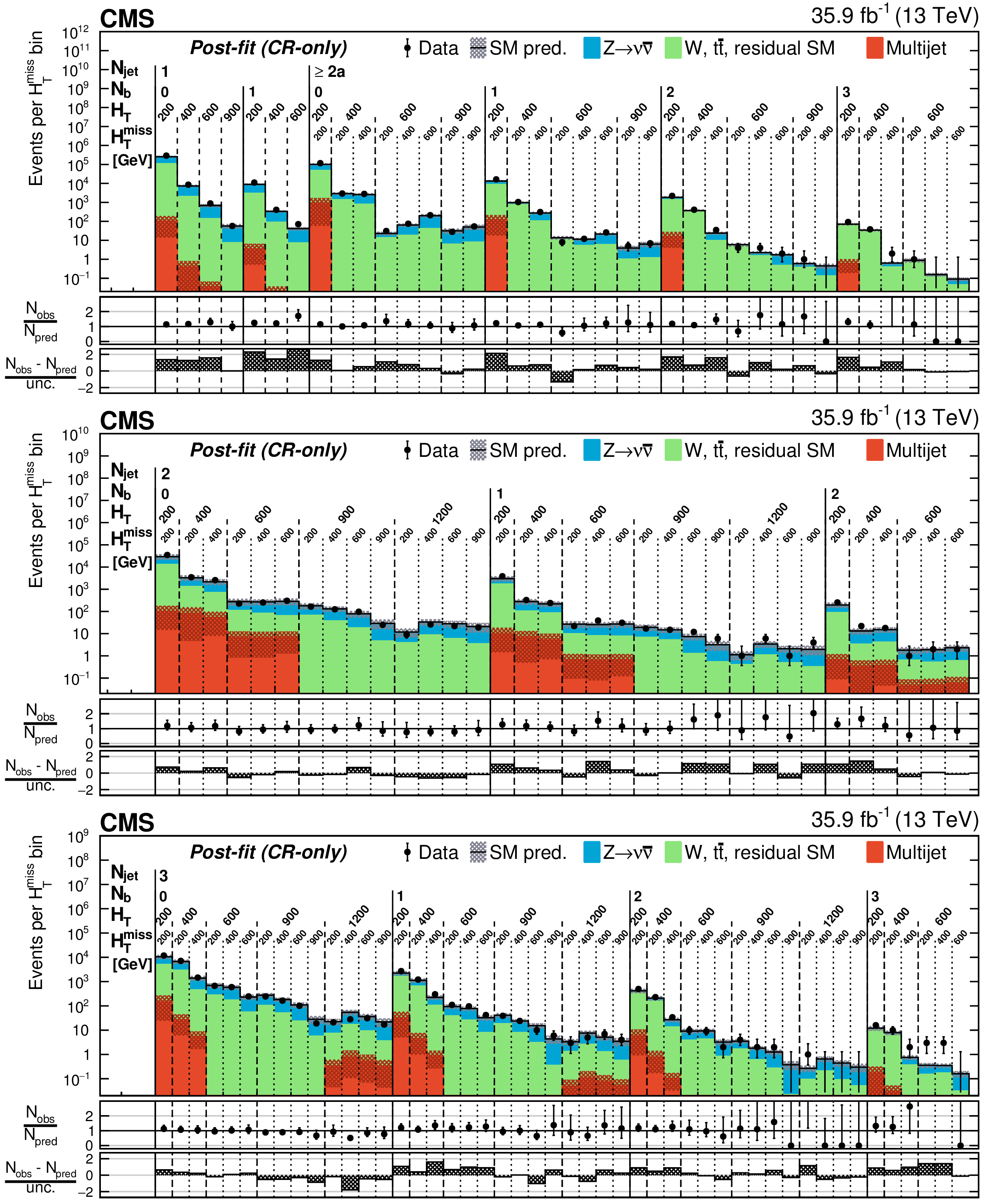
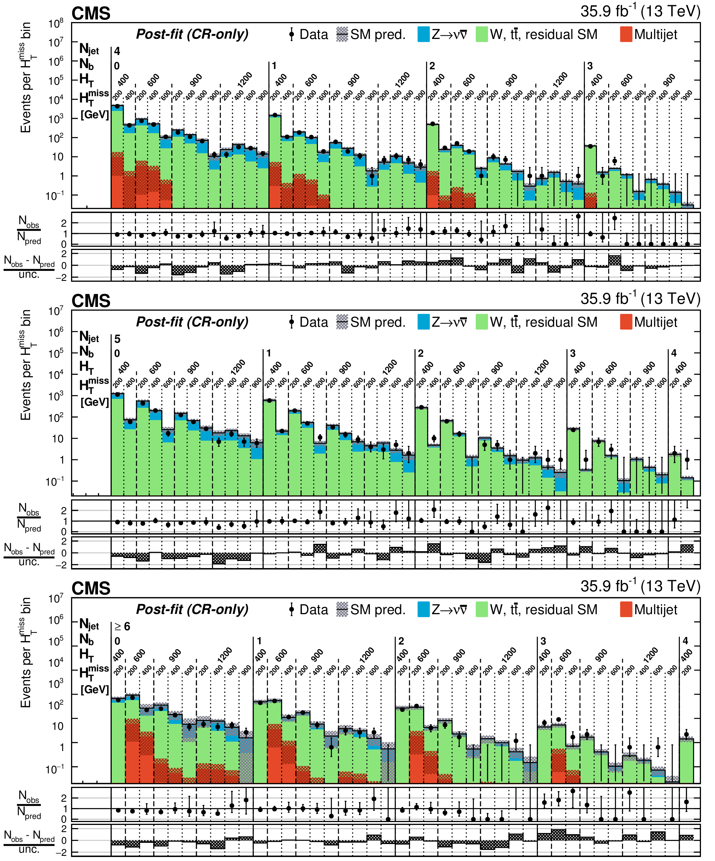
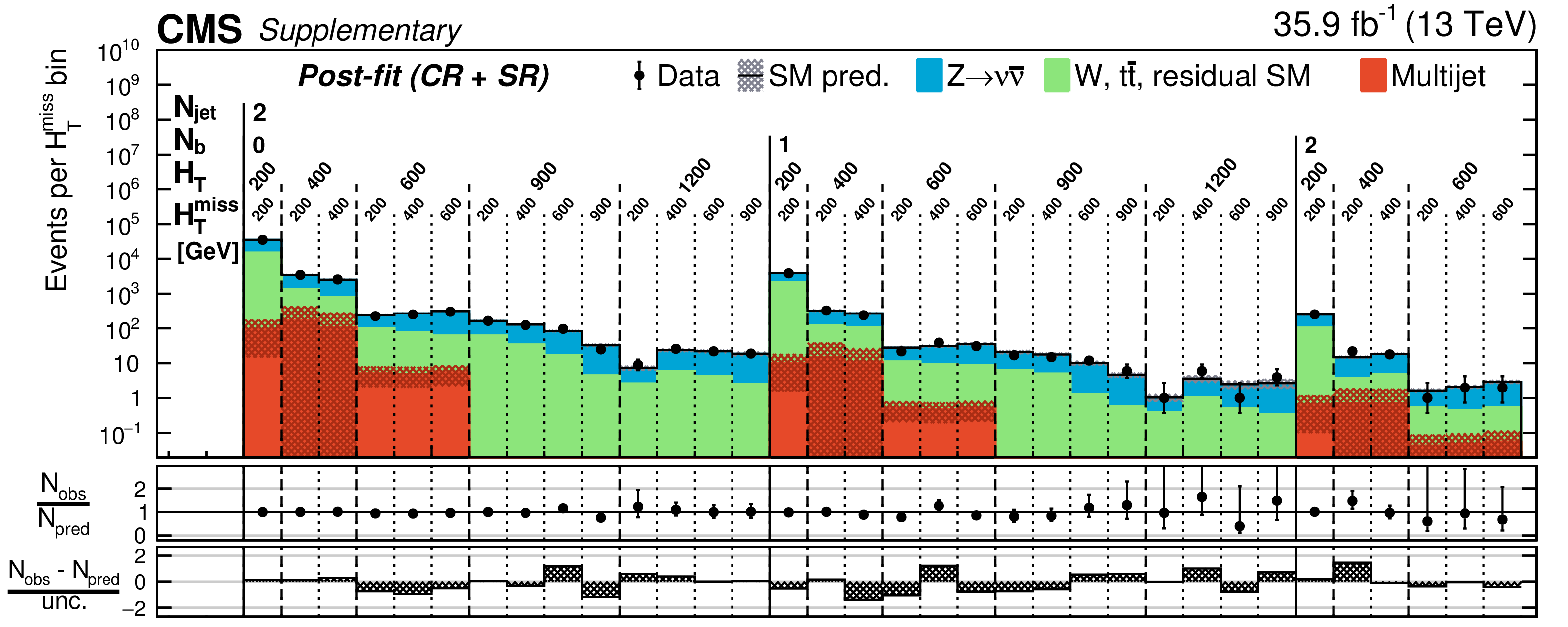
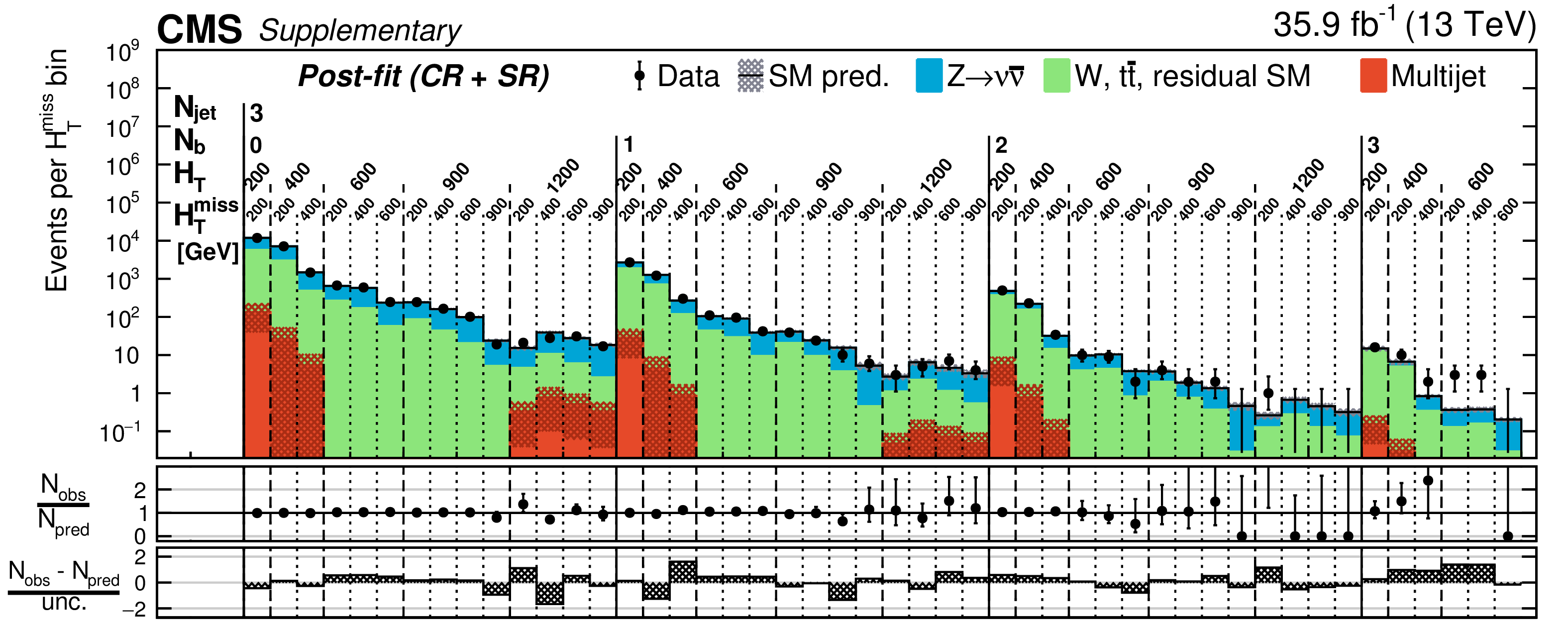
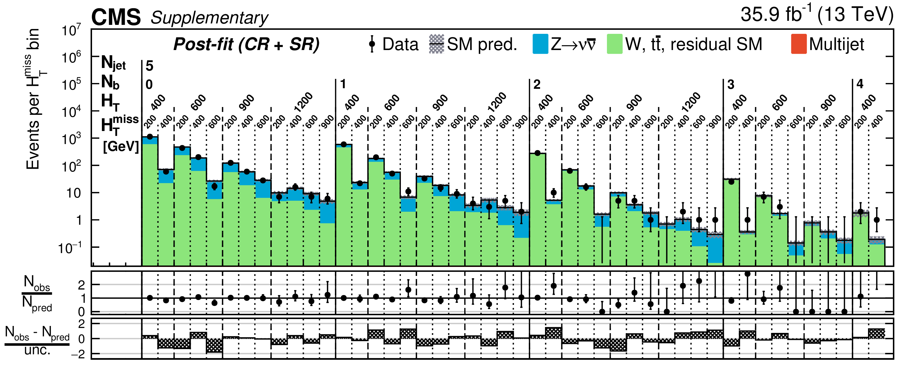
Figure 1:
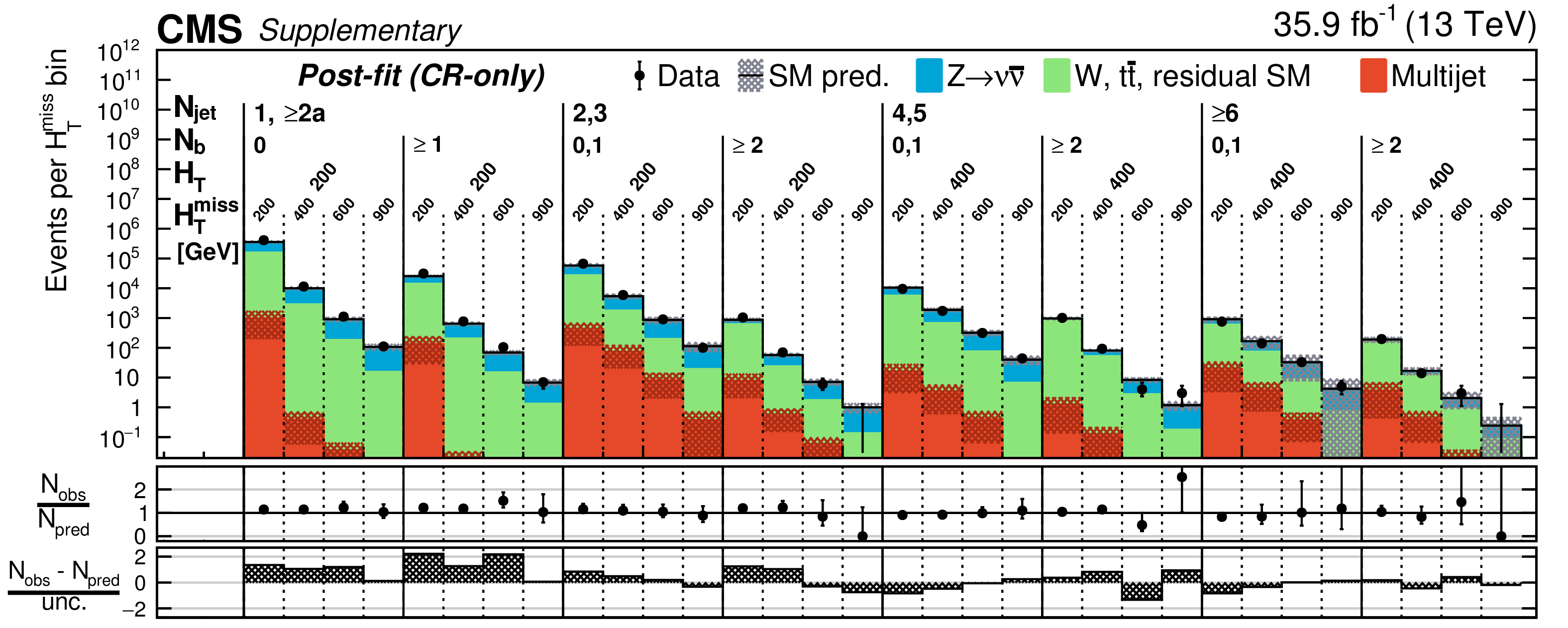
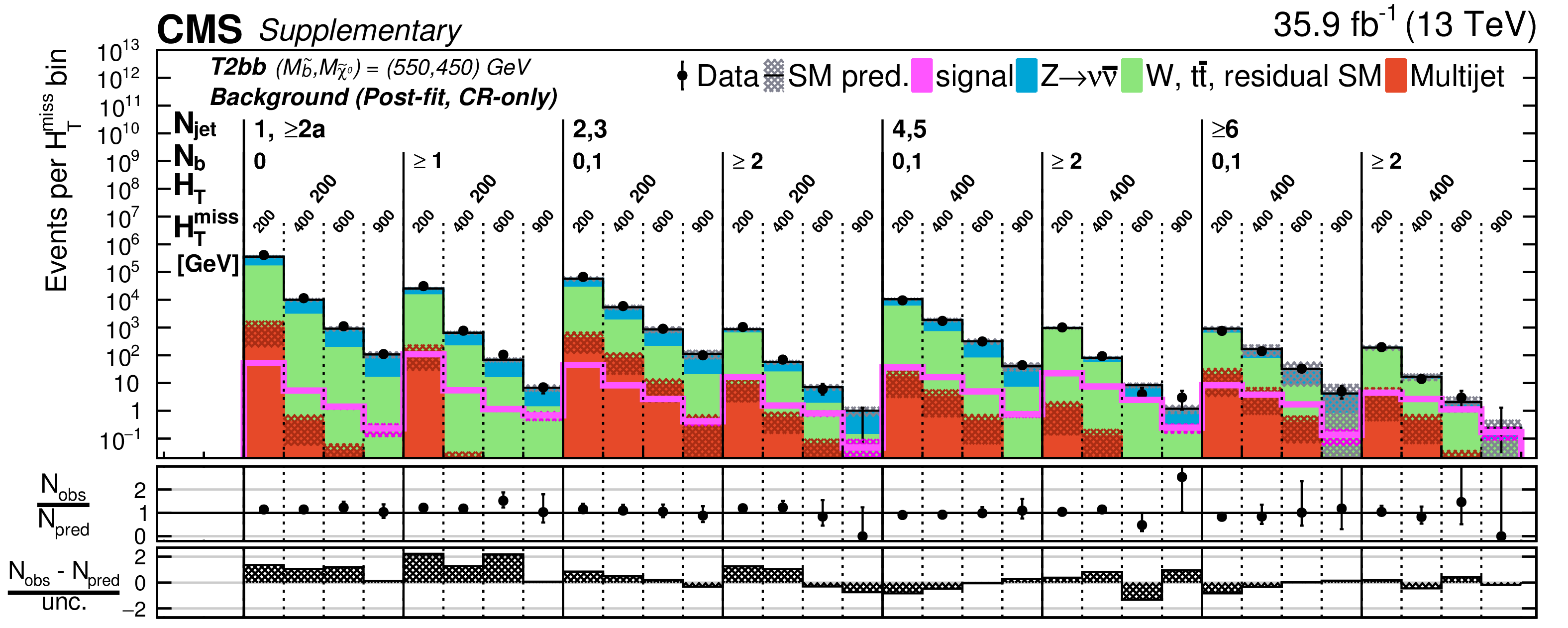
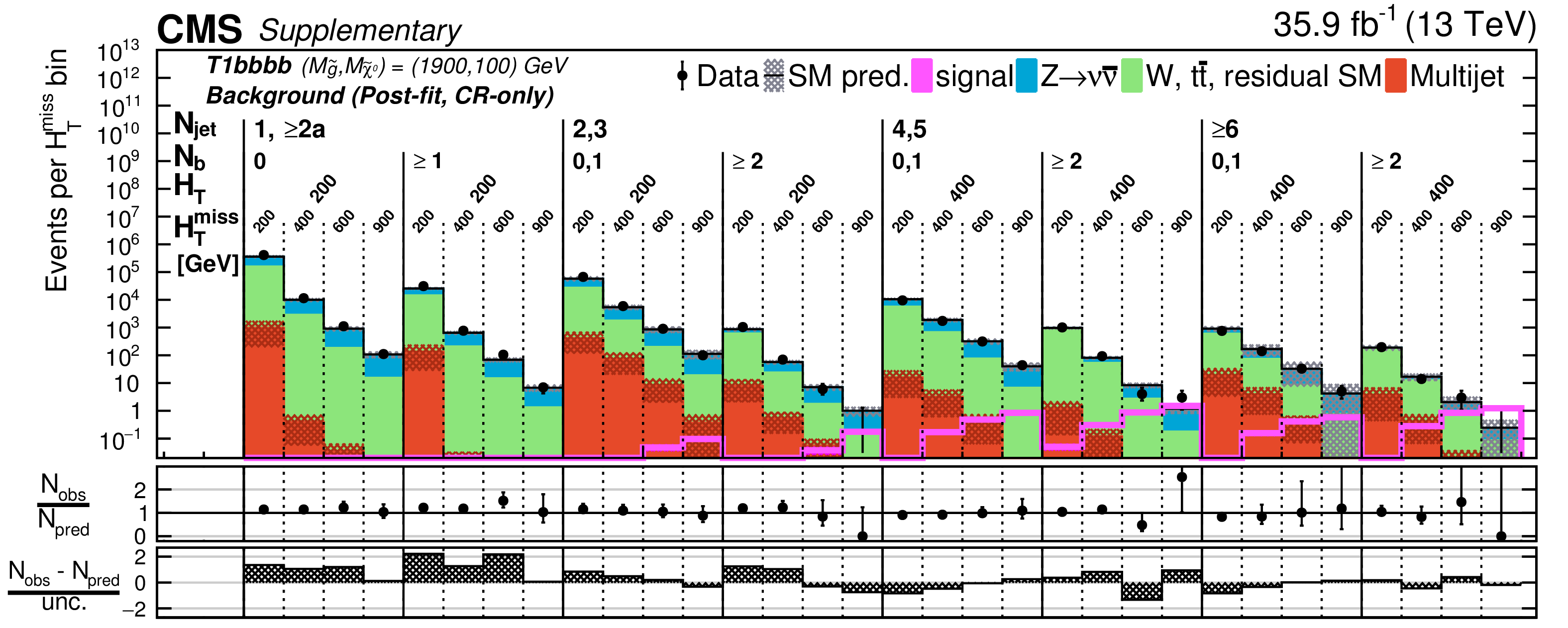
Counts of signal events (solid markers) and SM expectations with associated uncertainties (statistical and systematic, black histograms and shaded bands) as determined from the CR-only fit as a function of $ {n_{\mathrm {b}}} $, $ {H_{\mathrm {T}}} $, and $ {H_{\mathrm {T}}^{\text {miss}}} $ for the event categories $ {n_{\text {jet}}} = $ 1 and ${\geq}$ 2a (upper), $=$ 2 (middle), and $=$ 3 (lower). The centre panel of each subfigure shows the ratios of observed counts and the SM expectations, while the lower panel shows the significance of deviations observed in data with respect to the SM expectations expressed in terms of the total uncertainty in the SM expectations. |
png pdf |
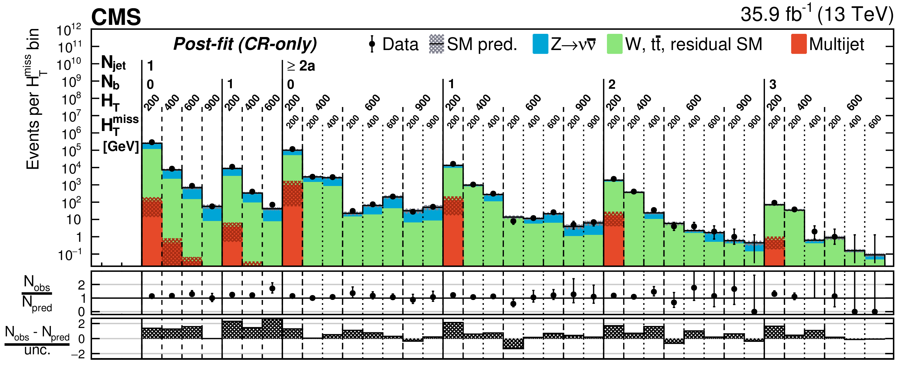
Figure 1-a:
Counts of signal events (solid markers) and SM expectations with associated uncertainties (statistical and systematic, black histograms and shaded bands) as determined from the CR-only fit as a function of $ {n_{\mathrm {b}}} $, $ {H_{\mathrm {T}}} $, and $ {H_{\mathrm {T}}^{\text {miss}}} $ for the event category $ {n_{\text {jet}}} = $ 1 and ${\geq}$ 2a. The centre panel shows the ratios of observed counts and the SM expectations, while the lower panel shows the significance of deviations observed in data with respect to the SM expectations expressed in terms of the total uncertainty in the SM expectations. |
png pdf |
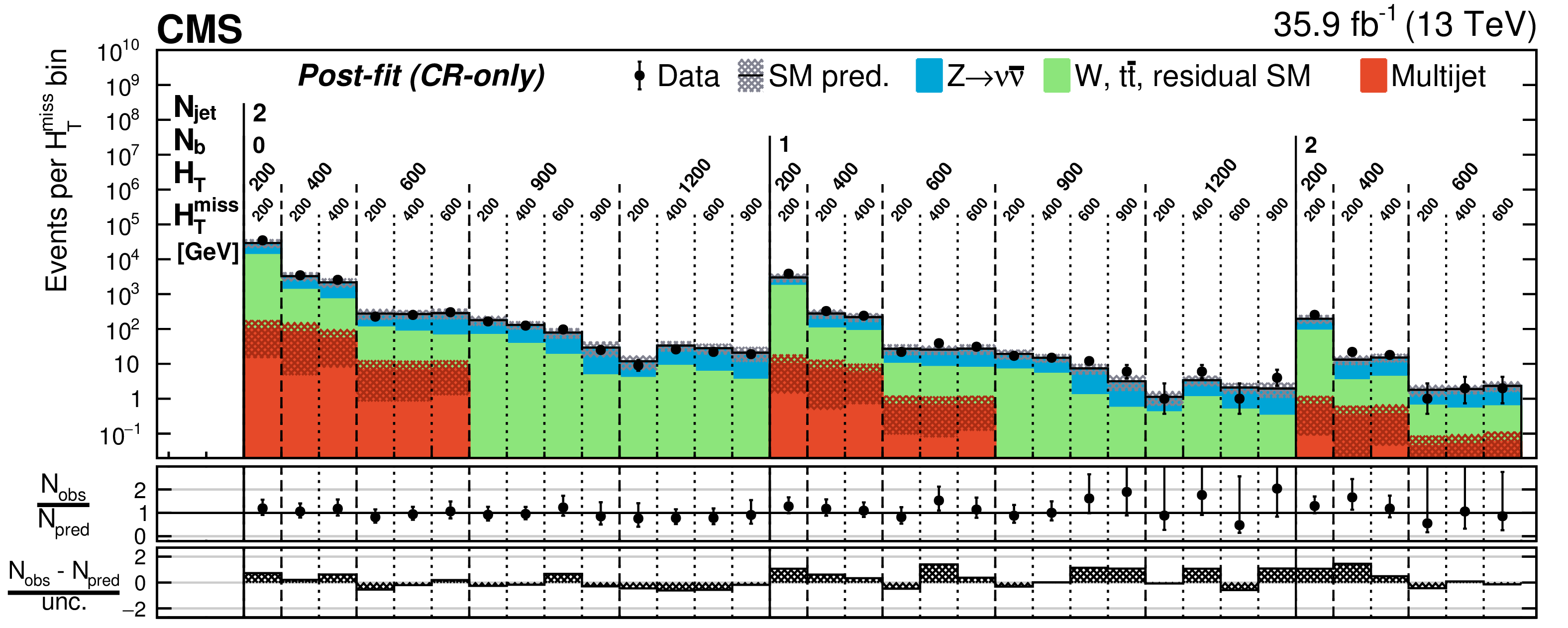
Figure 1-b:
Counts of signal events (solid markers) and SM expectations with associated uncertainties (statistical and systematic, black histograms and shaded bands) as determined from the CR-only fit as a function of $ {n_{\mathrm {b}}} $, $ {H_{\mathrm {T}}} $, and $ {H_{\mathrm {T}}^{\text {miss}}} $ for the event category $ {n_{\text {jet}}} =$ 2. The centre panel shows the ratios of observed counts and the SM expectations, while the lower panel shows the significance of deviations observed in data with respect to the SM expectations expressed in terms of the total uncertainty in the SM expectations. |
png pdf |
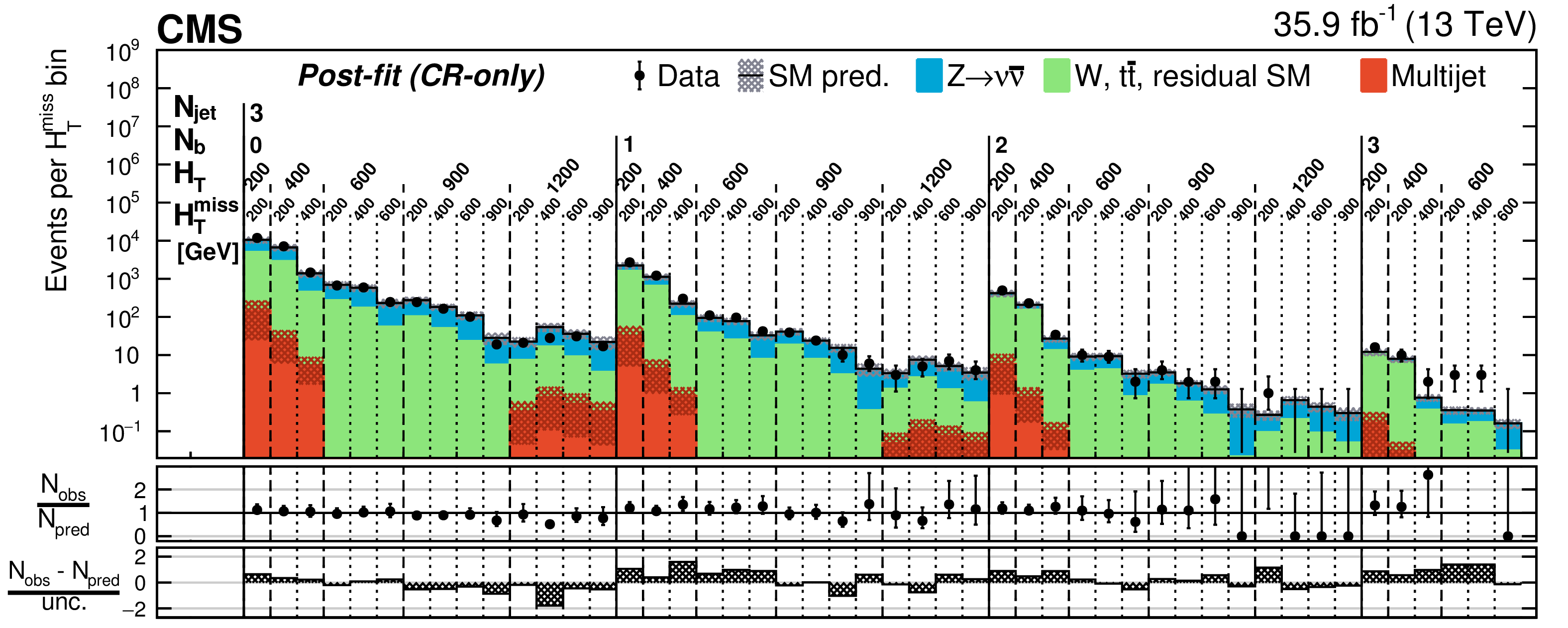
Figure 1-c:
Counts of signal events (solid markers) and SM expectations with associated uncertainties (statistical and systematic, black histograms and shaded bands) as determined from the CR-only fit as a function of $ {n_{\mathrm {b}}} $, $ {H_{\mathrm {T}}} $, and $ {H_{\mathrm {T}}^{\text {miss}}} $ for the event category $ {n_{\text {jet}}} =$ 3. The centre panel shows the ratios of observed counts and the SM expectations, while the lower panel shows the significance of deviations observed in data with respect to the SM expectations expressed in terms of the total uncertainty in the SM expectations. |
png pdf csv |
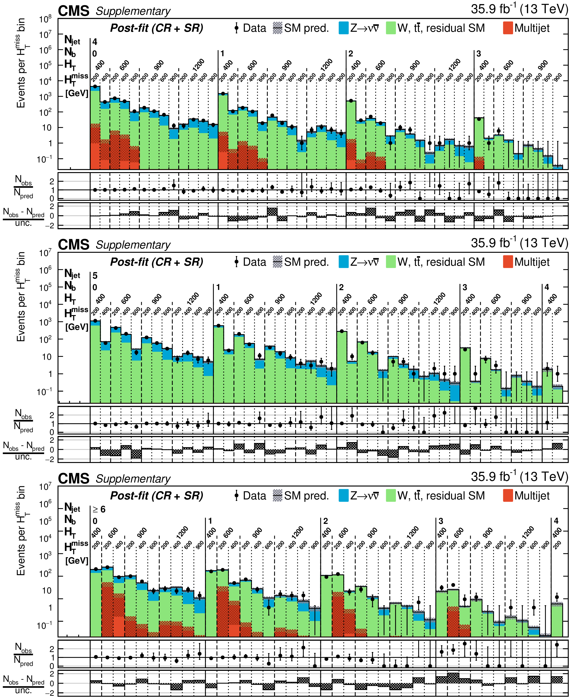
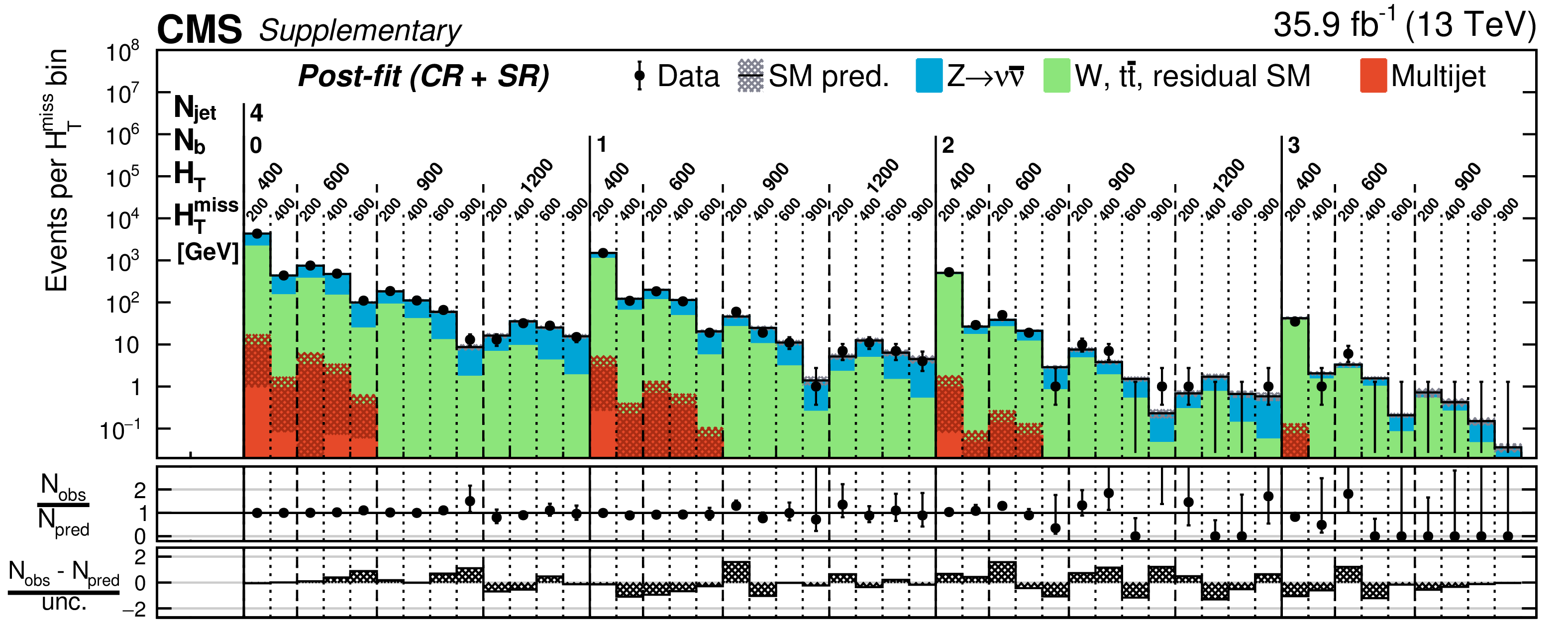
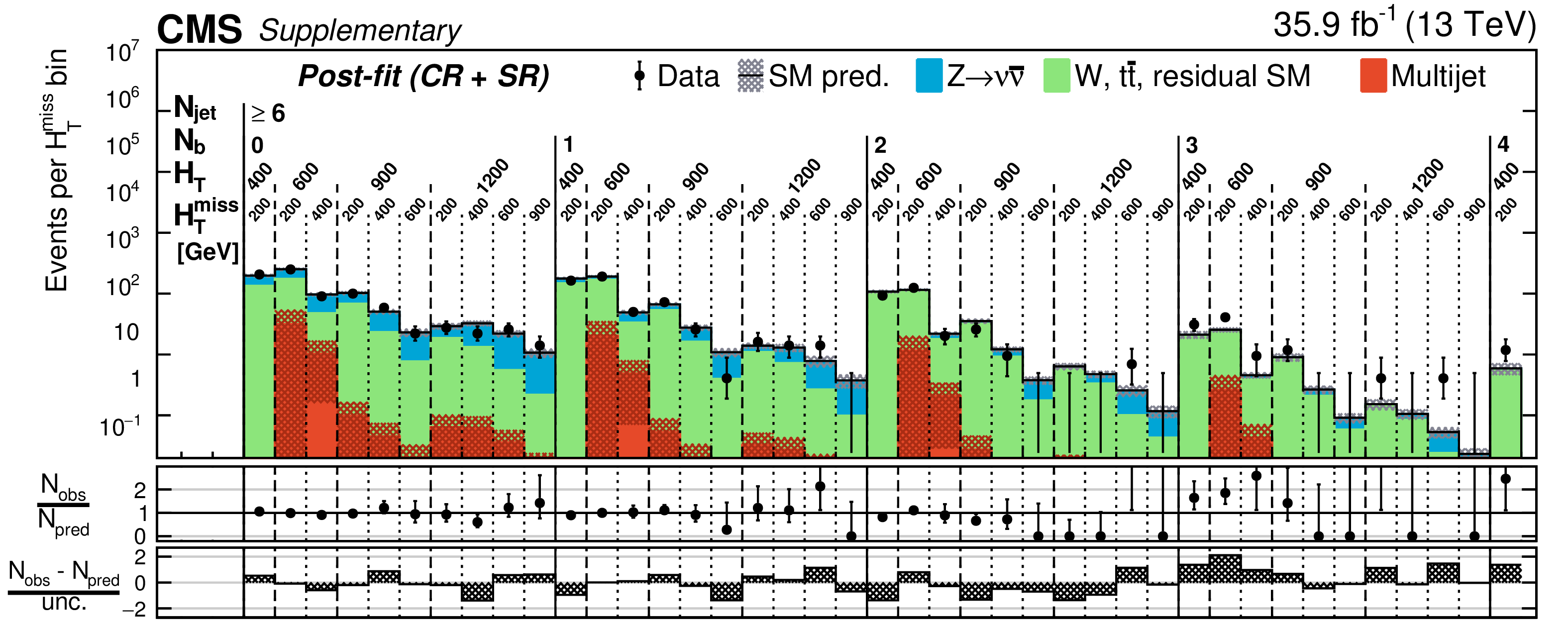
Figure 2:
Counts of signal events (solid markers) and SM expectations with associated uncertainties (statistical and systematic, black histograms and shaded bands) as determined from the CR-only fit as a function of $ {n_{\mathrm {b}}} $, $ {H_{\mathrm {T}}} $, and $ {H_{\mathrm {T}}^{\text {miss}}} $ for the event categories $ {n_{\text {jet}}} = $ 4 (upper), $= $ 5 (middle), and ${\geq}$ 6 (lower). The lower panels are described in the caption of Fig.1. |
png pdf |
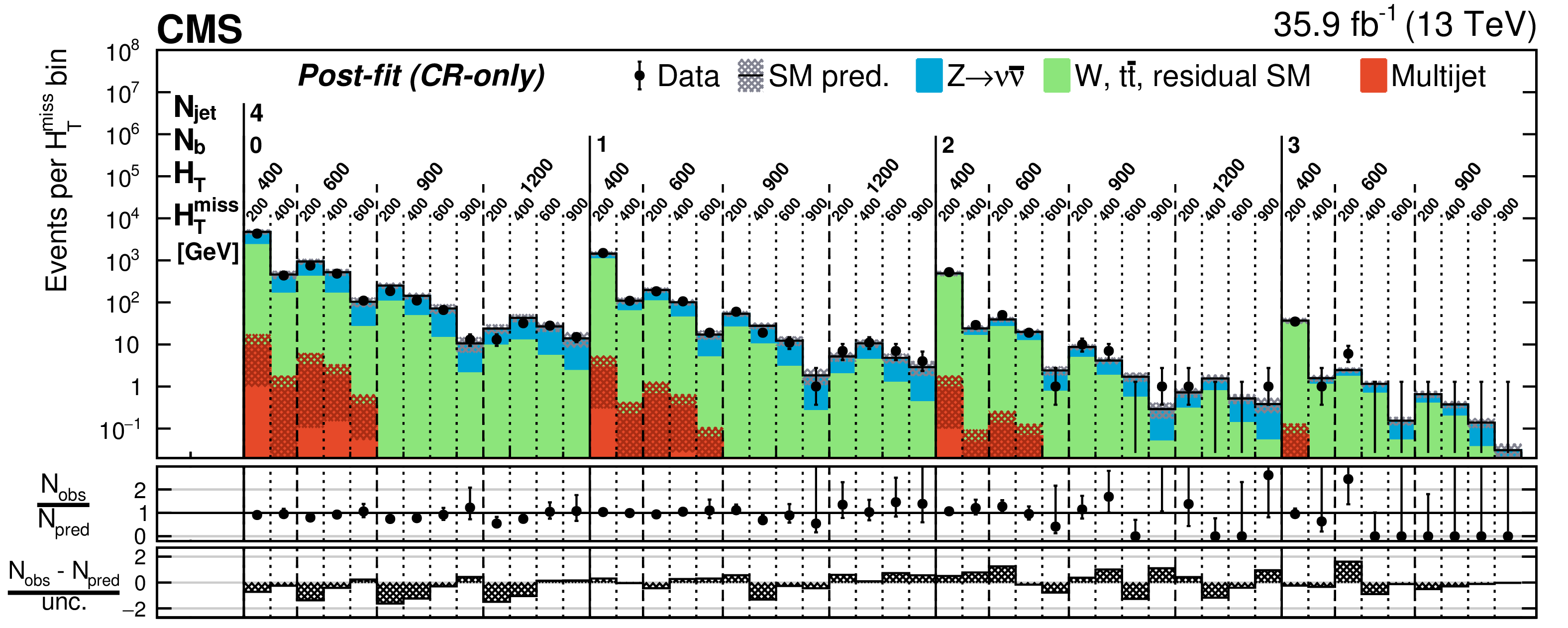
Figure 2-a:
Counts of signal events (solid markers) and SM expectations with associated uncertainties (statistical and systematic, black histograms and shaded bands) as determined from the CR-only fit as a function of $ {n_{\mathrm {b}}} $, $ {H_{\mathrm {T}}} $, and $ {H_{\mathrm {T}}^{\text {miss}}} $ for the event category $ {n_{\text {jet}}} = $ 4. The lower panel is described in the caption of Fig.1. |
png pdf |
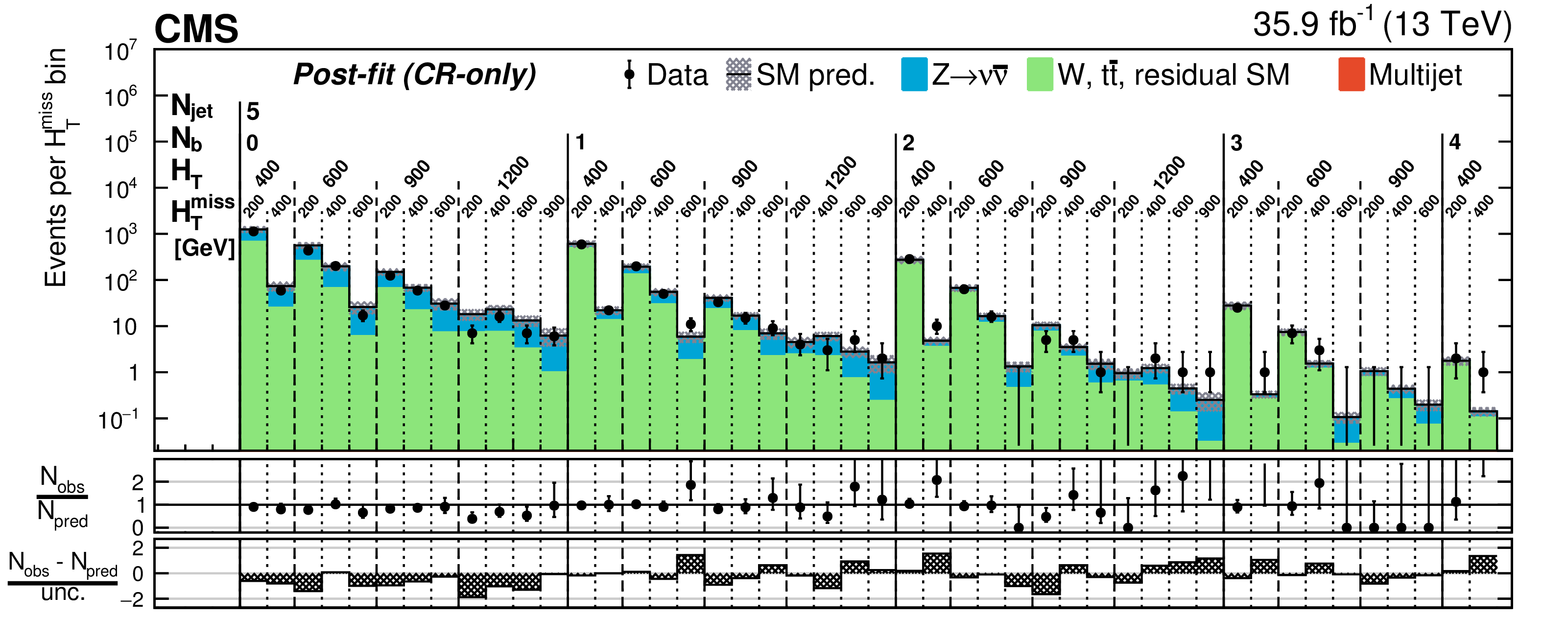
Figure 2-b:
Counts of signal events (solid markers) and SM expectations with associated uncertainties (statistical and systematic, black histograms and shaded bands) as determined from the CR-only fit as a function of $ {n_{\mathrm {b}}} $, $ {H_{\mathrm {T}}} $, and $ {H_{\mathrm {T}}^{\text {miss}}} $ for the event category $ {n_{\text {jet}}} = $ 5. The lower panel is described in the caption of Fig.1. |
png pdf |
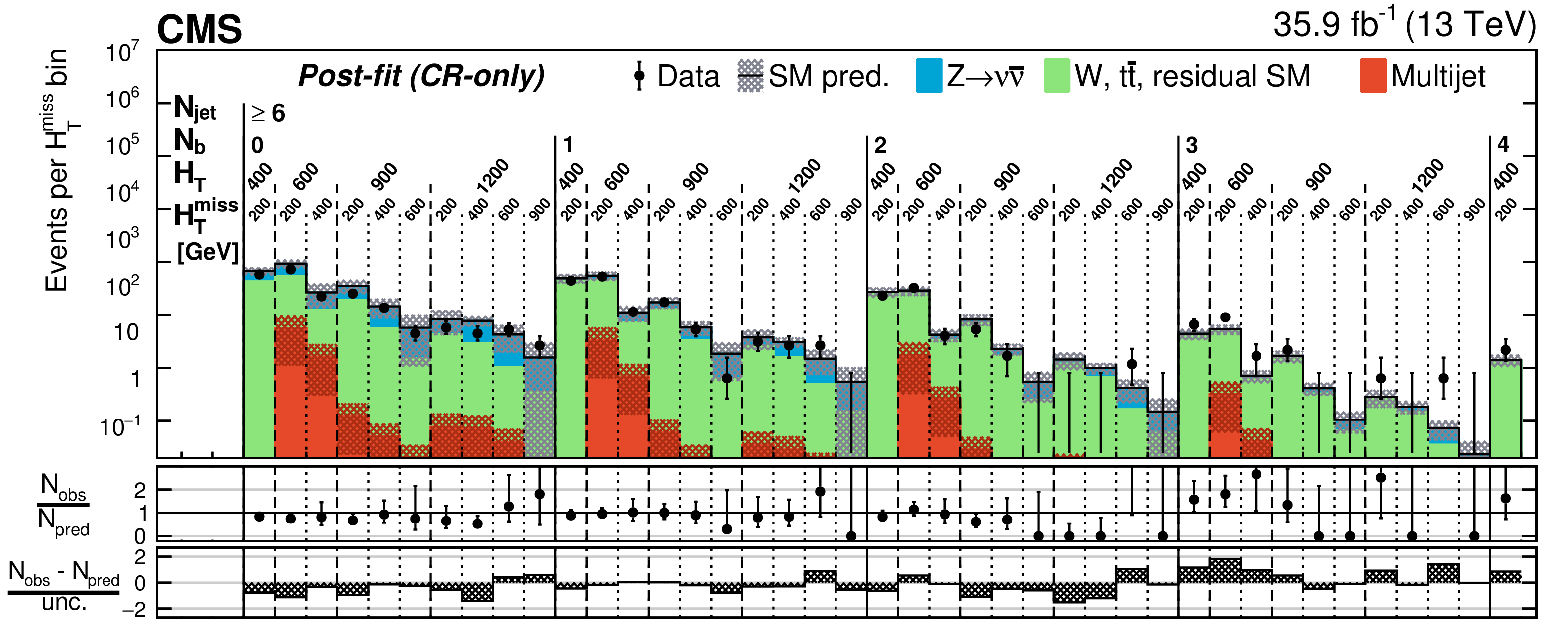
Figure 2-c:
Counts of signal events (solid markers) and SM expectations with associated uncertainties (statistical and systematic, black histograms and shaded bands) as determined from the CR-only fit as a function of $ {n_{\mathrm {b}}} $, $ {H_{\mathrm {T}}} $, and $ {H_{\mathrm {T}}^{\text {miss}}} $ for the event category $ {n_{\text {jet}}} {\geq}$ 6. The lower panel is described in the caption of Fig.1. |
png pdf |
Figure 3:
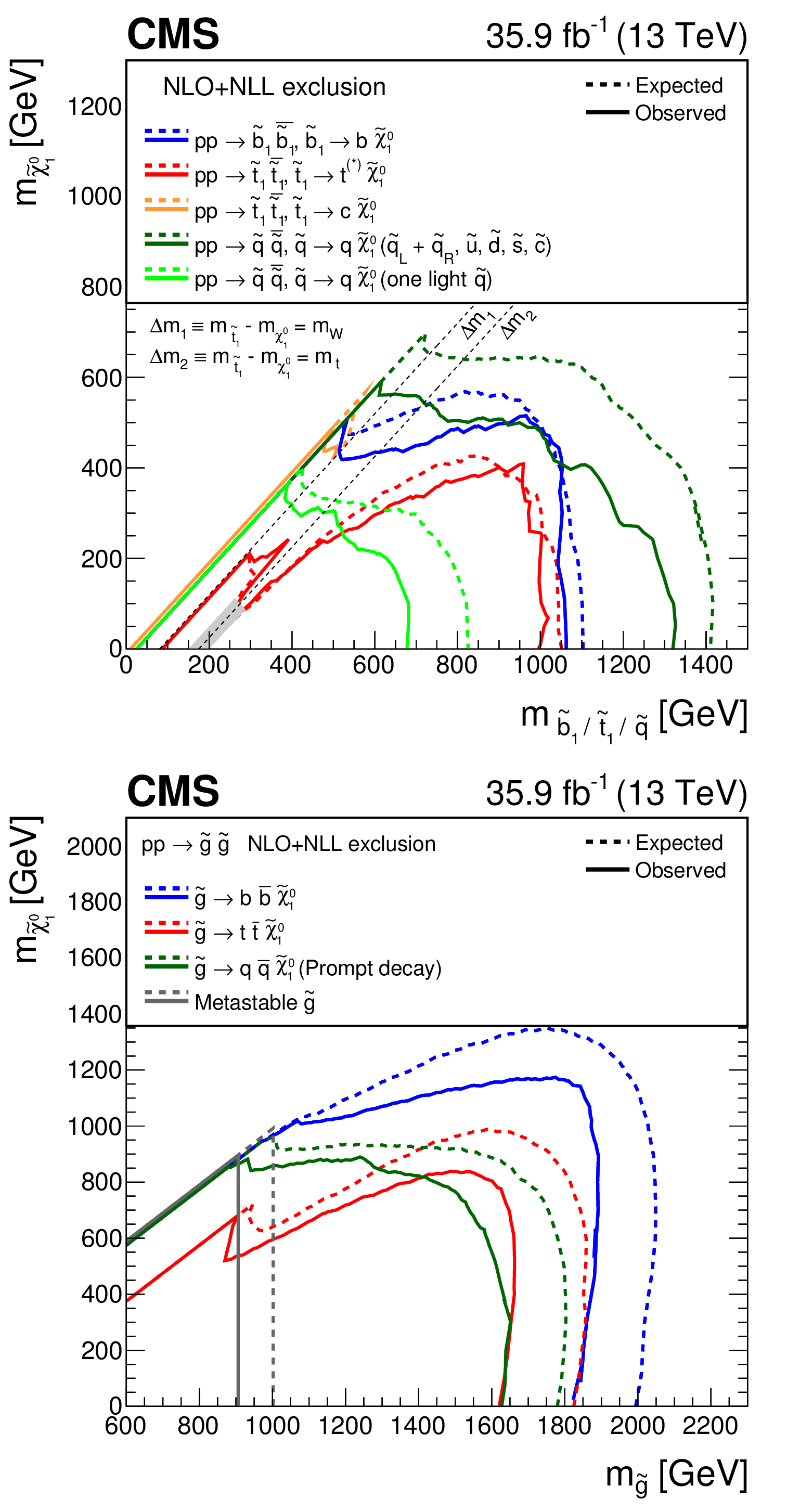
Observed and expected mass exclusions at 95% CL (indicated, respectively, by solid and dashed contours) for various families of simplified models. The upper subfigure summarises the mass exclusions for five model families that involve the direct pair production of squarks. The first scenario considers the pair production and decay of bottom squarks (T2bb). Two scenarios involve the production and decay of top squark pairs (T2tt and T2cc). The grey shaded region denotes T2tt models that are not considered for interpretation. Two further scenarios involve, respectively, the production and decay of light-flavour squarks, with different assumptions on the mass degeneracy of the squarks as described in the text (T2qq_8fold and T2qq_1fold). The lower subfigure summarises three scenarios that involve the production and prompt decay of gluino pairs via virtual squarks (T1bbbb, T1tttt, and T1qqqq). A final scenario involves the production of gluinos that are assumed to be metastable on the detector scale (T1qqqqLL). |

png pdf |
Figure 3-a:
Observed and expected mass exclusions at 95% CL (indicated, respectively, by solid and dashed contours) for various families of simplified models. The figure summarises the mass exclusions for five model families that involve the direct pair production of squarks. The first scenario considers the pair production and decay of bottom squarks (T2bb). Two scenarios involve the production and decay of top squark pairs (T2tt and T2cc). The grey shaded region denotes T2tt models that are not considered for interpretation. Two further scenarios involve, respectively, the production and decay of light-flavour squarks, with different assumptions on the mass degeneracy of the squarks as described in the text (T2qq_8fold and T2qq_1fold). |
png pdf |
Figure 3-b:
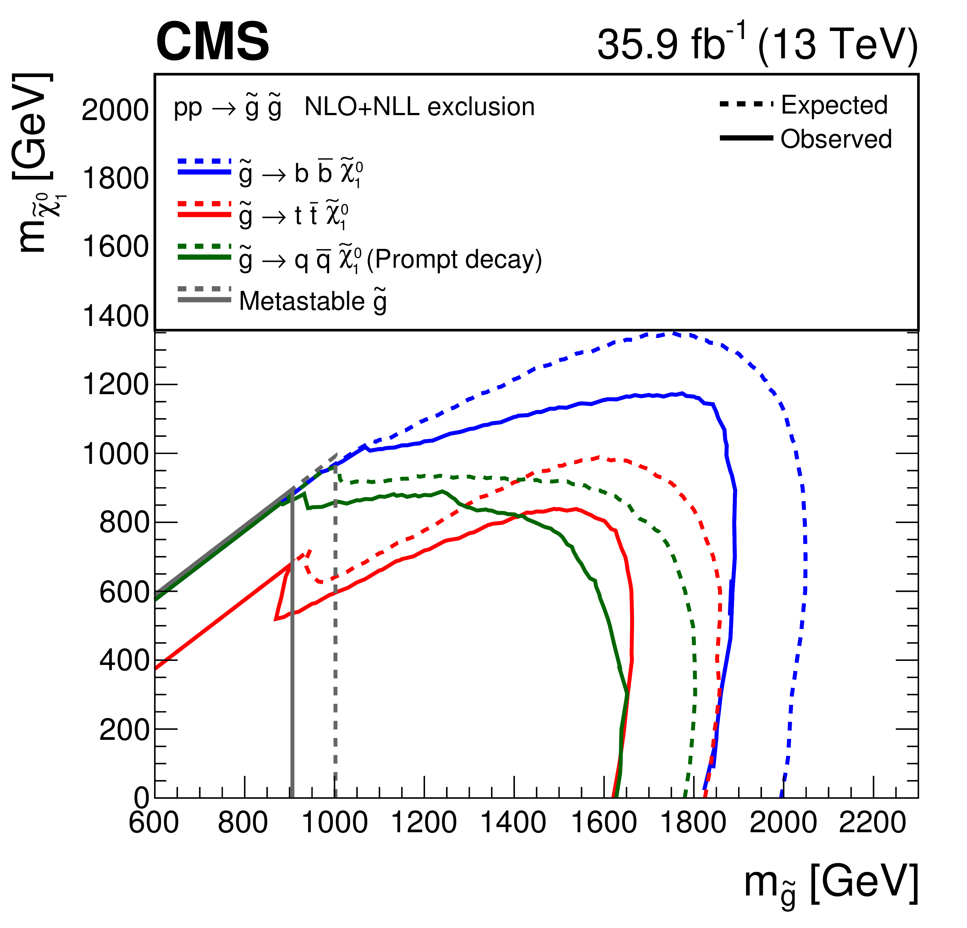
Observed and expected mass exclusions at 95% CL (indicated, respectively, by solid and dashed contours) for various families of simplified models. The figure summarises three scenarios that involve the production and prompt decay of gluino pairs via virtual squarks (T1bbbb, T1tttt, and T1qqqq). A final scenario involves the production of gluinos that are assumed to be metastable on the detector scale (T1qqqqLL). |

png pdf |
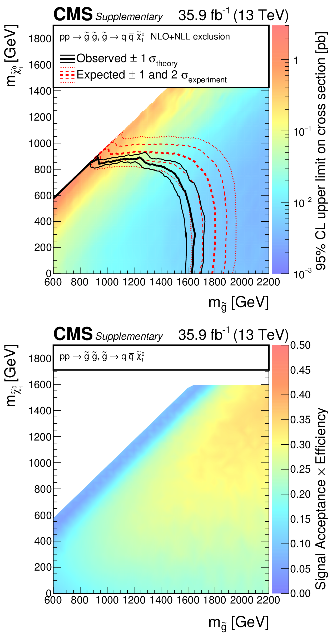
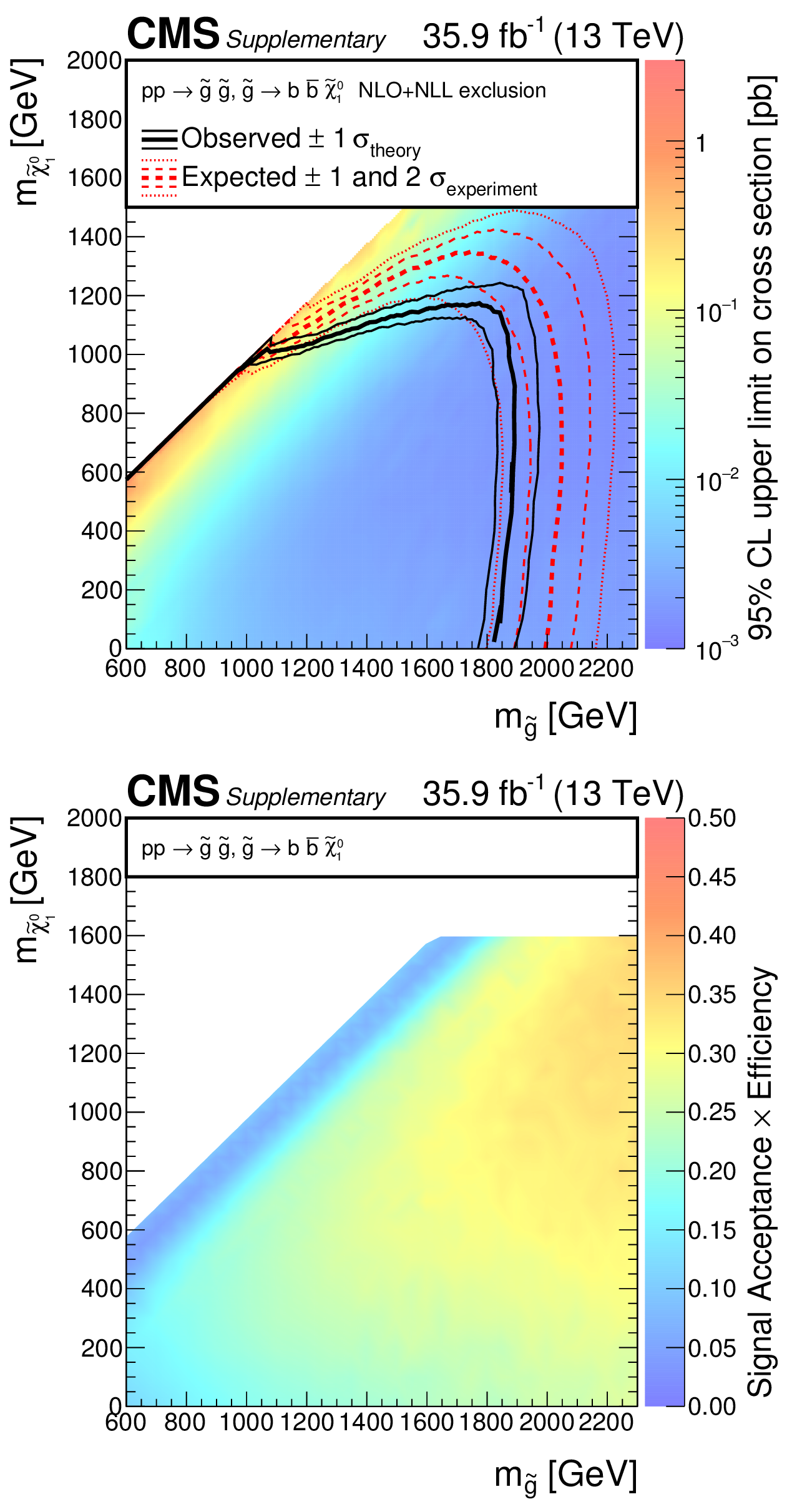
Figure 4:
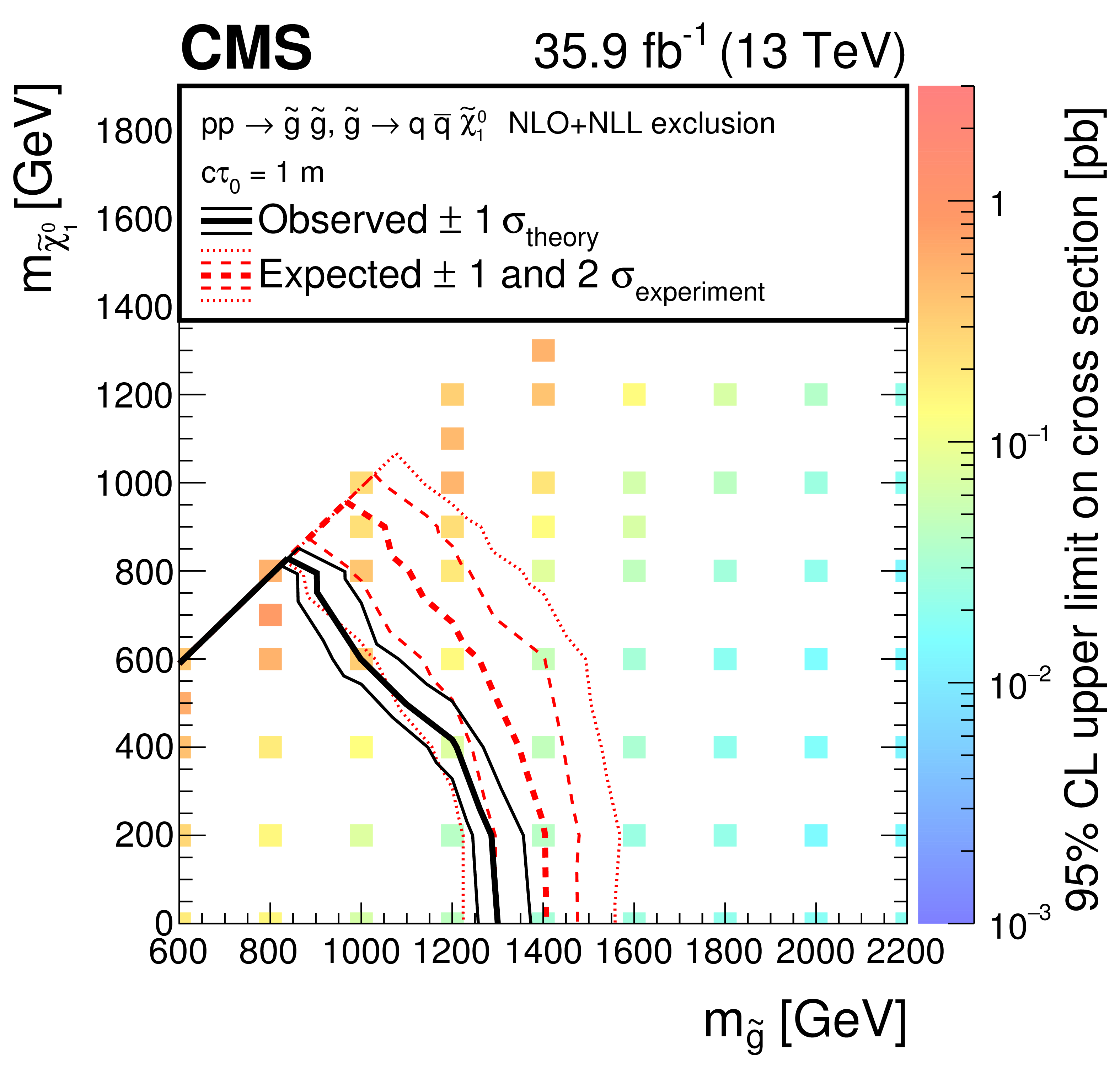
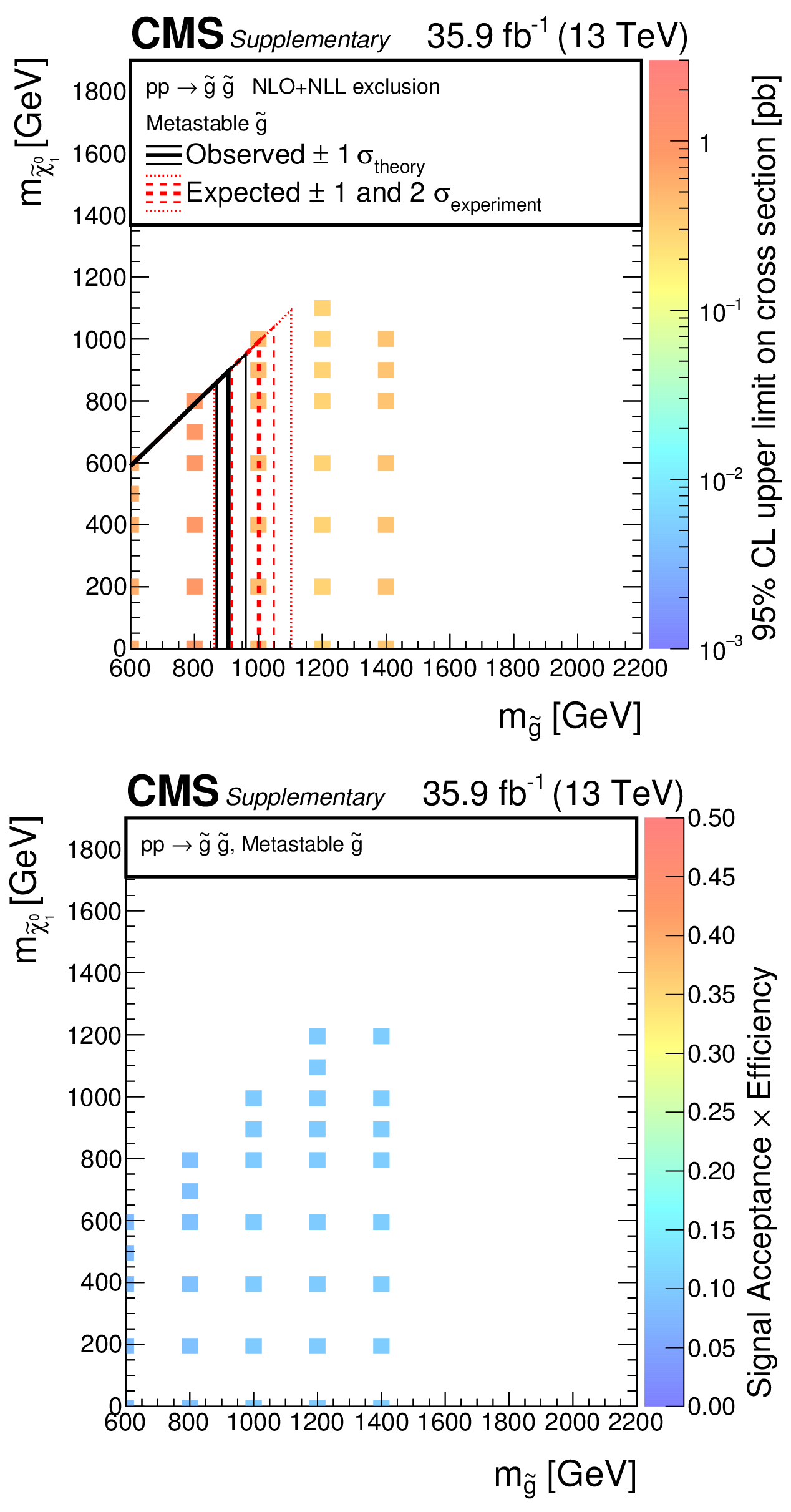
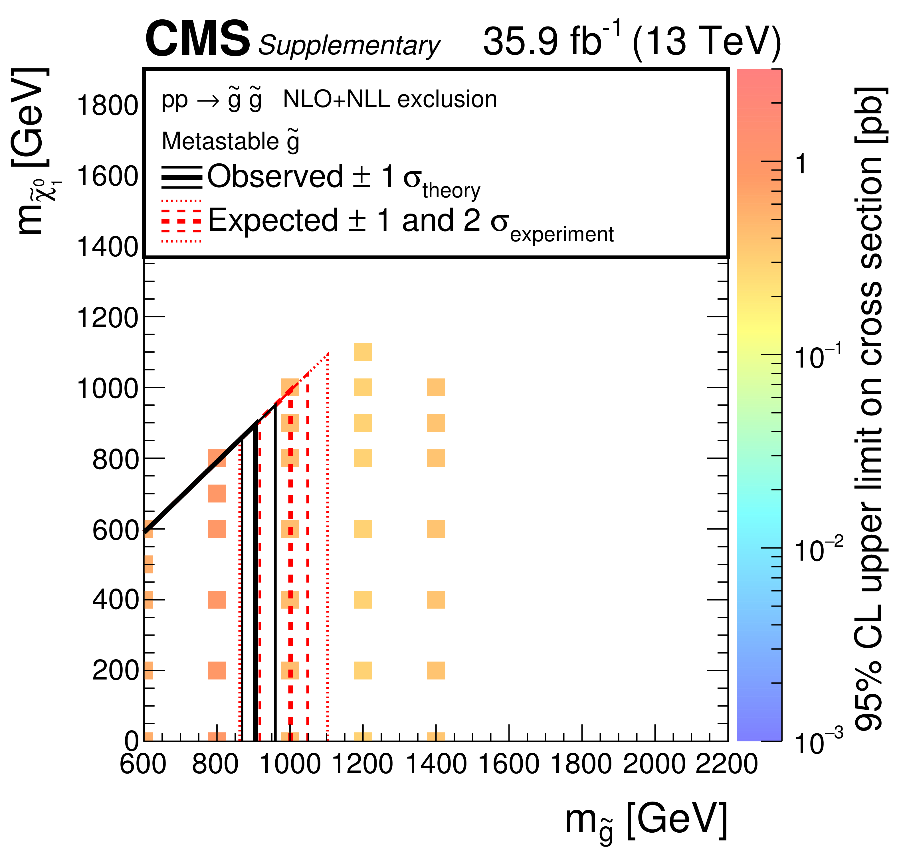
Observed upper limit in cross section at 95% CL (indicated by the colour scale) as a function of the $ \tilde{ \mathrm{g} }$ and $\tilde{\chi}^0_1$ masses for simplified models that assume the production of pairs of long-lived gluinos that each decay via highly virtual light-flavour squarks to the neutralino and SM particles (T1qqqqLL). Each subfigure represents a different gluino lifetime: $ {c\tau _{0}} = $ 1 (upper left), 10 (upper centre), and 100 $\mu$m (upper right); 1 (middle left), 10 (middle centre), and 100 mm (middle right); and 1 (lower left), 10 (lower centre), and 100 m (lower right). The thick (thin) black solid line indicates the observed excluded region assuming the nominal (${\pm}$1 standard deviation in theoretical uncertainty) production cross section. The red thick dashed (thin dashed and dotted) line indicates the median (${\pm}$1 and 2 standard deviations in experimental uncertainty) expected excluded region. |

png pdf root |
Figure 4-a:
Observed upper limit in cross section at 95% CL (indicated by the colour scale) as a function of the $ \tilde{ \mathrm{g} }$ and $\tilde{\chi}^0_1$ masses for a simplified model that assume the production of pairs of long-lived gluinos that each decay via highly virtual light-flavour squarks to the neutralino and SM particles (T1qqqqLL). The figure represents a gluino lifetime of $ {c\tau _{0}} = $ 1 $\mu$m. The thick (thin) black solid line indicates the observed excluded region assuming the nominal (${\pm}$1 standard deviation in theoretical uncertainty) production cross section. The red thick dashed (thin dashed and dotted) line indicates the median (${\pm}$1 and 2 standard deviations in experimental uncertainty) expected excluded region. |

png pdf root |
Figure 4-b:
Observed upper limit in cross section at 95% CL (indicated by the colour scale) as a function of the $ \tilde{ \mathrm{g} }$ and $\tilde{\chi}^0_1$ masses for a simplified model that assume the production of pairs of long-lived gluinos that each decay via highly virtual light-flavour squarks to the neutralino and SM particles (T1qqqqLL). The figure represents a gluino lifetime of $ {c\tau _{0}} = $ 10 $\mu$m. The thick (thin) black solid line indicates the observed excluded region assuming the nominal (${\pm}$1 standard deviation in theoretical uncertainty) production cross section. The red thick dashed (thin dashed and dotted) line indicates the median (${\pm}$1 and 2 standard deviations in experimental uncertainty) expected excluded region. |

png pdf root |
Figure 4-c:
Observed upper limit in cross section at 95% CL (indicated by the colour scale) as a function of the $ \tilde{ \mathrm{g} }$ and $\tilde{\chi}^0_1$ masses for a simplified model that assume the production of pairs of long-lived gluinos that each decay via highly virtual light-flavour squarks to the neutralino and SM particles (T1qqqqLL). The figure represents a gluino lifetime of $ {c\tau _{0}} = $ 100 $\mu$m. The thick (thin) black solid line indicates the observed excluded region assuming the nominal (${\pm}$1 standard deviation in theoretical uncertainty) production cross section. The red thick dashed (thin dashed and dotted) line indicates the median (${\pm}$1 and 2 standard deviations in experimental uncertainty) expected excluded region. |
png pdf root |
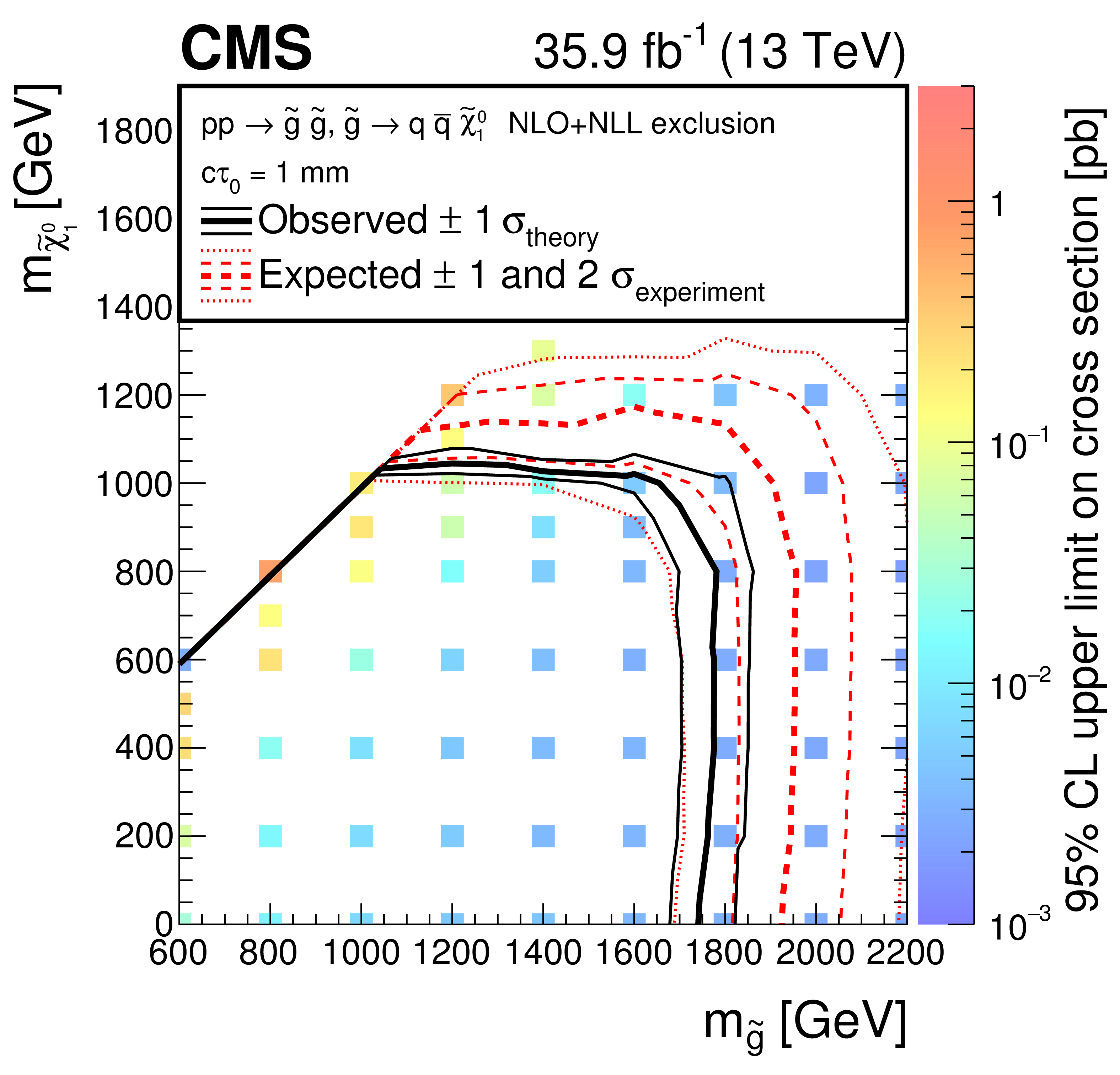
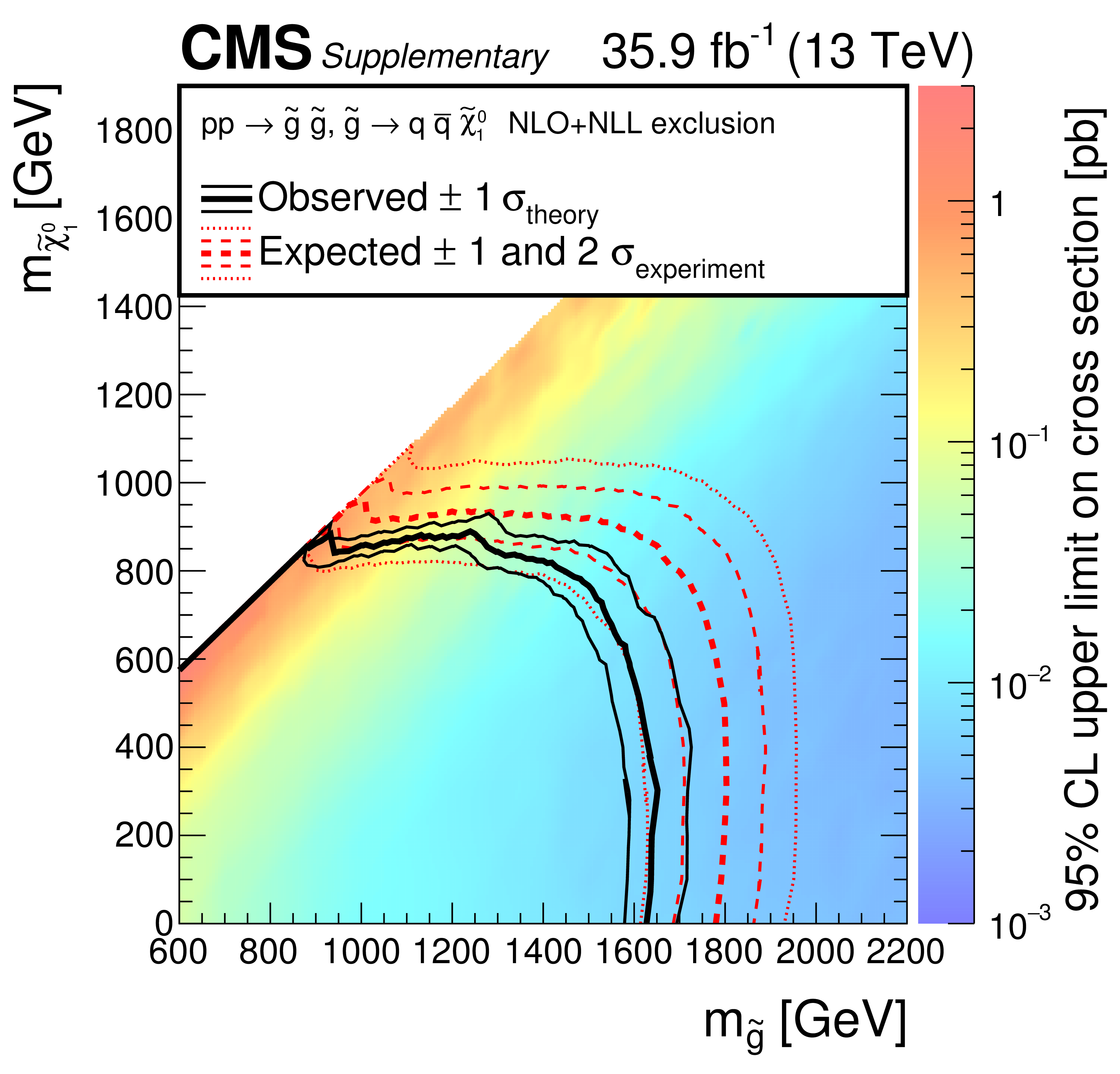
Figure 4-d:
Observed upper limit in cross section at 95% CL (indicated by the colour scale) as a function of the $ \tilde{ \mathrm{g} }$ and $\tilde{\chi}^0_1$ masses for a simplified model that assume the production of pairs of long-lived gluinos that each decay via highly virtual light-flavour squarks to the neutralino and SM particles (T1qqqqLL). The figure represents a gluino lifetime of $ {c\tau _{0}} = $ 1 mm. The thick (thin) black solid line indicates the observed excluded region assuming the nominal (${\pm}$1 standard deviation in theoretical uncertainty) production cross section. The red thick dashed (thin dashed and dotted) line indicates the median (${\pm}$1 and 2 standard deviations in experimental uncertainty) expected excluded region. |
png pdf root |
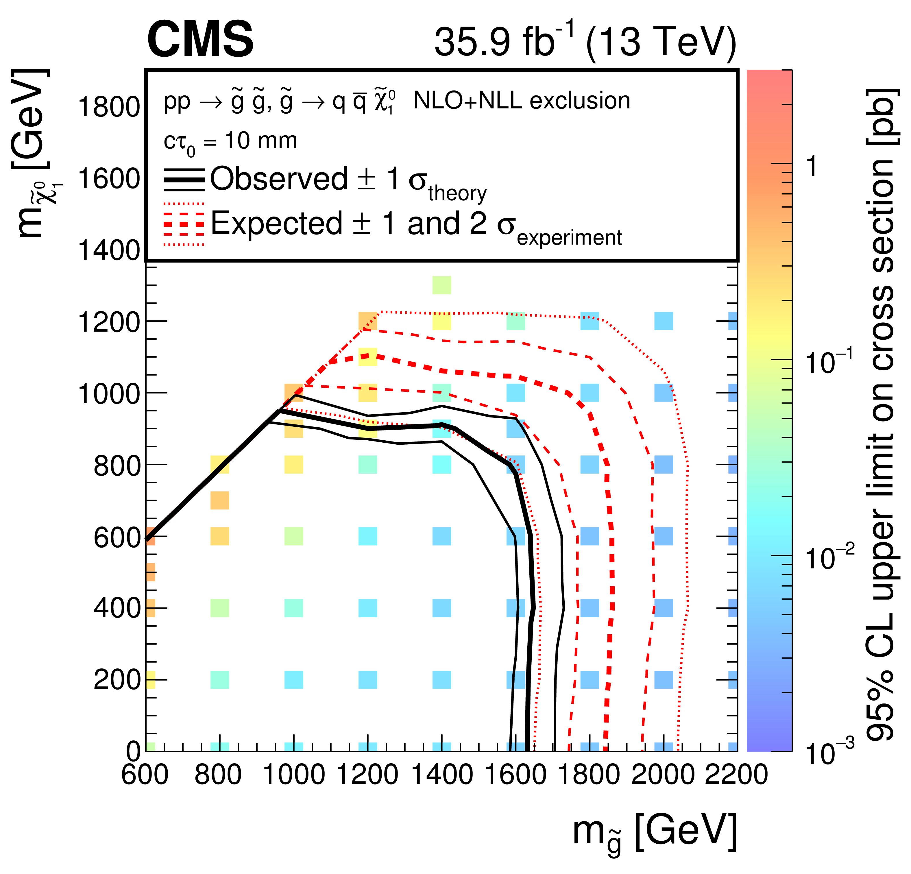
Figure 4-e:
Observed upper limit in cross section at 95% CL (indicated by the colour scale) as a function of the $ \tilde{ \mathrm{g} }$ and $\tilde{\chi}^0_1$ masses for a simplified model that assume the production of pairs of long-lived gluinos that each decay via highly virtual light-flavour squarks to the neutralino and SM particles (T1qqqqLL). The figure represents a gluino lifetime of $ {c\tau _{0}} = $ 10 mm. The thick (thin) black solid line indicates the observed excluded region assuming the nominal (${\pm}$1 standard deviation in theoretical uncertainty) production cross section. The red thick dashed (thin dashed and dotted) line indicates the median (${\pm}$1 and 2 standard deviations in experimental uncertainty) expected excluded region. |

png pdf root |
Figure 4-f:
Observed upper limit in cross section at 95% CL (indicated by the colour scale) as a function of the $ \tilde{ \mathrm{g} }$ and $\tilde{\chi}^0_1$ masses for a simplified model that assume the production of pairs of long-lived gluinos that each decay via highly virtual light-flavour squarks to the neutralino and SM particles (T1qqqqLL). The figure represents a gluino lifetime of $ {c\tau _{0}} = $ 100 mm. The thick (thin) black solid line indicates the observed excluded region assuming the nominal (${\pm}$1 standard deviation in theoretical uncertainty) production cross section. The red thick dashed (thin dashed and dotted) line indicates the median (${\pm}$1 and 2 standard deviations in experimental uncertainty) expected excluded region. |
png pdf root |
Figure 4-g:
Observed upper limit in cross section at 95% CL (indicated by the colour scale) as a function of the $ \tilde{ \mathrm{g} }$ and $\tilde{\chi}^0_1$ masses for a simplified model that assume the production of pairs of long-lived gluinos that each decay via highly virtual light-flavour squarks to the neutralino and SM particles (T1qqqqLL). The figure represents a gluino lifetime of $ {c\tau _{0}} = $ 1 m. The thick (thin) black solid line indicates the observed excluded region assuming the nominal (${\pm}$1 standard deviation in theoretical uncertainty) production cross section. The red thick dashed (thin dashed and dotted) line indicates the median (${\pm}$1 and 2 standard deviations in experimental uncertainty) expected excluded region. |

png pdf root |
Figure 4-h:
Observed upper limit in cross section at 95% CL (indicated by the colour scale) as a function of the $ \tilde{ \mathrm{g} }$ and $\tilde{\chi}^0_1$ masses for a simplified model that assume the production of pairs of long-lived gluinos that each decay via highly virtual light-flavour squarks to the neutralino and SM particles (T1qqqqLL). The figure represents a gluino lifetime of $ {c\tau _{0}} = $ 10 m. The thick (thin) black solid line indicates the observed excluded region assuming the nominal (${\pm}$1 standard deviation in theoretical uncertainty) production cross section. The red thick dashed (thin dashed and dotted) line indicates the median (${\pm}$1 and 2 standard deviations in experimental uncertainty) expected excluded region. |

png pdf root |
Figure 4-i:
Observed upper limit in cross section at 95% CL (indicated by the colour scale) as a function of the $ \tilde{ \mathrm{g} }$ and $\tilde{\chi}^0_1$ masses for a simplified model that assume the production of pairs of long-lived gluinos that each decay via highly virtual light-flavour squarks to the neutralino and SM particles (T1qqqqLL). The figure represents a gluino lifetime of $ {c\tau _{0}} = $ 100 m. The thick (thin) black solid line indicates the observed excluded region assuming the nominal (${\pm}$1 standard deviation in theoretical uncertainty) production cross section. The red thick dashed (thin dashed and dotted) line indicates the median (${\pm}$1 and 2 standard deviations in experimental uncertainty) expected excluded region. |
png pdf root |
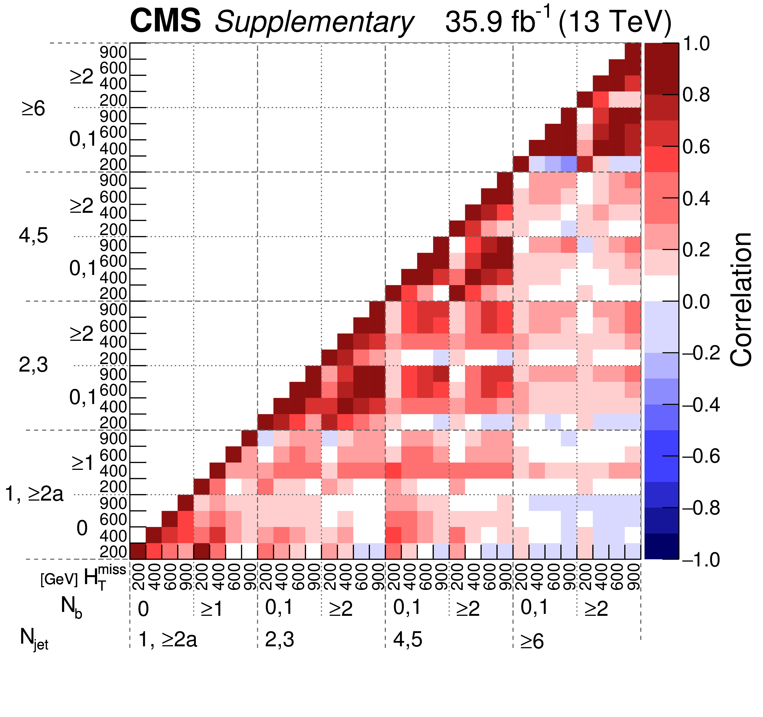
Figure 5:
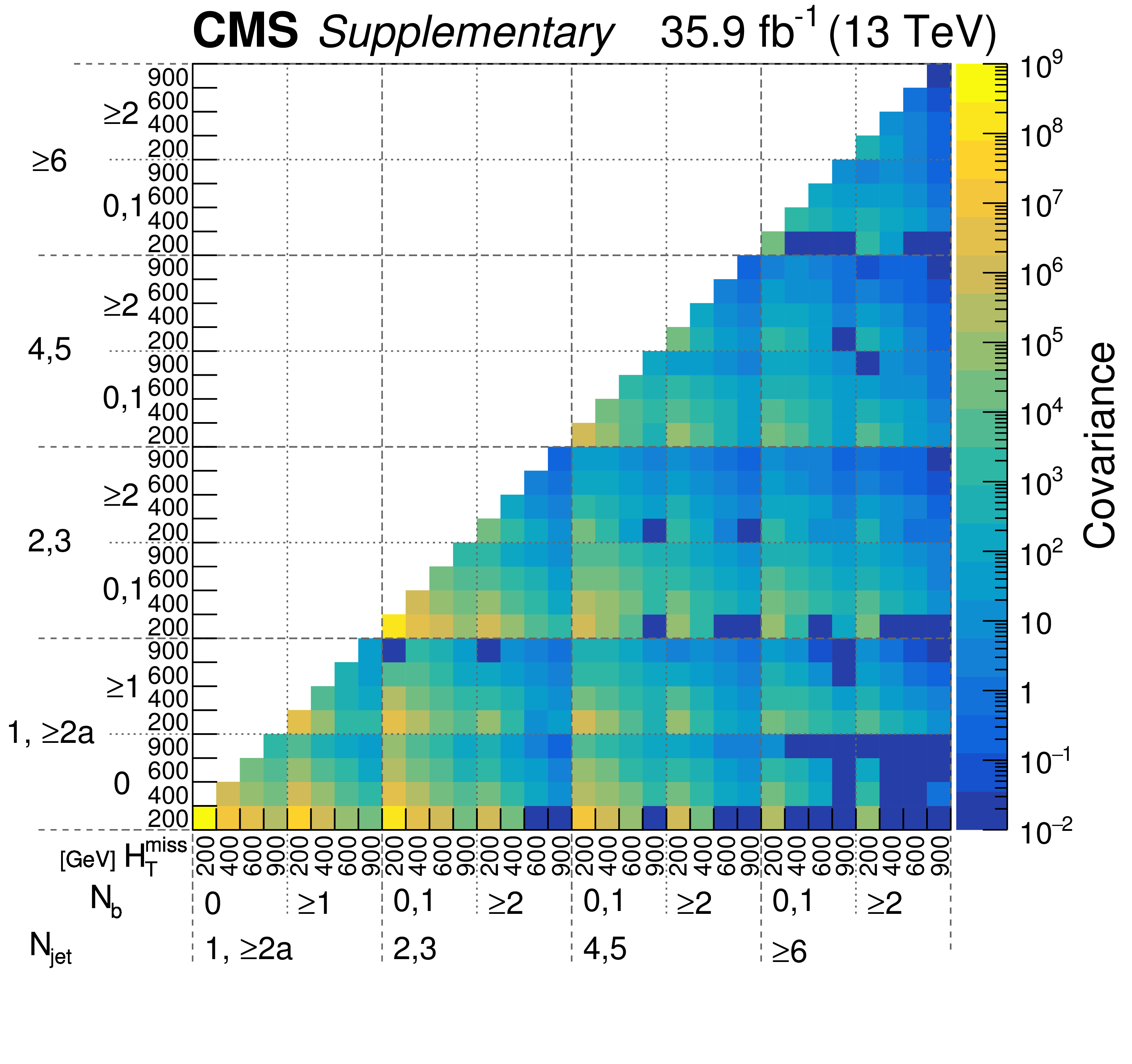
Correlation matrix for the SM background estimates determined from the CR-only fit using the simplified binning schema defined in Table 7. |
| Tables | |
png pdf |
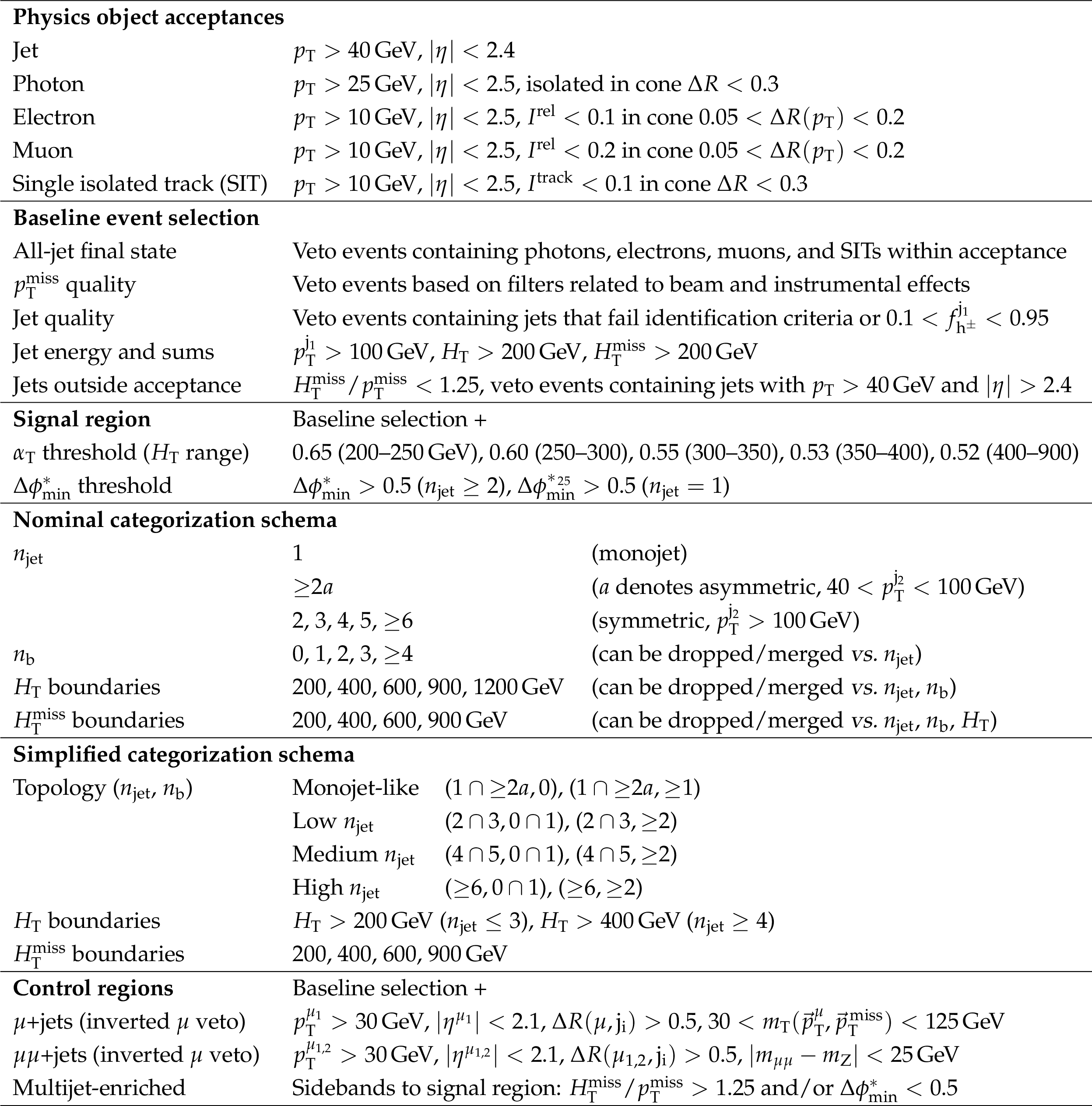
Table 1:
Summary of the physics object acceptances, the baseline event selection, the signal and control regions, and the event categorization schemas. The nominal categorization schema is defined in full in Appendix. |

png pdf |
Table 2:
Systematic uncertainties in the $ {\ell _\text {lost}} $ and $ {{\mathrm {Z}}\to {\nu} {\overline {\nu}}} $ background evaluation. The quoted ranges are representative of the minimum and maximum variations observed across all bins of the signal region. Pairs of ranges are quoted for uncertainties determined from closure tests in data, which correspond to variations as a function of ${n_{\text {jet}}}$ and ${H_{\mathrm {T}}}$, respectively. |
png pdf |
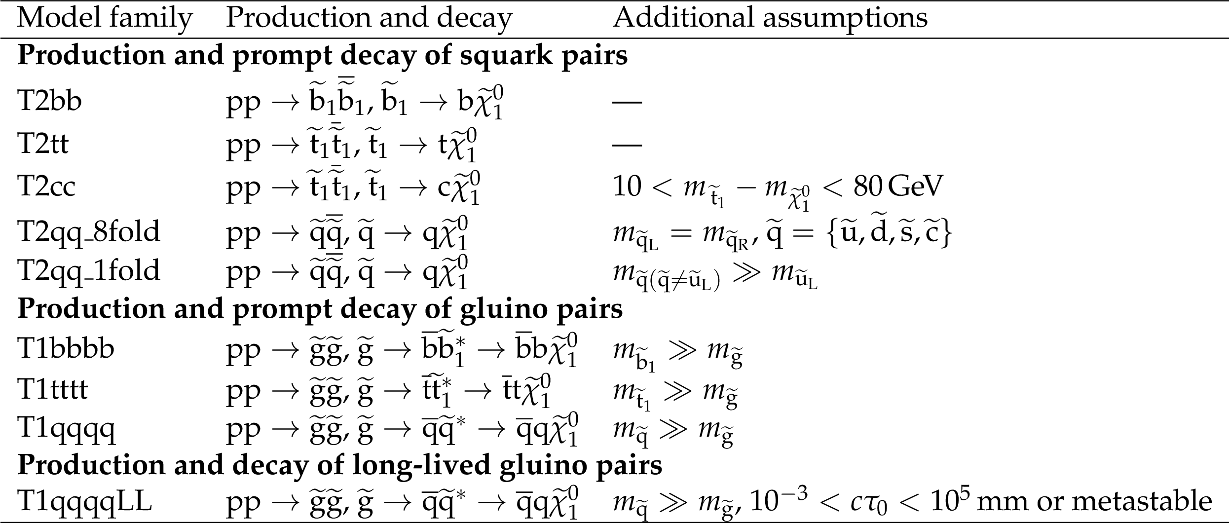
Table 3:
Summary of the simplified SUSY models used to interpret the result of this search. |
png pdf |
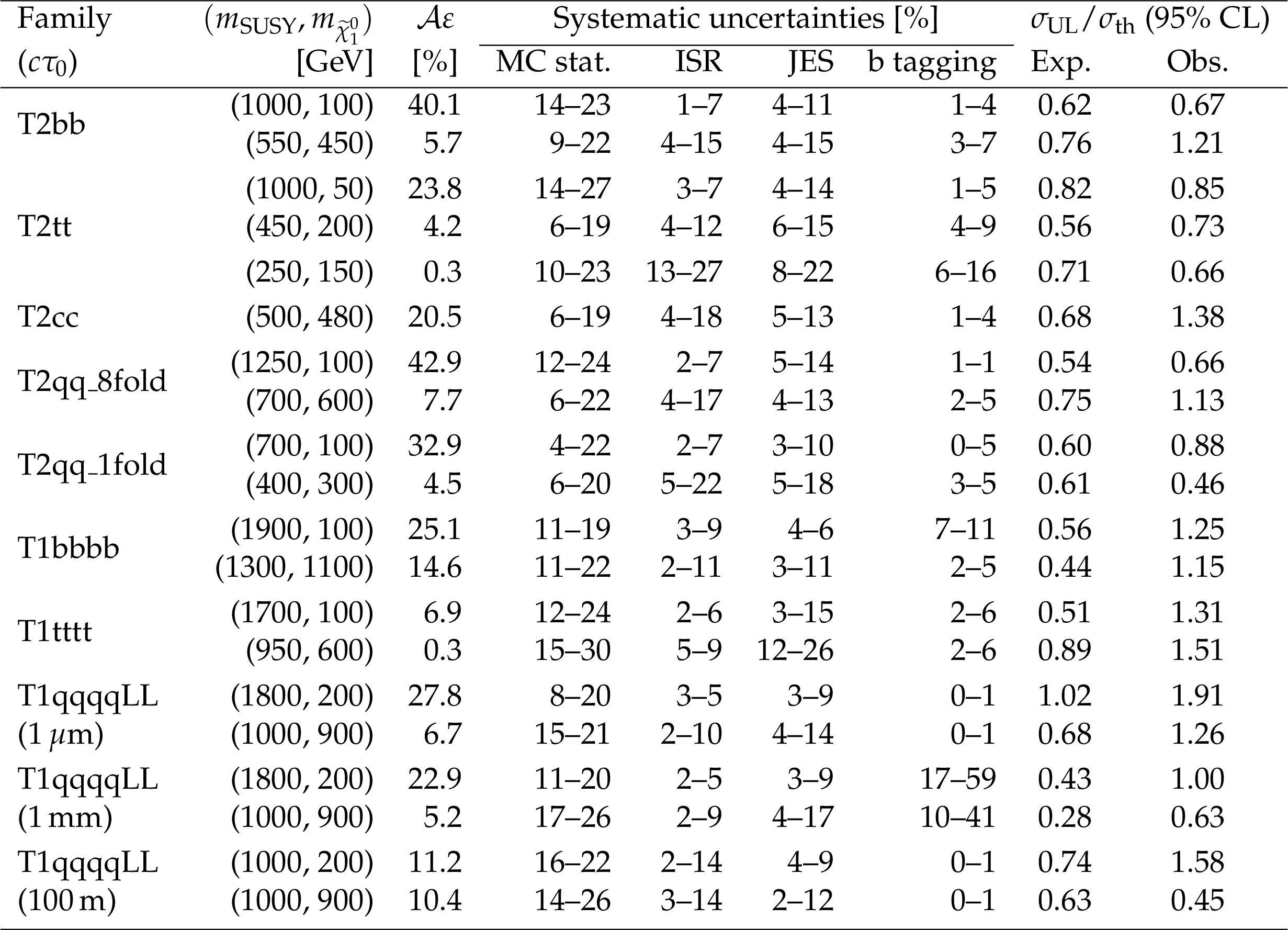
Table 4:
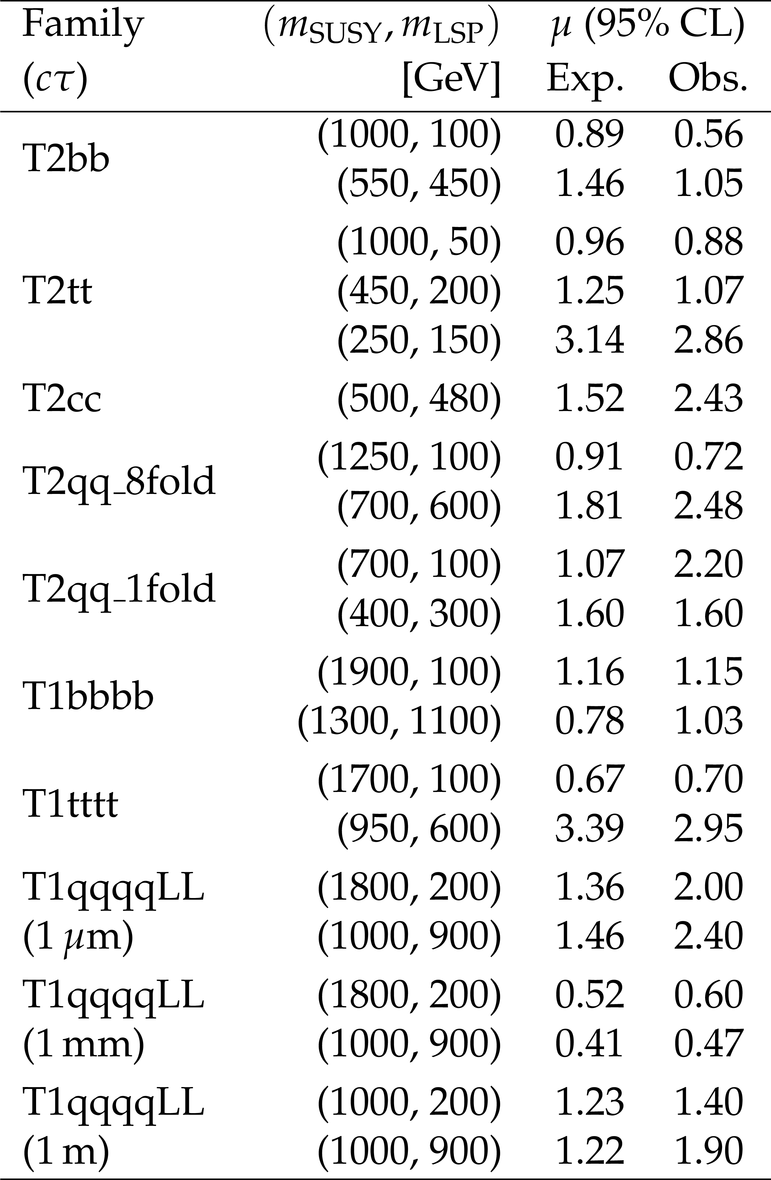
A list of benchmark simplified models organized according to production and decay modes (family), the ${\mathcal {A}\varepsilon}$, representative values for some of the dominant sources of systematic uncertainty, and the expected and observed upper limits on the production cross section $\sigma _\text {UL}$ relative to the theoretical value $\sigma _\text {th}$ calculated at NLO+NLL accuracy. Additional uncertainties concerning the T1qqqqLL models are not listed here and are discussed in the text. |
png pdf |
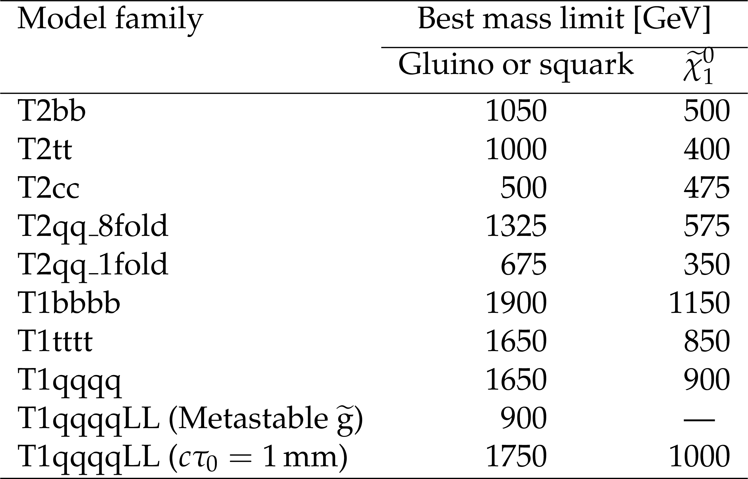
Table 5:
Summary of the mass limits obtained for each family of simplified models. The limits indicate the strongest observed mass exclusions for the parent SUSY particle (gluino or squark) and $ \tilde{\chi}^0_1$ . |
png pdf |
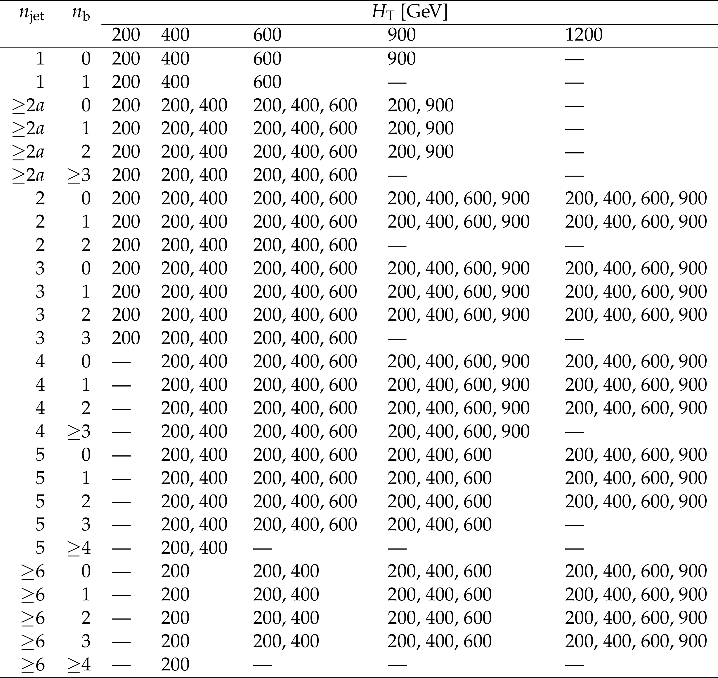
Table 6:
Summary of the nominal ($ {n_{\text {jet}}} $, $ {n_{\mathrm {b}}} $, $ {H_{\mathrm {T}}} $, $ {H_{\mathrm {T}}^{\text {miss}}} $) binning schema. Each entry (and the following entry, if present) signifies the lower (upper) bound of an $ {H_{\mathrm {T}}^{\text {miss}}} $ bin within a given ($ {n_{\text {jet}}} $, $ {n_{\mathrm {b}}} $, $ {H_{\mathrm {T}}} $) bin. Unique or final entries represent $ {H_{\mathrm {T}}^{\text {miss}}} $ bins unbounded from above. A dash ({\text {--}}) signifies that the $ {H_{\mathrm {T}}} $ bin in a given ($ {n_{\text {jet}}} $, $ {n_{\mathrm {b}}} $) category is not used in the analysis, in which case counts in high-$ {H_{\mathrm {T}}} $ bins are integrated into the adjacent lower-$ {H_{\mathrm {T}}} $ bin. For monojet events, $ {H_{\mathrm {T}}} \equiv {H_{\mathrm {T}}^{\text {miss}}} $. The "a" denotes asymmetric $ {p_{\mathrm {T}}} $ thresholds for the two highest $ {p_{\mathrm {T}}} $ jets. |
png pdf |
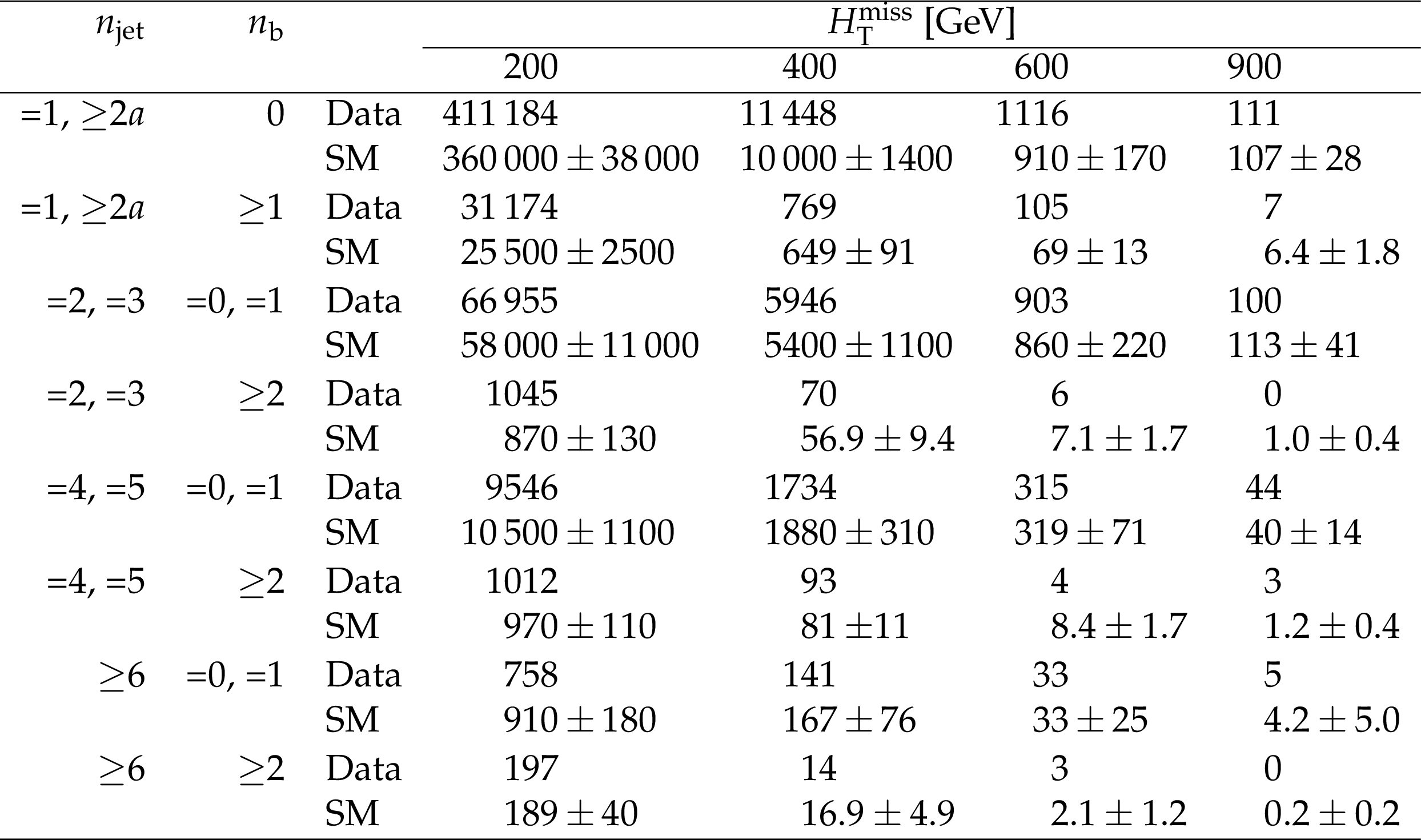
Table 7:
Observed counts of candidate signal events and SM expectations determined from the CR-only fit using the simplified binning schema, as a function of $ {n_{\text {jet}}} $, $ {n_{\mathrm {b}}} $, and $ {H_{\mathrm {T}}^{\text {miss}}} $. All counts are integrated over $ {H_{\mathrm {T}}} $. The uncertainties include both statistical and systematic contributions. The "a" denotes asymmetric $ {p_{\mathrm {T}}} $ thresholds for the two highest $ {p_{\mathrm {T}}} $ jets. |
| Summary |
|
A search for supersymmetry with the CMS experiment is reported, based on a data sample of pp collisions collected in 2016 at $\sqrt{s} = $ 13 TeV that corresponds to an integrated luminosity of 35.9 $\pm$ 0.9 fb$^{-1}$ . Final states with jets and significant missing transverse momentum $ \vec{p}_{\mathrm{T}}^{\text{miss}} $, as expected from the production and decay of massive gluinos and squarks, are considered. Signal events are categorized according to the number of reconstructed jets, the number of jets identified as originating from bottom quarks, and the scalar and vector sums of the transverse momenta of jets. The standard model background is estimated from a binned likelihood fit to event yields in the signal region and data control samples. The observed yields in the signal region are found to be in agreement with the expected contributions from standard model processes. Supplemental material is provided to aid further interpretation of the result in Appendix. Limits are determined in the parameter spaces of simplified models that assume the production and prompt decay of gluino or squark pairs. The strongest exclusion bounds (95% confidence level) for squark masses are 1050, 1000, and 1325 GeV for bottom, top, and mass-degenerate light-flavour squarks, respectively. The corresponding mass bounds on the neutralino $\tilde{\chi}^0_1$ from squark decays are 500, 400, and 575 GeV. The gluino mass is probed up to 1900, 1650, and 1650 GeV when the gluino decays via virtual states of the aforementioned squarks. The strongest mass bound on the $\tilde{\chi}^0_1$ from the gluino decay is 1150 GeV. Sensitivity to simplified models inspired by split supersymmetry is also demonstrated. These models assume the production of long-lived gluino pairs that decay to final states containing displaced jets and $ \vec{p}_{\mathrm{T}}^{\text{miss}} $ from the undetected $\tilde{\chi}^0_1 $ particles. The long-lived gluino, with an assumed proper decay length ${c\tau_{0}} $, is expected to hadronize with SM particles and form a bound state known as an R-hadron. The model-dependent matter interactions of R-hadrons are not considered by default. The sensitivity of this search is only moderately dependent on these matter interactions for models with ${c\tau_{0}} > $ 1 m, while no dependence is found for models with ${c\tau_{0}} $ below 1 m. Models that assume a $\tilde{\chi}^0_1$ mass of 100 GeV and gluino masses up to 1600 GeV are excluded for a proper decay length ${c\tau_{0}} $ below 0.1 mm. The bound on the gluino mass strengthens to 1750 GeV at ${c\tau_{0}} = $ 1 mm, before weakening to 900-1000 GeV for models with ${c\tau_{0}} > $ 10 m. For all values of ${c\tau_{0}} $ considered, the exclusion bounds on the gluino mass weaken to about 1 TeV when the difference between the gluino and $\tilde{\chi}^0_1$ mass is small. The search provides coverage of the ${c\tau_{0}} $ parameter space for models involving long-lived gluinos, such as the region ${c\tau_{0}} < $ 1 mm, that is complementary to the coverage provided by dedicated techniques at the LHC. |
| Additional Figures | |

png pdf |
Additional Figure 1:
Graphical representation of the production and decay of supersymmetric particles in the T1qqqq model. |

png pdf |
Additional Figure 2:
Graphical representation of the production and decay of supersymmetric particles in the T2qq model. |
png pdf |
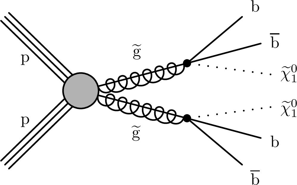
Additional Figure 3:
Graphical representation of the production and decay of supersymmetric particles in the T1bbbb model. |

png pdf |
Additional Figure 4:
Graphical representation of the production and decay of supersymmetric particles in the T1tttt model. |

png pdf |
Additional Figure 5:
Graphical representation of the production and decay of supersymmetric particles in the T2bb model. |
png pdf |
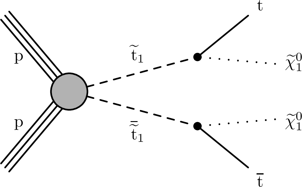
Additional Figure 6:
Graphical representation of the production and decay of supersymmetric particles in the T2tt model. |

png pdf |
Additional Figure 7:
Graphical representation of the production and decay of supersymmetric particles in the T2cc model. |
png pdf |
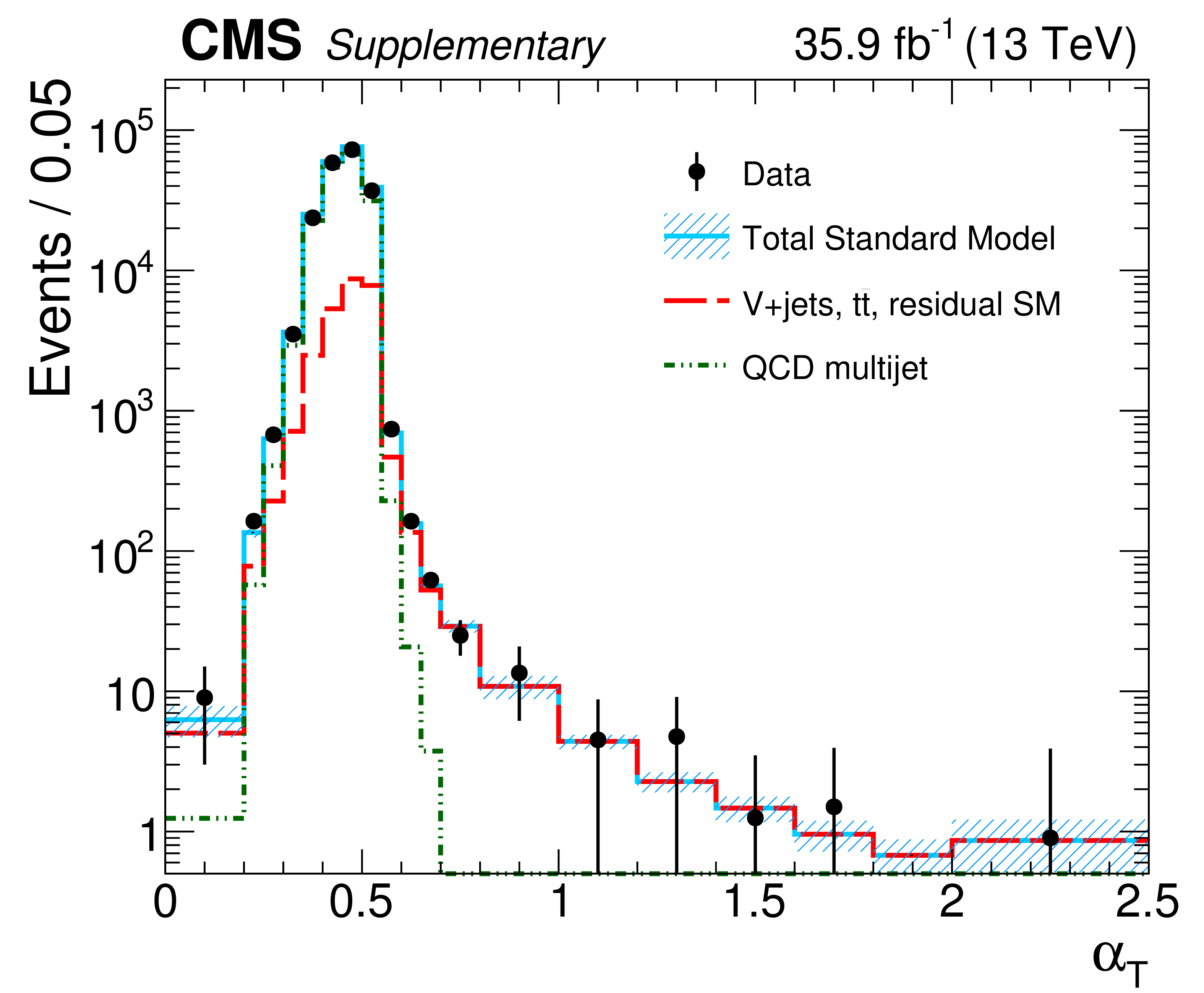
Additional Figure 8:
The $ {\alpha _{\mathrm {T}}} $ distribution in data and simulation for events satisfying the baseline selection criteria plus the additional requirements $ {n_{\text {jet}}} \geq $ 2, $ {p_{\mathrm {T}}} ^{{\mathrm {j}_\text {2}}} > $ 100 GeV, and $ {H_{\text {T}}} > $ 900 GeV. The statistical uncertainties for the multijet and SM expectations are represented by the hatched areas (visible only for statistically limited bins). The final bin of this distribution contains the overflow events. |
png pdf |
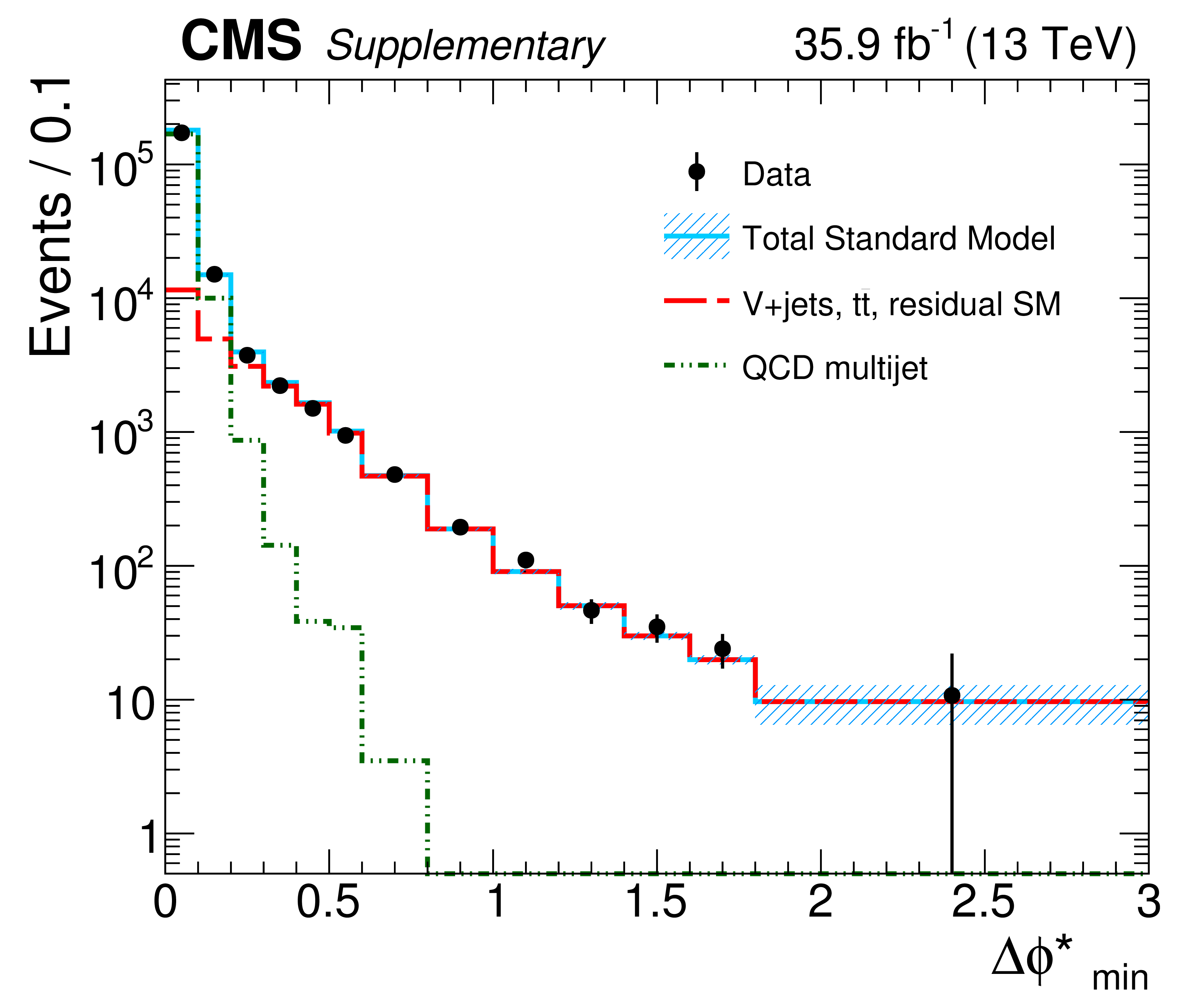
Additional Figure 9:
The $ {\Delta \phi ^{*}_\text {min}} $ distribution in data and simulation for events satisfying the baseline selection criteria plus the additional requirements $ {n_{\text {jet}}} \geq $ 2, $ {p_{\mathrm {T}}} ^{{\mathrm {j}_\text {2}}} > $ 100 GeV, and $ {H_{\text {T}}} > $ 900 GeV. The statistical uncertainties for the multijet and SM expectations are represented by the hatched areas (visible only for statistically limited bins). The final bin of this distribution contains the overflow events. |
png pdf root |
Additional Figure 10:
Covariance matrix for the SM background estimates determined from the CR-only fit using the simplified binning schema defined in the paper. |
png pdf csv |
Additional Figure 11:
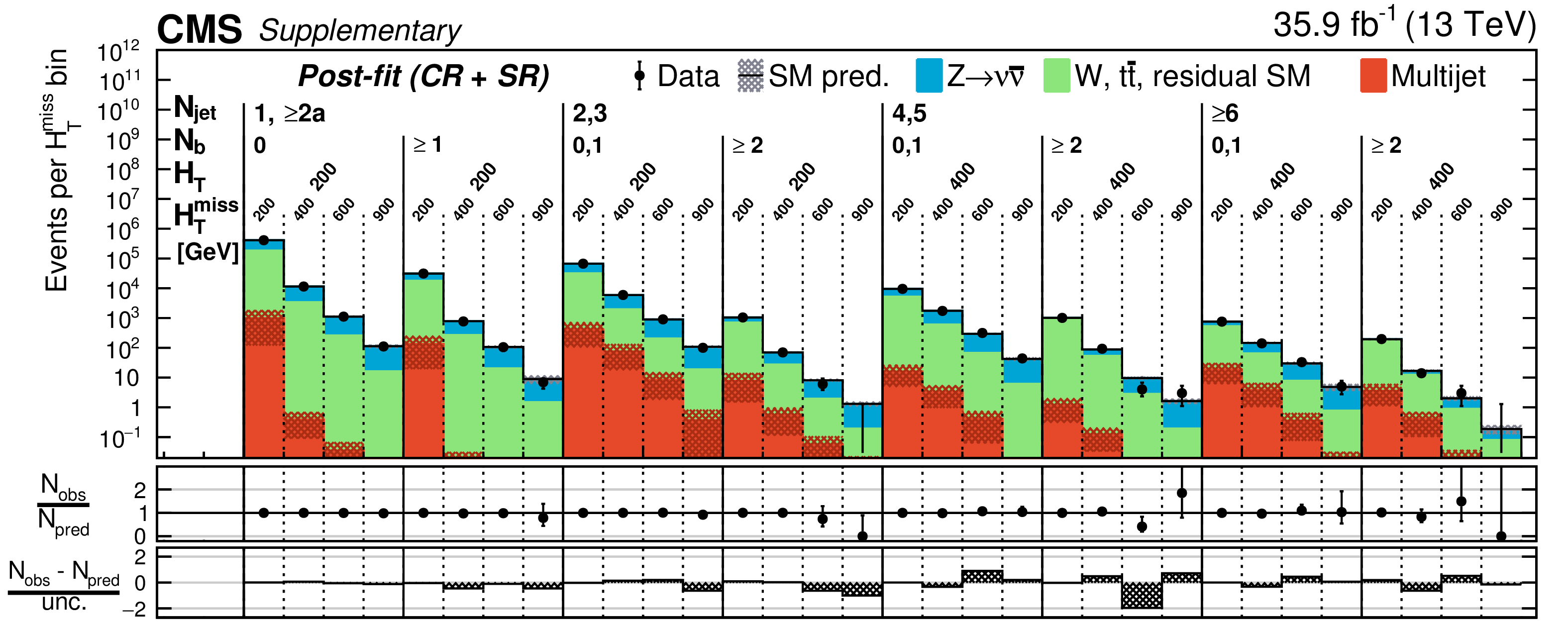
Counts of signal events (solid markers) and SM expectations with associated uncertainties (statistical and systematic, black histograms and shaded bands) as determined from the CR-only fit for the simplified binning scheme. The centre panel shows the ratios of observed counts and the SM expectations, while the lower panel shows the significance of deviations observed in data with respect to the SM expectations expressed in terms of the total uncertainty in the SM expectations. |
png pdf csv |
Additional Figure 12:
Counts of signal events (solid markers) and SM expectations with associated uncertainties (statistical and systematic, black histograms and shaded bands) as determined by the full fit to signal and control regions. for the simplified binning scheme. The centre panel shows the ratios of observed counts and the SM expectations, while the lower panel shows the significance of deviations observed in data with respect to the SM expectations expressed in terms of the total uncertainty in the SM expectations. |
png pdf csv |
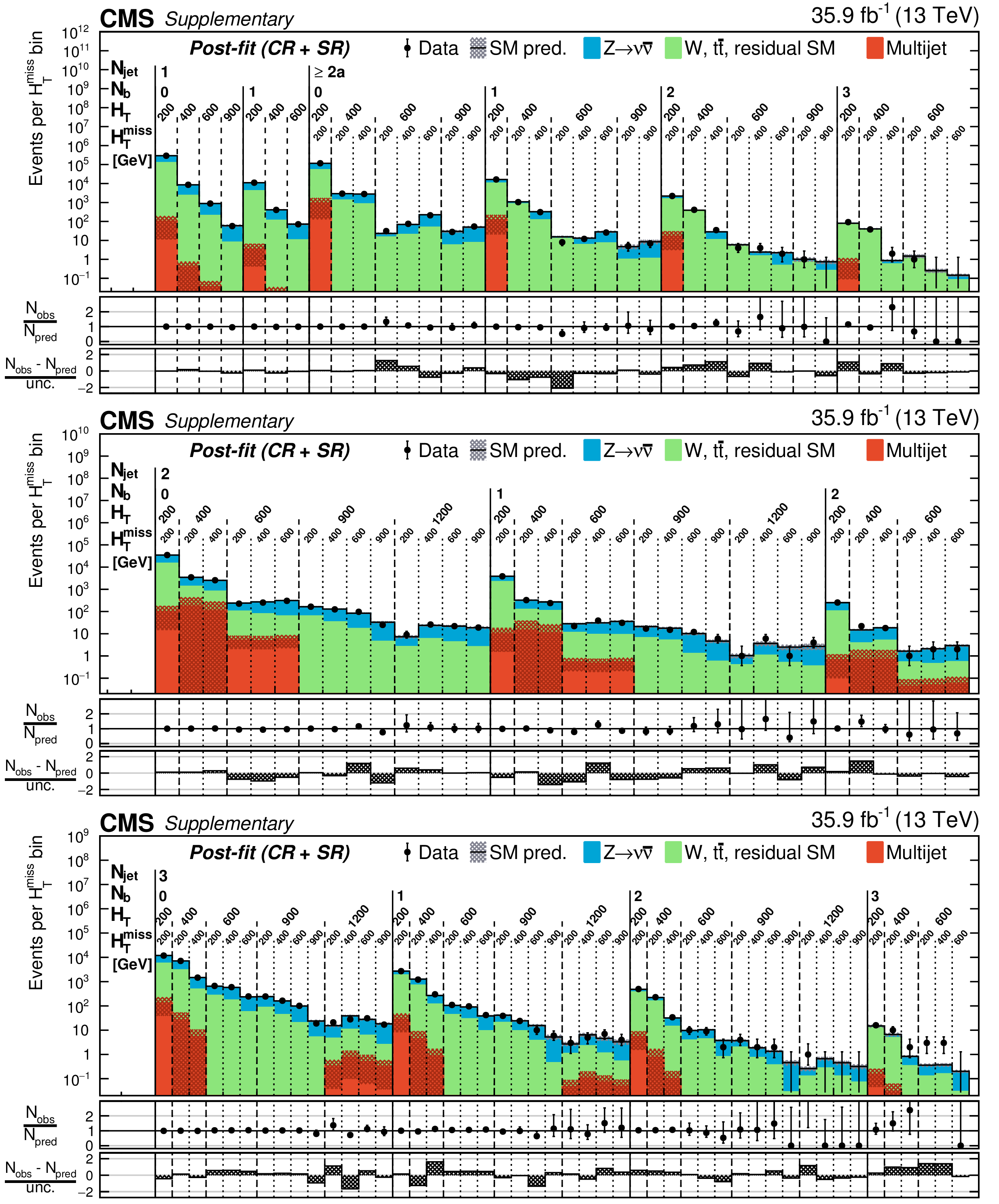
Additional Figure 13:
Counts of signal events (solid markers) and SM expectations with associated uncertainties (statistical and systematic, black histograms and shaded bands) as determined by the full fit to signal and control regions. as a function of $ {n_{\text {b}}}, {H_{\text {T}}} $, and $ {H_{\mathrm {T}}^{\text {miss}}} $ for the event categories $ {n_{\text {jet}}} =$ 1 and ${\geq}2a$ (a), $=2$ (b), and $=3$ (c). The centre panel shows the ratios of observed counts and the SM expectations, while the lower panel shows the significance of deviations observed in data with respect to the SM expectations expressed in terms of the total uncertainty in the SM expectations. |

png pdf |
Additional Figure 13-a:
Counts of signal events (solid markers) and SM expectations with associated uncertainties (statistical and systematic, black histograms and shaded bands) as determined by the full fit to signal and control regions. as a function of $ {n_{\text {b}}}, {H_{\text {T}}} $, and $ {H_{\mathrm {T}}^{\text {miss}}} $ for the event categories $ {n_{\text {jet}}} =$ 1 and ${\geq}2a$ (a), $=2$ (b), and $=3$ (c). The centre panel shows the ratios of observed counts and the SM expectations, while the lower panel shows the significance of deviations observed in data with respect to the SM expectations expressed in terms of the total uncertainty in the SM expectations. |
png pdf |
Additional Figure 13-b:
Counts of signal events (solid markers) and SM expectations with associated uncertainties (statistical and systematic, black histograms and shaded bands) as determined by the full fit to signal and control regions. as a function of $ {n_{\text {b}}}, {H_{\text {T}}} $, and $ {H_{\mathrm {T}}^{\text {miss}}} $ for the event categories $ {n_{\text {jet}}} =$ 1 and ${\geq}2a$ (a), $=2$ (b), and $=3$ (c). The centre panel shows the ratios of observed counts and the SM expectations, while the lower panel shows the significance of deviations observed in data with respect to the SM expectations expressed in terms of the total uncertainty in the SM expectations. |
png pdf |
Additional Figure 13-c:
Counts of signal events (solid markers) and SM expectations with associated uncertainties (statistical and systematic, black histograms and shaded bands) as determined by the full fit to signal and control regions. as a function of $ {n_{\text {b}}}, {H_{\text {T}}} $, and $ {H_{\mathrm {T}}^{\text {miss}}} $ for the event categories $ {n_{\text {jet}}} =$ 1 and ${\geq}2a$ (a), $=2$ (b), and $=3$ (c). The centre panel shows the ratios of observed counts and the SM expectations, while the lower panel shows the significance of deviations observed in data with respect to the SM expectations expressed in terms of the total uncertainty in the SM expectations. |
png pdf csv |
Additional Figure 14:
Counts of signal events (solid markers) and SM expectations with associated uncertainties (statistical and systematic, black histograms and shaded bands) as determined by the full fit to signal and control regions. as a function of $ {n_{\text {b}}}, {H_{\text {T}}} $, and $ {H_{\mathrm {T}}^{\text {miss}}} $ for the event categories $ {n_{\text {jet}}} =$ 4 (a), $= $ 5 (b), and ${\geq}$ 6 (c). The centre panel shows the ratios of observed counts and the SM expectations, while the lower panel shows the significance of deviations observed in data with respect to the SM expectations expressed in terms of the total uncertainty in the SM expectations. |
png pdf |
Additional Figure 14-a:
Counts of signal events (solid markers) and SM expectations with associated uncertainties (statistical and systematic, black histograms and shaded bands) as determined by the full fit to signal and control regions. as a function of $ {n_{\text {b}}}, {H_{\text {T}}} $, and $ {H_{\mathrm {T}}^{\text {miss}}} $ for the event categories $ {n_{\text {jet}}} =$ 4 (a), $= $ 5 (b), and ${\geq}$ 6 (c). The centre panel shows the ratios of observed counts and the SM expectations, while the lower panel shows the significance of deviations observed in data with respect to the SM expectations expressed in terms of the total uncertainty in the SM expectations. |
png pdf |
Additional Figure 14-b:
Counts of signal events (solid markers) and SM expectations with associated uncertainties (statistical and systematic, black histograms and shaded bands) as determined by the full fit to signal and control regions. as a function of $ {n_{\text {b}}}, {H_{\text {T}}} $, and $ {H_{\mathrm {T}}^{\text {miss}}} $ for the event categories $ {n_{\text {jet}}} =$ 4 (a), $= $ 5 (b), and ${\geq}$ 6 (c). The centre panel shows the ratios of observed counts and the SM expectations, while the lower panel shows the significance of deviations observed in data with respect to the SM expectations expressed in terms of the total uncertainty in the SM expectations. |
png pdf |
Additional Figure 14-c:
Counts of signal events (solid markers) and SM expectations with associated uncertainties (statistical and systematic, black histograms and shaded bands) as determined by the full fit to signal and control regions. as a function of $ {n_{\text {b}}}, {H_{\text {T}}} $, and $ {H_{\mathrm {T}}^{\text {miss}}} $ for the event categories $ {n_{\text {jet}}} =$ 4 (a), $= $ 5 (b), and ${\geq}$ 6 (c). The centre panel shows the ratios of observed counts and the SM expectations, while the lower panel shows the significance of deviations observed in data with respect to the SM expectations expressed in terms of the total uncertainty in the SM expectations. |
png pdf |
Additional Figure 15:
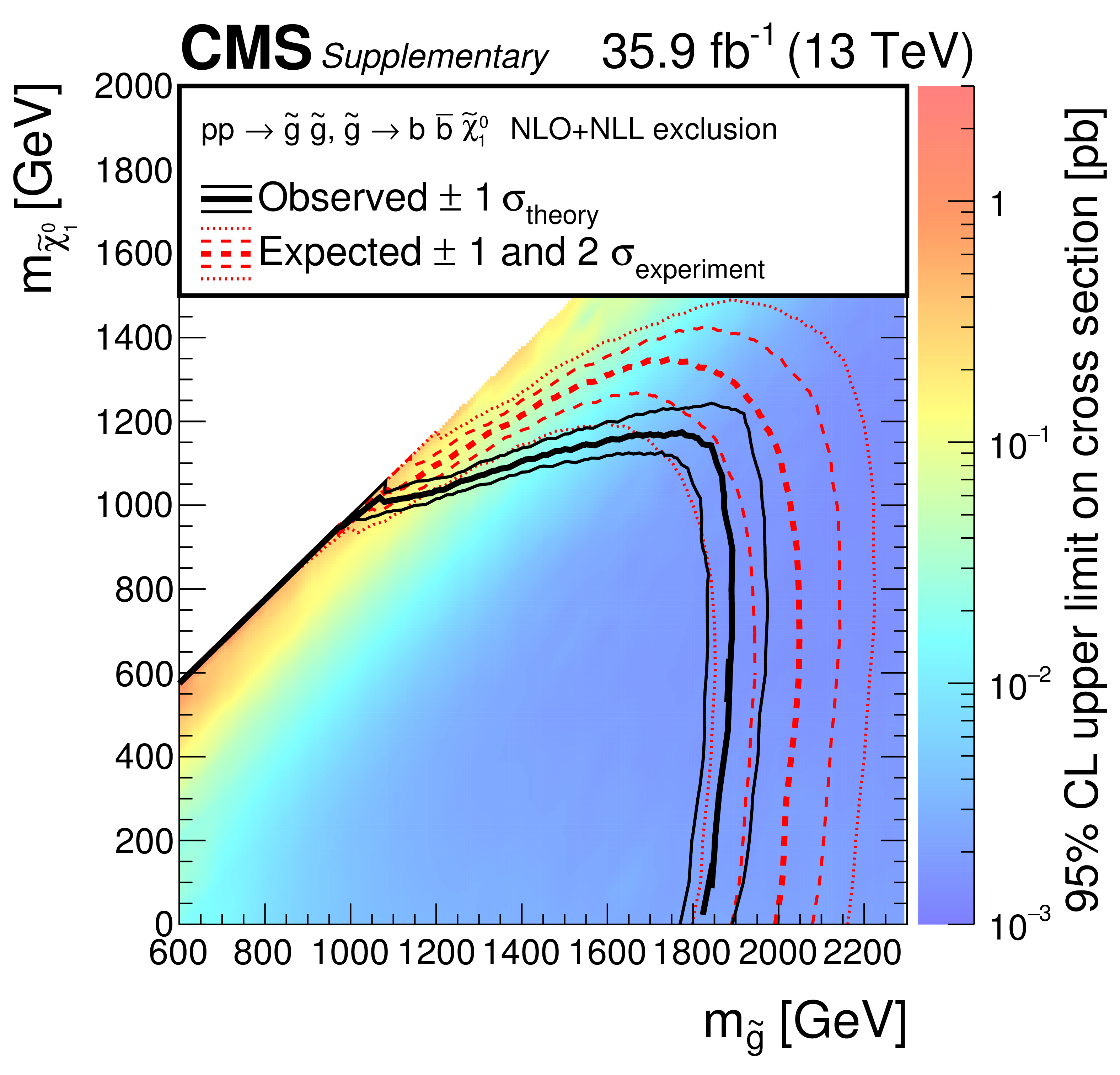
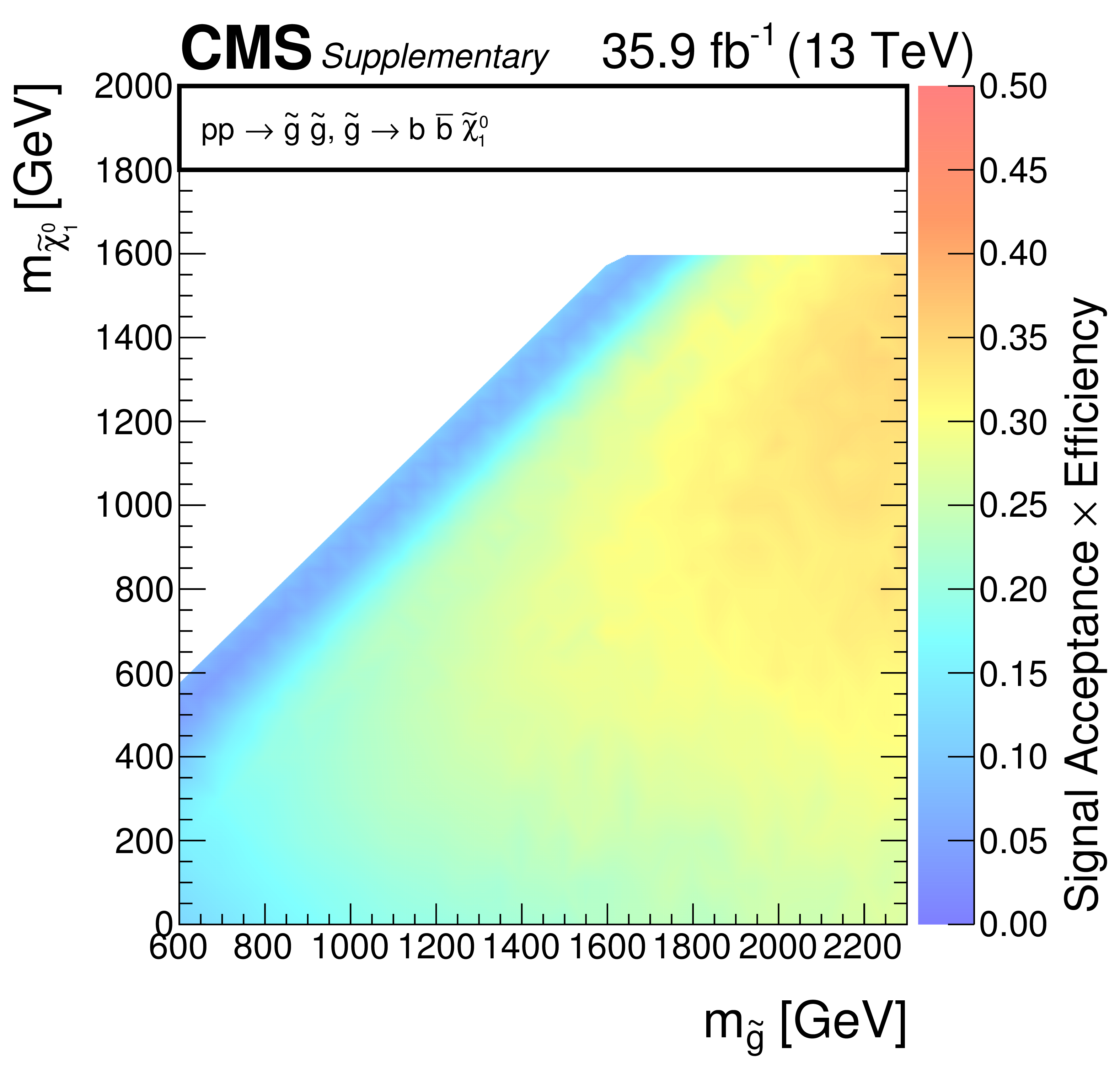
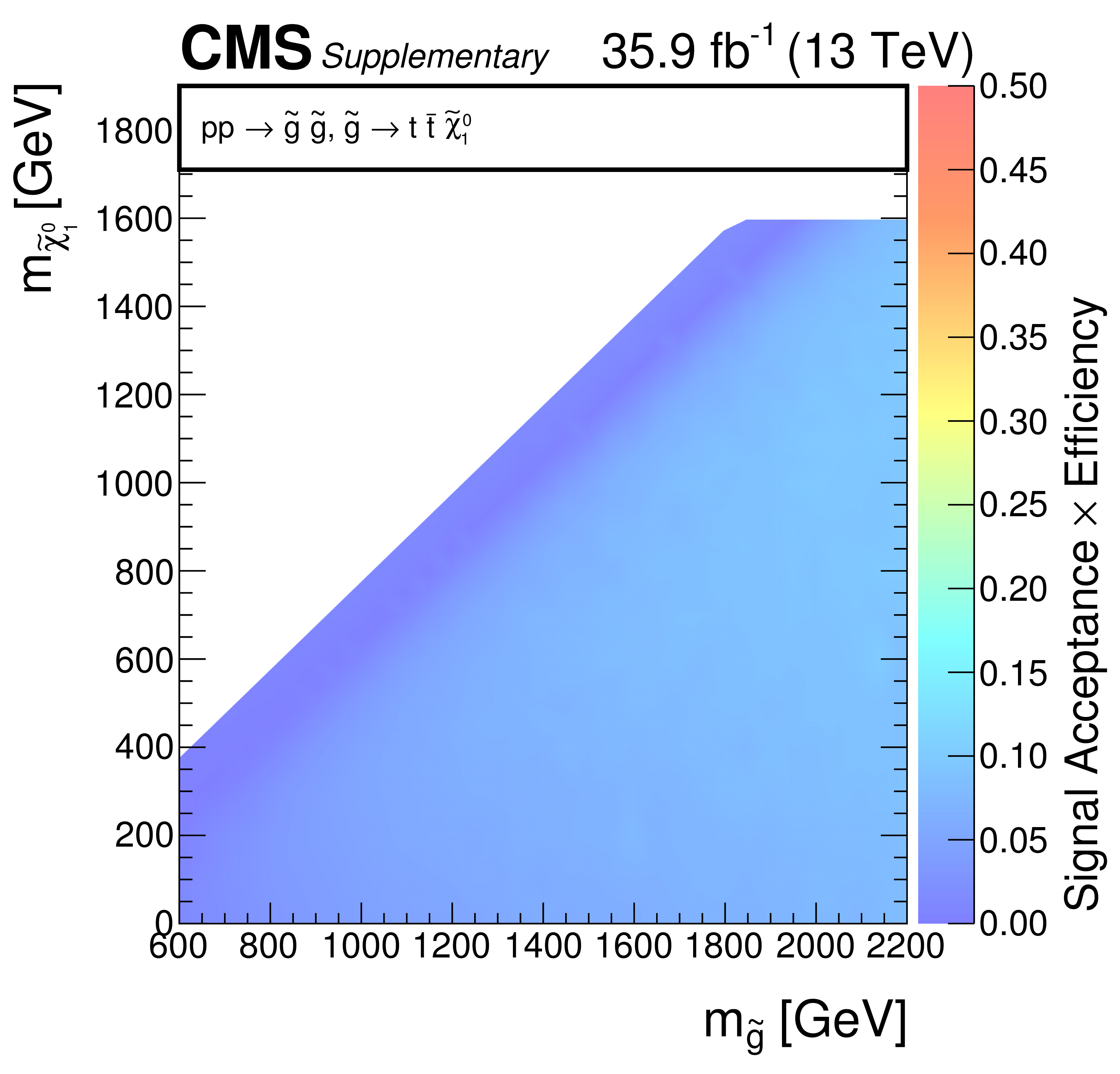
(a) Observed upper limit in cross section at 95% CL (indicated by the colour scale) as a function of the $ \tilde{g}$ and $ {\tilde{\chi}^{0}_{1}} $ masses for the T1qqqq simplified model. The black solid thick (thin) line indicates the observed excluded region assuming the nominal (${\pm}1$ standard deviation in theoretical uncertainty) production cross section. The red dashed thick (thin) line indicates the median (${\pm}1$ standard deviation in experimental uncertainty) expected excluded region. (b) The signal acceptance times efficiency as a function of the $ \tilde{g}$ and $ {\tilde{\chi}^{0}_{1}} $ masses following the application of the event selection criteria for the signal region. |
png pdf root |
Additional Figure 15-a:
(a) Observed upper limit in cross section at 95% CL (indicated by the colour scale) as a function of the $ \tilde{g}$ and $ {\tilde{\chi}^{0}_{1}} $ masses for the T1qqqq simplified model. The black solid thick (thin) line indicates the observed excluded region assuming the nominal (${\pm}1$ standard deviation in theoretical uncertainty) production cross section. The red dashed thick (thin) line indicates the median (${\pm}1$ standard deviation in experimental uncertainty) expected excluded region. (b) The signal acceptance times efficiency as a function of the $ \tilde{g}$ and $ {\tilde{\chi}^{0}_{1}} $ masses following the application of the event selection criteria for the signal region. |

png pdf root |
Additional Figure 15-b:
(a) Observed upper limit in cross section at 95% CL (indicated by the colour scale) as a function of the $ \tilde{g}$ and $ {\tilde{\chi}^{0}_{1}} $ masses for the T1qqqq simplified model. The black solid thick (thin) line indicates the observed excluded region assuming the nominal (${\pm}1$ standard deviation in theoretical uncertainty) production cross section. The red dashed thick (thin) line indicates the median (${\pm}1$ standard deviation in experimental uncertainty) expected excluded region. (b) The signal acceptance times efficiency as a function of the $ \tilde{g}$ and $ {\tilde{\chi}^{0}_{1}} $ masses following the application of the event selection criteria for the signal region. |
png pdf |
Additional Figure 16:
(a) Observed upper limit in cross section at 95% CL (indicated by the colour scale) as a function of the $ \tilde{g}$ and $ {\tilde{\chi}^{0}_{1}} $ masses for the T1bbbb simplified model. The black solid thick (thin) line indicates the observed excluded region assuming the nominal (${\pm}1$ standard deviation in theoretical uncertainty) production cross section. The red dashed thick (thin) line indicates the median (${\pm}1$ standard deviation in experimental uncertainty) expected excluded region. (b) The signal acceptance times efficiency as a function of the $ \tilde{g}$ and $ {\tilde{\chi}^{0}_{1}} $ masses following the application of the event selection criteria for the signal region. |
png pdf root |
Additional Figure 16-a:
(a) Observed upper limit in cross section at 95% CL (indicated by the colour scale) as a function of the $ \tilde{g}$ and $ {\tilde{\chi}^{0}_{1}} $ masses for the T1bbbb simplified model. The black solid thick (thin) line indicates the observed excluded region assuming the nominal (${\pm}1$ standard deviation in theoretical uncertainty) production cross section. The red dashed thick (thin) line indicates the median (${\pm}1$ standard deviation in experimental uncertainty) expected excluded region. (b) The signal acceptance times efficiency as a function of the $ \tilde{g}$ and $ {\tilde{\chi}^{0}_{1}} $ masses following the application of the event selection criteria for the signal region. |
png pdf root |
Additional Figure 16-b:
(a) Observed upper limit in cross section at 95% CL (indicated by the colour scale) as a function of the $ \tilde{g}$ and $ {\tilde{\chi}^{0}_{1}} $ masses for the T1bbbb simplified model. The black solid thick (thin) line indicates the observed excluded region assuming the nominal (${\pm}1$ standard deviation in theoretical uncertainty) production cross section. The red dashed thick (thin) line indicates the median (${\pm}1$ standard deviation in experimental uncertainty) expected excluded region. (b) The signal acceptance times efficiency as a function of the $ \tilde{g}$ and $ {\tilde{\chi}^{0}_{1}} $ masses following the application of the event selection criteria for the signal region. |
png pdf |
Additional Figure 17:
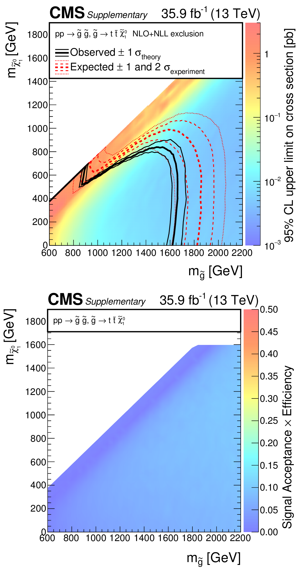
(a) Observed upper limit in cross section at 95% CL (indicated by the colour scale) as a function of the $ \tilde{g}$ and $ {\tilde{\chi}^{0}_{1}} $ masses for the T1tttt simplified model. The black solid thick (thin) line indicates the observed excluded region assuming the nominal (${\pm}1$ standard deviation in theoretical uncertainty) production cross section. The red dashed thick (thin) line indicates the median (${\pm}1$ standard deviation in experimental uncertainty) expected excluded region. An electronic version of this figure is available as CMS-SUS-16-038\_Figure-aux\_017-a.root. (b) The signal acceptance times efficiency as a function of the $ \tilde{g}$ and $ {\tilde{\chi}^{0}_{1}} $ masses following the application of the event selection criteria for the signal region. |

png pdf root |
Additional Figure 17-a:
(a) Observed upper limit in cross section at 95% CL (indicated by the colour scale) as a function of the $ \tilde{g}$ and $ {\tilde{\chi}^{0}_{1}} $ masses for the T1tttt simplified model. The black solid thick (thin) line indicates the observed excluded region assuming the nominal (${\pm}1$ standard deviation in theoretical uncertainty) production cross section. The red dashed thick (thin) line indicates the median (${\pm}1$ standard deviation in experimental uncertainty) expected excluded region. An electronic version of this figure is available as CMS-SUS-16-038\_Figure-aux\_017-a.root. (b) The signal acceptance times efficiency as a function of the $ \tilde{g}$ and $ {\tilde{\chi}^{0}_{1}} $ masses following the application of the event selection criteria for the signal region. -a |
png pdf root |
Additional Figure 17-b:
(a) Observed upper limit in cross section at 95% CL (indicated by the colour scale) as a function of the $ \tilde{g}$ and $ {\tilde{\chi}^{0}_{1}} $ masses for the T1tttt simplified model. The black solid thick (thin) line indicates the observed excluded region assuming the nominal (${\pm}1$ standard deviation in theoretical uncertainty) production cross section. The red dashed thick (thin) line indicates the median (${\pm}1$ standard deviation in experimental uncertainty) expected excluded region. An electronic version of this figure is available as CMS-SUS-16-038\_Figure-aux\_017-a.root. (b) The signal acceptance times efficiency as a function of the $ \tilde{g}$ and $ {\tilde{\chi}^{0}_{1}} $ masses following the application of the event selection criteria for the signal region. -b |
png pdf |
Additional Figure 18:
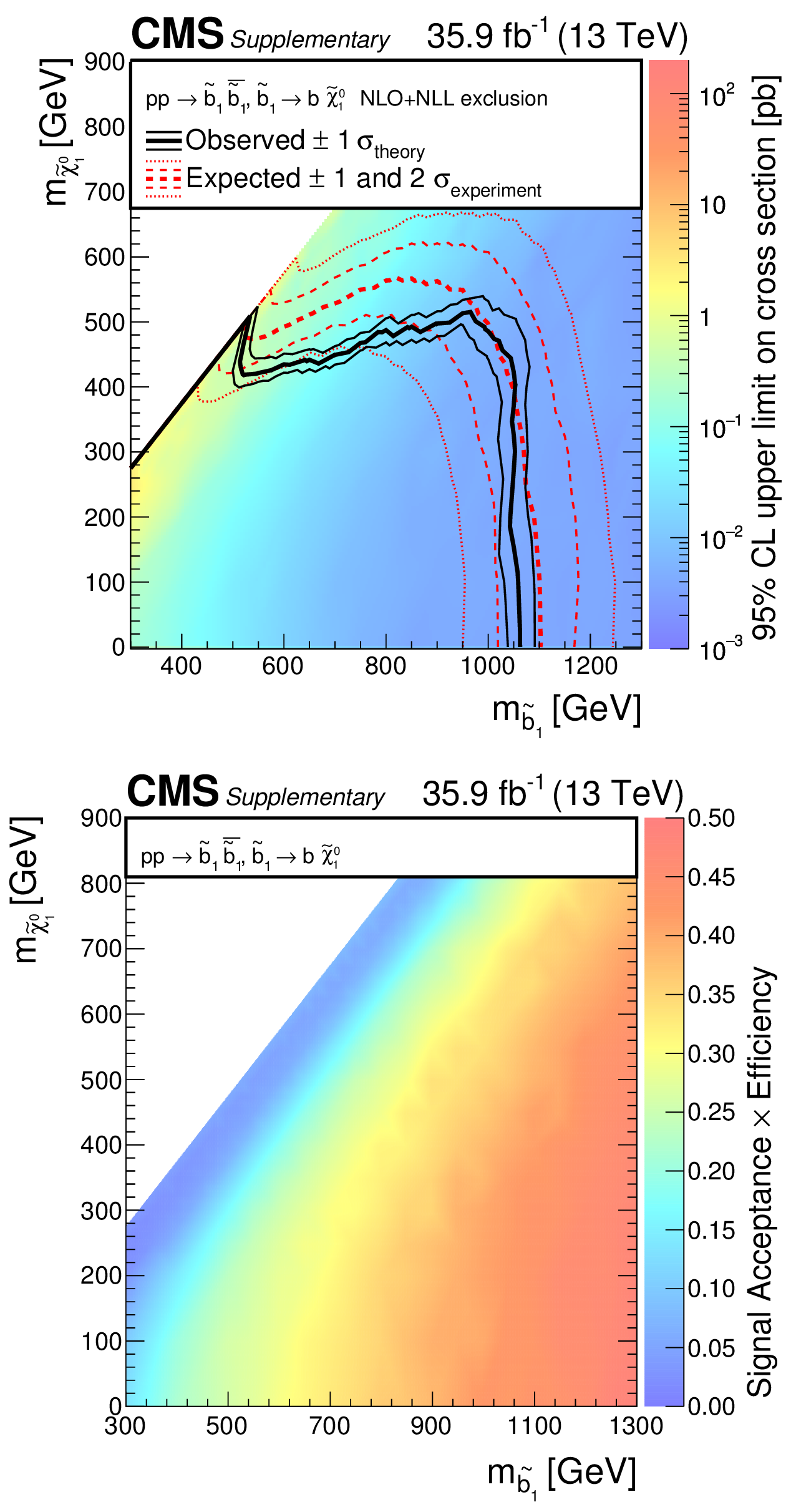
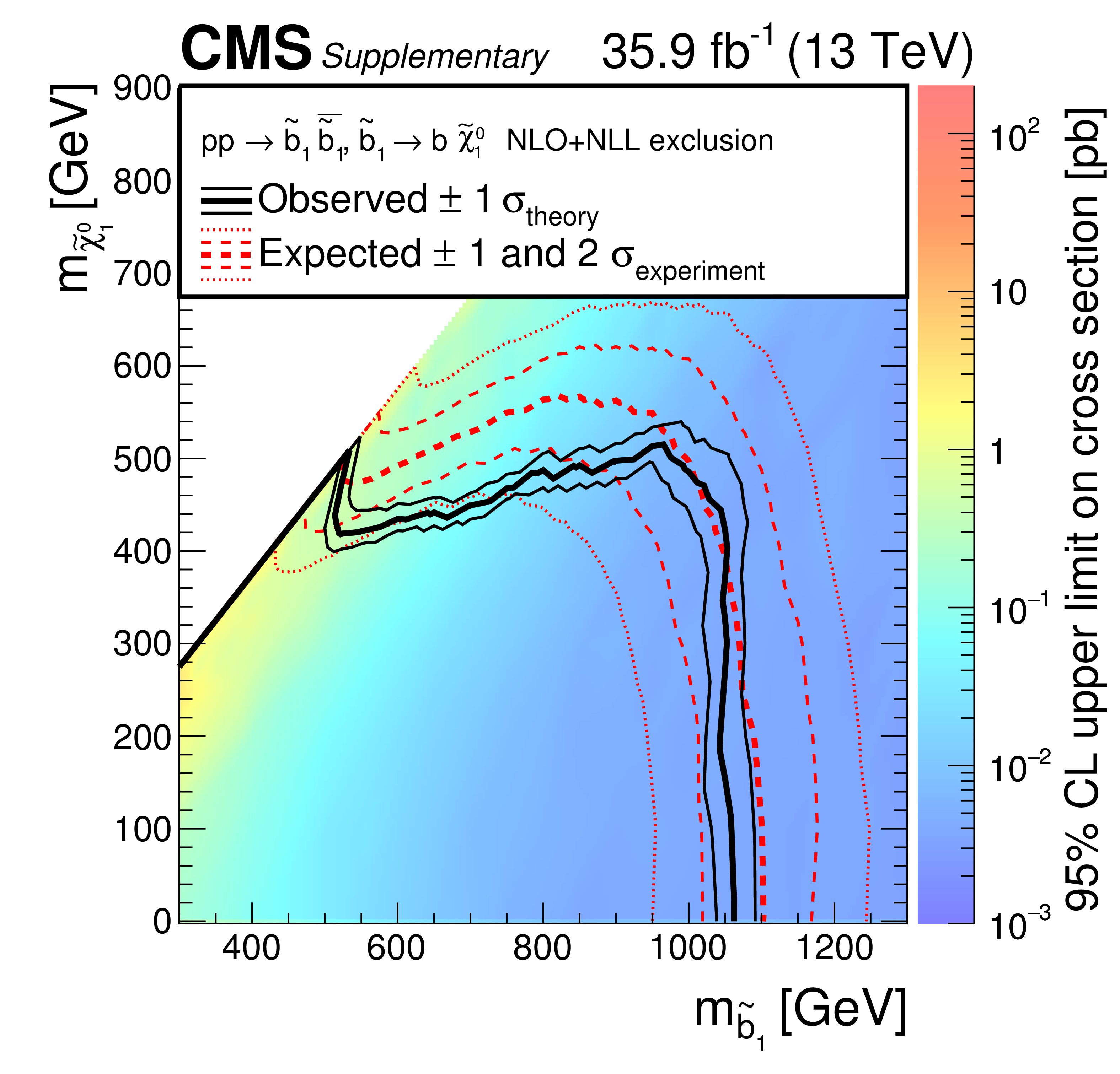
(a) Observed upper limit in cross section at 95% CL (indicated by the colour scale) as a function of the $ \tilde{ \mathrm{b} }$ and $ {\tilde{\chi}^{0}_{1}} $ masses for the T2bb simplified model. The black solid thick (thin) line indicates the observed excluded region assuming the nominal (${\pm}1$ standard deviation in theoretical uncertainty) production cross section. The red dashed thick (thin) line indicates the median (${\pm}1$ standard deviation in experimental uncertainty) expected excluded region. An electronic version of this figure is available as CMS-SUS-16-038\_Figure-aux\_018-a.root. (b) The signal acceptance times efficiency as a function of the $ \tilde{ \mathrm{b} }$ and $ {\tilde{\chi}^{0}_{1}} $ masses following the application of the event selection criteria for the signal region. |
png pdf root |
Additional Figure 18-a:
(a) Observed upper limit in cross section at 95% CL (indicated by the colour scale) as a function of the $ \tilde{ \mathrm{b} }$ and $ {\tilde{\chi}^{0}_{1}} $ masses for the T2bb simplified model. The black solid thick (thin) line indicates the observed excluded region assuming the nominal (${\pm}1$ standard deviation in theoretical uncertainty) production cross section. The red dashed thick (thin) line indicates the median (${\pm}1$ standard deviation in experimental uncertainty) expected excluded region. An electronic version of this figure is available as CMS-SUS-16-038\_Figure-aux\_018-a.root. (b) The signal acceptance times efficiency as a function of the $ \tilde{ \mathrm{b} }$ and $ {\tilde{\chi}^{0}_{1}} $ masses following the application of the event selection criteria for the signal region. -a |

png pdf root |
Additional Figure 18-b:
(a) Observed upper limit in cross section at 95% CL (indicated by the colour scale) as a function of the $ \tilde{ \mathrm{b} }$ and $ {\tilde{\chi}^{0}_{1}} $ masses for the T2bb simplified model. The black solid thick (thin) line indicates the observed excluded region assuming the nominal (${\pm}1$ standard deviation in theoretical uncertainty) production cross section. The red dashed thick (thin) line indicates the median (${\pm}1$ standard deviation in experimental uncertainty) expected excluded region. An electronic version of this figure is available as CMS-SUS-16-038\_Figure-aux\_018-a.root. (b) The signal acceptance times efficiency as a function of the $ \tilde{ \mathrm{b} }$ and $ {\tilde{\chi}^{0}_{1}} $ masses following the application of the event selection criteria for the signal region. -b |
png pdf |
Additional Figure 19:
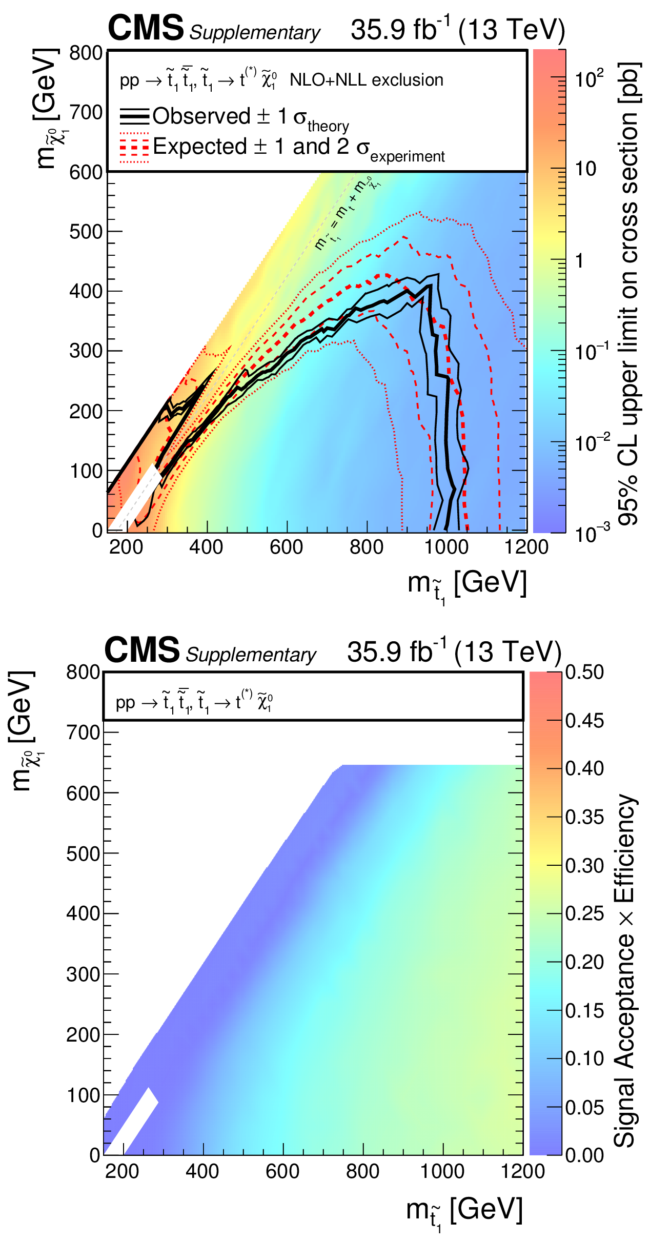
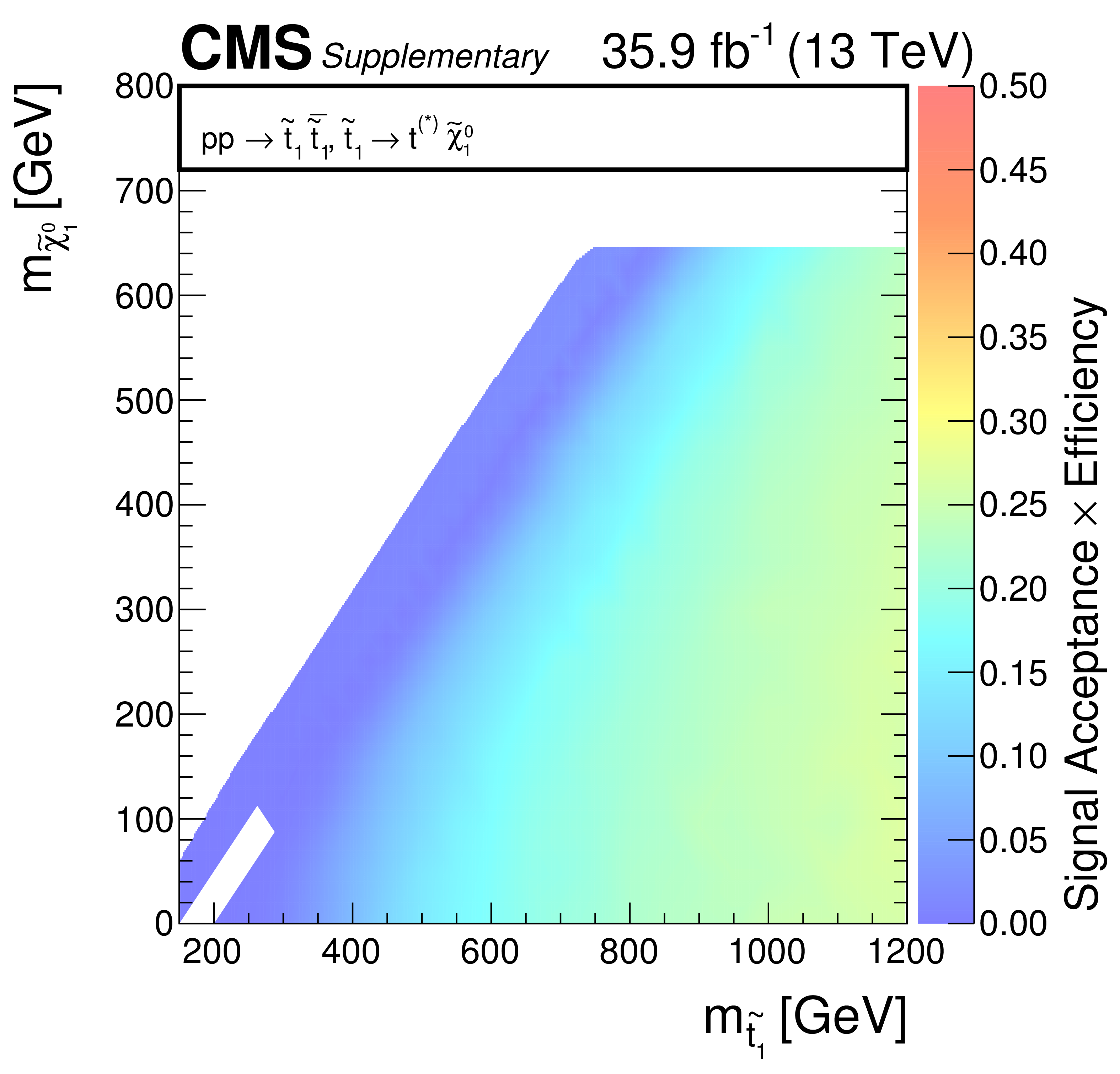
(a) Observed upper limit in cross section at 95% CL (indicated by the colour scale) as a function of the $ \tilde{ \mathrm{t} } $ and $ {\tilde{\chi}^{0}_{1}} $ masses for the T2tt simplified model. The black solid thick (thin) line indicates the observed excluded region assuming the nominal (${\pm}1$ standard deviation in theoretical uncertainty) production cross section. The red dashed thick (thin) line indicates the median (${\pm}1$ standard deviation in experimental uncertainty) expected excluded region. An electronic version of this figure is available as CMS-SUS-16-038\_Figure-aux\_019-a.root. (b) The signal acceptance times efficiency as a function of the $ \tilde{ \mathrm{t} } $ and $ {\tilde{\chi}^{0}_{1}} $ masses following the application of the event selection criteria for the signal region. |
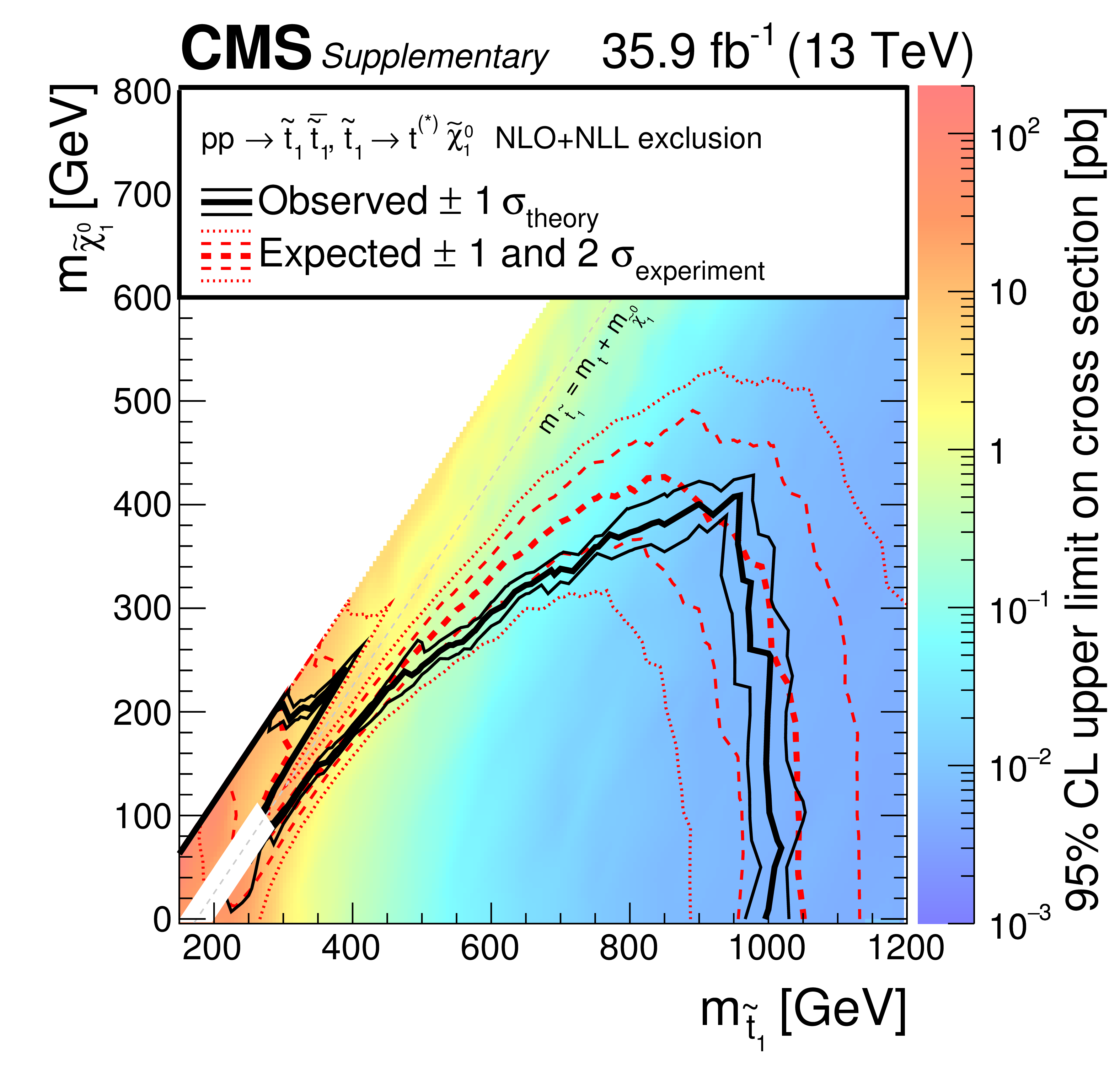
png pdf root |
Additional Figure 19-a:
(a) Observed upper limit in cross section at 95% CL (indicated by the colour scale) as a function of the $ \tilde{ \mathrm{t} } $ and $ {\tilde{\chi}^{0}_{1}} $ masses for the T2tt simplified model. The black solid thick (thin) line indicates the observed excluded region assuming the nominal (${\pm}1$ standard deviation in theoretical uncertainty) production cross section. The red dashed thick (thin) line indicates the median (${\pm}1$ standard deviation in experimental uncertainty) expected excluded region. An electronic version of this figure is available as CMS-SUS-16-038\_Figure-aux\_019-a.root. (b) The signal acceptance times efficiency as a function of the $ \tilde{ \mathrm{t} } $ and $ {\tilde{\chi}^{0}_{1}} $ masses following the application of the event selection criteria for the signal region. -a |
png pdf root |
Additional Figure 19-b:
(a) Observed upper limit in cross section at 95% CL (indicated by the colour scale) as a function of the $ \tilde{ \mathrm{t} } $ and $ {\tilde{\chi}^{0}_{1}} $ masses for the T2tt simplified model. The black solid thick (thin) line indicates the observed excluded region assuming the nominal (${\pm}1$ standard deviation in theoretical uncertainty) production cross section. The red dashed thick (thin) line indicates the median (${\pm}1$ standard deviation in experimental uncertainty) expected excluded region. An electronic version of this figure is available as CMS-SUS-16-038\_Figure-aux\_019-a.root. (b) The signal acceptance times efficiency as a function of the $ \tilde{ \mathrm{t} } $ and $ {\tilde{\chi}^{0}_{1}} $ masses following the application of the event selection criteria for the signal region. -b |
png pdf |
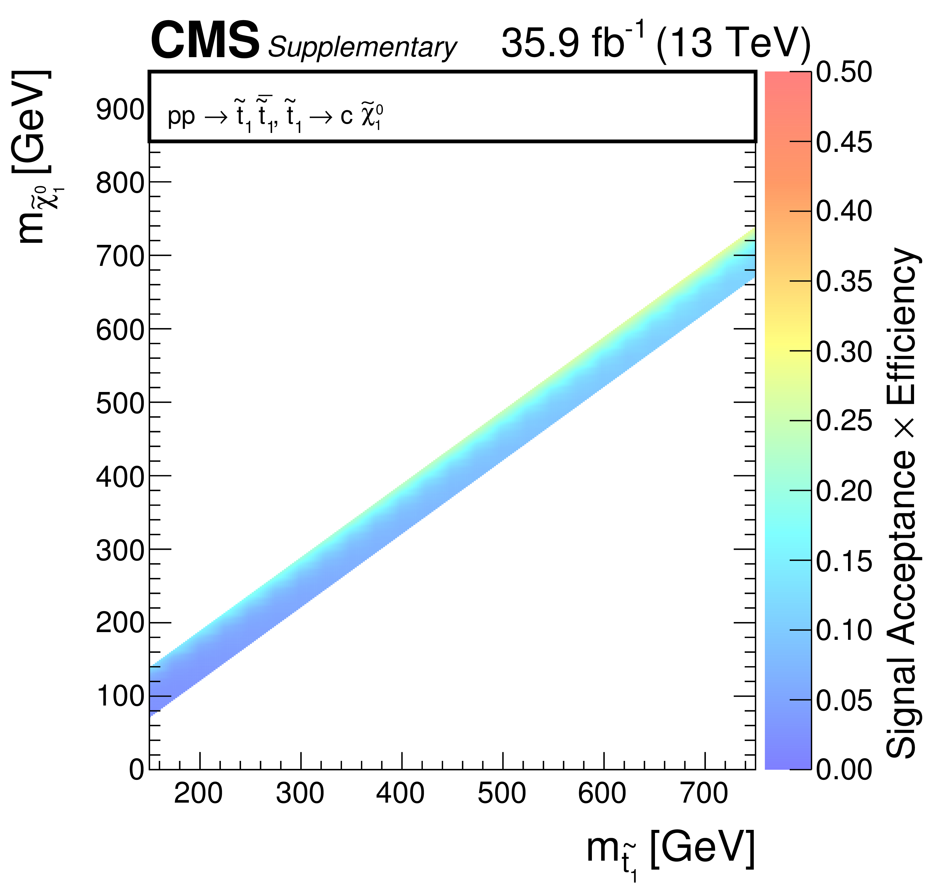
Additional Figure 20:
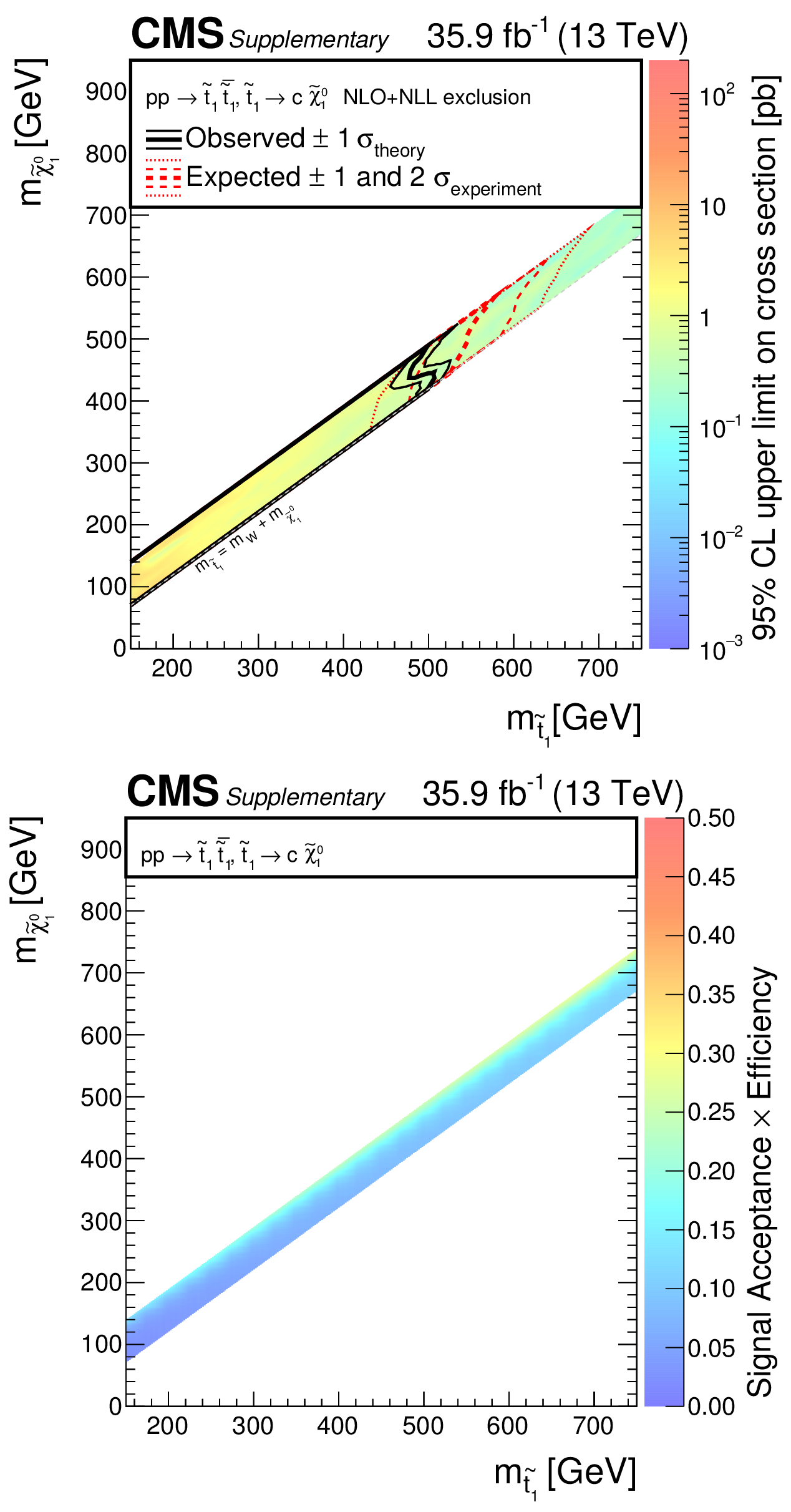
(a) Observed upper limit in cross section at 95% CL (indicated by the colour scale) as a function of the $ \tilde{ \mathrm{t} } $ and $ {\tilde{\chi}^{0}_{1}} $ masses for the T2cc simplified model. The black solid thick (thin) line indicates the observed excluded region assuming the nominal (${\pm}1$ standard deviation in theoretical uncertainty) production cross section. The red dashed thick (thin) line indicates the median (${\pm}1$ standard deviation in experimental uncertainty) expected excluded region. An electronic version of this figure is available as CMS-SUS-16-038\_Figure-aux\_020-a.root. (b) The signal acceptance times efficiency as a function of the $ \tilde{ \mathrm{t} } $ and $ {\tilde{\chi}^{0}_{1}} $ masses following the application of the event selection criteria for the signal region. |
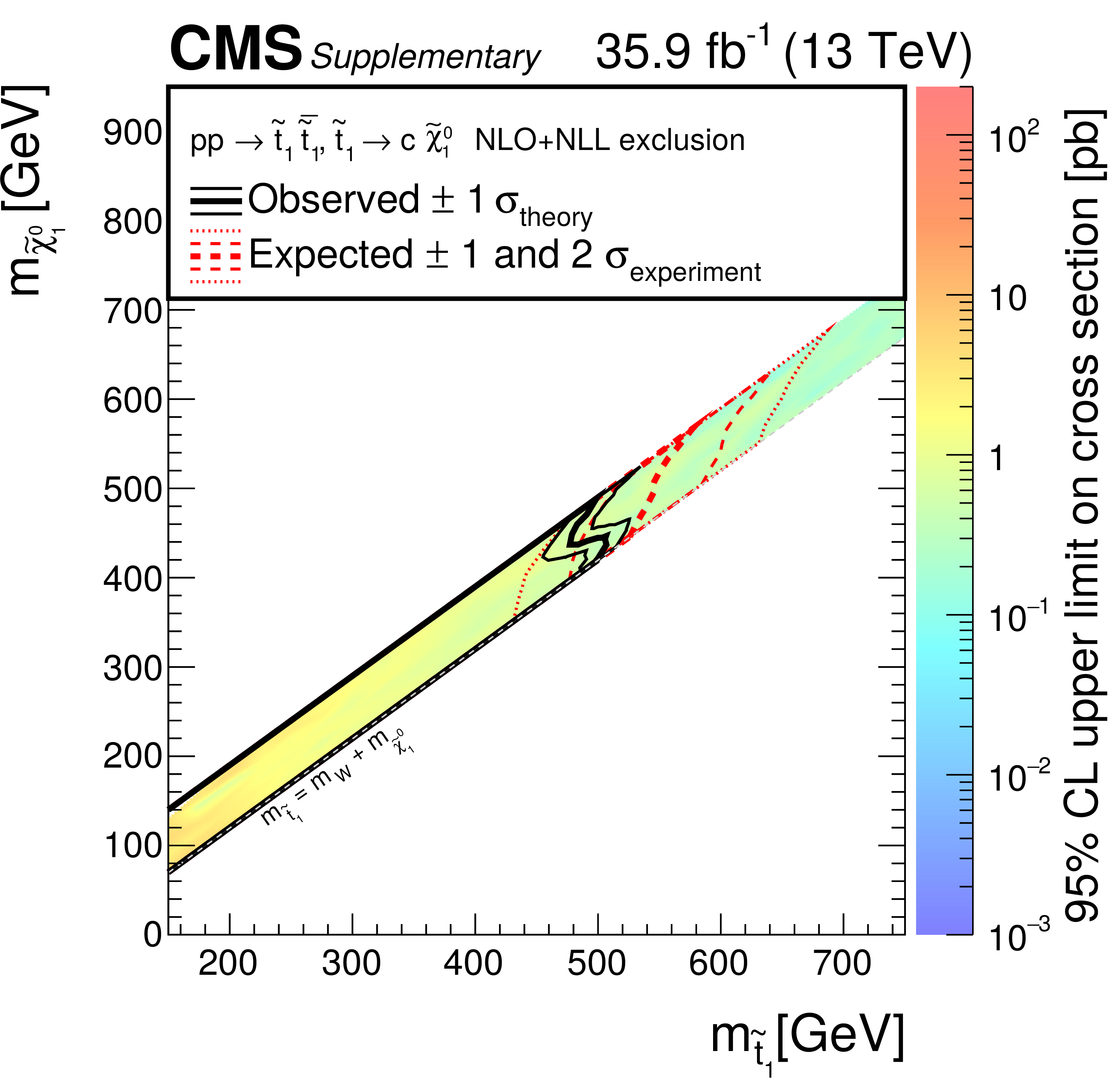
png pdf root |
Additional Figure 20-a:
(a) Observed upper limit in cross section at 95% CL (indicated by the colour scale) as a function of the $ \tilde{ \mathrm{t} } $ and $ {\tilde{\chi}^{0}_{1}} $ masses for the T2cc simplified model. The black solid thick (thin) line indicates the observed excluded region assuming the nominal (${\pm}1$ standard deviation in theoretical uncertainty) production cross section. The red dashed thick (thin) line indicates the median (${\pm}1$ standard deviation in experimental uncertainty) expected excluded region. An electronic version of this figure is available as CMS-SUS-16-038\_Figure-aux\_020-a.root. (b) The signal acceptance times efficiency as a function of the $ \tilde{ \mathrm{t} } $ and $ {\tilde{\chi}^{0}_{1}} $ masses following the application of the event selection criteria for the signal region. -a |
png pdf root |
Additional Figure 20-b:
(a) Observed upper limit in cross section at 95% CL (indicated by the colour scale) as a function of the $ \tilde{ \mathrm{t} } $ and $ {\tilde{\chi}^{0}_{1}} $ masses for the T2cc simplified model. The black solid thick (thin) line indicates the observed excluded region assuming the nominal (${\pm}1$ standard deviation in theoretical uncertainty) production cross section. The red dashed thick (thin) line indicates the median (${\pm}1$ standard deviation in experimental uncertainty) expected excluded region. An electronic version of this figure is available as CMS-SUS-16-038\_Figure-aux\_020-a.root. (b) The signal acceptance times efficiency as a function of the $ \tilde{ \mathrm{t} } $ and $ {\tilde{\chi}^{0}_{1}} $ masses following the application of the event selection criteria for the signal region. -b |
png pdf |
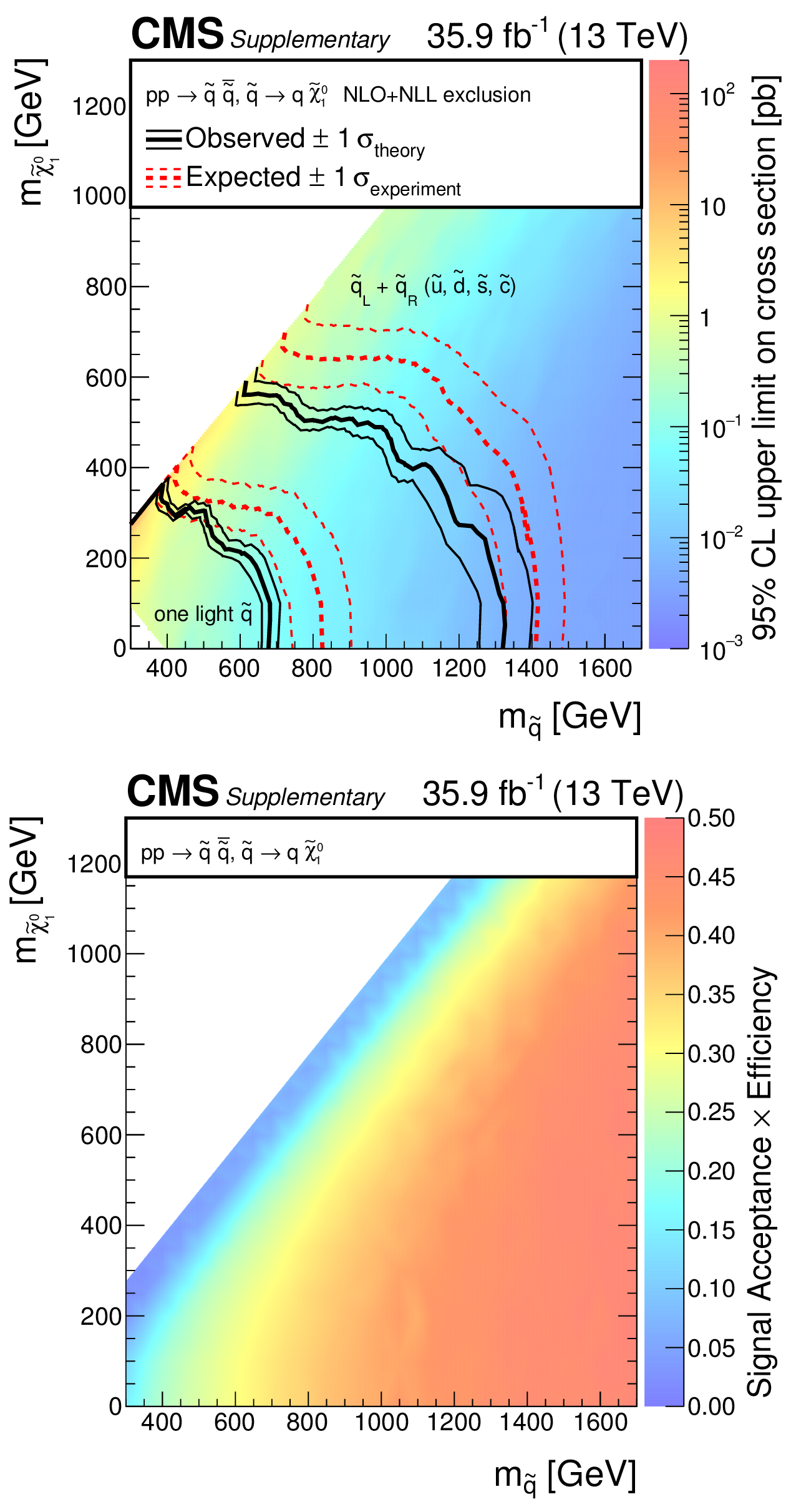
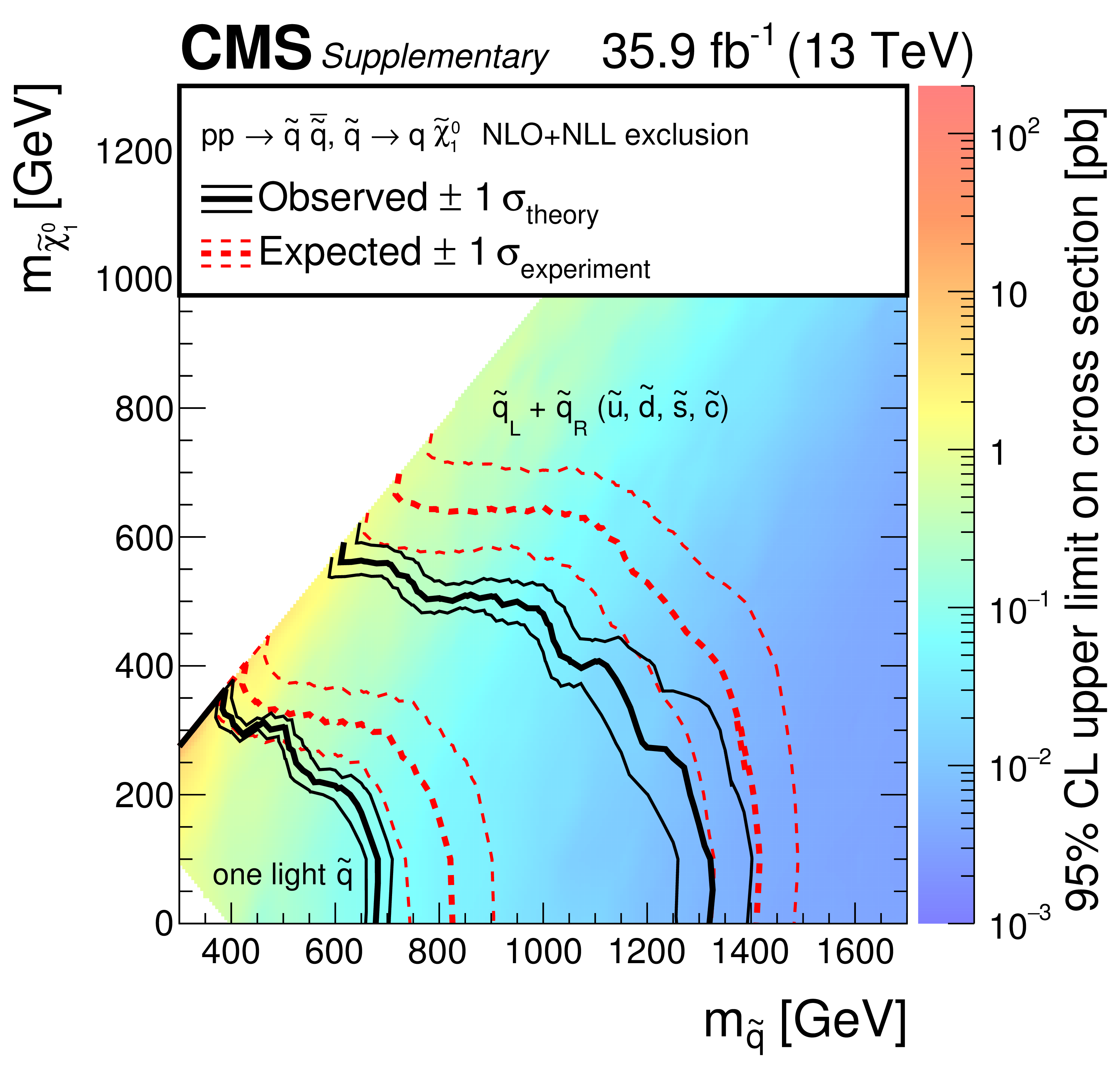
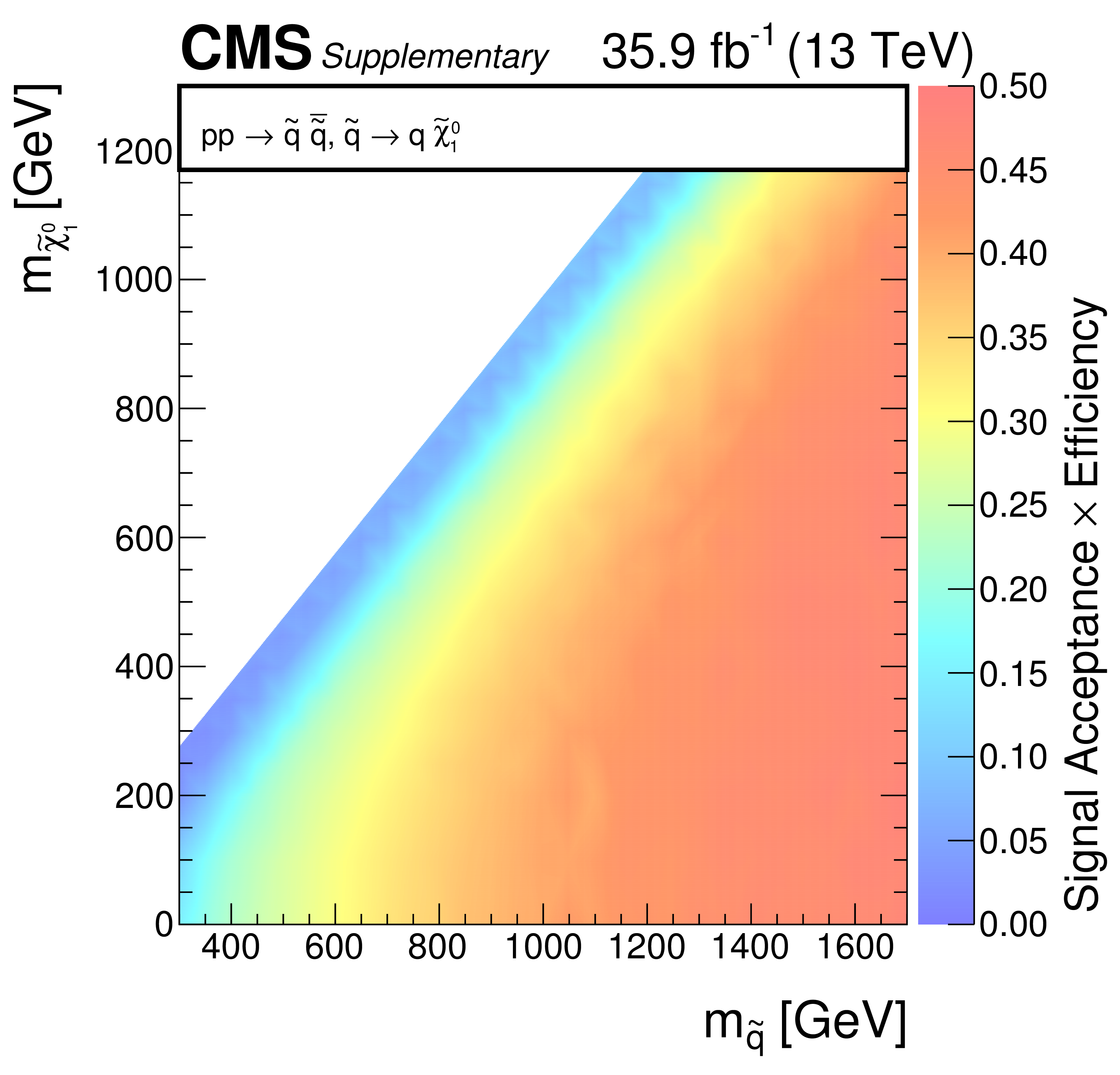
Additional Figure 21:
(a) Observed upper limit in cross section at 95% CL (indicated by the colour scale) as a function of the $ {\tilde{\mathrm {q}}} $ and $ {\tilde{\chi}^{0}_{1}} $ masses for the T2qq simplified model. The black solid thick (thin) line indicates the observed excluded region assuming the nominal (${\pm}1$ standard deviation in theoretical uncertainty) production cross section. The red dashed thick (thin) line indicates the median (${\pm}1$ standard deviation in experimental uncertainty) expected excluded region. An electronic version of this figure is available as CMS-SUS-16-038\_Figure-aux\_021-a.root. (b) The signal acceptance times efficiency as a function of the $ {\tilde{\mathrm {q}}} $ and $ {\tilde{\chi}^{0}_{1}} $ masses following the application of the event selection criteria for the signal region. |
png pdf root |
Additional Figure 21-a:
(a) Observed upper limit in cross section at 95% CL (indicated by the colour scale) as a function of the $ {\tilde{\mathrm {q}}} $ and $ {\tilde{\chi}^{0}_{1}} $ masses for the T2qq simplified model. The black solid thick (thin) line indicates the observed excluded region assuming the nominal (${\pm}1$ standard deviation in theoretical uncertainty) production cross section. The red dashed thick (thin) line indicates the median (${\pm}1$ standard deviation in experimental uncertainty) expected excluded region. An electronic version of this figure is available as CMS-SUS-16-038\_Figure-aux\_021-a.root. (b) The signal acceptance times efficiency as a function of the $ {\tilde{\mathrm {q}}} $ and $ {\tilde{\chi}^{0}_{1}} $ masses following the application of the event selection criteria for the signal region. -a |
png pdf root |
Additional Figure 21-b:
(a) Observed upper limit in cross section at 95% CL (indicated by the colour scale) as a function of the $ {\tilde{\mathrm {q}}} $ and $ {\tilde{\chi}^{0}_{1}} $ masses for the T2qq simplified model. The black solid thick (thin) line indicates the observed excluded region assuming the nominal (${\pm}1$ standard deviation in theoretical uncertainty) production cross section. The red dashed thick (thin) line indicates the median (${\pm}1$ standard deviation in experimental uncertainty) expected excluded region. An electronic version of this figure is available as CMS-SUS-16-038\_Figure-aux\_021-a.root. (b) The signal acceptance times efficiency as a function of the $ {\tilde{\mathrm {q}}} $ and $ {\tilde{\chi}^{0}_{1}} $ masses following the application of the event selection criteria for the signal region. -b |
png pdf |
Additional Figure 22:
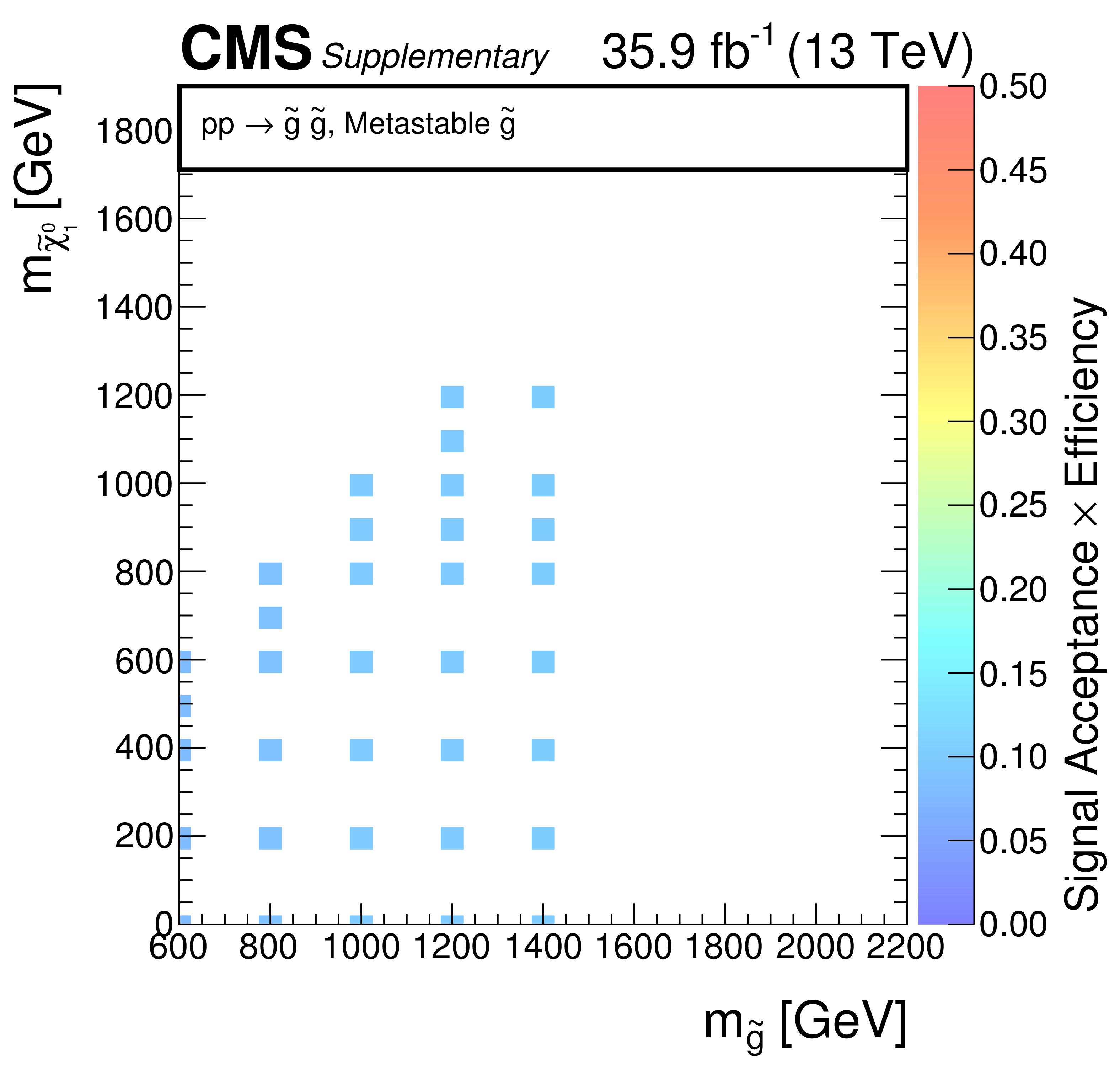
(a) Observed upper limit in cross section at 95% CL (indicated by the colour scale) as a function of the $ \tilde{g}$ and $ {\tilde{\chi}^{0}_{1}} $ masses for the T1qqqq split-SUSY model with meta-stable gluinos. The black solid thick (thin) line indicates the observed excluded region assuming the nominal (${\pm}1$ standard deviation in theoretical uncertainty) production cross section. The red dashed thick (thin) line indicates the median (${\pm}1$ standard deviation in experimental uncertainty) expected excluded region. An electronic version of this figure is available as CMS-SUS-16-038\_Figure-aux\_022-a.root. (b) The signal acceptance times efficiency as a function of the $ \\tilde{g}$ and $ {\tilde{\chi}^{0}_{1}} $ masses following the application of the event selection criteria for the signal region. |
png pdf root |
Additional Figure 22-a:
(a) Observed upper limit in cross section at 95% CL (indicated by the colour scale) as a function of the $ \tilde{g}$ and $ {\tilde{\chi}^{0}_{1}} $ masses for the T1qqqq split-SUSY model with meta-stable gluinos. The black solid thick (thin) line indicates the observed excluded region assuming the nominal (${\pm}1$ standard deviation in theoretical uncertainty) production cross section. The red dashed thick (thin) line indicates the median (${\pm}1$ standard deviation in experimental uncertainty) expected excluded region. An electronic version of this figure is available as CMS-SUS-16-038\_Figure-aux\_022-a.root. (b) The signal acceptance times efficiency as a function of the $ \\tilde{g}$ and $ {\tilde{\chi}^{0}_{1}} $ masses following the application of the event selection criteria for the signal region. -a |
png pdf root |
Additional Figure 22-b:
(a) Observed upper limit in cross section at 95% CL (indicated by the colour scale) as a function of the $ \tilde{g}$ and $ {\tilde{\chi}^{0}_{1}} $ masses for the T1qqqq split-SUSY model with meta-stable gluinos. The black solid thick (thin) line indicates the observed excluded region assuming the nominal (${\pm}1$ standard deviation in theoretical uncertainty) production cross section. The red dashed thick (thin) line indicates the median (${\pm}1$ standard deviation in experimental uncertainty) expected excluded region. An electronic version of this figure is available as CMS-SUS-16-038\_Figure-aux\_022-a.root. (b) The signal acceptance times efficiency as a function of the $ \\tilde{g}$ and $ {\tilde{\chi}^{0}_{1}} $ masses following the application of the event selection criteria for the signal region. -b |
png pdf |
Additional Figure 23:
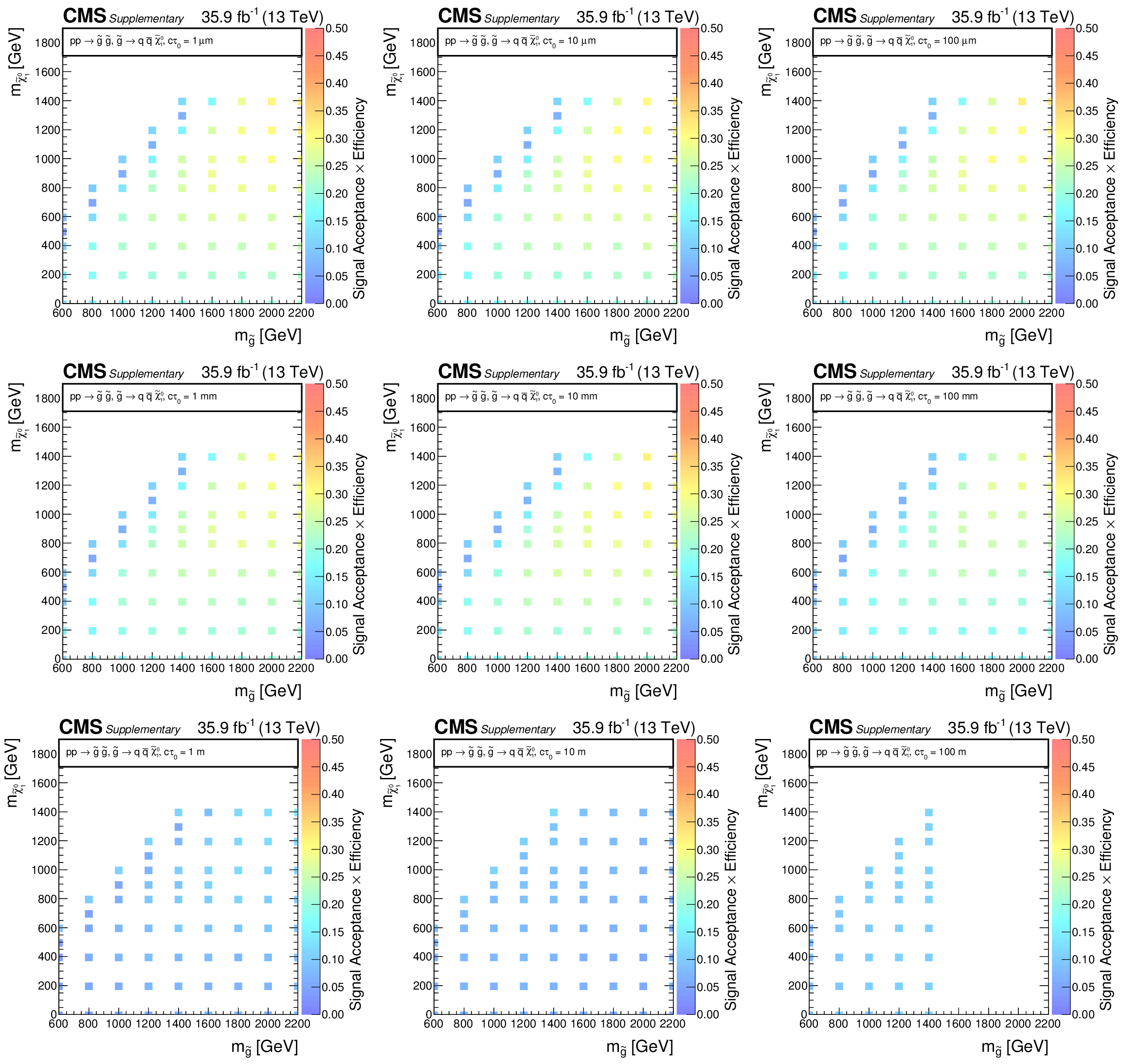
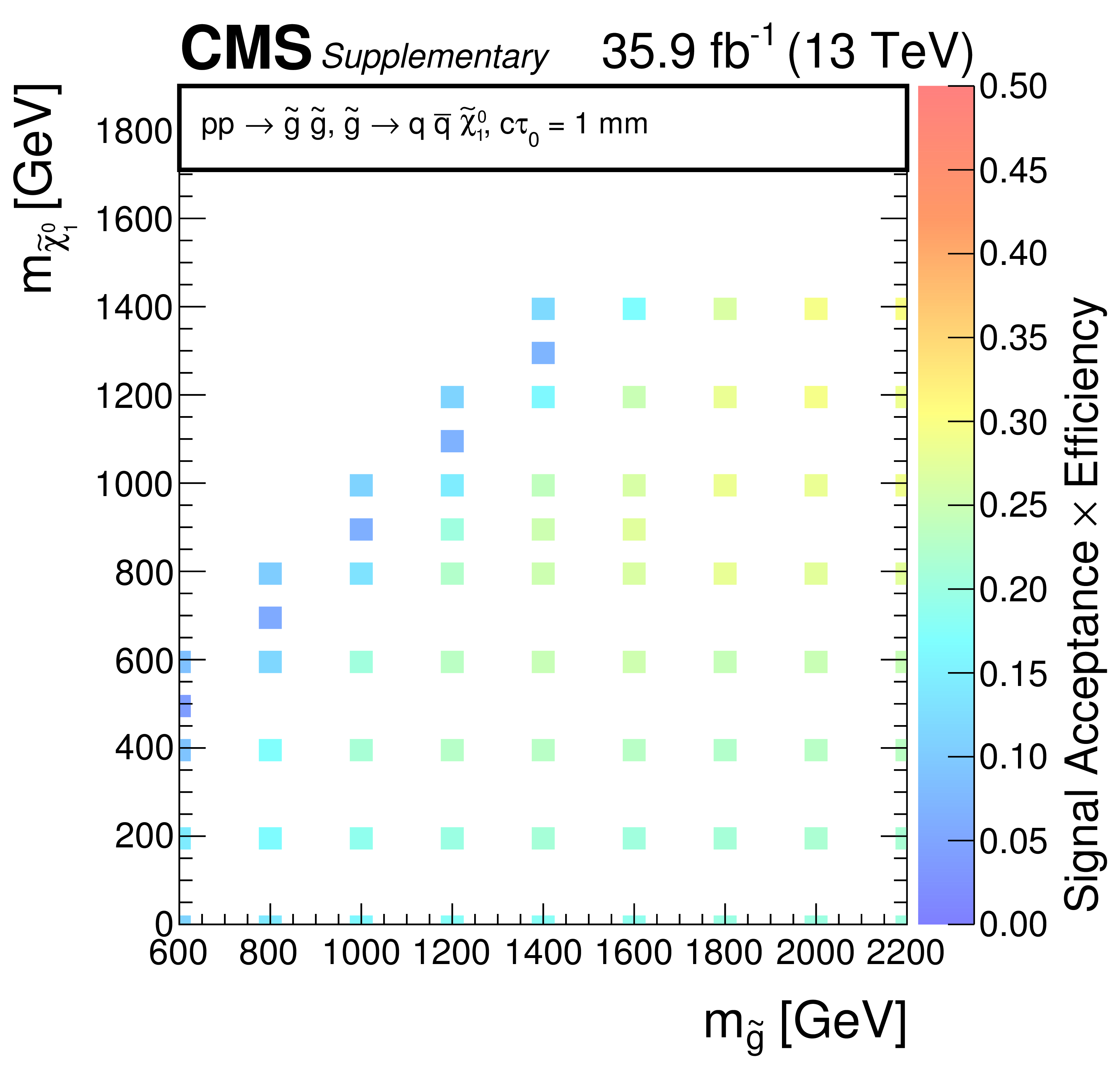
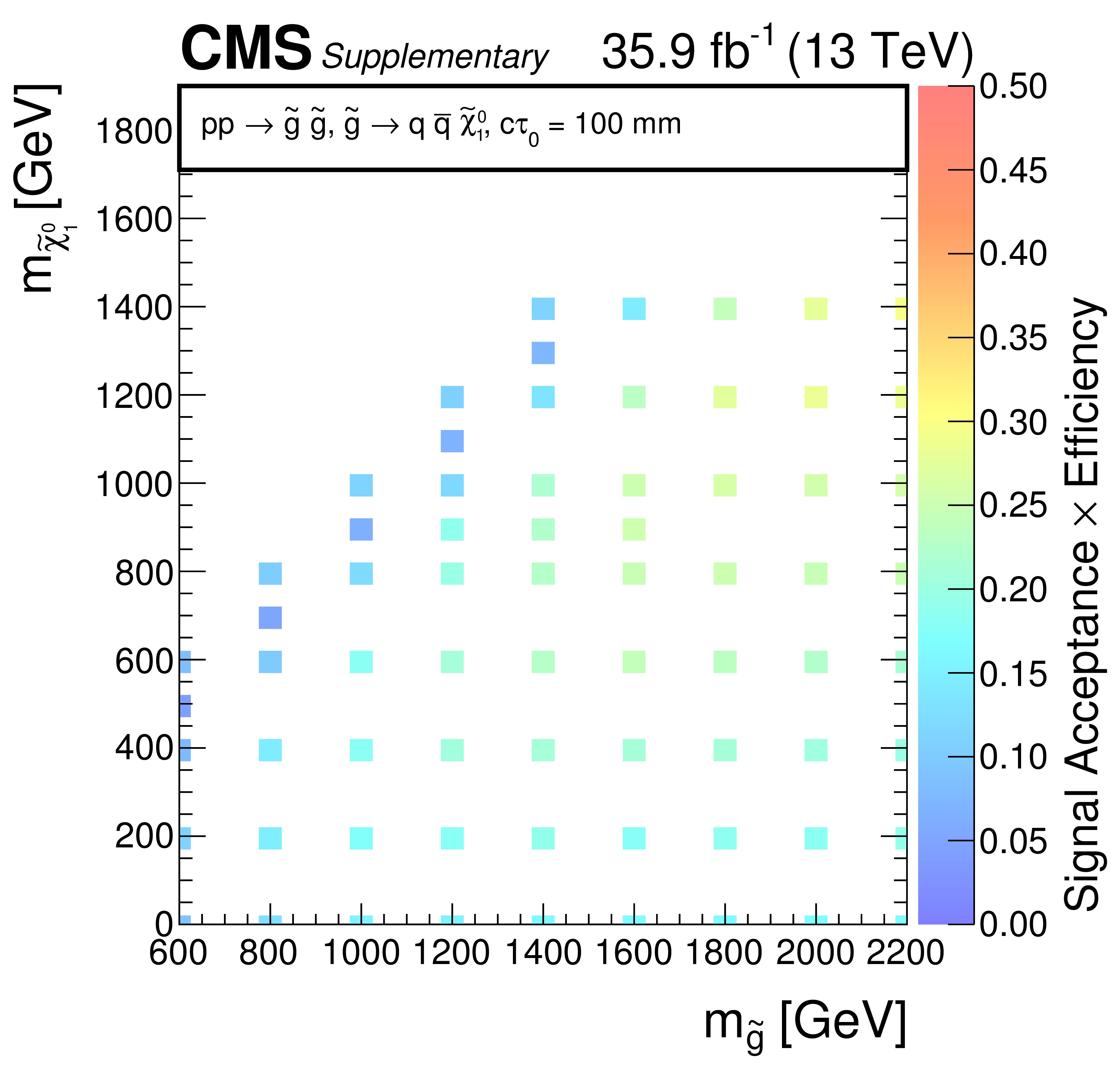
The signal acceptance times efficiency as a function of the $ \tilde{g}$ and $ {\tilde{\chi}^{0}_{1}} $ masses for simplified models that assume the production of pairs of long-lived gluinos that each decay via highly virtual light-flavour squarks to the neutralino and SM particles (T1qqqqLL). Each subfigure represents a different gluino lifetime: $ {c\tau _{0}} =$ 1 (a), 10 (b), and 100 m (c); 1 (d), 10 (e), and 100 mm (f); and 1 (g), 10 (h), and 100 m (j). |

png pdf root |
Additional Figure 23-a:
The signal acceptance times efficiency as a function of the $ \tilde{g}$ and $ {\tilde{\chi}^{0}_{1}} $ masses for simplified models that assume the production of pairs of long-lived gluinos that each decay via highly virtual light-flavour squarks to the neutralino and SM particles (T1qqqqLL). Each subfigure represents a different gluino lifetime: $ {c\tau _{0}} =$ 1 (a), 10 (b), and 100 m (c); 1 (d), 10 (e), and 100 mm (f); and 1 (g), 10 (h), and 100 m (j). |

png pdf root |
Additional Figure 23-b:
The signal acceptance times efficiency as a function of the $ \tilde{g}$ and $ {\tilde{\chi}^{0}_{1}} $ masses for simplified models that assume the production of pairs of long-lived gluinos that each decay via highly virtual light-flavour squarks to the neutralino and SM particles (T1qqqqLL). Each subfigure represents a different gluino lifetime: $ {c\tau _{0}} =$ 1 (a), 10 (b), and 100 m (c); 1 (d), 10 (e), and 100 mm (f); and 1 (g), 10 (h), and 100 m (j). |

png pdf root |
Additional Figure 23-c:
The signal acceptance times efficiency as a function of the $ \tilde{g}$ and $ {\tilde{\chi}^{0}_{1}} $ masses for simplified models that assume the production of pairs of long-lived gluinos that each decay via highly virtual light-flavour squarks to the neutralino and SM particles (T1qqqqLL). Each subfigure represents a different gluino lifetime: $ {c\tau _{0}} =$ 1 (a), 10 (b), and 100 m (c); 1 (d), 10 (e), and 100 mm (f); and 1 (g), 10 (h), and 100 m (j). |
png pdf root |
Additional Figure 23-d:
The signal acceptance times efficiency as a function of the $ \tilde{g}$ and $ {\tilde{\chi}^{0}_{1}} $ masses for simplified models that assume the production of pairs of long-lived gluinos that each decay via highly virtual light-flavour squarks to the neutralino and SM particles (T1qqqqLL). Each subfigure represents a different gluino lifetime: $ {c\tau _{0}} =$ 1 (a), 10 (b), and 100 m (c); 1 (d), 10 (e), and 100 mm (f); and 1 (g), 10 (h), and 100 m (j). |

png pdf root |
Additional Figure 23-e:
The signal acceptance times efficiency as a function of the $ \tilde{g}$ and $ {\tilde{\chi}^{0}_{1}} $ masses for simplified models that assume the production of pairs of long-lived gluinos that each decay via highly virtual light-flavour squarks to the neutralino and SM particles (T1qqqqLL). Each subfigure represents a different gluino lifetime: $ {c\tau _{0}} =$ 1 (a), 10 (b), and 100 m (c); 1 (d), 10 (e), and 100 mm (f); and 1 (g), 10 (h), and 100 m (j). |
png pdf root |
Additional Figure 23-f:
The signal acceptance times efficiency as a function of the $ \tilde{g}$ and $ {\tilde{\chi}^{0}_{1}} $ masses for simplified models that assume the production of pairs of long-lived gluinos that each decay via highly virtual light-flavour squarks to the neutralino and SM particles (T1qqqqLL). Each subfigure represents a different gluino lifetime: $ {c\tau _{0}} =$ 1 (a), 10 (b), and 100 m (c); 1 (d), 10 (e), and 100 mm (f); and 1 (g), 10 (h), and 100 m (j). |

png pdf root |
Additional Figure 23-g:
The signal acceptance times efficiency as a function of the $ \tilde{g}$ and $ {\tilde{\chi}^{0}_{1}} $ masses for simplified models that assume the production of pairs of long-lived gluinos that each decay via highly virtual light-flavour squarks to the neutralino and SM particles (T1qqqqLL). Each subfigure represents a different gluino lifetime: $ {c\tau _{0}} =$ 1 (a), 10 (b), and 100 m (c); 1 (d), 10 (e), and 100 mm (f); and 1 (g), 10 (h), and 100 m (j). |

png pdf root |
Additional Figure 23-h:
The signal acceptance times efficiency as a function of the $ \tilde{g}$ and $ {\tilde{\chi}^{0}_{1}} $ masses for simplified models that assume the production of pairs of long-lived gluinos that each decay via highly virtual light-flavour squarks to the neutralino and SM particles (T1qqqqLL). Each subfigure represents a different gluino lifetime: $ {c\tau _{0}} =$ 1 (a), 10 (b), and 100 m (c); 1 (d), 10 (e), and 100 mm (f); and 1 (g), 10 (h), and 100 m (j). |

png pdf root |
Additional Figure 23-i:
The signal acceptance times efficiency as a function of the $ \tilde{g}$ and $ {\tilde{\chi}^{0}_{1}} $ masses for simplified models that assume the production of pairs of long-lived gluinos that each decay via highly virtual light-flavour squarks to the neutralino and SM particles (T1qqqqLL). Each subfigure represents a different gluino lifetime: $ {c\tau _{0}} =$ 1 (a), 10 (b), and 100 m (c); 1 (d), 10 (e), and 100 mm (f); and 1 (g), 10 (h), and 100 m (j). |

png pdf |
Additional Figure 24:
Observed and expected mass exclusions at 95% CL (indicated, respectively, by solid and dashed contours) for simplified models with an intermediate squark. Five model families involve the direct pair production of squarks. The first scenario considers the pair production and decay of bottom squarks (T2bb). Two scenarios involve the production and decay of top squark pairs (T2tt and T2cc). The grey shaded region denotes T2tt models that are not considered for interpretation. Two further scenarios involve, respectively, the production and decay of light-flavour squarks, with different assumptions on the mass degeneracy of the squarks as described in the text (T2qq\_8fold and T2qq\_1fold). |
png pdf |
Additional Figure 25:
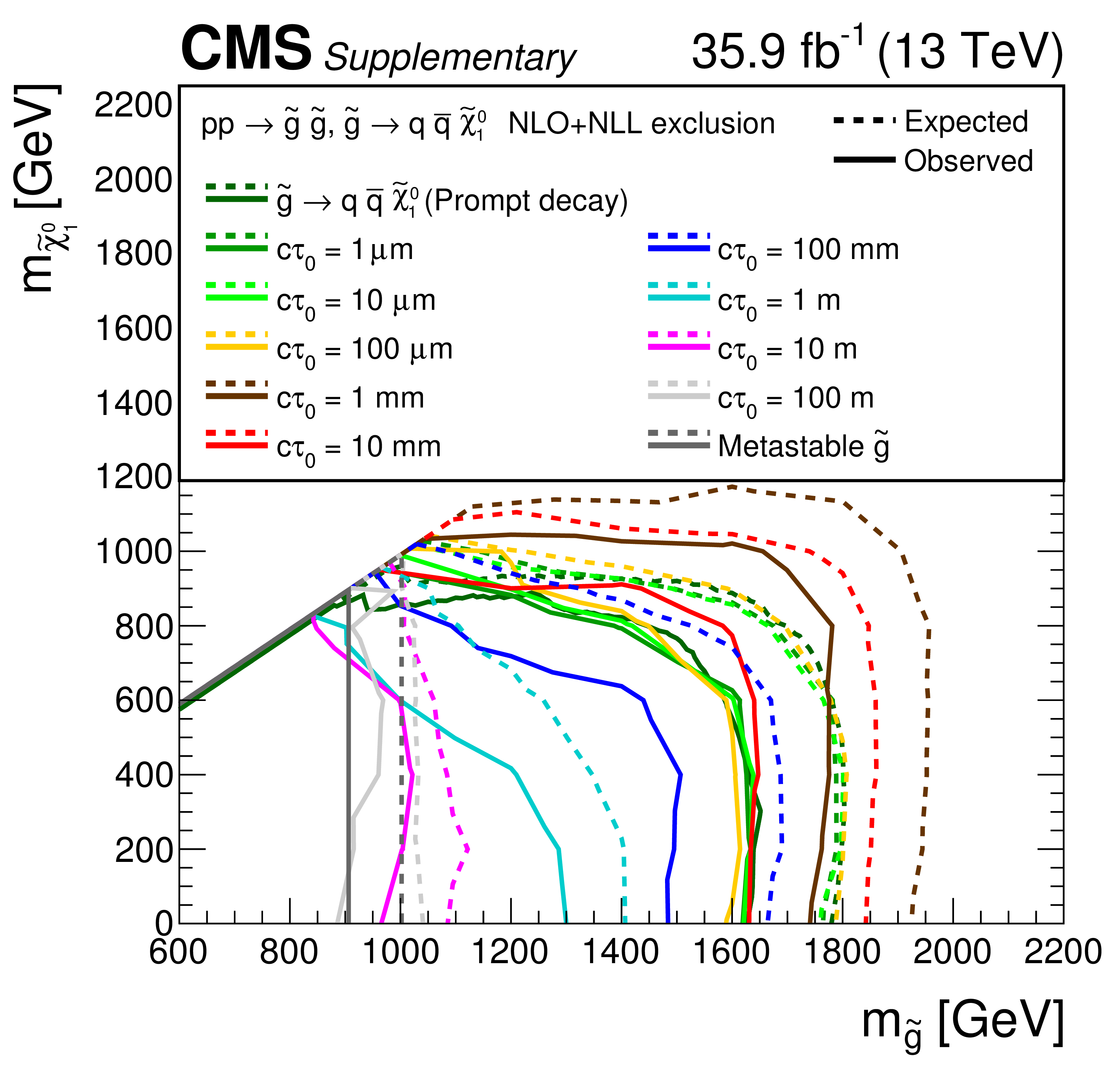
Observed and expected mass exclusions at 95% CL (indicated, respectively, by solid and dashed contours) for simplified models that assume the production of pairs of long-lived gluinos that each decay via highly virtual light-flavour squarks to the neutralino and SM particles (T1qqqqLL). The mass exclusion contours are shown for each value of the gluino proper decay length ${c\tau _{0}}$ considered by this search. |
png pdf |
Additional Figure 26:
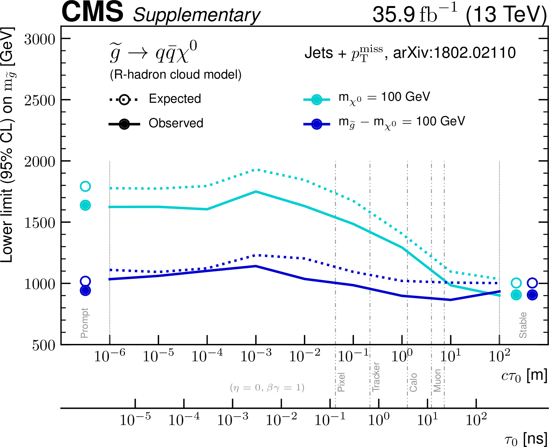
Observed and expected gluino mass exclusions at 95% CL (indicated, respectively, by solid and dashed contours) for simplified models that assume the production of pairs of long-lived gluinos that each decay via highly virtual light-flavour squarks to the neutralino and SM particles (T1qqqqLL). The gluino mass exclusions are shown for two different assumptions on the neutralino mass and as a function of the gluino proper decay length ${c\tau _{0}}$. The prompt and stable values refer to the mass exclusions obtained with the T1qqqq and T1qqqqLL metastable ($ {c\tau _{0}} = 10^{18} $ mm) scenarios, respectively. |
png pdf csv |
Additional Figure 27:
Counts of events in the signal region from data (solid markers), SM expectations with associated uncertainties (statistical and systematic, black histograms and shaded bands) as determined from the CR-only fit, and the predicted signal shape and uncertainty assuming a production cross section calculated at NLO+NLL accuracy for the T2bb benchmark model with ($m_{\tilde{ \mathrm{b} }}$, $m_{{\tilde{\chi}^{0}_{1}}}) = $ (550, 450) GeV (magenta histogram and shaded band), as a function of ${n_{\text {jet}}}$, $ {n_{\text {b}}}$, ${H_{\text {T}}} $, and $ {H_{\mathrm {T}}^{\text {miss}}} $ using the simplified binning schema. The centre panel of each subfigure shows the ratios of observed counts and the SM expectations, while the lower panel shows the significance of deviations observed in data with respect to the SM expectations expressed in terms of the total uncertainty in the SM expectations. |

png pdf csv |
Additional Figure 28:
Counts of events in the signal region from data (solid markers), SM expectations with associated uncertainties (statistical and systematic, black histograms and shaded bands) as determined from the CR-only fit, and the predicted signal shape and uncertainty assuming a production cross section calculated at NLO+NLL accuracy for the T2cc benchmark model with ($m_{\tilde{ \mathrm{t} }}$, $m_{{\tilde{\chi}^{0}_{1}}}$) = (500, 480) GeV (magenta histogram and shaded band), as a function of ${n_{\text {jet}}}$, $ {n_{\text {b}}}$, ${H_{\text {T}}} $, and $ {H_{\mathrm {T}}^{\text {miss}}} $ using the simplified binning schema. The centre panel of each subfigure shows the ratios of observed counts and the SM expectations, while the lower panel shows the significance of deviations observed in data with respect to the SM expectations expressed in terms of the total uncertainty in the SM expectations. |
png pdf csv |
Additional Figure 29:
Counts of events in the signal region from data (solid markers), SM expectations with associated uncertainties (statistical and systematic, black histograms and shaded bands) as determined from the CR-only fit, and the predicted signal shape and uncertainty assuming a production cross section calculated at NLO+NLL accuracy for the T1bbbb benchmark model with ($m_{\tilde{g}}$, $m_{{\tilde{\chi}^{0}_{1}}}) = $ (1900, 100) GeV (magenta histogram and shaded band), as a function of ${n_{\text {jet}}}$, $ {n_{\text {b}}}$, $ {H_{\text {T}}} $, and $ {H_{\mathrm {T}}^{\text {miss}}} $ using the simplified binning schema. The centre panel of each subfigure shows the ratios of observed counts and the SM expectations, while the lower panel shows the significance of deviations observed in data with respect to the SM expectations expressed in terms of the total uncertainty in the SM expectations. |

png pdf csv |
Additional Figure 30:
Counts of events in the signal region from data (solid markers), SM expectations with associated uncertainties (statistical and systematic, black histograms and shaded bands) as determined from the CR-only fit, and the predicted signal shape and uncertainty assuming a production cross section calculated at NLO+NLL accuracy for the T1qqqqLL benchmark model with $ {c\tau _{0}} =1$\nobreakspace {}mm, ($m_{\tilde{g}}$, $m_{{\tilde{\chi}^{0}_{1}}}) = $ (1800, 200) GeV (magenta histogram and shaded band), as a function of ${n_{\text {jet}}}$, $ {n_{\text {b}}}$, $ {H_{\text {T}}} $, and $ {H_{\mathrm {T}}^{\text {miss}}} $ using the simplified binning schema. The centre panel of each subfigure shows the ratios of observed counts and the SM expectations, while the lower panel shows the significance of deviations observed in data with respect to the SM expectations expressed in terms of the total uncertainty in the SM expectations. |
| Additional Tables | |
png pdf |
Additional Table 1:
A list of benchmark simplified models organized according to production and decay modes (family), and the expected and observed upper limits on the production cross section $\sigma _\text {UL}$ relative to the theoretical value $\sigma _\text {th}$ calculated at NLO+NLL accuracy. See the paper for a discussion of the uncertainties and signal acceptance times efficiency |

png pdf |
Additional Table 2:
A summary of the cumulative signal acceptance times efficiency, $\mathcal {A}\epsilon $ [%], for various benchmark models found in Table 4 of the paper, following the successive application of the event selection criteria used to define the signal region. See discussion and Table 1 in the paper for detailed descriptions of the selection. |
|
To help with re-interpretation of these results the following information is made available in machine-readable formats:
|
| References | ||||
| 1 | Y. A. Gol'fand and E. P. Likhtman | Extension of the algebra of Poincare group generators and violation of p invariance | JEPTL 13 (1971) 323 | |
| 2 | J. Wess and B. Zumino | Supergauge transformations in four dimensions | NPB 70 (1974) 39 | |
| 3 | R. Barbieri, S. Ferrara, and C. A. Savoy | Gauge models with spontaneously broken local supersymmetry | PLB 119 (1982) 343 | |
| 4 | H. P. Nilles | Supersymmetry, supergravity and particle physics | PR 110 (1984) 1 | |
| 5 | E. Witten | Dynamical breaking of supersymmetry | NPB 188 (1981) 513 | |
| 6 | S. Dimopoulos and H. Georgi | Softly broken supersymmetry and SU(5) | NPB 193 (1981) 150 | |
| 7 | S. Dimopoulos, S. Raby, and F. Wilczek | Supersymmetry and the scale of unification | PRD 24 (1981) 1681 | |
| 8 | L. E. Ibanez and G. G. Ross | Low-energy predictions in supersymmetric grand unified theories | PLB 105 (1981) 439 | |
| 9 | W. J. Marciano and G. Senjanovi\'c | Predictions of supersymmetric grand unified theories | PRD 25 (1982) 3092 | |
| 10 | G. R. Farrar and P. Fayet | Phenomenology of the production, decay, and detection of new hadronic states associated with supersymmetry | PLB 76 (1978) 575 | |
| 11 | G. Jungman, M. Kamionkowski, and K. Griest | Supersymmetric dark matter | PR 267 (1996) 195 | hep-ph/9506380 |
| 12 | Particle Data Group, C. Patrignani et al. | Review of Particle Physics | CPC 40 (2016) 100001 | |
| 13 | R. Barbieri and D. Pappadopulo | S-particles at their naturalness limits | JHEP 10 (2009) 061 | 0906.4546 |
| 14 | ATLAS Collaboration | Observation of a new particle in the search for the standard model Higgs boson with the ATLAS detector at the LHC | PLB 716 (2012) 1 | 1207.7214 |
| 15 | CMS Collaboration | Observation of a new boson at a mass of 125 GeV with the CMS experiment at the LHC | PLB 716 (2012) 30 | CMS-HIG-12-028 1207.7235 |
| 16 | CMS Collaboration | Observation of a new boson with mass near 125 GeV in pp collisions at $ \sqrt{s} = $ 7 and 8 TeV | JHEP 06 (2013) 081 | CMS-HIG-12-036 1303.4571 |
| 17 | CMS Collaboration | Precise determination of the mass of the Higgs boson and tests of compatibility of its couplings with the standard model predictions using proton collisions at 7 and 8 TeV | EPJC 75 (2015) 212 | CMS-HIG-14-009 1412.8662 |
| 18 | ATLAS Collaboration | Measurement of the Higgs boson mass from the $ \textrm{H}\rightarrow \gamma\gamma $ and $ \textrm{H} \rightarrow \textrm{ZZ}^{*} \rightarrow 4\ell $ channels with the ATLAS detector using 25 fb$ ^{-1} $ of $ {\mathrm{p}}{\mathrm{p}} $ collision data | PRD 90 (2014) 052004 | 1406.3827 |
| 19 | ATLAS and CMS Collaborations | Combined measurement of the Higgs boson mass in $ {\mathrm{p}}{\mathrm{p}} $ collisions at $ \sqrt{s}= $ 7 and 8 TeV with the ATLAS and CMS experiments | PRL 114 (2015) 191803 | 1503.07589 |
| 20 | N. Arkani-Hamed and S. Dimopoulos | Supersymmetric unification without low energy supersymmetry and signatures for fine-tuning at the LHC | JHEP 06 (2005) 073 | hep-th/0405159 |
| 21 | G. F. Giudice and A. Romanino | Split supersymmetry | NPB 699 (2004) 65 | hep-ph/0406088 |
| 22 | M. Fairbairn et al. | Stable massive particles at colliders | PR 438 (2007) 1 | hep-ph/0611040 |
| 23 | CMS Collaboration | CMS luminosity measurements for the 2016 data taking period | CMS-PAS-LUM-17-001 | CMS-PAS-LUM-17-001 |
| 24 | CMS Collaboration | Search for supersymmetry in $ {\mathrm{p}}{\mathrm{p}} $ collisions at 7 TeV in events with jets and missing transverse energy | PLB 698 (2011) 196 | CMS-SUS-10-003 1101.1628 |
| 25 | CMS Collaboration | Search for supersymmetry at the LHC in events with jets and missing transverse energy | PRL 107 (2011) 221804 | CMS-SUS-11-003 1109.2352 |
| 26 | CMS Collaboration | Search for supersymmetry in final states with missing transverse energy and 0, 1, 2, or $ {\ge}3 $ b-quark jets in 7 $ TeV {\mathrm{p}}{\mathrm{p}} $ collisions using the variable $ \alpha_\mathrm{T} $ | JHEP 01 (2013) 077 | CMS-SUS-11-022 1210.8115 |
| 27 | CMS Collaboration | Search for supersymmetry in hadronic final states with missing transverse energy using the variables $ \alpha_T $ and b-quark multiplicity in $ {\mathrm{p}}{\mathrm{p}} $ collisions at $ \sqrt s = $ 8 TeV | EPJC 73 (2013) 2568 | CMS-SUS-12-028 1303.2985 |
| 28 | CMS Collaboration | Search for top squark pair production in compressed-mass-spectrum scenarios in proton-proton collisions at $ \sqrt{s} = $ 8 TeV using the $ \alpha_T $ variable | PLB 767 (2017) 403 | CMS-SUS-14-006 1605.08993 |
| 29 | CMS Collaboration | A search for new phenomena in $ {\mathrm{p}}{\mathrm{p}} $ collisions at $ \sqrt{s} = $ 13 TeV in final states with missing transverse momentum and at least one jet using the $ \alpha_{\mathrm{T}} $ variable | EPJC 77 (2017) 294 | CMS-SUS-15-005 1611.00338 |
| 30 | J. Alwall, P. Schuster, and N. Toro | Simplified models for a first characterization of new physics at the LHC | PRD 79 (2009) 075020 | 0810.3921 |
| 31 | J. Alwall, M.-P. Le, M. Lisanti, and J. G. Wacker | Model-independent jets plus missing energy searches | PRD 79 (2009) 015005 | 0809.3264 |
| 32 | D. Alves et al. | Simplified models for LHC new physics searches | JPG 39 (2012) 105005 | 1105.2838 |
| 33 | ATLAS Collaboration | Search for squarks and gluinos in final states with jets and missing transverse momentum at $ \sqrt{s} = $ 13 TeV with the ATLAS detector | EPJC 76 (2016) 392 | 1605.03814 |
| 34 | CMS Collaboration | Search for supersymmetry in multijet events with missing transverse momentum in proton-proton collisions at 13 TeV | PRD 96 (2017) 032003 | CMS-SUS-16-033 1704.07781 |
| 35 | CMS Collaboration | Search for new phenomena with the $ M_{\mathrm {T2}} $ variable in the all-hadronic final state produced in proton-proton collisions at $ \sqrt{s} = $ 13 TeV | EPJC 77 (2017) 710 | CMS-SUS-16-036 1705.04650 |
| 36 | CMS Collaboration | Search for stopped gluinos in $ {\mathrm{p}}{\mathrm{p}} $ collisions at $ \sqrt{s} = $ 7 TeV | PRL 106 (2011) 011801 | CMS-EXO-10-003 1011.5861 |
| 37 | CMS Collaboration | Search for heavy stable charged particles in pp collisions at $ \sqrt{s} = $ 7 TeV | JHEP 03 (2011) 024 | CMS-EXO-10-011 1101.1645 |
| 38 | ATLAS Collaboration | Search for stable hadronising squarks and gluinos with the ATLAS experiment at the LHC | PLB 701 (2011) 1 | 1103.1984 |
| 39 | ATLAS Collaboration | Search for decays of stopped, long-lived particles from 7 TeV $ {\mathrm{p}}{\mathrm{p}} $ collisions with the ATLAS detector | EPJC 72 (2012) 1965 | 1201.5595 |
| 40 | CMS Collaboration | Search for heavy long-lived charged particles in pp collisions at $ \sqrt{s} = $ 7 TeV | PLB 713 (2012) 408 | CMS-EXO-11-022 1205.0272 |
| 41 | ATLAS Collaboration | Search for long-lived stopped R-hadrons decaying out-of-time with $ {\mathrm{p}}{\mathrm{p}} $ collisions using the ATLAS detector | PRD 88 (2013) 112003 | 1310.6584 |
| 42 | CMS Collaboration | Search for decays of stopped long-lived particles produced in proton-proton collisions at $ \sqrt{s} = $ 8 TeV | EPJC 75 (2015) 151 | CMS-EXO-12-036 1501.05603 |
| 43 | ATLAS Collaboration | Search for massive, long-lived particles using multitrack displaced vertices or displaced lepton pairs in $ {\mathrm{p}}{\mathrm{p}} $ collisions at $ \sqrt{s} = $ 8 TeV with the ATLAS detector | PRD 92 (2015) 072004 | 1504.05162 |
| 44 | ATLAS Collaboration | Search for metastable heavy charged particles with large ionization energy loss in $ {\mathrm{p}}{\mathrm{p}} $ collisions at $ \sqrt{s} = $ 13 TeV using the ATLAS experiment | PRD 93 (2016) 112015 | 1604.04520 |
| 45 | CMS Collaboration | Search for long-lived charged particles in proton-proton collisions at $ \sqrt s= $ 13 TeV | PRD 94 (2016) 112004 | CMS-EXO-15-010 1609.08382 |
| 46 | ATLAS Collaboration | Search for long-lived, massive particles in events with displaced vertices and missing transverse momentum in $ \sqrt{s} = 13 TeV {\mathrm{p}}{\mathrm{p}} $ collisions with the ATLAS detector | Submitted to \it PRD | 1710.04901 |
| 47 | CMS Collaboration | The CMS experiment at the CERN LHC | JINST 3 (2008) S08004 | CMS-00-001 |
| 48 | CMS Collaboration | The CMS trigger system | JINST 12 (2017) P01020 | CMS-TRG-12-001 1609.02366 |
| 49 | CMS Collaboration | Particle-flow reconstruction and global event description with the CMS detector | JINST 12 (2017) P10003 | CMS-PRF-14-001 1706.04965 |
| 50 | CMS Collaboration | Performance of photon reconstruction and identification with the CMS detector in proton-proton collisions at $ \sqrt{s} = $ 8 TeV | JINST 10 (2015) P08010 | CMS-EGM-14-001 1502.02702 |
| 51 | CMS Collaboration | Performance of electron reconstruction and selection with the CMS detector in proton-proton collisions at $ \sqrt{s} = $ 8 TeV | JINST 10 (2015) P06005 | CMS-EGM-13-001 1502.02701 |
| 52 | CMS Collaboration | Performance of CMS muon reconstruction in $ {\mathrm{p}}{\mathrm{p}} $ collision events at $ \sqrt{s} = $ 7 TeV | JINST 7 (2012) P10002 | CMS-MUO-10-004 1206.4071 |
| 53 | M. Cacciari, G. P. Salam, and G. Soyez | The anti-$ {k_{\mathrm{T}}} $ jet clustering algorithm | JHEP 04 (2008) 063 | 0802.1189 |
| 54 | M. Cacciari, G. P. Salam, and G. Soyez | FastJet user manual | EPJC 72 (2012) 1896 | 1111.6097 |
| 55 | M. Cacciari and G. P. Salam | Pileup subtraction using jet areas | PLB 659 (2008) 119 | 0707.1378 |
| 56 | K. Rehermann and B. Tweedie | Efficient identification of boosted semileptonic top quarks at the LHC | JHEP 03 (2011) 059 | 1007.2221 |
| 57 | CMS Collaboration | Study of pileup removal algorithms for jets | CMS-PAS-JME-14-001 | CMS-PAS-JME-14-001 |
| 58 | CMS Collaboration | Jet energy scale and resolution in the CMS experiment in $ {\mathrm{p}}{\mathrm{p}} $ collisions at 8 TeV | JINST 12 (2017) P02014 | CMS-JME-13-004 1607.03663 |
| 59 | CMS | Determination of jet energy calibration and transverse momentum resolution in CMS | JINST 6 (2011) 11002 | 1107.4277 |
| 60 | CMS Collaboration | Identification of heavy-flavour jets with the CMS detector in $ {\mathrm{p}}{\mathrm{p}} $ collisions at 13 TeV | Submitted to \it JINST | CMS-BTV-16-002 1712.07158 |
| 61 | CMS Collaboration | Performance of missing energy reconstruction in 13 TeV pp collision data using the CMS detector | CMS-PAS-JME-16-004 | CMS-PAS-JME-16-004 |
| 62 | CMS Collaboration | Performance of the CMS missing transverse momentum reconstruction in $ {\mathrm{p}}{\mathrm{p}} $ data at $ \sqrt{s} = $ 8 TeV | JINST 10 (2015) P02006 | CMS-JME-13-003 1411.0511 |
| 63 | L. Randall and D. Tucker-Smith | Dijet searches for supersymmetry at the Large Hadron Collider | PRL 101 (2008) 221803 | 0806.1049 |
| 64 | J. Alwall et al. | The automated computation of tree-level and next-to-leading order differential cross sections, and their matching to parton shower simulations | JHEP 07 (2014) 079 | 1405.0301 |
| 65 | J. H. Kuhn, A. Kulesza, S. Pozzorini, and M. Schulze | Electroweak corrections to hadronic photon production at large transverse momenta | JHEP 03 (2006) 059 | hep-ph/0508253 |
| 66 | CMS Collaboration | Search for dark matter in proton-proton collisions at 8 TeV with missing transverse momentum and vector boson tagged jets | JHEP 12 (2016) 083 | CMS-EXO-12-055 1607.05764 |
| 67 | CMS Collaboration | Search for top-squark pair production in the single-lepton final state in $ {\mathrm{p}}{\mathrm{p}} $ collisions at $ \sqrt{s} = $ 8 TeV | EPJC 73 (2013) 2677 | CMS-SUS-13-011 1308.1586 |
| 68 | S. Alioli, P. Nason, C. Oleari, and E. Re | A general framework for implementing NLO calculations in shower Monte Carlo programs: the POWHEG BOX | JHEP 06 (2010) 043 | 1002.2581 |
| 69 | E. Re | Single-top $ \mathrm{W}\Pqt-channel $ production matched with parton showers using the POWHEG method | EPJC 71 (2011) 1547 | 1009.2450 |
| 70 | T. Sjostrand et al. | An introduction to PYTHIA 8.2 | CPC 191 (2015) 159 | 1410.3012 |
| 71 | NNPDF Collaboration | Parton distributions for the LHC Run II | JHEP 04 (2015) 040 | 1410.8849 |
| 72 | R. Gavin, Y. Li, F. Petriello, and S. Quackenbush | $ \mathrm{W} $ physics at the LHC with FEWZ 2.1 | CPC 184 (2013) 208 | 1201.5896 |
| 73 | R. Gavin, Y. Li, F. Petriello, and S. Quackenbush | FEWZ 2.0: A code for hadronic $ \mathrm{Z} $ production at next-to-next-to-leading order | CPC 182 (2011) 2388 | 1011.3540 |
| 74 | T. Melia, P. Nason, R. Rontsch, and G. Zanderighi | $ \mathrm{W} ^+ \mathrm{W} ^- $, $ \mathrm{W}\mathrm{Z} $ and $ \mathrm{Z}\mathrm{Z} $ production in the POWHEG BOX | JHEP 11 (2011) 078 | 1107.5051 |
| 75 | M. Czakon and A. Mitov | Top++: A program for the calculation of the top-pair cross-section at hadron colliders | CPC 185 (2014) 2930 | 1112.5675 |
| 76 | S. Alioli, P. Nason, C. Oleari, and E. Re | NLO single-top production matched with shower in POWHEG: $ s $- and $ t $-channel contributions | JHEP 09 (2009) 111 | 0907.4076 |
| 77 | W. Beenakker, R. Hopker, M. Spira, and P. M. Zerwas | Squark and gluino production at hadron colliders | NPB 492 (1997) 51 | hep-ph/9610490 |
| 78 | A. Kulesza and L. Motyka | Threshold resummation for squark-antisquark and gluino-pair production at the LHC | PRL 102 (2009) 111802 | 0807.2405 |
| 79 | A. Kulesza and L. Motyka | Soft gluon resummation for the production of gluino-gluino and squark-antisquark pairs at the LHC | PRD 80 (2009) 095004 | 0905.4749 |
| 80 | W. Beenakker et al. | Soft-gluon resummation for squark and gluino hadroproduction | JHEP 12 (2009) 041 | 0909.4418 |
| 81 | W. Beenakker et al. | Squark and gluino hadroproduction | Int. J. Mod. Phys. A 26 (2011) 2637 | 1105.1110 |
| 82 | C. Borschensky et al. | Squark and gluino production cross sections in pp collisions at $ \sqrt{s} = $ 13, 14, 33 and 100 TeV | EPJC 74 (2014) 3174 | 1407.5066 |
| 83 | P. Skands, S. Carrazza, and J. Rojo | Tuning PYTHIA 8.1: the Monash 2013 Tune | EPJC 74 (2014) 3024 | 1404.5630 |
| 84 | CMS Collaboration | Event generator tunes obtained from underlying event and multiparton scattering measurements | EPJC 76 (2016) 155 | CMS-GEN-14-001 1512.00815 |
| 85 | A. C. Kraan | Interactions of heavy stable hadronizing particles | EPJC 37 (2004) 91 | hep-ex/0404001 |
| 86 | R. Mackeprang and A. Rizzi | Interactions of coloured heavy stable particles in matter | EPJC 50 (2007) 353 | hep-ph/0612161 |
| 87 | O. Buchmueller et al. | Simplified models for displaced dark matter signatures | JHEP 09 (2017) 076 | 1704.06515 |
| 88 | GEANT4 Collaboration | GEANT4---a simulation toolkit | Nucl. Instr. Meth. A 506 (2003) 250 | |
| 89 | CMS Collaboration | The fast simulation of the CMS detector at LHC | J. Phys. Conf. Ser. 331 (2011) 032049 | |
| 90 | J. Butterworth et al. | PDF4LHC recommendations for LHC Run II | JPG 43 (2016) 023001 | 1510.03865 |
| 91 | ATLAS Collaboration | Measurement of the inelastic proton-proton cross section at $ \sqrt{s} = $ 13 TeV with the ATLAS detector at the LHC | PRL 117 (2016) 182002 | 1606.02625 |
| 92 | J. S. Conway | Incorporating nuisance parameters in likelihoods for multisource spectra | in PHYSTAT 2011 Workshop on Statistical Issues Related to Discovery Claims in Search Experiments and Unfolding, H. B. Prosper and L. Lyons, eds., p. 115 CERN | |
| 93 | ATLAS and CMS Collaborations, and LHC Higgs Combination Group | Procedure for the LHC Higgs boson search combination in Summer 2011 | CMS-NOTE-2011-005 | |
| 94 | T. Junk | Confidence level computation for combining searches with small statistics | Nucl. Instr. Meth. A 434 (1999) 435 | hep-ex/9902006 |
| 95 | A. L. Read | Presentation of search results: the CLs technique | JPG 28 (2002) 2693 | |
| 96 | G. Cowan, K. Cranmer, E. Gross, and O. Vitells | Asymptotic formulae for likelihood-based tests of new physics | EPJC 71 (2011) 1554 | 1007.1727 |
|
|
Compact Muon Solenoid LHC, CERN |
|

|

|

|

|

|