

Compact Muon Solenoid
LHC, CERN
| CMS-EXO-20-001 ; CERN-EP-2021-102 | ||
| Search for ${\mathrm{W}\gamma} $ resonances in proton-proton collisions at $\sqrt{s} = $ 13 TeV using hadronic decays of Lorentz-boosted W bosons | ||
| CMS Collaboration | ||
| 19 June 2021 | ||
| Phys. Lett. B 826 (2022) 136888 | ||
| Abstract: A search for $ {\mathrm{W}\gamma} $ resonances in the mass range between 0.7 and 6.0 TeV is presented. The W boson is reconstructed via its hadronic decays, with the final-state products forming a single large-radius jet, owing to a high Lorentz boost of the W boson. The search is based on proton-proton collision data at $\sqrt{s} = $ 13 TeV, corresponding to an integrated luminosity of 137 fb$^{-1}$, collected with the CMS detector at the LHC in 2016-2018. The $ {\mathrm{W}\gamma} $ mass spectrum is parameterized with a smoothly falling background function and examined for the presence of resonance-like signals. No significant excess above the predicted background is observed. Model-specific upper limits at 95% confidence level on the product of the cross section and branching fraction to the $ {\mathrm{W}\gamma} $ channel are set. Limits for narrow resonances and for resonances with an intrinsic width equal to 5% of their mass, for spin-0 and spin-1 hypotheses, range between 0.17 fb at 6.0 TeV and 55 fb at 0.7 TeV. These are the most restrictive limits to date on the existence of such resonances. In specific narrow-resonance benchmark models, heavy scalar (vector) triplet resonances with masses between 0.75 (1.15) and 1.40 (1.36) TeV are excluded for a range of model parameters. Model-independent limits on the product of the cross section, signal acceptance, and branching fraction to the $ {\mathrm{W}\gamma} $ channel are set for minimum $ {\mathrm{W}\gamma} $ mass thresholds between 1.5 and 8.0 TeV. | ||
| Links: e-print arXiv:2106.10509 [hep-ex] (PDF) ; CDS record ; inSPIRE record ; HepData record ; CADI line (restricted) ; | ||
| Figures | |

png pdf |
Figure 1:
Definitions of the signal and control regions in data, based on the jet mass ${m_\mathrm {J}^\text {SD}}$. The stacked filled histograms represent dominant backgrounds from simulation, normalized to the $ {{p_{\mathrm {T}}} ^{\gamma}} $ spectrum in the signal region. The red circles (black squares) correspond to data in the signal (control) region. Benchmark narrow spin-0 signal distributions, normalized to a cross section of 2 pb for two masses, 1.0 and 3.5 TeV, are shown by the solid orange and dashed magenta lines, respectively. The lower panel shows the data-to-simulation ratio in the control and signal regions. The gray hatched band shows the statistical uncertainty in the background estimation. |
png pdf |
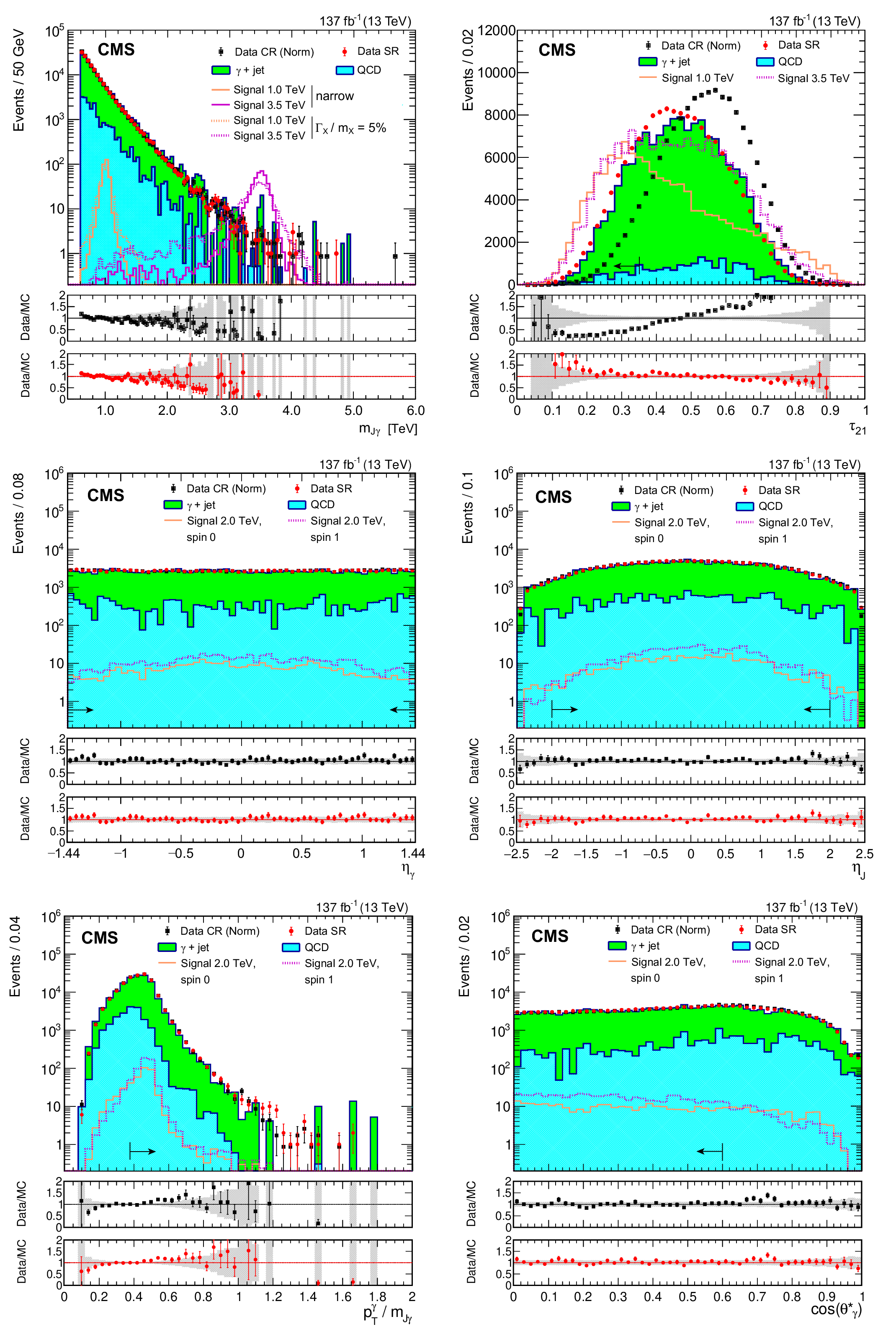
Figure 2:
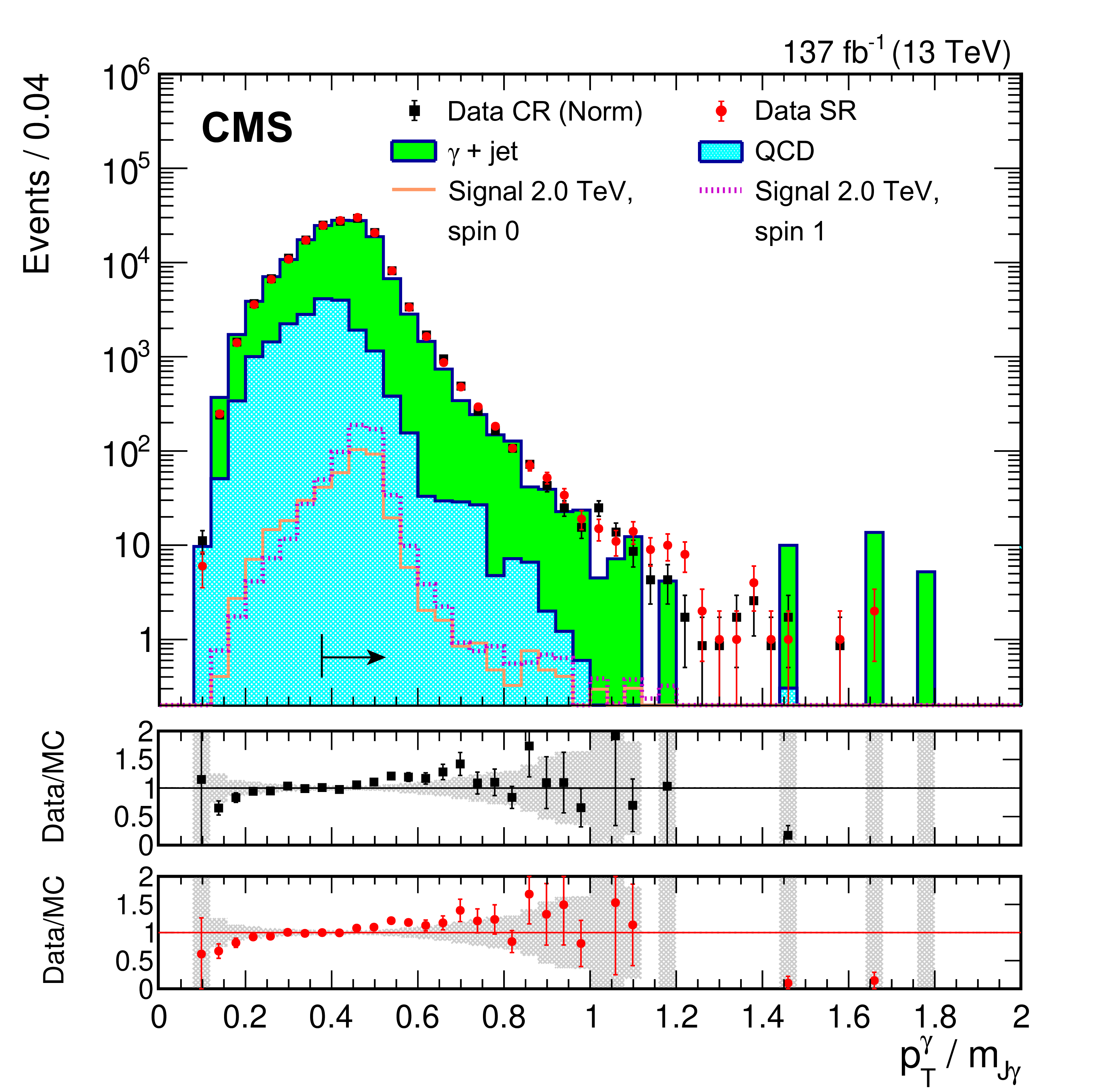
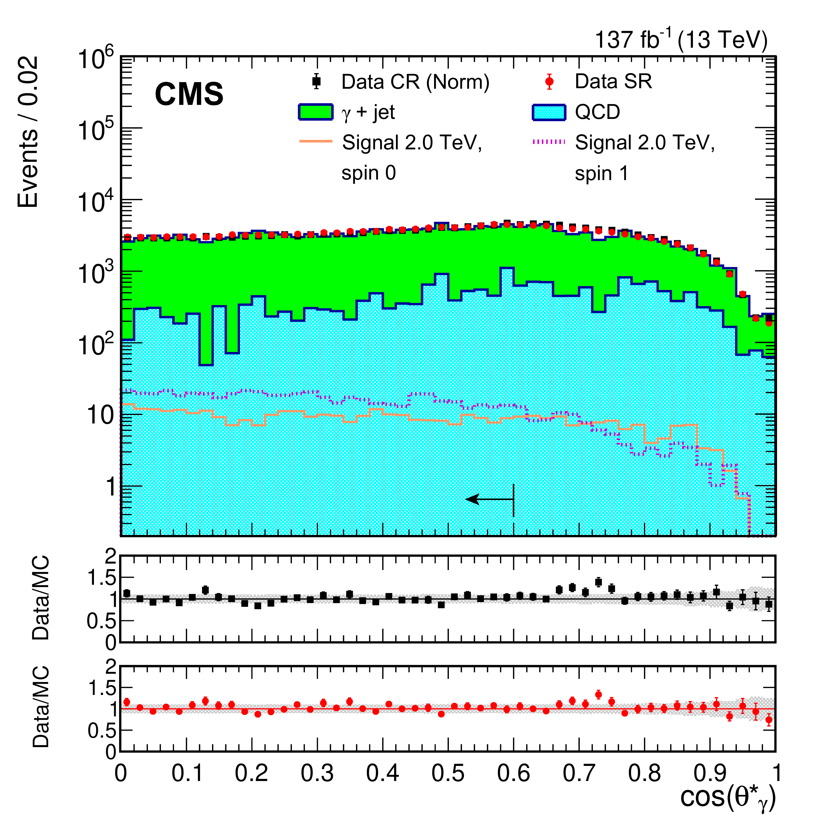
Distributions of some of the kinematic variables used in the analysis. Upper row: ${m_{{\mathrm {J}\gamma}}}$ (left), ${\tau _{21}}$ (right); middle row: $ {\eta _\gamma} $ (left), $ {\eta _\mathrm {J}} $ (right); lower row: $ {{p_{\mathrm {T}}} ^{\gamma}} / {m_{{\mathrm {J}\gamma}}} $ (left), ${\cos\theta ^*_\gamma}$ (right), except that the yield in the control region is normalized to that in the signal region. Several benchmark signals are also shown, as indicated by the legend. By default, the spin-0, narrow width hypothesis is used unless indicated otherwise. Signals are normalized to a cross section of 5 fb, except for the ${\tau _{21}}$ distribution, for which the normalization is 2 pb. Optimized selections are indicated with the black arrows. The two lower panels show the data-to-simulation ratio in the control and signal regions, respectively. The gray hatched band shows the statistical uncertainty in the background estimation. |
png pdf |
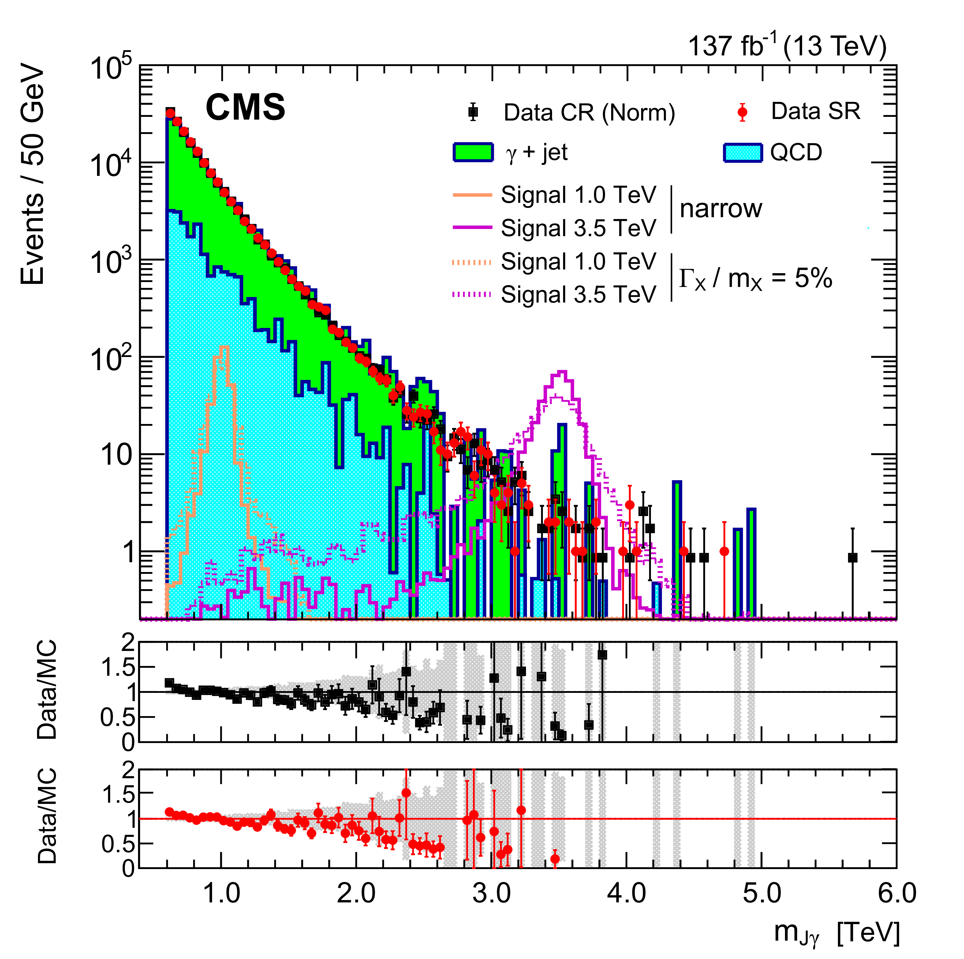
Figure 2-a:
Distribution of ${m_{{\mathrm {J}\gamma}}}$. The yield in the control region is normalized to that in the signal region. Several benchmark signals are also shown, as indicated by the legend. The spin-0, narrow width hypothesis is used unless indicated otherwise. Signals are normalized to a cross section of 5 fb. Optimized selections are indicated with the black arrows. The two lower panels show the data-to-simulation ratio in the control and signal regions, respectively. The gray hatched band shows the statistical uncertainty in the background estimation. |
png pdf |
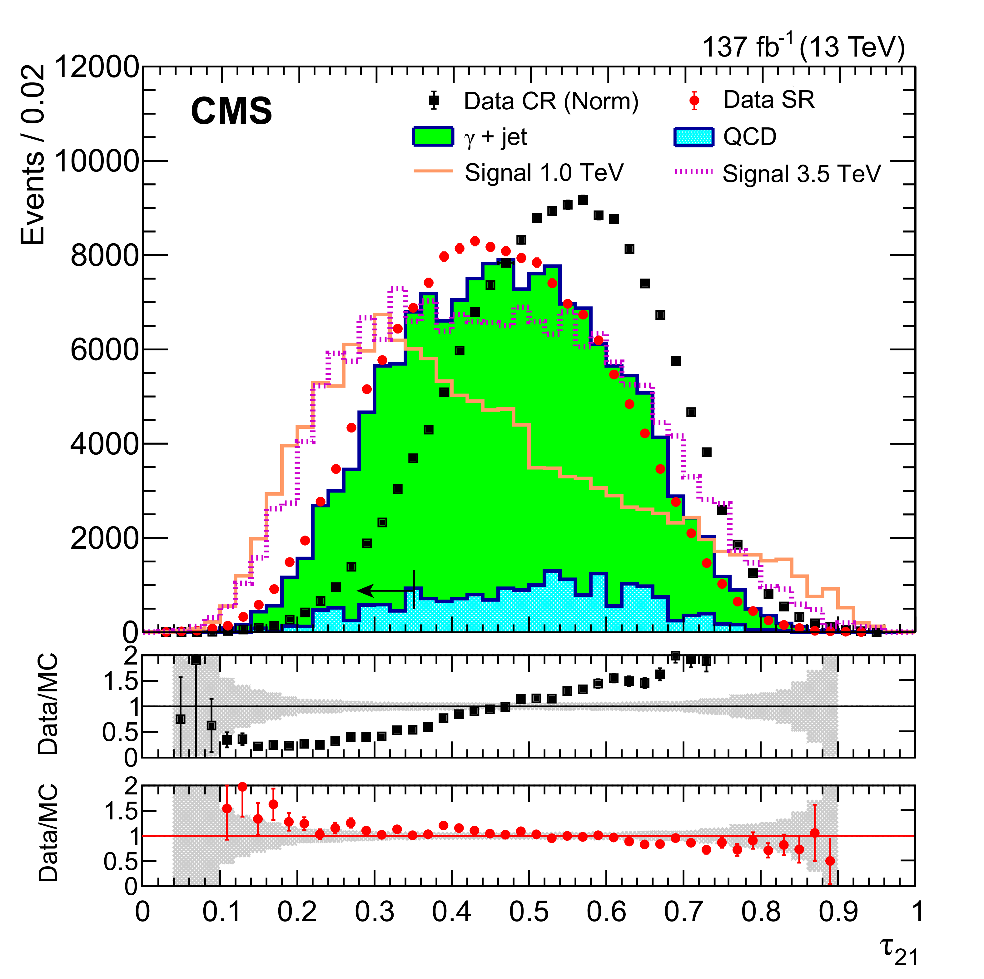
Figure 2-b:
Distribution of ${\tau _{21}}$. The yield in the control region is normalized to that in the signal region. Several benchmark signals are also shown, as indicated by the legend. The spin-0, narrow width hypothesis is used. Signals are normalized to a cross section of 2 pb. Optimized selections are indicated with the black arrows. The two lower panels show the data-to-simulation ratio in the control and signal regions, respectively. The gray hatched band shows the statistical uncertainty in the background estimation. |
png pdf |
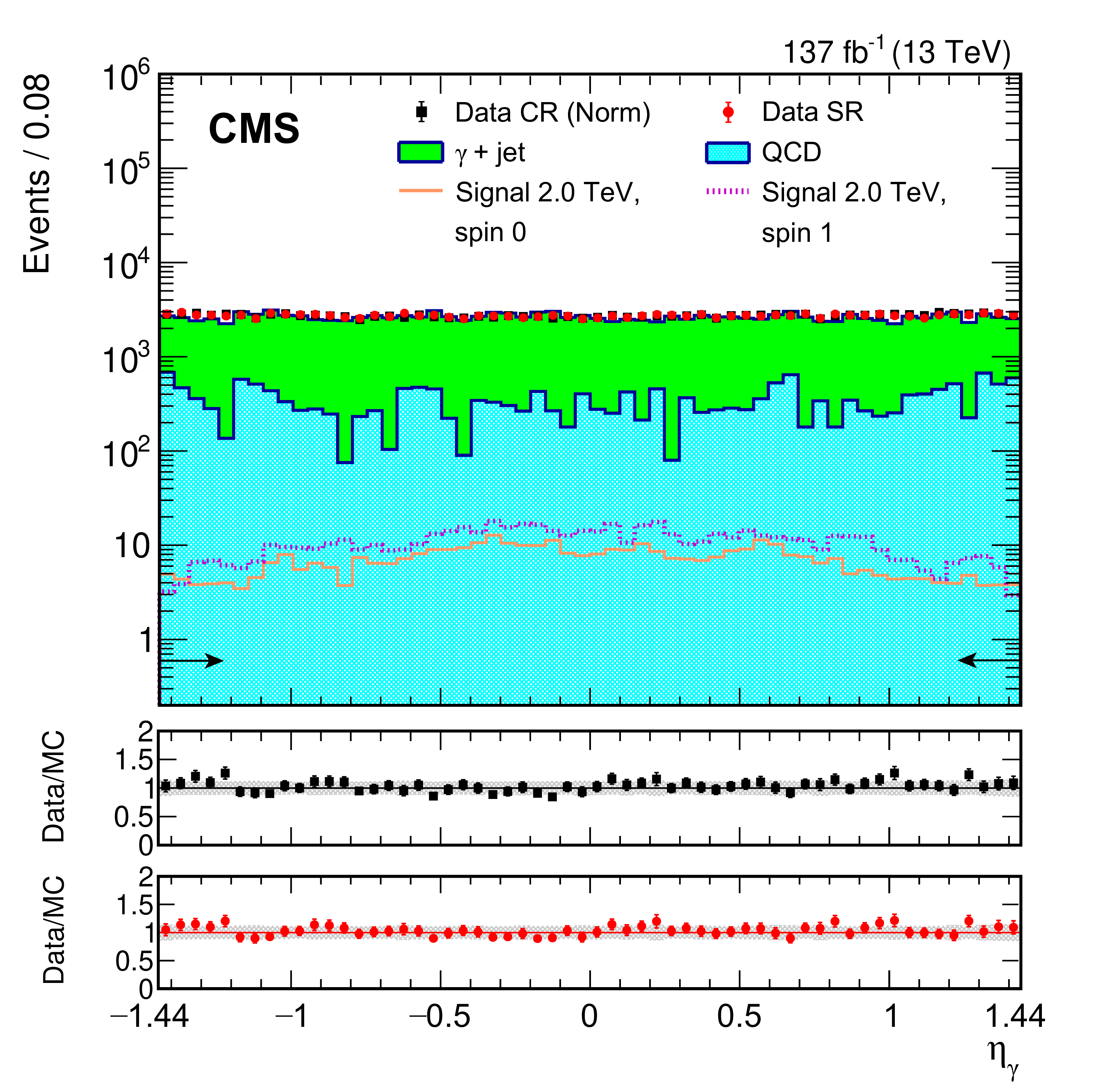
Figure 2-c:
Distribution of $ {\eta _\gamma} $. The yield in the control region is normalized to that in the signal region. Several benchmark signals are also shown, as indicated by the legend. The spin-0, narrow width hypothesis is used. Signals are normalized to a cross section of 5 fb. Optimized selections are indicated with the black arrows. The two lower panels show the data-to-simulation ratio in the control and signal regions, respectively. The gray hatched band shows the statistical uncertainty in the background estimation. |

png pdf |
Figure 2-d:
Distribution of $ {\eta _\mathrm {J}} $. The yield in the control region is normalized to that in the signal region. Several benchmark signals are also shown, as indicated by the legend. The spin-0, narrow width hypothesis is used. Signals are normalized to a cross section of 5 fb. Optimized selections are indicated with the black arrows. The two lower panels show the data-to-simulation ratio in the control and signal regions, respectively. The gray hatched band shows the statistical uncertainty in the background estimation. |
png pdf |
Figure 2-e:
Distribution of $ {{p_{\mathrm {T}}} ^{\gamma}} / {m_{{\mathrm {J}\gamma}}} $. The yield in the control region is normalized to that in the signal region. Several benchmark signals are also shown, as indicated by the legend. The spin-0, narrow width hypothesis is used. Signals are normalized to a cross section of 5 fb. Optimized selections are indicated with the black arrows. The two lower panels show the data-to-simulation ratio in the control and signal regions, respectively. The gray hatched band shows the statistical uncertainty in the background estimation. |
png pdf |
Figure 2-f:
Distribution of ${\cos\theta ^*_\gamma}$. The yield in the control region is normalized to that in the signal region. Several benchmark signals are also shown, as indicated by the legend. The spin-0, narrow width hypothesis is used. Signals are normalized to a cross section of 5 fb. Optimized selections are indicated with the black arrows. The two lower panels show the data-to-simulation ratio in the control and signal regions, respectively. The gray hatched band shows the statistical uncertainty in the background estimation. |

png pdf |
Figure 3:
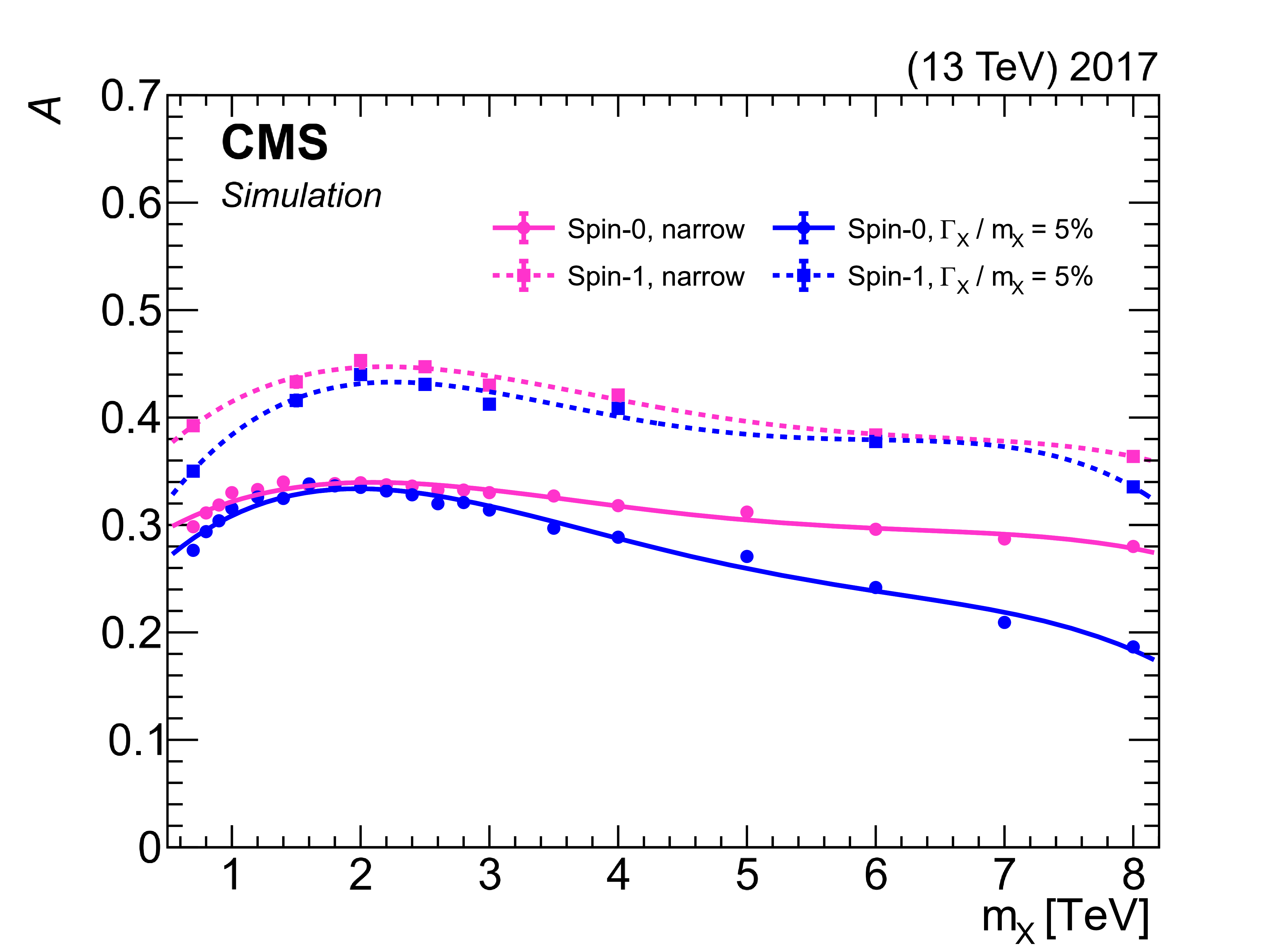
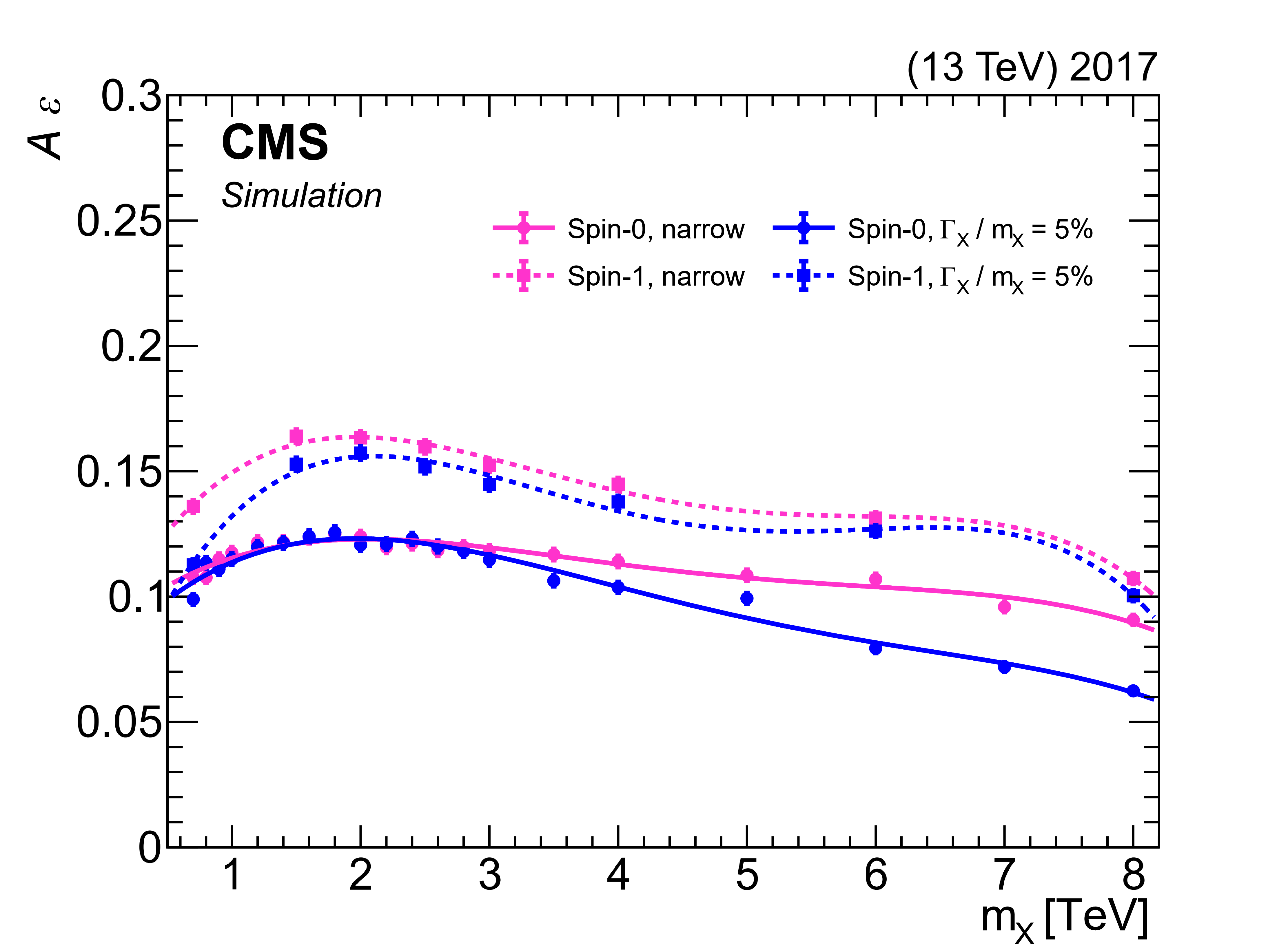
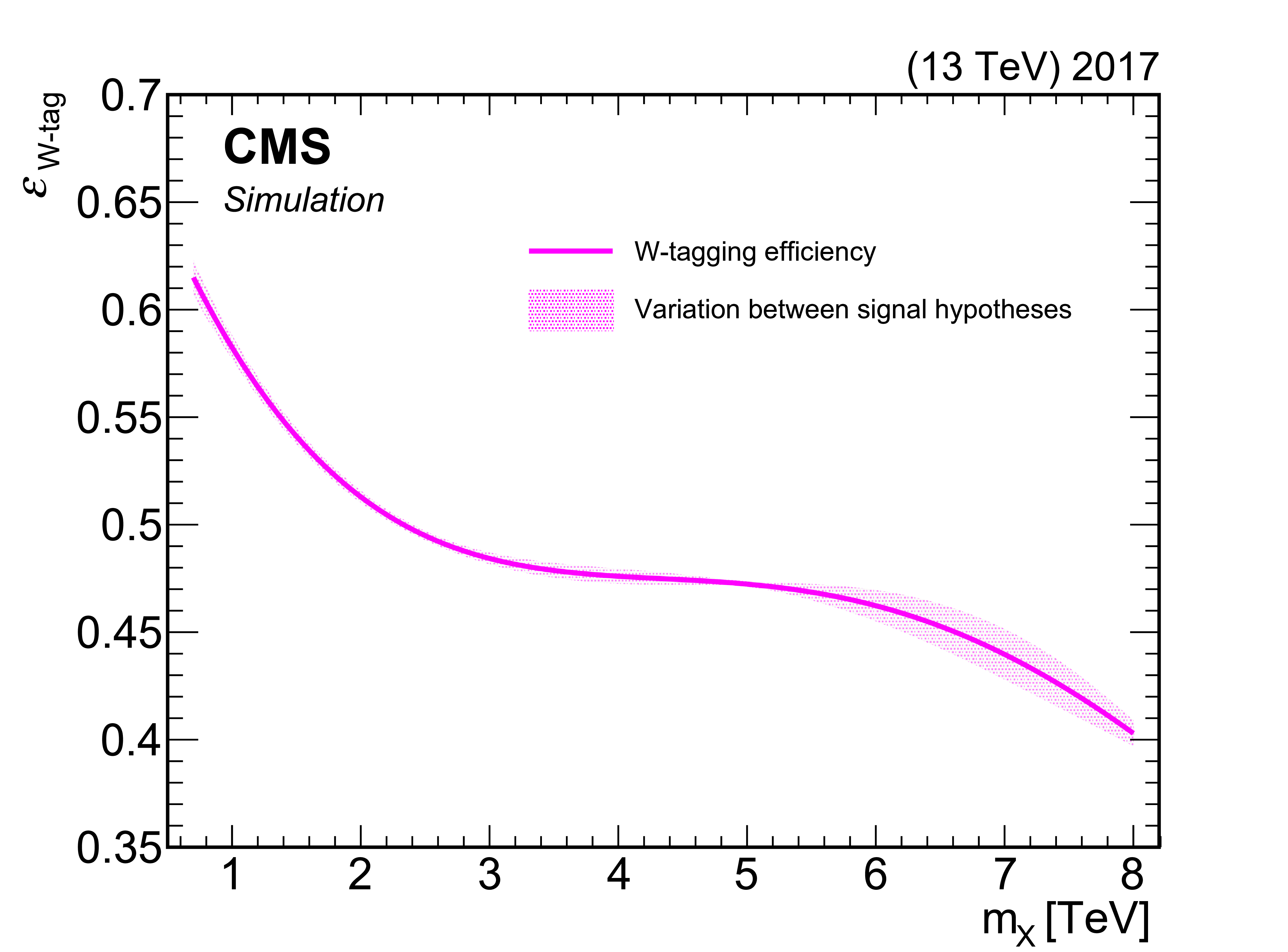
Signal acceptance $\mathcal {A}$ (upper left), the product of the signal acceptance and selection efficiency $\mathcal {A}\varepsilon $ (upper right), and the W tagging efficiency (lower) for spin-0 (solid lines) and spin-1 (dashed lines) resonances, for the narrow (pink) and broad (blue) hypotheses. The curves are obtained by fitting fourth-order polynomials to the set of discrete mass points, for which simulated signal samples are available. For the W tagging efficiency, the average value obtained for the different spin and width hypotheses and the spread of the individual efficiencies about the average are shown with the solid line and the shaded band, respectively. |
png pdf |
Figure 3-a:
Signal acceptance $\mathcal {A}$ for spin-0 (solid lines) and spin-1 (dashed lines) resonances, for the narrow (pink) and broad (blue) hypotheses. The curves are obtained by fitting fourth-order polynomials to the set of discrete mass points, for which simulated signal samples are available. |
png pdf |
Figure 3-b:
The product of the signal acceptance and selection efficiency $\mathcal {A}\varepsilon $ for spin-0 (solid lines) and spin-1 (dashed lines) resonances, for the narrow (pink) and broad (blue) hypotheses. The curves are obtained by fitting fourth-order polynomials to the set of discrete mass points, for which simulated signal samples are available. |
png pdf |
Figure 3-c:
The W tagging efficiency for spin-0 (solid lines) and spin-1 (dashed lines) resonances, for the narrow (pink) and broad (blue) hypotheses. The curves are obtained by fitting fourth-order polynomials to the set of discrete mass points, for which simulated signal samples are available. The average value obtained for the different spin and width hypotheses and the spread of the individual efficiencies about the average are shown with the solid line and the shaded band, respectively. |
png pdf |
Figure 4:
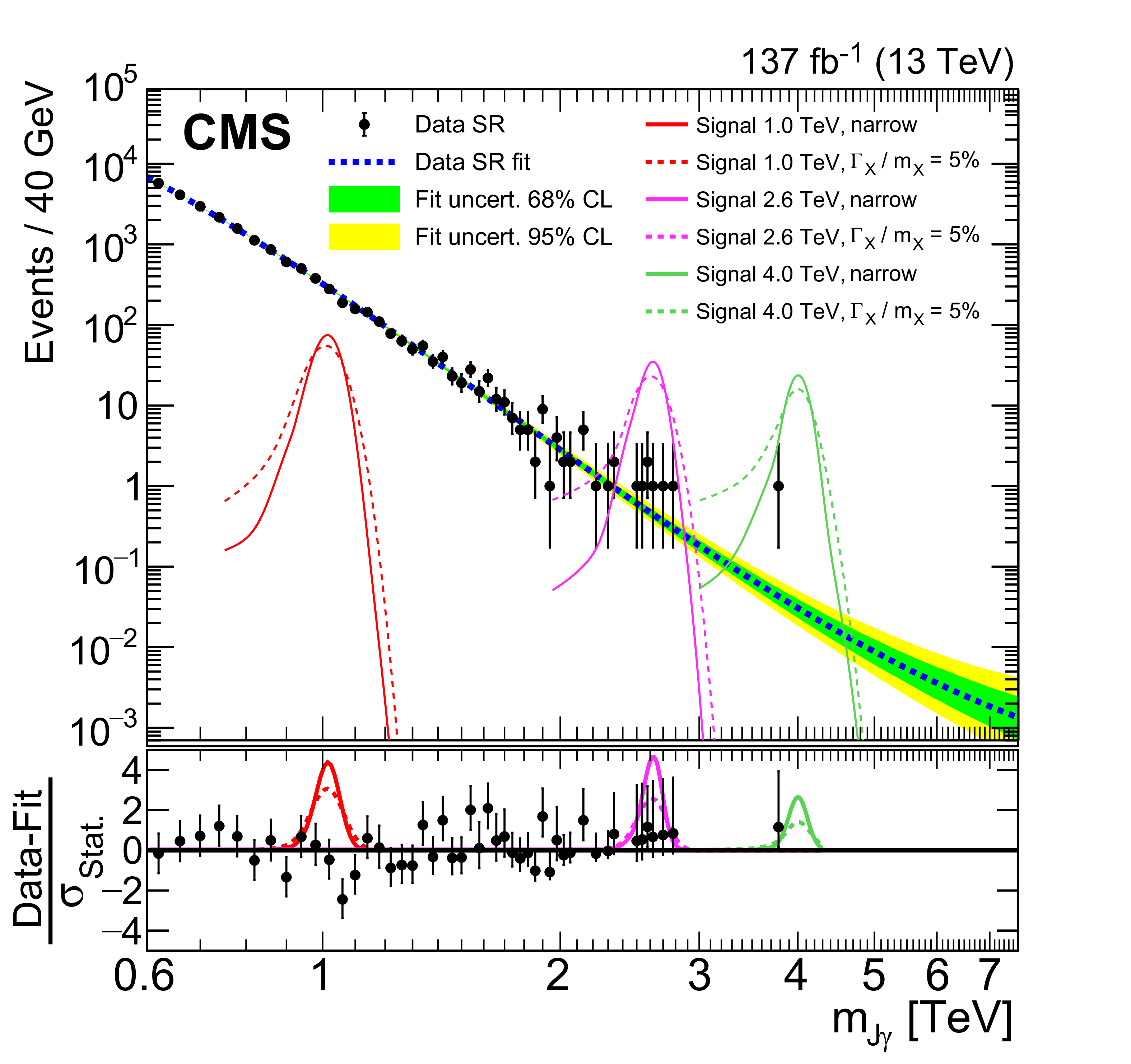
Background-only fit to data (black points) with the chosen background function. The green (inner) and yellow (outer) bands show, respectively, the 68 and 95% confidence level statistical uncertainties in the fit. The lower panel contains the pull distribution, defined as the difference between the data yield and the background prediction, divided by their combined uncertainty. Expected signal shapes are also shown in the lower panel for three different resonance mass hypotheses, 1.0 TeV (red), 2.6 TeV (magenta), and 4.0 TeV (green), and for both the narrow (solid) and broad (dashed) cases. Signal normalizations are set to 15, 1.0, and 0.30 fb, respectively, for illustrative purposes. |
png pdf |
Figure 5:
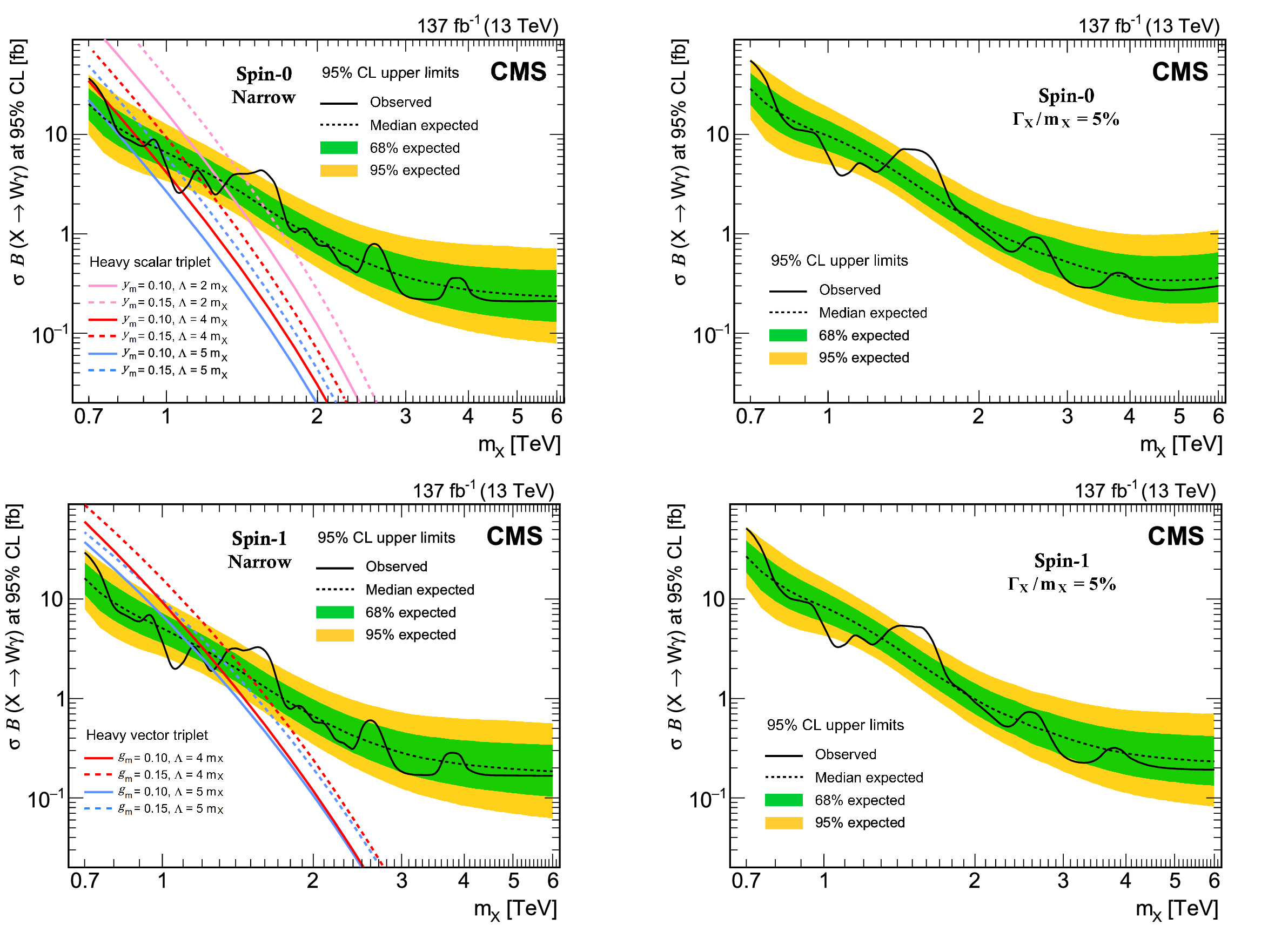
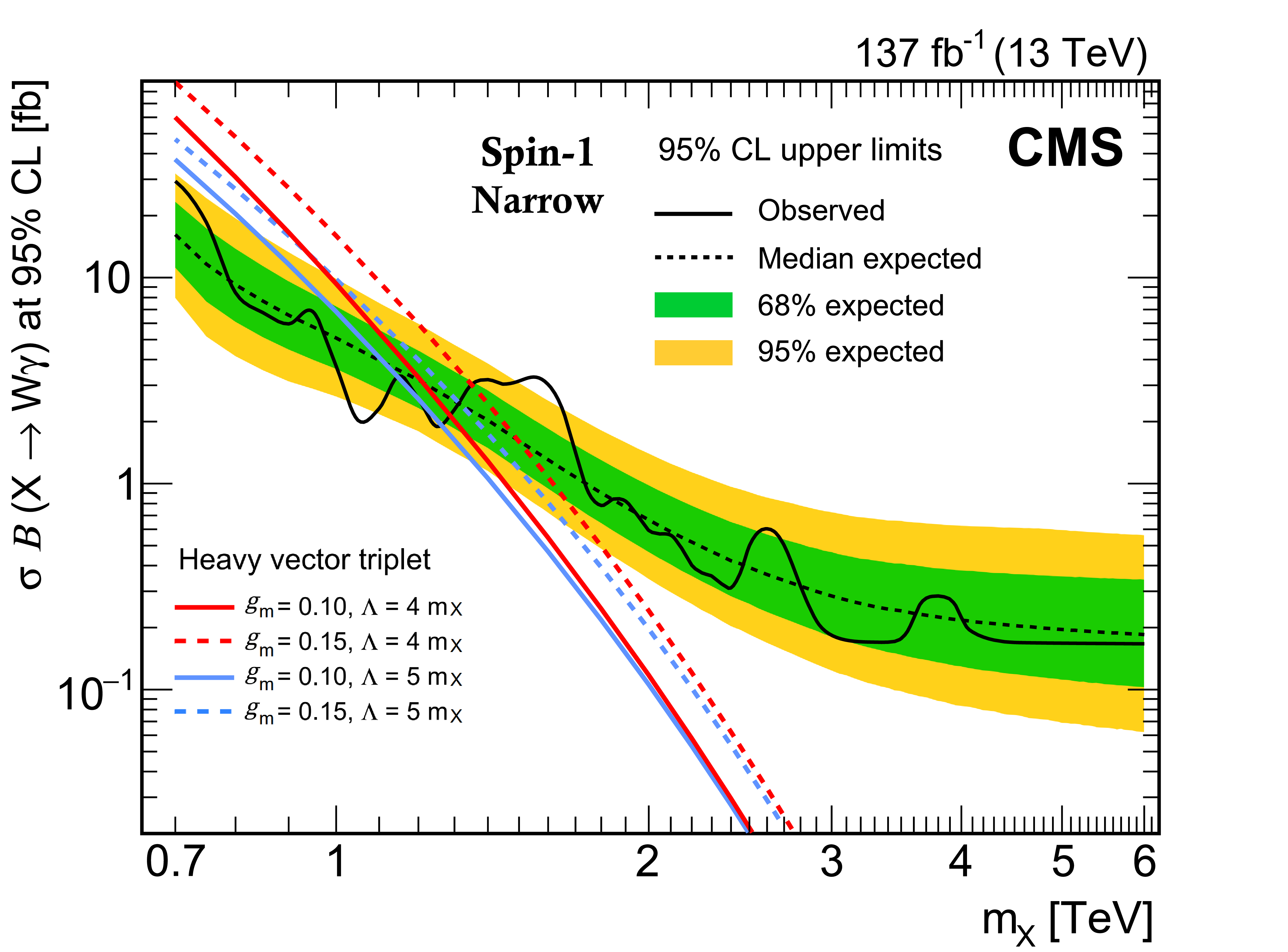
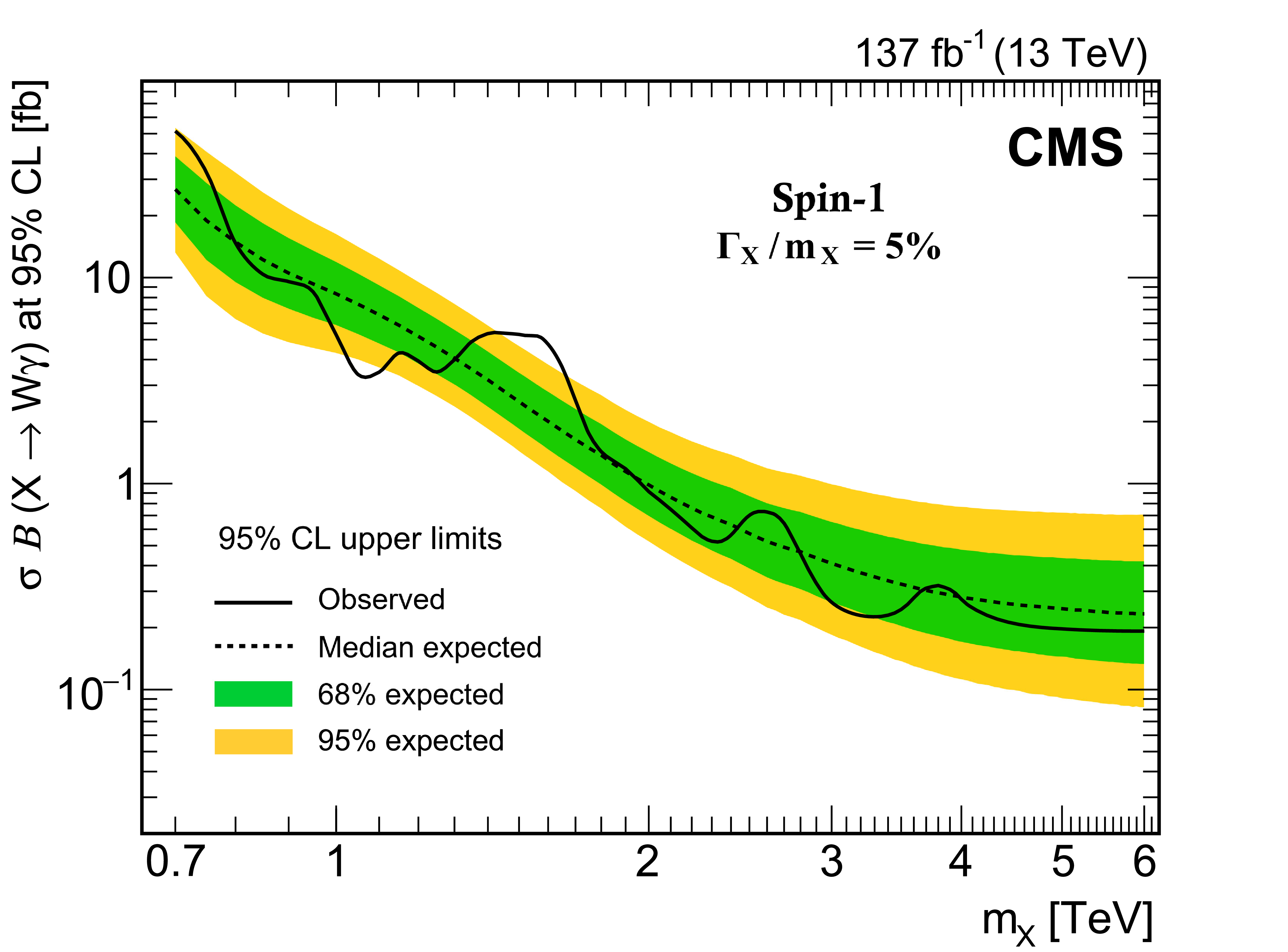
Expected and observed 95% confidence level limits on $\sigma \mathcal {B}(\mathrm{X} \to {\mathrm{W} \gamma})$ for the spin-0 (upper row) and spin-1 (lower row) resonances for the narrow (left column) and broad (right column) resonance cases. Also shown, for spin-0 (spin-1) narrow-resonance case, theoretical cross sections for heavy scalar (vector) triplet resonance production in the benchmark model of Ref. [25], which can be probed by this search. |
png pdf |
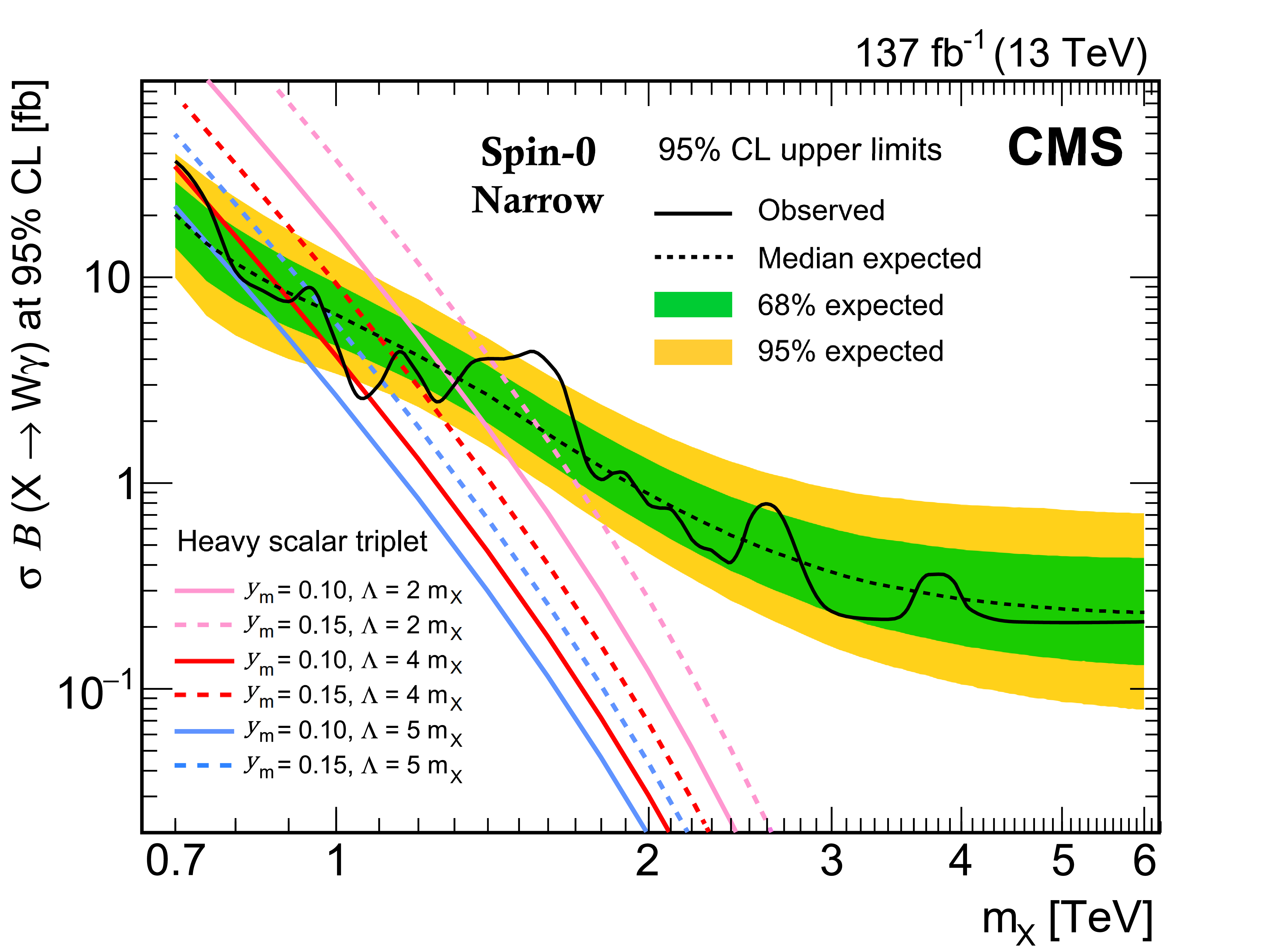
Figure 5-a:
Expected and observed 95% confidence level limits on $\sigma \mathcal {B}(\mathrm{X} \to {\mathrm{W} \gamma})$ for a spin-0 resonance for the narrow resonance case. Also shown, theoretical cross sections for heavy scalar triplet resonance production in the benchmark model of Ref. [25], which can be probed by this search. |

png pdf |
Figure 5-b:
Expected and observed 95% confidence level limits on $\sigma \mathcal {B}(\mathrm{X} \to {\mathrm{W} \gamma})$ for a spin-0 resonance for the broad resonance case. Also shown, theoretical cross sections for heavy scalar triplet resonance production in the benchmark model of Ref. [25], which can be probed by this search. |
png pdf |
Figure 5-c:
Expected and observed 95% confidence level limits on $\sigma \mathcal {B}(\mathrm{X} \to {\mathrm{W} \gamma})$ for a spin-1 resonance for the narrow resonance case. Also shown, theoretical cross sections for heavy vector triplet resonance production in the benchmark model of Ref. [25], which can be probed by this search. |
png pdf |
Figure 5-d:
Expected and observed 95% confidence level limits on $\sigma \mathcal {B}(\mathrm{X} \to {\mathrm{W} \gamma})$ for a spin-1 resonance for the broad resonance case. Also shown, theoretical cross sections for heavy vector triplet resonance production in the benchmark model of Ref. [25], which can be probed by this search. |

png pdf |
Figure 6:
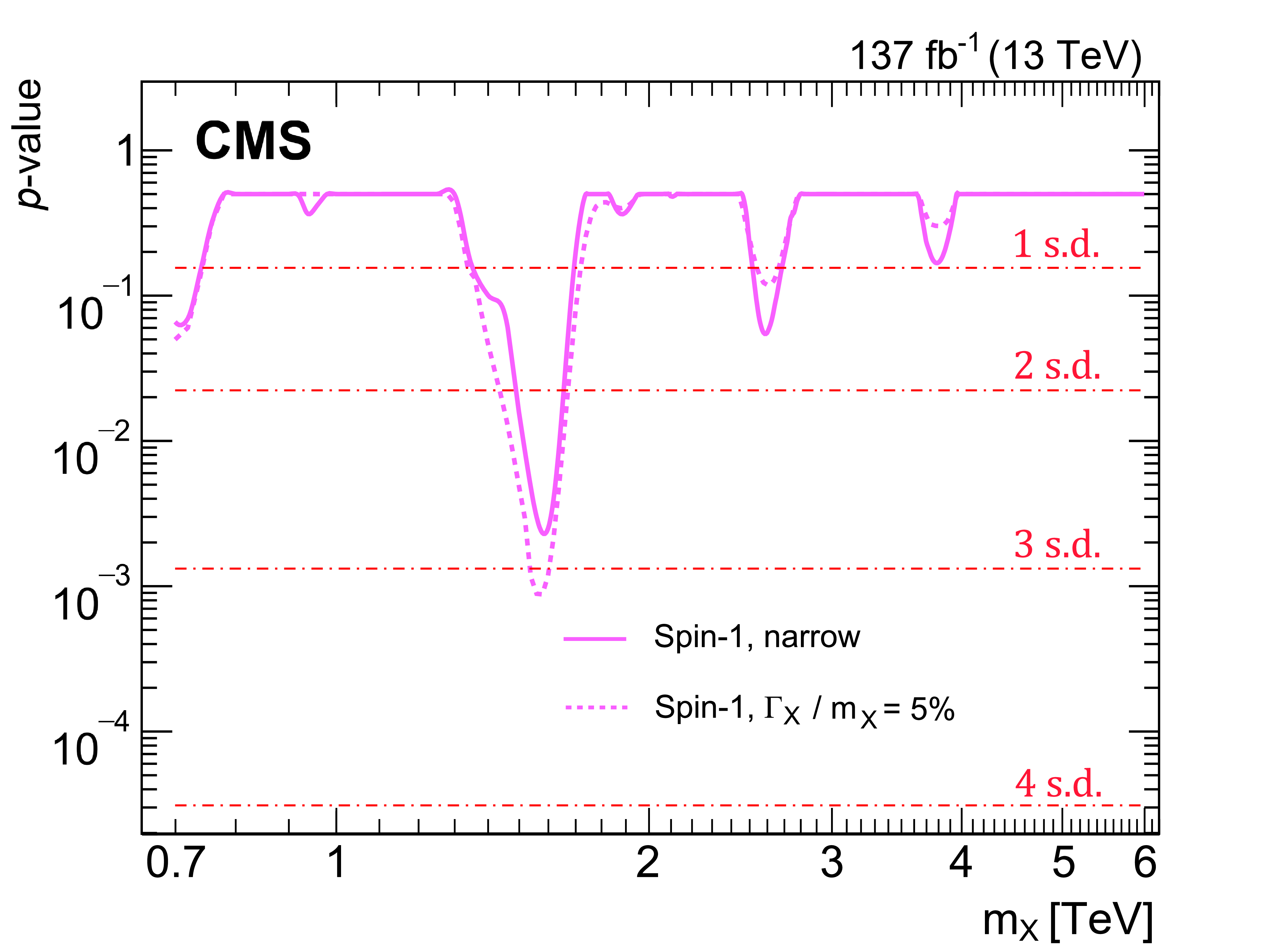
Observed local $p$-values for spin-0 (left) and spin-1 (right) resonance hypotheses. The largest excess observed at 1.58 TeV corresponds to a local significance of 2.8 (3.1) standard deviations (s.d.) for narrow (broad) signals, for both spin hypotheses. |

png pdf |
Figure 6-a:
Observed local $p$-values for the spin-0 resonance hypothesis. The largest excess observed at 1.58 TeV corresponds to a local significance of 2.8 (3.1) standard deviations (s.d.) for narrow (broad) signals. |
png pdf |
Figure 6-b:
Observed local $p$-values for the spin-1 resonance hypothesis. The largest excess observed at 1.58 TeV corresponds to a local significance of 2.8 (3.1) standard deviations (s.d.) for narrow (broad) signals. |
png pdf |
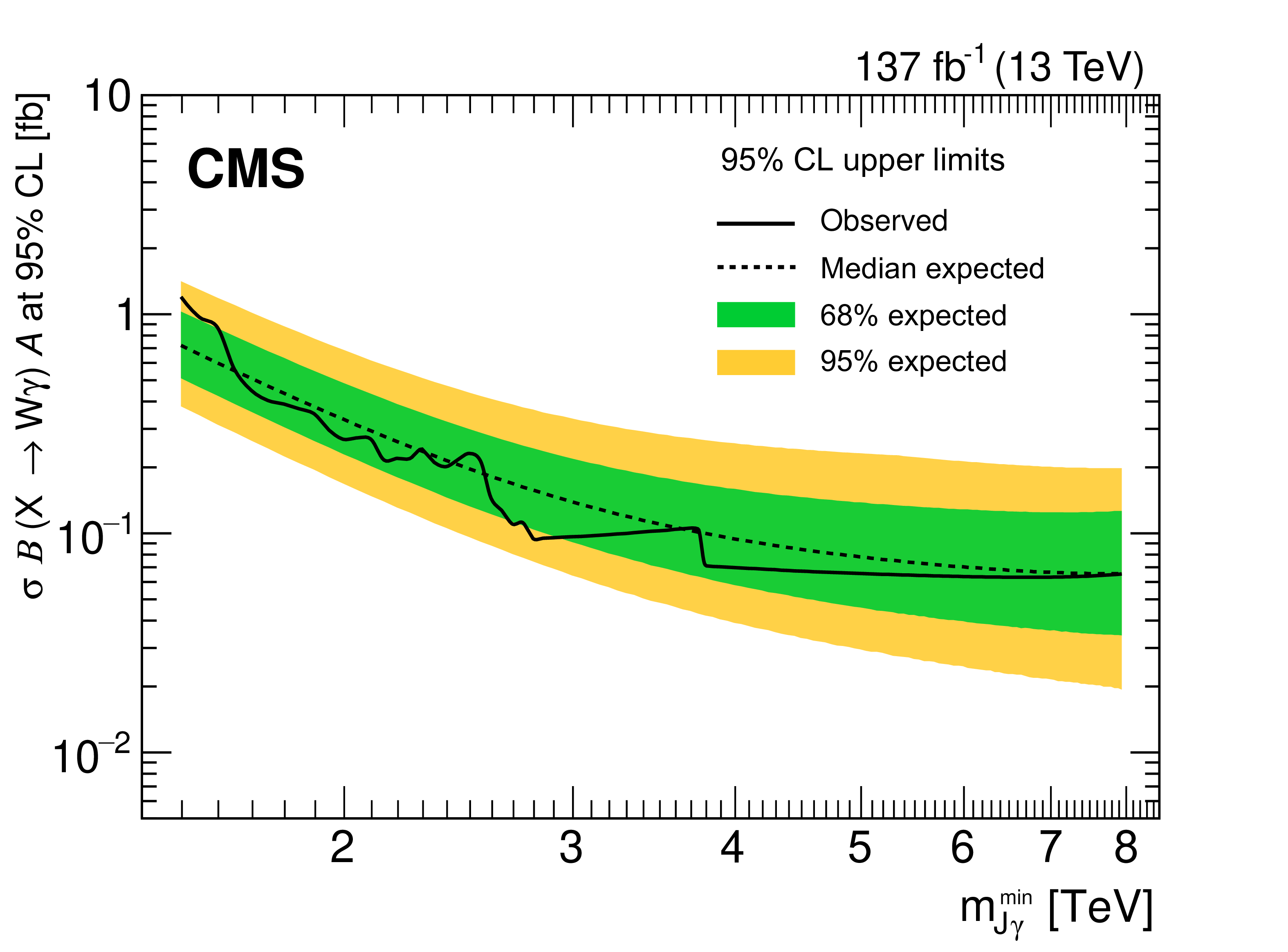
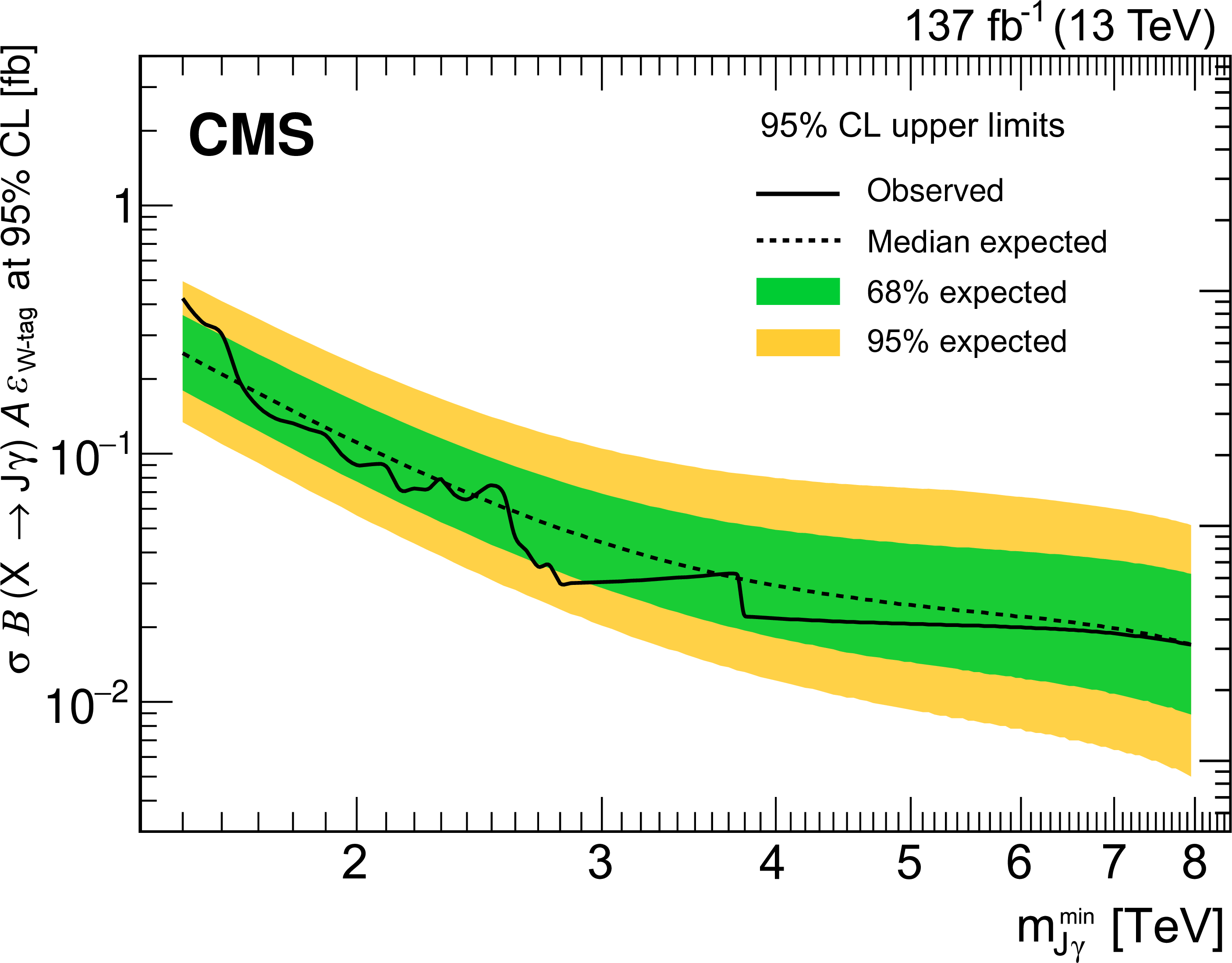
Figure 7:
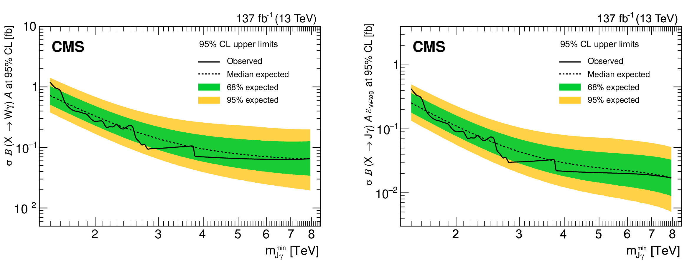
Expected and observed 95% confidence level model-independent limits on $\sigma \mathcal {B}(\mathrm{X} \to {\mathrm{W} \gamma}) \mathcal {A}$ (left) and $\sigma \mathcal {B}(\mathrm{X} \to {\mathrm {J}\gamma}) \mathcal {A} \epsilon _{\mathrm{W} \text {-tag}}$ (right), as a function of the minimum invariant mass requirement on the ${\mathrm {J}\gamma}$ system. |
png pdf |
Figure 7-a:
Expected and observed 95% confidence level model-independent limits on $\sigma \mathcal {B}(\mathrm{X} \to {\mathrm{W} \gamma}) \mathcal {A}$, as a function of the minimum invariant mass requirement on the ${\mathrm {J}\gamma}$ system. |
png pdf |
Figure 7-b:
Expected and observed 95% confidence level model-independent limits on $\sigma \mathcal {B}(\mathrm{X} \to {\mathrm {J}\gamma}) \mathcal {A} \epsilon _{\mathrm{W} \text {-tag}}$, as a function of the minimum invariant mass requirement on the ${\mathrm {J}\gamma}$ system. |
| Tables | |
png pdf |
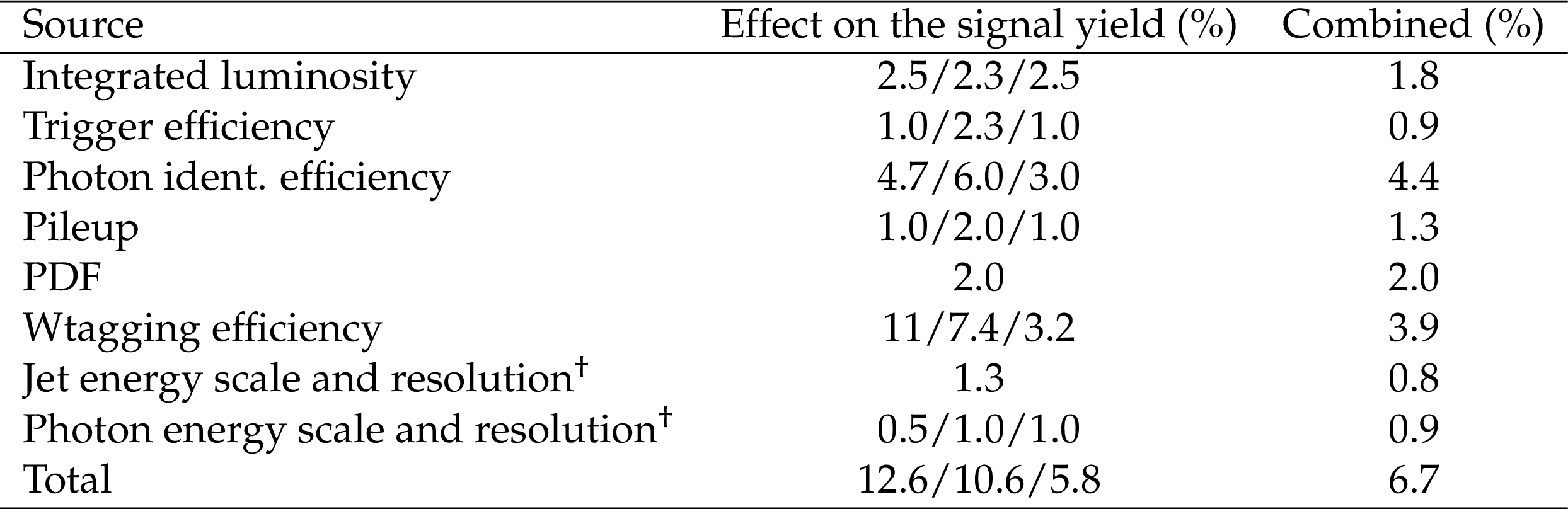
Table 1:
Systematic uncertainties affecting the signal description. Uncertainties marked with "$\dagger $" affect both the yield and the shape of the signal distribution, while the rest only affect the signal yield. In cases where the uncertainty is different for various data-taking periods, the three numbers given in the second column correspond to the 2016/2017/2018 data taking, while the third column shows the combined uncertainties across the three years, taking into account the year-to-year correlations. The effect on the signal yield is the same for all the signal hypotheses studied. |
| Summary |
| A search for $ {\mathrm{W}\gamma} $ resonances in the mass range between 0.7 and 6.0 TeV has been presented. The W boson is reconstructed from its hadronic decay, in which the final-state products form a single large-radius jet owing to the large Lorentz boost of the W boson. The search is based on proton-proton collision data collected at $\sqrt{s} = $ 13 TeV with the CMS detector at the LHC in 2016-2018, corresponding to an integrated luminosity of 137 fb$^{-1}$. No significant excess above the smoothly falling background is observed. Limits at 95% confidence level on the product of the cross section and branching fraction for $ {\mathrm{W}\gamma} $ resonances are set, ranging from 37 (55) to 0.21 (0.30) fb for the narrow (broad) spin-0 hypothesis, and from 29 (51) to 0.17 (0.19) fb for the for the narrow (broad) spin-1 hypothesis. The results reported are the most restrictive limits to date on the existence of such resonances. In specific narrow-resonance benchmark models, heavy scalar (vector) triplet resonances with masses between 0.75 (1.15) and 1.40 (1.35) TeV are excluded for a range of model parameters probed. In addition, model-independent limits are set on the product of the cross section, branching fraction, and signal acceptance, as functions of the minimum invariant mass of the jet-photon system, making possible the interpretation of these results in the context of a broader class of models predicting similar signatures. |
| References | ||||
| 1 | ATLAS Collaboration | Observation of a new particle in the search for the standard model Higgs boson with the ATLAS detector at the LHC | PLB 716 (2012) 1 | 1207.7214 |
| 2 | CMS Collaboration | Observation of a new boson at a mass of 125 GeV with the CMS experiment at the LHC | PLB 716 (2012) 30 | CMS-HIG-12-028 1207.7235 |
| 3 | CMS Collaboration | Observation of a new boson with mass near 125 GeV in pp collisions at $ \sqrt{s} = $ 7 and 8 TeV | JHEP 06 (2013) 081 | CMS-HIG-12-036 1303.4571 |
| 4 | J. F. Gunion, G. L. Kane, and J. Wudka | Search techniques for charged and neutral intermediate mass Higgs bosons | NPB 299 (1988) 231 | |
| 5 | J. F. Gunion, H. E. Haber, G. L. Kane, and S. Dawson | The Higgs hunter's guide | volume 80 of Frontiers in Physics Westview Press, Boulder, Colorado | |
| 6 | M. Capdequi Peyranere, H. E. Haber, and P. Irulegui | $ H^\pm \to W^\pm\gamma $ and $ H^\pm \to W^\pm Z $ in two Higgs doublet models. 1. The large fermion mass limit | PRD 44 (1991) 191 | |
| 7 | S. Weinberg | Implications of dynamical symmetry breaking | PRD 13 (1976) 974 | |
| 8 | L. Susskind | Dynamics of spontaneous symmetry breaking in the Weinberg--Salam theory | PRD 20 (1979) 2619 | |
| 9 | K. D. Lane and E. Eichten | Two scale technicolor | PLB 222 (1989) 274 | |
| 10 | E. Eichten and K. Lane | Low-scale technicolor at the Tevatron and LHC | PLB 669 (2008) 235 | 0706.2339 |
| 11 | D. Pappadopulo, A. Thamm, R. Torre, and A. Wulzer | Heavy vector triplets: Bridging theory and data | JHEP 09 (2014) 060 | 1402.4431 |
| 12 | K. Howe, S. Knapen, and D. J. Robinson | Diphotons from electroweak triplet-singlet mixing | PRD 94 (2016) 035021 | 1603.08932 |
| 13 | G. Burdman et al. | The quirky collider signals of folded supersymmetry | PRD 78 (2008) 075028 | 0805.4667 |
| 14 | ATLAS Collaboration | Measurements of $ W \gamma $ and $ Z \gamma $ production in $ pp $ collisions at $ \sqrt{s} = $ 7 TeV with the ATLAS detector at the LHC | PRD 87 (2013) 112003 | 1302.1283 |
| 15 | ATLAS Collaboration | Search for new resonances in $ W\gamma $ and $ Z\gamma $ final states in $ pp $ collisions at $ \sqrt s= $ 8 TeV with the ATLAS detector | PLB 738 (2014) 428 | 1407.8150 |
| 16 | ATLAS Collaboration | Search for heavy resonances decaying to a photon and a hadronically decaying $ Z/W/H $ boson in $ pp $ collisions at $ \sqrt{s}= 13 \mathrm{TeV} $ with the ATLAS detector | PRD 98 (2018) 032015 | 1805.01908 |
| 17 | CMS Collaboration | HEPData record for this analysis | link | |
| 18 | CMS Collaboration | The CMS trigger system | JINST 12 (2017) P01020 | CMS-TRG-12-001 1609.02366 |
| 19 | CMS Collaboration | Performance of the CMS Level-1 trigger in proton-proton collisions at $ \sqrt{s} = $ 13 TeV | JINST 15 (2020) P10017 | CMS-TRG-17-001 2006.10165 |
| 20 | CMS Collaboration | The CMS experiment at the CERN LHC | JINST 3 (2008) S08004 | CMS-00-001 |
| 21 | CMS Collaboration | CMS luminosity measurements for the 2016 data-taking period | CMS-PAS-LUM-17-001 | CMS-PAS-LUM-17-001 |
| 22 | CMS Collaboration | CMS luminosity measurements for the 2017 data-taking period at $ \sqrt{s} = $ 13 TeV | CMS-PAS-LUM-17-004 | CMS-PAS-LUM-17-004 |
| 23 | CMS Collaboration | CMS luminosity measurements for the 2018 data-taking period at $ \sqrt{s} = $ 13 TeV | CMS-PAS-LUM-18-002 | CMS-PAS-LUM-18-002 |
| 24 | N. Arkani-Hamed, R. T. D'Agnolo, M. Low, and D. Pinner | Unification and new particles at the LHC | JHEP 11 (2016) 082 | 1608.01675 |
| 25 | R. M. Capdevilla, R. Harnik, and A. Martin | The radiation valley and exotic resonances in $ W\gamma $ production at the LHC | JHEP 03 (2020) 117 | 1912.08234 |
| 26 | J. Alwall et al. | The automated computation of tree-level and next-to-leading order differential cross sections, and their matching to parton shower simulations | JHEP 07 (2014) 079 | 1405.0301 |
| 27 | NNPDF Collaboration | Parton distributions for the LHC Run II | JHEP 04 (2015) 040 | 1410.8849 |
| 28 | NNPDF Collaboration | Parton distributions from high-precision collider data | EPJC 77 (2017) 663 | 1706.00428 |
| 29 | T. Sjostrand et al. | An introduction to PYTHIA 8.2 | CPC 191 (2015) 159 | 1410.3012 |
| 30 | P. Skands, S. Carrazza, and J. Rojo | Tuning PYTHIA 8.1: the Monash 2013 tune | EPJC 74 (2014) 3024 | 1404.5630 |
| 31 | CMS Collaboration | Event generator tunes obtained from underlying event and multiparton scattering measurements | EPJC 76 (2016) 155 | CMS-GEN-14-001 1512.00815 |
| 32 | CMS Collaboration | Extraction and validation of a new set of CMS PYTHIA8 tunes from underlying-event measurements | EPJC 80 (2020) 4 | CMS-GEN-17-001 1903.12179 |
| 33 | GEANT4 Collaboration | GEANT4 --- a simulation toolkit | NIMA 506 (2003) 250 | |
| 34 | CMS Collaboration | Particle-flow reconstruction and global event description with the CMS detector | JINST 12 (2017) P10003 | CMS-PRF-14-001 1706.04965 |
| 35 | M. Cacciari, G. P. Salam, and G. Soyez | The anti-$ k_\text{t} $ jet clustering algorithm | JHEP 04 (2008) 063 | 0802.1189 |
| 36 | M. Cacciari, G. P. Salam, and G. Soyez | FastJet user manual | EPJC 72 (2012) 1896 | 1111.6097 |
| 37 | CMS Collaboration | Performance of photon reconstruction and identification with the CMS detector in proton-proton collisions at $ \sqrt{s} = $ 8 TeV | JINST 10 (2015) P08010 | CMS-EGM-14-001 1502.02702 |
| 38 | CMS Collaboration | Pileup mitigation at CMS in 13 TeV data | JINST 15 (2020) P09018 | CMS-JME-18-001 2003.00503 |
| 39 | D. Bertolini, P. Harris, M. Low, and N. Tran | Pileup per particle identification | JHEP 10 (2014) 059 | 1407.6013 |
| 40 | CMS Collaboration | Jet energy scale and resolution in the CMS experiment in pp collisions at 8 TeV | JINST 12 (2017) P02014 | CMS-JME-13-004 1607.03663 |
| 41 | CMS Collaboration | Jet algorithms performance in 13 TeV data | CMS-PAS-JME-16-003 | CMS-PAS-JME-16-003 |
| 42 | A. J. Larkoski, S. Marzani, G. Soyez, and J. Thaler | Soft drop | JHEP 05 (2014) 146 | 1402.2657 |
| 43 | CMS Collaboration | Search for a massive resonance decaying to a pair of Higgs bosons in the four b quark final state in proton-proton collisions at $ \sqrt{s}= $ 13 TeV | PLB 781 (2018) 244 | 1710.04960 |
| 44 | J. Thaler and K. Van Tilburg | Identifying boosted objects with $ N $-subjettiness | JHEP 03 (2011) 015 | 1011.2268 |
| 45 | M. J. Oreglia | A study of the reactions $\psi' \to \gamma\gamma \psi$ | PhD thesis, Stanford University, 1980 SLAC Report SLAC-R-236, see A | |
| 46 | A. L. Read | Linear interpolation of histograms | NIMA 425 (1999) 357 | |
| 47 | CMS Collaboration | Measurement of the inelastic proton-proton cross section at $ \sqrt{s}= $ 13 TeV | JHEP 07 (2018) 161 | CMS-FSQ-15-005 1802.02613 |
| 48 | J. Butterworth et al. | PDF4LHC recommendations for LHC Run II | JPG 43 (2016) 023001 | 1510.03865 |
| 49 | T. Junk | Confidence level computation for combining searches with small statistics | NIMA 434 (1999) 435 | hep-ex/9902006 |
| 50 | A. L. Read | Presentation of search results: the $ \mathrm{CL_s} $ technique | JPG 28 (2002) 2693 | |
| 51 | ATLAS and CMS Collaborations | Procedure for the LHC Higgs boson search combination in Summer 2011 | ATL-PHYS-PUB-2011-011, CMS NOTE-2011/005 | |
| 52 | G. Cowan, K. Cranmer, E. Gross, and O. Vitells | Asymptotic formulae for likelihood-based tests of new physics | EPJC 71 (2011) 1554 | 1007.1727 |
| 53 | E. Gross and O. Vitells | Trial factors for the look elsewhere effect in high energy physics | EPJC 70 (2010) 525 | 1005.1891 |
|
|
Compact Muon Solenoid LHC, CERN |
|

|

|

|

|

|