

Compact Muon Solenoid
LHC, CERN
| CMS-EXO-20-015 ; CERN-EP-2021-125 | ||
| Search for long-lived particles decaying in the CMS endcap muon detectors in proton-proton collisions at $\sqrt{s} = $ 13 TeV | ||
| CMS Collaboration | ||
| 10 July 2021 | ||
| Phy. Rev. Lett. 127 (2021) 261804 | ||
| Abstract: A search for long-lived particles (LLPs) produced in decays of standard model (SM) Higgs bosons is presented. The data sample consists of 137 fb$^{-1}$ of proton-proton collisions at $\sqrt{s} = $ 13 TeV, recorded at the LHC in 2016-2018. A novel technique is employed to reconstruct decays of LLPs in the endcap muon detectors. The search is sensitive to a broad range of LLP decay modes and to masses as low as a few GeV. No excess of events above the SM background is observed. The most stringent limits to date on the branching fraction of the Higgs boson to LLPs subsequently decaying to quarks and $\tau^{+}\tau^{-}$ are found for proper decay lengths greater than 6, 20, and 40 m, for LLP masses of 7, 15, and 40 GeV, respectively. | ||
| Links: e-print arXiv:2107.04838 [hep-ex] (PDF) ; CDS record ; inSPIRE record ; HepData record ; Physics Briefing ; CADI line (restricted) ; | ||
| Figures | Summary | Additional Figures & Material | References | CMS Publications |
|---|
| Instructions for reinterpretation can be found here |
| Figures | |

png pdf |
Figure 1:
The signal efficiency of the combined cluster reconstruction, veto, and identification selections as a function of the simulated $r$ and $z$ decay positions of S decaying to $\mathrm{b} {}\mathrm{\bar{b}} $, for a mass of 15 GeV and a uniformly distributed mixture of events with $c\tau $ between 1-10 m. The barrel and endcap muon stations are drawn as black boxes and labeled by their station names, showing the geometry of the muon detectors. Regions occupied by the steel return yoke are shaded in gray. |
png pdf |
Figure 2:
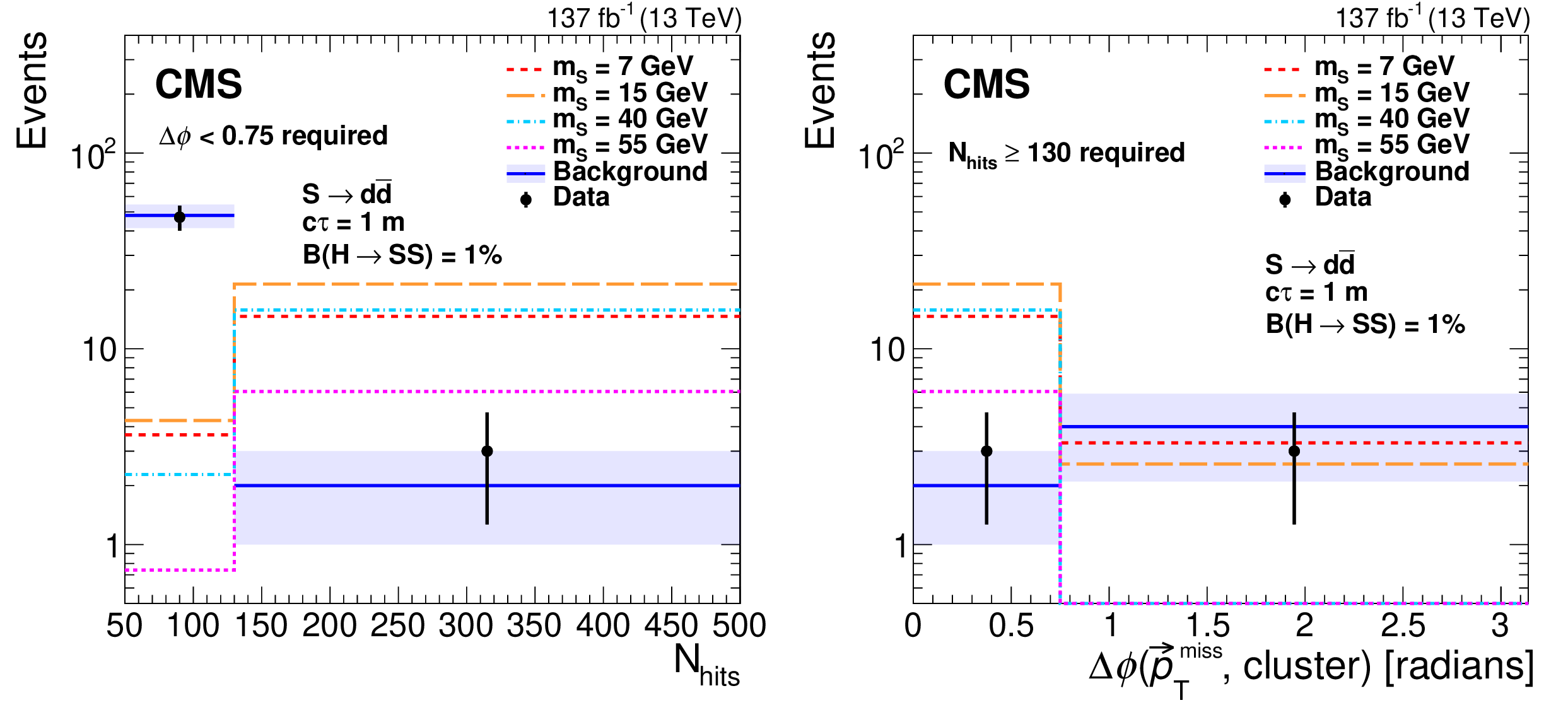
Distributions of $N_\text {hits}$ (left) and $\Delta \phi _{\mathrm {c}}$ (right) in the search region. The background predicted by the fit is shown in blue with the shaded region showing the fitted uncertainty. The expected signal with $ {\mathcal {B}({\mathrm{H} \to \mathrm{S} \mathrm{S}})} = $ 1%, $\mathrm{S} \to {\mathrm{d} \mathrm{\bar{d}}} $, and $c\tau = $ 1 m is shown for $m_\mathrm{S} $ of 7, 15, 40, and 55 GeV in various colors and dotted lines. The $N_\text {hits}$ distribution includes only events in bins C and D, while the $\Delta \phi _{\mathrm {c}}$ includes only events in bins A and D. The last bin in the $N_\text {hits}$ distributions includes overflow events. |

png pdf |
Figure 2-a:
Distribution of $N_\text {hits}$ in the search region. The background predicted by the fit is shown in blue with the shaded region showing the fitted uncertainty. The expected signal with $ {\mathcal {B}({\mathrm{H} \to \mathrm{S} \mathrm{S}})} = $ 1%, $\mathrm{S} \to {\mathrm{d} \mathrm{\bar{d}}} $, and $c\tau = $ 1 m is shown for $m_\mathrm{S} $ of 7, 15, 40, and 55 GeV in various colors and dotted lines. The $N_\text {hits}$ distribution includes only events in bins C and D, while the $\Delta \phi _{\mathrm {c}}$ includes only events in bins A and D. The last bin in the $N_\text {hits}$ distributions includes overflow events. |

png pdf |
Figure 2-b:
Distribution of $\Delta \phi _{\mathrm {c}}$ in the search region. The background predicted by the fit is shown in blue with the shaded region showing the fitted uncertainty. The expected signal with $ {\mathcal {B}({\mathrm{H} \to \mathrm{S} \mathrm{S}})} = $ 1%, $\mathrm{S} \to {\mathrm{d} \mathrm{\bar{d}}} $, and $c\tau = $ 1 m is shown for $m_\mathrm{S} $ of 7, 15, 40, and 55 GeV in various colors and dotted lines. The $N_\text {hits}$ distribution includes only events in bins C and D, while the $\Delta \phi _{\mathrm {c}}$ includes only events in bins A and D. The last bin in the $N_\text {hits}$ distributions includes overflow events. |

png pdf |
Figure 3:
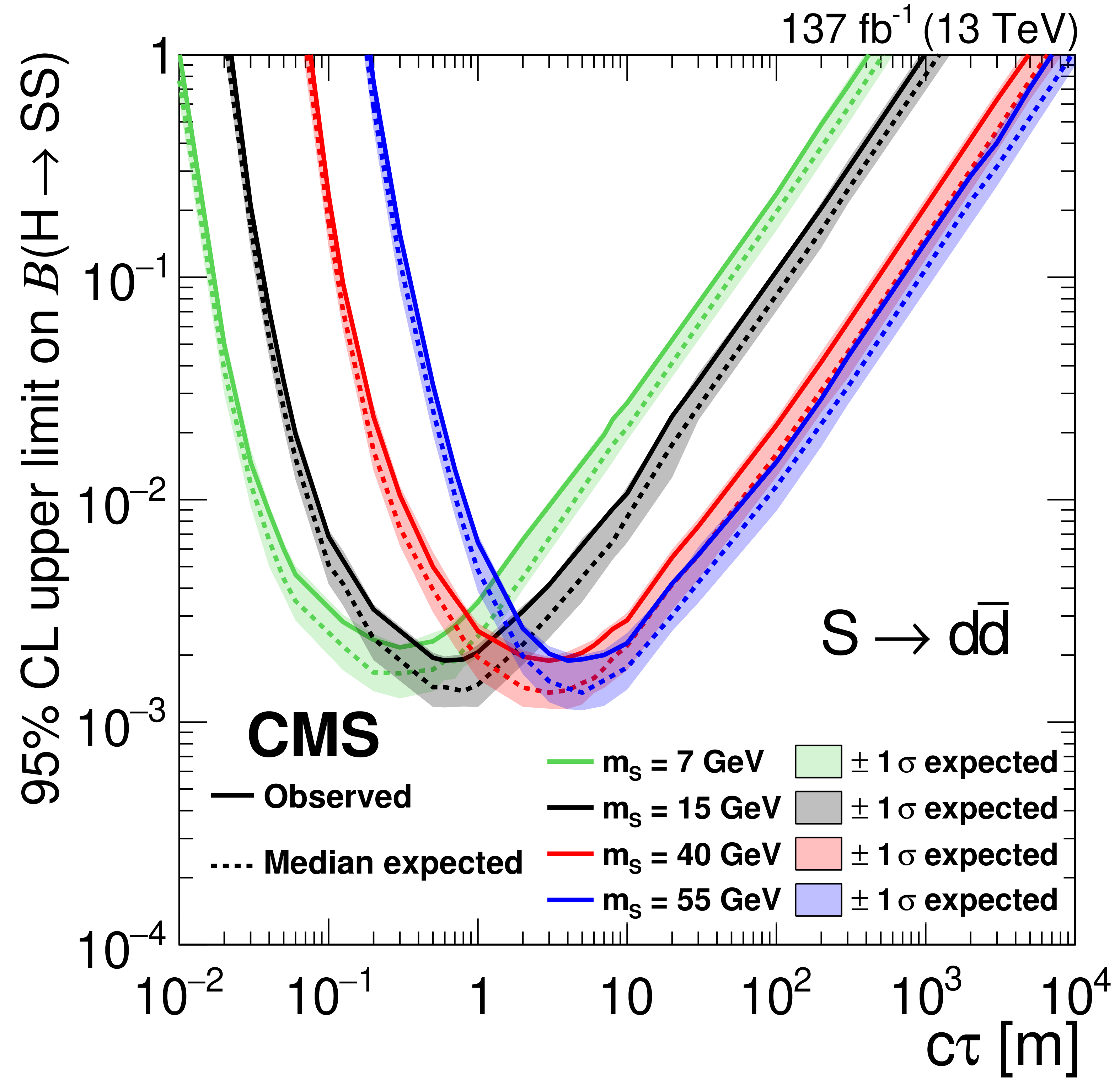
The 95% CL expected (dotted curves) and observed (solid curves) upper limits on the branching fraction $ {\mathcal {B}({\mathrm{H} \to \mathrm{S} \mathrm{S}})} $ as functions of $c\tau $ for the $\mathrm{S} \to {\mathrm{d} \mathrm{\bar{d}}} $ (left) and $\mathrm{S} \to \tau^{+} \tau^{-} $ (right) decay modes. The exclusion limits are shown for four different mass hypotheses: 7, 15, 40, and 55 GeV. |
png pdf |
Figure 3-a:
The 95% CL expected (dotted curves) and observed (solid curves) upper limits on the branching fraction $ {\mathcal {B}({\mathrm{H} \to \mathrm{S} \mathrm{S}})} $ as a function of the $c\tau $ for the $\mathrm{S} \to {\mathrm{d} \mathrm{\bar{d}}} $ decay mode. The exclusion limits are shown for four different mass hypotheses: 7, 15, 40, and 55 GeV. |

png pdf |
Figure 3-b:
The 95% CL expected (dotted curves) and observed (solid curves) upper limits on the branching fraction $ {\mathcal {B}({\mathrm{H} \to \mathrm{S} \mathrm{S}})} $ as a function of the $c\tau $ for the $\mathrm{S} \to \tau^{+} \tau^{-} $ decay mode. The exclusion limits are shown for four different mass hypotheses: 7, 15, 40, and 55 GeV. |
| Summary |
| In summary, proton-proton collision data at $\sqrt{s} = $ 13 TeV recorded by the CMS experiment in 2016--2018, corresponding to an integrated luminosity of 137 fb$^{-1}$, have been used to conduct the first search for beyond the standard model (SM) long-lived particles (LLPs) using the CMS endcap muon detectors as a calorimeter. Based on a unique detector signature, the search is largely model-independent, with sensitivity to a broad range of LLP decay modes and to LLP masses as low as a few GeV. With the excellent shielding provided by the inner CMS detector, the background is suppressed to a low level and a search for a single LLP decay is possible. No significant deviation from the SM background is observed, and the most stringent limits on the branching fraction of Higgs boson to LLP decaying to $\mathrm{d\bar{d}}$, $\mathrm{b\bar{b}}$, and $\tau^{+}\tau^{-}$ are set for proper decay lengths $c\tau > $ 6, 20, and 40 m, and LLP masses of 7, 15, and 40GeV, respectively. For $c\tau > $ 100 m, this search outperforms the previous best limits [30,31] by a factor of 6 (2) for an LLP mass of 7 ($\ge$15) GeV. |
| Additional Figures | |
png pdf |
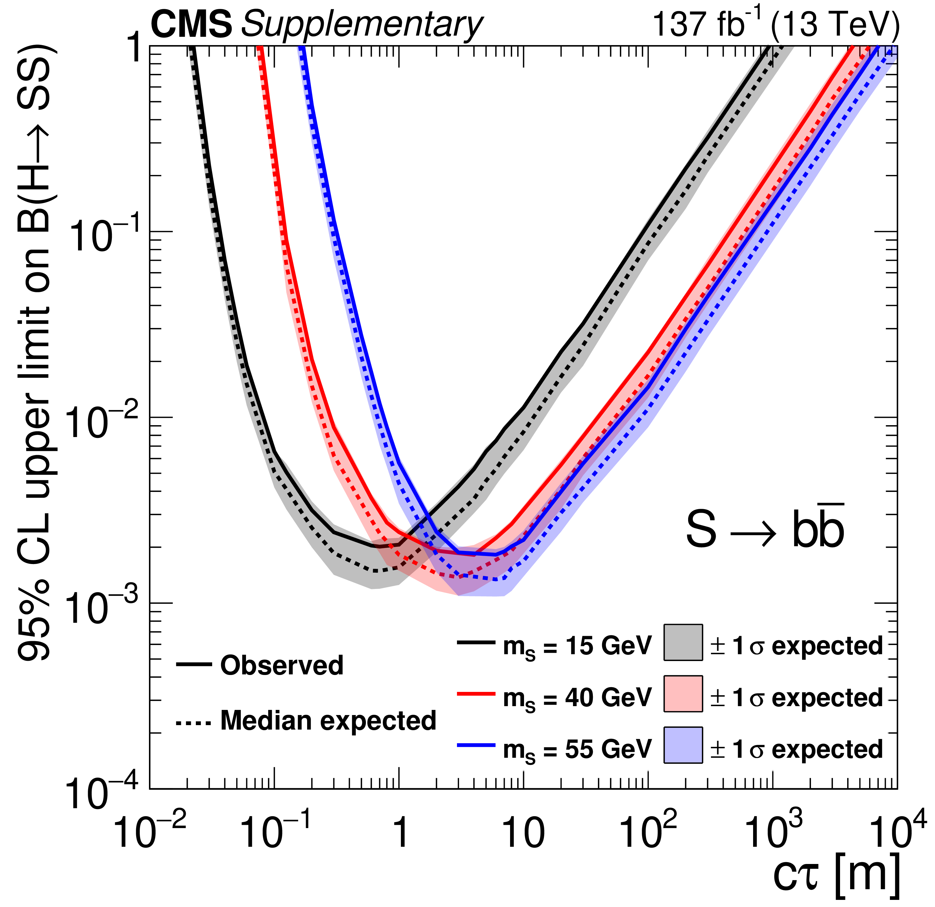
Additional Figure 1:
The 95% CL expected (dotted curves) and observed (solid curves) upper limits on the branching fraction $ {\mathcal {B}({{\mathrm {h}^0} \rightarrow {\mathrm {S}} {\mathrm {S}}})} $ as a function of $c\tau $ for the $ {\mathrm {S}} \rightarrow {{\mathrm {b}} {\overline {\mathrm {b}}}} $ decay mode. The exclusion limits are shown for three different mass hypotheses: 15 (black), 40 (red), and 55 (blue) GeV. |
png pdf |
Additional Figure 2:
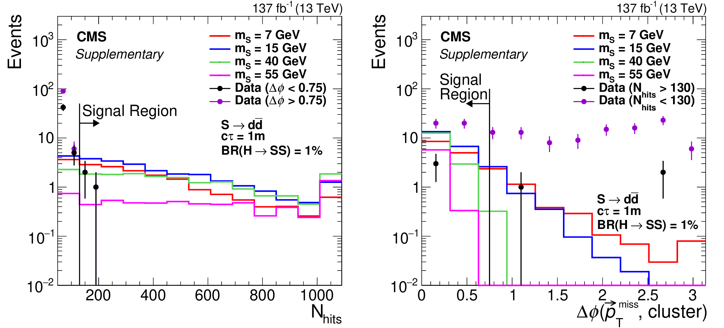
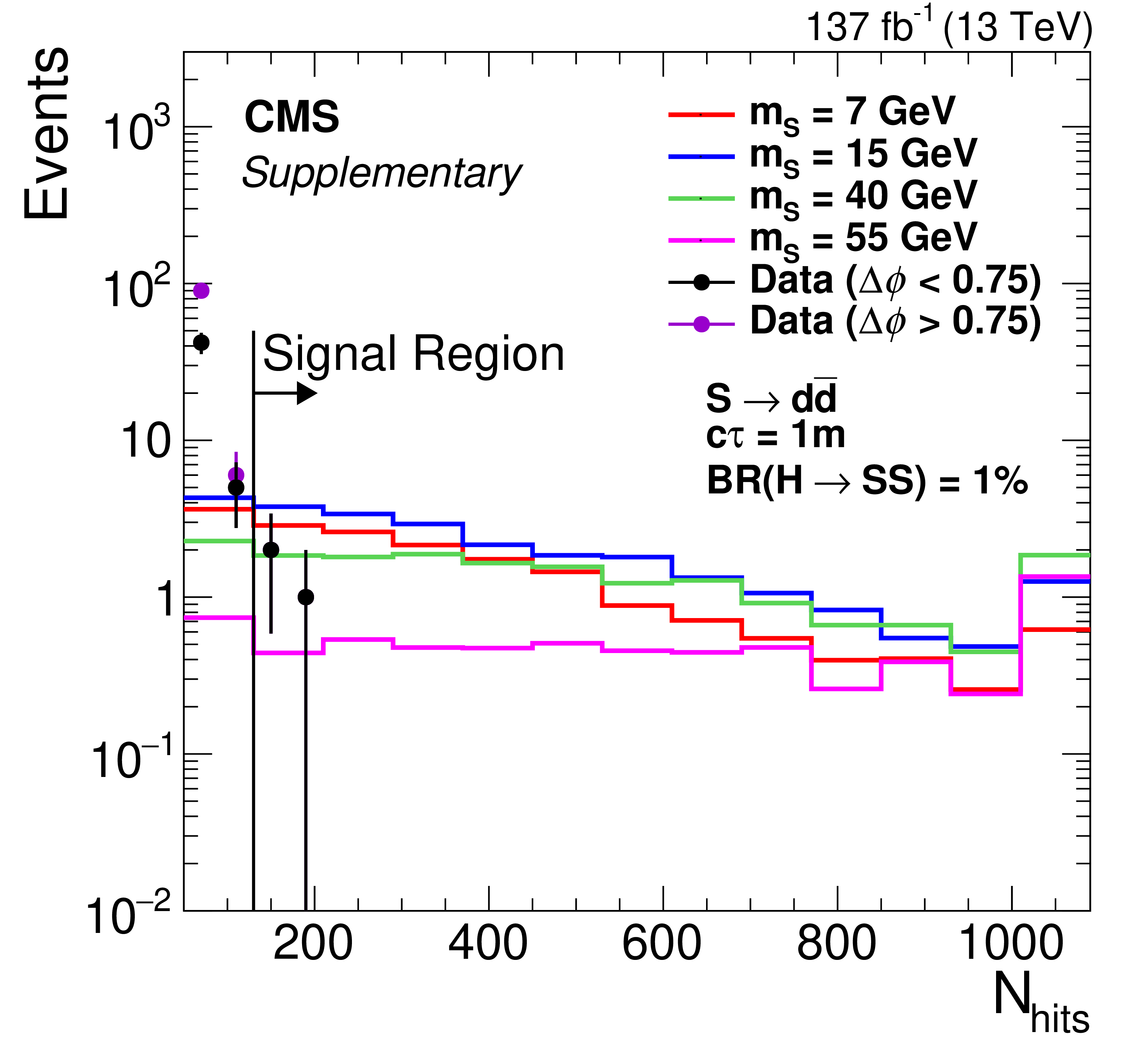
The $N_\mathrm {hits}$ (left) and $\Delta \phi ({\vec{p}_{\mathrm {T}}^{\,\text {miss}}},\mathrm {cluster})$ (right) distributions. The signal (assuming $ {\mathcal {B}({{\mathrm {h}^0} \rightarrow {\mathrm {S}} {\mathrm {S}}})} = $ 1%, $ {\mathrm {S}} \rightarrow {{\mathrm {d}} {\overline {\mathrm {d}}}} $, and $c\tau =$ 1 m) and data (black) distributions have $\Delta \phi < $ 0.75 ($N_\mathrm {hits} > $ 130) selections applied in the left (right) plot. The data distribution shown in magenta includes the inverted cut $\Delta \phi > $ 0.75 ($N_\mathrm {hits} < $ 130) applied in the left (right) plot. The last bin in the $N_\mathrm {hits}$ distributions includes all events in the overflow. |
png pdf |
Additional Figure 2-a:
The $N_\mathrm {hits}$ distribution. The signal (assuming $ {\mathcal {B}({{\mathrm {h}^0} \rightarrow {\mathrm {S}} {\mathrm {S}}})} = $ 1%, $ {\mathrm {S}} \rightarrow {{\mathrm {d}} {\overline {\mathrm {d}}}} $, and $c\tau =$ 1 m) and data (black) distributions have the $\Delta \phi < $ 0.75 selection applied. The data distribution shown in magenta applies the inverted cut $\Delta \phi > $ 0.75. The last bin includes all events in the overflow. |

png pdf |
Additional Figure 2-b:
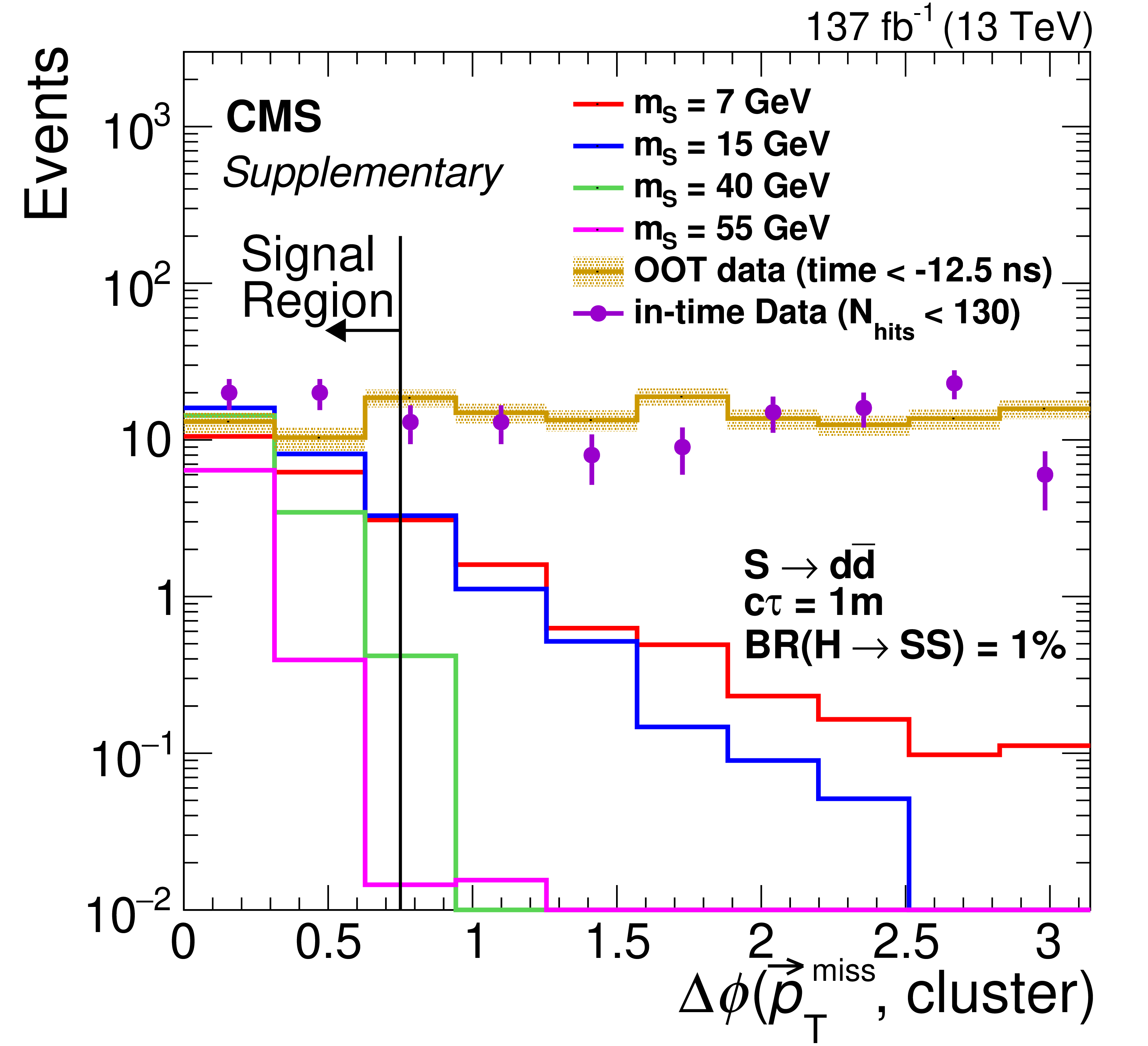
The $\Delta \phi ({\vec{p}_{\mathrm {T}}^{\,\text {miss}}},\mathrm {cluster})$ distribution. The signal (assuming $ {\mathcal {B}({{\mathrm {h}^0} \rightarrow {\mathrm {S}} {\mathrm {S}}})} = $ 1%, $ {\mathrm {S}} \rightarrow {{\mathrm {d}} {\overline {\mathrm {d}}}} $, and $c\tau =$ 1 m) and data (black) distributions have the $N_\mathrm {hits} > $ 130 selection applied. The data distribution shown in magenta applies the inverted cut $N_\mathrm {hits} < $ 130. |
png pdf |
Additional Figure 3:
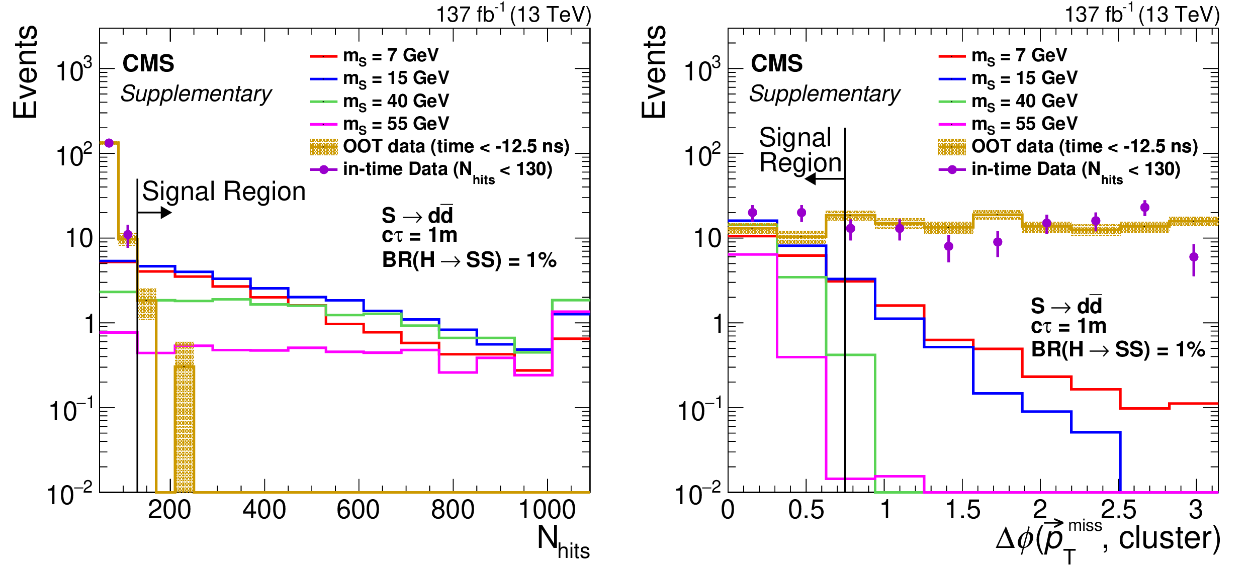
The signal (assuming $ {\mathcal {B}({{\mathrm {h}^0} \rightarrow {\mathrm {S}} {\mathrm {S}}})} = $ 1%, $ {\mathrm {S}} \rightarrow {{\mathrm {d}} {\overline {\mathrm {d}}}} $, and $c\tau =$ 1 m), in-time data ($N_\mathrm {hits} < $ 130), and out-of-time data (inclusive in $N_\mathrm {hits}$) distributions of $N_\mathrm {hits}$ (left) and $\Delta \phi ({\vec{p}_{\mathrm {T}}^{\,\text {miss}}},\mathrm {cluster})$ (right). The signal distributions include events from regions A, B, C, and D (as defined in the analysis summary), the in-time data distributions include events from regions B and C, and the OOT data are out-of-time clusters from previous bunch crossings, with the yield normalized to that of the in-time distribution. The last bin in the $N_\mathrm {hits}$ distributions includes all events in the overflow. |

png pdf |
Additional Figure 3-a:
The signal (assuming $ {\mathcal {B}({{\mathrm {h}^0} \rightarrow {\mathrm {S}} {\mathrm {S}}})} = $ 1%, $ {\mathrm {S}} \rightarrow {{\mathrm {d}} {\overline {\mathrm {d}}}} $, and $c\tau =$ 1 m), in-time data ($N_\mathrm {hits} < $ 130), and out-of-time data (inclusive in $N_\mathrm {hits}$) distributions of $N_\mathrm {hits}$. The signal distributions include events from regions A, B, C, and D (as defined in the analysis summary), the in-time data distributions include events from regions B and C, and the OOT data are out-of-time clusters from previous bunch crossings, with the yield normalized to that of the in-time distribution. The last bin includes all events in the overflow. |
png pdf |
Additional Figure 3-b:
The signal (assuming $ {\mathcal {B}({{\mathrm {h}^0} \rightarrow {\mathrm {S}} {\mathrm {S}}})} = $ 1%, $ {\mathrm {S}} \rightarrow {{\mathrm {d}} {\overline {\mathrm {d}}}} $, and $c\tau =$ 1 m), in-time data ($N_\mathrm {hits} < $ 130), and out-of-time data (inclusive in $N_\mathrm {hits}$) distributions of $\Delta \phi ({\vec{p}_{\mathrm {T}}^{\,\text {miss}}},\mathrm {cluster})$. The signal distributions include events from regions A, B, C, and D (as defined in the analysis summary), the in-time data distributions include events from regions B and C, and the OOT data are out-of-time clusters from previous bunch crossings, with the yield normalized to that of the in-time distribution. |

png pdf |
Additional Figure 4:
The event display of a simulated signal event for $m_ {\mathrm {S}} = $ 40 GeV, $c\tau =$ 1 m, and $ {\mathrm {S}} \rightarrow {{\mathrm {b}} {\overline {\mathrm {b}}}} $ in $rz$-plane (left) and $r\phi $-plane (right). The LLP decayed at the position $x, y, z =$ $-$364, 92, 796 cm and produced a CSC hit cluster with 711 hits (orange dots). The green lines represent the tracks. The yellow lines represent jets. The red arrow represents the MET direction. The red and blue cones represent the ECAL and HCAL energy deposits, respectively. |

png pdf |
Additional Figure 4-a:
The event display of a simulated signal event for $m_ {\mathrm {S}} = $ 40 GeV, $c\tau =$ 1 m, and $ {\mathrm {S}} \rightarrow {{\mathrm {b}} {\overline {\mathrm {b}}}} $ in $rz$-plane. The LLP decayed at the position $x, y, z =$ $-$364, 92, 796 cm and produced a CSC hit cluster with 711 hits (orange dots). The green lines represent the tracks. The yellow lines represent jets. The red arrow represents the MET direction. The red and blue cones represent the ECAL and HCAL energy deposits, respectively. |

png pdf |
Additional Figure 4-b:
The event display of a simulated signal event for $m_ {\mathrm {S}} = $ 40 GeV, $c\tau =$ 1 m, and $ {\mathrm {S}} \rightarrow {{\mathrm {b}} {\overline {\mathrm {b}}}} $ in $r\phi $-plane. The LLP decayed at the position $x, y, z =$ $-$364, 92, 796 cm and produced a CSC hit cluster with 711 hits (orange dots). The green lines represent the tracks. The yellow lines represent jets. The red arrow represents the MET direction. The red and blue cones represent the ECAL and HCAL energy deposits, respectively. |

png pdf |
Additional Figure 5:
Distributions of cluster time in data and in simulated $ {\mathrm {S}} \rightarrow {{\mathrm {b}} {\overline {\mathrm {b}}}} $ signal events. The signal distribution contains equal fractions of events with mass of 15, 40, and 55 GeV, each simulated with a uniform mixture of $c\tau $ between 0.1 and 100 m. Both distributions are normalized to unit area and are required to pass the veto requirements as defined in the analysis summary. |

png pdf |
Additional Figure 6:
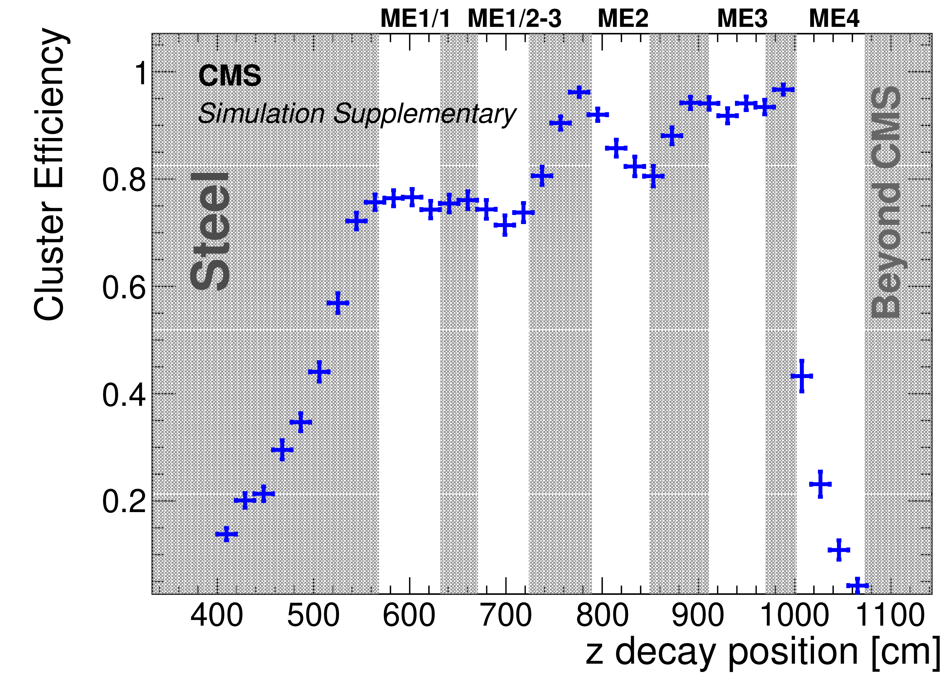
The clustering efficiency requiring $ > 50$ hits (left) and the overall signal efficiency of the clustering requiring $ > $50 hits, veto, and identification selections (right), as defined in the analysis summary, as a function of the simulated $z$ decay positions of ${\mathrm {S}}$ decaying to $ {{\mathrm {b}} {\overline {\mathrm {b}}}} $, for a mass of 15 GeV and a uniform mixture of $c\tau $ between 1 and 100 m. The endcap muon stations are labeled by their station names. Regions occupied by steel shielding are shaded in gray. |
png pdf |
Additional Figure 6-a:
The clustering efficiency requiring $ > 50$ hits, as defined in the analysis summary, as a function of the simulated $z$ decay positions of ${\mathrm {S}}$ decaying to $ {{\mathrm {b}} {\overline {\mathrm {b}}}} $, for a mass of 15 GeV and a uniform mixture of $c\tau $ between 1 and 100 m. The endcap muon stations are labeled by their station names. Regions occupied by steel shielding are shaded in gray. |

png pdf |
Additional Figure 6-b:
The overall signal efficiency of the clustering requiring $ > $50 hits, veto, and identification selections, as defined in the analysis summary, as a function of the simulated $z$ decay positions of ${\mathrm {S}}$ decaying to $ {{\mathrm {b}} {\overline {\mathrm {b}}}} $, for a mass of 15 GeV and a uniform mixture of $c\tau $ between 1 and 100 m. The endcap muon stations are labeled by their station names. Regions occupied by steel shielding are shaded in gray. |
png pdf |
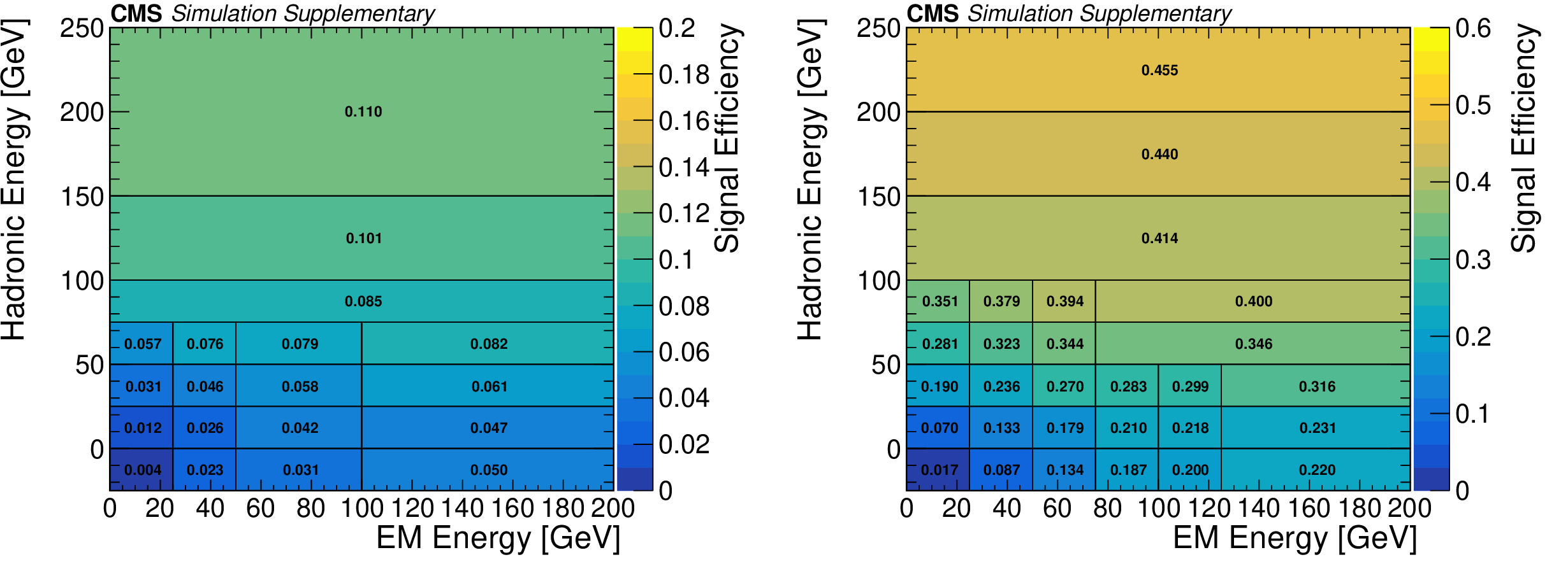
Additional Figure 7:
The cluster efficiency in bins of hadronic and EM energy in region A (left) and B (right), estimated with LLPs decaying to ${{\tau}^{+} {\tau}^{-}}$. The sample contains equal fractions of events with LLP mass of 7, 15, 40, and 55 GeV and LLP lifetime of 0.1, 1, 10, and 100m. The first hadronic energy bins correspond to LLPs that decayed leptonically with 0 hadronic energy. Region A is defined as 391 cm $ < r < $ 695.5 cm and 400 cm $ < |z| < $ 671 cm. Region B is defined as 671 cm $ < |z| < $ 1100 cm, $r < $ 695.5 cm and $|\eta | < $ 2. The cluster efficiency includes all cluster-level selections described in the paper, except for the jet veto, time cut, and $\Delta \phi ({\vec{p}_{\mathrm {T}}^{\,\text {miss}}},\mathrm {cluster})$ cut. The full simulation signal yield prediction for samples with various LLP mass between 7 - 55 GeV, lifetime between 0.1 - 100 m, and decay mode to $ {{\mathrm {d}} {\overline {\mathrm {d}}}} $ and $ {{\tau}^{+} {\tau}^{-}} $ can be reproduced using this parameterization to within 35% and 20% for region A and B, respectively. The statistical uncertainty for each bin is documented in Figure 7 of the HEPData record of this paper. |
png pdf |
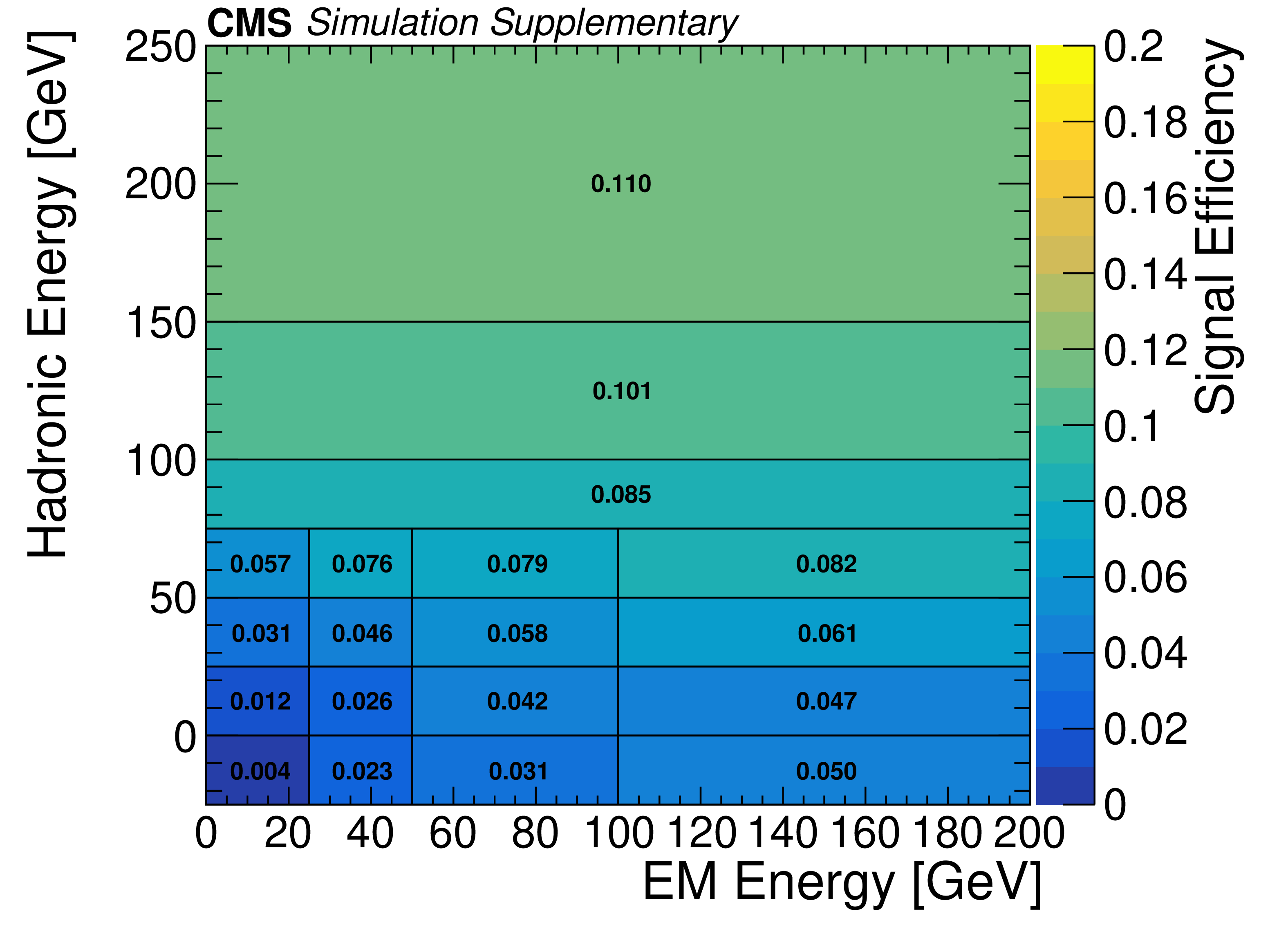
Additional Figure 7-a:
The cluster efficiency in bins of hadronic and EM energy in region A, estimated with LLPs decaying to ${{\tau}^{+} {\tau}^{-}}$. The sample contains equal fractions of events with LLP mass of 7, 15, 40, and 55 GeV and LLP lifetime of 0.1, 1, 10, and 100m. The first hadronic energy bins correspond to LLPs that decayed leptonically with 0 hadronic energy. Region A is defined as 391 cm $ < r < $ 695.5 cm and 400 cm $ < |z| < $ 671 cm. The cluster efficiency includes all cluster-level selections described in the paper, except for the jet veto, time cut, and $\Delta \phi ({\vec{p}_{\mathrm {T}}^{\,\text {miss}}},\mathrm {cluster})$ cut. The full simulation signal yield prediction for samples with various LLP mass between 7 - 55 GeV, lifetime between 0.1 - 100 m, and decay mode to $ {{\mathrm {d}} {\overline {\mathrm {d}}}} $ and $ {{\tau}^{+} {\tau}^{-}} $ can be reproduced using this parameterization to within 35% for region A. The statistical uncertainty for each bin is documented in Figure 7 of the HEPData record of this paper. |
png pdf |
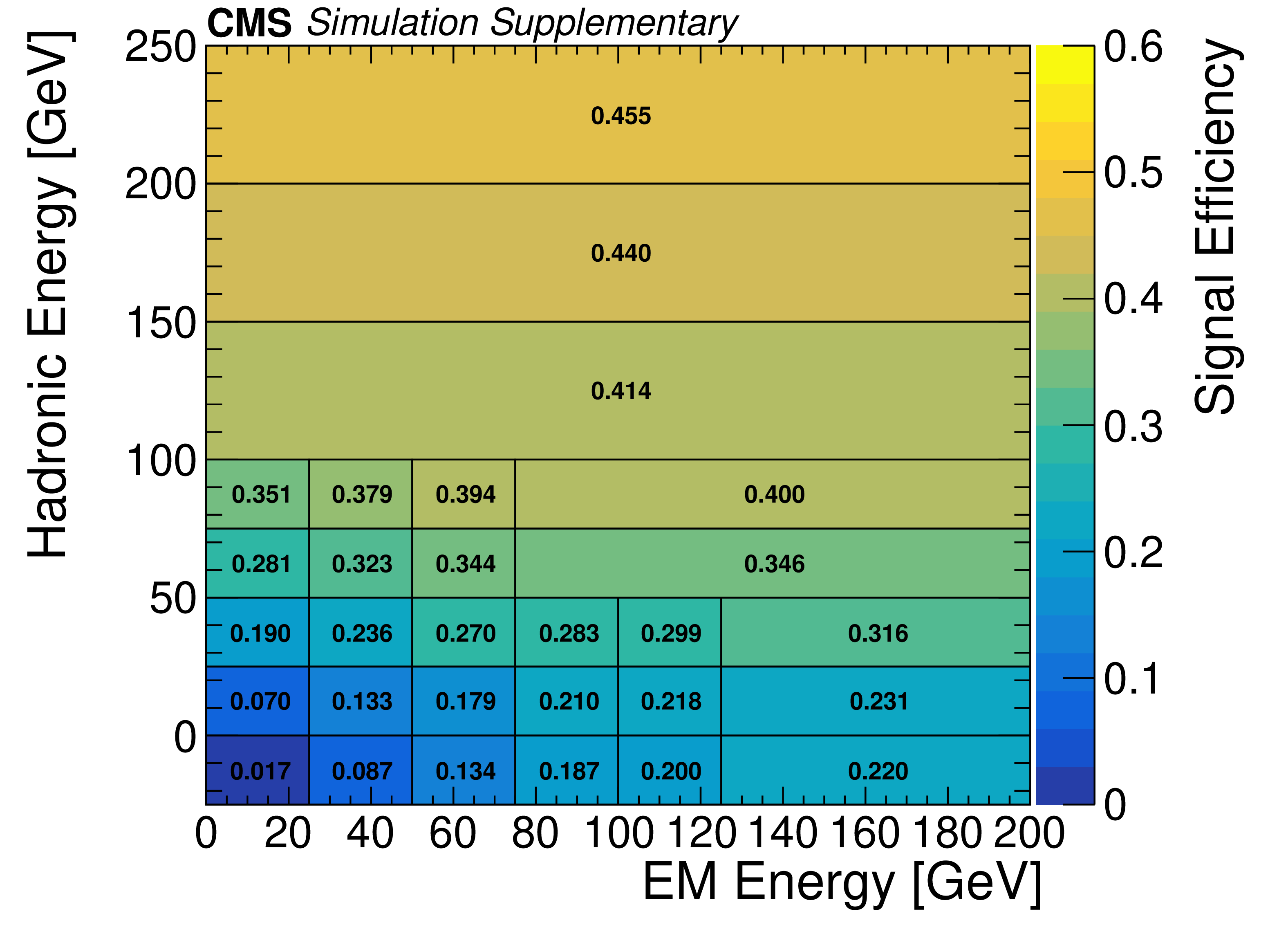
Additional Figure 7-b:
The cluster efficiency in bins of hadronic and EM energy in region B, estimated with LLPs decaying to ${{\tau}^{+} {\tau}^{-}}$. The sample contains equal fractions of events with LLP mass of 7, 15, 40, and 55 GeV and LLP lifetime of 0.1, 1, 10, and 100m. The first hadronic energy bins correspond to LLPs that decayed leptonically with 0 hadronic energy. Region B is defined as 671 cm $ < |z| < $ 1100 cm, $r < $ 695.5 cm and $|\eta | < $ 2. The cluster efficiency includes all cluster-level selections described in the paper, except for the jet veto, time cut, and $\Delta \phi ({\vec{p}_{\mathrm {T}}^{\,\text {miss}}},\mathrm {cluster})$ cut. The full simulation signal yield prediction for samples with various LLP mass between 7 - 55 GeV, lifetime between 0.1 - 100 m, and decay mode to $ {{\mathrm {d}} {\overline {\mathrm {d}}}} $ and $ {{\tau}^{+} {\tau}^{-}} $ can be reproduced using this parameterization to within 20% for region B. The statistical uncertainty for each bin is documented in Figure 7 of the HEPData record of this paper. |
png pdf |
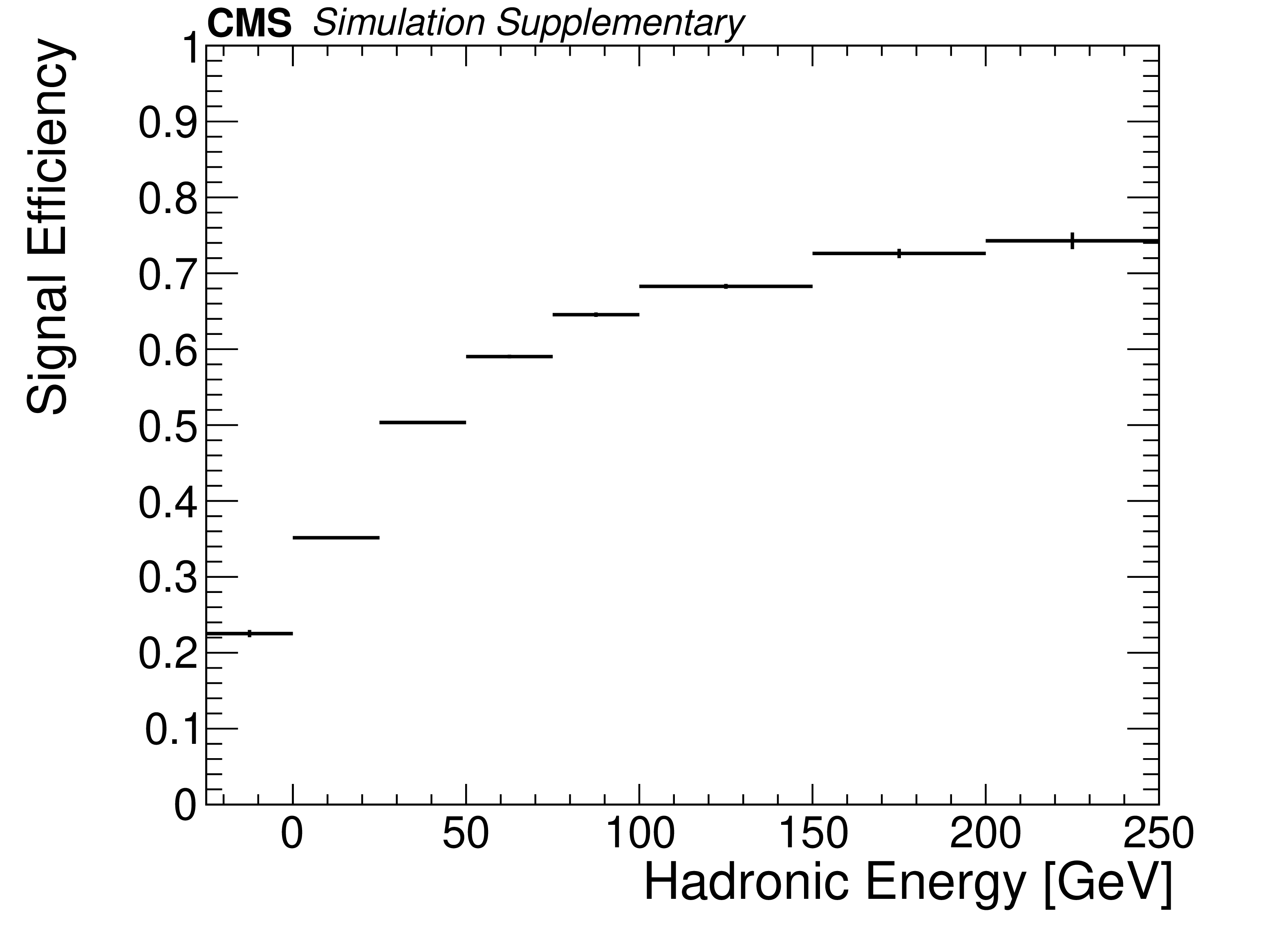
Additional Figure 8:
The efficiency of $N_{station} > 1$ requirement in bins of hadronic energy in region B, estimated with LLPs decaying to ${{\tau}^{+} {\tau}^{-}}$. The sample contains equal fractions of events with LLP mass of 7, 15, 40, and 55 GeV and LLP lifetime of 0.1, 1, 10, and 100m. This efficiency is independent of the EM energy. The first hadronic energy bin corresponds to LLPs that decayed leptonically with 0 hadronic energy. Region B is defined as 671 cm $ < |z| < $ 1100 cm, $r < $ 695.5 cm and $|\eta | < $ 2. The efficiency is calculated with respect to clusters that pass all the cluster-level cuts described in the paper, except for the jet veto, time cut, and $\Delta \phi ({\vec{p}_{\mathrm {T}}^{\,\text {miss}}},\mathrm {cluster})$ cut. The full simulation signal yield prediction for samples with various LLP mass between 7 - 55 GeV, lifetime between 0.1 - 100 m, and decay mode to $ {{\mathrm {d}} {\overline {\mathrm {d}}}} $ and $ {{\tau}^{+} {\tau}^{-}} $ can be reproduced using this parameterization to within 10%. |
png pdf |
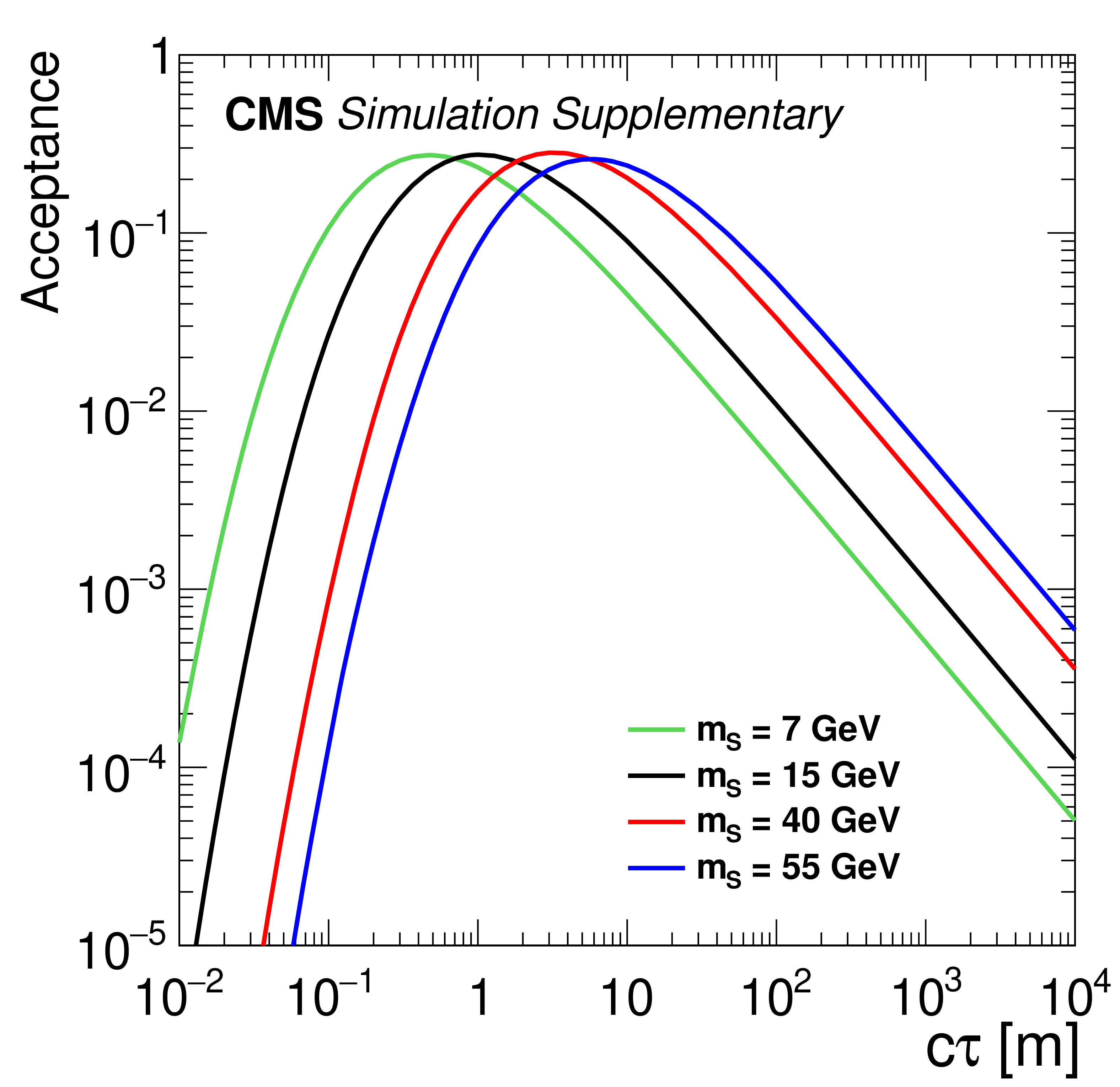
Additional Figure 9:
The geometric signal acceptance as a function of $c\tau $. The acceptance is shown for four different LLP mass hypotheses: 7 (green), 15 (black), 40 (red), and 55 (blue) GeV. The acceptance is defined by requiring at least 1 LLP to decay in the region defined as 400 cm $ < |z| < $ 1100 cm, $r < $ 695.5 cm, and $|\eta | < $ 2.4. |
| Instructions for Reinterpretation |
|
We provide signal efficiency parameterization for the cluster-level selections that allows for reproduction of the full-simulation signal yield for various LLP masses (7-55 GeV), lifetimes (0.1 - 100 m) and decay modes (dd̅ and τ+τ-). In order to recast this analysis, only the generator level LLP hadronic energy, EM energy, and decay position are needed. The following selection efficiencies are needed to account for all cluster-level selections mentioned in the paper:
cut_based_id.py attached. The function uses the LLP decay position to predict the average station of the cluster (AvgStation function in the code) and the Nstation > 1 efficiency parameterization (Additional Figure 8). As described in the paper, the cluster ID requirement applies different η cuts depending on the Nstation and average station number. We need a parametrization of the efficiency of the Nstation > 1 requirement and a transfer function that takes gen-level LLP decay position to RECO-level cluster average station (only for clusters with Nstation = 1 ). Since the entire region A is in an η region (|η| < 1.3) that passes all the η selections used in the cut-based ID (tightest cut is |η| < 1.6), the cut-based ID efficiency in this region is 100%. The focus of the parameterization will be on region B only. The efficiency of Nstation > 1 in region B is provided in bins of LLP hadronic energy (Additional Figure 8) and the efficiency is independent of the LLP EM energy. The average station transfer function is provided as the AvgStation function in the code attached. The full simulation signal yield prediction for samples with various LLP mass between 7 - 55 GeV, lifetime between 0.1 - 100 m, and decay mode to dd̅ and τ+τ- can be reproduced using this parameterization to within 10%.
|
| References | ||||
| 1 | G. F. Giudice and A. Romanino | Split supersymmetry | NPB 699 (2004) 65 | hep-ph/0406088 |
| 2 | J. L. Hewett, B. Lillie, M. Masip, and T. G. Rizzo | Signatures of long-lived gluinos in split supersymmetry | JHEP 09 (2004) 070 | hep-ph/0408248 |
| 3 | N. Arkani-Hamed, S. Dimopoulos, G. F. Giudice, and A. Romanino | Aspects of split supersymmetry | NPB 709 (2005) 3 | hep-ph/0409232 |
| 4 | P. Gambino, G. F. Giudice, and P. Slavich | Gluino decays in split supersymmetry | NPB 726 (2005) 35 | hep-ph/0506214 |
| 5 | A. Arvanitaki, N. Craig, S. Dimopoulos, and G. Villadoro | Mini-split | JHEP 02 (2013) 126 | 1210.0555 |
| 6 | N. Arkani-Hamed et al. | Simply unnatural supersymmetry | 1212.6971 | |
| 7 | P. Fayet | Supergauge invariant extension of the Higgs mechanism and a model for the electron and its neutrino | NPB 90 (1975) 104 | |
| 8 | G. R. Farrar and P. Fayet | Phenomenology of the production, decay, and detection of new hadronic states associated with supersymmetry | PLB 76 (1978) 575 | |
| 9 | S. Weinberg | Supersymmetry at ordinary energies. Masses and conservation laws | PRD 26 (1982) 287 | |
| 10 | R. Barbier et al. | $ R $-parity violating supersymmetry | PR 420 (2005) 1 | hep-ph/0406039 |
| 11 | G. F. Giudice and R. Rattazzi | Theories with gauge mediated supersymmetry breaking | PR 322 (1999) 419 | hep-ph/9801271 |
| 12 | P. Meade, N. Seiberg, and D. Shih | General gauge mediation | Prog. Theor. Phys. Suppl. 177 (2009) 143 | 0801.3278 |
| 13 | M. Buican, P. Meade, N. Seiberg, and D. Shih | Exploring general gauge mediation | JHEP 03 (2009) 016 | 0812.3668 |
| 14 | J. Fan, M. Reece, and J. T. Ruderman | Stealth supersymmetry | JHEP 11 (2011) 012 | 1105.5135 |
| 15 | J. Fan, M. Reece, and J. T. Ruderman | A stealth supersymmetry sampler | JHEP 07 (2012) 196 | 1201.4875 |
| 16 | M. J. Strassler and K. M. Zurek | Echoes of a hidden valley at hadron colliders | PLB 651 (2007) 374 | hep-ph/0604261 |
| 17 | M. J. Strassler and K. M. Zurek | Discovering the Higgs through highly-displaced vertices | PLB 661 (2008) 263 | hep-ph/0605193 |
| 18 | T. Han, Z. Si, K. M. Zurek, and M. J. Strassler | Phenomenology of hidden valleys at hadron colliders | JHEP 07 (2008) 008 | 0712.2041 |
| 19 | Y. Cui, L. Randall, and B. Shuve | A WIMPy baryogenesis miracle | JHEP 04 (2012) 075 | 1112.2704 |
| 20 | Y. Cui and R. Sundrum | Baryogenesis for weakly interacting massive particles | PRD 87 (2013) 116013 | 1212.2973 |
| 21 | Y. Cui and B. Shuve | Probing baryogenesis with displaced vertices at the LHC | JHEP 02 (2015) 049 | 1409.6729 |
| 22 | D. Smith and N. Weiner | Inelastic dark matter | PRD 64 (2001) 043502 | hep-ph/0101138 |
| 23 | Z. Chacko, H.-S. Goh, and R. Harnik | Natural electroweak breaking from a mirror symmetry | PRL 96 (2006) 231802 | hep-ph/0506256 |
| 24 | D. Curtin and C. B. Verhaaren | Discovering uncolored naturalness in exotic Higgs decays | JHEP 12 (2015) 072 | 1506.06141 |
| 25 | H.-C. Cheng, S. Jung, E. Salvioni, and Y. Tsai | Exotic quarks in twin Higgs models | JHEP 03 (2016) 074 | 1512.02647 |
| 26 | N. Craig, A. Katz, M. Strassler, and R. Sundrum | Naturalness in the dark at the LHC | JHEP 07 (2015) 105 | 1501.05310 |
| 27 | M. J. Strassler | On the phenomenology of hidden valleys with heavy flavor | 0806.2385 | |
| 28 | J. E. Juknevich, D. Melnikov, and M. J. Strassler | A pure-glue hidden valley I. states and decays | JHEP 07 (2009) 055 | 0903.0883 |
| 29 | CMS Collaboration | Search for long-lived particles using displaced jets in proton-proton collisions at $ \sqrt{s} = $ 13 TeV | Submitted to \emphPRD | CMS-EXO-19-021 2012.01581 |
| 30 | ATLAS Collaboration | Search for long-lived particles produced in $ pp $ collisions at $ \sqrt{s}= $ 13 TeV that decay into displaced hadronic jets in the ATLAS muon spectrometer | PRD 99 (2019) 052005 | 1811.07370 |
| 31 | ATLAS Collaboration | Search for long-lived neutral particles produced in $ pp $ collisions at $ \sqrt{s} = $ 13 TeV decaying into displaced hadronic jets in the ATLAS inner detector and muon spectrometer | PRD 101 (2020) 052013 | 1911.12575 |
| 32 | CMS Collaboration | HEPData record for this analysis | link | |
| 33 | CMS Collaboration | The CMS experiment at the CERN LHC | JINST 3 (2008) S08004 | CMS-00-001 |
| 34 | CMS Collaboration | Performance of the CMS cathode strip chambers with cosmic rays | JINST 5 (2010) T03018 | CMS-CFT-09-011 0911.4992 |
| 35 | CMS Collaboration | Particle-flow reconstruction and global event description with the CMS detector | JINST 12 (2017) P10003 | CMS-PRF-14-001 1706.04965 |
| 36 | M. Cacciari and G. P. Salam | Dispelling the $ N^{3} $ myth for the $ {k_{\mathrm{T}}} $ jet-finder | PLB 641 (2006) 57 | hep-ph/0512210 |
| 37 | M. Cacciari, G. P. Salam, and G. Soyez | The anti-$ {k_{\mathrm{T}}} $ jet clustering algorithm | JHEP 04 (2008) 063 | 0802.1189 |
| 38 | M. Cacciari, G. P. Salam, and G. Soyez | FastJet user manual | EPJC 72 (2012) 1896 | 1111.6097 |
| 39 | M. Cacciari and G. P. Salam | Pileup subtraction using jet areas | PLB 659 (2008) 119 | 0707.1378 |
| 40 | P. Nason | A new method for combining NLO QCD with shower Monte Carlo algorithms | JHEP 11 (2004) 040 | hep-ph/0409146 |
| 41 | S. Frixione, P. Nason, and C. Oleari | Matching NLO QCD computations with parton shower simulations: the POWHEG method | JHEP 11 (2007) 070 | 0709.2092 |
| 42 | S. Alioli, P. Nason, C. Oleari, and E. Re | A general framework for implementing NLO calculations in shower Monte Carlo programs: the POWHEG | JHEP 06 (2010) 043 | 1002.2581 |
| 43 | E. Re | Single-top Wt-channel production matched with parton showers using the POWHEG method | EPJC 71 (2011) 1547 | 1009.2450 |
| 44 | T. Sjostrand et al. | An introduction to $ PYTHIA $ 8.2 | CPC 191 (2015) 159 | 1410.3012 |
| 45 | CMS Collaboration | Event generator tunes obtained from underlying event and multiparton scattering measurements | EPJC 76 (2016) 155 | CMS-GEN-14-001 1512.00815 |
| 46 | CMS Collaboration | Extraction and validation of a new set of CMS PYTHIA8 tunes from underlying-event measurements | EPJC 80 (2020) 4 | CMS-GEN-17-001 1903.12179 |
| 47 | NNPDF Collaboration | Parton distributions for the LHC Run II | JHEP 04 (2015) 040 | 1410.8849 |
| 48 | NNPDF Collaboration | Parton distributions from high-precision collider data | EPJC 77 (2017) 663 | 1706.00428 |
| 49 | GEANT4 Collaboration | GEANT4--a simulation toolkit | NIMA 506 (2003) 250 | |
| 50 | CMS Collaboration | The CMS trigger system | JINST 12 (2017) P01020 | CMS-TRG-12-001 1609.02366 |
| 51 | CMS Collaboration | Electron and photon reconstruction and identification with the CMS experiment at the CERN LHC | JINST 16 (2021) P05014 | CMS-EGM-17-001 2012.06888 |
| 52 | CMS Collaboration | Performance of the CMS muon detector and muon reconstruction with proton-proton collisions at $ \sqrt{s}= $ 13 TeV | JINST 13 (2018) P06015 | CMS-MUO-16-001 1804.04528 |
| 53 | CMS Collaboration | Performance of the reconstruction and identification of high-momentum muons in proton-proton collisions at $ \sqrt{s} = $ 13 TeV | JINST 15 (2020) P02027 | CMS-MUO-17-001 1912.03516 |
| 54 | M. Ester, H.-P. Kriegel, J. Sander, and X. Xu | A density-based algorithm for discovering clusters in large spatial databases with noise | in Proceedings of the Second International Conference on Knowledge Discovery and Data Mining,Association for the Advancement of Artificial Intelligence | |
| 55 | CMS Collaboration | Missing transverse energy performance of the CMS detector | JINST 6 (2011) P09001 | CMS-JME-10-009 1106.5048 |
| 56 | CMS Collaboration | Jet energy scale and resolution in the CMS experiment in pp collisions at 8 TeV | JINST 12 (2017) P02014 | CMS-JME-13-004 1607.03663 |
| 57 | CMS Collaboration | CMS luminosity measurements for the 2016 data-taking period | CMS-PAS-LUM-17-001 | CMS-PAS-LUM-17-001 |
| 58 | CMS Collaboration | CMS luminosity measurements for the 2017 data-taking period at $ \sqrt{s} = $ 13 TeV | CMS-PAS-LUM-17-004 | CMS-PAS-LUM-17-004 |
| 59 | CMS Collaboration | CMS luminosity measurements for the 2018 data-taking period at $ \sqrt{s} = $ 13 TeV | CMS-PAS-LUM-18-002 | CMS-PAS-LUM-18-002 |
| 60 | T. Junk | Confidence level computation for combining searches with small statistics | NIMA 434 (1999) 435 | hep-ex/9902006 |
| 61 | A. L. Read | Presentation of search results: the CL$ _\mathrm{s} $ technique | JPG 28 (2002) 2693 | |
| 62 | The ATLAS Collaboration, The CMS Collaboration, The LHC Higgs Combination Group | Procedure for the LHC Higgs boson search combination in Summer 2011 | CMS-NOTE-2011-005 | |
|
|
Compact Muon Solenoid LHC, CERN |
|

|

|

|

|

|