

Compact Muon Solenoid
LHC, CERN
| CMS-HIG-17-006 ; CERN-EP-2017-168 | ||
| Search for resonant and nonresonant Higgs boson pair production in the $\mathrm{ b \bar{b} } \ell\nu \ell\nu$ final state in proton-proton collisions at $ \sqrt{s} = $ 13 TeV | ||
| CMS Collaboration | ||
| 14 August 2017 | ||
| JHEP 01 (2018) 054 | ||
| Abstract: Searches for resonant and nonresonant pair-produced Higgs bosons (HH) decaying respectively into $\ell\nu \ell\nu$, through either W or Z bosons, and $\mathrm{ b \bar{b} }$ are presented. The analyses are based on a sample of proton-proton collisions at $ \sqrt{s} = $ 13 TeV, collected by the CMS experiment at the LHC, corresponding to an integrated luminosity of 35.9 fb$^{-1}$. Data and predictions from the standard model are in agreement within uncertainties. For the standard model HH hypothesis, the data exclude at 95% confidence level a product of the production cross section and branching fraction larger than 72 fb, corresponding to 79 times the prediction, consistent with expectations. Constraints are placed on different scenarios considering anomalous couplings, which could affect the rate and kinematics of HH production. Upper limits at 95% confidence level are set on the production cross section of narrow-width spin-0 and spin-2 particles decaying to Higgs boson pairs, the latter produced with minimal gravity-like coupling. | ||
| Links: e-print arXiv:1708.04188 [hep-ex] (PDF) ; CDS record ; inSPIRE record ; HepData record ; CADI line (restricted) ; | ||
| Figures | |
png pdf |
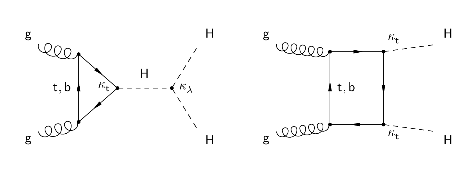
Figure 1:
Feynman diagrams for Higgs boson pair production via gluon fusion in the SM. The coupling modifiers for the Higgs boson self-coupling and the top quark Yukawa coupling are denoted by $\kappa _{\lambda }$ and $\kappa _\mathrm{ t } $, respectively. |
png pdf |
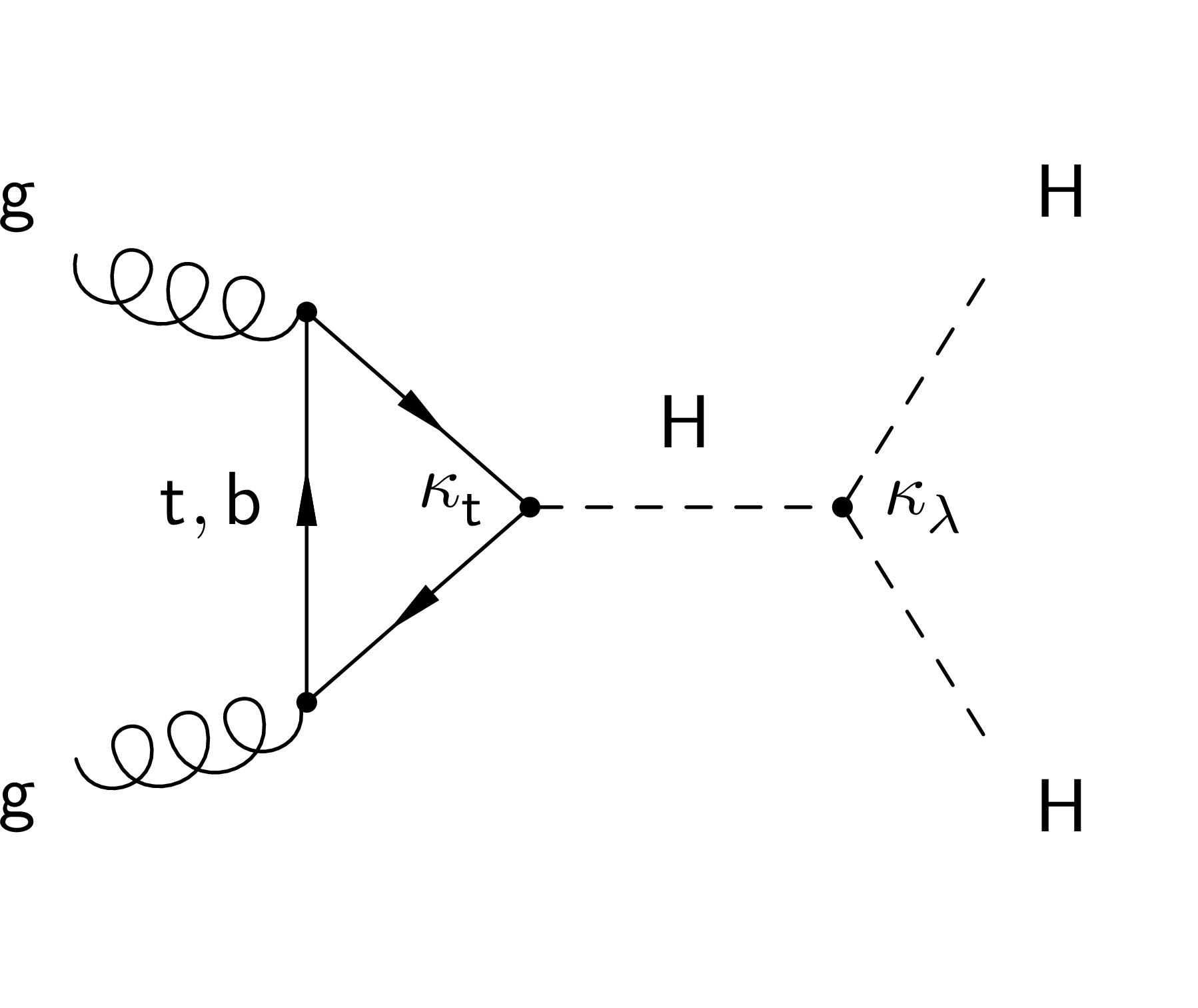
Figure 1-a:
Feynman diagram for Higgs boson pair production via gluon fusion in the SM. The coupling modifiers for the Higgs boson self-coupling and the top quark Yukawa coupling are denoted by $\kappa _{\lambda }$ and $\kappa _\mathrm{ t } $, respectively. |

png pdf |
Figure 1-b:
Feynman diagram for Higgs boson pair production via gluon fusion in the SM. The coupling modifier for the top quark Yukawa coupling is denoted by $\kappa _\mathrm{ t } $. |
png pdf |
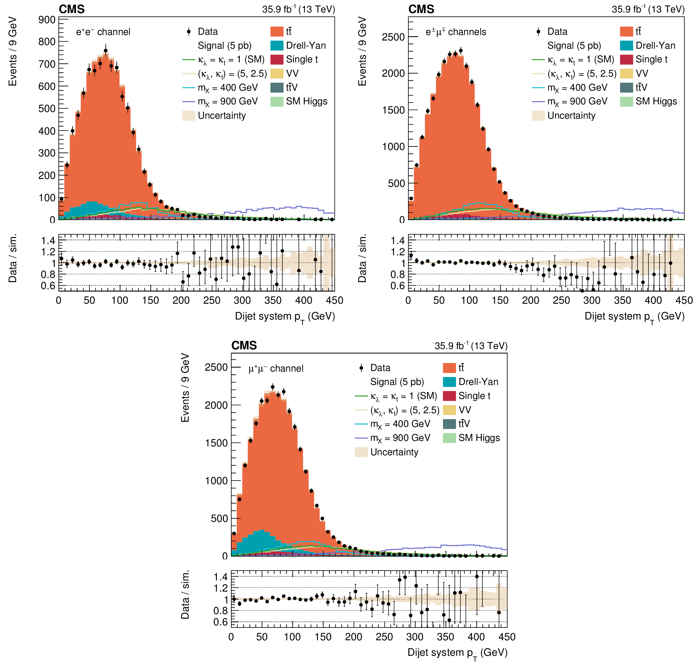
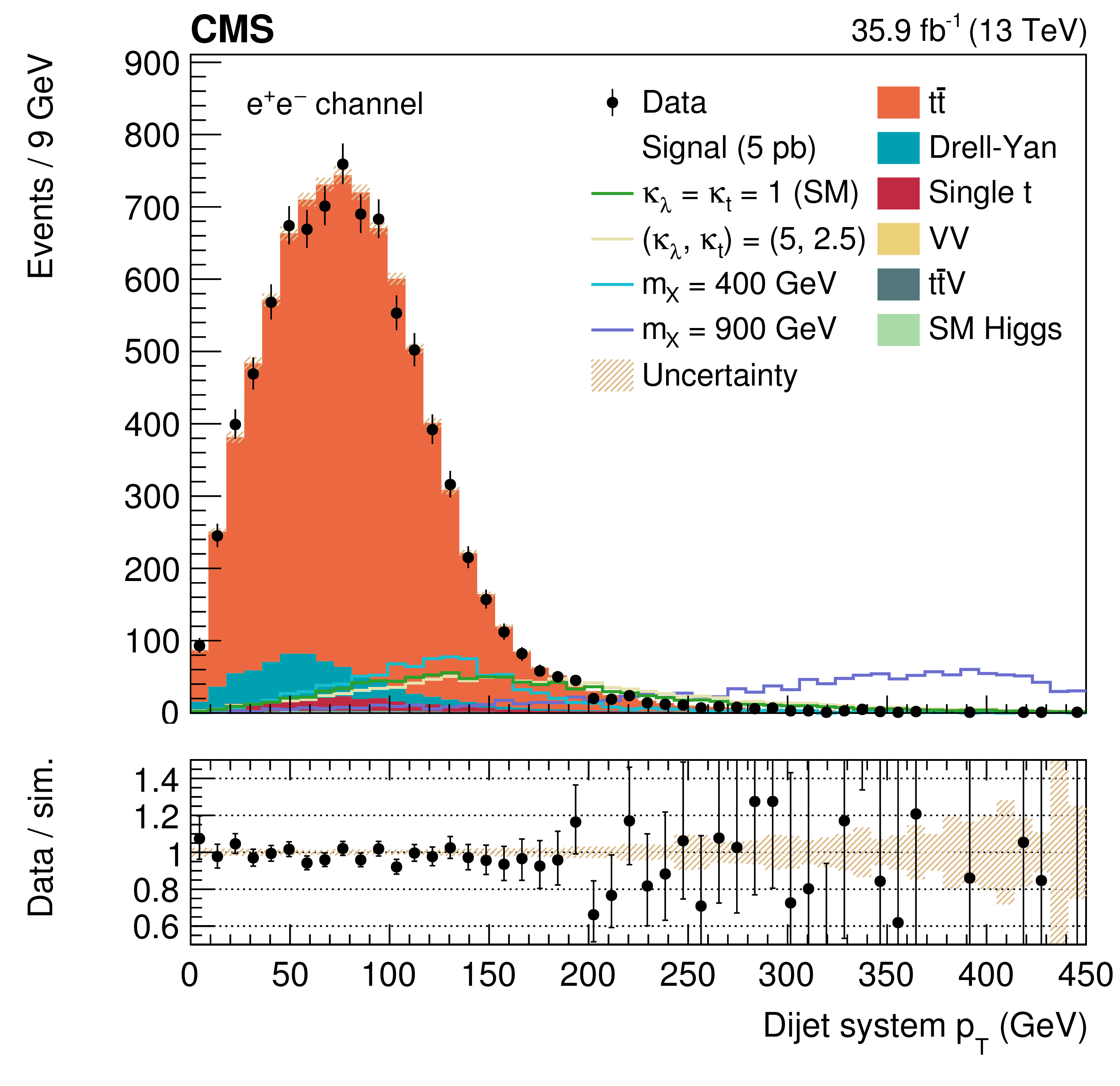
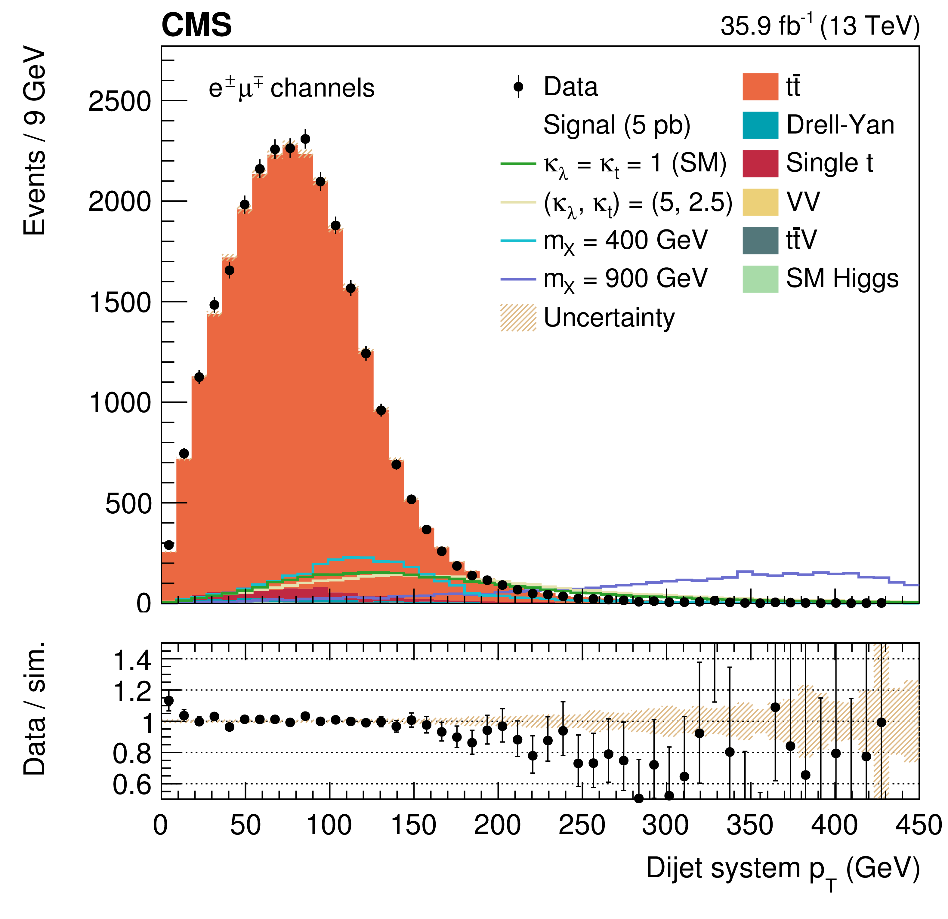
Figure 2:
The dijet $ {p_{\mathrm {T}}} $ distributions in data and simulated events after requiring two leptons, two b-tagged jets, and 12 $ < {m_{\ell \ell }} < m_{\mathrm{ Z } } - $ 15 GeV, for $\mathrm{ e }^{+} \mathrm{ e }^{-} $ (top left), $\mathrm{ e }^{\mp} {\mu ^\mp } $ (top right), and $\mu^{+} \mu^{-} $ (bottom) events. The various signal hypotheses displayed have been scaled to a cross section of 5 pb for display purposes. Error bars indicate statistical uncertainties, while shaded bands show post-fit systematic uncertainties. |
png pdf |
Figure 2-a:
The dijet $ {p_{\mathrm {T}}} $ distributions in data and simulated events after requiring two leptons, two b-tagged jets, and 12 $ < {m_{\ell \ell }} < m_{\mathrm{ Z } } - $ 15 GeV, for $\mathrm{ e }^{+} \mathrm{ e }^{-} $ events. The various signal hypotheses displayed have been scaled to a cross section of 5 pb for display purposes. Error bars indicate statistical uncertainties, while shaded bands show post-fit systematic uncertainties. |
png pdf |
Figure 2-b:
The dijet $ {p_{\mathrm {T}}} $ distributions in data and simulated events after requiring two leptons, two b-tagged jets, and 12 $ < {m_{\ell \ell }} < m_{\mathrm{ Z } } - $ 15 GeV, for $\mathrm{ e }^{\mp} {\mu ^\mp } $ events. The various signal hypotheses displayed have been scaled to a cross section of 5 pb for display purposes. Error bars indicate statistical uncertainties, while shaded bands show post-fit systematic uncertainties. |

png pdf |
Figure 2-c:
The dijet $ {p_{\mathrm {T}}} $ distributions in data and simulated events after requiring two leptons, two b-tagged jets, and 12 $ < {m_{\ell \ell }} < m_{\mathrm{ Z } } - $ 15 GeV, for $\mu^{+} \mu^{-} $ events. The various signal hypotheses displayed have been scaled to a cross section of 5 pb for display purposes. Error bars indicate statistical uncertainties, while shaded bands show post-fit systematic uncertainties. |
png pdf |
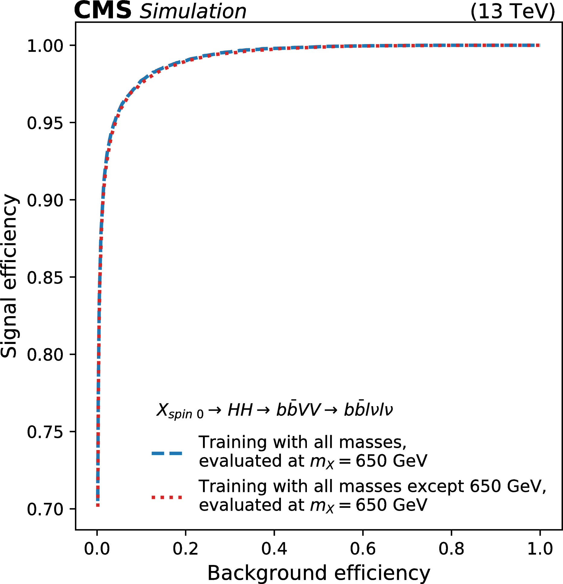
Figure 3:
Performance of the parameterised DNN for the resonant search, shown as the selection efficiency for the $ {m_{\text {X}}} =$ 650 GeV signal as a function of the selection efficiency for the background (ROC curve), for the combined $ {\mathrm {e}^+} {\mathrm {e}^-}$, $ {\mu ^+} {\mu ^-} $ and $ {\mathrm {e}^\pm} {\mu ^\mp} $ channels. The dashed line corresponds to the DNN used in the analysis, trained on all available signal samples, and evaluated at $ {m_{\text {X}}} =$ 650 GeV. The dotted line shows an alternative DNN trained using all signal samples except for $ {m_{\text {X}}} =$ 650 GeV, and evaluated at $ {m_{\text {X}}} =$ 650 GeV. Both curves overlap, indicating that the parameterised DNN is able to generalise to cases not seen during the training phase by interpolating the signal behaviour from nearby $ {m_{\text {X}}} $ points. |
png pdf |
Figure 3-a:
Performance of the parameterised DNN for the resonant search, shown as the selection efficiency for the $ {m_{\text {X}}} =$ 650 GeV signal as a function of the selection efficiency for the background (ROC curve), for the combined $ {\mathrm {e}^+} {\mathrm {e}^-}$, $ {\mu ^+} {\mu ^-} $ and $ {\mathrm {e}^\pm} {\mu ^\mp} $ channels. The dashed line corresponds to the DNN used in the analysis, trained on all available signal samples, and evaluated at $ {m_{\text {X}}} =$ 650 GeV. The dotted line shows an alternative DNN trained using all signal samples except for $ {m_{\text {X}}} =$ 650 GeV, and evaluated at $ {m_{\text {X}}} =$ 650 GeV. Both curves overlap, indicating that the parameterised DNN is able to generalise to cases not seen during the training phase by interpolating the signal behaviour from nearby $ {m_{\text {X}}} $ points. |

png pdf |
Figure 3-b:
Performance of the parameterised DNN for the resonant search, shown as the selection efficiency for the $ {m_{\text {X}}} =$ 650 GeV signal as a function of the selection efficiency for the background (ROC curve), for the combined $ {\mathrm {e}^+} {\mathrm {e}^-}$, $ {\mu ^+} {\mu ^-} $ and $ {\mathrm {e}^\pm} {\mu ^\mp} $ channels. The dashed line corresponds to the DNN used in the analysis, trained on all available signal samples, and evaluated at $ {m_{\text {X}}} =$ 650 GeV. The dotted line shows an alternative DNN trained using all signal samples except for $ {m_{\text {X}}} =$ 650 GeV, and evaluated at $ {m_{\text {X}}} =$ 650 GeV. Both curves overlap, indicating that the parameterised DNN is able to generalise to cases not seen during the training phase by interpolating the signal behaviour from nearby $ {m_{\text {X}}} $ points. |

png pdf |
Figure 3-c:
Performance of the parameterised DNN for the resonant search, shown as the selection efficiency for the $ {m_{\text {X}}} =$ 650 GeV signal as a function of the selection efficiency for the background (ROC curve), for the combined $ {\mathrm {e}^+} {\mathrm {e}^-}$, $ {\mu ^+} {\mu ^-} $ and $ {\mathrm {e}^\pm} {\mu ^\mp} $ channels. The dashed line corresponds to the DNN used in the analysis, trained on all available signal samples, and evaluated at $ {m_{\text {X}}} =$ 650 GeV. The dotted line shows an alternative DNN trained using all signal samples except for $ {m_{\text {X}}} =$ 650 GeV, and evaluated at $ {m_{\text {X}}} =$ 650 GeV. Both curves overlap, indicating that the parameterised DNN is able to generalise to cases not seen during the training phase by interpolating the signal behaviour from nearby $ {m_{\text {X}}} $ points. |
png pdf |
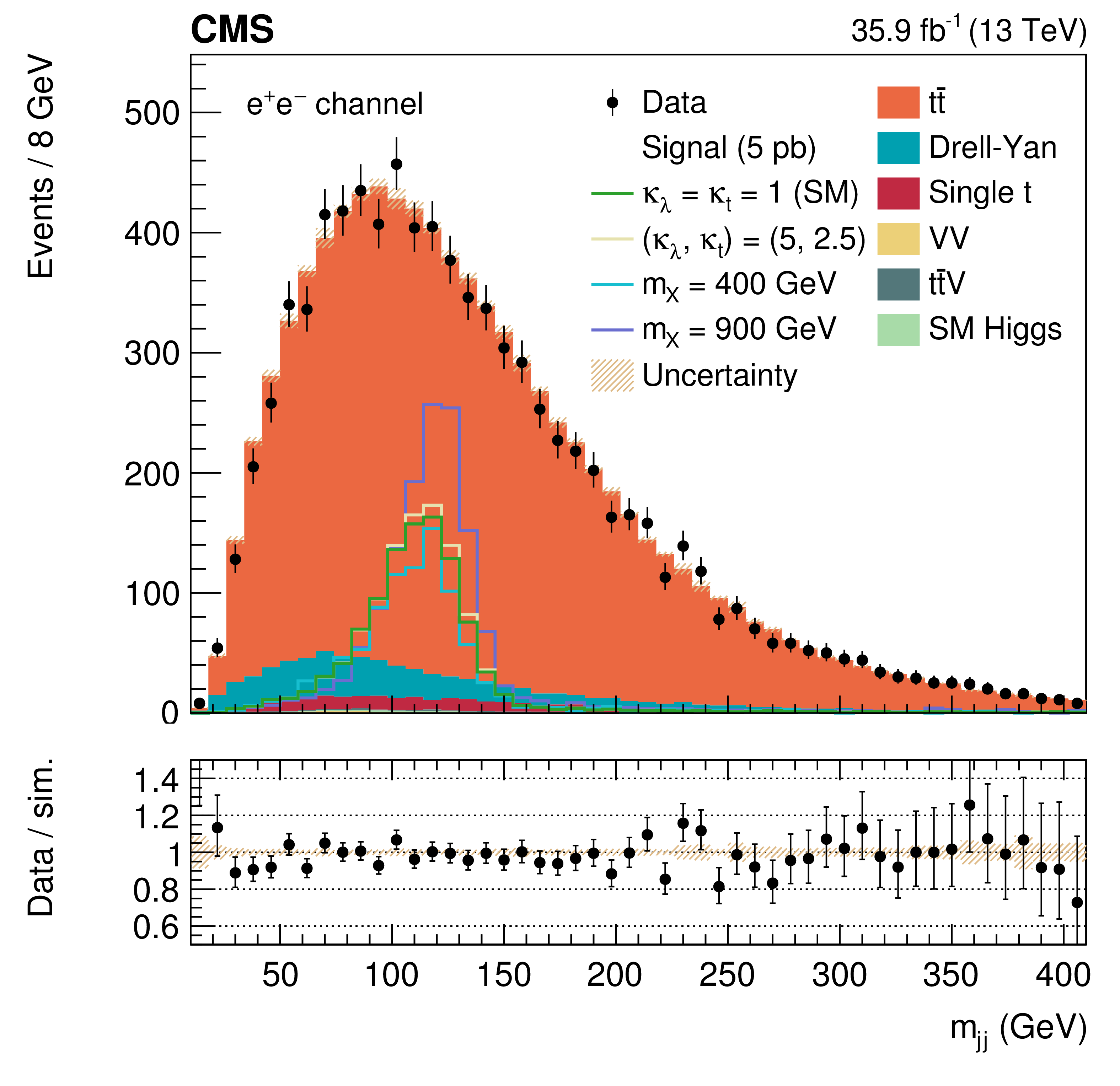
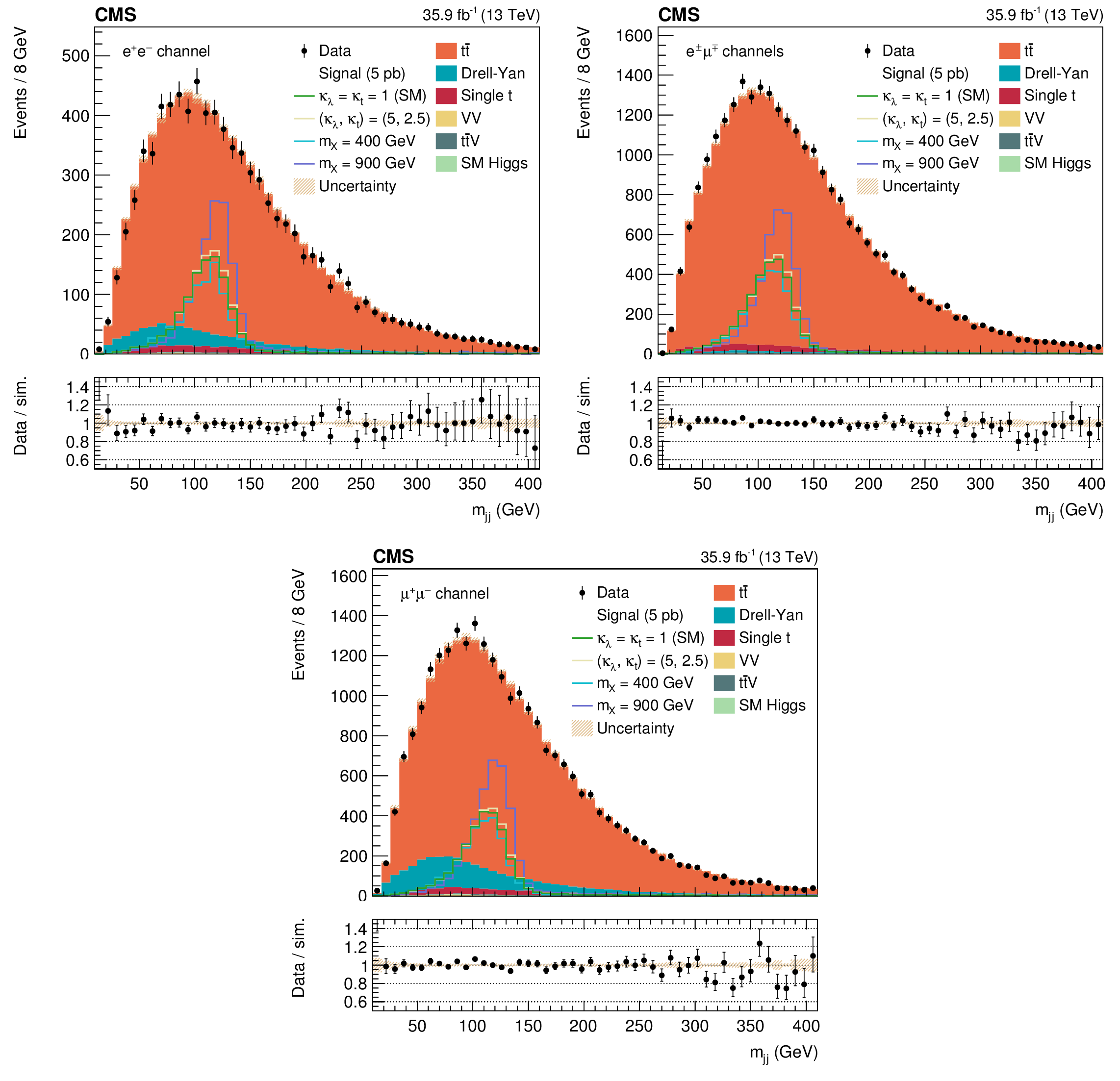
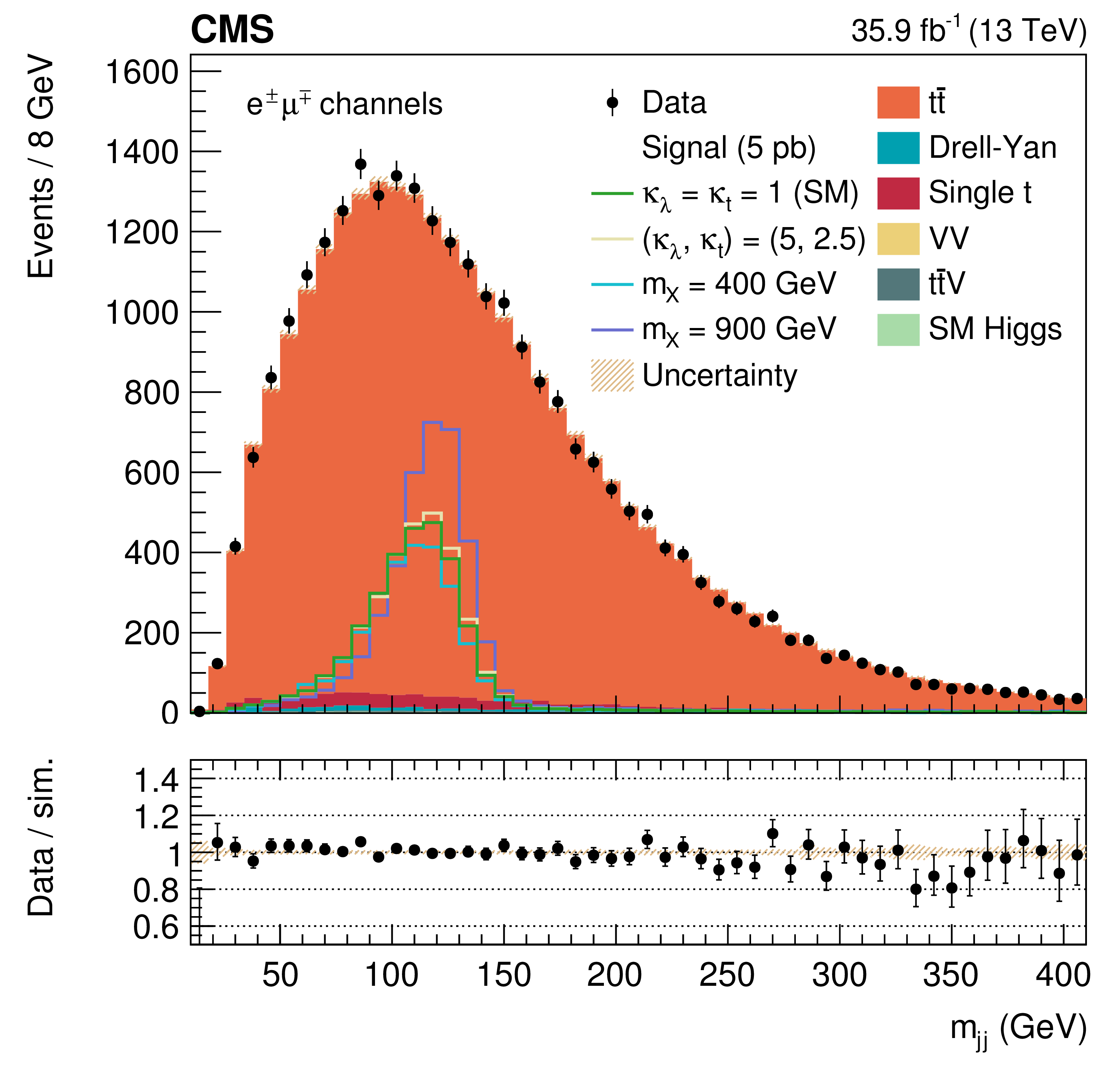
Figure 4:
The ${m_{ {\mathrm {j}} {\mathrm {j}} }}$ distribution in data and simulated events after requiring all selection criteria in the $\mathrm{ e }^{+} \mathrm{ e }^{-} $ (top left), $\mathrm{ e }^{\mp} {\mu ^\mp } $ (top right), and $\mu^{+} \mu^{-} $ (bottom) channels. The various signal hypotheses displayed have been scaled to a cross section of 5 pb for display purposes. Error bars indicate statistical uncertainties, while shaded bands show post-fit systematic uncertainties. |

png pdf |
Figure 4-a:
The ${m_{ {\mathrm {j}} {\mathrm {j}} }}$ distribution in data and simulated events after requiring all selection criteria in the $\mathrm{ e }^{+} \mathrm{ e }^{-} $ channel. The various signal hypotheses displayed have been scaled to a cross section of 5 pb for display purposes. Error bars indicate statistical uncertainties, while shaded bands show post-fit systematic uncertainties. |
png pdf |
Figure 4-b:
The ${m_{ {\mathrm {j}} {\mathrm {j}} }}$ distribution in data and simulated events after requiring all selection criteria in the $\mathrm{ e }^{\mp} {\mu ^\mp } $ channel. The various signal hypotheses displayed have been scaled to a cross section of 5 pb for display purposes. Error bars indicate statistical uncertainties, while shaded bands show post-fit systematic uncertainties. |

png pdf |
Figure 4-c:
The ${m_{ {\mathrm {j}} {\mathrm {j}} }}$ distribution in data and simulated events after requiring all selection criteria in the $\mu^{+} \mu^{-} $ channel. The various signal hypotheses displayed have been scaled to a cross section of 5 pb for display purposes. Error bars indicate statistical uncertainties, while shaded bands show post-fit systematic uncertainties. |

png pdf |
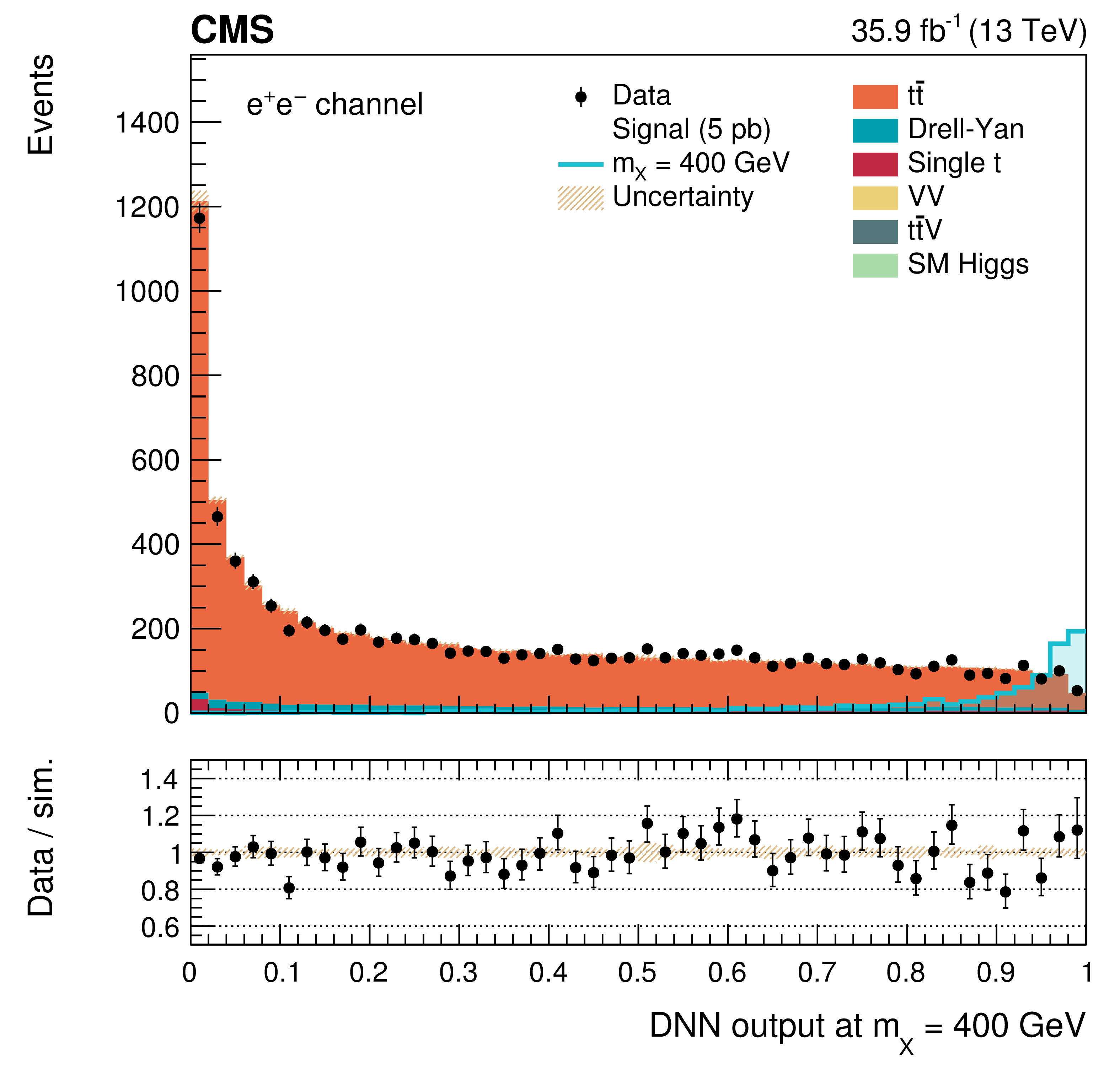
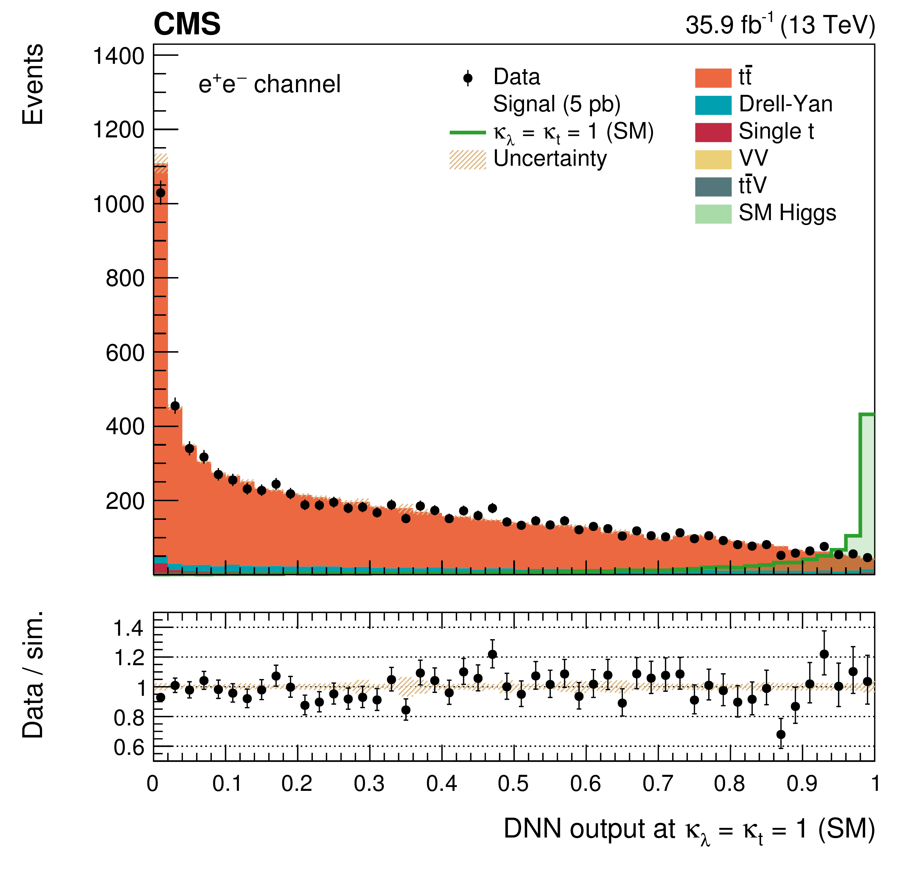
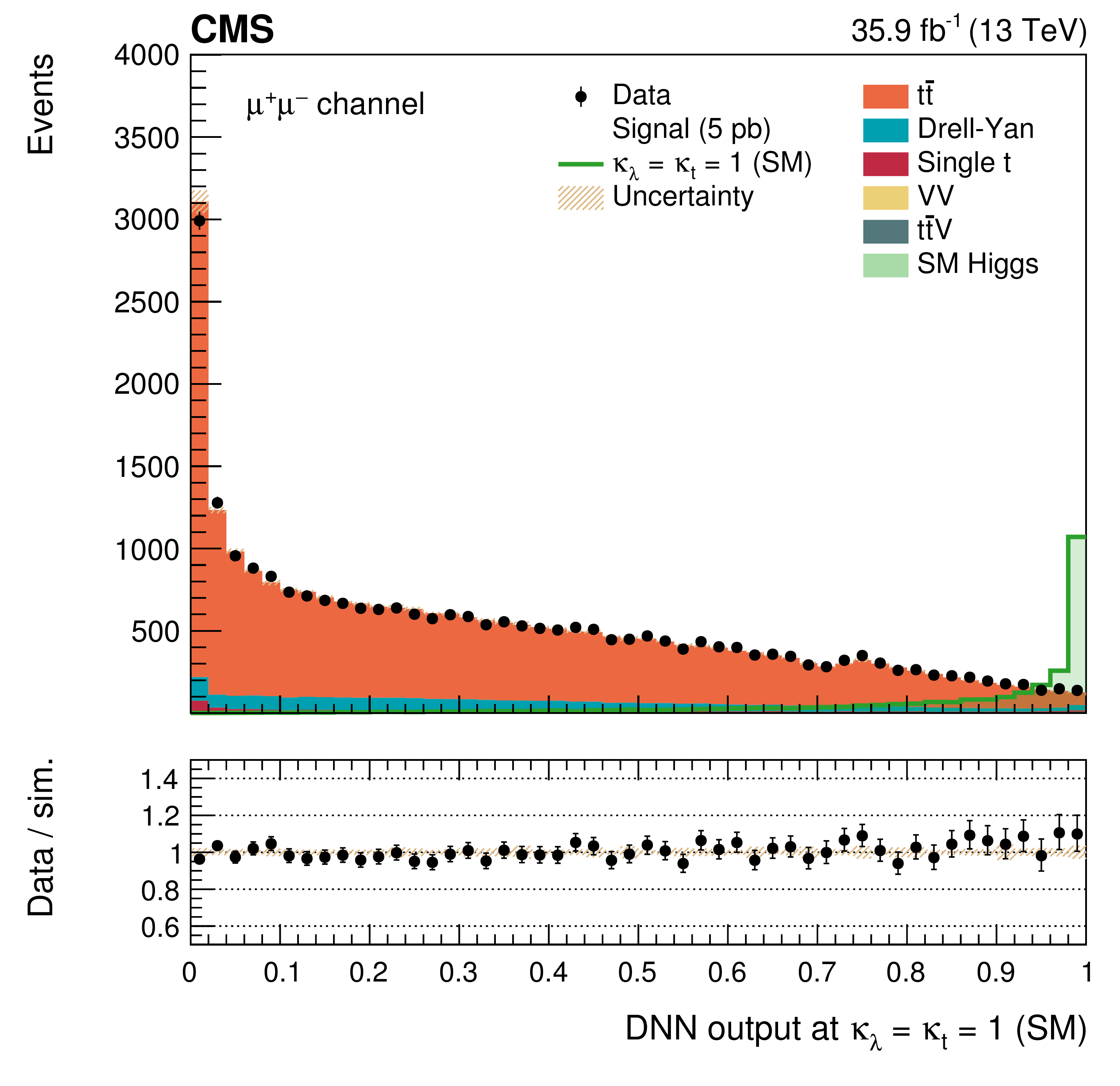
Figure 5:
The DNN output distributions in data and simulated events after requiring all selection criteria, in the $ {\mathrm {e}^+} {\mathrm {e}^-}$ (top), $ {\mathrm {e}^\pm} {} {\mu ^\mp} $ (middle), and $ {\mu ^+} {\mu ^-} $ (bottom) channels. Output values towards 0 are background-like, while output values towards 1 are signal-like. The parameterised resonant DNN output (left) is evaluated at $ {m_{\text {X}}} = $ 400 GeV and the parameterised nonresonant DNN output (right) is evaluated at $\kappa _{\lambda} =1$, $\kappa _{{\mathrm {t}}} =$ 1. The two signal hypotheses displayed have been scaled to a cross section of 5 pb for display purposes. Error bars indicate statistical uncertainties, while shaded bands show post-fit systematic uncertainties. |
png pdf |
Figure 5-a:
The DNN output distributions in data and simulated events after requiring all selection criteria, in the $ {\mathrm {e}^+} {\mathrm {e}^-}$ channel. Output values towards 0 are background-like, while output values towards 1 are signal-like. The parameterised resonant DNN output is evaluated at $ {m_{\text {X}}} = $ 400 GeV. The signal hypothesis has been scaled to a cross section of 5 pb for display purposes. Error bars indicate statistical uncertainties, while shaded bands show post-fit systematic uncertainties. |
png pdf |
Figure 5-b:
The DNN output distributions in data and simulated events after requiring all selection criteria, in the $ {\mathrm {e}^+} {\mathrm {e}^-}$ channel. Output values towards 0 are background-like, while output values towards 1 are signal-like. The parameterised nonresonant DNN output is evaluated at $\kappa _{\lambda} =1$, $\kappa _{{\mathrm {t}}} =$ 1. The signal hypothesis has been scaled to a cross section of 5 pb for display purposes. Error bars indicate statistical uncertainties, while shaded bands show post-fit systematic uncertainties. |

png pdf |
Figure 5-c:
The DNN output distributions in data and simulated events after requiring all selection criteria, in the $ {\mathrm {e}^\pm} {} {\mu ^\mp} $ channel. Output values towards 0 are background-like, while output values towards 1 are signal-like. The parameterised resonant DNN output is evaluated at $ {m_{\text {X}}} = $ 400 GeV. The signal hypothesis has been scaled to a cross section of 5 pb for display purposes. Error bars indicate statistical uncertainties, while shaded bands show post-fit systematic uncertainties. |

png pdf |
Figure 5-d:
The DNN output distributions in data and simulated events after requiring all selection criteria, in the $ {\mathrm {e}^\pm} {} {\mu ^\mp} $ channel. Output values towards 0 are background-like, while output values towards 1 are signal-like. The parameterised nonresonant DNN output is evaluated at $\kappa _{\lambda} =1$, $\kappa _{{\mathrm {t}}} =$ 1. The signal hypothesis has been scaled to a cross section of 5 pb for display purposes. Error bars indicate statistical uncertainties, while shaded bands show post-fit systematic uncertainties. |

png pdf |
Figure 5-e:
The DNN output distributions in data and simulated events after requiring all selection criteria, in the $ {\mu ^+} {\mu ^-} $ channel. Output values towards 0 are background-like, while output values towards 1 are signal-like. The parameterised resonant DNN output is evaluated at $ {m_{\text {X}}} = $ 400 GeV. The signal hypothesis has been scaled to a cross section of 5 pb for display purposes. Error bars indicate statistical uncertainties, while shaded bands show post-fit systematic uncertainties. |
png pdf |
Figure 5-f:
The DNN output distributions in data and simulated events after requiring all selection criteria, in the $ {\mu ^+} {\mu ^-} $ channel. Output values towards 0 are background-like, while output values towards 1 are signal-like. The parameterised nonresonant DNN output is evaluated at $\kappa _{\lambda} =1$, $\kappa _{{\mathrm {t}}} =$ 1. The signal hypothesis has been scaled to a cross section of 5 pb for display purposes. Error bars indicate statistical uncertainties, while shaded bands show post-fit systematic uncertainties. |
png pdf |
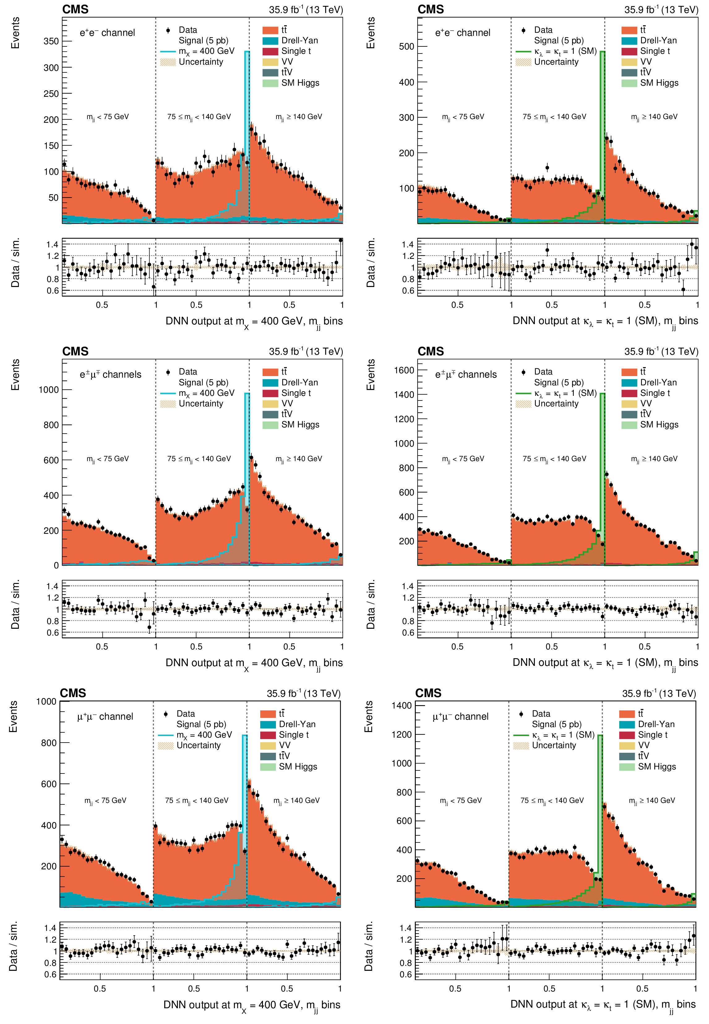
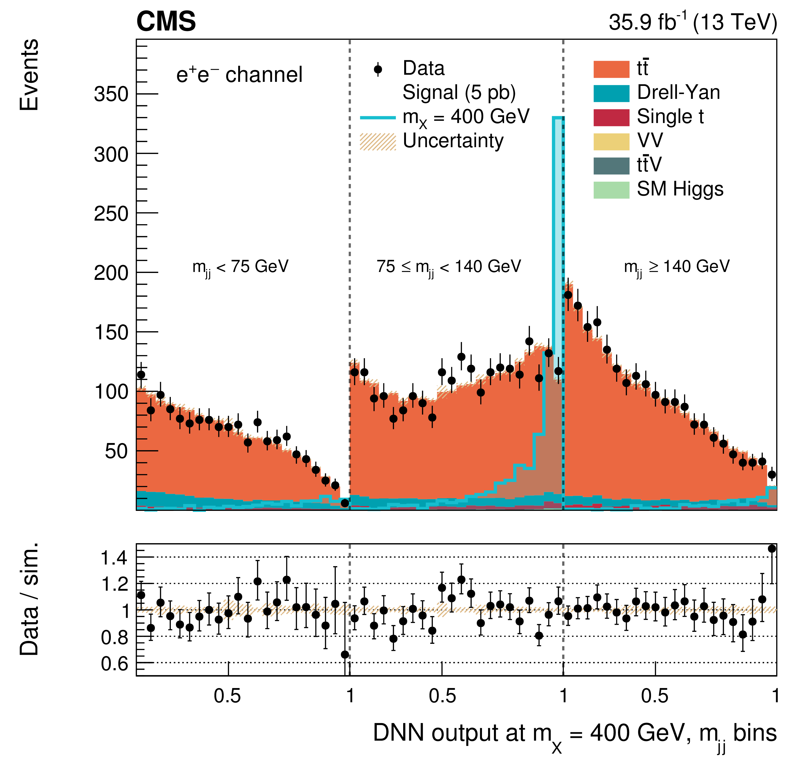
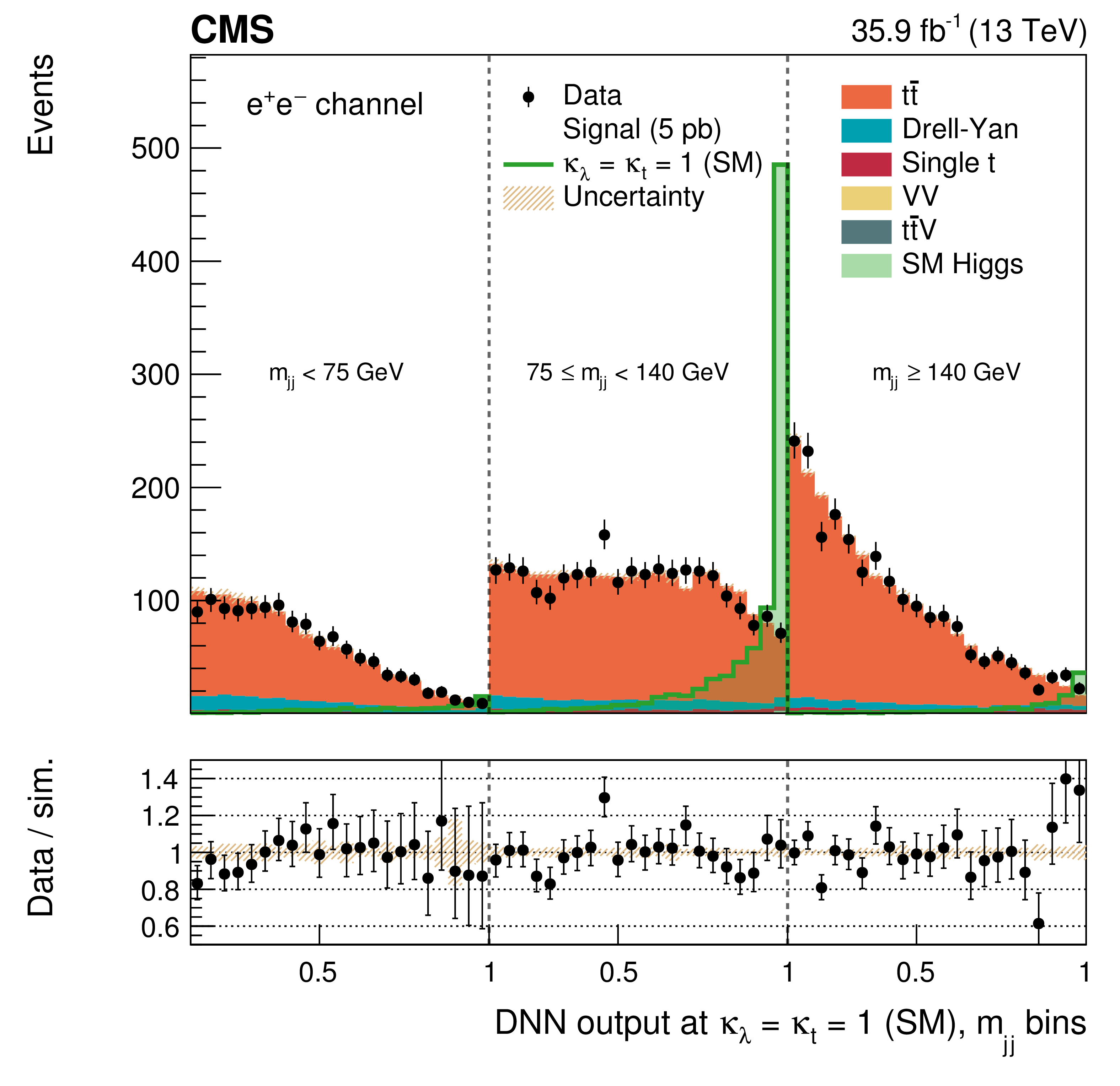
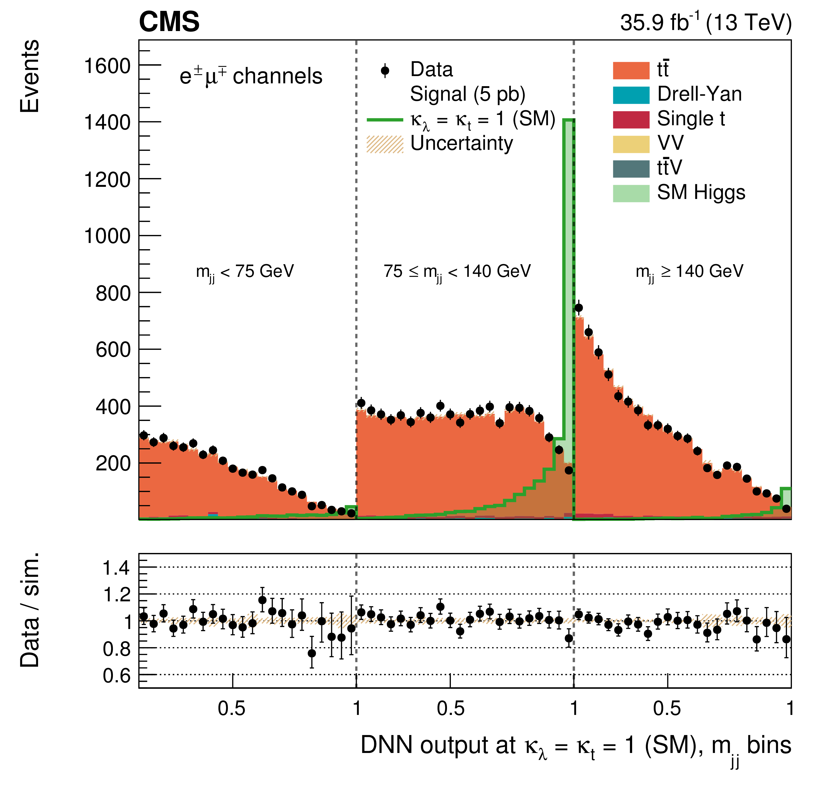
Figure 6:
The DNN output distributions in data and simulated events, for the $ {\mathrm {e}^+} {\mathrm {e}^-}$ (top), $ {\mathrm {e}^\pm} {} {\mu ^\mp} $ (middle), and $ {\mu ^+} {\mu ^-} $ (bottom) channels, in three different ${m_{{\mathrm {j}} {\mathrm {j}}}}$ regions: $ {m_{{\mathrm {j}} {\mathrm {j}}}} < $ 75 GeV, $ {m_{{\mathrm {j}} {\mathrm {j}}}} \in $ [75,140] GeV, and $ {m_{{\mathrm {j}} {\mathrm {j}}}} \geq $ 140 GeV. The parameterised resonant DNN output (left) is evaluated at $ {m_{\text {X}}} = $ 400 GeV and the parameterised nonresonant DNN output (right) is evaluated at $\kappa _{\lambda} = $ 1, $\kappa _{{\mathrm {t}}} = $ 1. The two signal hypotheses displayed have been scaled to a cross section of 5 pb for display purposes. Error bars indicate statistical uncertainties, while shaded bands show post-fit systematic uncertainties. |
png pdf |
Figure 6-a:
The DNN output distributions in data and simulated events, for the $ {\mathrm {e}^+} {\mathrm {e}^-}$ channel, in three different ${m_{{\mathrm {j}} {\mathrm {j}}}}$ regions: $ {m_{{\mathrm {j}} {\mathrm {j}}}} < $ 75 GeV, $ {m_{{\mathrm {j}} {\mathrm {j}}}} \in $ [75,140] GeV, and $ {m_{{\mathrm {j}} {\mathrm {j}}}} \geq $ 140 GeV. The parameterised resonant DNN output (left) is evaluated at $ {m_{\text {X}}} = $ 400 GeV. The signal hypothesis has been scaled to a cross section of 5 pb for display purposes. Error bars indicate statistical uncertainties, while shaded bands show post-fit systematic uncertainties. |
png pdf |
Figure 6-b:
The DNN output distributions in data and simulated events, for the $ {\mathrm {e}^+} {\mathrm {e}^-}$ channel, in three different ${m_{{\mathrm {j}} {\mathrm {j}}}}$ regions: $ {m_{{\mathrm {j}} {\mathrm {j}}}} < $ 75 GeV, $ {m_{{\mathrm {j}} {\mathrm {j}}}} \in $ [75,140] GeV, and $ {m_{{\mathrm {j}} {\mathrm {j}}}} \geq $ 140 GeV. The parameterised nonresonant DNN output is evaluated at $\kappa _{\lambda} = $ 1, $\kappa _{{\mathrm {t}}} = $ 1. The signal hypothesis has been scaled to a cross section of 5 pb for display purposes. Error bars indicate statistical uncertainties, while shaded bands show post-fit systematic uncertainties. |

png pdf |
Figure 6-c:
The DNN output distributions in data and simulated events, for the $ {\mathrm {e}^\pm} {} {\mu ^\mp} $ channel, in three different ${m_{{\mathrm {j}} {\mathrm {j}}}}$ regions: $ {m_{{\mathrm {j}} {\mathrm {j}}}} < $ 75 GeV, $ {m_{{\mathrm {j}} {\mathrm {j}}}} \in $ [75,140] GeV, and $ {m_{{\mathrm {j}} {\mathrm {j}}}} \geq $ 140 GeV. The parameterised resonant DNN output (left) is evaluated at $ {m_{\text {X}}} = $ 400 GeV. The signal hypothesis has been scaled to a cross section of 5 pb for display purposes. Error bars indicate statistical uncertainties, while shaded bands show post-fit systematic uncertainties. |
png pdf |
Figure 6-d:
The DNN output distributions in data and simulated events, for the $ {\mathrm {e}^\pm} {} {\mu ^\mp} $ channel, in three different ${m_{{\mathrm {j}} {\mathrm {j}}}}$ regions: $ {m_{{\mathrm {j}} {\mathrm {j}}}} < $ 75 GeV, $ {m_{{\mathrm {j}} {\mathrm {j}}}} \in $ [75,140] GeV, and $ {m_{{\mathrm {j}} {\mathrm {j}}}} \geq $ 140 GeV. The parameterised nonresonant DNN output is evaluated at $\kappa _{\lambda} = $ 1, $\kappa _{{\mathrm {t}}} = $ 1. The signal hypothesis has been scaled to a cross section of 5 pb for display purposes. Error bars indicate statistical uncertainties, while shaded bands show post-fit systematic uncertainties. |
png pdf |
Figure 6-e:
The DNN output distributions in data and simulated events, for the $ {\mu ^+} {\mu ^-} $ channel, in three different ${m_{{\mathrm {j}} {\mathrm {j}}}}$ regions: $ {m_{{\mathrm {j}} {\mathrm {j}}}} < $ 75 GeV, $ {m_{{\mathrm {j}} {\mathrm {j}}}} \in $ [75,140] GeV, and $ {m_{{\mathrm {j}} {\mathrm {j}}}} \geq $ 140 GeV. The parameterised resonant DNN output (left) is evaluated at $ {m_{\text {X}}} = $ 400 GeV. The signal hypothesis has been scaled to a cross section of 5 pb for display purposes. Error bars indicate statistical uncertainties, while shaded bands show post-fit systematic uncertainties. |
png pdf |
Figure 6-f:
The DNN output distributions in data and simulated events, for the $ {\mu ^+} {\mu ^-} $ channel, in three different ${m_{{\mathrm {j}} {\mathrm {j}}}}$ regions: $ {m_{{\mathrm {j}} {\mathrm {j}}}} < $ 75 GeV, $ {m_{{\mathrm {j}} {\mathrm {j}}}} \in $ [75,140] GeV, and $ {m_{{\mathrm {j}} {\mathrm {j}}}} \geq $ 140 GeV. The parameterised nonresonant DNN output is evaluated at $\kappa _{\lambda} = $ 1, $\kappa _{{\mathrm {t}}} = $ 1. The signal hypothesis has been scaled to a cross section of 5 pb for display purposes. Error bars indicate statistical uncertainties, while shaded bands show post-fit systematic uncertainties. |
png pdf |
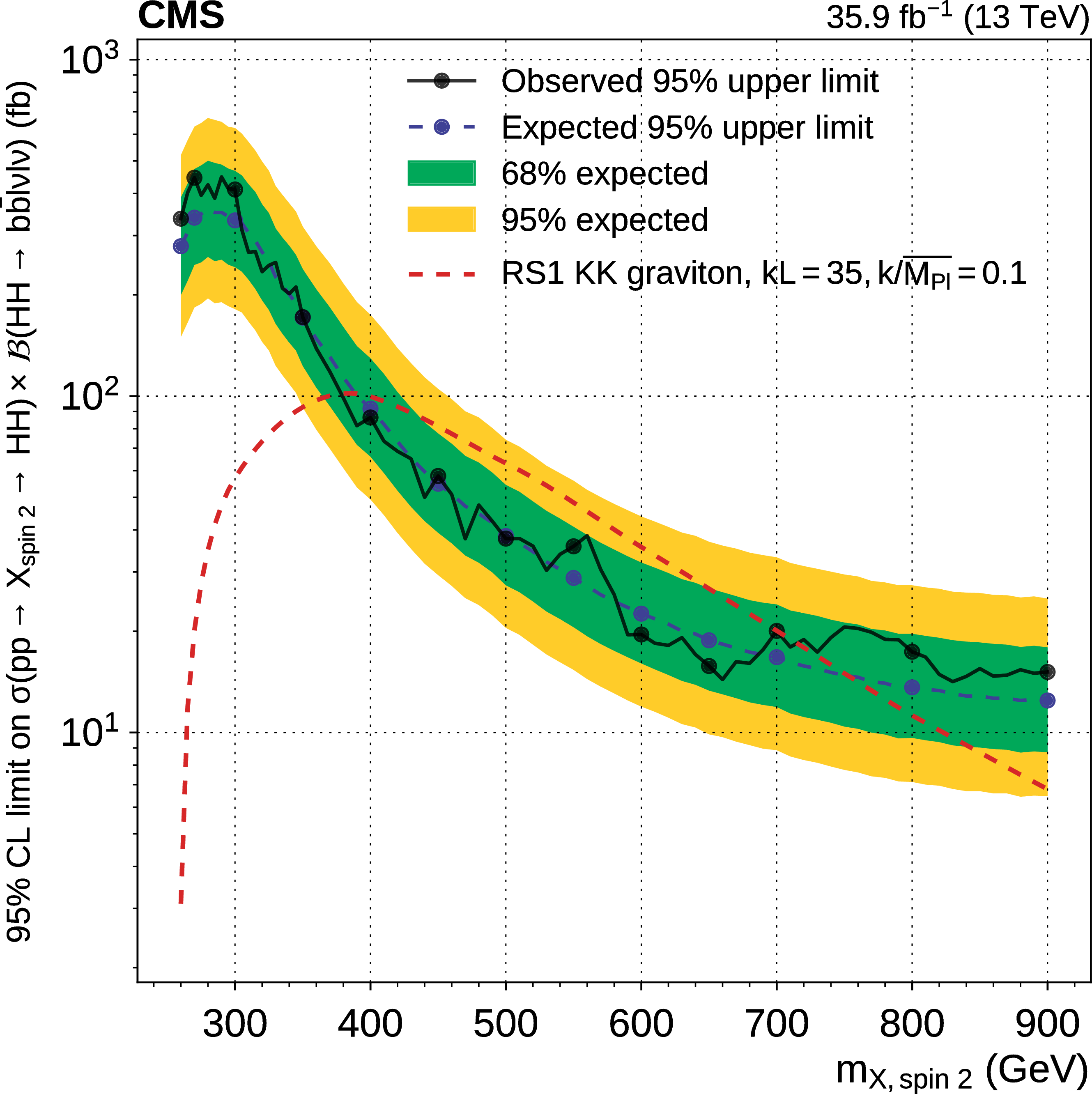
Figure 7:
Expected (dashed) and observed (continuous) 95% CL upper limits on the product of the production cross section for $\mathrm{X} $ and branching fraction for $\mathrm{X} \to \mathrm{ H } \mathrm{ H } \to {\mathrm{ b \bar{b} } } {\mathrm {V}} {\mathrm {V}} \to {\mathrm{ b \bar{b} } } \ell \nu \ell \nu $, as a function of $ {m_{\text {X}}} $. The inner (green) band and the outer (yellow) band indicate the regions containing 68 and 95%, respectively, of the distribution of limits expected under the background-only hypothesis. These limits are computed using the asymptotic $\mathrm {CL_s}$ method, combining the $\mathrm{ e }^{+} \mathrm{ e }^{-} $, $ \mu^+ \mu^-$ and $\mathrm{ e } ^{\pm }\mu ^{\mp }$ channels, for spin-0 (left) and spin-2 (right) hypotheses. The solid circles represent fully-simulated mass points. The dashed red lines represent possible cross sections for the production of a radion (left) or a Kaluza-Klein graviton (right), assuming absence of mixing with the Higgs boson [49]. Parameters used to compute these cross sections can be found in the legend. |
png pdf |
Figure 7-a:
Expected (dashed) and observed (continuous) 95% CL upper limits on the product of the production cross section for $\mathrm{X} $ and branching fraction for $\mathrm{X} \to \mathrm{ H } \mathrm{ H } \to {\mathrm{ b \bar{b} } } {\mathrm {V}} {\mathrm {V}} \to {\mathrm{ b \bar{b} } } \ell \nu \ell \nu $, as a function of $ {m_{\text {X}}} $. The inner (green) band and the outer (yellow) band indicate the regions containing 68 and 95%, respectively, of the distribution of limits expected under the background-only hypothesis. These limits are computed using the asymptotic $\mathrm {CL_s}$ method, combining the $\mathrm{ e }^{+} \mathrm{ e }^{-} $, $ \mu^+ \mu^-$ and $\mathrm{ e } ^{\pm }\mu ^{\mp }$ channels, for the spin-0 hypothesis. The solid circles represent fully-simulated mass points. The dashed red lines represent possible cross sections for the production of a radion, assuming absence of mixing with the Higgs boson [49]. Parameters used to compute these cross sections can be found in the legend. |
png pdf |
Figure 7-b:
Expected (dashed) and observed (continuous) 95% CL upper limits on the product of the production cross section for $\mathrm{X} $ and branching fraction for $\mathrm{X} \to \mathrm{ H } \mathrm{ H } \to {\mathrm{ b \bar{b} } } {\mathrm {V}} {\mathrm {V}} \to {\mathrm{ b \bar{b} } } \ell \nu \ell \nu $, as a function of $ {m_{\text {X}}} $. The inner (green) band and the outer (yellow) band indicate the regions containing 68 and 95%, respectively, of the distribution of limits expected under the background-only hypothesis. These limits are computed using the asymptotic $\mathrm {CL_s}$ method, combining the $\mathrm{ e }^{+} \mathrm{ e }^{-} $, $ \mu^+ \mu^-$ and $\mathrm{ e } ^{\pm }\mu ^{\mp }$ channels, for the spin-2 hypothesis. The solid circles represent fully-simulated mass points. The dashed red lines represent possible cross sections for the production of a Kaluza-Klein graviton, assuming absence of mixing with the Higgs boson [49]. Parameters used to compute these cross sections can be found in the legend. |

png pdf |
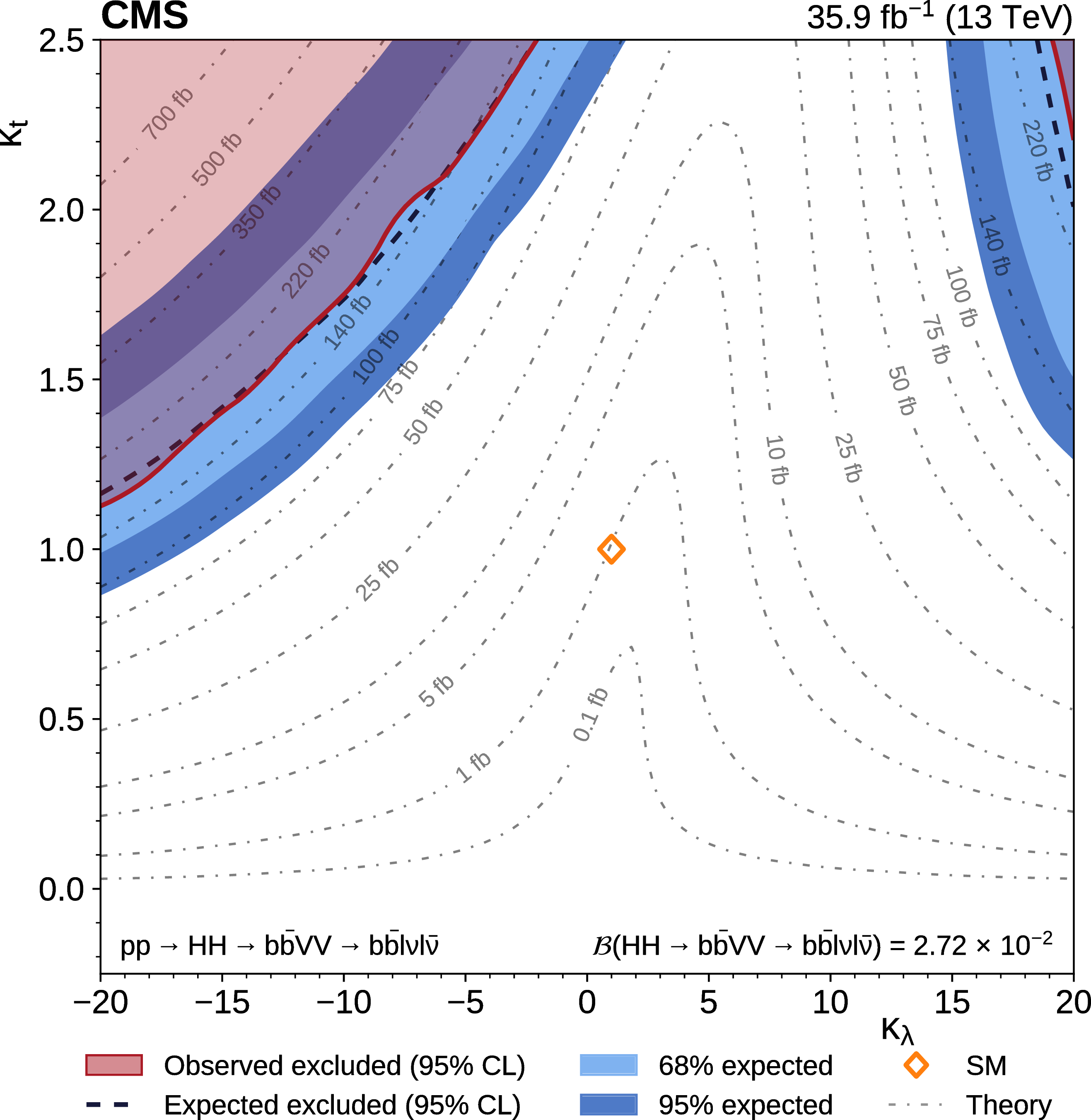
Figure 8:
Left: expected (dashed) and observed (continuous) 95% CL upper limits on the product of the Higgs boson pair production cross section and branching fraction for $\mathrm{ H } \mathrm{ H } \to {\mathrm{ b \bar{b} } } {\mathrm {V}} {\mathrm {V}} \to {\mathrm{ b \bar{b} } } \ell \nu \ell \nu $ as a function of $\kappa _{\lambda } / \kappa _{\mathrm{ t } }$. The inner (green) band and the outer (yellow) band indicate the regions containing 68 and 95%, respectively, of the distribution of limits expected under the background-only hypothesis. Red lines show the theoretical cross sections, along with their uncertainties, for $\kappa _{\mathrm{ t } } = $ 1 (SM) and $\kappa _{\mathrm{ t } } = $ 2. Right: exclusions in the ($\kappa _{\lambda }$, $\kappa _{\mathrm{ t } }$) plane. The red region corresponds to parameters excluded at 95% CL with the observed data, whereas the dashed black line and the blue areas correspond to the expected exclusions and the 68 and 95% bands (light and dark respectively). Isolines of the product of the theoretical cross section and branching fraction for $\mathrm{ H } \mathrm{ H } \to {\mathrm{ b \bar{b} } } {\mathrm {V}} {\mathrm {V}} \to {\mathrm{ b \bar{b} } } \ell \nu \ell \nu $ are shown as dashed-dotted lines. The diamond marker indicates the prediction of the SM. All theoretical predictions are extracted from Refs. [12,13,14,15,16,17,84]. |

png pdf |
Figure 8-a:
Expected (dashed) and observed (continuous) 95% CL upper limits on the product of the Higgs boson pair production cross section and branching fraction for $\mathrm{ H } \mathrm{ H } \to {\mathrm{ b \bar{b} } } {\mathrm {V}} {\mathrm {V}} \to {\mathrm{ b \bar{b} } } \ell \nu \ell \nu $ as a function of $\kappa _{\lambda } / \kappa _{\mathrm{ t } }$. The inner (green) band and the outer (yellow) band indicate the regions containing 68 and 95%, respectively, of the distribution of limits expected under the background-only hypothesis. Red lines show the theoretical cross sections, along with their uncertainties, for $\kappa _{\mathrm{ t } } = $ 1 (SM) and $\kappa _{\mathrm{ t } } = $ 2. |
png pdf |
Figure 8-b:
Exclusions in the ($\kappa _{\lambda }$, $\kappa _{\mathrm{ t } }$) plane. The red region corresponds to parameters excluded at 95% CL with the observed data, whereas the dashed black line and the blue areas correspond to the expected exclusions and the 68 and 95% bands (light and dark respectively). Isolines of the product of the theoretical cross section and branching fraction for $\mathrm{ H } \mathrm{ H } \to {\mathrm{ b \bar{b} } } {\mathrm {V}} {\mathrm {V}} \to {\mathrm{ b \bar{b} } } \ell \nu \ell \nu $ are shown as dashed-dotted lines. The diamond marker indicates the prediction of the SM. All theoretical predictions are extracted from Refs. [12,13,14,15,16,17,84]. |
| Tables | |
png pdf |
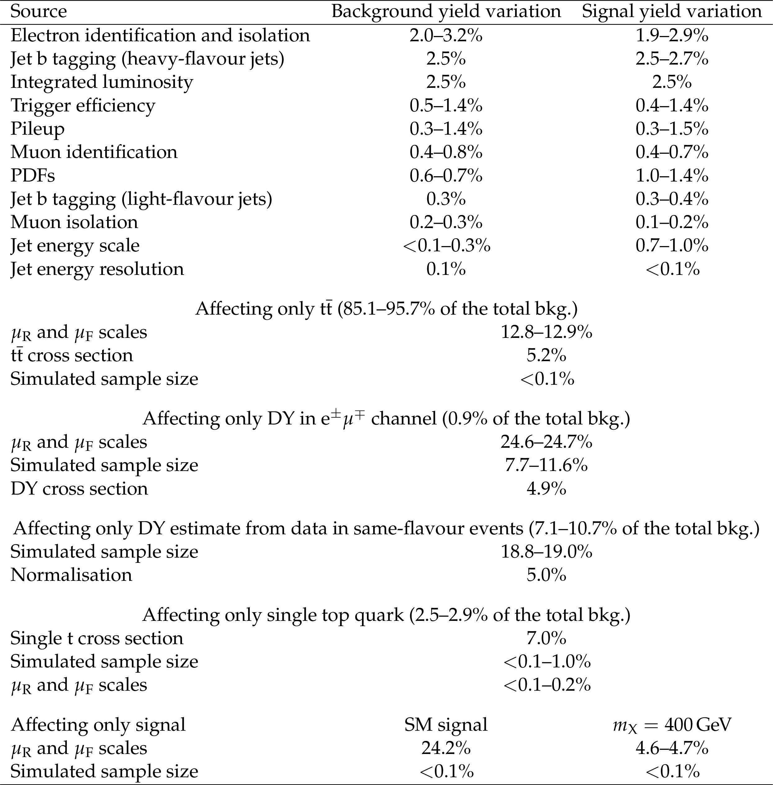
Table 1:
Summary of the systematic uncertainties and their impact on total background yields and on the SM and $ {m_{\text {X}}} = 400$ GeV signal hypotheses in the signal region. |
| Summary |
|
A search for resonant and nonresonant Higgs boson pair production (HH) is presented, where one of the Higgs bosons decays to $\mathrm{ b \bar{b} }$, and the other to $\mathrm{ V }\mathrm{ V } \to \ell\nu \ell\nu$, where V is either a W or a Z boson. The LHC proton-proton collision data at $\sqrt{s}= $ 13 TeV collected by the CMS experiment corresponding to an integrated luminosity of 35.9 fb$^{-1}$ are used. Masses are considered in the range between 260 and 900 GeV for the resonant search, while anomalous Higgs boson self-coupling and coupling to the top quark are considered in addition to the standard model case for the nonresonant search. The results obtained are in agreement, within uncertainties, with the predictions of the standard model. For the resonant search, the data exclude a product of the production cross section and branching fraction of narrow-width spin-0 particles from 430 to 17 fb, in agreement with the expectations of 340$^{+140}_{-100}$ to 14$^{+6}_{-4}$ fb, and narrow-width spin-2 particles produced with minimal gravity-like coupling from 450 to 14 fb, in agreement with the expectations of 360$^{+140}_{-100}$ to 13$^{+6}_{-4}$ fb. For the standard model HH hypothesis, the data exclude a product of the production cross section and branching fraction of 72 fb, corresponding to 79 times the SM cross section. The expected values exclude a product of the production cross section and branching fraction of 81$^{+42}_{-25}$ fb, corresponding to 89$^{+47}_{-28}$ times the SM cross section. |
| References | ||||
| 1 | F. Englert and R. Brout | Broken Symmetry and the Mass of Gauge Vector Mesons | PRL 13 (1964) 321 | |
| 2 | P. W. Higgs | Broken symmetries, massless particles and gauge fields | PL12 (1964) 132 | |
| 3 | P. W. Higgs | Broken Symmetries and the Masses of Gauge Bosons | PRL 13 (1964) 508 | |
| 4 | G. S. Guralnik, C. R. Hagen, and T. W. B. Kibble | Global conservation laws and massless particles | PRL 13 (1964) 585 | |
| 5 | P. W. Higgs | Spontaneous symmetry breakdown without massless bosons | PR145 (1966) 1156 | |
| 6 | T. W. B. Kibble | Symmetry breaking in non-abelian gauge theories | PR155 (1967) 1554 | |
| 7 | ATLAS Collaboration | Observation of a new particle in the search for the Standard Model Higgs boson with the ATLAS detector at the LHC | PLB 716 (2012) 1 | 1207.7214 |
| 8 | CMS Collaboration | Observation of a new boson at a mass of 125~GeV with the CMS experiment at the LHC | PLB 716 (2012) 30 | CMS-HIG-12-028 1207.7235 |
| 9 | CMS Collaboration | Observation of a new boson with mass near 125~GeV in $ {\mathrm{p}}{\mathrm{p}} $ collisions at $ \sqrt{s} = $ 7 and 8~TeV | JHEP 06 (2013) 081 | CMS-HIG-12-036 1303.4571 |
| 10 | CMS Collaboration | Higgs pair production at the High Luminosity LHC | CMS-PAS-FTR-15-002 | CMS-PAS-FTR-15-002 |
| 11 | CMS Collaboration | Projected performance of Higgs analyses at the HL-LHC for ECFA 2016 | CMS-PAS-FTR-16-002 | CMS-PAS-FTR-16-002 |
| 12 | D. de Florian et al. | Handbook of LHC Higgs cross sections: 4. deciphering the nature of the Higgs sector | CERN Yellow Report CERN-2017-002-M | 1610.07922 |
| 13 | D. de Florian and J. Mazzitelli | Higgs pair production at next-to-next-to-leading logarithmic accuracy at the LHC | JHEP 09 (2015) 053 | 1505.07122 |
| 14 | D. de Florian and J. Mazzitelli | Higgs boson pair production at next-to-next-to-leading order in QCD | PRL 111 (2013) 201801 | 1309.6594 |
| 15 | S. Borowka et al. | Higgs boson pair production in gluon fusion at next-to-leading order with full top-quark mass dependence | PRL 117 (2016) 012001 | 1604.06447 |
| 16 | S. Dawson, S. Dittmaier, and M. Spira | Neutral Higgs-boson pair production at hadron colliders: QCD corrections | PRD 58 (1998) 115012 | hep-ph/9805244 |
| 17 | J. Grigo, K. Melnikov, and M. Steinhauser | Virtual corrections to Higgs boson pair production in the large top quark mass limit | NPB 888 (2014) 17 | 1408.2422 |
| 18 | J. Grigo, J. Hoff, and M. Steinhauser | Higgs boson pair production: Top quark mass effects at NLO and NNLO | NPB 900 (2015) 412 | 1508.00909 |
| 19 | J. Grigo, J. Hoff, K. Melnikov, and M. Steinhauser | On the Higgs boson pair production at the LHC | NPB 875 (2013) 1 | 1305.7340 |
| 20 | R. Frederix et al. | Higgs pair production at the LHC with NLO and parton-shower effects | PLB 732 (2014) 142 | 1401.7340 |
| 21 | F. Maltoni, E. Vryonidou, and M. Zaro | Top-quark mass effects in double and triple Higgs production in gluon-gluon fusion at NLO | JHEP 11 (2014) 079 | 1408.6542 |
| 22 | A. Azatov, R. Contino, G. Panico, and M. Son | Effective field theory analysis of double Higgs boson production via gluon fusion | PRD 92 (2015) 035001 | 1502.00539 |
| 23 | F. Goertz, A. Papaefstathiou, L. L. Yang, and J. Zurita | Higgs boson pair production in the $ D = $ 6 extension of the SM | JHEP 04 (2015) 167 | 1410.3471 |
| 24 | B. Hespel, D. Lopez-Val, and E. Vryonidou | Higgs pair production via gluon fusion in the Two-Higgs-Doublet Model | JHEP 09 (2014) 124 | 1407.0281 |
| 25 | G. C. Branco et al. | Theory and phenomenology of two-Higgs-doublet models | PR 516 (2012) 1 | 1106.0034 |
| 26 | L. Randall and R. Sundrum | A large mass hierarchy from a small extra dimension | PRL 83 (1999) 3370 | hep-ph/9905221 |
| 27 | W. D. Goldberger and M. S. Wise | Modulus stabilization with bulk fields | PRL 83 (1999) 4922 | hep-ph/9907447 |
| 28 | O. DeWolfe, D. Freedman, S. Gubser, and A. Karch | Modeling the fifth dimension with scalars and gravity | PRD 62 (2000) 046008 | hep-th/9909134 |
| 29 | C. Csaki, M. Graesser, L. Randall, and J. Terning | Cosmology of brane models with radion stabilization | PRD 62 (2000) 045015 | hep-ph/9911406 |
| 30 | C. Csaki, J. Hubisz, and S. J. Lee | Radion phenomenology in realistic warped space models | PRD 76 (2007) 125015 | 0705.3844 |
| 31 | H. Davoudiasl, J. Hewett, and T. Rizzo | Phenomenology of the Randall-Sundrum gauge hierarchy model | PRL 84 (2000) 2080 | hep-ph/9909255 |
| 32 | C. Csaki, M. L. Graesser, and G. D. Kribs | Radion dynamics and electroweak physics | PRD 63 (2001) 065002 | hep-th/0008151 |
| 33 | CMS Collaboration | Search for two Higgs bosons in final states containing two photons and two bottom quarks in proton-proton collisions at 8~TeV | PRD 94 (2016) 052012 | CMS-HIG-13-032 1603.06896 |
| 34 | ATLAS Collaboration | Search for Higgs boson pair production in the $ \gamma\gamma \mathrm{b\bar{b}} $ Final State using $ {\mathrm{p}}{\mathrm{p}} $ collision Data at $ \sqrt{s}= $ 8 ~TeV from the ATLAS detector | PRL 114 (2015) 081802 | 1406.5053 |
| 35 | ATLAS Collaboration | Search for Higgs boson pair production in the $ \mathrm{b\bar{b}}\mathrm{b\bar{b}} $ final state from $ {\mathrm{p}}{\mathrm{p}} $ collisions at $ \sqrt{s} = $ 8 ~TeV with the ATLAS detector | EPJC 75 (2015) 412 | 1506.00285 |
| 36 | ATLAS Collaboration | Searches for Higgs boson pair production in the $ \mathrm{h}\mathrm{h}\to \mathrm{b}\mathrm{b}\tau\tau, \gamma\gamma \mathrm{W}\mathrm{W}^*, \gamma\gamma \mathrm{b}\mathrm{b}, \mathrm{b}\mathrm{b}\mathrm{b}\mathrm{b} $ channels with the ATLAS detector | PRD 92 (2015) 092004 | 1509.04670 |
| 37 | CMS Collaboration | A search for Higgs boson pair production in the $ \mathrm{b}\mathrm{b}\tau\tau $ final state in proton-proton collisions at $ \sqrt{s} = $ 8~TeV | Submitted to PRD | CMS-HIG-15-013 1707.00350 |
| 38 | ATLAS Collaboration | Search for pair production of Higgs bosons in the $ \mathrm{b\bar{b}}\mathrm{b\bar{b}} $ final state using proton--proton collisions at $ \sqrt{s} = $ 13 ~TeV with the ATLAS detector | PRD 94 (2016) 052002 | 1606.04782 |
| 39 | CMS Collaboration | Search for Higgs boson pair production in events with two bottom quarks and two tau leptons in proton-proton collisions at $ \sqrt{s} = $ 13~TeV | Submitted to PLB | CMS-HIG-17-002 1707.02909 |
| 40 | CMS Collaboration | The CMS experiment at the CERN LHC | JINST 03 (2008) S08004 | CMS-00-001 |
| 41 | P. Nason | A new method for combining NLO QCD with shower Monte Carlo algorithms | JHEP 11 (2004) 040 | hep-ph/0409146 |
| 42 | S. Frixione, P. Nason, and C. Oleari | Matching NLO QCD computations with parton shower simulations: the POWHEG method | JHEP 11 (2007) 070 | 0709.2092 |
| 43 | S. Alioli, P. Nason, C. Oleari, and E. Re | A general framework for implementing NLO calculations in shower Monte Carlo programs: the POWHEG BOX | JHEP 06 (2010) 043 | 1002.2581 |
| 44 | S. Alioli, S. O. Moch, and P. Uwer | Hadronic top-quark pair-production with one jet and parton showering | JHEP 01 (2012) 137 | 1110.5251 |
| 45 | S. Alioli, P. Nason, C. Oleari, and E. Re | NLO single-top production matched with shower in POWHEG: $ s $- and $ t $-channel contributions | JHEP 09 (2009) 111 | 0907.4076 |
| 46 | J. Alwall et al. | The automated computation of tree-level and next-to-leading order differential cross sections, and their matching to parton shower simulations | JHEP 07 (2014) 079 | 1405.0301 |
| 47 | R. Frederix and S. Frixione | Merging meets matching in MC@NLO | JHEP 12 (2012) 061 | 1209.6215 |
| 48 | P. Artoisenet, R. Frederix, O. Mattelaer, and R. Rietkerk | Automatic spin-entangled decays of heavy resonances in Monte Carlo simulations | JHEP 03 (2013) 015 | 1212.3460 |
| 49 | A. Oliveira | Gravity particles from warped extra dimensions, predictions for LHC | 1404.0102 | |
| 50 | C. C. ATLAS | Combined Measurement of the Higgs Boson Mass in $ {\mathrm{p}}{\mathrm{p}} $ Collisions at $ \sqrt{s}= $ 7 and 8~TeV with the ATLAS and CMS Experiments | PRL 114 (2015) 191803 | 1503.07589 |
| 51 | T. Sjostrand, S. Mrenna, and P. Z. Skands | PYTHIA 6.4 physics and manual | JHEP 05 (2006) 026 | hep-ph/0603175 |
| 52 | T. Sjostrand, S. Mrenna, and P. Z. Skands | A brief introduction to PYTHIA 8.1 | CPC 178 (2008) 852 | 0710.3820 |
| 53 | CMS Collaboration | Event generator tunes obtained from underlying event and multiparton scattering measurements | EPJC 76 (2015) 155 | CMS-GEN-14-001 1512.00815 |
| 54 | NNPDF Collaboration | Parton distributions for the LHC Run II | JHEP 04 (2015) 040 | 1410.8849 |
| 55 | GEANT4 Collaboration | GEANT4---a simulation toolkit | NIMA 506 (2003) 250 | |
| 56 | M. Czakon and A. Mitov | Top++: A program for the calculation of the top-pair cross-section at hadron colliders | CPC 185 (2014) 2930 | 1112.5675 |
| 57 | Y. Li and F. Petriello | Combining QCD and electroweak corrections to dilepton production in the framework of the FEWZ simulation code | PRD 86 (2012) 094034 | 1208.5967 |
| 58 | N. Kidonakis | Top Quark Production | 1311.0283 | |
| 59 | T. Gehrmann et al. | $ \mathrm{W}^+\mathrm{W}^- $ production at hadron colliders in next to next to leading order QCD | PRL 113 (2014) 212001 | 1408.5243 |
| 60 | J. M. Campbell, R. K. Ellis, and C. Williams | Vector boson pair production at the LHC | JHEP 07 (2011) 018 | 1105.0020 |
| 61 | CMS Collaboration | Measurement of the inclusive W and Z production cross sections in pp collisions at $ \sqrt{s} = $ 7 TeV with the CMS experiment | JHEP. 10 (2011) 132 | CMS-EWK-10-005 1107.4789 |
| 62 | CMS Collaboration | Performance of electron reconstruction and selection with the CMS detector in proton-proton collisions at $ \sqrt{s} = $ 8~TeV | JINST 10 (2015) P06005 | CMS-EGM-13-001 1502.02701 |
| 63 | CMS Collaboration | Performance of CMS muon reconstruction in $ {\mathrm{p}}{\mathrm{p}} $ collision events at $ \sqrt{s}= $ 7 ~TeV | JINST 7 (2012) P10002 | CMS-MUO-10-004 1206.4071 |
| 64 | CMS Collaboration | Particle-flow reconstruction and global event description with the CMS detector | JINST 12 (2017) P10003 | CMS-PRF-14-001 1706.04965 |
| 65 | M. Cacciari, G. P. Salam, and G. Soyez | The anti-$ {k_{\mathrm{T}}} $ jet clustering algorithm | JHEP 04 (2008) 063 | 0802.1189 |
| 66 | M. Cacciari, G. P. Salam, and G. Soyez | FastJet user manual | EPJC 72 (2012) 1896 | 1111.6097 |
| 67 | CMS Collaboration | Jet energy scale and resolution in the CMS experiment in $ {\mathrm{p}}{\mathrm{p}} $ collisions at 8~TeV | JINST 12 (2017) P02014 | CMS-JME-13-004 1607.03663 |
| 68 | CMS Collaboration | Performance of the CMS missing transverse momentum reconstruction in $ {\mathrm{p}}{\mathrm{p}} $ data at $ \sqrt{s} = $ 8~TeV | JINST 10 (2015) P02006 | CMS-JME-13-003 1411.0511 |
| 69 | CMS Collaboration | Performance of missing energy reconstruction in 13~$ TeV {\mathrm{p}}{\mathrm{p}} $ collision data using the CMS detector | CMS-PAS-JME-16-004 | CMS-PAS-JME-16-004 |
| 70 | CMS Collaboration | Identification of b-quark jets with the CMS experiment | JINST 8 (2013) P04013 | CMS-BTV-12-001 1211.4462 |
| 71 | CMS Collaboration | Identification of b quark jets at the CMS Experiment in the LHC Run 2 | CMS-PAS-BTV-15-001 | CMS-PAS-BTV-15-001 |
| 72 | H. Voss, A. Hocker, J. Stelzer, and F. Tegenfeldt | TMVA, the toolkit for multivariate data analysis with ROOT | in XIth International Workshop on Advanced Computing and Analysis Techniques in Physics Research (ACAT), p. 40 2007 | physics/0703039 |
| 73 | F. Chollet | keras | link | |
| 74 | P. Baldi et al. | Parameterized neural networks for high-energy physics | EPJC 76 (2016) 235 | 1601.07913 |
| 75 | CMS Collaboration | CMS Luminosity Measurements for the 2016 Data Taking Period | CMS-PAS-LUM-17-001 | CMS-PAS-LUM-17-001 |
| 76 | ATLAS Collaboration | Measurement of the Inelastic Proton-Proton Cross Section at $ \sqrt{s} = $ 13 ~TeV with the ATLAS Detector at the LHC | PRL 117 (2016) 182002 | 1606.02625 |
| 77 | M. Botje et al. | The PDF4LHC Working Group interim recommendations | 2011 | 1101.0538 |
| 78 | S. Alekhin et al. | The PDF4LHC Working Group interim report | 2011 | 1101.0536 |
| 79 | CMS Collaboration | Measurement of the production cross sections for a Z boson and one or more b jets in $ {\mathrm{p}}{\mathrm{p}} $ collisions at $ \sqrt{s} = $ 7 ~TeV | JHEP 06 (2014) 120 | CMS-SMP-13-004 1402.1521 |
| 80 | CMS Collaboration | Measurements of the associated production of a Z boson and b jets in $ {\mathrm{p}}{\mathrm{p}} $ collisions at $ \sqrt{s} = $ 8~TeV | Submitted to EPJC | CMS-SMP-14-010 1611.06507 |
| 81 | T. Junk | Confidence level computation for combining searches with small statistics | NIMA 434 (1999) 435 | hep-ex/9902006 |
| 82 | A. L. Read | Presentation of search results: the $ {CL_s} $ technique | JPG 28 (2002) 2693 | |
| 83 | G. Cowan, K. Cranmer, E. Gross, and O. Vitells | Asymptotic formulae for likelihood-based tests of new physics | EPJC 71 (2011) 1554 | 1007.1727 |
| 84 | A. Carvalho et al. | Analytical parametrization and shape classification of anomalous HH production in EFT approach | LHCHXSWG report | 1608.06578 |
|
|
Compact Muon Solenoid LHC, CERN |
|

|

|

|

|

|