

Compact Muon Solenoid
LHC, CERN
| CMS-HIG-17-002 ; CERN-EP-2017-126 | ||
| Search for Higgs boson pair production in events with two bottom quarks and two tau leptons in proton-proton collisions at $ \sqrt{s} = $ 13 TeV | ||
| CMS Collaboration | ||
| 10 July 2017 | ||
| Phys. Lett. B 778 (2018) 101 | ||
| Abstract: A search for the production of Higgs boson pairs in proton-proton collisions at a centre-of-mass energy of 13 TeV is presented, using a data sample corresponding to an integrated luminosity of 35.9 fb$^{-1}$ collected with the CMS detector at the LHC. Events with one Higgs boson decaying into two bottom quarks and the other decaying into two $\tau$ leptons are explored to investigate both resonant and nonresonant production mechanisms. The data are found to be consistent, within uncertainties, with the standard model background predictions. For resonant production, upper limits at the 95% confidence level are set on the production cross section for Higgs boson pairs as a function of the hypothesized resonance mass and are interpreted in the context of the minimal supersymmetric standard model. For nonresonant production, upper limits on the production cross section constrain the parameter space for anomalous Higgs boson couplings. The observed (expected) upper limit at 95% confidence level corresponds to about 30 (25) times the prediction of the standard model. | ||
| Links: e-print arXiv:1707.02909 [hep-ex] (PDF) ; CDS record ; inSPIRE record ; HepData record ; CADI line (restricted) ; | ||
| Figures & Tables | Summary | Additional Figures & Tables | References | CMS Publications |
|---|
| Figures | |
png pdf |
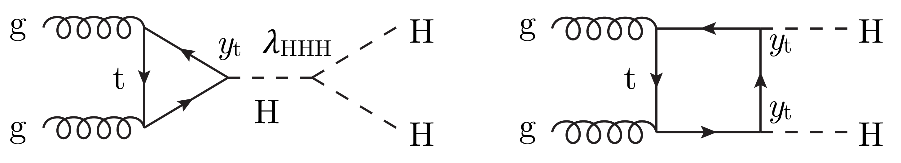
Figure 1:
Feynman diagrams contributing to Higgs pair production via gluon-gluon fusion at leading order at the LHC. |
png pdf |
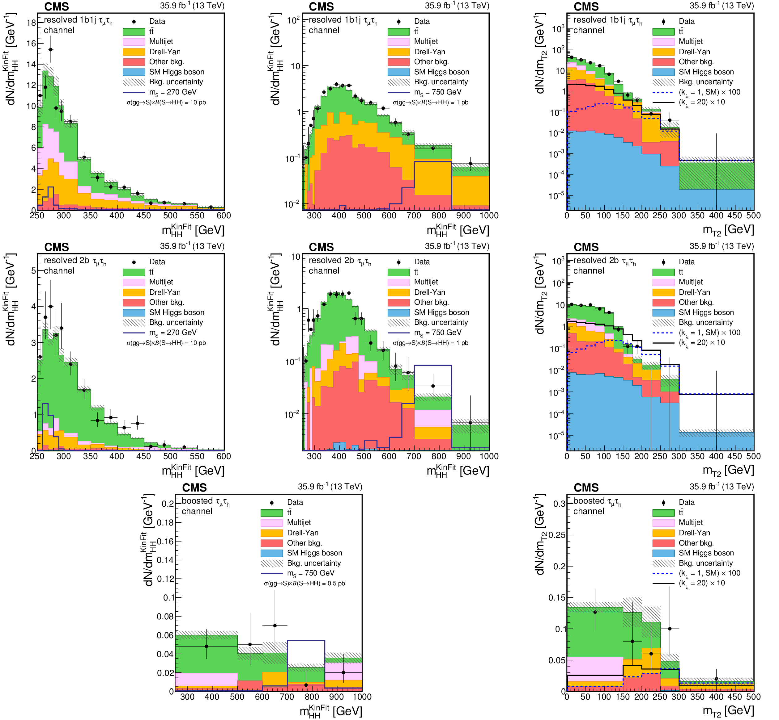
Figure 2:
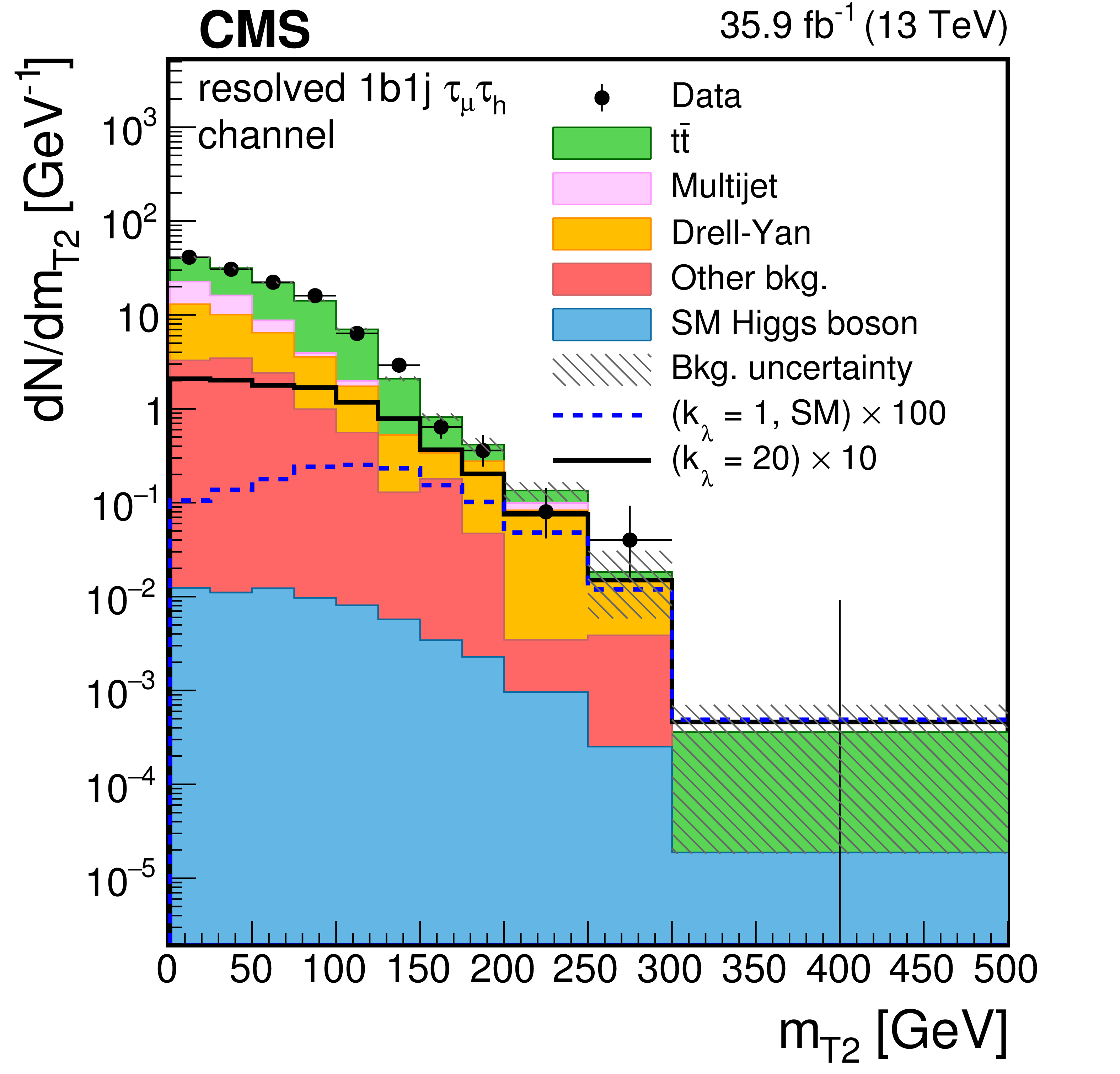
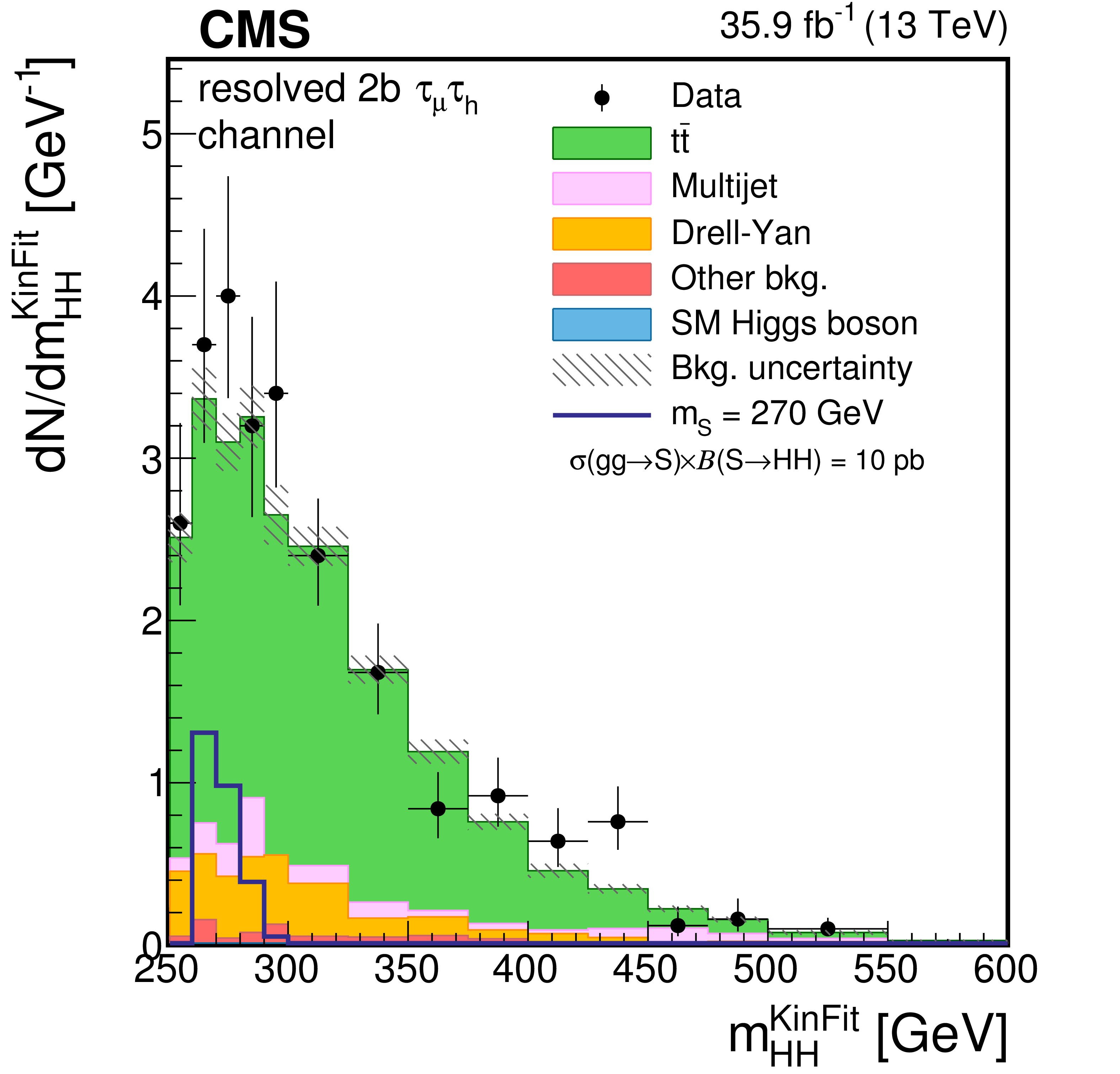
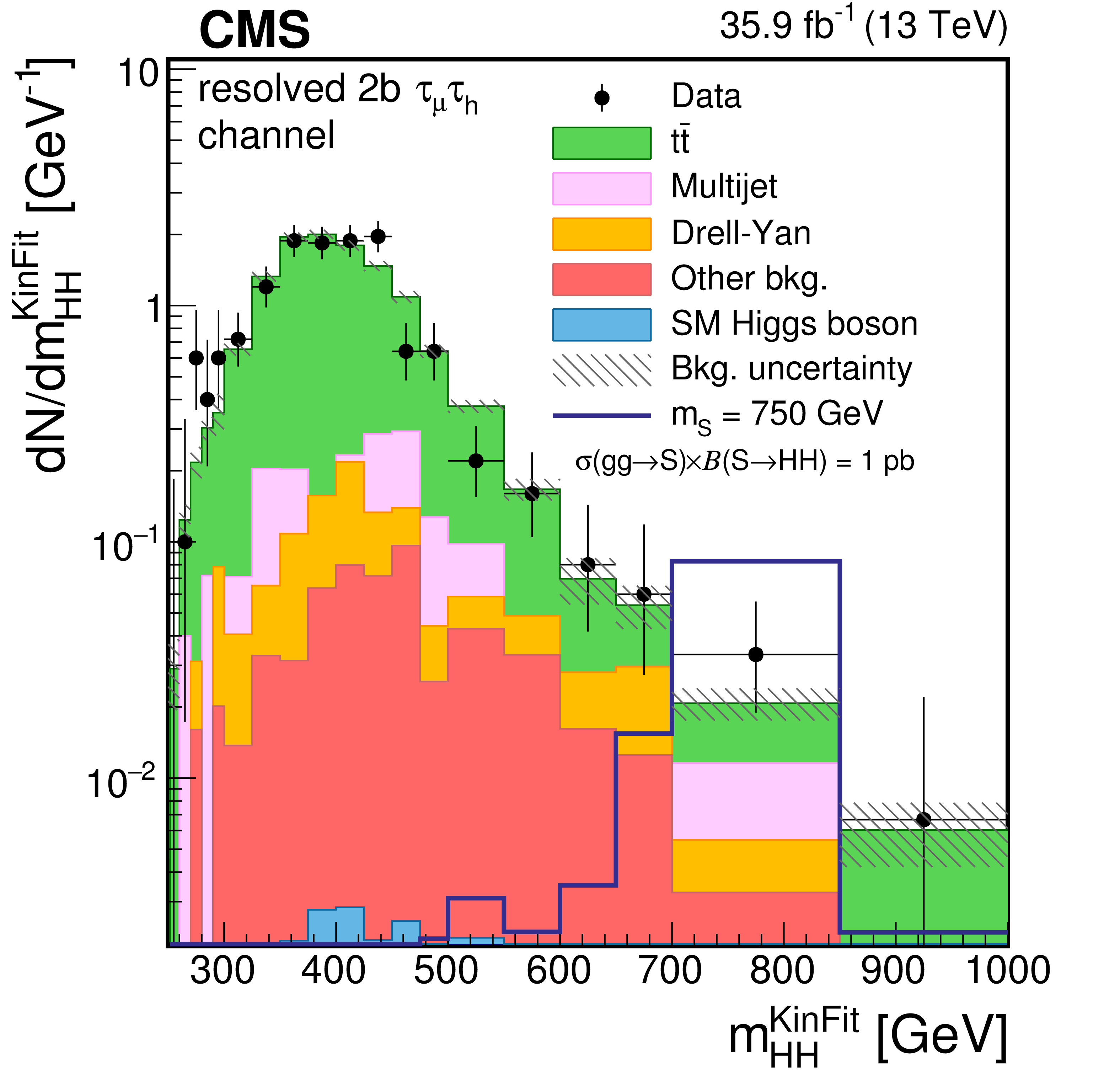
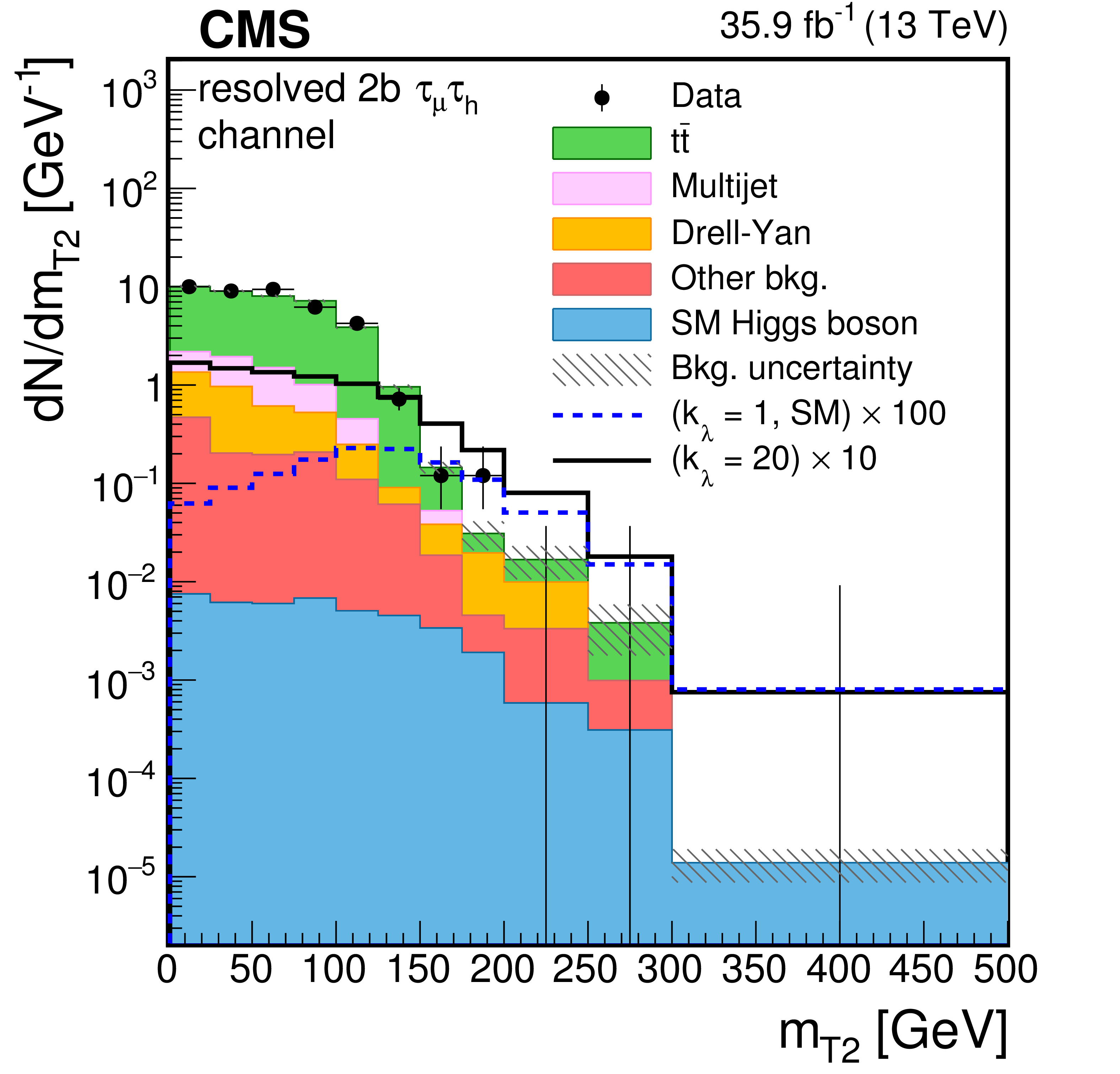
Distributions of the events observed in the signal regions of the $ {\tau _\mu {\tau _\mathrm {h}} } $ final state. The first, second, and third rows show the resolved 1b1j, 2b, and boosted regions, respectively. Panels in the right column show the distribution of the ${m_\text {T2}} $ variable, while the other panels show the distribution of the ${m_{ {\mathrm{ H } \mathrm{ H } } }^\text {KinFit} }$ variable, separated in the low-mass (LM, left panels) and high-mass (HM, central panels) regions for the resolved event categories. Data are represented by points with error bars and expected signal contributions are represented by the solid (BSM HH signals) and dashed (SM nonresonant HH signal) lines. Expected background contributions (shaded histograms) and associated systematic uncertainties (dashed areas) are shown as obtained after the maximum likelihood fit to the data under the background-only hypothesis. The background histograms are stacked while the signal histograms are not stacked. |
png pdf |
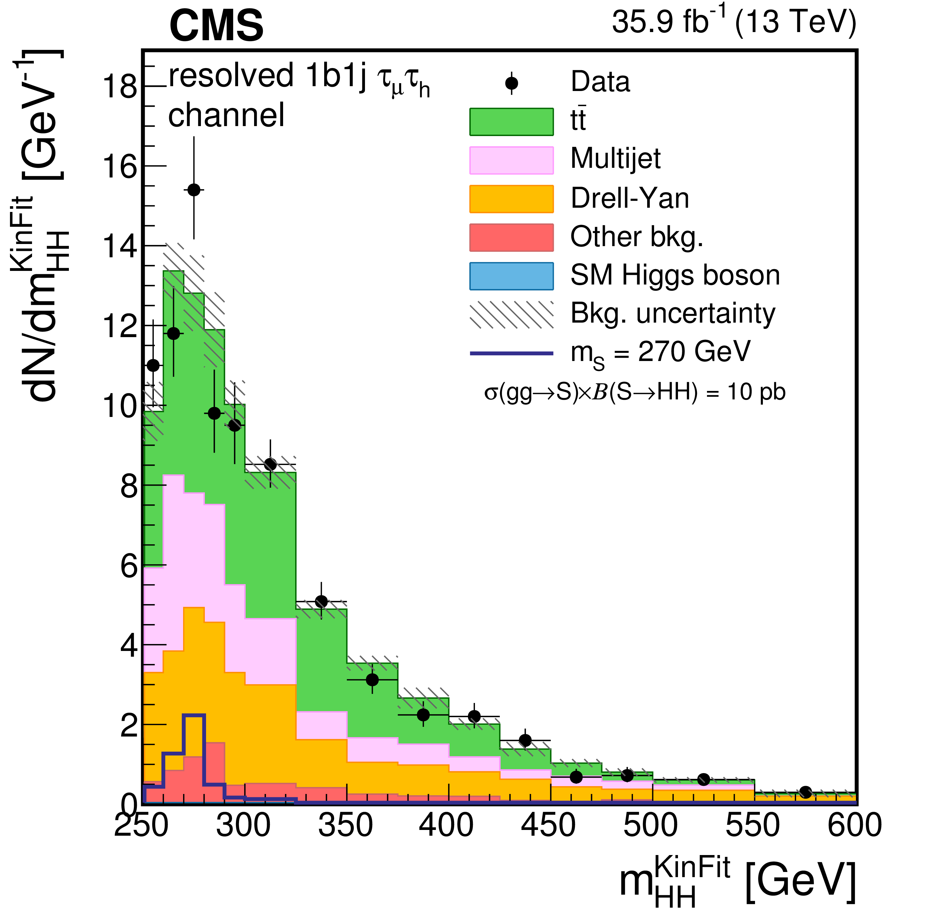
Figure 2-a:
Distribution of the ${m_{ {\mathrm{ H } \mathrm{ H } } }^\text {KinFit} }$ variable for events observed in the resolved 1b1j signal region of the $ {\tau _\mu {\tau _\mathrm {h}} } $ final state. The distribution is shown in the low-mass (LM) region. Data are represented by points with error bars and expected signal contributions are represented by the solid (BSM HH signals) and dashed (SM nonresonant HH signal) lines. Expected background contributions (shaded histograms) and associated systematic uncertainties (dashed areas) are shown as obtained after the maximum likelihood fit to the data under the background-only hypothesis. The background histograms are stacked while the signal histograms are not stacked. |
png pdf |
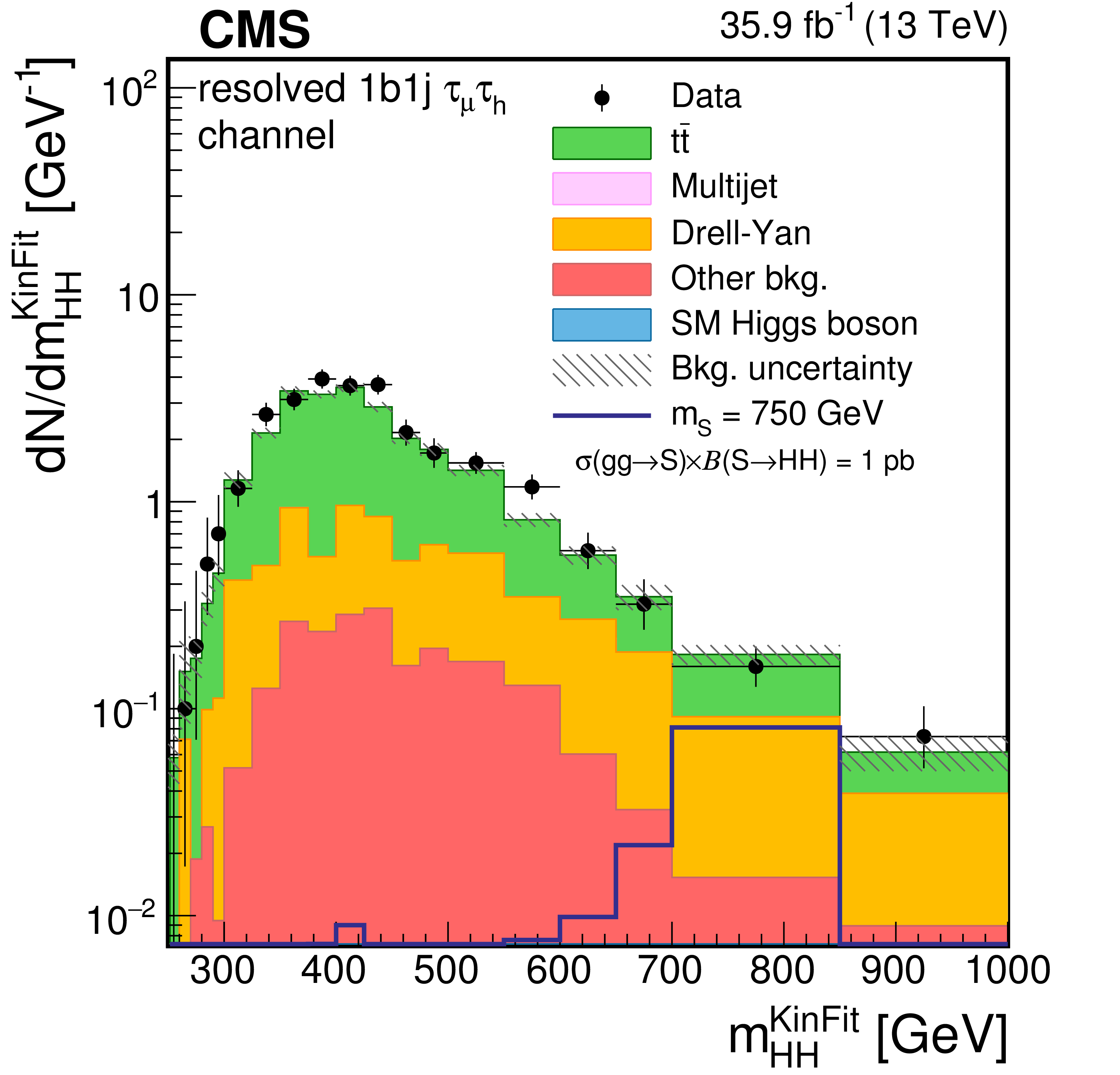
Figure 2-b:
Distribution of the ${m_{ {\mathrm{ H } \mathrm{ H } } }^\text {KinFit} }$ variable for events observed in the resolved 1b1j signal region of the $ {\tau _\mu {\tau _\mathrm {h}} } $ final state. The distribution is shown in the high-mass (HM) region. Data are represented by points with error bars and expected signal contributions are represented by the solid (BSM HH signals) and dashed (SM nonresonant HH signal) lines. Expected background contributions (shaded histograms) and associated systematic uncertainties (dashed areas) are shown as obtained after the maximum likelihood fit to the data under the background-only hypothesis. The background histograms are stacked while the signal histograms are not stacked. |
png pdf |
Figure 2-c:
Distribution of the ${m_\text {T2}} $ variable for events observed in the resolved 1b1j signal region of the $ {\tau _\mu {\tau _\mathrm {h}} } $ final state. Data are represented by points with error bars and expected signal contributions are represented by the solid (BSM HH signals) and dashed (SM nonresonant HH signal) lines. Expected background contributions (shaded histograms) and associated systematic uncertainties (dashed areas) are shown as obtained after the maximum likelihood fit to the data under the background-only hypothesis. The background histograms are stacked while the signal histograms are not stacked. |
png pdf |
Figure 2-d:
Distribution of the ${m_{ {\mathrm{ H } \mathrm{ H } } }^\text {KinFit} }$ variable for events observed in the resolved 2b signal region of the $ {\tau _\mu {\tau _\mathrm {h}} } $ final state. The distribution is shown in the low-mass (LM) region. Data are represented by points with error bars and expected signal contributions are represented by the solid (BSM HH signals) and dashed (SM nonresonant HH signal) lines. Expected background contributions (shaded histograms) and associated systematic uncertainties (dashed areas) are shown as obtained after the maximum likelihood fit to the data under the background-only hypothesis. The background histograms are stacked while the signal histograms are not stacked. |
png pdf |
Figure 2-e:
Distribution of the ${m_{ {\mathrm{ H } \mathrm{ H } } }^\text {KinFit} }$ variable for events observed in the resolved 2b signal region of the $ {\tau _\mu {\tau _\mathrm {h}} } $ final state. The distribution is shown in the high-mass (HM) region. Data are represented by points with error bars and expected signal contributions are represented by the solid (BSM HH signals) and dashed (SM nonresonant HH signal) lines. Expected background contributions (shaded histograms) and associated systematic uncertainties (dashed areas) are shown as obtained after the maximum likelihood fit to the data under the background-only hypothesis. The background histograms are stacked while the signal histograms are not stacked. |
png pdf |
Figure 2-f:
Distribution of the ${m_\text {T2}} $ variable for events observed in the resolved 2b signal region of the $ {\tau _\mu {\tau _\mathrm {h}} } $ final state. Data are represented by points with error bars and expected signal contributions are represented by the solid (BSM HH signals) and dashed (SM nonresonant HH signal) lines. Expected background contributions (shaded histograms) and associated systematic uncertainties (dashed areas) are shown as obtained after the maximum likelihood fit to the data under the background-only hypothesis. The background histograms are stacked while the signal histograms are not stacked. |
png pdf |
Figure 2-g:
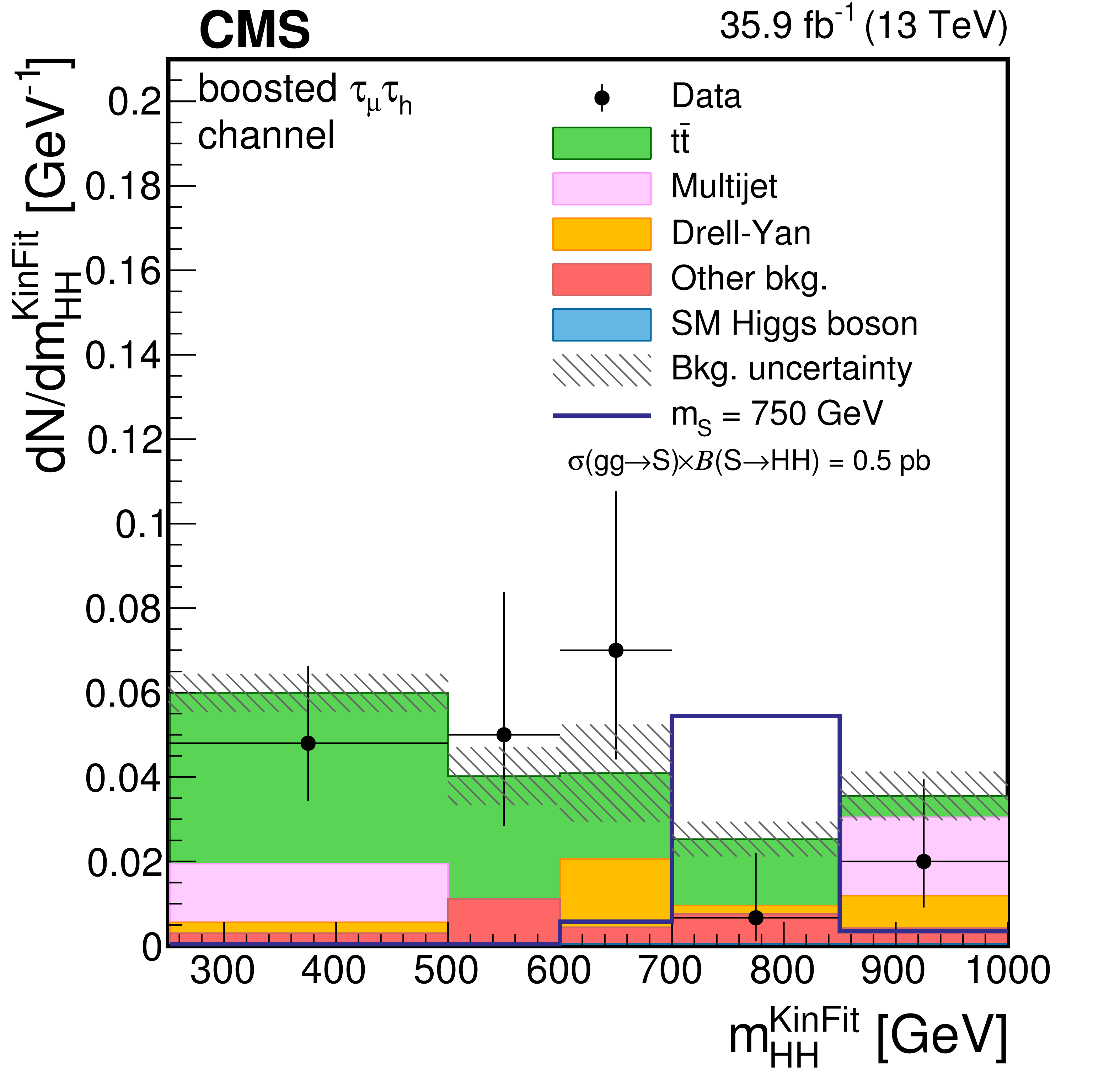
Distribution of the ${m_{ {\mathrm{ H } \mathrm{ H } } }^\text {KinFit} }$ variable for events observed in the boosted signal region of the $ {\tau _\mu {\tau _\mathrm {h}} } $ final state. Data are represented by points with error bars and expected signal contributions are represented by the solid (BSM HH signals) and dashed (SM nonresonant HH signal) lines. Expected background contributions (shaded histograms) and associated systematic uncertainties (dashed areas) are shown as obtained after the maximum likelihood fit to the data under the background-only hypothesis. The background histograms are stacked while the signal histograms are not stacked. |
png pdf |
Figure 2-h:
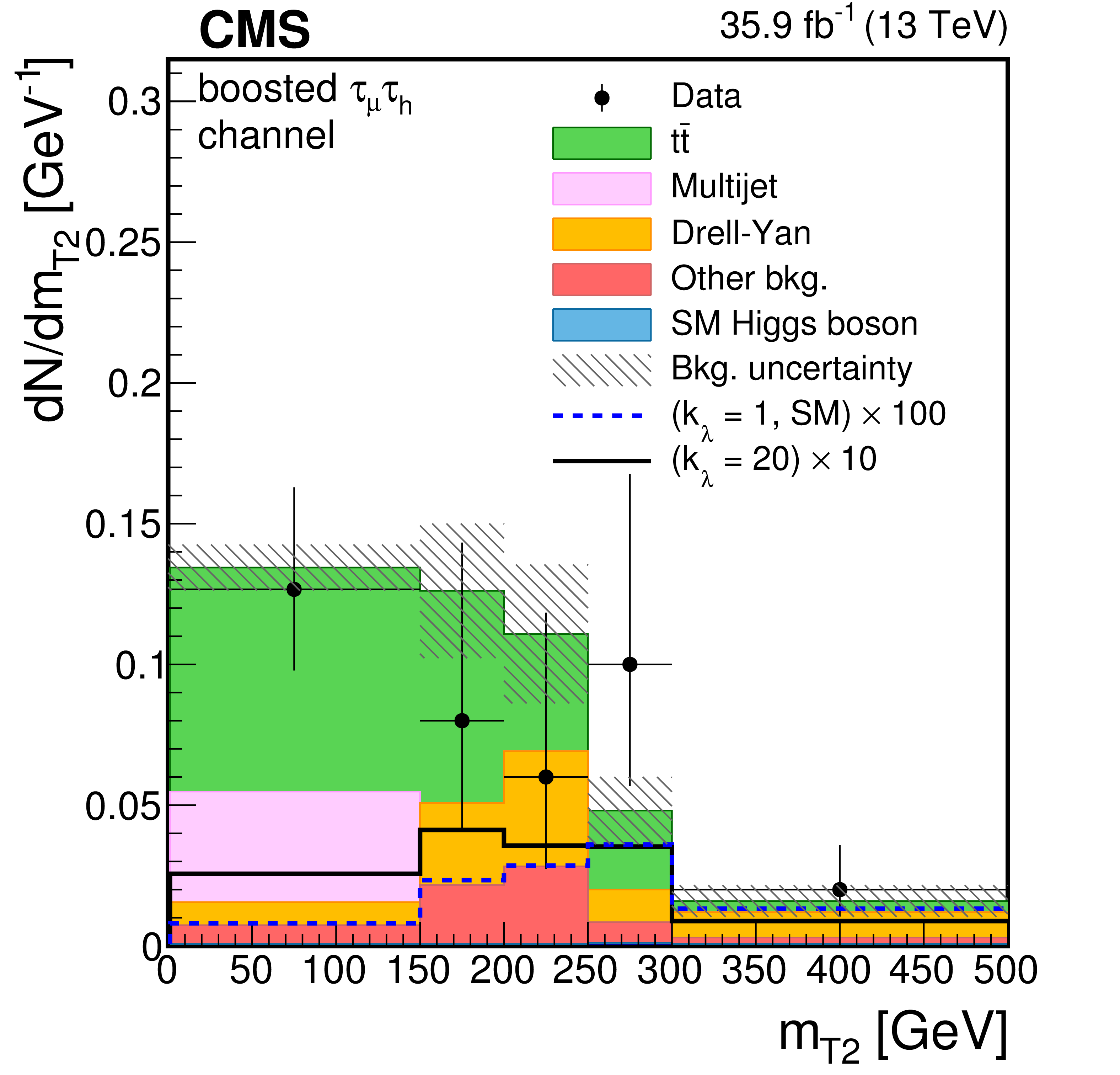
Distribution of the ${m_\text {T2}} $ variable for events observed in the boosted signal region of the $ {\tau _\mu {\tau _\mathrm {h}} } $ final state. Data are represented by points with error bars and expected signal contributions are represented by the solid (BSM HH signals) and dashed (SM nonresonant HH signal) lines. Expected background contributions (shaded histograms) and associated systematic uncertainties (dashed areas) are shown as obtained after the maximum likelihood fit to the data under the background-only hypothesis. The background histograms are stacked while the signal histograms are not stacked. |

png pdf |
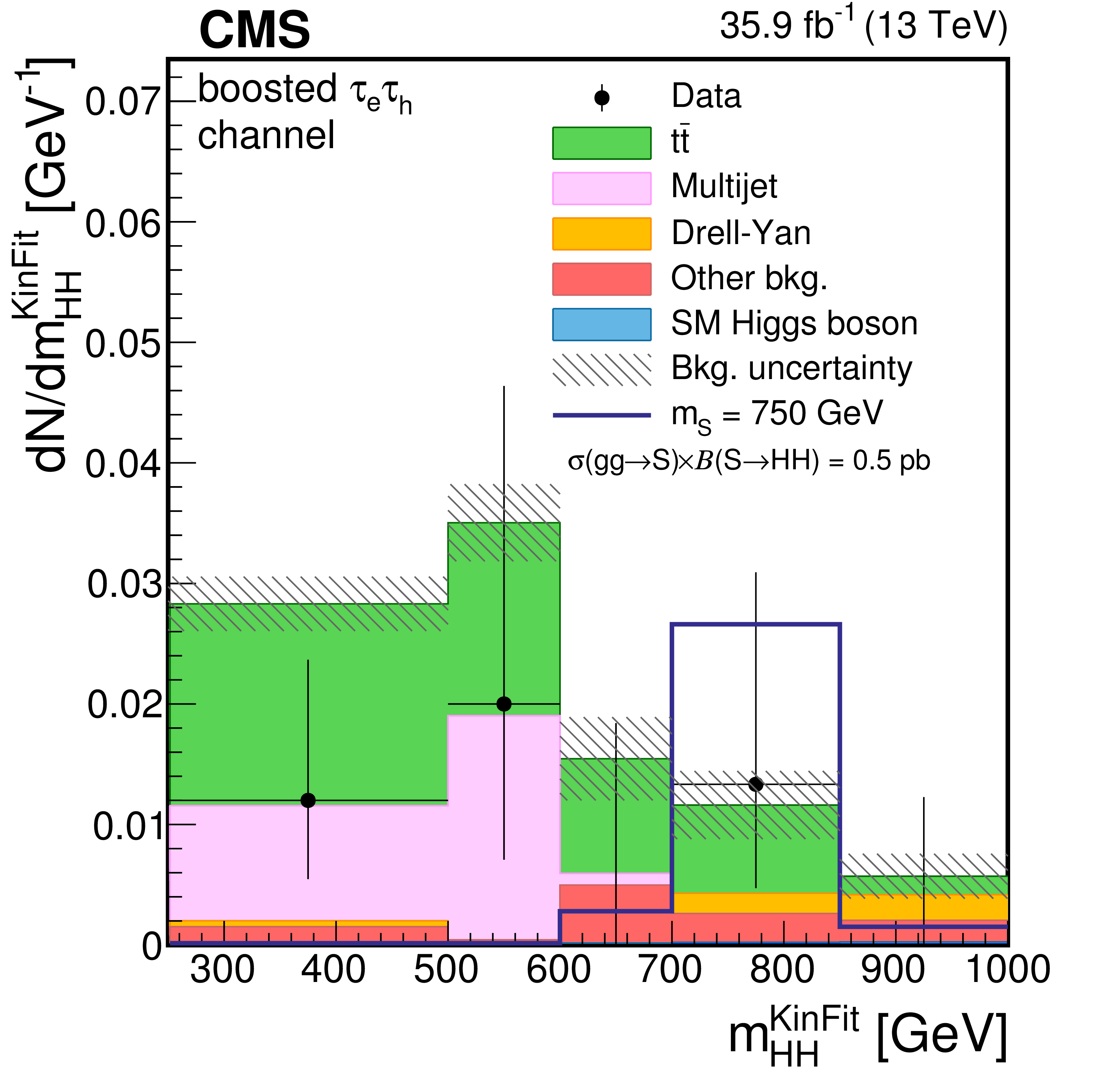
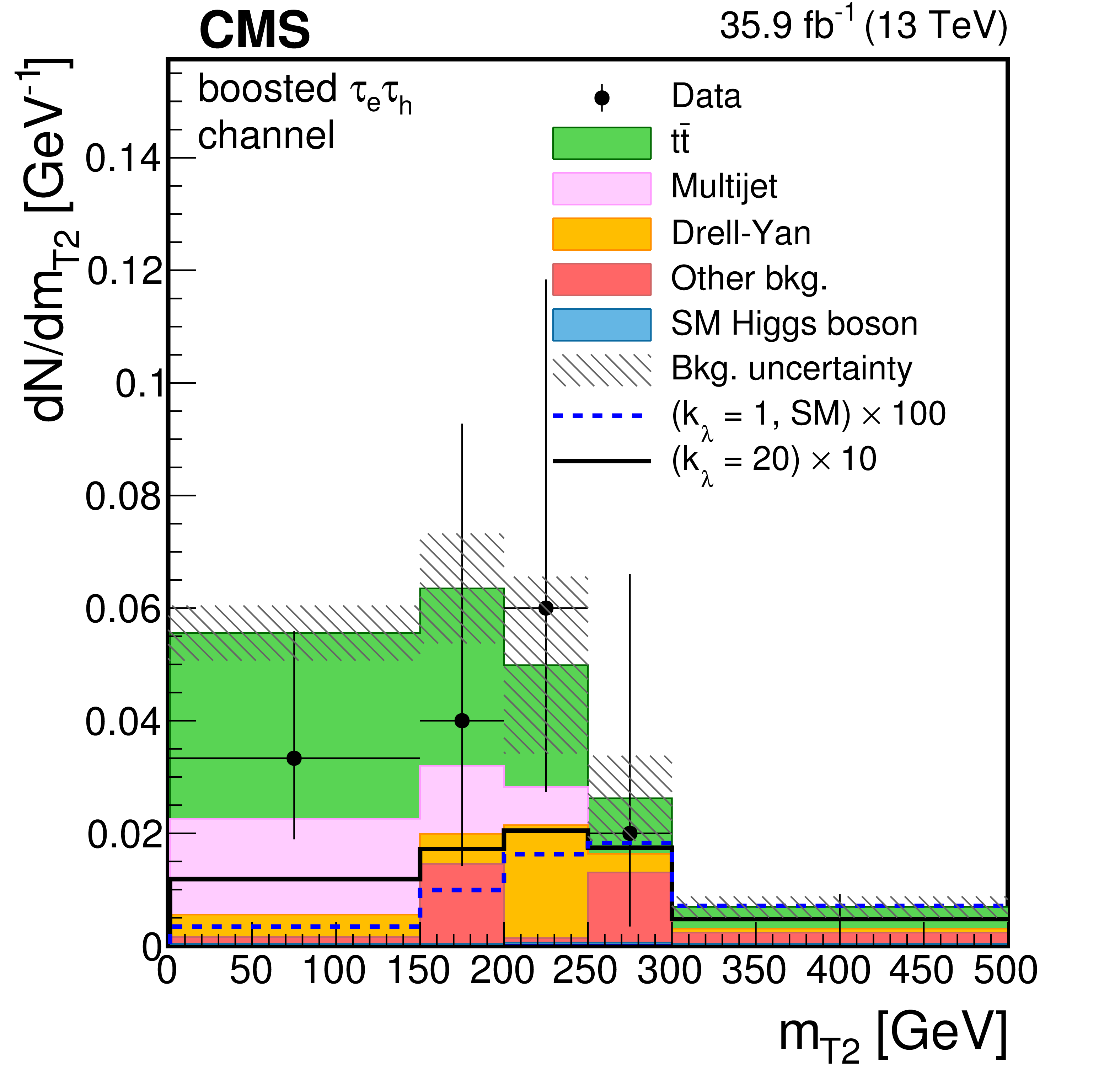
Figure 3:
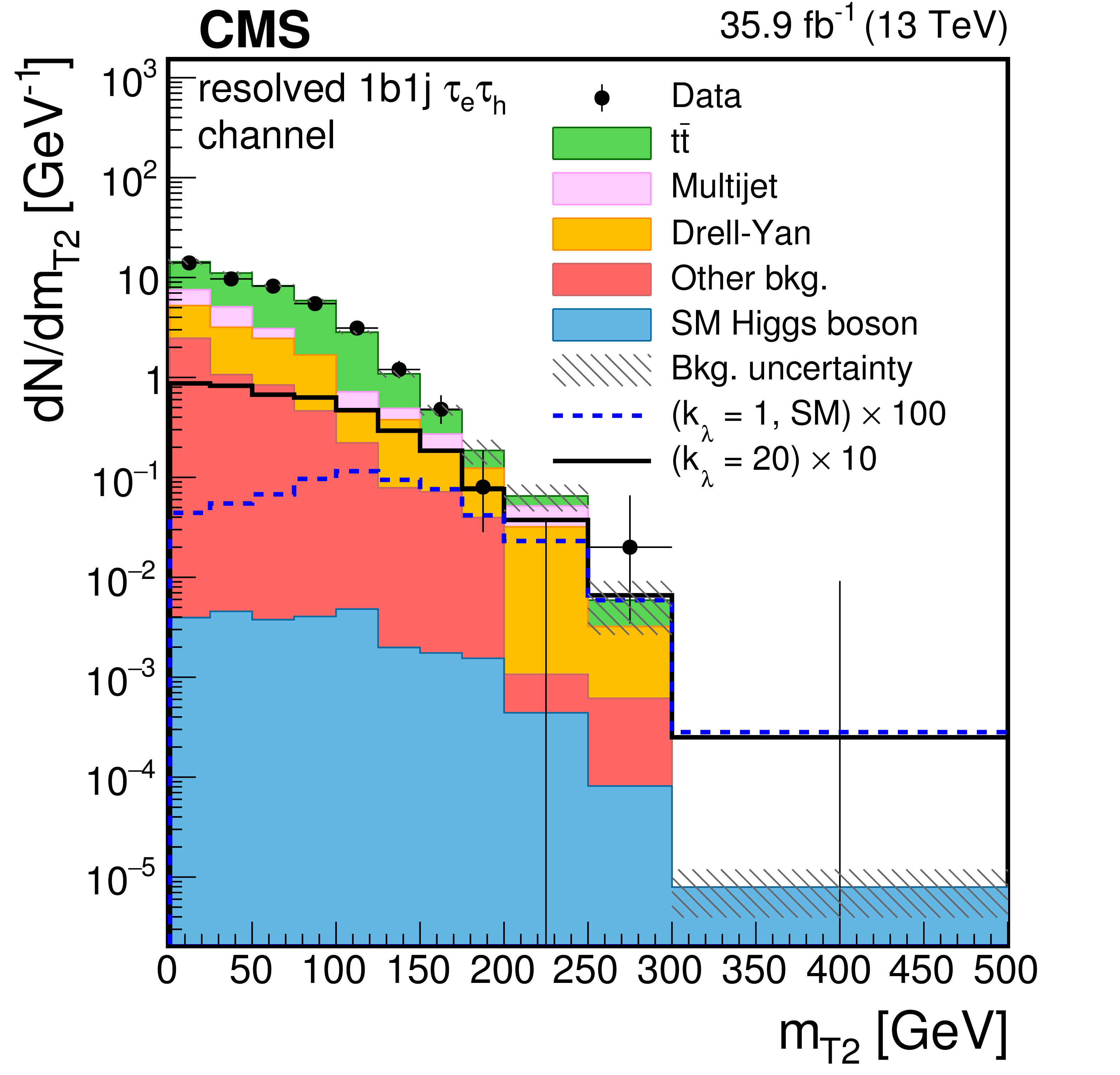
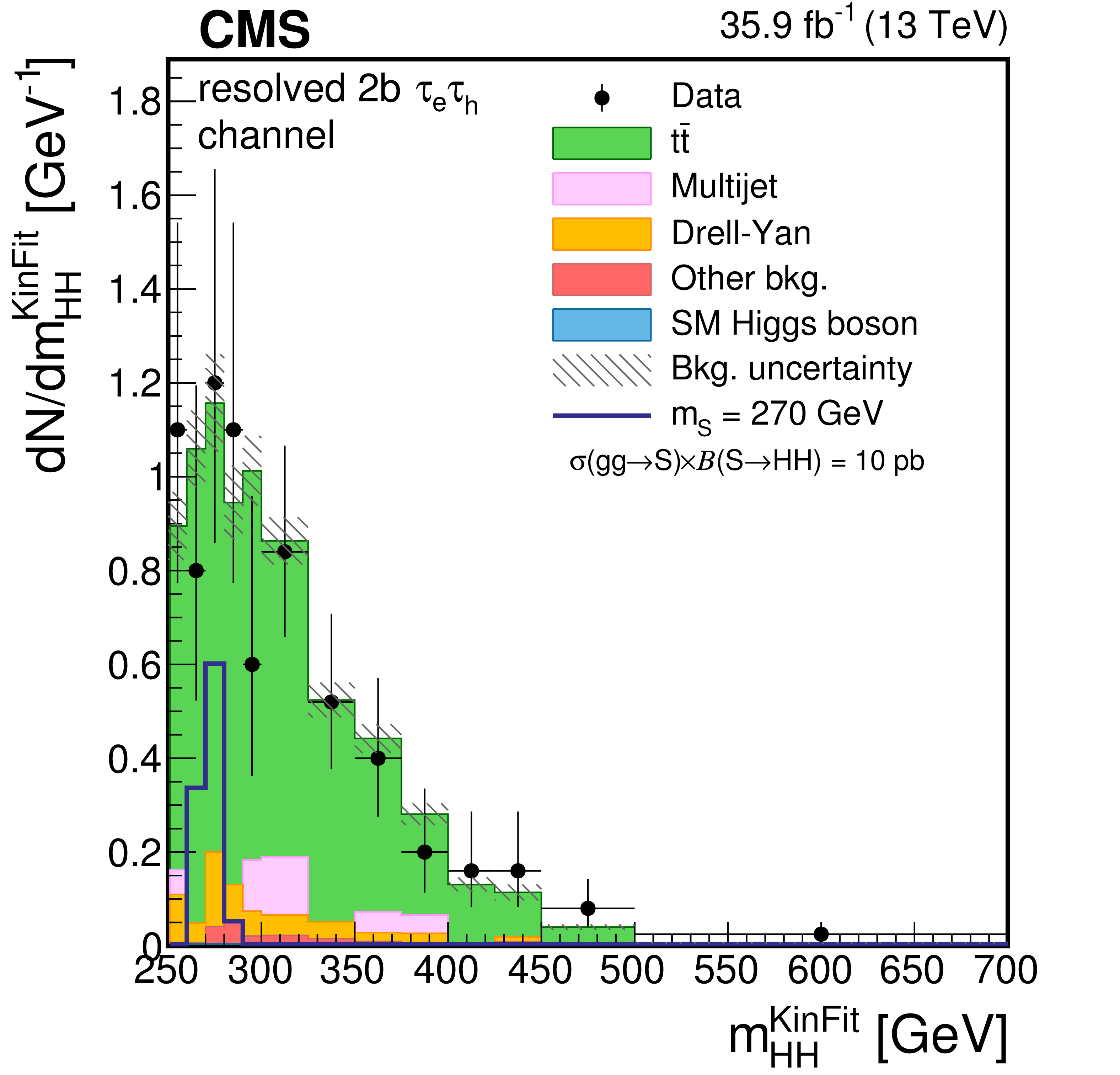
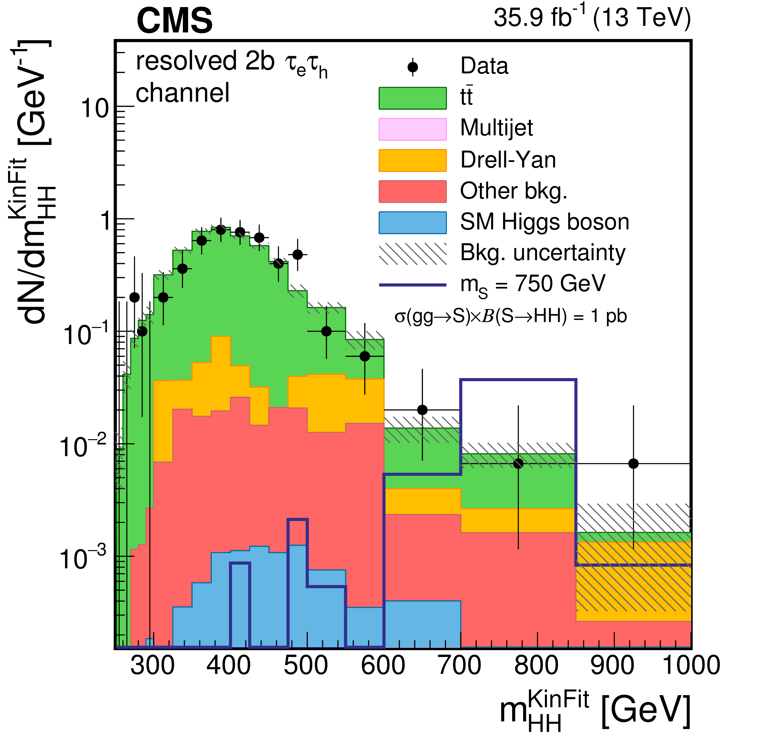
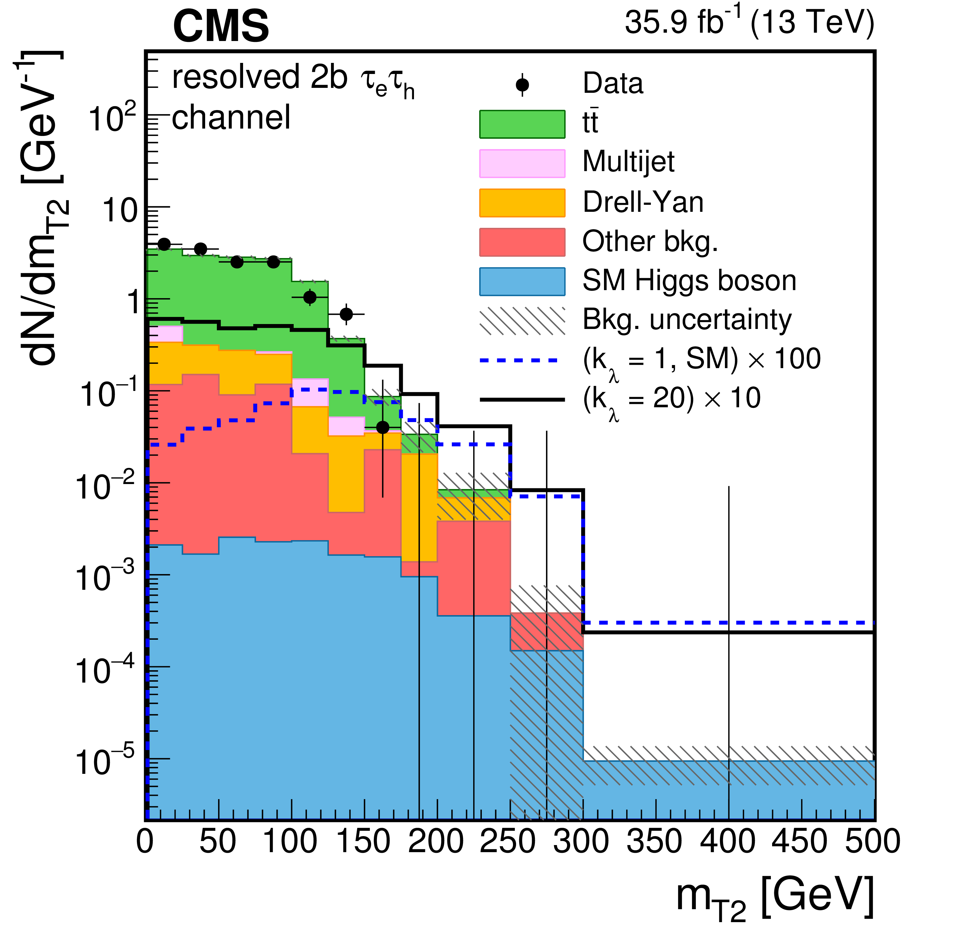
Distributions of the events observed in the signal regions of the $ {\tau _{\mathrm{e}} {\tau _\mathrm {h}} } $ final state. The first, second, and third rows show the resolved 1b1j, 2b, and boosted regions, respectively. Panels in the right column show the distribution of the ${m_\text {T2}} $ variable, while the other panels show the distribution of the ${m_{ {\mathrm{ H } \mathrm{ H } } }^\text {KinFit} }$ variable, separated in the low-mass (LM, left panels) and high-mass (HM, central panels) regions for the resolved event categories. Data are represented by points with error bars and expected signal contributions are represented by the solid (BSM HH signals) and dashed (SM nonresonant HH signal) lines. Expected background contributions (shaded histograms) and associated systematic uncertainties (dashed areas) are shown as obtained after the maximum likelihood fit to the data under the background-only hypothesis. The background histograms are stacked while the signal histograms are not stacked. |
png pdf |
Figure 3-a:
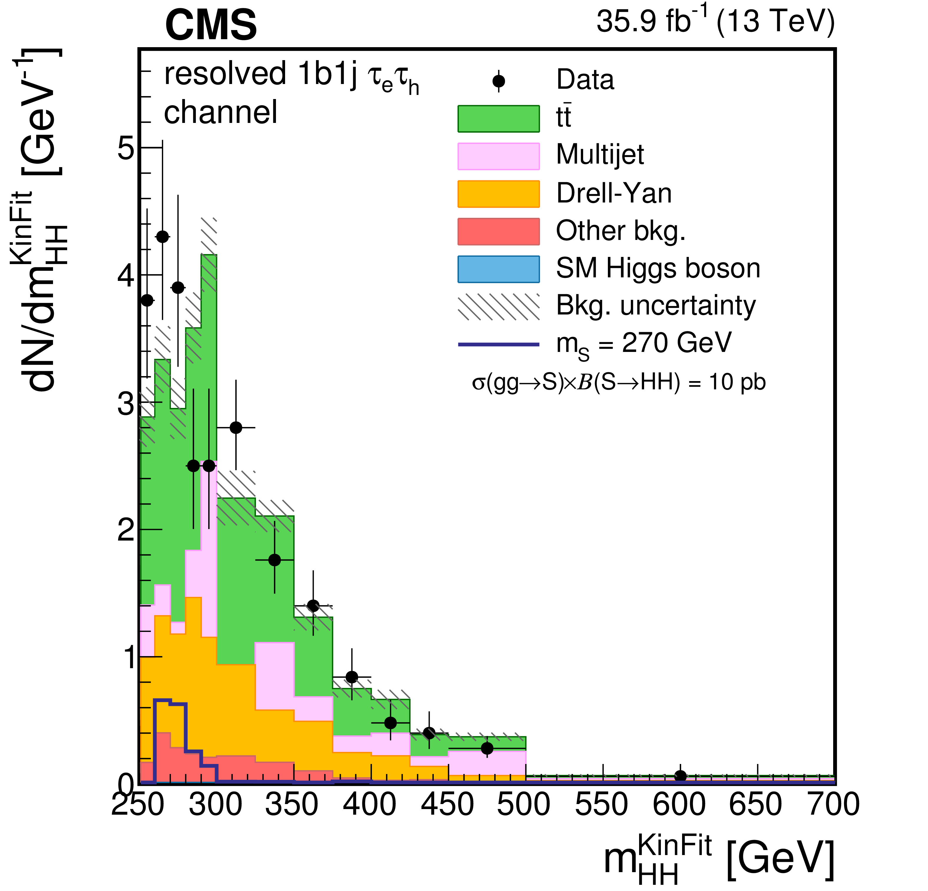
Distribution of the ${m_{ {\mathrm{ H } \mathrm{ H } } }^\text {KinFit} }$ variable for events observed in the resolved 1b1j signal region of the $ {\tau _{\mathrm{e}} {\tau _\mathrm {h}} } $ final state. The distribution is shown in the low-mass (LM) region. Data are represented by points with error bars and expected signal contributions are represented by the solid (BSM HH signals) and dashed (SM nonresonant HH signal) lines. Expected background contributions (shaded histograms) and associated systematic uncertainties (dashed areas) are shown as obtained after the maximum likelihood fit to the data under the background-only hypothesis. The background histograms are stacked while the signal histograms are not stacked. |
png pdf |
Figure 3-b:
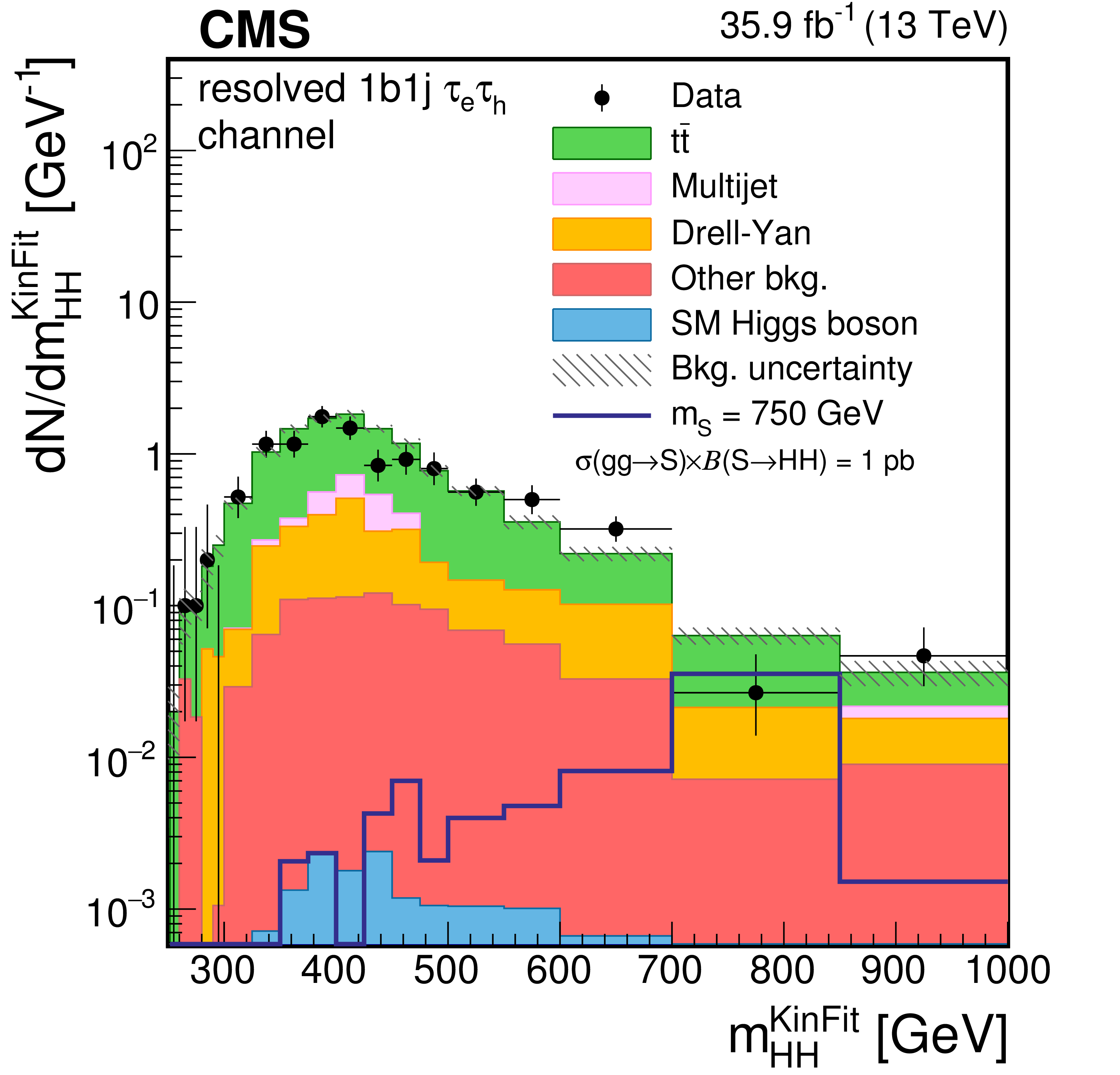
Distribution of the ${m_{ {\mathrm{ H } \mathrm{ H } } }^\text {KinFit} }$ variable for events observed in the resolved 1b1j signal region of the $ {\tau _{\mathrm{e}} {\tau _\mathrm {h}} } $ final state. The distribution is shown in the high-mass (HM) region. Data are represented by points with error bars and expected signal contributions are represented by the solid (BSM HH signals) and dashed (SM nonresonant HH signal) lines. Expected background contributions (shaded histograms) and associated systematic uncertainties (dashed areas) are shown as obtained after the maximum likelihood fit to the data under the background-only hypothesis. The background histograms are stacked while the signal histograms are not stacked. |
png pdf |
Figure 3-c:
Distribution of the ${m_\text {T2}} $ variable for events observed in the resolved 1b1j signal region of the $ {\tau _{\mathrm{e}} {\tau _\mathrm {h}} } $ final state. Data are represented by points with error bars and expected signal contributions are represented by the solid (BSM HH signals) and dashed (SM nonresonant HH signal) lines. Expected background contributions (shaded histograms) and associated systematic uncertainties (dashed areas) are shown as obtained after the maximum likelihood fit to the data under the background-only hypothesis. The background histograms are stacked while the signal histograms are not stacked. |
png pdf |
Figure 3-d:
Distribution of the ${m_{ {\mathrm{ H } \mathrm{ H } } }^\text {KinFit} }$ variable for events observed in the resolved 2b signal region of the $ {\tau _{\mathrm{e}} {\tau _\mathrm {h}} } $ final state. The distribution is shown in the low-mass (LM) region. Data are represented by points with error bars and expected signal contributions are represented by the solid (BSM HH signals) and dashed (SM nonresonant HH signal) lines. Expected background contributions (shaded histograms) and associated systematic uncertainties (dashed areas) are shown as obtained after the maximum likelihood fit to the data under the background-only hypothesis. The background histograms are stacked while the signal histograms are not stacked. |
png pdf |
Figure 3-e:
Distribution of the ${m_{ {\mathrm{ H } \mathrm{ H } } }^\text {KinFit} }$ variable for events observed in the resolved 2b signal region of the $ {\tau _{\mathrm{e}} {\tau _\mathrm {h}} } $ final state. The distribution is shown in the high-mass (HM) region. Data are represented by points with error bars and expected signal contributions are represented by the solid (BSM HH signals) and dashed (SM nonresonant HH signal) lines. Expected background contributions (shaded histograms) and associated systematic uncertainties (dashed areas) are shown as obtained after the maximum likelihood fit to the data under the background-only hypothesis. The background histograms are stacked while the signal histograms are not stacked. |
png pdf |
Figure 3-f:
Distribution of the ${m_\text {T2}} $ variable for events observed in the resolved 2b signal region of the $ {\tau _{\mathrm{e}} {\tau _\mathrm {h}} } $ final state. Data are represented by points with error bars and expected signal contributions are represented by the solid (BSM HH signals) and dashed (SM nonresonant HH signal) lines. Expected background contributions (shaded histograms) and associated systematic uncertainties (dashed areas) are shown as obtained after the maximum likelihood fit to the data under the background-only hypothesis. The background histograms are stacked while the signal histograms are not stacked. |
png pdf |
Figure 3-g:
Distribution of the ${m_{ {\mathrm{ H } \mathrm{ H } } }^\text {KinFit} }$ variable for events observed in the boosted signal region of the $ {\tau _{\mathrm{e}} {\tau _\mathrm {h}} } $ final state. Data are represented by points with error bars and expected signal contributions are represented by the solid (BSM HH signals) and dashed (SM nonresonant HH signal) lines. Expected background contributions (shaded histograms) and associated systematic uncertainties (dashed areas) are shown as obtained after the maximum likelihood fit to the data under the background-only hypothesis. The background histograms are stacked while the signal histograms are not stacked. |
png pdf |
Figure 3-h:
Distribution of the ${m_\text {T2}} $ variable for events observed in the boosted signal region of the $ {\tau _{\mathrm{e}} {\tau _\mathrm {h}} } $ final state. Data are represented by points with error bars and expected signal contributions are represented by the solid (BSM HH signals) and dashed (SM nonresonant HH signal) lines. Expected background contributions (shaded histograms) and associated systematic uncertainties (dashed areas) are shown as obtained after the maximum likelihood fit to the data under the background-only hypothesis. The background histograms are stacked while the signal histograms are not stacked. |
png pdf |
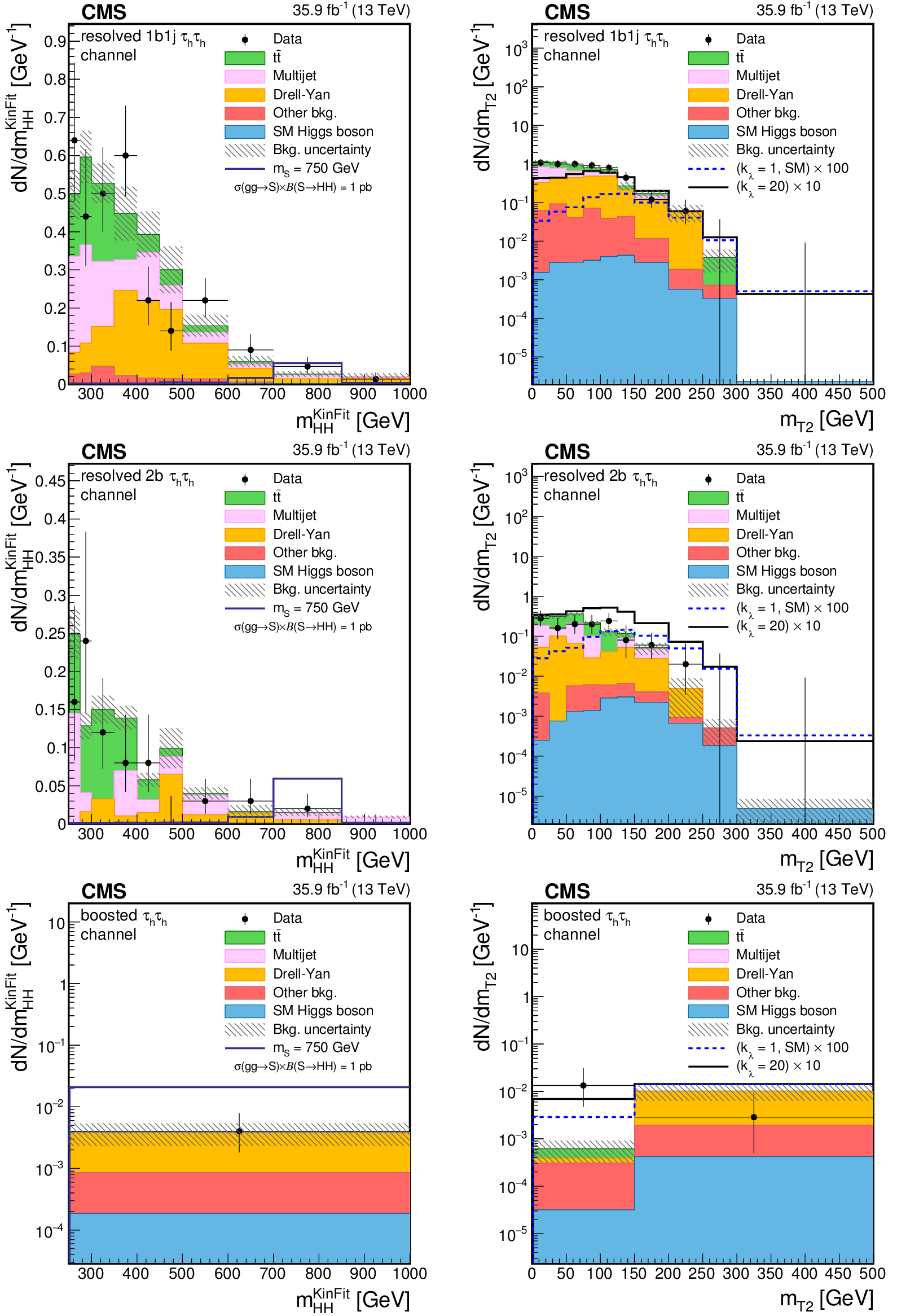
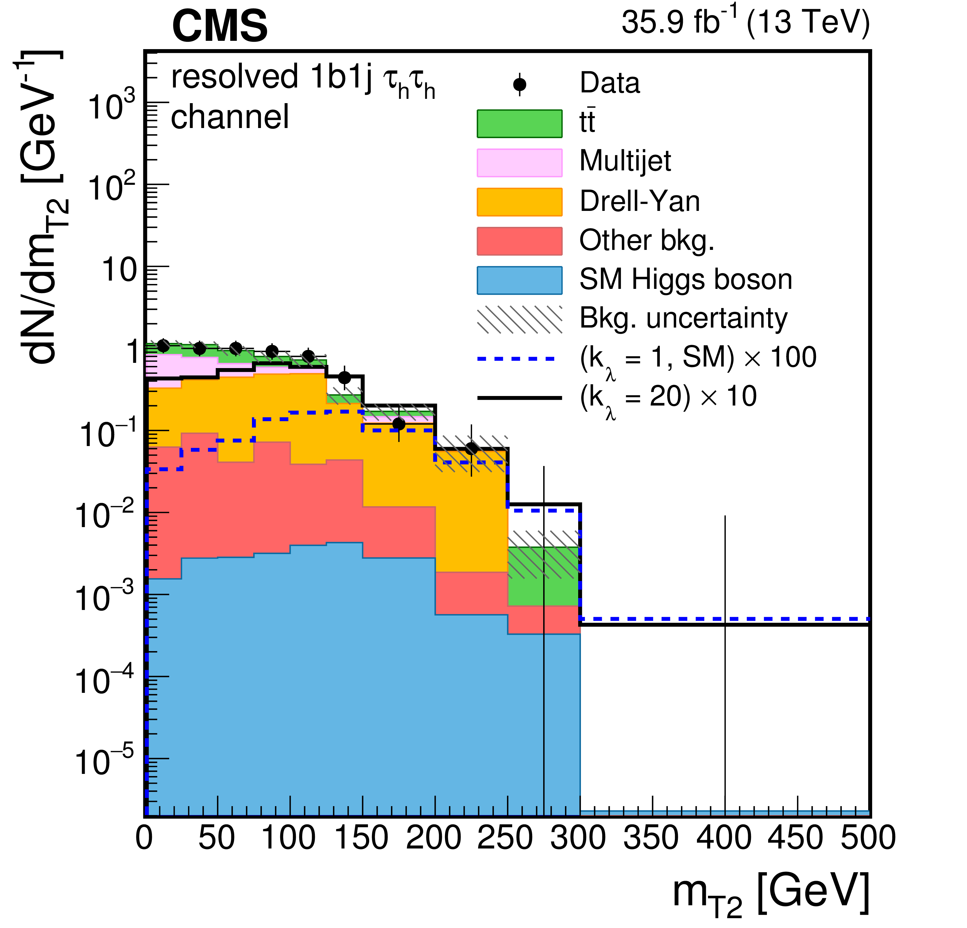
Figure 4:
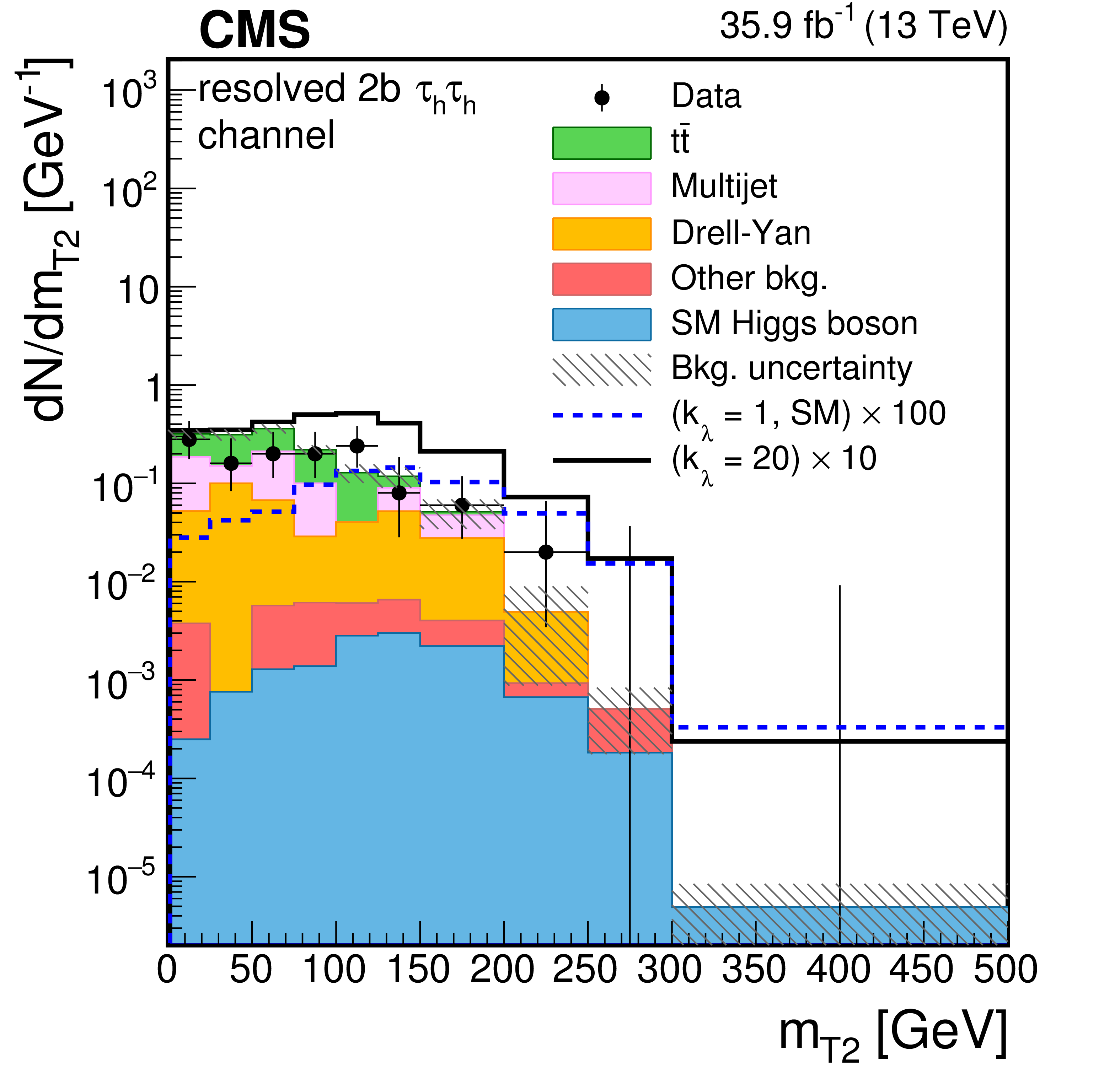
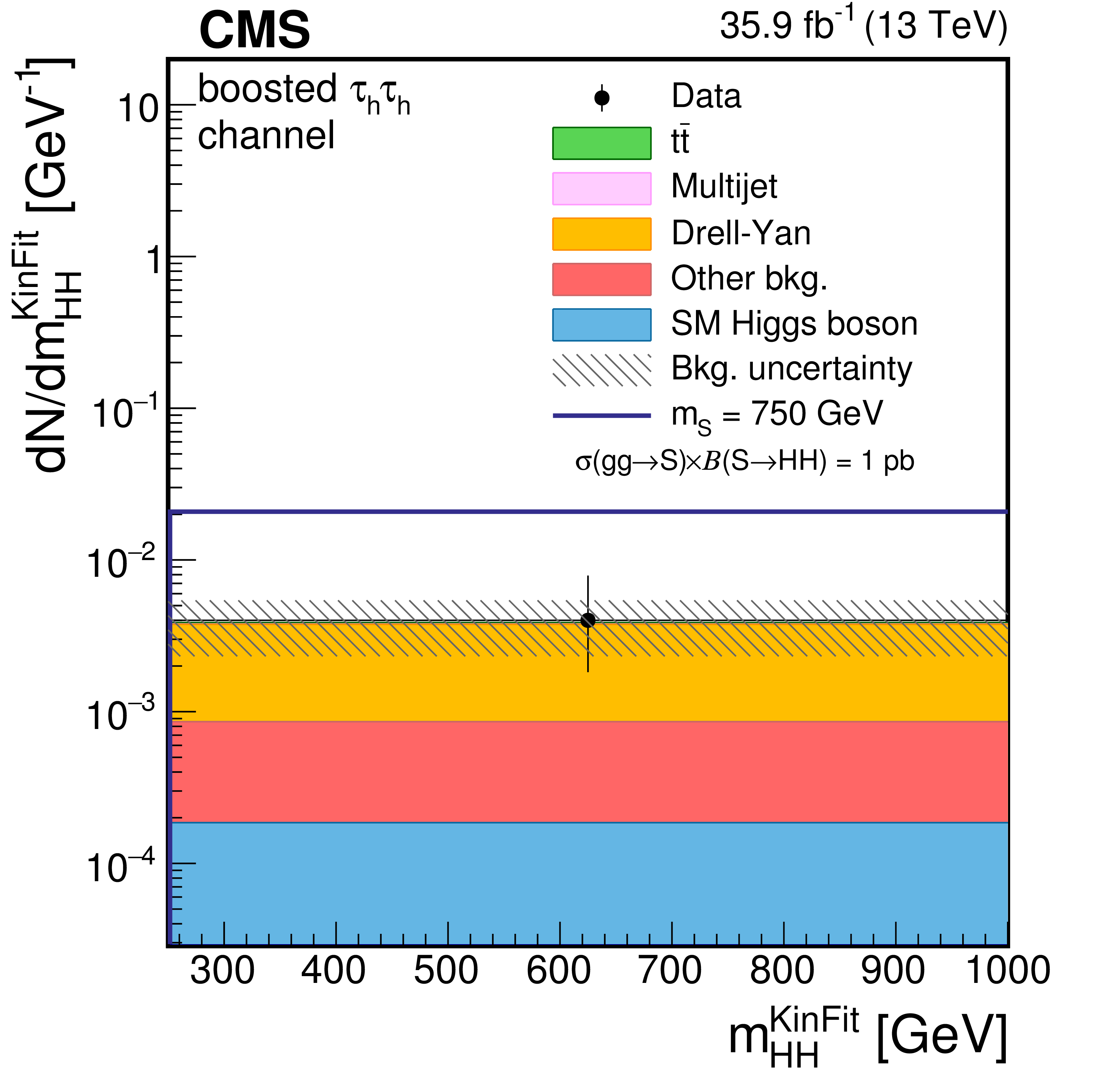
Distributions of the events observed in the signal regions of the $ { {\tau _\mathrm {h}} {\tau _\mathrm {h}} } $ final state. The first, second, and third rows show the resolved 1b1j, 2b, and boosted regions, respectively. Panels in the left column show the distribution of the ${m_{ {\mathrm{ H } \mathrm{ H } } }^\text {KinFit} }$ variable and panels in the right column show the distribution of the ${m_\text {T2}}$ variable. Data are represented by points with error bars and expected signal contributions are represented by the solid (BSM HH signals) and dashed (SM nonresonant HH signal) lines. Expected background contributions (shaded histograms) and associated systematic uncertainties (dashed areas) are shown as obtained after the maximum likelihood fit to the data under the background-only hypothesis. The background histograms are stacked while the signal histograms are not stacked. |

png pdf |
Figure 4-a:
Distribution of the ${m_{ {\mathrm{ H } \mathrm{ H } } }^\text {KinFit} }$ for events observed in the resolved 1b1j region of the $ { {\tau _\mathrm {h}} {\tau _\mathrm {h}} } $ final state. Data are represented by points with error bars and expected signal contributions are represented by the solid (BSM HH signals) and dashed (SM nonresonant HH signal) lines. Expected background contributions (shaded histograms) and associated systematic uncertainties (dashed areas) are shown as obtained after the maximum likelihood fit to the data under the background-only hypothesis. The background histograms are stacked while the signal histograms are not stacked. |
png pdf |
Figure 4-b:
Distribution of the ${m_\text {T2}}$ for events observed in the resolved 1b1j region of the $ { {\tau _\mathrm {h}} {\tau _\mathrm {h}} } $ final state. Data are represented by points with error bars and expected signal contributions are represented by the solid (BSM HH signals) and dashed (SM nonresonant HH signal) lines. Expected background contributions (shaded histograms) and associated systematic uncertainties (dashed areas) are shown as obtained after the maximum likelihood fit to the data under the background-only hypothesis. The background histograms are stacked while the signal histograms are not stacked. |

png pdf |
Figure 4-c:
Distribution of the ${m_{ {\mathrm{ H } \mathrm{ H } } }^\text {KinFit} }$ for events observed in the resolved 2b region of the $ { {\tau _\mathrm {h}} {\tau _\mathrm {h}} } $ final state. Data are represented by points with error bars and expected signal contributions are represented by the solid (BSM HH signals) and dashed (SM nonresonant HH signal) lines. Expected background contributions (shaded histograms) and associated systematic uncertainties (dashed areas) are shown as obtained after the maximum likelihood fit to the data under the background-only hypothesis. The background histograms are stacked while the signal histograms are not stacked. |
png pdf |
Figure 4-d:
Distribution of the ${m_\text {T2}}$ for events observed in the resolved 2b region of the $ { {\tau _\mathrm {h}} {\tau _\mathrm {h}} } $ final state. Data are represented by points with error bars and expected signal contributions are represented by the solid (BSM HH signals) and dashed (SM nonresonant HH signal) lines. Expected background contributions (shaded histograms) and associated systematic uncertainties (dashed areas) are shown as obtained after the maximum likelihood fit to the data under the background-only hypothesis. The background histograms are stacked while the signal histograms are not stacked. |
png pdf |
Figure 4-e:
Distribution of the ${m_{ {\mathrm{ H } \mathrm{ H } } }^\text {KinFit} }$ for events observed in the boosted region of the $ { {\tau _\mathrm {h}} {\tau _\mathrm {h}} } $ final state. Data are represented by points with error bars and expected signal contributions are represented by the solid (BSM HH signals) and dashed (SM nonresonant HH signal) lines. Expected background contributions (shaded histograms) and associated systematic uncertainties (dashed areas) are shown as obtained after the maximum likelihood fit to the data under the background-only hypothesis. The background histograms are stacked while the signal histograms are not stacked. |

png pdf |
Figure 4-f:
Distribution of the ${m_\text {T2}}$ for events observed in the boosted region of the $ { {\tau _\mathrm {h}} {\tau _\mathrm {h}} } $ final state. Data are represented by points with error bars and expected signal contributions are represented by the solid (BSM HH signals) and dashed (SM nonresonant HH signal) lines. Expected background contributions (shaded histograms) and associated systematic uncertainties (dashed areas) are shown as obtained after the maximum likelihood fit to the data under the background-only hypothesis. The background histograms are stacked while the signal histograms are not stacked. |
png pdf |
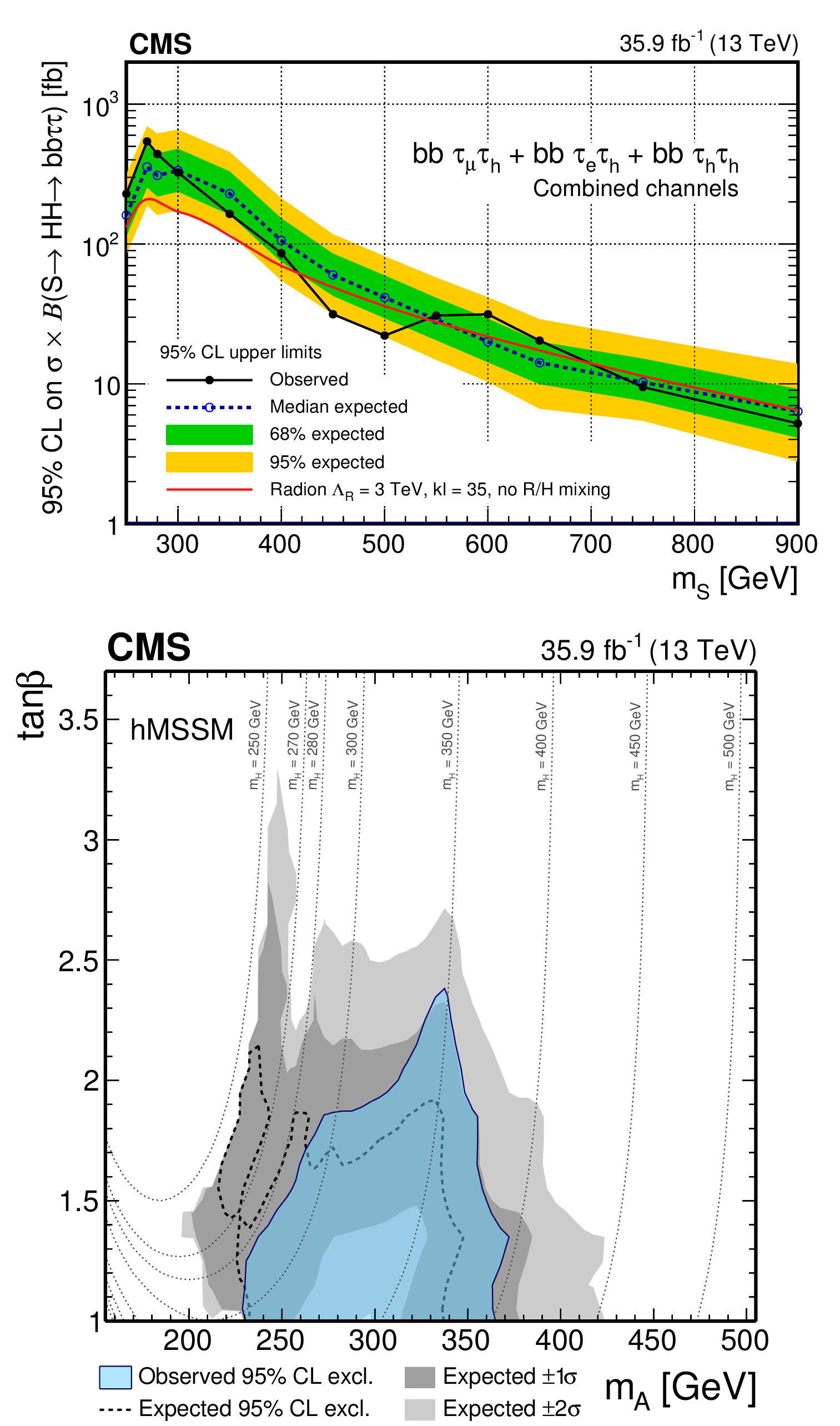
Figure 5:
(upper) Observed and expected 95% CL upper limits on cross section times branching fraction as a function of the mass of the resonance $ {m_\mathrm {S} }$ under the hypothesis that its intrinsic width is negligible with respect to the experimental resolution. The inner (green) band and the outer (yellow) band indicate the regions containing 68 and 95%, respectively, of the distribution of limits expected under the background-only hypothesis. The red line denotes the expectation for the production of a radion, a spin-0 state predicted in WED models, for the parameters $\Lambda _\text {R} = $ 3 TeV (mass scale) and $\text {kL} = $ 35 (size of the extra dimension), assuming the absence of mixing with the Higgs boson. (lower) Interpretation of the exclusion limit in the context of the hMSSM model, parametrized as a function of the $\tan\beta $ and $m_\mathrm {A}$ parameters. In this model, the CP-even lighter scalar is assumed to be the observed 125 GeV Higgs boson and is denoted as h, while the CP-even heavier scalar is denoted as H and the CP-odd scalar is denoted as A. The dotted lines indicate trajectories in the plane corresponding to equal values of the mass of the CP-even heavier scalar of the model, $m_\text {H}$. |

png pdf |
Figure 5-a:
Observed and expected 95% CL upper limits on cross section times branching fraction as a function of the mass of the resonance $ {m_\mathrm {S} }$ under the hypothesis that its intrinsic width is negligible with respect to the experimental resolution. The inner (green) band and the outer (yellow) band indicate the regions containing 68 and 95%, respectively, of the distribution of limits expected under the background-only hypothesis. The red line denotes the expectation for the production of a radion, a spin-0 state predicted in WED models, for the parameters $\Lambda _\text {R} = $ 3 TeV (mass scale) and $\text {kL} = $ 35 (size of the extra dimension), assuming the absence of mixing with the Higgs boson. |
png pdf |
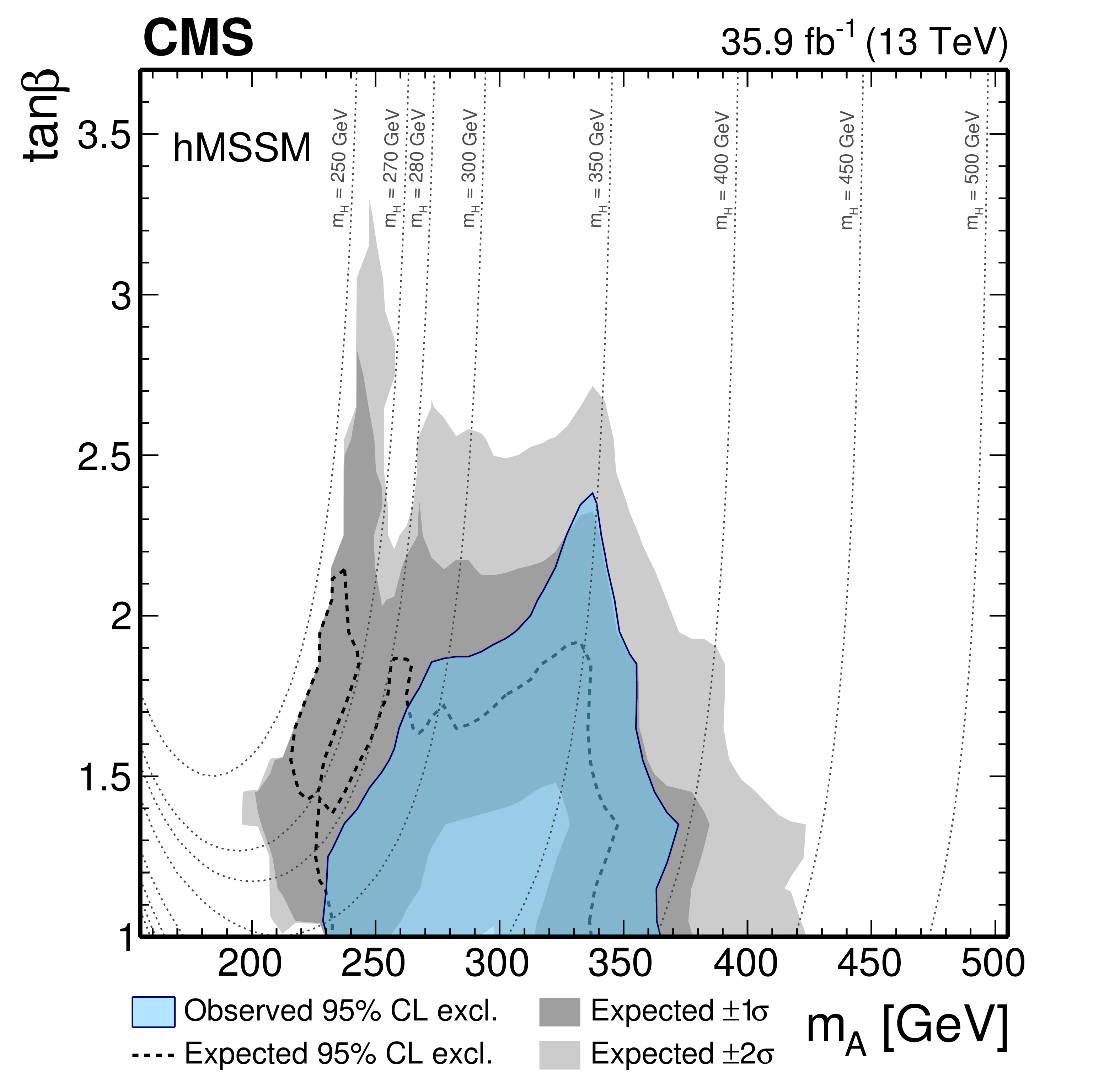
Figure 5-b:
Interpretation of the exclusion limit in the context of the hMSSM model, parametrized as a function of the $\tan\beta $ and $m_\mathrm {A}$ parameters. In this model, the CP-even lighter scalar is assumed to be the observed 125 GeV Higgs boson and is denoted as h, while the CP-even heavier scalar is denoted as H and the CP-odd scalar is denoted as A. The dotted lines indicate trajectories in the plane corresponding to equal values of the mass of the CP-even heavier scalar of the model, $m_\text {H}$. |
png pdf |
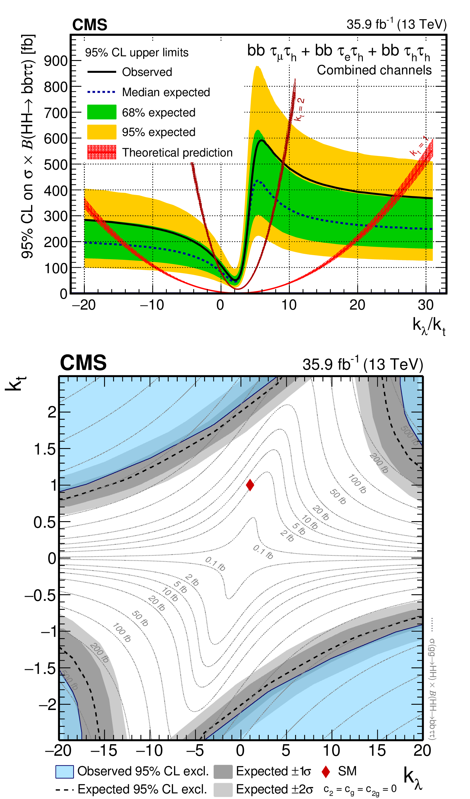
Figure 6:
Test of $k_\lambda $ and $k_\mathrm{ t } $ anomalous couplings. The blue region denotes the parameters excluded by the data at 95% CL, while the dashed black line and the grey regions denote the expected exclusions and the 1$\sigma $ and 2$\sigma $ bands. The dotted lines indicate trajectories in the plane with equal values of cross section times branching fraction that are displayed in the associated labels. The diamond-shaped symbol denotes the couplings predicted by the SM. The theory predictions and the expected and observed limits are symmetric through a $(k_\lambda $, $k_\mathrm{ t } ) \leftrightarrow (-k_\lambda , -k_\mathrm{ t } )$ transformation. The couplings that are not explicitly tested are assumed to correspond to the SM prediction. |
png pdf |
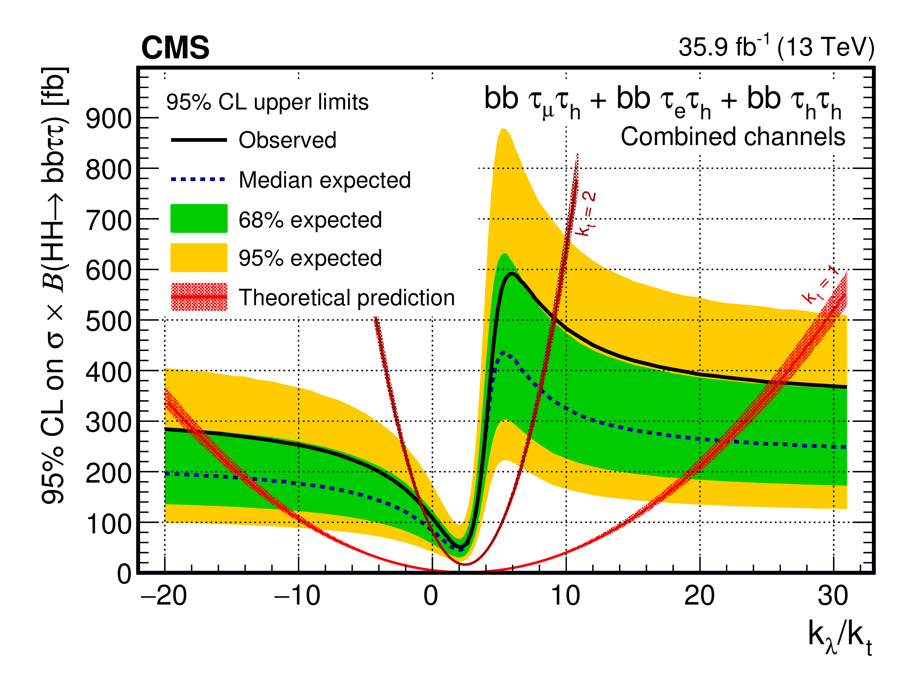
Figure 6-a:
Observed and expected 95% CL upper limits on cross section times branching fraction as a function of $k_\lambda /k_\mathrm{ t } $. The inner (green) band and the outer (yellow) band indicate the regions containing 68 and 95%, respectively, of the distribution of limits expected under the background-only hypothesis. The two red bands show the theoretical cross section expectations and the corresponding uncertainties for $k_\mathrm{ t } = $ 1 and $k_\mathrm{ t } = $ 2. The couplings that are not explicitly tested are assumed to correspond to the SM prediction. |
png pdf |
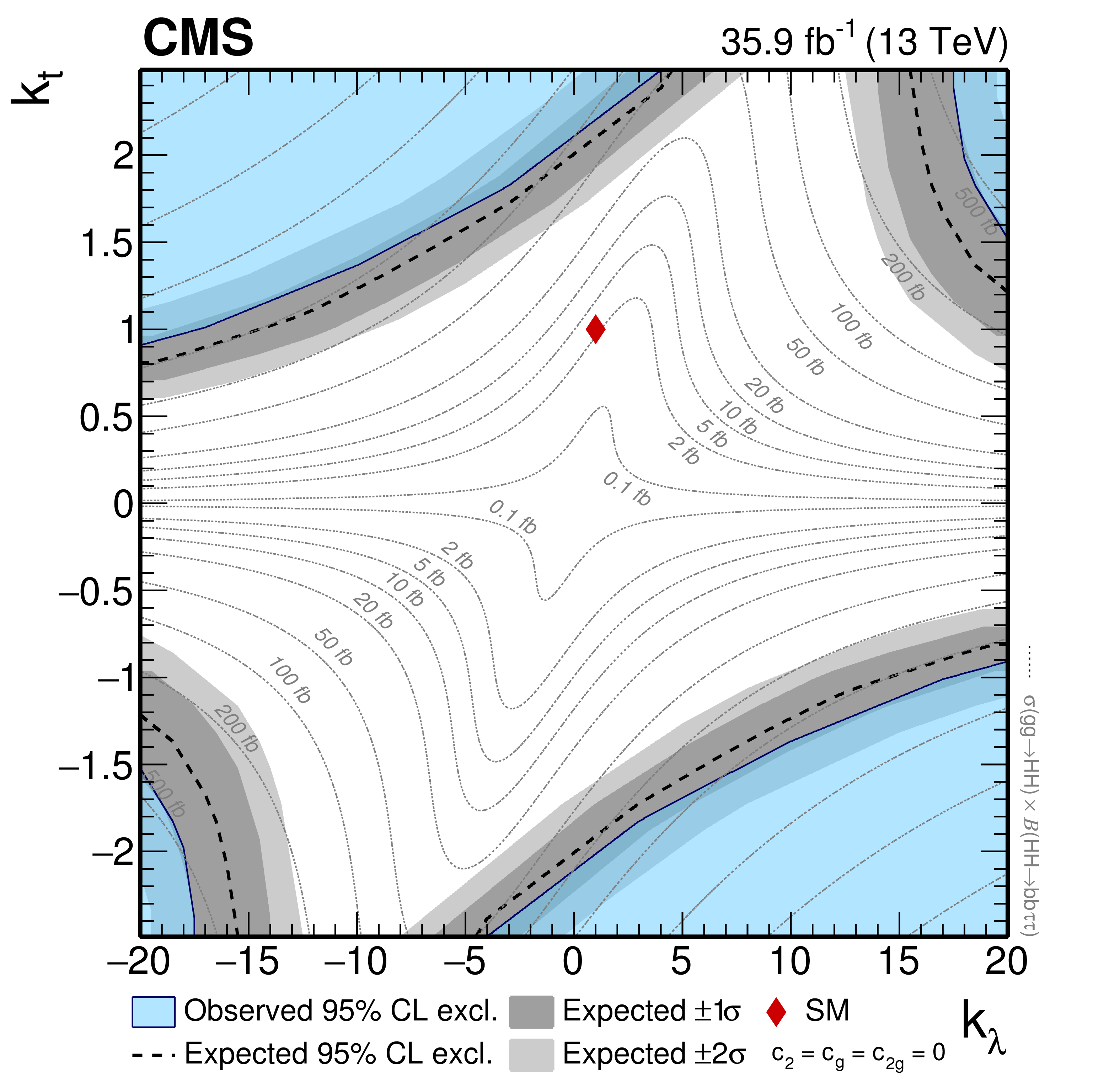
Figure 6-b:
Test of $k_\lambda $ and $k_\mathrm{ t } $ anomalous couplings. The blue region denotes the parameters excluded by the data at 95% CL, while the dashed black line and the grey regions denote the expected exclusions and the 1$\sigma $ and 2$\sigma $ bands. The dotted lines indicate trajectories in the plane with equal values of cross section times branching fraction that are displayed in the associated labels. The diamond-shaped symbol denotes the couplings predicted by the SM. The theory predictions and the expected and observed limits are symmetric through a $(k_\lambda $, $k_\mathrm{ t } ) \leftrightarrow (-k_\lambda , -k_\mathrm{ t } )$ transformation. The couplings that are not explicitly tested are assumed to correspond to the SM prediction. |
| Tables | |
png pdf |
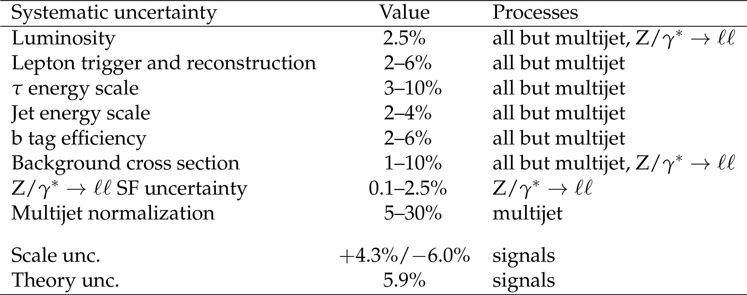
Table 1:
Systematic uncertainties affecting the normalization of the different processes. |
| Summary |
|
A search for resonant and nonresonant Higgs boson pair (HH) production in the $ \mathrm{ b\bar{b} } \tau\tau $ final state is presented. This search uses a data sample collected in proton-proton collisions at $ \sqrt{s} = $ 13 TeV that corresponds to an integrated luminosity of 35.9 fb$^{-1}$. The three most sensitive decay channels of the $\tau$ lepton pair, requiring the decay of one or both $\tau$ leptons into final-state hadrons and a neutrino, are used. The results are found to be statistically compatible with the expected standard model (SM) background contribution, and upper limits at the 95% confidence level are set on the HH production cross sections. For the resonant production mechanism, upper exclusion limits at 95% confidence level (CL) are obtained for the production of a narrow resonance of mass $m_{\mathrm{X}}$ ranging from 250 to 900 GeV. These model-independent results are interpreted in the context of the hMSSM scenario, where a region in the parameter space corresponding to values of $m_\mathrm{A}$ between 230 and 360 GeV and $ \tan \beta \lesssim 2 $ is excluded at 95% CL. For the nonresonant production mechanism, the theoretical framework of an effective Lagrangian is used to parametrize the cross section as a function of anomalous couplings of the Higgs boson. Upper limits at 95% CL on the HH cross section are obtained as a function of $k_\lambda = \lambda_{\mathrm{HHH}}/\lambda_{\mathrm{HHH}}^\text{SM}$ and $k_\mathrm{ t } = y_\mathrm{ t }/y^\text{SM}_\mathrm{ t }$. The observed 95% CL upper limit corresponds to approximately 30 times the theoretical prediction for the SM cross section, and the expected limit is about 25 times the SM prediction. This is the highest sensitivity achieved so far for SM HH production at the LHC. |
| Additional Figures | |

png pdf |
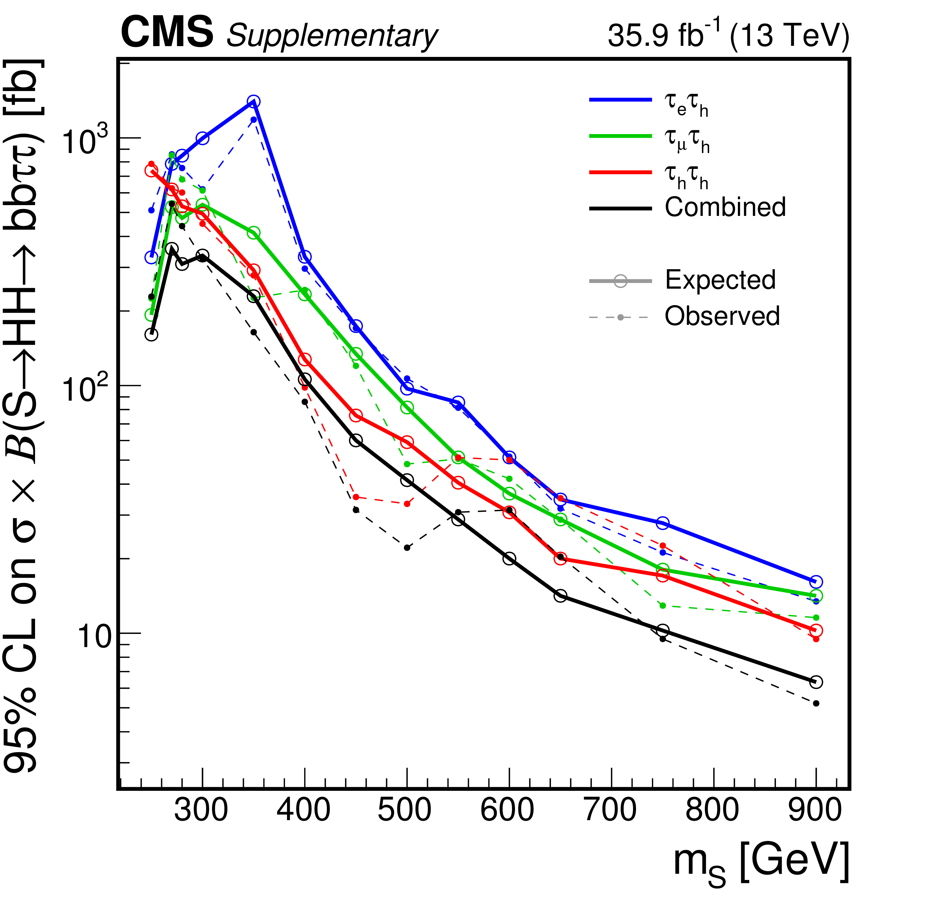
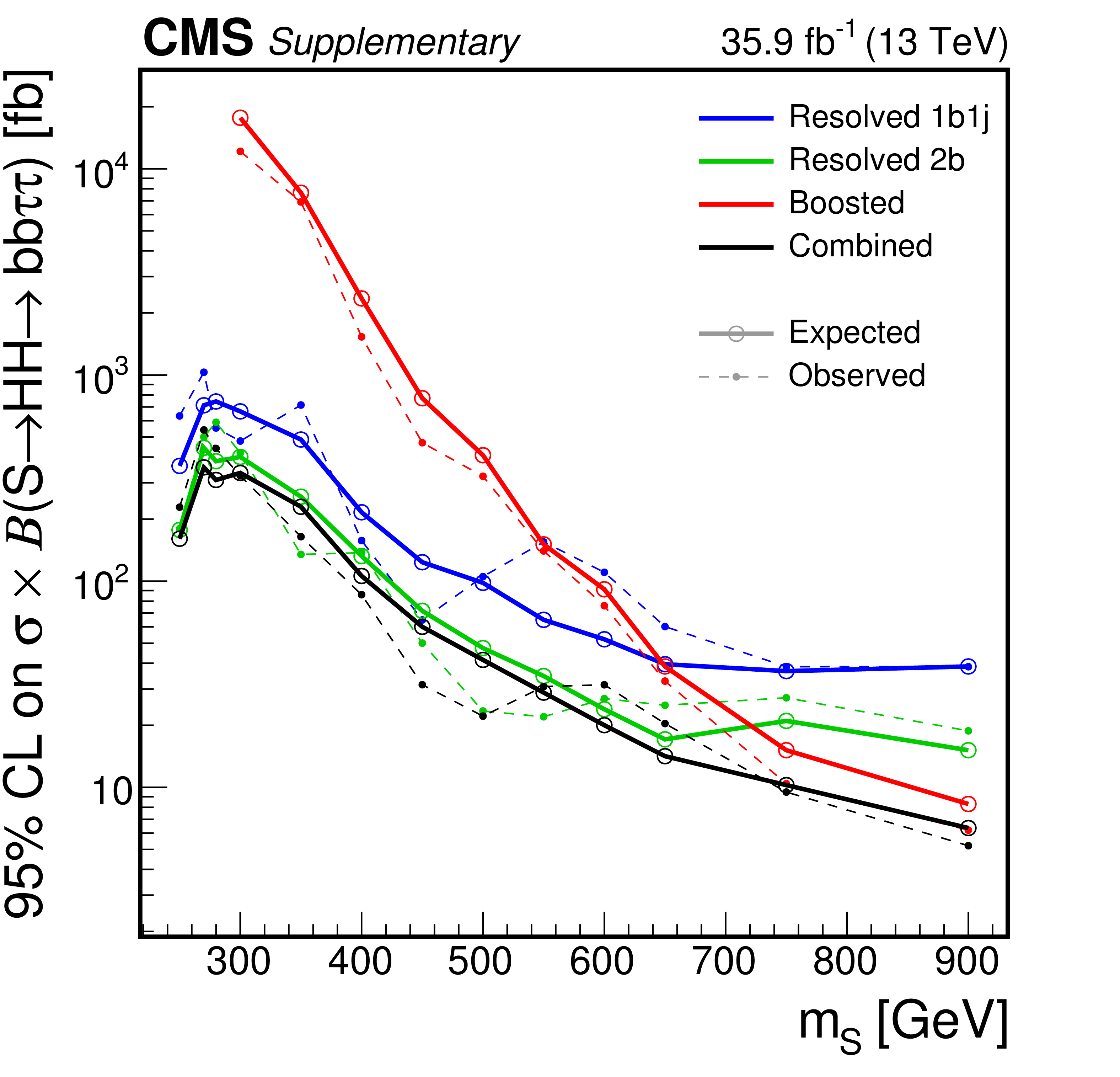
Additional Figure 1:
Upper limits at the 95% confidence level on $\sigma (\mathrm{g} \mathrm{g} \to \text {S})\times \mathcal {B}(\text {S}\to \mathrm{H} \mathrm{H} \to {\mathrm{b} \mathrm{b} \tau \tau})$, shown for the three event categories. The dashed and solid lines denote respectively the observed and expected upper limits. |
png pdf |
Additional Figure 1-a:
Upper limits at the 95% confidence level on $\sigma (\mathrm{g} \mathrm{g} \to \text {S})\times \mathcal {B}(\text {S}\to \mathrm{H} \mathrm{H} \to {\mathrm{b} \mathrm{b} \tau \tau})$, shown for the three decay channels. The dashed and solid lines denote respectively the observed and expected upper limits. |
png pdf |
Additional Figure 1-b:
Upper limits at the 95% confidence level on $\sigma (\mathrm{g} \mathrm{g} \to \text {S})\times \mathcal {B}(\text {S}\to \mathrm{H} \mathrm{H} \to {\mathrm{b} \mathrm{b} \tau \tau})$, shown for the three event categories. The dashed and solid lines denote respectively the observed and expected upper limits. |

png pdf |
Additional Figure 2:
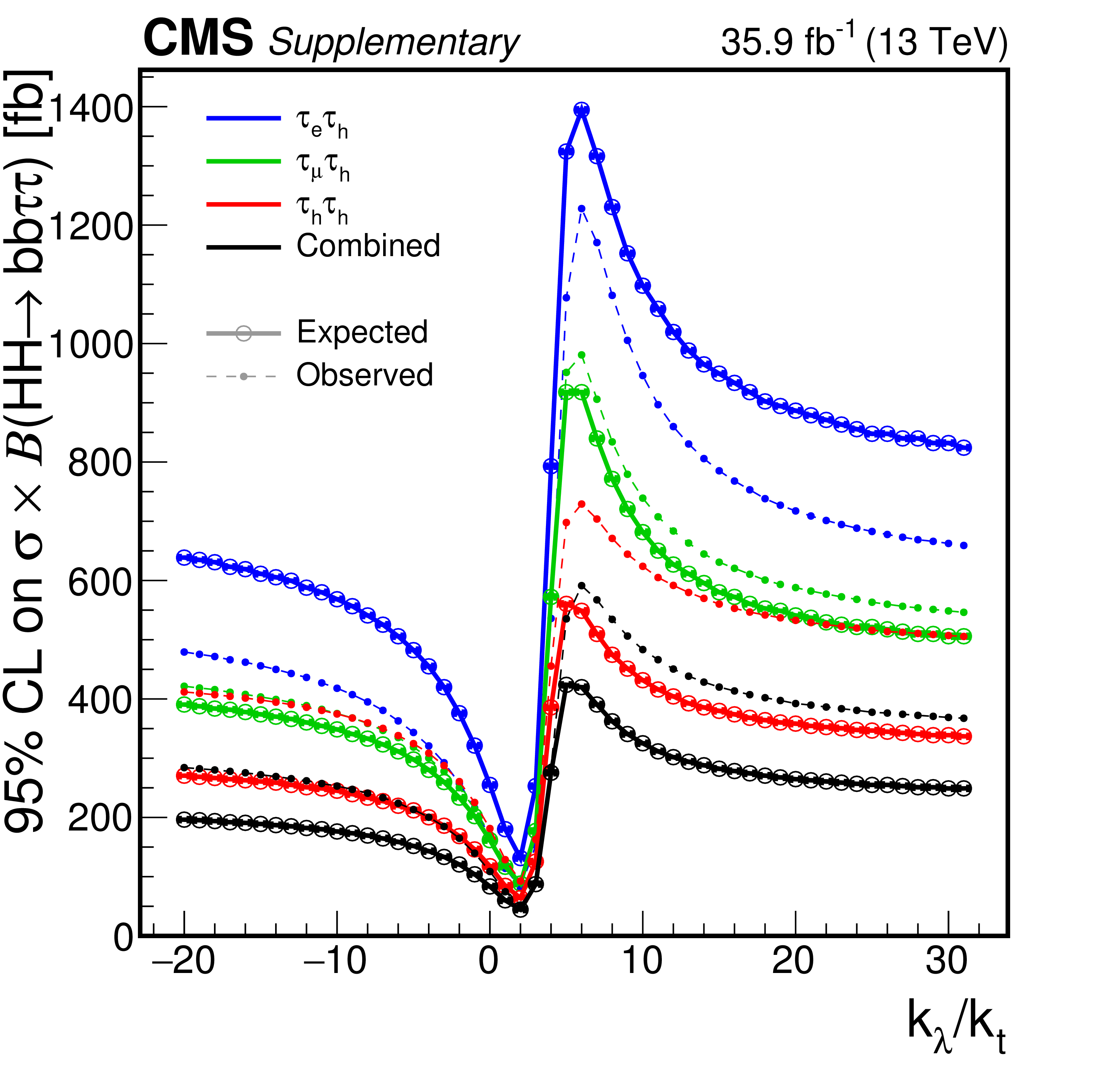
Upper limits at the 95% confidence level on $\sigma (\mathrm{g} \mathrm{g} \to \mathrm{H} \mathrm{H})\times \mathcal {B}(\mathrm{H} \mathrm{H} \to {\mathrm{b} \mathrm{b} \tau \tau})$, shown for the three decay channels (a) and the three event categories (b). The dashed and solid lines denote respectively the observed and expected upper limits. |
png pdf |
Additional Figure 2-a:
Upper limits at the 95% confidence level on $\sigma (\mathrm{g} \mathrm{g} \to \mathrm{H} \mathrm{H})\times \mathcal {B}(\mathrm{H} \mathrm{H} \to {\mathrm{b} \mathrm{b} \tau \tau})$, shown for the three decay channels. The dashed and solid lines denote respectively the observed and expected upper limits. |
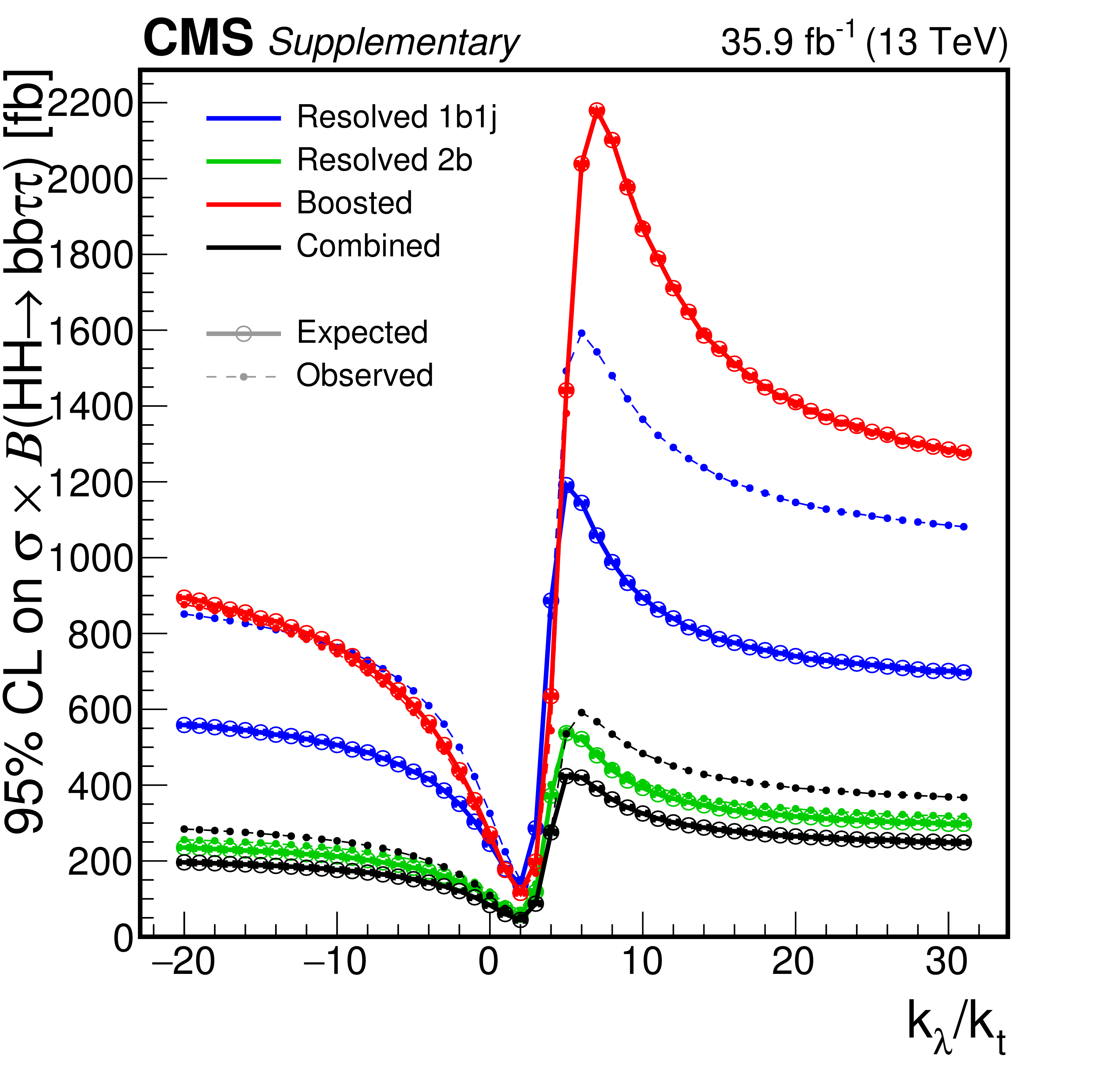
png pdf |
Additional Figure 2-b:
Upper limits at the 95% confidence level on $\sigma (\mathrm{g} \mathrm{g} \to \mathrm{H} \mathrm{H})\times \mathcal {B}(\mathrm{H} \mathrm{H} \to {\mathrm{b} \mathrm{b} \tau \tau})$, shown for the three event categories. The dashed and solid lines denote respectively the observed and expected upper limits. |
png pdf |
Additional Figure 3:
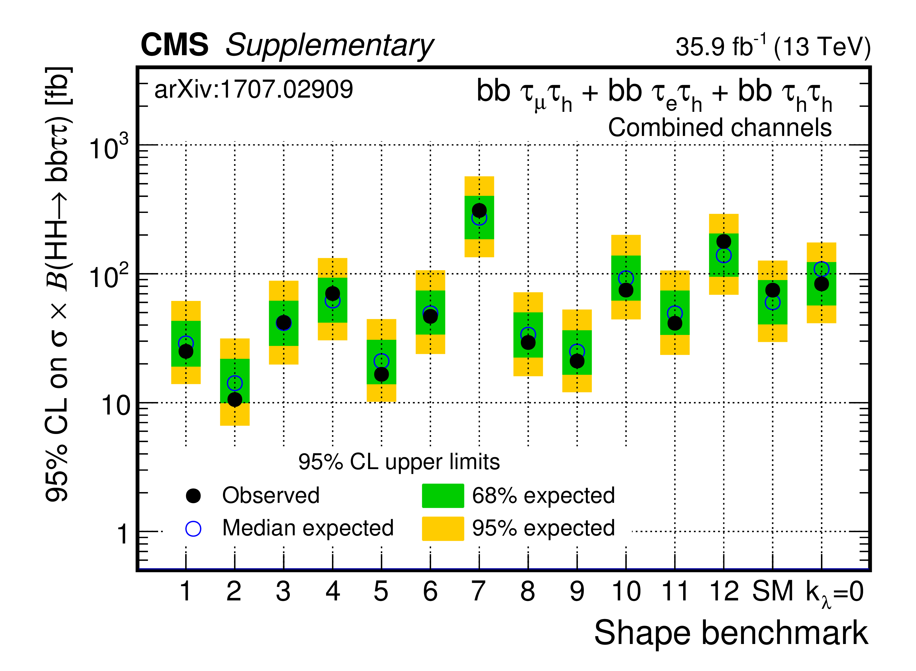
Observed and expected 95% CL upper limits on cross section times branching fraction for different combinations of Higgs boson couplings in the effective Lagrangian parametrization. The numbers from 1 to 12 denote the shape benchmarks defined in Ref. [1], corresponding to points in the five-dimensional parameter space with characteristic kinematic properties of the HH system. Also shown are the SM signal and the case where all couplings except $y_\text {t}$ vanish. The inner (green) band and the outer (yellow) band indicate the regions containing 68 and 95%, respectively, of the distribution of limits expected under the background-only hypothesis. |
png pdf |
Additional Figure 4:
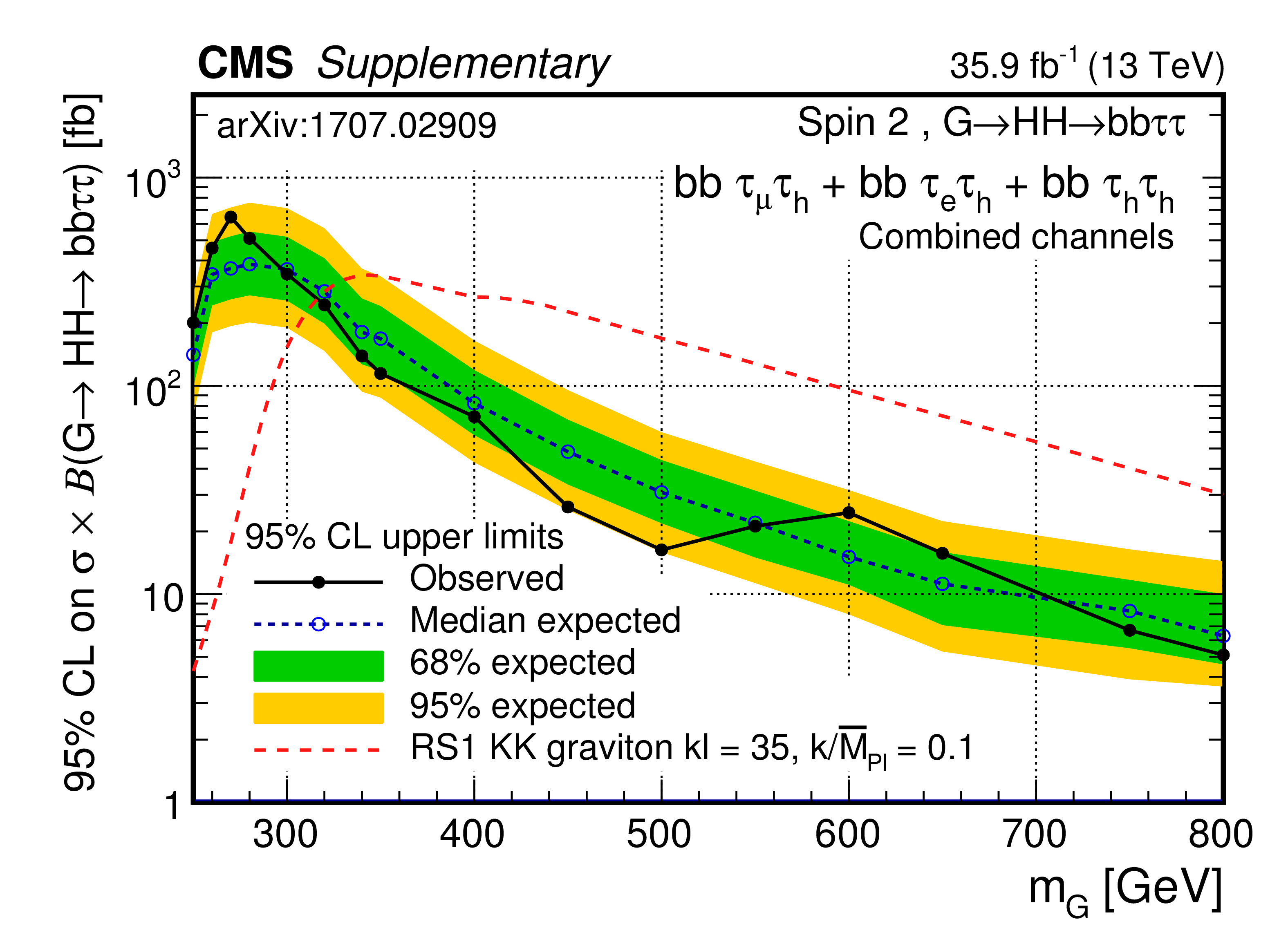
Observed and expected 95% CL upper limits on cross section times branching fraction as a function of the mass of the spin-2 resonance $m_\text {G}$ under the hypothesis that its intrinsic width is negligible with respect to the experimental resolution. The inner (green) band and the outer (yellow) band indicate the regions containing 68 and 95%, respectively, of the distribution of limits expected under the background-only hypothesis. The red line denotes the expectation for the production of a graviton, a spin-2 state predicted in WED models, for the parameters $\text {kl} = $ 35 (size of the extra dimension) and $k/\overline {M}_\text {pl} = $ 0.1 (coupling to matter fields, where $\overline {M}_\text {pl} = M_\text {pl}/\sqrt {8\pi}$). The absence of mixing with the Higgs boson is assumed. |
| Additional Tables | |

png pdf |
Additional Table 1:
Expected upper limits at the 95% confidence level on $\sigma (\mathrm{g} \mathrm{g} \to \text {S})\times \mathcal {B}(\text {S}\to \mathrm{H} \mathrm{H} \to {\mathrm{b} \mathrm{b} \tau \tau})$. The limits are computed for a spin-0 resonance, and are shown separately for the three decay channels (combining the three event categories) and for the three event categories (combining the three decay channels). The combined upper limit is also shown. |
png pdf |
Additional Table 2:
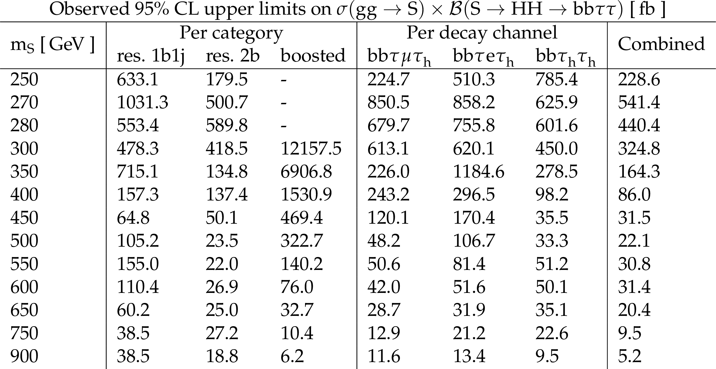
Observed upper limits at the 95% confidence level on $\sigma (\mathrm{g} \mathrm{g} \to \text {S})\times \mathcal {B}(\text {S}\to \mathrm{H} \mathrm{H} \to {\mathrm{b} \mathrm{b} \tau \tau})$. The limits are computed for a spin-0 resonance, and are shown separately for the three decay channels (combining the three event categories) and for the three event categories (combining the three decay channels). The combined upper limit is also shown. |
png pdf |
Additional Table 3:
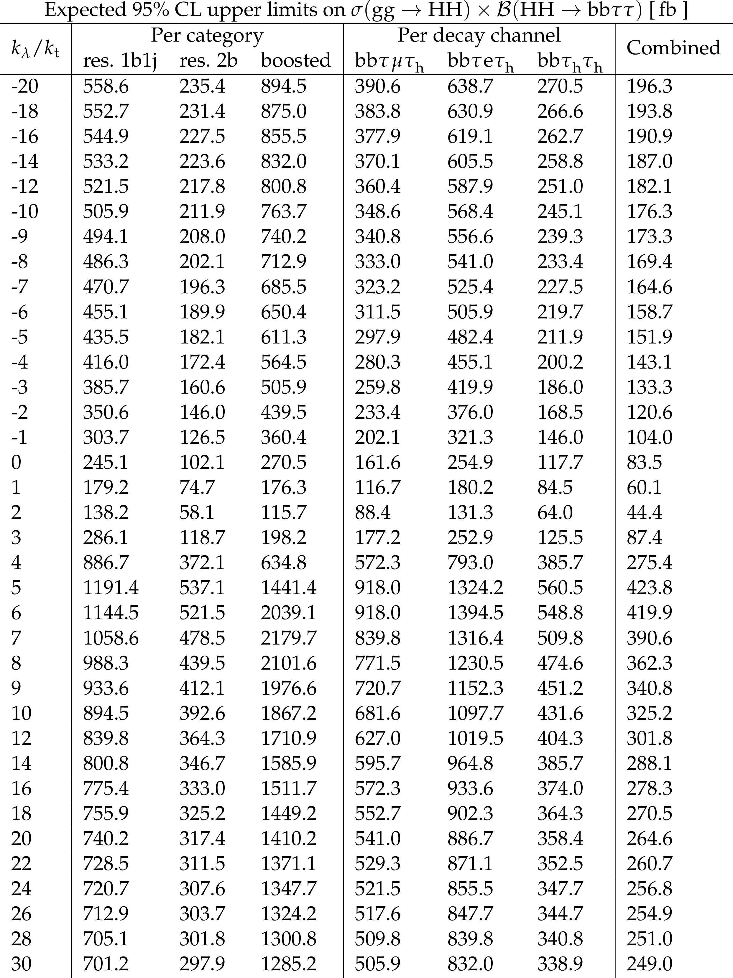
Expected upper limits at the 95% confidence level on $\sigma (\mathrm{g} \mathrm{g} \to \mathrm{H} \mathrm{H})\times \mathcal {B}(\mathrm{H} \mathrm{H} \to {\mathrm{b} \mathrm{b} \tau \tau})$. The limits are computed for different $k_\lambda /k_\text {t}$ hypotheses, and are shown separately for the three decay channels (combining the three event categories) and for the three event categories (combining the three decay channels). The combined upper limit is also shown. |
png pdf |
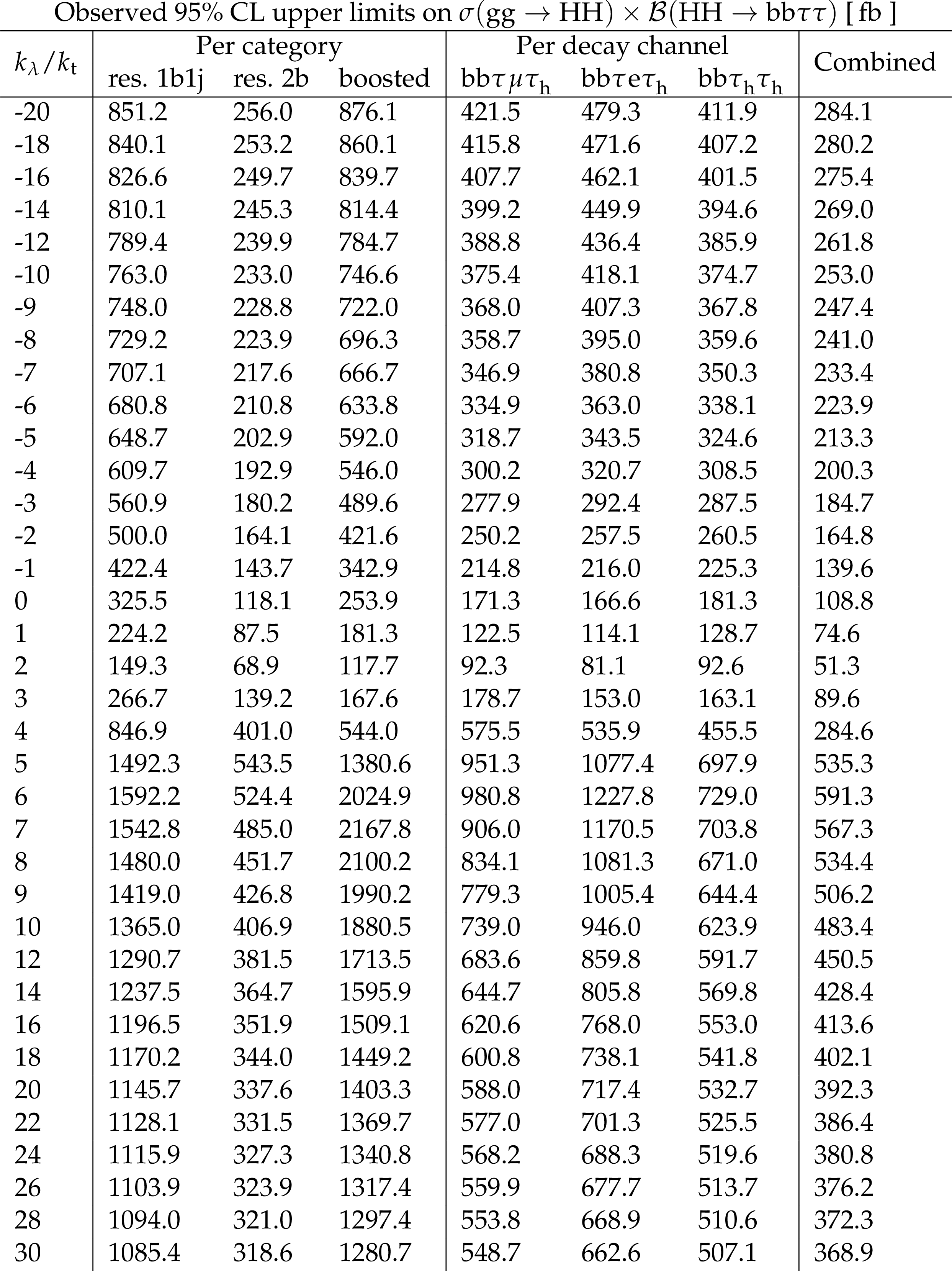
Additional Table 4:
Observed upper limits at the 95% confidence level on $\sigma (\mathrm{g} \mathrm{g} \to \mathrm{H} \mathrm{H})\times \mathcal {B}(\mathrm{H} \mathrm{H} \to {\mathrm{b} \mathrm{b} \tau \tau})$. The limits are computed for different $k_\lambda /k_\text {t}$ hypotheses, and are shown separately for the three decay channels (combining the three event categories) and for the three event categories (combining the three decay channels). The combined upper limit is also shown. |
| References | ||||
| 1 | ATLAS Collaboration | Observation of a new particle in the search for the Standard Model Higgs boson with the ATLAS detector at the LHC | PLB 716 (2012) 1 | 1207.7214 |
| 2 | CMS Collaboration | Observation of a new boson at a mass of 125 GeV with the CMS experiment at the LHC | PLB 716 (2012) 30 | CMS-HIG-12-028 1207.7235 |
| 3 | CMS Collaboration | Observation of a new boson with mass near 125 GeV in pp collisions at $ \sqrt{s} = $ 7 and 8 TeV | JHEP 06 (2013) 081 | CMS-HIG-12-036 1303.4571 |
| 4 | ATLAS and CMS Collaborations | Combined measurement of the Higgs boson mass in $ pp $ collisions at $ \sqrt{s}=$ 7 and 8 TeV with the ATLAS and CMS experiments | PRL 114 (2015) 191803 | 1503.07589 |
| 5 | ATLAS and CMS Collaborations | Measurements of the Higgs boson production and decay rates and constraints on its couplings from a combined ATLAS and CMS analysis of the LHC pp collision data at $ \sqrt{s}=$ 7 and 8 TeV | JHEP 08 (2016) 045 | 1606.02266 |
| 6 | J. Baglio et al. | The measurement of the Higgs self-coupling at the LHC: theoretical status | JHEP 04 (2013) 151 | 1212.5581 |
| 7 | D. de Florian et al. | Handbook of LHC Higgs cross sections: 4. deciphering the nature of the Higgs sector | CERN Report CERN-2017-002-M | 1610.07922 |
| 8 | T. Binoth and J. J. van der Bij | Influence of strongly coupled, hidden scalars on Higgs signals | Z. Phys. C 75 (1997) 17 | hep-ph/9608245 |
| 9 | R. M. Schabinger and J. D. Wells | Minimal spontaneously broken hidden sector and its impact on Higgs boson physics at the CERN Large Hadron Collider | PRD 72 (2005) 093007 | hep-ph/0509209 |
| 10 | B. Patt and F. Wilczek | Higgs-field portal into hidden sectors | hep-ph/0605188 | |
| 11 | G. C. Branco et al. | Theory and phenomenology of two-Higgs-doublet models | PR 516 (2012) 1 | 1106.0034 |
| 12 | P. Fayet | Supergauge invariant extension of the Higgs mechanism and a model for the electron and its neutrino | Nucl. Phys. B 90 (1975) 104 | |
| 13 | P. Fayet | Spontaneously broken supersymmetric theories of weak, electromagnetic and strong interactions | PLB 69 (1977) 489 | |
| 14 | K. Agashe, H. Davoudiasl, G. Perez, and A. Soni | Warped gravitons at the CERN LHC and beyond | PRD 76 (2007) 036006 | hep-ph/0701186 |
| 15 | A. L. Fitzpatrick, J. Kaplan, L. Randall, and L.-T. Wang | Searching for the Kaluza-Klein graviton in bulk RS models | JHEP 09 (2007) 013 | hep-ph/0701150 |
| 16 | F. Goertz, A. Papaefstathiou, L. L. Yang, and J. Zurita | Higgs boson pair production in the D=6 extension of the SM | JHEP 04 (2015) 167 | 1410.3471 |
| 17 | A. Carvalho et al. | Higgs pair production: choosing benchmarks with cluster analysis | JHEP 04 (2016) 126 | 1507.02245 |
| 18 | ATLAS Collaboration | Searches for Higgs boson pair production in the $ hh {\rightarrow}bb {\tau} {\tau} $, $ {\gamma} {\gamma}{W}{W}^{*} $, $ {\gamma} {\gamma}bb $, $ bbbb $ channels with the ATLAS detector | PRD 92 (2015) 092004 | 1509.04670 |
| 19 | ATLAS Collaboration | Search for pair production of Higgs bosons in the $ b\bar{b}b\bar{b} $ final state using proton--proton collisions at $ \sqrt{s} = 13 $ TeV with the ATLAS detector | PRD 94 (2016) 052002 | 1606.04782 |
| 20 | CMS Collaboration | Search for two Higgs bosons in final states containing two photons and two bottom quarks in proton-proton collisions at 8 TeV | PRD 94 (2016) 052012 | CMS-HIG-13-032 1603.06896 |
| 21 | CMS Collaboration | Search for resonant pair production of Higgs bosons decaying to two bottom quark-antiquark pairs in proton-proton collisions at 8 TeV | PLB 749 (2015) 560 | CMS-HIG-14-013 1503.04114 |
| 22 | CMS Collaboration | A search for Higgs boson pair production in the $ bb\tau\tau $ final state in proton-proton collisions at $ \sqrt{s} = $ 8TeV | Submitted to PRD | CMS-HIG-15-013 1707.00350 |
| 23 | CMS Collaboration | The CMS trigger system | JINST 12 (2017) P01020 | CMS-TRG-12-001 1609.02366 |
| 24 | CMS Collaboration | The CMS experiment at the CERN LHC | JINST 3 (2008) S08004 | CMS-00-001 |
| 25 | J. Alwall et al. | The automated computation of tree-level and next-to-leading order differential cross sections, and their matching to parton shower simulations | JHEP 07 (2014) 079 | 1405.0301 |
| 26 | A. Carvalho et al. | Analytical parametrization and shape classification of anomalous HH production in the EFT approach | 1608.06578 | |
| 27 | J. Alwall et al. | Comparative study of various algorithms for the merging of parton showers and matrix elements in hadronic collisions | EPJC 53 (2008) 473 | 0706.2569 |
| 28 | E. Re | Single-top $ Wt $-channel production matched with parton showers using the POWHEG method | EPJC 71 (2011) 1547 | 1009.2450 |
| 29 | J. M. Campbell, R. K. Ellis, P. Nason, and E. Re | Top-pair production and decay at NLO matched with parton showers | JHEP 04 (2015) 114 | 1412.1828 |
| 30 | NNPDF Collaboration | Parton distributions for the LHC Run II | JHEP 04 (2015) 040 | 1410.8849 |
| 31 | T. Sjostrand et al. | An introduction to PYTHIA 8.2 | CPC 191 (2015) 159 | 1410.3012 |
| 32 | CMS Collaboration | Event generator tunes obtained from underlying event and multiparton scattering measurements | EPJC 76 (2016) 155 | CMS-GEN-14-001 1512.00815 |
| 33 | M. Czakon and A. Mitov | Top++: A Program for the Calculation of the Top-Pair Cross-Section at Hadron Colliders | CPC 185 (2014) 2930 | 1112.5675 |
| 34 | Y. Li and F. Petriello | Combining QCD and electroweak corrections to dilepton production in FEWZ | PRD 86 (2012) 094034 | 1208.5967 |
| 35 | N. Kidonakis | Top quark production | in Proceedings, Helmholtz International Summer School on Physics of Heavy Quarks and Hadrons (HQ 2013), Dubna | 1311.0283 |
| 36 | J. M. Campbell, R. K. Ellis, and C. Williams | Vector boson pair production at the LHC | JHEP 07 (2011) 018 | 1105.0020 |
| 37 | CMS Collaboration | Particle-flow reconstruction and global event description with the CMS detector | Submitted to JINST | CMS-PRF-14-001 1706.04965 |
| 38 | M. Cacciari, G. P. Salam, and G. Soyez | The anti-$ k_t $ jet clustering algorithm | JHEP 04 (2008) 063 | 0802.1189 |
| 39 | M. Cacciari, G. P. Salam, and G. Soyez | FastJet user manual | EPJC 72 (2012) 1896 | 1111.6097 |
| 40 | J. M. Butterworth, A. R. Davison, M. Rubin, and G. P. Salam | Jet substructure as a new Higgs-search channel at the Large Hadron Collider | PRL 100 (2008) 242001 | 0802.2470 |
| 41 | A. J. Larkoski, S. Marzani, G. Soyez, and J. Thaler | Soft drop | JHEP 05 (2014) 146 | 1402.2657 |
| 42 | CMS Collaboration | Determination of jet energy calibration and transverse momentum resolution in CMS | JINST 6 (2011) P11002 | CMS-JME-10-011 1107.4277 |
| 43 | CMS Collaboration | Performance of missing energy reconstruction in 13 TeV pp collision data using the CMS detector | CMS-PAS-JME-16-004 | CMS-PAS-JME-16-004 |
| 44 | CMS Collaboration | Reconstruction and identification of $ \tau $ lepton decays to hadrons and $ \nu_\tau $ at CMS | JINST 11 (2016) P01019 | CMS-TAU-14-001 1510.07488 |
| 45 | CMS Collaboration | Performance of reconstruction and identification of tau leptons in their decays to hadrons and tau neutrino in LHC Run-2 | CMS-PAS-TAU-16-002 | CMS-PAS-TAU-16-002 |
| 46 | CMS Collaboration | Performance of electron reconstruction and selection with the CMS detector in proton-proton collisions at $ \sqrt{s} = $ 8 TeV | JINST 10 (2015) P06005 | CMS-EGM-13-001 1502.02701 |
| 47 | CMS Collaboration | Performance of CMS muon reconstruction in pp collision events at $ \sqrt{s}=$ 7 TeV | JINST 7 (2012) P10002 | CMS-MUO-10-004 1206.4071 |
| 48 | CMS Collaboration | Identification of b-quark jets with the CMS experiment | JINST 8 (2013) P04013 | CMS-BTV-12-001 1211.4462 |
| 49 | CMS Collaboration | Identification of b quark jets at the CMS Experiment in the LHC Run 2 | CMS-PAS-BTV-15-001 | CMS-PAS-BTV-15-001 |
| 50 | L. Bianchini, J. Conway, E. K. Friis, and C. Veelken | Reconstruction of the Higgs mass in $ H \to \tau\tau $ events by dynamical likelihood techniques | J. Phys. Conf. Ser. 513 (2014) 022035 | |
| 51 | H. Voss, A. Hocker, J. Stelzer, and F. Tegenfeldt | TMVA, the toolkit for multivariate data analysis with ROOT | in XIth International Workshop on Advanced Computing and Analysis Techniques in Physics Research (ACAT) 2007 | physics/0703039 |
| 52 | J. H. Friedman | Greedy function approximation: A gradient boosting machine | Ann. Statist. 29 (2001) 1189 | |
| 53 | CMS Collaboration | Searches for a heavy scalar boson H decaying to a pair of 125 GeV Higgs bosons hh or for a heavy pseudoscalar boson A decaying to Zh, in the final states with $ h \to \tau \tau $ | PLB 755 (2016) 217 | CMS-HIG-14-034 1510.01181 |
| 54 | C. G. Lester and D. J. Summers | Measuring masses of semiinvisibly decaying particles pair produced at hadron colliders | PLB 463 (1999) 99 | hep-ph/9906349 |
| 55 | A. Barr, C. Lester, and P. Stephens | A variable for measuring masses at hadron colliders when missing energy is expected; $ m_{T2} $: the truth behind the glamour | JPG 29 (2003) 2343 | hep-ph/0304226 |
| 56 | A. J. Barr, M. J. Dolan, C. Englert, and M. Spannowsky | Di-Higgs final states augMT2ed -- selecting $ hh $ events at the high luminosity LHC | PLB 728 (2014) 308 | 1309.6318 |
| 57 | C. G. Lester and B. Nachman | Bisection-based asymmetric MT2 computation: a higher precision calculator than existing symmetric methods | JHEP 03 (2015) 100 | 1411.4312 |
| 58 | CMS Collaboration | Measurements of differential production cross sections for a Z boson in association with jets in pp collisions at $ \sqrt{s}=$ 8 TeV | JHEP 04 (2017) 022 | CMS-SMP-14-013 1611.03844 |
| 59 | CMS Collaboration | CMS luminosity measurements for the 2016 data taking period | CMS-PAS-LUM-17-001 | CMS-PAS-LUM-17-001 |
| 60 | CMS Collaboration | Measurement of differential cross sections for top quark pair production using the lepton+jets final state in proton-proton collisions at 13 TeV | PRD 95 (2017) 092001 | CMS-TOP-16-008 1610.04191 |
| 61 | T. Junk | Confidence level computation for combining searches with small statistics | NIMA 434 (1999) 435 | hep-ex/9902006 |
| 62 | A. L. Read | Presentation of search results: the $ CL_s $ technique | JPG 28 (2002) 2693 | |
| 63 | A. Oliveira | Gravity particles from Warped Extra Dimensions, predictions for LHC | 1404.0102 | |
| 64 | A. Djouadi et al. | The post-Higgs MSSM scenario: habemus MSSM? | EPJC 73 (2013) 2650 | 1307.5205 |
| 65 | A. Djouadi et al. | Fully covering the MSSM Higgs sector at the LHC | JHEP 06 (2015) 168 | 1502.05653 |
|
|
Compact Muon Solenoid LHC, CERN |
|

|

|

|

|

|