

Compact Muon Solenoid
LHC, CERN
| CMS-HIG-17-017 ; CERN-EP-2018-269 | ||
| Search for nonresonant Higgs boson pair production in the ${\mathrm{b\bar{b}}\mathrm{b\bar{b}}}$ final state at $\sqrt{s} = $ 13 TeV | ||
| CMS Collaboration | ||
| 29 October 2018 | ||
| JHEP 04 (2019) 112 | ||
| Abstract: Results of a search for nonresonant production of Higgs boson pairs, with each Higgs boson decaying to a $ \mathrm{b\bar{b}} $ pair, are presented. This search uses data from proton-proton collisions at a centre-of-mass energy of 13 TeV, corresponding to an integrated luminosity of 35.9 fb$^{-1}$, collected by the CMS detector at the LHC. No signal is observed, and a 95% confidence level upper limit of 847fb is set on the cross section for standard model nonresonant Higgs boson pair production times the squared branching fraction of the Higgs boson decay to a $ \mathrm{b\bar{b}} $ pair. The same signature is studied, and upper limits are set, in the context of models of physics beyond the standard model that predict modified couplings of the Higgs boson. | ||
| Links: e-print arXiv:1810.11854 [hep-ex] (PDF) ; CDS record ; inSPIRE record ; HepData record ; CADI line (restricted) ; | ||
| Figures | |

png pdf |
Figure 1:
Feynman diagrams that contribute to HH production via gluon-gluon fusion at LO. Diagrams (a) and (b) correspond to SM-like processes, while diagrams (c), (d), and (e) correspond to pure BSM effects: (c) and (d) describe contact interactions between the Higgs boson and gluons, and (e) describes the contact interaction of two Higgs bosons with top quarks. |
png pdf |
Figure 2:
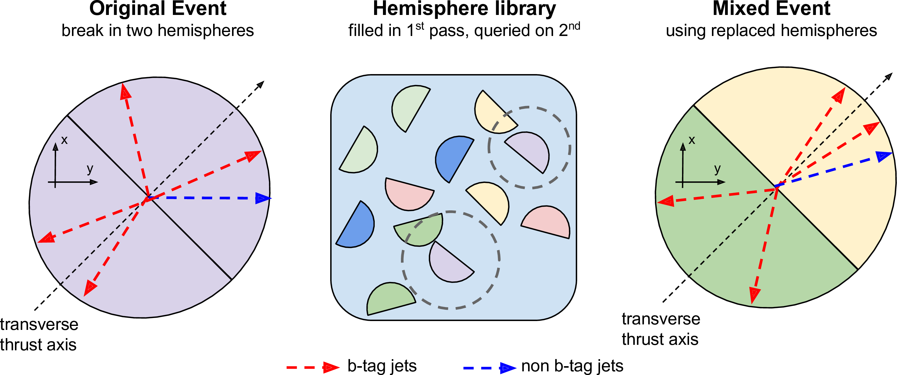
An illustration of the hemisphere mixing procedure. The transverse thrust axis is defined as the axis on which the sum of the absolute values of the projections of the $ {p_{\mathrm {T}}} $ of the jets is maximal. Once the thrust axis is identified, the event is divided into two halves by cutting along the axis perpendicular to the transverse thrust axis. One such half is called a hemisphere (h). In a preliminary step, each event in the original $N$-event data set is split into two hemispheres that are collected in a library of $2N$ hemispheres. Once the library is created, each event is used as a basis for creating artificial events. These are constructed by picking two hemispheres from the library that are similar to the two hemispheres that make up the original event. |
png pdf |
Figure 3:
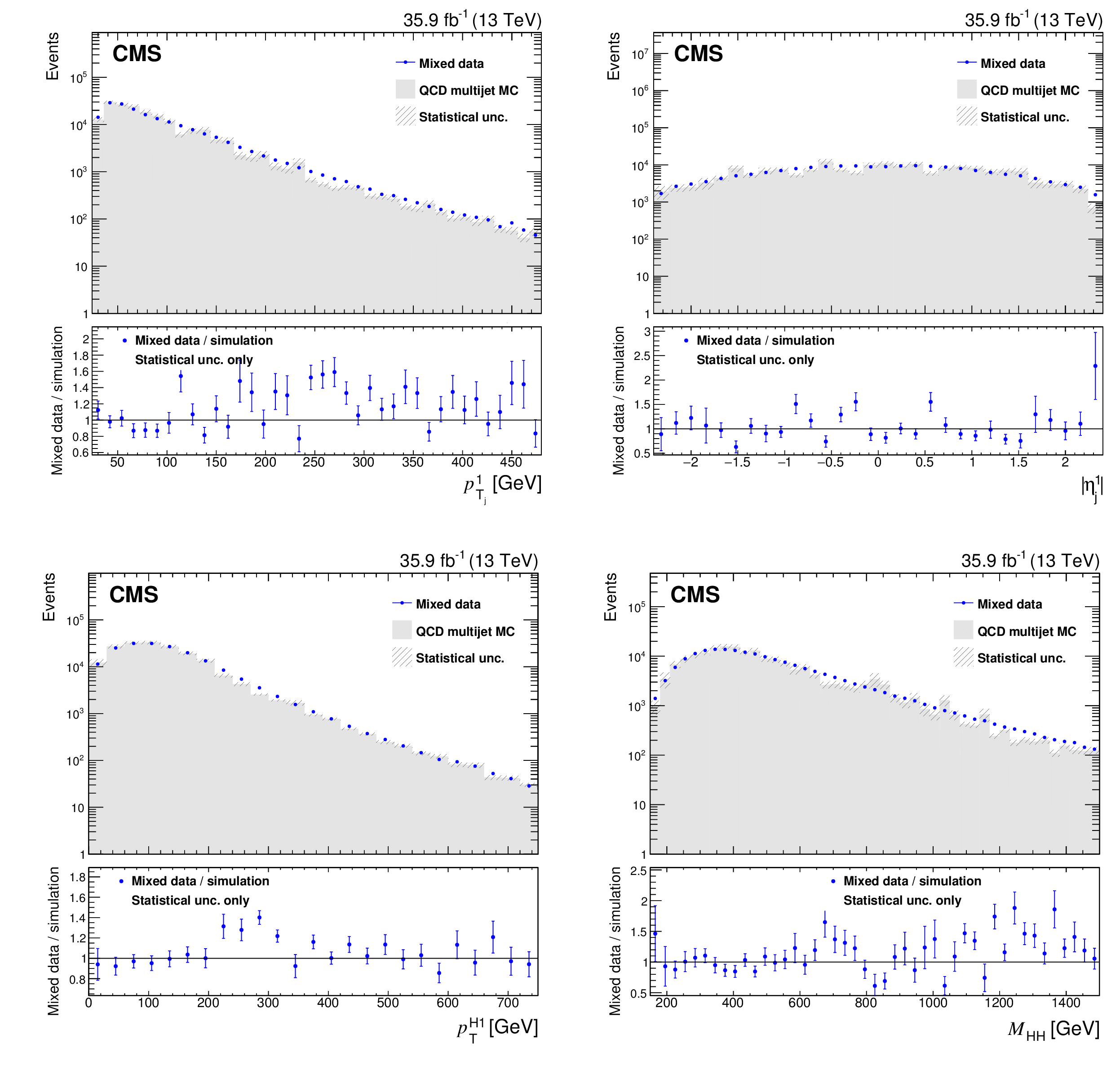
Comparison between the background model obtained with the hemisphere mixing technique and MC simulation of QCD multijet processes for $ {{{{p_{\mathrm {T}}}}_{\mathrm {j}}} ^{1}} $ (upper left), $ {\eta ^{1}_{\text {j}}} $ (upper right), ${{{p_{\mathrm {T}}} ^{{{\mathrm {H}} _1}}}}$ (lower left), and $ {M_{{\mathrm {H}} {\mathrm {H}}}} $ (lower right). Bias correction for the background model, described in Section 8.2, is applied by rescaling the weight of each event using the event yield ratio between corrected and uncorrected BDT distributions. Only statistical uncertainties are shown as the uncertainties related to the bias correction can not be propagated from the BDT classifier to a different variable. |

png pdf |
Figure 3-a:
Comparison between the background model obtained with the hemisphere mixing technique and MC simulation of QCD multijet processes for $ {{{{p_{\mathrm {T}}}}_{\mathrm {j}}} ^{1}} $. Bias correction for the background model, described in Section 8.2, is applied by rescaling the weight of each event using the event yield ratio between corrected and uncorrected BDT distributions. Only statistical uncertainties are shown as the uncertainties related to the bias correction can not be propagated from the BDT classifier to a different variable. |
png pdf |
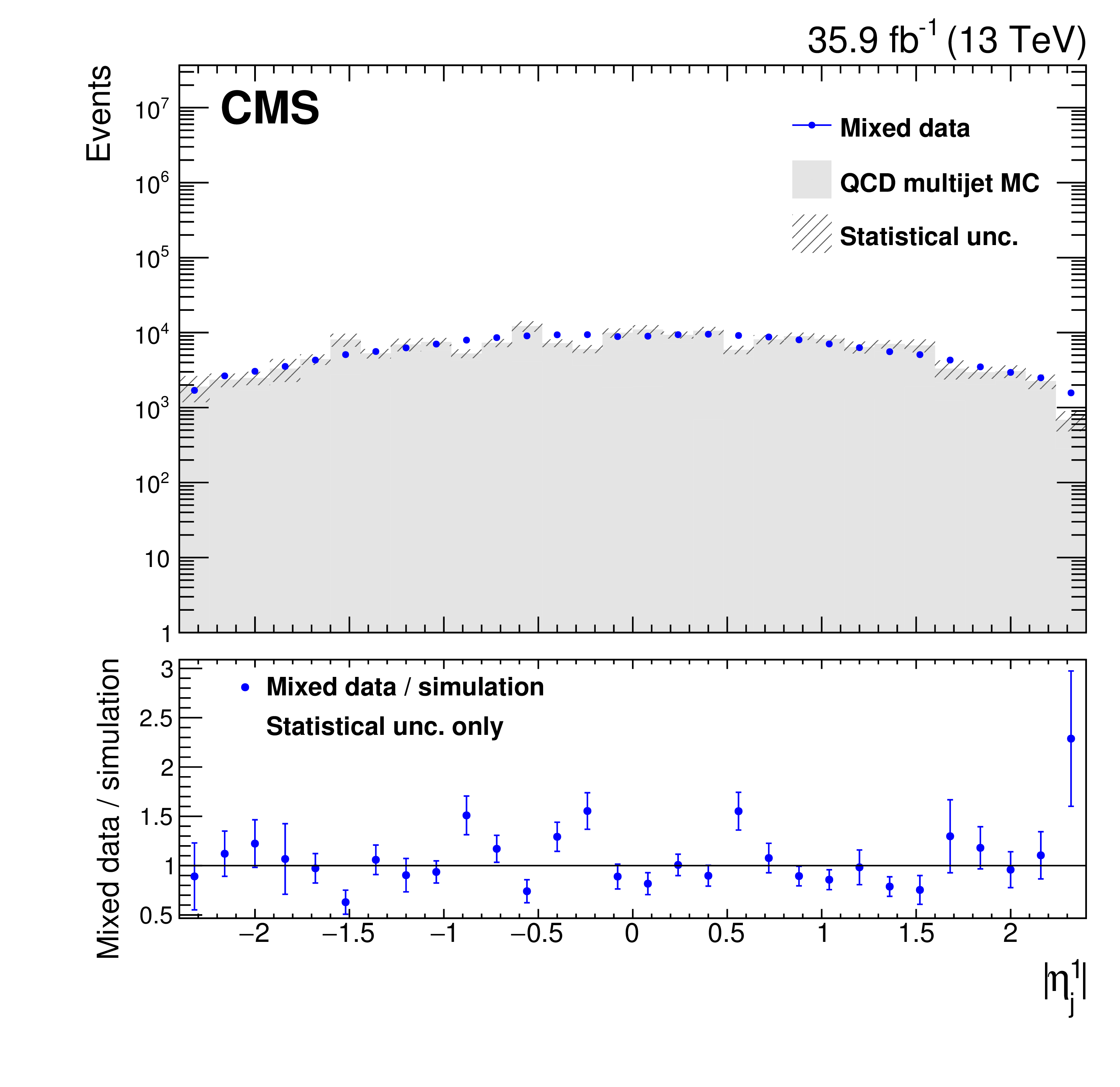
Figure 3-b:
Comparison between the background model obtained with the hemisphere mixing technique and MC simulation of QCD multijet processes for $ {\eta ^{1}_{\text {j}}} $. Bias correction for the background model, described in Section 8.2, is applied by rescaling the weight of each event using the event yield ratio between corrected and uncorrected BDT distributions. Only statistical uncertainties are shown as the uncertainties related to the bias correction can not be propagated from the BDT classifier to a different variable. |

png pdf |
Figure 3-c:
Comparison between the background model obtained with the hemisphere mixing technique and MC simulation of QCD multijet processes for ${{{p_{\mathrm {T}}} ^{{{\mathrm {H}} _1}}}}$. Bias correction for the background model, described in Section 8.2, is applied by rescaling the weight of each event using the event yield ratio between corrected and uncorrected BDT distributions. Only statistical uncertainties are shown as the uncertainties related to the bias correction can not be propagated from the BDT classifier to a different variable. |
png pdf |
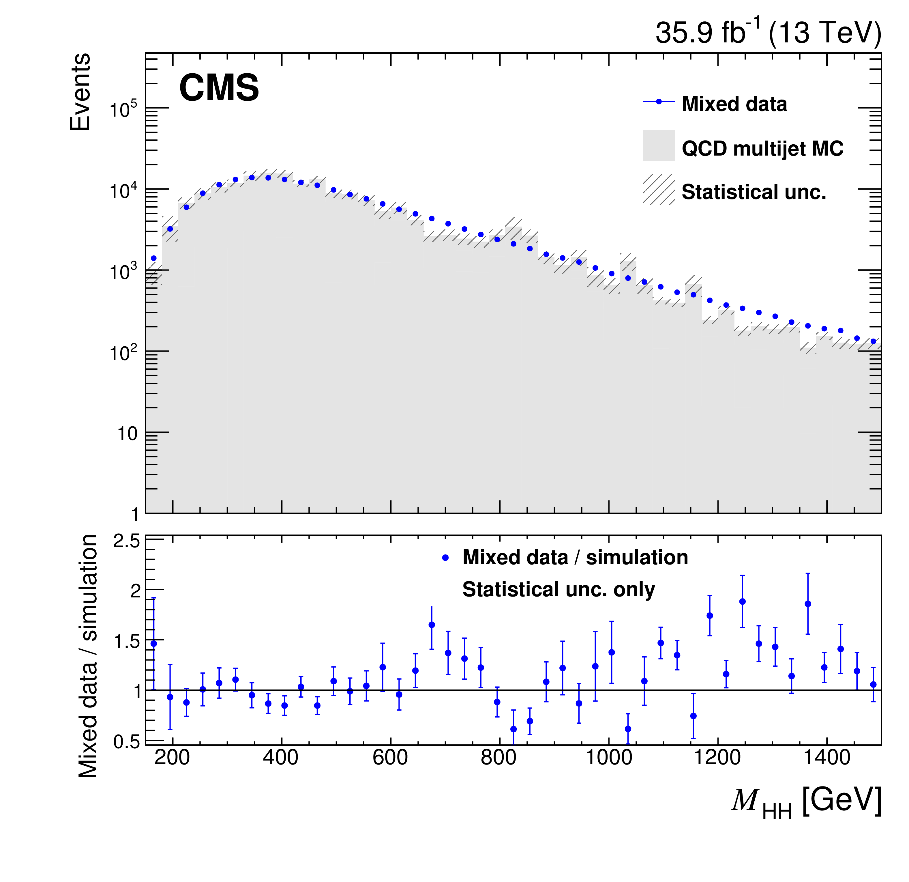
Figure 3-d:
Comparison between the background model obtained with the hemisphere mixing technique and MC simulation of QCD multijet processes for $ {M_{{\mathrm {H}} {\mathrm {H}}}} $. Bias correction for the background model, described in Section 8.2, is applied by rescaling the weight of each event using the event yield ratio between corrected and uncorrected BDT distributions. Only statistical uncertainties are shown as the uncertainties related to the bias correction can not be propagated from the BDT classifier to a different variable. |
png pdf |
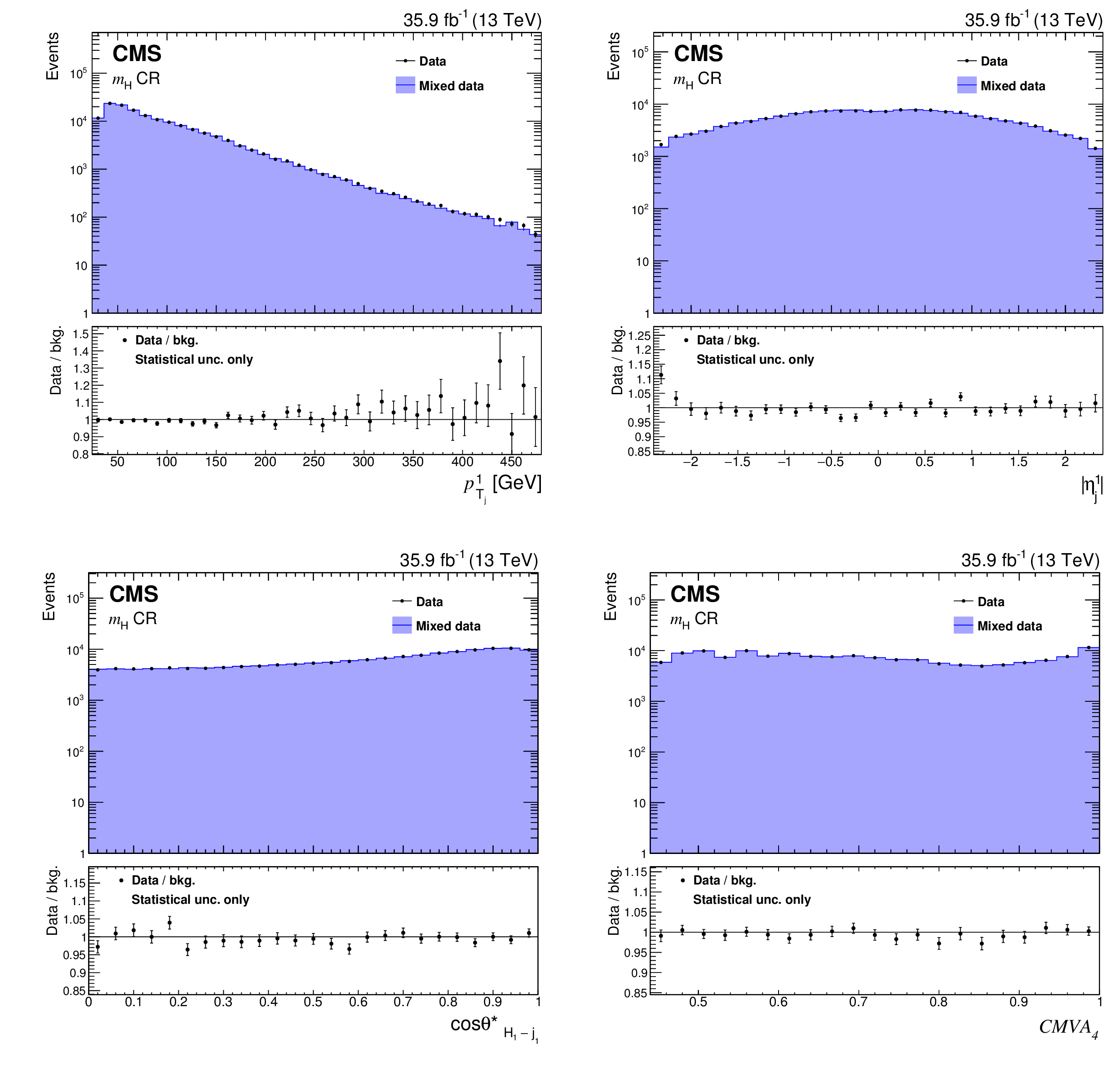
Figure 4:
Comparison between the background model obtained with the hemisphere mixing technique and data in the ${m_{{\mathrm {H}}}} $ CR for the variables $ {{{{p_{\mathrm {T}}}}_{\mathrm {j}}} ^{1}} $ (upper left), $ {\eta ^{1}_{\text {j}}} $ (upper right), ${\cos {\theta ^{*}} _{{{\mathrm {H}} _1} \text {-}\mathrm {j}_1}}$ (lower left), and $CMVA_{4} $ (lower right). Bias correction for the background model, described in Section 8.2, is applied by rescaling the weight of each event using the event yield ratio between corrected and uncorrected BDT distributions in this CR. Only statistical uncertainties are shown as the uncertainties related to the bias correction can not be propagated from the BDT classifier to a different variable. |
png pdf |
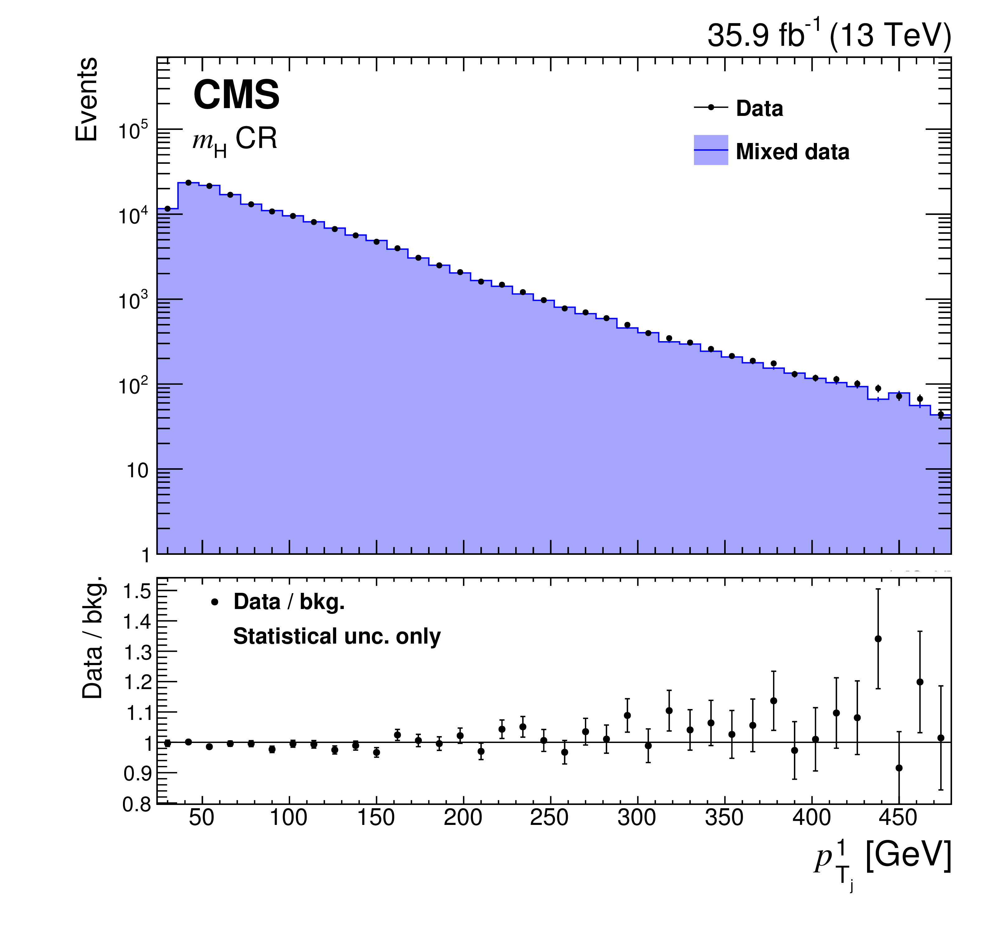
Figure 4-a:
Comparison between the background model obtained with the hemisphere mixing technique and data in the ${m_{{\mathrm {H}}}} $ CR for the $ {{{{p_{\mathrm {T}}}}_{\mathrm {j}}} ^{1}} $ variable. Bias correction for the background model, described in Section 8.2, is applied by rescaling the weight of each event using the event yield ratio between corrected and uncorrected BDT distributions in this CR. Only statistical uncertainties are shown as the uncertainties related to the bias correction can not be propagated from the BDT classifier to a different variable. |
png pdf |
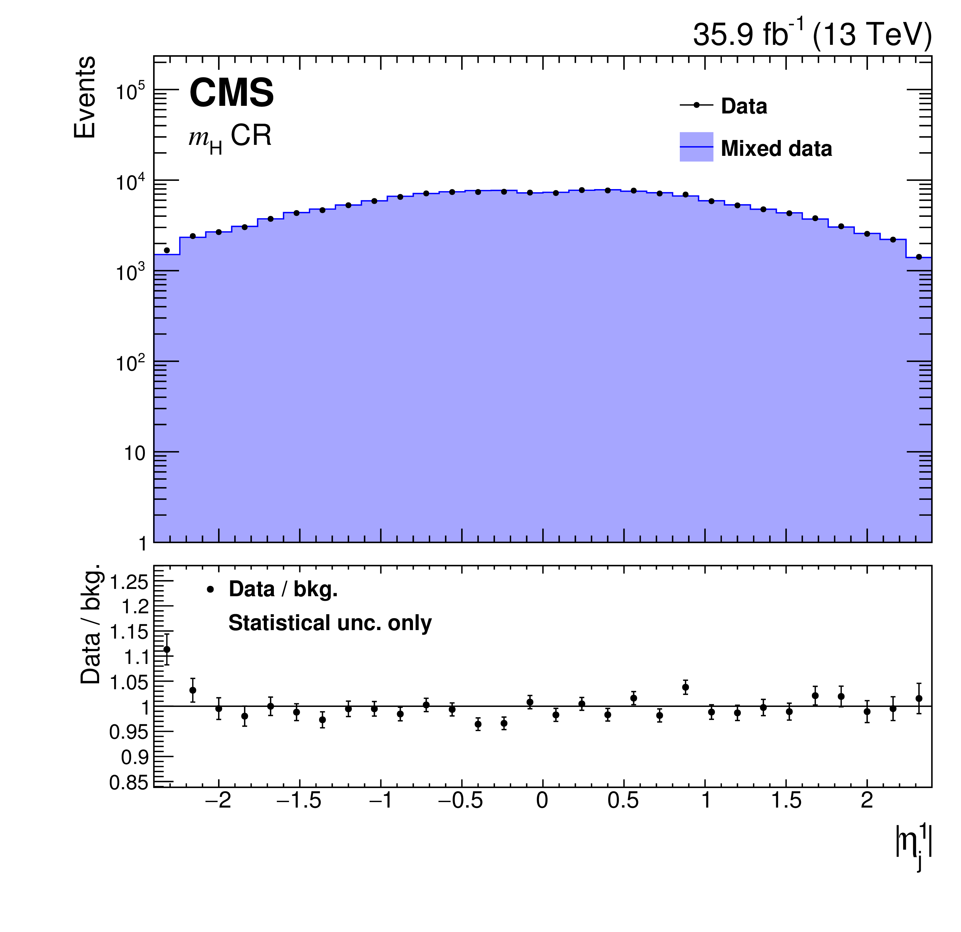
Figure 4-b:
Comparison between the background model obtained with the hemisphere mixing technique and data in the ${m_{{\mathrm {H}}}} $ CR for the $ {\eta ^{1}_{\text {j}}} $ variable. Bias correction for the background model, described in Section 8.2, is applied by rescaling the weight of each event using the event yield ratio between corrected and uncorrected BDT distributions in this CR. Only statistical uncertainties are shown as the uncertainties related to the bias correction can not be propagated from the BDT classifier to a different variable. |
png pdf |
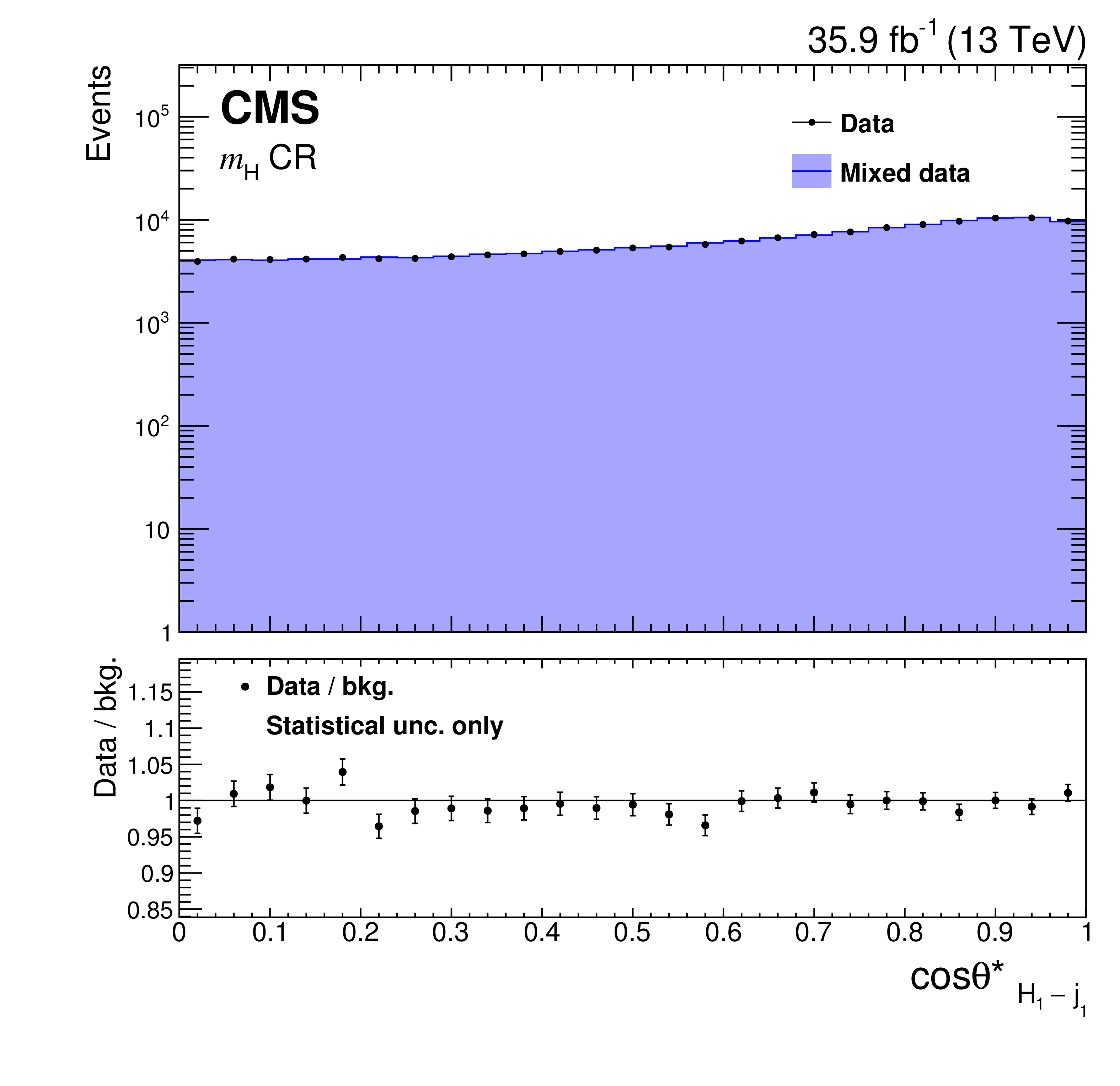
Figure 4-c:
Comparison between the background model obtained with the hemisphere mixing technique and data in the ${m_{{\mathrm {H}}}} $ CR for the ${\cos {\theta ^{*}} _{{{\mathrm {H}} _1} \text {-}\mathrm {j}_1}}$ variable. |
png pdf |
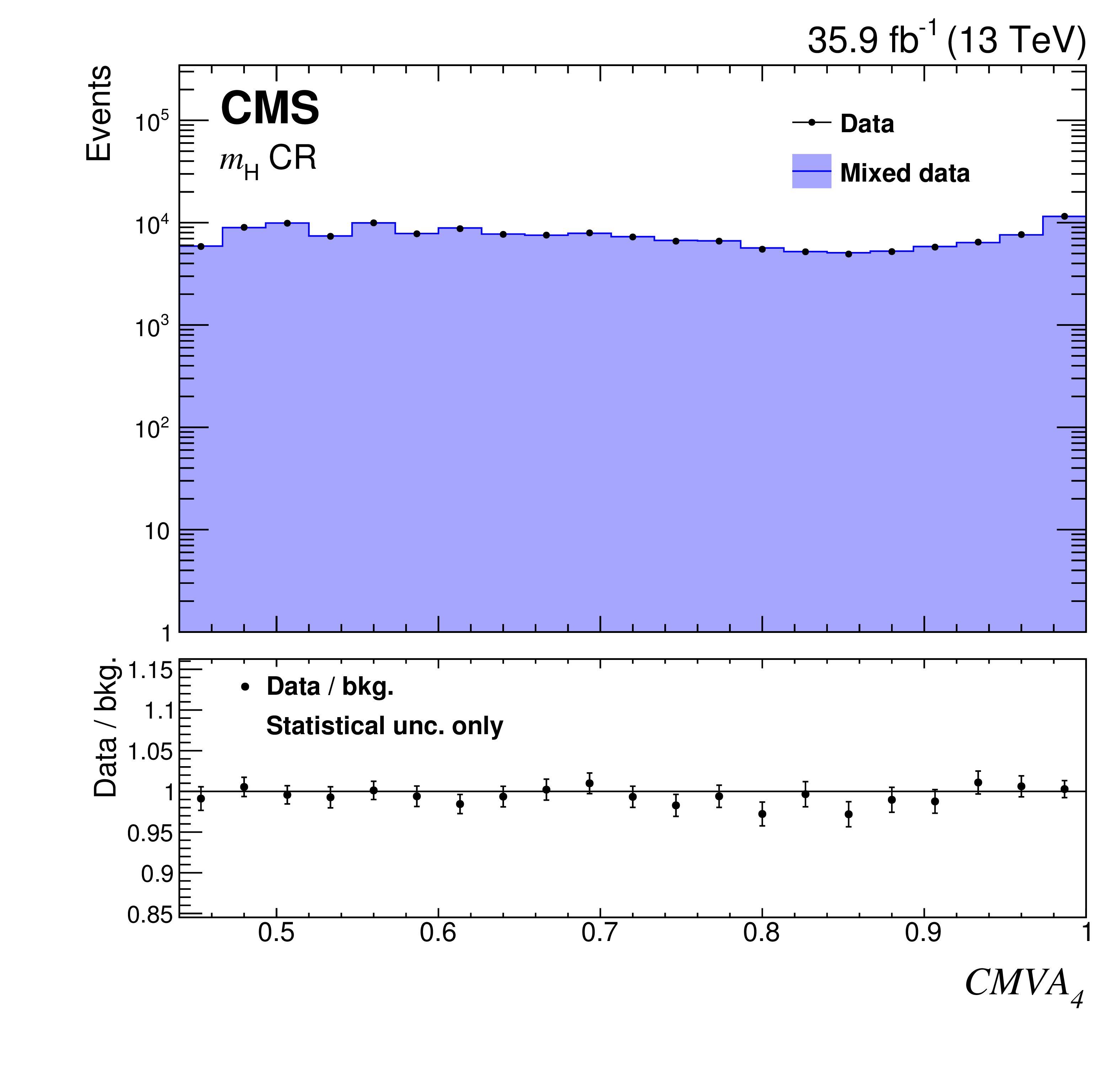
Figure 4-d:
Comparison between the background model obtained with the hemisphere mixing technique and data in the ${m_{{\mathrm {H}}}} $ CR for the $CMVA_{4} $ variable. Bias correction for the background model, described in Section 8.2, is applied by rescaling the weight of each event using the event yield ratio between corrected and uncorrected BDT distributions in this CR. Only statistical uncertainties are shown as the uncertainties related to the bias correction can not be propagated from the BDT classifier to a different variable. |

png pdf |
Figure 5:
Comparison between the background model obtained with the hemisphere mixing technique and data in the b tag CR for the variables $ {{{{p_{\mathrm {T}}}}_{\mathrm {j}}} ^{1}} $ (upper left), $ {\eta ^{1}_{\text {j}}} $ (upper right), ${M_{{{\mathrm {H}} _1}}}$ (lower left), and ${M_{{{\mathrm {H}} _2}}}$ (lower right). Bias correction for the background model, described in Section 8.2, is applied by rescaling the weight of each event using the event yield ratio between corrected and uncorrected BDT distributions in this CR. Only statistical uncertainties are shown as the uncertainties related to the bias correction can not be propagated from the BDT classifier to a different variable. |
png pdf |
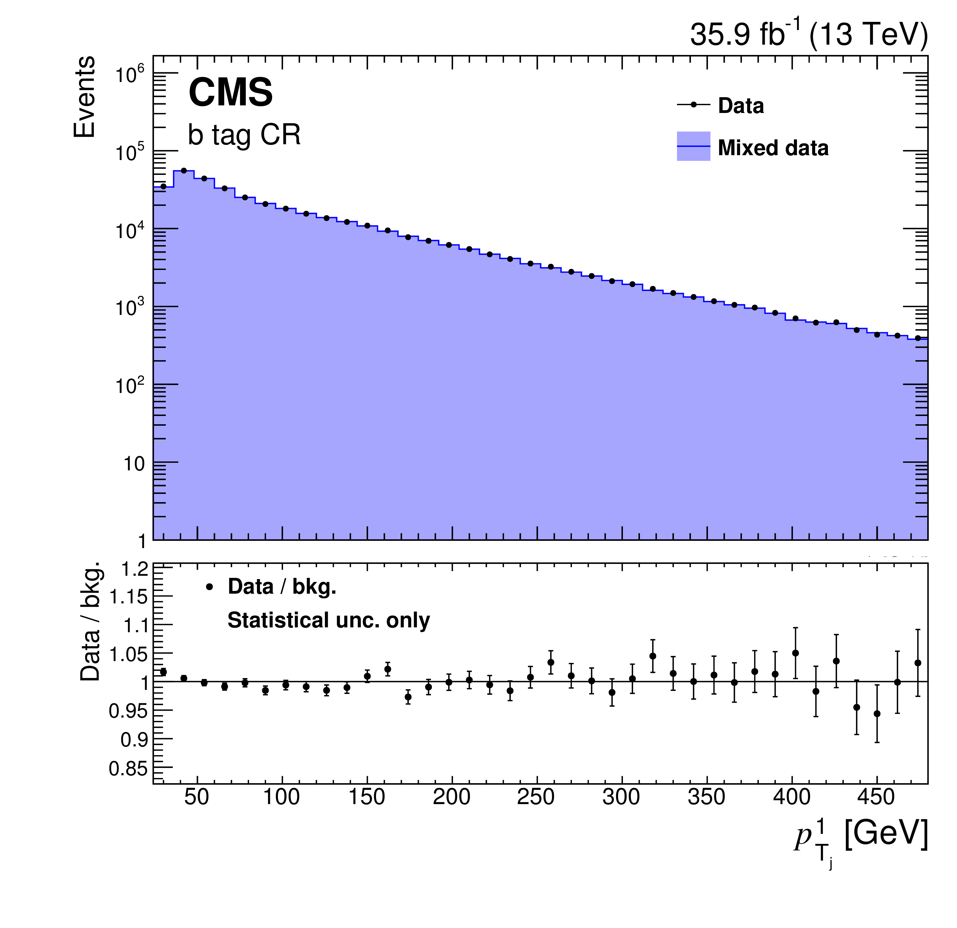
Figure 5-a:
Comparison between the background model obtained with the hemisphere mixing technique and data in the b tag CR for the $ {{{{p_{\mathrm {T}}}}_{\mathrm {j}}} ^{1}} $ variable. Bias correction for the background model, described in Section 8.2, is applied by rescaling the weight of each event using the event yield ratio between corrected and uncorrected BDT distributions in this CR. Only statistical uncertainties are shown as the uncertainties related to the bias correction can not be propagated from the BDT classifier to a different variable. |

png pdf |
Figure 5-b:
Comparison between the background model obtained with the hemisphere mixing technique and data in the b tag CR for the $ {\eta ^{1}_{\text {j}}} $ variable. Bias correction for the background model, described in Section 8.2, is applied by rescaling the weight of each event using the event yield ratio between corrected and uncorrected BDT distributions in this CR. Only statistical uncertainties are shown as the uncertainties related to the bias correction can not be propagated from the BDT classifier to a different variable. |

png pdf |
Figure 5-c:
Comparison between the background model obtained with the hemisphere mixing technique and data in the b tag CR for the ${M_{{{\mathrm {H}} _1}}}$ variable. Bias correction for the background model, described in Section 8.2, is applied by rescaling the weight of each event using the event yield ratio between corrected and uncorrected BDT distributions in this CR. Only statistical uncertainties are shown as the uncertainties related to the bias correction can not be propagated from the BDT classifier to a different variable. |

png pdf |
Figure 5-d:
Comparison between the background model obtained with the hemisphere mixing technique and data in the b tag CR for the ${M_{{{\mathrm {H}} _2}}}$ variable. Bias correction for the background model, described in Section 8.2, is applied by rescaling the weight of each event using the event yield ratio between corrected and uncorrected BDT distributions in this CR. Only statistical uncertainties are shown as the uncertainties related to the bias correction can not be propagated from the BDT classifier to a different variable. |
png pdf |
Figure 6:
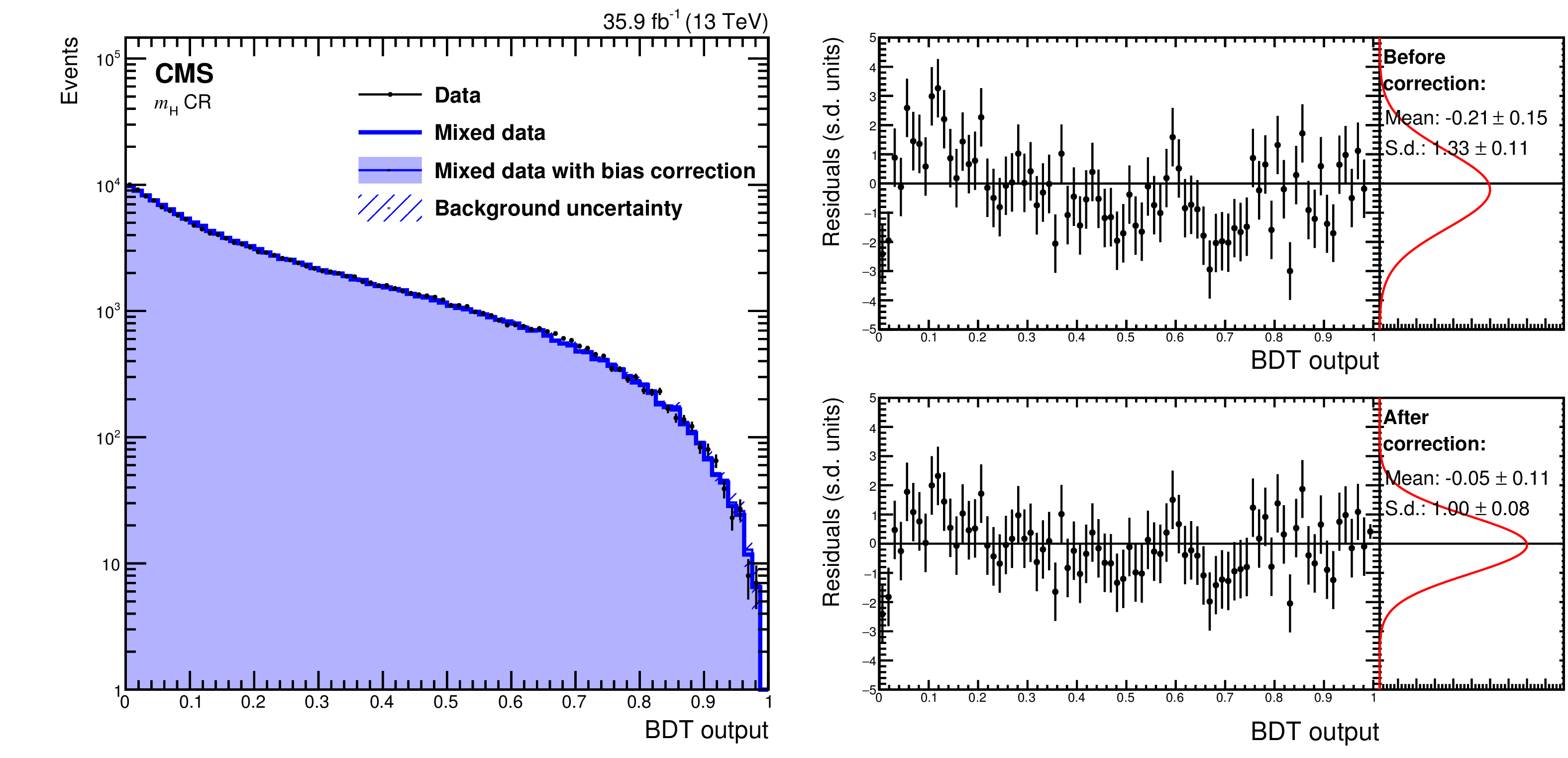
Left: comparison of the distribution of BDT output for data (left) selected in a region of the leading versus trailing Higgs boson candidate mass plane that excludes a 60- GeV -wide box around the most probable values of the dijet masses of signal events, with the corresponding output on an artificial sample obtained from the same data set by hemisphere mixing. Right: bin-by-bin differences between data and model, in s.d. units before (upper right) and after (lower right) bias correction; pull distribution for the differences, fit to a Gaussian distribution. The bias correction uncertainty is increased to take the s.d. of the residuals to 1.0. |

png pdf |
Figure 7:
Results of the fit to the BDT distribution for the SM HH production signal. In the bottom panel a comparison is shown between the best fit signal and best fit background subtracted from measured data. The band, centred at zero, shows the total uncertainty. |

png pdf |
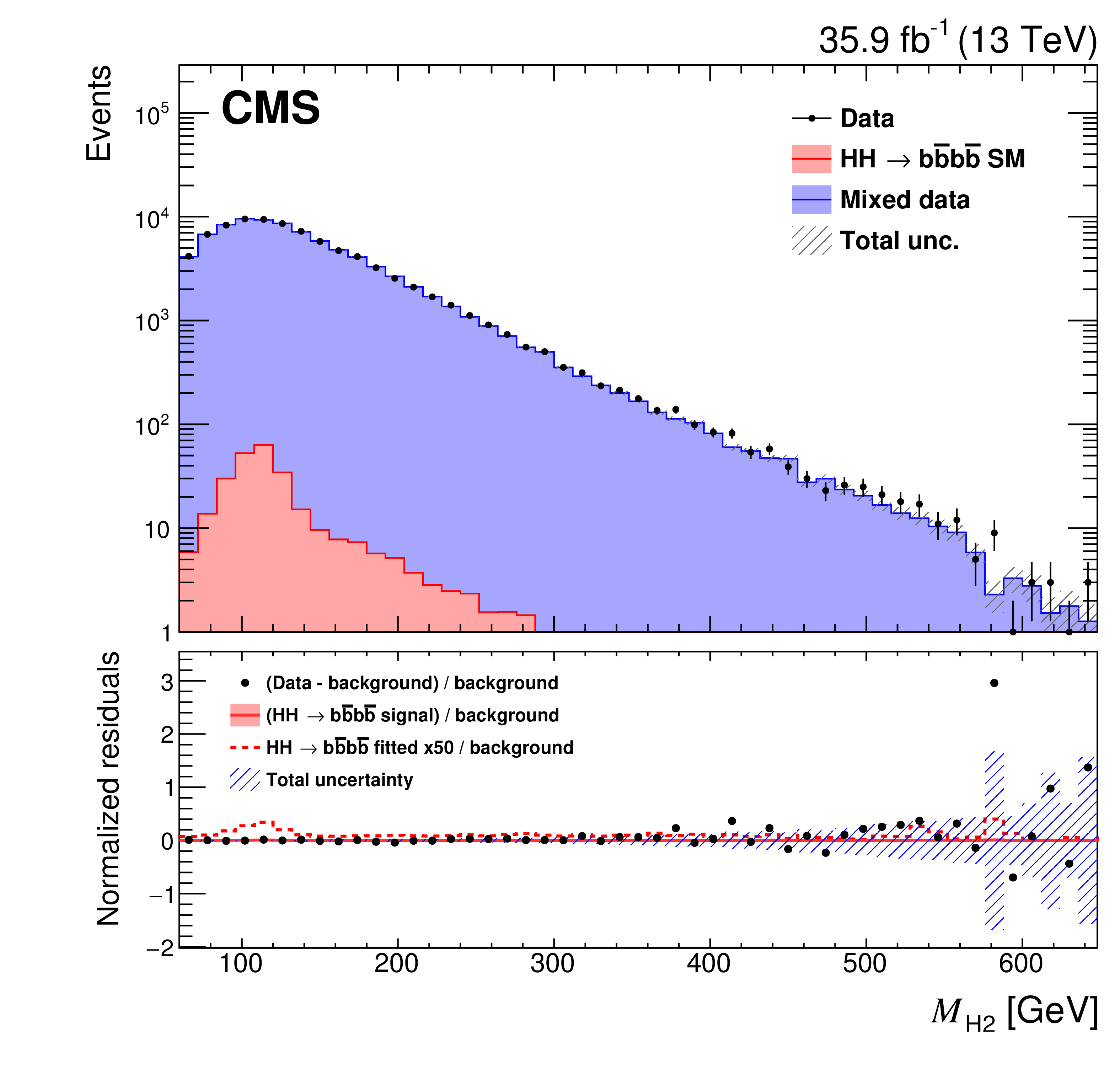
Figure 8:
Post-fit distribution of ${M_{{{\mathrm {H}} _1}}} $ (left) and ${M_{{{\mathrm {H}} _2}}} $ (right). Bias correction for the background model is applied by rescaling the weight of each event using the event yield ratio between corrected and uncorrected BDT distributions. |
png pdf |
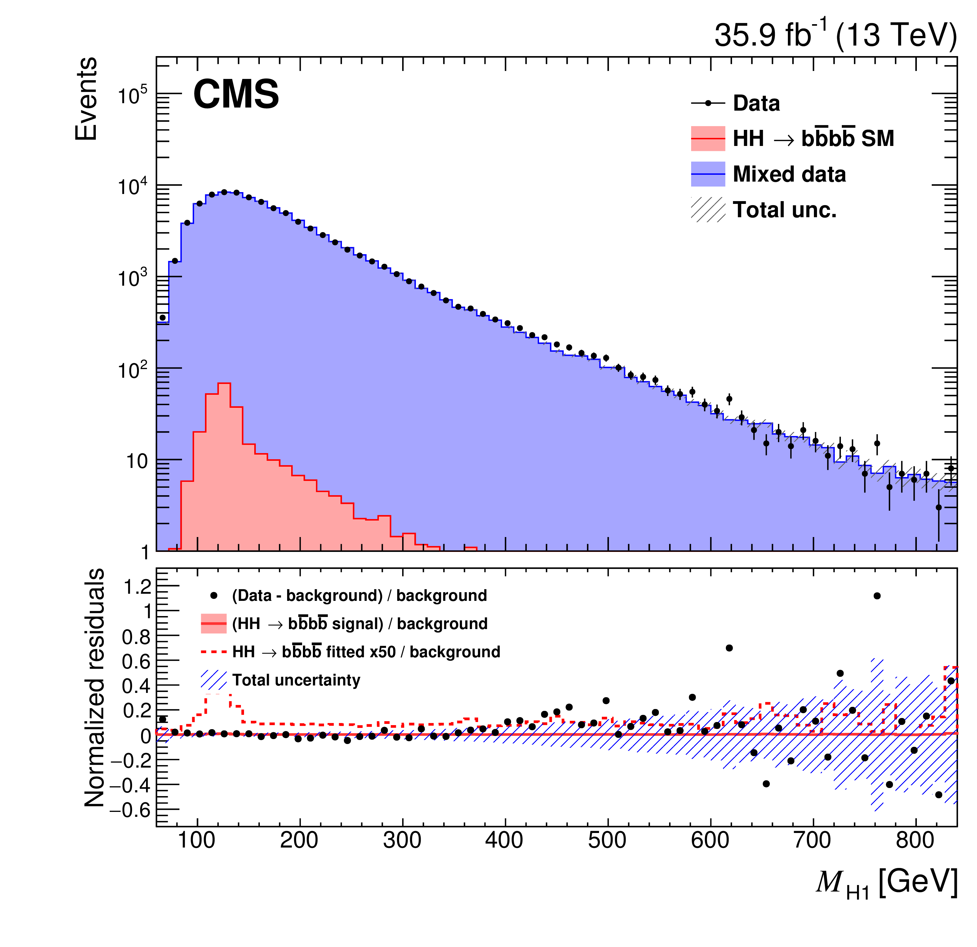
Figure 8-a:
Post-fit distribution of ${M_{{{\mathrm {H}} _1}}} $. Bias correction for the background model is applied by rescaling the weight of each event using the event yield ratio between corrected and uncorrected BDT distributions. |
png pdf |
Figure 8-b:
Post-fit distribution of ${M_{{{\mathrm {H}} _2}}} $. Bias correction for the background model is applied by rescaling the weight of each event using the event yield ratio between corrected and uncorrected BDT distributions. |
png pdf |
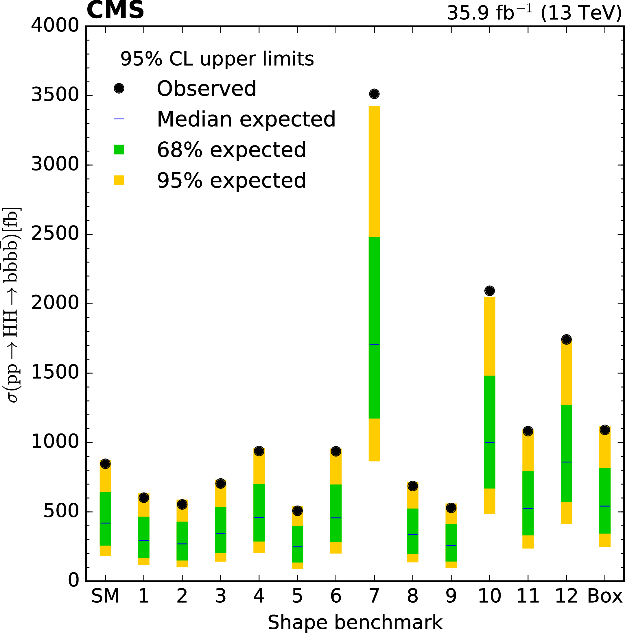
Figure 9:
The observed and expected upper limits at 95% CL on the ${\sigma {({{\mathrm {p}} {\mathrm {p}} \to {{\mathrm {H}} {\mathrm {H}} \to {{\mathrm {b}} {\overline {\mathrm {b}}}} {{\mathrm {b}} {\overline {\mathrm {b}}}}}})}}$ cross section for the 13 BSM models investigated. See Table 9 for their respective parameter values. |
png pdf |
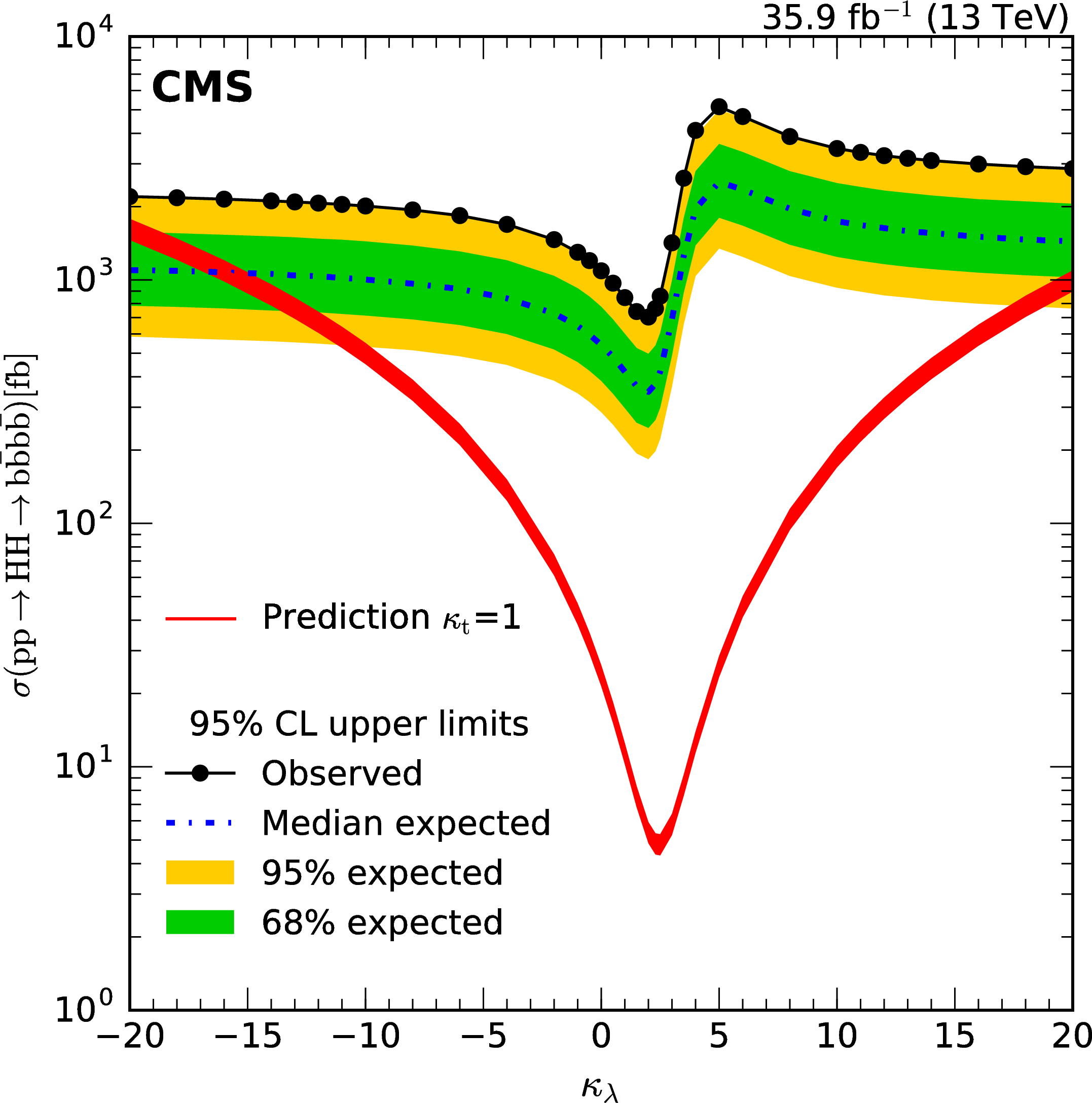
Figure 10:
95% CL cross section limits on ${\sigma {({{\mathrm {p}} {\mathrm {p}} \to {{\mathrm {H}} {\mathrm {H}} \to {{\mathrm {b}} {\overline {\mathrm {b}}}} {{\mathrm {b}} {\overline {\mathrm {b}}}}}})}}$ for values of ${\kappa _{{{\lambda}}}}$ in the [-20,20] range, assuming $ {\kappa _{{\mathrm {t}}}} = $ 1; the theoretical prediction with $ {\kappa _{{\mathrm {t}}}} = $ 1 is also shown. |

png pdf |
Figure 11:
Diagram describing the procedure used to estimate the background bias correction. All possible combinations of mixed hemispheres except those used for training are added together to create a large sample $M$ of $96N$ events from which we repeatedly subsample without replacement 200 replicas $M_i$ of $N$ events. The hemisphere mixing procedure is then carried out again for each of this replicas to produce a set of re-mixed data replicas $R_i$. The trained multivariate classifier trained is then evaluated over all the events of $M$ and each $R_i$. and the histograms of the classifier output are compared to obtain a the differences for each of the replicas. The median difference is taken as bias correction. |
png pdf |
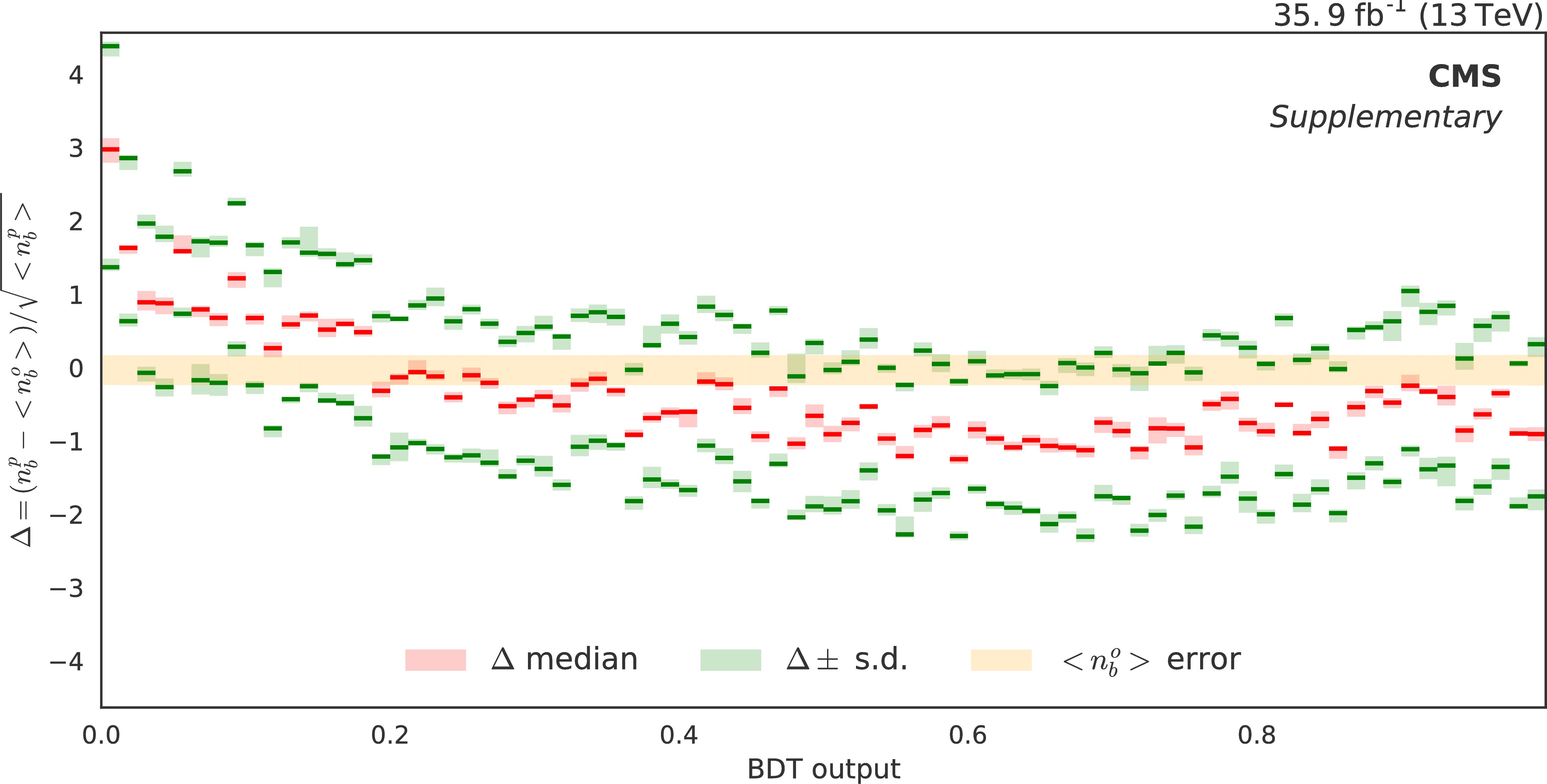
Figure 12:
Bias estimation by resampling, in relative units of the statistical uncertainty of the predicted background, used to correct the background estimation. The median (red line) and the upper and lower one s.d. quantiles (green lines) have been computed from 200 subsamples of the re-mixed data comparing the predicted background $n^p_b$ with the observed $n^o_b$. The variability due to the limited number of subsamples is estimated by bootstrap and it is shown for each estimation using a coloured shadow around the quantile estimation. The light yellow shadow represents the uncertainty due to the limited statistics of the reference observed sample. The separation between the one s.d. quantiles is compatible with the expected variance if the estimation was Poisson or Gaussian distributed. |
| Tables | |
png pdf |
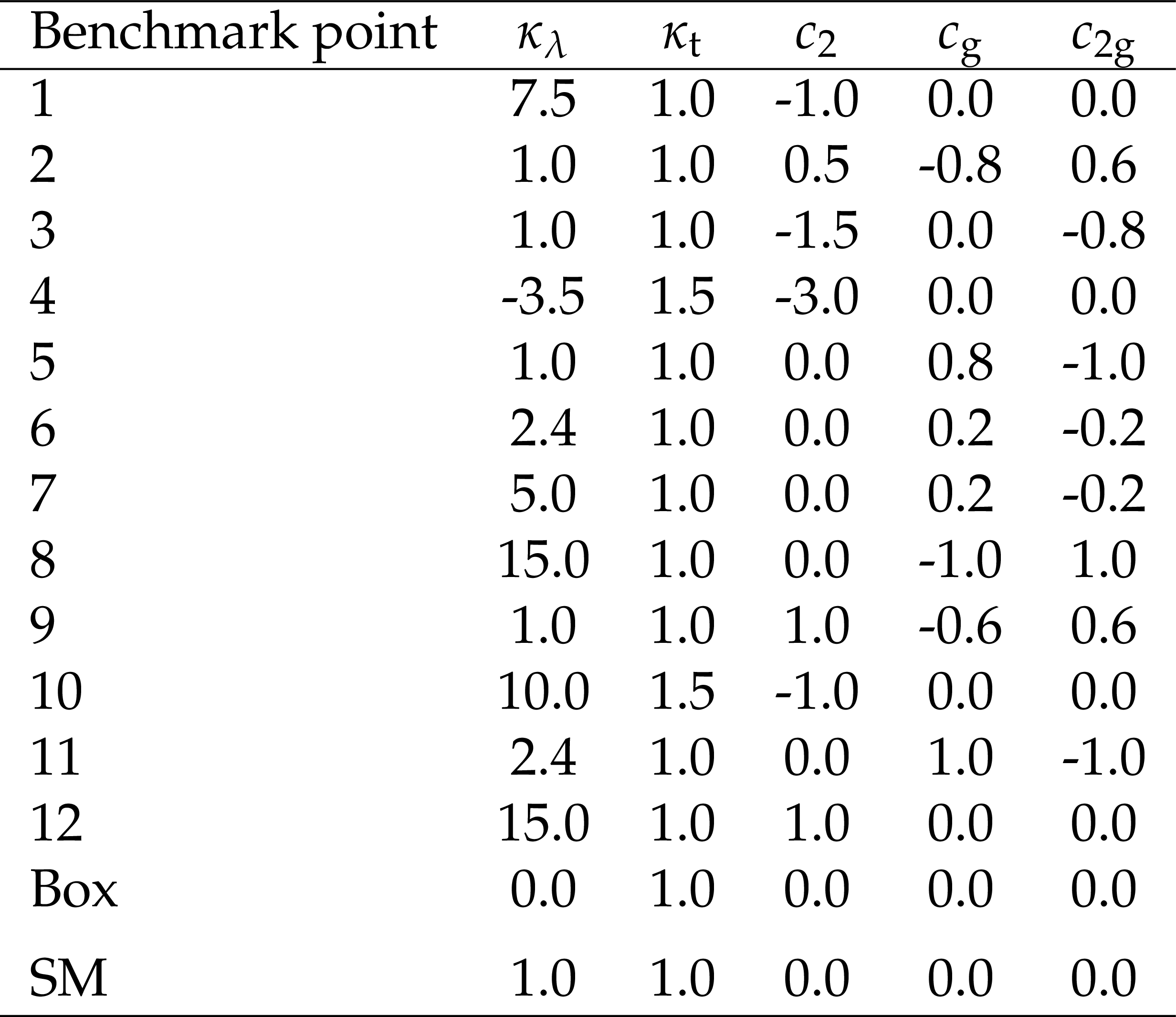
Table 1:
The values of the anomalous coupling parameters for the 13 benchmark models studied [28]. For reference, the values of the parameters in the SM are also included. |
png pdf |
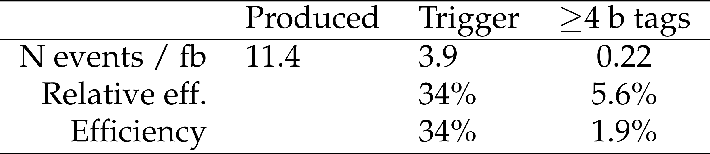
Table 2:
Cut-flow efficiency for the SM signal $ {{\mathrm {p}} {\mathrm {p}} \to {{\mathrm {H}} {\mathrm {H}} \to {{\mathrm {b}} {\overline {\mathrm {b}}}} {{\mathrm {b}} {\overline {\mathrm {b}}}}}} $; the efficiency and the relative reduction of each successive selection step is shown. The number of expected SM signal events for an integrated luminosity of 1 fb$^{-1}$ is also reported. |
png pdf |
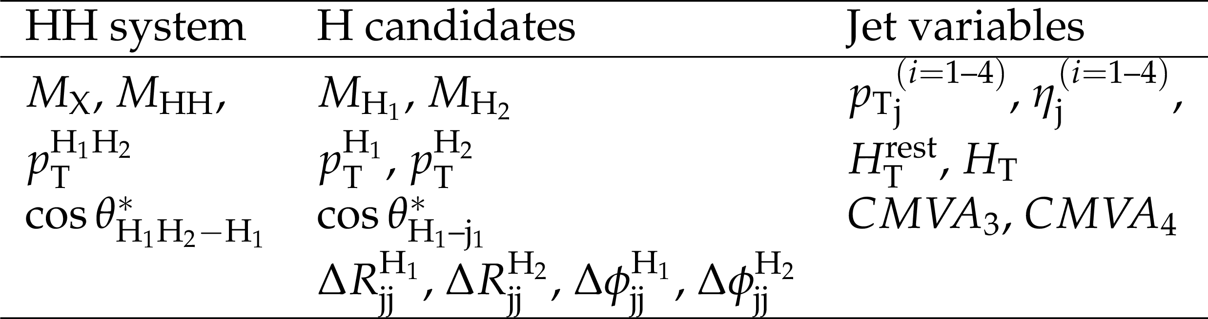
Table 3:
List of BDT input variables. |

png pdf |
Table 4:
Systematic uncertainties considered in the analysis and relative impact on the expected limit for the SM HH production. The relative impact is obtained by fixing the nuisance parameters corresponding to each source and recalculating the expected limit. |

png pdf |
Table 5:
The observed and expected upper limits on ${\sigma {({{\mathrm {p}} {\mathrm {p}} \to {{\mathrm {H}} {\mathrm {H}} \to {{\mathrm {b}} {\overline {\mathrm {b}}}} {{\mathrm {b}} {\overline {\mathrm {b}}}}}})}}$ in the SM at 95% CL in units of fb. |
png pdf |
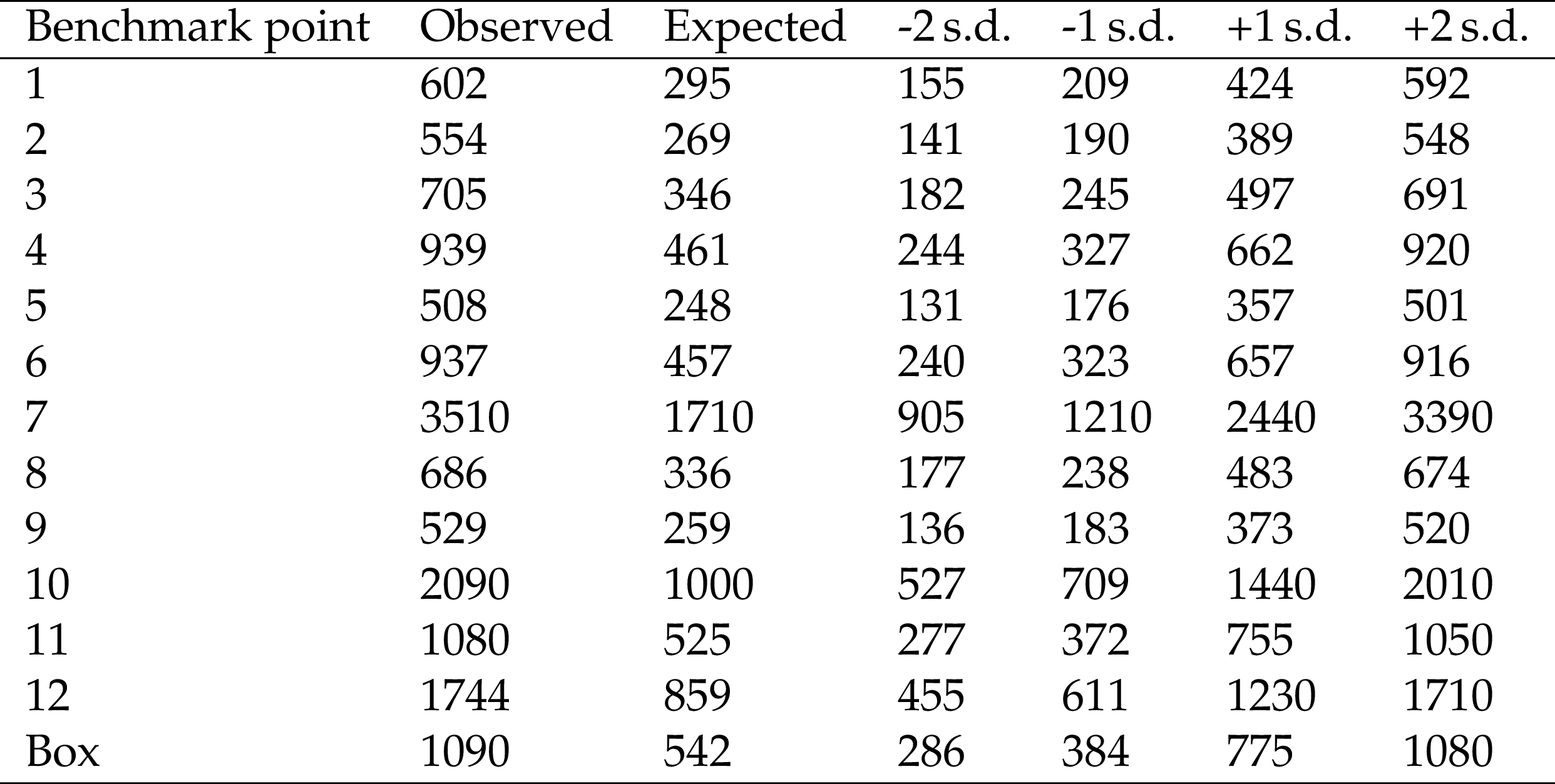
Table 6:
The observed and expected upper limits on the ${\sigma {({{\mathrm {p}} {\mathrm {p}} \to {{\mathrm {H}} {\mathrm {H}} \to {{\mathrm {b}} {\overline {\mathrm {b}}}} {{\mathrm {b}} {\overline {\mathrm {b}}}}}})}}$ cross section for the 13 BSM benchmark models at 95% CL in units of fb. |
| Summary |
| This paper presents a search for nonresonant Higgs boson pair (HH) production with both Higgs bosons decaying into $ \mathrm{b\bar{b}} $ pairs. The standard model (SM) production has been studied along with 13 beyond the SM (BSM) benchmark models, using a data set of $\sqrt{s} = $ 13 TeV proton-proton collision events, corresponding to an integrated luminosity of 35.9 fb$^{-1}$ collected by the CMS detector during the 2016 LHC run. The analysis of events acquired by a hadronic multijet trigger includes the selection of events with 4 b-tagged jets and a classification using boosted decision trees, optimized for discovery of the SM HH signal. Limits at 95% confidence level on the HH production cross section times the square of the branching fraction for the Higgs boson decay to b quark pairs are extracted for the SM and each BSM model considered, using binned likelihood fits of the shape of the boosted decision tree classifier output. The background model is derived from a novel technique based on data that provides a multidimensional representation of the dominant quantum chromodynamics multijet background and also models well the overall background distribution. The expected upper limit on ${\sigma{(\mathrm{pp\to HH \to b\bar{b}b\bar{b}})}}$ is 419 fb, corresponding to 37 times the expected value for the SM process. The observed upper limit is 847 fb. Anomalous couplings of the Higgs boson are also investigated. The upper limits extracted for the HH production cross section in the 13 BSM benchmark models range from 508 to 3513 fb. |
| References | ||||
| 1 | ATLAS Collaboration | Observation of a new particle in the search for the standard model Higgs boson with the ATLAS detector at the LHC | PLB 716 (2012) 1 | 1207.7214 |
| 2 | CMS Collaboration | Observation of a new boson at a mass of 125 GeV with the CMS experiment at the LHC | PLB 716 (2012) 30 | CMS-HIG-12-028 1207.7235 |
| 3 | CMS Collaboration | Observation of a new boson with mass near 125 GeV in pp collisions at $ \sqrt{s} = $ 7 and 8 TeV | JHEP 06 (2013) 081 | CMS-HIG-12-036 1303.4571 |
| 4 | ATLAS and CMS Collaborations | Measurements of the Higgs boson production and decay rates and constraints on its couplings from a combined ATLAS and CMS analysis of the LHC pp collision data at $ \sqrt{s} = $ 7 and 8 TeV | JHEP 08 (2016) 045 | 1606.02266 |
| 5 | ATLAS and CMS Collaborations | Combined measurement of the Higgs boson mass in pp collisions at $ \sqrt{s}= $ 7 and 8 TeV with the ATLAS and CMS experiments | PRL 114 (2015) 191803 | 1503.07589 |
| 6 | C. O. Dib, R. Rosenfeld, and A. Zerwekh | Double Higgs production and quadratic divergence cancellation in little Higgs models with T parity | JHEP 05 (2006) 074 | hep-ph/0509179 |
| 7 | R. Grober and M. Muhlleitner | Composite Higgs boson pair production at the LHC | JHEP 06 (2011) 020 | 1012.1562 |
| 8 | R. Contino et al. | Anomalous couplings in double Higgs production | JHEP 08 (2012) 154 | 1205.5444 |
| 9 | M. J. Dolan, C. Englert, and M. Spannowsky | New physics in LHC Higgs boson pair production | PRD 87 (2013) 055002 | 1210.8166 |
| 10 | S. Dawson, A. Ismail, and I. Low | What's in the loop? the anatomy of double Higgs production | PRD 91 (2015) 115008 | 1504.05596 |
| 11 | J. Baglio et al. | The measurement of the Higgs self-coupling at the LHC: theoretical status | JHEP 04 (2013) 151 | 1212.5581 |
| 12 | CMS Collaboration | Measurements of properties of the Higgs boson decaying into the four-lepton final state in pp collisions at $ \sqrt{s}= $ 13 TeV | JHEP 11 (2017) 047 | CMS-HIG-16-041 1706.09936 |
| 13 | LHC Higgs Cross Section Working Group | Handbook of LHC Higgs cross sections: 4. deciphering the nature of the Higgs sector | CERN (2016) | 1610.07922 |
| 14 | D. de Florian and J. Mazzitelli | Higgs boson pair production at next-to-next-to-leading order in QCD | PRL 111 (2013) 201801 | 1309.6594 |
| 15 | S. Dawson, S. Dittmaier, and M. Spira | Neutral Higgs boson pair production at hadron colliders: QCD corrections | PRD 58 (1998) 115012 | hep-ph/9805244 |
| 16 | S. Borowka et al. | Higgs boson pair production in gluon fusion at next-to-leading order with full top-quark mass dependence | PRL 117 (2016) 012001 | 1604.06447 |
| 17 | D. de Florian and J. Mazzitelli | Higgs pair production at next-to-next-to-leading logarithmic accuracy at the LHC | JHEP 09 (2015) 053 | 1505.07122 |
| 18 | CMS Collaboration | Search for Higgs boson pair production in events with two bottom quarks and two tau leptons in proton-proton collisions at $ \sqrt{s} = $ 13 TeV | PLB 778 (2018) 101 | CMS-HIG-17-002 1707.02909 |
| 19 | ATLAS Collaboration | Search for pair production of Higgs bosons in the $ b\bar{b}b\bar{b} $ final state using proton-proton collisions at $ \sqrt{s} = $ 13 TeV with the ATLAS detector | Submitted to JHEP | 1804.06174 |
| 20 | A. Carvalho et al. | Analytical parametrization and shape classification of anomalous HH production in the EFT approach | 1608.06578 | |
| 21 | ATLAS Collaboration | Search for Higgs boson pair production in the $ b\bar{b}b\bar{b} $ final state from pp collisions at $ \sqrt{s}= $ 8 TeV with the ATLAS detector | EPJC 75 (2015) 412 | 1506.00285 |
| 22 | CMS Collaboration | Search for Higgs boson pair production in the bb$\tau\tau $ final state in proton-proton collisions at $ \sqrt{s} = $ 8 TeV | PRD 96 (2017) 072004 | CMS-HIG-15-013 1707.00350 |
| 23 | CMS Collaboration | Search for resonant and nonresonant Higgs boson pair production in the $ \mathrm{b\bar{b}}\ell\nu\ell\nu $ final state in proton-proton collisions at $ \sqrt{s} = $ 13 TeV | JHEP 01 (2018) 054 | CMS-HIG-17-006 1708.04188 |
| 24 | CMS Collaboration | Search for Higgs boson pair production in the $ \gamma\gamma\mathrm{b\bar{b}} $ final state in pp collisions at $ \sqrt{s} = $ 13 TeV | Submitted to PLB | CMS-HIG-17-008 1806.00408 |
| 25 | CMS Collaboration | Search for production of Higgs boson pairs in the four b quark final state using large-area jets in proton-proton collisions at $ \sqrt{s}= $ 13 TeV | Submitted to JHEP | CMS-B2G-17-019 1808.01473 |
| 26 | A. Falkowski | Effective field theory approach to LHC Higgs data | Pramana 87 (2016) 39 | 1505.00046 |
| 27 | T. Corbett et al. | The Higgs legacy of the LHC run I | JHEP 08 (2015) 156 | 1505.05516 |
| 28 | A. Carvalho et al. | Higgs pair production: Choosing benchmarks with cluster analysis | JHEP 04 (2016) 126 | 1507.02245 |
| 29 | CMS Collaboration | The CMS trigger system | JINST 12 (2017) P01020 | CMS-TRG-12-001 1609.02366 |
| 30 | CMS Collaboration | The CMS experiment at the CERN LHC | JINST 3 (2008) S08004 | CMS-00-001 |
| 31 | CMS Collaboration | Identification of heavy-flavour jets with the CMS detector in pp collisions at 13 TeV | JINST 13 (2018) P05011 | CMS-BTV-16-002 1712.07158 |
| 32 | B. Hespel, D. L\'opez-Val, and E. Vryonidou | Higgs pair production via gluon fusion in the two-Higgs-doublet model | JHEP 09 (2014) 124 | 1407.0281 |
| 33 | J. Alwall et al. | The automated computation of tree-level and next-to-leading order differential cross sections, and their matching to parton shower simulations | JHEP 07 (2014) 079 | 1405.0301 |
| 34 | NNPDF Collaboration | Parton distributions for the LHC Run II | JHEP 04 (2015) 040 | 1410.8849 |
| 35 | A. Carvalho et al. | On the reinterpretation of non-resonant searches for Higgs boson pairs | 1710.08261 | |
| 36 | T. Sjostrand et al. | An introduction to PYTHIA 8.2 | CPC 191 (2015) 159 | 1410.3012 |
| 37 | J. Alwall et al. | Comparative study of various algorithms for the merging of parton showers and matrix elements in hadronic collisions | EPJC 53 (2008) 473 | 0706.2569 |
| 38 | P. Nason | A new method for combining NLO QCD with shower Monte Carlo algorithms | JHEP 11 (2004) 040 | hep-ph/0409146 |
| 39 | S. Frixione, P. Nason, and C. Oleari | Matching NLO QCD computations with parton shower simulations: the POWHEG method | JHEP 11 (2007) 070 | 0709.2092 |
| 40 | S. Alioli, P. Nason, C. Oleari, and E. Re | A general framework for implementing NLO calculations in shower Monte Carlo programs: the POWHEG BOX | JHEP 06 (2010) 043 | 1002.2581 |
| 41 | J. M. Campbell, R. K. Ellis, P. Nason, and E. Re | Top-pair production and decay at NLO matched with parton showers | JHEP 04 (2015) 114 | 1412.1828 |
| 42 | S. Alioli, P. Nason, C. Oleari, and E. Re | NLO single-top production matched with shower in POWHEG: $ s $- and $ t $-channel contributions | JHEP 09 (2009) 111 | 0907.4076 |
| 43 | H. B. Hartanto, B. Jager, L. Reina, and D. Wackeroth | Higgs boson production in association with top quarks in the POWHEG BOX | PRD 91 (2015) 094003 | 1501.04498 |
| 44 | E. Bagnaschi, G. Degrassi, P. Slavich, and A. Vicini | Higgs production via gluon fusion in the POWHEG approach in the SM and in the MSSM | JHEP 02 (2012) 088 | 1111.2854 |
| 45 | G. Luisoni, P. Nason, C. Oleari, and F. Tramontano | $ {\text{HW}^\pm}/\text{HZ} + 0 $ and 1 jet at NLO with the POWHEG BOX interfaced to GoSam and their merging within MiNLO | JHEP 10 (2013) 083 | 1306.2542 |
| 46 | CMS Collaboration | Investigations of the impact of the parton shower tuning in Pythia 8 in the modelling of $ \mathrm{t\overline{t}} $ at $ \sqrt{s}= $ 8 and 13 TeV | CMS-PAS-TOP-16-021 | CMS-PAS-TOP-16-021 |
| 47 | CMS Collaboration | Event generator tunes obtained from underlying event and multiparton scattering measurements | EPJC 76 (2016) 155 | CMS-GEN-14-001 1512.00815 |
| 48 | A. Buckley et al. | LHAPDF6: parton density access in the LHC precision era | EPJC 75 (2015) 132 | 1412.7420 |
| 49 | GEANT4 Collaboration | GEANT4--a simulation toolkit | NIMA 506 (2003) 250 | |
| 50 | CMS Collaboration | Particle-flow reconstruction and global event description with the CMS detector | JINST 12 (2017) P10003 | CMS-PRF-14-001 1706.04965 |
| 51 | M. Cacciari, G. P. Salam, and G. Soyez | The anti-$ {k_{\mathrm{T}}} $ jet clustering algorithm | JHEP 04 (2008) 063 | 0802.1189 |
| 52 | M. Cacciari, G. P. Salam, and G. Soyez | FastJet user manual | EPJC 72 (2012) 1896 | 1111.6097 |
| 53 | CMS Collaboration | Jet energy scale and resolution in the CMS experiment in pp collisions at 8 TeV | JINST 12 (2017) P02014 | CMS-JME-13-004 1607.03663 |
| 54 | CMS Collaboration | Pileup jet identification | CMS-PAS-JME-13-005 | CMS-PAS-JME-13-005 |
| 55 | T. Chen and C. Guestrin | XGBoost: A scalable tree boosting system | in Proceedings of the 22nd ACM SIGKDD International Conference on Knowledge Discovery and Data Mining, KDD '16 ACM, New York, NY, USA | |
| 56 | P. De Castro Manzano et al. | Hemisphere mixing: a fully data-driven model of QCD multijet backgrounds for LHC searches | in Proceedings, 2017 European Physical Society Conference on High Energy Physics (EPS-HEP 2017), volume EPS-HEP2017, p. 370 2017 | 1712.02538 |
| 57 | CMS Collaboration | Measurement of the inelastic proton-proton cross section at $ \sqrt{s}= $ 13 TeV | Submitted to JHEP | CMS-FSQ-15-005 1802.02613 |
| 58 | CMS Collaboration | CMS luminosity measurements or the 2016 data taking period | CMS-PAS-LUM-17-001 | CMS-PAS-LUM-17-001 |
| 59 | J. Butterworth et al. | PDF4LHC recommendations for LHC Run II | JPG 43 (2016) 023001 | 1510.03865 |
| 60 | G. Cowan, K. Cranmer, E. Gross, and O. Vitells | Asymptotic formulae for likelihood-based tests of new physics | EPJC 71 (2011) 1554 | 1007.1727 |
| 61 | A. L. Read | Presentation of search results: The CLs technique | JPG 28 (2002) | |
| 62 | T. Junk | Confidence level computation for combining searches with small statistics | NIMA 434 (1999) 435 | hep-ex/9902006 |
| 63 | The ATLAS Collaboration, The CMS Collaboration, The LHC Higgs Combination Group | Procedure for the LHC Higgs boson search combination in Summer 2011 | CMS-NOTE-2011-005 | |
|
|
Compact Muon Solenoid LHC, CERN |
|

|

|

|

|

|