

Compact Muon Solenoid
LHC, CERN
| CMS-TOP-17-001 ; CERN-EP-2018-317 | ||
| Measurement of the $ \mathrm{t\bar{t}} $ production cross section, the top quark mass, and the strong coupling constant using dilepton events in pp collisions at $\sqrt{s} = $ 13 TeV | ||
| CMS Collaboration | ||
| 27 December 2018 | ||
| Eur. Phys. J. C 79 (2019) 368 | ||
| Abstract: A measurement of the top quark-antiquark pair production cross section $ {\sigma_\mathrm{t\bar{t}}} $ in proton-proton collisions at a centre-of-mass energy of 13 TeV is presented. The data correspond to an integrated luminosity of 35.9 fb$^{-1}$, recorded by the CMS experiment at the CERN LHC in 2016. Dilepton events ($\mathrm{e}^{\pm}\mu^{\mp}$ , $\mu^{+}\mu^{-}$, $\mathrm{e^{+}e^{-}}$) are selected and the cross section is measured from a likelihood fit. For a top quark mass parameter in the simulation of $ {{m_{\mathrm{t}}} ^{\mathrm{MC}}} = $ 172.5 GeV the fit yields a measured cross section ${\sigma_\mathrm{t\bar{t}}} = $ 803 $\pm$ 2 (stat) $\pm$ 25 (syst) $\pm$ 20 (lumi) pb, in agreement with the expectation from the standard model calculation at next-to-next-to-leading order. A simultaneous fit of the cross section and the top quark mass parameter in the simulation is performed. The measured value of ${{m_{\mathrm{t}}} ^{\mathrm{MC}}} = $ 172.33 $\pm$ 0.14 (stat) $^{+0.66}_{-0.72}$ (syst) GeV is in good agreement with previous measurements. The resulting cross section is used, together with the theoretical prediction, to determine the top quark mass and to extract a value of the strong coupling constant with different sets of parton distribution functions. | ||
| Links: e-print arXiv:1812.10505 [hep-ex] (PDF) ; CDS record ; inSPIRE record ; CADI line (restricted) ; | ||
| Figures | |
png pdf |
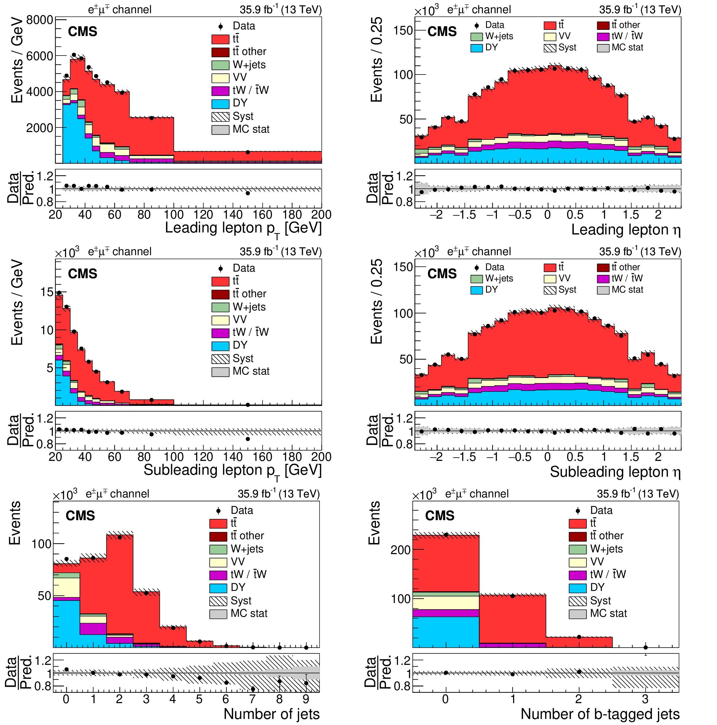
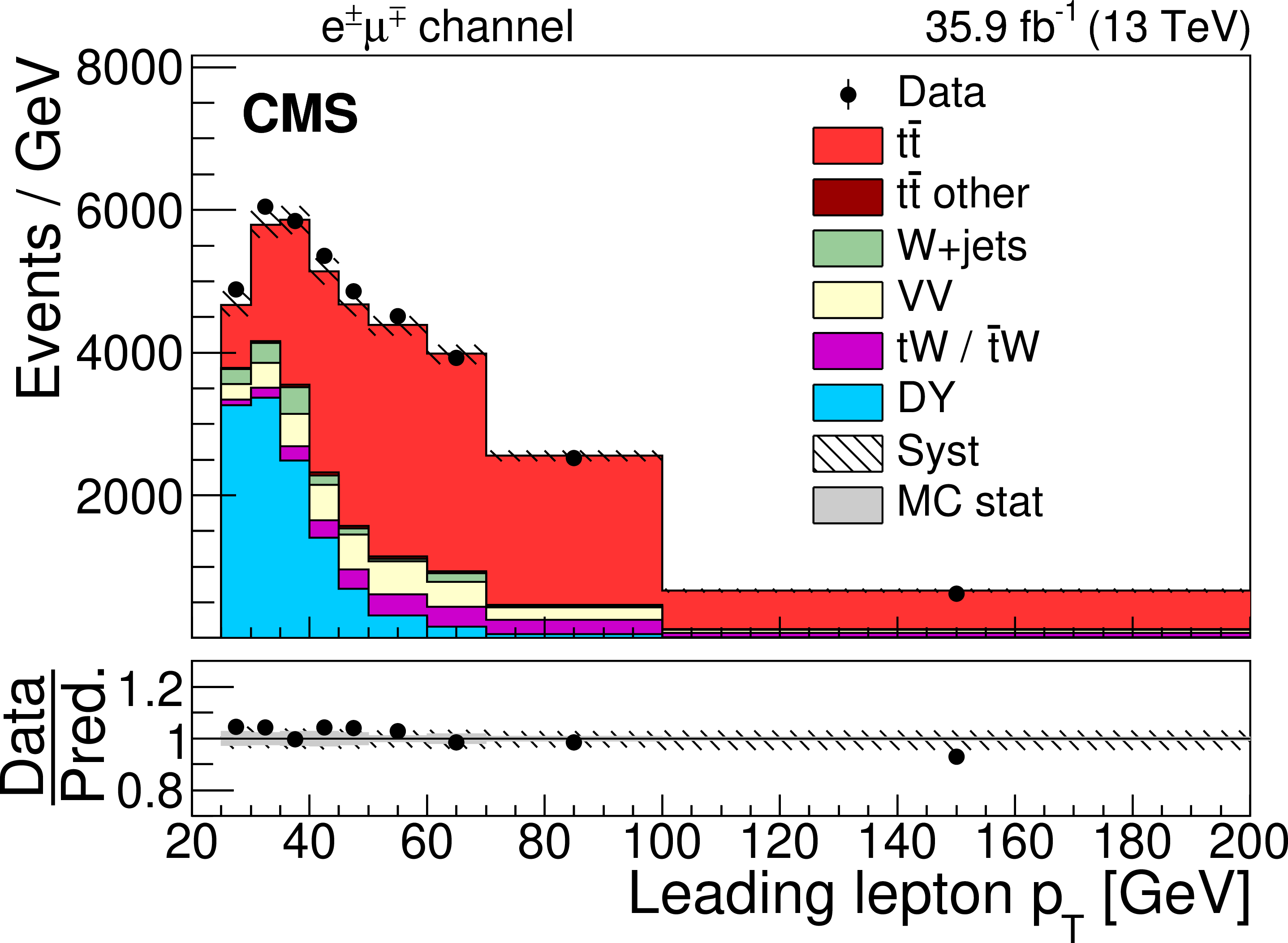
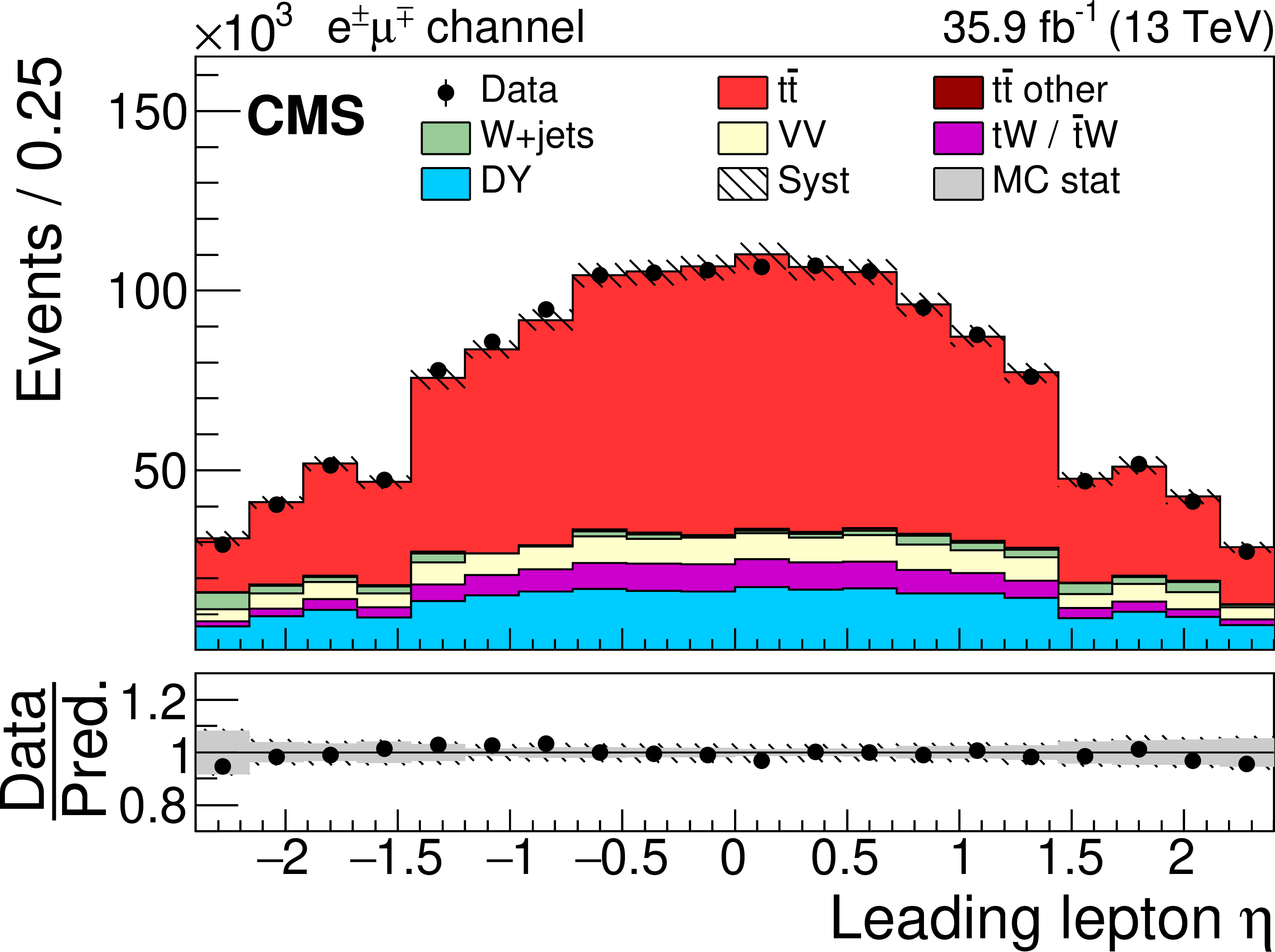
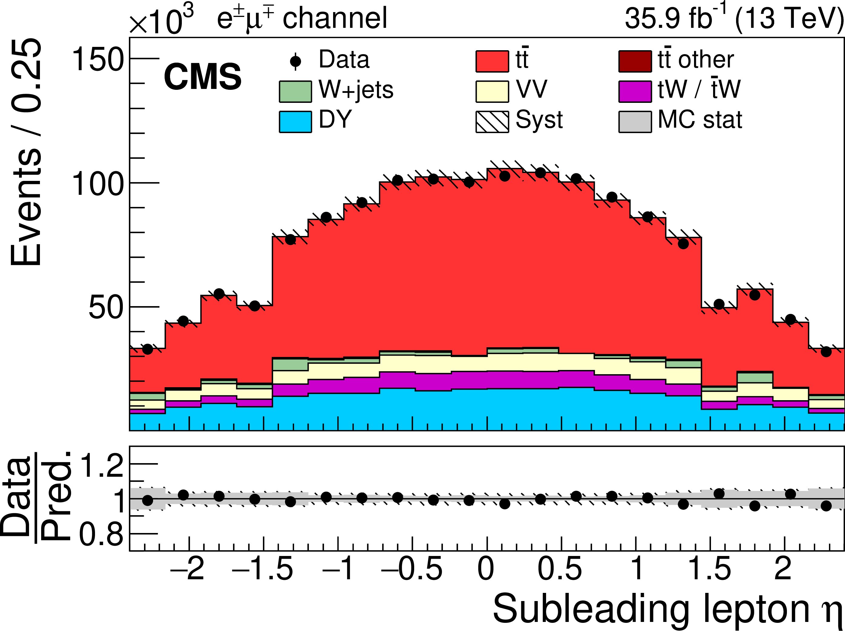
Figure 1:
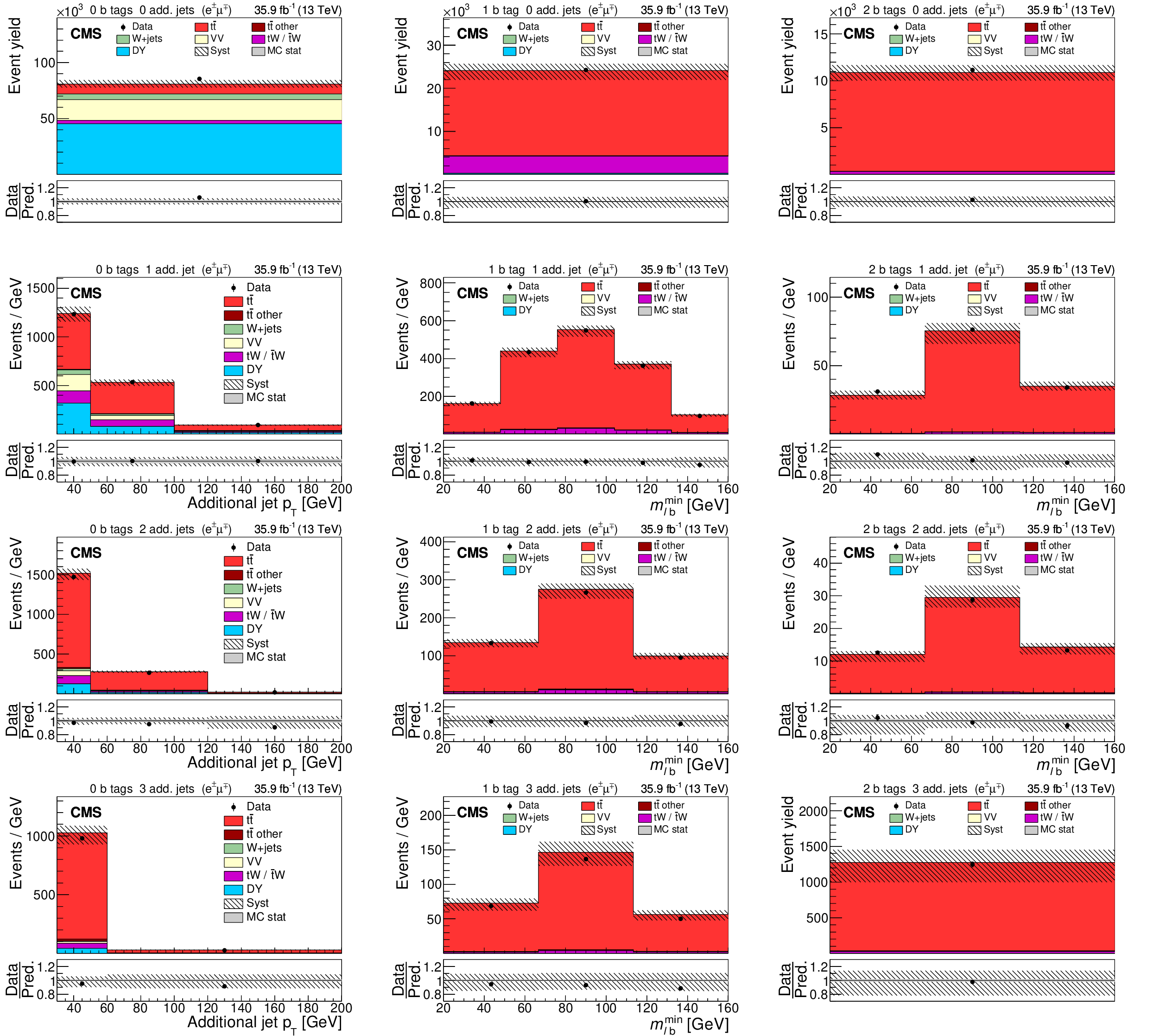
Distributions of the transverse momentum (left) and pseudorapidity (right) of the leading (upper) and subleading (middle) leptons in the ${\mathrm {e}}^{\pm} {{\mu}}^{\mp}$ channel after the event selection for the data (points) and the predictions for the signal and various backgrounds from the simulation (shaded histograms). The lower row shows the jet (left) and b-tagged jet (right) multiplicity distributions. The vertical bars on the points represent the statistical uncertainties in the data. The hatched bands correspond to the systematic uncertainty in the $ {{\mathrm {t}\overline {\mathrm {t}}}} $ signal MC simulation. The uncertainties in the integrated luminosity and background contributions are not included. The ratios of the data to the sum of the predicted yields are shown in the lower panel of each figure. Here, the solid gray band represents the contribution of the statistical uncertainty in the MC simulation. |
png pdf |
Figure 1-a:
Distribution of the transverse momentum of the leading lepton in the ${\mathrm {e}}^{\pm} {{\mu}}^{\mp}$ channel after the event selection for the data (points) and the predictions for the signal and various backgrounds from the simulation (shaded histograms). The vertical bars on the points represent the statistical uncertainties in the data. The hatched bands correspond to the systematic uncertainty in the $ {{\mathrm {t}\overline {\mathrm {t}}}} $ signal MC simulation. The uncertainties in the integrated luminosity and background contributions are not included. The ratios of the data to the sum of the predicted yields are shown in the lower panel of each figure. Here, the solid gray band represents the contribution of the statistical uncertainty in the MC simulation. |
png pdf |
Figure 1-b:
Distribution of the pseudorapidity of the leading lepton in the ${\mathrm {e}}^{\pm} {{\mu}}^{\mp}$ channel after the event selection for the data (points) and the predictions for the signal and various backgrounds from the simulation (shaded histograms). The vertical bars on the points represent the statistical uncertainties in the data. The hatched bands correspond to the systematic uncertainty in the $ {{\mathrm {t}\overline {\mathrm {t}}}} $ signal MC simulation. The uncertainties in the integrated luminosity and background contributions are not included. The ratios of the data to the sum of the predicted yields are shown in the lower panel of each figure. Here, the solid gray band represents the contribution of the statistical uncertainty in the MC simulation. |

png pdf |
Figure 1-c:
Distribution of the transverse momentum of the subleading lepton in the ${\mathrm {e}}^{\pm} {{\mu}}^{\mp}$ channel after the event selection for the data (points) and the predictions for the signal and various backgrounds from the simulation (shaded histograms). The vertical bars on the points represent the statistical uncertainties in the data. The hatched bands correspond to the systematic uncertainty in the $ {{\mathrm {t}\overline {\mathrm {t}}}} $ signal MC simulation. The uncertainties in the integrated luminosity and background contributions are not included. The ratios of the data to the sum of the predicted yields are shown in the lower panel of each figure. Here, the solid gray band represents the contribution of the statistical uncertainty in the MC simulation. |
png pdf |
Figure 1-d:
Distribution of the pseudorapidity of the subleading lepton in the ${\mathrm {e}}^{\pm} {{\mu}}^{\mp}$ channel after the event selection for the data (points) and the predictions for the signal and various backgrounds from the simulation (shaded histograms). The vertical bars on the points represent the statistical uncertainties in the data. The hatched bands correspond to the systematic uncertainty in the $ {{\mathrm {t}\overline {\mathrm {t}}}} $ signal MC simulation. The uncertainties in the integrated luminosity and background contributions are not included. The ratios of the data to the sum of the predicted yields are shown in the lower panel of each figure. Here, the solid gray band represents the contribution of the statistical uncertainty in the MC simulation. |
png pdf |
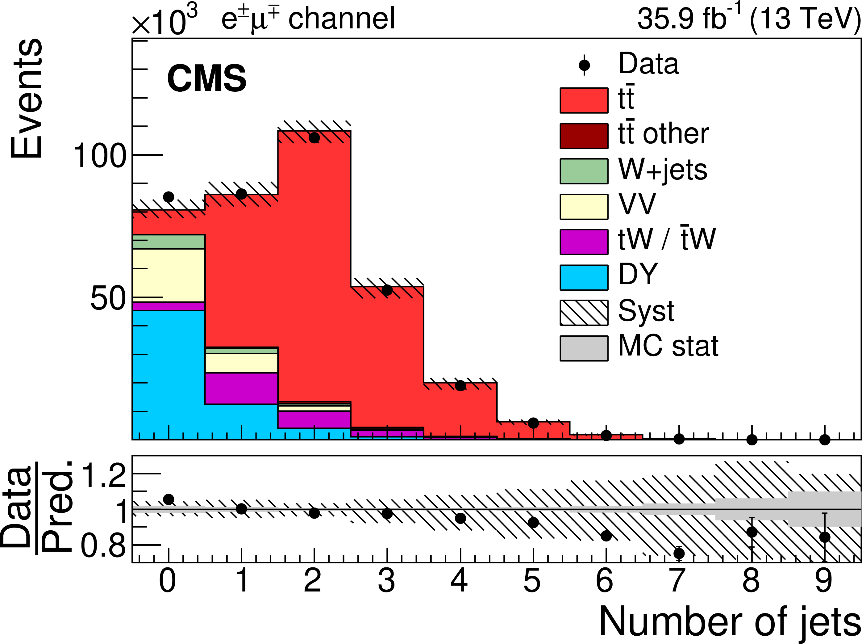
Figure 1-e:
Distribution of the jet multiplicity. The vertical bars on the points represent the statistical uncertainties in the data. The hatched bands correspond to the systematic uncertainty in the $ {{\mathrm {t}\overline {\mathrm {t}}}} $ signal MC simulation. The uncertainties in the integrated luminosity and background contributions are not included. The ratios of the data to the sum of the predicted yields are shown in the lower panel of each figure. Here, the solid gray band represents the contribution of the statistical uncertainty in the MC simulation. |
png pdf |
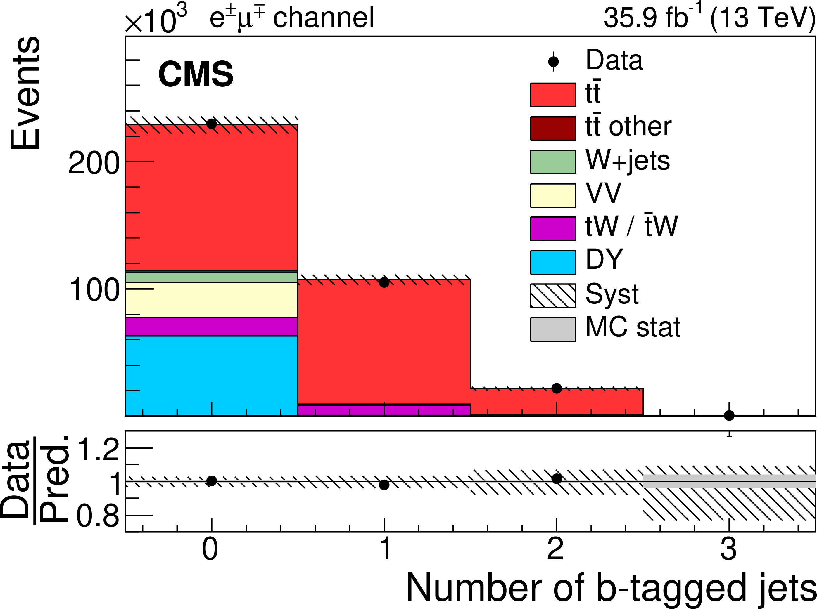
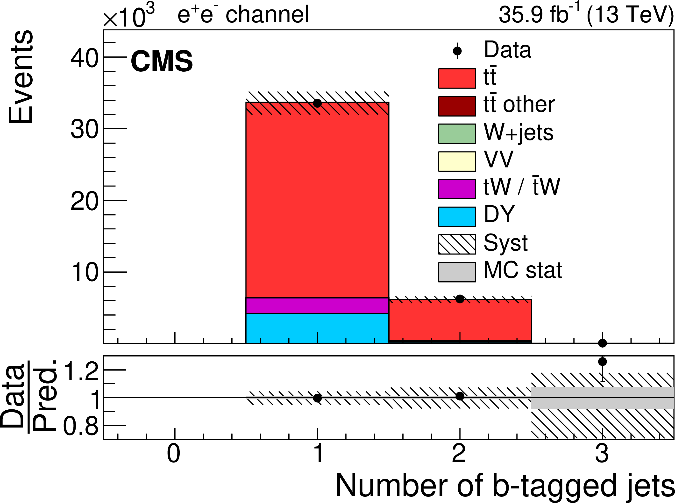
Figure 1-f:
Distribution of the b-tagged jet multiplicity. The vertical bars on the points represent the statistical uncertainties in the data. The hatched bands correspond to the systematic uncertainty in the $ {{\mathrm {t}\overline {\mathrm {t}}}} $ signal MC simulation. The uncertainties in the integrated luminosity and background contributions are not included. The ratios of the data to the sum of the predicted yields are shown in the lower panel of each figure. Here, the solid gray band represents the contribution of the statistical uncertainty in the MC simulation. |
png pdf |
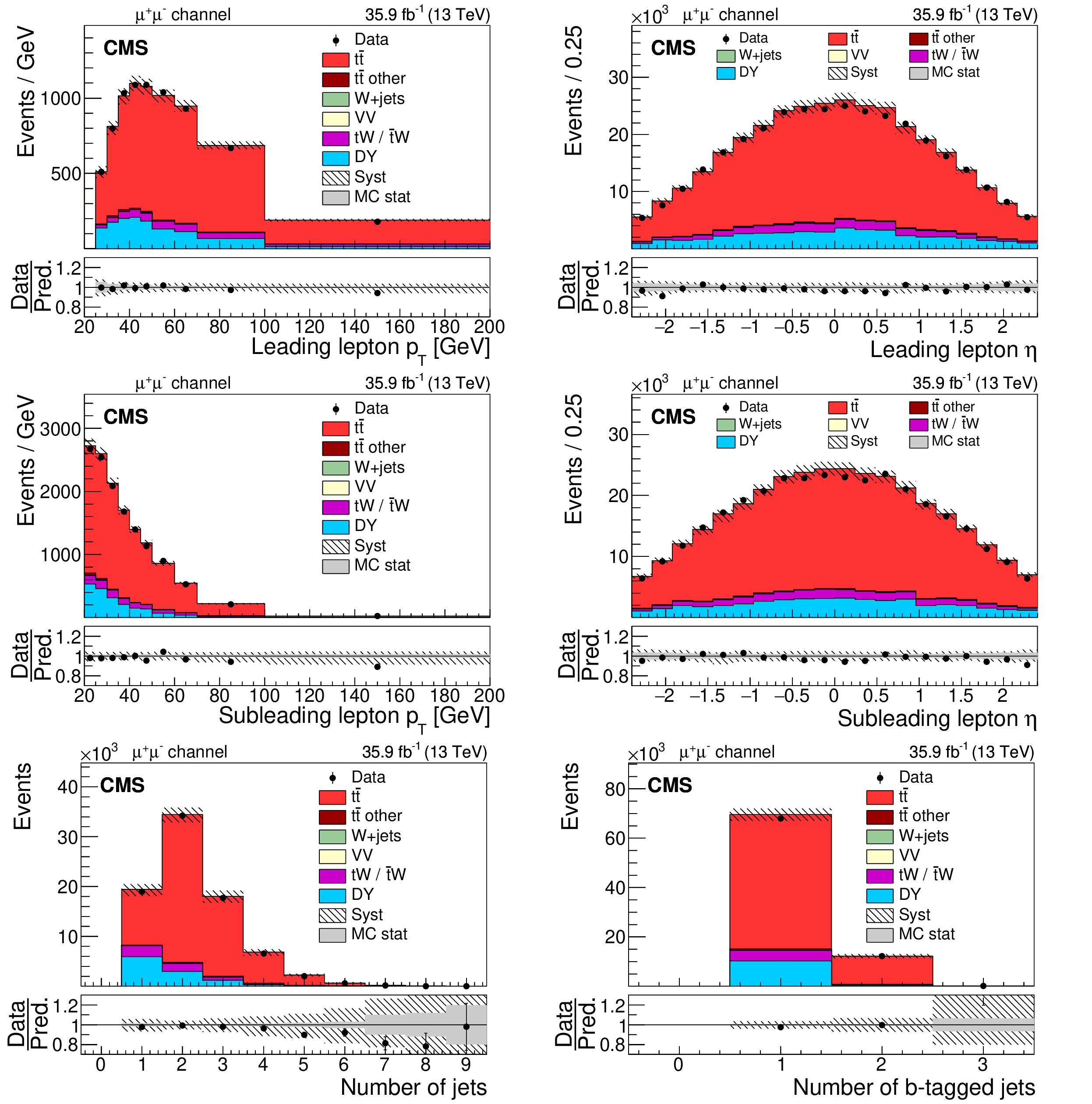
Figure 2:
The same distributions as in Fig. 1, but for the ${{{\mu ^{+}}} {{\mu ^{-}}}}$ channel. |

png pdf |
Figure 2-a:
The same distributions as in Fig. 1, but for the ${{{\mu ^{+}}} {{\mu ^{-}}}}$ channel. |

png pdf |
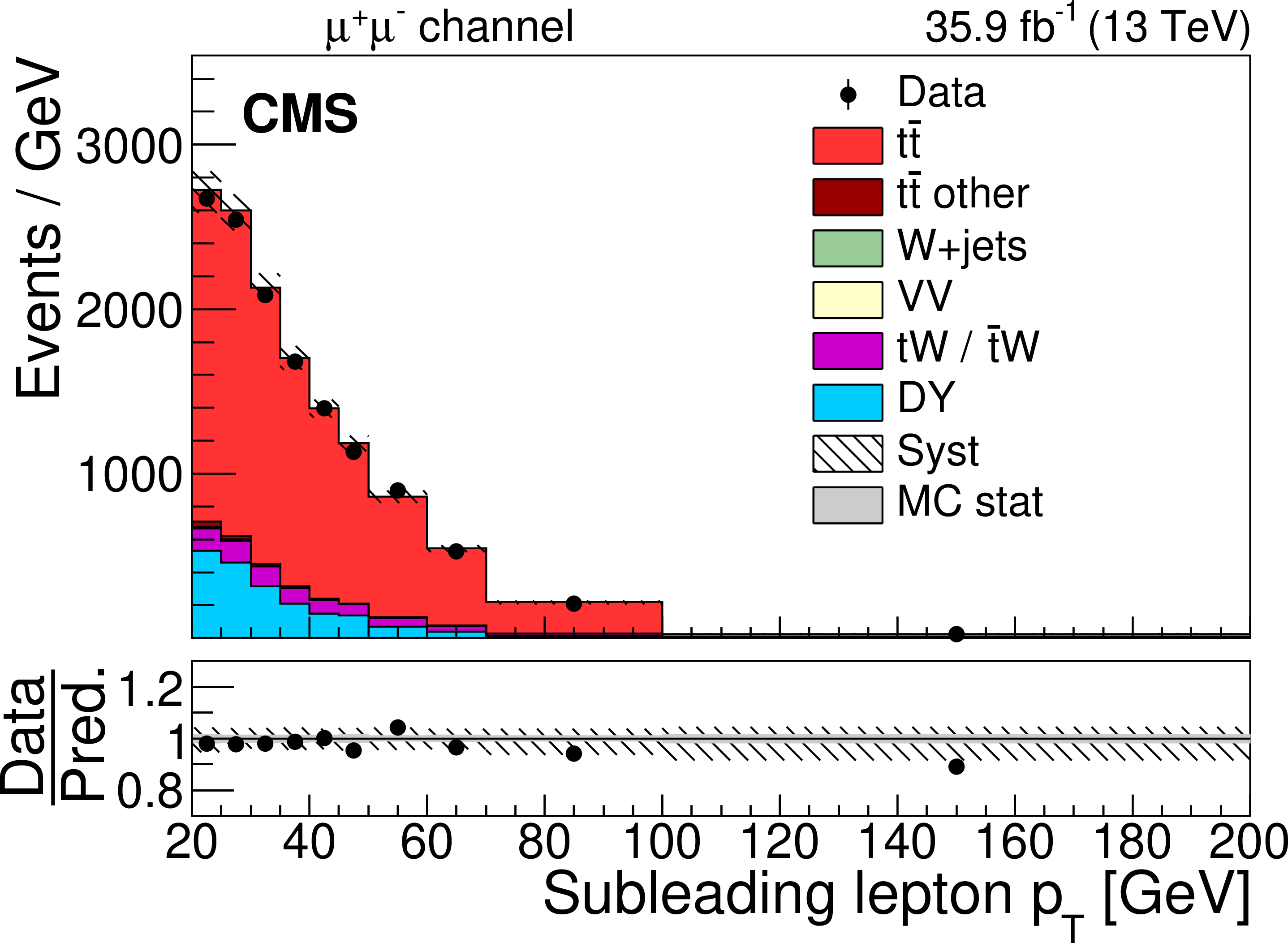
Figure 2-b:
The same distributions as in Fig. 1, but for the ${{{\mu ^{+}}} {{\mu ^{-}}}}$ channel. |
png pdf |
Figure 2-c:
The same distributions as in Fig. 1, but for the ${{{\mu ^{+}}} {{\mu ^{-}}}}$ channel. |
png pdf |
Figure 2-d:
The same distributions as in Fig. 1, but for the ${{{\mu ^{+}}} {{\mu ^{-}}}}$ channel. |

png pdf |
Figure 2-e:
The same distributions as in Fig. 1, but for the ${{{\mu ^{+}}} {{\mu ^{-}}}}$ channel. |
png pdf |
Figure 2-f:
The same distributions as in Fig. 1, but for the ${{{\mu ^{+}}} {{\mu ^{-}}}}$ channel. |
png pdf |
Figure 3:
The same distributions as in Fig. 1, but for the ${{\mathrm {e}^{+}} {\mathrm {e}^{-}}}$ channel. |
png pdf |
Figure 3-a:
The same distributions as in Fig. 1, but for the ${{\mathrm {e}^{+}} {\mathrm {e}^{-}}}$ channel. |
png pdf |
Figure 3-b:
The same distributions as in Fig. 1, but for the ${{\mathrm {e}^{+}} {\mathrm {e}^{-}}}$ channel. |
png pdf |
Figure 3-c:
The same distributions as in Fig. 1, but for the ${{\mathrm {e}^{+}} {\mathrm {e}^{-}}}$ channel. |
png pdf |
Figure 3-d:
The same distributions as in Fig. 1, but for the ${{\mathrm {e}^{+}} {\mathrm {e}^{-}}}$ channel. |
png pdf |
Figure 3-e:
The same distributions as in Fig. 1, but for the ${{\mathrm {e}^{+}} {\mathrm {e}^{-}}}$ channel. |
png pdf |
Figure 3-f:
The same distributions as in Fig. 1, but for the ${{\mathrm {e}^{+}} {\mathrm {e}^{-}}}$ channel. |
png pdf |
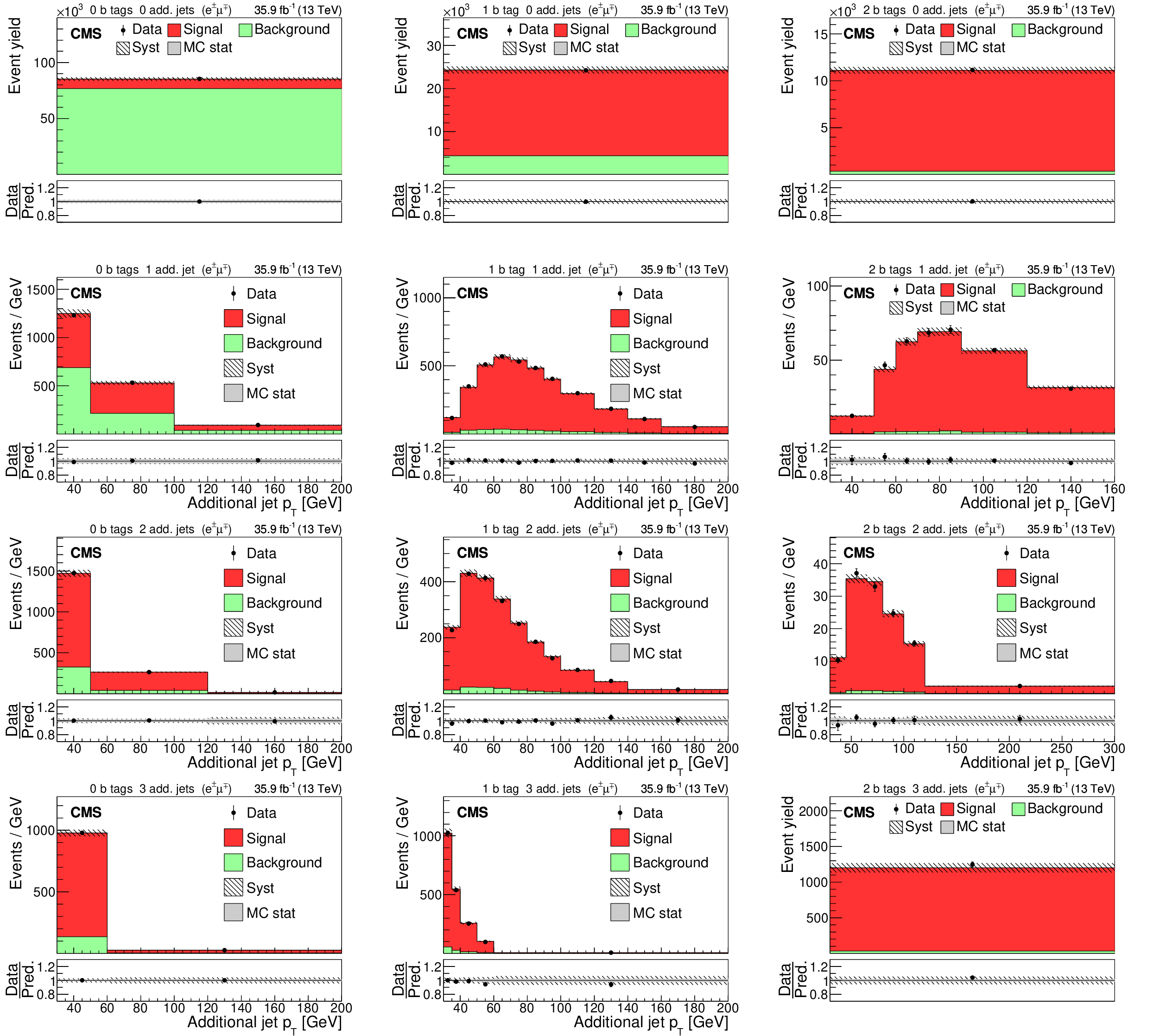
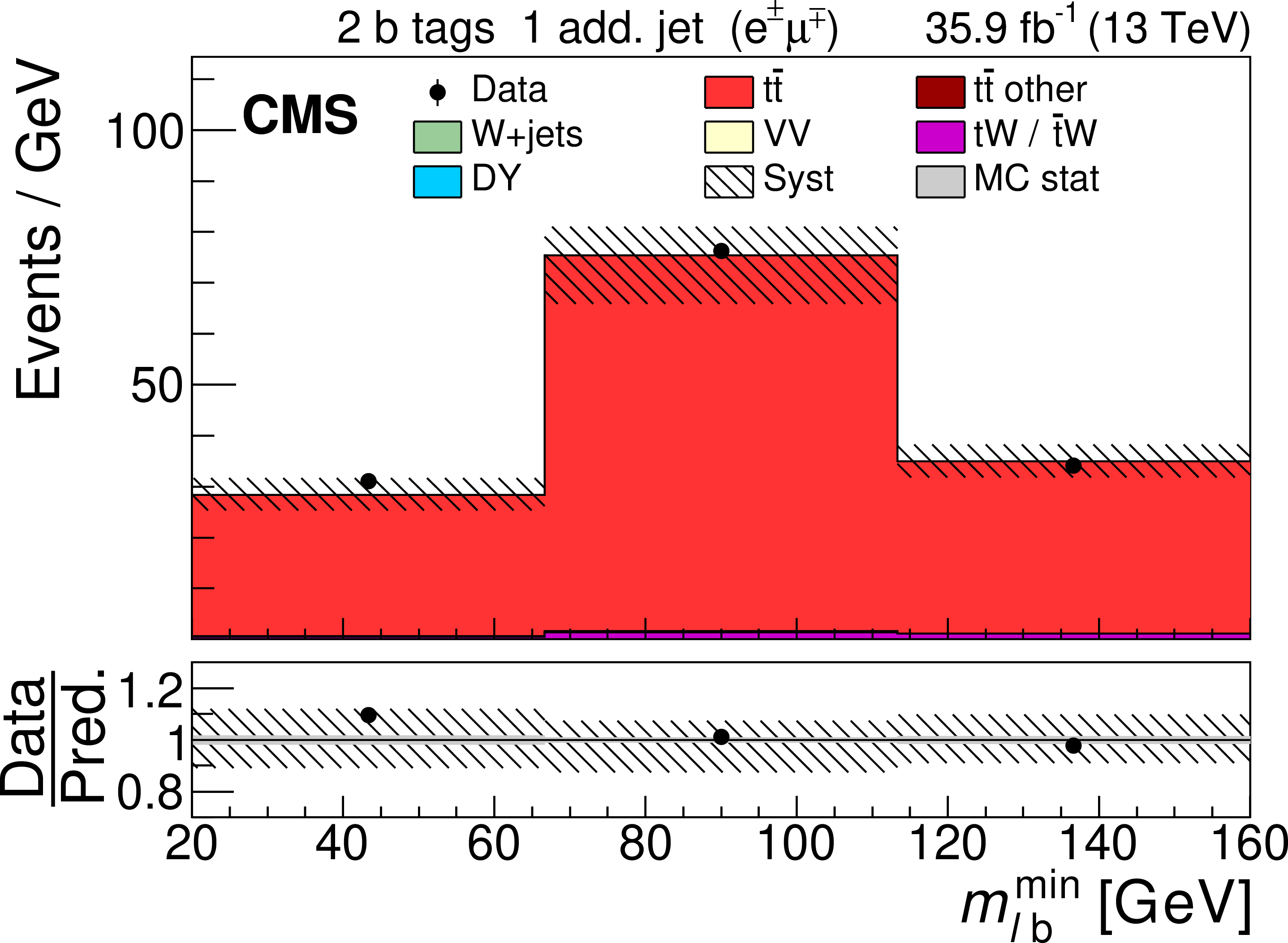
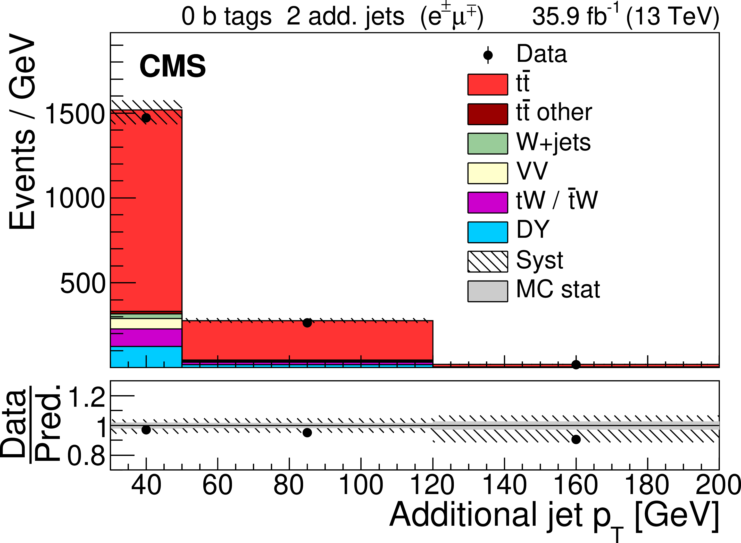
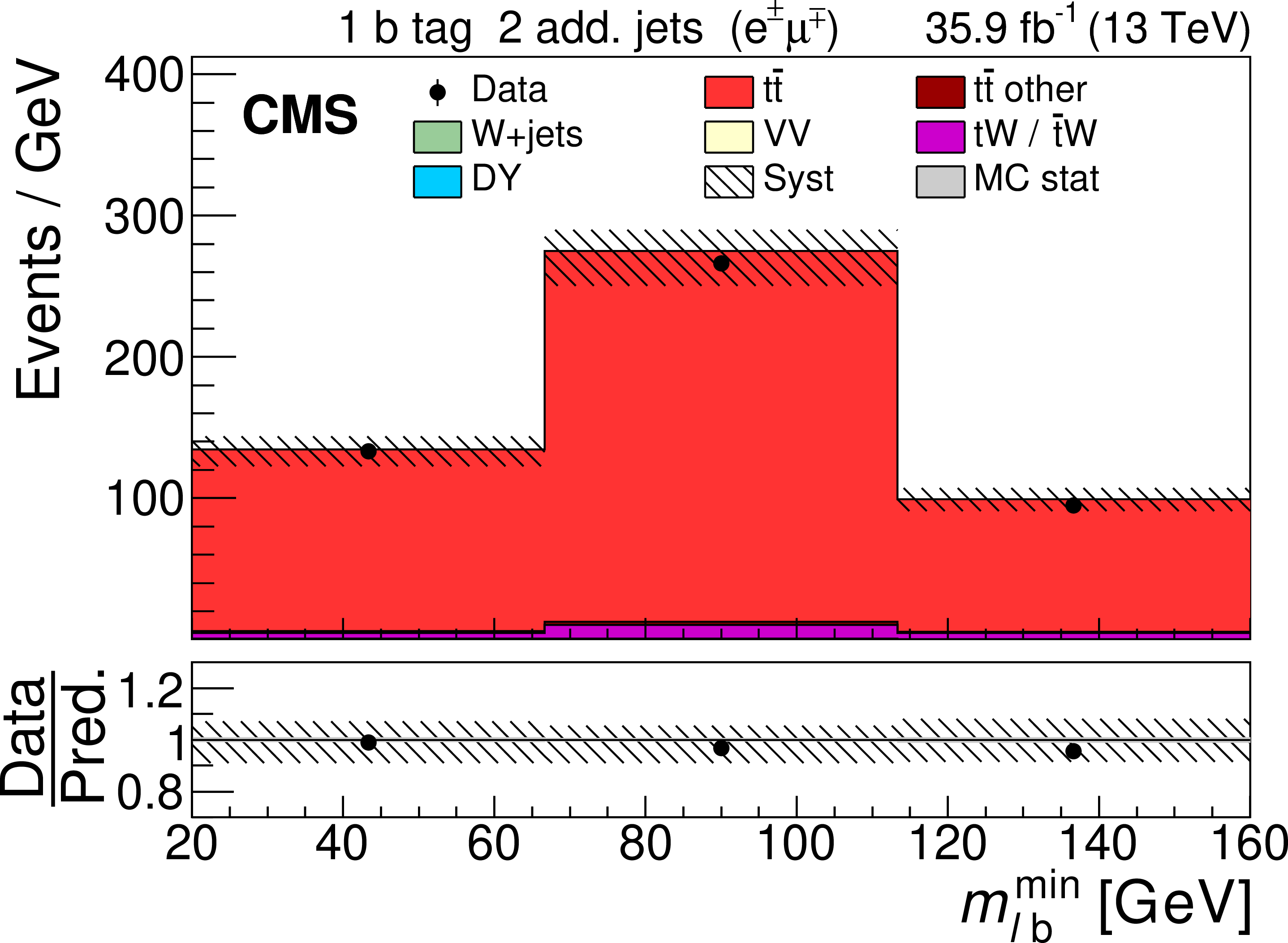
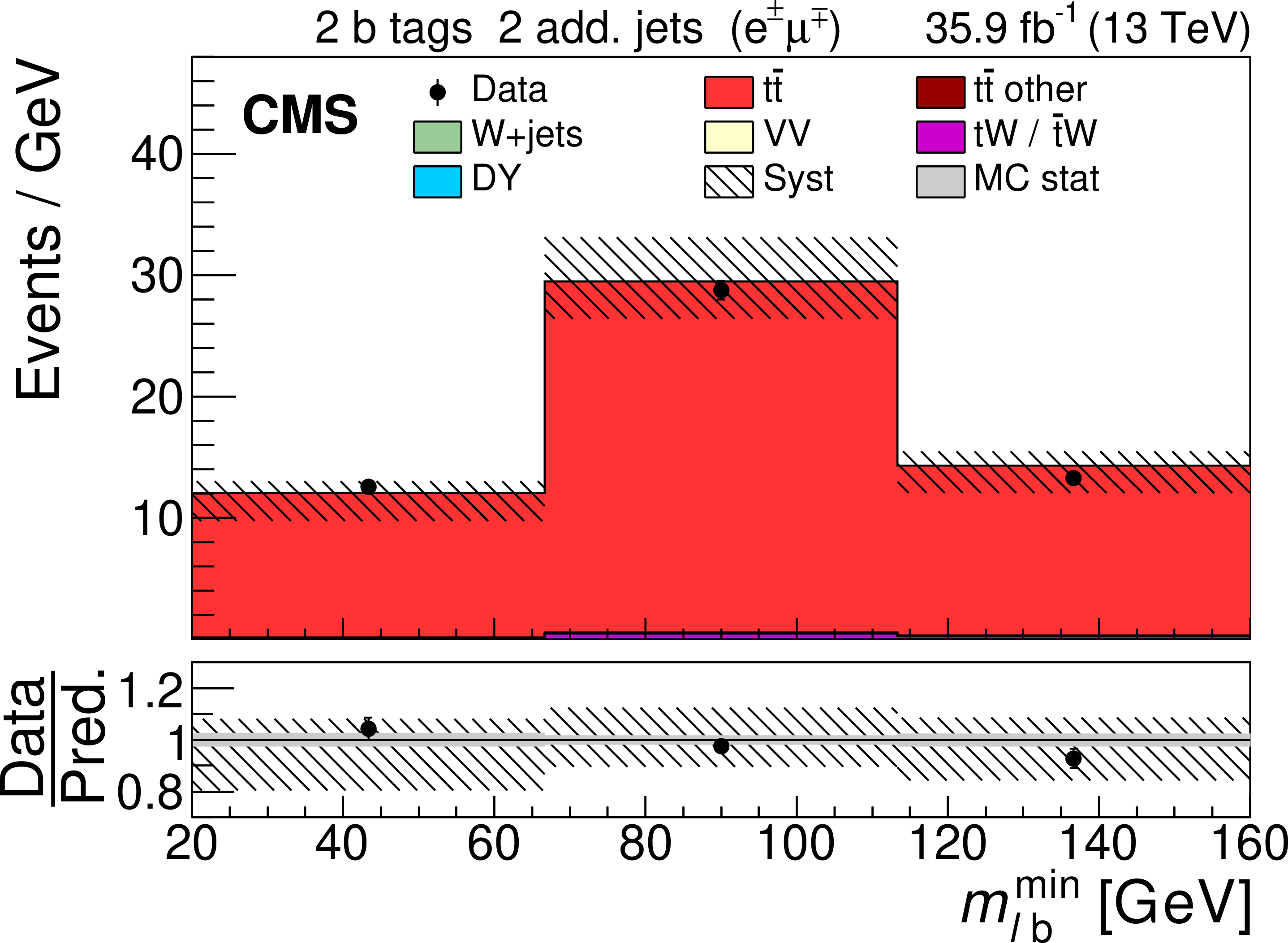
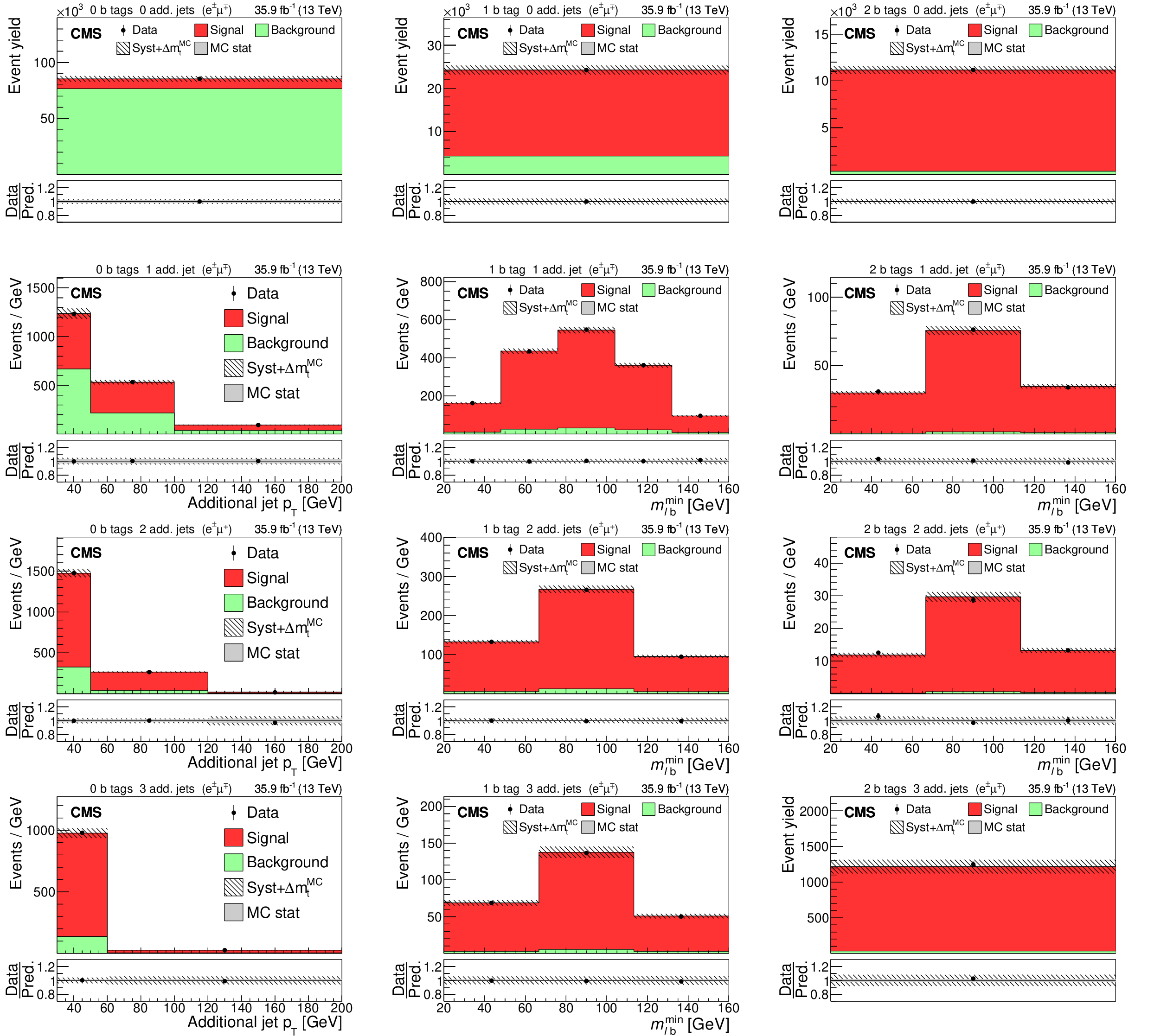
Figure 4:
Distributions in the ${\mathrm {e}}^{\pm} {{\mu}}^{\mp}$ channel after the fit to the data. In the left column events with zero or three or more b-tagged jets are shown. The middle (right) column shows events with exactly one (two) b-tagged jets. Events with zero, one, two, or three or more additional non-b-tagged jets are shown in the first, second, third, and fourth row, respectively. The hatched bands correspond to the total uncertainty in the sum of the predicted yields including all correlations. The ratios of the data to the sum of the simulated yields after the fit are shown in the lower panel of each figure. Here, the solid gray band represents the contribution of the statistical uncertainty in the MC simulation. |

png pdf |
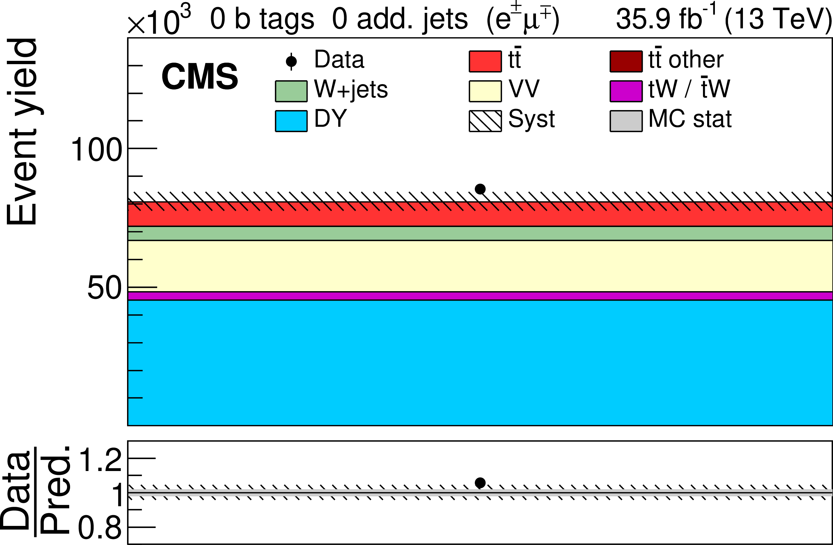
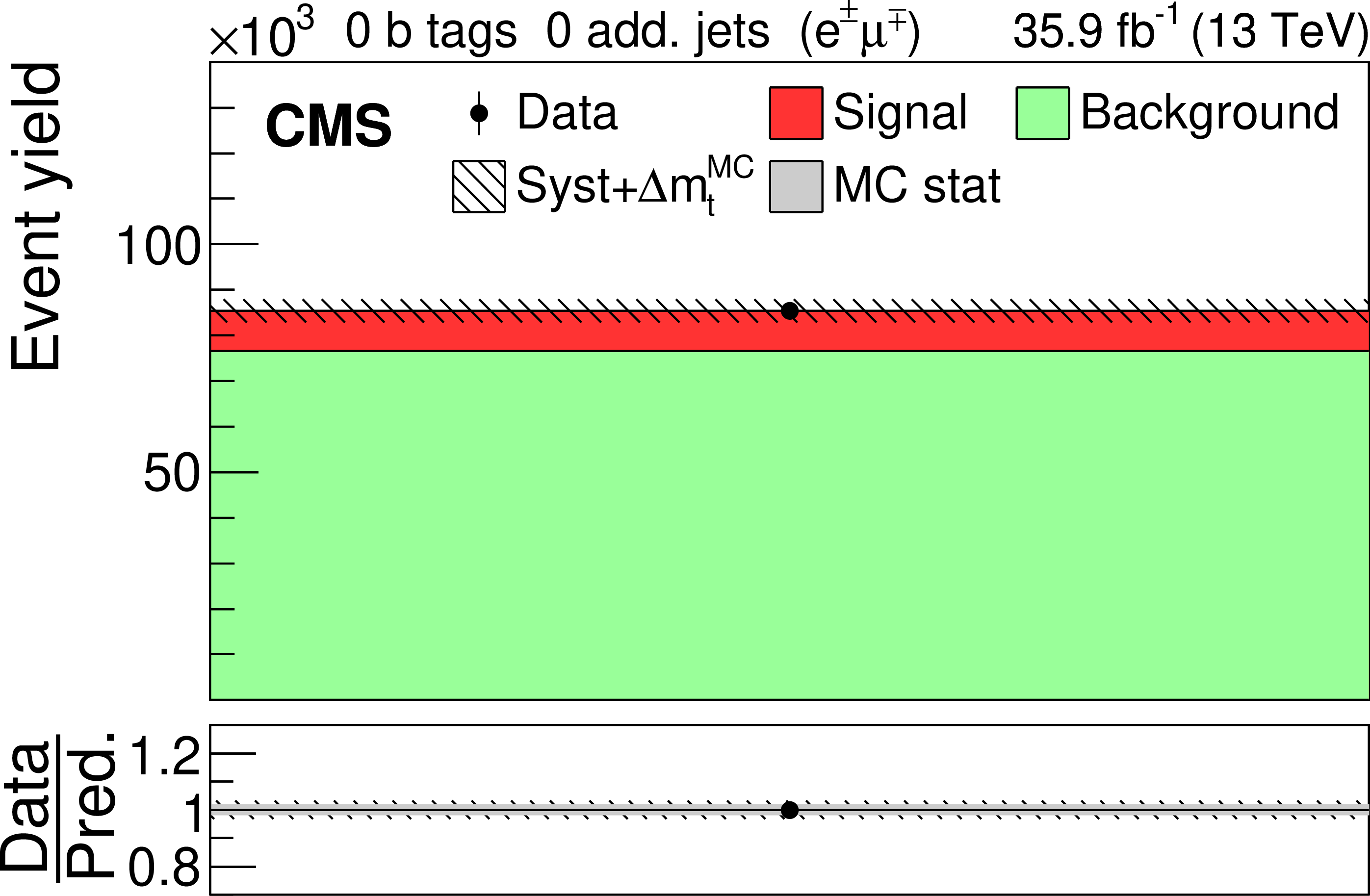
Figure 4-a:
Event yield in the ${\mathrm {e}}^{\pm} {{\mu}}^{\mp}$ channel after the fit to the data for events with zero or three or more b-tagged jets, and zero additional non-b-tagged jet. The hatched band corresponds to the total uncertainty in the sum of the predicted yields including all correlations. The ratios of the data to the sum of the simulated yields after the fit are shown in the lower panel. Here, the solid gray band represents the contribution of the statistical uncertainty in the MC simulation. |
png pdf |
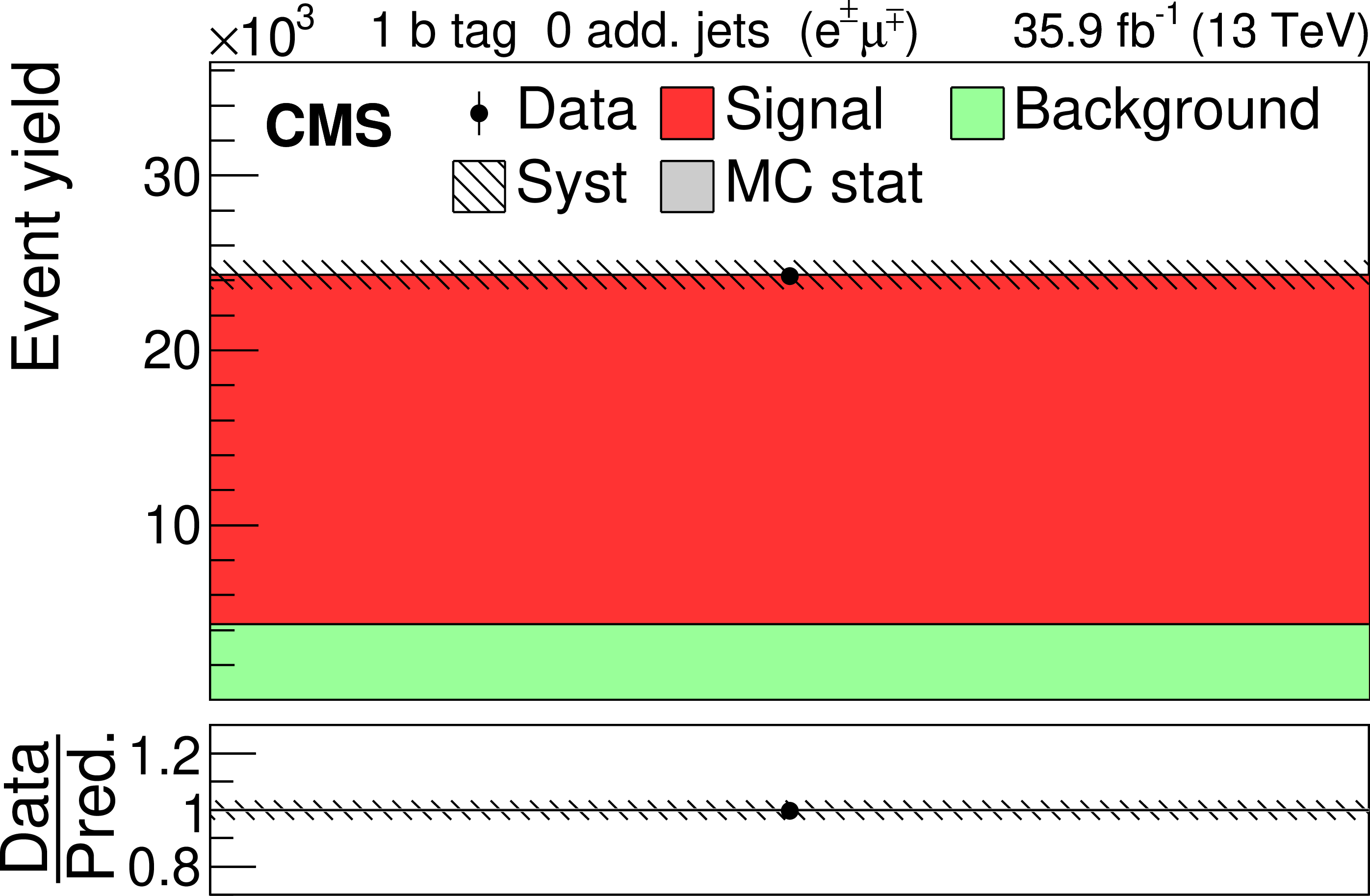
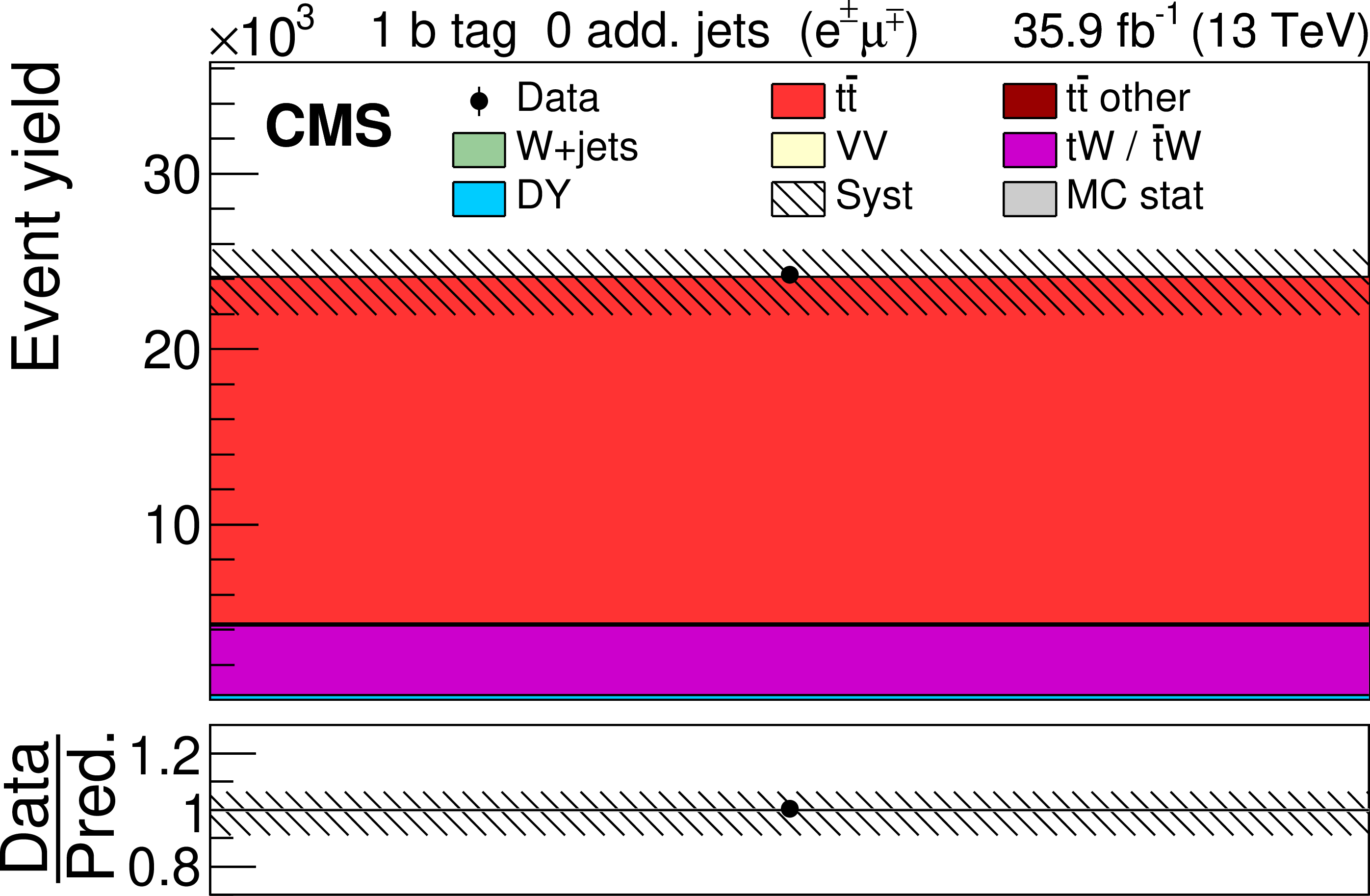
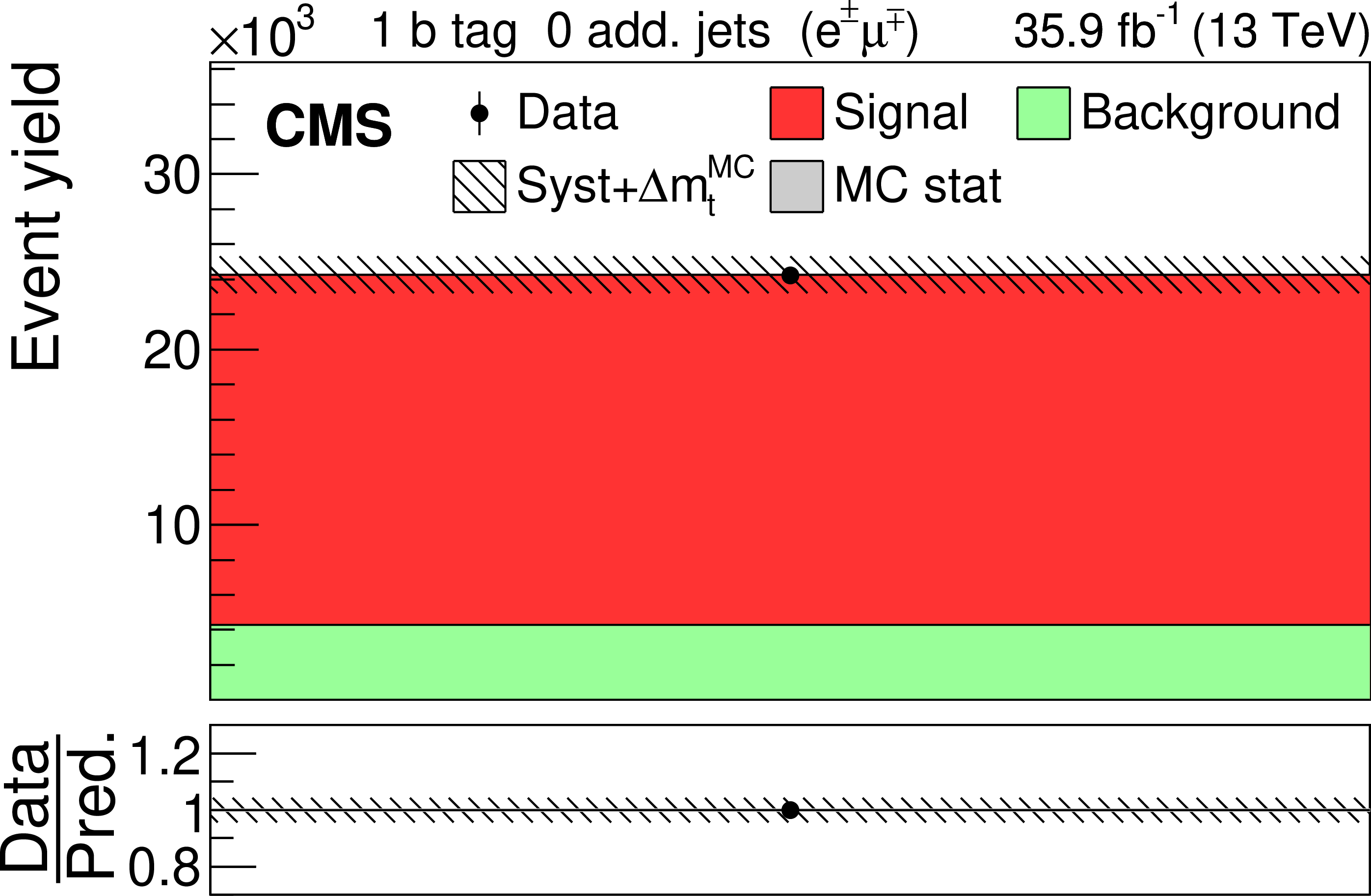
Figure 4-b:
Event yield in the ${\mathrm {e}}^{\pm} {{\mu}}^{\mp}$ channel after the fit to the data for events with exactly one b-tagged jets, and zero additional non-b-tagged jet. The hatched band corresponds to the total uncertainty in the sum of the predicted yields including all correlations. The ratios of the data to the sum of the simulated yields after the fit are shown in the lower panel. Here, the solid gray band represents the contribution of the statistical uncertainty in the MC simulation. |
png pdf |
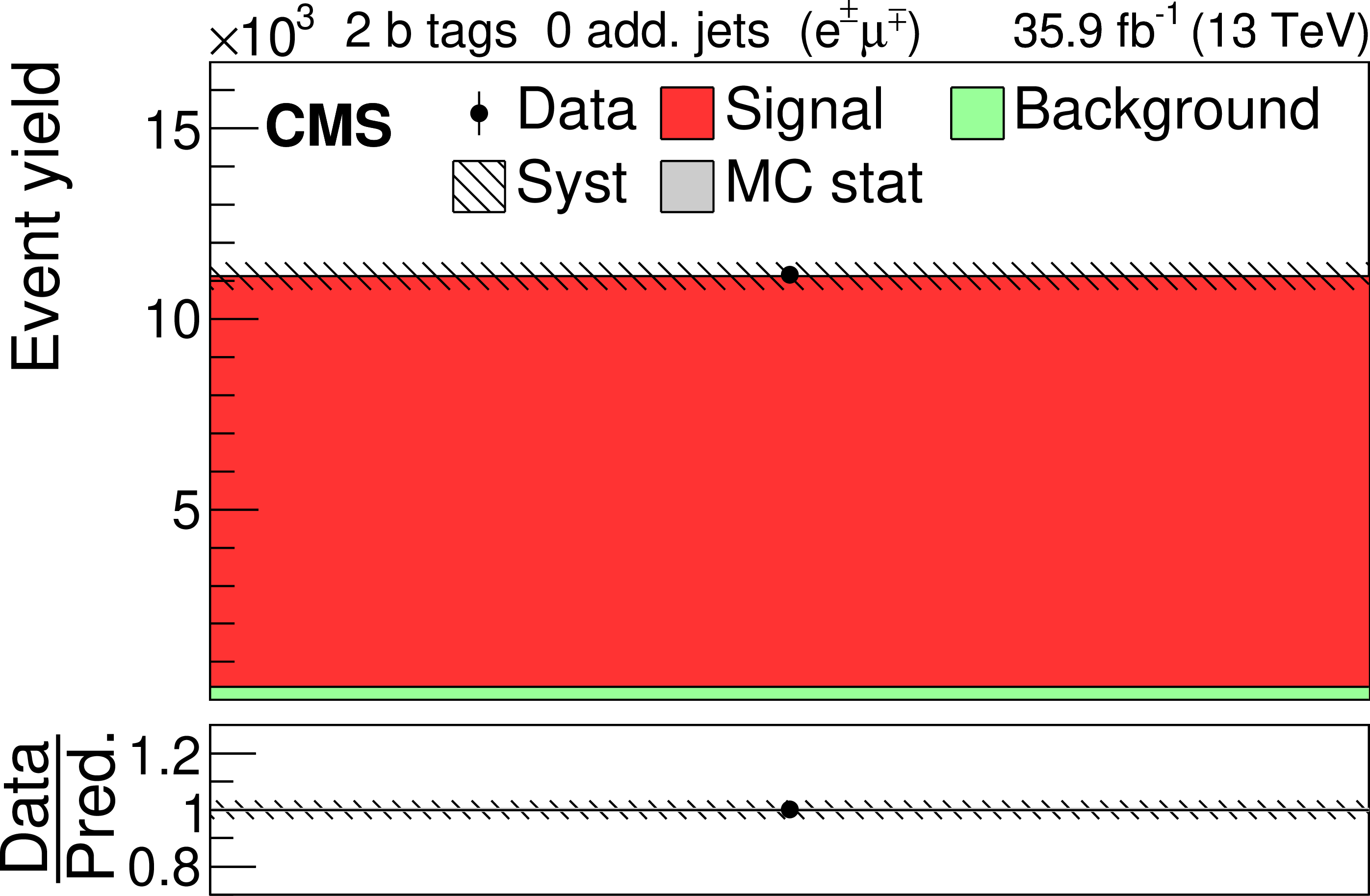
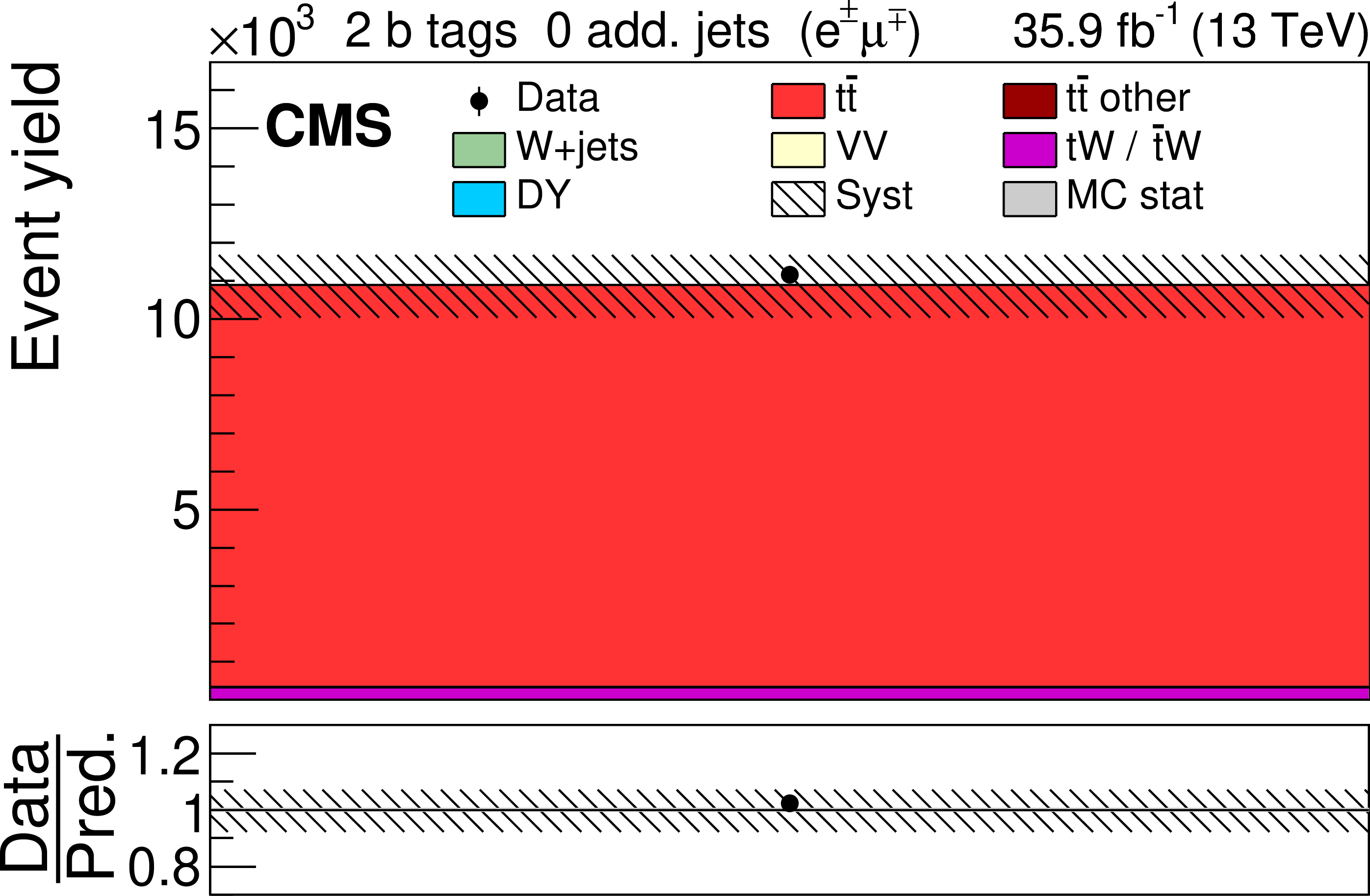
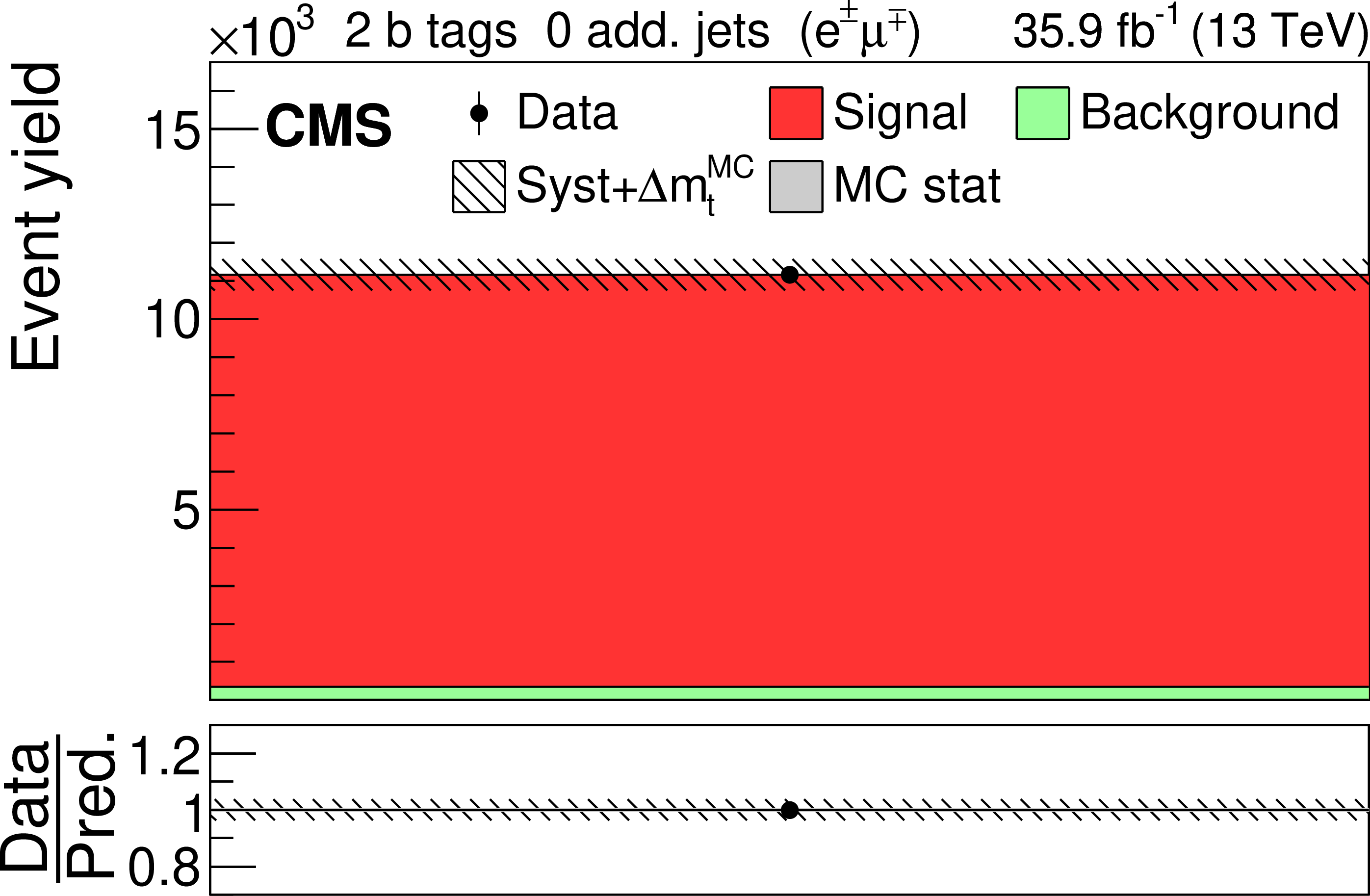
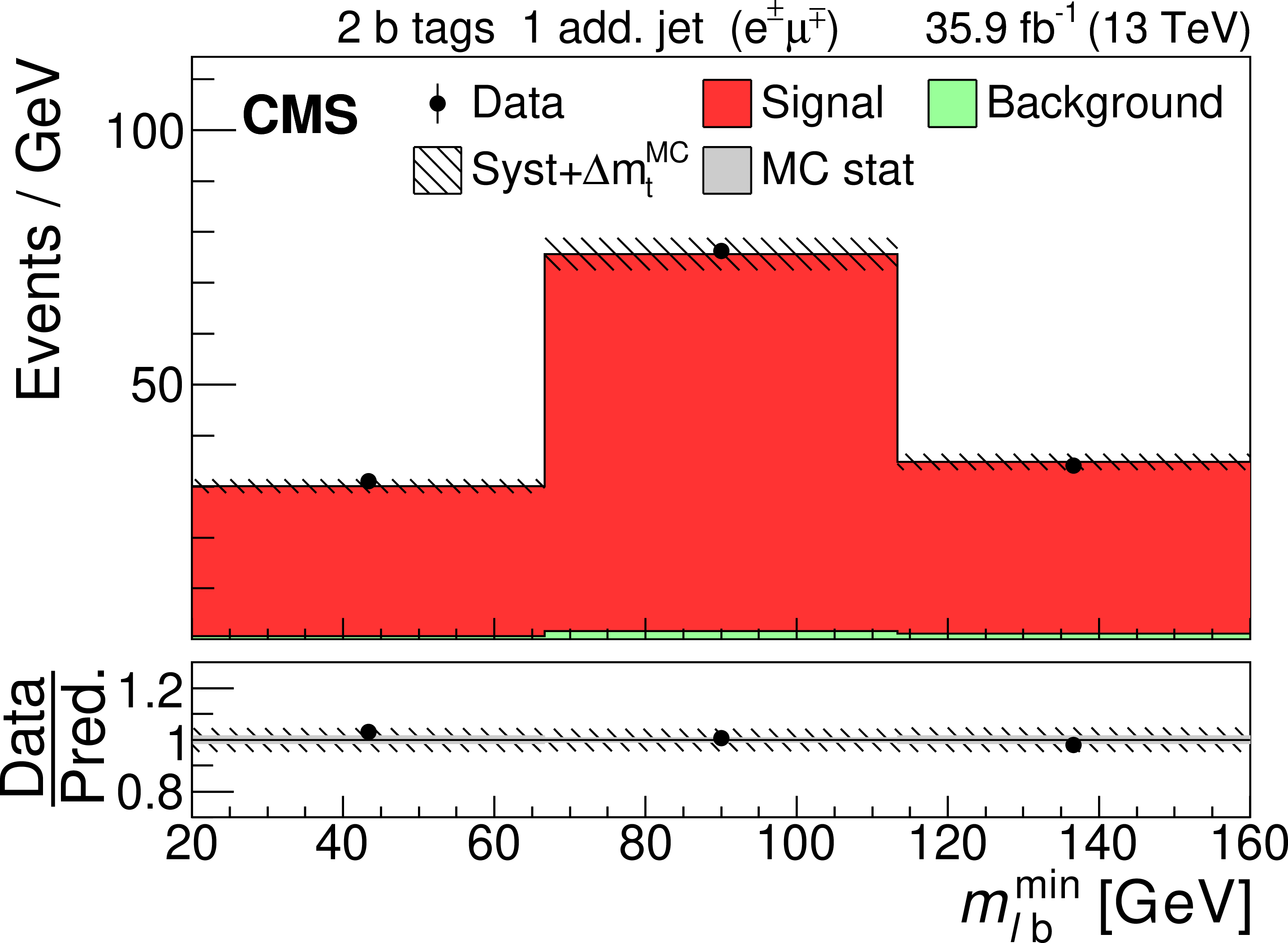
Figure 4-c:
Event yield in the ${\mathrm {e}}^{\pm} {{\mu}}^{\mp}$ channel after the fit to the data for events with exactly two b-tagged jets, and zero additional non-b-tagged jet. The hatched band corresponds to the total uncertainty in the sum of the predicted yields including all correlations. The ratios of the data to the sum of the simulated yields after the fit are shown in the lower panel. Here, the solid gray band represents the contribution of the statistical uncertainty in the MC simulation. |
png pdf |
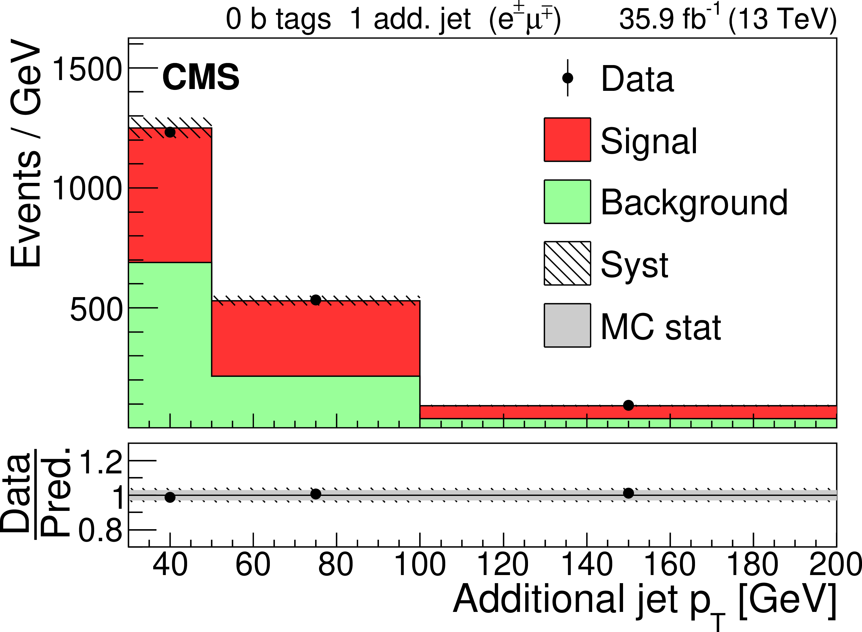
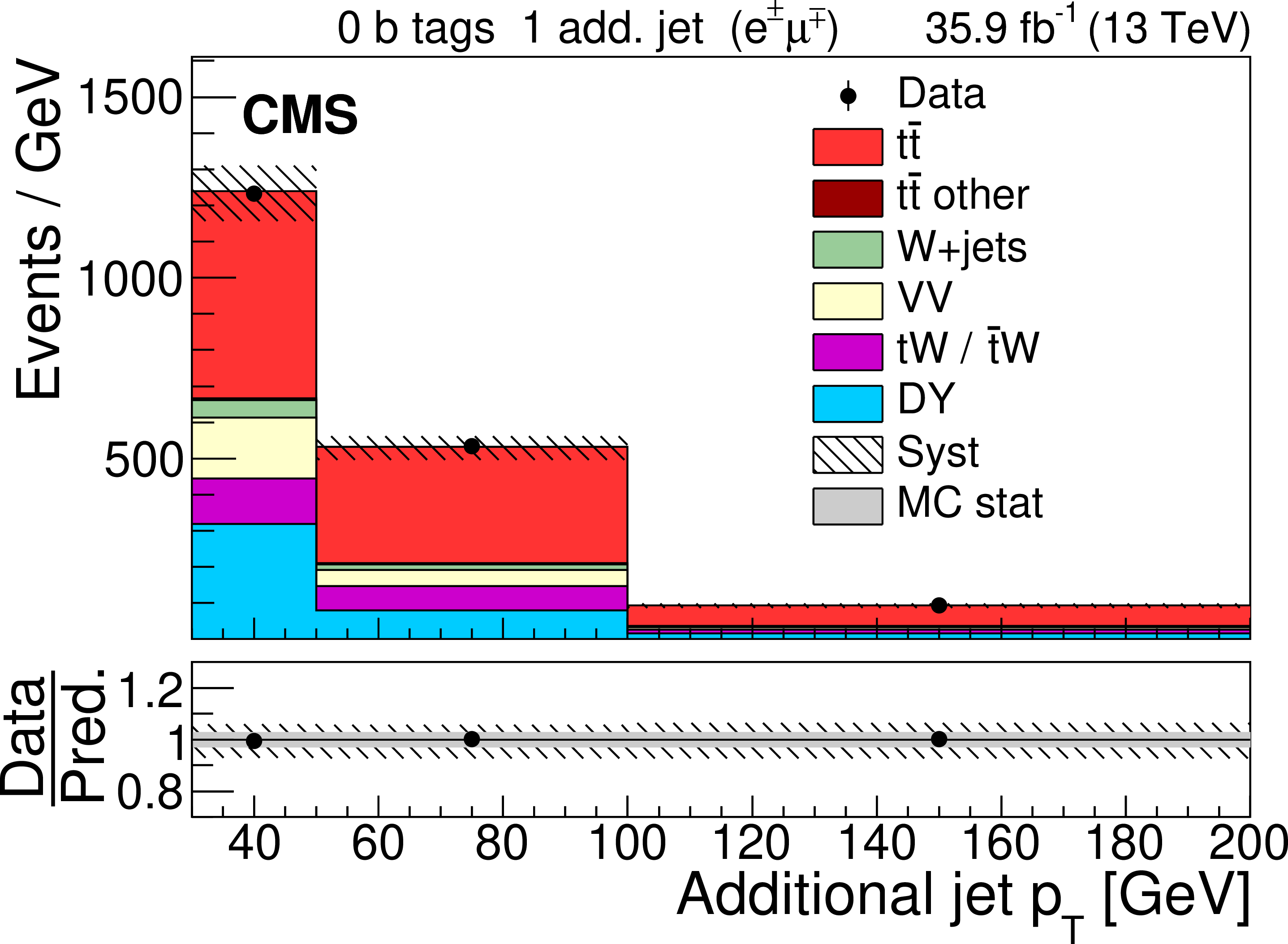
Figure 4-d:
Distribution in the ${\mathrm {e}}^{\pm} {{\mu}}^{\mp}$ channel after the fit to the data for events with zero or three or more b-tagged jets, and one additional non-b-tagged jet. The hatched band corresponds to the total uncertainty in the sum of the predicted yields including all correlations. The ratios of the data to the sum of the simulated yields after the fit are shown in the lower panel. Here, the solid gray band represents the contribution of the statistical uncertainty in the MC simulation. |
png pdf |
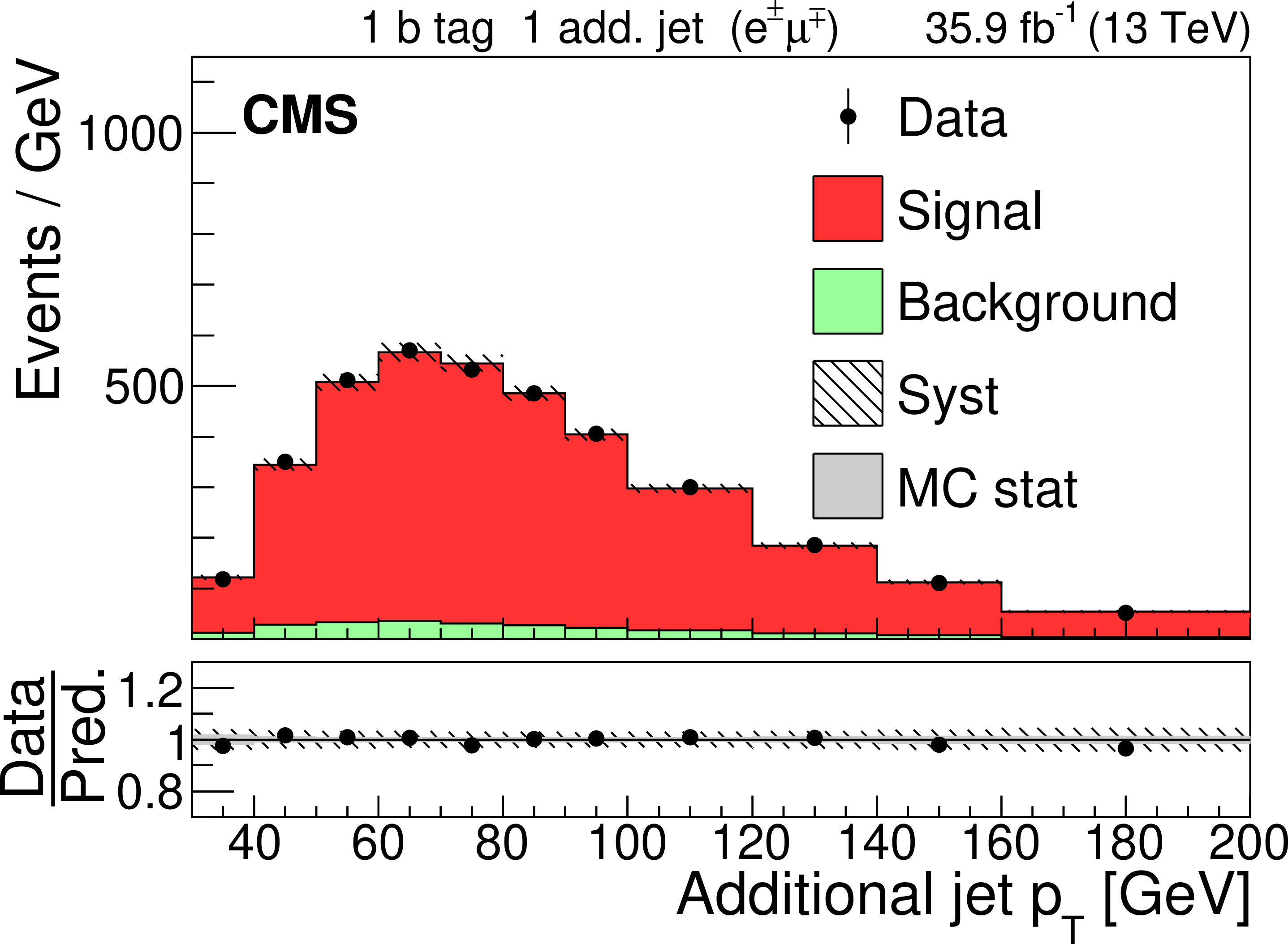
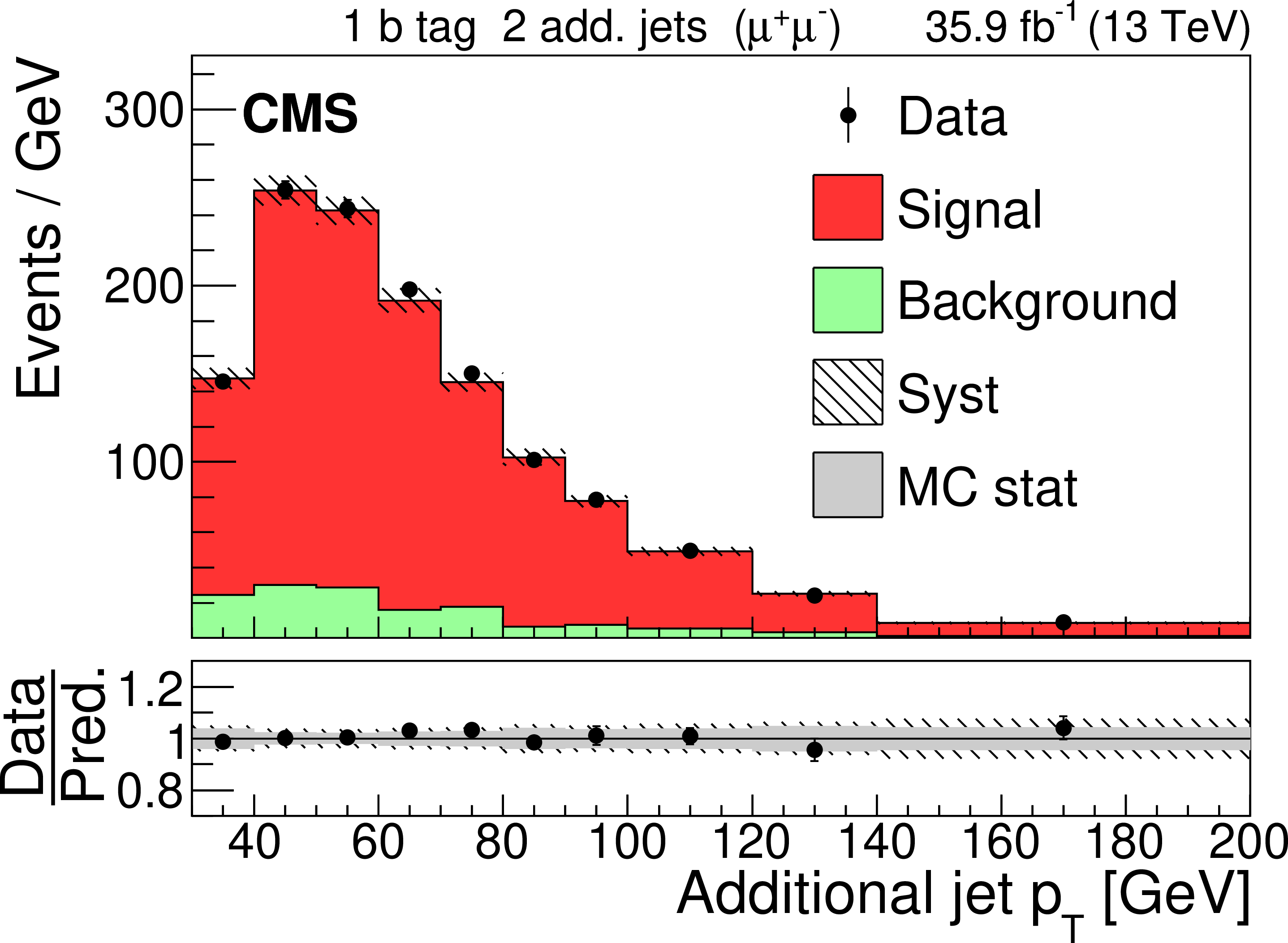
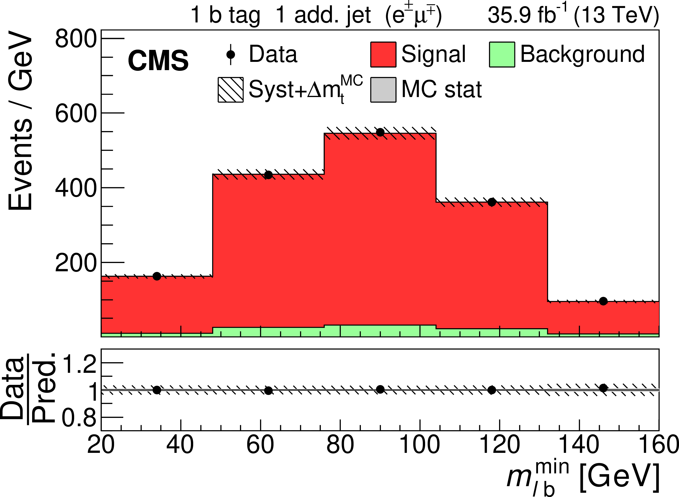
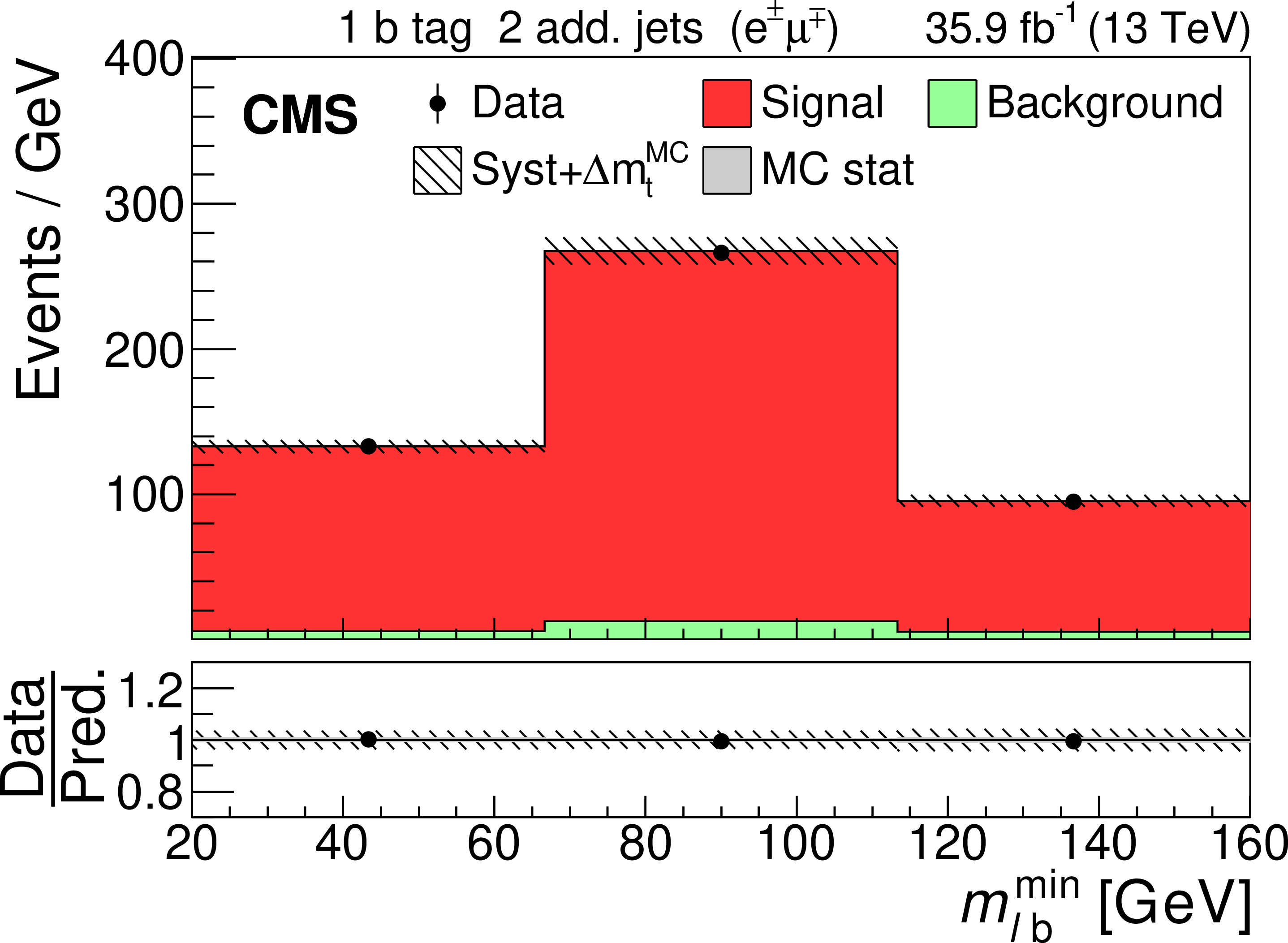
Figure 4-e:
Distribution in the ${\mathrm {e}}^{\pm} {{\mu}}^{\mp}$ channel after the fit to the data for events with exactly one b-tagged jets, and one additional non-b-tagged jet. The hatched band corresponds to the total uncertainty in the sum of the predicted yields including all correlations. The ratios of the data to the sum of the simulated yields after the fit are shown in the lower panel. Here, the solid gray band represents the contribution of the statistical uncertainty in the MC simulation. |

png pdf |
Figure 4-f:
Distribution in the ${\mathrm {e}}^{\pm} {{\mu}}^{\mp}$ channel after the fit to the data for events with exactly two b-tagged jets, and one additional non-b-tagged jet. The hatched band corresponds to the total uncertainty in the sum of the predicted yields including all correlations. The ratios of the data to the sum of the simulated yields after the fit are shown in the lower panel. Here, the solid gray band represents the contribution of the statistical uncertainty in the MC simulation. |
png pdf |
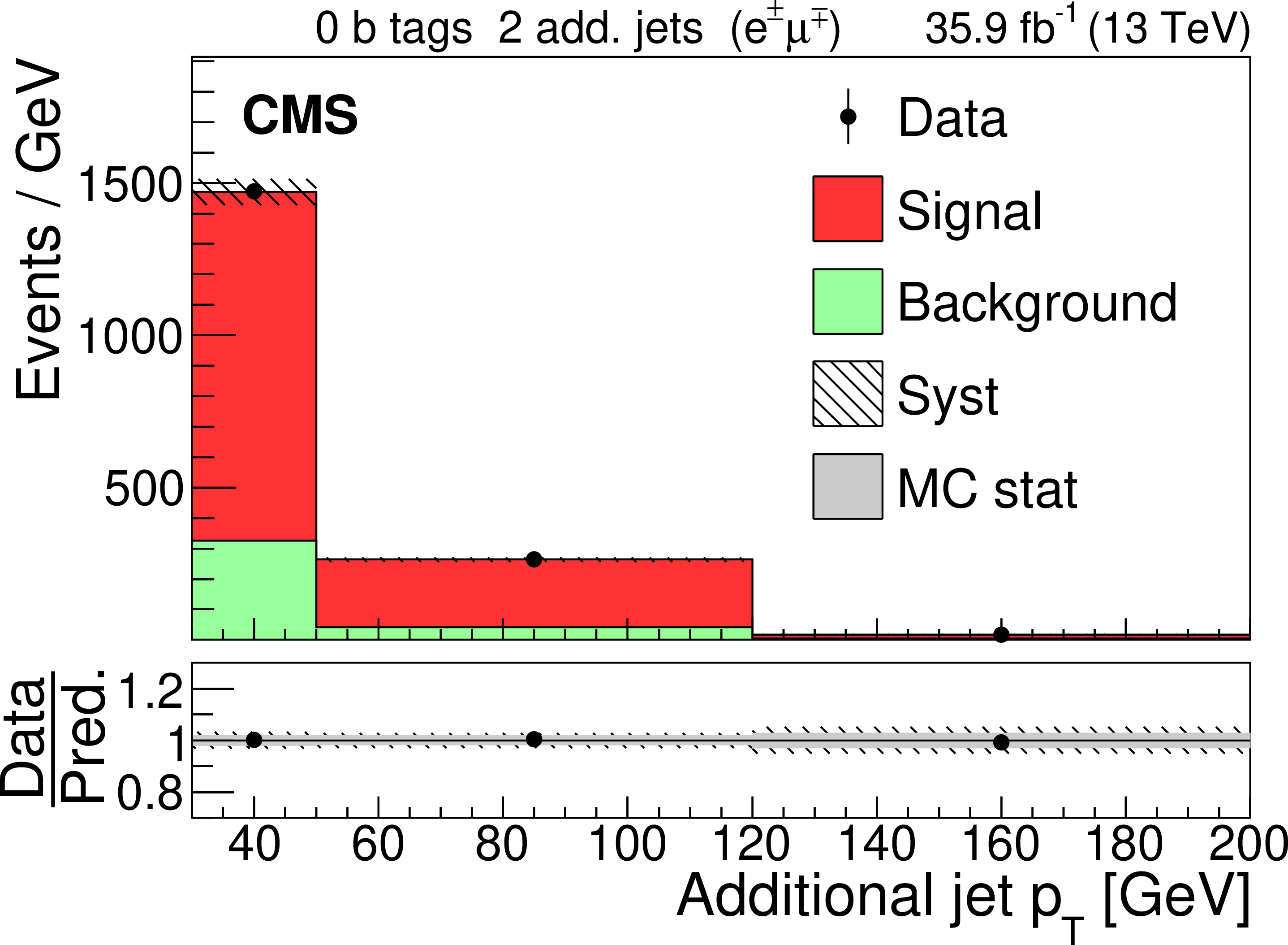
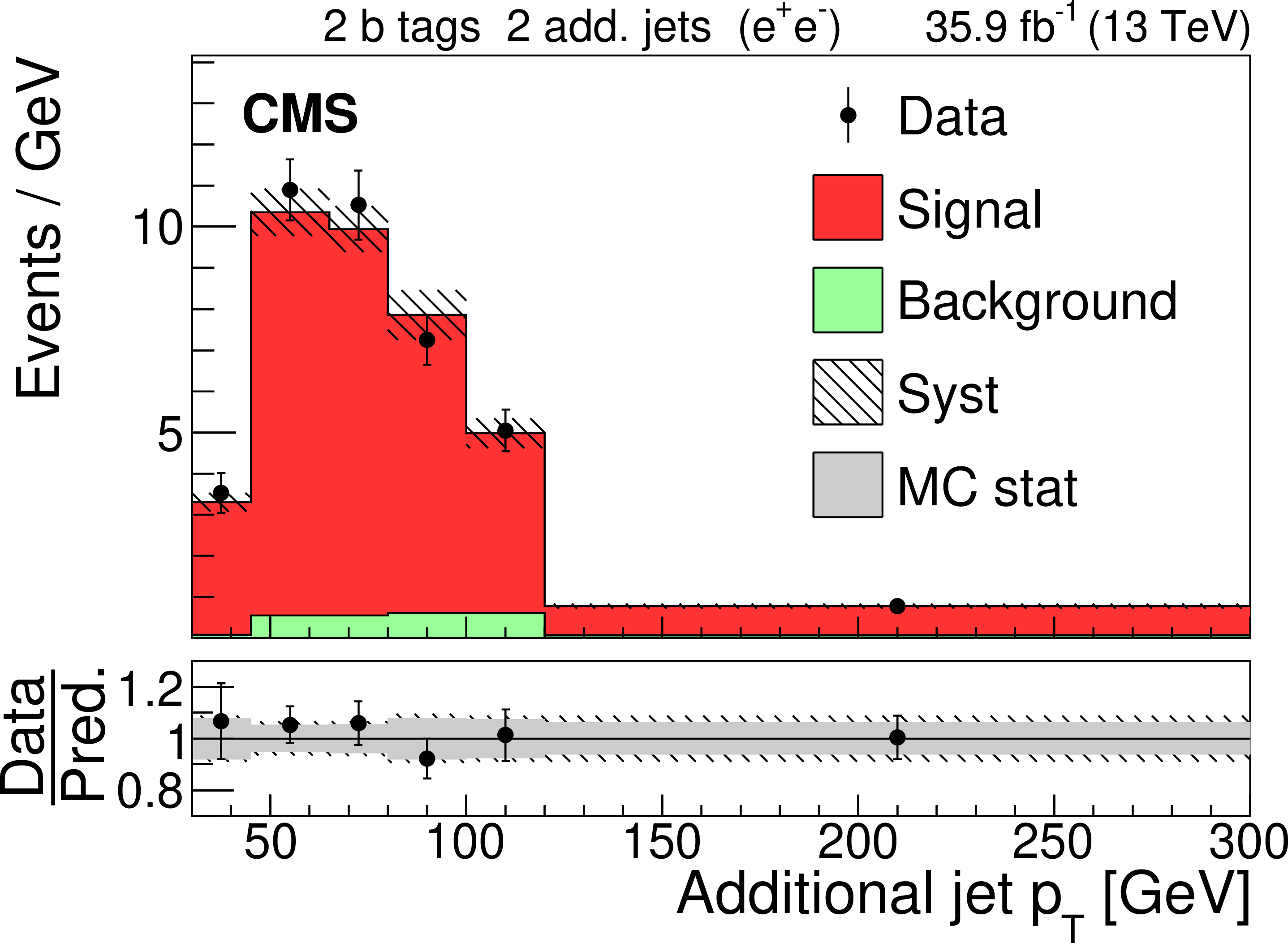
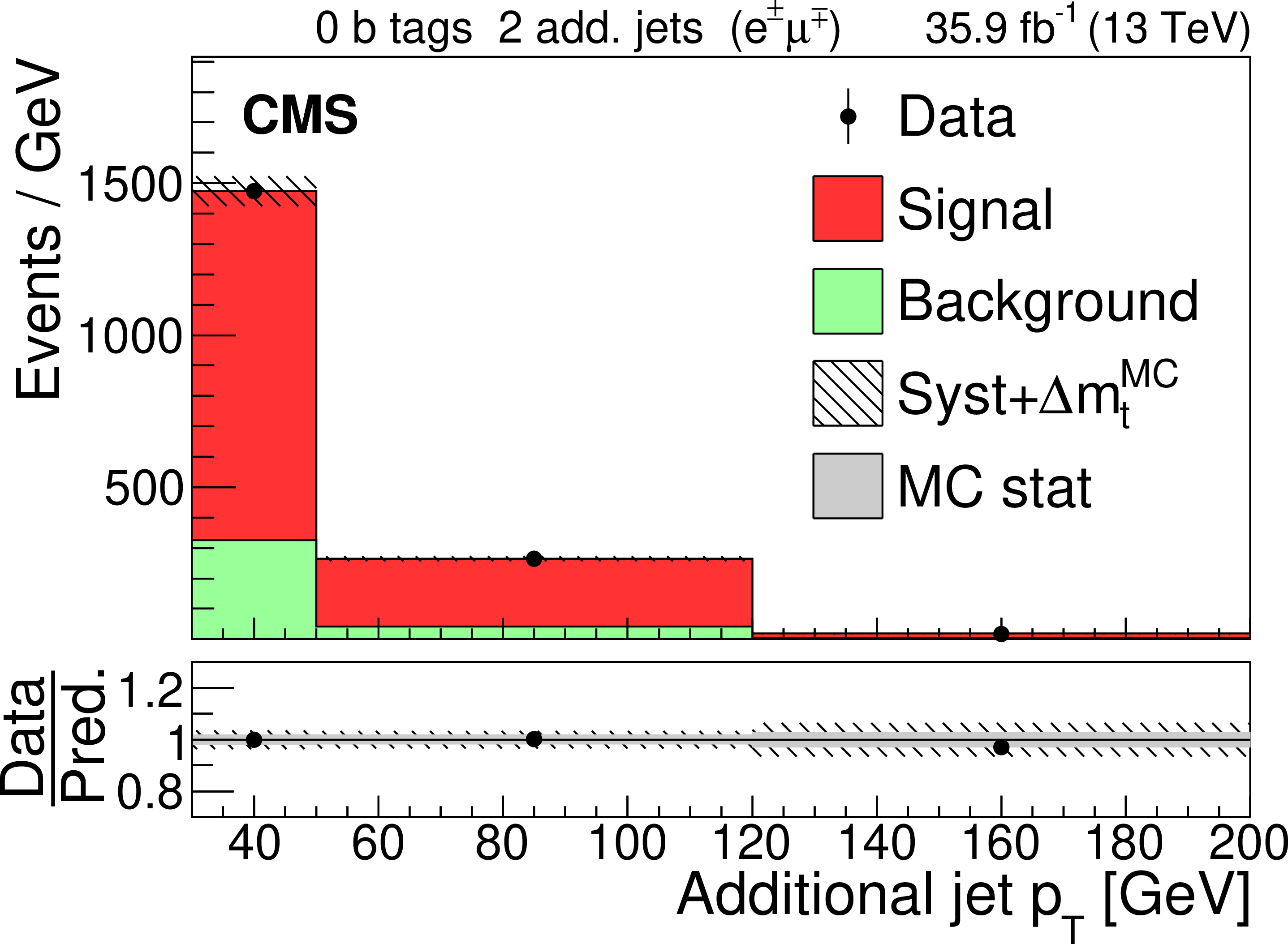
Figure 4-g:
Distribution in the ${\mathrm {e}}^{\pm} {{\mu}}^{\mp}$ channel after the fit to the data for events with zero or three or more b-tagged jets, and two additional non-b-tagged jets. The hatched band corresponds to the total uncertainty in the sum of the predicted yields including all correlations. The ratios of the data to the sum of the simulated yields after the fit are shown in the lower panel. Here, the solid gray band represents the contribution of the statistical uncertainty in the MC simulation. |
png pdf |
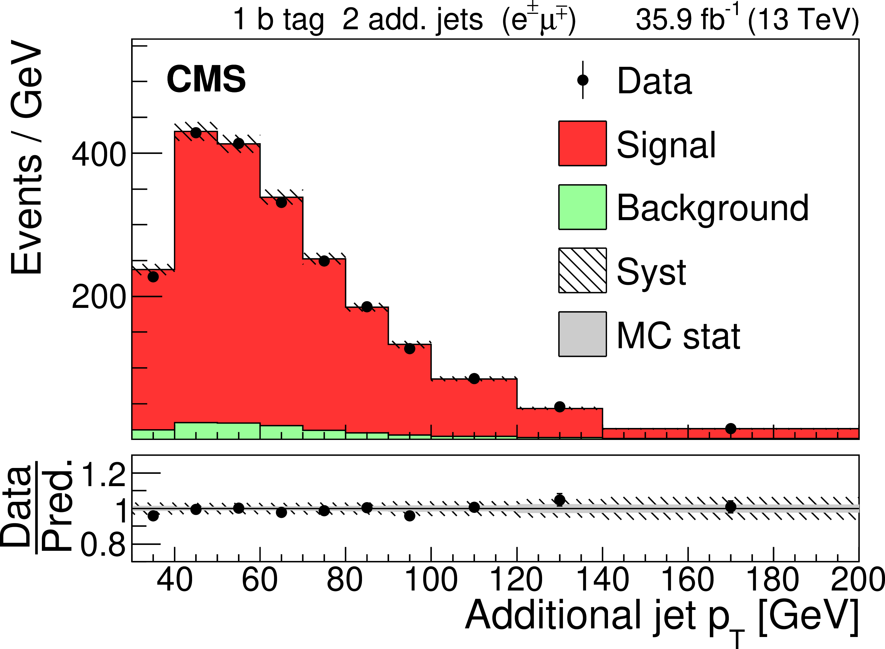
Figure 4-h:
Distribution in the ${\mathrm {e}}^{\pm} {{\mu}}^{\mp}$ channel after the fit to the data for events with exactly one b-tagged jets, and two additional non-b-tagged jets. The hatched band corresponds to the total uncertainty in the sum of the predicted yields including all correlations. The ratios of the data to the sum of the simulated yields after the fit are shown in the lower panel. Here, the solid gray band represents the contribution of the statistical uncertainty in the MC simulation. |

png pdf |
Figure 4-i:
Distribution in the ${\mathrm {e}}^{\pm} {{\mu}}^{\mp}$ channel after the fit to the data for events with exactly two b-tagged jets, and two additional non-b-tagged jets. The hatched band corresponds to the total uncertainty in the sum of the predicted yields including all correlations. The ratios of the data to the sum of the simulated yields after the fit are shown in the lower panel. Here, the solid gray band represents the contribution of the statistical uncertainty in the MC simulation. |
png pdf |
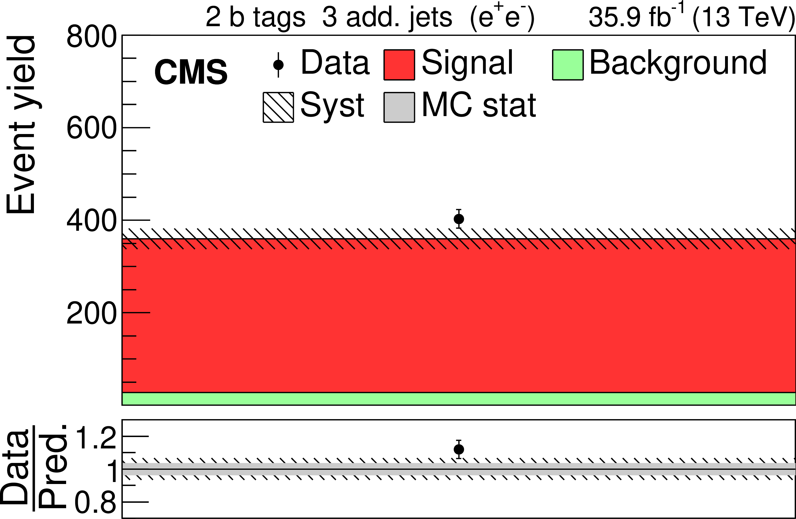
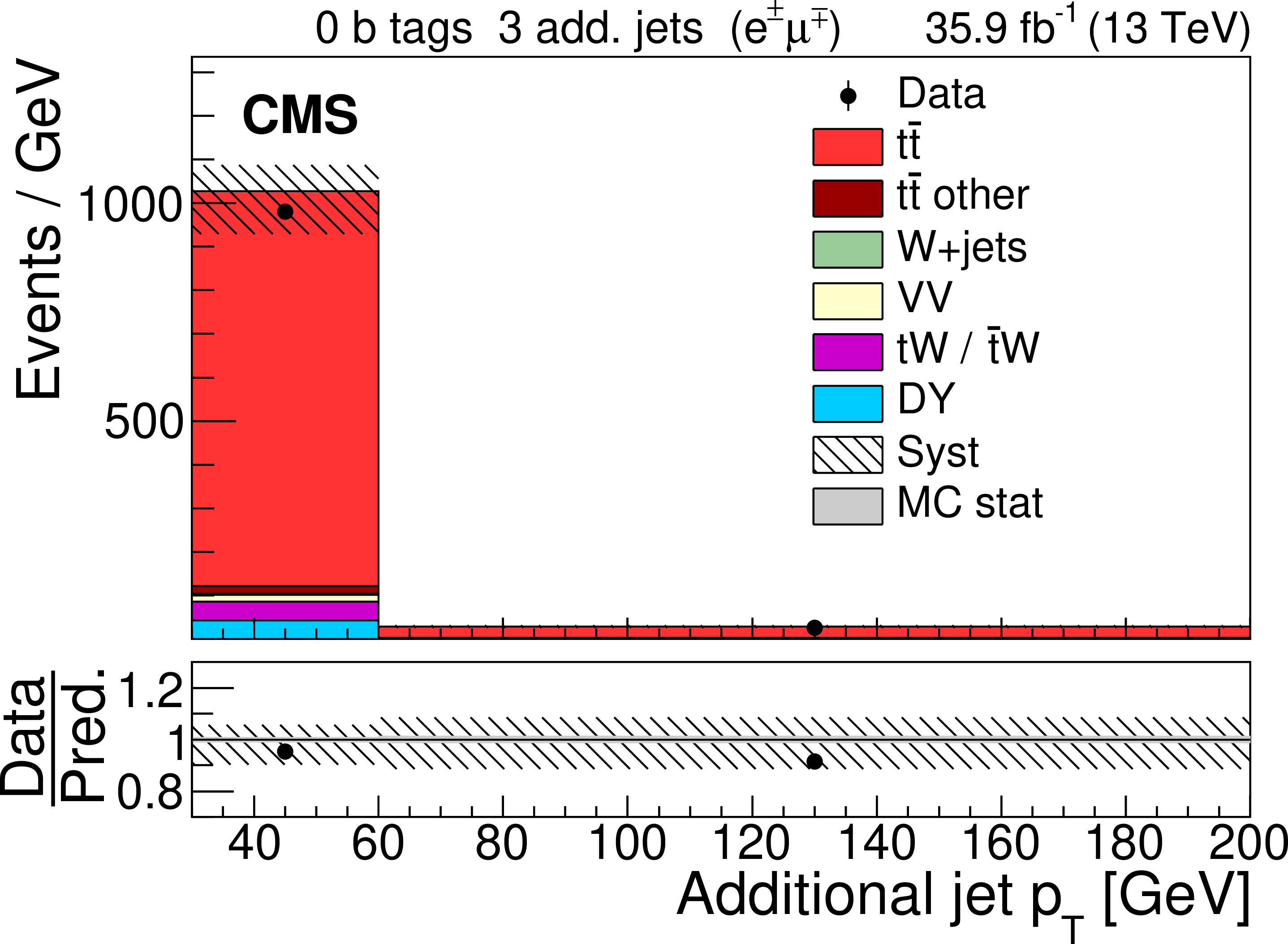
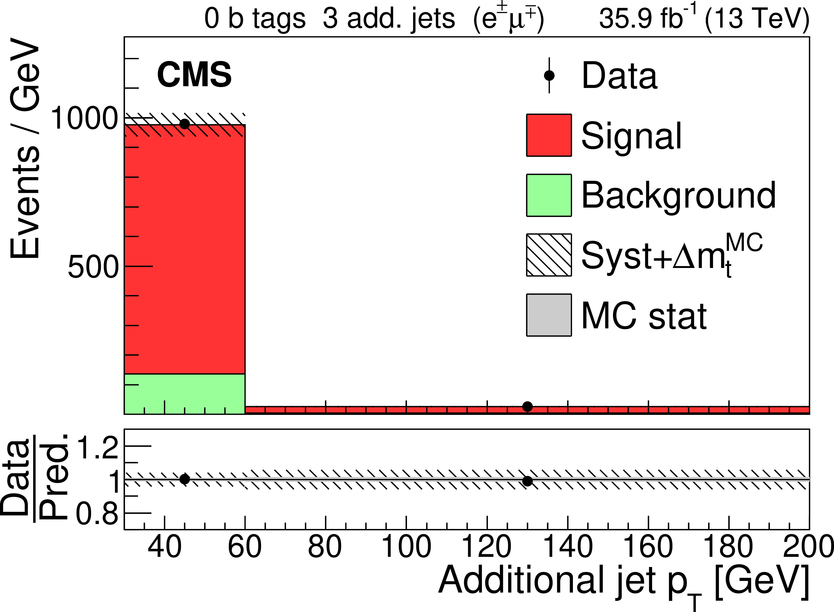
Figure 4-j:
Distribution in the ${\mathrm {e}}^{\pm} {{\mu}}^{\mp}$ channel after the fit to the data for events with zero or three or more b-tagged jets, and three or more additional non-b-tagged jets. The hatched band corresponds to the total uncertainty in the sum of the predicted yields including all correlations. The ratios of the data to the sum of the simulated yields after the fit are shown in the lower panel. Here, the solid gray band represents the contribution of the statistical uncertainty in the MC simulation. |
png pdf |
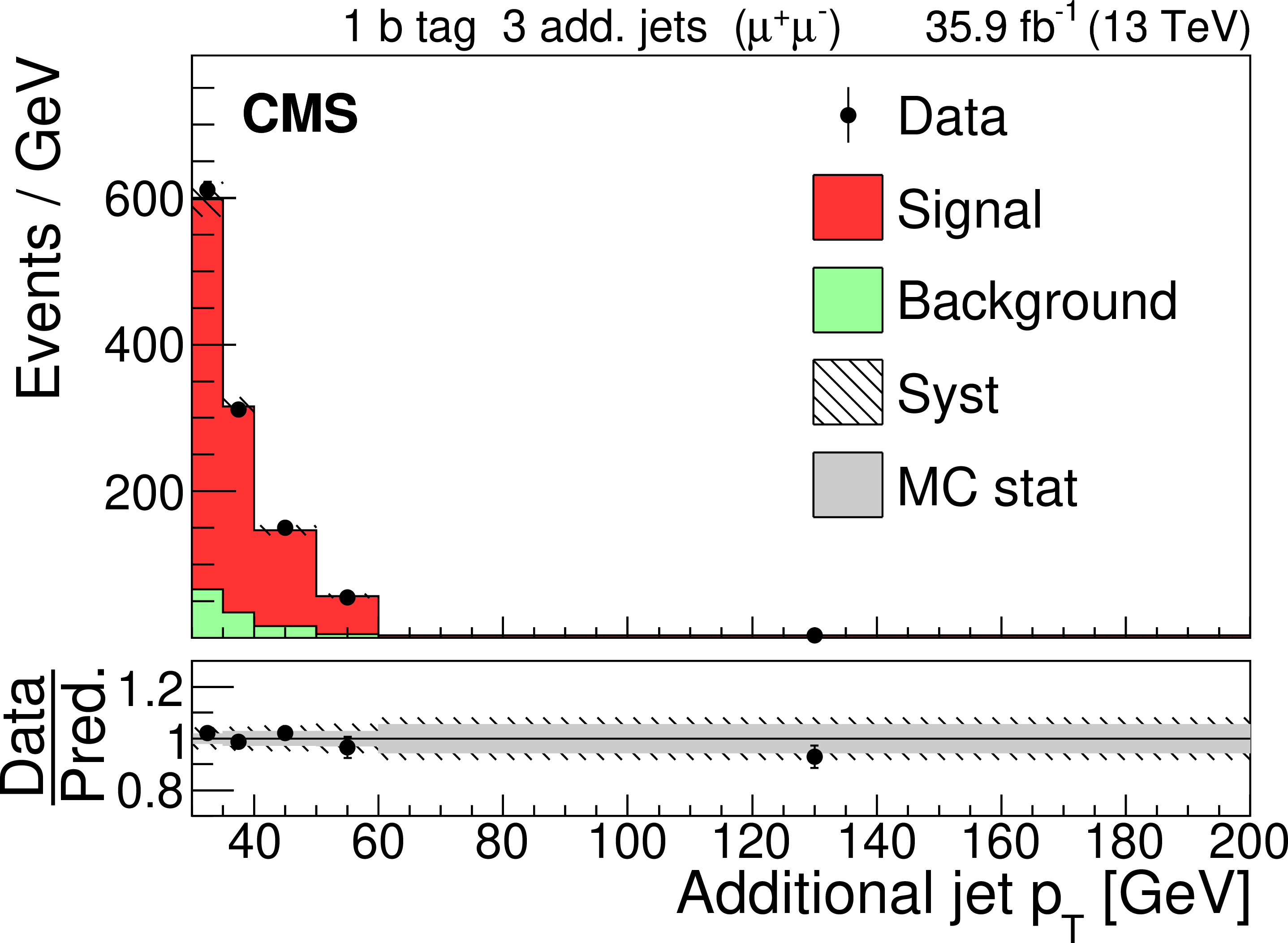
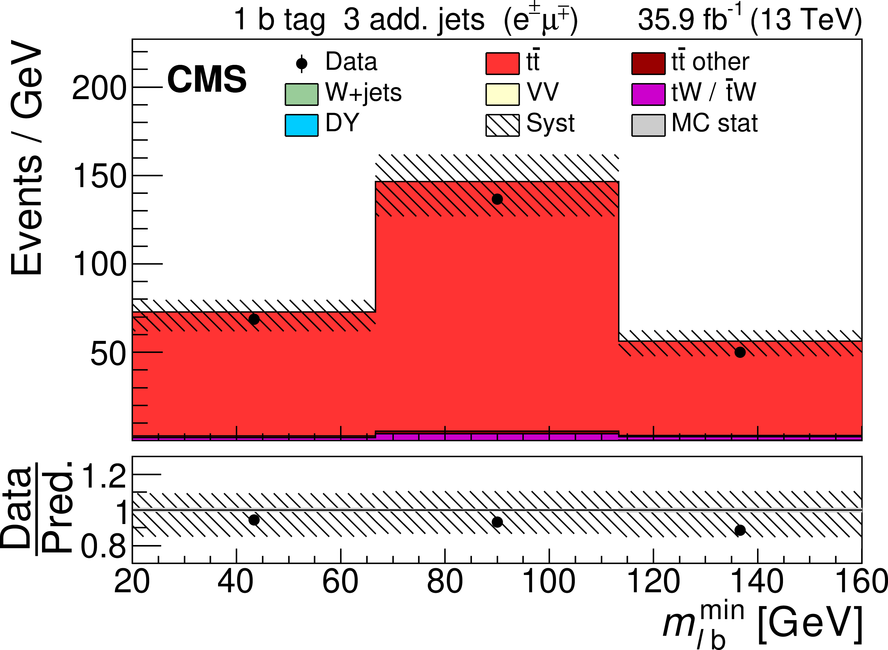
Figure 4-k:
Distribution in the ${\mathrm {e}}^{\pm} {{\mu}}^{\mp}$ channel after the fit to the data for events with exactly one b-tagged jets, and three or more additional non-b-tagged jets. The hatched band corresponds to the total uncertainty in the sum of the predicted yields including all correlations. The ratios of the data to the sum of the simulated yields after the fit are shown in the lower panel. Here, the solid gray band represents the contribution of the statistical uncertainty in the MC simulation. |

png pdf |
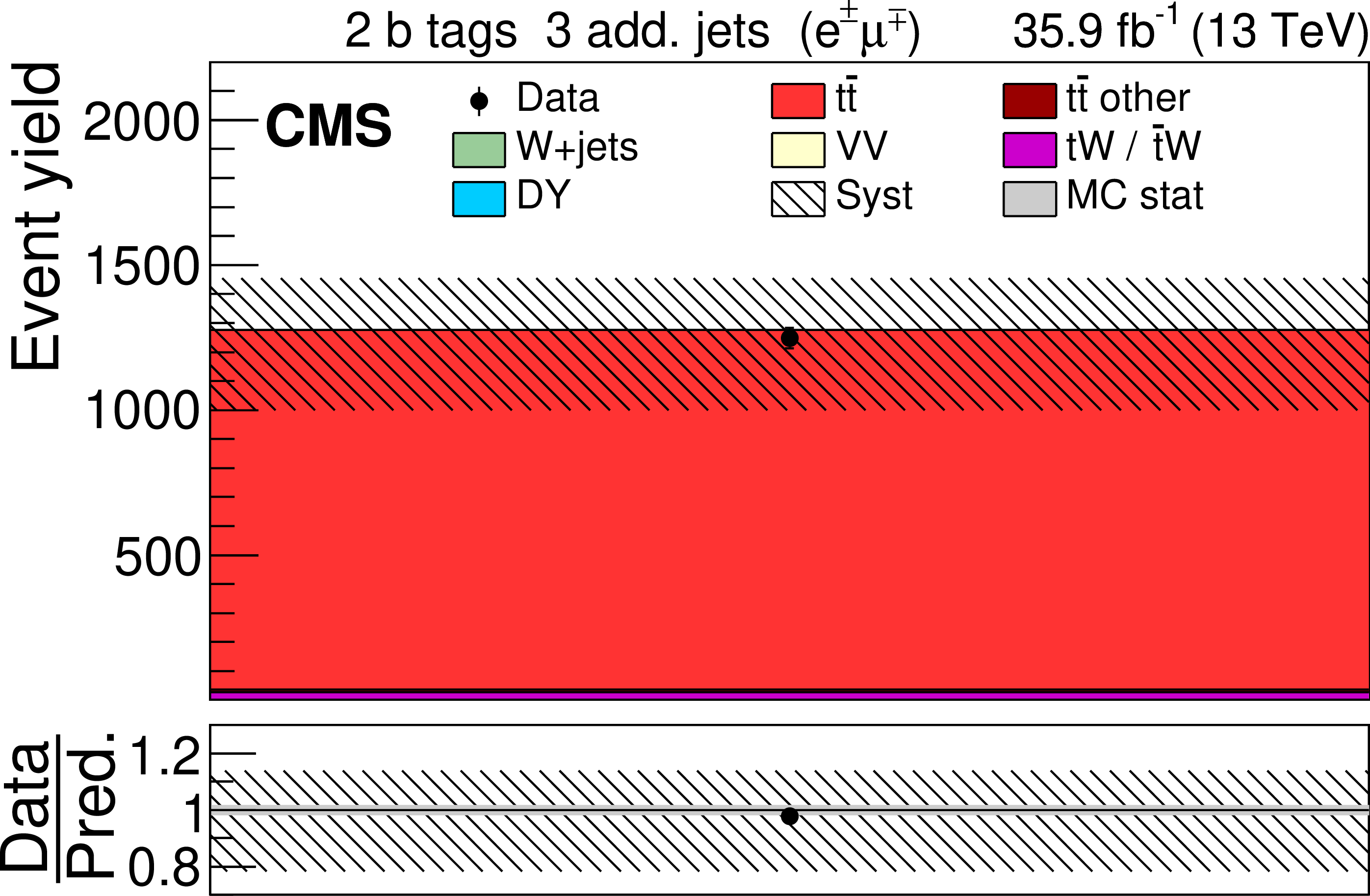
Figure 4-l:
Event yield in the ${\mathrm {e}}^{\pm} {{\mu}}^{\mp}$ channel after the fit to the data for events with exactly two b-tagged jets, and three or more additional non-b-tagged jets. The hatched band corresponds to the total uncertainty in the sum of the predicted yields including all correlations. The ratios of the data to the sum of the simulated yields after the fit are shown in the lower panel. Here, the solid gray band represents the contribution of the statistical uncertainty in the MC simulation. |

png pdf |
Figure 5:
Distributions in the ${{{\mu ^{+}}} {{\mu ^{-}}}}$ channel after the fit to the data. The left (right) column shows events with exactly one (two) b-tagged jets. Events with zero, one, two, or three or more additional non-b-tagged jets are shown in the first, second, third, and fourth row, respectively. The hatched bands correspond to the total uncertainty in the sum of the predicted yields including all correlations. The ratios of the data to the sum of the simulated yields after the fit are shown in the lower panel of each figure. Here, the solid gray band represents the contribution of the statistical uncertainty in the MC simulation. |
png pdf |
Figure 5-a:
Event yield in the ${{{\mu ^{+}}} {{\mu ^{-}}}}$ channel after the fit to the data for events with exactly one b-tagged jets and zero additional non-b-tagged jet. The hatched band corresponds to the total uncertainty in the sum of the predicted yields including all correlations. The ratios of the data to the sum of the simulated yields after the fit are shown in the lower panel. Here, the solid gray band represents the contribution of the statistical uncertainty in the MC simulation. |

png pdf |
Figure 5-b:
Event yield in the ${{{\mu ^{+}}} {{\mu ^{-}}}}$ channel after the fit to the data for events with exactly two b-tagged jets and zero additional non-b-tagged jet. The hatched band corresponds to the total uncertainty in the sum of the predicted yields including all correlations. The ratios of the data to the sum of the simulated yields after the fit are shown in the lower panel. Here, the solid gray band represents the contribution of the statistical uncertainty in the MC simulation. |
png pdf |
Figure 5-c:
Distribution in the ${{{\mu ^{+}}} {{\mu ^{-}}}}$ channel after the fit to the data for events with exactly one b-tagged jets and one additional non-b-tagged jet. The hatched band corresponds to the total uncertainty in the sum of the predicted yields including all correlations. The ratios of the data to the sum of the simulated yields after the fit are shown in the lower panel. Here, the solid gray band represents the contribution of the statistical uncertainty in the MC simulation. |

png pdf |
Figure 5-d:
Distribution in the ${{{\mu ^{+}}} {{\mu ^{-}}}}$ channel after the fit to the data for events with exactly two b-tagged jets and one additional non-b-tagged jet. The hatched band corresponds to the total uncertainty in the sum of the predicted yields including all correlations. The ratios of the data to the sum of the simulated yields after the fit are shown in the lower panel. Here, the solid gray band represents the contribution of the statistical uncertainty in the MC simulation. |
png pdf |
Figure 5-e:
Distribution in the ${{{\mu ^{+}}} {{\mu ^{-}}}}$ channel after the fit to the data for events with exactly one b-tagged jets and two additional non-b-tagged jets. The hatched band corresponds to the total uncertainty in the sum of the predicted yields including all correlations. The ratios of the data to the sum of the simulated yields after the fit are shown in the lower panel. Here, the solid gray band represents the contribution of the statistical uncertainty in the MC simulation. |

png pdf |
Figure 5-f:
Distribution in the ${{{\mu ^{+}}} {{\mu ^{-}}}}$ channel after the fit to the data for events with exactly two b-tagged jets and two additional non-b-tagged jets. The hatched band corresponds to the total uncertainty in the sum of the predicted yields including all correlations. The ratios of the data to the sum of the simulated yields after the fit are shown in the lower panel. Here, the solid gray band represents the contribution of the statistical uncertainty in the MC simulation. |
png pdf |
Figure 5-g:
Distribution in the ${{{\mu ^{+}}} {{\mu ^{-}}}}$ channel after the fit to the data for events with exactly one b-tagged jets and three or more additional non-b-tagged jets. The hatched band corresponds to the total uncertainty in the sum of the predicted yields including all correlations. The ratios of the data to the sum of the simulated yields after the fit are shown in the lower panel. Here, the solid gray band represents the contribution of the statistical uncertainty in the MC simulation. |
png pdf |
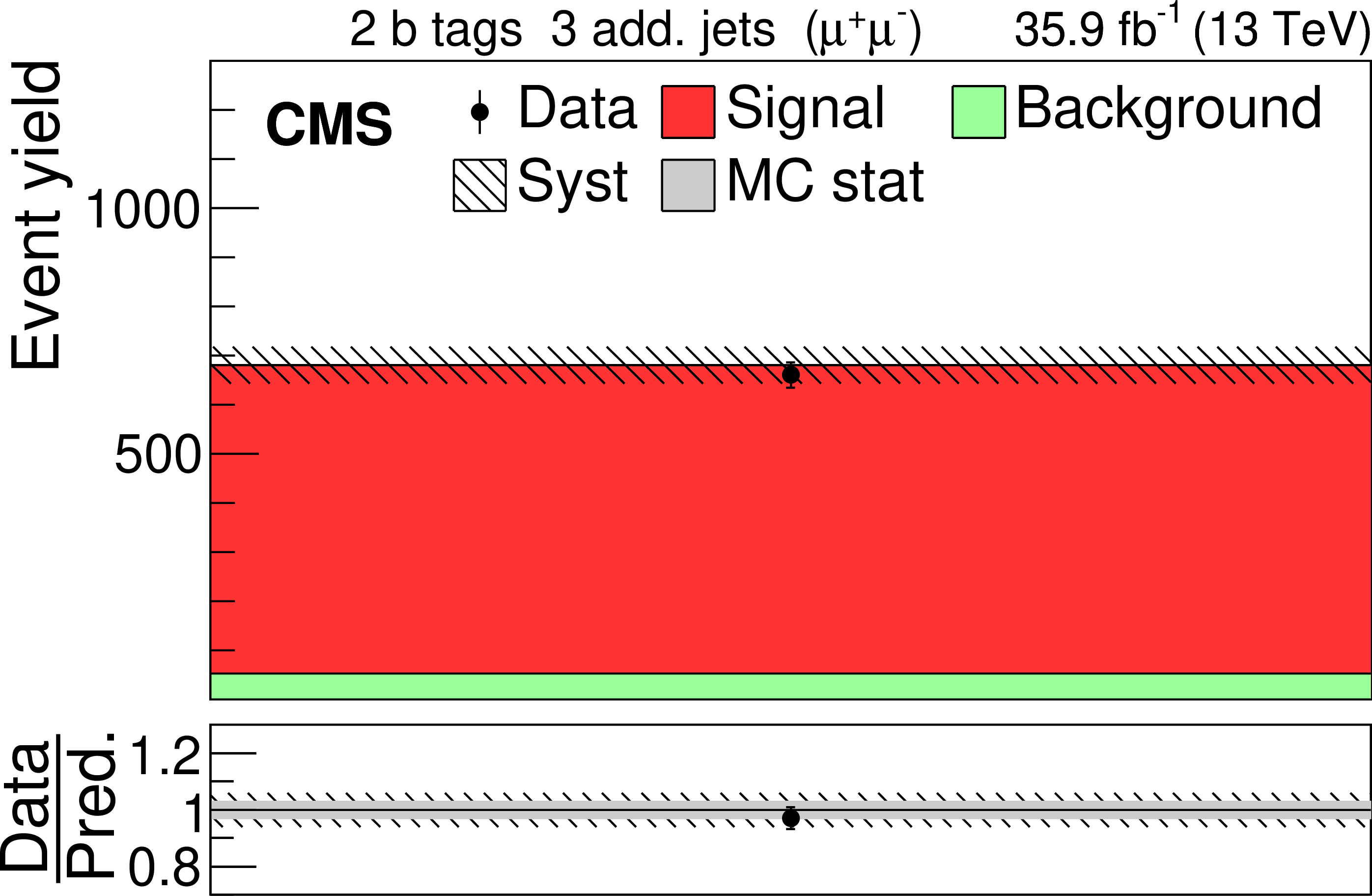
Figure 5-h:
Event yield in the ${{{\mu ^{+}}} {{\mu ^{-}}}}$ channel after the fit to the data for events with exactly two b-tagged jets and three or more additional non-b-tagged jets. The hatched band corresponds to the total uncertainty in the sum of the predicted yields including all correlations. The ratios of the data to the sum of the simulated yields after the fit are shown in the lower panel. Here, the solid gray band represents the contribution of the statistical uncertainty in the MC simulation. |
png pdf |
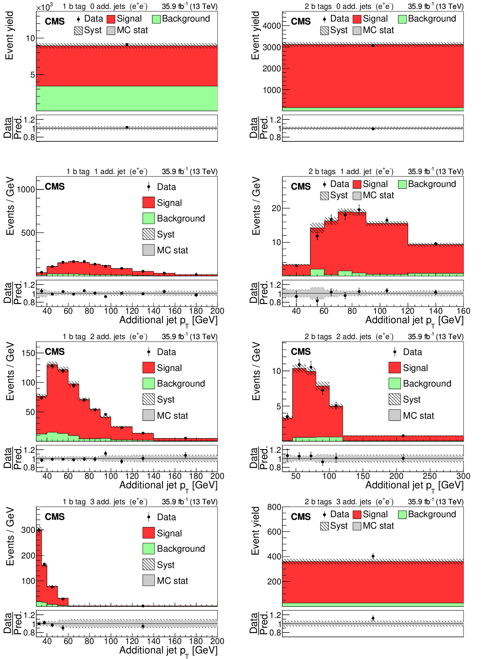
Figure 6:
Same distributions as in Fig. 5, but in the ${{\mathrm {e}^{+}} {\mathrm {e}^{-}}}$ channel. |
png pdf |
Figure 6-a:
Same distributions as in Fig. 5, but in the ${{\mathrm {e}^{+}} {\mathrm {e}^{-}}}$ channel. |
png pdf |
Figure 6-b:
Same distributions as in Fig. 5, but in the ${{\mathrm {e}^{+}} {\mathrm {e}^{-}}}$ channel. |
png pdf |
Figure 6-c:
Same distributions as in Fig. 5, but in the ${{\mathrm {e}^{+}} {\mathrm {e}^{-}}}$ channel. |
png pdf |
Figure 6-d:
Same distributions as in Fig. 5, but in the ${{\mathrm {e}^{+}} {\mathrm {e}^{-}}}$ channel. |

png pdf |
Figure 6-e:
Same distributions as in Fig. 5, but in the ${{\mathrm {e}^{+}} {\mathrm {e}^{-}}}$ channel. |
png pdf |
Figure 6-f:
Same distributions as in Fig. 5, but in the ${{\mathrm {e}^{+}} {\mathrm {e}^{-}}}$ channel. |

png pdf |
Figure 6-g:
Same distributions as in Fig. 5, but in the ${{\mathrm {e}^{+}} {\mathrm {e}^{-}}}$ channel. |
png pdf |
Figure 6-h:
Same distributions as in Fig. 5, but in the ${{\mathrm {e}^{+}} {\mathrm {e}^{-}}}$ channel. |
png pdf |
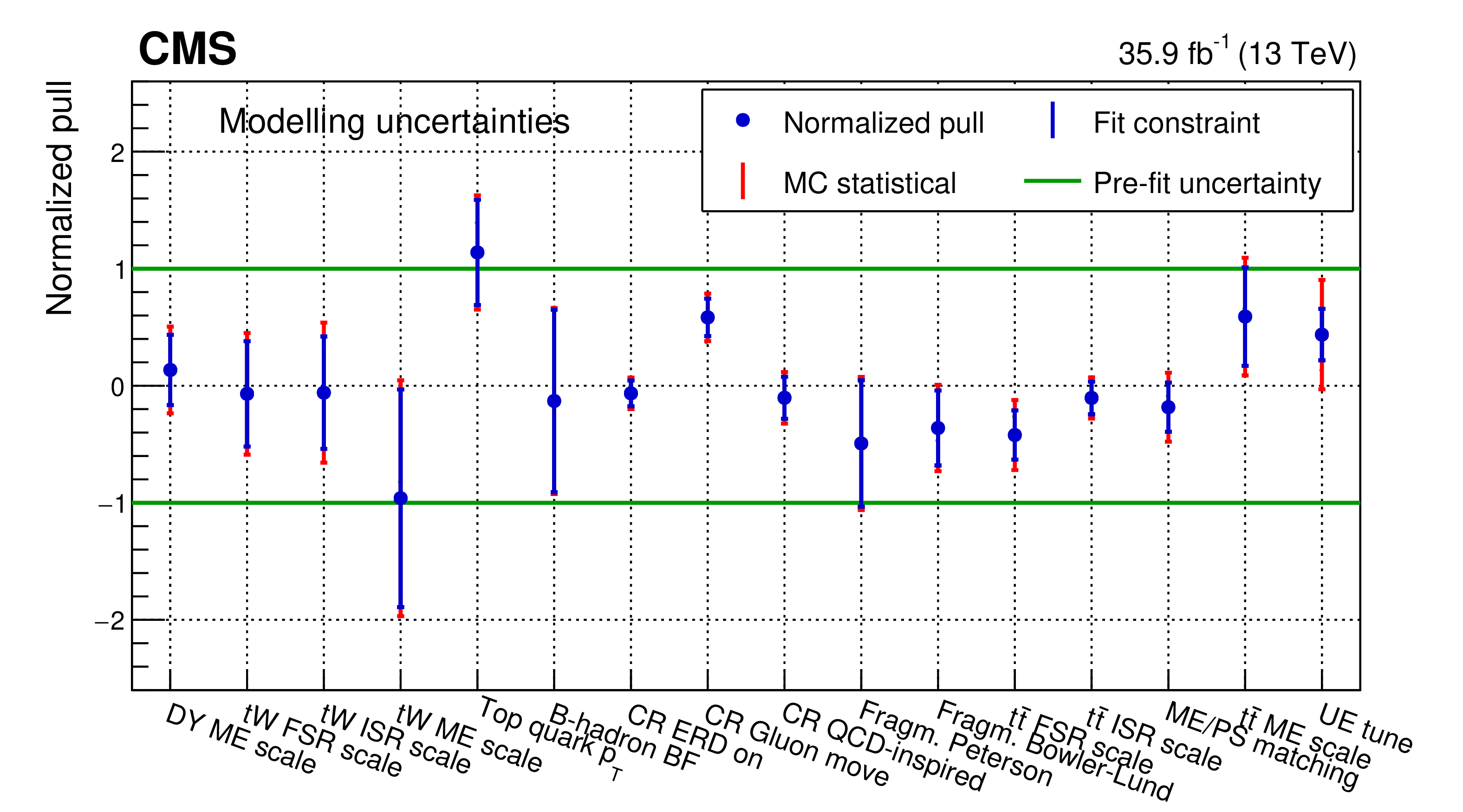
Figure 7:
Normalized pulls and constraints of the nuisance parameters related to the modelling uncertainties for the cross section fit. The markers denote the fitted values, while the inner vertical bars represent the constraint and the outer vertical bars denote the additional uncertainty as determ $ {\sigma _ {{\mathrm {t}\overline {\mathrm {t}}}}} $ ined from pseudo-experiments. The constraint is defined as the ratio of the post-fit uncertainty to the pre-fit uncertainty of a given nuisance parameter, while the normalized pull is the difference between the post-fit and the pre-fit values of the nuisance parameter normalized to its pre-fit uncertainty. The horizontal lines at $\pm$1 represent the pre-fit uncertainty. |
png pdf |
Figure 8:
Comparison of data (points) and pre-fit distributions of the expected signal and backgrounds from simulation (shaded histograms) used in the simultaneous fit of $ {\sigma _ {{\mathrm {t}\overline {\mathrm {t}}}}} $ and ${{m_\mathrm {{\mathrm {t}}}} ^{\mathrm {MC}}}$ in the ${\mathrm {e}}^{\pm} {{\mu}}^{\mp}$ channel. In the left column events with zero or three or more b-tagged jets are shown. The middle (right) column shows events with exactly one (two) b-tagged jets. Events with zero, one, two, or three or more additional non-b-tagged jets are shown in the first, second, third, and fourth row, respectively. The hatched bands correspond to the total uncertainty in the sum of the predicted yields. The ratios of data to the sum of the predicted yields are shown in the lower panel of each figure. Here, the solid gray band represents the contribution of the statistical uncertainty. |
png pdf |
Figure 8-a:
Comparison of data (points) and pre-fit distribution of the expected signal and backgrounds from simulation (shaded histograms) used in the simultaneous fit of $ {\sigma _ {{\mathrm {t}\overline {\mathrm {t}}}}} $ and ${{m_\mathrm {{\mathrm {t}}}} ^{\mathrm {MC}}}$ in the ${\mathrm {e}}^{\pm} {{\mu}}^{\mp}$ channel for events with zero or three or more b-tagged jets and zero additional non-b-tagged jet. The hatched band corresponds to the total uncertainty in the sum of the predicted yields. The ratios of data to the sum of the predicted yields are shown in the lower panel. Here, the solid gray band represents the contribution of the statistical uncertainty. |
png pdf |
Figure 8-b:
Comparison of data (points) and pre-fit distribution of the expected signal and backgrounds from simulation (shaded histograms) used in the simultaneous fit of $ {\sigma _ {{\mathrm {t}\overline {\mathrm {t}}}}} $ and ${{m_\mathrm {{\mathrm {t}}}} ^{\mathrm {MC}}}$ in the ${\mathrm {e}}^{\pm} {{\mu}}^{\mp}$ channel for events with exactly one b-tagged jets and zero additional non-b-tagged jet. The hatched band corresponds to the total uncertainty in the sum of the predicted yields. The ratios of data to the sum of the predicted yields are shown in the lower panel. Here, the solid gray band represents the contribution of the statistical uncertainty. |
png pdf |
Figure 8-c:
Comparison of data (points) and pre-fit distribution of the expected signal and backgrounds from simulation (shaded histograms) used in the simultaneous fit of $ {\sigma _ {{\mathrm {t}\overline {\mathrm {t}}}}} $ and ${{m_\mathrm {{\mathrm {t}}}} ^{\mathrm {MC}}}$ in the ${\mathrm {e}}^{\pm} {{\mu}}^{\mp}$ channel for events with exactly two b-tagged jets and zero additional non-b-tagged jet. The hatched band corresponds to the total uncertainty in the sum of the predicted yields. The ratios of data to the sum of the predicted yields are shown in the lower panel. Here, the solid gray band represents the contribution of the statistical uncertainty. |
png pdf |
Figure 8-d:
Comparison of data (points) and pre-fit distribution of the expected signal and backgrounds from simulation (shaded histograms) used in the simultaneous fit of $ {\sigma _ {{\mathrm {t}\overline {\mathrm {t}}}}} $ and ${{m_\mathrm {{\mathrm {t}}}} ^{\mathrm {MC}}}$ in the ${\mathrm {e}}^{\pm} {{\mu}}^{\mp}$ channel for events with zero or three or more b-tagged jets and one additional non-b-tagged jet. The hatched band corresponds to the total uncertainty in the sum of the predicted yields. The ratios of data to the sum of the predicted yields are shown in the lower panel. Here, the solid gray band represents the contribution of the statistical uncertainty. |

png pdf |
Figure 8-e:
Comparison of data (points) and pre-fit distribution of the expected signal and backgrounds from simulation (shaded histograms) used in the simultaneous fit of $ {\sigma _ {{\mathrm {t}\overline {\mathrm {t}}}}} $ and ${{m_\mathrm {{\mathrm {t}}}} ^{\mathrm {MC}}}$ in the ${\mathrm {e}}^{\pm} {{\mu}}^{\mp}$ channel for events with exactly one b-tagged jets and one additional non-b-tagged jet. The hatched band corresponds to the total uncertainty in the sum of the predicted yields. The ratios of data to the sum of the predicted yields are shown in the lower panel. Here, the solid gray band represents the contribution of the statistical uncertainty. |
png pdf |
Figure 8-f:
Comparison of data (points) and pre-fit distribution of the expected signal and backgrounds from simulation (shaded histograms) used in the simultaneous fit of $ {\sigma _ {{\mathrm {t}\overline {\mathrm {t}}}}} $ and ${{m_\mathrm {{\mathrm {t}}}} ^{\mathrm {MC}}}$ in the ${\mathrm {e}}^{\pm} {{\mu}}^{\mp}$ channel for events with exactly two b-tagged jets and one additional non-b-tagged jet. The hatched band corresponds to the total uncertainty in the sum of the predicted yields. The ratios of data to the sum of the predicted yields are shown in the lower panel. Here, the solid gray band represents the contribution of the statistical uncertainty. |
png pdf |
Figure 8-g:
Comparison of data (points) and pre-fit distribution of the expected signal and backgrounds from simulation (shaded histograms) used in the simultaneous fit of $ {\sigma _ {{\mathrm {t}\overline {\mathrm {t}}}}} $ and ${{m_\mathrm {{\mathrm {t}}}} ^{\mathrm {MC}}}$ in the ${\mathrm {e}}^{\pm} {{\mu}}^{\mp}$ channel for events with zero or three or more b-tagged jets and two additional non-b-tagged jets. The hatched band corresponds to the total uncertainty in the sum of the predicted yields. The ratios of data to the sum of the predicted yields are shown in the lower panel. Here, the solid gray band represents the contribution of the statistical uncertainty. |
png pdf |
Figure 8-h:
Comparison of data (points) and pre-fit distribution of the expected signal and backgrounds from simulation (shaded histograms) used in the simultaneous fit of $ {\sigma _ {{\mathrm {t}\overline {\mathrm {t}}}}} $ and ${{m_\mathrm {{\mathrm {t}}}} ^{\mathrm {MC}}}$ in the ${\mathrm {e}}^{\pm} {{\mu}}^{\mp}$ channel or events with exactly one b-tagged jets and two additional non-b-tagged jets. The hatched band corresponds to the total uncertainty in the sum of the predicted yields. The ratios of data to the sum of the predicted yields are shown in the lower panel. Here, the solid gray band represents the contribution of the statistical uncertainty. |
png pdf |
Figure 8-i:
Comparison of data (points) and pre-fit distribution of the expected signal and backgrounds from simulation (shaded histograms) used in the simultaneous fit of $ {\sigma _ {{\mathrm {t}\overline {\mathrm {t}}}}} $ and ${{m_\mathrm {{\mathrm {t}}}} ^{\mathrm {MC}}}$ in the ${\mathrm {e}}^{\pm} {{\mu}}^{\mp}$ channel for events with exactly two b-tagged jets and two additional non-b-tagged jets. The hatched band corresponds to the total uncertainty in the sum of the predicted yields. The ratios of data to the sum of the predicted yields are shown in the lower panel. Here, the solid gray band represents the contribution of the statistical uncertainty. |
png pdf |
Figure 8-j:
Comparison of data (points) and pre-fit distribution of the expected signal and backgrounds from simulation (shaded histograms) used in the simultaneous fit of $ {\sigma _ {{\mathrm {t}\overline {\mathrm {t}}}}} $ and ${{m_\mathrm {{\mathrm {t}}}} ^{\mathrm {MC}}}$ in the ${\mathrm {e}}^{\pm} {{\mu}}^{\mp}$ channel for events with zero or three or more b-tagged jets and three or more additional non-b-tagged jets. The hatched band corresponds to the total uncertainty in the sum of the predicted yields. The ratios of data to the sum of the predicted yields are shown in the lower panel. Here, the solid gray band represents the contribution of the statistical uncertainty. |
png pdf |
Figure 8-k:
Comparison of data (points) and pre-fit distribution of the expected signal and backgrounds from simulation (shaded histograms) used in the simultaneous fit of $ {\sigma _ {{\mathrm {t}\overline {\mathrm {t}}}}} $ and ${{m_\mathrm {{\mathrm {t}}}} ^{\mathrm {MC}}}$ in the ${\mathrm {e}}^{\pm} {{\mu}}^{\mp}$ channel for events with exactly one b-tagged jets and three or more additional non-b-tagged jets. The hatched band corresponds to the total uncertainty in the sum of the predicted yields. The ratios of data to the sum of the predicted yields are shown in the lower panel. Here, the solid gray band represents the contribution of the statistical uncertainty. |
png pdf |
Figure 8-l:
Comparison of data (points) and pre-fit distribution of the expected signal and backgrounds from simulation (shaded histograms) used in the simultaneous fit of $ {\sigma _ {{\mathrm {t}\overline {\mathrm {t}}}}} $ and ${{m_\mathrm {{\mathrm {t}}}} ^{\mathrm {MC}}}$ in the ${\mathrm {e}}^{\pm} {{\mu}}^{\mp}$ channel for events with exactly two b-tagged jets and three or more additional non-b-tagged jets. The hatched band corresponds to the total uncertainty in the sum of the predicted yields. The ratios of data to the sum of the predicted yields are shown in the lower panel. Here, the solid gray band represents the contribution of the statistical uncertainty. |
png pdf |
Figure 9:
Comparison of data (points) and post-fit distributions of the expected signal and backgrounds from simulation (shaded histograms) used in the simultaneous fit of $ {\sigma _ {{\mathrm {t}\overline {\mathrm {t}}}}} $ and ${{m_\mathrm {{\mathrm {t}}}} ^{\mathrm {MC}}}$ in the ${\mathrm {e}}^{\pm} {{\mu}}^{\mp}$ channel. In the left column events with zero or three or more b-tagged jets are shown. The middle (right) column shows events with exactly one (two) b-tagged jets. Events with zero, one, two, or three or more additional non-b-tagged jets are shown in the first, second, third, and fourth row, respectively. The hatched bands correspond to the total uncertainty in the sum of the predicted yields and include the contribution from the top quark mass ($\Delta {{m_\mathrm {{\mathrm {t}}}} ^{\mathrm {MC}}} $). The ratios of data to the sum of the predicted yields are shown in the lower panel of each figure. Here, the solid gray band represents the contribution of the statistical uncertainty. |
png pdf |
Figure 9-a:
Comparison of data (points) and post-fit distributions of the expected signal and backgrounds from simulation (shaded histograms) used in the simultaneous fit of $ {\sigma _ {{\mathrm {t}\overline {\mathrm {t}}}}} $ and ${{m_\mathrm {{\mathrm {t}}}} ^{\mathrm {MC}}}$ in the ${\mathrm {e}}^{\pm} {{\mu}}^{\mp}$ channel for events with zero or three or more b-tagged jets and zero additional non-b-tagged jet. The hatched band corresponds to the total uncertainty in the sum of the predicted yields and include the contribution from the top quark mass ($\Delta {{m_\mathrm {{\mathrm {t}}}} ^{\mathrm {MC}}} $). The ratios of data to the sum of the predicted yields are shown in the lower panel. Here, the solid gray band represents the contribution of the statistical uncertainty. |
png pdf |
Figure 9-b:
Comparison of data (points) and post-fit distributions of the expected signal and backgrounds from simulation (shaded histograms) used in the simultaneous fit of $ {\sigma _ {{\mathrm {t}\overline {\mathrm {t}}}}} $ and ${{m_\mathrm {{\mathrm {t}}}} ^{\mathrm {MC}}}$ in the ${\mathrm {e}}^{\pm} {{\mu}}^{\mp}$ channel for events with exactly one b-tagged jets and zero additional non-b-tagged jet. The hatched band corresponds to the total uncertainty in the sum of the predicted yields and include the contribution from the top quark mass ($\Delta {{m_\mathrm {{\mathrm {t}}}} ^{\mathrm {MC}}} $). The ratios of data to the sum of the predicted yields are shown in the lower panel. Here, the solid gray band represents the contribution of the statistical uncertainty. |
png pdf |
Figure 9-c:
Comparison of data (points) and post-fit distributions of the expected signal and backgrounds from simulation (shaded histograms) used in the simultaneous fit of $ {\sigma _ {{\mathrm {t}\overline {\mathrm {t}}}}} $ and ${{m_\mathrm {{\mathrm {t}}}} ^{\mathrm {MC}}}$ in the ${\mathrm {e}}^{\pm} {{\mu}}^{\mp}$ channel for events with exactly two b-tagged jets and zero additional non-b-tagged jet. The hatched band corresponds to the total uncertainty in the sum of the predicted yields and include the contribution from the top quark mass ($\Delta {{m_\mathrm {{\mathrm {t}}}} ^{\mathrm {MC}}} $). The ratios of data to the sum of the predicted yields are shown in the lower panel. Here, the solid gray band represents the contribution of the statistical uncertainty. |

png pdf |
Figure 9-d:
Comparison of data (points) and post-fit distributions of the expected signal and backgrounds from simulation (shaded histograms) used in the simultaneous fit of $ {\sigma _ {{\mathrm {t}\overline {\mathrm {t}}}}} $ and ${{m_\mathrm {{\mathrm {t}}}} ^{\mathrm {MC}}}$ in the ${\mathrm {e}}^{\pm} {{\mu}}^{\mp}$ channel for events with zero or three or more b-tagged jets and one additional non-b-tagged jet. The hatched band corresponds to the total uncertainty in the sum of the predicted yields and include the contribution from the top quark mass ($\Delta {{m_\mathrm {{\mathrm {t}}}} ^{\mathrm {MC}}} $). The ratios of data to the sum of the predicted yields are shown in the lower panel. Here, the solid gray band represents the contribution of the statistical uncertainty. |
png pdf |
Figure 9-e:
Comparison of data (points) and post-fit distributions of the expected signal and backgrounds from simulation (shaded histograms) used in the simultaneous fit of $ {\sigma _ {{\mathrm {t}\overline {\mathrm {t}}}}} $ and ${{m_\mathrm {{\mathrm {t}}}} ^{\mathrm {MC}}}$ in the ${\mathrm {e}}^{\pm} {{\mu}}^{\mp}$ channel for events with exactly one b-tagged jets and one additional non-b-tagged jet. The hatched band corresponds to the total uncertainty in the sum of the predicted yields and include the contribution from the top quark mass ($\Delta {{m_\mathrm {{\mathrm {t}}}} ^{\mathrm {MC}}} $). The ratios of data to the sum of the predicted yields are shown in the lower panel. Here, the solid gray band represents the contribution of the statistical uncertainty. |
png pdf |
Figure 9-f:
Comparison of data (points) and post-fit distributions of the expected signal and backgrounds from simulation (shaded histograms) used in the simultaneous fit of $ {\sigma _ {{\mathrm {t}\overline {\mathrm {t}}}}} $ and ${{m_\mathrm {{\mathrm {t}}}} ^{\mathrm {MC}}}$ in the ${\mathrm {e}}^{\pm} {{\mu}}^{\mp}$ channel for events with exactly two b-tagged jets and one additional non-b-tagged jet. The hatched band corresponds to the total uncertainty in the sum of the predicted yields and include the contribution from the top quark mass ($\Delta {{m_\mathrm {{\mathrm {t}}}} ^{\mathrm {MC}}} $). The ratios of data to the sum of the predicted yields are shown in the lower panel. Here, the solid gray band represents the contribution of the statistical uncertainty. |
png pdf |
Figure 9-g:
Comparison of data (points) and post-fit distributions of the expected signal and backgrounds from simulation (shaded histograms) used in the simultaneous fit of $ {\sigma _ {{\mathrm {t}\overline {\mathrm {t}}}}} $ and ${{m_\mathrm {{\mathrm {t}}}} ^{\mathrm {MC}}}$ in the ${\mathrm {e}}^{\pm} {{\mu}}^{\mp}$ channel for events with zero or three or more b-tagged jets and two additional non-b-tagged jets. The hatched band corresponds to the total uncertainty in the sum of the predicted yields and include the contribution from the top quark mass ($\Delta {{m_\mathrm {{\mathrm {t}}}} ^{\mathrm {MC}}} $). The ratios of data to the sum of the predicted yields are shown in the lower panel. Here, the solid gray band represents the contribution of the statistical uncertainty. |
png pdf |
Figure 9-h:
Comparison of data (points) and post-fit distributions of the expected signal and backgrounds from simulation (shaded histograms) used in the simultaneous fit of $ {\sigma _ {{\mathrm {t}\overline {\mathrm {t}}}}} $ and ${{m_\mathrm {{\mathrm {t}}}} ^{\mathrm {MC}}}$ in the ${\mathrm {e}}^{\pm} {{\mu}}^{\mp}$ channel for events with exactly one b-tagged jets and two additional non-b-tagged jets. The hatched band corresponds to the total uncertainty in the sum of the predicted yields and include the contribution from the top quark mass ($\Delta {{m_\mathrm {{\mathrm {t}}}} ^{\mathrm {MC}}} $). The ratios of data to the sum of the predicted yields are shown in the lower panel. Here, the solid gray band represents the contribution of the statistical uncertainty. |

png pdf |
Figure 9-i:
Comparison of data (points) and post-fit distributions of the expected signal and backgrounds from simulation (shaded histograms) used in the simultaneous fit of $ {\sigma _ {{\mathrm {t}\overline {\mathrm {t}}}}} $ and ${{m_\mathrm {{\mathrm {t}}}} ^{\mathrm {MC}}}$ in the ${\mathrm {e}}^{\pm} {{\mu}}^{\mp}$ channel for events with exactly two b-tagged jets and two additional non-b-tagged jets. The hatched band corresponds to the total uncertainty in the sum of the predicted yields and include the contribution from the top quark mass ($\Delta {{m_\mathrm {{\mathrm {t}}}} ^{\mathrm {MC}}} $). The ratios of data to the sum of the predicted yields are shown in the lower panel. Here, the solid gray band represents the contribution of the statistical uncertainty. |
png pdf |
Figure 9-j:
Comparison of data (points) and post-fit distributions of the expected signal and backgrounds from simulation (shaded histograms) used in the simultaneous fit of $ {\sigma _ {{\mathrm {t}\overline {\mathrm {t}}}}} $ and ${{m_\mathrm {{\mathrm {t}}}} ^{\mathrm {MC}}}$ in the ${\mathrm {e}}^{\pm} {{\mu}}^{\mp}$ channel for events with zero or three or more b-tagged jets and three or more additional non-b-tagged jets. The hatched band corresponds to the total uncertainty in the sum of the predicted yields and include the contribution from the top quark mass ($\Delta {{m_\mathrm {{\mathrm {t}}}} ^{\mathrm {MC}}} $). The ratios of data to the sum of the predicted yields are shown in the lower panel. Here, the solid gray band represents the contribution of the statistical uncertainty. |
png pdf |
Figure 9-k:
Comparison of data (points) and post-fit distributions of the expected signal and backgrounds from simulation (shaded histograms) used in the simultaneous fit of $ {\sigma _ {{\mathrm {t}\overline {\mathrm {t}}}}} $ and ${{m_\mathrm {{\mathrm {t}}}} ^{\mathrm {MC}}}$ in the ${\mathrm {e}}^{\pm} {{\mu}}^{\mp}$ channel for events with exactly one b-tagged jets and three or more additional non-b-tagged jets. The hatched band corresponds to the total uncertainty in the sum of the predicted yields and include the contribution from the top quark mass ($\Delta {{m_\mathrm {{\mathrm {t}}}} ^{\mathrm {MC}}} $). The ratios of data to the sum of the predicted yields are shown in the lower panel. Here, the solid gray band represents the contribution of the statistical uncertainty. |

png pdf |
Figure 9-l:
Comparison of data (points) and post-fit distributions of the expected signal and backgrounds from simulation (shaded histograms) used in the simultaneous fit of $ {\sigma _ {{\mathrm {t}\overline {\mathrm {t}}}}} $ and ${{m_\mathrm {{\mathrm {t}}}} ^{\mathrm {MC}}}$ in the ${\mathrm {e}}^{\pm} {{\mu}}^{\mp}$ channel for events with exactly two b-tagged jets and three or more additional non-b-tagged jets. The hatched band corresponds to the total uncertainty in the sum of the predicted yields and include the contribution from the top quark mass ($\Delta {{m_\mathrm {{\mathrm {t}}}} ^{\mathrm {MC}}} $). The ratios of data to the sum of the predicted yields are shown in the lower panel. Here, the solid gray band represents the contribution of the statistical uncertainty. |
png pdf |
Figure 10:
Normalized pulls and constraints of the nuisance parameters related to the modelling uncertainties for the simultaneous fit of ${\sigma _ {{\mathrm {t}\overline {\mathrm {t}}}}}$ and ${{m_\mathrm {{\mathrm {t}}}} ^{\mathrm {MC}}}$. The markers denote the fitted value, while the inner vertical bars represent the constraint and the outer vertical bars denote the additional uncertainty as determined from pseudo-experiments. The constraint is defined as the ratio of the post-fit uncertainty to the pre-fit uncertainty of a given nuisance parameter, while the normalized pull is the difference between the post-fit and the pre-fit values of the nuisance parameter normalized to its pre-fit uncertainty. The horizontal lines at $\pm$1 represent the pre-fit uncertainty. |

png pdf |
Figure 11:
Left: $ {\chi ^2} $ versus $ {{\alpha _S}} $ obtained from the comparison of the measured ${\sigma _ {{\mathrm {t}\overline {\mathrm {t}}}}}$ value to the NNLO prediction in the ${\mathrm {\overline {MS}}}$ scheme using different PDFs (symbols of different styles). Right: ${{{\alpha _S}} ({m_\mathrm {{\mathrm {Z}}}})}$ obtained from the comparison of the measured ${\sigma _ {{\mathrm {t}\overline {\mathrm {t}}}}}$ value to the theoretical prediction using different PDF sets in the ${\mathrm {\overline {MS}}}$ scheme. The corresponding value of ${{m_\mathrm {{\mathrm {t}}}} ({m_\mathrm {{\mathrm {t}}}})}$ is given for each PDF set. The inner horizontal bars on the points represent the experimental and PDF uncertainties added in quadrature. The outer horizontal bars show the total uncertainties. The vertical line displays the world-average ${{{\alpha _S}} ({m_\mathrm {{\mathrm {Z}}}})}$ value [29], with the hatched band representing its uncertainty. |
png pdf |
Figure 11-a:
$ {\chi ^2} $ versus $ {{\alpha _S}} $ obtained from the comparison of the measured ${\sigma _ {{\mathrm {t}\overline {\mathrm {t}}}}}$ value to the NNLO prediction in the ${\mathrm {\overline {MS}}}$ scheme using different PDFs (symbols of different styles). |
png pdf |
Figure 11-b:
${{{\alpha _S}} ({m_\mathrm {{\mathrm {Z}}}})}$ obtained from the comparison of the measured ${\sigma _ {{\mathrm {t}\overline {\mathrm {t}}}}}$ value to the theoretical prediction using different PDF sets in the ${\mathrm {\overline {MS}}}$ scheme. The corresponding value of ${{m_\mathrm {{\mathrm {t}}}} ({m_\mathrm {{\mathrm {t}}}})}$ is given for each PDF set. The inner horizontal bars on the points represent the experimental and PDF uncertainties added in quadrature. The outer horizontal bars show the total uncertainties. The vertical line displays the world-average ${{{\alpha _S}} ({m_\mathrm {{\mathrm {Z}}}})}$ value [29], with the hatched band representing its uncertainty. |
png pdf |
Figure 12:
Values of $ {{m_\mathrm {{\mathrm {t}}}} ({m_\mathrm {{\mathrm {t}}}})} $ obtained from comparing the $ {\sigma _ {{\mathrm {t}\overline {\mathrm {t}}}}} $ measurement to the theoretical NNLO predictions using different PDF sets. The inner horizontal bars on the points represent the quadratic sum of the experimental, PDF, and $ {{{\alpha _S}} ({m_\mathrm {{\mathrm {Z}}}})} $ uncertainties, while the outer horizontal bars give the total uncertainties. |
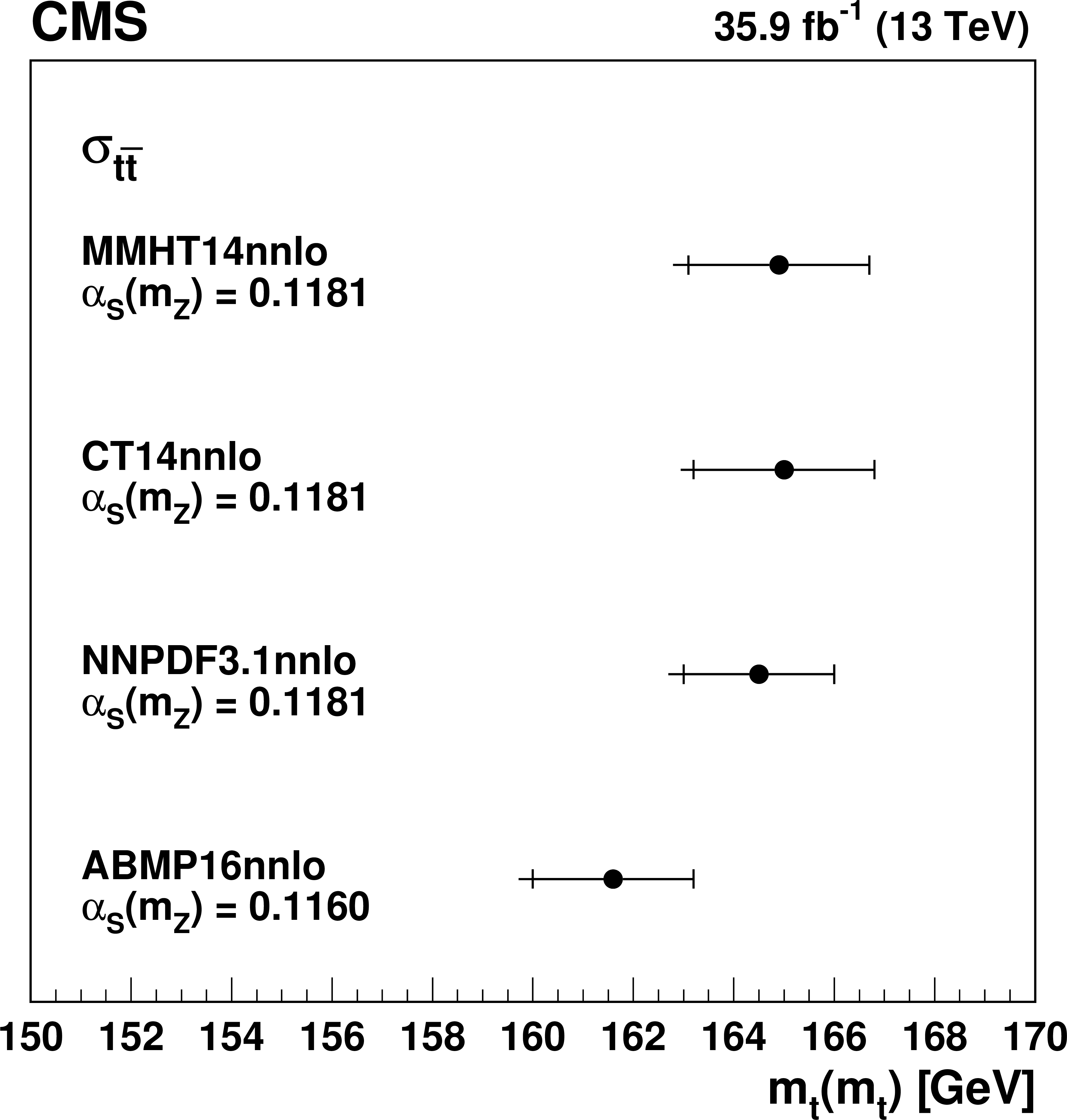
png pdf |
Figure 13:
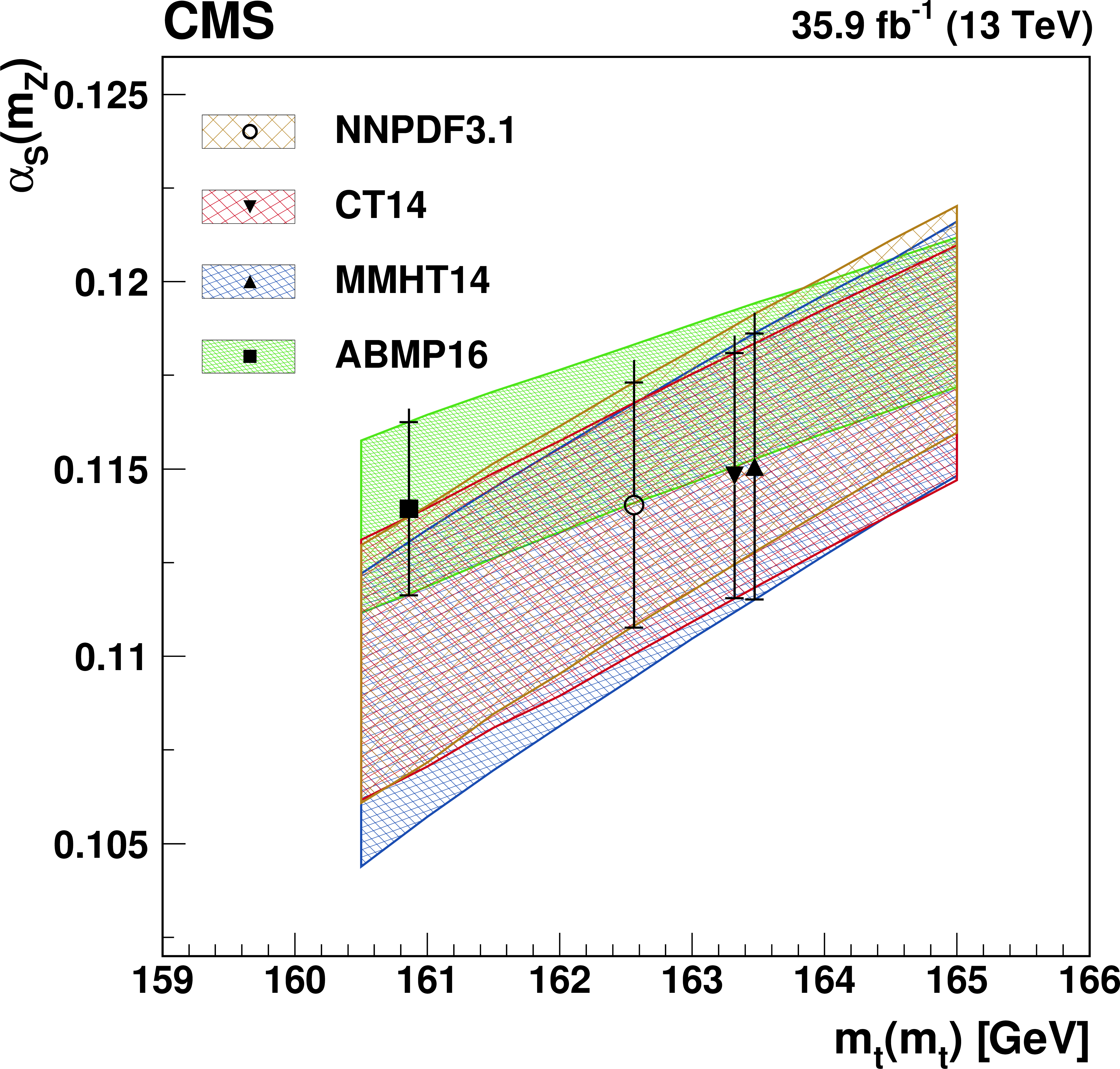
Values of $ {{{\alpha _S}} ({m_\mathrm {{\mathrm {Z}}}})} $ obtained in the comparison of the $ {\sigma _ {{\mathrm {t}\overline {\mathrm {t}}}}} $ measurement to the NNLO prediction using different PDFs, as a function of the $ {{m_\mathrm {{\mathrm {t}}}} ({m_\mathrm {{\mathrm {t}}}})} $ value used in the theoretical calculation. The results from using the different PDFs are shown by the bands with different shadings, with the band width corresponding to the quadratic sum of the experimental and PDF uncertainties in ${{{\alpha _S}} ({m_\mathrm {{\mathrm {Z}}}})}$. The resulting measured values of $ {{{\alpha _S}} ({m_\mathrm {{\mathrm {Z}}}})} $ are shown by the different style points at the $ {{m_\mathrm {{\mathrm {t}}}} ({m_\mathrm {{\mathrm {t}}}})} $ values used for each PDF. The inner vertical bars on the points represent the quadratic sum of the experimental and PDF uncertainties in ${{{\alpha _S}} ({m_\mathrm {{\mathrm {Z}}}})}$, while the outer vertical bars show the total uncertainties. |
| Tables | |
png pdf |
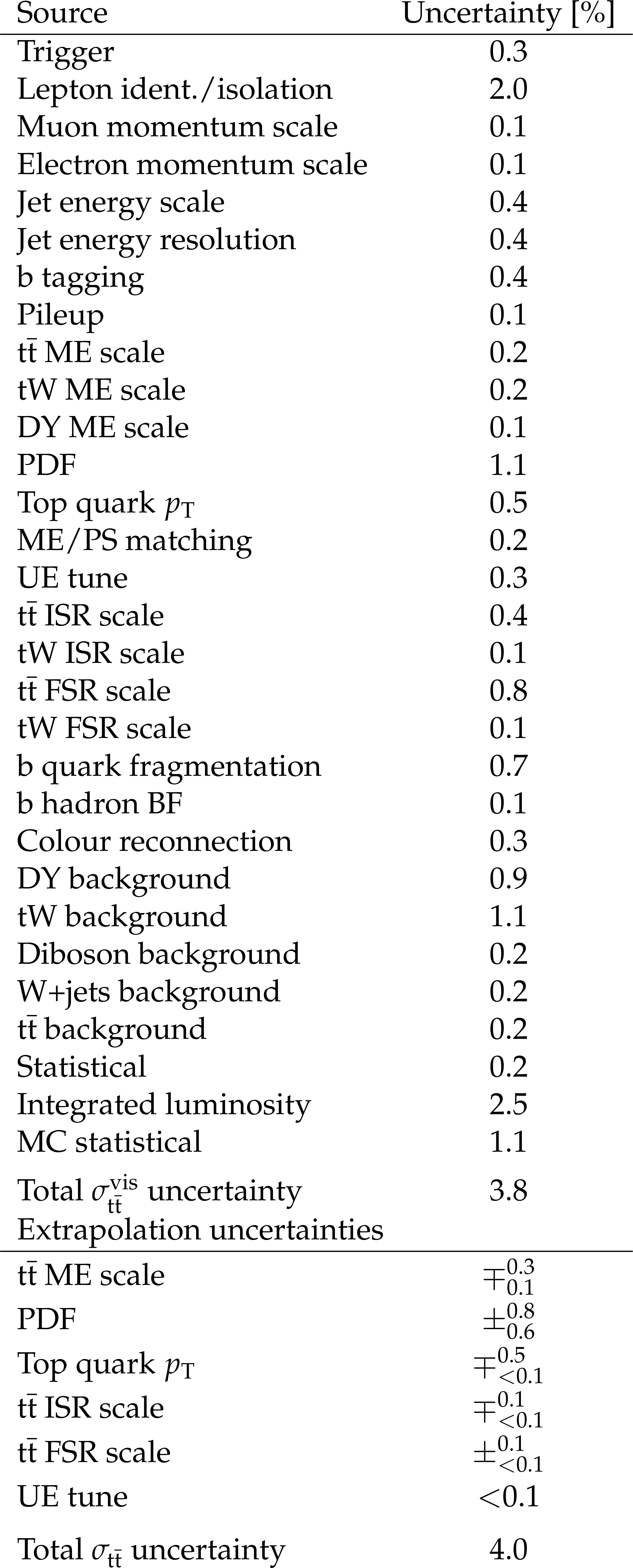
Table 1:
The relative uncertainties in ${\sigma _{{{\mathrm {t}\overline {\mathrm {t}}}}}^{\text {vis}}}$ and ${\sigma _ {{\mathrm {t}\overline {\mathrm {t}}}}}$ and their sources, as obtained from the template fit. The uncertainty in the integrated luminosity and the MC statistical uncertainty are determined separately. The individual uncertainties are given without their correlations, which are however accounted for in the total uncertainties. Extrapolation uncertainties only affect ${\sigma _ {{\mathrm {t}\overline {\mathrm {t}}}}}$. For these uncertainties, the $\pm $ notation is used if a positive variation produces an increase in ${\sigma _ {{\mathrm {t}\overline {\mathrm {t}}}}}$, while the $\mp $ notation is used otherwise. |
png pdf |
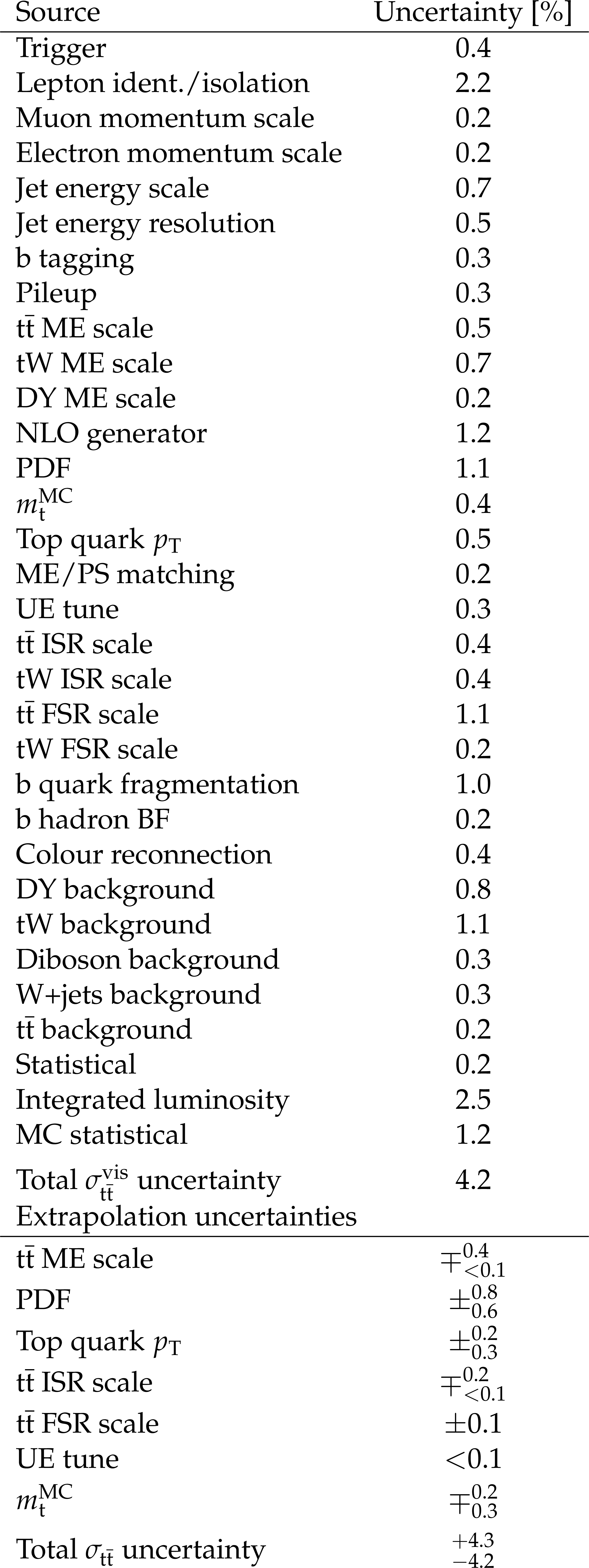
Table 2:
The same as Table 1, but for the simultaneous fit of $ {\sigma _ {{\mathrm {t}\overline {\mathrm {t}}}}} $ and ${{m_\mathrm {{\mathrm {t}}}} ^{\mathrm {MC}}}$. |
png pdf |
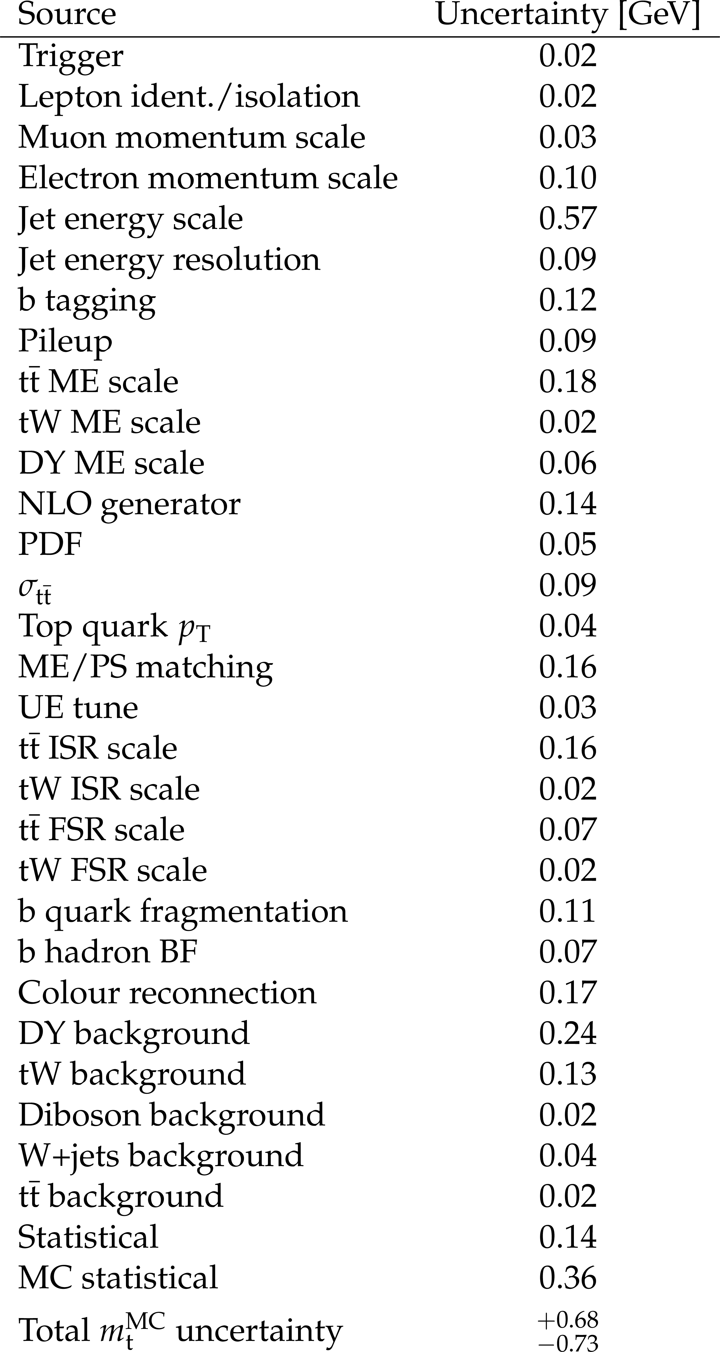
Table 3:
The absolute uncertainties in ${{m_\mathrm {{\mathrm {t}}}} ^{\mathrm {MC}}}$ and their sources, from the simultaneous fit of $ {\sigma _ {{\mathrm {t}\overline {\mathrm {t}}}}} $ and ${{m_\mathrm {{\mathrm {t}}}} ^{\mathrm {MC}}}$. The MC statistical uncertainty is determined separately. The individual uncertainties are given without their correlations, which are however accounted for in the total uncertainties. |
png pdf |
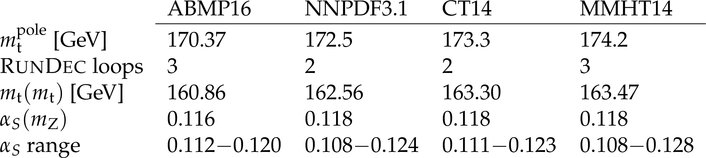
Table 4:
Values of the top quark pole mass ${{m_\mathrm {{\mathrm {t}}}} ^{\text {pole}}}$ and strong coupling constant ${{{\alpha _S}} ({m_\mathrm {{\mathrm {Z}}}})}$ used in the different PDF sets. Also shown are the corresponding ${{m_\mathrm {{\mathrm {t}}}} ({m_\mathrm {{\mathrm {t}}}})}$ values obtained using the {RunDec} [82,83] conversion, the number of loops in the conversion, and the ${{\alpha _S}}$ range used to estimate the PDF uncertainties. |

png pdf |
Table 5:
Values of $ {{{\alpha _S}} ({m_\mathrm {{\mathrm {Z}}}})} $ with their uncertainties obtained from a comparison of the measured $ {\sigma _ {{\mathrm {t}\overline {\mathrm {t}}}}} $ value to the NNLO prediction in the $ {\mathrm {\overline {MS}}} $ scheme using different PDF sets. The first uncertainty is the combination of the experimental and PDF uncertainties, and the second is from the variation of the renormalization and factorization scales. |
png pdf |
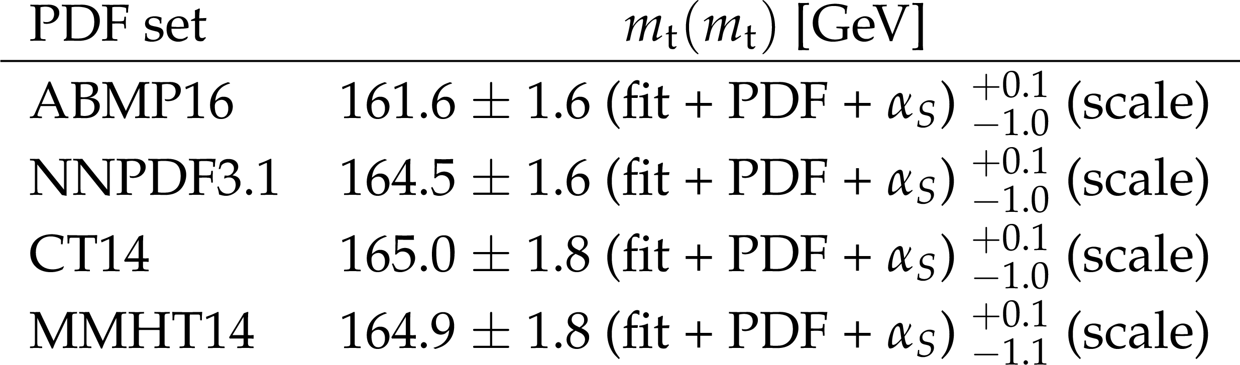
Table 6:
Values of $ {{m_\mathrm {{\mathrm {t}}}} ({m_\mathrm {{\mathrm {t}}}})} $ obtained from the comparison of the $ {\sigma _ {{\mathrm {t}\overline {\mathrm {t}}}}} $ measurement with the NNLO predictions using different PDF sets. The first uncertainty shown comes from the experimental, PDF, and $ {{{\alpha _S}} ({m_\mathrm {{\mathrm {Z}}}})} $ uncertainties, and the second from the variation in the renormalization and factorization scales. |
png pdf |
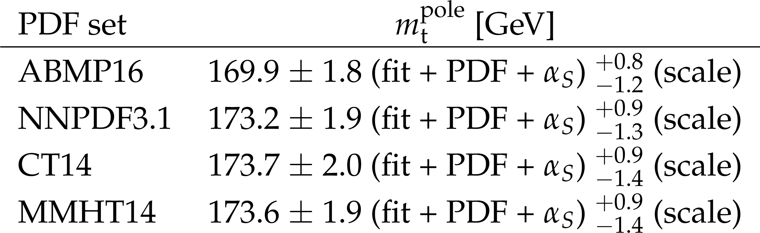
Table 7:
Values of ${{m_\mathrm {{\mathrm {t}}}} ^{\text {pole}}}$ obtained by comparing the $ {\sigma _ {{\mathrm {t}\overline {\mathrm {t}}}}} $ measurement with predictions at NNLO+NNLL using different PDF sets. |
| Summary |
|
A measurement of the top quark-antiquark pair production cross section $ {\sigma_\mathrm{t\bar{t}}} $ by the CMS Collaboration in proton-proton collisions at a centre-of-mass energy of 13 TeV is presented, corresponding to an integrated luminosity of 35.9 fb$^{-1}$. Assuming a top quark mass in the simulation of ${{m_{\mathrm{t}}} ^{\mathrm{MC}}} = $ 172.5 GeV, a visible cross section is measured in the fiducial region using dilepton events ($\mathrm{e}^{\pm}\mu^{\mp}$ , $\mu^{+}\mu^{-}$, $\mathrm{e^{+}e^{-}}$) and then extrapolated to the full phase space. The total $ \mathrm{t\bar{t}} $ production cross section is found to be ${\sigma_\mathrm{t\bar{t}}} = $ 803 $\pm$ 2 (stat) $\pm$ 25 (syst) $\pm$ 20 (lumi) pb. The measurement is in good agreement with the theoretical prediction calculated to next-to-next-to-leading order in perturbative QCD, including soft-gluon resummation to next-to-next-to-leading logarithm. The measurement is repeated including $ {{m_{\mathrm{t}}} ^{\mathrm{MC}}} $ as an additional free parameter in the fit. This yields a cross section of ${\sigma_\mathrm{t\bar{t}}} = $ 815 $\pm$ 2 (stat) $\pm$ 29 (syst) $pm$ 20 (lumi) pb and a value of ${{m_{\mathrm{t}}} ^{\mathrm{MC}}} = $ 172.33 $\pm$ 0.14 (stat) $^{+0.66}_{-0.72}$ (syst) GeV, in good agreement with previous measurements. The value of $ {\sigma_\mathrm{t\bar{t}}} $ obtained in the simultaneous fit is further used to extract the values of the top quark mass and the strong coupling constant at next-to-next-to-leading order in the minimal subtraction renormalization scheme, as well as the value of the top quark pole mass for different sets of parton distribution functions. |
| References | ||||
| 1 | ATLAS Collaboration | Measurement of the $ \mathrm{t\bar{t}} $ production cross-section using $ \mathrm{e}\mu $ events with b-tagged jets in $ pp $ collisions at $ \sqrt{s} = $ 7 and 8 TeV with the ATLAS detector | EPJC 74 (2014) 3109 | 1406.5375 |
| 2 | ATLAS Collaboration | Measurement of the $ \mathrm{t\bar{t}} $ production cross-section using $ \mathrm{e}\mu $ events with b-tagged jets in $ pp $ collisions at $ \sqrt{s} = $ 13 TeV with the ATLAS detector | PLB 761 (2016) 136 | 1606.02699 |
| 3 | CMS Collaboration | Measurement of the inclusive $ \mathrm{t\bar{t}} $ cross section in $ pp $ collisions at $ \sqrt{s}= $ 5.02 TeV using final states with at least one charged lepton | JHEP 03 (2018) 115 | CMS-TOP-16-023 1711.03143 |
| 4 | CMS Collaboration | Measurement of the $ \mathrm{t\bar{t}} $ production cross section in the $ \mathrm{e}\mu $ channel in proton-proton collisions at $ \sqrt{s}= $ 7 and 8 TeV | JHEP 08 (2016) 029 | CMS-TOP-13-004 1603.02303 |
| 5 | CMS Collaboration | Measurement of the $ \mathrm{t\bar{t}} $ production cross section using events with one lepton and at least one jet in $ pp $ collisions at $ \sqrt{s} = $ 13 TeV | JHEP 09 (2017) 051 | CMS-TOP-16-006 1701.06228 |
| 6 | P. Barnreuther, M. Czakon, and A. Mitov | Percent-level-precision physics at the Tevatron: next-to-next-to-leading order QCD corrections to $ \mathrm{q\bar{q}}{\rm \to}\mathrm{t\bar{t}}\mathbf{+}X $ | PRL 109 (2012) 132001 | 1204.5201 |
| 7 | M. Czakon and A. Mitov | NNLO corrections to top-pair production at hadron colliders: the all-fermionic scattering channels | JHEP 12 (2012) 054 | 1207.0236 |
| 8 | M. Czakon and A. Mitov | NNLO corrections to top pair production at hadron colliders: the quark-gluon reaction | JHEP 01 (2013) 080 | 1210.6832 |
| 9 | M. Czakon, P. Fiedler, and A. Mitov | Total top-quark pair-production cross section at hadron colliders through $ O({\alpha_{\text{s}}}^4) $ | PRL 110 (2013) 252004 | 1303.6254 |
| 10 | D0 Collaboration | Determination of the pole and $ \overline{MS} $ masses of the top quark from the $ \mathrm{t\bar{t}} $ cross section | PLB 703 (2011) 422 | 1104.2887 |
| 11 | CMS Collaboration | Determination of the top-quark pole mass and strong coupling constant from the $ \mathrm{t\bar{t}} $ production cross section in $ pp $ collisions at $ \sqrt{s} = $ 7 TeV | PLB 728 (2014) 496 | CMS-TOP-12-022 1307.1907 |
| 12 | D0 Collaboration | Measurement of the inclusive $ \mathrm{t\bar{t}} $ production cross section in $ {\mathrm{p}}\mathrm{\bar{p}} $ collisions at $ \sqrt{s}= $ 1.96 TeV and determination of the top quark pole mass | PRD 94 (2016) 092004 | 1605.06168 |
| 13 | T. Klijnsma, S. Bethke, G. Dissertori, and G. P. Salam | Determination of the strong coupling constant $ \alpha_{\text{s}}(M_{\mathrm{Z}}) $ from measurements of the total cross section for top-antitop quark production | EPJC 77 (2017) 778 | 1708.07495 |
| 14 | M. Czakon, M. L. Mangano, A. Mitov, and J. Rojo | Constraints on the gluon PDF from top quark pair production at hadron colliders | JHEP 07 (2013) 167 | 1303.7215 |
| 15 | M. Guzzi, K. Lipka, and S.-O. Moch | Top-quark pair production at hadron colliders: differential cross section and phenomenological applications with DiffTop | JHEP 01 (2015) 082 | 1406.0386 |
| 16 | CMS Collaboration | Measurement of double-differential cross sections for top quark pair production in $ pp $ collisions at $ \$ \sqrt{s} = $ 8 {TeV} $ and impact on parton distribution functions | EPJC 77 (2017) 459 | CMS-TOP-14-013 1703.01630 |
| 17 | S. Alekhin, J. Blumlein, S. Moch, and R. Placakyte | Parton distribution functions, $ \alpha_{\text{s}}, $ and heavy-quark masses for LHC Run II | PRD 96 (2017) 014011 | 1701.05838 |
| 18 | Gfitter Group Collaboration | The global electroweak fit at NNLO and prospects for the LHC and ILC | EPJC 74 (2014) 3046 | 1407.3792 |
| 19 | G. Degrassi et al. | Higgs mass and vacuum stability in the standard model at NNLO | JHEP 08 (2012) 098 | 1205.6497 |
| 20 | M. Dowling and S.-O. Moch | Differential distributions for top-quark hadro-production with a running mass | EPJC 74 (2014) 3167 | 1305.6422 |
| 21 | P. Marquard, A. V. Smirnov, V. A. Smirnov, and M. Steinhauser | Quark mass relations to four-loop order in perturbative QCD | PRL 114 (2015) 142002 | 1502.01030 |
| 22 | CDF and D0 Collaborations | Combination of CDF and $ D0 $ results on the mass of the top quark using up $ 9.7 fb$^{-1} at the Tevatron | 1608.01881 | |
| 23 | ATLAS Collaboration | Measurement of the top quark mass in the $ \mathrm{t\bar{t}} \to $ dilepton channel from $ \sqrt{s}= $ 8 TeV ATLAS data | PLB 761 (2016) 350 | 1606.02179 |
| 24 | ATLAS, CDF, CMS and D0 Collaborations | First combination of Tevatron and LHC measurements of the top-quark mass | 1403.4427 | |
| 25 | CMS Collaboration | Measurement of the top quark mass using proton-proton data at $ {\sqrt{s}} = $ 7 and 8 TeV | PRD 93 (2016) 072004 | CMS-TOP-14-022 1509.04044 |
| 26 | CMS Collaboration | Measurement of masses in the $ \mathrm{t\bar{t}} $ system by kinematic endpoints in $ pp $ collisions at $ \sqrt{s} = $ 7 TeV | EPJC 73 (2013) 2494 | CMS-TOP-11-027 1304.5783 |
| 27 | A. Buckley et al. | General-purpose event generators for LHC physics | PR 504 (2011) 145 | 1101.2599 |
| 28 | A. H. Hoang, S. Platzer, and D. Samitz | On the cutoff dependence of the quark mass parameter in angular ordered parton showers | JHEP 10 (2018) 200 | 1807.06617 |
| 29 | Particle Data Group, M. Tanabashi et al. | Review of particle physics | PRD 98 (2018) 030001 | |
| 30 | J. Kieseler, K. Lipka, and S.-O. Moch | Calibration of the top-quark Monte Carlo mass | PRL 116 (2016) 162001 | 1511.00841 |
| 31 | CMS Collaboration | Measurement of the top quark mass with lepton+jets final states using $ pp $ collisions at $ \sqrt{s} = $ 13 TeV | EPJC 78 (2018) 891 | CMS-TOP-17-007 1805.01428 |
| 32 | CMS Collaboration | The CMS experiment at the CERN LHC | JINST 3 (2008) S08004 | CMS-00-001 |
| 33 | CMS Collaboration | The CMS trigger system | JINST 12 (2017) P01020 | CMS-TRG-12-001 1609.02366 |
| 34 | S. Alioli, P. Nason, C. Oleari, and E. Re | A general framework for implementing NLO calculations in shower Monte Carlo programs: the POWHEG BOX | JHEP 06 (2010) 043 | 1002.2581 |
| 35 | S. Frixione, P. Nason, and C. Oleari | Matching NLO QCD computations with parton shower simulations: the POWHEG method | JHEP 11 (2007) 070 | 0709.2092 |
| 36 | P. Nason | A new method for combining NLO QCD with shower Monte Carlo algorithms | JHEP 11 (2004) 040 | hep-ph/0409146 |
| 37 | S. Frixione, P. Nason, and G. Ridolfi | A positive-weight next-to-leading-order Monte Carlo for heavy flavour hadroproduction | JHEP 09 (2007) 126 | 0707.3088 |
| 38 | NNPDF Collaboration | Parton distributions with LHC data | NPB 867 (2013) 244 | 1207.1303 |
| 39 | T. Sjostrand et al. | An introduction to PYTHIA 8.2 | CPC 191 (2015) 159 | 1410.3012 |
| 40 | CMS Collaboration | Investigations of the impact of the parton shower tuning in PYTHIA 8 in the modelling of $ \mathrm{t\bar{t}} $ at $ \sqrt{s}= $ 8 and 13 TeV | CMS-PAS-TOP-16-021 | CMS-PAS-TOP-16-021 |
| 41 | P. Skands, S. Carrazza, and J. Rojo | Tuning PYTHIA 8.1: the Monash 2013 Tune | EPJC 74 (2014) 3024 | 1404.5630 |
| 42 | A. Kardos, P. Nason, and C. Oleari | Three-jet production in POWHEG | JHEP 04 (2014) 043 | 1402.4001 |
| 43 | E. Re | Single-top Wt-channel production matched with parton showers using the POWHEG method | EPJC 71 (2011) 1547 | 1009.2450 |
| 44 | S. Alioli, P. Nason, C. Oleari, and E. Re | Vector boson plus one jet production in POWHEG | JHEP 01 (2011) 095 | 1009.5594 |
| 45 | CMS Collaboration | Event generator tunes obtained from underlying event and multiparton scattering measurements | EPJC 76 (2016) 155 | CMS-GEN-14-001 1512.00815 |
| 46 | J. Alwall et al. | The automated computation of tree-level and next-to-leading order differential cross sections, and their matching to parton shower simulations | JHEP 07 (2014) 079 | 1405.0301 |
| 47 | S. Frixione and B. R. Webber | Matching NLO QCD computations and parton shower simulations | JHEP 06 (2002) 029 | hep-ph/0204244 |
| 48 | R. Gavin, Y. Li, F. Petriello, and S. Quackenbush | FEWZ 2.0: a code for hadronic $ \mathrm{Z} $ production at next-to-next-to-leading order | CPC 182 (2011) 2388 | 1011.3540 |
| 49 | N. Kidonakis | Two-loop soft anomalous dimensions for single top quark associated production with $ \mathrm{W^{-}} $ or $ \mathrm{H}^{-} $ | PRD 82 (2010) 054018 | hep-ph/1005.4451 |
| 50 | J. M. Campbell, R. K. Ellis, and C. Williams | Vector boson pair production at the LHC | JHEP 07 (2011) 018 | 1105.0020 |
| 51 | M. Czakon and A. Mitov | TOPpp: a program for the calculation of the top-pair cross-section at hadron colliders | CPC 185 (2014) 2930 | 1112.5675 |
| 52 | S. Dulat et al. | New parton distribution functions from a global analysis of quantum chromodynamics | PRD 93 (2016) 033006 | 1506.07443 |
| 53 | CMS Collaboration | Particle-flow reconstruction and global event description with the CMS detector | JINST 12 (2017) P10003 | CMS-PRF-14-001 1706.04965 |
| 54 | CMS Collaboration | Performance of electron reconstruction and selection with the CMS detector in proton-proton collisions at $ \sqrt{s} = $ 8 TeV | JINST 10 (2015) P06005 | CMS-EGM-13-001 1502.02701 |
| 55 | CMS Collaboration | Performance of the CMS muon detector and muon reconstruction with proton-proton collisions at $ \sqrt{s} = $ 13 TeV | JINST 13 (2018) P06015 | CMS-MUO-16-001 1804.04528 |
| 56 | M. Cacciari, G. P. Salam, and G. Soyez | The anti-$ {k_{\mathrm{T}}} $ jet clustering algorithm | JHEP 04 (2008) 063 | 0802.1189 |
| 57 | M. Cacciari, G. P. Salam, and G. Soyez | FastJet user manual | EPJC 72 (2012) 1896 | 1111.6097 |
| 58 | CMS Collaboration | Jet energy scale and resolution in the CMS experiment in $ pp $ collisions at 8 TeV | JINST 12 (2017) P02014 | CMS-JME-13-004 1607.03663 |
| 59 | CMS Collaboration | Identification of heavy-flavour jets with the CMS detector in $ pp $ collisions at 13 TeV | JINST 13 (2018) P05011 | CMS-BTV-16-002 1712.07158 |
| 60 | F. James and M. Roos | Minuit: a system for function minimization and analysis of the parameter errors and correlations | CPC 10 (1975) 343 | |
| 61 | CMS Collaboration | Jet algorithms performance in 13 TeV data | CMS-PAS-JME-16-003 | CMS-PAS-JME-16-003 |
| 62 | ATLAS Collaboration | Measurement of the inelastic proton-proton cross section at $ \sqrt{s} = $ 13 TeV with the ATLAS detector at the LHC | PRL 117 (2016) 182002 | 1606.02625 |
| 63 | CMS Collaboration | CMS luminosity measurements for the 2016 data taking period | CMS-PAS-LUM-17-001 | CMS-PAS-LUM-17-001 |
| 64 | M. Cacciari et al. | The $ \mathrm{t\bar{t}} $ cross-section at 1.8 TeV and 1.96 TeV: a study of the systematics due to parton densities and scale dependence | JHEP 04 (2004) 068 | hep-ph/0303085 |
| 65 | S. Catani, D. de Florian, M. Grazzini, and P. Nason | Soft gluon resummation for Higgs boson production at hadron colliders | JHEP 07 (2003) 028 | hep-ph/0306211 |
| 66 | R. Frederix and S. Frixione | Merging meets matching in MCatNLO | JHEP 12 (2012) 061 | 1209.6215 |
| 67 | CMS Collaboration | Measurement of normalized differential $ \mathrm{t\bar{t}} $ cross sections in the dilepton channel from $ pp $ collisions at $ \sqrt{s}= $ 13 TeV | JHEP 04 (2018) 060 | CMS-TOP-16-007 1708.07638 |
| 68 | CMS Collaboration | Measurement of differential cross sections for top quark pair production using the lepton+jets final state in proton-proton collisions at 13 TeV | PRD 95 (2017) 092001 | CMS-TOP-16-008 1610.04191 |
| 69 | M. G. Bowler | $ \mathrm{e^{+}e^{-}} $ production of heavy quarks in the string model | Z. Phys. C 11 (1981) 169 | |
| 70 | C. Peterson, D. Schlatter, I. Schmitt, and P. M. Zerwas | Scaling violations in inclusive $ \mathrm{e^{+}e^{-}} $ annihilation spectra | PRD 27 (1983) 105 | |
| 71 | S. Argyropoulos and T. Sjostrand | Effects of color reconnection on $ \mathrm{t\bar{t}} $ final states at the LHC | JHEP 11 (2014) 043 | 1407.6653 |
| 72 | J. R. Christiansen and P. Z. Skands | String formation beyond leading colour | JHEP 08 (2015) 003 | 1505.01681 |
| 73 | CMS Collaboration | Measurement of the top quark pair production cross section in proton-proton collisions at $ \sqrt{s} = $ 13 TeV | PRL 116 (2016) 052002 | CMS-TOP-15-003 1510.05302 |
| 74 | CMS Collaboration | Measurement of the $ \mathrm{t\bar{t}} $ production cross section using events in the $ \mathrm{e}\mu $ final state in $ pp $ collisions at $ \sqrt{s} = $ 13 TeV | EPJC 77 (2017) 172 | CMS-TOP-16-005 1611.04040 |
| 75 | S. Alekhin et al. | HERAFitter | EPJC 75 (2015) 304 | 1410.4412 |
| 76 | H1 and ZEUS Collaborations | Combination of measurements of inclusive deep inelastic $ {\mathrm{e}^{\pm}{\mathrm{p}}} $ scattering cross sections and QCD analysis of HERA data | EPJC 75 (2015) 580 | 1506.06042 |
| 77 | CMS Collaboration | Measurement and QCD analysis of double-differential inclusive jet cross sections in pp collisions at $ \sqrt{s}= $ 8 TeV and cross section ratios to 2.76 and 7 TeV | JHEP 03 (2017) 156 | CMS-SMP-14-001 1609.05331 |
| 78 | M. Aliev et al. | Hathor: HAdronic Top and Heavy quarks crOss section calculatoR | CPC 182 (2011) 1034 | 1007.1327 |
| 79 | A. Buckley et al. | LHAPDF6: parton density access in the LHC precision era | EPJC 75 (2015) 132 | 1412.7420 |
| 80 | L. A. Harland-Lang, A. D. Martin, P. Motylinski, and R. S. Thorne | Parton distributions in the LHC era: MMHT 2014 PDFs | EPJC 75 (2015) 204 | 1412.3989 |
| 81 | NNPDF Collaboration | Parton distributions from high-precision collider data | EPJC 77 (2017) 663 | 1706.00428 |
| 82 | K. G. Chetyrkin, J. H. Kuhn, and M. Steinhauser | RunDec: a Mathematica package for running and decoupling of the strong coupling and quark masses | CPC 133 (2000) 43 | hep-ph/0004189 |
| 83 | B. Schmidt and M. Steinhauser | CRunDec: a C++ package for running and decoupling of the strong coupling and quark masses | CPC 183 (2012) 1845 | 1201.6149 |
| 84 | H1 Collaboration | Determination of the strong coupling constant $ \alpha_{\text{s}}(M_{\mathrm{Z}}) $ in next-to-next-to-leading order QCD using H1 jet cross section measurements | EPJC 77 (2017) 791 | 1709.07251 |
|
|
Compact Muon Solenoid LHC, CERN |
|

|

|

|

|

|