

Compact Muon Solenoid
LHC, CERN
| CMS-TOP-16-006 ; CERN-EP-2016-321 | ||
| Measurement of the $\mathrm{ t \bar{t} }$ production cross section using events with one lepton and at least one jet in pp collisions at $\sqrt{s}= $ 13 TeV | ||
| CMS Collaboration | ||
| 22 January 2017 | ||
| JHEP 09 (2017) 051 | ||
| Abstract: A measurement of the $\mathrm{ t \bar{t} }$ production cross section at $\sqrt{s}=$ 13 TeV is presented using proton-proton collisions, corresponding to an integrated luminosity of 2.2 fb$^{-1}$, collected with the CMS detector at the LHC. Final states with one isolated charged lepton (electron or muon) and at least one jet are selected and categorized according to the accompanying jet multiplicity. From a likelihood fit to the invariant mass distribution of the isolated lepton and a jet identified as coming from the hadronization of a bottom quark, the cross section is measured to be $\sigma(\mathrm{ t \bar{t} })=$ 888 $\pm$ 2 (stat) $^{+26}_{-28}$ (syst) $\pm$ 20 (lumi) pb, in agreement with the standard model prediction. Using the expected dependence of the cross section on the pole mass of the top quark ($m_{\mathrm{ t }}$), the value of $m_{\mathrm{ t }}$ is found to be 170.6 $\pm$ 2.7 GeV. | ||
| Links: e-print arXiv:1701.06228 [hep-ex] (PDF) ; CDS record ; inSPIRE record ; CADI line (restricted) ; | ||
| Figures & Tables | Summary | Additional Figures | References | CMS Publications |
|---|
| Figures | |
png pdf |
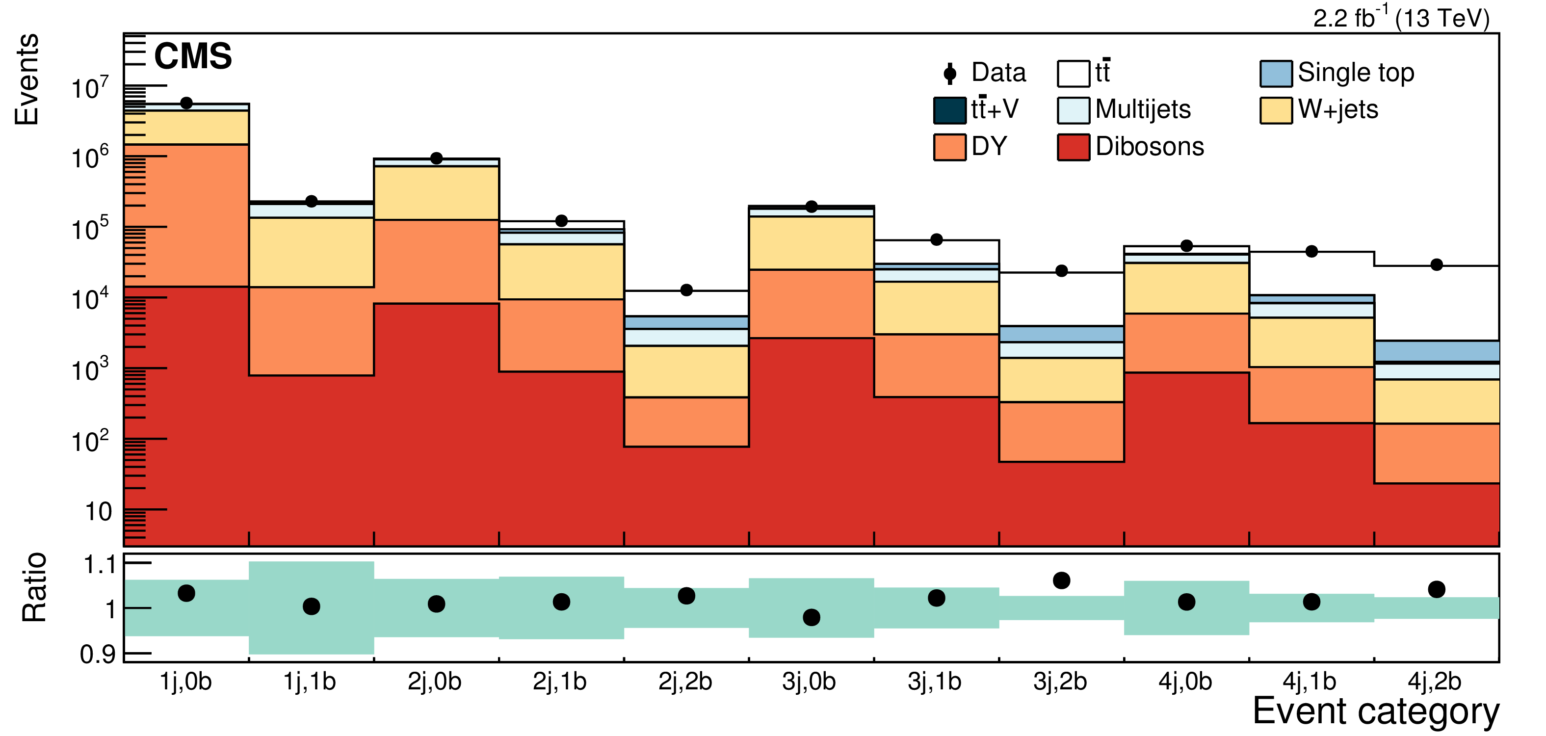
Figure 1:
Event yields from data and the expected $ {\mathrm{ t } \mathrm{ \bar{t} } } $ signal and backgrounds for each of the 11 independent categories. Distributions are combined for the two lepton charges and flavors. The bins represent the measured number of jets ({j}) and b-tagged jets ({b}). The bottom panel shows the ratio between the data and the expectations. The relative uncertainty owing to the statistical uncertainty in the simulations and the systematic uncertainty in the total integrated luminosity is represented as a shaded band. |
png pdf |
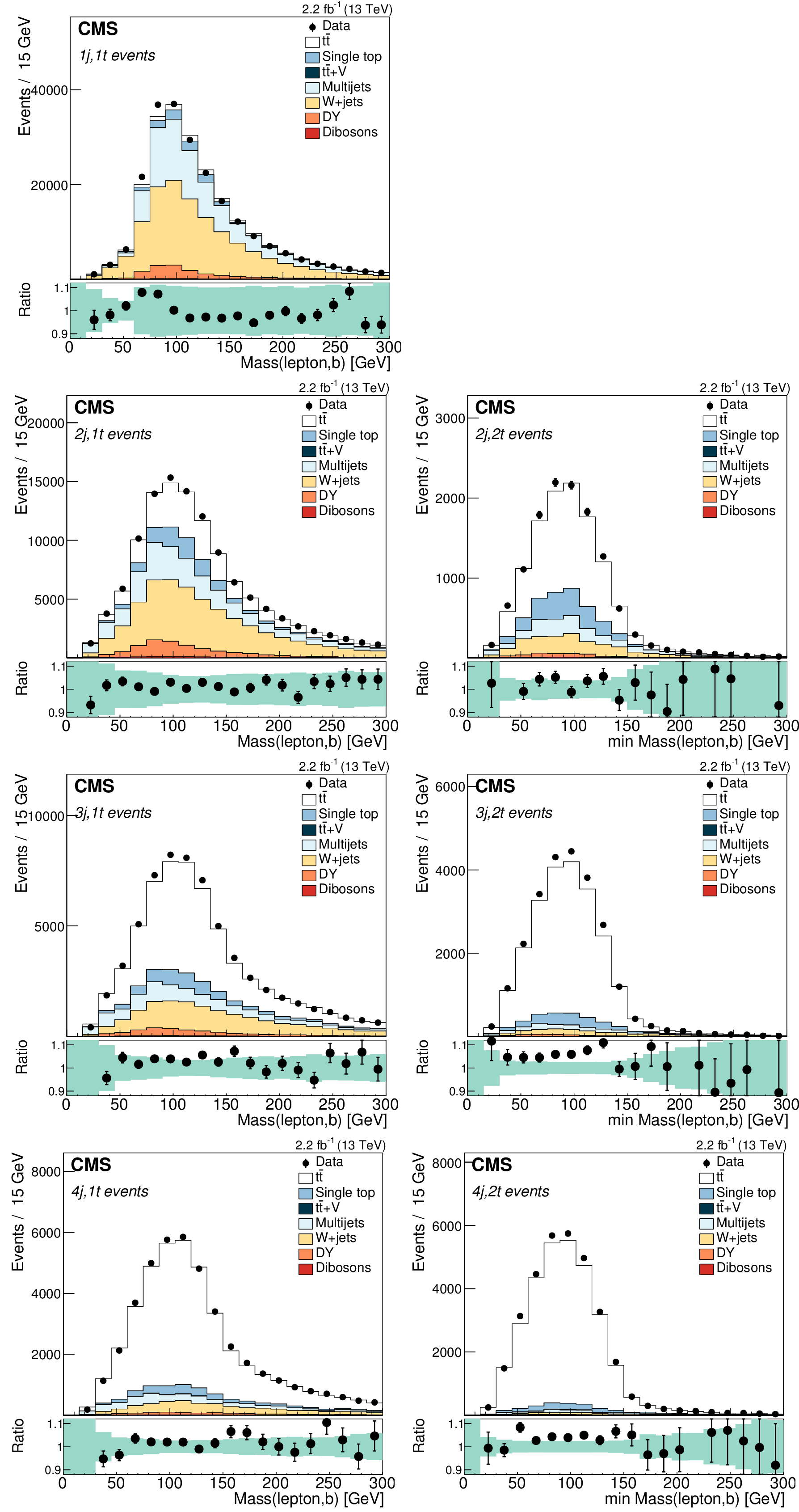
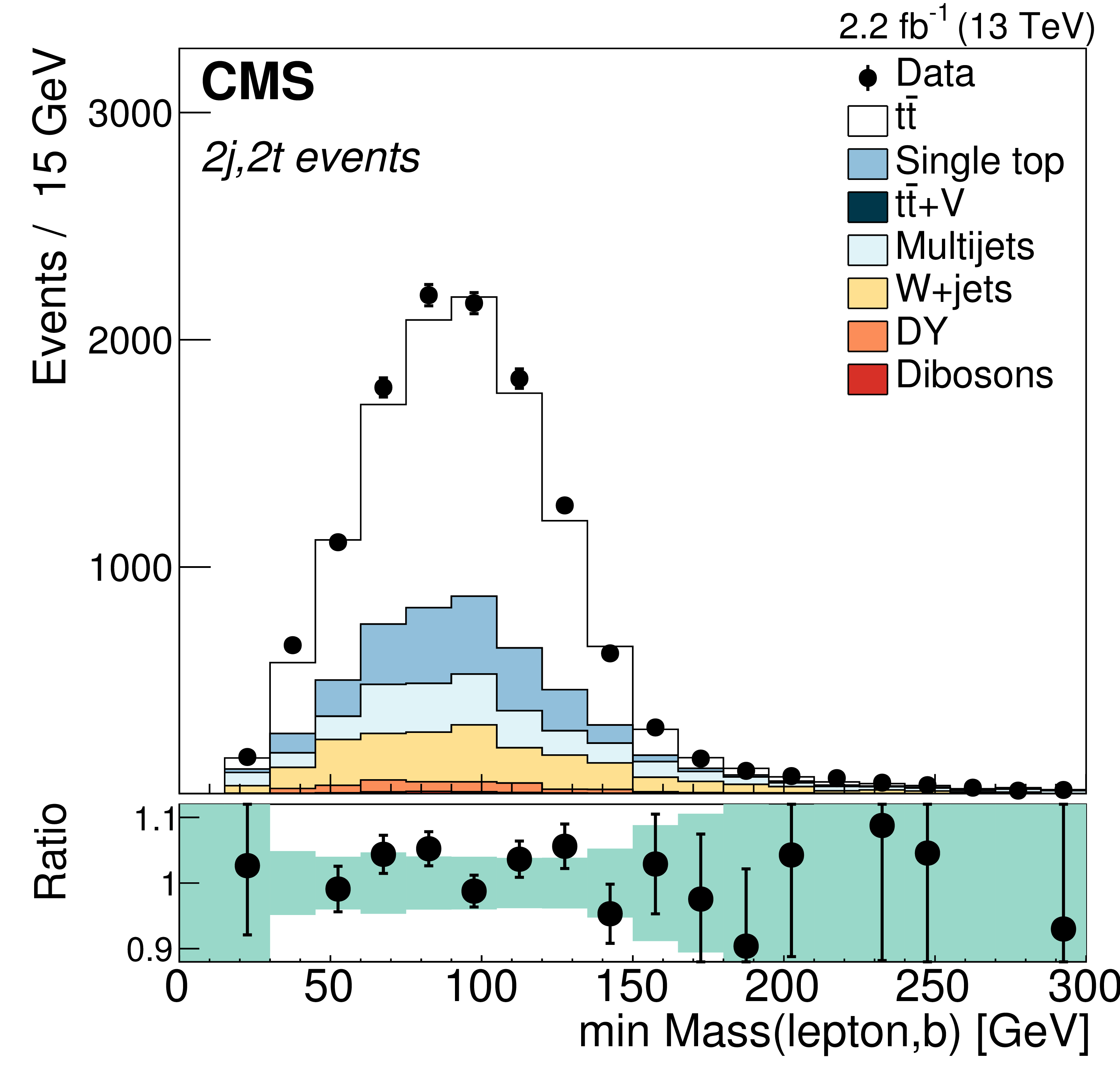
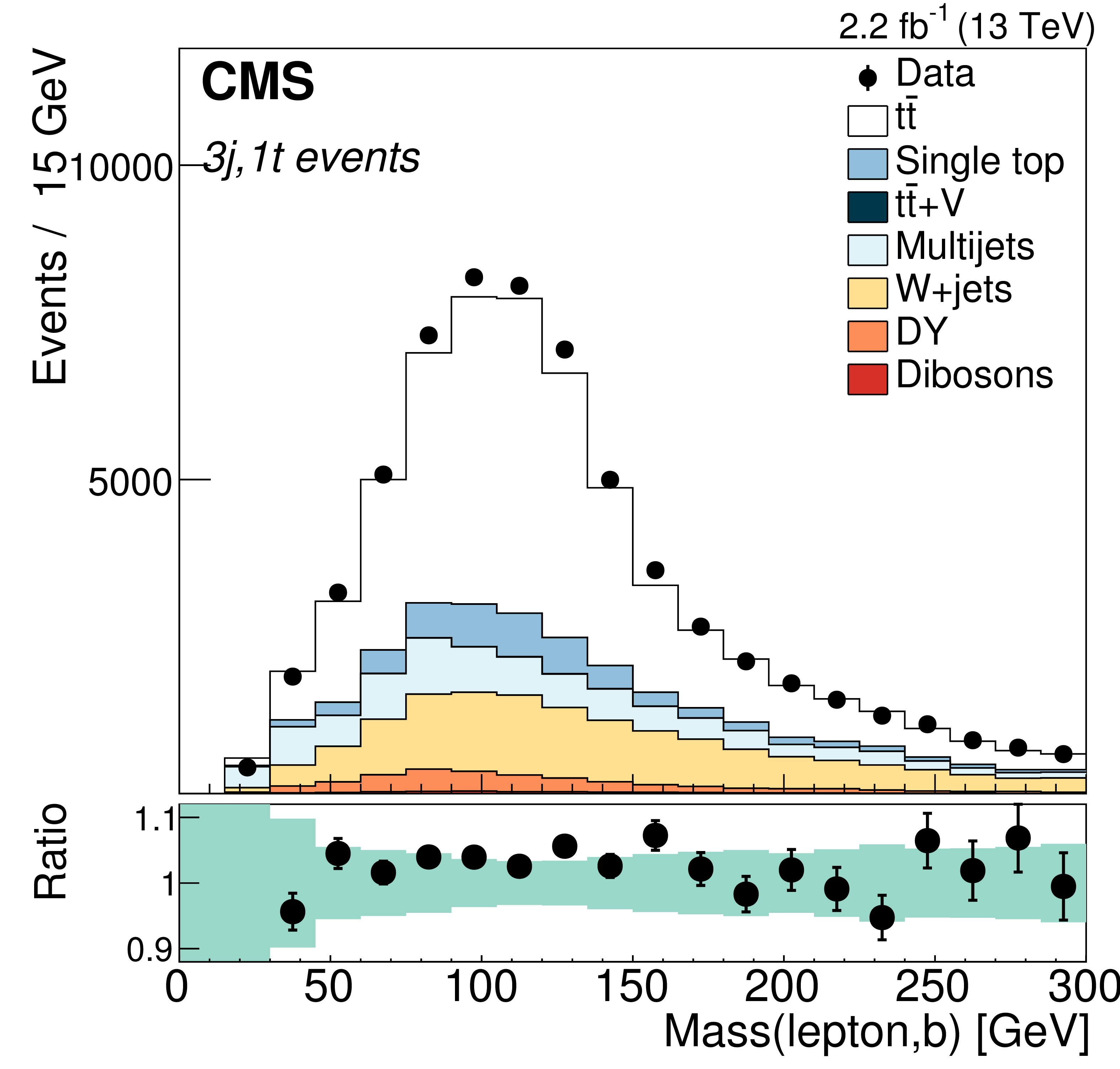
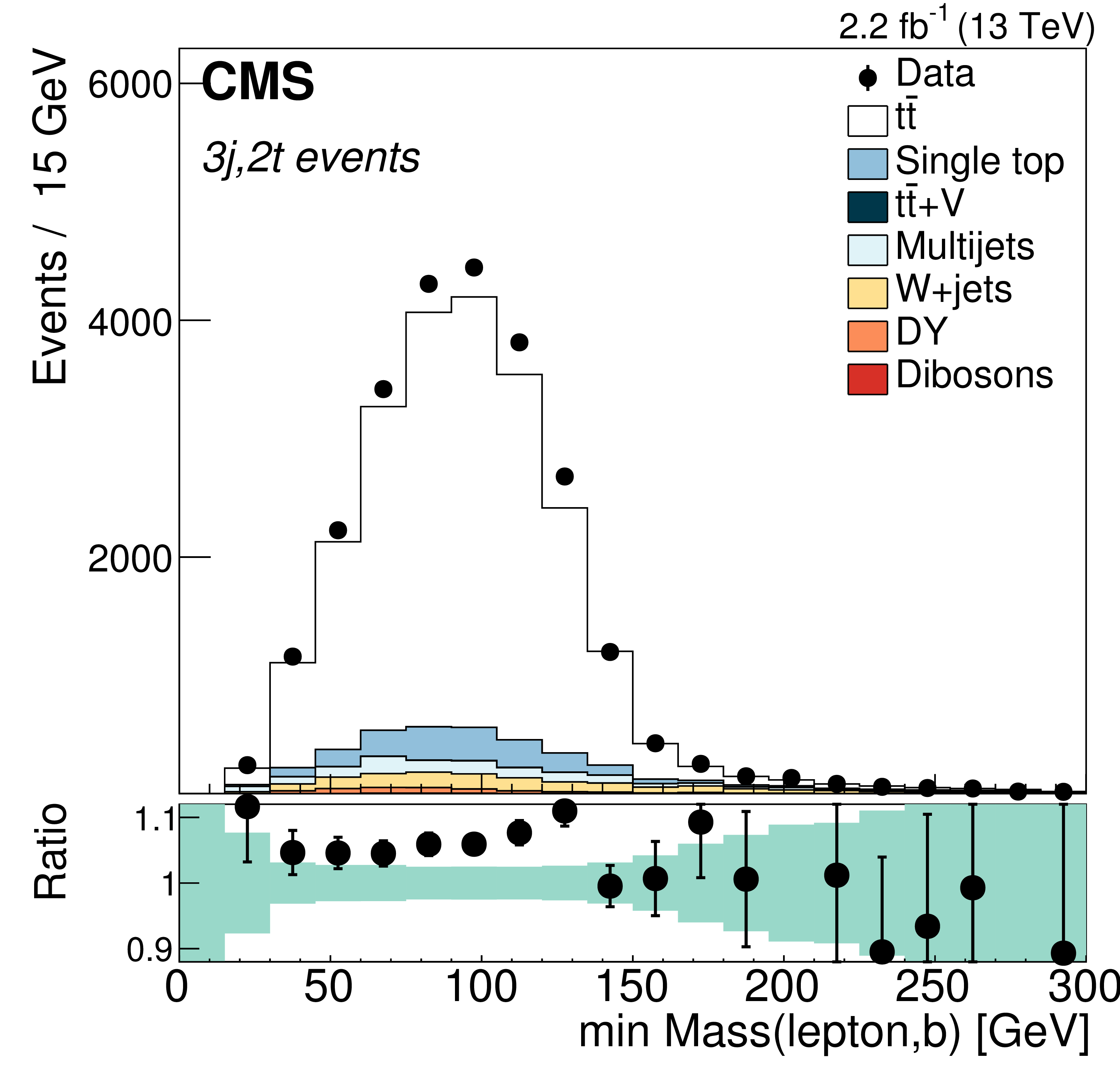
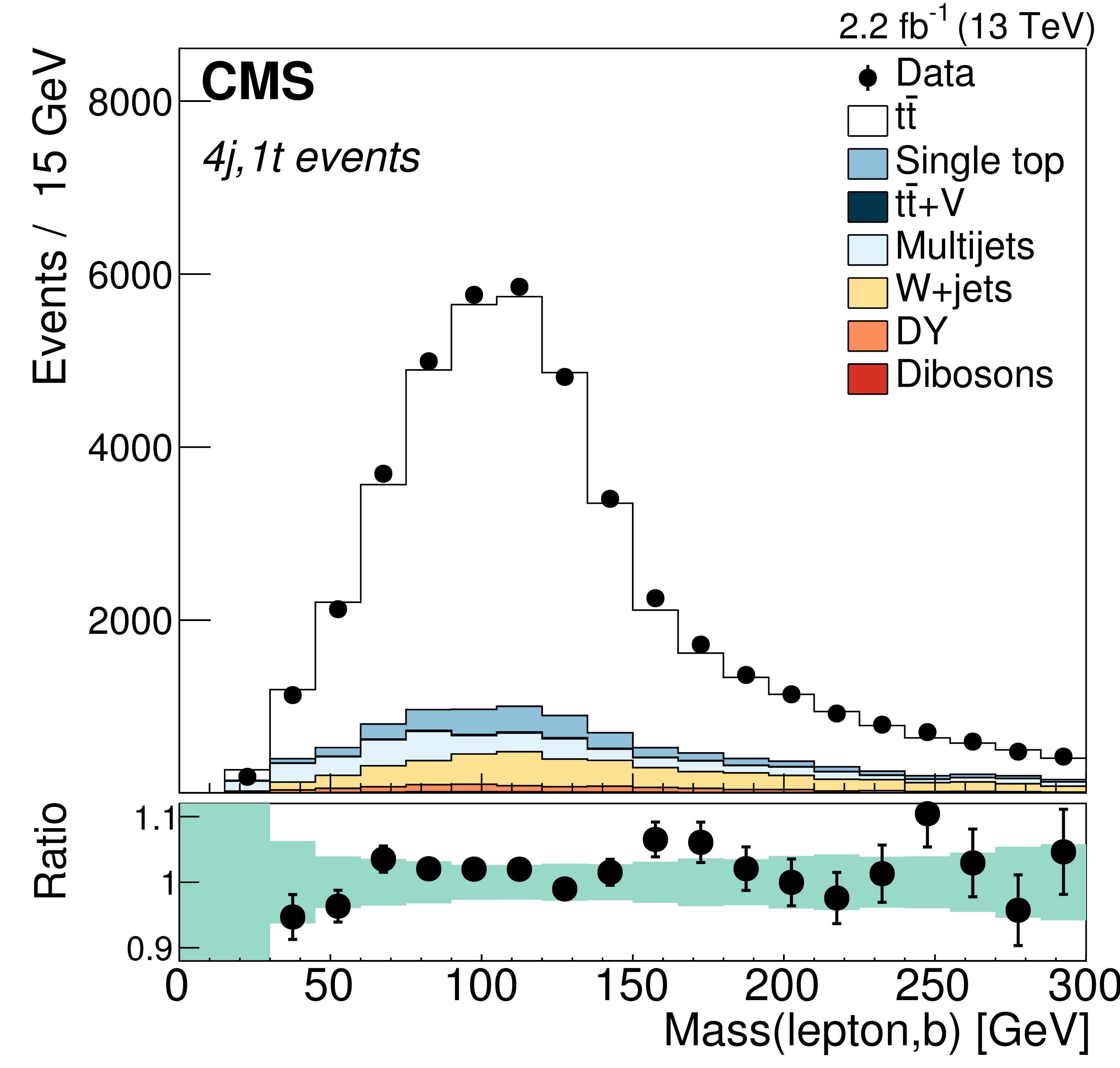
Figure 2:
Distributions in the observables used to fit the data with the contributions from all leptons and charges combined. Panels on the left show the distributions in $M(\ell ,\mathrm{ b } )$, and on the right in $\mathrm{min}\, M(\ell ,\mathrm{ b } )$, for events with one and two b-tagged jets, respectively. From top to bottom, the events correspond to those with 1, 2, 3, or at least 4 jets. The lower plot in each panel shows the ratio between the data and expectations. The relative uncertainty owing to the statistical uncertainty in the simulations and the systematic uncertainty in the total integrated luminosity is represented as a shaded band. |
png pdf |
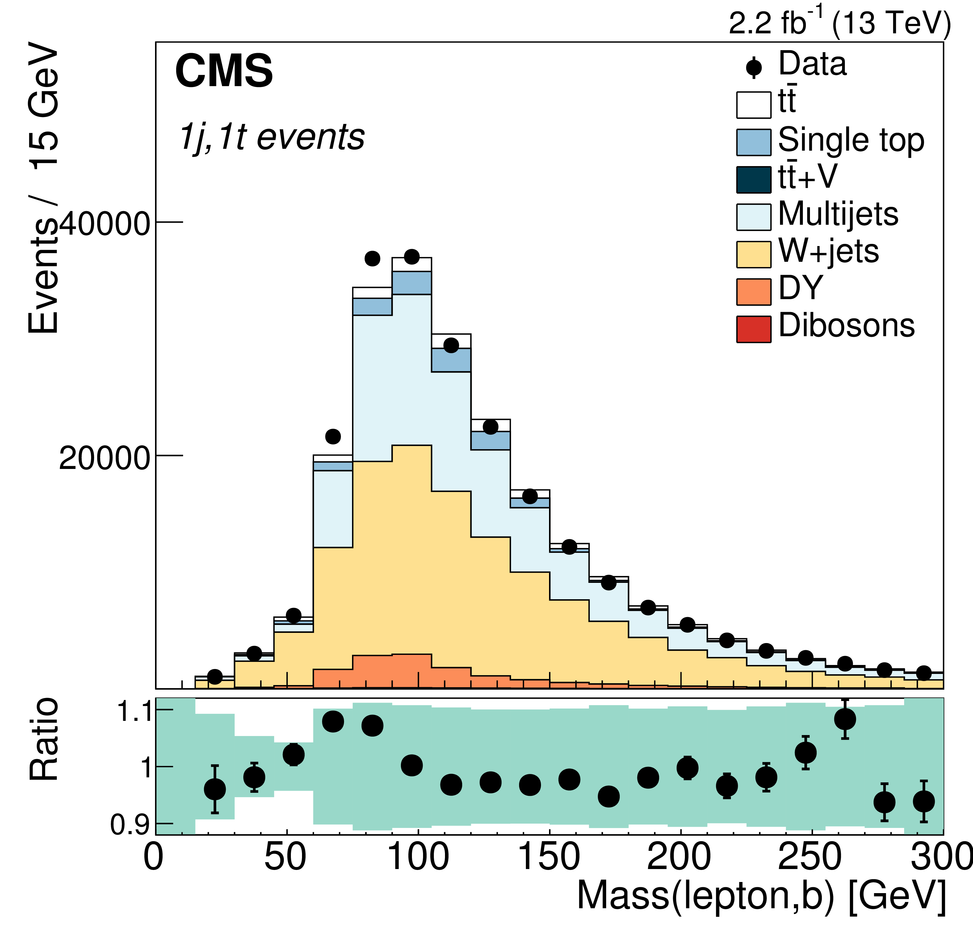
Figure 2-a:
Distributions in $M(\ell ,\mathrm{ b } )$ for events with one b-tagged jet for events with 1 jet, with the contributions from all leptons and charges combined. The lower plot shows the ratio between the data and expectations. The relative uncertainty owing to the statistical uncertainty in the simulations and the systematic uncertainty in the total integrated luminosity is represented as a shaded band. |
png pdf |
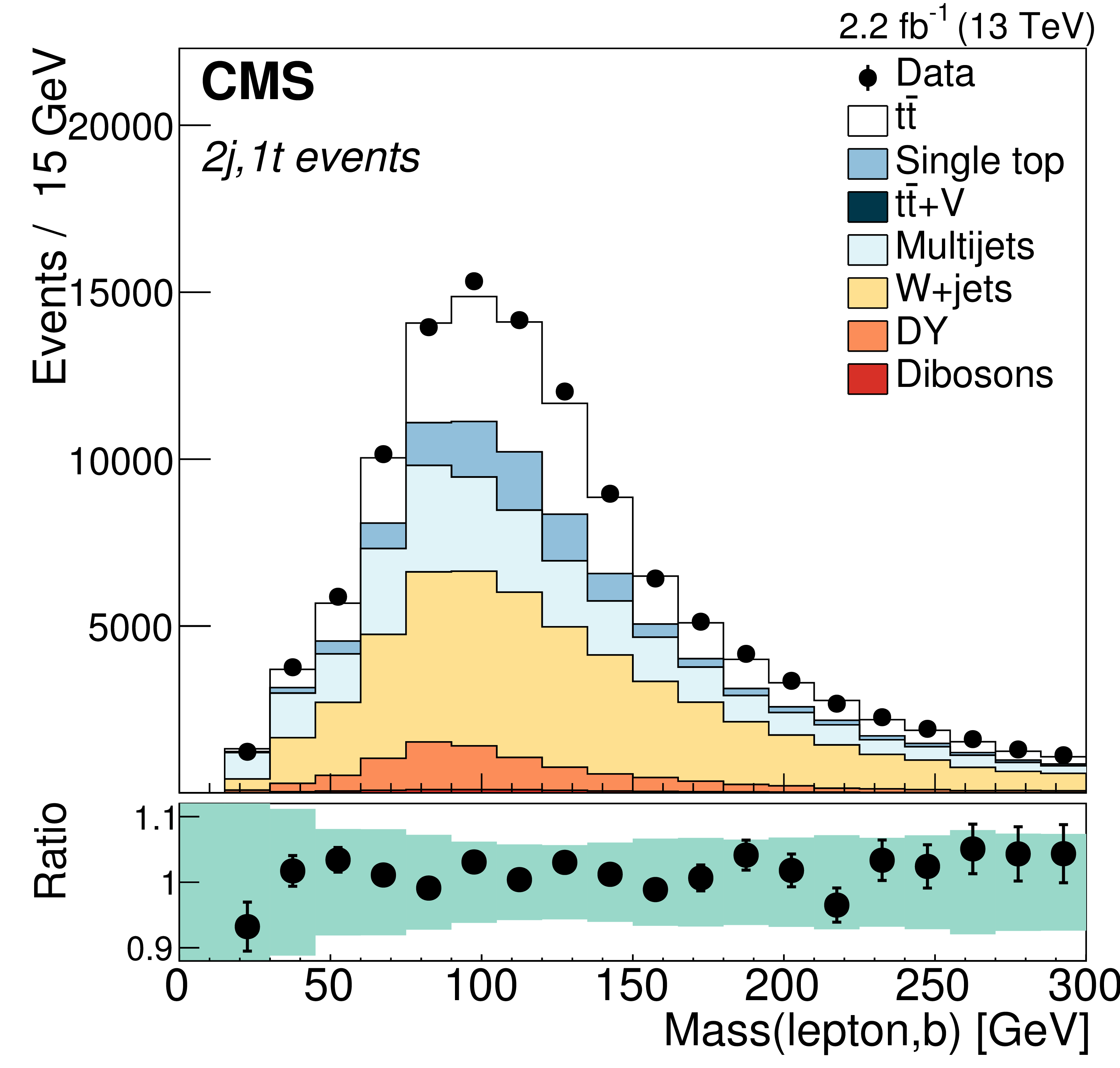
Figure 2-b:
Distributions in $M(\ell ,\mathrm{ b } )$ for events with one b-tagged jet, for events with 2 jets, with the contributions from all leptons and charges combined. The lower plot shows the ratio between the data and expectations. The relative uncertainty owing to the statistical uncertainty in the simulations and the systematic uncertainty in the total integrated luminosity is represented as a shaded band. |
png pdf |
Figure 2-c:
Distributions in $\mathrm{min}\, M(\ell ,\mathrm{ b } )$ for events with two b-tagged jets, for events with 2 jets, with the contributions from all leptons and charges combined. The lower plot shows the ratio between the data and expectations. The relative uncertainty owing to the statistical uncertainty in the simulations and the systematic uncertainty in the total integrated luminosity is represented as a shaded band. |
png pdf |
Figure 2-d:
Distributions in $M(\ell ,\mathrm{ b } )$ for events with one b-tagged jet, for events with 3 jets, with the contributions from all leptons and charges combined. The lower plot shows the ratio between the data and expectations. The relative uncertainty owing to the statistical uncertainty in the simulations and the systematic uncertainty in the total integrated luminosity is represented as a shaded band. |
png pdf |
Figure 2-e:
Distributions in $\mathrm{min}\, M(\ell ,\mathrm{ b } )$ for events with two b-tagged jets, for events with 3 jets, with the contributions from all leptons and charges combined. The lower plot shows the ratio between the data and expectations. The relative uncertainty owing to the statistical uncertainty in the simulations and the systematic uncertainty in the total integrated luminosity is represented as a shaded band. |
png pdf |
Figure 2-f:
Distributions in $M(\ell ,\mathrm{ b } )$ for events with one b-tagged jet, for events with at least 4 jets, with the contributions from all leptons and charges combined. The lower plot shows the ratio between the data and expectations. The relative uncertainty owing to the statistical uncertainty in the simulations and the systematic uncertainty in the total integrated luminosity is represented as a shaded band. |
png pdf |
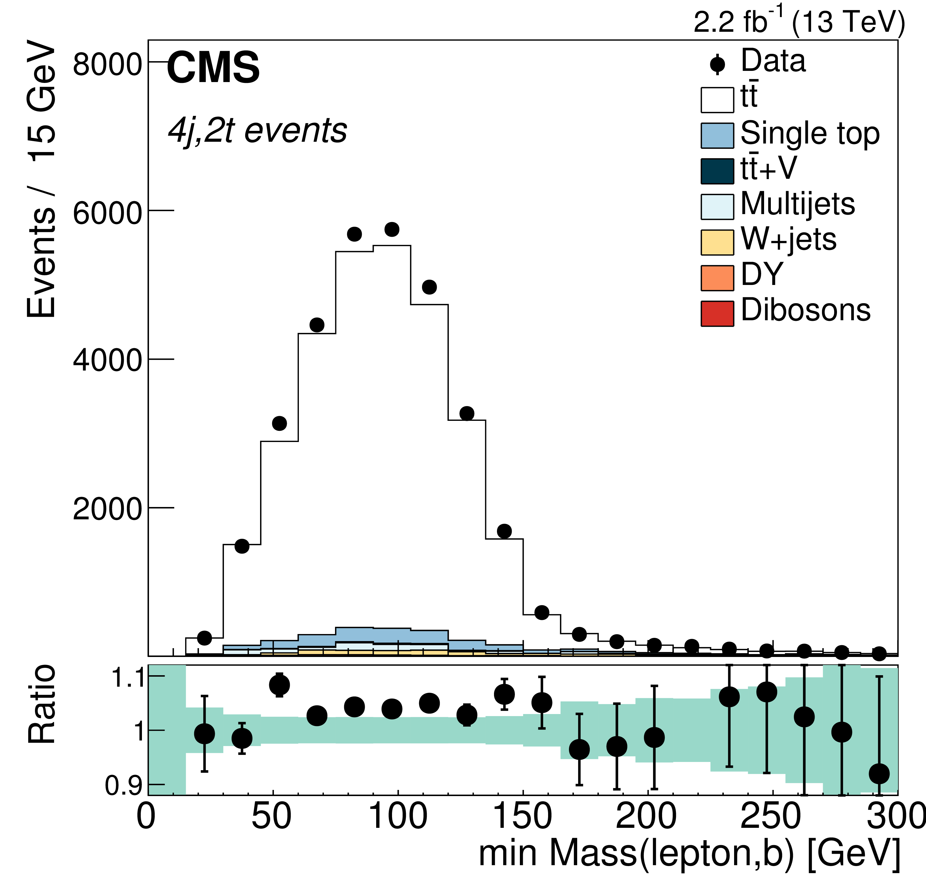
Figure 2-g:
Distributions in $\mathrm{min}\, M(\ell ,\mathrm{ b } )$ for events with two b-tagged jets, for events with at least 4 jets, with the contributions from all leptons and charges combined. The lower plot shows the ratio between the data and expectations. The relative uncertainty owing to the statistical uncertainty in the simulations and the systematic uncertainty in the total integrated luminosity is represented as a shaded band. |
png pdf |
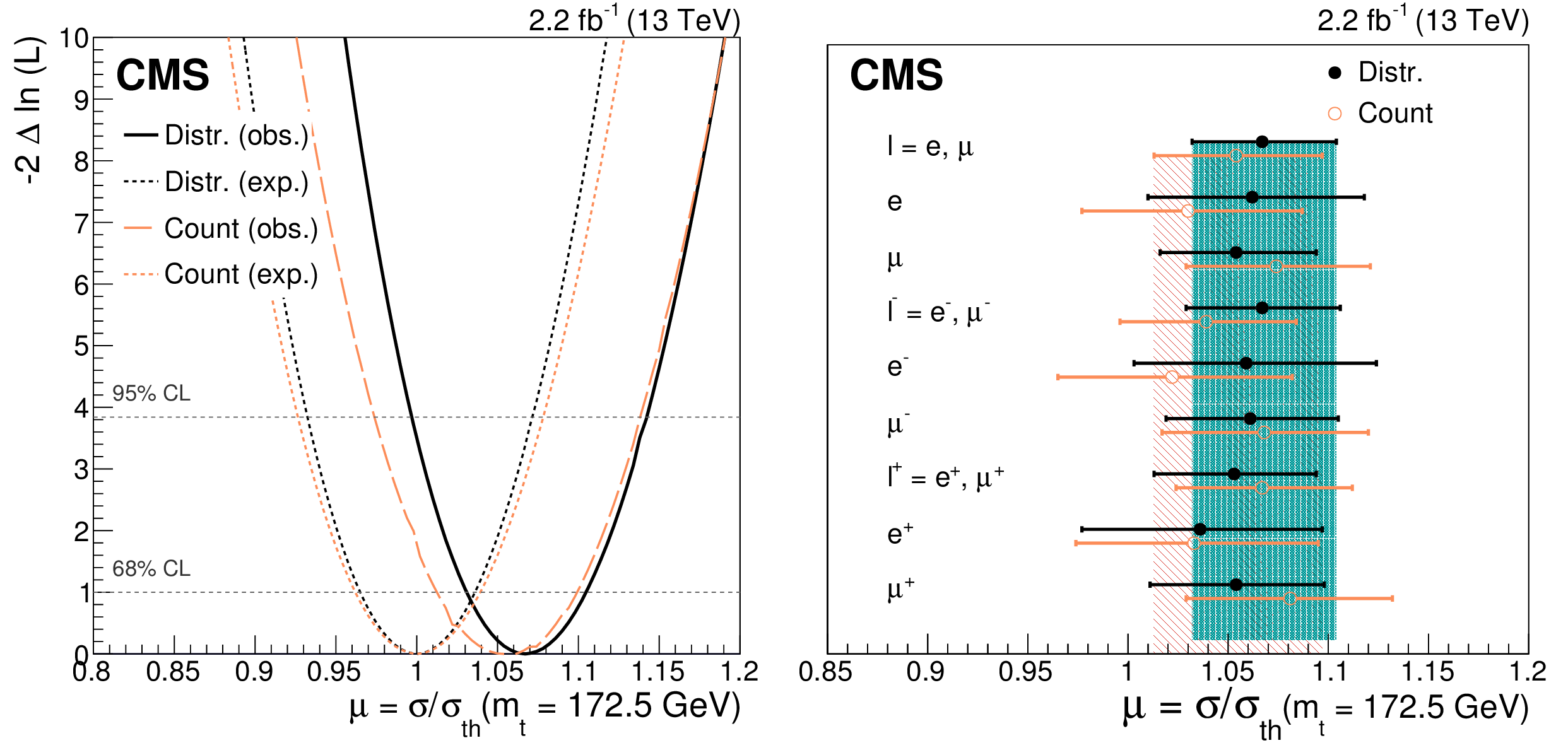
Figure 3:
(left) The observed (solid curve) and expected (dashed curve) variation of the likelihood as a function of the signal strength $\mu $ for the distribution-based analysis. The expected curve is obtained by performing the fit using simulated events with $m_\mathrm{ t } =$ 172.5 GeV. For comparison, the corresponding curves for the counting cross-check analysis are also shown. The two horizontal lines represent the values in the PLR that are used to determine the 68% and 95% confidence level (CL) intervals for the signal strength. (right) Comparison of the values of the signal strength extracted for different combinations of events for the distribution-based default analysis (solid circles) and the cross-check counting analysis (open circles). The horizontal bars represent the total uncertainties, except the beam energy uncertainty. The shaded bands represent the uncertainty in the final combined signal strength obtained from the distribution-based and cross-check analyses. |
png pdf |
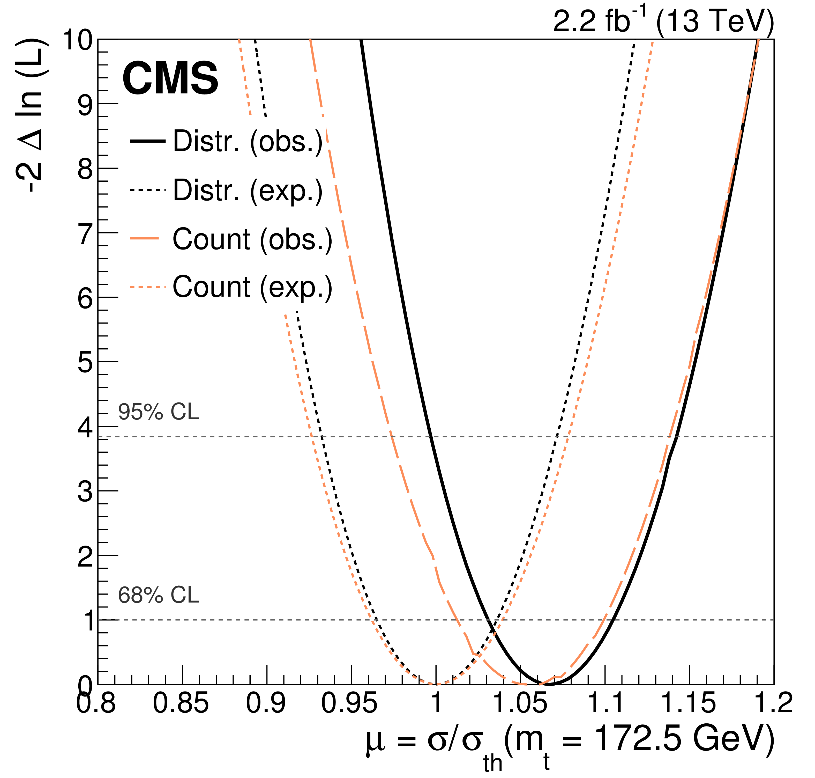
Figure 3-a:
The observed (solid curve) and expected (dashed curve) variation of the likelihood as a function of the signal strength $\mu $ for the distribution-based analysis. The expected curve is obtained by performing the fit using simulated events with $m_\mathrm{ t } =$ 172.5 GeV. For comparison, the corresponding curves for the counting cross-check analysis are also shown. The two horizontal lines represent the values in the PLR that are used to determine the 68% and 95% confidence level (CL) intervals for the signal strength. |

png pdf |
Figure 3-b:
Comparison of the values of the signal strength extracted for different combinations of events for the distribution-based default analysis (solid circles) and the cross-check counting analysis (open circles). The horizontal bars represent the total uncertainties, except the beam energy uncertainty. The shaded bands represent the uncertainty in the final combined signal strength obtained from the distribution-based and cross-check analyses. |
png pdf |
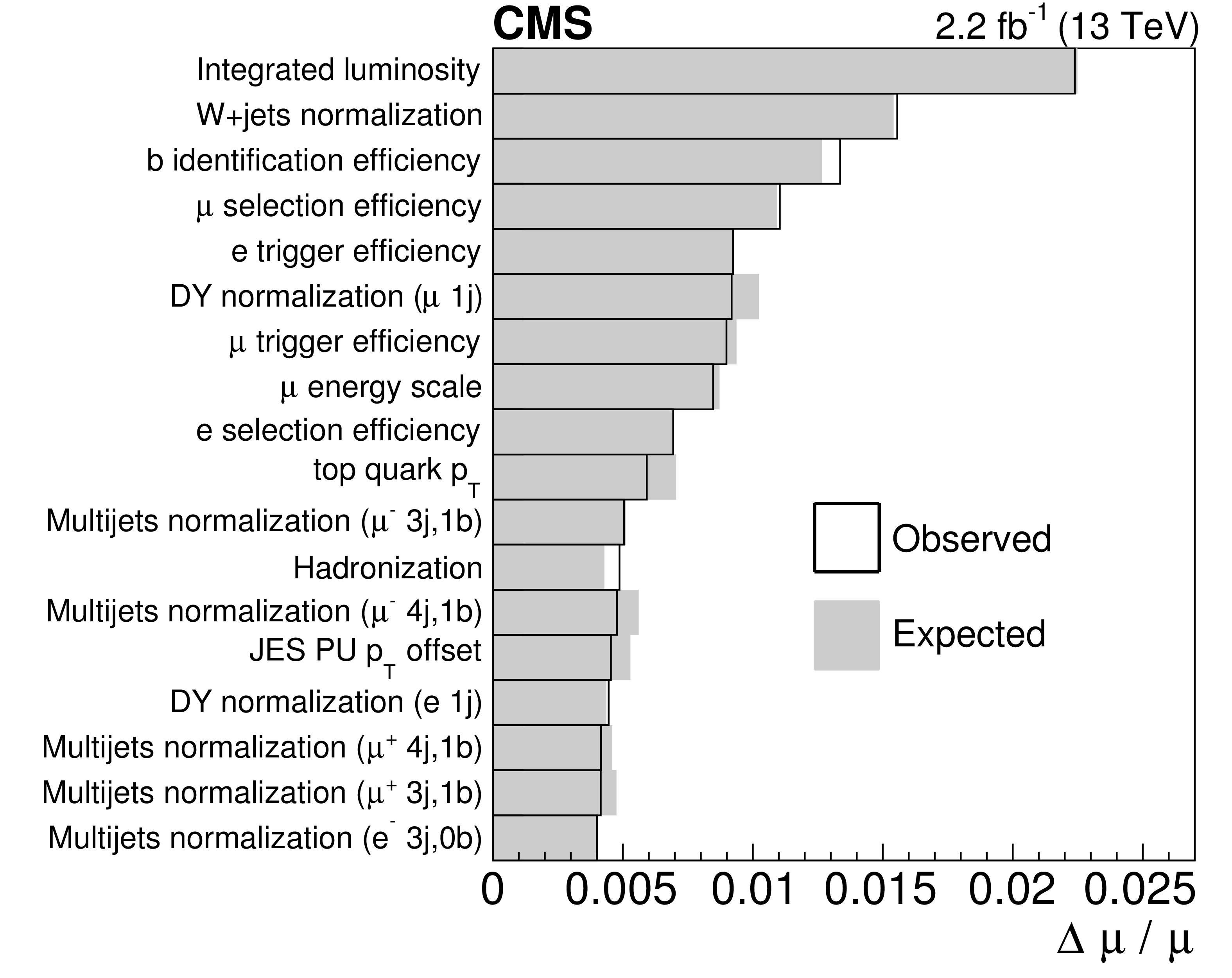
Figure 4:
Estimated change $\Delta \mu $ in the measured signal strength $\mu $, coming from the listed experimental and theoretical sources of uncertainties in the main analysis. The open bars represent the values of the observed impact relative to the fitted signal strength. The values are compared to the expectations (shaded bars) by performing the fit using simulated events with $m_\mathrm{ t } = $ 172.5 GeV. The various contributions are shown from the largest to the smallest observed impact. |
png pdf |
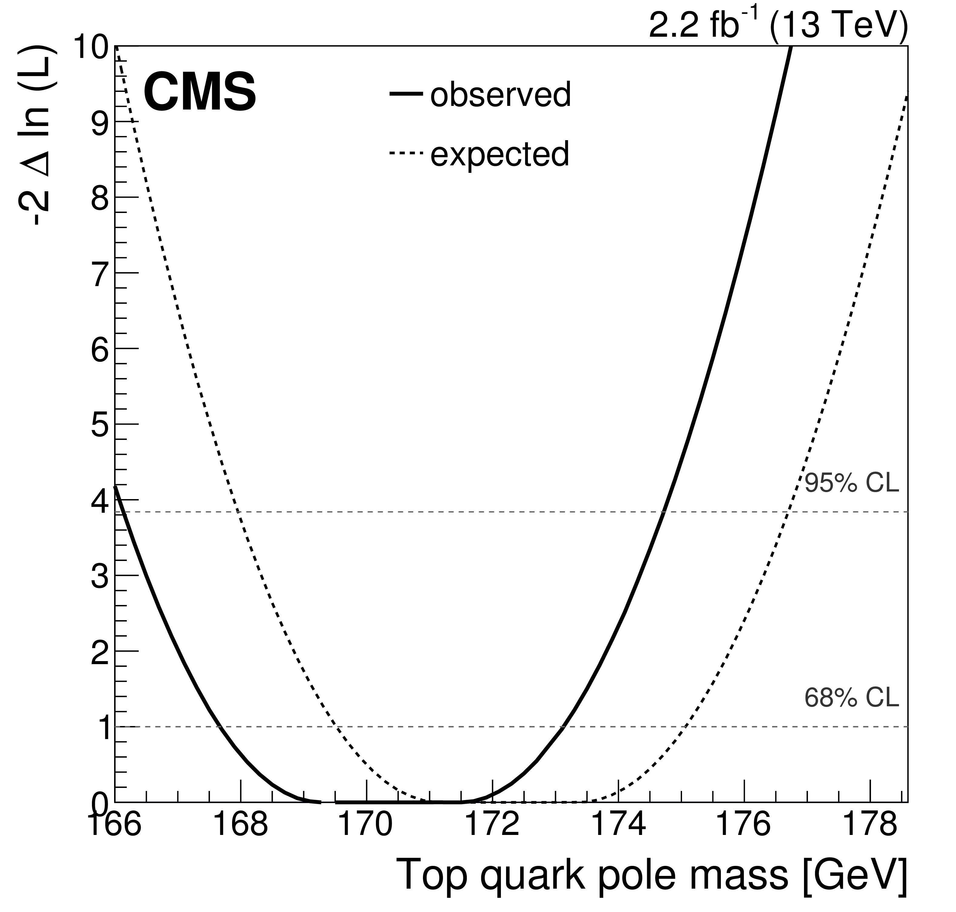
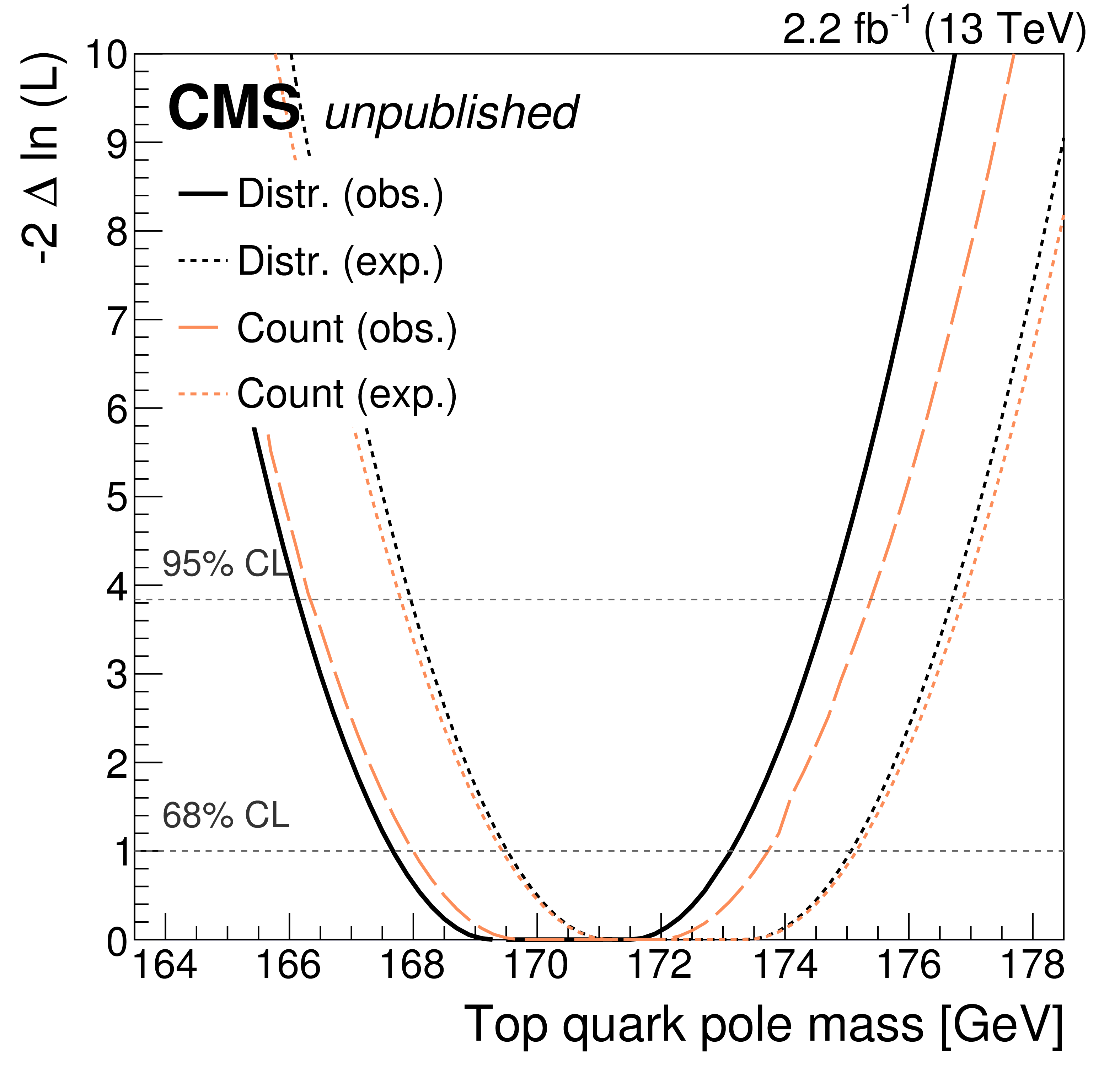
Figure 5:
Dependence of the likelihood on the top quark pole mass (solid curve). The expected dependence from the simulation, using the a priori set of nuisance parameters with their expected values at $m_\mathrm{ t } =$ 172.5 GeV, is shown for comparison as the dotted curve. The changes in the likelihood corresponding to the 68% and 95% confidence levels (CL) are shown by the dashed lines. |
| Tables | |
png pdf |
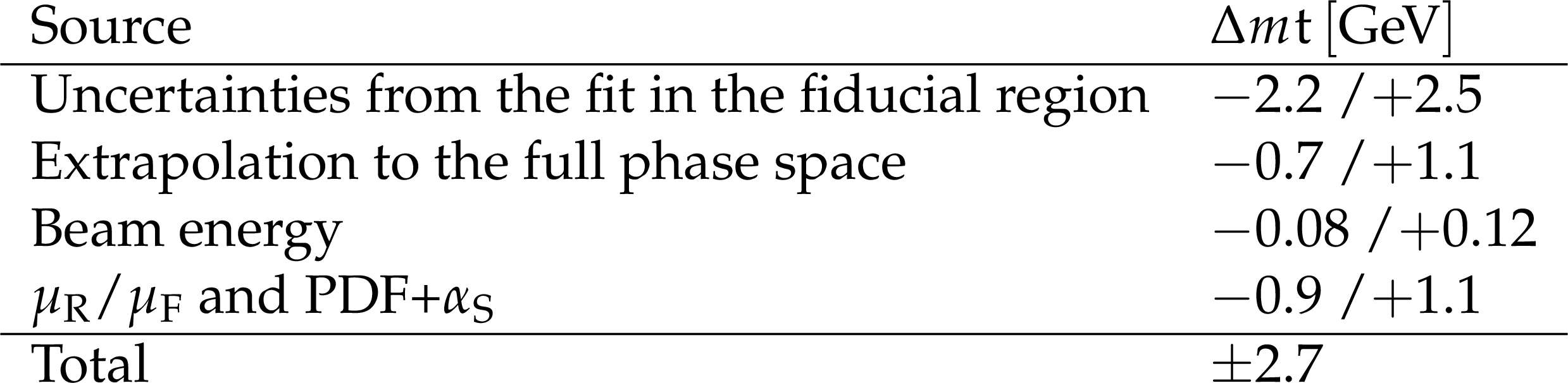
Table 1:
The source and value of the systematic uncertainties in the measurement of $m_\mathrm{ t } $. |
| Summary |
| A measurement of the $\mathrm{ t \bar{t} }$ production cross section at $\sqrt{s} =$ 13 TeV has been presented by CMS in final states containing one isolated lepton and at least one jet. The acceptance in the fiducial part of the phase space is estimated with an uncertainty of 1.6% and has a negligible dependence on $m_\mathrm{ t }$. By performing a simultaneous fit to event distributions in 44 independent categories, we measure the strength of the $\mathrm{ t \bar{t} }$ signal relative to the NNLO+NNLL computation [45] with an uncertainty of 3.9%. We obtain an inclusive $\mathrm{ t \bar{t} }$ production cross section $\sigma(\mathrm{ t \bar{t} })=$ 888 $\pm$ 2 (stat) $_{-26}^{+28}$ (syst) $\pm$ 20 (lumi) pb, which is compatible with the standard model prediction. In addition, the top quark pole mass, $m_\mathrm{ t }$, is extracted at NNLO using the same data and the CT14 PDF set and found to be $m_\mathrm{ t }=$ 170.6 $\pm$ 2.7 GeV. This value is in good agreement with measurements using other techniques. |
| Additional Figures | |
png pdf |
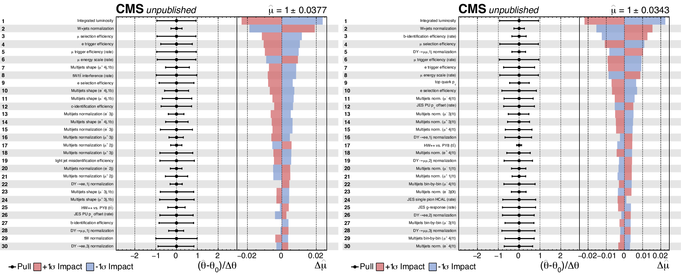
Additional Figure 1:
Summary of the impacts on $\delta \mu $ and pulls of the most significant nuisance parameters used in the count analysis (left) and in the analysis of distributions (right), when the fit is performed to the Asimov dataset for $m_\mathrm{ t } = $ 172.5 GeV is considered. In each plot the left panel shows the post-fit pull (value and uncertainty) of each nuisance, while the right panel displays the estimated impact on the fit for the signal strength. Only the first thirty nuisances are displayed, being their name shown at each row of the plots. |
png pdf |
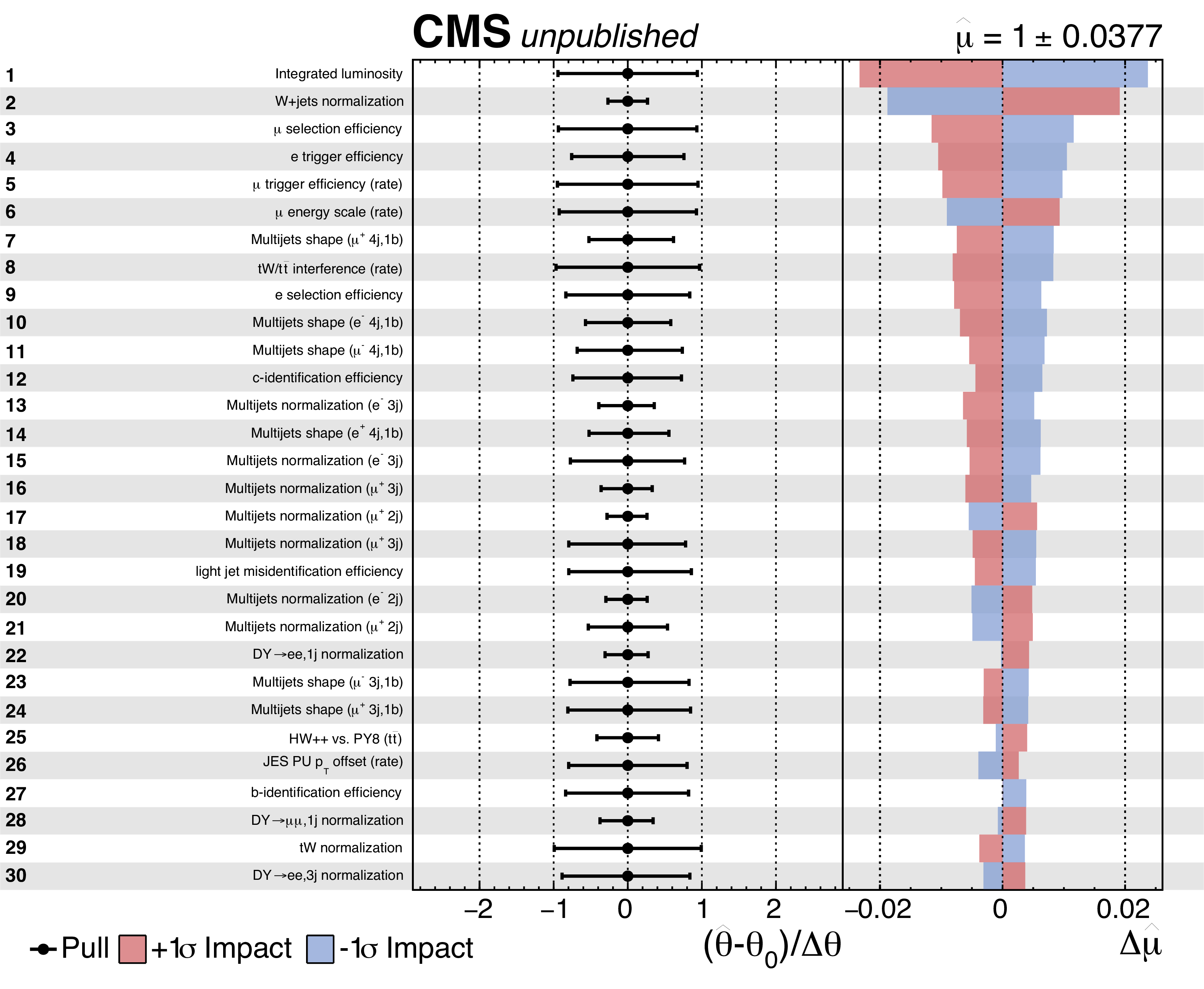
Additional Figure 1-a:
Summary of the impacts on $\delta \mu $ and pulls of the most significant nuisance parameters used in the count analysis, when the fit is performed to the Asimov dataset for $m_\mathrm{ t } = $ 172.5 GeV is considered. The left panel shows the post-fit pull (value and uncertainty) of each nuisance, while the right panel displays the estimated impact on the fit for the signal strength. Only the first thirty nuisances are displayed, being their name shown at each row of the plot. |
png pdf |
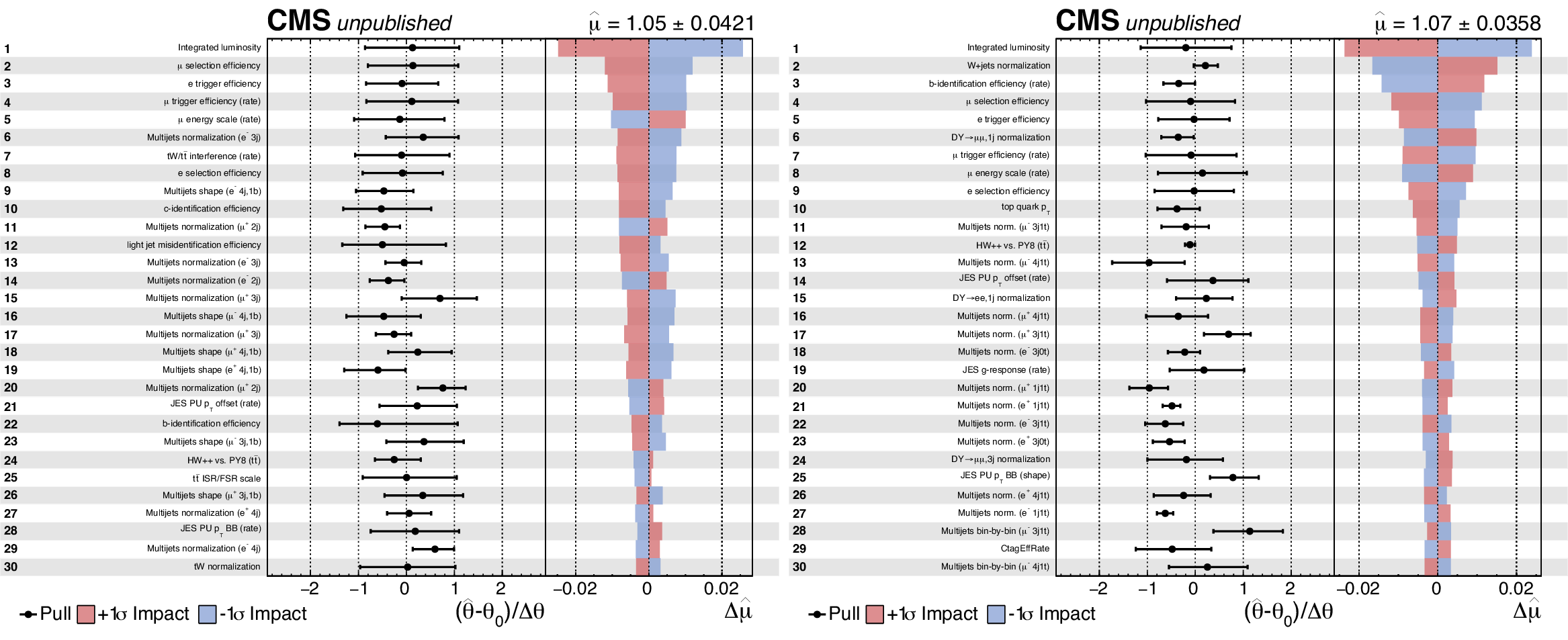
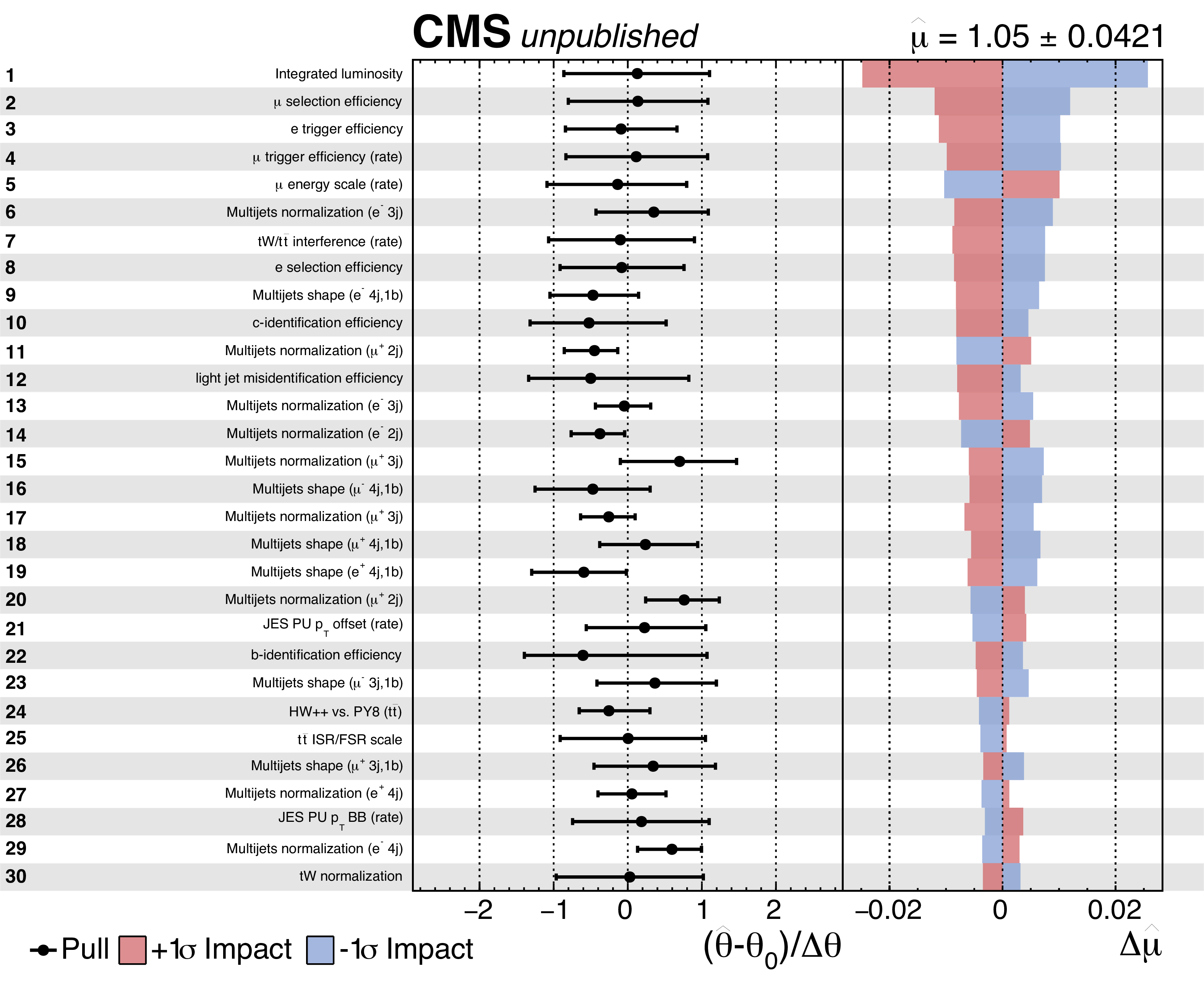
Additional Figure 1-b:
Summary of the impacts on $\delta \mu $ and pulls of the most significant nuisance parameters used in the analysis of distributions, when the fit is performed to the Asimov dataset for $m_\mathrm{ t } = $ 172.5 GeV is considered. The left panel shows the post-fit pull (value and uncertainty) of each nuisance, while the right panel displays the estimated impact on the fit for the signal strength. Only the first thirty nuisances are displayed, being their name shown at each row of the plot. |
png pdf |
Additional Figure 2:
Summary of the impacts on $\delta \mu $ and pulls of the most significant nuisance parameters used in the count analysis (left) and in the analysis of distributions (right), when the fit is performed to the data. In each plot the left panel shows the post-fit pull (value and uncertainty) of each nuisance, while the right panel displays the estimated impact on the fit for the signal strength. Only the first thirty nuisances are displayed, being their name shown at each row of the plots. |
png pdf |
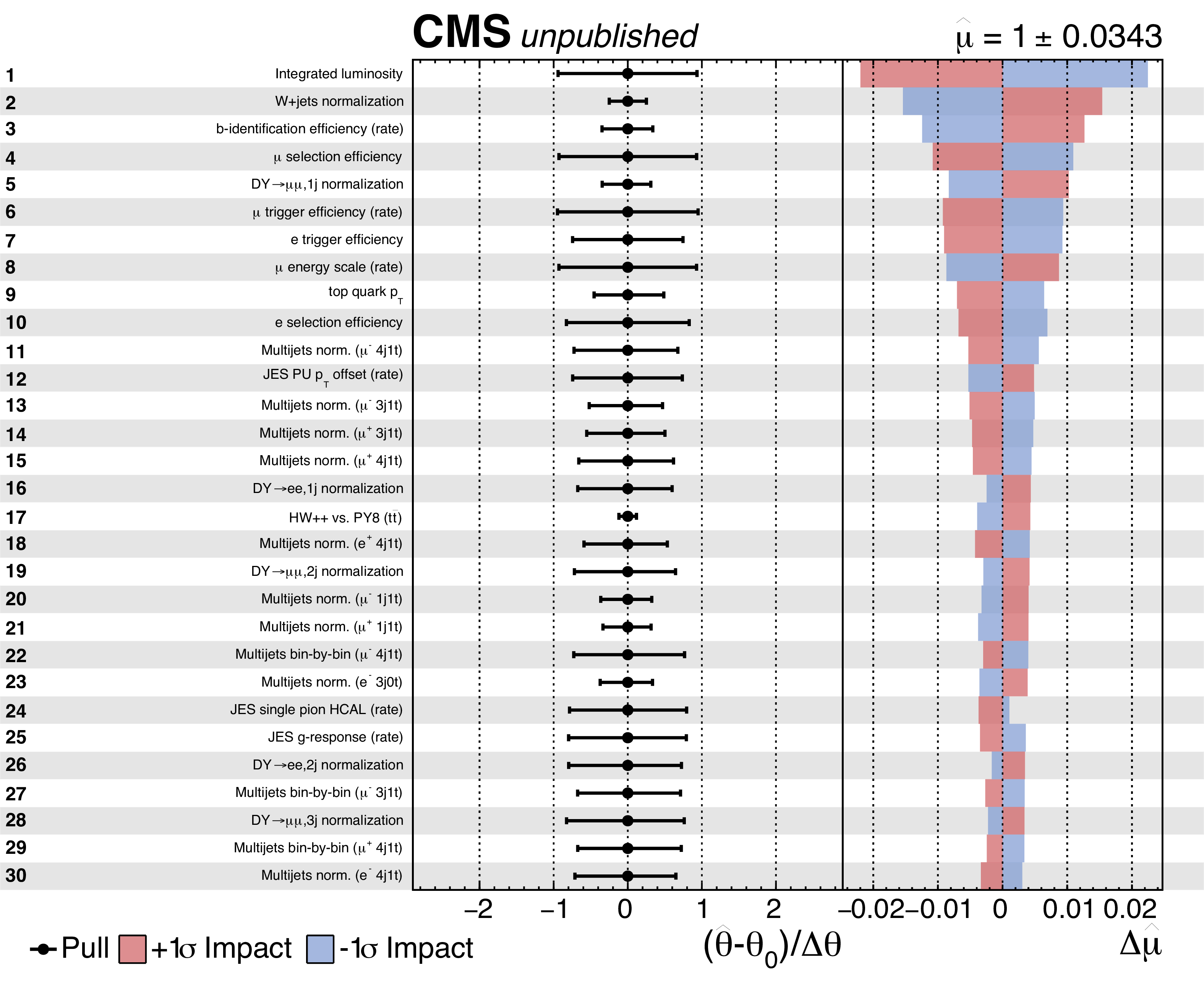
Additional Figure 2-a:
Summary of the impacts on $\delta \mu $ and pulls of the most significant nuisance parameters used in the count analysis, when the fit is performed to the data. The left panel shows the post-fit pull (value and uncertainty) of each nuisance, while the right panel displays the estimated impact on the fit for the signal strength. Only the first thirty nuisances are displayed, being their name shown at each row of the plot. |
png pdf |
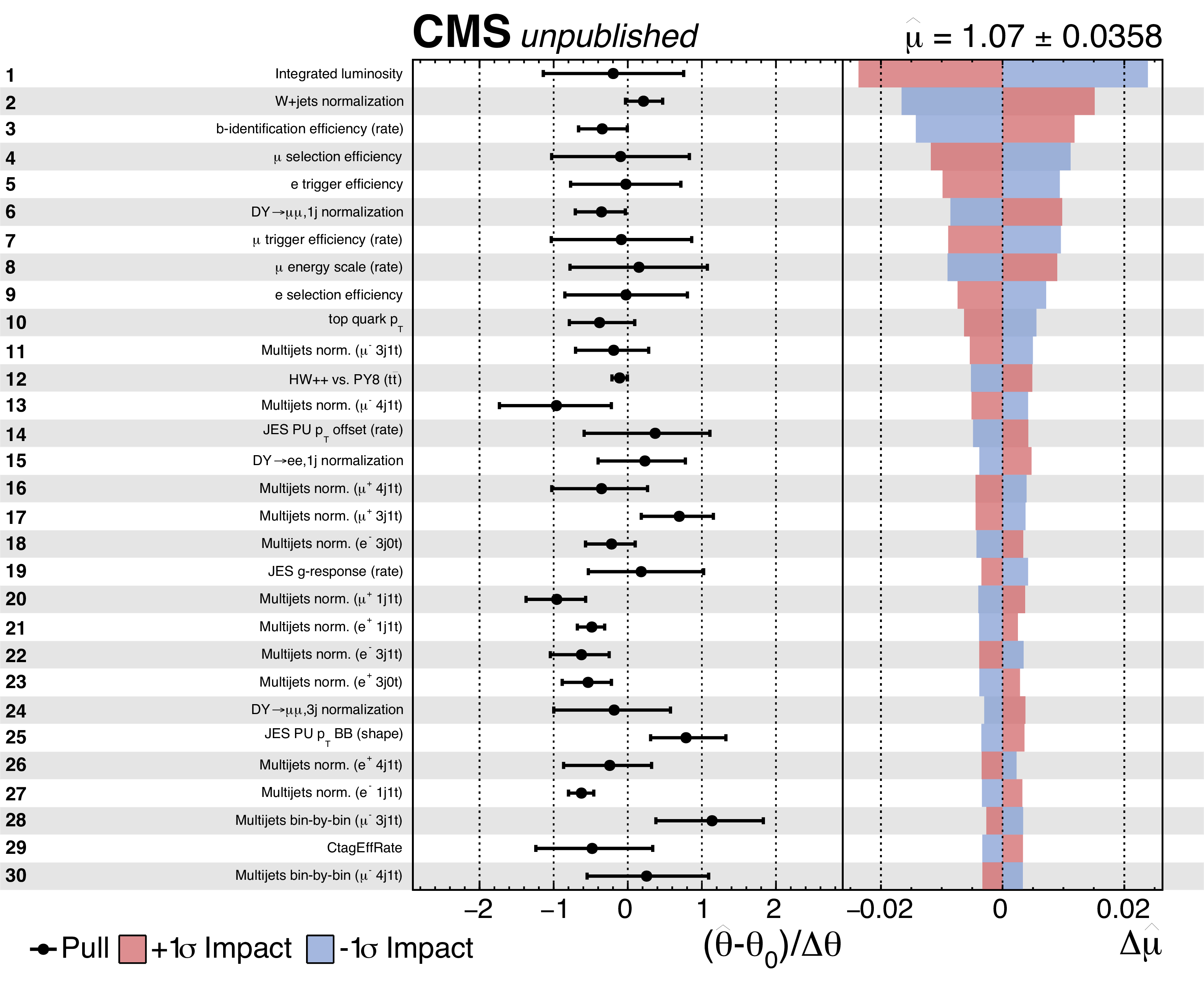
Additional Figure 2-b:
Summary of the impacts on $\delta \mu $ and pulls of the most significant nuisance parameters used in the analysis of distributions, when the fit is performed to the data. The left panel shows the post-fit pull (value and uncertainty) of each nuisance, while the right panel displays the estimated impact on the fit for the signal strength. Only the first thirty nuisances are displayed, being their name shown at each row of the plot. |

png pdf |
Additional Figure 3:
Correlation matrix after the fit is performed to the data for the nuisance parameters with most significant impact on the signal strength. The matrix obtained for the count analysis is shown on the left, while the one obtained for the analysis of distributions is shown on the right. |

png pdf |
Additional Figure 3-a:
Correlation matrix after the fit is performed to the data for the nuisance parameters with most significant impact on the signal strength, as obtained for the count analysis. |
png pdf |
Additional Figure 3-b:
Correlation matrix after the fit is performed to the data for the nuisance parameters with most significant impact on the signal strength, as obtained for the analysis of distributions. |
png pdf |
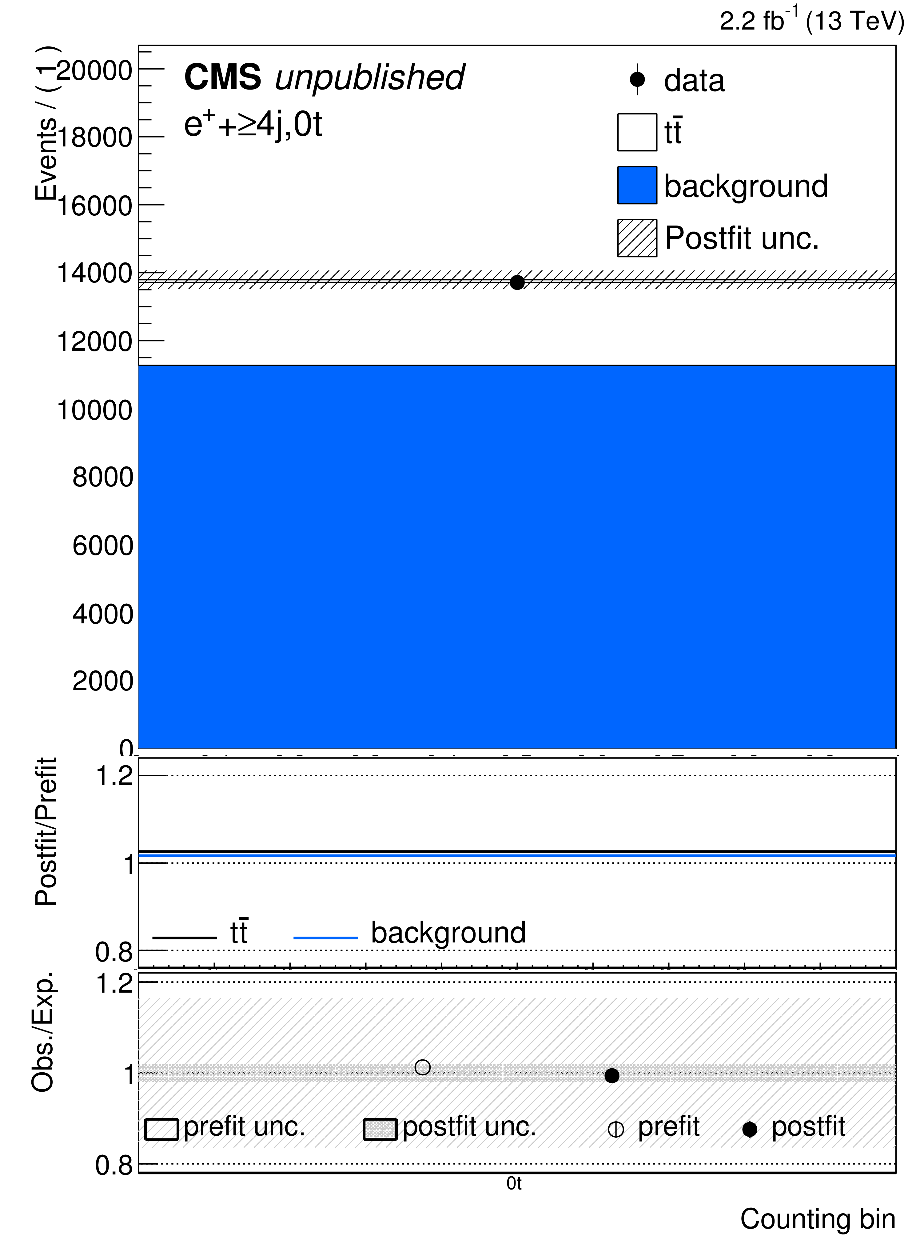
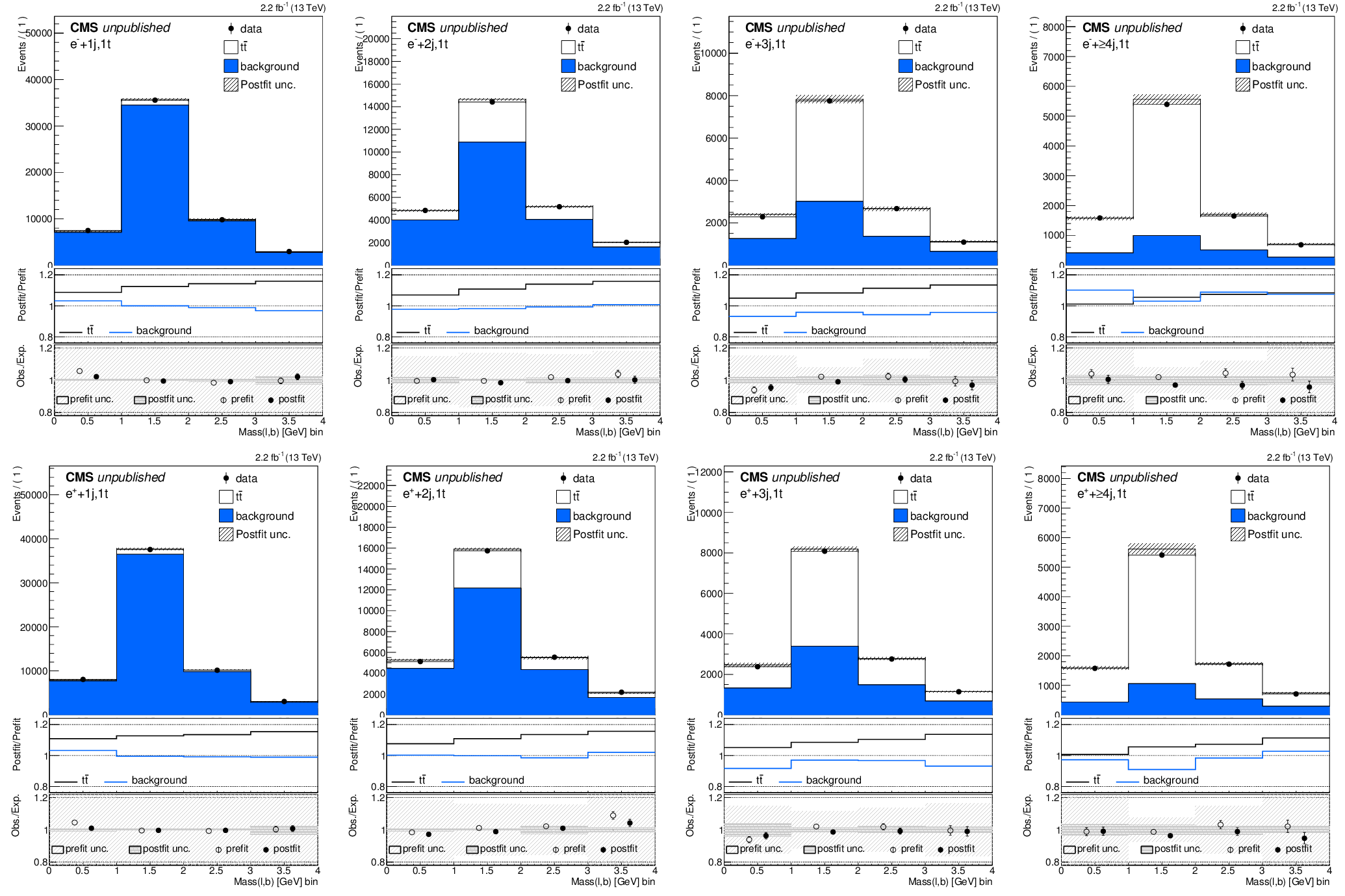
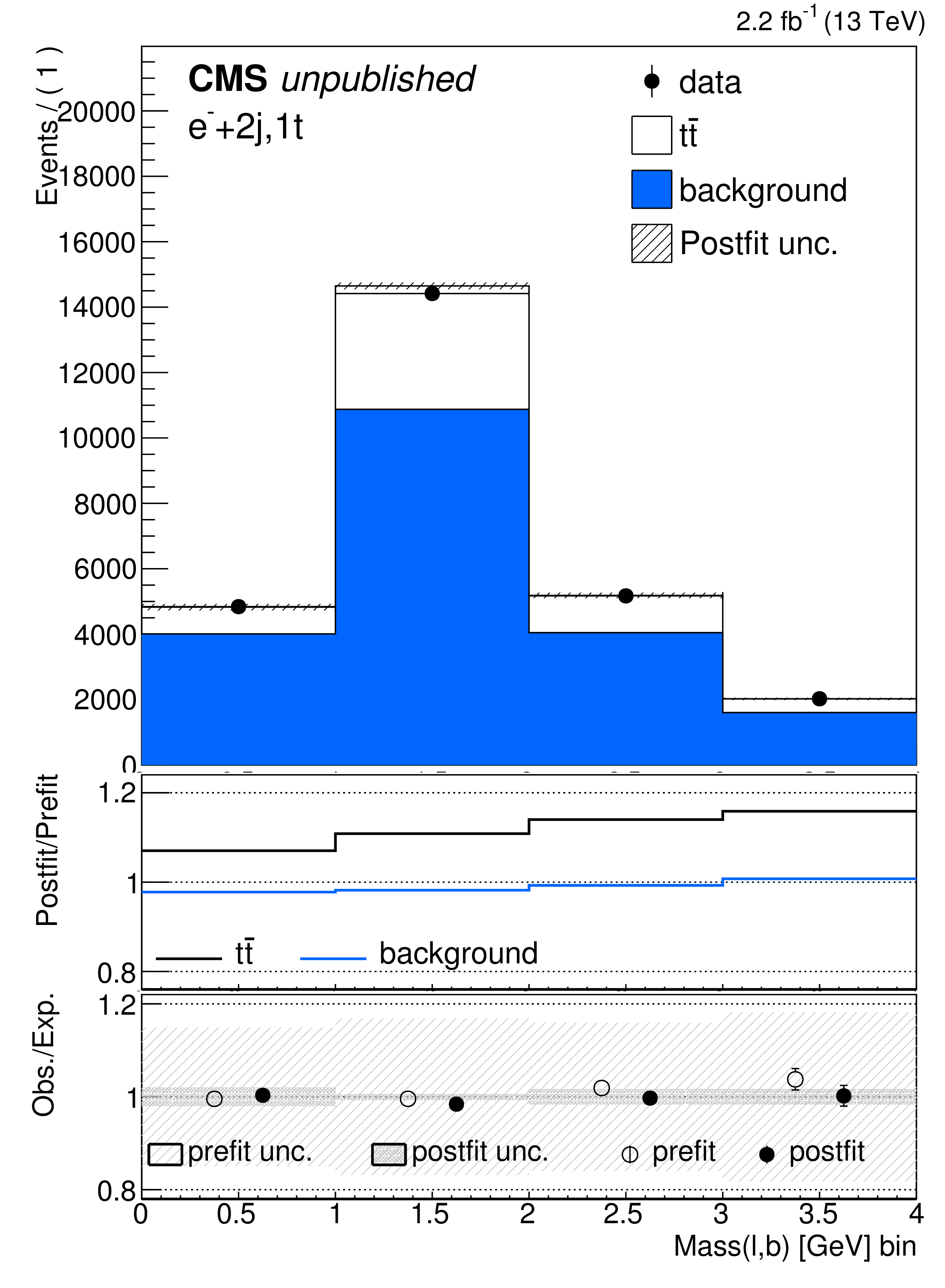
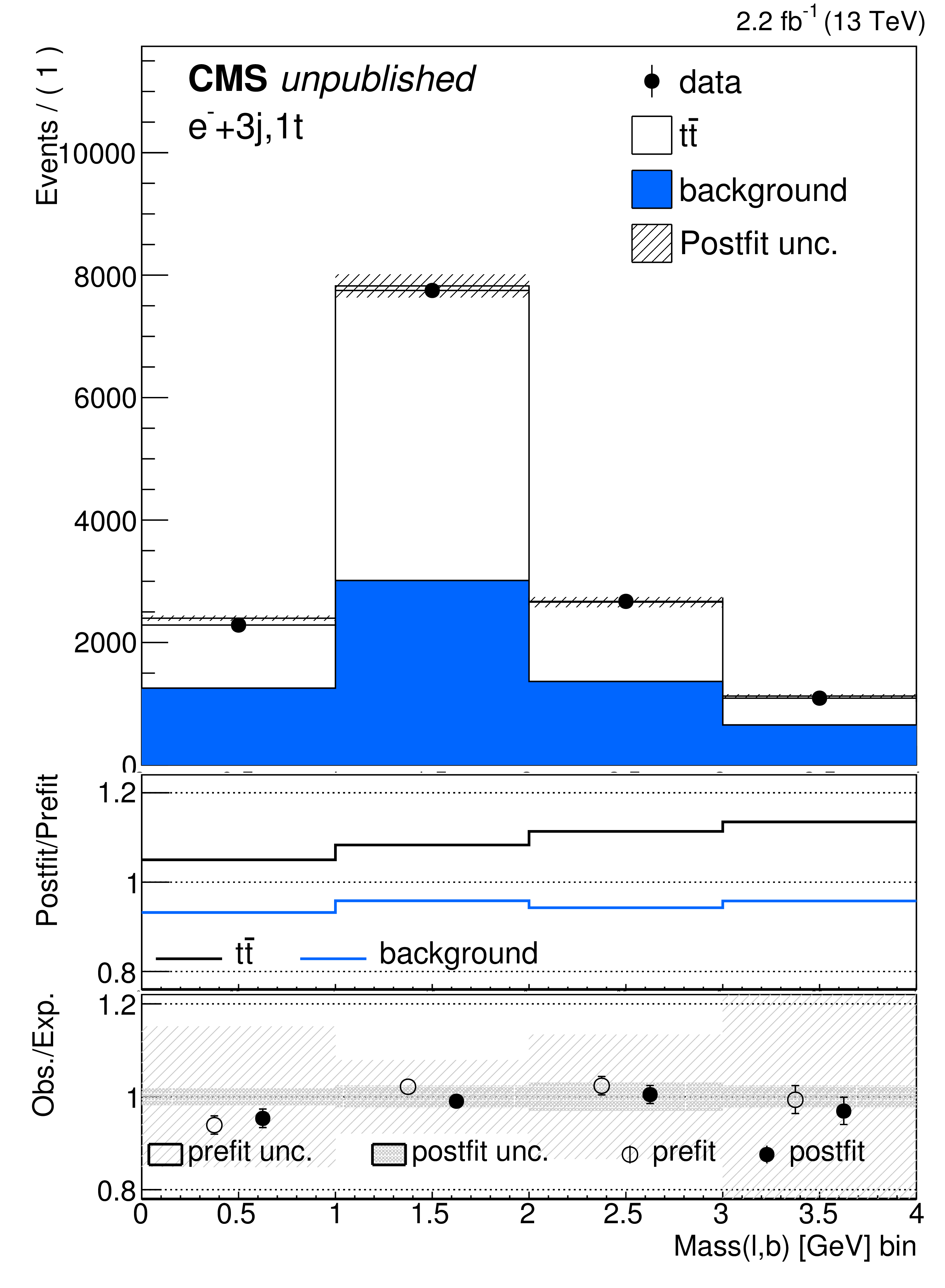
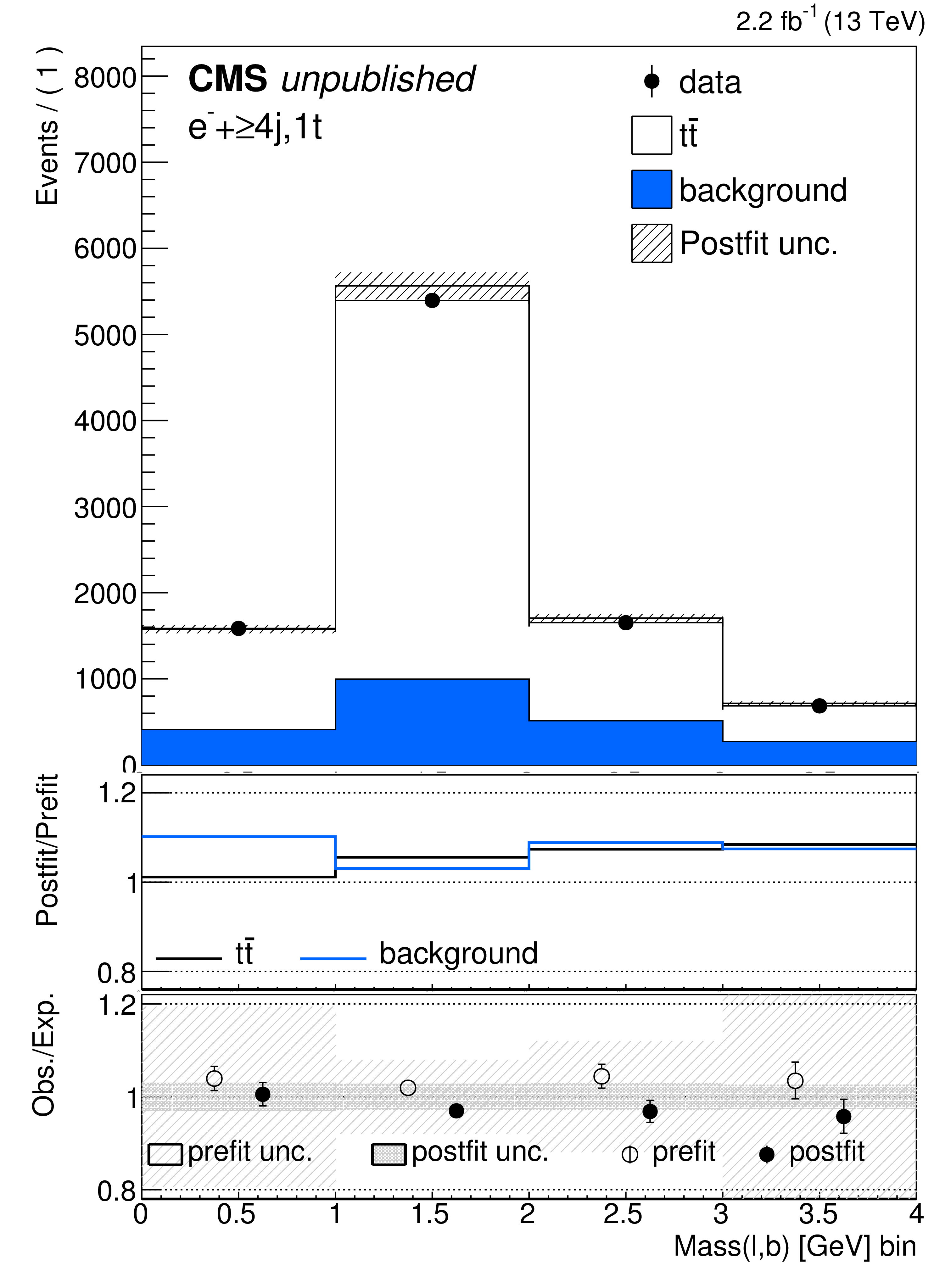
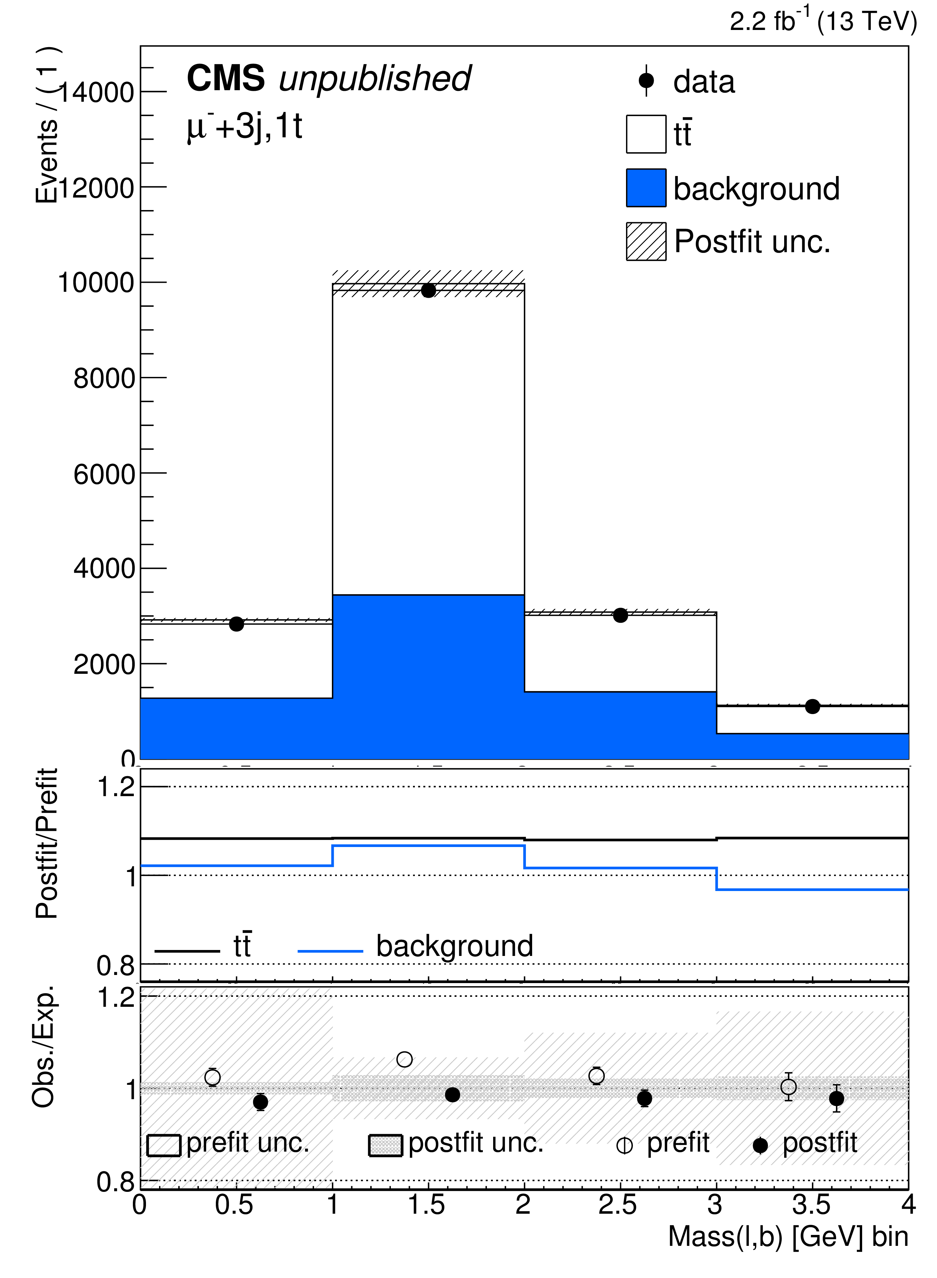
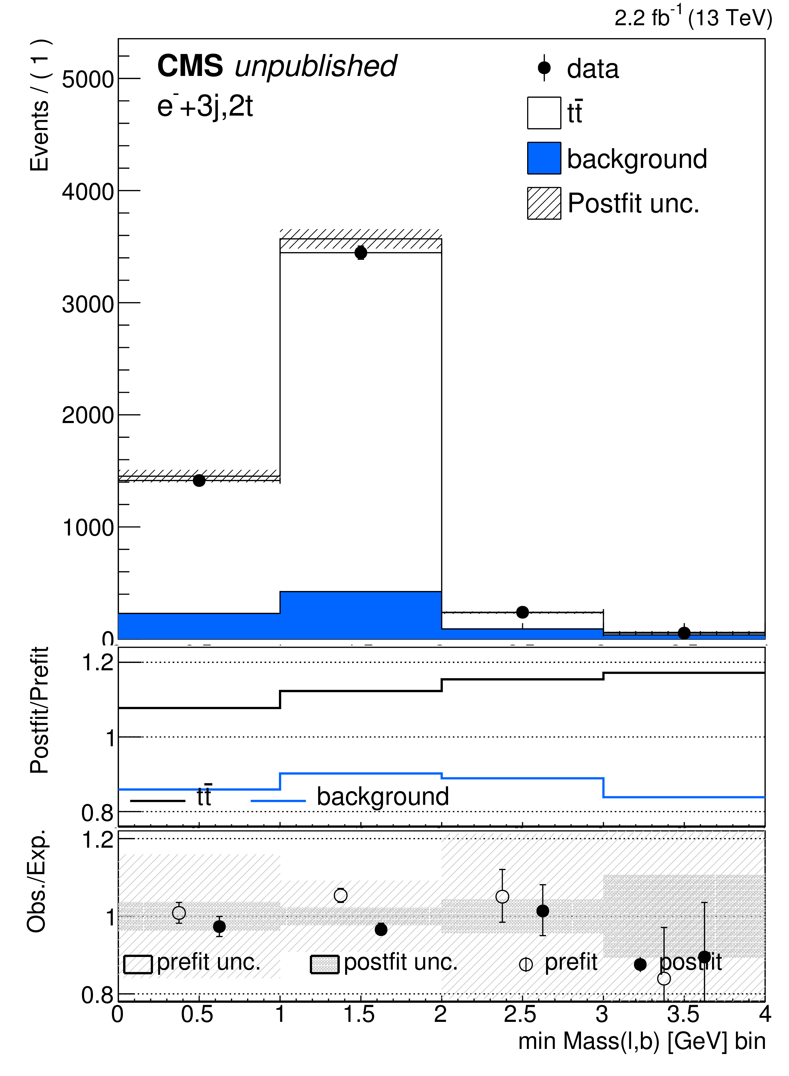
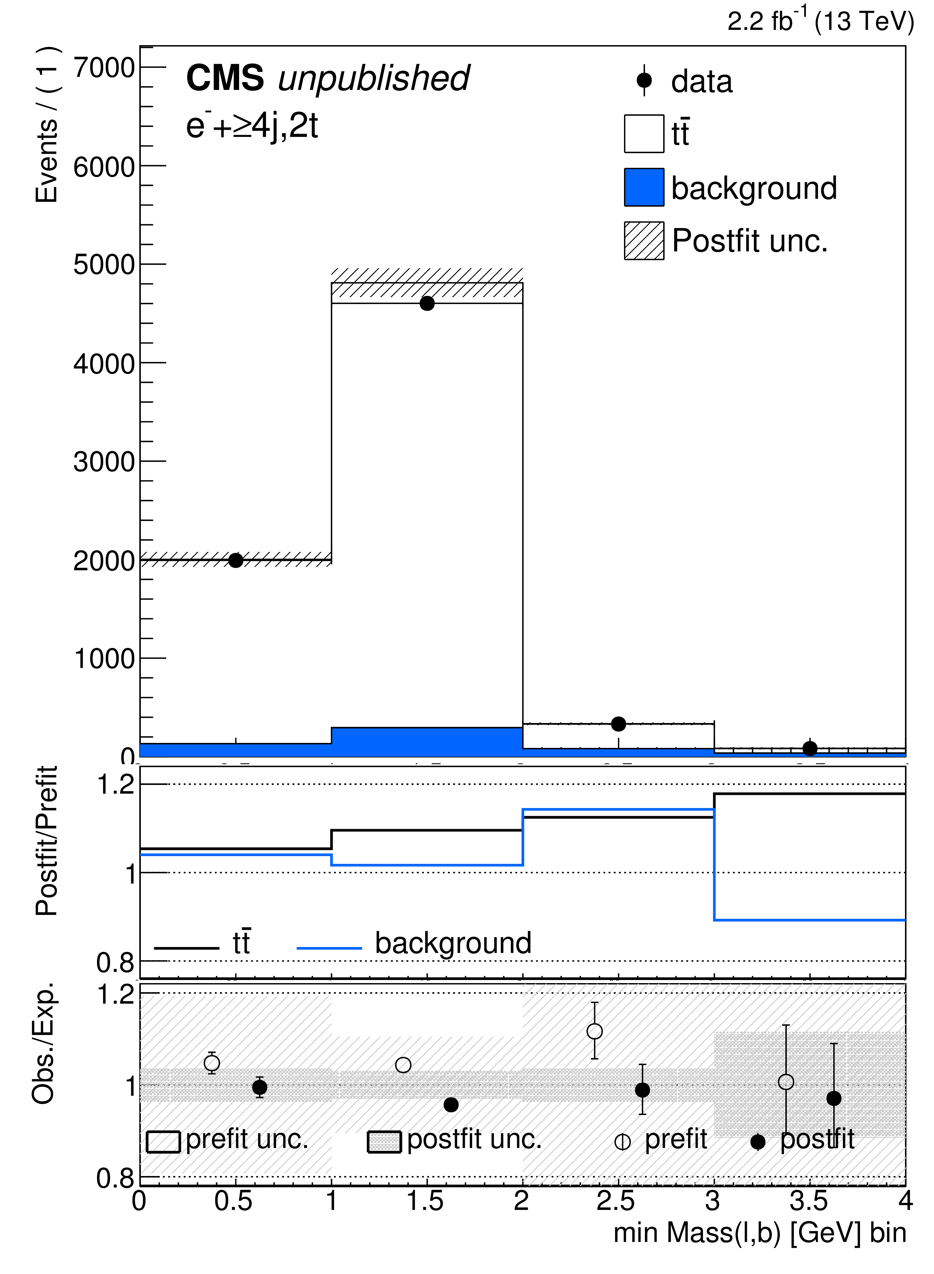
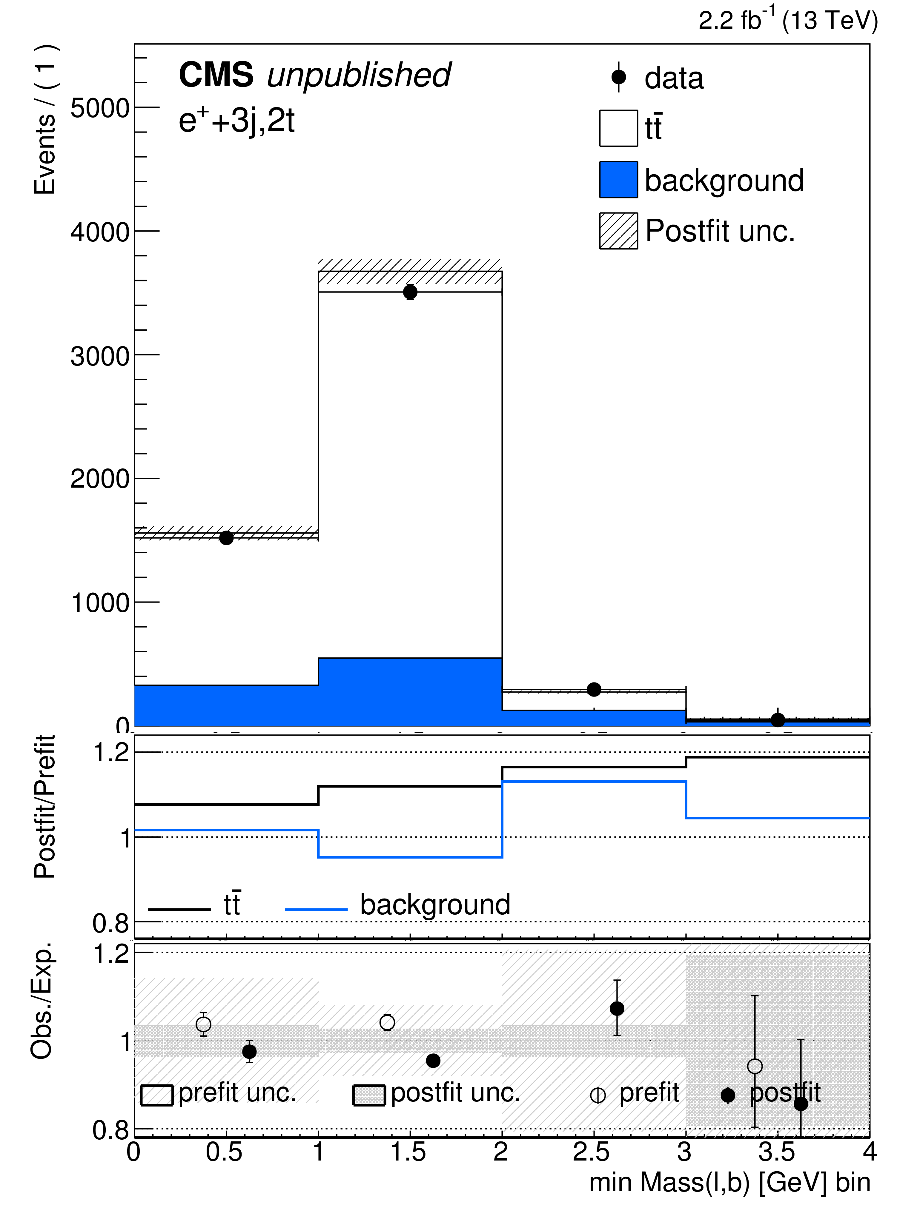
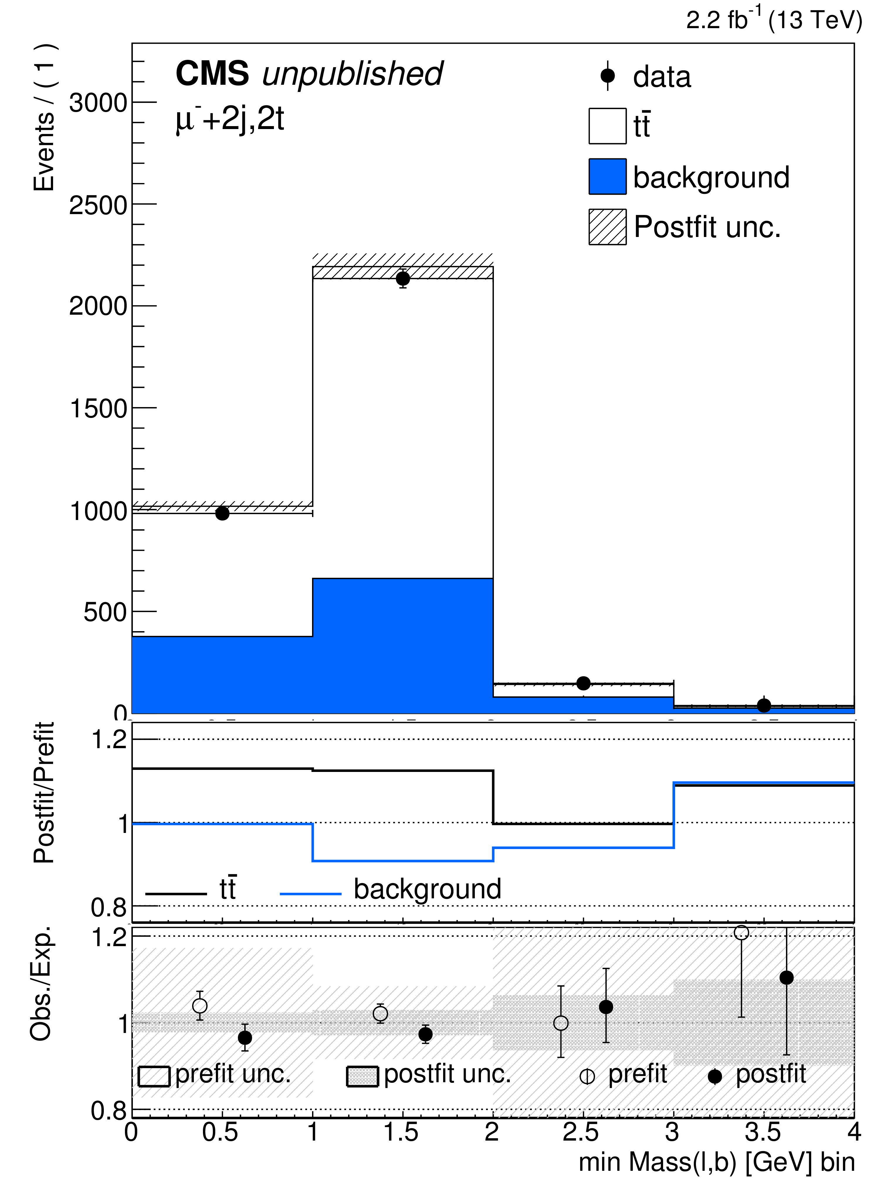
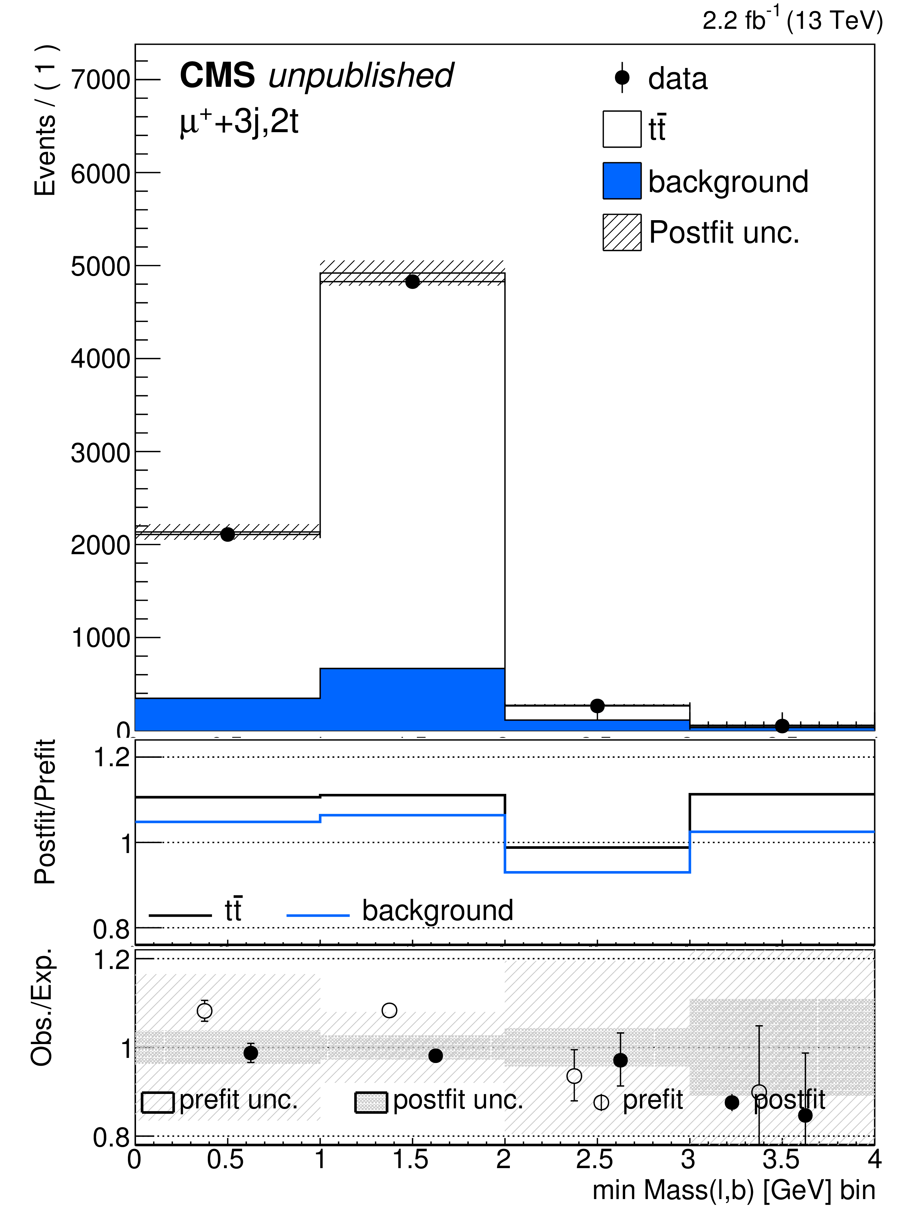
Additional Figure 4:
Comparison of the post-fit distributions with the data for electron events with no b-tagged jet. Negatively (positively) charged electrons are shown on the top (bottom) row. From left to right events with one, two, three or at least four jets are shown. The top panels show the stacked distributions of signal and background processes and the observed data. A shaded band represents the post-fit uncertainty. The middle panels show the ratio of the post-fit to pre-fit distributions for the signal and background sum. The bottom panel shows the data to signal plus background expectations, prior and after the fit. The error bar in the points is the statistics in data. A shaded band represents the relative postfit and prefit uncertainties. |
png pdf |
Additional Figure 4-a:
Comparison of the post-fit distributions with the data for electron events with no b-tagged jet. Events with a negatively charged electron and one jet are shown. The top panel shows the stacked distributions of signal and background processes and the observed data. A shaded band represents the post-fit uncertainty. The middle panel shows the ratio of the post-fit to pre-fit distributions for the signal and background sum. The bottom panel shows the data to signal plus background expectations, prior and after the fit. The error bar in the points is the statistics in data. A shaded band represents the relative postfit and prefit uncertainties. |

png pdf |
Additional Figure 4-b:
Comparison of the post-fit distributions with the data for electron events with no b-tagged jet. Events with a negatively charged electron and two jets are shown. The top panel shows the stacked distributions of signal and background processes and the observed data. A shaded band represents the post-fit uncertainty. The middle panel shows the ratio of the post-fit to pre-fit distributions for the signal and background sum. The bottom panel shows the data to signal plus background expectations, prior and after the fit. The error bar in the points is the statistics in data. A shaded band represents the relative postfit and prefit uncertainties. |

png pdf |
Additional Figure 4-c:
Comparison of the post-fit distributions with the data for electron events with no b-tagged jet. Events with a negatively charged electron and three jets are shown. The top panel shows the stacked distributions of signal and background processes and the observed data. A shaded band represents the post-fit uncertainty. The middle panel shows the ratio of the post-fit to pre-fit distributions for the signal and background sum. The bottom panel shows the data to signal plus background expectations, prior and after the fit. The error bar in the points is the statistics in data. A shaded band represents the relative postfit and prefit uncertainties. |

png pdf |
Additional Figure 4-d:
Comparison of the post-fit distributions with the data for electron events with no b-tagged jet. Events with a negatively charged electron and at least four jets are shown. The top panel shows the stacked distributions of signal and background processes and the observed data. A shaded band represents the post-fit uncertainty. The middle panel shows the ratio of the post-fit to pre-fit distributions for the signal and background sum. The bottom panel shows the data to signal plus background expectations, prior and after the fit. The error bar in the points is the statistics in data. A shaded band represents the relative postfit and prefit uncertainties. |

png pdf |
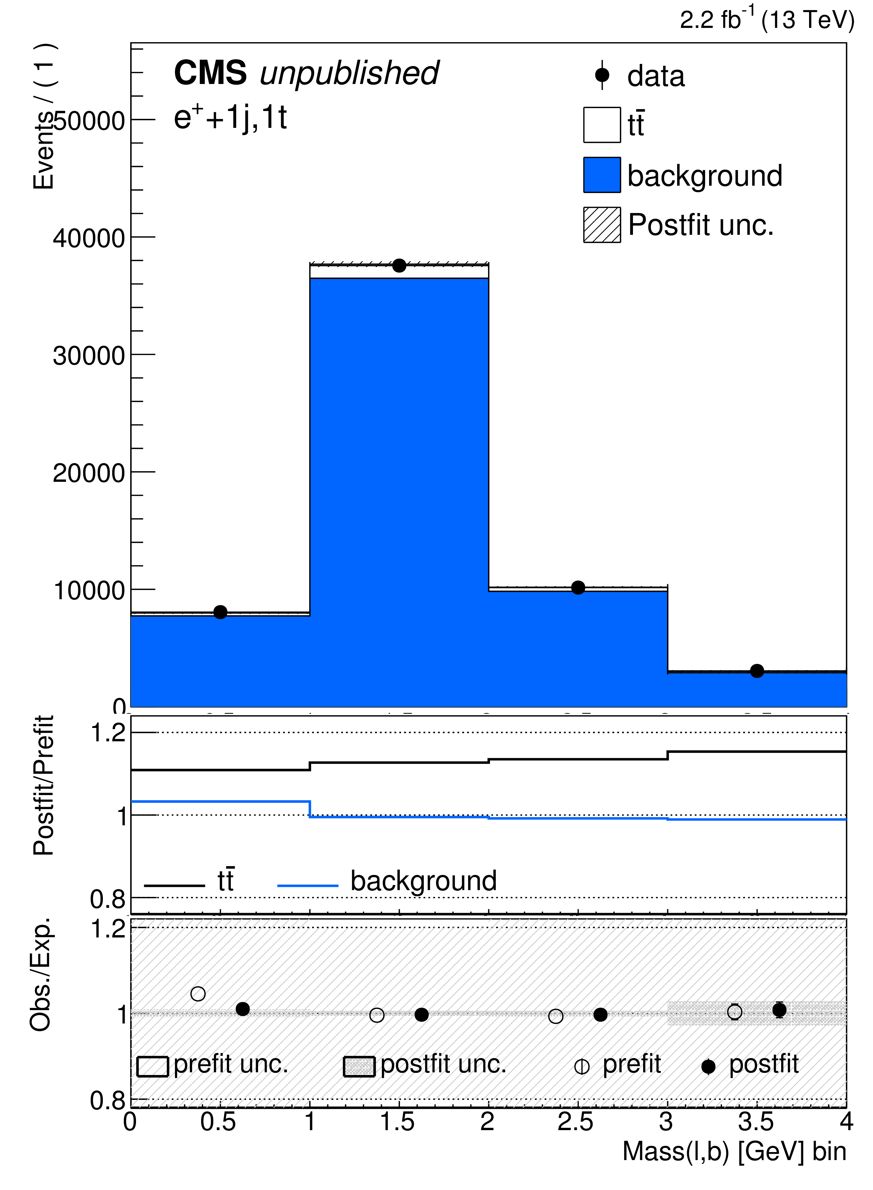
Additional Figure 4-e:
Comparison of the post-fit distributions with the data for electron events with no b-tagged jet. Positively charged electrons for events with one jet are shown. The top panel shows the stacked distributions of signal and background processes and the observed data. A shaded band represents the post-fit uncertainty. The middle panel shows the ratio of the post-fit to pre-fit distributions for the signal and background sum. The bottom panel shows the data to signal plus background expectations, prior and after the fit. The error bar in the points is the statistics in data. A shaded band represents the relative postfit and prefit uncertainties. |

png pdf |
Additional Figure 4-f:
Comparison of the post-fit distributions with the data for electron events with no b-tagged jet. Positively charged electrons for events with two jets are shown. The top panel shows the stacked distributions of signal and background processes and the observed data. A shaded band represents the post-fit uncertainty. The middle panel shows the ratio of the post-fit to pre-fit distributions for the signal and background sum. The bottom panel shows the data to signal plus background expectations, prior and after the fit. The error bar in the points is the statistics in data. A shaded band represents the relative postfit and prefit uncertainties. |
png pdf |
Additional Figure 4-g:
Comparison of the post-fit distributions with the data for electron events with no b-tagged jet. Positively charged electrons for events with three jets are shown. The top panel shows the stacked distributions of signal and background processes and the observed data. A shaded band represents the post-fit uncertainty. The middle panel shows the ratio of the post-fit to pre-fit distributions for the signal and background sum. The bottom panel shows the data to signal plus background expectations, prior and after the fit. The error bar in the points is the statistics in data. A shaded band represents the relative postfit and prefit uncertainties. |
png pdf |
Additional Figure 4-h:
Comparison of the post-fit distributions with the data for electron events with no b-tagged jet. Positively charged electrons for events with at least four jets are shown. The top panel shows the stacked distributions of signal and background processes and the observed data. A shaded band represents the post-fit uncertainty. The middle panel shows the ratio of the post-fit to pre-fit distributions for the signal and background sum. The bottom panel shows the data to signal plus background expectations, prior and after the fit. The error bar in the points is the statistics in data. A shaded band represents the relative postfit and prefit uncertainties. |
png pdf |
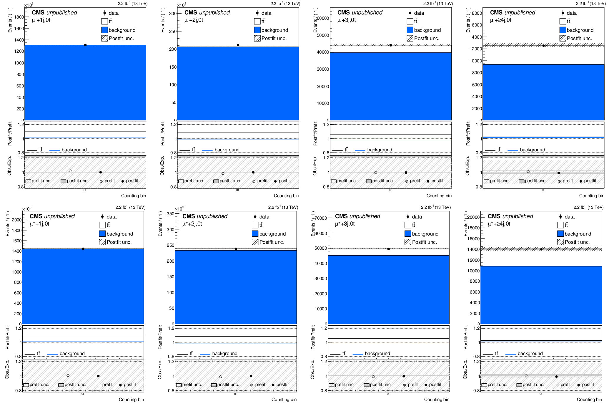
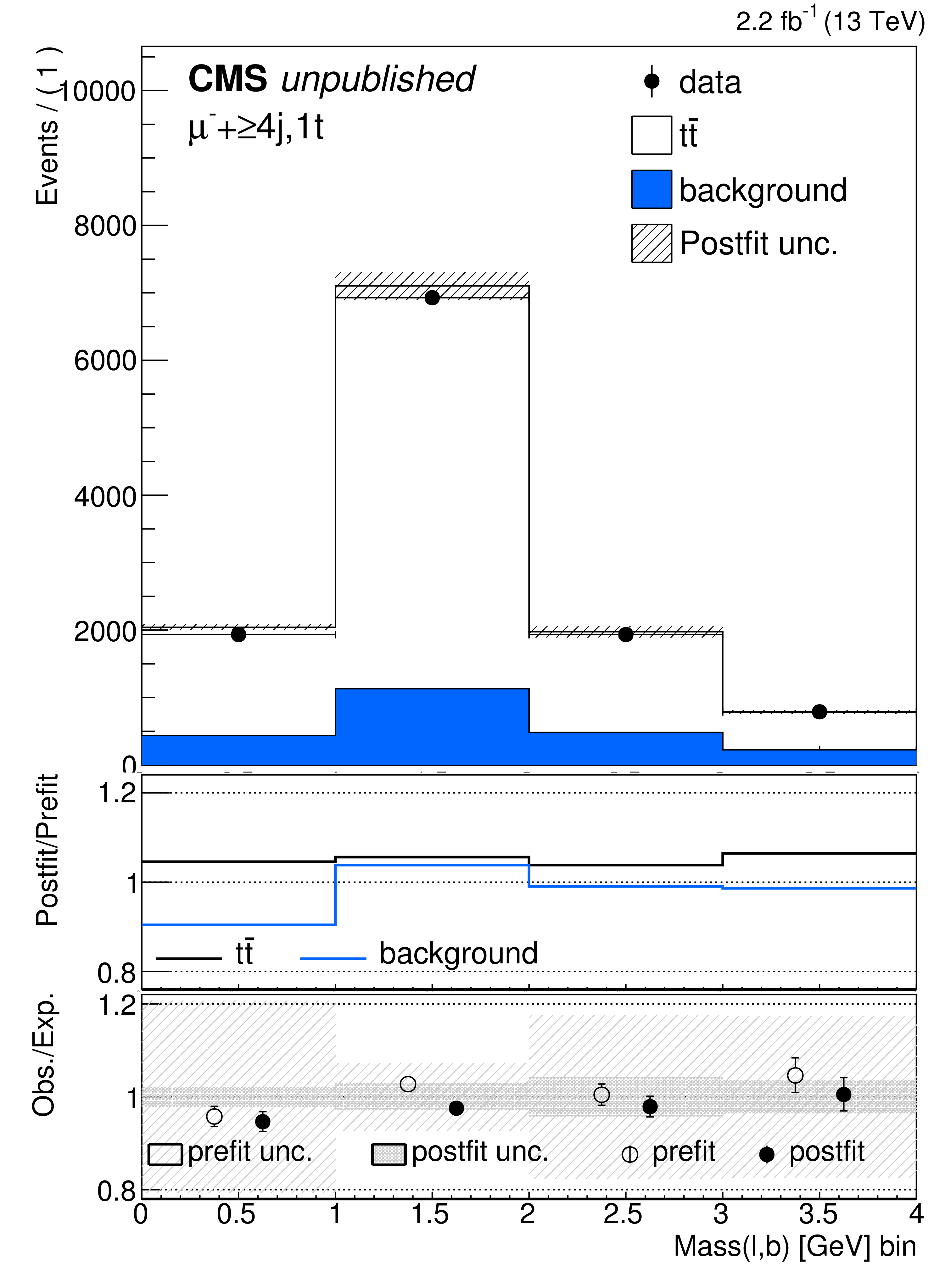
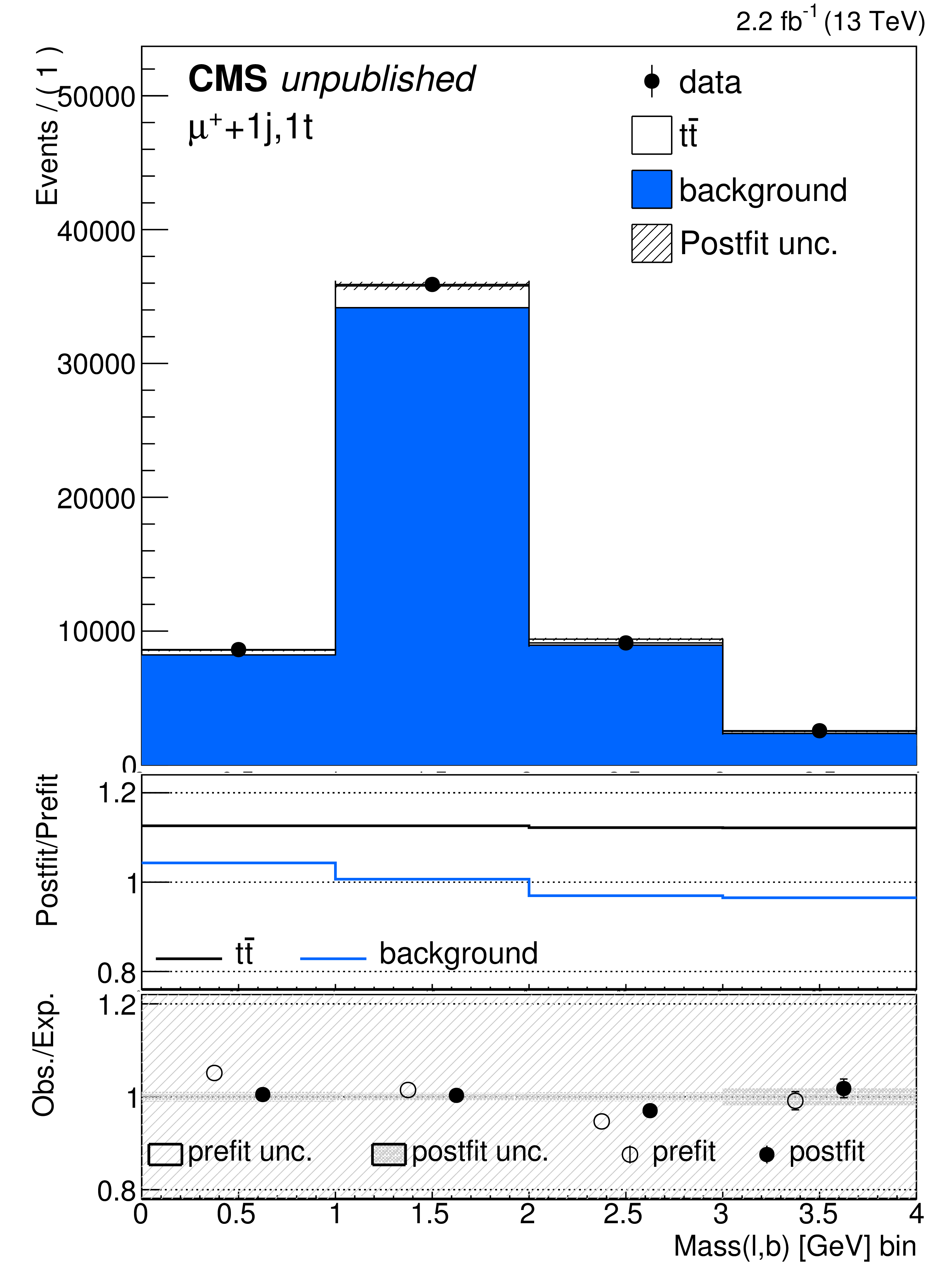
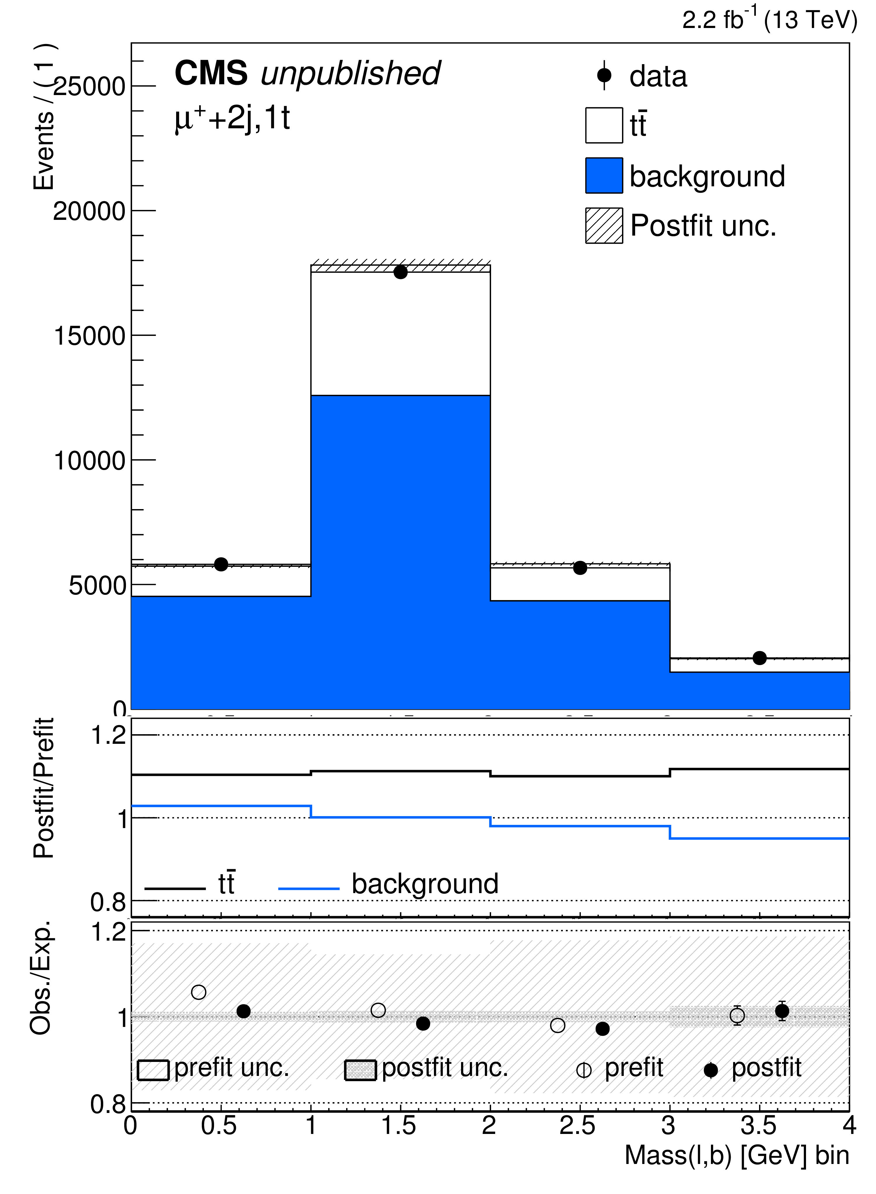
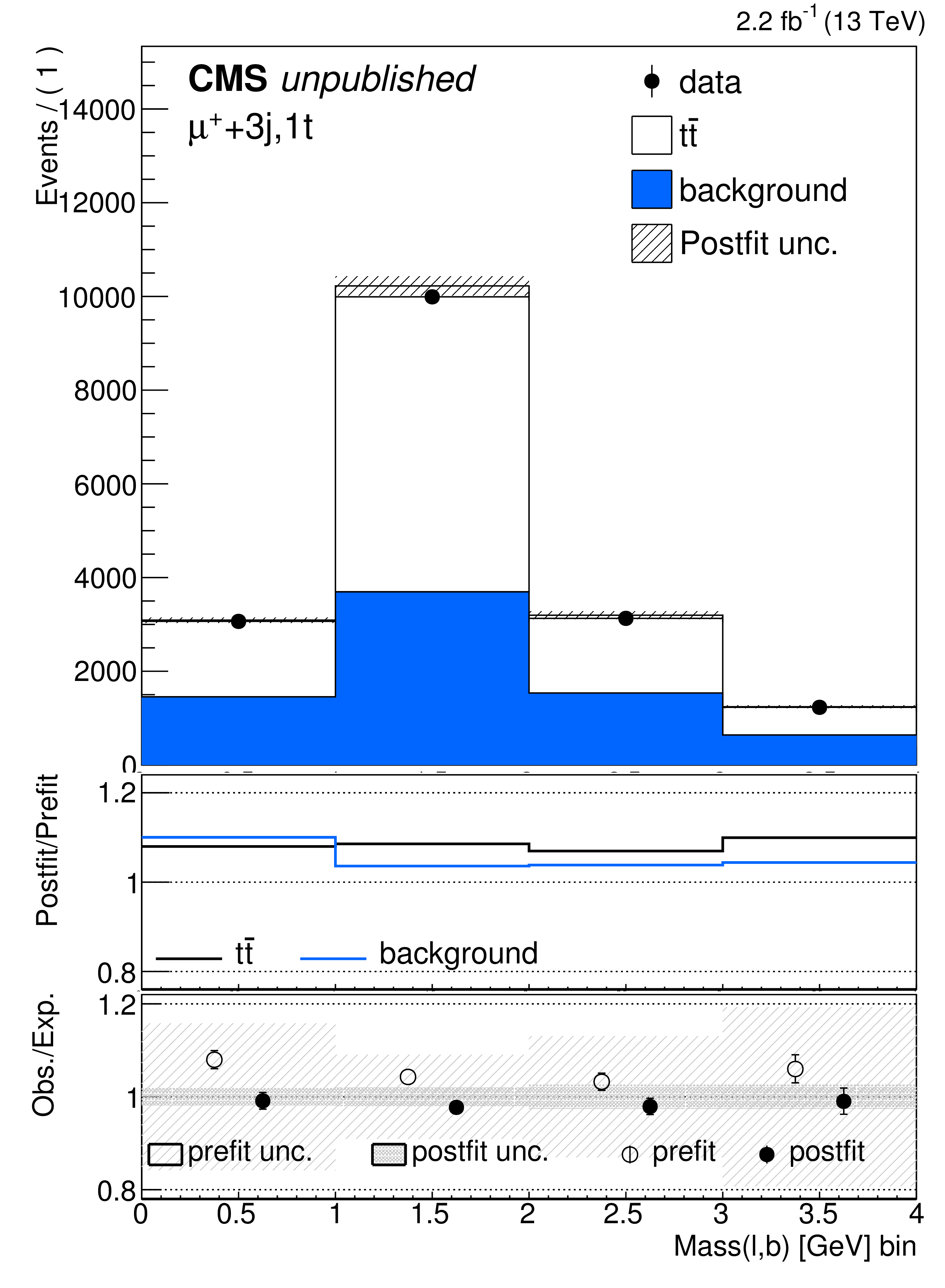
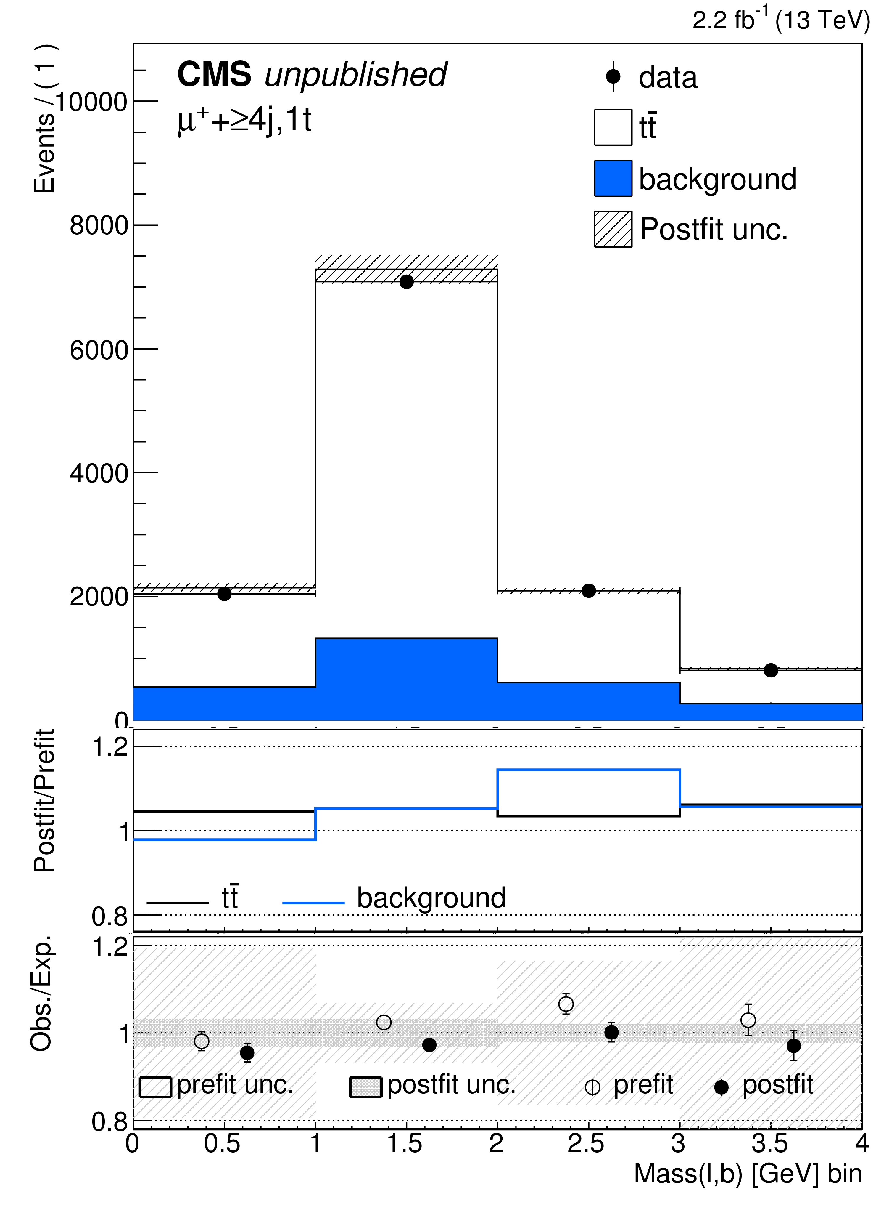
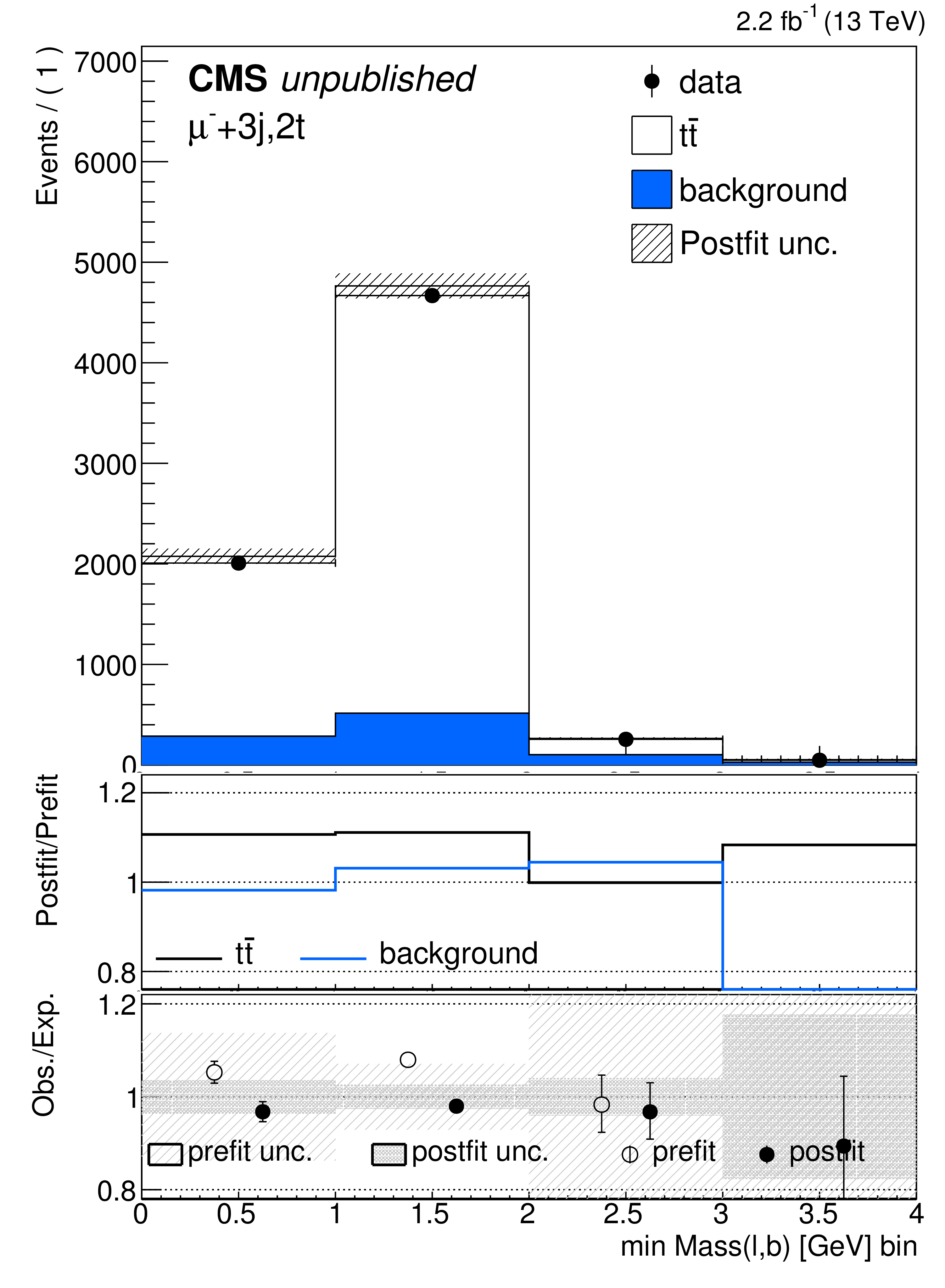
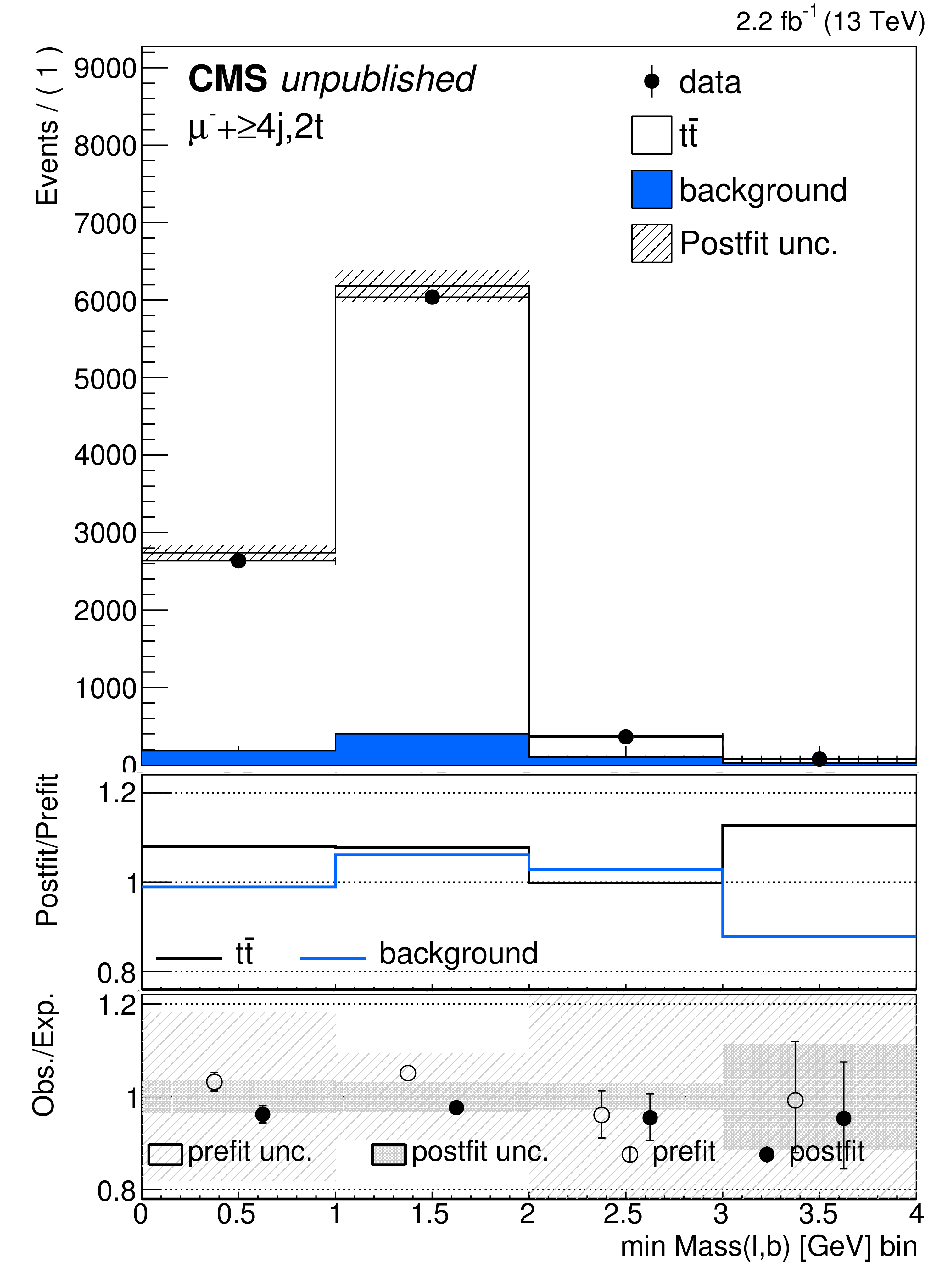
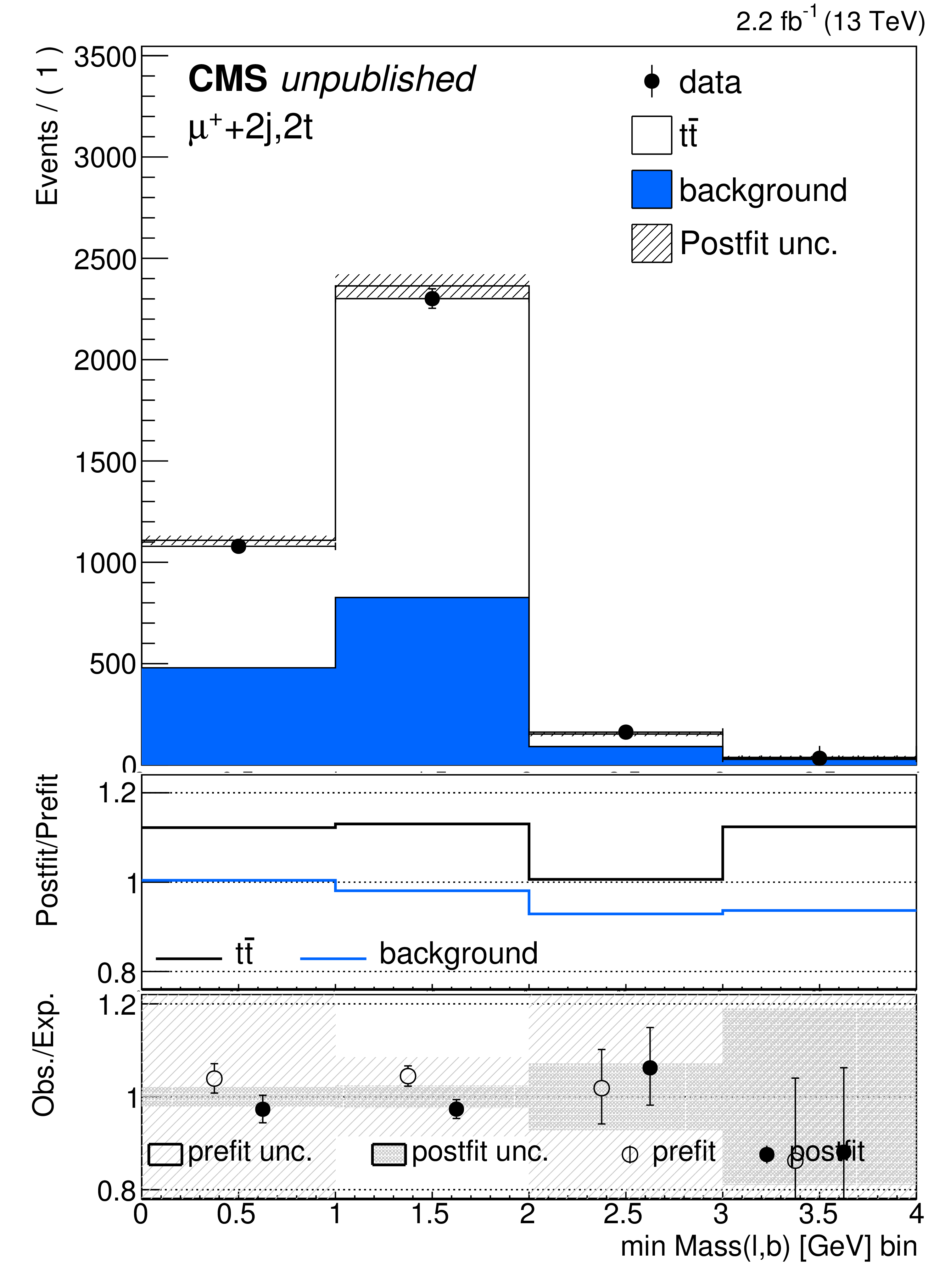
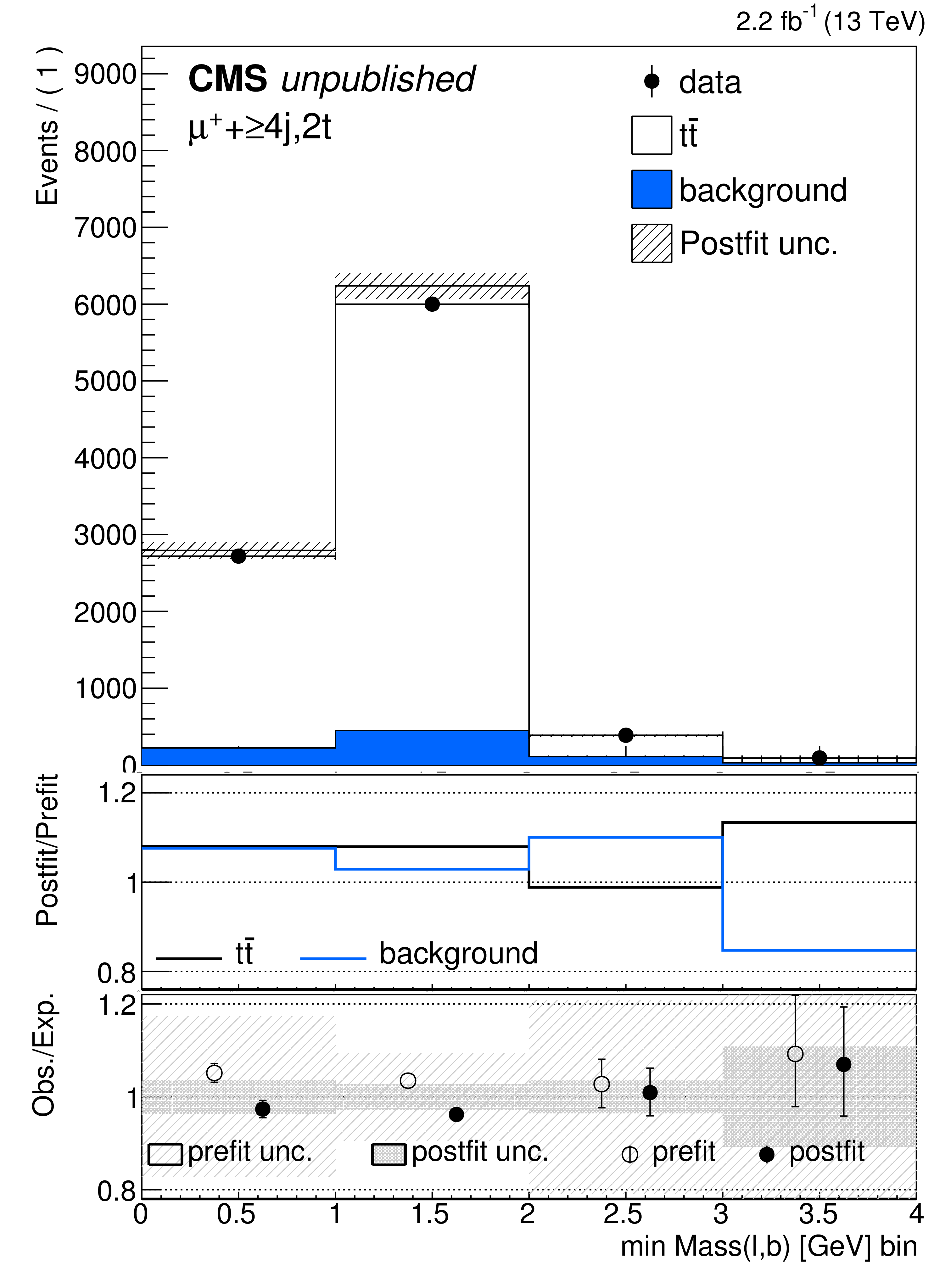
Additional Figure 5:
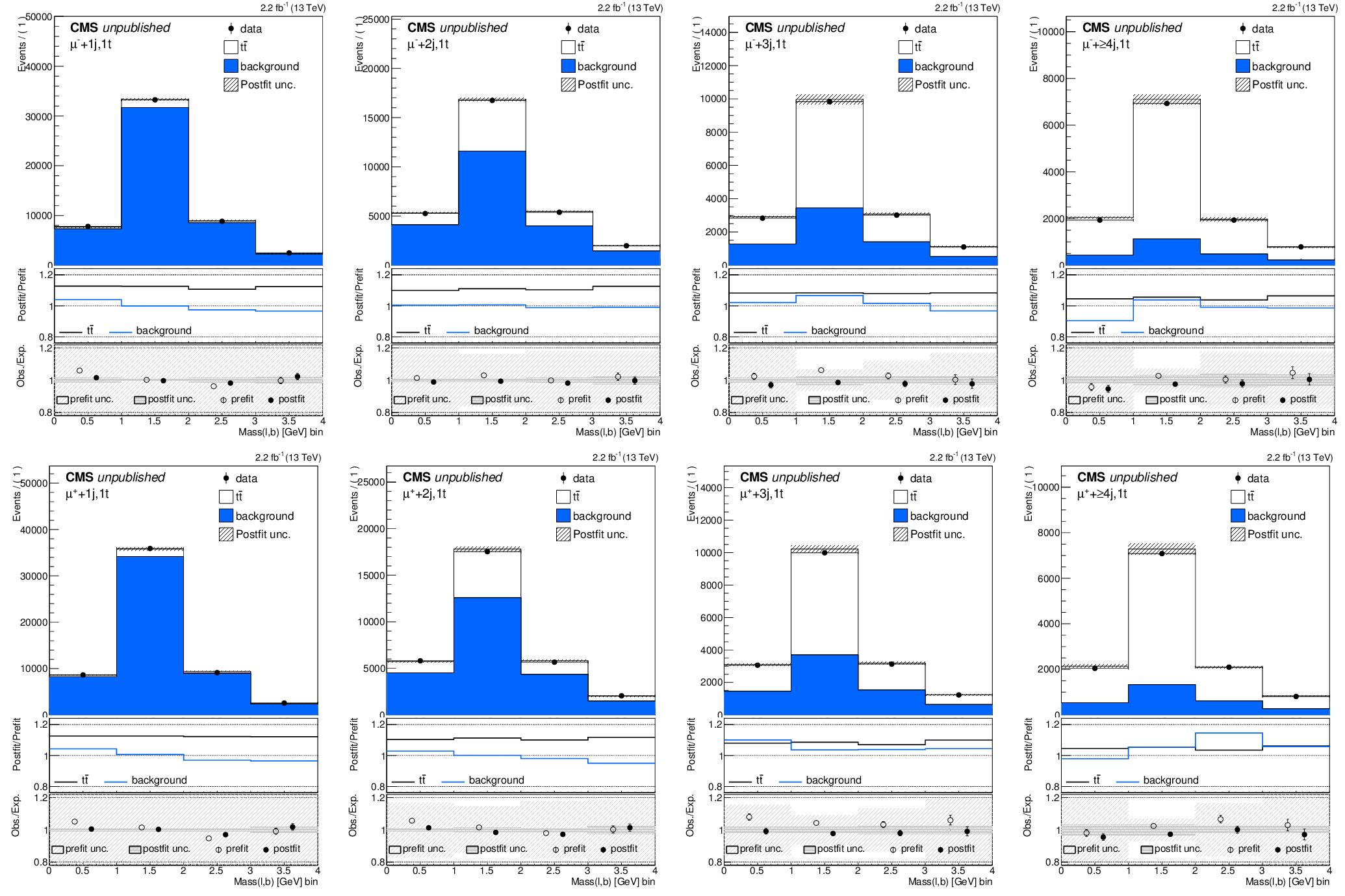
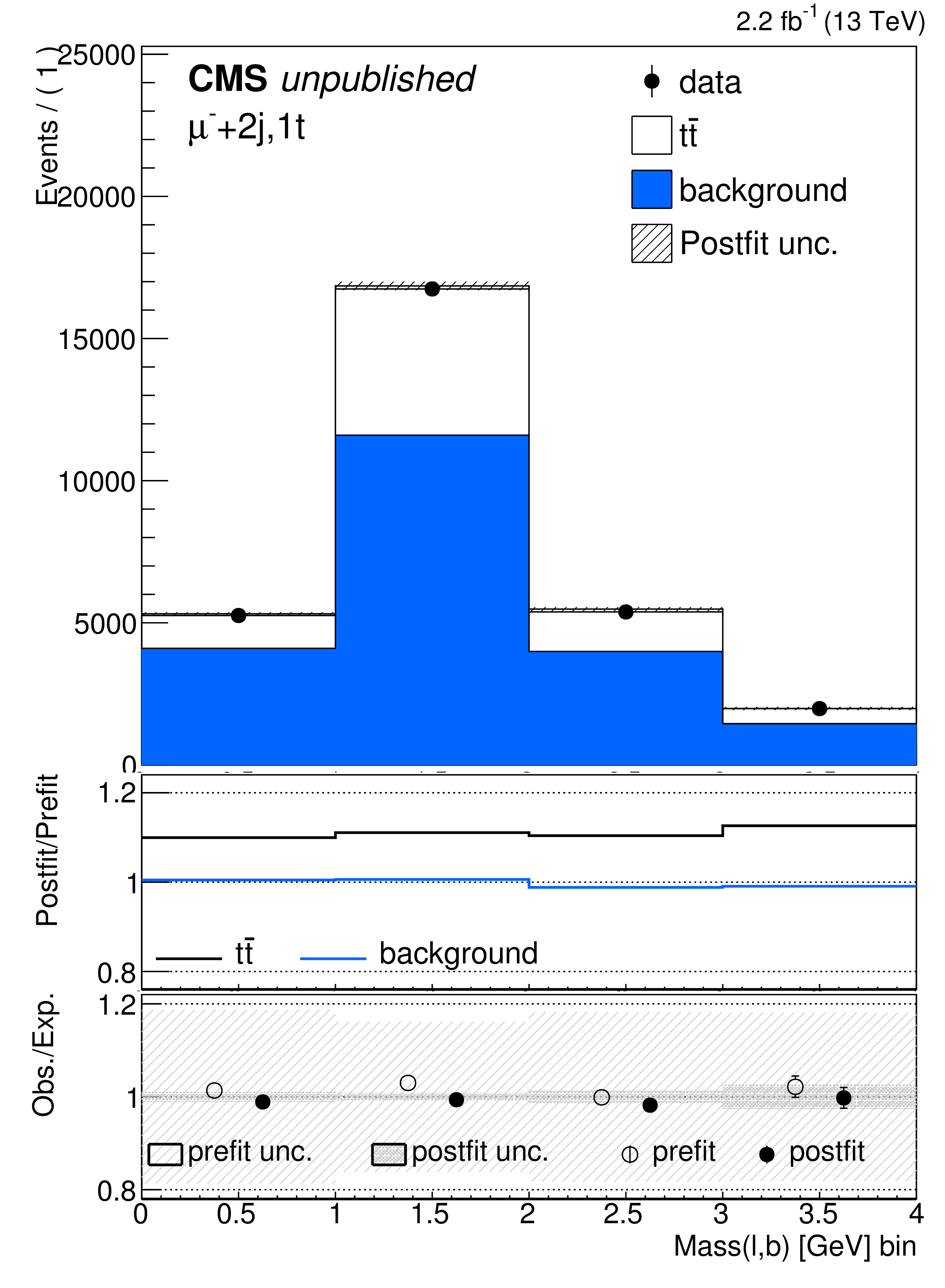
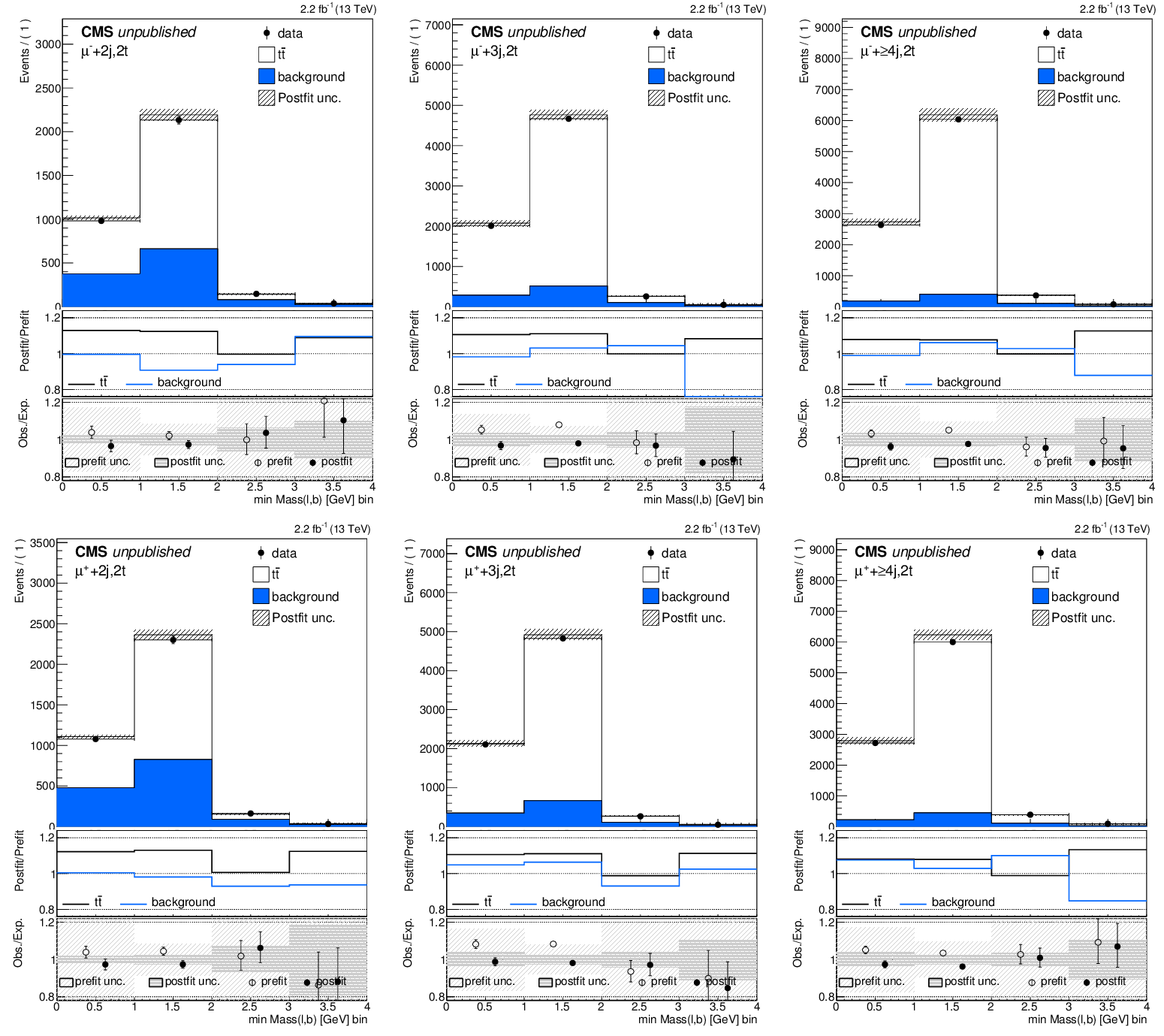
Comparison of the post-fit distributions with the data for muon events with no b-tagged jet. Negatively (positively) charged muons are shown on the top (bottom) row. From left to right events with one, two, three or at least four jets are shown. The top panels show the stacked distributions of signal and background processes and the observed data. A shaded band represents the post-fit uncertainty. The middle panels show the ratio of the post-fit to pre-fit distributions for the signal and background sum. The bottom panel shows the data to signal plus background expectations, prior and after the fit. The error bar in the points is the statistics in data. A shaded band represents the relative postfit and prefit uncertainties. |

png pdf |
Additional Figure 5-a:
Comparison of the post-fit distributions with the data for muon events with no b-tagged jet. Events with a negatively charged muon and one jet are shown. The top panel shows the stacked distributions of signal and background processes and the observed data. A shaded band represents the post-fit uncertainty. The middle panel shows the ratio of the post-fit to pre-fit distributions for the signal and background sum. The bottom panel shows the data to signal plus background expectations, prior and after the fit. The error bar in the points is the statistics in data. A shaded band represents the relative postfit and prefit uncertainties. |

png pdf |
Additional Figure 5-b:
Comparison of the post-fit distributions with the data for muon events with no b-tagged jet. Events with a negatively charged muon and two jets are shown. The top panel shows the stacked distributions of signal and background processes and the observed data. A shaded band represents the post-fit uncertainty. The middle panel shows the ratio of the post-fit to pre-fit distributions for the signal and background sum. The bottom panel shows the data to signal plus background expectations, prior and after the fit. The error bar in the points is the statistics in data. A shaded band represents the relative postfit and prefit uncertainties. |
png pdf |
Additional Figure 5-c:
Comparison of the post-fit distributions with the data for muon events with no b-tagged jet. Events with a negatively charged muon and three jets are shown. The top panel shows the stacked distributions of signal and background processes and the observed data. A shaded band represents the post-fit uncertainty. The middle panel shows the ratio of the post-fit to pre-fit distributions for the signal and background sum. The bottom panel shows the data to signal plus background expectations, prior and after the fit. The error bar in the points is the statistics in data. A shaded band represents the relative postfit and prefit uncertainties. |
png pdf |
Additional Figure 5-d:
Comparison of the post-fit distributions with the data for muon events with no b-tagged jet. Events with a negatively charged muon and at least four jets are shown. The top panel shows the stacked distributions of signal and background processes and the observed data. A shaded band represents the post-fit uncertainty. The middle panel shows the ratio of the post-fit to pre-fit distributions for the signal and background sum. The bottom panel shows the data to signal plus background expectations, prior and after the fit. The error bar in the points is the statistics in data. A shaded band represents the relative postfit and prefit uncertainties. |

png pdf |
Additional Figure 5-e:
Comparison of the post-fit distributions with the data for muon events with no b-tagged jet. Positively charged muons for events with one jet are shown. The top panel shows the stacked distributions of signal and background processes and the observed data. A shaded band represents the post-fit uncertainty. The middle panel shows the ratio of the post-fit to pre-fit distributions for the signal and background sum. The bottom panel shows the data to signal plus background expectations, prior and after the fit. The error bar in the points is the statistics in data. A shaded band represents the relative postfit and prefit uncertainties. |
png pdf |
Additional Figure 5-f:
Comparison of the post-fit distributions with the data for muon events with no b-tagged jet. Positively charged muons for events with two jets are shown. The top panel shows the stacked distributions of signal and background processes and the observed data. A shaded band represents the post-fit uncertainty. The middle panel shows the ratio of the post-fit to pre-fit distributions for the signal and background sum. The bottom panel shows the data to signal plus background expectations, prior and after the fit. The error bar in the points is the statistics in data. A shaded band represents the relative postfit and prefit uncertainties. |

png pdf |
Additional Figure 5-g:
Comparison of the post-fit distributions with the data for muon events with no b-tagged jet. Positively charged muons for events with three jets are shown. The top panel shows the stacked distributions of signal and background processes and the observed data. A shaded band represents the post-fit uncertainty. The middle panel shows the ratio of the post-fit to pre-fit distributions for the signal and background sum. The bottom panel shows the data to signal plus background expectations, prior and after the fit. The error bar in the points is the statistics in data. A shaded band represents the relative postfit and prefit uncertainties. |

png pdf |
Additional Figure 5-h:
Comparison of the post-fit distributions with the data for muon events with no b-tagged jet. Positively charged muons for events with at least four jets are shown. The top panel shows the stacked distributions of signal and background processes and the observed data. A shaded band represents the post-fit uncertainty. The middle panel shows the ratio of the post-fit to pre-fit distributions for the signal and background sum. The bottom panel shows the data to signal plus background expectations, prior and after the fit. The error bar in the points is the statistics in data. A shaded band represents the relative postfit and prefit uncertainties. |
png pdf |
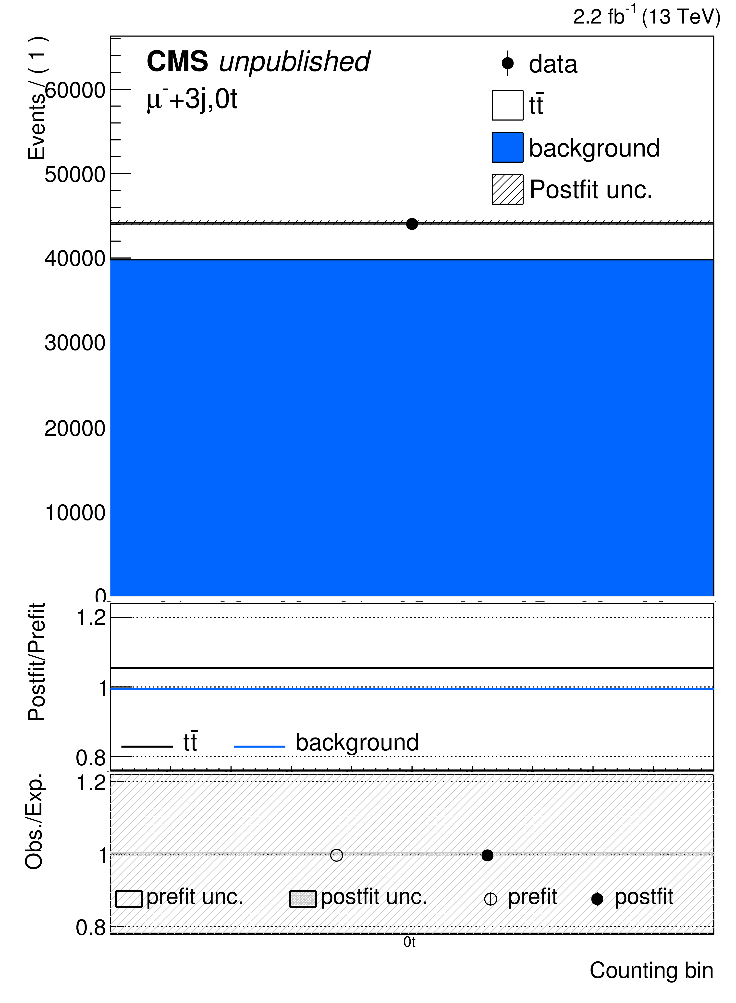
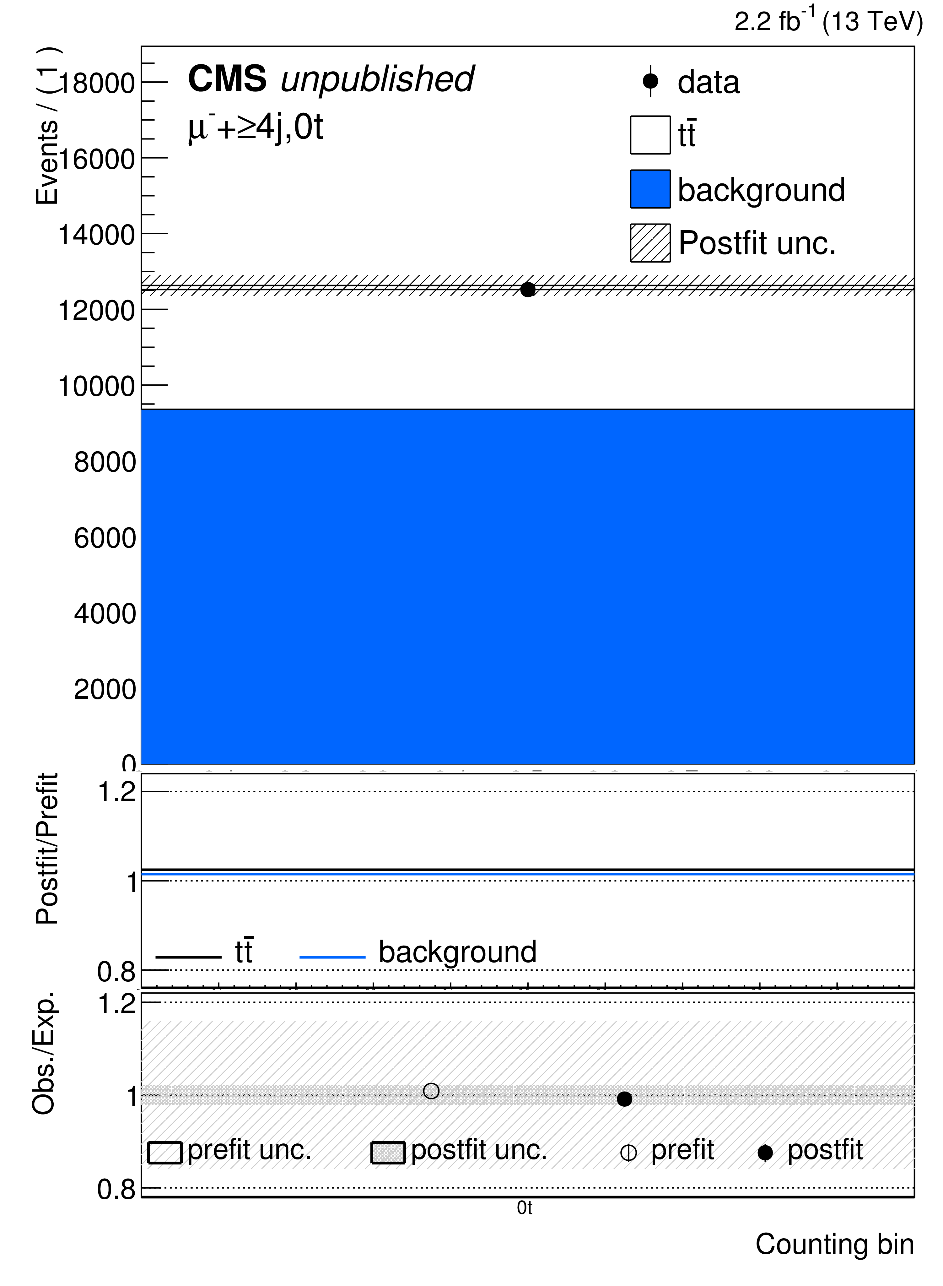
Additional Figure 6:
Comparison of the post-fit distributions with the data for electron events with one b-tagged jet. Negatively (positively) charged electrons are shown on the top (bottom) row. From left to right events with one, two, three or at least four jets are shown. The top panels show the stacked distributions of signal and background processes and the observed data. A shaded band represents the post-fit uncertainty. The middle panels show the ratio of the post-fit to pre-fit distributions for the signal and background sum. The bottom panel shows the data to signal plus background expectations, prior and after the fit. The error bar in the points is the statistics in data. A shaded band represents the relative postfit and prefit uncertainties. |

png pdf |
Additional Figure 6-a:
Comparison of the post-fit distributions with the data for electron events with one b-tagged jet. Events with a negatively charged electron and one jet are shown. The top panel shows the stacked distributions of signal and background processes and the observed data. A shaded band represents the post-fit uncertainty. The middle panel shows the ratio of the post-fit to pre-fit distributions for the signal and background sum. The bottom panel shows the data to signal plus background expectations, prior and after the fit. The error bar in the points is the statistics in data. A shaded band represents the relative postfit and prefit uncertainties. |
png pdf |
Additional Figure 6-b:
Comparison of the post-fit distributions with the data for electron events with one b-tagged jet. Events with a negatively charged electron and two jets are shown. The top panel shows the stacked distributions of signal and background processes and the observed data. A shaded band represents the post-fit uncertainty. The middle panel shows the ratio of the post-fit to pre-fit distributions for the signal and background sum. The bottom panel shows the data to signal plus background expectations, prior and after the fit. The error bar in the points is the statistics in data. A shaded band represents the relative postfit and prefit uncertainties. |
png pdf |
Additional Figure 6-c:
Comparison of the post-fit distributions with the data for electron events with one b-tagged jet. Events with a negatively charged electron and three jets are shown. The top panel shows the stacked distributions of signal and background processes and the observed data. A shaded band represents the post-fit uncertainty. The middle panel shows the ratio of the post-fit to pre-fit distributions for the signal and background sum. The bottom panel shows the data to signal plus background expectations, prior and after the fit. The error bar in the points is the statistics in data. A shaded band represents the relative postfit and prefit uncertainties. |
png pdf |
Additional Figure 6-d:
Comparison of the post-fit distributions with the data for electron events with one b-tagged jet. Events with a negatively charged electron and at least four jets are shown. The top panel shows the stacked distributions of signal and background processes and the observed data. A shaded band represents the post-fit uncertainty. The middle panel shows the ratio of the post-fit to pre-fit distributions for the signal and background sum. The bottom panel shows the data to signal plus background expectations, prior and after the fit. The error bar in the points is the statistics in data. A shaded band represents the relative postfit and prefit uncertainties. |
png pdf |
Additional Figure 6-e:
Comparison of the post-fit distributions with the data for electron events with one b-tagged jet. Positively charged electrons for events with one jet are shown. The top panel shows the stacked distributions of signal and background processes and the observed data. A shaded band represents the post-fit uncertainty. The middle panel shows the ratio of the post-fit to pre-fit distributions for the signal and background sum. The bottom panel shows the data to signal plus background expectations, prior and after the fit. The error bar in the points is the statistics in data. A shaded band represents the relative postfit and prefit uncertainties. |

png pdf |
Additional Figure 6-f:
Comparison of the post-fit distributions with the data for electron events with one b-tagged jet. Positively charged electrons for events with two jets are shown. The top panel shows the stacked distributions of signal and background processes and the observed data. A shaded band represents the post-fit uncertainty. The middle panel shows the ratio of the post-fit to pre-fit distributions for the signal and background sum. The bottom panel shows the data to signal plus background expectations, prior and after the fit. The error bar in the points is the statistics in data. A shaded band represents the relative postfit and prefit uncertainties. |

png pdf |
Additional Figure 6-g:
Comparison of the post-fit distributions with the data for electron events with one b-tagged jet. Positively charged electrons for events with three jets are shown. The top panel shows the stacked distributions of signal and background processes and the observed data. A shaded band represents the post-fit uncertainty. The middle panel shows the ratio of the post-fit to pre-fit distributions for the signal and background sum. The bottom panel shows the data to signal plus background expectations, prior and after the fit. The error bar in the points is the statistics in data. A shaded band represents the relative postfit and prefit uncertainties. |

png pdf |
Additional Figure 6-h:
Comparison of the post-fit distributions with the data for electron events with one b-tagged jet. Positively charged electrons for events with at least four jets are shown. The top panel shows the stacked distributions of signal and background processes and the observed data. A shaded band represents the post-fit uncertainty. The middle panel shows the ratio of the post-fit to pre-fit distributions for the signal and background sum. The bottom panel shows the data to signal plus background expectations, prior and after the fit. The error bar in the points is the statistics in data. A shaded band represents the relative postfit and prefit uncertainties. |
png pdf |
Additional Figure 7:
Comparison of the post-fit distributions with the data for muon events with one b-tagged jet. Negatively (positively) charged muons are shown on the top (bottom) row. From left to right events with one, two, three or at least four jets are shown. The top panels show the stacked distributions of signal and background processes and the observed data. A shaded band represents the post-fit uncertainty. The middle panels show the ratio of the post-fit to pre-fit distributions for the signal and background sum. The bottom panel shows the data to signal plus background expectations, prior and after the fit. The error bar in the points is the statistics in data. A shaded band represents the relative postfit and prefit uncertainties. |

png pdf |
Additional Figure 7-a:
Comparison of the post-fit distributions with the data for muon events with one b-tagged jet. Events with a negatively charged muon and one jet are shown. The top panel shows the stacked distributions of signal and background processes and the observed data. A shaded band represents the post-fit uncertainty. The middle panel shows the ratio of the post-fit to pre-fit distributions for the signal and background sum. The bottom panel shows the data to signal plus background expectations, prior and after the fit. The error bar in the points is the statistics in data. A shaded band represents the relative postfit and prefit uncertainties. |
png pdf |
Additional Figure 7-b:
Comparison of the post-fit distributions with the data for muon events with one b-tagged jet. Events with a negatively charged muon and two jets are shown. The top panel shows the stacked distributions of signal and background processes and the observed data. A shaded band represents the post-fit uncertainty. The middle panel shows the ratio of the post-fit to pre-fit distributions for the signal and background sum. The bottom panel shows the data to signal plus background expectations, prior and after the fit. The error bar in the points is the statistics in data. A shaded band represents the relative postfit and prefit uncertainties. |
png pdf |
Additional Figure 7-c:
Comparison of the post-fit distributions with the data for muon events with one b-tagged jet. Events with a negatively charged muon and three jets are shown. The top panel shows the stacked distributions of signal and background processes and the observed data. A shaded band represents the post-fit uncertainty. The middle panel shows the ratio of the post-fit to pre-fit distributions for the signal and background sum. The bottom panel shows the data to signal plus background expectations, prior and after the fit. The error bar in the points is the statistics in data. A shaded band represents the relative postfit and prefit uncertainties. |
png pdf |
Additional Figure 7-d:
Comparison of the post-fit distributions with the data for muon events with one b-tagged jet. Events with a negatively charged muon and at least four jets are shown. The top panel shows the stacked distributions of signal and background processes and the observed data. A shaded band represents the post-fit uncertainty. The middle panel shows the ratio of the post-fit to pre-fit distributions for the signal and background sum. The bottom panel shows the data to signal plus background expectations, prior and after the fit. The error bar in the points is the statistics in data. A shaded band represents the relative postfit and prefit uncertainties. |
png pdf |
Additional Figure 7-e:
Comparison of the post-fit distributions with the data for muon events with one b-tagged jet. Positively charged muons for events with one jet are shown. The top panel shows the stacked distributions of signal and background processes and the observed data. A shaded band represents the post-fit uncertainty. The middle panel shows the ratio of the post-fit to pre-fit distributions for the signal and background sum. The bottom panel shows the data to signal plus background expectations, prior and after the fit. The error bar in the points is the statistics in data. A shaded band represents the relative postfit and prefit uncertainties. |
png pdf |
Additional Figure 7-f:
Comparison of the post-fit distributions with the data for muon events with one b-tagged jet. Positively charged muons for events with two jets are shown. The top panel shows the stacked distributions of signal and background processes and the observed data. A shaded band represents the post-fit uncertainty. The middle panel shows the ratio of the post-fit to pre-fit distributions for the signal and background sum. The bottom panel shows the data to signal plus background expectations, prior and after the fit. The error bar in the points is the statistics in data. A shaded band represents the relative postfit and prefit uncertainties. |
png pdf |
Additional Figure 7-g:
Comparison of the post-fit distributions with the data for muon events with one b-tagged jet. Positively charged muons for events with three jets are shown. The top panel shows the stacked distributions of signal and background processes and the observed data. A shaded band represents the post-fit uncertainty. The middle panel shows the ratio of the post-fit to pre-fit distributions for the signal and background sum. The bottom panel shows the data to signal plus background expectations, prior and after the fit. The error bar in the points is the statistics in data. A shaded band represents the relative postfit and prefit uncertainties. |
png pdf |
Additional Figure 7-h:
Comparison of the post-fit distributions with the data for muon events with one b-tagged jet. Positively charged muons for events with at least four jets are shown. The top panel shows the stacked distributions of signal and background processes and the observed data. A shaded band represents the post-fit uncertainty. The middle panel shows the ratio of the post-fit to pre-fit distributions for the signal and background sum. The bottom panel shows the data to signal plus background expectations, prior and after the fit. The error bar in the points is the statistics in data. A shaded band represents the relative postfit and prefit uncertainties. |
png pdf |
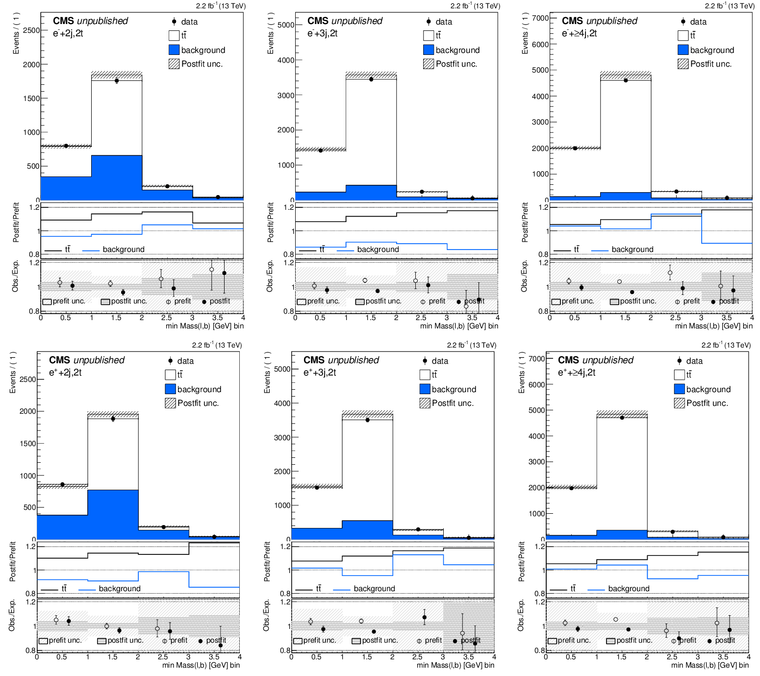
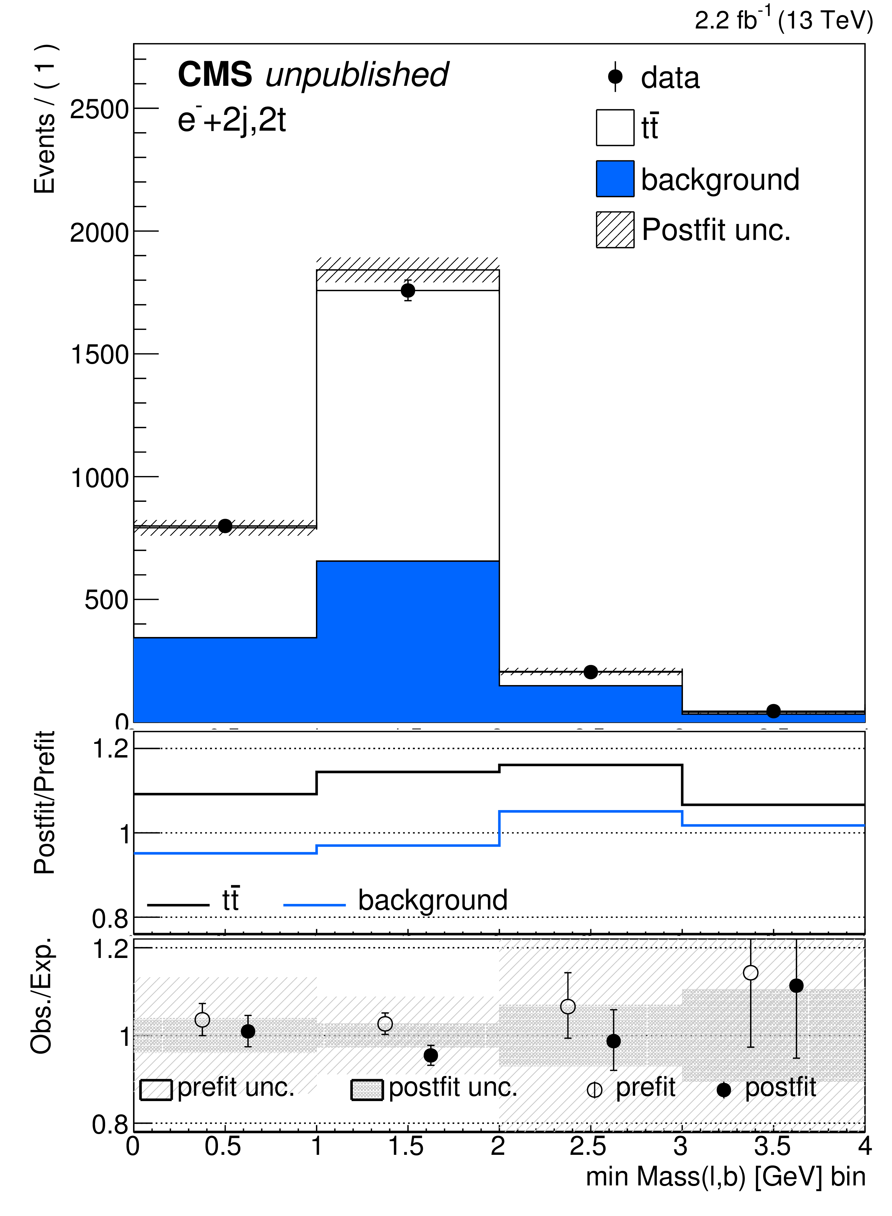
Additional Figure 8:
Comparison of the post-fit distributions with the data for electron events with at least two b-tagged jets. Negatively (positively) charged electrons are shown on the top (bottom) row. From left to right events with two, three or at least four jets are shown. The top panels show the stacked distributions of signal and background processes and the observed data. A shaded band represents the post-fit uncertainty. The middle panels show the ratio of the post-fit to pre-fit distributions for the signal and background sum. The bottom panel shows the data to signal plus background expectations, prior and after the fit. The error bar in the points is the statistics in data. A shaded band represents the relative postfit and prefit uncertainties. |
png pdf |
Additional Figure 8-a:
Comparison of the post-fit distributions with the data for electron events with at least two b-tagged jets. Events with a negatively charged electron and two jets are shown. The top panel shows the stacked distributions of signal and background processes and the observed data. A shaded band represents the post-fit uncertainty. The middle panel shows the ratio of the post-fit to pre-fit distributions for the signal and background sum. The bottom panel shows the data to signal plus background expectations, prior and after the fit. The error bar in the points is the statistics in data. A shaded band represents the relative postfit and prefit uncertainties. |
png pdf |
Additional Figure 8-b:
Comparison of the post-fit distributions with the data for electron events with at least two b-tagged jets. Events with a negatively charged electron and three jets are shown. The top panel shows the stacked distributions of signal and background processes and the observed data. A shaded band represents the post-fit uncertainty. The middle panel shows the ratio of the post-fit to pre-fit distributions for the signal and background sum. The bottom panel shows the data to signal plus background expectations, prior and after the fit. The error bar in the points is the statistics in data. A shaded band represents the relative postfit and prefit uncertainties. |
png pdf |
Additional Figure 8-c:
Comparison of the post-fit distributions with the data for electron events with at least two b-tagged jets. Events with a negatively charged electron and at least four jets are shown. The top panel shows the stacked distributions of signal and background processes and the observed data. A shaded band represents the post-fit uncertainty. The middle panel shows the ratio of the post-fit to pre-fit distributions for the signal and background sum. The bottom panel shows the data to signal plus background expectations, prior and after the fit. The error bar in the points is the statistics in data. A shaded band represents the relative postfit and prefit uncertainties. |

png pdf |
Additional Figure 8-d:
Comparison of the post-fit distributions with the data for electron events with at least two b-tagged jets. Positively charged electrons for events with two jets are shown. The top panel shows the stacked distributions of signal and background processes and the observed data. A shaded band represents the post-fit uncertainty. The middle panel shows the ratio of the post-fit to pre-fit distributions for the signal and background sum. The bottom panel shows the data to signal plus background expectations, prior and after the fit. The error bar in the points is the statistics in data. A shaded band represents the relative postfit and prefit uncertainties. |
png pdf |
Additional Figure 8-e:
Comparison of the post-fit distributions with the data for electron events with at least two b-tagged jets. Positively charged electrons for events with three jets are shown. The top panel shows the stacked distributions of signal and background processes and the observed data. A shaded band represents the post-fit uncertainty. The middle panel shows the ratio of the post-fit to pre-fit distributions for the signal and background sum. The bottom panel shows the data to signal plus background expectations, prior and after the fit. The error bar in the points is the statistics in data. A shaded band represents the relative postfit and prefit uncertainties. |

png pdf |
Additional Figure 8-f:
Comparison of the post-fit distributions with the data for electron events with at least two b-tagged jets. Positively charged electrons for events with at least four jets are shown. The top panel shows the stacked distributions of signal and background processes and the observed data. A shaded band represents the post-fit uncertainty. The middle panel shows the ratio of the post-fit to pre-fit distributions for the signal and background sum. The bottom panel shows the data to signal plus background expectations, prior and after the fit. The error bar in the points is the statistics in data. A shaded band represents the relative postfit and prefit uncertainties. |
png pdf |
Additional Figure 9:
Comparison of the post-fit distributions with the data for muon events with at least two b-tagged jets. Negatively (positively) charged muons are shown on the top (bottom) row. From left to right events with two, three or at least four jets are shown. The top panels show the stacked distributions of signal and background processes and the observed data. A shaded band represents the post-fit uncertainty. The middle panels show the ratio of the post-fit to pre-fit distributions for the signal and background sum. The bottom panel shows the data to signal plus background expectations, prior and after the fit. The error bar in the points is the statistics in data. A shaded band represents the relative postfit and prefit uncertainties. |
png pdf |
Additional Figure 9-a:
Comparison of the post-fit distributions with the data for muon events with at least two b-tagged jets. Events with a negatively charged muon and two jets are shown. The top panel shows the stacked distributions of signal and background processes and the observed data. A shaded band represents the post-fit uncertainty. The middle panel shows the ratio of the post-fit to pre-fit distributions for the signal and background sum. The bottom panel shows the data to signal plus background expectations, prior and after the fit. The error bar in the points is the statistics in data. A shaded band represents the relative postfit and prefit uncertainties. |
png pdf |
Additional Figure 9-b:
Comparison of the post-fit distributions with the data for muon events with at least two b-tagged jets. Events with a negatively charged muon and three jets are shown. The top panel shows the stacked distributions of signal and background processes and the observed data. A shaded band represents the post-fit uncertainty. The middle panel shows the ratio of the post-fit to pre-fit distributions for the signal and background sum. The bottom panel shows the data to signal plus background expectations, prior and after the fit. The error bar in the points is the statistics in data. A shaded band represents the relative postfit and prefit uncertainties. |
png pdf |
Additional Figure 9-c:
Comparison of the post-fit distributions with the data for muon events with at least two b-tagged jets. Events with a negatively charged muon and at least four jets are shown. The top panel shows the stacked distributions of signal and background processes and the observed data. A shaded band represents the post-fit uncertainty. The middle panel shows the ratio of the post-fit to pre-fit distributions for the signal and background sum. The bottom panel shows the data to signal plus background expectations, prior and after the fit. The error bar in the points is the statistics in data. A shaded band represents the relative postfit and prefit uncertainties. |
png pdf |
Additional Figure 9-d:
Comparison of the post-fit distributions with the data for muon events with at least two b-tagged jets. Positively charged muons for events with two jets are shown. The top panel shows the stacked distributions of signal and background processes and the observed data. A shaded band represents the post-fit uncertainty. The middle panel shows the ratio of the post-fit to pre-fit distributions for the signal and background sum. The bottom panel shows the data to signal plus background expectations, prior and after the fit. The error bar in the points is the statistics in data. A shaded band represents the relative postfit and prefit uncertainties. |
png pdf |
Additional Figure 9-e:
Comparison of the post-fit distributions with the data for muon events with at least two b-tagged jets. Positively charged muons for events with three jets are shown. The top panel shows the stacked distributions of signal and background processes and the observed data. A shaded band represents the post-fit uncertainty. The middle panel shows the ratio of the post-fit to pre-fit distributions for the signal and background sum. The bottom panel shows the data to signal plus background expectations, prior and after the fit. The error bar in the points is the statistics in data. A shaded band represents the relative postfit and prefit uncertainties. |
png pdf |
Additional Figure 9-f:
Comparison of the post-fit distributions with the data for muon events with at least two b-tagged jets. Positively charged muons for events with at least four jets are shown. The top panel shows the stacked distributions of signal and background processes and the observed data. A shaded band represents the post-fit uncertainty. The middle panel shows the ratio of the post-fit to pre-fit distributions for the signal and background sum. The bottom panel shows the data to signal plus background expectations, prior and after the fit. The error bar in the points is the statistics in data. A shaded band represents the relative postfit and prefit uncertainties. |
png pdf |
Additional Figure 10:
The dependence of the likelihood on the top quark pole mass is shown for the count analysis and the analysis of distributions, using the CT14nnlo PDF set. The expected dependence from the simulation, using the a priori set of nuisance parameters with their expected values at $m_\mathrm{ t } = $ 172.5 GeV, is also shown for comparison. The changes in the likelihood corresponding to the 68% and 95% confidence levels are shown by the dashed lines. |
| References | ||||
| 1 | ATLAS Collaboration | Measurement of the cross section for top-quark pair production in pp collisions at $ \sqrt{s} = $ 7 TeV with the ATLAS detector using final states with two high-$ p_{\mathrm{T}} $ leptons | JHEP 05 (2012) 059 | 1202.4892 |
| 2 | ATLAS Collaboration | Measurement of the top quark pair production cross section in pp collisions at $ \sqrt{s} = $ 7 TeV in dilepton final states with ATLAS | PLB 707 (2012) 459 | 1108.3699 |
| 3 | ATLAS Collaboration | Measurement of the top quark-pair production cross section with ATLAS in pp collisions at $ \sqrt{s} = $ 7 TeV | EPJC 71 (2011) 1577 | 1012.1792 |
| 4 | ATLAS Collaboration | Measurement of the top quark pair cross section with ATLAS in pp collisions at $ \sqrt{s} = $ 7 TeV using final states with an electron or a muon and a hadronically decaying $ \tau $ lepton | PLB 717 (2012) 89 | 1205.2067 |
| 5 | CMS Collaboration | First measurement of the cross section for top-quark pair production in proton-proton collisions at $ \sqrt{s} = $ 7 TeV | PLB 695 (2011) 424 | CMS-TOP-10-001 1010.5994 |
| 6 | CMS Collaboration | Measurement of the $ \mathrm{ t \bar{t} } $ production cross section and the top quark mass in the dilepton channel in pp collisions at $ \sqrt{s} = $ 7 TeV | JHEP 07 (2011) 049 | CMS-TOP-11-002 1105.5661 |
| 7 | CMS Collaboration | Measurement of the $ \mathrm{ t \bar{t} } $ production cross section in pp collisions at $ \sqrt{s} = $ 7 TeV using the kinematic properties of events with leptons and jets | EPJC 71 (2011) 1721 | CMS-TOP-10-002 1106.0902 |
| 8 | CMS Collaboration | Measurement of the $ t $-Channel Single Top Quark Production Cross Section in $ pp $ Collisions at $ \sqrt{s} = $ 7 TeV | PRL 107 (2011) 091802 | CMS-TOP-10-008 1106.3052 |
| 9 | CMS Collaboration | Measurement of the top quark pair production cross section in $ pp $ collisions at $ \sqrt{s} = $ 7 TeV in dilepton final states containing a $ \tau $ | PRD 85 (2012) 112007 | CMS-TOP-11-006 1203.6810 |
| 10 | CMS Collaboration | Measurement of the $ \mathrm{ t \bar{t} } $ production cross section in the dilepton channel in pp collisions at $ \sqrt{s} = $ 7 TeV | JHEP 11 (2012) 067 | CMS-TOP-11-005 1208.2671 |
| 11 | CMS Collaboration | Measurement of the top-quark mass in $ \mathrm{ t \bar{t} } $ events with lepton+jets final states in pp collisions at $ \sqrt{s} = $ 7 TeV | JHEP 12 (2012) 105 | CMS-TOP-11-015 1209.2319 |
| 12 | CMS Collaboration | Measurement of the top-antitop production cross section in the $ \tau $+jets channel in pp collisions at $ \sqrt{s} = $ 7 TeV | EPJC 73 (2013) 2386 | CMS-TOP-11-004 1301.5755 |
| 13 | CMS Collaboration | Measurement of the $ \mathrm{ t \bar{t} } $ production cross section in pp collisions at $ \sqrt{s} = $ 7 TeV with lepton+jets final states | PLB 720 (2013) 83 | CMS-TOP-11-003 1212.6682 |
| 14 | CMS Collaboration | Measurement of the $ \mathrm{ t \bar{t} } $ production cross section in the all-jet final state in pp collisions at $ \sqrt{s} = $ 7 TeV | JHEP 05 (2013) 065 | CMS-TOP-11-007 1302.0508 |
| 15 | ATLAS Collaboration | Measurement of the $ \mathrm{ t \bar{t} } $ production cross-section using e$ \mu $ events with b-tagged jets in pp collisions at $ \sqrt{s}= $ 7 and 8 TeV with the ATLAS detector | EPJC 74 (2014) 3109 | 1406.5375 |
| 16 | ATLAS Collaboration | Measurement of the top pair production cross section in 8 TeV proton-proton collisions using kinematic information in the lepton+jets final state with ATLAS | PRD 91 (2015) 112013 | 1504.04251 |
| 17 | CMS Collaboration | Measurement of the $ \mathrm{ t \bar{t} } $ production cross section in the dilepton channel in pp collisions at $ \sqrt{s} = $ 8 TeV | JHEP 02 (2014) 024 | CMS-TOP-12-007 1312.7582 |
| 18 | CMS Collaboration | Measurement of the $ \mathrm{ t \bar{t} } $ production cross section in pp collisions at $ \sqrt{s} = $ 8 TeV in dilepton final states containing one $ \tau $ lepton | PLB 739 (2014) 23 | CMS-TOP-12-026 1407.6643 |
| 19 | CMS Collaboration | Measurement of the $ \mathrm{t}\overline{{\mathrm{t}}} $ production cross section in the all-jets final state in pp collisions at $ \sqrt{s}= $ 8 TeV | EPJC 76 (2016) 128 | CMS-TOP-14-018 1509.06076 |
| 20 | CMS Collaboration | Measurements of the $ \mathrm{ t \bar{t} } $ production cross section in lepton+jets final states in pp collisions at 8 TeV and the ratio of 8 to 7 TeV cross sections | EPJC 77 (2017) 15 | CMS-TOP-12-006 1602.09024 |
| 21 | LHCb Collaboration | First Observation of Top Quark Production in the Forward Region | PRL 115 (2015) 112001 | 1506.00903 |
| 22 | LHCb Collaboration | Measurement of forward $ \mathrm{ t \bar{t} }, $ $ \mathrm{ W }+\mathrm{b }\overline{\mathrm{b }} $ and $ \mathrm{ W }+\mathrm{c }\overline{\mathrm{c }} $ production in $ pp $ collisions at $ \sqrt{s} = $ 8 TeV | PLB 767 (2017) 110 | 1610.08142 |
| 23 | CMS Collaboration | Measurement of the $ \mathrm{ t \bar{t} } $ production cross section in the e$ \mu $ channel in proton-proton collisions at $ \sqrt{s} = $ 7 and 8 TeV | JHEP 08 (2016) 029 | CMS-TOP-13-004 1603.02303 |
| 24 | CMS Collaboration | Measurement of the Top Quark Pair Production Cross Section in Proton-Proton Collisions at $ \sqrt{s} = $ 13 TeV | PRL 116 (2016) 052002 | CMS-TOP-15-003 1510.05302 |
| 25 | ATLAS Collaboration | Measurement of the $ \mathrm{ t \bar{t} } $ production cross-section using $ e\mu $ events with b-tagged jets in pp collisions at $ \sqrt{s} = $ 13 TeV with the ATLAS detector | PLB 761 (2016) 136 | 1606.02699 |
| 26 | CMS Collaboration | Measurement of the $ \mathrm{ t \bar{t} } $ production cross section using events in the e$ \mu $ final state in pp collisions at $ \sqrt{s} = $ 13 TeV | Submitted to EPJC | CMS-TOP-16-005 1611.04040 |
| 27 | CMS Collaboration | Determination of the top-quark pole mass and strong coupling constant from the $ \mathrm{ t \bar{t} } $ production cross section in pp collisions at $ \sqrt{s} = $ 7 TeV | PLB 728 (2014) 496 | CMS-TOP-12-022 1307.1907 |
| 28 | NNPDF Collaboration | Parton distributions for the LHC Run II | JHEP 04 (2015) 040 | 1410.8849 |
| 29 | L. A. Harland-Lang, A. D. Martin, P. Motylinski, and R. S. Thorne | Parton distributions in the LHC era: MMHT 2014 PDFs | EPJC 75 (2015) 204 | 1412.3989 |
| 30 | M. Czakon et al. | Closing the Stop Gap | PRL 113 (2014) 201803 | 1407.1043 |
| 31 | CMS Collaboration | The CMS experiment at the CERN LHC | JINST 3 (2008) S08004 | CMS-00-001 |
| 32 | CMS Collaboration | Preliminary CMS luminosity measurement for the 2015 data taking period | ||
| 33 | P. Nason | A New method for combining NLO QCD with shower Monte Carlo algorithms | JHEP 11 (2004) 040 | hep-ph/0409146 |
| 34 | S. Frixione, P. Nason, and C. Oleari | Matching NLO QCD computations with parton shower simulations: the POWHEG method | JHEP 11 (2007) 070 | 0709.2092 |
| 35 | S. Alioli, P. Nason, C. Oleari, and E. Re | A general framework for implementing NLO calculations in shower Monte Carlo programs: the POWHEG BOX | JHEP 06 (2010) 043 | 1002.2581 |
| 36 | S. Frixione, P. Nason, and G. Ridolfi | A Positive-weight next-to-leading-order Monte Carlo for heavy flavour hadroproduction | JHEP 09 (2007) 126 | 0707.3088 |
| 37 | T. Sjostrand, S. Mrenna, and P. Skands | PYTHIA 6.4 physics and manual | JHEP 05 (2006) 026 | hep-ph/0603175 |
| 38 | T. Sjostrand et al. | An introduction to PYTHIA 8.2 | CPC 191 (2015) 159 | 1410.3012 |
| 39 | F. Demartin et al. | The impact of PDF and $ \alpha_{\rm S} $ uncertainties on Higgs production in gluon fusion at hadron colliders | PRD 82 (2010) 014002 | 1004.0962 |
| 40 | CMS Collaboration | Event generator tunes obtained from underlying event and multiparton scattering measurements | EPJC 76 (2016) 155 | CMS-GEN-14-001 1512.00815 |
| 41 | P. Skands, S. Carrazza, and J. Rojo | Tuning PYTHIA 8.1: the Monash 2013 Tune | EPJC 74 (2014) 3024 | 1404.5630 |
| 42 | J. Alwall et al. | The automated computation of tree-level and next-to-leading order differential cross sections, and their matching to parton shower simulations | JHEP 07 (2014) 079 | 1405.0301 |
| 43 | P. Artoisenet, R. Frederix, O. Mattelaer, and R. Rietkerk | Automatic spin-entangled decays of heavy resonances in Monte Carlo simulations | JHEP 03 (2013) 015 | 1212.3460 |
| 44 | M. Bahr et al. | Herwig++ physics and manual | EPJC 58 (2008) 639 | 0803.0883 |
| 45 | M. Czakon and A. Mitov | Top++: a program for the calculation of the top-pair cross-section at hadron colliders | CPC 185 (2014) 2930 | 1112.5675 |
| 46 | S. Alioli, P. Nason, C. Oleari, and E. Re | NLO single-top production matched with shower in POWHEG: $ s $- and $ t $-channel contributions | JHEP 09 (2009) 111 | 0907.4076 |
| 47 | E. Re | Single-top $ Wt $-channel production matched with parton showers using the POWHEG method | EPJC 71 (2011) 1547 | 1009.2450 |
| 48 | N. Kidonakis | Top quark production | in Proceedings, Helmholtz International Summer School on Physics of Heavy Quarks and Hadrons (HQ 2013), p. 139 2014 | 1311.0283 |
| 49 | K. Melnikov and F. Petriello | Electroweak gauge boson production at hadron colliders through $ \mathcal{O}(\alpha_s^2) $ | PRD 74 (2006) 114017 | hep-ph/0609070 |
| 50 | T. Melia, P. Nason, R. Rontsch, and G. Zanderighi | $ \mathrm{ W }^+ $$ \mathrm{ W }^- $, WZ and ZZ production in the POWHEG BOX | JHEP 11 (2011) 078 | 1107.5051 |
| 51 | J. M. Campbell and R. K. Ellis | MCFM for the Tevatron and the LHC | NPPS 205-206 (2010) 10 | 1007.3492 |
| 52 | J. M. Campbell, R. K. Ellis, and C. Williams | Vector boson pair production at the LHC | JHEP 07 (2011) 018 | 1105.0020 |
| 53 | J. Allison et al. | GEANT4 developments and applications | IEEE Trans. Nucl. Sci. 53 (2006) 270 | |
| 54 | GEANT4 Collaboration | GEANT4---a simulation toolkit | NIMA 506 (2003) 250 | |
| 55 | CMS Collaboration | Measurements of inclusive $ W $ and $ Z $ cross sections in pp collisions at $ \sqrt{s} = $ 7 TeV | JHEP 01 (2011) 080 | CMS-EWK-10-002 1012.2466 |
| 56 | CMS Collaboration | Particle-flow reconstruction and global event description with the cms detector | Submitted to \it JINST | CMS-PRF-14-001 1706.04965 |
| 57 | CMS Collaboration | Performance of electron reconstruction and selection with the CMS detector in proton-proton collisions at $ \sqrt{s} = $ 8 TeV | JINST 10 (2015) P06005 | CMS-EGM-13-001 1502.02701 |
| 58 | CMS Collaboration | The performance of the CMS muon detector in proton-proton collisions at $ \sqrt{s} = $ 7 TeV at the LHC | JINST 8 (2013) P11002 | CMS-MUO-11-001 1306.6905 |
| 59 | M. Cacciari, G. P. Salam, and G. Soyez | The anti-$ k_t $ jet clustering algorithm | JHEP 04 (2008) 063 | 0802.1189 |
| 60 | M. Cacciari, G. P. Salam, and G. Soyez | FastJet user manual | EPJC 72 (2012) 1896 | 1111.6097 |
| 61 | CMS Collaboration | Jet energy scale and resolution in the CMS experiment in pp collisions at 8 TeV | Submitted to JHEP | CMS-JME-13-004 1607.03663 |
| 62 | M. Cacciari, G. P. Salam, and G. Soyez | The catchment area of jets | JHEP 04 (2008) 005 | 0802.1188 |
| 63 | M. Cacciari and G. P. Salam | Pileup subtraction using jet areas | PLB 659 (2008) 119 | 0707.1378 |
| 64 | CMS Collaboration | Identification of b-quark jets with the CMS experiment | JINST 8 (2013) P04013 | CMS-BTV-12-001 1211.4462 |
| 65 | J. M. Campbell and R. K. Ellis | An update on vector boson pair production at hadron colliders | PRD 60 (1999) 113006 | hep-ph/9905386 |
| 66 | CMS Collaboration | Measurement of masses in the $ \mathrm{ t \bar{t} } $ system by kinematic endpoints in pp collisions at $ \sqrt{s} = $ 7 TeV | EPJC 73 (2013) 2494 | CMS-TOP-11-027 1304.5783 |
| 67 | CMS and ATLAS Collaborations | Jet energy scale uncertainty correlations between ATLAS and CMS at 8 TeV | ||
| 68 | ATLAS Collaboration | Measurement of the Inelastic Proton-Proton Cross Section at $ \sqrt{s} = $ 13 TeV with the ATLAS Detector at the LHC | PRL 117 (2016) 182002 | 1606.02625 |
| 69 | CMS Collaboration | Measurement of the differential cross section for top quark pair production in pp collisions at $ \sqrt{s} = $ 8 TeV | EPJC 75 (2015) 542 | CMS-TOP-12-028 1505.04480 |
| 70 | S. Frixione et al. | Single-top hadroproduction in association with a W boson | JHEP 07 (2008) 029 | 0805.3067 |
| 71 | A. S. Belyaev, E. E. Boos, and L. V. Dudko | Single top quark at future hadron colliders: Complete signal and background study | PRD 59 (1999) 075001 | hep-ph/9806332 |
| 72 | C. D. White, S. Frixione, E. Laenen, and F. Maltoni | Isolating $ Wt $ production at the LHC | JHEP 11 (2009) 074 | 0908.0631 |
| 73 | T. M. P. Tait | The $ tW^- $ mode of single top production | PRD 61 (1999) 034001 | hep-ph/9909352 |
| 74 | G. Cowan, K. Cranmer, E. Gross, and O. Vitells | Asymptotic formulae for likelihood-based tests of new physics | EPJC 71 (2011) 1554 | 1007.1727 |
| 75 | J. Kieseler, K. Lipka, and S.-O. Moch | Calibration of the top-quark Monte Carlo mass | PRL 116 (2016) 162001 | 1511.00841 |
| 76 | S. Dulat et al. | New parton distribution functions from a global analysis of quantum chromodynamics | PRD 93 (2016) 033006 | 1506.07443 |
| 77 | J. Wenninger | Energy calibration of the LHC Beams at 4 TeV | Technical Report CERN-ATS-2013-040 | |
|
|
Compact Muon Solenoid LHC, CERN |
|

|

|

|

|

|