

Compact Muon Solenoid
LHC, CERN
| CMS-SUS-17-003 ; CERN-EP-2018-149 | ||
| Search for supersymmetry in events with a $ \tau $ lepton pair and missing transverse momentum in proton-proton collisions at $\sqrt{s} = $ 13 TeV | ||
| CMS Collaboration | ||
| 5 July 2018 | ||
| JHEP 11 (2018) 151 | ||
| Abstract: A search for the electroweak production of supersymmetric particles in proton-proton collisions at a center-of-mass energy of 13 TeV is presented in final states with a $ \tau $ lepton pair. Both hadronic and leptonic decay modes are considered for the $ \tau $ leptons. Scenarios involving the direct pair production of $ \tau $ sleptons, or their indirect production via the decays of charginos and neutralinos, are investigated. The data correspond to an integrated luminosity of 35.9 fb$^{-1}$ collected with the CMS detector in 2016. The observed number of events is consistent with the standard model background expectation. The results are interpreted as upper limits on the cross section for $ \tau $ slepton pair production in different scenarios. The strongest limits are observed in the scenario of a purely left-handed low mass $ \tau $ slepton decaying to a nearly massless neutralino. Exclusion limits are also set in the context of simplified models of chargino-neutralino and chargino pair production with decays to $ \tau $ leptons, and range up to 710 and 630 GeV, respectively. | ||
| Links: e-print arXiv:1807.02048 [hep-ex] (PDF) ; CDS record ; inSPIRE record ; CADI line (restricted) ; | ||
|
Additional information on efficiencies needed for reinterpretation of these results are available here Additional technical material for CMS speakers can be found here |
| Figures | |
png pdf |
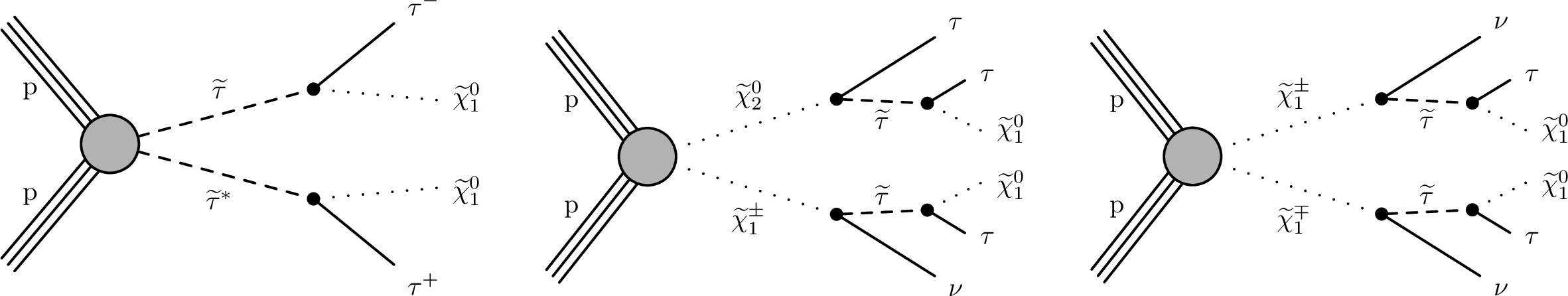
Figure 1:
Diagrams for the simplified models studied in this paper: direct $\tilde{\tau}$ pair production followed by each $\tilde{\tau}$ decaying to a ${\tau}$ lepton and $\tilde{ \chi }^{0}_{1}$ (left), and chargino-neutralino (middle) and chargino pair (right) production with subsequent decays leading to ${\tau}$ leptons in the final state. |

png pdf |
Figure 1-a:
Diagram for the direct $\tilde{\tau}$ pair production followed by each $\tilde{\tau}$ decaying to a ${\tau}$ lepton and $\tilde{ \chi }^{0}_{1}$. |
png pdf |
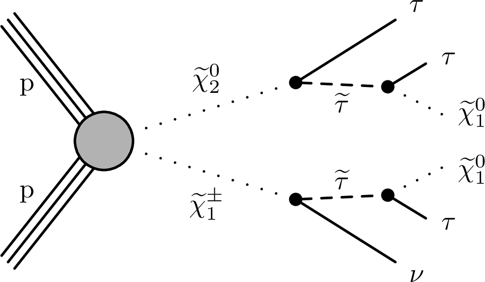
Figure 1-b:
Diagram for chargino-neutralino production with subsequent decays leading to ${\tau}$ leptons in the final state. |
png pdf |
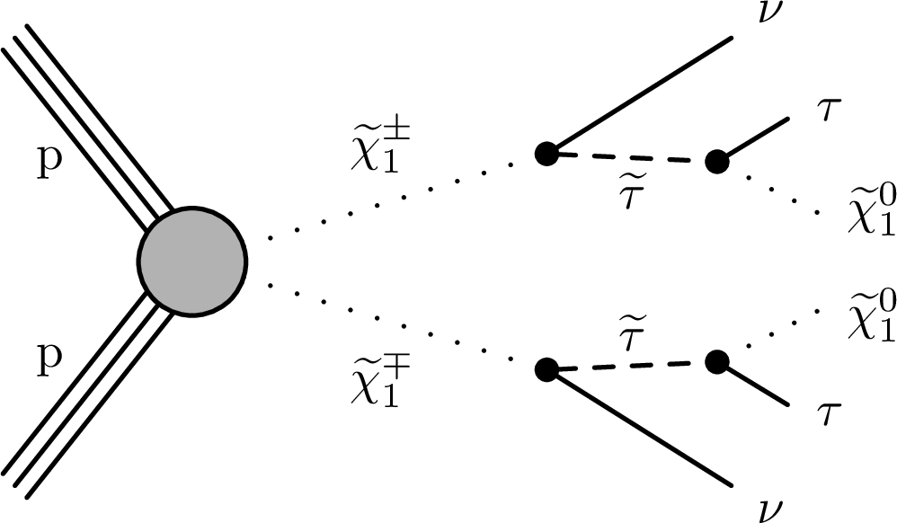
Figure 1-c:
Diagram for chargino pair production with subsequent decays leading to ${\tau}$ leptons in the final state. |
png pdf |
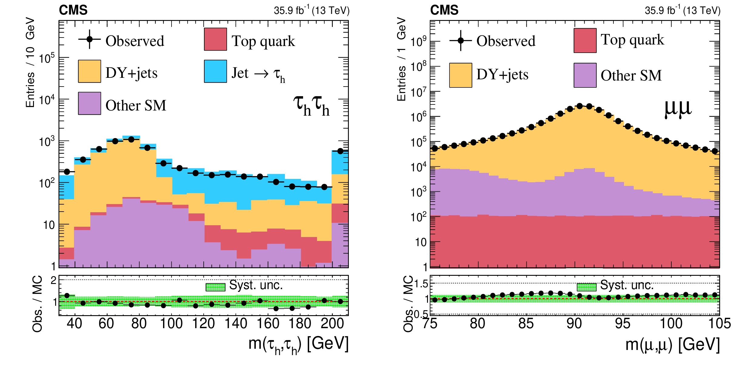
Figure 2:
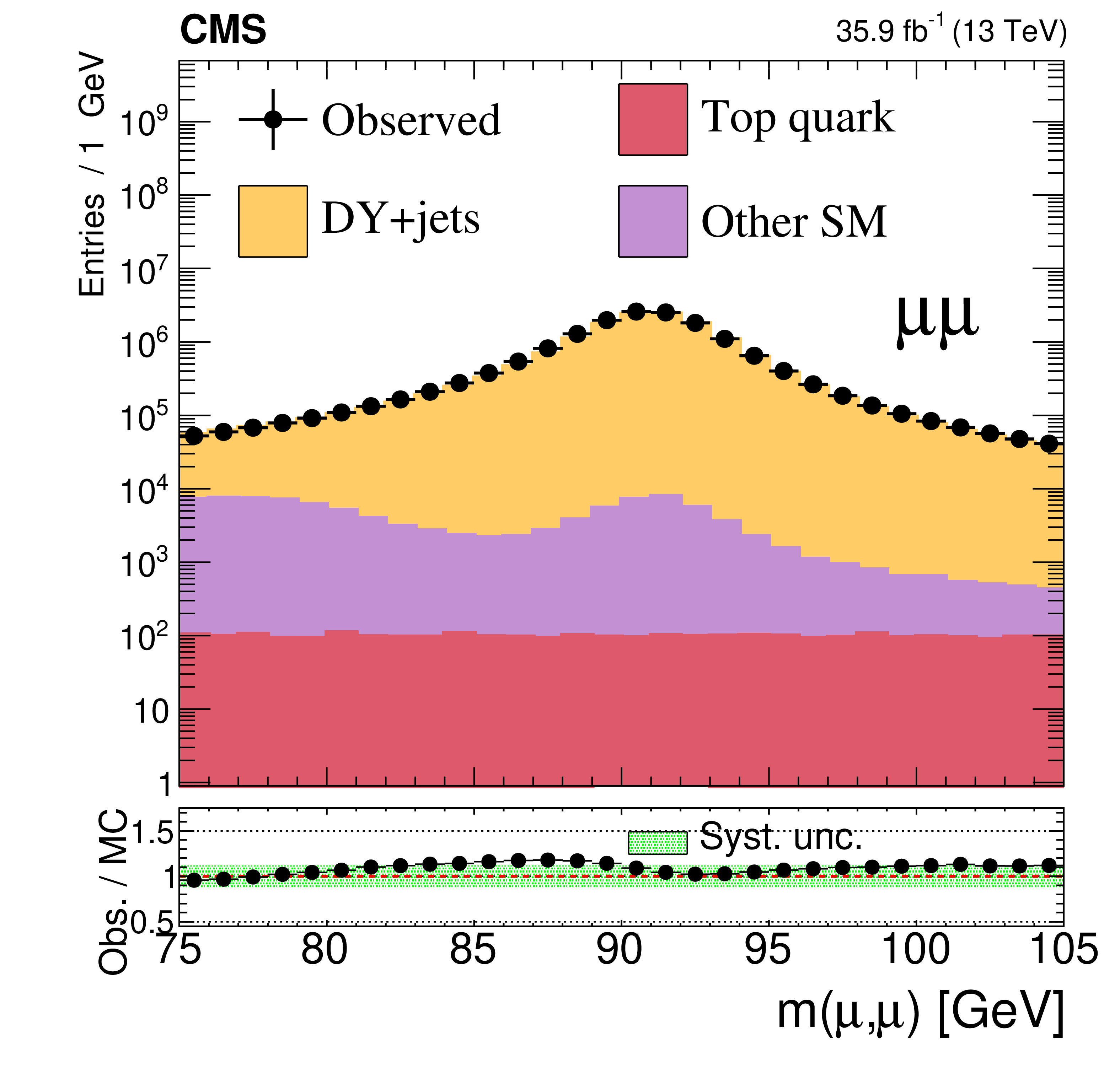
Left: visible mass spectrum used to validate the modeling of the DY+jets background in the ${{{\tau} _\mathrm {h}} {{\tau} _\mathrm {h}}}$ final state in a ${{\mathrm {Z}} \to {\tau} {\tau}}$ control sample selected with low ${m_{\mathrm {T2}}}$ or ${\Sigma {m_{\mathrm {T}}}}$ and a minimum ${{{\tau} _\mathrm {h}} {{\tau} _\mathrm {h}}}$ system ${p_{\mathrm {T}}}$ of 50 GeV. The last bin includes overflows. Right: dimuon mass distribution in the high-purity ${{\mathrm {Z}} \to \mu \mu}$ control sample after all estimated correction factors have been applied to the simulation. In the legend, "Top quark" refers to the background originating from ${{\mathrm {t}\overline {\mathrm {t}}}}$ and single top quark production. |

png pdf |
Figure 2-a:
Visible mass spectrum used to validate the modeling of the DY+jets background in the ${{{\tau} _\mathrm {h}} {{\tau} _\mathrm {h}}}$ final state in a ${{\mathrm {Z}} \to {\tau} {\tau}}$ control sample selected with low ${m_{\mathrm {T2}}}$ or ${\Sigma {m_{\mathrm {T}}}}$ and a minimum ${{{\tau} _\mathrm {h}} {{\tau} _\mathrm {h}}}$ system ${p_{\mathrm {T}}}$ of 50 GeV. The last bin includes overflows. |
png pdf |
Figure 2-b:
Dimuon mass distribution in the high-purity ${{\mathrm {Z}} \to \mu \mu}$ control sample after all estimated correction factors have been applied to the simulation. In the legend, "Top quark" refers to the background originating from ${{\mathrm {t}\overline {\mathrm {t}}}}$ and single top quark production. |
png pdf |
Figure 3:
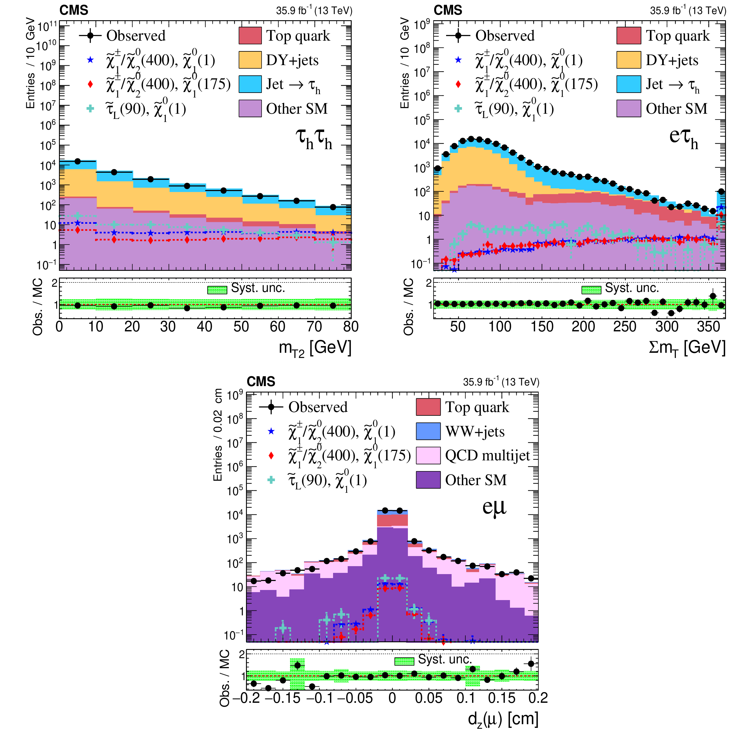
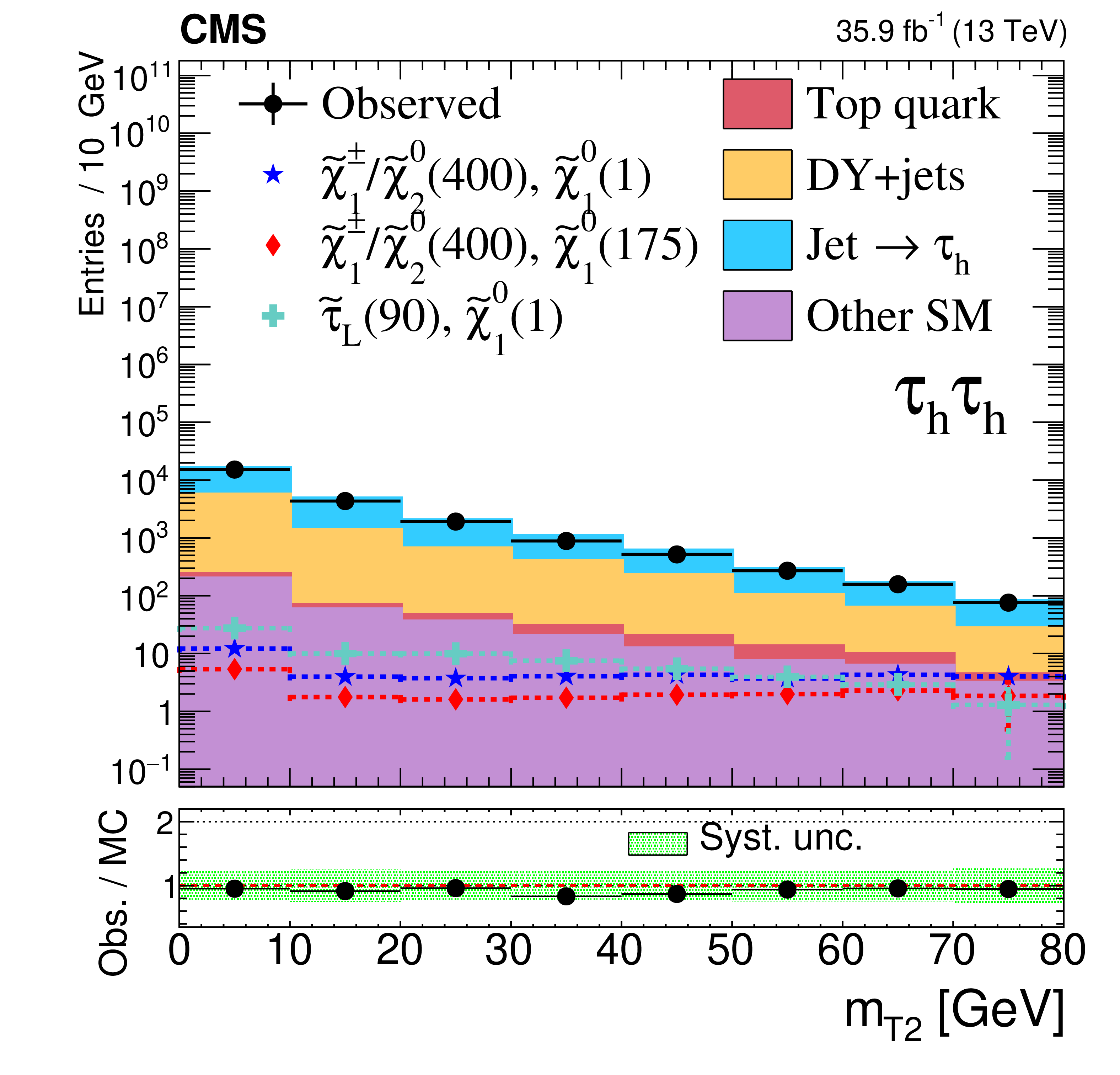
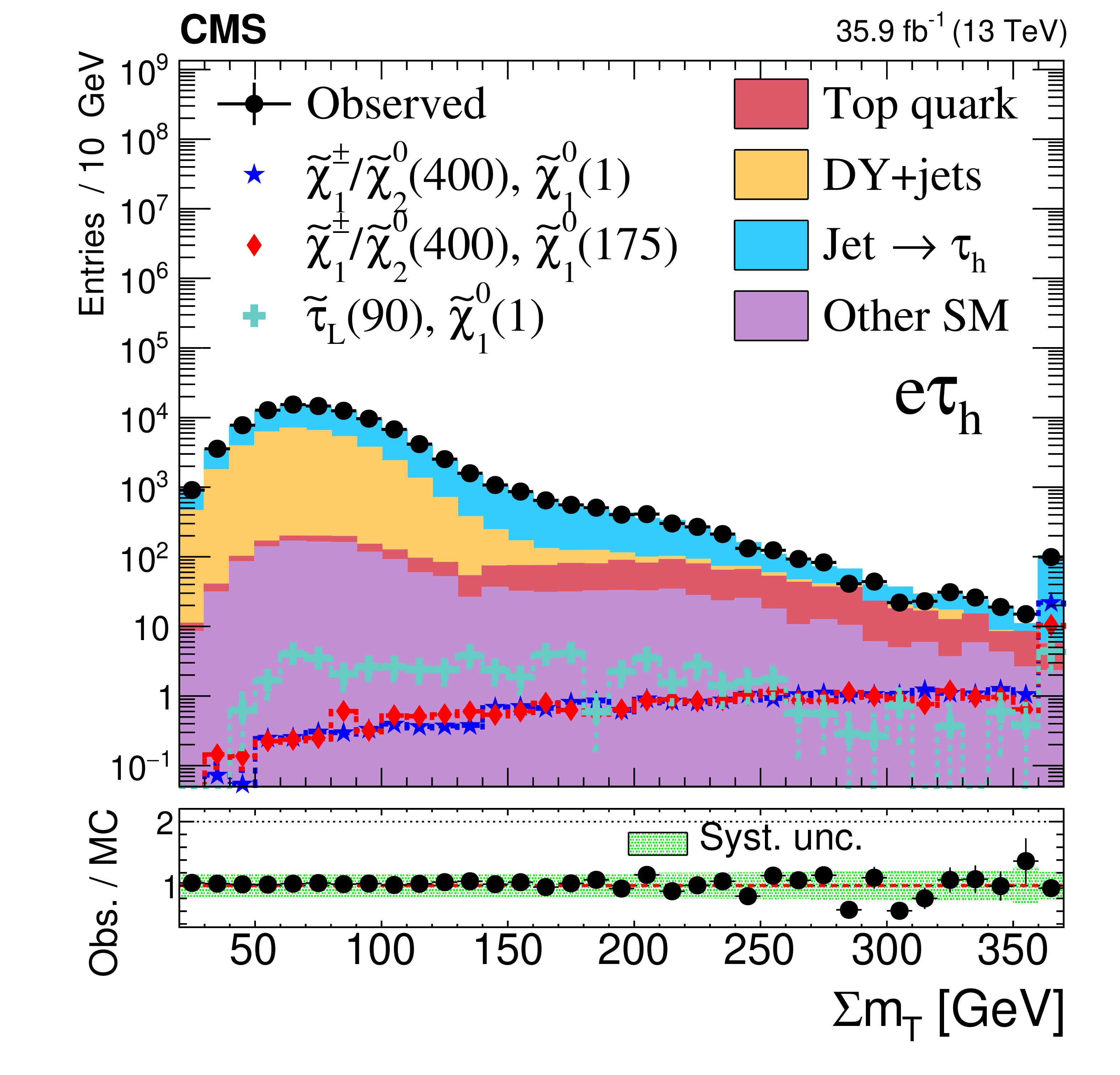
Top left: closure test for the method used to estimate the ${{\tau} _\mathrm {h}}$ misidentification rate for the ${{{\tau} _\mathrm {h}} {{\tau} _\mathrm {h}}}$ final state in a data control sample where the ${m_{\mathrm {T2}}}$ or ${\Sigma {m_{\mathrm {T}}}}$ requirements used in the SRs are inverted. Top right: ${\Sigma {m_{\mathrm {T}}}}$ distribution for events in the ${{\mathrm {e}} {{\tau} _\mathrm {h}}}$ final state after the baseline selection, showing the estimation of the background with a jet misidentified as a ${{\tau} _\mathrm {h}}$, which is determined in a signal depleted control region. The last bin includes overflows. Bottom: distribution of the muon ${d_{z}}$ in the ${{\mathrm {e}}\mu}$ final state after the baseline selection, showing the estimation of the QCD multijet background using the matrix method. In the legend,"Top quark" refers to the background originating from ${{\mathrm {t}\overline {\mathrm {t}}}}$ and single top quark production. In all cases, the predicted and observed yields show good agreement. Distributions for two benchmark models of chargino-neutralino production, and one of direct left-handed $\tilde{\tau}$ pair production, are overlaid. The ratio of signal to background is expected to be small for these selections. The numbers within parentheses in the legend correspond to the masses of the parent SUSY particle and the $\tilde{ \chi }^{0}_{1}$ in GeV for these benchmark models. |
png pdf |
Figure 3-a:
Closure test for the method used to estimate the ${{\tau} _\mathrm {h}}$ misidentification rate for the ${{{\tau} _\mathrm {h}} {{\tau} _\mathrm {h}}}$ final state in a data control sample where the ${m_{\mathrm {T2}}}$ or ${\Sigma {m_{\mathrm {T}}}}$ requirements used in the SRs are inverted. The predicted and observed yields show good agreement. Distributions for two benchmark models of chargino-neutralino production, and one of direct left-handed $\tilde{\tau}$ pair production, are overlaid. The ratio of signal to background is expected to be small for these selections. The numbers within parentheses in the legend correspond to the masses of the parent SUSY particle and the $\tilde{ \chi }^{0}_{1}$ in GeV for these benchmark models. |
png pdf |
Figure 3-b:
${\Sigma {m_{\mathrm {T}}}}$ distribution for events in the ${{\mathrm {e}} {{\tau} _\mathrm {h}}}$ final state after the baseline selection, showing the estimation of the background with a jet misidentified as a ${{\tau} _\mathrm {h}}$, which is determined in a signal depleted control region. The last bin includes overflows. The predicted and observed yields show good agreement. Distributions for two benchmark models of chargino-neutralino production, and one of direct left-handed $\tilde{\tau}$ pair production, are overlaid. The ratio of signal to background is expected to be small for these selections. The numbers within parentheses in the legend correspond to the masses of the parent SUSY particle and the $\tilde{ \chi }^{0}_{1}$ in GeV for these benchmark models. |

png pdf |
Figure 3-c:
Distribution of the muon ${d_{z}}$ in the ${{\mathrm {e}}\mu}$ final state after the baseline selection, showing the estimation of the QCD multijet background using the matrix method. In the legend,"Top quark" refers to the background originating from ${{\mathrm {t}\overline {\mathrm {t}}}}$ and single top quark production. The predicted and observed yields show good agreement. Distributions for two benchmark models of chargino-neutralino production, and one of direct left-handed $\tilde{\tau}$ pair production, are overlaid. The ratio of signal to background is expected to be small for these selections. The numbers within parentheses in the legend correspond to the masses of the parent SUSY particle and the $\tilde{ \chi }^{0}_{1}$ in GeV for these benchmark models. |
png pdf |
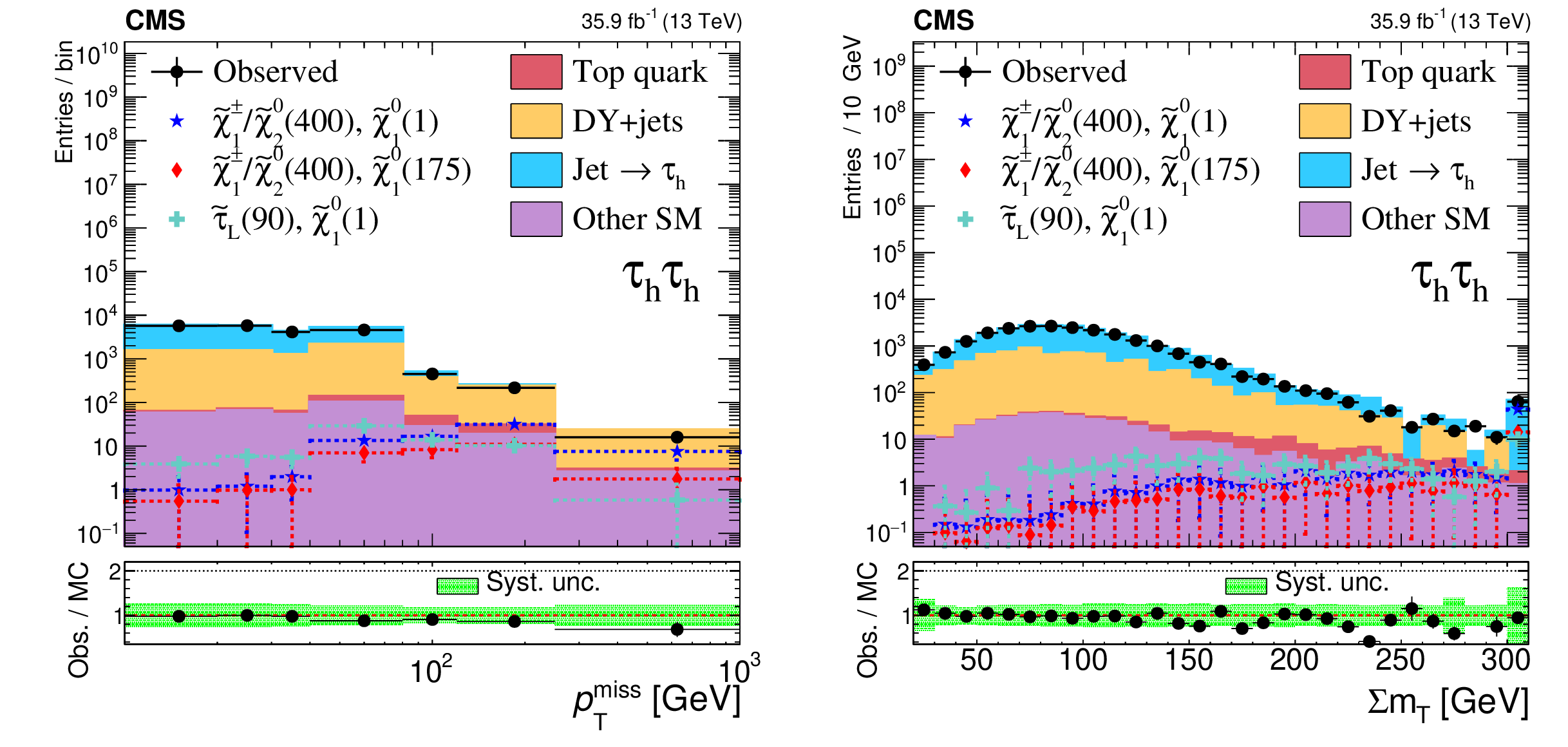
Figure 4:
Distributions of the search variables ${{p_{\mathrm {T}}} ^\text {miss}}$ (left) and ${\Sigma {m_{\mathrm {T}}}}$ (right) for the ${{{\tau} _\mathrm {h}} {{\tau} _\mathrm {h}}}$ final state for events after the baseline selection. The black points show the data. The background estimates are represented with stacked histograms. Distributions for two benchmark models of chargino-neutralino production, and one of direct left-handed $\tilde{\tau}$ pair production, are overlaid. The numbers within parentheses in the legend correspond to the masses of the parent SUSY particle and the $\tilde{ \chi }^{0}_{1}$ in GeV for these benchmark models. In both cases, the last bin includes overflows. |

png pdf |
Figure 4-a:
Distribution of ${{p_{\mathrm {T}}} ^\text {miss}}$ for the ${{{\tau} _\mathrm {h}} {{\tau} _\mathrm {h}}}$ final state for events after the baseline selection. The black points show the data. The background estimates are represented with stacked histograms. Distributions for two benchmark models of chargino-neutralino production, and one of direct left-handed $\tilde{\tau}$ pair production, are overlaid. The numbers within parentheses in the legend correspond to the masses of the parent SUSY particle and the $\tilde{ \chi }^{0}_{1}$ in GeV for these benchmark models. The last bin includes overflows. |
png pdf |
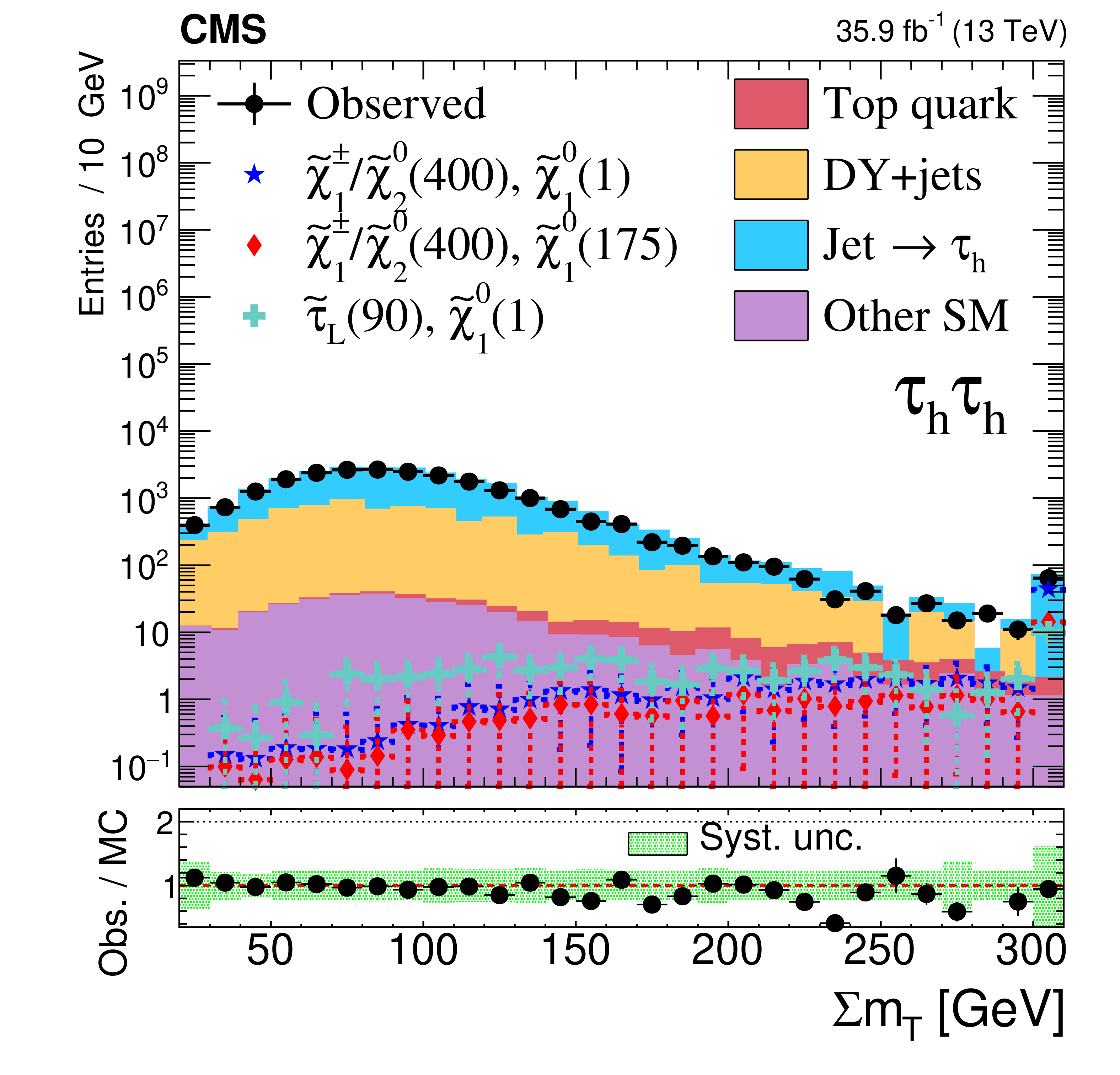
Figure 4-b:
Distribution of ${\Sigma {m_{\mathrm {T}}}}$ for the ${{{\tau} _\mathrm {h}} {{\tau} _\mathrm {h}}}$ final state for events after the baseline selection. The black points show the data. The background estimates are represented with stacked histograms. Distributions for two benchmark models of chargino-neutralino production, and one of direct left-handed $\tilde{\tau}$ pair production, are overlaid. The numbers within parentheses in the legend correspond to the masses of the parent SUSY particle and the $\tilde{ \chi }^{0}_{1}$ in GeV for these benchmark models. The last bin includes overflows. |
png pdf |
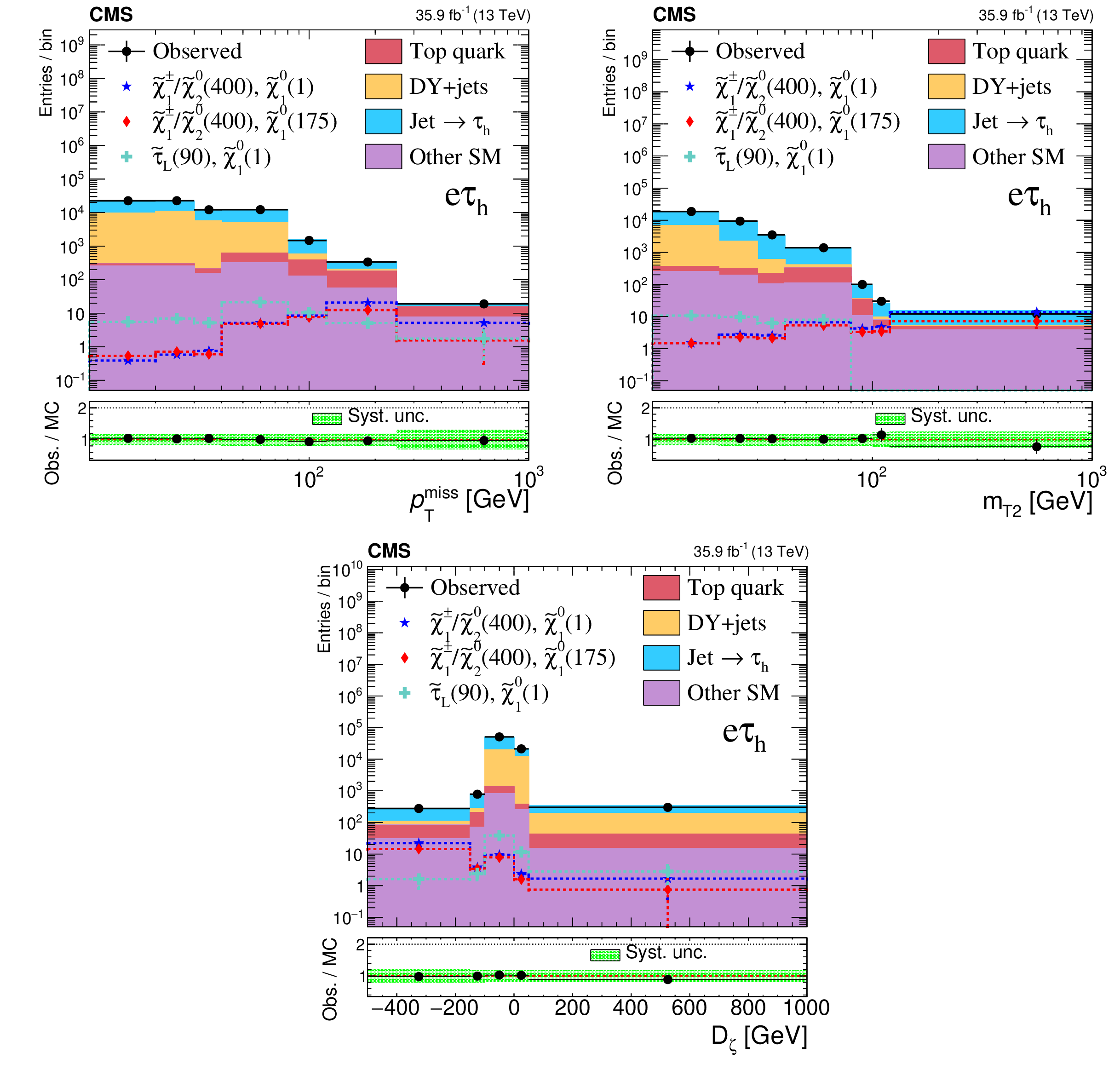
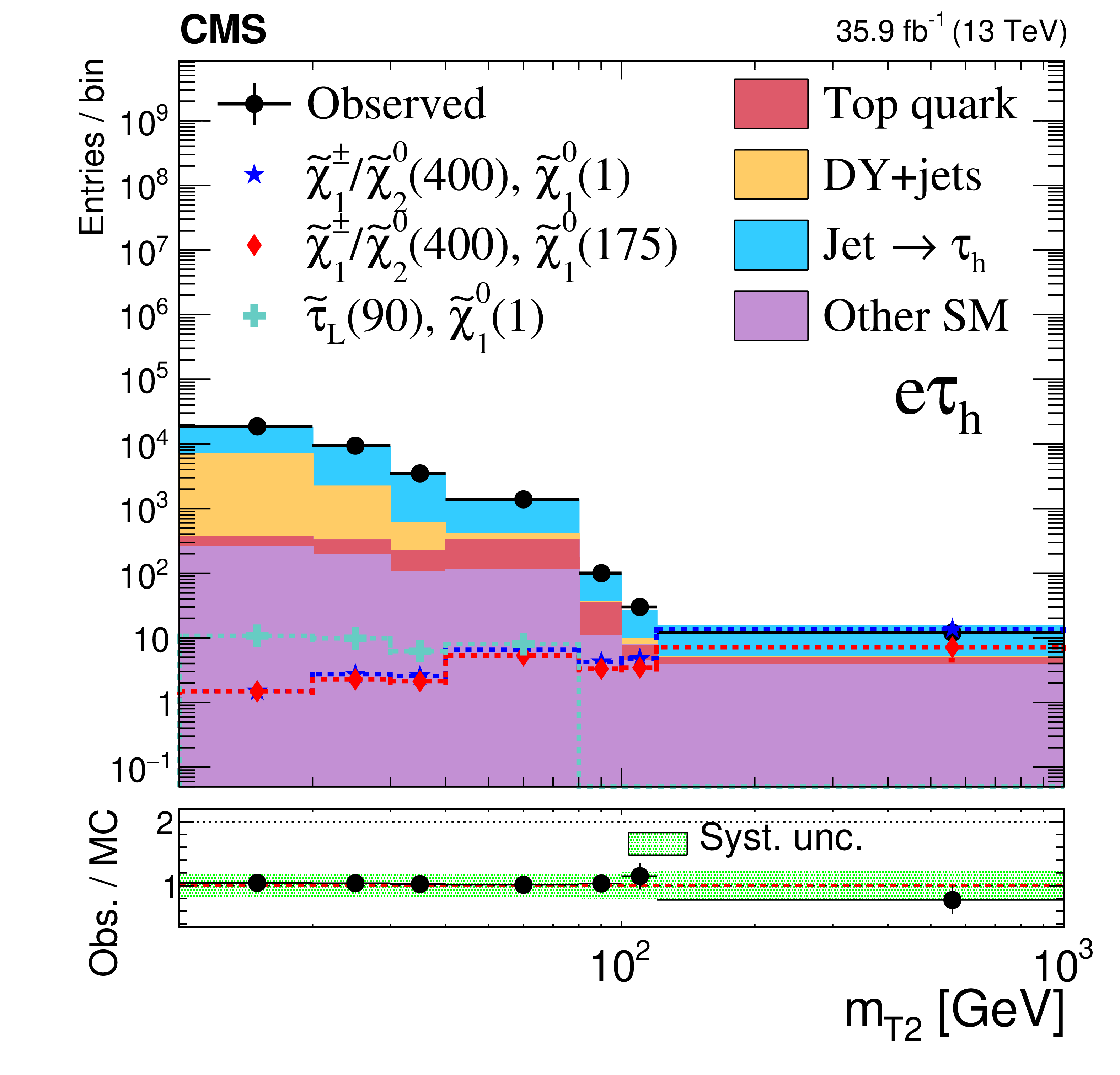
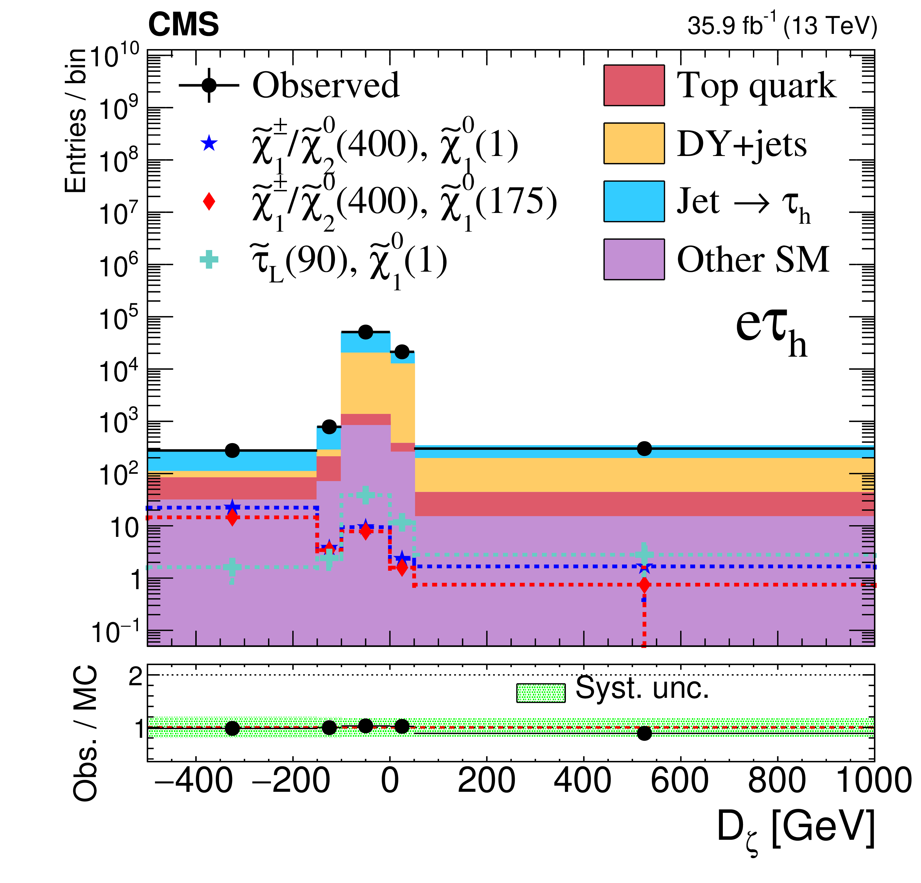
Figure 5:
Distributions of the search variables ${{p_{\mathrm {T}}} ^\text {miss}}$ (top left), ${m_{\mathrm {T2}}}$ (top right), and ${D_{\zeta}}$ (bottom) for the ${{\mathrm {e}} {{\tau} _\mathrm {h}}}$ final state for events after the baseline selection. The black points show the data. The background estimates are represented with stacked histograms. Distributions for two benchmark models of chargino-neutralino production, and one of direct left-handed $\tilde{\tau}$ pair production, are overlaid. The numbers within parentheses in the legend correspond to the masses of the parent SUSY particle and the $\tilde{ \chi }^{0}_{1}$ in GeV for these benchmark models. In all cases, the last bin includes overflows. |
png pdf |
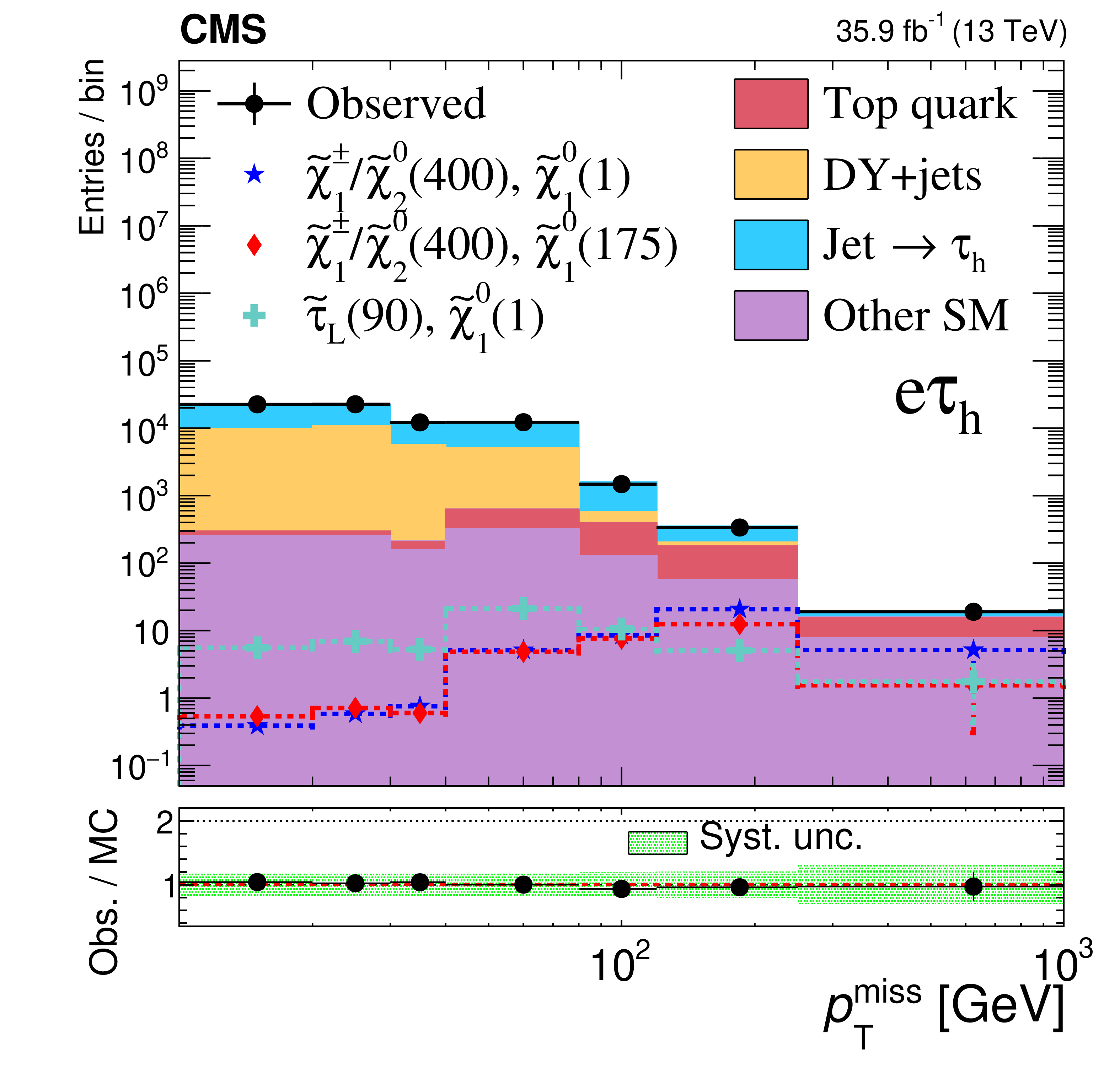
Figure 5-a:
Distribution of ${{p_{\mathrm {T}}} ^\text {miss}}$ for the ${{\mathrm {e}} {{\tau} _\mathrm {h}}}$ final state for events after the baseline selection. The black points show the data. The background estimates are represented with stacked histograms. Distributions for two benchmark models of chargino-neutralino production, and one of direct left-handed $\tilde{\tau}$ pair production, are overlaid. The numbers within parentheses in the legend correspond to the masses of the parent SUSY particle and the $\tilde{ \chi }^{0}_{1}$ in GeV for these benchmark models. The last bin includes overflows. |
png pdf |
Figure 5-b:
Distribution of ${m_{\mathrm {T2}}}$ for the ${{\mathrm {e}} {{\tau} _\mathrm {h}}}$ final state for events after the baseline selection. The black points show the data. The background estimates are represented with stacked histograms. Distributions for two benchmark models of chargino-neutralino production, and one of direct left-handed $\tilde{\tau}$ pair production, are overlaid. The numbers within parentheses in the legend correspond to the masses of the parent SUSY particle and the $\tilde{ \chi }^{0}_{1}$ in GeV for these benchmark models. The last bin includes overflows. |
png pdf |
Figure 5-c:
Distribution of ${D_{\zeta}}$ for the ${{\mathrm {e}} {{\tau} _\mathrm {h}}}$ final state for events after the baseline selection. The black points show the data. The background estimates are represented with stacked histograms. Distributions for two benchmark models of chargino-neutralino production, and one of direct left-handed $\tilde{\tau}$ pair production, are overlaid. The numbers within parentheses in the legend correspond to the masses of the parent SUSY particle and the $\tilde{ \chi }^{0}_{1}$ in GeV for these benchmark models. The last bin includes overflows. |

png pdf |
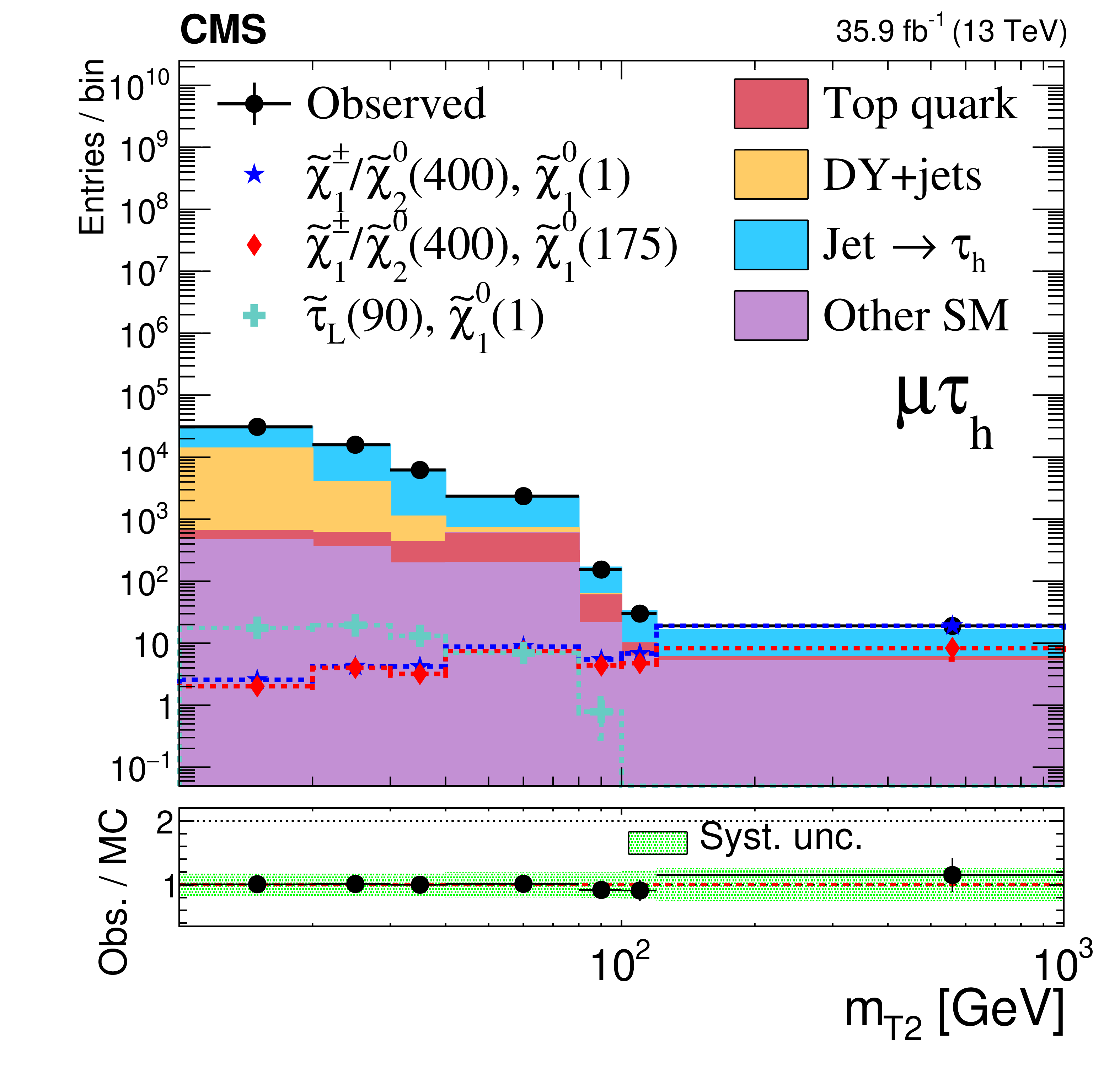
Figure 6:
Distributions of the search variables ${{p_{\mathrm {T}}} ^\text {miss}}$ (top left), ${m_{\mathrm {T2}}}$ (top right), and ${D_{\zeta}}$ (bottom) for the ${\mu {{\tau} _\mathrm {h}}}$ final state for events after the baseline selection. The black points show the data. The background estimates are represented with stacked histograms. Distributions for two benchmark models of chargino-neutralino production, and one of direct left-handed $\tilde{\tau}$ pair production, are overlaid. The numbers within parentheses in the legend correspond to the masses of the parent SUSY particle and the $\tilde{ \chi }^{0}_{1}$ in GeV for these benchmark models. In all cases, the last bin includes overflows. |

png pdf |
Figure 6-a:
Distributions of ${{p_{\mathrm {T}}} ^\text {miss}}$ for the ${\mu {{\tau} _\mathrm {h}}}$ final state for events after the baseline selection. The black points show the data. The background estimates are represented with stacked histograms. Distributions for two benchmark models of chargino-neutralino production, and one of direct left-handed $\tilde{\tau}$ pair production, are overlaid. The numbers within parentheses in the legend correspond to the masses of the parent SUSY particle and the $\tilde{ \chi }^{0}_{1}$ in GeV for these benchmark models. The last bin includes overflows. |
png pdf |
Figure 6-b:
Distributions of ${m_{\mathrm {T2}}}$ for the ${\mu {{\tau} _\mathrm {h}}}$ final state for events after the baseline selection. The black points show the data. The background estimates are represented with stacked histograms. Distributions for two benchmark models of chargino-neutralino production, and one of direct left-handed $\tilde{\tau}$ pair production, are overlaid. The numbers within parentheses in the legend correspond to the masses of the parent SUSY particle and the $\tilde{ \chi }^{0}_{1}$ in GeV for these benchmark models. The last bin includes overflows. |

png pdf |
Figure 6-c:
Distributions of ${D_{\zeta}}$ for the ${\mu {{\tau} _\mathrm {h}}}$ final state for events after the baseline selection. The black points show the data. The background estimates are represented with stacked histograms. Distributions for two benchmark models of chargino-neutralino production, and one of direct left-handed $\tilde{\tau}$ pair production, are overlaid. The numbers within parentheses in the legend correspond to the masses of the parent SUSY particle and the $\tilde{ \chi }^{0}_{1}$ in GeV for these benchmark models. The last bin includes overflows. |
png pdf |
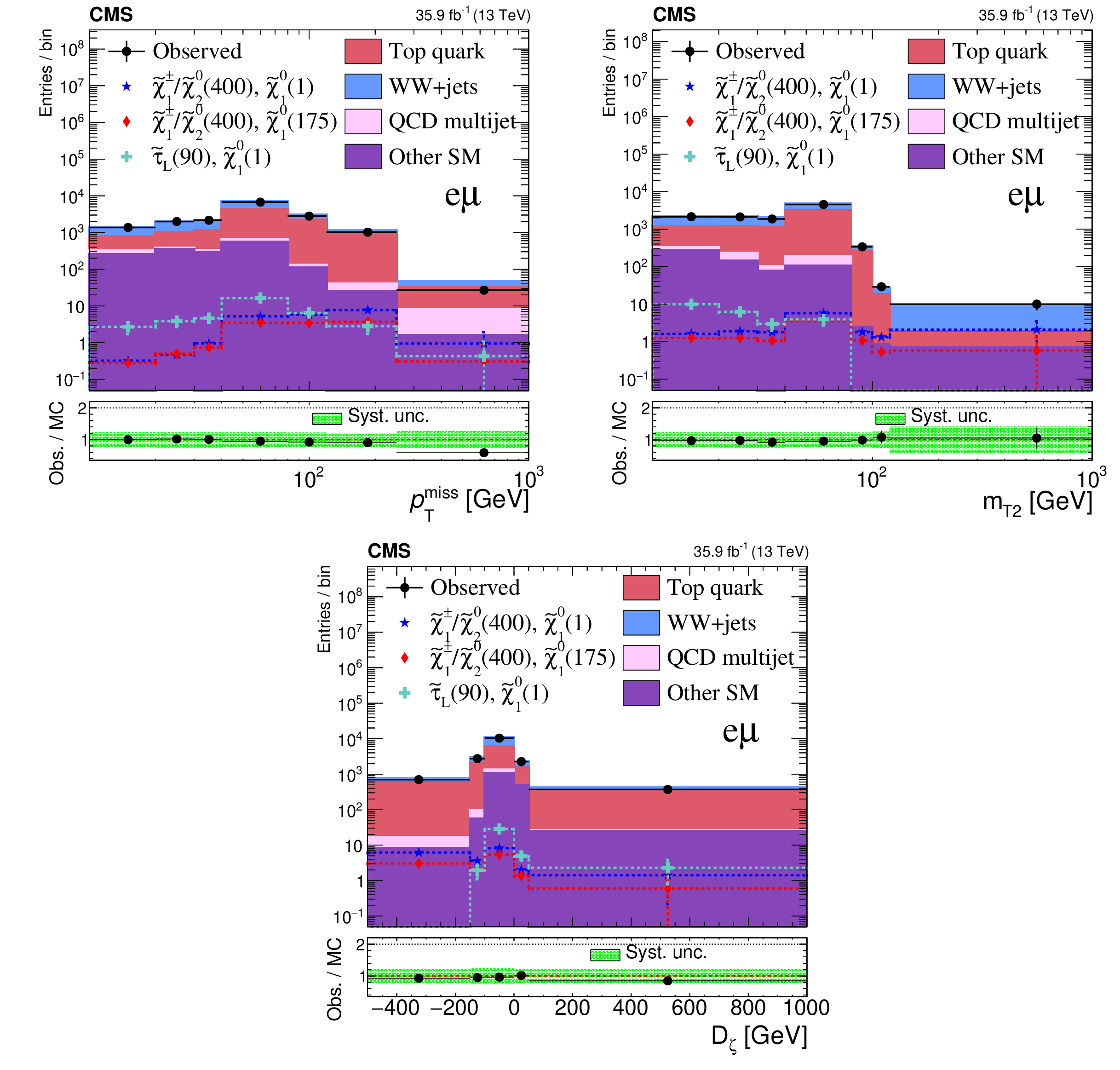
Figure 7:
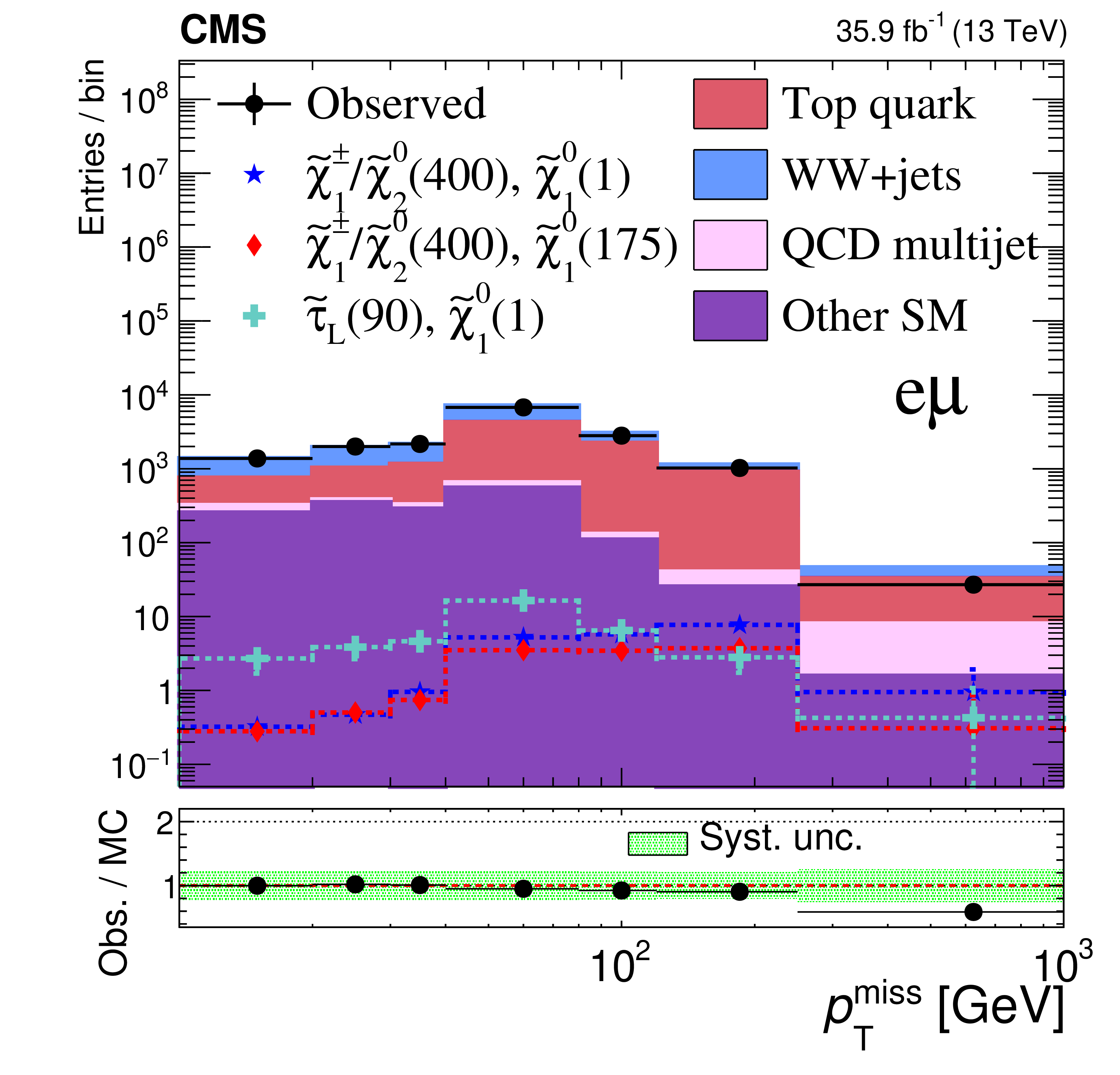
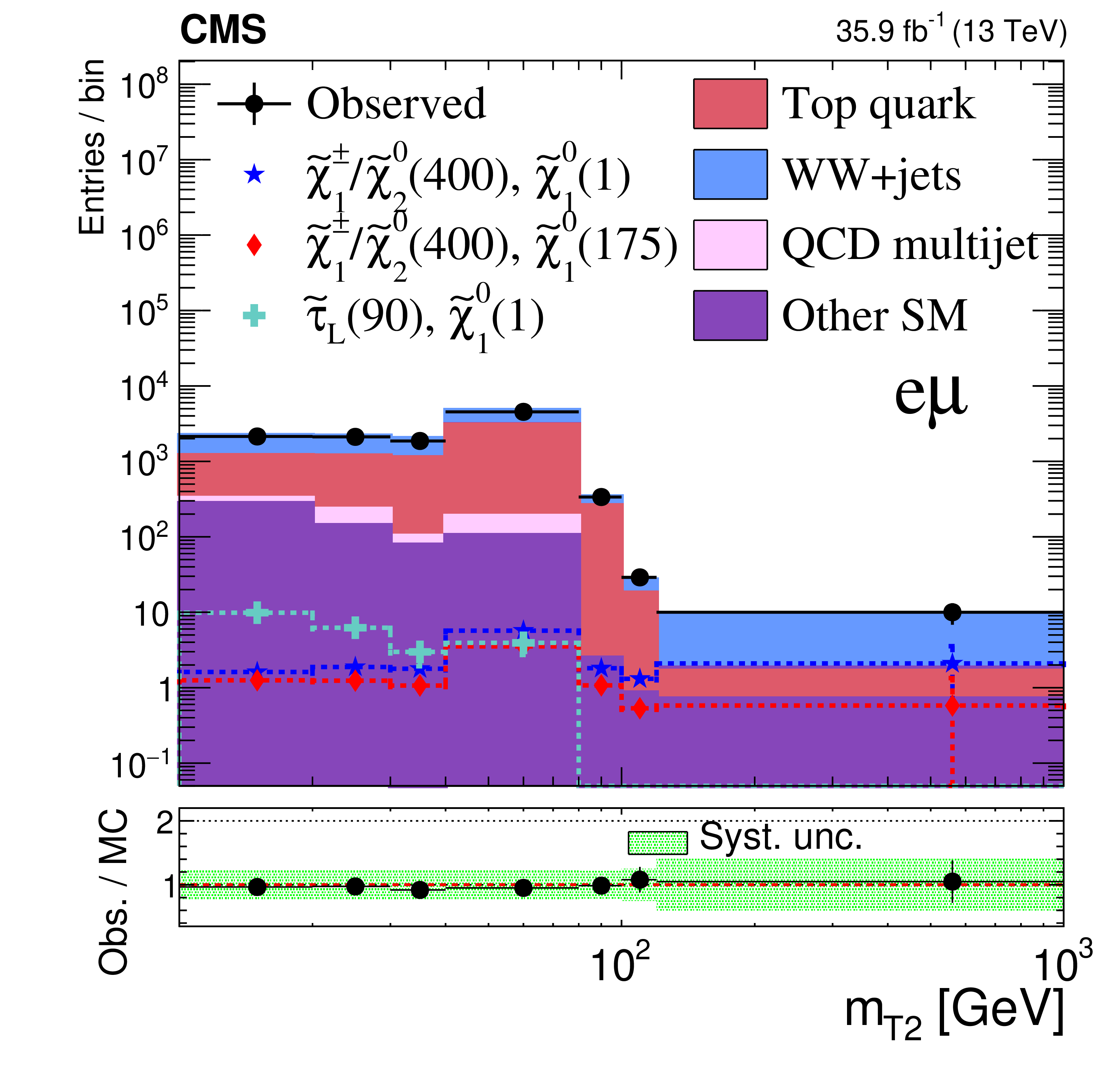
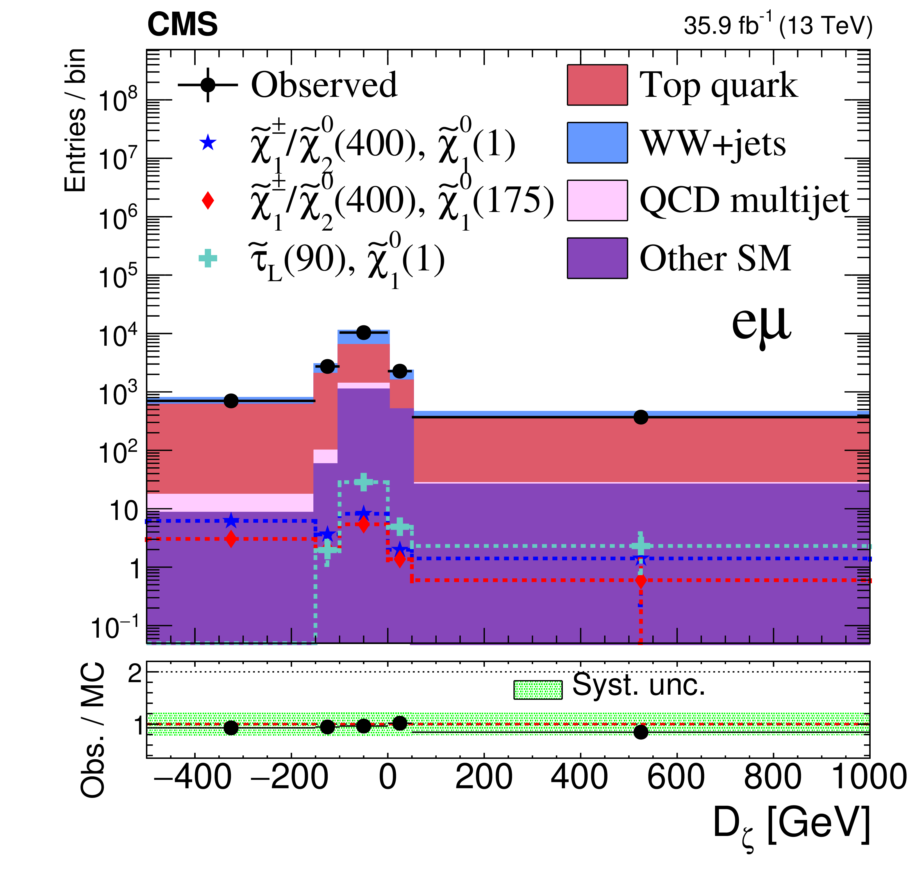
Distributions of the search variables ${{p_{\mathrm {T}}} ^\text {miss}}$ (top left), ${m_{\mathrm {T2}}}$ (top right), and ${D_{\zeta}}$ (bottom) for the ${{\mathrm {e}}\mu}$ final state for events after the baseline selection. The black points show the data. The background estimates are represented with stacked histograms. Distributions for two benchmark models of chargino-neutralino production, and one of direct left-handed $\tilde{\tau}$ pair production, are overlaid. The numbers within parentheses in the legend correspond to the masses of the parent SUSY particle and the $\tilde{ \chi }^{0}_{1}$ in GeV for these benchmark models. In all cases, the last bin includes overflows. |
png pdf |
Figure 7-a:
Distribution of ${{p_{\mathrm {T}}} ^\text {miss}}$ for the ${{\mathrm {e}}\mu}$ final state for events after the baseline selection. The black points show the data. The background estimates are represented with stacked histograms. Distributions for two benchmark models of chargino-neutralino production, and one of direct left-handed $\tilde{\tau}$ pair production, are overlaid. The numbers within parentheses in the legend correspond to the masses of the parent SUSY particle and the $\tilde{ \chi }^{0}_{1}$ in GeV for these benchmark models. The last bin includes overflows. |
png pdf |
Figure 7-b:
Distribution of ${m_{\mathrm {T2}}}$ for the ${{\mathrm {e}}\mu}$ final state for events after the baseline selection. The black points show the data. The background estimates are represented with stacked histograms. Distributions for two benchmark models of chargino-neutralino production, and one of direct left-handed $\tilde{\tau}$ pair production, are overlaid. The numbers within parentheses in the legend correspond to the masses of the parent SUSY particle and the $\tilde{ \chi }^{0}_{1}$ in GeV for these benchmark models. The last bin includes overflows. |
png pdf |
Figure 7-c:
Distribution of ${D_{\zeta}}$ for the ${{\mathrm {e}}\mu}$ final state for events after the baseline selection. The black points show the data. The background estimates are represented with stacked histograms. Distributions for two benchmark models of chargino-neutralino production, and one of direct left-handed $\tilde{\tau}$ pair production, are overlaid. The numbers within parentheses in the legend correspond to the masses of the parent SUSY particle and the $\tilde{ \chi }^{0}_{1}$ in GeV for these benchmark models. The last bin includes overflows. |
png pdf |
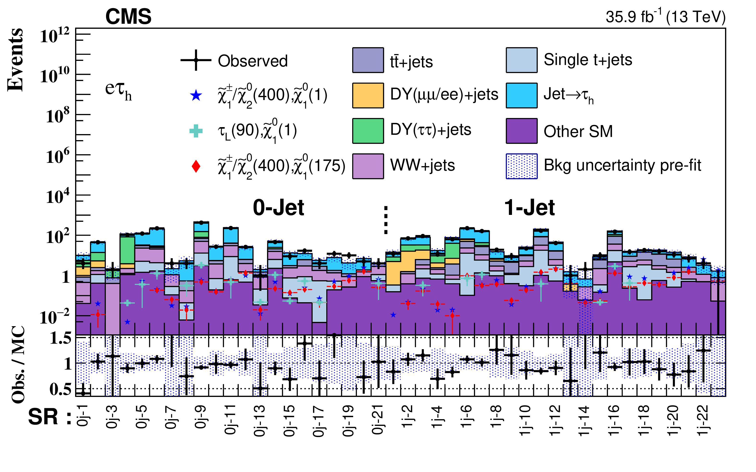
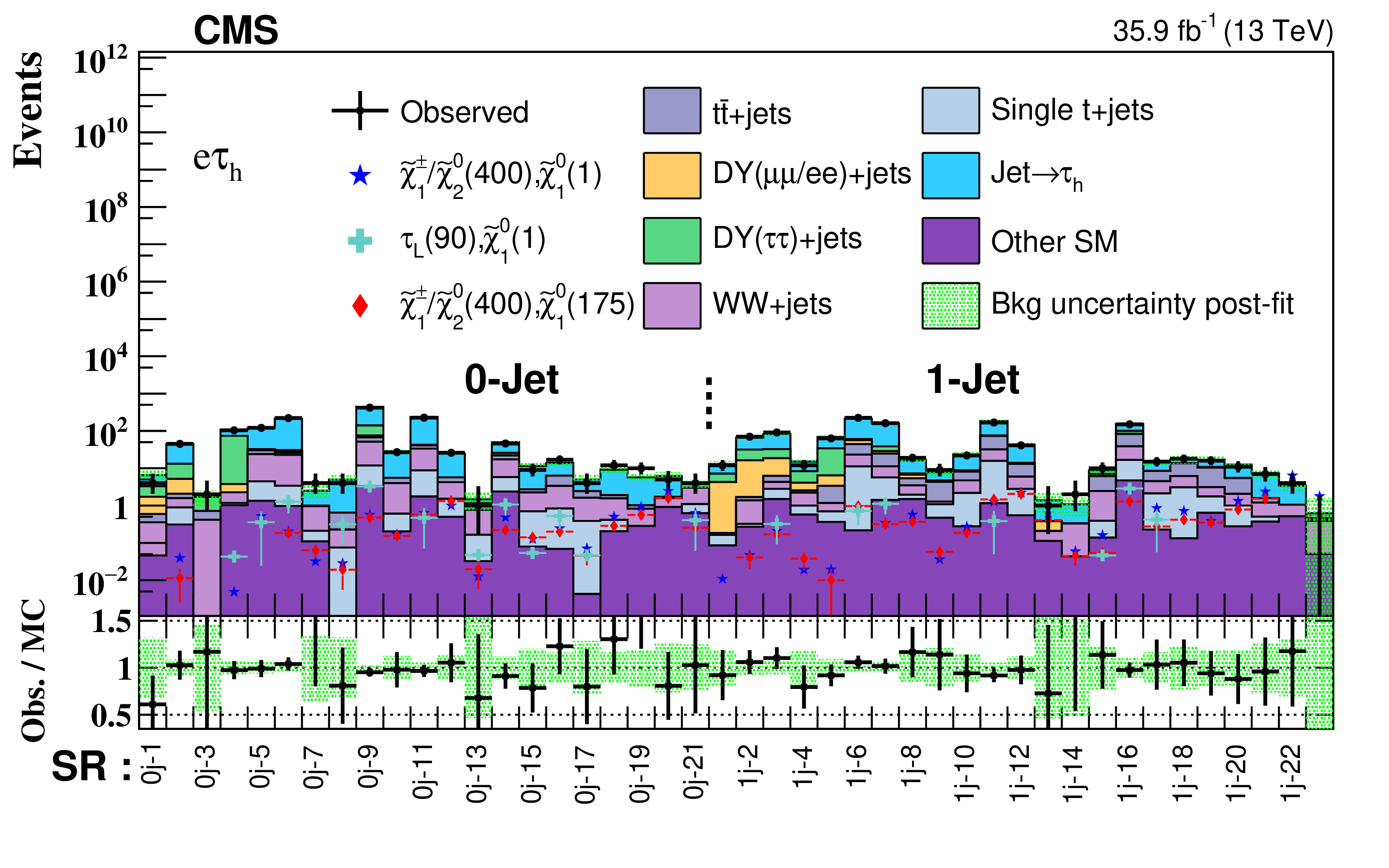
Figure 8:
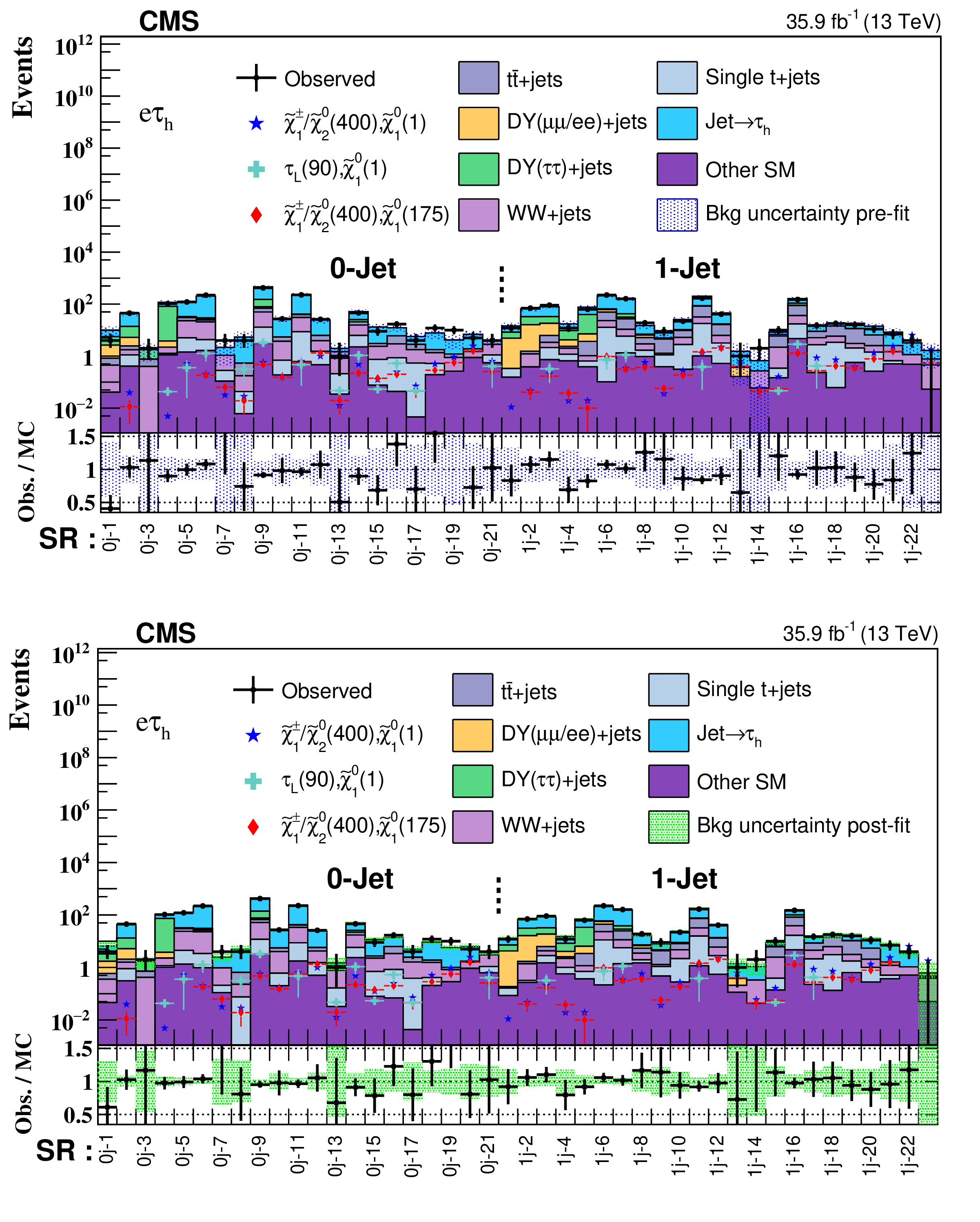
Pre-fit (upper) and post-fit (lower) results for the SRs used for the final signal extraction in the ${{\mathrm {e}} {{\tau} _\mathrm {h}}}$ final state. Distributions for two benchmark models of chargino-neutralino production, and one of direct left-handed $\tilde{\tau}$ pair production, are overlaid. The numbers within parentheses in the legend correspond to the masses of the parent SUSY particle and the $\tilde{ \chi }^{0}_{1}$ in GeV for these benchmark models. In the ratio panels, the black markers indicate the ratio of the observed data in each SR to the corresponding pre-fit or post-fit SM background prediction. |
png pdf |
Figure 8-a:
Pre-fit results for the SRs used for the final signal extraction in the ${{\mathrm {e}} {{\tau} _\mathrm {h}}}$ final state. Distributions for two benchmark models of chargino-neutralino production, and one of direct left-handed $\tilde{\tau}$ pair production, are overlaid. The numbers within parentheses in the legend correspond to the masses of the parent SUSY particle and the $\tilde{ \chi }^{0}_{1}$ in GeV for these benchmark models. In the ratio panel, the black markers indicate the ratio of the observed data in each SR to the corresponding SM background prediction. |
png pdf |
Figure 8-b:
Post-fit results for the SRs used for the final signal extraction in the ${{\mathrm {e}} {{\tau} _\mathrm {h}}}$ final state. Distributions for two benchmark models of chargino-neutralino production, and one of direct left-handed $\tilde{\tau}$ pair production, are overlaid. The numbers within parentheses in the legend correspond to the masses of the parent SUSY particle and the $\tilde{ \chi }^{0}_{1}$ in GeV for these benchmark models. In the ratio panel, the black markers indicate the ratio of the observed data in each SR to the corresponding SM background prediction. |
png pdf |
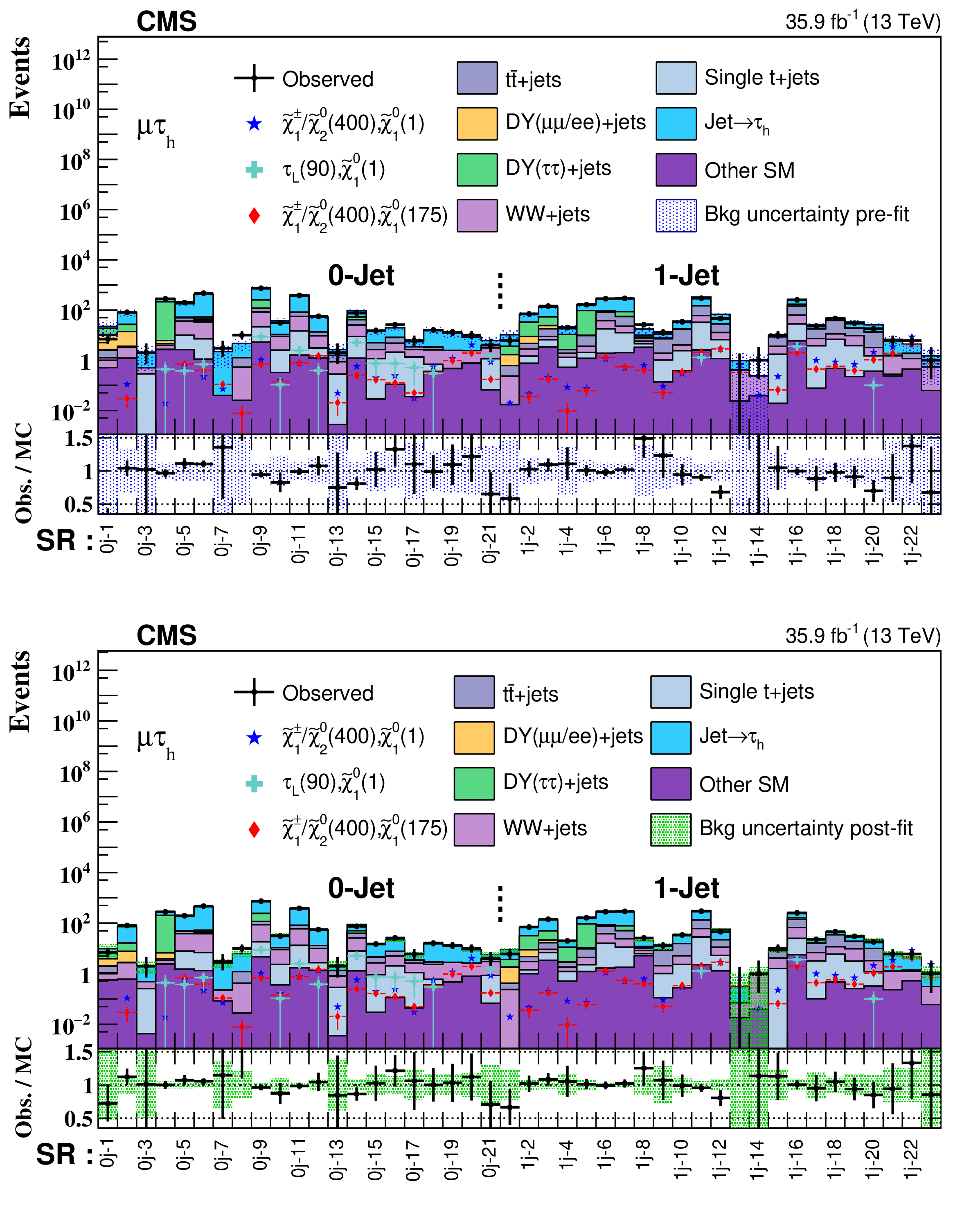
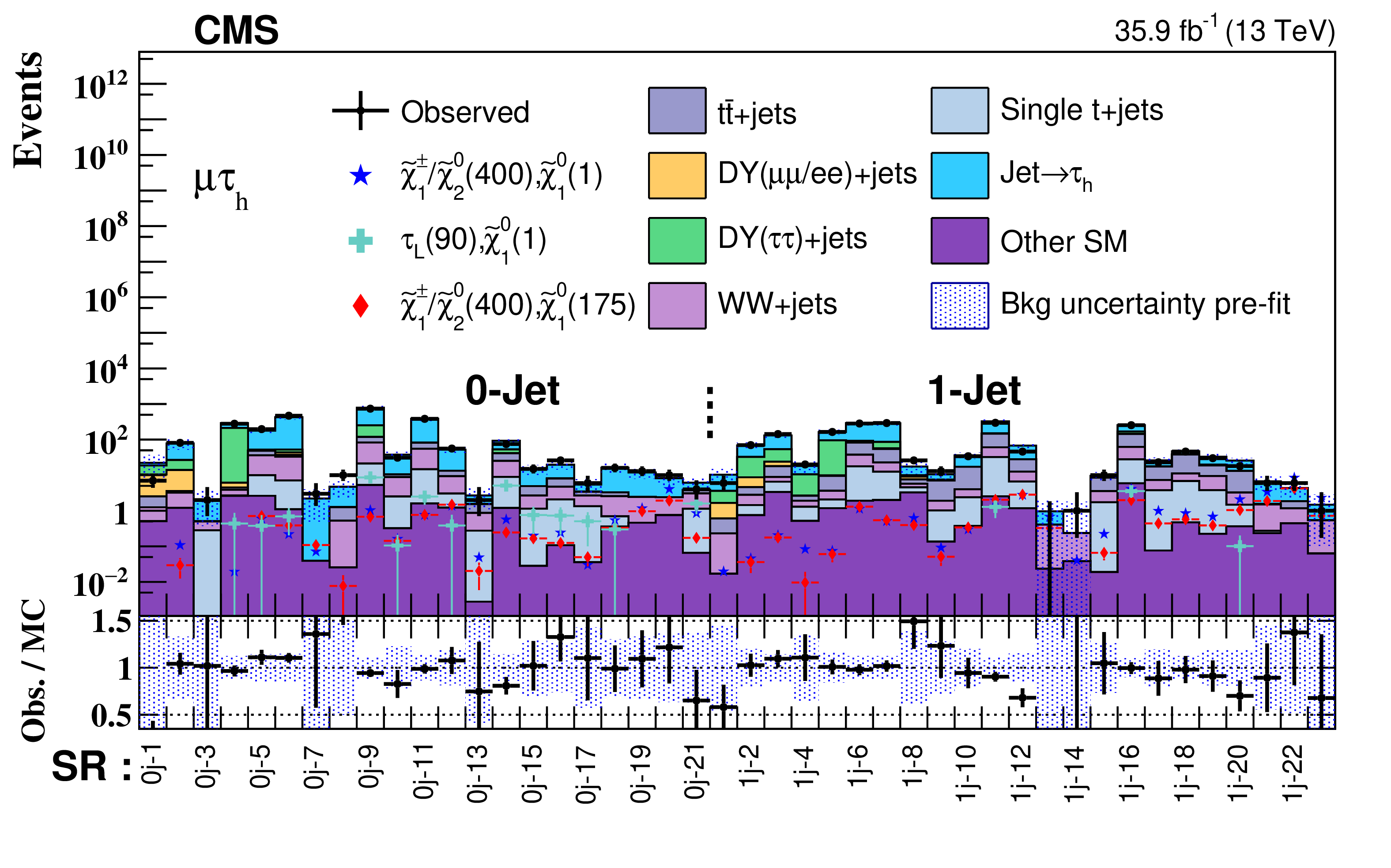
Figure 9:
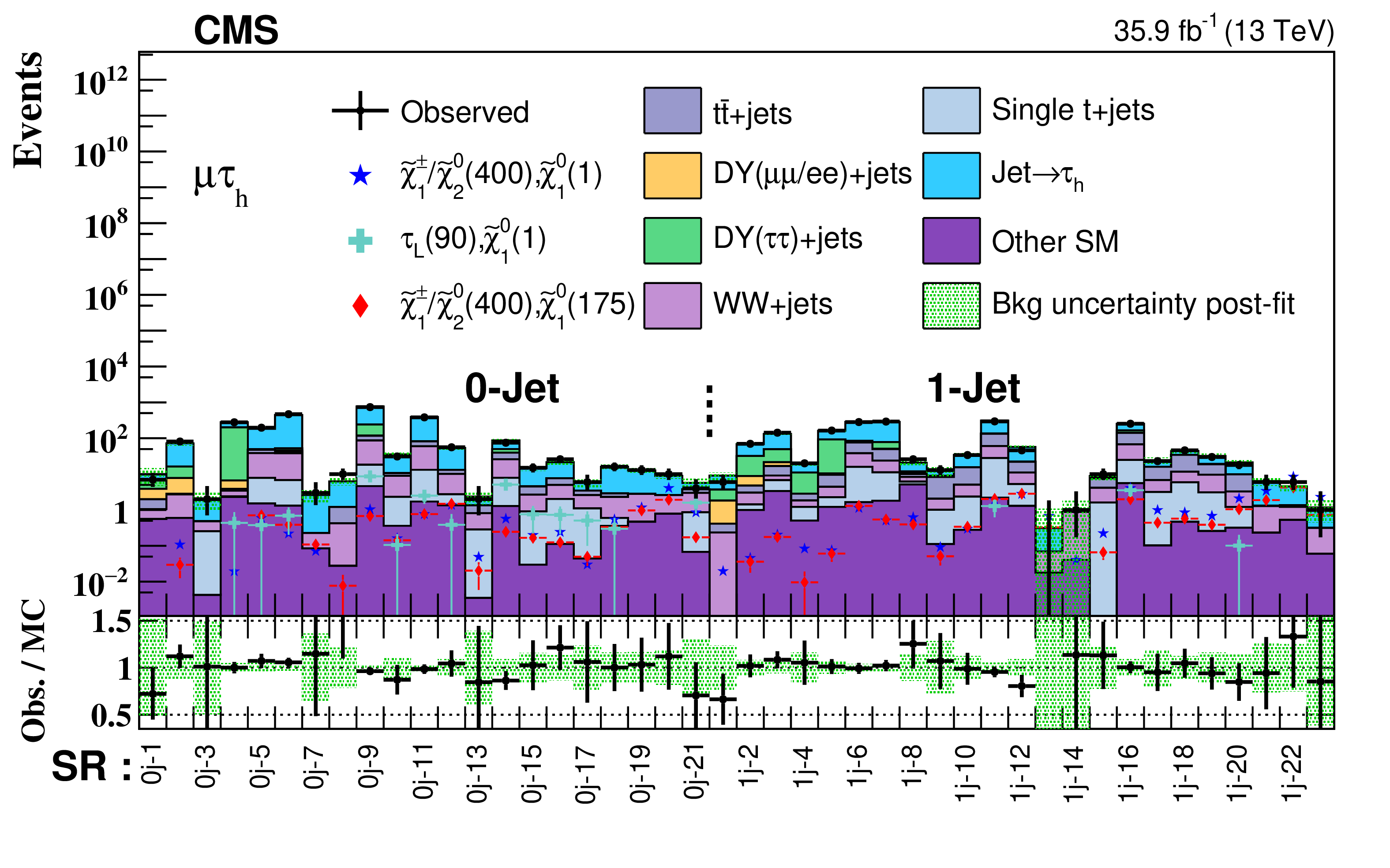
Pre-fit (upper) and post-fit (lower) results for the SRs used for the final signal extraction in the ${\mu {{\tau} _\mathrm {h}}}$ final state. Distributions for two benchmark models of chargino-neutralino production, and one of direct left-handed $\tilde{\tau}$ pair production, are overlaid. The numbers within parentheses in the legend correspond to the masses of the parent SUSY particle and the $\tilde{ \chi }^{0}_{1}$ in GeV for these benchmark models. In the ratio panels, the black markers indicate the ratio of the observed data in each SR to the corresponding pre-fit or post-fit SM background prediction. |
png pdf |
Figure 9-a:
Pre-fit results for the SRs used for the final signal extraction in the ${\mu {{\tau} _\mathrm {h}}}$ final state. Distributions for two benchmark models of chargino-neutralino production, and one of direct left-handed $\tilde{\tau}$ pair production, are overlaid. The numbers within parentheses in the legend correspond to the masses of the parent SUSY particle and the $\tilde{ \chi }^{0}_{1}$ in GeV for these benchmark models. In the ratio panel, the black markers indicate the ratio of the observed data in each SR to the corresponding SM background prediction. |
png pdf |
Figure 9-b:
Post-fit results for the SRs used for the final signal extraction in the ${\mu {{\tau} _\mathrm {h}}}$ final state. Distributions for two benchmark models of chargino-neutralino production, and one of direct left-handed $\tilde{\tau}$ pair production, are overlaid. The numbers within parentheses in the legend correspond to the masses of the parent SUSY particle and the $\tilde{ \chi }^{0}_{1}$ in GeV for these benchmark models. In the ratio panel, the black markers indicate the ratio of the observed data in each SR to the corresponding SM background prediction. |

png pdf |
Figure 10:
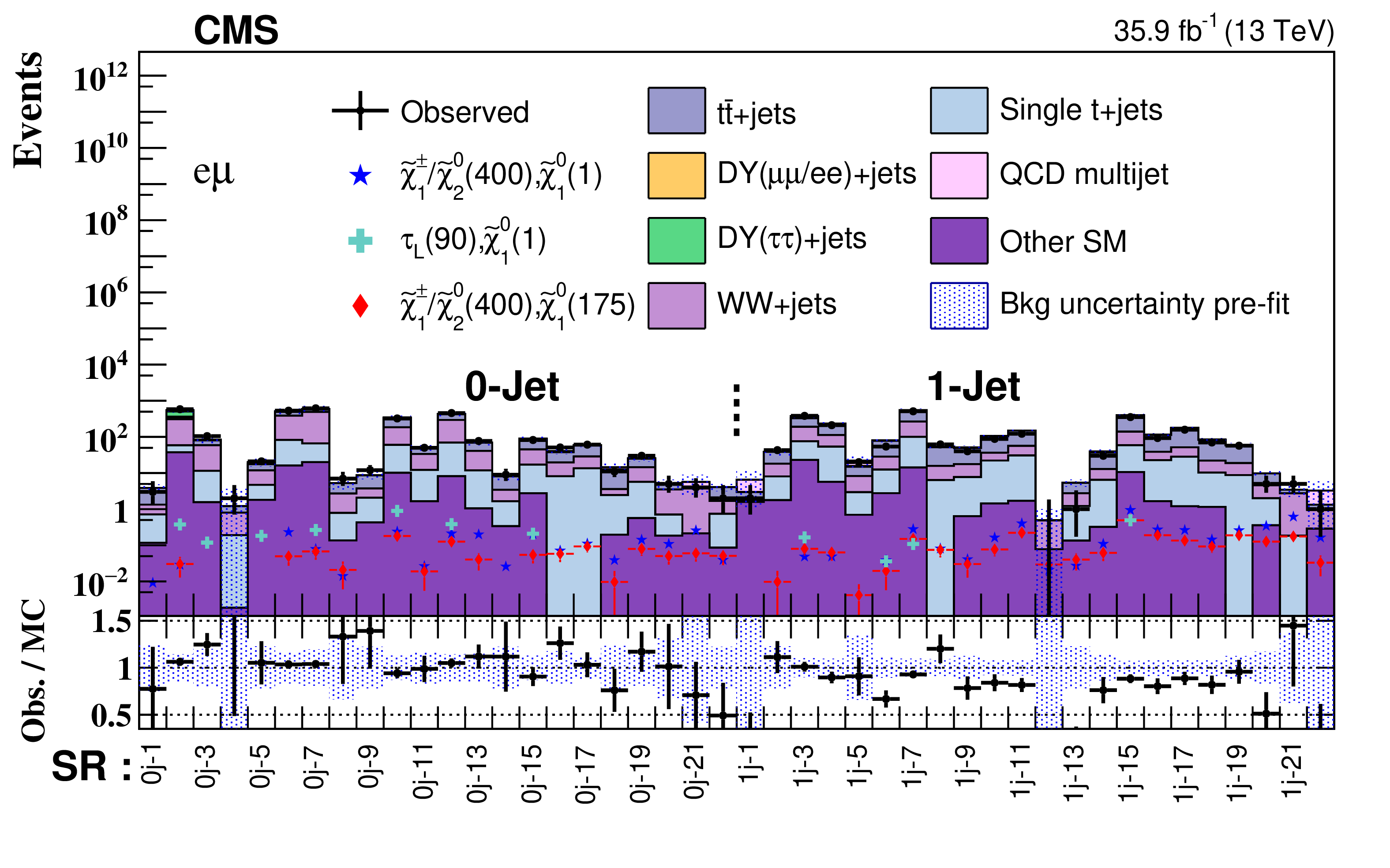
Pre-fit (upper) and post-fit (lower) results for the SRs used for the final signal extraction in the ${{\mathrm {e}}\mu}$ final state. Distributions for two benchmark models of chargino-neutralino production, and one of direct left-handed $\tilde{\tau}$ pair production, are overlaid. The numbers within parentheses in the legend correspond to the masses of the parent SUSY particle and the $\tilde{ \chi }^{0}_{1}$ in GeV for these benchmark models. In the ratio panels, the black markers indicate the ratio of the observed data in each SR to the corresponding pre-fit or post-fit SM background prediction. |
png pdf |
Figure 10-a:
Pre-fit results for the SRs used for the final signal extraction in the ${{\mathrm {e}}\mu}$ final state. Distributions for two benchmark models of chargino-neutralino production, and one of direct left-handed $\tilde{\tau}$ pair production, are overlaid. The numbers within parentheses in the legend correspond to the masses of the parent SUSY particle and the $\tilde{ \chi }^{0}_{1}$ in GeV for these benchmark models. In the ratio panel, the black markers indicate the ratio of the observed data in each SR to the corresponding pre-fit or post-fit SM background prediction. |

png pdf |
Figure 10-b:
Post-fit results for the SRs used for the final signal extraction in the ${{\mathrm {e}}\mu}$ final state. Distributions for two benchmark models of chargino-neutralino production, and one of direct left-handed $\tilde{\tau}$ pair production, are overlaid. The numbers within parentheses in the legend correspond to the masses of the parent SUSY particle and the $\tilde{ \chi }^{0}_{1}$ in GeV for these benchmark models. In the ratio panel, the black markers indicate the ratio of the observed data in each SR to the corresponding pre-fit or post-fit SM background prediction. |
png pdf |
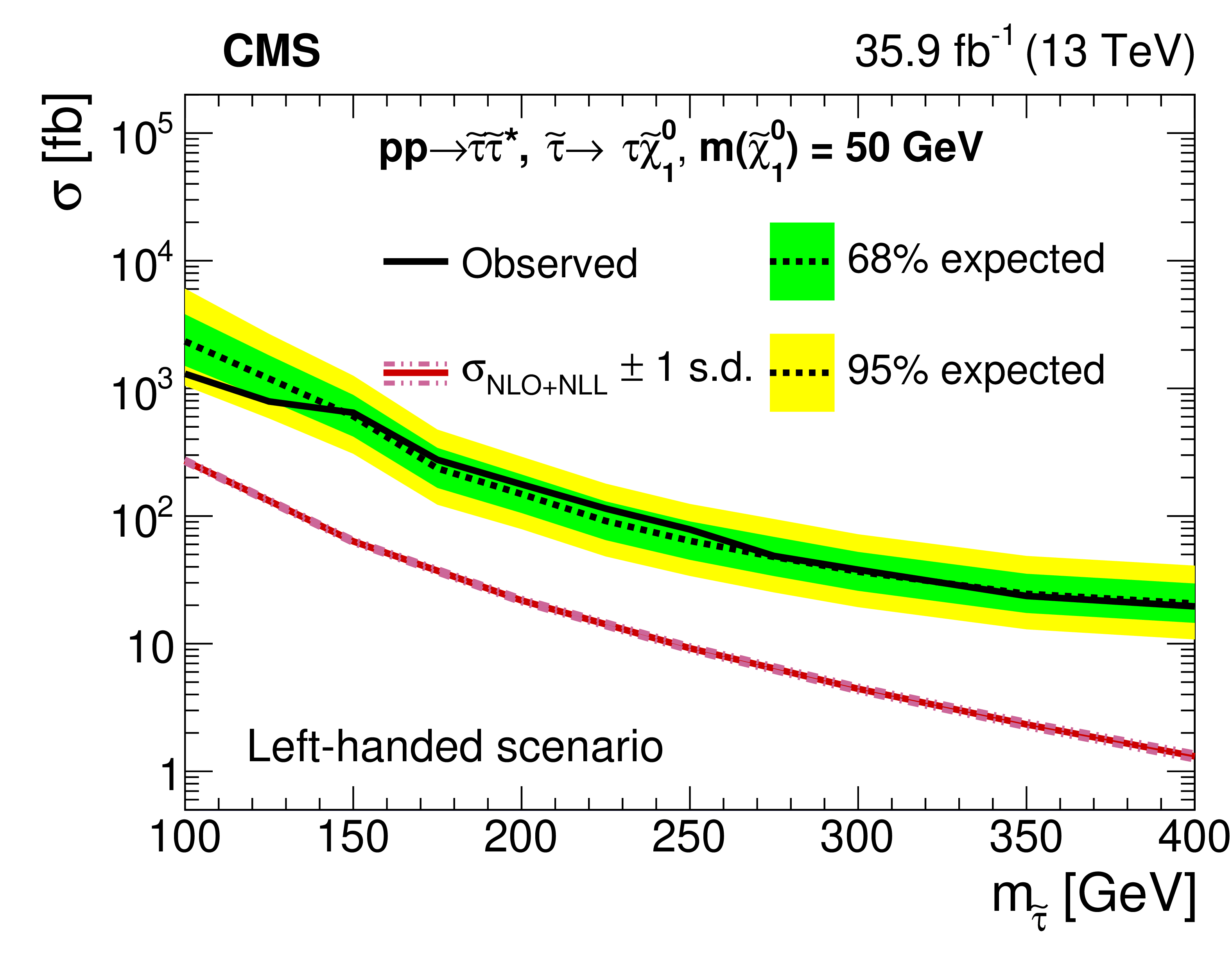
Figure 11:
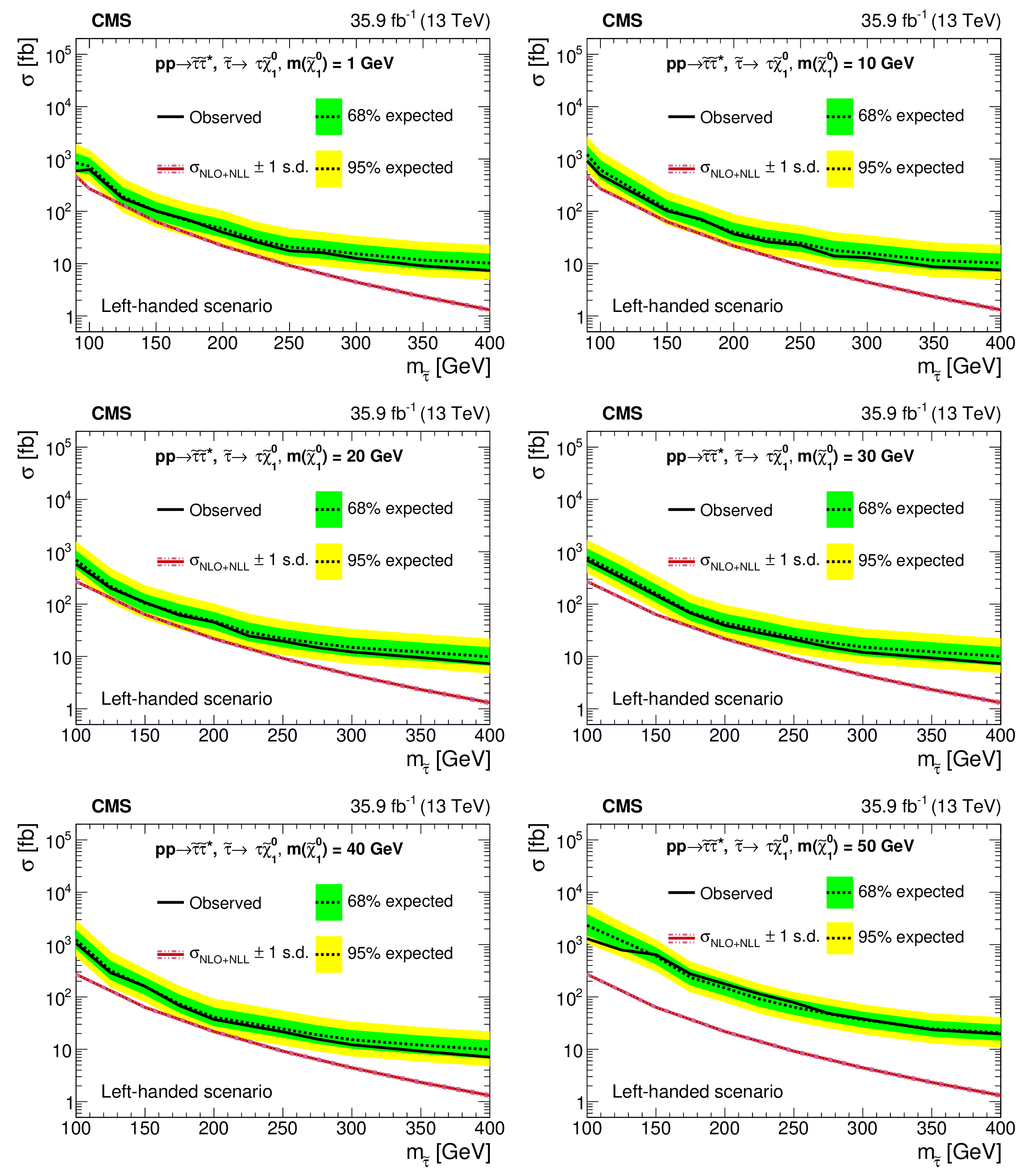
Excluded $\tilde{\tau}$ pair production cross section as a function of the $\tilde{\tau}$ mass for the left-handed $\tilde{\tau}$ scenario, and for different $\tilde{ \chi }^{0}_{1}$ masses of 1, 10, 20, 30, 40, and 50 GeV from upper left to lower right, respectively. The inner (green) band and the outer (yellow) band indicate the regions containing 68 and 95%, respectively, of the distribution of limits expected under the background-only hypothesis. The red line indicates the NLO+NLL prediction for the signal production cross section calculated with Resummino [47], while the red hatched band represents the uncertainty in the prediction. |

png pdf root |
Figure 11-a:
Excluded $\tilde{\tau}$ pair production cross section as a function of the $\tilde{\tau}$ mass for the left-handed $\tilde{\tau}$ scenario, and for a $\tilde{ \chi }^{0}_{1}$ mass of 1 GeV. The inner (green) band and the outer (yellow) band indicate the regions containing 68 and 95%, respectively, of the distribution of limits expected under the background-only hypothesis. The red line indicates the NLO+NLL prediction for the signal production cross section calculated with Resummino [47], while the red hatched band represents the uncertainty in the prediction. |

png pdf root |
Figure 11-b:
Excluded $\tilde{\tau}$ pair production cross section as a function of the $\tilde{\tau}$ mass for the left-handed $\tilde{\tau}$ scenario, and for a $\tilde{ \chi }^{0}_{1}$ mass of 10 GeV. The inner (green) band and the outer (yellow) band indicate the regions containing 68 and 95%, respectively, of the distribution of limits expected under the background-only hypothesis. The red line indicates the NLO+NLL prediction for the signal production cross section calculated with Resummino [47], while the red hatched band represents the uncertainty in the prediction. |

png pdf root |
Figure 11-c:
Excluded $\tilde{\tau}$ pair production cross section as a function of the $\tilde{\tau}$ mass for the left-handed $\tilde{\tau}$ scenario, and for a $\tilde{ \chi }^{0}_{1}$ mass of 20 GeV. The inner (green) band and the outer (yellow) band indicate the regions containing 68 and 95%, respectively, of the distribution of limits expected under the background-only hypothesis. The red line indicates the NLO+NLL prediction for the signal production cross section calculated with Resummino [47], while the red hatched band represents the uncertainty in the prediction. |
png pdf root |
Figure 11-d:
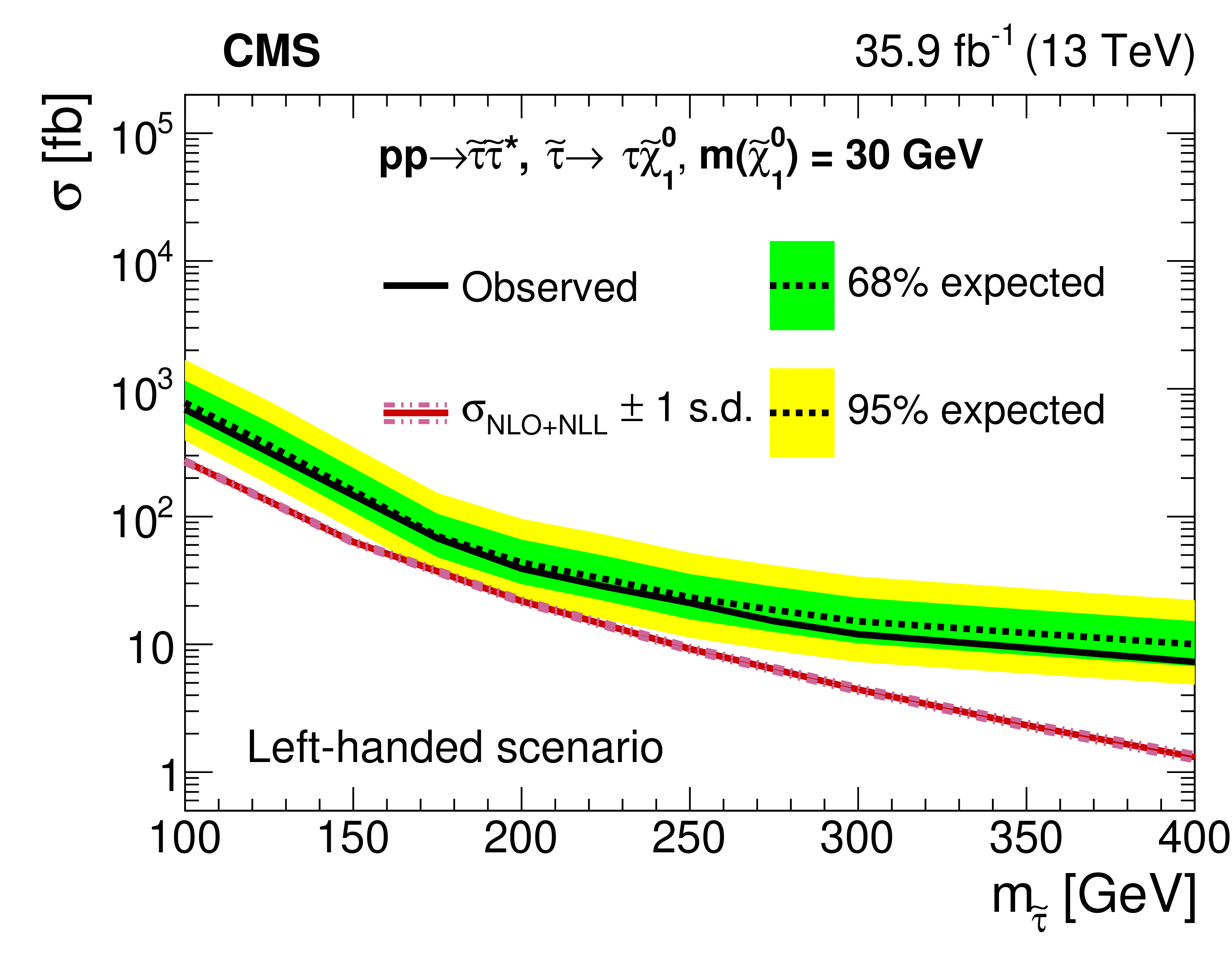
Excluded $\tilde{\tau}$ pair production cross section as a function of the $\tilde{\tau}$ mass for the left-handed $\tilde{\tau}$ scenario, and for a $\tilde{ \chi }^{0}_{1}$ mass of 30 GeV. The inner (green) band and the outer (yellow) band indicate the regions containing 68 and 95%, respectively, of the distribution of limits expected under the background-only hypothesis. The red line indicates the NLO+NLL prediction for the signal production cross section calculated with Resummino [47], while the red hatched band represents the uncertainty in the prediction. |

png pdf root |
Figure 11-e:
Excluded $\tilde{\tau}$ pair production cross section as a function of the $\tilde{\tau}$ mass for the left-handed $\tilde{\tau}$ scenario, and for a $\tilde{ \chi }^{0}_{1}$ mass of 40 GeV. The inner (green) band and the outer (yellow) band indicate the regions containing 68 and 95%, respectively, of the distribution of limits expected under the background-only hypothesis. The red line indicates the NLO+NLL prediction for the signal production cross section calculated with Resummino [47], while the red hatched band represents the uncertainty in the prediction. |
png pdf root |
Figure 11-f:
Excluded $\tilde{\tau}$ pair production cross section as a function of the $\tilde{\tau}$ mass for the left-handed $\tilde{\tau}$ scenario, and for a $\tilde{ \chi }^{0}_{1}$ mass of 50 GeV. The inner (green) band and the outer (yellow) band indicate the regions containing 68 and 95%, respectively, of the distribution of limits expected under the background-only hypothesis. The red line indicates the NLO+NLL prediction for the signal production cross section calculated with Resummino [47], while the red hatched band represents the uncertainty in the prediction. |
png pdf |
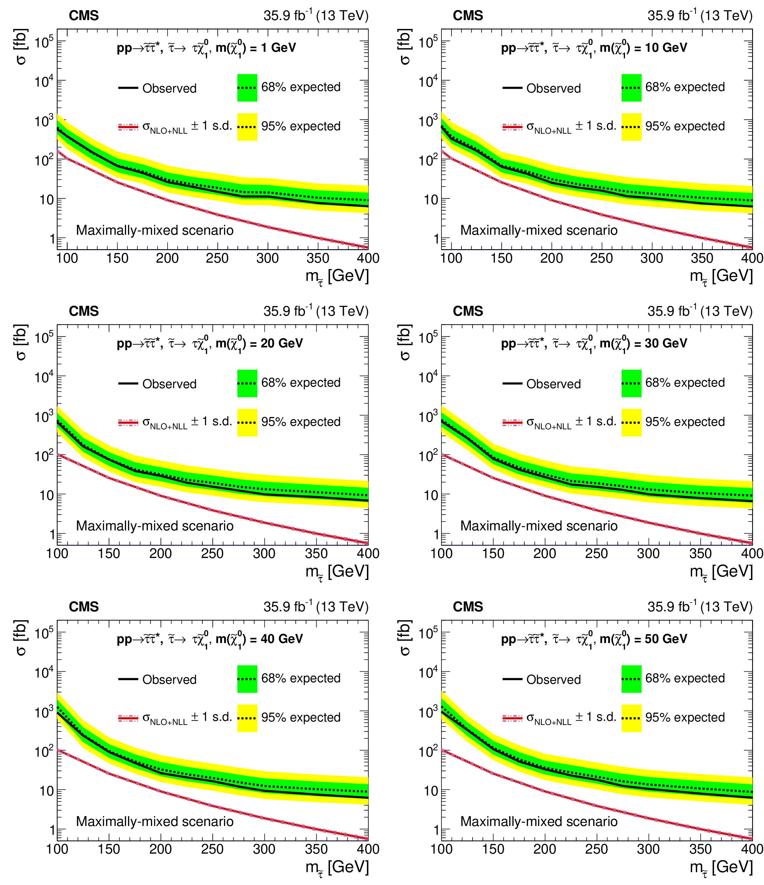
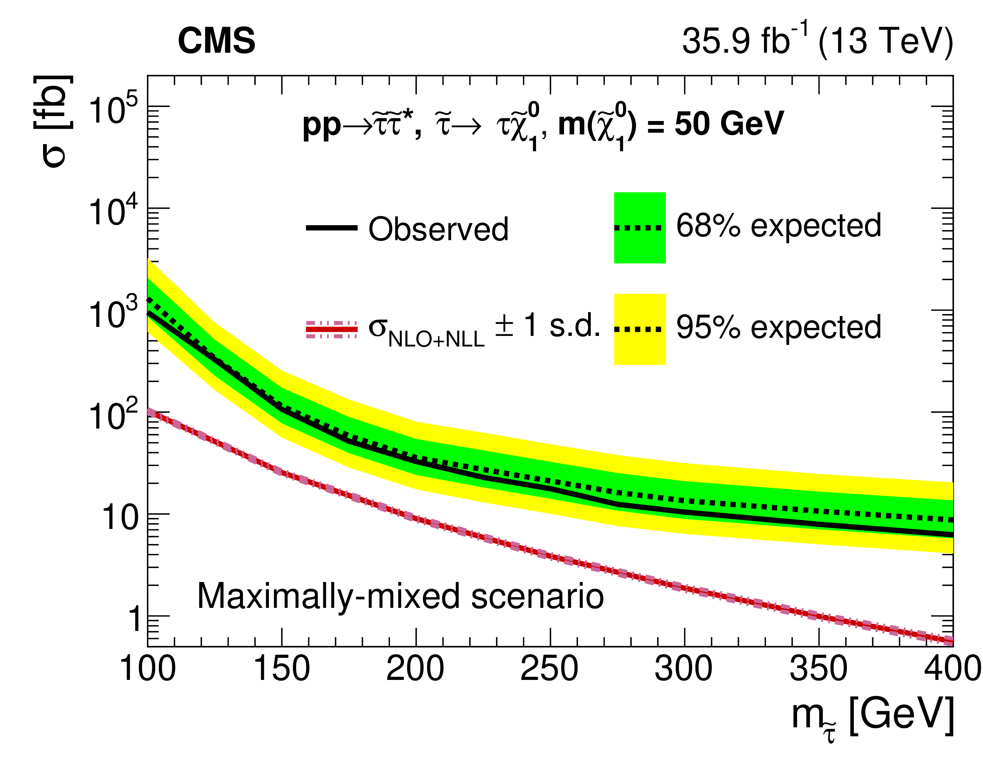
Figure 12:
Excluded $\tilde{\tau}$ pair production cross section as a function of the $\tilde{\tau}$ mass for the maximally-mixed $\tilde{\tau}$ scenario, and for different $\tilde{ \chi }^{0}_{1}$ masses of 1, 10, 20, 30, 40, and 50 GeV from upper left to lower right, respectively. The inner (green) band and the outer (yellow) band indicate the regions containing 68 and 95%, respectively, of the distribution of limits expected under the background-only hypothesis. The red line indicates the NLO+NLL prediction for the signal production cross section calculated with Resummino [47], while the red hatched band represents the uncertainty in the prediction. |

png pdf root |
Figure 12-a:
Excluded $\tilde{\tau}$ pair production cross section as a function of the $\tilde{\tau}$ mass for the maximally-mixed $\tilde{\tau}$ scenario, and for a $\tilde{ \chi }^{0}_{1}$ mass of 1 GeV. The inner (green) band and the outer (yellow) band indicate the regions containing 68 and 95%, respectively, of the distribution of limits expected under the background-only hypothesis. The red line indicates the NLO+NLL prediction for the signal production cross section calculated with Resummino [47], while the red hatched band represents the uncertainty in the prediction. |

png pdf root |
Figure 12-b:
Excluded $\tilde{\tau}$ pair production cross section as a function of the $\tilde{\tau}$ mass for the maximally-mixed $\tilde{\tau}$ scenario, and for a $\tilde{ \chi }^{0}_{1}$ mass of 10 GeV. The inner (green) band and the outer (yellow) band indicate the regions containing 68 and 95%, respectively, of the distribution of limits expected under the background-only hypothesis. The red line indicates the NLO+NLL prediction for the signal production cross section calculated with Resummino [47], while the red hatched band represents the uncertainty in the prediction. |

png pdf root |
Figure 12-c:
Excluded $\tilde{\tau}$ pair production cross section as a function of the $\tilde{\tau}$ mass for the maximally-mixed $\tilde{\tau}$ scenario, and for a $\tilde{ \chi }^{0}_{1}$ mass of 20 GeV. The inner (green) band and the outer (yellow) band indicate the regions containing 68 and 95%, respectively, of the distribution of limits expected under the background-only hypothesis. The red line indicates the NLO+NLL prediction for the signal production cross section calculated with Resummino [47], while the red hatched band represents the uncertainty in the prediction. |
png pdf root |
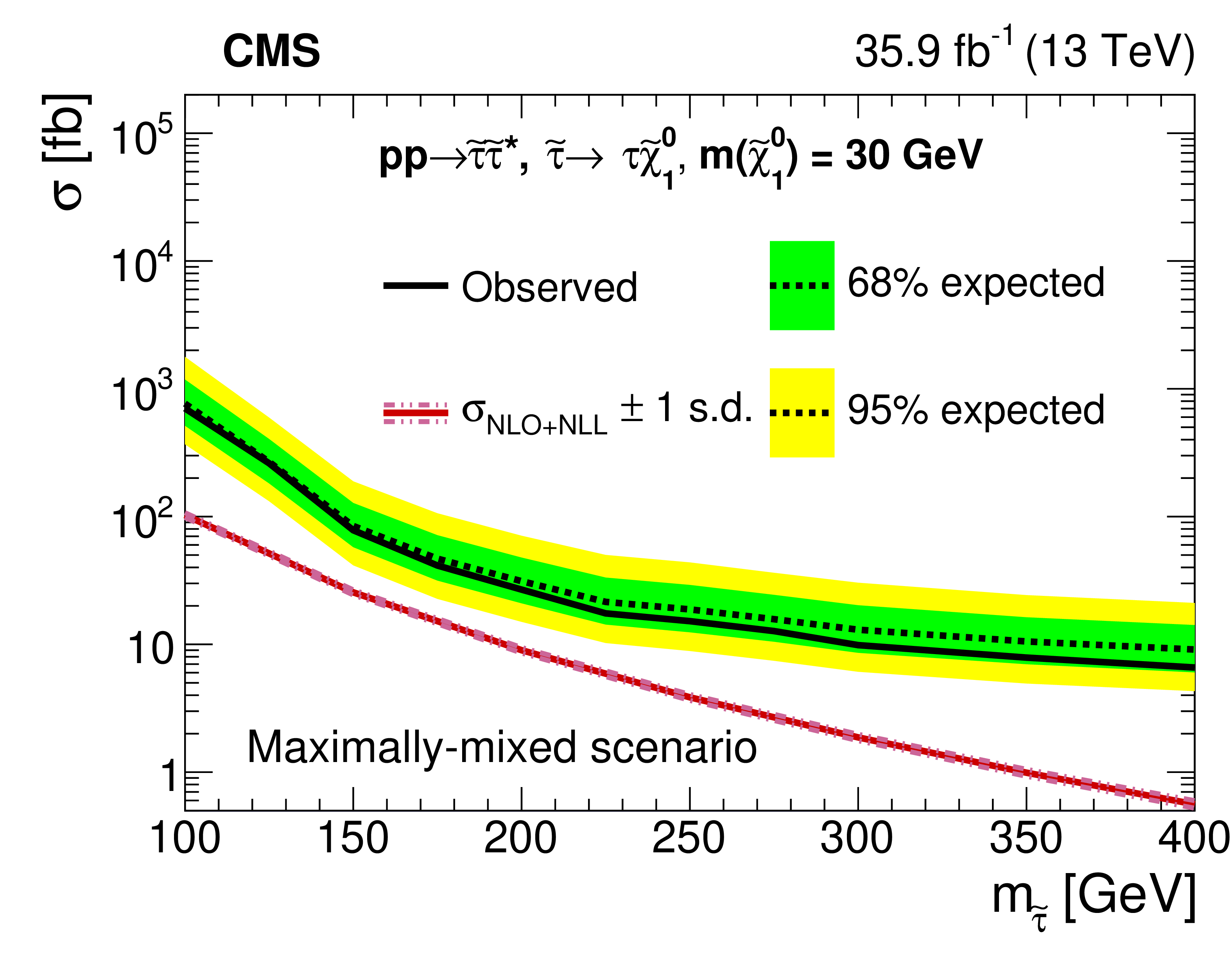
Figure 12-d:
Excluded $\tilde{\tau}$ pair production cross section as a function of the $\tilde{\tau}$ mass for the maximally-mixed $\tilde{\tau}$ scenario, and for a $\tilde{ \chi }^{0}_{1}$ mass of 30 GeV. The inner (green) band and the outer (yellow) band indicate the regions containing 68 and 95%, respectively, of the distribution of limits expected under the background-only hypothesis. The red line indicates the NLO+NLL prediction for the signal production cross section calculated with Resummino [47], while the red hatched band represents the uncertainty in the prediction. |
png pdf root |
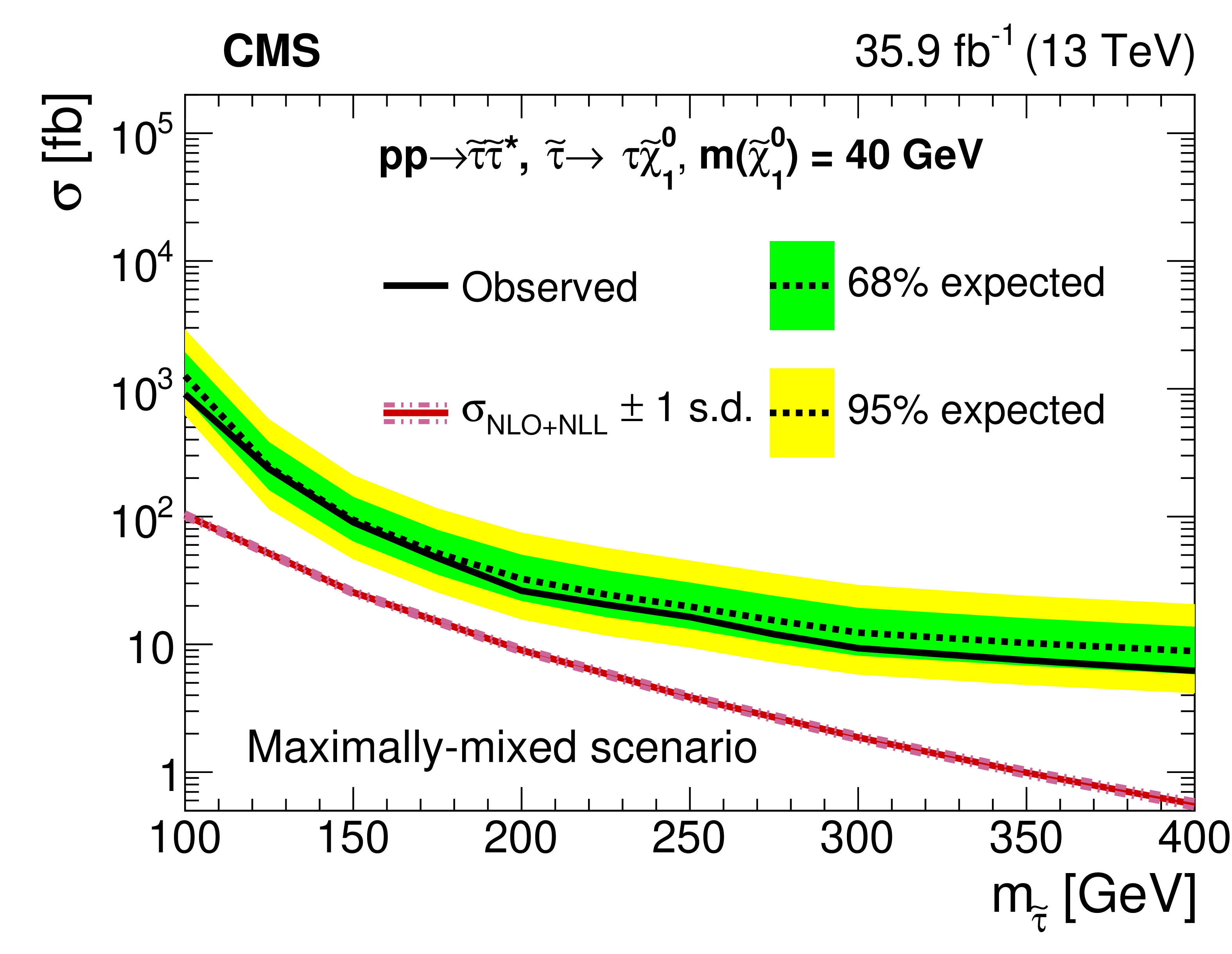
Figure 12-e:
Excluded $\tilde{\tau}$ pair production cross section as a function of the $\tilde{\tau}$ mass for the maximally-mixed $\tilde{\tau}$ scenario, and for a $\tilde{ \chi }^{0}_{1}$ mass of 40 GeV. The inner (green) band and the outer (yellow) band indicate the regions containing 68 and 95%, respectively, of the distribution of limits expected under the background-only hypothesis. The red line indicates the NLO+NLL prediction for the signal production cross section calculated with Resummino [47], while the red hatched band represents the uncertainty in the prediction. |
png pdf root |
Figure 12-f:
Excluded $\tilde{\tau}$ pair production cross section as a function of the $\tilde{\tau}$ mass for the maximally-mixed $\tilde{\tau}$ scenario, and for a $\tilde{ \chi }^{0}_{1}$ mass of 50 GeV. The inner (green) band and the outer (yellow) band indicate the regions containing 68 and 95%, respectively, of the distribution of limits expected under the background-only hypothesis. The red line indicates the NLO+NLL prediction for the signal production cross section calculated with Resummino [47], while the red hatched band represents the uncertainty in the prediction. |
png pdf |
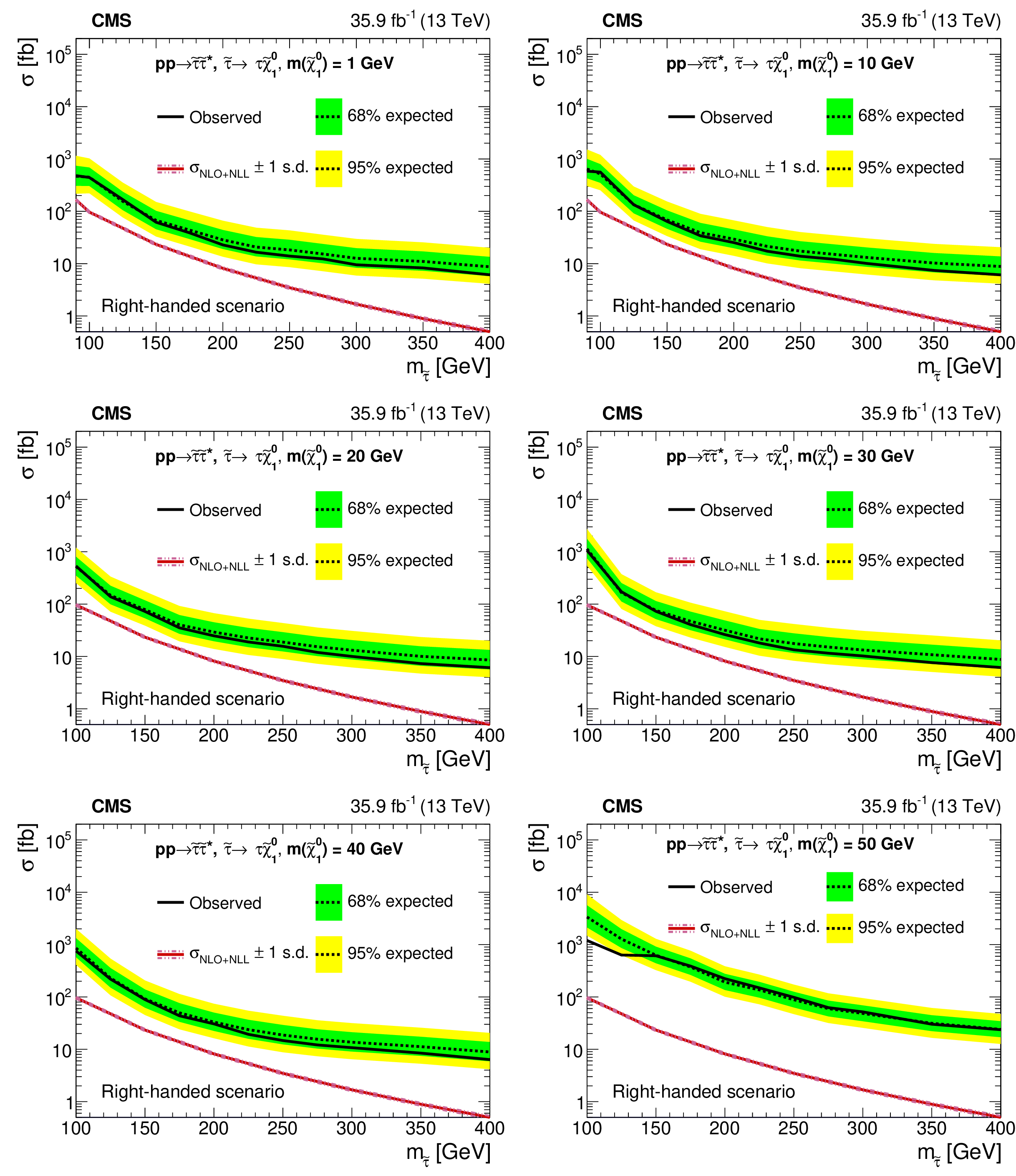
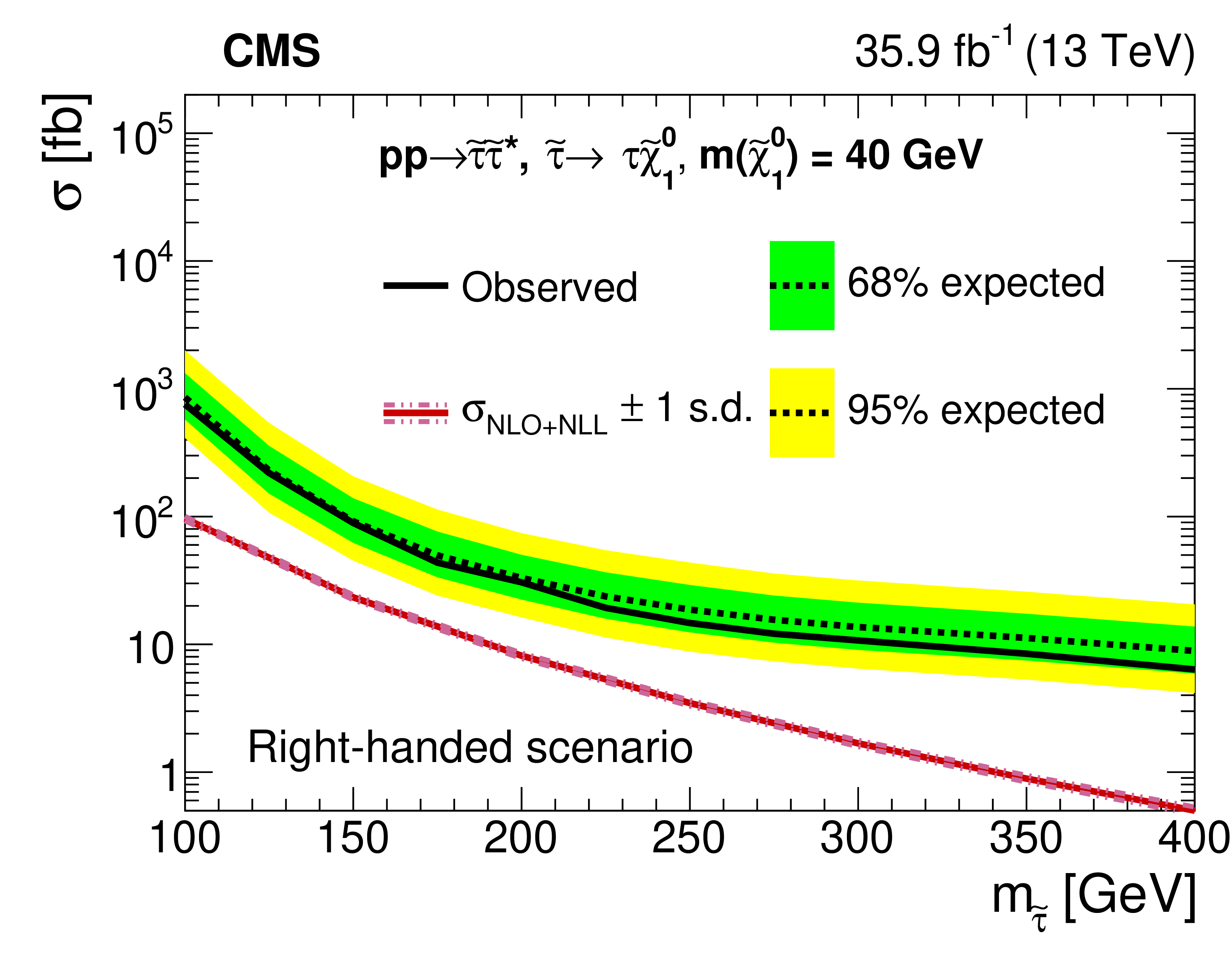
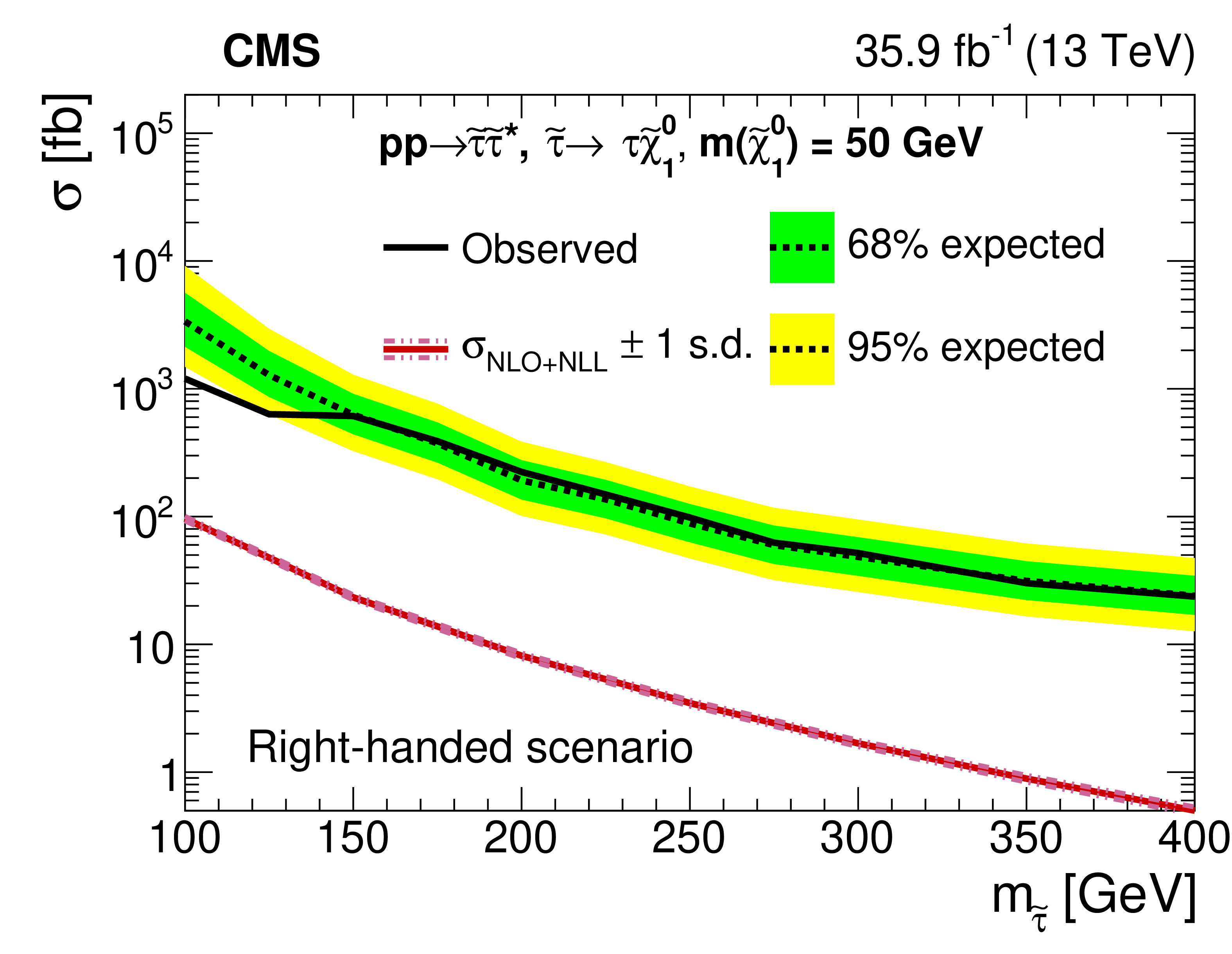
Figure 13:
Excluded $\tilde{\tau}$ pair production cross section as a function of the $\tilde{\tau}$ mass for the right-handed $\tilde{\tau}$ scenario, and for different $\tilde{ \chi }^{0}_{1}$ masses of 1, 10, 20, 30, 40, and 50 GeV from upper right to lower right, respectively. The inner (green) band and the outer (yellow) band indicate the regions containing 68 and 95%, respectively, of the distribution of limits expected under the background-only hypothesis. The red line indicates the NLO+NLL prediction for the signal production cross section calculated with Resummino [47], while the red hatched band represents the uncertainty in the prediction. |
png pdf root |
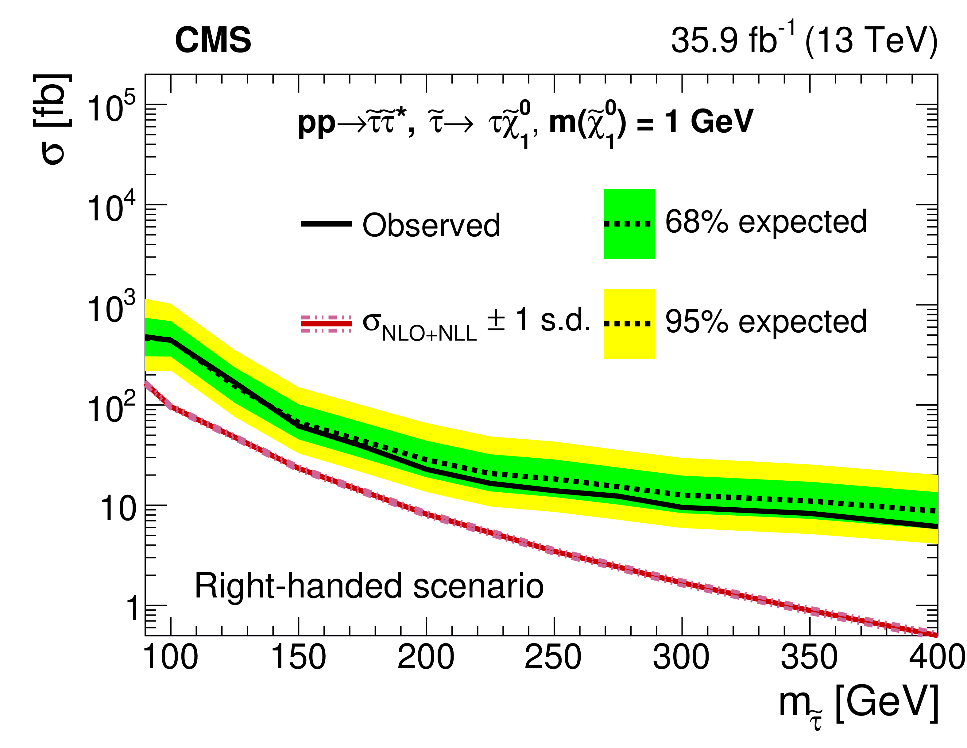
Figure 13-a:
Excluded $\tilde{\tau}$ pair production cross section as a function of the $\tilde{\tau}$ mass for the right-handed $\tilde{\tau}$ scenario, and for a $\tilde{ \chi }^{0}_{1}$ mass of 1 GeV. The inner (green) band and the outer (yellow) band indicate the regions containing 68 and 95%, respectively, of the distribution of limits expected under the background-only hypothesis. The red line indicates the NLO+NLL prediction for the signal production cross section calculated with Resummino [47], while the red hatched band represents the uncertainty in the prediction. |

png pdf root |
Figure 13-b:
Excluded $\tilde{\tau}$ pair production cross section as a function of the $\tilde{\tau}$ mass for the right-handed $\tilde{\tau}$ scenario, and for a $\tilde{ \chi }^{0}_{1}$ mass of 10 GeV. The inner (green) band and the outer (yellow) band indicate the regions containing 68 and 95%, respectively, of the distribution of limits expected under the background-only hypothesis. The red line indicates the NLO+NLL prediction for the signal production cross section calculated with Resummino [47], while the red hatched band represents the uncertainty in the prediction. |
png pdf root |
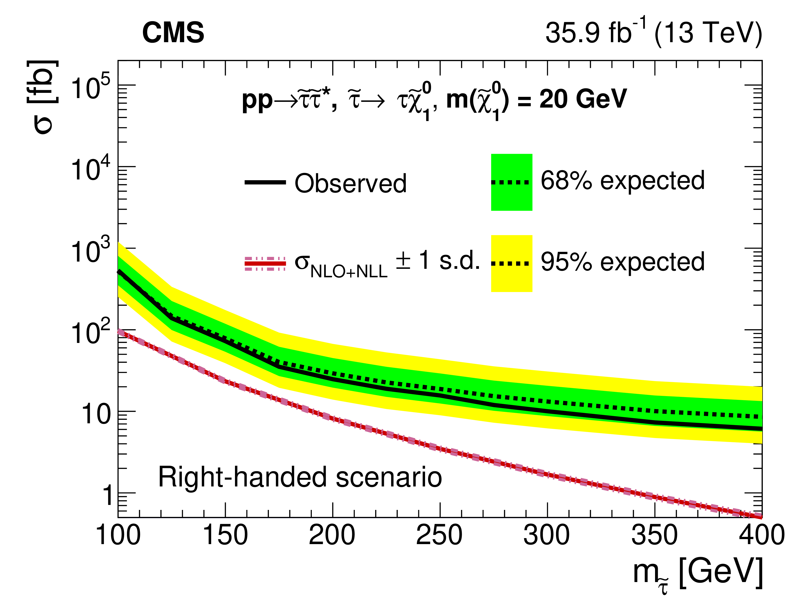
Figure 13-c:
Excluded $\tilde{\tau}$ pair production cross section as a function of the $\tilde{\tau}$ mass for the right-handed $\tilde{\tau}$ scenario, and for a $\tilde{ \chi }^{0}_{1}$ mass of 20 GeV. The inner (green) band and the outer (yellow) band indicate the regions containing 68 and 95%, respectively, of the distribution of limits expected under the background-only hypothesis. The red line indicates the NLO+NLL prediction for the signal production cross section calculated with Resummino [47], while the red hatched band represents the uncertainty in the prediction. |

png pdf root |
Figure 13-d:
Excluded $\tilde{\tau}$ pair production cross section as a function of the $\tilde{\tau}$ mass for the right-handed $\tilde{\tau}$ scenario, and for a $\tilde{ \chi }^{0}_{1}$ mass of 30 GeV. The inner (green) band and the outer (yellow) band indicate the regions containing 68 and 95%, respectively, of the distribution of limits expected under the background-only hypothesis. The red line indicates the NLO+NLL prediction for the signal production cross section calculated with Resummino [47], while the red hatched band represents the uncertainty in the prediction. |
png pdf root |
Figure 13-e:
Excluded $\tilde{\tau}$ pair production cross section as a function of the $\tilde{\tau}$ mass for the right-handed $\tilde{\tau}$ scenario, and for a $\tilde{ \chi }^{0}_{1}$ mass of 40 GeV. The inner (green) band and the outer (yellow) band indicate the regions containing 68 and 95%, respectively, of the distribution of limits expected under the background-only hypothesis. The red line indicates the NLO+NLL prediction for the signal production cross section calculated with Resummino [47], while the red hatched band represents the uncertainty in the prediction. |
png pdf root |
Figure 13-f:
Excluded $\tilde{\tau}$ pair production cross section as a function of the $\tilde{\tau}$ mass for the right-handed $\tilde{\tau}$ scenario, and for a $\tilde{ \chi }^{0}_{1}$ mass of 50 GeV. The inner (green) band and the outer (yellow) band indicate the regions containing 68 and 95%, respectively, of the distribution of limits expected under the background-only hypothesis. The red line indicates the NLO+NLL prediction for the signal production cross section calculated with Resummino [47], while the red hatched band represents the uncertainty in the prediction. |
png pdf root |
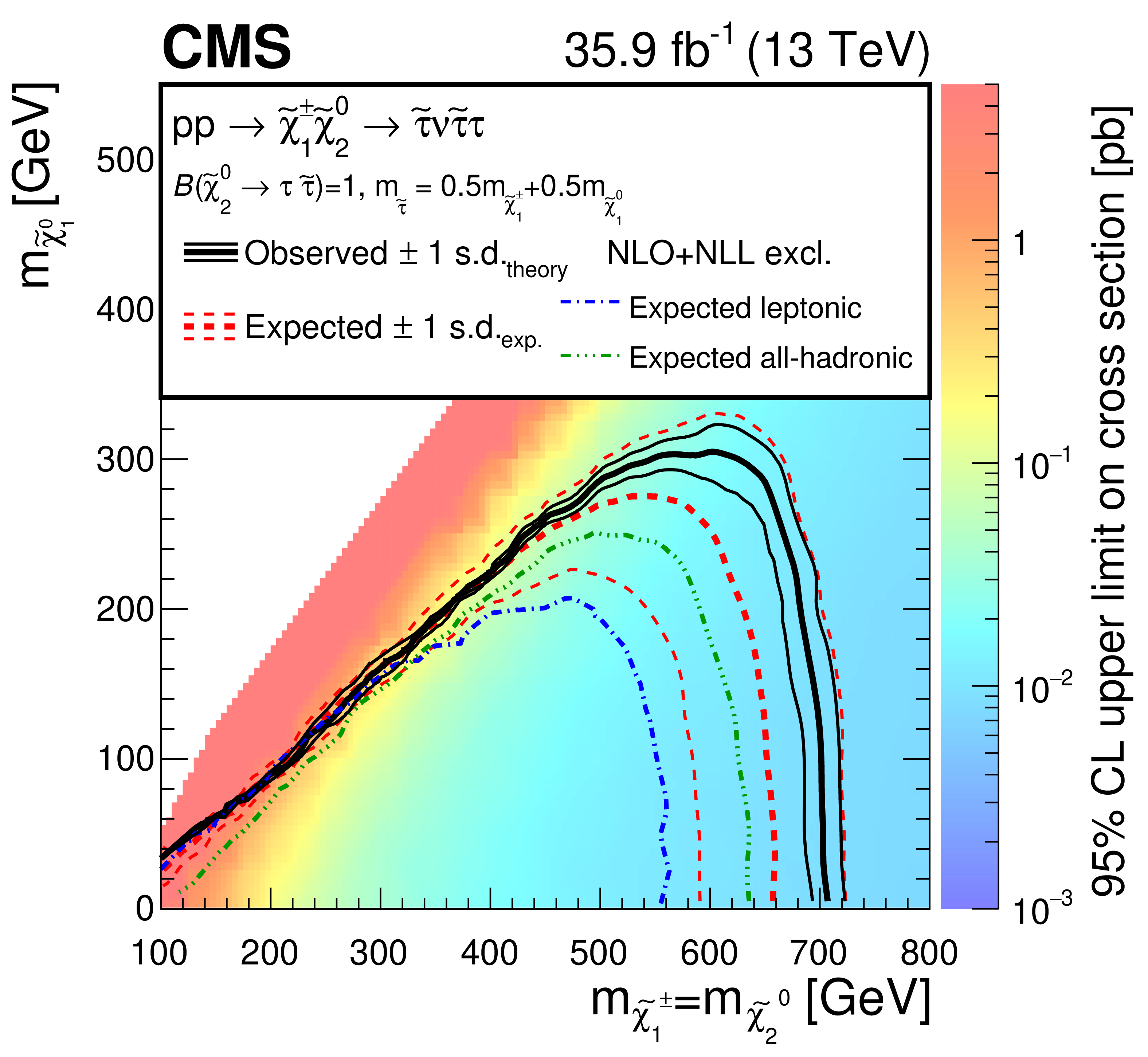
Figure 14:
Exclusion limits at 95% CL for chargino-neutralino production with decays through $\tilde{\tau}$ to final states with ${\tau}$ leptons. The production cross sections are computed at NLO+NLL precision assuming mass-degenerate wino ${\tilde{\chi}^{0}_{2}}$, light bino $\tilde{ \chi }^{0}_{1}$, and with all the other sparticles assumed to be heavy and decoupled [72,73]. The regions enclosed by the thick black curves represent the observed exclusion at 95% CL, while the thick dashed red line indicates the expected exclusion at 95% CL. The thin black lines show the effect of variations of the signal cross sections within theoretical uncertainties on the observed exclusion. The thin red dashed lines indicate the region containing 68% of the distribution of limits expected under the background-only hypothesis. The green and blue dashed lines show separately the expected exclusion regions for the analyses in the all-hadronic and leptonic final states, respectively. |
png pdf root |
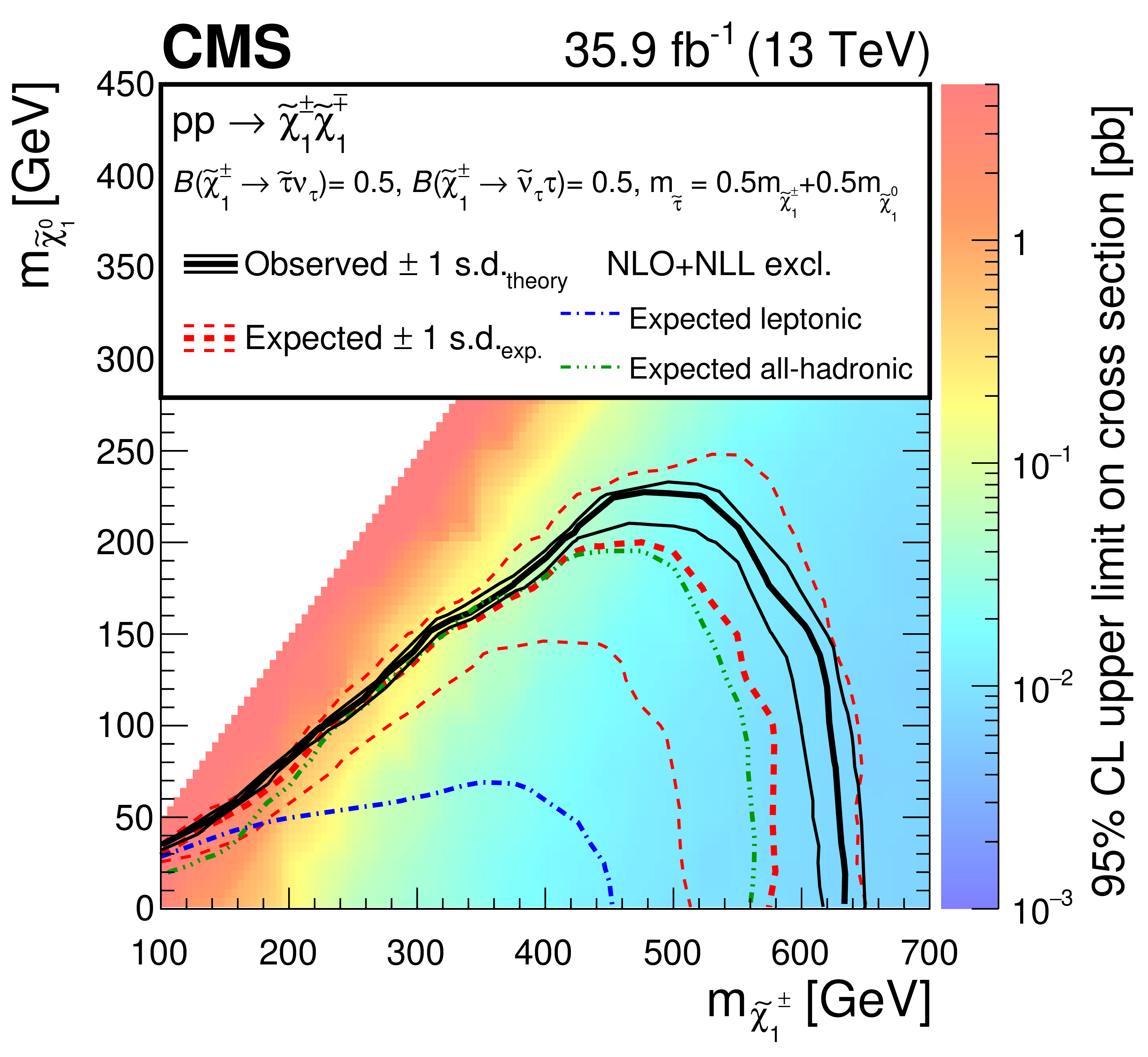
Figure 15:
Exclusion limits at 95% CL for chargino pair production with decays through $\tilde{\tau}$ to final states with ${\tau}$ leptons. The production cross sections are computed at NLO+NLL precision assuming a wino-like ${\tilde{\chi}^\pm _{1}}$, light bino $\tilde{ \chi }^{0}_{1}$, and with all the other sparticles assumed to be heavy and decoupled [72,73]. The regions enclosed by the thick black curves represent the observed exclusion at 95% CL, while the thick dashed red line indicates the expected exclusion at 95% CL. The thin black lines show the effect of variations of the signal cross sections within theoretical uncertainties on the observed exclusion. The thin red dashed lines indicate the region containing 68% of the distribution of limits expected under the background-only hypothesis. The green and blue dashed lines show separately the expected exclusion regions for the analyses in the all-hadronic and leptonic final states, respectively. |
| Tables | |
png pdf |
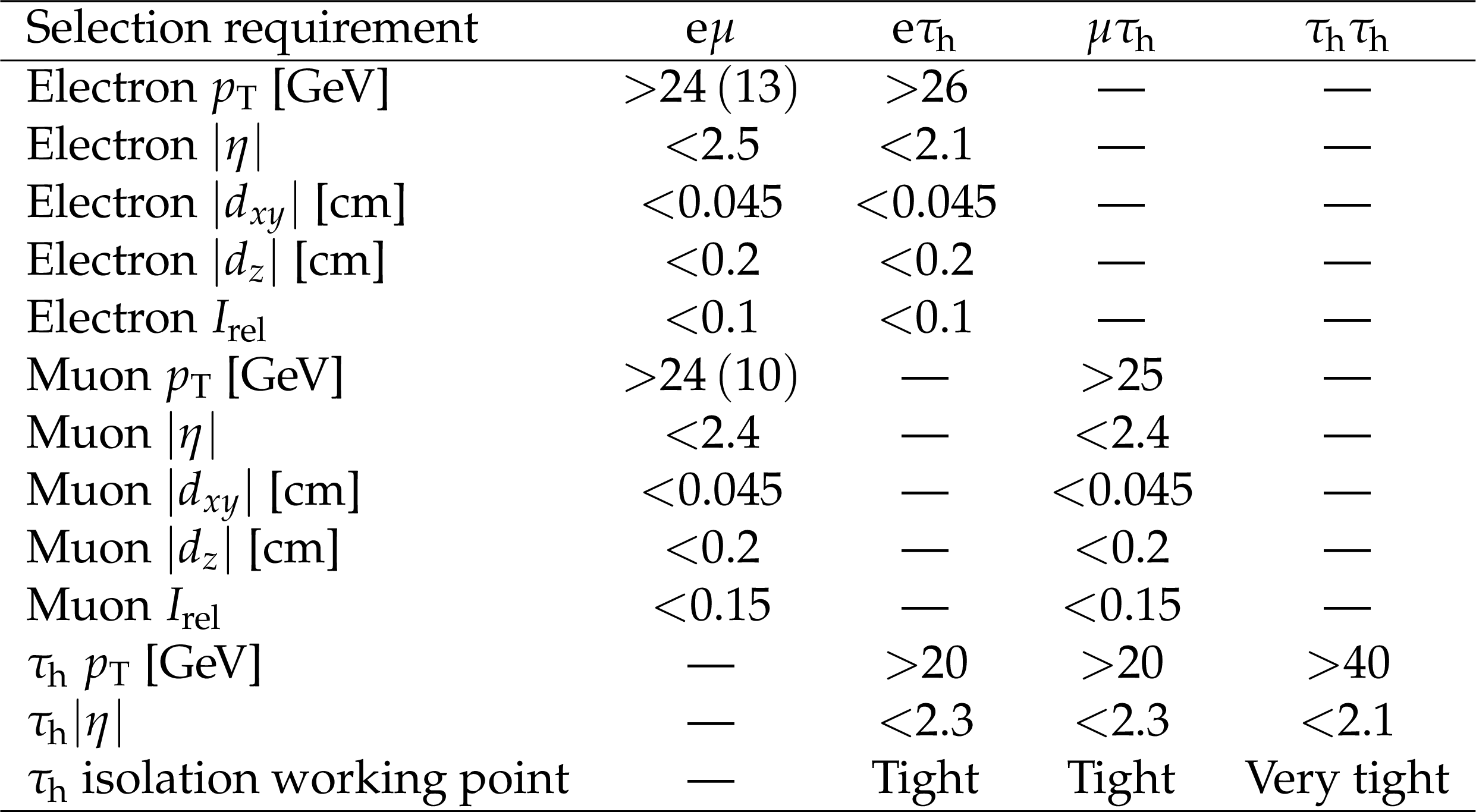
Table 1:
Summary of lepton selection requirements for the analysis. Entries with a second value in parentheses refer to the lepton with the higher (lower) ${p_{\mathrm {T}}}$. |

png pdf |
Table 2:
Summary of requirements for identifying additional electrons and muons. |
png pdf |
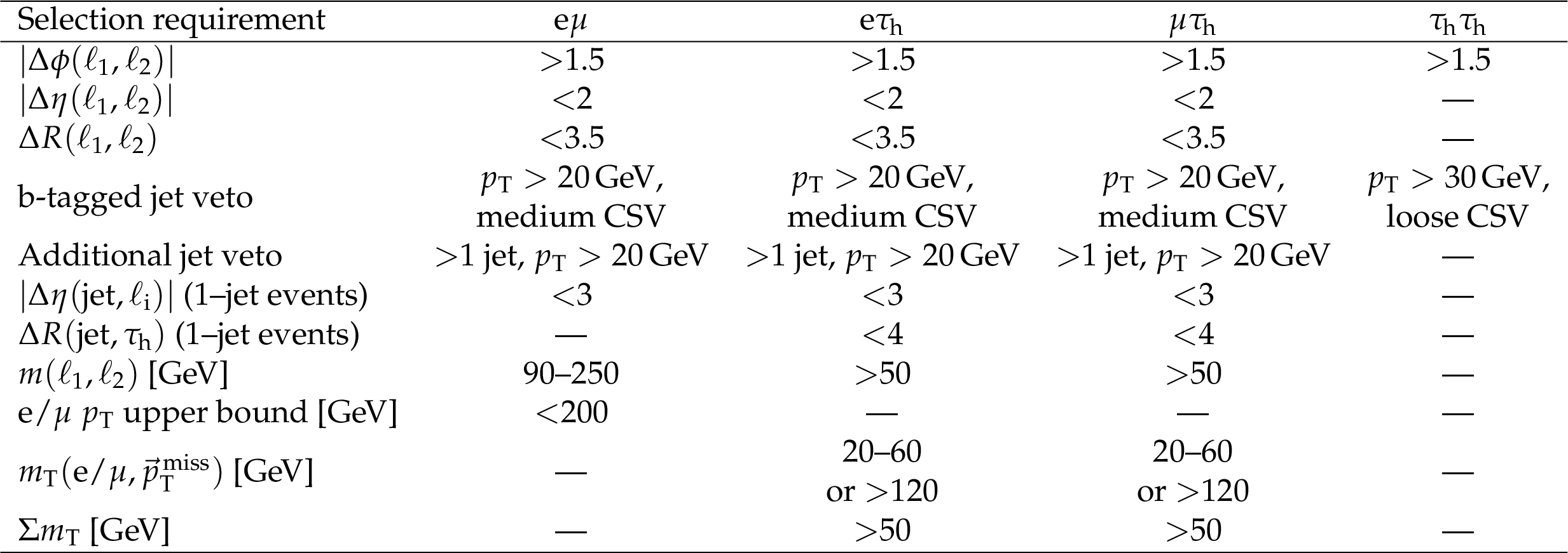
Table 3:
Summary of baseline selection requirements in each final state. |
png pdf |
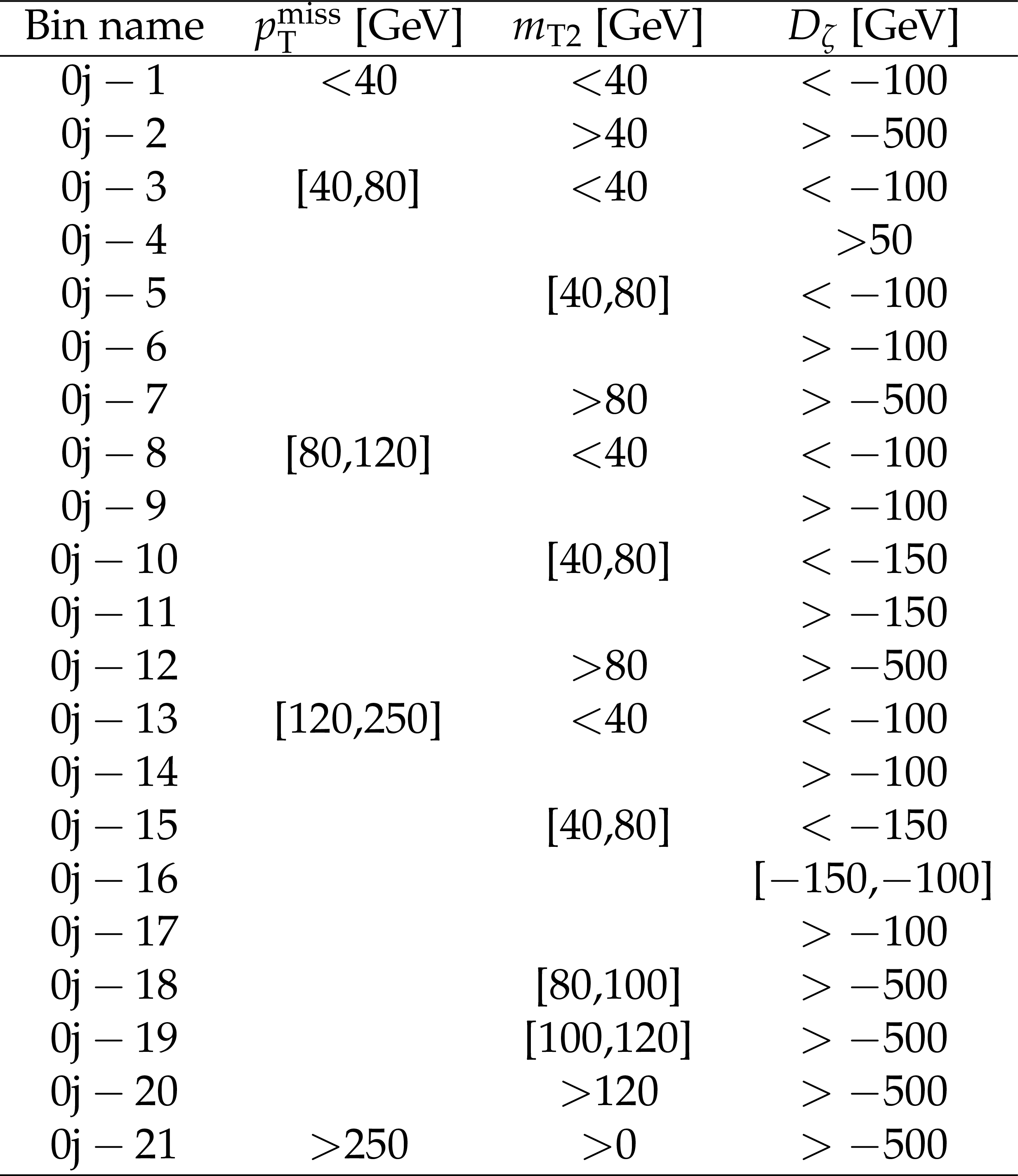
Table 4:
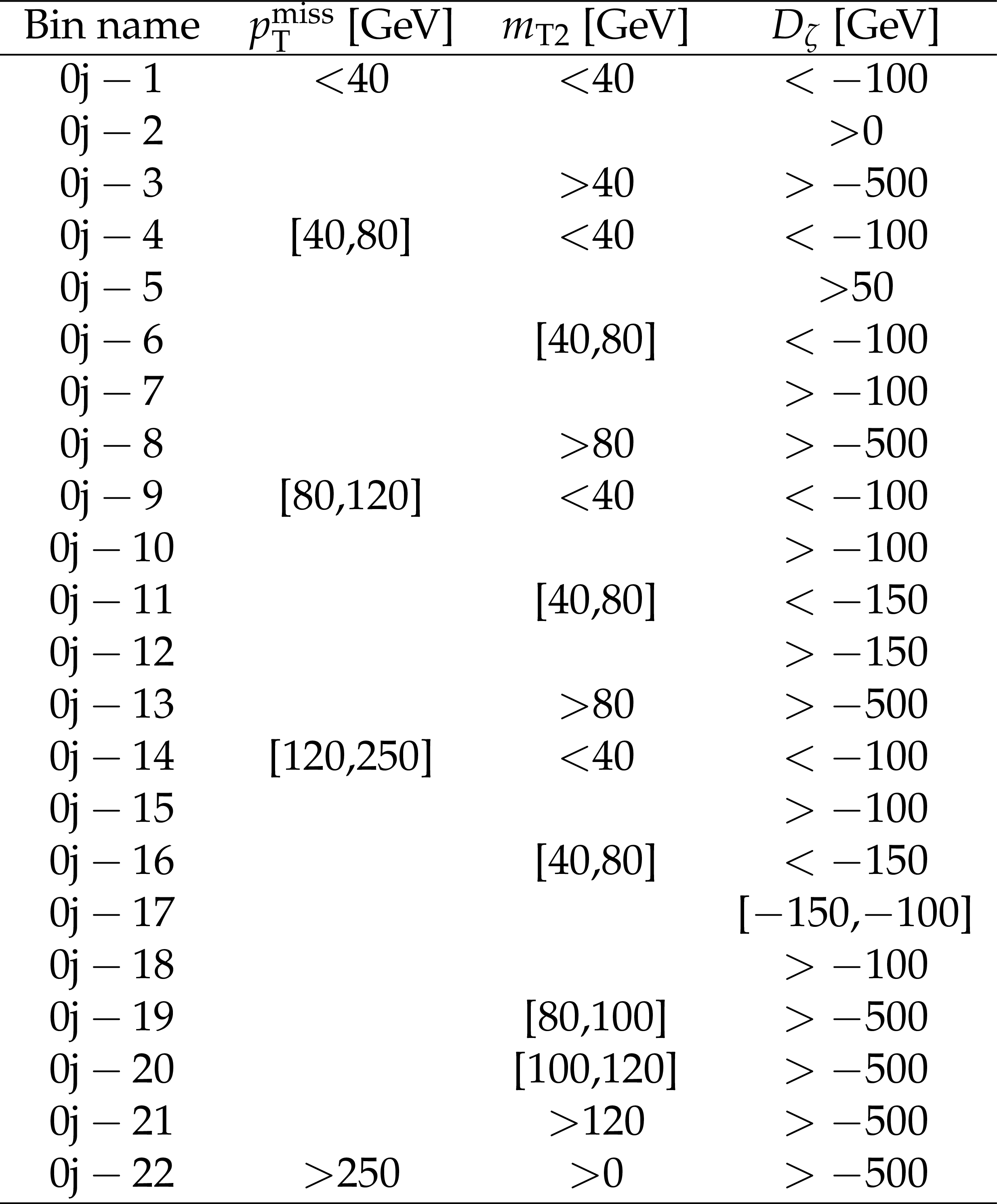
Definition of SRs in the 0-jet category for the ${{\mathrm {e}} {{\tau} _\mathrm {h}}}$ and ${\mu {{\tau} _\mathrm {h}}}$ final states. |
png pdf |
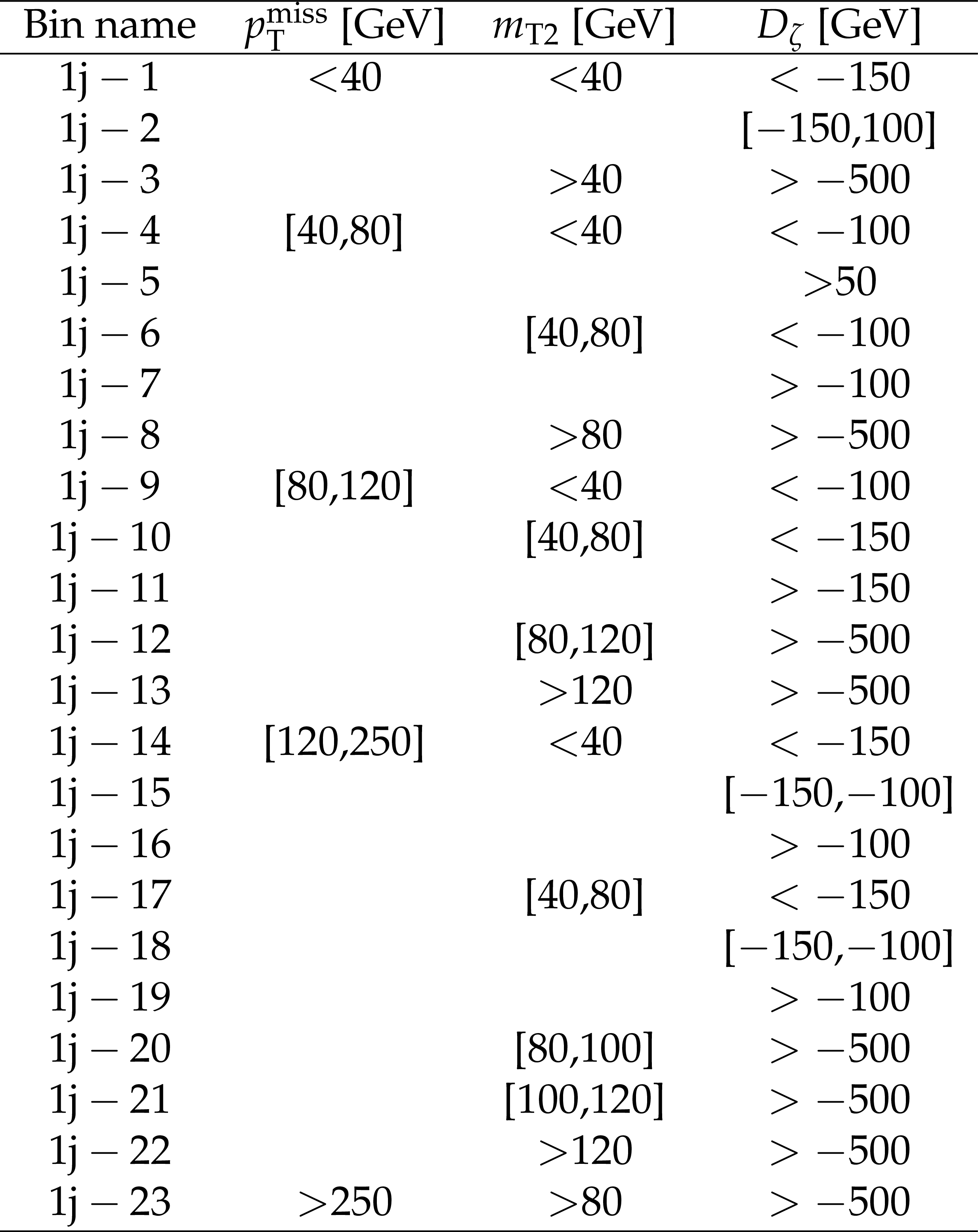
Table 5:
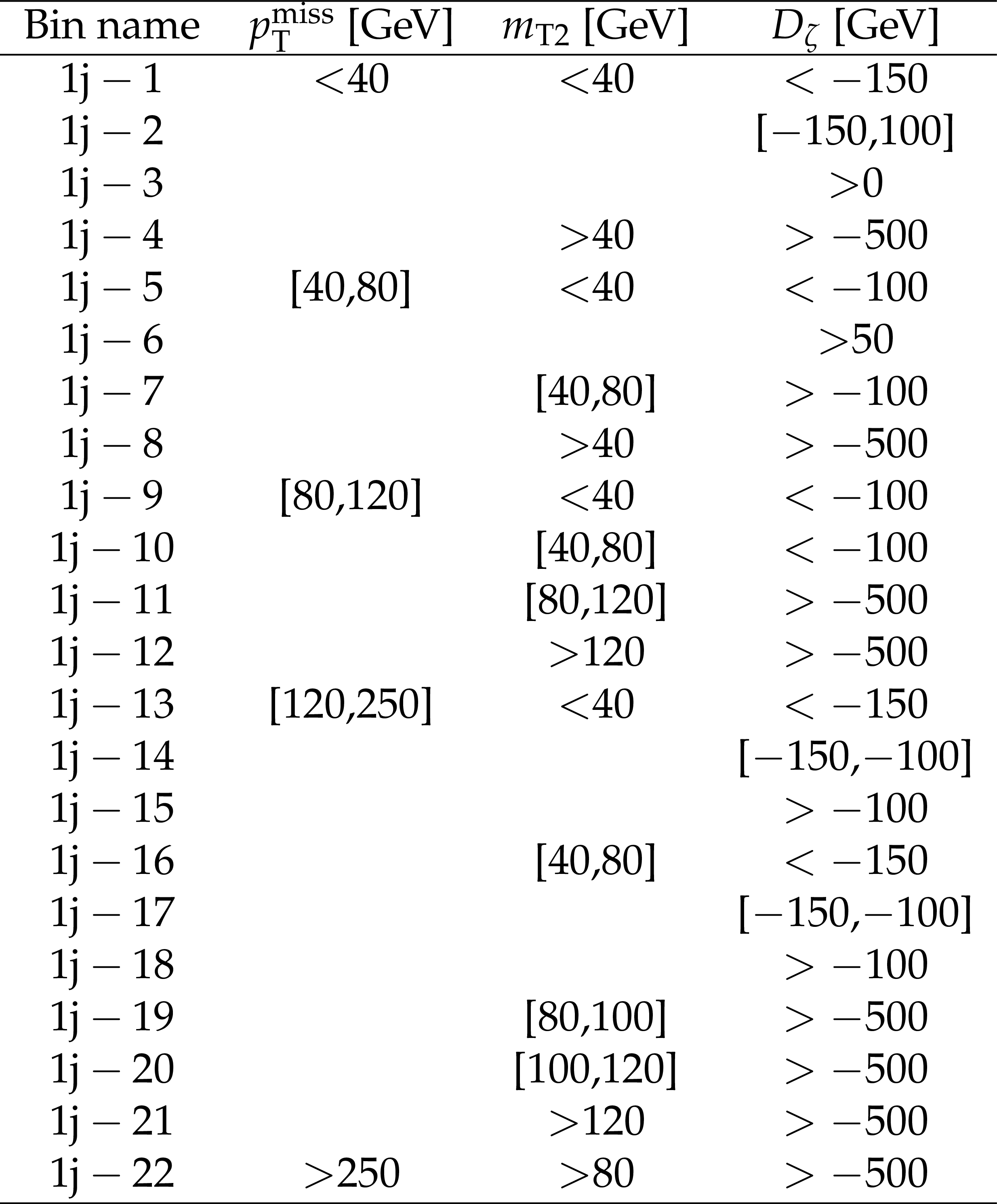
Definition of SRs in the 1-jet category for the ${{\mathrm {e}} {{\tau} _\mathrm {h}}}$ and ${\mu {{\tau} _\mathrm {h}}}$ final states. |
png pdf |
Table 6:
Definition of SRs in the 0-jet category for the ${{\mathrm {e}}\mu}$ final state. |
png pdf |
Table 7:
Definition of SRs in the 1-jet category for the ${{\mathrm {e}}\mu}$ final state. |
png pdf |
Table 8:
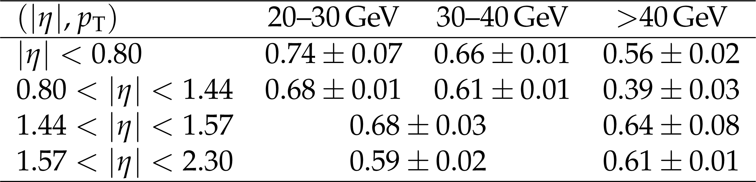
Transfer factor $R$ determined from the W+jets control sample according to Eq. (4), as a function of ${p_{\mathrm {T}}}$ and $\eta $ of the ${{\tau} _\mathrm {h}}$ candidate. The uncertainties are statistical only. |
png pdf |
Table 9:
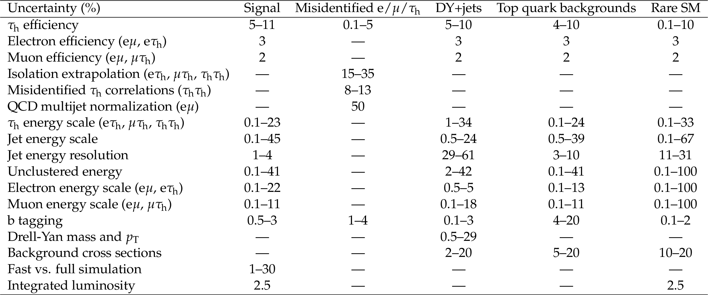
Systematic uncertainties in the analysis for the signal models and the different SM background predictions. The uncertainty values are evaluated separately for each signal model and mass hypothesis studied and are listed as percentages. |

png pdf |
Table 10:
Final predicted and observed event yields in the three SRs defined for the ${{{\tau} _\mathrm {h}} {{\tau} _\mathrm {h}}}$ final state with all statistical and systematic uncertainties combined. For the background estimates with no event in the corresponding data control region or in the simulated sample after the SR selection, the predicted yield is indicated as being less than the one standard deviation upper bound evaluated for that estimate. The central value and the uncertainties for the total background estimate are then extracted from the full pre-fit likelihood. Expected yields are also given for signal models of direct $\tilde{\tau}$ pair production in the purely left- and right-handed scenarios and in the maximally mixed scenario, with the $\tilde{\tau}$ and $\tilde{ \chi }^{0}_{1}$ masses in GeV indicated in parentheses. |
png pdf |
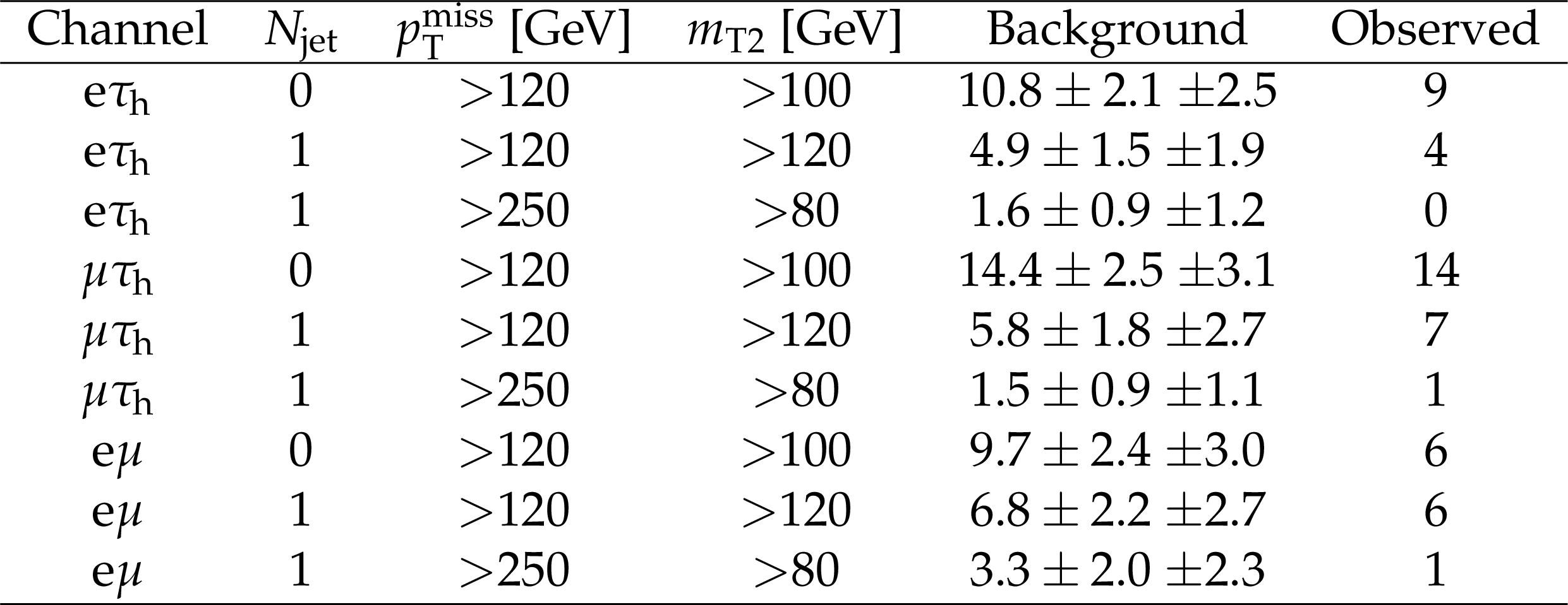
Table 11:
Definition of the aggregate SRs to be used for easier reinterpretation of the results in the ${{\mathrm {e}} {{\tau} _\mathrm {h}}}$, ${\mu {{\tau} _\mathrm {h}}}$, and ${{\mathrm {e}}\mu}$ final states. In all of these regions, a selection requirement of $ {D_{\zeta}} > -500 GeV $ is applied. |
| Summary |
| A search for the direct and indirect production of $ \tau $ sleptons has been performed in proton-proton collisions at a center-of-mass energy of 13 TeV in events with a $ \tau $ lepton pair and significant missing transverse momentum in the final state. Both leptonic and hadronic decay modes of the $ \tau $ leptons are considered. Search regions are defined using discriminating kinematic observables that exploit expected differences between signal and background. The data sample used for this search corresponds to an integrated luminosity of 35.9 fb$^{-1}$. No excess above the expected standard model background has been observed. Upper limits on the cross section of direct $\tilde{\tau}$ pair production are derived for simplified models in which each $\tilde{\tau}$ decays to a $ \tau $ lepton and the lightest neutralino, with the latter being assumed to be the lightest supersymmetric particle (LSP). The analysis is most sensitive to a $\tilde{\tau}$ that is purely left-handed. For a left-handed $\tilde{\tau}$ of 90 GeV decaying to a nearly massless LSP, the observed limit is 1.26 times the expected production cross section in the simplified model. The limits obtained for direct $\tilde{\tau}$ pair production represent a considerable improvement in sensitivity for this production mechanism with respect to previous ATLAS and CMS measurements. Exclusion limits are also derived for simplified models of chargino-neutralino and chargino pair production with decays to $ \tau $ leptons that involve indirect $\tilde{\tau}$ production via the chargino and neutralino decay chains. In the chargino-neutralino production model, in which the parent chargino and second-lightest neutralino are assumed to have the same mass, we exclude chargino masses up to 710 GeV under the hypothesis of a nearly massless LSP. In the chargino pair production model, we exclude chargino masses up to 630 GeV under the same hypothesis. In both cases, we significantly extend the exclusion limits with respect to previous CMS measurements. |
| References | ||||
| 1 | P. Ramond | Dual theory for free fermions | PRD 3 (1971) 2415 | |
| 2 | Y. A. Gol'fand and E. P. Likhtman | Extension of the algebra of Poincar$ \'e $ group generators and violation of P invariance | JEPTL 13 (1971)323 | |
| 3 | A. Neveu and J. H. Schwarz | Factorizable dual model of pions | NPB 31 (1971) 86 | |
| 4 | D. V. Volkov and V. P. Akulov | Possible universal neutrino interaction | JEPTL 16 (1972)438 | |
| 5 | J. Wess and B. Zumino | A Lagrangian model invariant under supergauge transformations | PLB 49 (1974) 52 | |
| 6 | J. Wess and B. Zumino | Supergauge transformations in four dimensions | NPB 70 (1974) 39 | |
| 7 | P. Fayet | Supergauge invariant extension of the Higgs mechanism and a model for the electron and its neutrino | NPB 90 (1975) 104 | |
| 8 | H. P. Nilles | Supersymmetry, supergravity and particle physics | Phys. Rep. 110 (1984) 1 | |
| 9 | G. 't Hooft | Naturalness, chiral symmetry, and spontaneous chiral symmetry breaking | NATO Sci. Ser. B 59 (1980)135 | |
| 10 | E. Witten | Dynamical breaking of supersymmetry | NPB 188 (1981) 513 | |
| 11 | M. Dine, W. Fischler, and M. Srednicki | Supersymmetric technicolor | NPB 189 (1981) 575 | |
| 12 | S. Dimopoulos and S. Raby | Supercolor | NPB 192 (1981) 353 | |
| 13 | S. Dimopoulos and H. Georgi | Softly broken supersymmetry and SU(5) | NPB 193 (1981) 150 | |
| 14 | R. K. Kaul and P. Majumdar | Cancellation of quadratically divergent mass corrections in globally supersymmetric spontaneously broken gauge theories | NPB 199 (1982) 36 | |
| 15 | ATLAS Collaboration | Observation of a new particle in the search for the standard model Higgs boson with the ATLAS detector at the LHC | PLB 716 (2012) 1 | 1207.7214 |
| 16 | CMS Collaboration | Observation of a new boson at a mass of 125 GeV with the CMS experiment at the LHC | PLB 716 (2012) 30 | CMS-HIG-12-028 1207.7235 |
| 17 | CMS Collaboration | Observation of a new boson with mass near 125 GeV in $ {\mathrm{p}}{\mathrm{p}} $ collisions at $ \sqrt{s} = $ 7 and 8 TeV | JHEP 06 (2013) 081 | CMS-HIG-12-036 1303.4571 |
| 18 | ATLAS Collaboration | Measurement of the Higgs boson mass from the $ \textrm{H}\rightarrow \gamma\gamma $ and $ \textrm{H} \rightarrow \textrm{ZZ}^{*} \rightarrow 4\ell $ channels with the ATLAS detector using 25 fb$ ^{-1} $ of pp collision data | PRD 90 (2014) 052004 | 1406.3827 |
| 19 | CMS Collaboration | Precise determination of the mass of the Higgs boson and tests of compatibility of its couplings with the standard model predictions using proton collisions at 7 and 8 TeV | EPJC 75 (2015) 212 | CMS-HIG-14-009 1412.8662 |
| 20 | ATLAS and CMS Collaborations | Combined measurement of the Higgs boson mass in pp collisions at $ \sqrt{s}= $ 7 and 8 TeV with the ATLAS and CMS experiments | PRL 114 (2015) 191803 | 1503.07589 |
| 21 | G. R. Farrar and P. Fayet | Phenomenology of the production, decay, and detection of new hadronic states associated with supersymmetry | PLB 76 (1978) 575 | |
| 22 | C. Boehm, A. Djouadi, and M. Drees | Light scalar top quarks and supersymmetric dark matter | PRD 62 (2000) 035012 | hep-ph/9911496 |
| 23 | C. Bal\'azs, M. Carena, and C. E. M. Wagner | Dark matter, light stops and electroweak baryogenesis | PRD 70 (2004) 015007 | hep-ph/403224 |
| 24 | G. Jungman, M. Kamionkowski, and K. Griest | Supersymmetric dark matter | PR 267 (1996) 195 | hep-ph/9506380 |
| 25 | G. Belanger, S. Biswas, C. Boehm, and B. Mukhopadhyaya | Light Neutralino Dark Matter in the MSSM and Its Implication for LHC Searches for Staus | JHEP 12 (2012) 076 | 1206.5404 |
| 26 | E. Arganda, V. Martin-Lozano, A. D. Medina, and N. Mileo | Potential discovery of staus through heavy Higgs boson decays at the LHC | JHEP 09 (2018) 056 | 1804.10698 |
| 27 | G. Hinshaw et al. | Nine-year Wilkinson Microwave Anisotropy Probe (WMAP) observations: cosmological parameter results | Astrophys. J. Suppl. 208 (2013) 19 | 1212.5226 |
| 28 | K. Griest and D. Seckel | Three exceptions in the calculation of relic abundances | PRD 43 (1991) 3191 | |
| 29 | D. A. Vasquez, G. Belanger, and C. Boehm | Revisiting light neutralino scenarios in the MSSM | PRD 84 (2011) 095015 | 1108.1338 |
| 30 | S. F. King, J. P. Roberts, and D. P. Roy | Natural dark matter in SUSY GUTs with non-universal gaugino masses | JHEP 10 (2007) 106 | 0705.4219 |
| 31 | M. Battaglia et al. | Proposed post-LEP benchmarks for supersymmetry | EPJC 22 (2001) 535 | hep-ph/0106204 |
| 32 | R. L. Arnowitt et al. | Determining the dark matter relic density in the minimal supergravity stau-neutralino co-annihilation region at the Large Hadron Collider | PRL 100 (2008) 231802 | 0802.2968 |
| 33 | CMS Collaboration | Interpretation of searches for supersymmetry with simplified models | PRD 88 (2013) 052017 | CMS-SUS-11-016 1301.2175 |
| 34 | J. Alwall, P. Schuster, and N. Toro | Simplified models for a first characterization of new physics at the LHC | PRD 79 (2009) 075020 | |
| 35 | J. Alwall, M.-P. Le, M. Lisanti, and J. Wacker | Model-independent jets plus missing energy searches | PRD 79 (2009) 015005 | |
| 36 | LHC New Physics Working Group | Simplified models for LHC new physics searches | JPG 39 (2012) 105005 | 1105.2838 |
| 37 | ALEPH Collaboration | Search for scalar leptons in e$ ^{+} $e$ ^{-} $ collisions at center-of-mass energies up to 209 GeV | PLB 526 (2002) 206 | hep-ex/0112011 |
| 38 | DELPHI Collaboration | Searches for supersymmetric particles in e$ ^{+} $e$ ^{-} $ collisions up to 208 GeV and interpretation of the results within the MSSM | EPJC 31 (2003) 421 | hep-ex/0311019 |
| 39 | L3 Collaboration | Search for scalar leptons and scalar quarks at LEP | PLB 580 (2004) 37 | hep-ex/0310007 |
| 40 | OPAL Collaboration | Search for anomalous production of dilepton events with missing transverse momentum in e$ ^{+} $e$ ^{-} $ collisions at $ \sqrt{s} = $ 183 GeV to 209 GeV | EPJC 32 (2004) 453 | hep-ex/0309014 |
| 41 | LEP SUSY Working Group (ALEPH, DELPHI, L3, OPAL) | Combined LEP selectron/smuon/stau results, 183-208 GeV | LEPSUSYWG/04-01.1 | |
| 42 | ATLAS Collaboration | Search for the direct production of charginos, neutralinos and staus in final states with at least two hadronically decaying taus and missing transverse momentum in pp collisions at $ \sqrt{s} = $ 8 TeV with the ATLAS detector | JHEP 10 (2014) 96 | 1407.0350 |
| 43 | ATLAS Collaboration | Search for the electroweak production of supersymmetric particles in $ \sqrt{s} = $ 8 TeV pp collisions with the ATLAS detector | PRD 93 (2016) 052002 | 1509.07152 |
| 44 | CMS Collaboration | Search for electroweak production of charginos in final states with two tau leptons in pp collisions at $ \sqrt{s}= $ 8 TeV | JHEP 04 (2017) 018 | CMS-SUS-14-022 1610.04870 |
| 45 | CMS Collaboration | Search for supersymmetry in the vector-boson fusion topology in proton-proton collisions at $ \sqrt{s}= $ 8 TeV | JHEP 11 (2015) 189 | CMS-SUS-14-005 1508.07628 |
| 46 | ATLAS Collaboration | Search for the direct production of charginos and neutralinos in final states with tau leptons in $ \sqrt{s} = $ 13 TeV pp collisions with the ATLAS detector | EPJC 78 (2018) 154 | 1708.07875 |
| 47 | B. Fuks, M. Klasen, D. R. Lamprea, and M. Rothering | Revisiting slepton pair production at the Large Hadron Collider | JHEP 01 (2014) 168 | 1310.2621 |
| 48 | CMS Collaboration | The CMS trigger system | JINST 12 (2017) P01020 | CMS-TRG-12-001 1609.02366 |
| 49 | CMS Collaboration | The CMS experiment at the CERN LHC | JINST 3 (2008) S08004 | CMS-00-001 |
| 50 | CMS Collaboration | Particle-flow reconstruction and global event description with the CMS detector | JINST 12 (2017) P10003 | CMS-PRF-14-001 1706.04965 |
| 51 | CMS Collaboration | Performance of missing energy reconstruction in 13 TeV pp collision data using the CMS detector | CMS-PAS-JME-16-004 | CMS-PAS-JME-16-004 |
| 52 | M. Cacciari, G. P. Salam, and G. Soyez | The anti-$ {k_{\mathrm{T}}} $ jet clustering algorithm | JHEP 04 (2008) 063 | 0802.1189 |
| 53 | M. Cacciari, G. P. Salam, and G. Soyez | FastJet user manual | EPJC 72 (2012) 1896 | 1111.6097 |
| 54 | CMS Collaboration | Study of pileup removal algorithms for jets | CMS-PAS-JME-14-001 | CMS-PAS-JME-14-001 |
| 55 | CMS Collaboration | Identification of b-quark jets with the CMS experiment | JINST 8 (2013) P04013 | CMS-BTV-12-001 1211.4462 |
| 56 | CMS Collaboration | Identification of heavy-flavour jets with the CMS detector in pp collisions at 13 TeV | JINST 13 (2018) P05011 | CMS-BTV-16-002 1712.07158 |
| 57 | CMS Collaboration | Performance of electron reconstruction and selection with the CMS detector in proton-proton collisions at $ \sqrt{s} = $ 8 TeV | JINST 10 (2015) P06005 | CMS-EGM-13-001 1502.02701 |
| 58 | CMS Collaboration | Performance of CMS muon reconstruction in pp collision events at $ \sqrt{s} = $ 7 TeV | JINST 7 (2012) P10002 | CMS-MUO-10-004 1206.4071 |
| 59 | CMS Collaboration | Performance of tau-lepton reconstruction and identification in CMS | JINST 7 (2012) P01001 | CMS-TAU-11-001 1109.6034 |
| 60 | CMS Collaboration | Reconstruction and identification of $ \tau $ lepton decays to hadrons and $ \nu_\tau $ at CMS | JINST 11 (2016) P01019 | CMS-TAU-14-001 1510.07488 |
| 61 | CMS Collaboration | Performance of reconstruction and identification of tau leptons in their decays to hadrons and tau neutrino in LHC Run-2 | CMS-PAS-TAU-16-002 | CMS-PAS-TAU-16-002 |
| 62 | J. Alwall et al. | The automated computation of tree-level and next-to-leading order differential cross sections, and their matching to parton shower simulations | JHEP 07 (2014) 079 | 1405.0301 |
| 63 | NNPDF Collaboration | Parton distributions for the LHC Run II | JHEP 04 (2015) 040 | 1410.8849 |
| 64 | P. Nason | A new method for combining NLO QCD with shower Monte Carlo algorithms | JHEP 11 (2004) 040 | hep-ph/0409146 |
| 65 | S. Frixione, P. Nason, and C. Oleari | Matching NLO QCD computations with Parton Shower simulations: the POWHEG method | JHEP 11 (2007) 070 | 0709.2092 |
| 66 | S. Alioli, P. Nason, C. Oleari, and E. Re | A general framework for implementing NLO calculations in shower Monte Carlo programs: the POWHEG BOX | JHEP 06 (2010) 043 | 1002.2581 |
| 67 | E. Re | Single-top $ Wt $-channel production matched with parton showers using the POWHEG method | EPJC 71 (2011) 1547 | 1009.2450 |
| 68 | T. Sjostrand et al. | An introduction to PYTHIA 8.2 | CPC 191 (2015) 159 | 1410.3012 |
| 69 | GEANT4 Collaboration | GEANT4 --- a simulation toolkit | NIMA 506 (2003) 250 | |
| 70 | A. Kalogeropoulos and J. Alwall | The SysCalc code: A tool to derive theoretical systematic uncertainties | 1801.08401 | |
| 71 | S. Abdullin et al. | The fast simulation of the CMS detector at LHC | J. Phys. Conf. Ser. 331 (2011) 032049 | |
| 72 | B. Fuks, M. Klasen, D. R. Lamprea, and M. Rothering | Gaugino production in proton-proton collisions at a center-of-mass energy of 8 TeV | JHEP 10 (2012) 081 | 1207.2159 |
| 73 | B. Fuks, M. Klasen, D. R. Lamprea, and M. Rothering | Precision predictions for electroweak superpartner production at hadron colliders with Resummino | EPJC 73 (2013) 2480 | 1304.0790 |
| 74 | C. G. Lester and D. J. Summers | Measuring masses of semiinvisibly decaying particles pair produced at hadron colliders | PLB 463 (1999) 99 | hep-ph/9906349 |
| 75 | A. Barr, C. Lester, and P. Stephens | A variable for measuring masses at hadron colliders when missing energy is expected; $ m_{\mathrm{T2}} $: the truth behind the glamour | JPG 29 (2003) 2343 | hep-ph/0304226 |
| 76 | C. Cuenca Almenar | Search for the neutral MSSM Higgs bosons in the ditau decay channels at CDF Run II | PhD thesis, Valencia U., IFIC | |
| 77 | CMS Collaboration | Search for neutral MSSM Higgs bosons decaying to a pair of tau leptons in pp collisions | JHEP 10 (2014) 160 | CMS-HIG-13-021 1408.3316 |
| 78 | CMS Collaboration | Measurement of the differential cross section for top quark pair production in pp collisions at $ \sqrt{s} = $ 8 TeV | EPJC 75 (2015) 542 | CMS-TOP-12-028 1505.04480 |
| 79 | CMS Collaboration | Measurement of normalized differential $ \mathrm{t}\overline{\mathrm{t}} $ cross sections in the dilepton channel from pp collisions at $ \sqrt{s}= $ 13 TeV | JHEP 04 (2018) 060 | CMS-TOP-16-007 1708.07638 |
| 80 | CMS Collaboration | CMS luminosity measurements for the 2016 data taking period | CMS-PAS-LUM-17-001 | CMS-PAS-LUM-17-001 |
| 81 | CMS Collaboration | Search for top-squark pair production in the single-lepton final state in pp collisions at $ \sqrt{s} = $ 8 TeV | EPJC 73 (2013) 2677 | CMS-SUS-13-011 1308.1586 |
| 82 | The ATLAS Collaboration, The CMS Collaboration, The LHC Higgs Combination Group | Procedure for the LHC Higgs boson search combination in Summer 2011 | CMS-NOTE-2011-005 | |
| 83 | T. Junk | Confidence level computation for combining searches with small statistics | NIMA 434 (1999) 435 | hep-ex/9902006 |
| 84 | A. L. Read | Presentation of search results: the $ \text{CL}_\text{s} $ technique | JPG 28 (2002) 2693 | |
| 85 | G. Cowan, K. Cranmer, E. Gross, and O. Vitells | Asymptotic formulae for likelihood-based tests of new physics | EPJC 71 (2011) 1554 | 1007.1727 |
|
|
Compact Muon Solenoid LHC, CERN |
|

|

|

|

|

|