

Compact Muon Solenoid
LHC, CERN
| CMS-B2G-19-005 ; CERN-EP-2020-154 | ||
| A search for bottom-type, vector-like quark pair production in a fully hadronic final state in proton-proton collisions at $\sqrt{s} = $ 13 TeV | ||
| CMS Collaboration | ||
| 22 August 2020 | ||
| Phys. Rev. D 102 (2020) 112004 | ||
| Abstract: A search is described for the production of a pair of bottom-type vector-like quarks (VLQs), each decaying into a $\mathrm{b}$ or $\mathrm{\bar{b}}$ quark and either a Higgs or a Z boson, with a mass greater than 1000 GeV. The analysis is based on data from proton-proton collisions at a 13 TeV center-of-mass energy recorded at the CERN LHC, corresponding to a total integrated luminosity of 137 fb$^{-1}$. As the predominant decay modes of the Higgs and Z bosons are to a pair of quarks, the analysis focuses on final states consisting of jets resulting from the six quarks produced in the events. Since the two jets produced in the decay of a highly Lorentz-boosted Higgs or Z boson can merge to form a single jet, nine independent analyses are performed, categorized by the number of observed jets and the reconstructed event mode. No signal in excess of the expected background is observed. Lower limits are set on the VLQ mass at 95% confidence level equal to 1570 GeV in the case where the VLQ decays exclusively to a b quark and a Higgs boson, 1390 GeV for when it decays exclusively to a b quark and a Z boson, and 1450 GeV for when it decays equally in these two modes. These limits represent significant improvements over the previously published VLQ limits. | ||
| Links: e-print arXiv:2008.09835 [hep-ex] (PDF) ; CDS record ; inSPIRE record ; HepData record ; CADI line (restricted) ; | ||
| Figures | |
png pdf |
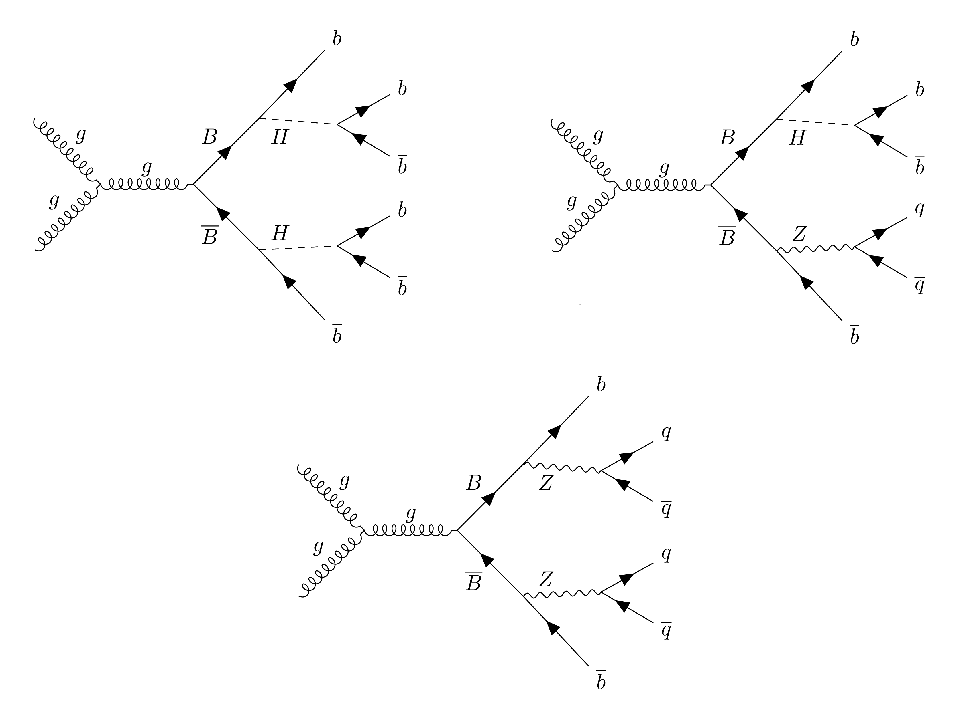
Figure 1:
Dominant diagrams of the pair production of bottom-type VLQs ($\mathrm{B}$) that subsequently decay to a $\mathrm{b}$ or $\mathrm{\bar{b}}$ quark and either a Higgs or Z boson. In events targeted by this analysis, the Z boson then decays to a pair of quarks, where $\mathrm{q}$ denotes any quark other than a top quark, while the Higgs boson decays to $\mathrm{b}$ quarks. Upper left: ${\mathrm{b} \mathrm{H} \mathrm{b} \mathrm{H}}$ mode, upper right: ${\mathrm{b} \mathrm{H} \mathrm{b} \mathrm{Z}}$ mode, lower: ${\mathrm{b} \mathrm{Z} \mathrm{b} \mathrm{Z}}$ mode. |

png pdf |
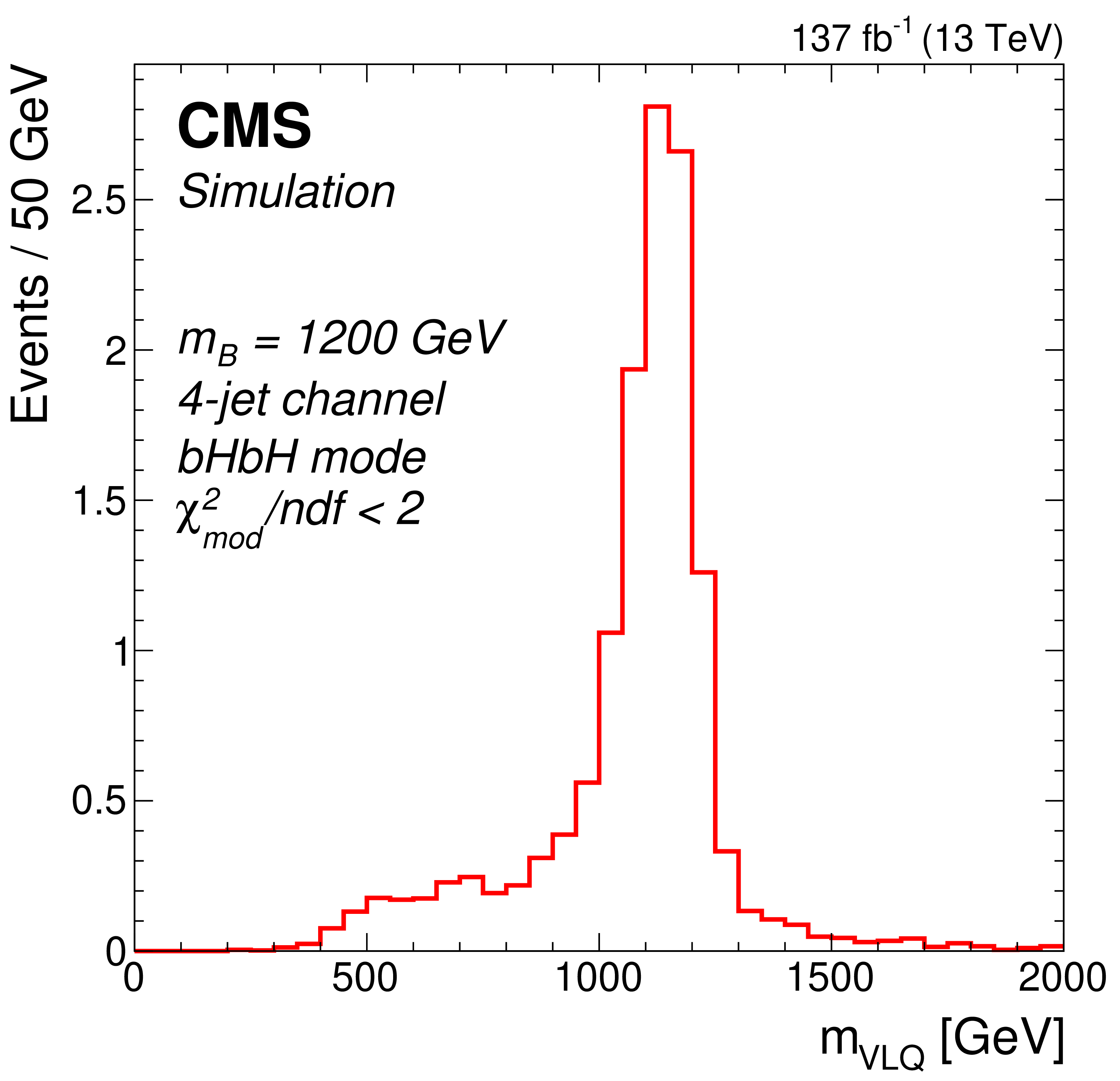
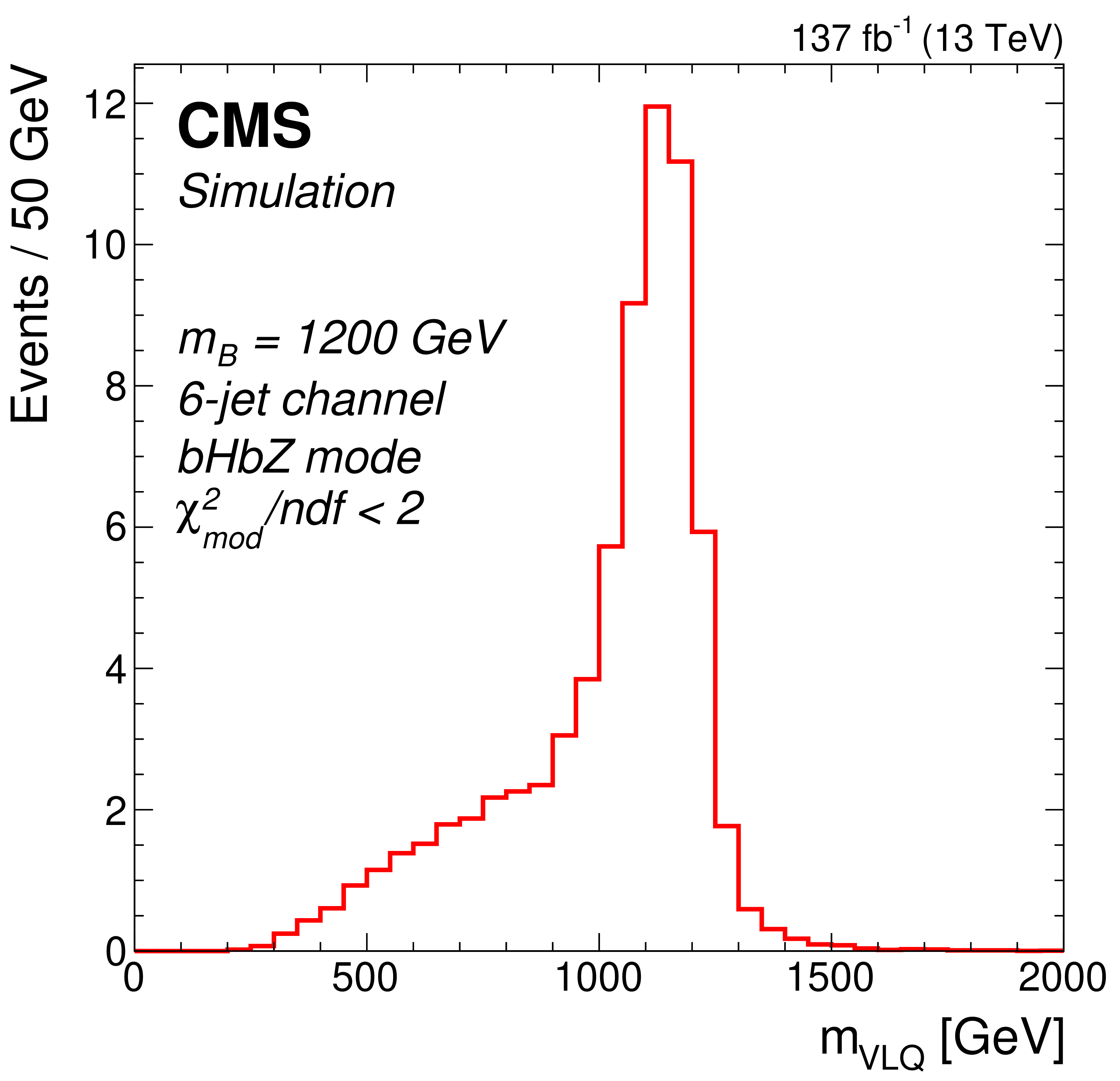
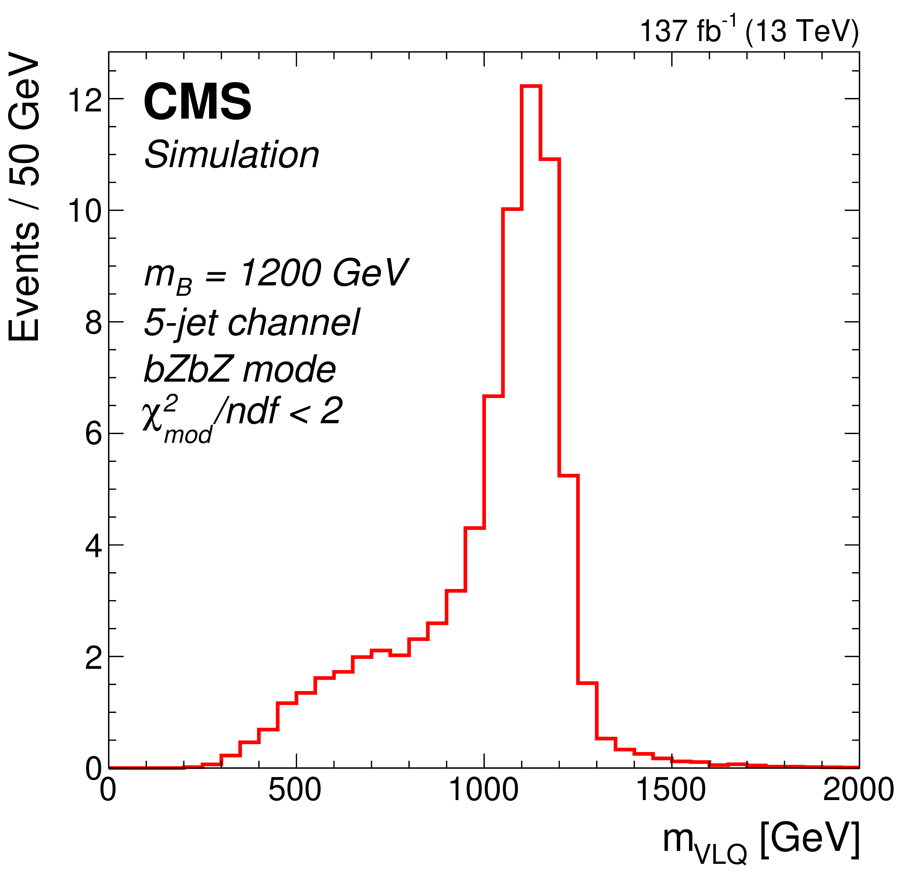
Figure 2:
Distributions of ${m_\text {VLQ}}$ for simulated signal events with a generated VLQ mass $m_{\mathrm{B}} = $ 1200 GeV. A requirement of $ {\chi ^2_\text {mod}/\text {ndf}} < $ 2 is applied to the events. Mass distributions for 4-jet (left), 5-jet (center), and 6-jet (right) events are shown for the three event modes: ${\mathrm{b} \mathrm{H} \mathrm{b} \mathrm{H}}$ (upper row), ${\mathrm{b} \mathrm{H} \mathrm{b} \mathrm{Z}}$ (middle row), and ${\mathrm{b} \mathrm{Z} \mathrm{b} \mathrm{Z}}$ (lower row). |
png pdf |
Figure 2-a:
Distribution of ${m_\text {VLQ}}$ for simulated 4-jet signal events with a generated VLQ mass $m_{\mathrm{B}} = $ 1200 GeV, for the ${\mathrm{b} \mathrm{H} \mathrm{b} \mathrm{H}}$ event mode. A requirement of $ {\chi ^2_\text {mod}/\text {ndf}} < $ 2 is applied to the events. |

png pdf |
Figure 2-b:
Distribution of ${m_\text {VLQ}}$ for simulated 5-jet signal events with a generated VLQ mass $m_{\mathrm{B}} = $ 1200 GeV, for the ${\mathrm{b} \mathrm{H} \mathrm{b} \mathrm{H}}$ event mode. A requirement of $ {\chi ^2_\text {mod}/\text {ndf}} < $ 2 is applied to the events. |
png pdf |
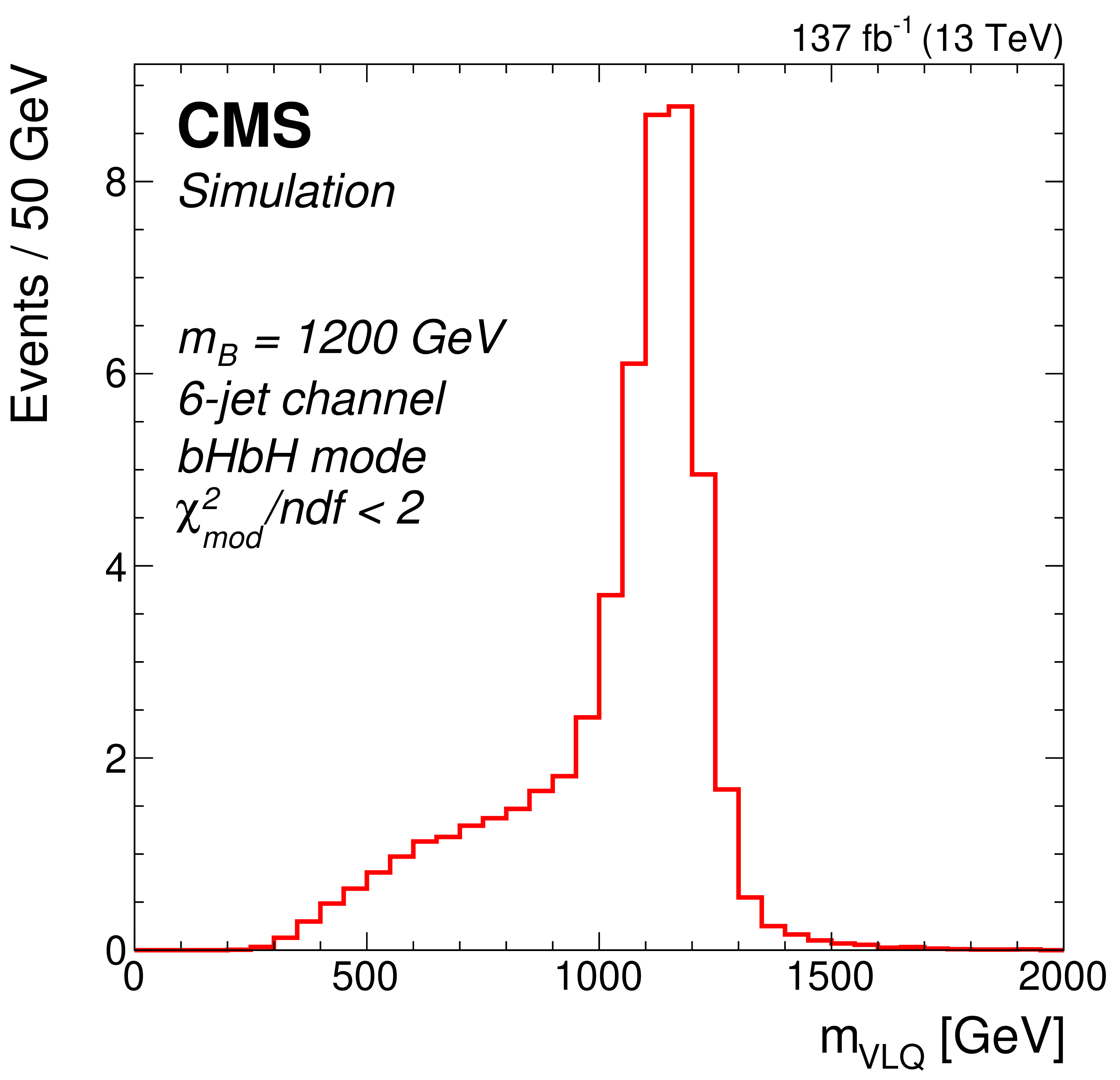
Figure 2-c:
Distribution of ${m_\text {VLQ}}$ for simulated 6-jet signal events with a generated VLQ mass $m_{\mathrm{B}} = $ 1200 GeV, for the ${\mathrm{b} \mathrm{H} \mathrm{b} \mathrm{H}}$ event mode. A requirement of $ {\chi ^2_\text {mod}/\text {ndf}} < $ 2 is applied to the events. |
png pdf |
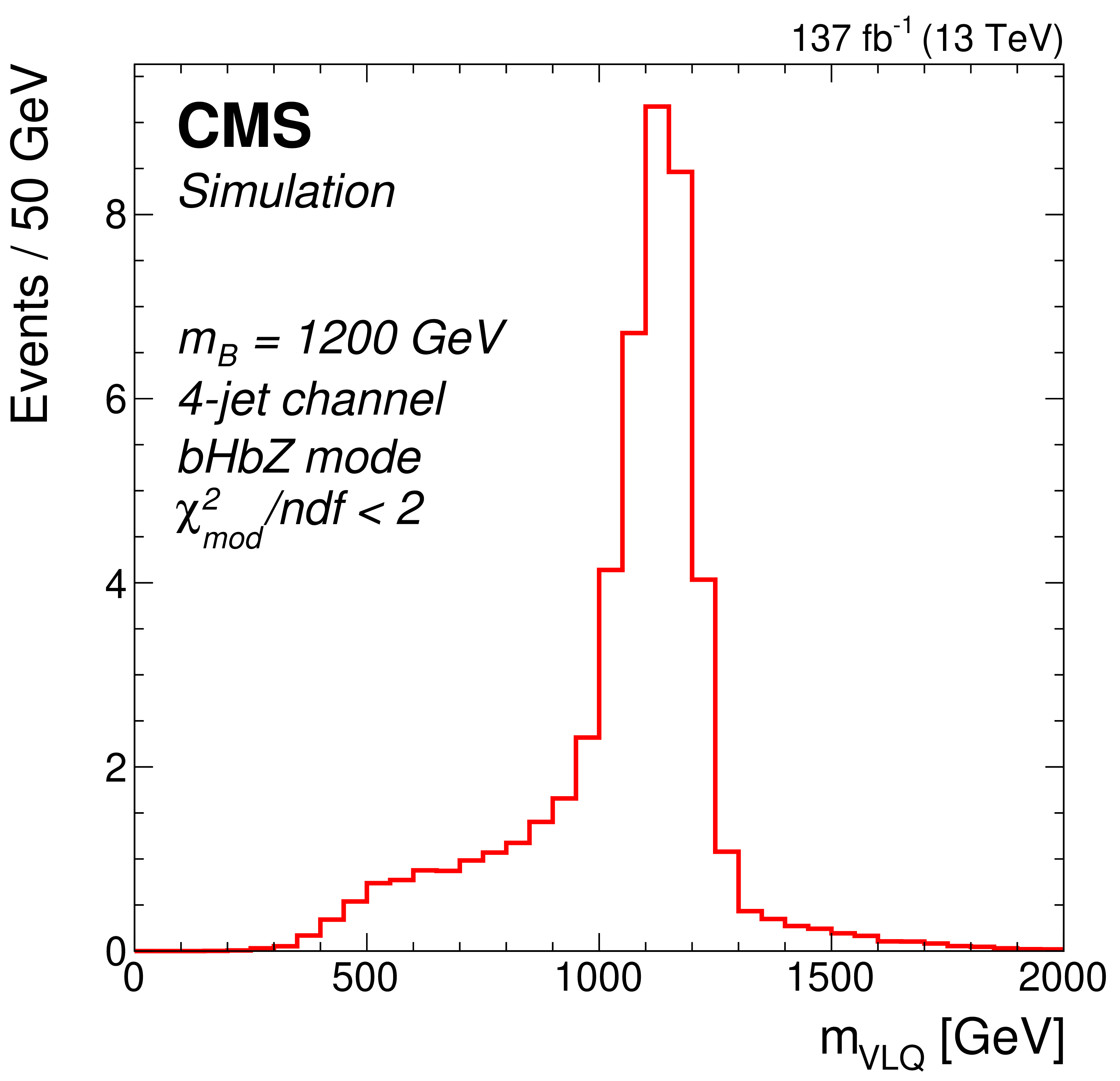
Figure 2-d:
Distribution of ${m_\text {VLQ}}$ for simulated 4-jet signal events with a generated VLQ mass $m_{\mathrm{B}} = $ 1200 GeV, for the ${\mathrm{b} \mathrm{H} \mathrm{b} \mathrm{Z}}$ event mode. A requirement of $ {\chi ^2_\text {mod}/\text {ndf}} < $ 2 is applied to the events. |

png pdf |
Figure 2-e:
Distribution of ${m_\text {VLQ}}$ for simulated 5-jet signal events with a generated VLQ mass $m_{\mathrm{B}} = $ 1200 GeV, for the ${\mathrm{b} \mathrm{H} \mathrm{b} \mathrm{Z}}$ event mode. A requirement of $ {\chi ^2_\text {mod}/\text {ndf}} < $ 2 is applied to the events. |
png pdf |
Figure 2-f:
Distribution of ${m_\text {VLQ}}$ for simulated 6-jet signal events with a generated VLQ mass $m_{\mathrm{B}} = $ 1200 GeV, for the ${\mathrm{b} \mathrm{H} \mathrm{b} \mathrm{Z}}$ event mode. A requirement of $ {\chi ^2_\text {mod}/\text {ndf}} < $ 2 is applied to the events. |

png pdf |
Figure 2-g:
Distribution of ${m_\text {VLQ}}$ for simulated 4-jet signal events with a generated VLQ mass $m_{\mathrm{B}} = $ 1200 GeV, for the ${\mathrm{b} \mathrm{Z} \mathrm{b} \mathrm{Z}}$ event mode. A requirement of $ {\chi ^2_\text {mod}/\text {ndf}} < $ 2 is applied to the events. |
png pdf |
Figure 2-h:
Distribution of ${m_\text {VLQ}}$ for simulated 5-jet signal events with a generated VLQ mass $m_{\mathrm{B}} = $ 1200 GeV, for the ${\mathrm{b} \mathrm{Z} \mathrm{b} \mathrm{Z}}$ event mode. A requirement of $ {\chi ^2_\text {mod}/\text {ndf}} < $ 2 is applied to the events. |

png pdf |
Figure 2-i:
Distribution of ${m_\text {VLQ}}$ for simulated 6-jet signal events with a generated VLQ mass $m_{\mathrm{B}} = $ 1200 GeV, for the ${\mathrm{b} \mathrm{Z} \mathrm{b} \mathrm{Z}}$ event mode. A requirement of $ {\chi ^2_\text {mod}/\text {ndf}} < $ 2 is applied to the events. |
png pdf |
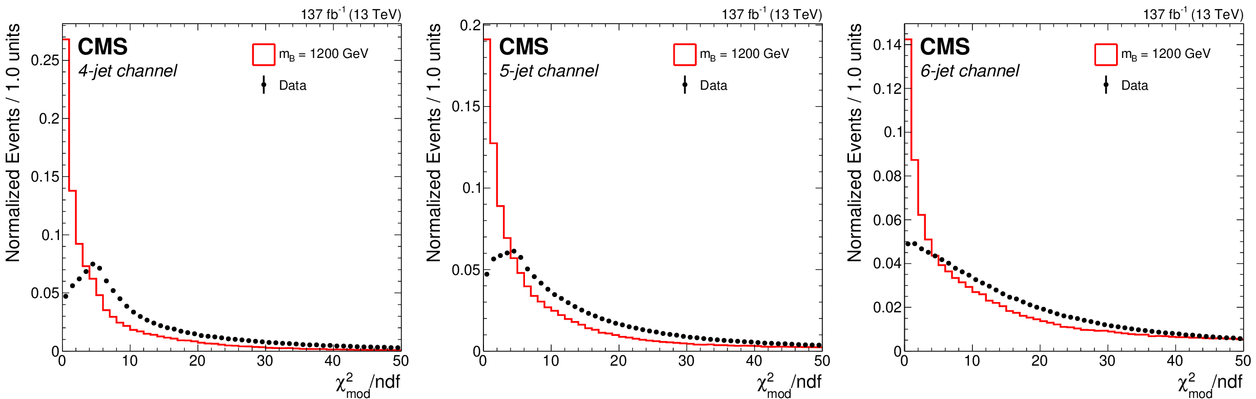
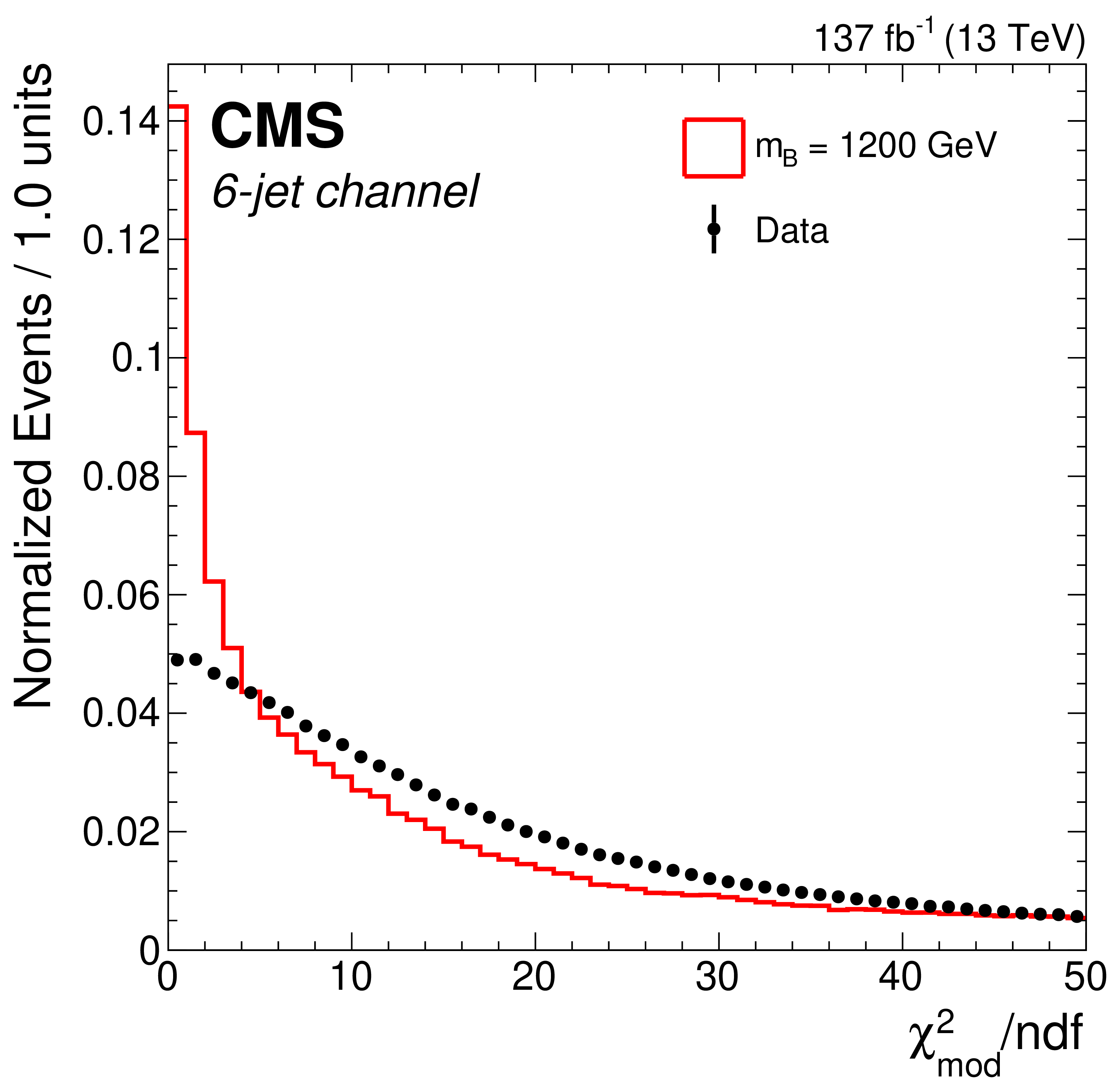
Figure 3:
Distribution of ${\chi ^2_\text {mod}/\text {ndf}}$ for the best jet combination for simulated 1200 GeV VLQ events (red histogram) and data (black points), for 4-jet (left), 5-jet (center), and 6-jet events (right). The simulated signal events and data events are normalized to the same integral value within the displayed ${\chi ^2_\text {mod}}$ range. |

png pdf |
Figure 3-a:
Distribution of ${\chi ^2_\text {mod}/\text {ndf}}$ for the best jet combination for simulated 1200 GeV VLQ events (red histogram) and data (black points), for 4-jet events. The simulated signal events and data events are normalized to the same integral value within the displayed ${\chi ^2_\text {mod}}$ range. |
png pdf |
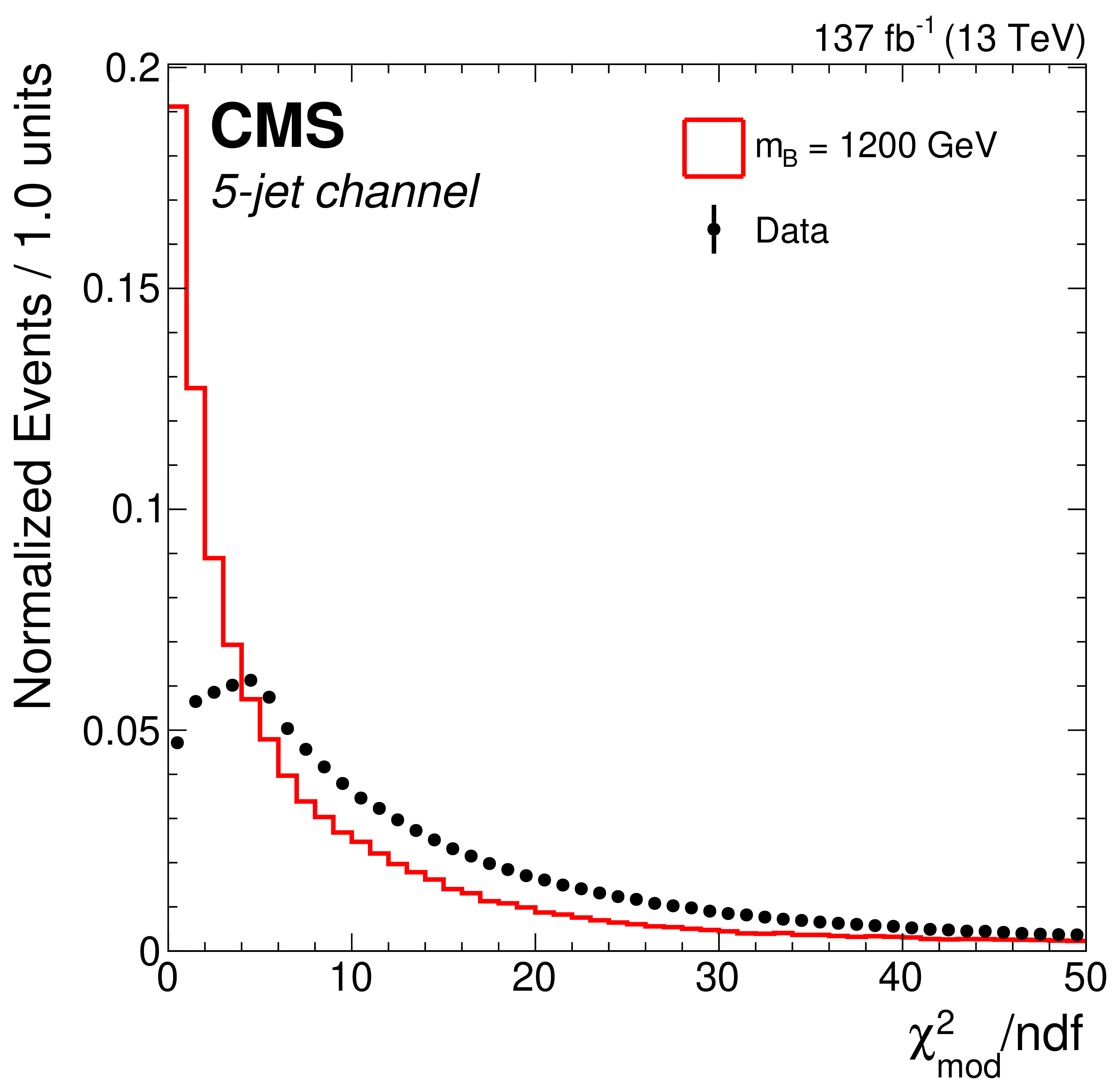
Figure 3-b:
Distribution of ${\chi ^2_\text {mod}/\text {ndf}}$ for the best jet combination for simulated 1200 GeV VLQ events (red histogram) and data (black points), for 5-jet events. The simulated signal events and data events are normalized to the same integral value within the displayed ${\chi ^2_\text {mod}}$ range. |
png pdf |
Figure 3-c:
Distribution of ${\chi ^2_\text {mod}/\text {ndf}}$ for the best jet combination for simulated 1200 GeV VLQ events (red histogram) and data (black points), for 6-jet events. The simulated signal events and data events are normalized to the same integral value within the displayed ${\chi ^2_\text {mod}}$ range. |
png pdf |
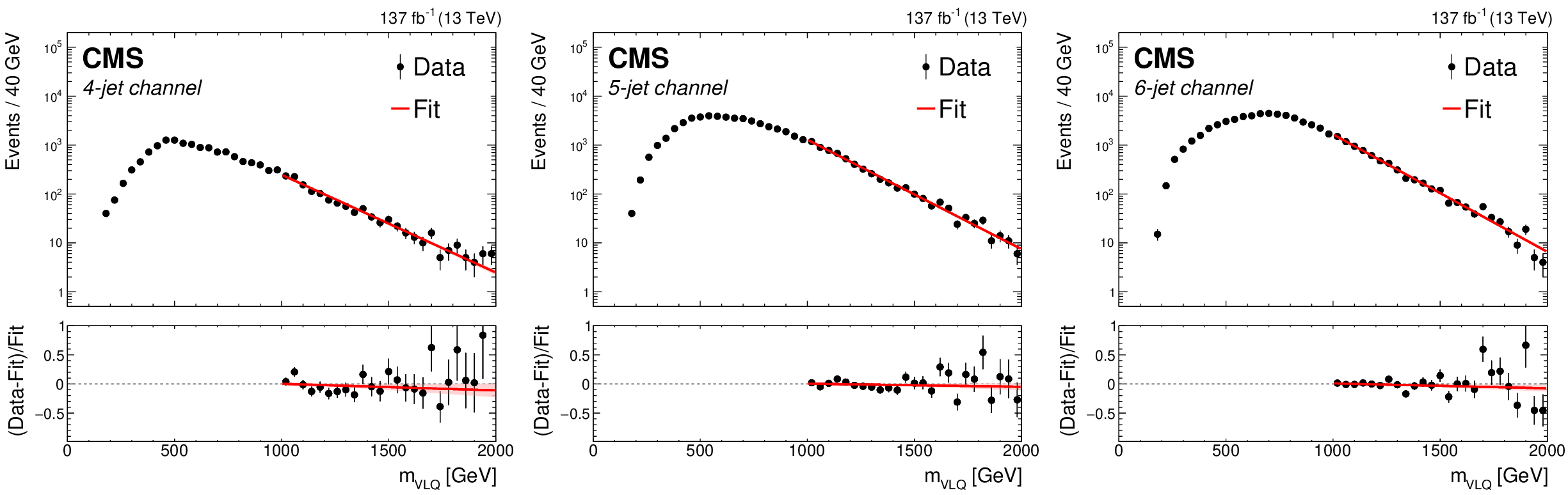
Figure 4:
Distributions of ${m_\text {VLQ}}$ for the jet combination with the lowest ${\chi ^2_\text {mod}}$ in 4-jet (left), 5-jet (center), and 6-jet (right) multiplicity events. The red lines show the exponential fit in the range 1000-2000 GeV. The lower panels show the fractional difference, $(\text {data}-\text {fit})/\text {fit}$. |

png pdf |
Figure 4-a:
Distribution of ${m_\text {VLQ}}$ for the jet combination with the lowest ${\chi ^2_\text {mod}}$ in 4-jet multiplicity events. The red lines show the exponential fit in the range 1000-2000 GeV. The lower panel shows the fractional difference, $(\text {data}-\text {fit})/\text {fit}$. |
png pdf |
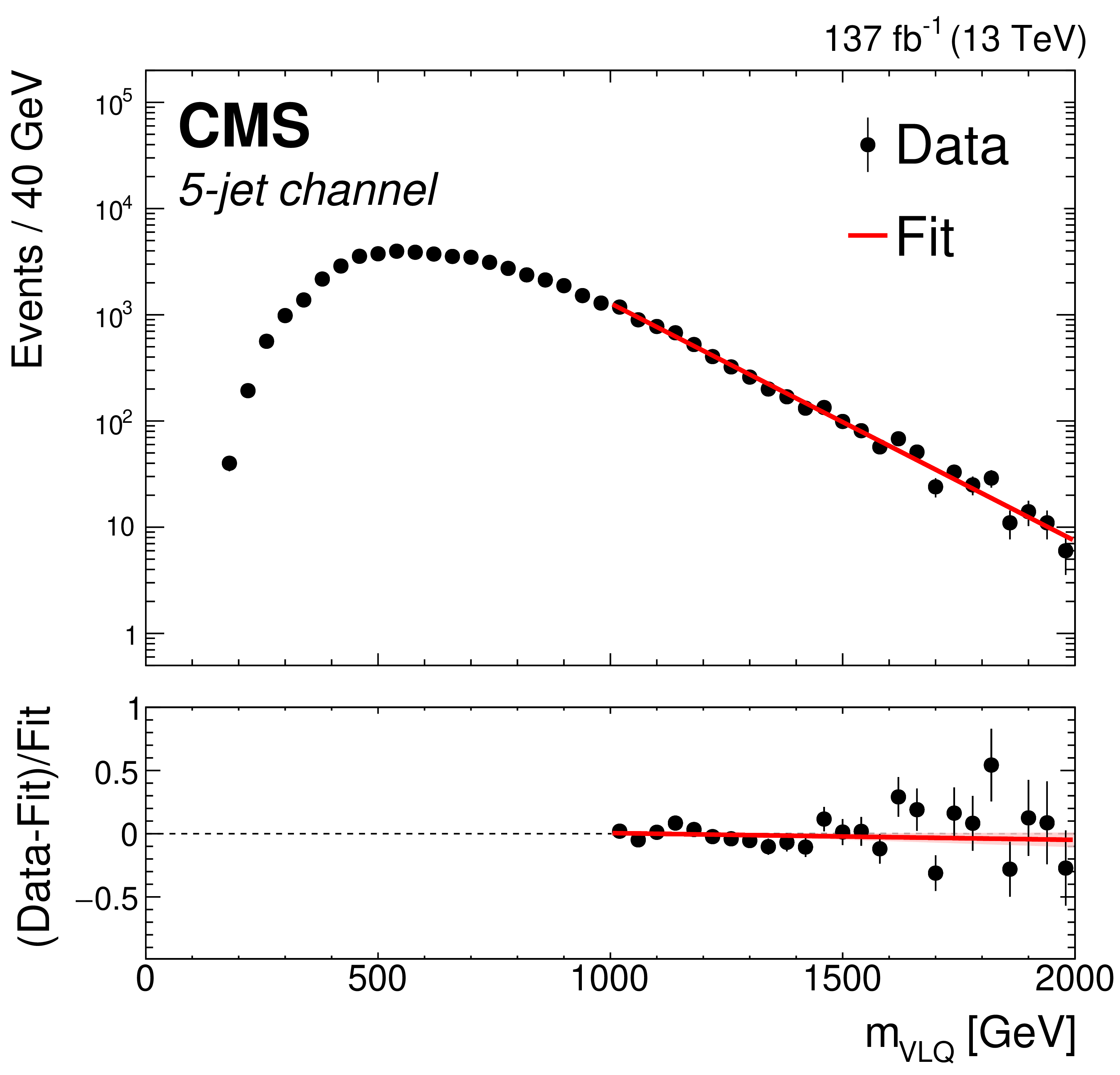
Figure 4-b:
Distribution of ${m_\text {VLQ}}$ for the jet combination with the lowest ${\chi ^2_\text {mod}}$ in 5-jet multiplicity events. The red lines show the exponential fit in the range 1000-2000 GeV. The lower panel shows the fractional difference, $(\text {data}-\text {fit})/\text {fit}$. |

png pdf |
Figure 4-c:
Distribution of ${m_\text {VLQ}}$ for the jet combination with the lowest ${\chi ^2_\text {mod}}$ in 6-jet multiplicity events. The red lines show the exponential fit in the range 1000-2000 GeV. The lower panel shows the fractional difference, $(\text {data}-\text {fit})/\text {fit}$. |
png pdf |
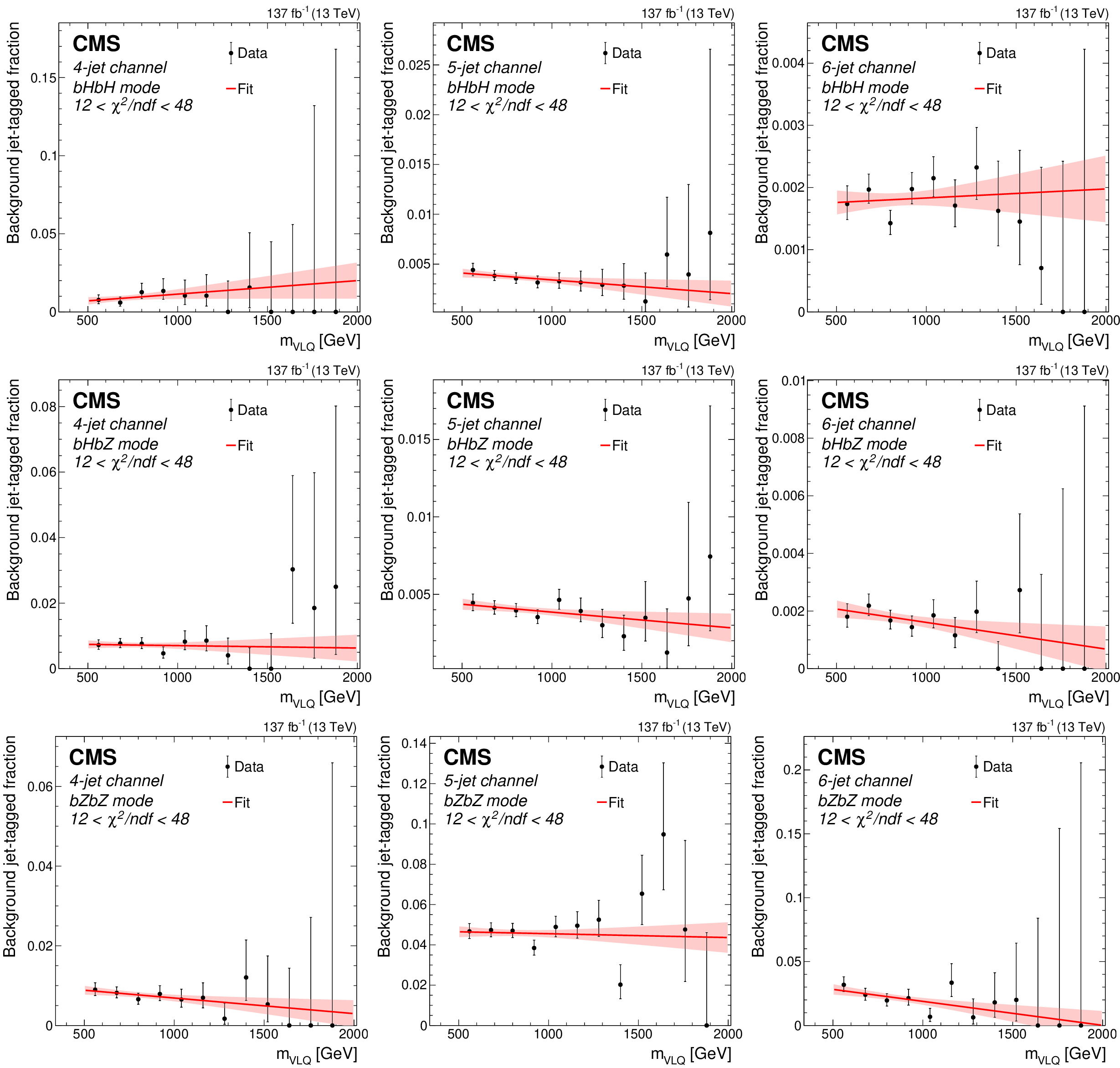
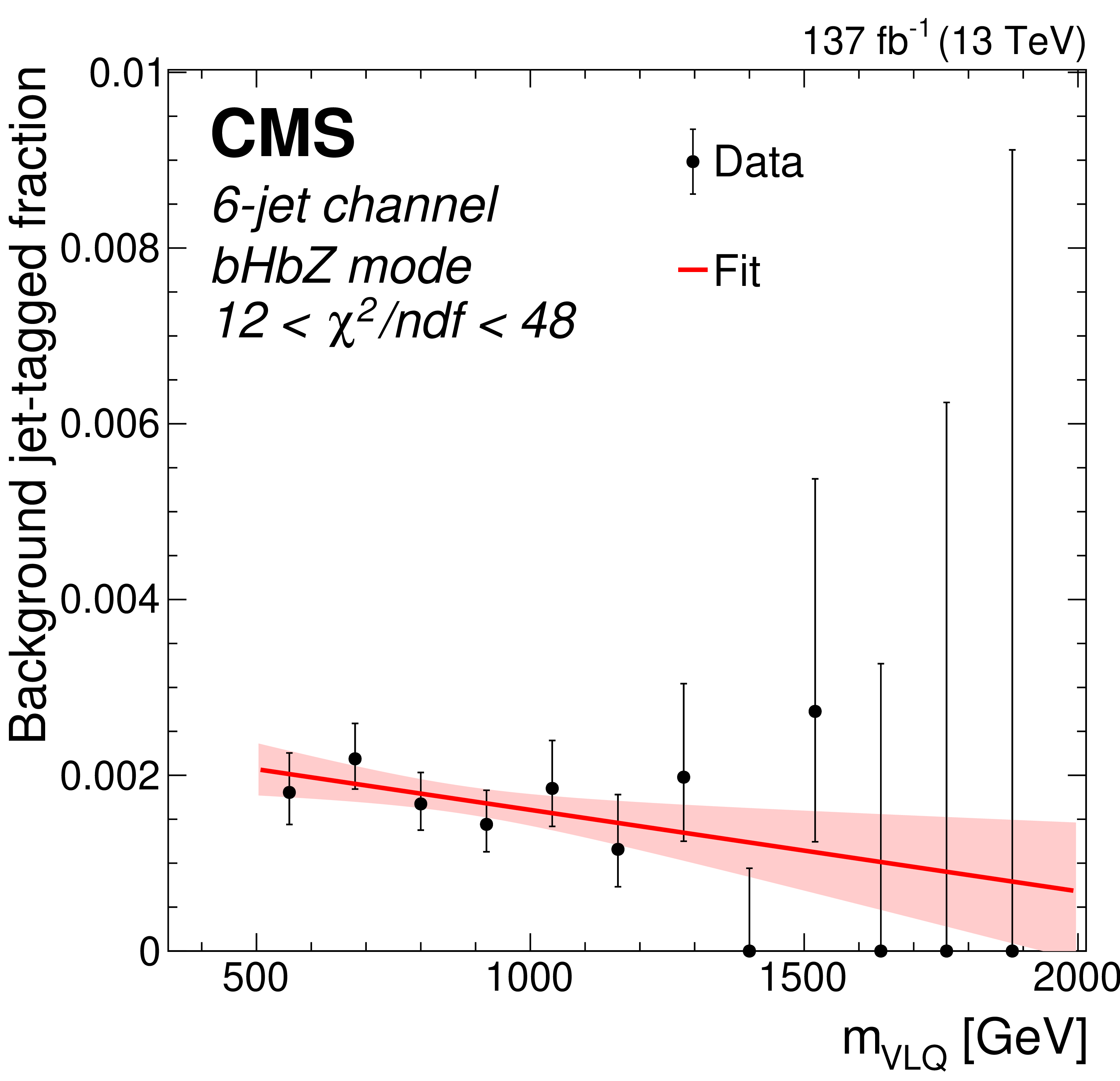
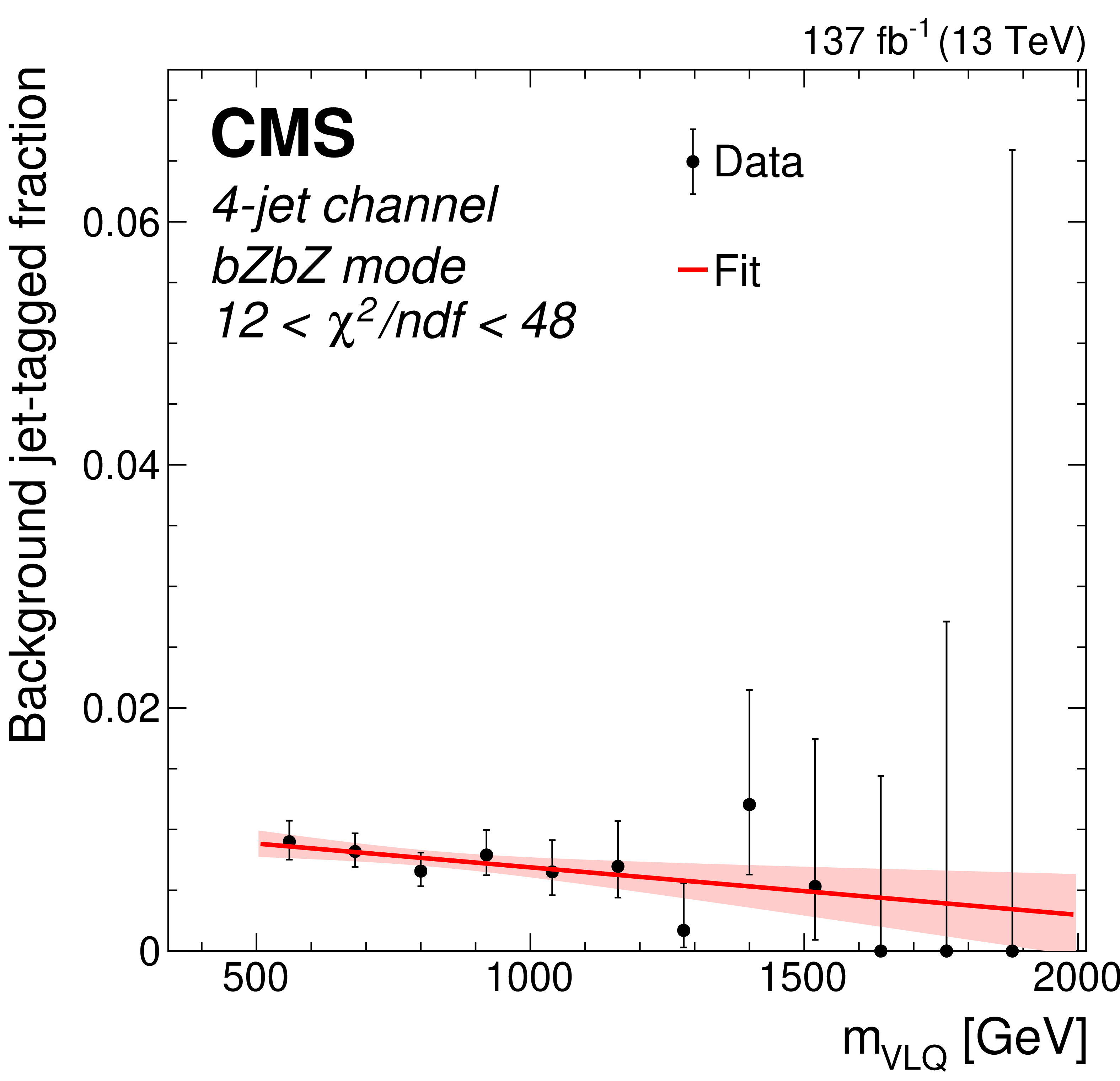
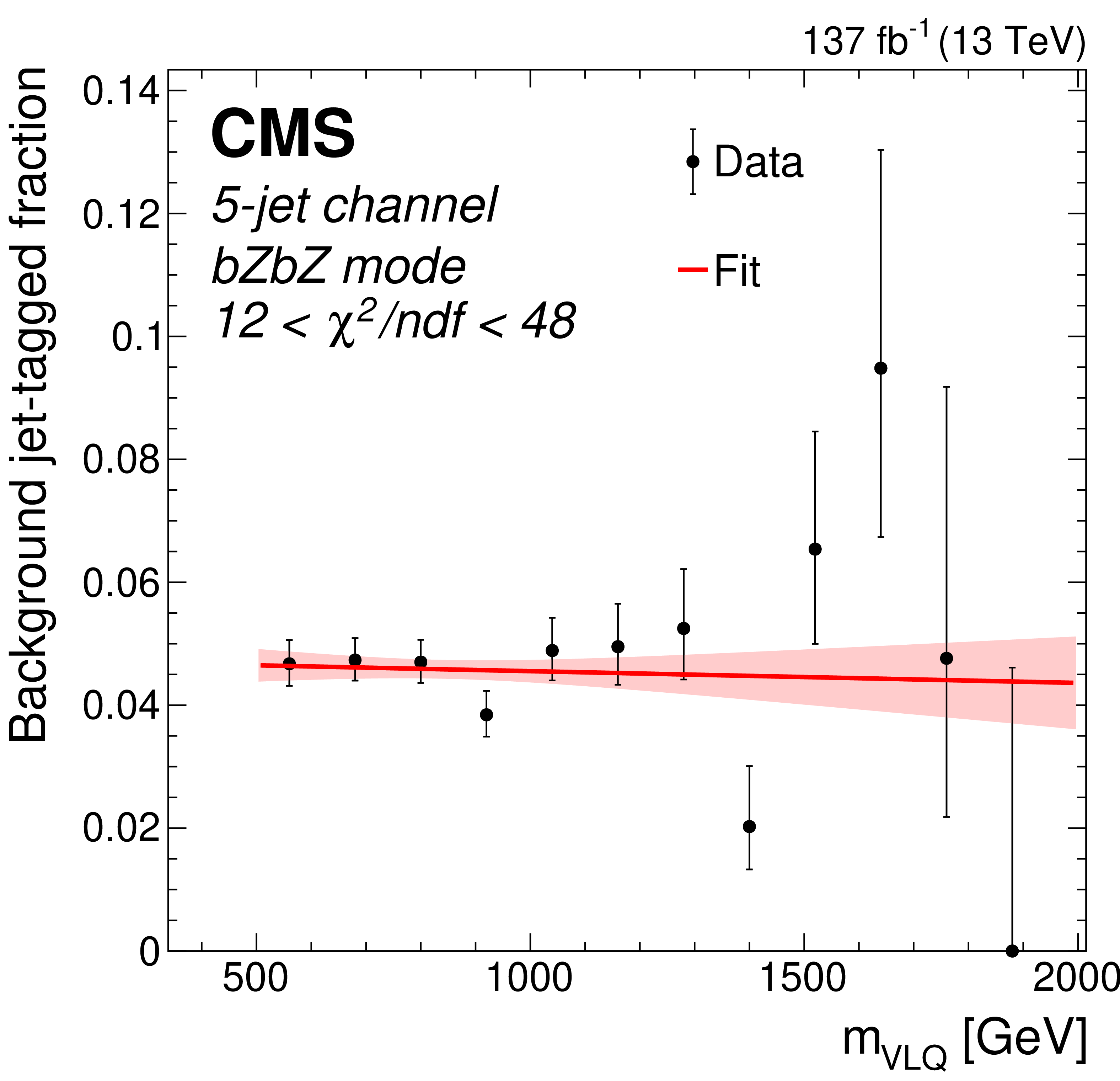
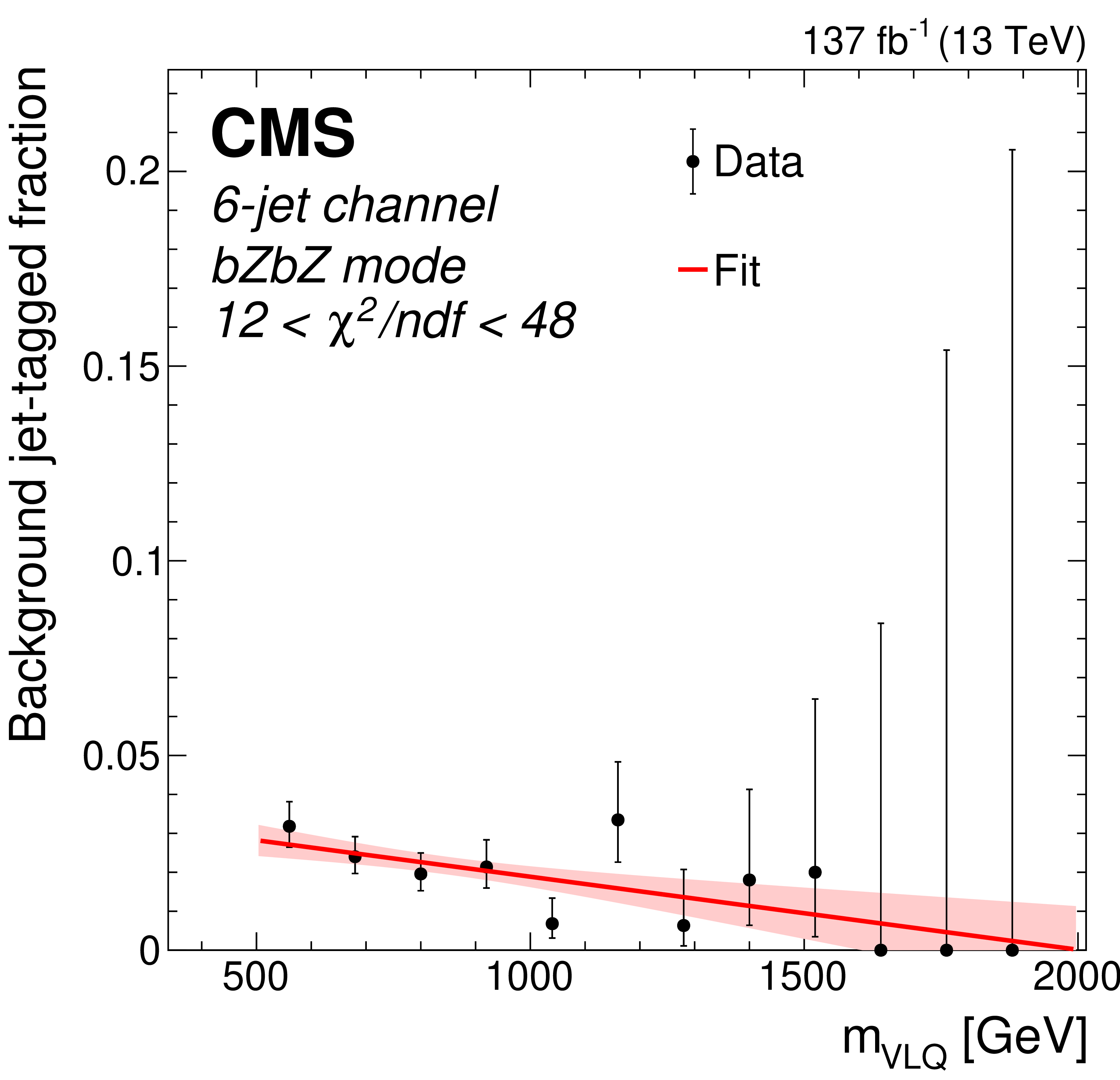
Figure 5:
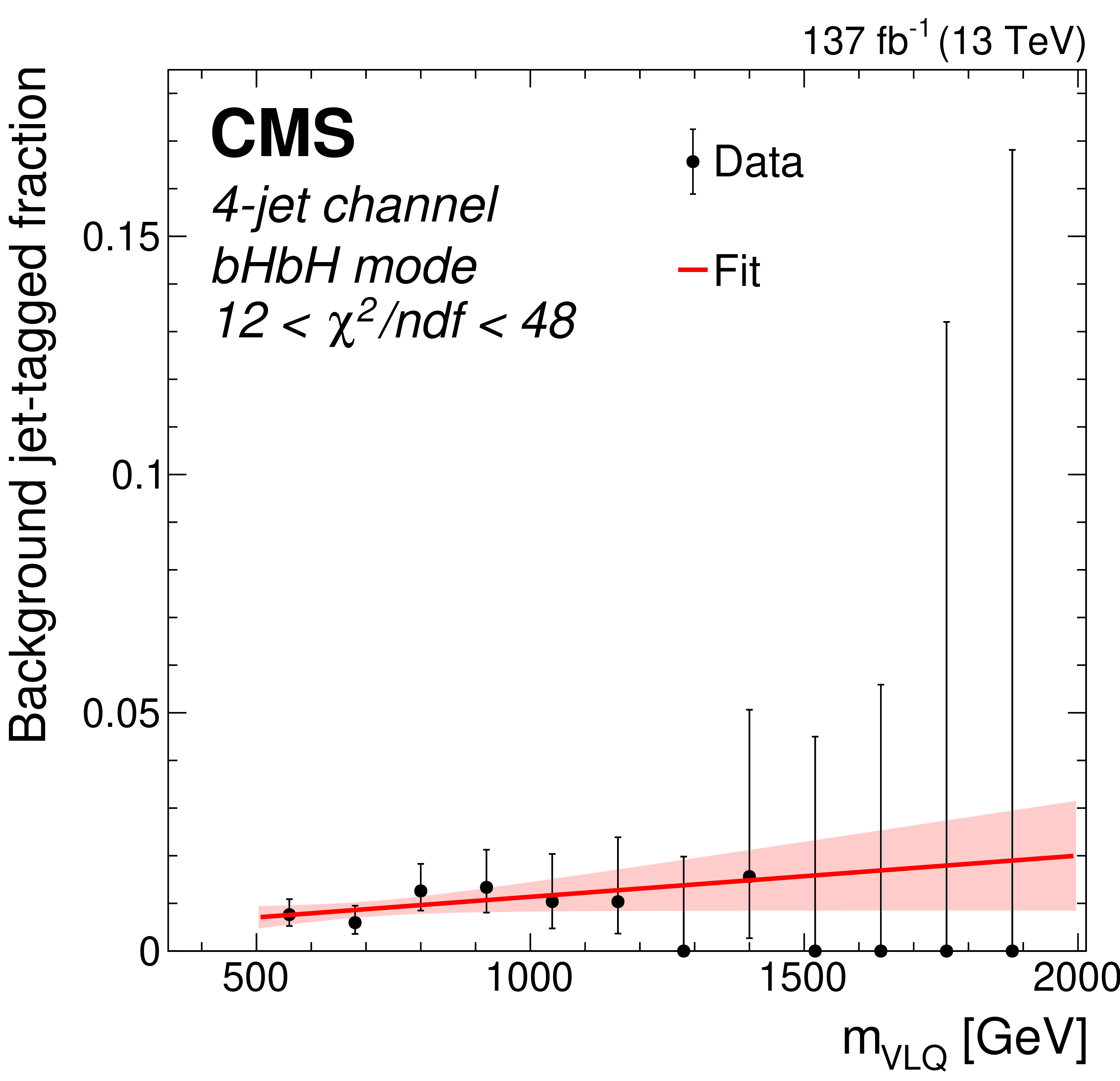
Dependence of the BJTF on ${m_\text {VLQ}}$ in the control region 12 $ < {\chi ^2_\text {mod}/\text {ndf}} < $ 48, for 4-jet (left column), 5-jet (center column), and 6-jet (right column) multiplicities, and for the ${\mathrm{b} \mathrm{H} \mathrm{b} \mathrm{H}}$ (upper row), ${\mathrm{b} \mathrm{H} \mathrm{b} \mathrm{Z}}$ (middle row), and ${\mathrm{b} \mathrm{Z} \mathrm{b} \mathrm{Z}}$ (lower row) event modes. The data are shown as black points with vertical error bars, and the linear fit and associated uncertainty are shown as a solid red line and the shaded red band. |
png pdf |
Figure 5-a:
Dependence of the BJTF on ${m_\text {VLQ}}$ in the control region 12 $ < {\chi ^2_\text {mod}/\text {ndf}} < $ 48, for 4-jet multiplicities, and for the ${\mathrm{b} \mathrm{H} \mathrm{b} \mathrm{H}}$ event mode. The data are shown as black points with vertical error bars, and the linear fit and associated uncertainty are shown as a solid red line and the shaded red band. |
png pdf |
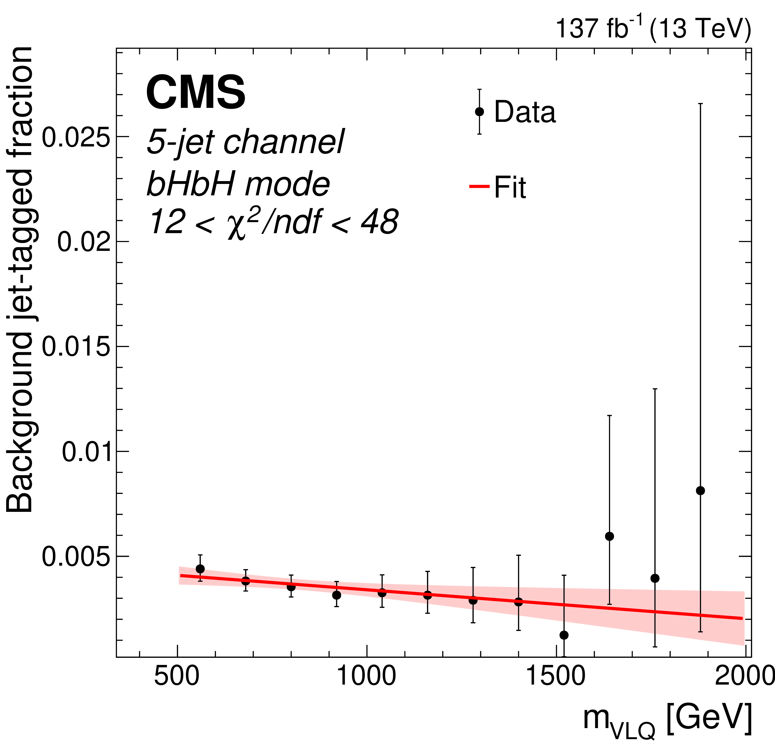
Figure 5-b:
Dependence of the BJTF on ${m_\text {VLQ}}$ in the control region 12 $ < {\chi ^2_\text {mod}/\text {ndf}} < $ 48, for 5-jet multiplicities, and for the ${\mathrm{b} \mathrm{H} \mathrm{b} \mathrm{H}}$ event mode. The data are shown as black points with vertical error bars, and the linear fit and associated uncertainty are shown as a solid red line and the shaded red band. |
png pdf |
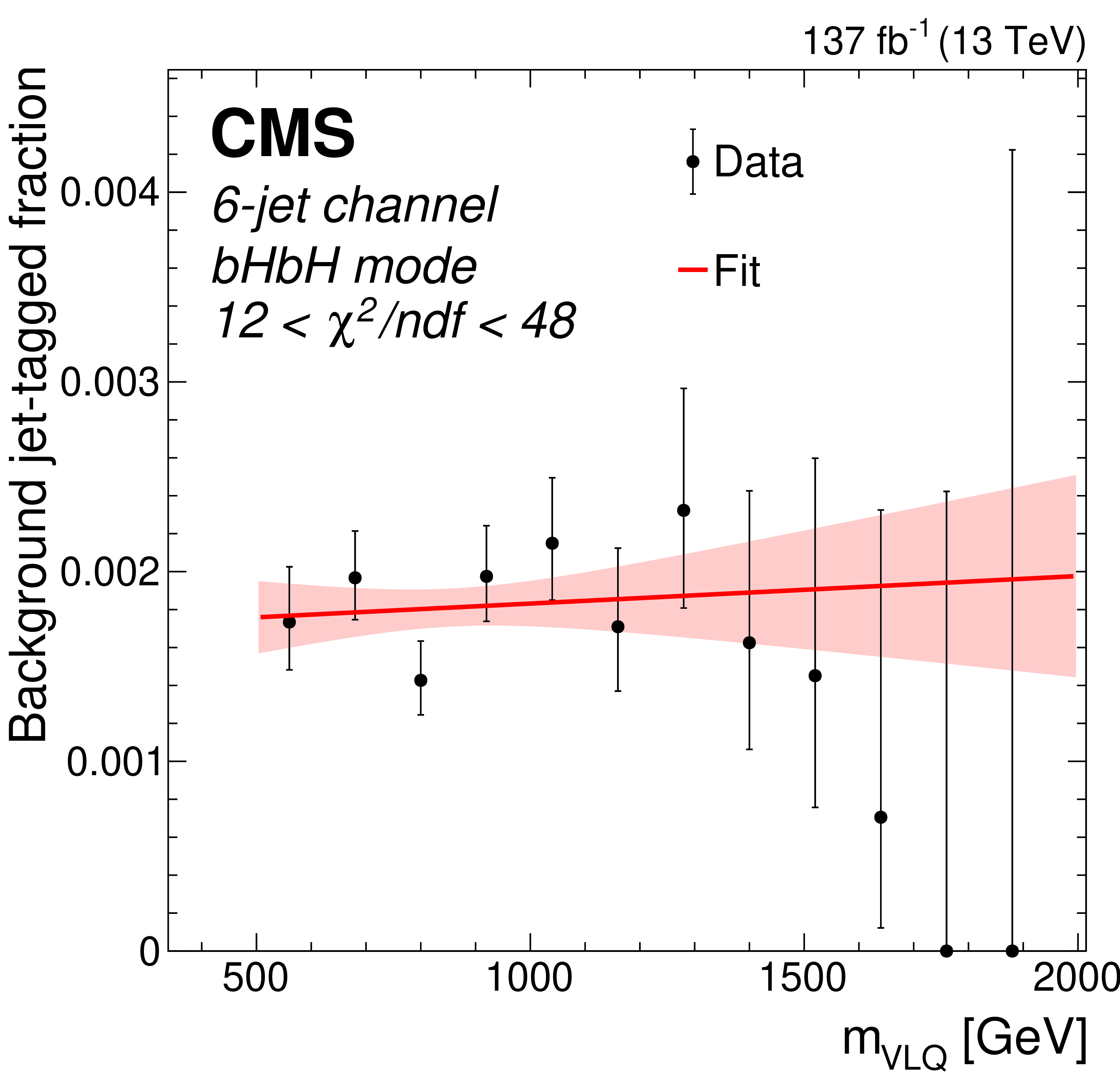
Figure 5-c:
Dependence of the BJTF on ${m_\text {VLQ}}$ in the control region 12 $ < {\chi ^2_\text {mod}/\text {ndf}} < $ 48, for 6-jet multiplicities, and for the ${\mathrm{b} \mathrm{H} \mathrm{b} \mathrm{H}}$ event mode. The data are shown as black points with vertical error bars, and the linear fit and associated uncertainty are shown as a solid red line and the shaded red band. |
png pdf |
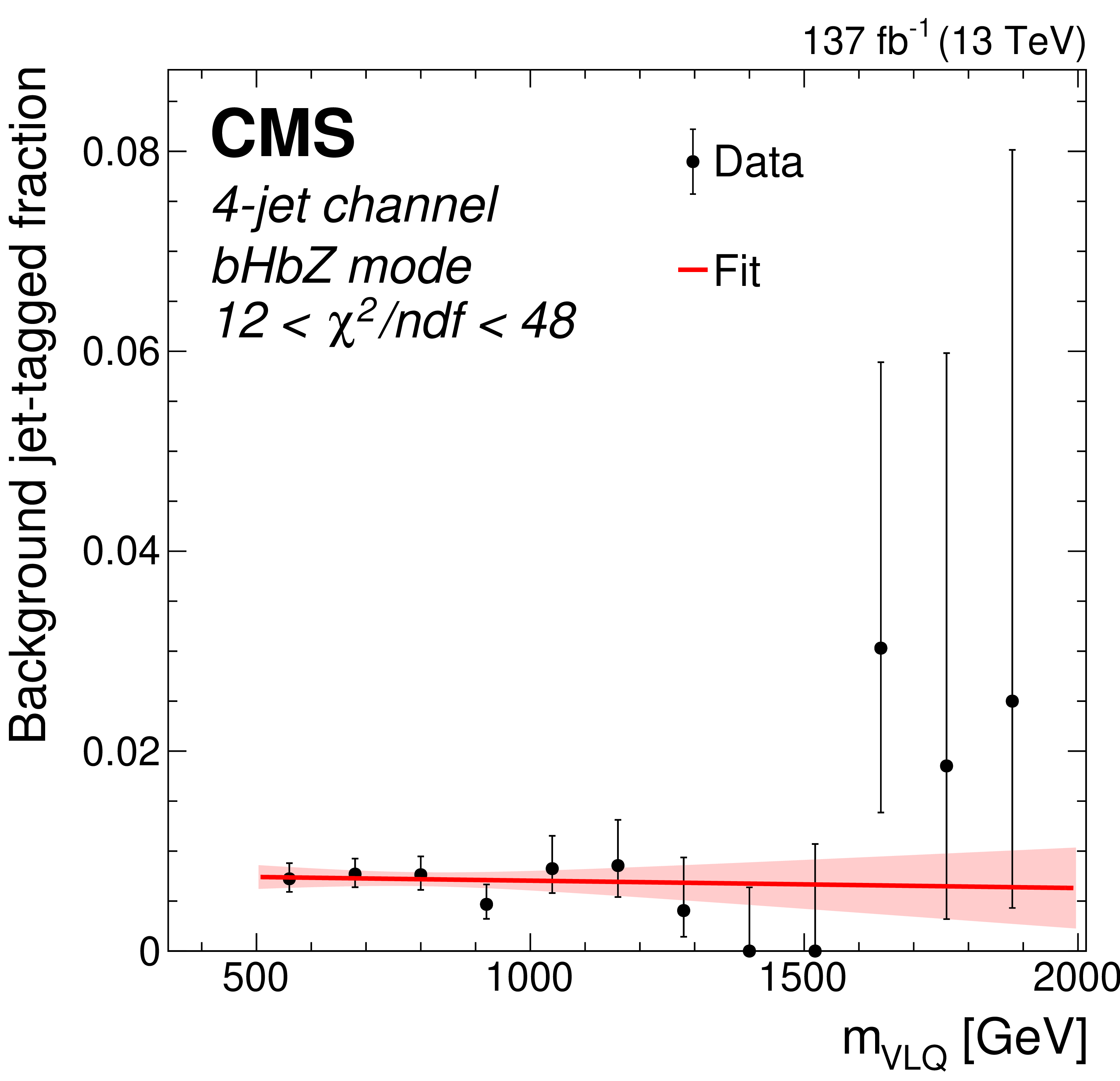
Figure 5-d:
Dependence of the BJTF on ${m_\text {VLQ}}$ in the control region 12 $ < {\chi ^2_\text {mod}/\text {ndf}} < $ 48, for 4-jet multiplicities, and for the ${\mathrm{b} \mathrm{H} \mathrm{b} \mathrm{Z}}$ event mode. The data are shown as black points with vertical error bars, and the linear fit and associated uncertainty are shown as a solid red line and the shaded red band. |

png pdf |
Figure 5-e:
Dependence of the BJTF on ${m_\text {VLQ}}$ in the control region 12 $ < {\chi ^2_\text {mod}/\text {ndf}} < $ 48, for 5-jet multiplicities, and for the ${\mathrm{b} \mathrm{H} \mathrm{b} \mathrm{Z}}$ event mode. The data are shown as black points with vertical error bars, and the linear fit and associated uncertainty are shown as a solid red line and the shaded red band. |
png pdf |
Figure 5-f:
Dependence of the BJTF on ${m_\text {VLQ}}$ in the control region 12 $ < {\chi ^2_\text {mod}/\text {ndf}} < $ 48, for 6-jet multiplicities, and for the ${\mathrm{b} \mathrm{H} \mathrm{b} \mathrm{Z}}$ event mode. The data are shown as black points with vertical error bars, and the linear fit and associated uncertainty are shown as a solid red line and the shaded red band. |
png pdf |
Figure 5-g:
Dependence of the BJTF on ${m_\text {VLQ}}$ in the control region 12 $ < {\chi ^2_\text {mod}/\text {ndf}} < $ 48, for 4-jet multiplicities, and for the ${\mathrm{b} \mathrm{H} \mathrm{b} \mathrm{H}}$ event mode. The data are shown as black points with vertical error bars, and the linear fit and associated uncertainty are shown as a solid red line and the shaded red band. |
png pdf |
Figure 5-h:
Dependence of the BJTF on ${m_\text {VLQ}}$ in the control region 12 $ < {\chi ^2_\text {mod}/\text {ndf}} < $ 48, for 5-jet multiplicities, and for the ${\mathrm{b} \mathrm{H} \mathrm{b} \mathrm{H}}$ event mode. The data are shown as black points with vertical error bars, and the linear fit and associated uncertainty are shown as a solid red line and the shaded red band. |
png pdf |
Figure 5-i:
Dependence of the BJTF on ${m_\text {VLQ}}$ in the control region 12 $ < {\chi ^2_\text {mod}/\text {ndf}} < $ 48, for 6-jet multiplicities, and for the ${\mathrm{b} \mathrm{H} \mathrm{b} \mathrm{H}}$ event mode. The data are shown as black points with vertical error bars, and the linear fit and associated uncertainty are shown as a solid red line and the shaded red band. |
png pdf |
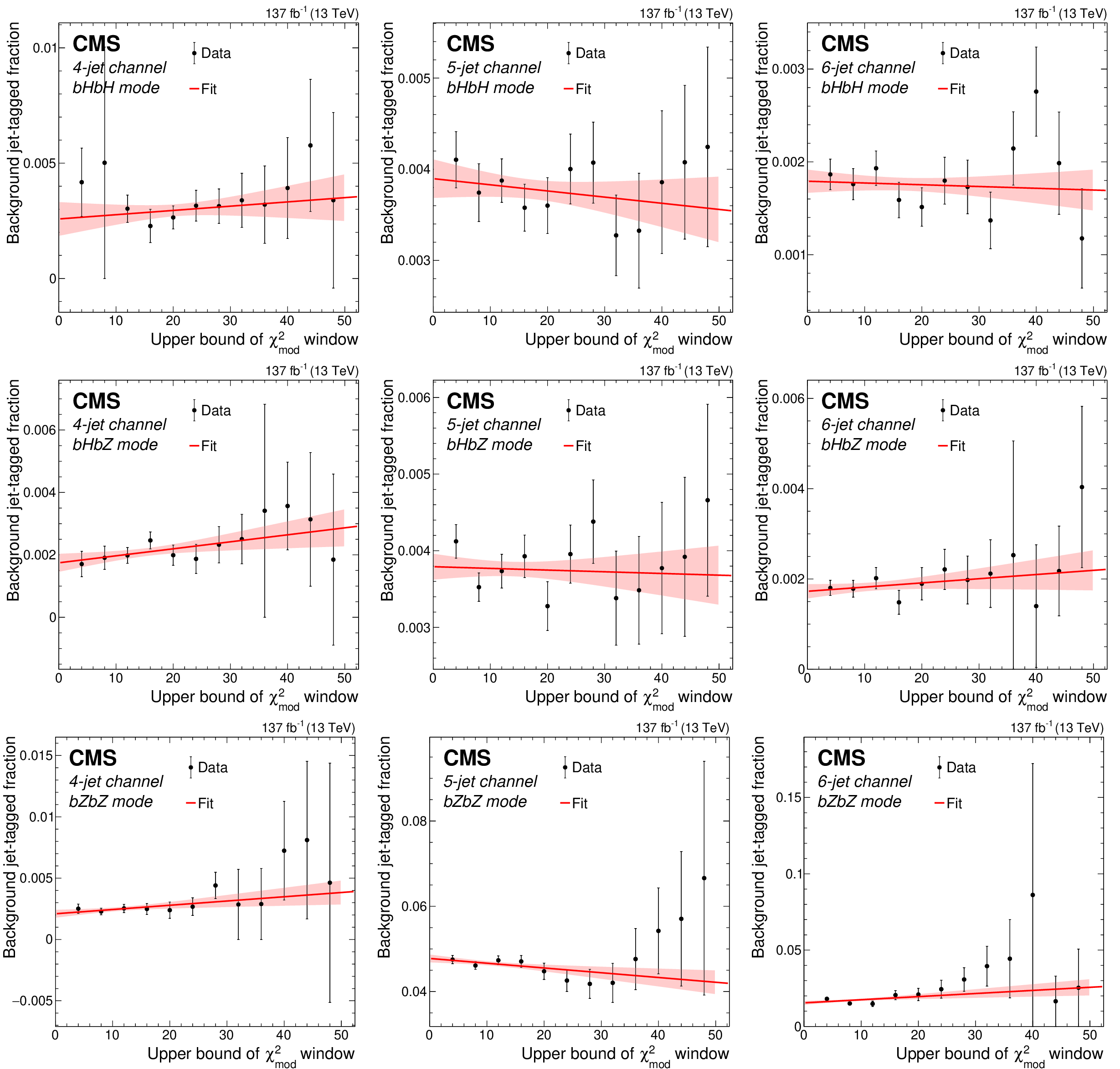
Figure 6:
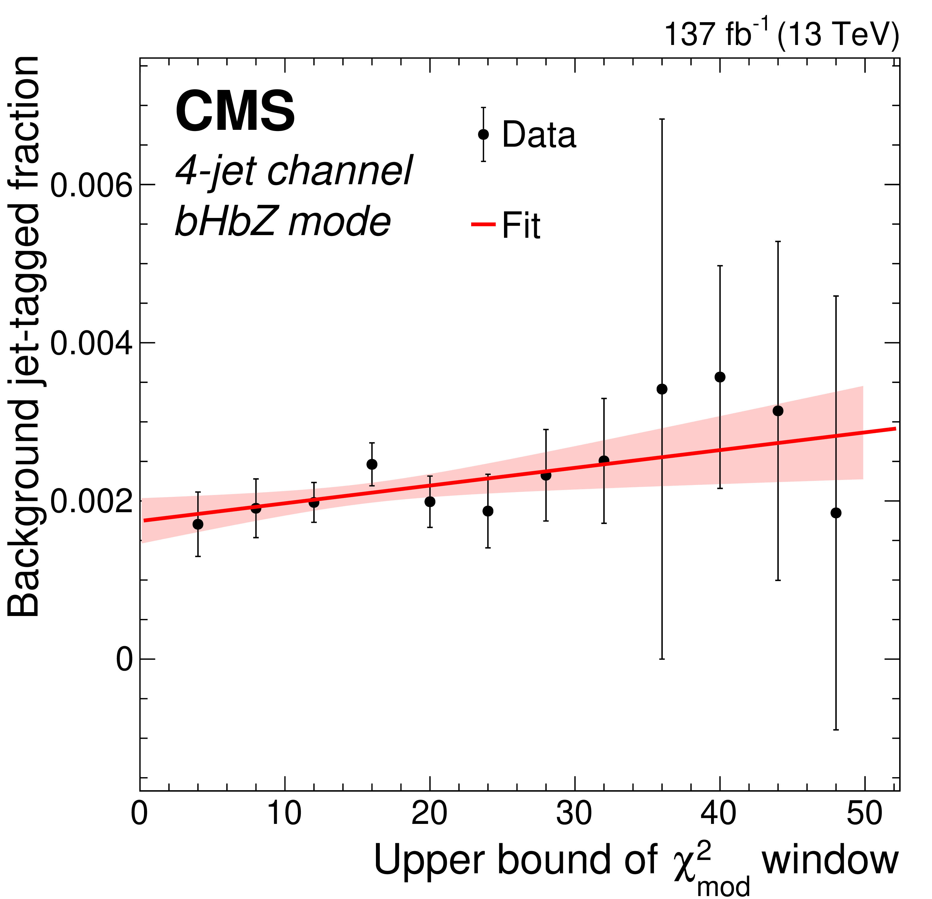
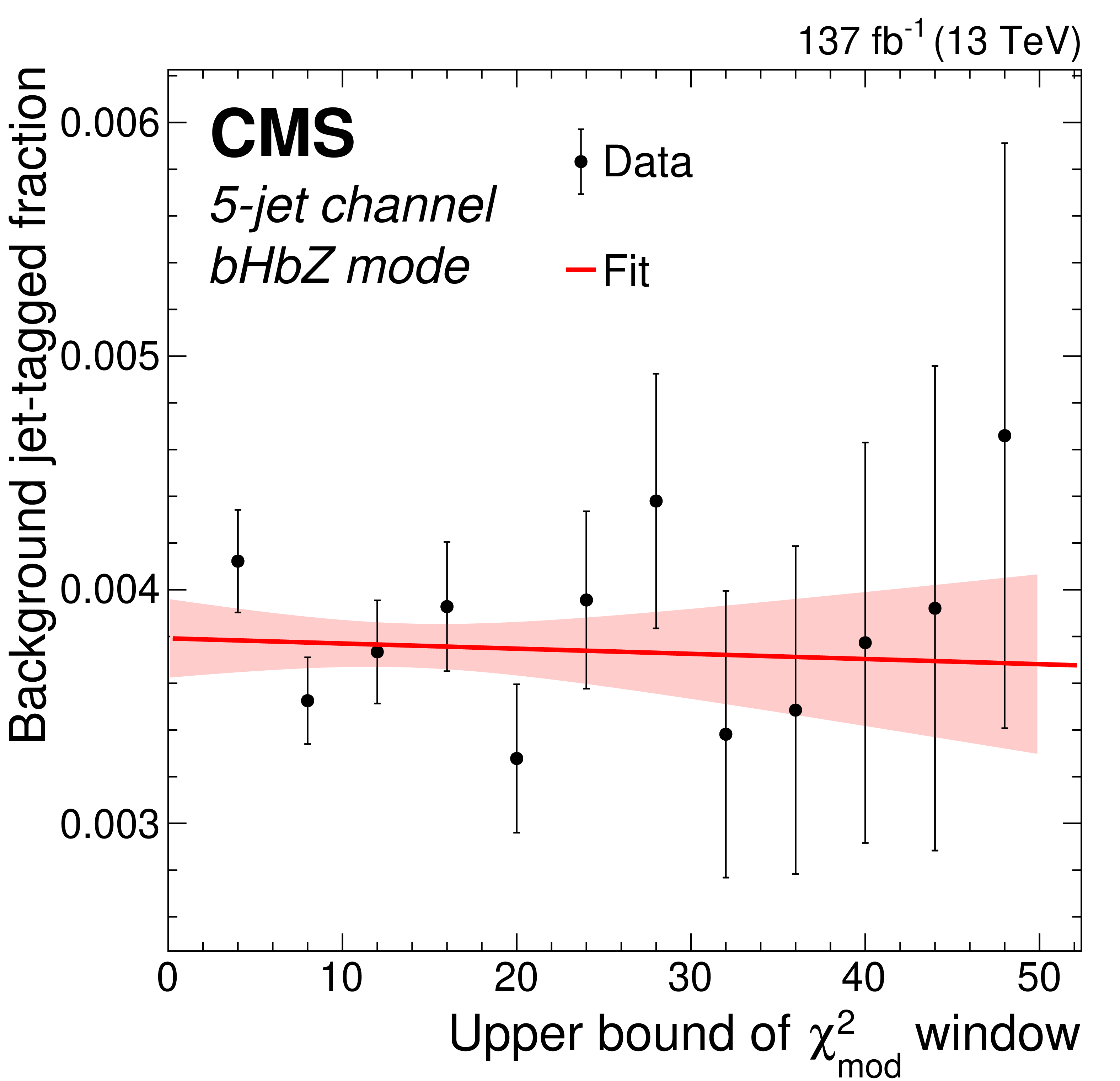
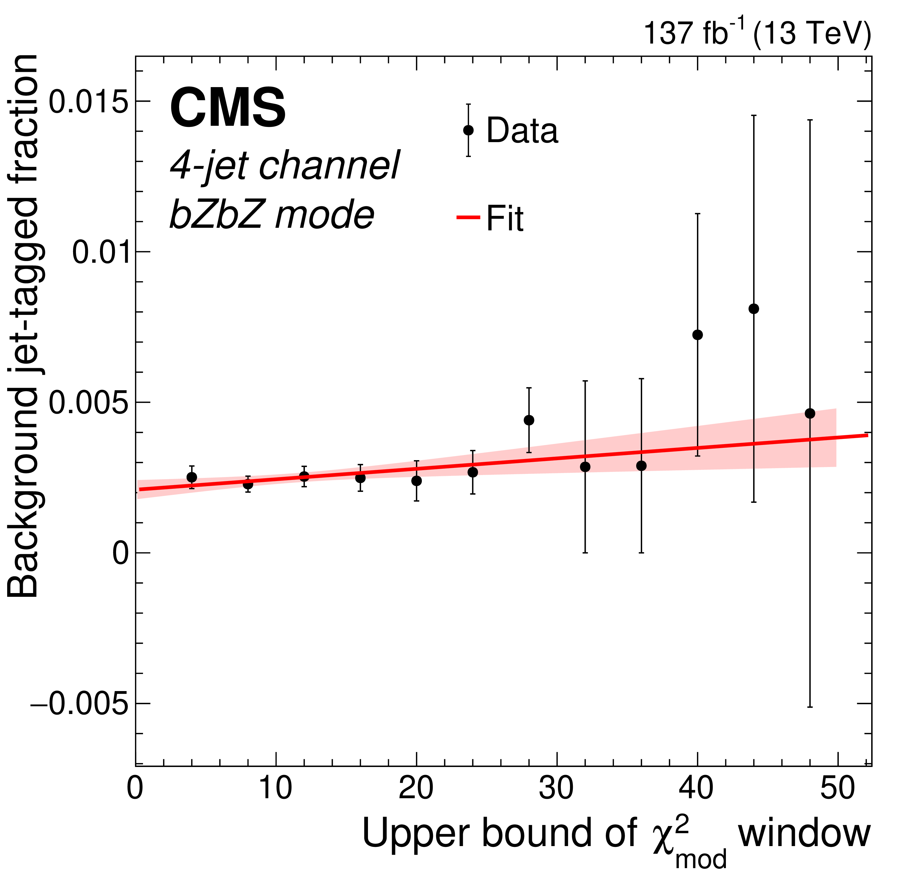
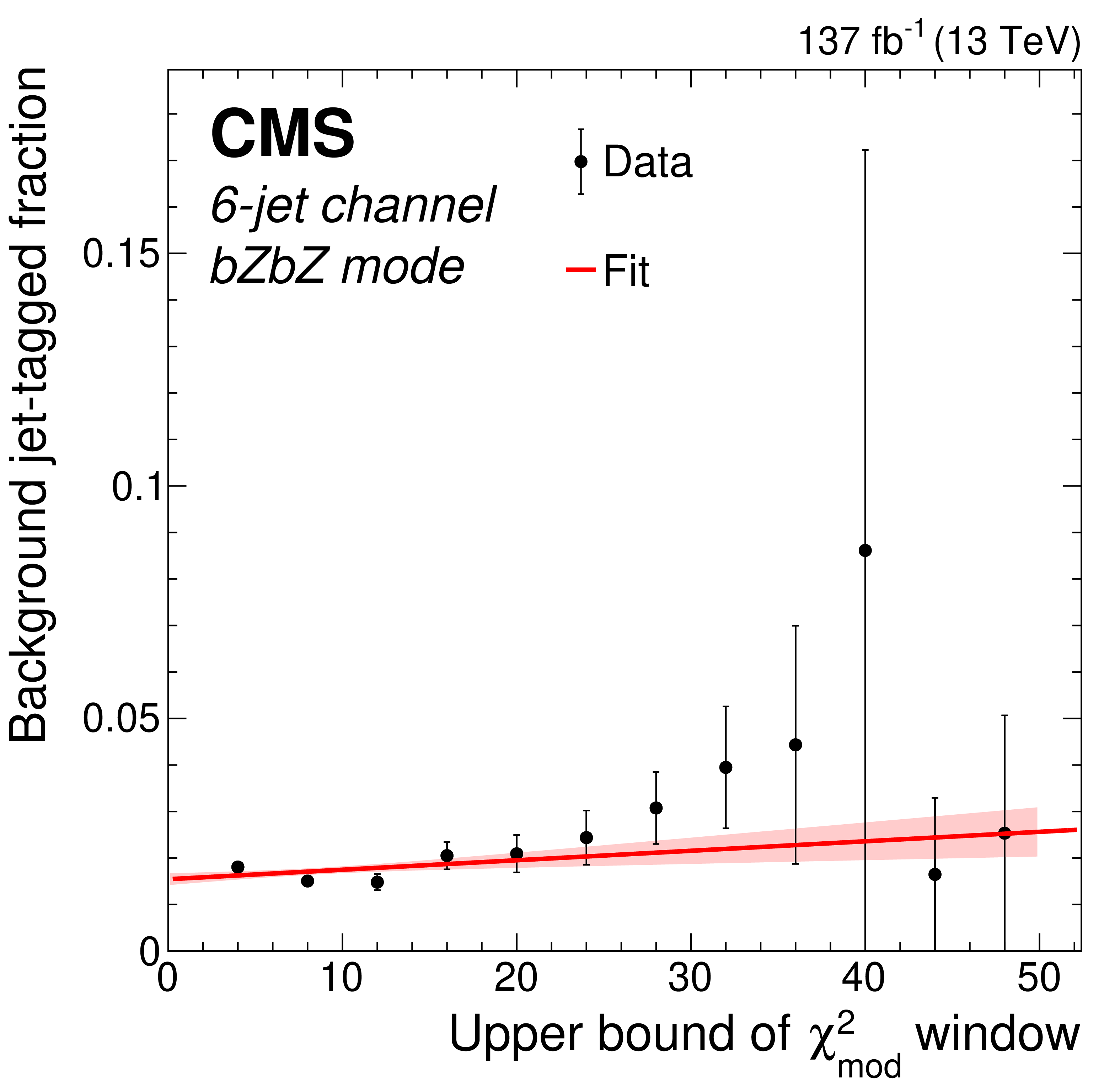
Dependence of the BJTF on ${\chi ^2_\text {mod}/\text {ndf}}$ in the low-mass (500-800 GeV) VLQ region, for 4-jet (left column), 5-jet (center column), and 6-jet (right column) multiplicities, and for the ${\mathrm{b} \mathrm{H} \mathrm{b} \mathrm{H}}$ (upper row), ${\mathrm{b} \mathrm{H} \mathrm{b} \mathrm{Z}}$ (middle row), and ${\mathrm{b} \mathrm{Z} \mathrm{b} \mathrm{Z}}$ (lower row) event modes. The data are shown as black points with vertical error bars, and the linear fit and associated uncertainty are shown as a solid red line and the shaded red band. |
png pdf |
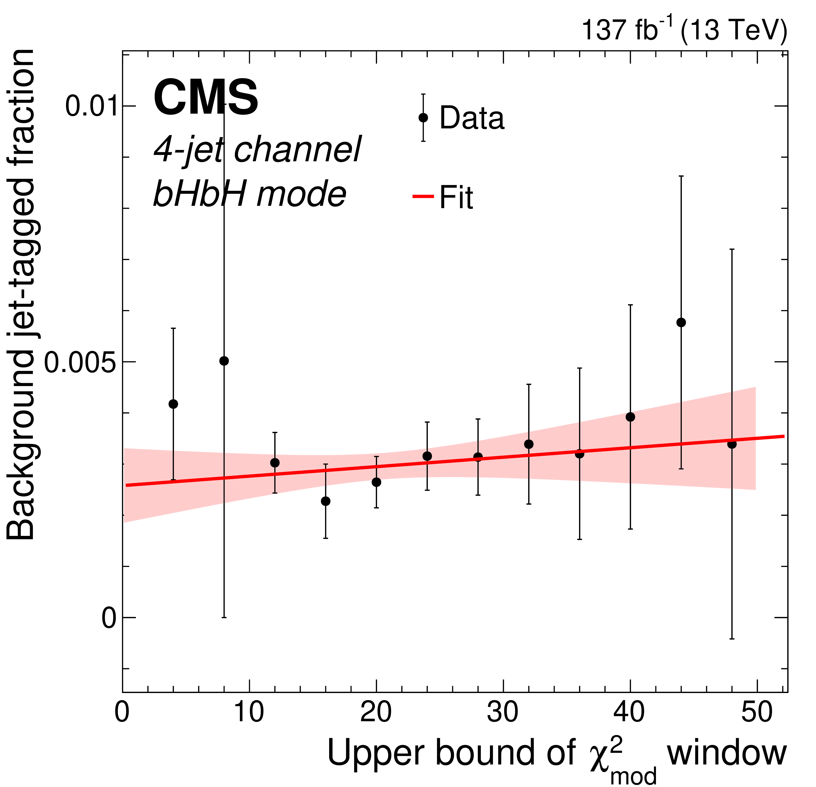
Figure 6-a:
Dependence of the BJTF on ${\chi ^2_\text {mod}/\text {ndf}}$ in the low-mass (500-800 GeV) VLQ region, for 4-jet multiplicities, and for the ${\mathrm{b} \mathrm{H} \mathrm{b} \mathrm{H}}$ event mode. The data are shown as black points with vertical error bars, and the linear fit and associated uncertainty are shown as a solid red line and the shaded red band. |
png pdf |
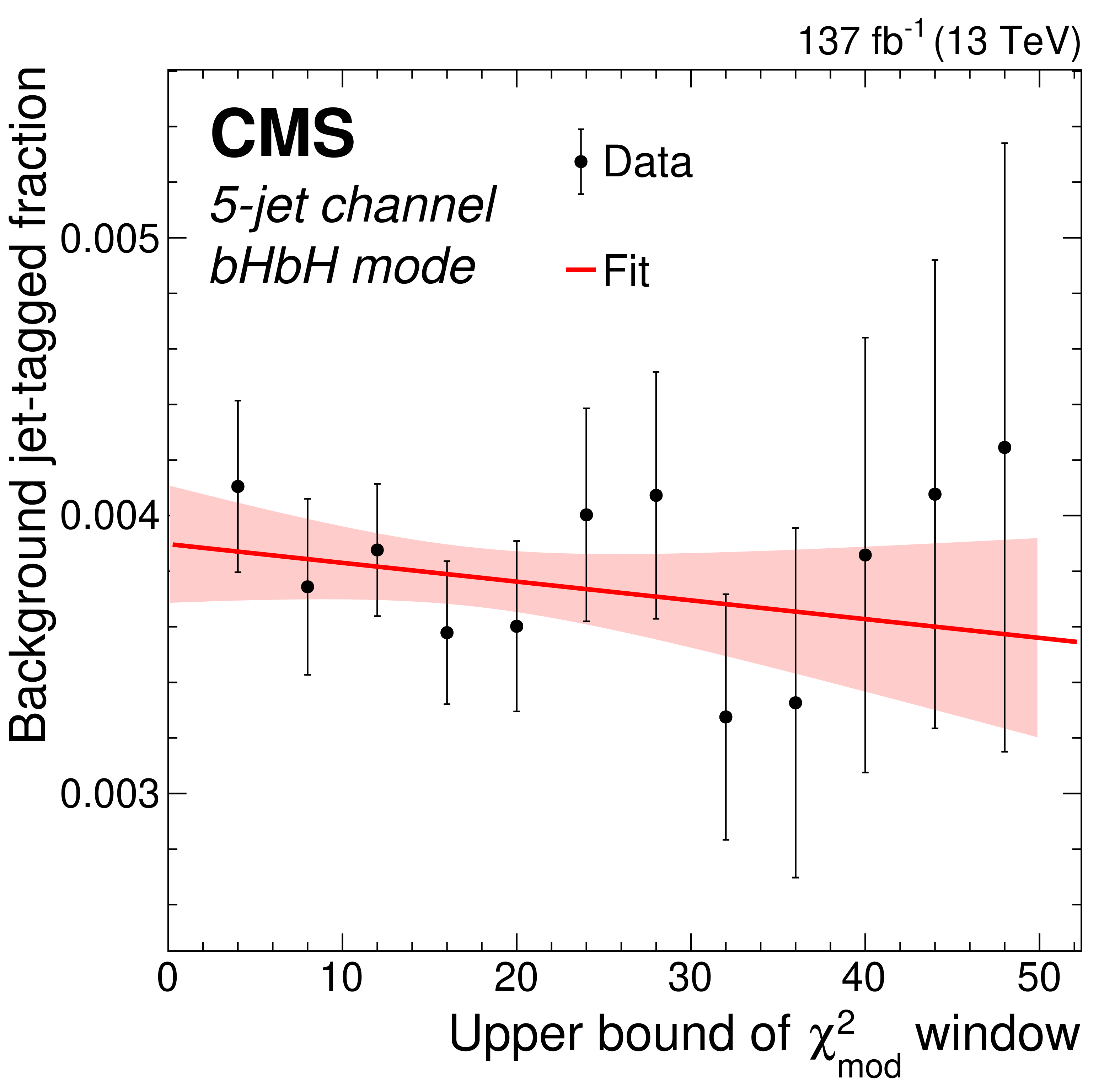
Figure 6-b:
Dependence of the BJTF on ${\chi ^2_\text {mod}/\text {ndf}}$ in the low-mass (500-800 GeV) VLQ region, for 5-jet multiplicities, and for the ${\mathrm{b} \mathrm{H} \mathrm{b} \mathrm{H}}$ event mode. The data are shown as black points with vertical error bars, and the linear fit and associated uncertainty are shown as a solid red line and the shaded red band. |
png pdf |
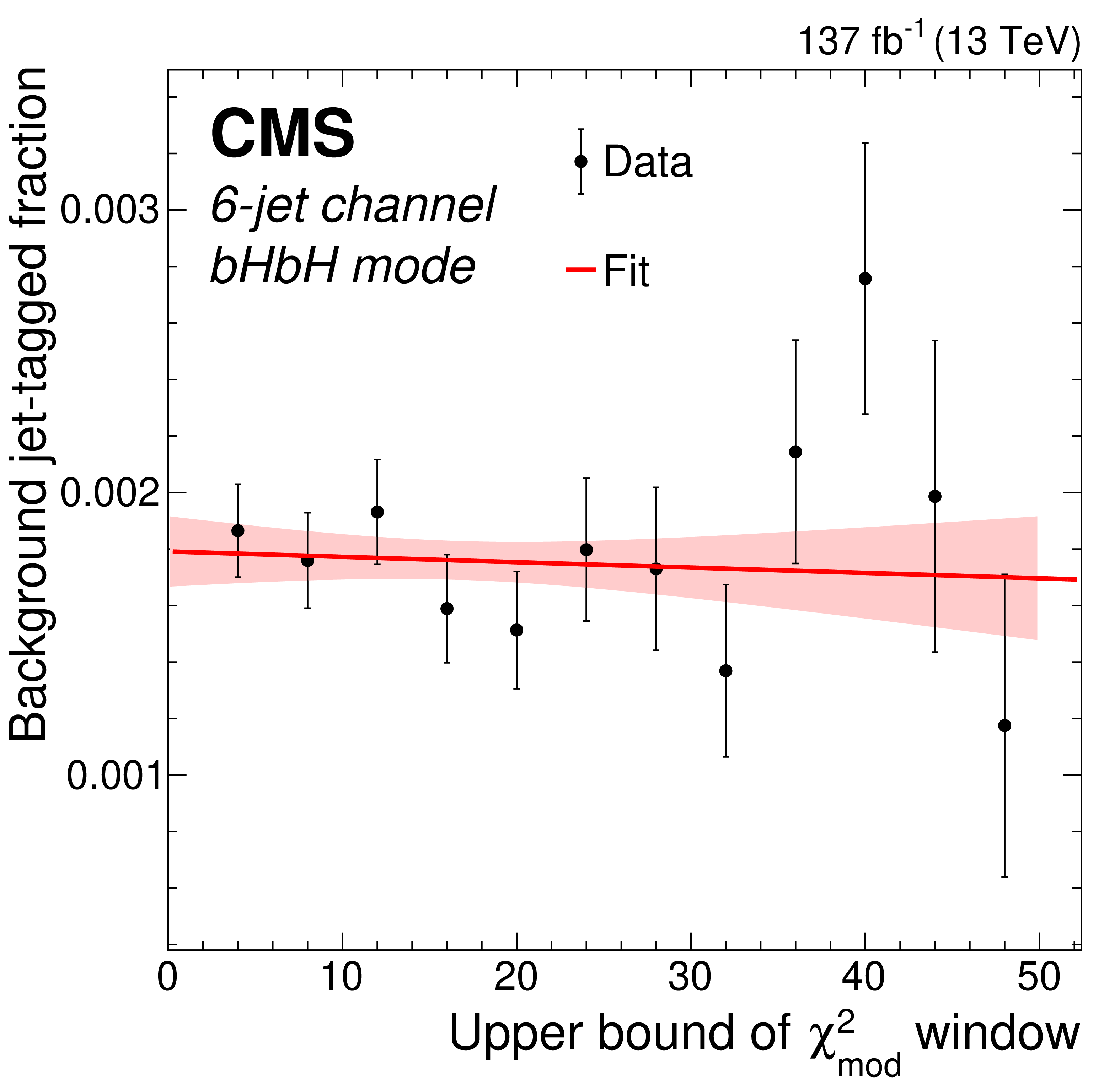
Figure 6-c:
Dependence of the BJTF on ${\chi ^2_\text {mod}/\text {ndf}}$ in the low-mass (500-800 GeV) VLQ region, for 6-jet multiplicities, and for the ${\mathrm{b} \mathrm{H} \mathrm{b} \mathrm{H}}$ event mode. The data are shown as black points with vertical error bars, and the linear fit and associated uncertainty are shown as a solid red line and the shaded red band. |
png pdf |
Figure 6-d:
Dependence of the BJTF on ${\chi ^2_\text {mod}/\text {ndf}}$ in the low-mass (500-800 GeV) VLQ region, for 4-jet multiplicities, and for the ${\mathrm{b} \mathrm{H} \mathrm{b} \mathrm{Z}}$ event mode. The data are shown as black points with vertical error bars, and the linear fit and associated uncertainty are shown as a solid red line and the shaded red band. |
png pdf |
Figure 6-e:
Dependence of the BJTF on ${\chi ^2_\text {mod}/\text {ndf}}$ in the low-mass (500-800 GeV) VLQ region, for 5-jet multiplicities, and for the ${\mathrm{b} \mathrm{H} \mathrm{b} \mathrm{Z}}$ event mode. The data are shown as black points with vertical error bars, and the linear fit and associated uncertainty are shown as a solid red line and the shaded red band. |

png pdf |
Figure 6-f:
Dependence of the BJTF on ${\chi ^2_\text {mod}/\text {ndf}}$ in the low-mass (500-800 GeV) VLQ region, for 6-jet multiplicities, and for the ${\mathrm{b} \mathrm{H} \mathrm{b} \mathrm{Z}}$ event mode. The data are shown as black points with vertical error bars, and the linear fit and associated uncertainty are shown as a solid red line and the shaded red band. |
png pdf |
Figure 6-g:
Dependence of the BJTF on ${\chi ^2_\text {mod}/\text {ndf}}$ in the low-mass (500-800 GeV) VLQ region, for 4-jet multiplicities, and for the ${\mathrm{b} \mathrm{Z} \mathrm{b} \mathrm{Z}}$ event mode. The data are shown as black points with vertical error bars, and the linear fit and associated uncertainty are shown as a solid red line and the shaded red band. |

png pdf |
Figure 6-h:
Dependence of the BJTF on ${\chi ^2_\text {mod}/\text {ndf}}$ in the low-mass (500-800 GeV) VLQ region, for 5-jet multiplicities, and for the ${\mathrm{b} \mathrm{Z} \mathrm{b} \mathrm{Z}}$ event mode. The data are shown as black points with vertical error bars, and the linear fit and associated uncertainty are shown as a solid red line and the shaded red band. |
png pdf |
Figure 6-i:
Dependence of the BJTF on ${\chi ^2_\text {mod}/\text {ndf}}$ in the low-mass (500-800 GeV) VLQ region, for 6-jet multiplicities, and for the ${\mathrm{b} \mathrm{Z} \mathrm{b} \mathrm{Z}}$ event mode. The data are shown as black points with vertical error bars, and the linear fit and associated uncertainty are shown as a solid red line and the shaded red band. |
png pdf |
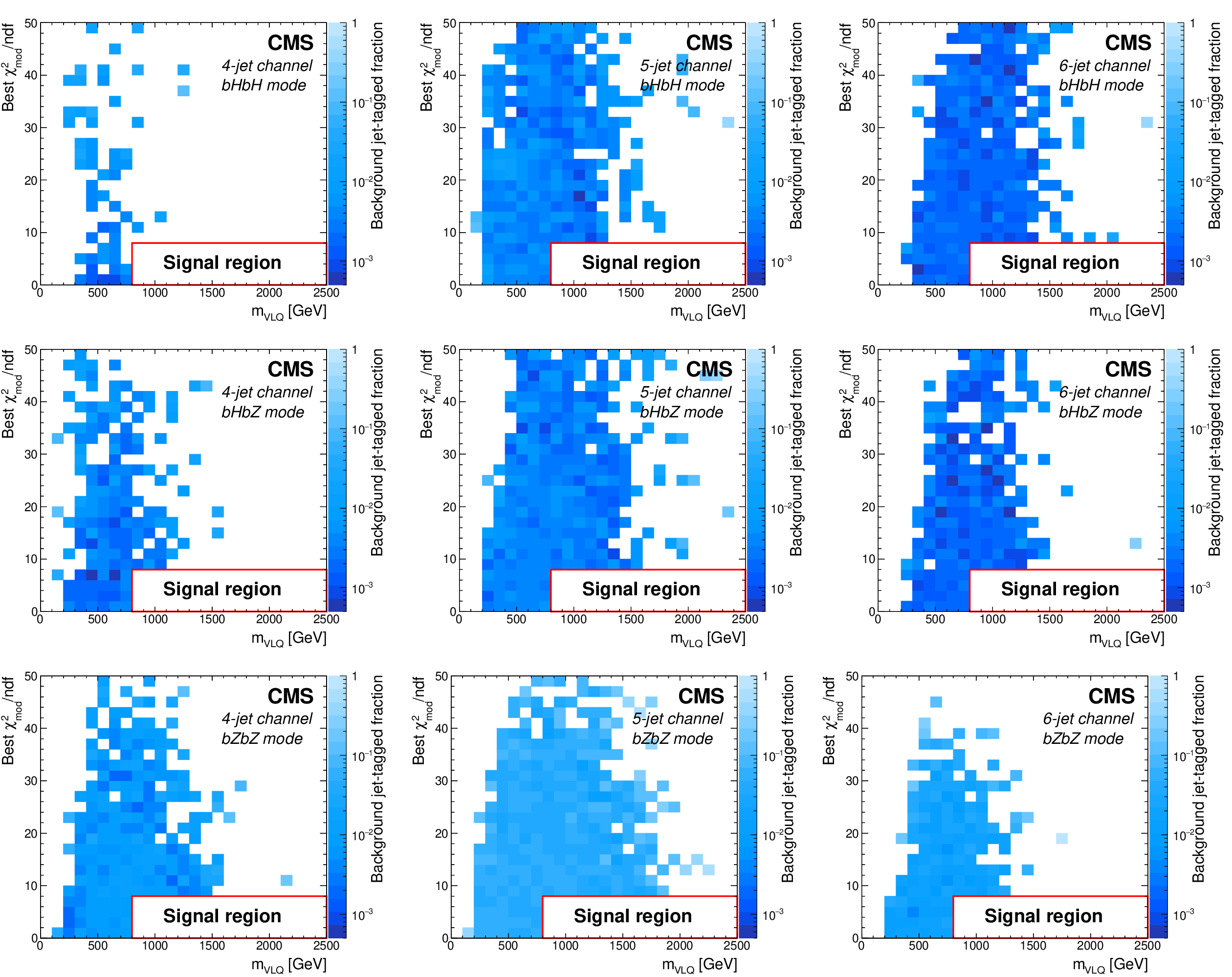
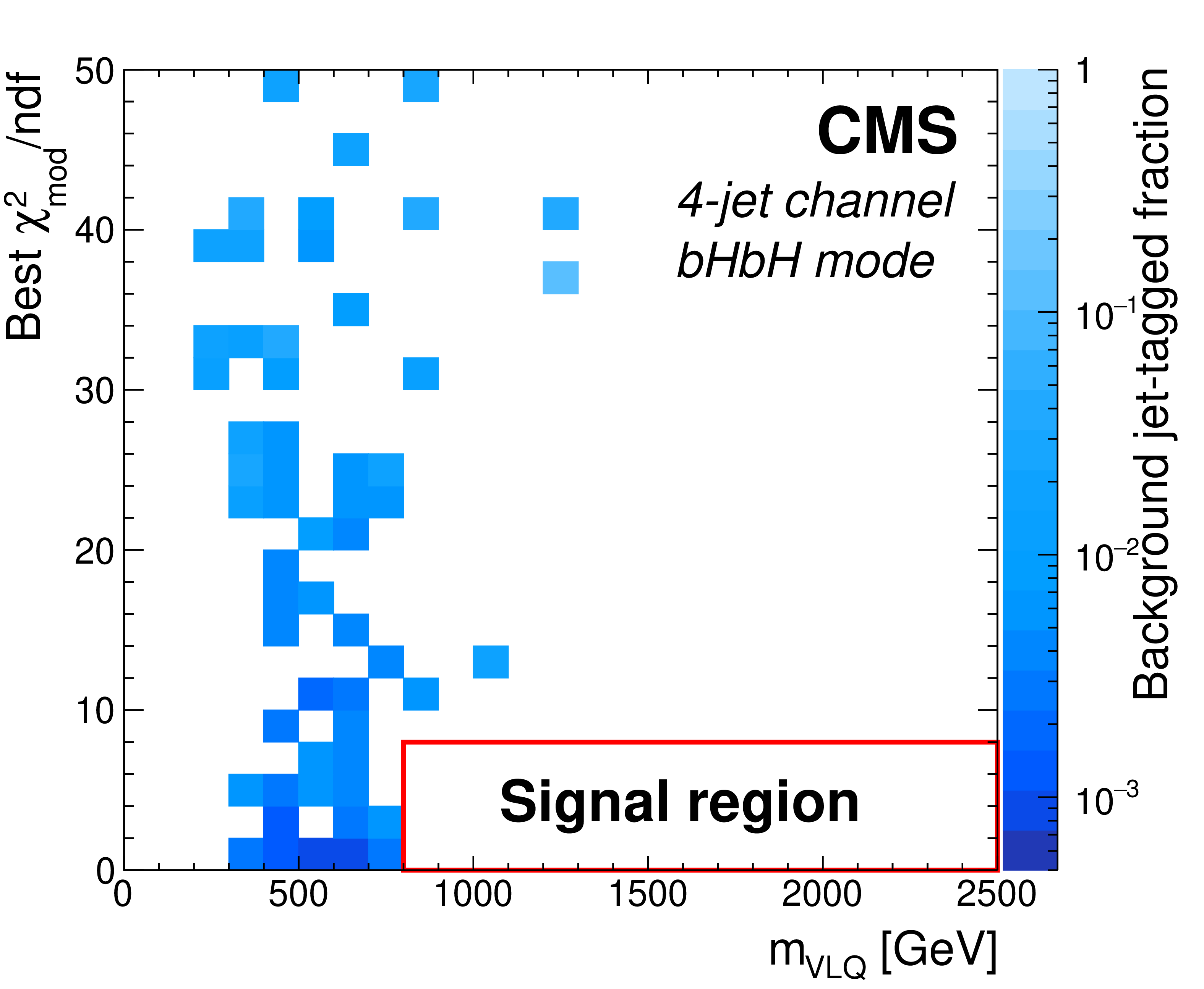
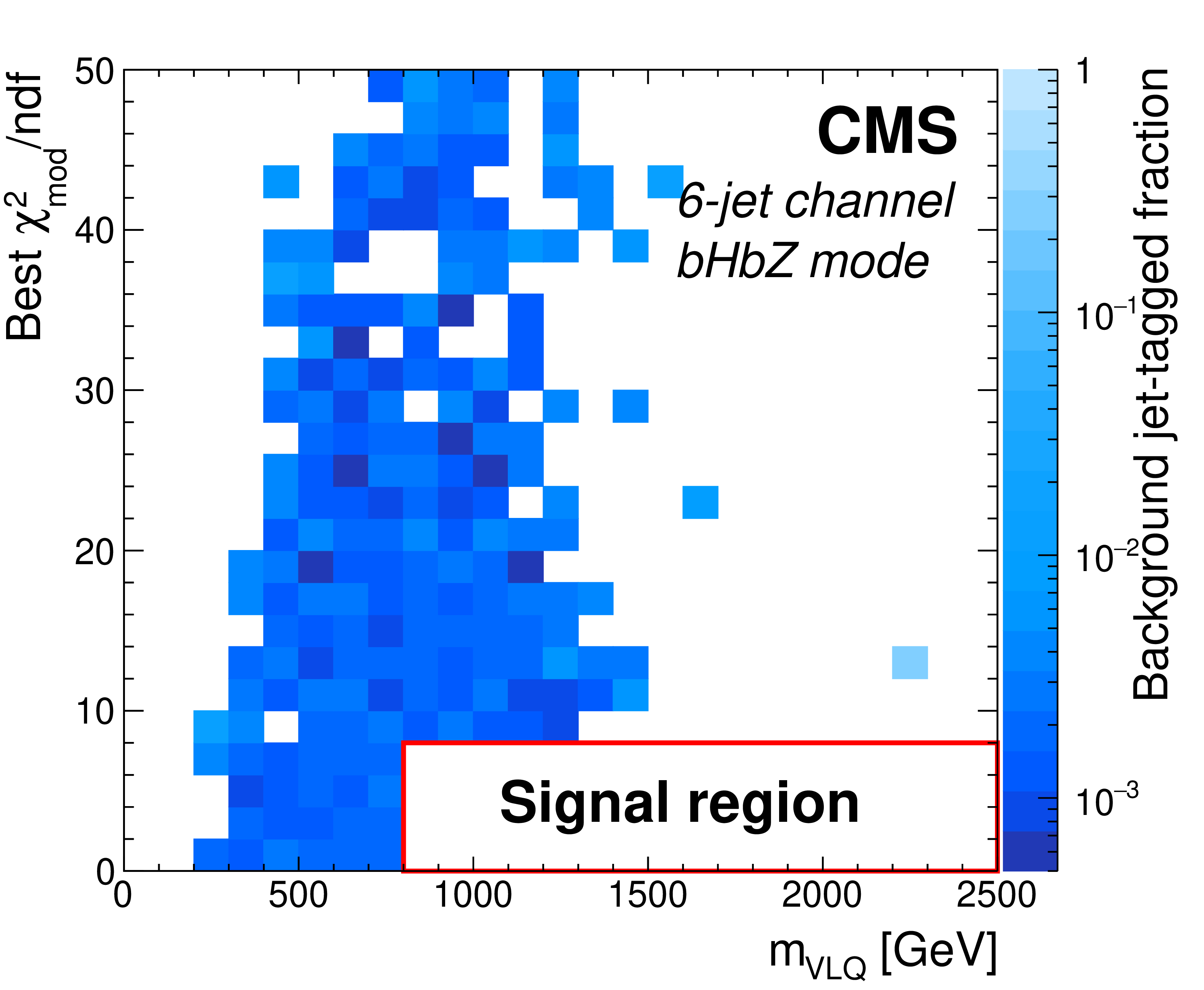
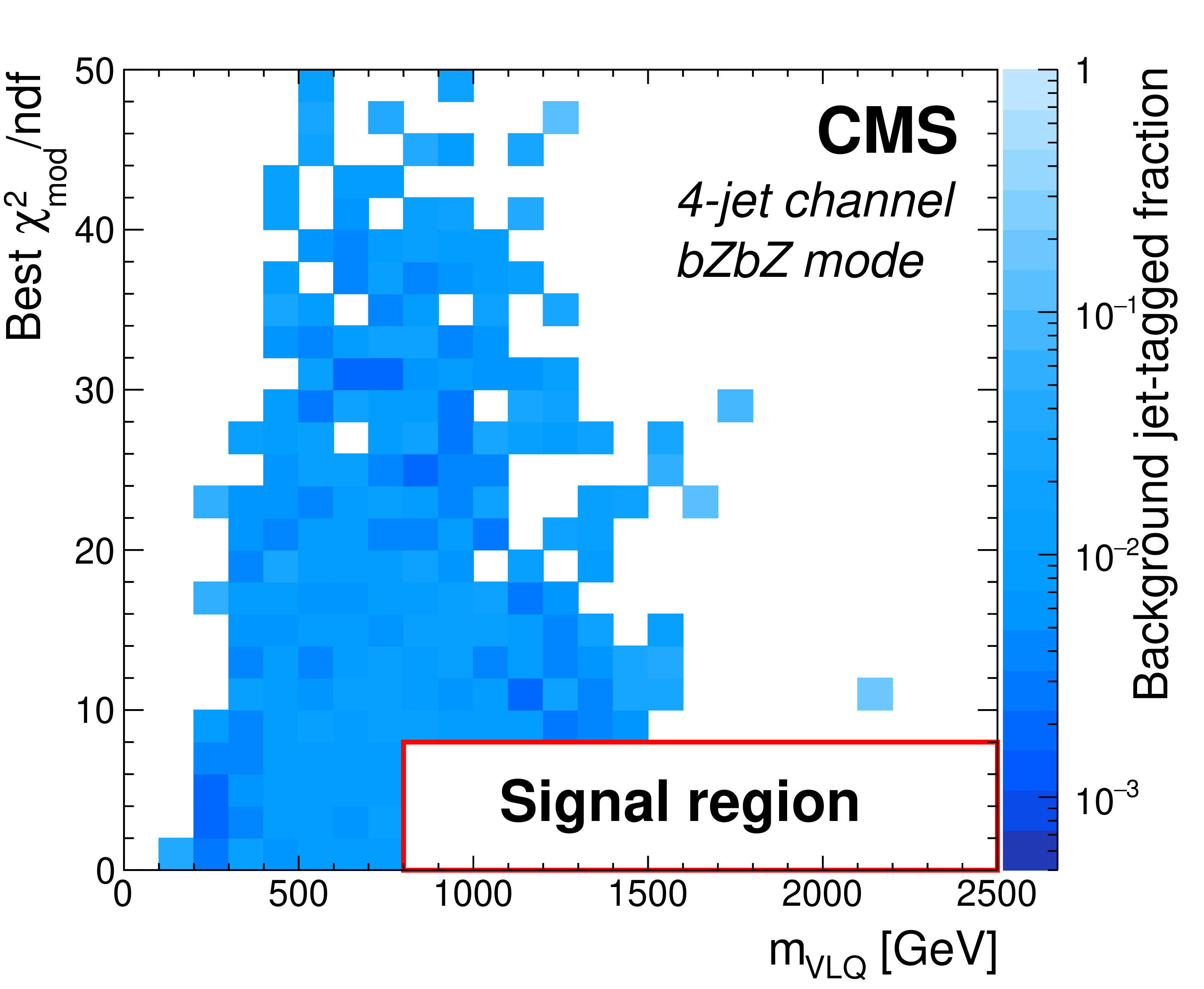
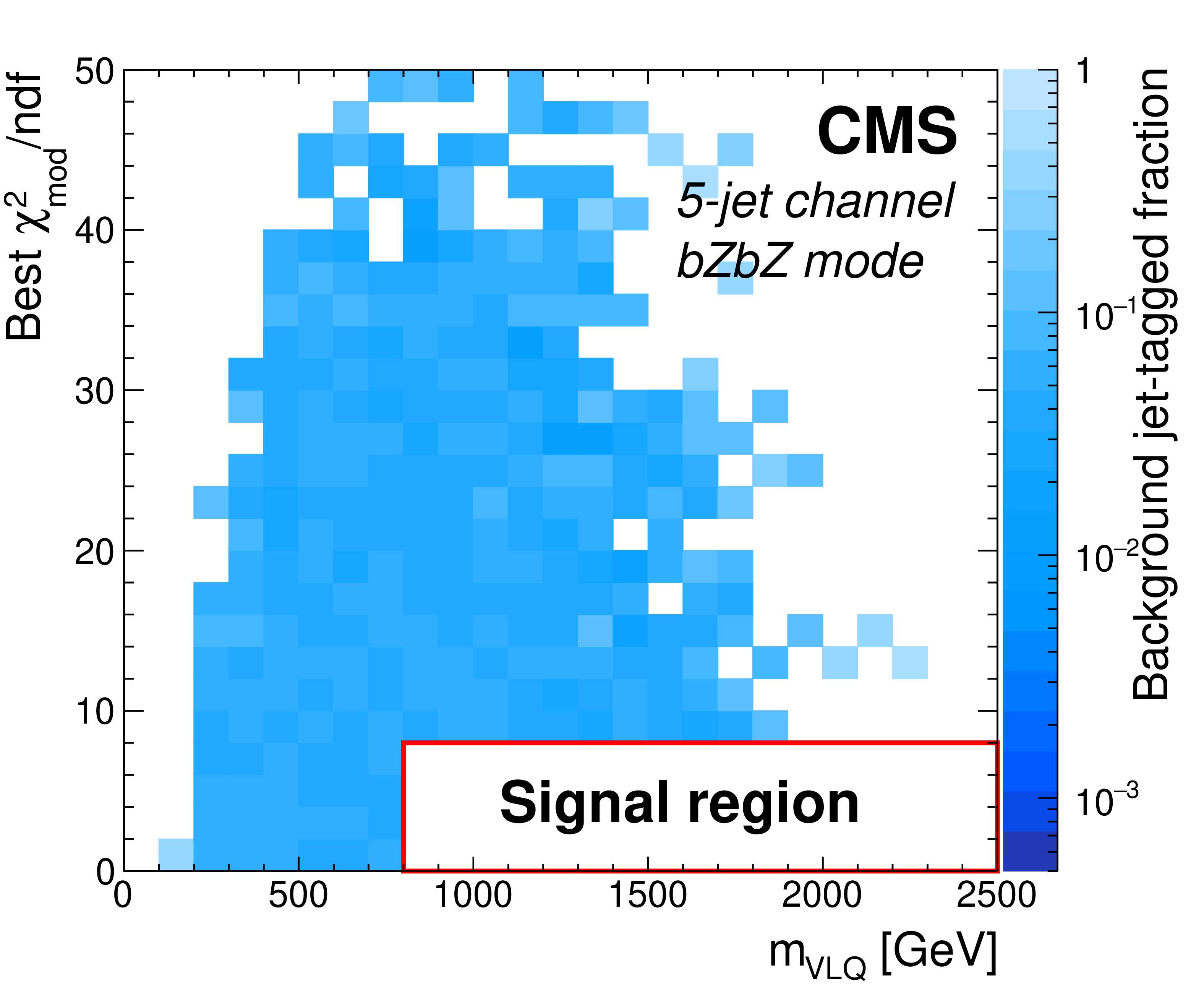
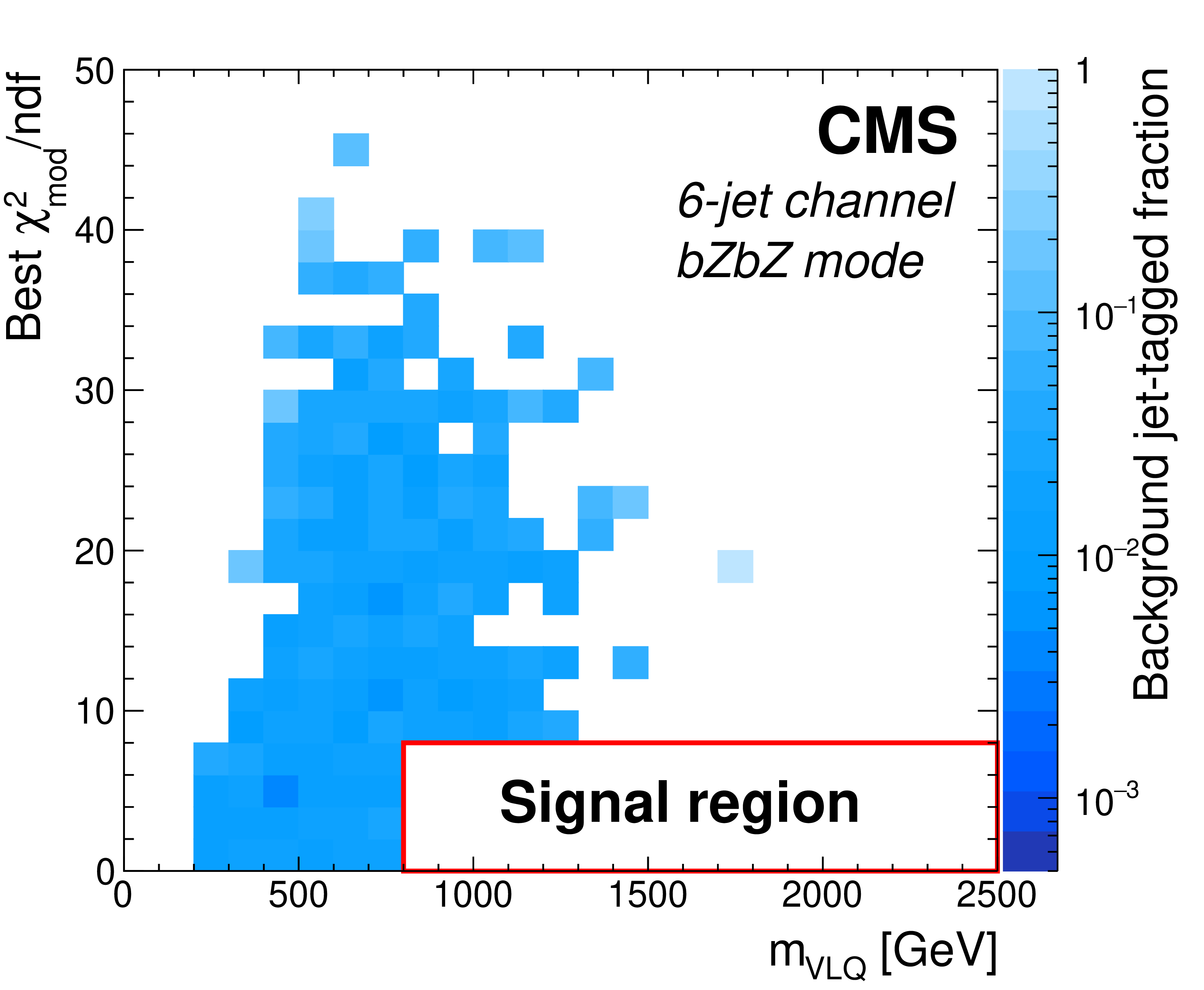
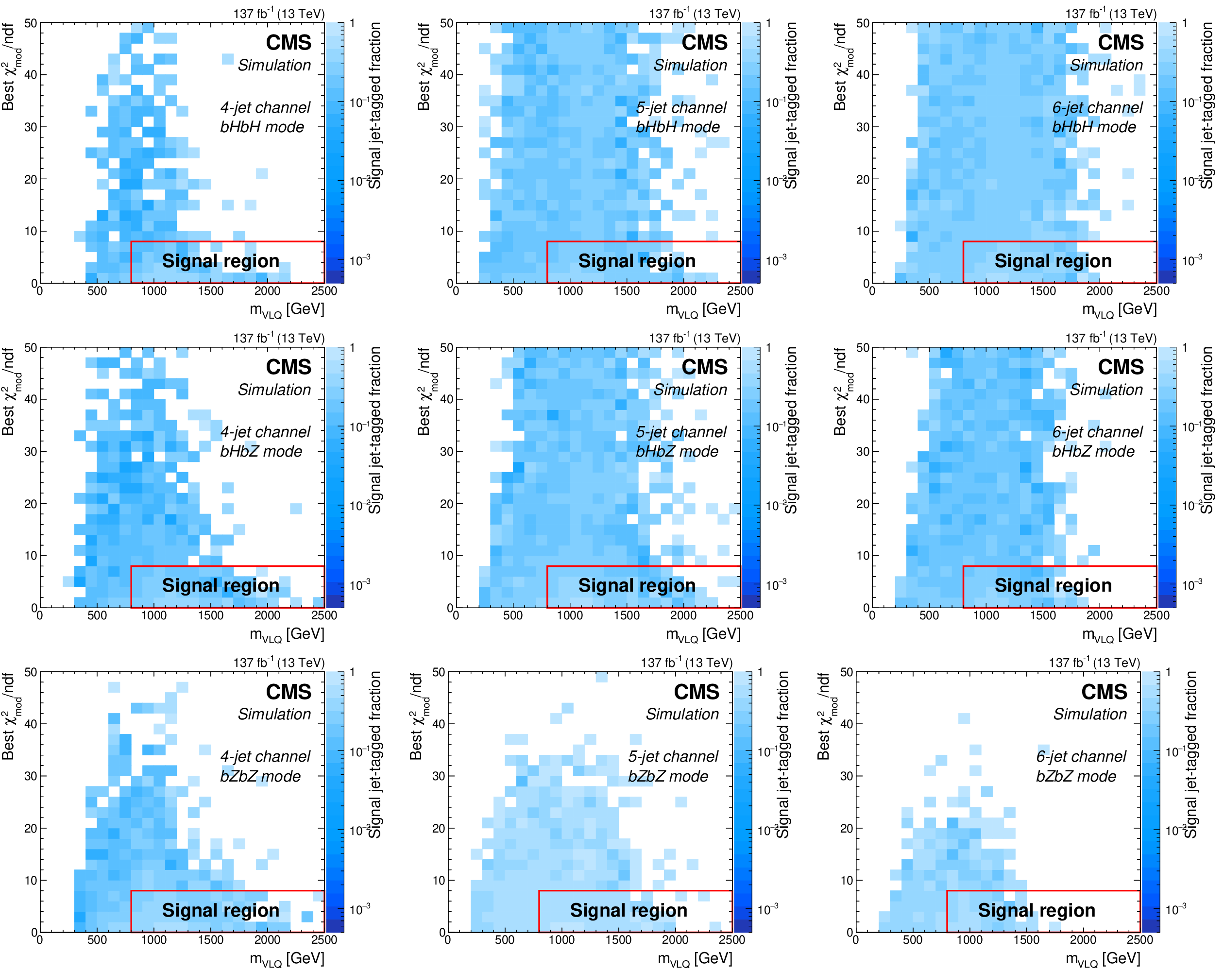
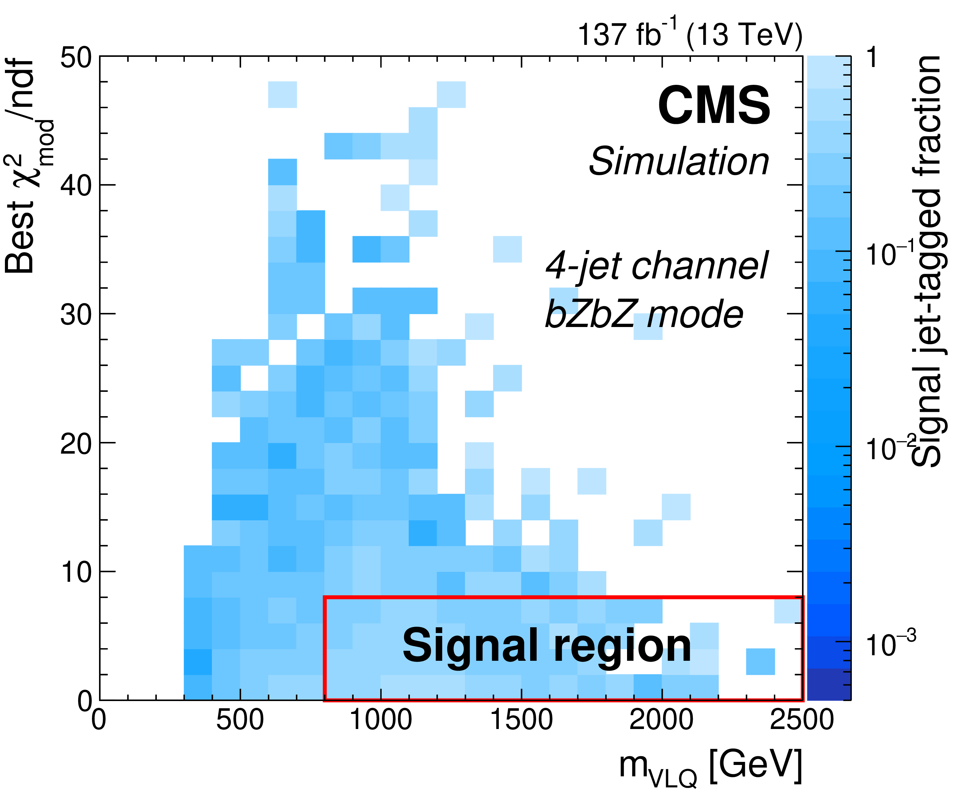
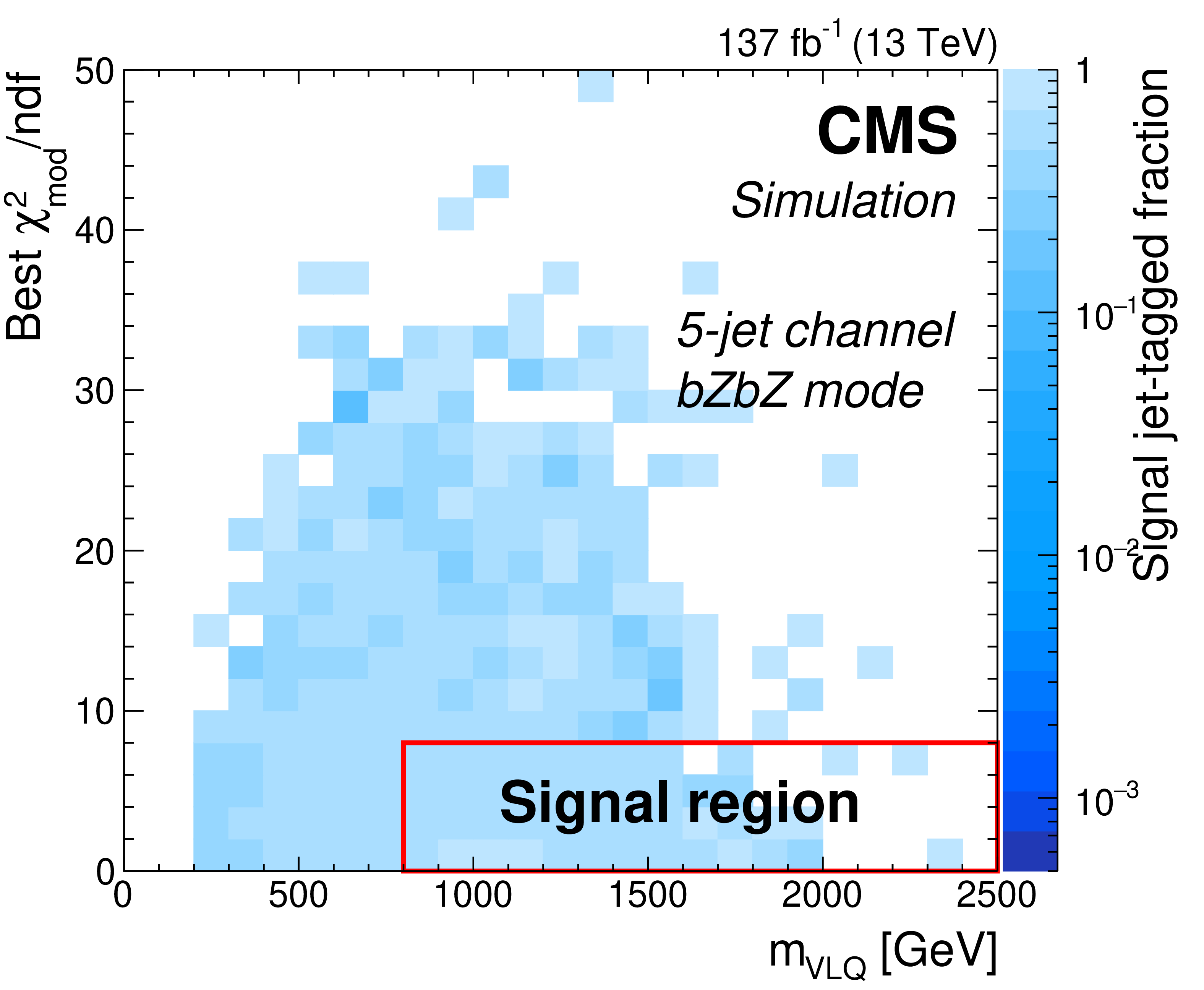
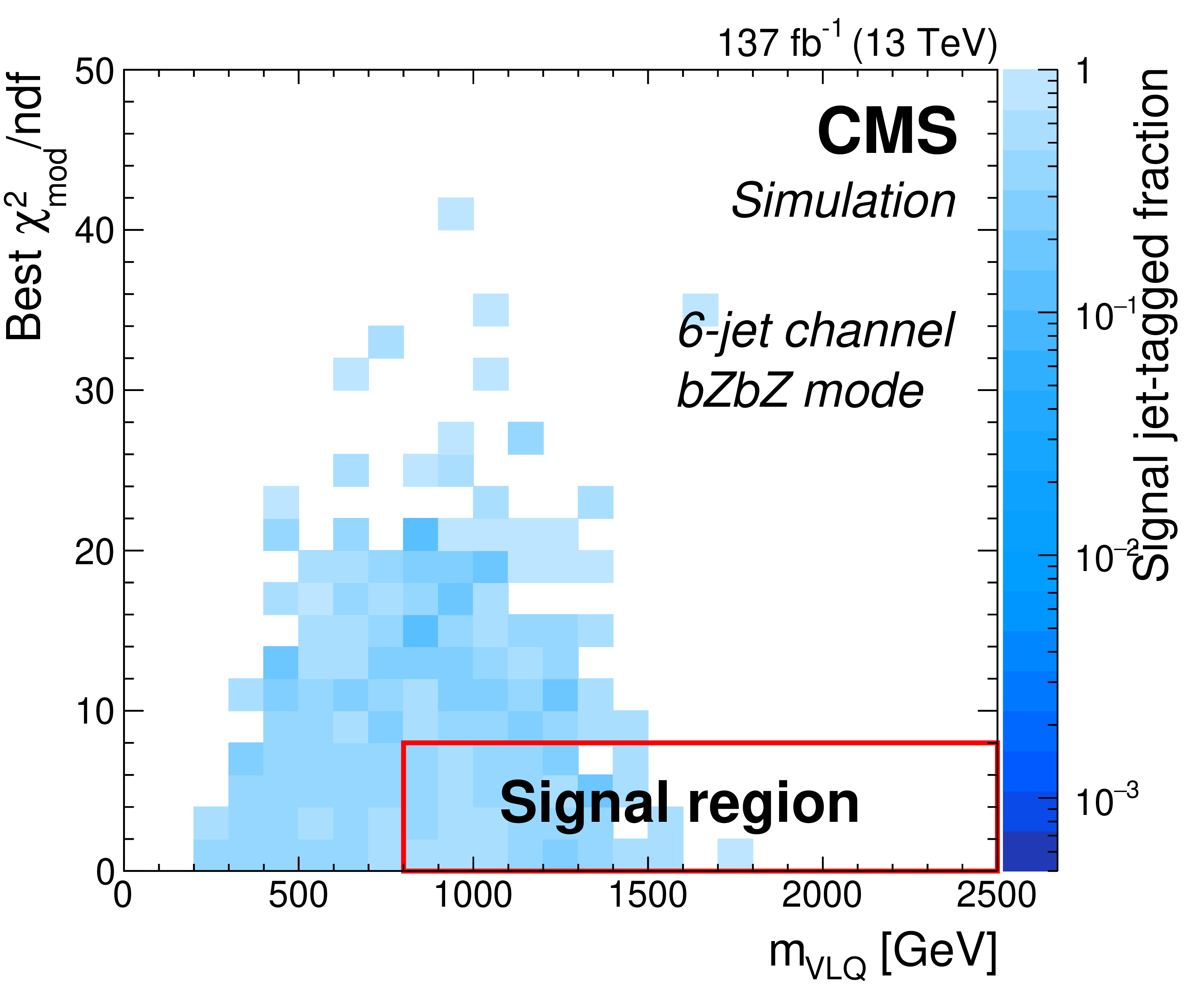
Figure 7:
Dependence of the BJTF on ${m_\text {VLQ}}$ and the best ${\chi ^2_\text {mod}/\text {ndf}}$ in data events, for 4-jet (left column), 5-jet (center column), and 6-jet (right column) multiplicities, and for the ${\mathrm{b} \mathrm{H} \mathrm{b} \mathrm{H}}$ (upper row), ${\mathrm{b} \mathrm{H} \mathrm{b} \mathrm{Z}}$ (middle row), and ${\mathrm{b} \mathrm{Z} \mathrm{b} \mathrm{Z}}$ (lower row) event modes. The red box indicates the signal region, which is excluded from these plots. |
png pdf |
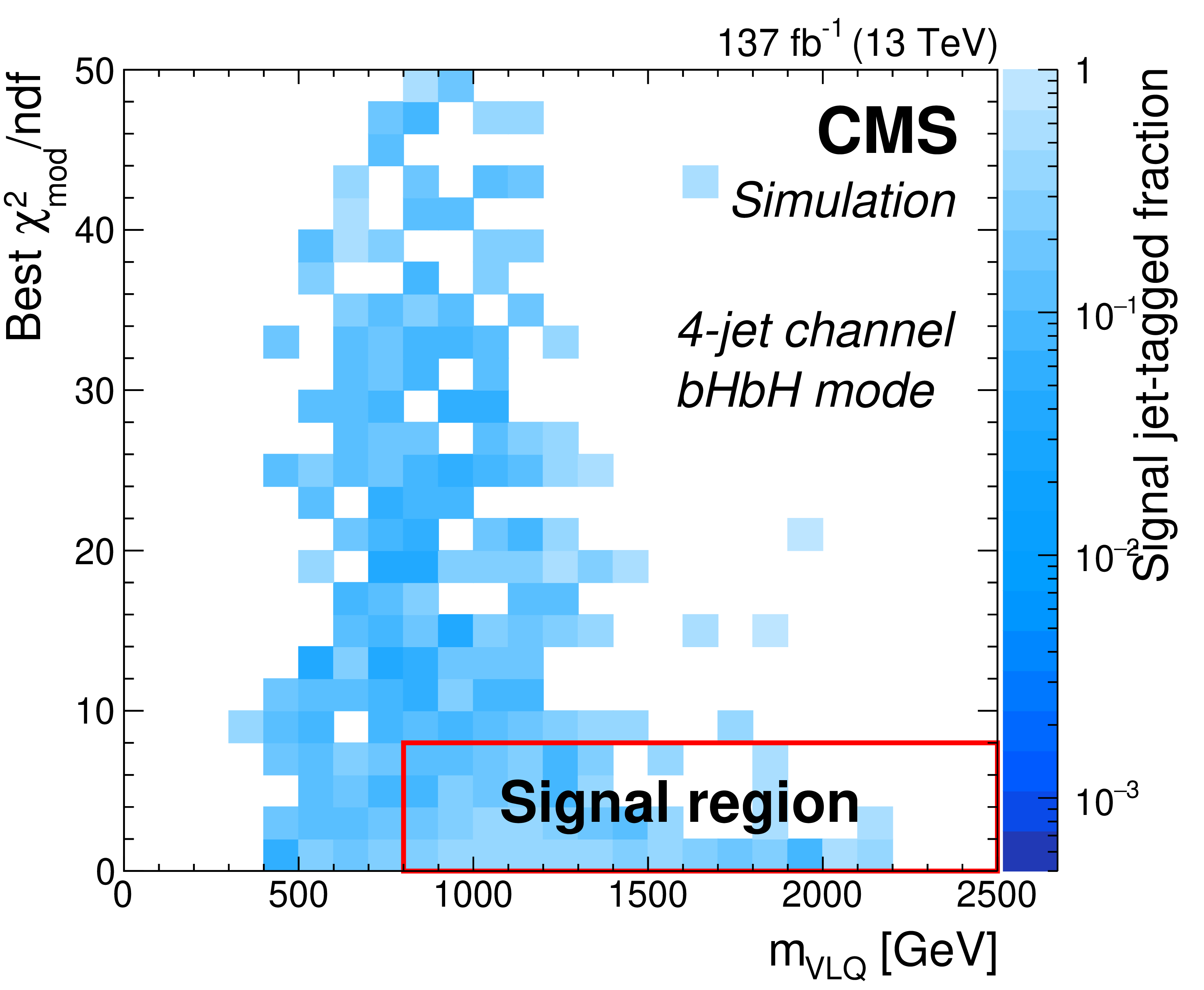
Figure 7-a:
Dependence of the BJTF on ${m_\text {VLQ}}$ and the best ${\chi ^2_\text {mod}/\text {ndf}}$ in data events, for 4-jet multiplicities, and for the ${\mathrm{b} \mathrm{H} \mathrm{b} \mathrm{H}}$ ${\mathrm{b} \mathrm{H} \mathrm{b} \mathrm{Z}}$ ${\mathrm{b} \mathrm{Z} \mathrm{b} \mathrm{Z}}$ event mode. The red box indicates the signal region, which is excluded from these plots. |
png pdf |
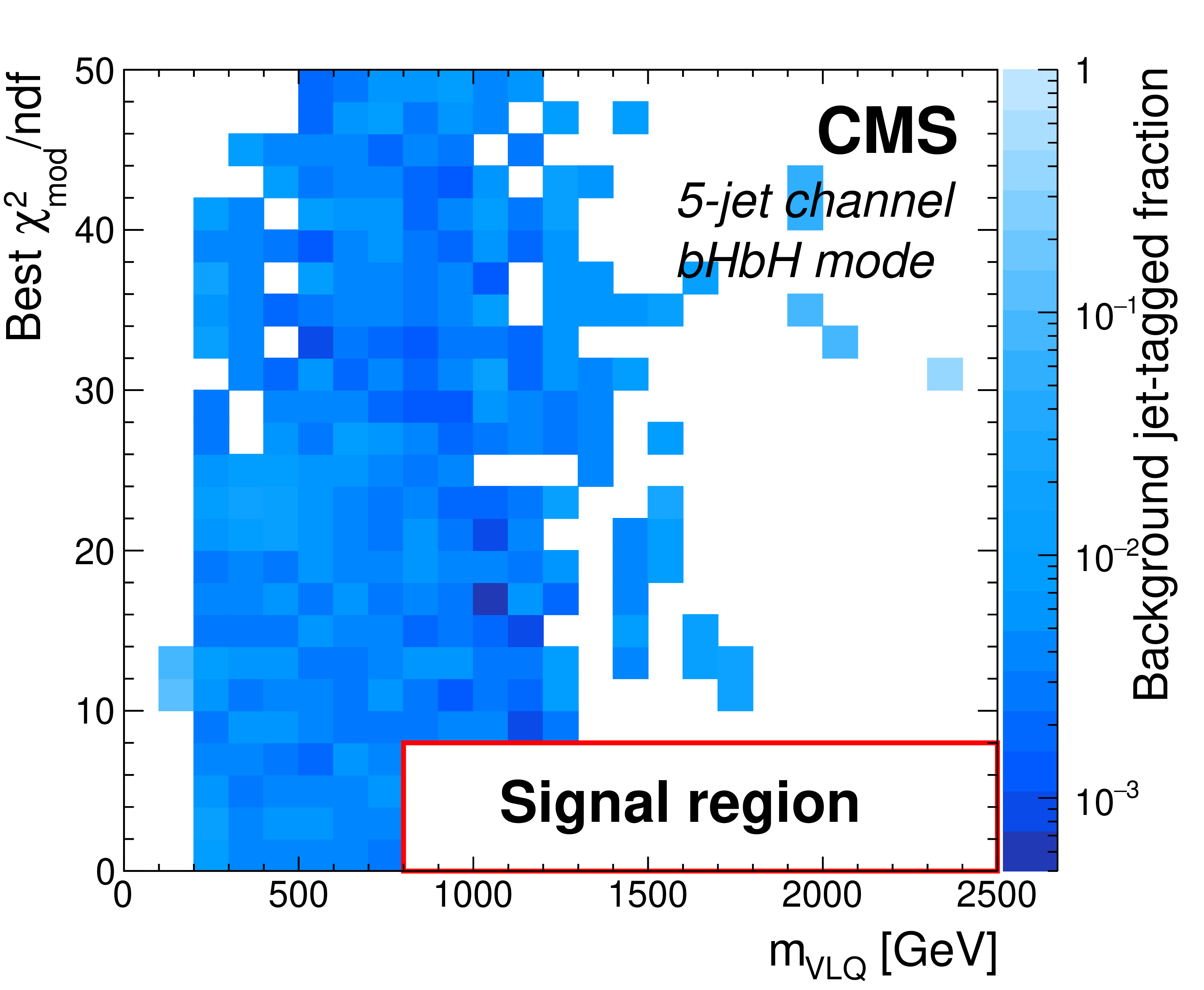
Figure 7-b:
Dependence of the BJTF on ${m_\text {VLQ}}$ and the best ${\chi ^2_\text {mod}/\text {ndf}}$ in data events, for 5-jet multiplicities, and for the ${\mathrm{b} \mathrm{H} \mathrm{b} \mathrm{H}}$ ${\mathrm{b} \mathrm{H} \mathrm{b} \mathrm{Z}}$ ${\mathrm{b} \mathrm{Z} \mathrm{b} \mathrm{Z}}$ event mode. The red box indicates the signal region, which is excluded from these plots. |
png pdf |
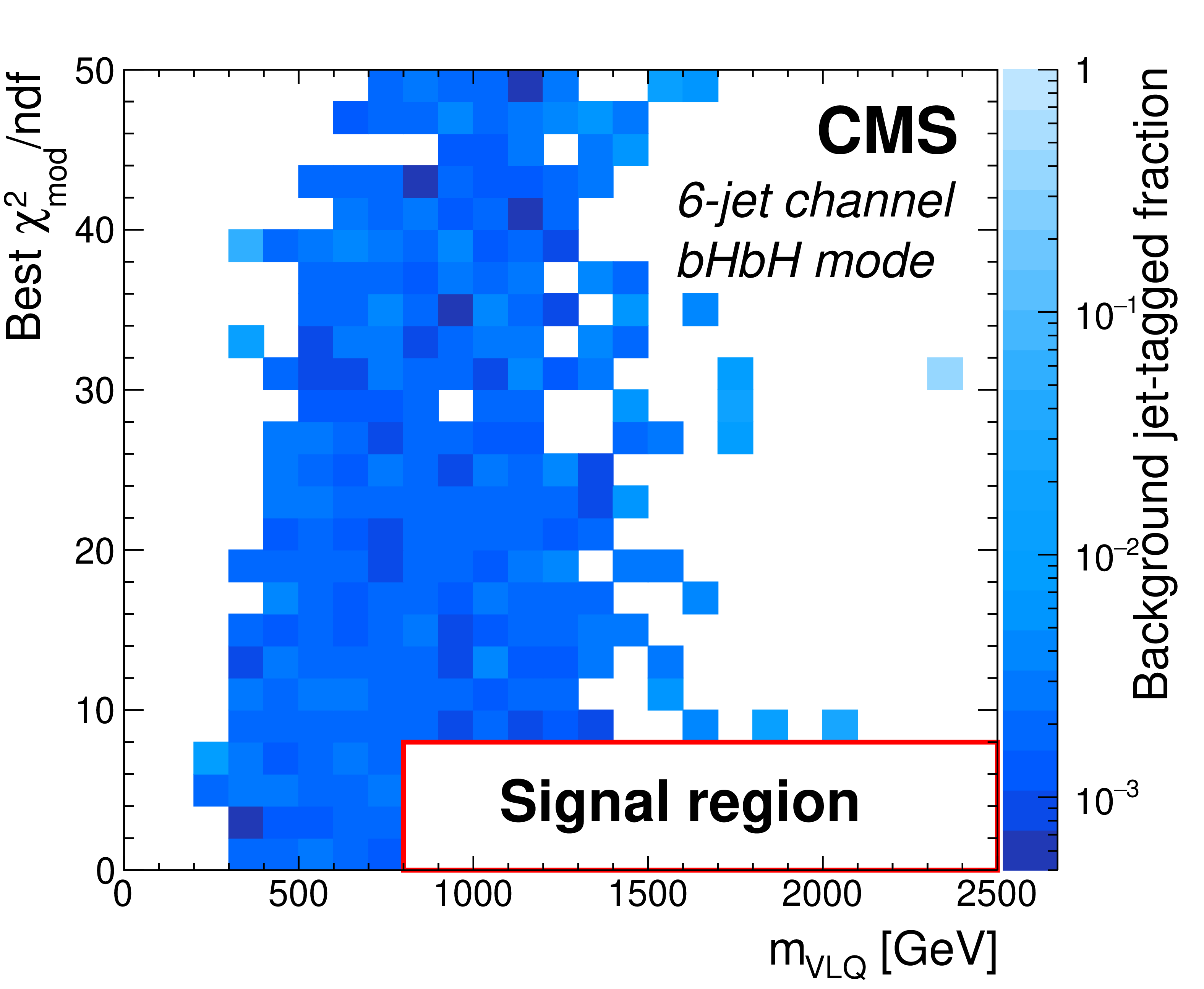
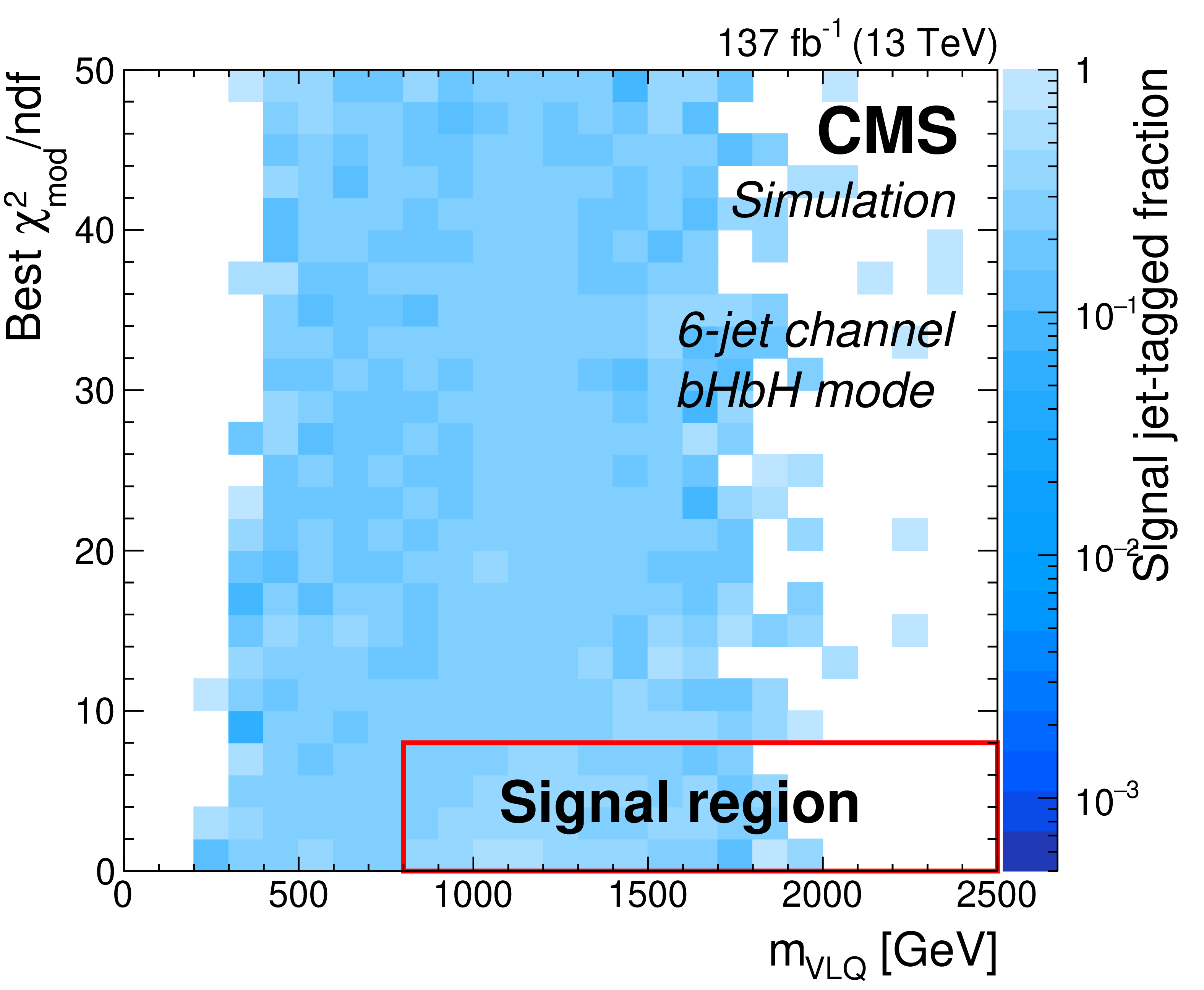
Figure 7-c:
Dependence of the BJTF on ${m_\text {VLQ}}$ and the best ${\chi ^2_\text {mod}/\text {ndf}}$ in data events, for 6-jet multiplicities, and for the ${\mathrm{b} \mathrm{H} \mathrm{b} \mathrm{H}}$ ${\mathrm{b} \mathrm{H} \mathrm{b} \mathrm{Z}}$ ${\mathrm{b} \mathrm{Z} \mathrm{b} \mathrm{Z}}$ event mode. The red box indicates the signal region, which is excluded from these plots. |

png pdf |
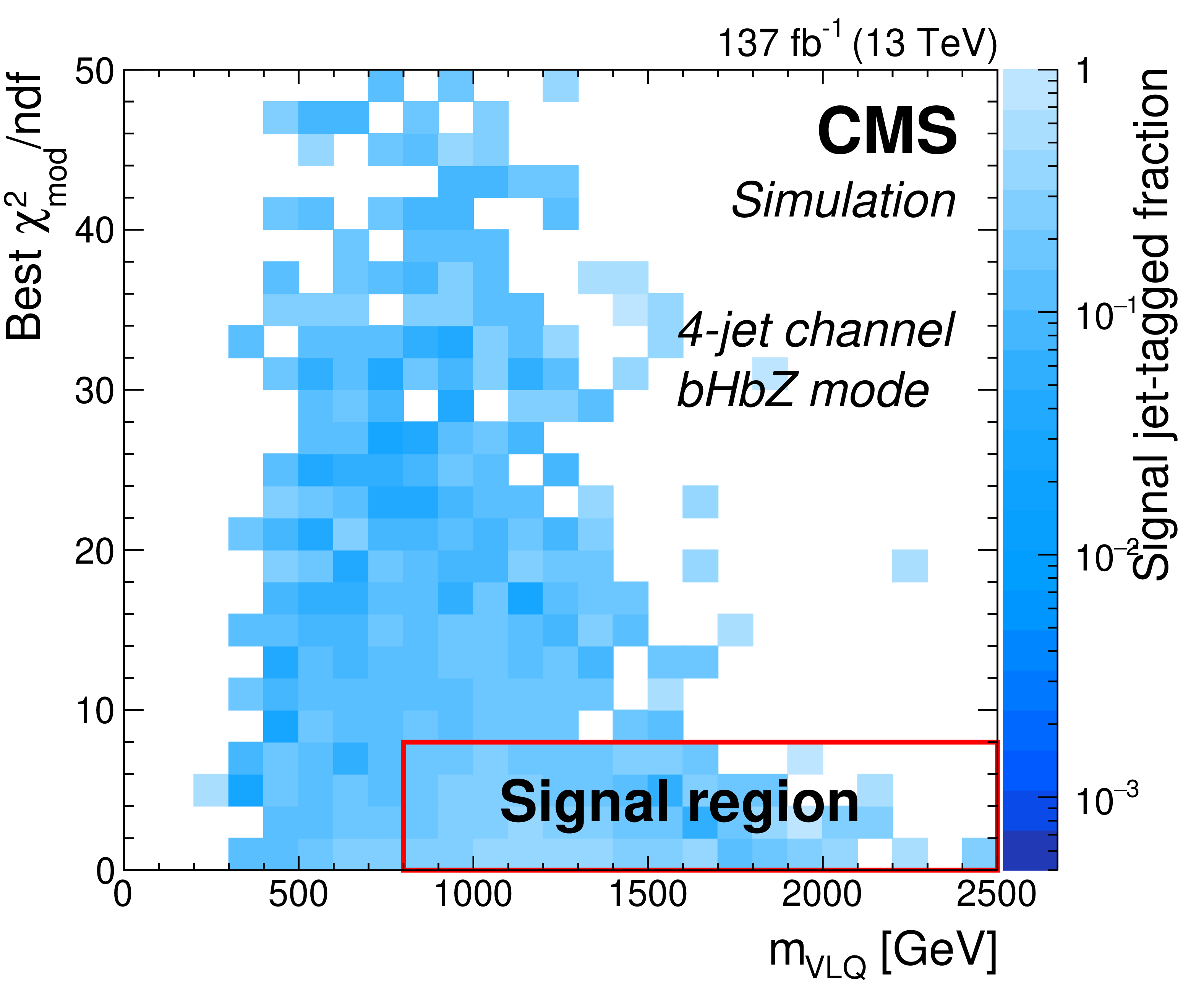
Figure 7-d:
Dependence of the BJTF on ${m_\text {VLQ}}$ and the best ${\chi ^2_\text {mod}/\text {ndf}}$ in data events, for 4-jet multiplicities, and for the ${\mathrm{b} \mathrm{H} \mathrm{b} \mathrm{H}}$ ${\mathrm{b} \mathrm{H} \mathrm{b} \mathrm{Z}}$ ${\mathrm{b} \mathrm{Z} \mathrm{b} \mathrm{Z}}$ event mode. The red box indicates the signal region, which is excluded from these plots. |

png pdf |
Figure 7-e:
Dependence of the BJTF on ${m_\text {VLQ}}$ and the best ${\chi ^2_\text {mod}/\text {ndf}}$ in data events, for 5-jet multiplicities, and for the ${\mathrm{b} \mathrm{H} \mathrm{b} \mathrm{H}}$ ${\mathrm{b} \mathrm{H} \mathrm{b} \mathrm{Z}}$ ${\mathrm{b} \mathrm{Z} \mathrm{b} \mathrm{Z}}$ event mode. The red box indicates the signal region, which is excluded from these plots. |
png pdf |
Figure 7-f:
Dependence of the BJTF on ${m_\text {VLQ}}$ and the best ${\chi ^2_\text {mod}/\text {ndf}}$ in data events, for 6-jet multiplicities, and for the ${\mathrm{b} \mathrm{H} \mathrm{b} \mathrm{H}}$ ${\mathrm{b} \mathrm{H} \mathrm{b} \mathrm{Z}}$ ${\mathrm{b} \mathrm{Z} \mathrm{b} \mathrm{Z}}$ event mode. The red box indicates the signal region, which is excluded from these plots. |
png pdf |
Figure 7-g:
Dependence of the BJTF on ${m_\text {VLQ}}$ and the best ${\chi ^2_\text {mod}/\text {ndf}}$ in data events, for 4-jet multiplicities, and for the ${\mathrm{b} \mathrm{H} \mathrm{b} \mathrm{H}}$ ${\mathrm{b} \mathrm{H} \mathrm{b} \mathrm{Z}}$ ${\mathrm{b} \mathrm{Z} \mathrm{b} \mathrm{Z}}$ event mode. The red box indicates the signal region, which is excluded from these plots. |
png pdf |
Figure 7-h:
Dependence of the BJTF on ${m_\text {VLQ}}$ and the best ${\chi ^2_\text {mod}/\text {ndf}}$ in data events, for 5-jet multiplicities, and for the ${\mathrm{b} \mathrm{H} \mathrm{b} \mathrm{H}}$ ${\mathrm{b} \mathrm{H} \mathrm{b} \mathrm{Z}}$ ${\mathrm{b} \mathrm{Z} \mathrm{b} \mathrm{Z}}$ event mode. The red box indicates the signal region, which is excluded from these plots. |
png pdf |
Figure 7-i:
Dependence of the BJTF on ${m_\text {VLQ}}$ and the best ${\chi ^2_\text {mod}/\text {ndf}}$ in data events, for 6-jet multiplicities, and for the ${\mathrm{b} \mathrm{H} \mathrm{b} \mathrm{H}}$ ${\mathrm{b} \mathrm{H} \mathrm{b} \mathrm{Z}}$ ${\mathrm{b} \mathrm{Z} \mathrm{b} \mathrm{Z}}$ event mode. The red box indicates the signal region, which is excluded from these plots. |
png pdf |
Figure 8:
Dependence of the BJTF on ${m_\text {VLQ}}$ and the best ${\chi ^2_\text {mod}/\text {ndf}}$ in simulated VLQ signal events with $m_{\mathrm{B}} = $ 1200 GeV, for 4-jet (left column), 5-jet (center column), and 6-jet (right column) multiplicities, and for the ${\mathrm{b} \mathrm{H} \mathrm{b} \mathrm{H}}$ (upper row), ${\mathrm{b} \mathrm{H} \mathrm{b} \mathrm{Z}}$ (middle row), and ${\mathrm{b} \mathrm{Z} \mathrm{b} \mathrm{Z}}$ (lower row) event modes. The red box indicates the signal region. |
png pdf |
Figure 8-a:
Dependence of the BJTF on ${m_\text {VLQ}}$ and the best ${\chi ^2_\text {mod}/\text {ndf}}$ in simulated VLQ signal events with $m_{\mathrm{B}} = $ 1200 GeV, for 4-jet multiplicities, and for the ${\mathrm{b} \mathrm{H} \mathrm{b} \mathrm{H}}$ event mode. The red box indicates the signal region. |

png pdf |
Figure 8-b:
Dependence of the BJTF on ${m_\text {VLQ}}$ and the best ${\chi ^2_\text {mod}/\text {ndf}}$ in simulated VLQ signal events with $m_{\mathrm{B}} = $ 1200 GeV, for 5-jet multiplicities, and for the ${\mathrm{b} \mathrm{H} \mathrm{b} \mathrm{H}}$ event mode. The red box indicates the signal region. |
png pdf |
Figure 8-c:
Dependence of the BJTF on ${m_\text {VLQ}}$ and the best ${\chi ^2_\text {mod}/\text {ndf}}$ in simulated VLQ signal events with $m_{\mathrm{B}} = $ 1200 GeV, for 6-jet multiplicities, and for the ${\mathrm{b} \mathrm{H} \mathrm{b} \mathrm{H}}$ event mode. The red box indicates the signal region. |
png pdf |
Figure 8-d:
Dependence of the BJTF on ${m_\text {VLQ}}$ and the best ${\chi ^2_\text {mod}/\text {ndf}}$ in simulated VLQ signal events with $m_{\mathrm{B}} = $ 1200 GeV, for 4-jet multiplicities, and for the ${\mathrm{b} \mathrm{H} \mathrm{b} \mathrm{Z}}$ event mode. The red box indicates the signal region. |

png pdf |
Figure 8-e:
Dependence of the BJTF on ${m_\text {VLQ}}$ and the best ${\chi ^2_\text {mod}/\text {ndf}}$ in simulated VLQ signal events with $m_{\mathrm{B}} = $ 1200 GeV, for 5-jet multiplicities, and for the ${\mathrm{b} \mathrm{H} \mathrm{b} \mathrm{Z}}$ event mode. The red box indicates the signal region. |

png pdf |
Figure 8-f:
Dependence of the BJTF on ${m_\text {VLQ}}$ and the best ${\chi ^2_\text {mod}/\text {ndf}}$ in simulated VLQ signal events with $m_{\mathrm{B}} = $ 1200 GeV, for 6-jet multiplicities, and for the ${\mathrm{b} \mathrm{H} \mathrm{b} \mathrm{Z}}$ event mode. The red box indicates the signal region. |
png pdf |
Figure 8-g:
Dependence of the BJTF on ${m_\text {VLQ}}$ and the best ${\chi ^2_\text {mod}/\text {ndf}}$ in simulated VLQ signal events with $m_{\mathrm{B}} = $ 1200 GeV, for 4-jet multiplicities, and for the ${\mathrm{b} \mathrm{Z} \mathrm{b} \mathrm{Z}}$ event mode. The red box indicates the signal region. |
png pdf |
Figure 8-h:
Dependence of the BJTF on ${m_\text {VLQ}}$ and the best ${\chi ^2_\text {mod}/\text {ndf}}$ in simulated VLQ signal events with $m_{\mathrm{B}} = $ 1200 GeV, for 5-jet multiplicities, and for the ${\mathrm{b} \mathrm{Z} \mathrm{b} \mathrm{Z}}$ event mode. The red box indicates the signal region. |
png pdf |
Figure 8-i:
Dependence of the BJTF on ${m_\text {VLQ}}$ and the best ${\chi ^2_\text {mod}/\text {ndf}}$ in simulated VLQ signal events with $m_{\mathrm{B}} = $ 1200 GeV, for 6-jet multiplicities, and for the ${\mathrm{b} \mathrm{Z} \mathrm{b} \mathrm{Z}}$ event mode. The red box indicates the signal region. |
png pdf |
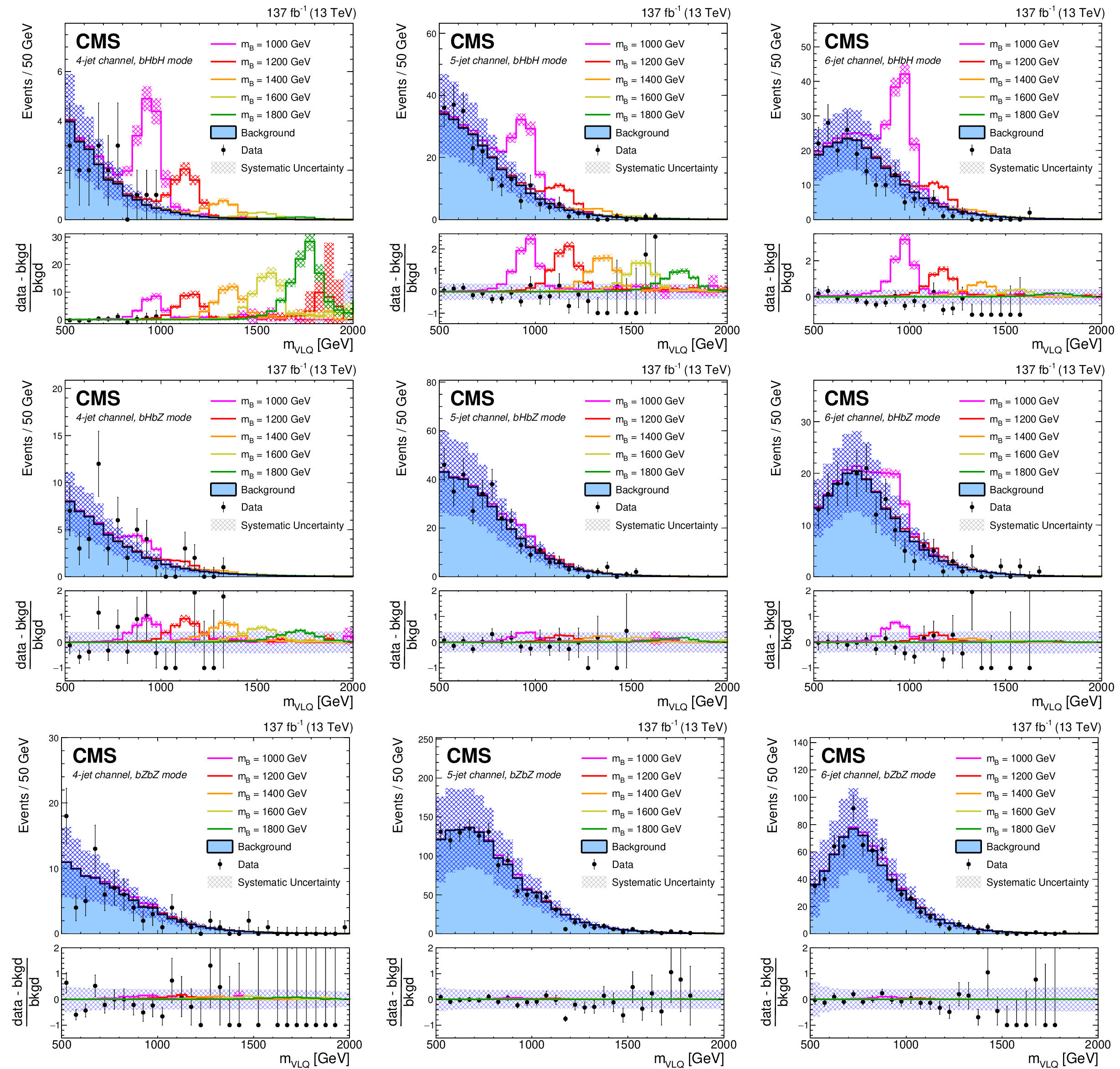
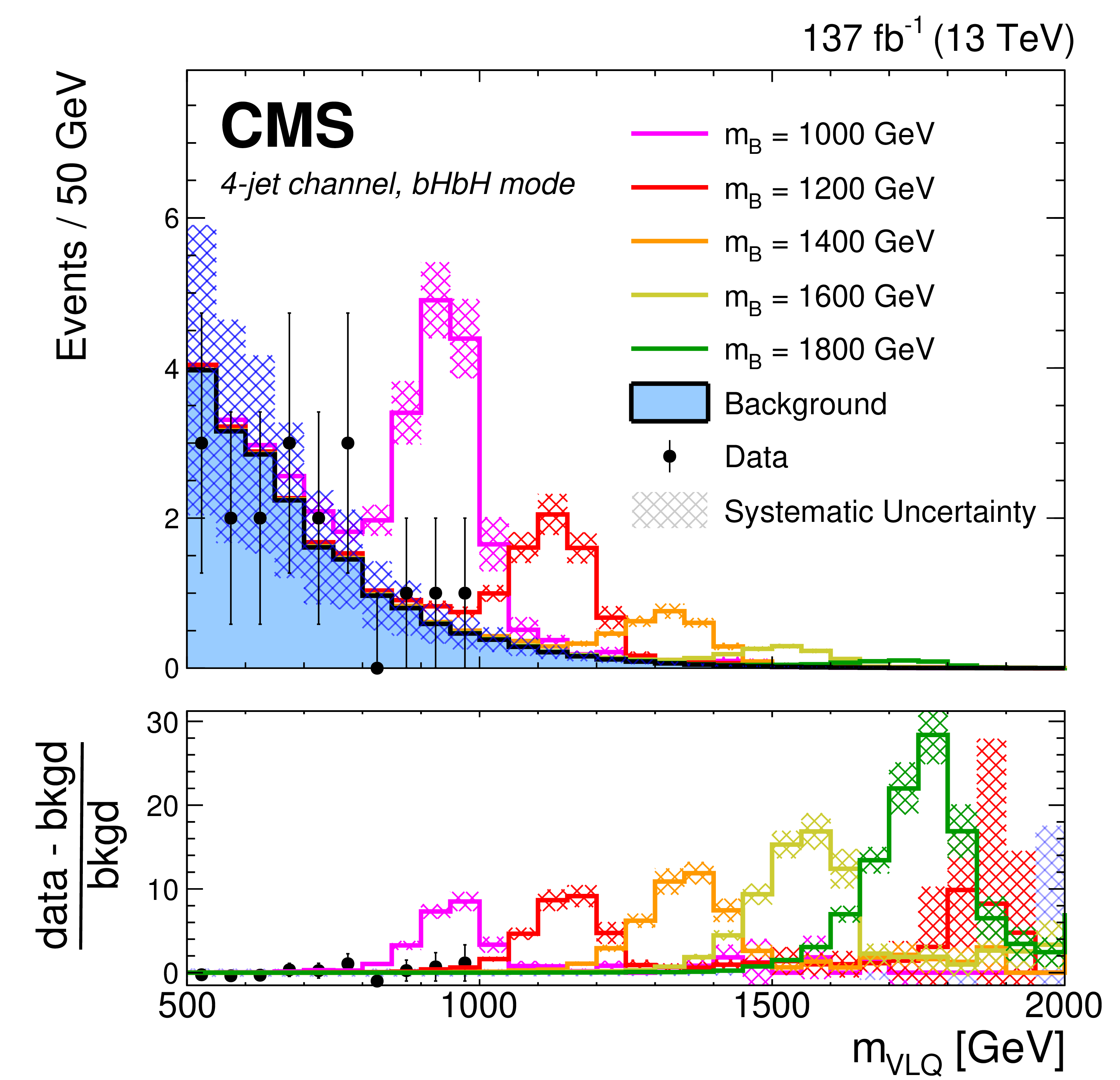
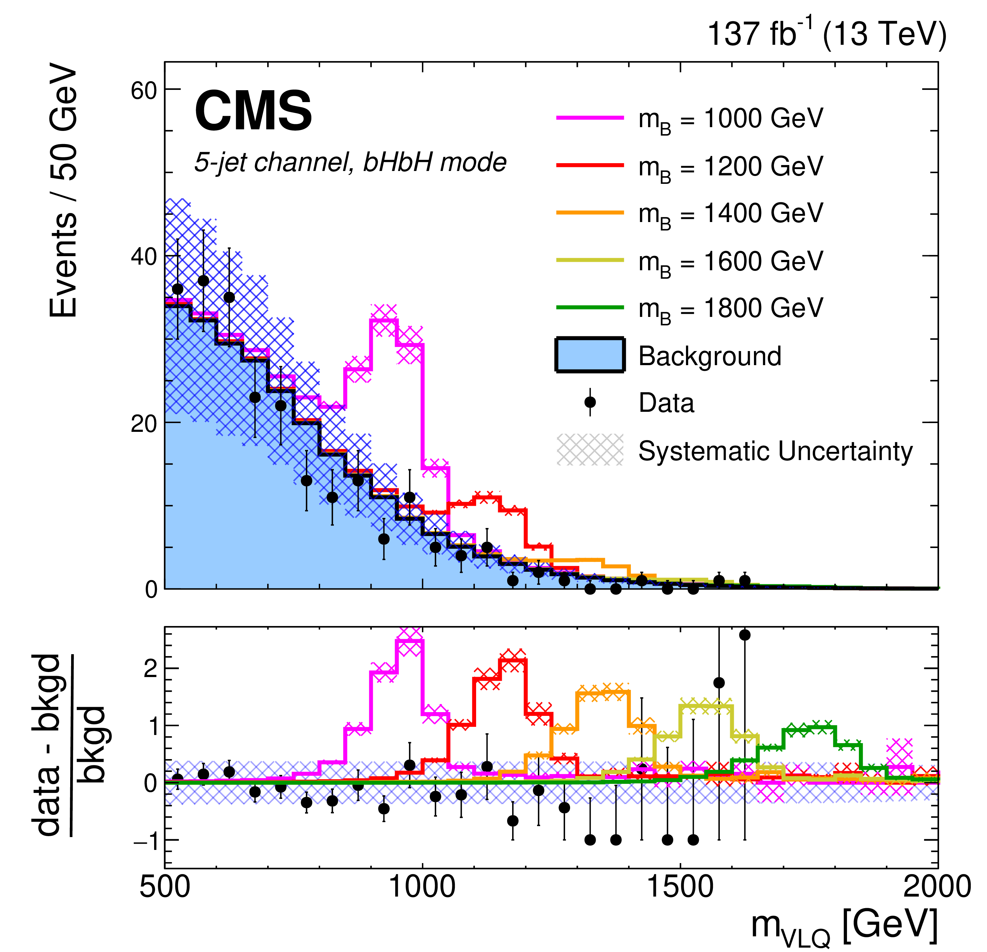
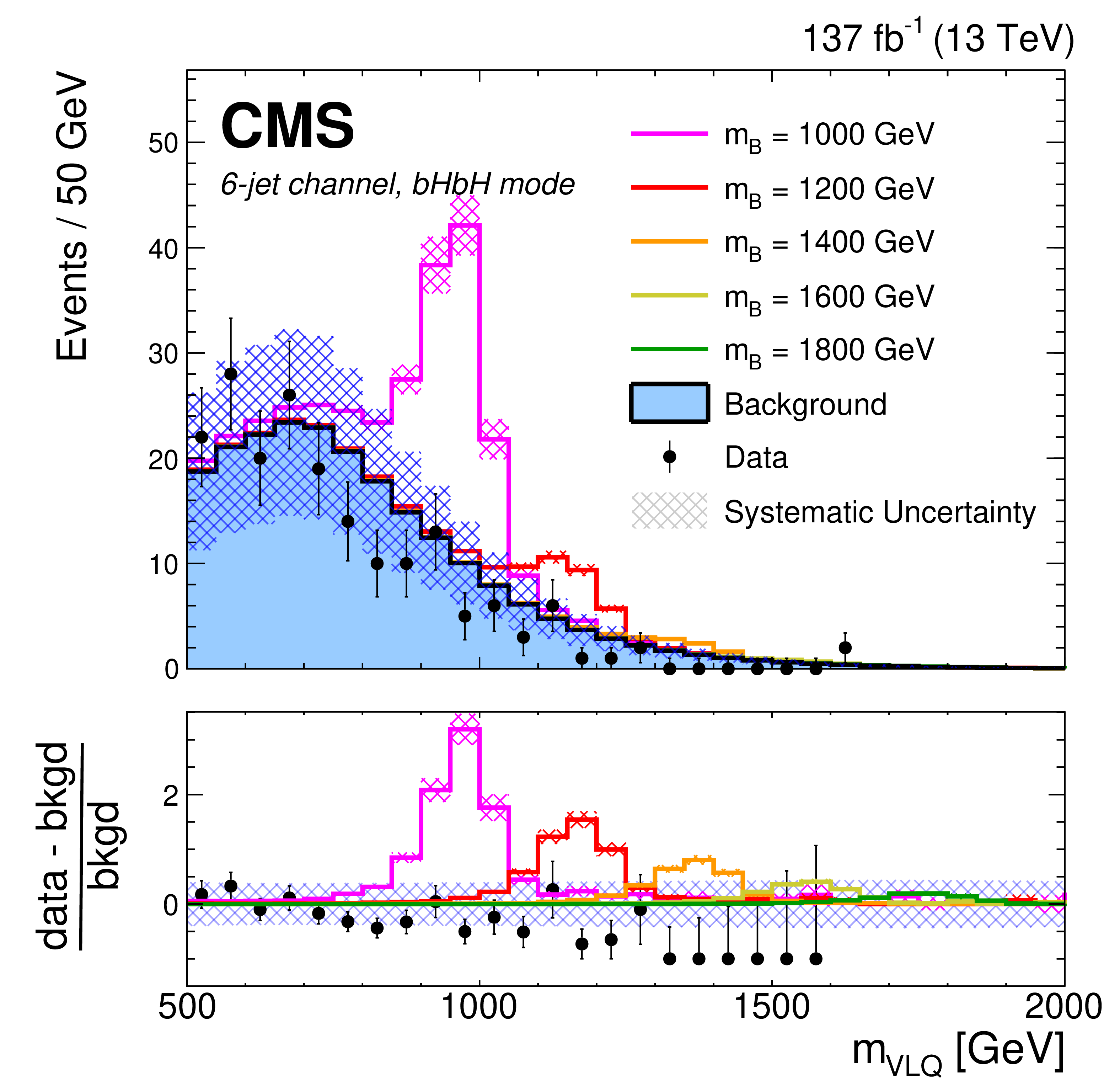
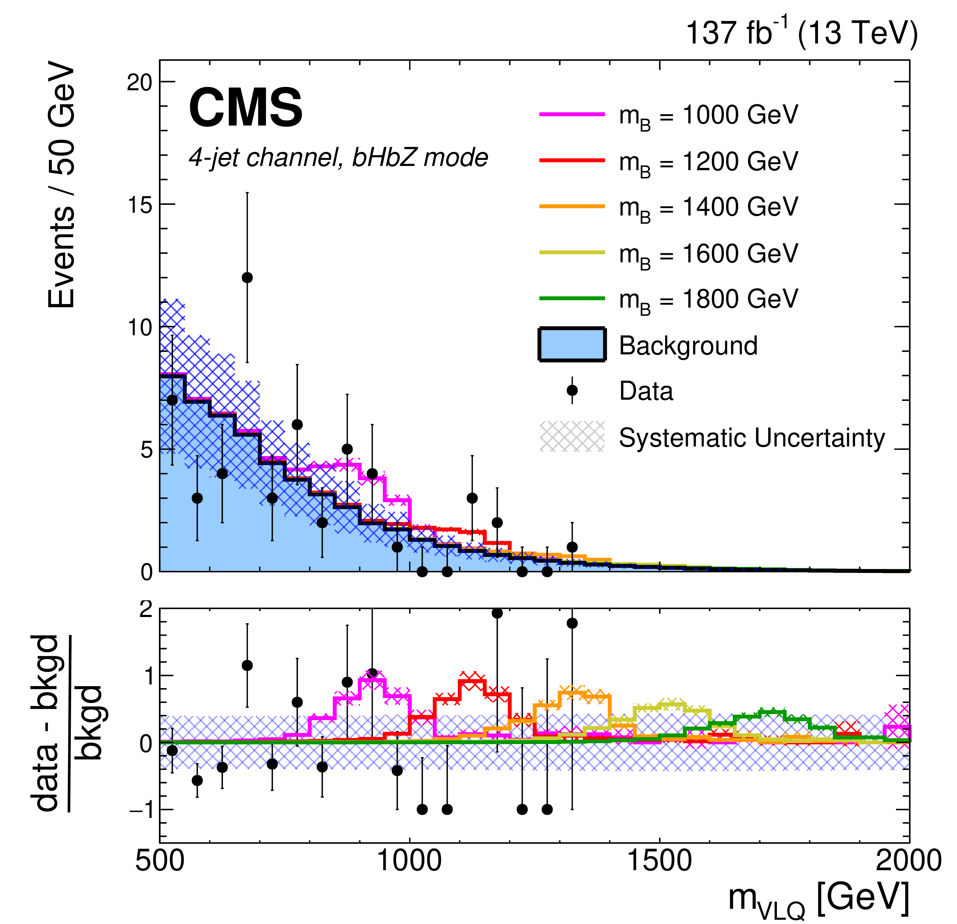
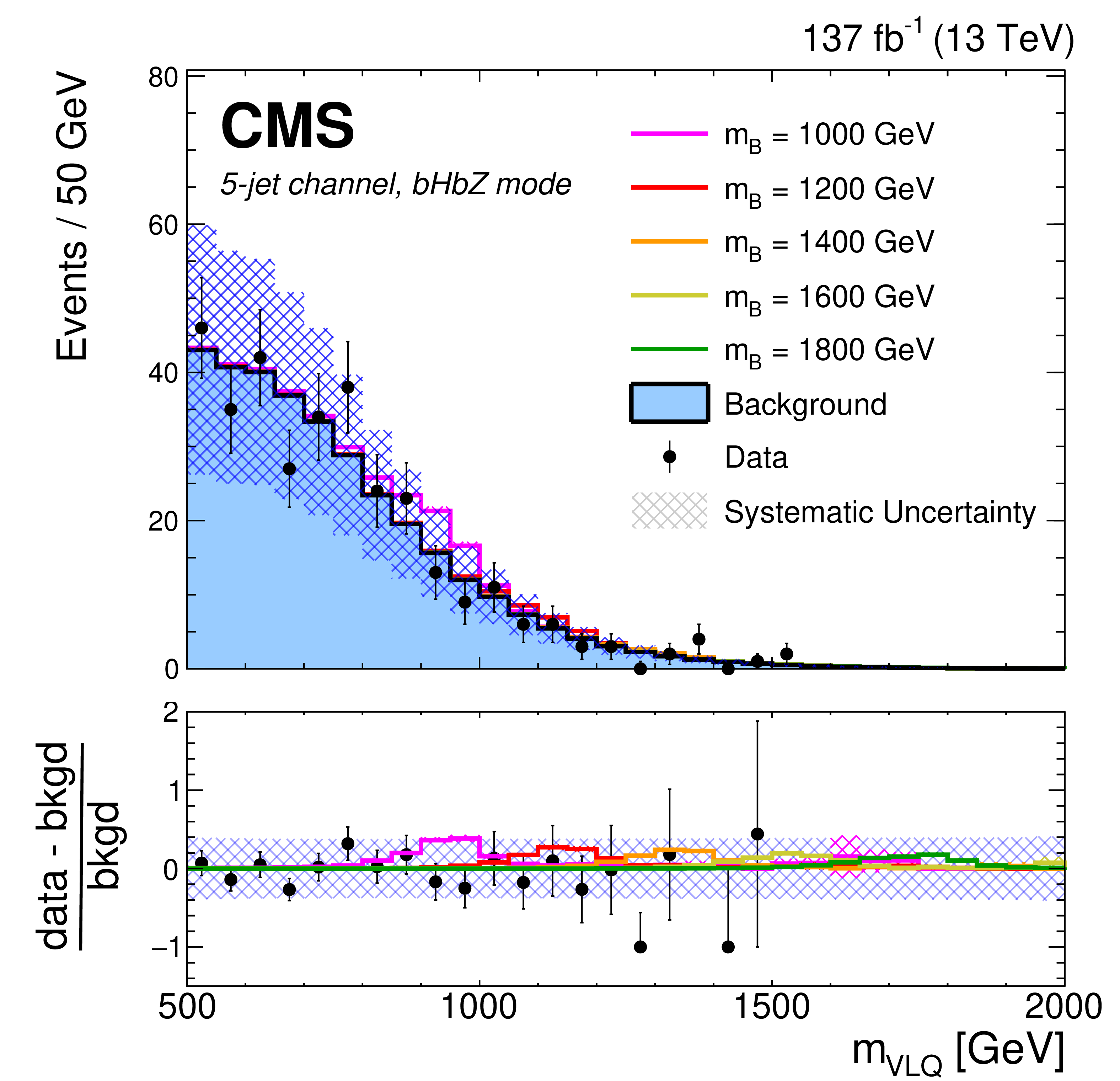
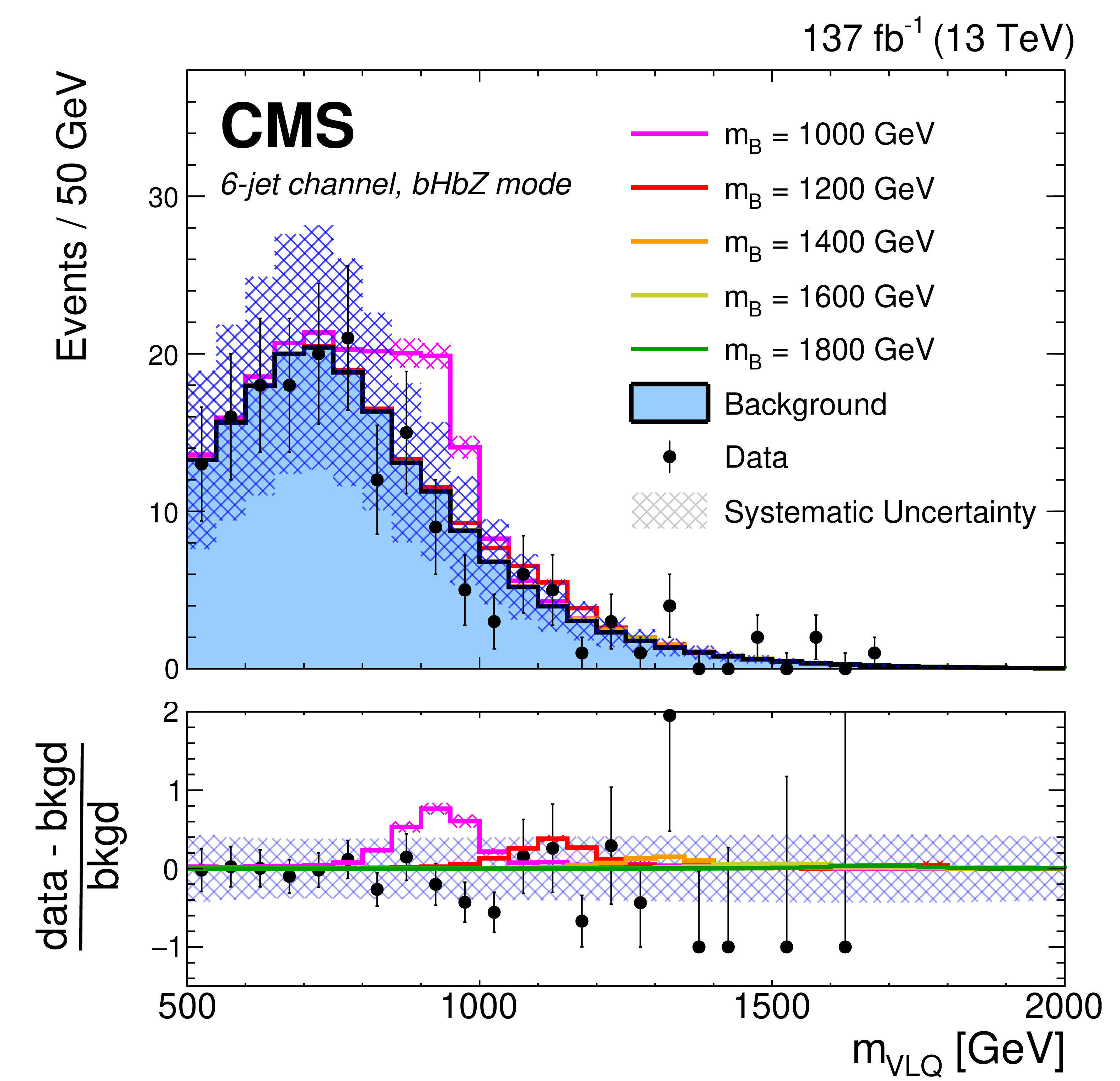
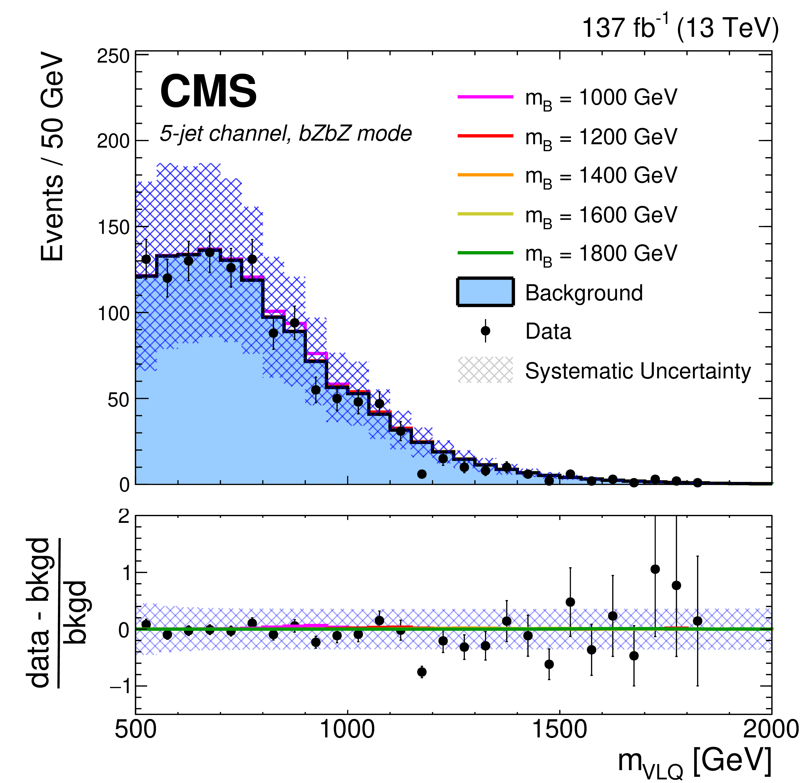
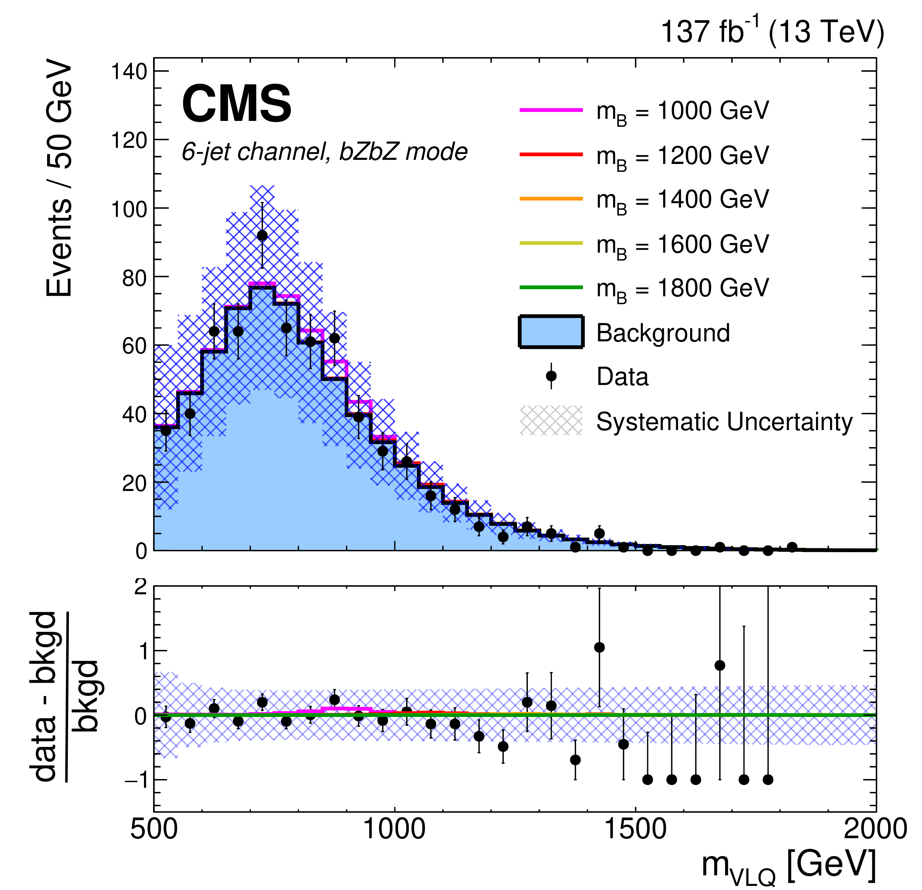
Figure 9:
Data (black points), expected background (solid blue histogram), and expected background plus a VLQ signal for different VLQ masses (colored lines), for 4-jet (left column), 5-jet (center column), and 6-jet (right column) multiplicities and for ${\mathrm{b} \mathrm{H} \mathrm{b} \mathrm{H}}$ (upper row), ${\mathrm{b} \mathrm{H} \mathrm{b} \mathrm{Z}}$ (middle row), and ${\mathrm{b} \mathrm{Z} \mathrm{b} \mathrm{Z}}$ (lower row) event modes. For the signal, $ {\mathcal {B}(\mathrm{B} \to \mathrm{b} \mathrm{H})} = $ 100% is assumed. The hatched regions for the background and background plus signal distributions indicate the systematic uncertainties. All three data-taking years are combined. |
png pdf |
Figure 9-a:
Data (black points), expected background (solid blue histogram), and expected background plus a VLQ signal for different VLQ masses (colored lines), for 4-jet multiplicities and for ${\mathrm{b} \mathrm{H} \mathrm{b} \mathrm{H}}$ event mode. For the signal, $ {\mathcal {B}(\mathrm{B} \to \mathrm{b} \mathrm{H})} = $ 100% is assumed. The hatched regions for the background and background plus signal distributions indicate the systematic uncertainties. All three data-taking years are combined. |
png pdf |
Figure 9-b:
Data (black points), expected background (solid blue histogram), and expected background plus a VLQ signal for different VLQ masses (colored lines), for 5-jet multiplicities and for ${\mathrm{b} \mathrm{H} \mathrm{b} \mathrm{H}}$ event mode. For the signal, $ {\mathcal {B}(\mathrm{B} \to \mathrm{b} \mathrm{H})} = $ 100% is assumed. The hatched regions for the background and background plus signal distributions indicate the systematic uncertainties. All three data-taking years are combined. |
png pdf |
Figure 9-c:
Data (black points), expected background (solid blue histogram), and expected background plus a VLQ signal for different VLQ masses (colored lines), for 6-jet multiplicities and for ${\mathrm{b} \mathrm{H} \mathrm{b} \mathrm{H}}$ event mode. For the signal, $ {\mathcal {B}(\mathrm{B} \to \mathrm{b} \mathrm{H})} = $ 100% is assumed. The hatched regions for the background and background plus signal distributions indicate the systematic uncertainties. All three data-taking years are combined. |
png pdf |
Figure 9-d:
Data (black points), expected background (solid blue histogram), and expected background plus a VLQ signal for different VLQ masses (colored lines), for 4-jet multiplicities and for ${\mathrm{b} \mathrm{H} \mathrm{b} \mathrm{Z}}$ event mode. For the signal, $ {\mathcal {B}(\mathrm{B} \to \mathrm{b} \mathrm{H})} = $ 100% is assumed. The hatched regions for the background and background plus signal distributions indicate the systematic uncertainties. All three data-taking years are combined. |
png pdf |
Figure 9-e:
Data (black points), expected background (solid blue histogram), and expected background plus a VLQ signal for different VLQ masses (colored lines), for 5-jet multiplicities and for ${\mathrm{b} \mathrm{H} \mathrm{b} \mathrm{Z}}$ event mode. For the signal, $ {\mathcal {B}(\mathrm{B} \to \mathrm{b} \mathrm{H})} = $ 100% is assumed. The hatched regions for the background and background plus signal distributions indicate the systematic uncertainties. All three data-taking years are combined. |
png pdf |
Figure 9-f:
Data (black points), expected background (solid blue histogram), and expected background plus a VLQ signal for different VLQ masses (colored lines), for 6-jet multiplicities and for ${\mathrm{b} \mathrm{H} \mathrm{b} \mathrm{Z}}$ event mode. For the signal, $ {\mathcal {B}(\mathrm{B} \to \mathrm{b} \mathrm{H})} = $ 100% is assumed. The hatched regions for the background and background plus signal distributions indicate the systematic uncertainties. All three data-taking years are combined. |

png pdf |
Figure 9-g:
Data (black points), expected background (solid blue histogram), and expected background plus a VLQ signal for different VLQ masses (colored lines), for 4-jet multiplicities and for ${\mathrm{b} \mathrm{Z} \mathrm{b} \mathrm{Z}}$ event mode. For the signal, $ {\mathcal {B}(\mathrm{B} \to \mathrm{b} \mathrm{H})} = $ 100% is assumed. The hatched regions for the background and background plus signal distributions indicate the systematic uncertainties. All three data-taking years are combined. |
png pdf |
Figure 9-h:
Data (black points), expected background (solid blue histogram), and expected background plus a VLQ signal for different VLQ masses (colored lines), for 5-jet multiplicities and for ${\mathrm{b} \mathrm{Z} \mathrm{b} \mathrm{Z}}$ event mode. For the signal, $ {\mathcal {B}(\mathrm{B} \to \mathrm{b} \mathrm{H})} = $ 100% is assumed. The hatched regions for the background and background plus signal distributions indicate the systematic uncertainties. All three data-taking years are combined. |
png pdf |
Figure 9-i:
Data (black points), expected background (solid blue histogram), and expected background plus a VLQ signal for different VLQ masses (colored lines), for 6-jet multiplicities and for ${\mathrm{b} \mathrm{Z} \mathrm{b} \mathrm{Z}}$ event mode. For the signal, $ {\mathcal {B}(\mathrm{B} \to \mathrm{b} \mathrm{H})} = $ 100% is assumed. The hatched regions for the background and background plus signal distributions indicate the systematic uncertainties. All three data-taking years are combined. |
png pdf |
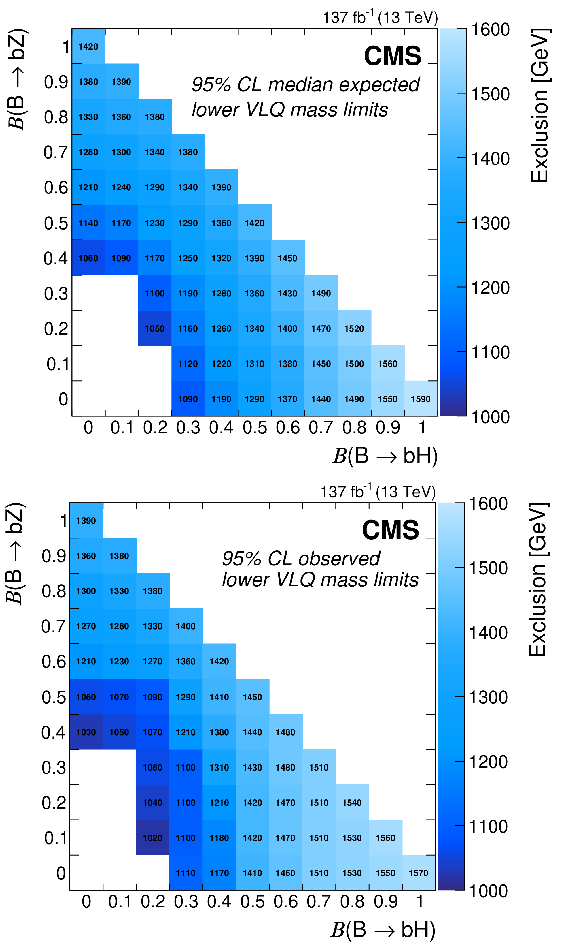
Figure 10:
Expected (upper) and observed (lower) limits on the VLQ mass at 95% CL as a function of the branching fractions ${\mathcal {B}(\mathrm{B} \to \mathrm{b} \mathrm{H})}$ and ${\mathcal {B}(\mathrm{B} \to \mathrm{b} \mathrm{Z})}$. |

png pdf |
Figure 10-a:
Expected limit on the VLQ mass at 95% CL as a function of the branching fractions ${\mathcal {B}(\mathrm{B} \to \mathrm{b} \mathrm{H})}$ and ${\mathcal {B}(\mathrm{B} \to \mathrm{b} \mathrm{Z})}$. |

png pdf |
Figure 10-b:
Observed limit on the VLQ mass at 95% CL as a function of the branching fractions ${\mathcal {B}(\mathrm{B} \to \mathrm{b} \mathrm{H})}$ and ${\mathcal {B}(\mathrm{B} \to \mathrm{b} \mathrm{Z})}$. |
png pdf |
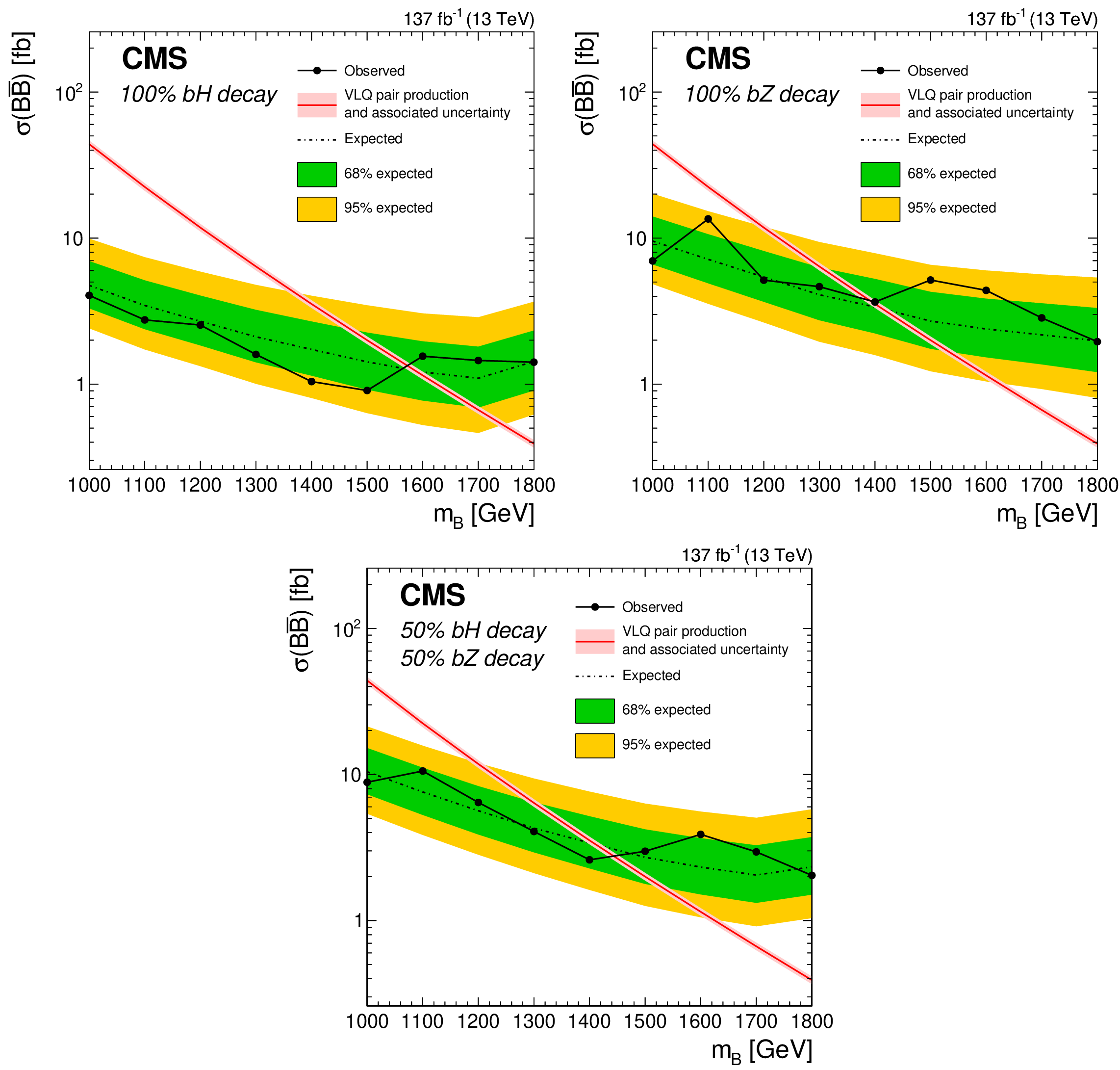
Figure 11:
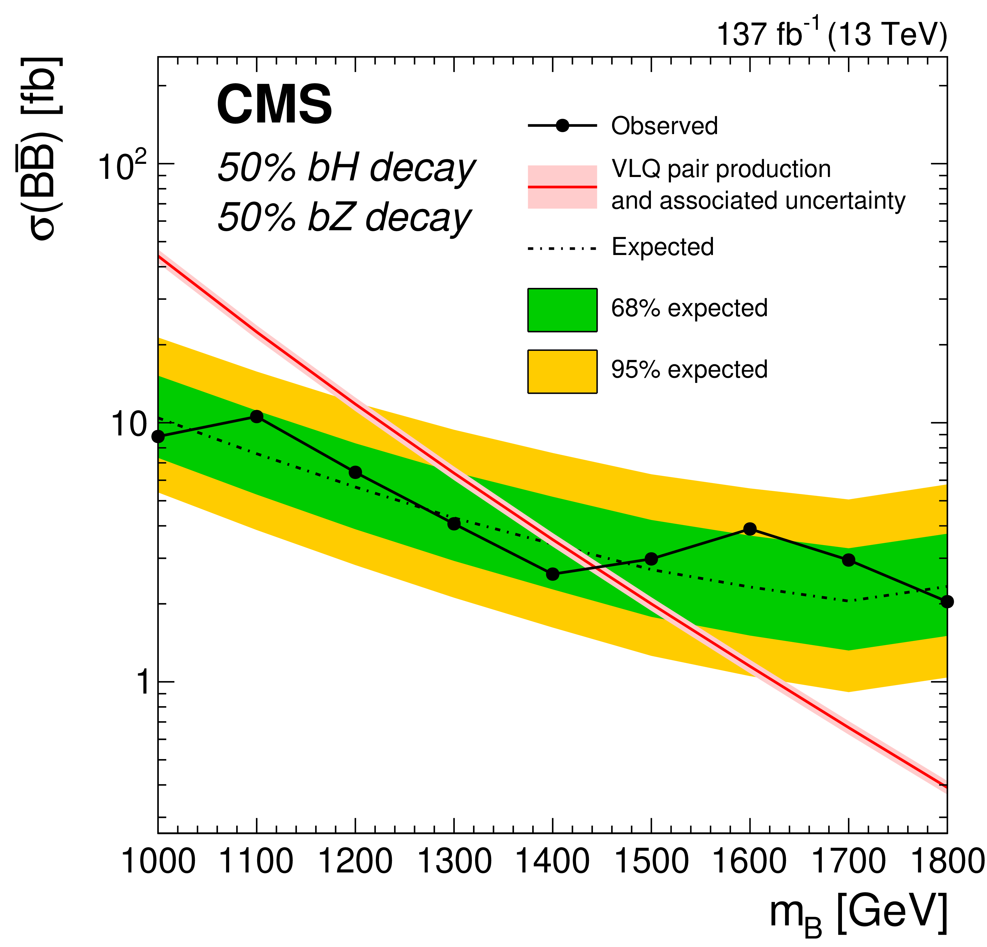
The 95% confidence limit on the cross section for VLQ pair production as a function of VLQ mass for three branching fraction hypotheses: $ {\mathcal {B}(\mathrm{B} \to \mathrm{b} \mathrm{H})} = $ 100% (upper left), $ {\mathcal {B}(\mathrm{B} \to \mathrm{b} \mathrm{Z})} = $ 100% (upper right), and $ {\mathcal {B}(\mathrm{B} \to \mathrm{b} \mathrm{H})} = {\mathcal {B}(\mathrm{B} \to \mathrm{b} \mathrm{Z})} = $ 50% (lower). The solid black line indicates the observed limit and the dashed line indicates the expected limit with 1 sigma (green band) and 2 sigma (yellow band) uncertainties. The theoretical cross section and its uncertainty are shown as the red line and pale red band; the band is only slightly visible outside the line. |
png pdf |
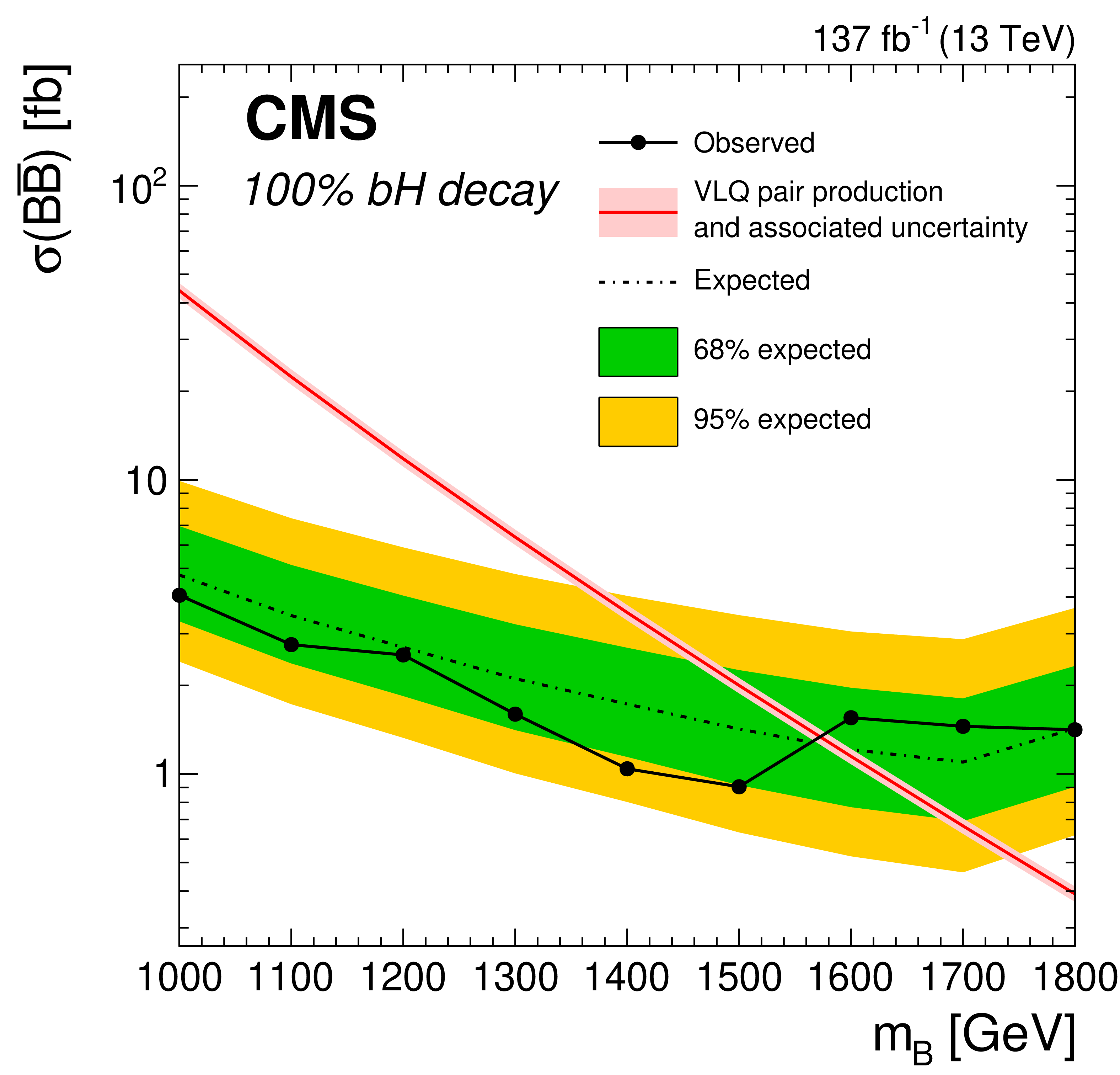
Figure 11-a:
The 95% confidence limit on the cross section for VLQ pair production as a function of VLQ mass for the $ {\mathcal {B}(\mathrm{B} \to \mathrm{b} \mathrm{H})} = $ 100% branching fraction hypothesis. The solid black line indicates the observed limit and the dashed line indicates the expected limit with 1 sigma (green band) and 2 sigma (yellow band) uncertainties. The theoretical cross section and its uncertainty are shown as the red line and pale red band; the band is only slightly visible outside the line. |
png pdf |
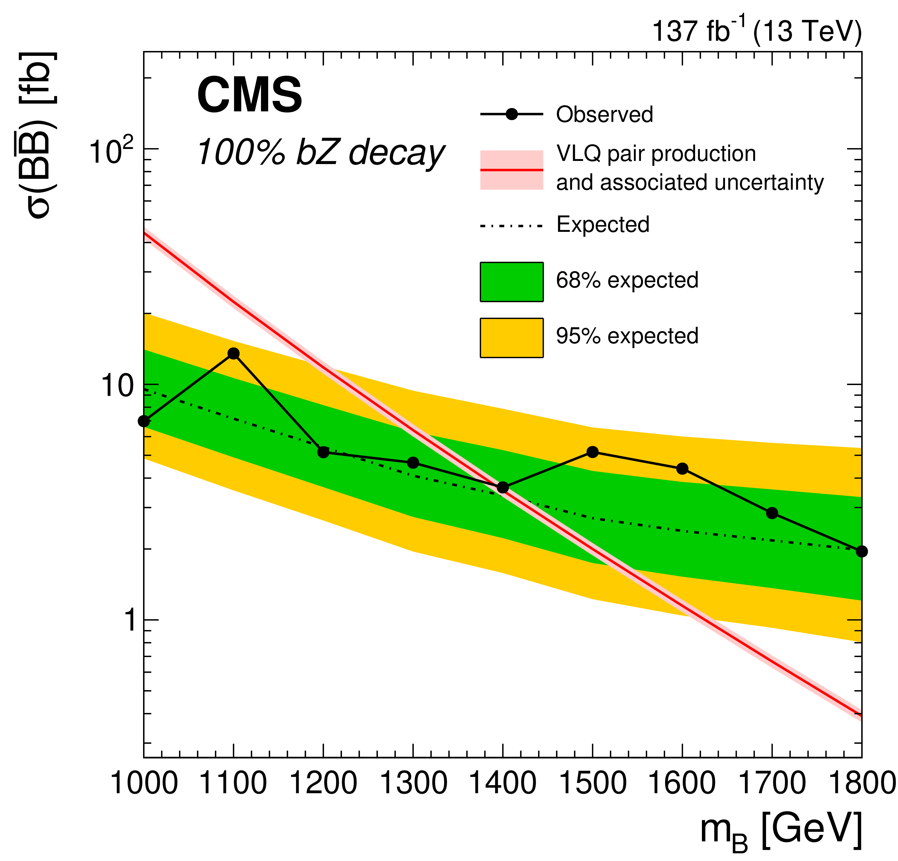
Figure 11-b:
The 95% confidence limit on the cross section for VLQ pair production as a function of VLQ mass for the $ {\mathcal {B}(\mathrm{B} \to \mathrm{b} \mathrm{Z})} = $ 100% branching fraction hypothesis. The solid black line indicates the observed limit and the dashed line indicates the expected limit with 1 sigma (green band) and 2 sigma (yellow band) uncertainties. The theoretical cross section and its uncertainty are shown as the red line and pale red band; the band is only slightly visible outside the line. |
png pdf |
Figure 11-c:
The 95% confidence limit on the cross section for VLQ pair production as a function of VLQ mass for the $ {\mathcal {B}(\mathrm{B} \to \mathrm{b} \mathrm{H})} = {\mathcal {B}(\mathrm{B} \to \mathrm{b} \mathrm{Z})} = $ 50% branching fraction hypothesis. The solid black line indicates the observed limit and the dashed line indicates the expected limit with 1 sigma (green band) and 2 sigma (yellow band) uncertainties. The theoretical cross section and its uncertainty are shown as the red line and pale red band; the band is only slightly visible outside the line. |
| Tables | |
png pdf |
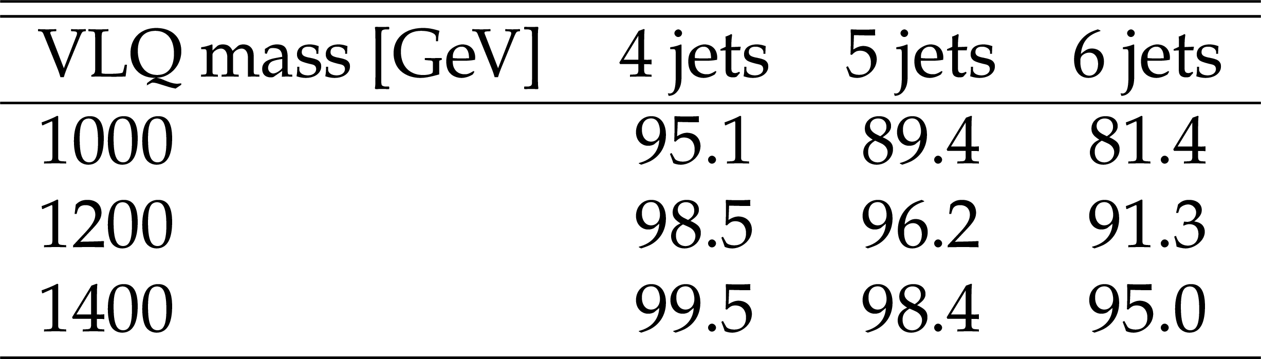
Table 1:
Signal efficiencies of the offline ${H_{\mathrm {T}}}$ selection, in%, for each of the jet multiplicity channels, for three VLQ masses (1000, 1200, and 1400 GeV). The efficiency is the fraction of events in each jet multiplicity category satisfying the $ {H_{\mathrm {T}}} > $ 1350 GeV selection. Statistical uncertainties are negligible and therefore omitted. |
png pdf |
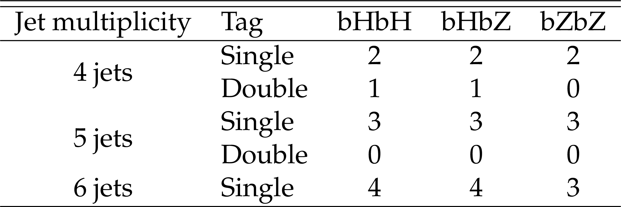
Table 2:
Summary of the minimum number of single and double $\mathrm{b}$ tags required for each jet multiplicity and event mode. |
png pdf |
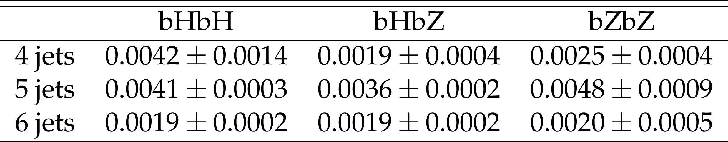
Table 3:
Values of the BJTF for data events with ${m_\text {VLQ}}$ in the range 500-800 GeV for each of the three event modes and three jet multiplicities. |
png pdf |
Table 4:
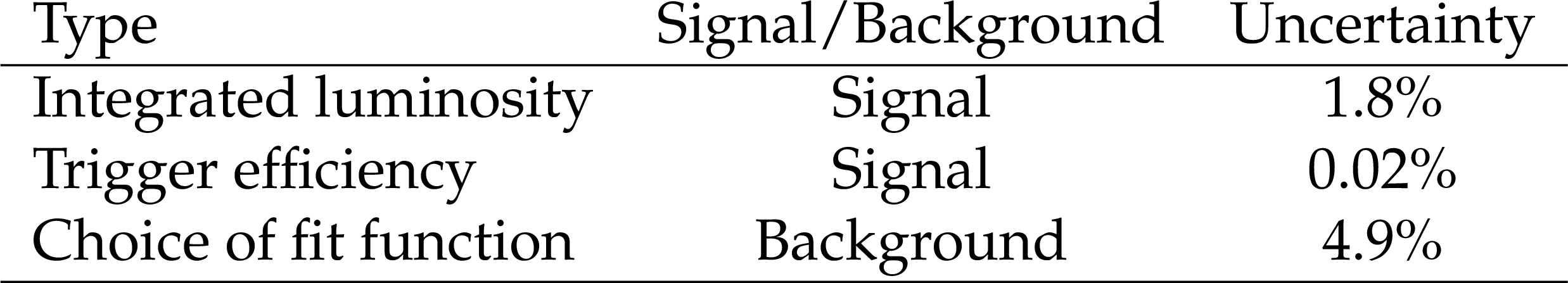
Systematic uncertainties common to all three event modes and all three jet multiplicities. All uncertainties listed here are rate uncertainties, meaning they affect only the normalization. |
png pdf |
Table 5:
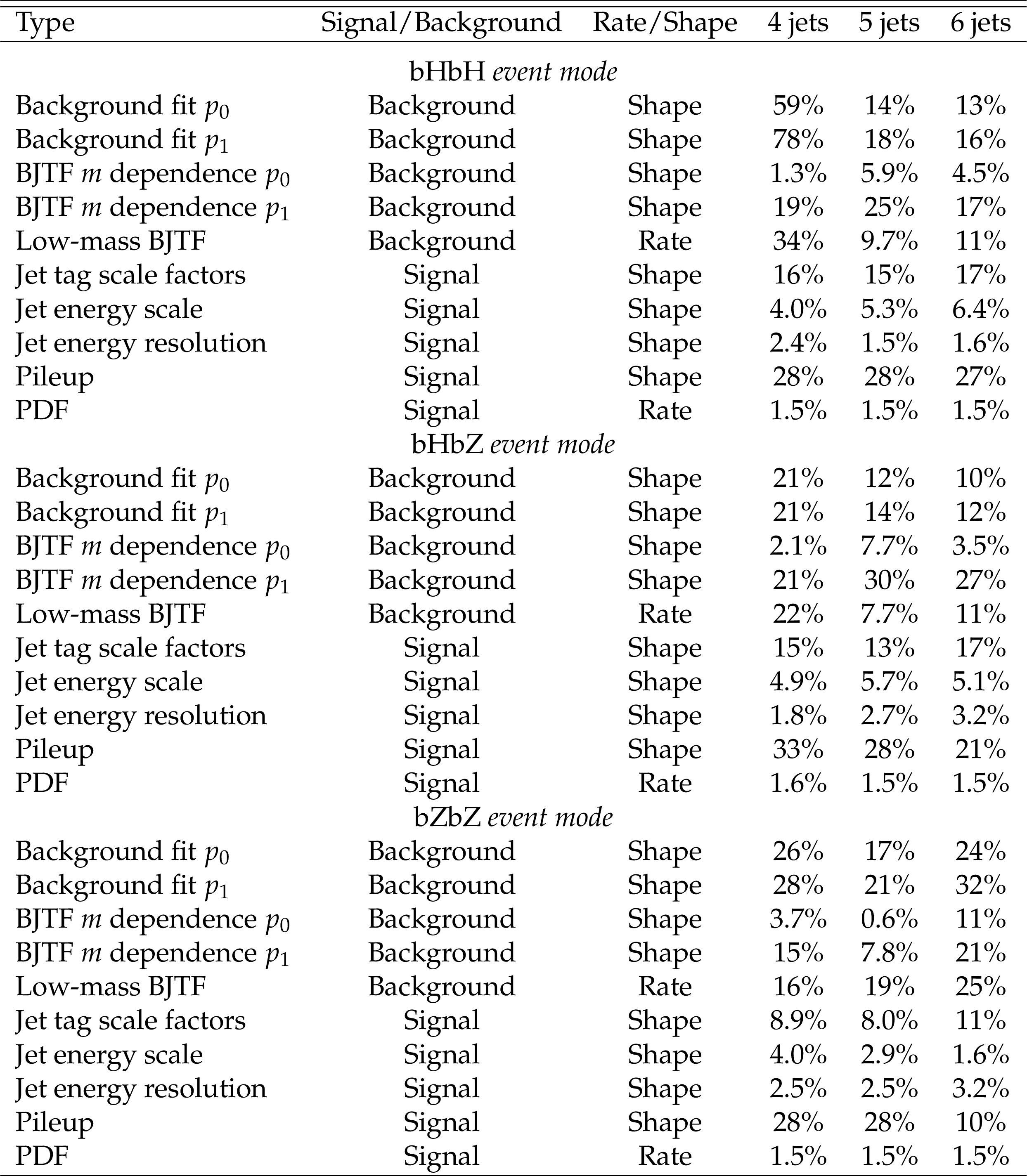
Systematic uncertainties for each event mode and jet multiplicity. The reported values indicate the uncertainty in the event yield in a $\pm $75 GeV window about the signal peak for a generated signal mass $m_{\mathrm{B}} = $ 1600 GeV. |
png pdf |
Table 6:
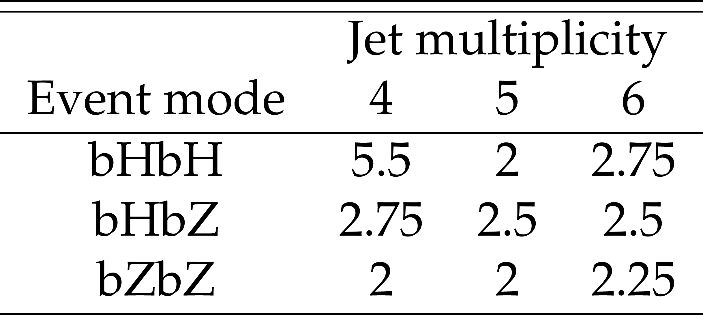
Optimized values of the ${\chi ^2_\text {mod}/\text {ndf}}$ selection as a function of jet multiplicity and event mode. |
| Summary |
| This paper describes a search for bottom-type, vector-like quark (VLQ) pair production in data collected by the CMS detector in 2016-2018 at $\sqrt{s} = $ 13 TeV, where the VLQ B decays into a $\mathrm{b}$ or $\mathrm{\bar{b}}$ quark and either a Higgs boson H or a Z boson. The analysis targets the fully hadronic ${\mathrm{B} \to \mathrm{b}\mathrm{H}}$ and ${\mathrm{B} \to \mathrm{b}\mathrm{Z}}$ decays by tagging jets and using a modified ${\chi^2}$ metric to reconstruct the event. Different jet multiplicity categories were used to account for the fact that Higgs or Z boson decays can produce either two distinct jets or, if highly Lorentz boosted, a single merged jet. Backgrounds were estimated from a region of low VLQ mass and extrapolated into the signal region using a modified ${\chi^2}$ control region. Limits were set on the VLQ mass at 95% confidence level as a function of the branching fractions for ${\mathrm{B} \to \mathrm{b}\mathrm{H}}$ and ${\mathrm{B} \to \mathrm{b}\mathrm{Z}}$. Compared to previous measurements [18,17], limits on the B VLQ mass have been increased from 1010 to 1570 GeV in the ${\mathcal{B}(\mathrm{B} \to \mathrm{b}\mathrm{H})} = $ 100% case, from 1070 to 1390 GeV in the ${\mathcal{B}(\mathrm{B} \to \mathrm{b}\mathrm{Z})} = $ 100% case, and from 1025 to 1450 GeV in the ${\mathcal{B}(\mathrm{B} \to \mathrm{b}\mathrm{H})} = {\mathcal{B}(\mathrm{B} \to \mathrm{b}\mathrm{Z})} = $ 50% case. |
| References | ||||
| 1 | G. 't Hooft | Naturalness, chiral symmetry, and spontaneous chiral symmetry breaking | NATO Sci. Ser. B 59 (1980) 135 | |
| 2 | J. Wess and B. Zumino | A Lagrangian model invariant under supergauge transformations | PLB 49 (1974) 52 | |
| 3 | P. Fayet and S. Ferrara | Supersymmetry | PR 32 (1977) 249 | |
| 4 | H. Georgi and A. Pais | Calculability and naturalness in gauge theories | PRD 10 (1974) 539 | |
| 5 | D. B. Kaplan, H. Georgi, and S. Dimopoulos | Composite Higgs scalars | PLB 136 (1984) 187 | |
| 6 | K. Agashe, R. Contino, and A. Pomarol | The minimal composite Higgs model | NPB 719 (2005) 165 | hep-ph/0412089 |
| 7 | N. Arkani-Hamed, A. G. Cohen, and H. Georgi | Electroweak symmetry breaking from dimensional deconstruction | PLB 513 (2001) 232 | hep-ph/0105239 |
| 8 | N. Arkani-Hamed, A. G. Cohen, E. Katz, and A. E. Nelson | The littlest Higgs | JHEP 07 (2002) 034 | hep-ph/0206021 |
| 9 | F. del Aguila and M. J. Bowick | The possibility of new fermions with $ \Delta I = $ 0 mass | NPB 224 (1983) 107 | |
| 10 | ATLAS Collaboration | Combined measurements of Higgs boson production and decay using up to 80 fb$ ^{-1} $ of proton-proton collision data at $ \sqrt{s}= $ 13 TeV collected with the ATLAS experiment | PRD 101 (2020) 012002 | 1909.02845 |
| 11 | CMS Collaboration | Measurement and interpretation of differential cross sections for Higgs boson production at $ \sqrt{s} = $ 13 TeV | PLB 792 (2019) 369 | CMS-HIG-17-028 1812.06504 |
| 12 | J. A. Aguilar-Saavedra, R. Benbrik, S. Heinemeyer, and M. P\'erez-Victoria | Handbook of vectorlike quarks: Mixing and single production | PRD 88 (2013) 094010 | 1306.0572 |
| 13 | F. del Aguila, M. P\'erez-Victoria, and J. Santiago | Observable contributions of new exotic quarks to quark mixing | JHEP 09 (2000) 011 | hep-ph/0007316 |
| 14 | J. A. Aguilar-Saavedra | Mixing with vector-like quarks: constraints and expectations | EPJ Web Conf. 60 (2013) 16012 | 1306.4432 |
| 15 | A. Atre, M. Carena, T. Han, and J. Santiago | Heavy quarks above the top at the Tevatron | PRD 79 (2009) 054018 | 0806.3966 |
| 16 | A. Atre et al. | Model-independent searches for new quarks at the LHC | JHEP 08 (2011) 080 | 1102.1987 |
| 17 | ATLAS Collaboration | Search for pair production of heavy vector-like quarks decaying into hadronic final states in $ pp $ collisions at $ \sqrt{s} = $ 13 TeV with the ATLAS detector | PRD 98 (2018) 092005 | 1808.01771 |
| 18 | CMS Collaboration | Search for pair production of vectorlike quarks in the fully hadronic final state | PRD 100 (2019) 072001 | CMS-B2G-18-005 1906.11903 |
| 19 | ATLAS Collaboration | Combination of the searches for pair-produced vector-like partners of the third-generation quarks at $ \sqrt{s} = $ 13 TeV with the ATLAS detector | PRL 121 (2018) 211801 | 1808.02343 |
| 20 | The ATLAS Collaboration, The CMS Collaboration, The LHC Higgs Combination Group | Procedure for the LHC Higgs boson search combination in Summer 2011 | CMS-NOTE-2011-005 | |
| 21 | CMS Collaboration | Jet energy scale and resolution in the CMS experiment in pp collisions at 8 TeV | JINST 12 (2017) P02014 | CMS-JME-13-004 1607.03663 |
| 22 | CMS Collaboration | The CMS trigger system | JINST 12 (2017) P01020 | CMS-TRG-12-001 1609.02366 |
| 23 | CMS Collaboration | The CMS experiment at the CERN LHC | JINST 3 (2008) S08004 | CMS-00-001 |
| 24 | CMS Collaboration | CMS luminosity measurement for the 2016 data taking period | CMS-PAS-LUM-17-001 | CMS-PAS-LUM-17-001 |
| 25 | CMS Collaboration | CMS luminosity measurement for the 2017 data-taking period at $ \sqrt{s} = $ 13 TeV | CMS-PAS-LUM-17-004 | CMS-PAS-LUM-17-004 |
| 26 | CMS Collaboration | CMS luminosity measurement for the 2018 data-taking period at $ \sqrt{s} = $ 13 TeV | CMS-PAS-LUM-18-002 | CMS-PAS-LUM-18-002 |
| 27 | J. Alwall et al. | The automated computation of tree-level and next-to-leading order differential cross sections, and their matching to parton shower simulations | JHEP 07 (2014) 079 | 1405.0301 |
| 28 | NNPDF Collaboration | Parton distributions for the LHC Run II | JHEP 04 (2015) 040 | 1410.8849 |
| 29 | T. Sjostrand et al. | An introduction to PYTHIA 8.2 | CPC 191 (2015) 159 | 1410.3012 |
| 30 | CMS Collaboration | Event generator tunes obtained from underlying event and multiparton scattering measurements | EPJC 76 (2016) 155 | CMS-GEN-14-001 1512.00815 |
| 31 | CMS Collaboration | Extraction and validation of a new set of CMS PYTHIA8 tunes from underlying-event measurements | EPJC 80 (2020) 4 | CMS-GEN-17-001 1903.12179 |
| 32 | M. Czakon, P. Fiedler, and A. Mitov | Total top-quark pair-production cross section at hadron colliders through $ O(\alpha^4_S) $ | PRL 110 (2013) 252004 | 1303.6254 |
| 33 | M. R. Whalley, D. Bourilkov, and R. C. Group | The Les Houches accord PDFs (LHAPDF) and LHAGLUE | in HERA and the LHC: A workshop on the implications of HERA for LHC physics. Proceedings, Part B, p. 575 2005 | hep-ph/0508110 |
| 34 | CMS Collaboration | Search for vector-like T and B quark pairs in final states with leptons at $ \sqrt{s} = $ 13 TeV | JHEP 08 (2018) 177 | CMS-B2G-17-011 1805.04758 |
| 35 | LHCb Collaboration | Measurement of the inelastic $ pp $ cross-section at a centre-of-mass energy of 13 TeV | JHEP 06 (2018) 100 | 1803.10974 |
| 36 | GEANT4 Collaboration | GEANT4--a simulation toolkit | NIMA 506 (2003) 250 | |
| 37 | J. Allison et al. | Geant4 developments and applications | IEEE Trans. Nucl. Sci. 53 (2006) 270 | |
| 38 | CMS Collaboration | Performance of the DeepJet b tagging algorithm using 41.9/fb of data from proton-proton collisions at 13 TeV with phase 1 CMS detector | CDS | |
| 39 | CMS Collaboration | Identification of heavy-flavour jets with the CMS detector in pp collisions at 13 TeV | JINST 13 (2018) P05011 | CMS-BTV-16-002 1712.07158 |
| 40 | CMS Collaboration | Particle-flow reconstruction and global event description with the CMS detector | JINST 12 (2017) P10003 | CMS-PRF-14-001 1706.04965 |
| 41 | M. Cacciari, G. P. Salam, and G. Soyez | The anti-$ {k_{\mathrm{T}}} $ jet clustering algorithm | JHEP 04 (2008) 063 | 0802.1189 |
| 42 | M. Cacciari, G. P. Salam, and G. Soyez | FastJet user manual | EPJC 72 (2012) 1896 | 1111.6097 |
| 43 | D. Bertolini, P. Harris, M. Low, and N. Tran | Pileup per particle identification | JHEP 10 (2014) 059 | 1407.6013 |
| 44 | CMS Collaboration | Jet algorithms performance in 13 TeV data | CMS-PAS-JME-16-003 | CMS-PAS-JME-16-003 |
| 45 | Y. L. Dokshitzer, G. D. Leder, S. Moretti, and B. R. Webber | Better jet clustering algorithms | JHEP 08 (1997) 001 | hep-ph/9707323 |
| 46 | M. Wobisch and T. Wengler | Hadronization corrections to jet cross-sections in deep inelastic scattering | in Proceedings of the Workshop on Monte Carlo Generators for HERA Physics, Hamburg, Germany, p. 270 1998 | hep-ph/9907280 |
| 47 | M. Dasgupta, A. Fregoso, S. Marzani, and G. P. Salam | Towards an understanding of jet substructure | JHEP 09 (2013) 029 | 1307.0007 |
| 48 | J. M. Butterworth, A. R. Davison, M. Rubin, and G. P. Salam | Jet substructure as a new Higgs search channel at the LHC | PRL 100 (2008) 242001 | 0802.2470 |
| 49 | A. J. Larkoski, S. Marzani, G. Soyez, and J. Thaler | Soft drop | JHEP 05 (2014) 146 | 1402.2657 |
| 50 | F. M. Fisher | Tests of equality between sets of coefficients in two linear regressions: An expository note | Econometrica 38 (1970) 361 | |
| 51 | J. Butterworth et al. | PDF4LHC recommendations for LHC Run II | JPG 43 (2016) 023001 | 1510.03865 |
| 52 | T. Junk | Confidence level computation for combining searches with small statistics | NIMA 434 (1999) 435 | hep-ex/9902006 |
| 53 | A. L. Read | Presentation of search results: The CL$ _{\text{s}} $ technique | JPG 28 (2002) 2693 | |
| 54 | G. Cowan, K. Cranmer, E. Gross, and O. Vitells | Asymptotic formulae for likelihood-based tests of new physics | EPJC 71 (2011) 1554 | 1007.1727 |
|
|
Compact Muon Solenoid LHC, CERN |
|

|

|

|

|

|