

Compact Muon Solenoid
LHC, CERN
| CMS-B2G-18-005 ; CERN-EP-2019-129 | ||
| Search for pair production of vector-like quarks in the fully hadronic final state | ||
| CMS Collaboration | ||
| 28 June 2019 | ||
| Phys. Rev. D 100 (2019) 072001 | ||
| Abstract: The results of two searches for pair production of vector-like T or B quarks in fully hadronic final states are presented, using data from the CMS experiment at a center-of-mass energy of 13 TeV. The data were collected at the LHC during 2016 and correspond to an integrated luminosity of 35.9 fb$^{-1}$. A cut-based analysis specifically targets the qW decay mode of the T quark and allows for the reconstruction of the T quark candidates. In a second analysis, a multiclassification algorithm, the "boosted event shape tagger,'' is deployed to label candidate jets as originating from top quarks, and W, Z, and H. Candidate events are categorized according to the multiplicities of identified jets, and the scalar sum of all observed jet momenta is used to discriminate signal events from the quantum chromodynamics multijet background. Both analyses probe all possible branching fraction combinations of the T and B quarks and set limits at 95% confidence level on their masses, ranging from 740 to 1370 GeV. These results represent a significant improvement relative to existing searches in the fully hadronic final state. | ||
| Links: e-print arXiv:1906.11903 [hep-ex] (PDF) ; CDS record ; inSPIRE record ; CADI line (restricted) ; | ||
| Figures & Tables | Summary | Additional Figures | References | CMS Publications |
|---|
| Figures | |
png pdf |
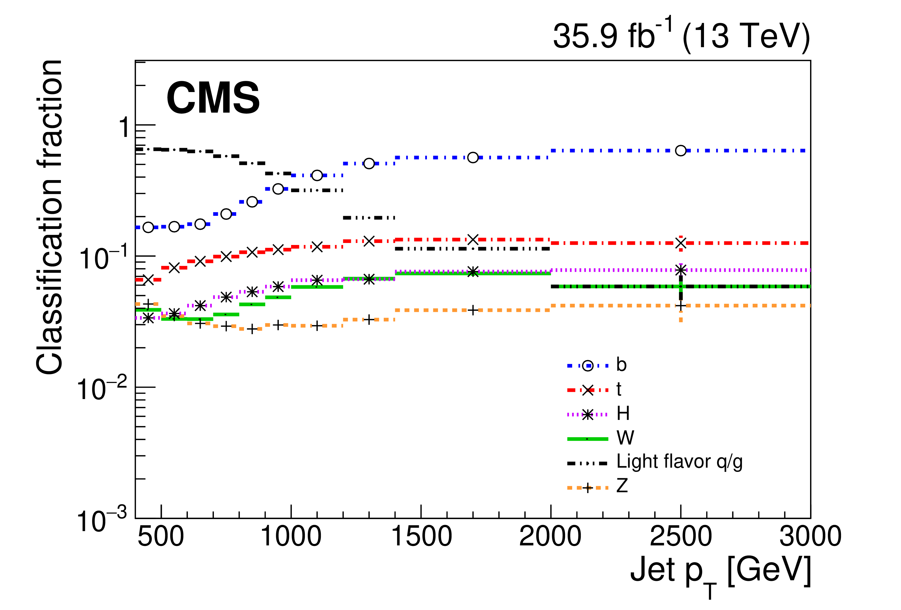
Figure 1:
classification fractions for the six categories of the BEST algorithm, measured in data events as a function of jet ${p_{\mathrm {T}}}$. Error bars shown indicate statistical uncertainties in the fractions to be propagated to the estimate of the QCD multijet background contribution. The rightmost bin includes jets with ${p_{\mathrm {T}}}$ values above 3 TeV. |
png pdf |
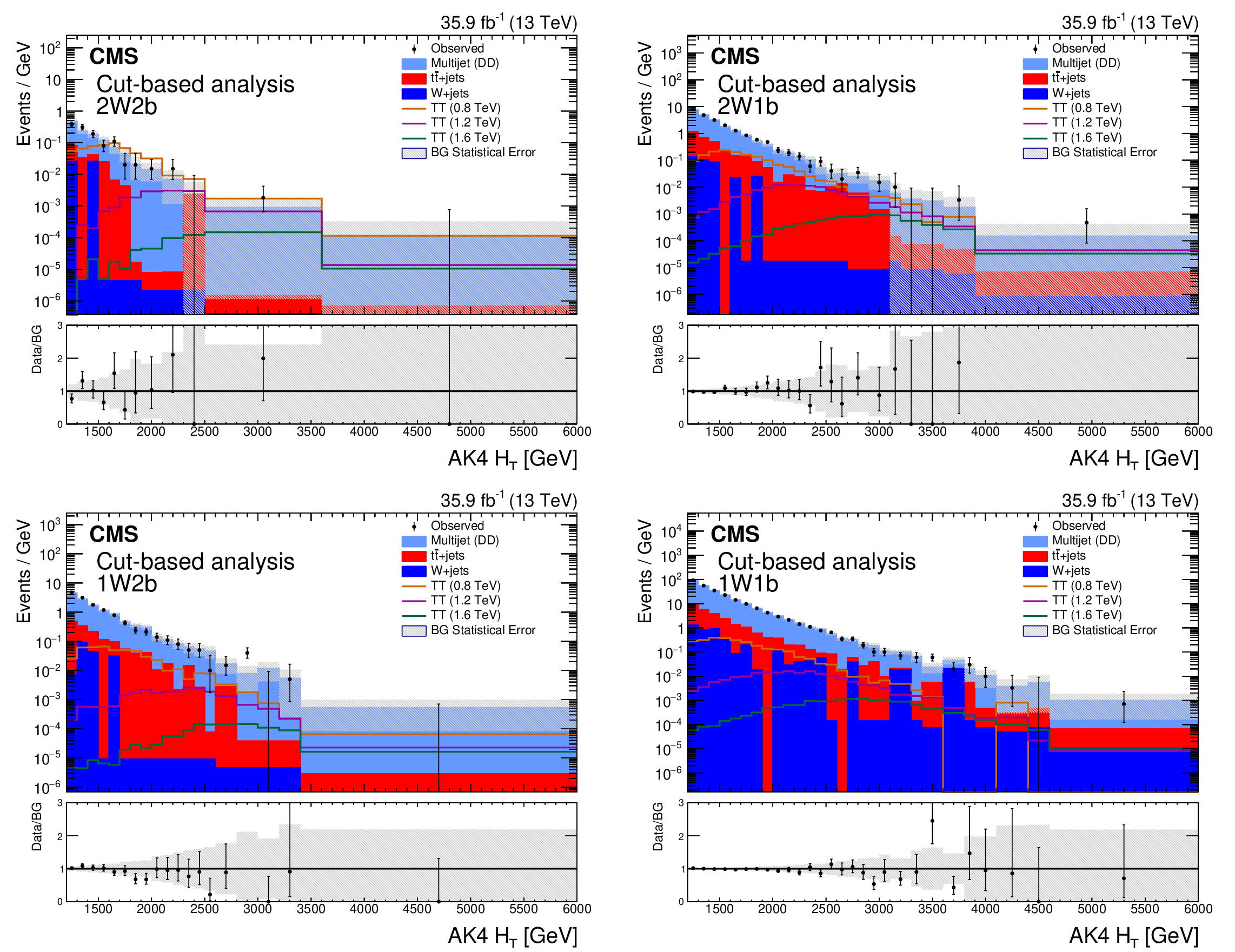
Figure 2:
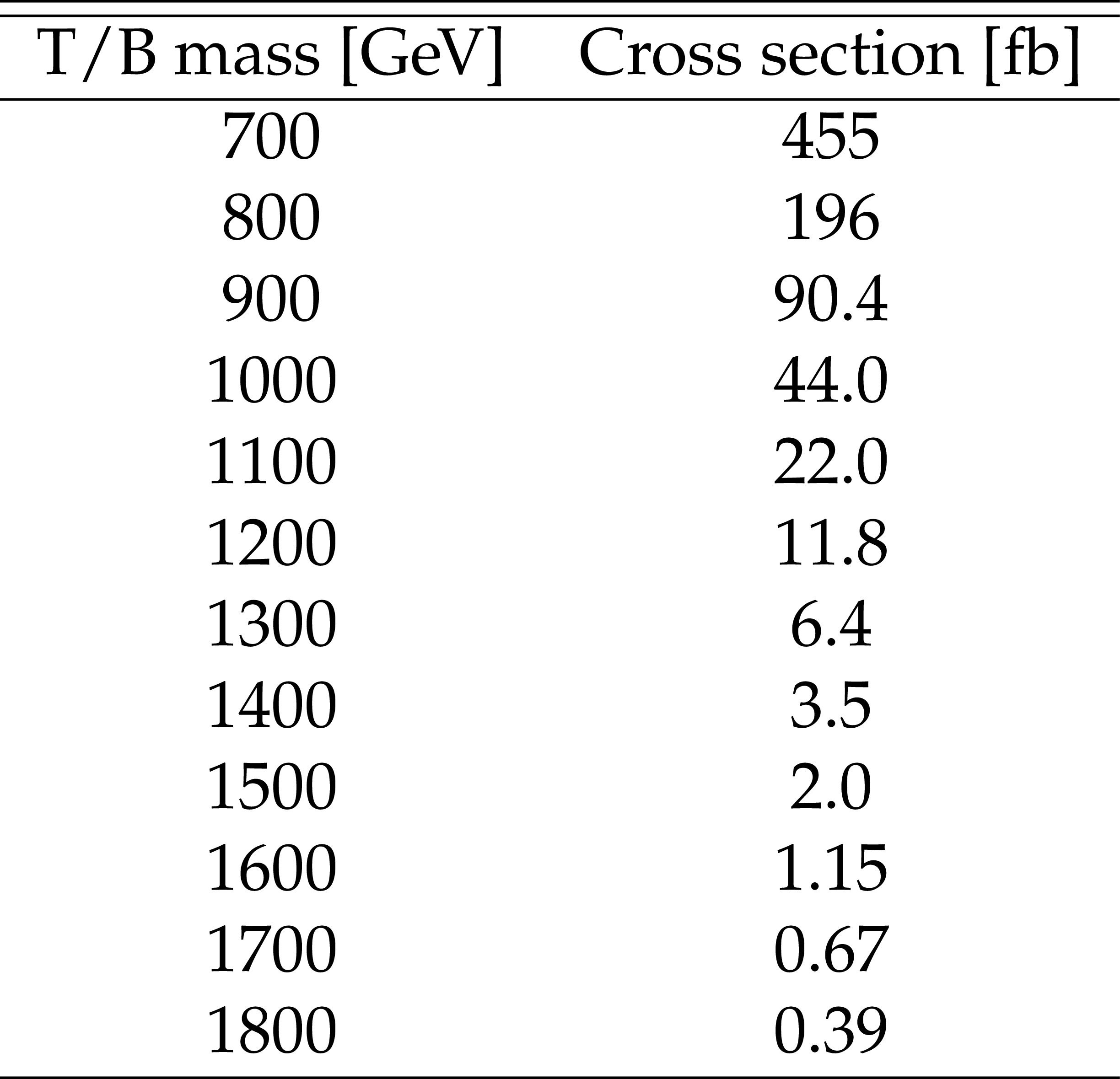
The distributions of ${{H_{\mathrm {T}}} ^{\mathrm {AK4}}}$ for each of the four signal region categories in the cut-based analysis. The upper row shows channels with 2W tags, and 2 or 1b tags, respectively. The lower row is for 1W tag. The shaded error band represents the statistical uncertainty in the background. These distributions reflect the nuisance parameters evaluated after a likelihood fit to a background plus signal hypothesis, where the hypothesized signal is a T quark with a mass of 1200 GeV and 100% branching fraction to bW. The signal distributions show the expected yield of events assuming the cross section values in Table 1. The vertical axis labels denote that bin contents in these distributions have been scaled by their corresponding bin widths. The lower panel of each plot shows the ratio of the observed number of events in a bin to the expected number. |
png pdf |
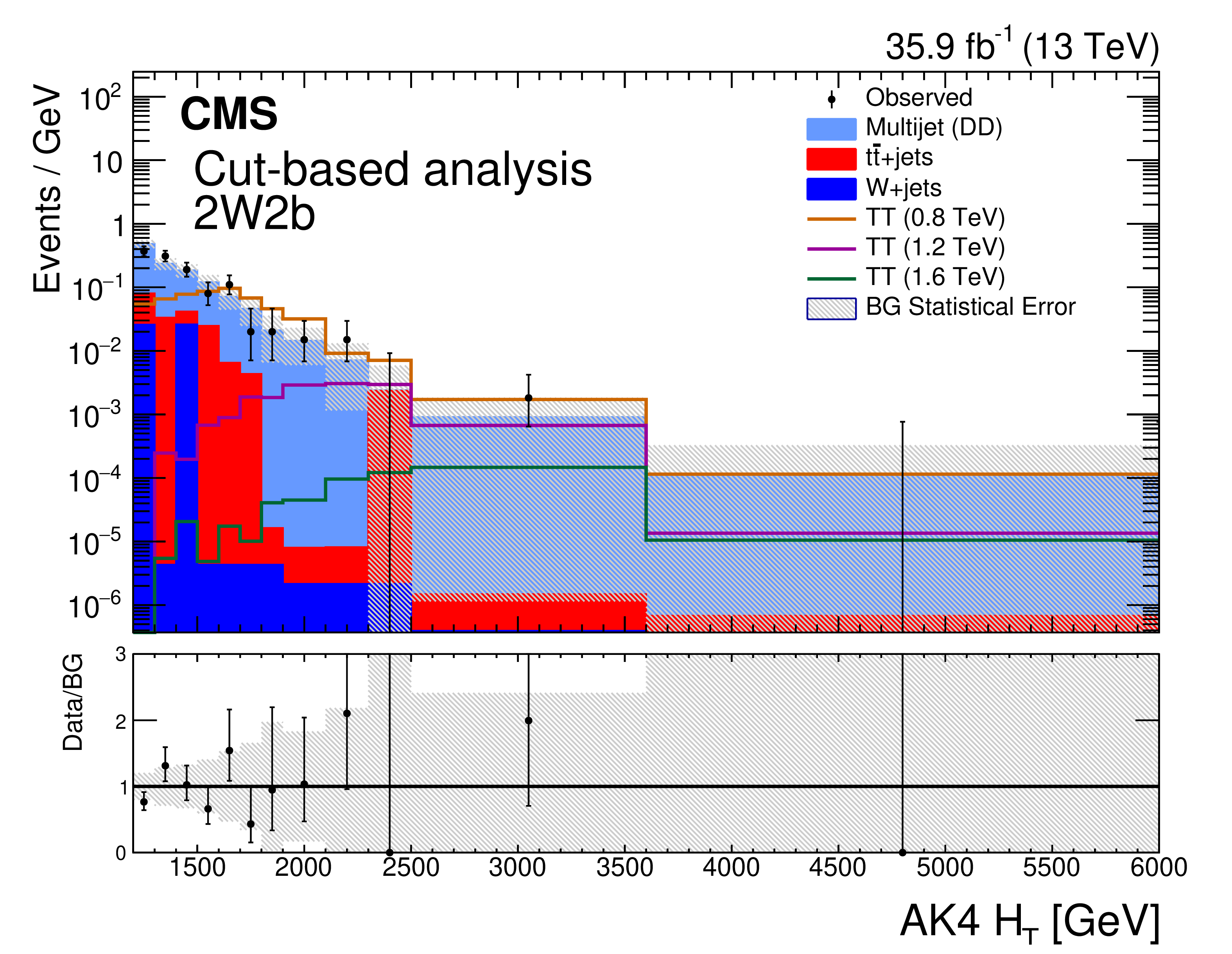
Figure 2-a:
The distribution of ${{H_{\mathrm {T}}} ^{\mathrm {AK4}}}$ for the 2W2b signal region category in the cut-based analysis. The shaded error band represents the statistical uncertainty in the background. These distributions reflect the nuisance parameters evaluated after a likelihood fit to a background plus signal hypothesis, where the hypothesized signal is a T quark with a mass of 1200 GeV and 100% branching fraction to bW. The signal distributions show the expected yield of events assuming the cross section values in Table 1. The vertical axis labels denote that bin contents in these distributions have been scaled by their corresponding bin widths. The lower panel shows the ratio of the observed number of events in a bin to the expected number. |

png pdf |
Figure 2-b:
The distribution of ${{H_{\mathrm {T}}} ^{\mathrm {AK4}}}$ for the 2W1b signal region category in the cut-based analysis. The shaded error band represents the statistical uncertainty in the background. These distributions reflect the nuisance parameters evaluated after a likelihood fit to a background plus signal hypothesis, where the hypothesized signal is a T quark with a mass of 1200 GeV and 100% branching fraction to bW. The signal distributions show the expected yield of events assuming the cross section values in Table 1. The vertical axis labels denote that bin contents in these distributions have been scaled by their corresponding bin widths. The lower panel shows the ratio of the observed number of events in a bin to the expected number. |
png pdf |
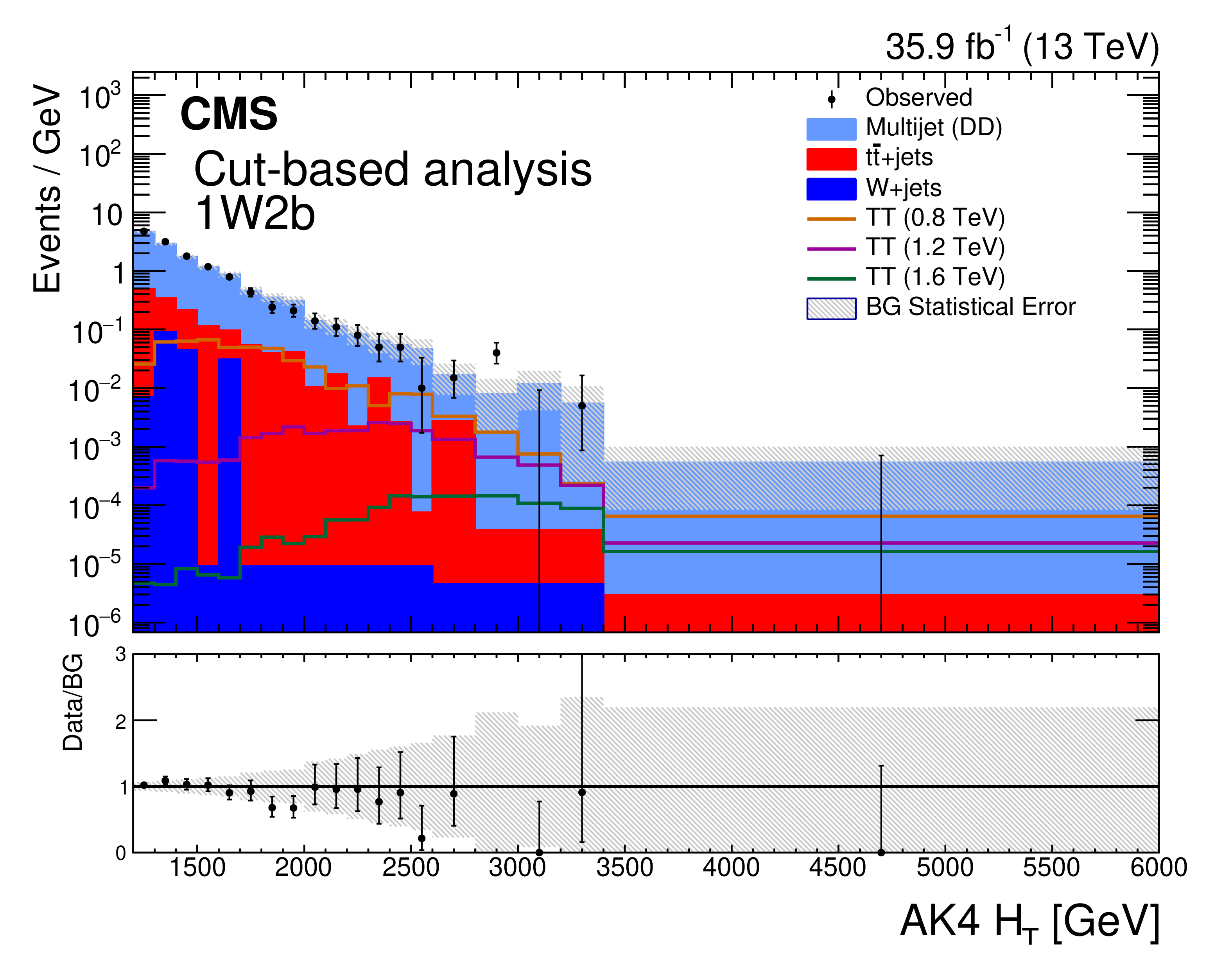
Figure 2-c:
The distribution of ${{H_{\mathrm {T}}} ^{\mathrm {AK4}}}$ for the 1W2b signal region category in the cut-based analysis. The shaded error band represents the statistical uncertainty in the background. These distributions reflect the nuisance parameters evaluated after a likelihood fit to a background plus signal hypothesis, where the hypothesized signal is a T quark with a mass of 1200 GeV and 100% branching fraction to bW. The signal distributions show the expected yield of events assuming the cross section values in Table 1. The vertical axis labels denote that bin contents in these distributions have been scaled by their corresponding bin widths. The lower panel shows the ratio of the observed number of events in a bin to the expected number. |

png pdf |
Figure 2-d:
The distribution of ${{H_{\mathrm {T}}} ^{\mathrm {AK4}}}$ for the 1W1b signal region category in the cut-based analysis. The shaded error band represents the statistical uncertainty in the background. These distributions reflect the nuisance parameters evaluated after a likelihood fit to a background plus signal hypothesis, where the hypothesized signal is a T quark with a mass of 1200 GeV and 100% branching fraction to bW. The signal distributions show the expected yield of events assuming the cross section values in Table 1. The vertical axis labels denote that bin contents in these distributions have been scaled by their corresponding bin widths. The lower panel shows the ratio of the observed number of events in a bin to the expected number. |
png pdf |
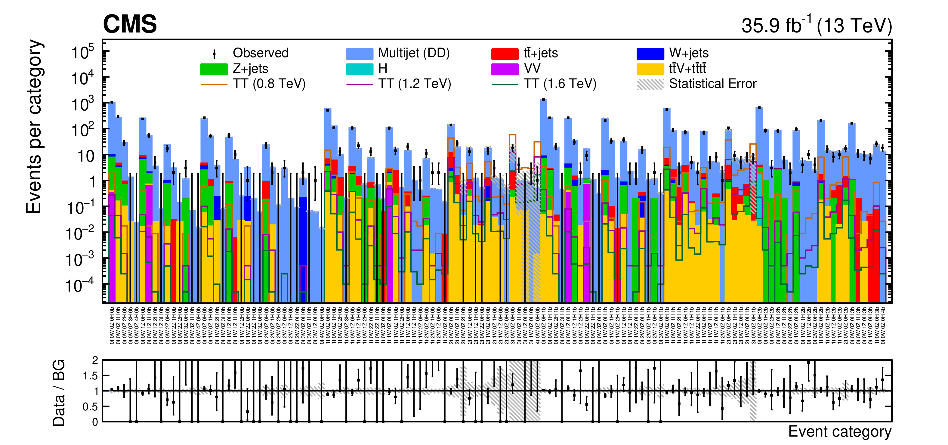
Figure 3:
A summary of the 126 signal region categories used in the NN analysis. This figure shows the expected yields in each category, while the signal discrimination is performed with the ${{H_{\mathrm {T}}} ^{\mathrm {AK8}}}$ distributions from each of the categories. The bottom panel shows the ratio of observed data to total background in each category, with Poisson error bars where applicable, along with the total background uncertainty shown for each category by the gray band. |
png pdf |
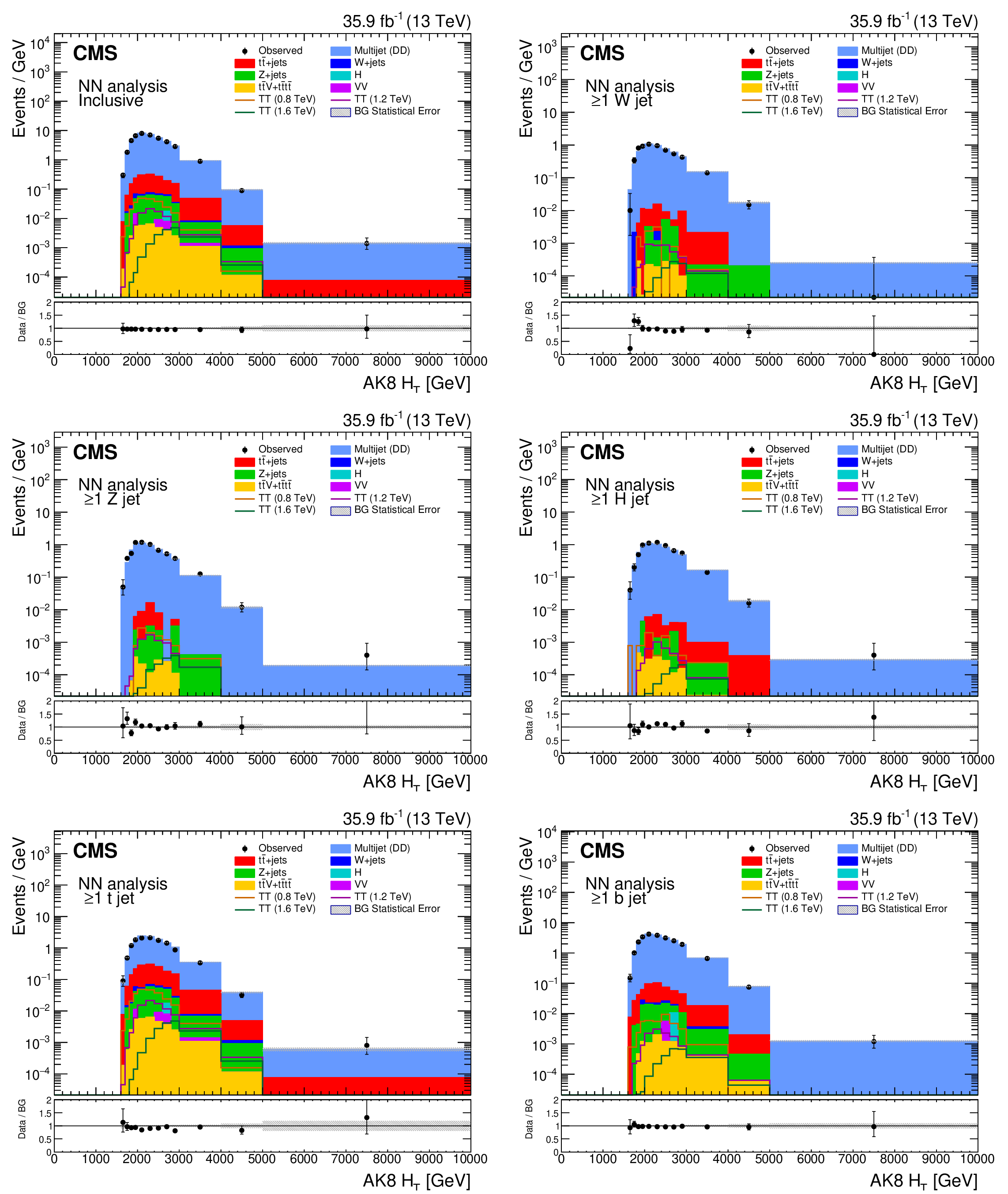
Figure 4:
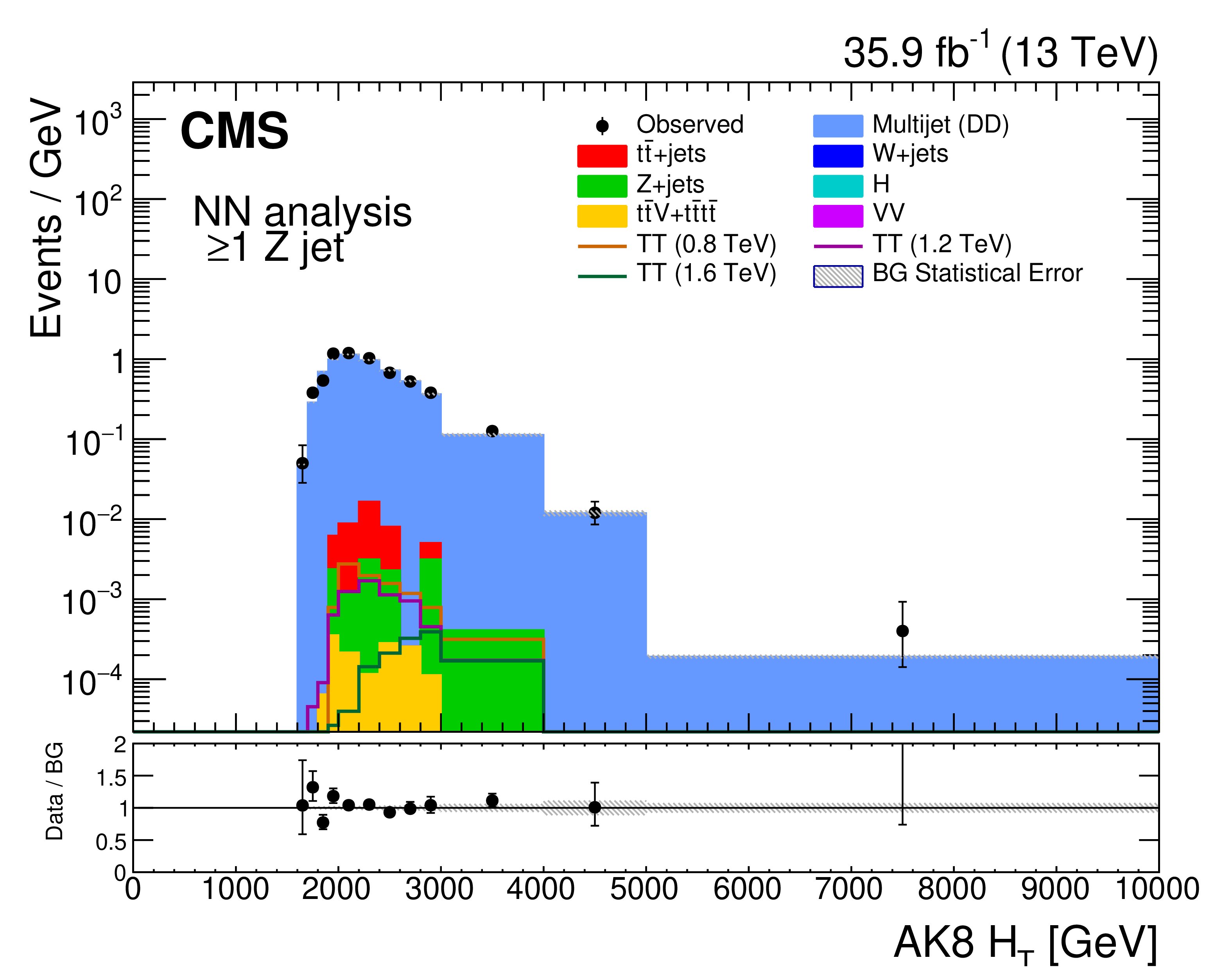
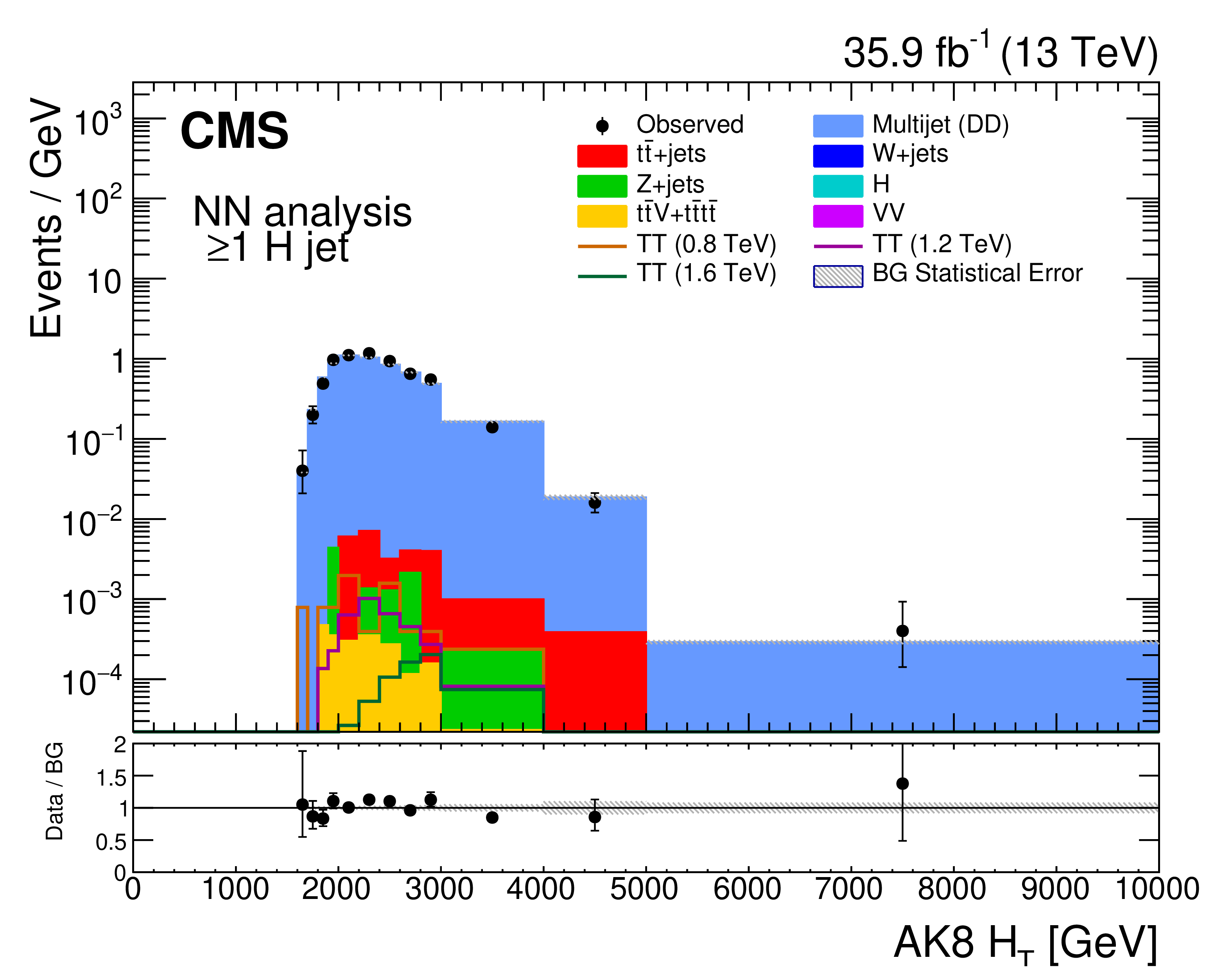
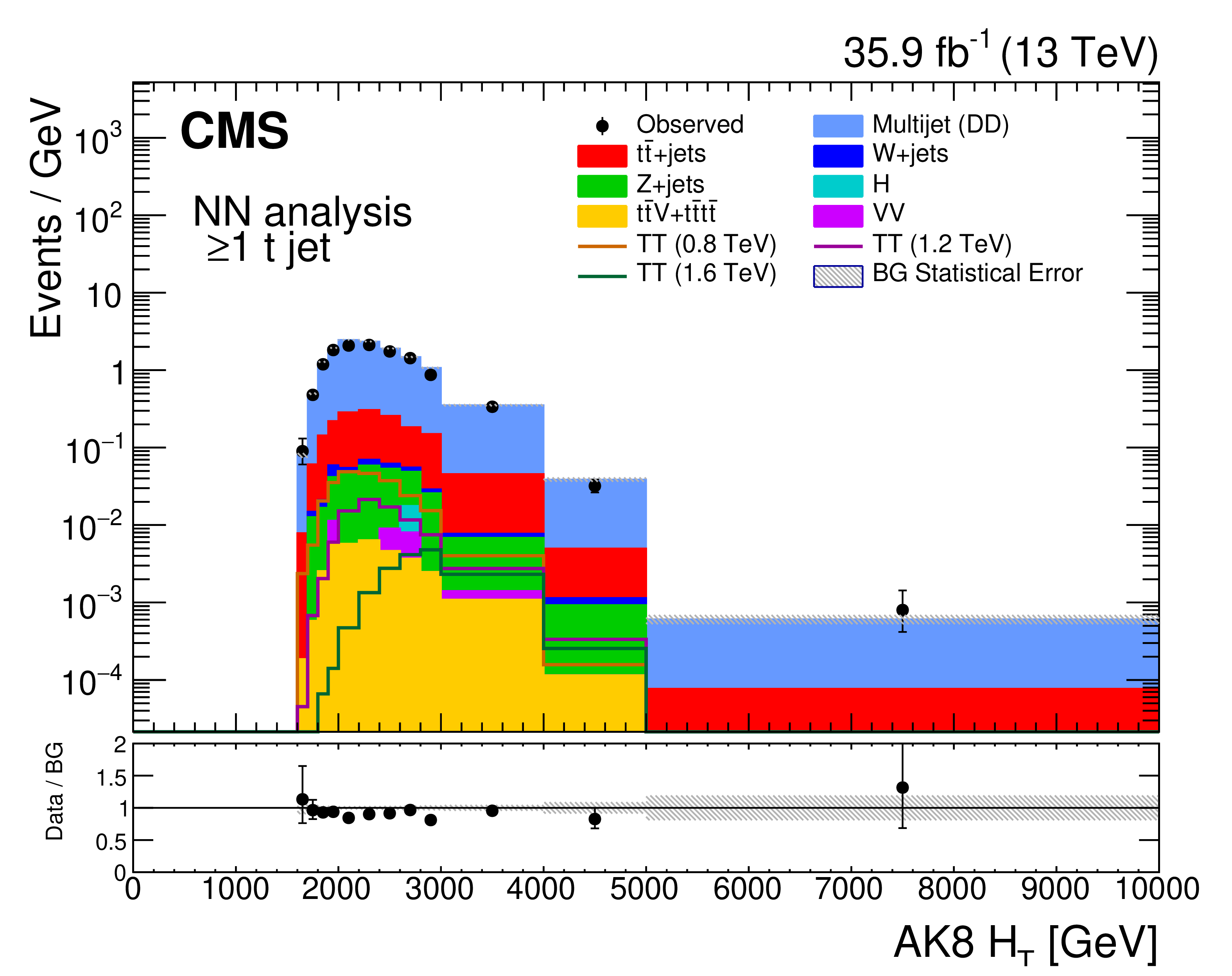
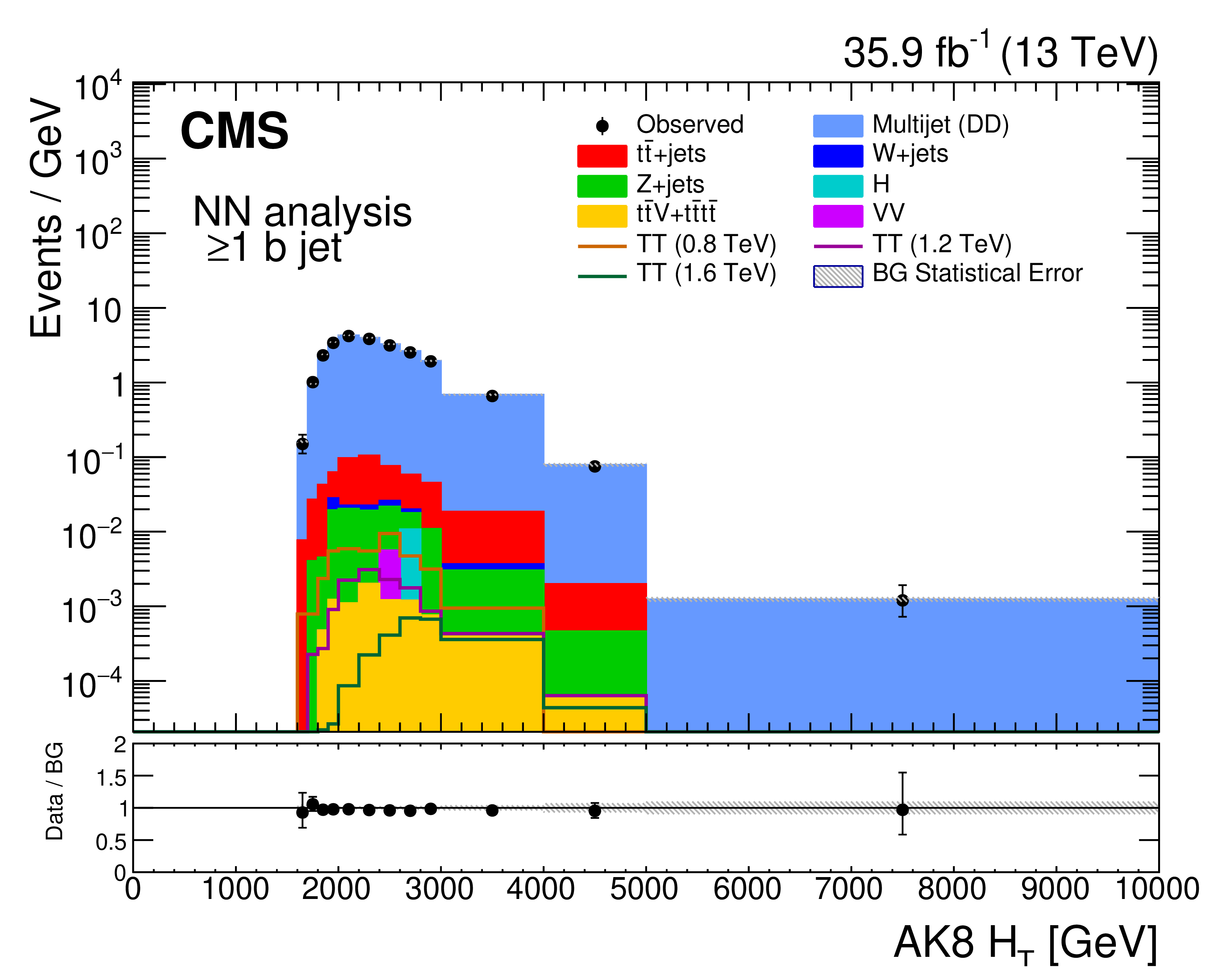
Distributions of ${{H_{\mathrm {T}}} ^{\mathrm {AK8}}}$ for all events entering the 126 signal regions of the NN analysis (upper left), as well as for only categories containing at least one candidate of each of the particle types identified by the BEST algorithm: $\geq $1W jet (upper right), $\geq $1Z jet (middle left), $\geq $1H jet (middle right), $\geq $1t jet (lower left), and $\geq $1b jet (lower right). The plots shown here are not mutually exclusive, as a particular signal region may satisfy several of the criteria for the individual summary categories. The vertical axis labels denote that bin contents in these distributions have been scaled by their corresponding bin widths. The lower panel of each plot shows the ratio of the observed number of events in a bin to the expected number. |
png pdf |
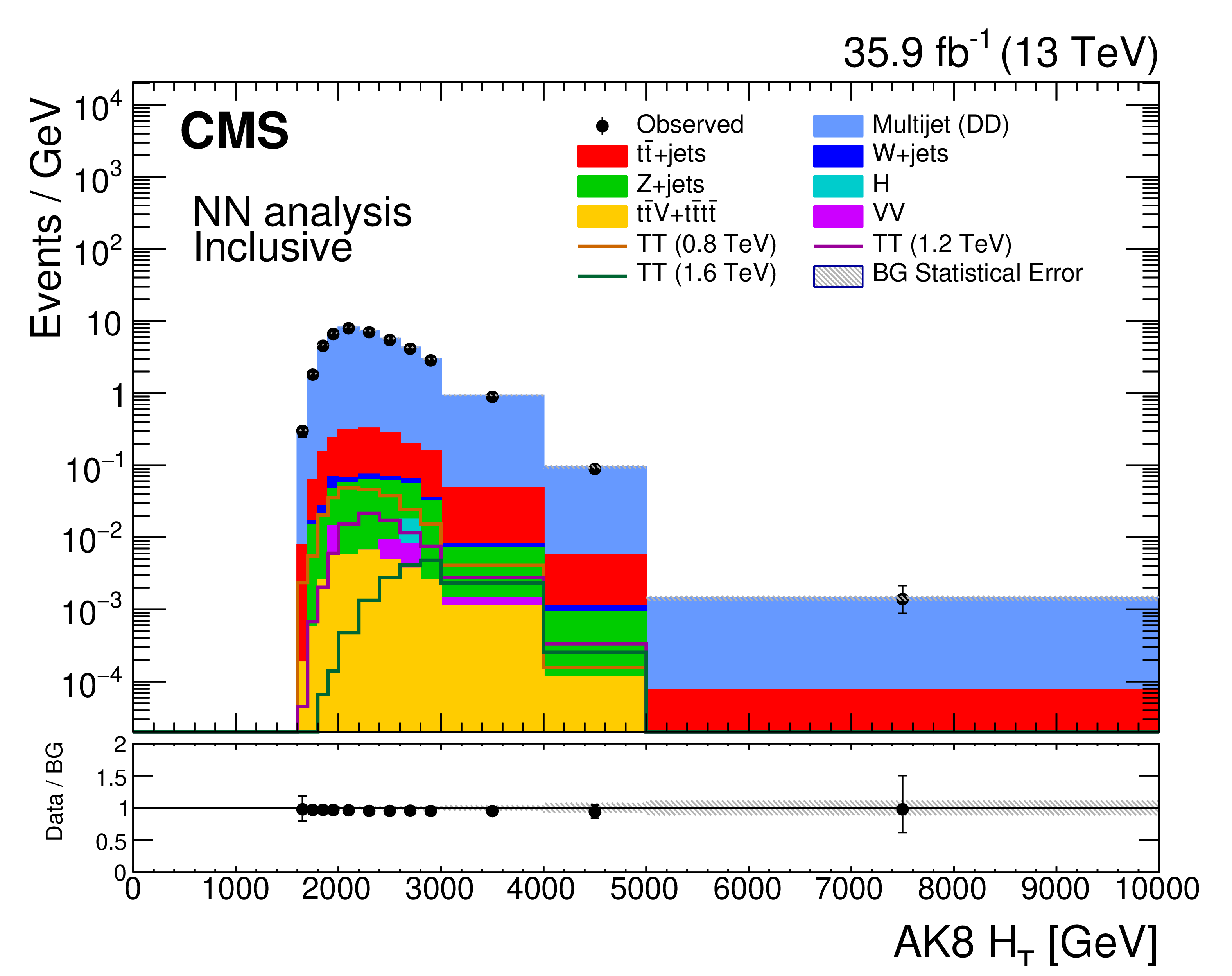
Figure 4-a:
Distribution of ${{H_{\mathrm {T}}} ^{\mathrm {AK8}}}$ for all events entering the 126 signal regions of the NN analysis. The vertical axis labels denote that bin contents in these distributions have been scaled by their corresponding bin widths. The lower panel shows the ratio of the observed number of events in a bin to the expected number. |
png pdf |
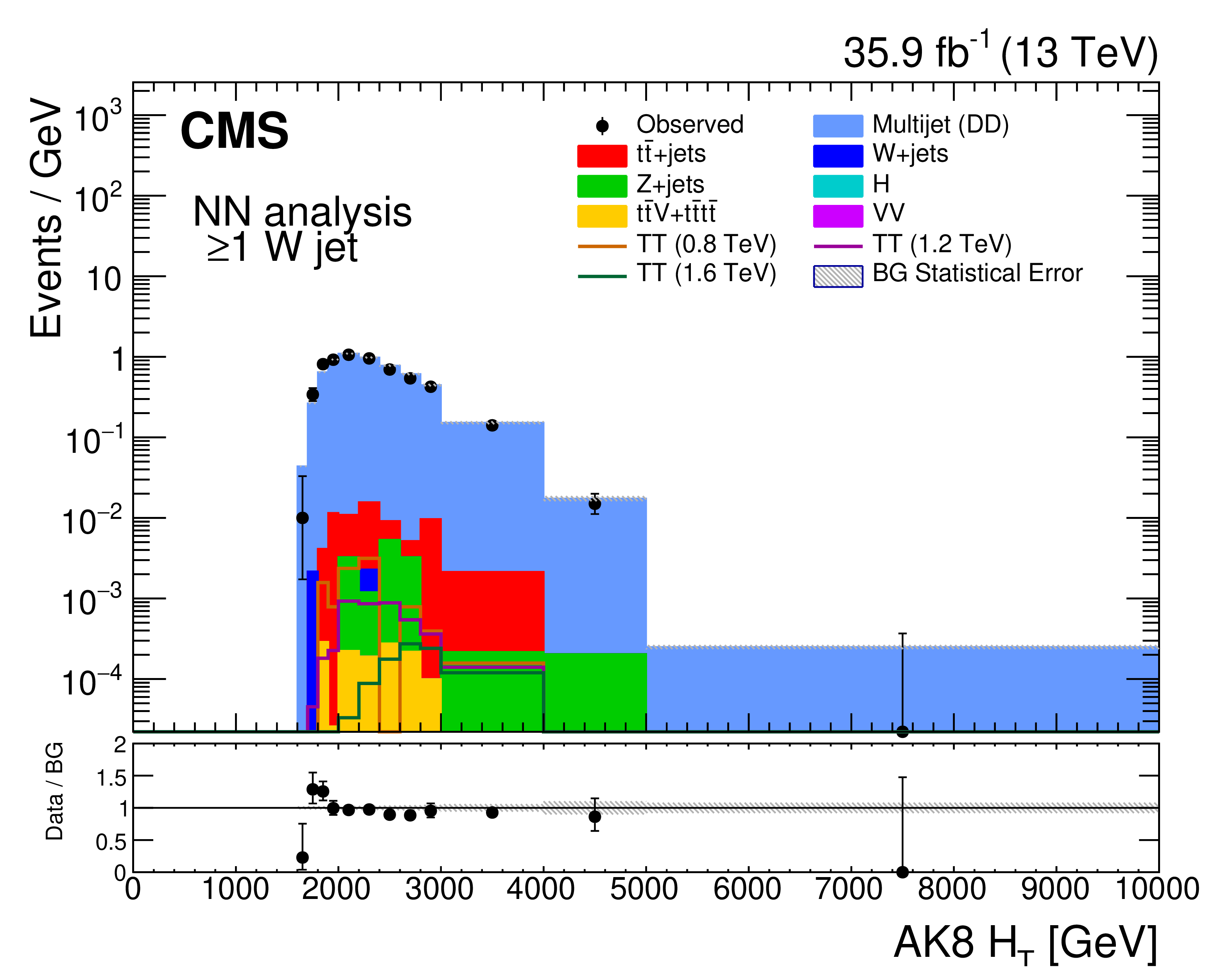
Figure 4-b:
Distribution of ${{H_{\mathrm {T}}} ^{\mathrm {AK8}}}$ for the $\geq $1W jet category, which contains at least one candidate of each of the particle types identified by the BEST algorithm. The vertical axis labels denote that bin contents in these distributions have been scaled by their corresponding bin widths. The lower panel shows the ratio of the observed number of events in a bin to the expected number. |
png pdf |
Figure 4-c:
Distribution of ${{H_{\mathrm {T}}} ^{\mathrm {AK8}}}$ for the $\geq $1Z jet category, which contains at least one candidate of each of the particle types identified by the BEST algorithm. The vertical axis labels denote that bin contents in these distributions have been scaled by their corresponding bin widths. The lower panel shows the ratio of the observed number of events in a bin to the expected number. |
png pdf |
Figure 4-d:
Distribution of ${{H_{\mathrm {T}}} ^{\mathrm {AK8}}}$ for the $\geq $1H jet category, which contains at least one candidate of each of the particle types identified by the BEST algorithm. The vertical axis labels denote that bin contents in these distributions have been scaled by their corresponding bin widths. The lower panel shows the ratio of the observed number of events in a bin to the expected number. |
png pdf |
Figure 4-e:
Distribution of ${{H_{\mathrm {T}}} ^{\mathrm {AK8}}}$ for the $\geq $1t jet category, which contains at least one candidate of each of the particle types identified by the BEST algorithm. The vertical axis labels denote that bin contents in these distributions have been scaled by their corresponding bin widths. The lower panel shows the ratio of the observed number of events in a bin to the expected number. |
png pdf |
Figure 4-f:
Distribution of ${{H_{\mathrm {T}}} ^{\mathrm {AK8}}}$ for the $\geq $1b jet category, which contains at least one candidate of each of the particle types identified by the BEST algorithm. The vertical axis labels denote that bin contents in these distributions have been scaled by their corresponding bin widths. The lower panel shows the ratio of the observed number of events in a bin to the expected number. |
png pdf |
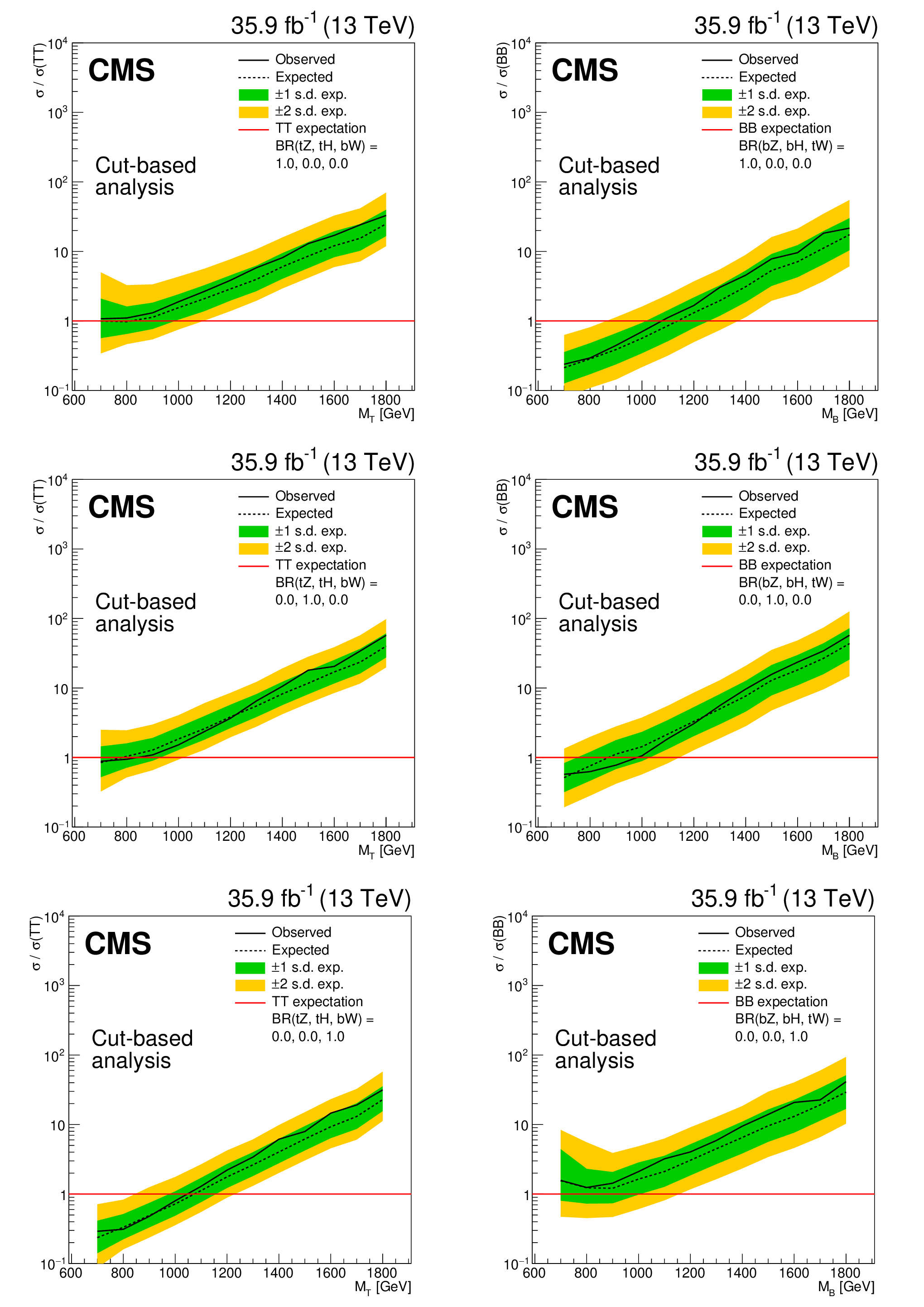
Figure 5:
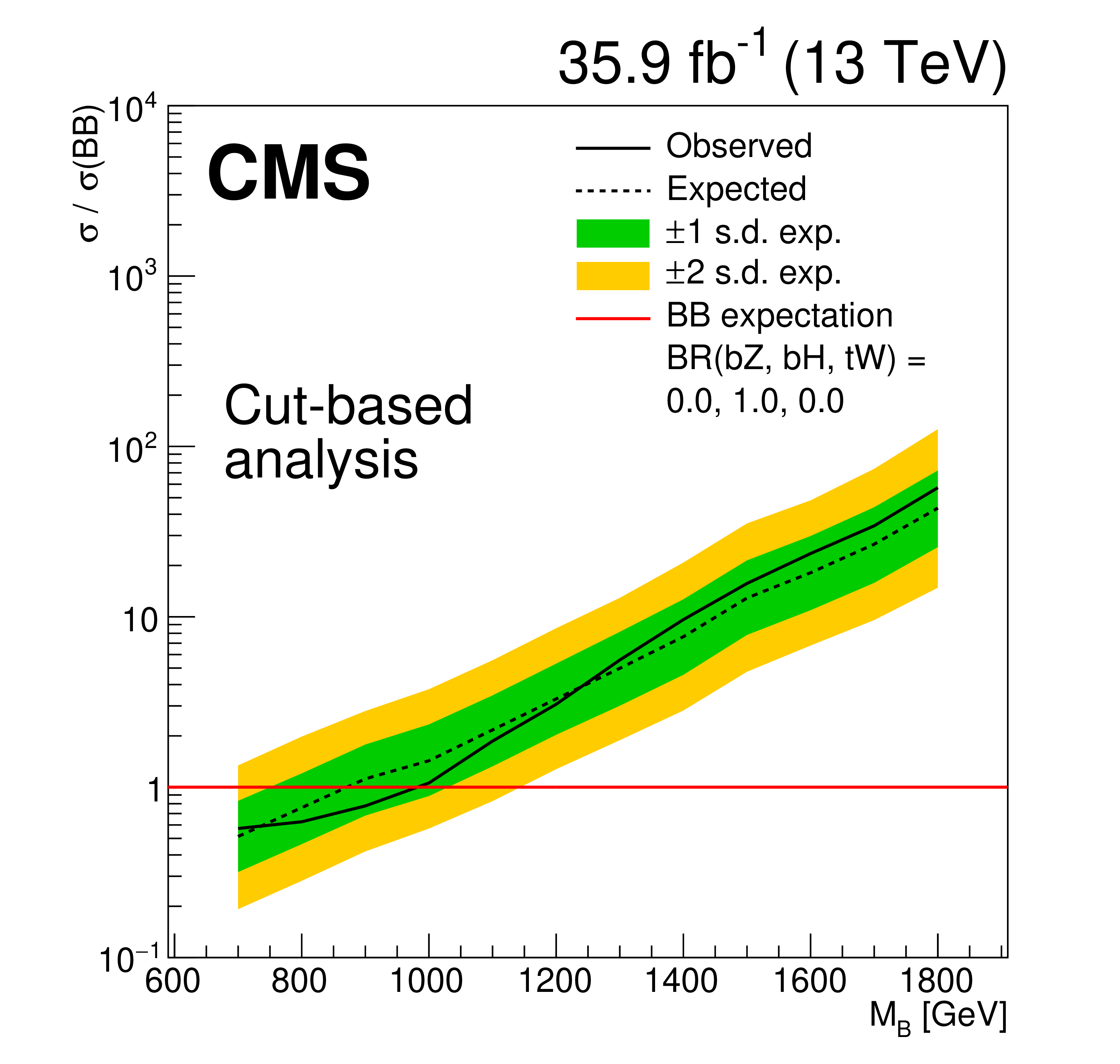
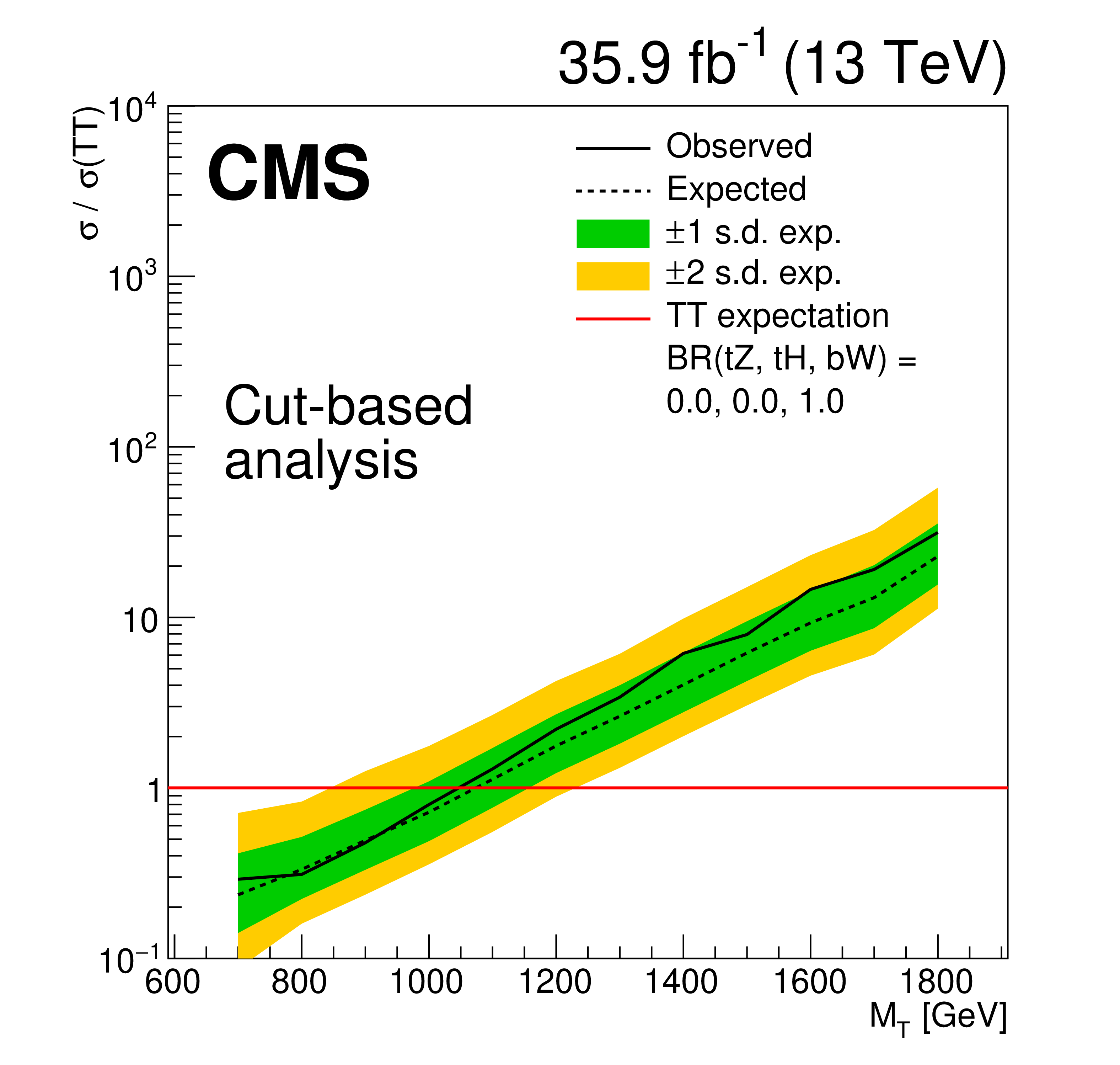
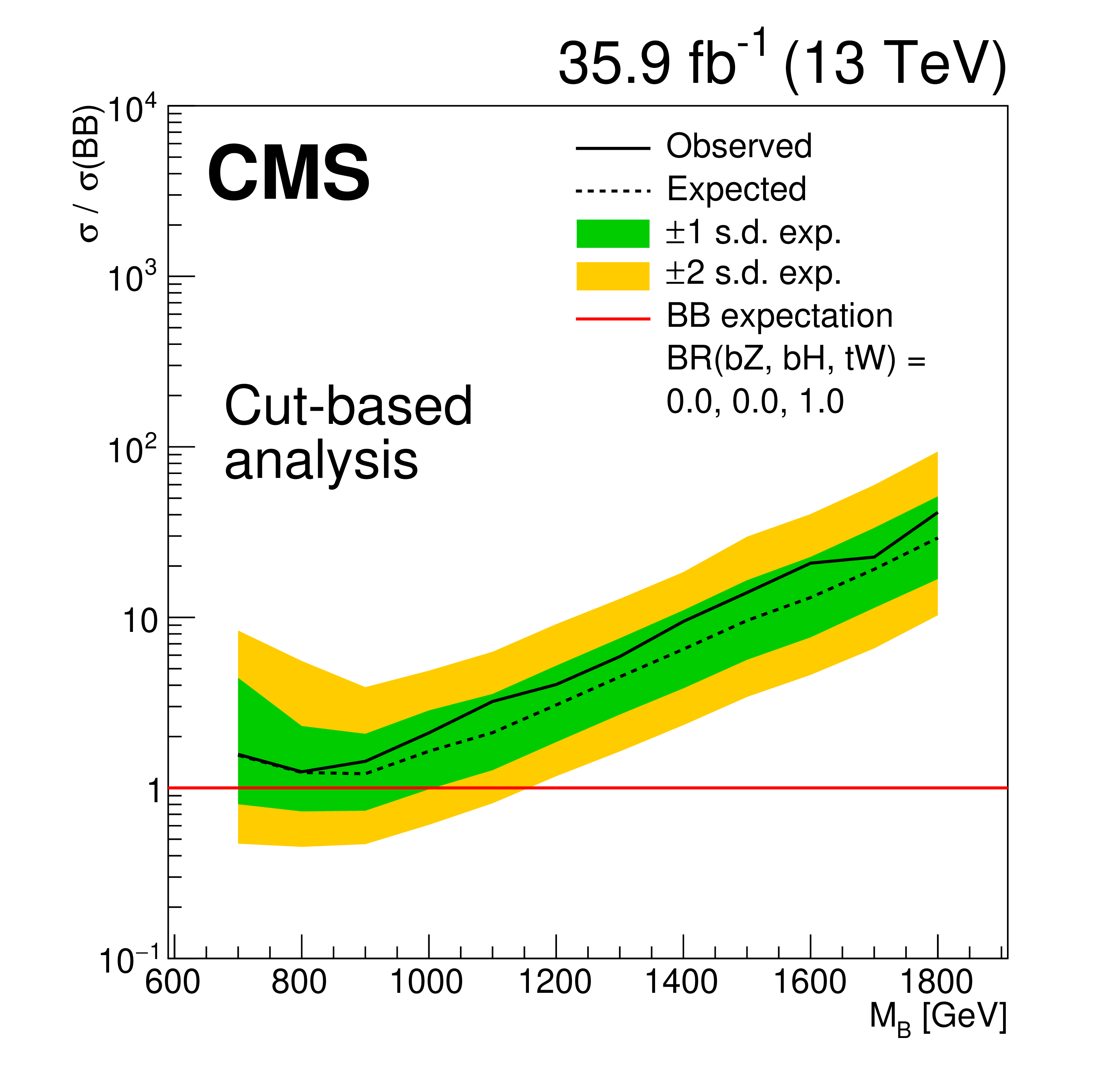
Limits at 95% confidence level on the ratio of the cross section to the theoretical cross section for pair production T quarks (left) and B quarks (right) in the cut-based analysis, with decays solely to $\mathrm{t} {}\mathrm{Z} {}/\mathrm{b} {}\mathrm{Z}$ (upper), $\mathrm{t} {}\mathrm{H} {}/\mathrm{b} {}\mathrm{H} $ (middle), and $ \mathrm{b} {}\mathrm{W} {}/\mathrm{t} {}\mathrm{W} $ (lower). The solid black line shows the observed limit, while the dashed black line shows the median of the distribution of limits expected under the background-only hypothesis. The inner (green) band and the outer (yellow) band indicate the regions containing 68 and 95%, respectively, of the distribution of limits expected under the background-only hypothesis. |
png pdf |
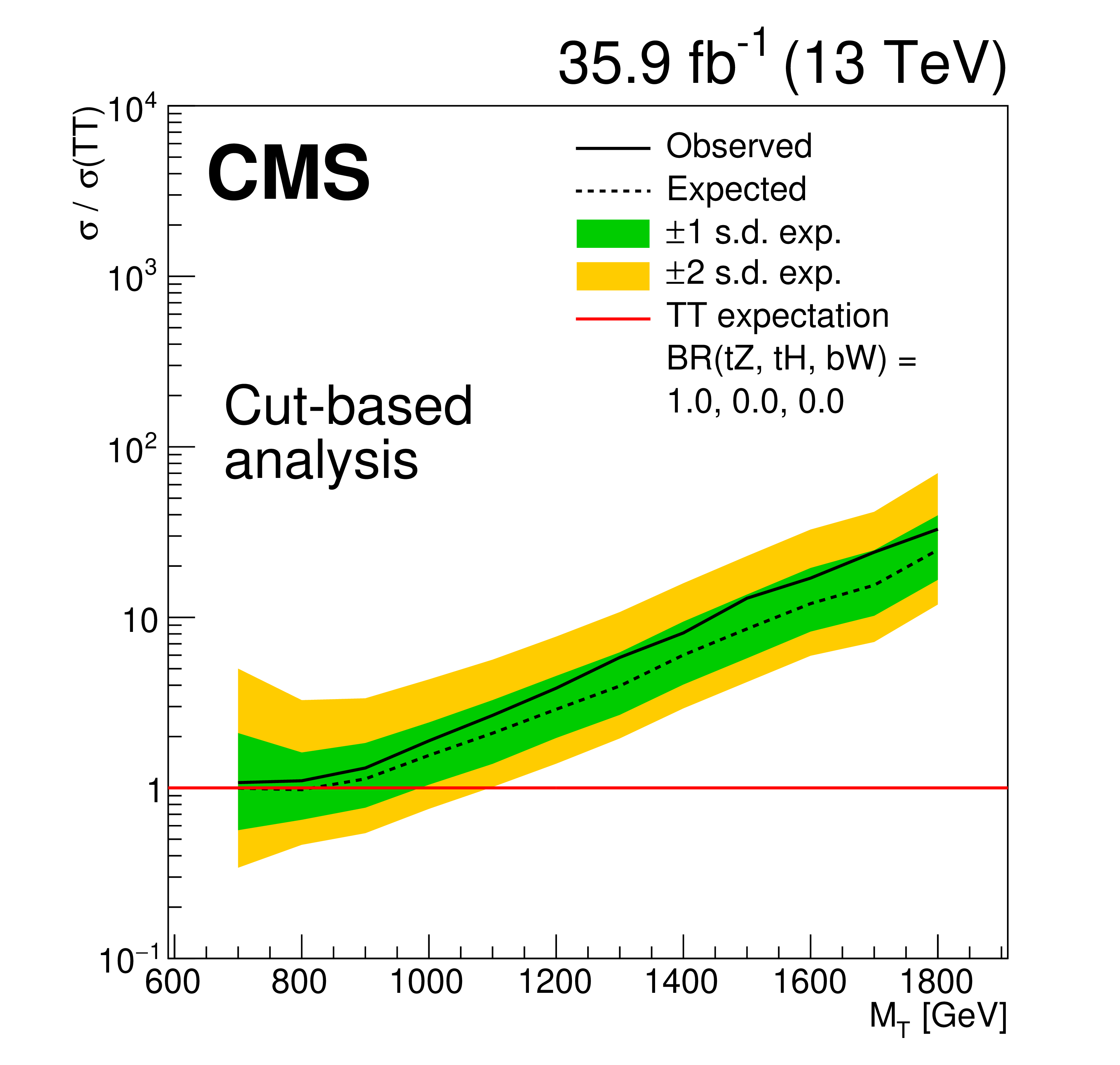
Figure 5-a:
Limits at 95% confidence level on the ratio of the cross section to the theoretical cross section for pair production T quarks in the cut-based analysis, with decays solely to $\mathrm{t} {}\mathrm{Z} {}/\mathrm{b} {}\mathrm{Z}$. The solid black line shows the observed limit, while the dashed black line shows the median of the distribution of limits expected under the background-only hypothesis. The inner (green) band and the outer (yellow) band indicate the regions containing 68 and 95%, respectively, of the distribution of limits expected under the background-only hypothesis. |
png pdf |
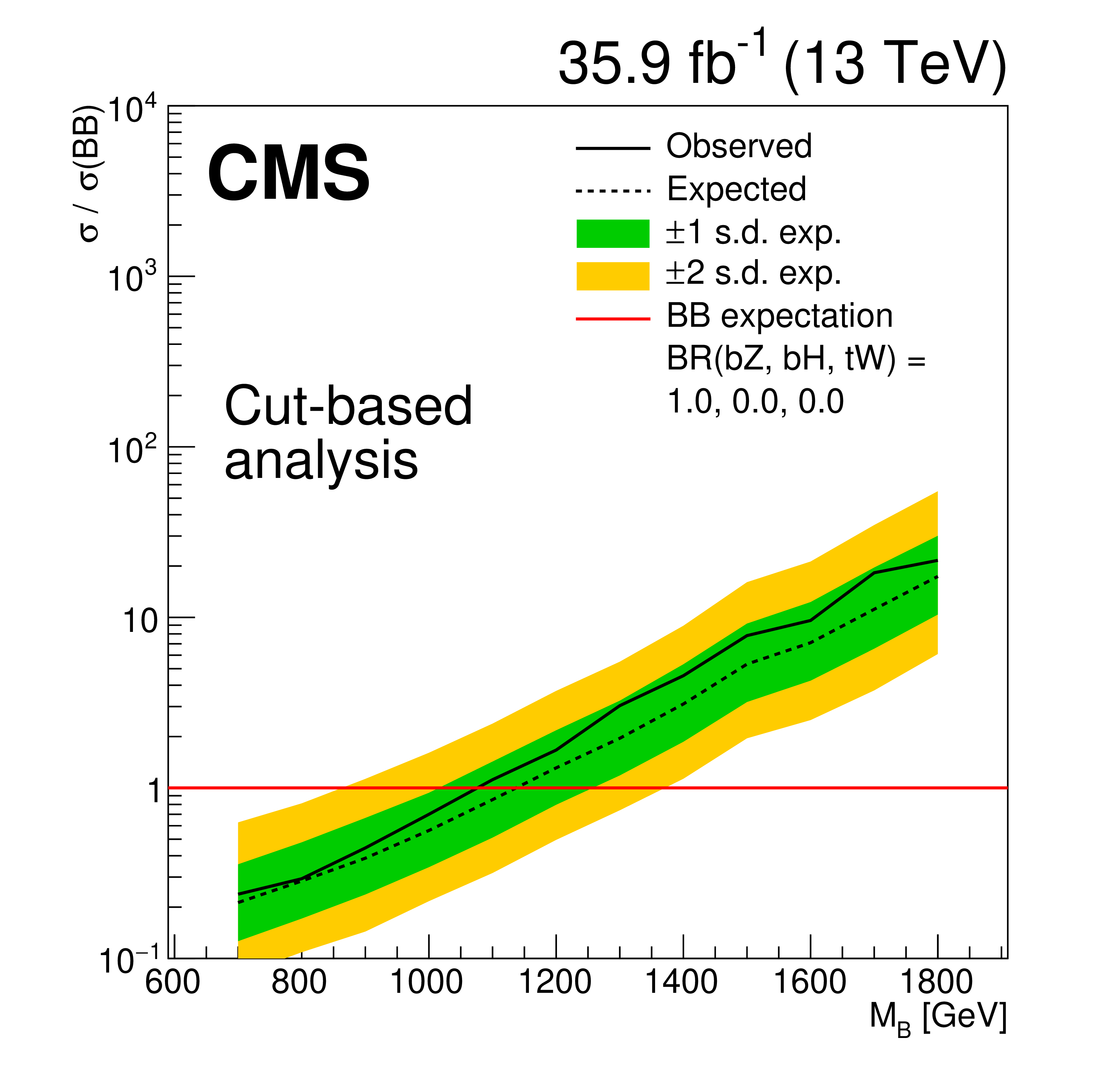
Figure 5-b:
Limits at 95% confidence level on the ratio of the cross section to the theoretical cross section for pair production B quarks in the cut-based analysis, with decays solely to $\mathrm{t} {}\mathrm{Z} {}/\mathrm{b} {}\mathrm{Z}$. The solid black line shows the observed limit, while the dashed black line shows the median of the distribution of limits expected under the background-only hypothesis. The inner (green) band and the outer (yellow) band indicate the regions containing 68 and 95%, respectively, of the distribution of limits expected under the background-only hypothesis. |
png pdf |
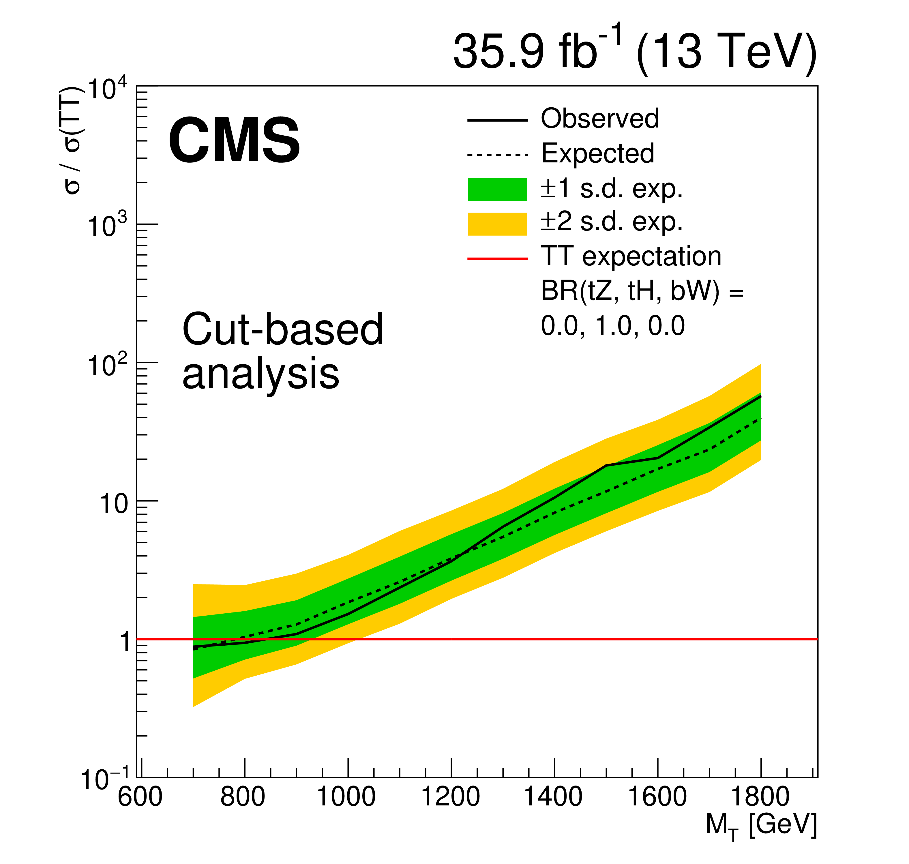
Figure 5-c:
Limits at 95% confidence level on the ratio of the cross section to the theoretical cross section for pair production T quarks in the cut-based analysis, with decays solely to $\mathrm{t} {}\mathrm{H} {}/\mathrm{b} {}\mathrm{H} $. The solid black line shows the observed limit, while the dashed black line shows the median of the distribution of limits expected under the background-only hypothesis. The inner (green) band and the outer (yellow) band indicate the regions containing 68 and 95%, respectively, of the distribution of limits expected under the background-only hypothesis. |
png pdf |
Figure 5-d:
Limits at 95% confidence level on the ratio of the cross section to the theoretical cross section for pair production B quarks in the cut-based analysis, with decays solely to $\mathrm{t} {}\mathrm{H} {}/\mathrm{b} {}\mathrm{H} $. The solid black line shows the observed limit, while the dashed black line shows the median of the distribution of limits expected under the background-only hypothesis. The inner (green) band and the outer (yellow) band indicate the regions containing 68 and 95%, respectively, of the distribution of limits expected under the background-only hypothesis. |
png pdf |
Figure 5-e:
Limits at 95% confidence level on the ratio of the cross section to the theoretical cross section for pair production T quarks in the cut-based analysis, with decays solely to $ \mathrm{b} {}\mathrm{W} {}/\mathrm{t} {}\mathrm{W} $. The solid black line shows the observed limit, while the dashed black line shows the median of the distribution of limits expected under the background-only hypothesis. The inner (green) band and the outer (yellow) band indicate the regions containing 68 and 95%, respectively, of the distribution of limits expected under the background-only hypothesis. |
png pdf |
Figure 5-f:
Limits at 95% confidence level on the ratio of the cross section to the theoretical cross section for pair production B quarks in the cut-based analysis, with decays solely to $ \mathrm{b} {}\mathrm{W} {}/\mathrm{t} {}\mathrm{W} $. The solid black line shows the observed limit, while the dashed black line shows the median of the distribution of limits expected under the background-only hypothesis. The inner (green) band and the outer (yellow) band indicate the regions containing 68 and 95%, respectively, of the distribution of limits expected under the background-only hypothesis. |
png pdf |
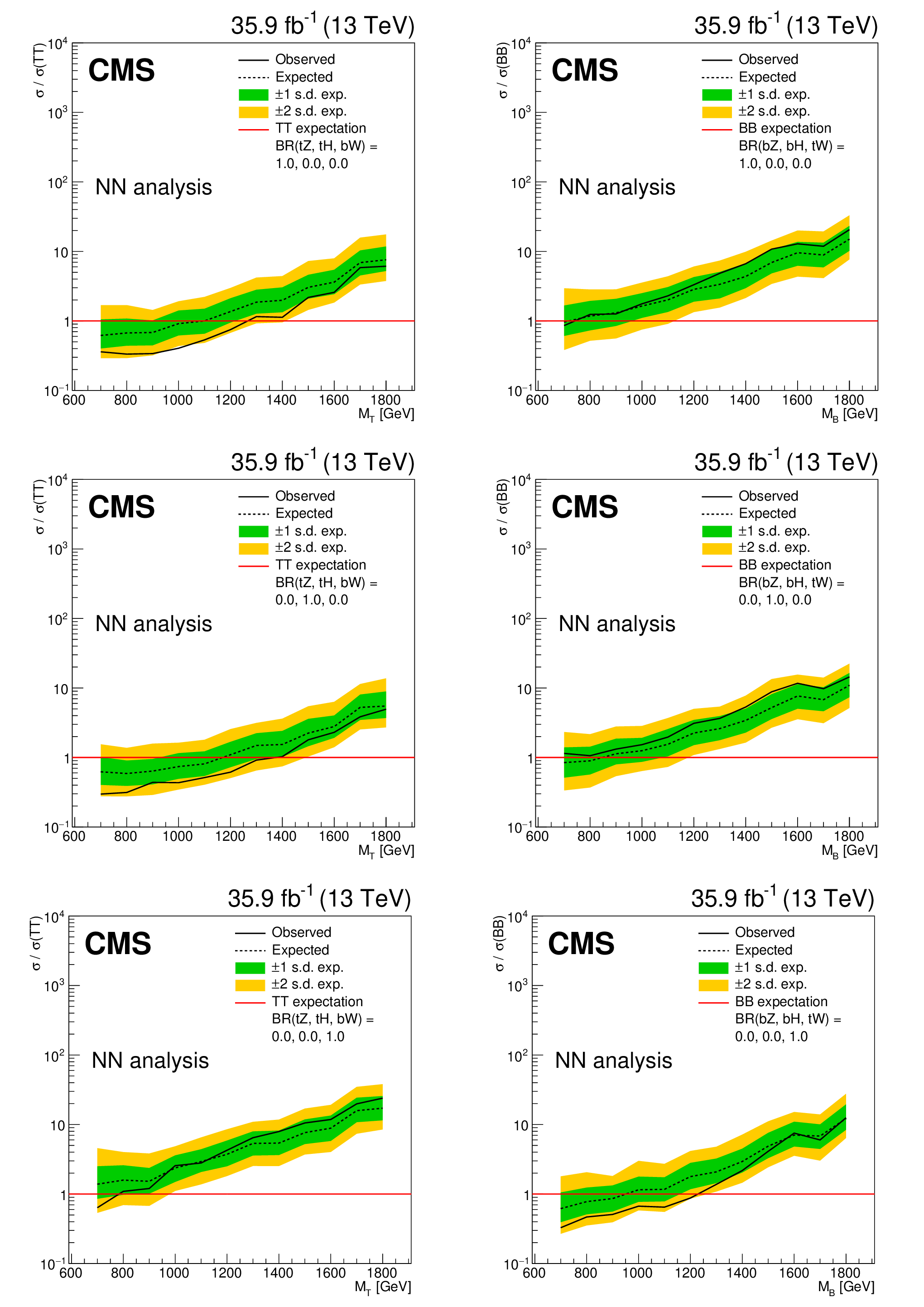
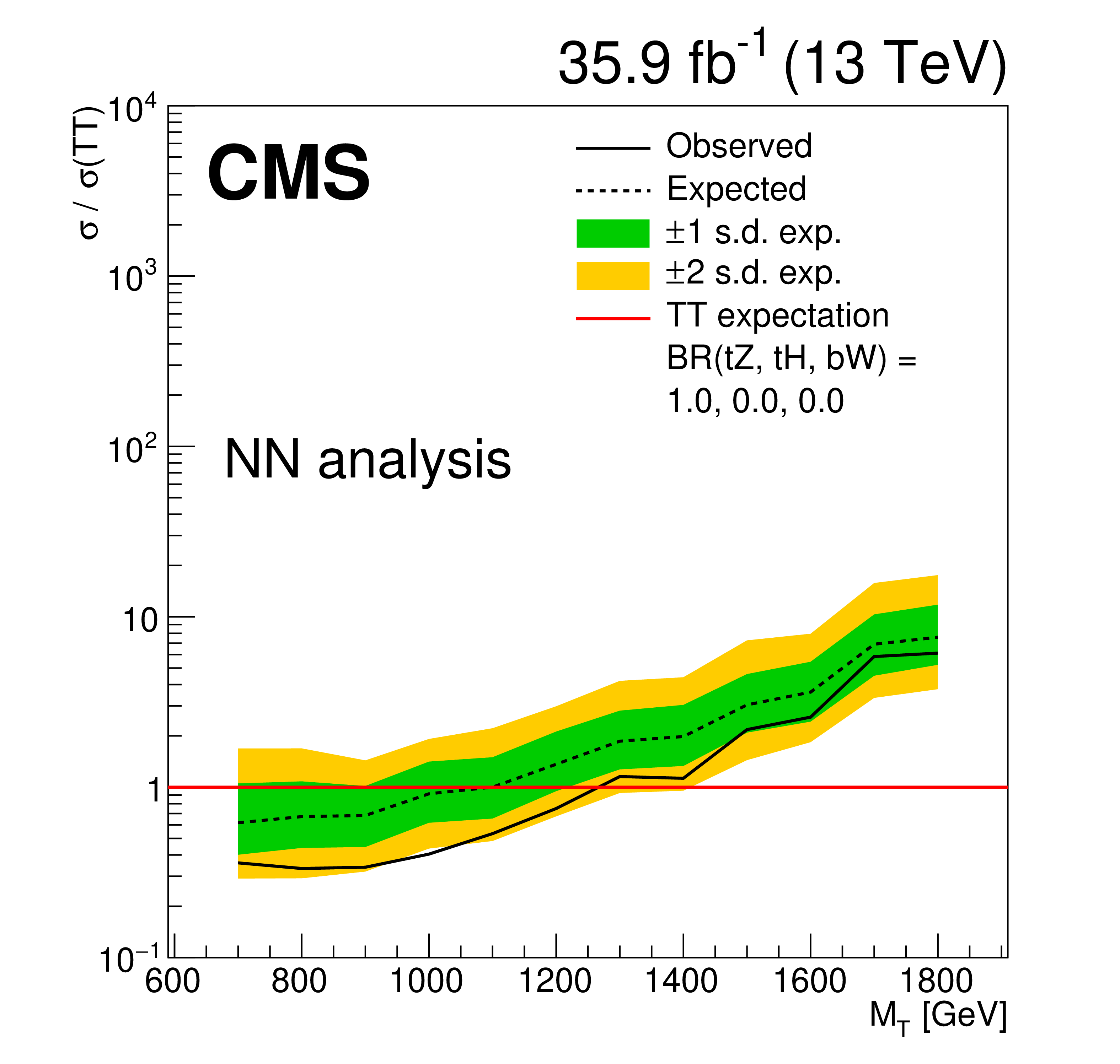
Figure 6:
Limits at 95% confidence level on the ratio of the cross section to the theoretical cross section for pair production T quarks (left) and B quarks (right) in the NN analysis, with decays solely to $\mathrm{t} {}\mathrm{Z} {}/\mathrm{b} {}\mathrm{Z}$ (upper), $\mathrm{t} {}\mathrm{H} {}/\mathrm{b} {}\mathrm{H} $ (middle), and $ \mathrm{b} {}\mathrm{W} {}/\mathrm{t} {}\mathrm{W} $ (lower). The solid black line shows the observed limit, while the dashed black line shows the median of the distribution of limits expected under the background-only hypothesis. The inner (green) band and the outer (yellow) band indicate the regions containing 68 and 95%, respectively, of the distribution of limits expected under the background-only hypothesis. |
png pdf |
Figure 6-a:
Limits at 95% confidence level on the ratio of the cross section to the theoretical cross section for pair production T quarks in the NN analysis, with decays solely to $\mathrm{t} {}\mathrm{Z} {}/\mathrm{b} {}\mathrm{Z}$. The solid black line shows the observed limit, while the dashed black line shows the median of the distribution of limits expected under the background-only hypothesis. The inner (green) band and the outer (yellow) band indicate the regions containing 68 and 95%, respectively, of the distribution of limits expected under the background-only hypothesis. |
png pdf |
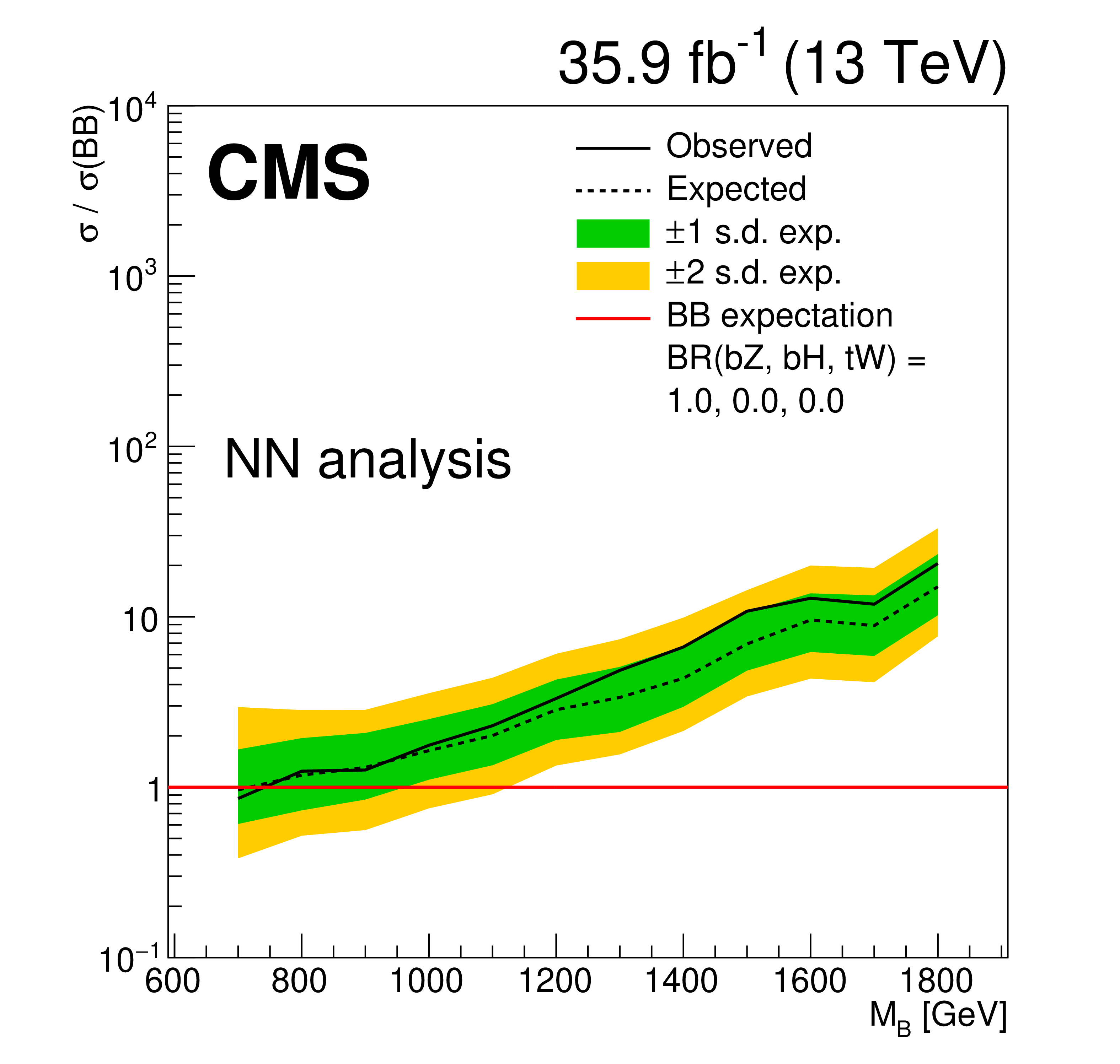
Figure 6-b:
Limits at 95% confidence level on the ratio of the cross section to the theoretical cross section for pair production B quarks in the NN analysis, with decays solely to $\mathrm{t} {}\mathrm{Z} {}/\mathrm{b} {}\mathrm{Z}$. The solid black line shows the observed limit, while the dashed black line shows the median of the distribution of limits expected under the background-only hypothesis. The inner (green) band and the outer (yellow) band indicate the regions containing 68 and 95%, respectively, of the distribution of limits expected under the background-only hypothesis. |

png pdf |
Figure 6-c:
Limits at 95% confidence level on the ratio of the cross section to the theoretical cross section for pair production T quarks in the NN analysis, with decays solely to $\mathrm{t} {}\mathrm{H} {}/\mathrm{b} {}\mathrm{H} $. The solid black line shows the observed limit, while the dashed black line shows the median of the distribution of limits expected under the background-only hypothesis. The inner (green) band and the outer (yellow) band indicate the regions containing 68 and 95%, respectively, of the distribution of limits expected under the background-only hypothesis. |

png pdf |
Figure 6-d:
Limits at 95% confidence level on the ratio of the cross section to the theoretical cross section for pair production B quarks in the NN analysis, with decays solely to $\mathrm{t} {}\mathrm{H} {}/\mathrm{b} {}\mathrm{H} $. The solid black line shows the observed limit, while the dashed black line shows the median of the distribution of limits expected under the background-only hypothesis. The inner (green) band and the outer (yellow) band indicate the regions containing 68 and 95%, respectively, of the distribution of limits expected under the background-only hypothesis. |
png pdf |
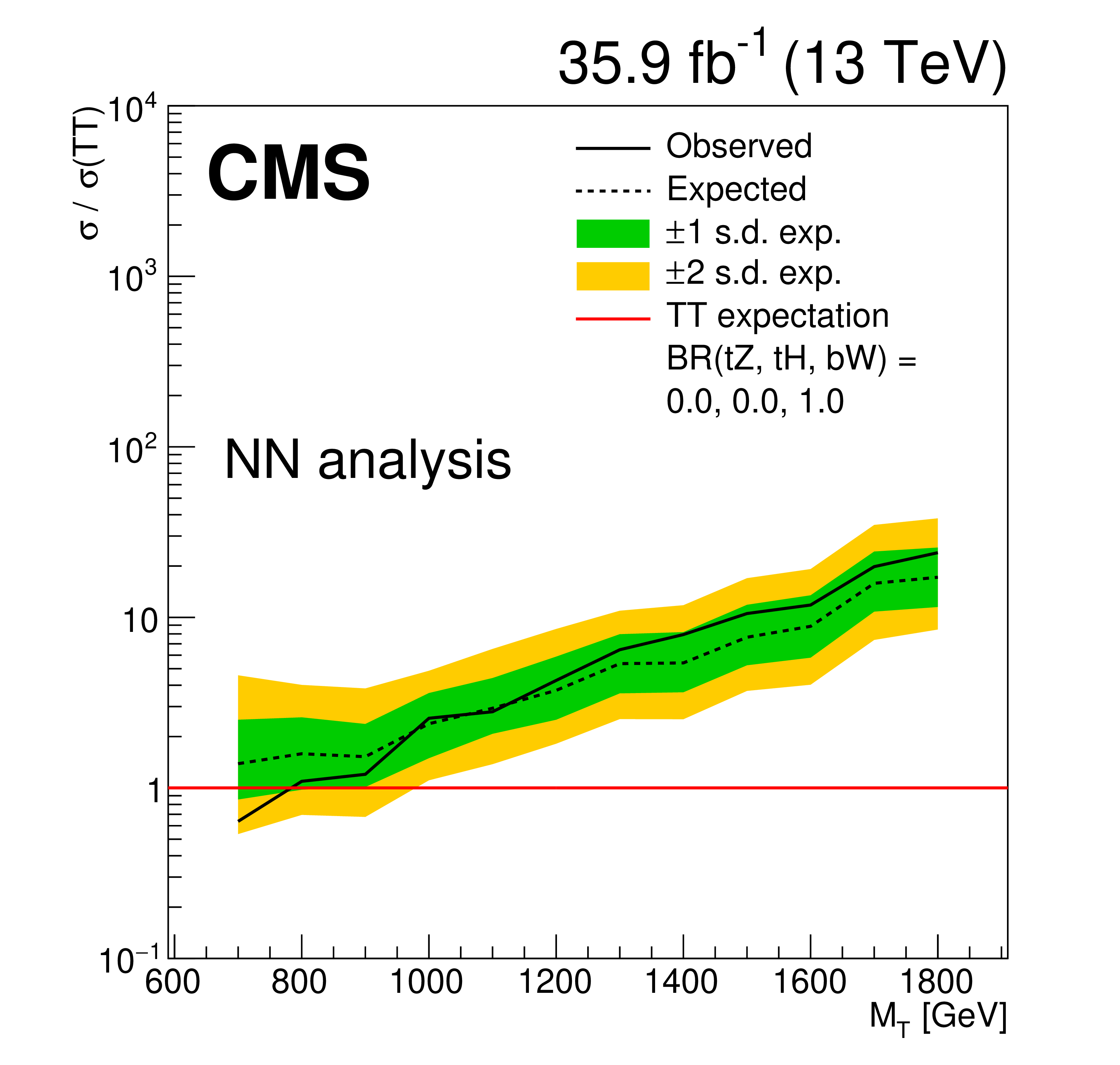
Figure 6-e:
Limits at 95% confidence level on the ratio of the cross section to the theoretical cross section for pair production T quarks in the NN analysis, with decays solely to $ \mathrm{b} {}\mathrm{W} {}/\mathrm{t} {}\mathrm{W} $. The solid black line shows the observed limit, while the dashed black line shows the median of the distribution of limits expected under the background-only hypothesis. The inner (green) band and the outer (yellow) band indicate the regions containing 68 and 95%, respectively, of the distribution of limits expected under the background-only hypothesis. |
png pdf |
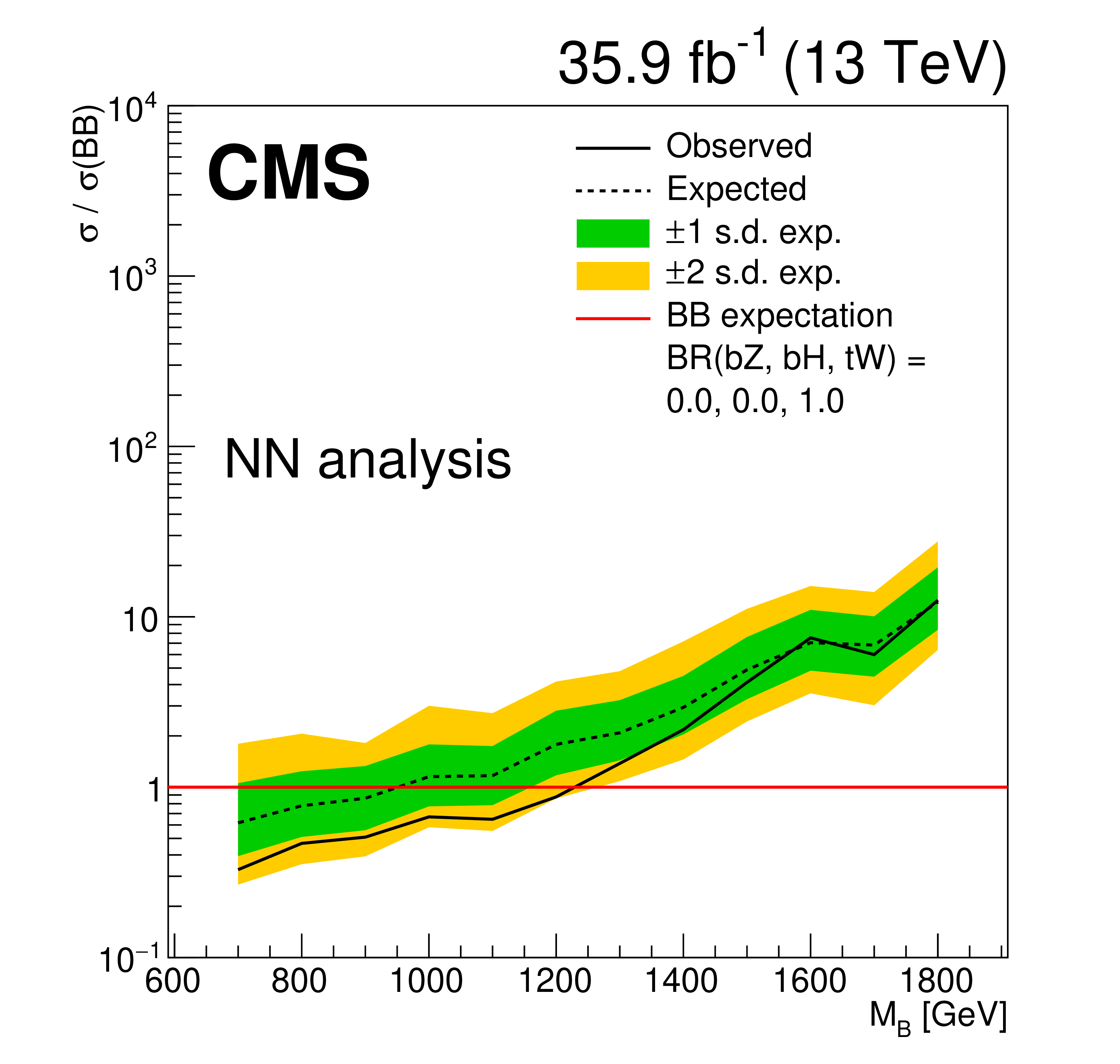
Figure 6-f:
Limits at 95% confidence level on the ratio of the cross section to the theoretical cross section for pair production B quarks in the NN analysis, with decays solely to $ \mathrm{b} {}\mathrm{W} {}/\mathrm{t} {}\mathrm{W} $. The solid black line shows the observed limit, while the dashed black line shows the median of the distribution of limits expected under the background-only hypothesis. The inner (green) band and the outer (yellow) band indicate the regions containing 68 and 95%, respectively, of the distribution of limits expected under the background-only hypothesis. |
png pdf |
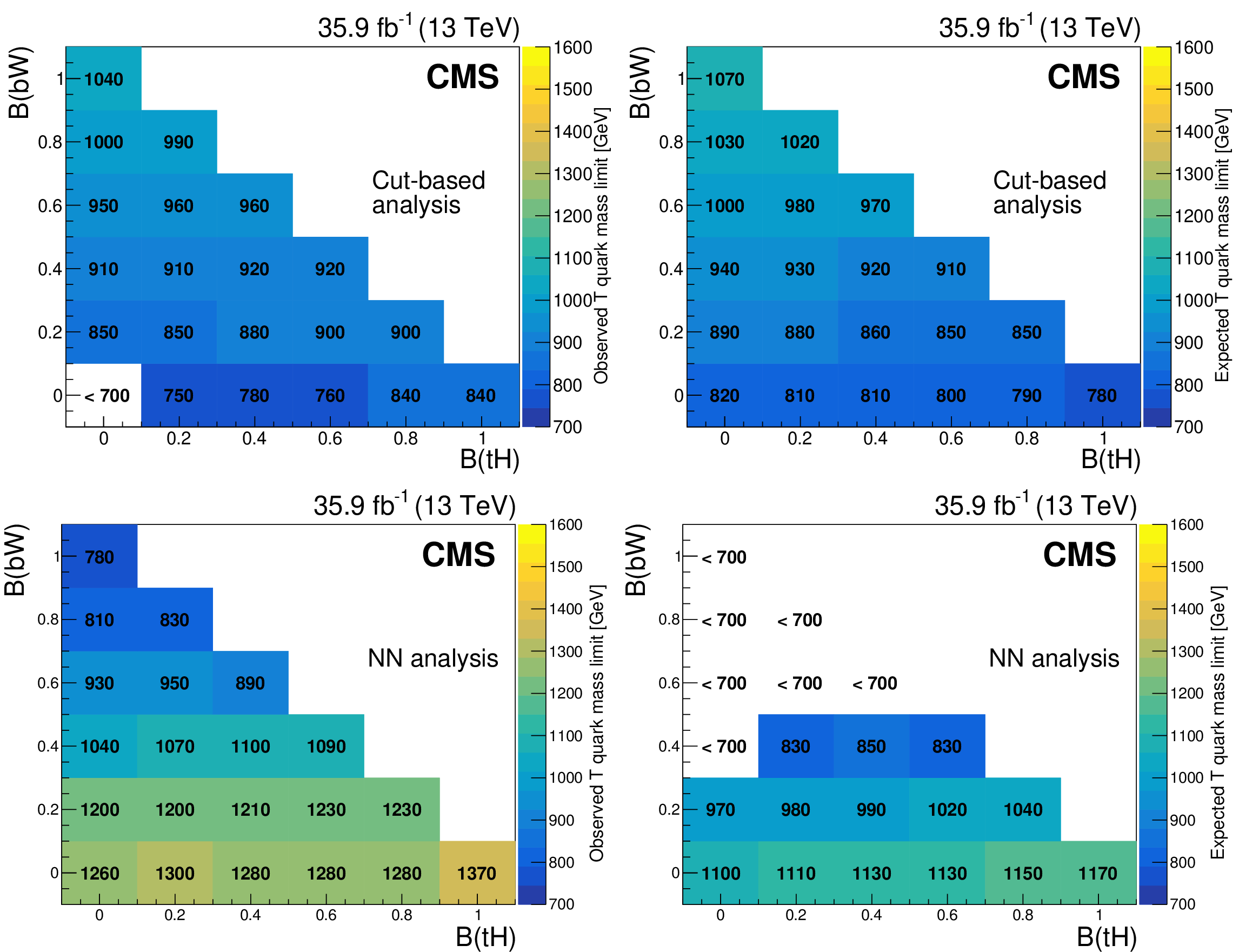
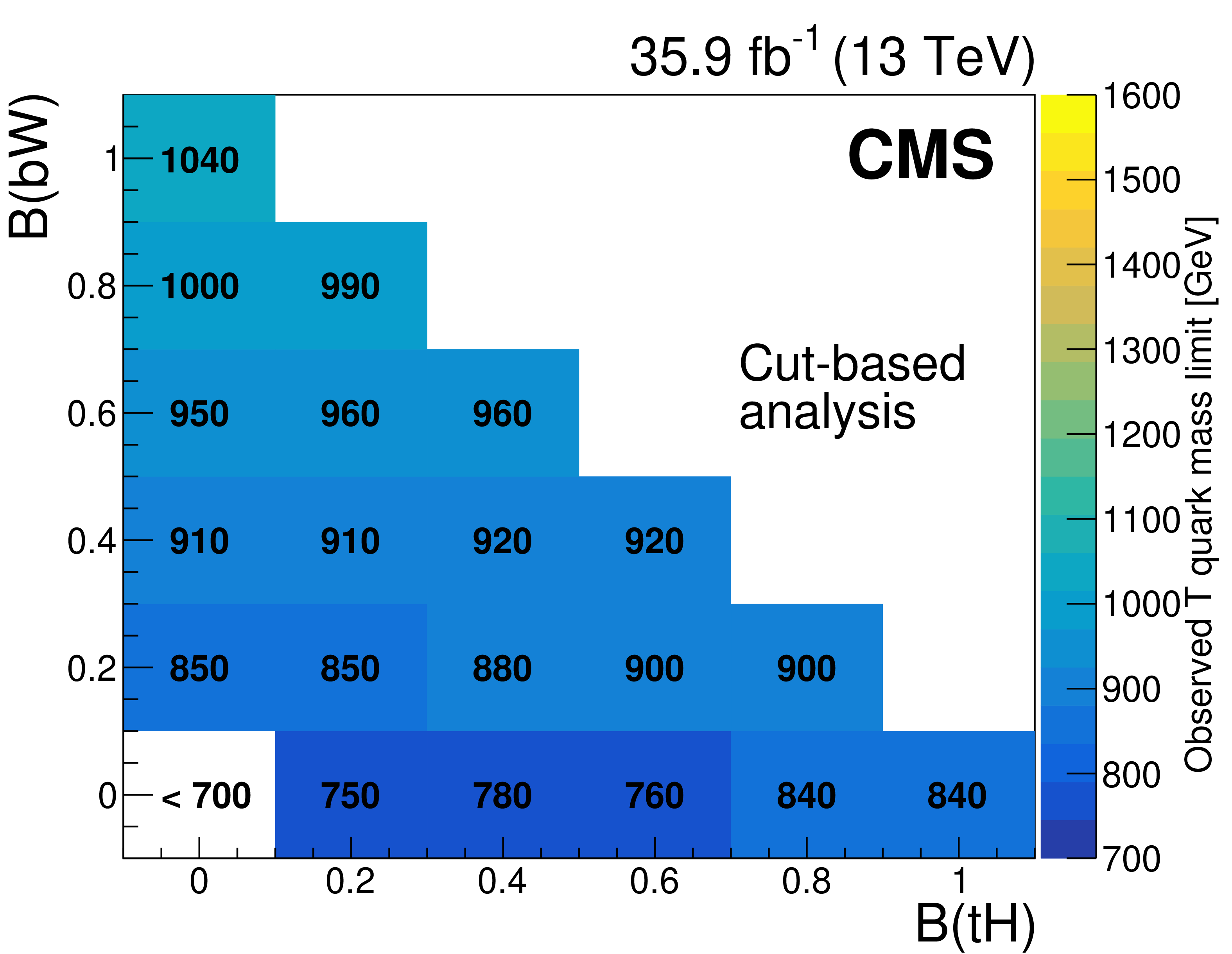
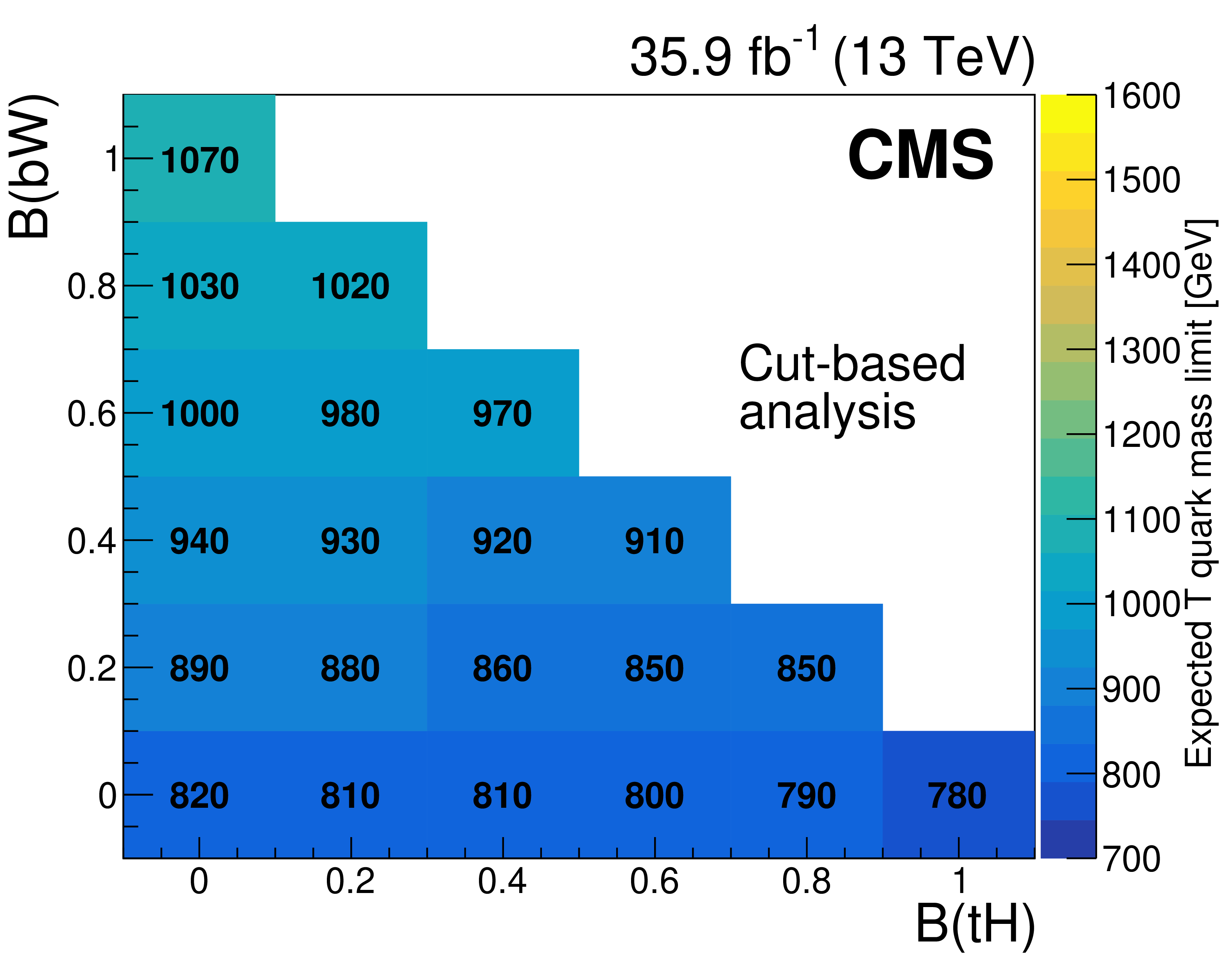
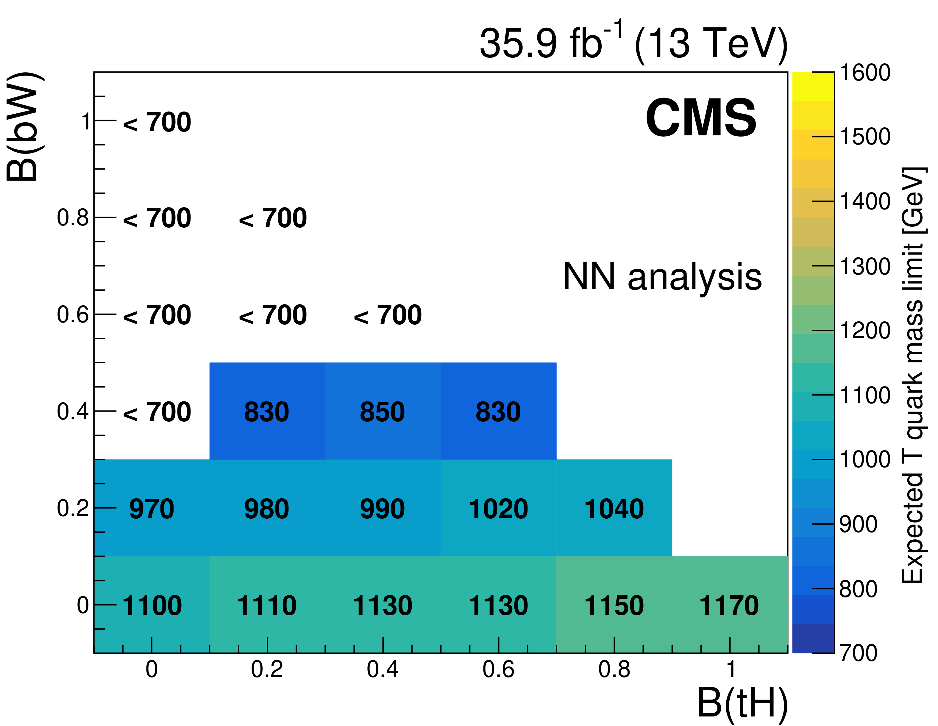
Figure 7:
Observed (left) and expected (right) mass exclusion limits at 95% confidence level for each combination of T quark branching fractions, in the cut-based analysis (upper) and NN analysis (lower). |
png pdf |
Figure 7-a:
Observed mass exclusion limits at 95% confidence level for each combination of T quark branching fractions, in the cut-based analysis. |
png pdf |
Figure 7-b:
Expected mass exclusion limits at 95% confidence level for each combination of T quark branching fractions, in the NN analysis. |

png pdf |
Figure 7-c:
Observed mass exclusion limits at 95% confidence level for each combination of T quark branching fractions, in the cut-based analysis. |
png pdf |
Figure 7-d:
Expected mass exclusion limits at 95% confidence level for each combination of T quark branching fractions, in the NN analysis. |
png pdf |
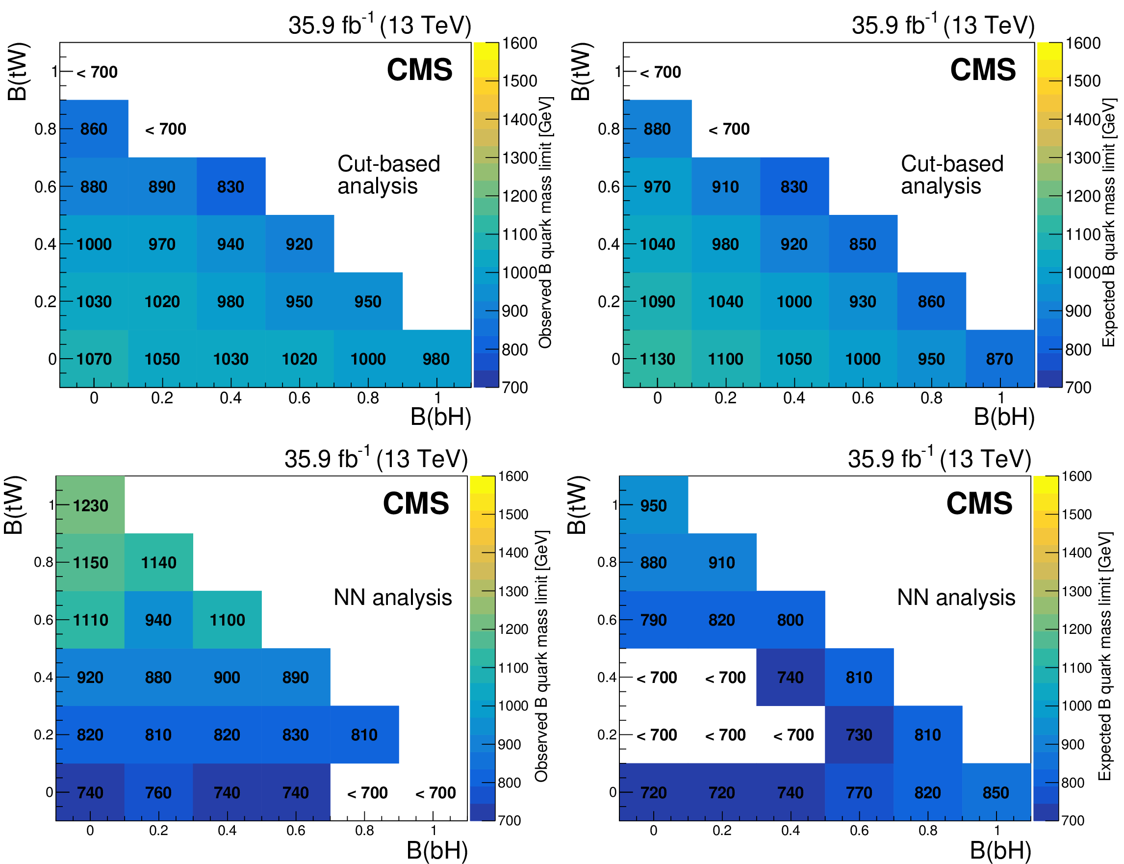
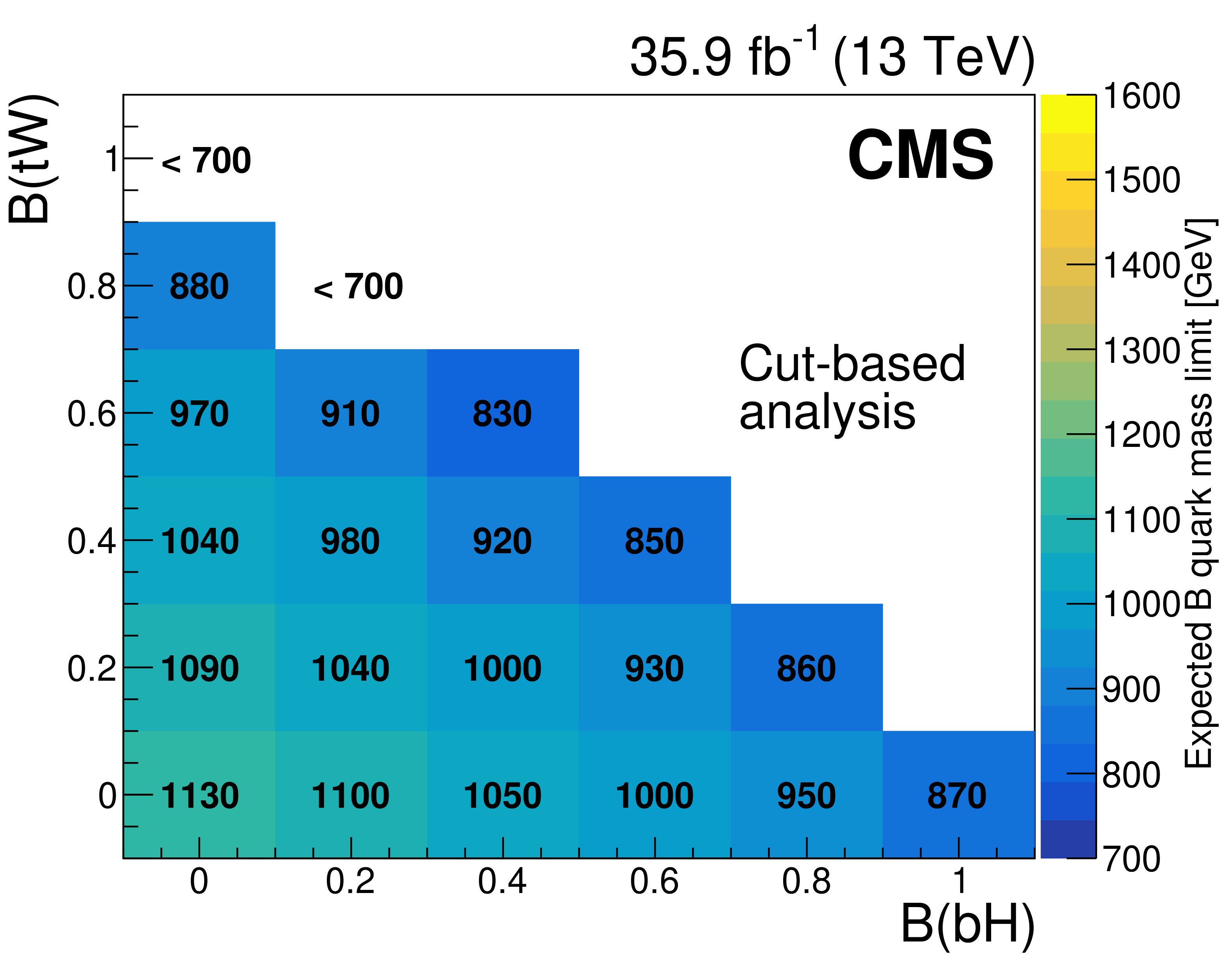
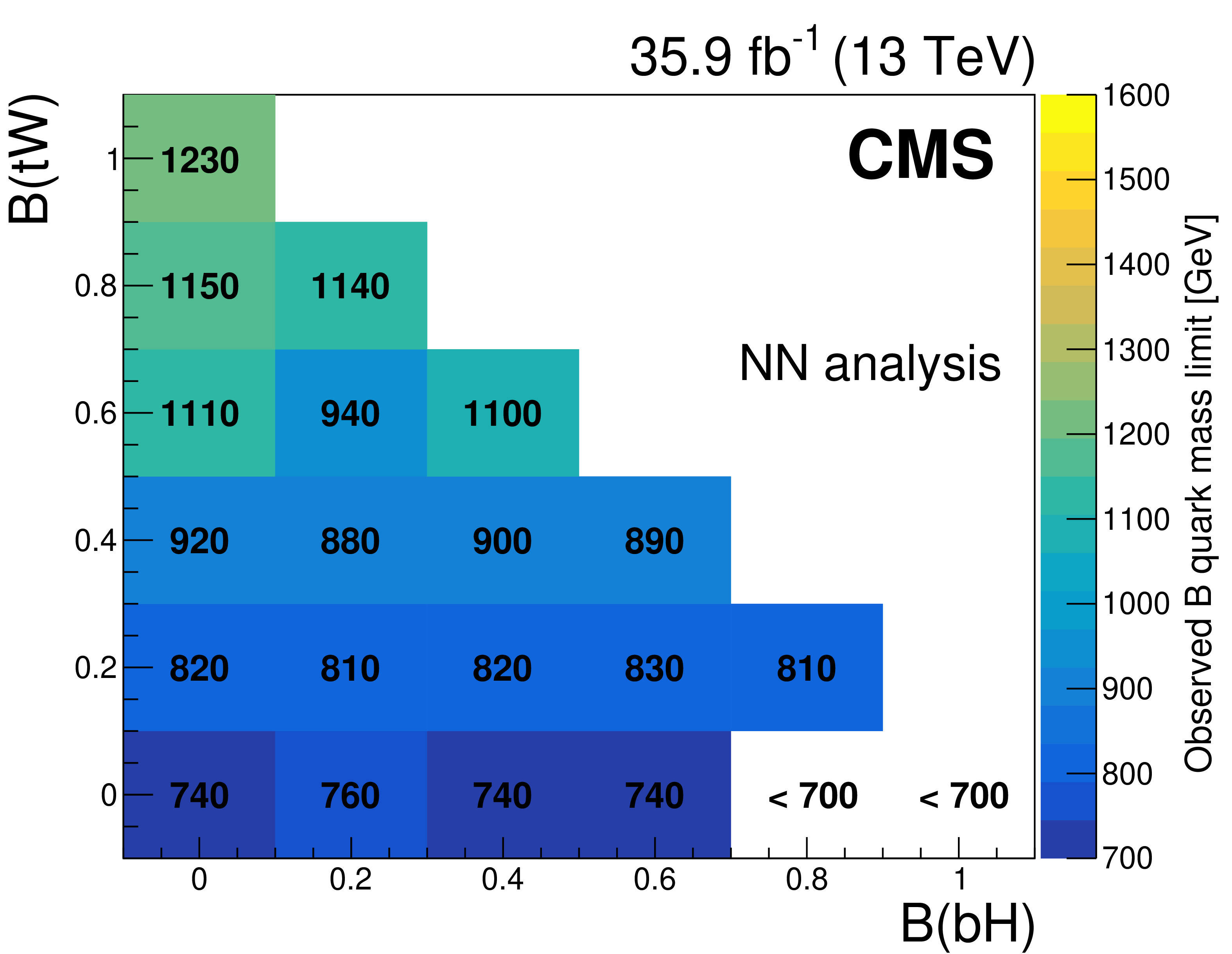
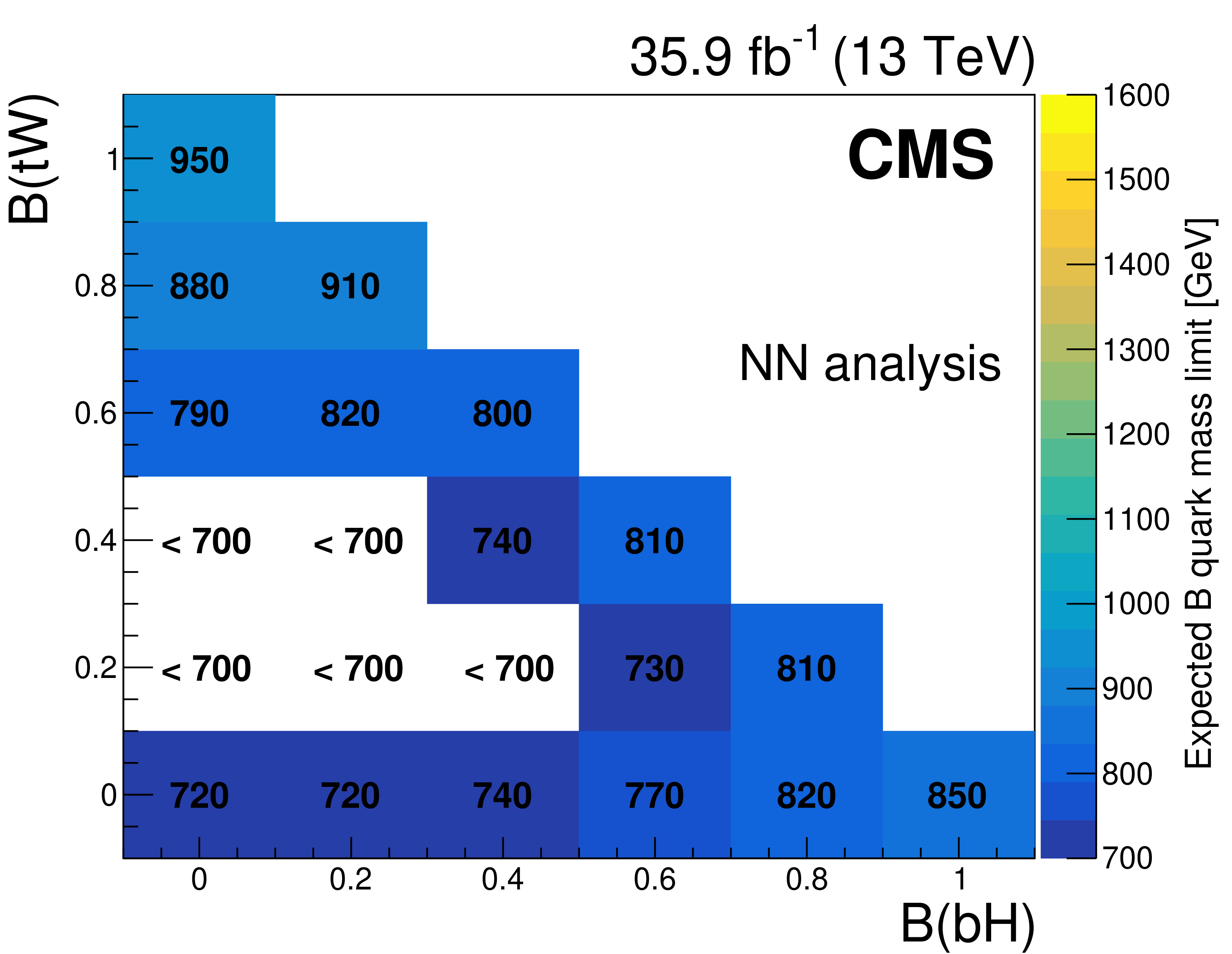
Figure 8:
Observed (left) and expected (right) mass exclusion limits at 95% confidence level for each combination of B quark branching fractions, in the cut-based analysis (upper) and NN analysis (lower). |

png pdf |
Figure 8-a:
Observed mass exclusion limits at 95% confidence level for each combination of B quark branching fractions, in the cut-based analysis. |
png pdf |
Figure 8-b:
Expected mass exclusion limits at 95% confidence level for each combination of B quark branching fractions, in the NN analysis. |
png pdf |
Figure 8-c:
Observed mass exclusion limits at 95% confidence level for each combination of B quark branching fractions, in the cut-based analysis. |
png pdf |
Figure 8-d:
Expected mass exclusion limits at 95% confidence level for each combination of B quark branching fractions, in the NN analysis. |
| Tables | |
png pdf |
Table 1:
Theoretical cross sections for TT and BB production, calculated at NNLO with Top++2.0. |
png pdf |
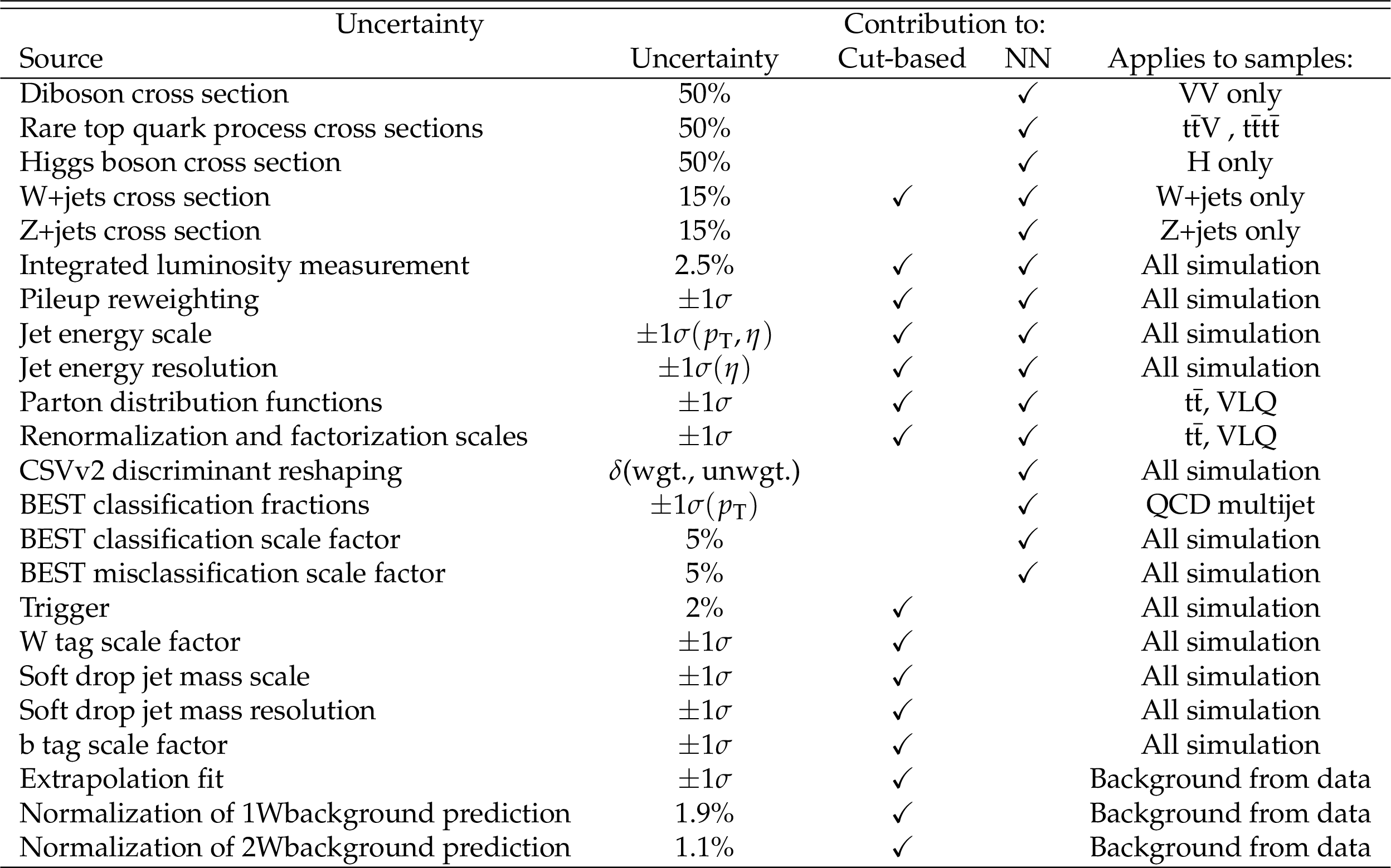
Table 2:
Sources of systematic uncertainties that affect the ${{H_{\mathrm {T}}} ^{\mathrm {AK4}}}$ or ${{H_{\mathrm {T}}} ^{\mathrm {AK8}}}$ distribution in each analysis. Systematic sources with an uncertainty of "$ \pm $1$ \sigma $'' affect the shape and rate, all others affect the rate only. Sources of systematic error that affect "all simulation'' impact both the signal simulation and simulated backgrounds. |
png pdf |
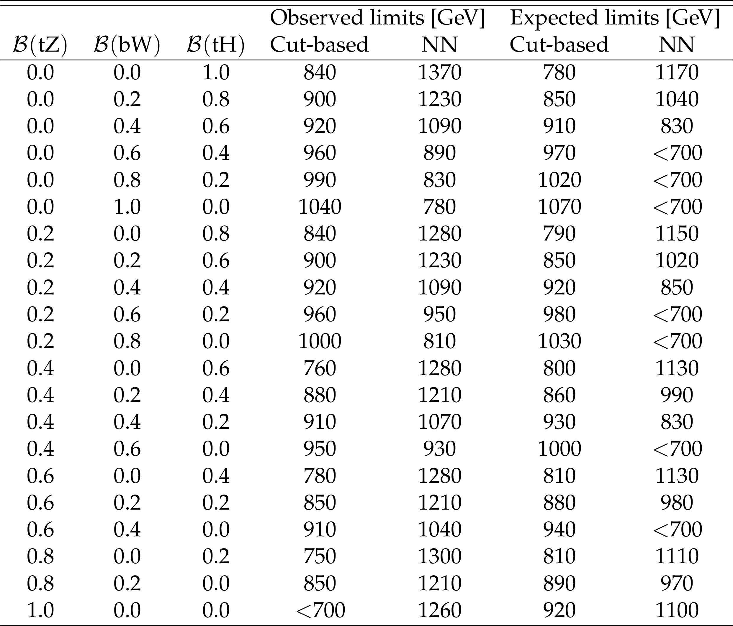
Table 3:
Exclusion limits at 95% confidence level presented in terms of the T quark mass, for the different branching fraction scenarios considered, in each of the two analyses. |
png pdf |
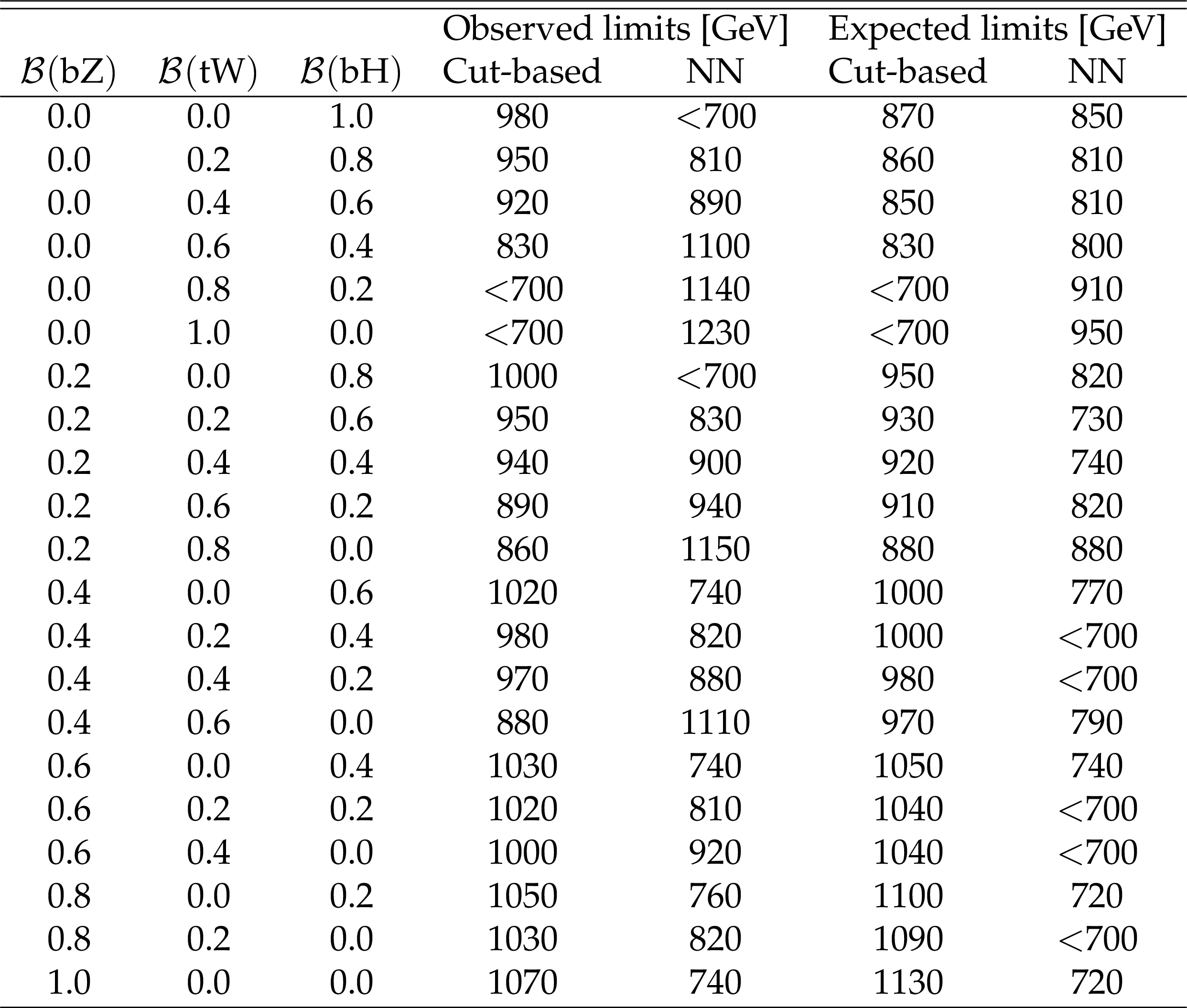
Table 4:
Exclusion limits at 95% confidence level presented in terms of the B quark mass, for the different branching fraction scenarios considered, in each of the two analyses. |
| Summary |
|
Two independent searches for vector-like T and B quarks using the fully hadronic final states have been presented. Both searches use data collected by the CMS experiment in 2016 at a center-of-mass energy of 13 TeV, corresponding to an integrated luminosity of 35.9 fb$^{-1}$. A cut-based analysis, using jet substructure observables to identify hadronic decays of boosted W bosons, targets the qW decay mode of the T quark, and improves sensitivity relative to results of such searches conducted previously. The analysis uses a quantum chromodynamics multijet background estimation method based on shape and rate extrapolations from various control regions to the signal region. Improvements in W tagging techniques, as well as the addition of signal regions requiring just a single W-tagged jet, enhance the performance of this analysis relative to previous searches based on different strategies. This search extends the T quark mass exclusion to 1040 GeV, relative to the previous exclusion of 705 GeV obtained by a similar analysis targeting the qW decay mode using data collected at 8 TeV [56]. A new strategy is presented and compared with the traditional cut-based approach. The neural network analysis uses a multiclassification technique, the boosted event shape tagger algorithm, to identify jets originating from heavy objects such as t or b quarks, and W, Z, or H. This allows the analysis to be sensitive to all decay modes of the T and B quarks. Using classification fractions, the dominant multijet background is estimated using data. The neural network analysis provides sensitivity for the tH and tZ decay modes competitive with that obtained by other searches utilizing lepton+jets or multilepton topologies. For each analysis, results are presented in terms of cross section limits for the pair production of T and B quarks, along with exclusion limits in terms of the T and B quark masses, for the different combinations of branching fractions considered. The mass exclusion limits at 95% confidence level for the neural network analysis range from 740 to 1370 GeV, providing comparable sensitivity to the searches utilizing leptons, which exclude vector-like quark masses in the range 910-1300 GeV [13]. These results represent the most stringent limits on pair produced vector-like quarks in the fully hadronic channel to date. |
| Additional Figures | |
png pdf |
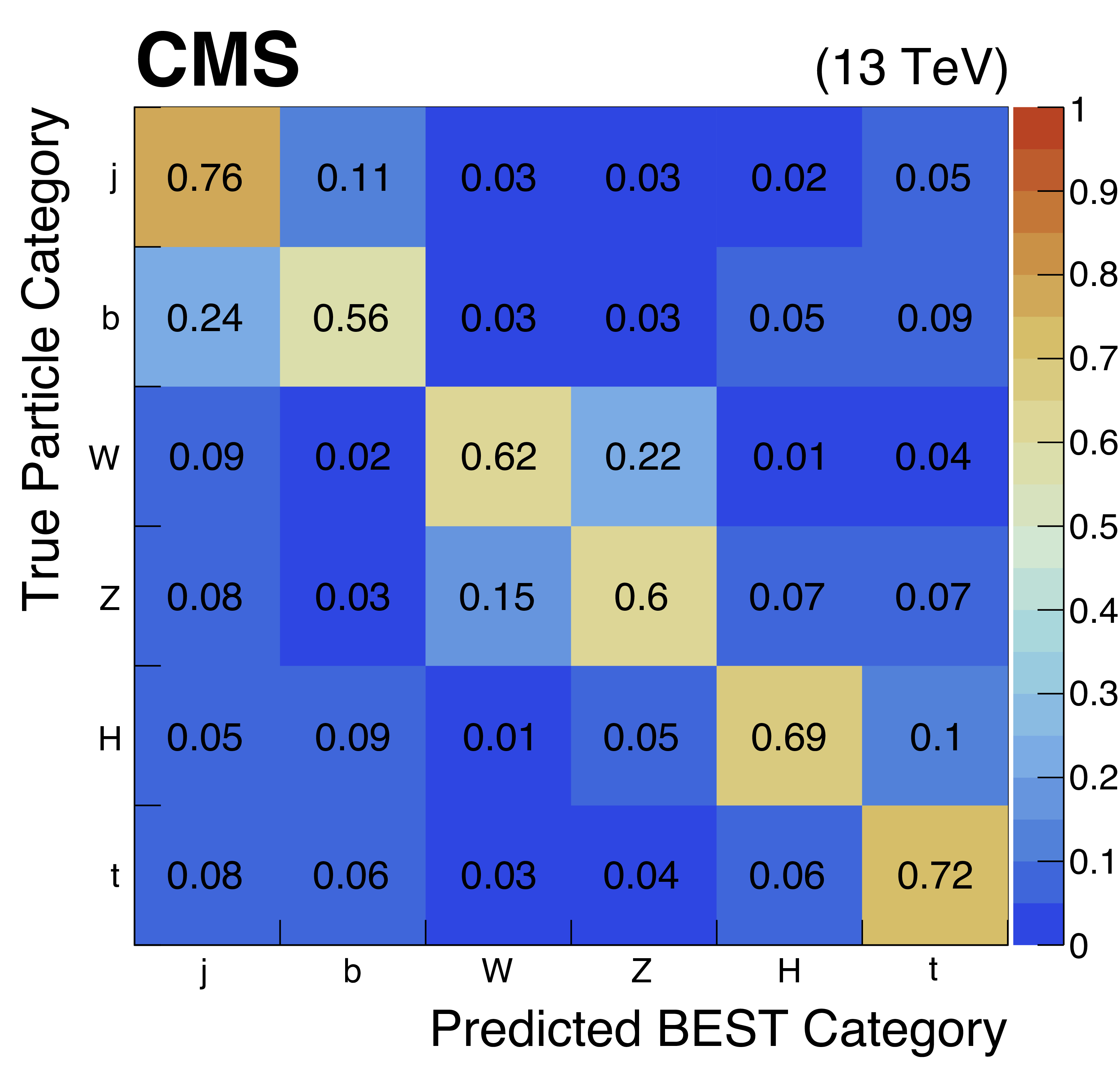
Additional Figure 1:
The confusion matrix from the training of the BEST algorithm. The y-axis shows the truth-level information about the particle species from which the jet originates, while the x-axis shows the predicted categories after evaluating the BEST algorithm. Good performance is seen on the diagonal, which represents correct classifications. The label 'j' represents light-flavor jets (u/d/s/c quark and gluon). |
png pdf |
Additional Figure 2:
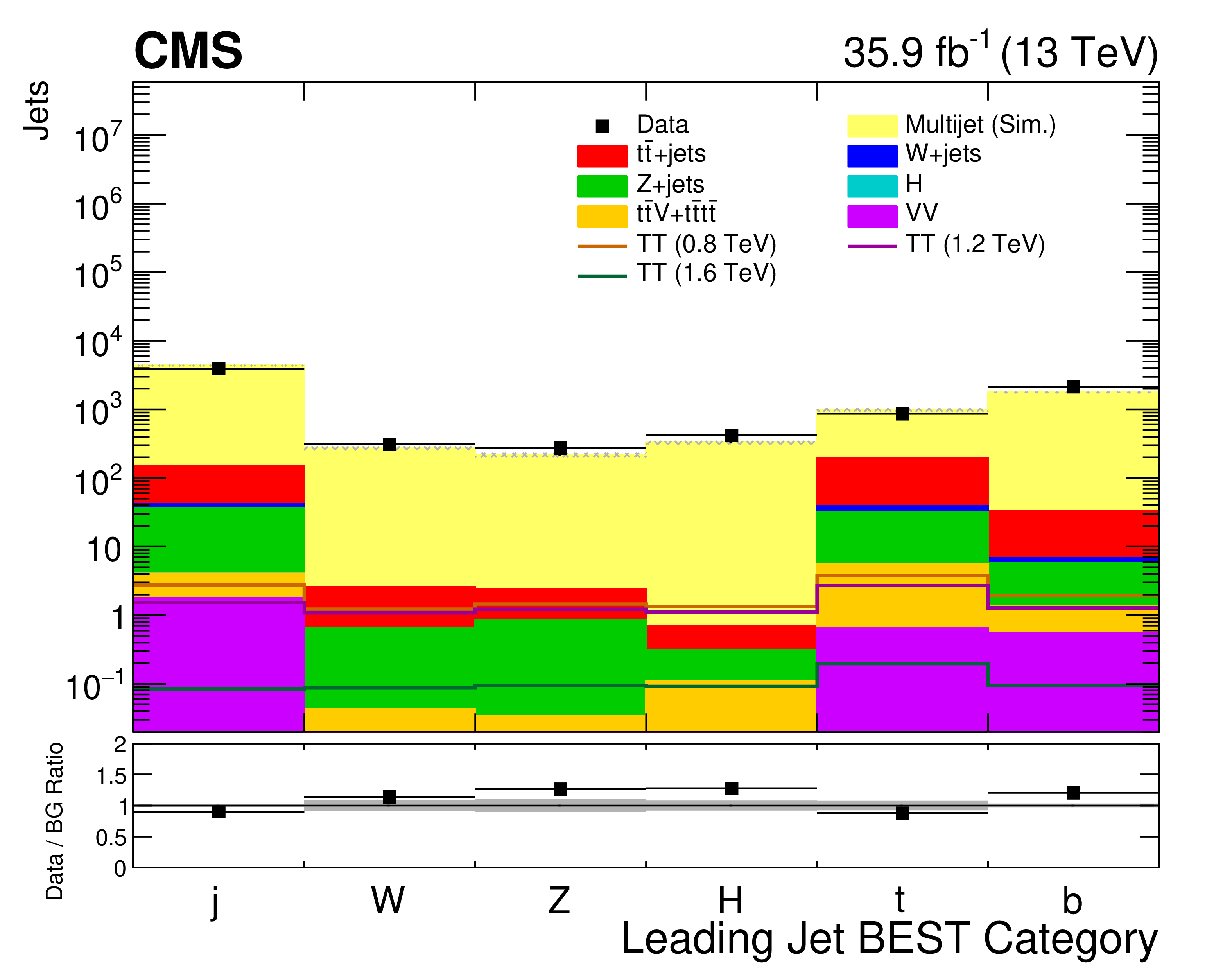
Distribution of the predicted categories of the BEST algorithm for the leading jet in the inclusive 4-jet sample. The category 'j' represents light flavor jets (u/d/s/c/g). The yellow histogram shows the expectation from QCD multijet processes, and here is shown taken from simulation. This component is scaled by a k-factor to equalize the total normalization between data and the summed background components. The shaded band represents the statistical uncertainty on the backgrounds only. The mistag rates used in the analysis are derived from data in this sample. Jets entering this distribution are not matched to any generator-level particles, meaning the leading jet in a given process may not be the heavy object of interest and may be categorized differently than expected. |

png pdf |
Additional Figure 3:
The jet soft drop mass distribution shown for the training samples (t, W, Z, H, b, light flavor jets) of the BEST algorithm. The histograms are each normalized to unit area. This quantity is one of the inputs to the BEST algorithm. |
png pdf |
Additional Figure 4:
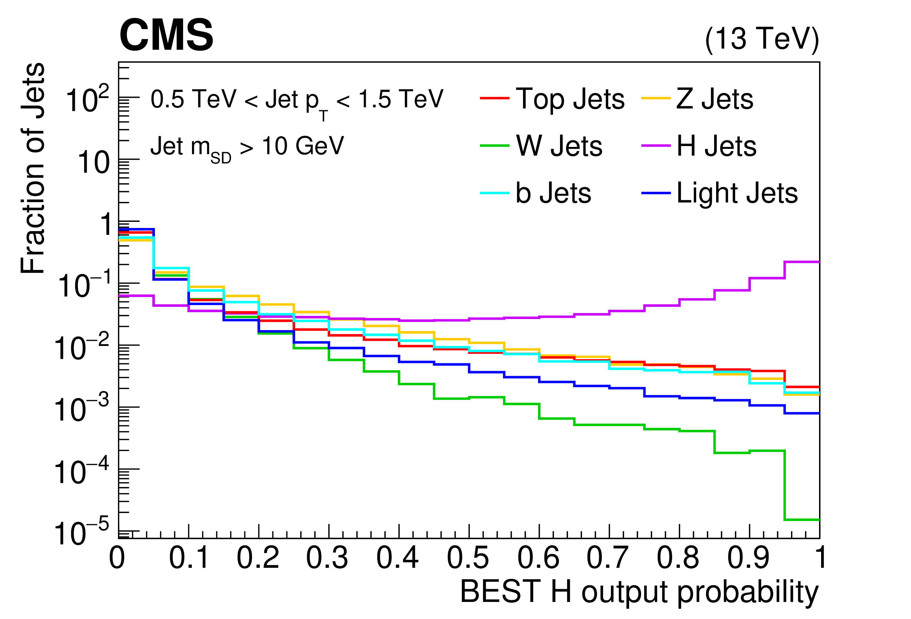
The output probability for H classification, after evaluating the samples (t, W, Z, H, b, light flavor jets) used with the BEST algorithm training/testing procedure. The histograms are each normalized to unit area. |
png pdf |
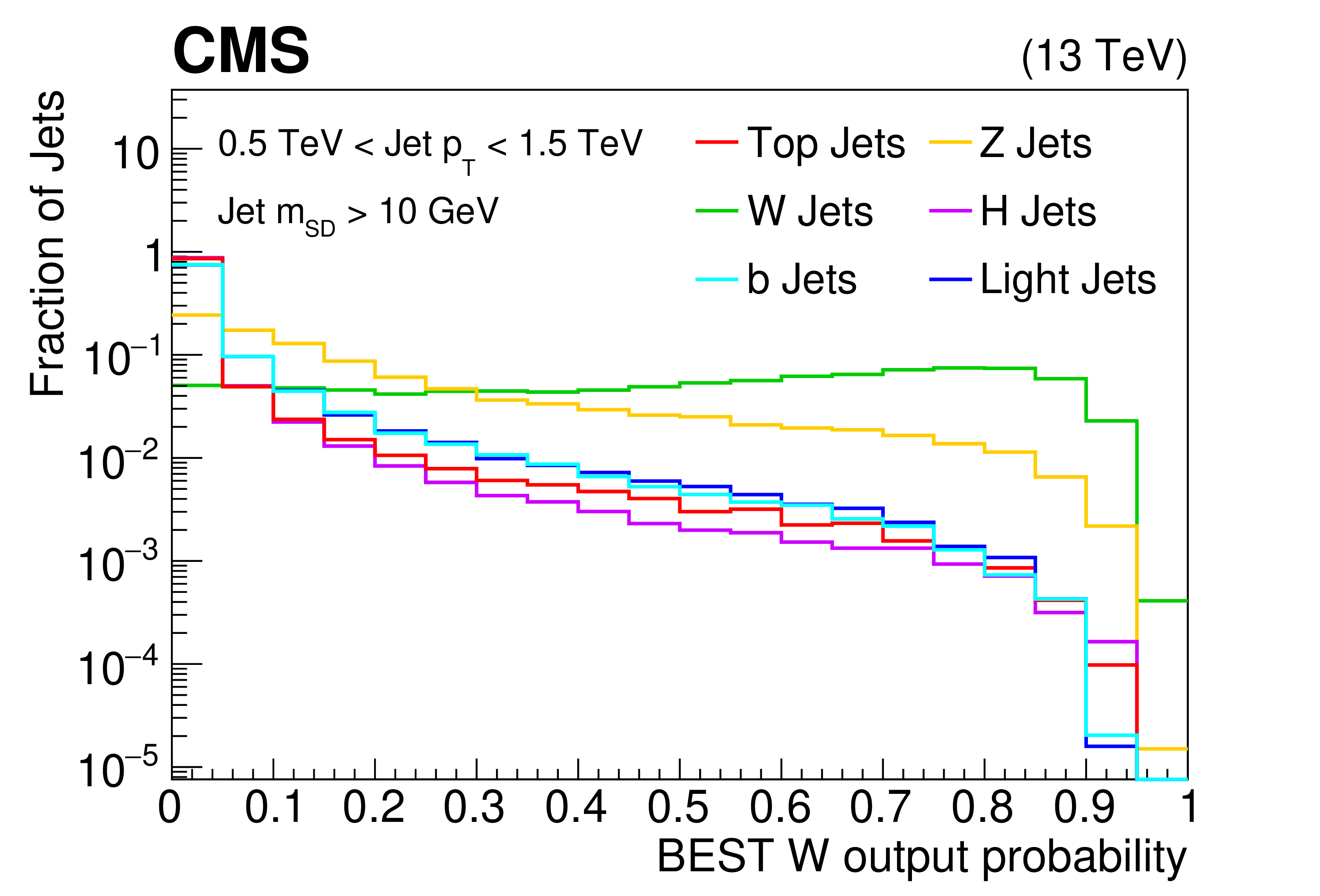
Additional Figure 5:
The output probability for W classification, after evaluating the samples (t, W, Z, H, b, light flavor jets) used with the BEST algorithm training/testing procedure. The histograms are each normalized to unit area. |

png pdf |
Additional Figure 6:
The output probability for Z classification, after evaluating the samples (t, W, Z, H, b, light flavor jets) used with the BEST algorithm training/testing procedure. The histograms are each normalized to unit area. |
png pdf |
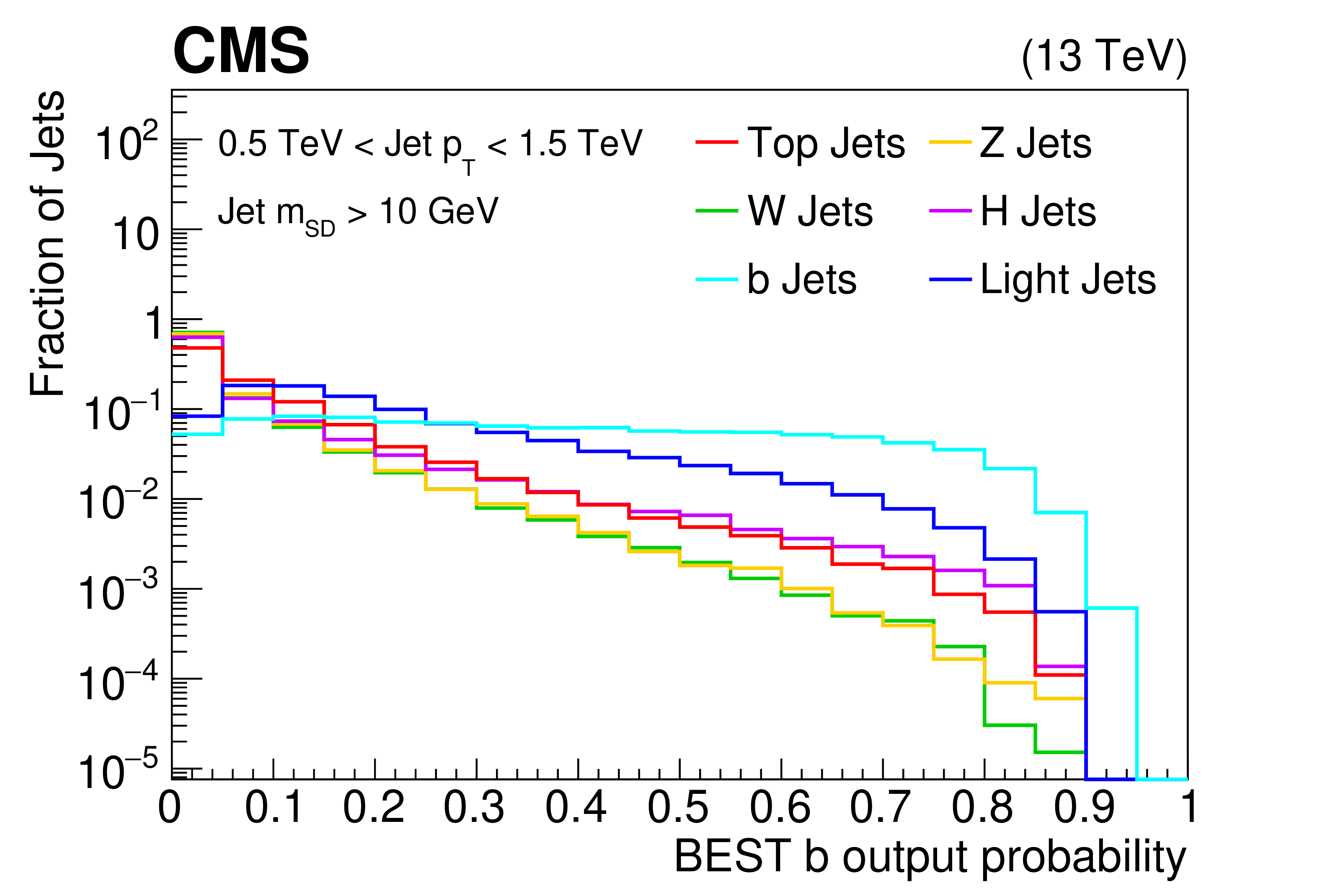
Additional Figure 7:
The output probability for b classification, after evaluating the samples (t, W, Z, H, b, light flavor jets) used with the BEST algorithm training/testing procedure. The histograms are each normalized to unit area. |
png pdf |
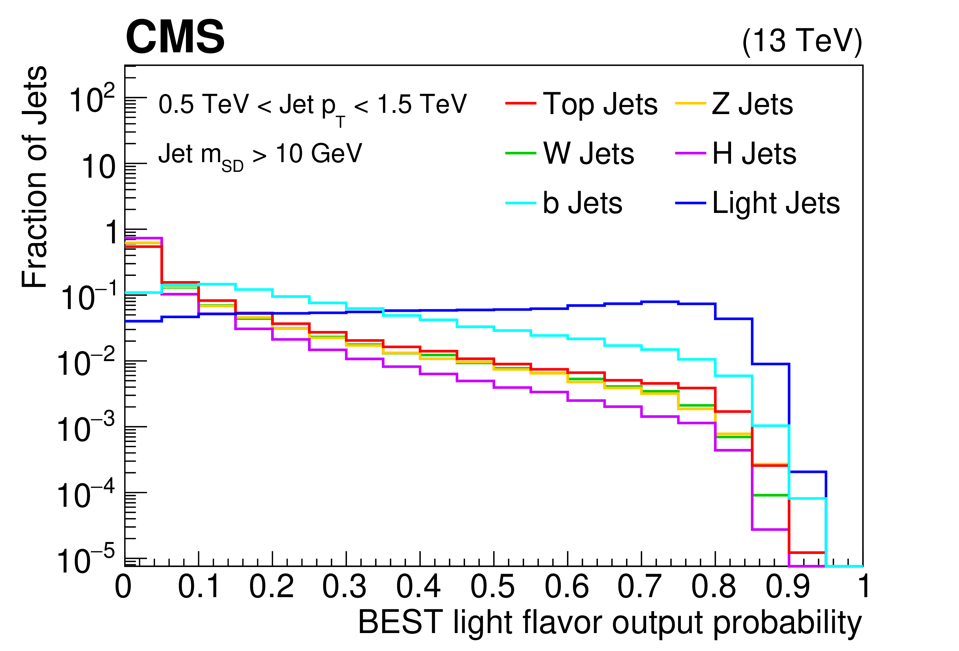
Additional Figure 8:
The output probability for light flavor classification, after evaluating the samples (t, W, Z, H, b, light flavor jets) used with the BEST algorithm training/testing procedure. The histograms are each normalized to unit area. |
png pdf |
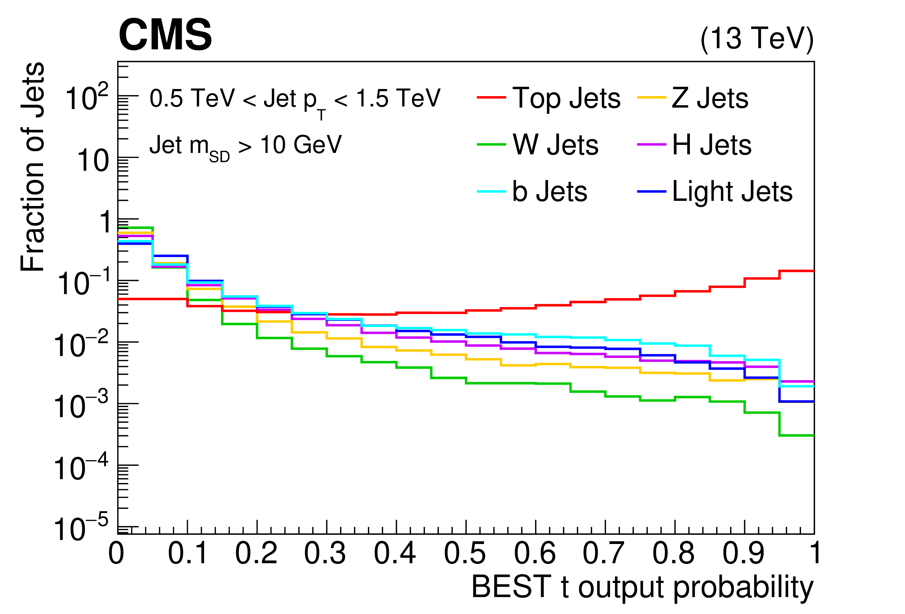
Additional Figure 9:
The output probability for t classification, after evaluating the samples (t, W, Z, H, b, light flavor jets) used with the BEST algorithm training/testing procedure. The histograms are each normalized to unit area. |
png pdf |
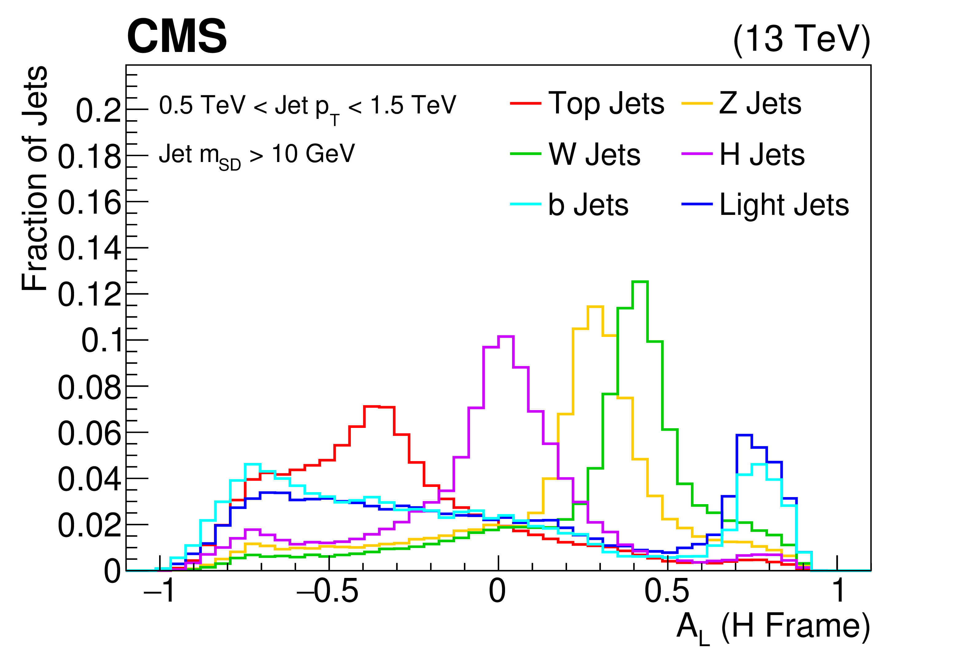
Additional Figure 10:
The longitudinal jet asymmetry ($A_L$, defined as the ratio of the sum of the subjet momenta longitudinal components to the sum of subjet momenta magnitudes) distribution shown for the training samples (t, W, Z, H, b, light flavor jets) of the BEST algorithm after boosting the jet constituents assuming the H rest frame. The histograms are each normalized to unit area. This quantity is one of the inputs to the BEST algorithm. |
png pdf |
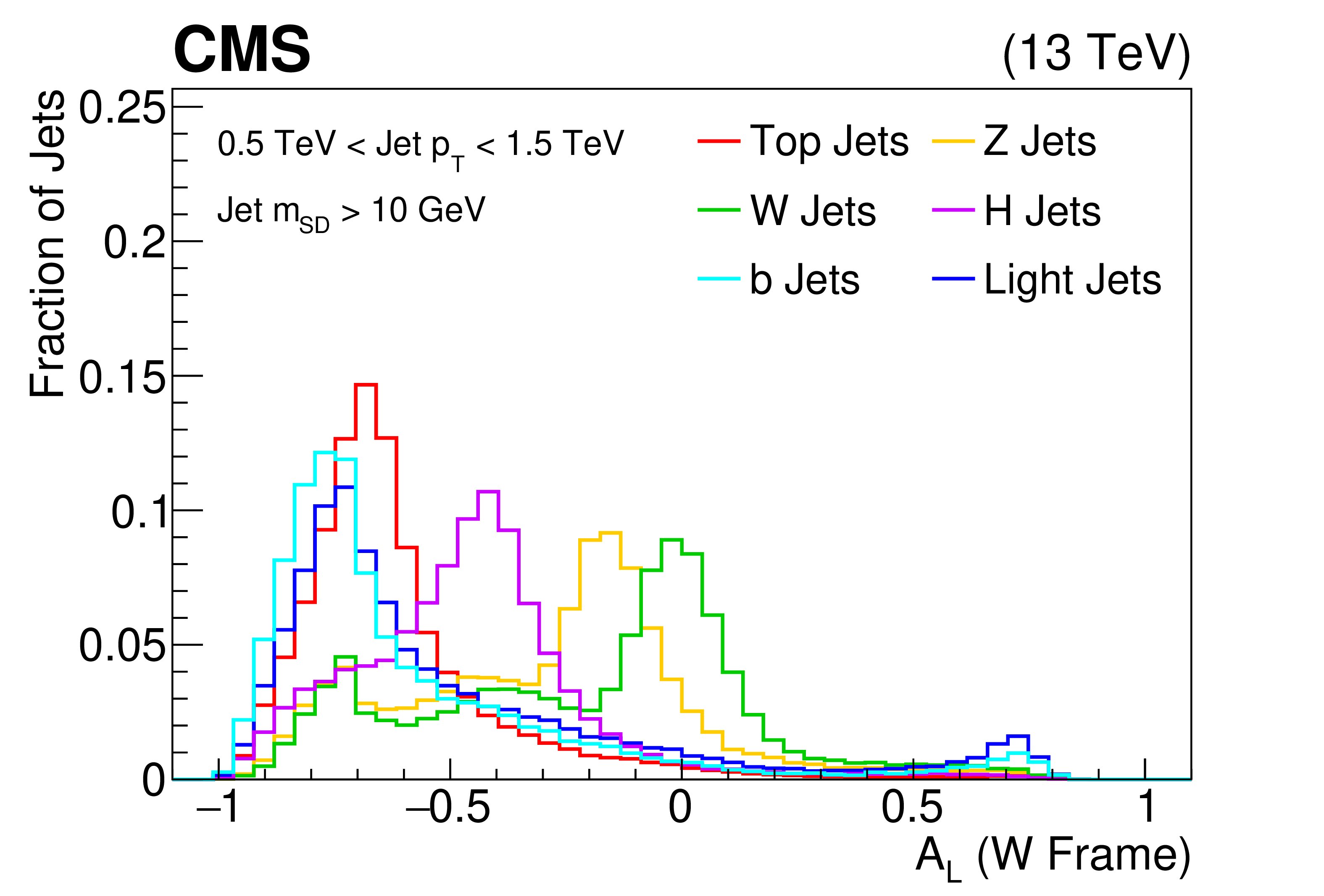
Additional Figure 11:
The longitudinal jet asymmetry ($A_L$, defined as the ratio of the sum of the subjet momenta longitudinal components to the sum of subjet momenta magnitudes) distribution shown for the training samples (t, W, Z, H, b, light flavor jets) of the BEST algorithm after boosting the jet constituents assuming the W rest frame. The histograms are each normalized to unit area. This quantity is one of the inputs to the BEST algorithm. |
png pdf |
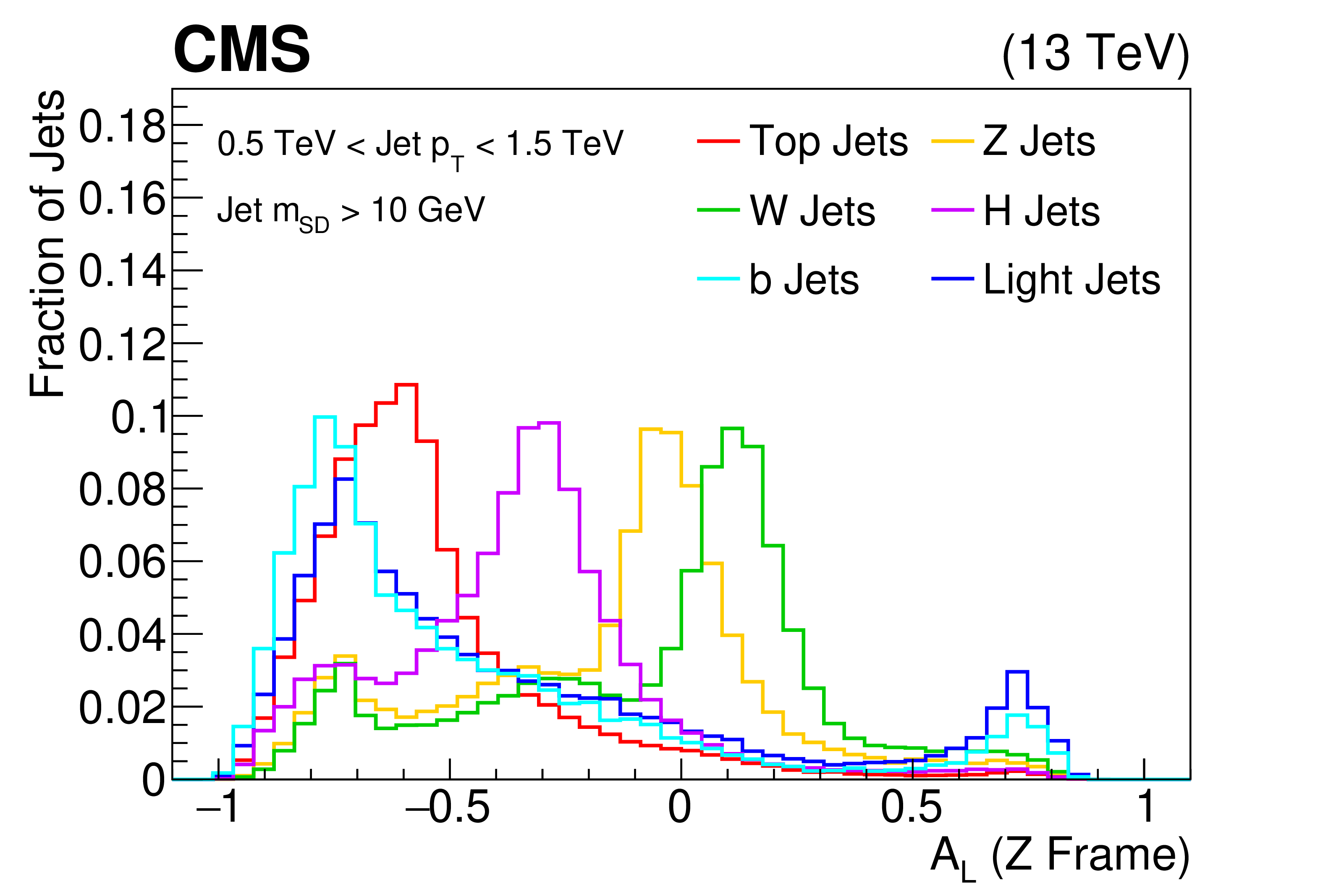
Additional Figure 12:
The longitudinal jet asymmetry ($A_L$, defined as the ratio of the sum of the subjet momenta longitudinal components to the sum of subjet momenta magnitudes) distribution shown for the training samples (t, W, Z, H, b, light flavor jets) of the BEST algorithm after boosting the jet constituents assuming the Z rest frame. The histograms are each normalized to unit area. This quantity is one of the inputs to the BEST algorithm. |
png pdf |
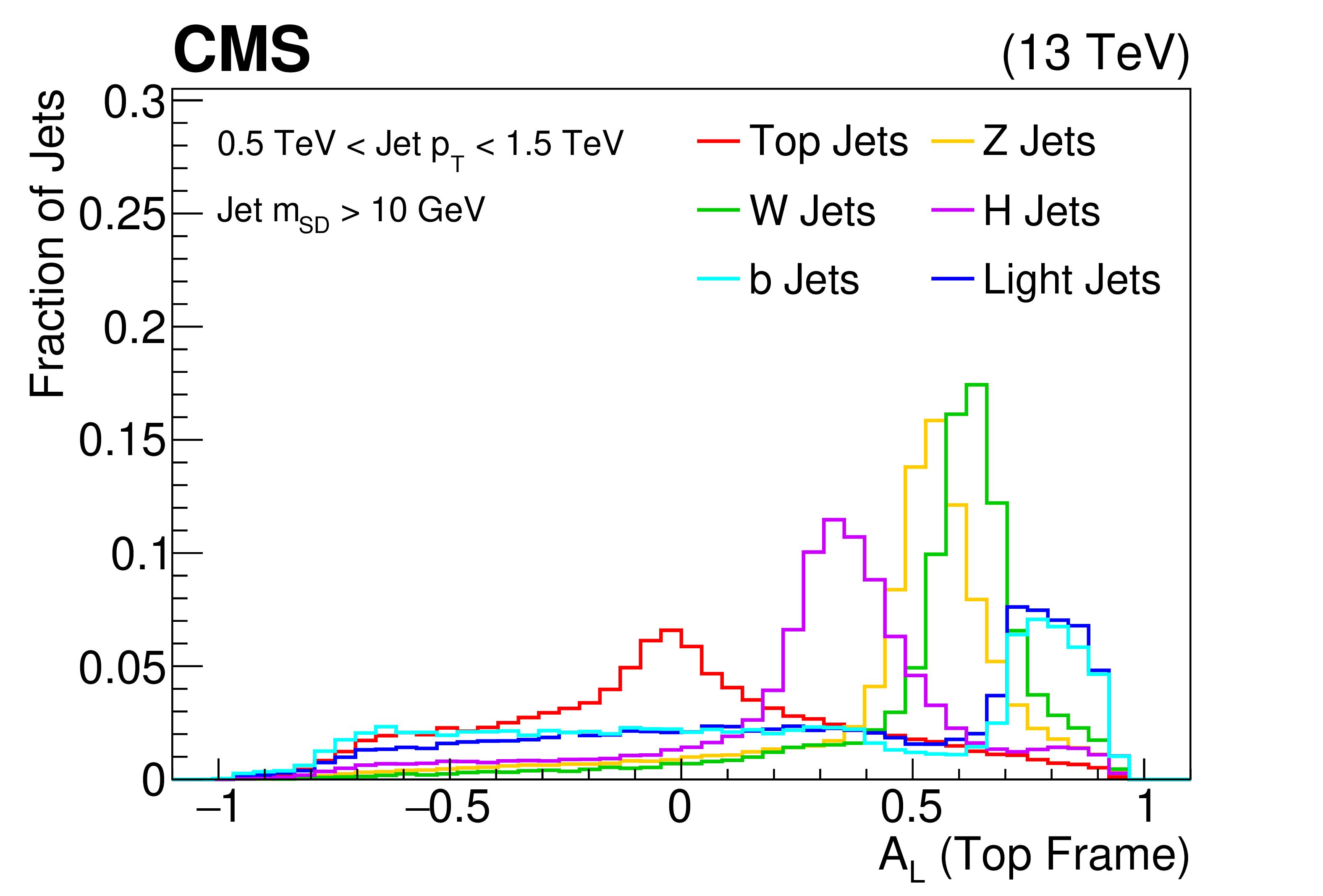
Additional Figure 13:
The longitudinal jet asymmetry ($A_L$, defined as the ratio of the sum of the subjet momenta longitudinal components to the sum of subjet momenta magnitudes) distribution shown for the training samples (t, W, Z, H, b, light flavor jets) of the BEST algorithm after boosting the jet constituents assuming the top quark rest frame. The histograms are each normalized to unit area. This quantity is one of the inputs to the BEST algorithm. |
png pdf |
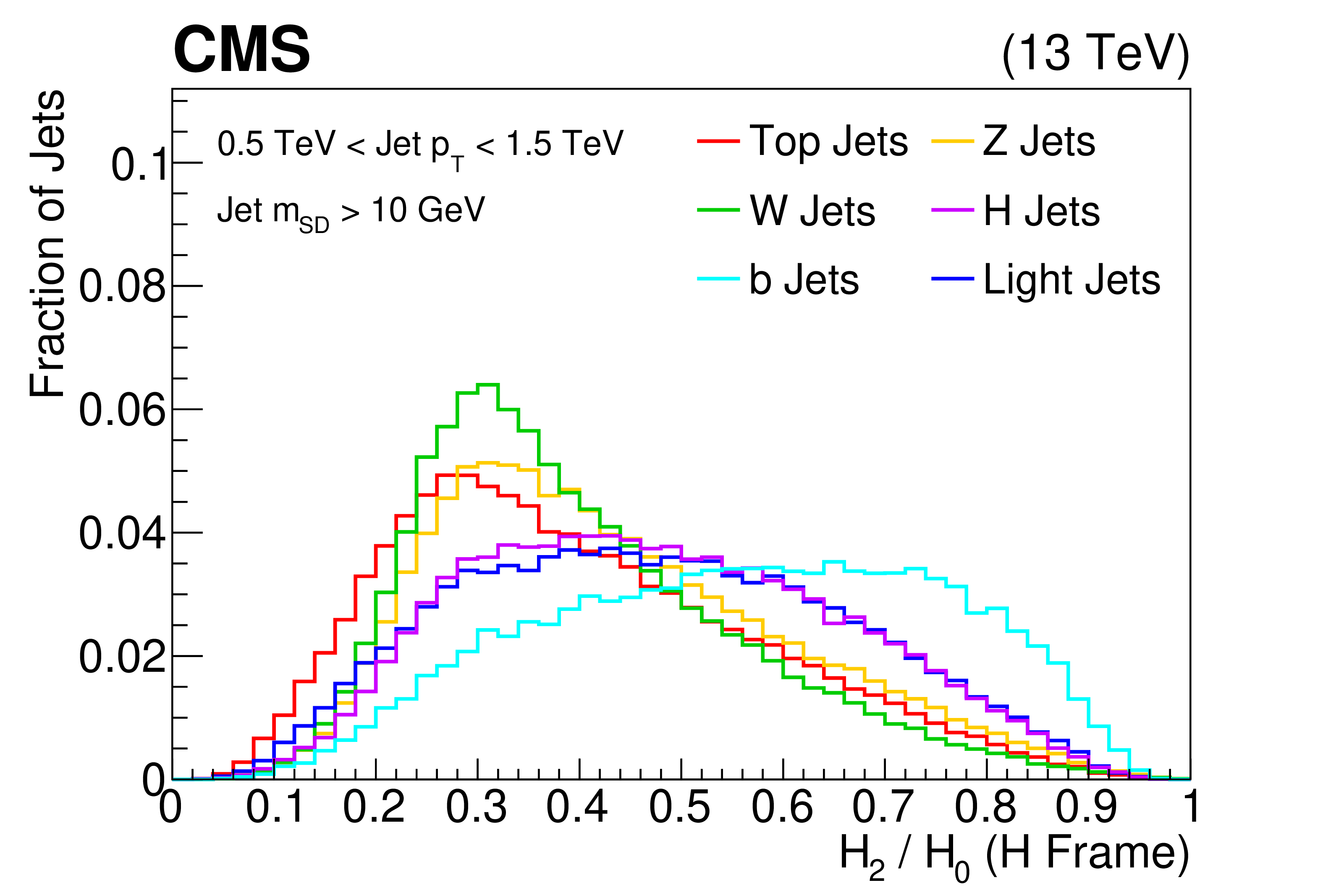
Additional Figure 14:
The distribution of the ratio of two Fox-Wolfram moments (indices 2 and 0), shown for the training samples (t, W, Z, H, b, light flavor jets) of the BEST algorithm after boosting the jet constituents assuming the H rest frame. The histograms are each normalized to unit area. This quantity is one of the inputs to the BEST algorithm. |
png pdf |
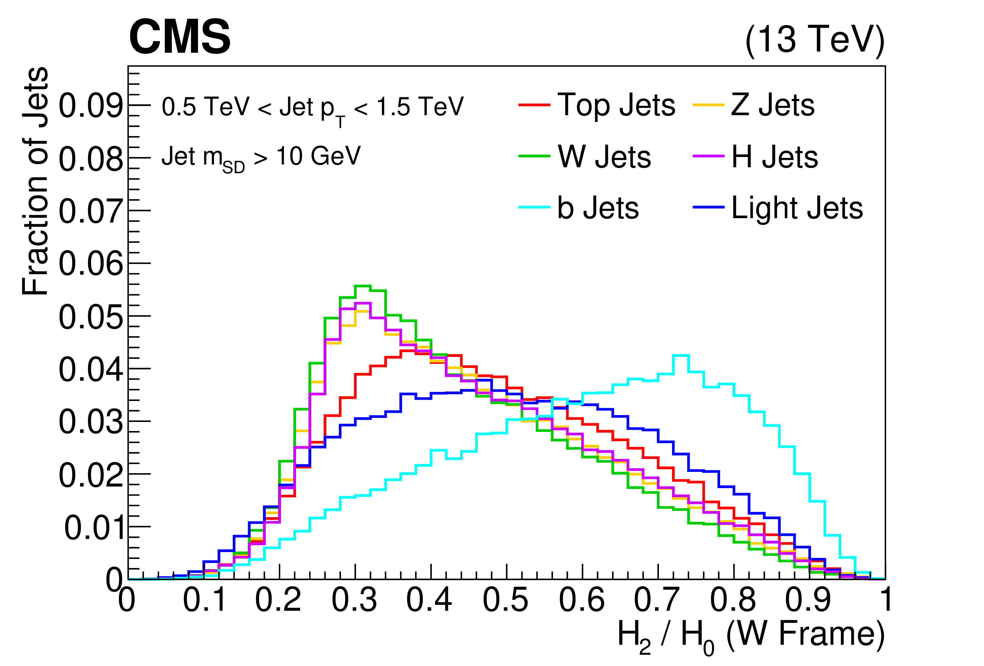
Additional Figure 15:
The distribution of the ratio of two Fox-Wolfram moments (indices 2 and 0), shown for the training samples (t, W, Z, H, b, light flavor jets) of the BEST algorithm after boosting the jet constituents assuming the W rest frame. The histograms are each normalized to unit area. This quantity is one of the inputs to the BEST algorithm. |
png pdf |
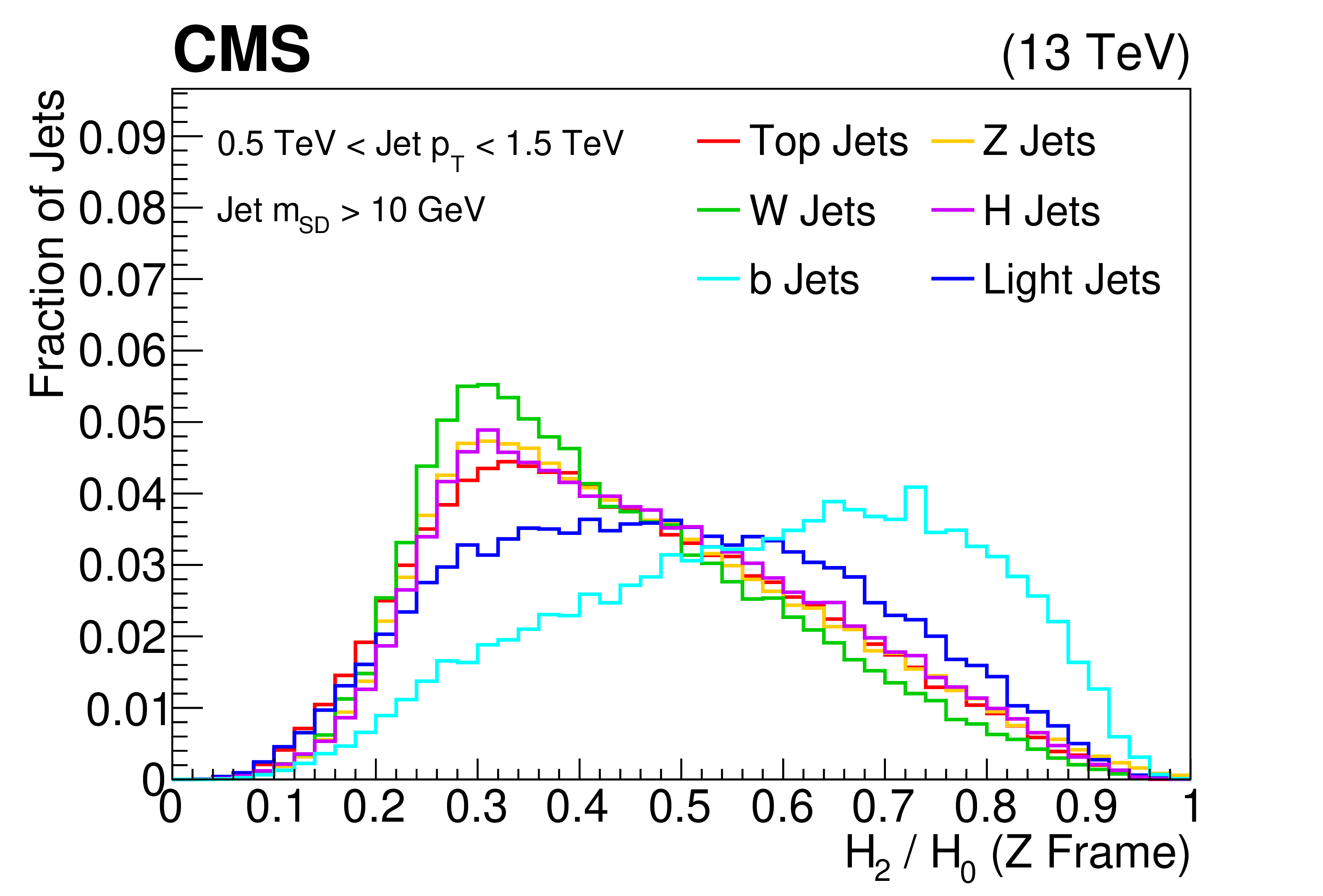
Additional Figure 16:
The distribution of the ratio of two Fox-Wolfram moments (indices 2 and 0), shown for the training samples (t, W, Z, H, b, light flavor jets) of the BEST algorithm after boosting the jet constituents assuming the Z rest frame. The histograms are each normalized to unit area. This quantity is one of the inputs to the BEST algorithm. |
png pdf |
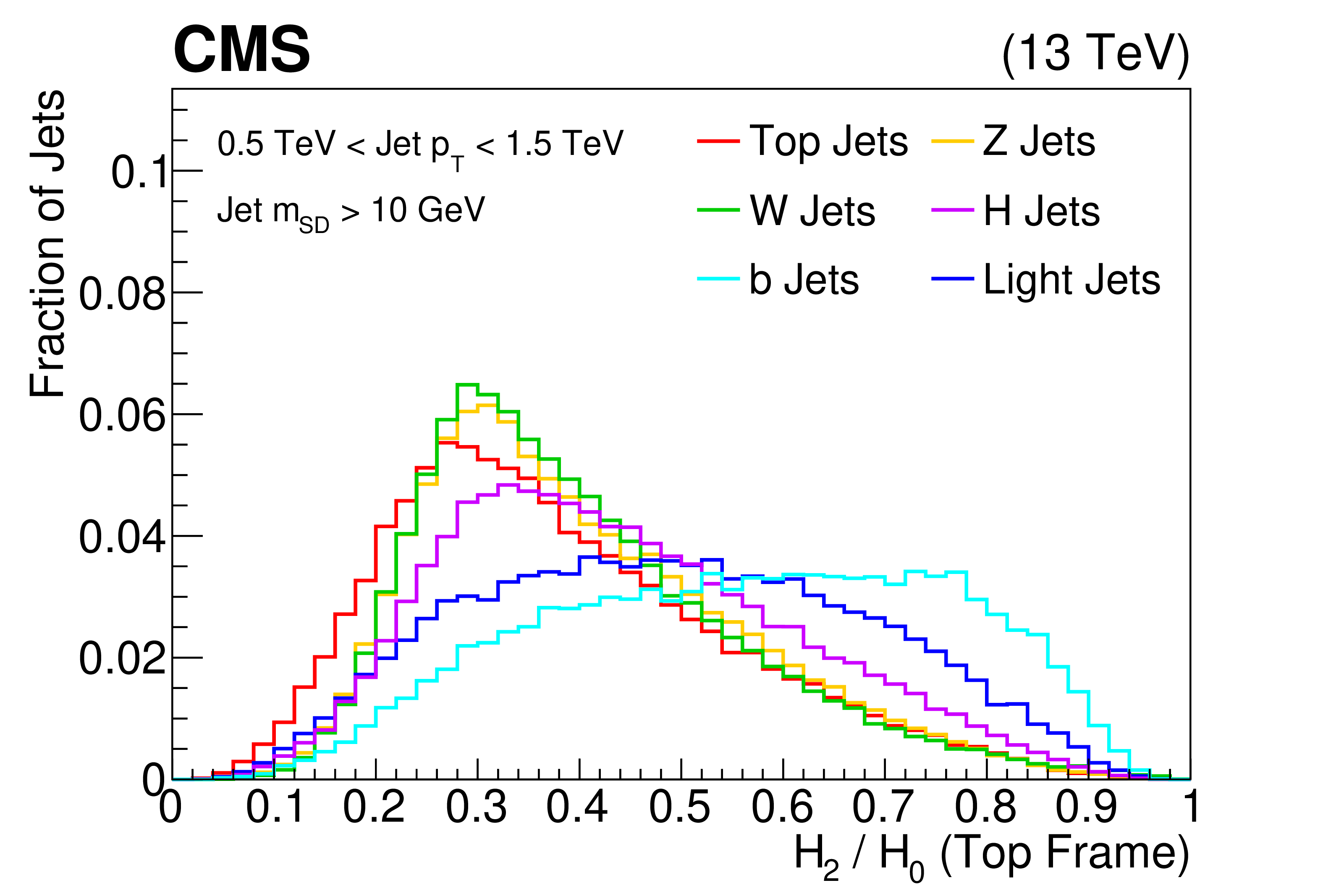
Additional Figure 17:
The distribution of the ratio of two Fox-Wolfram moments (indices 2 and 0), shown for the training samples (t, W, Z, H, b, light flavor jets) of the BEST algorithm after boosting the jet constituents assuming the top quark rest frame. The histograms are each normalized to unit area. This quantity is one of the inputs to the BEST algorithm. |
png pdf |
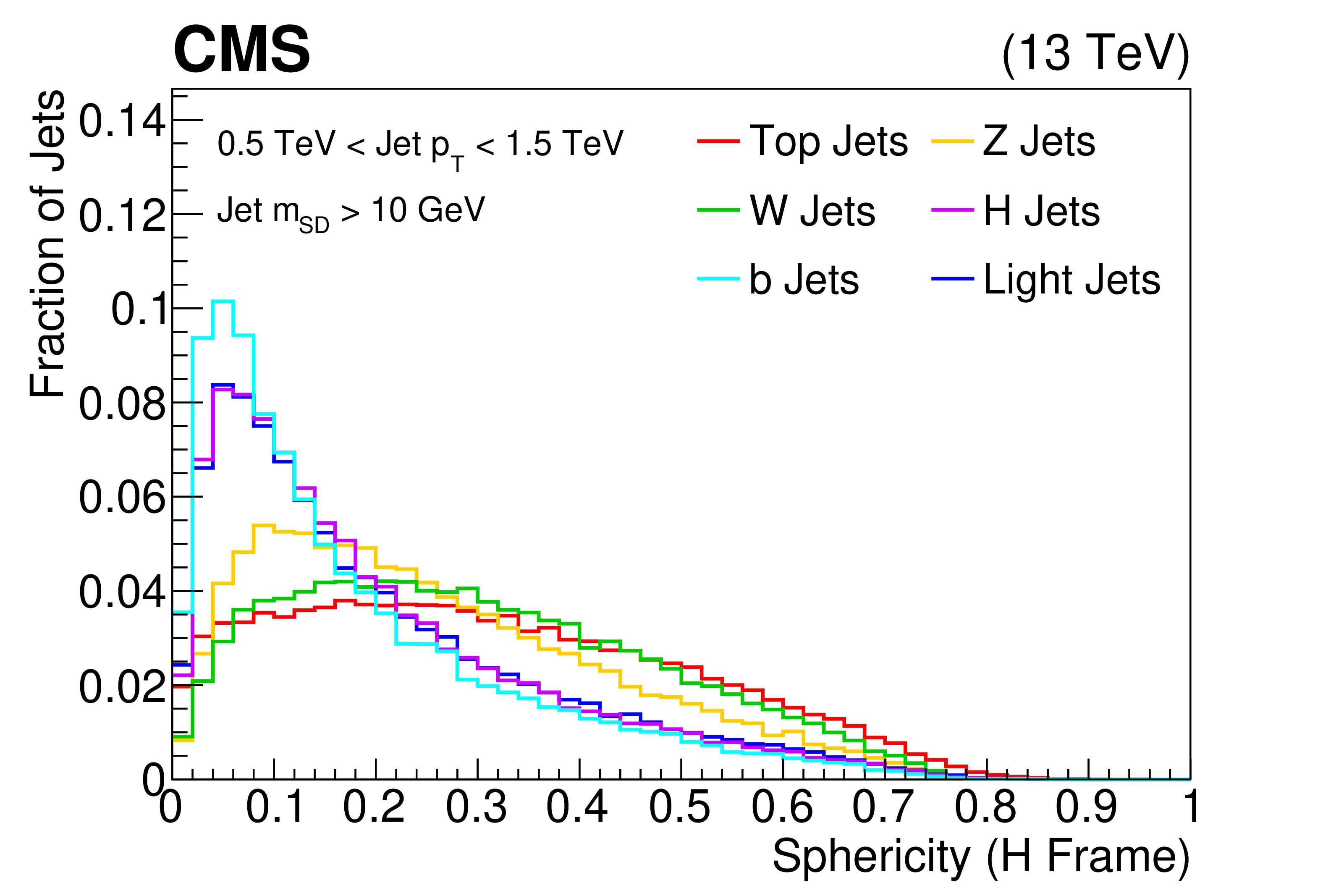
Additional Figure 18:
The distribution of the sphericity, shown for the training samples (t, W, Z, H, b, light flavor jets) of the BEST algorithm after boosting the jet constituents assuming the H rest frame. The histograms are each normalized to unit area. This quantity is one of the inputs to the BEST algorithm. |

png pdf |
Additional Figure 19:
The distribution of the sphericity, shown for the training samples (t, W, Z, H, b, light flavor jets) of the BEST algorithm after boosting the jet constituents assuming the W rest frame. The histograms are each normalized to unit area. This quantity is one of the inputs to the BEST algorithm. |
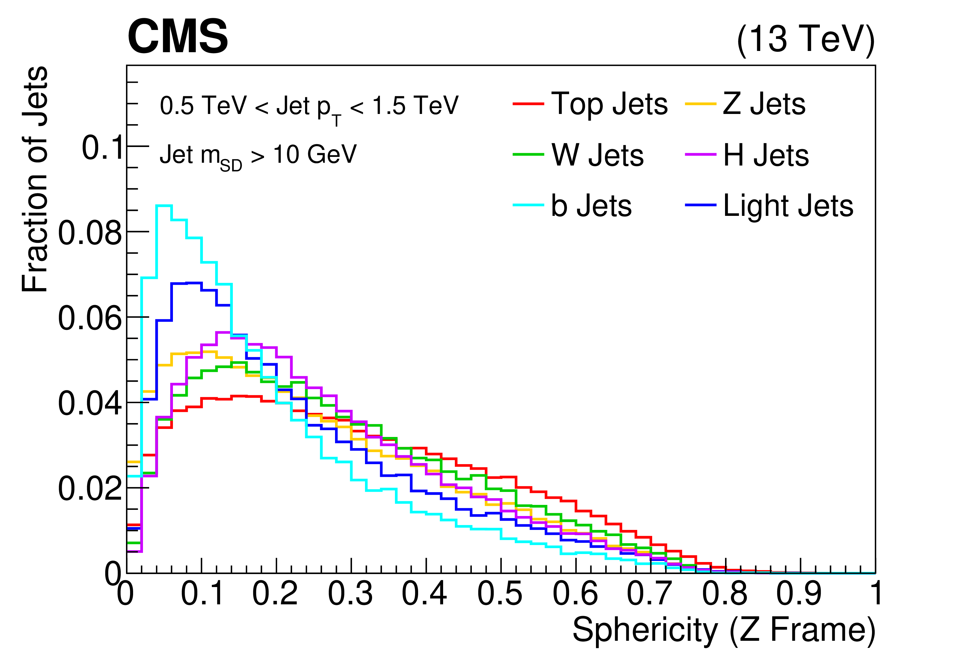
png pdf |
Additional Figure 20:
The distribution of the sphericity, shown for the training samples (t, W, Z, H, b, light flavor jets) of the BEST algorithm after boosting the jet constituents assuming the Z rest frame. The histograms are each normalized to unit area. This quantity is one of the inputs to the BEST algorithm. |
png pdf |
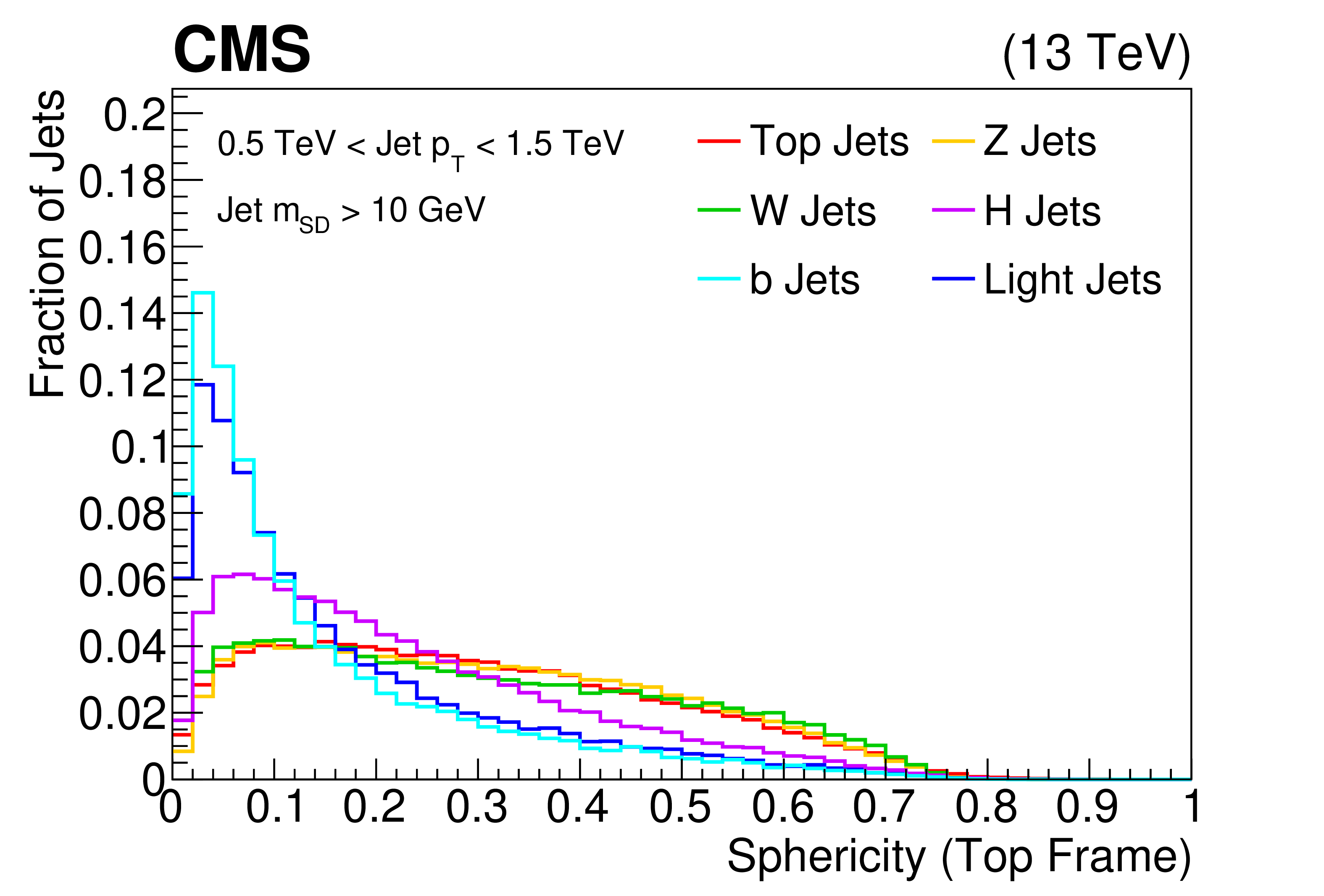
Additional Figure 21:
The distribution of the sphericity, shown for the training samples (t, W, Z, H, b, light flavor jets) of the BEST algorithm after boosting the jet constituents assuming the top quark rest frame. The histograms are each normalized to unit area. This quantity is one of the inputs to the BEST algorithm. |
| References | ||||
| 1 | ATLAS Collaboration | Observation of a new particle in the search for the standard model Higgs boson with the ATLAS detector at the LHC | PLB 716 (2012) 1 | 1207.7214 |
| 2 | CMS Collaboration | Observation of a new boson at a mass of 125 GeV with the CMS experiment at the LHC | PLB 716 (2012) 30 | CMS-HIG-12-028 1207.7235 |
| 3 | CMS Collaboration | Observation of a new boson with mass near 125 GeV in $ \mathrm{pp} $ Collisions at $ \sqrt{s} = $ 7 and 8 TeV | JHEP 06 (2013) 081 | CMS-HIG-12-036 1303.4571 |
| 4 | R. Contino, L. Da Rold, and A. Pomarol | Light custodians in natural composite Higgs models | PRD 75 (2007) 055014 | hep-ph/0612048 |
| 5 | R. Contino, T. Kramer, M. Son, and R. Sundrum | Warped/composite phenomenology simplified | JHEP 05 (2007) 074 | hep-ph/0612180 |
| 6 | D. B. Kaplan | Flavor at SSC energies: A new mechanism for dynamically generated fermion masses | NPB 365 (1991) 259 | |
| 7 | M. J. Dugan, H. Georgi, and D. B. Kaplan | Anatomy of a composite Higgs model | NPB 254 (1985) 299 | |
| 8 | M. Perelstein, M. E. Peskin, and A. Pierce | Top quarks and electroweak symmetry breaking in little Higgs models | PRD 69 (2004) 075002 | hep-ph/0310039 |
| 9 | O. Matsedonskyi, G. Panico, and A. Wulzer | Light top partners for a light composite Higgs | JHEP 01 (2013) 164 | 1204.6333 |
| 10 | A. De Simone, O. Matsedonskyi, R. Rattazzi, and A. Wulzer | A first top partner hunter's guide | JHEP 04 (2013) 004 | 1211.5663 |
| 11 | J. A. Aguilar-Saavedra, R. Benbrik, S. Heinemeyer, and M. P\'erez-Victoria | Handbook of vectorlike quarks: Mixing and single production | PRD 88 (2013) 094010 | 1306.0572 |
| 12 | CMS Collaboration | Search for vector-like quarks in events with two oppositely charged leptons and jets in proton-proton collisions at $ \sqrt{s} = $ 13 TeV | Submitted to: EPJC (2018) | CMS-B2G-17-012 1812.09768 |
| 13 | CMS Collaboration | Search for vector-like T and B quark pairs in final states with leptons at $ \sqrt{s} = $ 13 TeV | JHEP 08 (2018) 177 | CMS-B2G-17-011 1805.04758 |
| 14 | CMS Collaboration | Search for pair production of vector-like quarks in the bW$ \overline{\mathrm{b}} $W channel from proton-proton collisions at $ \sqrt{s} = $ 13 TeV | PLB 779 (2018) 82 | CMS-B2G-17-003 1710.01539 |
| 15 | ATLAS Collaboration | Search for pair production of heavy vector-like quarks decaying into hadronic final states in $ pp $ collisions at $ \sqrt{s} = $ 13 TeV with the ATLAS detector | PRD 98 (2018) 092005 | 1808.01771 |
| 16 | ATLAS Collaboration | Combination of the searches for pair-produced vector-like partners of the third-generation quarks at $ \sqrt{s} = $ 13 TeV with the ATLAS detector | PRL 121 (2018) 211801 | 1808.02343 |
| 17 | CMS Collaboration | The CMS trigger system | JINST 12 (2017) P01020 | CMS-TRG-12-001 1609.02366 |
| 18 | CMS Collaboration | The CMS experiment at the CERN LHC | JINST 3 (2008) S08004 | CMS-00-001 |
| 19 | CMS Collaboration | Particle-flow reconstruction and global event description with the CMS detector | JINST 12 (2017) P10003 | CMS-PRF-14-001 1706.04965 |
| 20 | M. Cacciari, G. P. Salam, and G. Soyez | The anti-$ {k_{\mathrm{T}}} $ jet clustering algorithm | JHEP 04 (2008) 063 | 0802.1189 |
| 21 | M. Cacciari, G. P. Salam, and G. Soyez | FastJet user manual | EPJC 72 (2012) 1896 | 1111.6097 |
| 22 | CMS Collaboration | Jet energy scale and resolution in the CMS experiment in pp collisions at 8 TeV | JINST 12 (2017) P02014 | CMS-JME-13-004 1607.03663 |
| 23 | Y. L. Dokshitzer, G. D. Leder, S. Moretti, and B. R. Webber | Better jet clustering algorithms | JHEP 08 (1997) 001 | hep-ph/9707323 |
| 24 | M. Wobisch and T. Wengler | Hadronization corrections to jet cross-sections in deep inelastic scattering | in Proceedings of the Workshop on Monte Carlo Generators for HERA Physics, Hamburg, Germany, p. 270 1998 | hep-ph/9907280 |
| 25 | M. Dasgupta, A. Fregoso, S. Marzani, and G. P. Salam | Towards an understanding of jet substructure | JHEP 09 (2013) 029 | 1307.0007 |
| 26 | A. J. Larkoski, S. Marzani, G. Soyez, and J. Thaler | Soft drop | JHEP 05 (2014) 146 | 1402.2657 |
| 27 | J. Thaler and K. Van Tilburg | Identifying boosted objects with $ N $-subjettiness | JHEP 03 (2011) 015 | 1011.2268 |
| 28 | J. Thaler and K. Van Tilburg | Maximizing boosted top identification by minimizing $ N $-subjettiness | JHEP 02 (2012) 093 | 1108.2701 |
| 29 | CMS Collaboration | Identification of heavy-flavour jets with the CMS detector in pp collisions at 13 TeV | JINST 13 (2018) P05011 | CMS-BTV-16-002 1712.07158 |
| 30 | CMS Collaboration | Jet algorithms performance in 13 TeV data | CMS-PAS-JME-16-003 | CMS-PAS-JME-16-003 |
| 31 | J. S. Conway, R. Bhaskar, R. D. Erbacher, and J. Pilot | Identification of high-momentum top quarks, Higgs bosons, and W and Z bosons using boosted event shapes | PRD 94 (2016) 094027 | 1606.06859 |
| 32 | G. C. Fox and S. Wolfram | Observables for the analysis of event shapes in $ {e}^{+}{e}^{{-}} $ annihilation and other processes | PRL 41 (1978) 1581 | |
| 33 | J. D. Bjorken and S. J. Brodsky | Statistical model for electron-positron annihilation into hadrons | PRD 1 (1970) 1416 | |
| 34 | E. Farhi | Quantum chromodynamics test for jets | PRL 39 (1977) 1587 | |
| 35 | F. Pedregosa et al. | Scikit-learn: Machine learning in Python | J. Mach. Learn. Res. 12 (2011) 2825 | 1201.0490 |
| 36 | CMS Collaboration | CMS Physics Analysis Summary in preparation | ||
| 37 | T. Sjostrand, S. Mrenna, and P. Z. Skands | A Brief Introduction to PYTHIA 8.1 | CPC 178 (2008) 852 | 0710.3820 |
| 38 | T. Sjostrand et al. | An Introduction to PYTHIA 8.2 | CPC 191 (2015) 159 | 1410.3012 |
| 39 | P. Nason | A new method for combining NLO QCD with shower Monte Carlo algorithms | JHEP 11 (2004) 040 | hep-ph/0409146 |
| 40 | S. Frixione, P. Nason, and C. Oleari | Matching NLO QCD computations with parton shower simulations: the POWHEG method | JHEP 11 (2007) 070 | 0709.2092 |
| 41 | CMS Collaboration | Investigations of the impact of the parton shower tuning in Pythia 8 in the modelling of $ \mathrm{t\overline{t}} $ at $ \sqrt{s}= $ 8 and 13 TeV | CMS-PAS-TOP-16-021 | CMS-PAS-TOP-16-021 |
| 42 | J. Alwall et al. | The automated computation of tree-level and next-to-leading order differential cross sections, and their matching to parton shower simulations | JHEP 07 (2014) 079 | 1405.0301 |
| 43 | R. Frederix and S. Frixione | Merging meets matching in MC@NLO | JHEP 12 (2012) 061 | 1209.6215 |
| 44 | CMS Collaboration | Event generator tunes obtained from underlying event and multiparton scattering measurements | EPJC 76 (2016) 155 | CMS-GEN-14-001 1512.00815 |
| 45 | J. Alwall et al. | Madgraph 5: going beyond | JHEP 06 (2011) 128 | 1106.0522 |
| 46 | M. Czakon and A. Mitov | Top++: A program for the calculation of the top-pair cross-section at hadron colliders | CPC 185 (2014) 2930 | 1112.5675 |
| 47 | CMS Collaboration | Measurement of the differential cross sections for the associated production of a W boson and jets in proton-proton collisions at $ \sqrt{s}= $ 13 TeV | PRD 96 (2017) 072005 | CMS-SMP-16-005 1707.05979 |
| 48 | CMS Collaboration | Measurement of differential cross sections for Z boson production in association with jets in proton-proton collisions at $ \sqrt{s}= $ 13 TeV | EPJC 78 (2018) 965 | CMS-SMP-16-015 1804.05252 |
| 49 | CMS Collaboration | CMS luminosity measurements for the 2016 data taking period | CMS-PAS-LUM-17-001 | CMS-PAS-LUM-17-001 |
| 50 | CMS Collaboration | Measurement of the inelastic proton-proton cross section at $ \sqrt{s}= $ 13 TeV | JHEP 07 (2018) 161 | CMS-FSQ-15-005 1802.02613 |
| 51 | ATLAS Collaboration | Measurement of the inelastic proton-proton cross section at $ \sqrt{s} = $ 13 TeV with the atlas detector at the lhc | PRL 117 (2016) 182002 | 1606.02625 |
| 52 | NNPDF Collaboration | Parton distributions for the LHC Run II | JHEP 04 (2015) 040 | 1410.8849 |
| 53 | J. Butterworth et al. | PDF4LHC recommendations for LHC Run II | JPG 43 (2016) 023001 | 1510.03865 |
| 54 | J. Ott | Theta --- A framework for template-based modeling and inference | 2010 \url http://www-ekp.physik.uni-karlsruhe.de/\ ott/theta/theta-auto | |
| 55 | R. J. Barlow and C. Beeston | Fitting using finite Monte Carlo samples | CPC 77 (1993) 219 | |
| 56 | CMS Collaboration | Search for vectorlike charge 2/3 T quarks in proton-proton collisions at $ \sqrt{s}= $ 8 TeV | PRD 93 (2016) 012003 | CMS-B2G-13-005 1509.04177 |
|
|
Compact Muon Solenoid LHC, CERN |
|

|

|

|

|

|