

Compact Muon Solenoid
LHC, CERN
| CMS-HIG-18-002 ; CERN-EP-2018-329 | ||
| Measurements of the Higgs boson width and anomalous HVV couplings from on-shell and off-shell production in the four-lepton final state | ||
| CMS Collaboration | ||
| 1 January 2019 | ||
| Phys. Rev. D 99 (2019) 112003 | ||
| Abstract: Studies of on-shell and off-shell Higgs boson production in the four-lepton final state are presented, using data from the CMS experiment at the LHC that correspond to an integrated luminosity of 80.2 fb$^{-1}$ at a center-of-mass energy of 13 TeV. Joint constraints are set on the Higgs boson total width and parameters that express its anomalous couplings to two electroweak vector bosons. These results are combined with those obtained from the data collected at center-of-mass energies of 7 and 8 TeV, corresponding to integrated luminosities of 5.1 and 19.7 fb$^{-1}$, respectively. Kinematic information from the decay particles and the associated jets are combined using matrix element techniques to identify the production mechanism and to increase sensitivity to the Higgs boson couplings in both production and decay. The constraints on anomalous HVV couplings are found to be consistent with the standard model expectation in both the on-shell and off-shell regions. Under the assumption of a coupling structure similar to that in the standard model, the Higgs boson width is constrained to be 3.2$^{+2.8}_{-2.2}$ MeV while the expected constraint based on simulation is 4.1$^{+5.0}_{-4.0}$ MeV. The constraints on the width remain similar with the inclusion of the tested anomalous HVV interactions. | ||
| Links: e-print arXiv:1901.00174 [hep-ex] (PDF) ; CDS record ; inSPIRE record ; CADI line (restricted) ; | ||
| Figures & Tables | Summary | Additional Figures | References | CMS Publications |
|---|
| Figures | |
png pdf |
Figure 1:
Three topologies of the H boson production and decay: vector boson fusion $ {\mathrm{q} \mathrm{q}} \to {\mathrm {VV}} ({\mathrm{q} \mathrm{q}}) \to \mathrm{H} ({\mathrm{q} \mathrm{q}}) \to {\mathrm {VV}} ({\mathrm{q} \mathrm{q}})$ (left); associated production $ {\mathrm{q} \mathrm{q}} \to {\mathrm {V}} \to {\mathrm {V}} \mathrm{H} \to ({\mathrm {f}\mathrm {\overline {f}}})\ \mathrm{H} \to ({\mathrm {f}\mathrm {\overline {f}}})\ {\mathrm {VV}} $ (middle); and gluon fusion $\mathrm{g} \mathrm{g} \to \mathrm{H} \to {\mathrm {VV}} \to 4\ell $ (right) representing the topology without associated particles. The incoming particles are shown in brown, the intermediate vector bosons and their fermion daughters are shown in green, the H boson and its vector boson daughters are shown in red, and angles are shown in blue. In the first two cases the production and decay $\mathrm{H} \to {\mathrm {VV}} $ are followed by the same four-lepton decay shown in the third case. The angles are defined in either the H or V boson rest frames [47,54]. |
png pdf |
Figure 1-a:
Vector boson fusion $ {\mathrm{q} \mathrm{q}} \to {\mathrm {VV}} ({\mathrm{q} \mathrm{q}}) \to \mathrm{H} ({\mathrm{q} \mathrm{q}}) \to {\mathrm {VV}} ({\mathrm{q} \mathrm{q}})$, representing the topology without associated particles. The incoming particles are shown in brown, the intermediate vector bosons and their fermion daughters are shown in green, the H boson and its vector boson daughters are shown in red, and angles are shown in blue. In the first two cases the production and decay $\mathrm{H} \to {\mathrm {VV}} $ are followed by the same four-lepton decay. The angles are defined in either the H or V boson rest frames [47,54]. |
png pdf |
Figure 1-b:
Associated production $ {\mathrm{q} \mathrm{q}} \to {\mathrm {V}} \to {\mathrm {V}} \mathrm{H} \to ({\mathrm {f}\mathrm {\overline {f}}})\ \mathrm{H} \to ({\mathrm {f}\mathrm {\overline {f}}})\ {\mathrm {VV}} $, representing the topology without associated particles. The incoming particles are shown in brown, the intermediate vector bosons and their fermion daughters are shown in green, the H boson and its vector boson daughters are shown in red, and angles are shown in blue. In the first two cases the production and decay $\mathrm{H} \to {\mathrm {VV}} $ are followed by the same four-lepton decay. The angles are defined in either the H or V boson rest frames [47,54]. |
png pdf |
Figure 1-c:
Gluon fusion $\mathrm{g} \mathrm{g} \to \mathrm{H} \to {\mathrm {VV}} \to 4\ell $, representing the topology without associated particles. The incoming particles are shown in brown, the intermediate vector bosons and their fermion daughters are shown in green, the H boson and its vector boson daughters are shown in red, and angles are shown in blue. In the first two cases the production and decay $\mathrm{H} \to {\mathrm {VV}} $ are followed by the same four-lepton decay, as shown. The angles are defined in either the H or V boson rest frames [47,54]. |
png pdf |
Figure 2:
The distributions of events for $\text{max}\left (\mathcal {D}_\text {2jet}^{{\mathrm {VBF}}}, \mathcal {D}_\text {2jet}^{{\mathrm {VBF}},{\mathrm {0-}}} \right)$ (left) and $\text{max}\left (\mathcal {D}_\text {2jet}^{{\mathrm{W} \mathrm{H}}}, \mathcal {D}_\text {2jet}^{{\mathrm{W} \mathrm{H}},{\mathrm {0-}}}, \mathcal {D}_\text {2jet}^{{\mathrm{Z} \mathrm{H}}}, \mathcal {D}_\text {2jet}^{{\mathrm{Z} \mathrm{H}},{\mathrm {0-}}} \right)$ (right) in the on-shell region in the data from 2016 and 2017 from the analysis of the ${a_{3}}$ coupling for a pseudoscalar contribution. The requirement $ {{\mathcal {D}}_{\text {bkg}}} > $ 0.5 is applied in order to enhance the signal contribution over the background. The VBF signal under both the SM and pseudoscalar hypotheses is enhanced in the region above 0.5 for the former variable, and the WH and ZH signals are similarly enhanced in the region above 0.5 for the latter variable. |
png pdf |
Figure 2-a:
The distribution of events for $\text{max}\left (\mathcal {D}_\text {2jet}^{{\mathrm {VBF}}}, \mathcal {D}_\text {2jet}^{{\mathrm {VBF}},{\mathrm {0-}}} \right)$ in the on-shell region in the data from 2016 and 2017 from the analysis of the ${a_{3}}$ coupling for a pseudoscalar contribution. The requirement $ {{\mathcal {D}}_{\text {bkg}}} > $ 0.5 is applied in order to enhance the signal contribution over the background. The VBF signal under both the SM and pseudoscalar hypotheses is enhanced in the region above 0.5 for the former variable, and the WH and ZH signals are similarly enhanced in the region above 0.5 for the latter variable. |
png pdf |
Figure 2-b:
The distribution of events for $\text{max}\left (\mathcal {D}_\text {2jet}^{{\mathrm{W} \mathrm{H}}}, \mathcal {D}_\text {2jet}^{{\mathrm{W} \mathrm{H}},{\mathrm {0-}}}, \mathcal {D}_\text {2jet}^{{\mathrm{Z} \mathrm{H}}}, \mathcal {D}_\text {2jet}^{{\mathrm{Z} \mathrm{H}},{\mathrm {0-}}} \right)$ in the on-shell region in the data from 2016 and 2017 from the analysis of the ${a_{3}}$ coupling for a pseudoscalar contribution. The requirement $ {{\mathcal {D}}_{\text {bkg}}} > $ 0.5 is applied in order to enhance the signal contribution over the background. The VBF signal under both the SM and pseudoscalar hypotheses is enhanced in the region above 0.5 for the former variable, and the WH and ZH signals are similarly enhanced in the region above 0.5 for the latter variable. |

png pdf |
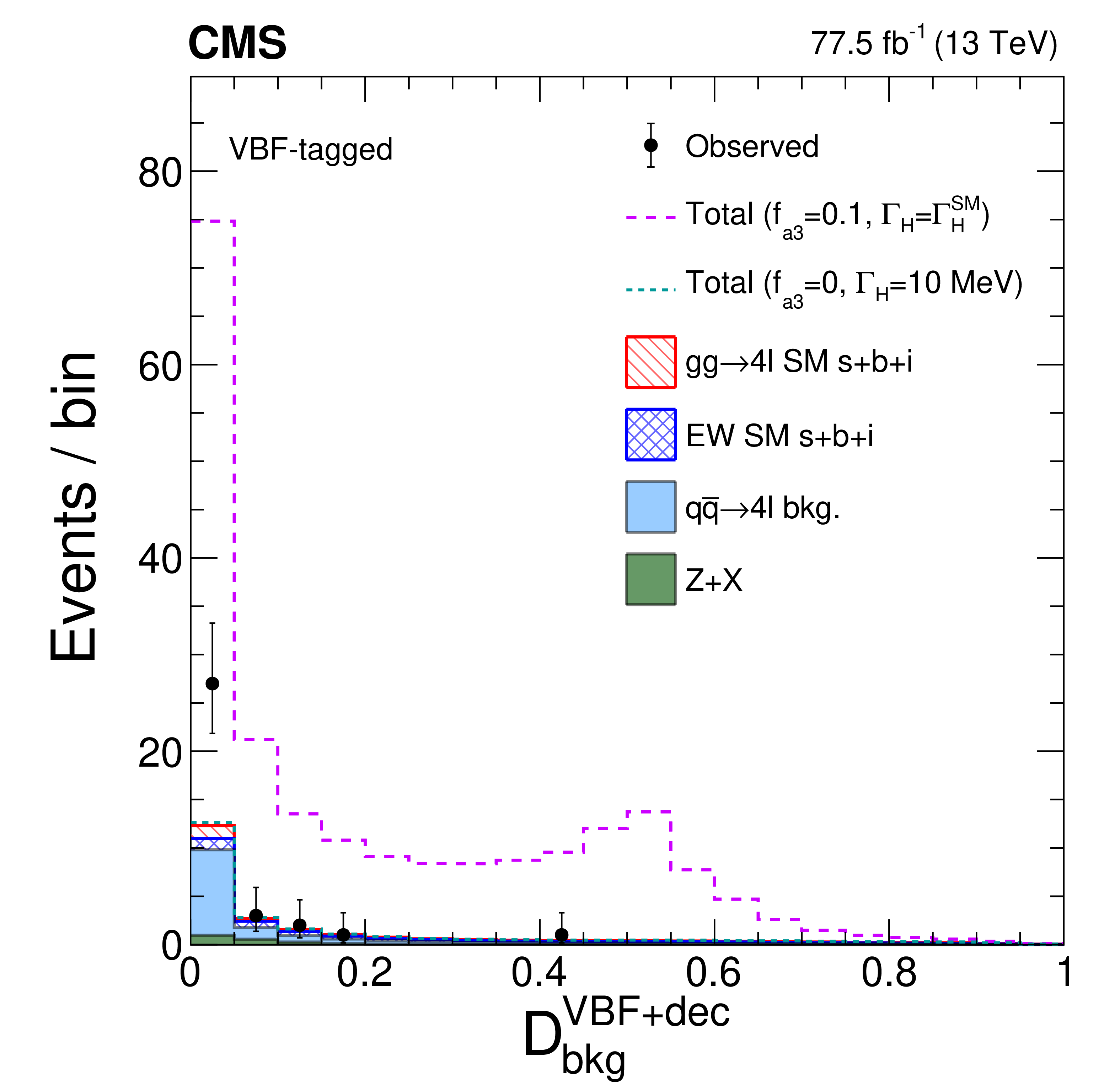
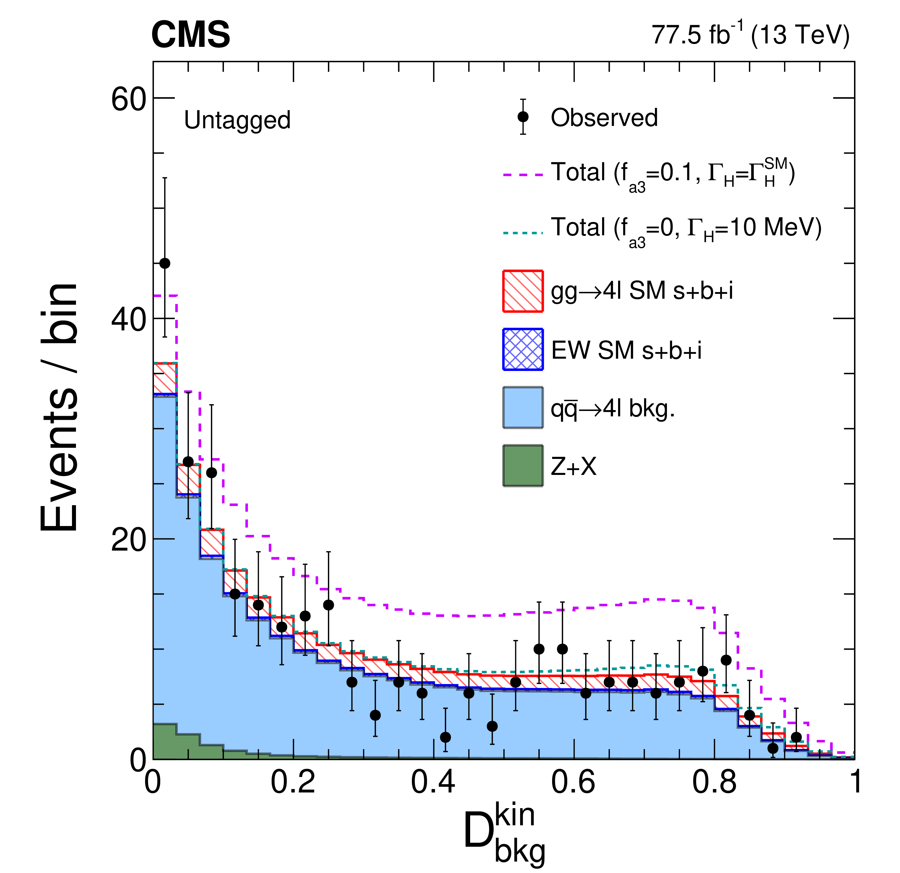
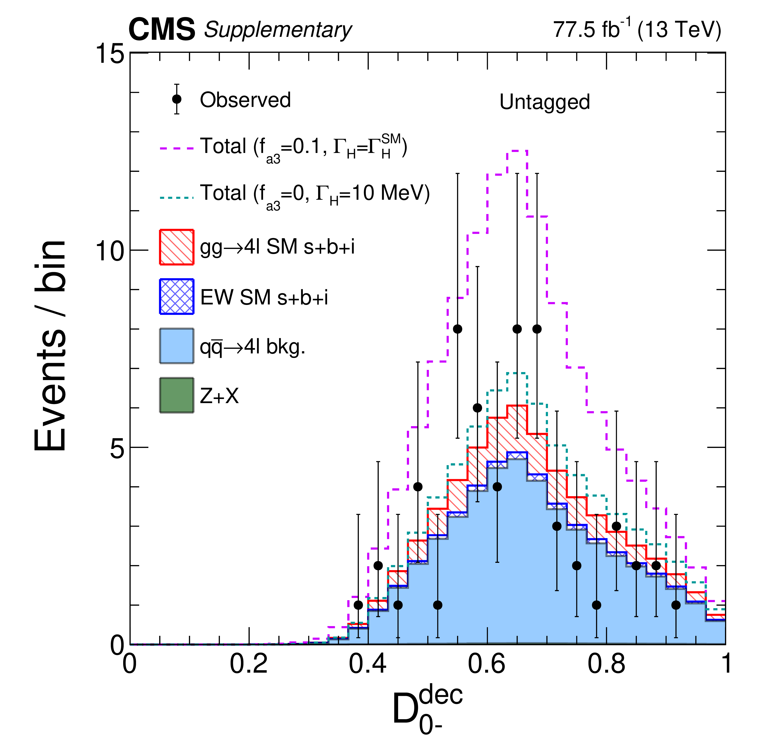
Figure 3:
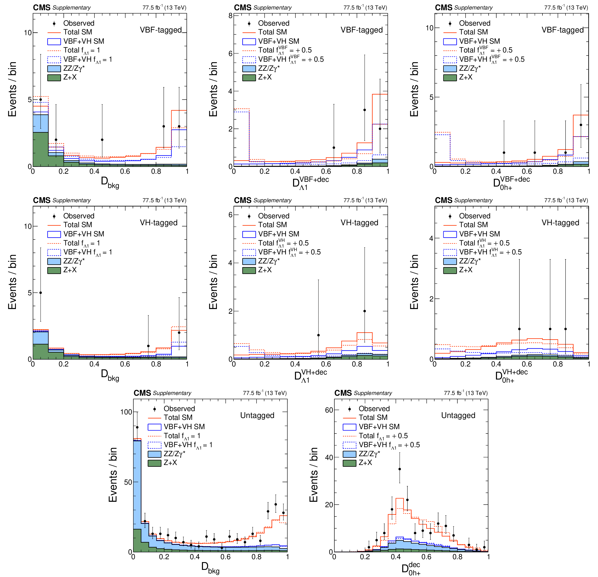
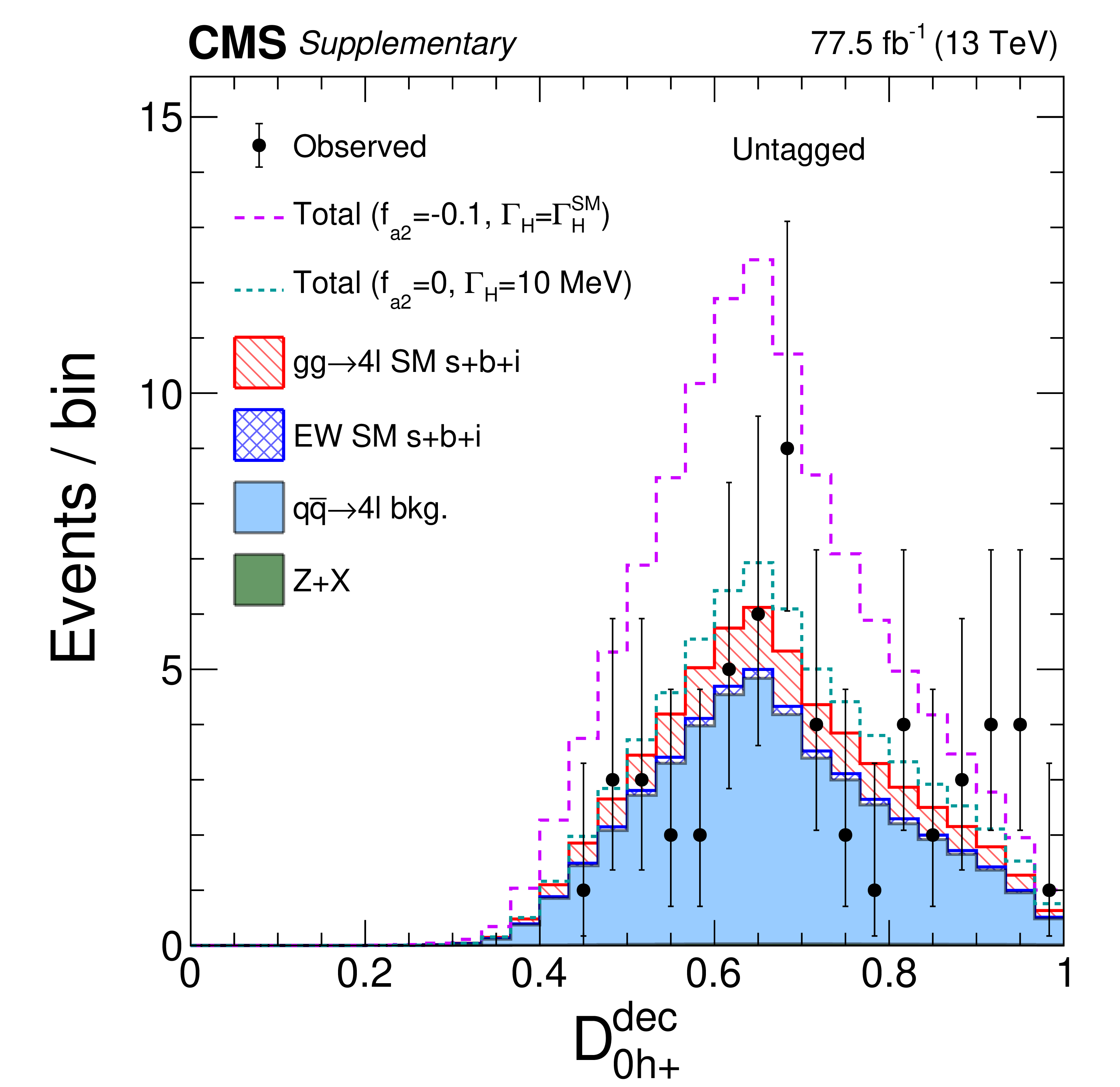
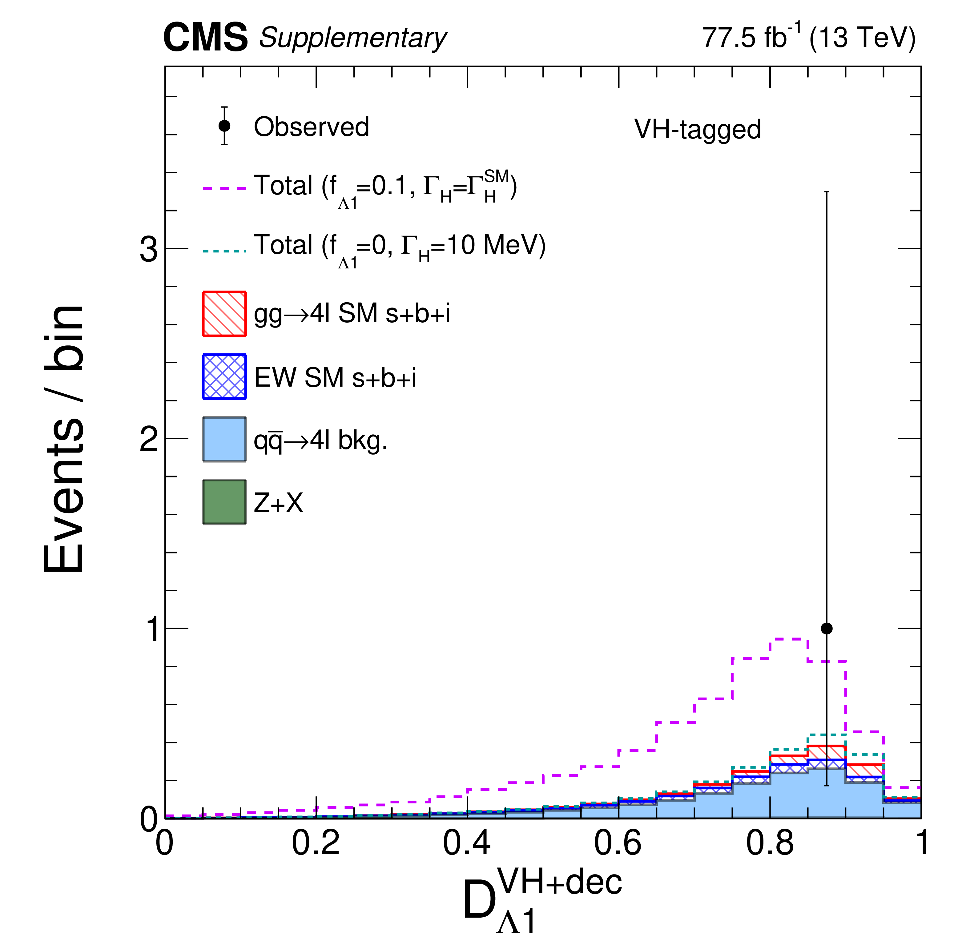
The distributions of events in the on-shell region in the data from 2016 and 2017. The top row shows ${{\mathcal {D}}_{\text {bkg}}}$ in the VBF-tagged (left), VH-tagged (middle), and untagged (right) categories of the analysis of the ${a_{3}}$ coupling for a pseudoscalar contribution. The rest of the distributions are shown with the requirement $ {{\mathcal {D}}_{\text {bkg}}} > $ 0.5 in order to enhance signal over background contributions. The middle row shows $\mathcal {D}_{0-}$ in the corresponding three categories. The bottom row shows $\mathcal {D}_{CP}^\text {dec}$ of the ${a_{3}}$, $\mathcal {D}_{0h+}^\text {dec}$ of the ${a_{2}}$, and $\mathcal {D}_{\Lambda 1}^\text {dec}$ of the ${\Lambda _{1}}$ analyses in the untagged categories. |
png pdf |
Figure 3-a:
Distribution of $\mathcal {D}_{\rm bkg}$ in the VBF-tagged category of the ${a_{3}}$ analysis for events events in the on-shell region in the data from 2016 and 2017. |
png pdf |
Figure 3-b:
Distribution of $\mathcal {D}_{\rm bkg}$ in the VH-tagged category of the ${a_{3}}$ analysis for events events in the on-shell region in the data from 2016 and 2017. |
png pdf |
Figure 3-c:
Distribution of $\mathcal {D}_{\rm bkg}$ in the untagged category of the ${a_{3}}$ analysis for events events in the on-shell region in the data from 2016 and 2017. |
png pdf |
Figure 3-d:
Distribution of $\mathcal {D}_{0-}$ in the VBF-tagged category of the ${a_{3}}$ analysis for events events in the on-shell region in the data from 2016 and 2017. The distribution is shown with the requirement $\mathcal {D}_{\rm bkg} > $ 0.5 in order to enhance signal over background contributions. |
png pdf |
Figure 3-e:
Distribution of $\mathcal {D}_{0-}$ in the VH-tagged category of the ${a_{3}}$ analysis for events events in the on-shell region in the data from 2016 and 2017. The distribution is shown with the requirement $\mathcal {D}_{\rm bkg} > $ 0.5 in order to enhance signal over background contributions. |
png pdf |
Figure 3-f:
Distribution of $\mathcal {D}_{0-}$ in the untagged category of the ${a_{3}}$ analysis for events events in the on-shell region in the data from 2016 and 2017. The distribution is shown with the requirement $\mathcal {D}_{\rm bkg} > $ 0.5 in order to enhance signal over background contributions. |

png pdf |
Figure 3-g:
Distribution of $\mathcal {D}_{CP}^{\rm dec}$ of the ${a_{3}}$ analysis in the untagged category, for events events in the on-shell region in the data from 2016 and 2017. The distribution is shown with the requirement $\mathcal {D}_{\rm bkg} > $ 0.5 in order to enhance signal over background contributions. |
png pdf |
Figure 3-h:
Distribution of $\mathcal {D}_{0h+}^{\rm dec}$ of the ${a_{2}}$ analysis in the untagged category, for events events in the on-shell region in the data from 2016 and 2017. The distribution is shown with the requirement $\mathcal {D}_{\rm bkg} > $ 0.5 in order to enhance signal over background contributions. |
png pdf |
Figure 3-i:
Distribution of $\mathcal {D}_{\Lambda 1}^{\rm dec}$ of the ${\Lambda _{1}}$ analysis in the untagged category, for events events in the on-shell region in the data from 2016 and 2017. The distribution is shown with the requirement $\mathcal {D}_{\rm bkg} > $ 0.5 in order to enhance signal over background contributions. |
png pdf |
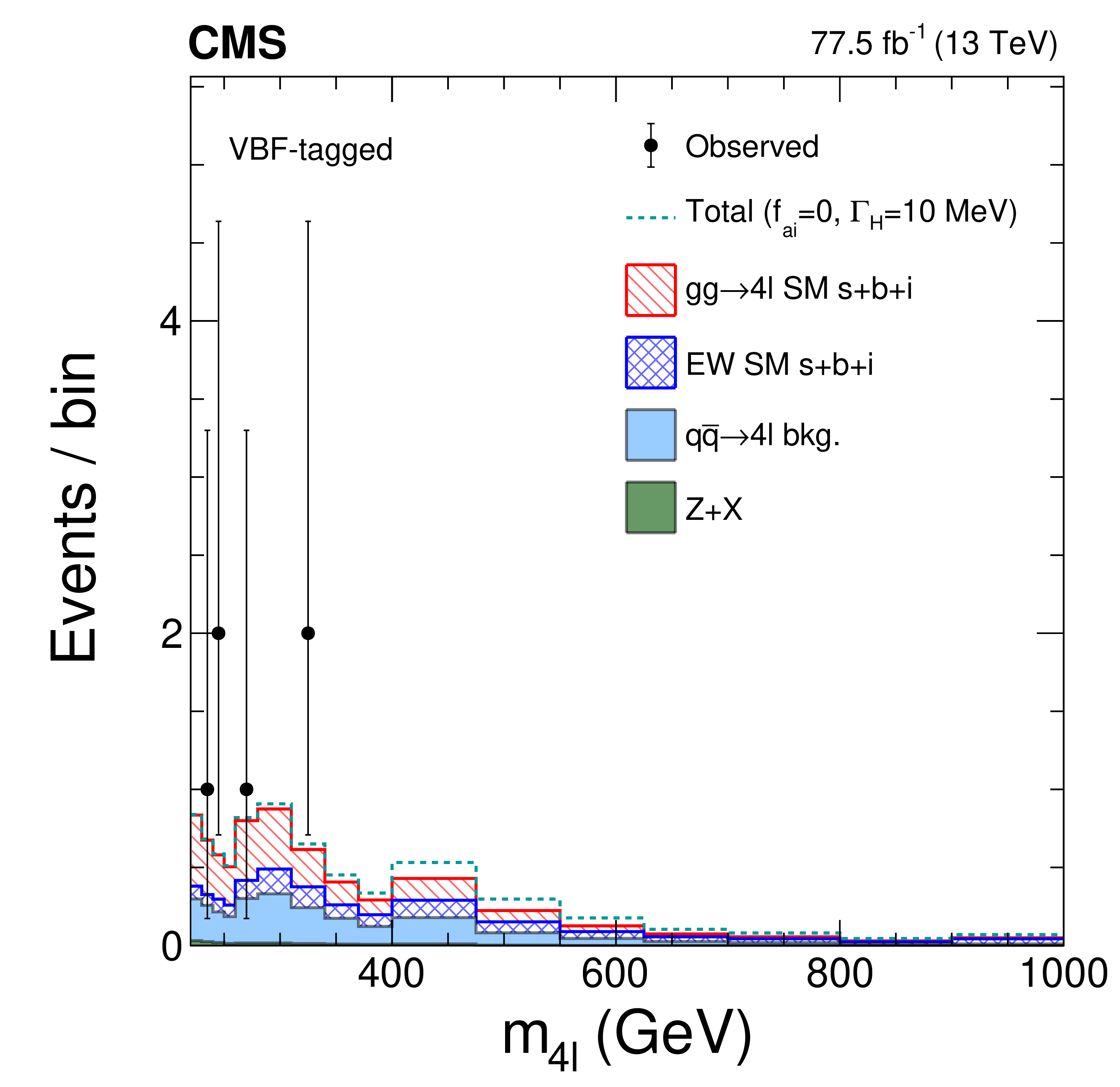
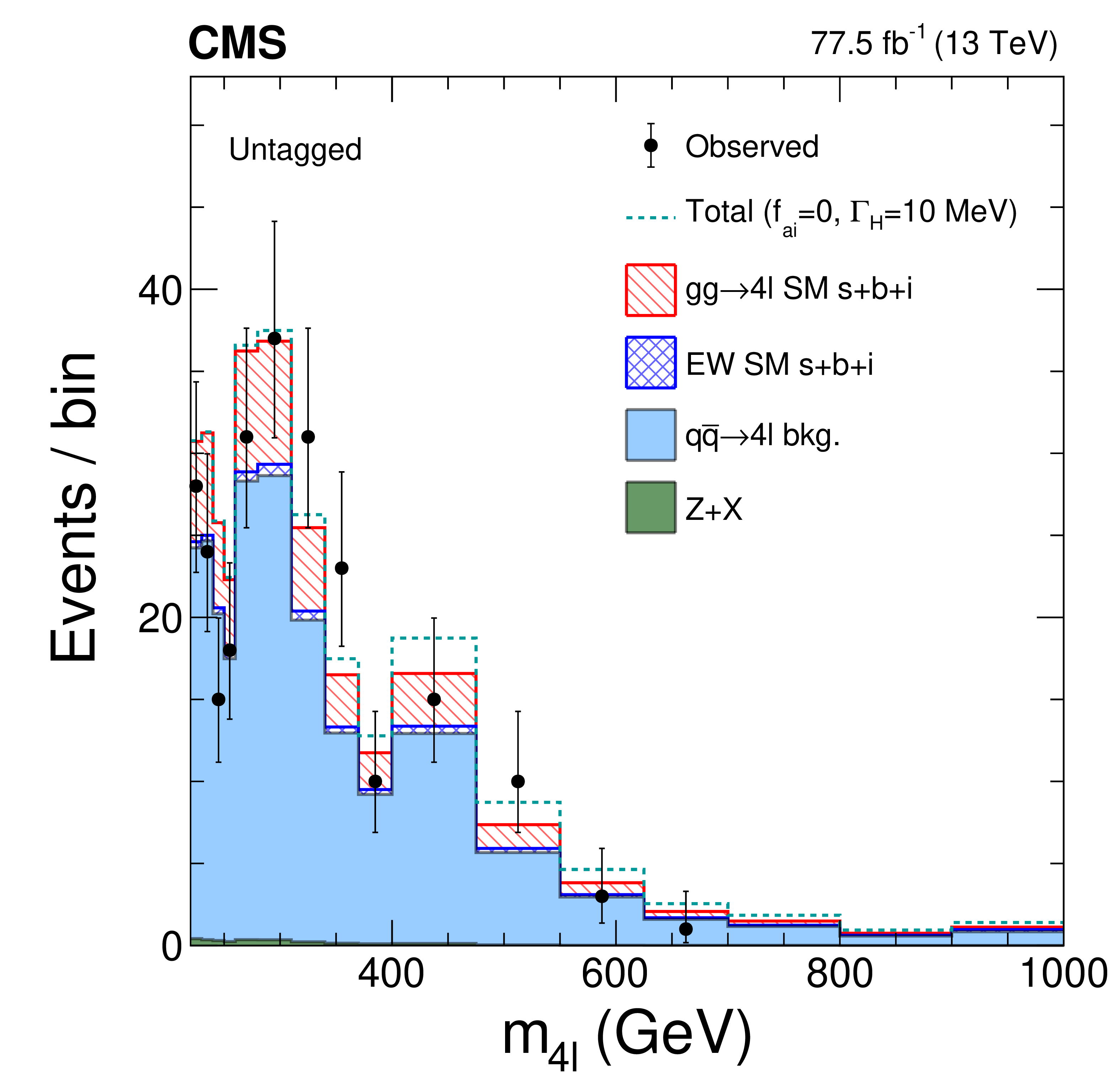
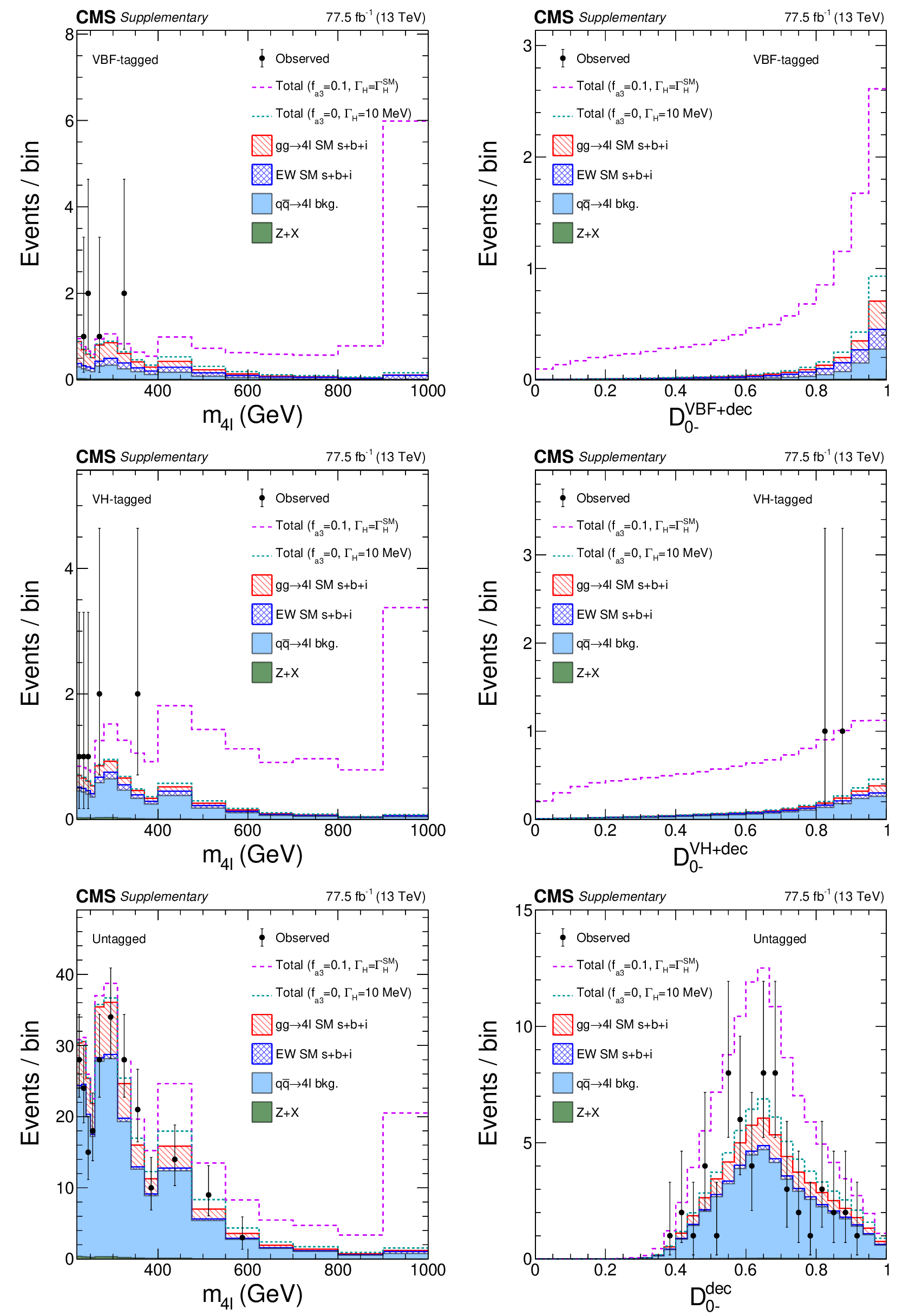
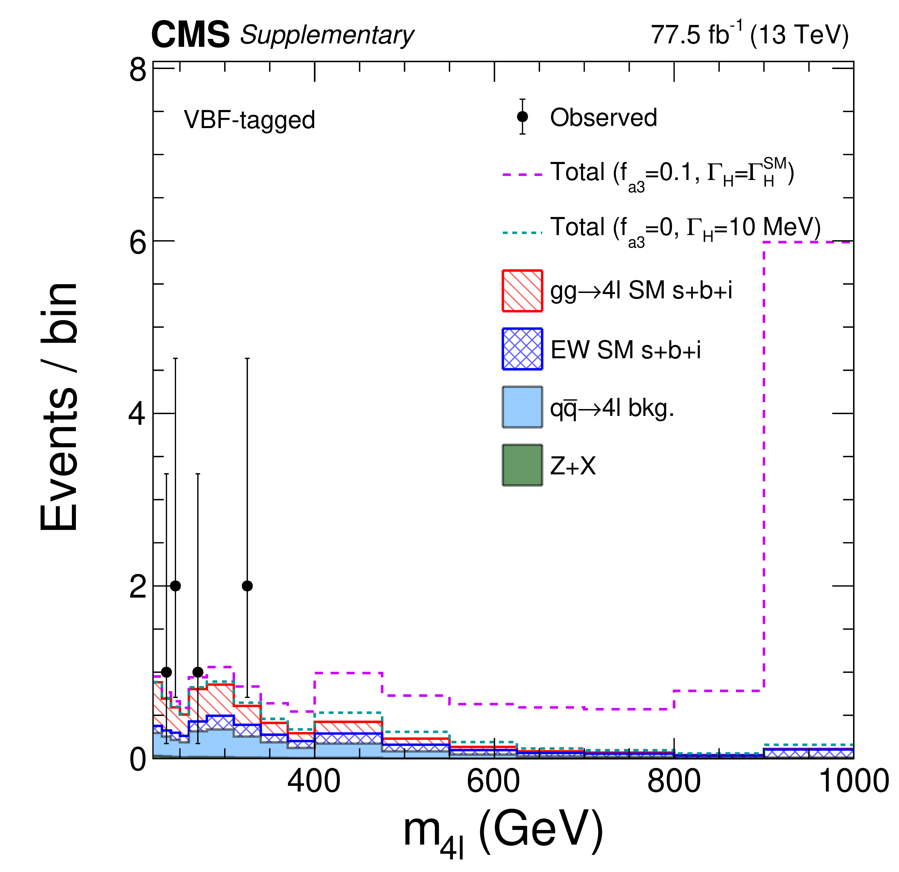
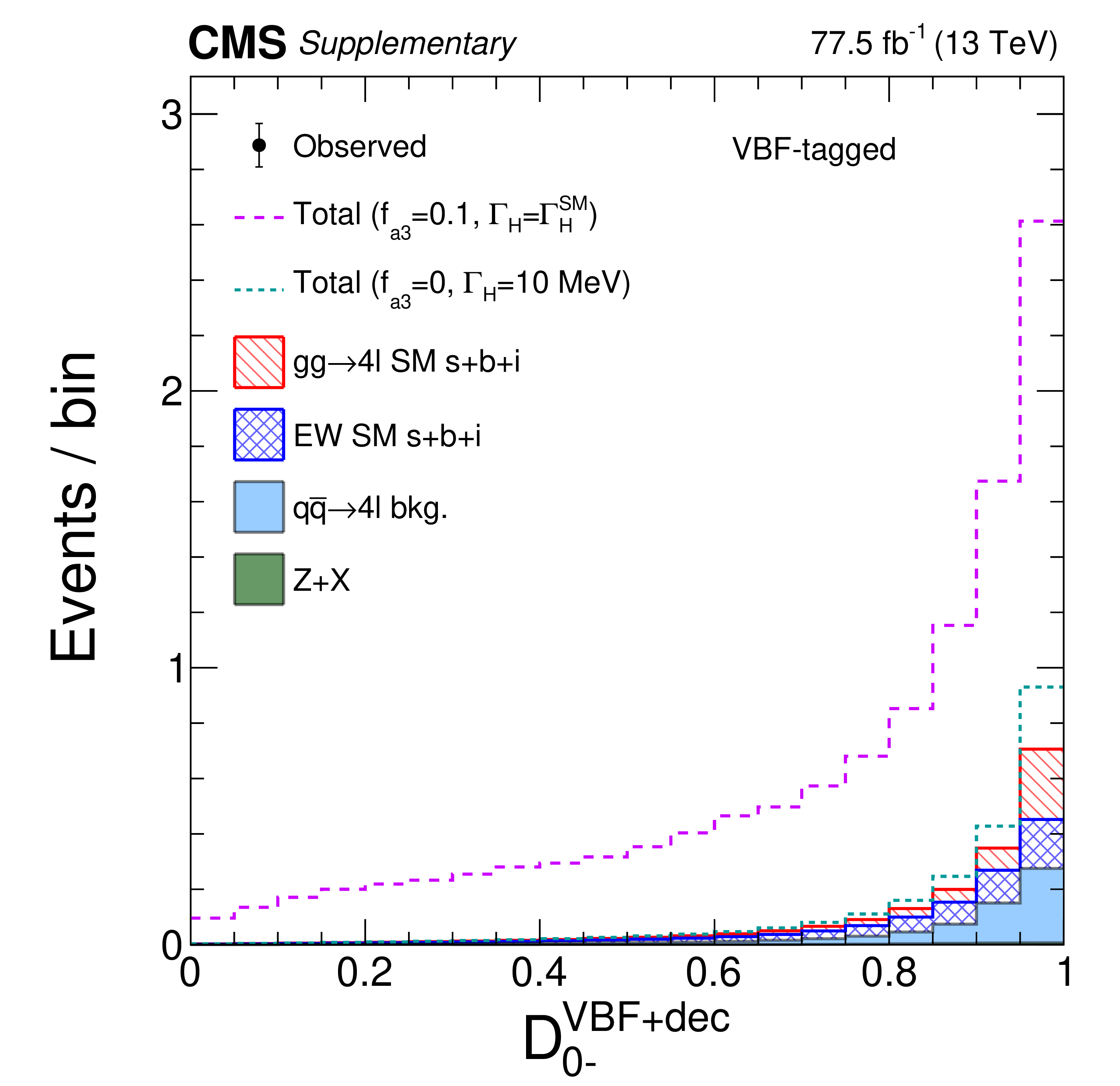
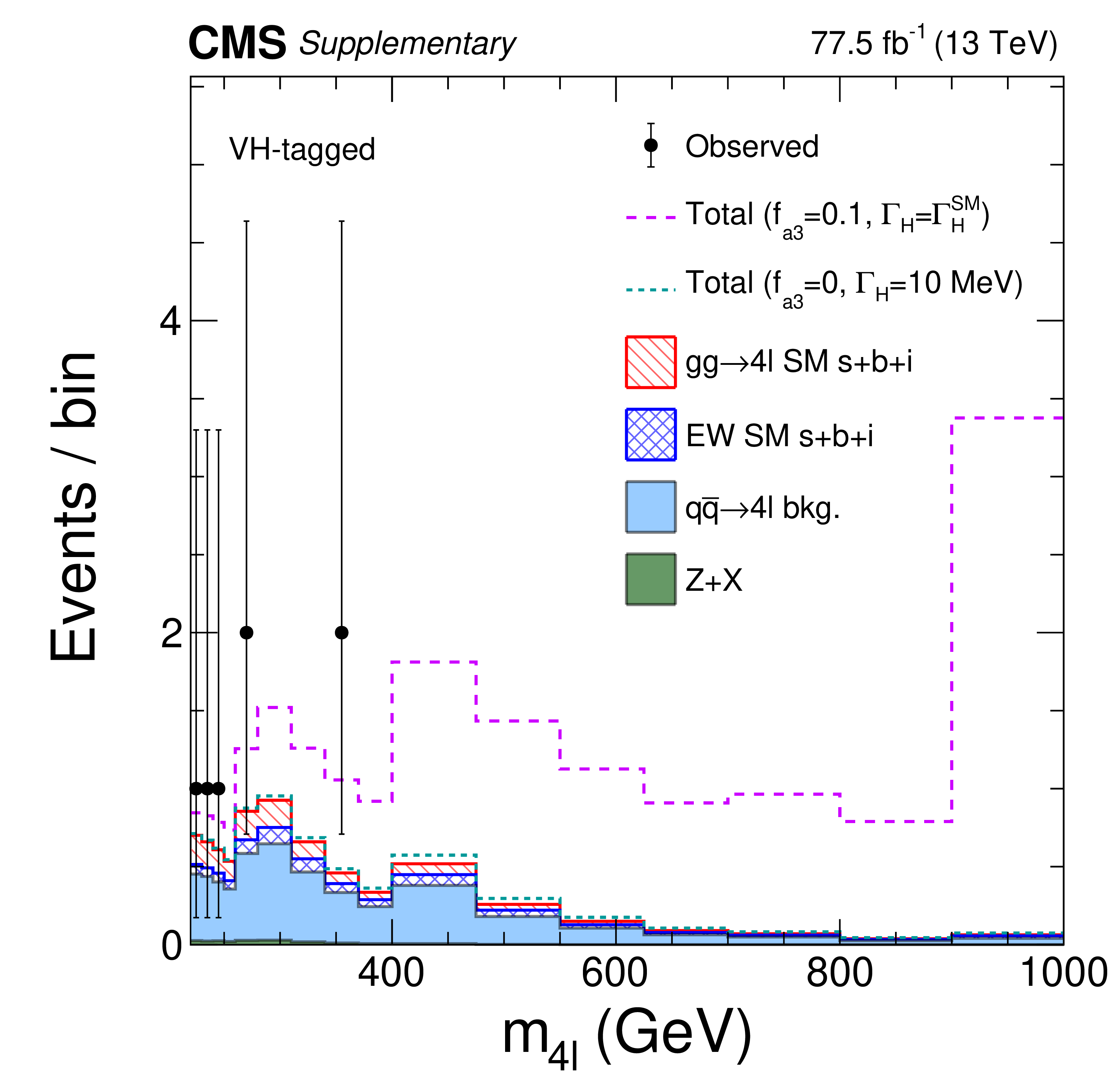
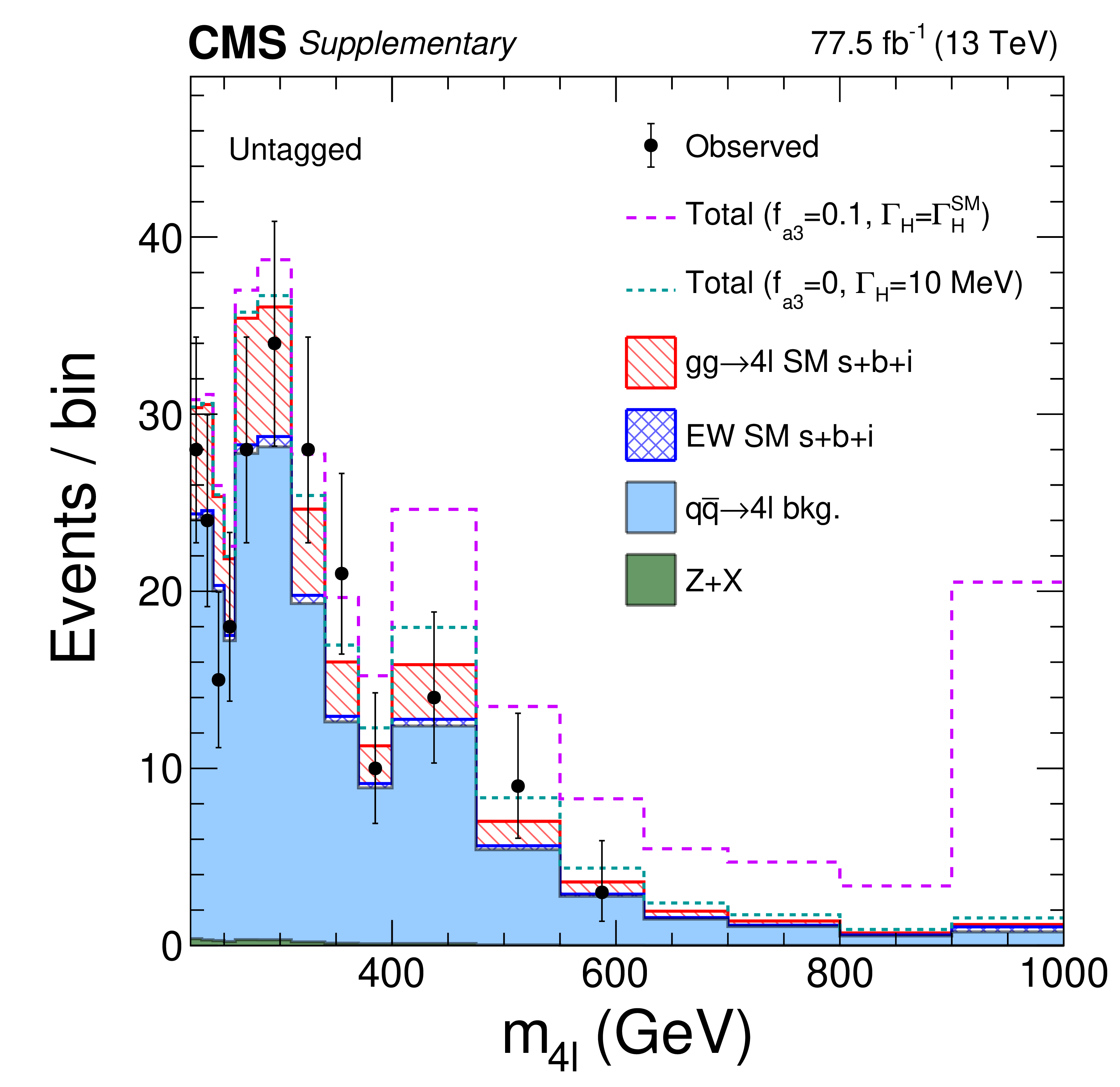
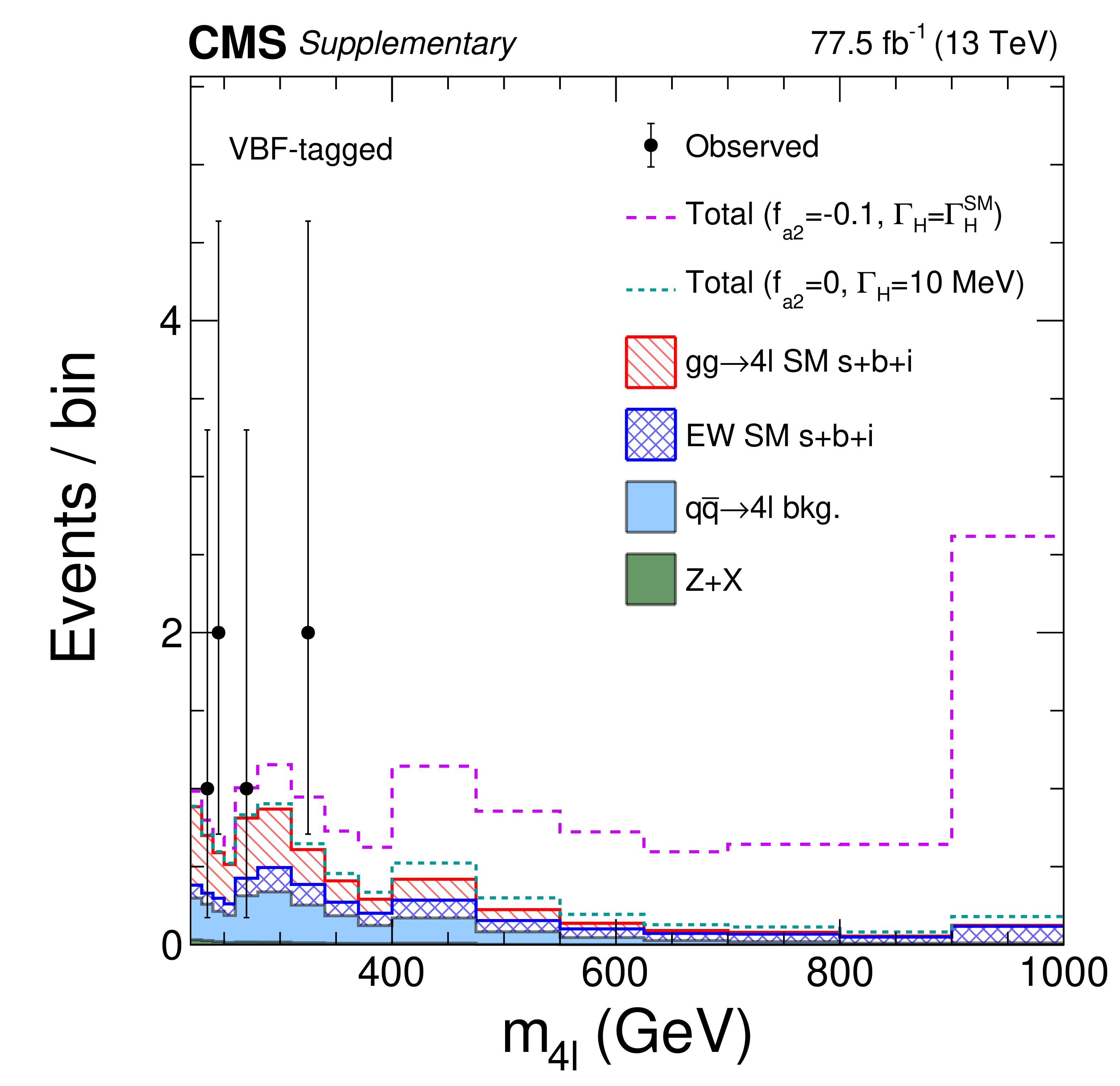
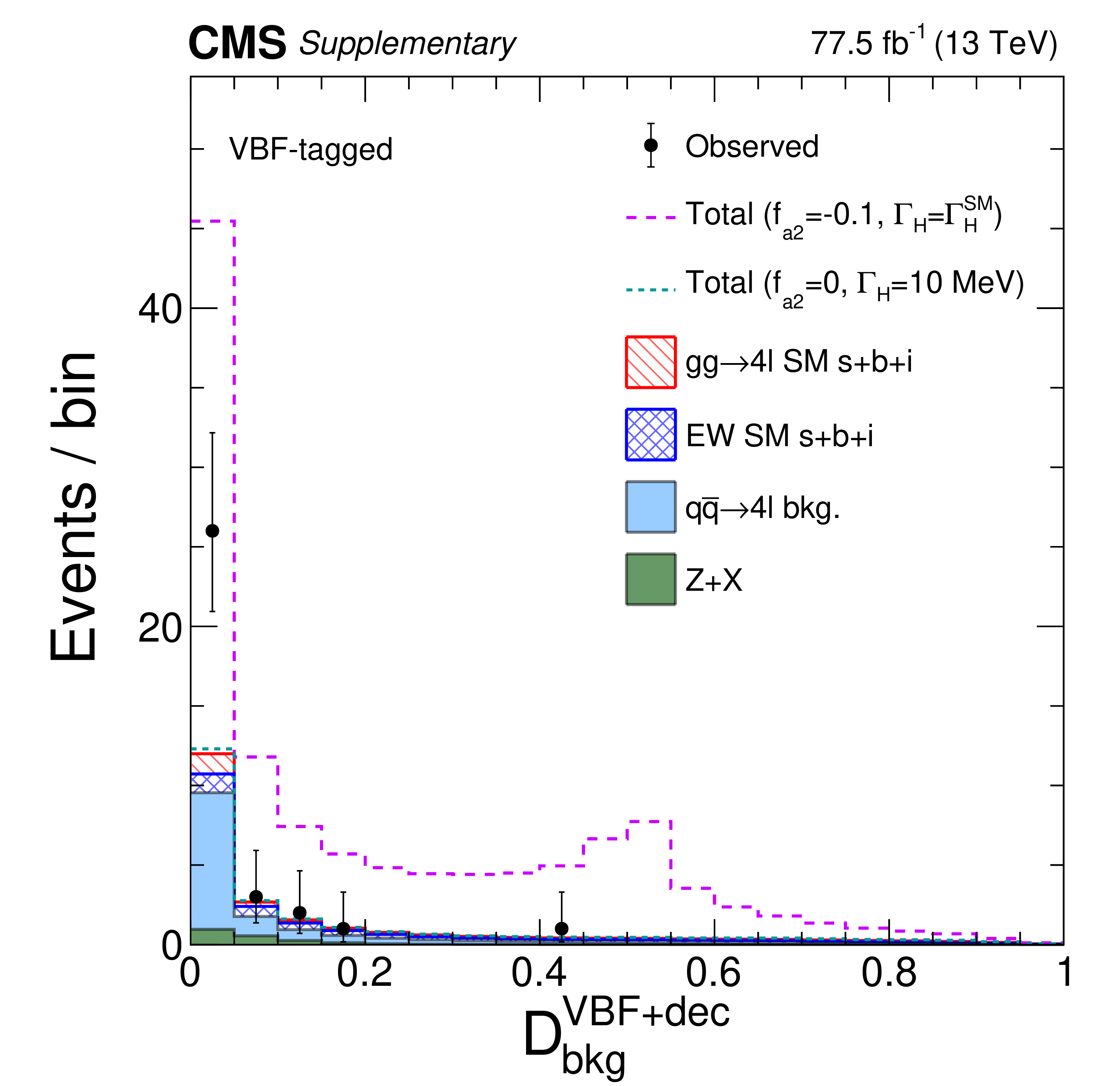
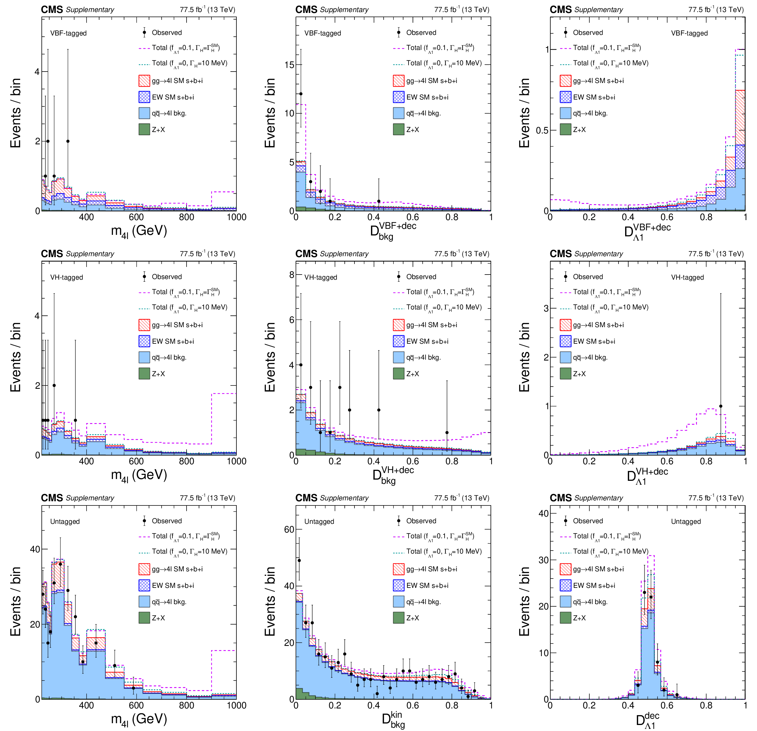
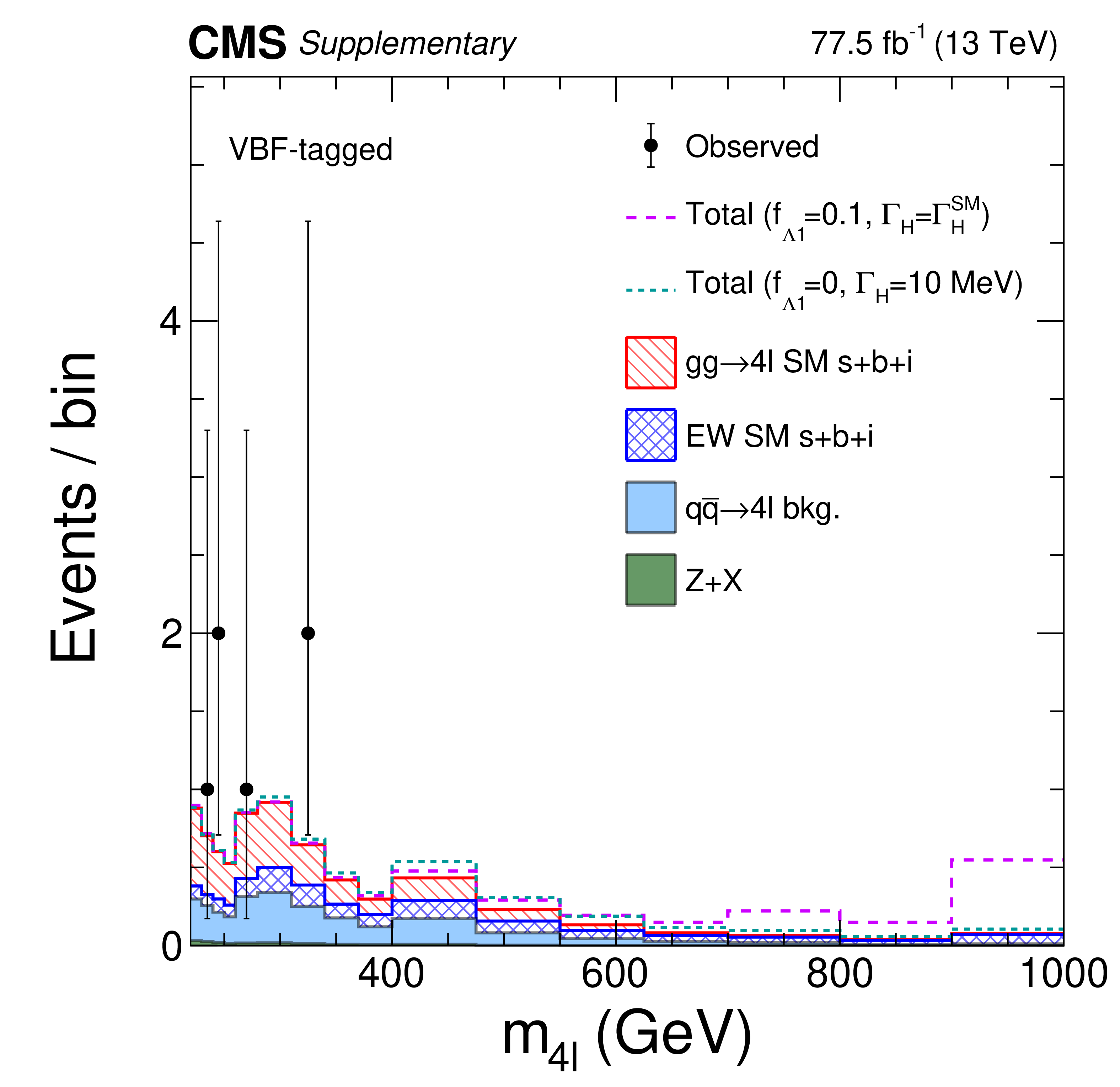
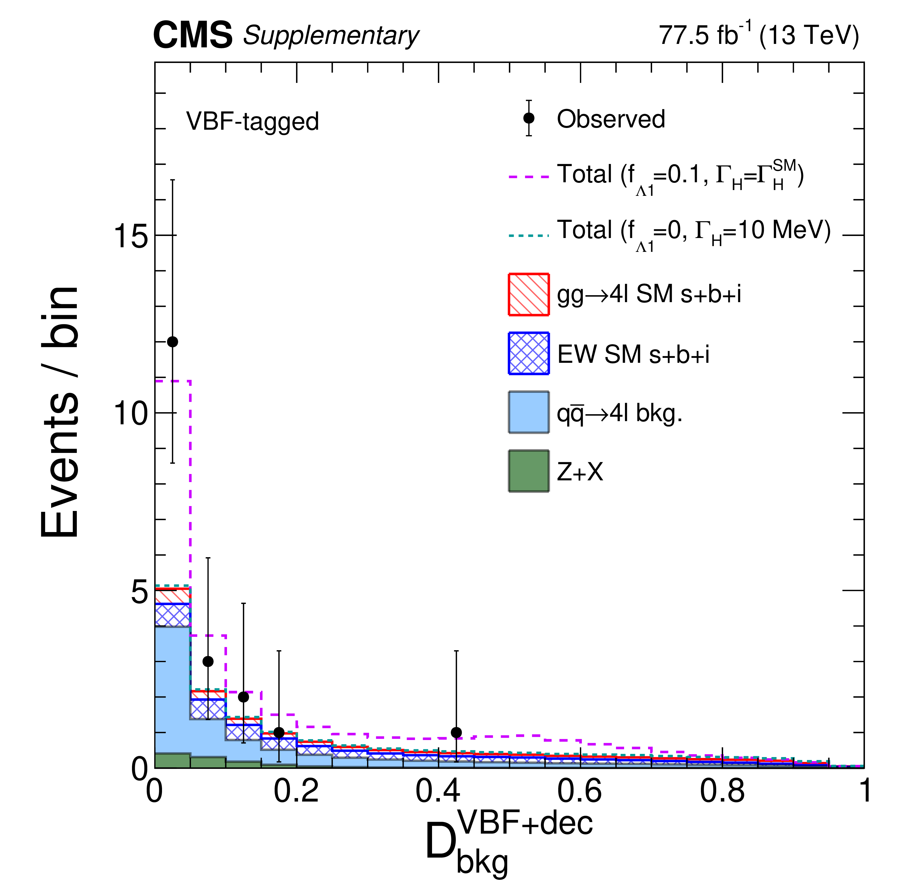
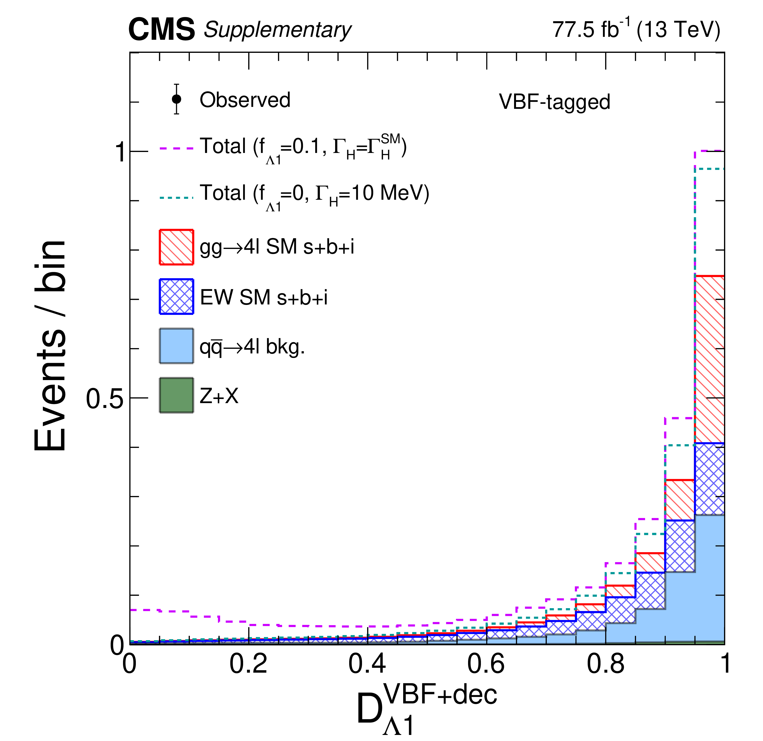
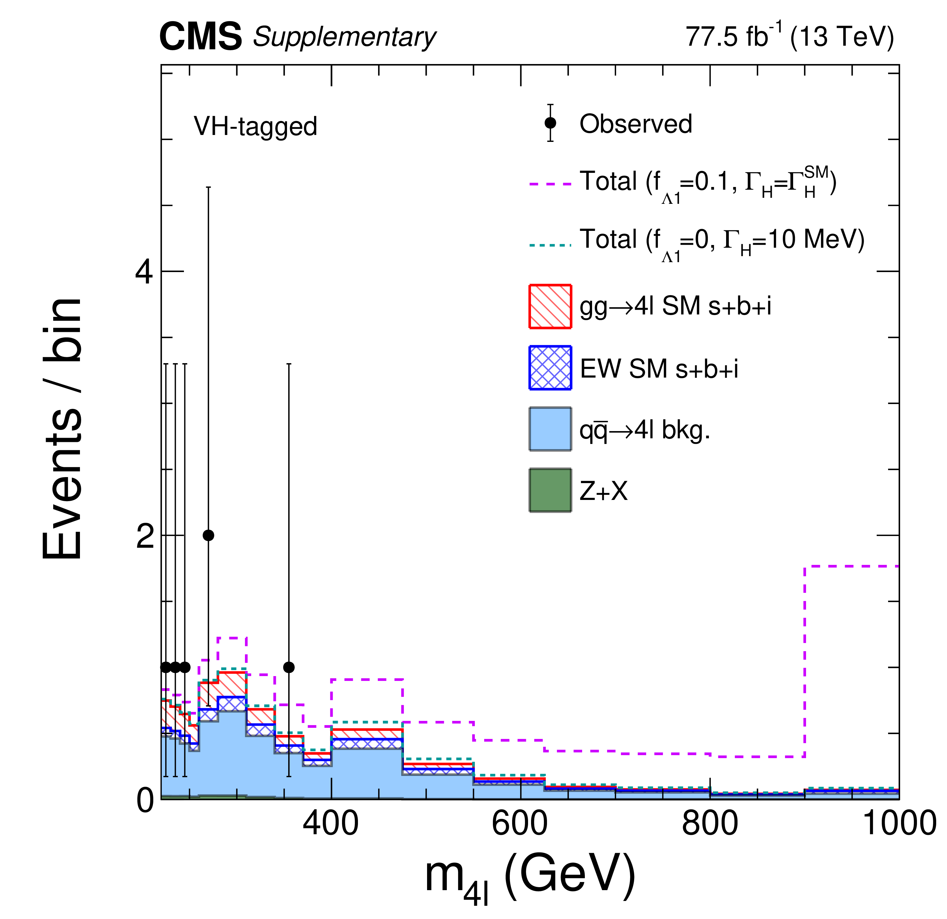
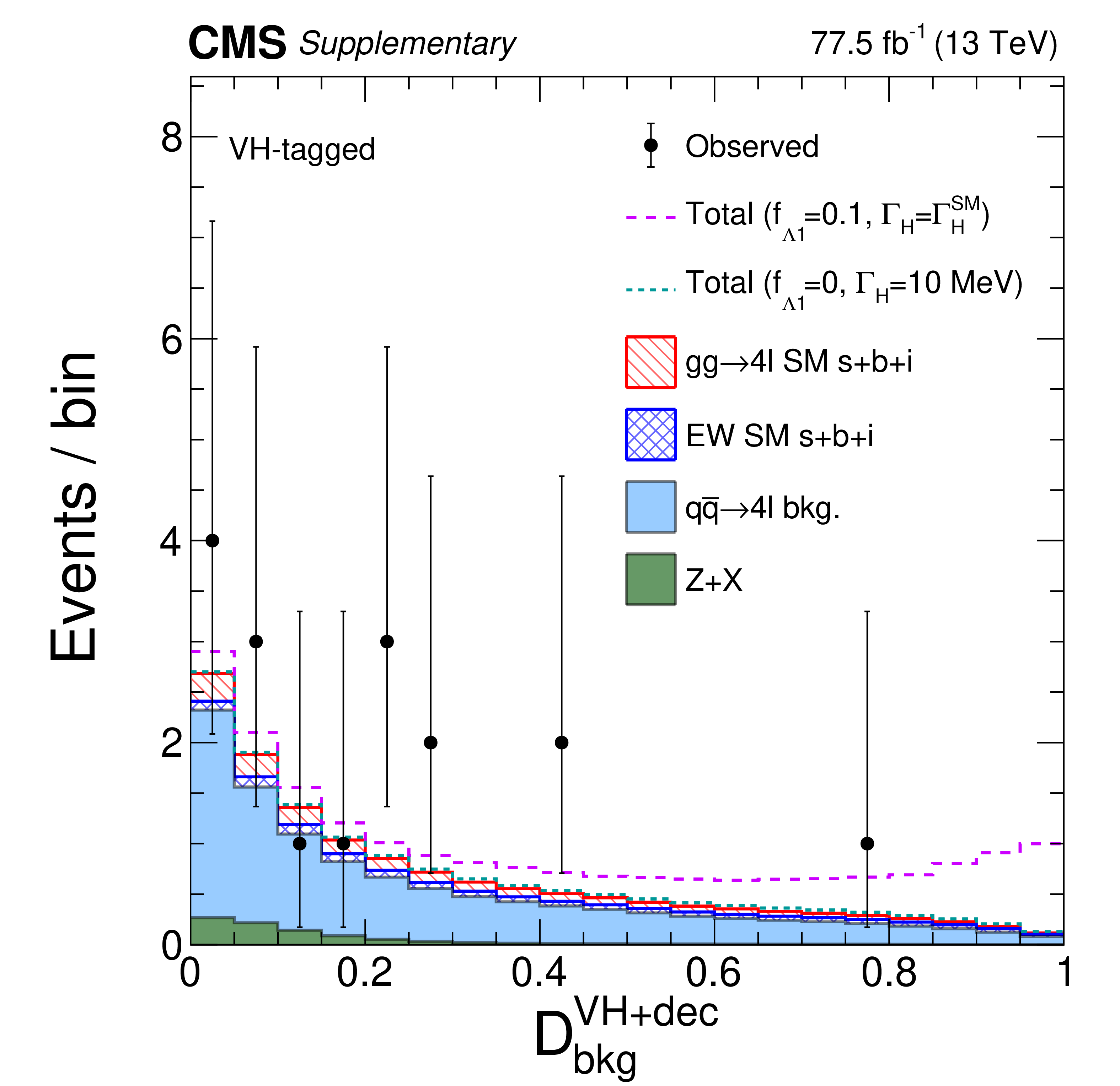
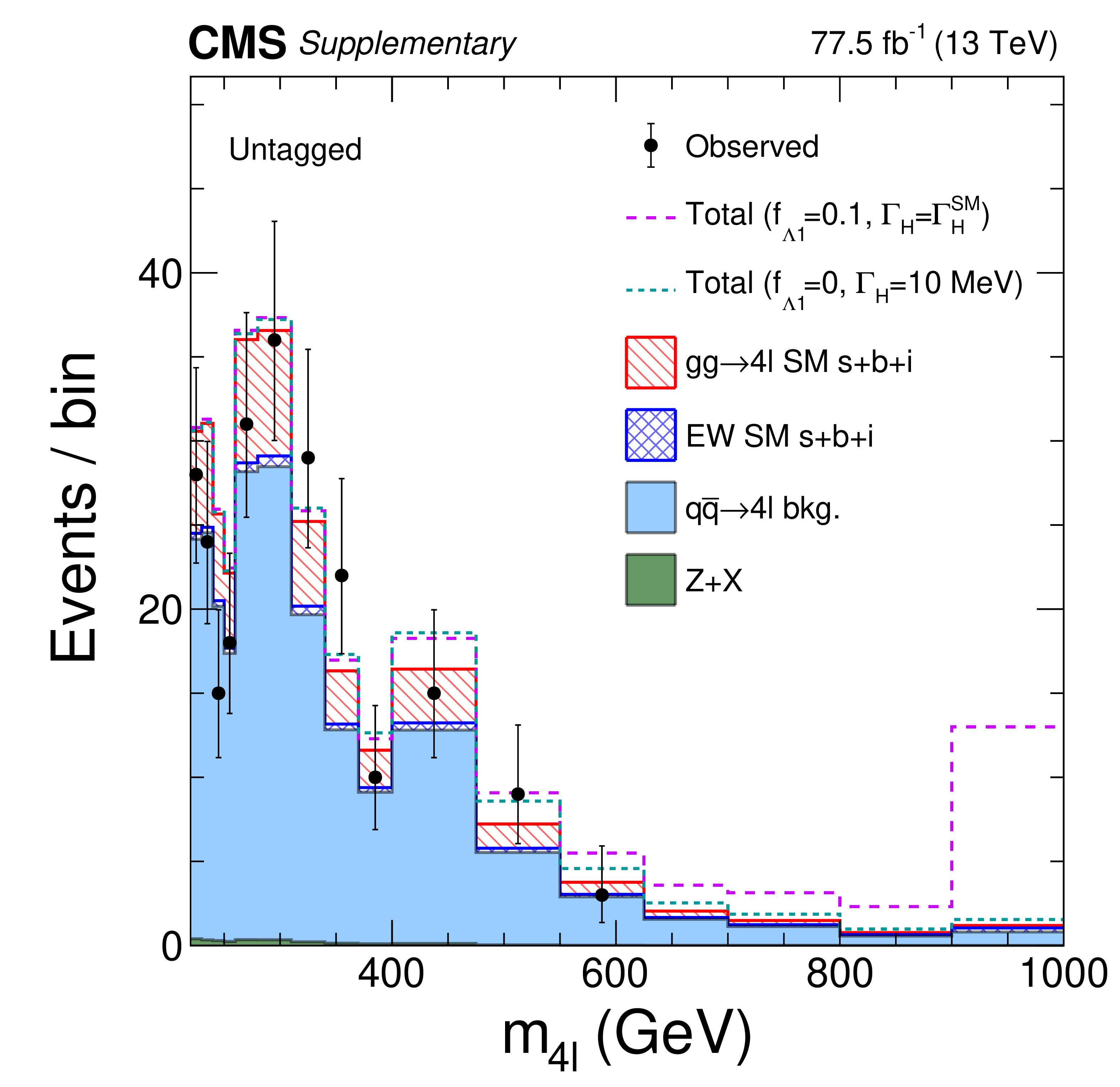
Figure 4:
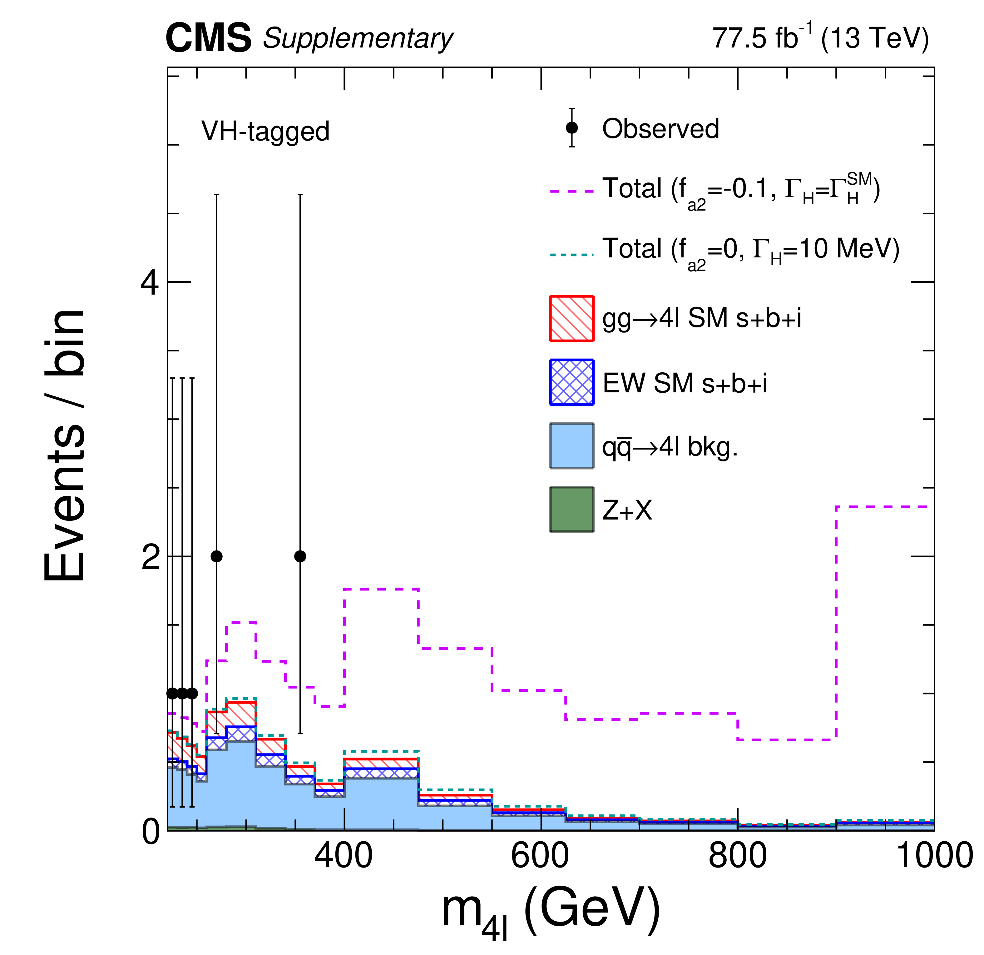
The distributions of events in the off-shell region in the data from 2016 and 2017. The top row shows $ {m_{4\ell}} $ in the VBF-tagged (left), VH-tagged (middle), and untagged (right) categories in the dedicated SM-like width analysis where a requirement on $\mathcal {D}^{{{\mathrm {VBF}}}+{\text {dec}}}_\text {bkg}$, $\mathcal {D}^{{{{\mathrm {V}} \mathrm{H}}}+{\text {dec}}}_\text {bkg}$, or $ {{\mathcal {D}}^{\text {kin}}_{\text {bkg}}} > $ 0.6 is applied in order to enhance signal over background contributions. The middle row shows $\mathcal {D}^{{{\mathrm {VBF}}}+{\text {dec}}}_\text {bkg}$ (left), $\mathcal {D}^{{{{\mathrm {V}} \mathrm{H}}}+{\text {dec}}}_\text {bkg}$ (middle), $\mathcal {D}^\text {kin}_\text {bkg}$ (right) of the ${a_{3}}$ analysis in the corresponding three categories. The requirement $ {m_{4\ell}} > $ 340 GeV is applied in order to enhance signal over background contributions. The bottom row shows $\mathcal {D}_\mathrm {bsi}$ in the corresponding three categories in the dedicated SM-like width analysis with both of the ${m_{4\ell}}$ and ${{\mathcal {D}}^{\text {kin}}_{\text {bkg}}}$ requirements enhancing the signal contribution. The acronym $\mathrm {s}+\mathrm {b}+\mathrm {i}$ designates the sum of the signal (s), background (b), and their interference contributions (i). |
png pdf |
Figure 4-a:
The distribution of $ {m_{4\ell}} $ for events in the off-shell region in the data from 2016 and 2017, in the VBF-tagged category. The distribution is obtained in the dedicated SM-like width analysis where a requirement on $\mathcal {D}^{{\rm VBF}+{\rm dec}}_{\rm bkg} > $ 0.6 is applied in order to enhance signal over background contributions. |

png pdf |
Figure 4-b:
The distribution of $ {m_{4\ell}} $ for events in the off-shell region in the data from 2016 and 2017, in the VH-tagged category. The distribution is obtained in the dedicated SM-like width analysis where a requirement on $ \mathcal {D}^{{\mathrm {V}} {\mathrm {H}} +{\rm dec}}_{\rm bkg} > $ 0.6 is applied in order to enhance signal over background contributions. |
png pdf |
Figure 4-c:
The distribution of $ {m_{4\ell}} $ for events in the off-shell region in the data from 2016 and 2017, in the untagged category. The distribution is obtained in the dedicated SM-like width analysis where a requirement on $ \mathcal {D}_{\rm bkg} > $ 0.6 is applied in order to enhance signal over background contributions. |
png pdf |
Figure 4-d:
The distribution of $\mathcal {D}^{{\rm VBF}+{\rm dec}}_{\rm bkg}$ of the ${a_{3}}$ analysis, for events in the off-shell region in the data from 2016 and 2017, in the VBF-tagged category. The requirement $ {m_{4\ell}} > $ 340 GeV is applied in order to enhance signal over background contributions. |

png pdf |
Figure 4-e:
The distribution of $\mathcal {D}^{{\mathrm {V}} {\mathrm {H}} +{\rm dec}}_{\rm bkg}$ of the ${a_{3}}$ analysis, for events in the off-shell region in the data from 2016 and 2017, in the VH-tagged category. The requirement $ {m_{4\ell}} > $ 340 GeV is applied in order to enhance signal over background contributions. |
png pdf |
Figure 4-f:
The distribution of $\mathcal {D}^{\rm kin}_{\rm bkg}$ of the ${a_{3}}$ analysis, for events in the off-shell region in the data from 2016 and 2017, in the untagged category. The requirement $ {m_{4\ell}} > $ 340 GeV is applied in order to enhance signal over background contributions. |
png pdf |
Figure 4-g:
The distribution of $\mathcal {D}_{\rm bsi}$ for events in the off-shell region in the data from 2016 and 2017, in the VBF-tagged category. The distribution is obtained in the dedicated SM-like width analysis where a requirement on $\mathcal {D}^{{\rm VBF}+{\rm dec}}_{\rm bkg} > $ 0.6, and the requirement $ {m_{4\ell}} > $ 340 GeV, are applied in order to enhance signal over background contributions. |
png pdf |
Figure 4-h:
The distribution of $\mathcal {D}_{\rm bsi}$ for events in the off-shell region in the data from 2016 and 2017, in the VH-tagged category. The distribution is obtained in the dedicated SM-like width analysis where a requirement on $\mathcal {D}^{{\mathrm {V}} {\mathrm {H}} +{\rm dec}}_{\rm bkg} > $ 0.6, and the requirement $ {m_{4\ell}} > $ 340 GeV, are applied in order to enhance signal over background contributions. |
png pdf |
Figure 4-i:
The distribution of $\mathcal {D}_{\rm bsi}$ for events in the off-shell region in the data from 2016 and 2017, in the untagged category. The distribution is obtained in the dedicated SM-like width analysis where a requirement on $\mathcal {D}_{\rm bkg} > $ 0.6, and the requirement $ {m_{4\ell}} > $ 340 GeV, are applied in order to enhance signal over background contributions. |
png pdf |
Figure 5:
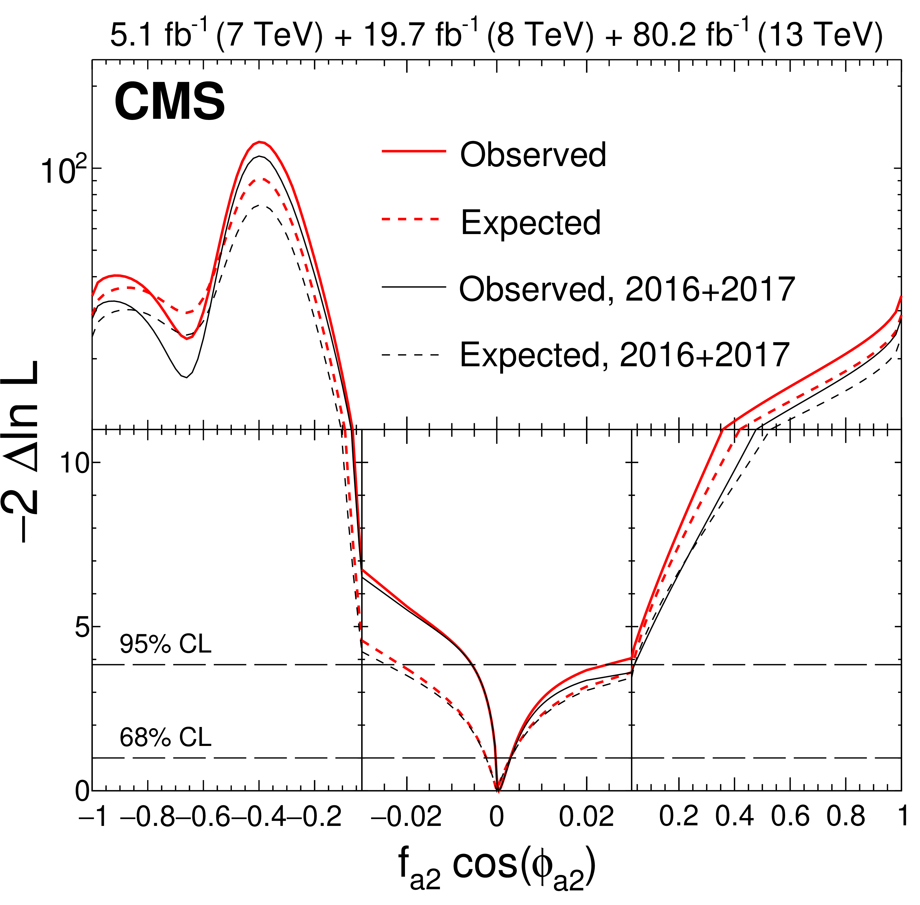
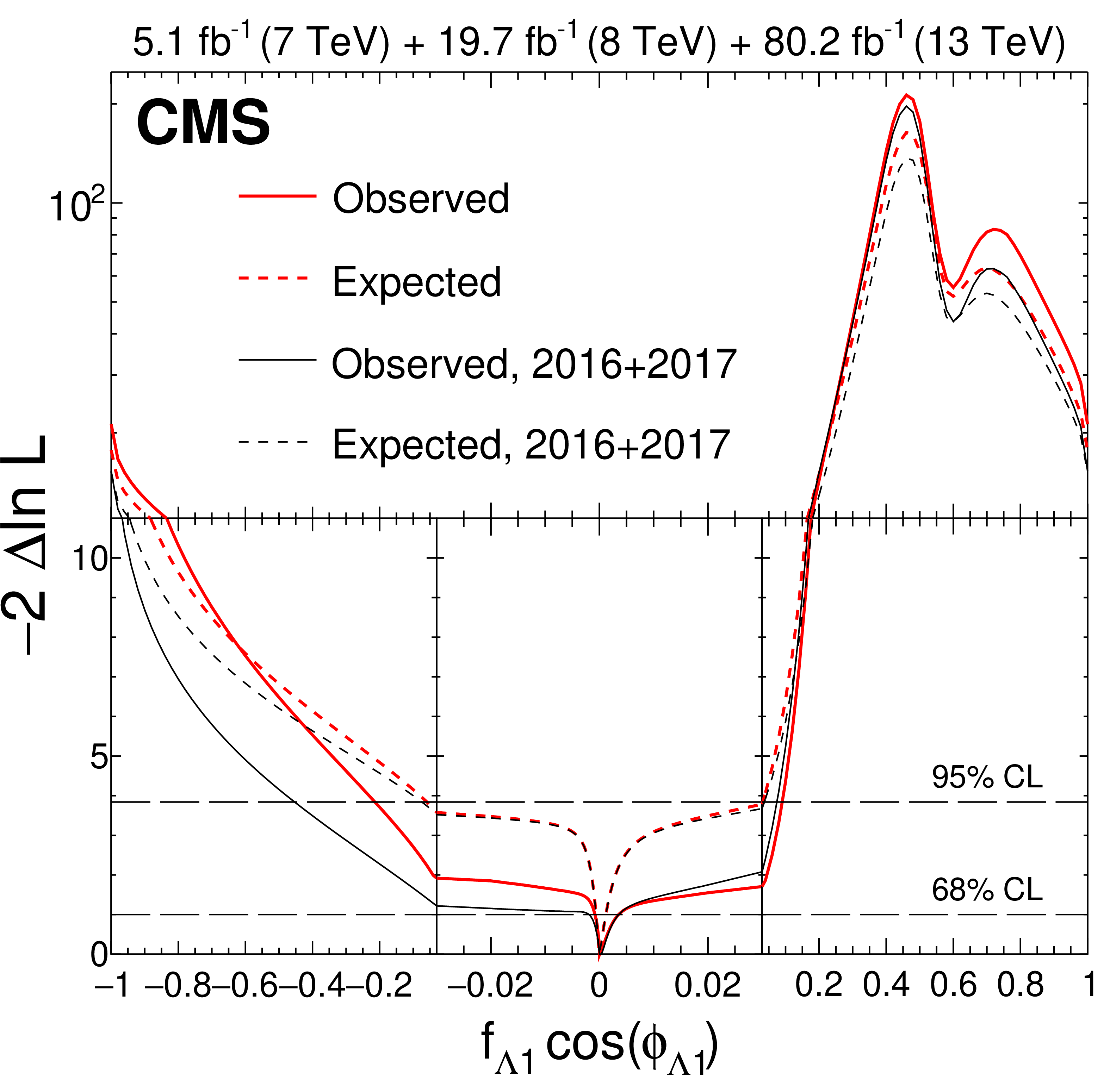
Observed (solid) and expected (dashed) likelihood scans of ${{f_{a 3}} {\cos\left ({\phi _{a 3}} \right)}}$ (top left), ${{f_{a 2}} {\cos\left ({\phi _{a 2}} \right)}}$ (top right), ${{f_{\Lambda 1}} {\cos\left ({\phi _{\Lambda 1}} \right)}}$ (bottom left), and ${{{f_{\Lambda 1}} ^{\mathrm{Z} \gamma}} {\cos\left ({{\phi _{\Lambda 1}} ^{\mathrm{Z} \gamma}} \right)}}$ (bottom right) using on-shell events only. Results of analysis of the data from 2016 and 2017 only (black) and the combined Run 1 and Run 2 analysis (red) are shown. The dashed horizontal lines show the 68 and 95% CL regions. |

png pdf |
Figure 5-a:
Observed (solid) and expected (dashed) likelihood scans of $ {{f_{a 2}} {\cos\left ({\phi _{a 2}} \right)}} $, using on-shell events only. Results of analysis of the data from 2016 and 2017 only (black) and the combined Run 1 and Run 2 analysis (red) are shown. The dashed horizontal lines show the 68% and 95% CL regions. |
png pdf |
Figure 5-b:
Observed (solid) and expected (dashed) likelihood scans of ${{f_{a 3}} {\cos ({\phi _{a 3}} )}}$, using on-shell events only. Results of analysis of the data from 2016 and 2017 only (black) and the combined Run 1 and Run 2 analysis (red) are shown. The dashed horizontal lines show the 68% and 95% CL regions. |
png pdf |
Figure 5-c:
Observed (solid) and expected (dashed) likelihood scans of $ {{f_{\Lambda 1}} {\cos\left ({\phi _{\Lambda 1}} \right)}} $, using on-shell events only. Results of analysis of the data from 2016 and 2017 only (black) and the combined Run 1 and Run 2 analysis (red) are shown. The dashed horizontal lines show the 68% and 95% CL regions. |

png pdf |
Figure 5-d:
Observed (solid) and expected (dashed) likelihood scans of $ {{{f_{\Lambda 1}} ^{{\mathrm {Z}} \gamma}} {\cos\left ({{\phi _{\Lambda 1}} ^{{\mathrm {Z}} \gamma}} \right)}} $, using on-shell events only. Results of analysis of the data from 2016 and 2017 only (black) and the combined Run 1 and Run 2 analysis (red) are shown. The dashed horizontal lines show the 68% and 95% CL regions. |
png pdf |
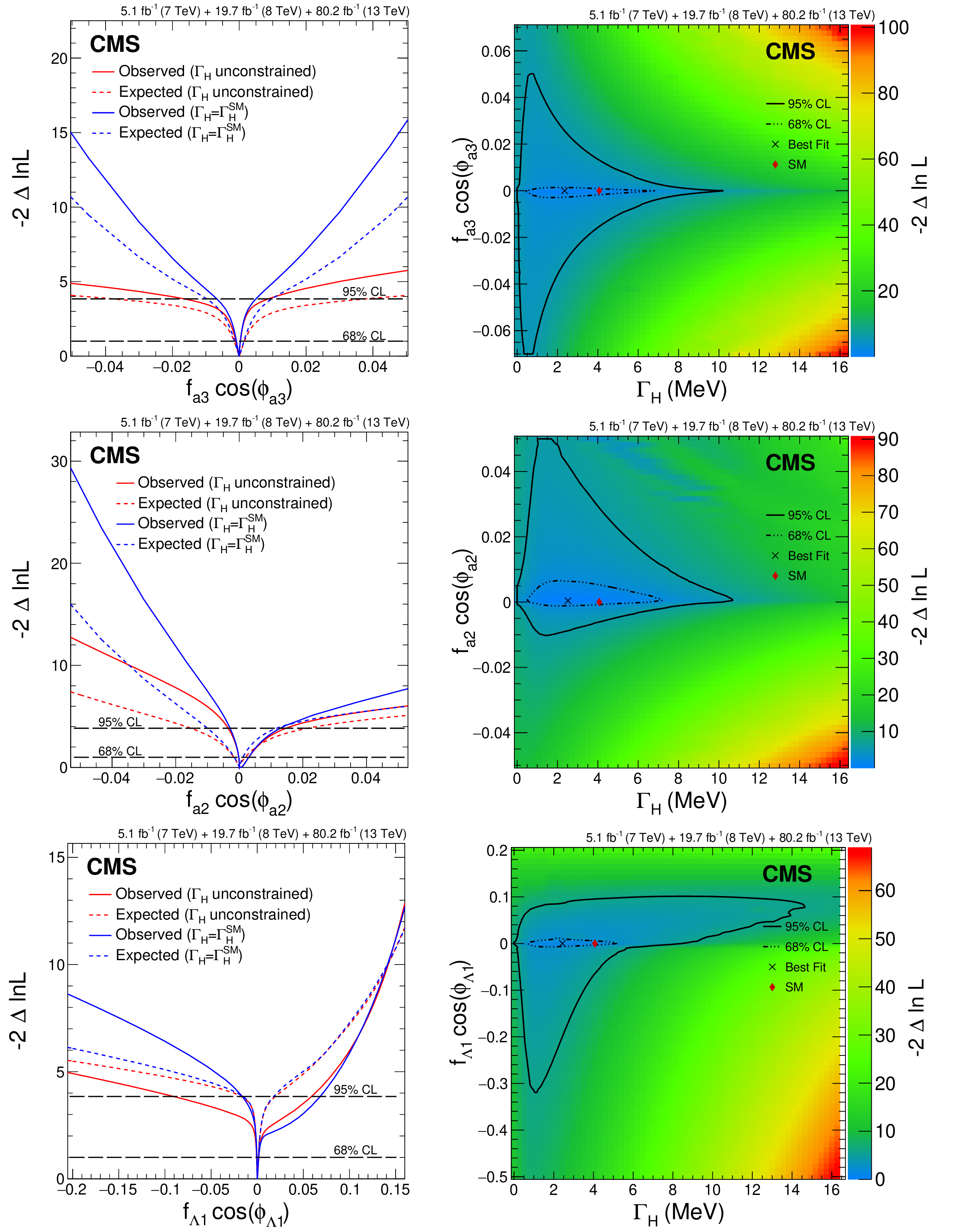
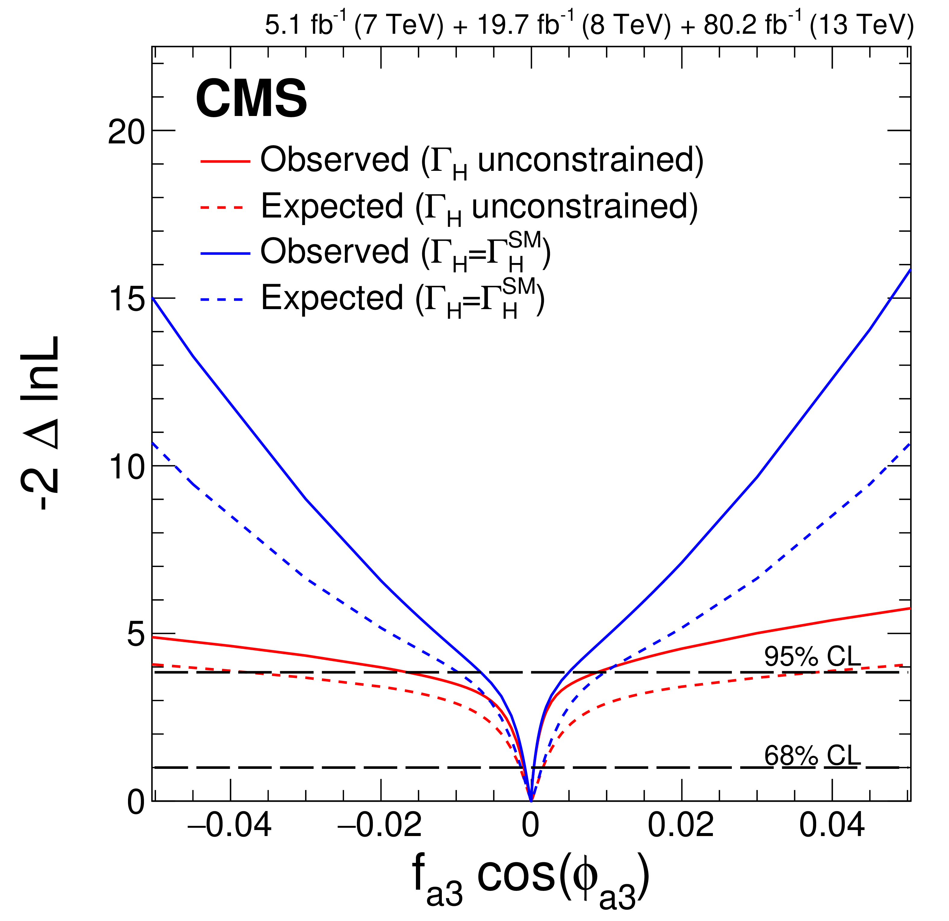
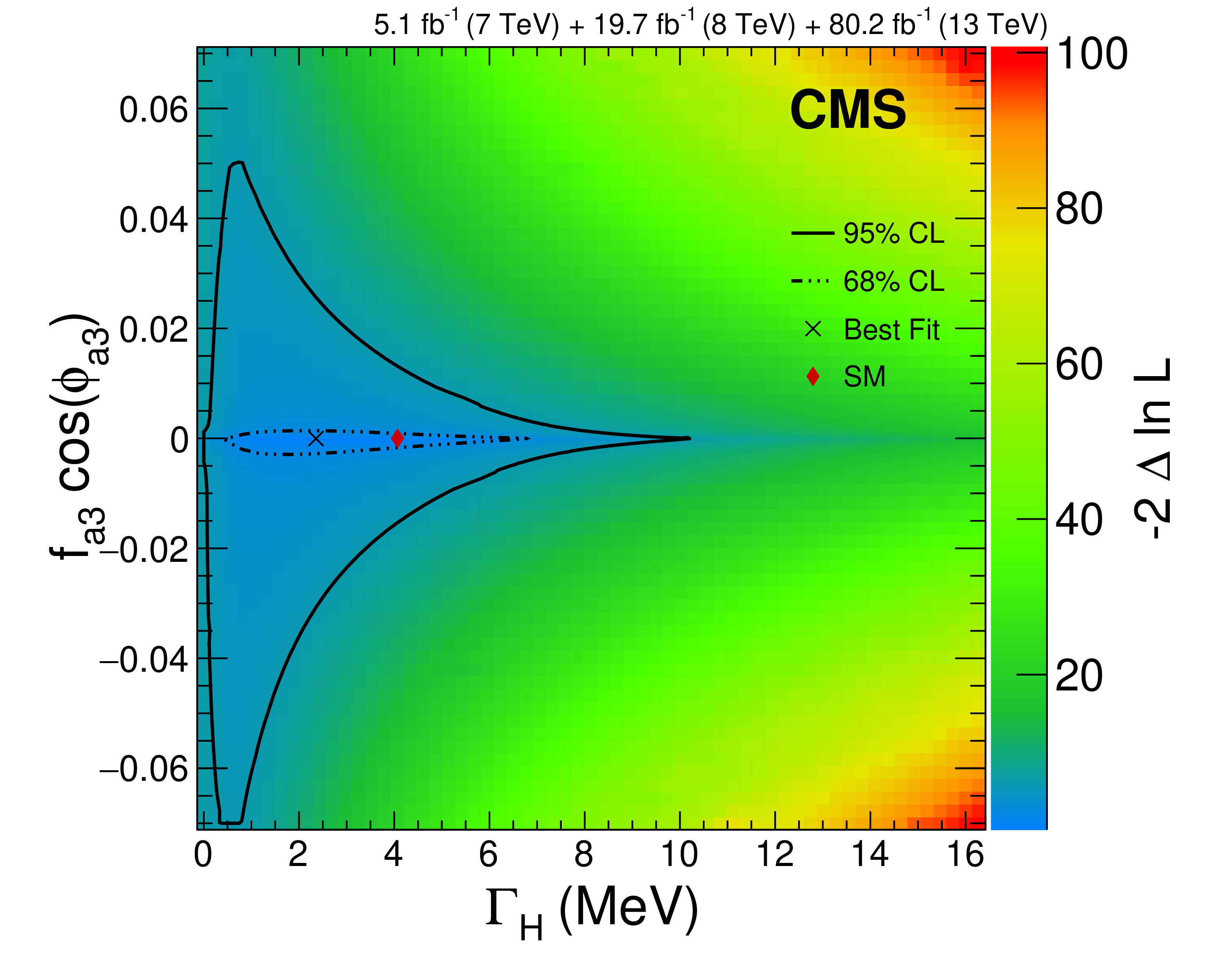
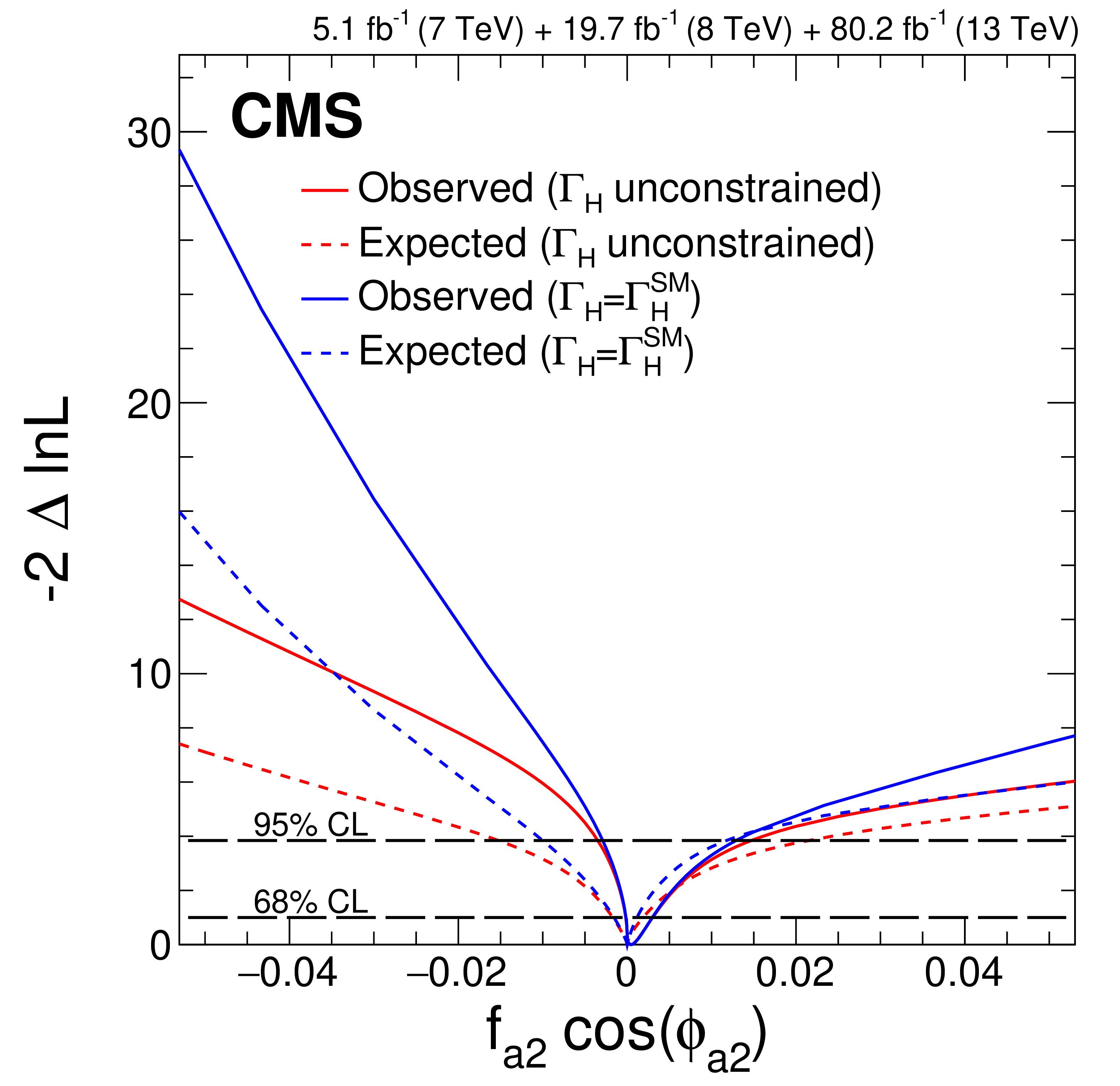
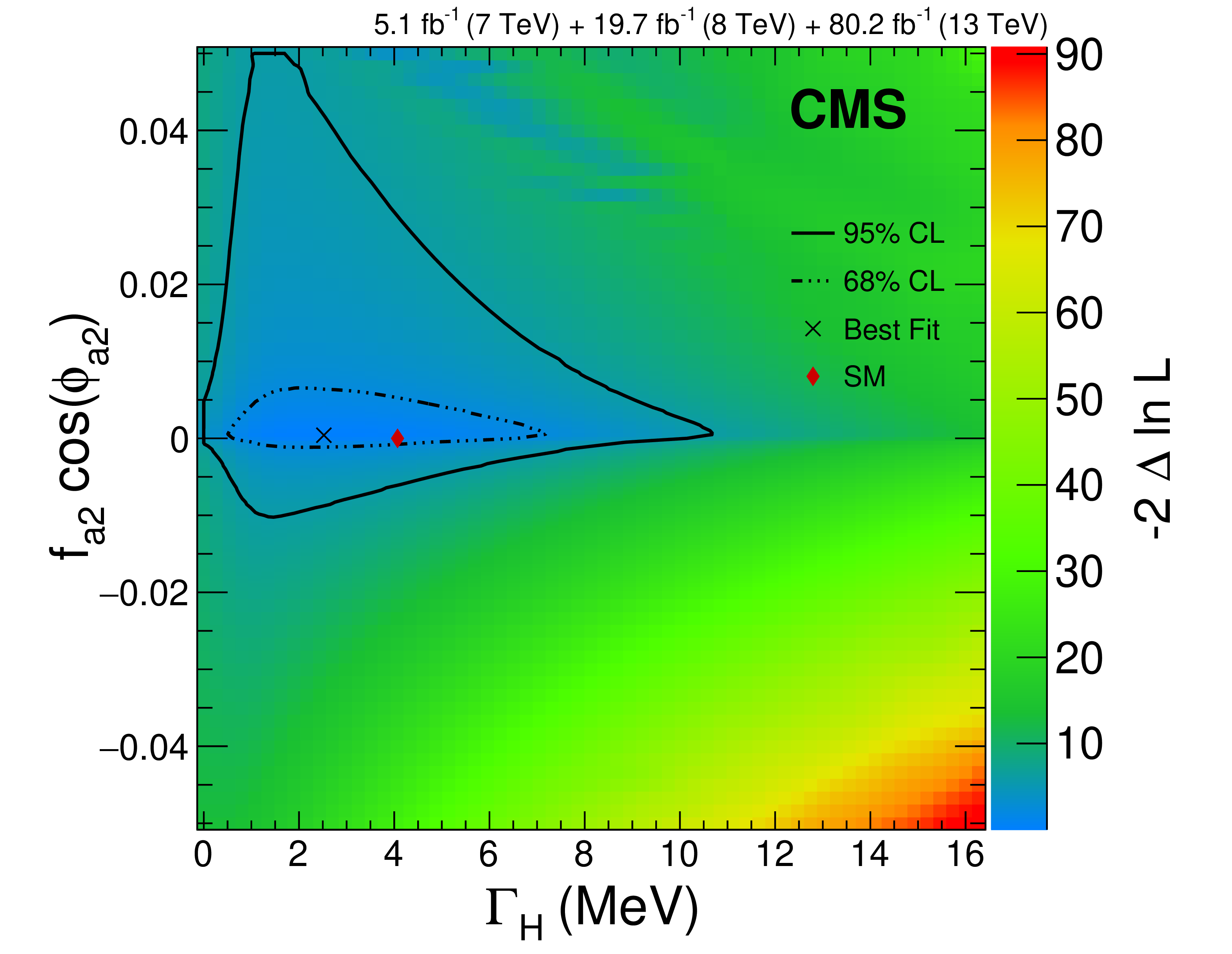
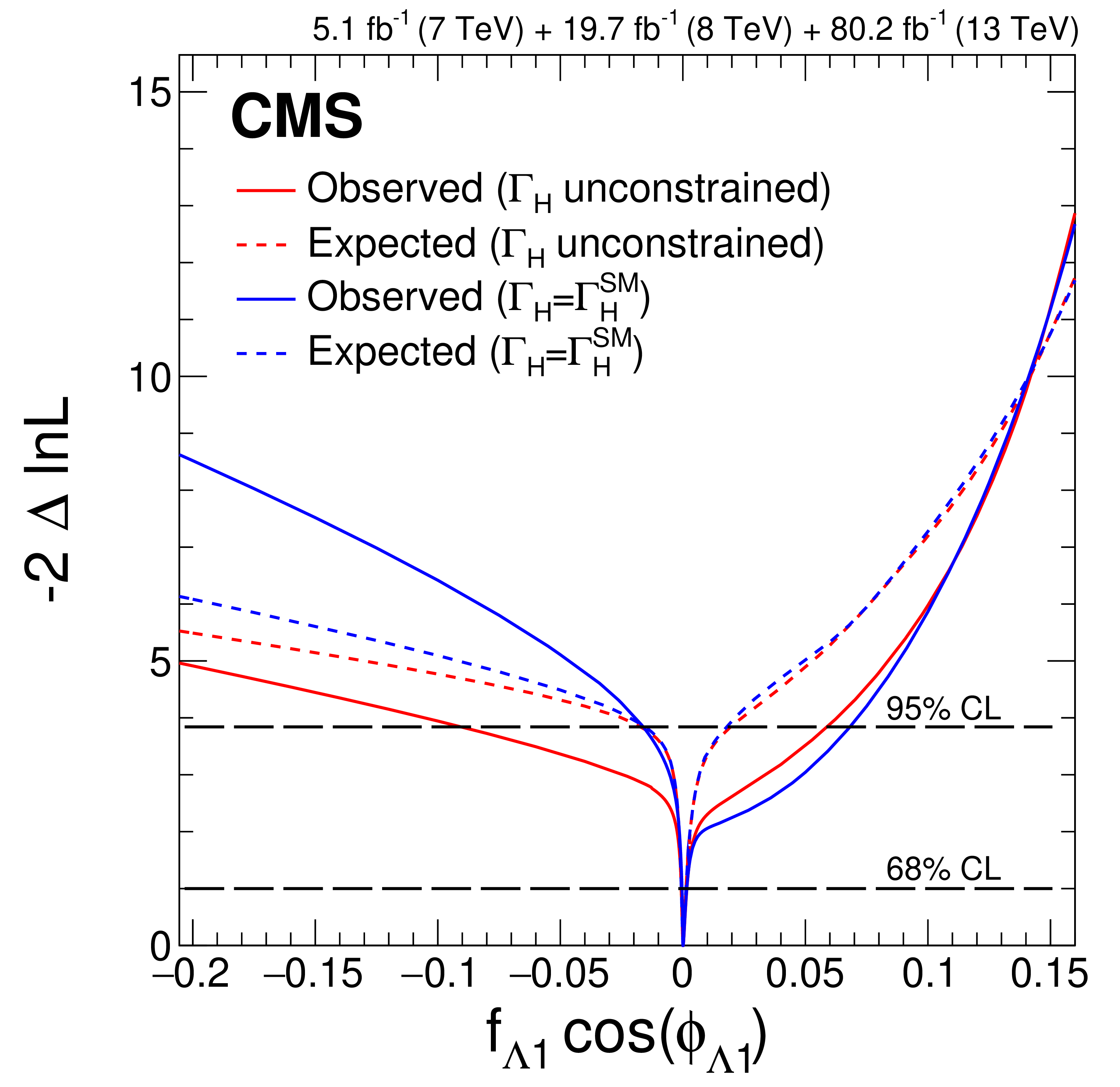
Figure 6:
Constraints on ${{f_{a 3}} {\cos\left ({\phi _{a 3}} \right)}}$ (top), ${{f_{a 2}} {\cos\left ({\phi _{a 2}} \right)}}$ (middle), and ${{f_{\Lambda 1}} {\cos\left ({\phi _{\Lambda 1}} \right)}}$ (bottom) from the combined Run 1 and Run 2 data set using both on-shell and off-shell events. Left plots: likelihood scans of the parameters of interest with unconstrained ${\Gamma _\mathrm{H}}$ (red) or assuming $ {\Gamma _\mathrm{H}} = {\Gamma _\mathrm{H} ^{\mathrm {SM}}} $ (blue). The dashed horizontal lines show the 68 and 95% CL regions. Right plots: observed two-parameter (${\Gamma _\mathrm{H}}$, ${{f_{a i}} {\cos\left ({\phi _{a i}} \right)}}$) likelihood scans. The two-parameter 68 and 95% CL regions are indicated with the dashed and solid curves, respectively. |
png pdf |
Figure 6-a:
Constraints on $ {{f_{a 3}} {\cos\left ({\phi _{a 3}} \right)}} $ from the combined Run 1 and Run 2 data set using both on-shell and off-shell events: Likelihood scans of the parameters of interest with unconstrained $ {\Gamma _ {\mathrm {H}}} $ (red) or assuming $ {\Gamma _ {\mathrm {H}}} = {\Gamma _ {\mathrm {H}} ^{\mathrm {SM}}} $ (blue). The dashed horizontal lines show the 68 and 95% CL regions. |
png pdf |
Figure 6-b:
Constraints on $ {{f_{a 3}} {\cos\left ({\phi _{a 3}} \right)}} $ from the combined Run 1 and Run 2 data set using both on-shell and off-shell events: Observed two-parameter (${\Gamma _ {\mathrm {H}}}, {{f_{a i}} {\cos\left ({\phi _{a i}} \right)}}$) likelihood scans. The two-parameter 68 and 95% CL regions are indicated with the dashed and solid curves, respectively. |
png pdf |
Figure 6-c:
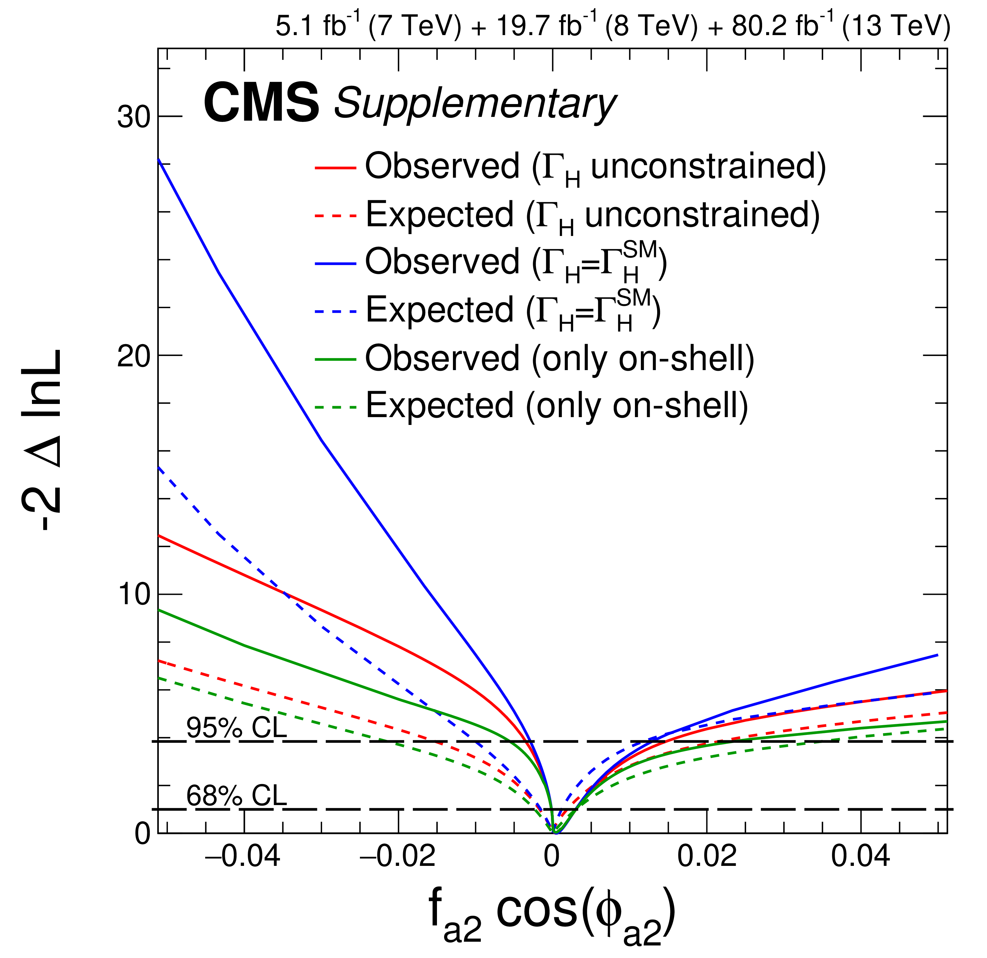
Constraints on $ {{f_{a 2}} {\cos\left ({\phi _{a 2}} \right)}} $ from the combined Run 1 and Run 2 data set using both on-shell and off-shell events: Likelihood scans of the parameters of interest with unconstrained $ {\Gamma _ {\mathrm {H}}} $ (red) or assuming $ {\Gamma _ {\mathrm {H}}} = {\Gamma _ {\mathrm {H}} ^{\mathrm {SM}}} $ (blue). The dashed horizontal lines show the 68 and 95% CL regions. |
png pdf |
Figure 6-d:
Constraints on $ {{f_{a 2}} {\cos\left ({\phi _{a 2}} \right)}} $ from the combined Run 1 and Run 2 data set using both on-shell and off-shell events: Observed two-parameter (${\Gamma _ {\mathrm {H}}}, {{f_{a i}} {\cos\left ({\phi _{a i}} \right)}}$) likelihood scans. The two-parameter 68 and 95% CL regions are indicated with the dashed and solid curves, respectively. |
png pdf |
Figure 6-e:
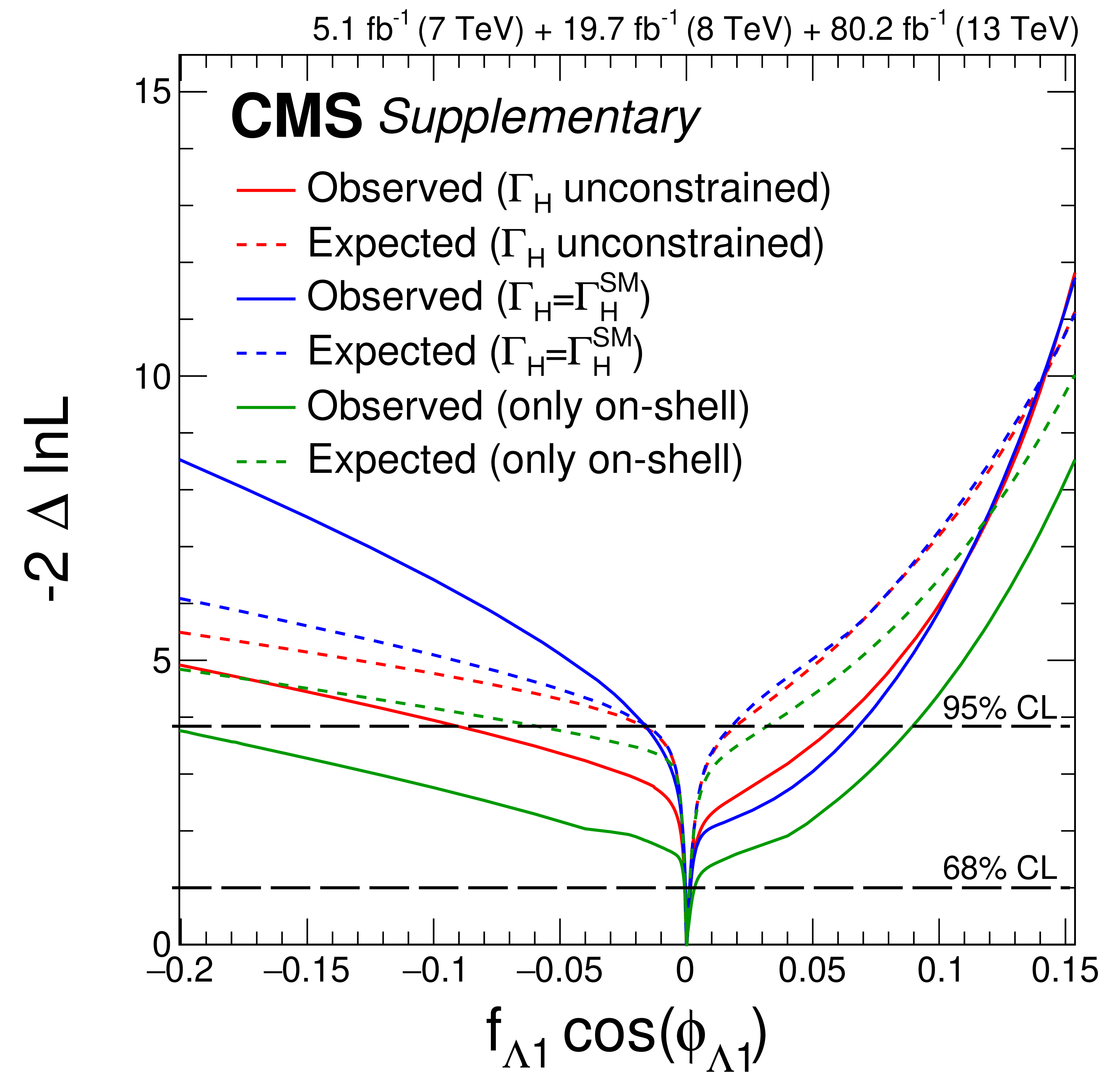
Constraints on $ {{f_{\Lambda 1}} {\cos\left ({\phi _{\Lambda 1}} \right)}} $ from the combined Run 1 and Run 2 data set using both on-shell and off-shell events: Likelihood scans of the parameters of interest with unconstrained $ {\Gamma _ {\mathrm {H}}} $ (red) or assuming $ {\Gamma _ {\mathrm {H}}} = {\Gamma _ {\mathrm {H}} ^{\mathrm {SM}}} $ (blue). The dashed horizontal lines show the 68 and 95% CL regions. |
png pdf |
Figure 6-f:
Constraints on $ {{f_{\Lambda 1}} {\cos\left ({\phi _{\Lambda 1}} \right)}} $ from the combined Run 1 and Run 2 data set using both on-shell and off-shell events: Observed two-parameter (${\Gamma _ {\mathrm {H}}}, {{f_{a i}} {\cos\left ({\phi _{a i}} \right)}}$) likelihood scans. The two-parameter 68 and 95% CL regions are indicated with the dashed and solid curves, respectively. |

png pdf |
Figure 7:
Observed (solid) and expected (dashed) likelihood scans of ${\Gamma _\mathrm{H}}$. Left plot: results of the SM-like couplings analysis are shown using the data only from 2016 and 2017 (black) or from the combination of Run 1 and Run 2 (red), which do not include 2015 data. Right plot: results of the combined Run 1 and Run 2 data analyses, with 2015 data included in the on-shell case, for the SM-like couplings or with three unconstrained anomalous coupling parameters, ${{f_{a 3}} {\cos\left ({\phi _{a 3}} \right)}}$ (red), ${{f_{a 2}} {\cos\left ({\phi _{a 2}} \right)}}$ (blue), and ${{f_{\Lambda 1}} {\cos\left ({\phi _{\Lambda 1}} \right)}}$ (violet). The dashed horizontal lines show the 68% and 95% CL regions. |
png pdf |
Figure 7-a:
Observed (solid) and expected (dashed) likelihood scans of ${\Gamma _ {\mathrm {H}}}$: Results of the SM-like couplings analysis are shown using the data only from 2016 and 2017 (black) or from the combination of Run 1 and Run 2 (red), which do not include 2015 data. |
png pdf |
Figure 7-b:
Observed (solid) and expected (dashed) likelihood scans of ${\Gamma _ {\mathrm {H}}}$: Results of the combined Run 1 and Run 2 data analyses, with 2015 data included in the on-shell case, for the SM-like couplings or with three unconstrained anomalous coupling parameters, $ {{f_{a 3}} {\cos\left ({\phi _{a 3}} \right)}} $ (red), $ {{f_{a 2}} {\cos\left ({\phi _{a 2}} \right)}} $ (blue), and $ {{f_{\Lambda 1}} {\cos\left ({\phi _{\Lambda 1}} \right)}} $ (violet). The dashed horizontal lines show the 68% and 95% CL regions. |
| Tables | |
png pdf |
Table 1:
List of the anomalous HVV couplings considered in the measurements assuming a spin-zero H boson. The definition of the effective fractions $ {f_{a i}} $ is discussed in the text and the translation constants are the cross-section ratios corresponding to the processes $\mathrm{H} \to 2\mathrm{e} 2\mu $ with the H boson mass $m_{\mathrm{H}} = $ 125 GeV and calculated using JHUGen [47,50,54]. |
png pdf |
Table 2:
Summary of the three production categories in the on-shell ${m_{4\ell}}$ region. The selection requirements on the $\mathcal {D}_\text {2jet}$ discriminants are quoted for each category, and further requirements can be found in the text. Two or three observables (abbreviated as obs.) are listed for each analysis and for each category. All discriminants are calculated with the JHUGen signal matrix elements and mcfm background matrix elements. The discriminants ${{\mathcal {D}}_{\text {bkg}}}$ in the tagged categories also include probabilities using associated jets and decay in addition to the ${m_{4\ell}}$ probability. The VH interference discriminants in the hadronic VH-tagged categories are defined as the simple average of the ones corresponding to the WH and ZH processes. |
png pdf |
Table 3:
Summary of the three production categories in the off-shell ${m_{4\ell}}$ region, listed in a similar manner, as in Table 2. All discriminants are calculated with the JHUGen or mcfm /JHUGen signal, and mcfm background matrix elements. The VH interference discriminant in the SM-like analysis hadronic VH-tagged category is defined as the simple average of the ones corresponding to the WH and ZH processes. |
png pdf |
Table 4:
The numbers of events expected in the SM (or $ {f_{a 3}} =$ 1 in parentheses) for the different signal and background contributions and the total numbers of observed events are listed across the three ${a_{3}}$ analysis categories in the on-shell region for the combined 2016 and 2017 data set. |
png pdf |
Table 5:
The numbers of events expected in the SM-like analysis (or $ {f_{a 3}} =$ 0 in the ${a_{3}}$ analysis categorization, divided with a vertical bar) for the different signal and background contributions and the total observed numbers of events are listed across the three SM $|$ ${a_{3}}$ analysis categories in the off-shell region for the combined 2016 and 2017 data set. The signal, background, and interference contributions are shown separately for the gluon fusion (gg) and EW processes (VV) under the $ {\Gamma _\mathrm{H}} = {\Gamma _\mathrm{H} ^{\mathrm {SM}}} $ assumption. |
png pdf |
Table 6:
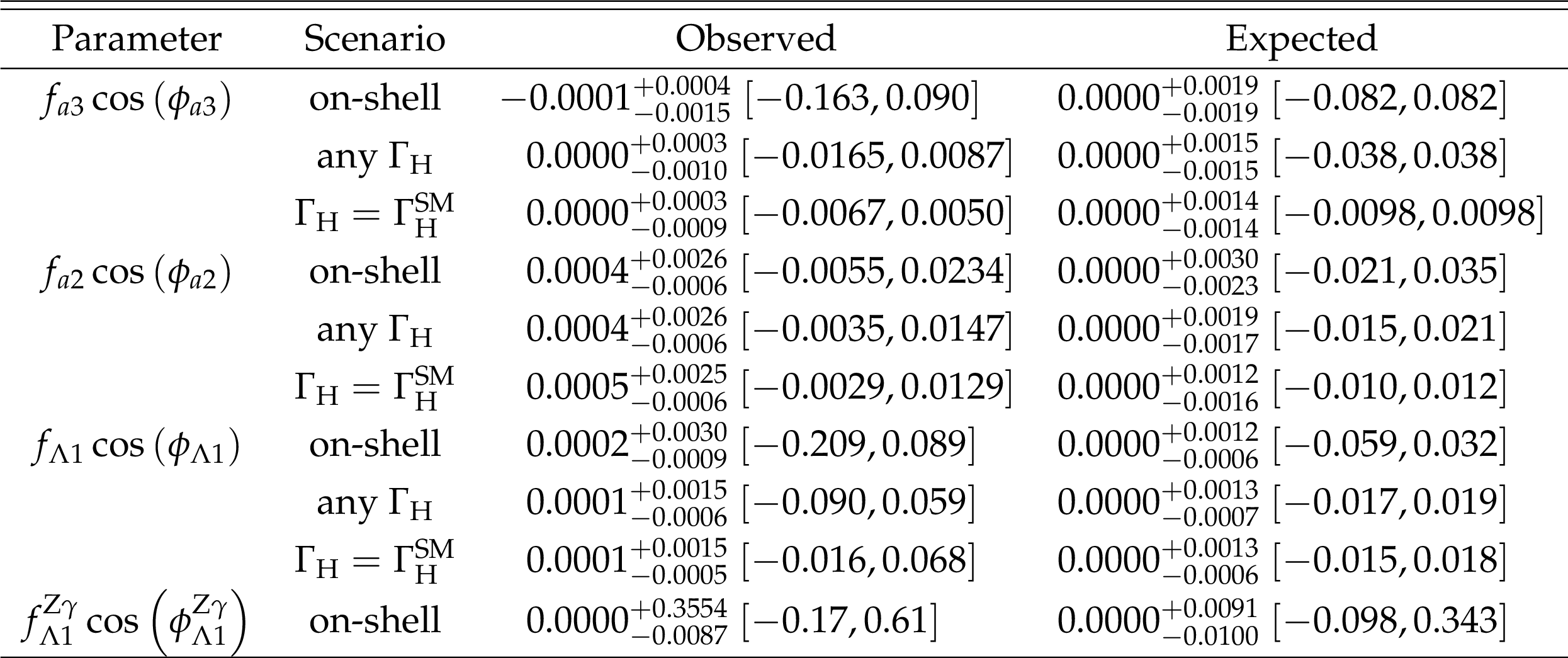
Summary of allowed 68% CL (central values with uncertainties) and 95% CL (in square brackets) intervals for the anomalous coupling parameters ${{f_{a i}} {\cos\left ({\phi _{a i}} \right)}}$ obtained from the analysis of the combination of Run 1 (only on-shell) and Run 2 (on-shell and off-shell) data sets. Three constraint scenarios are shown: using only on-shell events, using both on-shell and off-shell events with the $ {\Gamma _\mathrm{H}} $ left unconstrained, or with the constraint $ {\Gamma _\mathrm{H}} = {\Gamma _\mathrm{H} ^{\mathrm {SM}}} $. |
png pdf |
Table 7:
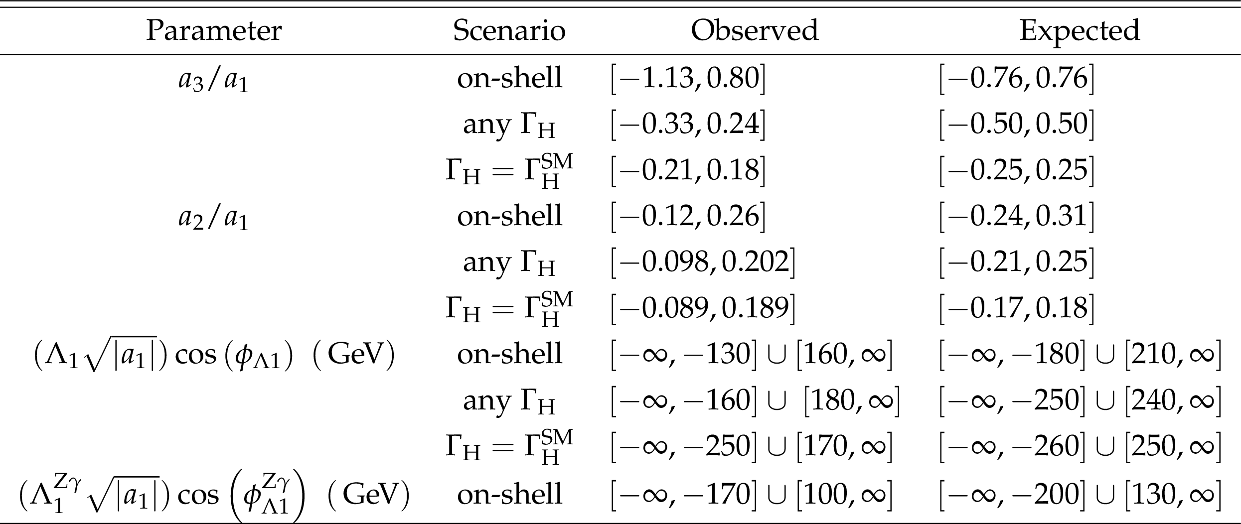
Summary of the allowed 95% CL intervals for the anomalous HVV couplings using results in Table 7. The coupling ratios are assumed to be real and include the factor $ {\cos\left ({\phi _{\Lambda 1}} \right)} $ or $ {\cos\left ({{\phi _{\Lambda 1}} ^{\mathrm{Z} \gamma}} \right)} = \pm$1. |

png pdf |
Table 8:
Summary of the total width ${\Gamma _\mathrm{H}}$ measurement, showing the allowed 68% CL (central values with uncertainties) and 95% CL (in square brackets). The limits are reported for the SM-like couplings using the Run 1 and Run 2 combination. |
png pdf |
Table 9:
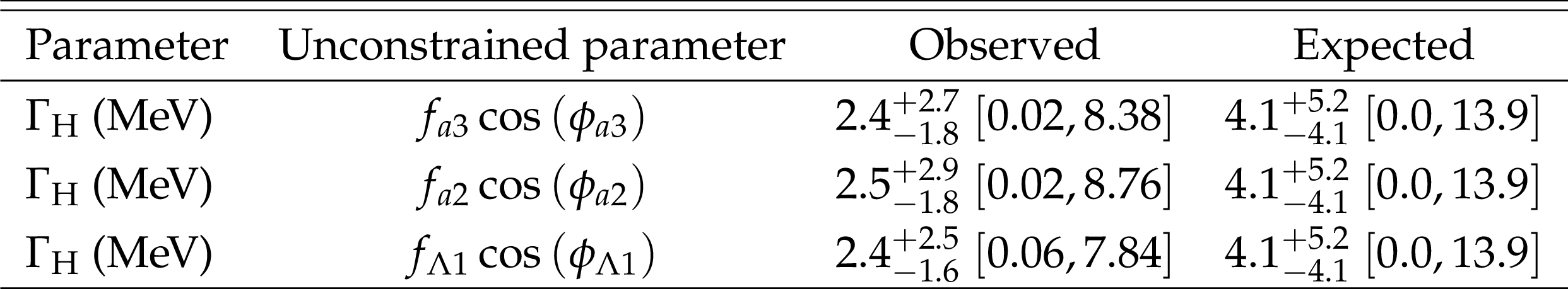
Summary of the total width ${\Gamma _\mathrm{H}}$ measurements, showing allowed 68% CL (central values with uncertainties) and 95% CL (in square brackets). The ${\Gamma _\mathrm{H}}$ limits are reported for the anomalous coupling parameter of interest unconstrained using the Run 1 and Run 2 combination. |
png pdf |
Table 10:
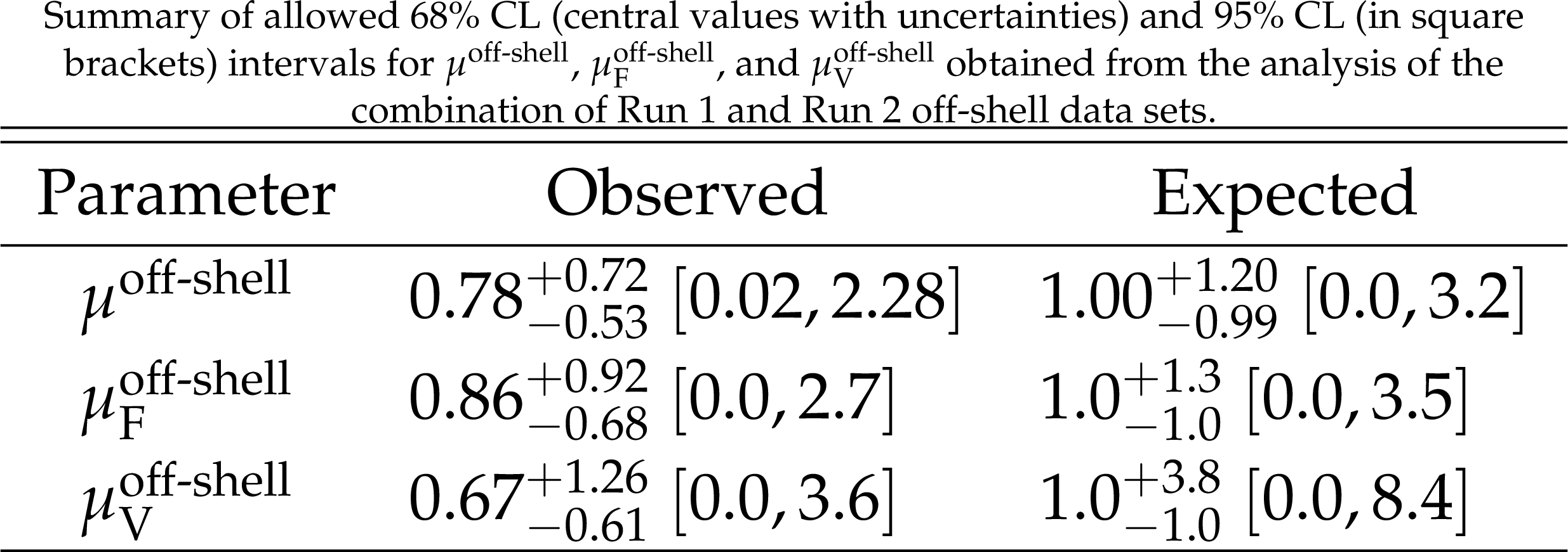
Summary of allowed 68% CL (central values with uncertainties) and 95% CL (in square brackets) intervals for $\mu ^\text {off-shell}$, $ {\mu _{{\mathrm {F}}}} ^\text {off-shell}$, and $ {\mu _{{\mathrm {V}}}} ^\text {off-shell}$ obtained from the analysis of the combination of Run 1 and Run 2 off-shell data sets. |
| Summary |
| Studies of on-shell and off-shell H boson production in the four-lepton final state are presented, using data from the CMS experiment at the LHC that correspond to an integrated luminosity of 80.2 fb$^{-1}$ at a center-of-mass energy of 13 TeV. Joint constraints are set on the H boson total width and parameters that express its anomalous couplings to two electroweak vector bosons. These results are combined with those obtained from the data collected at center-of-mass energies of 7 and 8 TeV, corresponding to integrated luminosities of 5.1 and 19.7 fb$^{-1}$, respectively. Kinematic information from the decay particles and the associated jets are combined using matrix element techniques to identify the production mechanism and increase sensitivity to the H boson couplings in both production and decay. The constraints on anomalous HVV couplings are found to be consistent with the standard model expectation in both on-shell and off-shell regions, as presented in Tables 6 and 7. Under the assumption of a coupling structure similar to that in the standard model, the H boson width is constrained to be 3.2$^{+2.8}_{-2.2}$ MeV while the expected constraint based on simulation is 4.1$^{+5.0}_{-4.0}$ MeV, as shown in Table 8. The constraints on the width remain similar with the inclusion of the tested anomalous HVV interactions and are summarized in Table 9. The width results are also interpreted in terms of the H boson signal strength in the off-shell region in Table 10. The observed off-shell signal strength, or equivalently a nonzero value of the width, is more than 2 standard deviations away from a background-only hypothesis, which provides a new direction to measure H boson properties when more data are available. |
| Additional Figures | |
png pdf |
Additional Figure 1:
The distributions of events for $\text{max}\left (\mathcal {D}_\text {2jet}^{\text {VBF}}, \mathcal {D}_\text {2jet}^{\text {VBF},{\mathrm {0h+}}} \right)$ in the on-shell region in the data from 2016 and 2017 from the analysis of the $a_2$ coupling. The requirement $\mathcal {D}_\text {bkg} > $ 0.5 is applied in order to enhance the signal contribution over the background. The VBF signal under both the SM and anomalous hypotheses is enhanced in the region above 0.5. |
png pdf |
Additional Figure 2:
The distributions of events for $\text{max}\left (\mathcal {D}_\text {2jet}^{{\mathrm {W}} {\mathrm {H}}}, \mathcal {D}_\text {2jet}^{{\mathrm {W}} {\mathrm {H}},{\mathrm {0h+}}}, \mathcal {D}_\text {2jet}^{{\mathrm {Z}} {\mathrm {H}}}, \mathcal {D}_\text {2jet}^{{\mathrm {Z}} {\mathrm {H}},{\mathrm {0h+}}} \right)$ in the on-shell region in the data from 2016 and 2017 from the analysis of the $a_2$ coupling. The requirement $\mathcal {D}_\text {bkg} > $ 0.5 is applied in order to enhance the signal contribution over the background. The WH and ZH signals under both the SM and anomalous hypotheses are enhanced in the region above 0.5. |
png pdf |
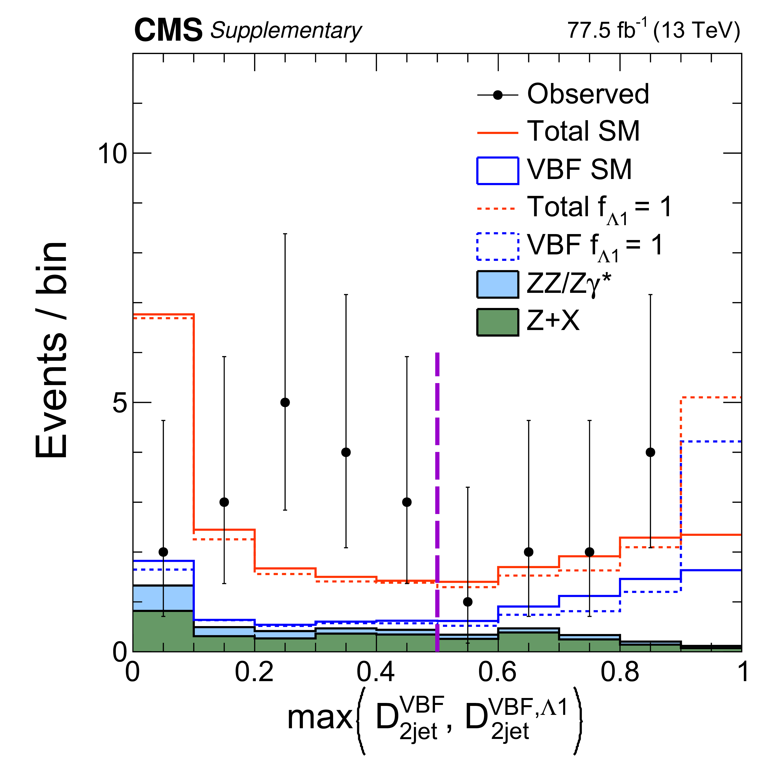
Additional Figure 3:
The distributions of events for $\text{max}\left (\mathcal {D}_\text {2jet}^{\text {VBF}}, \mathcal {D}_\text {2jet}^{\text {VBF},\Lambda 1} \right)$ in the on-shell region in the data from 2016 and 2017 from the analysis of the $\Lambda _1$ coupling. The requirement $\mathcal {D}_\text {bkg} > $ 0.5 is applied in order to enhance the signal contribution over the background. The VBF signal under both the SM and anomalous hypotheses is enhanced in the region above 0.5. |
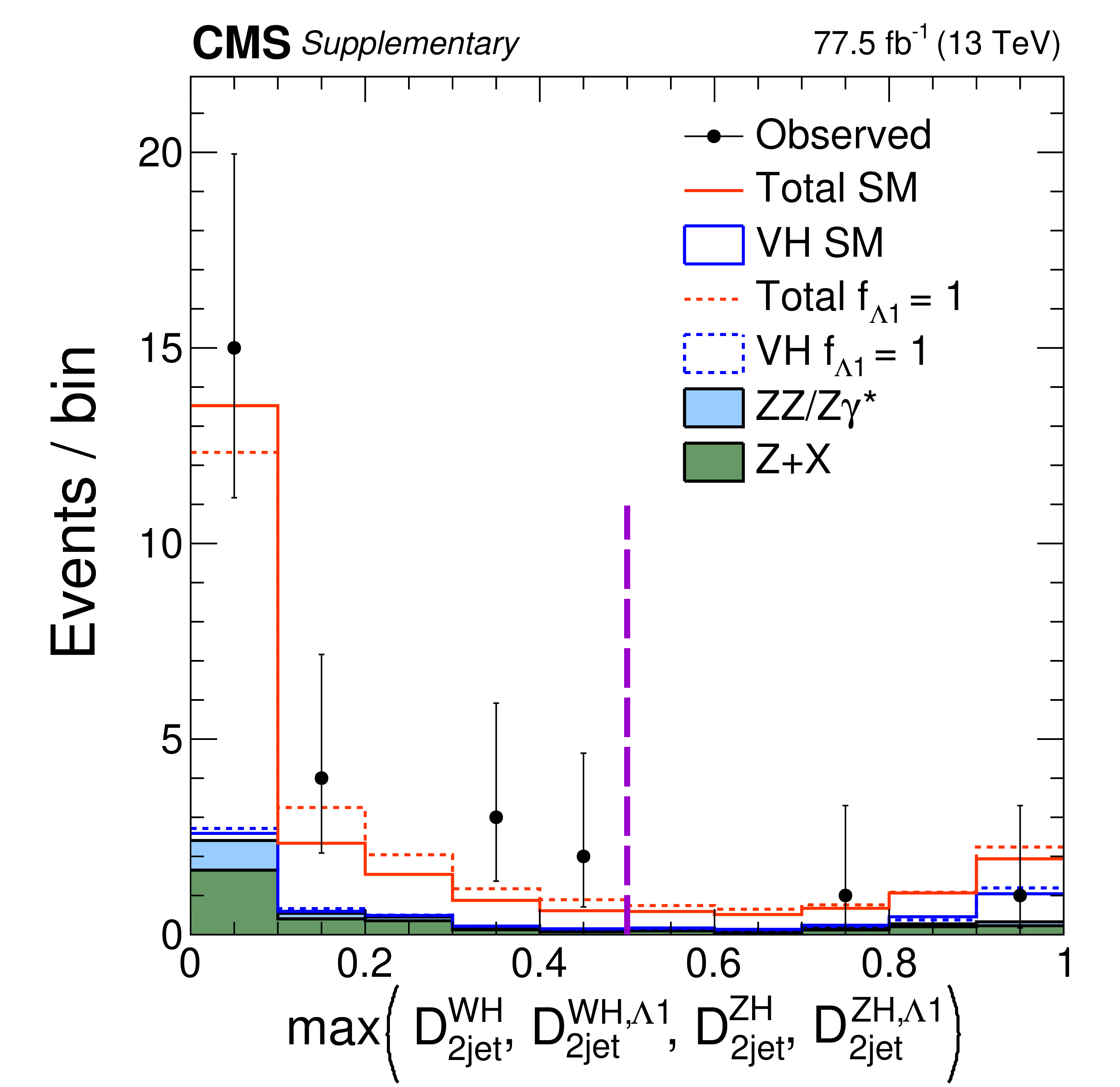
png pdf |
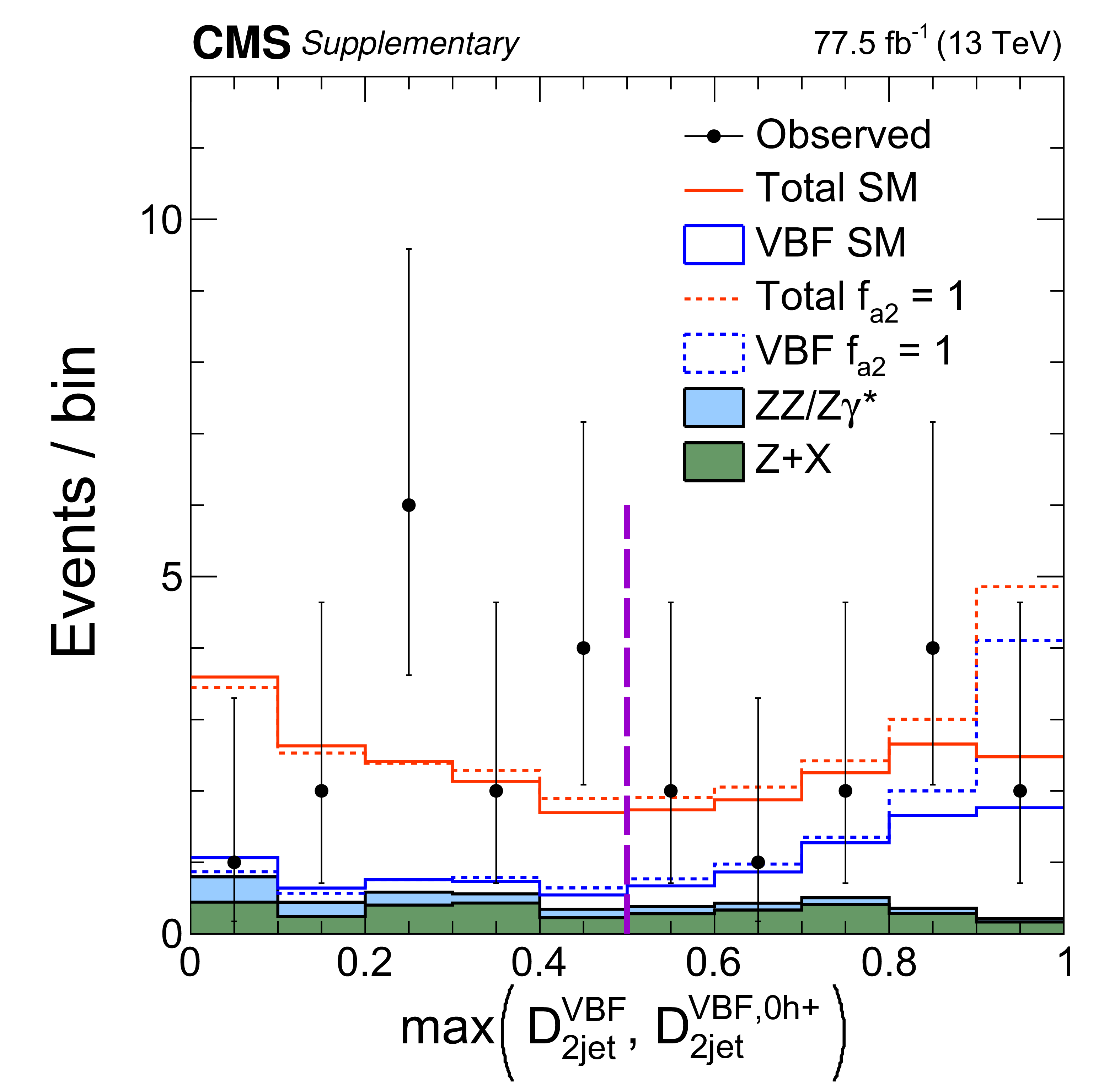
Additional Figure 4:
The distributions of events for $\text{max}\left (\mathcal {D}_\text {2jet}^{{\mathrm {W}} {\mathrm {H}}}, \mathcal {D}_\text {2jet}^{{\mathrm {W}} {\mathrm {H}},\Lambda 1}, \mathcal {D}_\text {2jet}^{{\mathrm {Z}} {\mathrm {H}}}, \mathcal {D}_\text {2jet}^{{\mathrm {Z}} {\mathrm {H}},\Lambda 1} \right)$ in the on-shell region in the data from 2016 and 2017 from the analysis of the $\Lambda _1$ coupling. The requirement $\mathcal {D}_\text {bkg} > $ 0.5 is applied in order to enhance the signal contribution over the background. The WH and ZH signals under both the SM and anomalous hypotheses are enhanced in the region above 0.5. |
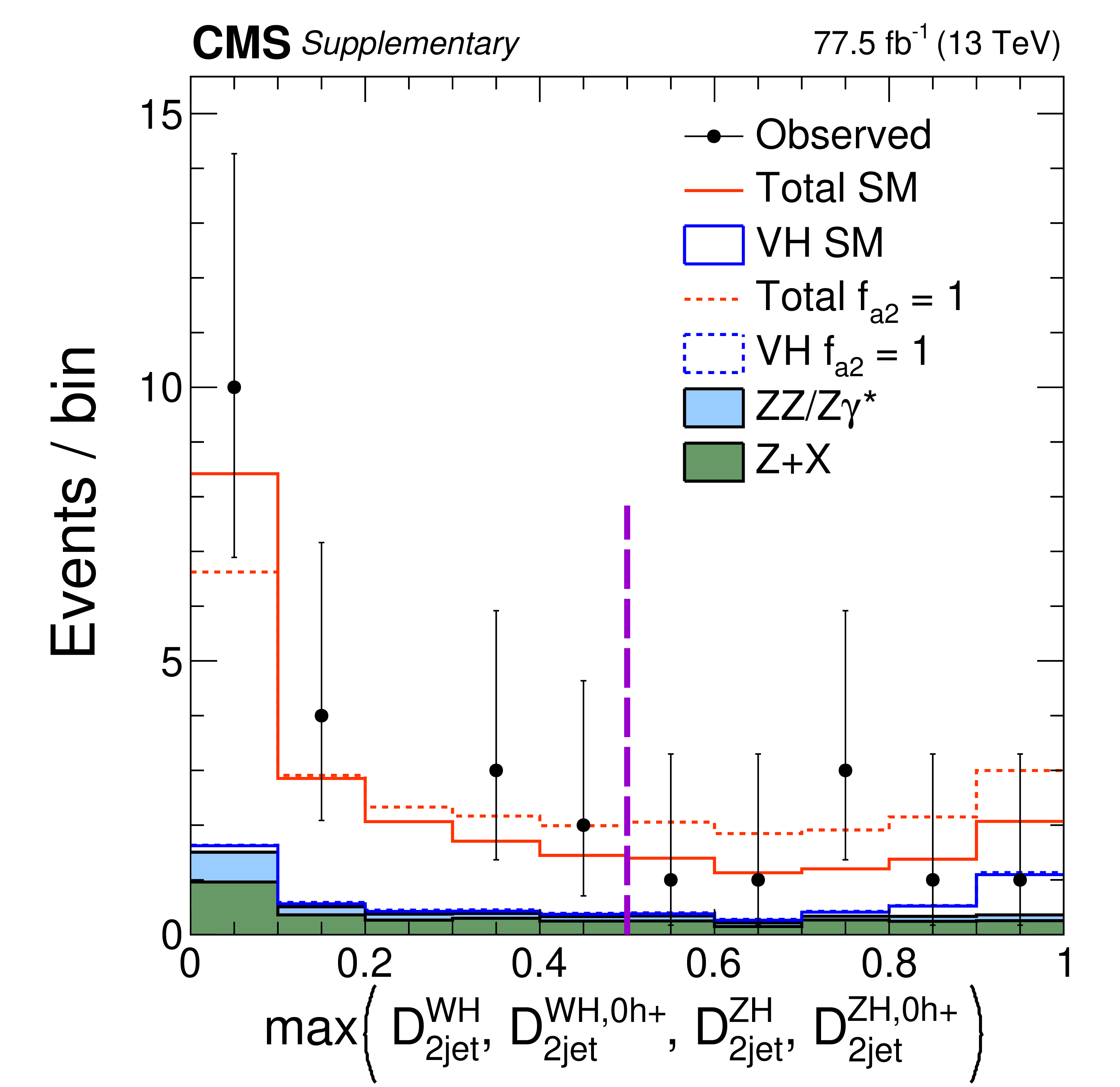
png pdf |
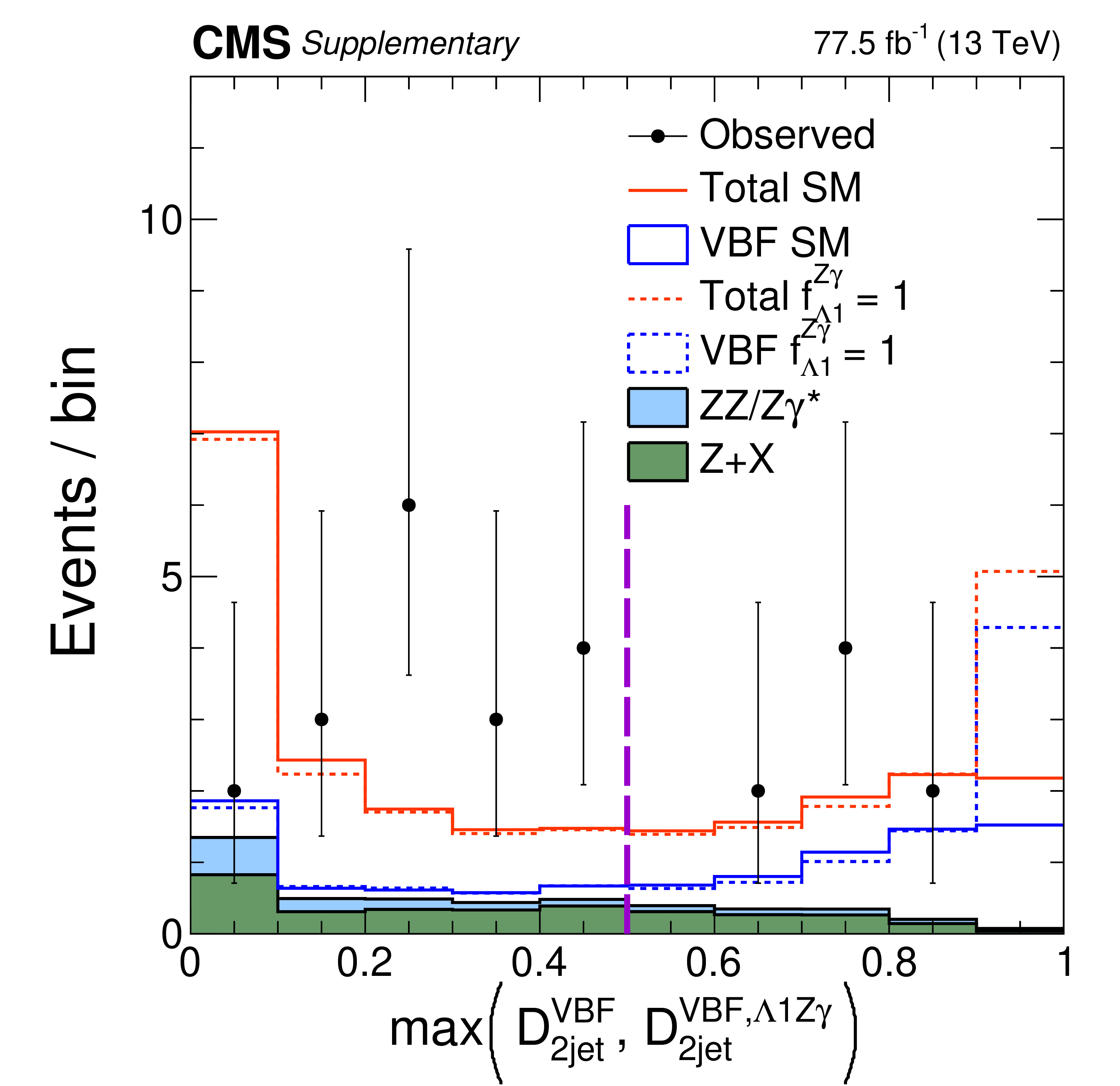
Additional Figure 5:
The distributions of events for $\text{max}\left (\mathcal {D}_\text {2jet}^{\text {VBF}}, \mathcal {D}_\text {2jet}^{\text {VBF},\Lambda 1 {\mathrm {Z}} \gamma} \right)$ in the on-shell region in the data from 2016 and 2017 from the analysis of the $\Lambda _1^{{\mathrm {Z}} \gamma}$ coupling. The requirement $\mathcal {D}_\text {bkg} > $ 0.5 is applied in order to enhance the signal contribution over the background. The VBF signal under both the SM and anomalous hypotheses is enhanced in the region above 0.5. |
png pdf |
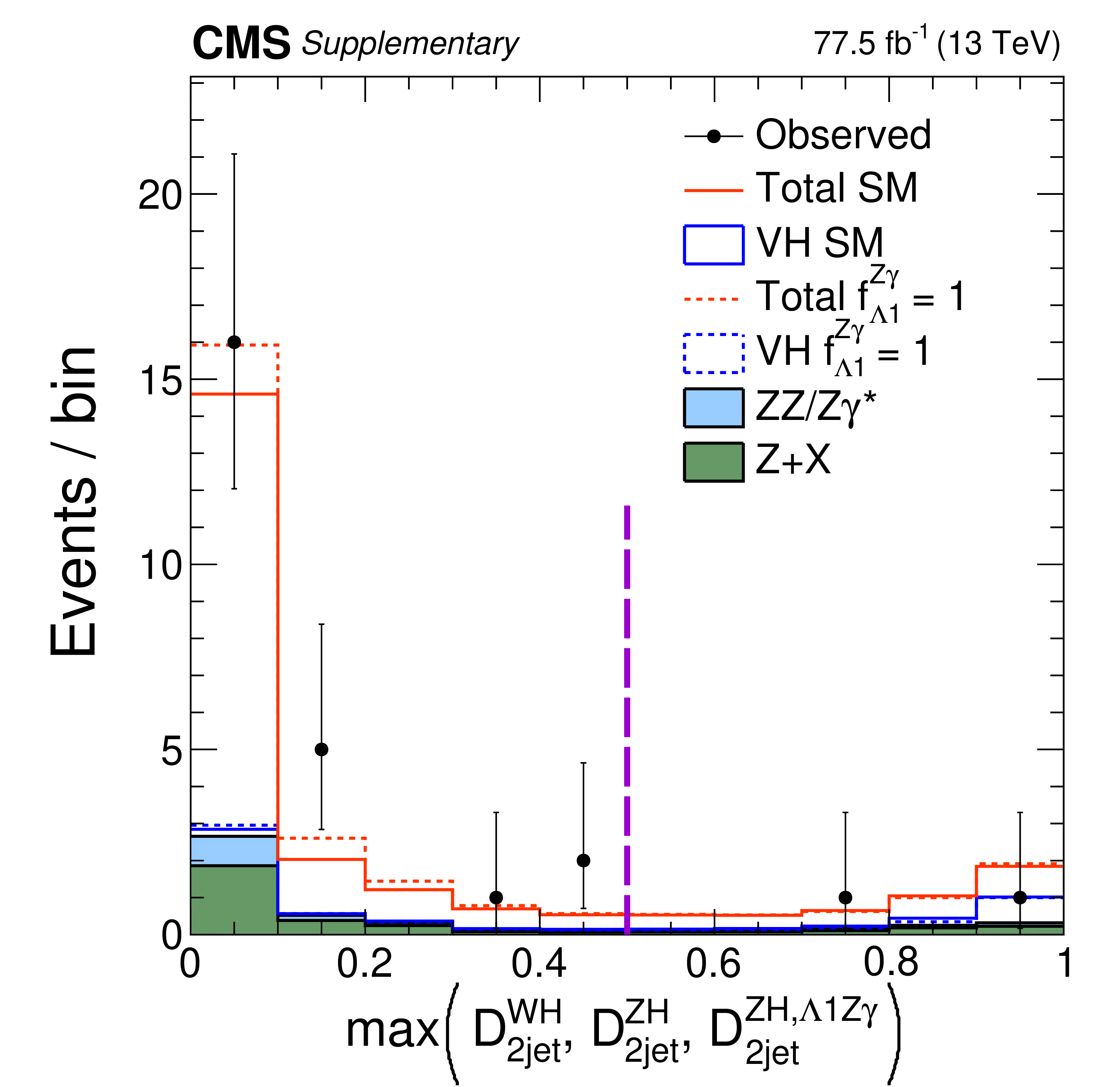
Additional Figure 6:
The distributions of events for $\text{max}\left (\mathcal {D}_\text {2jet}^{{\mathrm {W}} {\mathrm {H}}}, \mathcal {D}_\text {2jet}^{{\mathrm {Z}} {\mathrm {H}}}, \mathcal {D}_\text {2jet}^{{\mathrm {Z}} {\mathrm {H}},\Lambda 1 {\mathrm {Z}} \gamma} \right)$ in the on-shell region in the data from 2016 and 2017 from the analysis of the $\Lambda _1^{{\mathrm {Z}} \gamma}$ coupling. The requirement $\mathcal {D}_\text {bkg} > $ 0.5 is applied in order to enhance the signal contribution over the background. The WH and ZH signals under both the SM and anomalous hypotheses are enhanced in the region above 0.5. |
png pdf |
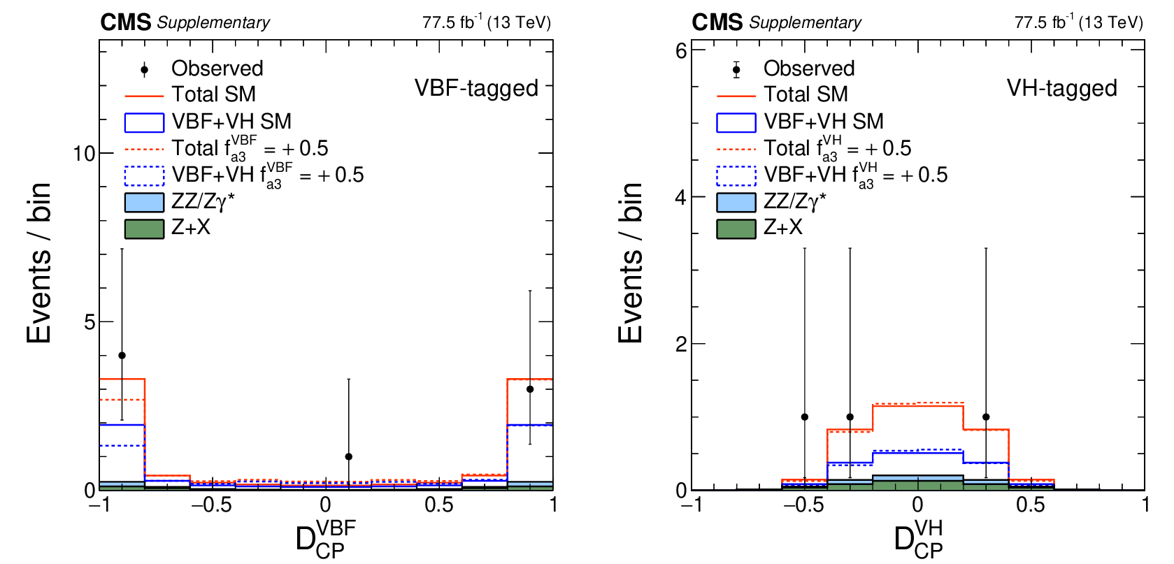
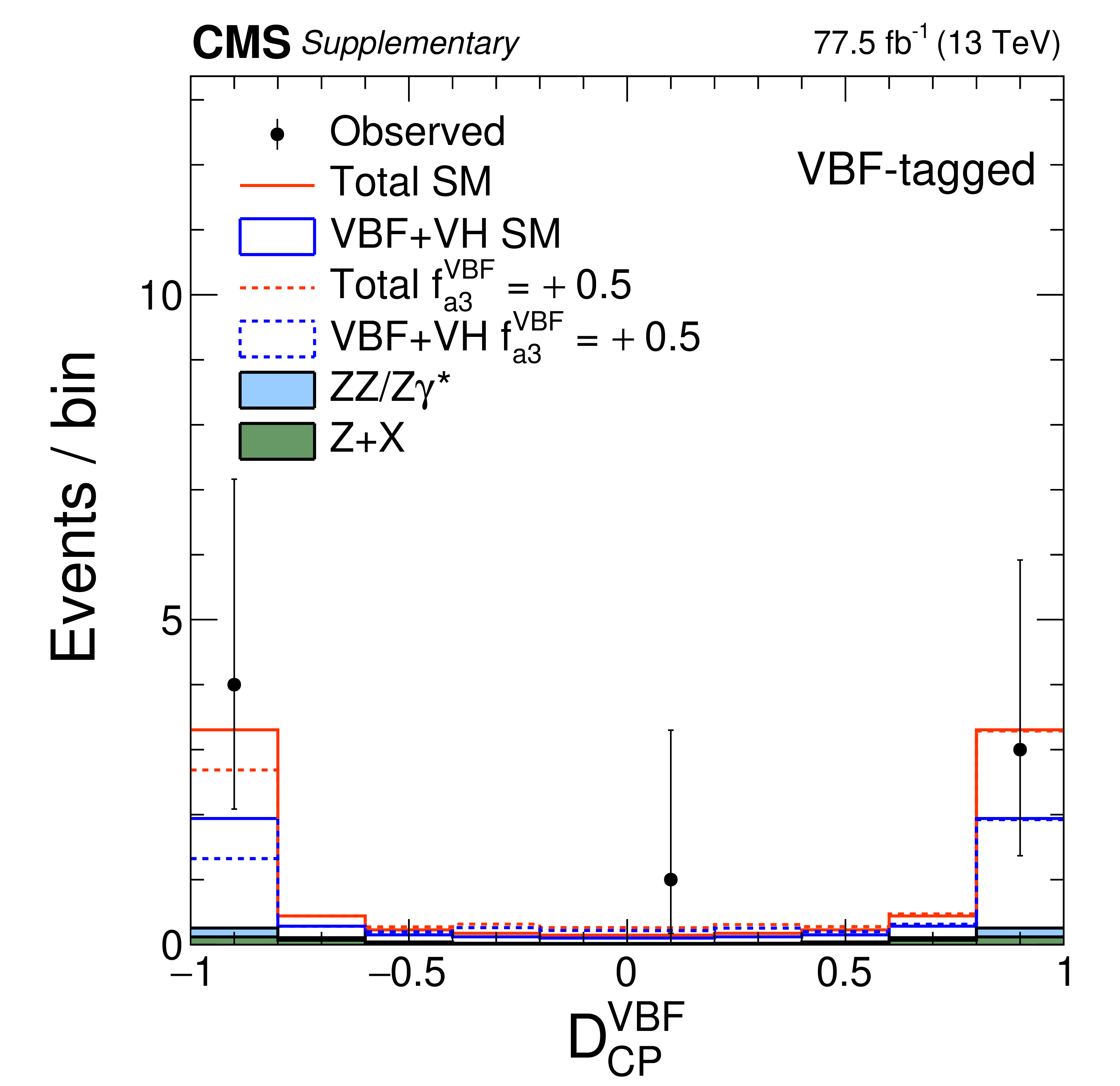
Additional Figure 7:
Distributions of $\mathcal {D}_{CP}$ in the on-shell $f_{a3}$ analysis. Two tagging categories are shown: VBF-tagged (a) and VH-tagged (b). The decay or production information used in the discriminants depends on the tagging category. $f_{a3}^\mathrm {VBF}$ and $f_{a3}^{\mathrm {V} {\mathrm {H}}}$ are defined by analogy with $f_{a3}$, but using the cross sections for the VBF and VH processes, respectively. Points with error bars show data and histograms show expectations for background and SM or BSM signal as indicated in the legend. |
png pdf |
Additional Figure 7-a:
Distribution of $\mathcal {D}^{\text{VBF}}_{CP}$ in the on-shell $f_{a3}$ analysis for events in the VBF-tagged category. $f_{a3}^\mathrm {VBF}$ is defined by analogy with $f_{a3}$, but using the cross section for the VBF process. Points with error bars show data and histograms show expectations for background and SM or BSM signal as indicated in the legend. |
png pdf |
Additional Figure 7-b:
Distribution of $\mathcal {D}^{\text{VH}}_{CP}$ in the on-shell $f_{a3}$ analysis for events in the VH-tagged category. $f_{a3}^{\mathrm {V} {\mathrm {H}}}$ is defined by analogy with $f_{a3}$, but using the cross section for the VH process. Points with error bars show data and histograms show expectations for background and SM or BSM signal as indicated in the legend. |
png pdf |
Additional Figure 8:
Distributions of kinematic discriminants in the on-shell $f_{a2}$ analysis: $\mathcal {D}_\mathrm {bkg}$ (a), (d), (g), $\mathcal {D}_{0h+}$ (b), (e), and $\mathcal {D}_\mathrm {int}$ (c), (f), (h). Three tagging categories are shown: VBF-tagged (a)-(c), VH-tagged (d)-(f), and untagged (g), (h). The decay or production information used in the discriminants depends on the tagging category. $f_{a2}^\mathrm {VBF}$ and $f_{a2}^{\mathrm {V} {\mathrm {H}}}$ are defined by analogy with $f_{a2}$, but using the cross sections for the VBF and VH processes, respectively. Points with error bars show data and histograms show expectations for background and SM or BSM signal as indicated in the legend. |
png pdf |
Additional Figure 8-a:
Distribution the $\mathcal {D}_\mathrm {bkg}$ kinematic discriminant in the on-shell $f_{a2}$ analysis for events in the VBF-tagged category. Points with error bars show data and histograms show expectations for background and SM or BSM signal as indicated in the legend. |
png pdf |
Additional Figure 8-b:
Distribution the $\mathcal {D}^{\text{VBF+dec}}_{0h+}$ kinematic discriminant in the on-shell $f_{a2}$ analysis for events in the VBF-tagged category. $f_{a2}^\mathrm {VBF}$ is defined by analogy with $f_{a2}$, but using the cross section for the VBF processes. Points with error bars show data and histograms show expectations for background and SM or BSM signal as indicated in the legend. |
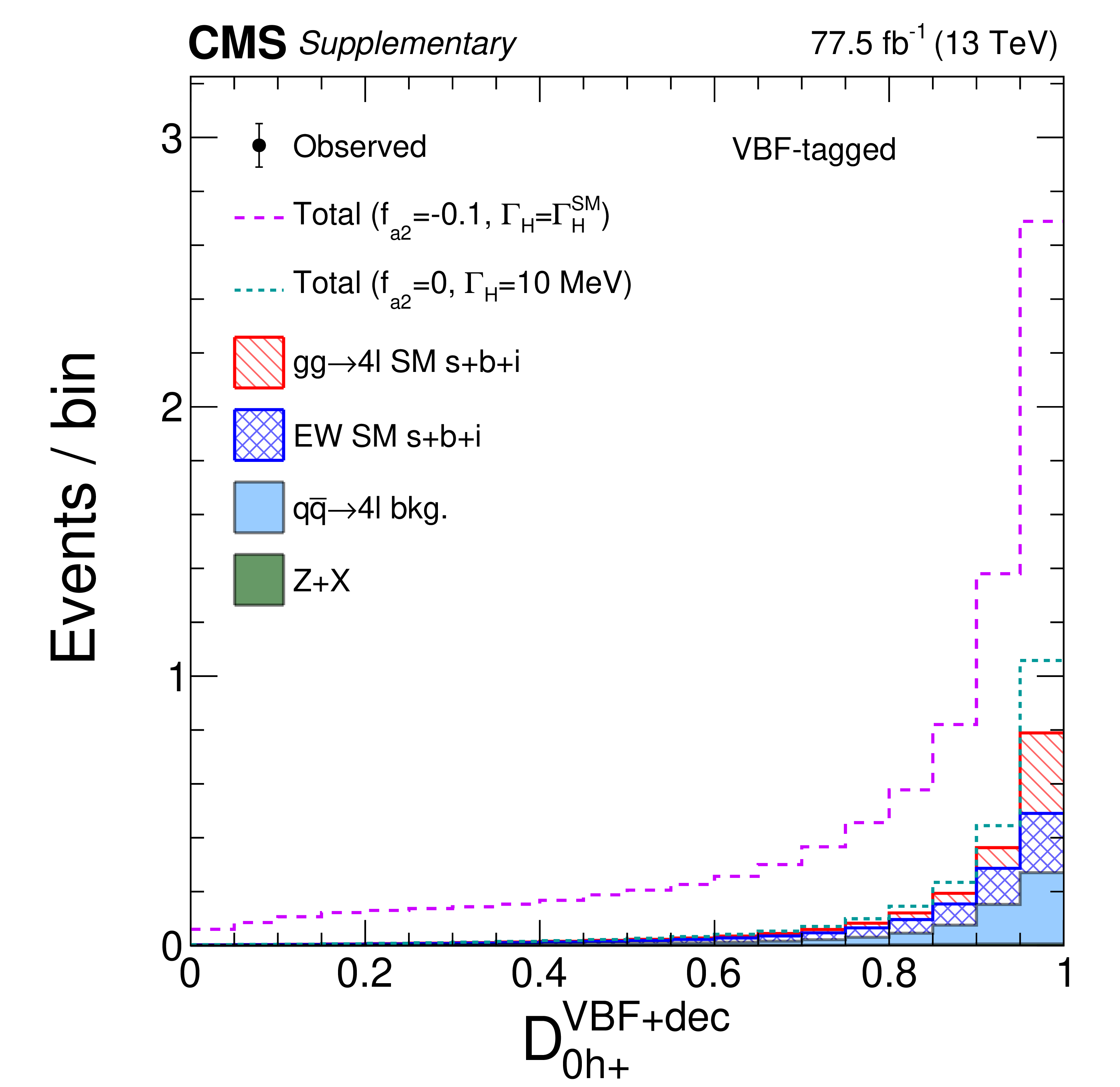
png pdf |
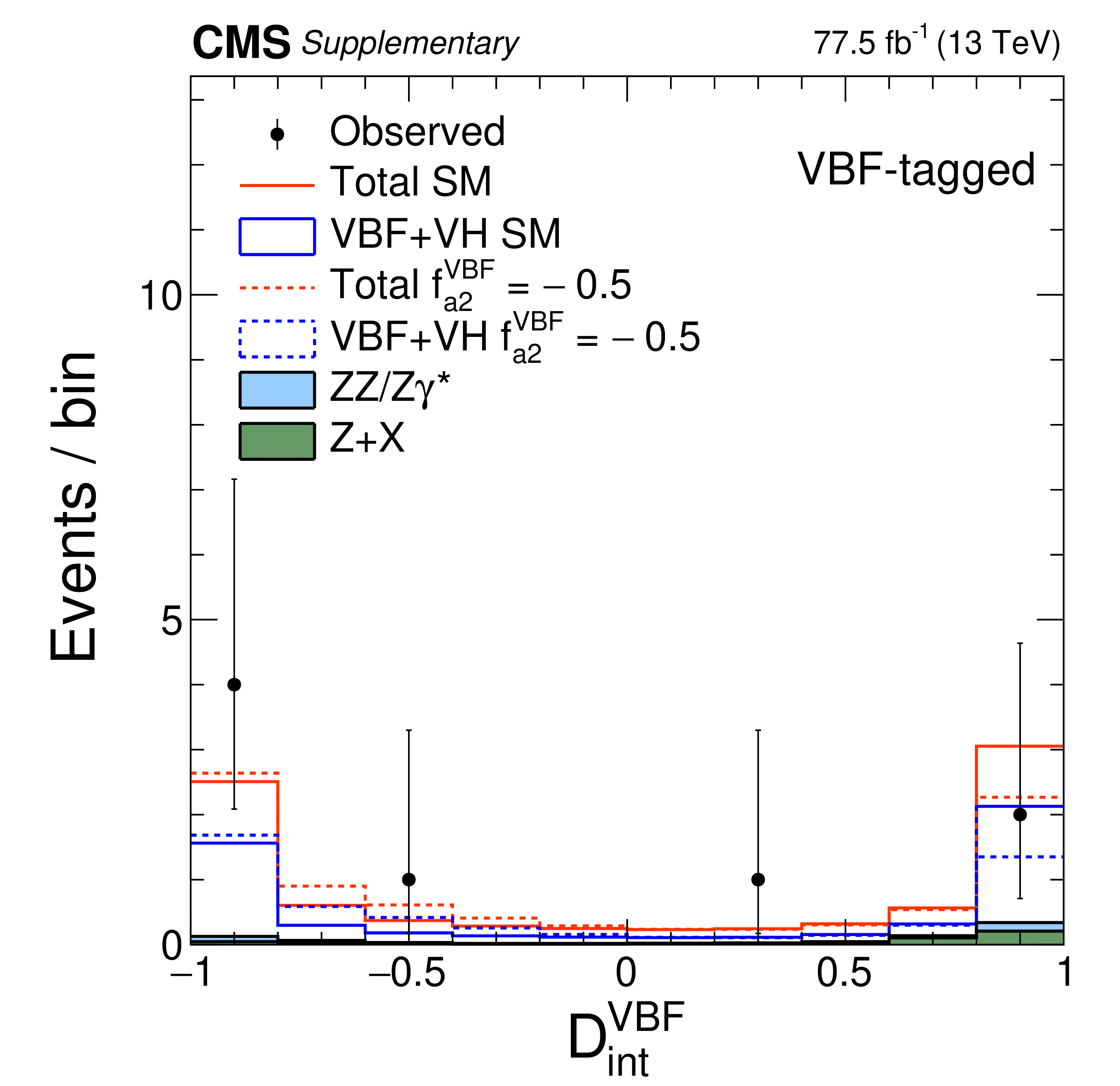
Additional Figure 8-c:
Distribution the $\mathcal {D}^{\text{VBF}}_\mathrm {int}$ kinematic discriminant in the on-shell $f_{a2}$ analysis for events in the VBF-tagged category. $f_{a2}^\mathrm {VBF}$ is defined by analogy with $f_{a2}$, but using the cross section for the VBF processes. Points with error bars show data and histograms show expectations for background and SM or BSM signal as indicated in the legend. |
png pdf |
Additional Figure 8-d:
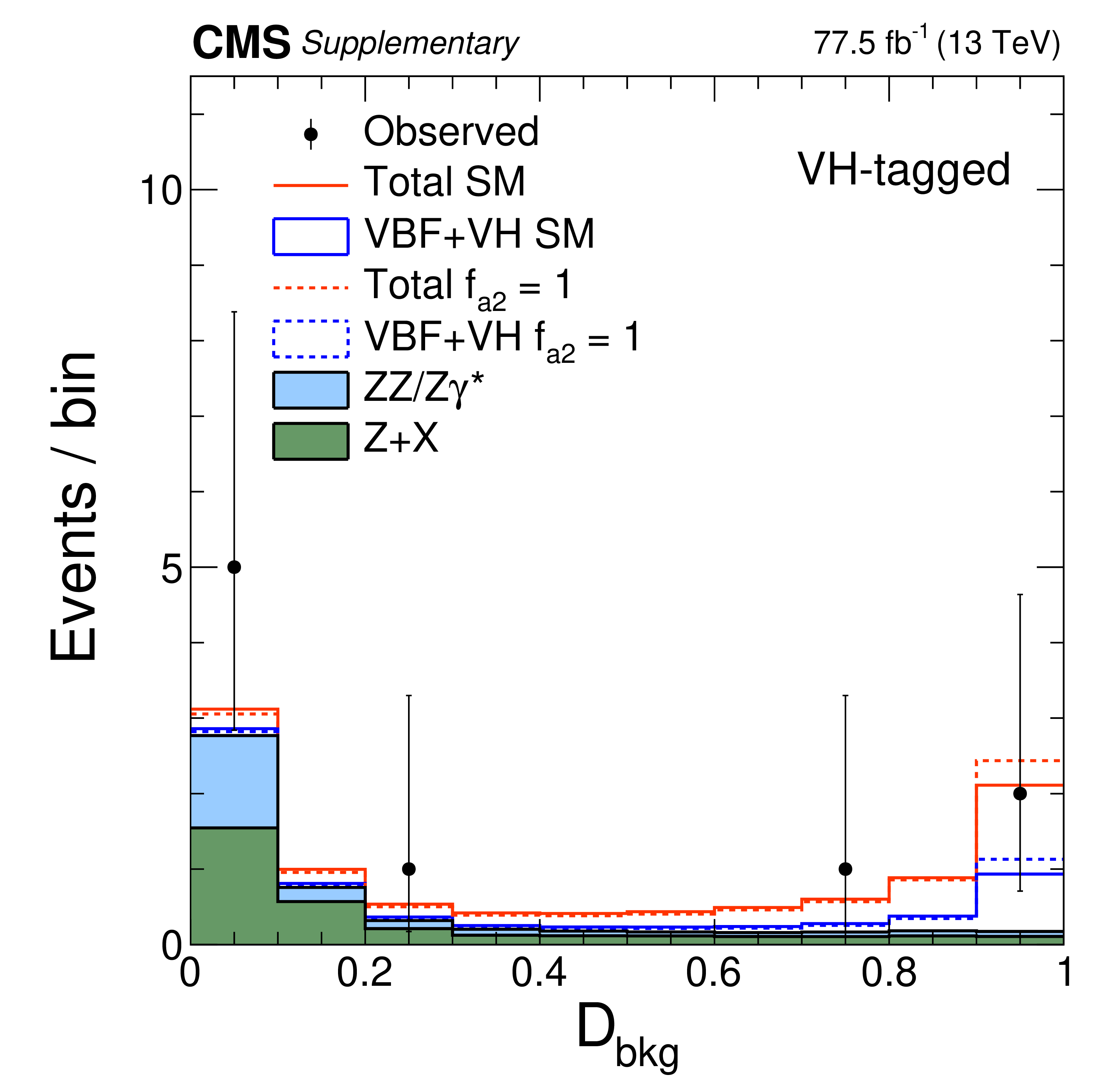
Distribution the $\mathcal {D}_\mathrm {bkg}$ kinematic discriminant in the on-shell $f_{a2}$ analysis for events in the VH-tagged category. $f_{a2}^{\mathrm {V} {\mathrm {H}}}$ is defined by analogy with $f_{a2}$, but using the cross section for the VH processes. Points with error bars show data and histograms show expectations for background and SM or BSM signal as indicated in the legend. |

png pdf |
Additional Figure 8-e:
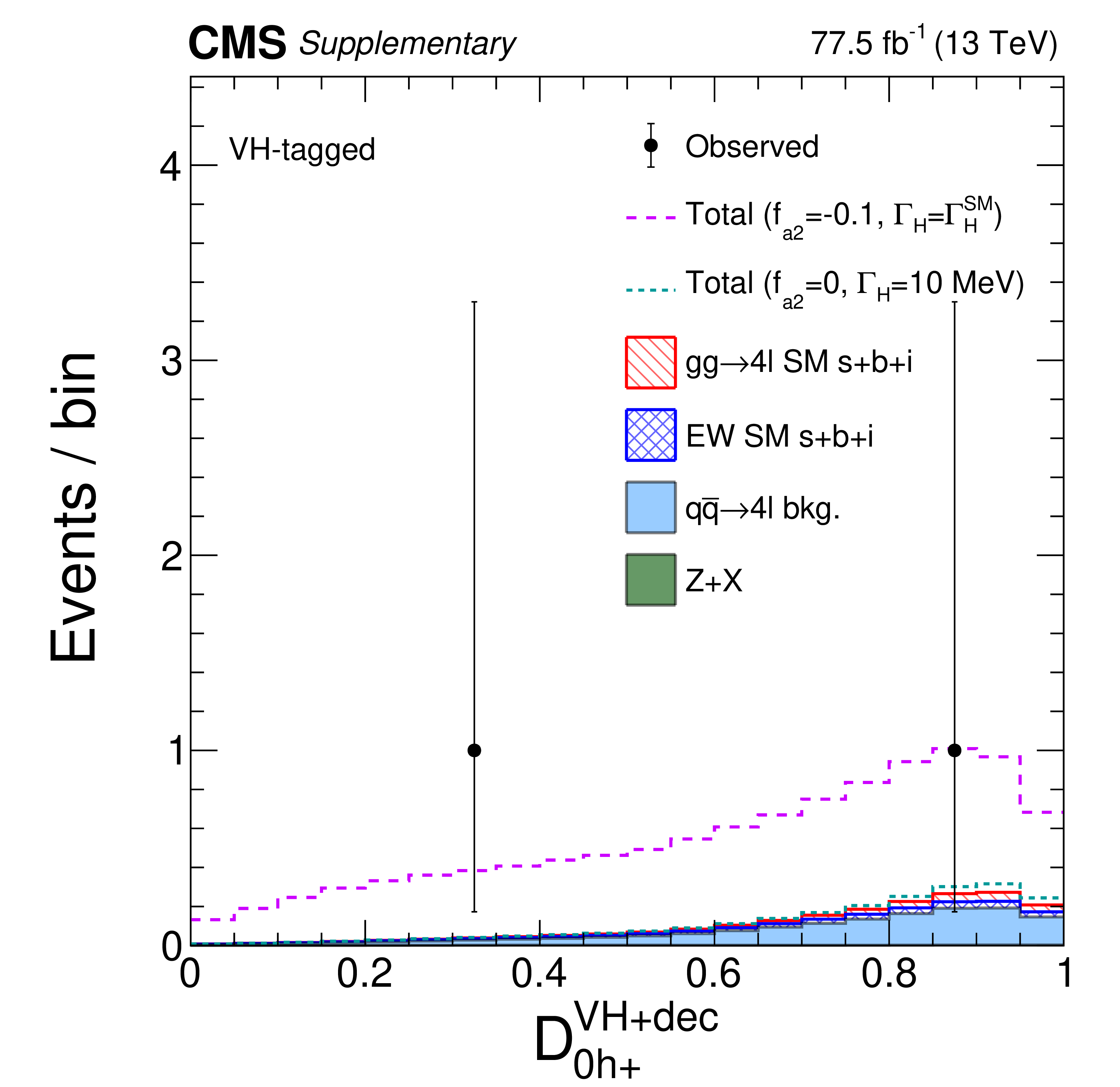
Distribution the $\mathcal {D}^{\text{VH+dec}}_{0h+}$ kinematic discriminant in the on-shell $f_{a2}$ analysis for events in the VH-tagged category. $f_{a2}^{\mathrm {V} {\mathrm {H}}}$ is defined by analogy with $f_{a2}$, but using the cross section for the VH processes. Points with error bars show data and histograms show expectations for background and SM or BSM signal as indicated in the legend. |
png pdf |
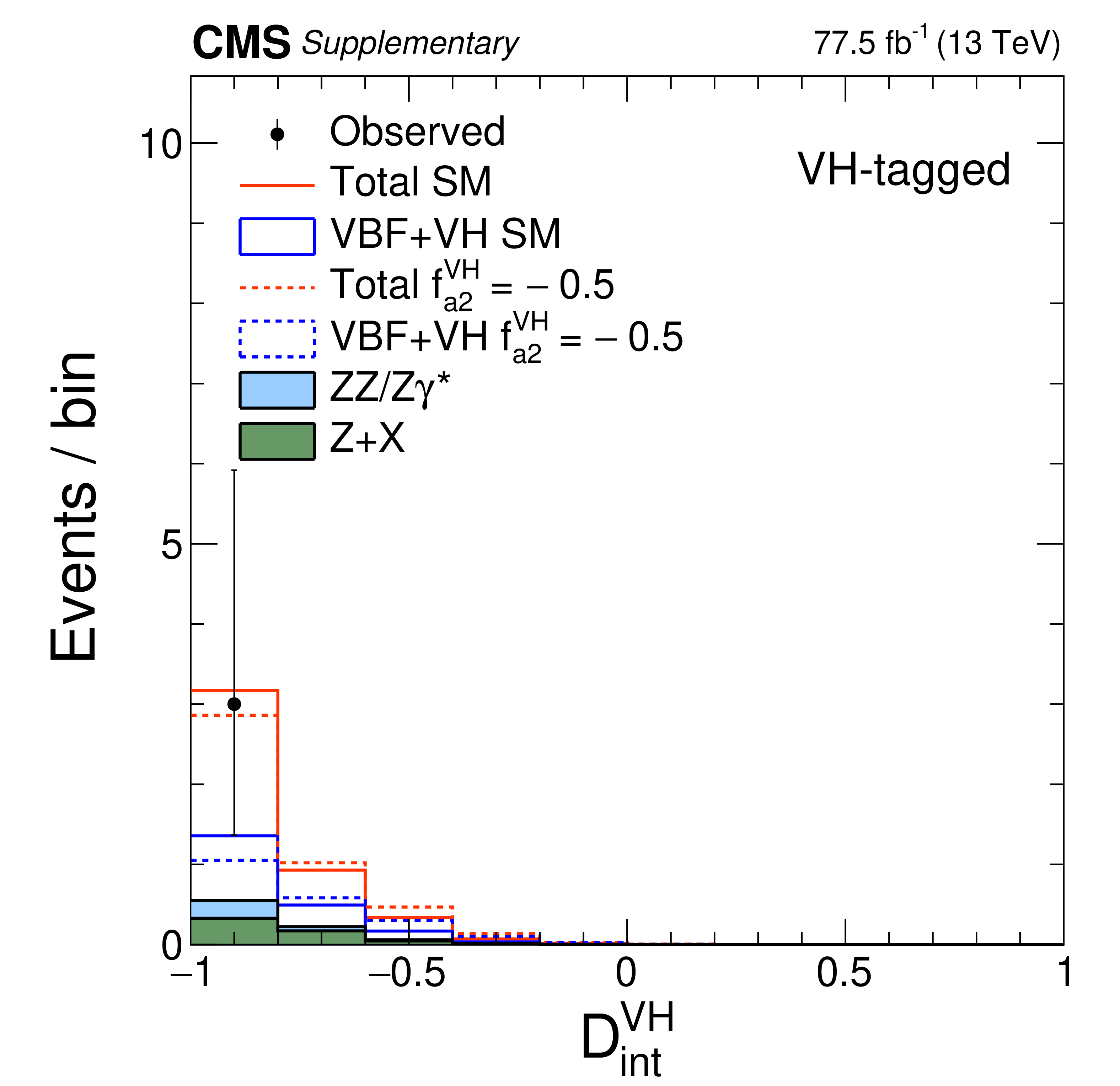
Additional Figure 8-f:
Distribution the $\mathcal {D}^{\text{VH}}_\mathrm {int}$ kinematic discriminant in the on-shell $f_{a2}$ analysis for events in the VH-tagged category. $f_{a2}^{\mathrm {V} {\mathrm {H}}}$ is defined by analogy with $f_{a2}$, but using the cross section for the VH processes. Points with error bars show data and histograms show expectations for background and SM or BSM signal as indicated in the legend. |
png pdf |
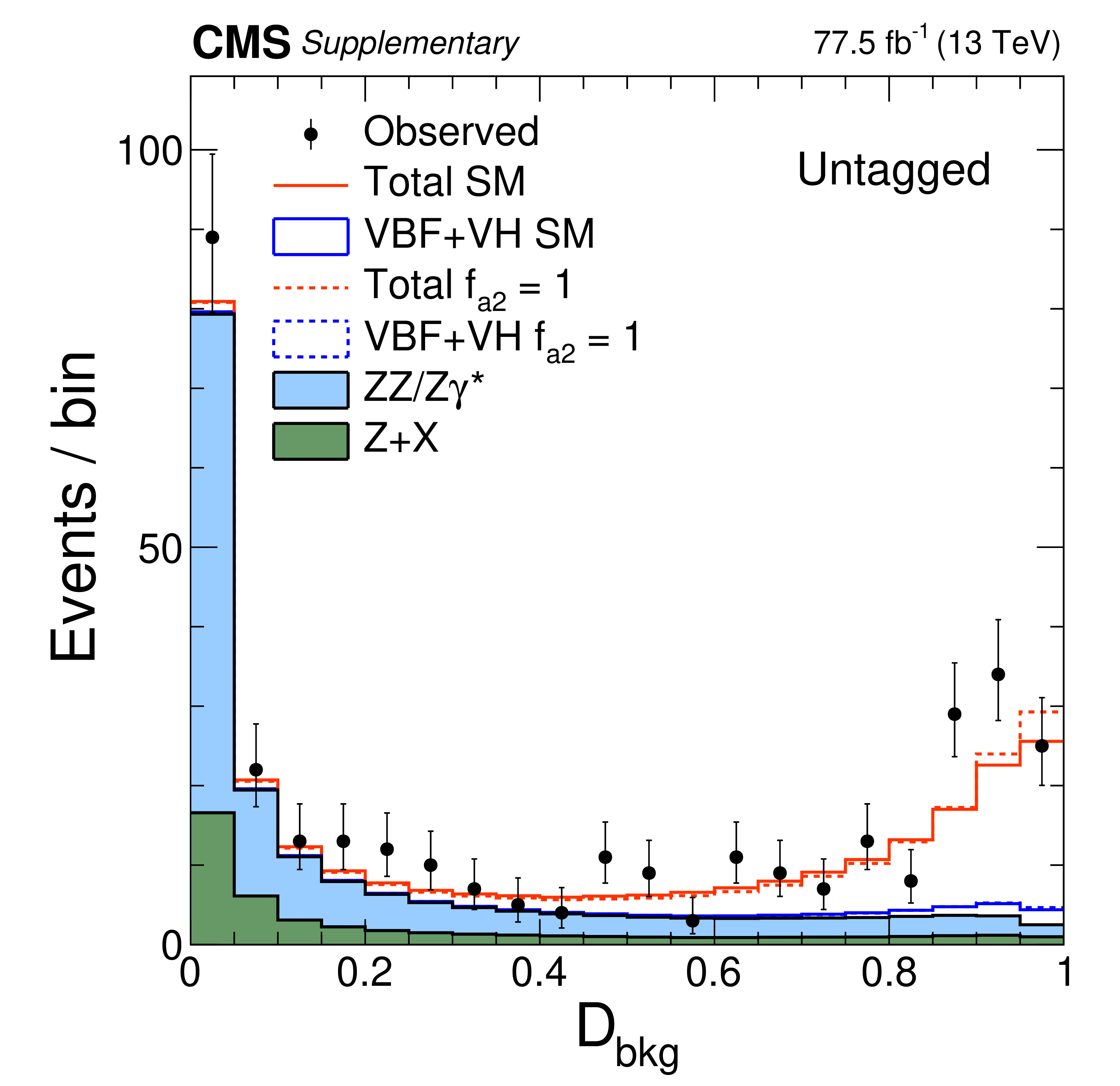
Additional Figure 8-g:
Distribution the $\mathcal {D}_\mathrm {bkg}$ kinematic discriminant in the on-shell $f_{a2}$ analysis for events in the untagged category. Points with error bars show data and histograms show expectations for background and SM or BSM signal as indicated in the legend. |
png pdf |
Additional Figure 8-h:
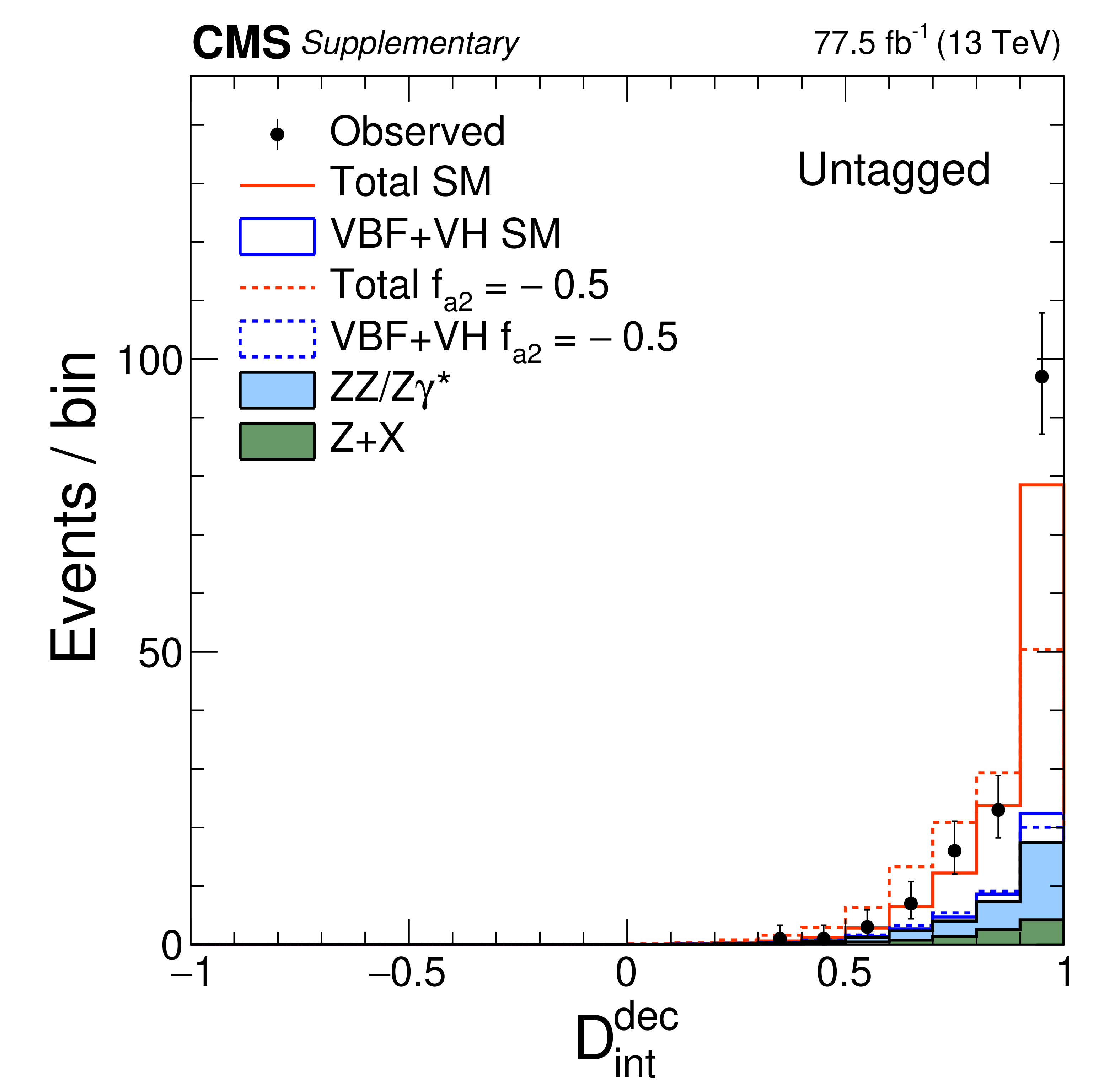
Distribution the $\mathcal {D}^{\text{dec}}_\mathrm {int}$ kinematic discriminant in the on-shell $f_{a2}$ analysis for events in the untagged category. Points with error bars show data and histograms show expectations for background and SM or BSM signal as indicated in the legend. |
png pdf |
Additional Figure 9:
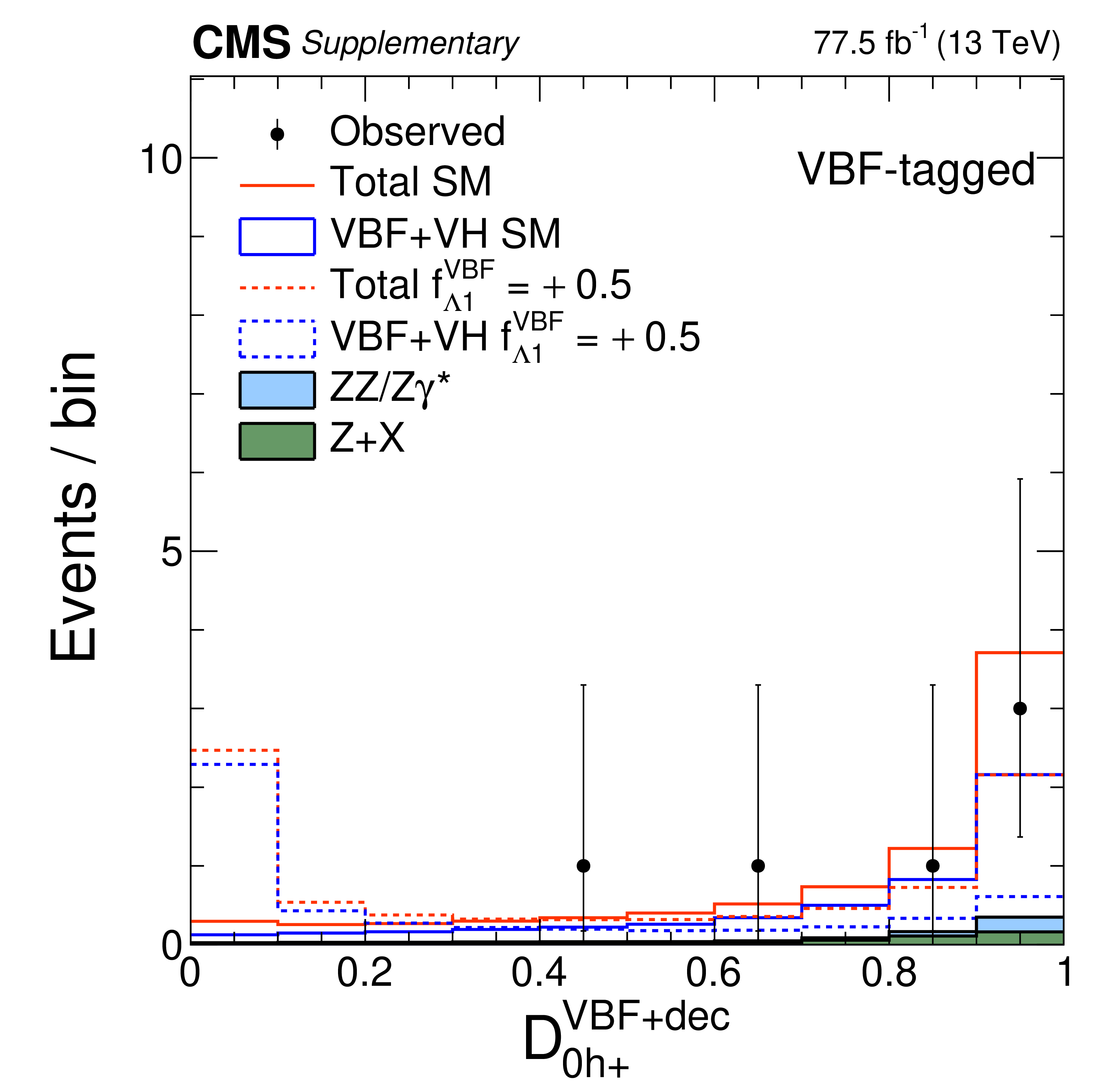
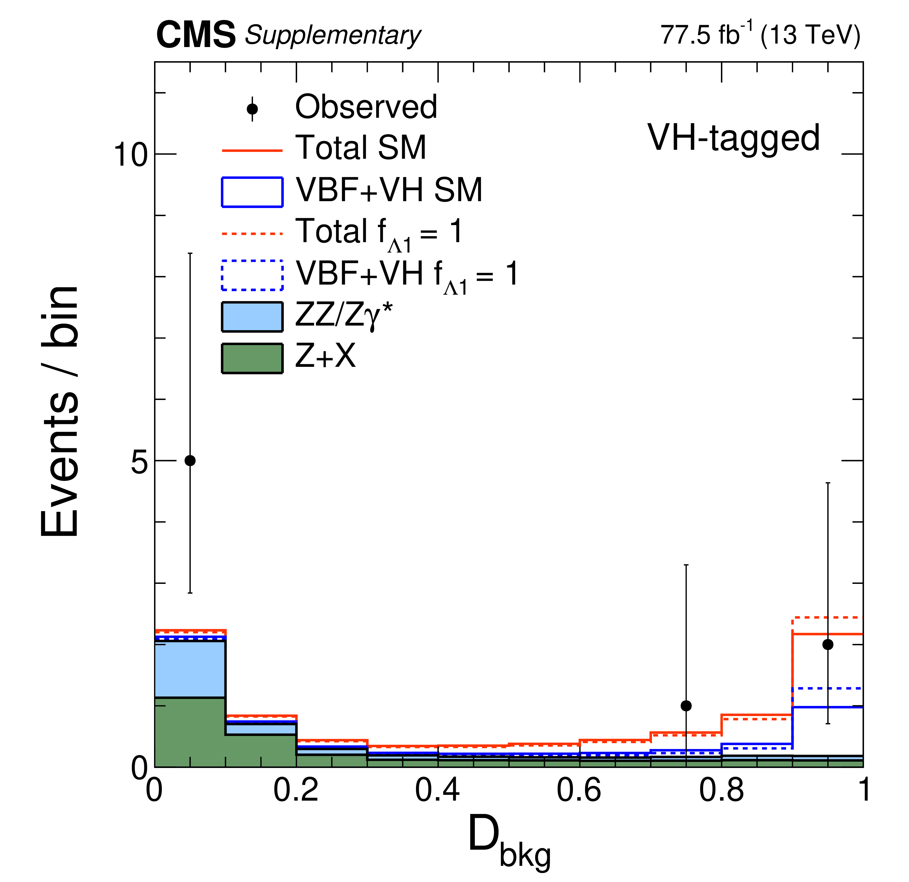
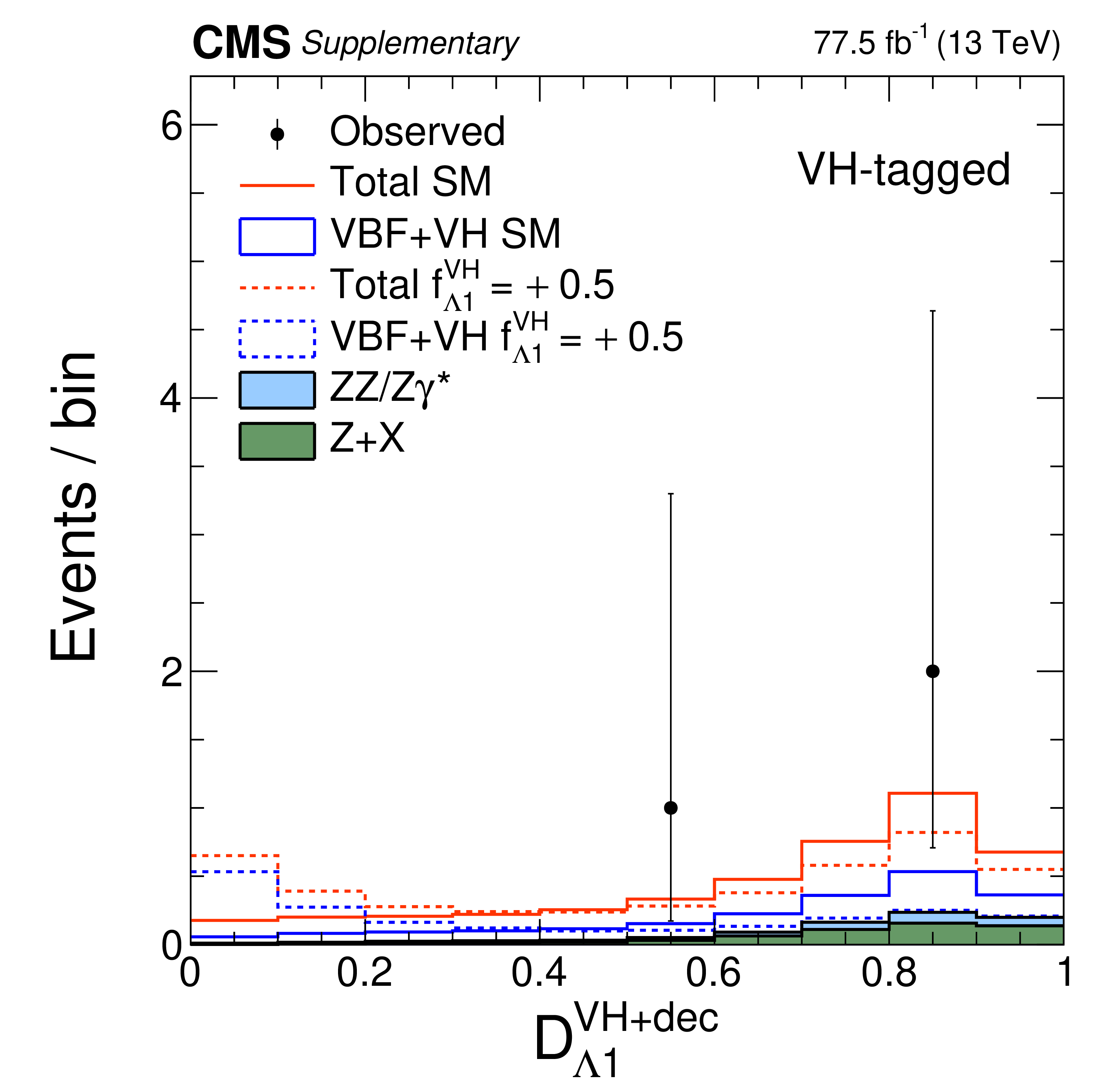
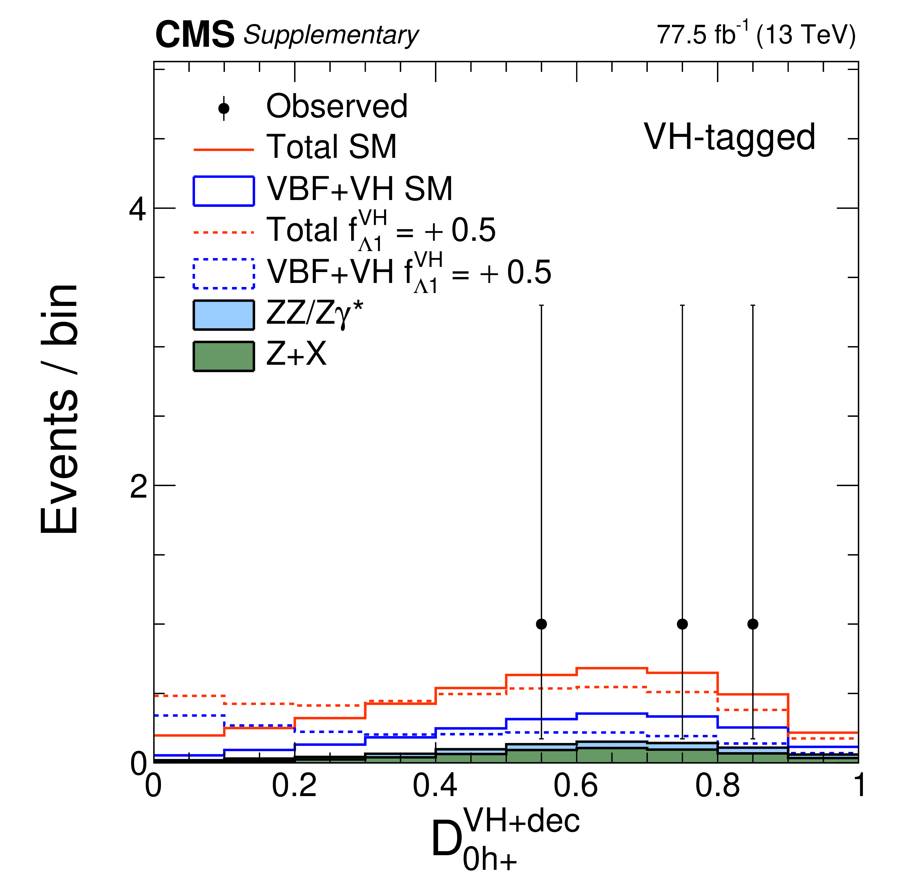
Distributions of kinematic discriminants in the on-shell $f_{\Lambda 1}$ analysis: $\mathcal {D}_\mathrm {bkg}$ (a), (d), (g), $\mathcal {D}_{\Lambda 1}$ (b), (e), and $\mathcal {D}_{0h+}$ (c), (f), (h). Three tagging categories are shown: VBF-tagged (a)-(c), VH-tagged (d)-(f), and untagged (g), (h). The decay or production information used in the discriminants depends on the tagging category. $f_{\Lambda 1}^\mathrm {VBF}$ and $f_{\Lambda 1}^{\mathrm {V} {\mathrm {H}}}$ are defined by analogy with $f_{\Lambda 1}$, but using the cross sections for the VBF and VH processes, respectively. Points with error bars show data and histograms show expectations for background and SM or BSM signal as indicated in the legend. |
png pdf |
Additional Figure 9-a:
Distribution of the $\mathcal {D}_\mathrm {bkg}$ kinematic discriminant in the on-shell $f_{\Lambda 1}$ analysis for events in the VBF-tagged category. Points with error bars show data and histograms show expectations for background and SM or BSM signal as indicated in the legend. |
png pdf |
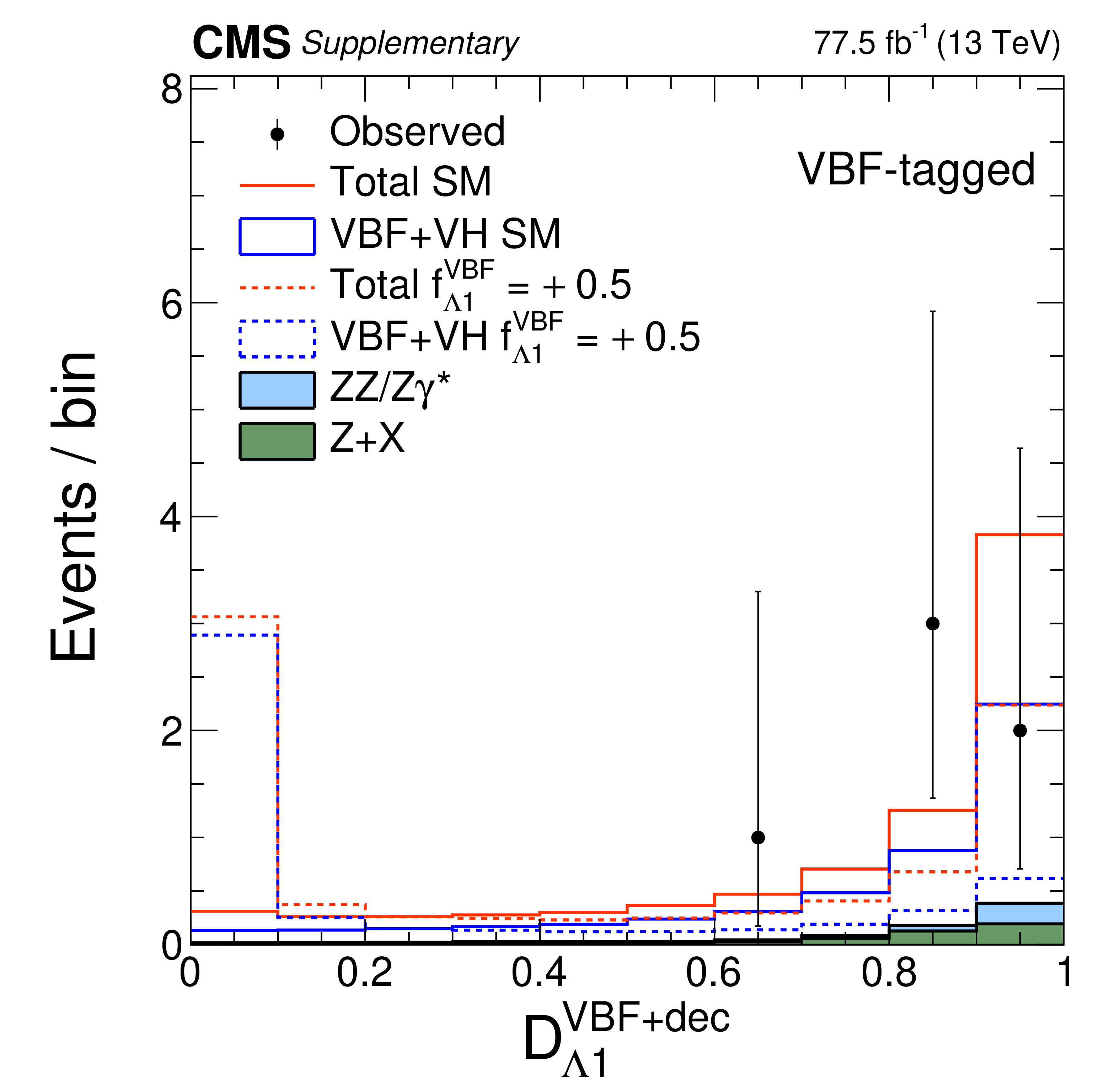
Additional Figure 9-b:
Distribution of the $\mathcal {D}^{\text{VBF+dec}}_{\Lambda 1}$ kinematic discriminant in the on-shell $f_{\Lambda 1}$ analysis for events in the VBF-tagged category. $f_{\Lambda 1}^\mathrm {VBF}$ is defined by analogy with $f_{\Lambda 1}$, but using the cross section for the VBF process. Points with error bars show data and histograms show expectations for background and SM or BSM signal as indicated in the legend. |
png pdf |
Additional Figure 9-c:
Distribution of the $\mathcal {D}^{\text{VBF+dec}}_{0h+}$ kinematic discriminant in the on-shell $f_{\Lambda 1}$ analysis for events in the VBF-tagged category. $f_{\Lambda 1}^\mathrm {VBF}$ is defined by analogy with $f_{\Lambda 1}$, but using the cross section for the VBF process. Points with error bars show data and histograms show expectations for background and SM or BSM signal as indicated in the legend. |
png pdf |
Additional Figure 9-d:
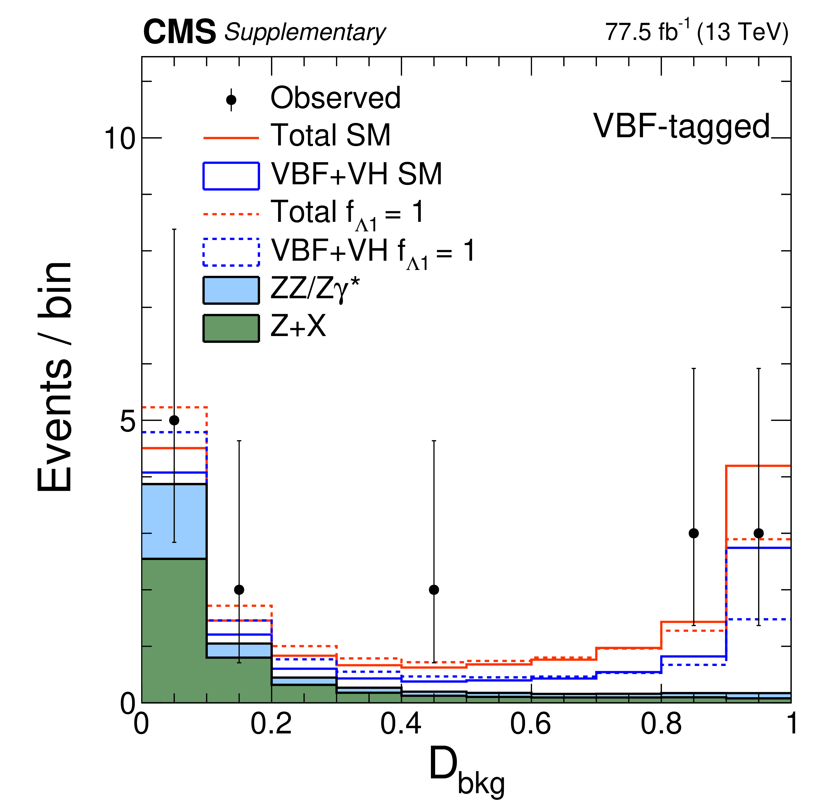
Distribution of the $\mathcal {D}_\mathrm {bkg}$ kinematic discriminant in the on-shell $f_{\Lambda 1}$ analysis for events in the VH-tagged category. Points with error bars show data and histograms show expectations for background and SM or BSM signal as indicated in the legend. |
png pdf |
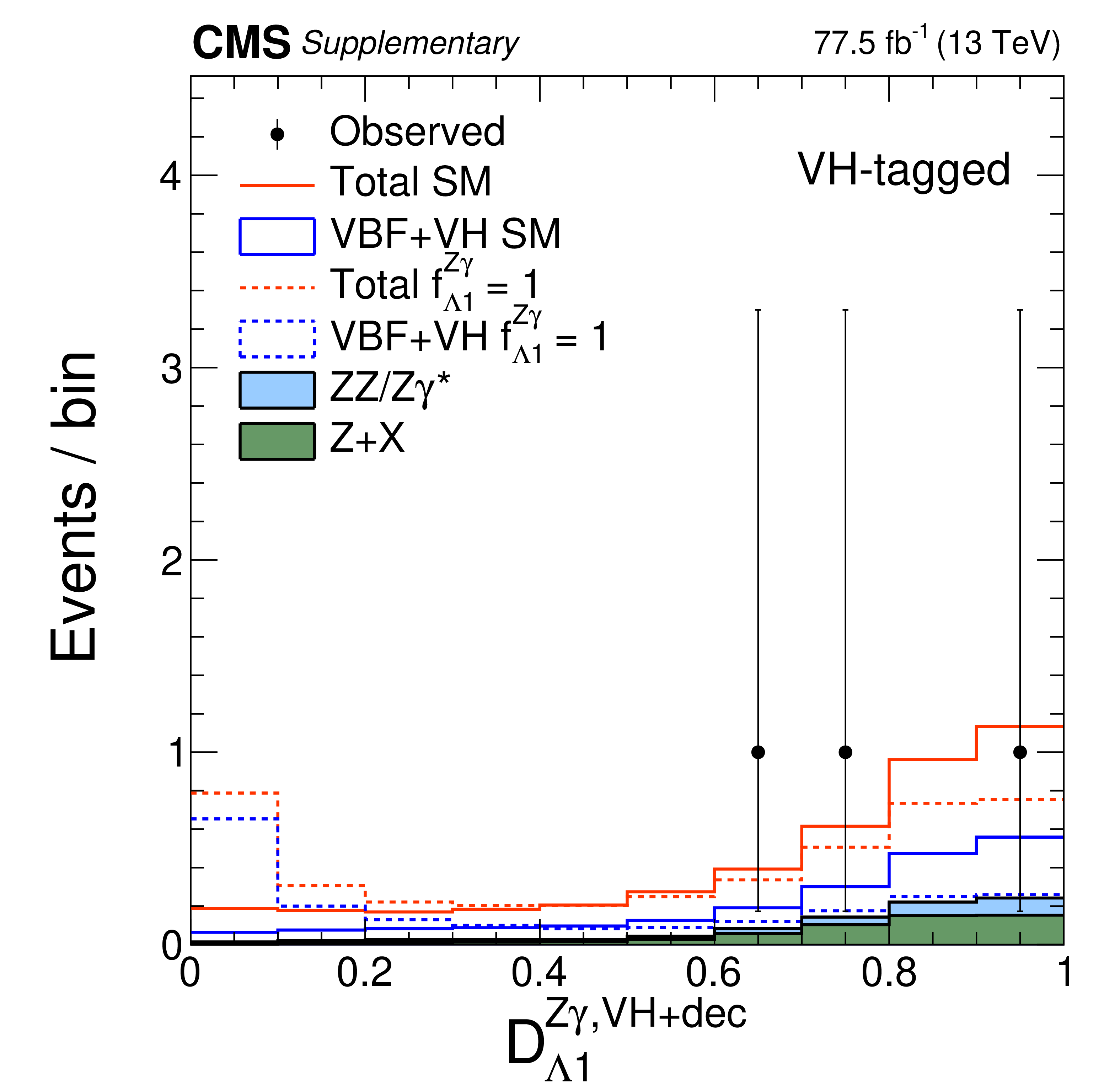
Additional Figure 9-e:
Distribution of the $\mathcal {D}^{\text{VH+dec}}_{\Lambda 1}$ kinematic discriminant in the on-shell $f_{\Lambda 1}$ analysis for events in the VH-tagged category. $f_{\Lambda 1}^{\mathrm {V} {\mathrm {H}}}$ is defined by analogy with $f_{\Lambda 1}$, but using the cross section for the VH process. Points with error bars show data and histograms show expectations for background and SM or BSM signal as indicated in the legend. |
png pdf |
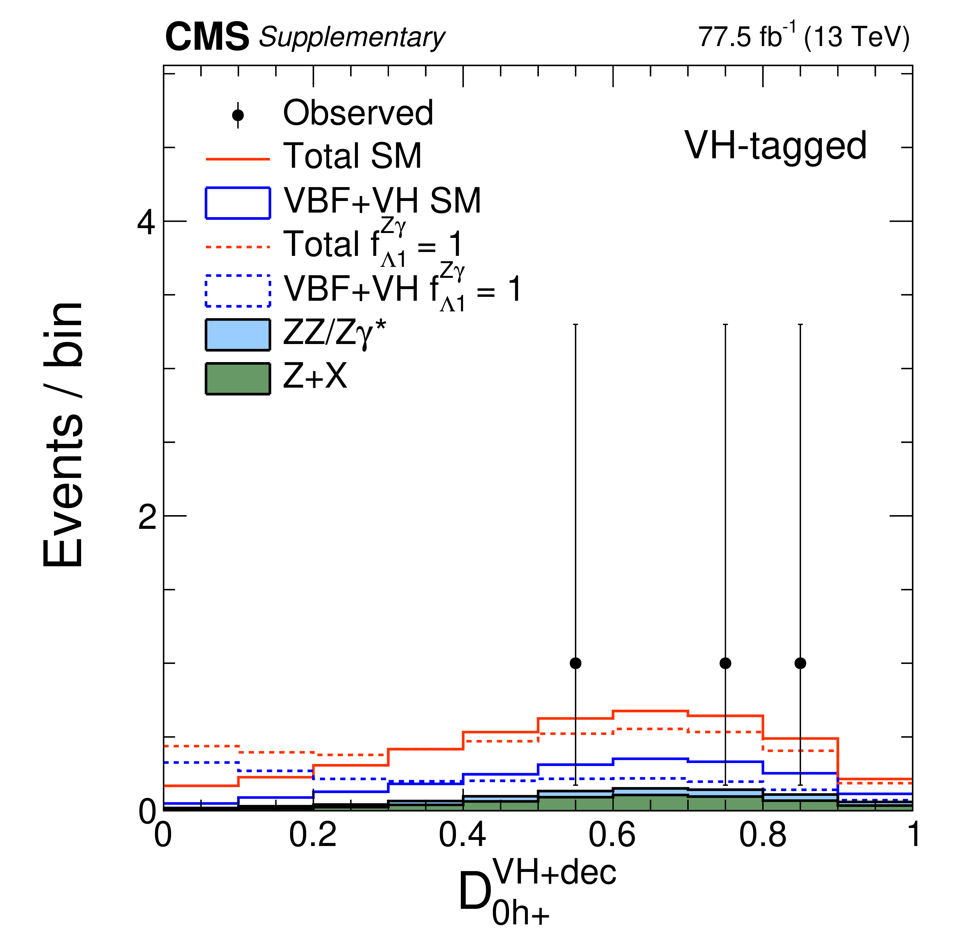
Additional Figure 9-f:
Distribution of the $\mathcal {D}^{\text{VH+dec}}_{0h+}$ kinematic discriminant in the on-shell $f_{\Lambda 1}$ analysis for events in the VH-tagged category. $f_{\Lambda 1}^{\mathrm {V} {\mathrm {H}}}$ is defined by analogy with $f_{\Lambda 1}$, but using the cross section for the VH process. Points with error bars show data and histograms show expectations for background and SM or BSM signal as indicated in the legend. |
png pdf |
Additional Figure 9-g:
Distribution of the $\mathcal {D}_\mathrm {bkg}$ kinematic discriminant in the on-shell $f_{\Lambda 1}$ analysis for events in the untagged category. Points with error bars show data and histograms show expectations for background and SM or BSM signal as indicated in the legend. |
png pdf |
Additional Figure 9-h:
Distribution of the $\mathcal {D}^{\text{dec}}_{0h+}$ kinematic discriminant in the on-shell $f_{\Lambda 1}$ analysis for events in the untagged category. Points with error bars show data and histograms show expectations for background and SM or BSM signal as indicated in the legend. |
png pdf |
Additional Figure 10:
Distributions of kinematic discriminants in the on-shell $f_{\Lambda 1}^{{\mathrm {Z}} \gamma}$ analysis: $\mathcal {D}_\mathrm {bkg}$ (a), (d), (g), $\mathcal {D}_{\Lambda 1}^{{\mathrm {Z}} \gamma}$ (b), (e), and $\mathcal {D}_{0h+}$ (c), (f), (h). Three tagging categories are shown: VBF-tagged (a)-(c), VH-tagged (d)-(f), and untagged (g), (h). The decay or production information used in the discriminants depends on the tagging category. Points with error bars show data and histograms show expectations for background and SM or BSM signal as indicated in the legend. |

png pdf |
Additional Figure 10-a:
Distribution of the $\mathcal {D}_\mathrm {bkg}$ kinematic discriminant in the on-shell $f_{\Lambda 1}^{{\mathrm {Z}} \gamma}$ analysis for events in the VBF-tagged category. Points with error bars show data and histograms show expectations for background and SM or BSM signal as indicated in the legend. |
png pdf |
Additional Figure 10-b:
Distribution of the $\mathcal {D}_{\Lambda 1}^{{\mathrm {Z}} \gamma, \text{VBF+dec}}$ kinematic discriminant in the on-shell $f_{\Lambda 1}^{{\mathrm {Z}} \gamma}$ analysis for events in the VBF-tagged category. Points with error bars show data and histograms show expectations for background and SM or BSM signal as indicated in the legend. |
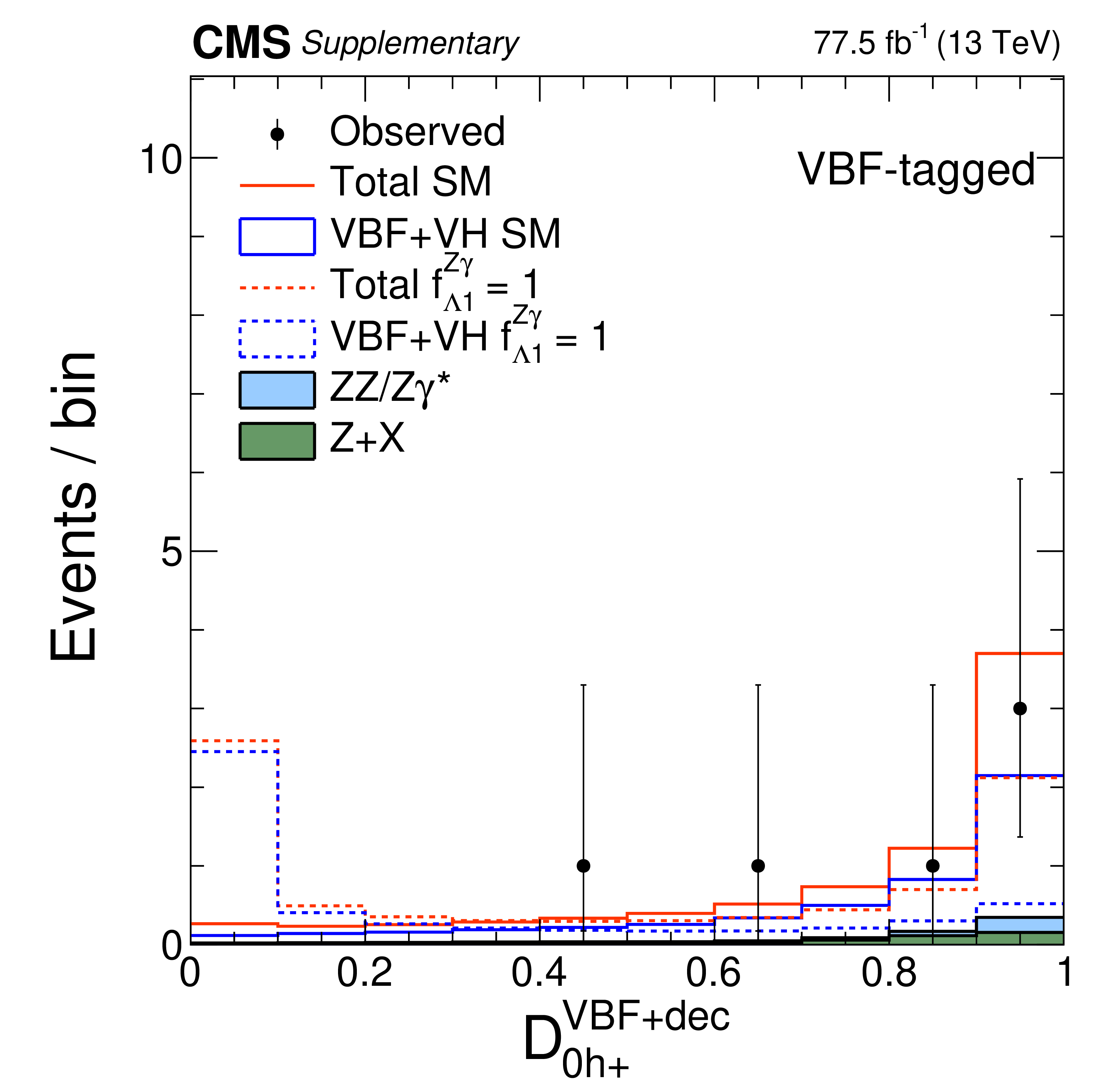
png pdf |
Additional Figure 10-c:
Distribution of the $\mathcal {D}^{\text{VBF+dec}}_{0h+}$ kinematic discriminant in the on-shell $f_{\Lambda 1}^{{\mathrm {Z}} \gamma}$ analysis for events in the VBF-tagged category. Points with error bars show data and histograms show expectations for background and SM or BSM signal as indicated in the legend. |
png pdf |
Additional Figure 10-d:
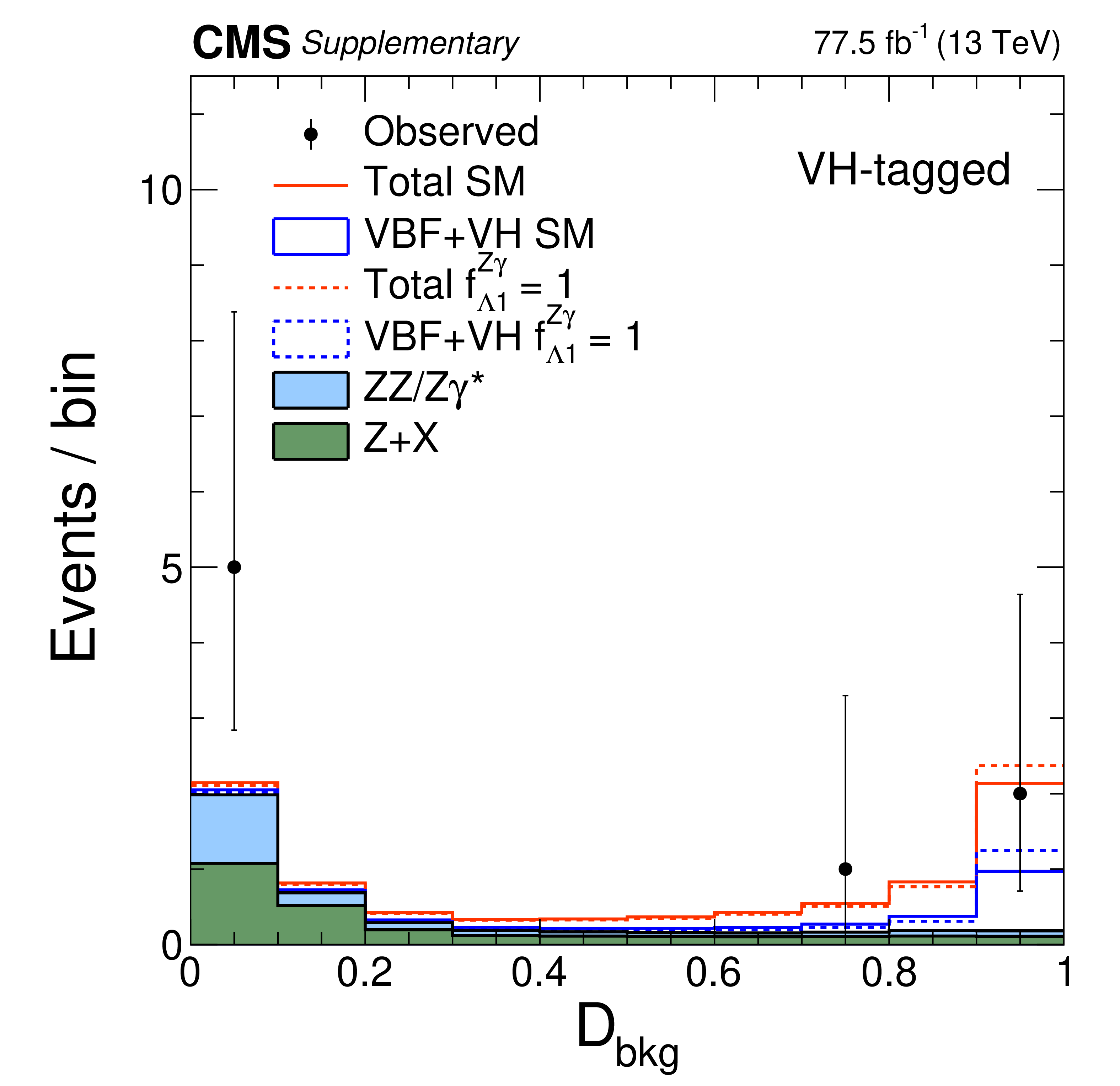
Distribution of the $\mathcal {D}_\mathrm {bkg}$ kinematic discriminant in the on-shell $f_{\Lambda 1}^{{\mathrm {Z}} \gamma}$ analysis for events in the VH-tagged category. Points with error bars show data and histograms show expectations for background and SM or BSM signal as indicated in the legend. |
png pdf |
Additional Figure 10-e:
Distribution of the $\mathcal {D}_{\Lambda 1}^{{\mathrm {Z}} \gamma, \text{VH+dec}}$ kinematic discriminant in the on-shell $f_{\Lambda 1}^{{\mathrm {Z}} \gamma}$ analysis for events in the VH-tagged category. Points with error bars show data and histograms show expectations for background and SM or BSM signal as indicated in the legend. |
png pdf |
Additional Figure 10-f:
Distribution of the $\mathcal {D}^{\text{VH+dec}}_{0h+}$ kinematic discriminant in the on-shell $f_{\Lambda 1}^{{\mathrm {Z}} \gamma}$ analysis for events in the VH-tagged category. Points with error bars show data and histograms show expectations for background and SM or BSM signal as indicated in the legend. |

png pdf |
Additional Figure 10-g:
Distribution of the $\mathcal {D}_\mathrm {bkg}$ kinematic discriminant in the on-shell $f_{\Lambda 1}^{{\mathrm {Z}} \gamma}$ analysis for events in the untagged category. Points with error bars show data and histograms show expectations for background and SM or BSM signal as indicated in the legend. |
png pdf |
Additional Figure 10-h:
Distribution of the $\mathcal {D}^{\text{dec}}_{0h+}$ kinematic discriminant in the on-shell $f_{\Lambda 1}^{{\mathrm {Z}} \gamma}$ analysis for events in the untagged category. Points with error bars show data and histograms show expectations for background and SM or BSM signal as indicated in the legend. |

png pdf |
Additional Figure 11:
Distributions of $\mathcal {D}_\mathrm {bkg}$ kinematic discriminants in the off-shell SM-like width analysis. Three tagging categories are shown: VBF-tagged (a), VH-tagged (b), and untagged (c). The decay or production information used in the discriminants depends on the tagging category. The requirement $m_{4\ell} > $ 340 GeV is applied in order to enhance signal over background contributions. Points with error bars show data and histograms show expectations for background and SM or BSM signal as indicated in the legend. |
png pdf |
Additional Figure 11-a:
Distribution of the $\mathcal {D}^{\text{VBF+dec}}_\mathrm {bkg}$ kinematic discriminant in the off-shell SM-like width analysis for events in the VBF-tagged category. The requirement $m_{4\ell} > $ 340 GeV is applied in order to enhance signal over background contributions. Points with error bars show data and histograms show expectations for background and SM or BSM signal as indicated in the legend. |
png pdf |
Additional Figure 11-b:
Distribution of the $\mathcal {D}^{\text{VH+dec}}_\mathrm {bkg}$ kinematic discriminant in the off-shell SM-like width analysis for events in the VH-tagged category. The requirement $m_{4\ell} > $ 340 GeV is applied in order to enhance signal over background contributions. Points with error bars show data and histograms show expectations for background and SM or BSM signal as indicated in the legend. |
png pdf |
Additional Figure 11-c:
Distribution of the $\mathcal {D}^{\text{kin}}_\mathrm {bkg}$ kinematic discriminant in the off-shell SM-like width analysis for events in the untagged category. The requirement $m_{4\ell} > $ 340 GeV is applied in order to enhance signal over background contributions. Points with error bars show data and histograms show expectations for background and SM or BSM signal as indicated in the legend. |
png pdf |
Additional Figure 12:
Distributions of kinematic discriminants in the off-shell $f_{a3}$ analysis: $m_{4\ell}$ (a), (c), (e), and $\mathcal {D}_{0-}$ (b), (d), (f). Three tagging categories are shown: VBF-tagged (a), (b), VH-tagged (c), (d), and untagged (e), (f). The decay or production information used in the discriminants depends on the tagging category. The requirement $m_{4\ell} > $ 340 GeV is applied in order to enhance signal over background contributions. Points with error bars show data and histograms show expectations for background and SM or BSM signal as indicated in the legend. |
png pdf |
Additional Figure 12-a:
Distribution of $m_{4\ell}$ in the off-shell $f_{a3}$ analysis for events in the VBF-tagged category. The requirement $m_{4\ell} > $ 340 GeV is applied in order to enhance signal over background contributions. Points with error bars show data and histograms show expectations for background and SM or BSM signal as indicated in the legend. |
png pdf |
Additional Figure 12-b:
Distribution of the $\mathcal {D}^{\text{VBF+dec}}_{0-}$ kinematic discriminant in the off-shell $f_{a3}$ analysis for events in the VBF-tagged category. The requirement $m_{4\ell} > $ 340 GeV is applied in order to enhance signal over background contributions. Points with error bars show data and histograms show expectations for background and SM or BSM signal as indicated in the legend. |
png pdf |
Additional Figure 12-c:
Distribution of $m_{4\ell}$ in the off-shell $f_{a3}$ analysis for events in the VH-tagged category. The requirement $m_{4\ell} > $ 340 GeV is applied in order to enhance signal over background contributions. Points with error bars show data and histograms show expectations for background and SM or BSM signal as indicated in the legend. |

png pdf |
Additional Figure 12-d:
Distribution of the $\mathcal {D}^{\text{VH+dec}}_{0-}$ kinematic discriminant in the off-shell $f_{a3}$ analysis for events in the VH-tagged category. The requirement $m_{4\ell} > $ 340 GeV is applied in order to enhance signal over background contributions. Points with error bars show data and histograms show expectations for background and SM or BSM signal as indicated in the legend. |
png pdf |
Additional Figure 12-e:
Distribution of $m_{4\ell}$ in the off-shell $f_{a3}$ analysis for events in the untagged category. The requirement $m_{4\ell} > $ 340 GeV is applied in order to enhance signal over background contributions. Points with error bars show data and histograms show expectations for background and SM or BSM signal as indicated in the legend. |
png pdf |
Additional Figure 12-f:
Distribution of the $\mathcal {D}^{\text{dec}}_{0-}$ kinematic discriminant in the off-shell $f_{a3}$ analysis for events in the untagged category. The requirement $m_{4\ell} > $ 340 GeV is applied in order to enhance signal over background contributions. Points with error bars show data and histograms show expectations for background and SM or BSM signal as indicated in the legend. |

png pdf |
Additional Figure 13:
Distributions of kinematic discriminants in the off-shell $f_{a2}$ analysis: $m_{4\ell}$ (a), (d), (g), $\mathcal {D}_\mathrm {bkg}$ (b), (e), (h), and $\mathcal {D}_{0h+}$ (c), (f), (i). Three tagging categories are shown: VBF-tagged (a)-(c), VH-tagged (d)-(f), and untagged (g)-(i). The decay or production information used in the discriminants depends on the tagging category. The requirement $m_{4\ell} > $ 340 GeV is applied in order to enhance signal over background contributions. Points with error bars show data and histograms show expectations for background and SM or BSM signal as indicated in the legend. |
png pdf |
Additional Figure 13-a:
Distribution of $m_{4\ell}$ in the off-shell $f_{a2}$ analysis for events in the VBF-tagged category. The requirement $m_{4\ell} > $ 340 GeV is applied in order to enhance signal over background contributions. Points with error bars show data and histograms show expectations for background and SM or BSM signal as indicated in the legend. |
png pdf |
Additional Figure 13-b:
Distribution of the $\mathcal {D}^{\text{VBF+dec}}_\mathrm {bkg}$ kinematic discriminant in the off-shell $f_{a2}$ analysis for events in the VBF-tagged category. The requirement $m_{4\ell} > $ 340 GeV is applied in order to enhance signal over background contributions. Points with error bars show data and histograms show expectations for background and SM or BSM signal as indicated in the legend. |
png pdf |
Additional Figure 13-c:
Distribution of the $\mathcal {D}^{\text{VBF+dec}}_{0h+}$ kinematic discriminant in the off-shell $f_{a2}$ analysis for events in the VBF-tagged category. The requirement $m_{4\ell} > $ 340 GeV is applied in order to enhance signal over background contributions. Points with error bars show data and histograms show expectations for background and SM or BSM signal as indicated in the legend. |
png pdf |
Additional Figure 13-d:
Distribution of $m_{4\ell}$ in the off-shell $f_{a2}$ analysis for events in the VH-tagged category. The requirement $m_{4\ell} > $ 340 GeV is applied in order to enhance signal over background contributions. Points with error bars show data and histograms show expectations for background and SM or BSM signal as indicated in the legend. |

png pdf |
Additional Figure 13-e:
Distribution of the $\mathcal {D}^{\text{VH+dec}}_\mathrm {bkg}$ kinematic discriminant in the off-shell $f_{a2}$ analysis for events in the VH-tagged category. The requirement $m_{4\ell} > $ 340 GeV is applied in order to enhance signal over background contributions. Points with error bars show data and histograms show expectations for background and SM or BSM signal as indicated in the legend. |
png pdf |
Additional Figure 13-f:
Distribution of the $\mathcal {D}^{\text{VH+dec}}_{0h+}$ kinematic discriminant in the off-shell $f_{a2}$ analysis for events in the VH-tagged category. The requirement $m_{4\ell} > $ 340 GeV is applied in order to enhance signal over background contributions. Points with error bars show data and histograms show expectations for background and SM or BSM signal as indicated in the legend. |

png pdf |
Additional Figure 13-g:
Distribution of $m_{4\ell}$ in the off-shell $f_{a2}$ analysis for events in the untagged category. The requirement $m_{4\ell} > $ 340 GeV is applied in order to enhance signal over background contributions. Points with error bars show data and histograms show expectations for background and SM or BSM signal as indicated in the legend. |

png pdf |
Additional Figure 13-h:
Distribution of the $\mathcal {D}^{\text{kin}}_\mathrm {bkg}$ kinematic discriminant in the off-shell $f_{a2}$ analysis for events in the untagged category. The requirement $m_{4\ell} > $ 340 GeV is applied in order to enhance signal over background contributions. Points with error bars show data and histograms show expectations for background and SM or BSM signal as indicated in the legend. |
png pdf |
Additional Figure 13-i:
Distribution of the $\mathcal {D}^{\text{dec}}_{0h+}$ kinematic discriminant in the off-shell $f_{a2}$ analysis for events in the untagged category. The requirement $m_{4\ell} > $ 340 GeV is applied in order to enhance signal over background contributions. Points with error bars show data and histograms show expectations for background and SM or BSM signal as indicated in the legend. |
png pdf |
Additional Figure 14:
Distributions of kinematic discriminants in the off-shell $f_{\Lambda 1}$ analysis: $m_{4\ell}$ (a), (d), (g), $\mathcal {D}_\mathrm {bkg}$ (b), (e), (h), and $\mathcal {D}_{\Lambda 1}$ (c), (f), (i). Three tagging categories are shown: VBF-tagged (a)-(c), VH-tagged (d)-(f), and untagged (g)-(i). The decay or production information used in the discriminants depends on the tagging category. The requirement $m_{4\ell} > $ 340 GeV is applied in order to enhance signal over background contributions. Points with error bars show data and histograms show expectations for background and SM or BSM signal as indicated in the legend. |
png pdf |
Additional Figure 14-a:
Distribution of $m_{4\ell}$ in the off-shell $f_{\Lambda 1}$ analysis for events in the VBF-tagged category. The requirement $m_{4\ell} > $ 340 GeV is applied in order to enhance signal over background contributions. Points with error bars show data and histograms show expectations for background and SM or BSM signal as indicated in the legend. |
png pdf |
Additional Figure 14-b:
Distribution of the $\mathcal {D}^{\text{VBF-dec}}_\mathrm {bkg}$ kinematic discriminant in the off-shell $f_{\Lambda 1}$ analysis for events in the VBF-tagged category. The requirement $m_{4\ell} > $ 340 GeV is applied in order to enhance signal over background contributions. Points with error bars show data and histograms show expectations for background and SM or BSM signal as indicated in the legend. |
png pdf |
Additional Figure 14-c:
Distribution of the $\mathcal {D}^{\text{VBF+dec}}_{\Lambda 1}$ kinematic discriminant in the off-shell $f_{\Lambda 1}$ analysis for events in the VBF-tagged category. The requirement $m_{4\ell} > $ 340 GeV is applied in order to enhance signal over background contributions. Points with error bars show data and histograms show expectations for background and SM or BSM signal as indicated in the legend. |
png pdf |
Additional Figure 14-d:
Distribution of $m_{4\ell}$ in the off-shell $f_{\Lambda 1}$ analysis for events in the VH-tagged category. The requirement $m_{4\ell} > $ 340 GeV is applied in order to enhance signal over background contributions. Points with error bars show data and histograms show expectations for background and SM or BSM signal as indicated in the legend. |
png pdf |
Additional Figure 14-e:
Distribution of the $\mathcal {D}^{\text{VH-dec}}_\mathrm {bkg}$ kinematic discriminant in the off-shell $f_{\Lambda 1}$ analysis for events in the VH-tagged category. The requirement $m_{4\ell} > $ 340 GeV is applied in order to enhance signal over background contributions. Points with error bars show data and histograms show expectations for background and SM or BSM signal as indicated in the legend. |
png pdf |
Additional Figure 14-f:
Distribution of the $\mathcal {D}^{\text{VH+dec}}_{\Lambda 1}$ kinematic discriminant in the off-shell $f_{\Lambda 1}$ analysis for events in the VH-tagged category. The requirement $m_{4\ell} > $ 340 GeV is applied in order to enhance signal over background contributions. Points with error bars show data and histograms show expectations for background and SM or BSM signal as indicated in the legend. |
png pdf |
Additional Figure 14-g:
Distribution of $m_{4\ell}$ in the off-shell $f_{\Lambda 1}$ analysis for events in the untagged category. The requirement $m_{4\ell} > $ 340 GeV is applied in order to enhance signal over background contributions. Points with error bars show data and histograms show expectations for background and SM or BSM signal as indicated in the legend. |
png pdf |
Additional Figure 14-h:
Distribution of the $\mathcal {D}^{\text{kin}}_\mathrm {bkg}$ kinematic discriminant in the off-shell $f_{\Lambda 1}$ analysis for events in the untagged category. The requirement $m_{4\ell} > $ 340 GeV is applied in order to enhance signal over background contributions. Points with error bars show data and histograms show expectations for background and SM or BSM signal as indicated in the legend. |
png pdf |
Additional Figure 14-i:
Distribution of the $\mathcal {D}^{\text{dec}}_{\Lambda 1}$ kinematic discriminant in the off-shell $f_{\Lambda 1}$ analysis for events in the untagged category. The requirement $m_{4\ell} > $ 340 GeV is applied in order to enhance signal over background contributions. Points with error bars show data and histograms show expectations for background and SM or BSM signal as indicated in the legend. |
png pdf |
Additional Figure 15:
Observed (solid) and expected (dashed) likelihood scans of $f_{a3}$ (a), $f_{a2}$ (b), and $f_{\Lambda 1}$ (c). Three constraint scenarios are shown: using only on-shell events (green), using both on-shell and off-shell events with the $\Gamma _{{\mathrm {H}}}$ left unconstrained (red), or with the constraint $\Gamma _{{\mathrm {H}}}=\Gamma _{{\mathrm {H}}}^\mathrm {SM}$ (blue). The dashed horizontal lines show the 68 and 95% CL regions. |
png pdf |
Additional Figure 15-a:
Observed (solid) and expected (dashed) likelihood scans of $f_{a3}$. Three constraint scenarios are shown: using only on-shell events (green), using both on-shell and off-shell events with the $\Gamma _{{\mathrm {H}}}$ left unconstrained (red), or with the constraint $\Gamma _{{\mathrm {H}}}=\Gamma _{{\mathrm {H}}}^\mathrm {SM}$ (blue). The dashed horizontal lines show the 68 and 95% CL regions. |
png pdf |
Additional Figure 15-b:
Observed (solid) and expected (dashed) likelihood scans of $f_{a2}$. Three constraint scenarios are shown: using only on-shell events (green), using both on-shell and off-shell events with the $\Gamma _{{\mathrm {H}}}$ left unconstrained (red), or with the constraint $\Gamma _{{\mathrm {H}}}=\Gamma _{{\mathrm {H}}}^\mathrm {SM}$ (blue). The dashed horizontal lines show the 68 and 95% CL regions. |
png pdf |
Additional Figure 15-c:
Observed (solid) and expected (dashed) likelihood scans of $f_{\Lambda 1}$. Three constraint scenarios are shown: using only on-shell events (green), using both on-shell and off-shell events with the $\Gamma _{{\mathrm {H}}}$ left unconstrained (red), or with the constraint $\Gamma _{{\mathrm {H}}}=\Gamma _{{\mathrm {H}}}^\mathrm {SM}$ (blue). The dashed horizontal lines show the 68 and 95% CL regions. |

png pdf |
Additional Figure 16:
Summary of confidence level intervals of anomalous coupling parameters in $ {\mathrm {H}} \mathrm {V}\mathrm {V}$ interactions under the assumption that all the coupling ratios are real ($\phi _{ai}^{\mathrm {V}\mathrm {V}}=0$ or $\pi $). The $ {\mathrm {H}} {\mathrm {Z}} {\mathrm {Z}} + {\mathrm {H}} {\mathrm {W}} {\mathrm {W}}$ coupling limits assume that $a_{i}^{{\mathrm {Z}} {\mathrm {Z}}}=a_{i}^{{\mathrm {W}} {\mathrm {W}}}$. The expected 68% and 95% CL regions are shown as green and yellow bands. The observed intervals for 68% CL are shown as points with error bars, and the excluded regions at 95% CL are indicated with the hatched areas. The limits on $f_{a2,3}^{{\mathrm {Z}} \gamma,\gamma \gamma}$ are from Ref. [25], and the limits on $f_{\Lambda Q}$ are from Ref. [13]. |
| References | ||||
| 1 | S. L. Glashow | Partial-symmetries of weak interactions | NP 22 (1961) 579 | |
| 2 | F. Englert and R. Brout | Broken symmetry and the mass of gauge vector mesons | PRL 13 (1964) 321 | |
| 3 | P. W. Higgs | Broken symmetries, massless particles and gauge fields | PL12 (1964) 132 | |
| 4 | P. W. Higgs | Broken symmetries and the masses of gauge bosons | PRL 13 (1964) 508 | |
| 5 | G. S. Guralnik, C. R. Hagen, and T. W. B. Kibble | Global conservation laws and massless particles | PRL 13 (1964) 585 | |
| 6 | S. Weinberg | A model of leptons | PRL 19 (1967) 1264 | |
| 7 | A. Salam | Weak and electromagnetic interactions | in Elementary particle physics: relativistic groups and analyticity, N. Svartholm, ed., p. 367 Almqvist \& Wiksell, Stockholm, 1968 Proceedings of the eighth Nobel symposium | |
| 8 | ATLAS Collaboration | Observation of a new particle in the search for the Standard Model Higgs boson with the ATLAS detector at the LHC | PLB 716 (2012) 1 | 1207.7214 |
| 9 | CMS Collaboration | Observation of a new boson at a mass of 125 GeV with the CMS experiment at the LHC | PLB 716 (2012) 30 | CMS-HIG-12-028 1207.7235 |
| 10 | CMS Collaboration | Observation of a new boson with mass near 125 GeV in $ {\mathrm{p}}{\mathrm{p}} $ collisions at $ \sqrt{s}= $ 7 and~8 TeV | JHEP 06 (2013) 081 | CMS-HIG-12-036 1303.4571 |
| 11 | CMS Collaboration | Constraints on the Higgs boson width from off-shell production and decay to $ \mathrm{Z} $-boson pairs | PLB 736 (2014) 64 | CMS-HIG-14-002 1405.3455 |
| 12 | ATLAS Collaboration | Constraints on the off-shell Higgs boson signal strength in the high-mass ZZ and WW final states with the ATLAS detector | EPJC 75 (2015) 335 | 1503.01060 |
| 13 | CMS Collaboration | Limits on the Higgs boson lifetime and width from its decay to four charged leptons | PRD 92 (2015) 072010 | CMS-HIG-14-036 1507.06656 |
| 14 | CMS Collaboration | Search for Higgs boson off-shell production in proton-proton collisions at 7 and 8 TeV and derivation of constraints on its total decay width | JHEP 09 (2016) 051 | CMS-HIG-14-032 1605.02329 |
| 15 | ATLAS Collaboration | Constraints on off-shell Higgs boson production and the Higgs boson total width in $ \mathrm{Z}Z\to4\ell $ and $ \mathrm{Z}Z\to2\ell2\mathrm{g}n $ final states with the ATLAS detector | PLB 786 (2018) 223 | 1808.01191 |
| 16 | F. Caola and K. Melnikov | Constraining the Higgs boson width with ZZ production at the LHC | PRD 88 (2013) 054024 | 1307.4935 |
| 17 | N. Kauer and G. Passarino | Inadequacy of zero-width approximation for a light Higgs boson signal | JHEP 08 (2012) 116 | 1206.4803 |
| 18 | J. M. Campbell, R. K. Ellis, and C. Williams | Bounding the Higgs width at the LHC using full analytic results for $ \mathrm{g}\mathrm{g}\to \mathrm{e}^{-}\mathrm{e}^{+} \mu^{-} \mu^{+} $ | JHEP 04 (2014) 060 | 1311.3589 |
| 19 | CMS Collaboration | Precise determination of the mass of the Higgs boson and tests of compatibility of its couplings with the standard model predictions using proton collisions at 7 and 8 TeV | EPJC 75 (2015) 212 | CMS-HIG-14-009 1412.8662 |
| 20 | ATLAS Collaboration | Measurement of the Higgs boson mass from the $ \mathrm{H}\rightarrow \gamma\gamma $ and $ \mathrm{H} \rightarrow \mathrm{Z}\mathrm{Z}^{*} \rightarrow 4\ell $ channels with the ATLAS detector using 25$ fb$^{-1} of $ {\mathrm{p}}{\mathrm{p}} $ collision data | PRD 90 (2014) 052004 | 1406.3827 |
| 21 | CMS Collaboration | Measurements of properties of the Higgs boson decaying into the four-lepton final state in $ {\mathrm{p}}{\mathrm{p}} $ collisions at $ \sqrt{s} = $ 13 TeV | JHEP 11 (2017) 047 | CMS-HIG-16-041 1706.09936 |
| 22 | D. de Florian et al. | Handbook of LHC Higgs cross sections: 4. deciphering the nature of the Higgs sector | CERN-2017-002-M | 1610.07922 |
| 23 | CMS Collaboration | On the mass and spin-parity of the Higgs boson candidate via its decays to $ \mathrm{Z} $ boson pairs | PRL 110 (2013) 081803 | CMS-HIG-12-041 1212.6639 |
| 24 | CMS Collaboration | Measurement of the properties of a Higgs boson in the four-lepton final state | PRD 89 (2014) 092007 | CMS-HIG-13-002 1312.5353 |
| 25 | CMS Collaboration | Constraints on the spin-parity and anomalous HVV couplings of the Higgs boson in proton collisions at 7 and 8 TeV | PRD 92 (2015) 012004 | CMS-HIG-14-018 1411.3441 |
| 26 | CMS Collaboration | Combined search for anomalous pseudoscalar HVV couplings in VH ($ \mathrm{H}\to\mathrm{b\bar{b}} $) production and $ \mathrm{H}\to\mathrm{VV} $ decay | PLB 759 (2016) 672 | CMS-HIG-14-035 1602.04305 |
| 27 | CMS Collaboration | Constraints on anomalous Higgs boson couplings using production and decay information in the four-lepton final state | PLB 775 (2017) 1 | CMS-HIG-17-011 1707.00541 |
| 28 | ATLAS Collaboration | Evidence for the spin-0 nature of the Higgs boson using ATLAS data | PLB 726 (2013) 120 | 1307.1432 |
| 29 | ATLAS Collaboration | Study of the spin and parity of the Higgs boson in diboson decays with the ATLAS detector | EPJC 75 (2015) 476 | 1506.05669 |
| 30 | ATLAS Collaboration | Test of CP Invariance in vector-boson fusion production of the Higgs boson using the Optimal Observable method in the ditau decay channel with the ATLAS detector | EPJC 76 (2016) 658 | 1602.04516 |
| 31 | ATLAS Collaboration | Measurement of inclusive and differential cross sections in the $ \mathrm{H} \rightarrow \mathrm{Z}\mathrm{Z}^{*} \rightarrow 4\ell $ decay channel in $ {\mathrm{p}}{\mathrm{p}} $ collisions at $ \sqrt{s} = $ 13 TeV with the ATLAS detector | JHEP 10 (2017) 132 | 1708.02810 |
| 32 | ATLAS Collaboration | Measurement of the Higgs boson coupling properties in the $ H\rightarrow ZZ^{*} \rightarrow 4\ell $ decay channel at $ \sqrt{s} = $ 13 TeV with the ATLAS detector | JHEP 03 (2018) 095 | 1712.02304 |
| 33 | ATLAS Collaboration | Measurements of Higgs boson properties in the diphoton decay channel with 36 fb$ ^{-1} $ of $ {\mathrm{p}}{\mathrm{p}} $ collision data at $ \sqrt{s} = $ 13 TeV with the ATLAS detector | PRD 98 (2018) 052005 | 1802.04146 |
| 34 | J. S. Gainer et al. | Beyond geolocating: Constraining higher dimensional operators in $ \mathrm{H} \to 4\ell $ with off-shell production and more | PRD 91 (2015) 035011 | 1403.4951 |
| 35 | C. Englert and M. Spannowsky | Limitations and opportunities of off-shell coupling measurements | PRD 90 (2014) 053003 | 1405.0285 |
| 36 | M. Ghezzi, G. Passarino, and S. Uccirati | Bounding the Higgs width using effective field theory | in Proceedings, 12th DESY Workshop on Elementary Particle Physics: Loops and Legs in Quantum Field Theory (LL2014), p. 072 Weimar, Germany, April, 2014 [PoS(LL2014)072] | 1405.1925 |
| 37 | CMS Collaboration | Search for a new scalar resonance decaying to a pair of $ \mathrm{Z} $ bosons in proton-proton collisions at $ \sqrt{s} = $ 13 TeV | JHEP 06 (2018) 127 | CMS-HIG-17-012 1804.01939 |
| 38 | C. A. Nelson | Correlation between decay planes in Higgs-boson decays into a $ \mathrm{W} $ Pair (into a $ \mathrm{Z} $ Pair) | PRD 37 (1988) 1220 | |
| 39 | A. Soni and R. M. Xu | Probing CP violation via Higgs decays to four leptons | PRD 48 (1993) 5259 | hep-ph/9301225 |
| 40 | T. Plehn, D. L. Rainwater, and D. Zeppenfeld | Determining the structure of Higgs couplings at the LHC | PRL 88 (2002) 051801 | hep-ph/0105325 |
| 41 | S. Y. Choi, D. J. Miller, M. M. M uhlleitner, and P. M. Zerwas | Identifying the Higgs spin and parity in decays to Z pairs | PLB 553 (2003) 61 | hep-ph/0210077 |
| 42 | C. P. Buszello, I. Fleck, P. Marquard, and J. J. van der Bij | Prospective analysis of spin- and CP-sensitive variables in $ \mathrm{H} \to \mathrm{Z}\mathrm{Z} \to \ell_1^+ \ell_1^- \ell_2^+ \ell_2^- $ at the LHC | EPJC 32 (2004) 209 | hep-ph/0212396 |
| 43 | V. Hankele, G. Klamke, D. Zeppenfeld, and T. Figy | Anomalous Higgs boson couplings in vector boson fusion at the CERN LHC | PRD 74 (2006) 095001 | hep-ph/0609075 |
| 44 | E. Accomando et al. | Workshop on CP studies and non-standard Higgs physics | hep-ph/0608079 | |
| 45 | R. M. Godbole, D. J. Miller, and M. M. M uhlleitner | Aspects of CP violation in the $ \mathrm{H}\mathrm{Z}\mathrm{Z} $ coupling at the LHC | JHEP 12 (2007) 031 | 0708.0458 |
| 46 | K. Hagiwara, Q. Li, and K. Mawatari | Jet angular correlation in vector-boson fusion processes at hadron colliders | JHEP 07 (2009) 101 | 0905.4314 |
| 47 | Y. Gao et al. | Spin determination of single-produced resonances at hadron colliders | PRD 81 (2010) 075022 | 1001.3396 |
| 48 | A. De R\' ujula et al. | Higgs look-alikes at the LHC | PRD 82 (2010) 013003 | 1001.5300 |
| 49 | N. D. Christensen, T. Han, and Y. Li | Testing CP Violation in ZZH Interactions at the LHC | PLB 693 (2010) 28 | 1005.5393 |
| 50 | S. Bolognesi et al. | Spin and parity of a single-produced resonance at the LHC | PRD 86 (2012) 095031 | 1208.4018 |
| 51 | J. Ellis, D. S. Hwang, V. Sanz, and T. You | A fast track towards the `Higgs' spin and parity | JHEP 11 (2012) 134 | 1208.6002 |
| 52 | Y. Chen, N. Tran, and R. Vega-Morales | Scrutinizing the Higgs signal and background in the $ 2\mathrm{e}2\mu $ golden channel | JHEP 01 (2013) 182 | 1211.1959 |
| 53 | P. Artoisenet et al. | A framework for Higgs characterisation | JHEP 11 (2013) 043 | 1306.6464 |
| 54 | I. Anderson et al. | Constraining anomalous HVV interactions at proton and lepton colliders | PRD 89 (2014) 035007 | 1309.4819 |
| 55 | M. Chen et al. | Role of interference in unraveling the ZZ couplings of the newly discovered boson at the LHC | PRD 89 (2014) 034002 | 1310.1397 |
| 56 | M. J. Dolan, P. Harris, M. Jankowiak, and M. Spannowsky | Constraining $ CP $-violating Higgs sectors at the LHC using gluon fusion | PRD 90 (2014) 073008 | 1406.3322 |
| 57 | M. Gonzalez-Alonso, A. Greljo, G. Isidori, and D. Marzocca | Pseudo-observables in Higgs decays | EPJC 75 (2015) 128 | 1412.6038 |
| 58 | A. Greljo, G. Isidori, J. M. Lindert, and D. Marzocca | Pseudo-observables in electroweak Higgs production | EPJC 76 (2016) 158 | 1512.06135 |
| 59 | A. V. Gritsan, R. Rontsch, M. Schulze, and M. Xiao | Constraining anomalous Higgs boson couplings to the heavy flavor fermions using matrix element techniques | PRD 94 (2016) 055023 | 1606.03107 |
| 60 | CMS Collaboration | The CMS experiment at the CERN LHC | JINST 3 (2008) S08004 | CMS-00-001 |
| 61 | S. Frixione, P. Nason, and C. Oleari | Matching NLO QCD computations with parton shower simulations: the POWHEG method | JHEP 11 (2007) 070 | 0709.2092 |
| 62 | E. Bagnaschi, G. Degrassi, P. Slavich, and A. Vicini | Higgs production via gluon fusion in the POWHEG approach in the SM and in the MSSM | JHEP 02 (2012) 088 | 1111.2854 |
| 63 | P. Nason and C. Oleari | NLO Higgs boson production via vector-boson fusion matched with shower in POWHEG | JHEP 02 (2010) 037 | 0911.5299 |
| 64 | G. Luisoni, P. Nason, C. Oleari, and F. Tramontano | $ \mathrm{H}\mathrm{W}^{\pm} $/$ \mathrm{H}\mathrm{Z} $ + 0 and 1 jet at NLO with the POWHEG BOX interfaced to GoSam and their merging within MiNLO | JHEP 10 (2013) 083 | 1306.2542 |
| 65 | H. B. Hartanto, B. Jager, L. Reina, and D. Wackeroth | Higgs boson production in association with top quarks in the POWHEG BOX | PRD 91 (2015) 094003 | 1501.04498 |
| 66 | K. Hamilton, P. Nason, and G. Zanderighi | MINLO: multi-scale improved NLO | JHEP 10 (2012) 155 | 1206.3572 |
| 67 | J. M. Campbell and R. K. Ellis | MCFM for the Tevatron and the LHC | NPPS 205-206 (2010) 10 | 1007.3492 |
| 68 | J. M. Campbell, R. K. Ellis, and C. Williams | Vector boson pair production at the LHC | JHEP 07 (2011) 018 | 1105.0020 |
| 69 | J. M. Campbell and R. K. Ellis | Higgs constraints from vector boson fusion and scattering | JHEP 04 (2015) 030 | 1502.02990 |
| 70 | A. Ballestrero et al. | PHANTOM: a Monte Carlo event generator for six parton final states at high energy colliders | CPC 180 (2009) 401 | 0801.3359 |
| 71 | S. Catani and M. Grazzini | An NNLO subtraction formalism in hadron collisions and its application to Higgs boson production at the LHC | PRL 98 (2007) 222002 | hep-ph/0703012 |
| 72 | M. Grazzini | NNLO predictions for the Higgs boson signal in the $ \mathrm{H} \to \mathrm{WW} \to\ell\mathrm{g}n\ell\mathrm{g}n $ and $ \mathrm{H} \to \mathrm{ZZ} \to 4\ell $ decay channels | JHEP 02 (2008) 043 | 0801.3232 |
| 73 | M. Grazzini and H. Sargsyan | Heavy-quark mass effects in Higgs boson production at the LHC | JHEP 09 (2013) 129 | 1306.4581 |
| 74 | F. Caola, K. Melnikov, R. Rontsch, and L. Tancredi | QCD corrections to ZZ production in gluon fusion at the LHC | PRD 92 (2015) 094028 | 1509.06734 |
| 75 | K. Melnikov and M. Dowling | Production of two $ \mathrm{Z} $-bosons in gluon fusion in the heavy top quark approximation | PLB 744 (2015) 43 | 1503.01274 |
| 76 | J. M. Campbell, R. K. Ellis, M. Czakon, and S. Kirchner | Two loop correction to interference in $ \mathrm{g}\mathrm{g} \to \mathrm{Z}Z $ | JHEP 08 (2016) 011 | 1605.01380 |
| 77 | F. Caola et al. | QCD corrections to vector boson pair production in gluon fusion including interference effects with off-shell Higgs at the LHC | JHEP 07 (2016) 087 | 1605.04610 |
| 78 | M. Grazzini, S. Kallweit, and D. Rathlev | $ \mathrm{Z}\mathrm{Z} $ production at the LHC: fiducial cross sections and distributions in NNLO QCD | PLB 750 (2015) 407 | 1507.06257 |
| 79 | S. Gieseke, T. Kasprzik, and J. H. Kuehn | Vector-boson pair production and electroweak corrections in HERWIG++ | EPJC 74 (2014) 2988 | 1401.3964 |
| 80 | J. Baglio, L. D. Ninh, and M. M. Weber | Massive gauge boson pair production at the LHC: a next-to-leading order story | PRD 88 (2013) 113005 | 1307.4331 |
| 81 | NNPDF Collaboration | Unbiased global determination of parton distributions and their uncertainties at NNLO and at LO | NPB 855 (2012) 153 | 1107.2652 |
| 82 | T. Sjostrand et al. | An introduction to PYTHIA 8.2 | CPC 191 (2015) 159 | 1410.3012 |
| 83 | GEANT4 Collaboration | GEANT4 -- a simulation toolkit | NIMA 506 (2003) 250 | |
| 84 | CMS Collaboration | Particle-flow reconstruction and global event description with the cms detector | JINST 12 (2017) P10003 | CMS-PRF-14-001 1706.04965 |
| 85 | M. Cacciari, G. P. Salam, and G. Soyez | The anti-$ {k_{\mathrm{T}}} $ jet clustering algorithm | JHEP 04 (2008) 063 | 0802.1189 |
| 86 | M. Cacciari, G. P. Salam, and G. Soyez | FastJet user manual | EPJC 72 (2012) 1896 | 1111.6097 |
| 87 | CMS Collaboration | Identification of $ \mathrm{b} $-quark jets with the CMS experiment | JINST 8 (2013) P04013 | CMS-BTV-12-001 1211.4462 |
| 88 | CMS Collaboration | Identification of heavy-flavour jets with the CMS detector in $ {\mathrm{p}}{\mathrm{p}} $ collisions at 13 TeV | JINST 13 (2018) P05011 | CMS-BTV-16-002 1712.07158 |
| 89 | R. J. Barlow | Extended maximum likelihood | NIMA 297 (1990) 496 | |
| 90 | M. J. Oreglia | A study of the reactions $\psi' \to \gamma\gamma \psi$ | PhD thesis, Stanford University, 1980 SLAC Report SLAC-R-236, see A | |
| 91 | W. Verkerke and D. P. Kirkby | The RooFit toolkit for data modeling | in 13$^\textth$ International Conference for Computing in High-Energy and Nuclear Physics (CHEP03) 2003 CHEP-2003-MOLT007 | physics/0306116 |
| 92 | R. Brun and F. Rademakers | ROOT: An object oriented data analysis framework | NIMA 389 (1997) 81 | |
| 93 | S. S. Wilks | The large-sample distribution of the likelihood ratio for testing composite hypotheses | Annals Math. Statist. 9 (1938) 60 | |
| 94 | CMS Collaboration | CMS luminosity measurements for the 2016 data taking period | CMS-PAS-LUM-17-001 | CMS-PAS-LUM-17-001 |
| 95 | CMS Collaboration | CMS luminosity measurement for the 2017 data taking period at $ \sqrt{s} = $ 13 TeV | CMS-PAS-LUM-17-004 | CMS-PAS-LUM-17-004 |
|
|
Compact Muon Solenoid LHC, CERN |
|

|

|

|

|

|