

Compact Muon Solenoid
LHC, CERN
| CMS-HIG-18-020 ; CERN-EP-2019-083 | ||
| Search for a light charged Higgs boson decaying to a W boson and a CP-odd Higgs boson in final states with $\mathrm{e}\mu\mu$ or $ \mu\mu\mu$ in proton-proton collisions at $\sqrt{s} = $ 13 TeV | ||
| CMS Collaboration | ||
| 18 May 2019 | ||
| Phys. Rev. Lett. 123 (2019) 131802 | ||
| Abstract: A search for a light charged Higgs boson ($\mathrm{H}^{+}$) decaying to a W boson and a CP-odd Higgs boson (A) in final states with $\mathrm{e}\mu\mu$ or $ \mu\mu\mu$ is performed using data from pp collisions at $\sqrt{s} = $ 13 TeV, recorded by the CMS detector at the LHC and corresponding to an integrated luminosity of 35.9 fb$^{-1}$. In this search, it is assumed that the $\mathrm{H}^{+}$ boson is produced in decays of top quarks, and the A boson decays to two oppositely charged muons. The presence of signals for $\mathrm{H}^{+}$ boson masses between 100 and 160 GeV and A boson masses between 15 and 75 GeV is investigated. No evidence for the production of the $\mathrm{H}^{+}$ boson is found. Assuming branching fractions ${\mathcal{B}({\mathrm{H}^{+}\to\mathrm{W^{+}}\mathrm{A} })}=$ 1 and ${\mathcal{B}({\mathrm{A} }\to\mu^{+}\mu^{-})}=3\times10^{-4}$, upper limits at 95% confidence level on the branching fraction of the top quark, ${\mathcal{B}({\mathrm{t}\to\mathrm{b}\mathrm{H}^{+}})}$, of 0.63 to 2.9% are obtained, depending on the masses of the $\mathrm{H}^{+}$ and A bosons. These are the first limits on ${\mathcal{B}({\mathrm{t}\to\mathrm{b}\mathrm{H}^{+}})}$ in the decay mode of the $\mathrm{H}^{+}$ boson: ${\mathrm{H}^{+}\to\mathrm{W^{+}}\mathrm{A} }\to\mathrm{W^{+}}\mu^{+}\mu^{-}$. | ||
| Links: e-print arXiv:1905.07453 [hep-ex] (PDF) ; CDS record ; inSPIRE record ; HepData record ; CADI line (restricted) ; | ||
| Figures | |

png pdf |
Figure 1:
The Feynman diagram of signal processes ($\ell = {\mathrm {e}}$ or $ {{\mu}}$, $ {\mathrm {W}} {\mathrm {W}}\to \ell {\nu} {\mathrm {q}} {\overline {\mathrm {q}}}^{\prime}$). |

png pdf |
Figure 2:
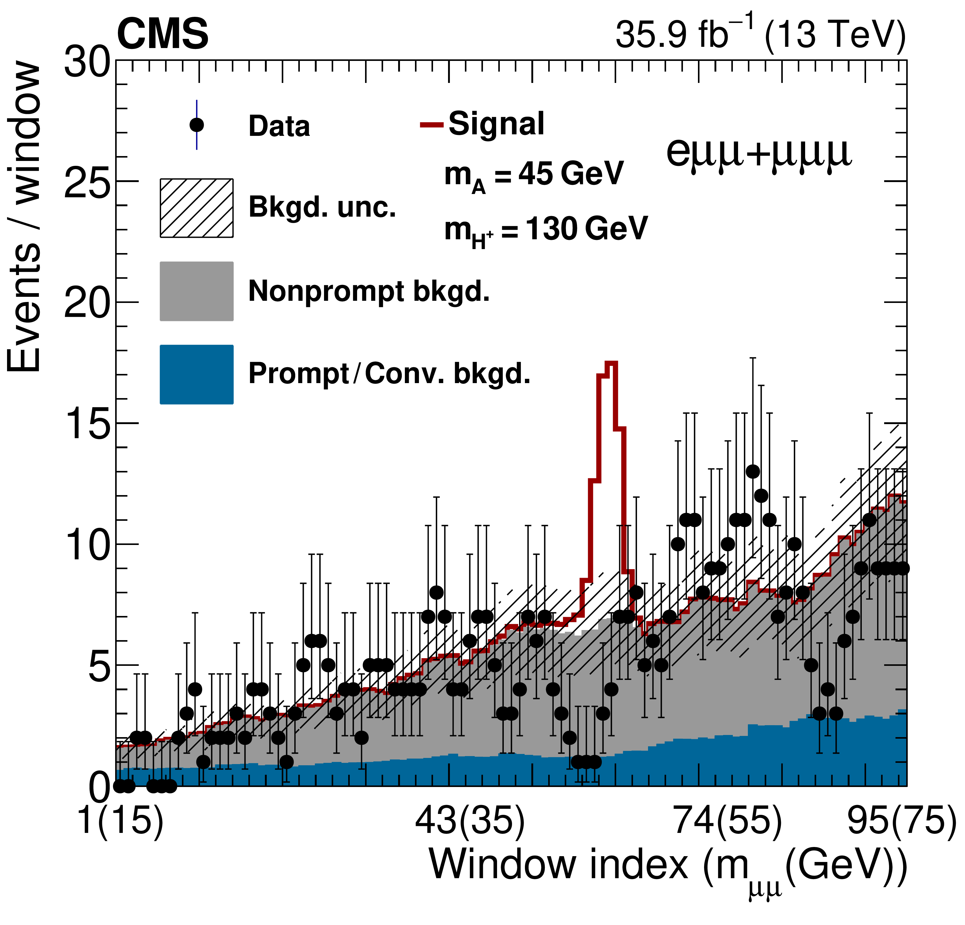
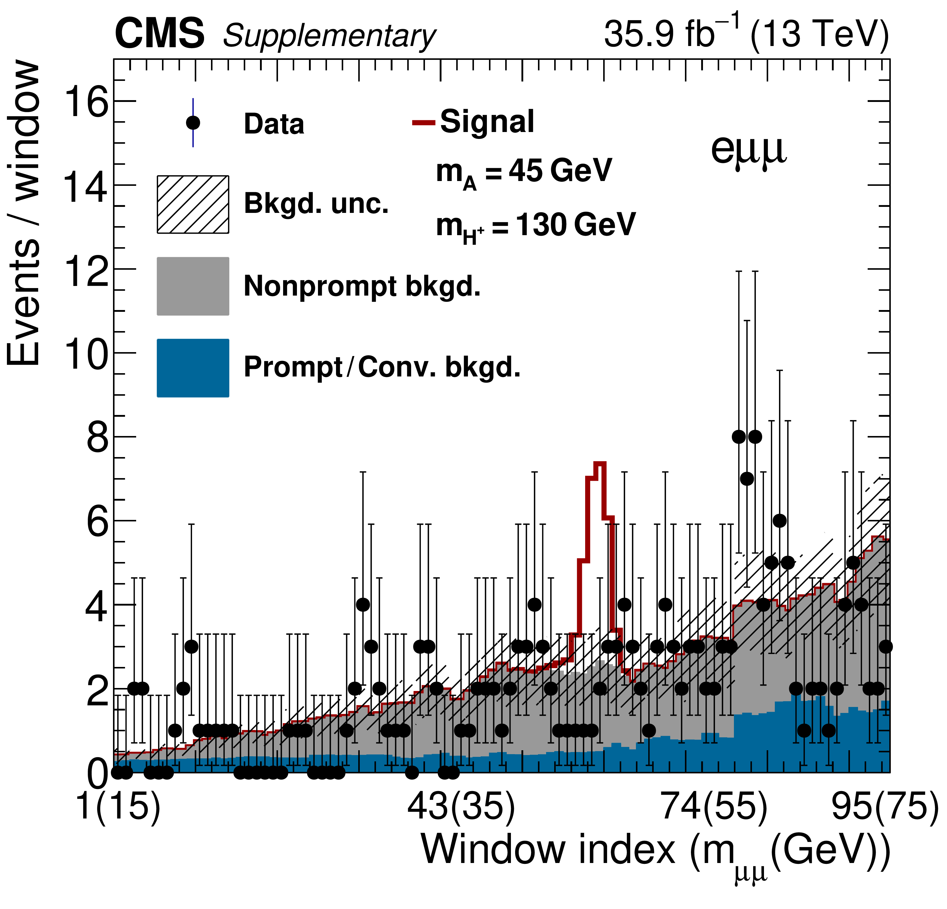
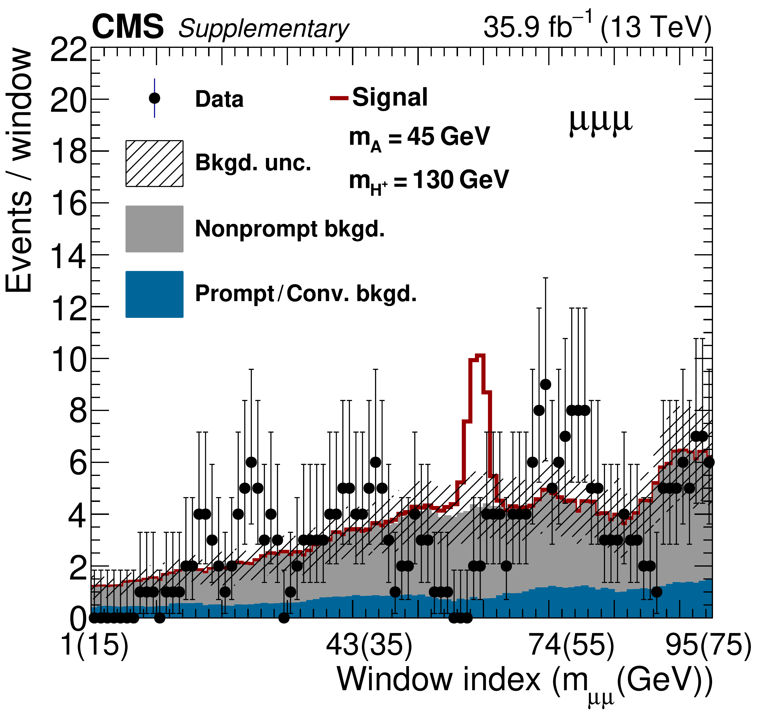
The $ {\mathit {m}_{{{\mu}} {{\mu}}}}$ distribution of candidate muon pairs from A bosons (left) and the event yields in each signal window (right) in the $ {{\mathrm {e}} {{\mu}} {{\mu}}}$ and $ {{{\mu}} {{\mu}} {{\mu}}}$ final states. A constant bin size (1 GeV) is used in the left figure except the last bin of $[80,\,81.2]$ (GeV). Values of $ {\mathit {m}_{{{\mu}} {{\mu}}}}$ at centers of the corresponding windows are written in the parentheses on the $x$ axis of the right figure. The expected signal distribution for $ {\mathit {m}_{{{\mathrm {H}} ^{+}}}}=$ 130 and $ {\mathit {m}_{{\mathrm {A}}}} = $ 45 GeV is also shown on top of the expected backgrounds assuming $ {\sigma ({{\mathrm {t}\overline {\mathrm {t}}}})}=$ 832 pb, $ {\mathcal {B}({{\mathrm {t}}\to {\mathrm {b}} {\mathrm {H}} ^{+}})}=$ 0.02, $ {\mathcal {B}({{\mathrm {H}} ^{+}\to {\mathrm {W^+}} {\mathrm {A}}})}=$ 1, and $ {\mathcal {B}({{\mathrm {A}} \to {{{\mu ^+}} {{\mu ^-}}}})}=3\times 10^{-4}$. |

png pdf |
Figure 2-a:
The $ {\mathit {m}_{{{\mu}} {{\mu}}}}$ distribution of candidate muon pairs from A bosons in the $ {{\mathrm {e}} {{\mu}} {{\mu}}}$ and $ {{{\mu}} {{\mu}} {{\mu}}}$ final states. A constant bin size (1 GeV) is used except the last bin of $[80,\,81.2]$ (GeV). The expected signal distribution for $ {\mathit {m}_{{{\mathrm {H}} ^{+}}}}=$ 130 and $ {\mathit {m}_{{\mathrm {A}}}} = $ 45 GeV is also shown on top of the expected backgrounds assuming $ {\sigma ({{\mathrm {t}\overline {\mathrm {t}}}})}=$ 832 pb, $ {\mathcal {B}({{\mathrm {t}}\to {\mathrm {b}} {\mathrm {H}} ^{+}})}=$ 0.02, $ {\mathcal {B}({{\mathrm {H}} ^{+}\to {\mathrm {W^+}} {\mathrm {A}}})}=$ 1, and $ {\mathcal {B}({{\mathrm {A}} \to {{{\mu ^+}} {{\mu ^-}}}})}=3\times 10^{-4}$. |
png pdf |
Figure 2-b:
The event yields in each signal window in the $ {{\mathrm {e}} {{\mu}} {{\mu}}}$ and $ {{{\mu}} {{\mu}} {{\mu}}}$ final states. Values of $ {\mathit {m}_{{{\mu}} {{\mu}}}}$ at centers of the corresponding windows are written in the parentheses on the $x$ axis of the figure. The expected signal distribution for $ {\mathit {m}_{{{\mathrm {H}} ^{+}}}}=$ 130 and $ {\mathit {m}_{{\mathrm {A}}}} = $ 45 GeV is also shown on top of the expected backgrounds assuming $ {\sigma ({{\mathrm {t}\overline {\mathrm {t}}}})}=$ 832 pb, $ {\mathcal {B}({{\mathrm {t}}\to {\mathrm {b}} {\mathrm {H}} ^{+}})}=$ 0.02, $ {\mathcal {B}({{\mathrm {H}} ^{+}\to {\mathrm {W^+}} {\mathrm {A}}})}=$ 1, and $ {\mathcal {B}({{\mathrm {A}} \to {{{\mu ^+}} {{\mu ^-}}}})}=3\times 10^{-4}$. |

png pdf |
Figure 3:
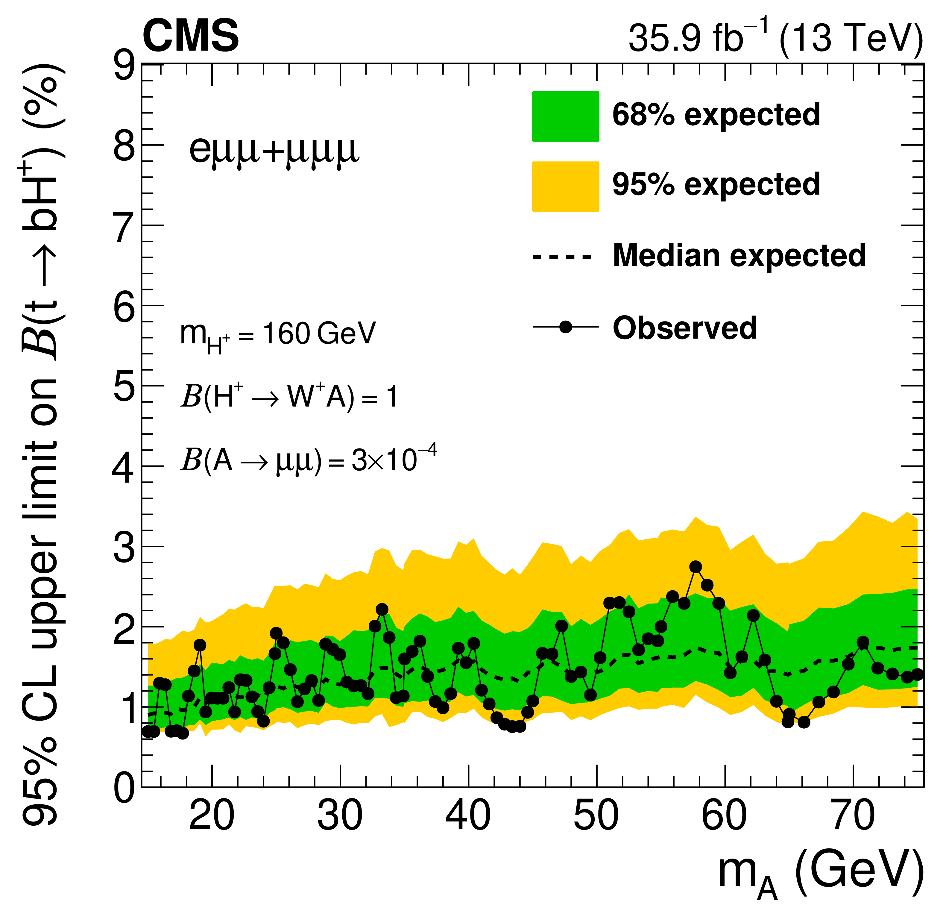
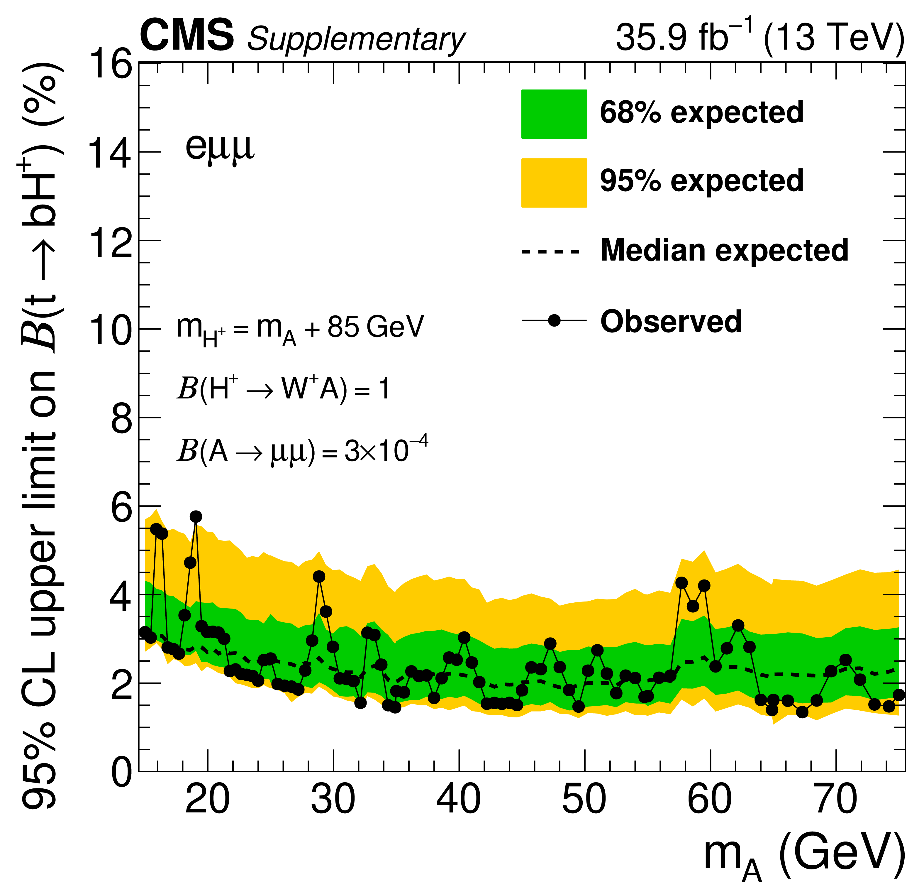
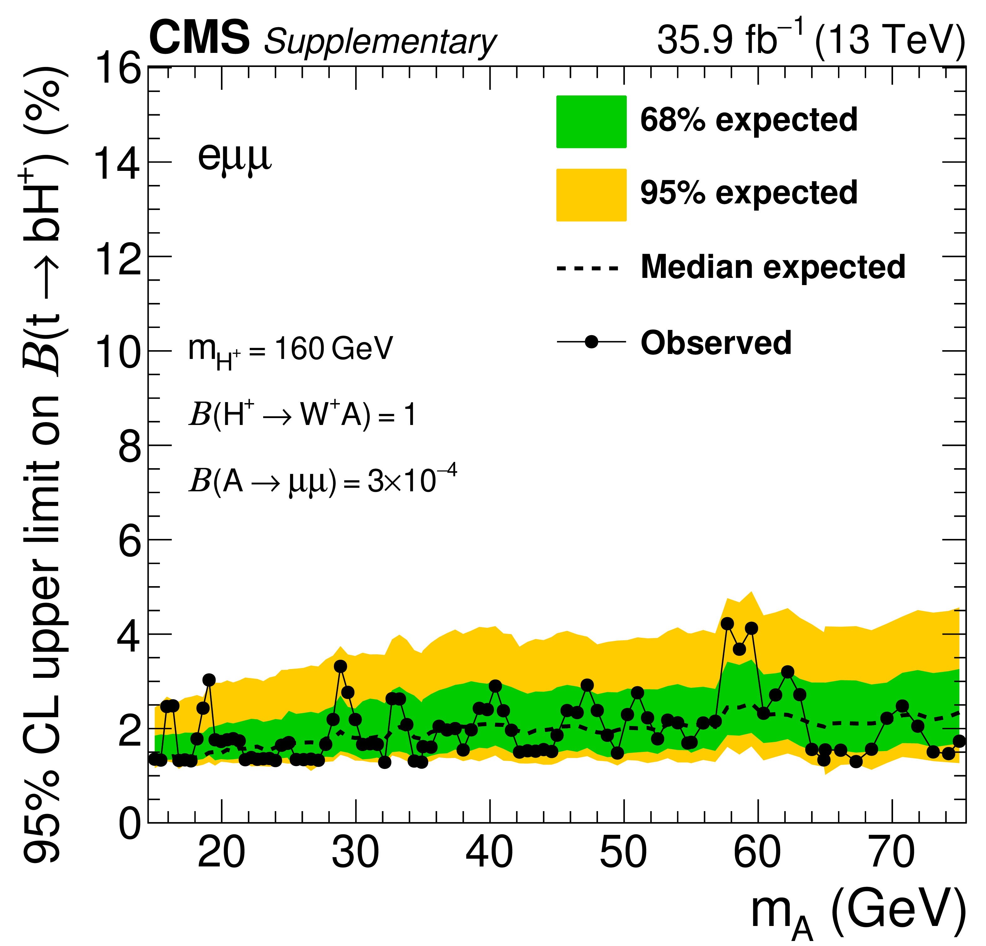
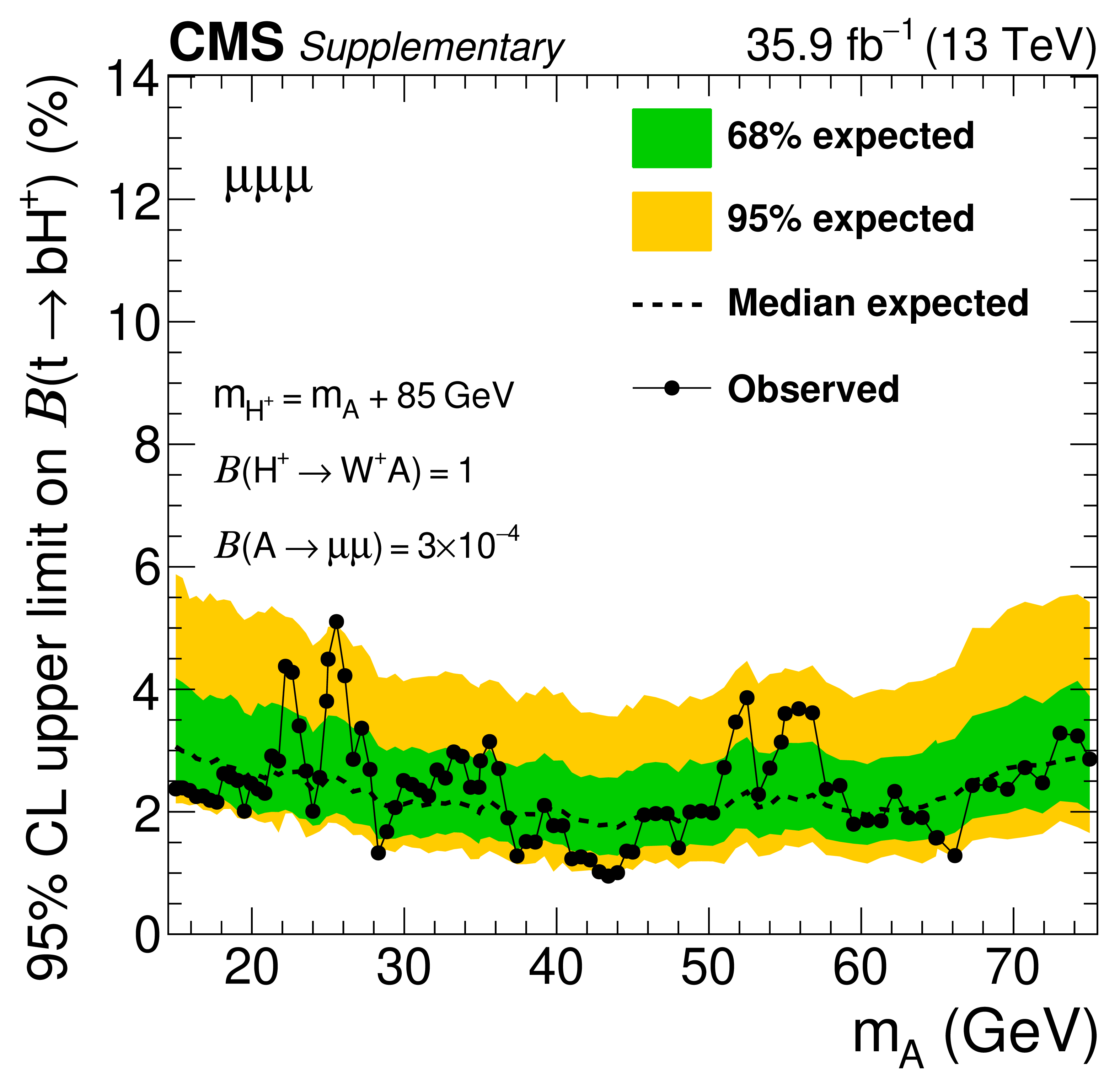
Expected and observed upper limits at 95% CL on $ {\mathcal {B}({{\mathrm {t}}\to {\mathrm {b}} {\mathrm {H}} ^{+}})}$ for the $ {\mathit {m}_{{\mathrm {A}}}}$ values defined in Table 1, with an assumption of $ {\mathit {m}_{{{\mathrm {H}} ^{+}}}}= {\mathit {m}_{{\mathrm {A}}}}+85 GeV $ (left) or $ {\mathit {m}_{{{\mathrm {H}} ^{+}}}} = $ 160 GeV (right). The same values of $ {\mathcal {B}({{\mathrm {H}} ^{+}\to {\mathrm {W^+}} {\mathrm {A}}})}$, $ {\mathcal {B}({{\mathrm {A}} \to {{{\mu ^+}} {{\mu ^-}}}})}$, and $ {\sigma ({{\mathrm {t}\overline {\mathrm {t}}}})}$ as in Fig. 2 are assumed. The green (yellow) bands indicate the regions containing 68 (95)% of the limit values expected under the background-only hypothesis. |

png pdf |
Figure 3-a:
Expected and observed upper limits at 95% CL on $ {\mathcal {B}({{\mathrm {t}}\to {\mathrm {b}} {\mathrm {H}} ^{+}})}$ for the $ {\mathit {m}_{{\mathrm {A}}}}$ values defined in Table 1, with an assumption of $ {\mathit {m}_{{{\mathrm {H}} ^{+}}}}= {\mathit {m}_{{\mathrm {A}}}}+85 GeV $. The same values of $ {\mathcal {B}({{\mathrm {H}} ^{+}\to {\mathrm {W^+}} {\mathrm {A}}})}$, $ {\mathcal {B}({{\mathrm {A}} \to {{{\mu ^+}} {{\mu ^-}}}})}$, and $ {\sigma ({{\mathrm {t}\overline {\mathrm {t}}}})}$ as in Fig. 2 are assumed. The green (yellow) bands indicate the regions containing 68 (95)% of the limit values expected under the background-only hypothesis. |
png pdf |
Figure 3-b:
Expected and observed upper limits at 95% CL on $ {\mathcal {B}({{\mathrm {t}}\to {\mathrm {b}} {\mathrm {H}} ^{+}})}$ for the $ {\mathit {m}_{{\mathrm {A}}}}$ values defined in Table 1, with an assumption of $ {\mathit {m}_{{{\mathrm {H}} ^{+}}}} = $ 160 GeV. The same values of $ {\mathcal {B}({{\mathrm {H}} ^{+}\to {\mathrm {W^+}} {\mathrm {A}}})}$, $ {\mathcal {B}({{\mathrm {A}} \to {{{\mu ^+}} {{\mu ^-}}}})}$, and $ {\sigma ({{\mathrm {t}\overline {\mathrm {t}}}})}$ as in Fig. 2 are assumed. The green (yellow) bands indicate the regions containing 68 (95)% of the limit values expected under the background-only hypothesis. |
png pdf |
Figure A1:
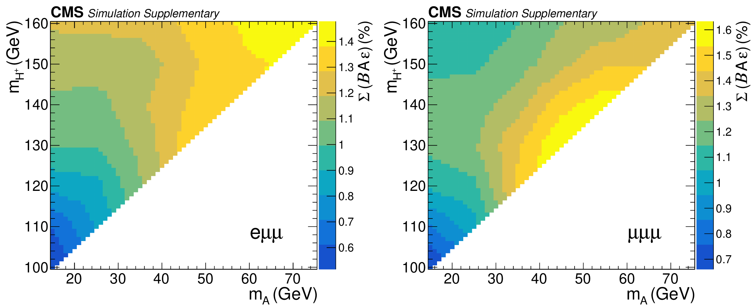
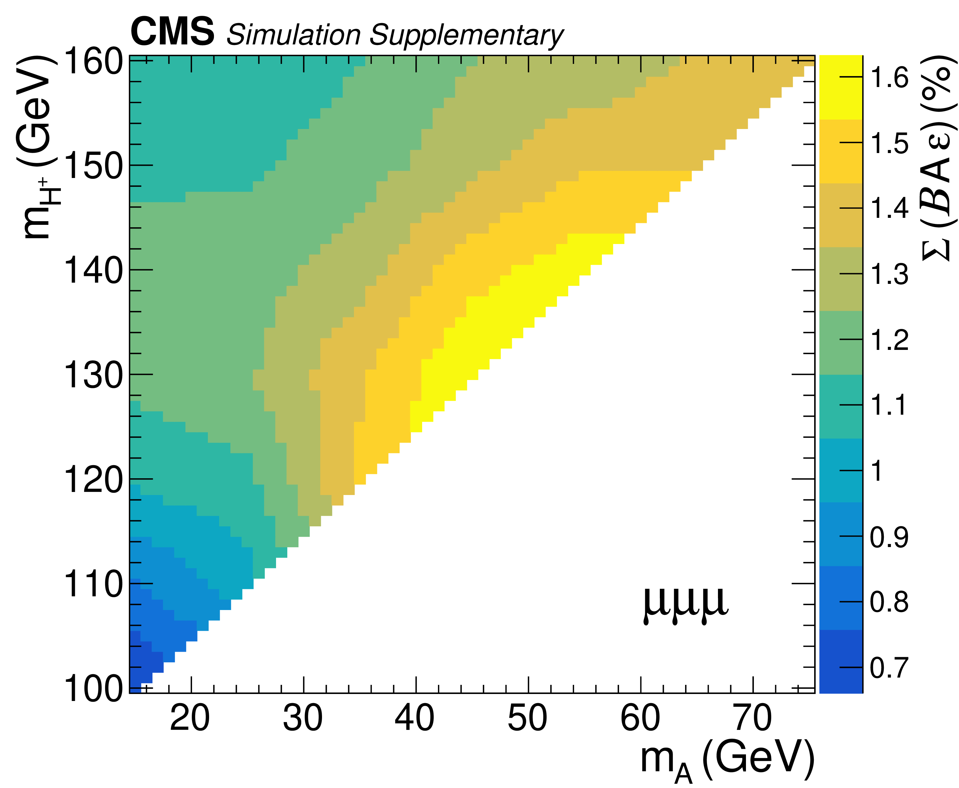
The fraction of signal events passing the final event selection in the $ {{\mathrm {e}} {{\mu}} {{\mu}}}$ (left) and $ {{{\mu}} {{\mu}} {{\mu}}}$ (right) final states. The fraction is relative to the yield before the decays of the two W bosons in the signal processes ($ {{\mathrm {t}\overline {\mathrm {t}}}} \to {{\mathrm {b}} {\overline {\mathrm {b}}}} {\mathrm {W^+}} {\mathrm {W^-}} {{{\mu ^+}} {{\mu ^-}}} $), which include the branching fraction of each decay mode of the two W bosons ($\mathcal {B}$) and the acceptance (A) times efficiency ($\varepsilon $) of the event selection for the decay mode. All decay modes of the two W bosons are considered in the calculation except the cases where both of the bosons decay hadronically. |

png pdf |
Figure A1-a:
The fraction of signal events passing the final event selection in the $ {{\mathrm {e}} {{\mu}} {{\mu}}}$ final state. The fraction is relative to the yield before the decays of the two W bosons in the signal processes ($ {{\mathrm {t}\overline {\mathrm {t}}}} \to {{\mathrm {b}} {\overline {\mathrm {b}}}} {\mathrm {W^+}} {\mathrm {W^-}} {{{\mu ^+}} {{\mu ^-}}} $), which include the branching fraction of each decay mode of the two W bosons ($\mathcal {B}$) and the acceptance (A) times efficiency ($\varepsilon $) of the event selection for the decay mode. All decay modes of the two W bosons are considered in the calculation except the cases where both of the bosons decay hadronically. |
png pdf |
Figure A1-b:
The fraction of signal events passing the final event selection in the $ {{{\mu}} {{\mu}} {{\mu}}}$ final state. The fraction is relative to the yield before the decays of the two W bosons in the signal processes ($ {{\mathrm {t}\overline {\mathrm {t}}}} \to {{\mathrm {b}} {\overline {\mathrm {b}}}} {\mathrm {W^+}} {\mathrm {W^-}} {{{\mu ^+}} {{\mu ^-}}} $), which include the branching fraction of each decay mode of the two W bosons ($\mathcal {B}$) and the acceptance (A) times efficiency ($\varepsilon $) of the event selection for the decay mode. All decay modes of the two W bosons are considered in the calculation except the cases where both of the bosons decay hadronically. |

png pdf |
Figure A2:
The $ {\mathit {m}_{{{\mu}} {{\mu}}}}$ distribution of candidate muon pairs from A bosons (left) and the event yields in each signal window (right) in the $ {{\mathrm {e}} {{\mu}} {{\mu}}}$ (upper) and $ {{{\mu}} {{\mu}} {{\mu}}}$ (lower) final states. A constant bin size (1 GeV) is used in the left figures except the last bin of $[80,\,81.2]$ (GeV). Values of $ {\mathit {m}_{{{\mu}} {{\mu}}}}$ at centers of the corresponding windows are written in the parentheses on the $x$ axis of the right figures. The expected signal distribution for $ {\mathit {m}_{{{\mathrm {H}} ^{+}}}}=$ 130 and $ {\mathit {m}_{{\mathrm {A}}}} = $ 45 GeV is also shown on top of the expected backgrounds assuming $ {\sigma ({{\mathrm {t}\overline {\mathrm {t}}}})}=$ 832 pb, $ {\mathcal {B}({{\mathrm {t}}\to {\mathrm {b}} {\mathrm {H}} ^{+}})}=$ 0.02, $ {\mathcal {B}({{\mathrm {H}} ^{+}\to {\mathrm {W^+}} {\mathrm {A}}})}=$ 1, and $ {\mathcal {B}({{\mathrm {A}} \to {{{\mu ^+}} {{\mu ^-}}}})}=3\times 10^{-4}$. |

png pdf |
Figure A2-a:
The $ {\mathit {m}_{{{\mu}} {{\mu}}}}$ distribution of candidate muon pairs from A bosons in the $ {{\mathrm {e}} {{\mu}} {{\mu}}}$ final state. A constant bin size (1 GeV) is used except the last bin of $[80,\,81.2]$ (GeV). The expected signal distribution for $ {\mathit {m}_{{{\mathrm {H}} ^{+}}}}=$ 130 and $ {\mathit {m}_{{\mathrm {A}}}} = $ 45 GeV is also shown on top of the expected backgrounds assuming $ {\sigma ({{\mathrm {t}\overline {\mathrm {t}}}})}=$ 832 pb, $ {\mathcal {B}({{\mathrm {t}}\to {\mathrm {b}} {\mathrm {H}} ^{+}})}=$ 0.02, $ {\mathcal {B}({{\mathrm {H}} ^{+}\to {\mathrm {W^+}} {\mathrm {A}}})}=$ 1, and $ {\mathcal {B}({{\mathrm {A}} \to {{{\mu ^+}} {{\mu ^-}}}})}=3\times 10^{-4}$. |
png pdf |
Figure A2-b:
The $ {\mathit {m}_{{{\mu}} {{\mu}}}}$ distribution of candidate muon pairs from A bosons in the $ {{{\mu}} {{\mu}} {{\mu}}}$ final state. A constant bin size (1 GeV) is used except the last bin of $[80,\,81.2]$ (GeV). The expected signal distribution for $ {\mathit {m}_{{{\mathrm {H}} ^{+}}}}=$ 130 and $ {\mathit {m}_{{\mathrm {A}}}} = $ 45 GeV is also shown on top of the expected backgrounds assuming $ {\sigma ({{\mathrm {t}\overline {\mathrm {t}}}})}=$ 832 pb, $ {\mathcal {B}({{\mathrm {t}}\to {\mathrm {b}} {\mathrm {H}} ^{+}})}=$ 0.02, $ {\mathcal {B}({{\mathrm {H}} ^{+}\to {\mathrm {W^+}} {\mathrm {A}}})}=$ 1, and $ {\mathcal {B}({{\mathrm {A}} \to {{{\mu ^+}} {{\mu ^-}}}})}=3\times 10^{-4}$. |

png pdf |
Figure A2-c:
The event yields in each signal window in the $ {{\mathrm {e}} {{\mu}} {{\mu}}}$ final state. Values of $ {\mathit {m}_{{{\mu}} {{\mu}}}}$ at centers of the corresponding windows are written in the parentheses on the $x$ axis of the figures. The expected signal distribution for $ {\mathit {m}_{{{\mathrm {H}} ^{+}}}}=$ 130 and $ {\mathit {m}_{{\mathrm {A}}}} = $ 45 GeV is also shown on top of the expected backgrounds assuming $ {\sigma ({{\mathrm {t}\overline {\mathrm {t}}}})}=$ 832 pb, $ {\mathcal {B}({{\mathrm {t}}\to {\mathrm {b}} {\mathrm {H}} ^{+}})}=$ 0.02, $ {\mathcal {B}({{\mathrm {H}} ^{+}\to {\mathrm {W^+}} {\mathrm {A}}})}=$ 1, and $ {\mathcal {B}({{\mathrm {A}} \to {{{\mu ^+}} {{\mu ^-}}}})}=3\times 10^{-4}$. |
png pdf |
Figure A2-d:
The event yields in each signal window in the $ {{{\mu}} {{\mu}} {{\mu}}}$ final state. Values of $ {\mathit {m}_{{{\mu}} {{\mu}}}}$ at centers of the corresponding windows are written in the parentheses on the $x$ axis of the figures. The expected signal distribution for $ {\mathit {m}_{{{\mathrm {H}} ^{+}}}}=$ 130 and $ {\mathit {m}_{{\mathrm {A}}}} = $ 45 GeV is also shown on top of the expected backgrounds assuming $ {\sigma ({{\mathrm {t}\overline {\mathrm {t}}}})}=$ 832 pb, $ {\mathcal {B}({{\mathrm {t}}\to {\mathrm {b}} {\mathrm {H}} ^{+}})}=$ 0.02, $ {\mathcal {B}({{\mathrm {H}} ^{+}\to {\mathrm {W^+}} {\mathrm {A}}})}=$ 1, and $ {\mathcal {B}({{\mathrm {A}} \to {{{\mu ^+}} {{\mu ^-}}}})}=3\times 10^{-4}$. |

png pdf |
Figure A3:
Upper limits at 95% CL on $ {\mathcal {B}({{\mathrm {t}}\to {\mathrm {b}} {\mathrm {H}} ^{+}})}$ for the 95 $ {\mathit {m}_{{\mathrm {A}}}}$ values, with an assumption of $ {\mathit {m}_{{{\mathrm {H}} ^{+}}}}= {\mathit {m}_{{\mathrm {A}}}}$+85 GeV (left) or $ {\mathit {m}_{{{\mathrm {H}} ^{+}}}} = $ 160 GeV (right), for individual final states (upper: $ {{\mathrm {e}} {{\mu}} {{\mu}}}$ and lower: $ {{{\mu}} {{\mu}} {{\mu}}}$ final states). In the calculation, the same values of $ {\mathcal {B}({{\mathrm {H}} ^{+}\to {\mathrm {W^+}} {\mathrm {A}}})}$, $ {\mathcal {B}({{\mathrm {A}} \to {{{\mu ^+}} {{\mu ^-}}}})}$, and $ {\sigma ({{\mathrm {t}\overline {\mathrm {t}}}})}$ as in Fig. A2 are assumed. |
png pdf |
Figure A3-a:
Upper limits at 95% CL on $ {\mathcal {B}({{\mathrm {t}}\to {\mathrm {b}} {\mathrm {H}} ^{+}})}$ for the 95 $ {\mathit {m}_{{\mathrm {A}}}}$ values, with an assumption of $ {\mathit {m}_{{{\mathrm {H}} ^{+}}}}= {\mathit {m}_{{\mathrm {A}}}}$+85 GeV, for the $ {{\mathrm {e}} {{\mu}} {{\mu}}}$ final state. In the calculation, the same values of $ {\mathcal {B}({{\mathrm {H}} ^{+}\to {\mathrm {W^+}} {\mathrm {A}}})}$, $ {\mathcal {B}({{\mathrm {A}} \to {{{\mu ^+}} {{\mu ^-}}}})}$, and $ {\sigma ({{\mathrm {t}\overline {\mathrm {t}}}})}$ as in Fig. A2 are assumed. |
png pdf |
Figure A3-b:
Upper limits at 95% CL on $ {\mathcal {B}({{\mathrm {t}}\to {\mathrm {b}} {\mathrm {H}} ^{+}})}$ for the 95 $ {\mathit {m}_{{\mathrm {A}}}}$ values, with an assumption of $ {\mathit {m}_{{{\mathrm {H}} ^{+}}}} = $ 160 GeV, for the $ {{\mathrm {e}} {{\mu}} {{\mu}}}$ final state. In the calculation, the same values of $ {\mathcal {B}({{\mathrm {H}} ^{+}\to {\mathrm {W^+}} {\mathrm {A}}})}$, $ {\mathcal {B}({{\mathrm {A}} \to {{{\mu ^+}} {{\mu ^-}}}})}$, and $ {\sigma ({{\mathrm {t}\overline {\mathrm {t}}}})}$ as in Fig. A2 are assumed. |
png pdf |
Figure A3-c:
Upper limits at 95% CL on $ {\mathcal {B}({{\mathrm {t}}\to {\mathrm {b}} {\mathrm {H}} ^{+}})}$ for the 95 $ {\mathit {m}_{{\mathrm {A}}}}$ values, with an assumption of $ {\mathit {m}_{{{\mathrm {H}} ^{+}}}}= {\mathit {m}_{{\mathrm {A}}}}$+85 GeV, for the $ {{{\mu}} {{\mu}} {{\mu}}}$ final state. In the calculation, the same values of $ {\mathcal {B}({{\mathrm {H}} ^{+}\to {\mathrm {W^+}} {\mathrm {A}}})}$, $ {\mathcal {B}({{\mathrm {A}} \to {{{\mu ^+}} {{\mu ^-}}}})}$, and $ {\sigma ({{\mathrm {t}\overline {\mathrm {t}}}})}$ as in Fig. A2 are assumed. |

png pdf |
Figure A3-d:
Upper limits at 95% CL on $ {\mathcal {B}({{\mathrm {t}}\to {\mathrm {b}} {\mathrm {H}} ^{+}})}$ for the 95 $ {\mathit {m}_{{\mathrm {A}}}}$ values, with an assumption of $ {\mathit {m}_{{{\mathrm {H}} ^{+}}}} = $ 160 GeV, for the $ {{{\mu}} {{\mu}} {{\mu}}}$ final state. In the calculation, the same values of $ {\mathcal {B}({{\mathrm {H}} ^{+}\to {\mathrm {W^+}} {\mathrm {A}}})}$, $ {\mathcal {B}({{\mathrm {A}} \to {{{\mu ^+}} {{\mu ^-}}}})}$, and $ {\sigma ({{\mathrm {t}\overline {\mathrm {t}}}})}$ as in Fig. A2 are assumed. |
| Tables | |
png pdf |
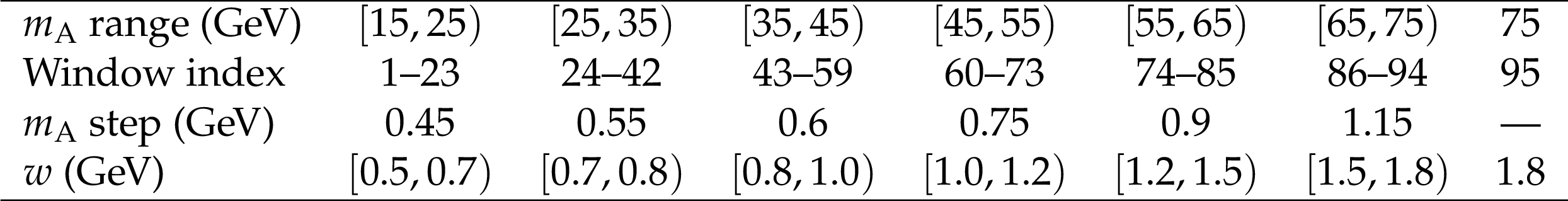
Table 1:
Summary of mass windows ($ {| {\mathit {m}_{{{\mu}} {{\mu}}}}- {\mathit {m}_{{\mathrm {A}}}} |} < w$) for each $ {\mathit {m}_{{\mathrm {A}}}}$ hypothesis. |
| Summary |
| In summary, a search is performed for a charged Higgs boson $\mathrm{H}^{+}$, produced in the decay of a top quark, and decaying further into a W boson and a CP-odd Higgs boson A, where the A boson decays to two muons. The analysis uses proton-proton collision data at $\sqrt{s}=$ 13 TeV, recorded by the CMS experiment, corresponding to an integrated luminosity of 35.9 fb$^{-1}$. A resonant signature in the dimuon mass spectrum is searched in trilepton events for the ranges of $m_{\mathrm{A}}$ between 15 and 75 GeV and $m_{\mathrm{H}^{+}}$ between ($m_{\mathrm{A}}$+85 GeV) and 160 GeV. No statistically significant excess is found. Assuming branching fractions ${\mathcal{B}({\mathrm{H}^{+}\to\mathrm{W^{+}}\mathrm{A} })}=$ 1 and ${\mathcal{B}({\mathrm{A} }\to\mu^{+}\mu^{-})}=3\times10^{-4}$, upper limits at 95% confidence level on the branching fraction of the top quark, ${\mathcal{B}({\mathrm{t}\to\mathrm{b}\mathrm{H}^{+}})}$, of 0.63 to 2.9% are obtained, depending on the masses of of the $\mathrm{H}^{+}$ and A bosons. The reported analysis constitutes the first search for the ${\mathrm{H}^{+}\to\mathrm{W^{+}}\mathrm{A} } $ process in the $\mathrm{A}\to\mu^{+}\mu^{-}$ decay channel. |
| References | ||||
| 1 | ATLAS Collaboration | Observation of a new particle in the search for the Standard Model Higgs boson with the ATLAS detector at the LHC | PLB 716 (2012) 1 | 1207.7214 |
| 2 | CMS Collaboration | Observation of a new boson at a mass of 125 GeV with the CMS experiment at the LHC | PLB 716 (2012) 30 | CMS-HIG-12-028 1207.7235 |
| 3 | CMS Collaboration | Observation of a new boson with mass near 125 GeV in pp collisions at $ \sqrt{s}= $ 7 and 8 TeV | JHEP 06 (2013) 081 | CMS-HIG-12-036 1303.4571 |
| 4 | ATLAS and CMS Collaborations | Measurements of the Higgs boson production and decay rates and constraints on its couplings from a combined ATLAS and CMS analysis of the LHC pp collision data at $ \sqrt{s}= $ 7 and 8 TeV | JHEP 08 (2016) 045 | 1606.02266 |
| 5 | CMS Collaboration | Combined measurements of Higgs boson couplings in proton-proton collisions at $ \sqrt{s}= $ 13 TeV | Submitted to: EPJC | CMS-HIG-17-031 1809.10733 |
| 6 | H. E. Haber and G. L. Kane | The search for supersymmetry: Probing physics beyond the standard model | Phys. Rep. 117 (1985) 75 | |
| 7 | N. Turok and J. Zadrozny | Dynamical generation of baryons at the electroweak transition | PRL 65 (1990) 2331 | |
| 8 | G. B. Gelmini and M. Roncadelli | Left-handed neutrino mass scale and spontaneously broken lepton number | PLB 99 (1981) 411 | |
| 9 | T. D. Lee | A theory of spontaneous T violation | PRD 8 (1973) 1226 | |
| 10 | G. C. Branco et al. | Theory and phenomenology of two-Higgs-doublet models | Phys. Rep. 516 (2012) 1 | 1106.0034 |
| 11 | R. Dermisek, E. Lunghi, and A. Raval | Trilepton signatures of light charged and CP-odd Higgs bosons in top quark decays | JHEP 04 (2013) 063 | 1212.5021 |
| 12 | F. Kling, A. Pyarelal, and S. Su | Light charged Higgs bosons to AW/HW via top decay | JHEP 11 (2015) 051 | 1504.06624 |
| 13 | A. Arhrib, R. Benbrik, and S. Moretti | Bosonic decays of charged Higgs bosons in a 2HDM type-I | EPJC 77 (2017) 621 | 1607.02402 |
| 14 | CDF Collaboration | Search for charged Higgs bosons from top quark decays in $ p\bar{p} $ collisions at $ \sqrt{s}= $ 1.96 TeV | PRL 96 (2006) 042003 | hep-ex/0510065 |
| 15 | CDF Collaboration | Search for a very light CP-odd Higgs boson in top quark decays from $ p\bar{p} $ collisions at $ \sqrt{s}= $ 1.96 TeV | PRL 107 (2011) 031801 | 1104.5701 |
| 16 | DELPHI Collaboration | Search for charged Higgs bosons at LEP in general two Higgs doublet models | EPJC 34 (2004) 399 | hep-ex/0404012 |
| 17 | OPAL Collaboration | Search for charged Higgs bosons in $ e^{+}e^{-} $ collisions at $ \sqrt{s}= $ 189--209 GeV | EPJC 72 (2012) 2076 | 0812.0267 |
| 18 | ALEPH, DELPHI, L3, and OPAL Collaborations, and the LEP working group for Higgs boson searches | Search for charged Higgs bosons: combined results using LEP data | EPJC 73 (2013) 2463 | 1301.6065 |
| 19 | CMS Collaboration | Particle-flow reconstruction and global event description with the CMS detector | JINST 12 (2017) P10003 | CMS-PRF-14-001 1706.04965 |
| 20 | CMS Collaboration | Performance of the CMS muon detector and muon reconstruction with proton-proton collisions at $ \sqrt{s}= $ 13 TeV | JINST 13 (2018) P06015 | CMS-MUO-16-001 1804.04528 |
| 21 | M. Cacciari and G. P. Salam | Pileup subtraction using jet areas | PLB 659 (2008) 119 | 0707.1378 |
| 22 | M. Aoki, S. Kanemura, K. Tsumura, and K. Yagyu | Models of Yukawa interaction in the two Higgs doublet model, and their collider phenomenology | PRD 80 (2009) 015017 | 0902.4665 |
| 23 | CMS Collaboration | The CMS experiment at the CERN LHC | JINST 3 (2008) S08004 | CMS-00-001 |
| 24 | CMS Collaboration | Technical proposal for the Phase-II upgrade of the Compact Muon Solenoid | CMS-PAS-TDR-15-002 | CMS-PAS-TDR-15-002 |
| 25 | M. Cacciari, G. P. Salam, and G. Soyez | The anti-$ {k_{\mathrm{T}}} $ jet clustering algorithm | JHEP 04 (2008) 063 | 0802.1189 |
| 26 | M. Cacciari, G. P. Salam, and G. Soyez | Fastjet user manual | EPJC 72 (2012) 1896 | 1111.6097 |
| 27 | CMS Collaboration | Performance of electron reconstruction and selection with the CMS detector in proton-proton collisions at $ \sqrt{s} = $ 8 TeV | JINST 10 (2015) P06005 | CMS-EGM-13-001 1502.02701 |
| 28 | CMS Collaboration | Identification of heavy-flavour jets with the CMS detector in pp collisions at 13 TeV | JINST 13 (2018) P05011 | CMS-BTV-16-002 1712.07158 |
| 29 | CMS Collaboration | The CMS trigger system | JINST 12 (2017) P01020 | CMS-TRG-12-001 1609.02366 |
| 30 | J. Alwall et al. | The automated computation of tree-level and next-to-leading order differential cross sections, and their matching to parton shower simulations | JHEP 07 (2014) 079 | 1405.0301 |
| 31 | CMS Collaboration | Measurement of the $ \mathrm{t\bar{t}} $ production cross section in the dilepton channel in pp collisions at $ \sqrt{s}= $ 8 TeV | JHEP 02 (2014) 024 | CMS-TOP-12-007 1312.7582 |
| 32 | CMS Collaboration | Measurement of the $ \mathrm{t\bar{t}} $ production cross section in the all-jets final state in pp collisions at $ \sqrt{s}= $ 8 TeV | EPJC 76 (2016) 128 | CMS-TOP-14-018 1509.06076 |
| 33 | CMS Collaboration | Measurements of the $ \mathrm{t\bar{t}} $ production cross section in lepton+jets final states in pp collisions at 8 TeV and ratio of 8 to 7 TeV cross sections | EPJC 77 (2017) 15 | CMS-TOP-12-006 1602.09024 |
| 34 | Particle Data Group | Review of particle physics | PRD 98 (2018) 030001 | |
| 35 | P. Nason | A new method for combining NLO QCD with shower Monte Carlo algorithms | JHEP 11 (2004) 040 | hep-ph/0409146 |
| 36 | S. Frixione, P. Nason, and C. Oleari | Matching NLO QCD computations with parton shower simulations: the POWHEG method | JHEP 11 (2007) 070 | 0709.2092 |
| 37 | S. Alioli, P. Nason, C. Oleari, and E. Re | NLO Higgs boson production via gluon fusion matched with shower in POWHEG | JHEP 04 (2009) 002 | 0812.0578 |
| 38 | P. Nason and C. Oleari | NLO Higgs boson production via vector-boson fusion matched with shower in POWHEG | JHEP 02 (2010) 037 | 0911.5299 |
| 39 | S. Alioli, P. Nason, C. Oleari, and E. Re | A general framework for implementing NLO calculations in shower Monte Carlo programs: the POWHEG BOX | JHEP 06 (2010) 043 | 1002.2581 |
| 40 | P. Nason and G. Zanderighi | $ \mathrm{{W}^{+}{W}^{-}} $, WZ and ZZ production in the POWHEG-BOX-V2 | EPJC 74 (2014) 2702 | 1311.1365 |
| 41 | H. B. Hartanto, B. Jager, L. Reina, and D. Wackeroth | Higgs boson production in association with top quarks in the POWHEG BOX | PRD 91 (2015) 094003 | 1501.04498 |
| 42 | J. Alwall et al. | Comparative study of various algorithms for the merging of parton showers and matrix elements in hadronic collisions | EPJC 53 (2008) 473 | 0706.2569 |
| 43 | R. Frederix and S. Frixione | Merging meets matching in MC@NLO | JHEP 12 (2012) 061 | 1209.6215 |
| 44 | F. Cascioli et al. | ZZ production at hadron colliders in NNLO QCD | PLB 735 (2014) 311 | 1405.2219 |
| 45 | M. Grazzini, S. Kallweit, D. Rathlev, and M. Wiesemann | $ \mathrm{W^{\pm}Z} $ production at hadron colliders in NNLO QCD | PLB 761 (2016) 179 | 1604.08576 |
| 46 | LHC Higgs Cross Section Working Group | Handbook of LHC Higgs cross sections: 4. deciphering the nature of the Higgs sector | CERN-2017-002-M | 1610.07922 |
| 47 | CMS Collaboration | Search for evidence of the type-III seesaw mechanism in multilepton final states in proton-proton collisions at $ \sqrt{s}= $ 13 TeV | PRL 119 (2017) 221802 | CMS-EXO-17-006 1708.07962 |
| 48 | NNPDF Collaboration | Parton distributions for the LHC Run II | JHEP 04 (2015) 040 | 1410.8849 |
| 49 | T. Sjöstrand et al. | An introduction to PYTHIA 8.2 | CPC 191 (2015) 159 | 1410.3012 |
| 50 | CMS Collaboration | Event generator tunes obtained from underlying event and multiparton scattering measurements | EPJC 76 (2016) 155 | CMS-GEN-14-001 1512.00815 |
| 51 | GEANT4 Collaboration | GEANT4--a simulation toolkit | NIMA 506 (2003) 250 | |
| 52 | CMS Collaboration | Search for new physics in same-sign dilepton events in proton-proton collisions at $ \sqrt{s}= $ 13 TeV | EPJC 76 (2016) 439 | CMS-SUS-15-008 1605.03171 |
| 53 | G. Cowan, K. Cranmer, E. Gross, and O. Vitells | Asymptotic formulae for likelihood-based tests of new physics | EPJC 71 (2011) 1554 | 1007.1727 |
| 54 | T. Junk | Confidence level computation for combining searches with small statistics | NIMA 434 (1999) 435 | hep-ex/9902006 |
| 55 | A. L. Read | Presentation of search results: the CL$ _{\text{s}} $ technique | JPG 28 (2002) 2693 | |
| 56 | ATLAS and CMS Collaborations and LHC Higgs Combination Group | Procedure for the LHC Higgs boson search combination in summer 2011 | CMS-NOTE-2011-005 | |
| 57 | M. Czakon and A. Mitov | Top++: a program for the calculation of the top-pair cross-section at hadron colliders | CPC 185 (2014) 2930 | 1112.5675 |
| 58 | CMS Collaboration | Jet energy scale and resolution in the CMS experiment in pp collisions at 8 TeV | JINST 12 (2017) P02014 | CMS-JME-13-004 1607.03663 |
| 59 | CMS Collaboration | Performance of missing energy reconstruction in 13 TeV pp collision data using the CMS detector | CMS-PAS-JME-16-004 | CMS-PAS-JME-16-004 |
| 60 | CMS Collaboration | CMS luminosity measurements for the 2016 data-taking period | CMS-PAS-LUM-17-001 | CMS-PAS-LUM-17-001 |
| 61 | J. Butterworth et al. | PDF4LHC recommendations for LHC Run II | JPG 43 (2016) 023001 | 1510.03865 |
|
|
Compact Muon Solenoid LHC, CERN |
|

|

|

|

|

|