Compact Muon Solenoid
LHC, CERN

Visit us: CMS Public Website, CMS Physics ; Contact us: CMS Publications Committee

CMS-SUS-17-010 ; CERN-EP-2018-186

Searches for pair production of charginos and top squarks in final states with two oppositely charged leptons in proton-proton collisions at $\sqrt{s} = $ 13 TeV

CMS Collaboration

20 July 2018

JHEP 11 (2018) 079

Abstract: A search for pair production of supersymmetric particles in events with two oppositely charged leptons (electrons or muons) and missing transverse momentum is reported. The data sample corresponds to an integrated luminosity of 35.9 fb$^{-1}$ of proton-proton collisions at $\sqrt{s} = $ 13 TeV collected with the CMS detector during the 2016 data taking period at the LHC. No significant deviation is observed from the predicted standard model background. The results are interpreted in terms of several simplified models for chargino and top squark pair production, assuming $R$-parity conservation and with the neutralino as the lightest supersymmetric particle. When the chargino is assumed to undergo a cascade decay through sleptons, with a slepton mass equal to the average of the chargino and neutralino masses, exclusion limits at 95% confidence level are set on the masses of the chargino and neutralino up to 800 and 320 GeV, respectively. For the top squark pair production, the search focuses on models with a small mass difference between the top squark and the lightest neutralino. When the top squark decays into an off-shell top quark and a neutralino, the limits extend up to 420 and 360 GeV for the top squark and neutralino masses, respectively.

Links: e-print arXiv:1807.07799 [hep-ex] (PDF) ; CDS record ; inSPIRE record ; CADI line (restricted) ;

Additional information on efficiencies needed for reinterpretation of these results are available here. Additional technical material for CMS speakers can be found here.

Figures
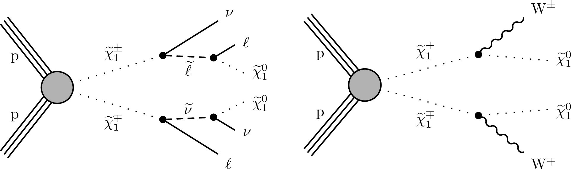
png pdf	Figure 1: Simplified-models diagrams of the chargino pair production with two benchmark decay modes: the left plot shows decays through intermediate sleptons or sneutrinos, while the right one displays prompt decays into a W boson and the lightest neutralino.
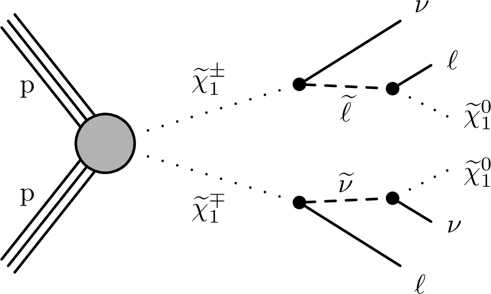
png pdf	Figure 1-a: Simplified-model diagram of the chargino pair production with decays through intermediate sleptons or sneutrinos.
png pdf	Figure 1-b: Simplified-model diagram of the chargino pair production with prompt decays into a W boson and the lightest neutralino.
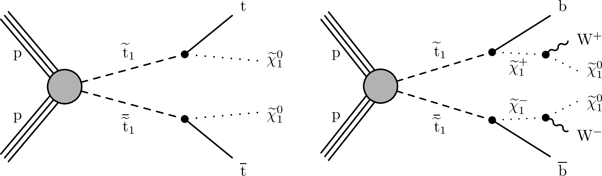
png pdf	Figure 2: Simplified-models diagrams of the top squark pair production with two benchmark decay modes of the top squark: the left plot shows decays into a top quark and the lightest neutralino, while the right one displays prompt decays into a bottom quark and a chargino, further decaying into a neutralino and a W boson.
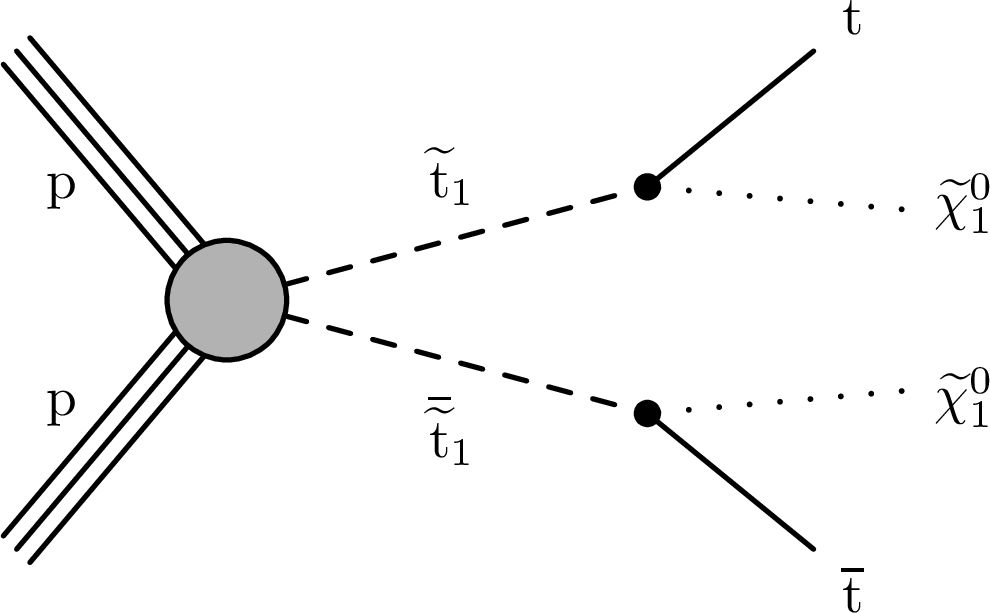
png pdf	Figure 2-a: Simplified-model diagram of the top squark pair production with top squark decays into a top quark and the lightest neutralino.
png pdf	Figure 2-b: Simplified-model diagram of the top squark pair production with top squark prompt decays into a bottom quark and a chargino, further decaying into a neutralino and a W boson.
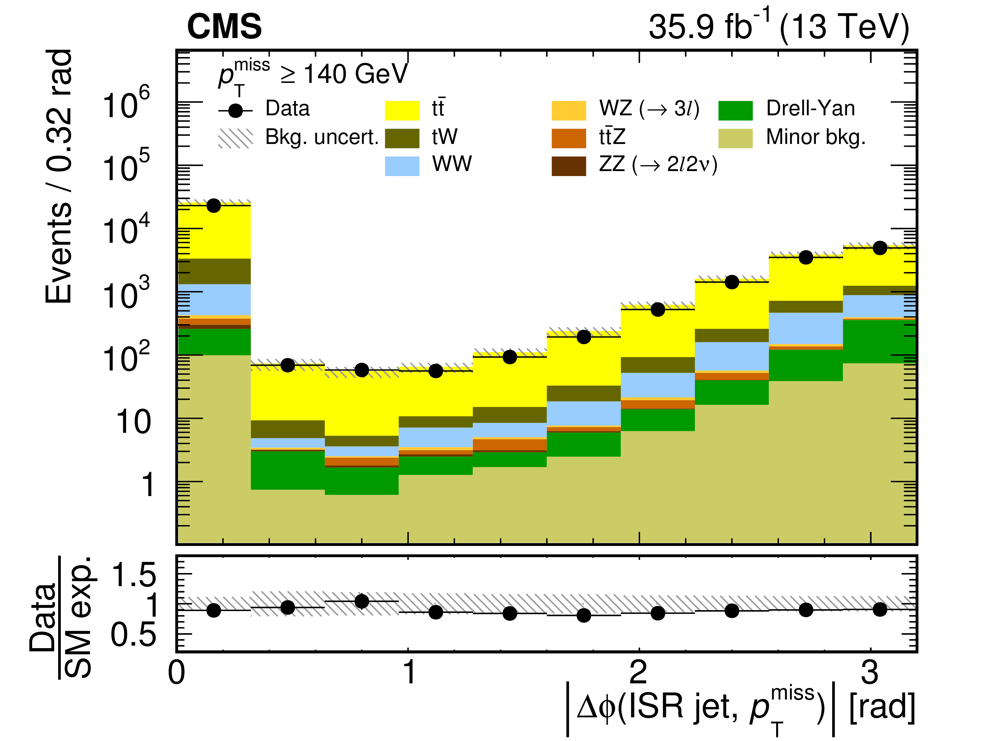
png pdf	Figure 3: Observed and SM expected distributions of some observables used to define the SRs for events with two OC isolated leptons and $ {{p_{\mathrm {T}}} ^\text {miss}} \geq $ 140 GeV. Clockwise from top left: ${{p_{\mathrm {T}}} ^\text {miss}}$, ${{m_\mathrm {T2}} (\ell \ell)}$, ${\Delta \phi}$ between the ${\vec{p}}_{\mathrm {T}}^{\,\text {miss}} $ and the leading jet (required not to be b-tagged and with $ {p_{\mathrm {T}}} > $ 150 GeV, events missing this requirements are shown in the first bin), and multiplicity of b-tagged jets in the event. The last bin includes the overflow entries. In the bottom panel, the ratio of observed and expected yields is shown. The hatched band represents the total uncertainty in the background expectation, as described in Section 7.
png pdf	Figure 3-a: Observed and SM expected distributions of ${{p_{\mathrm {T}}} ^\text {miss}}$, one of the observables used to define the SRs for events with two OC isolated leptons and $ {{p_{\mathrm {T}}} ^\text {miss}} \geq $ 140 GeV. The last bin includes the overflow entries. In the bottom panel, the ratio of observed and expected yields is shown. The hatched band represents the total uncertainty in the background expectation, as described in Section 7.
png pdf	Figure 3-b: Observed and SM expected distributions of ${{m_\mathrm {T2}} (\ell \ell)}$, one of the observables used to define the SRs for events with two OC isolated leptons and $ {{p_{\mathrm {T}}} ^\text {miss}} \geq $ 140 GeV. The last bin includes the overflow entries. In the bottom panel, the ratio of observed and expected yields is shown. The hatched band represents the total uncertainty in the background expectation, as described in Section 7.
png pdf	Figure 3-c: Observed and SM expected distributions of the multiplicity of b-tagged jets in the event, one of the observables used to define the SRs for events with two OC isolated leptons and $ {{p_{\mathrm {T}}} ^\text {miss}} \geq $ 140 GeV. The last bin includes the overflow entries. In the bottom panel, the ratio of observed and expected yields is shown. The hatched band represents the total uncertainty in the background expectation, as described in Section 7.
png pdf	Figure 3-d: Observed and SM expected distributions of ${\Delta \phi}$ between the ${\vec{p}}_{\mathrm {T}}^{\,\text {miss}} $ and the leading jet (required not to be b-tagged and with $ {p_{\mathrm {T}}} > $ 150 GeV, events missing this requirements are shown in the first bin), one of the observables used to define the SRs for events with two OC isolated leptons and $ {{p_{\mathrm {T}}} ^\text {miss}} \geq $ 140 GeV. The last bin includes the overflow entries. In the bottom panel, the ratio of observed and expected yields is shown. The hatched band represents the total uncertainty in the background expectation, as described in Section 7.
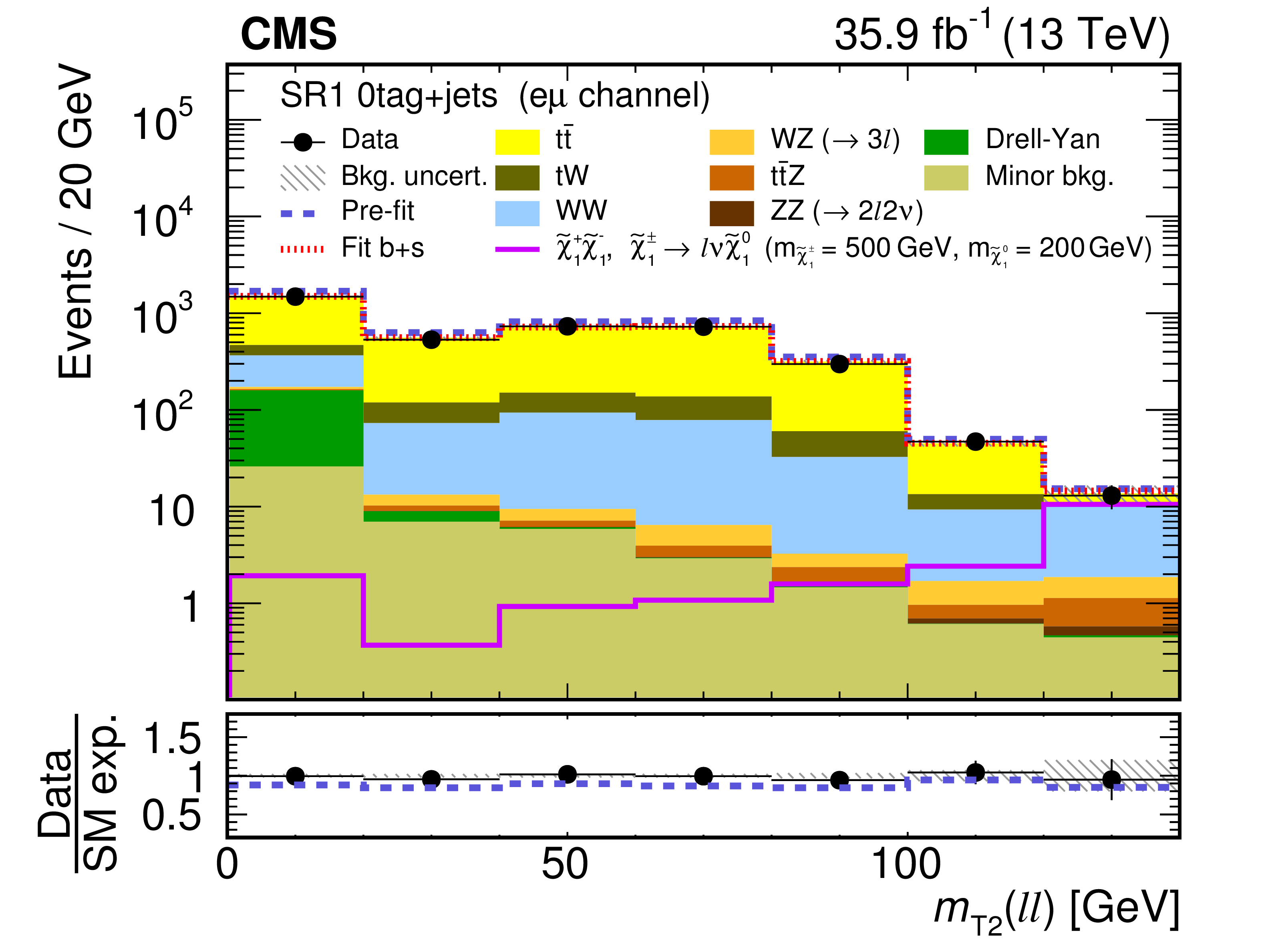
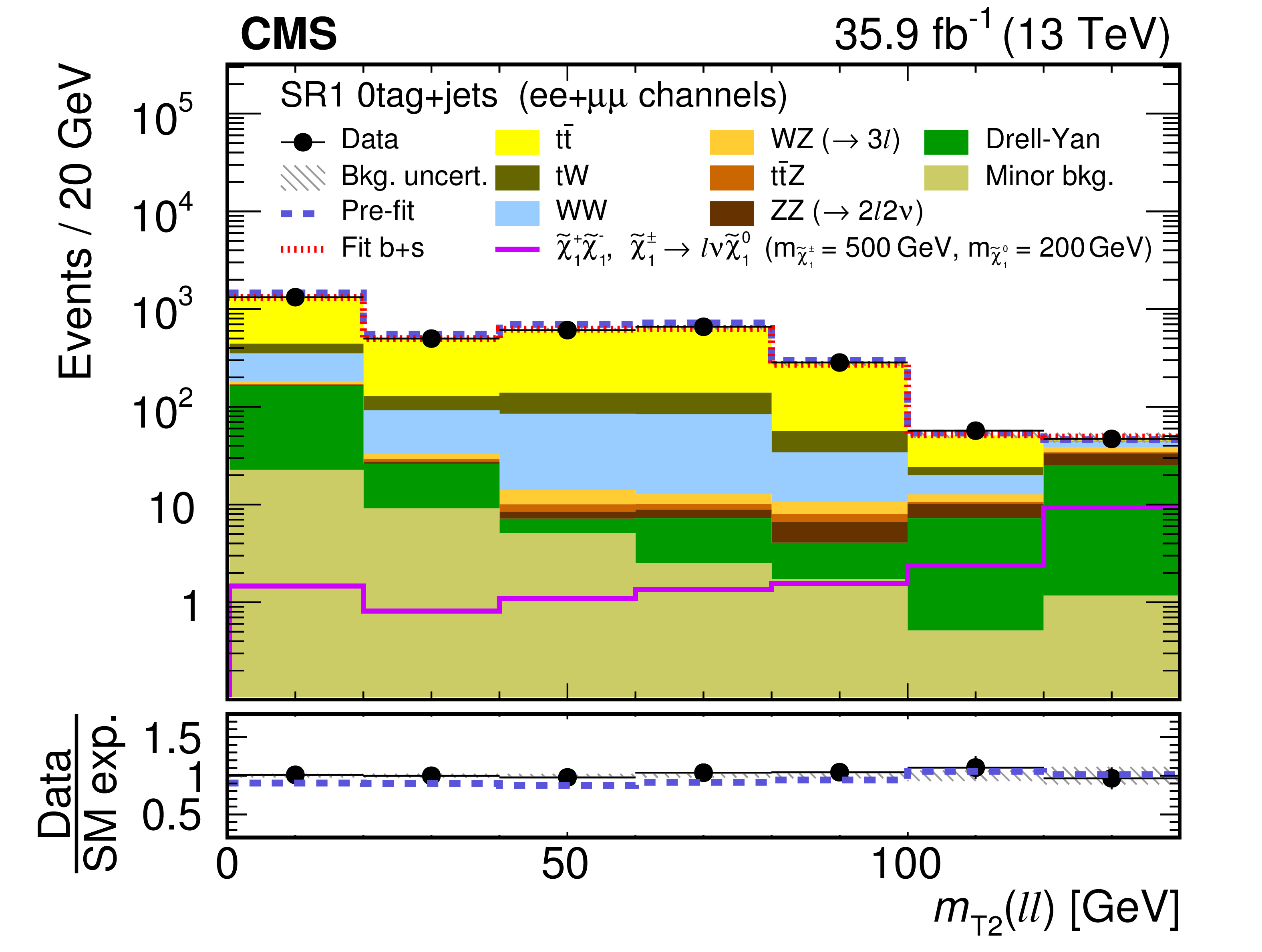
png pdf	Figure 4: Distributions of ${{m_\mathrm {T2}} (\ell \ell)}$ after the fit to data in the chargino SRs with 140 $ < {{p_{\mathrm {T}}} ^\text {miss}} < $ 200 GeV (upper plots), 200 $ < {{p_{\mathrm {T}}} ^\text {miss}} < $ 300 GeV (middle), and $ {{p_{\mathrm {T}}} ^\text {miss}} > $ 300 GeV (lower), for DF events without b-tagged jets and at least one jet (left plots) and no jets (right plots). The lower plot for the SR with $ {{p_{\mathrm {T}}} ^\text {miss}} > $ 300 GeV shows all the events without b-tagged jets regardless of their jet multiplicity. The solid magenta histogram shows the expected ${{m_\mathrm {T2}} (\ell \ell)}$ distribution for chargino pair production with $ {m_{\tilde{\chi}^\pm _{1}}} = $ 500 GeV and $ {m_{\tilde{\chi}^{0}_{1}}} = $ 200 GeV. Expected total SM contributions before the fit (dark blue dashed line) and after a background+signal fit (dark red dotted line) are also shown. The last bin includes the overflow entries. In the bottom panel, the ratio of data and SM expectations is shown for the expected total SM contribution after the fit using the background-only hypothesis (black dots) and before any fit (dark blue dashed line). The hatched band represents the total uncertainty after the fit.
png pdf	Figure 4-a: Distribution of ${{m_\mathrm {T2}} (\ell \ell)}$ after the fit to data in the chargino SR with 140 $ < {{p_{\mathrm {T}}} ^\text {miss}} < $ 200 GeV for DF events without b-tagged jets and at least one jet. The solid magenta histogram shows the expected ${{m_\mathrm {T2}} (\ell \ell)}$ distribution for chargino pair production with $ {m_{\tilde{\chi}^\pm _{1}}} = $ 500 GeV and $ {m_{\tilde{\chi}^{0}_{1}}} = $ 200 GeV. Expected total SM contributions before the fit (dark blue dashed line) and after a background+signal fit (dark red dotted line) are also shown. The last bin includes the overflow entries. In the bottom panel, the ratio of data and SM expectations is shown for the expected total SM contribution after the fit using the background-only hypothesis (black dots) and before any fit (dark blue dashed line). The hatched band represents the total uncertainty after the fit.
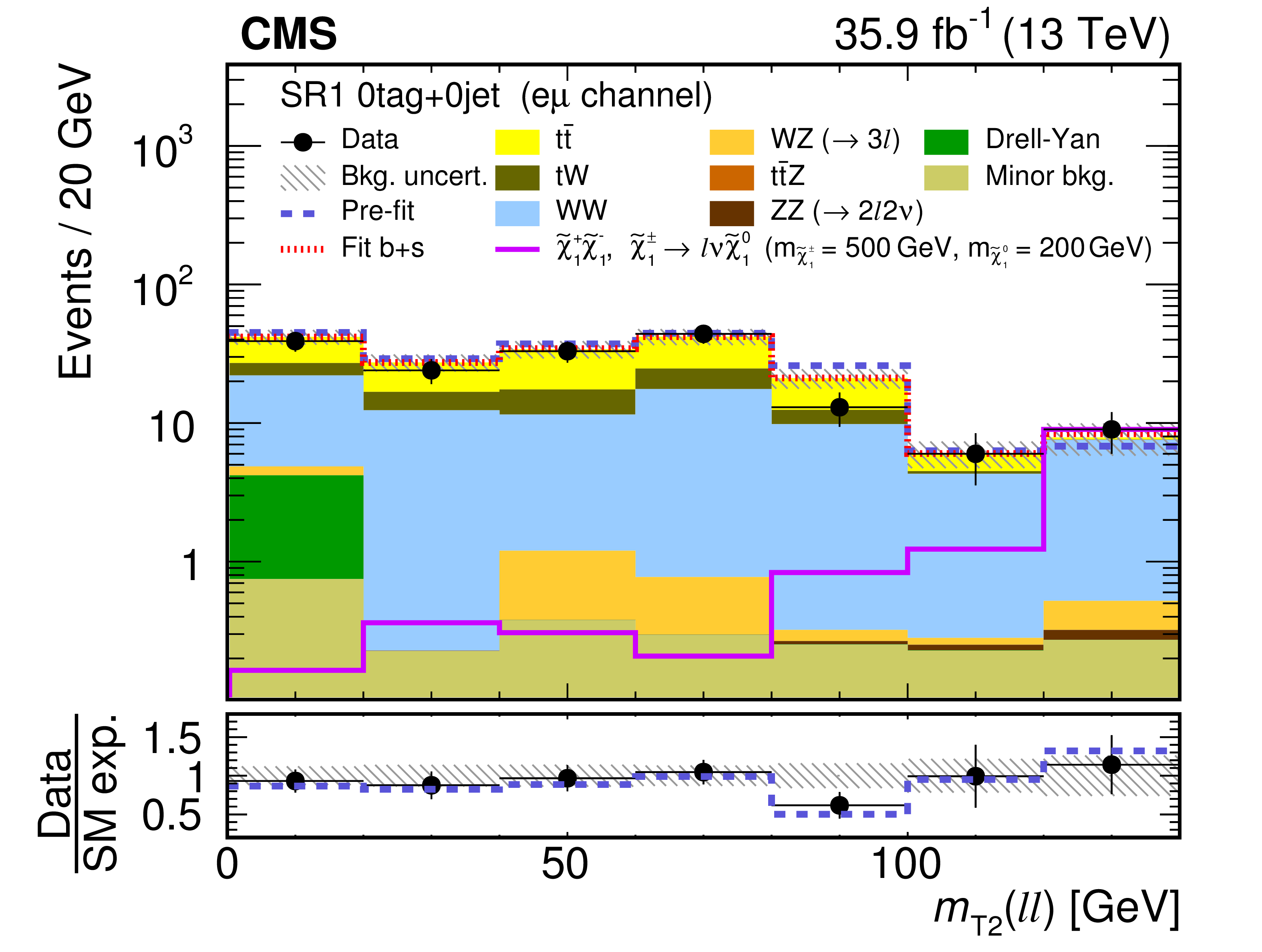
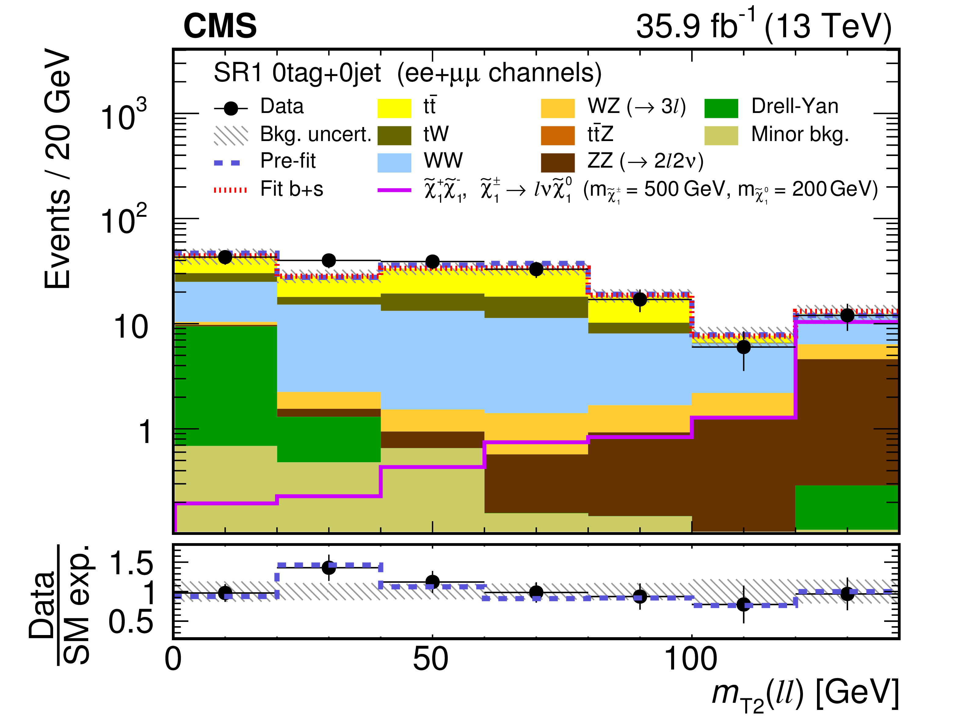
png pdf	Figure 4-b: Distribution of ${{m_\mathrm {T2}} (\ell \ell)}$ after the fit to data in the chargino SR with 140 $ < {{p_{\mathrm {T}}} ^\text {miss}} < $ 200 GeV for DF events with no jet. The solid magenta histogram shows the expected ${{m_\mathrm {T2}} (\ell \ell)}$ distribution for chargino pair production with $ {m_{\tilde{\chi}^\pm _{1}}} = $ 500 GeV and $ {m_{\tilde{\chi}^{0}_{1}}} = $ 200 GeV. Expected total SM contributions before the fit (dark blue dashed line) and after a background+signal fit (dark red dotted line) are also shown. The last bin includes the overflow entries. In the bottom panel, the ratio of data and SM expectations is shown for the expected total SM contribution after the fit using the background-only hypothesis (black dots) and before any fit (dark blue dashed line). The hatched band represents the total uncertainty after the fit.
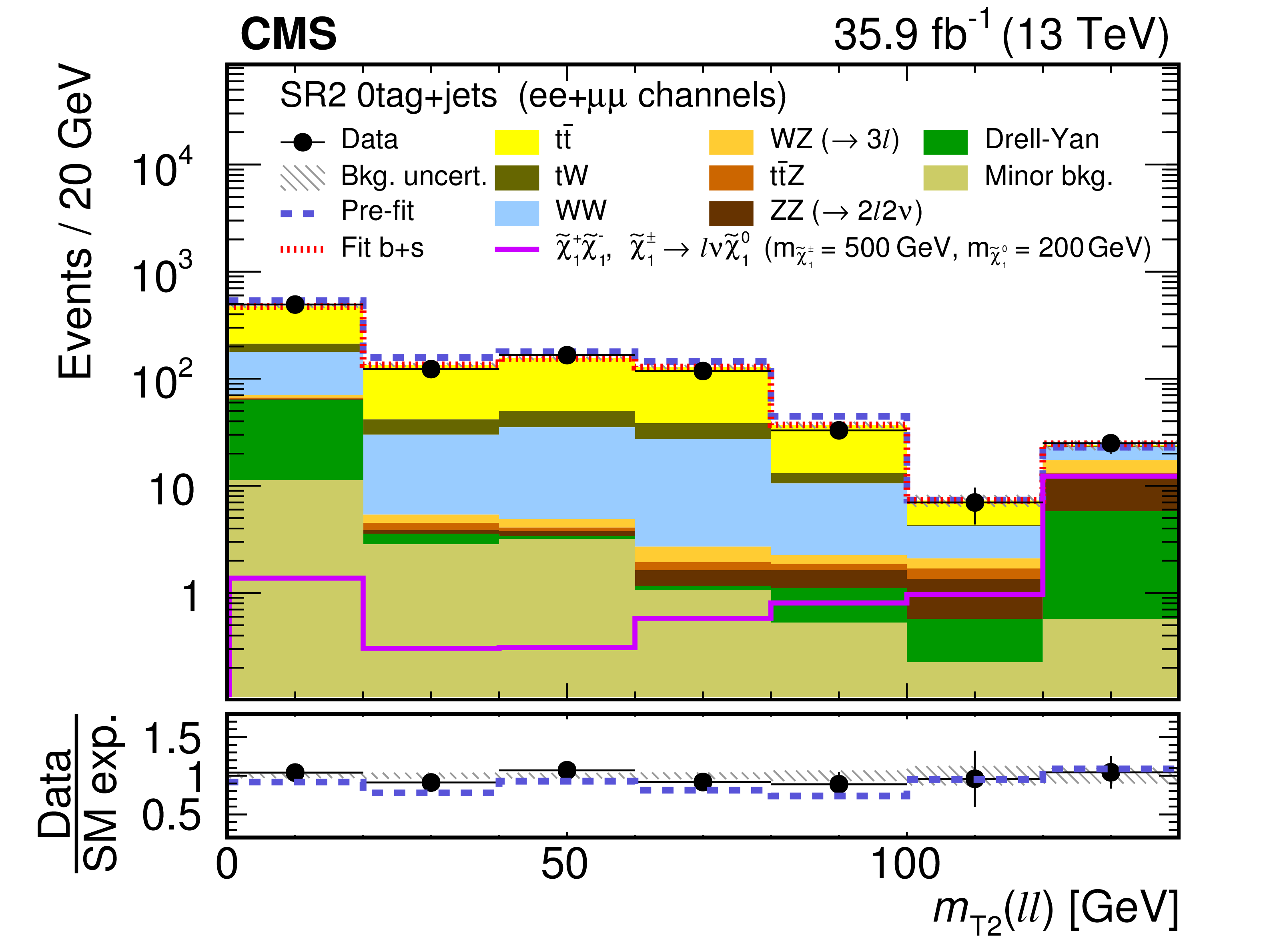
png pdf	Figure 4-c: Distribution of ${{m_\mathrm {T2}} (\ell \ell)}$ after the fit to data in the chargino SR with 200 $ < {{p_{\mathrm {T}}} ^\text {miss}} < $ 300 GeV for DF events without b-tagged jets and at least one jet. The solid magenta histogram shows the expected ${{m_\mathrm {T2}} (\ell \ell)}$ distribution for chargino pair production with $ {m_{\tilde{\chi}^\pm _{1}}} = $ 500 GeV and $ {m_{\tilde{\chi}^{0}_{1}}} = $ 200 GeV. Expected total SM contributions before the fit (dark blue dashed line) and after a background+signal fit (dark red dotted line) are also shown. The last bin includes the overflow entries. In the bottom panel, the ratio of data and SM expectations is shown for the expected total SM contribution after the fit using the background-only hypothesis (black dots) and before any fit (dark blue dashed line). The hatched band represents the total uncertainty after the fit.
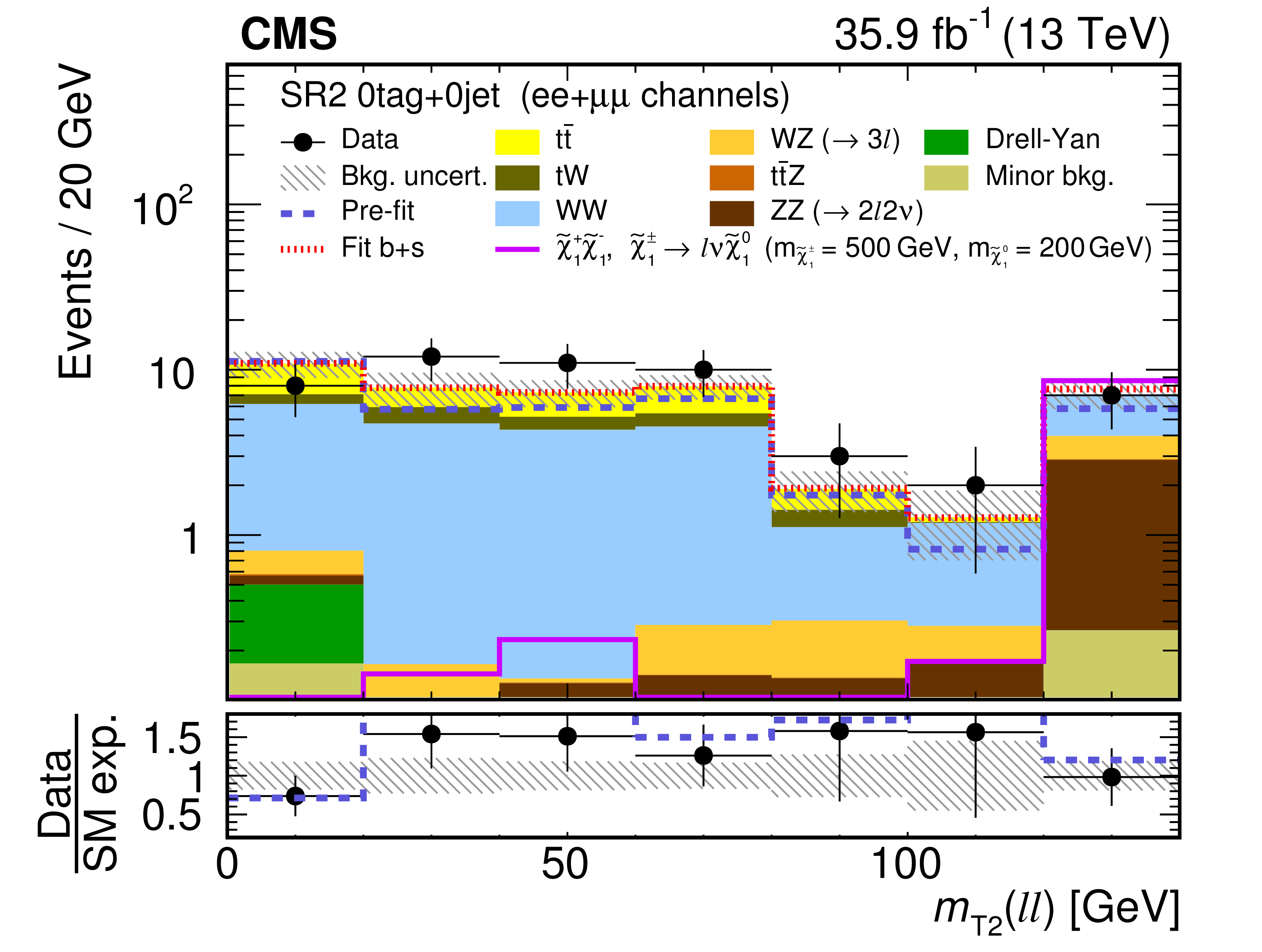
png pdf	Figure 4-d: Distribution of ${{m_\mathrm {T2}} (\ell \ell)}$ after the fit to data in the chargino SR with 200 $ < {{p_{\mathrm {T}}} ^\text {miss}} < $ 300 GeV for DF events with no jet. The solid magenta histogram shows the expected ${{m_\mathrm {T2}} (\ell \ell)}$ distribution for chargino pair production with $ {m_{\tilde{\chi}^\pm _{1}}} = $ 500 GeV and $ {m_{\tilde{\chi}^{0}_{1}}} = $ 200 GeV. Expected total SM contributions before the fit (dark blue dashed line) and after a background+signal fit (dark red dotted line) are also shown. The last bin includes the overflow entries. In the bottom panel, the ratio of data and SM expectations is shown for the expected total SM contribution after the fit using the background-only hypothesis (black dots) and before any fit (dark blue dashed line). The hatched band represents the total uncertainty after the fit.
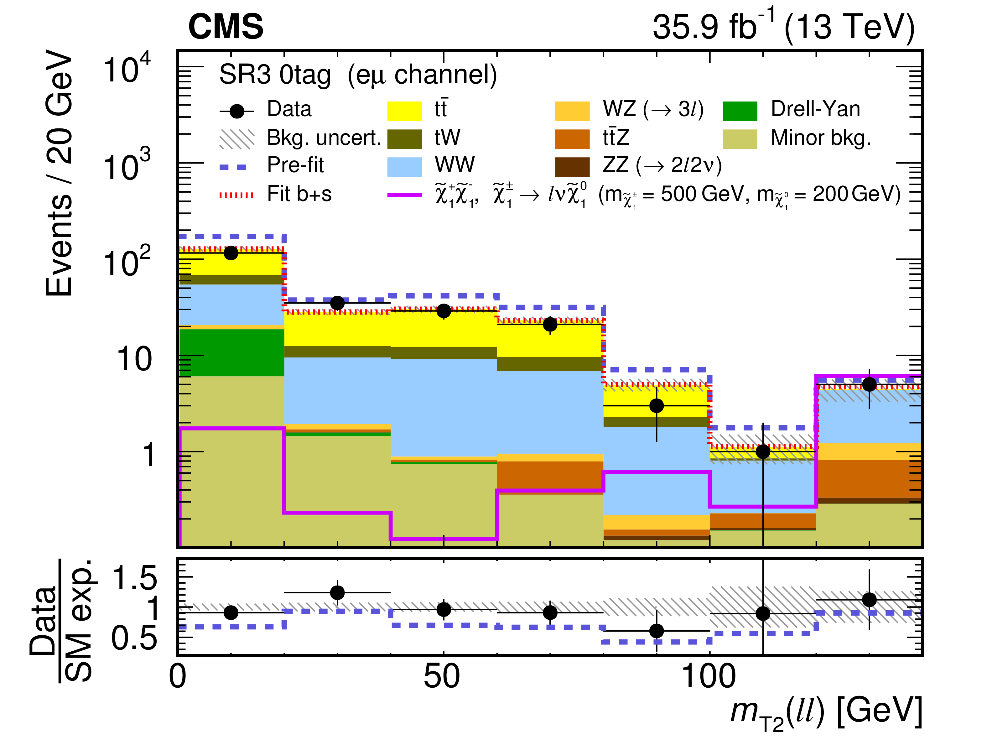
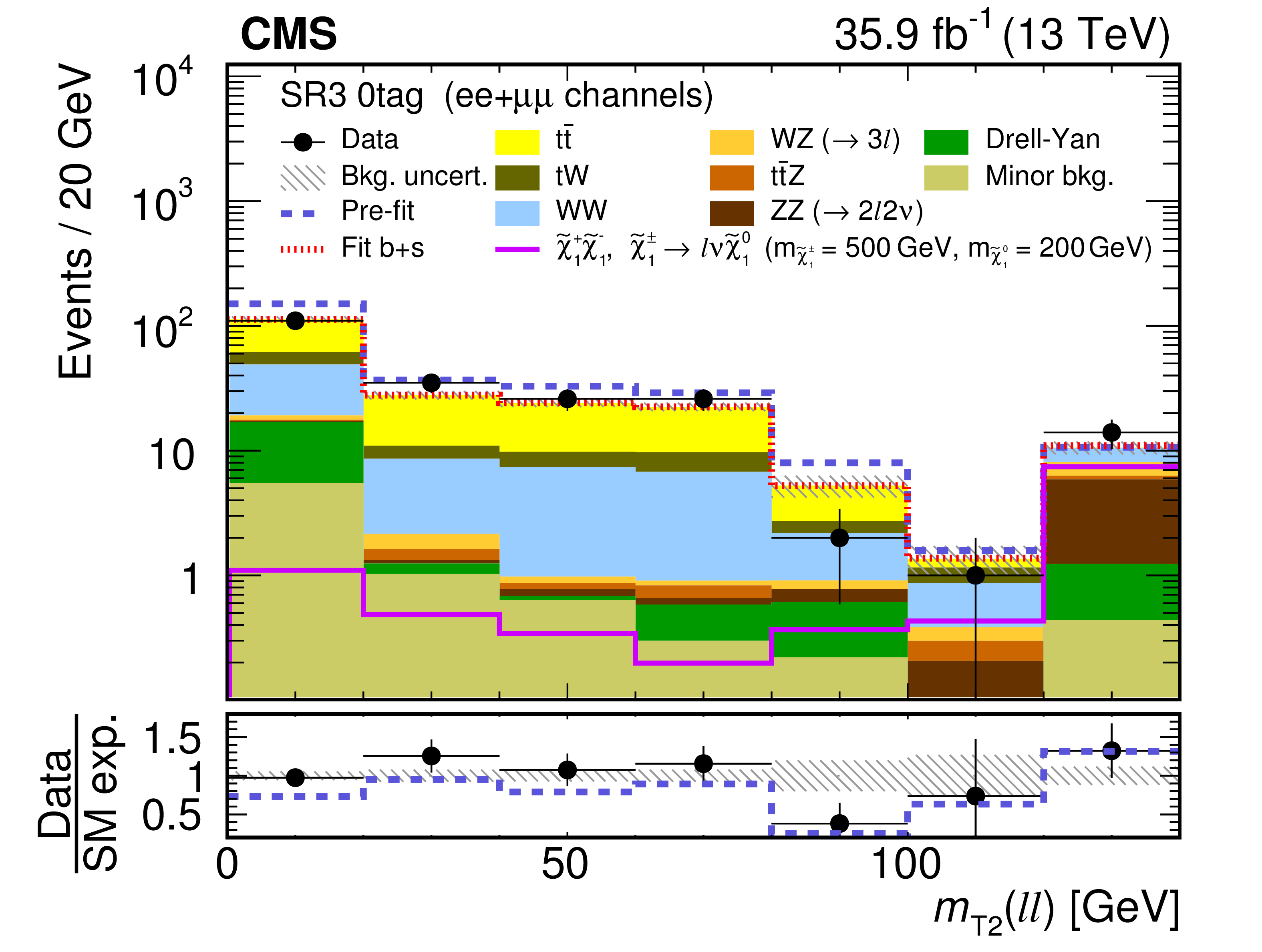
png pdf	Figure 4-e: Distribution of ${{m_\mathrm {T2}} (\ell \ell)}$ after the fit to data in the chargino SR with $ {{p_{\mathrm {T}}} ^\text {miss}} > $ 300 GeV for DF events without b-tagged jets regardless of their jet multiplicity. The solid magenta histogram shows the expected ${{m_\mathrm {T2}} (\ell \ell)}$ distribution for chargino pair production with $ {m_{\tilde{\chi}^\pm _{1}}} = $ 500 GeV and $ {m_{\tilde{\chi}^{0}_{1}}} = $ 200 GeV. Expected total SM contributions before the fit (dark blue dashed line) and after a background+signal fit (dark red dotted line) are also shown. The last bin includes the overflow entries. In the bottom panel, the ratio of data and SM expectations is shown for the expected total SM contribution after the fit using the background-only hypothesis (black dots) and before any fit (dark blue dashed line). The hatched band represents the total uncertainty after the fit.
png pdf	Figure 5: The same distributions of ${{m_\mathrm {T2}} (\ell \ell)}$ as Fig. 4, but for SF events.
png pdf	Figure 5-a: The same distribution of ${{m_\mathrm {T2}} (\ell \ell)}$ as Fig. 4-a, but for SF events.
png pdf	Figure 5-b: The same distribution of ${{m_\mathrm {T2}} (\ell \ell)}$ as Fig. 4-b, but for SF events.
png pdf	Figure 5-c: The same distribution of ${{m_\mathrm {T2}} (\ell \ell)}$ as Fig. 4-c, but for SF events.
png pdf	Figure 5-d: The same distribution of ${{m_\mathrm {T2}} (\ell \ell)}$ as Fig. 4-d, but for SF events.
png pdf	Figure 5-e: The same distribution of ${{m_\mathrm {T2}} (\ell \ell)}$ as Fig. 4-e, but for SF events.
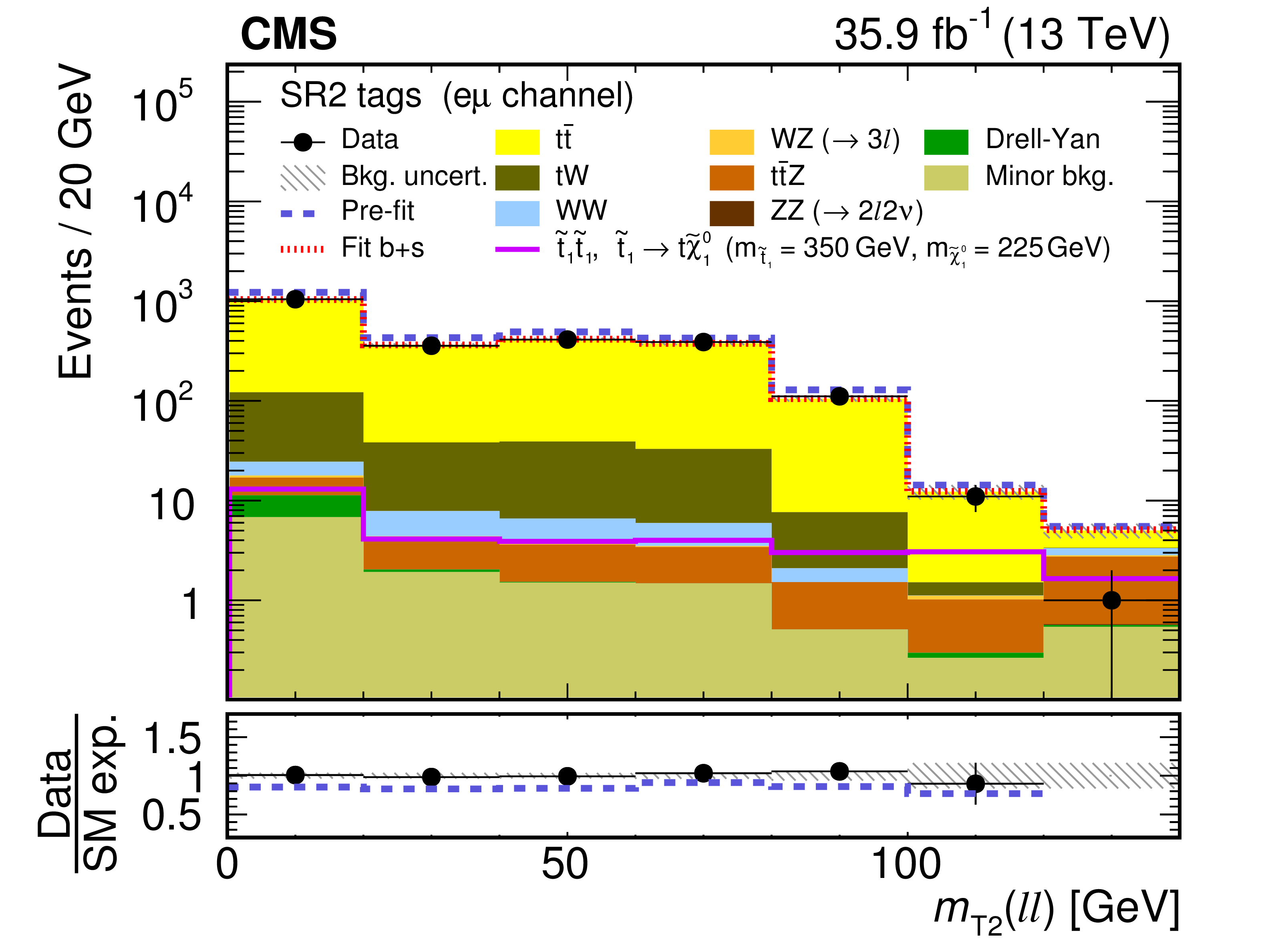
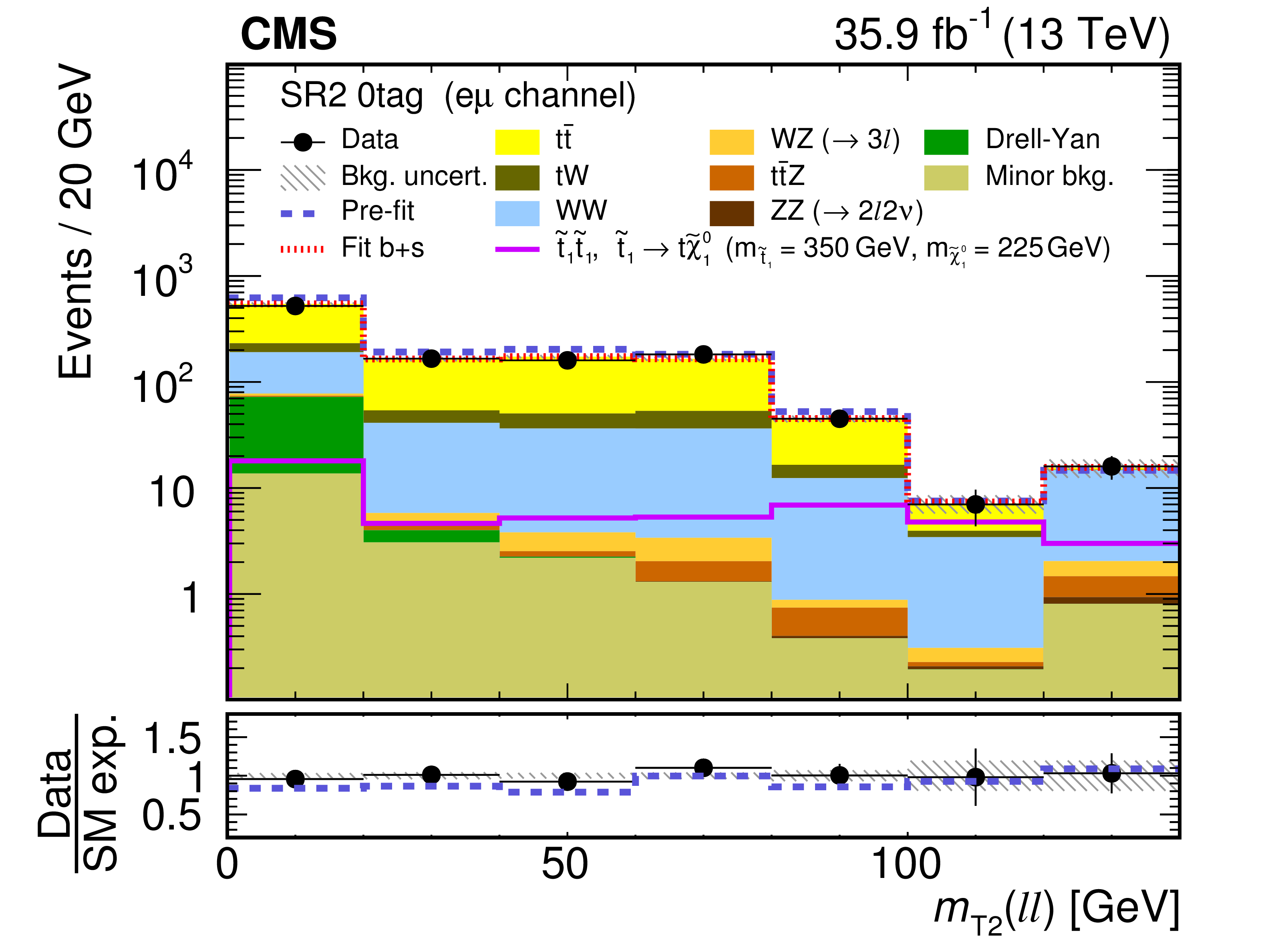
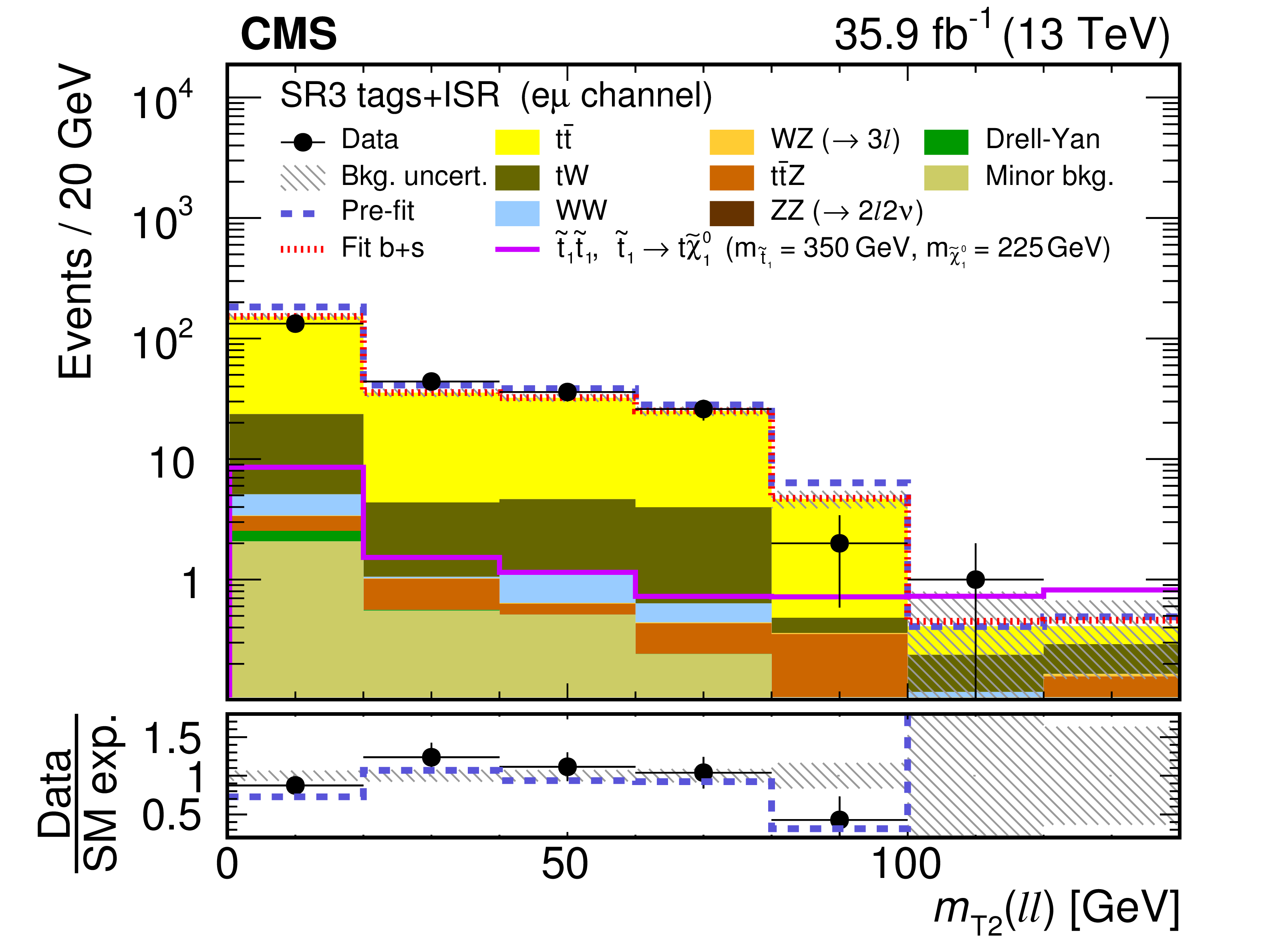
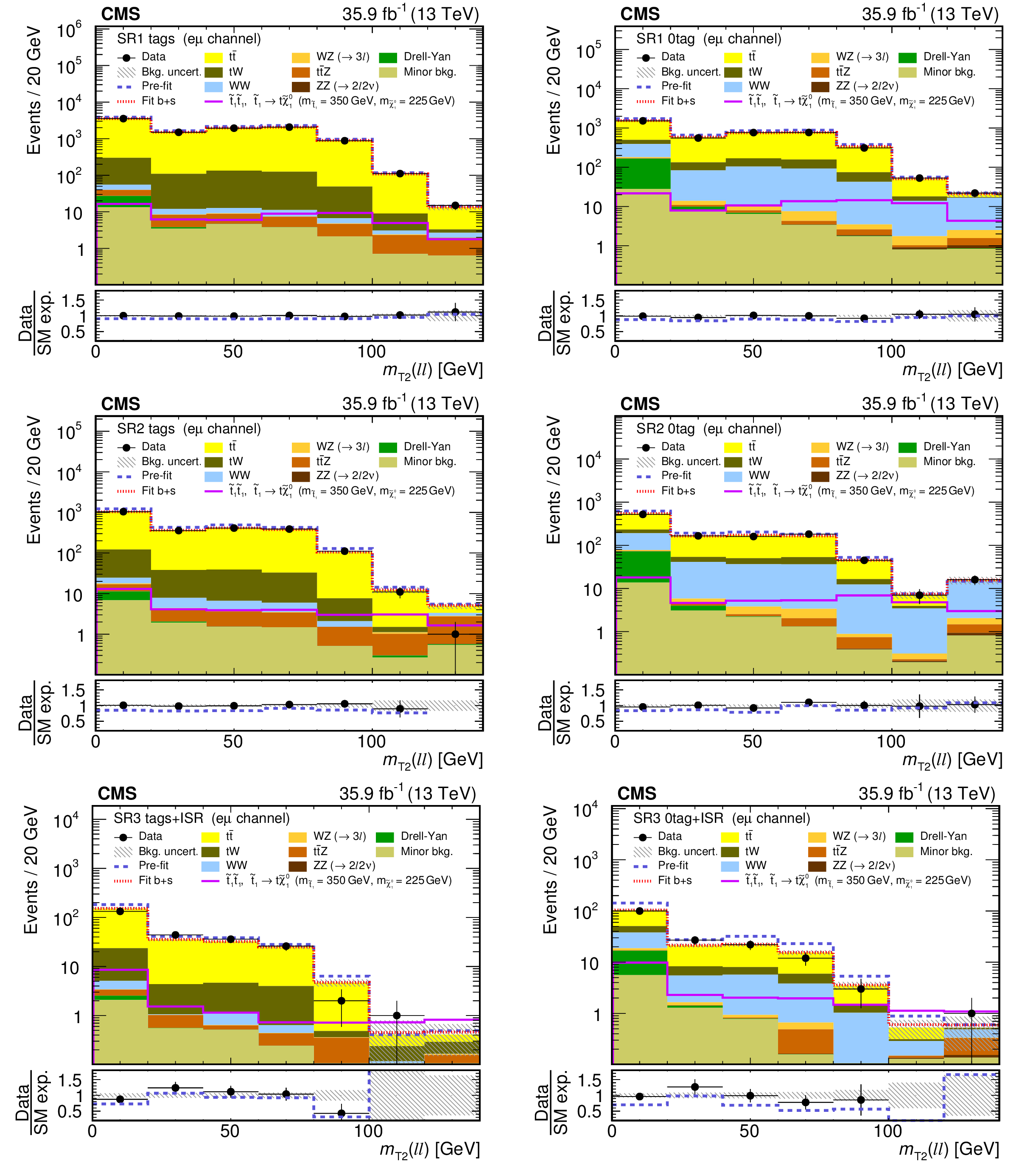
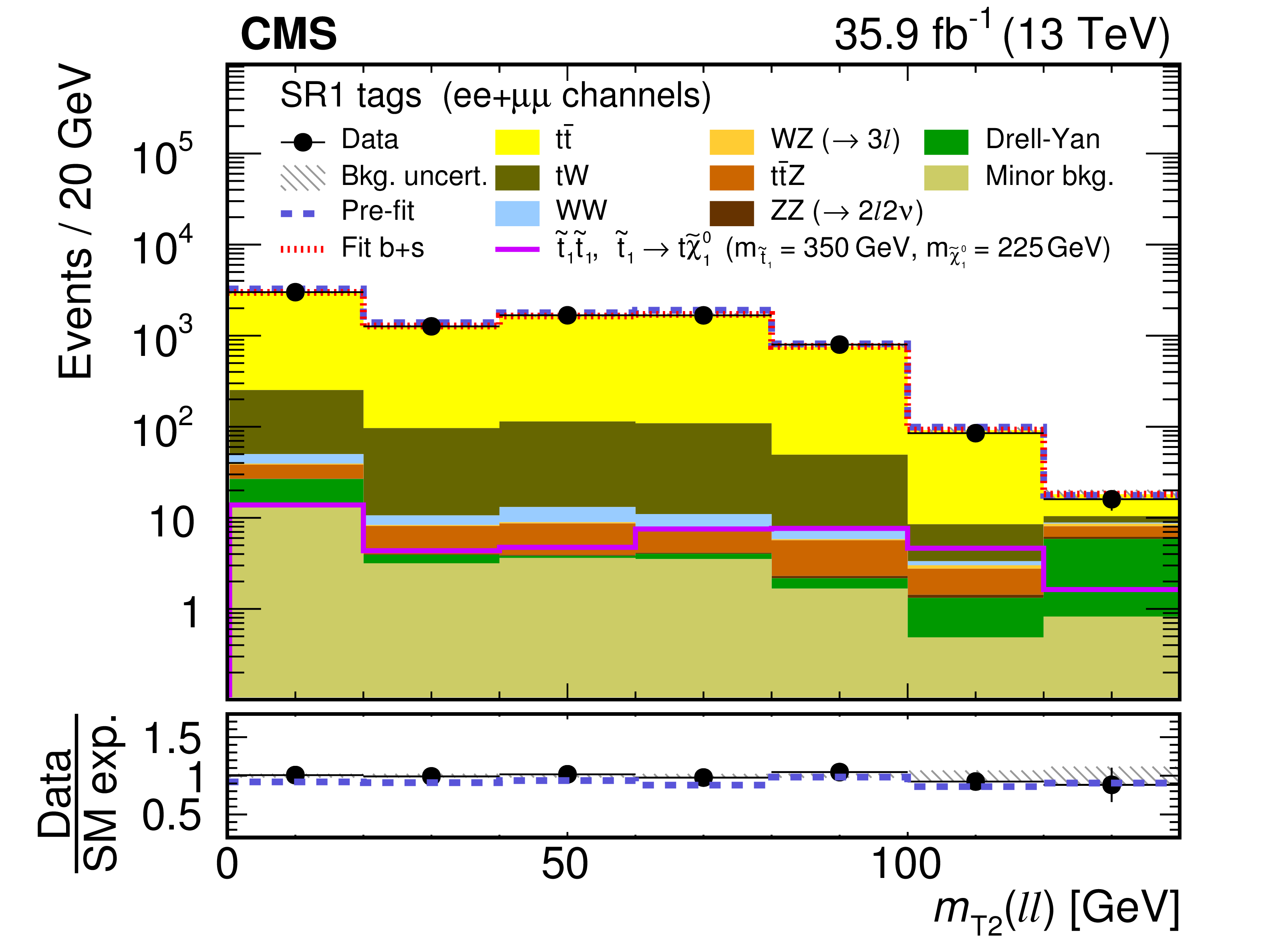
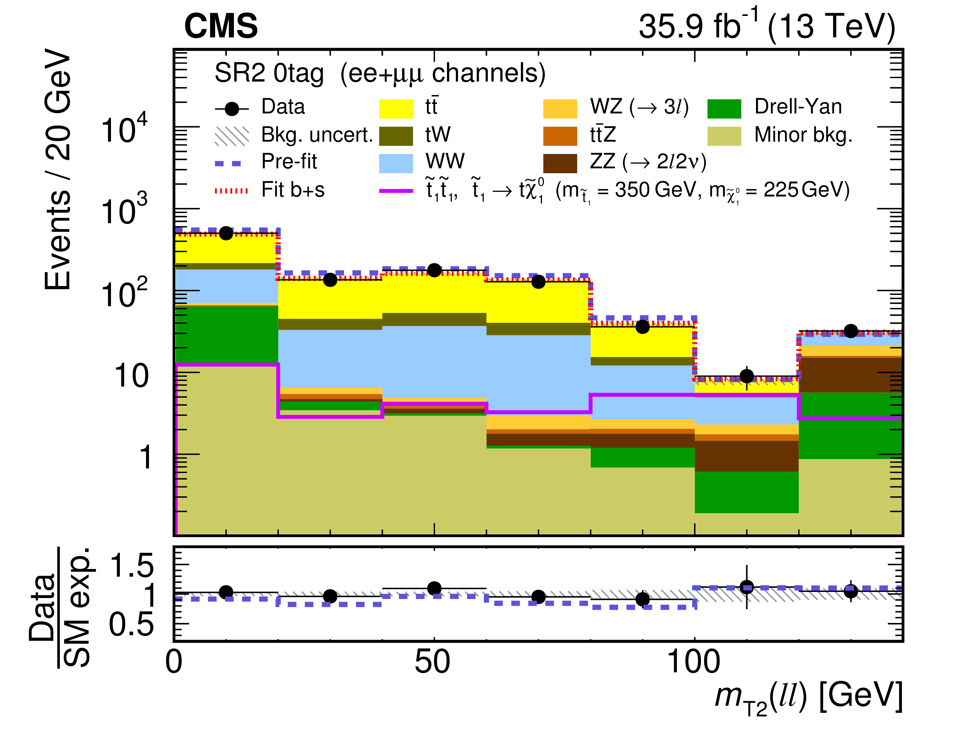
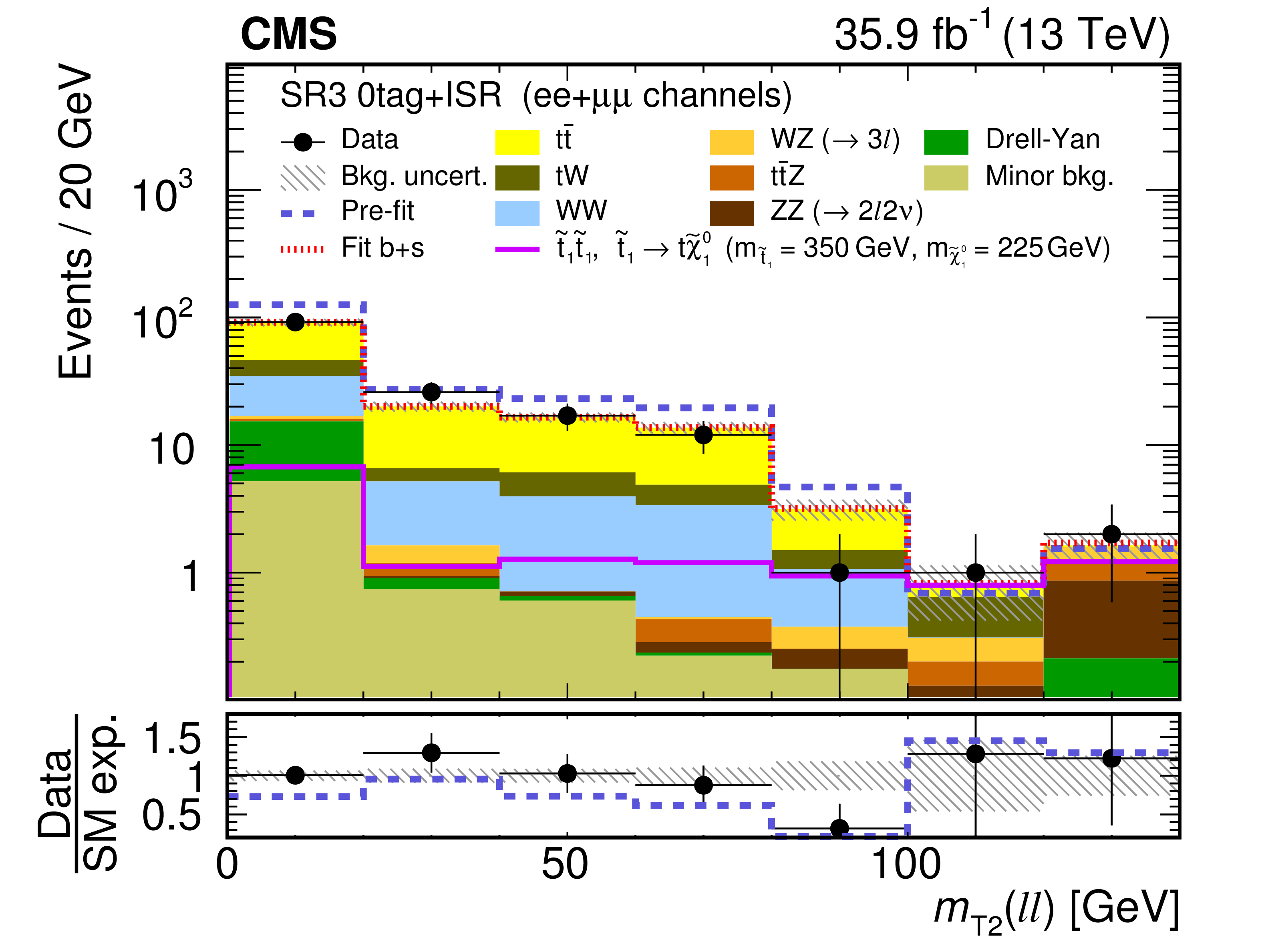
png pdf	Figure 6: Distributions of ${{m_\mathrm {T2}} (\ell \ell)}$ after the fit to data in the top squark SRs with 140 $ < {{p_{\mathrm {T}}} ^\text {miss}} < $ 200 GeV (upper plots), 200 $ < {{p_{\mathrm {T}}} ^\text {miss}} < $ 300 GeV (middle), or $ {{p_{\mathrm {T}}} ^\text {miss}} > $ 300 GeV (lower), for DF events with b-tagged jets (left plots) and without b-tagged jets (right plots). The solid magenta histogram shows the expected ${{m_\mathrm {T2}} (\ell \ell)}$ distribution for top squark pair production with $ {m_{\tilde{\mathrm {t}}_1}} = $ 350 GeV and $ {m_{\tilde{\chi}^{0}_{1}}} = $ 225 GeV. Expected total SM contributions before the fit (dark blue dashed line) and after a background+signal fit (dark red dotted line) are also shown. The last bin includes the overflow entries. In the bottom panel, the ratio of data and SM expectations is shown for the expected total SM contribution after the fit using the background-only hypothesis (black dots) and before any fit (dark blue dashed line). The hatched band represents the total uncertainty after the fit.
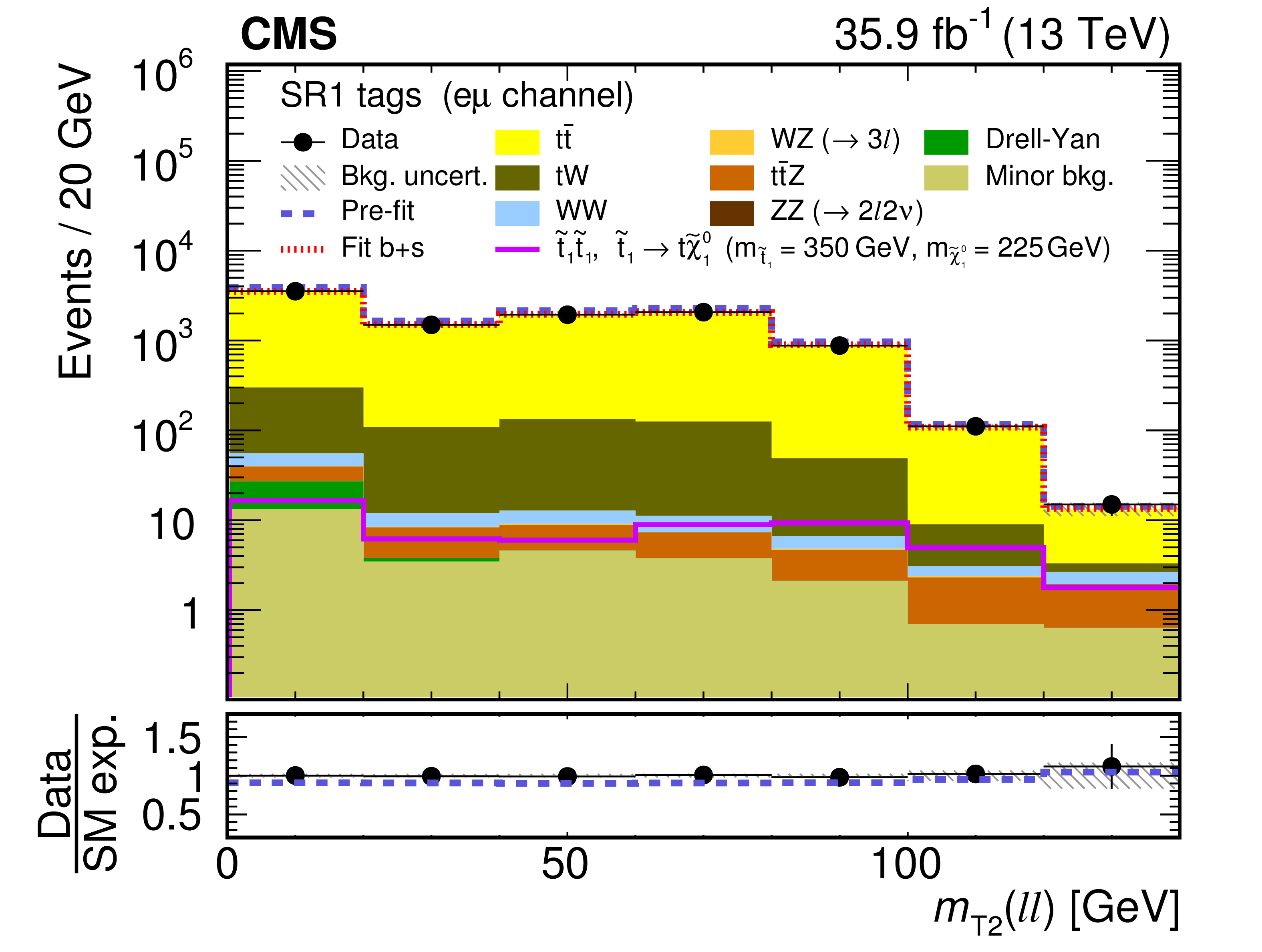
png pdf	Figure 6-a: Distribution of ${{m_\mathrm {T2}} (\ell \ell)}$ after the fit to data in the top squark SR with 140 $ < {{p_{\mathrm {T}}} ^\text {miss}} < $ 200 GeV, for DF events with b-tagged jets. The solid magenta histogram shows the expected ${{m_\mathrm {T2}} (\ell \ell)}$ distribution for top squark pair production with $ {m_{\tilde{\mathrm {t}}_1}} = $ 350 GeV and $ {m_{\tilde{\chi}^{0}_{1}}} = $ 225 GeV. Expected total SM contributions before the fit (dark blue dashed line) and after a background+signal fit (dark red dotted line) are also shown. The last bin includes the overflow entries. In the bottom panel, the ratio of data and SM expectations is shown for the expected total SM contribution after the fit using the background-only hypothesis (black dots) and before any fit (dark blue dashed line). The hatched band represents the total uncertainty after the fit.
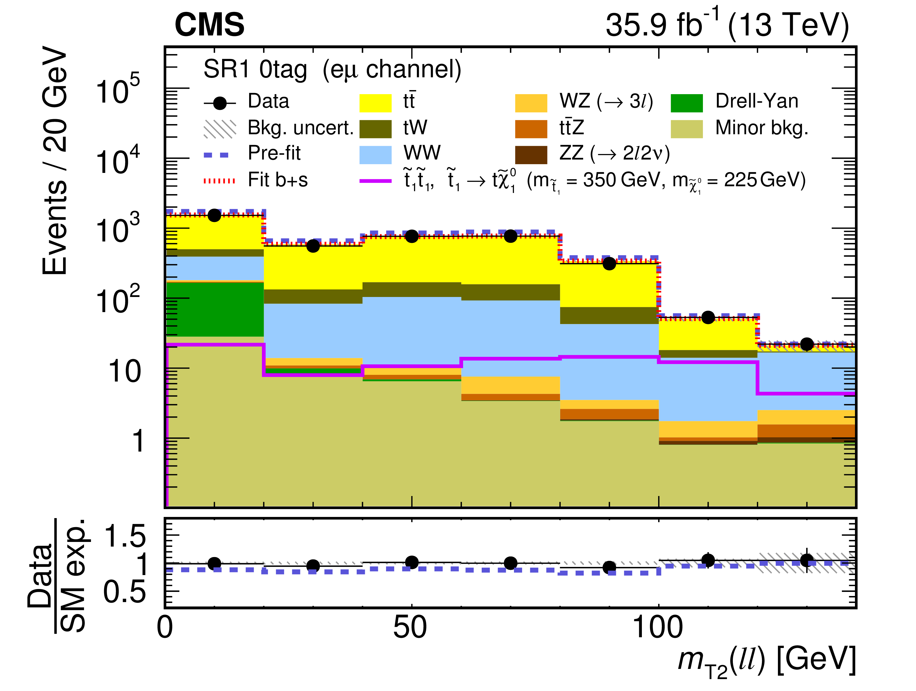
png pdf	Figure 6-b: Distribution of ${{m_\mathrm {T2}} (\ell \ell)}$ after the fit to data in the top squark SR with 140 $ < {{p_{\mathrm {T}}} ^\text {miss}} < $ 200 GeV, for DF events without b-tagged jets. The solid magenta histogram shows the expected ${{m_\mathrm {T2}} (\ell \ell)}$ distribution for top squark pair production with $ {m_{\tilde{\mathrm {t}}_1}} = $ 350 GeV and $ {m_{\tilde{\chi}^{0}_{1}}} = $ 225 GeV. Expected total SM contributions before the fit (dark blue dashed line) and after a background+signal fit (dark red dotted line) are also shown. The last bin includes the overflow entries. In the bottom panel, the ratio of data and SM expectations is shown for the expected total SM contribution after the fit using the background-only hypothesis (black dots) and before any fit (dark blue dashed line). The hatched band represents the total uncertainty after the fit.
png pdf	Figure 6-c: Distribution of ${{m_\mathrm {T2}} (\ell \ell)}$ after the fit to data in the top squark SR with 200 $ < {{p_{\mathrm {T}}} ^\text {miss}} < $ 300 GeV, for DF events with b-tagged jets. The solid magenta histogram shows the expected ${{m_\mathrm {T2}} (\ell \ell)}$ distribution for top squark pair production with $ {m_{\tilde{\mathrm {t}}_1}} = $ 350 GeV and $ {m_{\tilde{\chi}^{0}_{1}}} = $ 225 GeV. Expected total SM contributions before the fit (dark blue dashed line) and after a background+signal fit (dark red dotted line) are also shown. The last bin includes the overflow entries. In the bottom panel, the ratio of data and SM expectations is shown for the expected total SM contribution after the fit using the background-only hypothesis (black dots) and before any fit (dark blue dashed line). The hatched band represents the total uncertainty after the fit.
png pdf	Figure 6-d: Distribution of ${{m_\mathrm {T2}} (\ell \ell)}$ after the fit to data in the top squark SR with 200 $ < {{p_{\mathrm {T}}} ^\text {miss}} < $ 300 GeV, for DF events without b-tagged jets. The solid magenta histogram shows the expected ${{m_\mathrm {T2}} (\ell \ell)}$ distribution for top squark pair production with $ {m_{\tilde{\mathrm {t}}_1}} = $ 350 GeV and $ {m_{\tilde{\chi}^{0}_{1}}} = $ 225 GeV. Expected total SM contributions before the fit (dark blue dashed line) and after a background+signal fit (dark red dotted line) are also shown. The last bin includes the overflow entries. In the bottom panel, the ratio of data and SM expectations is shown for the expected total SM contribution after the fit using the background-only hypothesis (black dots) and before any fit (dark blue dashed line). The hatched band represents the total uncertainty after the fit.
png pdf	Figure 6-e: Distribution of ${{m_\mathrm {T2}} (\ell \ell)}$ after the fit to data in the top squark SR with $ {{p_{\mathrm {T}}} ^\text {miss}} > $ 300 GeV, for DF events with b-tagged jets. The solid magenta histogram shows the expected ${{m_\mathrm {T2}} (\ell \ell)}$ distribution for top squark pair production with $ {m_{\tilde{\mathrm {t}}_1}} = $ 350 GeV and $ {m_{\tilde{\chi}^{0}_{1}}} = $ 225 GeV. Expected total SM contributions before the fit (dark blue dashed line) and after a background+signal fit (dark red dotted line) are also shown. The last bin includes the overflow entries. In the bottom panel, the ratio of data and SM expectations is shown for the expected total SM contribution after the fit using the background-only hypothesis (black dots) and before any fit (dark blue dashed line). The hatched band represents the total uncertainty after the fit.
png pdf	Figure 6-f: Distribution of ${{m_\mathrm {T2}} (\ell \ell)}$ after the fit to data in the top squark SR with $ {{p_{\mathrm {T}}} ^\text {miss}} > $ 300 GeV, for DF events without b-tagged jets. The solid magenta histogram shows the expected ${{m_\mathrm {T2}} (\ell \ell)}$ distribution for top squark pair production with $ {m_{\tilde{\mathrm {t}}_1}} = $ 350 GeV and $ {m_{\tilde{\chi}^{0}_{1}}} = $ 225 GeV. Expected total SM contributions before the fit (dark blue dashed line) and after a background+signal fit (dark red dotted line) are also shown. The last bin includes the overflow entries. In the bottom panel, the ratio of data and SM expectations is shown for the expected total SM contribution after the fit using the background-only hypothesis (black dots) and before any fit (dark blue dashed line). The hatched band represents the total uncertainty after the fit.
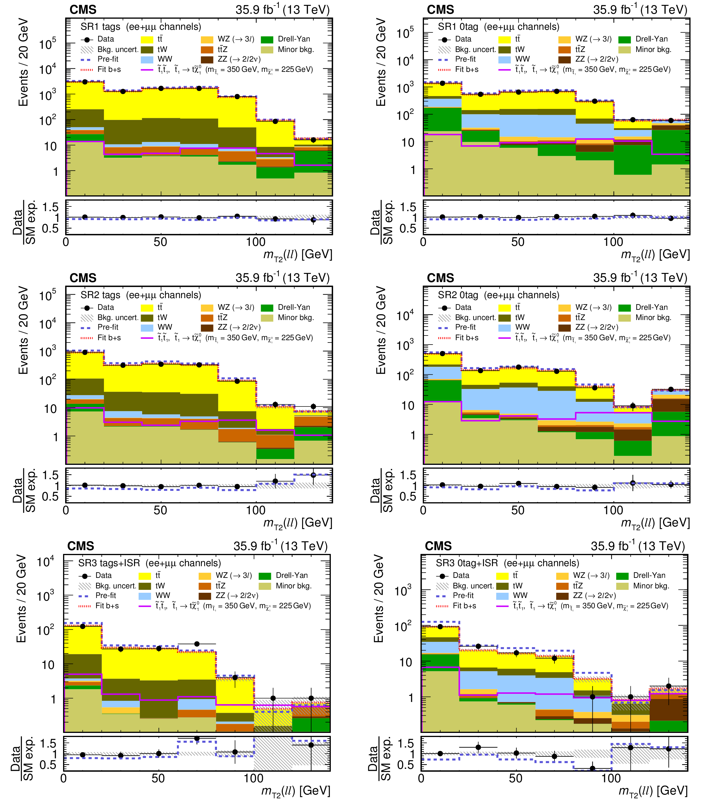
png pdf	Figure 7: The same distributions of ${{m_\mathrm {T2}} (\ell \ell)}$ as Fig. 6, but for SF events.
png pdf	Figure 7-a: The same distribution of ${{m_\mathrm {T2}} (\ell \ell)}$ as Fig. 6-a, but for SF events.
png pdf	Figure 7-b: The same distribution of ${{m_\mathrm {T2}} (\ell \ell)}$ as Fig. 6-b, but for SF events.
png pdf	Figure 7-c: The same distribution of ${{m_\mathrm {T2}} (\ell \ell)}$ as Fig. 6-c, but for SF events.
png pdf	Figure 7-d: The same distribution of ${{m_\mathrm {T2}} (\ell \ell)}$ as Fig. 6-d, but for SF events.
png pdf	Figure 7-e: The same distribution of ${{m_\mathrm {T2}} (\ell \ell)}$ as Fig. 6-e, but for SF events.
png pdf	Figure 7-f: The same distribution of ${{m_\mathrm {T2}} (\ell \ell)}$ as Fig. 6-f, but for SF events.
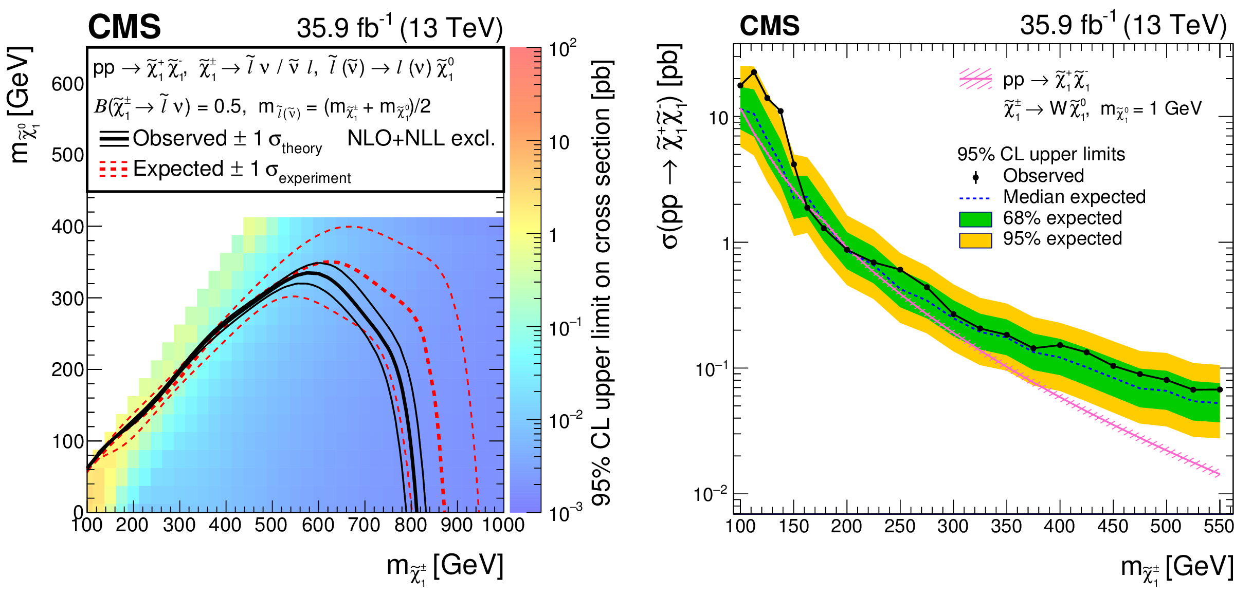
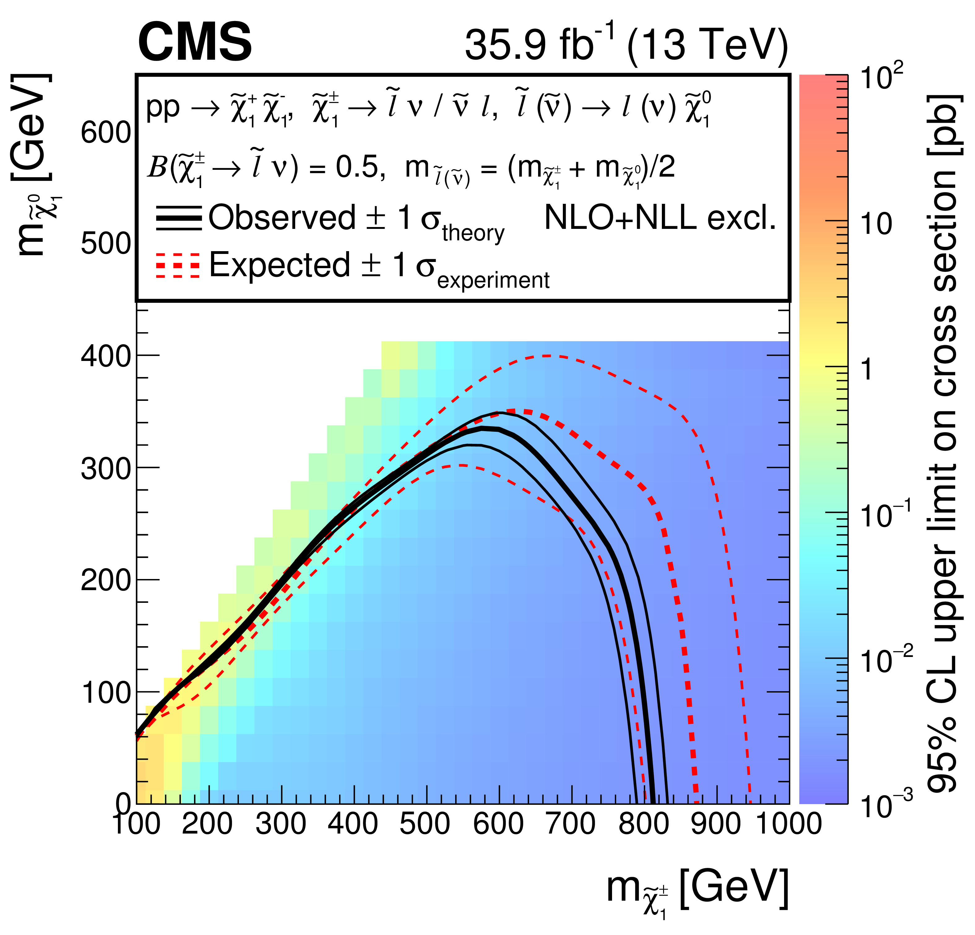
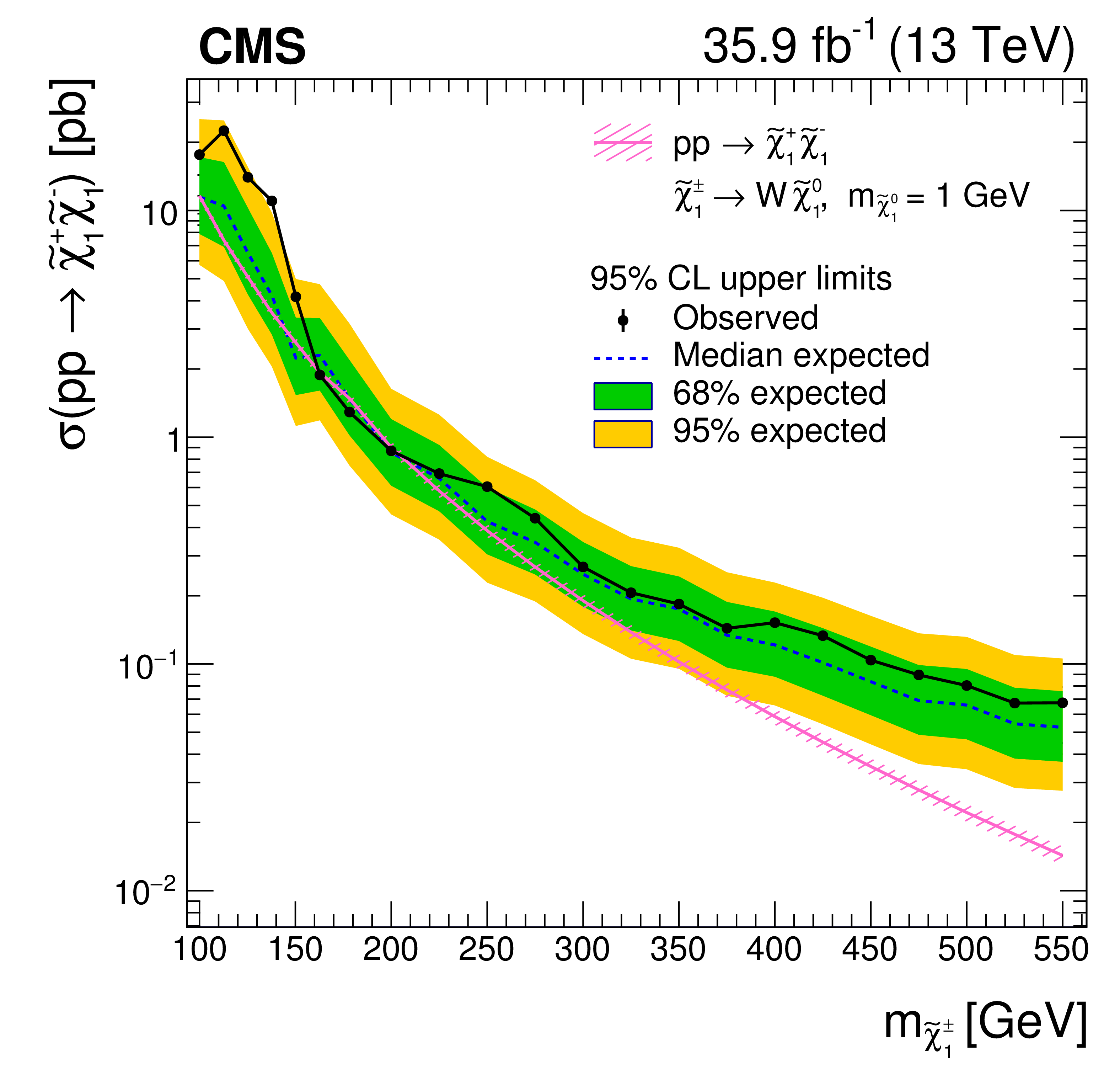
png pdf	Figure 8: Left: upper limits at 95% CL on the chargino pair production cross section as a function of the chargino and neutralino masses, when the chargino undergoes a cascade decay ${\tilde{\chi}^\pm _{1}} \to {\tilde{\ell}}\nu (\ell {\tilde{\nu}} ) \to \ell \nu \tilde{\chi}^{0}_{1}$. Exclusion regions in the plane (${m_{\tilde{\chi}^\pm _{1}}}$, ${m_{\tilde{\chi}^{0}_{1}}}$) are determined by comparing the upper limits with the NLO+NLL production cross sections. The thick dashed red line shows the expected exclusion region. The thin dashed red lines show the variation of the exclusion regions due to the experimental uncertainties. The thick black line shows the observed exclusion region, while the thin black lines show the variation of the exclusion regions due to the theoretical uncertainties in the production cross section. Right: observed and expected upper limits at 95% CL as a function of the chargino mass for a neutralino mass of 1 GeV, assuming chargino decays into a neutralino and a W boson ($ \tilde{\chi}^\pm _{1} \to {\mathrm {W}} \tilde{\chi}^{0}_{1} $).
png pdf root	Figure 8-a: Upper limits at 95% CL on the chargino pair production cross section as a function of the chargino and neutralino masses, when the chargino undergoes a cascade decay ${\tilde{\chi}^\pm _{1}} \to {\tilde{\ell}}\nu (\ell {\tilde{\nu}} ) \to \ell \nu \tilde{\chi}^{0}_{1}$. Exclusion regions in the plane (${m_{\tilde{\chi}^\pm _{1}}}$, ${m_{\tilde{\chi}^{0}_{1}}}$) are determined by comparing the upper limits with the NLO+NLL production cross sections. The thick dashed red line shows the expected exclusion region. The thin dashed red lines show the variation of the exclusion regions due to the experimental uncertainties. The thick black line shows the observed exclusion region, while the thin black lines show the variation of the exclusion regions due to the theoretical uncertainties in the production cross section.
png pdf root	Figure 8-b: Observed and expected upper limits at 95% CL as a function of the chargino mass for a neutralino mass of 1 GeV, assuming chargino decays into a neutralino and a W boson ($ \tilde{\chi}^\pm _{1} \to {\mathrm {W}} \tilde{\chi}^{0}_{1} $).
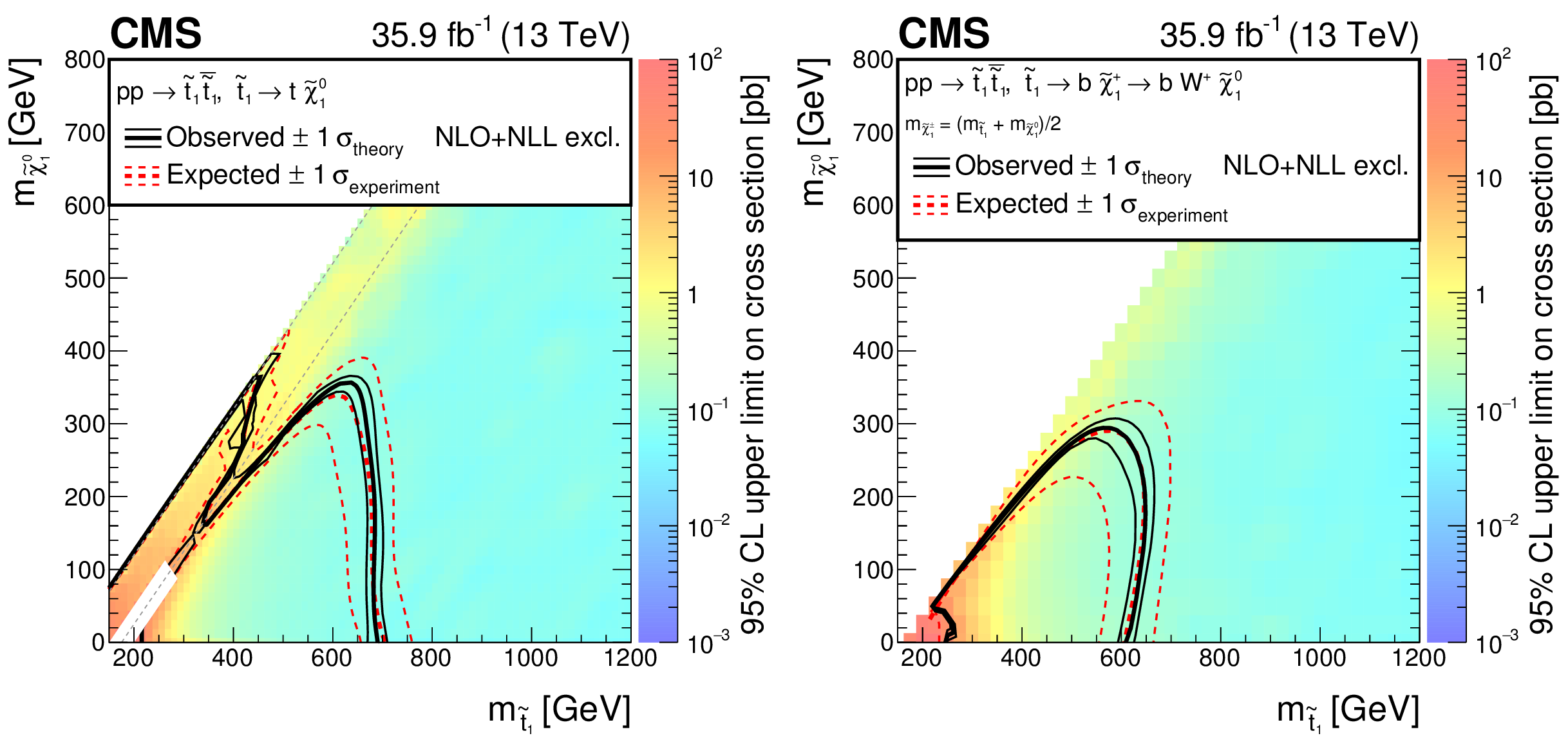
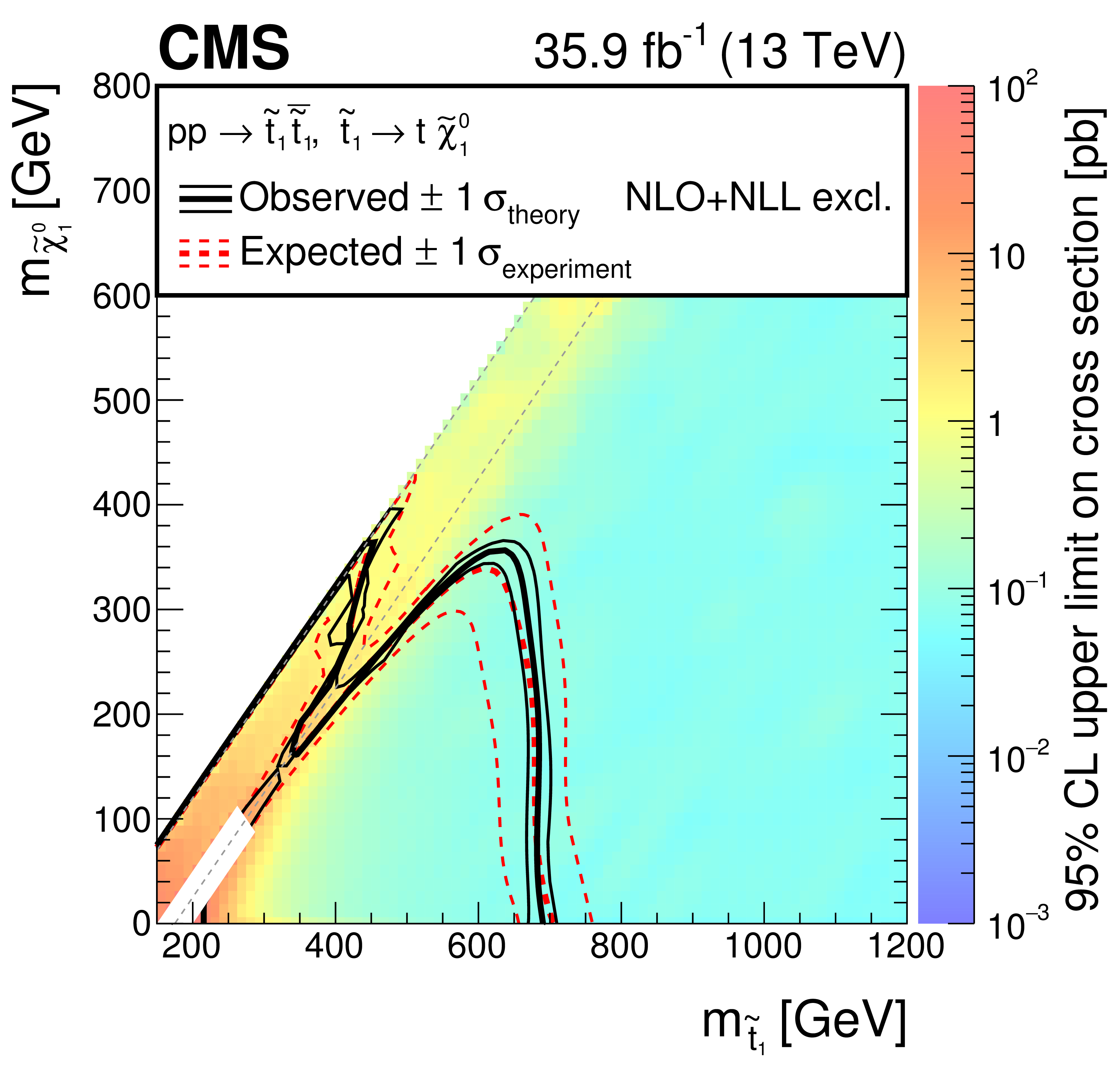
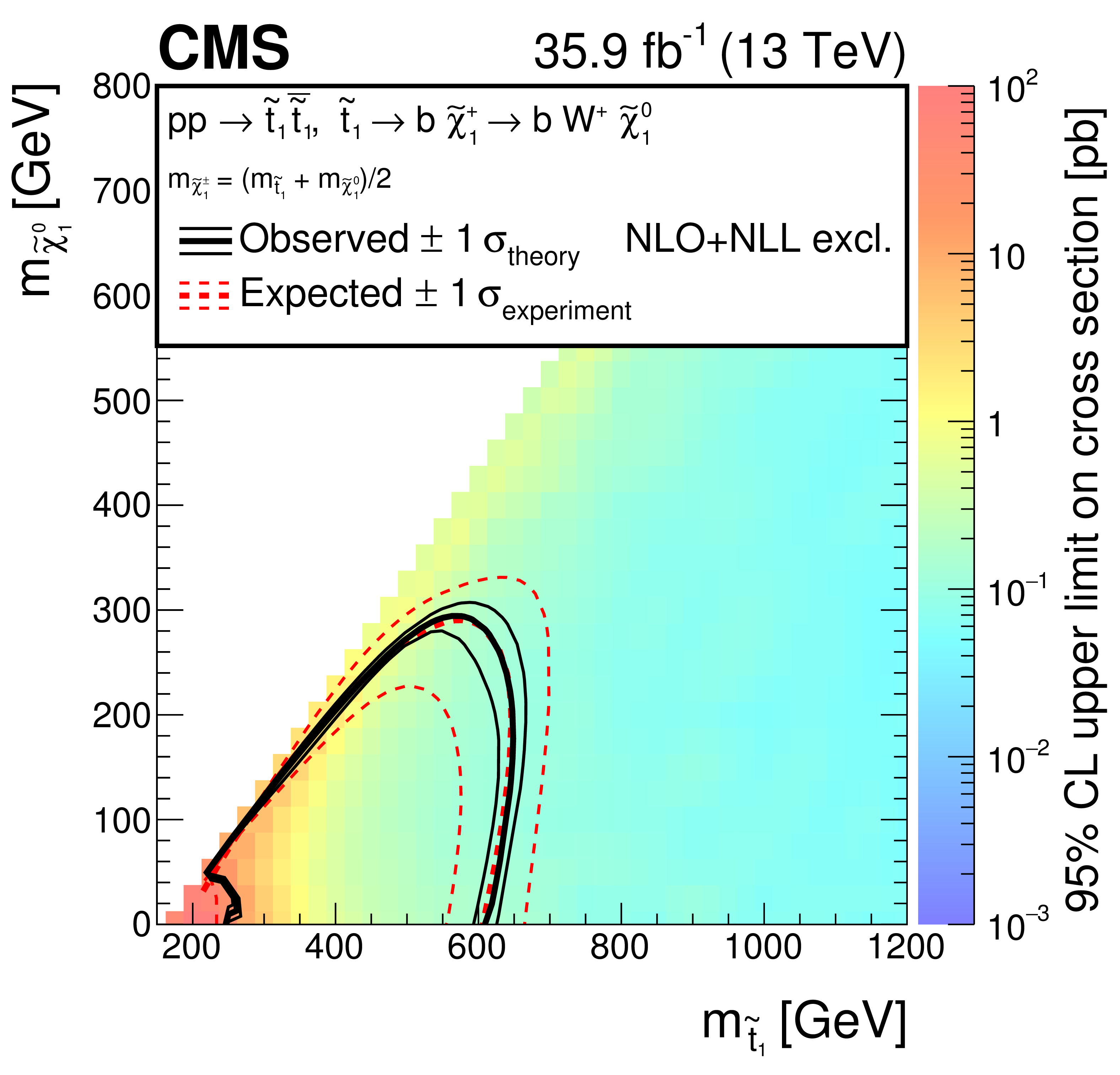
png pdf	Figure 9: Upper limits at 95% CL on the top squark production cross section as a function of the top squark and neutralino masses. The plot on the left shows the results when top squark decays into a top quark and a neutralino are assumed. The two diagonal gray dashed lines enclose the compressed region where $ {m_{{\mathrm {W}}}} < {m_{\tilde{\mathrm {t}}_1}} - {m_{\tilde{\chi}^{0}_{1}}} < {m_{{\mathrm {t}}}} $. The plot on the right gives the limits for top squarks decaying into a bottom quark and a chargino, with the latter successively decaying into a W boson and a neutralino. The mass of the chargino is assumed to be equal to the average of the top squark and neutralino masses. Exclusion regions in the plane (${m_{\tilde{\mathrm {t}}_1}}$, ${m_{\tilde{\chi}^{0}_{1}}}$) are determined by comparing the upper limits with the NLO+NLL production cross sections. The thick dashed red line shows the expected exclusion region. The thin dashed red lines show the variation of the exclusion regions due to the experimental uncertainties. The thick black line shows the observed exclusion region, while the thin black lines show the variation of the exclusion regions due to the theoretical uncertainties in the production cross section.
png pdf root	Figure 9-a: Upper limits at 95% CL on the top squark production cross section as a function of the top squark and neutralino masses. The plot shows the results when top squark decays into a top quark and a neutralino are assumed. The two diagonal gray dashed lines enclose the compressed region where $ {m_{{\mathrm {W}}}} < {m_{\tilde{\mathrm {t}}_1}} - {m_{\tilde{\chi}^{0}_{1}}} < {m_{{\mathrm {t}}}} $. Exclusion regions in the plane (${m_{\tilde{\mathrm {t}}_1}}$, ${m_{\tilde{\chi}^{0}_{1}}}$) are determined by comparing the upper limits with the NLO+NLL production cross sections. The thick dashed red line shows the expected exclusion region. The thin dashed red lines show the variation of the exclusion regions due to the experimental uncertainties. The thick black line shows the observed exclusion region, while the thin black lines show the variation of the exclusion regions due to the theoretical uncertainties in the production cross section.
png pdf root	Figure 9-b: Upper limits at 95% CL on the top squark production cross section as a function of the top squark and neutralino masses. The plot gives the limits for top squarks decaying into a bottom quark and a chargino, with the latter successively decaying into a W boson and a neutralino. The mass of the chargino is assumed to be equal to the average of the top squark and neutralino masses. Exclusion regions in the plane (${m_{\tilde{\mathrm {t}}_1}}$, ${m_{\tilde{\chi}^{0}_{1}}}$) are determined by comparing the upper limits with the NLO+NLL production cross sections. The thick dashed red line shows the expected exclusion region. The thin dashed red lines show the variation of the exclusion regions due to the experimental uncertainties. The thick black line shows the observed exclusion region, while the thin black lines show the variation of the exclusion regions due to the theoretical uncertainties in the production cross section.

Tables
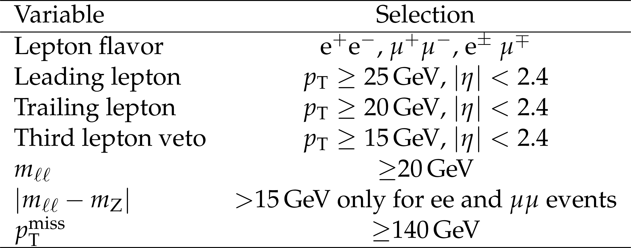
png pdf	Table 1: Definition of the baseline selection used in the searches for chargino and top squark pair production.
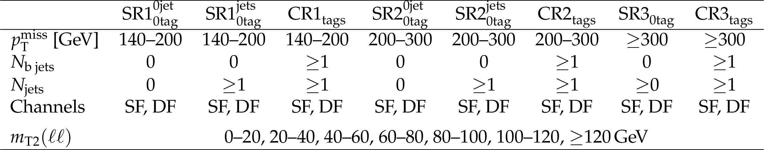
png pdf	Table 2: Definition of the SRs for the chargino search as a function of the ${{p_{\mathrm {T}}} ^\text {miss}} $ value, the b-jet multiplicity and jet multiplicity. Also shown are the CRs with b-tagged jets used for the normalization of the ${{\mathrm {t}\overline {\mathrm {t}}}}$ and ${{\mathrm {t}} {\mathrm {W}}}$ backgrounds. Each of the regions is further divided in seven ${{m_\mathrm {T2}} (\ell \ell)}$ bins as described in the last row.
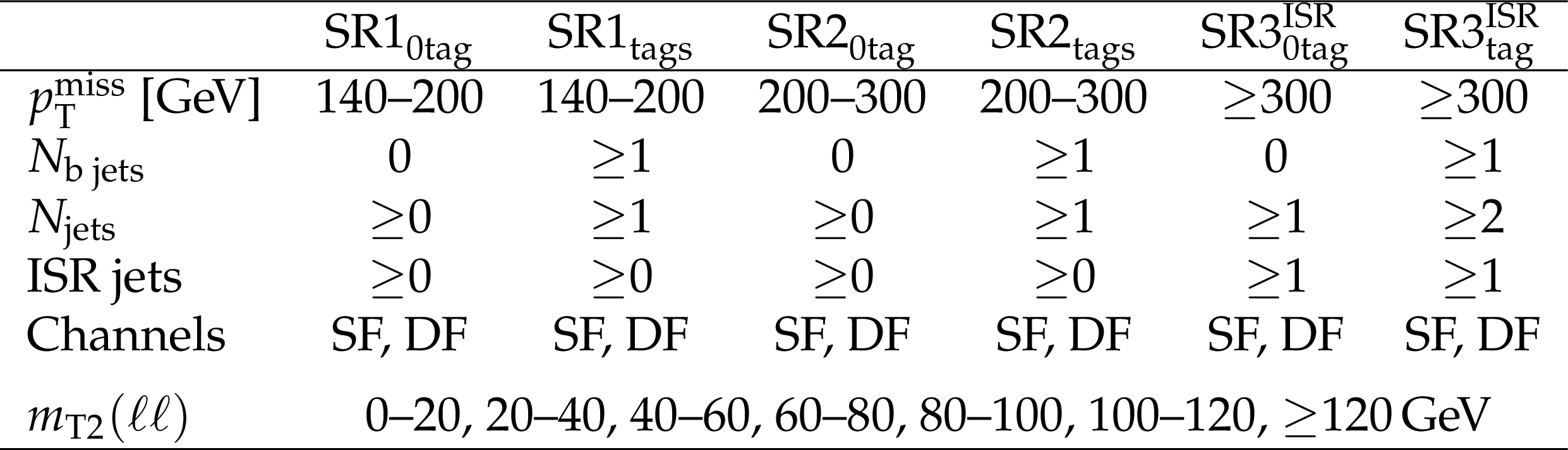
png pdf	Table 3: Definition of the SRs for the top squark production search as a function of the ${{p_{\mathrm {T}}} ^\text {miss}} $ value, the b-jet multiplicity and the ISR jet requirement. Each of the regions is further divided in seven ${{m_\mathrm {T2}} (\ell \ell)}$ bins as described in the last row.
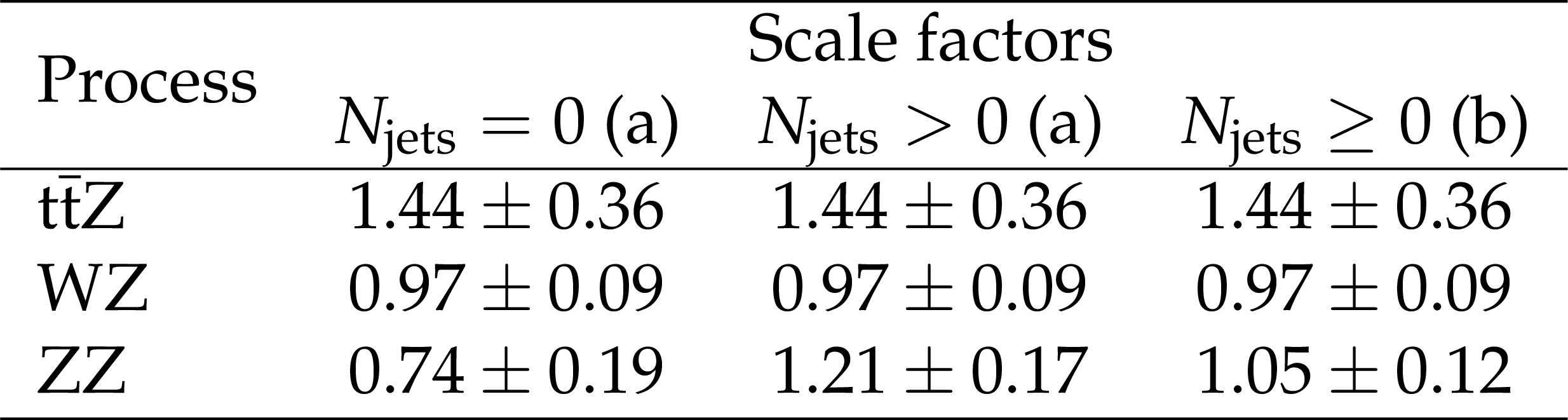
png pdf	Table 4: Summary of the normalization scale factors for ${{{\mathrm {t}\overline {\mathrm {t}}}} {\mathrm {Z}}}$, ${{\mathrm {W}} {\mathrm {Z}}}$, and ${{\mathrm {Z}} {\mathrm {Z}}}$ backgrounds in the SRs used for the chargino (a) and top squark (b) searches. Uncertainties include the statistical uncertainties of data and simulated event samples, and the systematic uncertainties in the purity of the CRs.
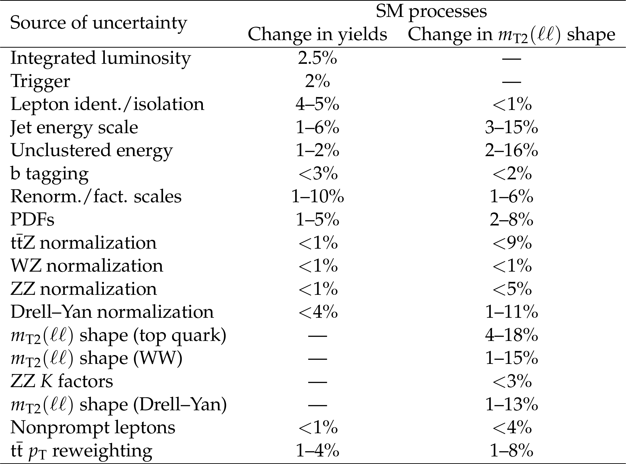
png pdf	Table 5: Sizes of systematic uncertainties in the predicted yields for SM processes. The first column shows the range of the uncertainties in the global background normalization across the different SRs. The second column quantifies the effect on the ${{m_\mathrm {T2}} (\ell \ell)}$ shape. This is computed by taking the maximum variation across the ${{m_\mathrm {T2}} (\ell \ell)}$ bins (after renormalizing for the global change of all the distribution) in each SR. The range of this variation across the SRs is given.
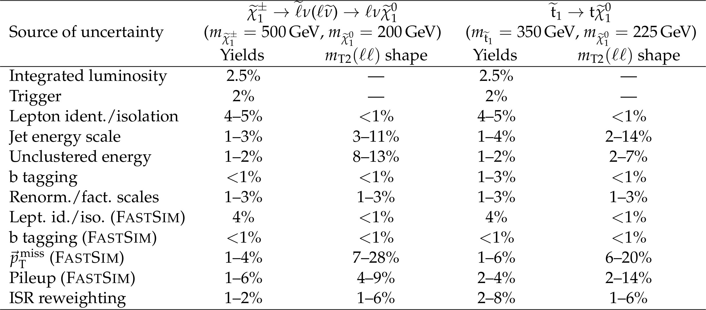
png pdf	Table 6: Same as in Table 5 for two representative signal points, one for chargino pair production and one for top squark pair production.
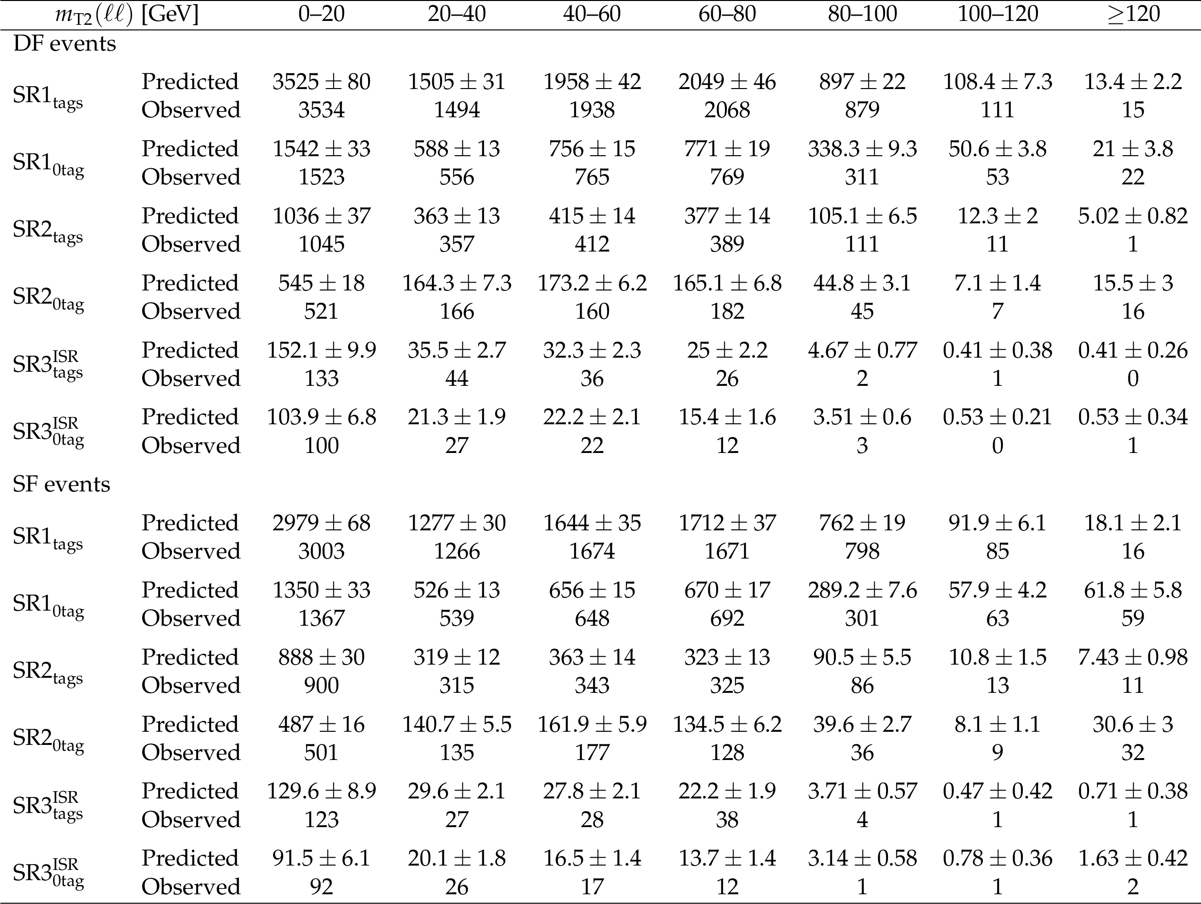
png pdf	Table 7: Observed and expected yields of DF (the upper half of Table) and SF (the lower half) events in the SRs for the chargino search. The quoted uncertainties in the background predictions include statistical and systematic contributions.
png pdf	Table 8: Observed and expected yields of DF (the upper half of Table) and SF (the lower half) events in the SRs for the top squark search. The quoted uncertainties in the background predictions include statistical and systematic contributions.

Summary

A search has been presented for pair production of supersymmetric particles in events with two oppositely charged isolated leptons and missing transverse momentum. The data used consist of a sample of proton-proton collisions collected with the CMS detector during the 2016 LHC run at a center-of-mass energy of 13 TeV, corresponding to an integrated luminosity of 35.9 fb$^{-1}$. No evidence for a deviation with respect to standard model predictions was observed in data. The results have been interpreted as upper limits on the cross sections of supersymmetric particle production for several simplified model spectra. Chargino pair production has been investigated in two possible decay modes. If the chargino is assumed to undergo a cascade decay through sleptons, an exclusion region in the ($m_{\tilde{\chi}^{\pm}_1}$, $m_{\tilde{\chi}^0_1}$) plane can be derived, extending to chargino masses of 800 GeV and neutralino masses of 320 GeV. These are the most stringent limits on this model to date. For chargino decays into a neutralino and a W boson, limits on the production cross section have been derived assuming a neutralino mass of 1 GeV, and chargino masses in the range 170-200 GeV have been excluded. Top squark pair production was also tested, with a focus on compressed decay modes. A model with the top squark decaying into a top quark and a neutralino was considered. In the region where $m_{\mathrm{W}} < m_{\tilde{\mathrm{t}}_{1}}-m_{\tilde{\chi}^0_1} < m_{\mathrm{t}}$, limits extend up to 420 and 360 GeV for the top squark and neutralino masses, respectively. An alternative model has also been considered, where the top squark decays into a chargino and a bottom quark, with the chargino subsequently decaying into a W boson and the lightest neutralino. The mass of the chargino is assumed to be average between the top squark and neutralino masses, which gives a lower bound to the mass difference (${\Delta m} $) between the top squark and the neutralino of ${\Delta m} \approx 2\,m_{\mathrm{W}}$. This search reduces by about 50 GeV the minimum ${\Delta m}$ excluded in the previous result with two leptons in the final state [30] from the CMS Collaboration, excluding top squark masses in the range 225-325 GeV for ${\Delta m} \approx 2\,m_{\mathrm{W}}$. In summary, by exploiting the full data set collected by the CMS experiment in 2016, this search extends the existing exclusion limits on the pair production of charginos decaying via sleptons [29], improving by about 70 GeV the limit on the chargino mass for a massless neutralino. Exclusion limits on the top squark pair production extend the results obtained by the CMS Collaboration in final states with two oppositely charged leptons [30] to the compressed region, where they are competitive with the results obtained by the ATLAS Collaboration in the same decay channel [35].

Additional Figures
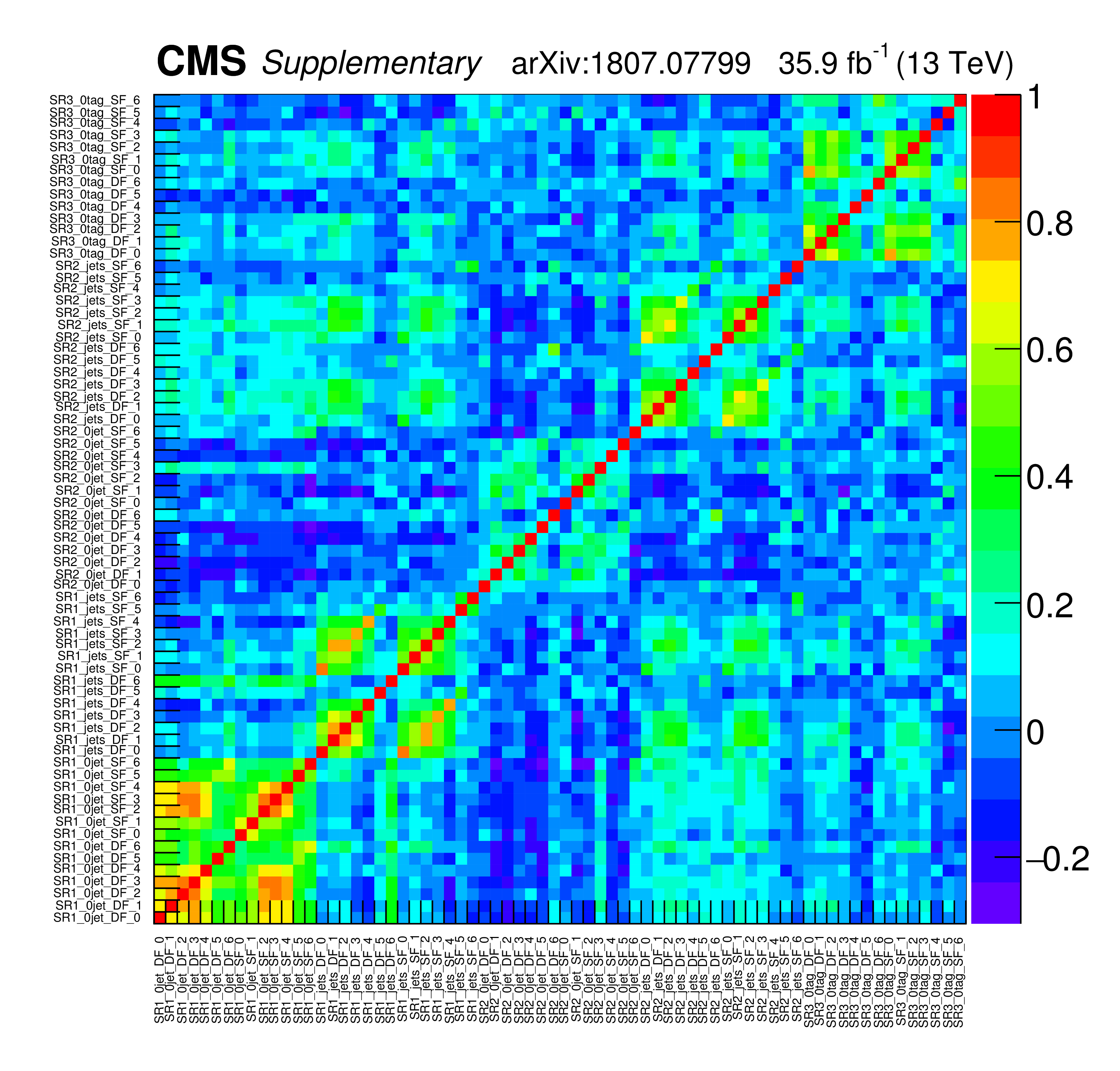
png pdf root	Additional Figure 1: Correlation matrix for the background between the signal regions used in the chargino pair production search.
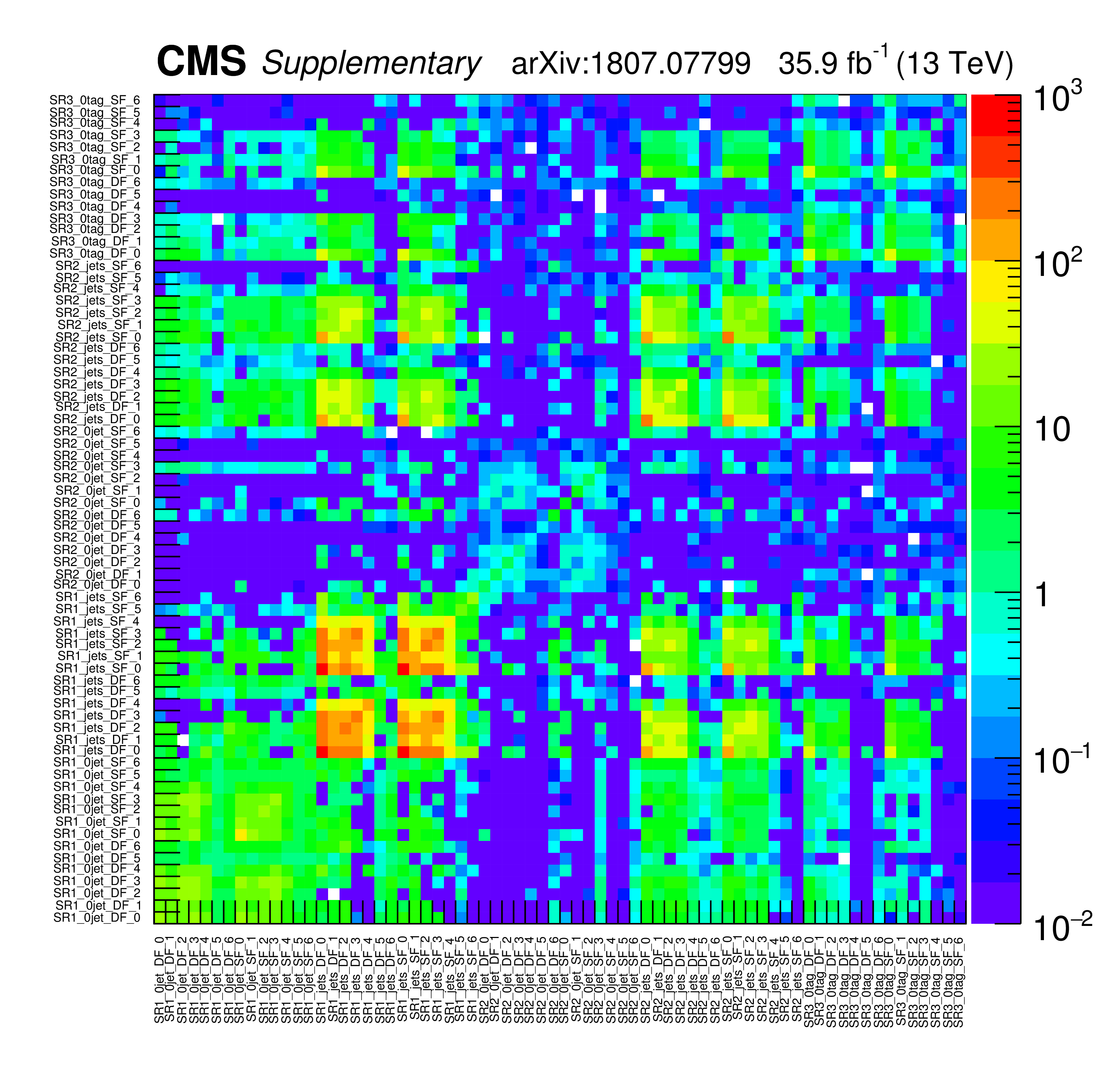
png pdf root	Additional Figure 2: Covariance matrix for the background between the signal regions used in the chargino pair production search.
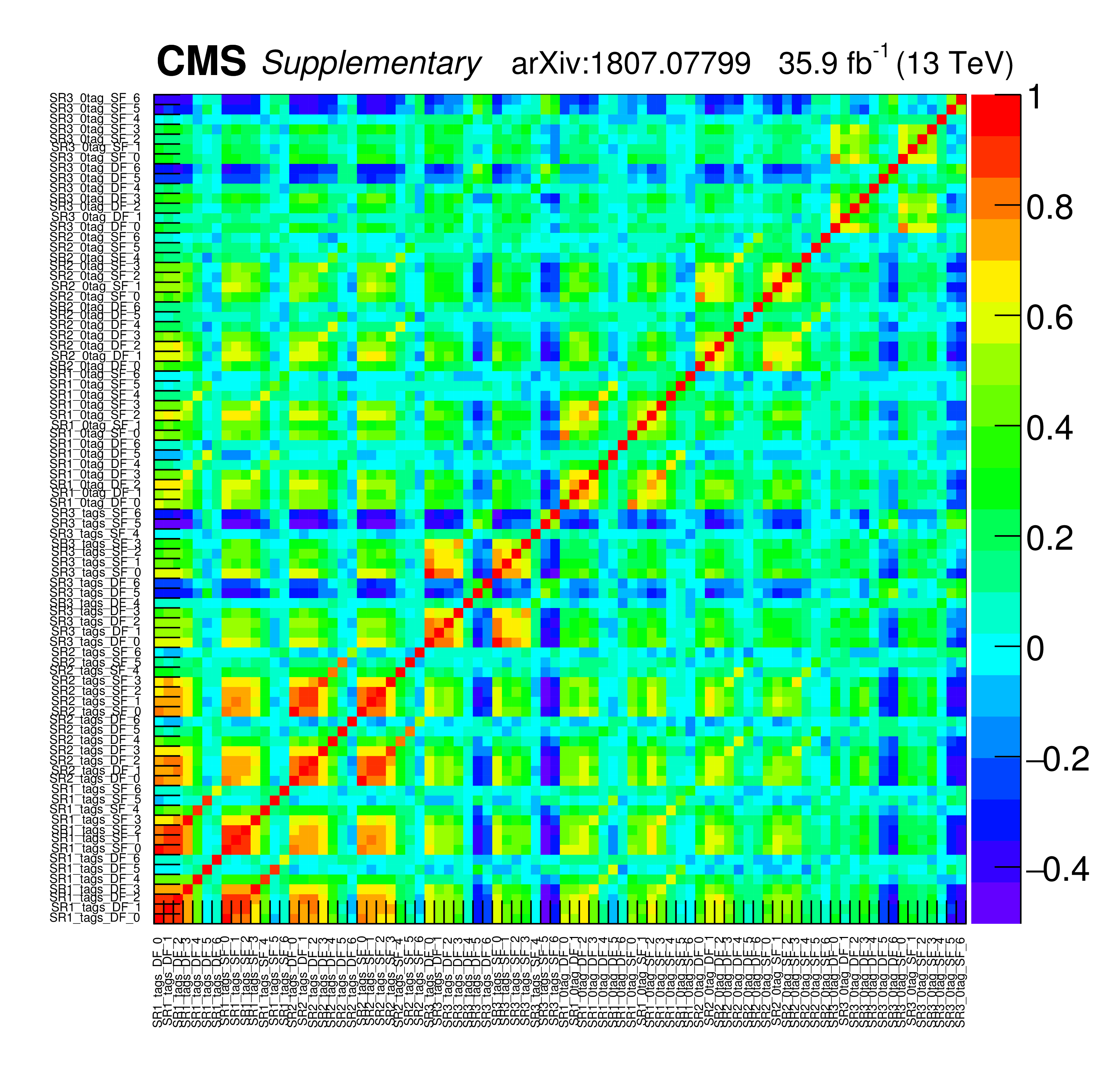
png pdf root	Additional Figure 3: Correlation matrix for the background between the signal regions used in the top squark pair production search.
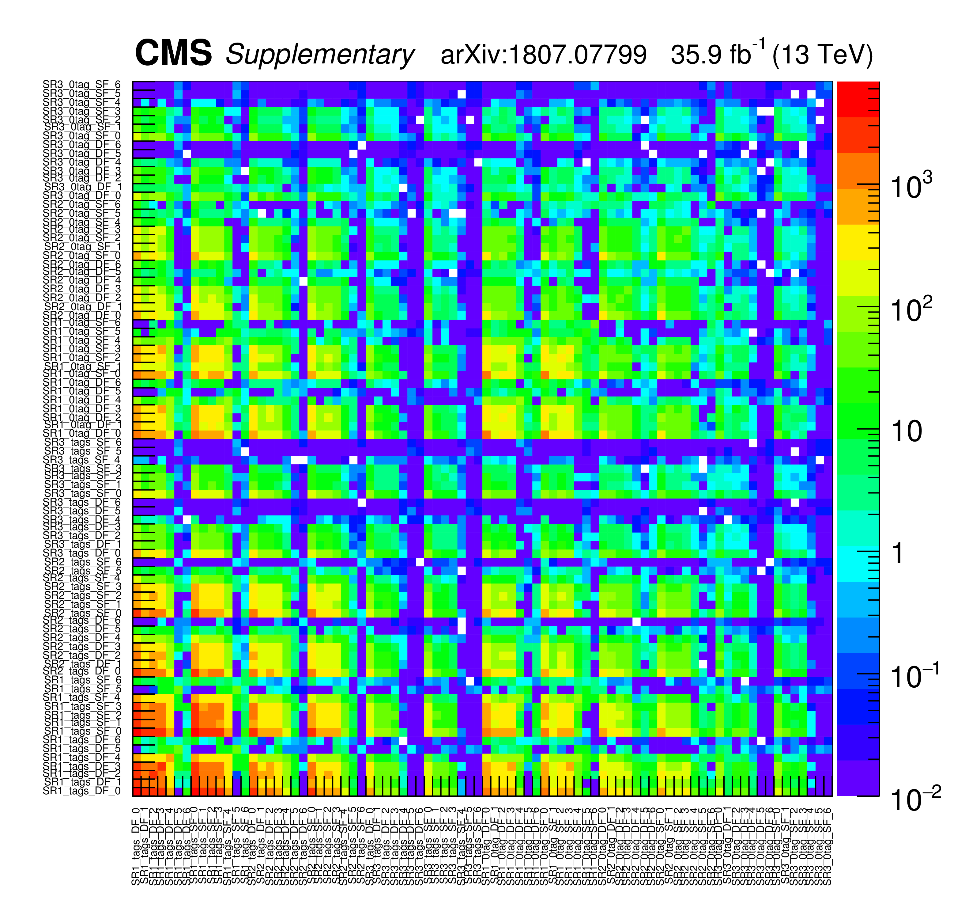
png pdf root	Additional Figure 4: Covariance matrix for the background between the signal regions used in the top squark pair production search.

Additional Tables
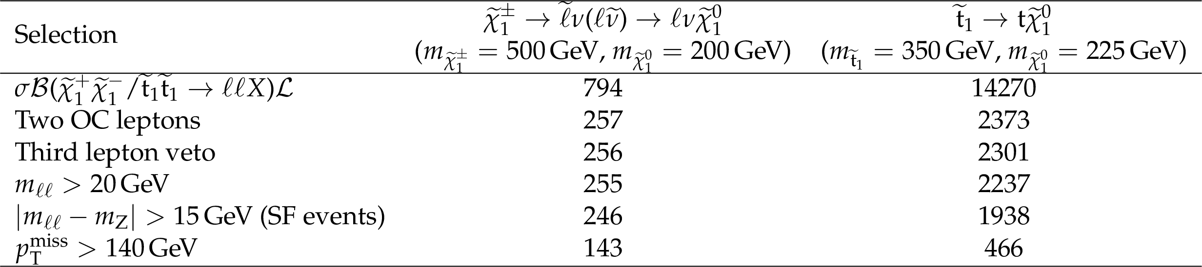
png pdf	Additional Table 1: Expected signal yields at different stages of the baseline event selection for two representative signal points, one for chargino pair production and one for top squark pair production. The yields are normalized to an integrated luminosity of 35.9 fb$^{-1}$.
png pdf	Additional Table 2: Expected yields of DF (the upper half of Table) and SF (the lower half) events in the signal regions used in the chargino search, for a reference ${{\tilde{\chi}^\pm _{1}} \to {\tilde{\ell}}\nu \text (\ell {\tilde{\nu}} \text )\to \ell \nu {\tilde{\chi}^{0}_{1}}}$ signal with $ {m_{{\tilde{\chi}^\pm _{1}}}} = $ 500 GeV and $ {m_{{\tilde{\chi}^{0}_{1}}}} = $ 200 GeV. The yields are normalized to an integrated luminosity of 35.9 fb$^{-1}$. Quoted uncertainties are statistical only.
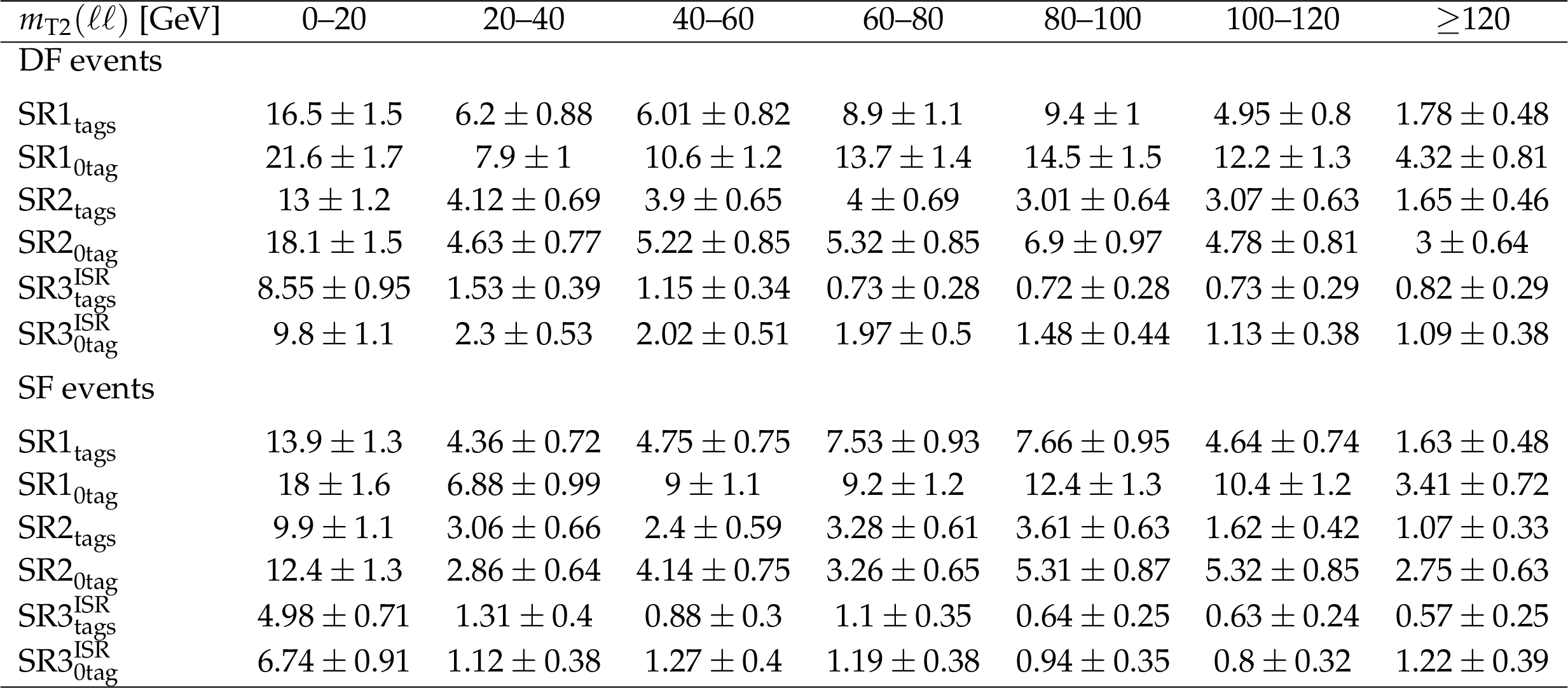
png pdf	Additional Table 3: Expected yields of DF (the upper half of Table) and SF (the lower half) events in the signal regions used in the top squark search, for a reference $ {\tilde{\mathrm {t}}_1} \to {\mathrm {t}} {\tilde{\chi}^{0}_{1}} $ signal with $ {m_{{\tilde{\mathrm {t}}_1}}} = $ 350 GeV and $ {m_{{\tilde{\chi}^{0}_{1}}}} = $ 225 GeV. The yields are normalized to an integrated luminosity of 35.9 fb$^{-1}$. Quoted uncertainties are statistical only.

References
1	E. Gildener and S. Weinberg	Symmetry breaking and scalar bosons	PRD 13 (1976) 3333
2	G. 't Hooft	Naturalness, chiral symmetry, and spontaneous chiral symmetry breaking	NATO Sci. Ser. B 59 (1980) 135
3	G. Bertone, D. Hooper, and J. Silk	Particle dark matter: evidence, candidates and constraints	PR 405 (2005) 279	hep-ph/0404175
4	J. L. Feng	Dark matter candidates from particle physics and methods of detection	Ann. Rev. Astron. Astrophys. 48 (2010) 495	1003.0904
5	T. A. Porter, R. P. Johnson, and P. W. Graham	Dark matter searches with astroparticle data	Ann. Rev. Astron. Astrophys. 49 (2011) 155	1104.2836
6	P. Ramond	Dual theory for free fermions	PRD 3 (1971) 2415
7	Y. A. Golfand and E. P. Likhtman	Extension of the algebra of Poincar$ \'e $ group generators and violation of P invariance	JEPTL 13 (1971)323
8	A. Neveu and J. H. Schwarz	Factorizable dual model of pions	NPB 31 (1971) 86
9	D. V. Volkov and V. P. Akulov	Possible universal neutrino interaction	JEPTL 16 (1972)438
10	J. Wess and B. Zumino	A Lagrangian model invariant under supergauge transformations	PLB 49 (1974) 52
11	J. Wess and B. Zumino	Supergauge transformations in four dimensions	NPB 70 (1974) 39
12	P. Fayet	Supergauge invariant extension of the Higgs mechanism and a model for the electron and its neutrino	NPB 90 (1975) 104
13	H. P. Nilles	Supersymmetry, supergravity and particle physics	Phys. Rep. 110 (1984) 1
14	S. P. Martin	A Supersymmetry primer	Advanced Series on Directions in High Energy Physics 18 (2016) 1	hep-ph/9709356
15	E. Witten	Dynamical breaking of supersymmetry	NPB 188 (1981) 513
16	S. Dimopoulos and H. Georgi	Softly broken supersymmetry and SU(5)	NPB 193 (1981) 150
17	Kaul, R. K. and Majumdar, P.	Cancellation of quadratically divergent mass corrections in globally supersymmetric spontaneously broken gauge theories	NPB 199 (1982) 36
18	G. R. Farrar and P. Fayet	Phenomenology of the production, decay, and detection of new hadronic states associated with supersymmetry	PLB 76 (1978) 575
19	CMS Collaboration	The CMS experiment at the CERN LHC	JINST 3 (2008) S08004	CMS-00-001
20	J. Alwall, P. Schuster, and N. Toro	Simplified models for a first characterization of new physics at the LHC	PRD 79 (2009) 075020	0810.3921
21	J. Alwall, M.-P. Le, M. Lisanti, and J. G. Wacker	Model-independent jets plus missing energy searches	PRD 79 (2009) 015005	0809.3264
22	D. Alves et al.	Simplified models for LHC new physics searches	JPG 39 (2012) 105005	1105.2838
23	CMS Collaboration	Searches for electroweak production of charginos, neutralinos, and sleptons decaying to leptons and W, Z, and Higgs bosons in pp collisions at 8 TeV	EPJC 74 (2014) 3036	CMS-SUS-13-006 1405.7570
24	ATLAS Collaboration	Search for direct production of charginos, neutralinos and sleptons in final states with two leptons and missing transverse momentum in pp collisions at $ \sqrt{s} = $ 8 TeV with the ATLAS detector	JHEP 05 (2014) 071	1403.5294
25	ATLAS Collaboration	Search for the direct production of charginos, neutralinos and staus in final states with at least two hadronically decaying taus and missing transverse momentum in pp collisions at $ \sqrt{s} = $ 8 TeV with the ATLAS detector	JHEP 10 (2014) 096	1407.0350
26	ATLAS Collaboration	Search for the electroweak production of supersymmetric particles in $ \sqrt{s} = $ 8 TeV pp collisions with the ATLAS detector	PRD 93 (2016) 052002	1509.07152
27	ATLAS Collaboration	Search for the direct production of charginos and neutralinos in final states with tau leptons in $ \sqrt{s} = $ 13 TeV pp collisions with the ATLAS detector	EPJC 78 (2018) 154	1708.07875
28	ATLAS Collaboration	Search for electroweak production of supersymmetric states in scenarios with compressed mass spectra at $ \sqrt{s}= $ 13 TeV with the ATLAS detector	PRD 97 (2018) 052010	1712.08119
29	ATLAS Collaboration	Search for electroweak production of supersymmetric particles in final states with two or three leptons at $ \sqrt{s}= $ 13 TeV with the ATLAS detector	Submitted to EPJC	1803.02762
30	CMS Collaboration	Search for top squarks and dark matter particles in opposite-charge dilepton final states at $ \sqrt{s} = $ 13 TeV	PRD 97 (2018) 032009	CMS-SUS-17-001 1711.00752
31	CMS Collaboration	Search for top squark pair production in pp collisions at $ \sqrt{s} = $ 13 TeV using single lepton events	JHEP 10 (2017) 019	CMS-SUS-16-051 1706.04402
32	CMS Collaboration	Search for direct production of supersymmetric partners of the top quark in the all-jets final state in proton-proton collisions at $ \sqrt{s} = $ 13 TeV	JHEP 10 (2017) 005	CMS-SUS-16-049 1707.03316
33	ATLAS Collaboration	Search for a scalar partner of the top quark in the jets plus missing transverse momentum final state at $ \sqrt{s}= $ 13 TeV with the ATLAS detector	JHEP 12 (2017) 085	1709.04183
34	ATLAS Collaboration	Search for top-squark pair production in final states with one lepton, jets, and missing transverse momentum using $ 36 fb$^{-1} of $ \sqrt{s}= $ 13 TeV pp collision data with the ATLAS detector	Submitted to JHEP	1711.11520
35	ATLAS Collaboration	Search for direct top squark pair production in final states with two leptons in $ \sqrt{s}= $ 13 TeV pp collisions with the ATLAS detector	EPJC 77 (2017) 898	1708.03247
36	CMS Collaboration	The CMS trigger system	JINST 12 (2017) P01020	CMS-TRG-12-001 1609.02366
37	P. Nason	A new method for combining NLO QCD with shower Monte Carlo algorithms	JHEP 11 (2004) 040	hep-ph/0409146
38	S. Frixione, P. Nason, and C. Oleari	Matching NLO QCD computations with parton shower simulations: the POWHEG method	JHEP 11 (2007) 070	0709.2092
39	S. Alioli, P. Nason, C. Oleari, and E. Re	A general framework for implementing NLO calculations in shower Monte Carlo programs: the POWHEG BOX	JHEP 06 (2010) 043	1002.2581
40	M. Czakon and A. Mitov	Top++: A program for the calculation of the top-pair cross-section at hadron colliders	CPC 185 (2014) 2930	1112.5675
41	E. Re	Single-top Wt-channel production matched with parton showers using the POWHEG method	EPJC 71 (2011) 1547	1009.2450
42	Kidonakis, N.	NNLL threshold resummation for top-pair and single-top production	Phys. Part. Nucl. 45 (2014) 714	1210.7813
43	Melia, T. and Nason, P. and Rontsch, R. and Zanderighi, G.	W$ ^+ $W$ ^- $, WZ and ZZ production in the POWHEG BOX	JHEP 11 (2011) 078	1107.5051
44	P. Nason and G. Zanderighi	W$ ^+ $W$ ^- $, WZ and ZZ production in the POWHEG-BOX-V2	EPJC 74 (2014) 2702	1311.1365
45	T. Gehrmann et al.	W$ ^{+} $W$ ^{-} $ production at hadron colliders in NNLO QCD	PRL 113 (2014) 212001	1408.5243
46	CMS Collaboration	Measurements of properties of the Higgs boson decaying into the four-lepton final state in pp collisions at $ \sqrt{s}= $ 13 TeV	JHEP 11 (2017) 047	CMS-HIG-16-041 1706.09936
47	J. M. Campbell and R. K. Ellis	MCFM for the Tevatron and the LHC	NPPS 205 (2010) 10	1007.3492
48	F. Caola, K. Melnikov, R. Rtsch, and L. Tancredi	QCD corrections to W$ ^+ $W$ ^{-} $ production through gluon fusion	PLB 754 (2016) 275	1511.08617
49	J. Alwall et al.	The automated computation of tree-level and next-to-leading order differential cross sections, and their matching to parton shower simulations	JHEP 07 (2014) 079	1405.0301
50	R. Gavin, Y. Li, F. Petriello, and S. Quackenbush	FEWZ 2.0: A code for hadronic Z production at next-to-next-to-leading order	CPC 182 (2011) 2388	1011.3540
51	M. V. Garzelli, A. Kardos, C. G. Papadopoulos, and Z. Trocsanyi	$ \mathrm{t\bar{t}} $W$ ^{\pm} $ and $ \mathrm{t\bar{t}} $Z hadroproduction at NLO accuracy in QCD with parton shower and hadronization effects	JHEP 11 (2012) 056	1208.2665
52	LHC Higgs Cross Section Working Group	Handbook of LHC Higgs cross sections: 3. Higgs Properties	CERN (2013)	1307.1347
53	W. Beenakker et al.	Production of charginos, neutralinos, and sleptons at hadron colliders	PRL 83 (1999) 3780	hep-ph/9906298
54	B. Fuks, M. Klasen, D. R. Lamprea, and M. Rothering	Gaugino production in proton-proton collisions at a center-of-mass energy of 8 TeV	JHEP 10 (2012) 081	1207.2159
55	B. Fuks, M. Klasen, D. R. Lamprea, and M. Rothering	Precision predictions for electroweak superpartner production at hadron colliders with $ \sc $ resummino	EPJC 73 (2013) 2480	1304.0790
56	W. Beenakker, R. Hopker, M. Spira, and P. M. Zerwas	Squark and gluino production at hadron colliders	NPB 492 (1997) 51	hep-ph/9610490
57	A. Kulesza and L. Motyka	Threshold resummation for squark-antisquark and gluino-pair production at the LHC	PRL 102 (2009) 111802	0807.2405
58	A. Kulesza and L. Motyka	Soft gluon resummation for the production of gluino-gluino and squark-antisquark pairs at the LHC	PRD 80 (2009) 095004	0905.4749
59	W. Beenakker et al.	Soft-gluon resummation for squark and gluino hadroproduction	JHEP 12 (2009) 041	0909.4418
60	W. Beenakker et al.	Squark and gluino hadroproduction	Int. J. Mod. Phys. A 26 (2011) 2637	1105.1110
61	C. Borschensky et al.	Squark and gluino production cross sections in pp collisions at $ \sqrt{s} = $ 13, 14, 33 and 100 TeV	EPJC 74 (2014) 3174	1407.5066
62	NNPDF Collaboration	Parton distributions for the LHC Run II	JHEP 04 (2015) 040	1410.8849
63	T. Sjostrand et al.	An Introduction to PYTHIA 8.2	CPC 191 (2015) 159	1410.3012
64	CMS Collaboration	Event generator tunes obtained from underlying event and multiparton scattering measurements	EPJC 76 (2016) 155	CMS-GEN-14-001 1512.00815
65	CMS Collaboration	Investigations of the impact of the parton shower tuning in Pythia 8 in the modelling of $ \mathrm{t\bar{t}} $ at $ \sqrt{s}= $ 8 TeV and 13 TeV	CDS
66	A. Kalogeropoulos and J. Alwall	The SysCalc code: A tool to derive theoretical systematic uncertainties		1801.08401
67	GEANT4 Collaboration	$ GEANT4--a $ simulation toolkit	NIMA 506 (2003) 250
68	S. Abdullin et al.	The Fast Simulation of the CMS detector at LHC	in J. Phys. Conf. Ser., volume 331, p. 032049 2011
69	CMS Collaboration	Search for top-squark pair production in the single-lepton final state in pp collisions at $ \sqrt{s}= $ 8 TeV	EPJC 73 (2013) 2677	CMS-SUS-13-011 1308.1586
70	CMS Collaboration	Particle-flow reconstruction and global event description with the CMS detector	JINST 12 (2017) P10003	CMS-PRF-14-001 1706.04965
71	M. Cacciari, G. P. Salam, and G. Soyez	The anti-$ {k_{\mathrm{T}}} $ jet clustering algorithm	JHEP 04 (2008) 063	0802.1189
72	M. Cacciari, G. P. Salam, and G. Soyez	FastJet user manual	EPJC 72 (2012) 1896	1111.6097
73	CMS Collaboration	Performance of CMS muon reconstruction in pp collision events at $ \sqrt{s} = $ 7 TeV	JINST 7 (2012) P10002	CMS-MUO-10-004 1206.4071
74	CMS Collaboration	Performance of electron reconstruction and selection with the CMS detector in proton-proton collisions at $ \sqrt{s} = $ 8 TeV	JINST 10 (2015) P06005	CMS-EGM-13-001 1502.02701
75	CMS Collaboration	Jet energy scale and resolution in the CMS experiment in pp collisions at 8 TeV	JINST 12 (2017) P02014	CMS-JME-13-004 1607.03663
76	CMS Collaboration	Identification of heavy-flavour jets with the CMS detector in pp collisions at 13 TeV	JINST 13 (2018) P05011	CMS-BTV-16-002 1712.07158
77	CMS Collaboration	Performance of the CMS missing transverse energy reconstruction in pp data at $ \sqrt{s}= $ 8 TeV	JINST 10 (2015) P02006	CMS-JME-13-003 1411.0511
78	C. G. Lester and D. J. Summers	Measuring masses of semiinvisibly decaying particles pair produced at hadron colliders	PLB 463 (1999) 99	hep-ph/9906349
79	CMS Collaboration	CMS luminosity measurements for the 2016 data-taking period	CMS-PAS-LUM-17-001	CMS-PAS-LUM-17-001
80	CMS Collaboration	Measurement of differential cross sections for top quark pair production using the lepton+jets final state in proton-proton collisions at 13 TeV	PRD 95 (2017) 092001	CMS-TOP-16-008 1610.04191
81	CMS Collaboration	Measurement of the differential cross section for top quark pair production in pp collisions at $ \sqrt{s}= $ 8 TeV	EPJC 75 (2015) 542	CMS-TOP-12-028 1505.04480
82	CMS Collaboration	Measurement of the $ \mathrm{t\bar{t}} $ production cross section in the all-jets final state in pp collisions at $ \sqrt{s}= $ 8 TeV	EPJC 76 (2016) 128	CMS-TOP-14-018 1509.06076
83	T. Junk	Confidence level computation for combining searches with small statistics	NIMA 434 (1999) 435	hep-ex/9902006
84	A. L. Read	Presentation of search results: The CL$ _{\text{s}} $ technique	JPG 28 (2002) 2693
85	G. Cowan, K. Cranmer, E. Gross, and O. Vitells	Asymptotic formulae for likelihood-based tests of new physics	EPJC 71 (2011) 1554	1007.1727

Compact Muon Solenoid LHC, CERN

© Copyright CERN 2018 for the benefit of the CMS Collaboration