

Compact Muon Solenoid
LHC, CERN
| CMS-SUS-19-004 ; CERN-EP-2021-015 | ||
| Search for top squarks in final states with two top quarks and several light-flavor jets in proton-proton collisions at $\sqrt{s} = $ 13 TeV | ||
| CMS Collaboration | ||
| 13 February 2021 | ||
| Phys. Rev. D 104 (2021) 032006 | ||
| Abstract: Many new physics models, including versions of supersymmetry characterized by $R$-parity violation (RPV), compressed mass spectra, long decay chains, or additional hidden sectors, predict the production of events with top quarks, low missing transverse momentum, and many additional quarks or gluons. The results of a search for new physics in events with two top quarks and additional jets are reported. The search is performed using events with at least seven jets and exactly one electron or muon. No requirement on missing transverse momentum is imposed. The study is based on a sample of proton-proton collisions at $\sqrt{s} = $ 13 TeV corresponding to 137 fb$^{-1}$ of integrated luminosity collected with the CMS detector at the LHC in 2016-2018. The data are used to determine best fit values and upper limits on the cross section for pair production of top squarks in scenarios of RPV and stealth supersymmetry. Top squark masses up to 670 (870) GeV are excluded at 95% confidence level for the RPV (stealth) scenario, and the maximum observed local significance is 2.8 standard deviations for the RPV scenario with top squark mass of 400 GeV. | ||
| Links: e-print arXiv:2102.06976 [hep-ex] (PDF) ; CDS record ; inSPIRE record ; HepData record ; CADI line (restricted) ; | ||
| Figures & Tables | Summary | Additional Figures & Tables | References | CMS Publications |
|---|
|
Additional information on efficiencies needed for reinterpretation of these results are available here A Github repository is available and details how to setup and run the neural network used for the analysis. Example input and output are also provided. |
| Figures | |
png pdf |
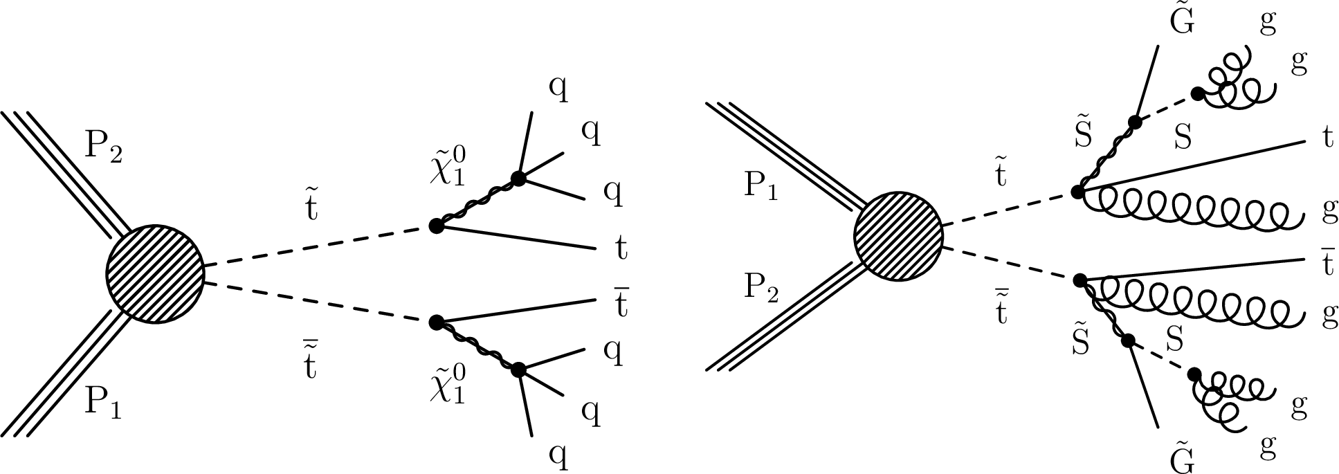
Figure 1:
Diagrams of top squark pair production with decays to top quarks and additional light-flavor quarks for the RPV SUSY model (left) and with decays to top quarks and gluons for the stealth $\mathrm{S}\mathrm{Y}\overline{\mathrm{Y}}$ model (right). |
png pdf |
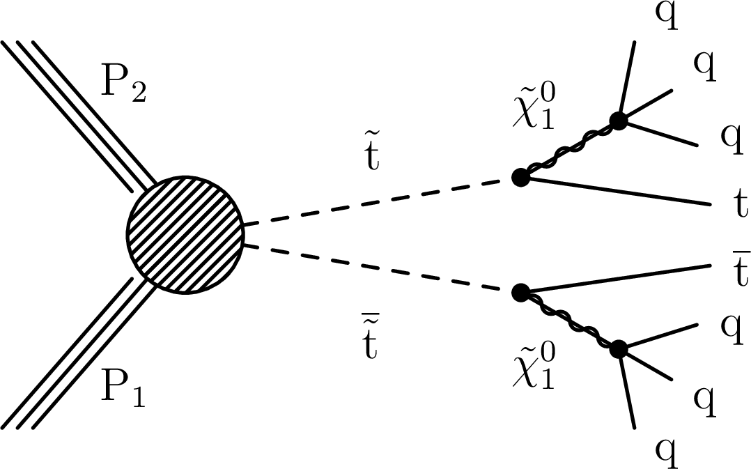
Figure 1-a:
Diagram of top squark pair production with decays to top quarks and additional light-flavor quarks for the RPV SUSY model. |
png pdf |
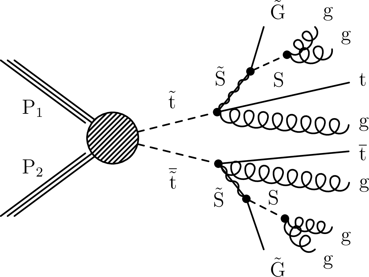
Figure 1-b:
Diagram of top squark pair production with decays to top quarks and gluons for the stealth $\mathrm{S}\mathrm{Y}\overline{\mathrm{Y}}$ model. |

png pdf |
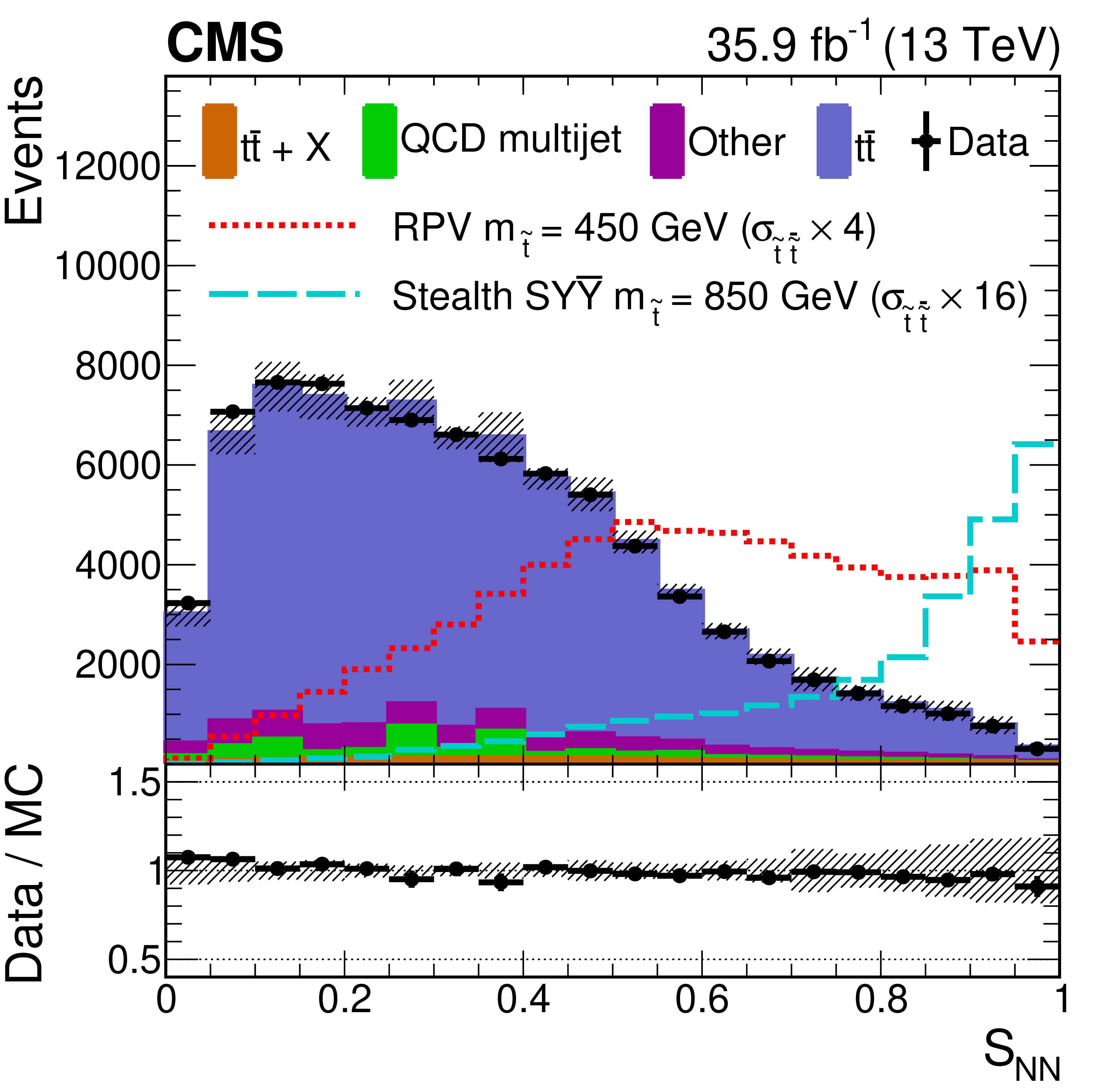
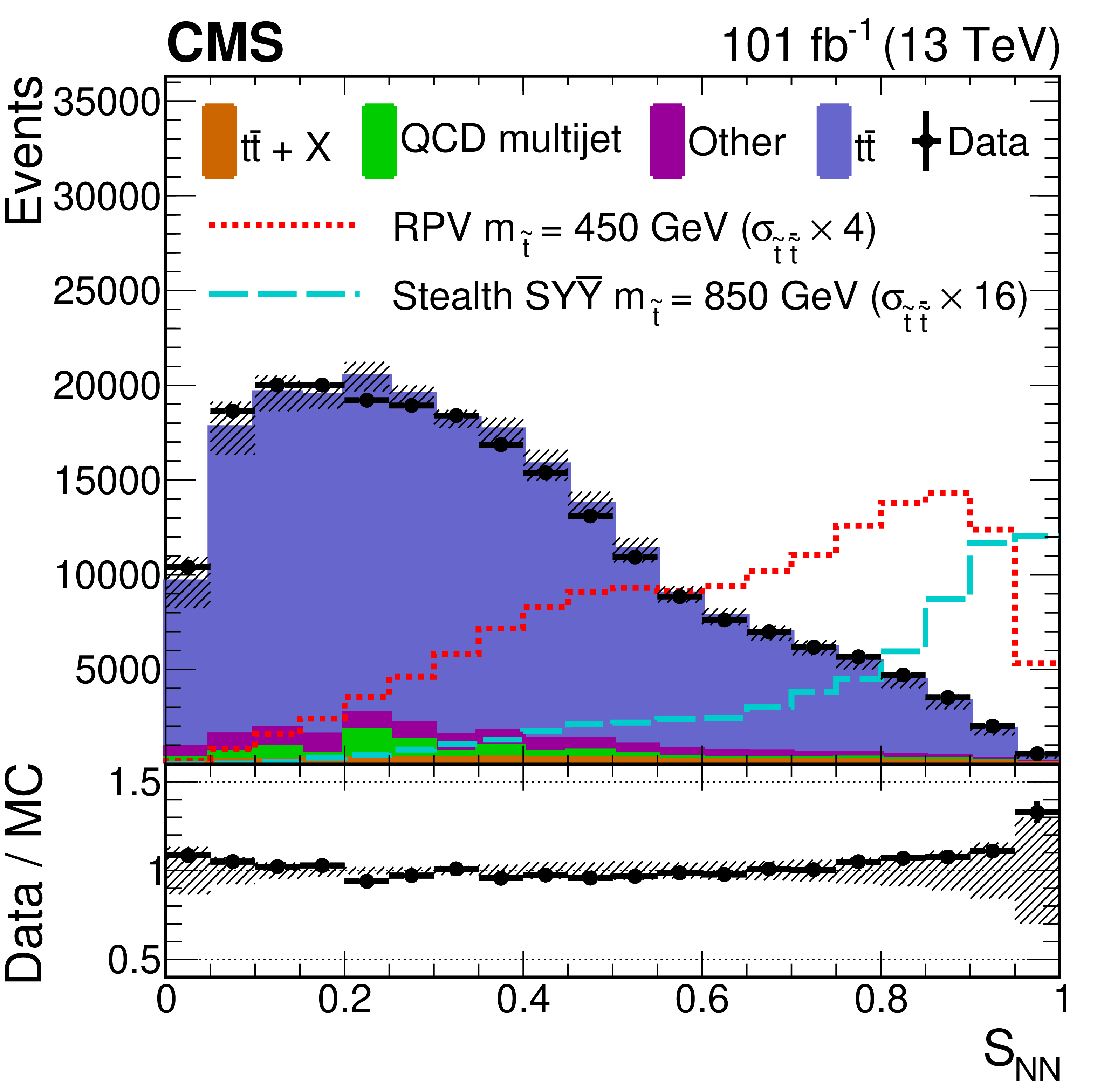
Figure 2:
The ${S_\mathrm {NN}}$ distributions for 2016 (left) and 2017+2018 (right) show the data in the SR (black points); simulated background normalized to the number of data events (filled histograms); RPV signal model with ${m_{\tilde{\mathrm{t}}}}$ of 450 GeV (red short dashed); and stealth $\mathrm{S}\mathrm{Y}\overline{\mathrm{Y}}$ signal model with ${m_{\tilde{\mathrm{t}}}}$ of 850 GeV (cyan long dashed). All events shown pass the SR event selection. The band on the total background histogram denotes the dominant systematic uncertainties related to the modeling of ${H_{\mathrm {T}}}$, jet mass, and jet ${p_{\mathrm {T}}}$ in the ${\mathrm{t} \mathrm{\bar{t}}}$ simulation, as well as the statistical uncertainty for the non-${\mathrm{t} \mathrm{\bar{t}}}$ components. The lower panel shows the ratio of the number of data events to the number of normalized simulated events with the band representing the difference between the nominal ratio and the ratio obtained when varying the total background by its uncertainty. |
png pdf |
Figure 2-a:
The ${S_\mathrm {NN}}$ distribution for 2016 shows the data in the SR (black points); simulated background normalized to the number of data events (filled histograms); RPV signal model with ${m_{\tilde{\mathrm{t}}}}$ of 450 GeV (red short dashed); and stealth $\mathrm{S}\mathrm{Y}\overline{\mathrm{Y}}$ signal model with ${m_{\tilde{\mathrm{t}}}}$ of 850 GeV (cyan long dashed). All events shown pass the SR event selection. The band on the total background histogram denotes the dominant systematic uncertainties related to the modeling of ${H_{\mathrm {T}}}$, jet mass, and jet ${p_{\mathrm {T}}}$ in the ${\mathrm{t} \mathrm{\bar{t}}}$ simulation, as well as the statistical uncertainty for the non-${\mathrm{t} \mathrm{\bar{t}}}$ components. The lower panel shows the ratio of the number of data events to the number of normalized simulated events with the band representing the difference between the nominal ratio and the ratio obtained when varying the total background by its uncertainty. |
png pdf |
Figure 2-b:
The ${S_\mathrm {NN}}$ distribution for 2017+2018 shows the data in the SR (black points); simulated background normalized to the number of data events (filled histograms); RPV signal model with ${m_{\tilde{\mathrm{t}}}}$ of 450 GeV (red short dashed); and stealth $\mathrm{S}\mathrm{Y}\overline{\mathrm{Y}}$ signal model with ${m_{\tilde{\mathrm{t}}}}$ of 850 GeV (cyan long dashed). All events shown pass the SR event selection. The band on the total background histogram denotes the dominant systematic uncertainties related to the modeling of ${H_{\mathrm {T}}}$, jet mass, and jet ${p_{\mathrm {T}}}$ in the ${\mathrm{t} \mathrm{\bar{t}}}$ simulation, as well as the statistical uncertainty for the non-${\mathrm{t} \mathrm{\bar{t}}}$ components. The lower panel shows the ratio of the number of data events to the number of normalized simulated events with the band representing the difference between the nominal ratio and the ratio obtained when varying the total background by its uncertainty. |
png pdf |
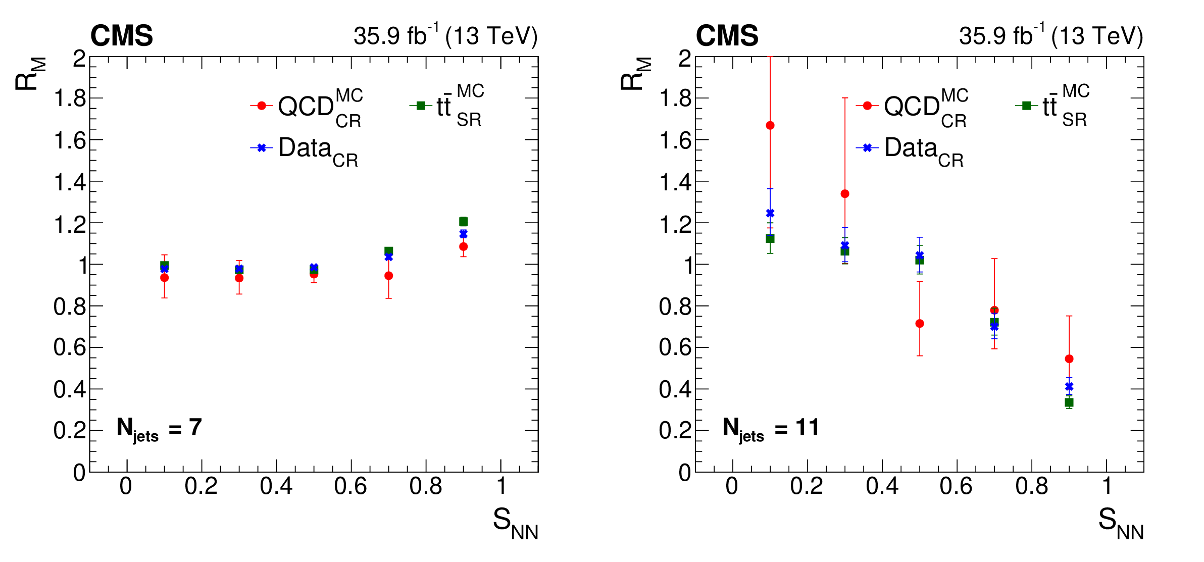
Figure 3:
Distribution in ${S_\mathrm {NN}}$ of the ratio $R_M$, as defined in the text, for $ {N_\text {jets}} = $ 7 (left) and 11 (right), for the QCD CR simulation (red circles), the ${\mathrm{t} \mathrm{\bar{t}}}$ SR simulation (green squares), and data in the CR (blue crosses) for the 2016 data period. The error bars indicate the statistical uncertainty in the value of $R_M$. |
png pdf |
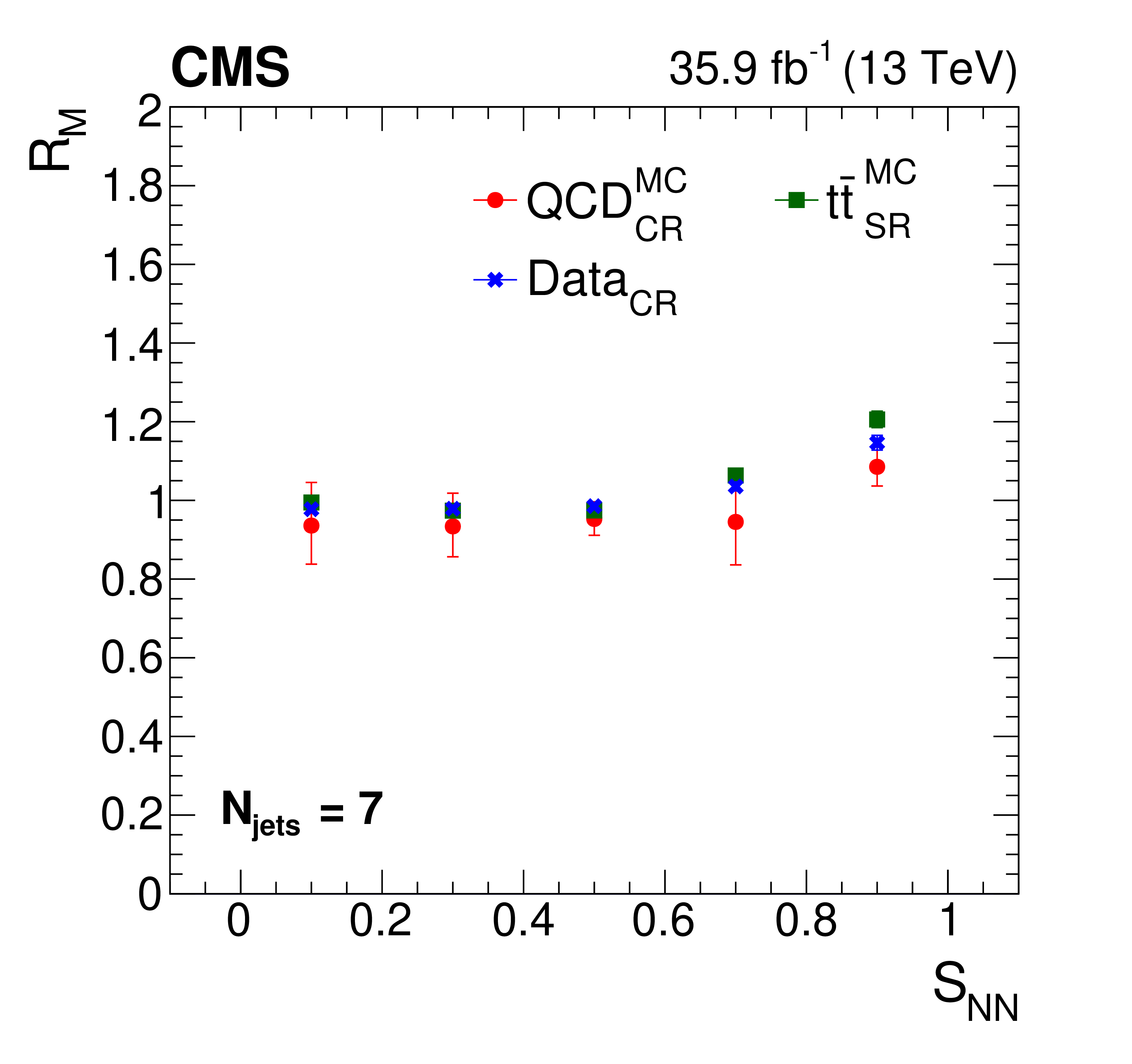
Figure 3-a:
Distribution in ${S_\mathrm {NN}}$ of the ratio $R_M$, as defined in the text, for $ {N_\text {jets}} = $ 7, for the QCD CR simulation (red circles), the ${\mathrm{t} \mathrm{\bar{t}}}$ SR simulation (green squares), and data in the CR (blue crosses) for the 2016 data period. The error bars indicate the statistical uncertainty in the value of $R_M$. |
png pdf |
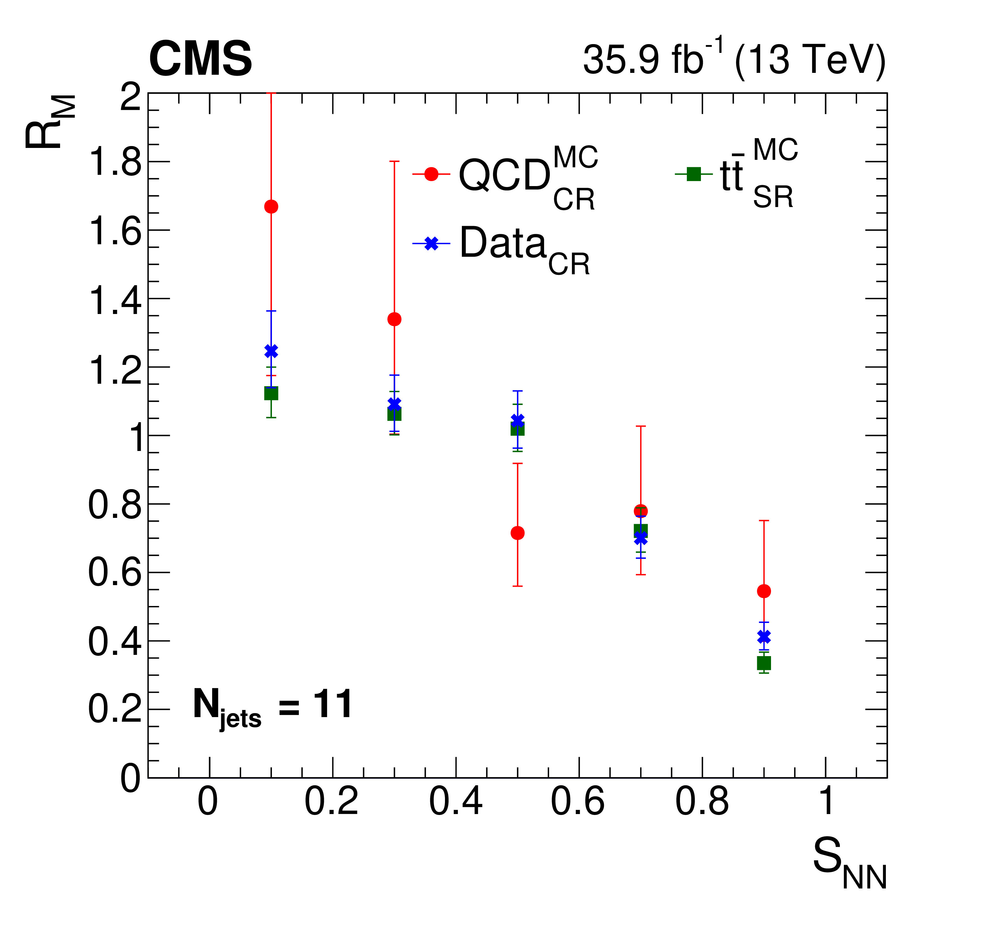
Figure 3-b:
Distribution in ${S_\mathrm {NN}}$ of the ratio $R_M$, as defined in the text, for $ {N_\text {jets}} = $ 11, for the QCD CR simulation (red circles), the ${\mathrm{t} \mathrm{\bar{t}}}$ SR simulation (green squares), and data in the CR (blue crosses) for the 2016 data period. The error bars indicate the statistical uncertainty in the value of $R_M$. |

png pdf |
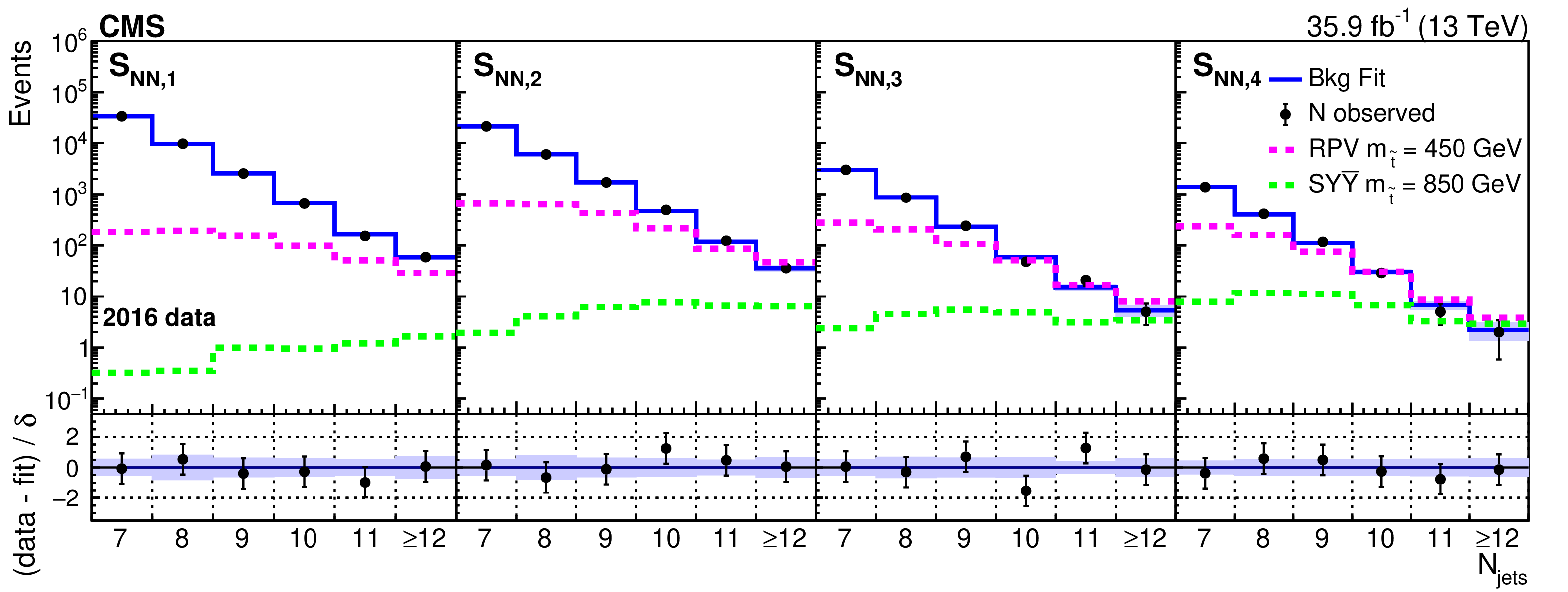
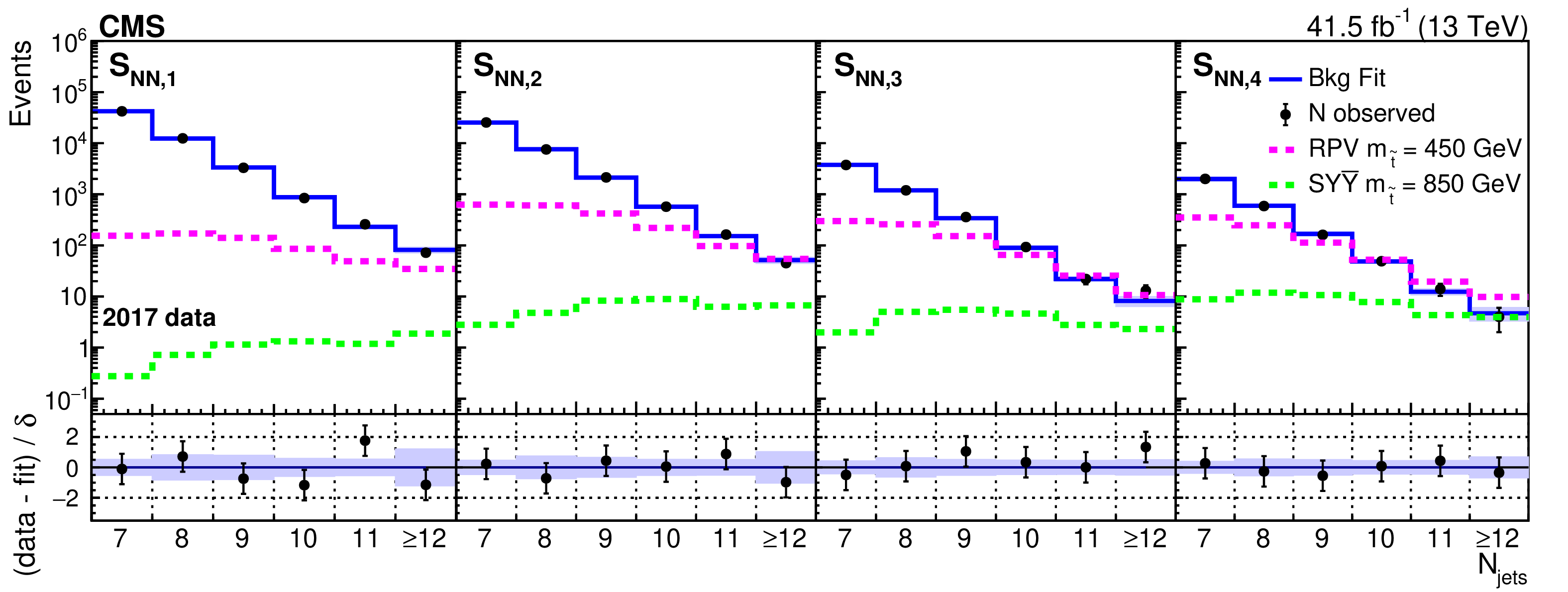
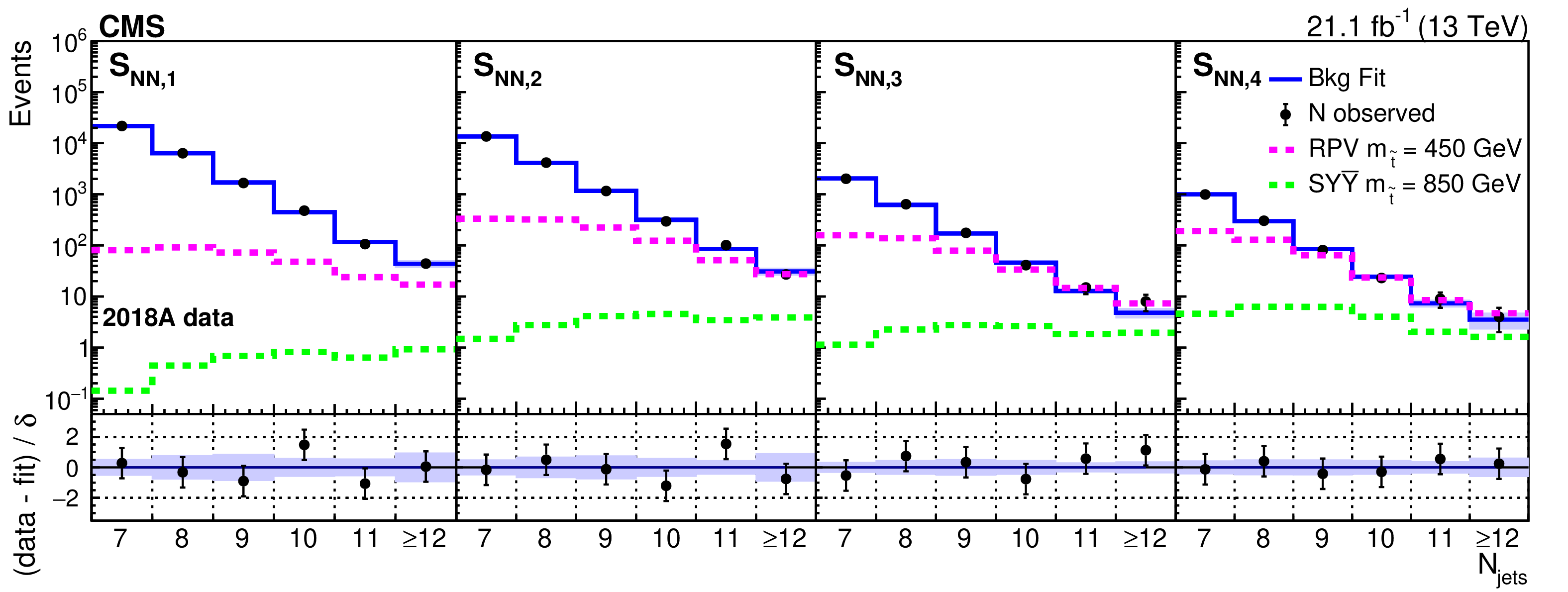
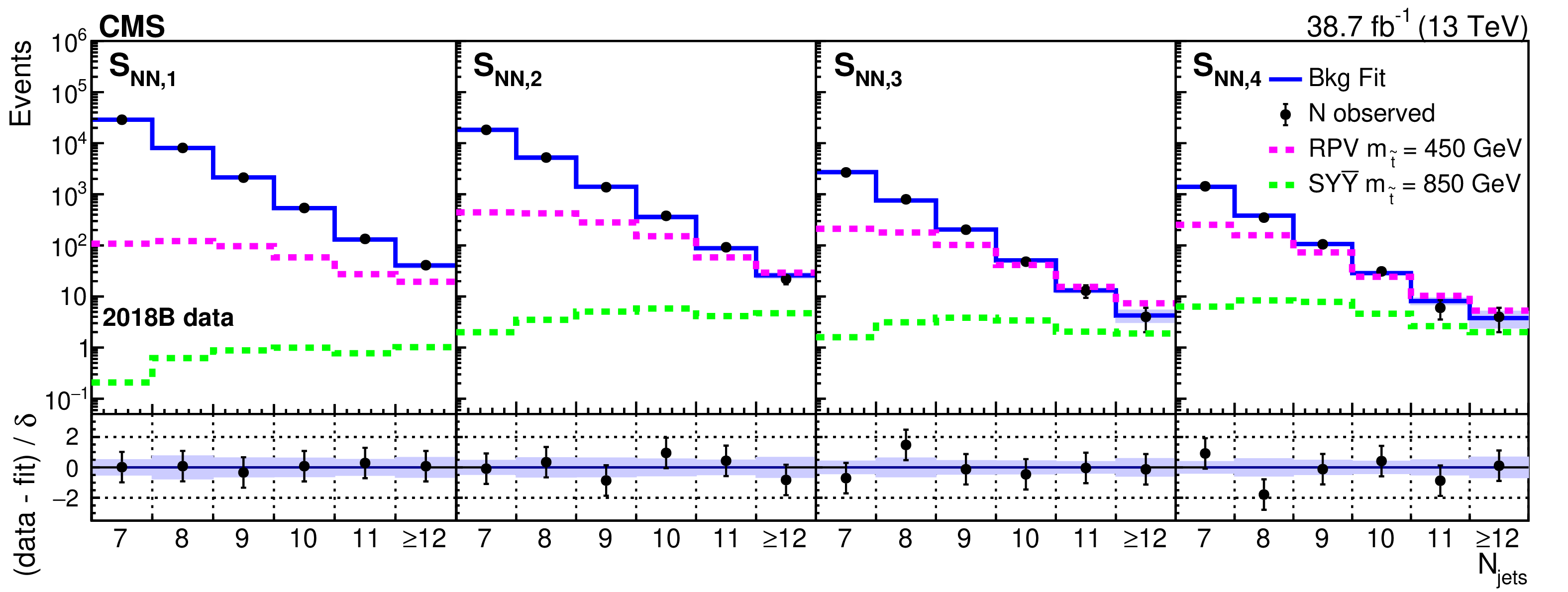
Figure 4:
Fitted background prediction and observed data counts for 2016, 2017, 2018A, and 2018B (from upper to lower rows) as functions of ${N_\text {jets}}$ in each of the four bins in ${S_\mathrm {NN}}$. The signal distributions normalized to the predicted cross section for the RPV model with $ {m_{\tilde{\mathrm{t}}}} = $ 450 GeV and the stealth $\mathrm{S}\mathrm{Y}\overline{\mathrm{Y}}$ model with $ {m_{\tilde{\mathrm{t}}}} = $ 850 GeV are shown for comparison. The lower panel of each plot displays the difference between the number of observed events and the number of events determined by the fit divided by the statistical uncertainty associated with the observed number of events ($\delta $) as black points with error bars denoting $\delta $. The blue band shows the total systematic uncertainty in the fit from all nuisance parameters. |
png pdf root |
Figure 4-a:
Fitted background prediction and observed data counts for 2016 as functions of ${N_\text {jets}}$ in each of the four bins in ${S_\mathrm {NN}}$. The signal distributions normalized to the predicted cross section for the RPV model with $ {m_{\tilde{\mathrm{t}}}} = $ 450 GeV and the stealth $\mathrm{S}\mathrm{Y}\overline{\mathrm{Y}}$ model with $ {m_{\tilde{\mathrm{t}}}} = $ 850 GeV are shown for comparison. The lower panel displays the difference between the number of observed events and the number of events determined by the fit divided by the statistical uncertainty associated with the observed number of events ($\delta $) as black points with error bars denoting $\delta $. The blue band shows the total systematic uncertainty in the fit from all nuisance parameters. |
png pdf root |
Figure 4-b:
Fitted background prediction and observed data counts for 2017 as functions of ${N_\text {jets}}$ in each of the four bins in ${S_\mathrm {NN}}$. The signal distributions normalized to the predicted cross section for the RPV model with $ {m_{\tilde{\mathrm{t}}}} = $ 450 GeV and the stealth $\mathrm{S}\mathrm{Y}\overline{\mathrm{Y}}$ model with $ {m_{\tilde{\mathrm{t}}}} = $ 850 GeV are shown for comparison. The lower panel displays the difference between the number of observed events and the number of events determined by the fit divided by the statistical uncertainty associated with the observed number of events ($\delta $) as black points with error bars denoting $\delta $. The blue band shows the total systematic uncertainty in the fit from all nuisance parameters. |
png pdf root |
Figure 4-c:
Fitted background prediction and observed data counts for 2018A as functions of ${N_\text {jets}}$ in each of the four bins in ${S_\mathrm {NN}}$. The signal distributions normalized to the predicted cross section for the RPV model with $ {m_{\tilde{\mathrm{t}}}} = $ 450 GeV and the stealth $\mathrm{S}\mathrm{Y}\overline{\mathrm{Y}}$ model with $ {m_{\tilde{\mathrm{t}}}} = $ 850 GeV are shown for comparison. The lower panel displays the difference between the number of observed events and the number of events determined by the fit divided by the statistical uncertainty associated with the observed number of events ($\delta $) as black points with error bars denoting $\delta $. The blue band shows the total systematic uncertainty in the fit from all nuisance parameters. |
png pdf root |
Figure 4-d:
Fitted background prediction and observed data counts for 2018B as functions of ${N_\text {jets}}$ in each of the four bins in ${S_\mathrm {NN}}$. The signal distributions normalized to the predicted cross section for the RPV model with $ {m_{\tilde{\mathrm{t}}}} = $ 450 GeV and the stealth $\mathrm{S}\mathrm{Y}\overline{\mathrm{Y}}$ model with $ {m_{\tilde{\mathrm{t}}}} = $ 850 GeV are shown for comparison. The lower panel displays the difference between the number of observed events and the number of events determined by the fit divided by the statistical uncertainty associated with the observed number of events ($\delta $) as black points with error bars denoting $\delta $. The blue band shows the total systematic uncertainty in the fit from all nuisance parameters. |
png pdf |
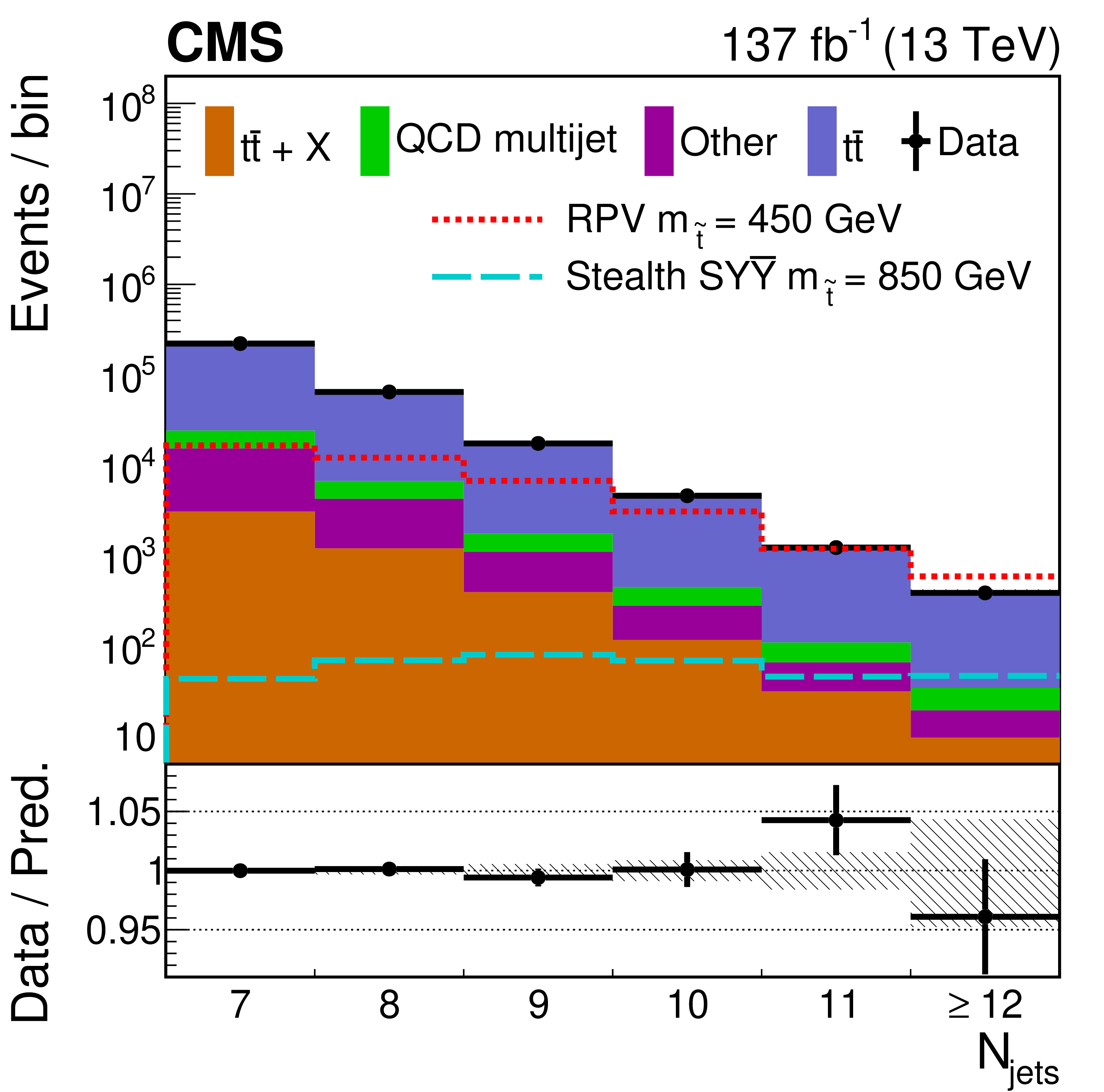
Figure 5:
Background prediction from the background-only fit and observed data counts as a function of ${N_\text {jets}}$ summed over data periods and ${S_\mathrm {NN}}$ bins. Overlaid are expected distributions for the RPV and stealth $\mathrm{S}\mathrm{Y}\overline{\mathrm{Y}}$ models with $ {m_{\tilde{\mathrm{t}}}} = $ 450 and 850 GeV, respectively, normalized according to the top squark pair production cross section. For visualization purposes, the hatched band in the lower panel shows the quadrature sum of all of the uncertainties on the background prediction. |
png pdf |
Figure 6:
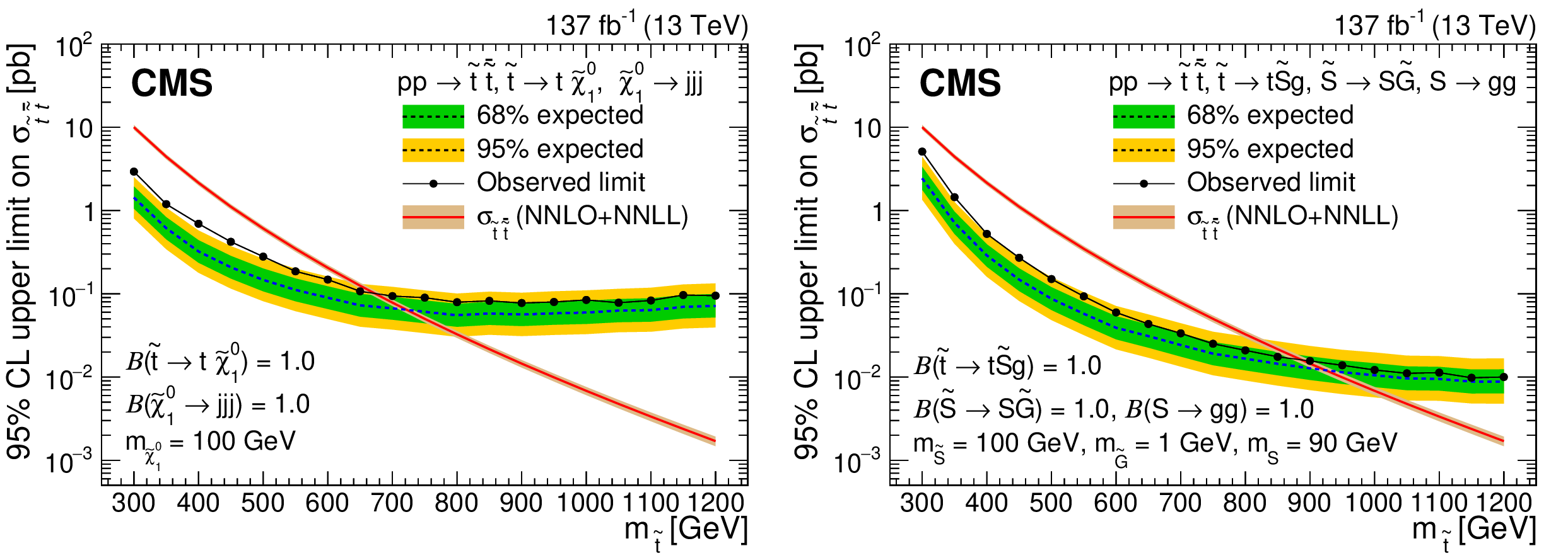
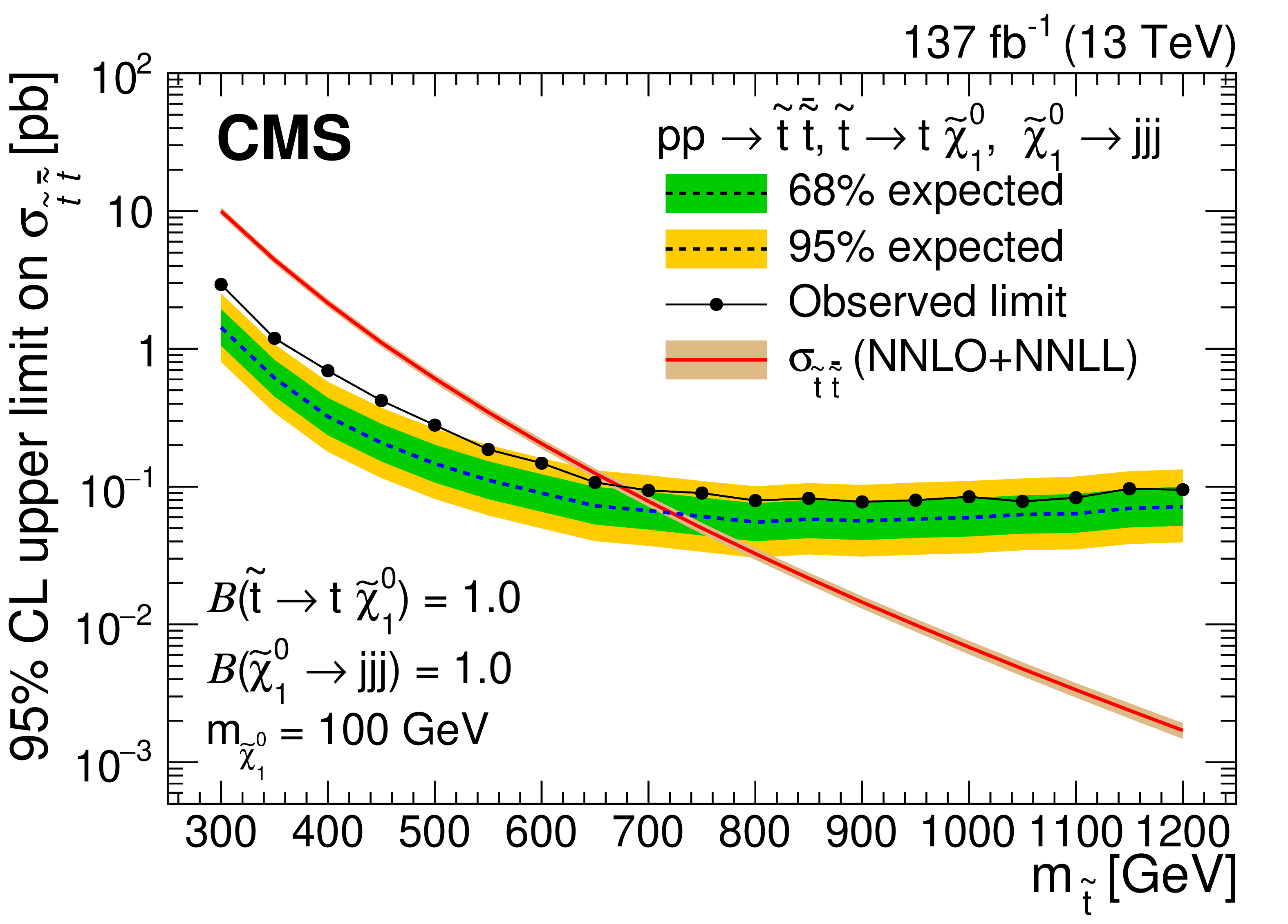
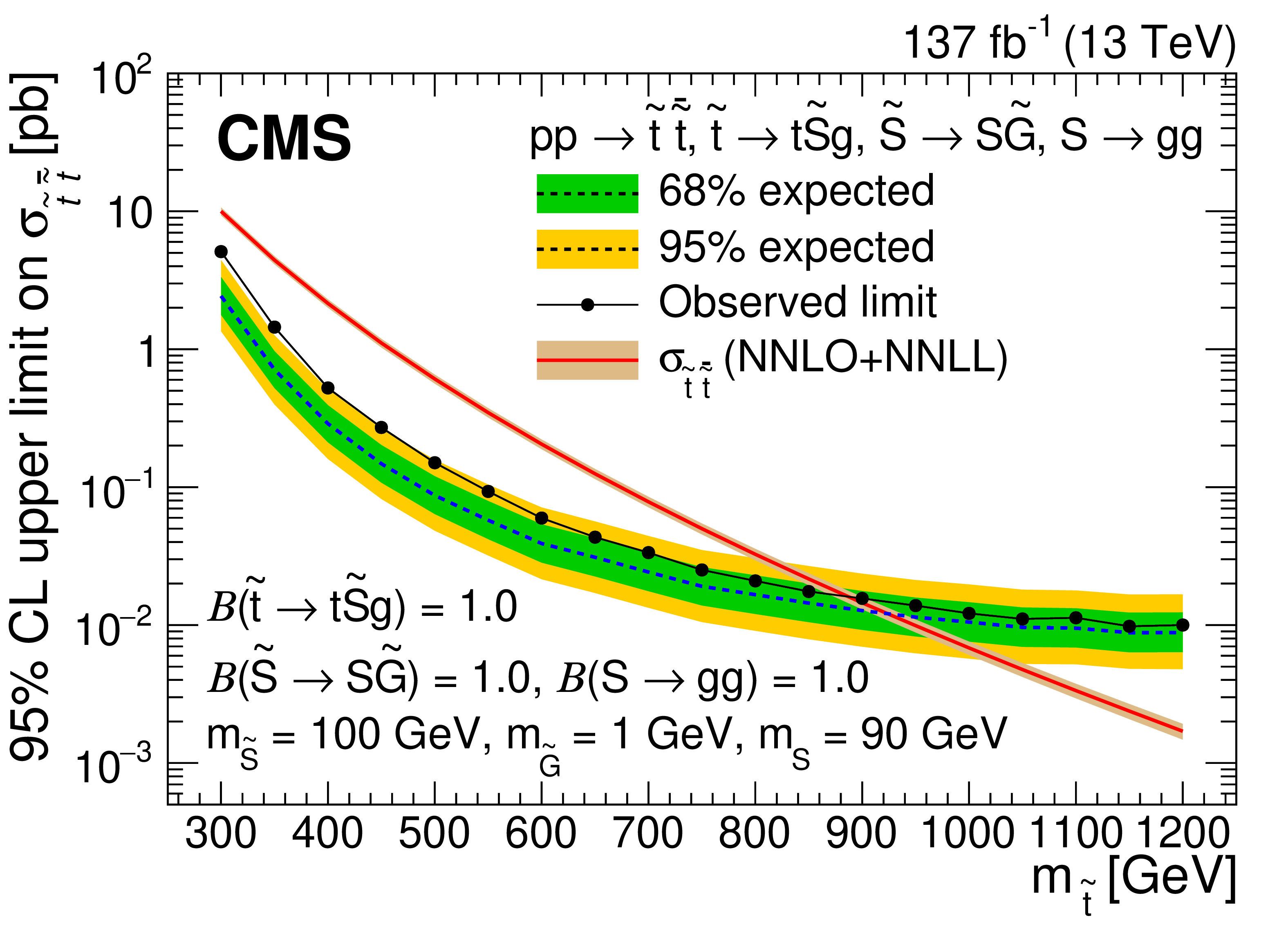
Expected and observed 95% CL upper limit on the top squark pair production cross section as a function of the top squark mass for the RPV (left) and stealth $\mathrm{S}\mathrm{Y}\overline{\mathrm{Y}}$ (right) SUSY models. Particle masses and branching fractions assumed for each model are included on each plot. The expected cross section computed at NNLO+NNLL accuracy is shown in the red curve. |
png pdf root |
Figure 6-a:
Expected and observed 95% CL upper limit on the top squark pair production cross section as a function of the top squark mass for the RPV SUSY model. Particle masses and branching fractions assumed for the model are included. The expected cross section computed at NNLO+NNLL accuracy is shown in the red curve. |
png pdf root |
Figure 6-b:
Expected and observed 95% CL upper limit on the top squark pair production cross section as a function of the top squark mass for the stealth $\mathrm{S}\mathrm{Y}\overline{\mathrm{Y}}$ SUSY model. Particle masses and branching fractions assumed for the model are included. The expected cross section computed at NNLO+NNLL accuracy is shown in the red curve. |

png pdf |
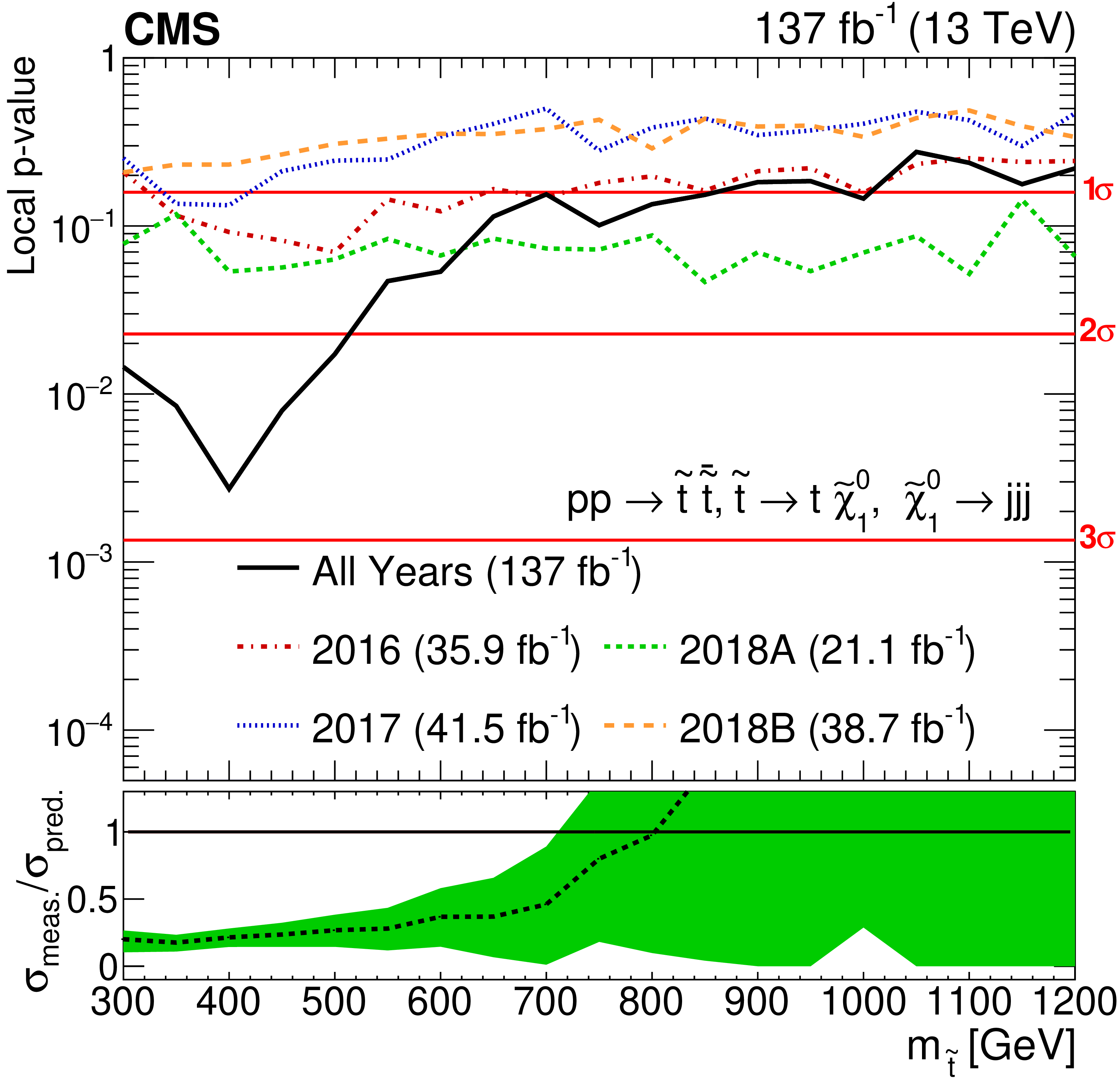
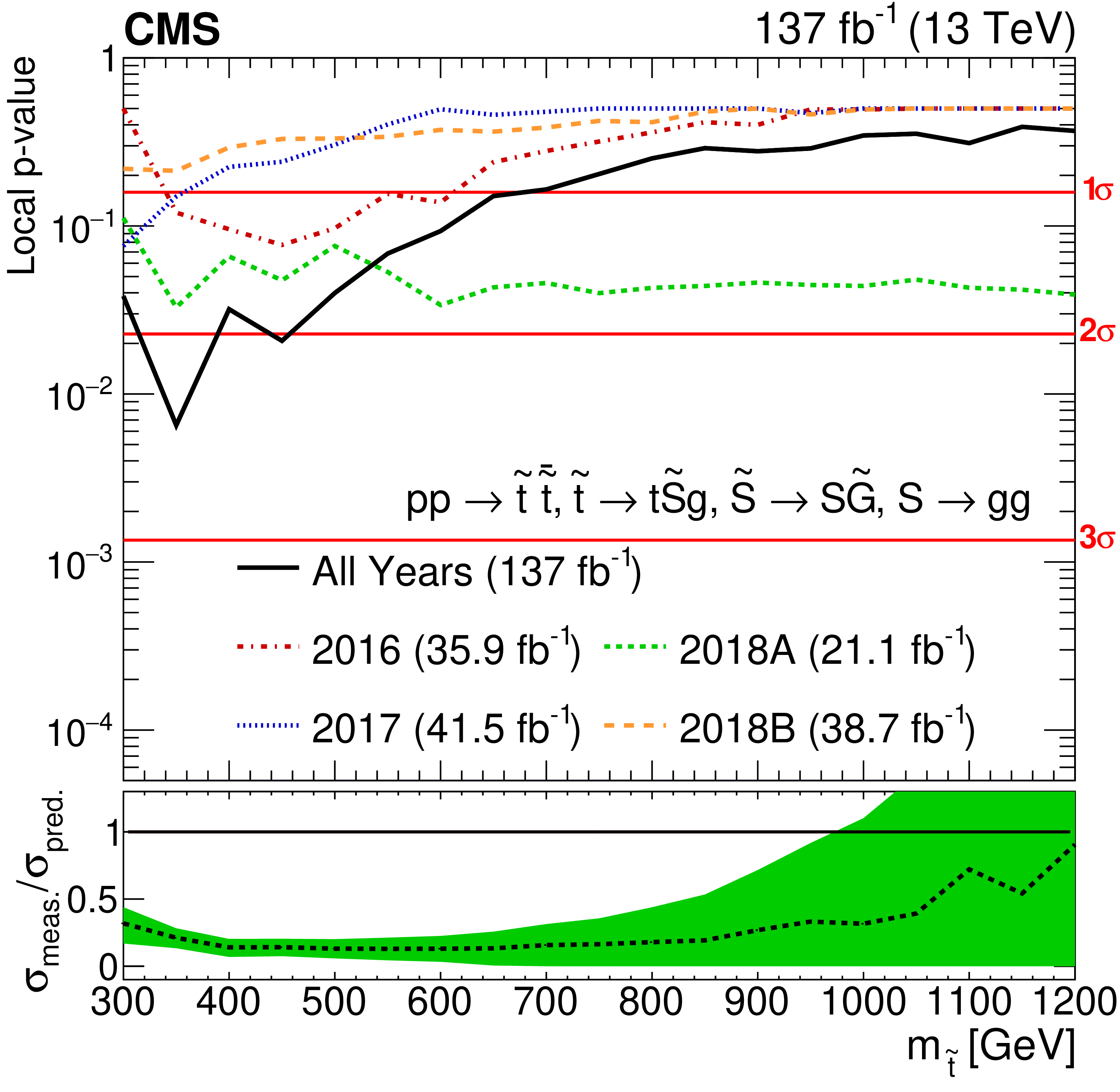
Figure 7:
Local $p$-value as a function of top squark mass for the RPV (left) and stealth $\mathrm{S}\mathrm{Y}\overline{\mathrm{Y}}$ models (right). The colored lines show the $p$-values for separate fits of the 2016 (red dash dotted), 2017 (blue dotted), 2018A (green short dashed), and 2018B (orange long dashed) data sets; the black line shows the $p$-value for the simultaneous fit of data sets. The lower panels show the best fit signal strength ($\sigma _\text {meas.}/\sigma _\text {pred.}$) as a function of top squark mass with uncertainty denoted by the green band. |
png pdf |
Figure 7-a:
Local $p$-value as a function of top squark mass for the RPV model. The colored lines show the $p$-values for separate fits of the 2016 (red dash dotted), 2017 (blue dotted), 2018A (green short dashed), and 2018B (orange long dashed) data sets; the black line shows the $p$-value for the simultaneous fit of data sets. The lower panel shows the best fit signal strength ($\sigma _\text {meas.}/\sigma _\text {pred.}$) as a function of top squark mass with uncertainty denoted by the green band. |
png pdf |
Figure 7-b:
Local $p$-value as a function of top squark mass for the stealth $\mathrm{S}\mathrm{Y}\overline{\mathrm{Y}}$ model. The colored lines show the $p$-values for separate fits of the 2016 (red dash dotted), 2017 (blue dotted), 2018A (green short dashed), and 2018B (orange long dashed) data sets; the black line shows the $p$-value for the simultaneous fit of data sets. The lower panel shows the best fit signal strength ($\sigma _\text {meas.}/\sigma _\text {pred.}$) as a function of top squark mass with uncertainty denoted by the green band. |
png pdf |
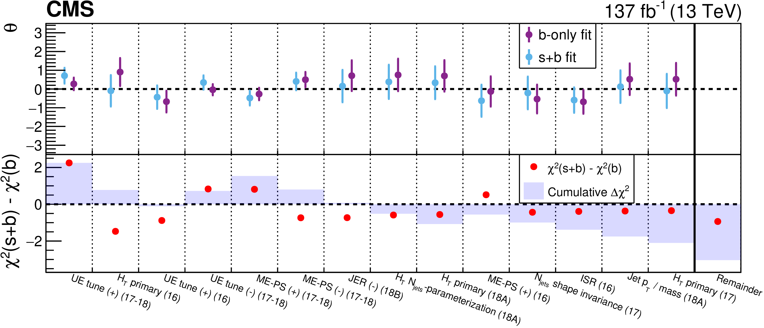
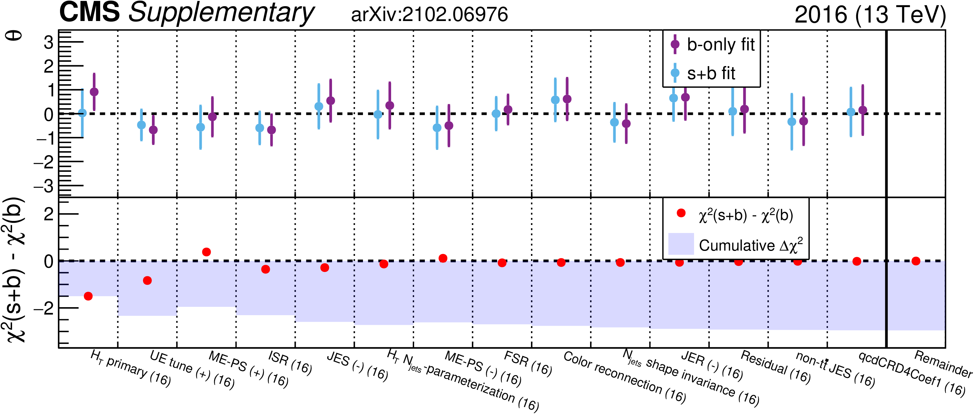
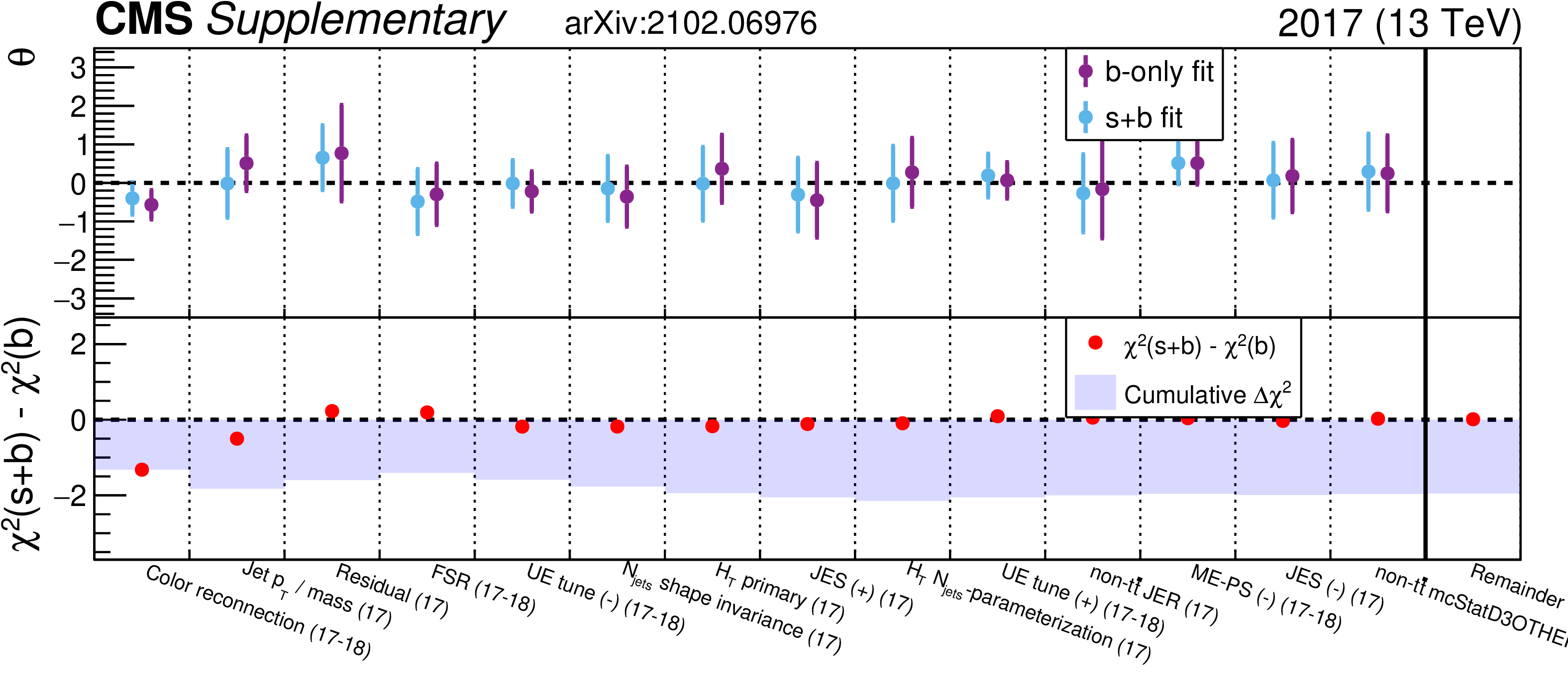
Figure 8:
The upper panel shows the fit values ($\theta $) and uncertainties ($\delta _\theta $) for a selection of nuisance parameters (NP) from both the background-only fit (purple) and signal+background fit (blue) for the RPV model with $ {m_{\tilde{\mathrm{t}}}} = $ 400 GeV. The x-axis labels refer to the NP sources described in Section 5, the data period (16, 17, etc.), and the direction of variation ($+$,$-$). The lower panel shows the $\Delta \chi ^{2}\equiv \chi ^{2}(\mathrm {s}+\mathrm {b})-\chi ^{2}(\mathrm {b})$ difference of $\chi ^2\equiv (\theta /\delta _\theta)^2$ from the signal+background (s+b) and background-only (b) fits as a red point for each NP and the cumulative sum of $\Delta \chi ^2$ from left to right as a blue shaded histogram. The fourteen selected NP are those with $| \Delta \chi ^2| > 0.3$, and the NP are ordered from left to right by decreasing $| \Delta \chi ^2| $. The rightmost bin, separated by a vertical solid line, shows the sum of $\Delta \chi ^2$ for all NP not displayed in the figure (red point) and the sum of $\Delta \chi ^2$ for all NP (blue shaded histogram). |
| Tables | |

png pdf |
Table 1:
Summary of the impact of systematic uncertainties in the expected event yields for the ${\mathrm{t} \mathrm{\bar{t}}}$ background, minor backgrounds (both ${{\mathrm{t} \mathrm{\bar{t}}}}$+X and other), and the RPV signal model with $ {m_{\tilde{\mathrm{t}}}} = $ 550 GeV. Abbreviated names for each source of uncertainty are explained in the text. For sources of uncertainty for which the size of the impact depends on ${N_\text {jets}}$ and ${S_\mathrm {NN}}$, a representative range of values showing the 16$^{\mathrm {th}}$ and 84$^{\mathrm {th}}$ percentile of all the corrections is listed with the maximum value from all bins shown in parentheses. All values are in units of percent. |
| Summary |
|
A first of its kind search for top squark pair production with subsequent decay characterized by two top quarks, additional gluons or light-flavor quarks, and low missing transverse momentum (${p_{\mathrm{T}}}^{\text{miss}}$) is described. Events containing exactly one electron or muon and at least seven jets, of which at least one should be b tagged, are selected from a sample of proton-proton collisions at $\sqrt{s} = $ 13 TeV corresponding to an integrated luminosity of 137 fb$^{-1}$ collected with the CMS detector in 2016-2018. No requirement is made on ${p_{\mathrm{T}}}^{\text{miss}}$. The dominant $\mathrm{t\bar{t}}$ background is predicted from data using a simultaneous fit of the jet multiplicity distribution across four bins of a neural network score. The results are interpreted in terms of top squark pair production in the context of $R$-parity violating (RPV) and stealth supersymmetry models. Top squark masses (${m_{\tilde{\mathrm{t}}}} $) up to 670 GeV are excluded at 95% confidence level for the RPV model in which the top squark decays to a top quark and the lightest neutralino, which subsequently decays to three light-flavor quarks via an off-shell squark through a trilinear coupling ${\lambda}''$. Top squark masses up to 870 GeV are excluded for the stealth supersymmetry model in which the top squark decays to a top quark, three gluons, and a gravitino via intermediate hidden sector particles. The maximum observed local significance is 2.8 standard deviations corresponding to a best fit signal strength of 0.21 $\pm$ 0.07 for the RPV model with ${m_{\tilde{\mathrm{t}}}} = $ 400 GeV. |
| Additional Figures | |
png pdf |
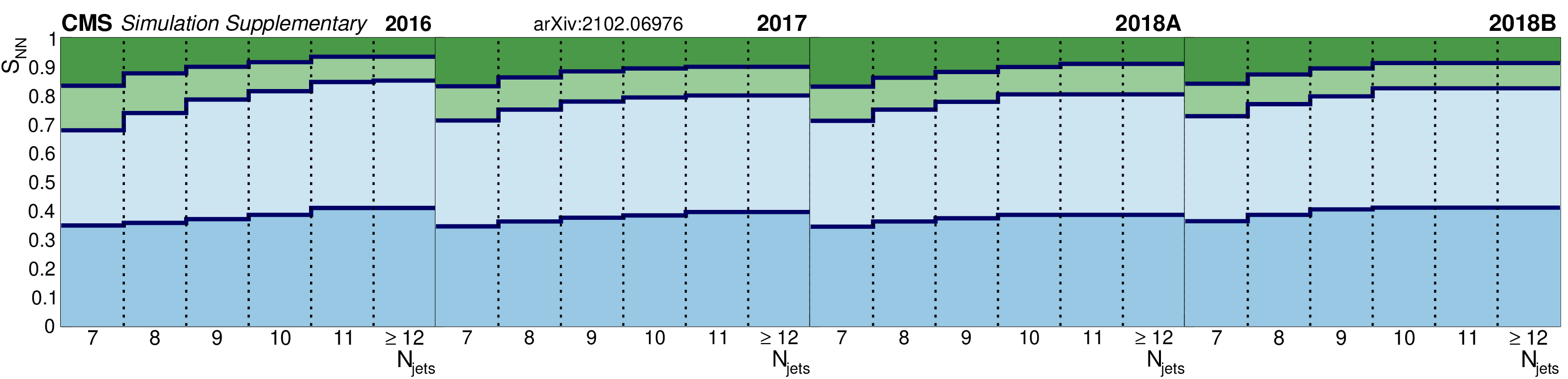
Additional Figure 1:
Shown are the chosen bin edges for the four $S_{\textrm {NN}}$ bins (vertical) as a function of $N_{\textrm {jets}}$ (horizontal) for the four data taking periods. Edges are chosen (per-data taking period) by maximizing a simple significance-like metric with the constraint that the fraction of $\mathrm{t\bar{t}}$ in a given $S_{\textrm {NN}}$ bin is the same for each $N_{\textrm {jets}}$. $S_{\textrm {NN},1}$ is shown in dark blue, $S_{\textrm {NN},2}$ in light blue, $S_{\textrm {NN},3}$ in light green, and $S_{\textrm {NN},4}$ in dark green. |
png pdf |
Additional Figure 5-2:
Shown is the $\chi ^2$ distribution for all nuisance parameters in the fit. This is done for the combined fit to data assuming the RPV 400 stop mass. Background-only (blue) and signal+background (purple) results are displayed. |
png pdf |
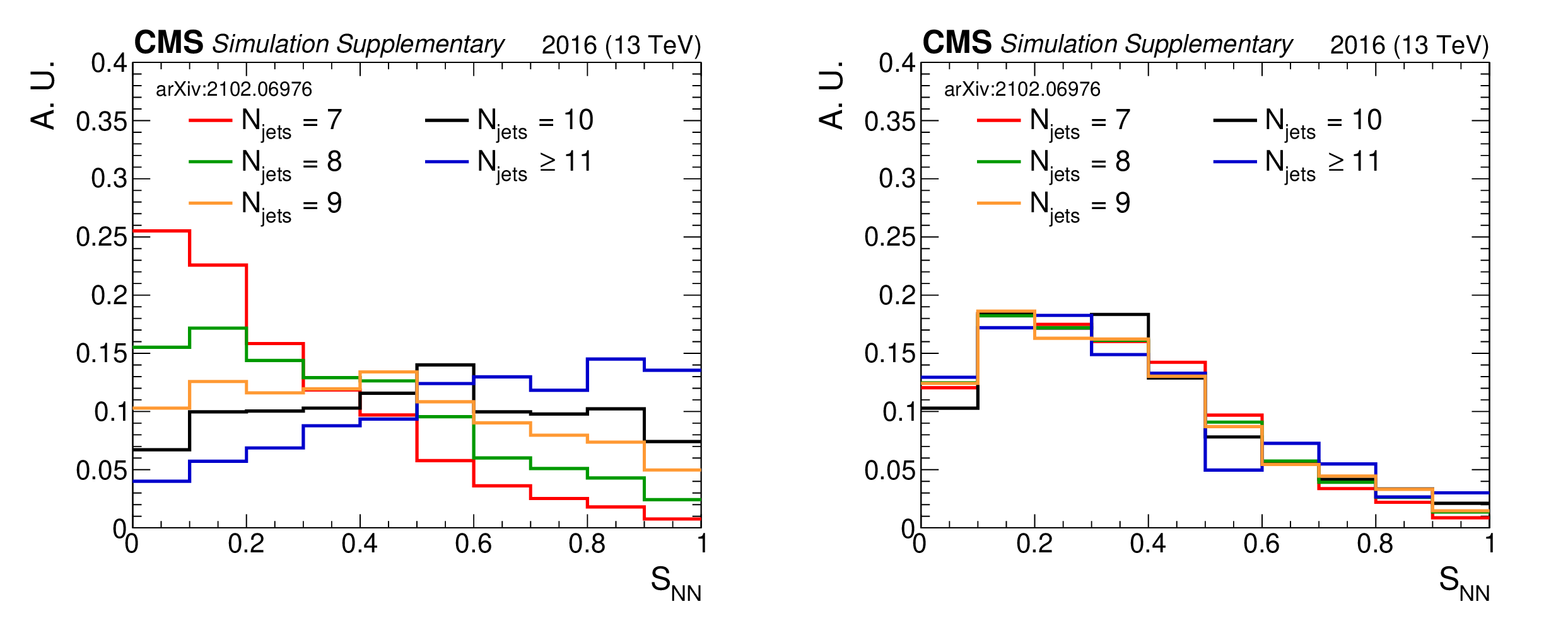
Additional Figure 2-a:
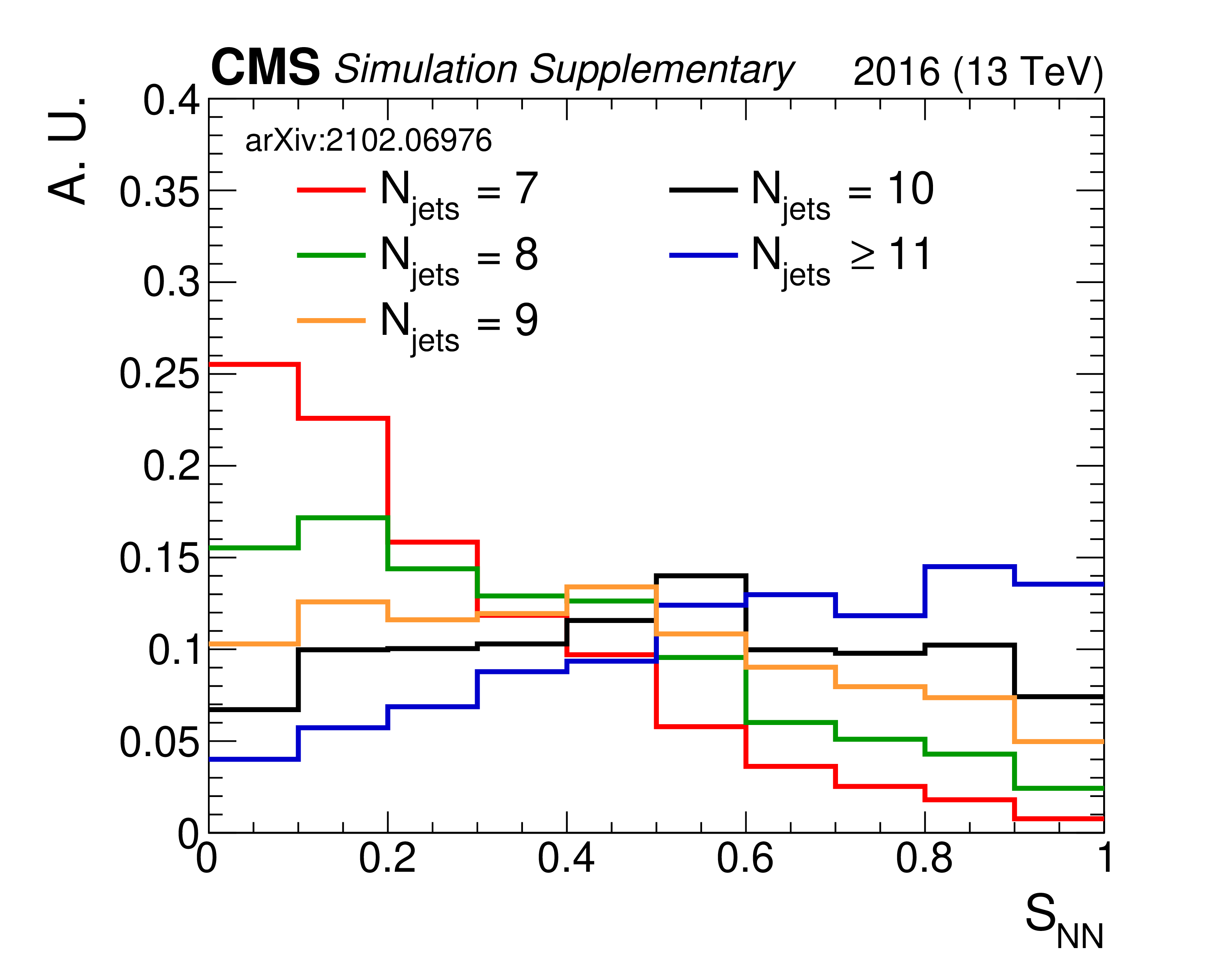
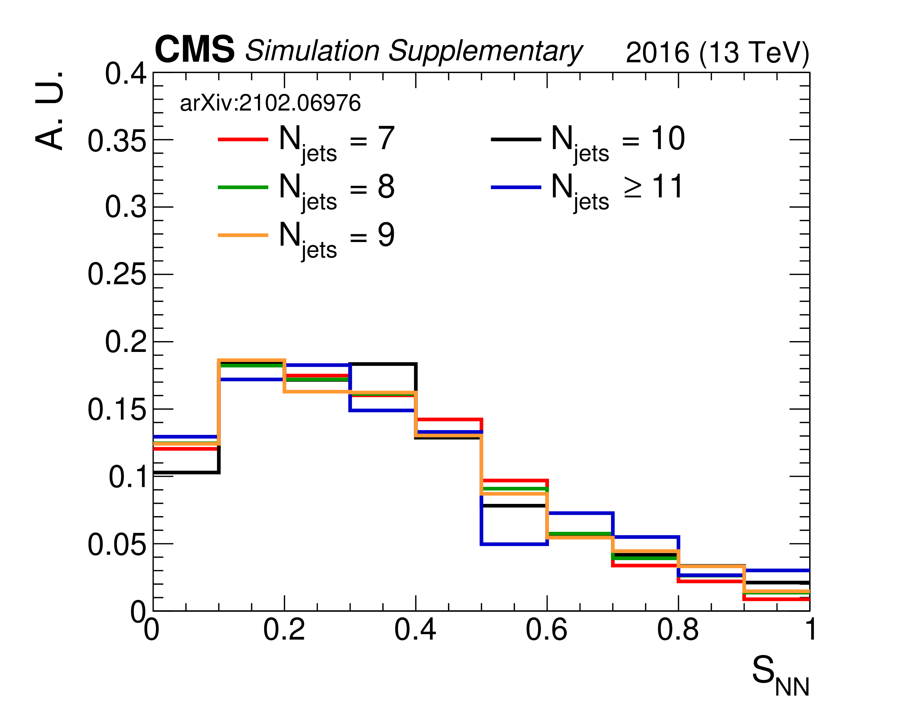
The $S_{\textrm {NN}}$ distribution for $\mathrm{t\bar{t}}$ events grouped by the number of jets in the event. Shown is the result when not using gradient reversal in the NN to remove dependence on $N_{\textrm {jets}}$. |
png pdf |
Additional Figure 2-b:
The $S_{\textrm {NN}}$ distribution for $\mathrm{t\bar{t}}$ events grouped by the number of jets in the event. Shown is the result when gradient reversal is employed, resulting in a much more similar $S_{\textrm {NN}}$ for $\mathrm{t\bar{t}}$ events, regardless of the number of jets in the event. |
png pdf |
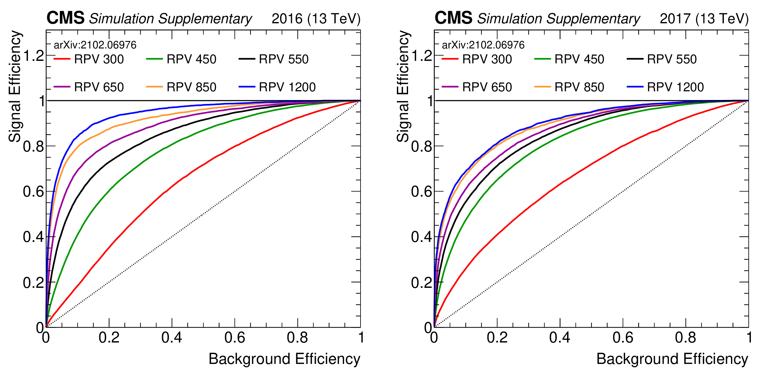
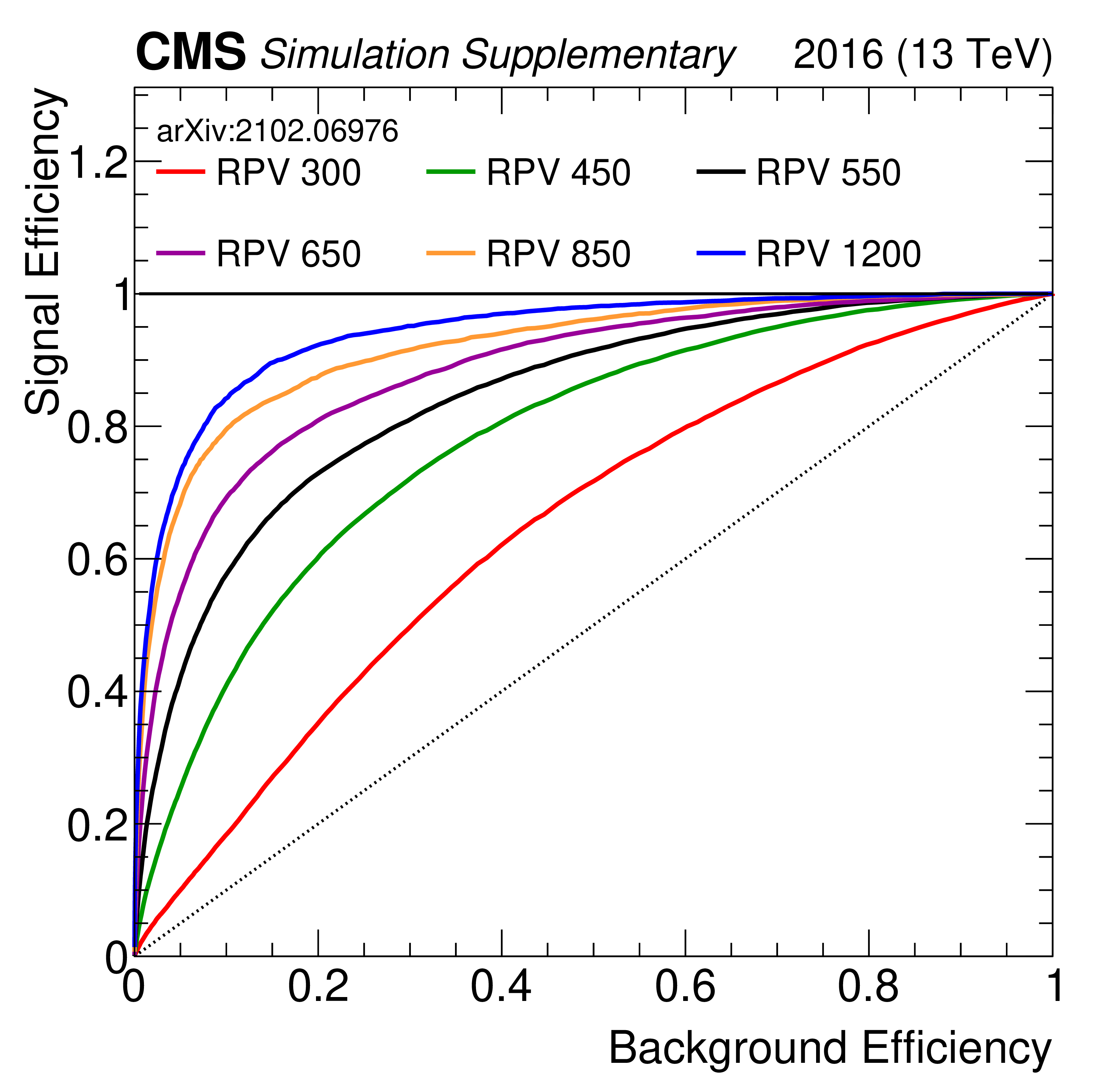
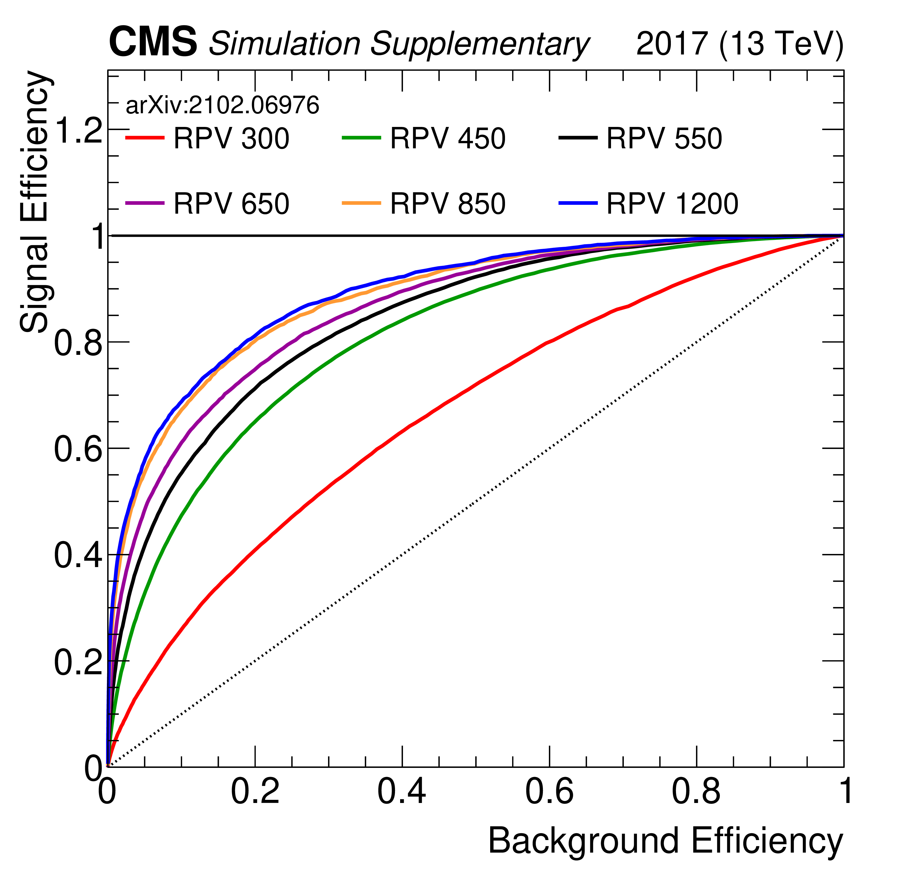
Additional Figure 3:
Shown are the ROC curves for the 2016 (left) and 2017 (right) trainings of the NN. In different colors are the result for a specific stop mass for the RPV model. Note that the NN was trained on all signal masses. |
png pdf |
Additional Figure 3-a:
Shown are the ROC curves for the 2016 training of the NN. In different colors are the result for a specific stop mass for the RPV model. Note that the NN was trained on all signal masses. |
png pdf |
Additional Figure 3-b:
Shown are the ROC curves for the 2017 training of the NN. In different colors are the result for a specific stop mass for the RPV model. Note that the NN was trained on all signal masses. |

png pdf |
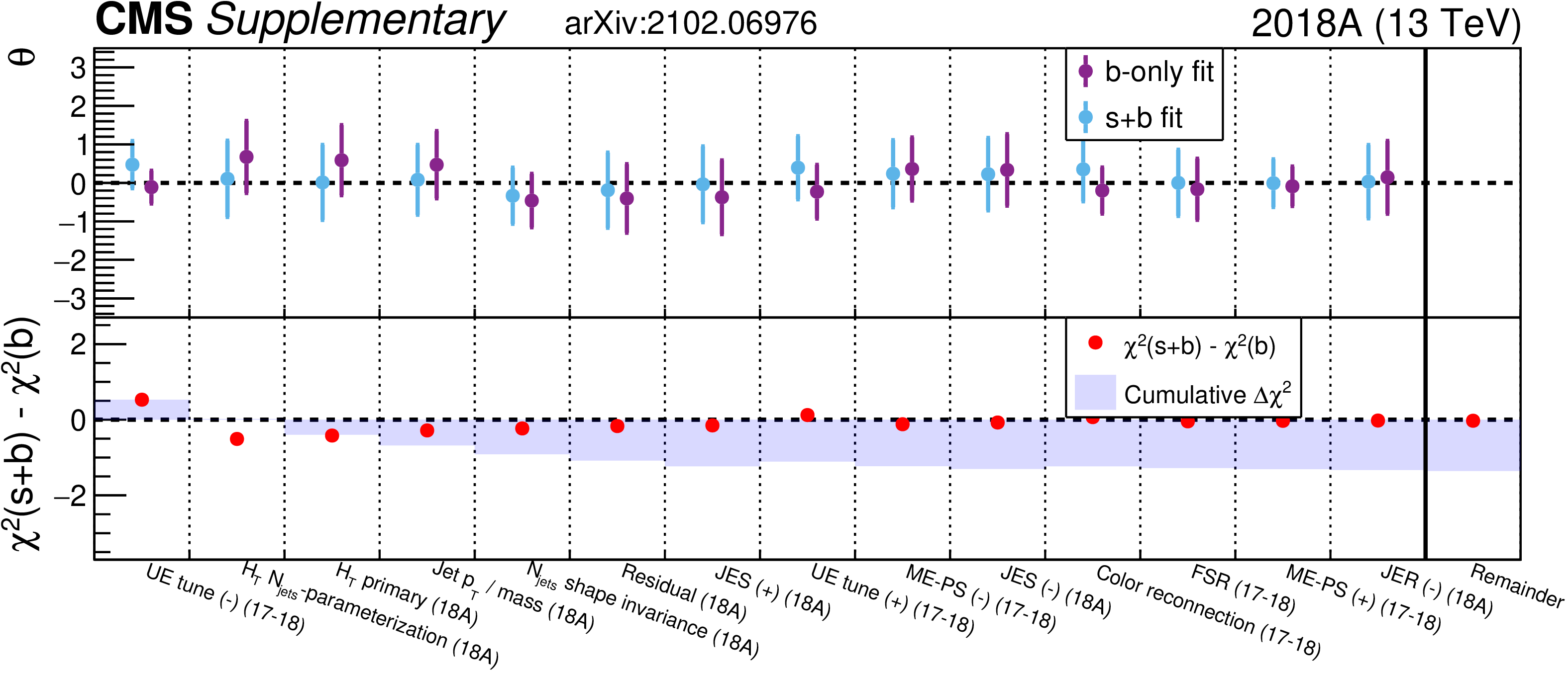
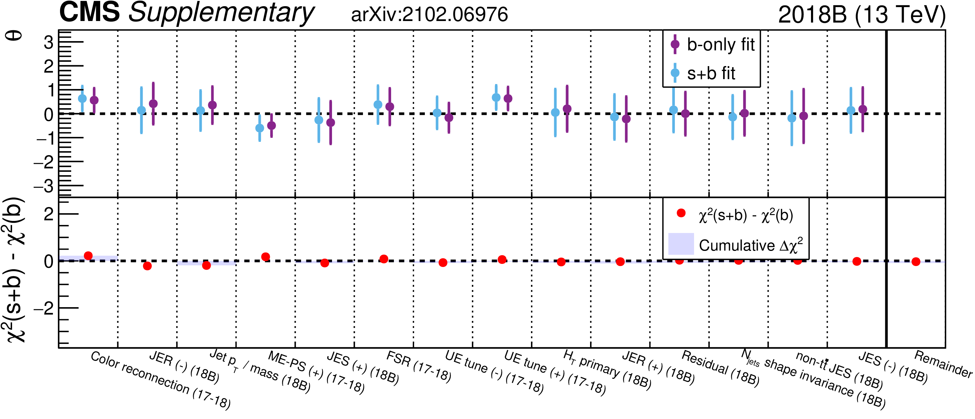
Additional Figure 4:
Shown, for 2016, 2017, 2018A, 2018B, is the value of the nuisance parameters when doing the background-only (purple) and signal+background (blue) fit assuming the RPV 400 signal. Then in red is the $\Delta \chi ^{2}$ for each nuisance parameter when going from background-only to signal+background. NPs are sorted by magnitude of $\Delta \chi ^{2}$. |
png pdf |
Additional Figure 4-a:
Shown, for 2016, is the value of the nuisance parameters when doing the background-only (purple) and signal+background (blue) fit assuming the RPV 400 signal. Then in red is the $\Delta \chi ^{2}$ for each nuisance parameter when going from background-only to signal+background. NPs are sorted by magnitude of $\Delta \chi ^{2}$. |
png pdf |
Additional Figure 4-b:
Shown, for 2017, is the value of the nuisance parameters when doing the background-only (purple) and signal+background (blue) fit assuming the RPV 400 signal. Then in red is the $\Delta \chi ^{2}$ for each nuisance parameter when going from background-only to signal+background. NPs are sorted by magnitude of $\Delta \chi ^{2}$. |
png pdf |
Additional Figure 4-c:
Shown, for 2018A, is the value of the nuisance parameters when doing the background-only (purple) and signal+background (blue) fit assuming the RPV 400 signal. Then in red is the $\Delta \chi ^{2}$ for each nuisance parameter when going from background-only to signal+background. NPs are sorted by magnitude of $\Delta \chi ^{2}$. |
png pdf |
Additional Figure 4-d:
Shown, for 2018B, is the value of the nuisance parameters when doing the background-only (purple) and signal+background (blue) fit assuming the RPV 400 signal. Then in red is the $\Delta \chi ^{2}$ for each nuisance parameter when going from background-only to signal+background. NPs are sorted by magnitude of $\Delta \chi ^{2}$. |
png pdf |
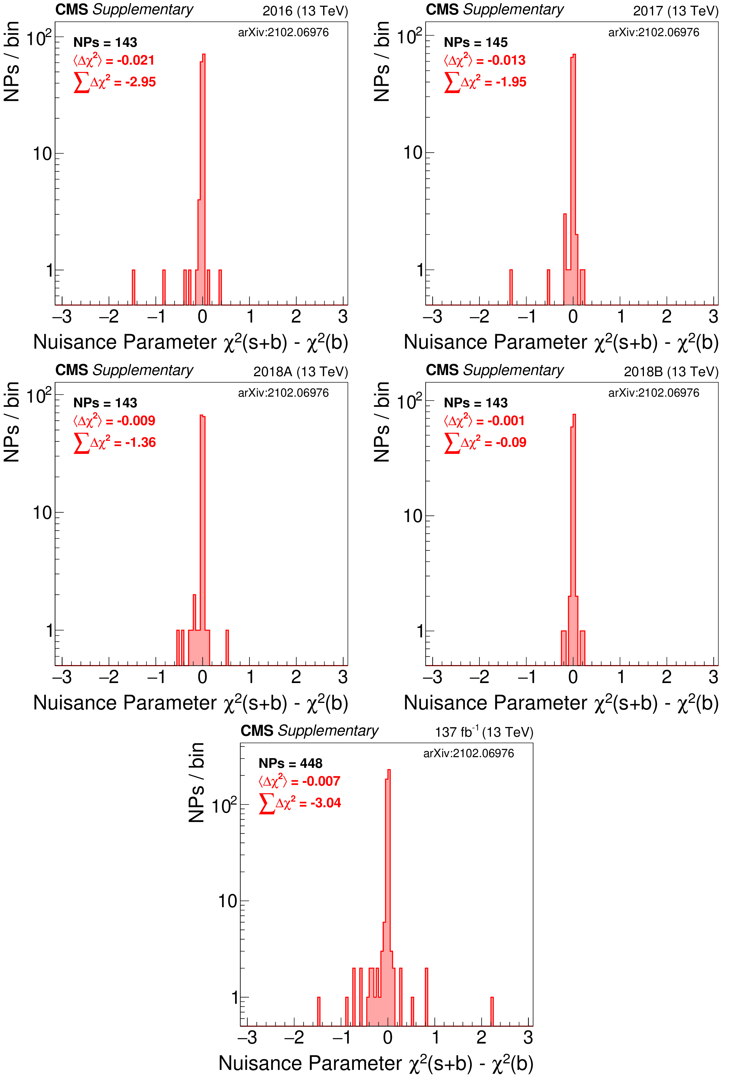
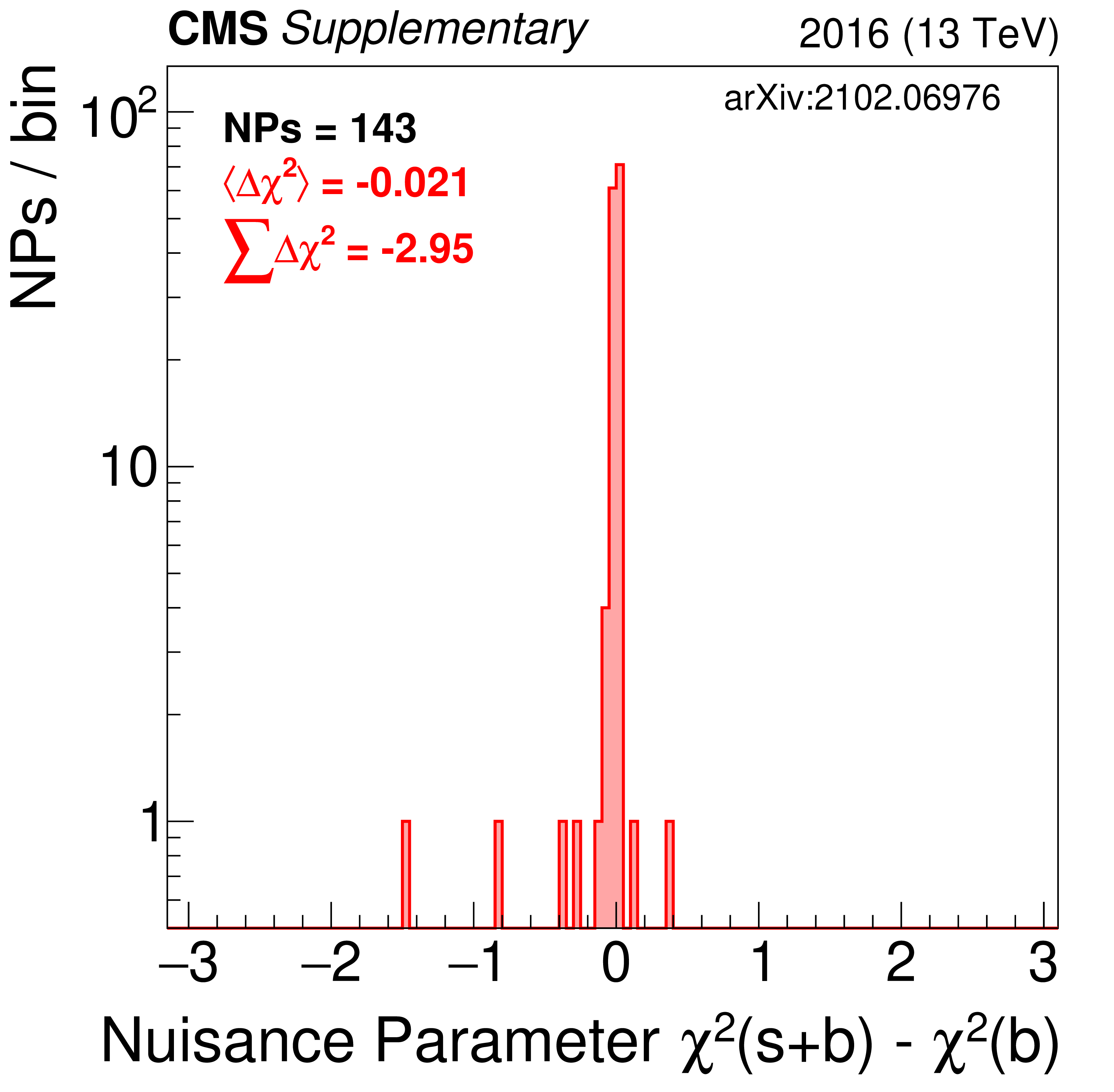
Additional Figure 5:
Shown is the $\chi ^2$ distribution for all nuisance parameters in the fit. This is done for the individual year and combined fit to data assuming the RPV 400 stop mass. Background-only (blue) and signal+background (purple) results are displayed. |
png pdf |
Additional Figure 5-a:
Shown is the $\chi ^2$ distribution for all nuisance parameters in the fit. This is done for the 2016 fit to data assuming the RPV 400 stop mass. Background-only (blue) and signal+background (purple) results are displayed. |
png pdf |
Additional Figure 5-b:
Shown is the $\chi ^2$ distribution for all nuisance parameters in the fit. This is done for the 2017 fit to data assuming the RPV 400 stop mass. Background-only (blue) and signal+background (purple) results are displayed. |

png pdf |
Additional Figure 5-c:
Shown is the $\chi ^2$ distribution for all nuisance parameters in the fit. This is done for the 2018A combined fit to data assuming the RPV 400 stop mass. Background-only (blue) and signal+background (purple) results are displayed. |
png pdf |
Additional Figure 5-d:
Shown is the $\chi ^2$ distribution for all nuisance parameters in the fit. This is done for the 2018B combined fit to data assuming the RPV 400 stop mass. Background-only (blue) and signal+background (purple) results are displayed. |
png pdf |
Additional Figure 5-e:
Shown is the $\chi ^2$ distribution for all nuisance parameters in the fit. This is done for the individual year and combined fit to data assuming the RPV 400 stop mass. Background-only (blue) and signal+background (purple) results are displayed. |
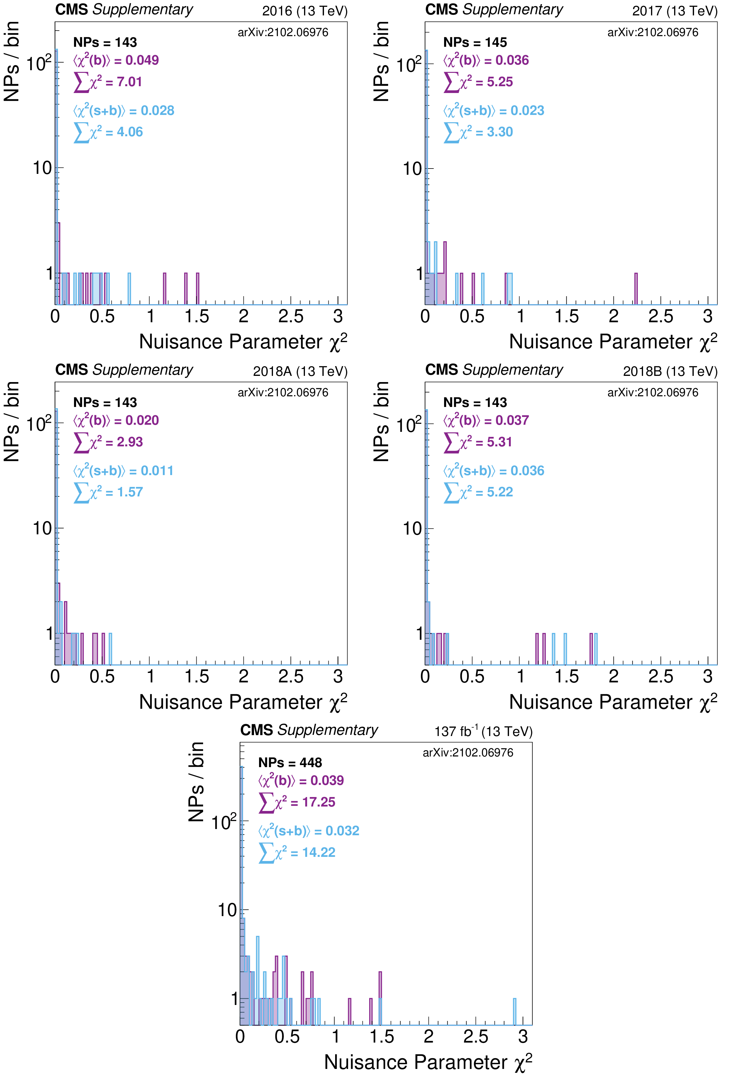
png pdf |
Additional Figure 6:
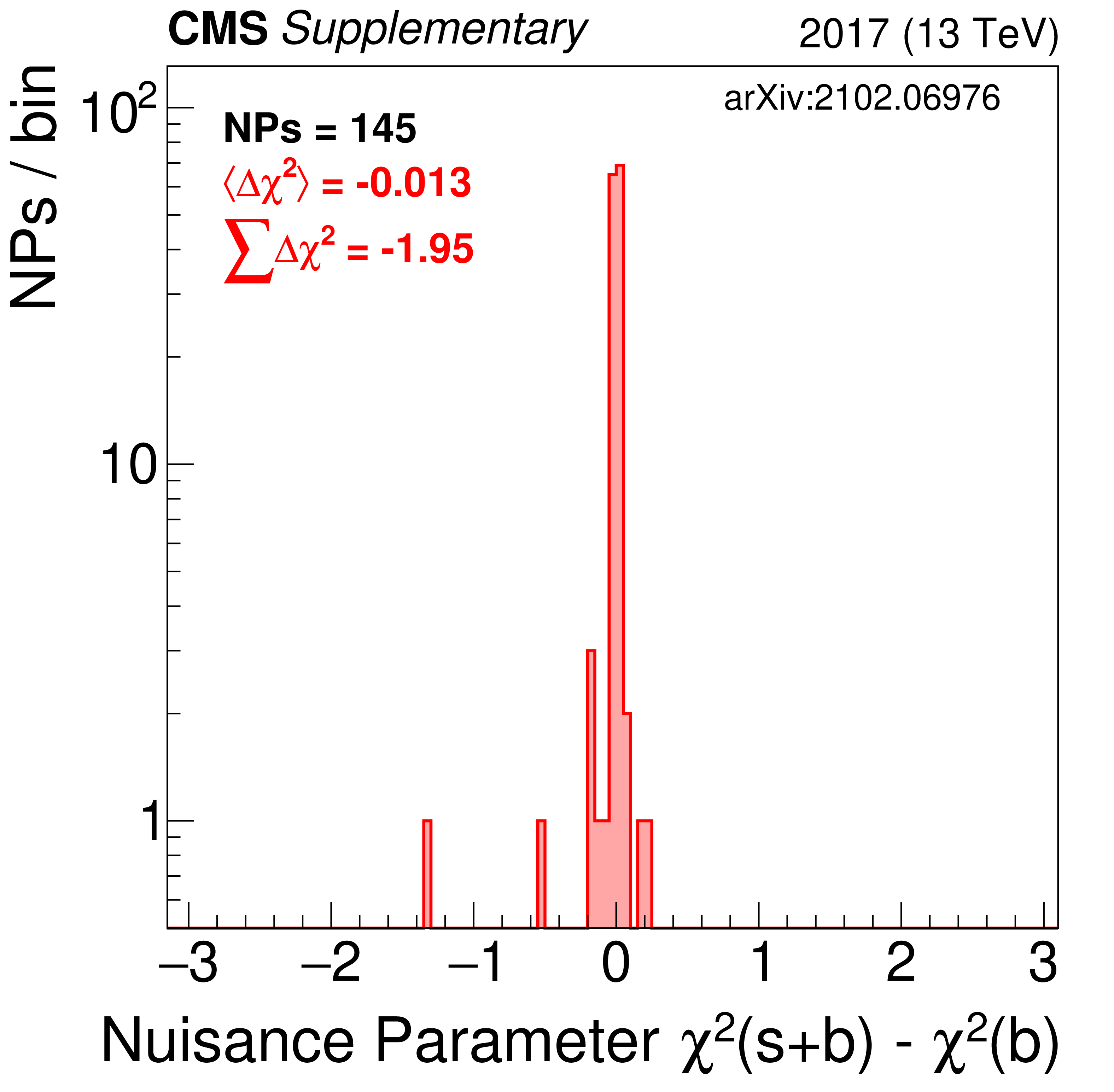
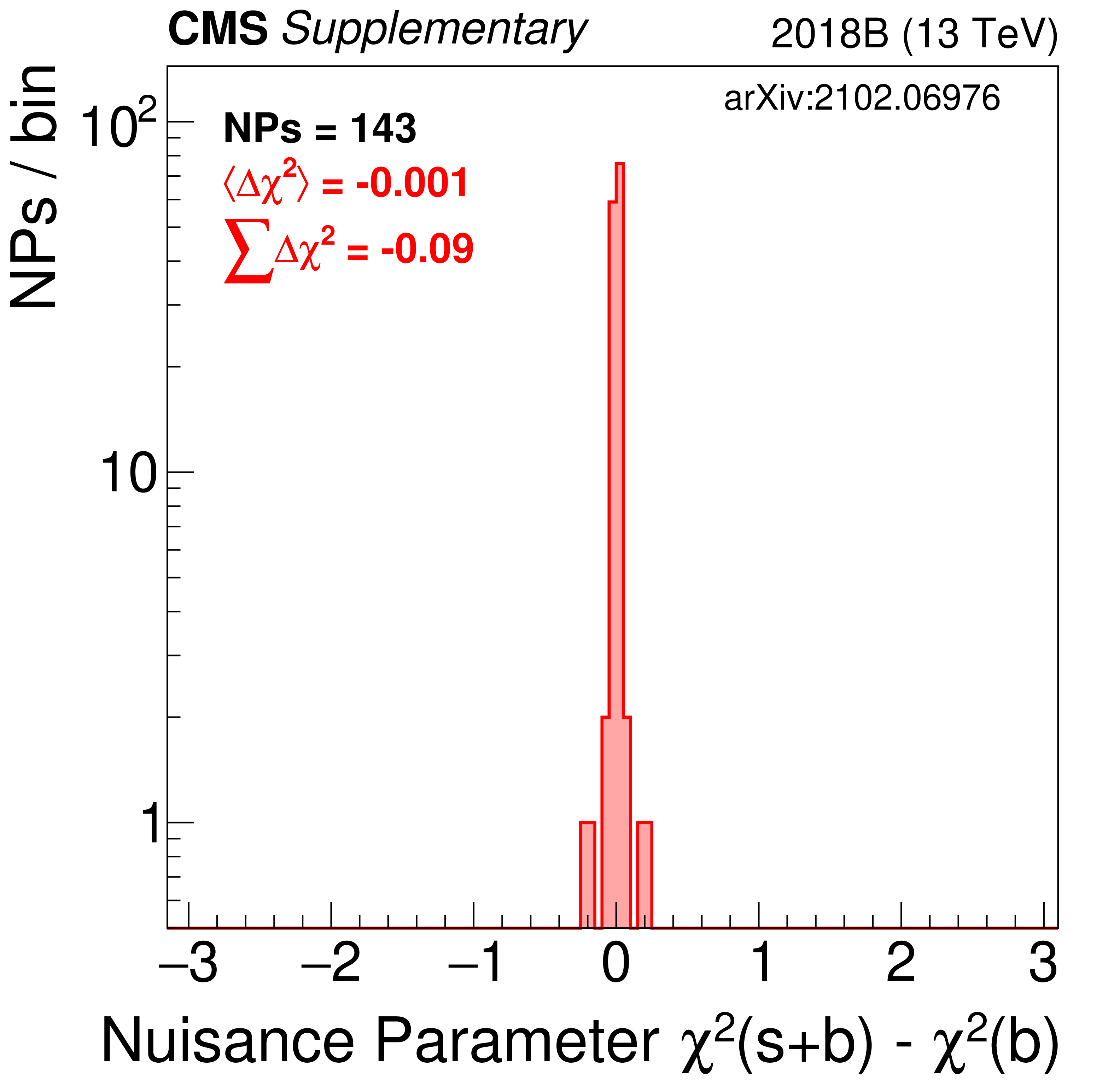
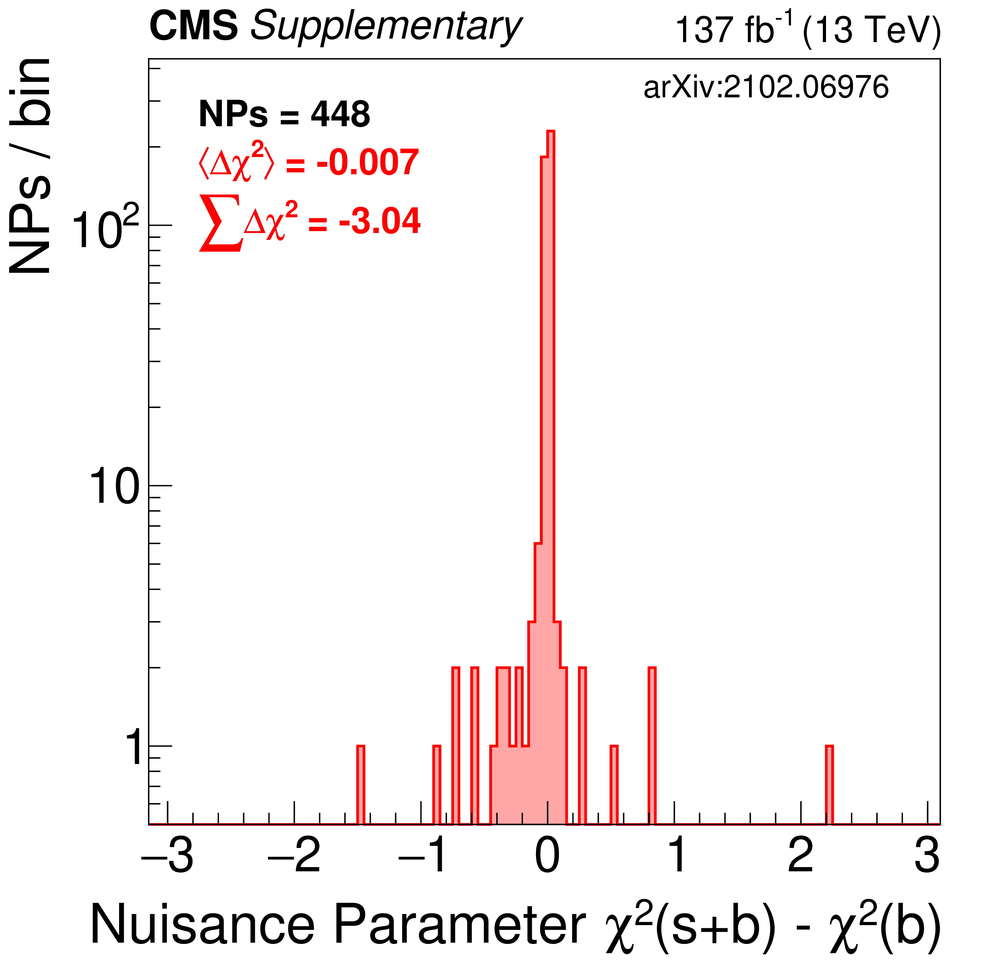
Shown is the $\Delta \chi ^2$ distribution for all nuisance parameters in the fit. This is done for the individual year and combined fit to data assuming the RPV 400 signal hypothesis. The difference is between the NP $\chi $ value found with the signal+background fit and that found for the background only fit. |
png pdf |
Additional Figure 6-a:
Shown is the $\Delta \chi ^2$ distribution for all nuisance parameters in the fit. This is done for the 2016 fit to data assuming the RPV 400 signal hypothesis. The difference is between the NP $\chi $ value found with the signal+background fit and that found for the background only fit. |
png pdf |
Additional Figure 6-b:
Shown is the $\Delta \chi ^2$ distribution for all nuisance parameters in the fit. This is done for the 2017 fit to data assuming the RPV 400 signal hypothesis. The difference is between the NP $\chi $ value found with the signal+background fit and that found for the background only fit. |

png pdf |
Additional Figure 6-c:
Shown is the $\Delta \chi ^2$ distribution for all nuisance parameters in the fit. This is done for the 2018A fit to data assuming the RPV 400 signal hypothesis. The difference is between the NP $\chi $ value found with the signal+background fit and that found for the background only fit. |
png pdf |
Additional Figure 6-d:
Shown is the $\Delta \chi ^2$ distribution for all nuisance parameters in the fit. This is done for the 2018B fit to data assuming the RPV 400 signal hypothesis. The difference is between the NP $\chi $ value found with the signal+background fit and that found for the background only fit. |
png pdf |
Additional Figure 6-e:
Shown is the $\Delta \chi ^2$ distribution for all nuisance parameters in the fit. This is done for the combined fit to data assuming the RPV 400 signal hypothesis. The difference is between the NP $\chi $ value found with the signal+background fit and that found for the background only fit. |
png pdf |
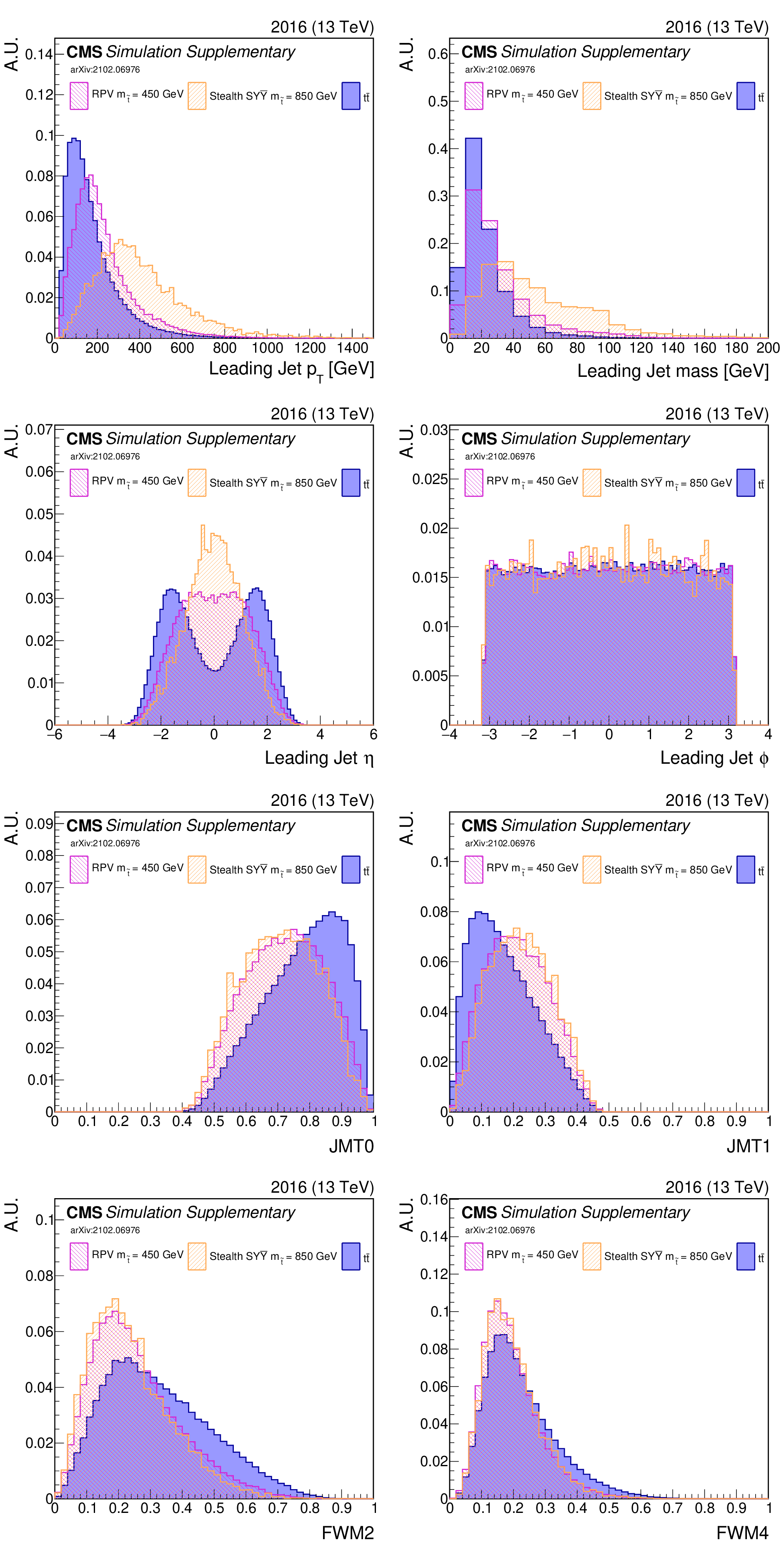
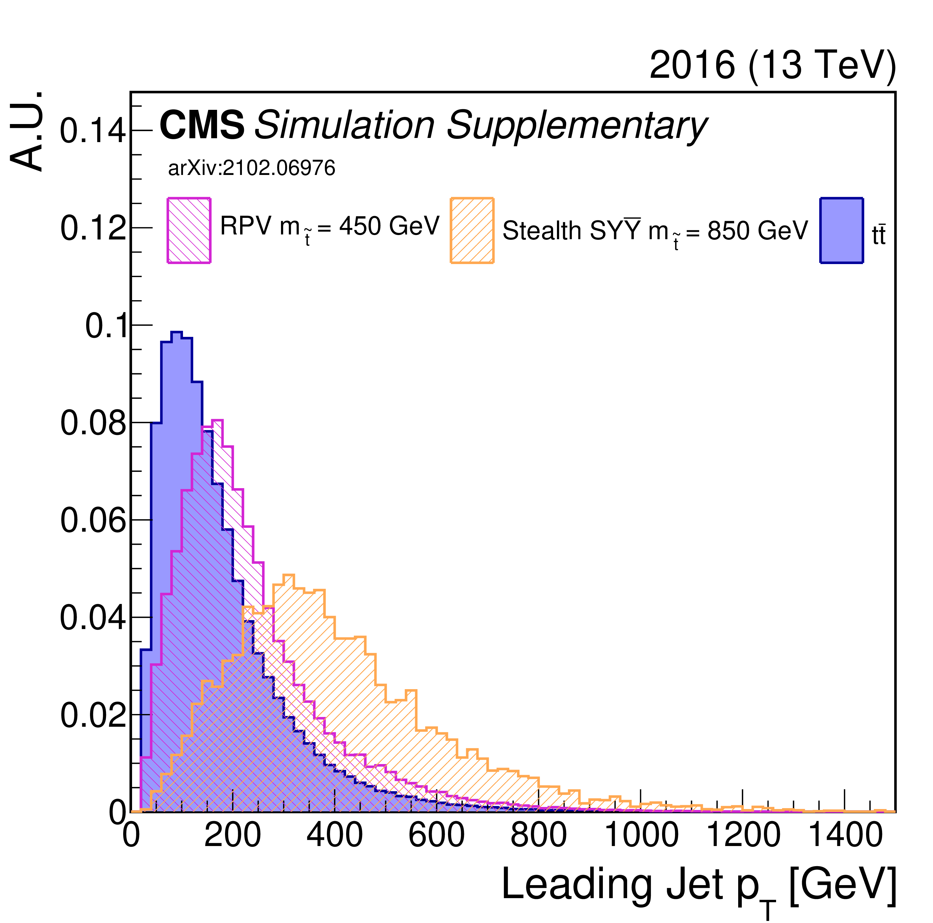
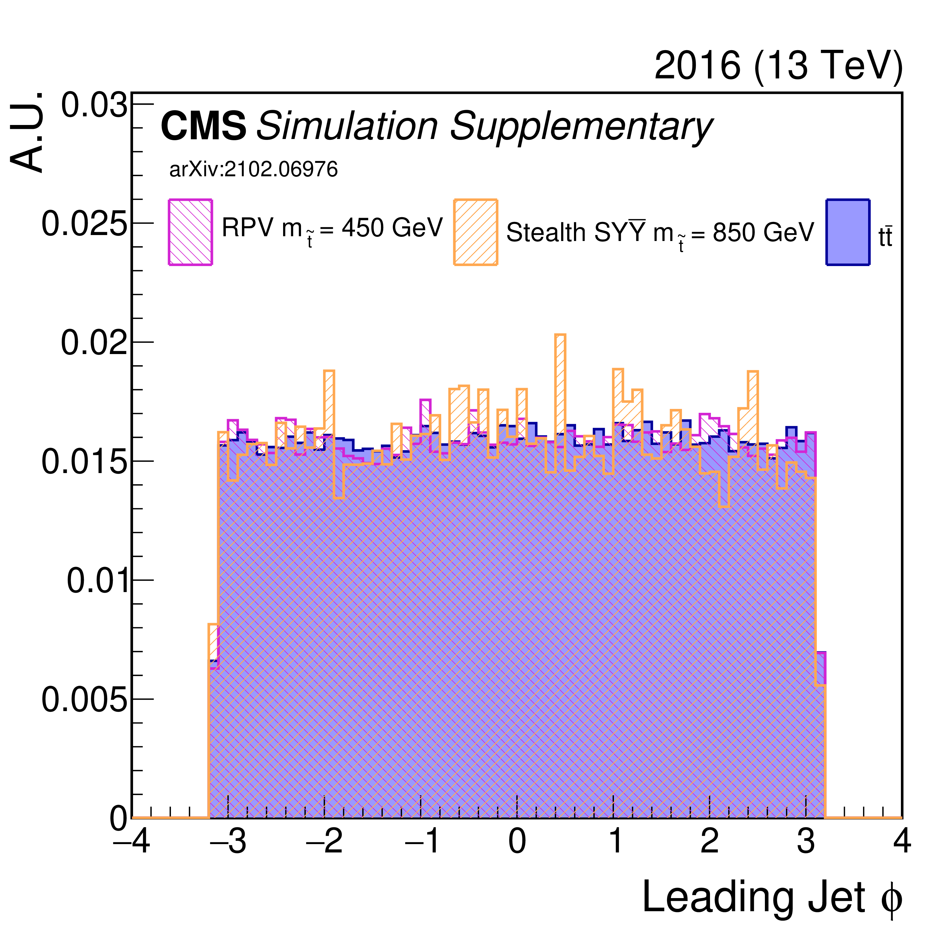
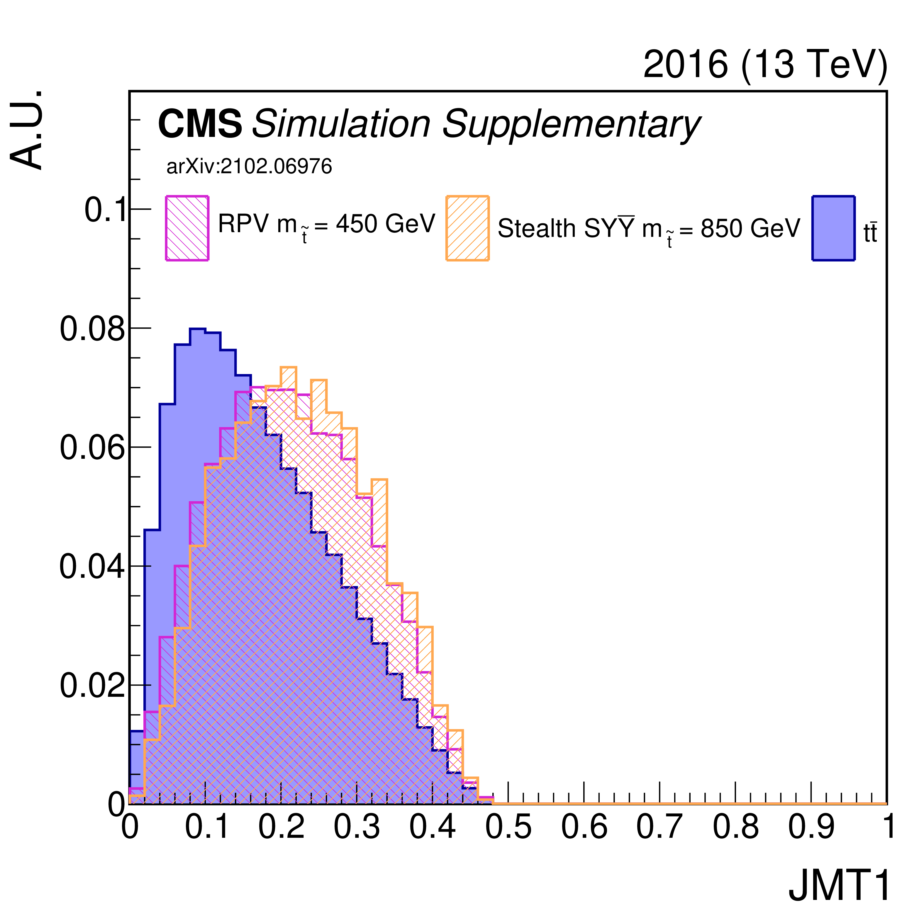
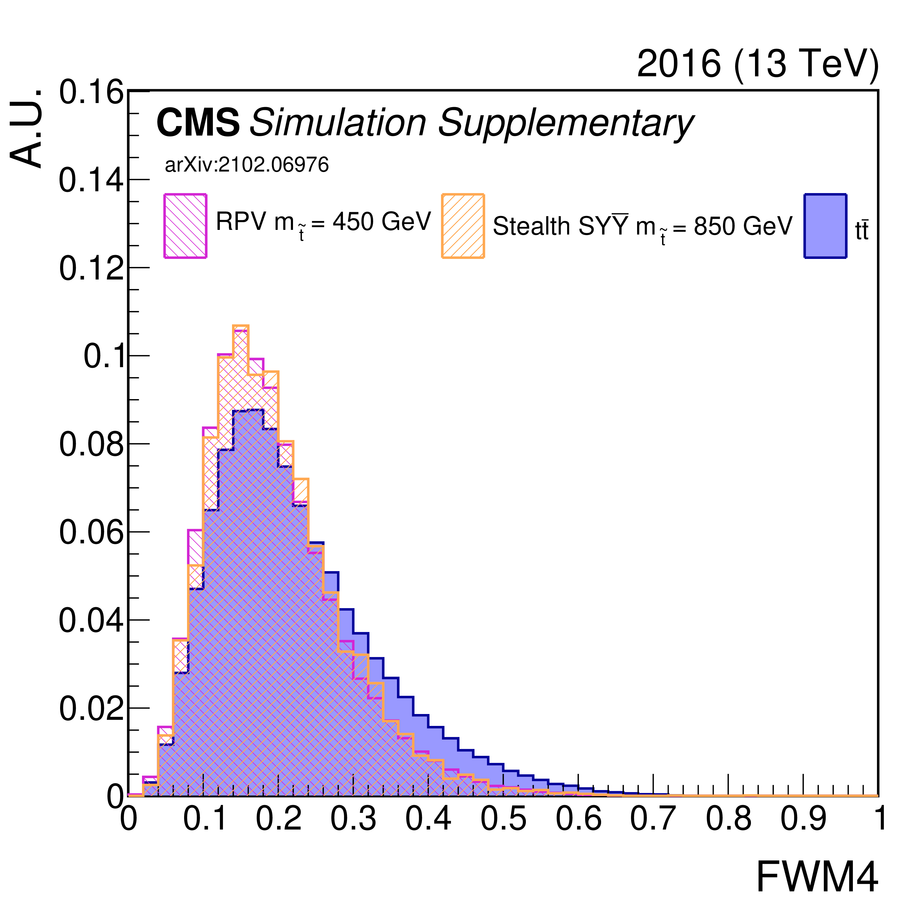
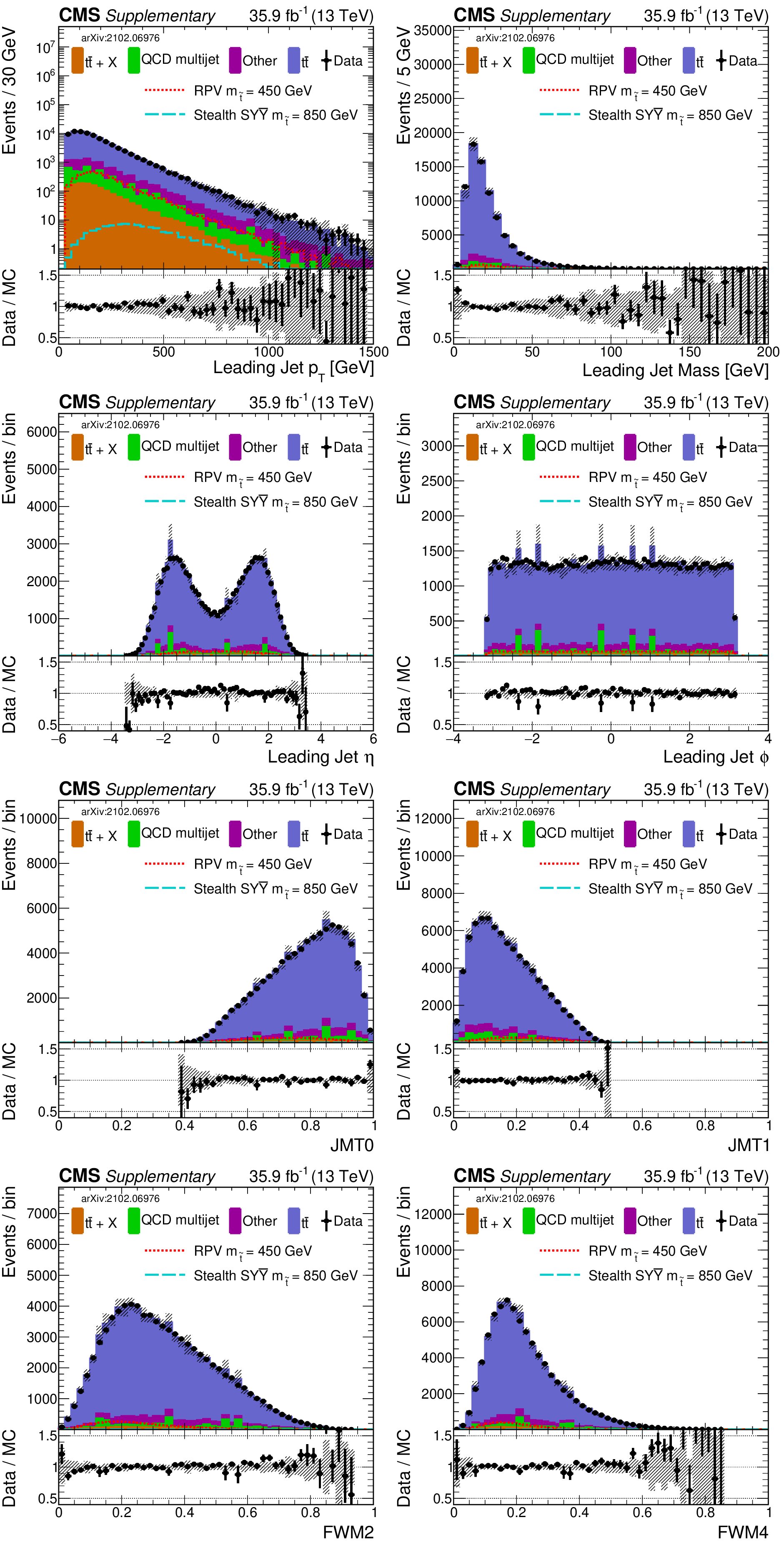
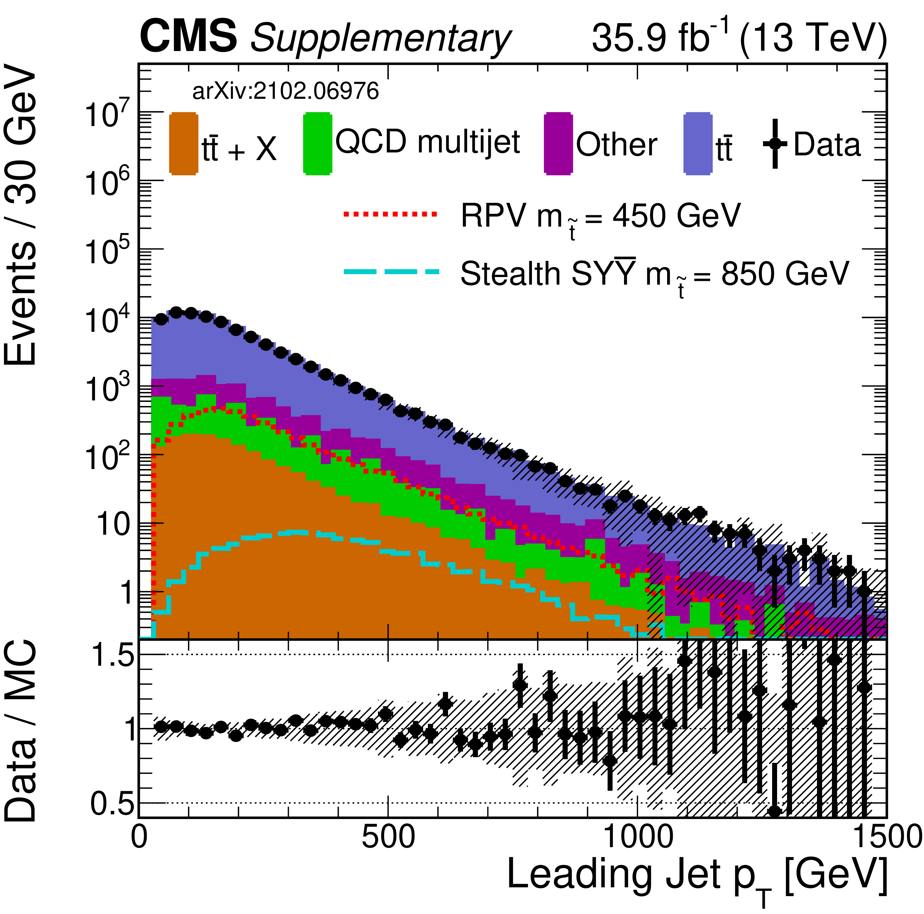
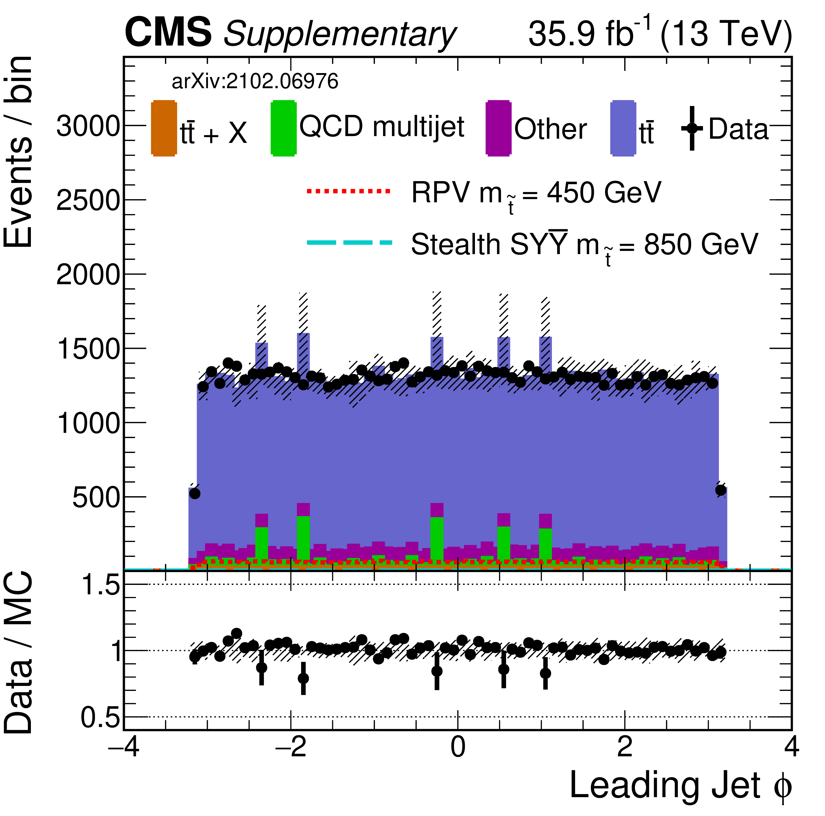
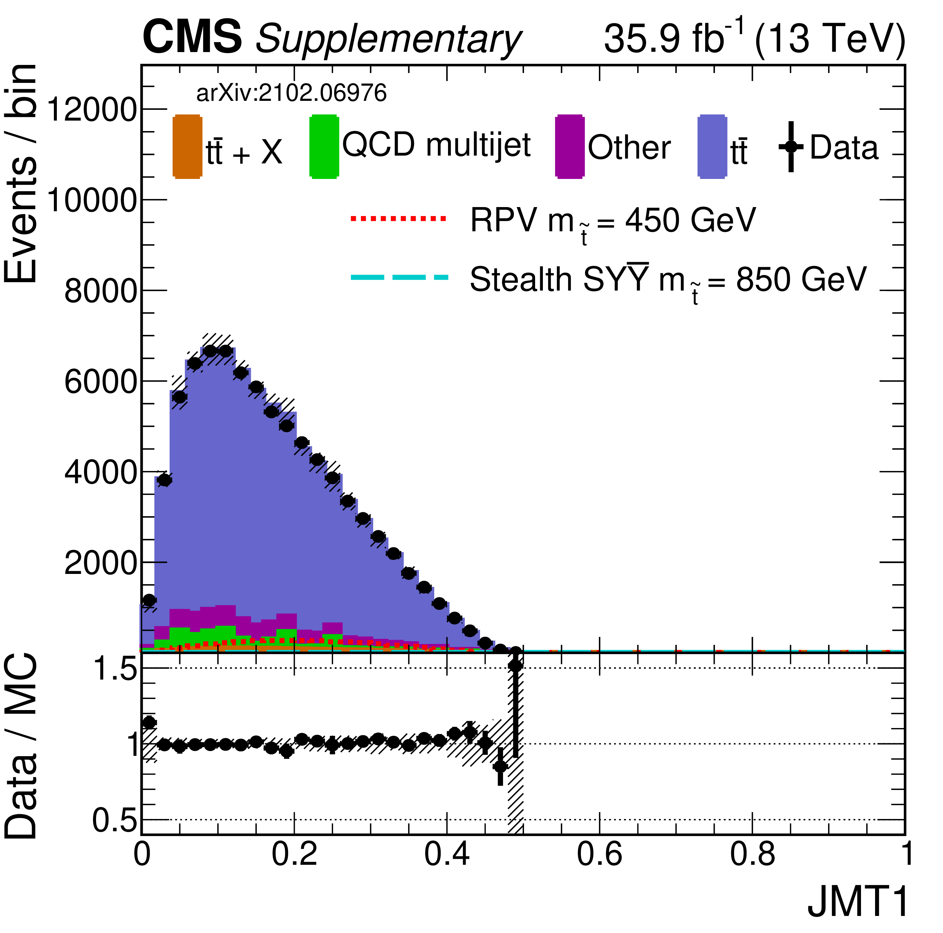
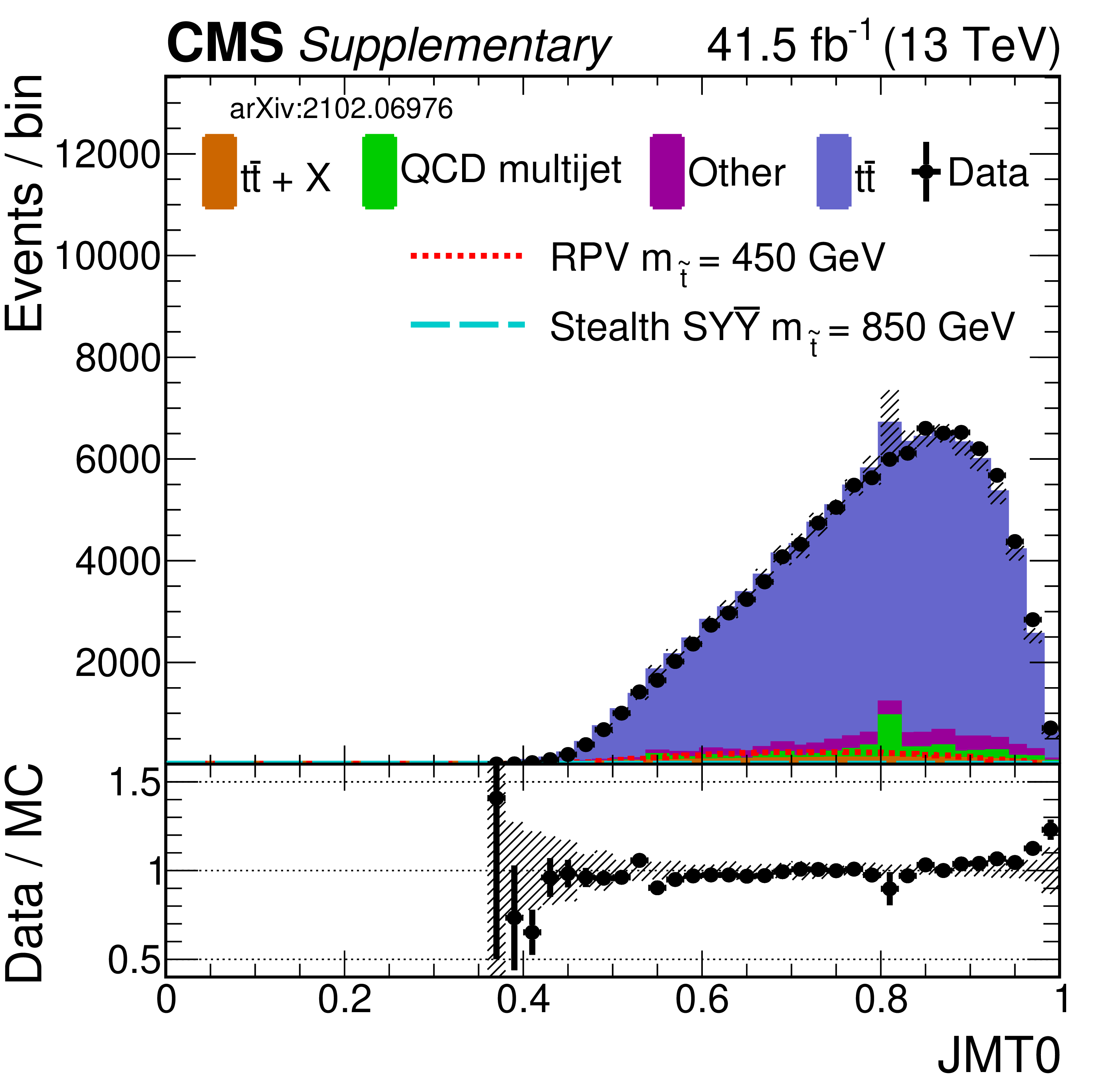
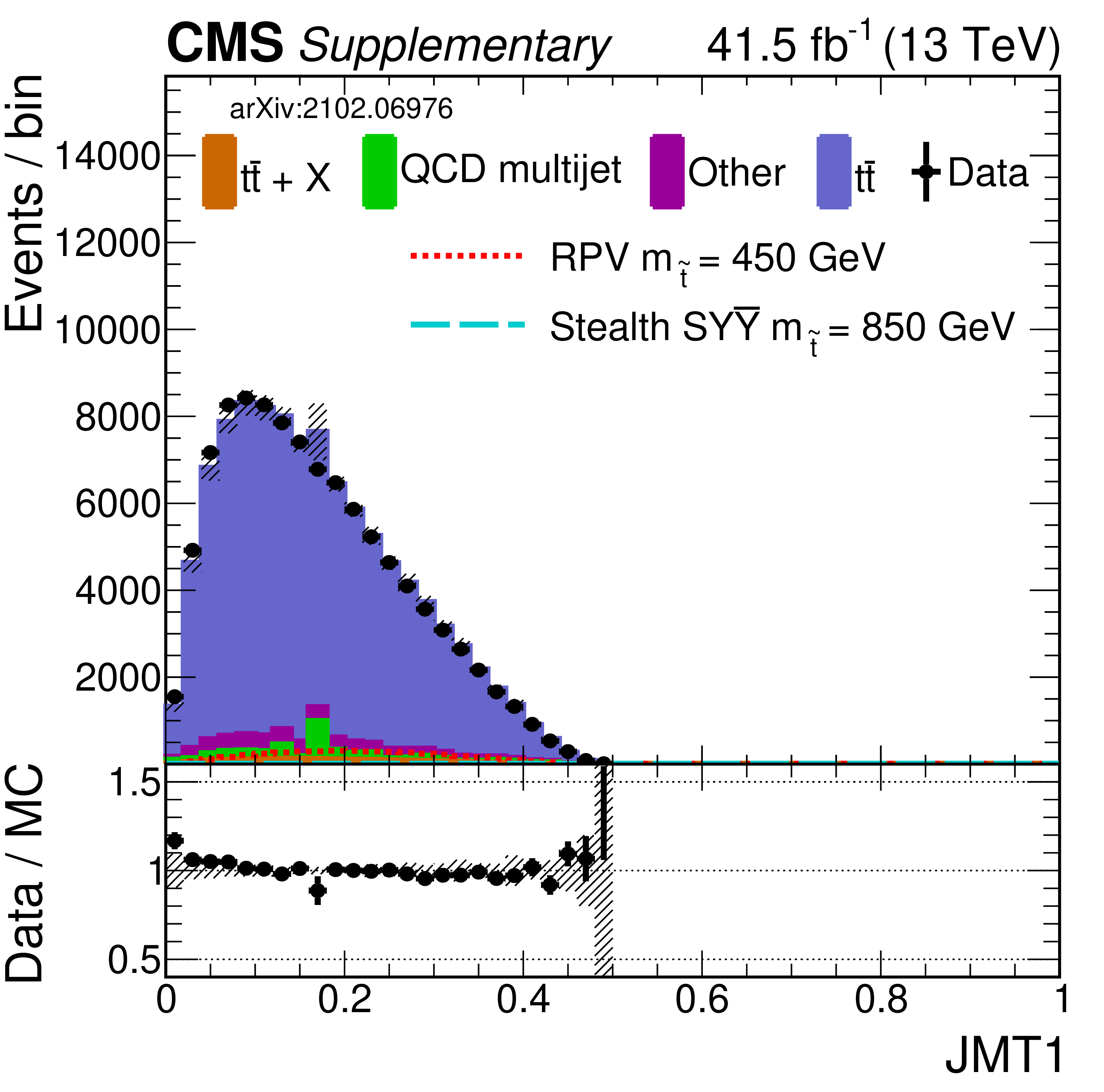
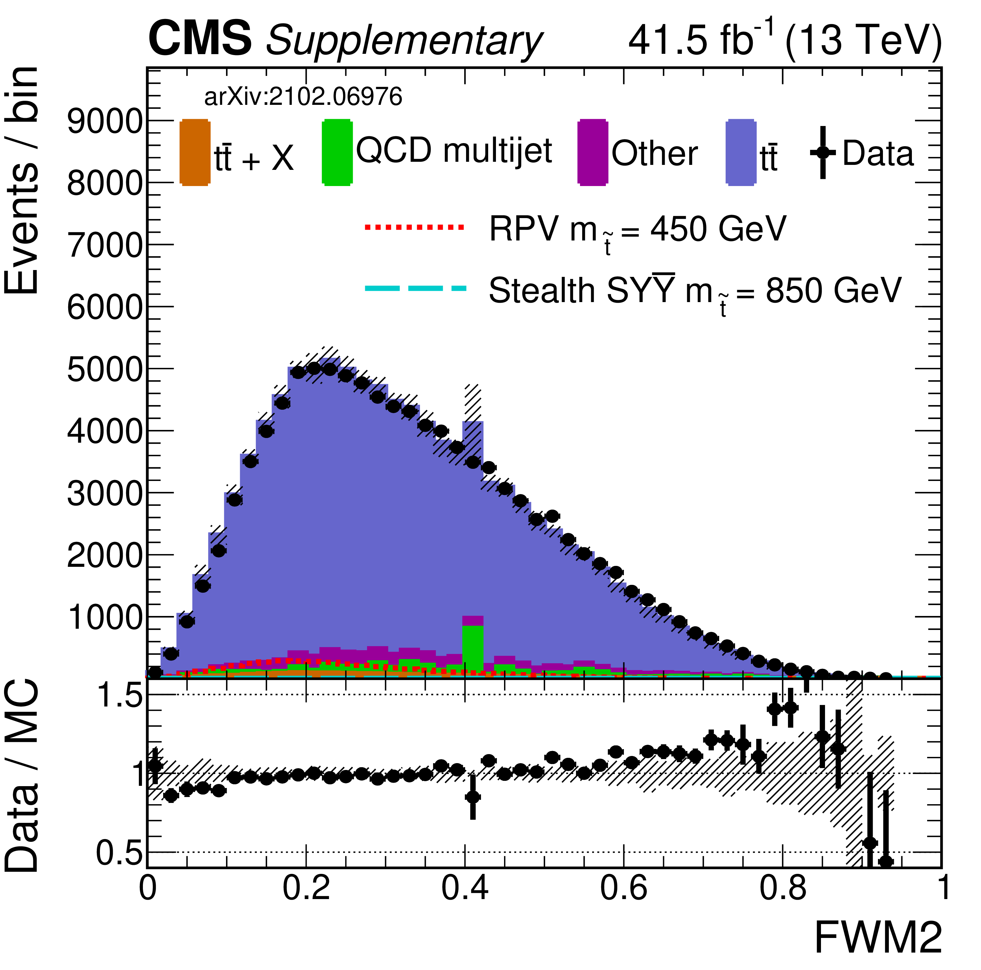
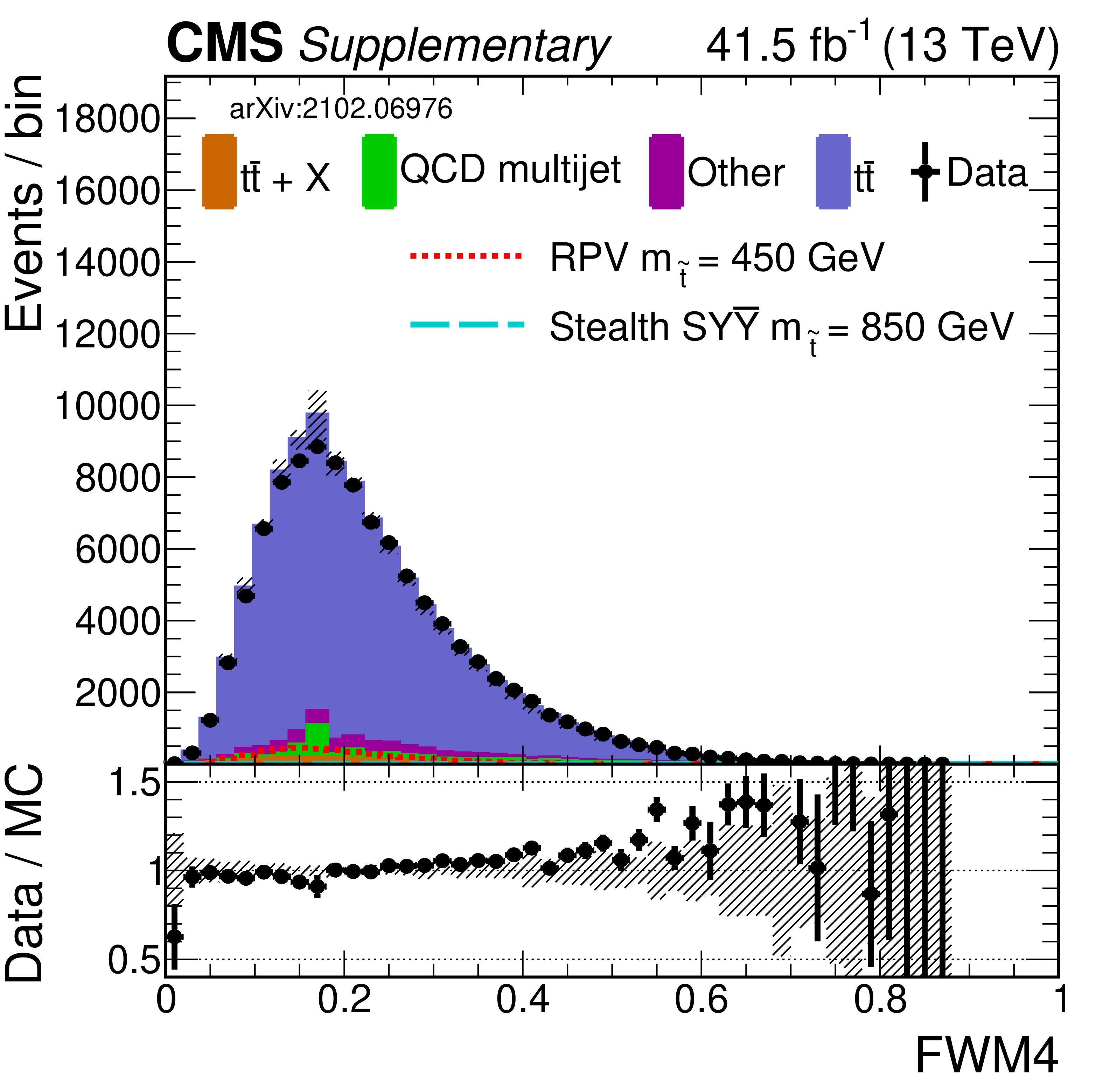
Additional Figure 7:
Shown are some of the input variables to the NN (2016). A comparison is made between $\mathrm{t\bar{t}}$ (blue) and two signal model/mass hypotheses. |
png pdf |
Additional Figure 7-a:
Shown is an input variable to the NN (2016). A comparison is made between $\mathrm{t\bar{t}}$ (blue) and two signal model/mass hypotheses. |
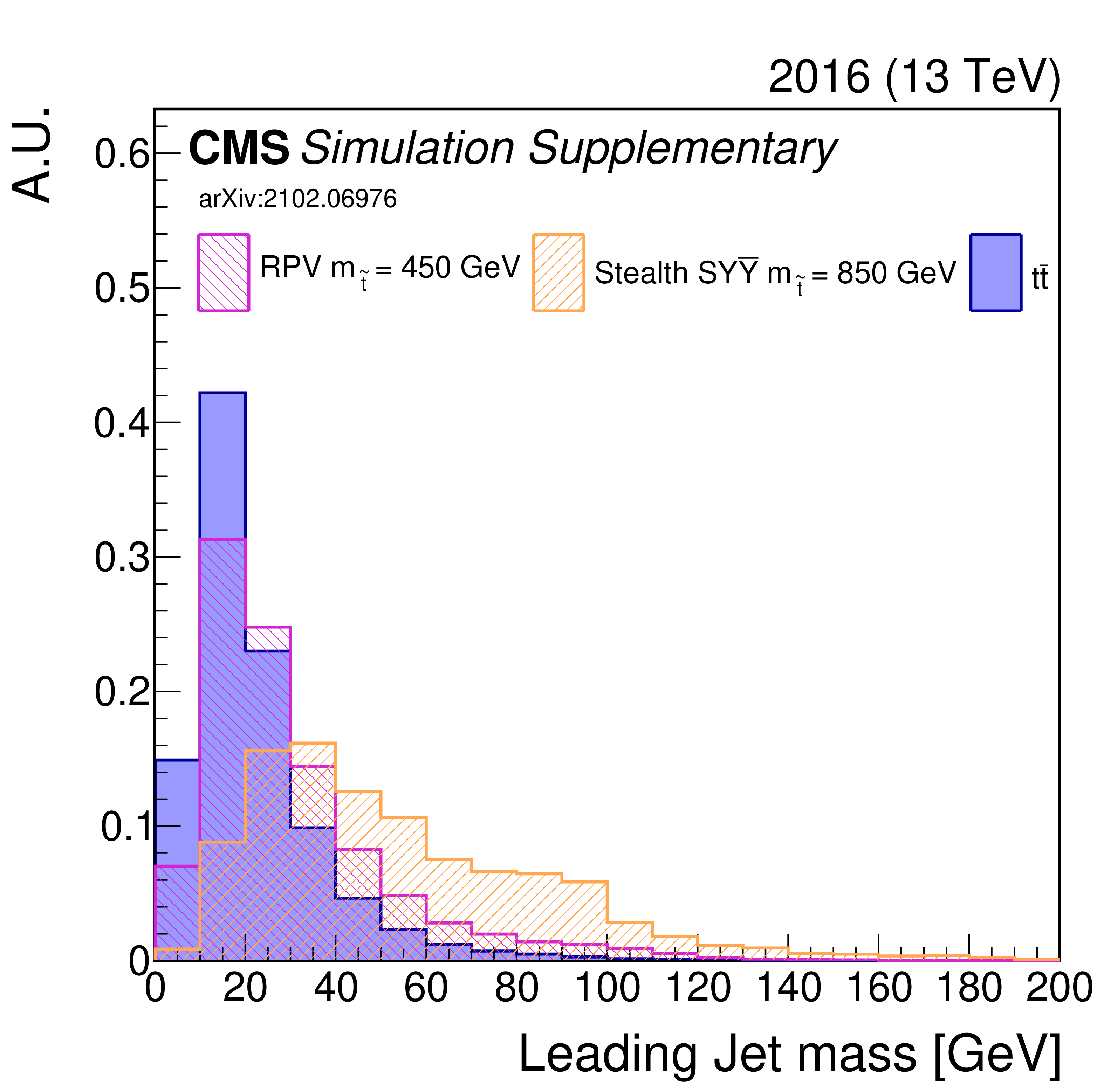
png pdf |
Additional Figure 7-b:
Shown is an input variable to the NN (2016). A comparison is made between $\mathrm{t\bar{t}}$ (blue) and two signal model/mass hypotheses. |
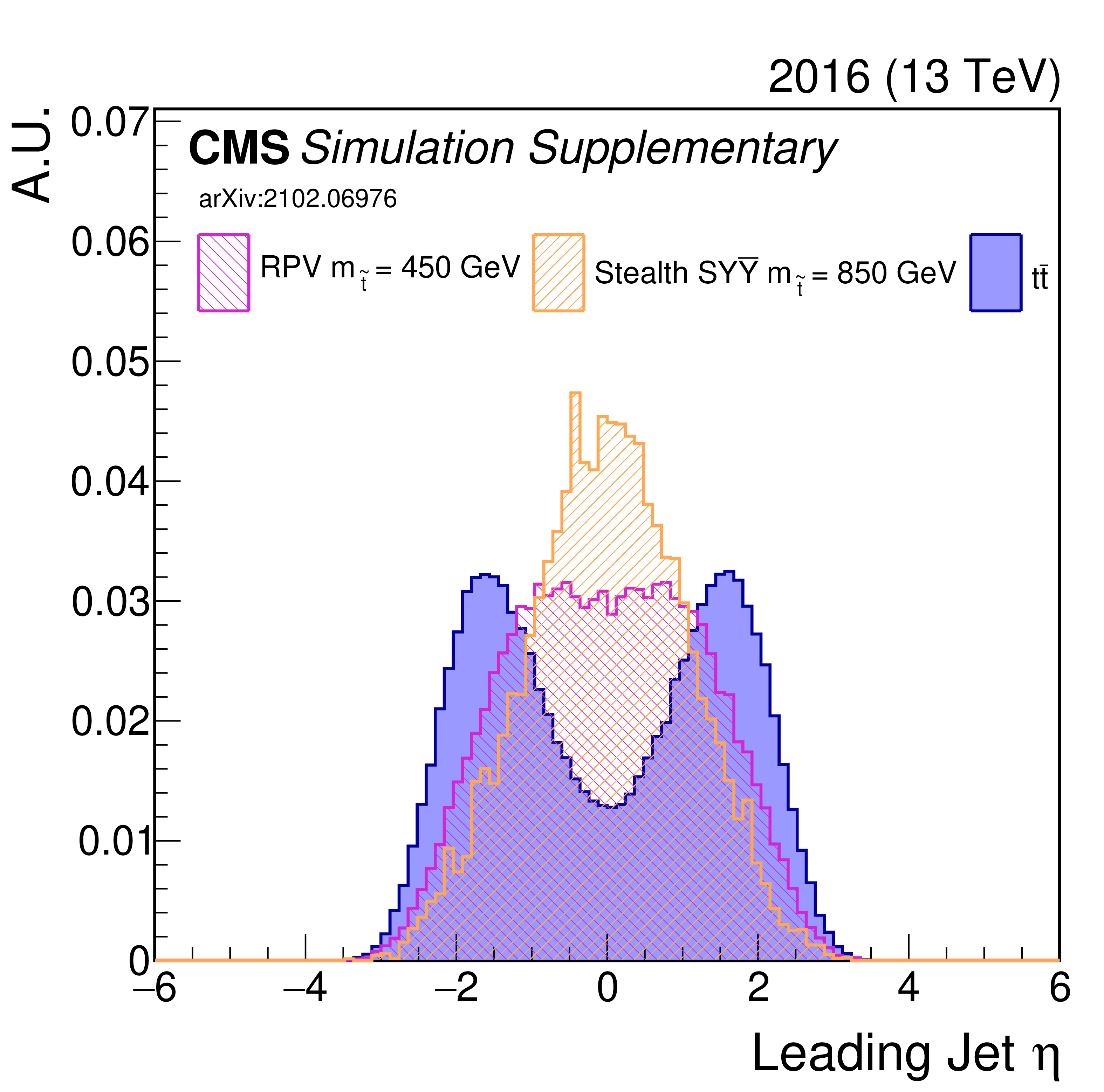
png pdf |
Additional Figure 7-c:
Shown is an input variable to the NN (2016). A comparison is made between $\mathrm{t\bar{t}}$ (blue) and two signal model/mass hypotheses. |
png pdf |
Additional Figure 7-d:
Shown is an input variable to the NN (2016). A comparison is made between $\mathrm{t\bar{t}}$ (blue) and two signal model/mass hypotheses. |

png pdf |
Additional Figure 7-e:
Shown is an input variable to the NN (2016). A comparison is made between $\mathrm{t\bar{t}}$ (blue) and two signal model/mass hypotheses. |
png pdf |
Additional Figure 7-f:
Shown is an input variable to the NN (2016). A comparison is made between $\mathrm{t\bar{t}}$ (blue) and two signal model/mass hypotheses. |

png pdf |
Additional Figure 7-g:
Shown is an input variable to the NN (2016). A comparison is made between $\mathrm{t\bar{t}}$ (blue) and two signal model/mass hypotheses. |
png pdf |
Additional Figure 7-h:
Shown is an input variable to the NN (2016). A comparison is made between $\mathrm{t\bar{t}}$ (blue) and two signal model/mass hypotheses. |
png pdf |
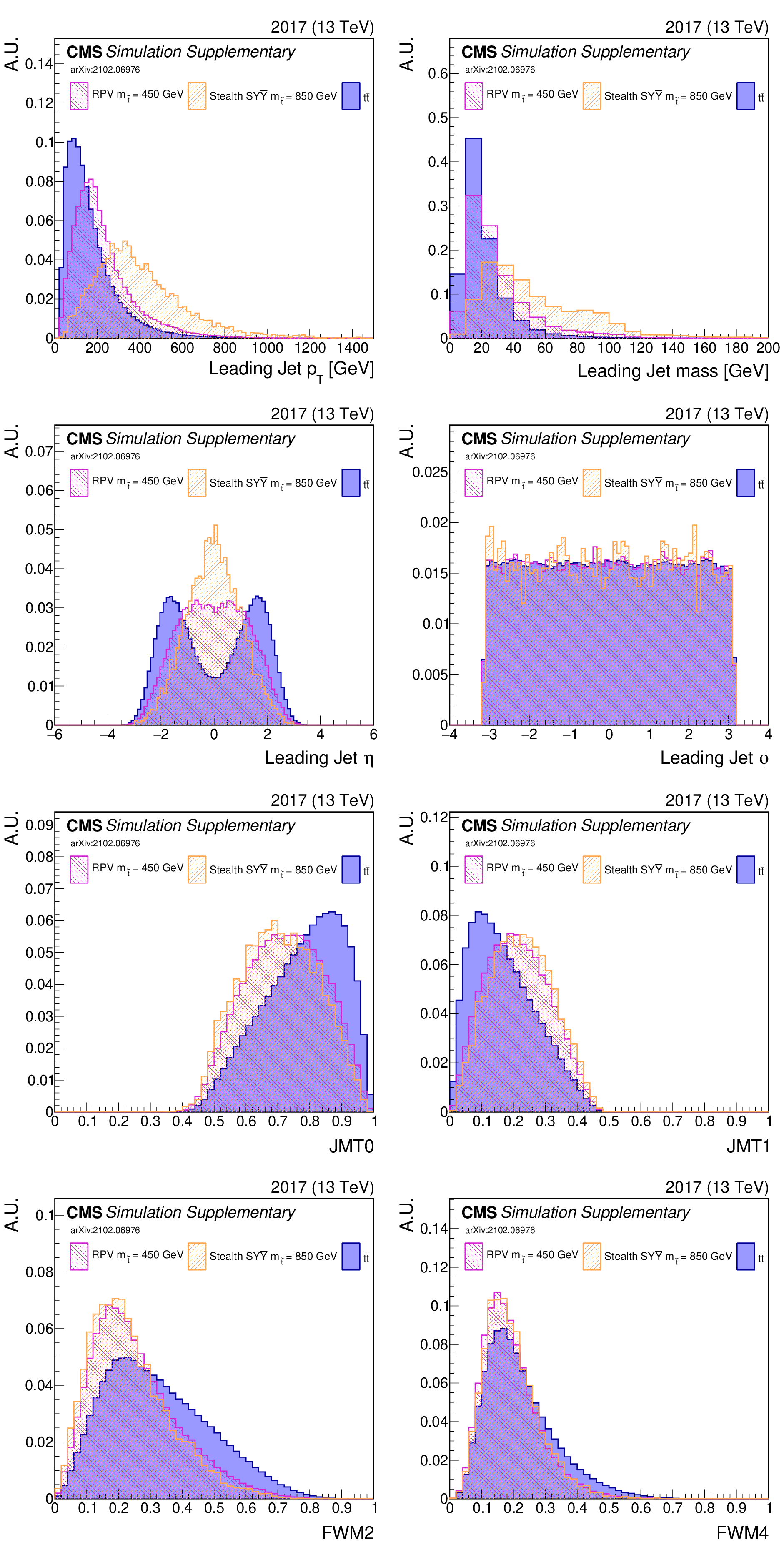
Additional Figure 8:
Shown are some of the input variables to the NN (2017). A comparison is made between $\mathrm{t\bar{t}}$ (blue) and two signal model/mass hypotheses. |
png pdf |
Additional Figure 8-a:
Shown is an input variable to the NN (2017). A comparison is made between $\mathrm{t\bar{t}}$ (blue) and two signal model/mass hypotheses. |
png pdf |
Additional Figure 8-b:
Shown is an input variable to the NN (2017). A comparison is made between $\mathrm{t\bar{t}}$ (blue) and two signal model/mass hypotheses. |
png pdf |
Additional Figure 8-c:
Shown is an input variable to the NN (2017). A comparison is made between $\mathrm{t\bar{t}}$ (blue) and two signal model/mass hypotheses. |
png pdf |
Additional Figure 8-d:
Shown is an input variable to the NN (2017). A comparison is made between $\mathrm{t\bar{t}}$ (blue) and two signal model/mass hypotheses. |
png pdf |
Additional Figure 8-e:
Shown is an input variable to the NN (2017). A comparison is made between $\mathrm{t\bar{t}}$ (blue) and two signal model/mass hypotheses. |
png pdf |
Additional Figure 8-f:
Shown is an input variable to the NN (2017). A comparison is made between $\mathrm{t\bar{t}}$ (blue) and two signal model/mass hypotheses. |
png pdf |
Additional Figure 8-g:
Shown is an input variable to the NN (2017). A comparison is made between $\mathrm{t\bar{t}}$ (blue) and two signal model/mass hypotheses. |
png pdf |
Additional Figure 8-h:
Shown is an input variable to the NN (2017). A comparison is made between $\mathrm{t\bar{t}}$ (blue) and two signal model/mass hypotheses. |
png pdf |
Additional Figure 9:
Shown is a comparison of data and simulation (2016) for the same selection of input variables as shown in Fig. 7. Simulation has been normalized to data. The uncertainty band in the ratio panel includes several of the main systematic uncertainties (added in quadrature). |
png pdf |
Additional Figure 9-a:
Shown is a comparison of data and simulation (2016) for the same selection of input variables as shown in Fig. 7. Simulation has been normalized to data. The uncertainty band in the ratio panel includes several of the main systematic uncertainties (added in quadrature). |

png pdf |
Additional Figure 9-b:
Shown is a comparison of data and simulation (2016) for the same selection of input variables as shown in Fig. 7. Simulation has been normalized to data. The uncertainty band in the ratio panel includes several of the main systematic uncertainties (added in quadrature). |

png pdf |
Additional Figure 9-c:
Shown is a comparison of data and simulation (2016) for the same selection of input variables as shown in Fig. 7. Simulation has been normalized to data. The uncertainty band in the ratio panel includes several of the main systematic uncertainties (added in quadrature). |
png pdf |
Additional Figure 9-d:
Shown is a comparison of data and simulation (2016) for the same selection of input variables as shown in Fig. 7. Simulation has been normalized to data. The uncertainty band in the ratio panel includes several of the main systematic uncertainties (added in quadrature). |

png pdf |
Additional Figure 9-e:
Shown is a comparison of data and simulation (2016) for the same selection of input variables as shown in Fig. 7. Simulation has been normalized to data. The uncertainty band in the ratio panel includes several of the main systematic uncertainties (added in quadrature). |
png pdf |
Additional Figure 9-f:
Shown is a comparison of data and simulation (2016) for the same selection of input variables as shown in Fig. 7. Simulation has been normalized to data. The uncertainty band in the ratio panel includes several of the main systematic uncertainties (added in quadrature). |
png pdf |
Additional Figure 9-g:
Shown is a comparison of data and simulation (2016) for the same selection of input variables as shown in Fig. 7. Simulation has been normalized to data. The uncertainty band in the ratio panel includes several of the main systematic uncertainties (added in quadrature). |

png pdf |
Additional Figure 9-h:
Shown is a comparison of data and simulation (2016) for the same selection of input variables as shown in Fig. 7. Simulation has been normalized to data. The uncertainty band in the ratio panel includes several of the main systematic uncertainties (added in quadrature). |

png pdf |
Additional Figure 10:
Shown is a comparison of data and simulation (2017) for the same selection of input variables as shown in Fig. 8. Simulation has been normalized to data. The uncertainty band in the ratio panel includes several of the main systematic uncertainties (added in quadrature). |
png pdf |
Additional Figure 10-a:
Shown is a comparison of data and simulation (2017) for the same selection of input variables as shown in Fig. 8. Simulation has been normalized to data. The uncertainty band in the ratio panel includes several of the main systematic uncertainties (added in quadrature). |
png pdf |
Additional Figure 10-b:
Shown is a comparison of data and simulation (2017) for the same selection of input variables as shown in Fig. 8. Simulation has been normalized to data. The uncertainty band in the ratio panel includes several of the main systematic uncertainties (added in quadrature). |

png pdf |
Additional Figure 10-c:
Shown is a comparison of data and simulation (2017) for the same selection of input variables as shown in Fig. 8. Simulation has been normalized to data. The uncertainty band in the ratio panel includes several of the main systematic uncertainties (added in quadrature). |
png pdf |
Additional Figure 10-d:
Shown is a comparison of data and simulation (2017) for the same selection of input variables as shown in Fig. 8. Simulation has been normalized to data. The uncertainty band in the ratio panel includes several of the main systematic uncertainties (added in quadrature). |
png pdf |
Additional Figure 10-e:
Shown is a comparison of data and simulation (2017) for the same selection of input variables as shown in Fig. 8. Simulation has been normalized to data. The uncertainty band in the ratio panel includes several of the main systematic uncertainties (added in quadrature). |
png pdf |
Additional Figure 10-f:
Shown is a comparison of data and simulation (2017) for the same selection of input variables as shown in Fig. 8. Simulation has been normalized to data. The uncertainty band in the ratio panel includes several of the main systematic uncertainties (added in quadrature). |
png pdf |
Additional Figure 10-g:
Shown is a comparison of data and simulation (2017) for the same selection of input variables as shown in Fig. 8. Simulation has been normalized to data. The uncertainty band in the ratio panel includes several of the main systematic uncertainties (added in quadrature). |
png pdf |
Additional Figure 10-h:
Shown is a comparison of data and simulation (2017) for the same selection of input variables as shown in Fig. 8. Simulation has been normalized to data. The uncertainty band in the ratio panel includes several of the main systematic uncertainties (added in quadrature). |
png pdf |
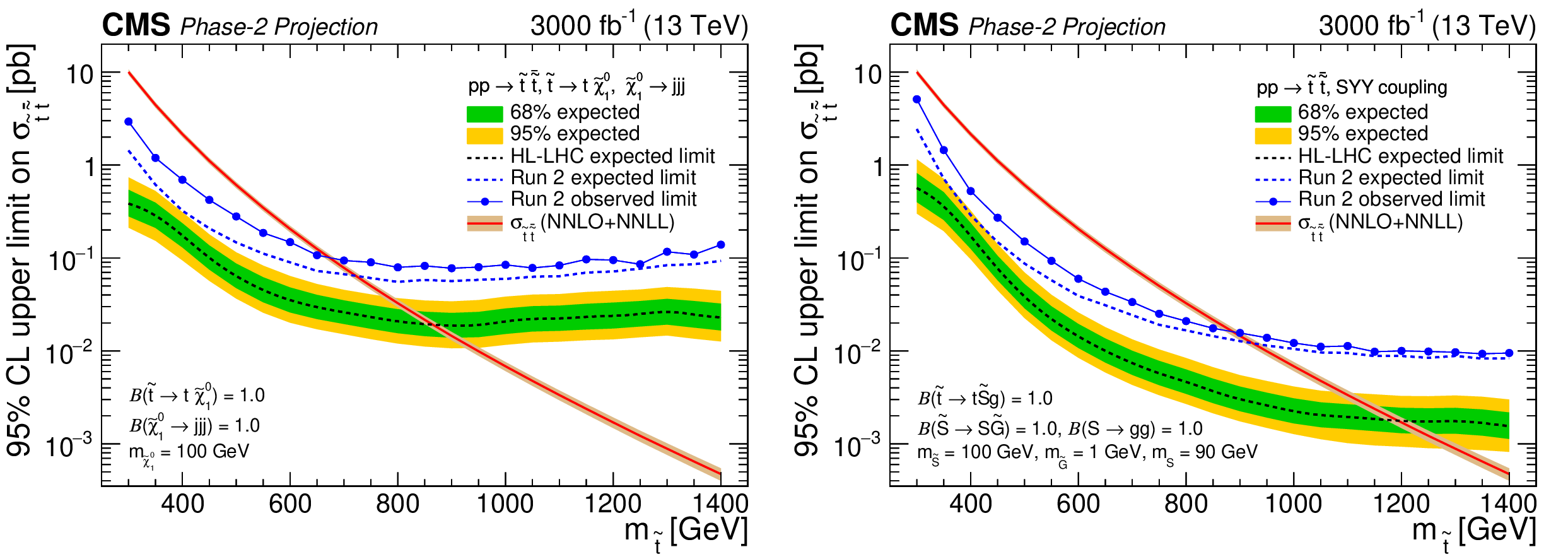
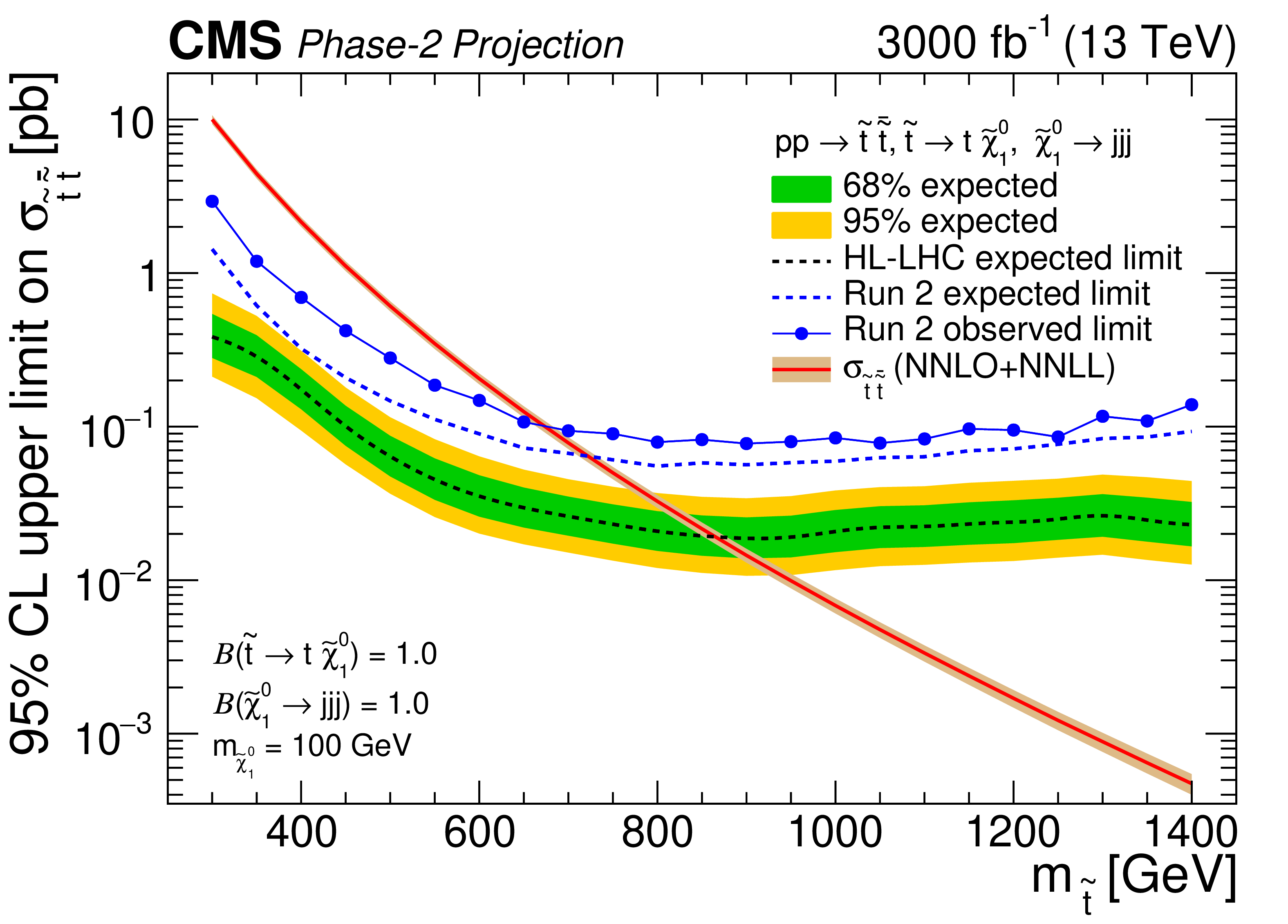
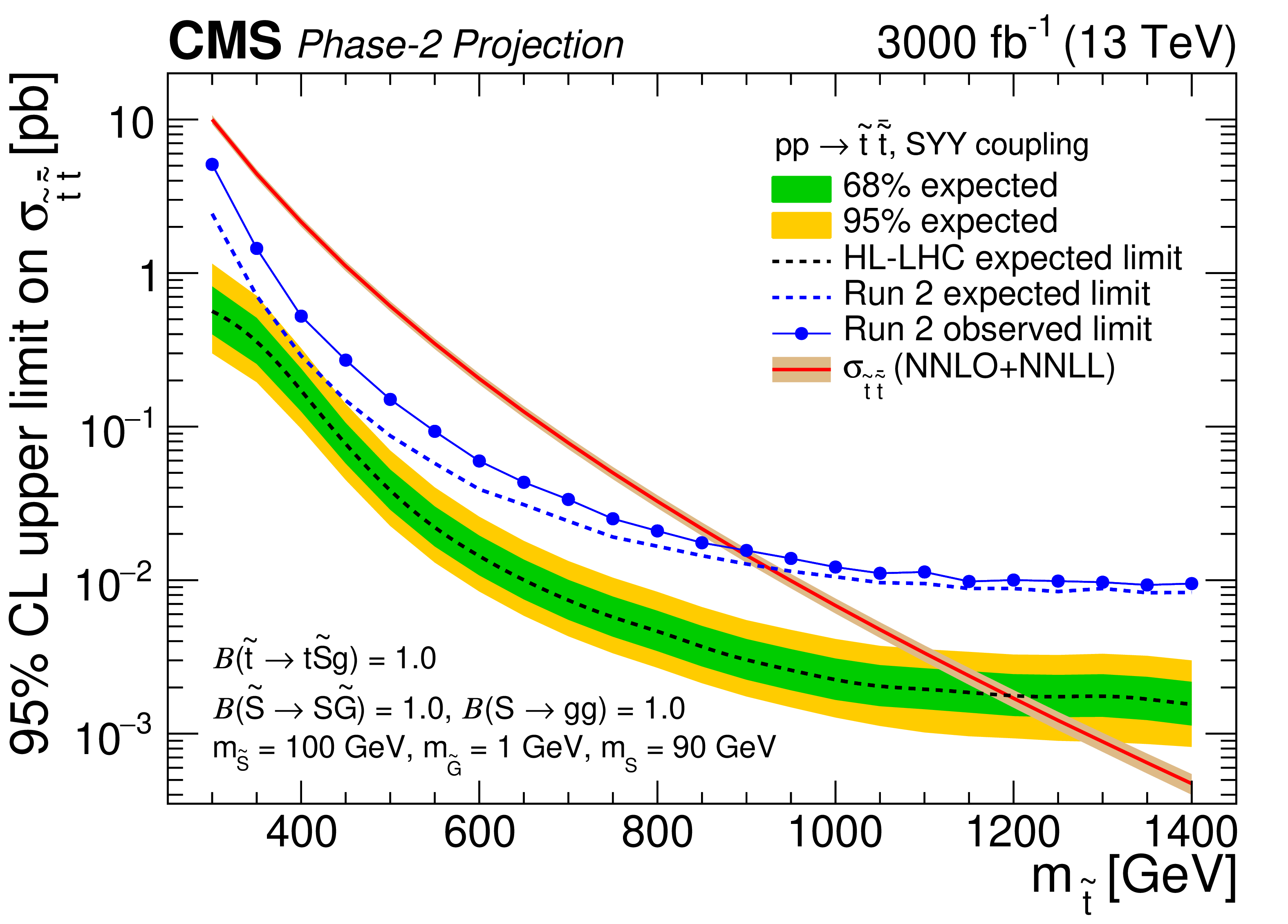
Additional Figure 11:
Projected 95% CL upper limits on the top squark pair production cross section as a function of the top squark mass for the RPV (left) and stealth (right) SUSY models with the 3000 fb$^{-1}$ expected at the HL-LHC. Systematic uncertainties from Run 2 are reduced based on the expected improvements detailed in Refs. [85,86]. Accordingly, uncertainties associated with modeling are reduced by 50%. Those related to available statistics are scaled down by the square root of the luminosity ratio. Experimental uncertainties are reduced according to the prescribed recommendations. Uncertainties with negligible impacts either remain unchanged from Run 2 or are removed entirely. Observed limits with the Run 2 dataset of 137 fb$^{-1}$ are also overlaid. Assumed particle masses and branching fractions are included on the plot. The expected cross section computed at NNLO+NNLL accuracy is shown in the red curve. Relative to Run 2, the expected cross-section sensitivity is projected to improve by a factor of 3-7. Exclusion limits on the top squark mass are projected to reach approximately 870 GeV (1190 GeV) in the RPV (stealth) SUSY scenario, compared to 670 GeV (870 GeV) for Run 2. |
png pdf |
Additional Figure 11-a:
Projected 95% CL upper limits on the top squark pair production cross section as a function of the top squark mass for the RPV model with the 3000 fb$^{-1}$ expected at the HL-LHC. Systematic uncertainties from Run 2 are reduced based on the expected improvements detailed in Refs. [85,86]. Accordingly, uncertainties associated with modeling are reduced by 50%. Those related to available statistics are scaled down by the square root of the luminosity ratio. Experimental uncertainties are reduced according to the prescribed recommendations. Uncertainties with negligible impacts either remain unchanged from Run 2 or are removed entirely. Observed limits with the Run 2 dataset of 137 fb$^{-1}$ are also overlaid. Assumed particle masses and branching fractions are included on the plot. The expected cross section computed at NNLO+NNLL accuracy is shown in the red curve. Relative to Run 2, the expected cross-section sensitivity is projected to improve by a factor of 3-7. Exclusion limits on the top squark mass are projected to reach approximately 870 GeV in the RPV scenario, compared to 670 GeV for Run 2. |
png pdf |
Additional Figure 11-b:
Projected 95% CL upper limits on the top squark pair production cross section as a function of the top squark mass for the stealth SUSY model with the 3000 fb$^{-1}$ expected at the HL-LHC. Systematic uncertainties from Run 2 are reduced based on the expected improvements detailed in Refs. [85,86]. Accordingly, uncertainties associated with modeling are reduced by 50%. Those related to available statistics are scaled down by the square root of the luminosity ratio. Experimental uncertainties are reduced according to the prescribed recommendations. Uncertainties with negligible impacts either remain unchanged from Run 2 or are removed entirely. Observed limits with the Run 2 dataset of 137 fb$^{-1}$ are also overlaid. Assumed particle masses and branching fractions are included on the plot. The expected cross section computed at NNLO+NNLL accuracy is shown in the red curve. Relative to Run 2, the expected cross-section sensitivity is projected to improve by a factor of 3-7. Exclusion limits on the top squark mass are projected to reach approximately 1190 GeV in the stealth SUSY scenario, compared to 870 GeV for Run 2. |
| Additional Tables | |
png pdf |
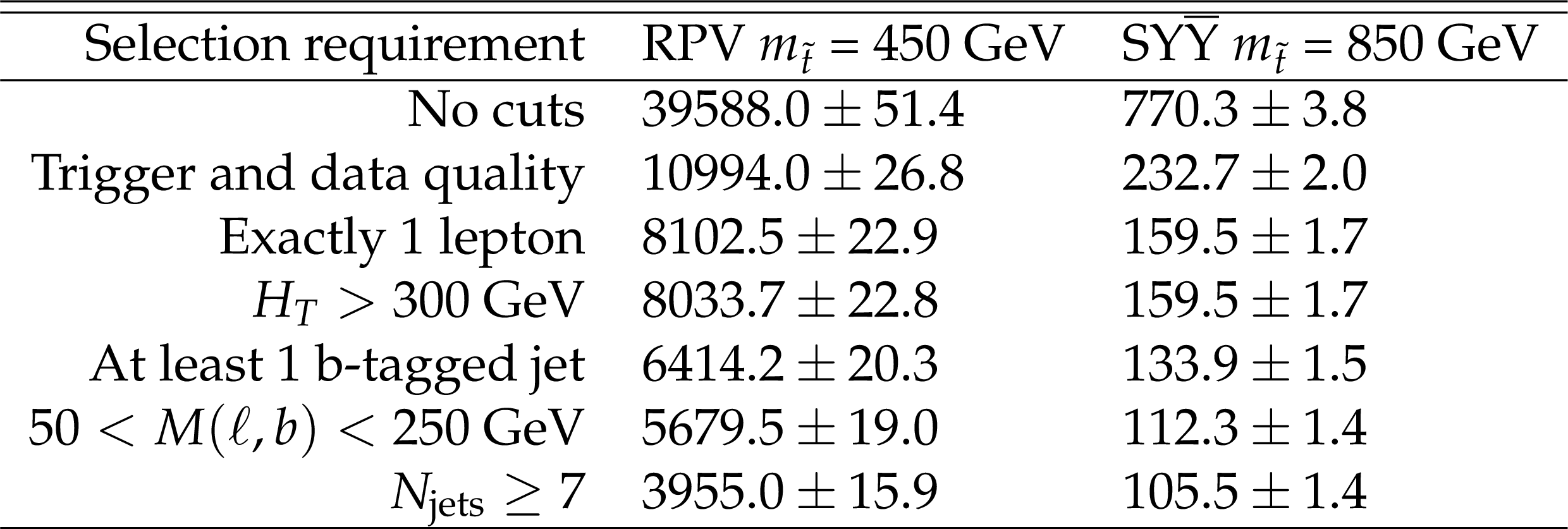
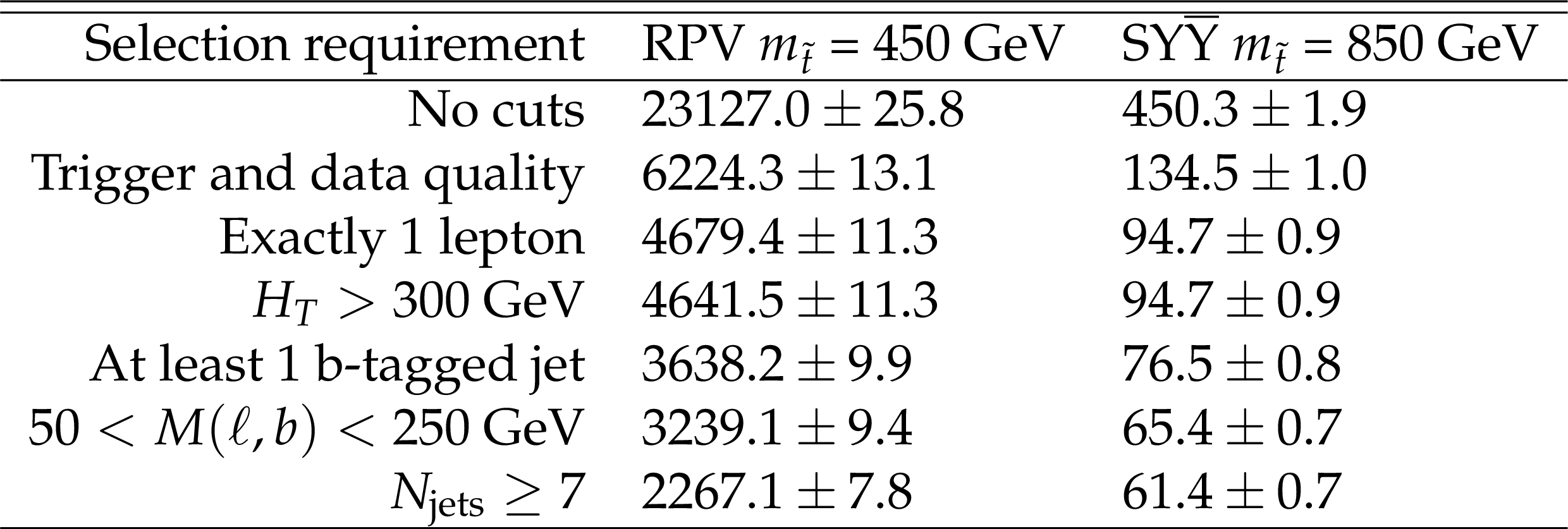
Additional Table 1:
Cut flow of the two signals shown in Fig. 4a (2016). $M(\ell,\mathrm{b})$ refers to the invariant mass of the system formed by the b-tagged jet and the lepton. At each stage of the cut flow all event weights used for the signal region are applied. |

png pdf |
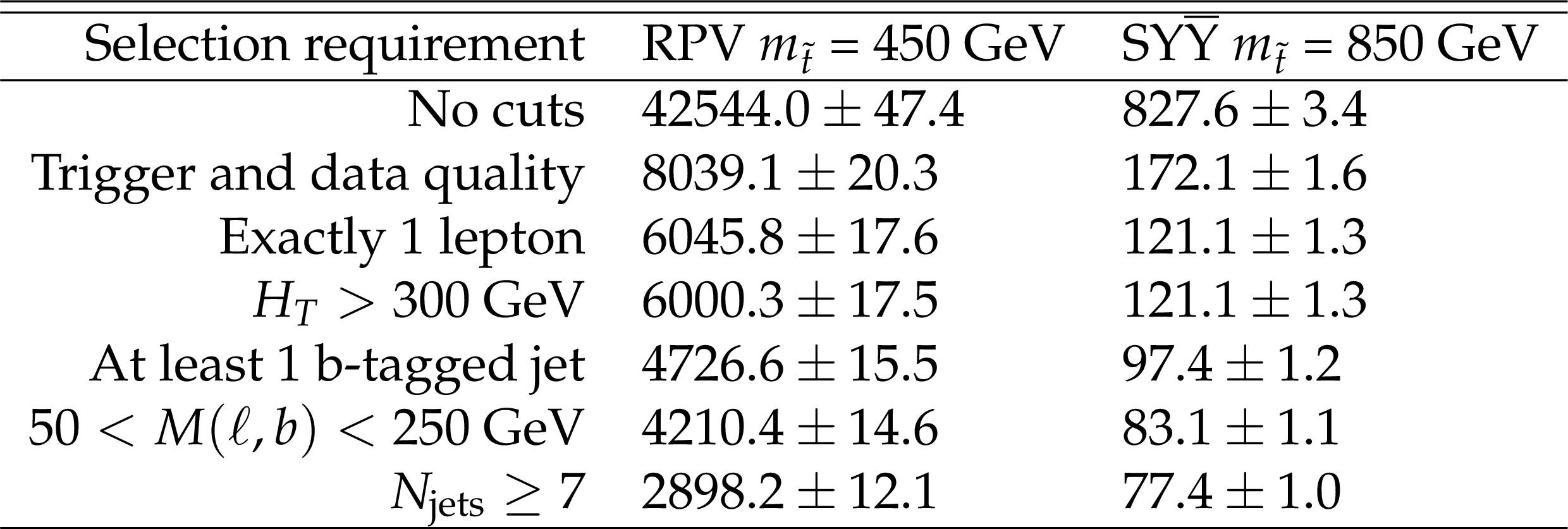
Additional Table 2:
Cut flow of the two signals shown in Fig. 4b (2017). $M(\ell,\mathrm{b})$ refers to the invariant mass of the system formed by the b-tagged jet and the lepton. At each stage of the cut flow all event weights used for the signal region are applied. |
png pdf |
Additional Table 3:
Cut flow of the two signals shown in Fig. 4c (2018A). $M(\ell,\mathrm{b})$ refers to the invariant mass of the system formed by the b-tagged jet and the lepton. At each stage of the cut flow all event weights used for the signal region are applied. |
png pdf |
Additional Table 4:
Cut flow of the two signals shown in Fig. 4d (2018B). $M(\ell,\mathrm{b})$ refers to the invariant mass of the system formed by the b-tagged jet and the lepton. At each stage of the cut flow all event weights used for the signal region are applied. |
| References | ||||
| 1 | P. Fayet and S. Ferrara | Supersymmetry | PR 32 (1977) 249 | |
| 2 | S. P. Martin | A supersymmetry primer | Adv. Ser. Direct. High Energy Phys. 21 (1997) 1 | hep-ph/9709356 |
| 3 | S. Dimopoulos and G. F. Giudice | Naturalness constraints in supersymmetric theories with nonuniversal soft terms | PLB 357 (1995) 573 | hep-ph/9507282 |
| 4 | R. Barbieri and G. F. Giudice | Upper bounds on supersymmetric particle masses | NPB 306 (1988) 63 | |
| 5 | A. Pomarol and D. Tommasini | Horizontal symmetries for the supersymmetric flavor problem | NPB 466 (1996) 3 | hep-ph/9507462 |
| 6 | A. G. Cohen, D. B. Kaplan, and A. E. Nelson | The more minimal supersymmetric standard model | PLB 388 (1996) 588 | hep-ph/9607394 |
| 7 | M. Papucci, J. T. Ruderman, and A. Weiler | Natural SUSY endures | JHEP 09 (2012) 035 | 1110.6926 |
| 8 | C. Brust, A. Katz, S. Lawrence, and R. Sundrum | SUSY, the third generation and the LHC | JHEP 03 (2012) 103 | 1110.6670 |
| 9 | R. Barbier et al. | $ R $-parity violating supersymmetry | PR 420 (2005) 1 | hep-ph/0406039 |
| 10 | D. S. M. Alves, E. Izaguirre, and J. G. Wacker | Where the sidewalk ends: Jets and missing energy search strategies for the 7 TeV LHC | JHEP 10 (2011) 012 | 1102.5338 |
| 11 | M. Lisanti, P. Schuster, M. Strassler, and N. Toro | Study of LHC searches for a lepton and many jets | JHEP 11 (2012) 081 | 1107.5055 |
| 12 | J. Fan, M. Reece, and J. T. Ruderman | Stealth supersymmetry | JHEP 11 (2011) 012 | 1105.5135 |
| 13 | G. F. Giudice and R. Rattazzi | Theories with gauge mediated supersymmetry breaking | PR 322 (1999) 419 | hep-ph/9801271 |
| 14 | S. P. Martin | Compressed supersymmetry and natural neutralino dark matter from top squark-mediated annihilation to top quarks | PRD 75 (2007) 115005 | hep-ph/0703097 |
| 15 | T. J. LeCompte and S. P. Martin | Large Hadron Collider reach for supersymmetric models with compressed mass spectra | PRD 84 (2011) 015004 | 1105.4304 |
| 16 | M. J. Strassler | Why unparticle models with mass gaps are examples of hidden valleys | 0801.0629 | |
| 17 | CMS Collaboration | Search for supersymmetry in proton-proton collisions at 13 TeV using identified top quarks | PRD 97 (2018) 012007 | CMS-SUS-16-050 1710.11188 |
| 18 | CMS Collaboration | Search for direct production of supersymmetric partners of the top quark in the all-jets final state in proton-proton collisions at $ \sqrt{s}= $ 13 TeV | JHEP 10 (2017) 005 | CMS-SUS-16-049 1707.03316 |
| 19 | CMS Collaboration | Search for top squark pair production in pp collisions at $ \sqrt{s}= $ 13 TeV using single lepton events | JHEP 10 (2017) 019 | CMS-SUS-16-051 1706.04402 |
| 20 | CMS Collaboration | Search for top squarks and dark matter particles, in opposite-charge dilepton final states at $ \sqrt{s} = $ 13 TeV | PRD 97 (2018) 032009 | CMS-SUS-17-001 1711.00752 |
| 21 | ATLAS Collaboration | Search for a scalar partner of the top quark in the jets plus missing transverse momentum final state at $ \sqrt{s} = $ 13 TeV with the ATLAS detector | JHEP 12 (2017) 085 | 1709.04183 |
| 22 | ATLAS Collaboration | Search for top-squark pair production in final states with one lepton, jets, and missing transverse momentum using 36 fb$ ^{-1} $ of $ \sqrt{s}= $ 13 TeV pp collision data with the ATLAS detector | JHEP 06 (2018) 108 | 1711.11520 |
| 23 | J. Fan, M. Reece, and J. T. Ruderman | A stealth supersymmetry sampler | JHEP 07 (2012) 196 | 1201.4875 |
| 24 | J. Fan et al. | Stealth supersymmetry simplified | JHEP 07 (2016) 016 | 1512.05781 |
| 25 | ATLAS Collaboration | A search for pair-produced resonances in four-jet final states at $ \sqrt{s} = $ 13 TeV with the ATLAS detector | EPJC 78 (2018) 250 | 1710.07171 |
| 26 | CMS Collaboration | Search for pair-produced resonances decaying to quark pairs in proton-proton collisions at $ \sqrt{s}= $ 13 TeV | PRD 98 (2018) 112014 | CMS-EXO-17-021 1808.03124 |
| 27 | ATLAS Collaboration | Search for B-L $ R $-parity-violating top squarks in $ \sqrt{s} = $ 13 TeV pp collisions with the ATLAS experiment | PRD 97 (2018) 032003 | 1710.05544 |
| 28 | CMS Collaboration | Search for pair production of third-generation scalar leptoquarks and top squarks in proton--proton collisions at $ \sqrt{s} = $ 8 TeV | PLB 739 (2014) 229 | CMS-EXO-12-032 1408.0806 |
| 29 | CMS Collaboration | Search for $ R $-parity violating decays of a top squark in proton-proton collisions at $ \sqrt{s} = $ 8 TeV | PLB 760 (2016) 178 | CMS-EXO-14-013 1602.04334 |
| 30 | ATLAS Collaboration | Search for new phenomena in a lepton plus high jet multiplicity final state with the ATLAS experiment using $ \sqrt{s}= $ 13 TeV proton-proton collision data | JHEP 09 (2017) 088 | 1704.08493 |
| 31 | CMS Collaboration | Search for stealth supersymmetry in events with jets, either photons or leptons, and low missing transverse momentum in pp collisions at 8 TeV | PLB 743 (2015) 503 | CMS-SUS-14-009 1411.7255 |
| 32 | CMS Collaboration | Search for supersymmetry in events with photons and low missing transverse energy in pp collisions at $ \sqrt{s}= $ 7 TeV | PLB 719 (2013) 42 | CMS-SUS-12-014 1210.2052 |
| 33 | CMS Collaboration | The CMS experiment at the CERN LHC | JINST 3 (2008) S08004 | CMS-00-001 |
| 34 | CMS Collaboration | The CMS trigger system | JINST 12 (2017) P01020 | CMS-TRG-12-001 1609.02366 |
| 35 | CMS Collaboration | Particle-flow reconstruction and global event description with the CMS detector | JINST 12 (2017) P10003 | CMS-PRF-14-001 1706.04965 |
| 36 | M. Cacciari, G. P. Salam, and G. Soyez | The anti-$ {k_{\mathrm{T}}} $ jet clustering algorithm | JHEP 04 (2008) 063 | 0802.1189 |
| 37 | M. Cacciari, G. P. Salam, and G. Soyez | FastJet user manual | EPJC 72 (2012) 1896 | 1111.6097 |
| 38 | CMS Collaboration | Performance of electron reconstruction and selection with the CMS detector in proton-proton collisions at $ \sqrt{s} = $ 8 TeV | JINST 10 (2015) P06005 | CMS-EGM-13-001 1502.02701 |
| 39 | CMS Collaboration | Performance of the CMS muon detector and muon reconstruction with proton-proton collisions at $ \sqrt{s} = $ 13 TeV | JINST 13 (2018) P06015 | CMS-MUO-16-001 1804.04528 |
| 40 | K. Rehermann and B. Tweedie | Efficient identification of boosted semileptonic top quarks at the LHC | JHEP 03 (2011) 059 | 1007.2221 |
| 41 | CMS Collaboration | Jet performance in pp collisions at 7 TeV | CDS | |
| 42 | CMS Collaboration | Jet algorithms performance in 13 TeV data | CMS-PAS-JME-16-003 | CMS-PAS-JME-16-003 |
| 43 | CMS Collaboration | Jet energy scale and resolution in the CMS experiment in pp collisions at 8 TeV | JINST 12 (2017) P02014 | CMS-JME-13-004 1607.03663 |
| 44 | CMS Collaboration | Jet energy scale and resolution performance with 13 TeV data collected by CMS in 2016--2018 | CDS | |
| 45 | M. Cacciari and G. P. Salam | Pileup subtraction using jet areas | PLB 659 (2008) 119 | 0707.1378 |
| 46 | CMS Collaboration | Identification of heavy-flavour jets with the CMS detector in pp collisions at 13 TeV | JINST 13 (2018) P05011 | CMS-BTV-16-002 1712.07158 |
| 47 | P. Nason | A new method for combining NLO QCD with shower Monte Carlo algorithms | JHEP 11 (2004) 040 | hep-ph/0409146 |
| 48 | S. Frixione, P. Nason, and C. Oleari | Matching NLO QCD computations with parton shower simulations: the POWHEG method | JHEP 11 (2007) 070 | 0709.2092 |
| 49 | S. Alioli, P. Nason, C. Oleari, and E. Re | A general framework for implementing NLO calculations in shower Monte Carlo programs: the POWHEG box | JHEP 06 (2010) 043 | 1002.2581 |
| 50 | S. Frixione, P. Nason, and G. Ridolfi | A positive-weight next-to-leading-order Monte Carlo for heavy flavour hadroproduction | JHEP 09 (2007) 126 | 0707.3088 |
| 51 | R. Frederix, E. Re, and P. Torrielli | Single-top $ t $-channel hadroproduction in the four-flavour scheme with POWHEG and amc@nlo | JHEP 09 (2012) 130 | 1207.5391 |
| 52 | J. Alwall et al. | The automated computation of tree-level and next-to-leading order differential cross sections, and their matching to parton shower simulations | JHEP 07 (2014) 079 | 1405.0301 |
| 53 | A. Kalogeropoulos and J. Alwall | The SysCalc code: A tool to derive theoretical systematic uncertainties | 1801.08401 | |
| 54 | T. Sjostrand et al. | An introduction to PYTHIA 8.2 | CPC 191 (2015) 159 | 1410.3012 |
| 55 | C. Borschensky et al. | Squark and gluino production cross sections in pp collisions at $ \sqrt{s}= $ 13 , 14, 33 and 100 TeV | EPJC 74 (2014) 3174 | 1407.5066 |
| 56 | W. Beenakker et al. | NNLL-fast: predictions for coloured supersymmetric particle production at the LHC with threshold and Coulomb resummation | JHEP 12 (2016) 133 | 1607.07741 |
| 57 | NNPDF Collaboration | Parton distributions for the LHC Run II | JHEP 04 (2015) 040 | 1410.8849 |
| 58 | NNPDF Collaboration | Parton distributions from high-precision collider data | EPJC 77 (2017) 663 | 1706.00428 |
| 59 | CMS Collaboration | Event generator tunes obtained from underlying event and multiparton scattering measurements | EPJC 76 (2016) 155 | CMS-GEN-14-001 1512.00815 |
| 60 | CMS Collaboration | Investigations of the impact of the parton shower tuning in PYTHIA 8 in the modelling of $ \mathrm{t\bar{t}} $ at $ \sqrt{s}= $ 8 and 13 TeV | CMS-PAS-TOP-16-021 | CMS-PAS-TOP-16-021 |
| 61 | CMS Collaboration | Extraction and validation of a new set of CMS PYTHIA 8 tunes from underlying-event measurements | EPJC 80 (2020) 4 | CMS-GEN-17-001 1903.12179 |
| 62 | GEANT4 Collaboration | GEANT4--a simulation toolkit | NIMA 506 (2003) 250 | |
| 63 | M. Czakon and A. Mitov | Top++: A program for the calculation of the top-pair cross-section at hadron colliders | CPC 185 (2014) 2930 | 1112.5675 |
| 64 | P. Kant et al. | HATHOR for single top-quark production: Updated predictions and uncertainty estimates for single top-quark production in hadronic collisions | CPC 191 (2015) 74 | 1406.4403 |
| 65 | M. Aliev et al. | HATHOR: HAdronic Top and Heavy quarks crOss section calculatoR | CPC 182 (2011) 1034 | 1007.1327 |
| 66 | T. Gehrmann et al. | W$ ^+ $W$ ^- $ production at hadron colliders in next to next to leading order QCD | PRL 113 (2014) 212001 | 1408.5243 |
| 67 | J. M. Campbell and R. K. Ellis | An update on vector boson pair production at hadron colliders | PRD 60 (1999) 113006 | hep-ph/9905386 |
| 68 | J. M. Campbell, R. K. Ellis, and C. Williams | Vector boson pair production at the LHC | JHEP 07 (2011) 018 | 1105.0020 |
| 69 | Y. Li and F. Petriello | Combining QCD and electroweak corrections to dilepton production in FEWZ | PRD 86 (2012) 094034 | 1208.5967 |
| 70 | Y. Ganin and V. Lempitsky | Unsupervised domain adaptation by backpropagation | 1409.7495 | |
| 71 | G. C. Fox and S. Wolfram | Observables for the analysis of event shapes in $ \mathrm{e^{+}}\mathrm{e^{-}} $ annihilation and other processes | PRL 41 (1978) 1581 | |
| 72 | J. D. Bjorken and S. J. Brodsky | Statistical model for electron-positron annihilation into hadrons | PRD 1 (1970) 1416 | |
| 73 | E. Gerwick, T. Plehn, S. Schumann, and P. Schichtel | Scaling patterns for QCD jets | JHEP 10 (2012) 162 | 1208.3676 |
| 74 | M. Cacciari et al. | The $ \mathrm{t\bar{t}} $ cross-section at 1.8 TeV and 1.96 TeV: A study of the systematics due to parton densities and scale dependence | JHEP 04 (2004) 068 | hep-ph/0303085 |
| 75 | S. Catani, D. de Florian, M. Grazzini, and P. Nason | Soft gluon resummation for Higgs boson production at hadron colliders | JHEP 07 (2003) 028 | hep-ph/0306211 |
| 76 | CMS Collaboration | Measurement of the inelastic proton-proton cross section at $ \sqrt{s}= $ 13 TeV | JHEP 07 (2018) 161 | CMS-FSQ-15-005 1802.02613 |
| 77 | CMS Collaboration | CMS luminosity measurements for the 2016 data taking period | CMS-PAS-LUM-17-001 | CMS-PAS-LUM-17-001 |
| 78 | CMS Collaboration | CMS luminosity measurements for the 2017 data taking period at $ \sqrt{s}= $ 13 TeV | CMS-PAS-LUM-17-004 | CMS-PAS-LUM-17-004 |
| 79 | CMS Collaboration | CMS luminosity measurements for the 2018 data taking period at $ \sqrt{s}= $ 13 TeV | CMS-PAS-LUM-18-002 | CMS-PAS-LUM-18-002 |
| 80 | L. Demortier | $p$-values and nuisance parameters | in Statistical issues for LHC physics. Proceedings, Workshop, PHYSTAT-LHC, Geneva, Switzerland, June 27-29, 2007, p. 23 2008 | |
| 81 | ATLAS and CMS Collaborations, The LHC Higgs Combination Group | Procedure for the LHC Higgs boson search combination in Summer 2011 | CMS-NOTE-2011-005 | |
| 82 | T. Junk | Confidence level computation for combining searches with small statistics | NIMA 434 (1999) 435 | hep-ex/9902006 |
| 83 | A. L. Read | Presentation of search results: The CL$ _{\text{s}} $ technique | JPG 28 (2002) 2693 | |
| 84 | G. Cowan, K. Cranmer, E. Gross, and O. Vitells | Asymptotic formulae for likelihood-based tests of new physics | EPJC 71 (2011) 1554 | 1007.1727 |
| 85 | CMS Collaboration | Expected performance of the physics objects with the upgraded CMS detector at the HL-LHC | CMS-NOTE-2018-006, CERN-CMS-NOTE-2018-006 | |
| 86 | A. Dainese, M. Mangano, A. Meyer, A. Nisati, G. Salam, M. Vesterinen, A. Mika | Report on the Physics at the HL-LHC, and Perspectives for the HE-LHC | CERN-2019-007 | |
|
|
Compact Muon Solenoid LHC, CERN |
|

|

|

|

|

|