

Compact Muon Solenoid
LHC, CERN
| CMS-HIG-15-002 ; ATLAS-HIGG-2015-07 ; CERN-PH-2016-100 | ||
| Measurements of the Higgs boson production and decay rates and constraints on its couplings from a combined ATLAS and CMS analysis of the LHC $pp$ collision data at $\sqrt{s}=$ 7 and 8 TeV | ||
| ATLAS and CMS Collaborations | ||
| 7 June 2016 | ||
| J. High Energy Phys. 08 (2016) 045 | ||
| Abstract: Combined ATLAS and CMS measurements of the Higgs boson production and decay rates, as well as constraints on its couplings to vector bosons and fermions, are presented. The combination is based on the analysis of five production processes, namely gluon fusion, vector boson fusion, and associated production with a $W$ or a $Z$ boson or a pair of top quarks, and of the six decay modes $H \to ZZ, WW$, $\gamma\gamma$, $\tau\tau$, $b\bar{b}$, and $\mu\mu$. All results are reported assuming a value of 125.09 GeV for the Higgs boson mass, the result of the combined measurement by the ATLAS and CMS experiments. The analysis uses the CERN LHC proton--proton collision data recorded by the ATLAS and CMS experiments in 2011 and 2012, corresponding to integrated luminosities per experiment of approximately 5 fb$^{-1}$ at $\sqrt{s}=$ 7 TeV and 20 fb$^{-1}$ at $\sqrt{s} =$ 8 TeV. The Higgs boson production and decay rates measured by the two experiments are combined within the context of three generic parameterisations: two based on cross sections and branching fractions, and one on ratios of coupling modifiers. Several interpretations of the measurements with more model-dependent parameterisations are also given. The combined signal yield relative to the Standard Model prediction is measured to be 1.09 $\pm$ 0.11. The combined measurements lead to observed significances for the vector boson fusion production process and for the $Htt$ decay of 5.4 and 5.5 standard deviations, respectively. The data are consistent with the Standard Model predictions for all parameterisations considered. | ||
| Links: e-print arXiv:1606.02266 [hep-ex] (PDF) ; CDS record ; inSPIRE record ; HepData record ; CADI line (restricted) ; | ||
| Figures & Tables | Summary | Additional Figures & Tables | References | CMS Publications |
|---|
| Figures | |

png pdf |
Figure 1-a:
Example of leading-order Feynman diagram for Higgs boson production via the ${gg\mathrm {F}}$ production process. |

png pdf |
Figure 1-b:
Example of leading-order Feynman diagram for Higgs boson production via the VBF production process. |
png pdf |
Figure 2-a:
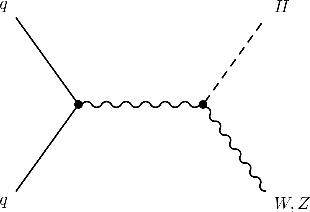
Example of leading-order Feynman diagram for Higgs boson production via the $qq \to VH$ production process. |
png pdf |
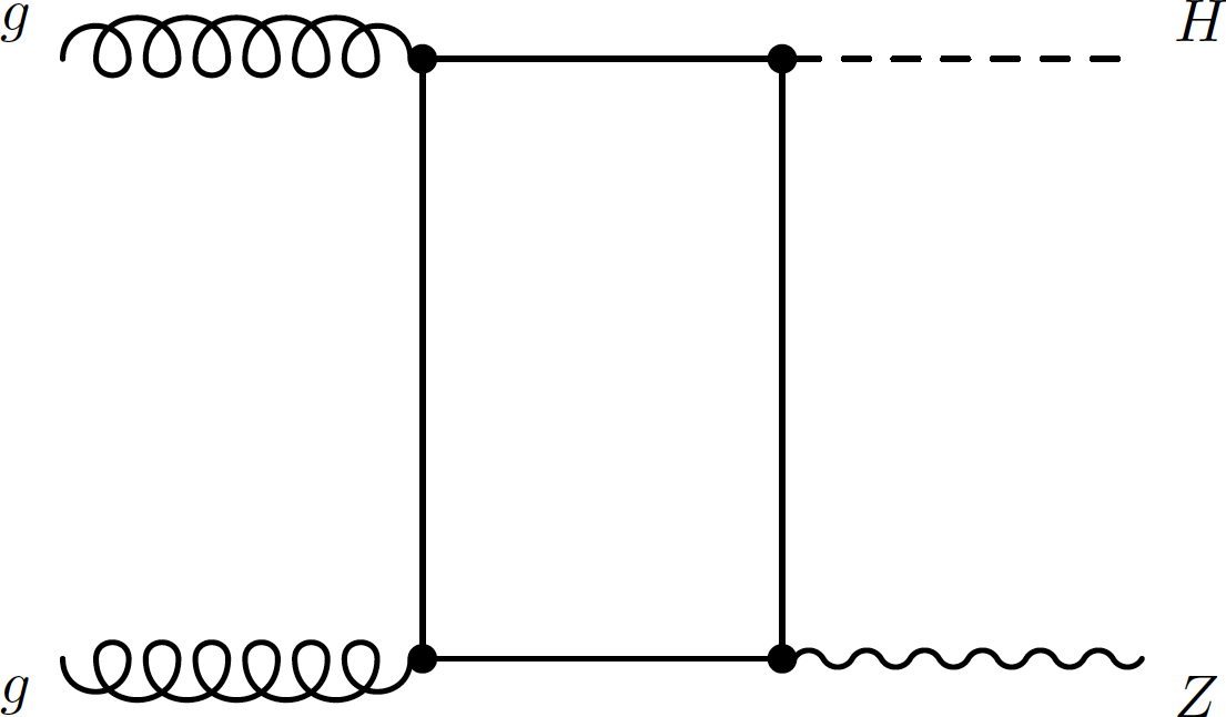
Figure 2-b:
Example of leading-order Feynman diagram for Higgs boson production via the ${gg\to ZH}$ production processes. |

png pdf |
Figure 2-c:
Example of leading-order Feynman diagram for Higgs boson production via the ${gg\to ZH}$ production processes. |
png pdf |
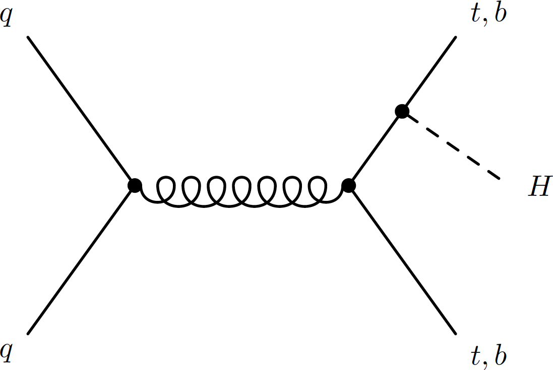
Figure 3-a:
Example of leading-order Feynman diagram for Higgs boson production via the ${qq \to ttH}$ and ${qq \to bbH}$ processes. |

png pdf |
Figure 3-b:
Example of leading-order Feynman diagram for Higgs boson production via the ${gg \to ttH}$ and ${gg \to bbH}$ processes. |

png pdf |
Figure 3-c:
Example of leading-order Feynman diagram for Higgs boson production via the ${gg \to ttH}$ and ${gg \to bbH}$ processes. |
png pdf |
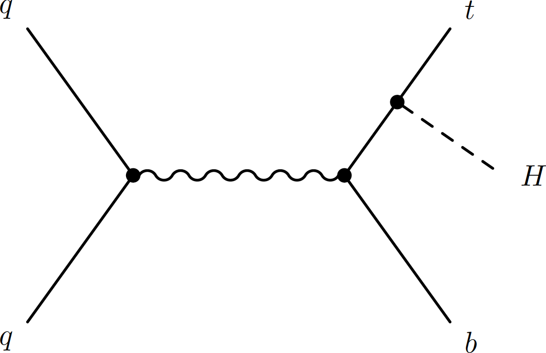
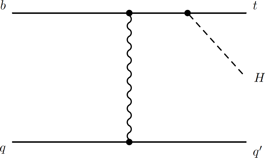
Figure 4-a:
Example of leading-order Feynman diagram for Higgs boson production in association with a single top quark via the ${tHq}$ production processes. |
png pdf |
Figure 4-b:
Example of leading-order Feynman diagram for Higgs boson production in association with a single top quark via the ${tHq}$ production processes. |
png pdf |
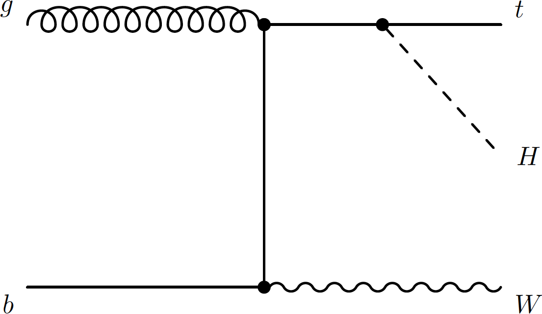
Figure 4-c:
Example of leading-order Feynman diagram for Higgs boson production in association with a single top quark via the ${tHW}$ production processes. |
png pdf |
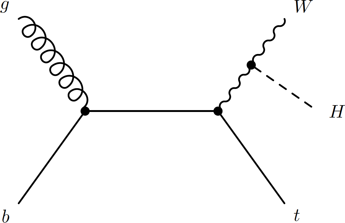
Figure 4-d:
Example of leading-order Feynman diagram for Higgs boson production in association with a single top quark via the ${tHW}$ production processes. |
png pdf |
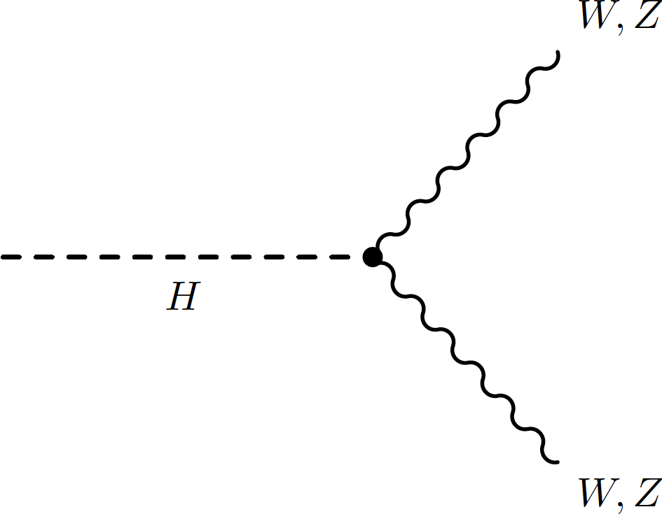
Figure 5-a:
Example of leading-order Feynman diagram for Higgs boson decays to $W$ and $Z$ bosons. |
png pdf |
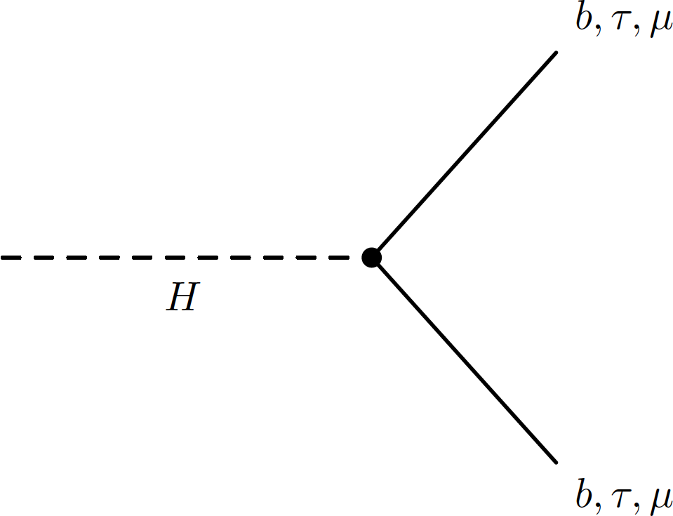
Figure 5-b:
Example of leading-order Feynman diagram for Higgs boson decays to fermions. |
png pdf |
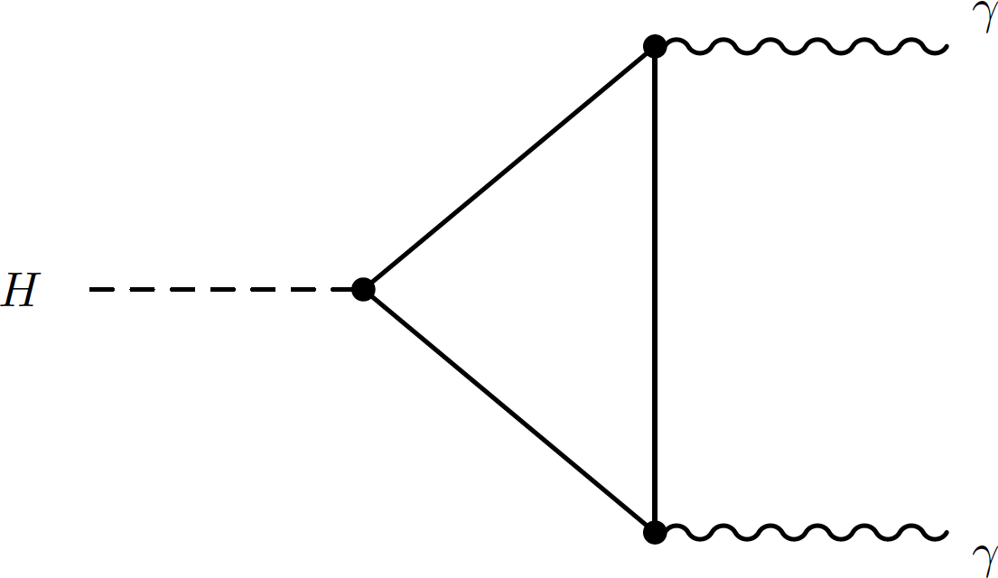
Figure 6-a:
Example of leading-order Feynman diagram for Higgs boson decays to a pair of photons. |
png pdf |
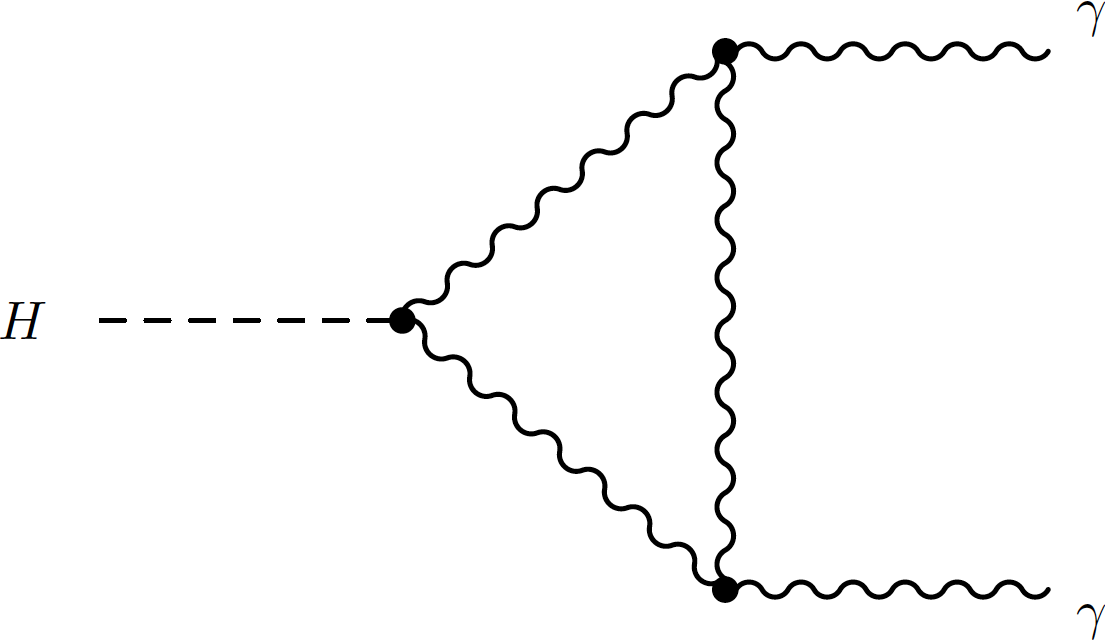
Figure 6-b:
Example of leading-order Feynman diagram for Higgs boson decays to a pair of photons. |

png pdf |
Figure 6-c:
Example of leading-order Feynman diagram for Higgs boson decays to a pair of photons. |
png pdf |
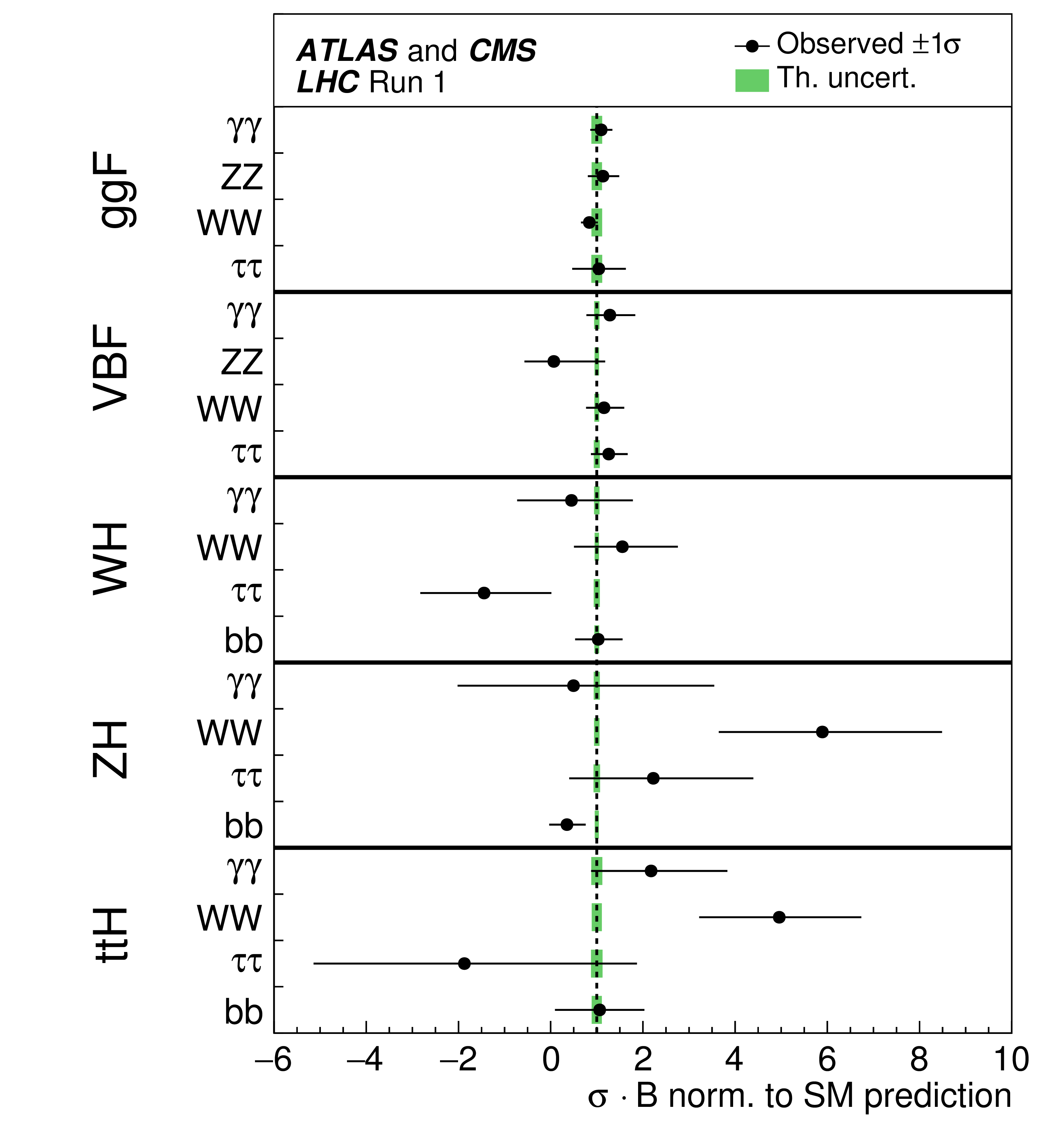
Figure 7:
Best fit values of $\sigma _i \cdot {\mathrm {B}}^f$ for each specific channel $i \to H\to f$, as obtained from the generic parameterisation with 23 parameters for the combination of the ATLAS and CMS measurements. The error bars indicate the 1$\sigma $ intervals. The fit results are normalised to the SM predictions for the various parameters and the shaded bands indicate the theoretical uncertainties in these predictions. Only 20 parameters are shown because some are either not measured with a meaningful precision, in the case of the $ {H\to ZZ}$ decay channel for the ${WH}$, ${ZH}$, and ${ttH}$ production processes, or not measured at all and therefore fixed to their corresponding SM predictions, in the case of the $H\to bb$ decay mode for the ${gg\mathrm {F}}$ and ${\mathrm {VBF}}$ production processes. |
png pdf |
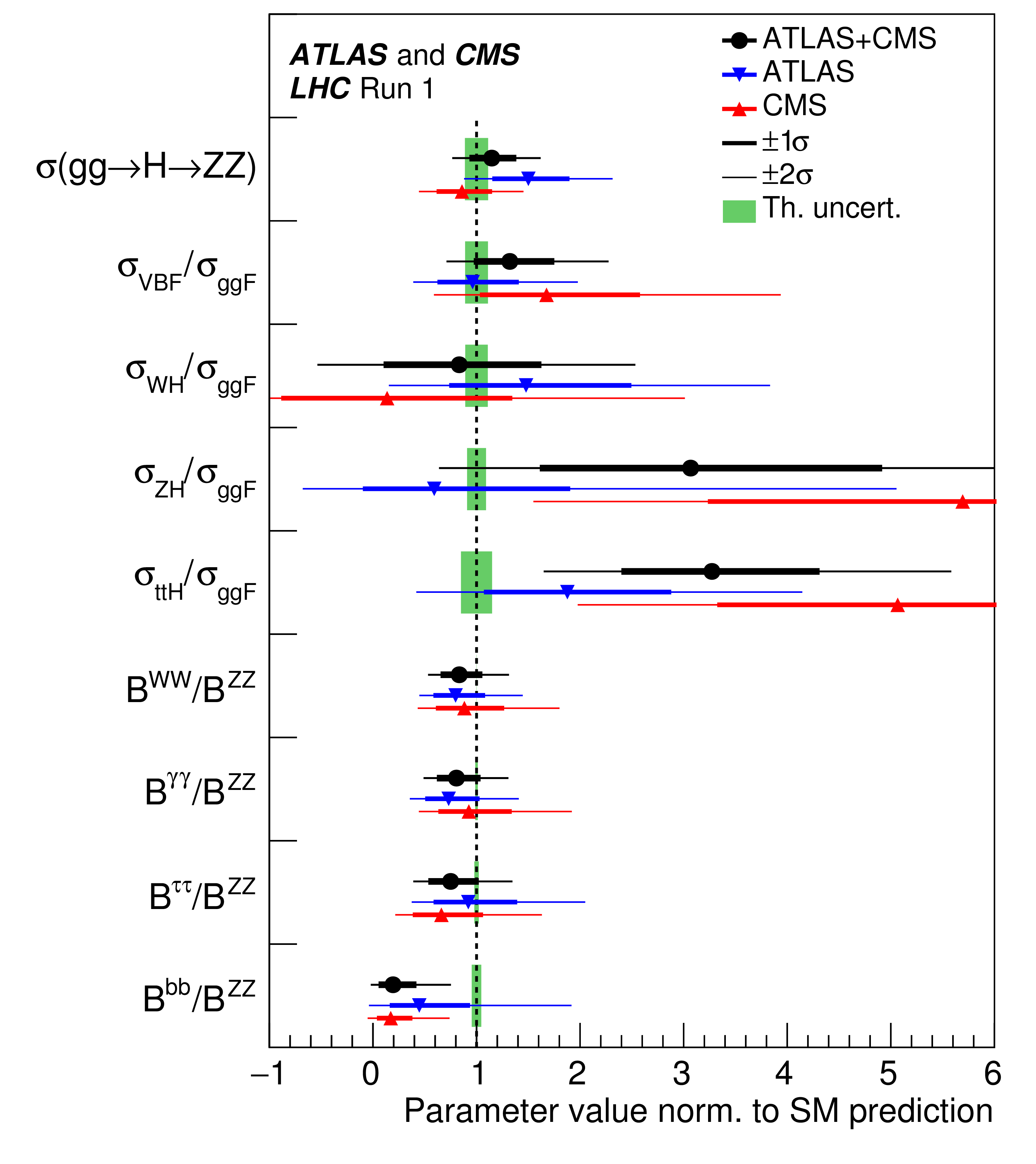
Figure 8:
Best fit values of the $\sigma (gg\to H\to ZZ)$ cross section and of ratios of cross sections and branching fractions, as obtained from the generic parameterisation with nine parameters and tabulated in Table 9 for the combination of the ATLAS and CMS measurements. Also shown are the results from each experiment. The values involving cross sections are given for $\sqrt {s}= $ 8 TeV, assuming the SM values for $\sigma _i(7\ \text{TeV})/\sigma _i(8\ \text{TeV} )$. The error bars indicate the 1$\sigma $ (thick lines) and 2$\sigma $ (thin lines) intervals. The fit results are normalised to the SM predictions for the various parameters and the shaded bands indicate the theoretical uncertainties in these predictions. |
png pdf |
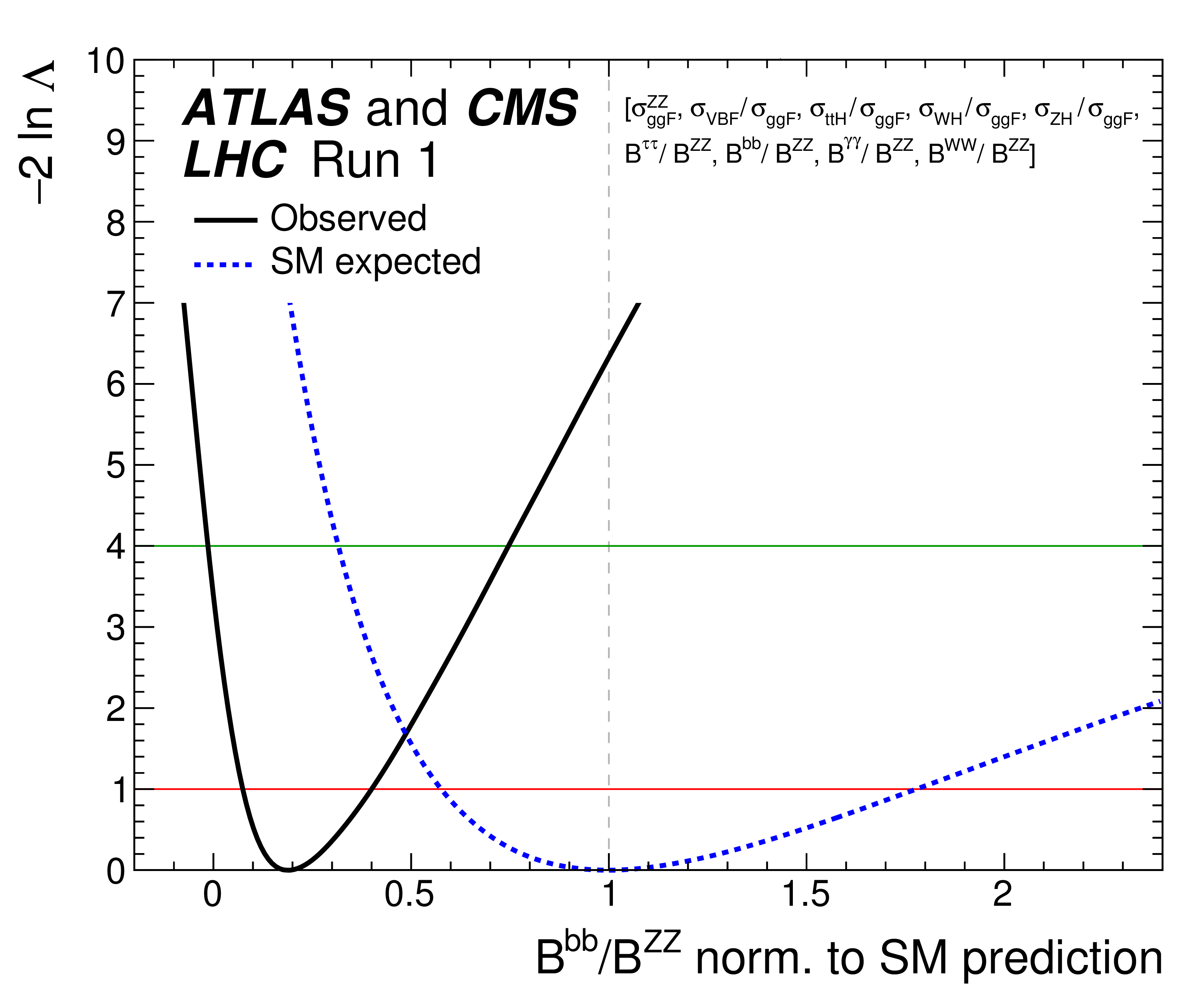
Figure 9:
Observed (solid line) and expected (dashed line) negative log-likelihood scan of the $ {\mathrm {B}}^{bb}/ {\mathrm {B}}^{ZZ}$ parameter normalised to the corresponding SM prediction. All the other parameters of interest are also varied in the minimisation procedure. The red (green) horizontal line at the $-2\Delta \ln\Lambda $ value of 1 (4) indicates the value of the profile likelihood ratio corresponding to a 1$\sigma $ (2$\sigma $) CL interval for the parameter of interest, assuming the asymptotic $\chi ^2$ distribution of the test statistic. The vertical dashed line indicates the SM prediction. |

png pdf |
Figure 10:
Best fit values of ratios of Higgs boson coupling modifiers, as obtained from the generic parameterisation described in the text and as tabulated in Table 10 for the combination of the ATLAS and CMS measurements. Also shown are the results from each experiment. The error bars indicate the 1$\sigma $ (thick lines) and 2$\sigma $ (thin lines) intervals. The hatched areas indicate the non-allowed regions for the parameters that are assumed to be positive without loss of generality. For those parameters with no sensitivity to the sign, only the absolute values are shown. |
png pdf |
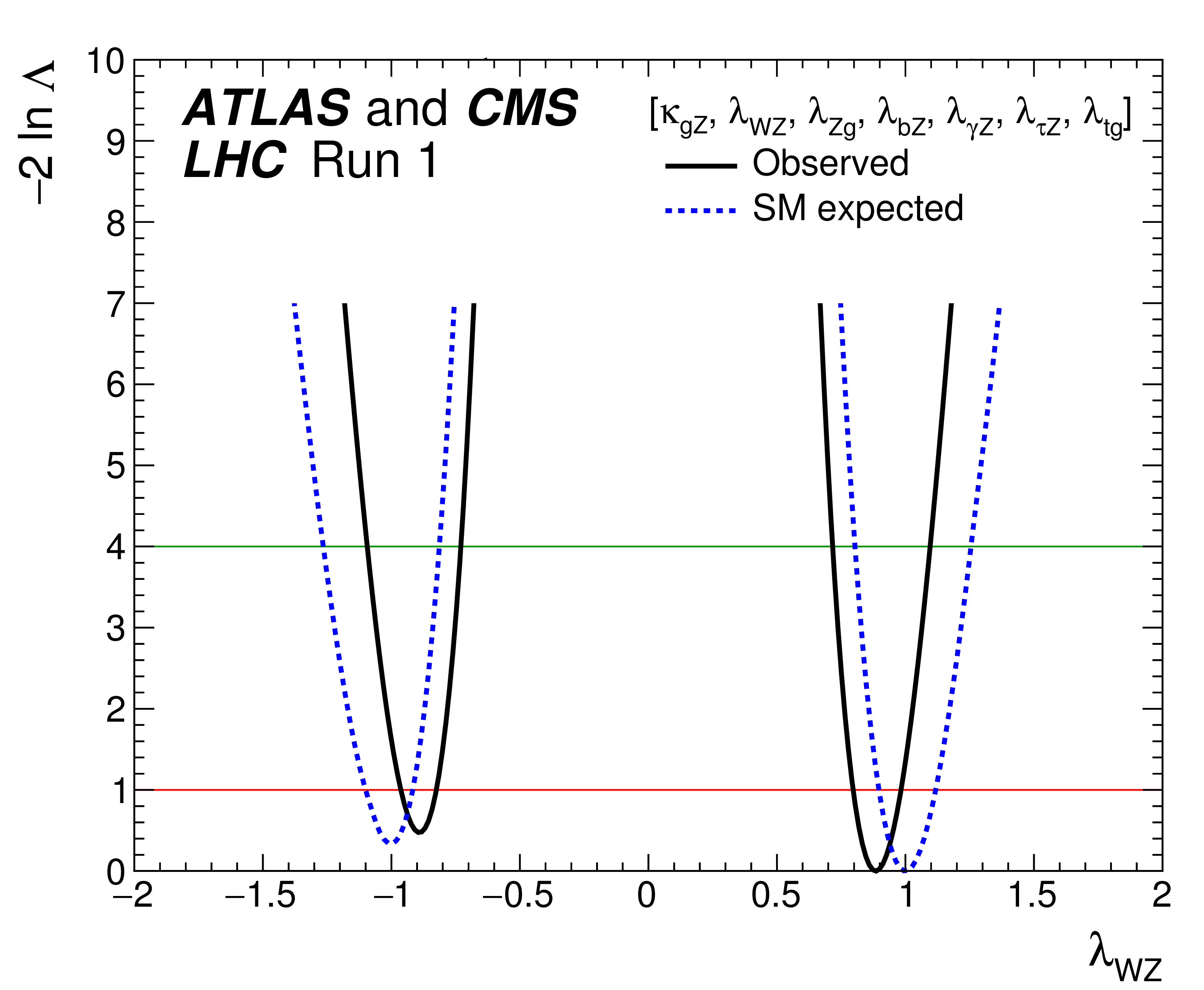
Figure 11-a:
Observed (solid line) and expected (dashed line) negative log-likelihood scans for $ {\lambda }_{WZ}$ (a) and $ {\lambda }_{tg}$ (b), the two parameters of Fig. 10 that are of interest in the negative range in the generic parameterisation of ratios of Higgs boson coupling modifiers described in the text. All the other parameters of interest from the list in the legend are also varied in the minimisation procedure. The red (green) horizontal lines at the $-2\Delta \ln\Lambda $ value of 1 (4) indicate the value of the profile likelihood ratio corresponding to a 1$\sigma $ (2$\sigma $) CL interval for the parameter of interest, assuming the asymptotic $\chi ^2$ distribution of the test statistic. |

png pdf |
Figure 11-b:
Observed (solid line) and expected (dashed line) negative log-likelihood scans for $ {\lambda }_{WZ}$ (a) and $ {\lambda }_{tg}$ (b), the two parameters of Fig. 10 that are of interest in the negative range in the generic parameterisation of ratios of Higgs boson coupling modifiers described in the text. All the other parameters of interest from the list in the legend are also varied in the minimisation procedure. The red (green) horizontal lines at the $-2\Delta \ln\Lambda $ value of 1 (4) indicate the value of the profile likelihood ratio corresponding to a 1$\sigma $ (2$\sigma $) CL interval for the parameter of interest, assuming the asymptotic $\chi ^2$ distribution of the test statistic. |

png pdf |
Figure 12:
Best fit results for the production signal strengths for the combination of ATLAS and CMS data. Also shown are the results from each experiment. The error bars indicate the 1$\sigma $ (thick lines) and 2$\sigma $ (thin lines) intervals. The measurements of the global signal strength $\mu $ are also shown. |
png pdf |
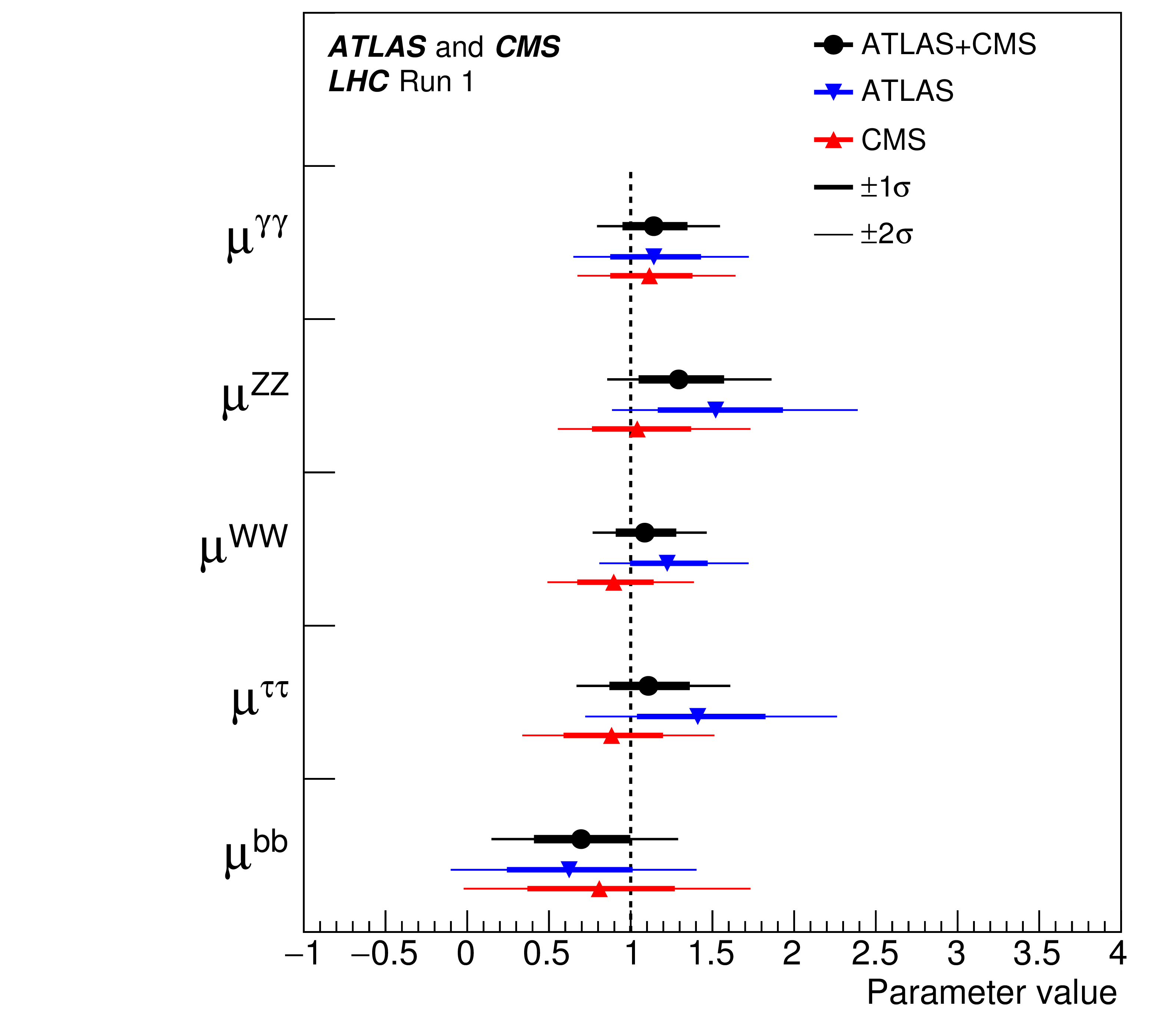
Figure 13:
Best fit results for the decay signal strengths for the combination of ATLAS and CMS data (the results for $\mu ^{\mu \mu }$ are reported in Table 13). Also shown are the results from each experiment. The error bars indicate the 1$\sigma $ (thick lines) and 2$\sigma $ (thin lines) intervals. |
png pdf |
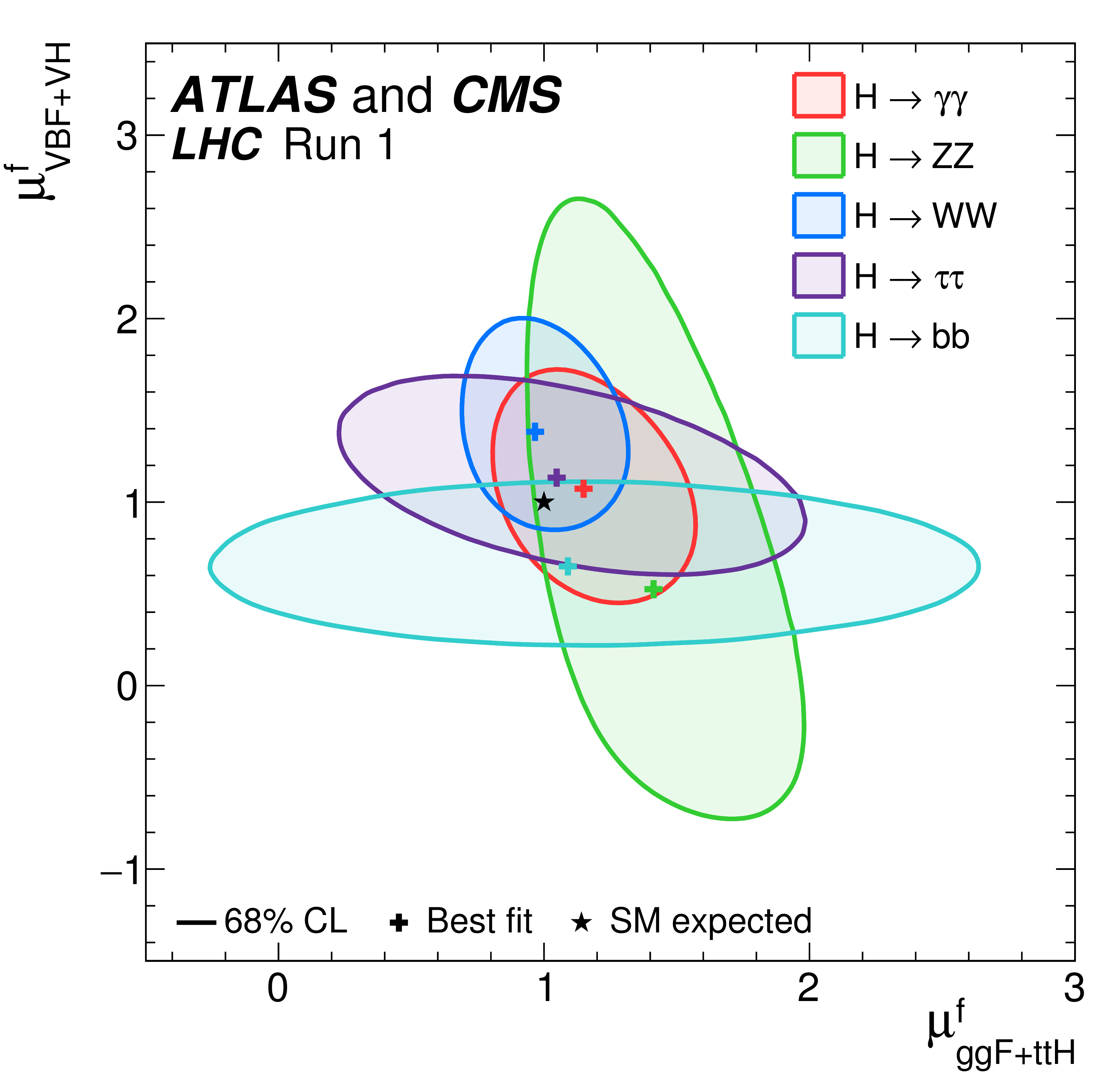
Figure 14:
Negative log-likelihood contours at 68% CL in the ($\mu _{ {gg\mathrm {F}}+ {ttH}}^f$, $\mu _{ {\mathrm {VBF}}+ {VH}}^f$) plane for the combination of ATLAS and CMS, as obtained from the ten-parameter fit described in the text for each of the five decay channels $ {H\to ZZ}$, $H\to WW$, $ {H\to \gamma \gamma }$, $H\to \tau \tau $, and $H\to bb$. The best fit values obtained for each of the five decay channels are also shown, together with the SM expectation. |
png pdf |
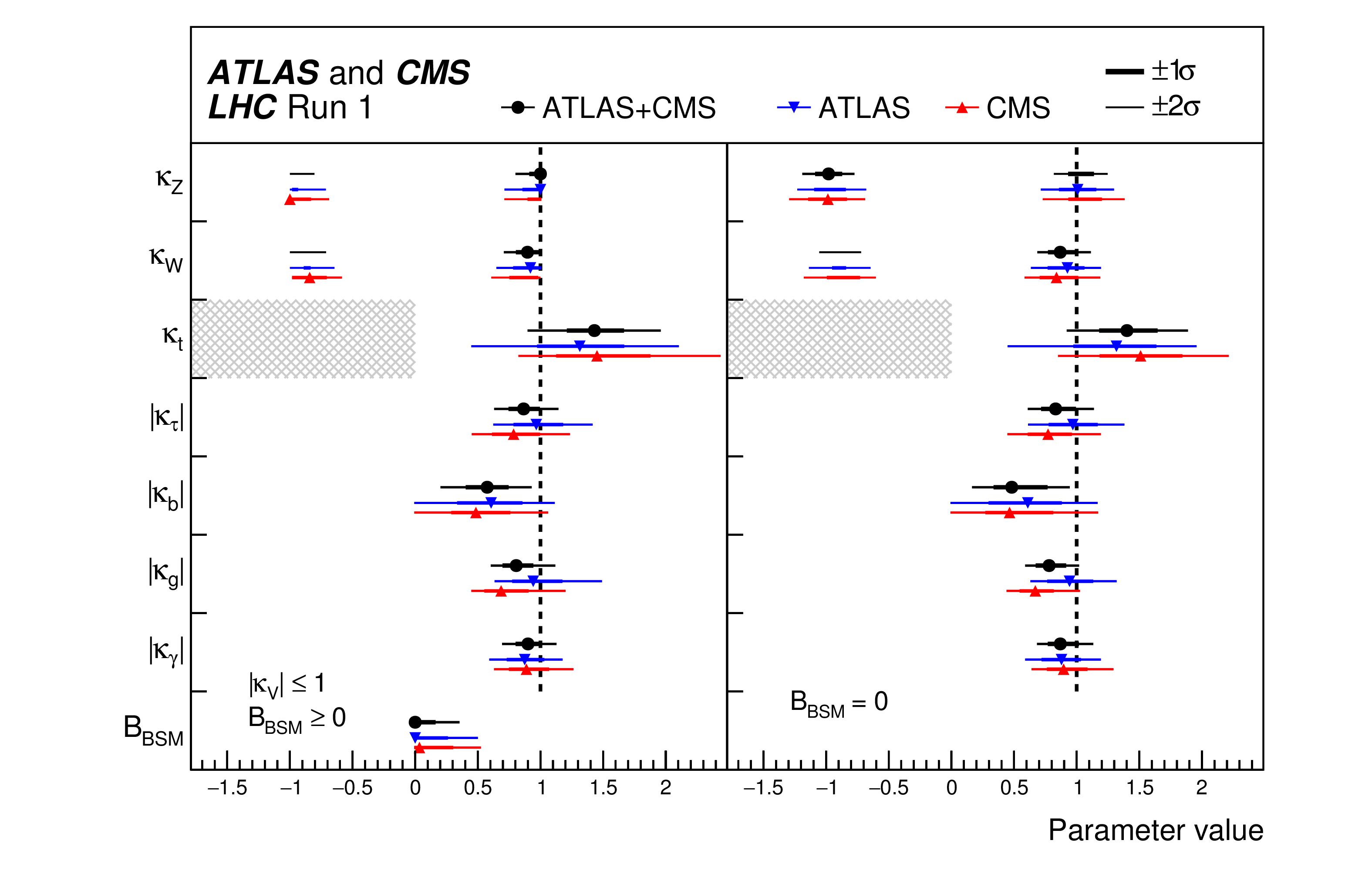
Figure 15:
Fit results for two parameterisations allowing BSM loop couplings discussed in the text: the first one assumes that $ {\mathrm {B_{BSM}}}\ge 0$ and that $| {\kappa }_{V}| \le 1$, where $ {\kappa }_{V}$ denotes $ {\kappa }_{Z}$ or $ {\kappa }_{W}$, and the second one assumes that there are no additional BSM contributions to the Higgs boson width, i.e. $ {\mathrm {B_{BSM}}}= $ 0 . The measured results for the combination of ATLAS and CMS are reported together with their uncertainties, as well as the individual results from each experiment. The hatched areas show the non-allowed regions for the ${\kappa _t}$ parameter, which is assumed to be positive without loss of generality. The error bars indicate the 1$\sigma $ (thick lines) and 2$\sigma $ (thin lines) intervals. When a parameter is constrained and reaches a boundary, namely $| {\kappa }_{V}| = $ 1 or $ {\mathrm {B_{BSM}}}= $ 0 , the uncertainty is not defined beyond this boundary. For those parameters with no sensitivity to the sign, only the absolute values are shown. |
png pdf |
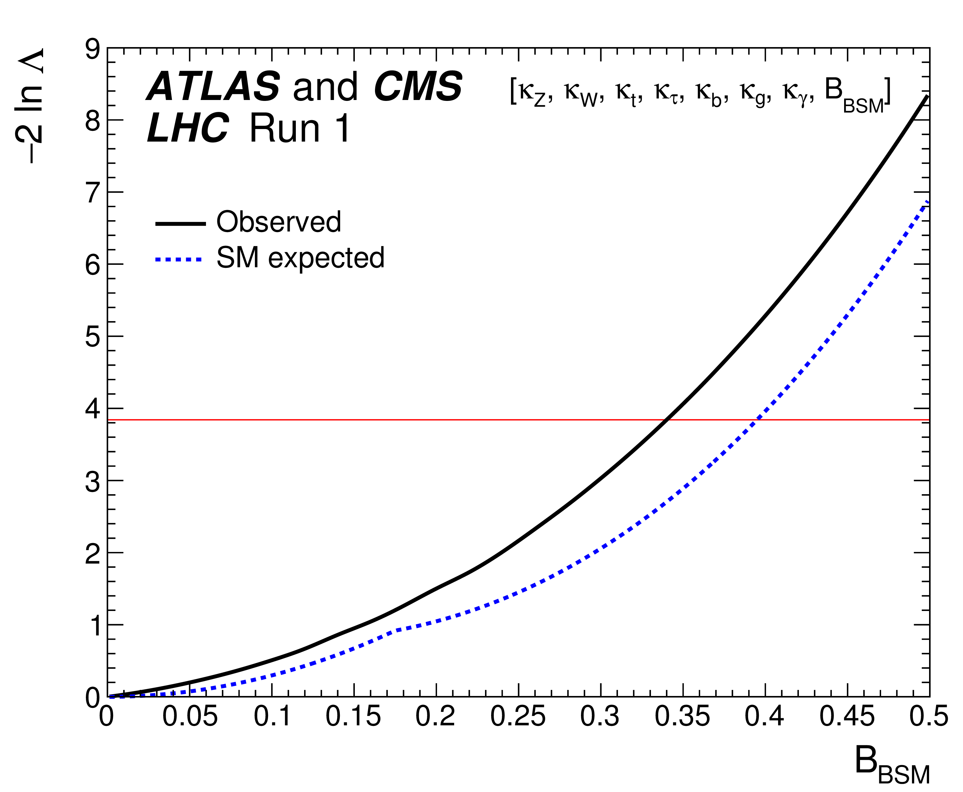
Figure 16:
Observed (solid line) and expected (dashed line) negative log-likelihood scan of $ {\mathrm {B_{BSM}}}$, shown for the combination of ATLAS and CMS when allowing additional BSM contributions to the Higgs boson width. The results are shown for the parameterisation with the assumptions that $| {\kappa }_{V}|\le$ 1 and $ {\mathrm {B_{BSM}}} \ge$ 0 in Fig. 15. All the other parameters of interest from the list in the legend are also varied in the minimisation procedure. The red horizontal line at 3.84 indicates the log-likelihood variation corresponding to the 95% CL upper limit, as discussed in Section 3.2. |
png pdf |
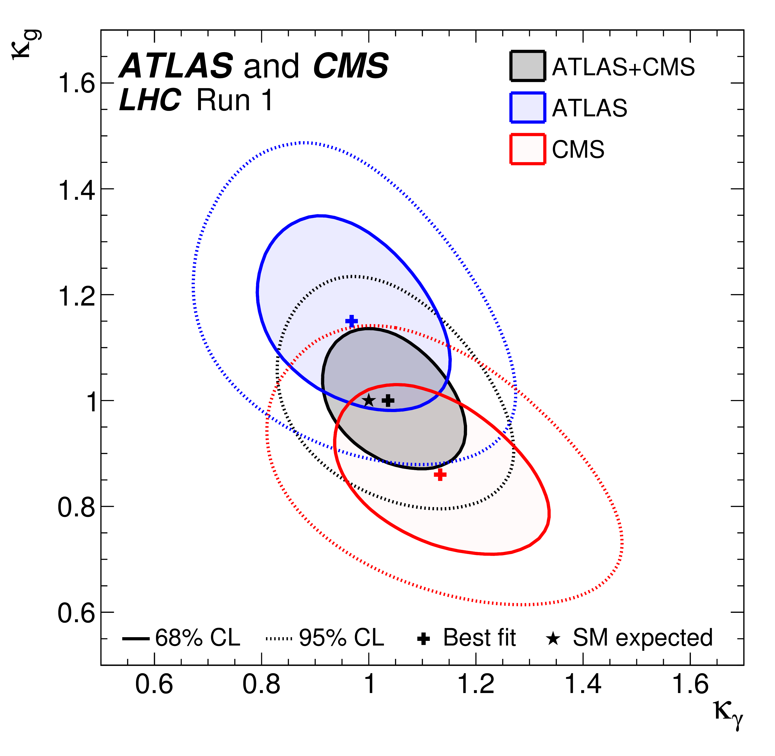
Figure 17:
Negative log-likelihood contours at 68% and 95% CL in the ($ {\kappa _\gamma }$, $ {\kappa _g}$) plane for the combination of ATLAS and CMS and for each experiment separately, as obtained from the fit to the parameterisation constraining all the other coupling modifiers to their SM values and assuming $ {\mathrm {B_{BSM}}}= $ 0 . |

png pdf |
Figure 18:
Best fit values of parameters for the combination of ATLAS and CMS data, and separately for each experiment, for the parameterisation assuming the absence of BSM particles in the loops, $ {\mathrm {B_{BSM}}}= $ 0 . The hatched area indicates the non-allowed region for the parameter that is assumed to be positive without loss of generality. The error bars indicate the 1$\sigma $ (thick lines) and 2$\sigma $ (thin lines) intervals. When a parameter is constrained and reaches a boundary, namely $|\kappa _\mu | = $ 0 , the uncertainty is not defined beyond this boundary. For those parameters with no sensitivity to the sign, only the absolute values are shown. |
png pdf |
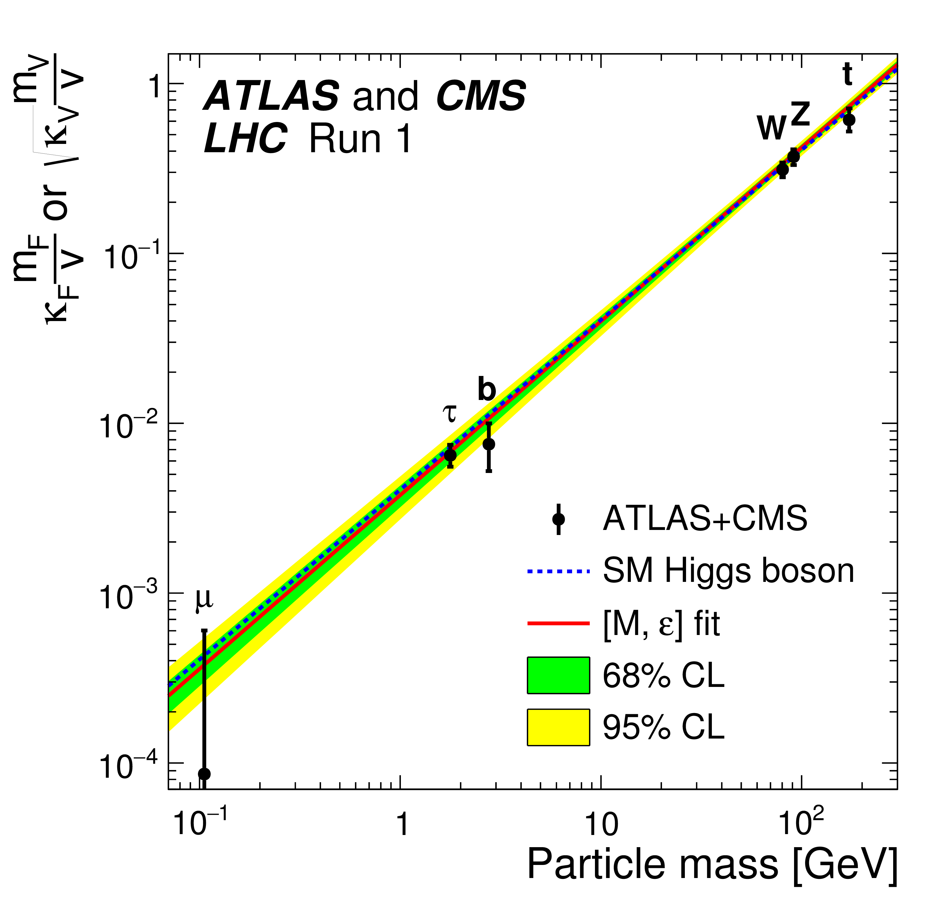
Figure 19:
Best fit values as a function of particle mass for the combination of ATLAS and CMS data in the case of the parameterisation described in the text, with parameters defined as $ {\kappa }_{F} \cdot \ m_{F}/v$ for the fermions, and as $\sqrt { {\kappa }_{V}} \cdot \ m_{V}/v$ for the weak vector bosons, where $v = $ 246 GeV is the vacuum expectation value of the Higgs field. The dashed (blue) line indicates the predicted dependence on the particle mass in the case of the SM Higgs boson. The solid (red) line indicates the best fit result to the $ [M,\epsilon ]$ phenomenological model of Ref. [128] with the corresponding 68% and 95% CL bands. |
png pdf |
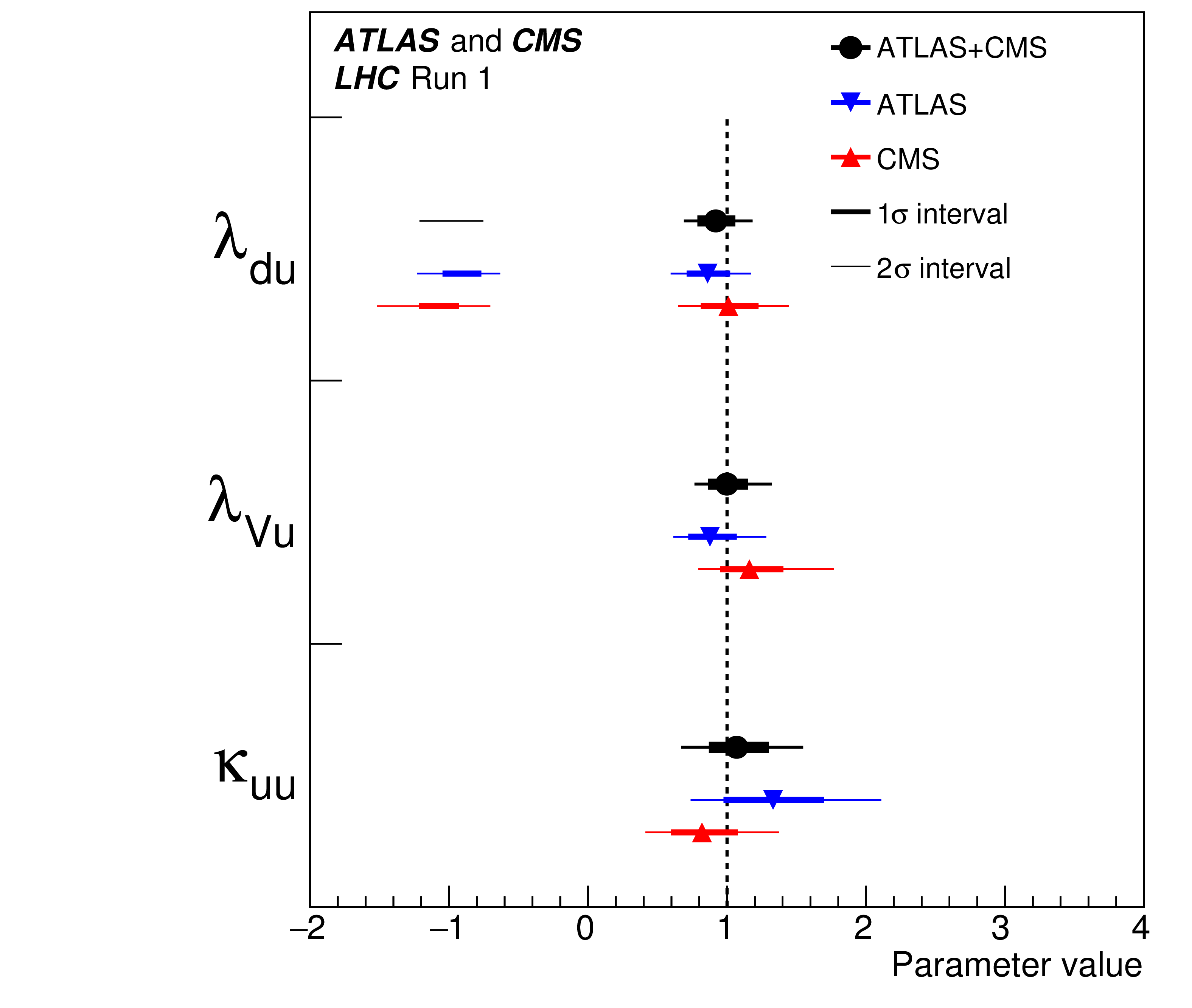
Figure 20:
Best fit values of parameters for the combination of ATLAS and CMS data, and separately for each experiment, for the parameterisation testing the up- and down-type fermion coupling ratios. The error bars indicate the 1$\sigma $ (thick lines) and 2$\sigma $ (thin lines) intervals. The parameter $\kappa _{uu}$ is positive definite since $ {\kappa _H}$ is always assumed to be positive. Negative values for the parameter $\lambda _{Vu}$ are excluded by more than $4\sigma $. |
png pdf |
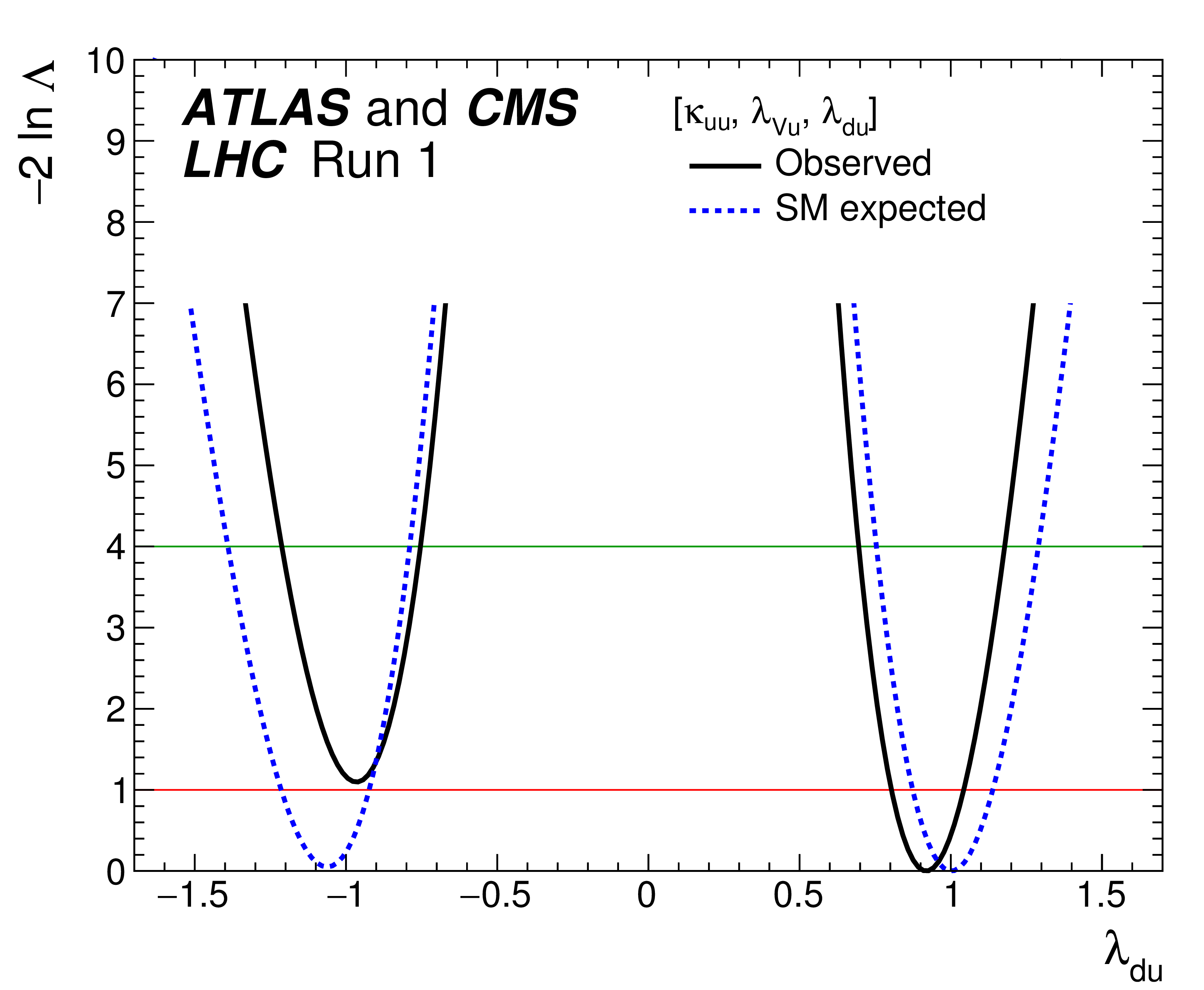
Figure 21:
Observed (solid line) and expected (dashed line) negative log-likelihood scan of the $\lambda _{du}$ parameter, probing the ratios of coupling modifiers for up-type versus down-type fermions for the combination of ATLAS and CMS. The other parameters of interest from the list in the legend are also varied in the minimisation procedure. The red (green) horizontal line at the $-2\Delta \ln\Lambda $ value of 1 (4) indicates the value of the profile likelihood ratio corresponding to a 1$\sigma $ (2$\sigma $) CL interval for the parameter of interest, assuming the asymptotic $\chi ^2$ distribution of the test statistic. |
png pdf |
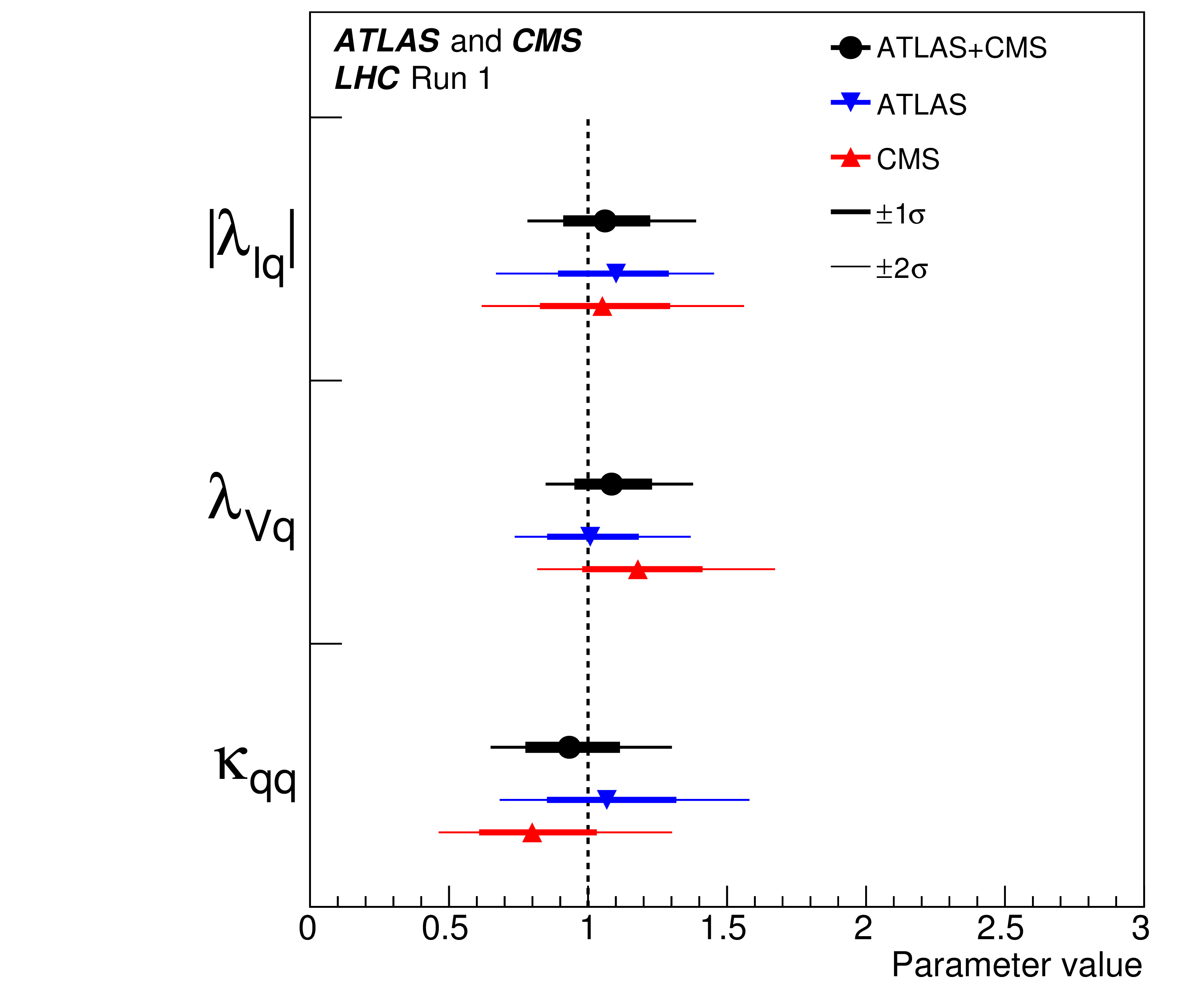
Figure 22:
Best fit values of parameters for the combination of ATLAS and CMS data, and separately for each experiment, for the parameterisation testing the lepton and quark coupling ratios. The error bars indicate the 1$\sigma $ (thick lines) and 2$\sigma $ (thin lines) intervals. For the parameter $\lambda _{lq}$, for which there is no sensitivity to the sign, only the absolute values are shown. The parameter $\kappa _{qq}$ is positive definite since $ {\kappa _H}$ is always assumed to be positive. Negative values for the parameter $\lambda _{Vq}$ are excluded by more than $4\sigma $. |
png pdf |
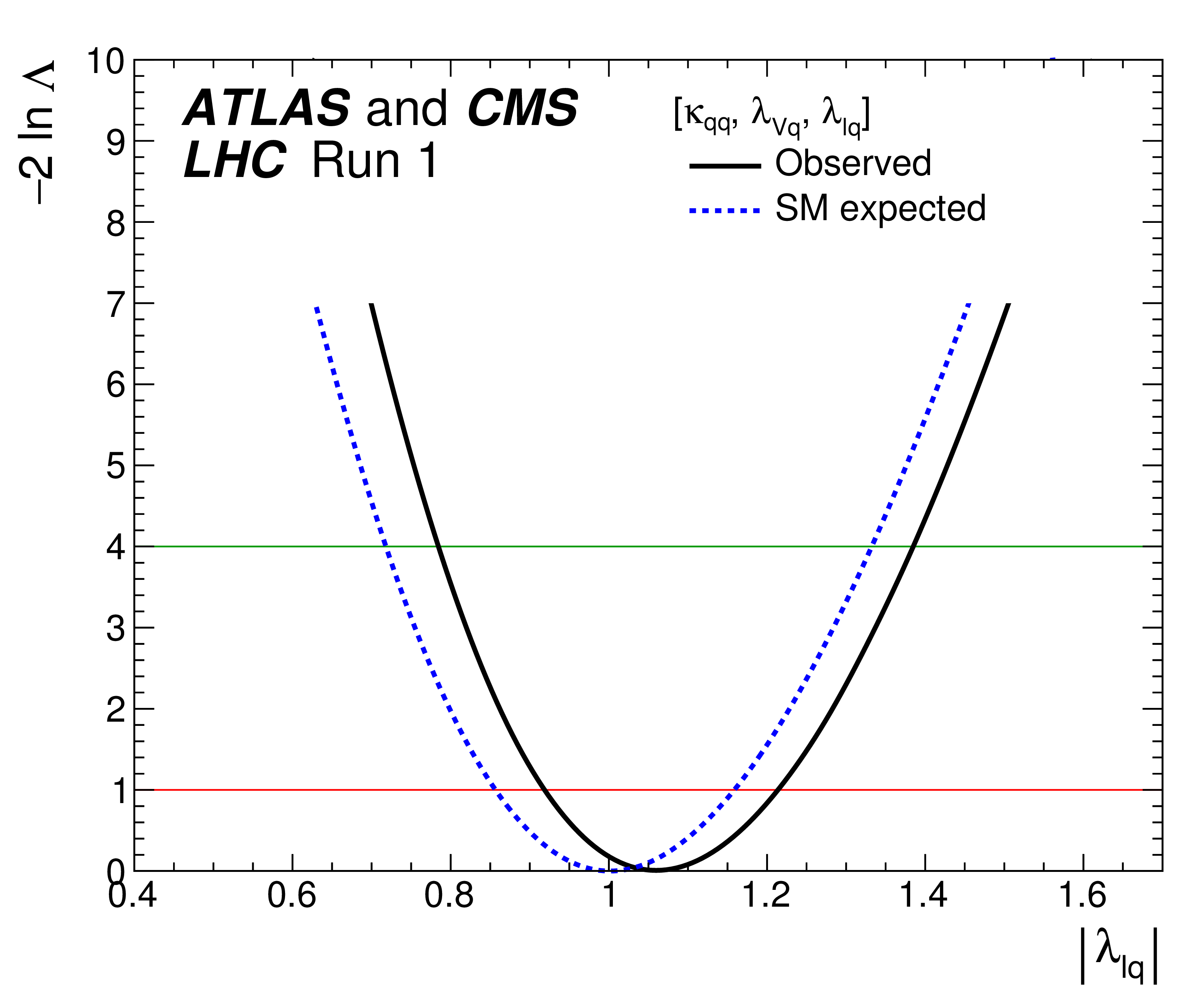
Figure 23:
Observed (solid line) and expected (dashed line) negative log-likelihood scan of the $\lambda _{lq}$ parameter, probing the ratios of coupling modifiers for leptons versus quarks for the combination of ATLAS and CMS. The other parameters of interest from the list in the legend are also varied in the minimisation procedure. The red (green) horizontal line at the $-2\Delta \ln\Lambda $ value of 1 (4) indicates the value of the profile likelihood ratio corresponding to a 1$\sigma $ (2$\sigma $) CL interval for the parameter of interest, assuming the asymptotic $\chi ^2$ distribution of the test statistic. |

png pdf |
Figure 24:
Negative log-likelihood contours at 68% and 95% CL in the ($\kappa _F^f$, $\kappa _V^f$) plane for the combination of ATLAS and CMS and for the individual decay channels, as well as for their combination ($\kappa _F$ versus $\kappa _V$ shown in black), without any assumption about the sign of the coupling modifiers. The other two quadrants (not shown) are symmetric with respect to the point (0,0). |
png pdf |
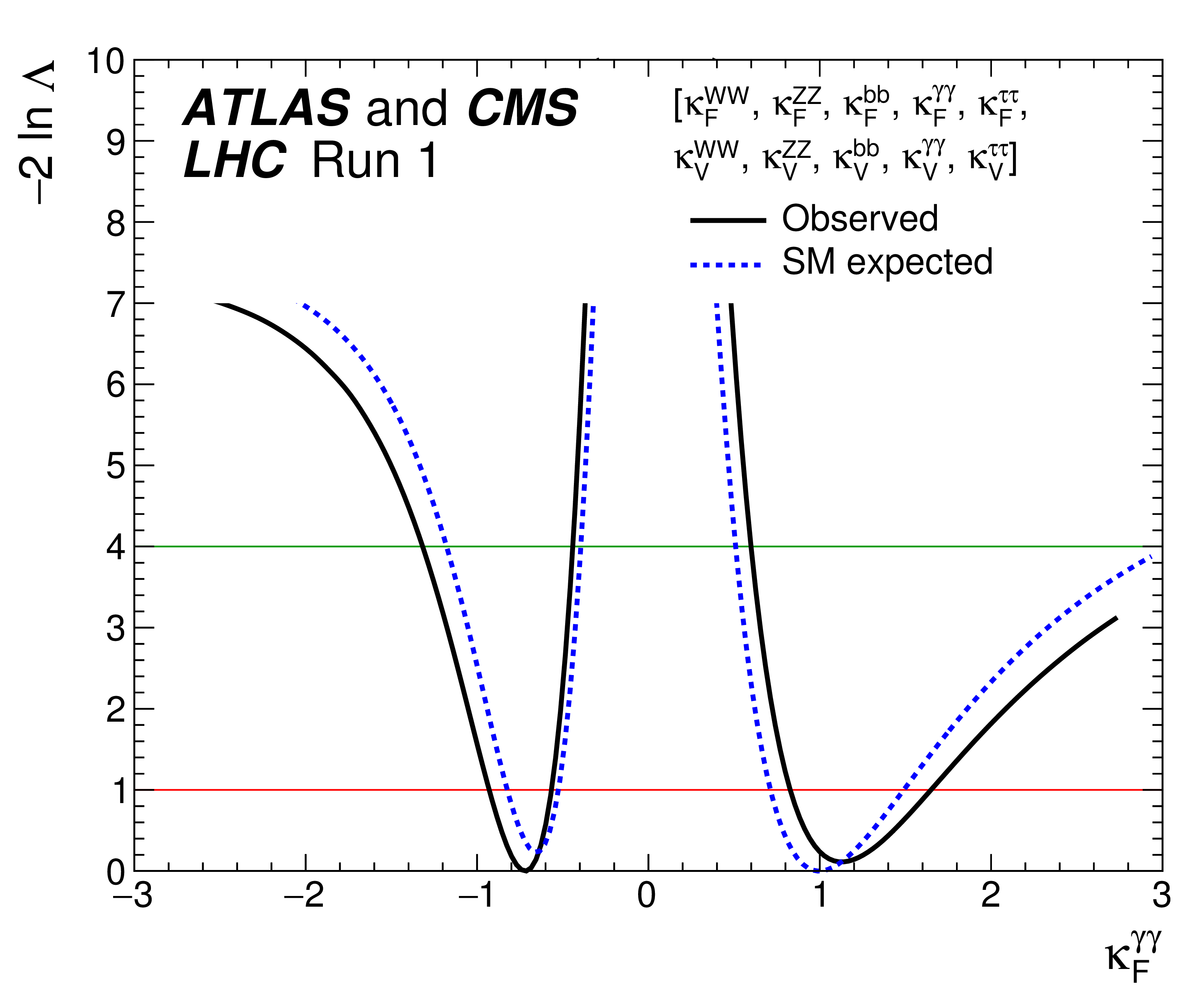
Figure 25-a:
Observed (solid line) and expected (dashed line) negative log-likelihood scans for the five $\kappa _F^f$ parameters, corresponding to each individual decay channel, and for the global $\kappa _F$ parameter, corresponding to the combination of all decay channels: (a) $\kappa _{F}^{\gamma \gamma }$, (b) $\kappa _{F}^{ZZ}$, (c) $\kappa _{F}^{WW}$, (d) $\kappa _{F}^{\tau \tau }$, (e) $\kappa _{F}^{bb}$, and (f) $\kappa _F$. All the other parameters of interest from the list in the legends are also varied in the minimisation procedure. The red (green) horizontal lines at the $-2\Delta \ln\Lambda $ value of 1 (4) indicate the value of the profile likelihood ratio corresponding to a 1$\sigma $ (2$\sigma $) CL interval for the parameter of interest, assuming the asymptotic $\chi ^2$ distribution of the test statistic. |

png pdf |
Figure 25-b:
Observed (solid line) and expected (dashed line) negative log-likelihood scans for the five $\kappa _F^f$ parameters, corresponding to each individual decay channel, and for the global $\kappa _F$ parameter, corresponding to the combination of all decay channels: (a) $\kappa _{F}^{\gamma \gamma }$, (b) $\kappa _{F}^{ZZ}$, (c) $\kappa _{F}^{WW}$, (d) $\kappa _{F}^{\tau \tau }$, (e) $\kappa _{F}^{bb}$, and (f) $\kappa _F$. All the other parameters of interest from the list in the legends are also varied in the minimisation procedure. The red (green) horizontal lines at the $-2\Delta \ln\Lambda $ value of 1 (4) indicate the value of the profile likelihood ratio corresponding to a 1$\sigma $ (2$\sigma $) CL interval for the parameter of interest, assuming the asymptotic $\chi ^2$ distribution of the test statistic. |
png pdf |
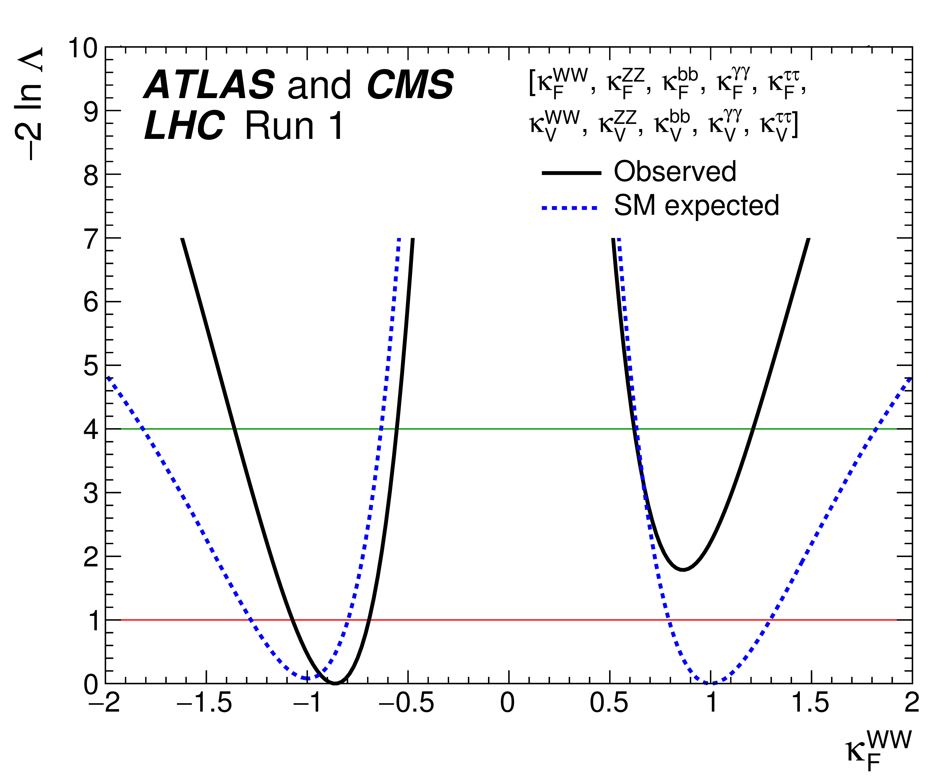
Figure 25-c:
Observed (solid line) and expected (dashed line) negative log-likelihood scans for the five $\kappa _F^f$ parameters, corresponding to each individual decay channel, and for the global $\kappa _F$ parameter, corresponding to the combination of all decay channels: (a) $\kappa _{F}^{\gamma \gamma }$, (b) $\kappa _{F}^{ZZ}$, (c) $\kappa _{F}^{WW}$, (d) $\kappa _{F}^{\tau \tau }$, (e) $\kappa _{F}^{bb}$, and (f) $\kappa _F$. All the other parameters of interest from the list in the legends are also varied in the minimisation procedure. The red (green) horizontal lines at the $-2\Delta \ln\Lambda $ value of 1 (4) indicate the value of the profile likelihood ratio corresponding to a 1$\sigma $ (2$\sigma $) CL interval for the parameter of interest, assuming the asymptotic $\chi ^2$ distribution of the test statistic. |
png pdf |
Figure 25-d:
Observed (solid line) and expected (dashed line) negative log-likelihood scans for the five $\kappa _F^f$ parameters, corresponding to each individual decay channel, and for the global $\kappa _F$ parameter, corresponding to the combination of all decay channels: (a) $\kappa _{F}^{\gamma \gamma }$, (b) $\kappa _{F}^{ZZ}$, (c) $\kappa _{F}^{WW}$, (d) $\kappa _{F}^{\tau \tau }$, (e) $\kappa _{F}^{bb}$, and (f) $\kappa _F$. All the other parameters of interest from the list in the legends are also varied in the minimisation procedure. The red (green) horizontal lines at the $-2\Delta \ln\Lambda $ value of 1 (4) indicate the value of the profile likelihood ratio corresponding to a 1$\sigma $ (2$\sigma $) CL interval for the parameter of interest, assuming the asymptotic $\chi ^2$ distribution of the test statistic. |

png pdf |
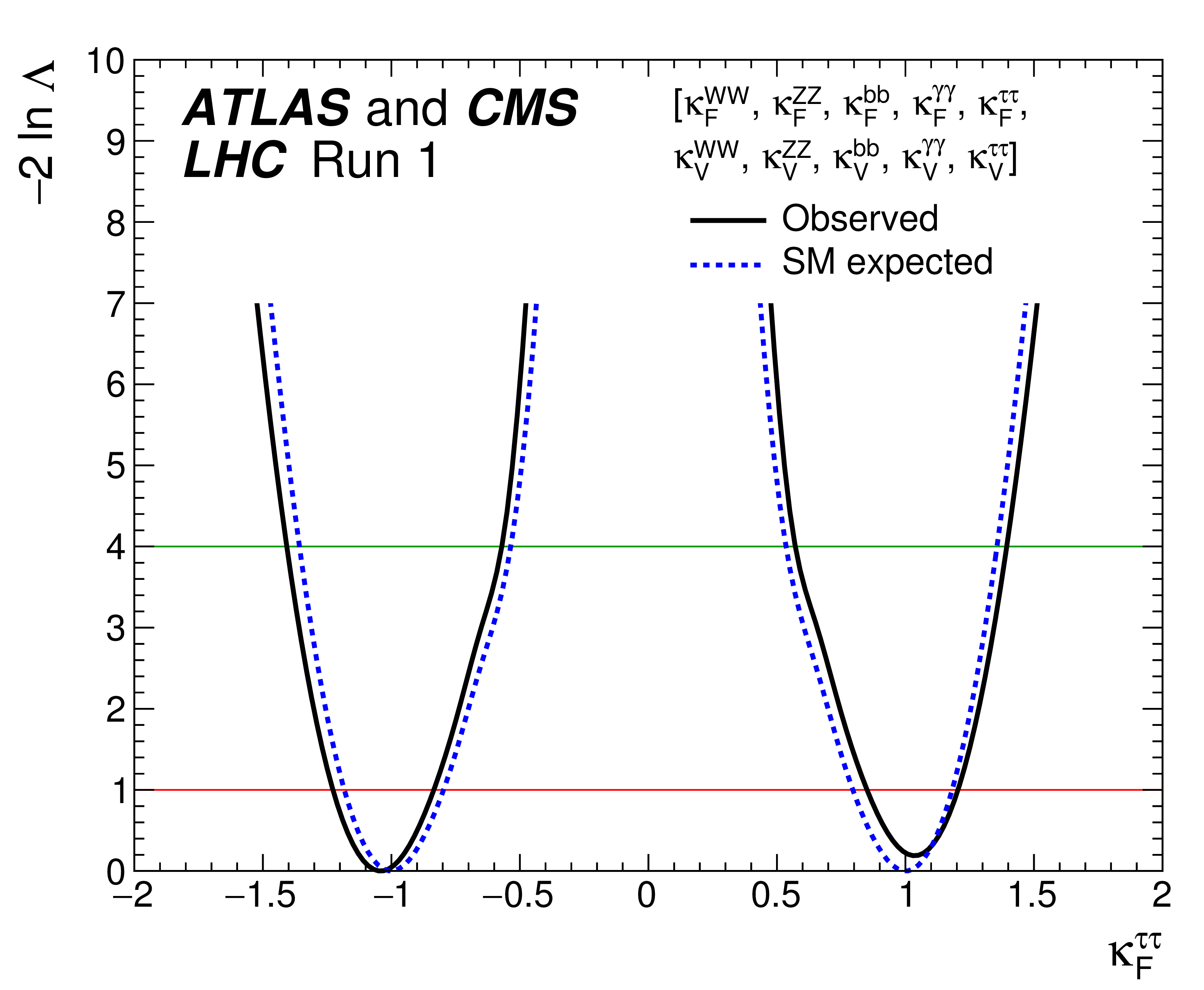
Figure 25-e:
Observed (solid line) and expected (dashed line) negative log-likelihood scans for the five $\kappa _F^f$ parameters, corresponding to each individual decay channel, and for the global $\kappa _F$ parameter, corresponding to the combination of all decay channels: (a) $\kappa _{F}^{\gamma \gamma }$, (b) $\kappa _{F}^{ZZ}$, (c) $\kappa _{F}^{WW}$, (d) $\kappa _{F}^{\tau \tau }$, (e) $\kappa _{F}^{bb}$, and (f) $\kappa _F$. All the other parameters of interest from the list in the legends are also varied in the minimisation procedure. The red (green) horizontal lines at the $-2\Delta \ln\Lambda $ value of 1 (4) indicate the value of the profile likelihood ratio corresponding to a 1$\sigma $ (2$\sigma $) CL interval for the parameter of interest, assuming the asymptotic $\chi ^2$ distribution of the test statistic. |

png pdf |
Figure 25-f:
Observed (solid line) and expected (dashed line) negative log-likelihood scans for the five $\kappa _F^f$ parameters, corresponding to each individual decay channel, and for the global $\kappa _F$ parameter, corresponding to the combination of all decay channels: (a) $\kappa _{F}^{\gamma \gamma }$, (b) $\kappa _{F}^{ZZ}$, (c) $\kappa _{F}^{WW}$, (d) $\kappa _{F}^{\tau \tau }$, (e) $\kappa _{F}^{bb}$, and (f) $\kappa _F$. All the other parameters of interest from the list in the legends are also varied in the minimisation procedure. The red (green) horizontal lines at the $-2\Delta \ln\Lambda $ value of 1 (4) indicate the value of the profile likelihood ratio corresponding to a 1$\sigma $ (2$\sigma $) CL interval for the parameter of interest, assuming the asymptotic $\chi ^2$ distribution of the test statistic. |
png pdf |
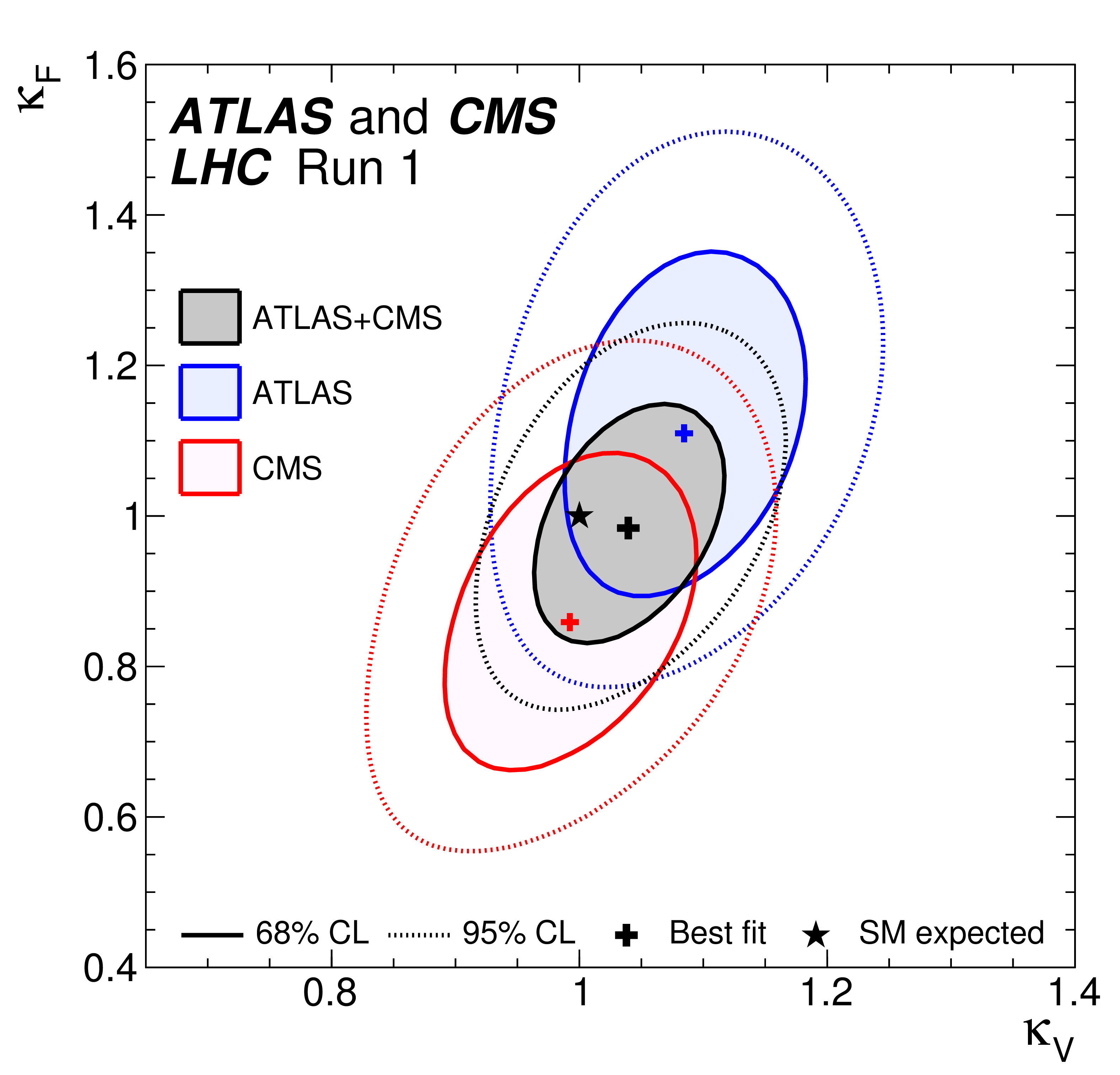
Figure 26-a:
Negative log-likelihood contours at 68% and 95% CL in the ($\kappa _F$, $\kappa _V$) plane on an enlarged scale for the combination of ATLAS and CMS and for the global fit of all channels. Also shown are the contours obtained for each experiment separately. |
png pdf |
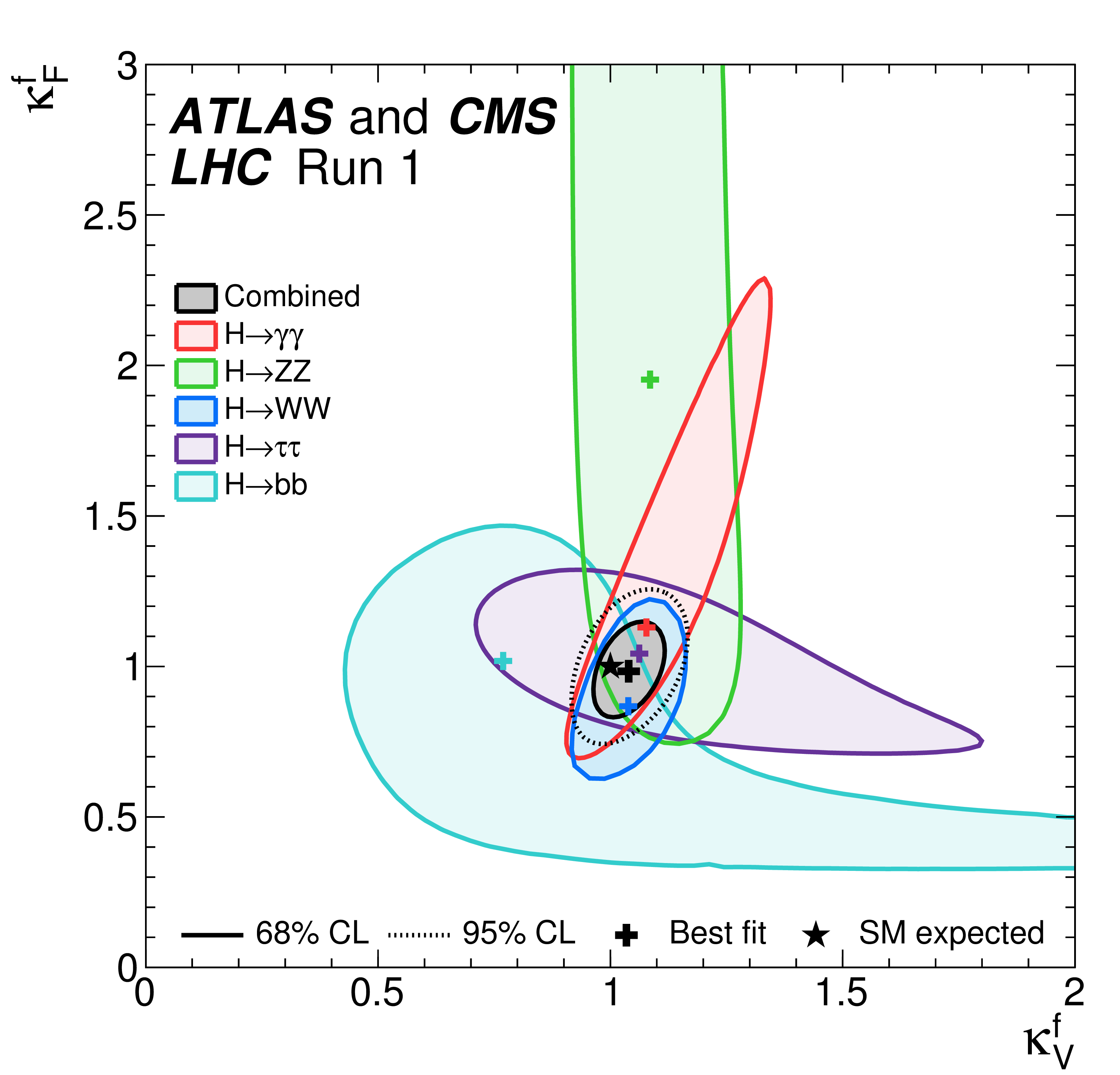
Figure 26-b:
Negative log-likelihood contours at 68% CL in the ($\kappa _F^f$, $\kappa _V^f$) plane for the combination of ATLAS and CMS and for the individual decay channels as well as for their global combination ($\kappa _F$ versus $\kappa _V$), assuming that all coupling modifiers are positive. |

png pdf |
Figure 27:
Correlation matrix obtained from the fit combining the ATLAS and CMS data using the generic parameterisation with 23 parameters described in Section 4.1.1. Only 20 parameters are shown because the other three, corresponding to the $ {H\to ZZ}$ decay channel for the ${WH}$, ${ZH}$, and ${ttH}$ production processes, are not measured with a meaningful precision. |
png pdf |
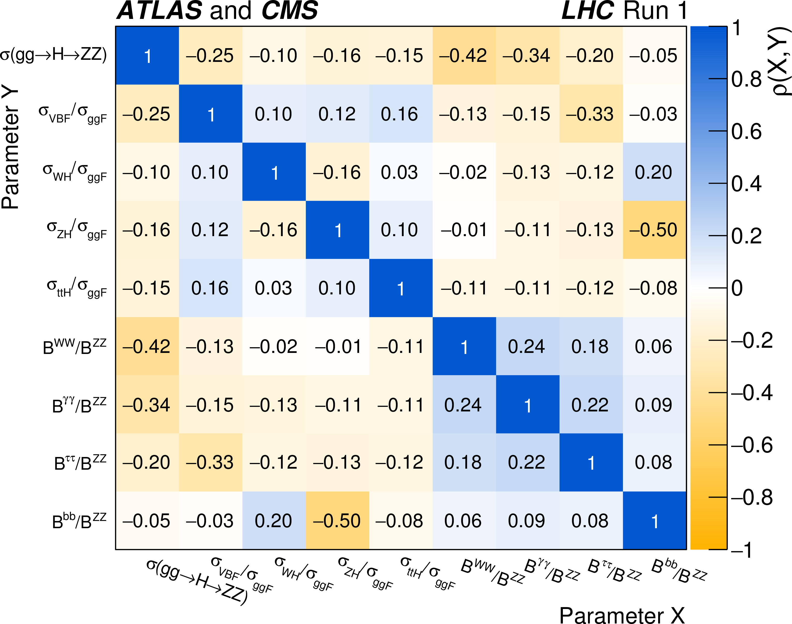
Figure 28:
Correlation matrix obtained from the fit combining the ATLAS and CMS data using the generic parameterisation with nine parameters described in Section 4.1.2. |
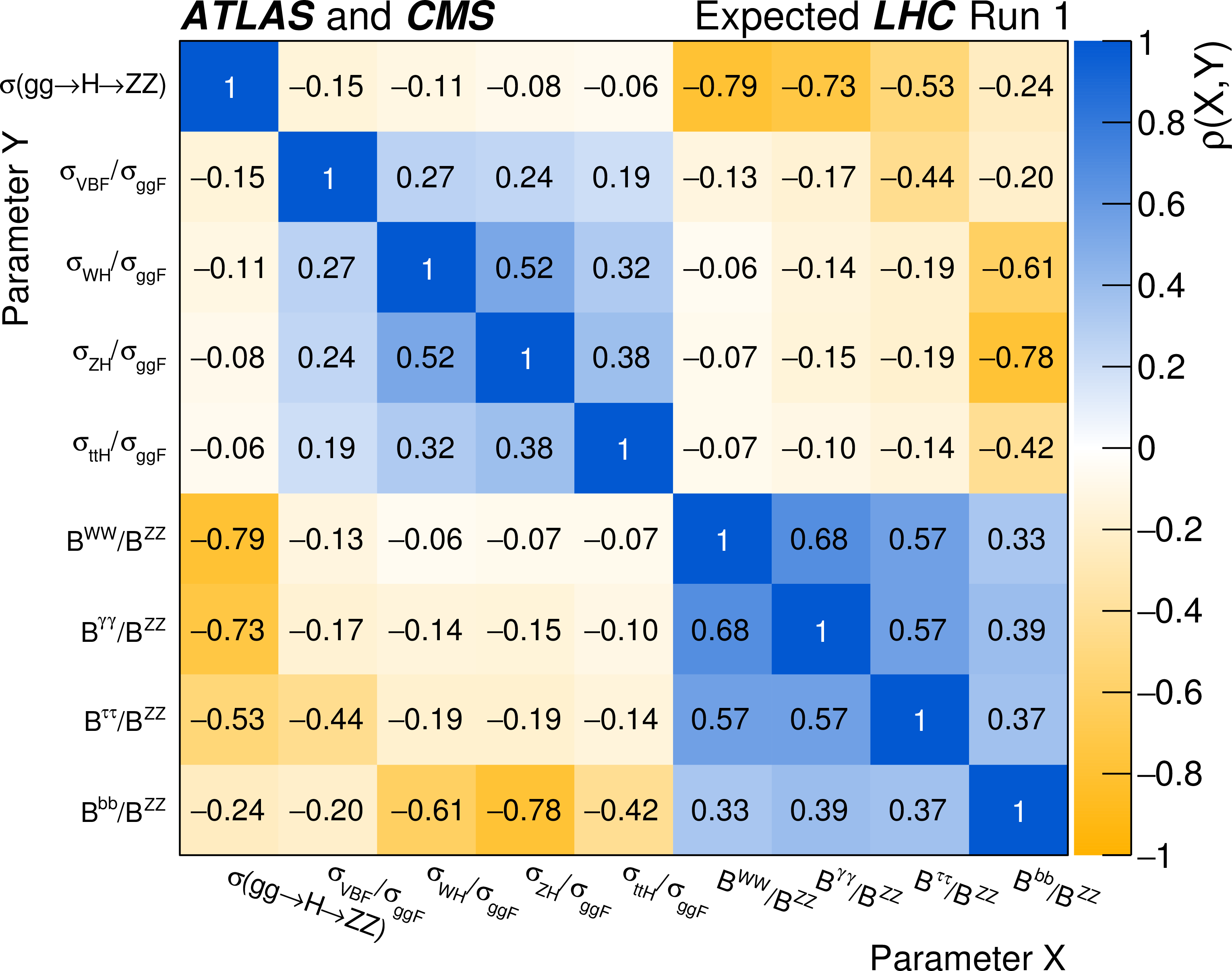
png pdf |
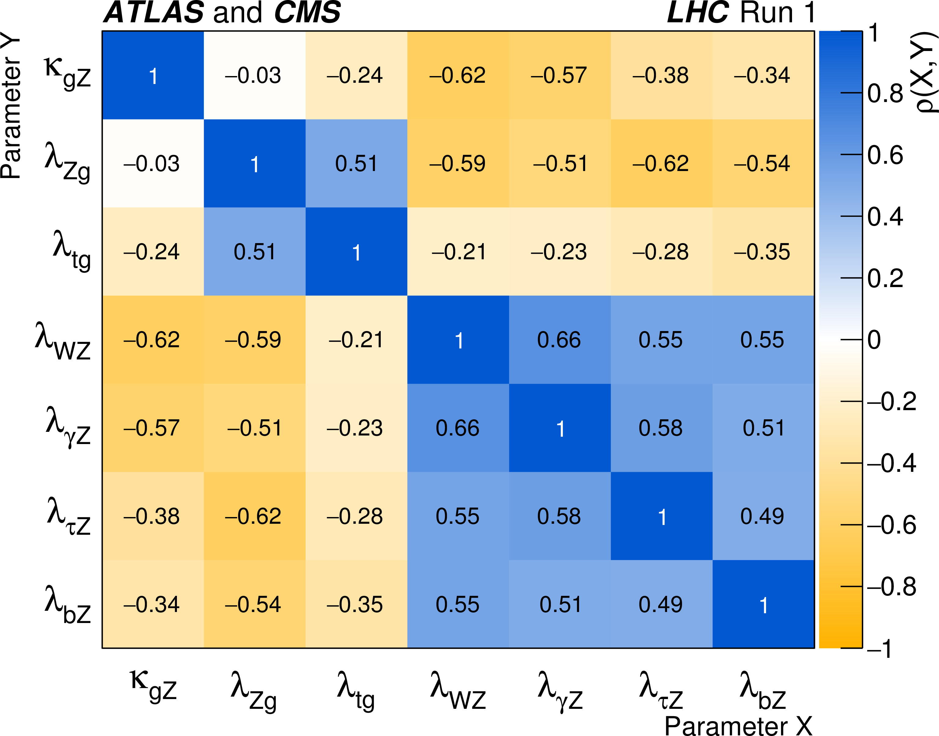
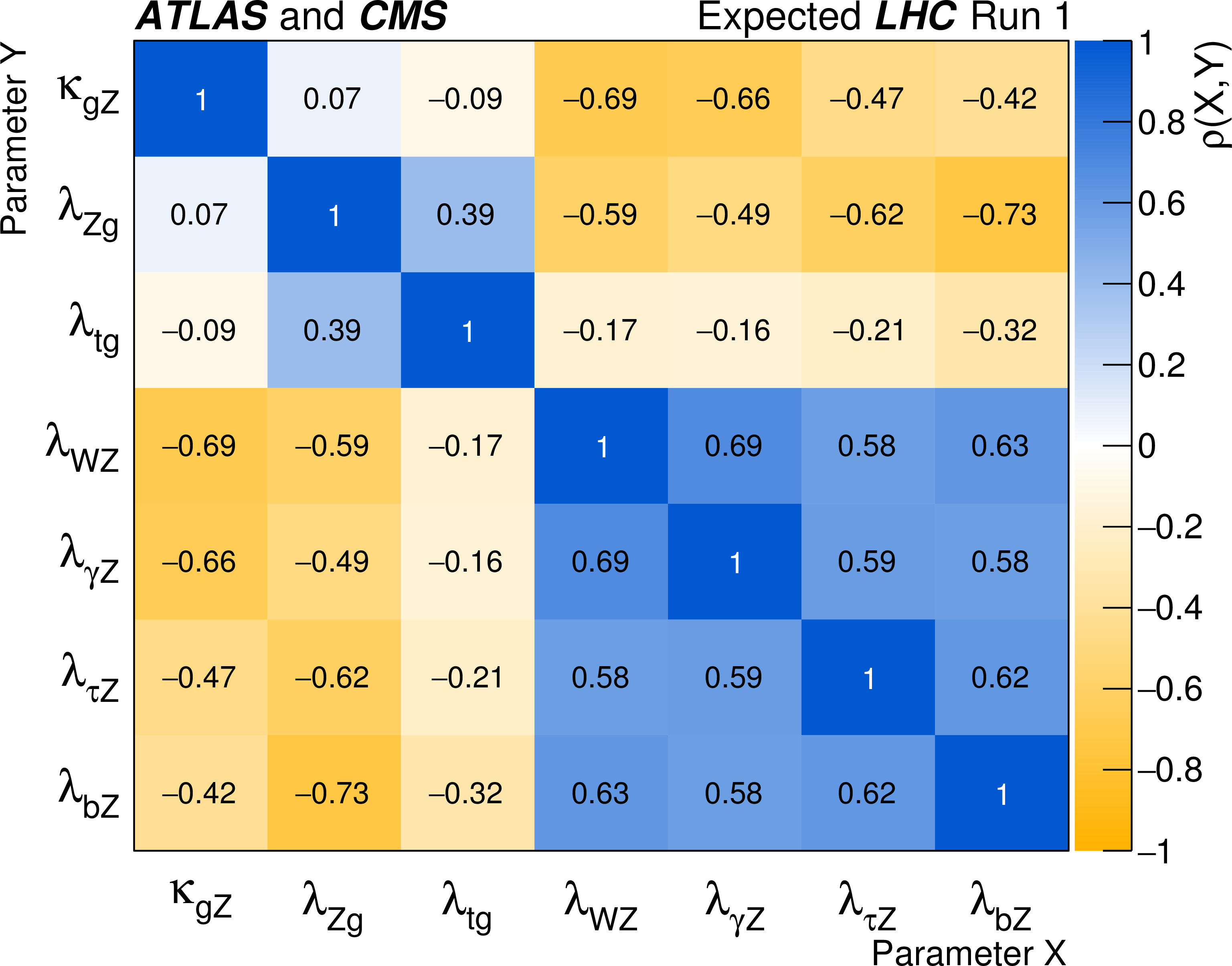
Figure 29:
Correlation matrix obtained from the fit combining the ATLAS and CMS data using the generic parameterisation with seven parameters described in Section 4.2. |
png pdf |
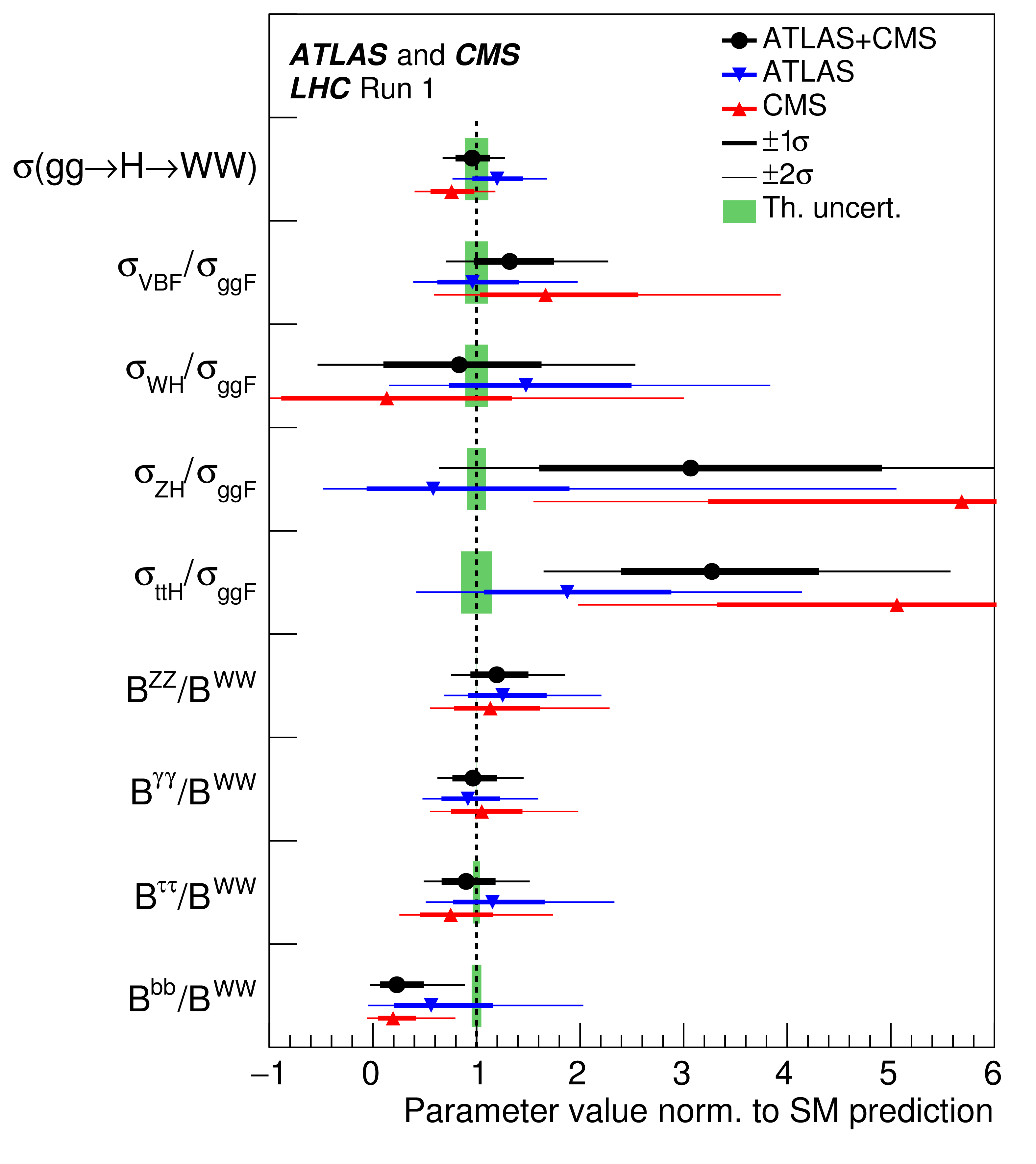
Figure 30:
Best fit values of the $gg\to H\to WW$ cross section and of ratios of cross sections and branching fractions, as obtained from the generic parameterisation described in Section 4.1.2 and as tabulated in Table 30 for the combination of the ATLAS and CMS measurements. Also shown are the results from each experiment. The values involving cross sections are given for $\sqrt {s}= $ 8 TeV, assuming the SM values for $\sigma _i(7\ \text{TeV})/\sigma _i(8\ \text{TeV} )$. The error bars indicate the 1$\sigma $ (thick lines) and 2$\sigma $ (thin lines) intervals. In this figure, the fit results are normalised to the SM predictions for the various parameters and the shaded bands indicate the theoretical uncertainties in these predictions. |

png pdf |
Figure 31:
Negative log-likelihood scan for $\lambda _{bZ}$ showing the minima obtained when considering all sign combinations (solid line) and each specific one separately (dashed lines). |
png pdf |
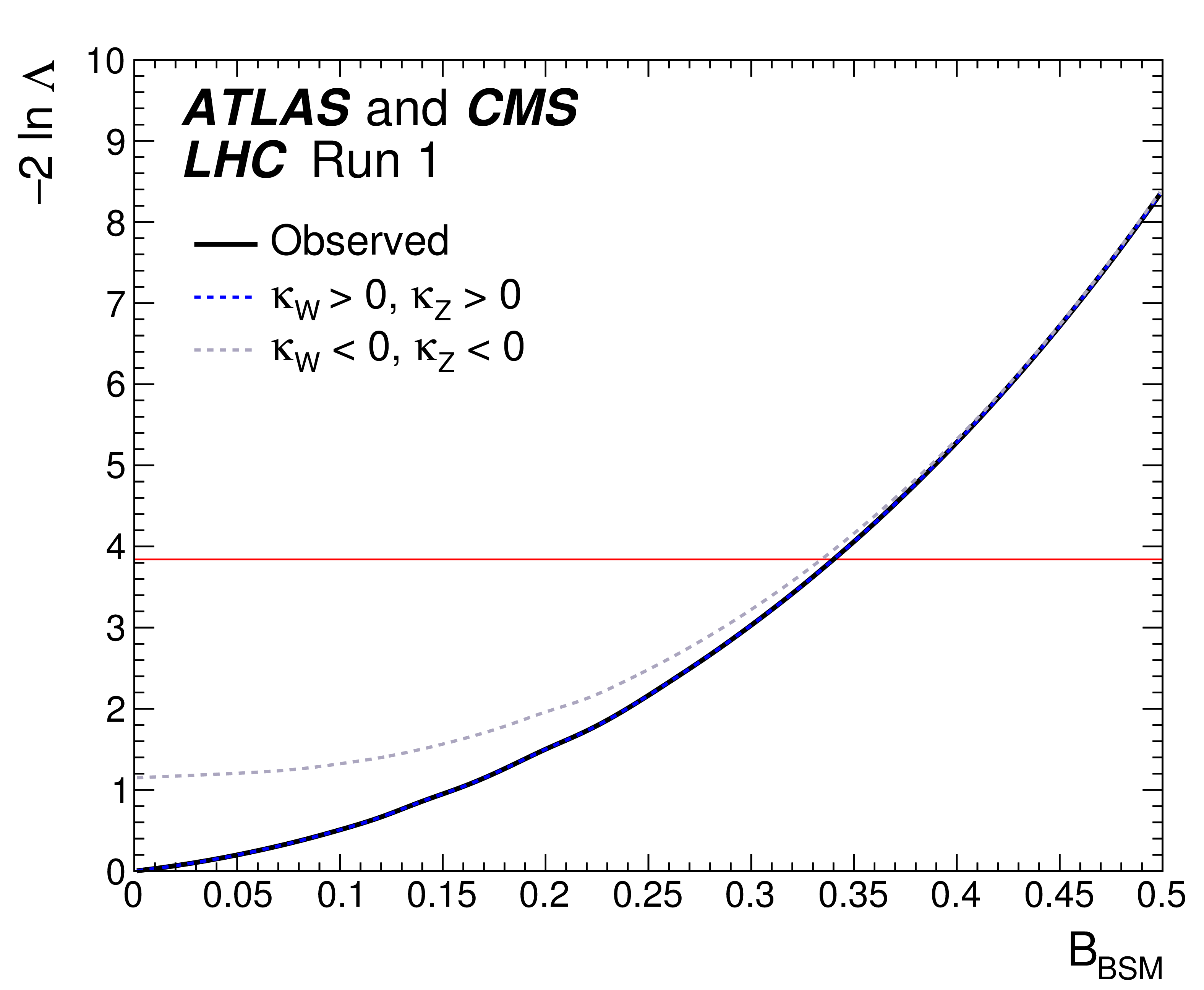
Figure 32-a:
Observed negative log-likelihood scan for $ {\mathrm {B_{BSM}}}$, the minima obtained when considering both sign combinations (solid line) and each specific one separately (dashed lines). |
png pdf |
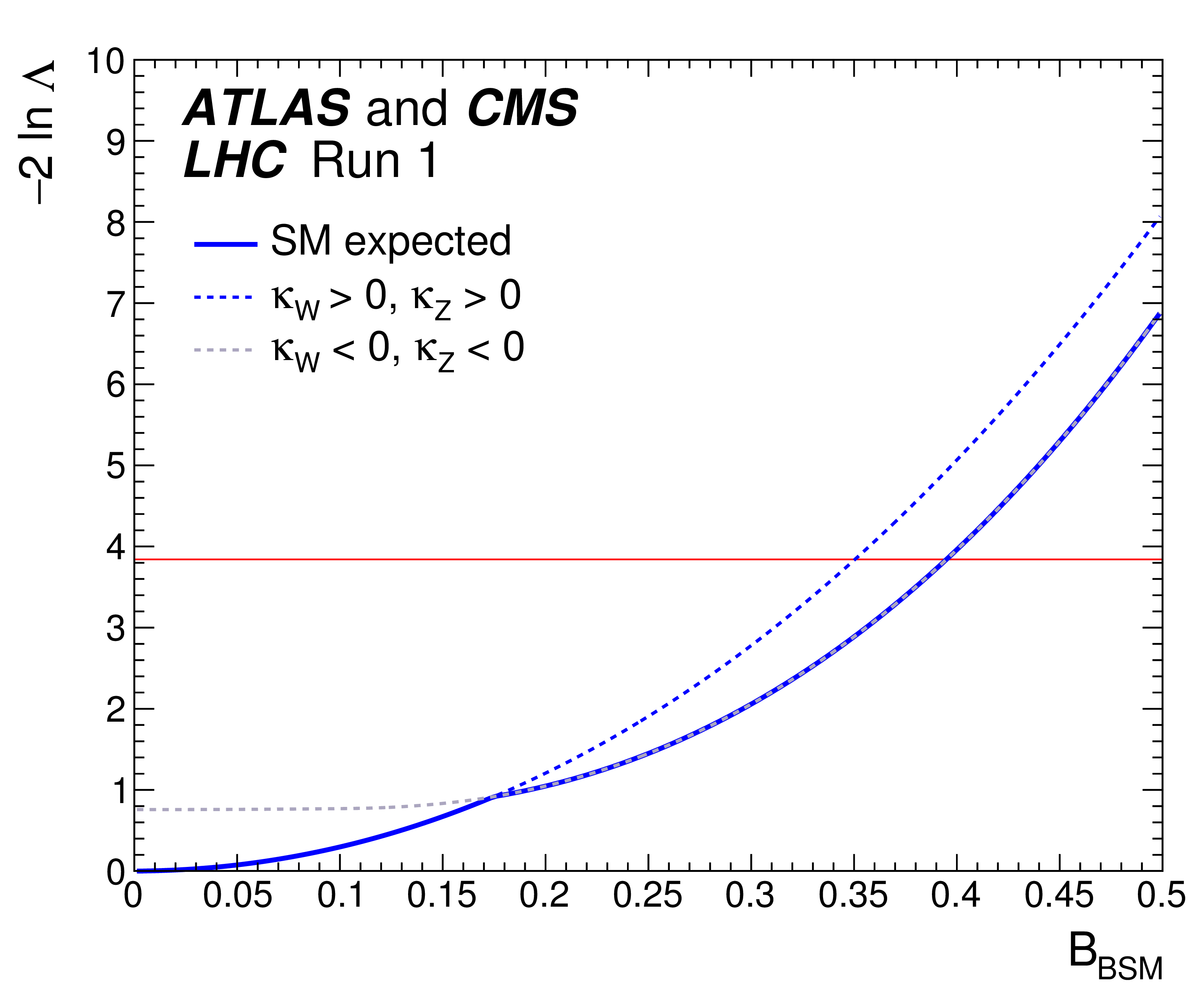
Figure 32-b:
Expected negative log-likelihood scan for $ {\mathrm {B_{BSM}}}$, the minima obtained when considering both sign combinations (solid line) and each specific one separately (dashed lines). |
| Tables | |
png pdf |
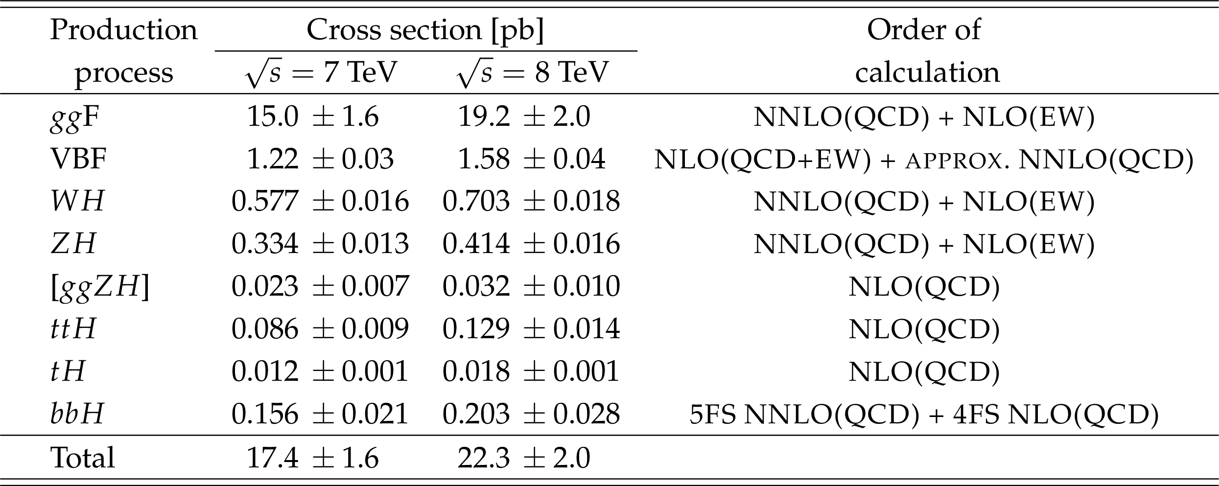
Table 1:
Standard Model predictions for the Higgs boson production cross sections together with their theoretical uncertainties. The value of the Higgs boson mass is assumed to be $m_H= $ 125.09 GeV and the predictions are obtained by linear interpolation between those at 125.0 and 125.1 GeV from Ref. [32] except for the ${tH}$ cross section, which is taken from Ref. [77]. The $pp \to ZH$ cross section, calculated at NNLO in QCD, includes both the quark-initiated, i.e. $qq \to ZH$ or $qg \to ZH$, and the $gg\to ZH$ contributions. The contribution from the $gg \to ZH$ production process, calculated only at NLO in QCD and indicated separately in brackets, is given with a theoretical uncertainty assumed to be 30%. The uncertainties in the cross sections are evaluated as the sum in quadrature of the uncertainties resulting from variations of the QCD scales, parton distribution functions, and $\alpha _{\text s}$. The uncertainty in the $tH$ cross section is calculated following the procedure of Ref. [78]. The order of the theoretical calculations for the different production processes is also indicated. In the case of $bbH$ production, the values are given for the mixture of five-flavour (5FS) and four-flavour (4FS) schemes recommended in Ref. [73]. |

png pdf |
Table 2:
Standard Model predictions for the decay branching fractions of a Higgs boson with a mass of 125.09 GeV, together with their uncertainties [32]. Included are decay modes that are either directly studied or important for the combination because of their contributions to the Higgs boson width. |
png pdf |
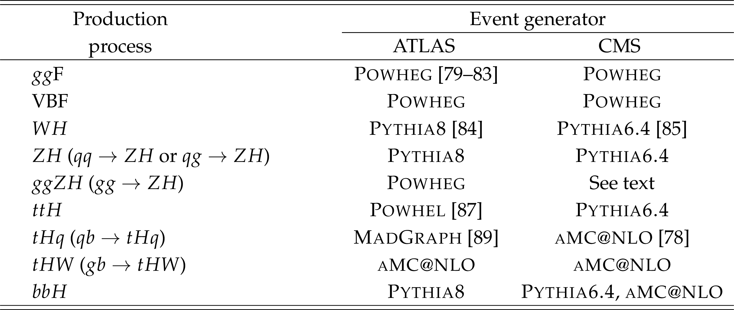
Table 3:
Summary of the event generators used by ATLAS and CMS to model the Higgs boson production processes and decay channels at $\sqrt {s}= $ 8 TeV. |

png pdf |
Table 4:
Higgs boson production cross sections $\sigma _{i}$, partial decay widths $\Gamma ^{f}$, and total decay width (in the absence of BSM decays) parameterised as a function of the $ {\kappa }$ coupling modifiers as discussed in the text, including higher-order QCD and EW corrections to the inclusive cross sections and decay partial widths. The coefficients in the expression for $\Gamma _{H}$ do not sum exactly to unity because some contributions that are negligible or not relevant to the analyses presented in this paper are not shown. |
png pdf |
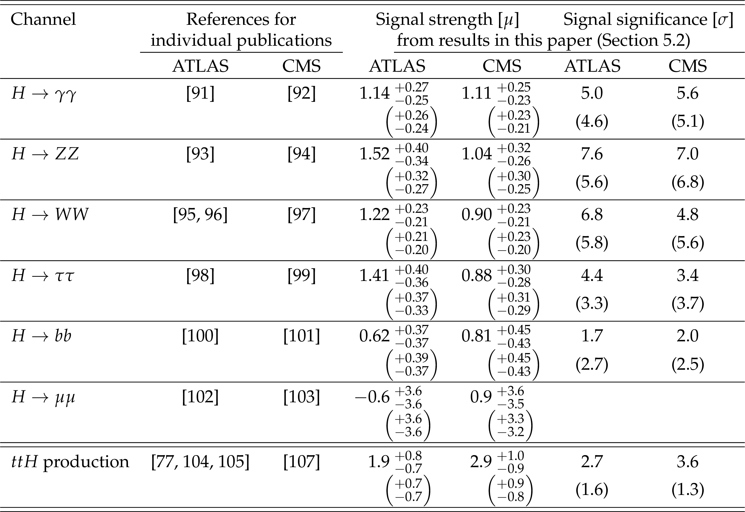
Table 5:
Overview of the decay channels analysed in this paper. The $ttH$ production process, which has contributions from all decay channels, is also shown. To show the relative importance of the various channels, the results from the combined analysis presented in this paper for $ {m_{H}} = $ 125.09 GeV (Tables 12 and 13 in Section 5.2) are reported as observed signal strengths $\mu $ with their measured uncertainties. The expected uncertainties are shown in parentheses. Also shown are the observed statistical significances, together with the expected significances in parentheses, except for the $H\to \mu \mu $ channel, which has very low sensitivity. For most decay channels, only the most sensitive analyses are quoted as references, e.g. the ${gg\mathrm {F}}$ and ${\mathrm {VBF}}$ analyses for the $H\to WW$ decay channel or the ${VH}$ analysis for the $H \to bb$ decay channel. Although not exactly the same, the results are close to those from the individual publications, in which slightly different values for the Higgs boson mass were assumed and in which the signal modelling and signal uncertainties were slightly different, as discussed in the text. |
png pdf |
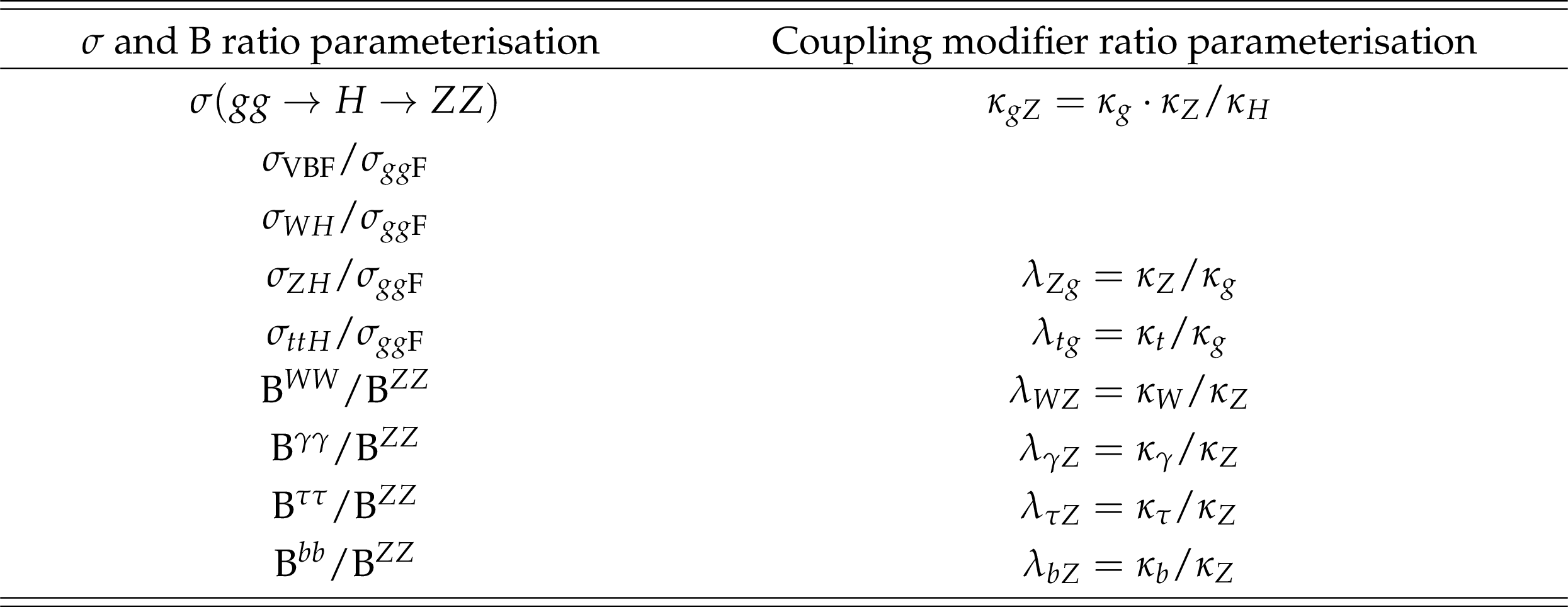
Table 6:
Parameters of interest in the two generic parameterisations described in Sections 4.1.2 and 4.2. For both parameterisations, the $gg \to H \to ZZ$ channel is chosen as a reference, expressed through the first row in the table. All other measurements are expressed as ratios of cross sections or branching fractions in the first column and of coupling modifiers in the second column. There are fewer parameters of interest in the case of the coupling parameterisation, in which the ratios of cross sections for the ${WH}$, ${ZH}$, and ${\mathrm {VBF}}$ processes can all be expressed as functions of the two parameters, $ {\lambda }_{Zg}$ and $ {\lambda }_{WZ}$. The slightly different additional assumptions in each parameterisation are discussed in the text. |
png pdf |
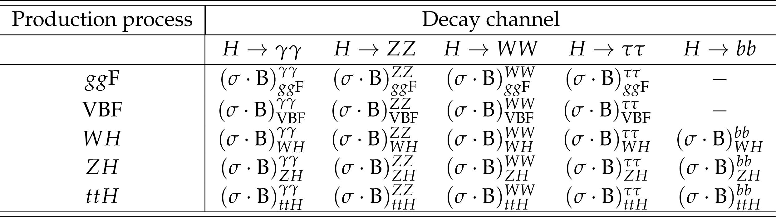
Table 7:
The signal parameterisation used to express the $\sigma _i \cdot {\mathrm {B}}^f$ values for each specific channel $i \to H\to f$. The values labelled with a "$-$" are not measured and are therefore fixed to the SM predictions. |

png pdf |
Table 8:
Best fit values of $\sigma _i \cdot {\mathrm {B}}^f$ for each specific channel $i \to H\to f$, as obtained from the generic parameterisation with 23 parameters for the combination of the ATLAS and CMS measurements, using the $\sqrt {s}= $ 7 and 8 TeV data. The cross sections are given for $\sqrt {s}= $ 8 TeV, assuming the SM values for $\sigma _i(7\ \text{TeV} )/\sigma _i(8\ \text{TeV} )$. The results are shown together with their total uncertainties and their breakdown into statistical and systematic components. The expected uncertainties in the measurements are displayed in parentheses. The SM predictions [32] and the ratios of the results to these SM predictions are also shown. The values labelled with a "$-$" are either not measured with a meaningful precision and therefore not quoted, in the case of the $ {H\to ZZ}$ decay channel for the ${WH}$, ${ZH}$, and ${ttH}$ production processes, or not measured at all and therefore fixed to their corresponding SM predictions, in the case of the $H\to bb$ decay mode for the ${gg\mathrm {F}}$ and ${\mathrm {VBF}}$ production processes. |
png pdf |
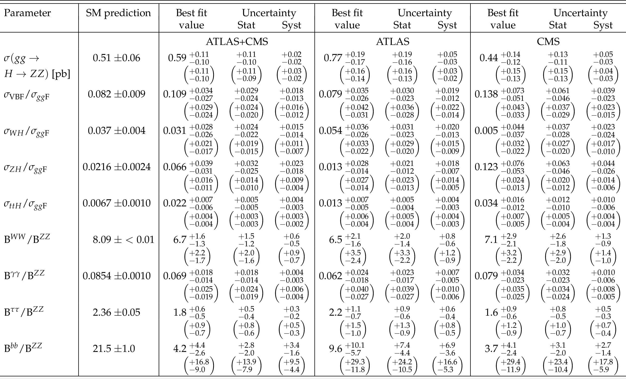
Table 9:
Best fit values of $\sigma (gg\to H\to ZZ)$, $\sigma _i/\sigma _{ {gg\mathrm {F}}}$, and $ {\mathrm {B}}^f/ {\mathrm {B}}^{ZZ}$, as obtained from the generic parameterisation with nine parameters for the combined analysis of the $\sqrt {s}= $ 7 and 8 TeV data. The values involving cross sections are given for $\sqrt {s}= $ 8 TeV, assuming the SM values for $\sigma _i(7\ \text{TeV} )/\sigma _i(8\ \text{TeV} )$. The results are reported for the combination of ATLAS and CMS and also separately for each experiment, together with their total uncertainties and their breakdown into statistical and systematic components. The expected uncertainties in the measurements are displayed in parentheses. The SM predictions [32] are also shown with their total uncertainties. |

png pdf |
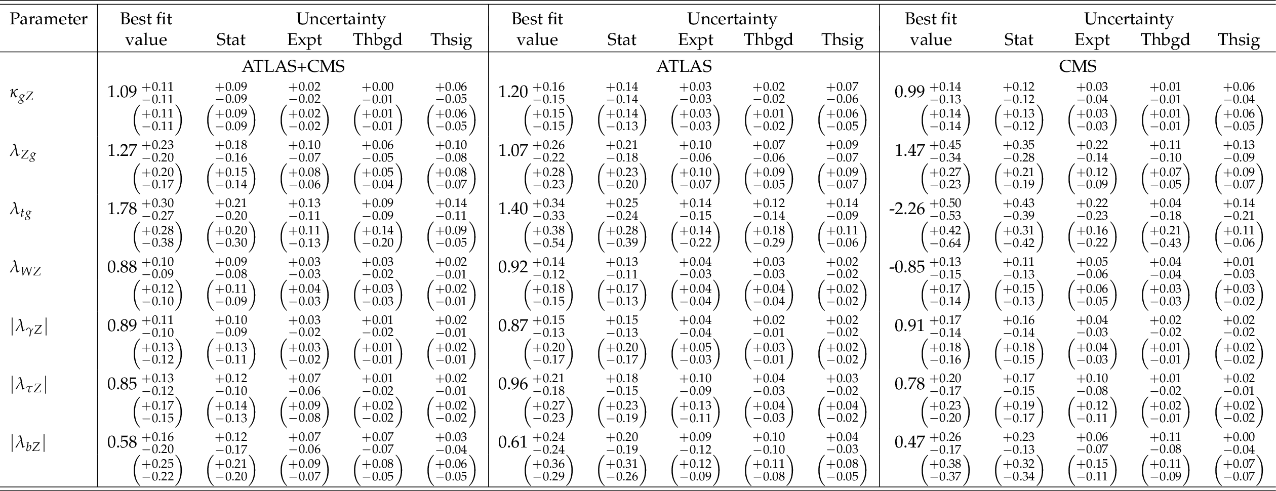
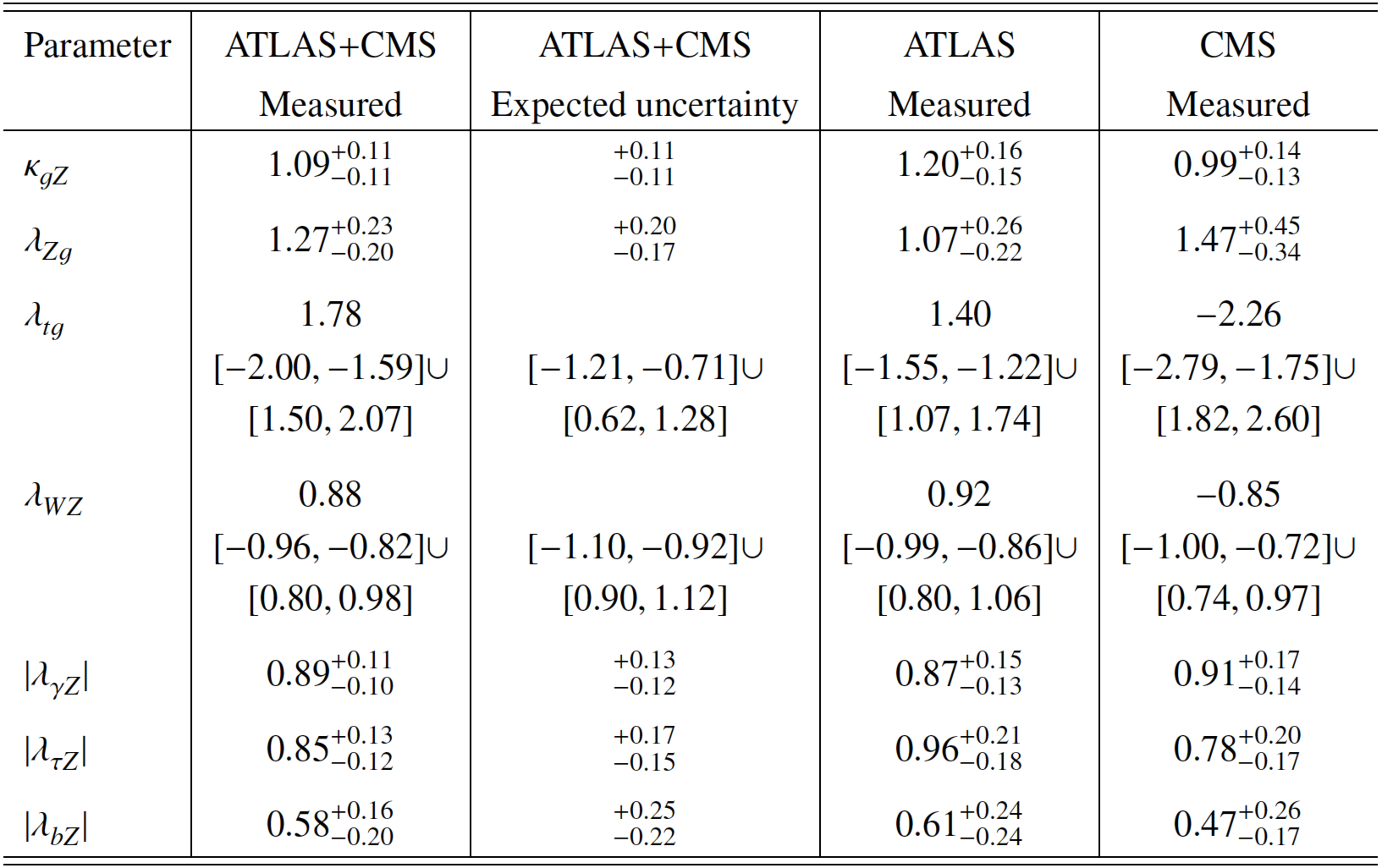
Table 10:
Best fit values of $ {\kappa }_{gZ}= {\kappa }_{g}\cdot {\kappa }_{Z} / {\kappa }_{H} $ and of the ratios of coupling modifiers, as defined in the parameterisation studied in the context of the $ {\kappa }$-framework, from the combined analysis of the $\sqrt {s}= $ 7 and 8 TeV data. The results are shown for the combination of ATLAS and CMS and also separately for each experiment, together with their total uncertainties and their breakdown into statistical and systematic components. The uncertainties in $\lambda _{tg}$ and $\lambda _{WZ}$, for which a negative solution is allowed, are calculated around the overall best fit value. The combined 1$\sigma $ CL intervals are $\lambda _{tg} = [-2.00,-1.59] \cup [1.50,2.07]$ and $\lambda _{WZ} = [-0.96,-0.82] \cup [0.80,0.98]$. The expected uncertainties in the measurements are displayed in parentheses. For those parameters with no sensitivity to the sign, only the absolute values are shown. |

png pdf |
Table 11:
Measured global signal strength $\mu $ and its total uncertainty, together with the breakdown of the uncertainty into its four components as defined in Section 3.3. The results are shown for the combination of ATLAS and CMS, and separately for each experiment. The expected uncertainty, with its breakdown, is also shown. |
png pdf |
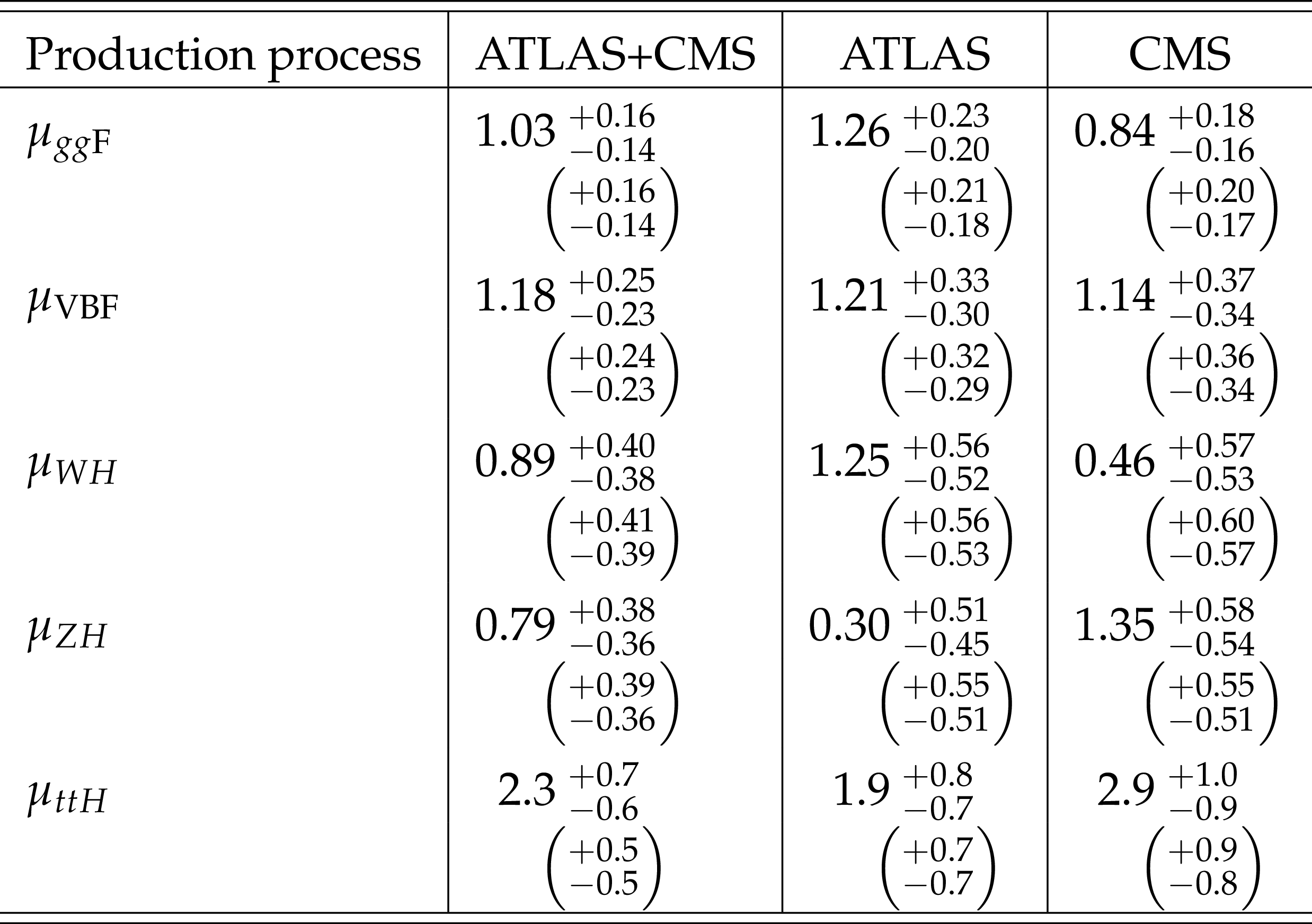
Table 12:
Measured signal strengths $\mu $ and their total uncertainties for different Higgs boson production processes. The results are shown for the combination of ATLAS and CMS, and separately for each experiment, for the combined $\sqrt {s}= $ 7 and 8 TeV data. The expected uncertainties in the measurements are displayed in parentheses. These results are obtained assuming that the Higgs boson branching fractions are the same as in the SM. |

png pdf |
Table 13:
Measured signal strengths $\mu $ and their total uncertainties for different Higgs boson decay channels. The results are shown for the combination of ATLAS and CMS, and separately for each experiment, for the combined $\sqrt {s}= $ 7 and 8 TeV data. The expected uncertainties in the measurements are displayed in parentheses. These results are obtained assuming that the Higgs boson production process cross sections at $\sqrt {s} = $ 7 and 8 TeV are the same as in the SM. |
png pdf |
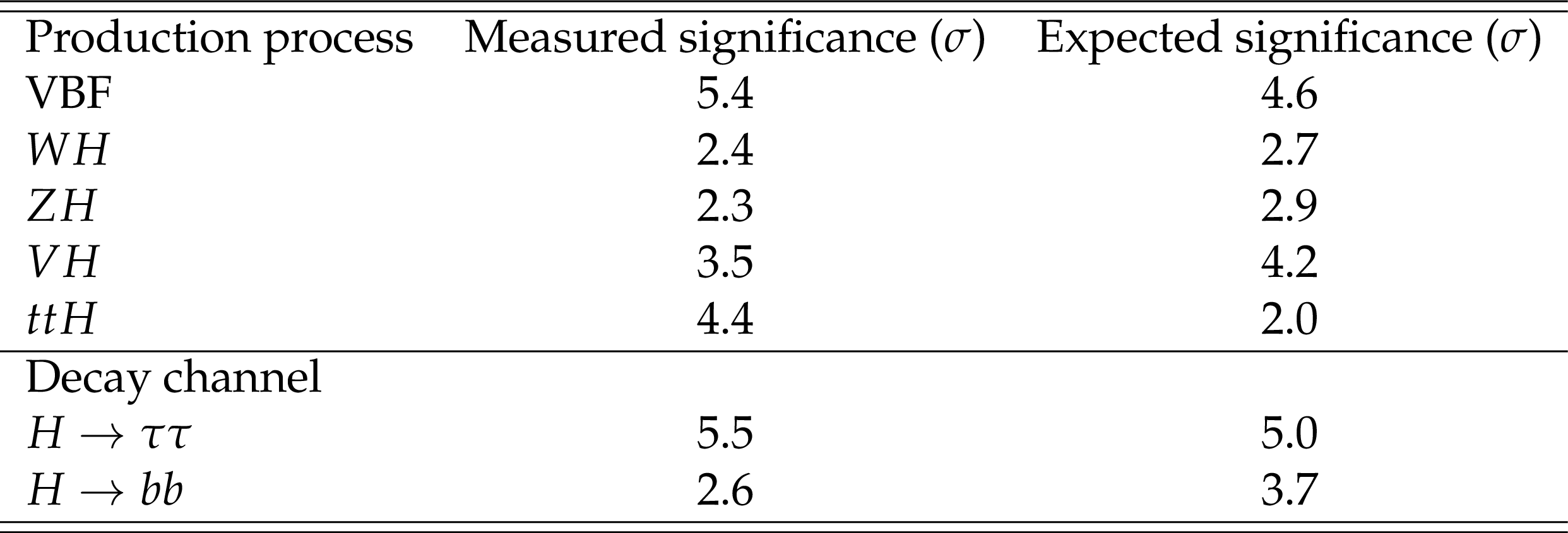
Table 14:
Measured and expected significances for the observation of Higgs boson production processes and decay channels for the combination of ATLAS and CMS. Not included are the ${gg\mathrm {F}}$ production process and the $ {H\to ZZ}$, $H\to WW$, and $ {H\to \gamma \gamma }$ decay channels, which have already been clearly observed. All results are obtained constraining the decay branching fractions to their SM values when considering the production processes, and constraining the production cross sections to their SM values when studying the decays. |
png pdf |
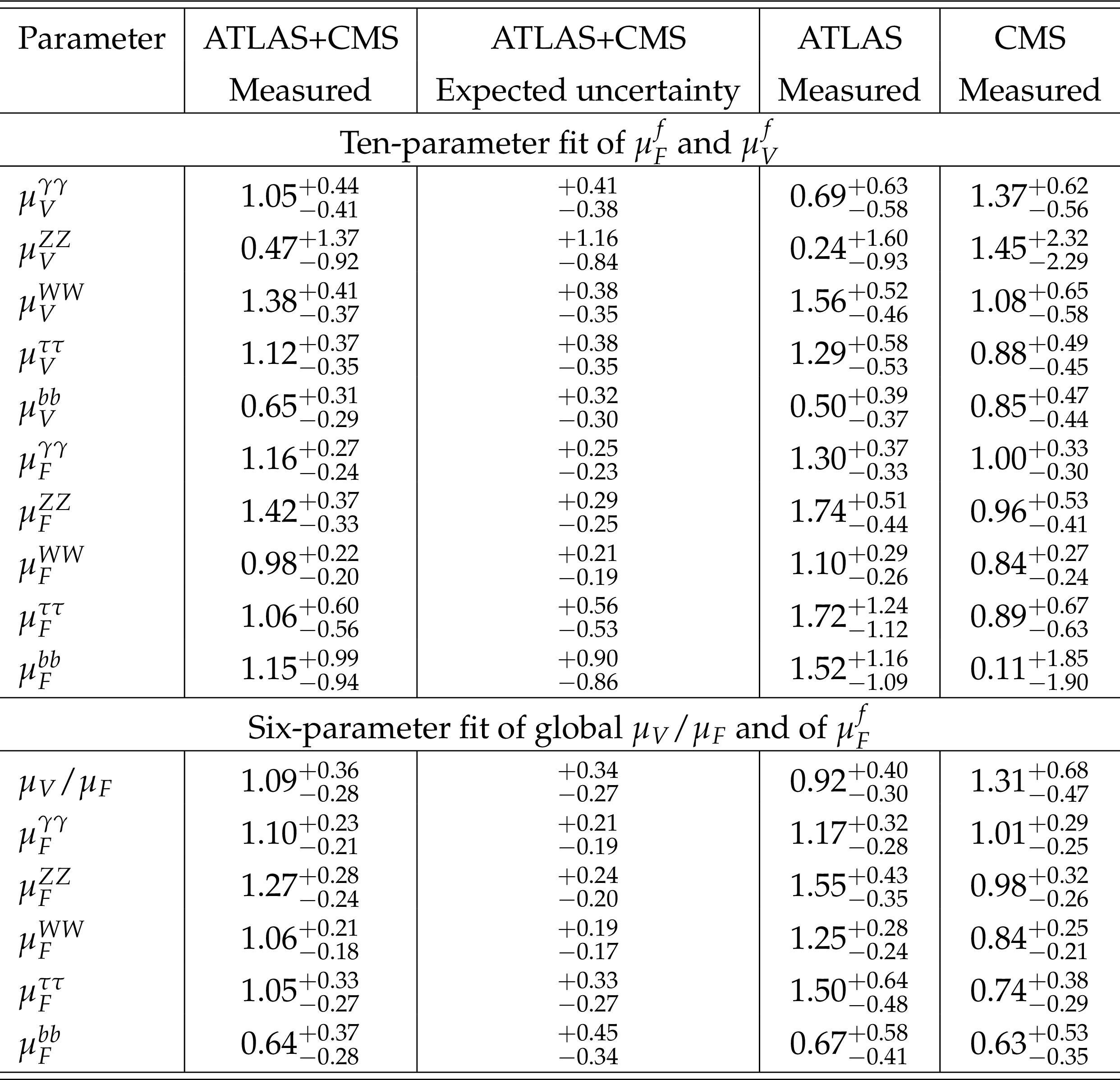
Table 15:
Results of the ten-parameter fit of $\mu _F^f = \mu _{ {gg\mathrm {F}}+ {ttH}}^f$ and $\mu _V^f = \mu _{ {\mathrm {VBF}}+ {VH}}^f$ for each of the five decay channels, and of the six-parameter fit of the global ratio $\mu _V/\mu _F = \mu _{ {\mathrm {VBF}}+ {VH}}/\mu _{ {gg\mathrm {F}}+ {ttH}}$ together with $\mu _F^f$ for each of the five decay channels. The results are shown for the combination of ATLAS and CMS, together with their measured and expected uncertainties. The measured results are also shown separately for each experiment. |

png pdf |
Table 16:
The two signal parameterisations used to scale the expected yields of the $5\times 5$ combinations of production processes and decay modes. The first parameterisation corresponds to the most general case with 25 independent parameters, while the second parameterisation corresponds to that expected for a single Higgs boson state. As explained in the text for the case of the general matrix parameterisation, the two parameters ${\mu _{ {gg\mathrm {F}}}^{bb}} $ and ${\lambda _{ {\mathrm {VBF}}}^{bb}} $ are set to unity in the fits, since the current analyses are not able to constrain them. |

png pdf |
Table 17:
Fit results for two parameterisations allowing BSM loop couplings discussed in the text: the first one assumes that $| {\kappa }_{V}| \le 1$, where $ {\kappa }_{V}$ denotes $ {\kappa }_{Z}$ or $ {\kappa }_{W}$, and that $ {\mathrm {B_{BSM}}}\ge 0$, while the second one assumes that there are no additional BSM contributions to the Higgs boson width, i.e. $ {\mathrm {B_{BSM}}}= $ 0 . The results for the combination of ATLAS and CMS are reported with their measured and expected uncertainties. Also shown are the results from each experiment. For the parameters with both signs allowed, the 1$\sigma $ intervals are shown on a second line. When a parameter is constrained and reaches a boundary, namely $ {\mathrm {B_{BSM}}}= $ 0 , the uncertainty is not indicated. For those parameters with no sensitivity to the sign, only the absolute values are shown. |

png pdf |
Table 18:
Fit results for the parameterisation assuming the absence of BSM particles in the loops ($ {\mathrm {B_{BSM}}}= $ 0 ). The results with their measured and expected uncertainties are reported for the combination of ATLAS and CMS, together with the individual results from each experiment. For the parameters with both signs allowed, the 1$\sigma $ CL intervals are shown on a second line. When a parameter is constrained and reaches a boundary, namely $|\kappa _\mu | = $ 0, the uncertainty is not indicated. For those parameters with no sensitivity to the sign, only the absolute values are shown. |

png pdf |
Table 19:
Summary of fit results for the two parameterisations probing the ratios of coupling modifiers for up-type versus down-type fermions and for leptons versus quarks. The results for the combination of ATLAS and CMS are reported together with their measured and expected uncertainties. Also shown are the results from each experiment. The parameters $\kappa _{uu}$ and $\kappa _{qq}$ are both positive definite since $ {\kappa _H}$ is always assumed to be positive. For the parameter $\lambda _{du}$, for which both signs are allowed, the 1$\sigma $ CL intervals are shown on a second line. For the parameter $\lambda _{lq}$, for which there is no sensitivity to the sign, only the absolute values are shown. Negative values for the parameters $\lambda _{Vu}$ and $\lambda _{Vq}$ are excluded by more than $4\sigma $. |

png pdf |
Table 20:
Best fit values of $\sigma (gg\to H\to ZZ)$, $\sigma _i/\sigma _{ {gg\mathrm {F}}}$, and $ {\mathrm {B}}^f/ {\mathrm {B}}^{ZZ}$ from the combined analysis of the $\sqrt {s}= $ 7 and 8 TeV data. The values involving cross sections are given for $\sqrt {s}= $ 8 TeV, assuming the SM values for $\sigma _i(7\ \text{TeV})/\sigma _i(8\ \text{TeV} )$. The results are shown for the combination of ATLAS and CMS, and also separately for each experiment, together with their total uncertainties and their breakdown into the four components described in the text. The expected total uncertainties in the measurements are also shown in parentheses. The SM predictions [32] are shown with their total uncertainties. |

png pdf |
Table 21:
Best fit values of $\sigma (gg\to H\to WW)$, $\sigma _i/\sigma _{ {gg\mathrm {F}}}$, and $ {\mathrm {B}}^f/ {\mathrm {B}}^{WW}$ from the combined analysis of the $\sqrt {s}= $ 7 and 8 TeV data. The values involving cross sections are given for $\sqrt {s}= $ 8 TeV, assuming the SM values for $\sigma _i(7\ \text{TeV})/\sigma _i(8\ \text{TeV} )$. The results are shown for the combination of ATLAS and CMS, and also separately for each experiment, together with their total uncertainties and their breakdown into the four components described in the text. The expected total uncertainties in the measurements are also shown in parentheses. The SM predictions [32] are shown with their total uncertainties. |
png pdf |
Table 22:
Best fit values of $ {\kappa }_{gZ}= {\kappa }_{g}\cdot {\kappa }_{Z} / {\kappa }_{H} $ and of the ratios of coupling modifiers, as defined in the most generic parameterisation described in the context of the $ {\kappa }$ framework, from the combined analysis of the $\sqrt {s}= $ 7 and 8 TeV data. The results are shown for the combination of ATLAS and CMS and also separately for each experiment, together with their total uncertainties and their breakdown into the four components described in the text. The uncertainties in $\lambda _{tg}$ and $\lambda _{WZ}$, for which a negative solution is allowed, are calculated around the overall best fit value. The combined 1$\sigma $ CL intervals are $\lambda _{tg} = [-2.00,-1.59] \cup [1.50,2.07]$ and $\lambda _{WZ} = [-0.96,-0.82] \cup [0.80,0.98]$. The expected total uncertainties in the measurements are also shown in parentheses. For those parameters with no sensitivity to the sign, only the absolute values are shown. |
| Summary |
|
An extensive set of combined ATLAS and CMS measurements of the Higgs boson production and decay rates is presented, and a number of constraints on its couplings to vector bosons and fermions are derived based on various sets of assumptions. The combination is based on the analysis of approximately 600 categories of selected events, concerning five production processes, $gg{\text{F}}$, ${\text{VBF}}$, $WH$, $ZH$, and $t\bar{t}H$, where $gg{\text{F}}$ and ${\text{VBF}}$ refer, respectively, to production through the gluon fusion and vector boson fusion processes; and six decay channels, $H \to ZZ$, $WW$, $\gamma\gamma$, $\tau\tau$, $b\bar{b}$, and $\mu\mu$. All results are reported assuming a value of 125.09 GeV for the Higgs boson mass, the result of the combined Higgs boson mass measurement by the two experiments [22]. The analysis uses the LHC proton-proton collision data sets recorded by the ATLAS and CMS detectors in 2011 and 2012, corresponding to integrated luminosities per experiment of approximately 5 fb$^{-1}$ at $\sqrt{s}= $ 7 TeV and 20 fb$^{-1}$ at $\sqrt{s} = $ 8 TeV. This paper presents the final Higgs boson coupling combined results from ATLAS and CMS based on the LHC Run 1 data. The combined analysis is sensitive to the couplings of the Higgs boson to the weak vector bosons and to the heavier fermions (top quarks, $b$ quarks, $\tau$ leptons, and - marginally - muons). The analysis is also sensitive to the effective couplings of the Higgs boson to the photon and the gluon. At the LHC, only products of cross sections and branching fractions are measured, so the width of the Higgs boson cannot be probed without assumptions beyond the main one used for all measurements presented here, namely that the Higgs boson production and decay kinematics are close to those predicted by the Standard Model (SM). In general, the combined analysis presented in this paper provides a significant improvement with respect to the individual combinations published by each experiment separately. The precision of the results improves in most cases by a factor of approximately $1/\sqrt 2$, as one would expect for the combination of two largely uncorrelated measurements based on similar-size data samples. A few illustrative results are summarised below. For the first time, results are shown for the most generic parameterisation of the observed event yields in terms of products of Higgs boson production cross sections times branching fractions, separately for each of 20 measurable $(\sigma_i$, $\mathrm{B}^f$) pairs of production processes and decay modes. These measurements do not rely on theoretical predictions for the inclusive cross sections and the uncertainties are mostly dominated by their statistical component. In the context of this parameterisation, one can test whether the observed yields arise from more than one Higgs boson, all with experimentally indistinguishable masses, but possibly with different coupling structures to the SM particles. The data are compatible with the hypothesis of a single Higgs boson, yielding a $p$-value of 29%. Fits to the observed event yields are also performed without any assumption about the Higgs boson width in the context of two other generic parameterisations. The first parameterisation is in terms of ratios of production cross sections and branching fractions, together with the reference cross section of the process $gg \to H \to ZZ$. All results are compatible with the SM. The best relative precision, of about 30%, is achieved for the ratio of cross sections $\sigma_{ {\text{VBF}}}/\sigma_{ gg{\text{F}}}$ and for the ratios of branching fractions $\mathrm{B}^{WW}/\mathrm{B}^{ZZ}$ and $\mathrm{B}^{\gamma\gamma}/\mathrm{B}^{ZZ}$. A relative precision of around 40% is achieved for the ratio of branching fractions $\mathrm{B}^{\tau\tau}/\mathrm{B}^{ZZ}$. The second parameterisation is in terms of ratios of coupling modifiers, together with one parameter expressing the $gg \to H \to ZZ$ reference process in terms of these modifiers. The ratios of coupling modifiers are measured with precisions of approximately 10-20%, where the improvement in precision in this second parameterisation arises because the signal yields are expressed as squares or products of these coupling modifiers. All measurements based on the generic parameterisations are compatible between the two experiments and with the predictions of the SM. The potential presence of physics beyond the SM (BSM) is also probed using specific parameterisations. With minimal additional assumptions, the overall branching fraction of the Higgs boson into BSM decays is determined to be less than 34% at 95% CL. This constraint applies to invisible decays into BSM particles, decays into BSM particles that are not detected as such, and modifications of the decays into SM particles that are not directly measured by the experiments. The combined signal yield relative to the SM expectation is measured to be 1.09 $\pm$ 0.07 (stat) $\pm$ 0.08 (syst), where the systematic uncertainty is dominated by the theoretical uncertainty in the inclusive cross sections. The measured (expected) significance for the direct observation of the ${\text{VBF}}$ production process is at the level of 5.4$\sigma$ (4.6$\sigma$), while that for the $H \to \tau \tau$ decay channel is at the level of 5.5$\sigma$ (5.0$\sigma$). |
| Additional Figures | |

png pdf |
Additional Figure 33:
Best fit values of $\sigma _i \cdot {\mathrm {B}}^f$ for each specific channel $i \to H\to f$, as obtained from the generic parameterisation with 23 parameters for the combination of the ATLAS and CMS measurements. The error bars indicate the 1$\sigma $ intervals. The fit results are normalised to the SM predictions for the various parameters and the shaded bands indicate the theoretical uncertainties in these predictions. Only 20 parameters are shown because some of them, indicated by the hatched areas, are either not measured with a meaningful precision, in the case of the $ {H\to ZZ}$ decay mode for the ${WH}$, ${ZH}$, and ${ttH}$ production processes, or not measured at all and therefore fixed to their corresponding SM predictions, in the case of the $H\to bb$ decay mode for the ${gg\mathrm {F}}$ and ${\mathrm {VBF}}$ production processes. |

png pdf |
Additional Figure 34:
Expected correlation matrix obtained from the fit combining ATLAS and CMS pre-fit Asimov data sets using the generic parameterisation with 23 parameters described in Section 4.1.1. Only 20 parameters are shown because the other three, corresponding to the $ {H\to ZZ}$ decay channel for the ${WH}$, ${ZH}$, and ${ttH}$ production processes, are not measured with a meaningful precision. |
png pdf |
Additional Figure 35:
Expected correlation matrix obtained from the fit combining ATLAS and CMS pre-fit Asimov data sets using the generic parameterisation with nine parameters described in Section 4.1.2. |
png pdf |
Additional Figure 36:
Expected correlation matrix obtained from the fit combining ATLAS and CMS pre-fit Asimov data sets using the generic parameterisation with seven parameters described in Section 4.2. |

png pdf |
Additional Figure 37:
Fit results for two parameterisations allowing BSM loop couplings: the first one assumes that $ {\mathrm {B_{BSM}}}\ge 0$ and that $| {\kappa }_{V}| \le 1$, where $ {\kappa }_{V}$ denotes $ {\kappa }_{Z}$ or $ {\kappa }_{W}$, and the second one assumes that there are no additional BSM contributions to the Higgs boson width, i.e. $ {\mathrm {B_{BSM}}}= $ 0 . The measured results for the combination of ATLAS and CMS are reported together with their uncertainties. The hatched area indicates the non-allowed region for the $ {\kappa }_{t}$ parameter, which is assumed to be positive without loss of generality. The error bars indicate the 1$\sigma $ (thick lines) and 2$\sigma $ (thin lines) intervals. When a parameter is constrained and reaches a boundary, namely $| {\kappa }_{V}| = $ 1 or $ {\mathrm {B_{BSM}}}= $ 0 , the uncertainty is not defined beyond this boundary. For those parameters with no sensitivity to the sign, only the absolute values are shown. |

png pdf |
Additional Figure 38:
Fit results for the parameterisation allowing BSM loop couplings and assuming that there are no additional BSM contributions to the Higgs boson width, i.e. $ {\mathrm {B_{BSM}}}= $ 0 . The measured results for the combination of ATLAS and CMS are reported together with their uncertainties, as well as the individual results from each experiment. The hatched area indicates the non-allowed region for the $ {\kappa }_{t}$ parameter, which is assumed to be positive without loss of generality. The error bars indicate the 1$\sigma $ (thick lines) and 2$\sigma $ (thin lines) intervals. For those parameters with no sensitivity to the sign, only the absolute values are shown. |

png pdf |
Additional Figure 39:
Fit results for the parameterisation allowing BSM loop couplings and assuming that $ {\mathrm {B_{BSM}}}\ge 0$ and that $| {\kappa }_{V}| \le 1$, where $ {\kappa }_{V}$ denotes $ {\kappa }_{Z}$ or $ {\kappa }_{W}$. The measured results for the combination of ATLAS and CMS are reported together with their uncertainties, as well as the individual results from each experiment. The hatched area indicates the non-allowed region for the $ {\kappa }_{t}$ parameter, which is assumed to be positive without loss of generality. The error bars indicate the 1$\sigma $ (thick lines) and 2$\sigma $ (thin lines) intervals. When a parameter is constrained and reaches a boundary, namely $| {\kappa }_{V}| = $ 1 or $ {\mathrm {B_{BSM}}}= $ 0 , the uncertainty is not defined beyond this boundary. For those parameters with no sensitivity to the sign, only the absolute values are shown. |

png pdf |
Additional Figure 40:
Best fit values as a function of particle mass for the combination of ATLAS and CMS data in the case of the parameterisation with parameters defined as $ {\kappa }_{F} \cdot \ m_{F}/v$ for the fermions, and as $\sqrt { {\kappa }_{V}} \cdot \ m_{V}/v$ for the weak vector bosons, where $v = $ 246 GeV is the vacuum expectation value of the Higgs field. The dashed (blue) line indicates the predicted dependence on the particle mass for the SM Higgs boson. The solid (red) line indicates the best fit result to the $ [M,\epsilon ]$ model of Ref. [128] with the corresponding 68% and 95% CL bands. The bottom panel shows the ratios of the reduced coupling modifiers to the SM predictions with their total uncertainties as a function of the particle mass. |

png pdf |
Additional Figure 41:
Negative log-likelihood contours at 68% CL (solid lines) and 95% CL (dashed lines) in the ($\mu _{ {gg\mathrm {F}}+ {ttH}}^f$, $\mu _{ {\mathrm {VBF}}+ {VH}}^f$) plane for the combination of ATLAS and CMS, as obtained from the ten-parameter fit described in Section 5.5 for each of the five decay modes $ {H\to ZZ}$, $H\to WW$, $ {H\to \gamma \gamma }$, $H\to \tau \tau $, and $H\to bb$. The best fit values obtained for each of the five decay modes are also shown, together with the SM expectation. The straight lower portion of the $ {H\to ZZ}$ contour at 95% CL is due to the large signal-over-background in this channel, leading to a negative signal-plus-background probability density function for large negative signal strengths. |
| Additional Tables | |

png pdf |
Additional Table 23:
Best fit values of $\sigma _i \cdot {\mathrm {B}}^f$ for each specific channel $i \to H\to f$, as obtained from the generic parameterisation with 23 parameters for the combination of the ATLAS and CMS measurements, using the $\sqrt {s}= $ 7 and 8 TeV data. The cross sections are given for $\sqrt {s}= $ 8 TeV, assuming the SM values for $\sigma _i(7\ \mathrm{TeV} )/\sigma _i(8\ \mathrm{TeV} )$. The values labelled with a "$-$" are either not measured with a meaningful precision and therefore not quoted, in the case of the $ {H\to ZZ}$ decay mode for the ${WH}$, ${ZH}$, and ${ttH}$ production processes, or not measured at all and therefore fixed to their corresponding SM predictions, in the case of the $H\to bb$ decay mode for the ${gg\mathrm {F}}$ and ${\mathrm {VBF}}$ production processes. |

png pdf |
Additional Table 24:
Best fit values of $\sigma (gg\to H\to ZZ)$, $\sigma _i/\sigma _{ {gg\mathrm {F}}}$, and $ {\mathrm {B}}^f/ {\mathrm {B}}^{ZZ}$, as obtained from the generic parameterisation with nine parameters for the combined analysis of the $\sqrt {s}= $ 7 and 8 TeV data. The cross section and the cross section ratios are given for $\sqrt {s}= $ 8 TeV, assuming the SM values for $\sigma _i(7\ \mathrm{TeV} )/\sigma _i(8\ \mathrm{TeV} )$. The results are reported for the combination of ATLAS and CMS and also separately for each experiment, together with their total uncertainties. The SM predictions [32] are also shown with their total uncertainties. |
png pdf |
Additional Table 25:
Best fit values of $ {\kappa }_{gZ}= {\kappa }_{g}\cdot {\kappa }_{Z} / {\kappa }_{H} $ and of the ratios of coupling modifiers, as defined in the parameterisation studied in the context of the $ {\kappa }$-framework, from the combined analysis of the $\sqrt {s}= $ 7 and 8 TeV data. The results with their measured and expected uncertainties are reported for the combination of ATLAS and CMS, together with the individual results from each experiment. For the parameters with both signs allowed, the 1$\sigma $ intervals are shown on a second line. For those parameters with no sensitivity to the sign, only the absolute values are shown. |

png pdf |
Additional Table 26:
Measured signal strengths $\mu $ and their total uncertainties for different Higgs boson production processes. The results are shown for the combination of ATLAS and CMS, and separately from each experiment, for the combined $\sqrt {s}= $ 7 and 8 TeV data. These results are derived assuming that the Higgs boson branching fractions are the same as in the SM. |

png pdf |
Additional Table 27:
Measured signal strengths $\mu $ and their total uncertainties for different Higgs boson decay channels. The results are shown for the combination of ATLAS and CMS, and separately from each experiment, for the combined $\sqrt {s}= $ 7 and 8 TeV data. These results are derived assuming that the Higgs boson production process cross sections at $\sqrt {s} = $ 7 and 8 TeV are the same as in the SM. |
png pdf |
Additional Table 28:
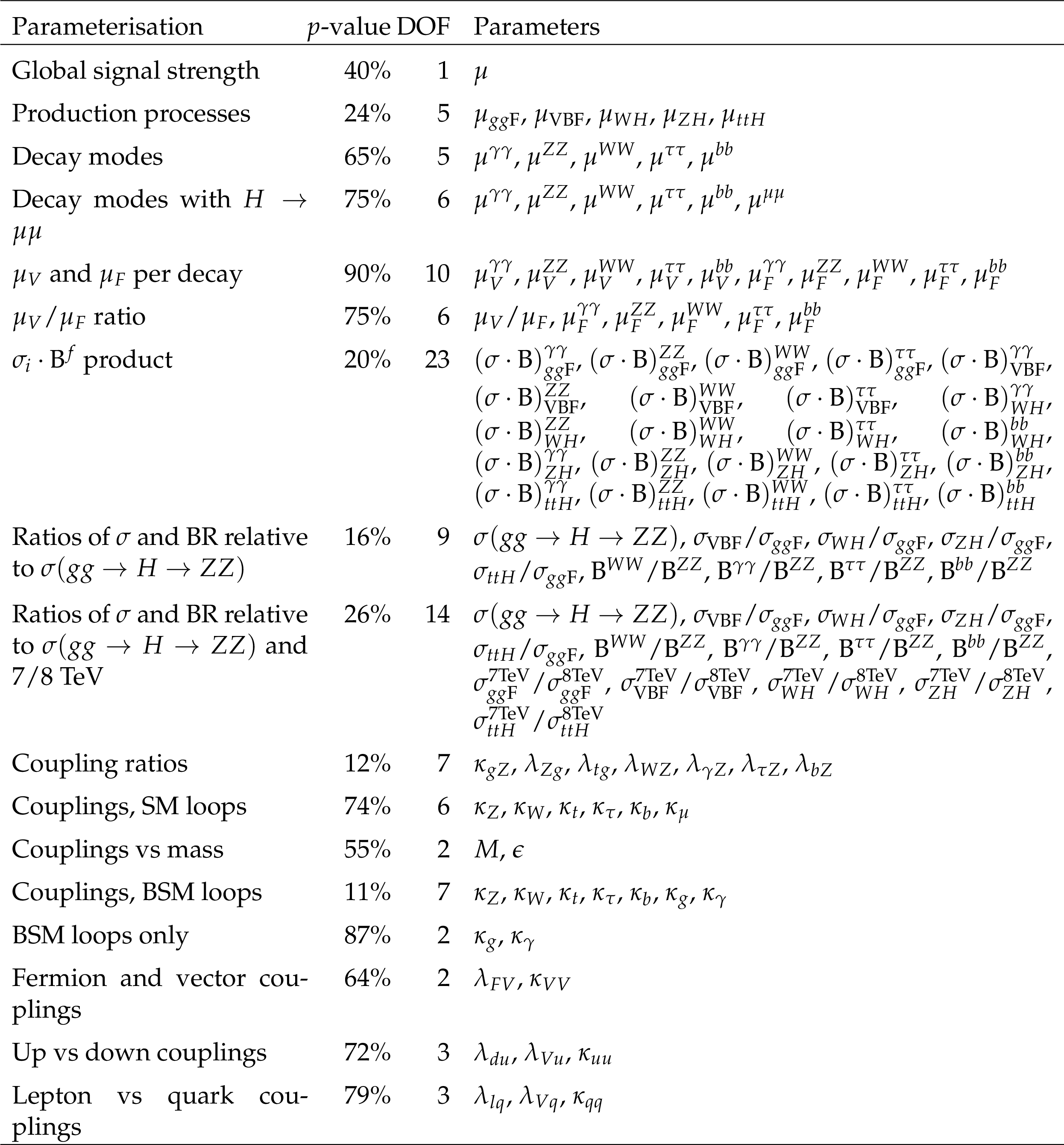
Compatibility with the SM prediction of fit results as a whole under the asymptotic approximation. For each parameterisation, the unconditional best fit is compared with the conditional fit where all parameters are set to their SM values. The conversion from $-2\ln\Lambda $ to the quoted $p$-value is performed assuming a two-sided distribution with the specified number of degrees of freedom (DOF). The quoted $p$-values are partially correlated between the different parameterisations. |
| References | ||||
| 1 | ATLAS Collaboration | The ATLAS Experiment at the CERN Large Hadron Collider | JINST 3 (2008) S08003 | |
| 2 | CMS Collaboration | The CMS experiment at the CERN LHC | JINST 3 (2008) S08004 | CMS-00-001 |
| 3 | S. L. Glashow | Partial-symmetries of weak interactions | NP 22 (1961) 579 | |
| 4 | S. Weinberg | A model of leptons | PRL 19 (1967) 1264 | |
| 5 | A. Salam | Weak and electromagnetic interactions | ||
| 6 | G. 't Hooft and M. Veltman | Regularization and Renormalization of Gauge Fields | NP B 44 (1972) 189 | |
| 7 | F. Englert and R. Brout | Broken Symmetry and the Mass of Gauge Vector Mesons | PRL 13 (1964) 321 | |
| 8 | P. W. Higgs | Broken symmetries, massless particles and gauge fields | PL12 (1964) 132 | |
| 9 | P. W. Higgs | Broken Symmetries and the Masses of Gauge Bosons | PRL 13 (1964) 508 | |
| 10 | G. S. Guralnik, C. R. Hagen, and T. W. B. Kibble | Global conservation laws and massless particles | PRL 13 (1964) 585 | |
| 11 | P. W. Higgs | Spontaneous symmetry breakdown without massless bosons | PR145 (1966) 1156 | |
| 12 | T. W. B. Kibble | Symmetry breaking in non-Abelian gauge theories | PR155 (1967) 1554 | |
| 13 | Y. Nambu and G. Jona-Lasinio | Dynamical Model of Elementary Particles Based on an Analogy with Superconductivity. I | PR122 (1961) 345 | |
| 14 | ATLAS Collaboration | Observation of a new particle in the search for the Standard Model Higgs boson with the ATLAS detector at the LHC | PLB 716 (2012) 1 | 1207.7214 |
| 15 | CMS Collaboration | Observation of a new boson at a mass of 125 GeV with the CMS experiment at the LHC | PLB 716 (2012) 30 | CMS-HIG-12-028 1207.7235 |
| 16 | CMS Collaboration | Observation of a new boson with mass near 125 GeV in pp collisions at $ \sqrt{s} $ = 7 and 8 TeV | JHEP 06 (2013) 081 | CMS-HIG-12-036 1303.4571 |
| 17 | ATLAS Collaboration | Measurements of the Higgs boson production and decay rates and coupling strengths using $ pp $ collision data at $ \sqrt{s}=7 $ and 8TeV in the ATLAS experiment | EPJC 76 (2016) 6 | 1507.04548 |
| 18 | CMS Collaboration | Precise determination of the mass of the Higgs boson and tests of compatibility of its couplings with the standard model predictions using proton collisions at 7 and 8 TeV | EPJC 75 (2015) 212 | CMS-HIG-14-009 1412.8662 |
| 19 | CMS Collaboration | Study of the Mass and Spin-Parity of the Higgs Boson Candidate via Its Decays to Z Boson Pairs | PRL 110 (2013) 081803 | CMS-HIG-12-041 1212.6639 |
| 20 | ATLAS Collaboration | Evidence for the spin-0 nature of the Higgs boson using ATLAS data | PLB 726 (2013) 120 | 1307.1432 |
| 21 | CMS Collaboration | Constraints on the spin-parity and anomalous HVV couplings of the Higgs boson in proton collisions at 7 and 8 TeV | PRD 92 (2015) 012004 | CMS-HIG-14-018 1411.3441 |
| 22 | ATLAS and CMS Collaborations | Combined Measurement of the Higgs Boson Mass in $ pp $ Collisions at $ \sqrt{s}=7 $ and 8 TeV with the ATLAS and CMS Experiments | PRL 114 (2015) 191803 | CMS-HIG-14-042 1503.07589 |
| 23 | ATLAS Collaboration | Constraints on the off-shell Higgs boson signal strength in the high-mass $ ZZ $ and $ WW $ final states with the ATLAS detector | EPJC 75 (2015) 335 | 1503.01060 |
| 24 | CMS Collaboration | Constraints on the Higgs boson width from off-shell production and decay to $ Z $-boson pairs, | PLB 736 (2014) 64 | CMS-HIG-14-002 1405.3455 |
| 25 | CMS Collaboration | Limits on the Higgs boson lifetime and width from its decay to four charged leptons | PRD 92 (2015) 072010 | CMS-HIG-14-036 1507.06656 |
| 26 | ATLAS Collaboration | Measurements of fiducial and differential cross sections for Higgs boson production in the diphoton decay channel at $ \sqrt{s}=$ 8 TeV with ATLAS | JHEP 09 (2014) 112 | 1407.4222 |
| 27 | ATLAS Collaboration | Fiducial and differential cross sections of Higgs boson production measured in the four-lepton decay channel in $ pp $ collisions at $ \sqrt{s}=$ 8 TeV with the ATLAS detector | PLB 738 (2014) 234 | 1408.3226 |
| 28 | CMS Collaboration | Measurement of differential cross sections for Higgs boson production in the diphoton decay channel in pp collisions at $ \sqrt{s} = 8 $ TeV | EPJC 76 (2016) 13 | CMS-HIG-14-016 1508.07819 |
| 29 | CMS Collaboration | Measurement of differential and integrated fiducial cross sections for Higgs boson production in the four-lepton decay channel in pp collisions at $ \sqrt{s}=7 $ and 8 TeV | JHEP 04 (2016) 005 | CMS-HIG-14-028 1512.08377 |
| 30 | S. Dittmaier et al. | Handbook of LHC Higgs Cross Sections: 1. Inclusive Observables | 1101.0593 | |
| 31 | S. Dittmaier et al. | Handbook of LHC Higgs Cross Sections: 2. Differential Distributions | 1201.3084 | |
| 32 | S. Heinemeyer et al. | Handbook of LHC Higgs Cross Sections: 3. Higgs Properties | 1307.1347 | |
| 33 | H. Georgi, S. Glashow, M. Machacek, and D. V. Nanopoulos | Higgs Bosons from Two Gluon Annihilation in Proton Proton Collisions | PRL 40 (1978) 692 | |
| 34 | A. Djouadi, M. Spira, and P. M. Zerwas | Production of Higgs bosons in proton colliders: QCD corrections | PLB 264 (1991) 440 | |
| 35 | S. Dawson | Radiative corrections to Higgs boson production | NP B 359 (1991) 283 | |
| 36 | M. Spira, A. Djouadi, D. Graudenz, and P. M. Zerwas | Higgs boson production at the LHC | NP B 453 (1995) 17 | arXiv:hep-ph/9504378 |
| 37 | R. V. Harlander and W. B. Kilgore | Next-to-next-to-leading order Higgs production at hadron colliders | PRL 88 (2002) 201801 | arXiv:hep-ph/0201206 |
| 38 | C. Anastasiou and K. Melnikov | Higgs boson production at hadron colliders in NNLO QCD | NP B 646 (2002) 220 | arXiv:hep-ph/0207004 |
| 39 | V. Ravindran, J. Smith, and W. L. van Neerven | NNLO corrections to the total cross section for Higgs boson production in hadron hadron collisions | NP B 665 (2003) 325 | arXiv:hep-ph/0302135 |
| 40 | S. Catani, D. de Florian, M. Grazzini, and P. Nason | Soft gluon resummation for Higgs boson production at hadron colliders | JHEP 07 (2003) 028 | hep-ph/0306211 |
| 41 | S. Actis, G. Passarino, C. Sturm, and S. Uccirati | NLO Electroweak Corrections to Higgs Boson Production at Hadron Colliders | PLB 670 (2008) 12 | 0809.1301 |
| 42 | C. Anastasiou, R. Boughezal, and F. Petriello | Mixed QCD-electroweak corrections to Higgs boson production in gluon fusion | JHEP 04 (2009) 003 | 0811.3458 |
| 43 | D. de Florian and M. Grazzini | Higgs production through gluon fusion: updated cross sections at the Tevatron and the LHC | PLB 674 (2009) 291 | 0901.2427 |
| 44 | D. de Florian and M. Grazzini | Higgs production at the LHC: updated cross sections at $ \sqrt{s}=$ 8 TeV | PLB 718 (2012) 117 | 1206.4133 |
| 45 | G. Bozzi, S. Catani, D. de Florian, and M. Grazzini | Transverse-momentum resummation and the spectrum of the Higgs boson at the LHC | NP B 737 (2006) 73 | hep-ph/0508068 |
| 46 | D. de Florian, G. Ferrera, M. Grazzini, and D. Tommasini | Transverse-momentum resummation: Higgs boson production at the Tevatron and the LHC | JHEP 11 (2011) 064 | 1109.2109 |
| 47 | M. Grazzini and H. Sargsyan | Heavy-quark mass effects in Higgs boson production at the LHC | JHEP 09 (2013) 129 | 1306.4581 |
| 48 | I. W. Stewart and F. J. Tackmann | Theory Uncertainties for Higgs and Other Searches Using Jet Bins | PRD 85 (2012) 034011 | 1107.2117 |
| 49 | A. Banfi, P. F. Monni, G. P. Salam, and G. Zanderighi | Higgs and Z-boson production with a jet veto | PRL 109 (2012) 202001 | 1206.4998 |
| 50 | A. Djouadi, J. Kalinowski, and M. Spira | HDECAY: A program for Higgs boson decays in the standard model and its supersymmetric extension | CPC 108 (1998) 56 | hep-ph/9704448 |
| 51 | A. Bredenstein, A. Denner, S. Dittmaier, and M. M. Weber | Precise predictions for the Higgs-boson decay H $ \rightarrow $ WW/ZZ $ \rightarrow $ 4 leptons | PRD 74 (2006) 013004 | arXiv:hep-ph/0604011 |
| 52 | A. Bredenstein, A. Denner, S. Dittmaier, and M. M. Weber | Radiative corrections to the semileptonic and hadronic Higgs-boson decays H $ \rightarrow $ WW/ZZ $ \rightarrow $ 4 fermions | JHEP 02 (2007) 080 | hep-ph/0611234 |
| 53 | A. Denner et al. | Standard Model Higgs-Boson Branching Ratios with Uncertainties | EPJC 71 (2011) 1753 | 1107.5909 |
| 54 | R. Cahn and S. Dawson | Production of Very Massive Higgs Bosons | PLB 136 (1984) 196 | |
| 55 | M. Ciccolini, A. Denner, and S. Dittmaier | Strong and electroweak corrections to the production of Higgs + 2 jets via weak interactions at the LHC | PRL 99 (2007) 161803 | 0707.0381 |
| 56 | M. Ciccolini, A. Denner, and S. Dittmaier | Electroweak and QCD corrections to Higgs production via vector-boson fusion at the LHC | PRD 77 (2008) 013002 | 0710.4749 |
| 57 | P. Bolzoni, F. Maltoni, S.-O. Moch, and M. Zaro | Higgs production via vector-boson fusion at NNLO in QCD | PRL 105 (2010) 011801 | 1003.4451 |
| 58 | M. Botje et al. | The PDF4LHC Working Group Interim Recommendations | 1101.0538 | |
| 59 | H. Lai et al. | New parton distributions for collider physics | PRD 82 (2010) 074024 | 1007.2241 |
| 60 | A. Martin, W. Stirling, R. Thorne, and G. Watt | Parton distributions for the LHC | EPJC 63 (2009) 189 | 0901.0002 |
| 61 | R. D. Ball et al. | A first unbiased global NLO determination of parton distributions and their uncertainties | NP B 838 (2010) 136 | 1002.4407 |
| 62 | S. Glashow, D. V. Nanopoulos, and A. Yildiz | Associated Production of Higgs Bosons and Z Particles | PRD 18 (1978) 1724 | |
| 63 | O. Brein, A. Djouadi, and R. Harlander | NNLO QCD corrections to the Higgs-strahlung processes at hadron colliders | PLB 579 (2004) 149 | arXiv:hep-ph/0307206 |
| 64 | A. Denner, S. Dittmaier, S. Kallweit, and A. M\"uck | Electroweak corrections to Higgs-strahlung off W/Z bosons at the Tevatron and the LHC with HAWK | JHEP 03 (2012) 075 | 1112.5142 |
| 65 | C. Englert, M. McCullough, and M. Spannowsky | Gluon-initiated associated production boosts Higgs physics | PRD 89 (2014) 013013 | 1310.4828 |
| 66 | G. Ferrera, M. Grazzini, and F. Tramontano | Associated ZH production at hadron colliders: the fully differential NNLO QCD calculation | PLB 740 (2015) 51 | 1407.4747 |
| 67 | R. Raitio and W. W. Wada | Higgs boson production at large transverse momentum in quantum chromodynamics | PRD 19 (1979) 941 | |
| 68 | W. Beenakker et al. | NLO QCD corrections to t$ \bar t $H production in hadron collisions | NP B 653 (2003) 151 | arXiv:hep-ph/0211352 |
| 69 | S. Dawson et al. | Associated Higgs production with top quarks at the Large Hadron Collider: NLO QCD corrections | PRD 68 (2003) 034022 | arXiv:hep-ph/0305087 |
| 70 | R. V. Harlander and W. B. Kilgore | Higgs boson production in bottom quark fusion at next-to-next-to-leading order | PRD 68 (2003) 013001 | arXiv:hep-ph/0304035 |
| 71 | S. Dittmaier, M. Kramer, and M. Spira | Higgs radiation off bottom quarks at the Tevatron and the CERN LHC | PRD 70 (2004) 074010 | hep-ph/0309204 |
| 72 | S. Dawson, C. Jackson, L. Reina, and D. Wackeroth | Exclusive Higgs boson production with bottom quarks at hadron colliders | PRD 69 (2004) 074027 | hep-ph/0311067 |
| 73 | R. Harlander, M. Kramer, and M. Schumacher | Bottom-quark associated Higgs-boson production: Reconciling the four- and five-flavour scheme approach | 1112.3478 | |
| 74 | M. Farina et al. | Lifting degeneracies in Higgs couplings using single top production in association with a Higgs boson | JHEP 05 (2013) 022 | 1211.3736 |
| 75 | D. Zeppenfeld, R. Kinnunen, A. Nikitenko, and E. Richter-Was | Measuring Higgs boson couplings at the CERN LHC | PRD 62 (2000) 013009 | hep-ph/0002036 |
| 76 | M. Duhrssen et al. | Extracting Higgs boson couplings from CERN LHC data | PRD 70 (2004) 113009 | hep-ph/0406323 |
| 77 | ATLAS Collaboration | Search for $ H \to \gamma\gamma $ produced in association with top quarks and constraints on the Yukawa coupling between the top quark and the Higgs boson using data taken at 7 TeV and 8 TeV with the ATLAS detector | PLB 740 (2015) 222 | 1409.3122 |
| 78 | J. Alwall et al. | The automated computation of tree-level and next-to-leading order differential cross sections, and their matching to parton shower simulations | JHEP 07 (2014) 079 | 1405.0301 |
| 79 | P. Nason | A New method for combining NLO QCD with shower Monte Carlo algorithms | JHEP 11 (2004) 040 | hep-ph/0409146 |
| 80 | S. Frixione, P. Nason, and C. Oleari | Matching NLO QCD computations with Parton Shower simulations: the POWHEG method | JHEP 11 (2007) 070 | 0709.2092 |
| 81 | S. Alioli, P. Nason, C. Oleari, and E. Re | NLO Higgs boson production via gluon fusion matched with shower in POWHEG | JHEP 04 (2009) 002 | 0812.0578 |
| 82 | S. Alioli, P. Nason, C. Oleari, and E. Re | A general framework for implementing NLO calculations in shower Monte Carlo programs: the POWHEG BOX | JHEP 06 (2010) 043 | 1002.2581 |
| 83 | E. Bagnaschi, G. Degrassi, P. Slavich, and A. Vicini | Higgs production via gluon fusion in the POWHEG approach in the SM and in the MSSM | JHEP 02 (2012) 088 | 1111.2854 |
| 84 | T. Sjostrand, S. Mrenna, and P. Z. Skands | A Brief Introduction to PYTHIA 8.1 | CPC 178 (2008) 852 | 0710.3820 |
| 85 | T. Sjostrand, S. Mrenna, and P. Z. Skands | PYTHIA 6.4 Physics and Manual | JHEP 05 (2006) 026 | hep-ph/0603175 |
| 86 | M. Bahr et al. | Herwig++ Physics and Manual | EPJC 58 (2008) 639 | 0803.0883 |
| 87 | G. Bevilacqua et al. | HELAC-NLO | CPC 184 (2013) 986 | 1110.1499 |
| 88 | M. V. Garzelli, A. Kardos, C. G. Papadopoulos, and Z. Trocsanyi | Standard Model Higgs boson production in association with a top anti-top pair at NLO with parton showering | Europhys. Lett. 96 (2011) 11001 | 1108.0387 |
| 89 | F. Maltoni and T. Stelzer | MadEvent: Automatic event generation with MadGraph | JHEP 02 (2003) 027 | hep-ph/0208156 |
| 90 | J. M. Campbell, R. K. Ellis, and G. Zanderighi | Next-to-Leading order Higgs + 2 jet production via gluon fusion | JHEP 10 (2006) 028 | hep-ph/0608194 |
| 91 | ATLAS Collaboration | Measurement of Higgs boson production in the diphoton decay channel in pp collisions at center-of-mass energies of 7 and 8 TeV with the ATLAS detector | PRD 90 (2014) 112015 | 1408.7084 |
| 92 | CMS Collaboration | Observation of the diphoton decay of the 125 GeV Higgs boson and measurement of its properties | EPJC 74 (2014) 3076 | CMS-HIG-13-001 1407.0558 |
| 93 | ATLAS Collaboration | Measurements of Higgs boson production and couplings in the four-lepton channel in pp collisions at center-of-mass energies of 7 and 8 TeV with the ATLAS detector | PRD 91 (2015) 012006 | 1408.5191 |
| 94 | CMS Collaboration | Measurement of the properties of a Higgs boson in the four-lepton final state | PRD 89 (2014) 092007 | CMS-HIG-13-002 1312.5353 |
| 95 | ATLAS Collaboration | Observation and measurement of Higgs boson decays to $ WW^{\ast} $ with the ATLAS detector | PRD 92 (2015) 012006 | 1412.2641 |
| 96 | ATLAS Collaboration | Study of the Higgs boson decaying to WW$ {}^* $ produced in association with a weak boson with the ATLAS detector at the LHC | JHEP 08 (2015) 137 | 1506.06641 |
| 97 | CMS Collaboration | Measurement of Higgs boson production and properties in the WW decay channel with leptonic final states | JHEP 01 (2014) 096 | CMS-HIG-13-023 1312.1129 |
| 98 | ATLAS Collaboration | Evidence for the Higgs-boson Yukawa coupling to tau leptons with the ATLAS detector | JHEP 04 (2015) 117 | 1501.04943 |
| 99 | CMS Collaboration | Evidence for the 125 GeV Higgs boson decaying to a pair of $ \tau $ leptons | JHEP 05 (2014) 104 | CMS-HIG-13-004 1401.5041 |
| 100 | ATLAS Collaboration | Search for the $ b\bar{b} $ decay of the Standard Model Higgs boson in associated $ (W/Z)H $ production with the ATLAS detector | JHEP 01 (2015) 069 | 1409.6212 |
| 101 | CMS Collaboration | Search for the standard model Higgs boson produced in association with a W or a Z boson and decaying to bottom quarks | PRD 89 (2014) 012003 | CMS-HIG-13-012 1310.3687 |
| 102 | ATLAS Collaboration | Search for the Standard Model Higgs boson decay to $ \mu^{+}\mu^{-} $ with the ATLAS detector | PLB 738 (2014) 68 | 1406.7663 |
| 103 | CMS Collaboration | Search for a standard model-like Higgs boson in the $ \mu^+\mu^- $ and $ {e^+e^-} $ decay channels at the LHC | PLB 744 (2015) 184 | CMS-HIG-13-007 1410.6679 |
| 104 | ATLAS Collaboration | Search for the Standard Model Higgs boson produced in association with top quarks and decaying into $ b\bar{b} $ in pp collisions at $ \sqrt{s} $ = 8 TeV with the ATLAS detector | EPJC 75 (2015) 349 | 1503.05066 |
| 105 | ATLAS Collaboration | Search for the associated production of the Higgs boson with a top quark pair in multi-lepton final states with the ATLAS detector | PLB 749 (2015) 519 | 1506.05988 |
| 106 | CMS Collaboration | Search for the standard model Higgs boson produced in association with a top-quark pair in pp collisions at the LHC | JHEP 05 (2013) 145 | CMS-HIG-12-035 1303.0763 |
| 107 | CMS Collaboration | Search for the associated production of the Higgs boson with a top-quark pair | JHEP 09 (2014) 087 | CMS-HIG-13-029 1408.1682 |
| 108 | ATLAS Collaboration | Search for Higgs boson decays to a photon and a Z boson in pp collisions at $ \sqrt{s} $ = 7 and 8 TeV with the ATLAS detector | PLB 732 (2014) 8 | 1402.3051 |
| 109 | CMS Collaboration | Search for a Higgs boson decaying into a Z and a photon in pp collisions at $ \sqrt{s} $ = 7 and 8 TeV | PLB 726 (2013) 587 | CMS-HIG-13-006 1307.5515 |
| 110 | CMS Collaboration | Search for the standard model Higgs boson produced through vector boson fusion and decaying to $ {b\bar{b}} $ | PRD 92 (2015) 032008 | CMS-HIG-14-004 1506.01010 |
| 111 | ATLAS Collaboration | Search for Invisible Decays of a Higgs Boson Produced in Association with a Z Boson in ATLAS | PRL 112 (2014) 201802 | 1402.3244 |
| 112 | ATLAS Collaboration | Search for invisible decays of the Higgs boson produced in association with a hadronically decaying vector boson in $ pp $ collisions at $ \sqrt{s} $ = 8 TeV with the ATLAS detector | EPJC 75 (2015) 337 | 1504.04324 |
| 113 | CMS Collaboration | Search for invisible decays of Higgs bosons in the vector boson fusion and associated ZH production modes | EPJC 74 (2014) 2980 | CMS-HIG-13-030 1404.1344 |
| 114 | ATLAS and CMS Collaborations | Procedure for the LHC Higgs boson search combination in Summer 2011 | ATL-PHYS-PUB-2011-011 CERN-CMS-NOTE-2011-005 |
|
| 115 | W. Verkerke and D. P. Kirkby | The RooFit toolkit for data modeling | physics/0306116 | |
| 116 | L. Moneta et al. | The RooStats Project | 1009.1003 | |
| 117 | K. Cranmer et al. | HistFactory: A tool for creating statistical models for use with RooFit and RooStats | ||
| 118 | G. Cowan, K. Cranmer, E. Gross, and O. Vitells | Asymptotic formulae for likelihood-based tests of new physics | EPJC 71 (2011) 1554 | 1007.1727 |
| 119 | G. J. Feldman and R. D. Cousins | Unified approach to the classical statistical analysis of small signals | PRD 57 (1998) 3873 | physics/9711021 |
| 120 | J. Wenninger | Energy Calibration of the LHC Beams at 4 TeV | ||
| 121 | J. F. Gunion, Y. Jiang, and S. Kraml | Could two NMSSM Higgs bosons be present near 125 GeV? | PRD 86 (2012) 071702 | 1207.1545 |
| 122 | B. Grzadkowski, J. F. Gunion, and M. Toharia | Higgs-Radion interpretation of the LHC data? | PLB 712 (2012) 70 | 1202.5017 |
| 123 | A. Drozd, B. Grzadkowski, J. F. Gunion, and Y. Jiang | Two-Higgs-doublet models and enhanced rates for a 125 GeV Higgs | JHEP 05 (2013) 72 | 1211.3580 |
| 124 | P. M. Ferreira, R. Santos, H. E. Haber, and J. P. Silva | Mass-degenerate Higgs bosons at 125 GeV in the two-Higgs-doublet model | PRD 87 (2011) 055009 | 1211.3131 |
| 125 | J. F. Gunion, Y. Jiang, and S. Kraml | Diagnosing Degenerate Higgs Bosons at 125 GeV | PRL 110 (2013) 051801 | 1208.1817 |
| 126 | Y. Grossman, Z. Surujon, and J. Zupan | How to test for mass degenerate Higgs resonances | JHEP 03 (2013) 176 | 1301.0328 |
| 127 | A. David, J. Heikkila, and G. Petrucciani | Searching for degenerate Higgs bosons | EPJC 75 (2015) 49 | 1409.6132 |
| 128 | J. Ellis and T. You | Updated global analysis of Higgs couplings | JHEP 06 (2013) 103 | 1303.3879 |
| 129 | T. D. Lee | A Theory of Spontaneous T Violation | PRD 8 (1973) 1226 | |
|
|
Compact Muon Solenoid LHC, CERN |
|

|

|

|

|

|