

Compact Muon Solenoid
LHC, CERN
| CMS-TOP-18-006 ; CERN-EP-2019-073 | ||
| Measurement of the top quark polarization and $\mathrm{t\bar{t}}$ spin correlations using dilepton final states in proton-proton collisions at $\sqrt{s} = $ 13 TeV | ||
| CMS Collaboration | ||
| 8 July 2019 | ||
| Phys. Rev. D 100 (2019) 072002 | ||
| Abstract: Measurements of the top quark polarization and top quark pair ($\mathrm{t\bar{t}}$) spin correlations are presented using events containing two oppositely charged leptons ($\mathrm{e^{+}}\mathrm{e^{-}}$ , $\mathrm{e}^{\pm}\mu^{\mp}$ , or $\mu\mu$) produced in proton-proton collisions at a center-of-mass energy of 13 TeV. The data were recorded by the CMS experiment at the LHC in 2016 and correspond to an integrated luminosity of 35.9 fb$^{-1}$. A set of parton-level normalized differential cross sections, sensitive to each of the independent coefficients of the spin-dependent parts of the $\mathrm{t\bar{t}}$ production density matrix, is measured for the first time at 13 TeV. The measured distributions and extracted coefficients are compared with standard model predictions from simulations at next-to-leading-order (NLO) accuracy in quantum chromodynamics (QCD), and from NLO QCD calculations including electroweak corrections. All measurements are found to be consistent with the expectations of the standard model. The normalized differential cross sections are used in fits to constrain the anomalous chromomagnetic and chromoelectric dipole moments of the top quark to $-0.24 < {C_\text{tG}/\Lambda^{2}} < 0.07 $ TeV$^{-2}$ and $-0.33 < {C^{I}_\text{tG}/\Lambda^{2}} < 0.20 $ TeV$^{-2}$, respectively, at 95% confidence level. | ||
| Links: e-print arXiv:1907.03729 [hep-ex] (PDF) ; CDS record ; inSPIRE record ; HepData record ; CADI line (restricted) ; | ||
| Figures | |
png pdf |
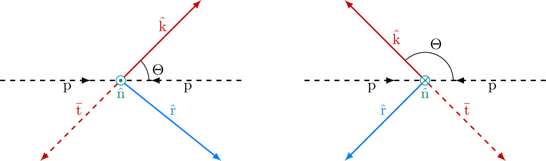
Figure 1:
Coordinate system used for the spin measurements, illustrated in the scattering plane for $\Theta < \pi /2$ (left) and $\Theta > \pi /2$ (right), where the signs of $\hat{r}$ and $\hat{n}$ are flipped at $\Theta =\pi /2$ as shown in Eq. (4). The $\hat{k}$ axis is defined by the top quark direction, measured in the ${\mathrm{t} \mathrm{\bar{t}}}$ CM frame. For the basis used to define the coefficient functions in Eq. (3), the incoming particles $\text {p}$ represent the incoming partons, while for the basis used to measure the coefficients in Eqs. (8)-(10) they represent the incoming protons. |
png pdf |
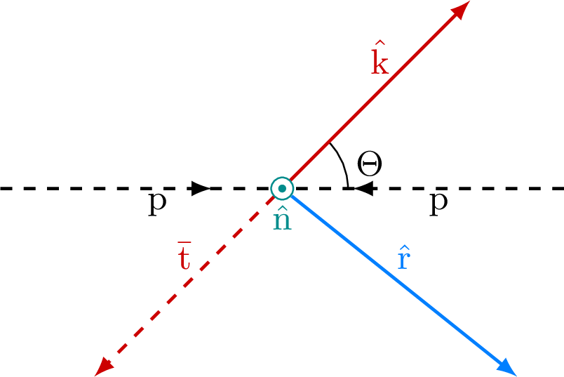
Figure 1-a:
Coordinate system used for the spin measurements, illustrated in the scattering plane for $\Theta < \pi /2$ (left) and $\Theta > \pi /2$ (right), where the signs of $\hat{r}$ and $\hat{n}$ are flipped at $\Theta =\pi /2$ as shown in Eq. (4). The $\hat{k}$ axis is defined by the top quark direction, measured in the ${\mathrm{t} \mathrm{\bar{t}}}$ CM frame. For the basis used to define the coefficient functions in Eq. (3), the incoming particles $\text {p}$ represent the incoming partons, while for the basis used to measure the coefficients in Eqs. (8)-(10) they represent the incoming protons. |
png pdf |
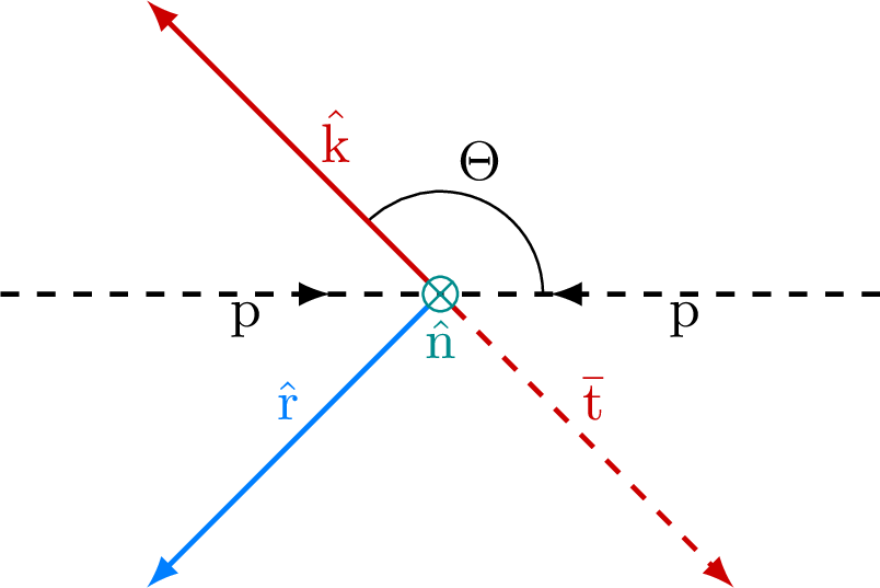
Figure 1-b:
Coordinate system used for the spin measurements, illustrated in the scattering plane for $\Theta < \pi /2$ (left) and $\Theta > \pi /2$ (right), where the signs of $\hat{r}$ and $\hat{n}$ are flipped at $\Theta =\pi /2$ as shown in Eq. (4). The $\hat{k}$ axis is defined by the top quark direction, measured in the ${\mathrm{t} \mathrm{\bar{t}}}$ CM frame. For the basis used to define the coefficient functions in Eq. (3), the incoming particles $\text {p}$ represent the incoming partons, while for the basis used to measure the coefficients in Eqs. (8)-(10) they represent the incoming protons. |
png pdf |
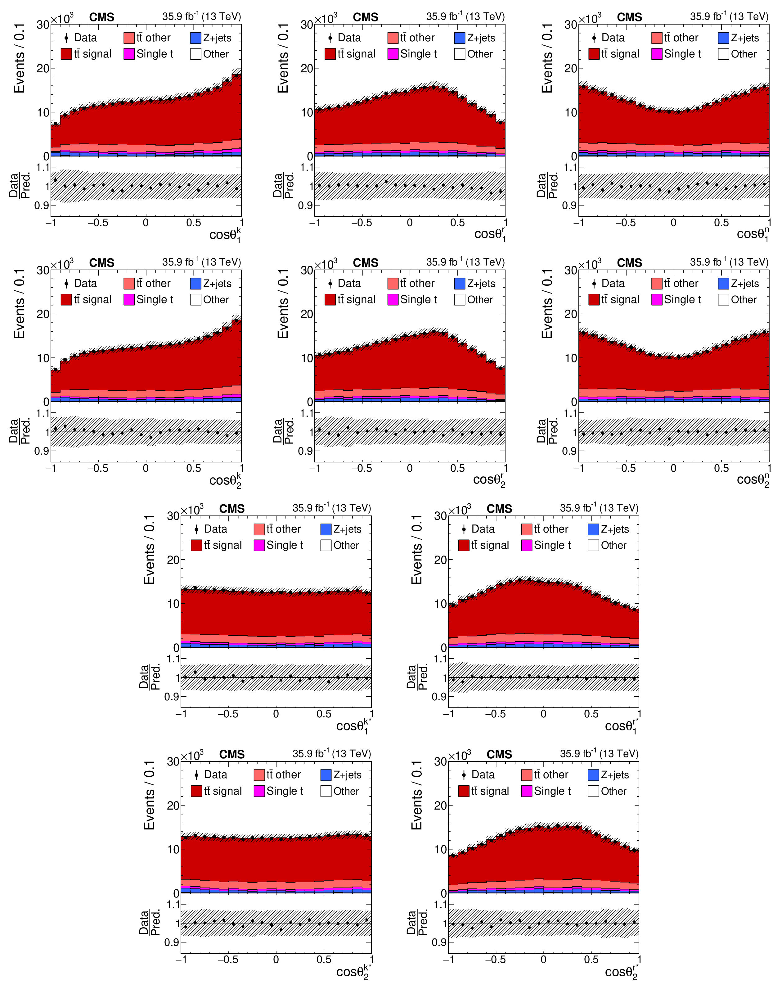
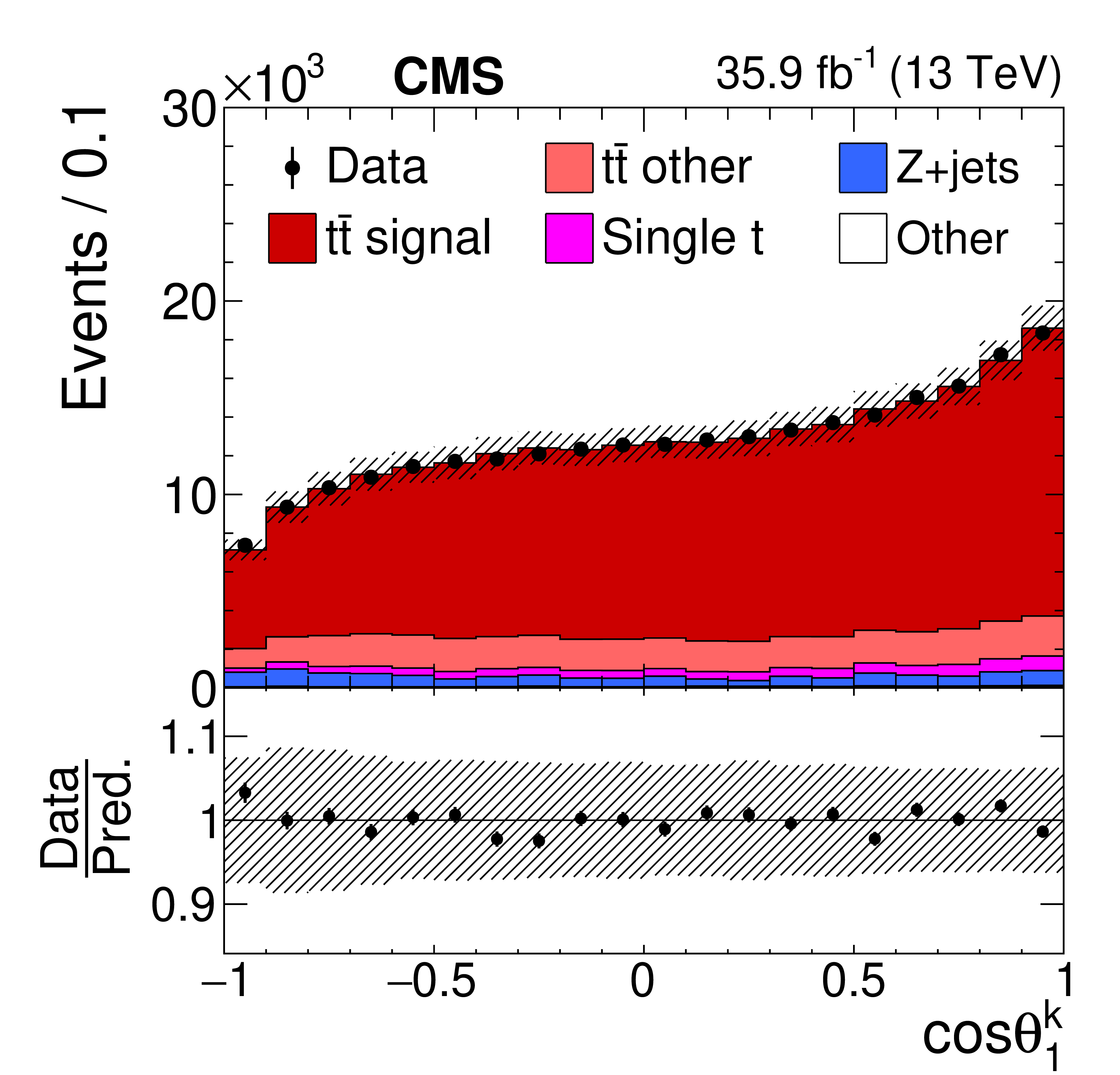
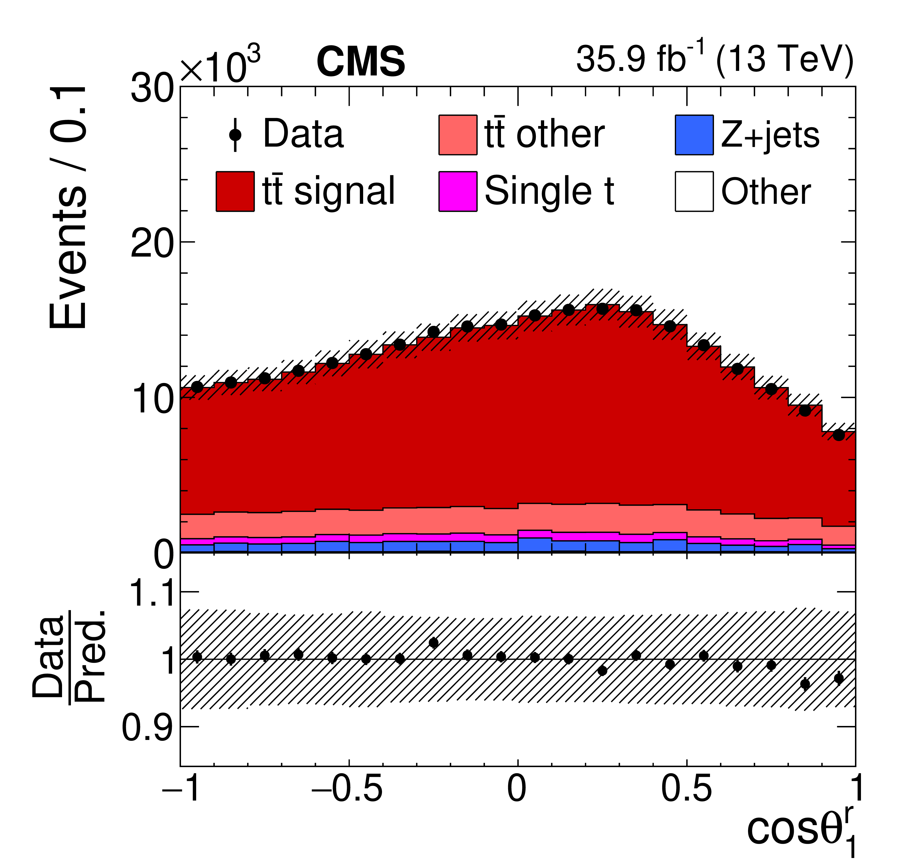
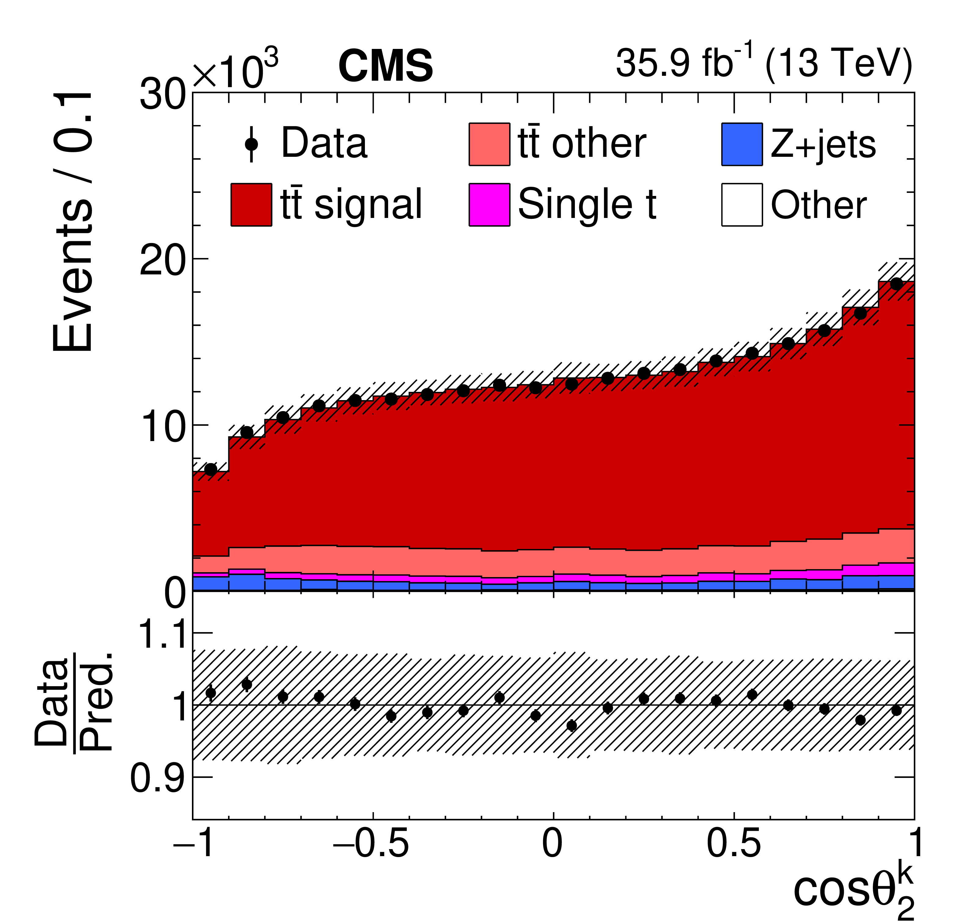
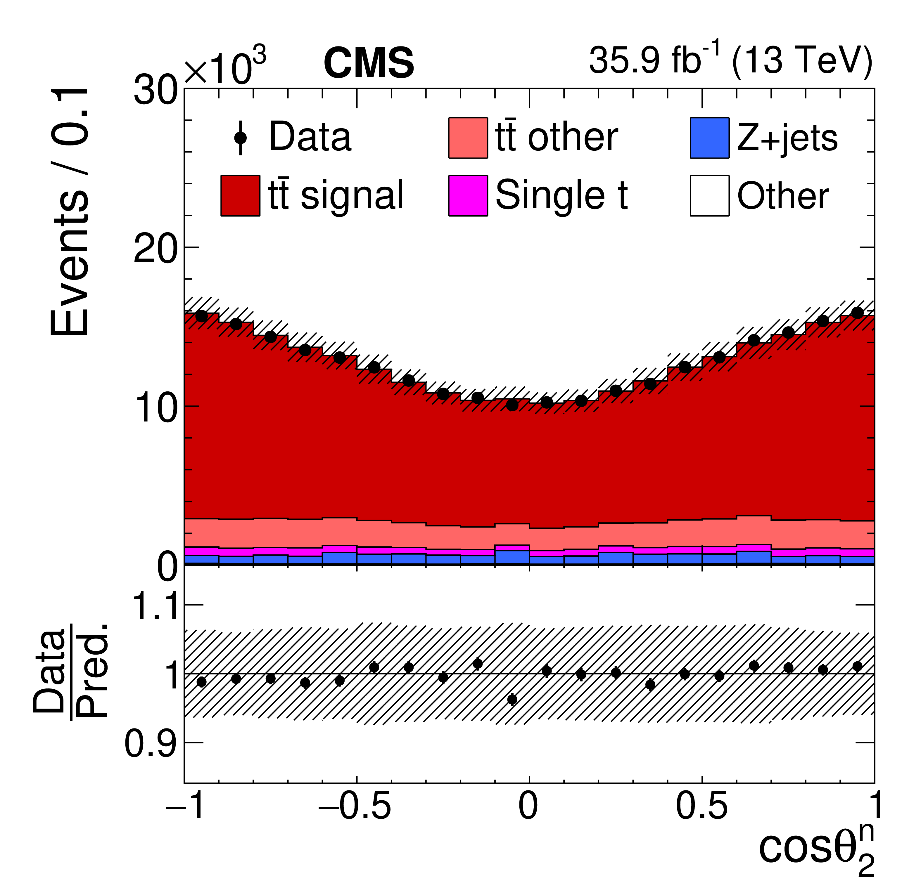
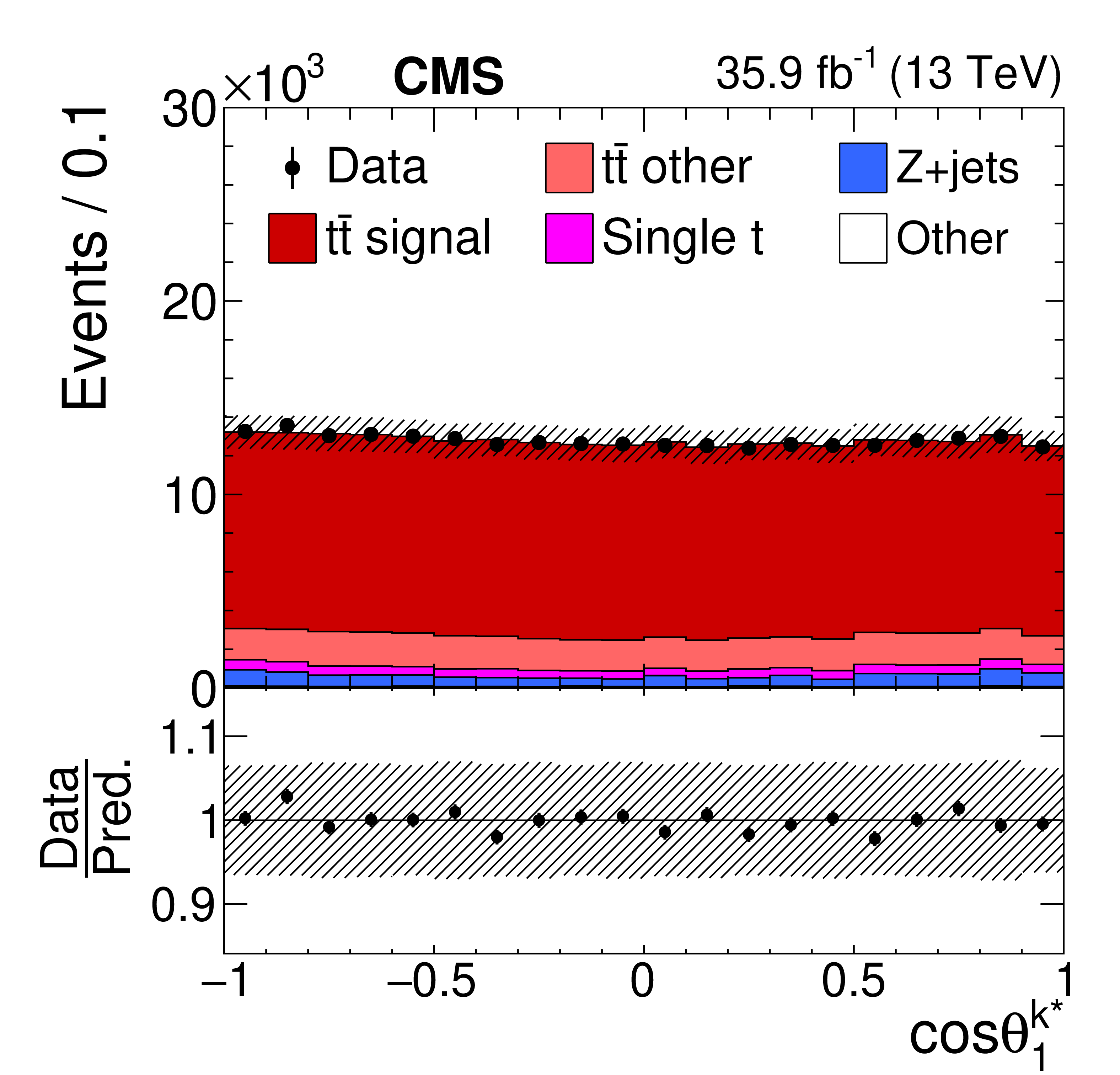
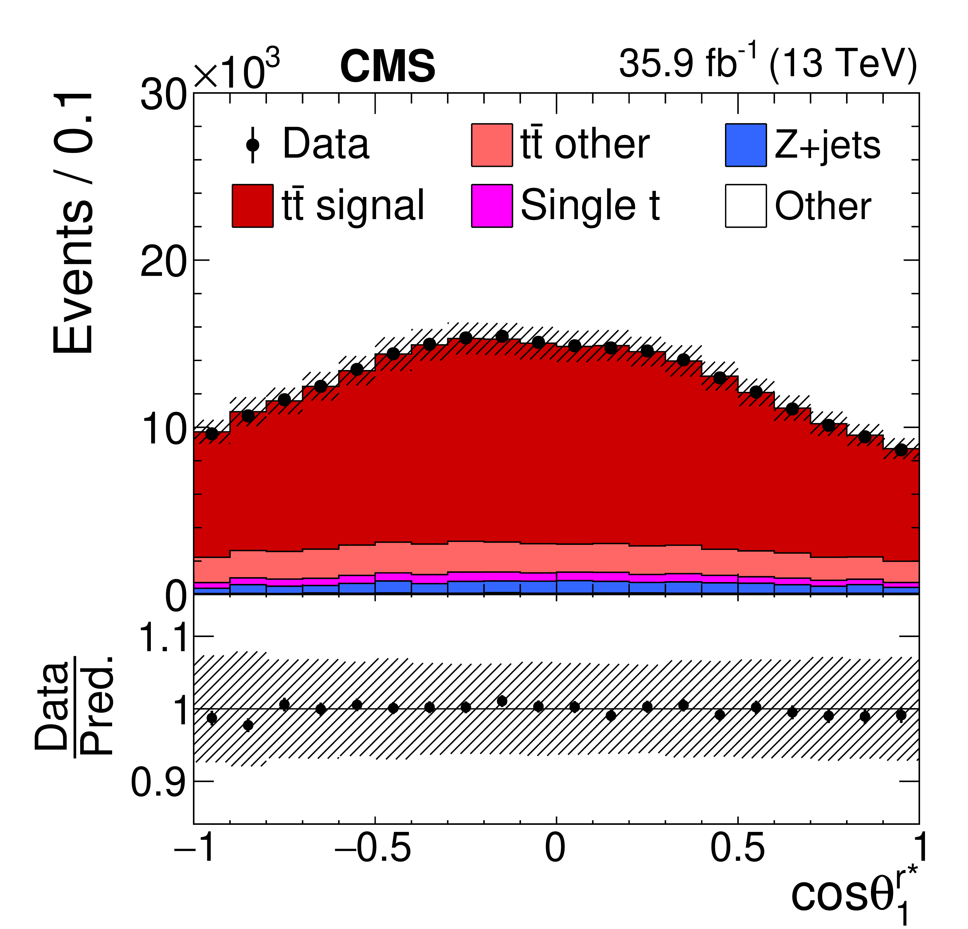
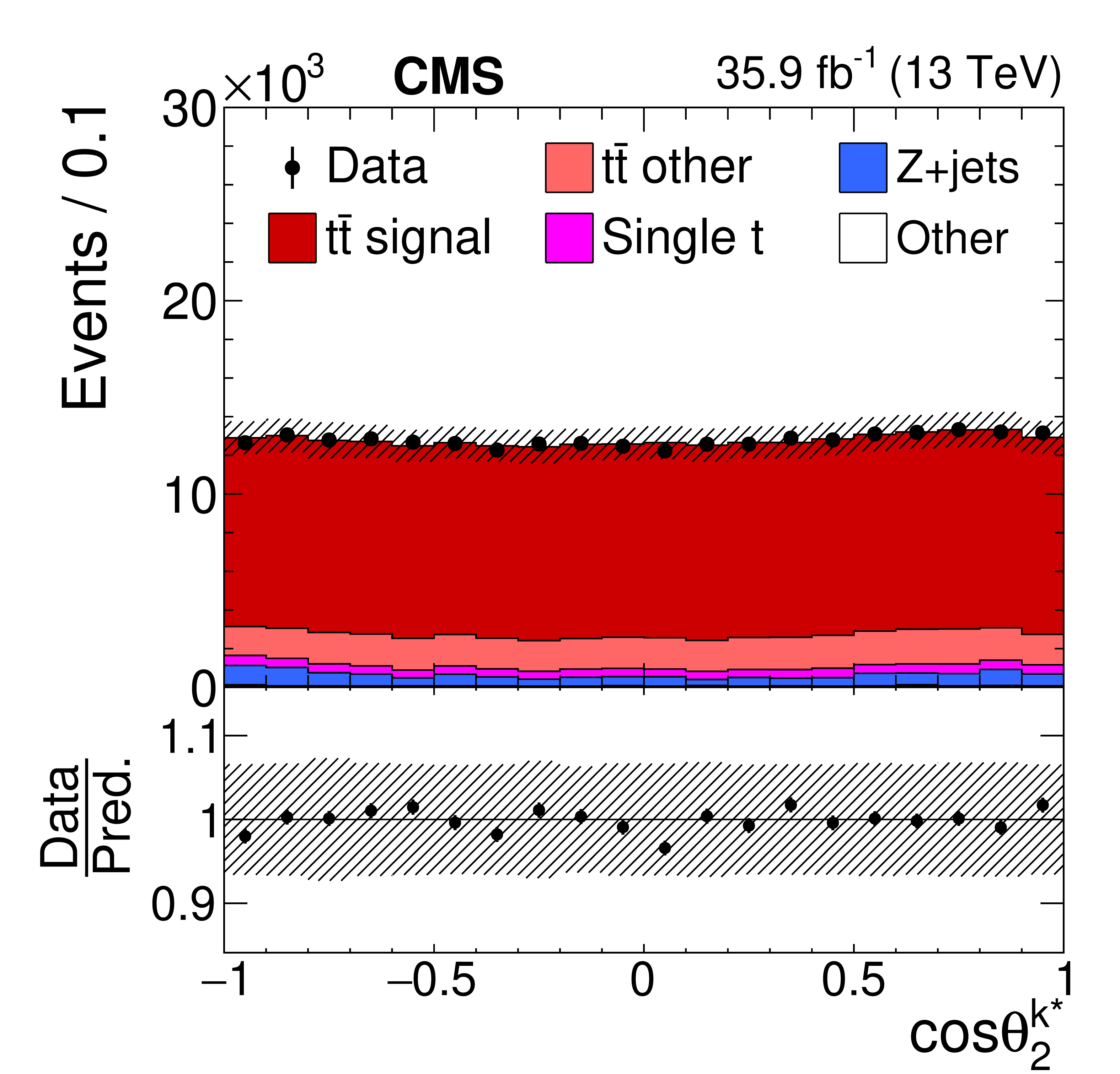
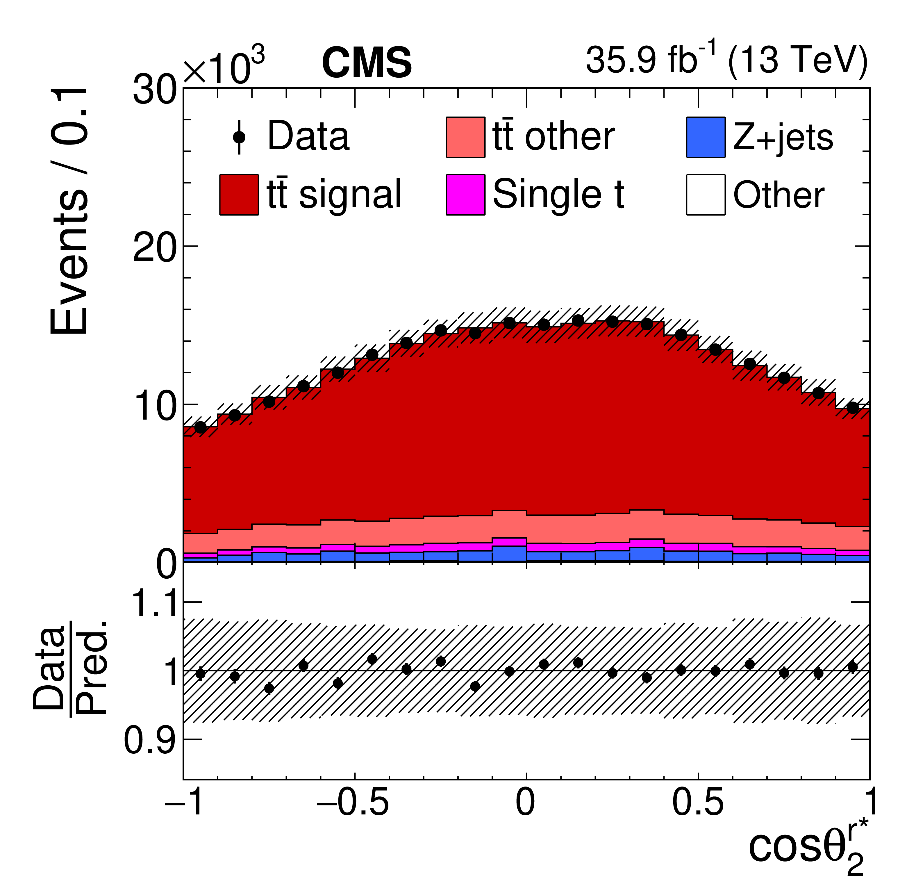
Figure 2:
Reconstructed distributions of $\cos\theta ^i$ for top quarks (antiquarks) in the first and third (second and fourth) rows, where $i$ refers to the reference axis with which the angle $\theta ^i$ is measured. From left to right, $i=\hat{k}$, $\hat{r}$, $\hat{n}$ (upper two rows), and $i=\hat{k}^*$, $\hat{r}^*$ (lower two rows). The data (points) are compared to the simulated predictions (histograms). The vertical bars on the points represent statistical uncertainties, and the estimated systematic uncertainties in the simulated histograms are indicated by hatched bands. The ratio of the data to the sum of the predicted signal and background is shown in the lower panels. |
png pdf |
Figure 2-a:
Reconstructed distributions of $\cos\theta ^i$ for top quarks (antiquarks) in the first and third (second and fourth) rows, where $i$ refers to the reference axis with which the angle $\theta ^i$ is measured. From left to right, $i=\hat{k}$, $\hat{r}$, $\hat{n}$ (upper two rows), and $i=\hat{k}^*$, $\hat{r}^*$ (lower two rows). The data (points) are compared to the simulated predictions (histograms). The vertical bars on the points represent statistical uncertainties, and the estimated systematic uncertainties in the simulated histograms are indicated by hatched bands. The ratio of the data to the sum of the predicted signal and background is shown in the lower panels. |
png pdf |
Figure 2-b:
Reconstructed distributions of $\cos\theta ^i$ for top quarks (antiquarks) in the first and third (second and fourth) rows, where $i$ refers to the reference axis with which the angle $\theta ^i$ is measured. From left to right, $i=\hat{k}$, $\hat{r}$, $\hat{n}$ (upper two rows), and $i=\hat{k}^*$, $\hat{r}^*$ (lower two rows). The data (points) are compared to the simulated predictions (histograms). The vertical bars on the points represent statistical uncertainties, and the estimated systematic uncertainties in the simulated histograms are indicated by hatched bands. The ratio of the data to the sum of the predicted signal and background is shown in the lower panels. |

png pdf |
Figure 2-c:
Reconstructed distributions of $\cos\theta ^i$ for top quarks (antiquarks) in the first and third (second and fourth) rows, where $i$ refers to the reference axis with which the angle $\theta ^i$ is measured. From left to right, $i=\hat{k}$, $\hat{r}$, $\hat{n}$ (upper two rows), and $i=\hat{k}^*$, $\hat{r}^*$ (lower two rows). The data (points) are compared to the simulated predictions (histograms). The vertical bars on the points represent statistical uncertainties, and the estimated systematic uncertainties in the simulated histograms are indicated by hatched bands. The ratio of the data to the sum of the predicted signal and background is shown in the lower panels. |
png pdf |
Figure 2-d:
Reconstructed distributions of $\cos\theta ^i$ for top quarks (antiquarks) in the first and third (second and fourth) rows, where $i$ refers to the reference axis with which the angle $\theta ^i$ is measured. From left to right, $i=\hat{k}$, $\hat{r}$, $\hat{n}$ (upper two rows), and $i=\hat{k}^*$, $\hat{r}^*$ (lower two rows). The data (points) are compared to the simulated predictions (histograms). The vertical bars on the points represent statistical uncertainties, and the estimated systematic uncertainties in the simulated histograms are indicated by hatched bands. The ratio of the data to the sum of the predicted signal and background is shown in the lower panels. |

png pdf |
Figure 2-e:
Reconstructed distributions of $\cos\theta ^i$ for top quarks (antiquarks) in the first and third (second and fourth) rows, where $i$ refers to the reference axis with which the angle $\theta ^i$ is measured. From left to right, $i=\hat{k}$, $\hat{r}$, $\hat{n}$ (upper two rows), and $i=\hat{k}^*$, $\hat{r}^*$ (lower two rows). The data (points) are compared to the simulated predictions (histograms). The vertical bars on the points represent statistical uncertainties, and the estimated systematic uncertainties in the simulated histograms are indicated by hatched bands. The ratio of the data to the sum of the predicted signal and background is shown in the lower panels. |
png pdf |
Figure 2-f:
Reconstructed distributions of $\cos\theta ^i$ for top quarks (antiquarks) in the first and third (second and fourth) rows, where $i$ refers to the reference axis with which the angle $\theta ^i$ is measured. From left to right, $i=\hat{k}$, $\hat{r}$, $\hat{n}$ (upper two rows), and $i=\hat{k}^*$, $\hat{r}^*$ (lower two rows). The data (points) are compared to the simulated predictions (histograms). The vertical bars on the points represent statistical uncertainties, and the estimated systematic uncertainties in the simulated histograms are indicated by hatched bands. The ratio of the data to the sum of the predicted signal and background is shown in the lower panels. |
png pdf |
Figure 2-g:
Reconstructed distributions of $\cos\theta ^i$ for top quarks (antiquarks) in the first and third (second and fourth) rows, where $i$ refers to the reference axis with which the angle $\theta ^i$ is measured. From left to right, $i=\hat{k}$, $\hat{r}$, $\hat{n}$ (upper two rows), and $i=\hat{k}^*$, $\hat{r}^*$ (lower two rows). The data (points) are compared to the simulated predictions (histograms). The vertical bars on the points represent statistical uncertainties, and the estimated systematic uncertainties in the simulated histograms are indicated by hatched bands. The ratio of the data to the sum of the predicted signal and background is shown in the lower panels. |
png pdf |
Figure 2-h:
Reconstructed distributions of $\cos\theta ^i$ for top quarks (antiquarks) in the first and third (second and fourth) rows, where $i$ refers to the reference axis with which the angle $\theta ^i$ is measured. From left to right, $i=\hat{k}$, $\hat{r}$, $\hat{n}$ (upper two rows), and $i=\hat{k}^*$, $\hat{r}^*$ (lower two rows). The data (points) are compared to the simulated predictions (histograms). The vertical bars on the points represent statistical uncertainties, and the estimated systematic uncertainties in the simulated histograms are indicated by hatched bands. The ratio of the data to the sum of the predicted signal and background is shown in the lower panels. |
png pdf |
Figure 2-i:
Reconstructed distributions of $\cos\theta ^i$ for top quarks (antiquarks) in the first and third (second and fourth) rows, where $i$ refers to the reference axis with which the angle $\theta ^i$ is measured. From left to right, $i=\hat{k}$, $\hat{r}$, $\hat{n}$ (upper two rows), and $i=\hat{k}^*$, $\hat{r}^*$ (lower two rows). The data (points) are compared to the simulated predictions (histograms). The vertical bars on the points represent statistical uncertainties, and the estimated systematic uncertainties in the simulated histograms are indicated by hatched bands. The ratio of the data to the sum of the predicted signal and background is shown in the lower panels. |
png pdf |
Figure 2-j:
Reconstructed distributions of $\cos\theta ^i$ for top quarks (antiquarks) in the first and third (second and fourth) rows, where $i$ refers to the reference axis with which the angle $\theta ^i$ is measured. From left to right, $i=\hat{k}$, $\hat{r}$, $\hat{n}$ (upper two rows), and $i=\hat{k}^*$, $\hat{r}^*$ (lower two rows). The data (points) are compared to the simulated predictions (histograms). The vertical bars on the points represent statistical uncertainties, and the estimated systematic uncertainties in the simulated histograms are indicated by hatched bands. The ratio of the data to the sum of the predicted signal and background is shown in the lower panels. |
png pdf |
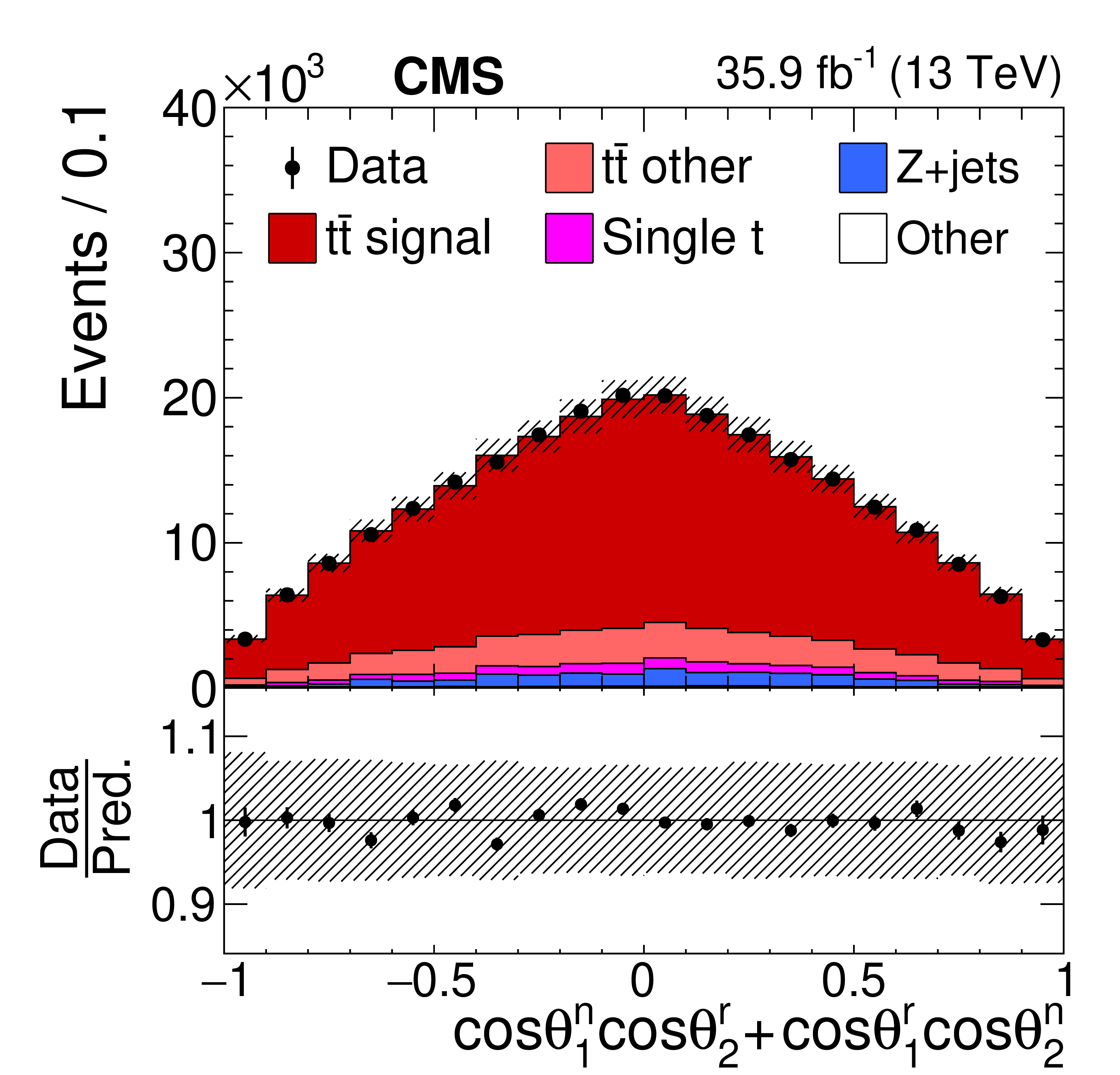
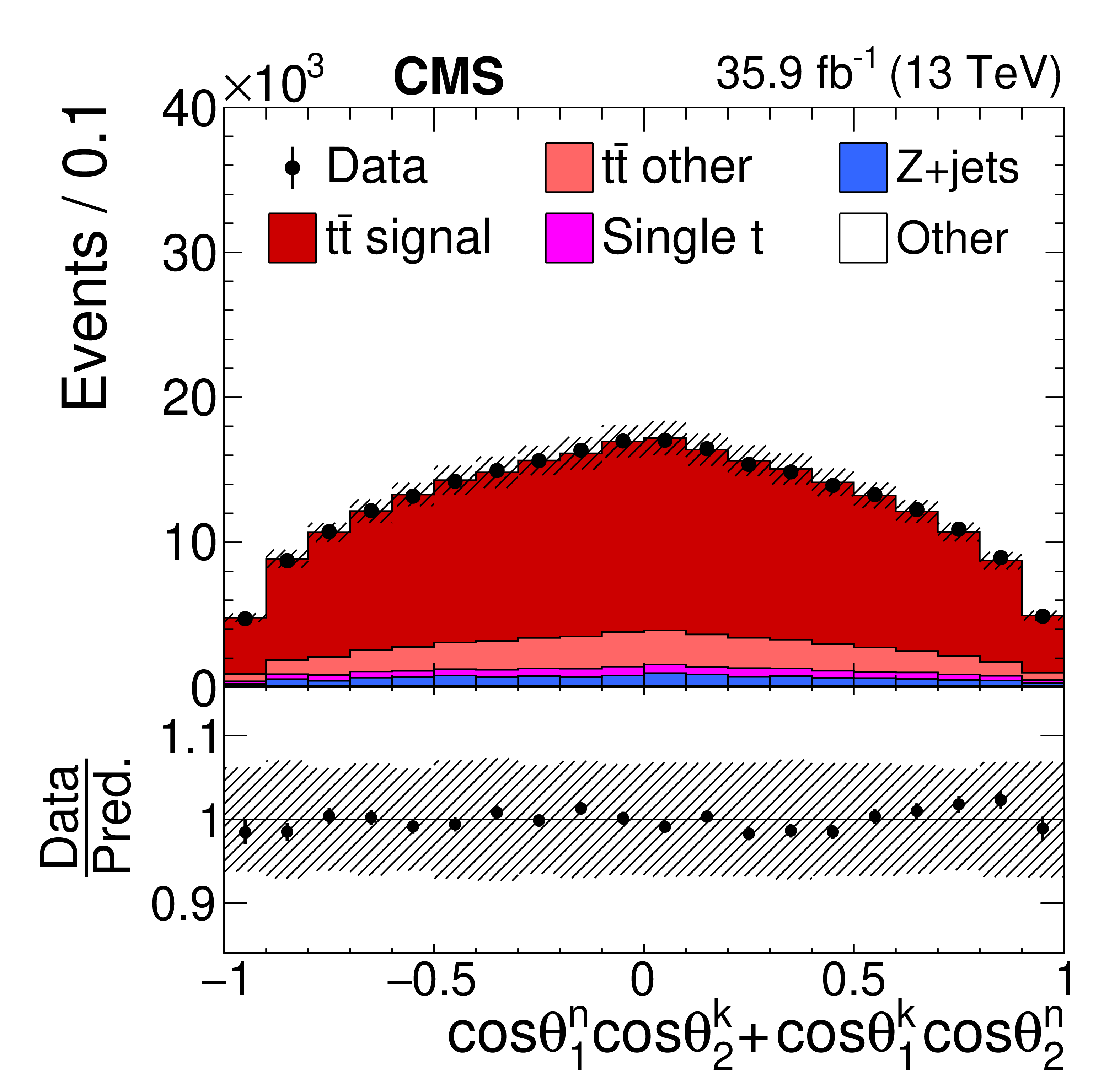
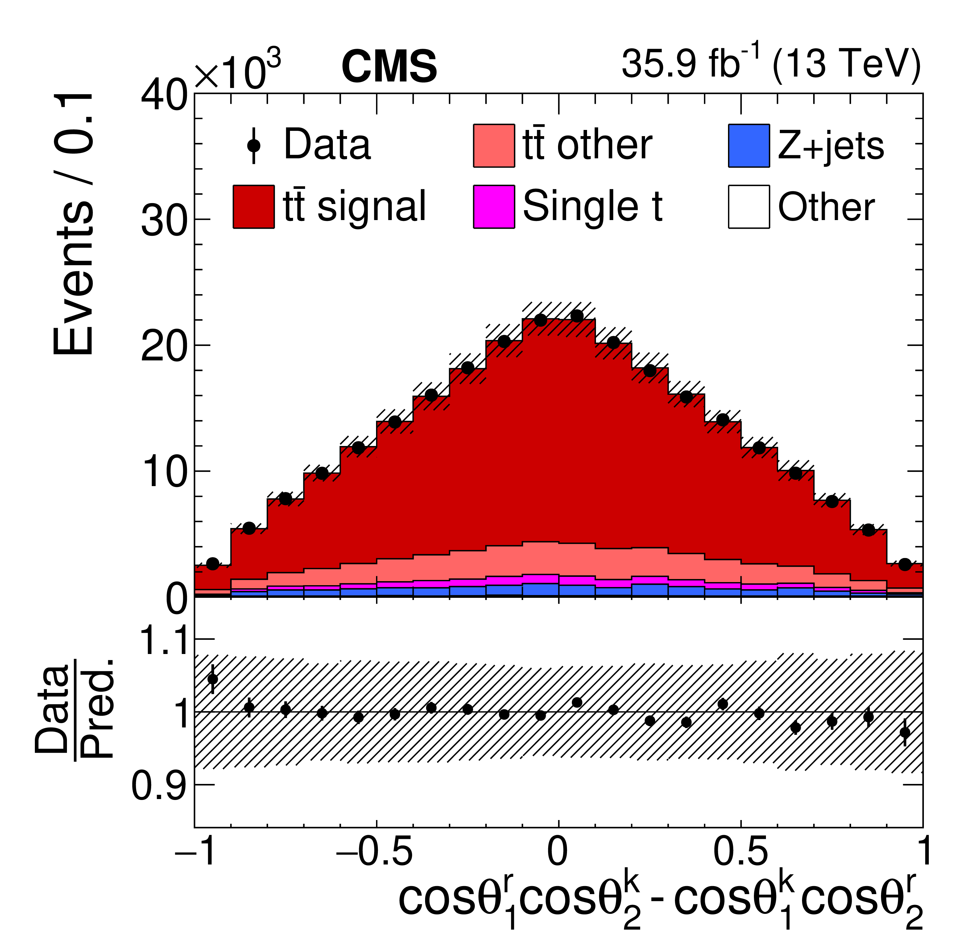
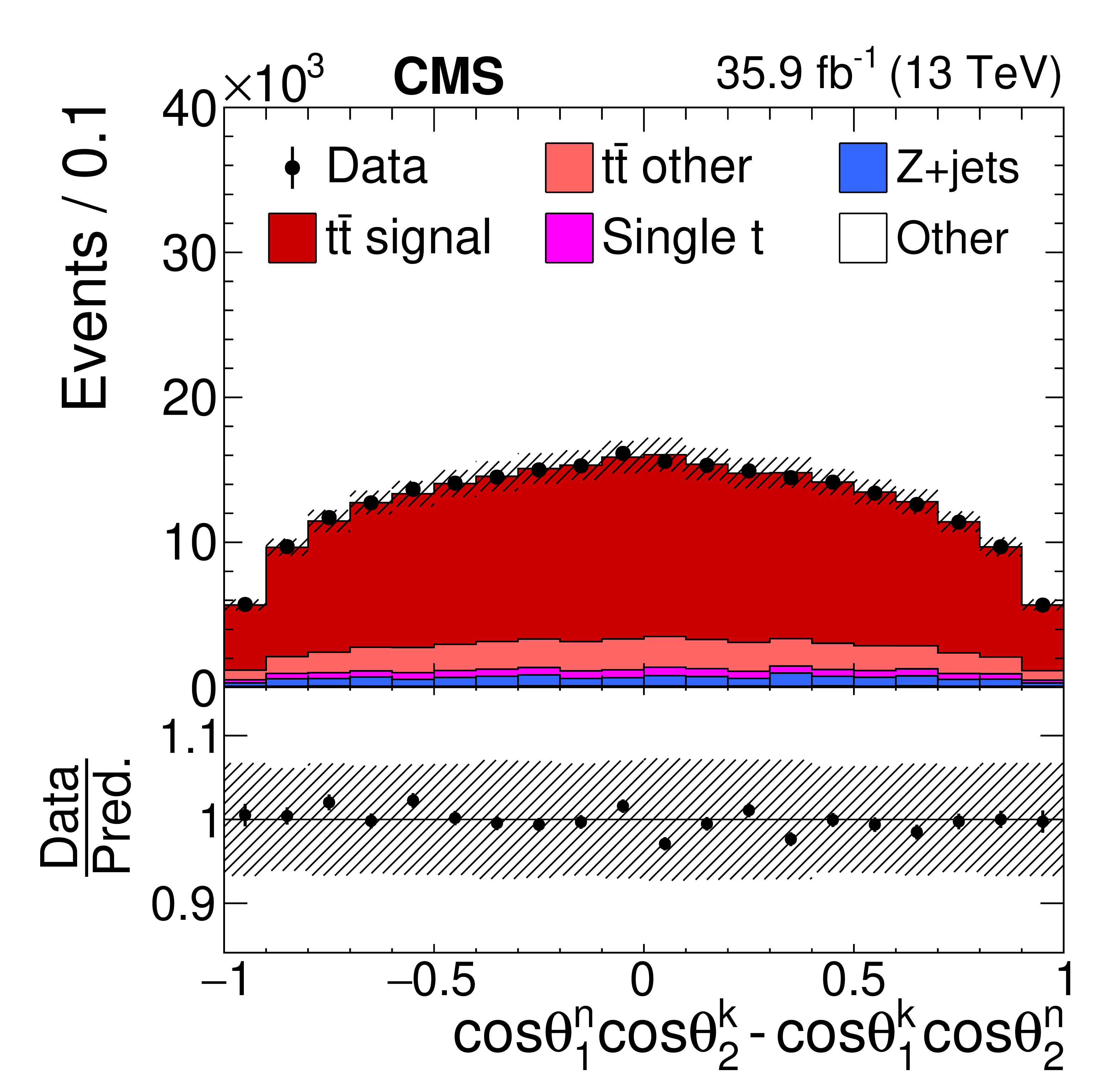
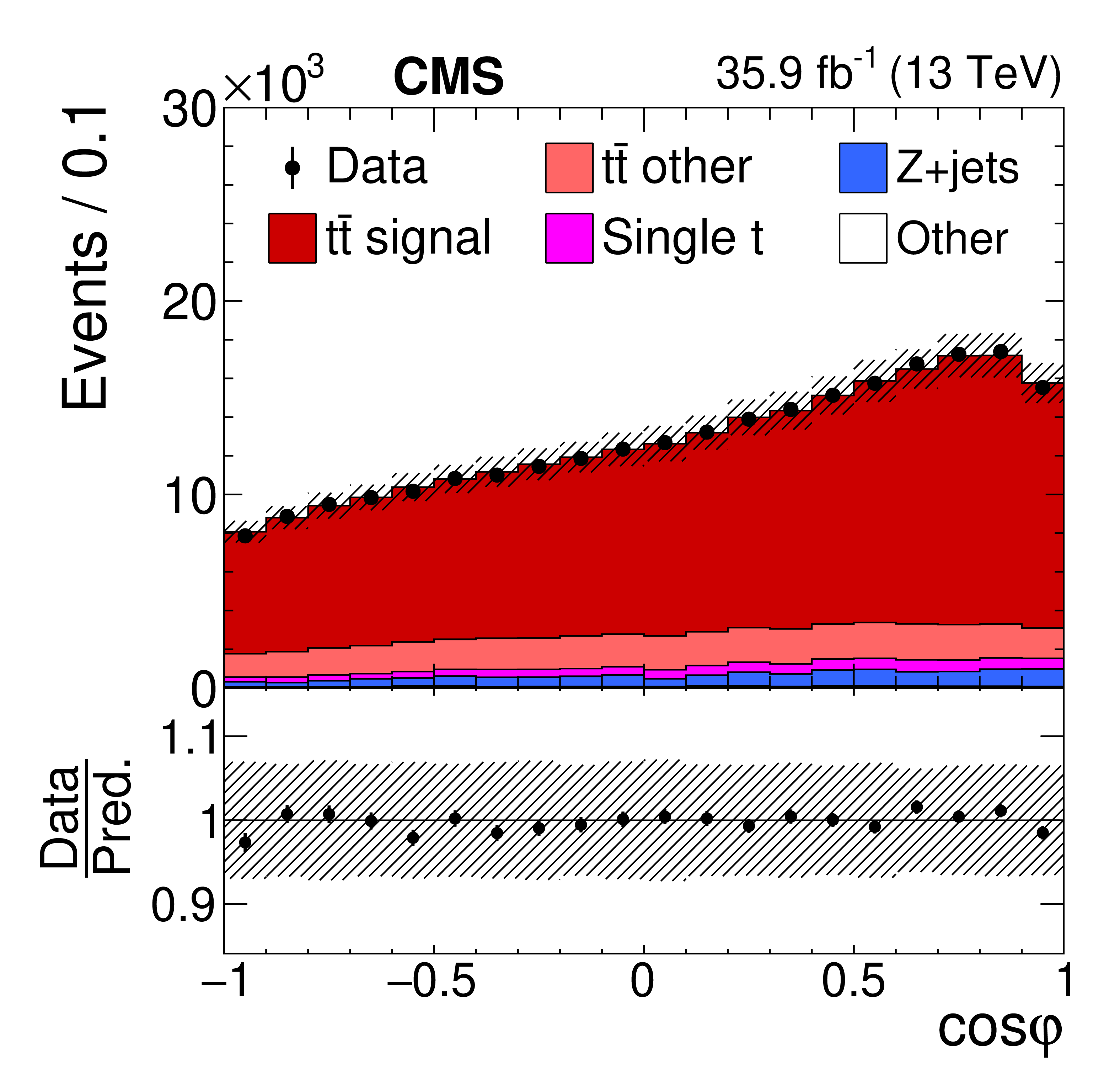
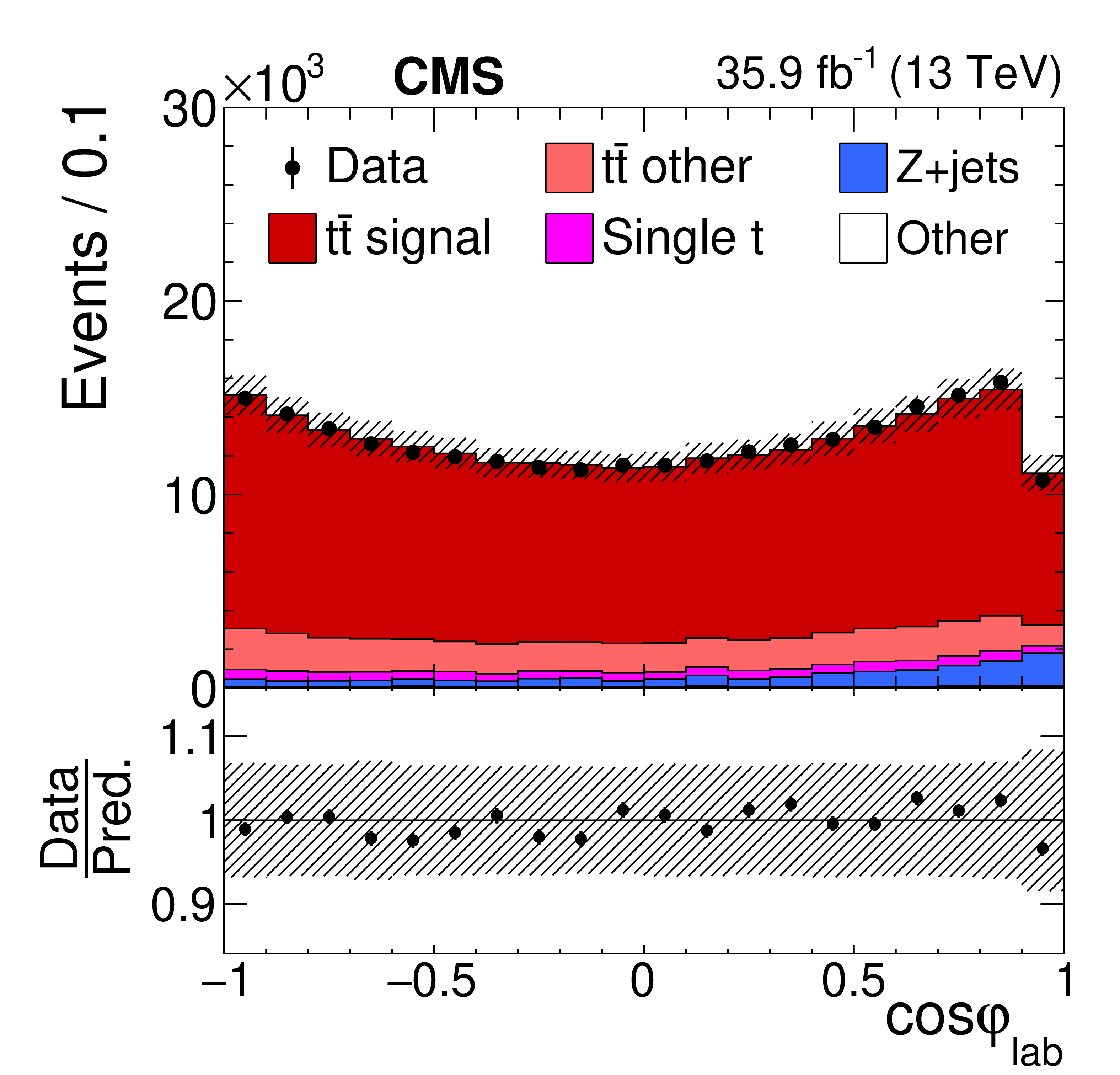
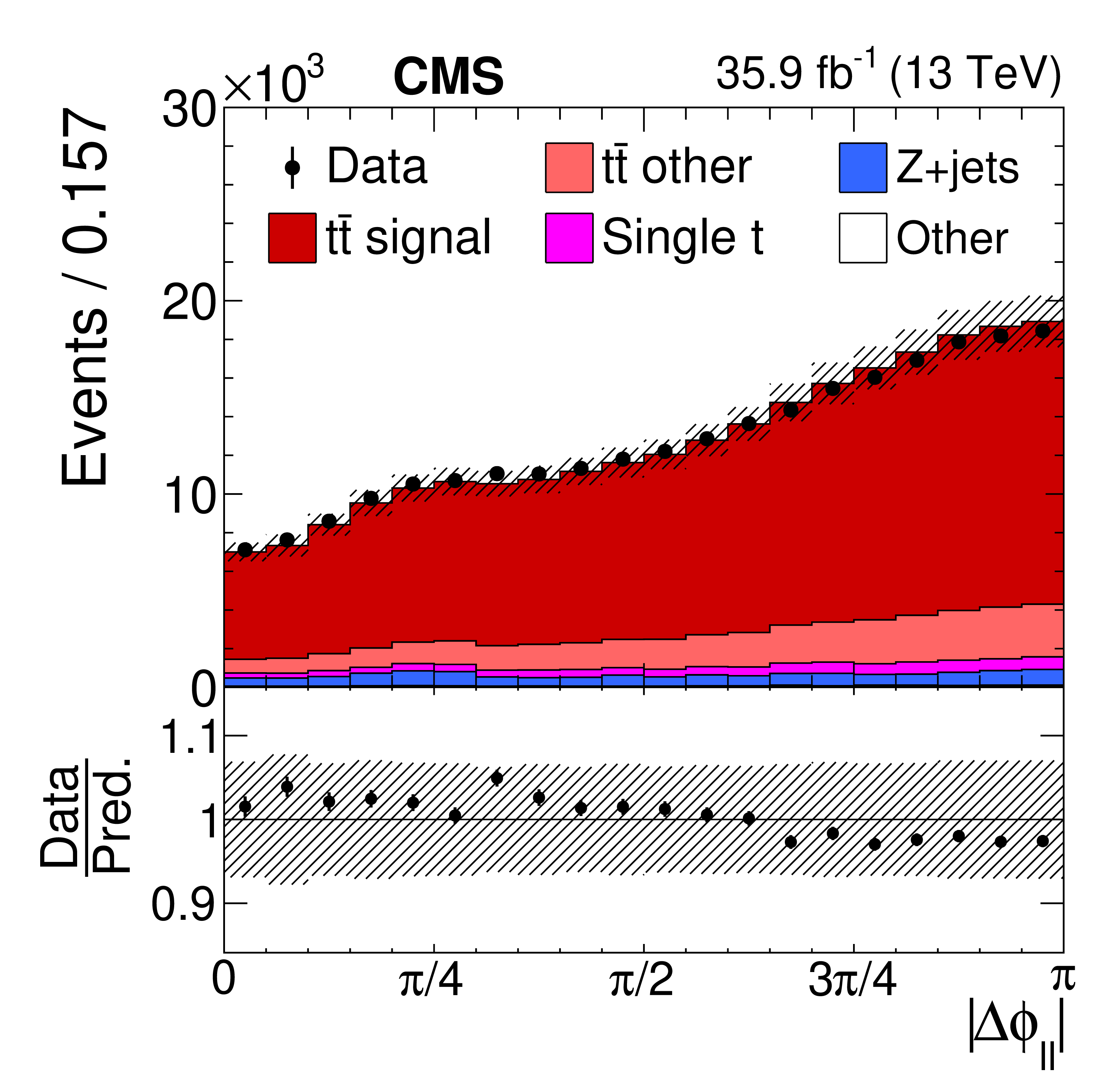
Figure 3:
Reconstructed angular distributions used in the measurement of the ${\mathrm{t} \mathrm{\bar{t}}}$ spin correlation observables. The data (points) are compared to the simulated predictions (histograms). The vertical bars on the points represent statistical uncertainties, and the estimated systematic uncertainties in the simulated histograms are indicated by hatched bands. The ratio of the data to the sum of the predicted signal and background is shown in the lower panels. |

png pdf |
Figure 3-a:
Reconstructed angular distributions used in the measurement of the ${\mathrm{t} \mathrm{\bar{t}}}$ spin correlation observables. The data (points) are compared to the simulated predictions (histograms). The vertical bars on the points represent statistical uncertainties, and the estimated systematic uncertainties in the simulated histograms are indicated by hatched bands. The ratio of the data to the sum of the predicted signal and background is shown in the lower panels. |
png pdf |
Figure 3-b:
Reconstructed angular distributions used in the measurement of the ${\mathrm{t} \mathrm{\bar{t}}}$ spin correlation observables. The data (points) are compared to the simulated predictions (histograms). The vertical bars on the points represent statistical uncertainties, and the estimated systematic uncertainties in the simulated histograms are indicated by hatched bands. The ratio of the data to the sum of the predicted signal and background is shown in the lower panels. |
png pdf |
Figure 3-c:
Reconstructed angular distributions used in the measurement of the ${\mathrm{t} \mathrm{\bar{t}}}$ spin correlation observables. The data (points) are compared to the simulated predictions (histograms). The vertical bars on the points represent statistical uncertainties, and the estimated systematic uncertainties in the simulated histograms are indicated by hatched bands. The ratio of the data to the sum of the predicted signal and background is shown in the lower panels. |
png pdf |
Figure 3-d:
Reconstructed angular distributions used in the measurement of the ${\mathrm{t} \mathrm{\bar{t}}}$ spin correlation observables. The data (points) are compared to the simulated predictions (histograms). The vertical bars on the points represent statistical uncertainties, and the estimated systematic uncertainties in the simulated histograms are indicated by hatched bands. The ratio of the data to the sum of the predicted signal and background is shown in the lower panels. |
png pdf |
Figure 3-e:
Reconstructed angular distributions used in the measurement of the ${\mathrm{t} \mathrm{\bar{t}}}$ spin correlation observables. The data (points) are compared to the simulated predictions (histograms). The vertical bars on the points represent statistical uncertainties, and the estimated systematic uncertainties in the simulated histograms are indicated by hatched bands. The ratio of the data to the sum of the predicted signal and background is shown in the lower panels. |
png pdf |
Figure 3-f:
Reconstructed angular distributions used in the measurement of the ${\mathrm{t} \mathrm{\bar{t}}}$ spin correlation observables. The data (points) are compared to the simulated predictions (histograms). The vertical bars on the points represent statistical uncertainties, and the estimated systematic uncertainties in the simulated histograms are indicated by hatched bands. The ratio of the data to the sum of the predicted signal and background is shown in the lower panels. |
png pdf |
Figure 3-g:
Reconstructed angular distributions used in the measurement of the ${\mathrm{t} \mathrm{\bar{t}}}$ spin correlation observables. The data (points) are compared to the simulated predictions (histograms). The vertical bars on the points represent statistical uncertainties, and the estimated systematic uncertainties in the simulated histograms are indicated by hatched bands. The ratio of the data to the sum of the predicted signal and background is shown in the lower panels. |

png pdf |
Figure 3-h:
Reconstructed angular distributions used in the measurement of the ${\mathrm{t} \mathrm{\bar{t}}}$ spin correlation observables. The data (points) are compared to the simulated predictions (histograms). The vertical bars on the points represent statistical uncertainties, and the estimated systematic uncertainties in the simulated histograms are indicated by hatched bands. The ratio of the data to the sum of the predicted signal and background is shown in the lower panels. |
png pdf |
Figure 3-i:
Reconstructed angular distributions used in the measurement of the ${\mathrm{t} \mathrm{\bar{t}}}$ spin correlation observables. The data (points) are compared to the simulated predictions (histograms). The vertical bars on the points represent statistical uncertainties, and the estimated systematic uncertainties in the simulated histograms are indicated by hatched bands. The ratio of the data to the sum of the predicted signal and background is shown in the lower panels. |
png pdf |
Figure 3-j:
Reconstructed angular distributions used in the measurement of the ${\mathrm{t} \mathrm{\bar{t}}}$ spin correlation observables. The data (points) are compared to the simulated predictions (histograms). The vertical bars on the points represent statistical uncertainties, and the estimated systematic uncertainties in the simulated histograms are indicated by hatched bands. The ratio of the data to the sum of the predicted signal and background is shown in the lower panels. |
png pdf |
Figure 3-k:
Reconstructed angular distributions used in the measurement of the ${\mathrm{t} \mathrm{\bar{t}}}$ spin correlation observables. The data (points) are compared to the simulated predictions (histograms). The vertical bars on the points represent statistical uncertainties, and the estimated systematic uncertainties in the simulated histograms are indicated by hatched bands. The ratio of the data to the sum of the predicted signal and background is shown in the lower panels. |
png pdf |
Figure 3-l:
Reconstructed angular distributions used in the measurement of the ${\mathrm{t} \mathrm{\bar{t}}}$ spin correlation observables. The data (points) are compared to the simulated predictions (histograms). The vertical bars on the points represent statistical uncertainties, and the estimated systematic uncertainties in the simulated histograms are indicated by hatched bands. The ratio of the data to the sum of the predicted signal and background is shown in the lower panels. |
png pdf |
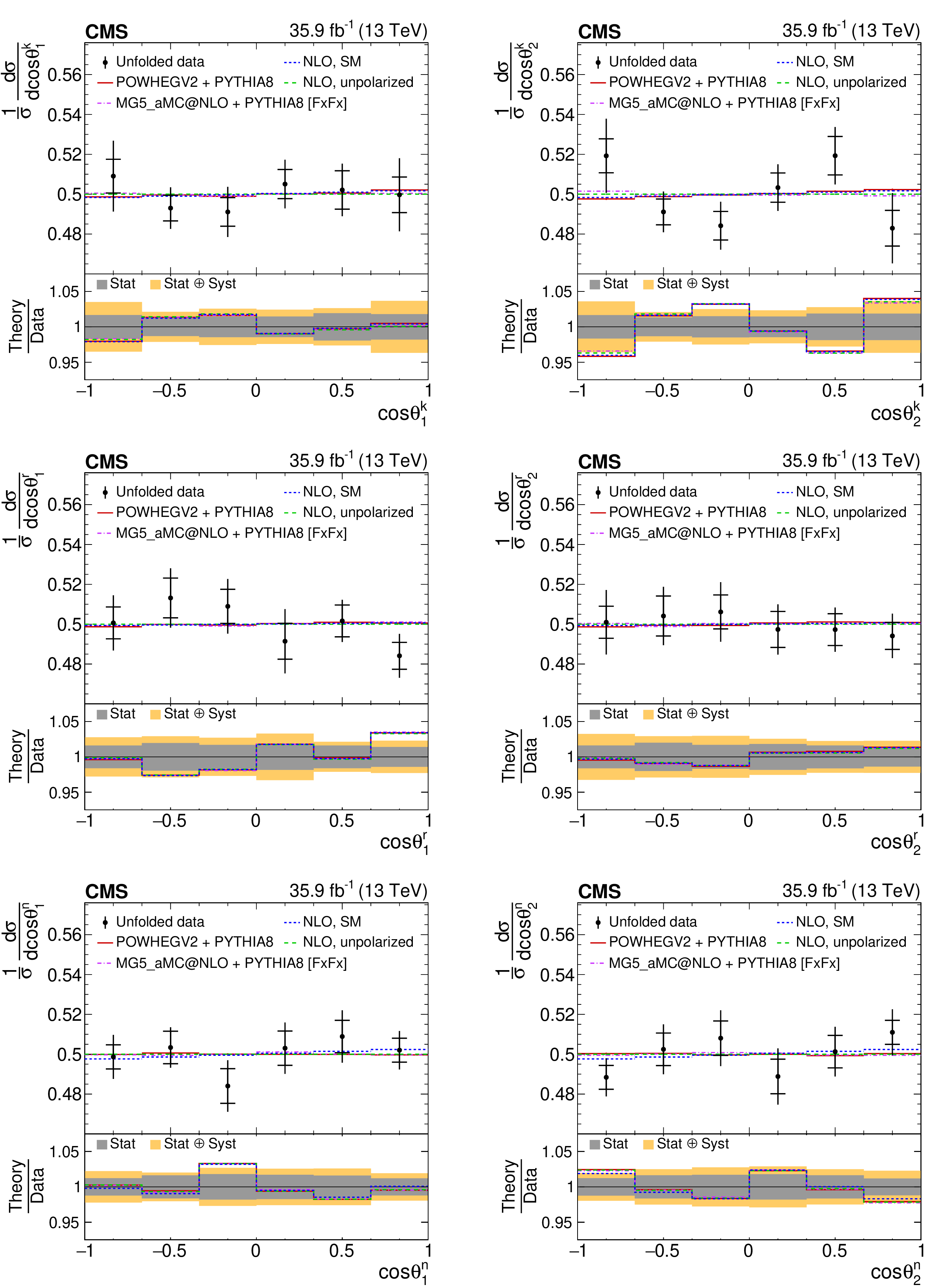
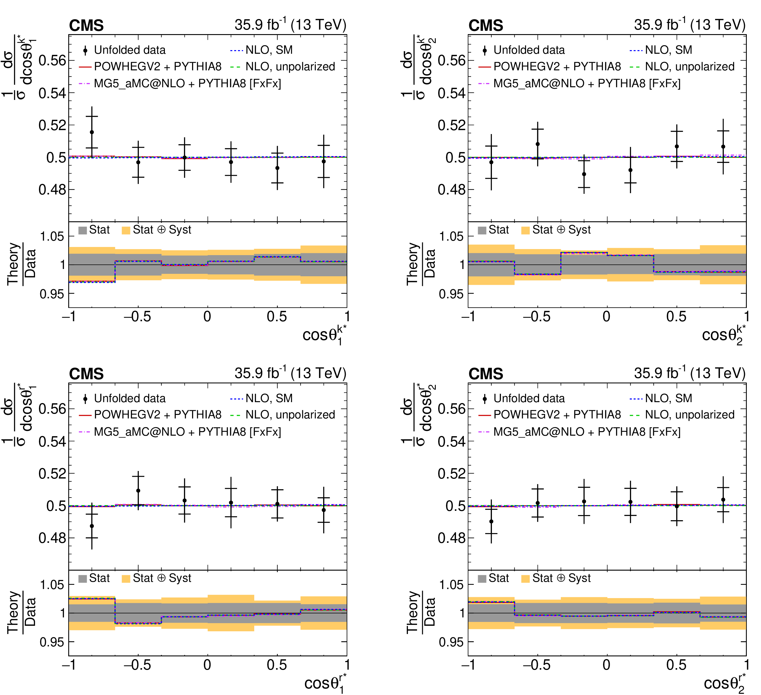
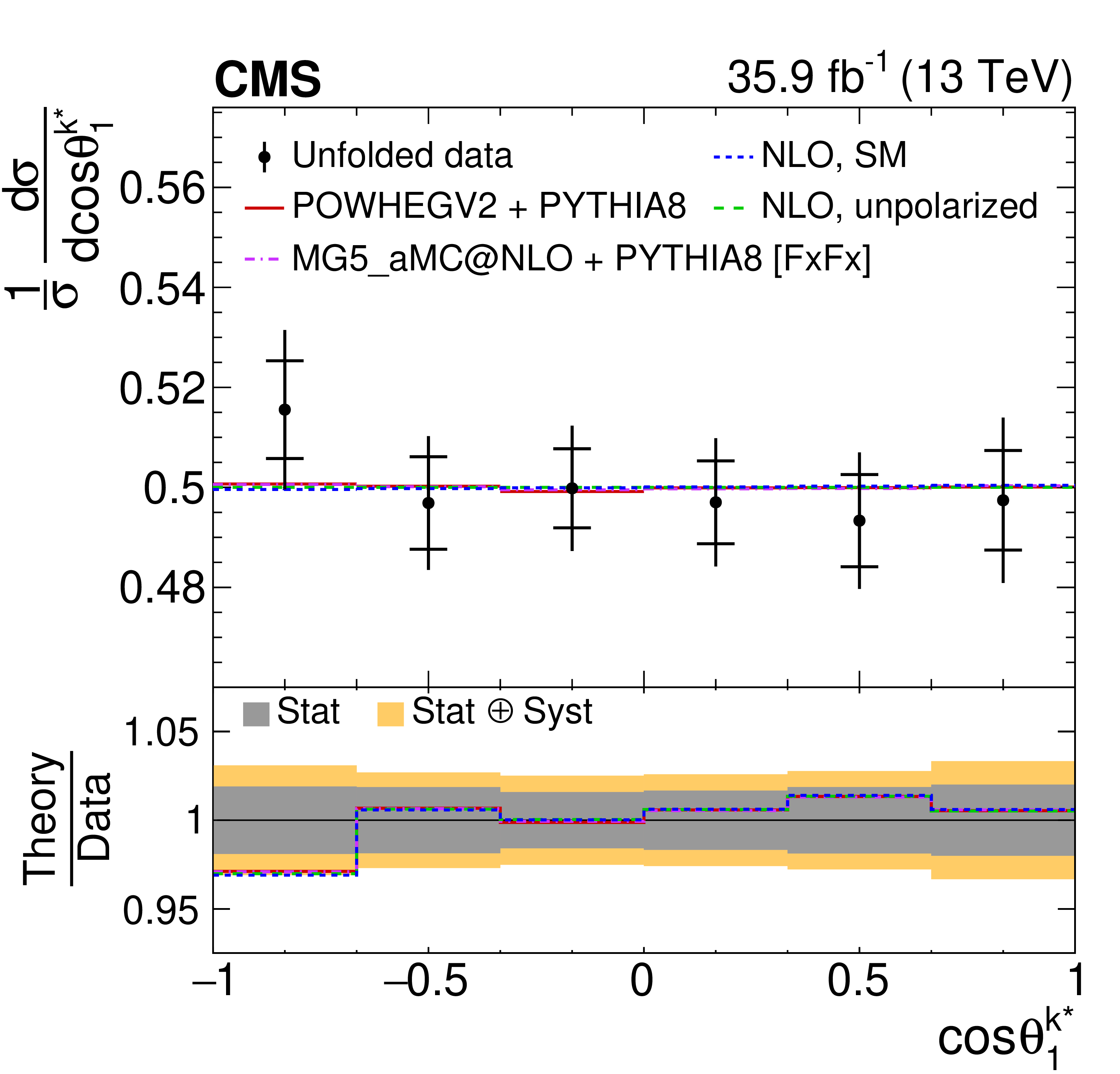
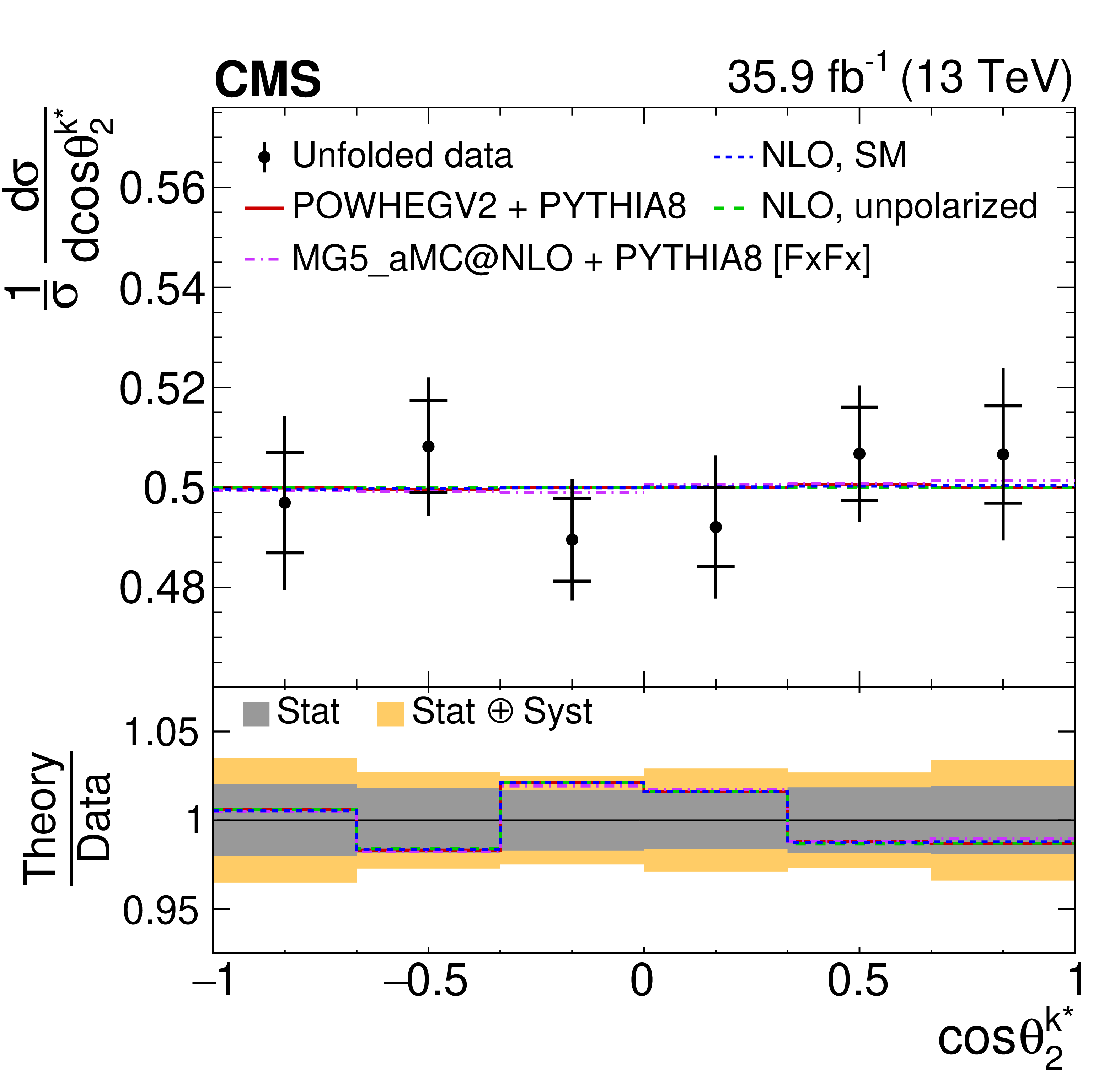
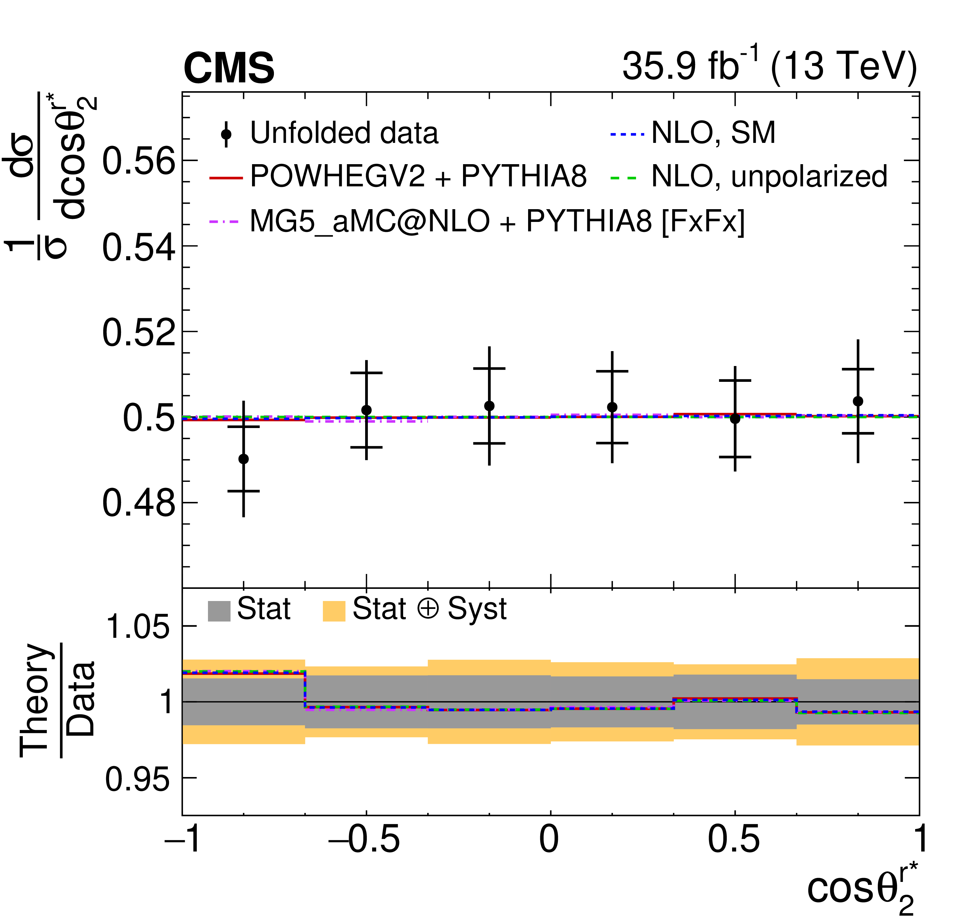
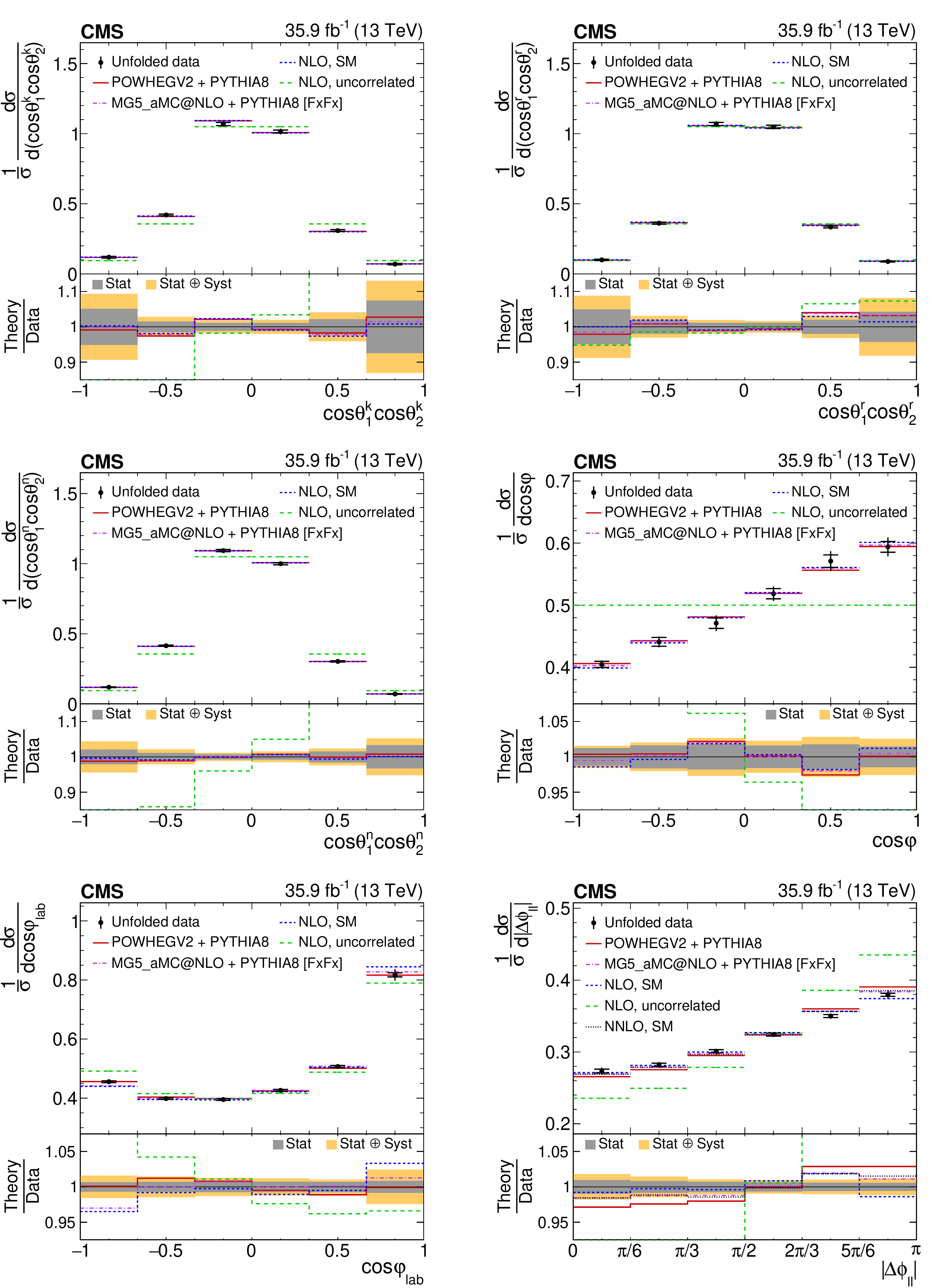
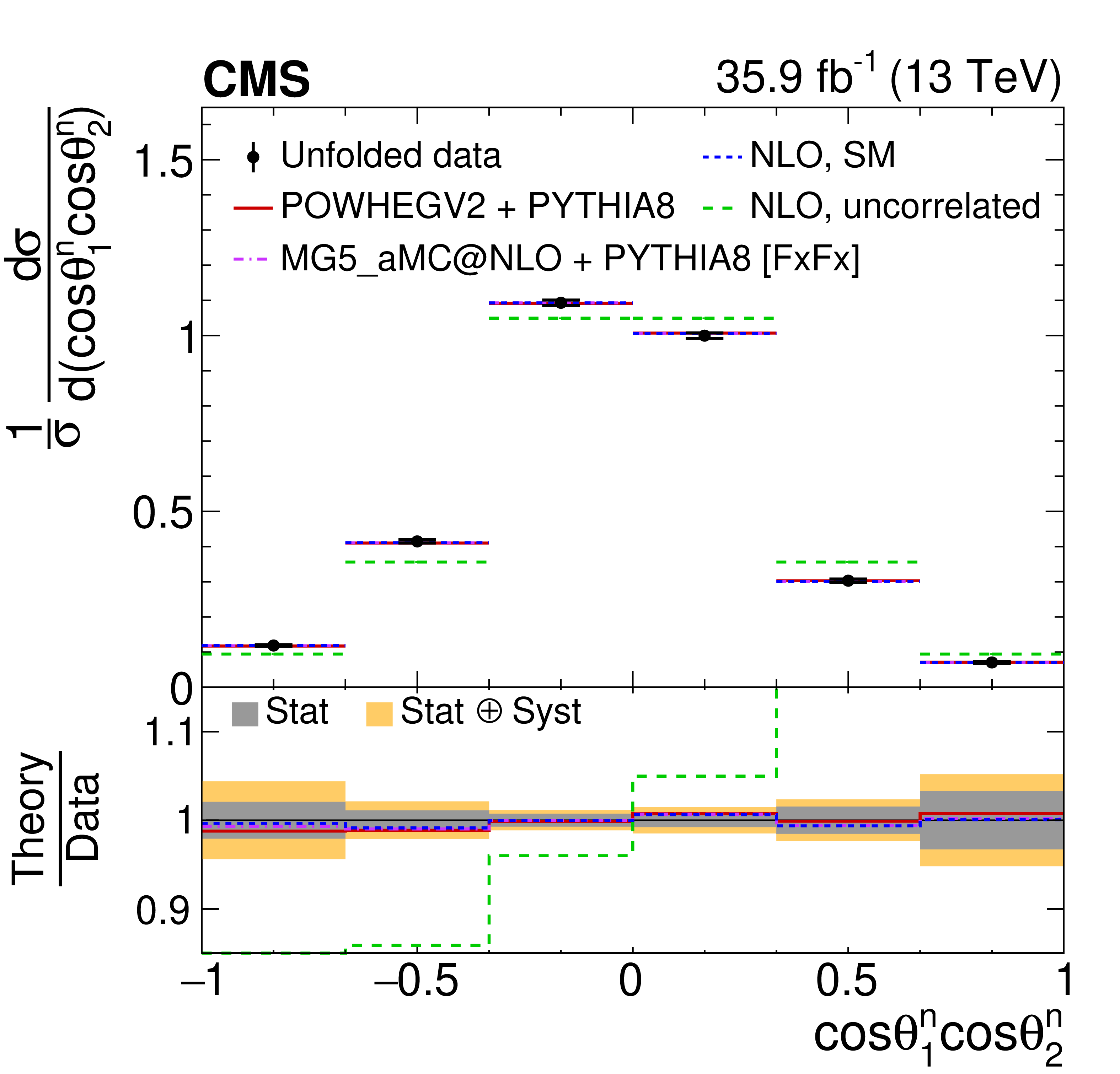
Figure 4:
Unfolded data (points) and predicted (horizontal lines) normalized differential cross sections with respect to $\cos\theta ^i$ for top quarks (antiquarks) in the first (second) column, probing polarization coefficients $B_{1}^{i}$ ($B_{2}^{i})$. From top to bottom, the reference axis $i=\hat{k}$, $\hat{r}$, $\hat{n}$. The vertical lines on the points represent the total uncertainties, with the statistical components indicated by horizontal bars. The ratios of various predictions to the data are shown in the lower panels. |
png pdf |
Figure 4-a:
Unfolded data (points) and predicted (horizontal lines) normalized differential cross sections with respect to $\cos\theta ^i$ for top quarks (antiquarks) in the first (second) column, probing polarization coefficients $B_{1}^{i}$ ($B_{2}^{i})$. From top to bottom, the reference axis $i=\hat{k}$, $\hat{r}$, $\hat{n}$. The vertical lines on the points represent the total uncertainties, with the statistical components indicated by horizontal bars. The ratios of various predictions to the data are shown in the lower panels. |

png pdf |
Figure 4-b:
Unfolded data (points) and predicted (horizontal lines) normalized differential cross sections with respect to $\cos\theta ^i$ for top quarks (antiquarks) in the first (second) column, probing polarization coefficients $B_{1}^{i}$ ($B_{2}^{i})$. From top to bottom, the reference axis $i=\hat{k}$, $\hat{r}$, $\hat{n}$. The vertical lines on the points represent the total uncertainties, with the statistical components indicated by horizontal bars. The ratios of various predictions to the data are shown in the lower panels. |
png pdf |
Figure 4-c:
Unfolded data (points) and predicted (horizontal lines) normalized differential cross sections with respect to $\cos\theta ^i$ for top quarks (antiquarks) in the first (second) column, probing polarization coefficients $B_{1}^{i}$ ($B_{2}^{i})$. From top to bottom, the reference axis $i=\hat{k}$, $\hat{r}$, $\hat{n}$. The vertical lines on the points represent the total uncertainties, with the statistical components indicated by horizontal bars. The ratios of various predictions to the data are shown in the lower panels. |
png pdf |
Figure 4-d:
Unfolded data (points) and predicted (horizontal lines) normalized differential cross sections with respect to $\cos\theta ^i$ for top quarks (antiquarks) in the first (second) column, probing polarization coefficients $B_{1}^{i}$ ($B_{2}^{i})$. From top to bottom, the reference axis $i=\hat{k}$, $\hat{r}$, $\hat{n}$. The vertical lines on the points represent the total uncertainties, with the statistical components indicated by horizontal bars. The ratios of various predictions to the data are shown in the lower panels. |
png pdf |
Figure 4-e:
Unfolded data (points) and predicted (horizontal lines) normalized differential cross sections with respect to $\cos\theta ^i$ for top quarks (antiquarks) in the first (second) column, probing polarization coefficients $B_{1}^{i}$ ($B_{2}^{i})$. From top to bottom, the reference axis $i=\hat{k}$, $\hat{r}$, $\hat{n}$. The vertical lines on the points represent the total uncertainties, with the statistical components indicated by horizontal bars. The ratios of various predictions to the data are shown in the lower panels. |

png pdf |
Figure 4-f:
Unfolded data (points) and predicted (horizontal lines) normalized differential cross sections with respect to $\cos\theta ^i$ for top quarks (antiquarks) in the first (second) column, probing polarization coefficients $B_{1}^{i}$ ($B_{2}^{i})$. From top to bottom, the reference axis $i=\hat{k}$, $\hat{r}$, $\hat{n}$. The vertical lines on the points represent the total uncertainties, with the statistical components indicated by horizontal bars. The ratios of various predictions to the data are shown in the lower panels. |
png pdf |
Figure 5:
Unfolded data (points) and predicted (horizontal lines) normalized differential cross sections with respect to $\cos\theta ^{i*}$ for top quarks (antiquarks) in the first (second) column, probing polarization coefficients $B_{1}^{{i*}}$ ($B_{2}^{{i*}})$. The reference axis $i^*=\hat{k}^*$ (top row) and $\hat{r}^*$ (bottom row). The vertical lines on the points represent the total uncertainties, with the statistical components indicated by horizontal bars. The ratios of various predictions to the data are shown in the lower panels. |
png pdf |
Figure 5-a:
Unfolded data (points) and predicted (horizontal lines) normalized differential cross sections with respect to $\cos\theta ^{i*}$ for top quarks (antiquarks) in the first (second) column, probing polarization coefficients $B_{1}^{{i*}}$ ($B_{2}^{{i*}})$. The reference axis $i^*=\hat{k}^*$ (top row) and $\hat{r}^*$ (bottom row). The vertical lines on the points represent the total uncertainties, with the statistical components indicated by horizontal bars. The ratios of various predictions to the data are shown in the lower panels. |
png pdf |
Figure 5-b:
Unfolded data (points) and predicted (horizontal lines) normalized differential cross sections with respect to $\cos\theta ^{i*}$ for top quarks (antiquarks) in the first (second) column, probing polarization coefficients $B_{1}^{{i*}}$ ($B_{2}^{{i*}})$. The reference axis $i^*=\hat{k}^*$ (top row) and $\hat{r}^*$ (bottom row). The vertical lines on the points represent the total uncertainties, with the statistical components indicated by horizontal bars. The ratios of various predictions to the data are shown in the lower panels. |

png pdf |
Figure 5-c:
Unfolded data (points) and predicted (horizontal lines) normalized differential cross sections with respect to $\cos\theta ^{i*}$ for top quarks (antiquarks) in the first (second) column, probing polarization coefficients $B_{1}^{{i*}}$ ($B_{2}^{{i*}})$. The reference axis $i^*=\hat{k}^*$ (top row) and $\hat{r}^*$ (bottom row). The vertical lines on the points represent the total uncertainties, with the statistical components indicated by horizontal bars. The ratios of various predictions to the data are shown in the lower panels. |
png pdf |
Figure 5-d:
Unfolded data (points) and predicted (horizontal lines) normalized differential cross sections with respect to $\cos\theta ^{i*}$ for top quarks (antiquarks) in the first (second) column, probing polarization coefficients $B_{1}^{{i*}}$ ($B_{2}^{{i*}})$. The reference axis $i^*=\hat{k}^*$ (top row) and $\hat{r}^*$ (bottom row). The vertical lines on the points represent the total uncertainties, with the statistical components indicated by horizontal bars. The ratios of various predictions to the data are shown in the lower panels. |
png pdf |
Figure 6:
Unfolded data (points) and predicted (horizontal lines) normalized differential cross sections for the diagonal spin correlation observables (first two rows) and the laboratory-frame observables (bottom row). The vertical lines on the points represent the total uncertainties, with the statistical components indicated by horizontal bars. The ratios of various predictions to the data are shown in the lower panels. |

png pdf |
Figure 6-a:
Unfolded data (points) and predicted (horizontal lines) normalized differential cross sections for the diagonal spin correlation observables (first two rows) and the laboratory-frame observables (bottom row). The vertical lines on the points represent the total uncertainties, with the statistical components indicated by horizontal bars. The ratios of various predictions to the data are shown in the lower panels. |

png pdf |
Figure 6-b:
Unfolded data (points) and predicted (horizontal lines) normalized differential cross sections for the diagonal spin correlation observables (first two rows) and the laboratory-frame observables (bottom row). The vertical lines on the points represent the total uncertainties, with the statistical components indicated by horizontal bars. The ratios of various predictions to the data are shown in the lower panels. |
png pdf |
Figure 6-c:
Unfolded data (points) and predicted (horizontal lines) normalized differential cross sections for the diagonal spin correlation observables (first two rows) and the laboratory-frame observables (bottom row). The vertical lines on the points represent the total uncertainties, with the statistical components indicated by horizontal bars. The ratios of various predictions to the data are shown in the lower panels. |

png pdf |
Figure 6-d:
Unfolded data (points) and predicted (horizontal lines) normalized differential cross sections for the diagonal spin correlation observables (first two rows) and the laboratory-frame observables (bottom row). The vertical lines on the points represent the total uncertainties, with the statistical components indicated by horizontal bars. The ratios of various predictions to the data are shown in the lower panels. |

png pdf |
Figure 6-e:
Unfolded data (points) and predicted (horizontal lines) normalized differential cross sections for the diagonal spin correlation observables (first two rows) and the laboratory-frame observables (bottom row). The vertical lines on the points represent the total uncertainties, with the statistical components indicated by horizontal bars. The ratios of various predictions to the data are shown in the lower panels. |
png pdf |
Figure 6-f:
Unfolded data (points) and predicted (horizontal lines) normalized differential cross sections for the diagonal spin correlation observables (first two rows) and the laboratory-frame observables (bottom row). The vertical lines on the points represent the total uncertainties, with the statistical components indicated by horizontal bars. The ratios of various predictions to the data are shown in the lower panels. |
png pdf |
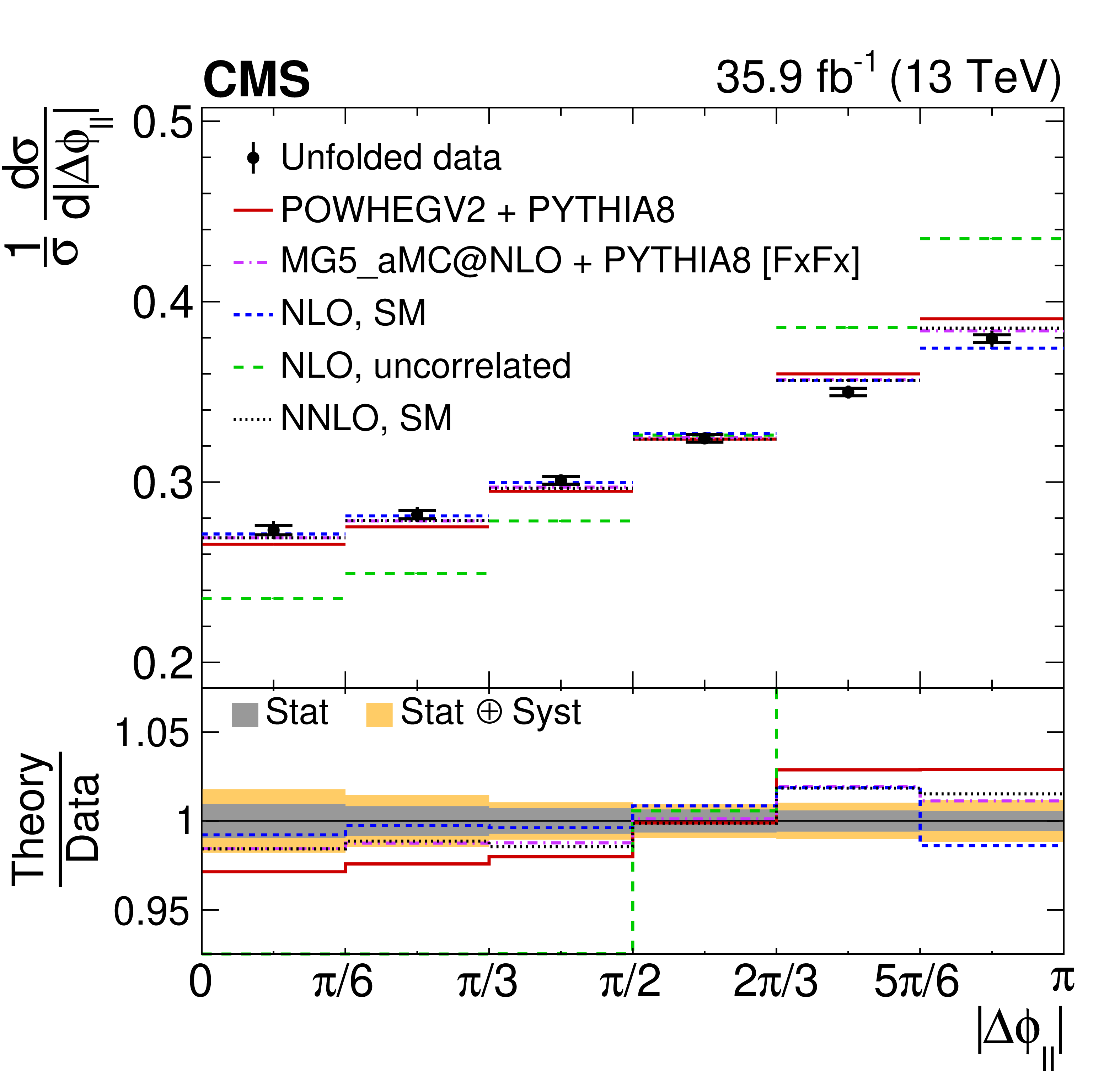
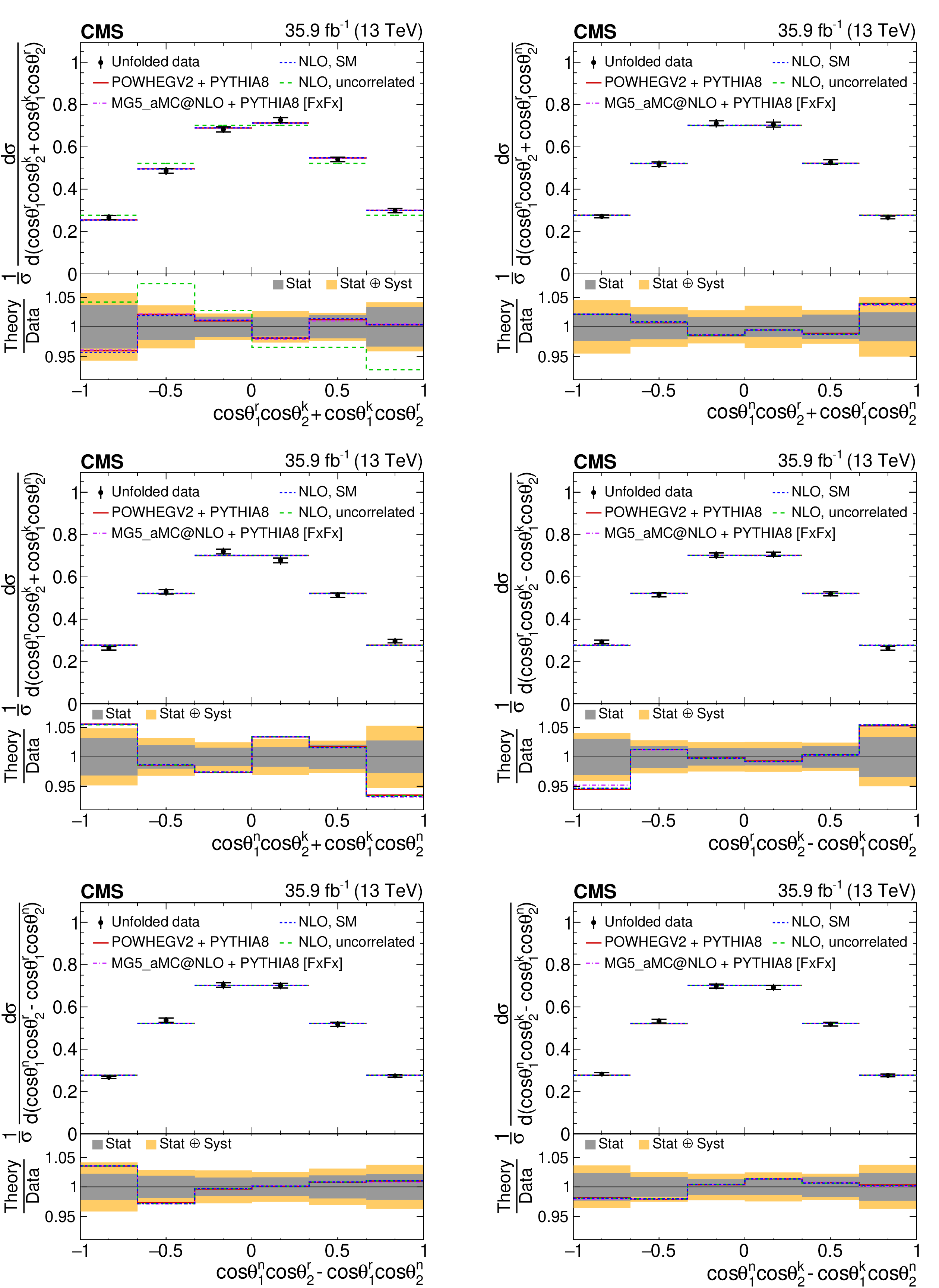
Figure 7:
Unfolded data (points) and predicted (horizontal lines) normalized differential cross sections for the cross spin correlation observables. The vertical lines on the points represent the total uncertainties, with the statistical components indicated by horizontal bars. The ratios of various predictions to the data are shown in the lower panels. |
png pdf |
Figure 7-a:
Unfolded data (points) and predicted (horizontal lines) normalized differential cross sections for the cross spin correlation observables. The vertical lines on the points represent the total uncertainties, with the statistical components indicated by horizontal bars. The ratios of various predictions to the data are shown in the lower panels. |
png pdf |
Figure 7-b:
Unfolded data (points) and predicted (horizontal lines) normalized differential cross sections for the cross spin correlation observables. The vertical lines on the points represent the total uncertainties, with the statistical components indicated by horizontal bars. The ratios of various predictions to the data are shown in the lower panels. |
png pdf |
Figure 7-c:
Unfolded data (points) and predicted (horizontal lines) normalized differential cross sections for the cross spin correlation observables. The vertical lines on the points represent the total uncertainties, with the statistical components indicated by horizontal bars. The ratios of various predictions to the data are shown in the lower panels. |

png pdf |
Figure 7-d:
Unfolded data (points) and predicted (horizontal lines) normalized differential cross sections for the cross spin correlation observables. The vertical lines on the points represent the total uncertainties, with the statistical components indicated by horizontal bars. The ratios of various predictions to the data are shown in the lower panels. |

png pdf |
Figure 7-e:
Unfolded data (points) and predicted (horizontal lines) normalized differential cross sections for the cross spin correlation observables. The vertical lines on the points represent the total uncertainties, with the statistical components indicated by horizontal bars. The ratios of various predictions to the data are shown in the lower panels. |

png pdf |
Figure 7-f:
Unfolded data (points) and predicted (horizontal lines) normalized differential cross sections for the cross spin correlation observables. The vertical lines on the points represent the total uncertainties, with the statistical components indicated by horizontal bars. The ratios of various predictions to the data are shown in the lower panels. |
png pdf |
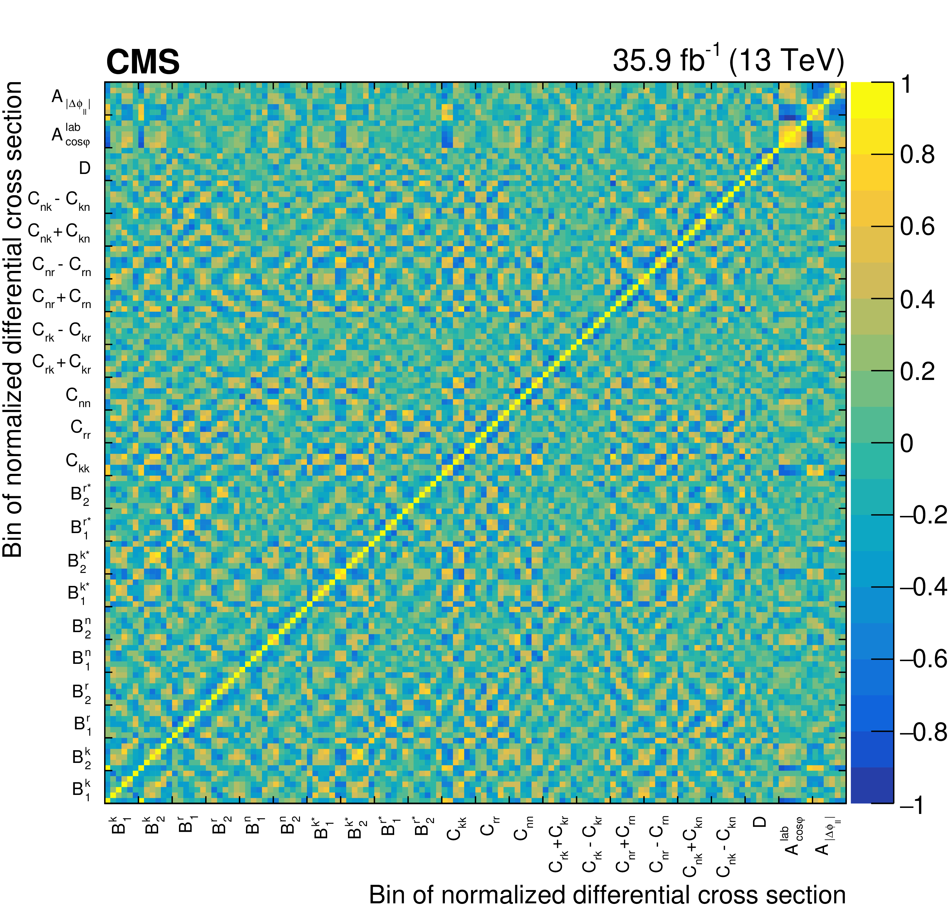
Figure 8:
Values of the total statistical correlation matrix using the gray scale on the right for all measured bins of the normalized differential cross sections. Each group of six bins along each axis corresponds to a measured distribution, and for conciseness is labeled by the name of the associated coefficient (as defined in Table 1). |
png pdf |
Figure 9:
Values of the total systematic correlation matrix using the gray scale on the right for all measured bins of the normalized differential cross sections. Each group of six bins along each axis corresponds to a measured distribution, and for conciseness is labeled by the name of the associated coefficient (as defined in Table 1). |
png pdf |
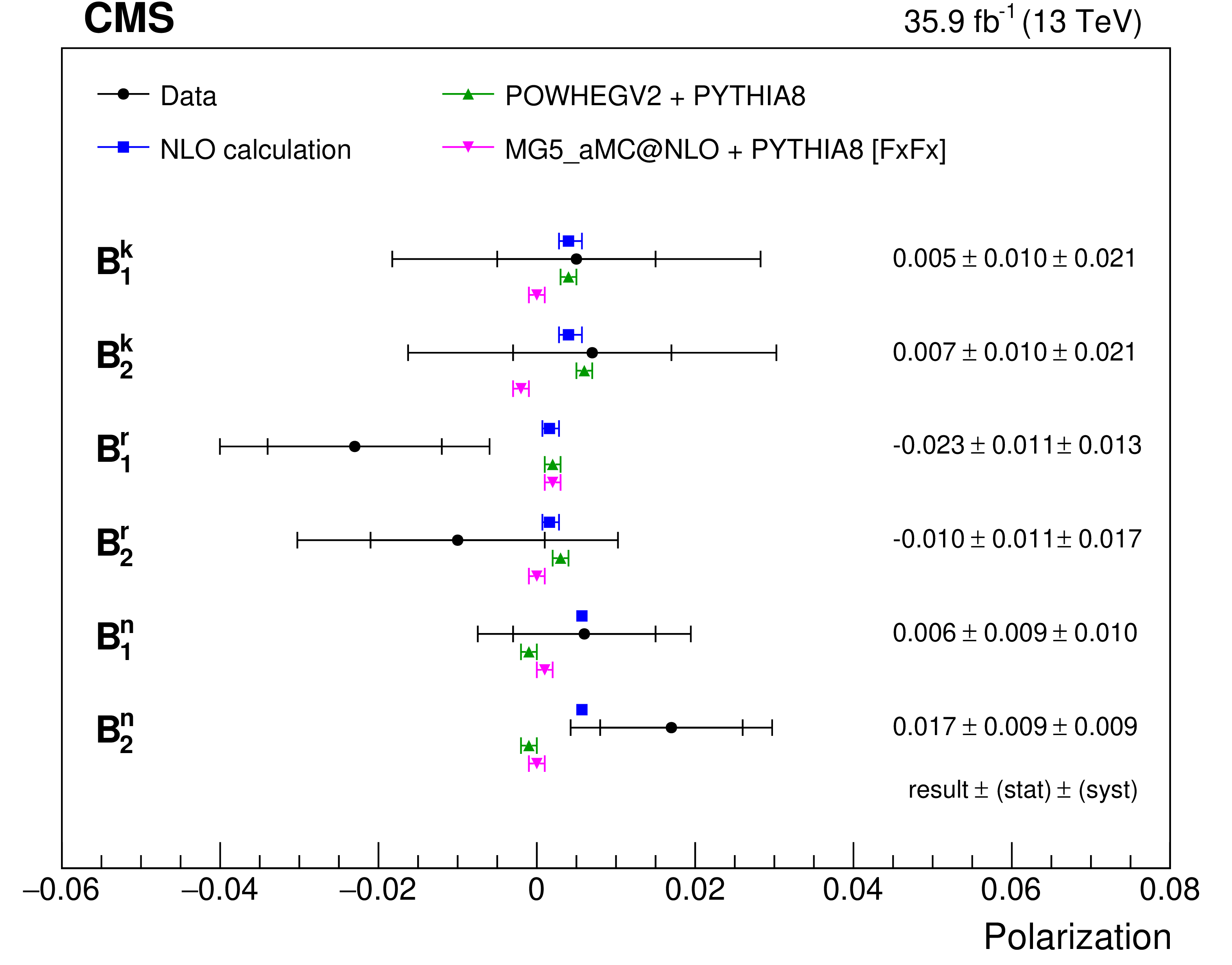
Figure 10:
Measured values of the polarization coefficients (circles) and the predictions from POWHEGv2 (triangles), MadGraph 5\_aMC@NLO (inverted triangles), and the NLO calculation [4] (squares). The inner vertical bars on the circles give the statistical uncertainty in the data and the outer bars the total uncertainty. The numerical measured values with their statistical and systematic uncertainties are given on the right. The vertical bars on the values from simulation represent a combination of the statistical and scale uncertainties, while for the calculated values they represent the scale uncertainties. |
png pdf |
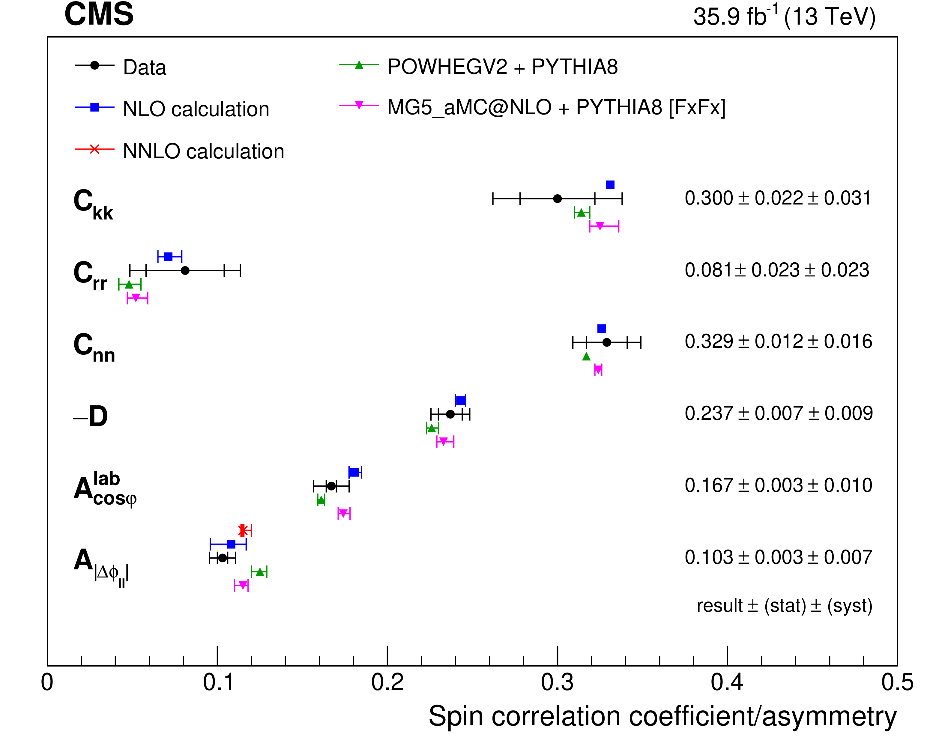
Figure 11:
Measured values of the spin correlation coefficients and asymmetries (circles) and the predictions from POWHEGv2 (triangles), MadGraph 5\_aMC@NLO (inverted triangles), the NLO calculation [3,4] (squares), and the NNLO calculation [69] (cross). The inner vertical bars on the circles give the statistical uncertainty in the data and the outer bars the total uncertainty. The numerical measured values with their statistical and systematic uncertainties are given on the right. The vertical bars on the values from simulation represent a combination of the statistical and scale uncertainties, while for the calculated values they represent the scale uncertainties. |

png pdf |
Figure 12:
Measured values of the cross spin correlation coefficients (circles) and the predictions from POWHEGv2 (triangles), MadGraph 5\_aMC@NLO (inverted triangles), and the NLO calculation [4] (squares). The inner vertical bars on the circles give the statistical uncertainty in the data and the outer bars the total uncertainty. The numerical measured values with their statistical and systematic uncertainties are given on the right. The vertical bars on the values from simulation represent a combination of the statistical and scale uncertainties, while for the calculated values they represent the scale uncertainties. |
png pdf |
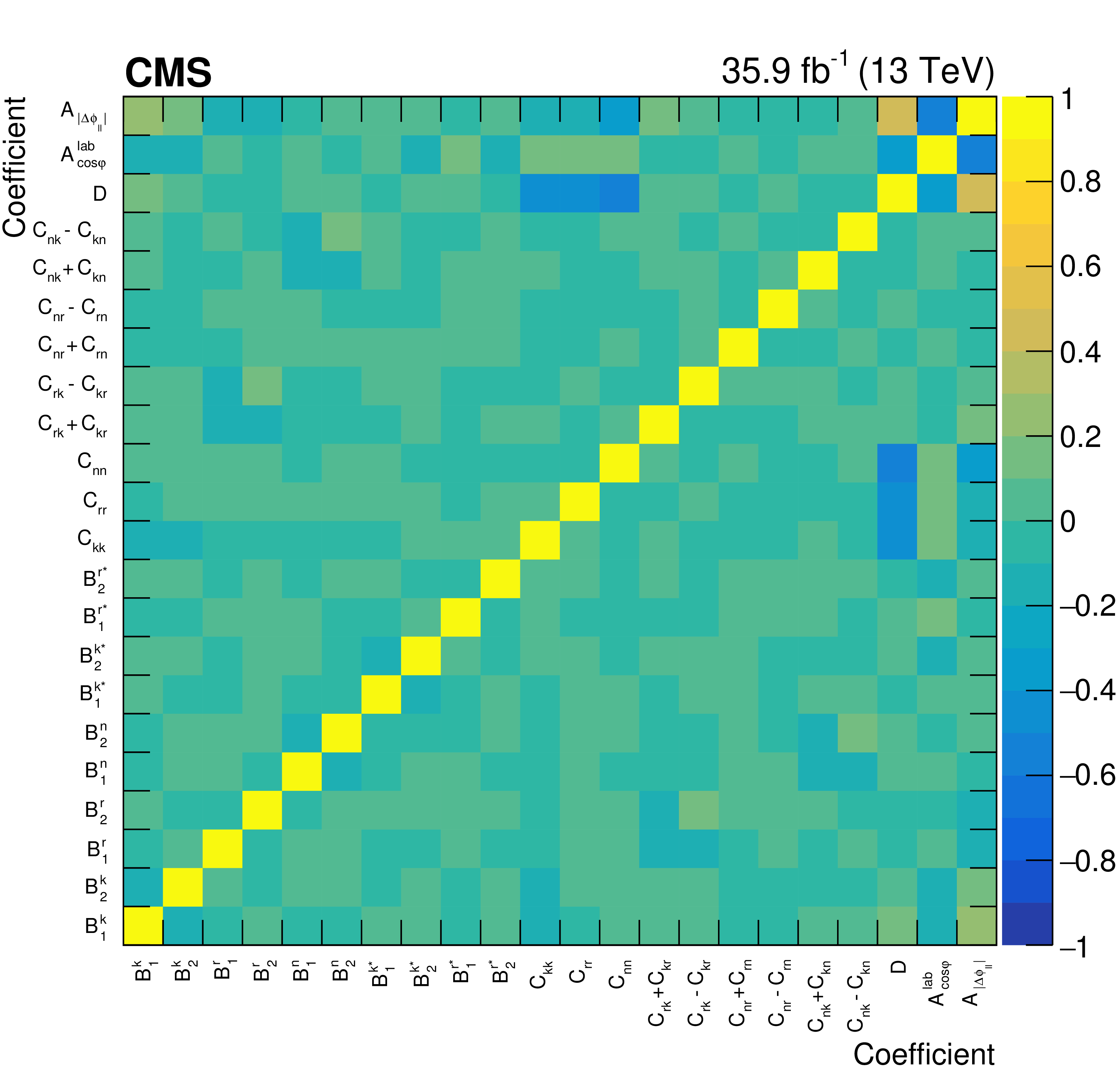
Figure 13:
Values of the total statistical correlation matrix using the gray scale on the right for all measured coefficients and the laboratory-frame asymmetries. |
png pdf |
Figure 14:
Values of the total systematic correlation matrix using the gray scale on the right for all measured coefficients and the laboratory-frame asymmetries. |
png pdf |
Figure 15:
Measured values of $f_{\mathrm {SM}}$, the strength of the measured spin correlations relative to the SM prediction. The inner vertical bars give the statistical uncertainty, the middle bars the total experimental uncertainty (statistical and systematic), and the outer bars the total uncertainty. The numerical measured values with their uncertainties are given on the right. |

png pdf |
Figure 16:
The $\Delta \chi ^{2}$ values from the fit to the data as a function of ${C_\text {tG}/\Lambda ^{2}}$. The solid line is the result of the nominal fit, and the dotted and dashed lines show the most-positive and most-negative shifts in best fit ${C_\text {tG}/\Lambda ^{2}}$, respectively, when the theoretical inputs are allowed to vary within their uncertainties. The vertical line denotes the best fit value from the nominal fit, and the inner and outer areas indicate the 68 and 95% CL, respectively. |
png pdf |
Figure 17:
Measured values of and uncertainties in the fitted anomalous couplings, assuming other anomalous couplings to be zero. The first and second quoted uncertainties are from experimental (statistical and systematic, at 68% CL) and theoretical sources, respectively, and are shown by the inner and outer vertical bars on the points. The expected SM value is shown by the vertical line. |

png pdf |
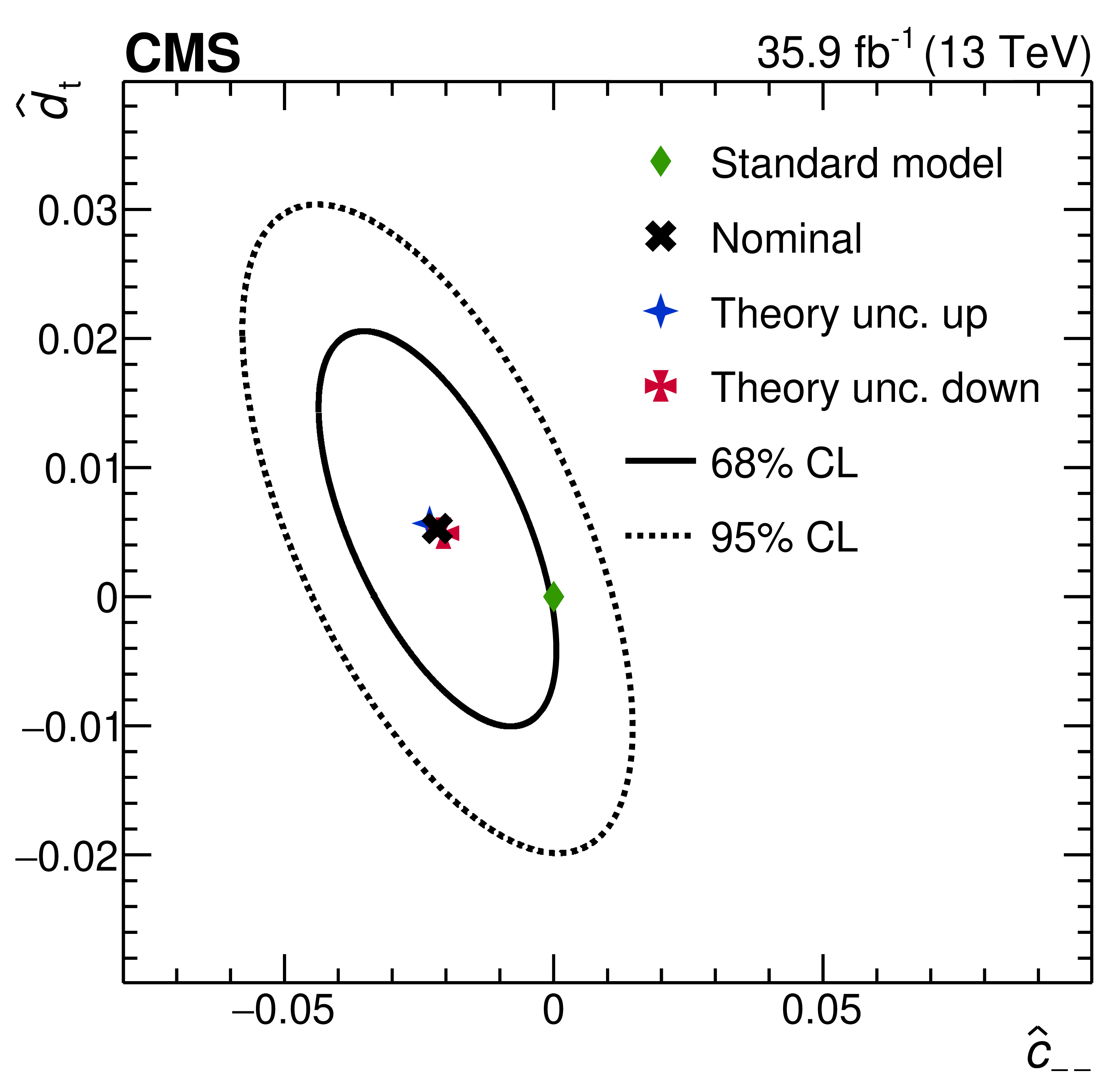
Figure 18:
The two-dimensional 68% (solid curve) and 95% (dotted curve) CL limits on (upper left) $ {\hat{\mu}_{\mathrm{t}}}$ vs. $ {\hat{c}_{\text {VV}}}$, (upper right) $ {\hat{\mu}_{\mathrm{t}}}$ vs. $ {\hat{c}_{1}}$, and (lower) $ {\hat{d}_{\mathrm{t}}}$ vs. $ {\hat{c}_{-\,-}}$. The central value from the nominal fit is shown by the cross and the SM prediction by the diamond. "Theory unc. up'' refers to the fit value when $\mu _\mathrm {R}$ and $\mu _\mathrm {F}$ are simultaneously increased by a factor of 2, and "theory unc. down'' when they are decreased by the same factor. |

png pdf |
Figure 18-a:
The two-dimensional 68% (solid curve) and 95% (dotted curve) CL limits on (upper left) $ {\hat{\mu}_{\mathrm{t}}}$ vs. $ {\hat{c}_{\text {VV}}}$, (upper right) $ {\hat{\mu}_{\mathrm{t}}}$ vs. $ {\hat{c}_{1}}$, and (lower) $ {\hat{d}_{\mathrm{t}}}$ vs. $ {\hat{c}_{-\,-}}$. The central value from the nominal fit is shown by the cross and the SM prediction by the diamond. "Theory unc. up'' refers to the fit value when $\mu _\mathrm {R}$ and $\mu _\mathrm {F}$ are simultaneously increased by a factor of 2, and "theory unc. down'' when they are decreased by the same factor. |
png pdf |
Figure 18-b:
The two-dimensional 68% (solid curve) and 95% (dotted curve) CL limits on (upper left) $ {\hat{\mu}_{\mathrm{t}}}$ vs. $ {\hat{c}_{\text {VV}}}$, (upper right) $ {\hat{\mu}_{\mathrm{t}}}$ vs. $ {\hat{c}_{1}}$, and (lower) $ {\hat{d}_{\mathrm{t}}}$ vs. $ {\hat{c}_{-\,-}}$. The central value from the nominal fit is shown by the cross and the SM prediction by the diamond. "Theory unc. up'' refers to the fit value when $\mu _\mathrm {R}$ and $\mu _\mathrm {F}$ are simultaneously increased by a factor of 2, and "theory unc. down'' when they are decreased by the same factor. |
png pdf |
Figure 18-c:
The two-dimensional 68% (solid curve) and 95% (dotted curve) CL limits on (upper left) $ {\hat{\mu}_{\mathrm{t}}}$ vs. $ {\hat{c}_{\text {VV}}}$, (upper right) $ {\hat{\mu}_{\mathrm{t}}}$ vs. $ {\hat{c}_{1}}$, and (lower) $ {\hat{d}_{\mathrm{t}}}$ vs. $ {\hat{c}_{-\,-}}$. The central value from the nominal fit is shown by the cross and the SM prediction by the diamond. "Theory unc. up'' refers to the fit value when $\mu _\mathrm {R}$ and $\mu _\mathrm {F}$ are simultaneously increased by a factor of 2, and "theory unc. down'' when they are decreased by the same factor. |
| Tables | |
png pdf |
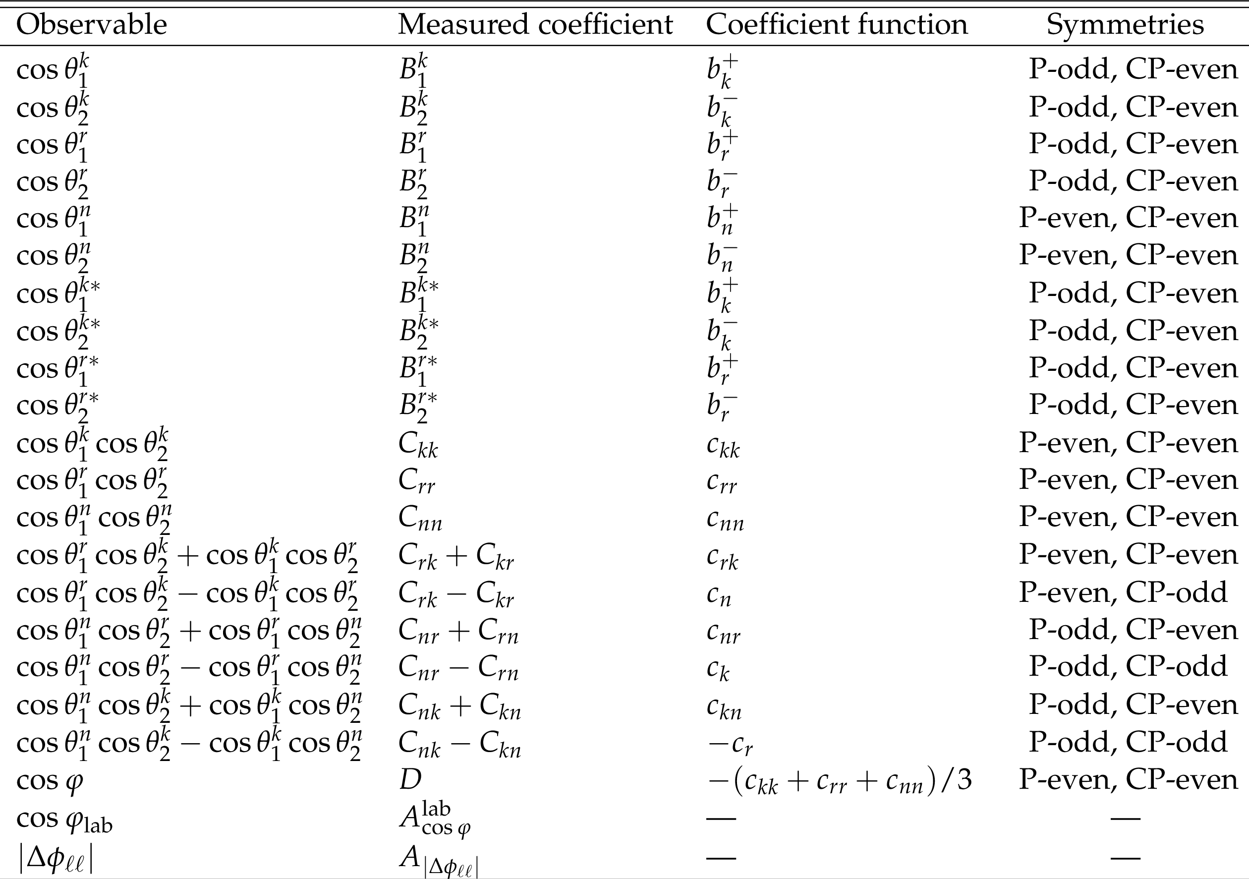
Table 1:
Observables and their corresponding measured coefficients, production spin density matrix coefficient functions, and P and CP symmetry properties. For the laboratory-frame asymmetries shown in the last two rows, there is no direct correspondence with the coefficient functions. |
png pdf |
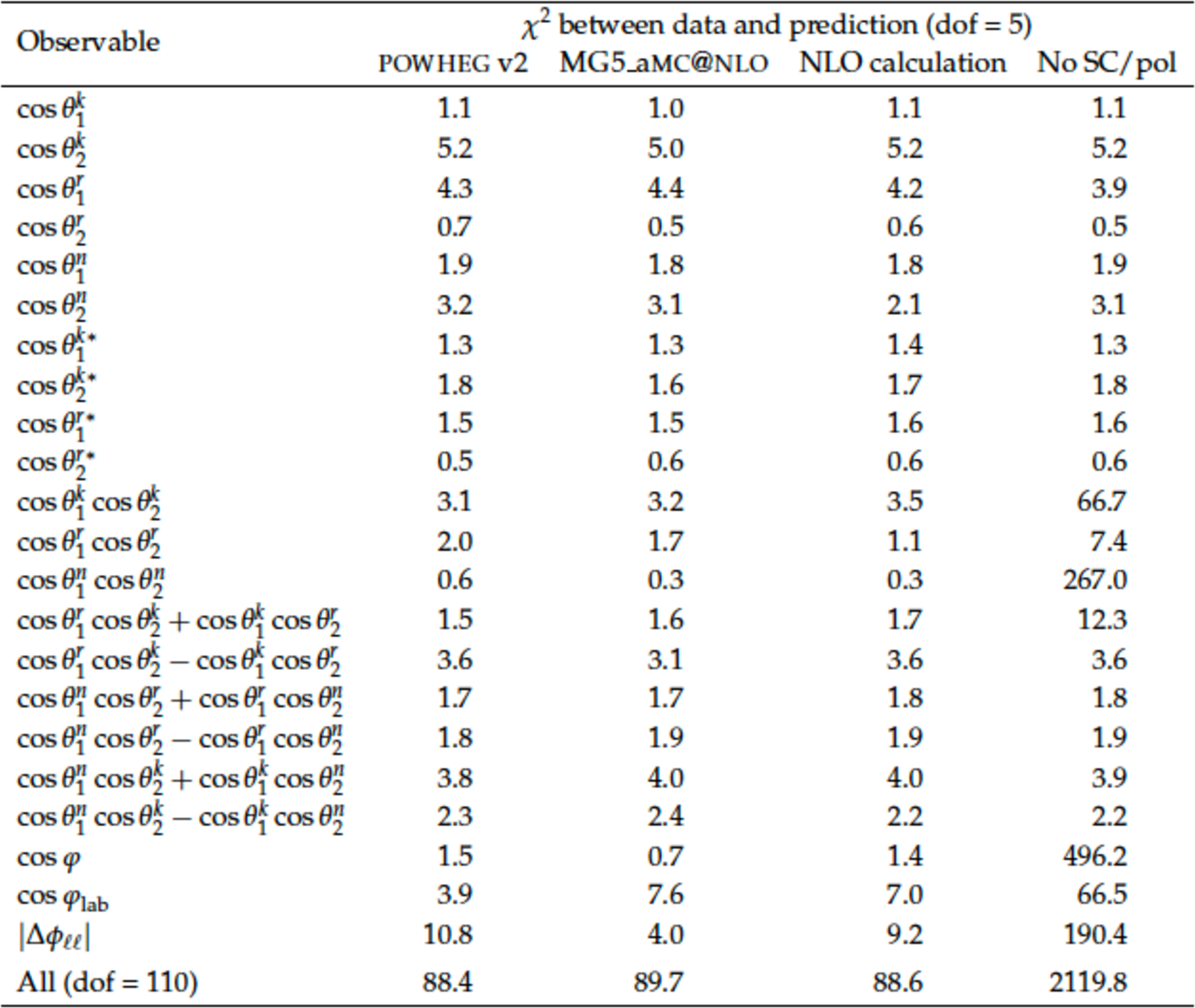
Table 2:
The $\chi ^2$ between the data and the predictions for all measured normalized differential cross sections (Figs. 4-7). The last column refers to the prediction in the case of no spin correlation (SC) or polarization (pol). The $\chi ^2$ values are evaluated using the sum of the measured statistical and systematic covariance matrices. The number of degrees of freedom (dof) is 5 for all observables. In the last row, the $\chi ^2$ values are given for the set of all measured bins. |
png pdf |
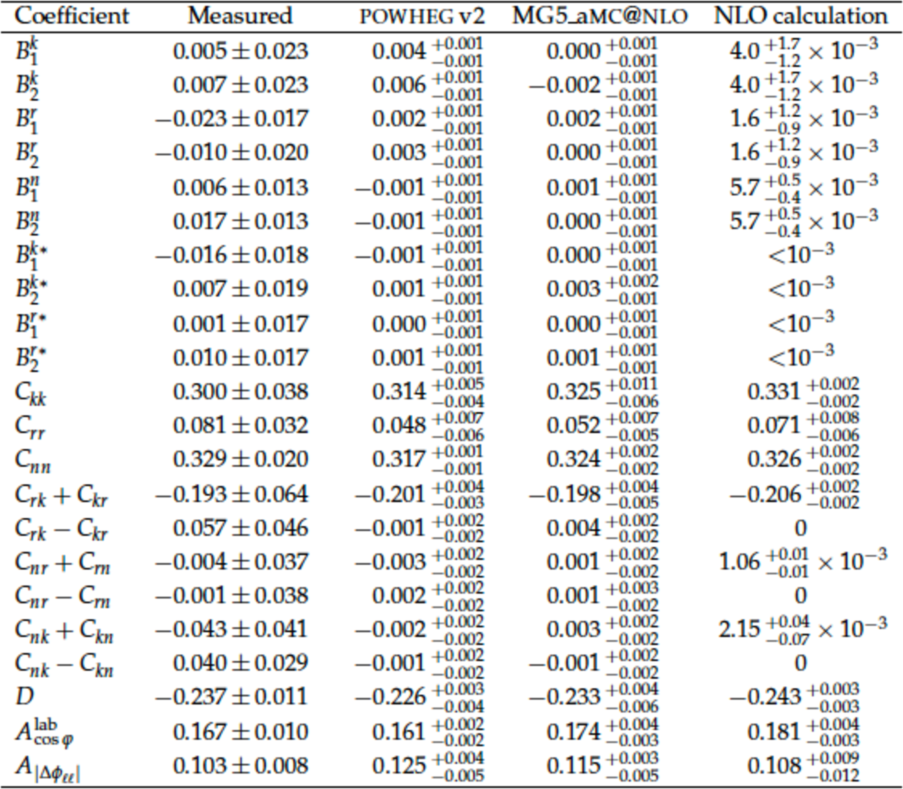
Table 3:
Measured coefficients and asymmetries and their total uncertainties. Predicted values from simulation are quoted with a combination of statistical and scale uncertainties, while the NLO calculated values are quoted with their scale uncertainties [3,4]. The NNLO QCD prediction for $ {A_{{{| \Delta \phi _{\ell \ell} |}}}}$, with scale uncertainties, is 0.115$^{+0.005}_{-0.001}$ [69]. |
png pdf |
Table 4:
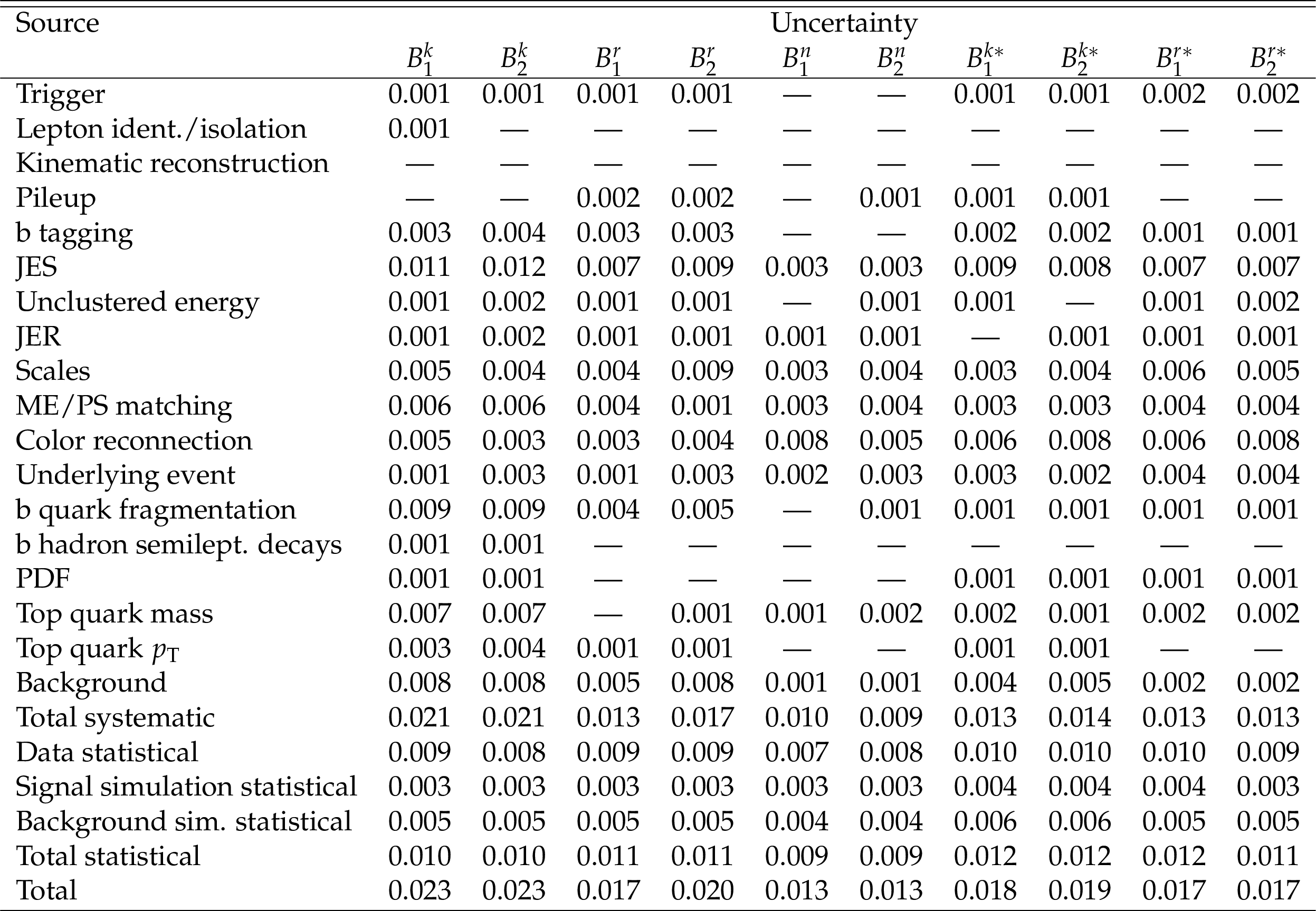
Summary of the systematic, statistical, and total uncertainties in the extracted top quark polarization coefficients. A dash (--) is shown where the values are ${<}$0.0005. |
png pdf |
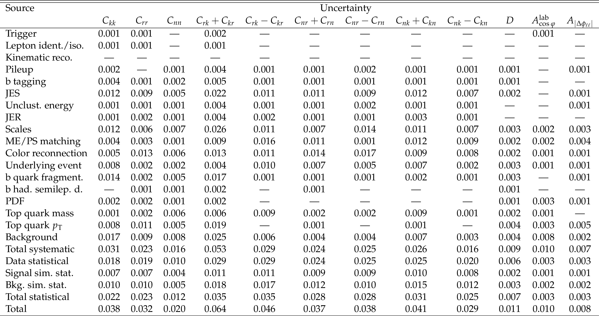
Table 5:
Summary of the systematic, statistical, and total uncertainties in the extracted ${\mathrm{t} \mathrm{\bar{t}}}$ spin correlation coefficients and asymmetries. A dash (--) is shown where the values are ${<}$0.0005. |
png pdf |
Table 6:
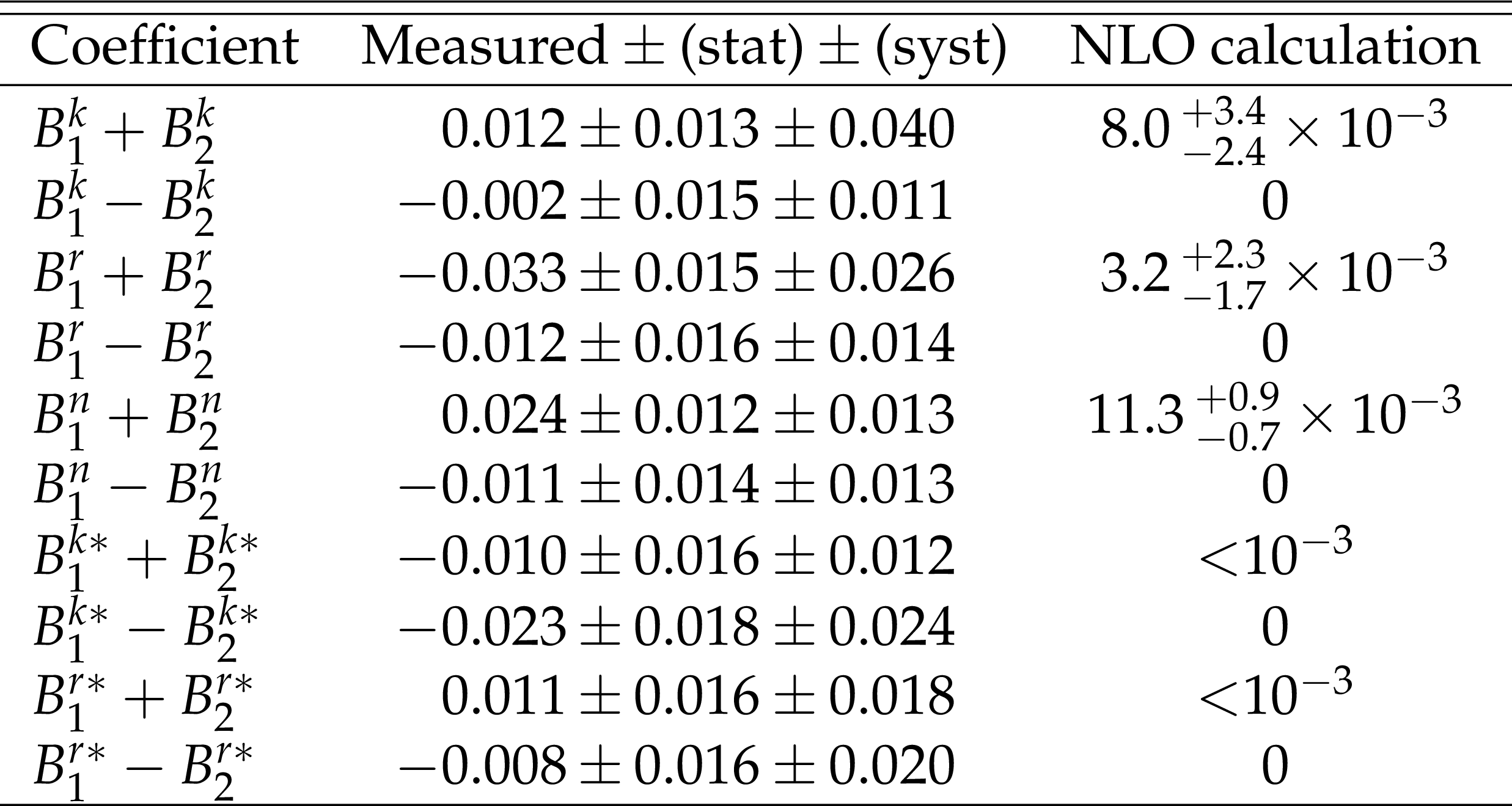
Measured sums and differences of the $B$ coefficients and their statistical and systematic uncertainties. The NLO calculated coefficients are quoted with their scale uncertainties [4]. |
png pdf |
Table 7:
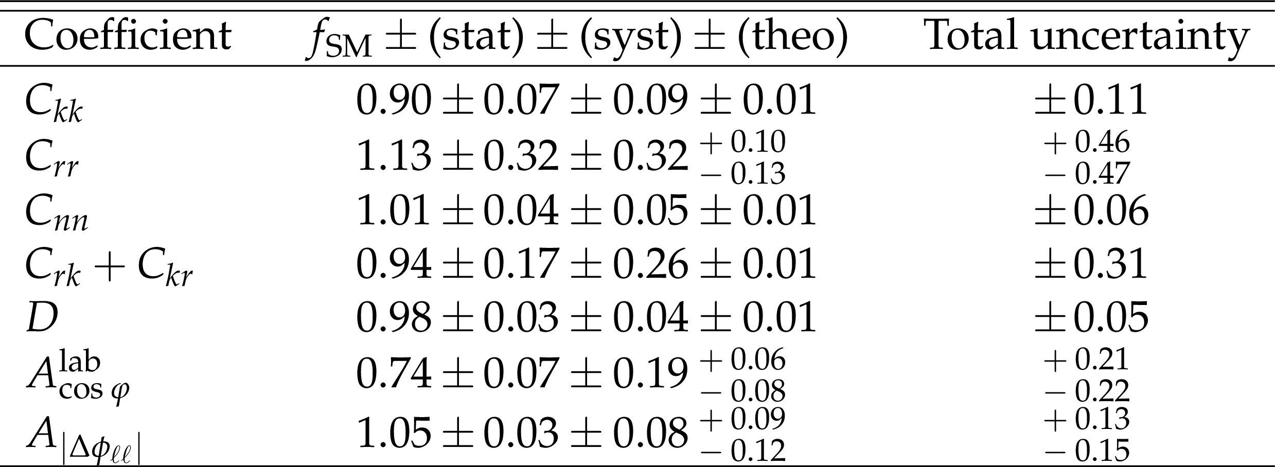
Values of $f_{\mathrm {SM}}$, the strength of the measured spin correlations relative to the SM prediction, derived from the measurements in Table 3. The uncertainties shown are statistical, systematic, and theoretical, respectively. Their sum in quadrature is shown in the last column. |

png pdf |
Table 8:
Anomalous couplings associated with the dimension-six operators relevant for hadronic ${\mathrm{t} \mathrm{\bar{t}}}$ production, the operator type of the effective interaction vertex they represent, and their P and CP symmetry properties. It is not possible to combine the isospin-1 operators such that they have definite properties with respect to C and P [4]. |
png pdf |
Table 9:
The 95% CL limits on the anomalous couplings listed in Table 8, derived from fitting the distributions measured in Section 8.1 and setting other anomalous couplings to zero. The confidence intervals include only the experimental uncertainties as in Section 9.1. The theoretical uncertainties, the $\chi ^2$ values (dof = 19), and the distributions used in each fit are given in the last three columns. For conciseness, the distributions are labeled by their associated coefficients (as defined in Table 1). A dash (--) is shown where the values are ${<}$0.0005. |
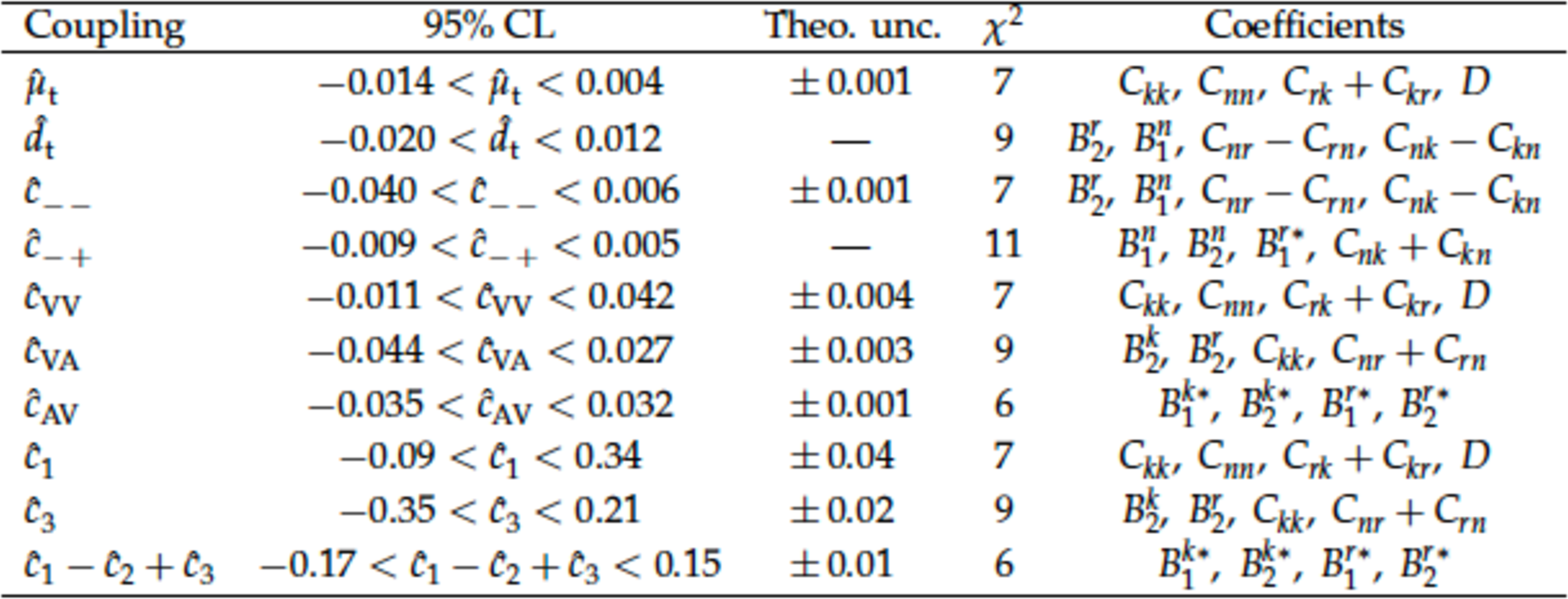
| Summary |
|
Measurements of the top quark polarization and $\mathrm{t\bar{t}}$ spin correlations are presented, probing all of the independent coefficients of the top quark spin-dependent parts of the $\mathrm{t\bar{t}}$ production density matrix for the first time in proton-proton collisions at $\sqrt{s} = $ 13 TeV. Each coefficient is extracted from a normalized differential cross section, unfolded to the parton level and extrapolated to the full phase space. The measurements are made using a data sample of events containing two oppositely charged leptons ($\mathrm{e^{+}}\mathrm{e^{-}}$ , $\mathrm{e}^{\pm}\mu^{\mp}$ , or $\mu\mu$) and two or more jets, of which at least one is identified as coming from the hadronization of a bottom quark. The data were recorded by the CMS experiment in 2016 and correspond to an integrated luminosity of 35.9 fb$^{-1}$. The measured normalized differential cross sections and coefficients are compared with standard model predictions from simulations with next-to-leading order (NLO) accuracy in quantum chromodynamics (QCD) and from NLO QCD calculations including electroweak corrections. The measured distribution of the absolute value of the difference in azimuthal angle between the two leptons in the laboratory frame is additionally compared with a next-to-next-to-leading-order QCD prediction. All of the measurements are found to be consistent with the expectations of the standard model. Statistical and systematic covariance matrices are provided for the set of all measured bins, and are used in simultaneous fits to constrain the contributions from ten dimension-six effective operators. Two of these operators represent the anomalous chromomagnetic and chromoelectric dipole moments of the top quark, and constraints on their Wilson coefficients of $-0.24 < {C_\text{tG}/\Lambda^{2}} < 0.07$ TeV$^{-2}$ and $-0.33 < {C^{I}_\text{tG}/\Lambda^{2}} < 0.20 $ TeV$^{-2}$, respectively, are obtained at 95% confidence level. This constitutes a substantial improvement over previous direct constraints. |
| References | ||||
| 1 | Particle Data Group | Review of particle physics | PRD 98 (2018) 030001 | |
| 2 | G. Mahlon and S. J. Parke | Spin correlation effects in top quark pair production at the LHC | PRD 81 (2010) 074024 | 1001.3422 |
| 3 | W. Bernreuther and Z.-G. Si | Top quark spin correlations and polarization at the LHC: Standard model predictions and effects of anomalous top chromo moments | PLB 725 (2013) 115 | 1305.2066 |
| 4 | W. Bernreuther, D. Heisler, and Z.-G. Si | A set of top quark spin correlation and polarization observables for the LHC: Standard model predictions and new physics contributions | JHEP 12 (2015) 026 | 1508.05271 |
| 5 | CMS Collaboration | CMS luminosity measurements for the 2016 data taking period | CMS-PAS-LUM-17-001 | CMS-PAS-LUM-17-001 |
| 6 | ATLAS Collaboration | Measurements of top quark spin observables in $ \mathrm{t\bar{t}} $ events using dilepton final states in $ \sqrt{s} = $ 8 TeV pp collisions with the ATLAS detector | JHEP 03 (2017) 113 | 1612.07004 |
| 7 | CMS Collaboration | Measurements of $ \mathrm{t\bar{t}} $ spin correlations and top-quark polarization using dilepton final states in pp collisions at $ \sqrt{s} = $ 7 TeV | PRL 112 (2014) 182001 | CMS-TOP-13-003 1311.3924 |
| 8 | ATLAS Collaboration | Measurements of spin correlation in top-antitop quark events from proton-proton collisions at $ \sqrt{s} = $ 7 TeV using the ATLAS detector | PRD 90 (2014) 112016 | 1407.4314 |
| 9 | ATLAS Collaboration | Measurement of the correlation between the polar angles of leptons from top quark decays in the helicity basis at $ \sqrt{s} = $ 7 TeV using the ATLAS detector | PRD 93 (2016) 012002 | 1510.07478 |
| 10 | CMS Collaboration | Measurements of $ \mathrm{t\bar{t}}\ $ spin correlations and top quark polarization using dilepton final states in pp collisions at $ \sqrt{s} = $ 8 TeV | PRD 93 (2016) 052007 | CMS-TOP-14-023 1601.01107 |
| 11 | ATLAS Collaboration | Measurements of top-quark pair spin correlations in the e$ \mu $ channel at $ \sqrt{s} = $ 13 TeV using pp collisions in the ATLAS detector | Submitted to EPJC | 1903.07570 |
| 12 | CMS Collaboration | Measurements of $ \mathrm{t\overline{t}} $ differential cross sections in proton-proton collisions at $ \sqrt{s}= $ 13 TeV using events containing two leptons | JHEP 02 (2019) 149 | CMS-TOP-17-014 1811.06625 |
| 13 | M. Baumgart and B. Tweedie | A new twist on top quark spin correlations | JHEP 03 (2013) 117 | 1212.4888 |
| 14 | M. Fabbrichesi, M. Pinamonti, and A. Tonero | Limits on anomalous top quark gauge couplings from Tevatron and LHC data | EPJC 74 (2014) 3193 | 1406.5393 |
| 15 | Q.-H. Cao, B. Yan, J.-H. Yu, and C. Zhang | A general analysis of Wtb anomalous couplings | CPC 41 (2017) 063101 | 1504.03785 |
| 16 | C. Degrande et al. | Non-resonant new physics in top pair production at hadron colliders | JHEP 03 (2011) 125 | 1010.6304 |
| 17 | A. Brandenburg, Z.-G. Si, and P. Uwer | QCD-corrected spin analysing power of jets in decays of polarized top quarks | PLB 539 (2002) 235 | hep-ph/0205023 |
| 18 | CMS Collaboration | The CMS trigger system | JINST 12 (2017) P01020 | CMS-TRG-12-001 1609.02366 |
| 19 | CMS Collaboration | The CMS experiment at the CERN LHC | JINST 3 (2008) S08004 | CMS-00-001 |
| 20 | S. Frixione, P. Nason, and G. Ridolfi | A positive-weight next-to-leading-order Monte Carlo for heavy flavour hadroproduction | JHEP 09 (2007) 126 | 0707.3088 |
| 21 | P. Nason | A new method for combining NLO QCD with shower Monte Carlo algorithms | JHEP 11 (2004) 040 | hep-ph/0409146 |
| 22 | S. Frixione, P. Nason, and C. Oleari | Matching NLO QCD computations with parton shower simulations: the POWHEG method | JHEP 11 (2007) 070 | 0709.2092 |
| 23 | S. Alioli, P. Nason, C. Oleari, and E. Re | A general framework for implementing NLO calculations in shower Monte Carlo programs: the POWHEG BOX | JHEP 06 (2010) 043 | 1002.2581 |
| 24 | CMS Collaboration | Investigations of the impact of the parton shower tuning in $ \Pythia\ $ in the modelling of $ \mathrm{t\overline{t}} $ at $ \sqrt{s}= $ 8 and 13 TeV | CMS-PAS-TOP-16-021 | CMS-PAS-TOP-16-021 |
| 25 | T. Sjostrand et al. | An introduction to PYTHIA 8.2 | CPC 191 (2015) 159 | 1410.3012 |
| 26 | CMS Collaboration | Event generator tunes obtained from underlying event and multiparton scattering measurements | EPJC 76 (2016) 155 | CMS-GEN-14-001 1512.00815 |
| 27 | P. Skands, S. Carrazza, and J. Rojo | Tuning PYTHIA 8.1: the Monash 2013 tune | EPJC 74 (2014) 3024 | 1404.5630 |
| 28 | J. Alwall et al. | The automated computation of tree-level and next-to-leading order differential cross sections, and their matching to parton shower simulations | JHEP 07 (2014) 079 | 1405.0301 |
| 29 | P. Artoisenet, R. Frederix, O. Mattelaer, and R. Rietkerk | Automatic spin-entangled decays of heavy resonances in Monte Carlo simulations | JHEP 03 (2013) 015 | 1212.3460 |
| 30 | R. Frederix and S. Frixione | Merging meets matching in MC@NLO | JHEP 12 (2012) 061 | 1209.6215 |
| 31 | J. Alwall et al. | Comparative study of various algorithms for the merging of parton showers and matrix elements in hadronic collisions | EPJC 53 (2008) 437 | 0706.2569 |
| 32 | S. Alioli, P. Nason, C. Oleari, and E. Re | NLO single-top production matched with shower in POWHEG: $ s $- and $ t $-channel contributions | JHEP 09 (2009) 111 | 0907.4076 |
| 33 | E. Re | Single-top Wt-channel production matched with parton showers using the POWHEG method | EPJC 71 (2011) 1547 | 1009.2450 |
| 34 | NNPDF Collaboration | Unbiased global determination of parton distributions and their uncertainties at NNLO and LO | NPB 855 (2012) 153 | 1107.2652 |
| 35 | NNPDF Collaboration | Parton distributions for the LHC Run II | JHEP 04 (2015) 040 | 1410.8849 |
| 36 | Y. Li and F. Petriello | Combining QCD and electroweak corrections to dilepton production in FEWZ | PRD 86 (2012) 094034 | 1208.5967 |
| 37 | N. Kidonakis | Two-loop soft anomalous dimensions for single top quark associated production with $ \mathrm{W^-} $ or $ \mathrm{H^-} $ | PRD 82 (2010) 054018 | hep-ph/1005.4451 |
| 38 | J. M. Campbell, R. K. Ellis, and C. Williams | Vector boson pair production at the LHC | JHEP 07 (2011) 018 | 1105.0020 |
| 39 | F. Maltoni, D. Pagani, and I. Tsinikos | Associated production of a top-quark pair with vector bosons at NLO in QCD: impact on $ \mathrm{t}\overline{\mathrm{t}}\mathrm{H} $ searches at the LHC | JHEP 02 (2016) 113 | 1507.05640 |
| 40 | M. Czakon and A. Mitov | TOP++: a program for the calculation of the top-pair cross-section at hadron colliders | CPC 185 (2014) 2930 | 1112.5675 |
| 41 | GEANT4 Collaboration | GEANT4--a simulation toolkit | NIMA 506 (2003) 250 | |
| 42 | CMS Collaboration | Particle-flow reconstruction and global event description with the CMS detector | JINST 12 (2017) P10003 | CMS-PRF-14-001 1706.04965 |
| 43 | CMS Collaboration | Performance of electron reconstruction and selection with the CMS detector in proton-proton collisions at $ \sqrt{s} = $ 8 TeV | JINST 10 (2015) P06005 | CMS-EGM-13-001 1502.02701 |
| 44 | CMS Collaboration | Performance of the CMS muon detector and muon reconstruction with proton-proton collisions at $ \sqrt{s}= $ 13 TeV | JINST 13 (2018) P06015 | CMS-MUO-16-001 1804.04528 |
| 45 | M. Cacciari, G. P. Salam, and G. Soyez | The anti-$ {k_{\mathrm{T}}} $ jet clustering algorithm | JHEP 04 (2008) 063 | 0802.1189 |
| 46 | M. Cacciari, G. P. Salam, and G. Soyez | FastJet user manual | EPJC 72 (2012) 1896 | 1111.6097 |
| 47 | CMS Collaboration | Identification and filtering of uncharacteristic noise in the CMS hadron calorimeter | JINST 5 (2010) T03014 | CMS-CFT-09-019 0911.4881 |
| 48 | CMS Collaboration | Identification of heavy-flavour jets with the CMS detector in pp collisions at 13 TeV | JINST 13 (2018) P05011 | CMS-BTV-16-002 1712.07158 |
| 49 | CMS Collaboration | Measurement of the differential cross section for top quark pair production in pp collisions at $ \sqrt{s} = $ 8 TeV | EPJC 75 (2015) 542 | CMS-TOP-12-028 1505.04480 |
| 50 | CMS Collaboration | Measurement of the top quark pair production cross section in proton-proton collisions at $ \sqrt{s} = $ 13 TeV with the CMS detector | PRL 116 (2016) 052002 | CMS-TOP-15-003 1510.05302 |
| 51 | S. Schmitt | TUnfold, an algorithm for correcting migration effects in high energy physics | JINST 7 (2012) T10003 | 1205.6201 |
| 52 | CMS Collaboration | Measurement of the $ \mathrm{t\overline{t}} $ production cross section, the top quark mass, and the strong coupling constant using dilepton events in pp collisions at $ \sqrt{s}= $ 13 TeV | EPJC 79 (2019) 368 | CMS-TOP-17-001 1812.10505 |
| 53 | CMS Collaboration | Measurement of the Drell--Yan cross sections in pp collisions at $ \sqrt{s} = $ 7 TeV with the CMS experiment | JHEP 10 (2011) 007 | CMS-EWK-10-007 1108.0566 |
| 54 | ATLAS Collaboration | Measurement of the inelastic proton-proton cross section at $ \sqrt{s} = $ 13 TeV with the ATLAS detector at the LHC | PRL 117 (2016) 182002 | 1606.02625 |
| 55 | CMS Collaboration | Jet energy scale and resolution in the CMS experiment in pp collisions at 8 TeV | JINST 12 (2017) P02014 | CMS-JME-13-004 1607.03663 |
| 56 | S. Argyropoulos and T. Sjostrand | Effects of color reconnection on $ \mathrm{t\bar{t}}\ $ final states at the LHC | JHEP 11 (2014) 043 | 1407.6653 |
| 57 | J. R. Christiansen and P. Z. Skands | String formation beyond leading colour | JHEP 08 (2015) 003 | 1505.01681 |
| 58 | M. G. Bowler | $ \text{e}^{+}\text{e}^{-} $ production of heavy quarks in the string model | Z. Phys. C 11 (1981) 169 | |
| 59 | C. Peterson, D. Schlatter, I. Schmitt, and P. M. Zerwas | Scaling violations in inclusive $ \text{e}^{+}\text{e}^{{-}} $ annihilation spectra | PRD 27 (1983) 105 | |
| 60 | J. Butterworth et al. | PDF4LHC recommendations for LHC Run II | JPG 43 (2016) 023001 | 1510.03865 |
| 61 | CMS Collaboration | Measurement of differential top-quark pair production cross sections in pp collisions at $ \sqrt{s} = $ 7 TeV | EPJC 73 (2013) 2339 | CMS-TOP-11-013 1211.2220 |
| 62 | CMS Collaboration | Measurement of the $ \mathrm{t}\overline{{\mathrm{t}}} $ production cross section in the all-jets final state in pp collisions at $ \sqrt{s}= $ 8 TeV | EPJC 76 (2016) 128 | CMS-TOP-14-018 1509.06076 |
| 63 | CMS Collaboration | Measurement of differential cross sections for top quark pair production using the lepton+jets final state in proton-proton collisions at 13 TeV | PRD 95 (2017) 092001 | CMS-TOP-16-008 1610.04191 |
| 64 | M. Guzzi, K. Lipka, and S.-O. Moch | Top-quark pair production at hadron colliders: differential cross section and phenomenological applications with DiffTop | JHEP 01 (2015) 082 | 1406.0386 |
| 65 | N. Kidonakis | NNNLO soft-gluon corrections for the top-quark $ {p_{\mathrm{T}}} $ and rapidity distributions | PRD 91 (2015) 031501 | 1411.2633 |
| 66 | M. Czakon et al. | Top-pair production at the LHC through NNLO QCD and NLO EW | JHEP 10 (2017) 186 | 1705.04105 |
| 67 | M. Czakon et al. | Resummation for (boosted) top-quark pair production at NNLO+NNLL' in QCD | JHEP 05 (2018) 149 | 1803.07623 |
| 68 | W. Bernreuther and Z.-G. Si | Distributions and correlations for top quark pair production and decay at the Tevatron and LHC | NPB 837 (2010) 90 | 1003.3926 |
| 69 | A. Behring et al. | Higher order corrections to spin correlations in top quark pair production at the LHC | 1901.05407 | |
| 70 | B. Efron | Bootstrap methods: Another look at the jackknife | Ann. Stat. 7 (1979) 1 | |
| 71 | D. Buarque Franzosi and C. Zhang | Probing the top-quark chromomagnetic dipole moment at next-to-leading order in QCD | PRD 91 (2015) 114010 | 1503.08841 |
| 72 | R. Martinez, M. A. Perez, and N. Poveda | Chromomagnetic dipole moment of the top quark revisited | EPJC 53 (2008) 221 | hep-ph/0701098 |
| 73 | W. Buchmuller and D. Wyler | Effective Lagrangian analysis of new interactions and flavor conservation | NPB 268 (1986) 621 | |
| 74 | B. Grzadkowski, M. Iskrzynski, M. Misiak, and J. Rosiek | Dimension-six terms in the standard model Lagrangian | JHEP 10 (2010) 085 | 1008.4884 |
| 75 | A. Buckley et al. | Rivet user manual | CPC 184 (2013) 2803 | 1003.0694 |
| 76 | Z. Hioki and K. Ohkuma | Latest constraint on nonstandard top-gluon couplings at hadron colliders and its future prospect | PRD 88 (2013) 017503 | 1306.5387 |
| 77 | J. A. Aguilar-Saavedra, B. Fuks, and M. L. Mangano | Pinning down top dipole moments with ultra-boosted tops | PRD 91 (2015) 094021 | 1412.6654 |
| 78 | D. Barducci et al. | Interpreting top-quark LHC measurements in the standard-model effective field theory | 1802.07237 | |
| 79 | C. A. Baker et al. | An improved experimental limit on the electric dipole moment of the neutron | PRL 97 (2006) 131801 | hep-ex/0602020 |
| 80 | J. M. Pendlebury et al. | Revised experimental upper limit on the electric dipole moment of the neutron | PRD 92 (2015) 092003 | 1509.04411 |
| 81 | J. Sjolin | LHC experimental sensitivity to CP violating g$ \mathrm{t\bar{t}} $ couplings | JPG 29 (2003) 543 | |
|
|
Compact Muon Solenoid LHC, CERN |
|

|

|

|

|

|