

Compact Muon Solenoid
LHC, CERN
| CMS-B2G-17-012 ; CERN-EP-2018-290 | ||
| Search for vector-like quarks in events with two oppositely charged leptons and jets in proton-proton collisions at $\sqrt{s} = $ 13 TeV | ||
| CMS Collaboration | ||
| 24 December 2018 | ||
| Eur. Phys. J. C 79 (2019) 364 | ||
| Abstract: A search for the pair production of heavy vector-like partners T and B of the top and bottom quarks has been performed by the CMS experiment at the CERN LHC using proton-proton collisions at $\sqrt{s} = $ 13 TeV. The data sample was collected in 2016 and corresponds to an integrated luminosity of 35.9 fb$^{-1}$. Final states studied for ${{\mathrm{T}} } {\overline{{\mathrm{T}} }}$ production include those where one of the T quarks decays via $ {{\mathrm{T}} \to\mathrm{t}\mathrm{Z}} $ and the other via $ {{\mathrm{T}} \to\mathrm{b}\mathrm{W}} $, $ {\mathrm{t}\mathrm{Z}} $, or $ {\mathrm{t}\mathrm{H}} $, where H is a Higgs boson. For the $ {{\mathrm{B}} } {\overline{{\mathrm{B}} }} $ case, final states include those where one of the B quarks decays via $ {{\mathrm{B}} \to\mathrm{b}\mathrm{Z}} $ and the other $ {{\mathrm{B}} \to\mathrm{t}\mathrm{W}} $, $ {\mathrm{b}\mathrm{Z}} $, or $ {\mathrm{b}\mathrm{H}} $. Events with two oppositely charged electrons or muons, consistent with coming from the decay of a Z boson, and jets are investigated. The number of observed events is consistent with standard model background estimations. Lower limits at 95% confidence level are placed on the masses of the T and B quarks for a range of branching fractions. Assuming 100% branching fractions for $ {{\mathrm{T}} \to\mathrm{t}\mathrm{Z}} $, and $ {{\mathrm{B}} \to\mathrm{b}\mathrm{Z}} $, T and B quark mass values below 1280 and 1130 GeV, respectively, are excluded. | ||
| Links: e-print arXiv:1812.09768 [hep-ex] (PDF) ; CDS record ; inSPIRE record ; HepData record ; CADI line (restricted) ; | ||
| Figures | |
png pdf |
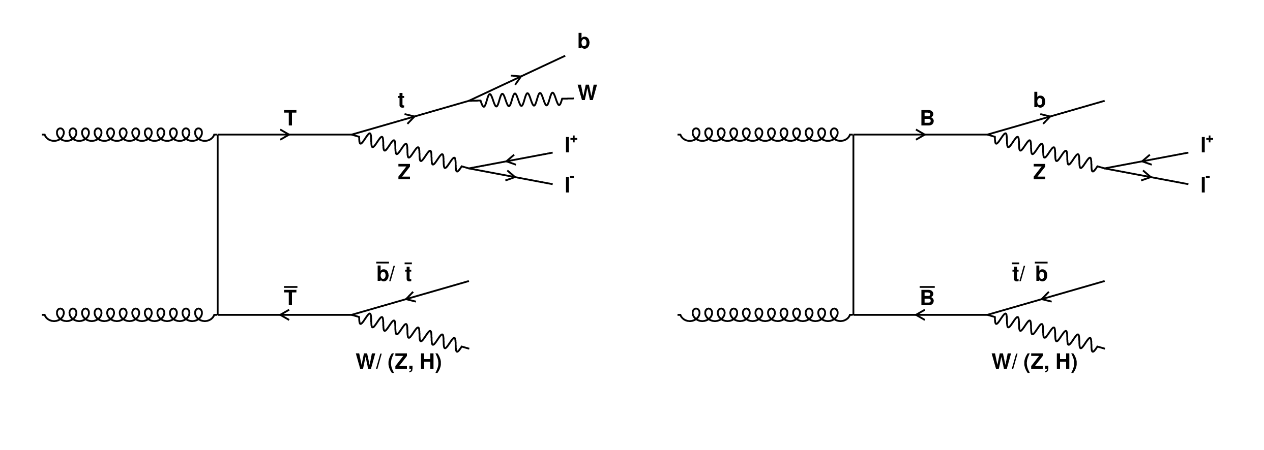
Figure 1:
Leading-order Feynman diagrams for the pair production and decay of T (left) and B (right) VLQs relevant to final states considered in this analysis. |
png pdf |
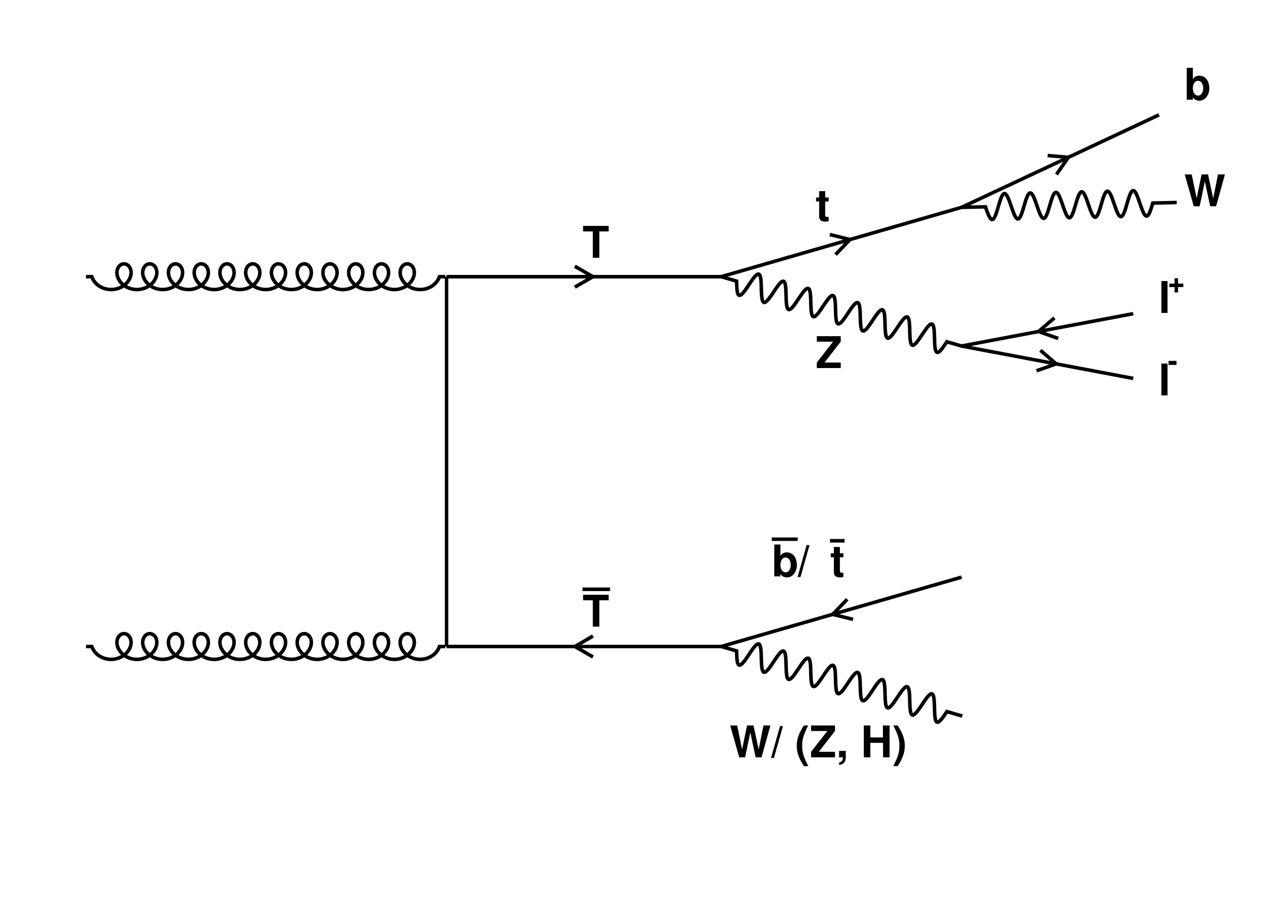
Figure 1-a:
Leading-order Feynman diagrams for the pair production and decay of T (left) and B (right) VLQs relevant to final states considered in this analysis. |
png pdf |
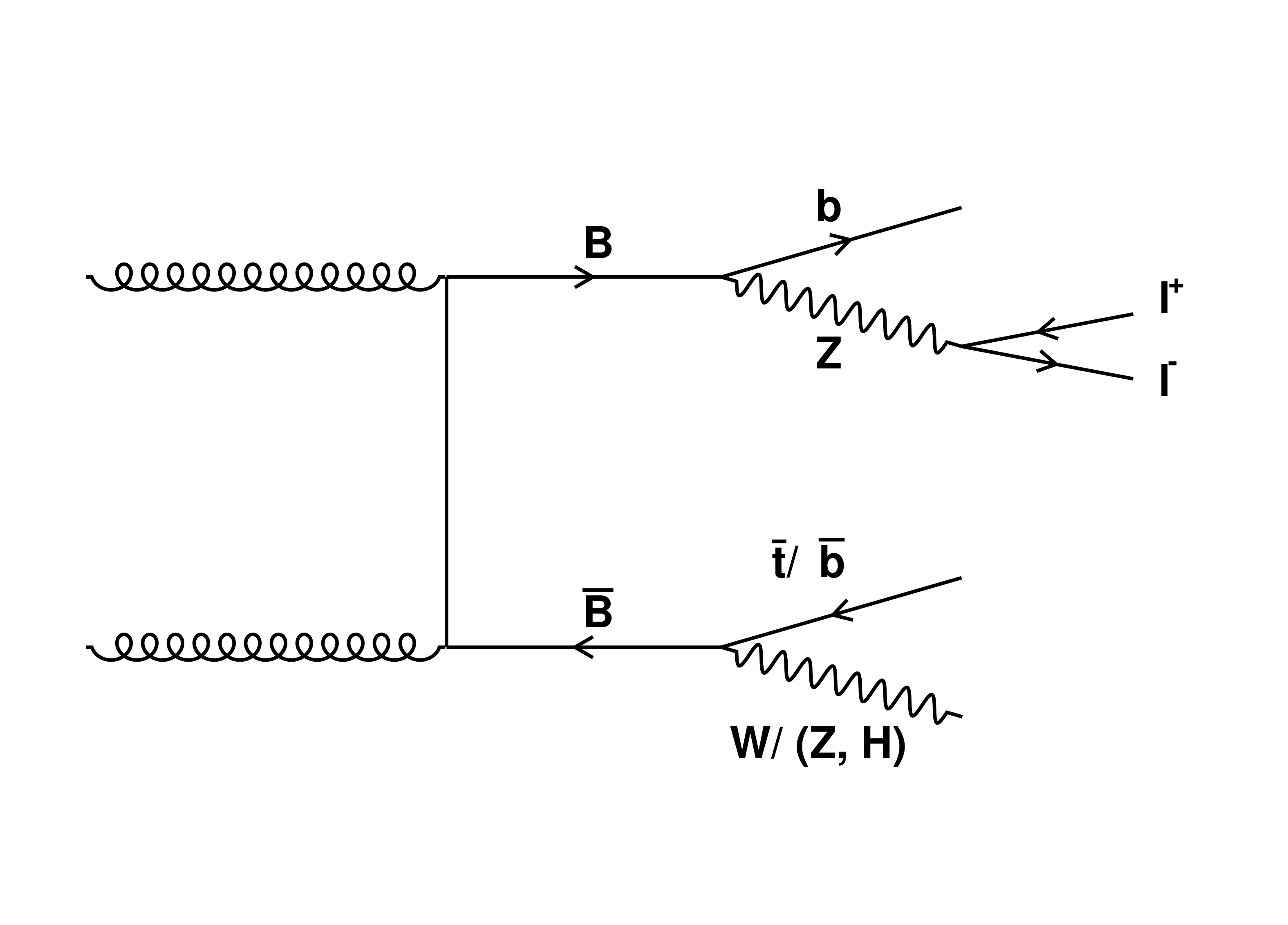
Figure 1-b:
Leading-order Feynman diagrams for the pair production and decay of T (left) and B (right) VLQs relevant to final states considered in this analysis. |
png pdf |
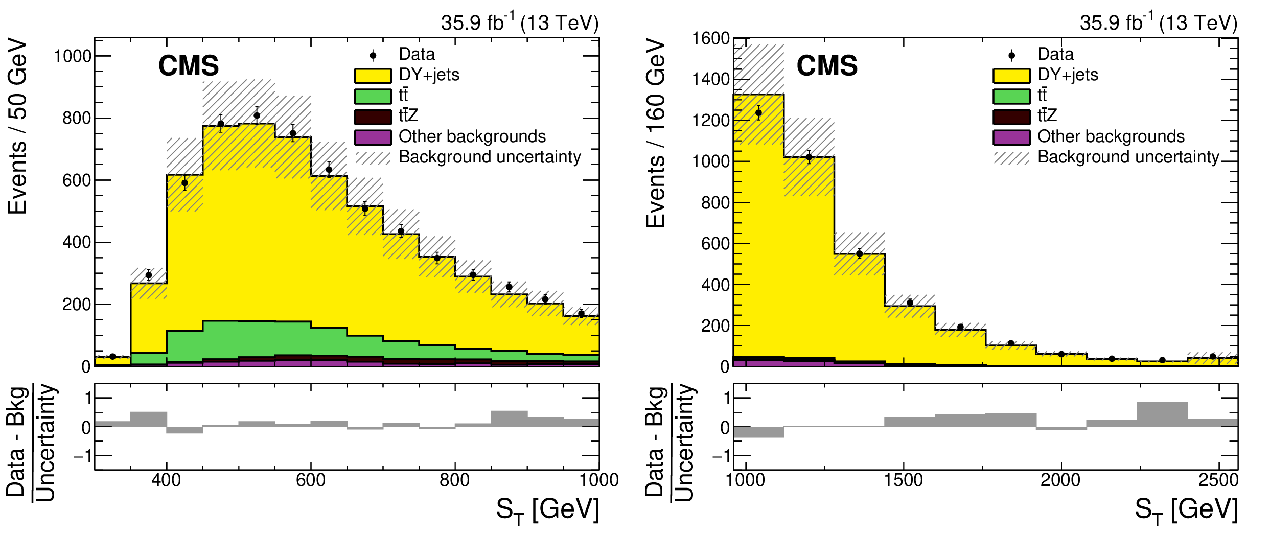
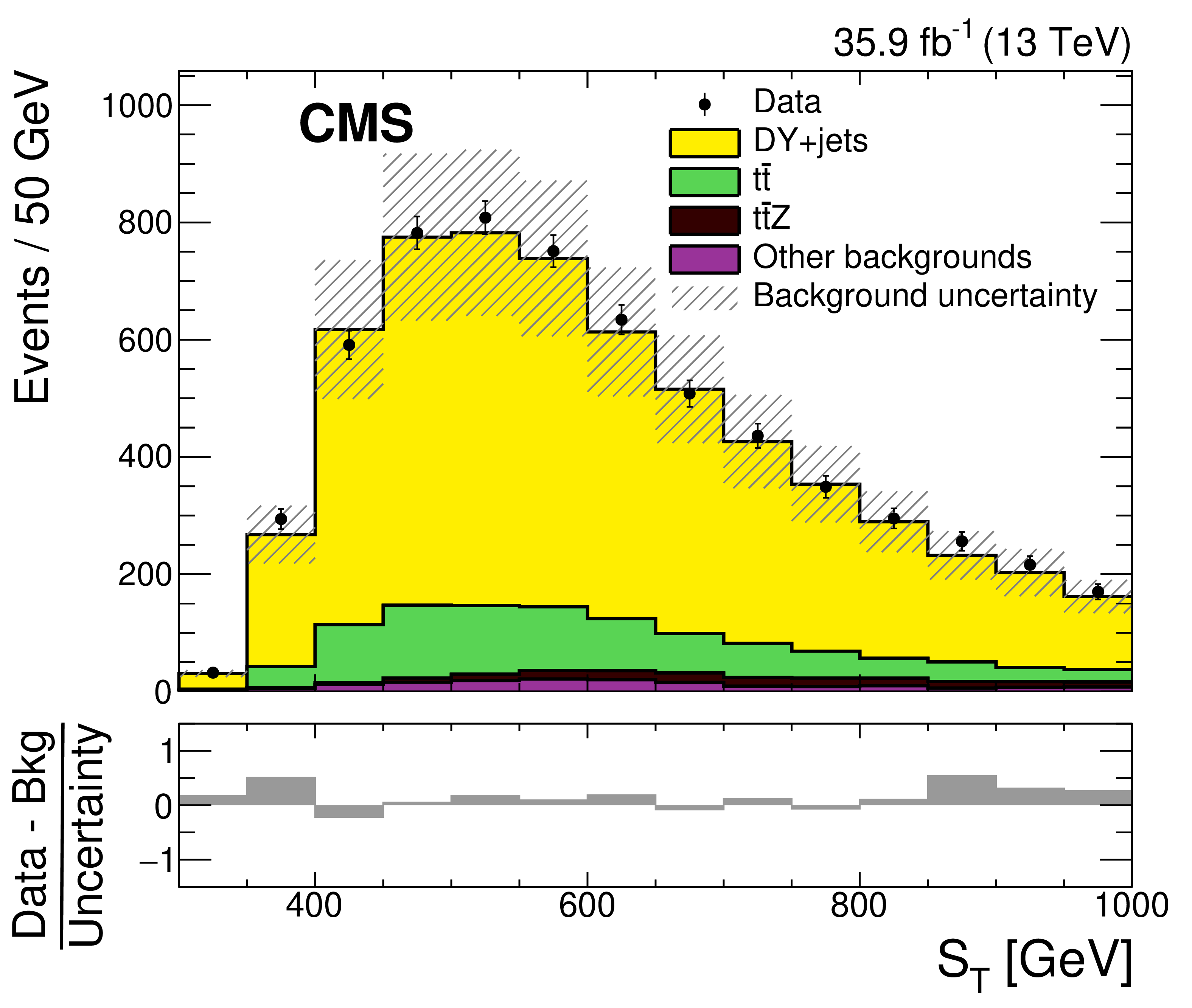
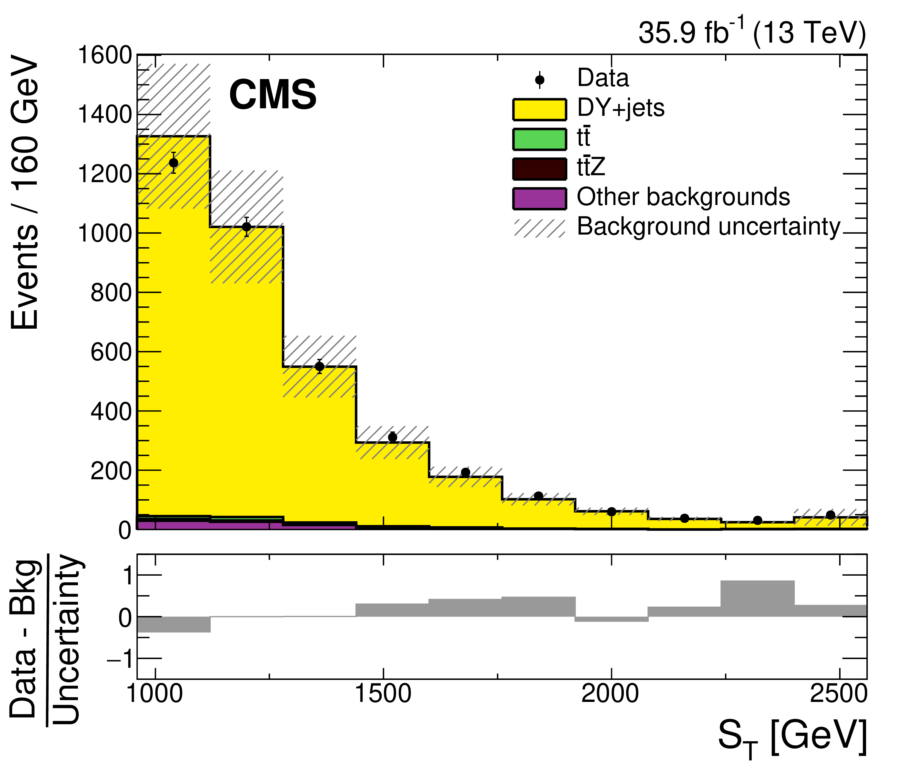
Figure 2:
The ${S_{\mathrm {T}}}$ distributions for the CR1 b+low-${S_{\mathrm {T}}}$ (left) and CR0 b+high-${S_{\mathrm {T}}}$ (right) control regions for the data (points) and the background simulations (shaded histograms) after applying the scale factors given in Table xxxxx. The vertical bars on the points represent the statistical uncertainties in the data. The hatched bands indicate the total uncertainties in the simulated background contributions added in quadrature. The lower plots show the difference between the data and the simulated background, divided by the total uncertainty. |
png pdf |
Figure 2-a:
The ${S_{\mathrm {T}}}$ distributions for the CR1 b+low-${S_{\mathrm {T}}}$ (left) and CR0 b+high-${S_{\mathrm {T}}}$ (right) control regions for the data (points) and the background simulations (shaded histograms) after applying the scale factors given in Table xxxxx. The vertical bars on the points represent the statistical uncertainties in the data. The hatched bands indicate the total uncertainties in the simulated background contributions added in quadrature. The lower plots show the difference between the data and the simulated background, divided by the total uncertainty. |
png pdf |
Figure 2-b:
The ${S_{\mathrm {T}}}$ distributions for the CR1 b+low-${S_{\mathrm {T}}}$ (left) and CR0 b+high-${S_{\mathrm {T}}}$ (right) control regions for the data (points) and the background simulations (shaded histograms) after applying the scale factors given in Table xxxxx. The vertical bars on the points represent the statistical uncertainties in the data. The hatched bands indicate the total uncertainties in the simulated background contributions added in quadrature. The lower plots show the difference between the data and the simulated background, divided by the total uncertainty. |
png pdf |
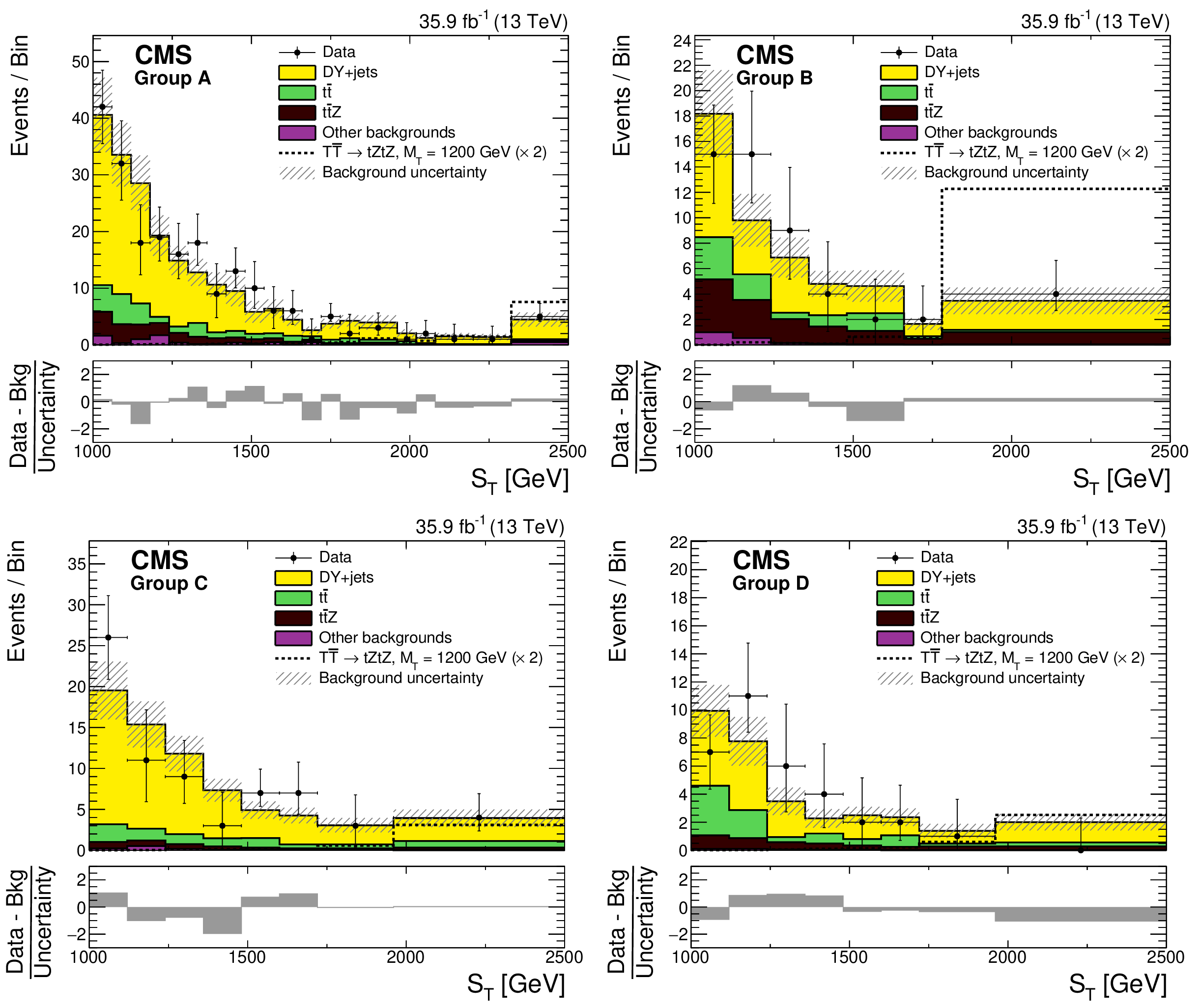
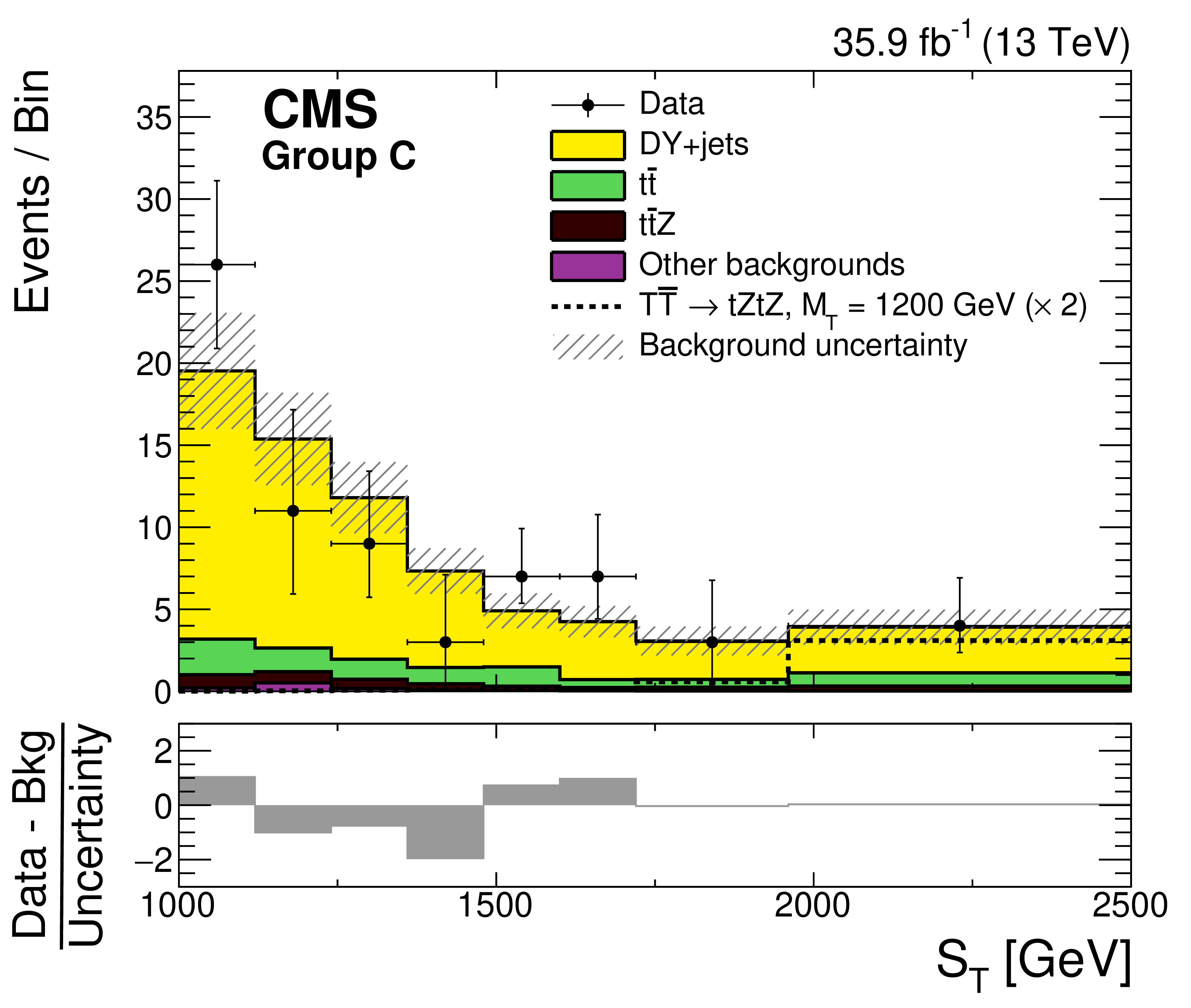
Figure 3:
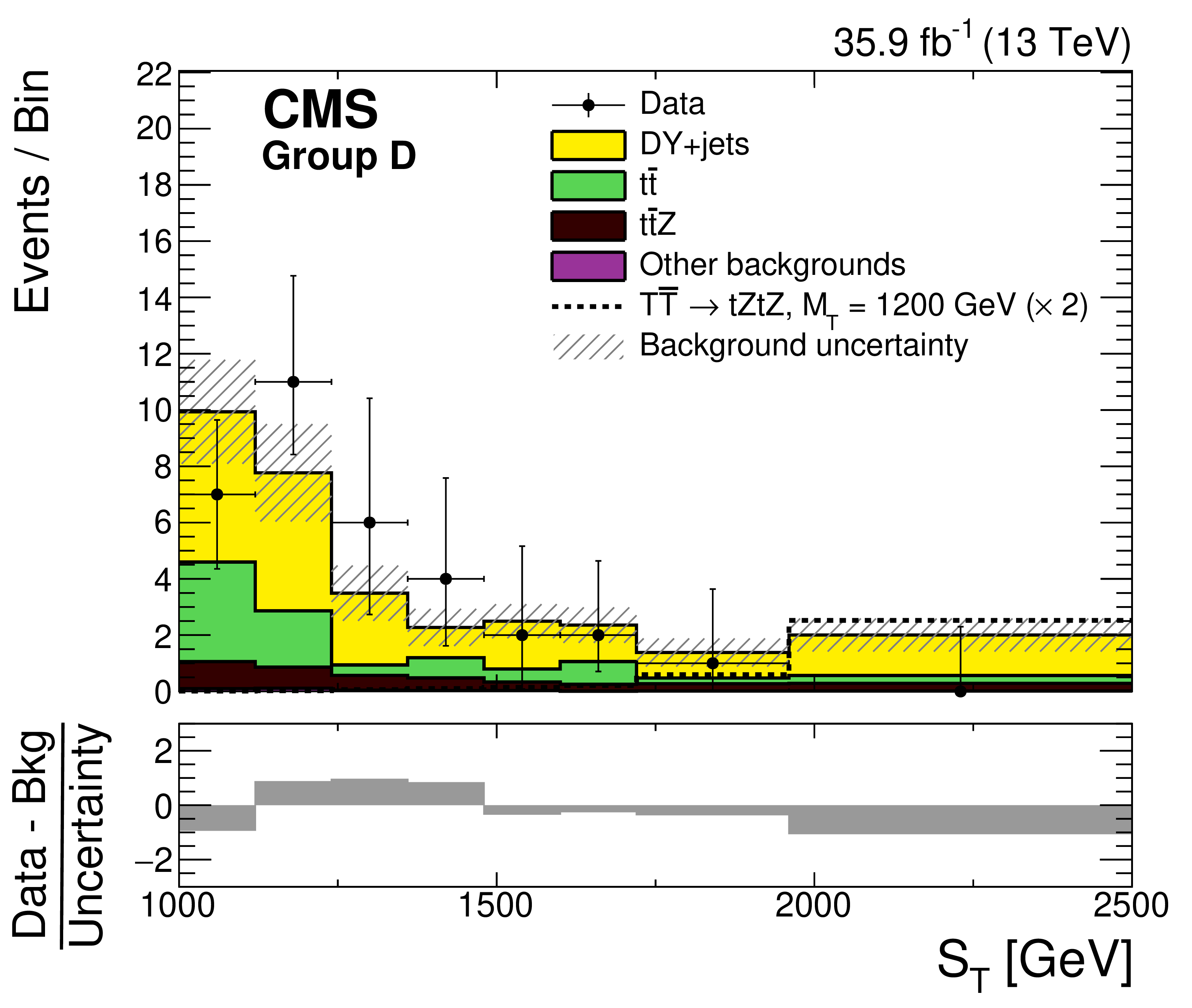
The ${S_{\mathrm {T}}}$ distributions for groups A, B, C, D (left to right, upper to lower) from data (points with vertical and horizontal bars), the expected SM backgrounds (shaded histograms), and the expected signal, scaled up by a factor 2, for $ {{{\mathrm {T}}} {\overline {{\mathrm {T}}}} \to {\mathrm {t}} {\mathrm {Z}} {\mathrm {t}} {\mathrm {Z}}} $ with $m_{{\mathrm {T}}} = $ 1200 GeV (dotted lines). The vertical bars on the points show the central 68% CL intervals for Poisson-distributed data. The horizontal bars give the bin widths. The hatched bands represent the statistical and systematic uncertainties in the total background contribution added in quadrature. The lower plots give the difference between the data and the total expected background, divided by the total background uncertainty. |

png pdf |
Figure 3-a:
The ${S_{\mathrm {T}}}$ distributions for groups A, B, C, D (left to right, upper to lower) from data (points with vertical and horizontal bars), the expected SM backgrounds (shaded histograms), and the expected signal, scaled up by a factor 2, for $ {{{\mathrm {T}}} {\overline {{\mathrm {T}}}} \to {\mathrm {t}} {\mathrm {Z}} {\mathrm {t}} {\mathrm {Z}}} $ with $m_{{\mathrm {T}}} = $ 1200 GeV (dotted lines). The vertical bars on the points show the central 68% CL intervals for Poisson-distributed data. The horizontal bars give the bin widths. The hatched bands represent the statistical and systematic uncertainties in the total background contribution added in quadrature. The lower plots give the difference between the data and the total expected background, divided by the total background uncertainty. |

png pdf |
Figure 3-b:
The ${S_{\mathrm {T}}}$ distributions for groups A, B, C, D (left to right, upper to lower) from data (points with vertical and horizontal bars), the expected SM backgrounds (shaded histograms), and the expected signal, scaled up by a factor 2, for $ {{{\mathrm {T}}} {\overline {{\mathrm {T}}}} \to {\mathrm {t}} {\mathrm {Z}} {\mathrm {t}} {\mathrm {Z}}} $ with $m_{{\mathrm {T}}} = $ 1200 GeV (dotted lines). The vertical bars on the points show the central 68% CL intervals for Poisson-distributed data. The horizontal bars give the bin widths. The hatched bands represent the statistical and systematic uncertainties in the total background contribution added in quadrature. The lower plots give the difference between the data and the total expected background, divided by the total background uncertainty. |
png pdf |
Figure 3-c:
The ${S_{\mathrm {T}}}$ distributions for groups A, B, C, D (left to right, upper to lower) from data (points with vertical and horizontal bars), the expected SM backgrounds (shaded histograms), and the expected signal, scaled up by a factor 2, for $ {{{\mathrm {T}}} {\overline {{\mathrm {T}}}} \to {\mathrm {t}} {\mathrm {Z}} {\mathrm {t}} {\mathrm {Z}}} $ with $m_{{\mathrm {T}}} = $ 1200 GeV (dotted lines). The vertical bars on the points show the central 68% CL intervals for Poisson-distributed data. The horizontal bars give the bin widths. The hatched bands represent the statistical and systematic uncertainties in the total background contribution added in quadrature. The lower plots give the difference between the data and the total expected background, divided by the total background uncertainty. |
png pdf |
Figure 3-d:
The ${S_{\mathrm {T}}}$ distributions for groups A, B, C, D (left to right, upper to lower) from data (points with vertical and horizontal bars), the expected SM backgrounds (shaded histograms), and the expected signal, scaled up by a factor 2, for $ {{{\mathrm {T}}} {\overline {{\mathrm {T}}}} \to {\mathrm {t}} {\mathrm {Z}} {\mathrm {t}} {\mathrm {Z}}} $ with $m_{{\mathrm {T}}} = $ 1200 GeV (dotted lines). The vertical bars on the points show the central 68% CL intervals for Poisson-distributed data. The horizontal bars give the bin widths. The hatched bands represent the statistical and systematic uncertainties in the total background contribution added in quadrature. The lower plots give the difference between the data and the total expected background, divided by the total background uncertainty. |
png pdf |
Figure 4:
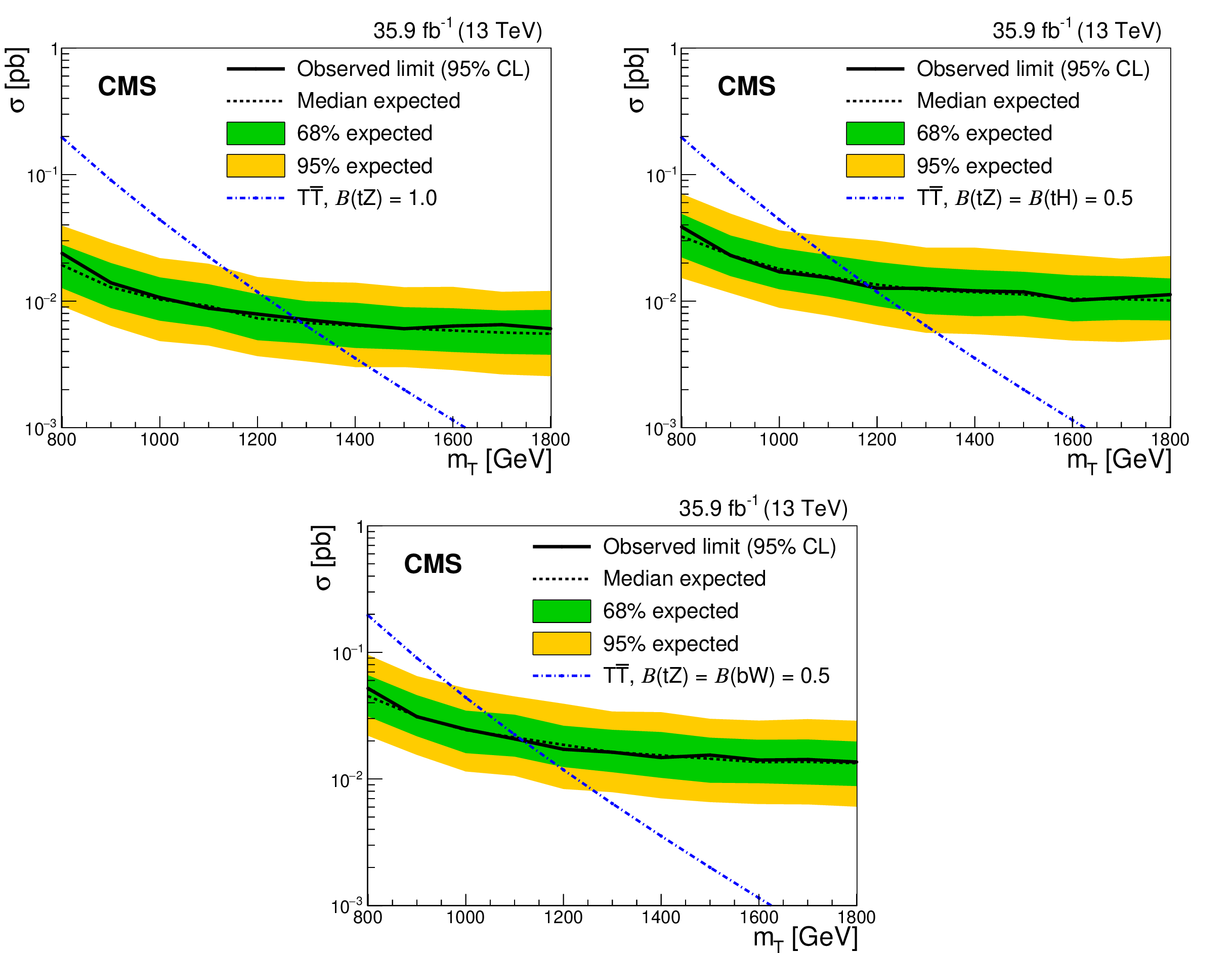
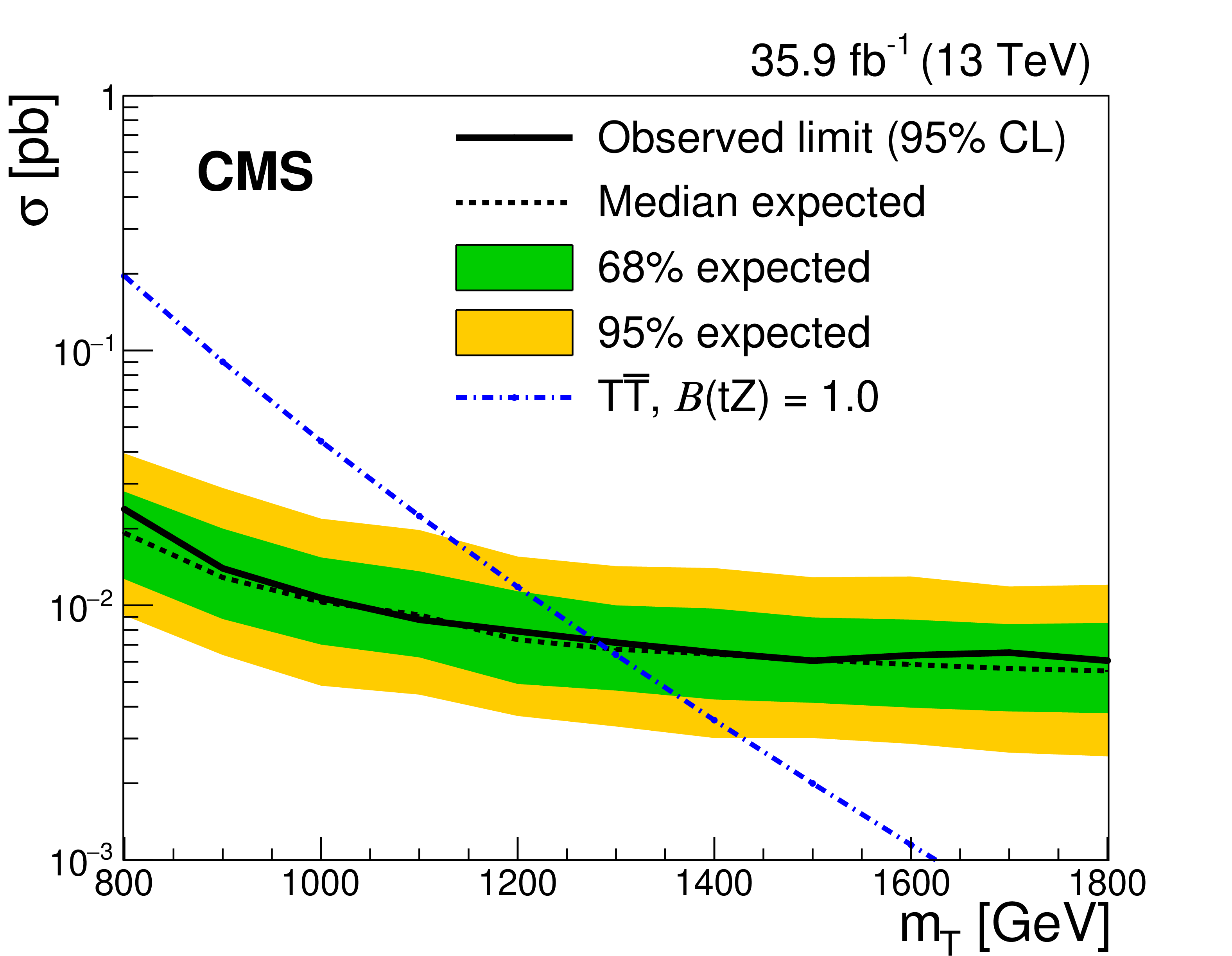
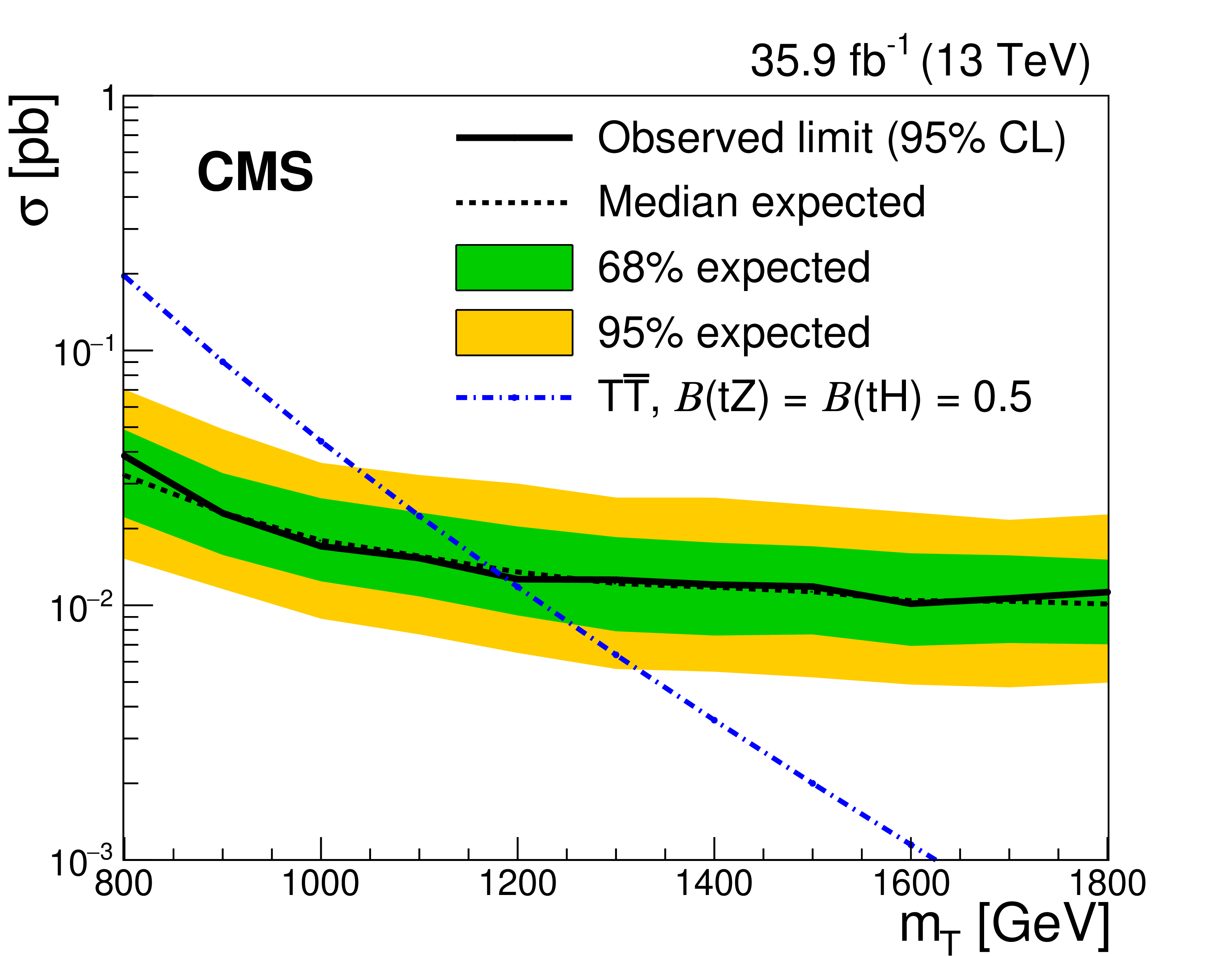
The observed (solid line) and expected (dashed line) 95% CL upper limits on the $ {{\mathrm {T}}} {\overline {{\mathrm {T}}}} $ cross section as a function of the T quark mass assuming (upper left) $\mathcal {B} ({{\mathrm {T}} \to {\mathrm {t}} {\mathrm {Z}}}) = $ 100%, (upper right) $\mathcal {B} ({{\mathrm {T}} \to {\mathrm {t}} {\mathrm {Z}}}) = \mathcal {B} ({{\mathrm {T}} \to {\mathrm {t}} {\mathrm {H}}}) = $ 50%, and (lower) $\mathcal {B} ({{\mathrm {T}} \to {\mathrm {t}} {\mathrm {Z}}}) = \mathcal {B} ({{\mathrm {T}} \to {\mathrm {b}} {\mathrm {W}}}) = $ 50%. The dotted-dashed curve displays the theoretical $ {{\mathrm {T}}} {\overline {{\mathrm {T}}}} $ production cross section. The inner and outer bands show the one and two standard deviation uncertainties in the expected limits, respectively. |
png pdf |
Figure 4-a:
The observed (solid line) and expected (dashed line) 95% CL upper limits on the $ {{\mathrm {T}}} {\overline {{\mathrm {T}}}} $ cross section as a function of the T quark mass assuming (upper left) $\mathcal {B} ({{\mathrm {T}} \to {\mathrm {t}} {\mathrm {Z}}}) = $ 100%, (upper right) $\mathcal {B} ({{\mathrm {T}} \to {\mathrm {t}} {\mathrm {Z}}}) = \mathcal {B} ({{\mathrm {T}} \to {\mathrm {t}} {\mathrm {H}}}) = $ 50%, and (lower) $\mathcal {B} ({{\mathrm {T}} \to {\mathrm {t}} {\mathrm {Z}}}) = \mathcal {B} ({{\mathrm {T}} \to {\mathrm {b}} {\mathrm {W}}}) = $ 50%. The dotted-dashed curve displays the theoretical $ {{\mathrm {T}}} {\overline {{\mathrm {T}}}} $ production cross section. The inner and outer bands show the one and two standard deviation uncertainties in the expected limits, respectively. |
png pdf |
Figure 4-b:
The observed (solid line) and expected (dashed line) 95% CL upper limits on the $ {{\mathrm {T}}} {\overline {{\mathrm {T}}}} $ cross section as a function of the T quark mass assuming (upper left) $\mathcal {B} ({{\mathrm {T}} \to {\mathrm {t}} {\mathrm {Z}}}) = $ 100%, (upper right) $\mathcal {B} ({{\mathrm {T}} \to {\mathrm {t}} {\mathrm {Z}}}) = \mathcal {B} ({{\mathrm {T}} \to {\mathrm {t}} {\mathrm {H}}}) = $ 50%, and (lower) $\mathcal {B} ({{\mathrm {T}} \to {\mathrm {t}} {\mathrm {Z}}}) = \mathcal {B} ({{\mathrm {T}} \to {\mathrm {b}} {\mathrm {W}}}) = $ 50%. The dotted-dashed curve displays the theoretical $ {{\mathrm {T}}} {\overline {{\mathrm {T}}}} $ production cross section. The inner and outer bands show the one and two standard deviation uncertainties in the expected limits, respectively. |

png pdf |
Figure 4-c:
The observed (solid line) and expected (dashed line) 95% CL upper limits on the $ {{\mathrm {T}}} {\overline {{\mathrm {T}}}} $ cross section as a function of the T quark mass assuming (upper left) $\mathcal {B} ({{\mathrm {T}} \to {\mathrm {t}} {\mathrm {Z}}}) = $ 100%, (upper right) $\mathcal {B} ({{\mathrm {T}} \to {\mathrm {t}} {\mathrm {Z}}}) = \mathcal {B} ({{\mathrm {T}} \to {\mathrm {t}} {\mathrm {H}}}) = $ 50%, and (lower) $\mathcal {B} ({{\mathrm {T}} \to {\mathrm {t}} {\mathrm {Z}}}) = \mathcal {B} ({{\mathrm {T}} \to {\mathrm {b}} {\mathrm {W}}}) = $ 50%. The dotted-dashed curve displays the theoretical $ {{\mathrm {T}}} {\overline {{\mathrm {T}}}} $ production cross section. The inner and outer bands show the one and two standard deviation uncertainties in the expected limits, respectively. |
png pdf |
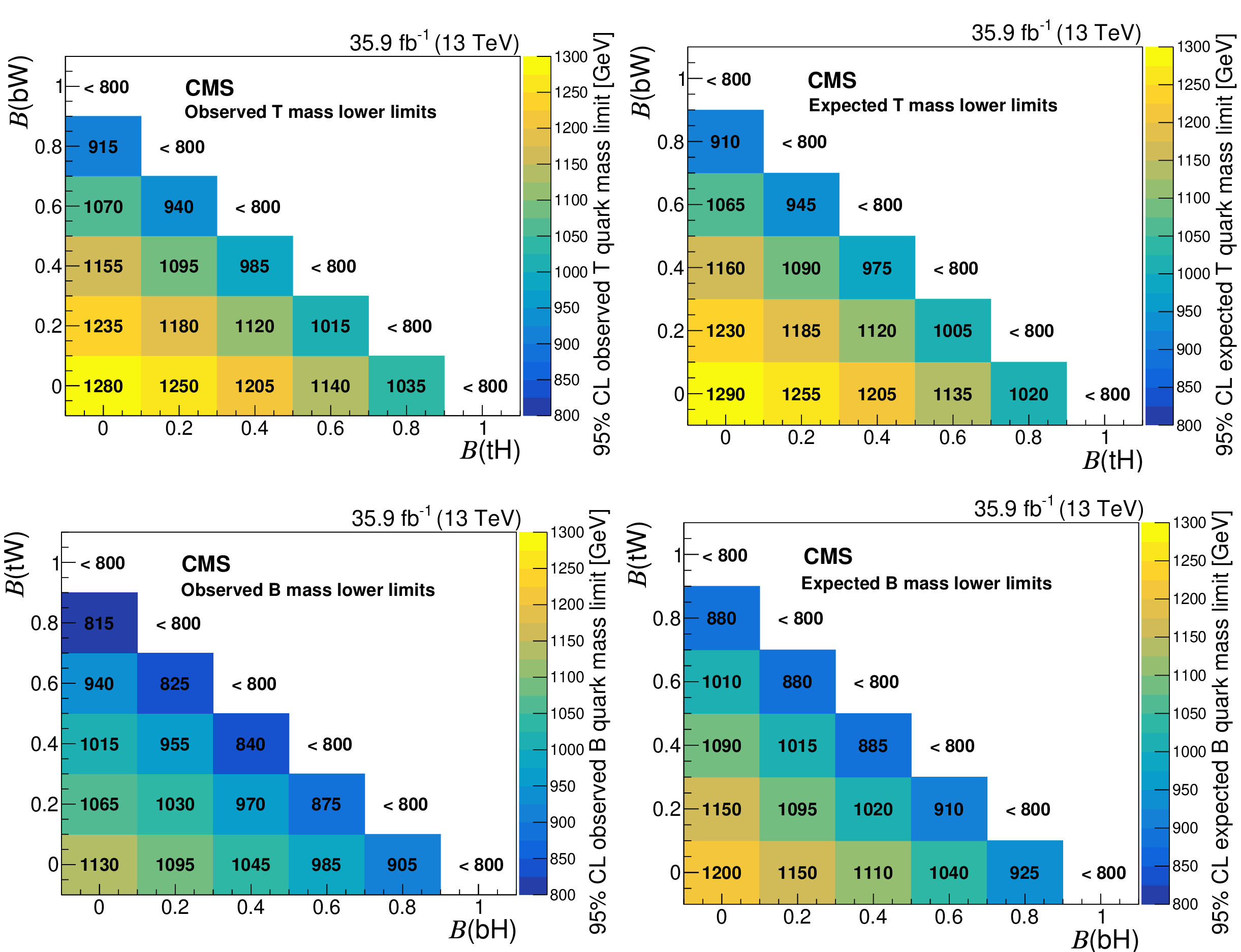
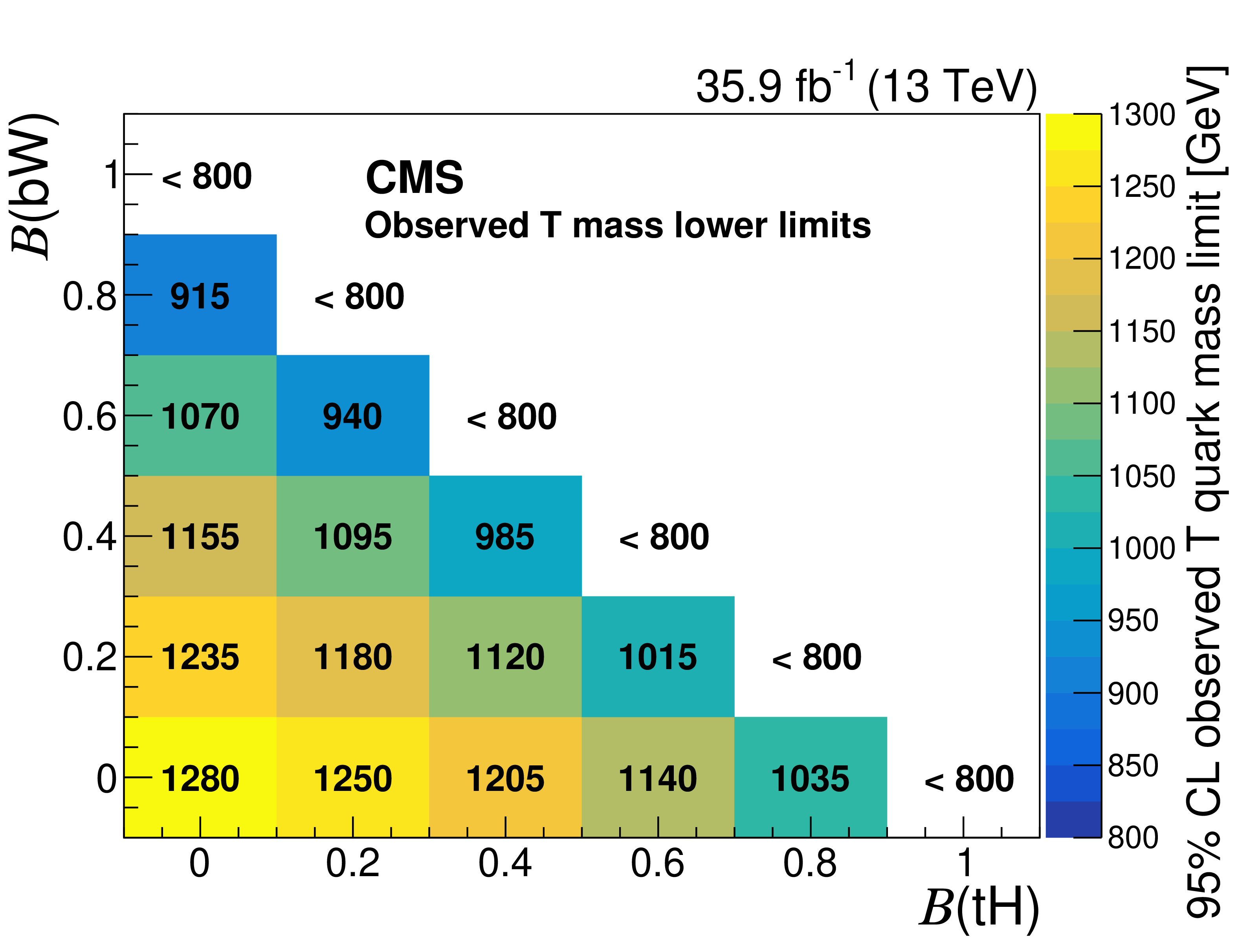
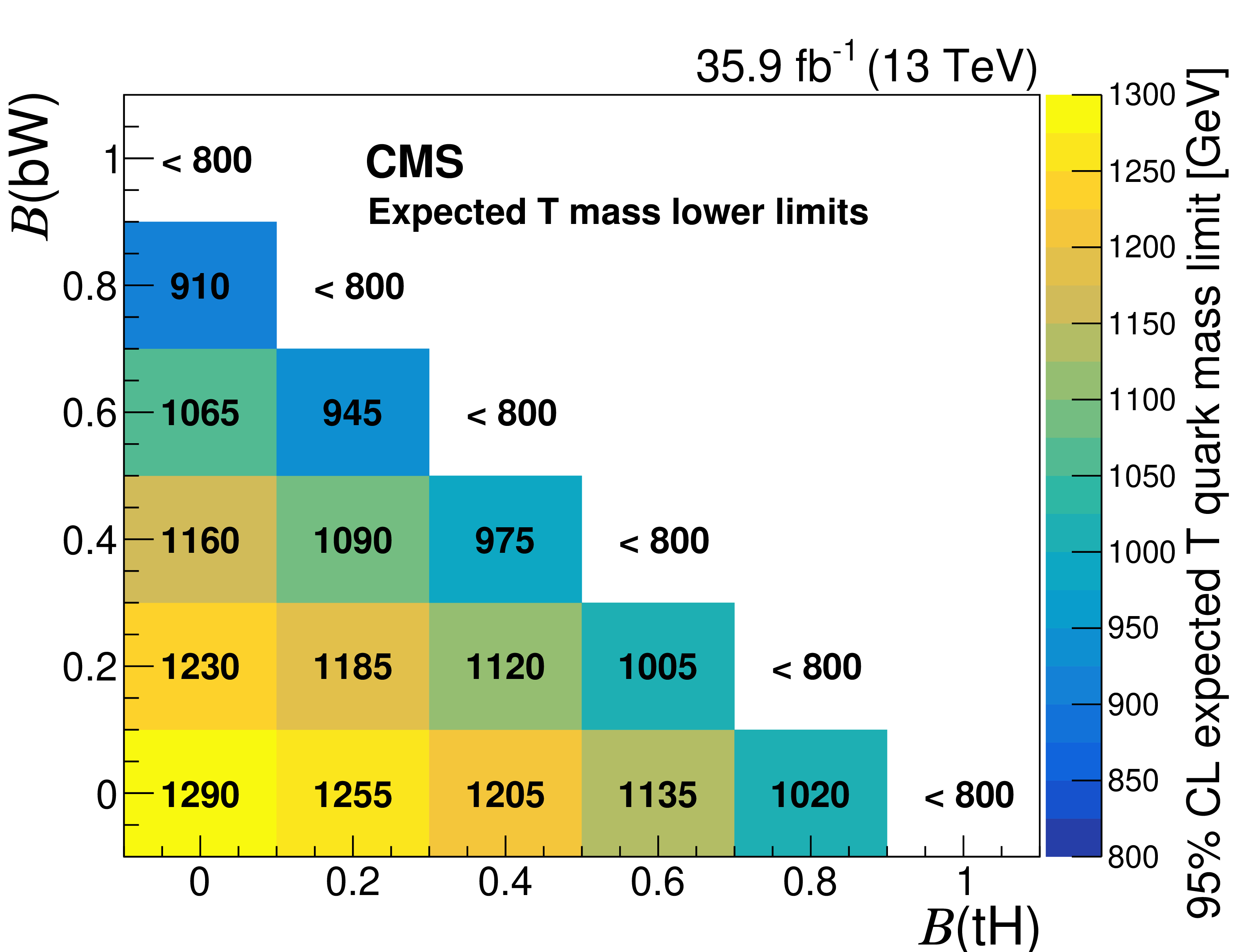
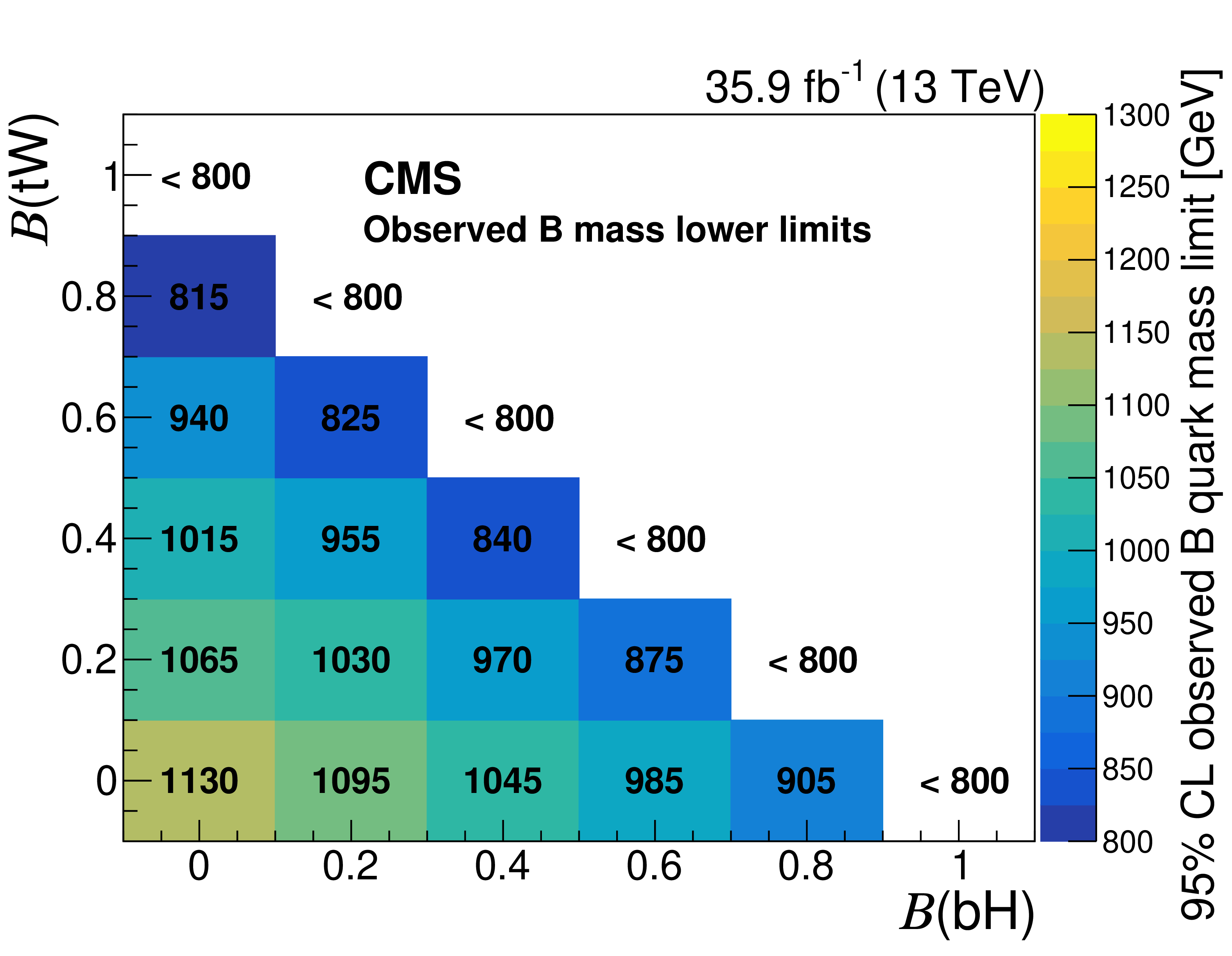
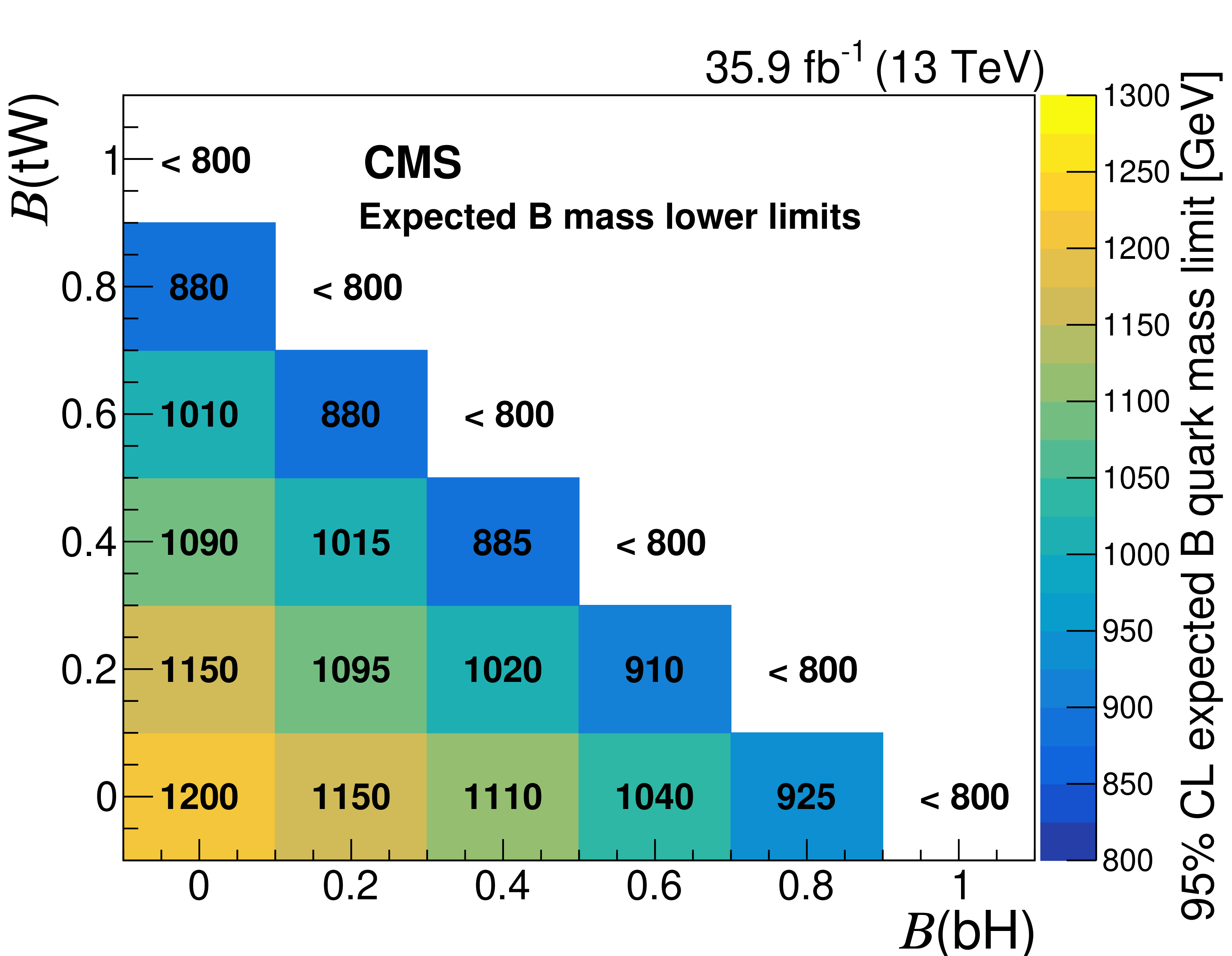
Figure 5:
The observed (left) and expected (right) 95% CL lower limits on the mass of the T (upper) and B (lower) quark, in GeV, for various branching fraction scenarios, assuming $\mathcal {B} ({{\mathrm {T}} \to {\mathrm {t}} {\mathrm {Z}}}) + \mathcal {B} ({{\mathrm {T}} \to {\mathrm {t}} {\mathrm {H}}}) + \mathcal {B} ({{\mathrm {T}} \to {\mathrm {b}} {\mathrm {W}}}) = $ 1 and $\mathcal {B} ({{\mathrm {B}} \to {\mathrm {b}} {\mathrm {Z}}}) + \mathcal {B} ({{\mathrm {B}} \to {\mathrm {b}} {\mathrm {H}}}) + \mathcal {B} ({{\mathrm {B}} \to {\mathrm {t}} {\mathrm {W}}}) = $ 1, respectively. |
png pdf |
Figure 5-a:
The observed (left) and expected (right) 95% CL lower limits on the mass of the T (upper) and B (lower) quark, in GeV, for various branching fraction scenarios, assuming $\mathcal {B} ({{\mathrm {T}} \to {\mathrm {t}} {\mathrm {Z}}}) + \mathcal {B} ({{\mathrm {T}} \to {\mathrm {t}} {\mathrm {H}}}) + \mathcal {B} ({{\mathrm {T}} \to {\mathrm {b}} {\mathrm {W}}}) = $ 1 and $\mathcal {B} ({{\mathrm {B}} \to {\mathrm {b}} {\mathrm {Z}}}) + \mathcal {B} ({{\mathrm {B}} \to {\mathrm {b}} {\mathrm {H}}}) + \mathcal {B} ({{\mathrm {B}} \to {\mathrm {t}} {\mathrm {W}}}) = $ 1, respectively. |
png pdf |
Figure 5-b:
The observed (left) and expected (right) 95% CL lower limits on the mass of the T (upper) and B (lower) quark, in GeV, for various branching fraction scenarios, assuming $\mathcal {B} ({{\mathrm {T}} \to {\mathrm {t}} {\mathrm {Z}}}) + \mathcal {B} ({{\mathrm {T}} \to {\mathrm {t}} {\mathrm {H}}}) + \mathcal {B} ({{\mathrm {T}} \to {\mathrm {b}} {\mathrm {W}}}) = $ 1 and $\mathcal {B} ({{\mathrm {B}} \to {\mathrm {b}} {\mathrm {Z}}}) + \mathcal {B} ({{\mathrm {B}} \to {\mathrm {b}} {\mathrm {H}}}) + \mathcal {B} ({{\mathrm {B}} \to {\mathrm {t}} {\mathrm {W}}}) = $ 1, respectively. |
png pdf |
Figure 5-c:
The observed (left) and expected (right) 95% CL lower limits on the mass of the T (upper) and B (lower) quark, in GeV, for various branching fraction scenarios, assuming $\mathcal {B} ({{\mathrm {T}} \to {\mathrm {t}} {\mathrm {Z}}}) + \mathcal {B} ({{\mathrm {T}} \to {\mathrm {t}} {\mathrm {H}}}) + \mathcal {B} ({{\mathrm {T}} \to {\mathrm {b}} {\mathrm {W}}}) = $ 1 and $\mathcal {B} ({{\mathrm {B}} \to {\mathrm {b}} {\mathrm {Z}}}) + \mathcal {B} ({{\mathrm {B}} \to {\mathrm {b}} {\mathrm {H}}}) + \mathcal {B} ({{\mathrm {B}} \to {\mathrm {t}} {\mathrm {W}}}) = $ 1, respectively. |
png pdf |
Figure 5-d:
The observed (left) and expected (right) 95% CL lower limits on the mass of the T (upper) and B (lower) quark, in GeV, for various branching fraction scenarios, assuming $\mathcal {B} ({{\mathrm {T}} \to {\mathrm {t}} {\mathrm {Z}}}) + \mathcal {B} ({{\mathrm {T}} \to {\mathrm {t}} {\mathrm {H}}}) + \mathcal {B} ({{\mathrm {T}} \to {\mathrm {b}} {\mathrm {W}}}) = $ 1 and $\mathcal {B} ({{\mathrm {B}} \to {\mathrm {b}} {\mathrm {Z}}}) + \mathcal {B} ({{\mathrm {B}} \to {\mathrm {b}} {\mathrm {H}}}) + \mathcal {B} ({{\mathrm {B}} \to {\mathrm {t}} {\mathrm {W}}}) = $ 1, respectively. |
png pdf |
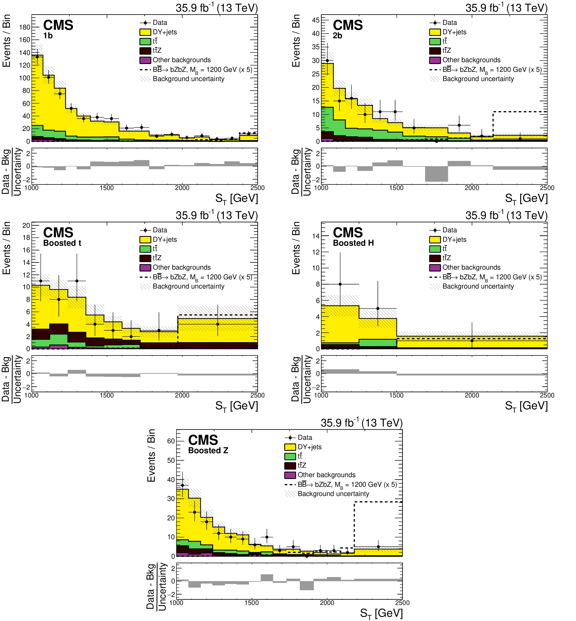
Figure 6:
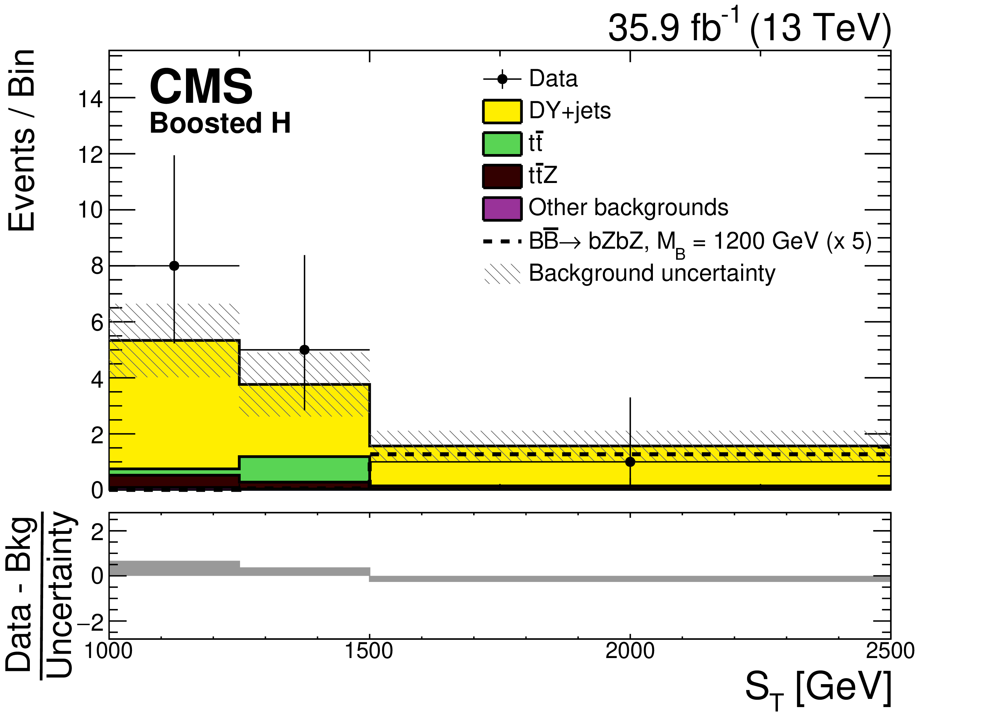
The ${S_{\mathrm {T}}}$ distributions for the 1 b, 2 b, boosted t, boosted H and boosted Z (left to right, upper to lower) event categories for the data (points with vertical and horizontal bars), and the expected background (shaded histograms). The vertical bars give the statistical uncertainty in the data, and the horizontal bars show the bin widths. The expected signal for $ {{{\mathrm {B}}} {\overline {{\mathrm {B}}}} \to {\mathrm {b}} {\mathrm {Z}} {\mathrm {b}} {\mathrm {Z}}} $ with $m_{{\mathrm {B}}} = $ 1200 GeV multiplied by a factor of 5 is shown by the dashed line. The statistical and systematic uncertainties in the SM background prediction, added in quadrature, are represented by the hatched bands. The lower panel in each plot show the difference between the data and the expected background, divided by the total uncertainty. |

png pdf |
Figure 6-a:
The ${S_{\mathrm {T}}}$ distributions for the 1 b, 2 b, boosted t, boosted H and boosted Z (left to right, upper to lower) event categories for the data (points with vertical and horizontal bars), and the expected background (shaded histograms). The vertical bars give the statistical uncertainty in the data, and the horizontal bars show the bin widths. The expected signal for $ {{{\mathrm {B}}} {\overline {{\mathrm {B}}}} \to {\mathrm {b}} {\mathrm {Z}} {\mathrm {b}} {\mathrm {Z}}} $ with $m_{{\mathrm {B}}} = $ 1200 GeV multiplied by a factor of 5 is shown by the dashed line. The statistical and systematic uncertainties in the SM background prediction, added in quadrature, are represented by the hatched bands. The lower panel in each plot show the difference between the data and the expected background, divided by the total uncertainty. |
png pdf |
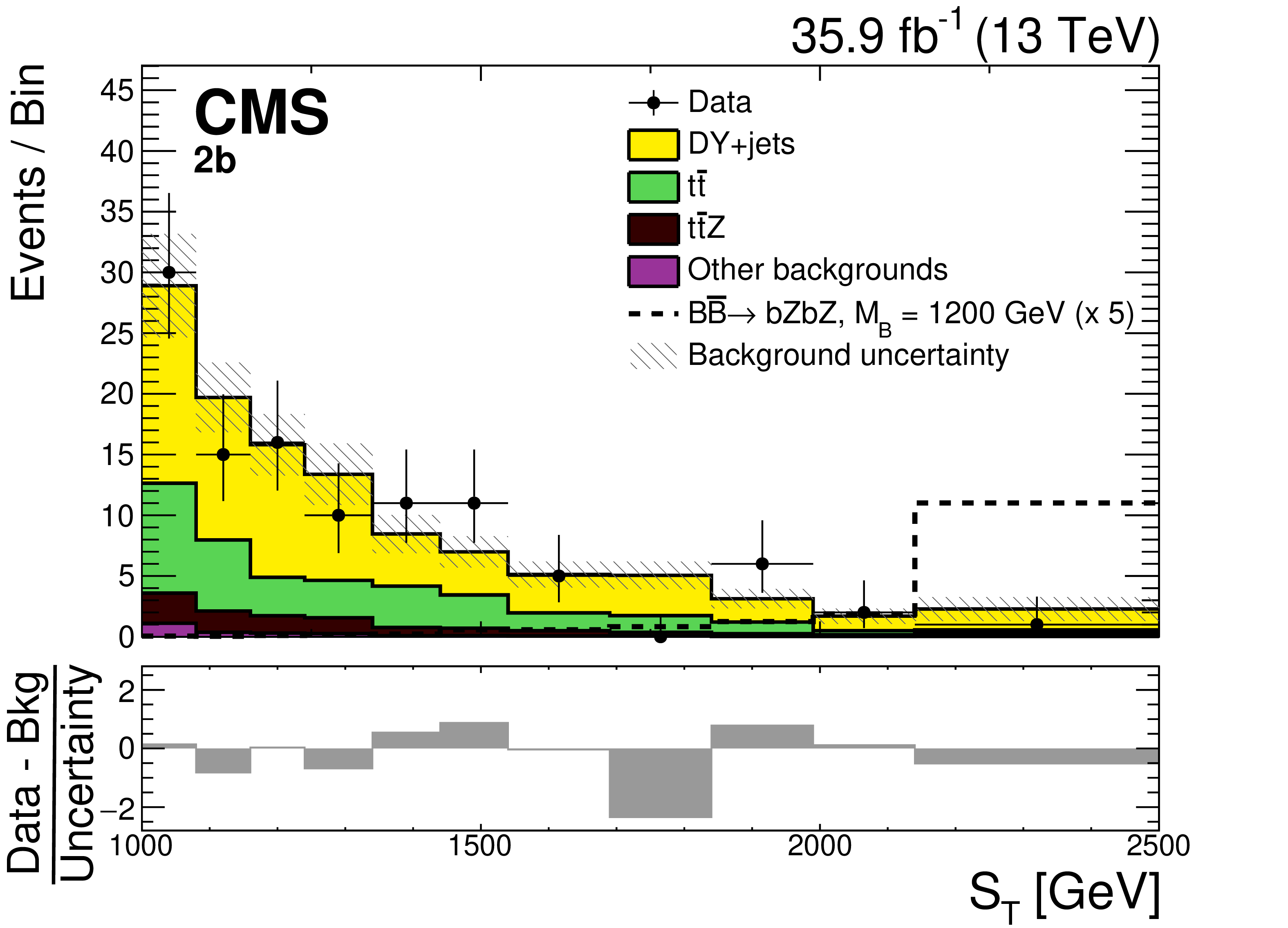
Figure 6-b:
The ${S_{\mathrm {T}}}$ distributions for the 1 b, 2 b, boosted t, boosted H and boosted Z (left to right, upper to lower) event categories for the data (points with vertical and horizontal bars), and the expected background (shaded histograms). The vertical bars give the statistical uncertainty in the data, and the horizontal bars show the bin widths. The expected signal for $ {{{\mathrm {B}}} {\overline {{\mathrm {B}}}} \to {\mathrm {b}} {\mathrm {Z}} {\mathrm {b}} {\mathrm {Z}}} $ with $m_{{\mathrm {B}}} = $ 1200 GeV multiplied by a factor of 5 is shown by the dashed line. The statistical and systematic uncertainties in the SM background prediction, added in quadrature, are represented by the hatched bands. The lower panel in each plot show the difference between the data and the expected background, divided by the total uncertainty. |
png pdf |
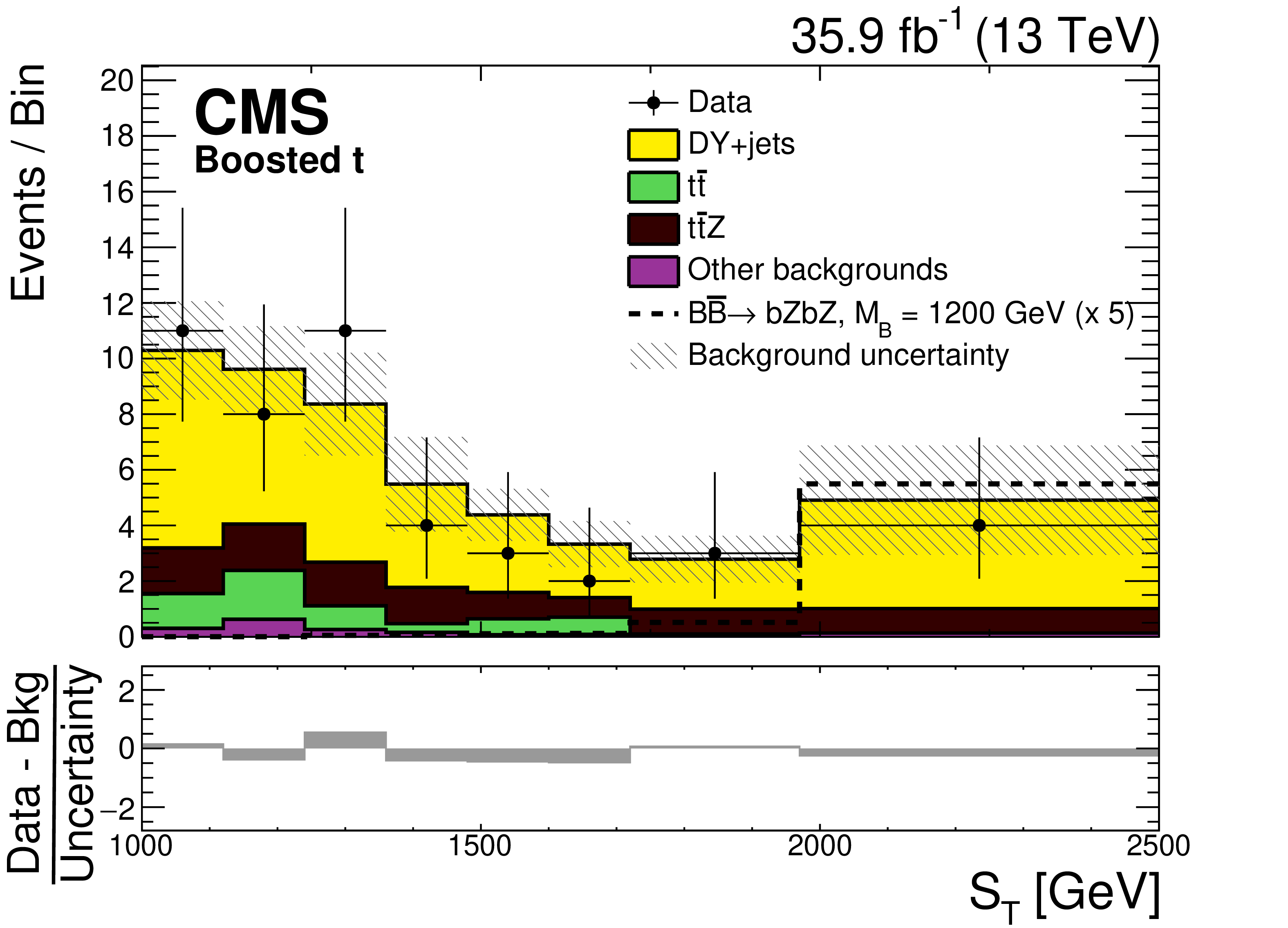
Figure 6-c:
The ${S_{\mathrm {T}}}$ distributions for the 1 b, 2 b, boosted t, boosted H and boosted Z (left to right, upper to lower) event categories for the data (points with vertical and horizontal bars), and the expected background (shaded histograms). The vertical bars give the statistical uncertainty in the data, and the horizontal bars show the bin widths. The expected signal for $ {{{\mathrm {B}}} {\overline {{\mathrm {B}}}} \to {\mathrm {b}} {\mathrm {Z}} {\mathrm {b}} {\mathrm {Z}}} $ with $m_{{\mathrm {B}}} = $ 1200 GeV multiplied by a factor of 5 is shown by the dashed line. The statistical and systematic uncertainties in the SM background prediction, added in quadrature, are represented by the hatched bands. The lower panel in each plot show the difference between the data and the expected background, divided by the total uncertainty. |
png pdf |
Figure 6-d:
The ${S_{\mathrm {T}}}$ distributions for the 1 b, 2 b, boosted t, boosted H and boosted Z (left to right, upper to lower) event categories for the data (points with vertical and horizontal bars), and the expected background (shaded histograms). The vertical bars give the statistical uncertainty in the data, and the horizontal bars show the bin widths. The expected signal for $ {{{\mathrm {B}}} {\overline {{\mathrm {B}}}} \to {\mathrm {b}} {\mathrm {Z}} {\mathrm {b}} {\mathrm {Z}}} $ with $m_{{\mathrm {B}}} = $ 1200 GeV multiplied by a factor of 5 is shown by the dashed line. The statistical and systematic uncertainties in the SM background prediction, added in quadrature, are represented by the hatched bands. The lower panel in each plot show the difference between the data and the expected background, divided by the total uncertainty. |

png pdf |
Figure 6-e:
The ${S_{\mathrm {T}}}$ distributions for the 1 b, 2 b, boosted t, boosted H and boosted Z (left to right, upper to lower) event categories for the data (points with vertical and horizontal bars), and the expected background (shaded histograms). The vertical bars give the statistical uncertainty in the data, and the horizontal bars show the bin widths. The expected signal for $ {{{\mathrm {B}}} {\overline {{\mathrm {B}}}} \to {\mathrm {b}} {\mathrm {Z}} {\mathrm {b}} {\mathrm {Z}}} $ with $m_{{\mathrm {B}}} = $ 1200 GeV multiplied by a factor of 5 is shown by the dashed line. The statistical and systematic uncertainties in the SM background prediction, added in quadrature, are represented by the hatched bands. The lower panel in each plot show the difference between the data and the expected background, divided by the total uncertainty. |
png pdf |
Figure 7:
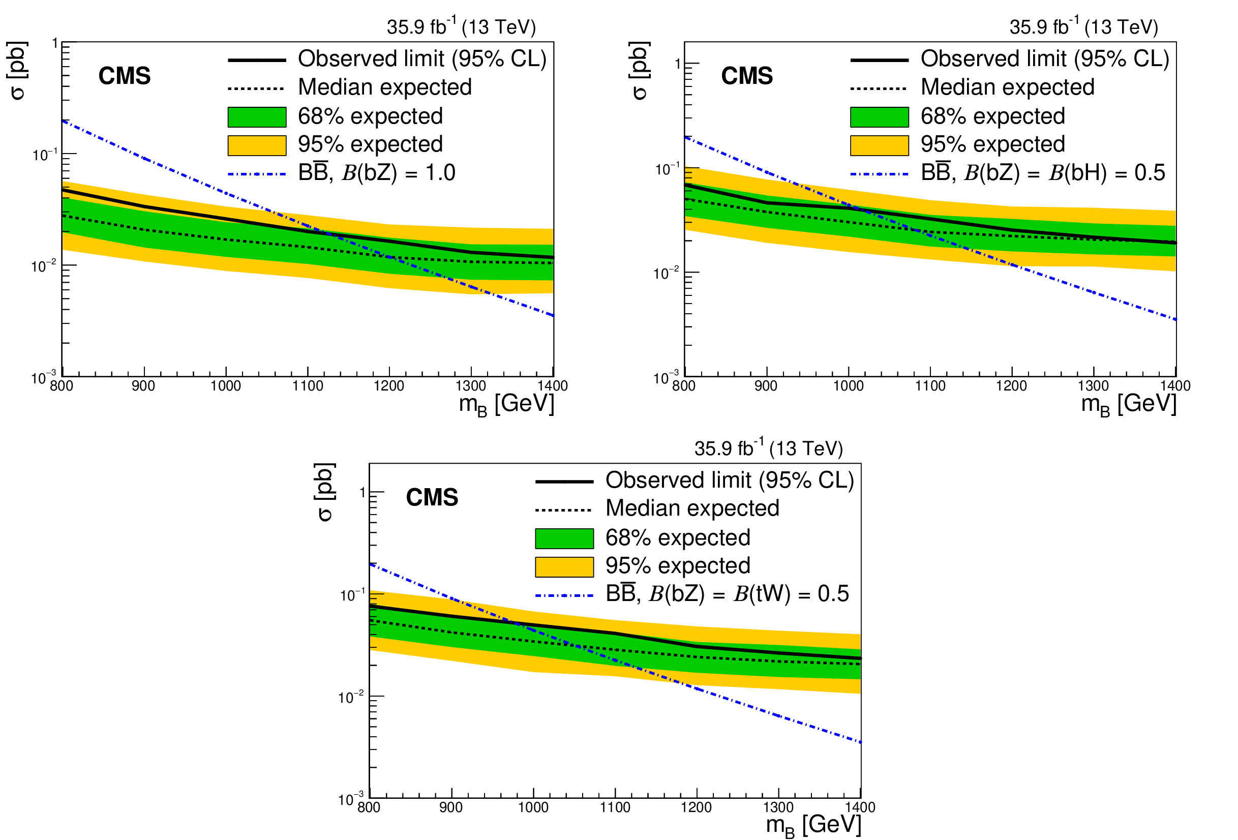
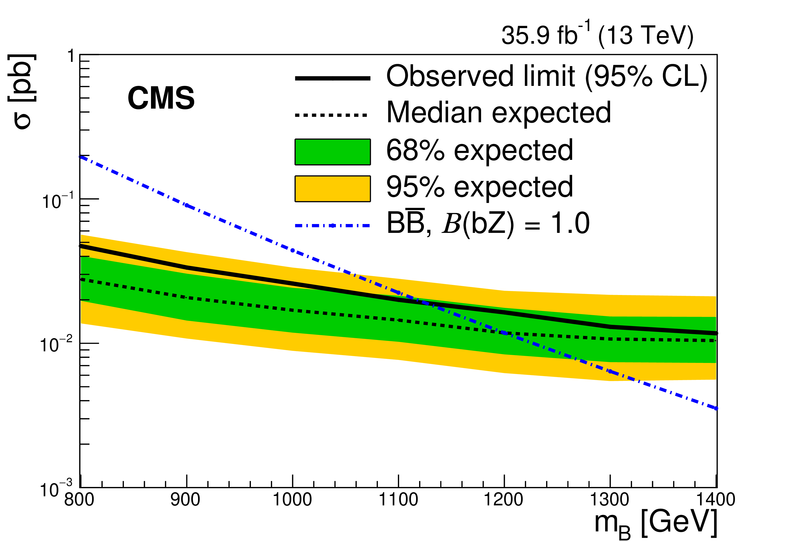
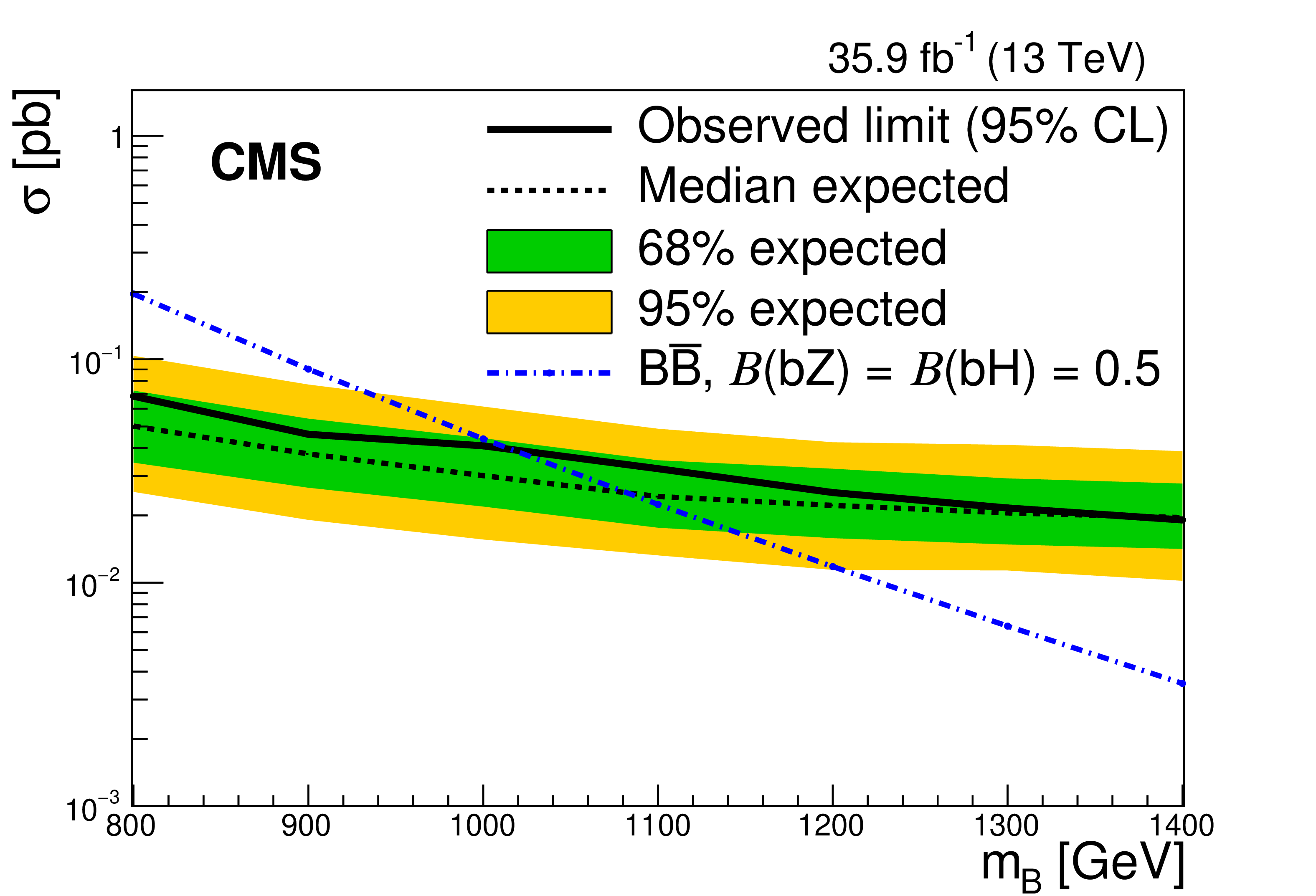
The observed (solid line) and expected (dashed line) 95% CL upper limits on the $ {{\mathrm {B}}} {\overline {{\mathrm {B}}}} $ production cross section versus the B quark mass for (upper left) $\mathcal {B} ({{\mathrm {B}} \to {\mathrm {b}} {\mathrm {Z}}}) = $ 100%, (upper right) $\mathcal {B} ({{\mathrm {B}} \to {\mathrm {b}} {\mathrm {Z}}}) = \mathcal {B} ({{\mathrm {B}} \to {\mathrm {b}} {\mathrm {H}}}) = $ 50%, and (lower) $\mathcal {B} ({{\mathrm {B}} \to {\mathrm {b}} {\mathrm {Z}}}) = \mathcal {B} ({{\mathrm {B}} \to {\mathrm {t}} {\mathrm {W}}}) = $ 50%. The dotted-dashed line displays the theoretical cross section. The inner and outer bands show the one and two standard deviation uncertainties in the expected limits, respectively. |
png pdf |
Figure 7-a:
The observed (solid line) and expected (dashed line) 95% CL upper limits on the $ {{\mathrm {B}}} {\overline {{\mathrm {B}}}} $ production cross section versus the B quark mass for (upper left) $\mathcal {B} ({{\mathrm {B}} \to {\mathrm {b}} {\mathrm {Z}}}) = $ 100%, (upper right) $\mathcal {B} ({{\mathrm {B}} \to {\mathrm {b}} {\mathrm {Z}}}) = \mathcal {B} ({{\mathrm {B}} \to {\mathrm {b}} {\mathrm {H}}}) = $ 50%, and (lower) $\mathcal {B} ({{\mathrm {B}} \to {\mathrm {b}} {\mathrm {Z}}}) = \mathcal {B} ({{\mathrm {B}} \to {\mathrm {t}} {\mathrm {W}}}) = $ 50%. The dotted-dashed line displays the theoretical cross section. The inner and outer bands show the one and two standard deviation uncertainties in the expected limits, respectively. |
png pdf |
Figure 7-b:
The observed (solid line) and expected (dashed line) 95% CL upper limits on the $ {{\mathrm {B}}} {\overline {{\mathrm {B}}}} $ production cross section versus the B quark mass for (upper left) $\mathcal {B} ({{\mathrm {B}} \to {\mathrm {b}} {\mathrm {Z}}}) = $ 100%, (upper right) $\mathcal {B} ({{\mathrm {B}} \to {\mathrm {b}} {\mathrm {Z}}}) = \mathcal {B} ({{\mathrm {B}} \to {\mathrm {b}} {\mathrm {H}}}) = $ 50%, and (lower) $\mathcal {B} ({{\mathrm {B}} \to {\mathrm {b}} {\mathrm {Z}}}) = \mathcal {B} ({{\mathrm {B}} \to {\mathrm {t}} {\mathrm {W}}}) = $ 50%. The dotted-dashed line displays the theoretical cross section. The inner and outer bands show the one and two standard deviation uncertainties in the expected limits, respectively. |

png pdf |
Figure 7-c:
The observed (solid line) and expected (dashed line) 95% CL upper limits on the $ {{\mathrm {B}}} {\overline {{\mathrm {B}}}} $ production cross section versus the B quark mass for (upper left) $\mathcal {B} ({{\mathrm {B}} \to {\mathrm {b}} {\mathrm {Z}}}) = $ 100%, (upper right) $\mathcal {B} ({{\mathrm {B}} \to {\mathrm {b}} {\mathrm {Z}}}) = \mathcal {B} ({{\mathrm {B}} \to {\mathrm {b}} {\mathrm {H}}}) = $ 50%, and (lower) $\mathcal {B} ({{\mathrm {B}} \to {\mathrm {b}} {\mathrm {Z}}}) = \mathcal {B} ({{\mathrm {B}} \to {\mathrm {t}} {\mathrm {W}}}) = $ 50%. The dotted-dashed line displays the theoretical cross section. The inner and outer bands show the one and two standard deviation uncertainties in the expected limits, respectively. |
| Tables | |
png pdf |
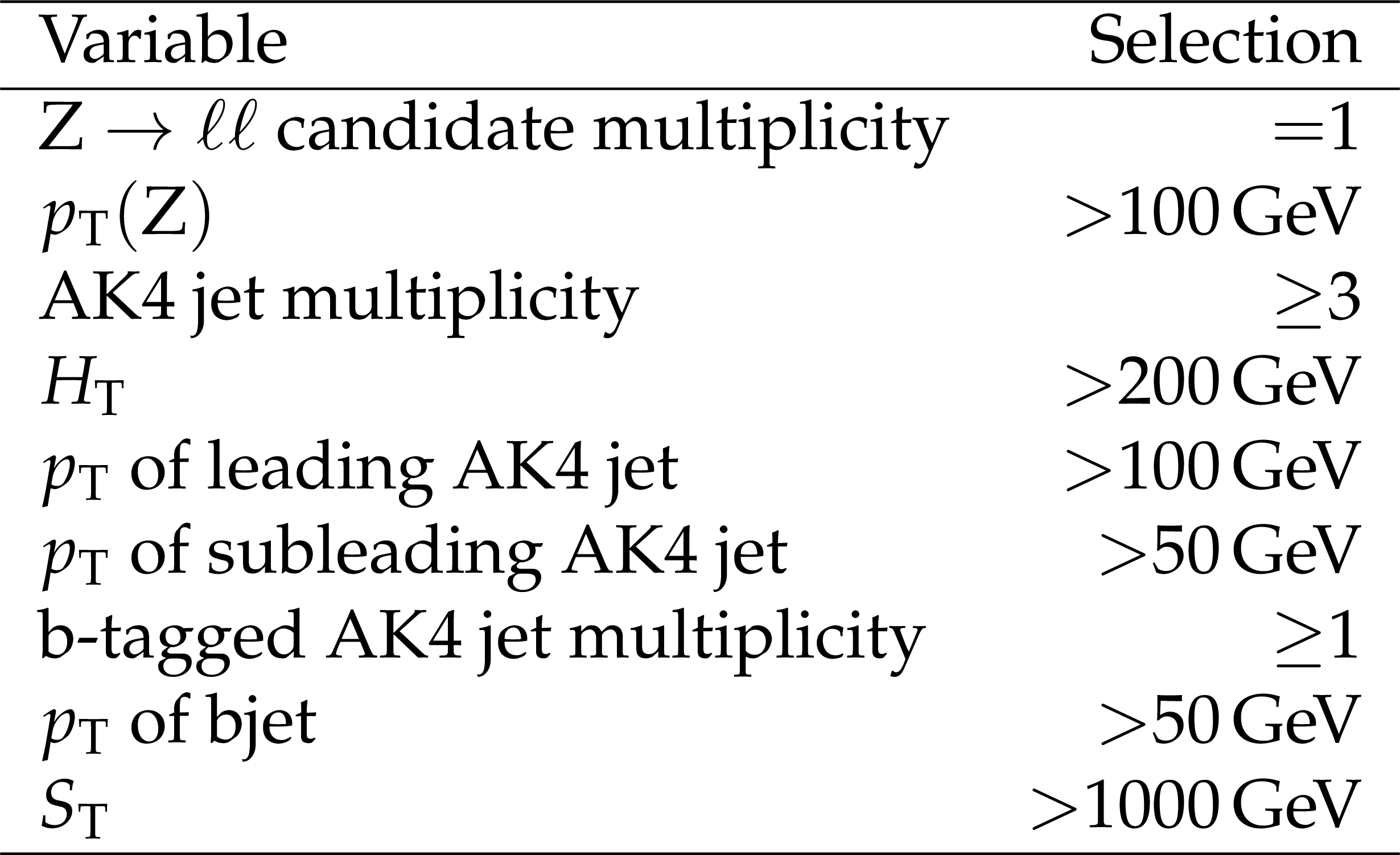
Table 1:
Event selection criteria. |
png pdf |
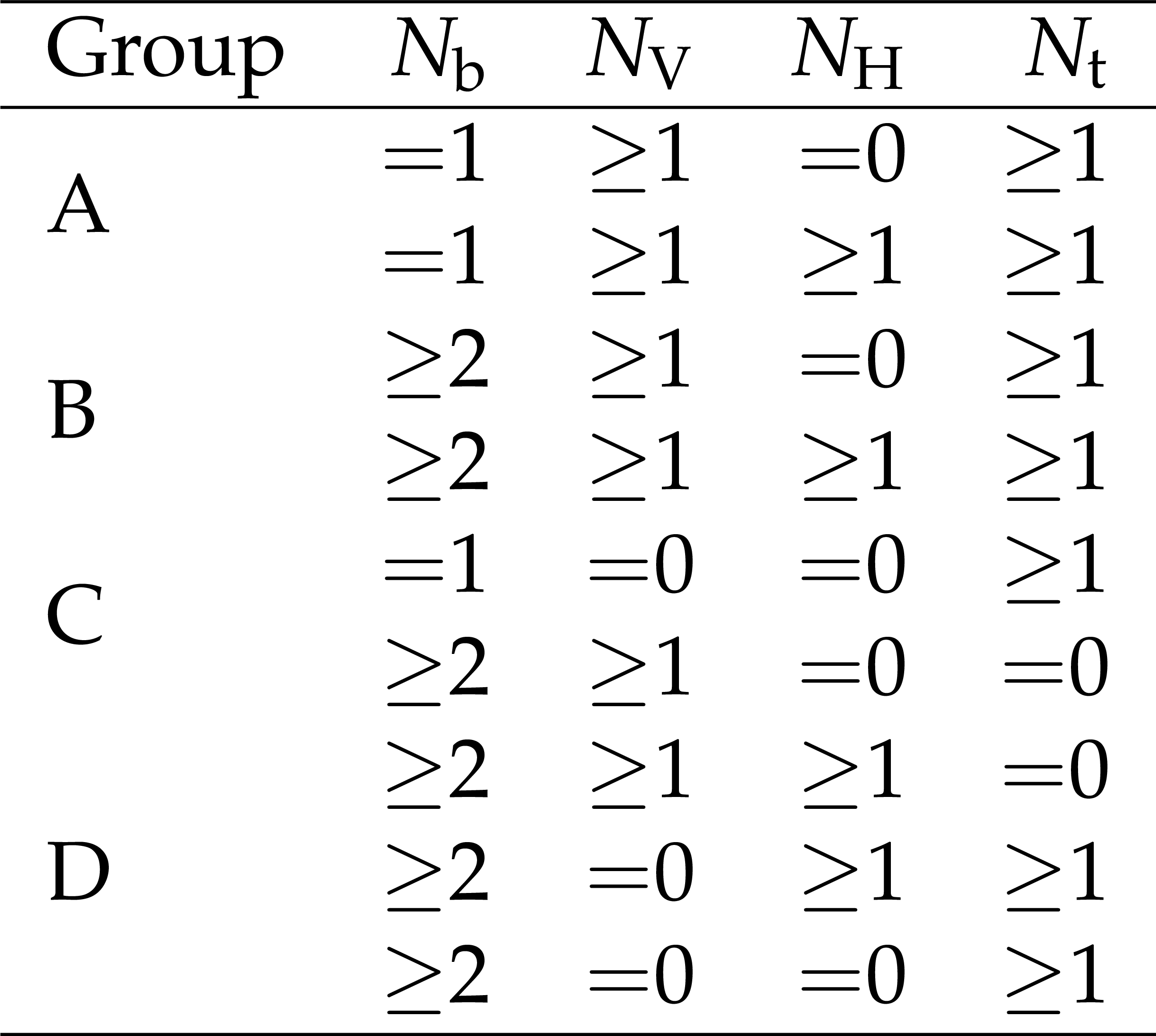
Table 2:
The different event groups used for the $ {{\mathrm {T}}} {\overline {{\mathrm {T}}}} $ search, classified according to the number of b-tagged jets $N_{{\mathrm {b}}}$ and the number of $ {{\mathrm {V}} \to {{\mathrm {q}} {\overline {\mathrm {q}}}}} $, $ {{\mathrm {H}} \to {{\mathrm {b}} {\overline {\mathrm {b}}}}} $, and $ {\mathrm {t}}\to {{\mathrm {q}} {\overline {\mathrm {q}}} ^\prime} {\mathrm {b}}$ candidates in the event, $N_{{\mathrm {V}}}$, $N_{{\mathrm {H}}}$ and $N_{{\mathrm {t}}}$, respectively, identified using both the jet substructure and resolved tagger algorithms. |
png pdf |
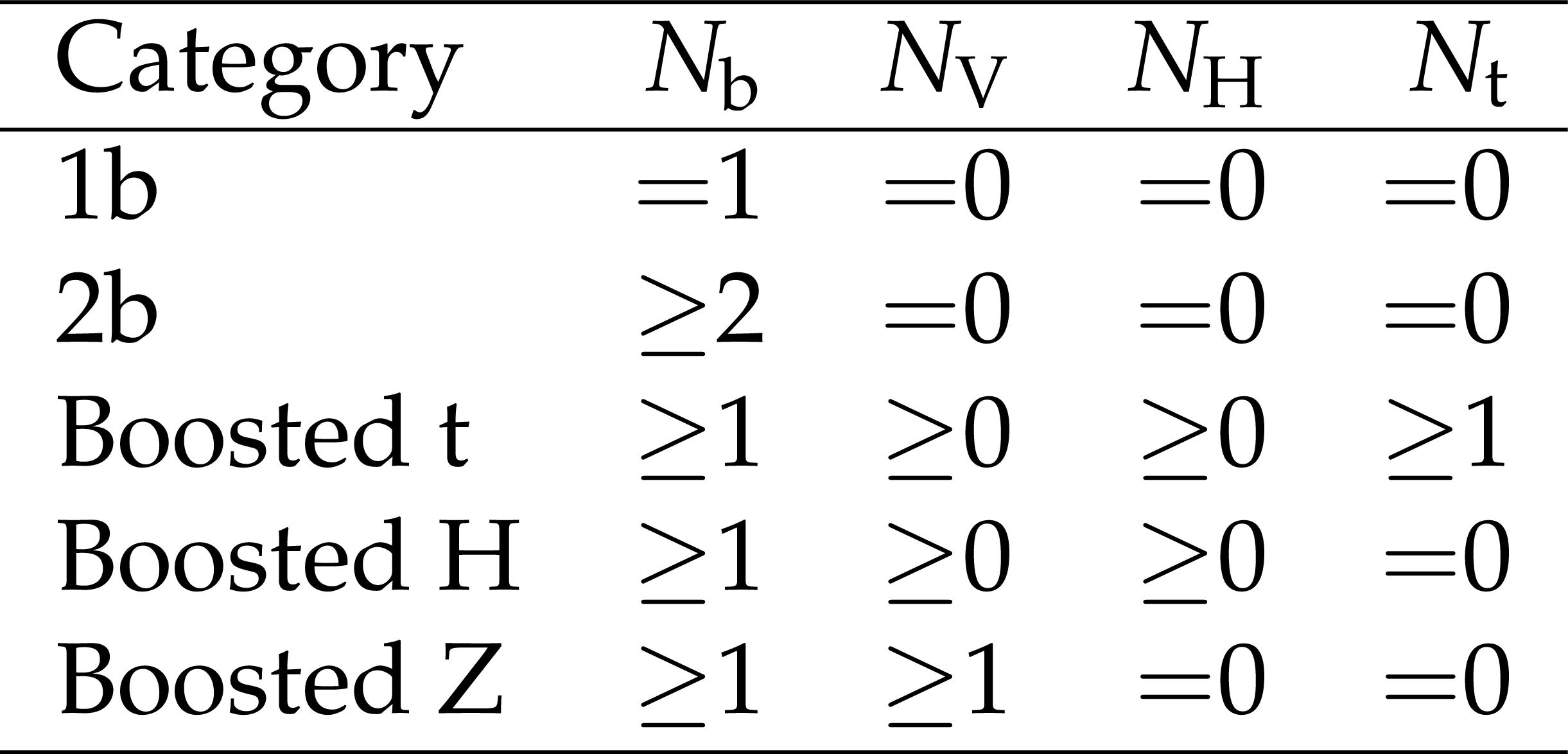
Table 3:
The different event categories used for the $ {{\mathrm {B}}} {\overline {{\mathrm {B}}}} $ search, classified according to the number of AK4 b-tagged jets $N_{{\mathrm {b}}}$ and the number of $ {{\mathrm {V}} \to {{\mathrm {q}} {\overline {\mathrm {q}}}}} $, $ {{\mathrm {H}} \to {{\mathrm {b}} {\overline {\mathrm {b}}}}} $, and $ {\mathrm {t}}\to {{\mathrm {q}} {\overline {\mathrm {q}}} ^\prime} {\mathrm {b}}$ candidates in the event, $N_{{\mathrm {V}}}$, $N_{{\mathrm {H}}}$, and $N_{{\mathrm {t}}}$, respectively, identified using the jet substructure algorithm. |
png pdf |
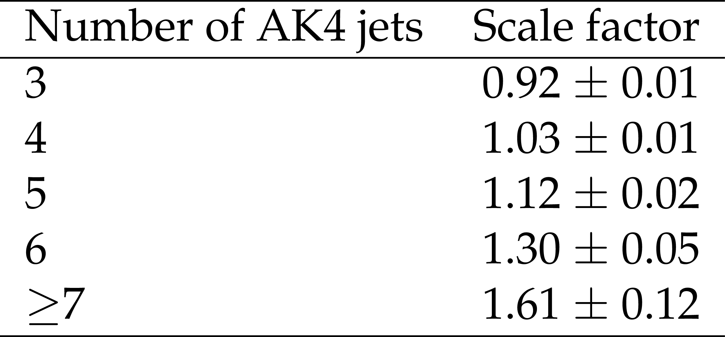
Table 4:
The scale factors determined from data for correcting the AK4 jet multiplicity distribution in the simulation. The quoted uncertainties in the scale factors are statistical only. |

png pdf |
Table 5:
The number of observed events and the predicted number of SM background events in the $ {{\mathrm {T}}} {\overline {{\mathrm {T}}}} $ search using $ {{\mathrm {Z}} \to {{\mathrm {e}^+} {\mathrm {e}^-}}} $ channel in the four event groups. The expected numbers of signal events for T quark masses of 800 and 1200 GeV for three different decay scenarios with assumed branching fractions $\mathcal {B} ({{\mathrm {T}} \to {\mathrm {t}} {\mathrm {Z}}}) = $ 100% (tZtZ), $\mathcal {B} ({{\mathrm {T}} \to {\mathrm {t}} {\mathrm {Z}}}) = \mathcal {B} ({{\mathrm {T}} \to {\mathrm {t}} {\mathrm {H}}}) = $ 50% (tZtH), and $\mathcal {B} ({{\mathrm {T}} \to {\mathrm {t}} {\mathrm {Z}}}) = \mathcal {B} ({{\mathrm {T}} \to {\mathrm {b}} {\mathrm {W}}}) = $ 50% (tZbW) are also shown. The uncertainties in the number of expected background events include the statistical and systematic uncertainties added in quadrature. |

png pdf |
Table 6:
The number of observed events and the predicted number of SM background events in the $ {{\mathrm {T}}} {\overline {{\mathrm {T}}}} $ search using $ {{\mathrm {Z}} \to {{{\mu ^+}} {{\mu ^-}}}} $ channel in the four event groups. The expected numbers of signal events for T quark masses of 800 and 1200 GeV for three different decay scenarios with assumed branching fractions $\mathcal {B} ({{\mathrm {T}} \to {\mathrm {t}} {\mathrm {Z}}}) = $ 100% (tZtZ), $\mathcal {B} ({{\mathrm {T}} \to {\mathrm {t}} {\mathrm {Z}}}) = \mathcal {B} ({{\mathrm {T}} \to {\mathrm {t}} {\mathrm {H}}}) = $ 50% (tZtH), and $\mathcal {B} ({{\mathrm {T}} \to {\mathrm {t}} {\mathrm {Z}}}) = \mathcal {B} ({{\mathrm {T}} \to {\mathrm {b}} {\mathrm {W}}}) = $ 50% (tZbW) are also shown. The uncertainties in the number of expected background events include the statistical and systematic uncertainties added in quadrature. |

png pdf |
Table 7:
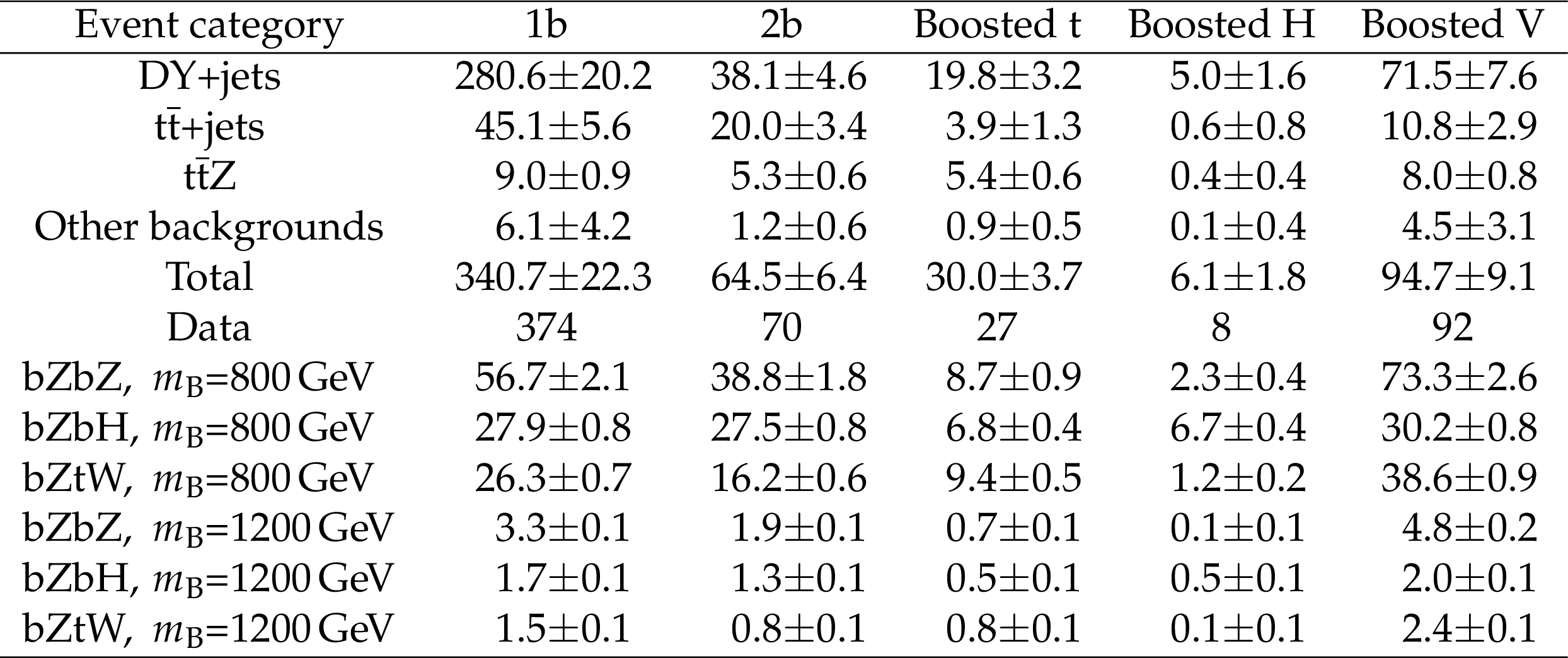
The numbers of observed events and the predicted number of SM background events in the $ {{\mathrm {B}}} {\overline {{\mathrm {B}}}} $ search for the five event categories using $ {{\mathrm {Z}} \to {{\mathrm {e}^+} {\mathrm {e}^-}}} $ channel. The expected numbers of signal events for B masses of 800 and 1200 GeV with branching fraction hypotheses for the three decay channels, $\mathcal {B} ({{\mathrm {B}} \to {\mathrm {b}} {\mathrm {Z}}}) = $ 100% (bZbZ), $\mathcal {B} ({{\mathrm {B}} \to {\mathrm {b}} {\mathrm {Z}}}) = \mathcal {B} ({{\mathrm {B}} \to {\mathrm {b}} {\mathrm {H}}}) = $ 50% (bZbH), and $\mathcal {B} ({{\mathrm {B}} \to {\mathrm {b}} {\mathrm {Z}}}) = \mathcal {B} ({{\mathrm {B}} \to {\mathrm {t}} {\mathrm {W}}}) = $ 50% (bZtW) are also shown. The uncertainties in the number of expected background events include the statistical and systematic uncertainties added in quadrature. |
png pdf |
Table 8:
The number of observed events and the predicted number of SM background events in the $ {{\mathrm {B}}} {\overline {{\mathrm {B}}}} $ search for the five event categories using $ {{\mathrm {Z}} \to {{{\mu ^+}} {{\mu ^-}}}} $ channel. The expected numbers of signal events for B masses of 800 and 1200 GeV with branching fraction hypotheses for the three decay channels, $\mathcal {B} ({{\mathrm {B}} \to {\mathrm {b}} {\mathrm {Z}}}) = $ 100% (bZbZ), $\mathcal {B} ({{\mathrm {B}} \to {\mathrm {b}} {\mathrm {Z}}}) = \mathcal {B} ({{\mathrm {B}} \to {\mathrm {b}} {\mathrm {H}}}) = $ 50% (bZbH), and $\mathcal {B} ({{\mathrm {B}} \to {\mathrm {b}} {\mathrm {Z}}}) = \mathcal {B} ({{\mathrm {B}} \to {\mathrm {t}} {\mathrm {W}}}) = $ 50% (bZtW) are also shown. The uncertainties in the number of expected background events include the statistical and systematic uncertainties added in quadrature. |
| Summary |
|
The results of a search have been presented for the pair production of vector-like top (T) and bottom (B) quark partners in proton-proton collisions at $\sqrt{s} = $ 13 TeV, using data collected by the CMS experiment at the CERN LHC, corresponding to an integrated luminosity of 35.9 fb$^{-1}$. The ${{\mathrm{T}} } {\overline{{\mathrm{T}} }}$ search is performed by looking for events in which one T quark decays via $ {{\mathrm{T}} \to\mathrm{t}\mathrm{Z}} $ and the other decays via $ {{\mathrm{T}} \to\mathrm{b}\mathrm{W}} $, $ {\mathrm{t}\mathrm{Z}} $, $ {\mathrm{t}\mathrm{H}} $, where H refers to the Higgs boson. The $ {{\mathrm{B}} } {\overline{{\mathrm{B}} }} $ search looks for events in which one B quark decays via $ {{\mathrm{B}} \to\mathrm{b}\mathrm{Z}} $ and the other via $ {{\mathrm{B}} \to\mathrm{t}\mathrm{W}} $, $ {\mathrm{b}\mathrm{Z}} $, or $ {\mathrm{b}\mathrm{H}} $. Events with two oppositely charged electrons or muons, consistent with coming from the decay of a Z boson, and jets are investigated, and are categorized according to the numbers of top quark and W, Z, and Higgs boson candidates. These categories are individually optimized for ${{\mathrm{T}} } {\overline{{\mathrm{T}} }}$ and $ {{\mathrm{B}} } {\overline{{\mathrm{B}} }} $ event topologies. The data are in agreement with the standard model background predictions for all the event categories. Upper limits at 95% confidence level on the ${{\mathrm{T}} } {\overline{{\mathrm{T}} }}$ and $ {{\mathrm{B}} } {\overline{{\mathrm{B}} }} $ production cross sections are obtained from a simultaneous binned maximum-likelihood fit to the observed distributions for the different event categories, under the assumption of various T and B quark branching fractions. Comparing these upper limits to the theoretical predictions for the ${{\mathrm{T}} } {\overline{{\mathrm{T}} }}$ and $ {{\mathrm{B}} } {\overline{{\mathrm{B}} }} $ cross sections as a function of the T and B quark masses, lower limits on the masses at 95% confidence level are determined for different branching fraction scenarios. In the case of a T quark decaying exclusively via $ {{\mathrm{T}} \to\mathrm{t}\mathrm{Z}} $, the lower mass limit is 1280 GeV, while for a B quark decaying only via $ {{\mathrm{B}} \to\mathrm{b}\mathrm{Z}} $, it is 1130 GeV. These lower limits are comparable with those measured by the ATLAS Collaboration [20], also using the Z boson dilepton decay channel. The results of the analysis presented in this paper are complementary to previous CMS measurements [21,22,23], and have extended sensitivity in reaching higher mass limits for T and B quarks. |
| References | ||||
| 1 | ATLAS Collaboration | Observation of a new particle in the search for the Standard Model Higgs boson with the ATLAS detector at the LHC | PLB 716 (2012) 1 | 1207.7214 |
| 2 | CMS Collaboration | Observation of a new boson at a mass of 125 GeV with the CMS experiment at the LHC | PLB 716 (2012) 30 | CMS-HIG-12-028 1207.7235 |
| 3 | CMS Collaboration | Observation of a new boson with mass near 125 GeV in pp collisions at $ \sqrt{s} = $ 7 and 8 TeV | JHEP 06 (2013) 081 | CMS-HIG-12-036 1303.4571 |
| 4 | ATLAS and CMS Collaborations | Combined measurement of the Higgs boson mass in $ {\mathrm{p}}{\mathrm{p}} $ collisions at $ \sqrt{s}= $ 7 and 8 TeV with the ATLAS and CMS Experiments | PRL 114 (2015) 191803 | 1503.07589 |
| 5 | CMS Collaboration | Measurements of properties of the Higgs boson decaying into the four-lepton final state in pp collisions at $ \sqrt{s} = $ 13 TeV | JHEP 11 (2017) 047 | CMS-HIG-16-041 1706.09936 |
| 6 | J. A. Aguilar-Saavedra, R. Benbrik, S. Heinemeyer, and M. P\'erez-Victoria | Handbook of vectorlike quarks: Mixing and single production | PRD 88 (2013) 094010 | 1306.0572 |
| 7 | J. Kang, P. Langacker, and B. D. Nelson | Theory and phenomenology of exotic isosinglet quarks and squarks | PRD 77 (2008) 035003 | 0708.2701v2 |
| 8 | D. Choudhury, T. Tait, and C. Wagner | Beautiful mirrors and precision electroweak data | PRD 65 (2002) 053002 | hep-ph/0109097 |
| 9 | L. Randall and R. Sundrum | A large mass hierarchy from a small extra dimension | PRL 83 (1999) 3370 | hep-ph/9905221 |
| 10 | N. Arkani-Hamed, A. G. Cohen, E. Katz, and A. E. Nelson | The littlest Higgs | JHEP 07 (2002) 034 | hep-ph/0206021 |
| 11 | M. Schmaltz | Physics beyond the standard model (theory): Introducing the Little Higgs | NPPS 117 (2003) 40 | hep-ph/0210415 |
| 12 | M. Schmaltz and D. Tucker-Smith | Little Higgs review | Ann. Rev. Nucl. Part. Sci. 55 (2005) 229 | hep-ph/0502182 |
| 13 | M. S. D. Marzocca and J. Shu | General composite Higgs models | JHEP 08 (2012) 013 | 1205.0770 |
| 14 | D. Guadagnoli, R. N. Mohapatra, and I. Sung | Gauged flavor group with left-right symmetry | JHEP 04 (2011) 093 | 1103.4170 |
| 15 | R. T. D'Agnolo and A. Hook | Finding the strong CP problem at the LHC | PLB 762 (2016) 421 | 1507.00336 |
| 16 | Y. Okada and L. Panizzi | LHC signatures of vector-like quarks | Adv. High Energy Phys. 2013 (2013) 364936 | 1207.5607 |
| 17 | ATLAS Collaboration | Search for pair production of vector-like top quarks in events with one lepton, jets, and missing transverse momentum in $ \sqrt{s}= $ 13 TeV pp collisions with the atlas detector | JHEP 08 (2017) 052 | 1705.10751 |
| 18 | ATLAS Collaboration | Search for pair production of heavy vector-like quarks decaying to high-$ p_{\mathrm T} $ W bosons and b quarks in the lepton-plus-jets final state in pp collisions at $ \sqrt{s}= $ 13 TeV with the atlas detector | JHEP 10 (2017) 141 | 1707.03347 |
| 19 | ATLAS Collaboration | Search for pair production of vector-like quarks into high-$ p_{\mathrm T} $ W bosons and top quarks in the lepton-plus-jets final state in pp collisions at $ \sqrt{s}= $ 13 TeV with the ATLAS detector | JHEP 08 (2018) 48 | 1806.01762 |
| 20 | ATLAS Collaboration | Search for pair- and single-production of vector-like quarks in final states with at least one Z boson decaying into a pair of electrons or muons in pp collision data collected with the ATLAS detector at $ \sqrt{s} = $ 13 TeV | Submitted to PRD | 1806.10555 |
| 21 | CMS Collaboration | Search for pair production of vector-like T and B quarks in single-lepton final states using boosted jet substructure in proton-proton collisions at $ \sqrt{s}= $ 13 TeV | JHEP 11 (2017) 085 | CMS-B2G-16-024 1706.03408 |
| 22 | CMS Collaboration | Search for pair production of vector-like quarks in the $ \mathrm{bW\overline{b}W} $ channel from proton-proton collisions at $ \sqrt{s}= $ 13 TeV | PLB 779 (2018) 82 | CMS-B2G-17-003 1710.01539 |
| 23 | CMS Collaboration | Search for vector-like T and B quark pairs in final states with leptons at $ \sqrt{s}= $ 13 TeV | JHEP 08 (2018) 177 | CMS-B2G-17-011 1805.04758 |
| 24 | CMS Collaboration | The CMS experiment at the CERN LHC | JINST 3 (2008) S08004 | CMS-00-001 |
| 25 | CMS Collaboration | The CMS trigger system | JINST 12 (2017) P01020 | CMS-TRG-12-001 1609.02366 |
| 26 | J. Alwall et al. | The automated computation of tree-level and next-to-leading order differential cross sections, and their matching to parton shower simulations | JHEP 07 (2014) 079 | 1405.0301 |
| 27 | NNPDF Collaboration | Parton distributions for the LHC Run II | JHEP 04 (2015) 040 | 1410.8849 |
| 28 | T. Sjostrand et al. | An introduction to PYTHIA 8.2 | CPC 191 (2015) 159 | 1410.3012 |
| 29 | CMS Collaboration | Event generator tunes obtained from underlying event and multiparton scattering measurements | EPJC 76 (2016) 155 | CMS-GEN-14-001 1512.00815 |
| 30 | M. Czakon, P. Fiedler, and A. Mitov | Total top quark pair production cross section at hadron colliders through $ {O}(\alpha_\mathrm{{S}}^4) $ | PRL 110 (2013) 252004 | 1303.6254 |
| 31 | M. R. Whalley, D. Bourilkov, and R. C. Group | The Les Houches accord PDFs (LHAPDF) and LHAGLUE | hep-ph/0508110 | |
| 32 | S. Frixione and B. R. Webber | Matching NLO QCD computations and parton shower simulations | JHEP 06 (2002) 029 | hep-ph/0204244 |
| 33 | R. Frederix and S. Frixione | Merging meets matching in MC@NLO | JHEP 12 (2012) 061 | 1209.6215 |
| 34 | T. Sjostrand, S. Mrenna, and P. Z. Skands | A brief introduction to PYTHIA 8.1 | CPC 178 (2008) 852 | 0710.3820 |
| 35 | S. Frixione, G. Ridolfi, and P. Nason | A positive-weight next-to-leading-order Monte Carlo for heavy flavour hadroproduction | JHEP 09 (2007) 126 | 0707.3088 |
| 36 | S. Frixione, P. Nason, and C. Oleari | Matching NLO QCD computations with parton shower simulations: the POWHEG method | JHEP 11 (2007) 070 | 0709.2092 |
| 37 | S. Alioli, P. Nason, C. Oleari, and E. Re | A general framework for implementing NLO calculations in shower Monte Carlo programs: the POWHEG BOX | JHEP 06 (2010) 043 | 1002.2581 |
| 38 | CMS Collaboration | Investigations of the impact of the parton shower tuning in PYTHIA 8 in the modelling of $ \rm{t\bar{t}} $ at $ \sqrt{s} = $ 8 and 13 TeV | CMS-PAS-TOP-16-021 | CMS-PAS-TOP-16-021 |
| 39 | J. Alwall et al. | Comparative study of various algorithms for the merging of parton showers and matrix elements in hadronic collisions | EPJC 53 (2008) 473 | 0706.2569 |
| 40 | J. M. Campbell, R. K. Ellis, and C. Williams | Vector boson pair production at the LHC | JHEP 07 (2011) 018 | 1105.0020 |
| 41 | F. Cascioli et al. | ZZ production at hadron colliders in NNLO QCD | PLB 735 (2014) 311 | 1405.2219v2 |
| 42 | T. Gehrmann et al. | W$ ^+ $W$ ^- $ production at hadron colliders in NNLO QCD | PRL 113 (2014) 212001 | 1408.5243 |
| 43 | D. de Florian et al. | Handbook of LHC Higgs cross sections:~4. Deciphering the nature of the Higgs sector | CERN-2017-002-M, CERN | 1610.07922 |
| 44 | GEANT4 Collaboration | GEANT4 -- a simulation toolkit | NIMA 506 (2003) 250 | |
| 45 | J. Allison et al. | GEANT4 developments and applications | IEEE Trans. Nucl. Sci. 53 (2006) 270 | |
| 46 | CMS Collaboration | Particle-flow reconstruction and global event description with the CMS detector | JINST 12 (2017) P10003 | CMS-PRF-14-001 1706.04965 |
| 47 | CMS Collaboration | Description and performance of track and primary-vertex reconstruction with the CMS tracker | JINST 9 (2014) P10009 | CMS-TRK-11-001 1405.6569 |
| 48 | M. Cacciari, G. P. Salam, and G. Soyez | The anti-$ {k_{\mathrm{T}}} $ jet clustering algorithm | JHEP 04 (2008) 063 | 0802.1189 |
| 49 | M. Cacciari, G. P. Salam, and G. Soyez | FastJet user manual | EPJC 72 (2012) 1896 | 1111.6097 |
| 50 | CMS Collaboration | Performance of electron reconstruction and selection with the CMS detector in proton-proton collisions at $ \sqrt{s} = $ 8 TeV | JINST 10 (2015) P06005 | CMS-EGM-13-001 1502.02701 |
| 51 | CMS Collaboration | Performance of the CMS muon detector and muon reconstruction with proton-proton collisions at $ \sqrt{s} = $ 13 TeV | JINST 13 (2018) P06015 | CMS-MUO-16-001 1804.04528 |
| 52 | M. Cacciari and G. P. Salam | Pileup subtraction using jet areas | PLB 659 (2008) 119 | 0707.1378 |
| 53 | CMS Collaboration | Determination of jet energy calibration and transverse momentum resolution in CMS | JINST 6 (2011) P11002 | CMS-JME-10-011 1107.4277 |
| 54 | CMS Collaboration | Jet energy scale and resolution in the CMS experiment in pp collisions at 8 TeV | JINST 12 (2017) P02014 | CMS-JME-13-004 1607.03663 |
| 55 | CMS Collaboration | Identification of heavy-flavour jets with the CMS detector in pp collisions at 13 TeV | JINST 13 (2018) P05011 | CMS-BTV-16-002 1712.07158 |
| 56 | W. S. Sarl | Neural networks and statistical models | in Proceedings of the Nineteenth Annual SAS Users Group International Conference 1994 | |
| 57 | CMS Collaboration | Performance of CMS muon reconstruction in pp collision events at $ \sqrt{s}= $ 7 TeV | JINST 7 (2012) P10002 | CMS-MUO-10-004 1206.4071 |
| 58 | S. D. Ellis, C. K. Vermilion, and J. R. Walsh | Techniques for improved heavy particle searches with jet substructure | PRD 80 (2009) 051501 | 0903.5081 |
| 59 | S. D. Ellis, C. K. Vermilion, and J. R. Walsh | Recombination algorithms and jet substructure: Pruning as a tool for heavy particle searches | PRD 81 (2010) 094023 | 0912.0033 |
| 60 | G. P. Salam | Towards jetography | EPJC 67 (2010) 637 | 0906.1833 |
| 61 | J. Thaler and K. Van Tilburg | Identifying boosted objects with N-subjettiness | JHEP 03 (2011) 015 | 1011.2268 |
| 62 | M. Dasgupta, A. Fregoso, S. Marzani, and G. P. Salam | Towards an understanding of jet substructure | JHEP 09 (2013) 029 | 1307.0007 |
| 63 | A. J. Larkoski, S. Marzani, G. Soyez, and J. Thaler | Soft drop | JHEP 05 (2014) 146 | 1402.2657 |
| 64 | CMS Collaboration | Jet algorithms performance in 13 TeV data | CMS-PAS-JME-16-003 | CMS-PAS-JME-16-003 |
| 65 | CMS Collaboration | Search for a massive resonance decaying to a pair of Higgs bosons in the four b quark final state in proton-proton collisions at $ \sqrt{s}= $ 13 TeV | PLB 781 (2018) 244 | 1710.04960 |
| 66 | CMS Collaboration | Measurement of differential cross sections for Z boson production in association with jets in proton-proton collisions at $ \sqrt{s}= $ 13 TeV | EPJC (2018) | CMS-SMP-16-015 1804.05252 |
| 67 | CMS Collaboration | Measurement of differential cross sections for top quark pair production using the lepton+jets final state in proton-proton collisions at 13 TeV | PRD 95 (2017) 092001 | CMS-TOP-16-008 1610.04191 |
| 68 | CMS Collaboration | Measurements of the $ {\mathrm{p}}{\mathrm{p}} \to \mathrm{Z}\mathrm{Z} $ production cross section and the $ \mathrm{Z} \to 4 \ell $ branching fraction, and constraints on anomalous triple gauge couplings at $ \sqrt{s}= $ 13 TeV | EPJC 78 (2018) 165 | CMS-SMP-16-017 1709.08601 |
| 69 | CMS Collaboration | Cms luminosity measurement for the 2016 data taking period | CMS-PAS-LUM-17-001 | CMS-PAS-LUM-17-001 |
| 70 | J. Butterworth et al. | PDF4LHC recommendations for LHC Run II | JPG 43 (2016) 023001 | 1510.03865 |
| 71 | S. Dulat et al. | The CT14 global analysis of quantum chromodynamics | PRD 93 (2015) 033006 | 1506.07443 |
| 72 | L. A. Harland-Lang, A. D. Martin, P. Motylinski, and R. S. Thorne | Parton distributions in the LHC era: MMHT 2014 PDFs | EPJC 75 (2015) 204 | 1412.3989 |
| 73 | CMS Collaboration | Jet energy scale and resolution performances with 13 TeV data | CDS | |
| 74 | Particle Data Group, M. Tanabashi et al. | Review of particle physics | PRD 98 (2018) 030001 | |
| 75 | J. Ott | $ \textscTheta--A $ framework for template-based modeling and inference | 2010 \url http://www-ekp.physik.uni-karlsruhe.de/\ ott/theta/theta-auto | |
|
|
Compact Muon Solenoid LHC, CERN |
|

|

|

|

|

|