

Compact Muon Solenoid
LHC, CERN
| CMS-HIG-17-026 ; CERN-EP-2018-065 | ||
| Search for $ {\mathrm{t\bar{t}}\mathrm{H}} $ production in the $ {\mathrm{H}\to\mathrm{b\bar{b}}} $ decay channel with leptonic $ \mathrm{t\bar{t}} $ decays in proton-proton collisions at $\sqrt{s} = $ 13 TeV | ||
| CMS Collaboration | ||
| 10 April 2018 | ||
| JHEP 03 (2019) 026 | ||
| Abstract: A search is presented for the associated production of a standard model Higgs boson with a top quark-antiquark pair ($ {\mathrm{t\bar{t}}\mathrm{H}} $), in which the Higgs boson decays into a b quark-antiquark pair, in proton-proton collisions at a centre-of-mass energy $\sqrt{s} = $ 13 TeV. The data correspond to an integrated luminosity of 35.9 fb$^{-1}$ recorded with the CMS detector at the CERN LHC. Candidate $ {\mathrm{t\bar{t}}\mathrm{H}} $ events are selected that contain either one or two electrons or muons from the $ \mathrm{t\bar{t}} $ decays and are categorised according to the number of jets. Multivariate techniques are employed to further classify the events and eventually discriminate between signal and background. The results are characterised by an observed $ {\mathrm{t\bar{t}}\mathrm{H}} $ signal strength relative to the standard model cross section, $\mu = \sigma/\sigma_{\mathrm{SM}}$, under the assumption of a Higgs boson mass of 125 GeV. A combined fit of multivariate discriminant distributions in all categories results in an observed (expected) upper limit on $\mu$ of 1.5 (0.9) at 95% confidence level, and a best fit value of 0.72 $\pm$ 0.24 (stat) $\pm$ 0.38 (syst), corresponding to an observed (expected) signal significance of 1.6 (2.2) standard deviations above the background-only hypothesis. | ||
| Links: e-print arXiv:1804.03682 [hep-ex] (PDF) ; CDS record ; inSPIRE record ; CADI line (restricted) ; | ||
| Figures & Tables | Summary | Additional Tables | References | CMS Publications |
|---|
| Figures | |
png pdf |
Figure 1:
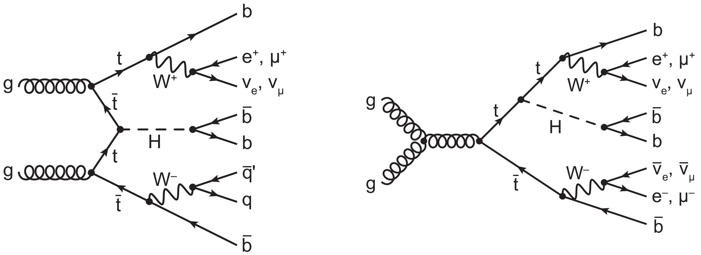
Representative leading-order Feynman diagrams for $ {{{\mathrm {t}\overline {\mathrm {t}}}} {\mathrm {H}}} $ production, including the subsequent decay of the Higgs boson into a b quark-antiquark pair, and the decay of the top quark-antiquark pair into final states with either one (single-lepton channel, left) or two (dilepton channel, right) electrons or muons. |
png pdf |
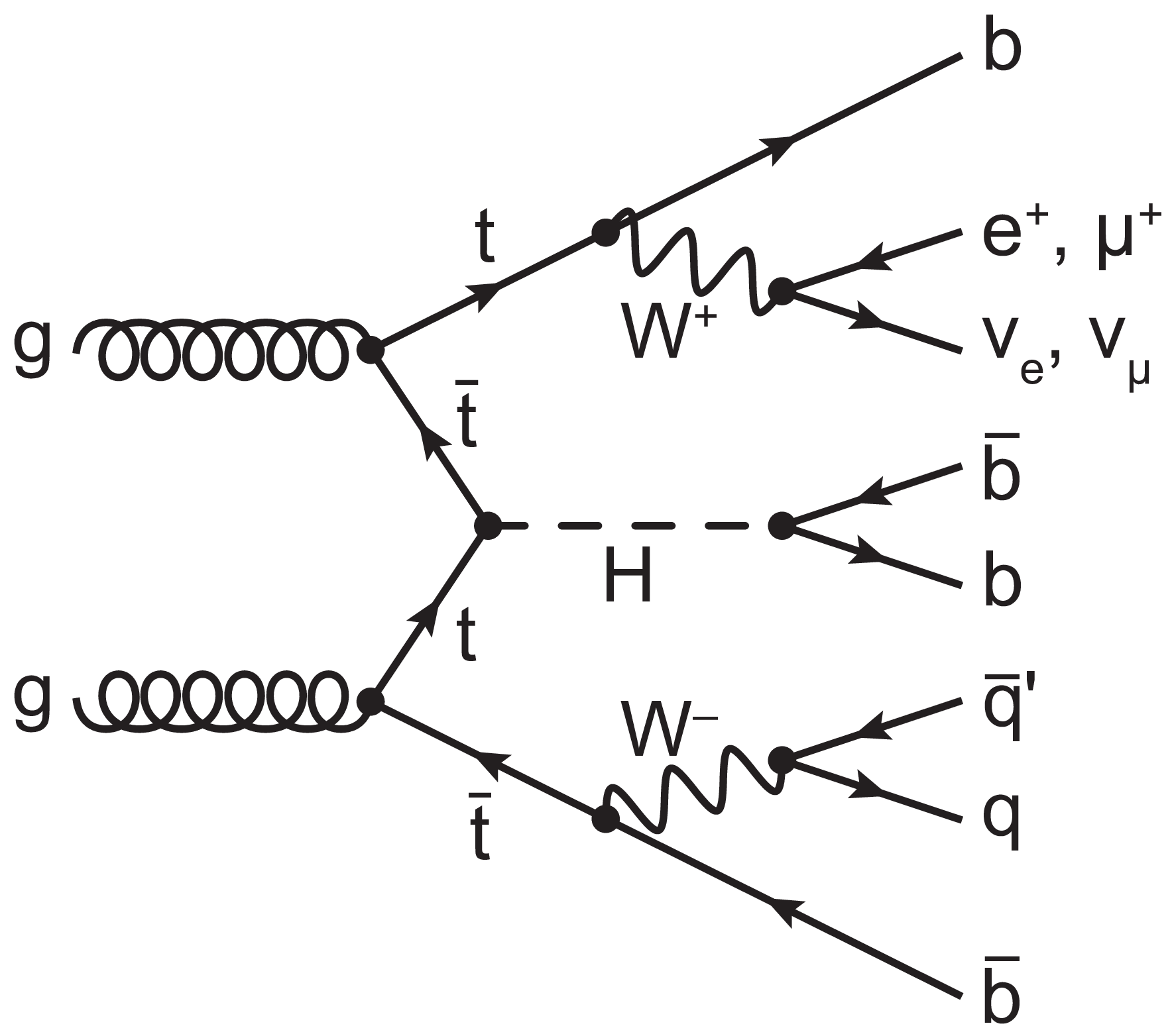
Figure 1-a:
Representative leading-order Feynman diagrams for $ {{{\mathrm {t}\overline {\mathrm {t}}}} {\mathrm {H}}} $ production, including the subsequent decay of the Higgs boson into a b quark-antiquark pair, and the decay of the top quark-antiquark pair into final states with one (single-lepton channel) electron or muon. |

png pdf |
Figure 1-b:
Representative leading-order Feynman diagrams for $ {{{\mathrm {t}\overline {\mathrm {t}}}} {\mathrm {H}}} $ production, including the subsequent decay of the Higgs boson into a b quark-antiquark pair, and the decay of the top quark-antiquark pair into final states with two (dilepton channel) electrons or muons. |

png pdf |
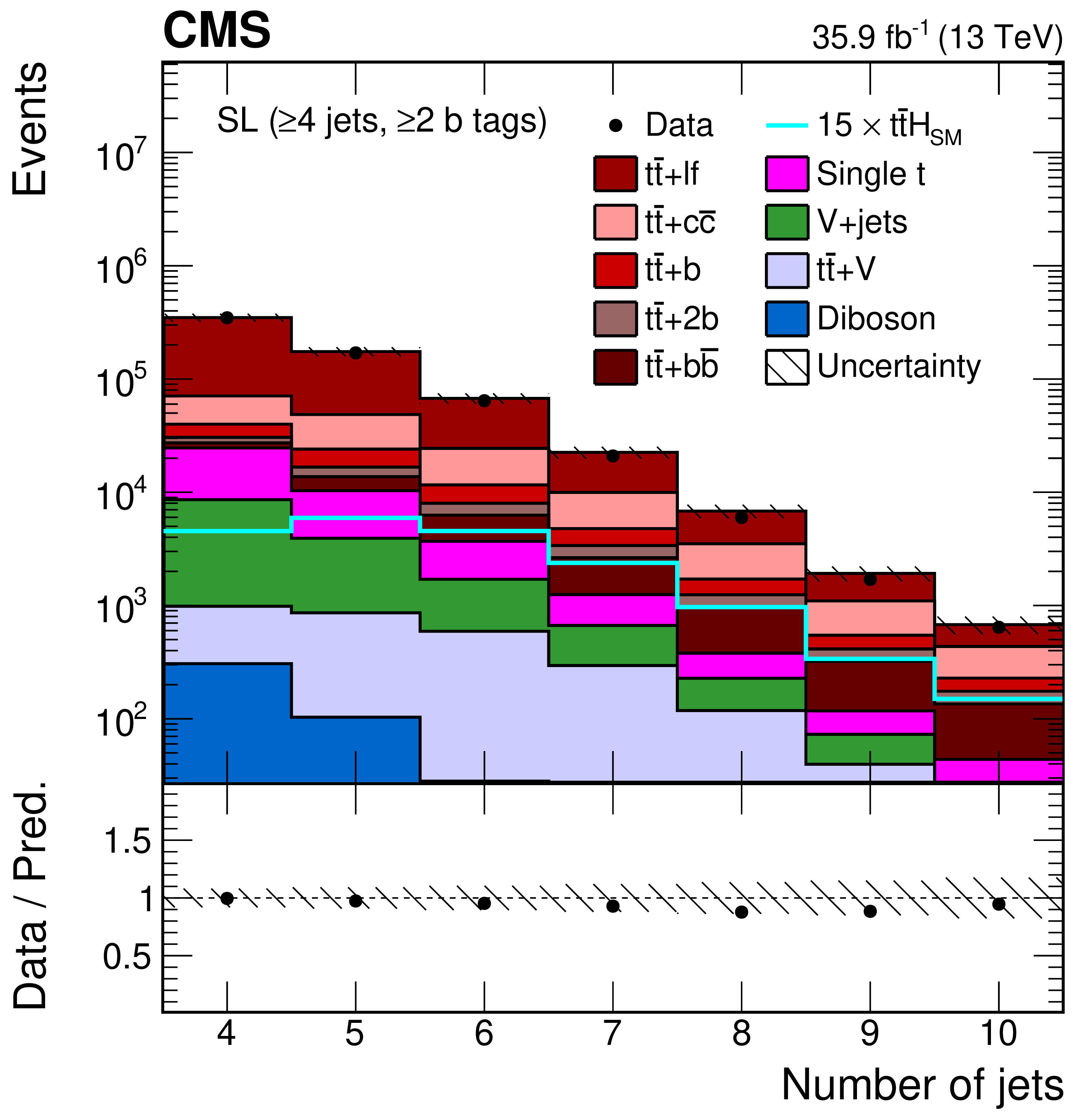
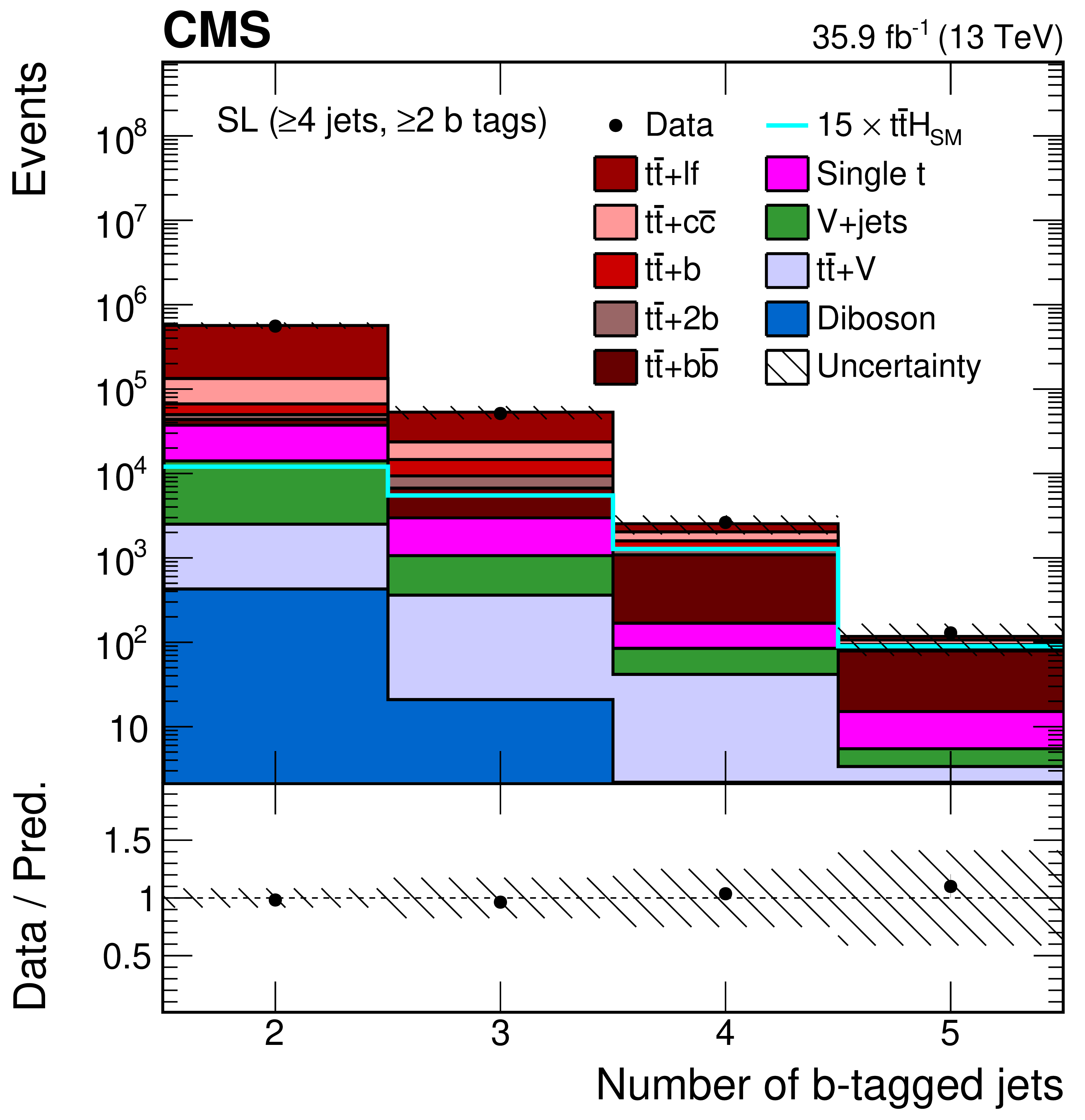
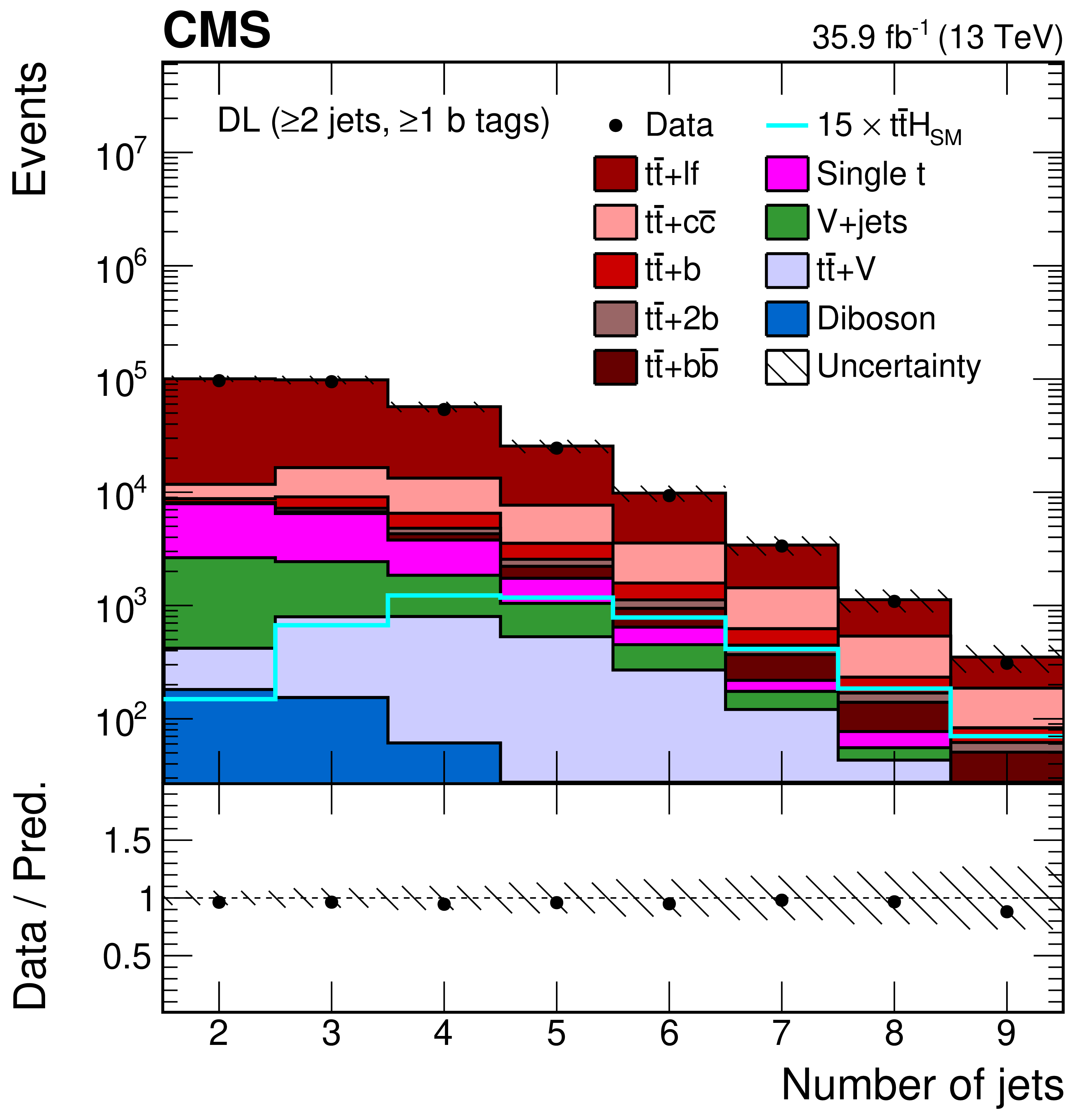
Figure 2:
Jet (left) and b-tagged jet (right) multiplicity in the single-lepton (SL) channel after the event selection described in the text. The expected background contributions (filled histograms) are stacked, and the expected signal distribution (line), which includes $ {{\mathrm {H}} \to {{\mathrm {b}} {\overline {\mathrm {b}}}}} $ and all other Higgs boson decay modes, is superimposed. Each contribution is normalised to an integrated luminosity of 35.9 fb$^{-1}$, and the signal distribution is additionally scaled by a factor of 15 for better visibility. The hatched uncertainty bands correspond to the total statistical and systematic uncertainties (excluding uncertainties that affect only the normalisation of the distribution) added in quadrature. The distributions observed in data (markers) are overlaid. The last bin includes overflow events. The lower plots show the ratio of the data to the background prediction. |
png pdf |
Figure 2-a:
Jet jet multiplicity in the single-lepton (SL) channel after the event selection described in the text. The expected background contributions (filled histograms) are stacked, and the expected signal distribution (line), which includes $ {{\mathrm {H}} \to {{\mathrm {b}} {\overline {\mathrm {b}}}}} $ and all other Higgs boson decay modes, is superimposed. Each contribution is normalised to an integrated luminosity of 35.9 fb$^{-1}$, and the signal distribution is additionally scaled by a factor of 15 for better visibility. The hatched uncertainty bands correspond to the total statistical and systematic uncertainties (excluding uncertainties that affect only the normalisation of the distribution) added in quadrature. The distribution observed in data (markers) is overlaid. The last bin includes overflow events. The lower plot shows the ratio of the data to the background prediction. |
png pdf |
Figure 2-b:
b-tagged jet multiplicity in the single-lepton (SL) channel after the event selection described in the text. The expected background contributions (filled histograms) are stacked, and the expected signal distribution (line), which includes $ {{\mathrm {H}} \to {{\mathrm {b}} {\overline {\mathrm {b}}}}} $ and all other Higgs boson decay modes, is superimposed. Each contribution is normalised to an integrated luminosity of 35.9 fb$^{-1}$, and the signal distribution is additionally scaled by a factor of 15 for better visibility. The hatched uncertainty bands correspond to the total statistical and systematic uncertainties (excluding uncertainties that affect only the normalisation of the distribution) added in quadrature. The distribution observed in data (markers) is overlaid. The last bin includes overflow events. The lower plot shows the ratio of the data to the background prediction. |
png pdf |
Figure 3:
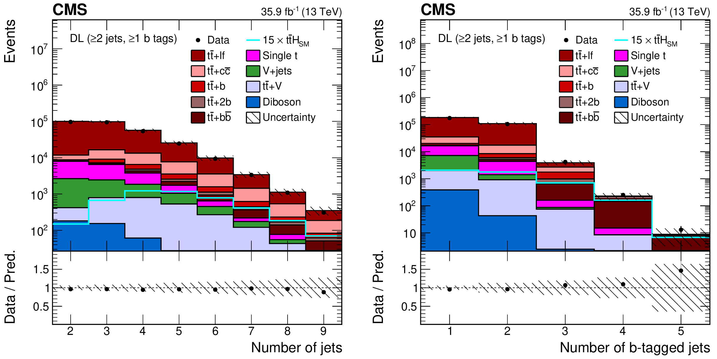
Jet (left) and b-tagged jet (right) multiplicity in the dilepton (DL) channel after the event selection described in the text. The expected background contributions (filled histograms) are stacked, and the expected signal distribution (line), which includes $ {{\mathrm {H}} \to {{\mathrm {b}} {\overline {\mathrm {b}}}}} $ and all other Higgs boson decay modes, is superimposed. Each contribution is normalised to an integrated luminosity of 35.9 fb$^{-1}$, and the signal distribution is additionally scaled by a factor of 15 for better visibility. The hatched uncertainty bands correspond to the total statistical and systematic uncertainties (excluding uncertainties that affect only the normalisation of the distribution) added in quadrature. The distributions observed in data (markers) are overlaid. The last bin includes overflow events. The lower plots show the ratio of the data to the background prediction. |
png pdf |
Figure 3-a:
Jet jet multiplicity in the dilepton (DL) channel after the event selection described in the text. The expected background contributions (filled histograms) are stacked, and the expected signal distribution (line), which includes $ {{\mathrm {H}} \to {{\mathrm {b}} {\overline {\mathrm {b}}}}} $ and all other Higgs boson decay modes, is superimposed. Each contribution is normalised to an integrated luminosity of 35.9 fb$^{-1}$, and the signal distribution is additionally scaled by a factor of 15 for better visibility. The hatched uncertainty bands correspond to the total statistical and systematic uncertainties (excluding uncertainties that affect only the normalisation of the distribution) added in quadrature. The distribution observed in data (markers) is overlaid. The last bin includes overflow events. The lower plot shows the ratio of the data to the background prediction. |

png pdf |
Figure 3-b:
b-tagged jet multiplicity in the dilepton (DL) channel after the event selection described in the text. The expected background contributions (filled histograms) are stacked, and the expected signal distribution (line), which includes $ {{\mathrm {H}} \to {{\mathrm {b}} {\overline {\mathrm {b}}}}} $ and all other Higgs boson decay modes, is superimposed. Each contribution is normalised to an integrated luminosity of 35.9 fb$^{-1}$, and the signal distribution is additionally scaled by a factor of 15 for better visibility. The hatched uncertainty bands correspond to the total statistical and systematic uncertainties (excluding uncertainties that affect only the normalisation of the distribution) added in quadrature. The distribution observed in data (markers) is overlaid. The last bin includes overflow events. The lower plot shows the ratio of the data to the background prediction. |
png pdf |
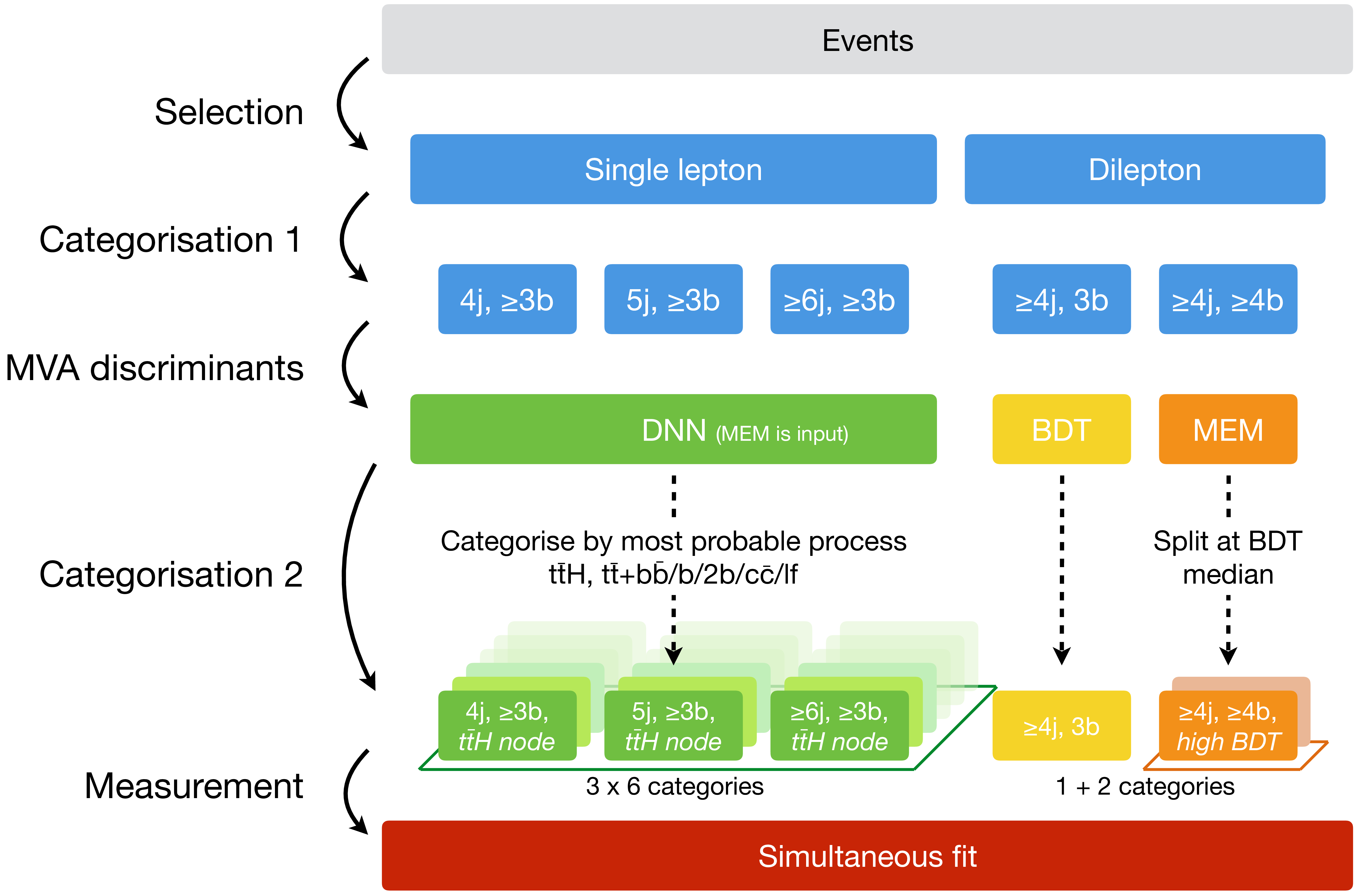
Figure 4:
Illustration of the analysis strategy. |
png pdf |
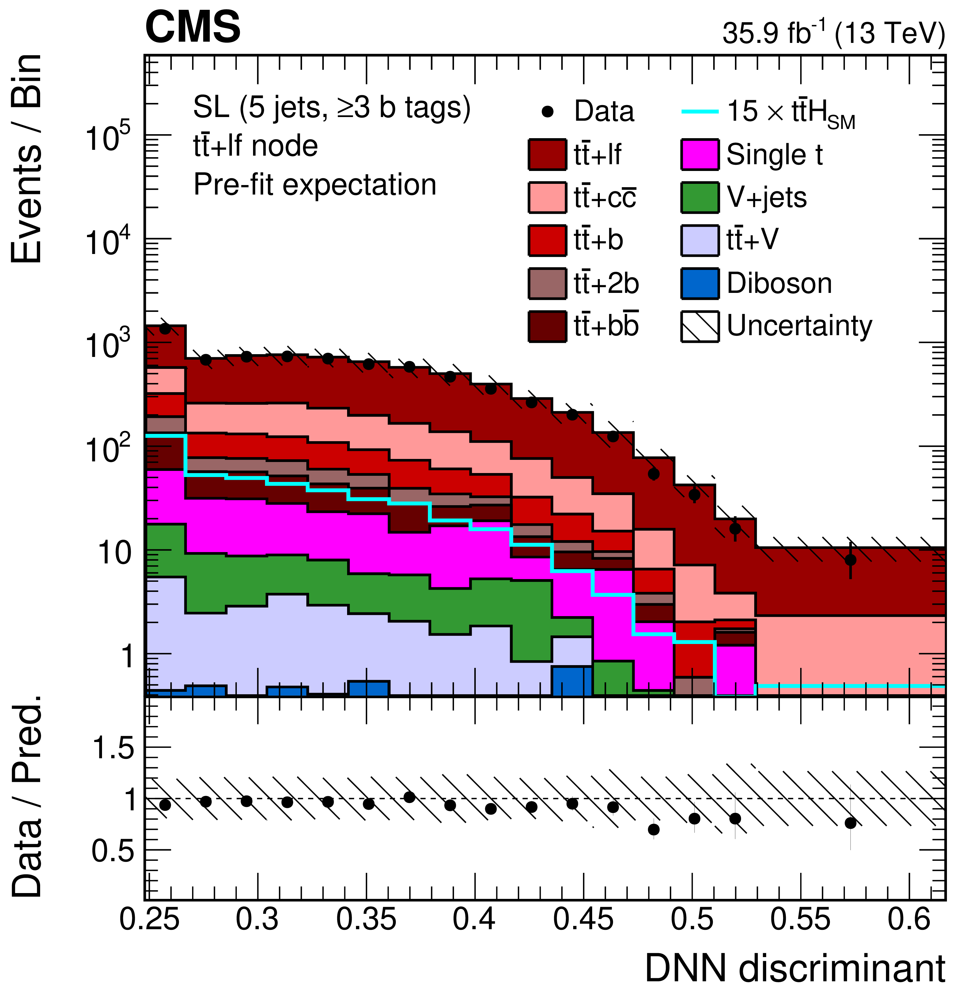
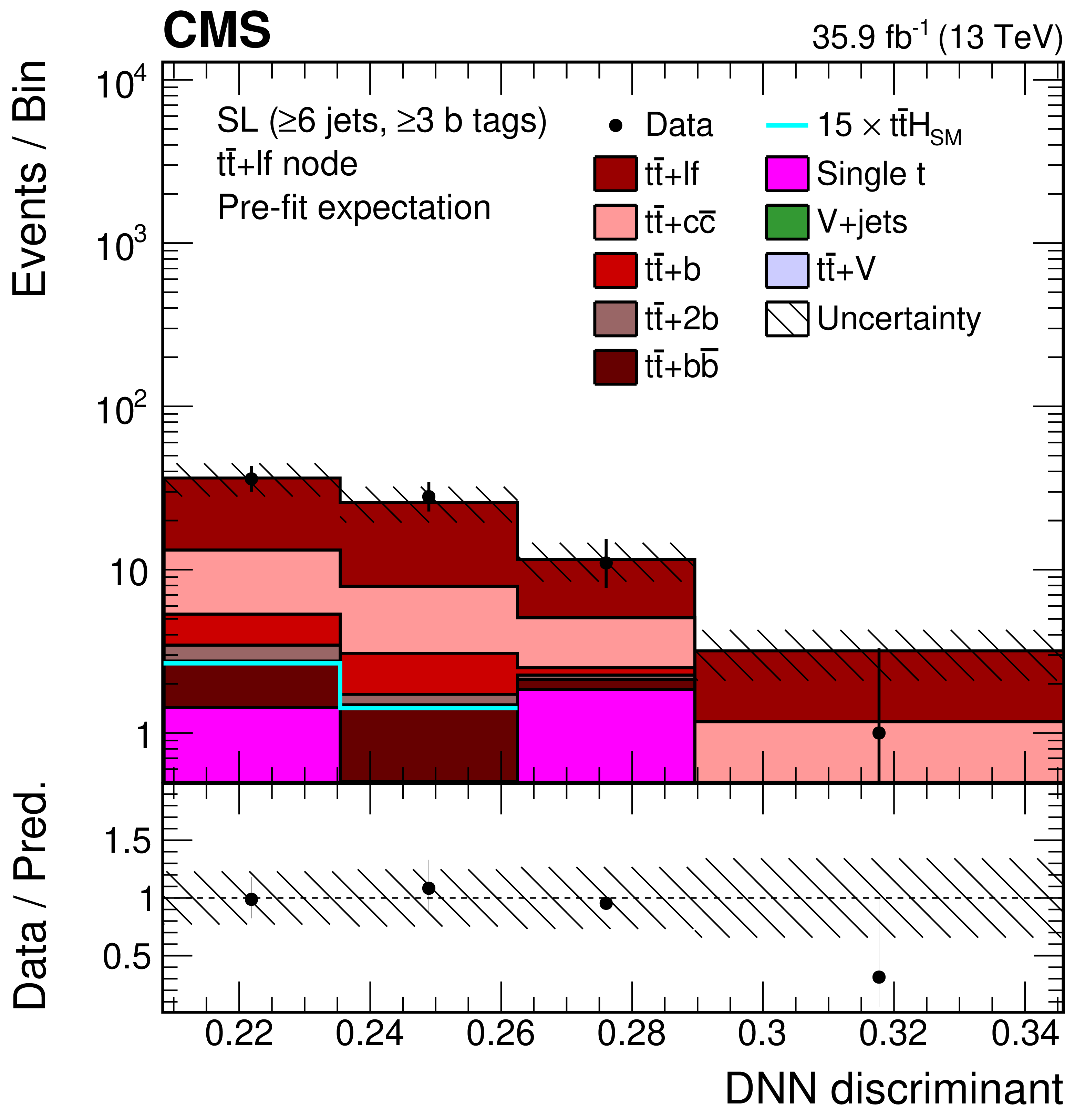
Figure 5:
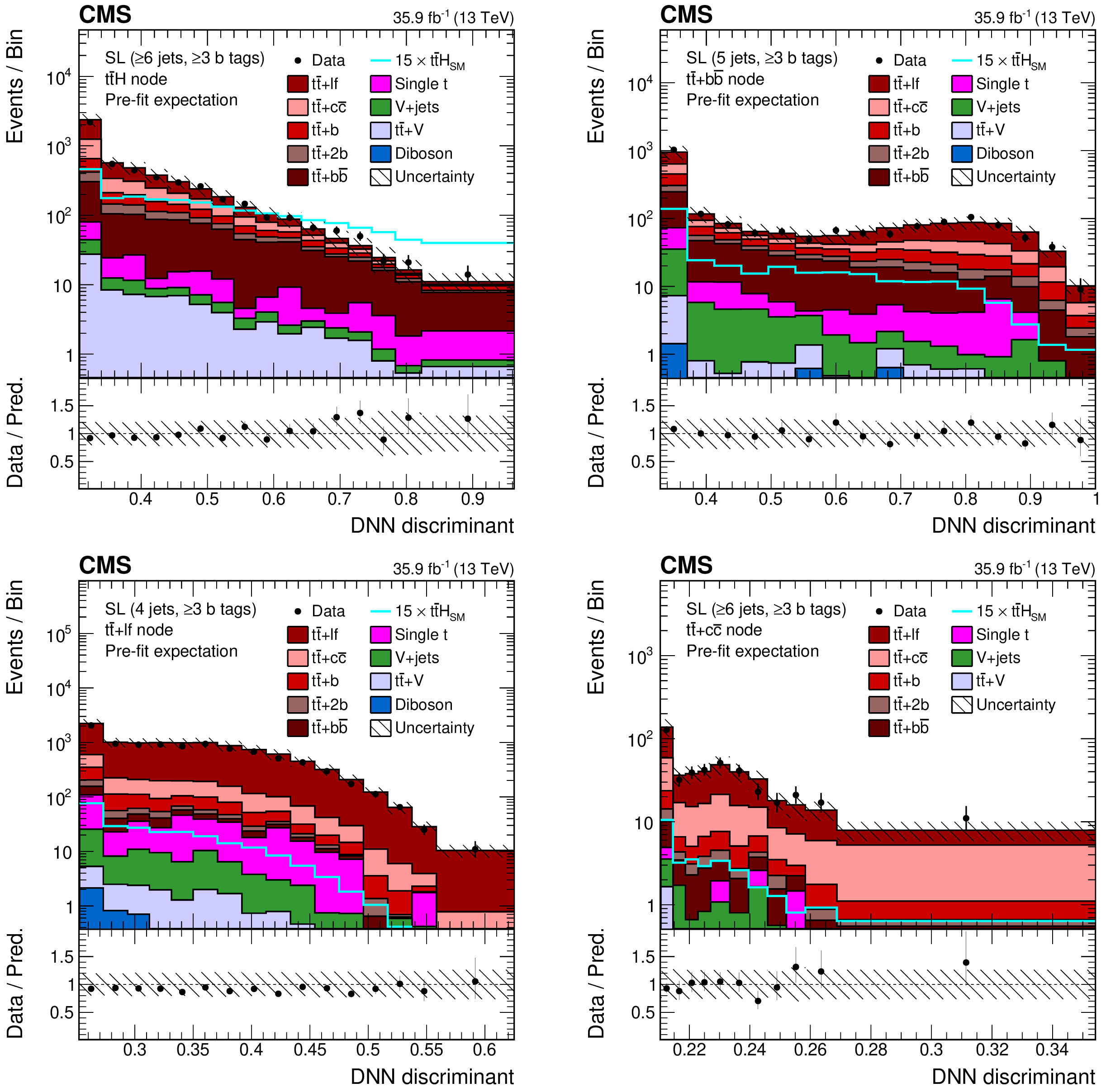
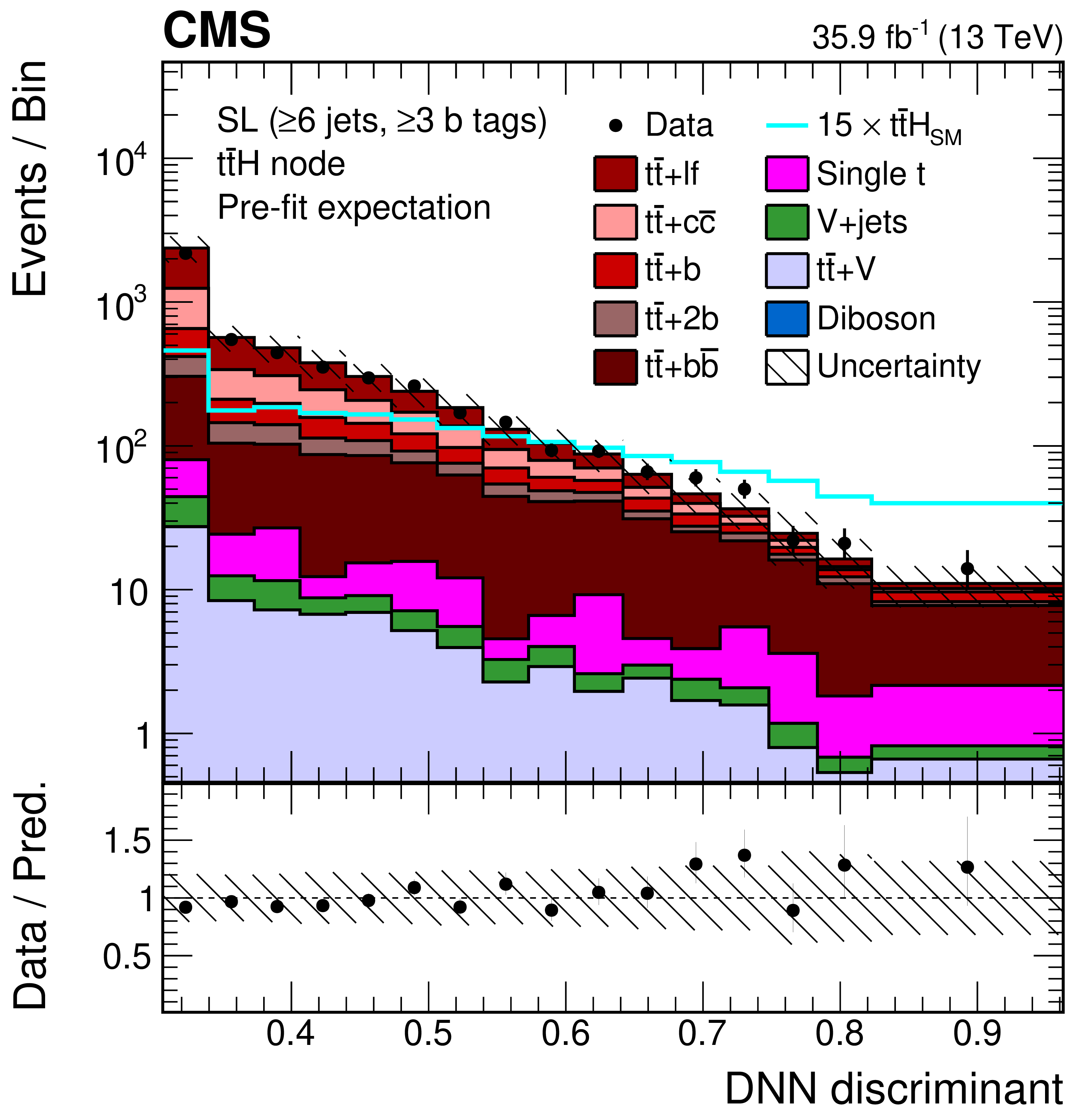
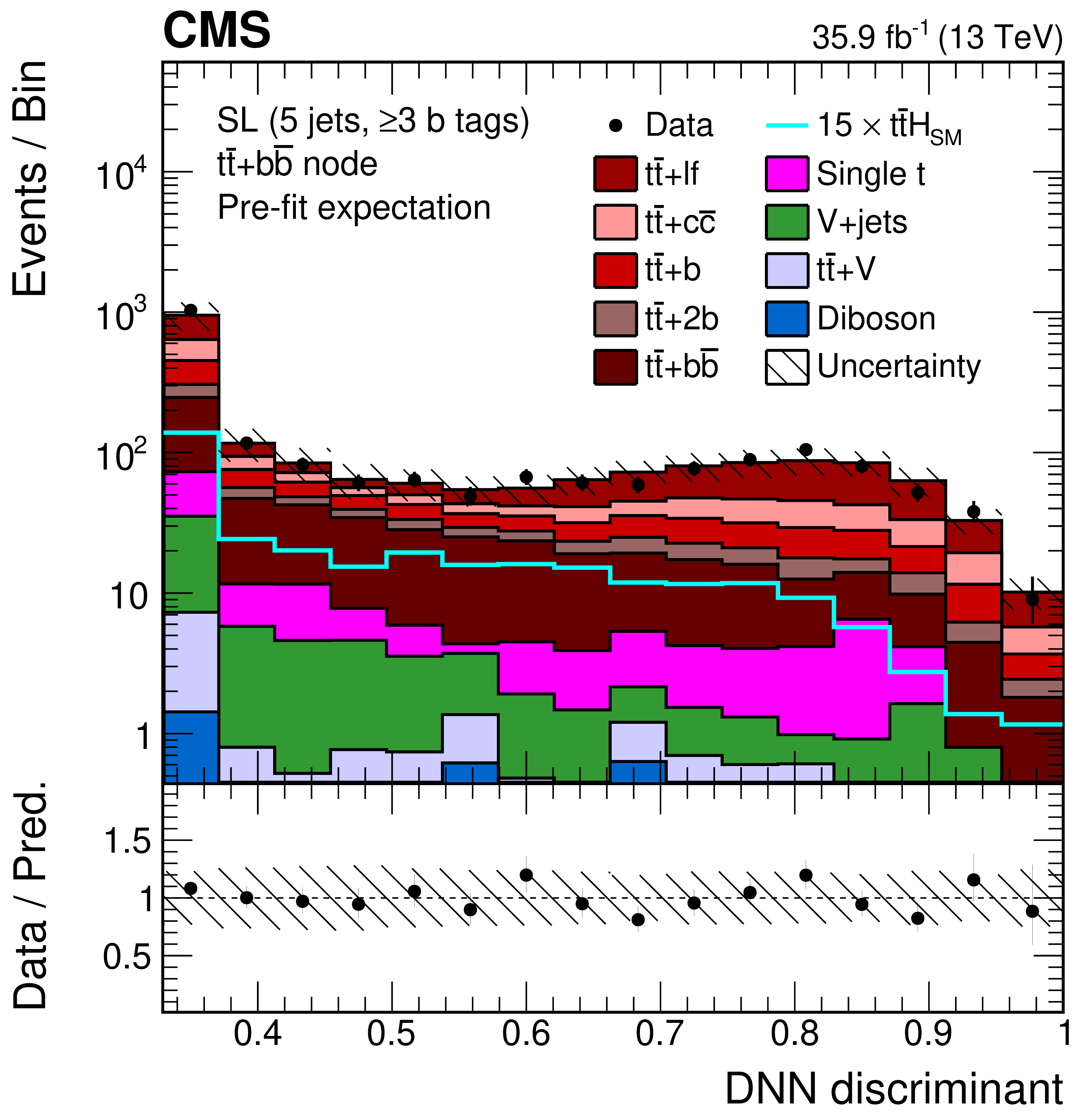
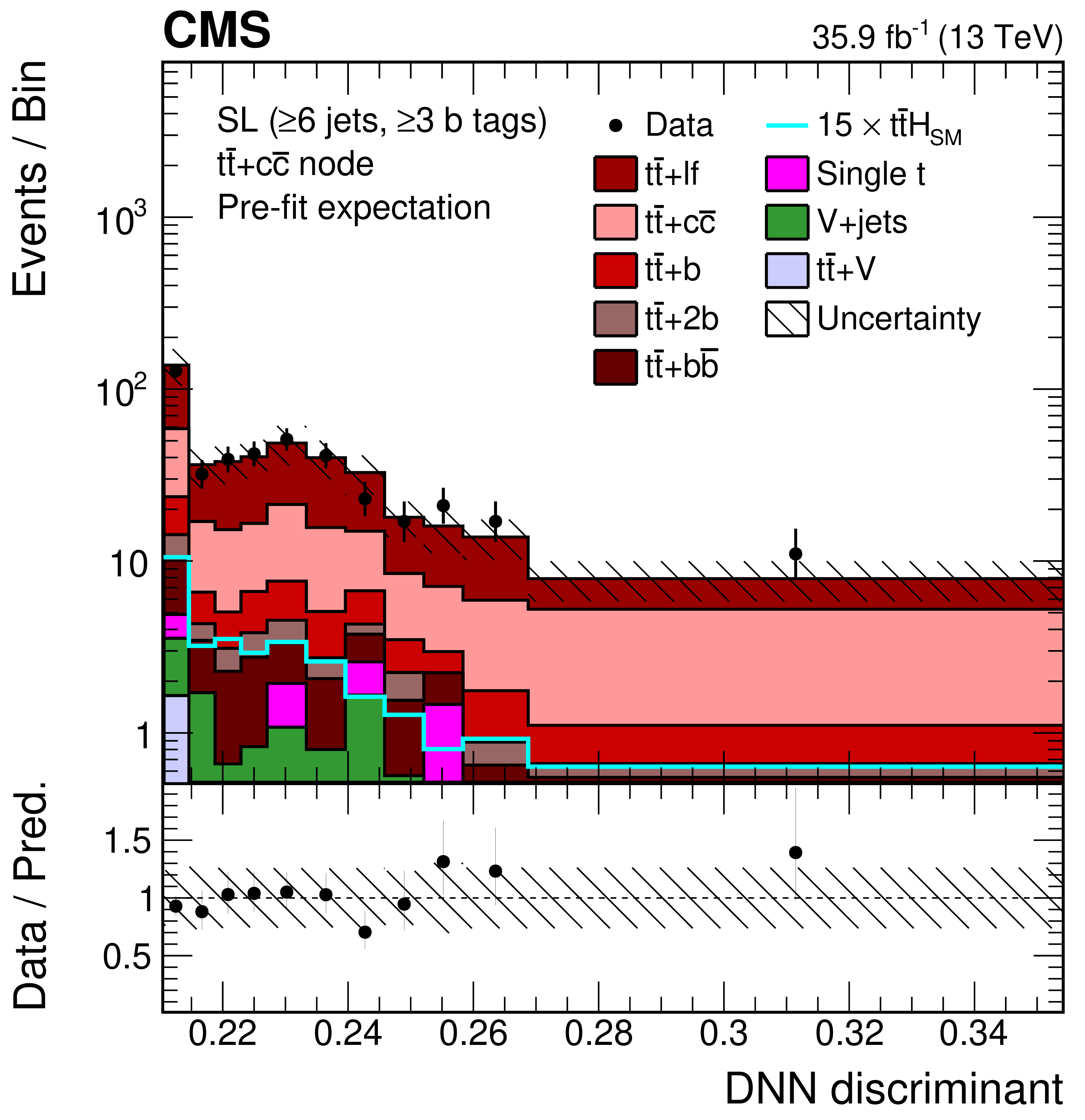
Final discriminant shapes in the single-lepton (SL) channel before the fit to data: DNN discriminant in the jet-process categories with $\geq $6 jets-$ {{{\mathrm {t}\overline {\mathrm {t}}}} {\mathrm {H}}} $ (upper left); 5 jets-$ {{{\mathrm {t}\overline {\mathrm {t}}}} \text {+} {{\mathrm {b}} {\overline {\mathrm {b}}}}} $ (upper right); 4 jets-$ {{{\mathrm {t}\overline {\mathrm {t}}}} \text {+}\text {lf}} $ (lower left); and $\geq $6 jets-$ {{{\mathrm {t}\overline {\mathrm {t}}}} \text {+} {{\mathrm {c}} {\overline {\mathrm {c}}}}} $ (lower right). The expected background contributions (filled histograms) are stacked, and the expected signal distribution (line), which includes $ {{\mathrm {H}} \to {{\mathrm {b}} {\overline {\mathrm {b}}}}} $ and all other Higgs boson decay modes, is superimposed. Each contribution is normalised to an integrated luminosity of 35.9 fb$^{-1}$, and the signal distribution is additionally scaled by a factor of 15 for better visibility. The hatched uncertainty bands include the total uncertainty of the fit model. The distributions observed in data (markers) are overlaid. The first and the last bins include underflow and overflow events, respectively. The lower plots show the ratio of the data to the background prediction. |
png pdf |
Figure 5-a:
Final discriminant shapes in the single-lepton (SL) channel before the fit to data: DNN discriminant in the jet-process categories with $\geq $6 jets-$ {{{\mathrm {t}\overline {\mathrm {t}}}} {\mathrm {H}}} $. The expected background contributions (filled histograms) are stacked, and the expected signal distribution (line), which includes $ {{\mathrm {H}} \to {{\mathrm {b}} {\overline {\mathrm {b}}}}} $ and all other Higgs boson decay modes, is superimposed. Each contribution is normalised to an integrated luminosity of 35.9 fb$^{-1}$, and the signal distribution is additionally scaled by a factor of 15 for better visibility. The hatched uncertainty bands include the total uncertainty of the fit model. The distribution observed in data (markers) is overlaid. The first and the last bins include underflow and overflow events, respectively. The lower plot shows the ratio of the data to the background prediction. |
png pdf |
Figure 5-b:
Final discriminant shapes in the single-lepton (SL) channel before the fit to data: DNN discriminant in the jet-process categories with 5 jets-$ {{{\mathrm {t}\overline {\mathrm {t}}}} \text {+} {{\mathrm {b}} {\overline {\mathrm {b}}}}} $. The expected background contributions (filled histograms) are stacked, and the expected signal distribution (line), which includes $ {{\mathrm {H}} \to {{\mathrm {b}} {\overline {\mathrm {b}}}}} $ and all other Higgs boson decay modes, is superimposed. Each contribution is normalised to an integrated luminosity of 35.9 fb$^{-1}$, and the signal distribution is additionally scaled by a factor of 15 for better visibility. The hatched uncertainty bands include the total uncertainty of the fit model. The distribution observed in data (markers) is overlaid. The first and the last bins include underflow and overflow events, respectively. The lower plot shows the ratio of the data to the background prediction. |

png pdf |
Figure 5-c:
Final discriminant shapes in the single-lepton (SL) channel before the fit to data: DNN discriminant in the jet-process categories with 4 jets-$ {{{\mathrm {t}\overline {\mathrm {t}}}} \text {+}\text {lf}} $. The expected background contributions (filled histograms) are stacked, and the expected signal distribution (line), which includes $ {{\mathrm {H}} \to {{\mathrm {b}} {\overline {\mathrm {b}}}}} $ and all other Higgs boson decay modes, is superimposed. Each contribution is normalised to an integrated luminosity of 35.9 fb$^{-1}$, and the signal distribution is additionally scaled by a factor of 15 for better visibility. The hatched uncertainty bands include the total uncertainty of the fit model. The distribution observed in data (markers) is overlaid. The first and the last bins include underflow and overflow events, respectively. The lower plot shows the ratio of the data to the background prediction. |
png pdf |
Figure 5-d:
Final discriminant shapes in the single-lepton (SL) channel before the fit to data: DNN discriminant in the jet-process categories with $\geq $6 jets-$ {{{\mathrm {t}\overline {\mathrm {t}}}} \text {+} {{\mathrm {c}} {\overline {\mathrm {c}}}}} $.The expected background contributions (filled histograms) are stacked, and the expected signal distribution (line), which includes $ {{\mathrm {H}} \to {{\mathrm {b}} {\overline {\mathrm {b}}}}} $ and all other Higgs boson decay modes, is superimposed. Each contribution is normalised to an integrated luminosity of 35.9 fb$^{-1}$, and the signal distribution is additionally scaled by a factor of 15 for better visibility. The hatched uncertainty bands include the total uncertainty of the fit model. The distribution observed in data (markers) is overlaid. The first and the last bins include underflow and overflow events, respectively. The lower plot shows the ratio of the data to the background prediction. |
png pdf |
Figure 6:
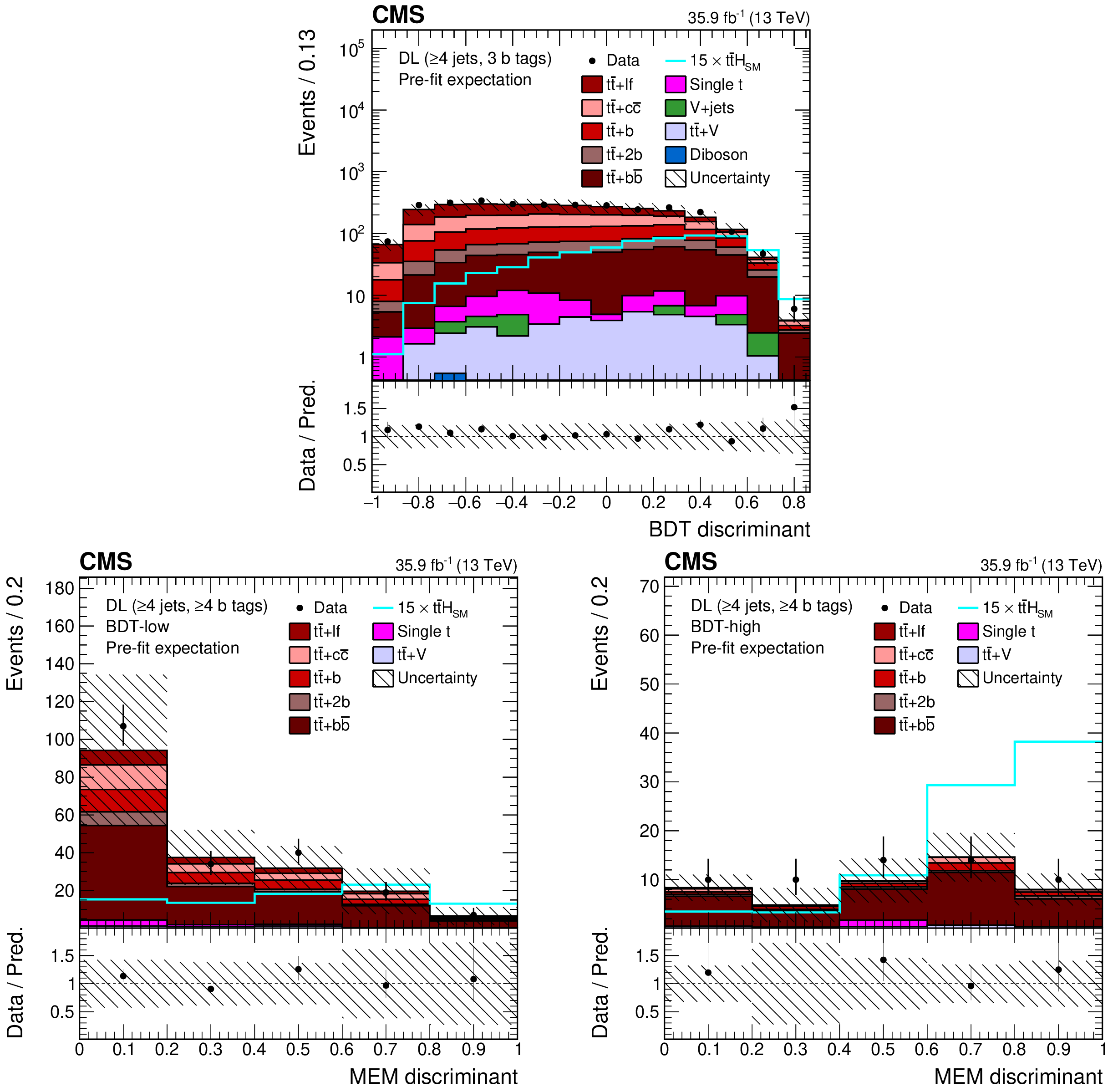
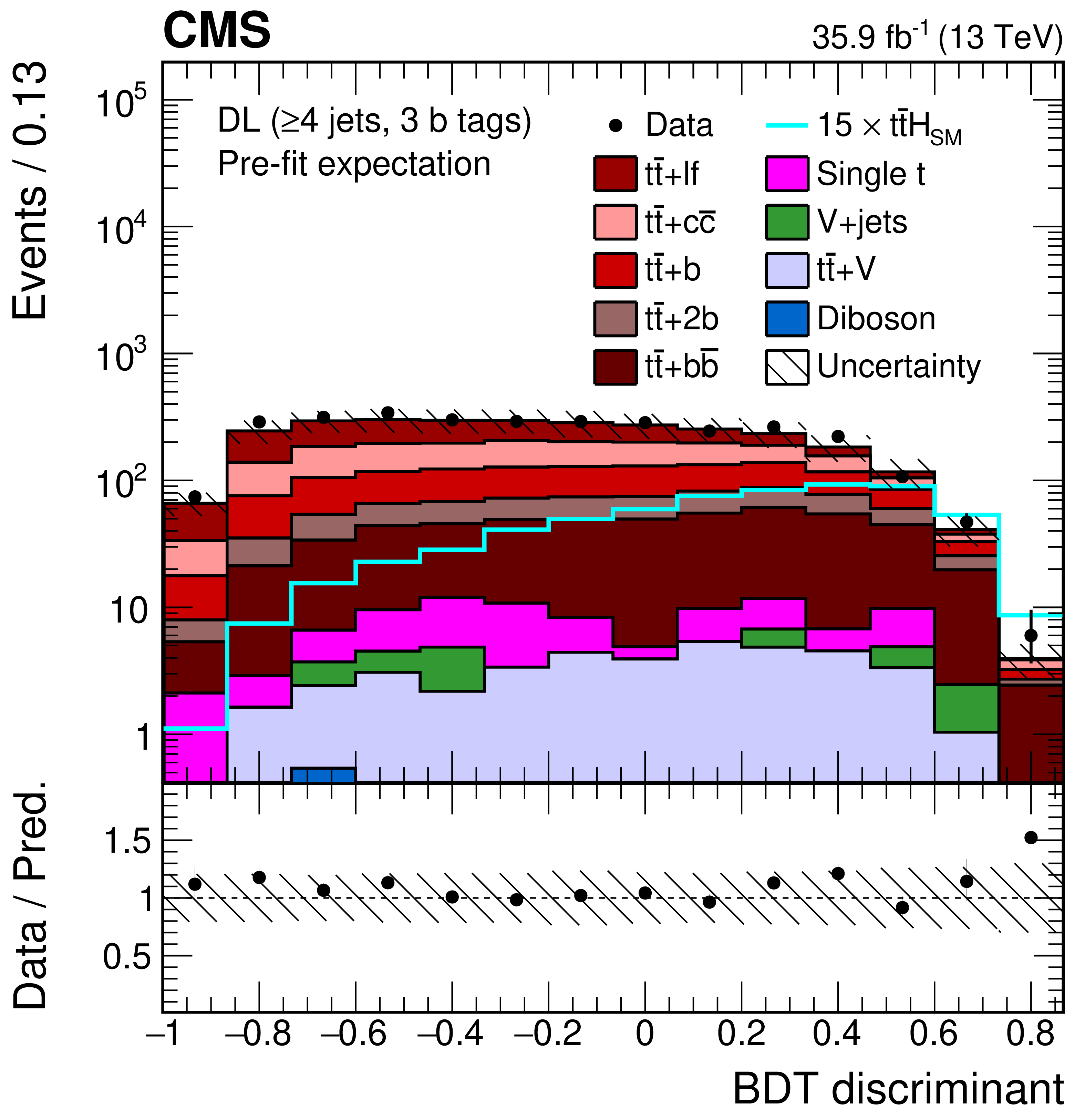
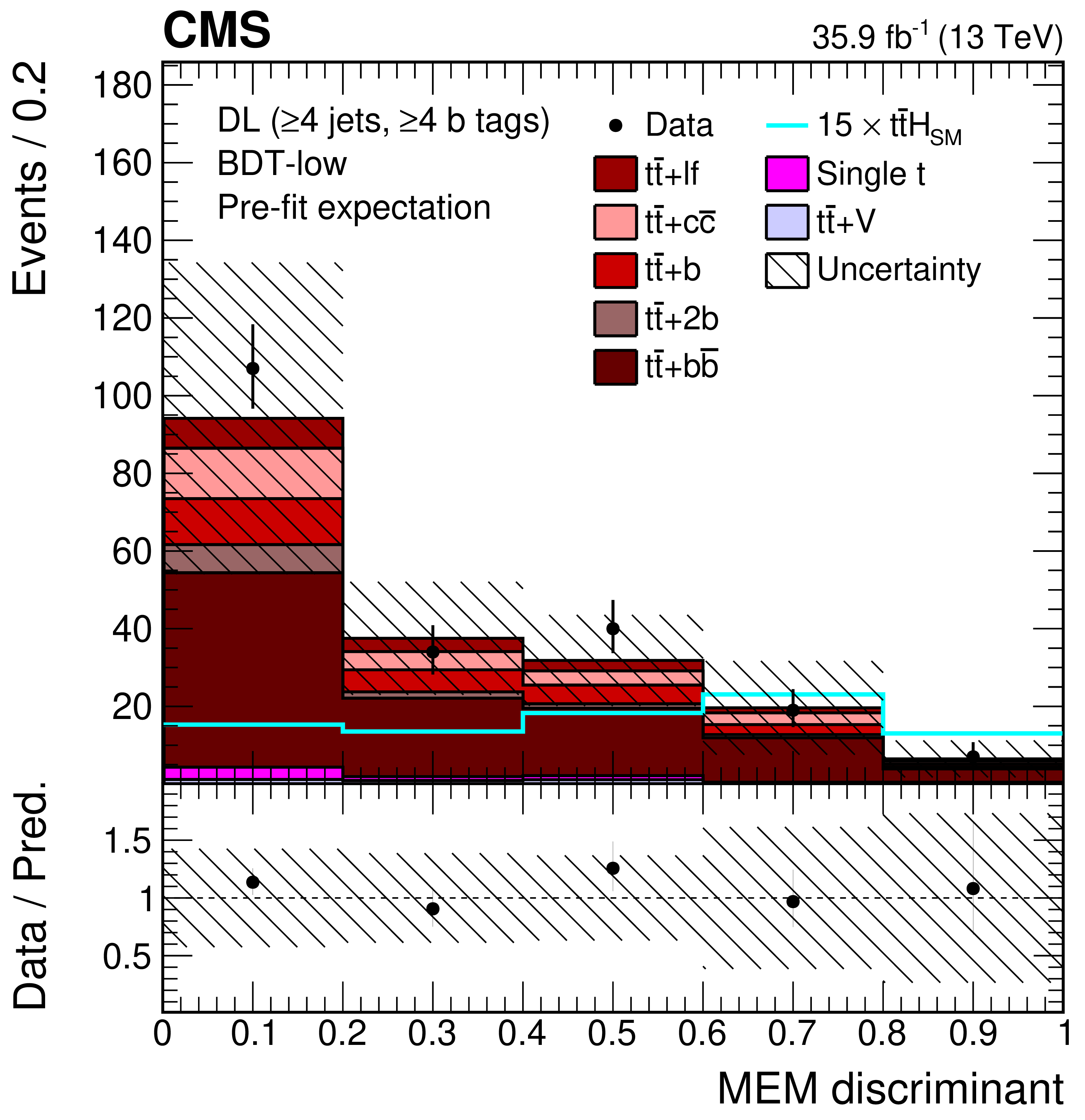
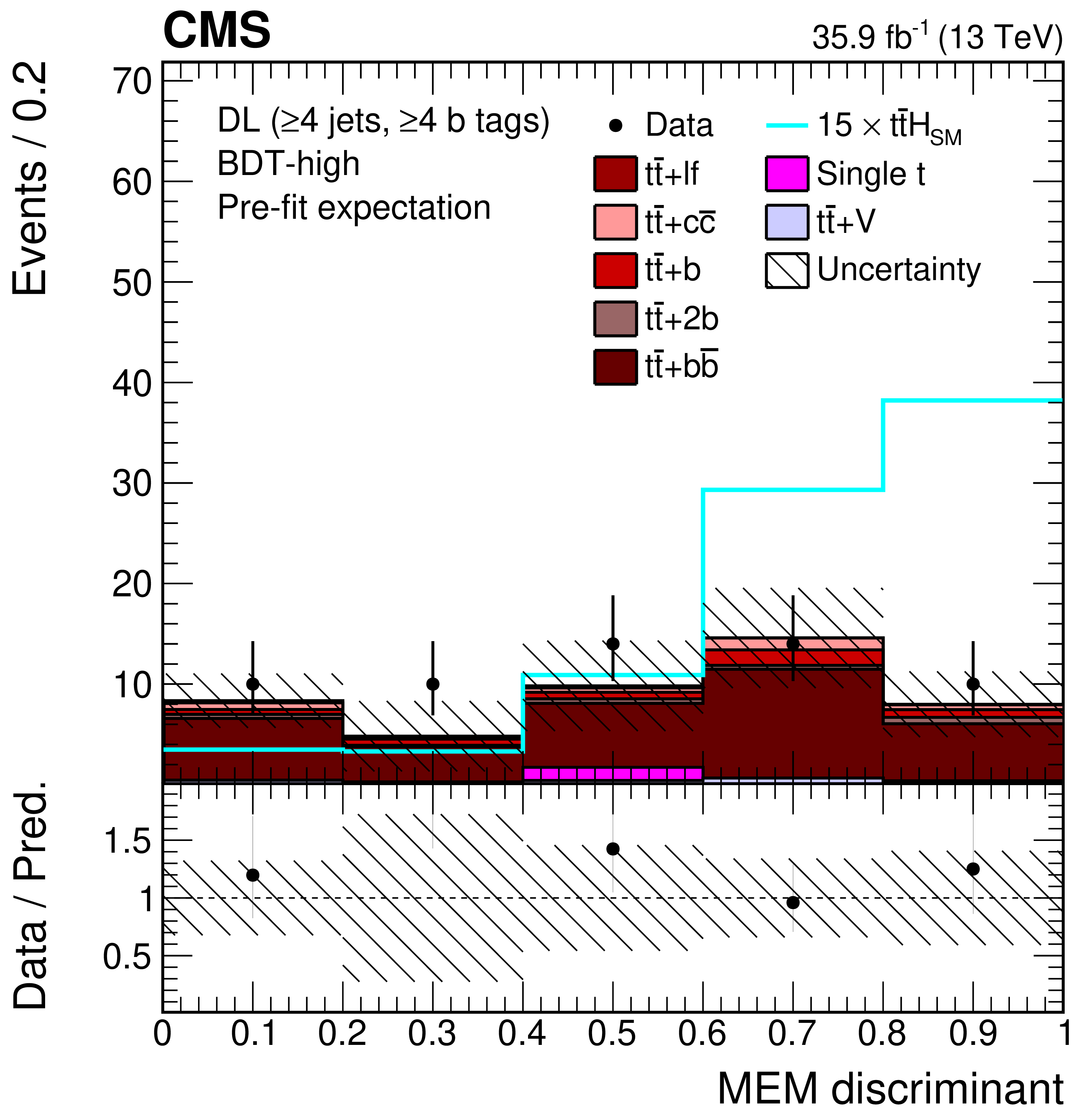
Final discriminant shapes in the dilepton (DL) channel before the fit to data: BDT discriminant in the analysis category with ($\geq$4 jets, 3 b tags) (upper row) and MEM discriminant in the analysis categories with ($\geq$4 jets, 4 b tags) (lower row) with low (left) and high (right) BDT output. The expected background contributions (filled histograms) are stacked, and the expected signal distribution (line), which includes $ {{\mathrm {H}} \to {{\mathrm {b}} {\overline {\mathrm {b}}}}} $ and all other Higgs boson decay modes, is superimposed. Each contribution is normalised to an integrated luminosity of 35.9 fb$^{-1}$, and the signal distribution is additionally scaled by a factor of 15 for better visibility. The hatched uncertainty bands include the total uncertainty of the fit model. The distributions observed in data (markers) are overlaid. The first and the last bins include underflow and overflow events, respectively. The lower plots show the ratio of the data to the background prediction. |
png pdf |
Figure 6-a:
Final discriminant shape in the dilepton (DL) channel before the fit to data: BDT discriminant in the analysis category with ($\geq$4 jets, 3 b tags). The expected background contributions (filled histograms) are stacked, and the expected signal distribution (line), which includes $ {{\mathrm {H}} \to {{\mathrm {b}} {\overline {\mathrm {b}}}}} $ and all other Higgs boson decay modes, is superimposed. Each contribution is normalised to an integrated luminosity of 35.9 fb$^{-1}$, and the signal distribution is additionally scaled by a factor of 15 for better visibility. The hatched uncertainty bands include the total uncertainty of the fit model. The distribution observed in data (markers) is overlaid. The first and the last bins include underflow and overflow events, respectively. The lower plot shows the ratio of the data to the background prediction. |
png pdf |
Figure 6-b:
Final discriminant shape in the dilepton (DL) channel before the fit to data: MEM discriminant in the analysis categories with ($\geq$4 jets, 4 b tags) with low BDT output. The expected background contributions (filled histograms) are stacked, and the expected signal distribution (line), which includes $ {{\mathrm {H}} \to {{\mathrm {b}} {\overline {\mathrm {b}}}}} $ and all other Higgs boson decay modes, is superimposed. Each contribution is normalised to an integrated luminosity of 35.9 fb$^{-1}$, and the signal distribution is additionally scaled by a factor of 15 for better visibility. The hatched uncertainty bands include the total uncertainty of the fit model. The distribution observed in data (markers) is overlaid. The first and the last bins include underflow and overflow events, respectively. The lower plot shows the ratio of the data to the background prediction. |
png pdf |
Figure 6-c:
Final discriminant shape in the dilepton (DL) channel before the fit to data: MEM discriminant in the analysis categories with ($\geq$4 jets, 4 b tags) with high BDT output. The expected background contributions (filled histograms) are stacked, and the expected signal distribution (line), which includes $ {{\mathrm {H}} \to {{\mathrm {b}} {\overline {\mathrm {b}}}}} $ and all other Higgs boson decay modes, is superimposed. Each contribution is normalised to an integrated luminosity of 35.9 fb$^{-1}$, and the signal distribution is additionally scaled by a factor of 15 for better visibility. The hatched uncertainty bands include the total uncertainty of the fit model. The distribution observed in data (markers) is overlaid. The first and the last bins include underflow and overflow events, respectively. The lower plot shows the ratio of the data to the background prediction. |
png pdf |
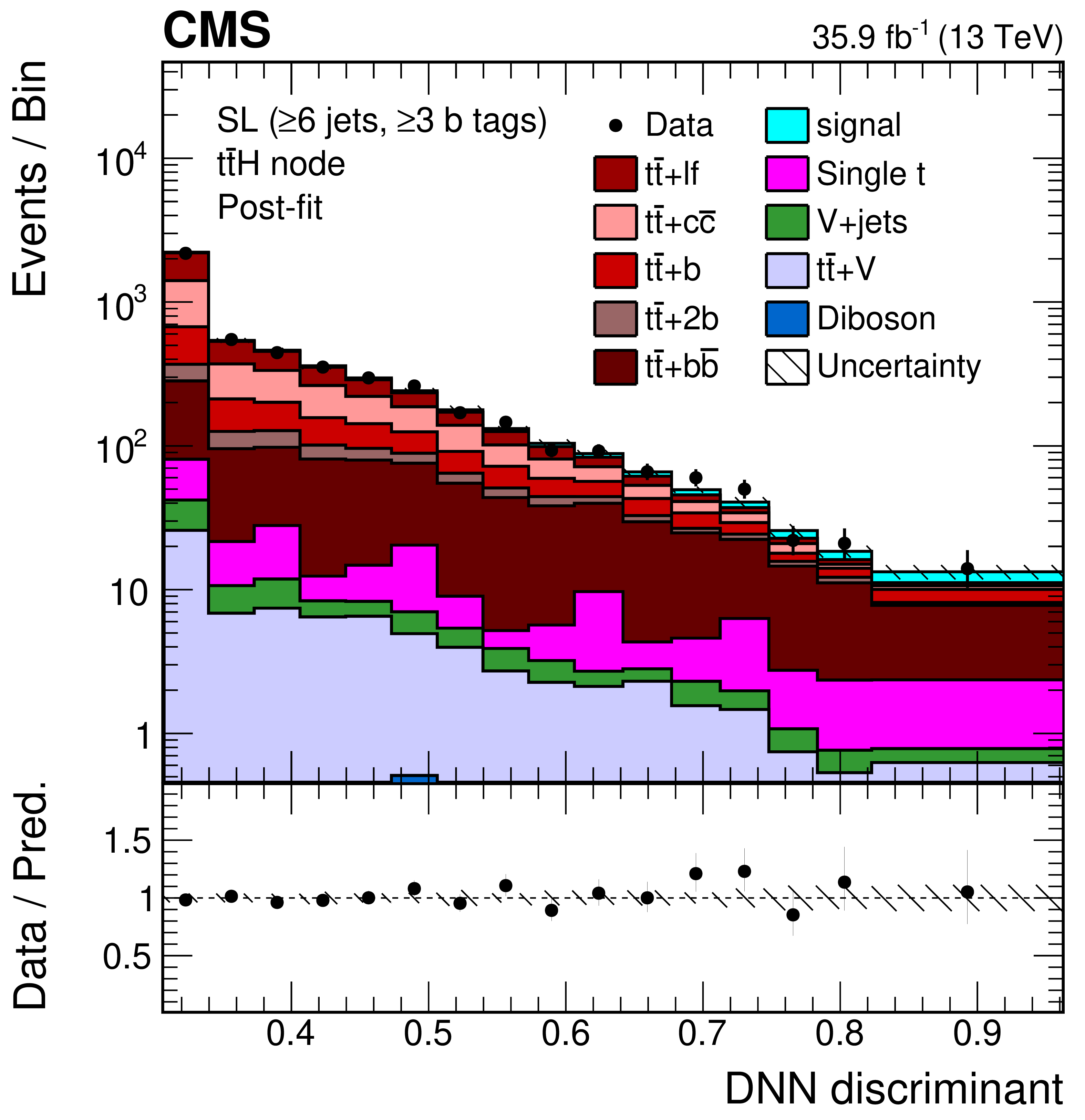
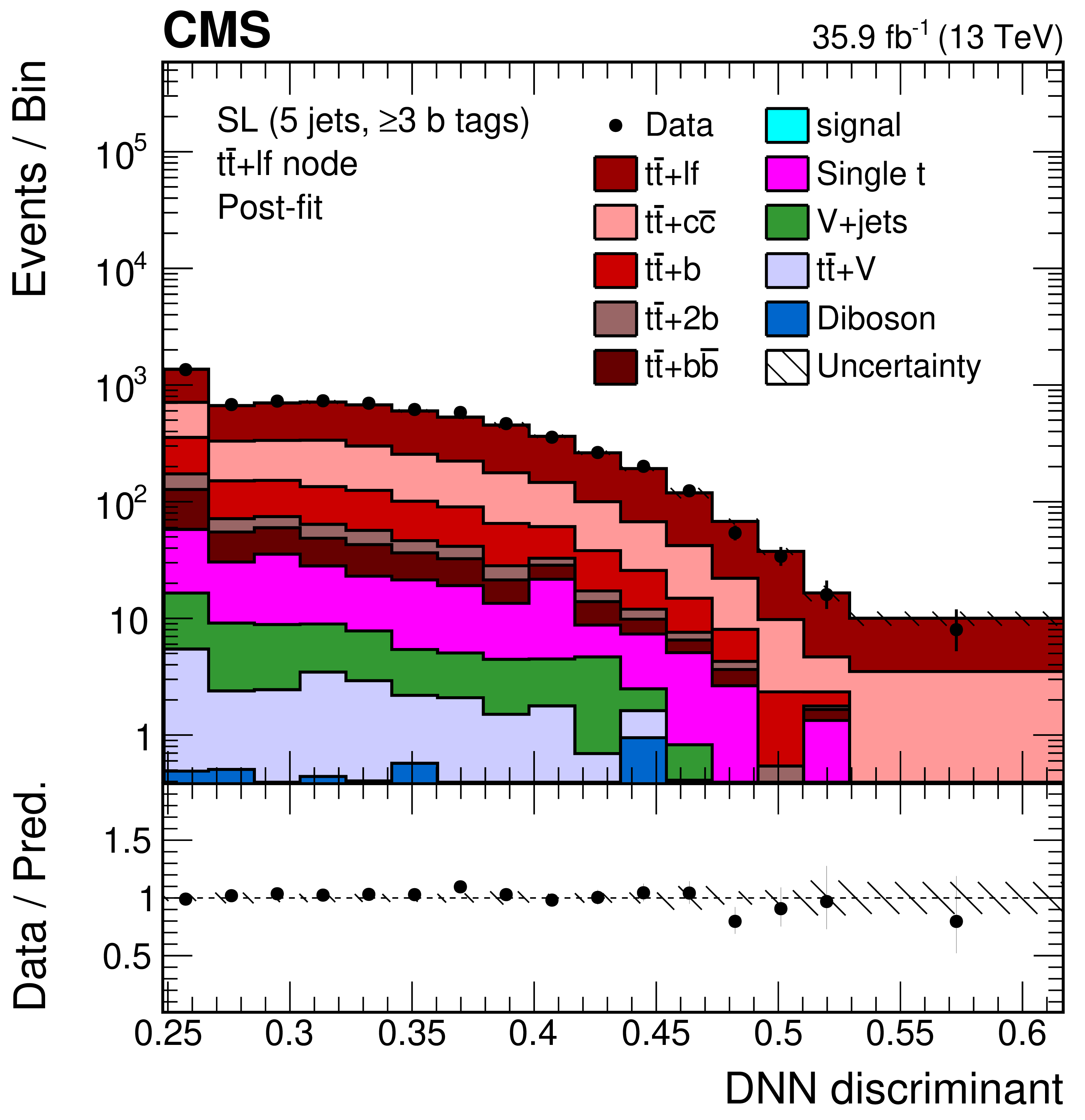
Figure 7:
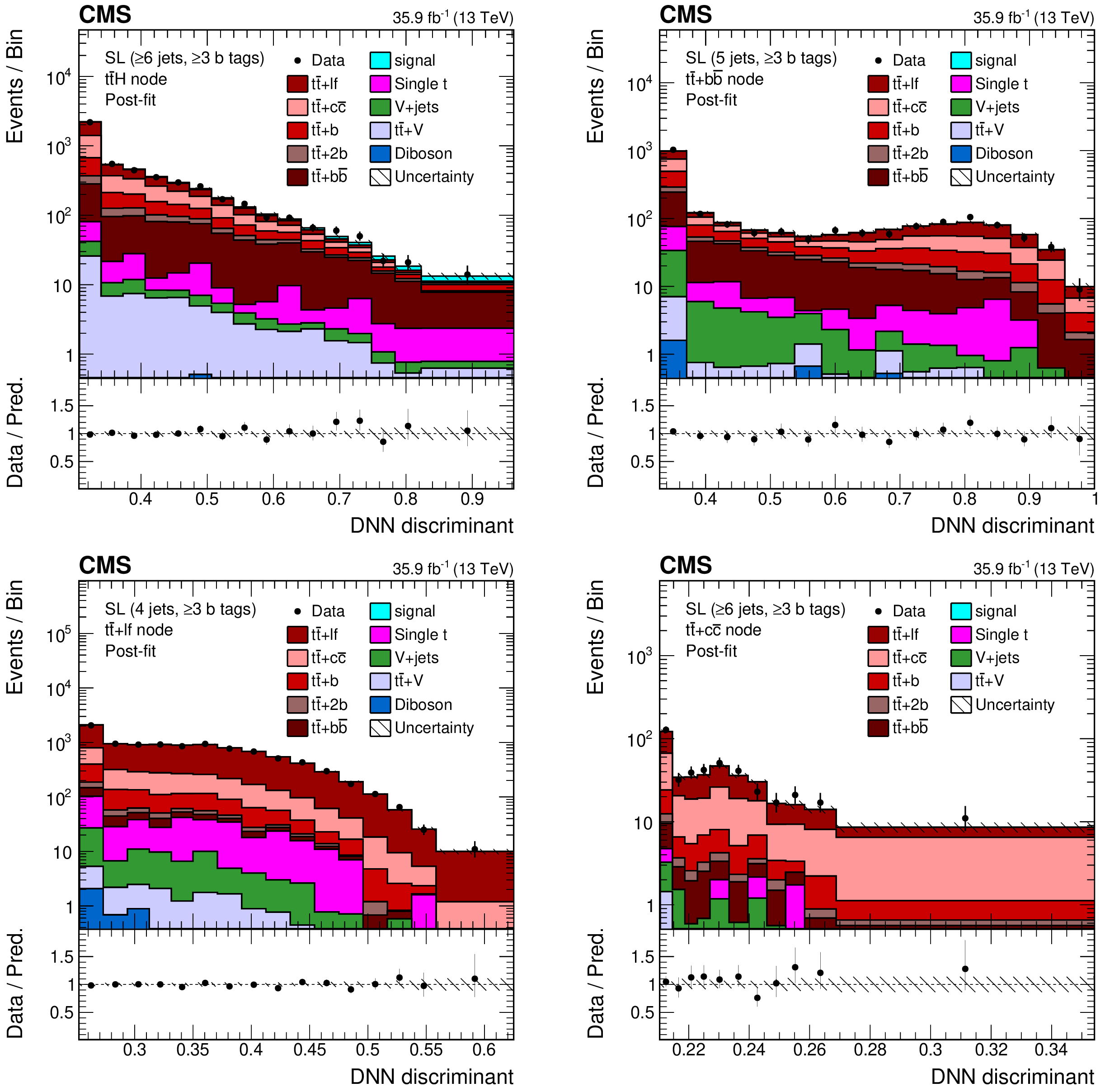
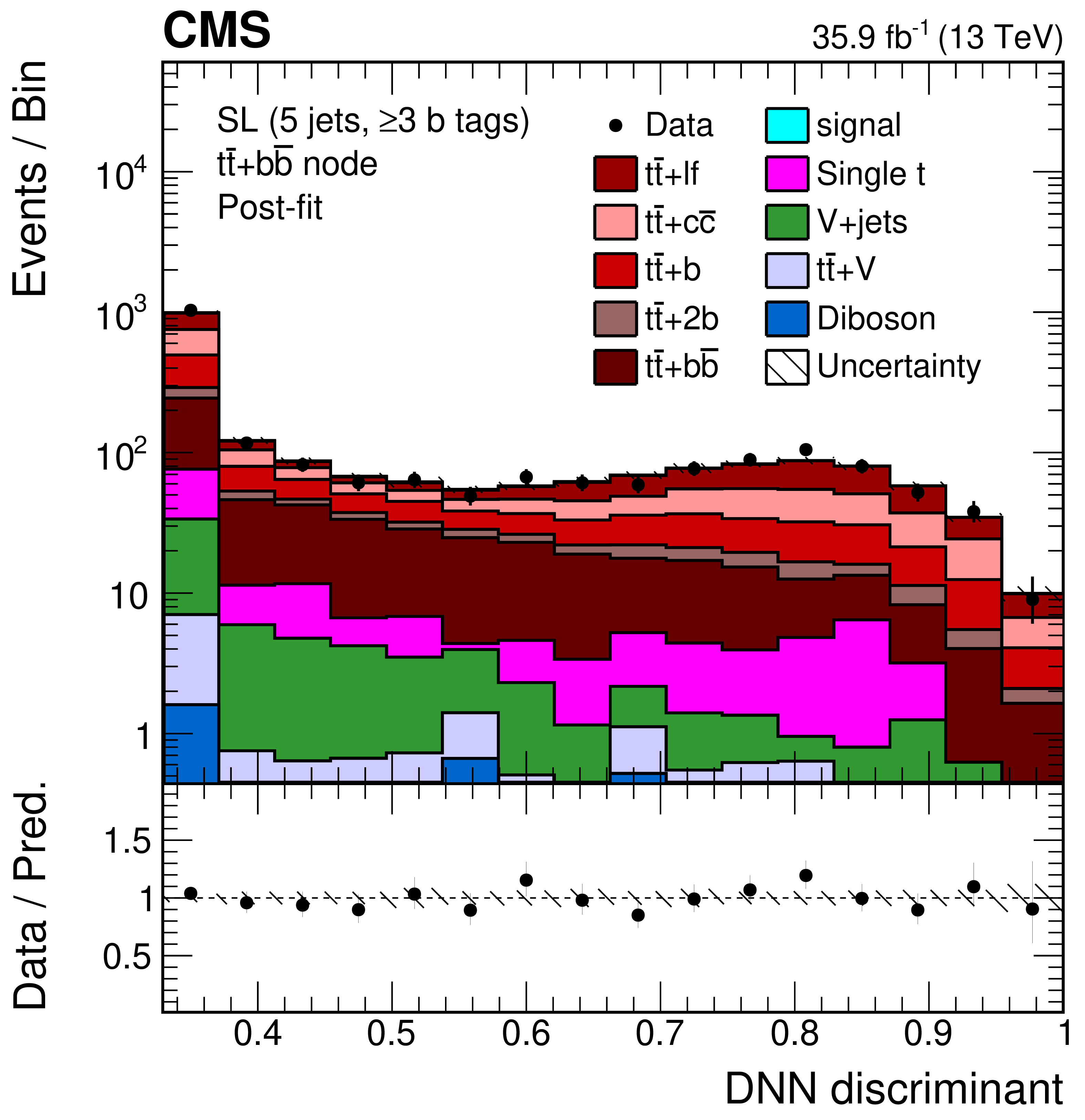
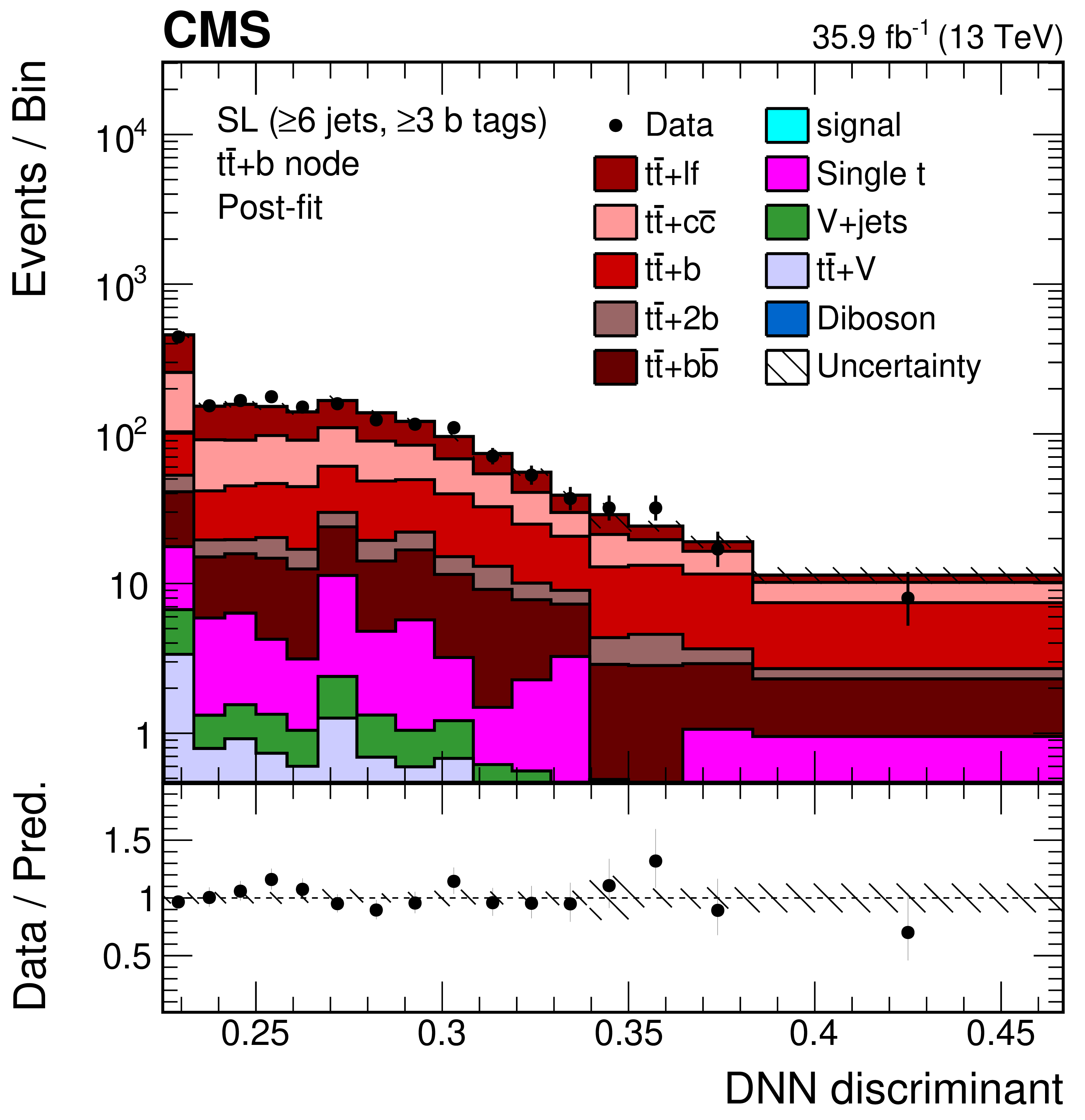
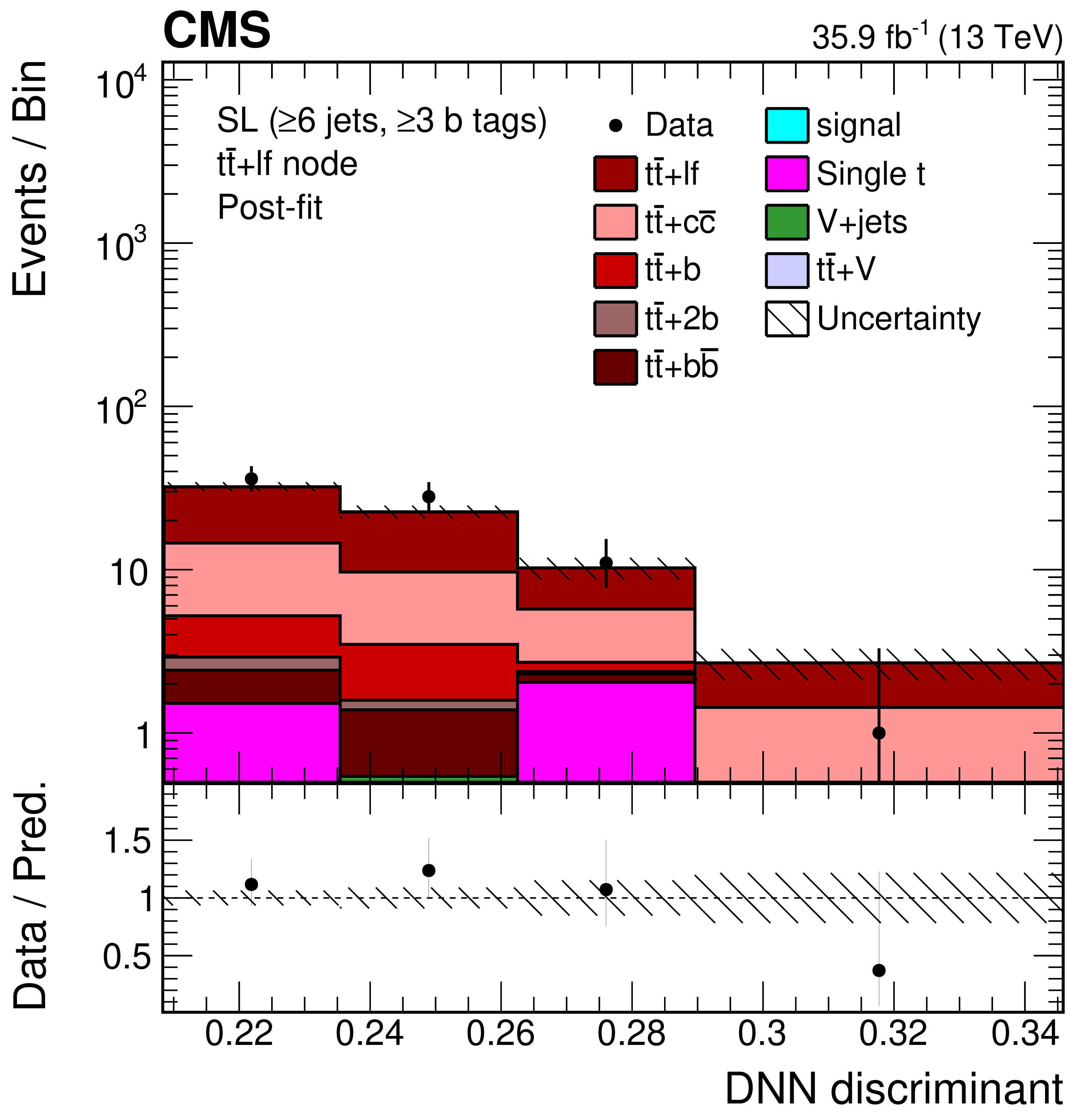
Final discriminant shapes in the single-lepton (SL) channel after the fit to data: DNN discriminant in the jet-process categories with $\geq $6 jets-$ {{{\mathrm {t}\overline {\mathrm {t}}}} {\mathrm {H}}} $ (upper left); 5 jets-$ {{{\mathrm {t}\overline {\mathrm {t}}}} \text {+} {{\mathrm {b}} {\overline {\mathrm {b}}}}} $ (upper right); 4 jets-$ {{{\mathrm {t}\overline {\mathrm {t}}}} \text {+}\text {lf}} $ (lower left); and $\geq $6 jets-$ {{{\mathrm {t}\overline {\mathrm {t}}}} \text {+} {{\mathrm {c}} {\overline {\mathrm {c}}}}} $ (lower right). The hatched uncertainty bands include the total uncertainty after the fit to data. The distributions observed in data (markers) are overlaid. The first and the last bins include underflow and overflow events, respectively. The lower plots show the ratio of the data to the post-fit background plus signal distribution. |
png pdf |
Figure 7-a:
Final discriminant shapes in the single-lepton (SL) channel after the fit to data: DNN discriminant in the jet-process categories with $\geq $6 jets-$ {{{\mathrm {t}\overline {\mathrm {t}}}} {\mathrm {H}}} $. The hatched uncertainty bands include the total uncertainty after the fit to data. The distribution observed in data (markers) is overlaid. The first and the last bins include underflow and overflow events, respectively. The lower plot shows the ratio of the data to the post-fit background plus signal distribution. |

png pdf |
Figure 7-b:
Final discriminant shapes in the single-lepton (SL) channel after the fit to data: DNN discriminant in the jet-process categories with 5 jets-$ {{{\mathrm {t}\overline {\mathrm {t}}}} \text {+} {{\mathrm {b}} {\overline {\mathrm {b}}}}} $. The hatched uncertainty bands include the total uncertainty after the fit to data. The distribution observed in data (markers) is overlaid. The first and the last bins include underflow and overflow events, respectively. The lower plot shows the ratio of the data to the post-fit background plus signal distribution. |

png pdf |
Figure 7-c:
Final discriminant shapes in the single-lepton (SL) channel after the fit to data: DNN discriminant in the jet-process categories with 4 jets-$ {{{\mathrm {t}\overline {\mathrm {t}}}} \text {+}\text {lf}} $. The hatched uncertainty bands include the total uncertainty after the fit to data. The distribution observed in data (markers) is overlaid. The first and the last bins include underflow and overflow events, respectively. The lower plot shows the ratio of the data to the post-fit background plus signal distribution. |
png pdf |
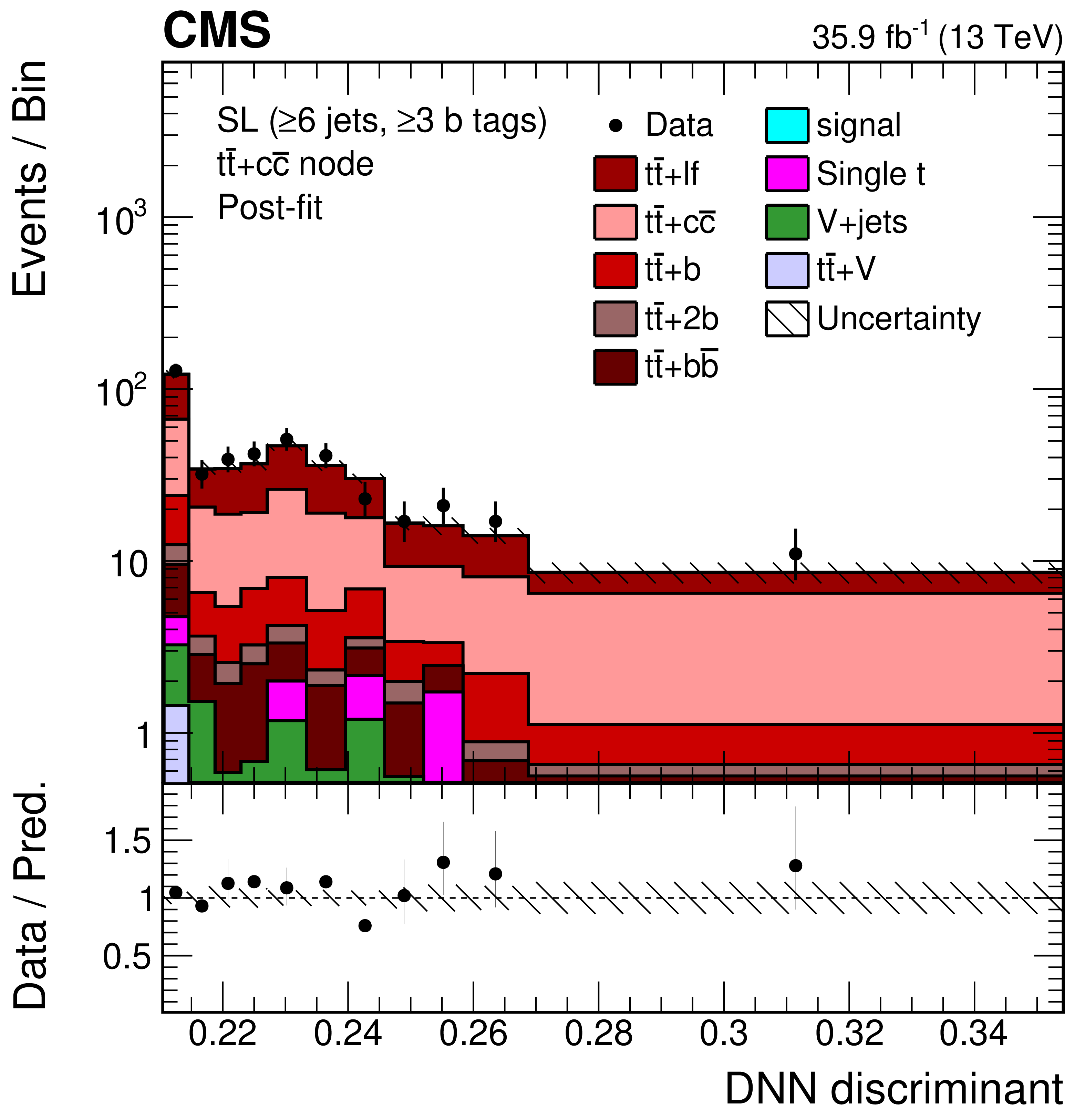
Figure 7-d:
Final discriminant shapes in the single-lepton (SL) channel after the fit to data: DNN discriminant in the jet-process categories with $\geq $6 jets-$ {{{\mathrm {t}\overline {\mathrm {t}}}} \text {+} {{\mathrm {c}} {\overline {\mathrm {c}}}}} $. The hatched uncertainty bands include the total uncertainty after the fit to data. The distribution observed in data (markers) is overlaid. The first and the last bins include underflow and overflow events, respectively. The lower plot shows the ratio of the data to the post-fit background plus signal distribution. |
png pdf |
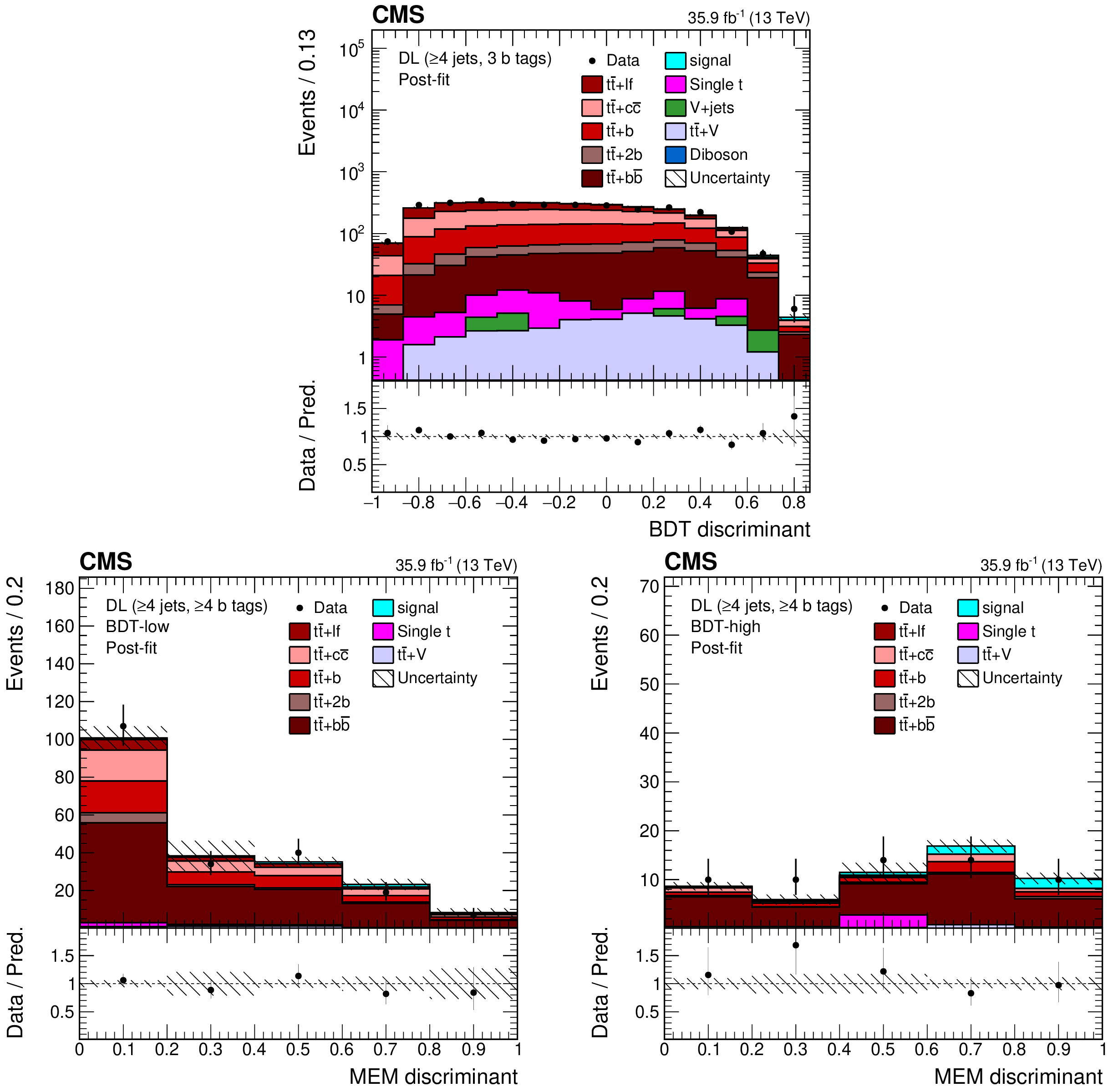
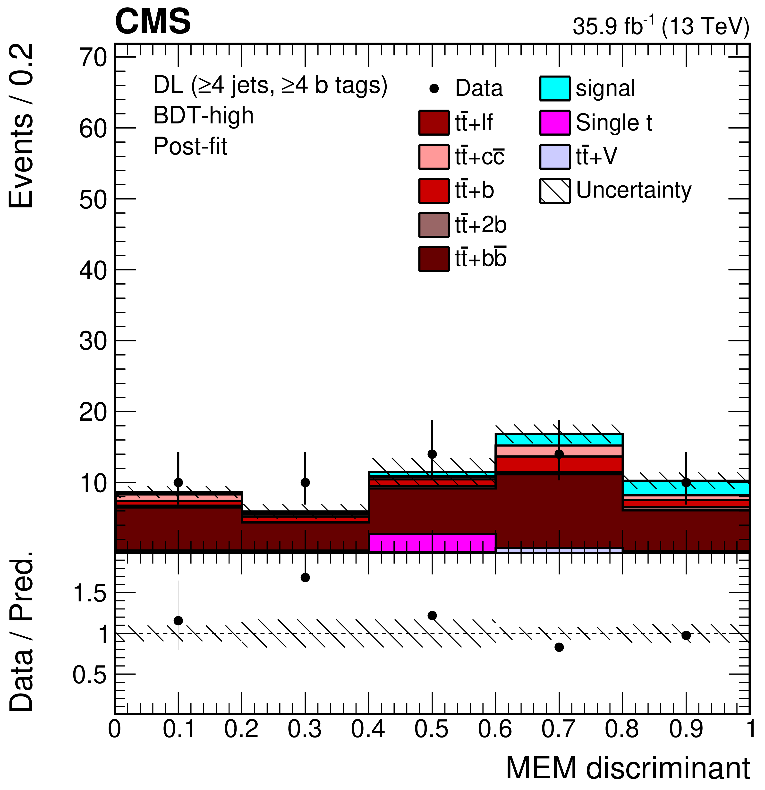
Figure 8:
Final discriminant shapes in the dilepton (DL) channel after the fit to data: BDT discriminant in the analysis category with ($\geq$4 jets, 3 b tags) (upper row) and MEM discriminant in the analysis categories with ($\geq$4 jets, 4 b tags) (lower row) with low (left) and high (right) BDT output. The hatched uncertainty bands include the total uncertainty after the fit to data. The distributions observed in data (markers) are overlaid. The first and the last bins include underflow and overflow events, respectively. The lower plots show the ratio of the data to the post-fit background plus signal distribution. |
png pdf |
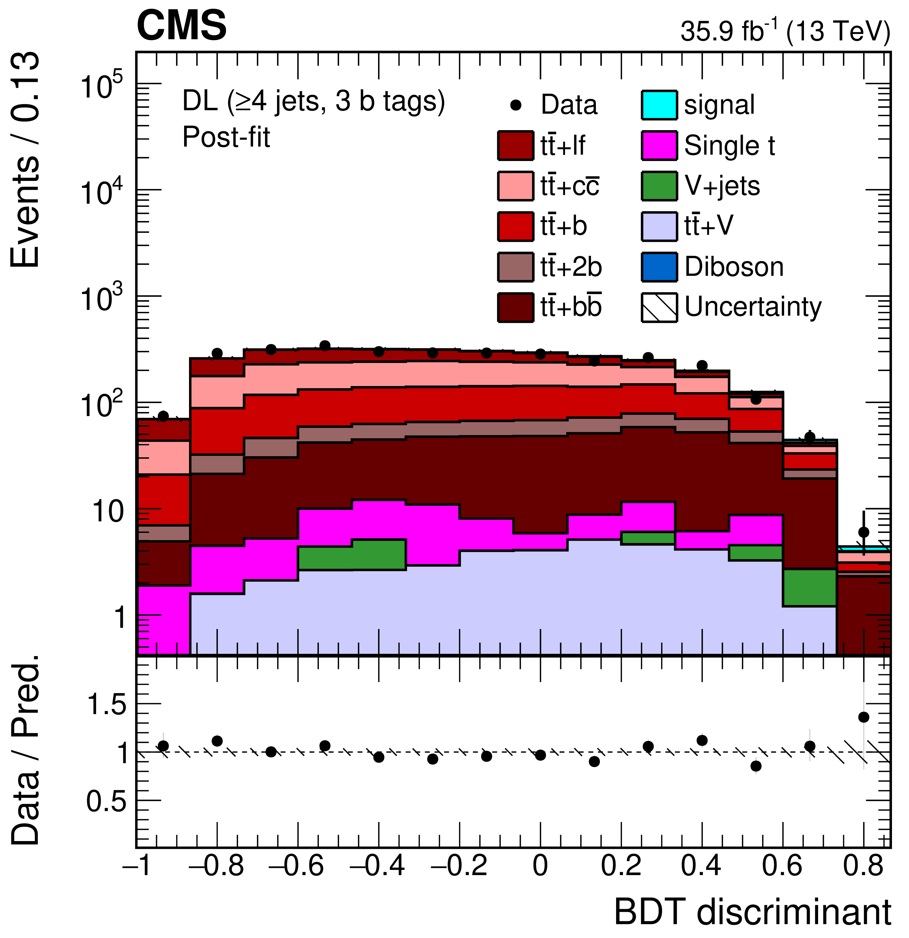
Figure 8-a:
Final discriminant shapes in the dilepton (DL) channel after the fit to data: BDT discriminant in the analysis category with ($\geq$4 jets, 3 b tags). The hatched uncertainty bands include the total uncertainty after the fit to data. The distribution observed in data (markers) is overlaid. The first and the last bins include underflow and overflow events, respectively. The lower plot shows the ratio of the data to the post-fit background plus signal distribution. |

png pdf |
Figure 8-b:
Final discriminant shapes in the dilepton (DL) channel after the fit to data: MEM discriminant in the analysis categories with ($\geq$4 jets, 4 b tags) (lower row) with low highBDT output. The hatched uncertainty bands include the total uncertainty after the fit to data. The distribution observed in data (markers) is overlaid. The first and the last bins include underflow and overflow events, respectively. The lower plot shows the ratio of the data to the post-fit background plus signal distribution. |
png pdf |
Figure 8-c:
Final discriminant shapes in the dilepton (DL) channel after the fit to data: MEM discriminant in the analysis categories with ($\geq$4 jets, 4 b tags) (lower row) with low highBDT output. The hatched uncertainty bands include the total uncertainty after the fit to data. The distribution observed in data (markers) is overlaid. The first and the last bins include underflow and overflow events, respectively. The lower plot shows the ratio of the data to the post-fit background plus signal distribution. |
png pdf |
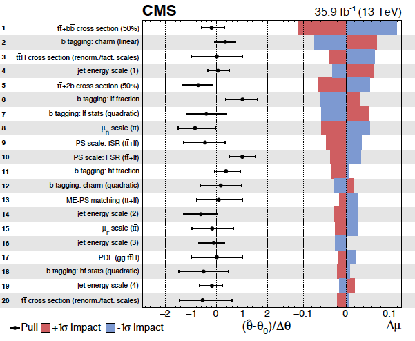
Figure 9:
Post-fit pull and impact on the signal strength $\mu$ of the nuisance parameters included in the fit, ordered by their impact. Only the 20 highest ranked parameters are shown, not including nuisance parameters describing the uncertainty due to the size of the simulated samples. The four highest-ranked nuisance parameters related to the jet energy scale uncertainty sources are shown as indicated in parentheses. The pulls of the nuisance parameters (black markers) are computed relative to their pre-fit values $\theta_{0}$ and uncertainties $\Delta \theta$. The impact $\Delta \mu$ is computed as the difference of the nominal best fit value of $\mu$ and the best fit value obtained when fixing the nuisance parameter under scrutiny to its best fit value $\hat{\theta}$ plus/minus its post-fit uncertainty (coloured areas). |
png pdf |
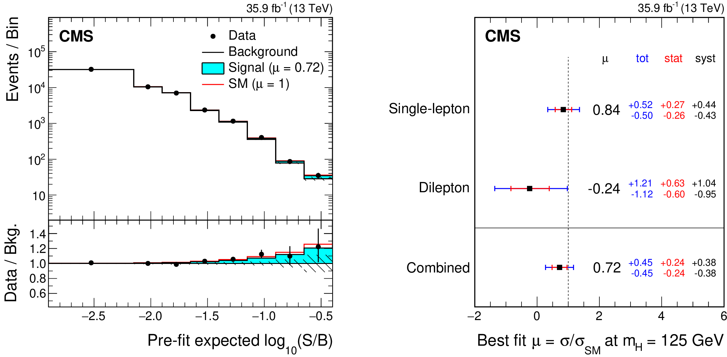
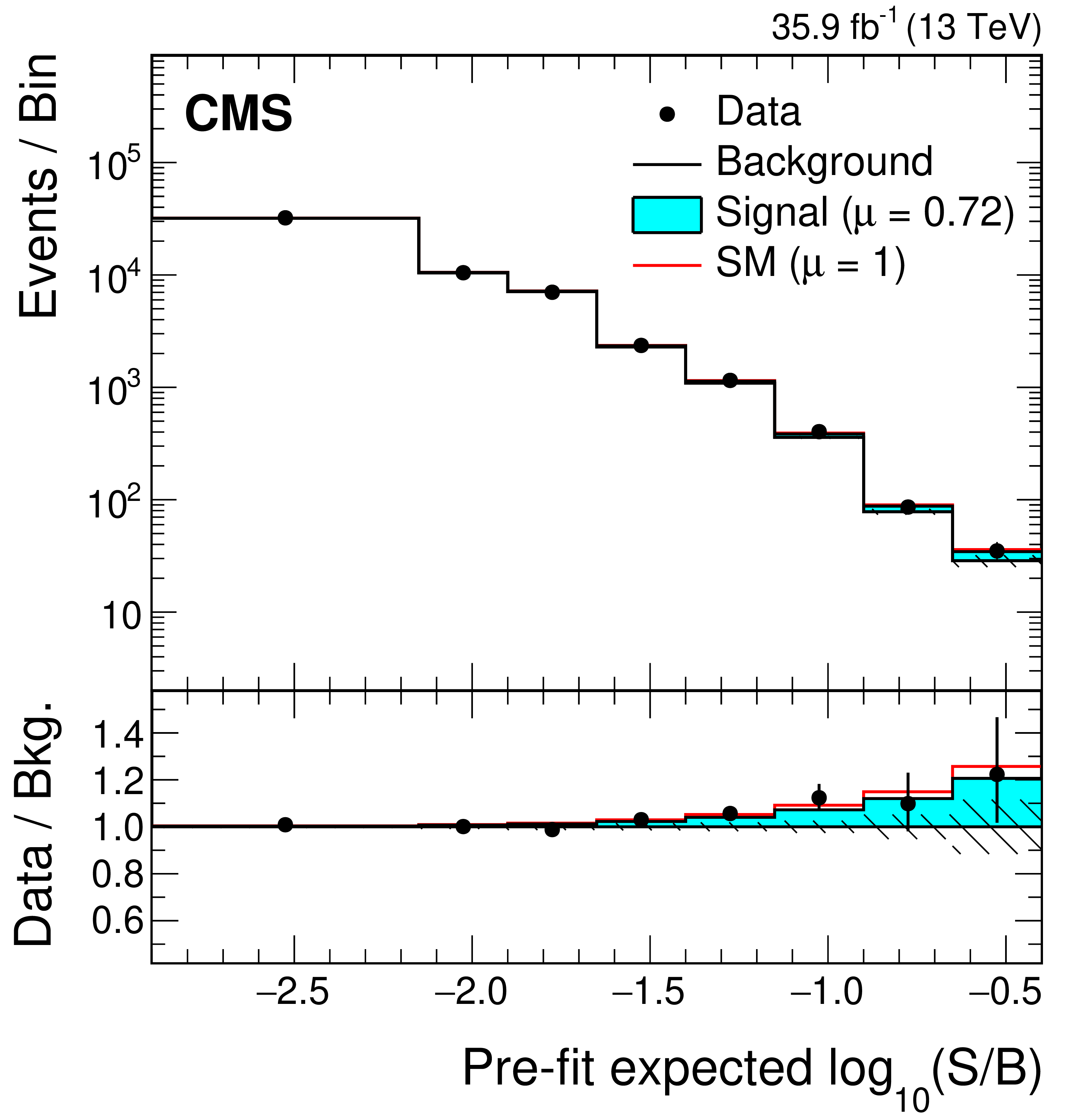
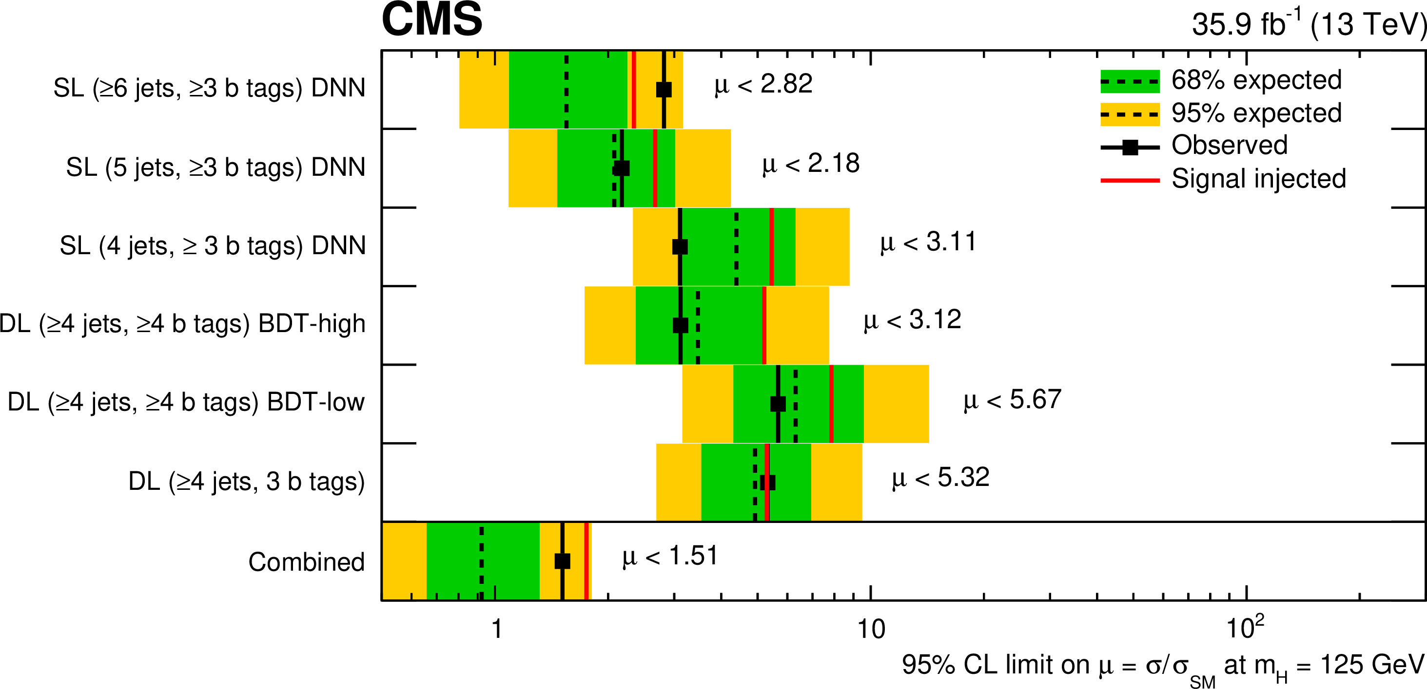
Figure 10:
Bins of the final discriminants as used in the fit (left), reordered by the pre-fit expected signal-to-background ratio (S/B). Each of the shown bins includes multiple bins of the final discriminants with similar S/B. The fitted signal (cyan) is compared to the expectation for the SM Higgs boson $\mu = 1$ (red). Best fit values of the signal strength modifiers $\mu $ (right) with their 68% expected confidence intervals (outer error bar), also split into their statistical (inner error bar) and systematic components. |
png pdf |
Figure 10-a:
Bins of the final discriminants as used in the fit, reordered by the pre-fit expected signal-to-background ratio (S/B). Each of the shown bins includes multiple bins of the final discriminants with similar S/B. The fitted signal (cyan) is compared to the expectation for the SM Higgs boson $\mu = 1$ (red). |

png pdf |
Figure 10-b:
Best fit values of the signal strength modifiers $\mu $ with their 68% expected confidence intervals (outer error bar), also split into their statistical (inner error bar) and systematic components. |
png pdf |
Figure 11:
Median expected (dashed line) and observed (markers) 95% CL upper limits on $\mu $. The inner (green) band and the outer (yellow) band indicate the regions containing 68 and 95%, respectively, of the distribution of limits expected under the background-only hypothesis. Also shown is the limit that is expected in case a SM $ {{{\mathrm {t}\overline {\mathrm {t}}}} {\mathrm {H}}} $ signal ($\mu =$ 1) is present in the data (solid red line). |
png pdf |
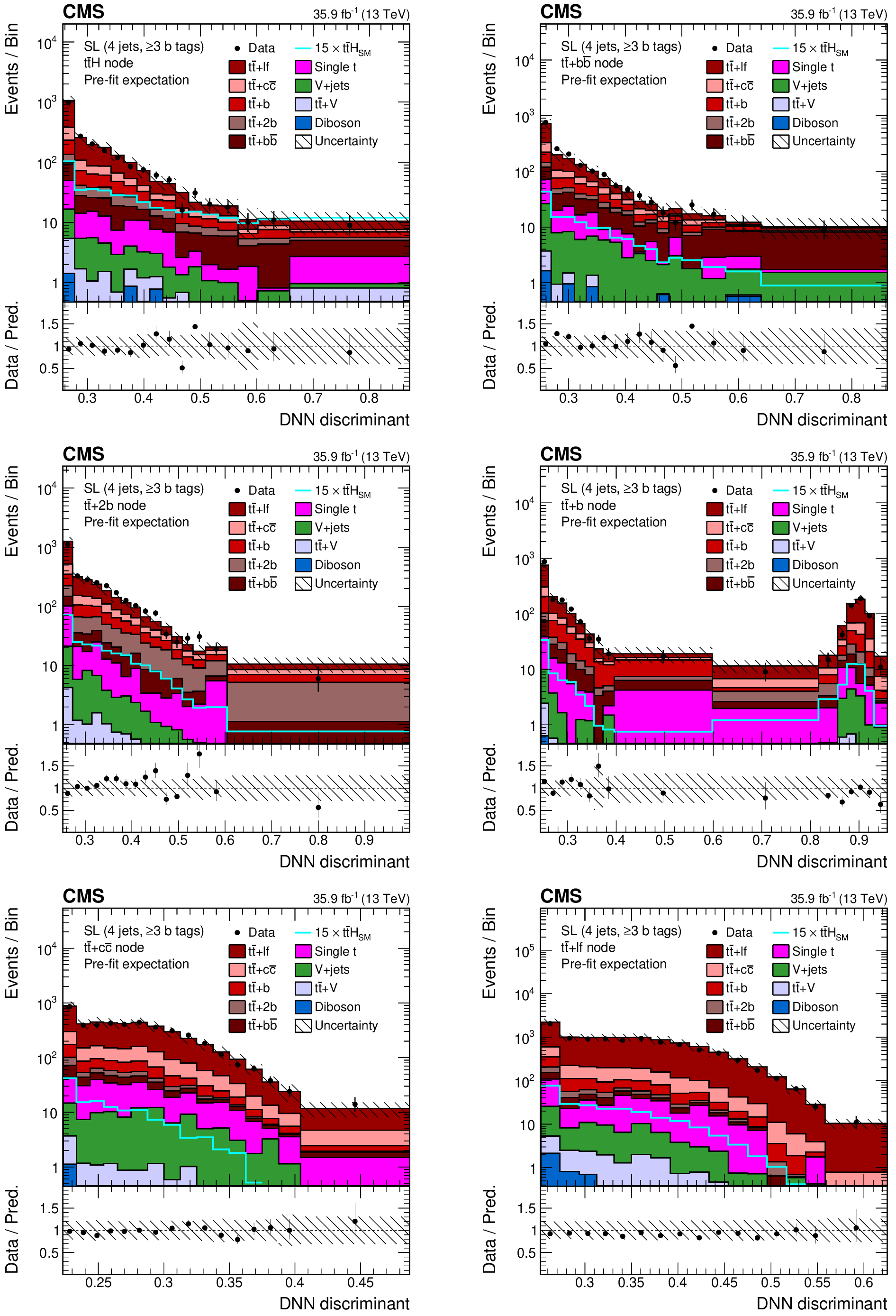
Figure 12:
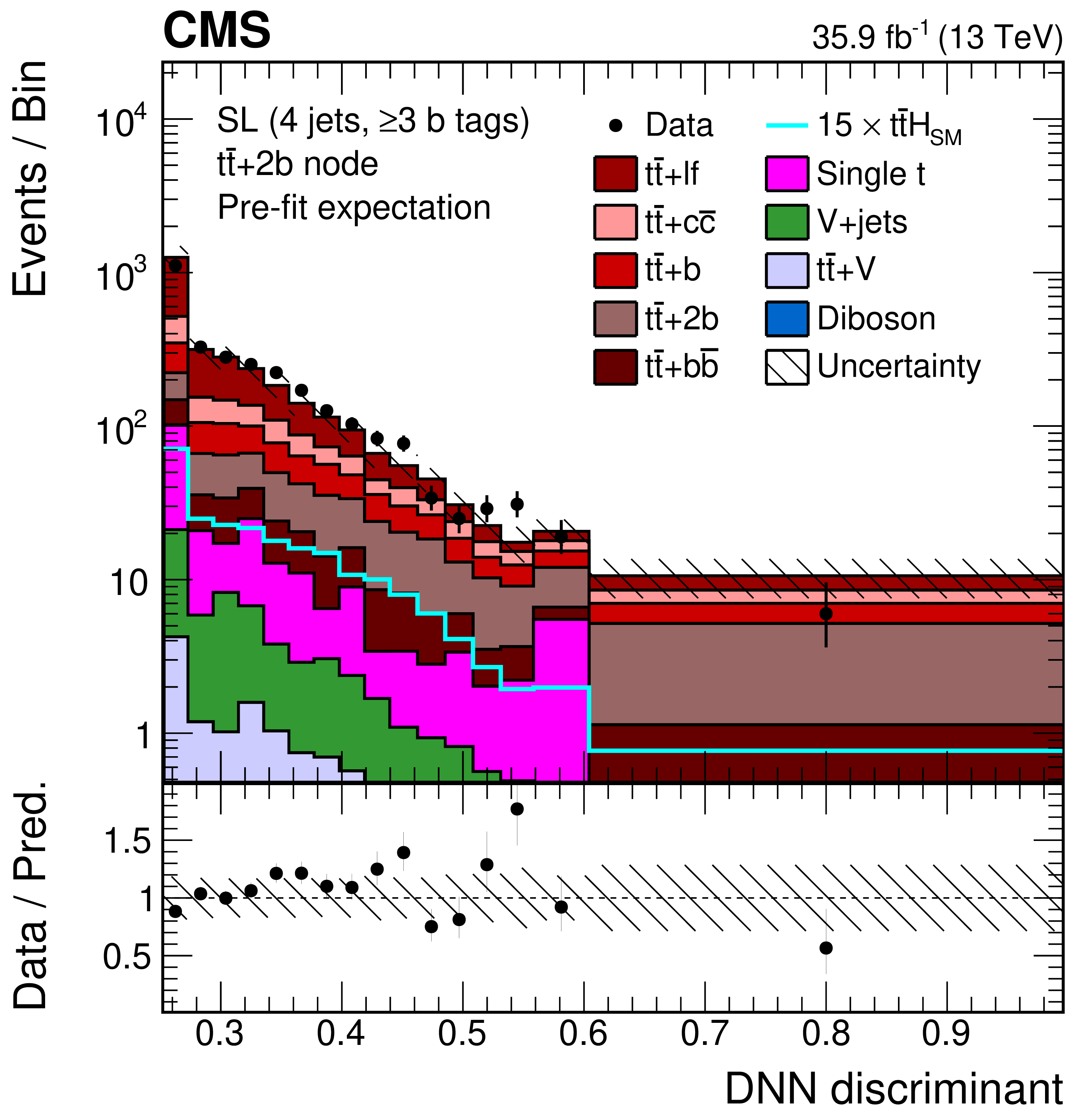
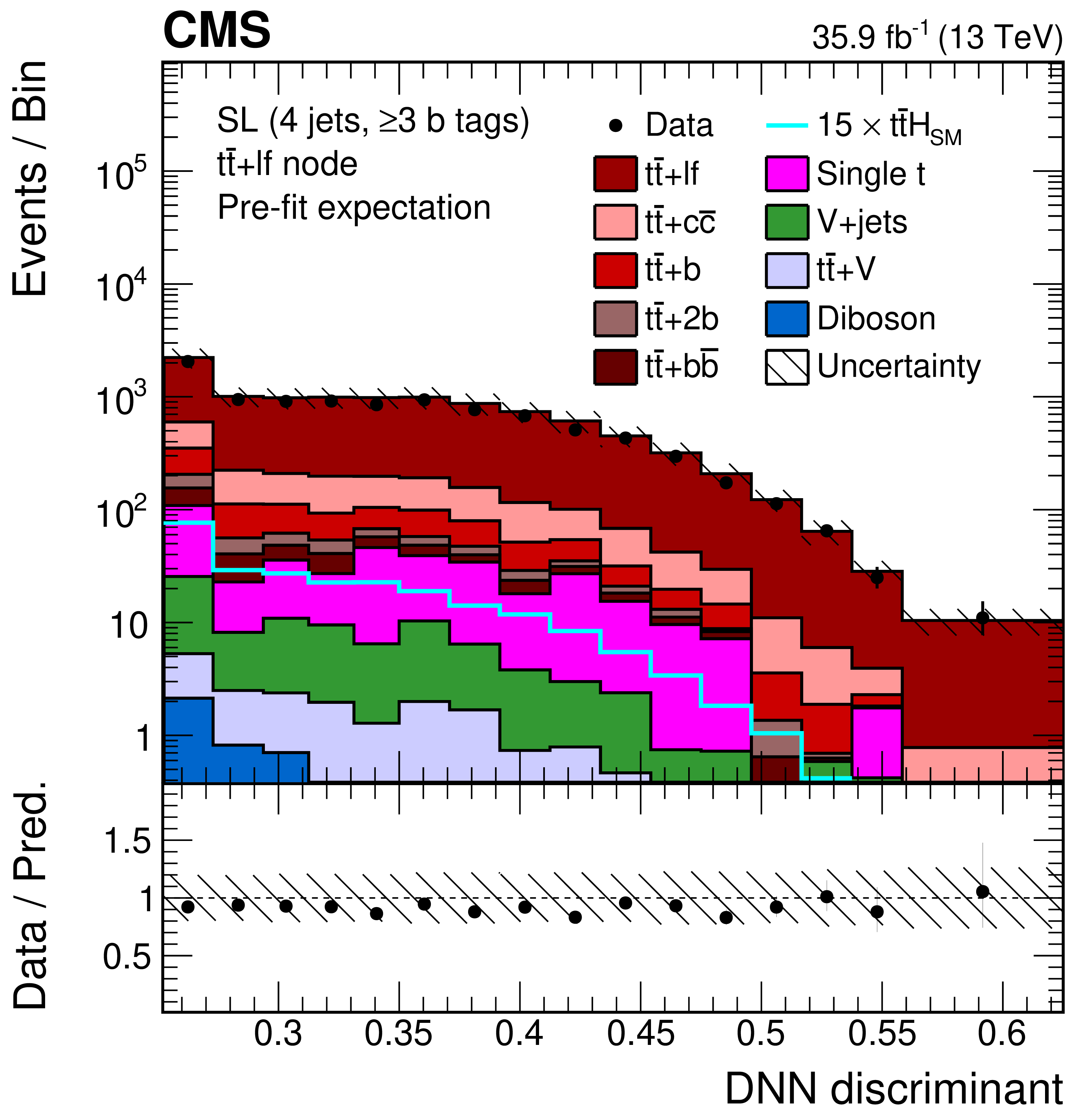
Final discriminant (DNN) shapes in the single-lepton (SL) channel before the fit to data, in the jet-process categories with (4 jets, $\geq$3 b tags) and (from upper left to lower right) $ {{{\mathrm {t}\overline {\mathrm {t}}}} {\mathrm {H}}} $, $ {{{\mathrm {t}\overline {\mathrm {t}}}} \text {+} {{\mathrm {b}} {\overline {\mathrm {b}}}}} $, $ {{{\mathrm {t}\overline {\mathrm {t}}}} \text {+}2 {\mathrm {b}}} $, $ {{{\mathrm {t}\overline {\mathrm {t}}}} \text {+} {\mathrm {b}}} $, $ {{{\mathrm {t}\overline {\mathrm {t}}}} \text {+} {{\mathrm {c}} {\overline {\mathrm {c}}}}} $, and $ {{{\mathrm {t}\overline {\mathrm {t}}}} \text {+}\text {lf}} $. The expected background contributions (filled histograms) are stacked, and the expected signal distribution (line), which includes $ {{\mathrm {H}} \to {{\mathrm {b}} {\overline {\mathrm {b}}}}} $ and all other Higgs boson decay modes, is superimposed. Each contribution is normalised to an integrated luminosity of 35.9 fb$^{-1}$, and the signal distribution is additionally scaled by a factor of 15 for better visibility. The hatched uncertainty bands include the total uncertainty of the fit model. The first and the last bins include underflow and overflow events, respectively. The lower plots show the ratio of the data to the background prediction. |
png pdf |
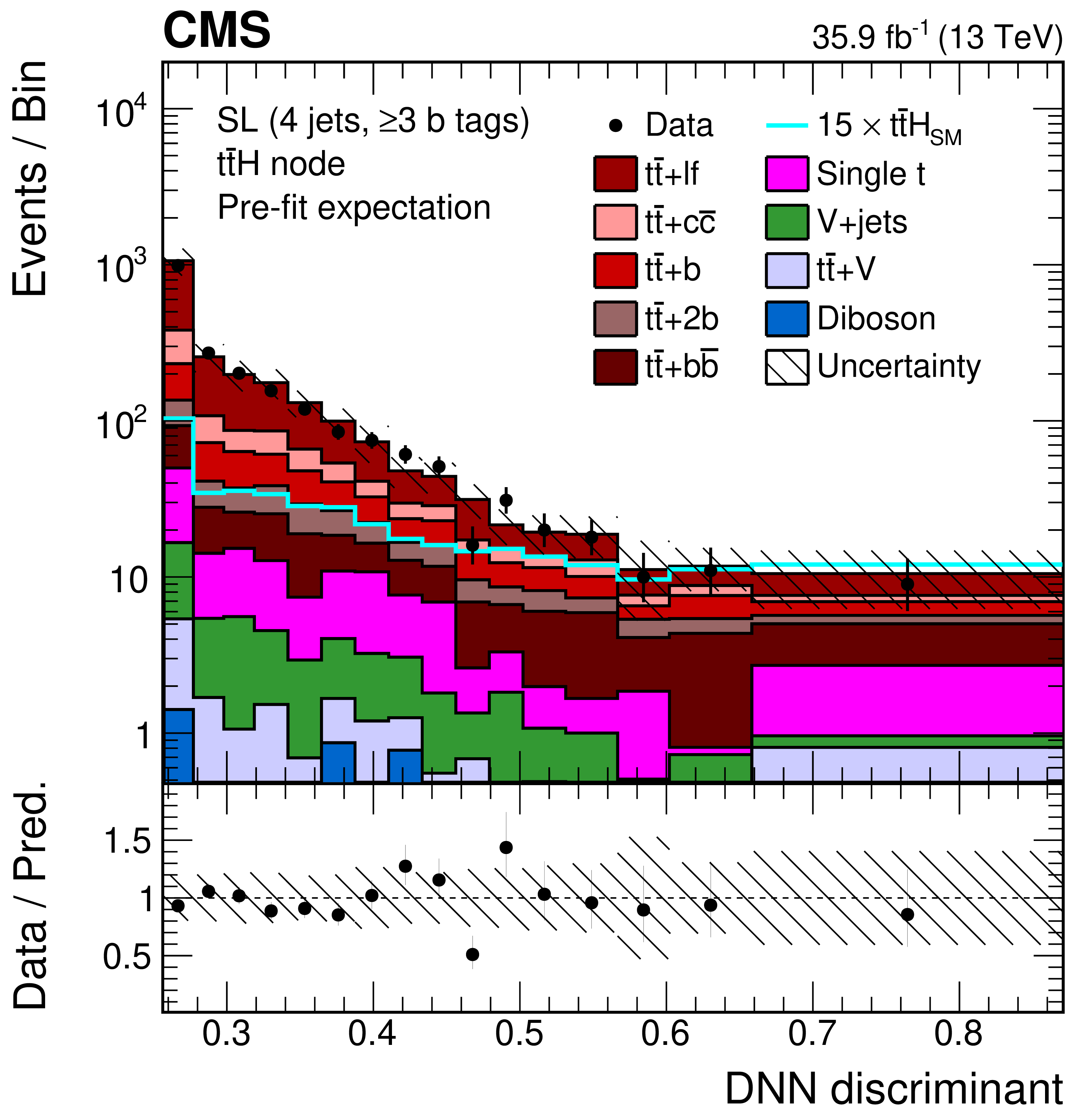
Figure 12-a:
Final discriminant (DNN) shapes in the single-lepton (SL) channel before the fit to data, in the jet-process categories with (4 jets, $\geq$3 b tags) and $ {{{\mathrm {t}\overline {\mathrm {t}}}} {\mathrm {H}}} $. The expected background contributions (filled histograms) are stacked, and the expected signal distribution (line), which includes $ {{\mathrm {H}} \to {{\mathrm {b}} {\overline {\mathrm {b}}}}} $ and all other Higgs boson decay modes, is superimposed. Each contribution is normalised to an integrated luminosity of 35.9 fb$^{-1}$, and the signal distribution is additionally scaled by a factor of 15 for better visibility. The hatched uncertainty bands include the total uncertainty of the fit model. The first and the last bins include underflow and overflow events, respectively. The lower plot shows the ratio of the data to the background prediction. |
png pdf |
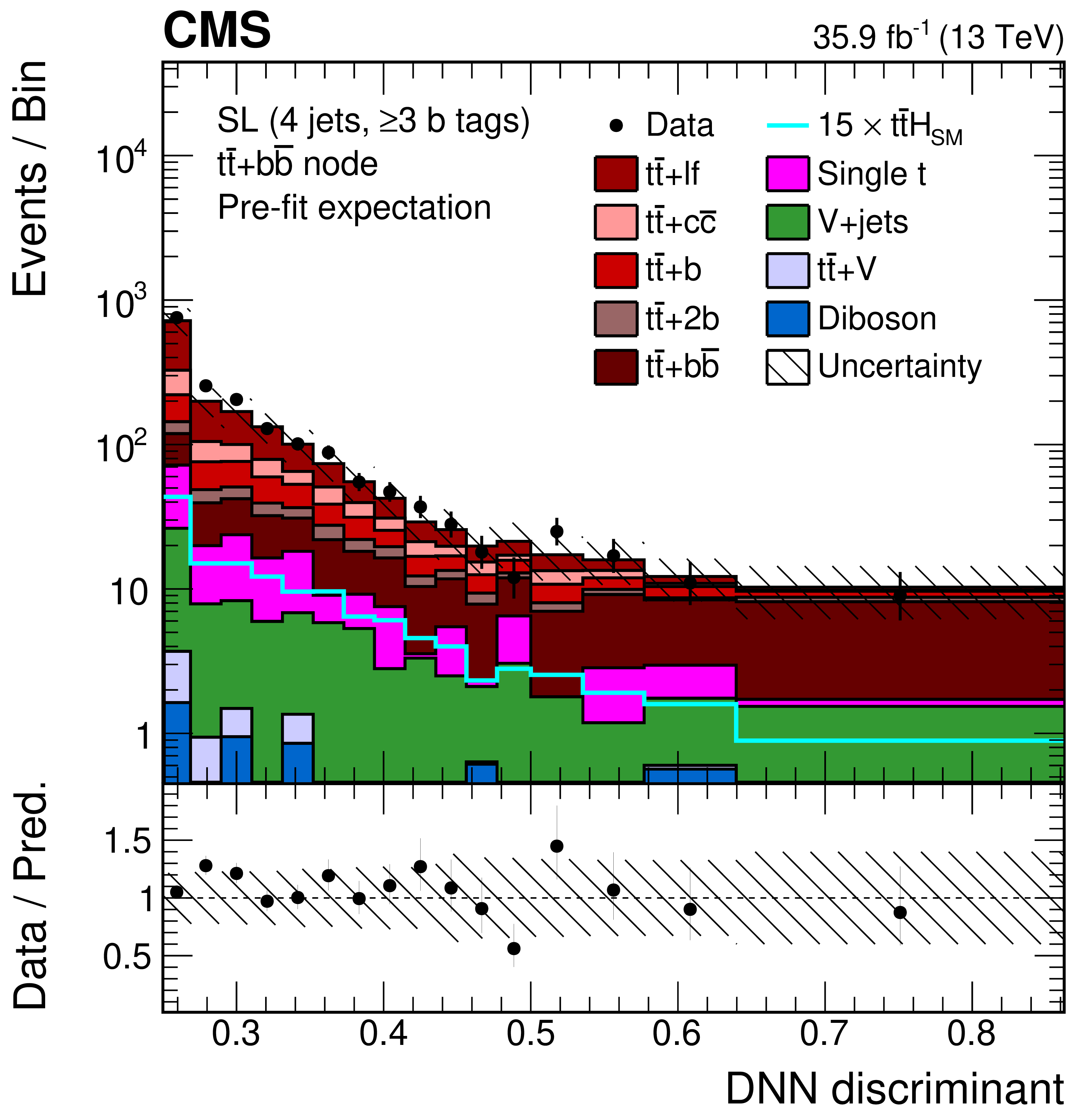
Figure 12-b:
Final discriminant (DNN) shapes in the single-lepton (SL) channel before the fit to data, in the jet-process categories with (4 jets, $\geq$3 b tags) and $ {{{\mathrm {t}\overline {\mathrm {t}}}} \text {+} {{\mathrm {b}} {\overline {\mathrm {b}}}}} $. The expected background contributions (filled histograms) are stacked, and the expected signal distribution (line), which includes $ {{\mathrm {H}} \to {{\mathrm {b}} {\overline {\mathrm {b}}}}} $ and all other Higgs boson decay modes, is superimposed. Each contribution is normalised to an integrated luminosity of 35.9 fb$^{-1}$, and the signal distribution is additionally scaled by a factor of 15 for better visibility. The hatched uncertainty bands include the total uncertainty of the fit model. The first and the last bins include underflow and overflow events, respectively. The lower plot shows the ratio of the data to the background prediction. |
png pdf |
Figure 12-c:
Final discriminant (DNN) shapes in the single-lepton (SL) channel before the fit to data, in the jet-process categories with (4 jets, $\geq$3 b tags) and $ {{{\mathrm {t}\overline {\mathrm {t}}}} \text {+}2 {\mathrm {b}}} $. The expected background contributions (filled histograms) are stacked, and the expected signal distribution (line), which includes $ {{\mathrm {H}} \to {{\mathrm {b}} {\overline {\mathrm {b}}}}} $ and all other Higgs boson decay modes, is superimposed. Each contribution is normalised to an integrated luminosity of 35.9 fb$^{-1}$, and the signal distribution is additionally scaled by a factor of 15 for better visibility. The hatched uncertainty bands include the total uncertainty of the fit model. The first and the last bins include underflow and overflow events, respectively. The lower plot shows the ratio of the data to the background prediction. |

png pdf |
Figure 12-d:
Final discriminant (DNN) shapes in the single-lepton (SL) channel before the fit to data, in the jet-process categories with (4 jets, $\geq$3 b tags) and $ {{{\mathrm {t}\overline {\mathrm {t}}}} \text {+} {\mathrm {b}}} $. The expected background contributions (filled histograms) are stacked, and the expected signal distribution (line), which includes $ {{\mathrm {H}} \to {{\mathrm {b}} {\overline {\mathrm {b}}}}} $ and all other Higgs boson decay modes, is superimposed. Each contribution is normalised to an integrated luminosity of 35.9 fb$^{-1}$, and the signal distribution is additionally scaled by a factor of 15 for better visibility. The hatched uncertainty bands include the total uncertainty of the fit model. The first and the last bins include underflow and overflow events, respectively. The lower plot shows the ratio of the data to the background prediction. |

png pdf |
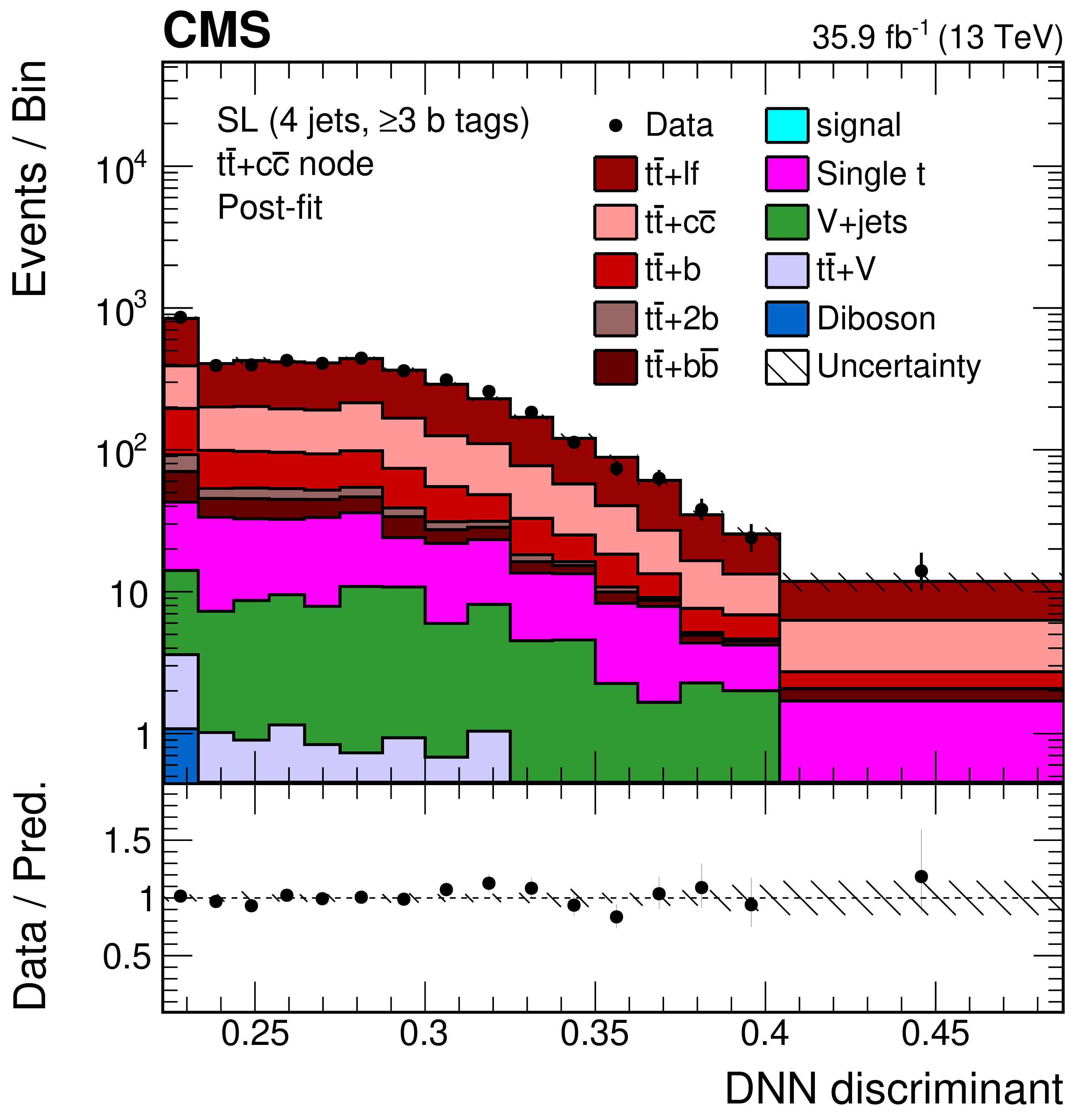
Figure 12-e:
Final discriminant (DNN) shapes in the single-lepton (SL) channel before the fit to data, in the jet-process categories with (4 jets, $\geq$3 b tags) and $ {{{\mathrm {t}\overline {\mathrm {t}}}} \text {+} {{\mathrm {c}} {\overline {\mathrm {c}}}}} $. The expected background contributions (filled histograms) are stacked, and the expected signal distribution (line), which includes $ {{\mathrm {H}} \to {{\mathrm {b}} {\overline {\mathrm {b}}}}} $ and all other Higgs boson decay modes, is superimposed. Each contribution is normalised to an integrated luminosity of 35.9 fb$^{-1}$, and the signal distribution is additionally scaled by a factor of 15 for better visibility. The hatched uncertainty bands include the total uncertainty of the fit model. The first and the last bins include underflow and overflow events, respectively. The lower plot shows the ratio of the data to the background prediction. |
png pdf |
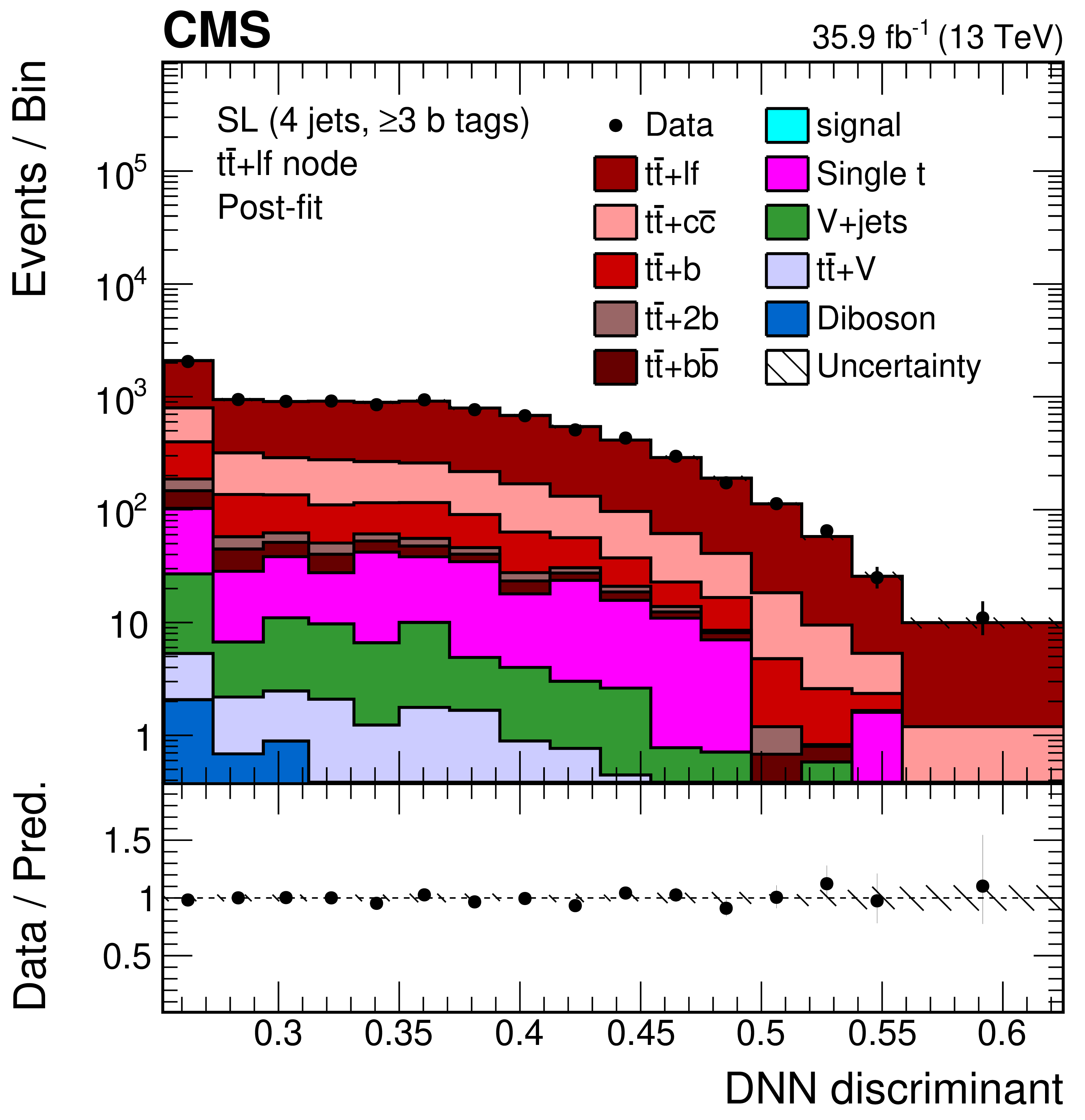
Figure 12-f:
Final discriminant (DNN) shapes in the single-lepton (SL) channel before the fit to data, in the jet-process categories with (4 jets, $\geq$3 b tags) and $ {{{\mathrm {t}\overline {\mathrm {t}}}} \text {+}\text {lf}} $. The expected background contributions (filled histograms) are stacked, and the expected signal distribution (line), which includes $ {{\mathrm {H}} \to {{\mathrm {b}} {\overline {\mathrm {b}}}}} $ and all other Higgs boson decay modes, is superimposed. Each contribution is normalised to an integrated luminosity of 35.9 fb$^{-1}$, and the signal distribution is additionally scaled by a factor of 15 for better visibility. The hatched uncertainty bands include the total uncertainty of the fit model. The first and the last bins include underflow and overflow events, respectively. The lower plot shows the ratio of the data to the background prediction. |

png pdf |
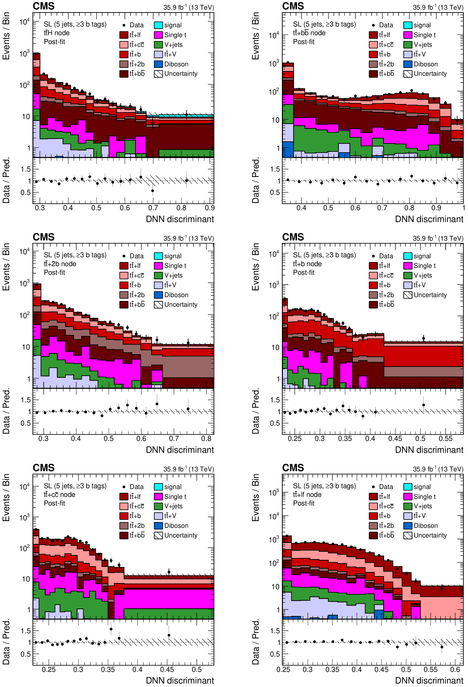
Figure 13:
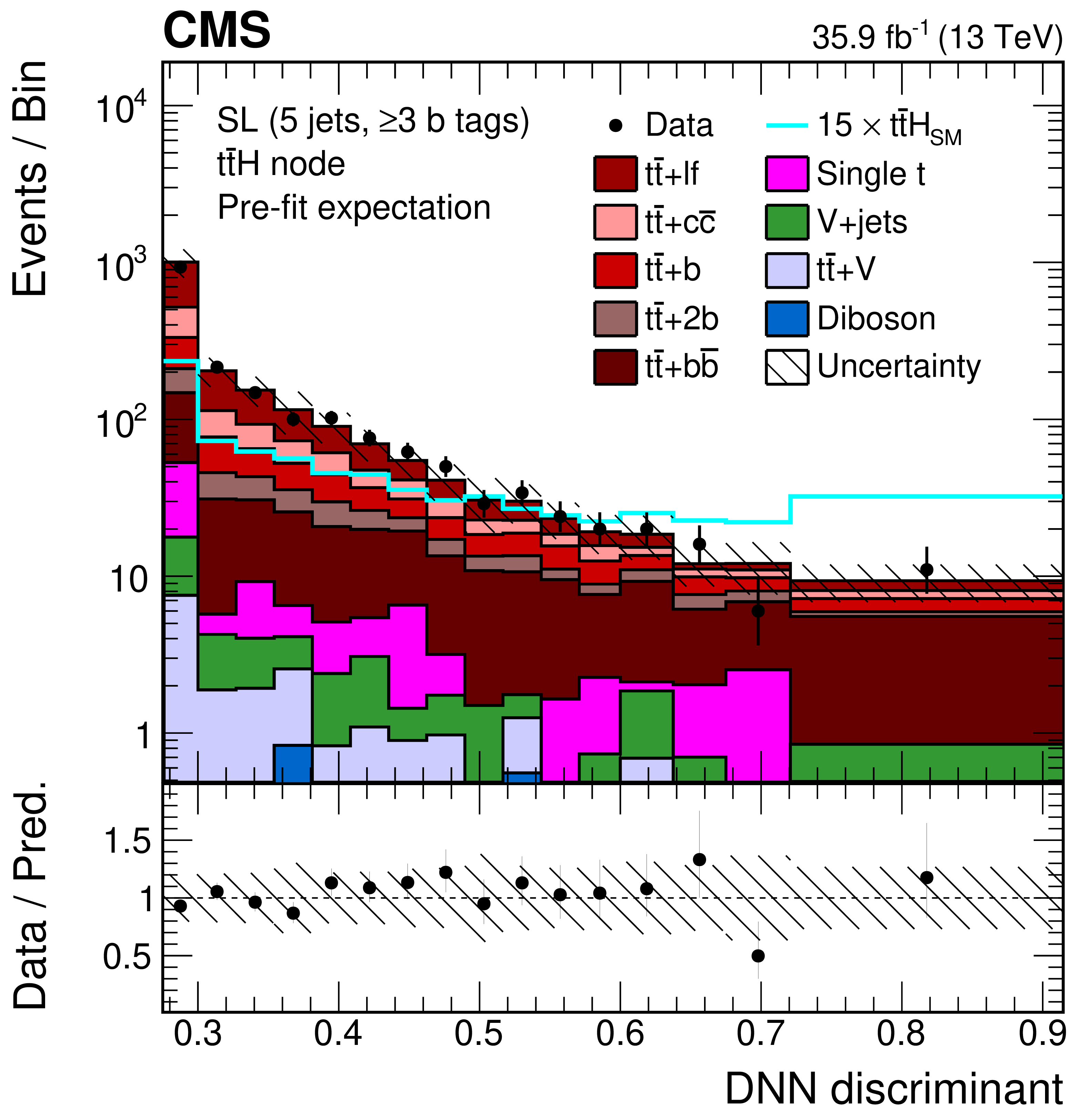
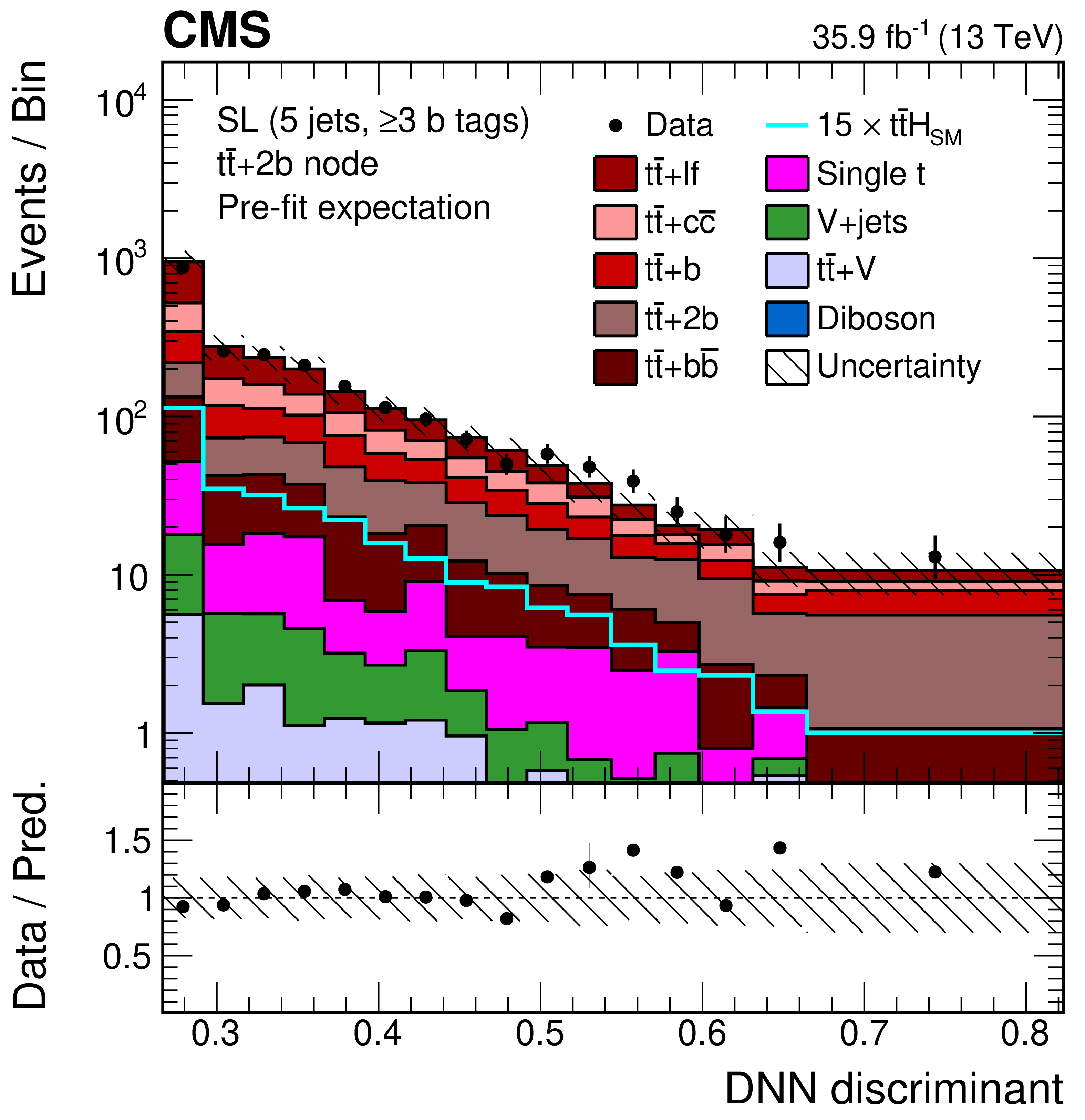
Final discriminant (DNN) shapes in the single-lepton (SL) channel before the fit to data, in the jet-process categories with (5 jets, $\geq$3 b tags) and (from upper left to lower right) $ {{{\mathrm {t}\overline {\mathrm {t}}}} {\mathrm {H}}} $, $ {{{\mathrm {t}\overline {\mathrm {t}}}} \text {+} {{\mathrm {b}} {\overline {\mathrm {b}}}}} $, $ {{{\mathrm {t}\overline {\mathrm {t}}}} \text {+}2 {\mathrm {b}}} $, $ {{{\mathrm {t}\overline {\mathrm {t}}}} \text {+} {\mathrm {b}}} $, $ {{{\mathrm {t}\overline {\mathrm {t}}}} \text {+} {{\mathrm {c}} {\overline {\mathrm {c}}}}} $, and $ {{{\mathrm {t}\overline {\mathrm {t}}}} \text {+}\text {lf}} $. The expected background contributions (filled histograms) are stacked, and the expected signal distribution (line), which includes $ {{\mathrm {H}} \to {{\mathrm {b}} {\overline {\mathrm {b}}}}} $ and all other Higgs boson decay modes, is superimposed. Each contribution is normalised to an integrated luminosity of 35.9 fb$^{-1}$, and the signal distribution is additionally scaled by a factor of 15 for better visibility. The hatched uncertainty bands include the total uncertainty of the fit model. The first and the last bins include underflow and overflow events, respectively. The lower plots show the ratio of the data to the background prediction. |
png pdf |
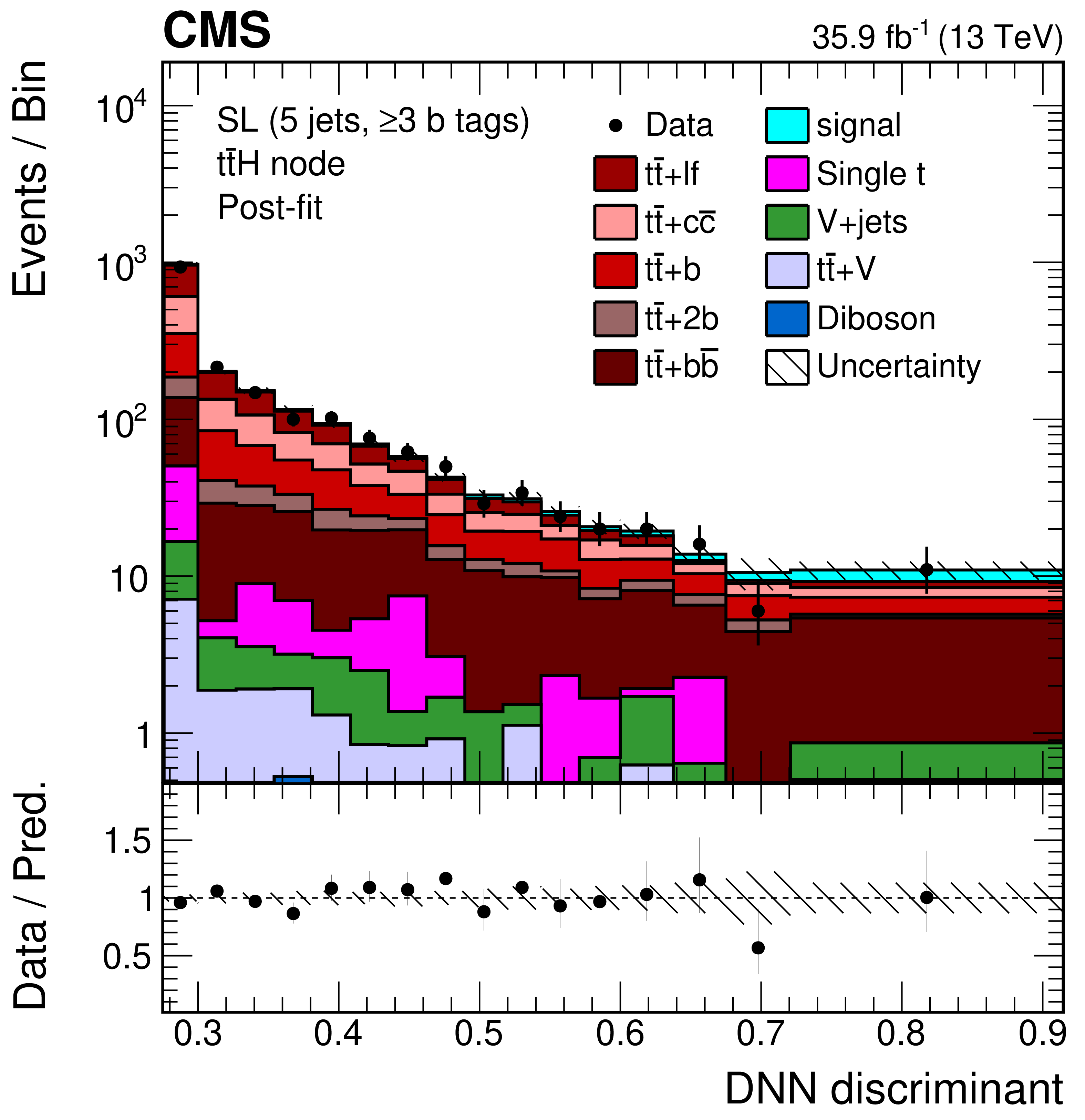
Figure 13-a:
Final discriminant (DNN) shapes in the single-lepton (SL) channel before the fit to data, in the jet-process categories with (5 jets, $\geq$3 b tags) and $ {{{\mathrm {t}\overline {\mathrm {t}}}} {\mathrm {H}}} $. The expected background contributions (filled histograms) are stacked, and the expected signal distribution (line), which includes $ {{\mathrm {H}} \to {{\mathrm {b}} {\overline {\mathrm {b}}}}} $ and all other Higgs boson decay modes, is superimposed. Each contribution is normalised to an integrated luminosity of 35.9 fb$^{-1}$, and the signal distribution is additionally scaled by a factor of 15 for better visibility. The hatched uncertainty bands include the total uncertainty of the fit model. The first and the last bins include underflow and overflow events, respectively. The lower plot shows the ratio of the data to the background prediction. |

png pdf |
Figure 13-b:
Final discriminant (DNN) shapes in the single-lepton (SL) channel before the fit to data, in the jet-process categories with (5 jets, $\geq$3 b tags) and $ {{{\mathrm {t}\overline {\mathrm {t}}}} \text {+} {{\mathrm {b}} {\overline {\mathrm {b}}}}} $. The expected background contributions (filled histograms) are stacked, and the expected signal distribution (line), which includes $ {{\mathrm {H}} \to {{\mathrm {b}} {\overline {\mathrm {b}}}}} $ and all other Higgs boson decay modes, is superimposed. Each contribution is normalised to an integrated luminosity of 35.9 fb$^{-1}$, and the signal distribution is additionally scaled by a factor of 15 for better visibility. The hatched uncertainty bands include the total uncertainty of the fit model. The first and the last bins include underflow and overflow events, respectively. The lower plot shows the ratio of the data to the background prediction. |
png pdf |
Figure 13-c:
Final discriminant (DNN) shapes in the single-lepton (SL) channel before the fit to data, in the jet-process categories with (5 jets, $\geq$3 b tags) and $ {{{\mathrm {t}\overline {\mathrm {t}}}} \text {+}2 {\mathrm {b}}} $. The expected background contributions (filled histograms) are stacked, and the expected signal distribution (line), which includes $ {{\mathrm {H}} \to {{\mathrm {b}} {\overline {\mathrm {b}}}}} $ and all other Higgs boson decay modes, is superimposed. Each contribution is normalised to an integrated luminosity of 35.9 fb$^{-1}$, and the signal distribution is additionally scaled by a factor of 15 for better visibility. The hatched uncertainty bands include the total uncertainty of the fit model. The first and the last bins include underflow and overflow events, respectively. The lower plot shows the ratio of the data to the background prediction. |

png pdf |
Figure 13-d:
Final discriminant (DNN) shapes in the single-lepton (SL) channel before the fit to data, in the jet-process categories with (5 jets, $\geq$3 b tags) and $ {{{\mathrm {t}\overline {\mathrm {t}}}} \text {+} {\mathrm {b}}} $. The expected background contributions (filled histograms) are stacked, and the expected signal distribution (line), which includes $ {{\mathrm {H}} \to {{\mathrm {b}} {\overline {\mathrm {b}}}}} $ and all other Higgs boson decay modes, is superimposed. Each contribution is normalised to an integrated luminosity of 35.9 fb$^{-1}$, and the signal distribution is additionally scaled by a factor of 15 for better visibility. The hatched uncertainty bands include the total uncertainty of the fit model. The first and the last bins include underflow and overflow events, respectively. The lower plot shows the ratio of the data to the background prediction. |

png pdf |
Figure 13-e:
Final discriminant (DNN) shapes in the single-lepton (SL) channel before the fit to data, in the jet-process categories with (5 jets, $\geq$3 b tags) and $ {{{\mathrm {t}\overline {\mathrm {t}}}} \text {+} {{\mathrm {c}} {\overline {\mathrm {c}}}}} $. The expected background contributions (filled histograms) are stacked, and the expected signal distribution (line), which includes $ {{\mathrm {H}} \to {{\mathrm {b}} {\overline {\mathrm {b}}}}} $ and all other Higgs boson decay modes, is superimposed. Each contribution is normalised to an integrated luminosity of 35.9 fb$^{-1}$, and the signal distribution is additionally scaled by a factor of 15 for better visibility. The hatched uncertainty bands include the total uncertainty of the fit model. The first and the last bins include underflow and overflow events, respectively. The lower plot shows the ratio of the data to the background prediction. |
png pdf |
Figure 13-f:
Final discriminant (DNN) shapes in the single-lepton (SL) channel before the fit to data, in the jet-process categories with (5 jets, $\geq$3 b tags) and $ {{{\mathrm {t}\overline {\mathrm {t}}}} \text {+}\text {lf}} $. The expected background contributions (filled histograms) are stacked, and the expected signal distribution (line), which includes $ {{\mathrm {H}} \to {{\mathrm {b}} {\overline {\mathrm {b}}}}} $ and all other Higgs boson decay modes, is superimposed. Each contribution is normalised to an integrated luminosity of 35.9 fb$^{-1}$, and the signal distribution is additionally scaled by a factor of 15 for better visibility. The hatched uncertainty bands include the total uncertainty of the fit model. The first and the last bins include underflow and overflow events, respectively. The lower plot shows the ratio of the data to the background prediction. |
png pdf |
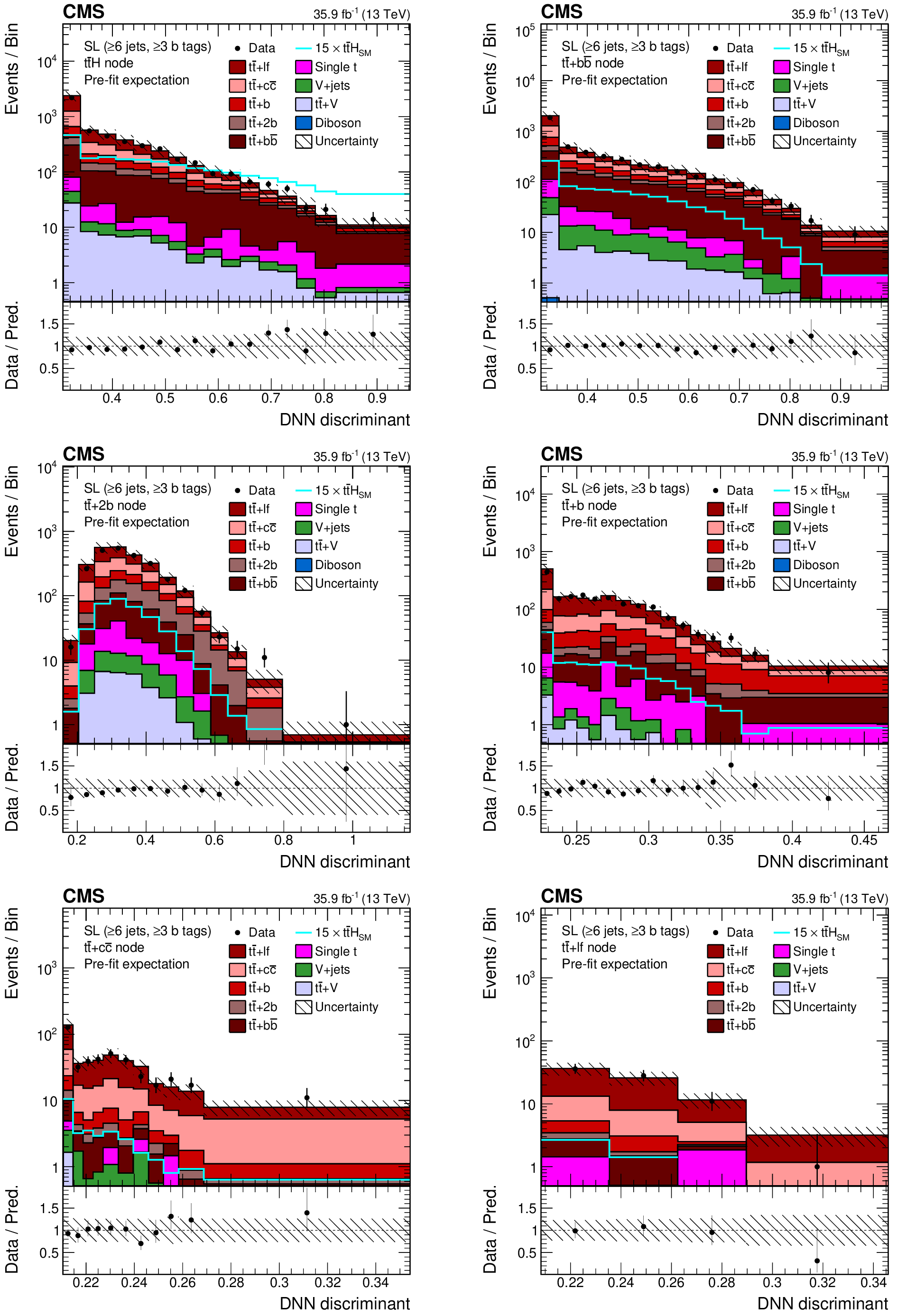
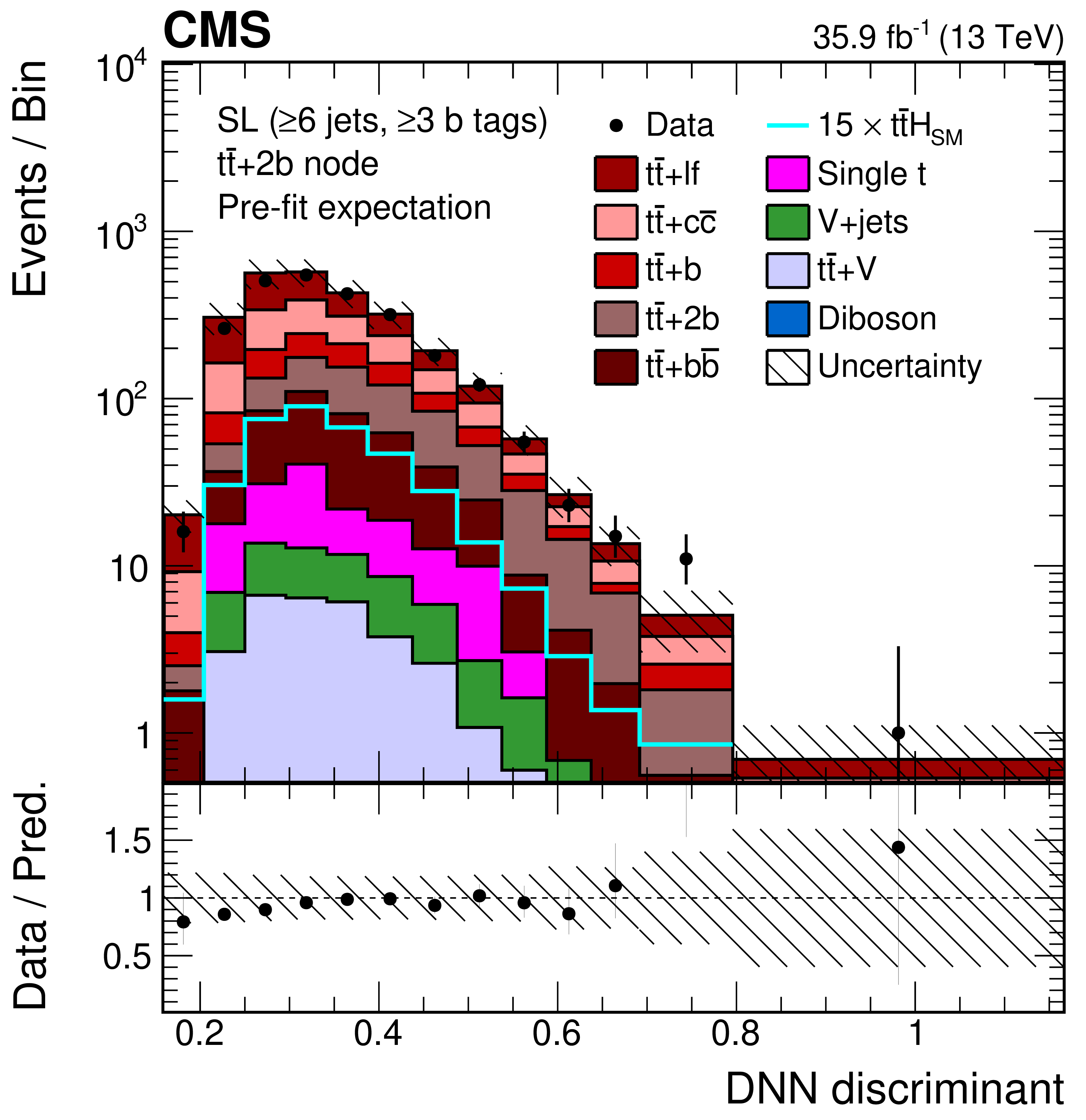
Figure 14:
Final discriminant (DNN) shapes in the single-lepton (SL) channel before the fit to data, in the jet-process categories with (6 jets, $\geq$3 b tags) and (from upper left to lower right) $ {{{\mathrm {t}\overline {\mathrm {t}}}} {\mathrm {H}}} $, $ {{{\mathrm {t}\overline {\mathrm {t}}}} \text {+} {{\mathrm {b}} {\overline {\mathrm {b}}}}} $, $ {{{\mathrm {t}\overline {\mathrm {t}}}} \text {+}2 {\mathrm {b}}} $, $ {{{\mathrm {t}\overline {\mathrm {t}}}} \text {+} {\mathrm {b}}} $, $ {{{\mathrm {t}\overline {\mathrm {t}}}} \text {+} {{\mathrm {c}} {\overline {\mathrm {c}}}}} $, and $ {{{\mathrm {t}\overline {\mathrm {t}}}} \text {+}\text {lf}} $. The expected background contributions (filled histograms) are stacked, and the expected signal distribution (line), which includes $ {{\mathrm {H}} \to {{\mathrm {b}} {\overline {\mathrm {b}}}}} $ and all other Higgs boson decay modes, is superimposed. Each contribution is normalised to an integrated luminosity of 35.9 fb$^{-1}$, and the signal distribution is additionally scaled by a factor of 15 for better visibility. The hatched uncertainty bands include the total uncertainty of the fit model. The first and the last bins include underflow and overflow events, respectively. The lower plots show the ratio of the data to the background prediction. |

png pdf |
Figure 14-a:
Final discriminant (DNN) shapes in the single-lepton (SL) channel before the fit to data, in the jet-process categories with (6 jets, $\geq$3 b tags) and $ {{{\mathrm {t}\overline {\mathrm {t}}}} {\mathrm {H}}} $. The expected background contributions (filled histograms) are stacked, and the expected signal distribution (line), which includes $ {{\mathrm {H}} \to {{\mathrm {b}} {\overline {\mathrm {b}}}}} $ and all other Higgs boson decay modes, is superimposed. Each contribution is normalised to an integrated luminosity of 35.9 fb$^{-1}$, and the signal distribution is additionally scaled by a factor of 15 for better visibility. The hatched uncertainty bands include the total uncertainty of the fit model. The first and the last bins include underflow and overflow events, respectively. The lower plot shows the ratio of the data to the background prediction. |

png pdf |
Figure 14-b:
Final discriminant (DNN) shapes in the single-lepton (SL) channel before the fit to data, in the jet-process categories with (6 jets, $\geq$3 b tags) and $ {{{\mathrm {t}\overline {\mathrm {t}}}} \text {+} {{\mathrm {b}} {\overline {\mathrm {b}}}}} $. The expected background contributions (filled histograms) are stacked, and the expected signal distribution (line), which includes $ {{\mathrm {H}} \to {{\mathrm {b}} {\overline {\mathrm {b}}}}} $ and all other Higgs boson decay modes, is superimposed. Each contribution is normalised to an integrated luminosity of 35.9 fb$^{-1}$, and the signal distribution is additionally scaled by a factor of 15 for better visibility. The hatched uncertainty bands include the total uncertainty of the fit model. The first and the last bins include underflow and overflow events, respectively. The lower plot shows the ratio of the data to the background prediction. |
png pdf |
Figure 14-c:
Final discriminant (DNN) shapes in the single-lepton (SL) channel before the fit to data, in the jet-process categories with (6 jets, $\geq$3 b tags) and $ {{{\mathrm {t}\overline {\mathrm {t}}}} \text {+}2 {\mathrm {b}}} $. The expected background contributions (filled histograms) are stacked, and the expected signal distribution (line), which includes $ {{\mathrm {H}} \to {{\mathrm {b}} {\overline {\mathrm {b}}}}} $ and all other Higgs boson decay modes, is superimposed. Each contribution is normalised to an integrated luminosity of 35.9 fb$^{-1}$, and the signal distribution is additionally scaled by a factor of 15 for better visibility. The hatched uncertainty bands include the total uncertainty of the fit model. The first and the last bins include underflow and overflow events, respectively. The lower plot shows the ratio of the data to the background prediction. |
png pdf |
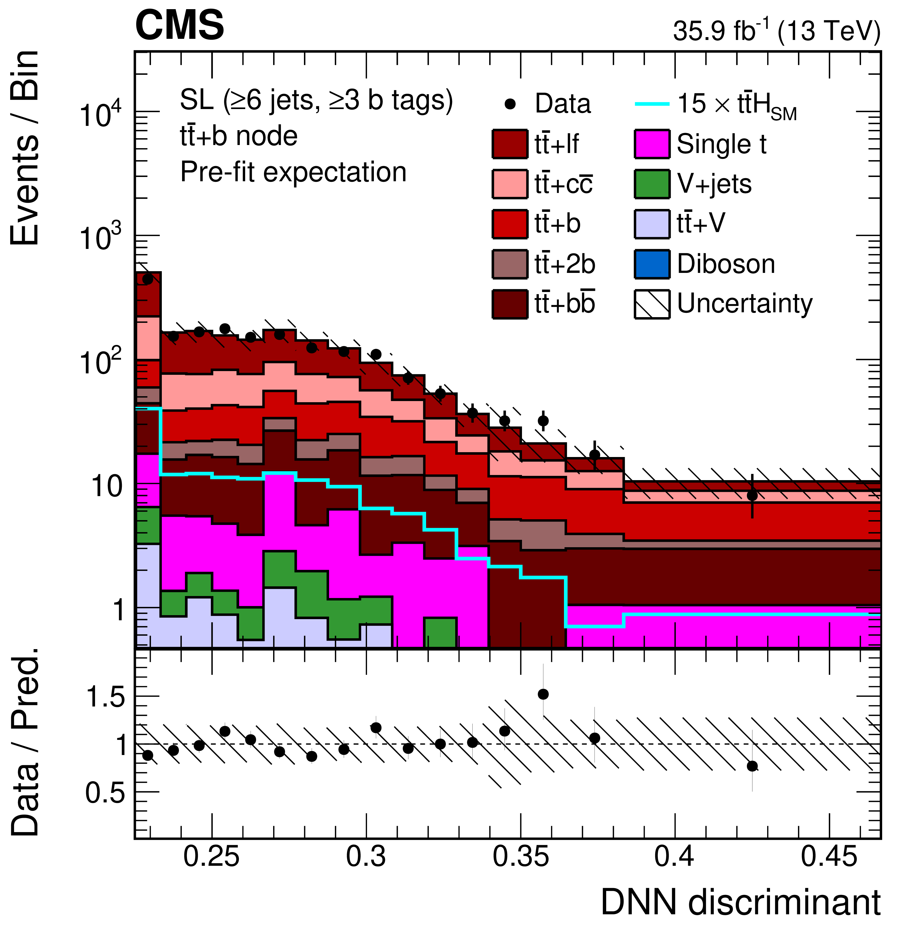
Figure 14-d:
Final discriminant (DNN) shapes in the single-lepton (SL) channel before the fit to data, in the jet-process categories with (6 jets, $\geq$3 b tags) and $ {{{\mathrm {t}\overline {\mathrm {t}}}} \text {+} {\mathrm {b}}} $. The expected background contributions (filled histograms) are stacked, and the expected signal distribution (line), which includes $ {{\mathrm {H}} \to {{\mathrm {b}} {\overline {\mathrm {b}}}}} $ and all other Higgs boson decay modes, is superimposed. Each contribution is normalised to an integrated luminosity of 35.9 fb$^{-1}$, and the signal distribution is additionally scaled by a factor of 15 for better visibility. The hatched uncertainty bands include the total uncertainty of the fit model. The first and the last bins include underflow and overflow events, respectively. The lower plot shows the ratio of the data to the background prediction. |

png pdf |
Figure 14-e:
Final discriminant (DNN) shapes in the single-lepton (SL) channel before the fit to data, in the jet-process categories with (6 jets, $\geq$3 b tags) and $ {{{\mathrm {t}\overline {\mathrm {t}}}} \text {+} {{\mathrm {c}} {\overline {\mathrm {c}}}}} $. The expected background contributions (filled histograms) are stacked, and the expected signal distribution (line), which includes $ {{\mathrm {H}} \to {{\mathrm {b}} {\overline {\mathrm {b}}}}} $ and all other Higgs boson decay modes, is superimposed. Each contribution is normalised to an integrated luminosity of 35.9 fb$^{-1}$, and the signal distribution is additionally scaled by a factor of 15 for better visibility. The hatched uncertainty bands include the total uncertainty of the fit model. The first and the last bins include underflow and overflow events, respectively. The lower plot shows the ratio of the data to the background prediction. |
png pdf |
Figure 14-f:
Final discriminant (DNN) shapes in the single-lepton (SL) channel before the fit to data, in the jet-process categories with (6 jets, $\geq$3 b tags) and $ {{{\mathrm {t}\overline {\mathrm {t}}}} \text {+}\text {lf}} $. The expected background contributions (filled histograms) are stacked, and the expected signal distribution (line), which includes $ {{\mathrm {H}} \to {{\mathrm {b}} {\overline {\mathrm {b}}}}} $ and all other Higgs boson decay modes, is superimposed. Each contribution is normalised to an integrated luminosity of 35.9 fb$^{-1}$, and the signal distribution is additionally scaled by a factor of 15 for better visibility. The hatched uncertainty bands include the total uncertainty of the fit model. The first and the last bins include underflow and overflow events, respectively. The lower plot shows the ratio of the data to the background prediction. |

png pdf |
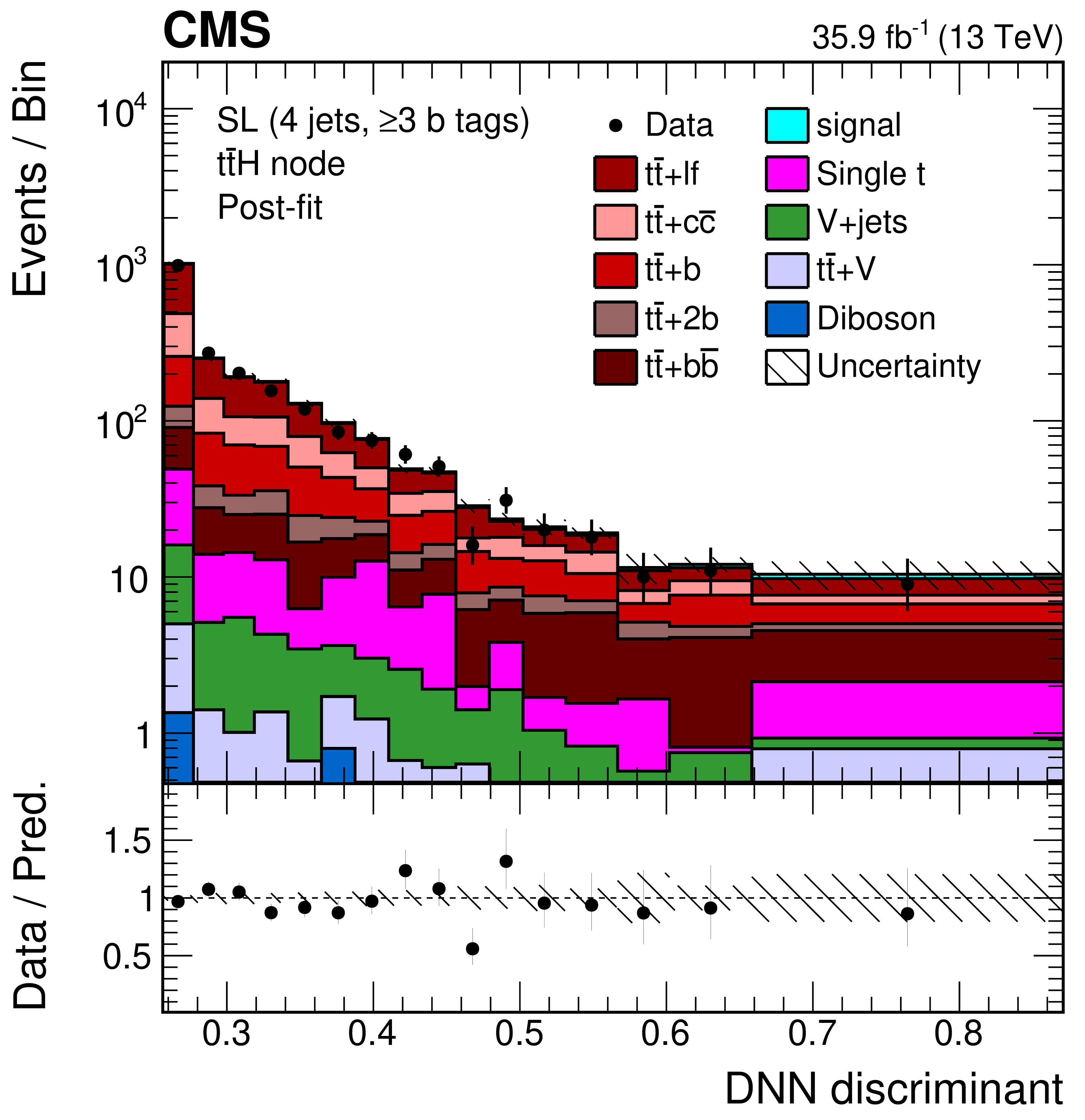
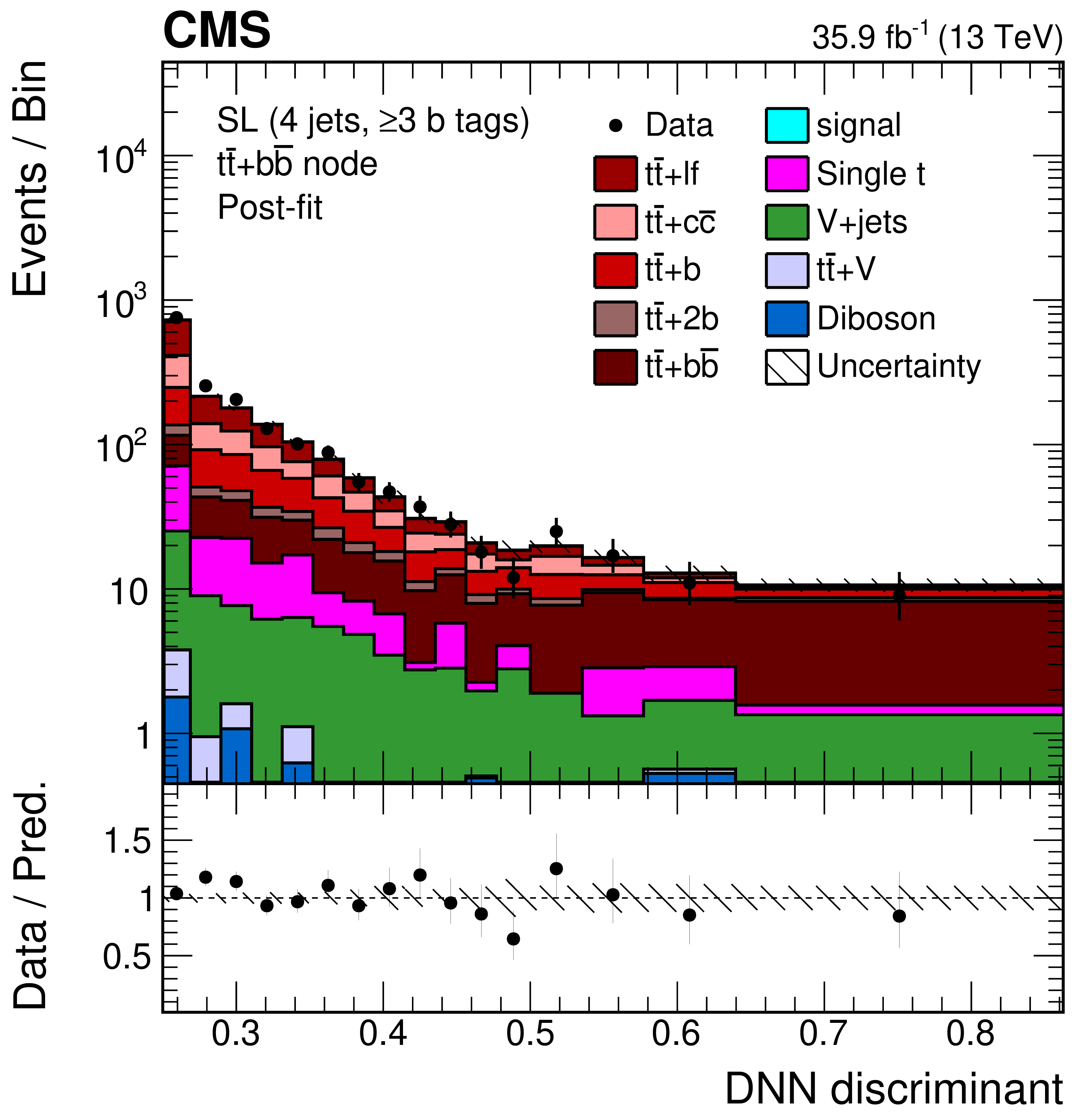
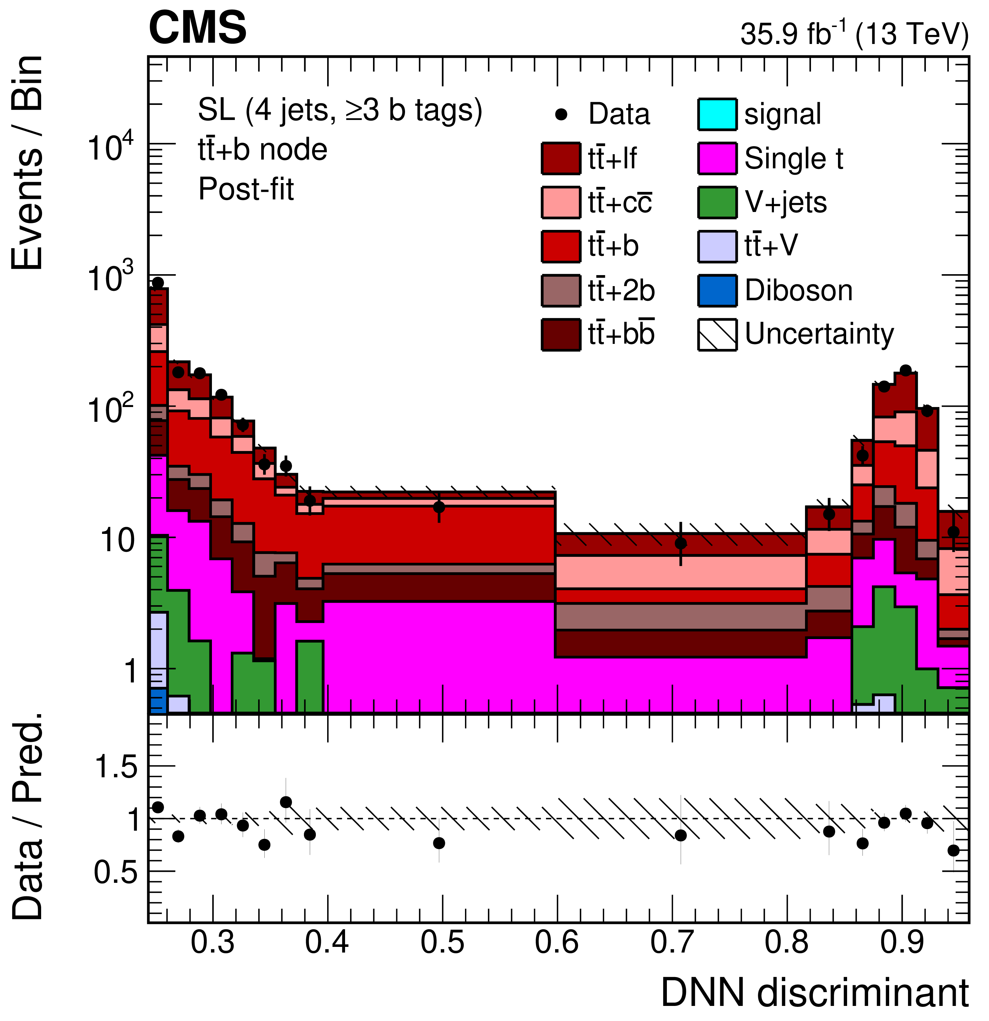
Figure 15:
Final discriminant (DNN) shapes in the single-lepton (SL) channel after the fit to data, in the jet-process categories with (4 jets, $\geq$3 b tags) and (from upper left to lower right) $ {{{\mathrm {t}\overline {\mathrm {t}}}} {\mathrm {H}}} $, $ {{{\mathrm {t}\overline {\mathrm {t}}}} \text {+} {{\mathrm {b}} {\overline {\mathrm {b}}}}} $, $ {{{\mathrm {t}\overline {\mathrm {t}}}} \text {+}2 {\mathrm {b}}} $, $ {{{\mathrm {t}\overline {\mathrm {t}}}} \text {+} {\mathrm {b}}} $, $ {{{\mathrm {t}\overline {\mathrm {t}}}} \text {+} {{\mathrm {c}} {\overline {\mathrm {c}}}}} $, and $ {{{\mathrm {t}\overline {\mathrm {t}}}} \text {+}\text {lf}} $. The error bands include the total uncertainty after the fit to data. The first and the last bins include underflow and overflow events, respectively. The lower plots show the ratio of the data to the post-fit background plus signal distribution. |
png pdf |
Figure 15-a:
Final discriminant (DNN) shapes in the single-lepton (SL) channel after the fit to data, in the jet-process categories with (4 jets, $\geq$3 b tags) and $ {{{\mathrm {t}\overline {\mathrm {t}}}} {\mathrm {H}}} $. The error bands include the total uncertainty after the fit to data. The first and the last bins include underflow and overflow events, respectively. The lower plot shows the ratio of the data to the post-fit background plus signal distribution. |
png pdf |
Figure 15-b:
Final discriminant (DNN) shapes in the single-lepton (SL) channel after the fit to data, in the jet-process categories with (4 jets, $\geq$3 b tags) and $ {{{\mathrm {t}\overline {\mathrm {t}}}} \text {+} {{\mathrm {b}} {\overline {\mathrm {b}}}}} $. The error bands include the total uncertainty after the fit to data. The first and the last bins include underflow and overflow events, respectively. The lower plot shows the ratio of the data to the post-fit background plus signal distribution. |

png pdf |
Figure 15-c:
Final discriminant (DNN) shapes in the single-lepton (SL) channel after the fit to data, in the jet-process categories with (4 jets, $\geq$3 b tags) and $ {{{\mathrm {t}\overline {\mathrm {t}}}} \text {+}2 {\mathrm {b}}} $. The error bands include the total uncertainty after the fit to data. The first and the last bins include underflow and overflow events, respectively. The lower plot shows the ratio of the data to the post-fit background plus signal distribution. |
png pdf |
Figure 15-d:
Final discriminant (DNN) shapes in the single-lepton (SL) channel after the fit to data, in the jet-process categories with (4 jets, $\geq$3 b tags) and $ {{{\mathrm {t}\overline {\mathrm {t}}}} \text {+} {\mathrm {b}}} $. The error bands include the total uncertainty after the fit to data. The first and the last bins include underflow and overflow events, respectively. The lower plot shows the ratio of the data to the post-fit background plus signal distribution. |
png pdf |
Figure 15-e:
Final discriminant (DNN) shapes in the single-lepton (SL) channel after the fit to data, in the jet-process categories with (4 jets, $\geq$3 b tags) and $ {{{\mathrm {t}\overline {\mathrm {t}}}} \text {+} {{\mathrm {c}} {\overline {\mathrm {c}}}}} $. The error bands include the total uncertainty after the fit to data. The first and the last bins include underflow and overflow events, respectively. The lower plot shows the ratio of the data to the post-fit background plus signal distribution. |
png pdf |
Figure 15-f:
Final discriminant (DNN) shapes in the single-lepton (SL) channel after the fit to data, in the jet-process categories with (4 jets, $\geq$3 b tags) and $ {{{\mathrm {t}\overline {\mathrm {t}}}} \text {+}\text {lf}} $. The error bands include the total uncertainty after the fit to data. The first and the last bins include underflow and overflow events, respectively. The lower plot shows the ratio of the data to the post-fit background plus signal distribution. |
png pdf |
Figure 16:
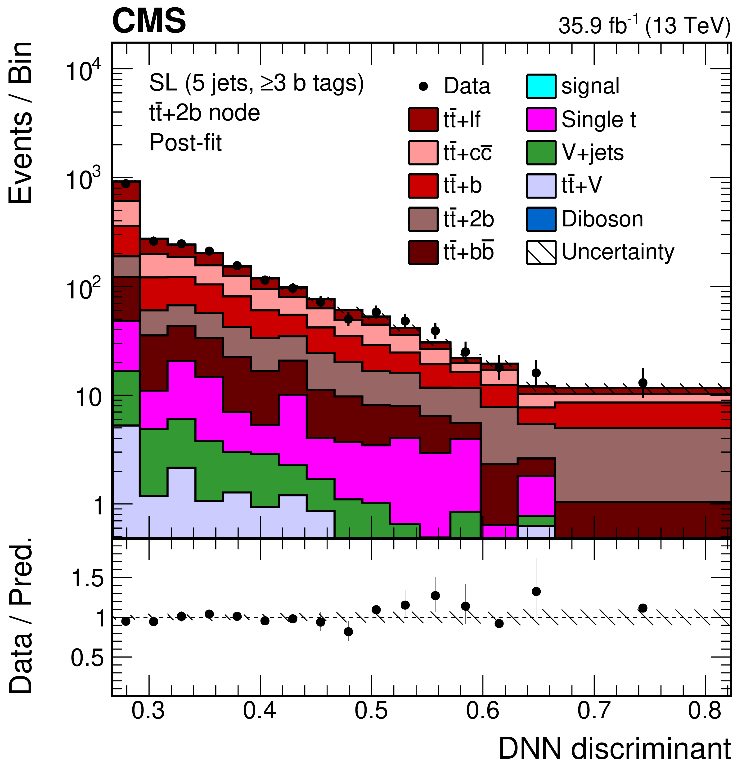
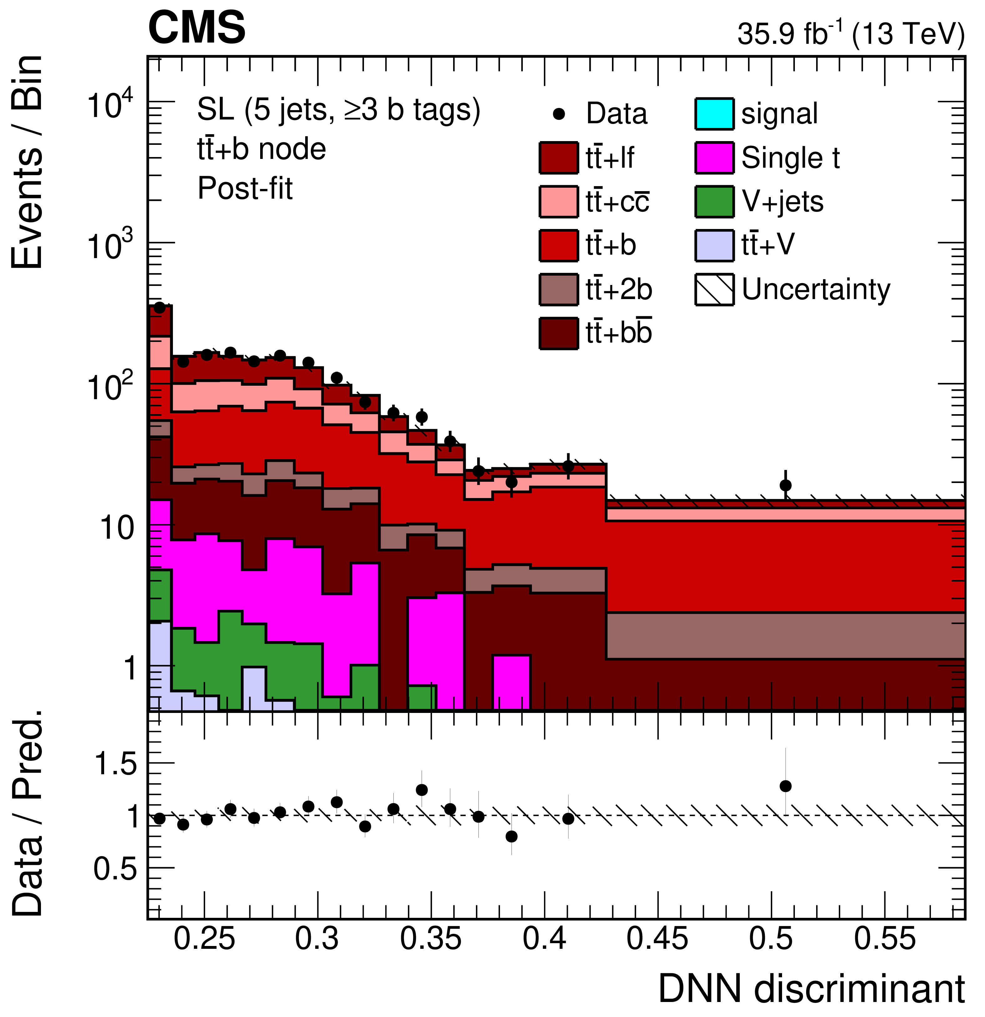
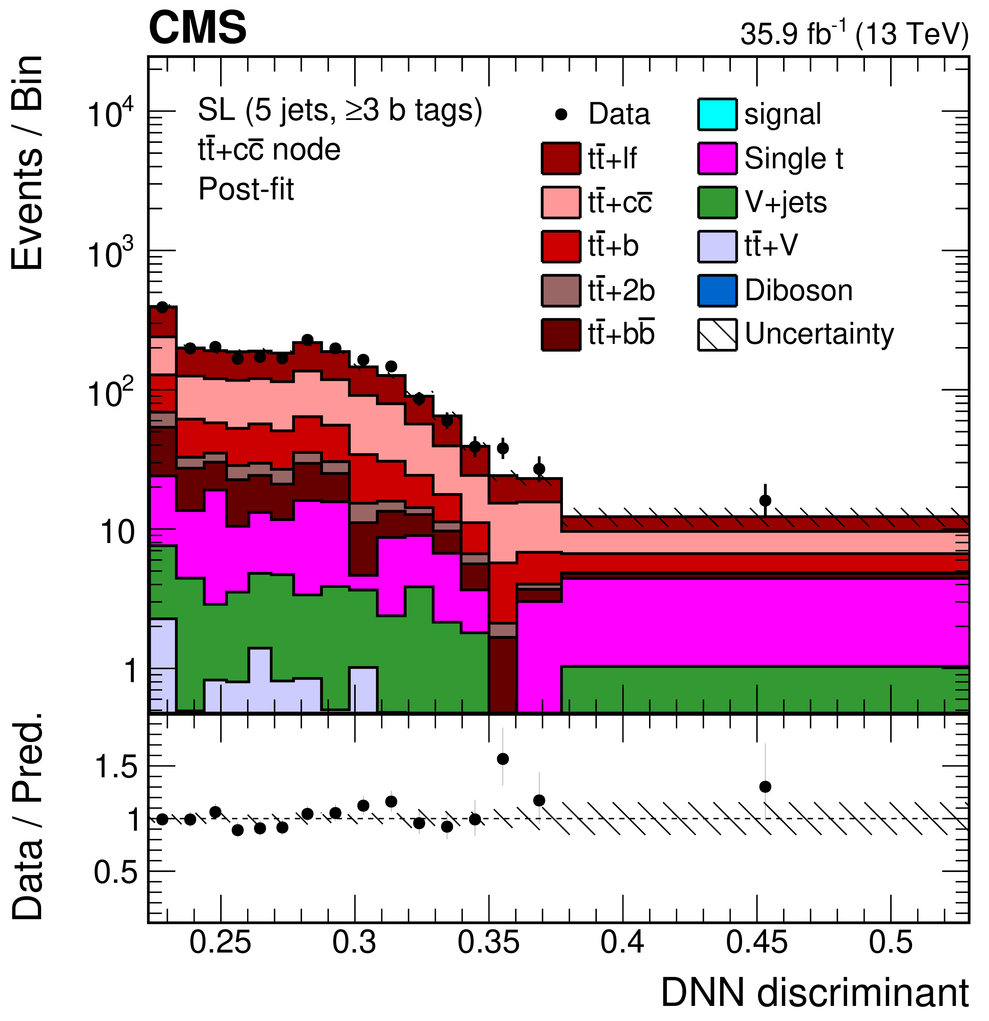
Final discriminant (DNN) shapes in the single-lepton (SL) channel after the fit to data, in the jet-process categories with (5 jets, $\geq$3 b tags) and (from upper left to lower right) $ {{{\mathrm {t}\overline {\mathrm {t}}}} {\mathrm {H}}} $, $ {{{\mathrm {t}\overline {\mathrm {t}}}} \text {+} {{\mathrm {b}} {\overline {\mathrm {b}}}}} $, $ {{{\mathrm {t}\overline {\mathrm {t}}}} \text {+}2 {\mathrm {b}}} $, $ {{{\mathrm {t}\overline {\mathrm {t}}}} \text {+} {\mathrm {b}}} $, $ {{{\mathrm {t}\overline {\mathrm {t}}}} \text {+} {{\mathrm {c}} {\overline {\mathrm {c}}}}} $, and $ {{{\mathrm {t}\overline {\mathrm {t}}}} \text {+}\text {lf}} $. The error bands include the total uncertainty after the fit to data. The first and the last bins include underflow and overflow events, respectively. The lower plots show the ratio of the data to the post-fit background plus signal distribution. |
png pdf |
Figure 16-a:
Final discriminant (DNN) shapes in the single-lepton (SL) channel after the fit to data, in the jet-process categories with (5 jets, $\geq$3 b tags) and $ {{{\mathrm {t}\overline {\mathrm {t}}}} {\mathrm {H}}} $. The error bands include the total uncertainty after the fit to data. The first and the last bins include underflow and overflow events, respectively. The lower plot shows the ratio of the data to the post-fit background plus signal distribution. |
png pdf |
Figure 16-b:
Final discriminant (DNN) shapes in the single-lepton (SL) channel after the fit to data, in the jet-process categories with (5 jets, $\geq$3 b tags) and $ {{{\mathrm {t}\overline {\mathrm {t}}}} \text {+} {{\mathrm {b}} {\overline {\mathrm {b}}}}} $. The error bands include the total uncertainty after the fit to data. The first and the last bins include underflow and overflow events, respectively. The lower plot shows the ratio of the data to the post-fit background plus signal distribution. |
png pdf |
Figure 16-c:
Final discriminant (DNN) shapes in the single-lepton (SL) channel after the fit to data, in the jet-process categories with (5 jets, $\geq$3 b tags) and $ {{{\mathrm {t}\overline {\mathrm {t}}}} \text {+}2 {\mathrm {b}}} $. The error bands include the total uncertainty after the fit to data. The first and the last bins include underflow and overflow events, respectively. The lower plot shows the ratio of the data to the post-fit background plus signal distribution. |
png pdf |
Figure 16-d:
Final discriminant (DNN) shapes in the single-lepton (SL) channel after the fit to data, in the jet-process categories with (5 jets, $\geq$3 b tags) and $ {{{\mathrm {t}\overline {\mathrm {t}}}} \text {+} {\mathrm {b}}} $. The error bands include the total uncertainty after the fit to data. The first and the last bins include underflow and overflow events, respectively. The lower plot shows the ratio of the data to the post-fit background plus signal distribution. |
png pdf |
Figure 16-e:
Final discriminant (DNN) shapes in the single-lepton (SL) channel after the fit to data, in the jet-process categories with (5 jets, $\geq$3 b tags) and $ {{{\mathrm {t}\overline {\mathrm {t}}}} \text {+} {{\mathrm {c}} {\overline {\mathrm {c}}}}} $. The error bands include the total uncertainty after the fit to data. The first and the last bins include underflow and overflow events, respectively. The lower plot shows the ratio of the data to the post-fit background plus signal distribution. |
png pdf |
Figure 16-f:
Final discriminant (DNN) shapes in the single-lepton (SL) channel after the fit to data, in the jet-process categories with (5 jets, $\geq$3 b tags) and $ {{{\mathrm {t}\overline {\mathrm {t}}}} \text {+}\text {lf}} $. The error bands include the total uncertainty after the fit to data. The first and the last bins include underflow and overflow events, respectively. The lower plot shows the ratio of the data to the post-fit background plus signal distribution. |
png pdf |
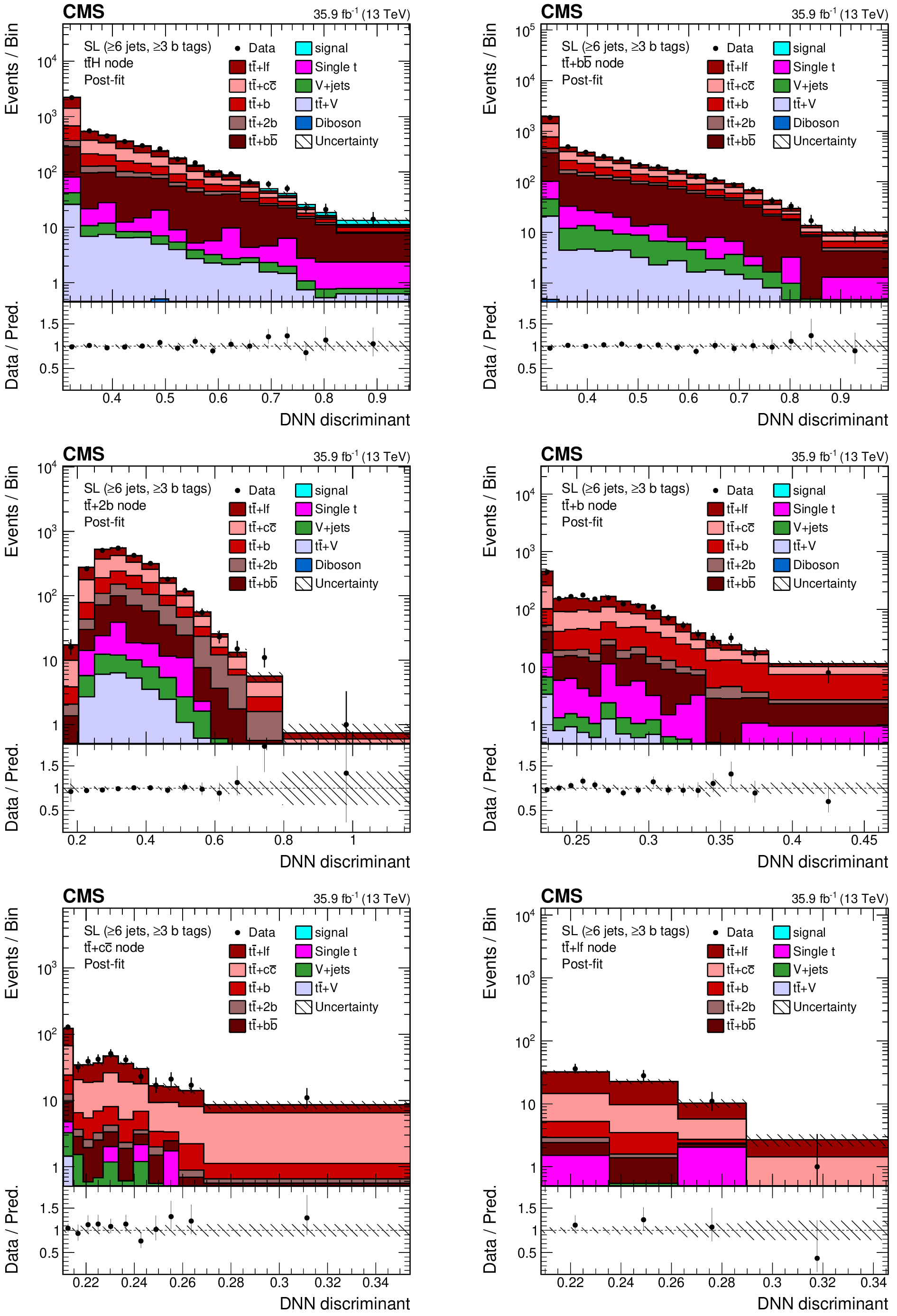
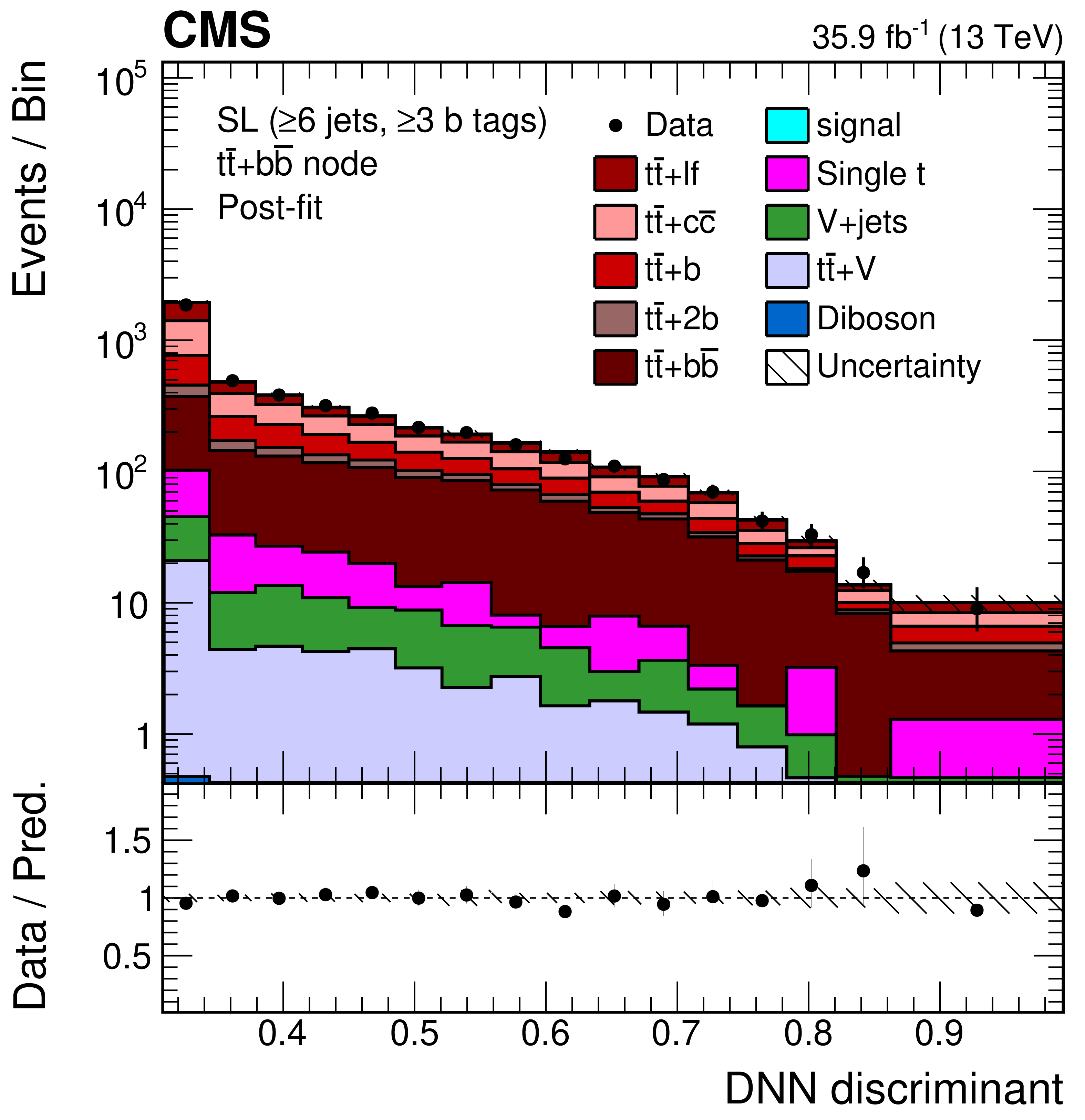
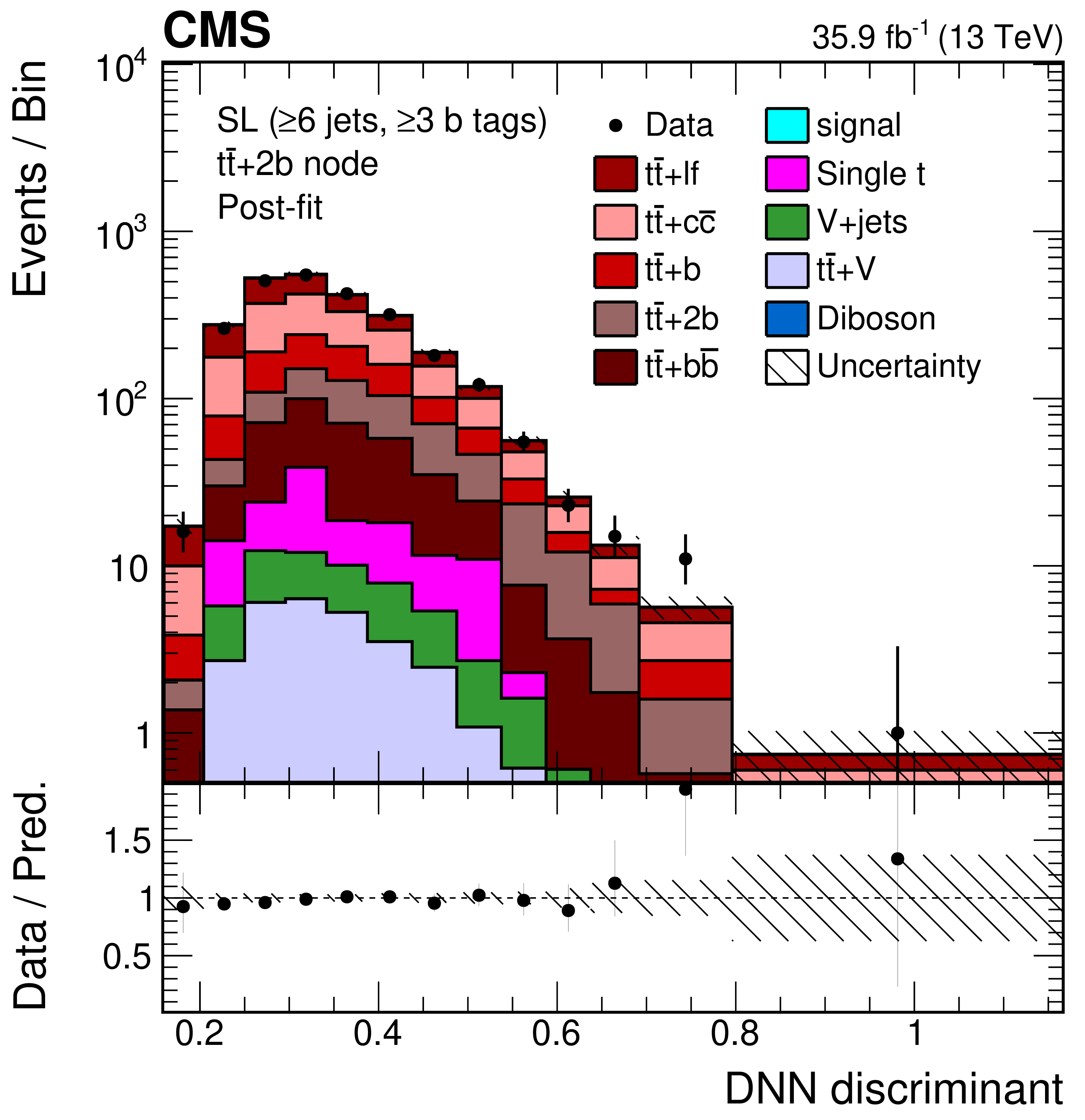
Figure 17:
Final discriminant (DNN) shapes in the single-lepton (SL) channel after the fit to data, in the jet-process categories with (6 jets, $\geq$3 b tags) and (from upper left to lower right) $ {{{\mathrm {t}\overline {\mathrm {t}}}} {\mathrm {H}}} $, $ {{{\mathrm {t}\overline {\mathrm {t}}}} \text {+} {{\mathrm {b}} {\overline {\mathrm {b}}}}} $, $ {{{\mathrm {t}\overline {\mathrm {t}}}} \text {+}2 {\mathrm {b}}} $, $ {{{\mathrm {t}\overline {\mathrm {t}}}} \text {+} {\mathrm {b}}} $, $ {{{\mathrm {t}\overline {\mathrm {t}}}} \text {+} {{\mathrm {c}} {\overline {\mathrm {c}}}}} $, and $ {{{\mathrm {t}\overline {\mathrm {t}}}} \text {+}\text {lf}} $. The error bands include the total uncertainty after the fit to data. The first and the last bins include underflow and overflow events, respectively. The lower plots show the ratio of the data to the post-fit background plus signal distribution. |

png pdf |
Figure 17-a:
Final discriminant (DNN) shapes in the single-lepton (SL) channel after the fit to data, in the jet-process categories with (6 jets, $\geq$3 b tags) and $ {{{\mathrm {t}\overline {\mathrm {t}}}} {\mathrm {H}}} $. The error bands include the total uncertainty after the fit to data. The first and the last bins include underflow and overflow events, respectively. The lower plot shows the ratio of the data to the post-fit background plus signal distribution. |
png pdf |
Figure 17-b:
Final discriminant (DNN) shapes in the single-lepton (SL) channel after the fit to data, in the jet-process categories with (6 jets, $\geq$3 b tags) and $ {{{\mathrm {t}\overline {\mathrm {t}}}} \text {+} {{\mathrm {b}} {\overline {\mathrm {b}}}}} $. The error bands include the total uncertainty after the fit to data. The first and the last bins include underflow and overflow events, respectively. The lower plot shows the ratio of the data to the post-fit background plus signal distribution. |
png pdf |
Figure 17-c:
Final discriminant (DNN) shapes in the single-lepton (SL) channel after the fit to data, in the jet-process categories with (6 jets, $\geq$3 b tags) and $ {{{\mathrm {t}\overline {\mathrm {t}}}} \text {+}2 {\mathrm {b}}} $. The error bands include the total uncertainty after the fit to data. The first and the last bins include underflow and overflow events, respectively. The lower plot shows the ratio of the data to the post-fit background plus signal distribution. |
png pdf |
Figure 17-d:
Final discriminant (DNN) shapes in the single-lepton (SL) channel after the fit to data, in the jet-process categories with (6 jets, $\geq$3 b tags) and $ {{{\mathrm {t}\overline {\mathrm {t}}}} \text {+} {\mathrm {b}}} $. The error bands include the total uncertainty after the fit to data. The first and the last bins include underflow and overflow events, respectively. The lower plot shows the ratio of the data to the post-fit background plus signal distribution. |

png pdf |
Figure 17-e:
Final discriminant (DNN) shapes in the single-lepton (SL) channel after the fit to data, in the jet-process categories with (6 jets, $\geq$3 b tags) and $ {{{\mathrm {t}\overline {\mathrm {t}}}} \text {+} {{\mathrm {c}} {\overline {\mathrm {c}}}}} $. The error bands include the total uncertainty after the fit to data. The first and the last bins include underflow and overflow events, respectively. The lower plot shows the ratio of the data to the post-fit background plus signal distribution. |
png pdf |
Figure 17-f:
Final discriminant (DNN) shapes in the single-lepton (SL) channel after the fit to data, in the jet-process categories with (6 jets, $\geq$3 b tags) and $ {{{\mathrm {t}\overline {\mathrm {t}}}} \text {+}\text {lf}} $. The error bands include the total uncertainty after the fit to data. The first and the last bins include underflow and overflow events, respectively. The lower plot shows the ratio of the data to the post-fit background plus signal distribution. |
| Tables | |

png pdf |
Table 1:
Event yields observed in data and predicted by the simulation after the selection requirements described in the text: at least four jets, at least two of which are b tagged in the single-lepton (SL) channel, and at least two jets, at least one of which is b tagged in the dilepton (DL) channel. The $ {{{\mathrm {t}\overline {\mathrm {t}}}} {\mathrm {H}}} $ signal includes $ {{\mathrm {H}} \to {{\mathrm {b}} {\overline {\mathrm {b}}}}} $ and all other Higgs boson decay modes. The quoted uncertainties are statistical only. |

png pdf |
Table 2:
Systematic uncertainties considered in the analysis, their corresponding type (affecting rate or shape of the distributions), and additional remarks. |
png pdf |
Table 3:
Observed and expected event yields per jet-process category (node) in the single-lepton channel with 4 jets and at least 3 b tags, prior to the fit to data (after the fit to data). The quoted uncertainties denote the total statistical and systematic components. |
png pdf |
Table 4:
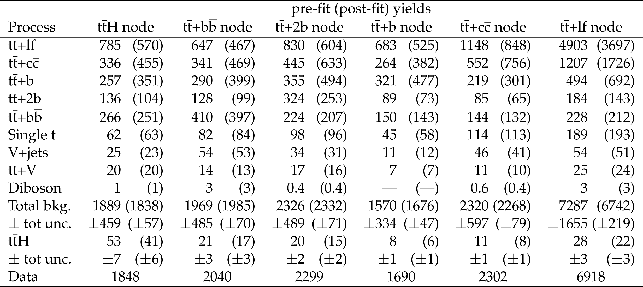
Observed and expected event yields per jet-process category (node) in the single-lepton channel with 5 jets and at least 3 b tags, prior to the fit to data (after the fit to data). The quoted uncertainties denote the total statistical and systematic uncertainty. |
png pdf |
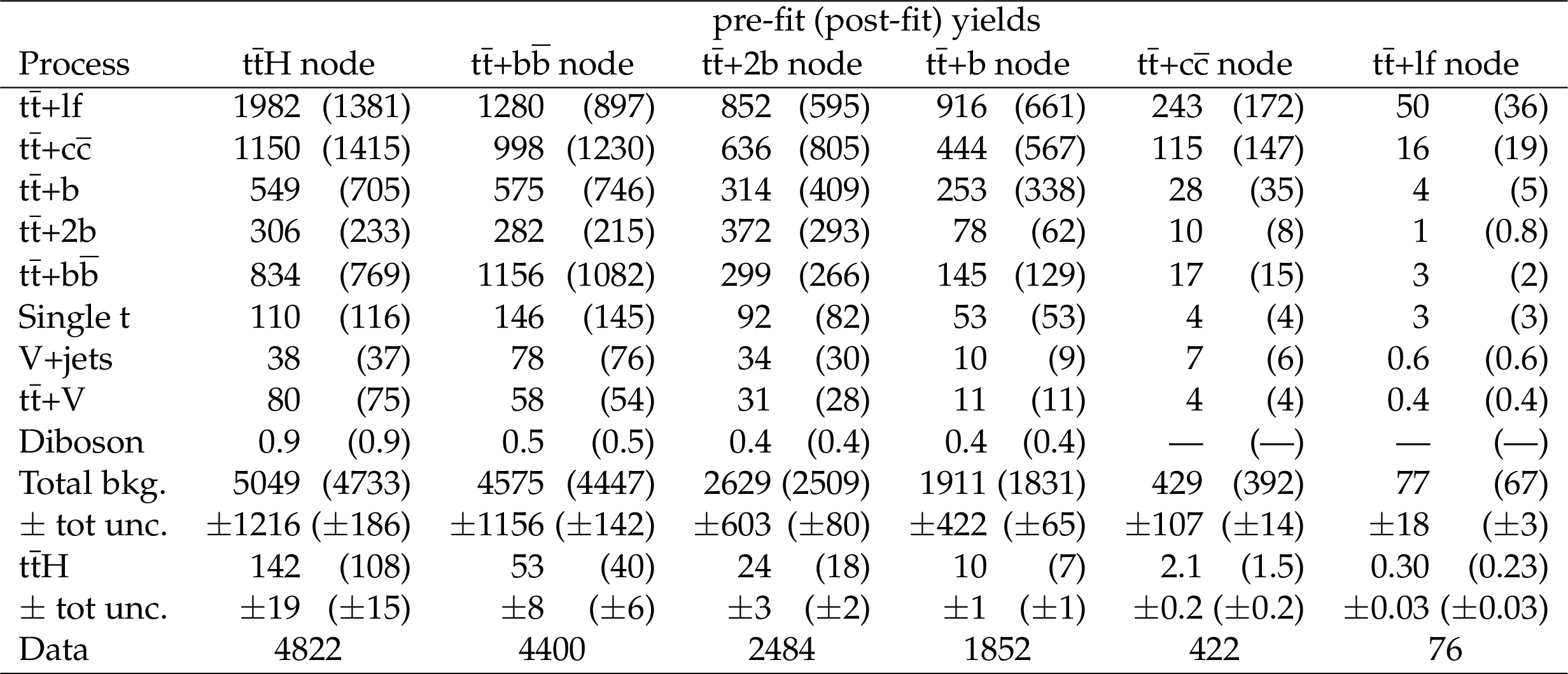
Table 5:
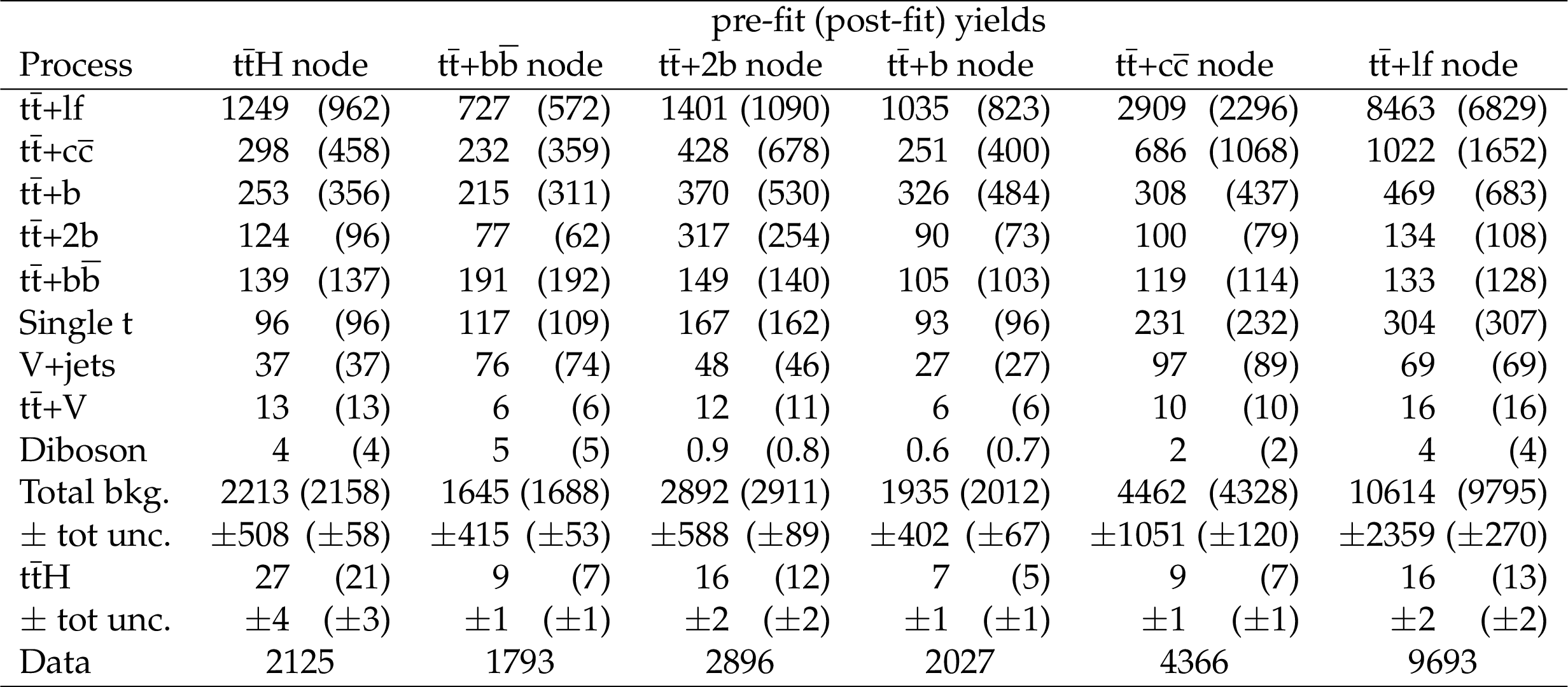
Observed and expected event yields per jet-process category (node) in the single-lepton channel with at least 6 jets and at least 3 b tags, prior to the fit to data (after the fit to data). The quoted uncertainties denote the total statistical and systematic uncertainty. |
png pdf |
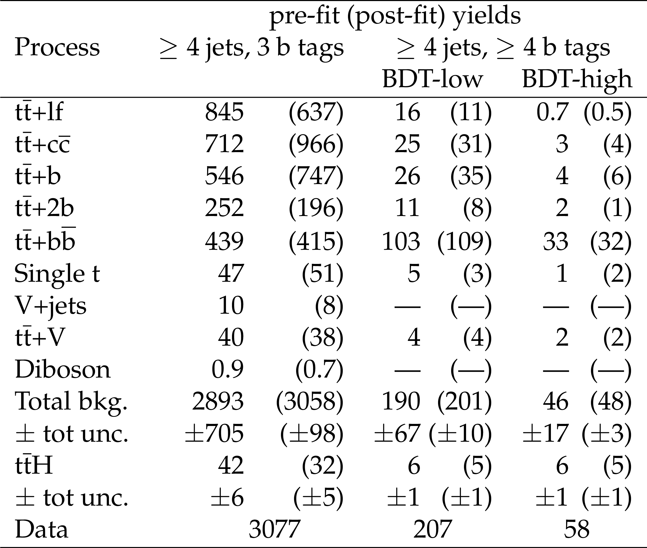
Table 6:
Observed and expected event yields per jet-tag category in the dilepton channel, prior to the fit to data (after the fit to data). The quoted uncertainties denote the total statistical and systematic uncertainty. |

png pdf |
Table 7:
Best fit value of the signal strength modifier $\mu $ and the observed and median expected 95% CL upper limits in the single-lepton and the dilepton channels as well as the combined results. The one standard deviation confidence intervals of the expected limit and the best fit value are also quoted, split into the statistical and systematic components in the latter case. |
png pdf |
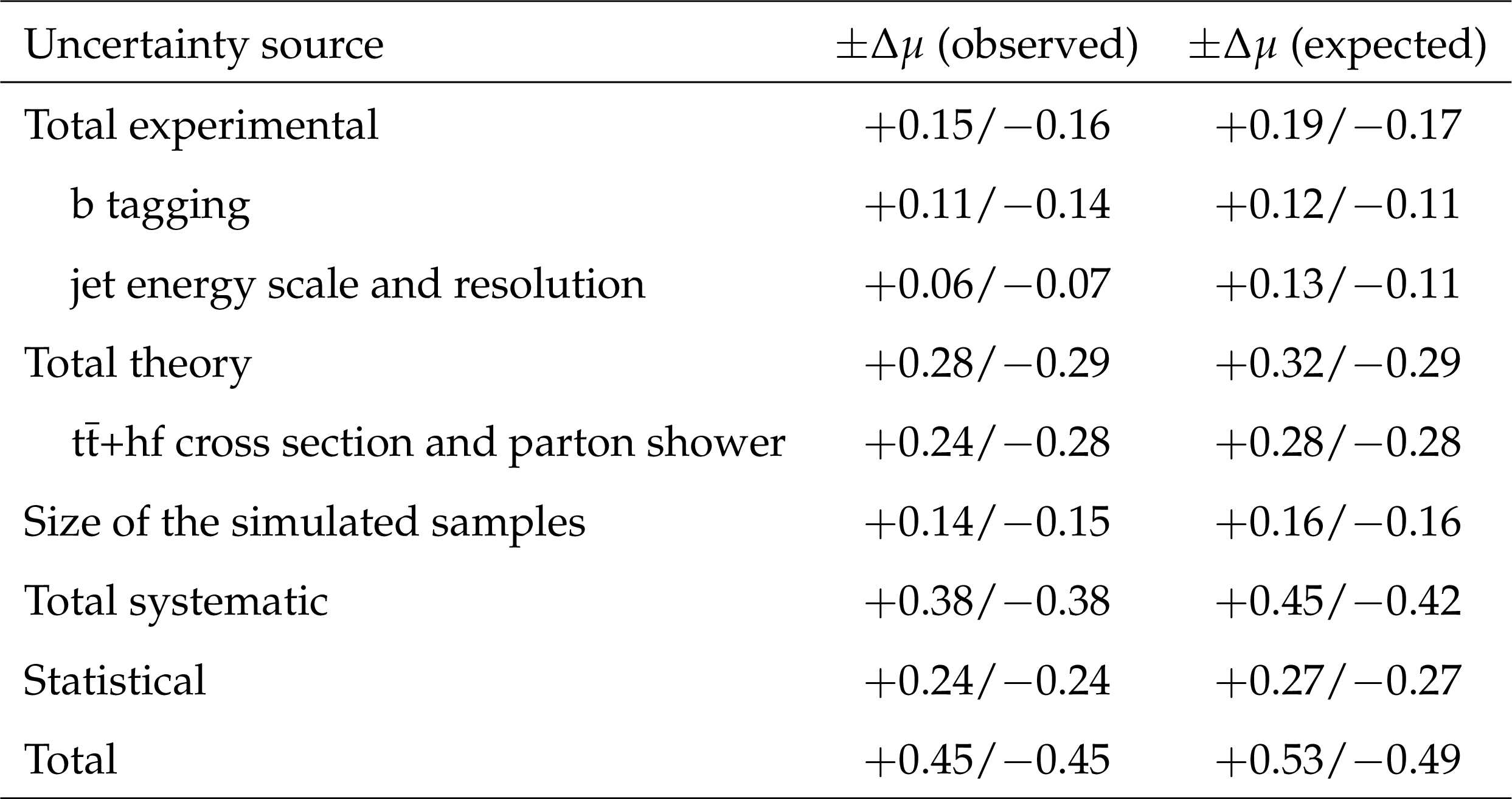
Table 8:
Contributions of different sources of uncertainties to the result for the fit to the data (observed) and to the expectation from simulation (expected). The quoted uncertainties $\Delta \mu $ in $\mu $ are obtained by fixing the listed sources of uncertainties to their post-fit values in the fit and subtracting the obtained result in quadrature from the result of the full fit. The statistical uncertainty is evaluated by fixing all nuisance parameters to their post-fit values. The quadratic sum of the contributions is different from the total uncertainty because of correlations between the nuisance parameters. |
png pdf |
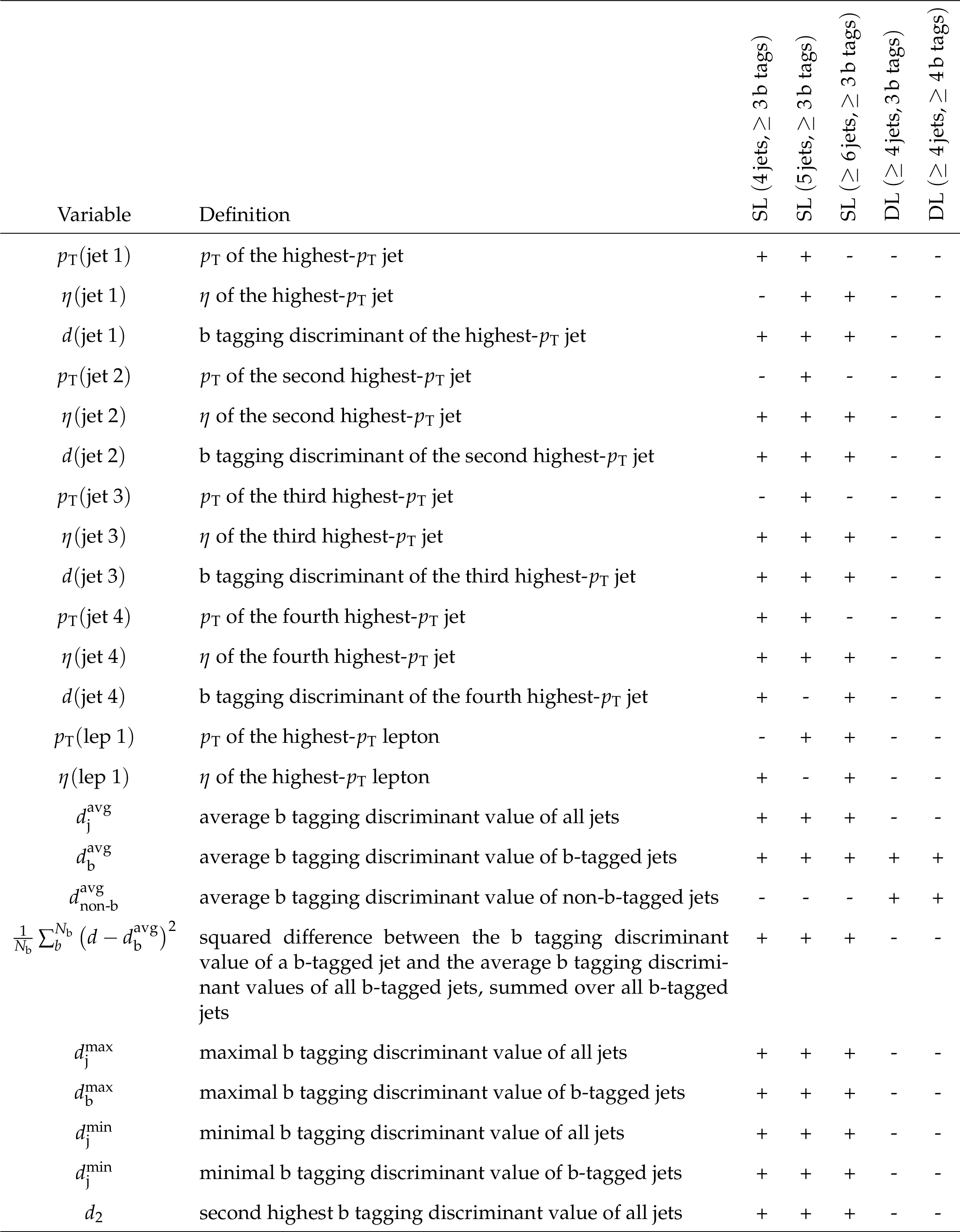
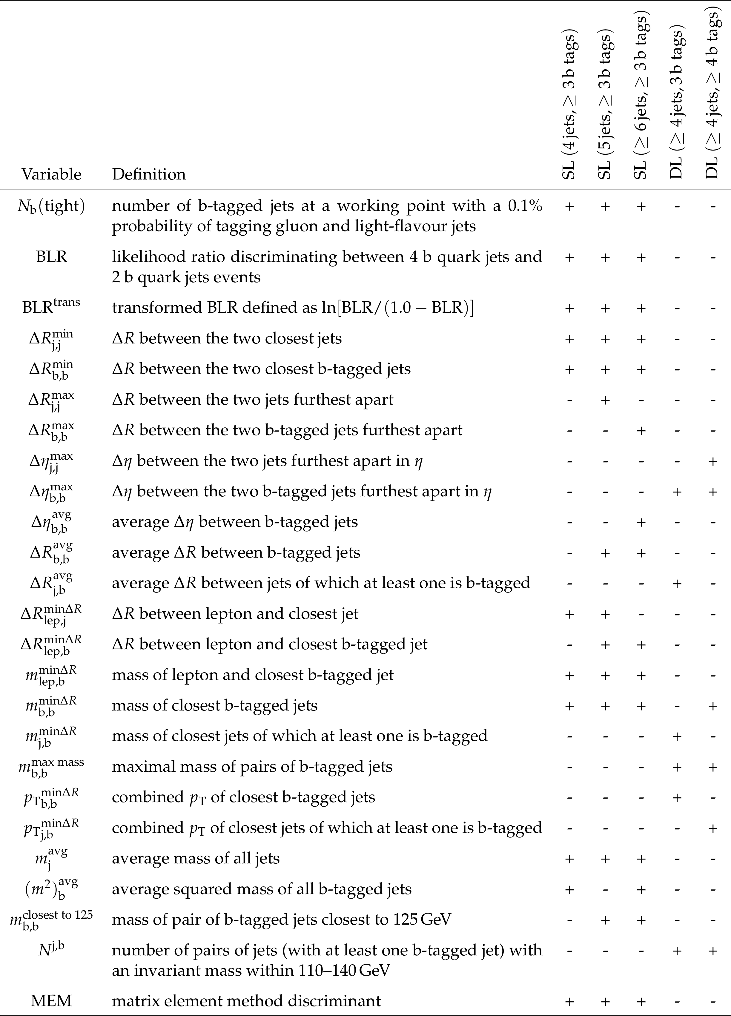
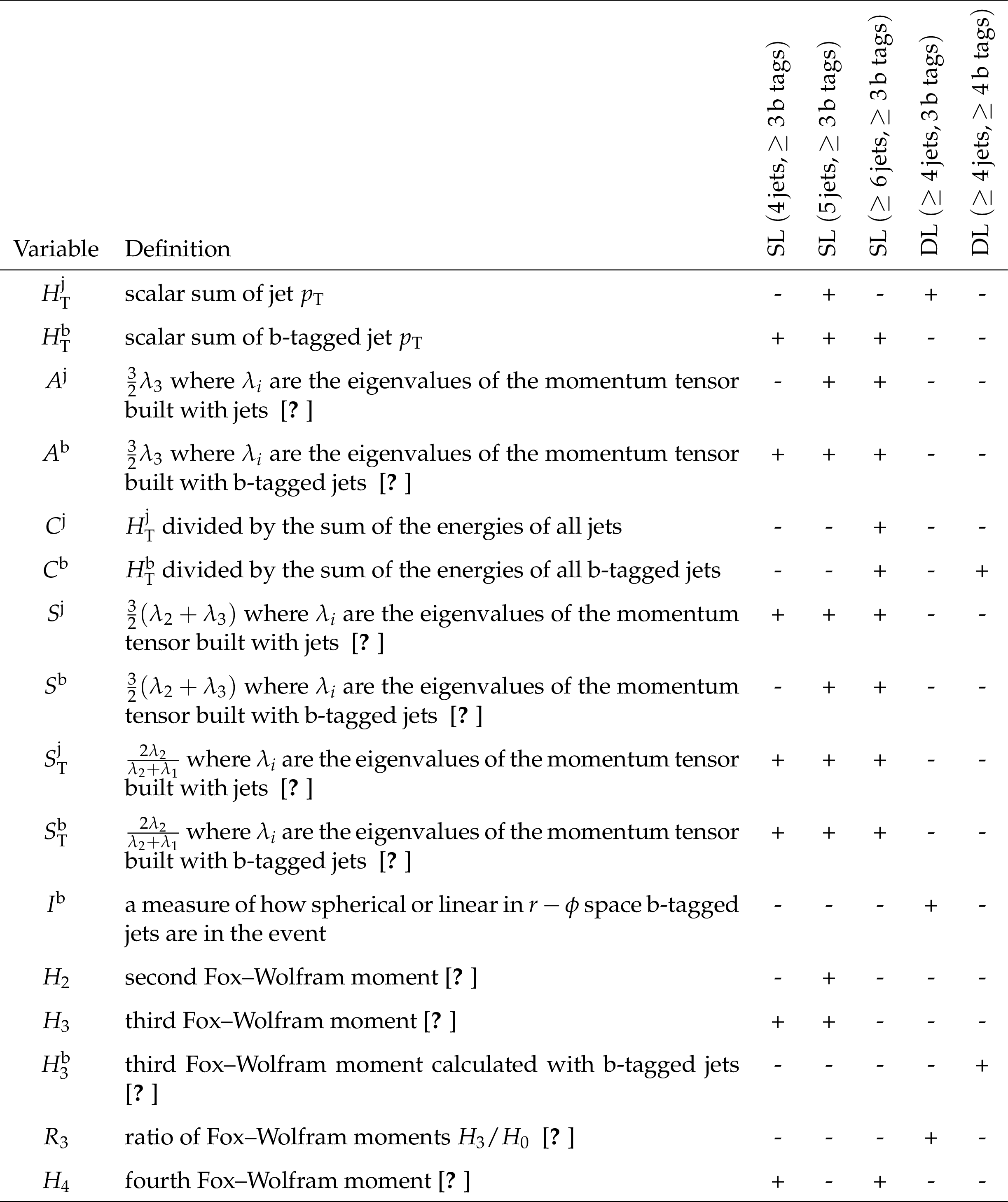
Table 9:
Input variables used in the DNNs or BDTs in the different categories of the single-lepton and dilepton channels. Variables used in a specific multivariate method and analysis category are denoted by a "$+$'' and unused variables by a "$-$''. (Continued in Tables 10 and 11.) |
png pdf |
Table 10:
Continued from Table 9 and continued in Table 11. |
png pdf |
Table 11:
Continued from Table 10. |
png pdf |
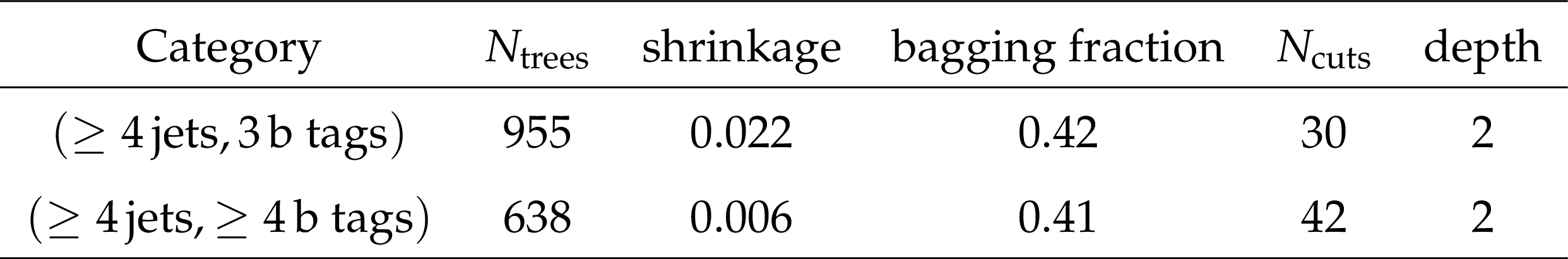
Table 12:
Configuration of the BDTs used in the dilepton channel. |
| Summary |
| A search for the associated production of a Higgs boson and a top quark-antiquark pair ($ {\mathrm{t\bar{t}}\mathrm{H}} $) is performed using pp collision data recorded with the CMS detector at a centre-of-mass energy of 13 TeV in 2016, corresponding to an integrated luminosity of 35.9 fb$^{-1}$. Candidate events are selected in final states compatible with the Higgs boson decaying into a b quark-antiquark pair and the single-lepton and dilepton decay channels of the $ \mathrm{t\bar{t}} $ system. Selected events are split into mutually exclusive categories according to their $ \mathrm{t\bar{t}} $ decay channel and jet content. In each category a powerful discriminant is constructed to separate the $ {\mathrm{t\bar{t}}\mathrm{H}} $ signal from the dominant ${\mathrm{t\bar{t}}}$+jets background, based on several multivariate analysis techniques (boosted decision trees, matrix element method, and deep neural networks). An observed (expected) upper limit on the $ {\mathrm{t\bar{t}}\mathrm{H}} $ production cross section $\mu$ relative to the SM expectations of 1.5 (0.9) at 95% confidence level is obtained. The best fit value of $\mu$ is 0.72 $\pm$ 0.24 (stat) $\pm$ 0.38 (syst). These results correspond to an observed (expected) significance of 1.6 (2.2) standard deviations above the background-only hypothesis. |
| Additional Tables | |
png pdf |
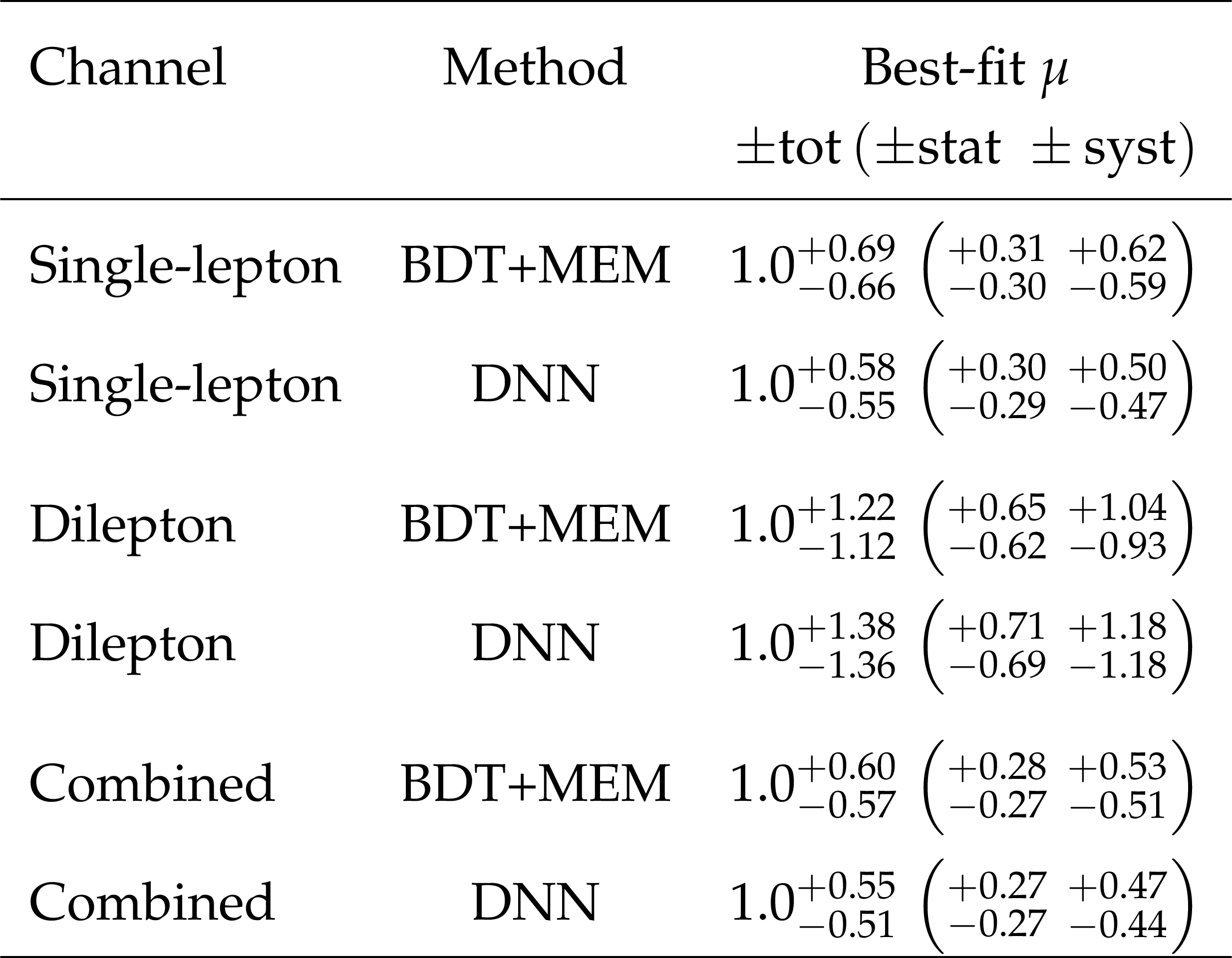
Additional Table 1:
Comparison of the sensitivity of the BDT+MEM and DNN methods using simulated data. The best-fit value of the signal strength modifier $\mu $ in the single-lepton and the dilepton channels as well as the combined results are listed, which have been obtained on Asimov data with a standard model signal injected. The one standard deviation confidence intervals are also quoted, split into the statistical and systematic components. |
| References | ||||
| 1 | ATLAS Collaboration | Observation of a new particle in the search for the standard model Higgs boson with the ATLAS detector at the LHC | PLB 716 (2012) 1 | 1207.7214 |
| 2 | CMS Collaboration | Observation of a new boson at a mass of 125 GeV with the CMS experiment at the LHC | PLB 716 (2012) 30 | CMS-HIG-12-028 1207.7235 |
| 3 | CMS Collaboration | A new boson with a mass of 125 GeV observed with the CMS experiment at the Large Hadron Collider | Science 338 (2012) 1569 | |
| 4 | ATLAS and CMS Collaborations | Combined measurement of the Higgs boson mass in pp collisions at $ \sqrt{s}= $ 7 and 8 TeV with the ATLAS and CMS experiments | PRL 114 (2015) 191803 | 1503.07589 |
| 5 | CMS Collaboration | Measurements of properties of the Higgs boson decaying into the four-lepton final state in pp collisions at $ \sqrt{s} = $ 13 TeV | JHEP 11 (2017) 047 | CMS-HIG-16-041 1706.09936 |
| 6 | CMS Collaboration | Evidence for the direct decay of the 125 GeV Higgs boson to fermions | NP 10 (2014) 557 | CMS-HIG-13-033 1401.6527 |
| 7 | ATLAS Collaboration | Evidence for the Higgs-boson Yukawa coupling to tau leptons with the ATLAS detector | JHEP 04 (2015) 117 | 1501.04943 |
| 8 | CMS Collaboration | Observation of the Higgs boson decay to a pair of $ \tau $ leptons with the CMS detector | PLB 779 (2018) 283 | CMS-HIG-16-043 1708.00373 |
| 9 | ATLAS Collaboration | Evidence for the $\mathrm{H} \to \mathrm{b \bar{b}} $ decay with the ATLAS detector | JHEP 12 (2017) 024 | 1708.03299 |
| 10 | CMS Collaboration | Evidence for the Higgs boson decay to a bottom quark-antiquark pair | Submitted to PLB | CMS-HIG-16-044 1709.07497 |
| 11 | ATLAS Collaboration | Measurements of Higgs boson production and couplings in diboson final states with the ATLAS detector at the LHC | PLB 726 (2013) 88 | 1307.1427 |
| 12 | CMS Collaboration | Precise determination of the mass of the Higgs boson and tests of compatibility of its couplings with the standard model predictions using proton collisions at 7 and 8 TeV | EPJC 75 (2015) 212 | CMS-HIG-14-009 1412.8662 |
| 13 | ATLAS Collaboration | Evidence for the spin-0 nature of the Higgs boson using ATLAS data | PLB 726 (2013) 120 | 1307.1432 |
| 14 | CMS Collaboration | Constraints on the spin-parity and anomalous HVV couplings of the Higgs boson in proton collisions at 7 and 8 TeV | PRD 92 (2015) 012004 | CMS-HIG-14-018 1411.3441 |
| 15 | CMS Collaboration | Search for standard model production of four top quarks with same-sign and multilepton final states in proton-proton collisions at $ \sqrt{s} = $ 13 TeV | EPJC 78 (2018) 140 | CMS-TOP-17-009 1710.10614 |
| 16 | LHC Higgs Cross Section Working Group | Handbook of LHC Higgs cross sections: 4. deciphering the nature of the Higgs sector | CERN (2016) | 1610.07922 |
| 17 | G. Burdman, M. Perelstein, and A. Pierce | Large Hadron Collider tests of the little Higgs model | PRL 90 (2003) 241802 | hep-ph/0212228 |
| 18 | T. Han, H. E. Logan, B. McElrath, and L.-T. Wang | Phenomenology of the little Higgs model | PRD 67 (2003) 095004 | hep-ph/0301040 |
| 19 | M. Perelstein, M. E. Peskin, and A. Pierce | Top quarks and electroweak symmetry breaking in little Higgs models | PRD 69 (2004) 075002 | hep-ph/0310039 |
| 20 | H.-C. Cheng, I. Low, and L.-T. Wang | Top partners in little Higgs theories with T-parity | PRD 74 (2006) 055001 | hep-ph/0510225 |
| 21 | H.-C. Cheng, B. A. Dobrescu, and C. T. Hill | Electroweak symmetry breaking and extra dimensions | NPB 589 (2000) 249 | hep-ph/9912343 |
| 22 | M. Carena, E. Ponton, J. Santiago, and C. E. M. Wagner | Light Kaluza-Klein states in Randall-Sundrum models with custodial SU(2) | NPB 759 (2006) 202 | hep-ph/0607106 |
| 23 | R. Contino, L. Da Rold, and A. Pomarol | Light custodians in natural composite Higgs models | PRD 75 (2007) 055014 | hep-ph/0612048 |
| 24 | G. Burdman and L. Da Rold | Electroweak symmetry breaking from a holographic fourth generation | JHEP 12 (2007) 086 | 0710.0623 |
| 25 | C. T. Hill | Topcolor: Top quark condensation in a gauge extension of the standard model | PLB 266 (1991) 419 | |
| 26 | A. Carmona, M. Chala, and J. Santiago | New Higgs production mechanism in composite Higgs models | JHEP 07 (2012) 049 | 1205.2378 |
| 27 | CMS Collaboration | Search for the associated production of the Higgs boson with a top-quark pair | JHEP 09 (2014) 087 | CMS-HIG-13-029 1408.1682 |
| 28 | ATLAS Collaboration | Search for the associated production of the Higgs boson with a top quark pair in multilepton final states with the ATLAS detector | PLB 749 (2015) 519 | 1506.05988 |
| 29 | CMS Collaboration | Search for a standard model Higgs boson produced in association with a top-quark pair and decaying to bottom quarks using a matrix element method | EPJC 75 (2015) 251 | CMS-HIG-14-010 1502.02485 |
| 30 | ATLAS Collaboration | Search for the standard model Higgs boson produced in association with top quarks and decaying into $ \mathrm{b\bar{b}} $ in pp collisions at $ \sqrt{s} = $ 8 TeV with the ATLAS detector | EPJC 75 (2015) 349 | 1503.05066 |
| 31 | LHC Higgs Cross Section Working Group | Handbook of LHC Higgs cross sections: 1. inclusive observables | CERN (2011) | 1101.0593 |
| 32 | CMS Collaboration | Search for ttH production in the all-jet final state in proton-proton collisions at $ \sqrt{s} = $ 13 TeV | Submitted to JHEP | CMS-HIG-17-022 1803.06986 |
| 33 | CMS Collaboration | Evidence for associated production of a Higgs boson with a top quark pair in final states with electrons, muons, and hadronically decaying $ \tau $ leptons at $ \sqrt{s} = $ 13 TeV | Submitted to JHEP | CMS-HIG-17-018 1803.05485 |
| 34 | ATLAS Collaboration | Evidence for the associated production of the Higgs boson and a top quark pair with the ATLAS detector | Submitted to PRD | 1712.08891 |
| 35 | ATLAS Collaboration | Search for the standard model Higgs boson produced in association with top quarks and decaying into a $ \mathrm{b\bar{b}} $ pair in pp collisions at $ \sqrt{s} = $ 13 TeV with the ATLAS detector | Submitted to PRD | 1712.08895 |
| 36 | T. J. Hastie, R. J. Tibshirani, and J. H. Friedman | The elements of statistical learning : data mining, inference, and prediction | Springer series in statistics. Springer, New York, NY, 2. ed., corr. at 10. print. edition, 2013 ISBN 978-0-387-84857-0 | |
| 37 | P. C. Bhat | Multivariate analysis methods in particle physics | Ann. Rev. Nucl. Part. Sci. 61 (2011) 281 | |
| 38 | A. Hocker et al. | TMVA: Toolkit for multivariate data analysis | PoS ACAT (2007) 040 | physics/0703039 |
| 39 | K. Kondo | Dynamical likelihood method for reconstruction of events with missing momentum. 1: Method and toy models | J. Phys. Soc. Jap. 57 (1988) 4126 | |
| 40 | D0 Collaboration | A precision measurement of the mass of the top quark | Nature 429 (2004) 638 | hep-ex/0406031 |
| 41 | CMS Collaboration | The CMS experiment at the CERN LHC | JINST 3 (2008) S08004 | CMS-00-001 |
| 42 | CMS Collaboration | The CMS trigger system | JINST 12 (2017) P01020 | CMS-TRG-12-001 1609.02366 |
| 43 | GEANT4 Collaboration | $ GEANT4--a $ simulation toolkit | NIMA 506 (2003) 250 | |
| 44 | P. Nason | A new method for combining NLO QCD with shower Monte Carlo algorithms | JHEP 11 (2004) 040 | hep-ph/0409146 |
| 45 | S. Frixione, P. Nason, and C. Oleari | Matching NLO QCD computations with parton shower simulations: the POWHEG method | JHEP 11 (2007) 070 | 0709.2092 |
| 46 | S. Alioli, P. Nason, C. Oleari, and E. Re | A general framework for implementing NLO calculations in shower Monte Carlo programs: the POWHEG BOX | JHEP 06 (2010) 043 | 1002.2581 |
| 47 | H. B. Hartanto, B. Jager, L. Reina, and D. Wackeroth | Higgs boson production in association with top quarks in the POWHEG BOX | PRD 91 (2015) 094003 | 1501.04498 |
| 48 | T. Sjostrand et al. | An introduction to PYTHIA 8.2 | CPC 191 (2015) 159 | 1410.3012 |
| 49 | J. Alwall et al. | The automated computation of tree-level and next-to-leading order differential cross sections, and their matching to parton shower simulations | JHEP 07 (2014) 079 | 1405.0301 |
| 50 | NNPDF Collaboration | Parton distributions for the LHC Run II | JHEP 04 (2015) 040 | 1410.8849 |
| 51 | S. Alioli, P. Nason, C. Oleari, and E. Re | NLO single-top production matched with shower in POWHEG: $ s $- and $ t $-channel contributions | JHEP 09 (2009) 111 | 0907.4076 |
| 52 | E. Re | Single-top Wt-channel production matched with parton showers using the POWHEG method | EPJC 71 (2011) 1547 | 1009.2450 |
| 53 | R. Frederix and S. Frixione | Merging meets matching in MC@NLO | JHEP 12 (2012) 061 | 1209.6215 |
| 54 | CMS Collaboration | Event generator tunes obtained from underlying event and multiparton scattering measurements | EPJC 76 (2016) 155 | CMS-GEN-14-001 1512.00815 |
| 55 | P. Skands, S. Carrazza, and J. Rojo | Tuning PYTHIA 8.1: the Monash 2013 tune | EPJC 74 (2014) 3024 | 1404.5630 |
| 56 | N. Kidonakis | Two-loop soft anomalous dimensions for single top quark associated production with $ \mathrm{W^-} $ or $ \mathrm{H^-} $ | PRD 82 (2010) 054018 | 1005.4451 |
| 57 | M. Aliev et al. | HATHOR: HAdronic Top and Heavy quarks crOss section calculatoR | CPC 182 (2011) 1034 | 1007.1327 |
| 58 | P. Kant et al. | HatHor for single top-quark production: Updated predictions and uncertainty estimates for single top-quark production in hadronic collisions | CPC 191 (2015) 74 | 1406.4403 |
| 59 | F. Maltoni, D. Pagani, and I. Tsinikos | Associated production of a top-quark pair with vector bosons at NLO in QCD: impact on $ \mathrm{t}\overline{\mathrm{t}}\mathrm{H} $ searches at the LHC | JHEP 02 (2016) 113 | 1507.05640 |
| 60 | J. M. Campbell, R. K. Ellis, and C. Williams | Vector boson pair production at the LHC | JHEP 07 (2011) 018 | 1105.0020 |
| 61 | M. Cacciari et al. | Top-pair production at hadron colliders with next-to-next-to-leading logarithmic soft-gluon resummation | PLB 710 (2012) 612 | 1111.5869 |
| 62 | P. Barnreuther, M. Czakon, and A. Mitov | Percent-level-precision physics at the Tevatron: next-to-next-to-leading order QCD corrections to $ \mathrm{ q \bar{q} } \to\mathrm{t\bar{t}}\text{+X} $ | PRL 109 (2012) 132001 | 1204.5201 |
| 63 | M. Czakon and A. Mitov | NNLO corrections to top-pair production at hadron colliders: the all-fermionic scattering channels | JHEP 12 (2012) 054 | 1207.0236 |
| 64 | M. Czakon and A. Mitov | NNLO corrections to top pair production at hadron colliders: the quark-gluon reaction | JHEP 01 (2013) 080 | 1210.6832 |
| 65 | M. Beneke, P. Falgari, S. Klein, and C. Schwinn | Hadronic top-quark pair production with NNLL threshold resummation | NPB 855 (2012) 695 | 1109.1536 |
| 66 | M. Czakon, P. Fiedler, and A. Mitov | Total top-quark pair-production cross section at hadron colliders through $ o({\alpha_s}^4) $ | PRL 110 (2013) 252004 | 1303.6254 |
| 67 | M. Czakon and A. Mitov | Top++: a program for the calculation of the top-pair cross-section at hadron colliders | CPC 185 (2014) 2930 | 1112.5675 |
| 68 | CMS Collaboration | Identification of heavy-flavour jets with the CMS detector in pp collisions at 13 TeV | Submitted to JINST | CMS-BTV-16-002 1712.07158 |
| 69 | CMS Collaboration | Particle-flow reconstruction and global event description with the CMS detector | JINST 12 (2017) P10003 | CMS-PRF-14-001 1706.04965 |
| 70 | CMS Collaboration | Performance of electron reconstruction and selection with the CMS detector in proton-proton collisions at $ \sqrt{s} = $ 8 TeV | JINST 10 (2015) P06005 | CMS-EGM-13-001 1502.02701 |
| 71 | CMS Collaboration | Performance of CMS muon reconstruction in pp collision events at $ \sqrt{s} = $ 7 TeV | JINST 7 (2012) P10002 | CMS-MUO-10-004 1206.4071 |
| 72 | M. Cacciari, G. P. Salam, and G. Soyez | The anti-$ {k_{\mathrm{T}}} $ jet clustering algorithm | JHEP 04 (2008) 063 | 0802.1189 |
| 73 | M. Cacciari, G. P. Salam, and G. Soyez | FastJet user manual | EPJC 72 (2012) 1896 | 1111.6097 |
| 74 | M. Cacciari, G. P. Salam, and G. Soyez | The catchment area of jets | JHEP 04 (2008) 005 | 0802.1188 |
| 75 | CMS Collaboration | Jet energy scale and resolution in the CMS experiment in pp collisions at 8 TeV | JINST 12 (2017) P02014 | CMS-JME-13-004 1607.03663 |
| 76 | J. H. Friedman | Stochastic gradient boosting | Comput. Stat. Data Anal. 38 (2002) 367 | |
| 77 | J. Kennedy and R. Eberhart | Particle swarm optimization | in Proceedings of the IEEE International Conference on neural networks, volume 4, p. 1942 1995 | |
| 78 | K. El Morabit | A study of the multivariate analysis of Higgs boson production in association with a top quark-antiquark pair in the boosted regime at the CMS experiment | Master's thesis, Karlsruher Institut f\"ur Technologie (KIT), 2015 EKP-2016-00035 | |
| 79 | I. Goodfellow, Y. Bengio, and A. Courville | Deep Learning | MIT Press | |
| 80 | CMS Collaboration | Investigations of the impact of the parton shower tuning in Pythia 8 in the modelling of $ \mathrm{t\bar{t}} $ at $ \sqrt{s}= $ 8 and 13 TeV | CMS-PAS-TOP-16-021 | CMS-PAS-TOP-16-021 |
| 81 | CMS Collaboration | CMS luminosity measurements for the 2016 data taking period | CMS-PAS-LUM-17-001 | CMS-PAS-LUM-17-001 |
| 82 | ATLAS Collaboration | Measurement of the inelastic proton-proton cross section at $ \sqrt{s} = $ 13 TeV with the ATLAS detector at the LHC | PRL 117 (2016) 182002 | 1606.02625 |
| 83 | CMS Collaboration | Measurements of $ \mathrm{t\bar{t}} $ cross sections in association with b jets and inclusive jets and their ratio using dilepton final states in pp collisions at $ \sqrt{s} = $ 13 TeV | PLB 776 (2018) 355 | CMS-TOP-16-010 1705.10141 |
| 84 | G. Bevilacqua, M. V. Garzelli, and A. Kardos | $ \text{t}\overline{\text{t}}\text{b}\overline{\text{b}} $ hadroproduction with massive bottom quarks with PowHel | 1709.06915 | |
| 85 | T. Jezo, J. M. Lindert, N. Moretti, and S. Pozzorini | New NLOPS predictions for $ \mathrm{t\bar{t}}\text{+b-jet} $ production at the LHC | 1802.00426 | |
| 86 | T. Gleisberg et al. | Event generation with SHERPA 1.1 | JHEP 02 (2009) 007 | 0811.4622 |
| 87 | F. Cascioli, P. Maierhofer, and S. Pozzorini | Scattering amplitudes with Open Loops | PRL 108 (2012) 111601 | 1111.5206 |
| 88 | CMS Collaboration | Measurement of differential cross sections for the production of top quark pairs and of additional jets in lepton+jets events from pp collisions at $ \sqrt{s} = $ 13 TeV | Submitted to PRD | CMS-TOP-17-002 1803.08856 |
| 89 | R. J. Barlow and C. Beeston | Fitting using finite Monte Carlo samples | CPC 77 (1993) 219 | |
| 90 | J. S. Conway | Incorporating nuisance parameters in likelihoods for multisource spectra | in Proceedings, PHYSTAT 2011 Workshop on Statistical Issues Related to Discovery Claims in Search Experiments and Unfolding, CERN,Geneva, Switzerland 17-20 January 2011 2011 | 1103.0354 |
| 91 | T. Junk | Confidence level computation for combining searches with small statistics | NIMA 434 (1999) 435 | hep-ex/9902006 |
| 92 | A. L. Read | Presentation of search results: the $ \text{CL}_{\mathrm{s}} $ technique | JPG 28 (2002) 2693 | |
| 93 | G. Cowan, K. Cranmer, E. Gross, and O. Vitells | Asymptotic formulae for likelihood-based tests of new physics | EPJC 71 (2011) 1554 | 1007.1727 |
| 94 | B. Efron | The Jackknife, the Bootstrap and Other Resampling Plans | Society for Industrial and Applied Mathematics | |
| 95 | J. D. Bjorken and S. J. Brodsky | Statistical model for electron-positron annihilation into hadrons | PRD 1 (1970) 1416 | |
| 96 | G. C. Fox and S. Wolfram | Event shapes in $ e^{+}e^{-} $ annihilation | NPB 157 (1979) 543 | |
|
|
Compact Muon Solenoid LHC, CERN |
|

|

|

|

|

|