

Compact Muon Solenoid
LHC, CERN
| CMS-HIG-17-022 ; CERN-EP-2018-038 | ||
| Search for $ {\mathrm{t\bar{t}} \mathrm{H}} $ production in the all-jet final state in proton-proton collisions at $\sqrt{s} = $ 13 TeV | ||
| CMS Collaboration | ||
| 19 March 2018 | ||
| JHEP 06 (2018) 101 | ||
| Abstract: A search is presented for the associated production of a Higgs boson with a top quark pair in the all-jet final state. Events containing seven or more jets are selected from a sample of proton-proton collisions at $\sqrt{s} = $ 13 TeV collected with the CMS detector at the LHC in 2016, corresponding to an integrated luminosity of 35.9 fb$^{-1}$. To separate the $ {\mathrm{t\bar{t}} \mathrm{H}} $ signal from the irreducible $ {\mathrm{t\bar{t}} + \mathrm{ b \bar{b} }}$ background, the analysis assigns leading order matrix element signal and background probability densities to each event. A likelihood-ratio statistic based on these probability densities is used to extract the signal. The results are provided in terms of an observed $ {\mathrm{t\bar{t}} \mathrm{H}} $ signal strength relative to the standard model production cross section $\mu=\sigma/\sigma_\mathrm{SM}$, assuming a Higgs boson mass of 125 GeV. The best fit value is ${\hat{\mu}} = $ 0.9 $\pm$ 0.7 (stat) $\pm$ 1.3 (syst) = 0.9 $\pm$ 1.5 (tot), and the observed and expected upper limits are, respectively, $\mu < $ 3.8 and $ < $ 3.1 at 95% confidence levels. | ||
| Links: e-print arXiv:1803.06986 [hep-ex] (PDF) ; CDS record ; inSPIRE record ; HepData record ; CADI line (restricted) ; | ||
| Figures & Tables | Summary | Additional Figures | References | CMS Publications |
|---|
| Figures | |

png pdf |
Figure 1:
An example of an LO Feynman diagram for $ {{{\mathrm {t}\overline {\mathrm {t}}}} {\mathrm {H}}} $ production, including the subsequent decay of the top quark-antiquark pair, as well as that of the Higgs boson into a bottom quark-antiquark pair. |

png pdf |
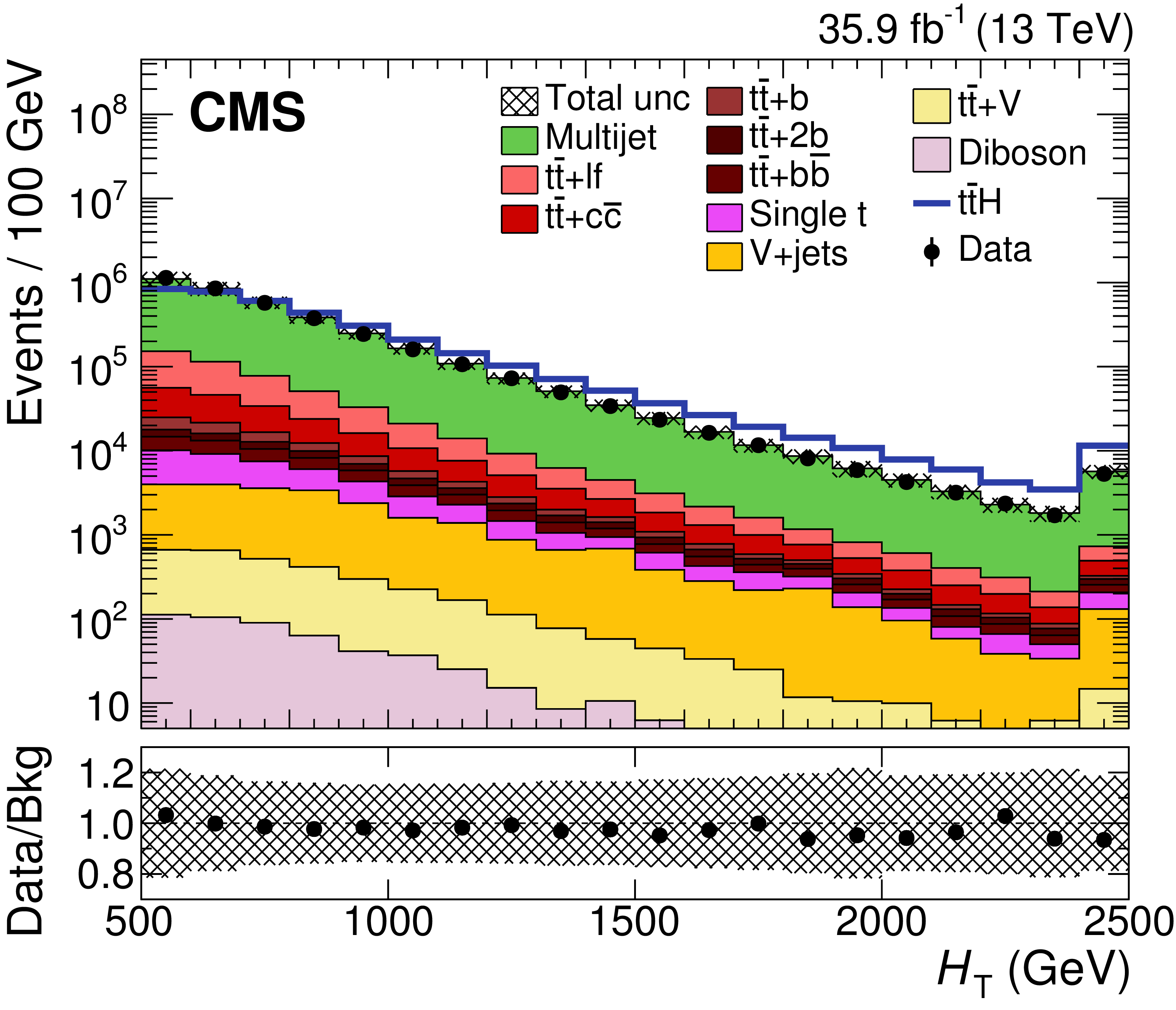
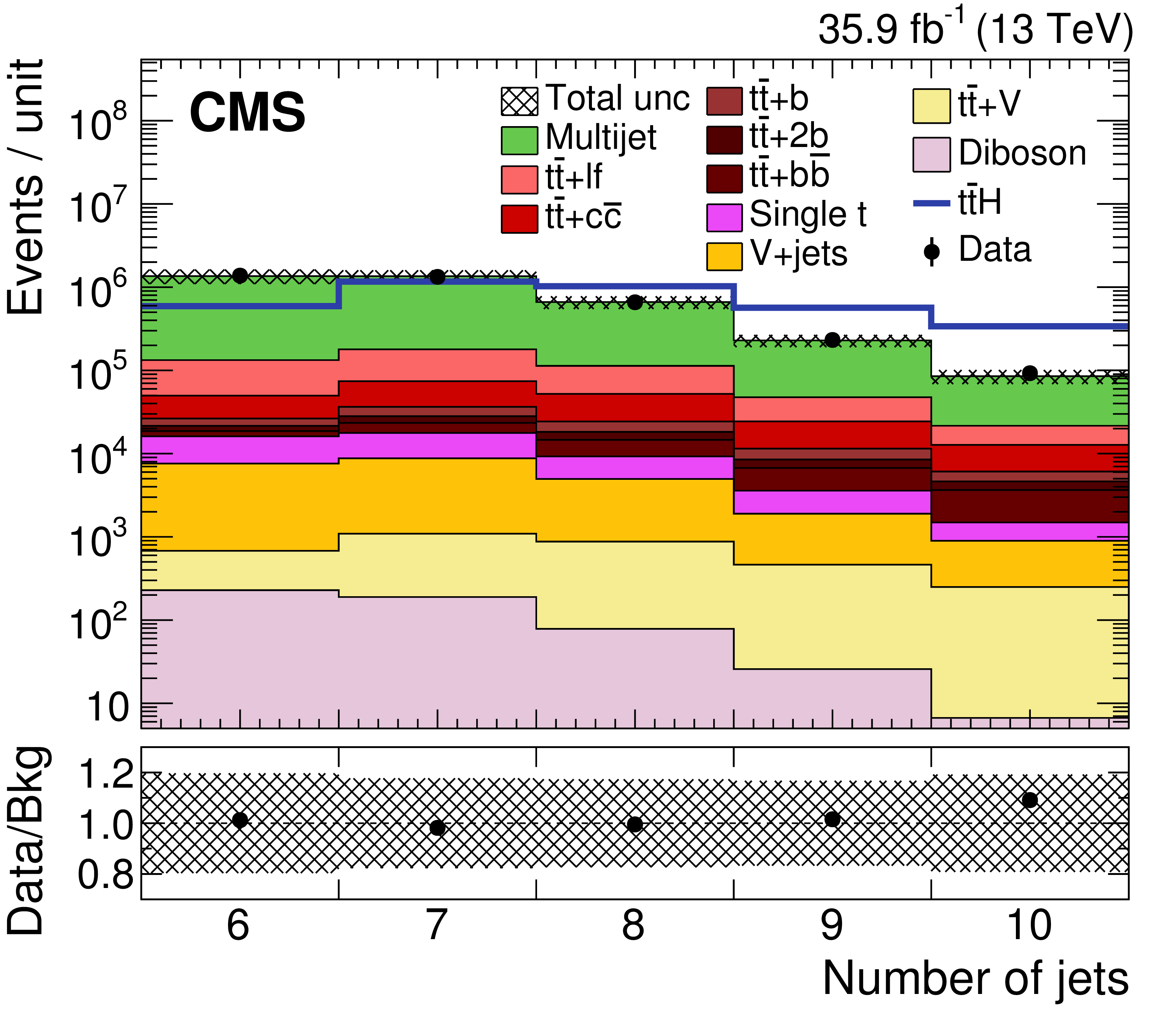
Figure 2:
Distribution in $ {H_{\mathrm {T}}} $ (left) and jet multiplicity (right) in data (black points) and in simulation (stacked histograms), after implementing the preselection. The simulated backgrounds are first scaled to the integrated luminosity of the data, and then the simulated QCD multijet background is rescaled to match the yield in data. The contribution from $ {{{\mathrm {t}\overline {\mathrm {t}}}} {\mathrm {H}}} $ signal (blue line) is scaled to the total background yield (equivalent to the yield in data) to enhance readability. The hatched bands reflect the total statistical and systematic uncertainties in the background prediction, prior to the fit to data, which are dominated by the systematic uncertainties in the simulated multijet background. The last bin includes event overflows. The ratios of data to background are given below the main panels. |
png pdf |
Figure 2-a:
Distribution in $ {H_{\mathrm {T}}} $ in data (black points) and in simulation (stacked histograms), after implementing the preselection. The simulated backgrounds are first scaled to the integrated luminosity of the data, and then the simulated QCD multijet background is rescaled to match the yield in data. The contribution from $ {{{\mathrm {t}\overline {\mathrm {t}}}} {\mathrm {H}}} $ signal (blue line) is scaled to the total background yield (equivalent to the yield in data) to enhance readability. The hatched bands reflect the total statistical and systematic uncertainties in the background prediction, prior to the fit to data, which are dominated by the systematic uncertainties in the simulated multijet background. The last bin includes event overflows. The ratio of data to background are given below the main panel. |
png pdf |
Figure 2-b:
Distribution in jet multiplicity in data (black points) and in simulation (stacked histograms), after implementing the preselection. The simulated backgrounds are first scaled to the integrated luminosity of the data, and then the simulated QCD multijet background is rescaled to match the yield in data. The contribution from $ {{{\mathrm {t}\overline {\mathrm {t}}}} {\mathrm {H}}} $ signal (blue line) is scaled to the total background yield (equivalent to the yield in data) to enhance readability. The hatched bands reflect the total statistical and systematic uncertainties in the background prediction, prior to the fit to data, which are dominated by the systematic uncertainties in the simulated multijet background. The last bin includes event overflows. The ratio of data to background are given below the main panel. |

png pdf |
Figure 3:
Comparison of the distributions in the quark-gluon likelihood ratio in data (black points) and in simulation (stacked histograms), after preselection, excluding the first 3 b-tagged jets. The simulated backgrounds are first scaled to the integrated luminosity of the data, and then the simulated multijet background is rescaled to match the yield in data. The contribution from signal (blue line) is scaled to the total background yield (equivalent to the yield in data) to enhance readability. The hatched bands reflect the total statistical and systematic uncertainties in the background prediction, prior to the fit to data, which are dominated by the systematic uncertainties in the simulated multijet background. The ratio of data to background is given below the main panel. |

png pdf |
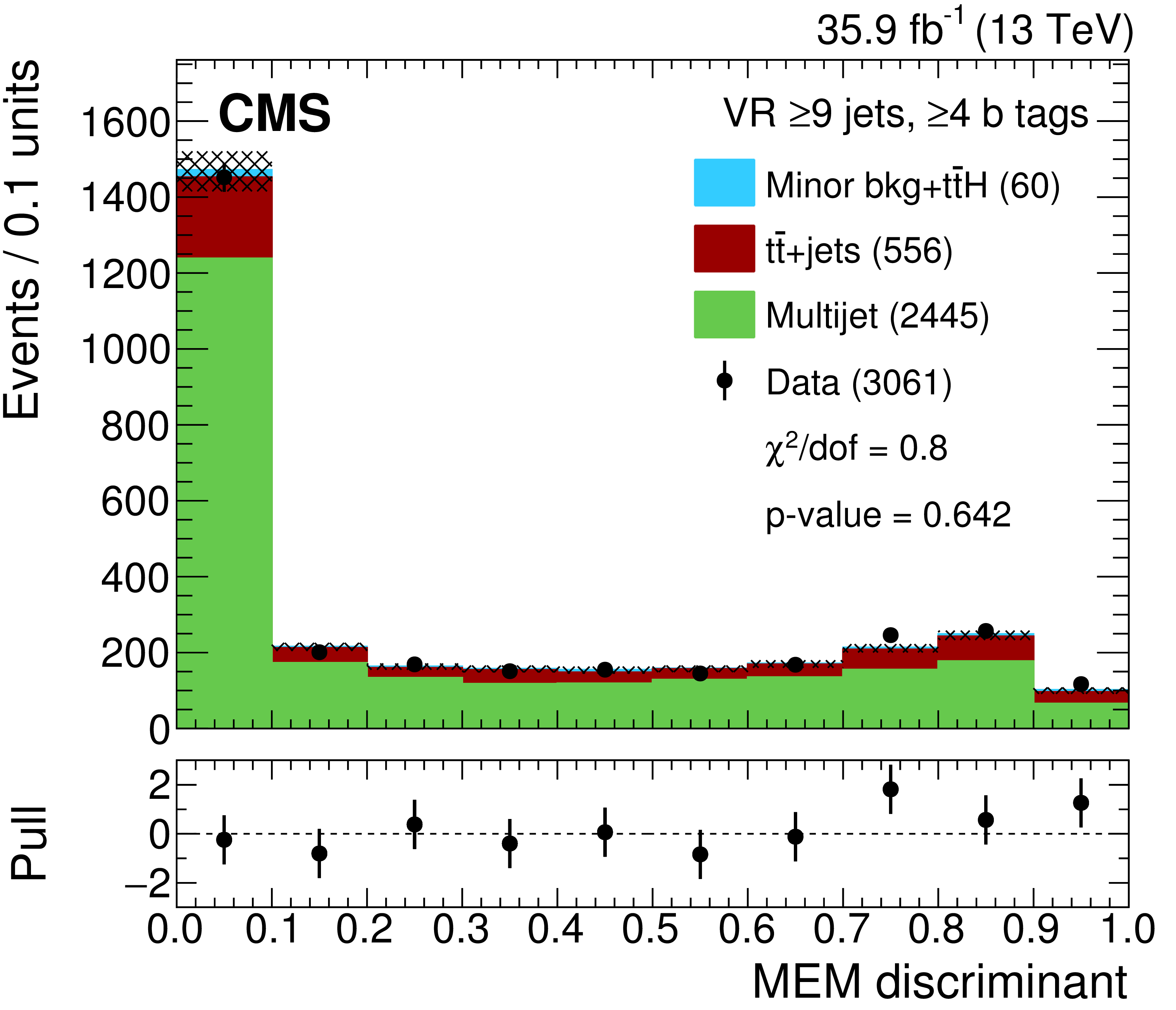
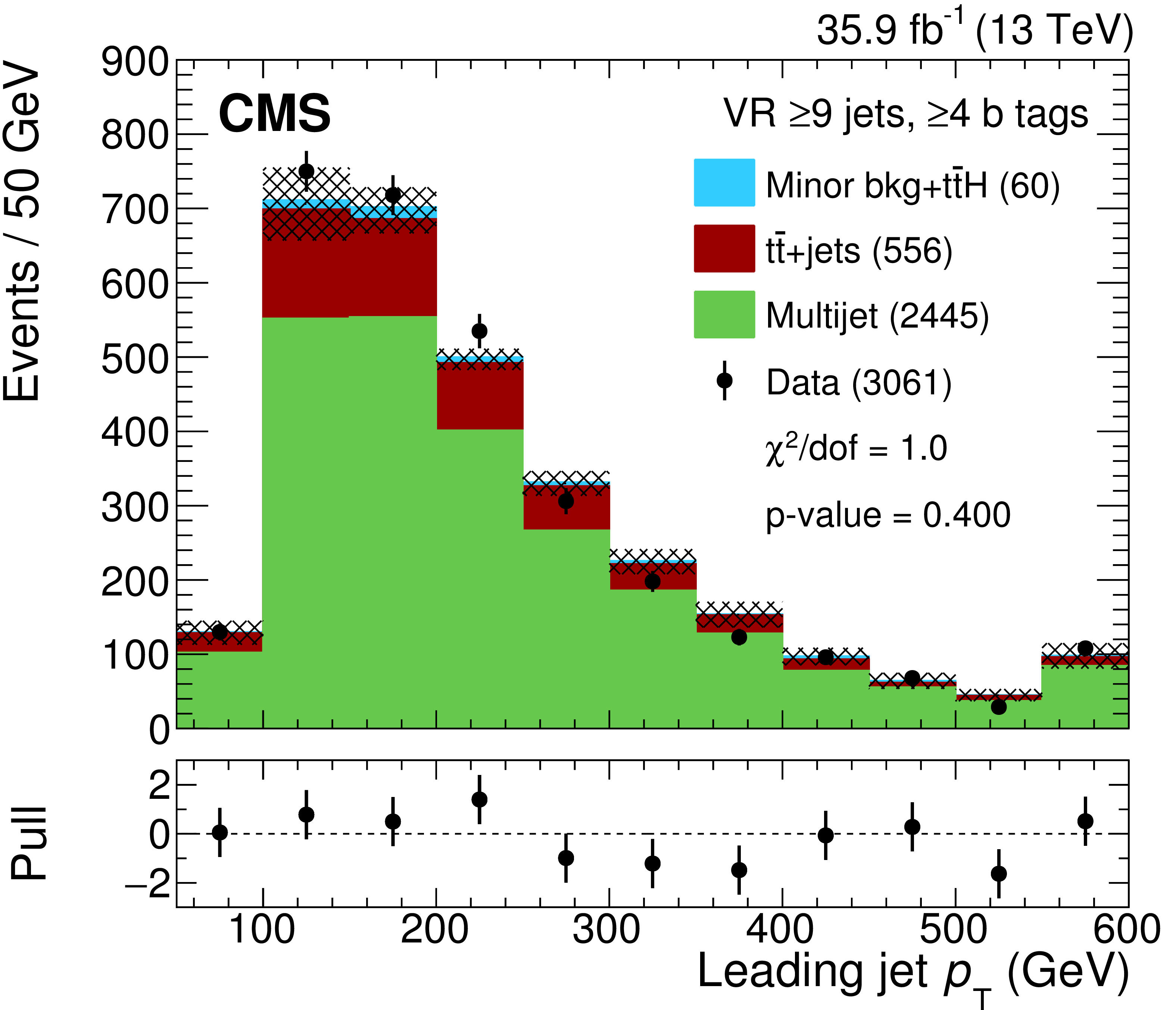
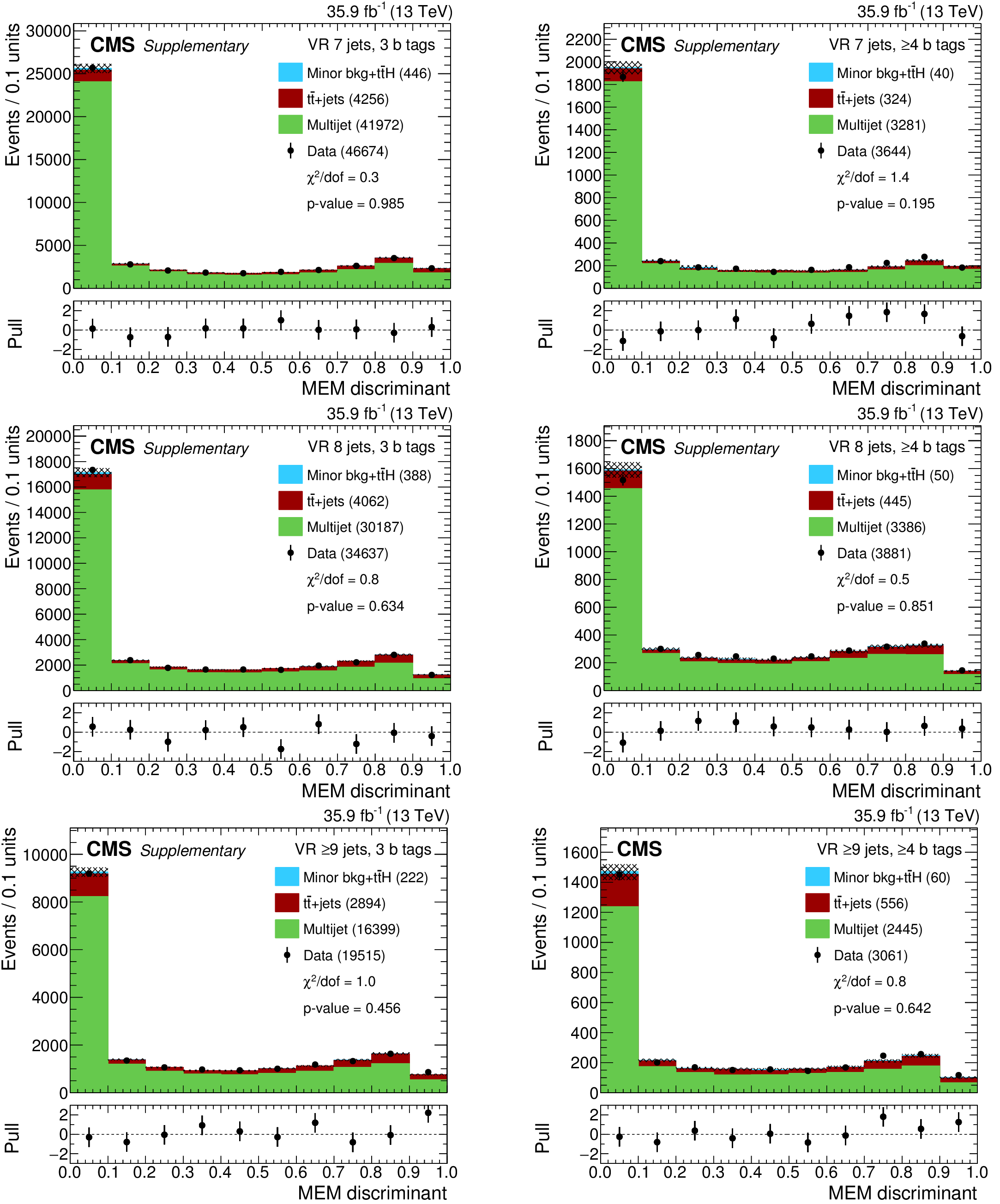
Figure 4:
Distributions in data, in simulated backgrounds, and in the estimated multijet background for the ($\geq $9j, $\geq $4b) VR category. The MEM discriminant (upper left), $ {H_{\mathrm {T}}} $ (upper right), $ {p_{\mathrm {T}}} $ of the leading jet (middle left), minimum $\Delta R$ between b jets (middle right), invariant mass of the closest b jet pair (lower left), and minimum mass of all jet pairs (lower right). The level of agreement between data and estimation is expressed in terms of a $\chi ^2$ divided by the number of degrees of freedom (dof), which are given along with their corresponding statistical $p$-values. The differences between data and the total estimates divided by the quadratic sum of the statistical and systematic uncertainties in the data and in the estimates (pulls) are given below the main panels. The numbers in parenthesis in the legends represent the total yields for the corresponding entries. The last bin includes event overflows. |
png pdf |
Figure 4-a:
Distribution in data, in simulated backgrounds, and in the estimated multijet background for the ($\geq $9j, $\geq $4b) VR category: the MEM discriminant. The level of agreement between data and estimation is expressed in terms of a $\chi ^2$ divided by the number of degrees of freedom (dof), which are given along with their corresponding statistical $p$-values. The differences between data and the total estimates divided by the quadratic sum of the statistical and systematic uncertainties in the data and in the estimates (pulls) are given below the main panel. The numbers in parenthesis in the legend represent the total yields for the corresponding entries. The last bin includes event overflows. |

png pdf |
Figure 4-b:
Distribution in data, in simulated backgrounds, and in the estimated multijet background for the ($\geq $9j, $\geq $4b) VR category: $ {H_{\mathrm {T}}} $. The level of agreement between data and estimation is expressed in terms of a $\chi ^2$ divided by the number of degrees of freedom (dof), which are given along with their corresponding statistical $p$-values. The differences between data and the total estimates divided by the quadratic sum of the statistical and systematic uncertainties in the data and in the estimates (pulls) are given below the main panel. The numbers in parenthesis in the legend represent the total yields for the corresponding entries. The last bin includes event overflows. |
png pdf |
Figure 4-c:
Distribution in data, in simulated backgrounds, and in the estimated multijet background for the ($\geq $9j, $\geq $4b) VR category: $ {p_{\mathrm {T}}} $ of the leading jet. The level of agreement between data and estimation is expressed in terms of a $\chi ^2$ divided by the number of degrees of freedom (dof), which are given along with their corresponding statistical $p$-values. The differences between data and the total estimates divided by the quadratic sum of the statistical and systematic uncertainties in the data and in the estimates (pulls) are given below the main panel. The numbers in parenthesis in the legend represent the total yields for the corresponding entries. The last bin includes event overflows. |

png pdf |
Figure 4-d:
Distribution in data, in simulated backgrounds, and in the estimated multijet background for the ($\geq $9j, $\geq $4b) VR category: minimum $\Delta R$ between b jets. The level of agreement between data and estimation is expressed in terms of a $\chi ^2$ divided by the number of degrees of freedom (dof), which are given along with their corresponding statistical $p$-values. The differences between data and the total estimates divided by the quadratic sum of the statistical and systematic uncertainties in the data and in the estimates (pulls) are given below the main panel. The numbers in parenthesis in the legend represent the total yields for the corresponding entries. The last bin includes event overflows. |

png pdf |
Figure 4-e:
Distribution in data, in simulated backgrounds, and in the estimated multijet background for the ($\geq $9j, $\geq $4b) VR category: invariant mass of the closest b jet pair. The level of agreement between data and estimation is expressed in terms of a $\chi ^2$ divided by the number of degrees of freedom (dof), which are given along with their corresponding statistical $p$-values. The differences between data and the total estimates divided by the quadratic sum of the statistical and systematic uncertainties in the data and in the estimates (pulls) are given below the main panel. The numbers in parenthesis in the legend represent the total yields for the corresponding entries. The last bin includes event overflows. |
png pdf |
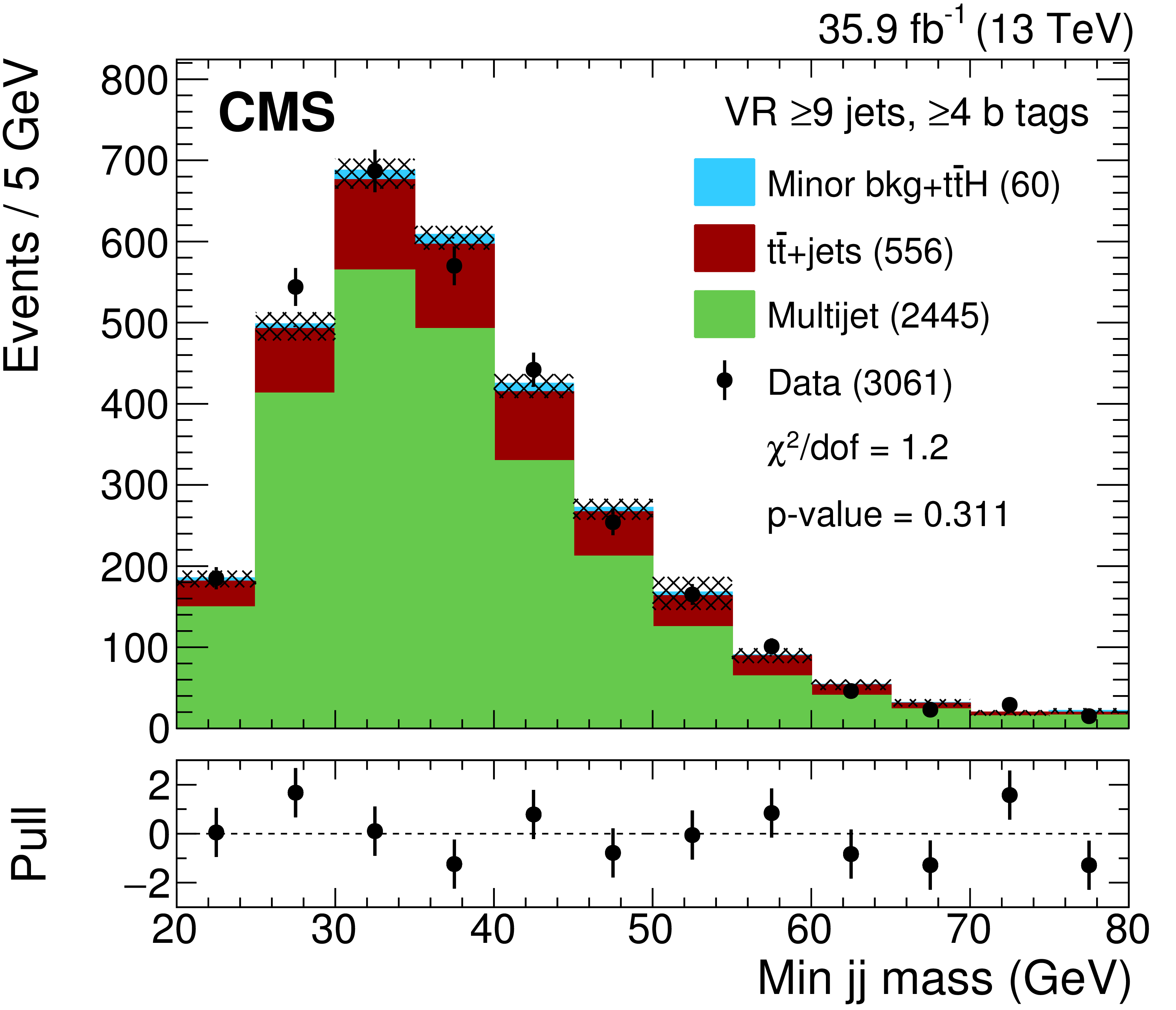
Figure 4-f:
Distribution in data, in simulated backgrounds, and in the estimated multijet background for the ($\geq $9j, $\geq $4b) VR category: minimum mass of all jet pairs. The level of agreement between data and estimation is expressed in terms of a $\chi ^2$ divided by the number of degrees of freedom (dof), which are given along with their corresponding statistical $p$-values. The differences between data and the total estimates divided by the quadratic sum of the statistical and systematic uncertainties in the data and in the estimates (pulls) are given below the main panel. The numbers in parenthesis in the legend represent the total yields for the corresponding entries. The last bin includes event overflows. |

png pdf |
Figure 5:
Examples of LO Feynman diagrams for the partonic processes of $ {\mathrm {g}} {\mathrm {g}}\to {{{\mathrm {t}\overline {\mathrm {t}}}} {\mathrm {H}}} $ and $ {\mathrm {g}} {\mathrm {g}}\to {{{\mathrm {t}\overline {\mathrm {t}}}} \text {+} {{\mathrm {b}} {\overline {\mathrm {b}}}}} $. |

png pdf |
Figure 5-a:
Example of LO Feynman diagram for the partonic processes of $ {\mathrm {g}} {\mathrm {g}}\to {{{\mathrm {t}\overline {\mathrm {t}}}} {\mathrm {H}}} $. |

png pdf |
Figure 5-b:
Example of LO Feynman diagram for the partonic processes of $ {\mathrm {g}} {\mathrm {g}}\to {{{\mathrm {t}\overline {\mathrm {t}}}} \text {+} {{\mathrm {b}} {\overline {\mathrm {b}}}}} $. |

png pdf |
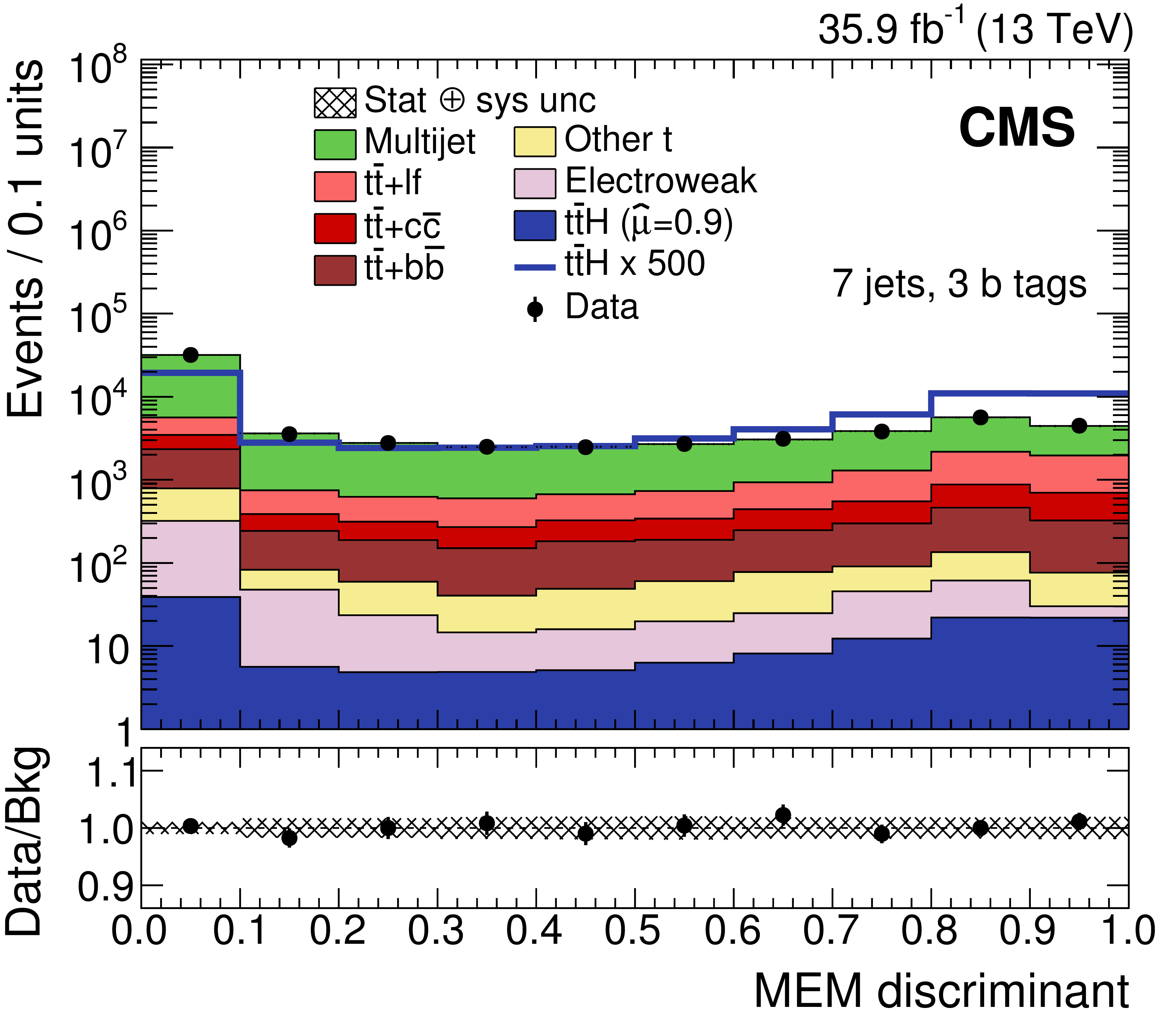
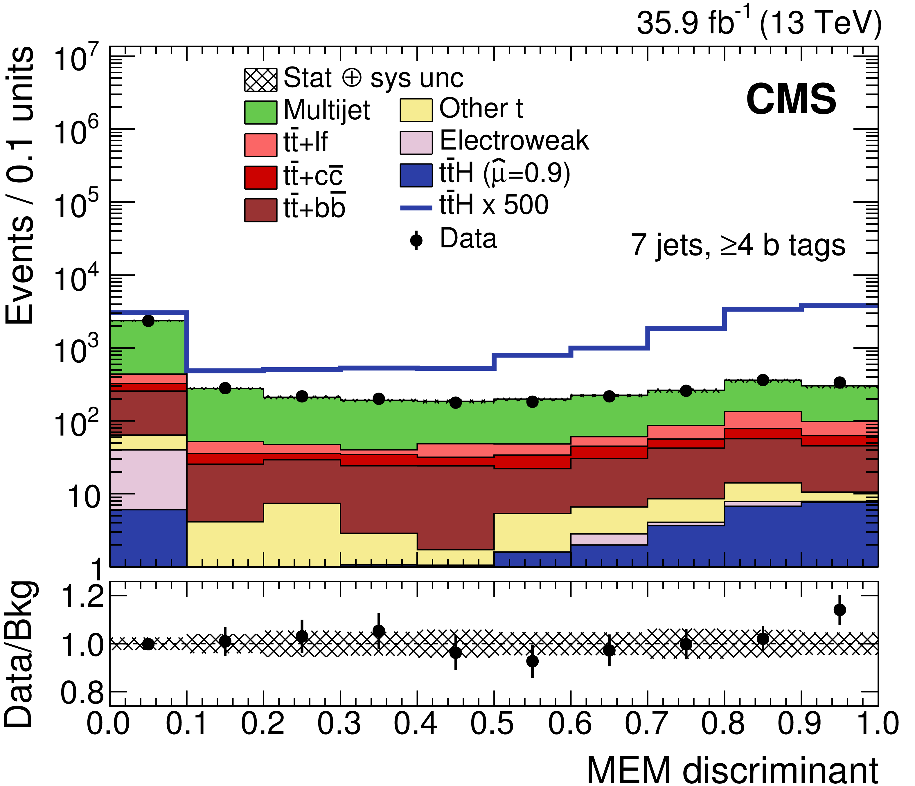
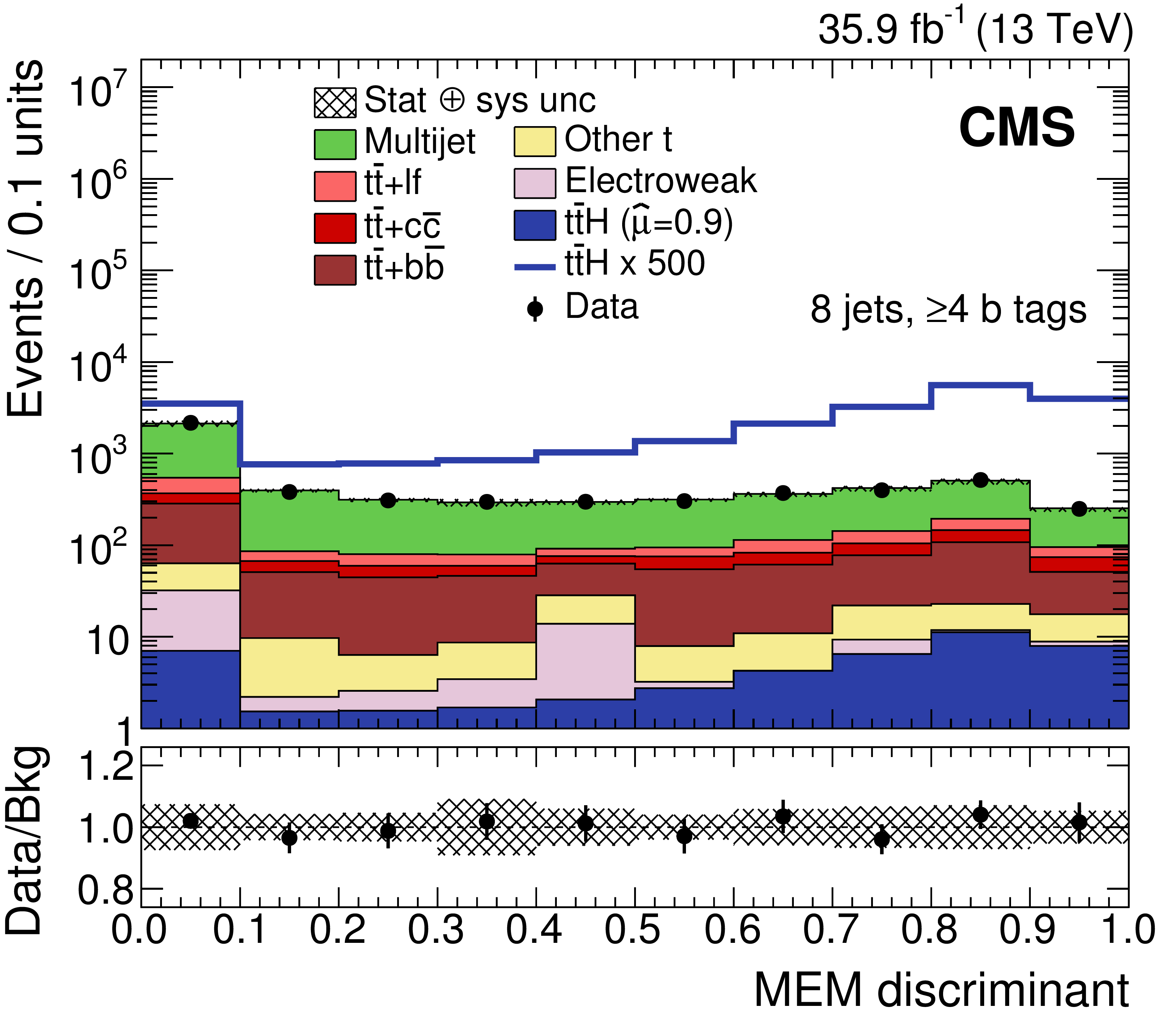
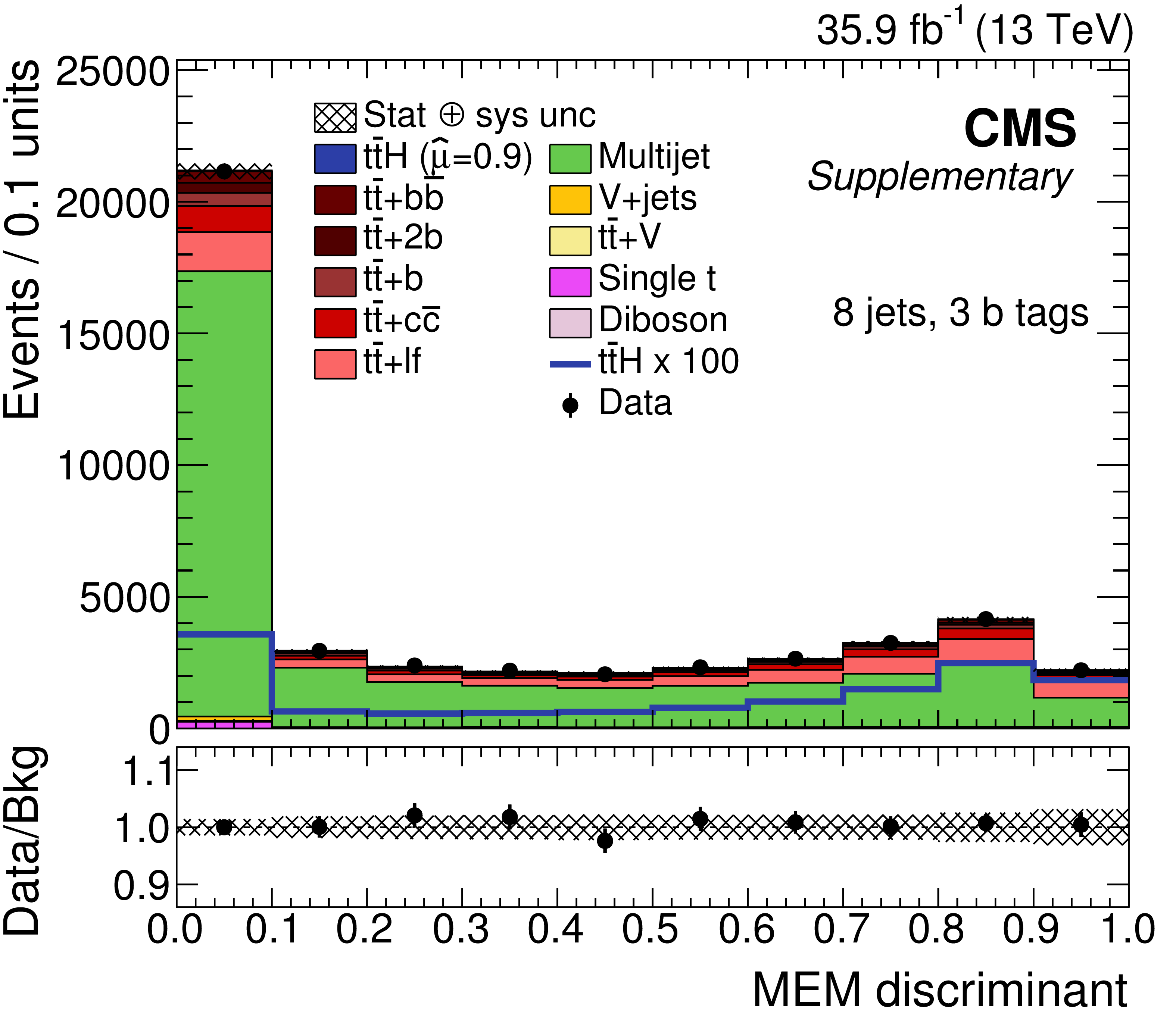
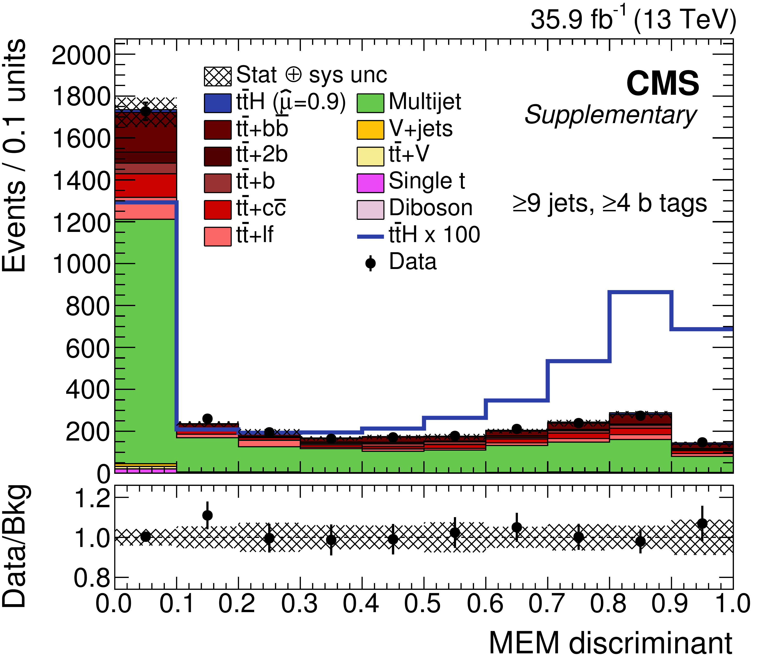
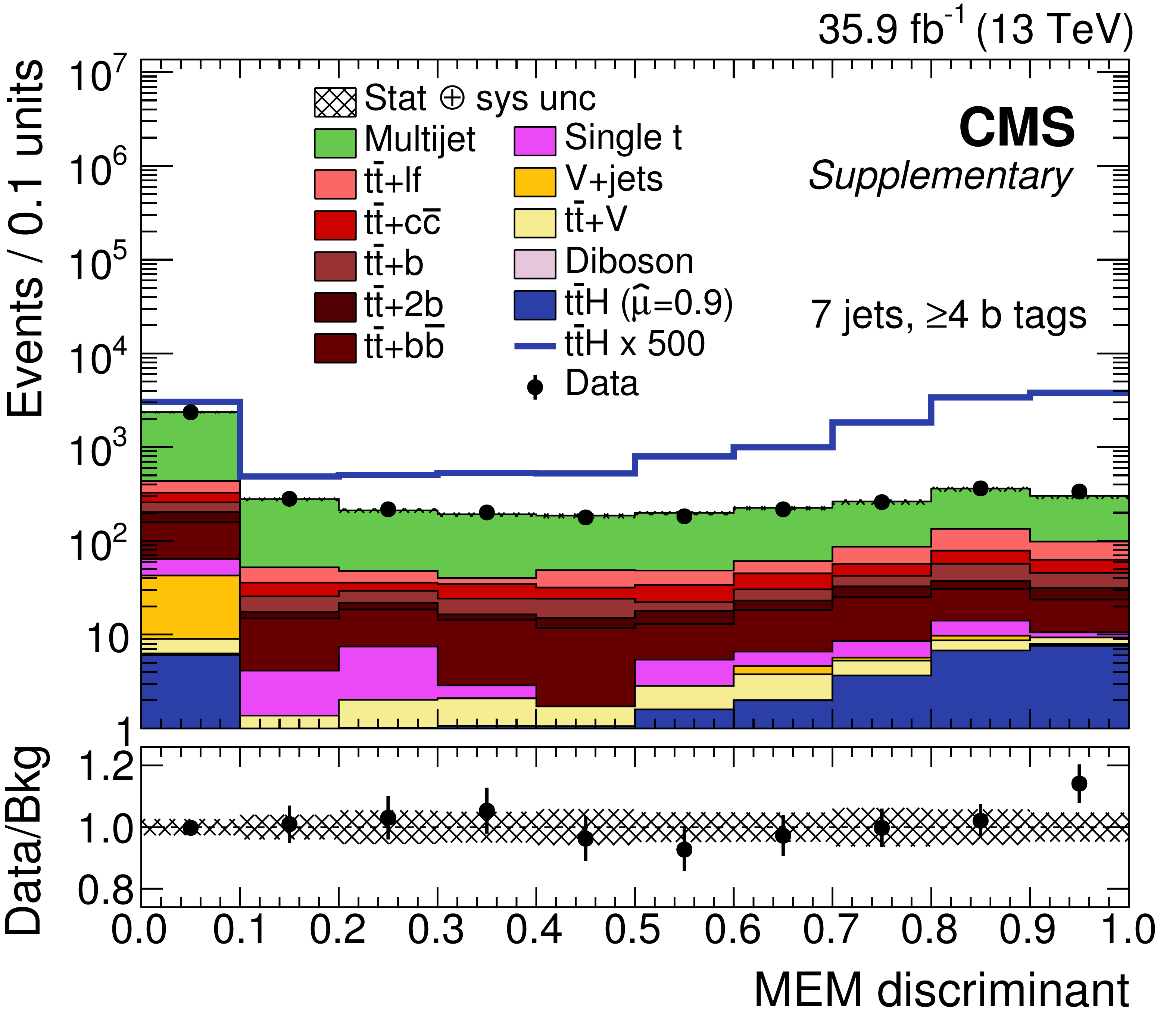
Figure 6:
Distributions in the fitted MEM discriminant for each analysis category. The contributions expected from signal and background processes (filled histograms) are shown stacked. The $ {{{\mathrm {t}\overline {\mathrm {t}}}} \text {+} {\mathrm {b}}} $ and $ {{{\mathrm {t}\overline {\mathrm {t}}}} \text {+} 2 {\mathrm {b}}} $ background process are shown combined with $ {{{\mathrm {t}\overline {\mathrm {t}}}} \text {+} {{\mathrm {b}} {\overline {\mathrm {b}}}}} $, the single t and ${{{\mathrm {t}\overline {\mathrm {t}}}} \text {+V}}$ processes are shown combined as "Other t'', and the V+jets and diboson processes are shown combined as "Electroweak''. The signal distributions (lines) for a Higgs boson mass of $ {m_{{\mathrm {H}}}} = $ 125 GeV are multiplied by a factor of 500 and superimposed on the data. The distributions in data are indicated by the black points. The ratios of data to background appear below the main panels. |
png pdf |
Figure 6-a:
Distribution in the fitted MEM discriminant for one analysis category. The contributions expected from signal and background processes (filled histograms) are shown stacked. The $ {{{\mathrm {t}\overline {\mathrm {t}}}} \text {+} {\mathrm {b}}} $ and $ {{{\mathrm {t}\overline {\mathrm {t}}}} \text {+} 2 {\mathrm {b}}} $ background process are shown combined with $ {{{\mathrm {t}\overline {\mathrm {t}}}} \text {+} {{\mathrm {b}} {\overline {\mathrm {b}}}}} $, the single t and ${{{\mathrm {t}\overline {\mathrm {t}}}} \text {+V}}$ processes are shown combined as "Other t'', and the V+jets and diboson processes are shown combined as "Electroweak''. The signal distributions (lines) for a Higgs boson mass of $ {m_{{\mathrm {H}}}} = $ 125 GeV are multiplied by a factor of 500 and superimposed on the data. The distribution in data is indicated by the black points. The ratios of data to background appear below the main panel. |
png pdf |
Figure 6-b:
Distribution in the fitted MEM discriminant for one analysis category. The contributions expected from signal and background processes (filled histograms) are shown stacked. The $ {{{\mathrm {t}\overline {\mathrm {t}}}} \text {+} {\mathrm {b}}} $ and $ {{{\mathrm {t}\overline {\mathrm {t}}}} \text {+} 2 {\mathrm {b}}} $ background process are shown combined with $ {{{\mathrm {t}\overline {\mathrm {t}}}} \text {+} {{\mathrm {b}} {\overline {\mathrm {b}}}}} $, the single t and ${{{\mathrm {t}\overline {\mathrm {t}}}} \text {+V}}$ processes are shown combined as "Other t'', and the V+jets and diboson processes are shown combined as "Electroweak''. The signal distributions (lines) for a Higgs boson mass of $ {m_{{\mathrm {H}}}} = $ 125 GeV are multiplied by a factor of 500 and superimposed on the data. The distribution in data is indicated by the black points. The ratios of data to background appear below the main panel. |

png pdf |
Figure 6-c:
Distribution in the fitted MEM discriminant for one analysis category. The contributions expected from signal and background processes (filled histograms) are shown stacked. The $ {{{\mathrm {t}\overline {\mathrm {t}}}} \text {+} {\mathrm {b}}} $ and $ {{{\mathrm {t}\overline {\mathrm {t}}}} \text {+} 2 {\mathrm {b}}} $ background process are shown combined with $ {{{\mathrm {t}\overline {\mathrm {t}}}} \text {+} {{\mathrm {b}} {\overline {\mathrm {b}}}}} $, the single t and ${{{\mathrm {t}\overline {\mathrm {t}}}} \text {+V}}$ processes are shown combined as "Other t'', and the V+jets and diboson processes are shown combined as "Electroweak''. The signal distributions (lines) for a Higgs boson mass of $ {m_{{\mathrm {H}}}} = $ 125 GeV are multiplied by a factor of 500 and superimposed on the data. The distribution in data is indicated by the black points. The ratios of data to background appear below the main panel. |
png pdf |
Figure 6-d:
Distribution in the fitted MEM discriminant for one analysis category. The contributions expected from signal and background processes (filled histograms) are shown stacked. The $ {{{\mathrm {t}\overline {\mathrm {t}}}} \text {+} {\mathrm {b}}} $ and $ {{{\mathrm {t}\overline {\mathrm {t}}}} \text {+} 2 {\mathrm {b}}} $ background process are shown combined with $ {{{\mathrm {t}\overline {\mathrm {t}}}} \text {+} {{\mathrm {b}} {\overline {\mathrm {b}}}}} $, the single t and ${{{\mathrm {t}\overline {\mathrm {t}}}} \text {+V}}$ processes are shown combined as "Other t'', and the V+jets and diboson processes are shown combined as "Electroweak''. The signal distributions (lines) for a Higgs boson mass of $ {m_{{\mathrm {H}}}} = $ 125 GeV are multiplied by a factor of 500 and superimposed on the data. The distribution in data is indicated by the black points. The ratios of data to background appear below the main panel. |

png pdf |
Figure 6-e:
Distribution in the fitted MEM discriminant for one analysis category. The contributions expected from signal and background processes (filled histograms) are shown stacked. The $ {{{\mathrm {t}\overline {\mathrm {t}}}} \text {+} {\mathrm {b}}} $ and $ {{{\mathrm {t}\overline {\mathrm {t}}}} \text {+} 2 {\mathrm {b}}} $ background process are shown combined with $ {{{\mathrm {t}\overline {\mathrm {t}}}} \text {+} {{\mathrm {b}} {\overline {\mathrm {b}}}}} $, the single t and ${{{\mathrm {t}\overline {\mathrm {t}}}} \text {+V}}$ processes are shown combined as "Other t'', and the V+jets and diboson processes are shown combined as "Electroweak''. The signal distributions (lines) for a Higgs boson mass of $ {m_{{\mathrm {H}}}} = $ 125 GeV are multiplied by a factor of 500 and superimposed on the data. The distribution in data is indicated by the black points. The ratios of data to background appear below the main panel. |

png pdf |
Figure 6-f:
Distribution in the fitted MEM discriminant for one analysis category. The contributions expected from signal and background processes (filled histograms) are shown stacked. The $ {{{\mathrm {t}\overline {\mathrm {t}}}} \text {+} {\mathrm {b}}} $ and $ {{{\mathrm {t}\overline {\mathrm {t}}}} \text {+} 2 {\mathrm {b}}} $ background process are shown combined with $ {{{\mathrm {t}\overline {\mathrm {t}}}} \text {+} {{\mathrm {b}} {\overline {\mathrm {b}}}}} $, the single t and ${{{\mathrm {t}\overline {\mathrm {t}}}} \text {+V}}$ processes are shown combined as "Other t'', and the V+jets and diboson processes are shown combined as "Electroweak''. The signal distributions (lines) for a Higgs boson mass of $ {m_{{\mathrm {H}}}} = $ 125 GeV are multiplied by a factor of 500 and superimposed on the data. The distribution in data is indicated by the black points. The ratios of data to background appear below the main panel. |
png pdf |
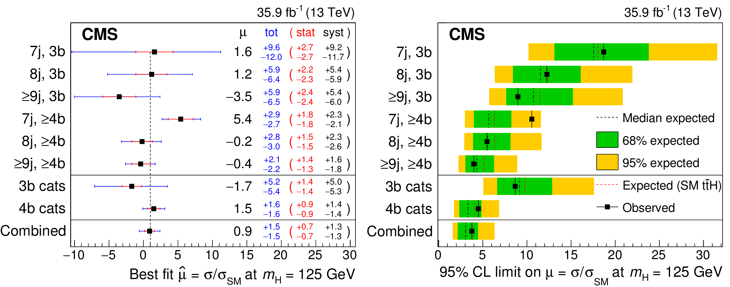
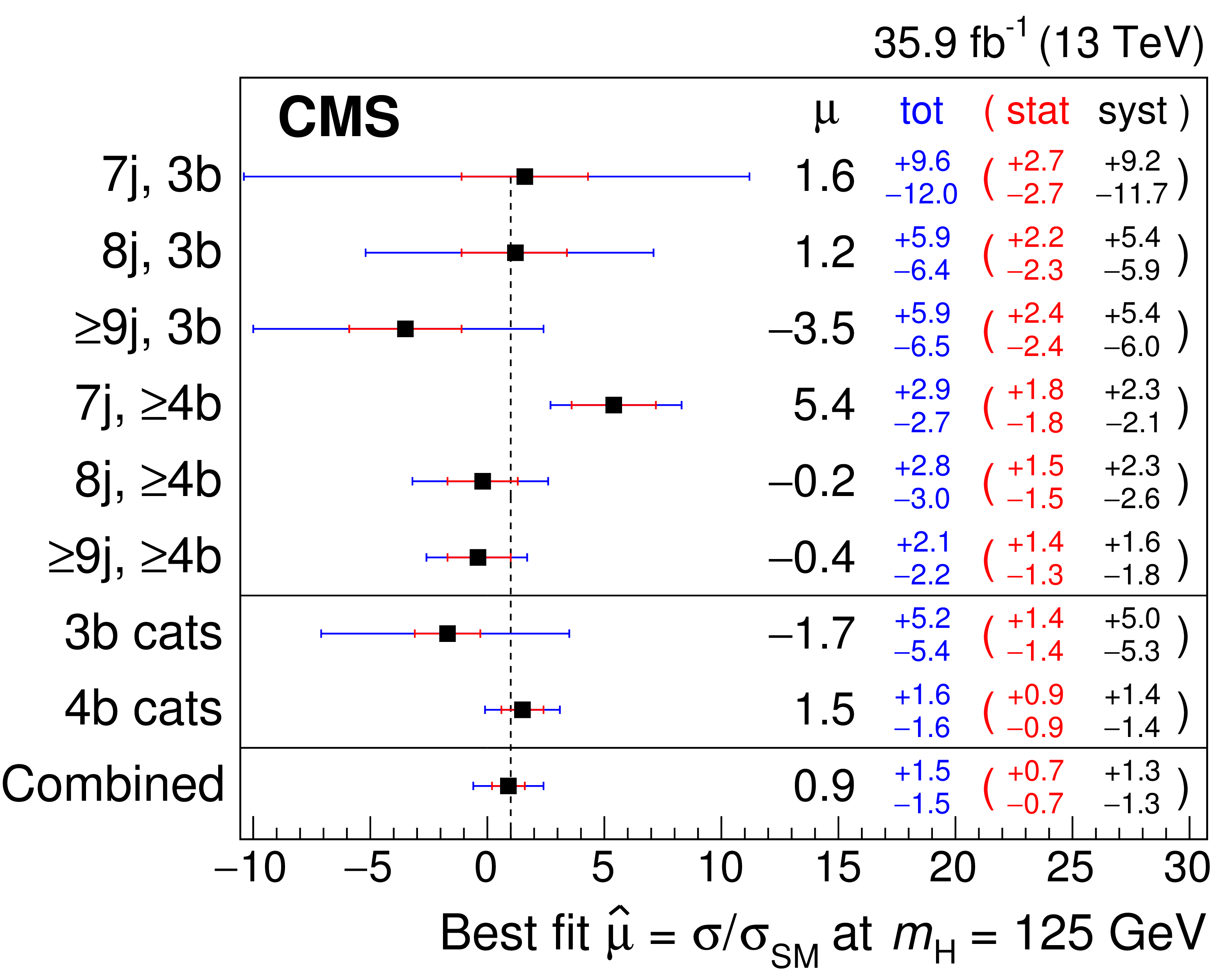
Figure 7:
Best fit values in the signal strength modifiers $ {\hat{\mu}} $, and their 68% CL intervals as split into the statistical and systematic components (left), and median expected and observed 95% CL upper limits on $\mu $ (right). The expected limits are displayed with their 68% and 95% CL intervals, as well as with the expectation for an injected SM signal of $\mu = $ 1. |
png pdf |
Figure 7-a:
Best fit values in the signal strength modifiers $ {\hat{\mu}} $, and their 68% CL intervals as split into the statistical and systematic components. |

png pdf |
Figure 7-b:
Median expected and observed 95% CL upper limits on $\mu $. The expected limits are displayed with their 68% and 95% CL intervals, as well as with the expectation for an injected SM signal of $\mu = $ 1. |

png pdf |
Figure 8:
Distribution in $\log_{10}(\text {S}/\text {B})$, where S and B indicate the respective bin-by-bin yields of the signal and background expected in the MEM discriminant distributions, obtained from a combined fit with the constraint in the cross section of $\mu =$ 1. |
| Tables | |

png pdf |
Table 1:
Definition and description of the four orthogonal regions in the analysis. |
png pdf |
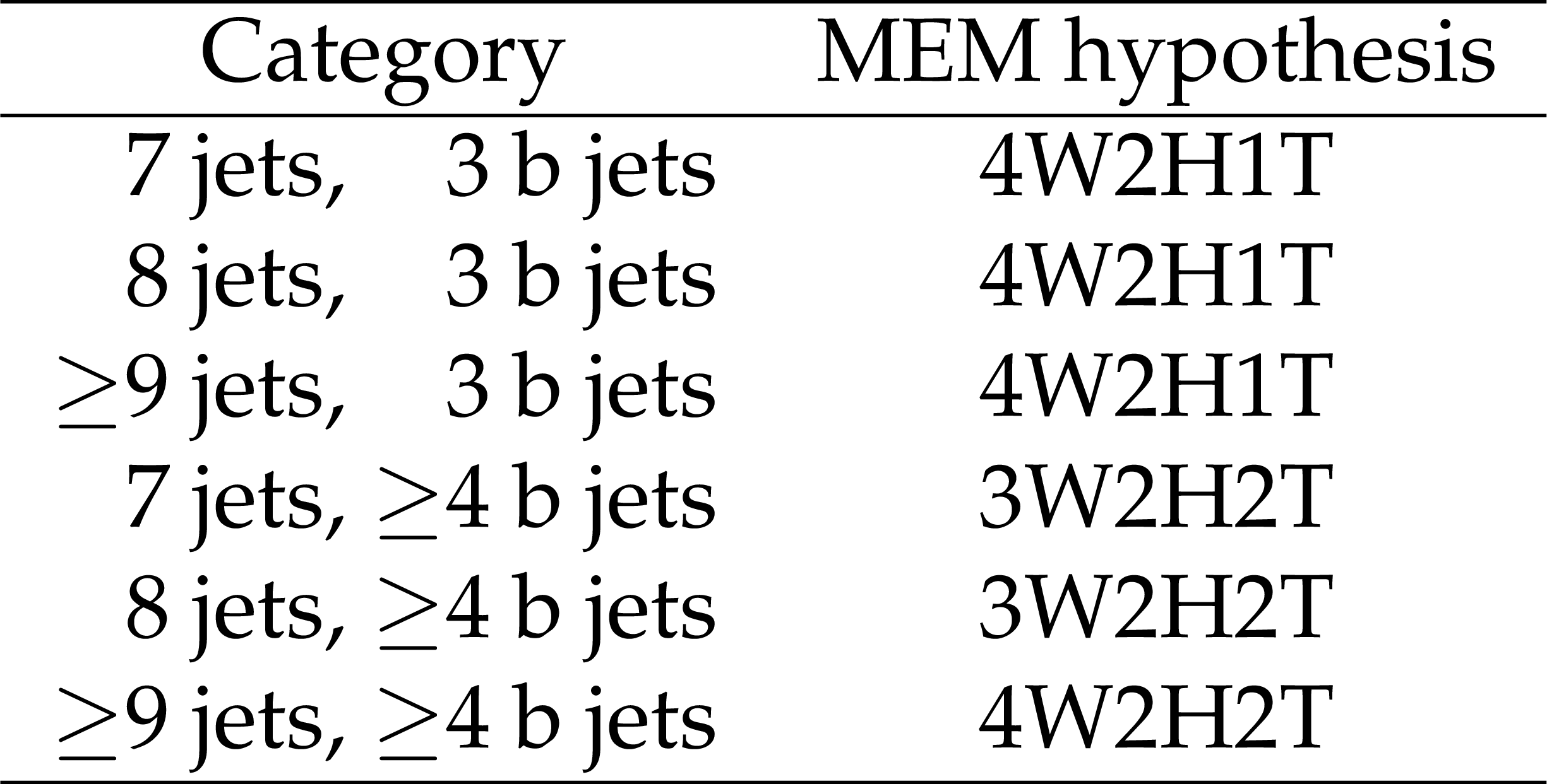
Table 2:
Selected MEM hypotheses for each event topology. The 4W2H1T hypothesis assumes 1 b quark from a top quark is lost, 3W2H2T assumes that 1 quark from a W boson is lost, and 4W2H2T represents the fully reconstructed hypothesis requiring at least 8 jets. |
png pdf |
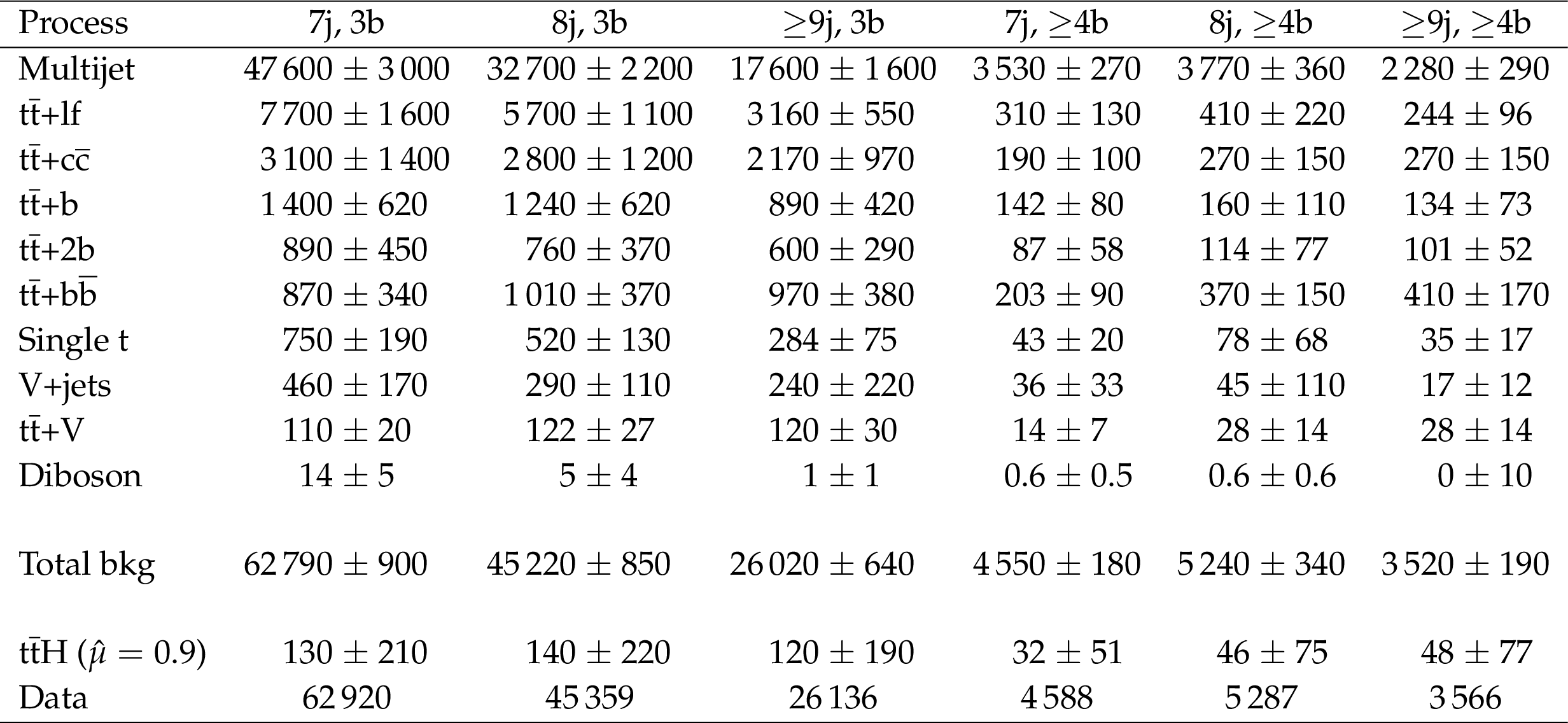
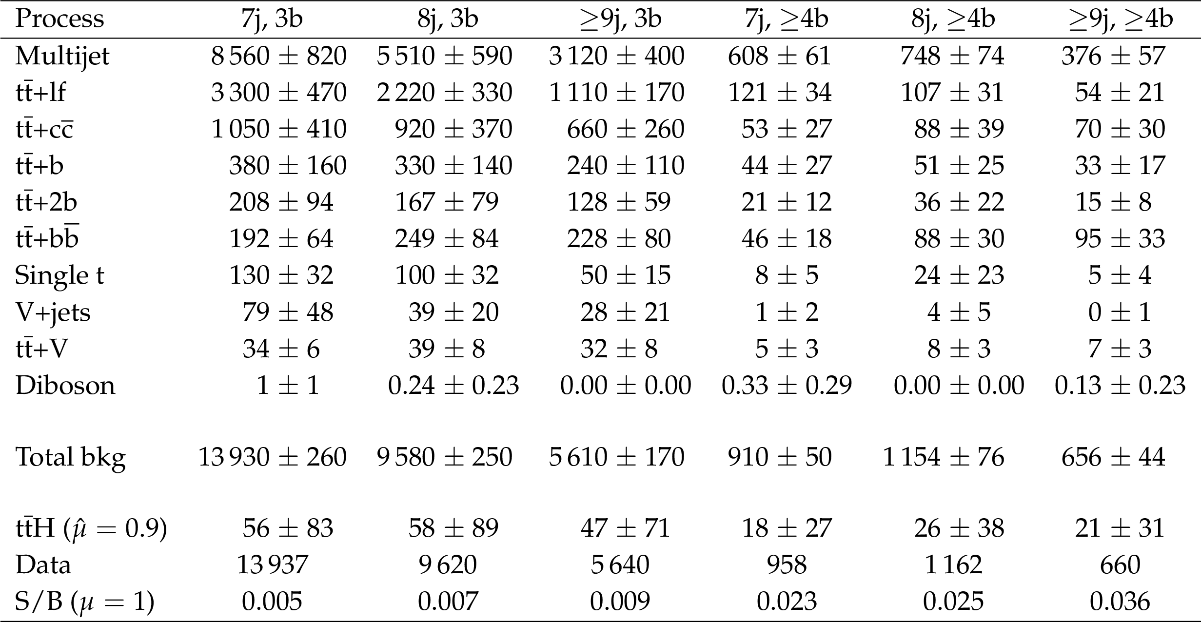
Table 3:
Expected numbers of $ {{{\mathrm {t}\overline {\mathrm {t}}}} {\mathrm {H}}} $ signal and background events, and the observed event yields for the six analysis categories, following the fit to data. The signal contributions are given at the best fit value. The quoted uncertainties contain all the contributions described in Section 7 added in quadrature, considering all correlations among the processes. |
png pdf |
Table 4:
Expected numbers of $ {{{\mathrm {t}\overline {\mathrm {t}}}} {\mathrm {H}}} $ signal and background events in the last three bins of the MEM discriminant for the six analysis categories, following the fit to data. The signal contributions are given at the best fit value. The quoted uncertainties contain all the contributions described in Section 7 added in quadrature, considering all correlations among the processes. Also given are the signal (S) to total background (B) ratios for the SM $ {{{\mathrm {t}\overline {\mathrm {t}}}} {\mathrm {H}}} $ expectation ($\mu = $ 1). |

png pdf |
Table 5:
Summary of the systematic uncertainties affecting the signal and background expectations. The second column indicates the range in yield of the affected processes, caused by changing the nuisance parameters by their uncertainties. The third column indicates whether the uncertainties impact the distribution in the MEM discriminant. A check mark indicates that the uncertainty applies to the stated processes. An asterisk (*) indicates that the uncertainty affects the multijet distribution indirectly, because of the subtraction of directly affected backgrounds in the CR in data. |

png pdf |
Table 6:
Best fit value of the signal-strength modifier $ {\hat{\mu}} $ and the median expected and observed 95% CL upper limits (UL) on $\mu $ in each of the six analysis categories, as well as the combined results. The best fit values are shown with their total uncertainties and the breakdown into the statistical and systematic components. The expected limits are given together with their 68% CL intervals. |
| Summary |
|
A search for the associated production of a Higgs boson with a top quark pair is performed using proton-proton collision data collected by the CMS experiment at a centre-of-mass energy of 13 TeV, corresponding to an integrated luminosity of 35.9 fb$^{-1}$. Events are selected to be compatible with the $ {\mathrm{H} \to \mathrm{b\bar{b}}} $ decay and the all-jet final state of the $ \mathrm{t\bar{t}} $ pair, and are divided into six categories according to their reconstructed jet and b jet multiplicities. The result of the search is presented in terms of the signal strength modifier $\mu$ for $ {\mathrm{t\bar{t}} \mathrm{H}} $ production, defined as the ratio of the measured $ {\mathrm{t\bar{t}} \mathrm{H}} $ production cross section to the one expected for a standard model Higgs boson with a mass of 125 GeV. From a combined fit of signal and background templates to the data in all event categories, observed and expected upper limits of $\mu < $ 3.8 and $ < $ 3.1, respectively, are obtained at 95% confidence levels. These limits correspond to a best fit value of ${\hat{\mu}} = $ 0.9 $\pm$ 0.7 (stat) $\pm$ 1.3 (syst) = 0.9 $\pm$ 1.5 (tot), which is compatible with the standard model expectation. |
| Additional Figures | |
png pdf |
Additional Figure 1:
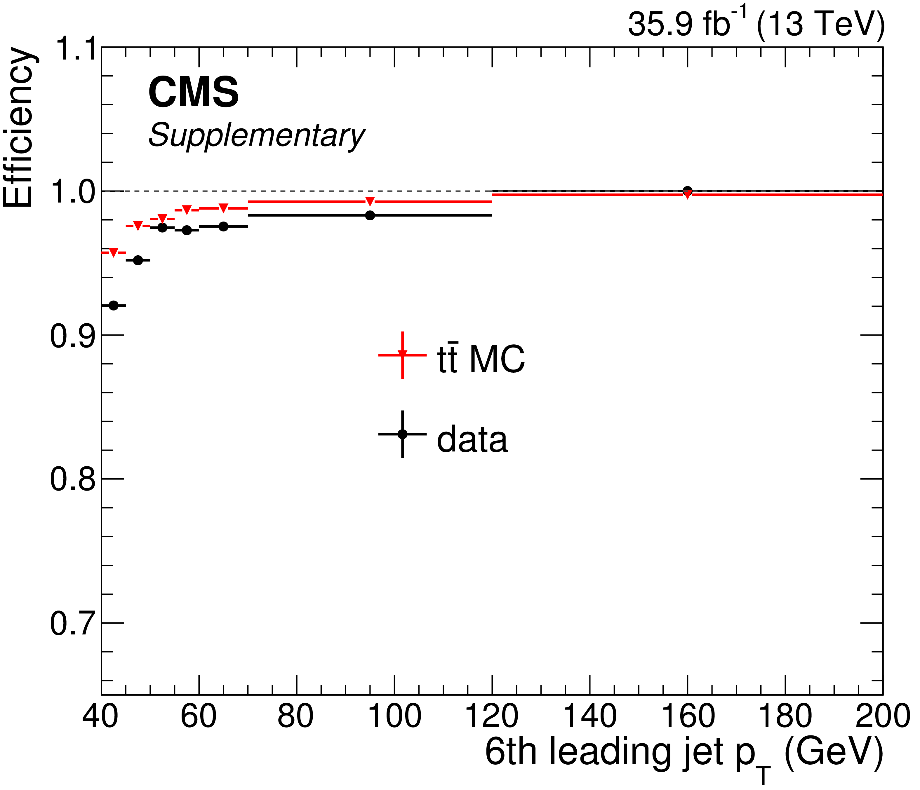
Trigger efficiencies of the OR of the dedicated triggers described in Section 4 as a function of the 6th jet ${p_{\mathrm {T}}}$. Events are selected using single-muon triggers, and shown after the preselection described in Section 4. |

png pdf |
Additional Figure 2:
Trigger efficiencies of the OR of the dedicated triggers described in Section 4 as a function of the $ {H_{\mathrm {T}}} $. Events are selected using single-muon triggers, and shown after the preselection described in Section 4. |
png pdf |
Additional Figure 3:
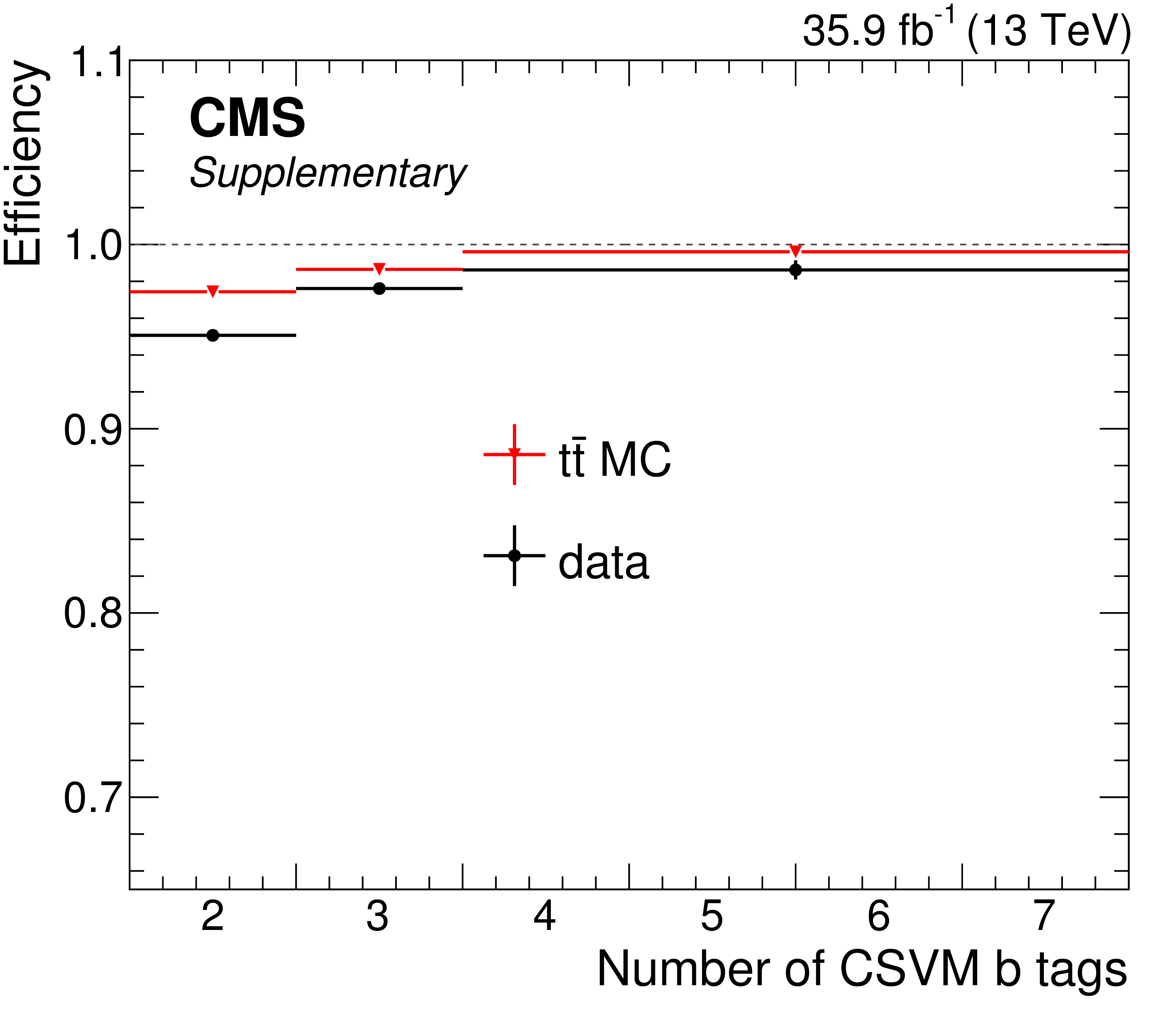
Trigger efficiencies of the OR of the dedicated triggers described in Section 4 as a function of the number of CSVM jets (right). Events are selected using single-muon triggers, and shown after the preselection described in Section 4. |
png pdf |
Additional Figure 4:
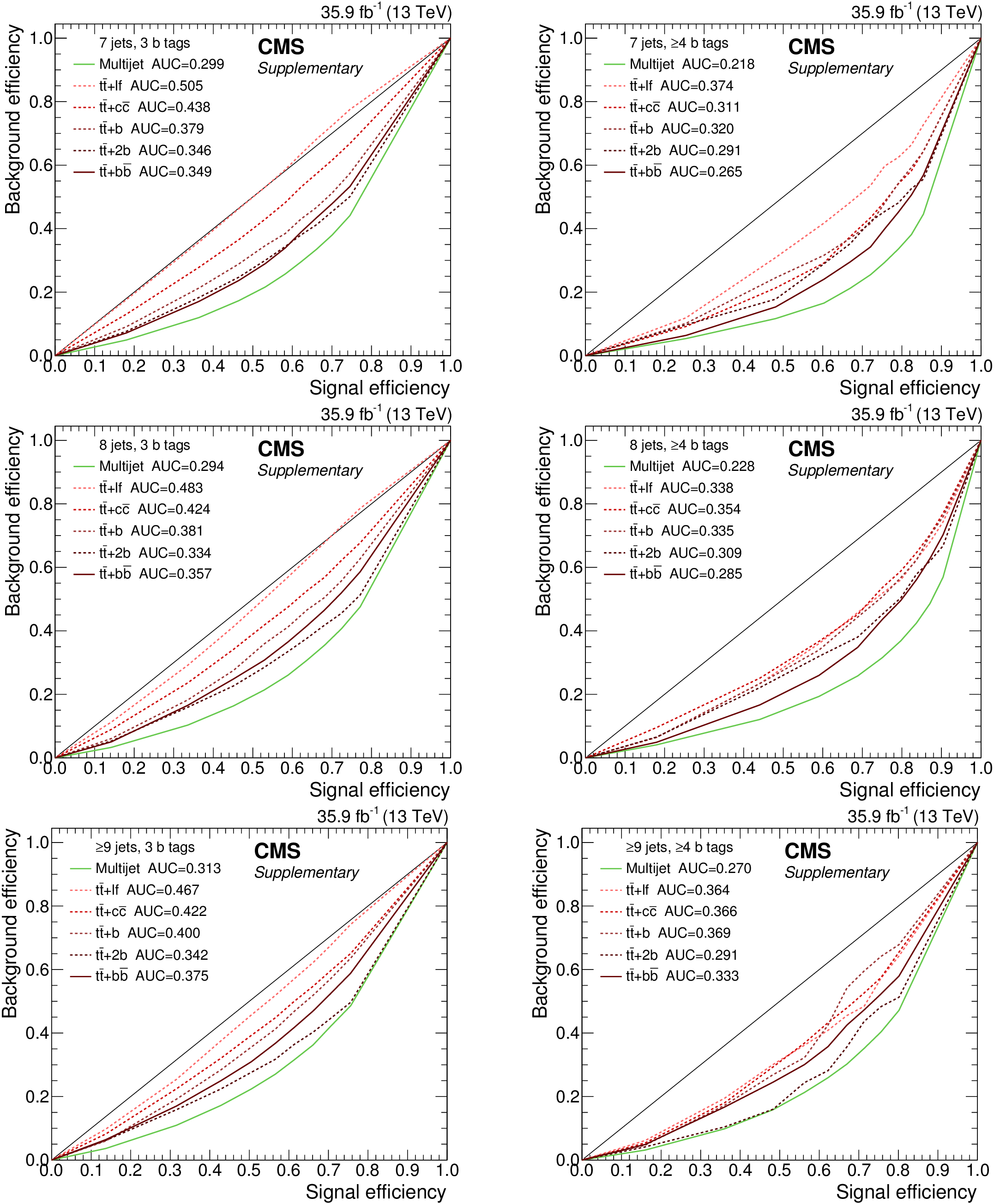
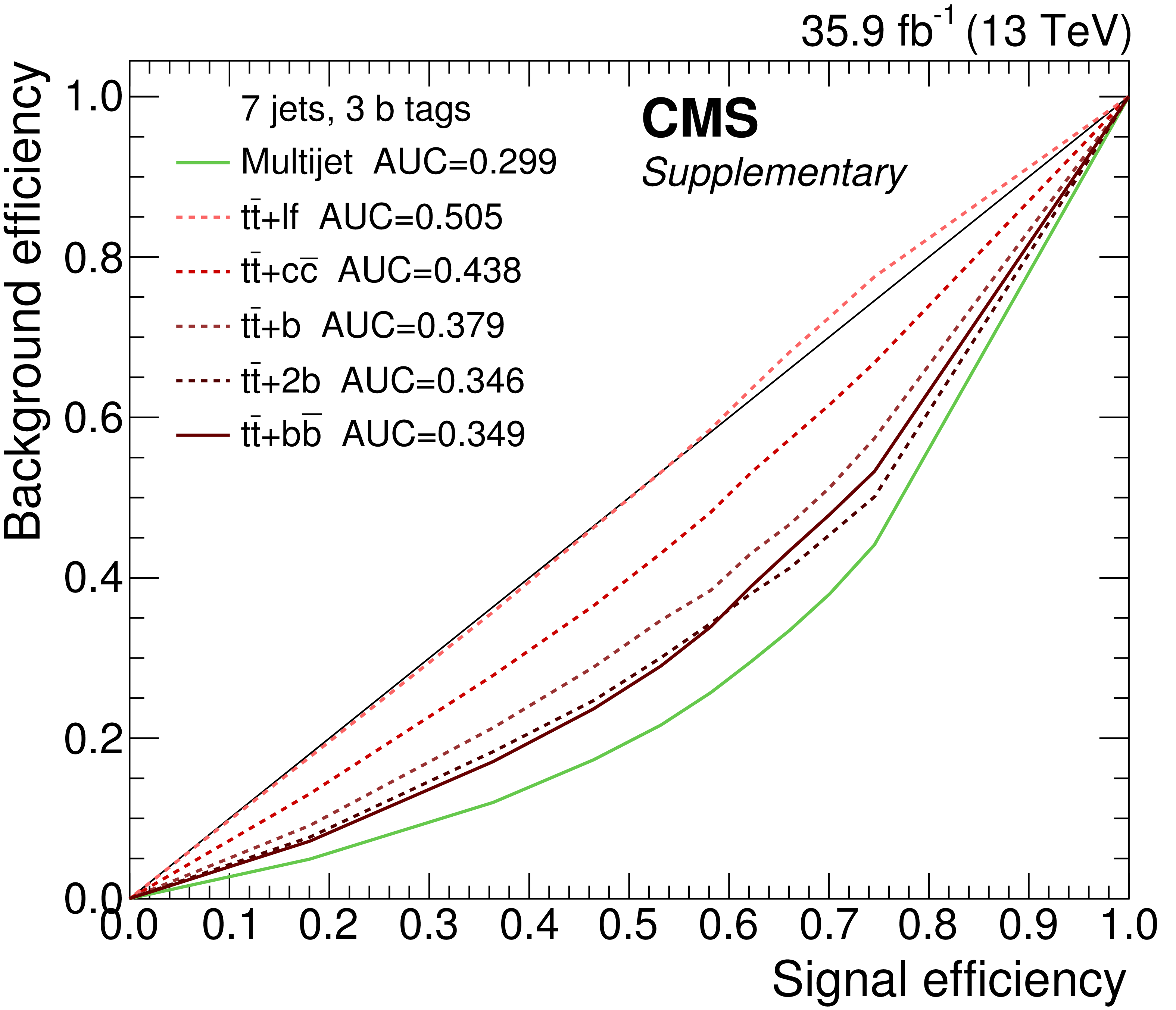
Performance of the MEM discriminator in terms of signal $ {\text {t}\overline {\text {t}}\text {H}} (\text {bb})$ vs. background (${\text {t}\overline {\text {t}}\text {+jets}}$ and multijet) efficiencies. The final discriminator hypothesis is shown in each category, as reported in Table 2. The area under the curve (labelled AUC) for each background process is shown in the legend. |
png pdf |
Additional Figure 4-a:
Performance of the MEM discriminator in terms of signal $ {\text {t}\overline {\text {t}}\text {H}} (\text {bb})$ vs. background (${\text {t}\overline {\text {t}}\text {+jets}}$ and multijet) efficiencies. The final discriminator hypothesis is shown in each category, as reported in Table 2. The area under the curve (labelled AUC) for each background process is shown in the legend. |
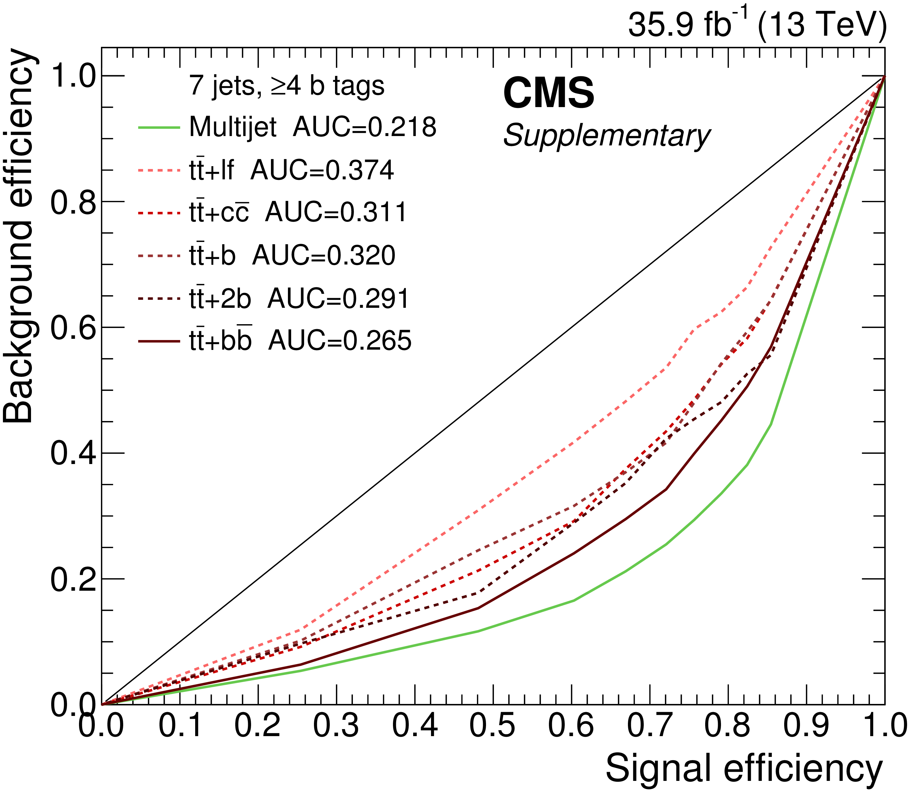
png pdf |
Additional Figure 4-b:
Performance of the MEM discriminator in terms of signal $ {\text {t}\overline {\text {t}}\text {H}} (\text {bb})$ vs. background (${\text {t}\overline {\text {t}}\text {+jets}}$ and multijet) efficiencies. The final discriminator hypothesis is shown in each category, as reported in Table 2. The area under the curve (labelled AUC) for each background process is shown in the legend. |
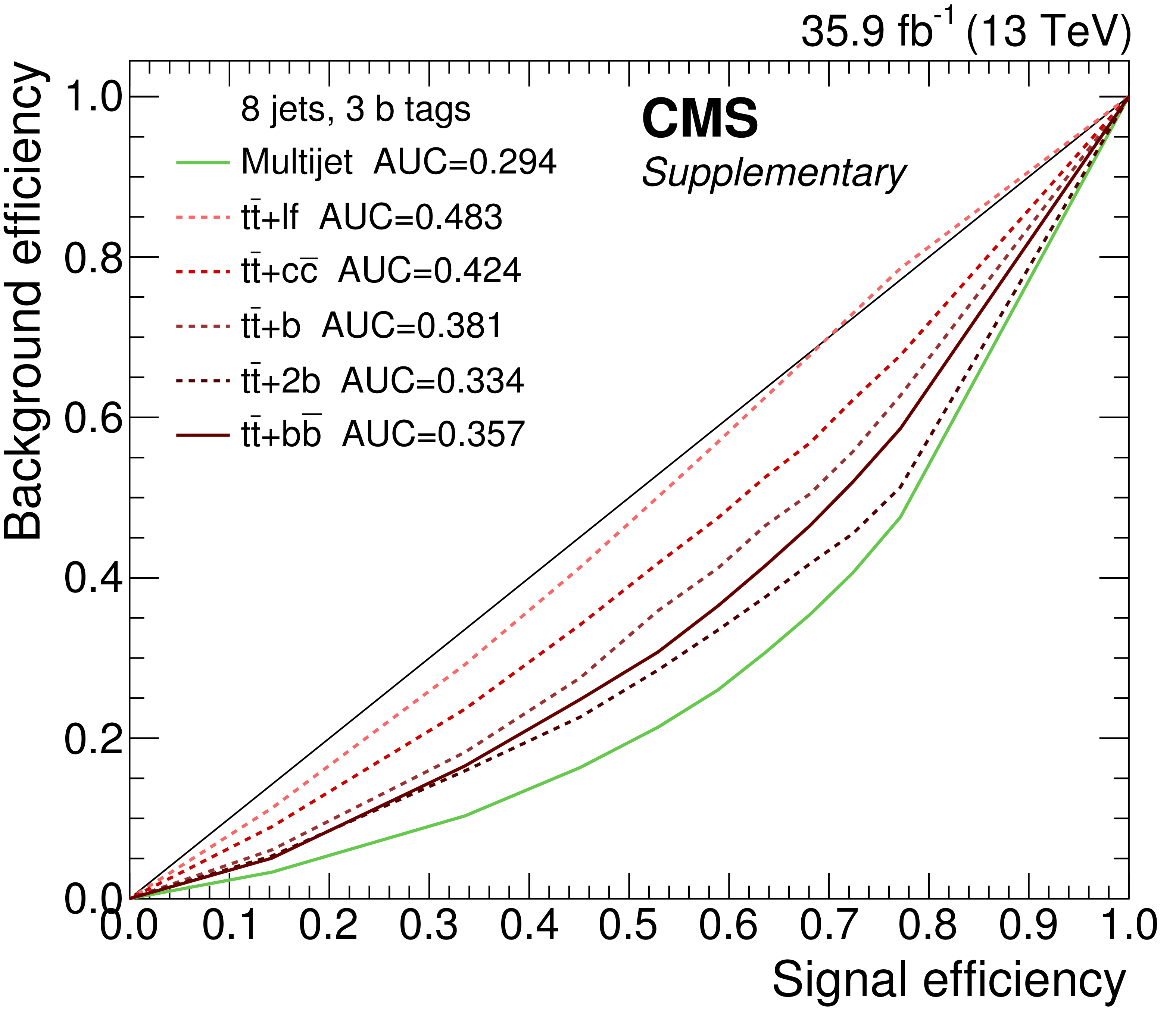
png pdf |
Additional Figure 4-c:
Performance of the MEM discriminator in terms of signal $ {\text {t}\overline {\text {t}}\text {H}} (\text {bb})$ vs. background (${\text {t}\overline {\text {t}}\text {+jets}}$ and multijet) efficiencies. The final discriminator hypothesis is shown in each category, as reported in Table 2. The area under the curve (labelled AUC) for each background process is shown in the legend. |

png pdf |
Additional Figure 4-d:
Performance of the MEM discriminator in terms of signal $ {\text {t}\overline {\text {t}}\text {H}} (\text {bb})$ vs. background (${\text {t}\overline {\text {t}}\text {+jets}}$ and multijet) efficiencies. The final discriminator hypothesis is shown in each category, as reported in Table 2. The area under the curve (labelled AUC) for each background process is shown in the legend. |

png pdf |
Additional Figure 4-e:
Performance of the MEM discriminator in terms of signal $ {\text {t}\overline {\text {t}}\text {H}} (\text {bb})$ vs. background (${\text {t}\overline {\text {t}}\text {+jets}}$ and multijet) efficiencies. The final discriminator hypothesis is shown in each category, as reported in Table 2. The area under the curve (labelled AUC) for each background process is shown in the legend. |
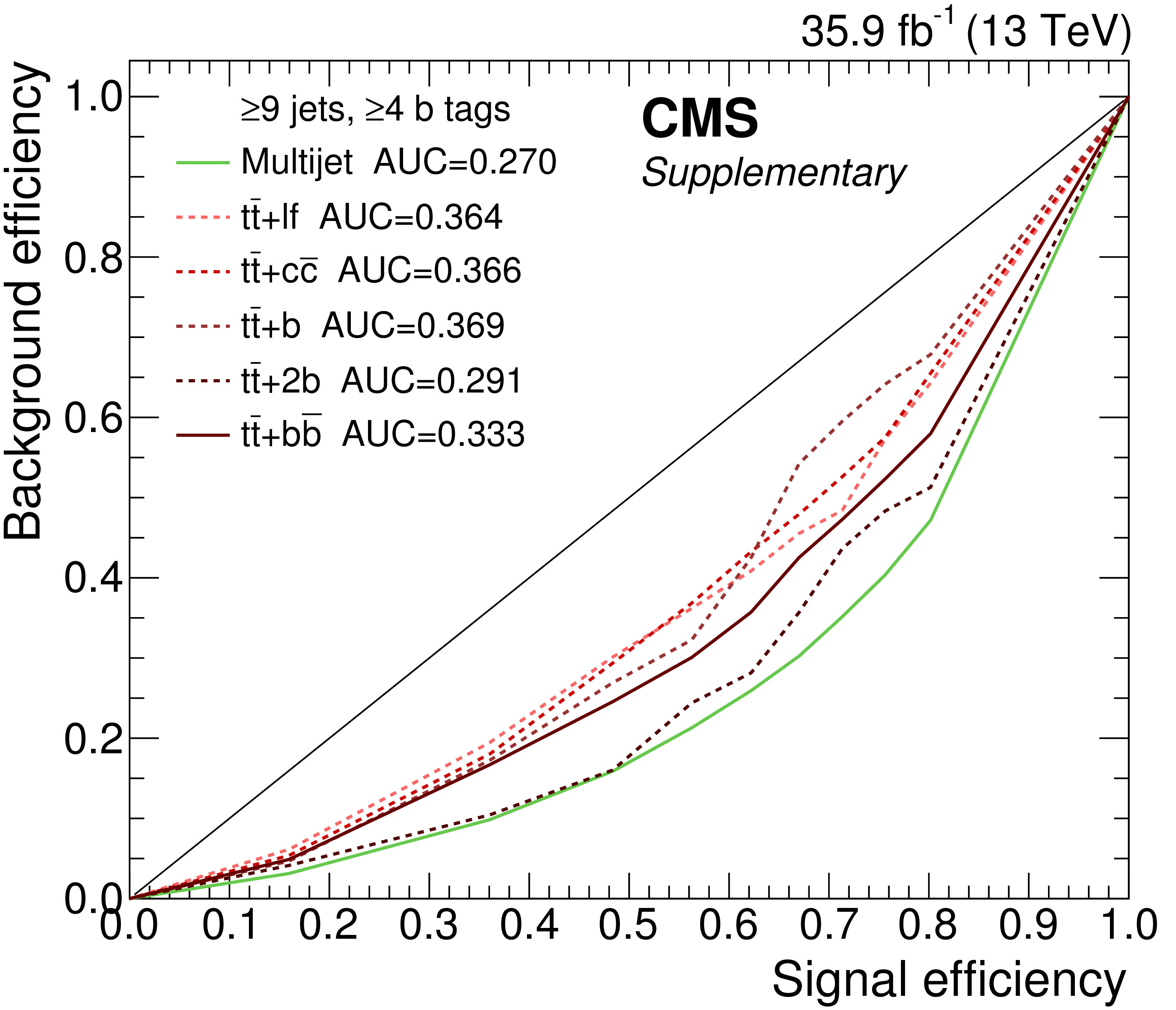
png pdf |
Additional Figure 4-f:
Performance of the MEM discriminator in terms of signal $ {\text {t}\overline {\text {t}}\text {H}} (\text {bb})$ vs. background (${\text {t}\overline {\text {t}}\text {+jets}}$ and multijet) efficiencies. The final discriminator hypothesis is shown in each category, as reported in Table 2. The area under the curve (labelled AUC) for each background process is shown in the legend. |

png pdf |
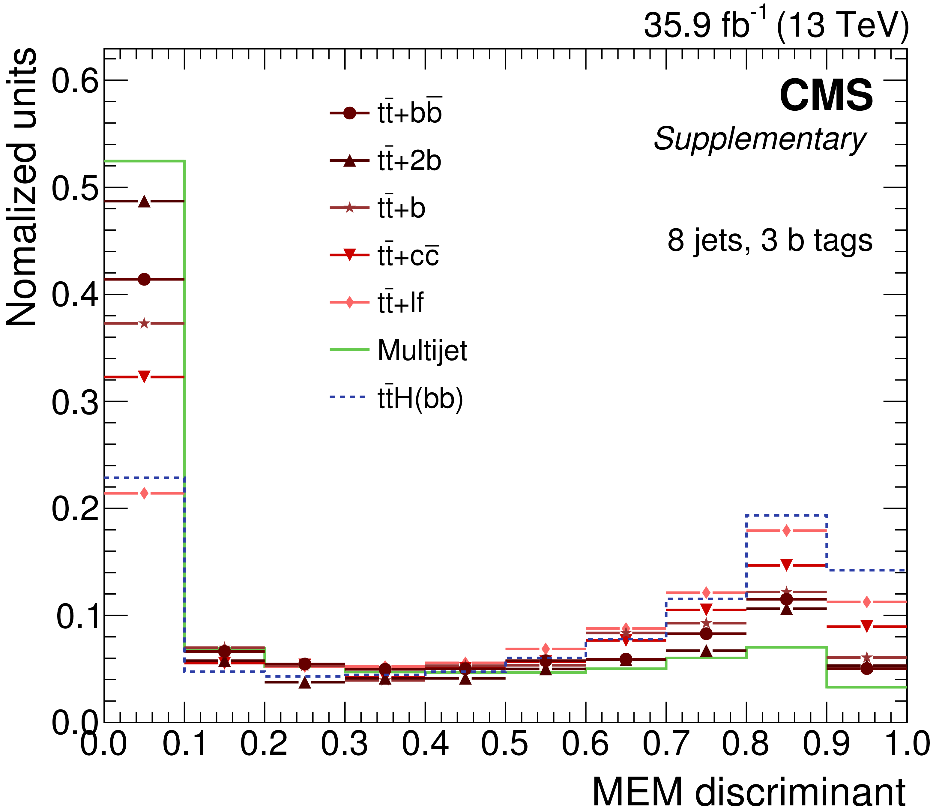
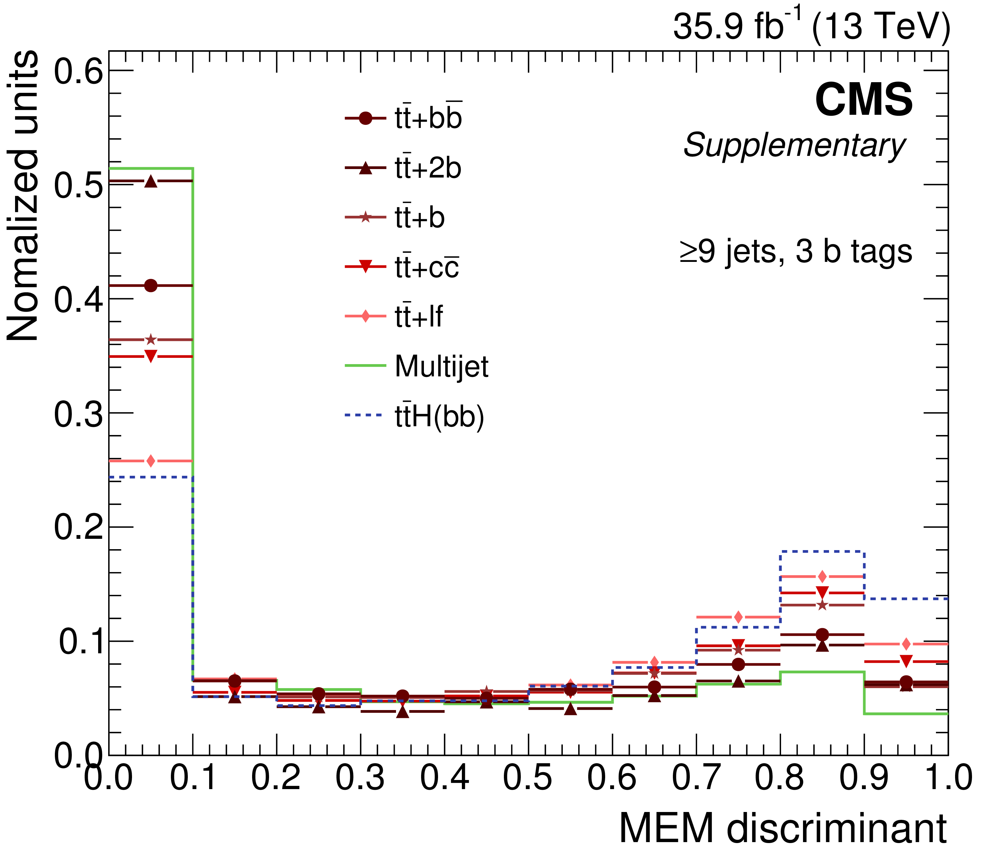
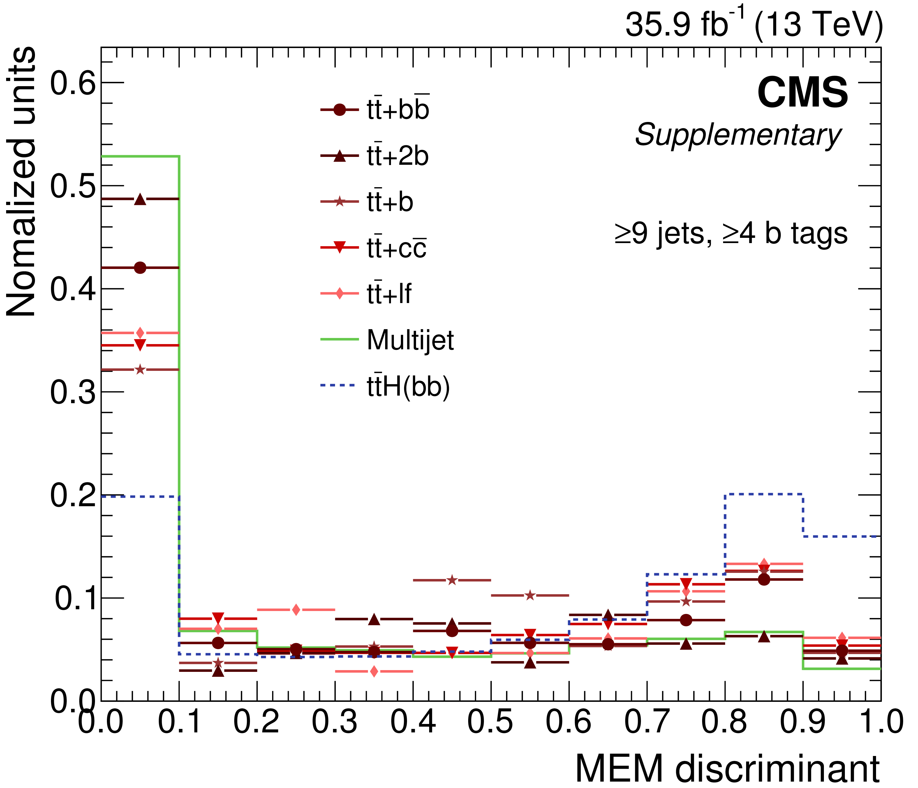
Additional Figure 5:
The distributions of the MEM discriminant in signal, multijet background, and the ${\mathrm{t} \mathrm{\bar{t}}}$ background subprocesses, normalized to unity. The final discriminator hypothesis is shown for each category, as reported in Table 2. |

png pdf |
Additional Figure 5-a:
The distributions of the MEM discriminant in signal, multijet background, and the ${\mathrm{t} \mathrm{\bar{t}}}$ background subprocesses, normalized to unity. The final discriminator hypothesis is shown for each category, as reported in Table 2. |

png pdf |
Additional Figure 5-b:
The distributions of the MEM discriminant in signal, multijet background, and the ${\mathrm{t} \mathrm{\bar{t}}}$ background subprocesses, normalized to unity. The final discriminator hypothesis is shown for each category, as reported in Table 2. |
png pdf |
Additional Figure 5-c:
The distributions of the MEM discriminant in signal, multijet background, and the ${\mathrm{t} \mathrm{\bar{t}}}$ background subprocesses, normalized to unity. The final discriminator hypothesis is shown for each category, as reported in Table 2. |

png pdf |
Additional Figure 5-d:
The distributions of the MEM discriminant in signal, multijet background, and the ${\mathrm{t} \mathrm{\bar{t}}}$ background subprocesses, normalized to unity. The final discriminator hypothesis is shown for each category, as reported in Table 2. |
png pdf |
Additional Figure 5-e:
The distributions of the MEM discriminant in signal, multijet background, and the ${\mathrm{t} \mathrm{\bar{t}}}$ background subprocesses, normalized to unity. The final discriminator hypothesis is shown for each category, as reported in Table 2. |
png pdf |
Additional Figure 5-f:
The distributions of the MEM discriminant in signal, multijet background, and the ${\mathrm{t} \mathrm{\bar{t}}}$ background subprocesses, normalized to unity. The final discriminator hypothesis is shown for each category, as reported in Table 2. |

png pdf |
Additional Figure 6:
Expected fraction of signal and background processes contributing to the analysis categories. |
png pdf |
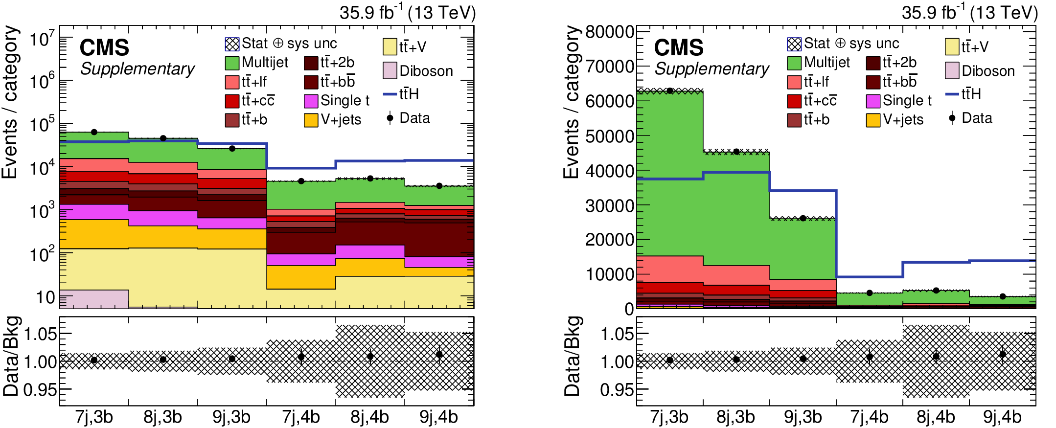
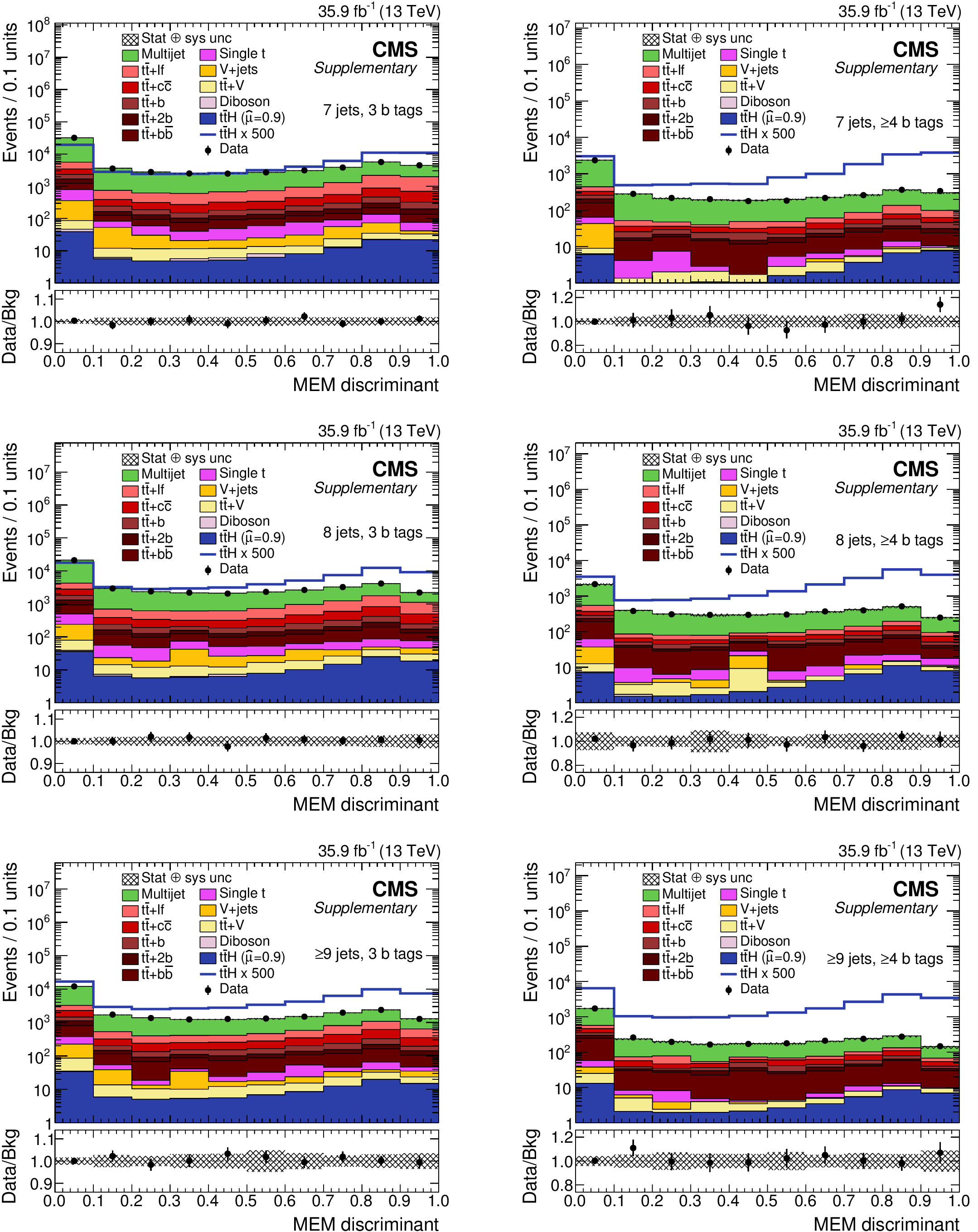
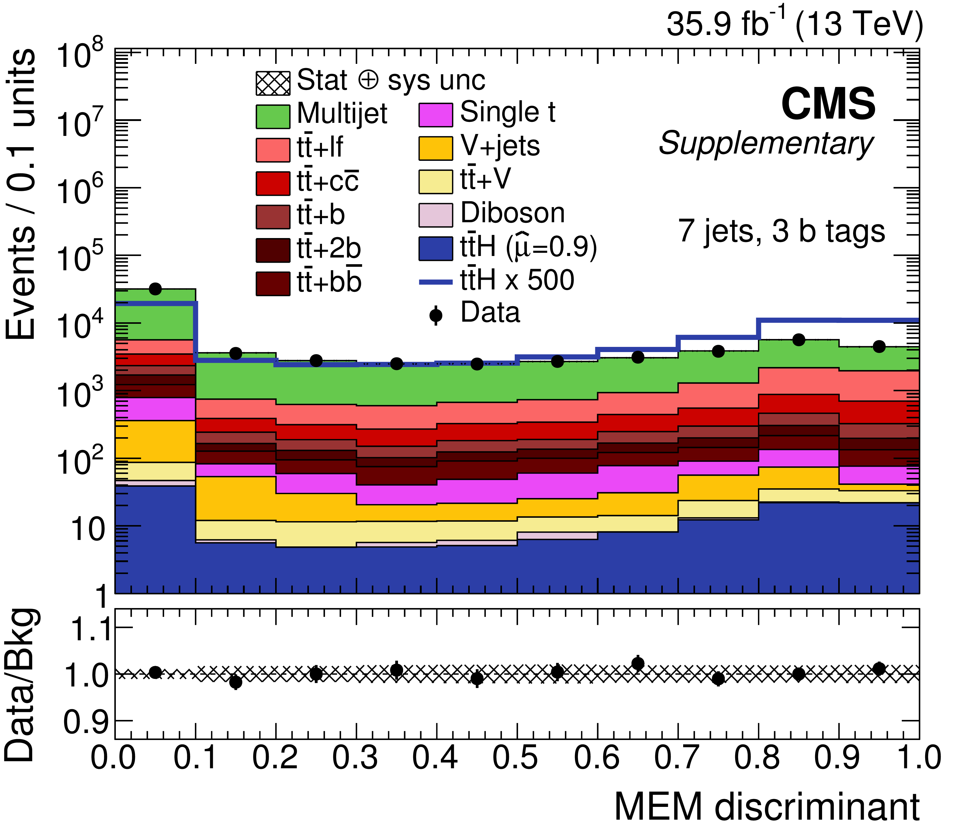
Additional Figure 7:
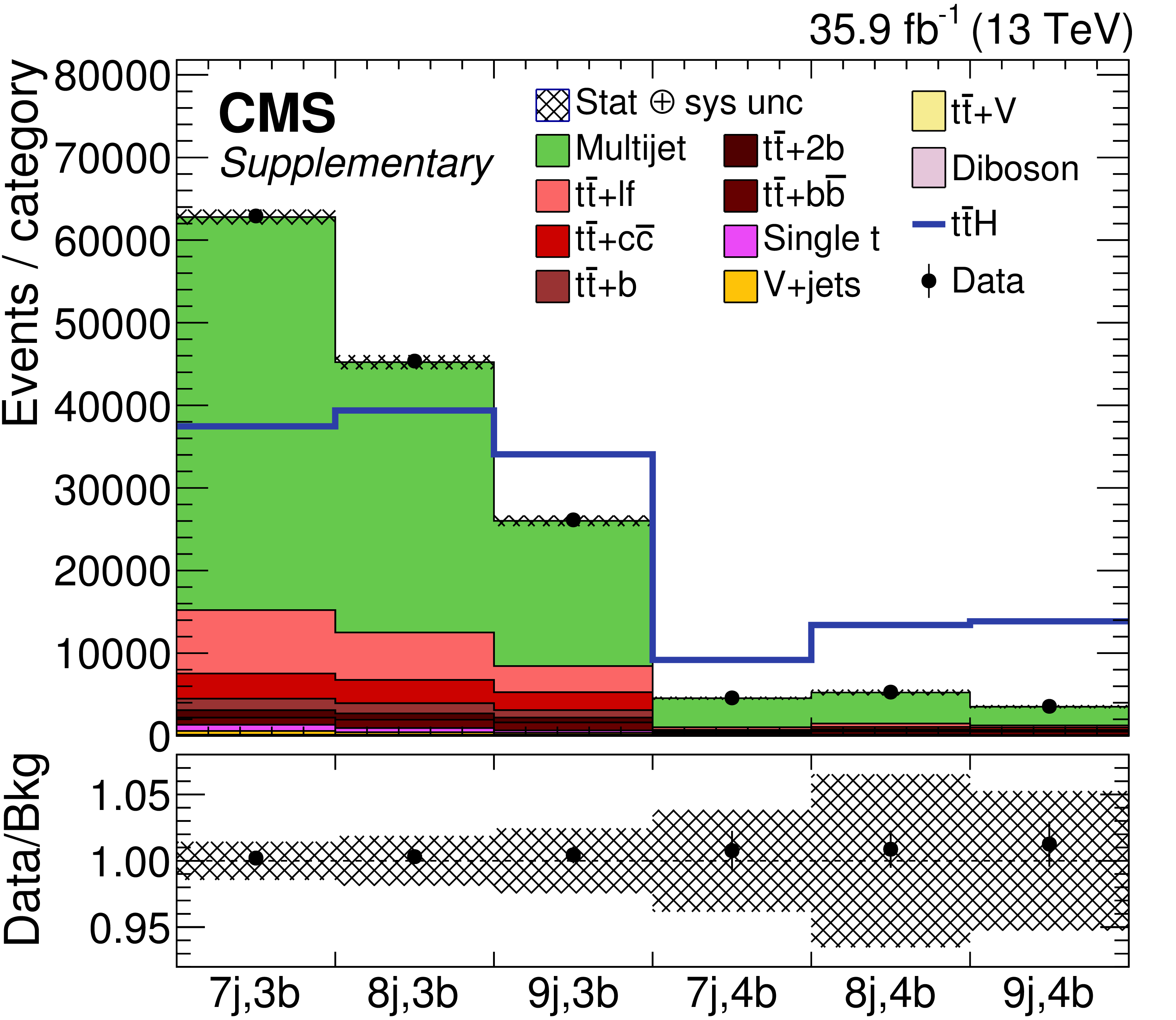
Predicted (histograms) and observed (data points) event yields in each analysis category after the combined fit to data, corresponding to an integrated luminosity of 35.9 fb$^{-1}$. The plots show the baseline categories defined in Section 6. The expected contributions from different background processes (filled histograms) are stacked, showing the total fitted uncertainty (striped error bands), and the expected signal distribution (line) for a Higgs boson mass of $ {m_\mathrm {H}} = $ 125 GeV, but scaled to the total background yield for ease of readability. The ratios of data to background are given below the main panels, with the full uncertainties. |

png pdf |
Additional Figure 7-a:
Predicted (histograms) and observed (data points) event yields in each analysis category after the combined fit to data, corresponding to an integrated luminosity of 35.9 fb$^{-1}$. The plot shows one of the baseline category defined in Section 6. The expected contributions from different background processes (filled histograms) are stacked, showing the total fitted uncertainty (striped error bands), and the expected signal distribution (line) for a Higgs boson mass of $ {m_\mathrm {H}} = $ 125 GeV, but scaled to the total background yield for ease of readability. The ratios of data to background are given below the main panels, with the full uncertainties. |
png pdf |
Additional Figure 7-b:
Predicted (histograms) and observed (data points) event yields in each analysis category after the combined fit to data, corresponding to an integrated luminosity of 35.9 fb$^{-1}$. The plot shows one of the baseline category defined in Section 6. The expected contributions from different background processes (filled histograms) are stacked, showing the total fitted uncertainty (striped error bands), and the expected signal distribution (line) for a Higgs boson mass of $ {m_\mathrm {H}} = $ 125 GeV, but scaled to the total background yield for ease of readability. The ratios of data to background are given below the main panels, with the full uncertainties. |

png pdf |
Additional Figure 8:
The $ {p_{\mathrm {T}}} $ of the leading jet after the preselection. Simulated events are used for the QCD multijet background, but its total yield is rescaled to match the data. The signal contribution is scaled to the total background yield (equivalent to the yield in data) to improve readability. The last bin includes overflow events. |

png pdf |
Additional Figure 9:
The b-tagged jet multiplicity after the preselection. Simulated events are used for the QCD multijet background, but its total yield is rescaled to match the data. The signal contribution is scaled to the total background yield (equivalent to the yield in data) to improve readability. The last bin includes overflow events. |
png pdf |
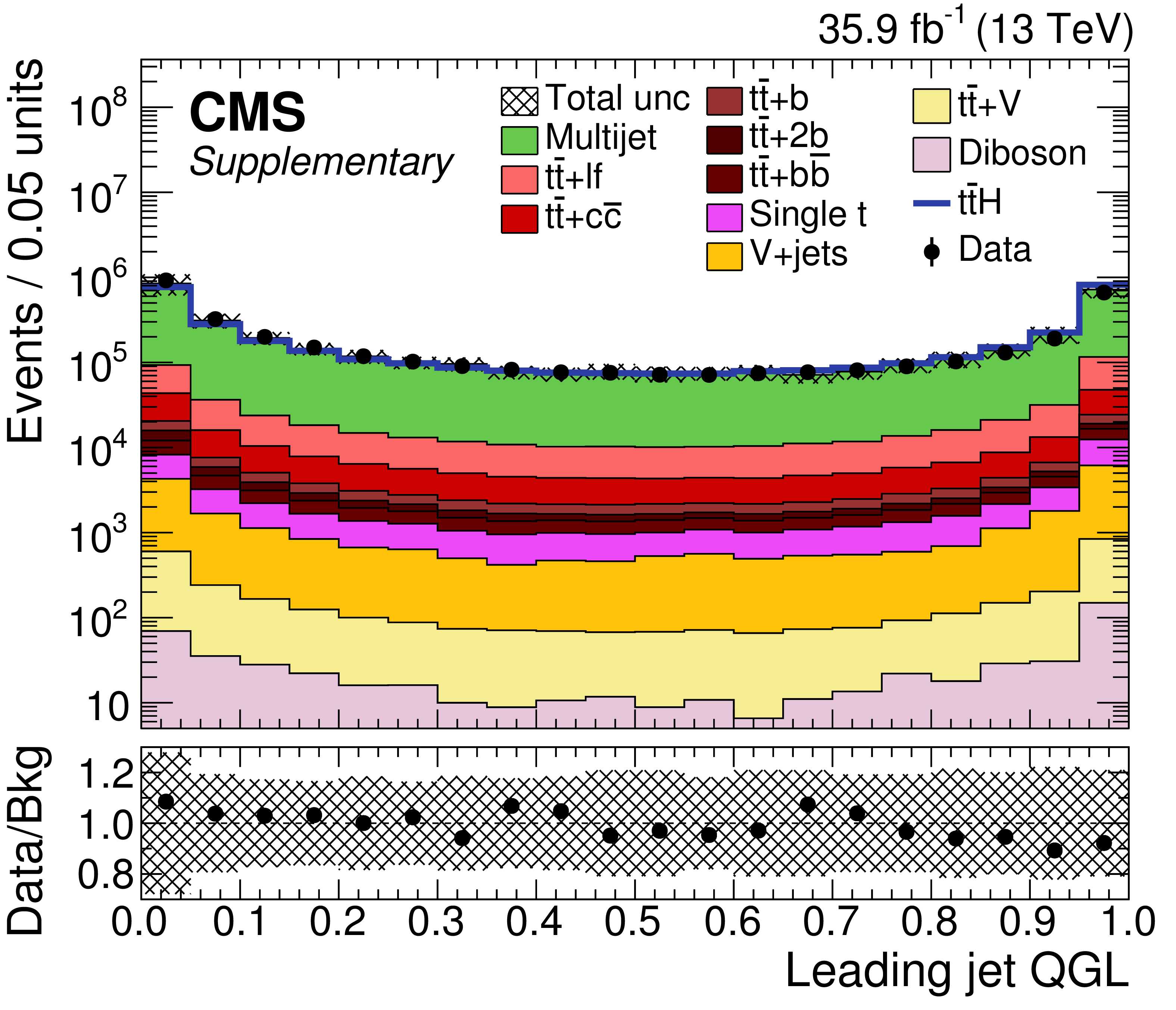
Additional Figure 10:
The QGL of the leading jet in $ {p_{\mathrm {T}}} $ after the preselection. Simulated events are used for the QCD multijet background, but its total yield is rescaled to match the data. The signal contribution is scaled to the total background yield (equivalent to the yield in data) to improve readability. |
png pdf |
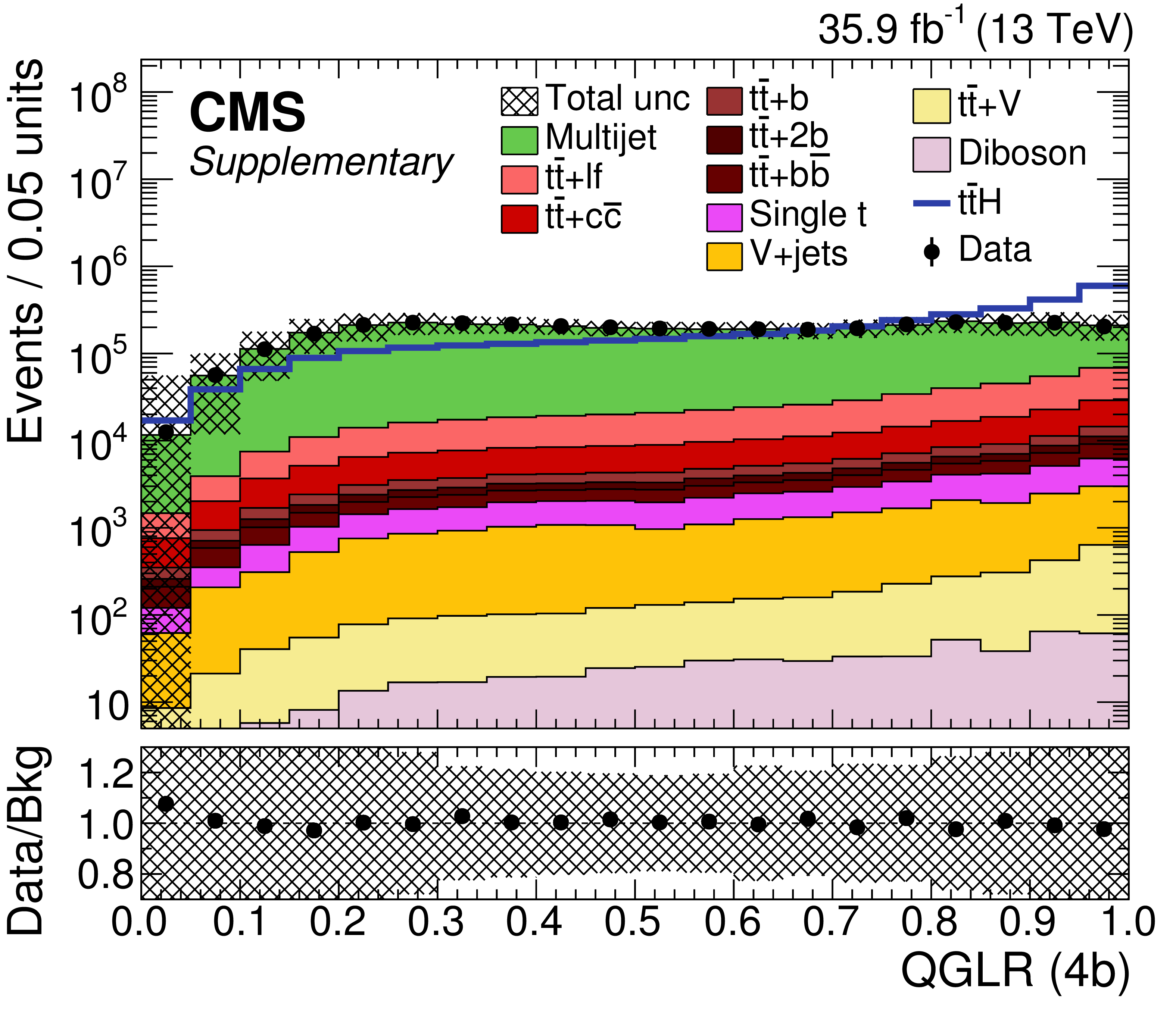
Additional Figure 11:
The QGLR calculated excluding the first 4 b-tagged jets after the preselection. Simulated events are used for the QCD multijet background, but its total yield is rescaled to match the data. The signal contribution is scaled to the total background yield (equivalent to the yield in data) to improve readability. |
png pdf |
Additional Figure 12:
Distributions in the MEM discriminant for each analysis category, after the fit to data. The fitted contributions expected from signal and background processes (filled histograms) are shown stacked. The signal distributions (lines) for an H mass of $ {m_\mathrm {H}} = $ 125 GeV are multiplied by a factor of 100 and superimposed on the data. The distributions observed in data (data points) are also shown. The ratios of data to background are given below the main panels. |

png pdf |
Additional Figure 12-a:
Distributions in the MEM discriminant for each analysis category, after the fit to data. The fitted contributions expected from signal and background processes (filled histograms) are shown stacked. The signal distributions (lines) for an H mass of $ {m_\mathrm {H}} = $ 125 GeV are multiplied by a factor of 100 and superimposed on the data. The distributions observed in data (data points) are also shown. The ratios of data to background are given below the main panels. |

png pdf |
Additional Figure 12-b:
Distributions in the MEM discriminant for each analysis category, after the fit to data. The fitted contributions expected from signal and background processes (filled histograms) are shown stacked. The signal distributions (lines) for an H mass of $ {m_\mathrm {H}} = $ 125 GeV are multiplied by a factor of 100 and superimposed on the data. The distributions observed in data (data points) are also shown. The ratios of data to background are given below the main panels. |
png pdf |
Additional Figure 12-c:
Distributions in the MEM discriminant for each analysis category, after the fit to data. The fitted contributions expected from signal and background processes (filled histograms) are shown stacked. The signal distributions (lines) for an H mass of $ {m_\mathrm {H}} = $ 125 GeV are multiplied by a factor of 100 and superimposed on the data. The distributions observed in data (data points) are also shown. The ratios of data to background are given below the main panels. |

png pdf |
Additional Figure 12-d:
Distributions in the MEM discriminant for each analysis category, after the fit to data. The fitted contributions expected from signal and background processes (filled histograms) are shown stacked. The signal distributions (lines) for an H mass of $ {m_\mathrm {H}} = $ 125 GeV are multiplied by a factor of 100 and superimposed on the data. The distributions observed in data (data points) are also shown. The ratios of data to background are given below the main panels. |

png pdf |
Additional Figure 12-e:
Distributions in the MEM discriminant for each analysis category, after the fit to data. The fitted contributions expected from signal and background processes (filled histograms) are shown stacked. The signal distributions (lines) for an H mass of $ {m_\mathrm {H}} = $ 125 GeV are multiplied by a factor of 100 and superimposed on the data. The distributions observed in data (data points) are also shown. The ratios of data to background are given below the main panels. |
png pdf |
Additional Figure 12-f:
Distributions in the MEM discriminant for each analysis category, after the fit to data. The fitted contributions expected from signal and background processes (filled histograms) are shown stacked. The signal distributions (lines) for an H mass of $ {m_\mathrm {H}} = $ 125 GeV are multiplied by a factor of 100 and superimposed on the data. The distributions observed in data (data points) are also shown. The ratios of data to background are given below the main panels. |
png pdf |
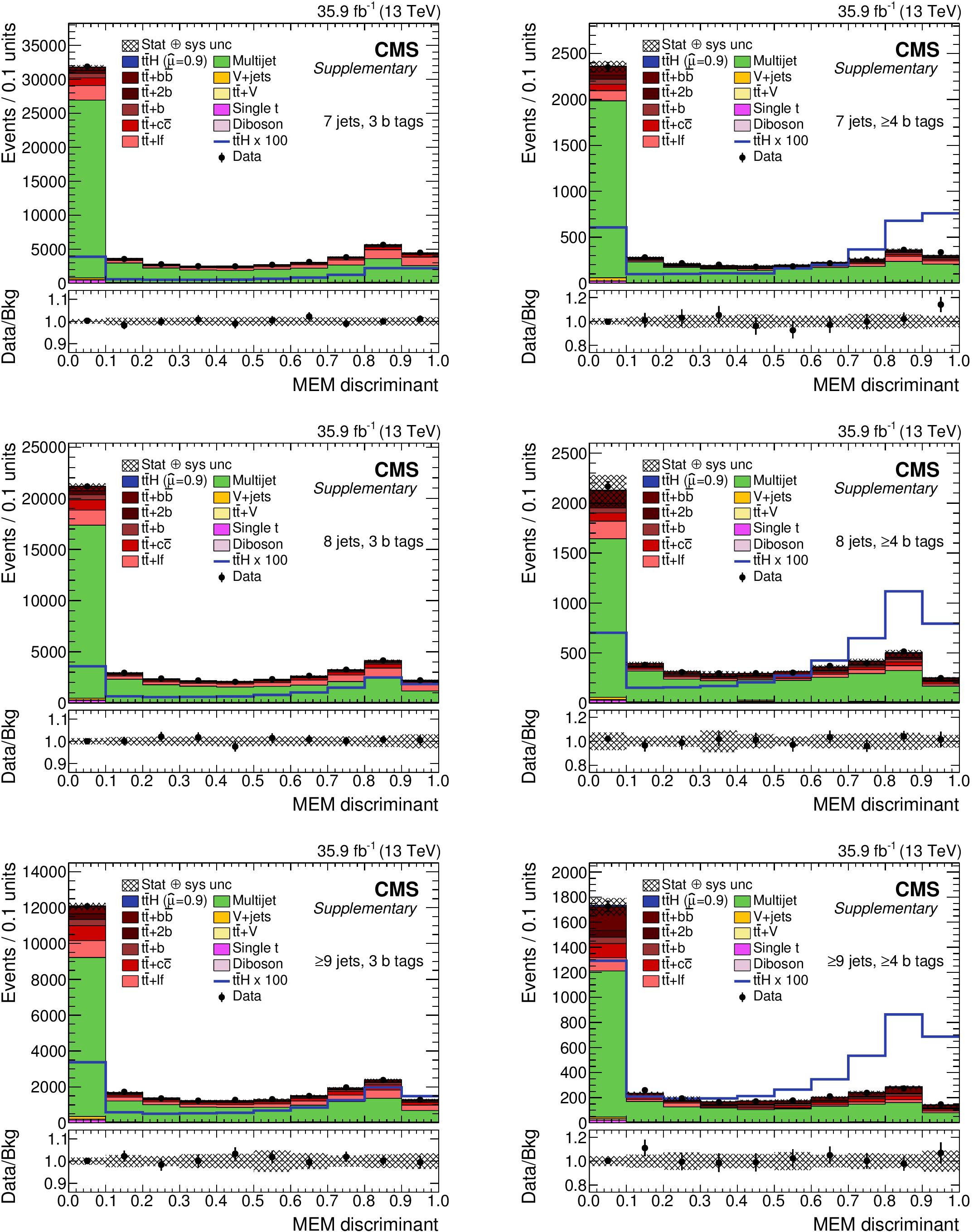
Additional Figure 13:
Distributions in the MEM discriminant for each analysis category, after the fit to data. The fitted contributions expected from signal and background processes (filled histograms) are shown stacked. The signal distributions (lines) for an H mass of $ {m_\mathrm {H}} = $ 125 GeV are multiplied by a factor of 500 and superimposed on the data. The distributions observed in data (data points) are also shown. The ratios of data to background are given below the main panels. |
png pdf |
Additional Figure 13-a:
Distributions in the MEM discriminant for each analysis category, after the fit to data. The fitted contributions expected from signal and background processes (filled histograms) are shown stacked. The signal distributions (lines) for an H mass of $ {m_\mathrm {H}} = $ 125 GeV are multiplied by a factor of 500 and superimposed on the data. The distributions observed in data (data points) are also shown. The ratios of data to background are given below the main panels. |
png pdf |
Additional Figure 13-b:
Distributions in the MEM discriminant for each analysis category, after the fit to data. The fitted contributions expected from signal and background processes (filled histograms) are shown stacked. The signal distributions (lines) for an H mass of $ {m_\mathrm {H}} = $ 125 GeV are multiplied by a factor of 500 and superimposed on the data. The distributions observed in data (data points) are also shown. The ratios of data to background are given below the main panels. |

png pdf |
Additional Figure 13-c:
Distributions in the MEM discriminant for each analysis category, after the fit to data. The fitted contributions expected from signal and background processes (filled histograms) are shown stacked. The signal distributions (lines) for an H mass of $ {m_\mathrm {H}} = $ 125 GeV are multiplied by a factor of 500 and superimposed on the data. The distributions observed in data (data points) are also shown. The ratios of data to background are given below the main panels. |

png pdf |
Additional Figure 13-d:
Distributions in the MEM discriminant for each analysis category, after the fit to data. The fitted contributions expected from signal and background processes (filled histograms) are shown stacked. The signal distributions (lines) for an H mass of $ {m_\mathrm {H}} = $ 125 GeV are multiplied by a factor of 500 and superimposed on the data. The distributions observed in data (data points) are also shown. The ratios of data to background are given below the main panels. |

png pdf |
Additional Figure 13-e:
Distributions in the MEM discriminant for each analysis category, after the fit to data. The fitted contributions expected from signal and background processes (filled histograms) are shown stacked. The signal distributions (lines) for an H mass of $ {m_\mathrm {H}} = $ 125 GeV are multiplied by a factor of 500 and superimposed on the data. The distributions observed in data (data points) are also shown. The ratios of data to background are given below the main panels. |

png pdf |
Additional Figure 13-f:
Distributions in the MEM discriminant for each analysis category, after the fit to data. The fitted contributions expected from signal and background processes (filled histograms) are shown stacked. The signal distributions (lines) for an H mass of $ {m_\mathrm {H}} = $ 125 GeV are multiplied by a factor of 500 and superimposed on the data. The distributions observed in data (data points) are also shown. The ratios of data to background are given below the main panels. |
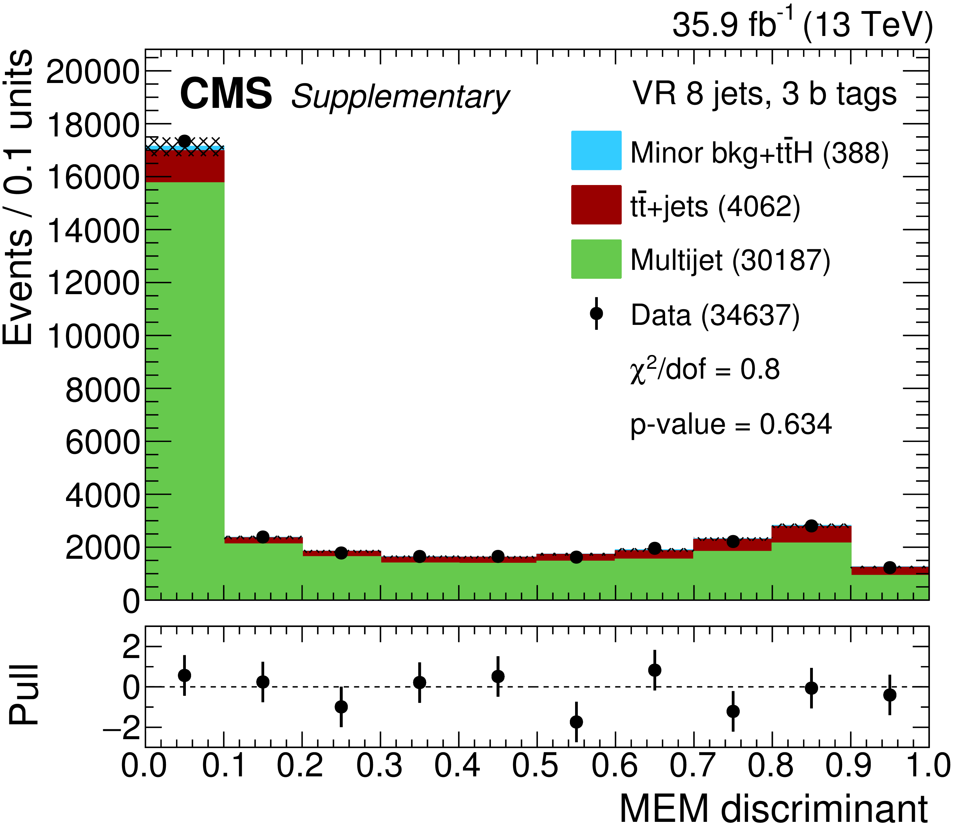
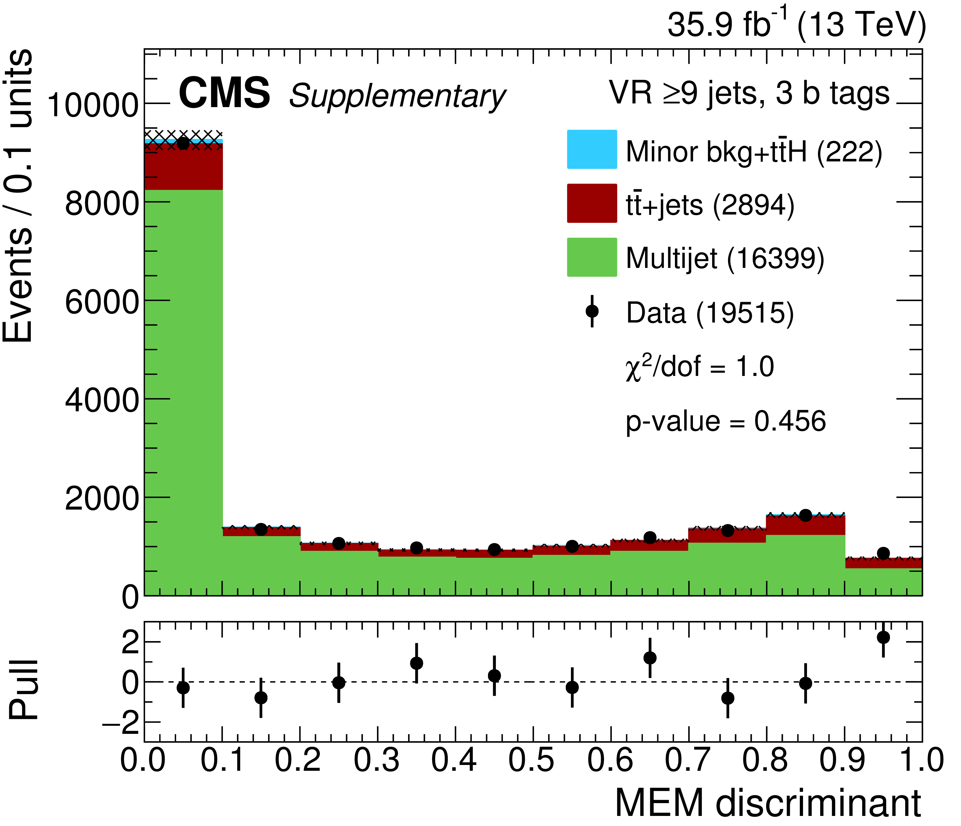
png pdf |
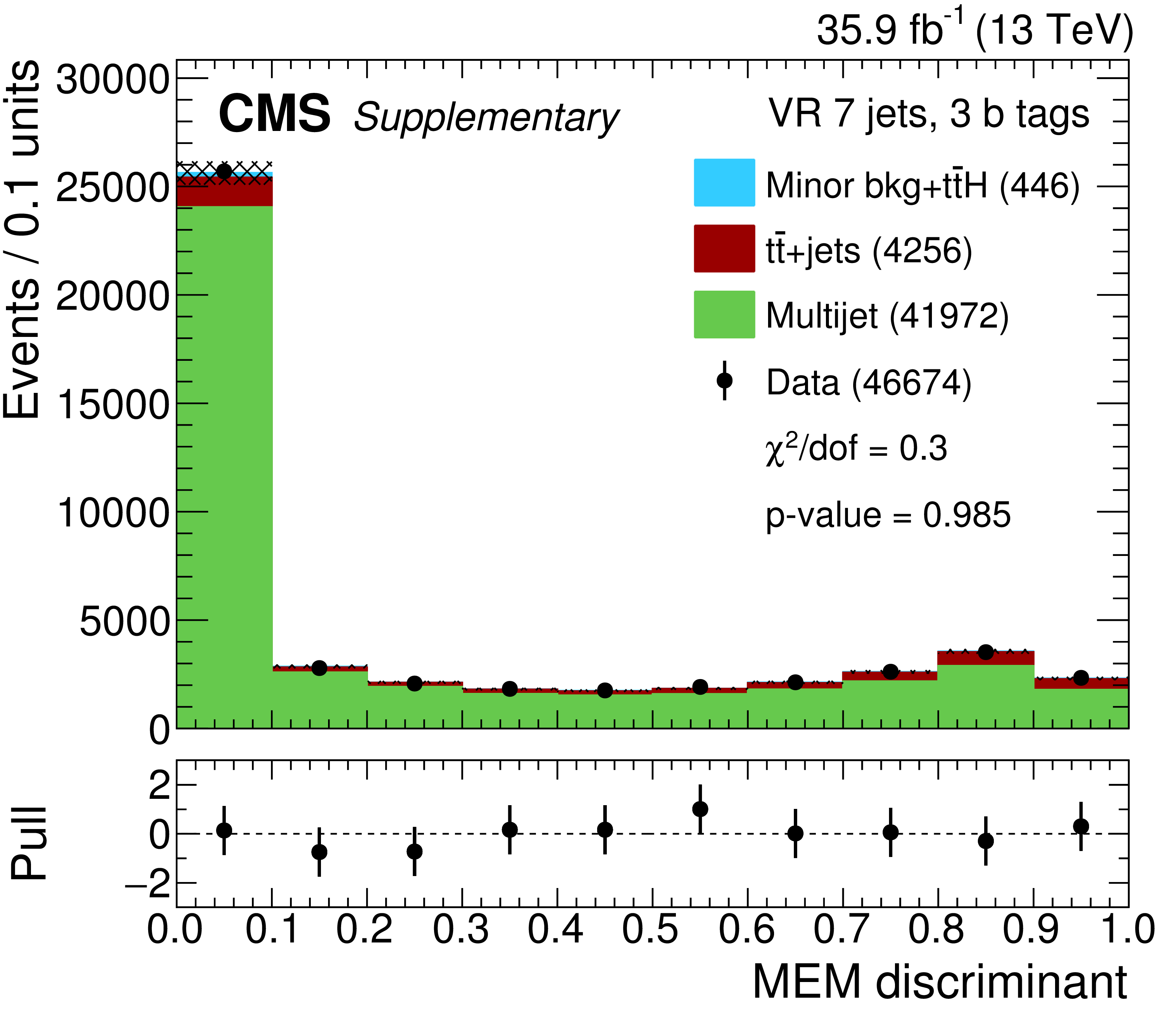
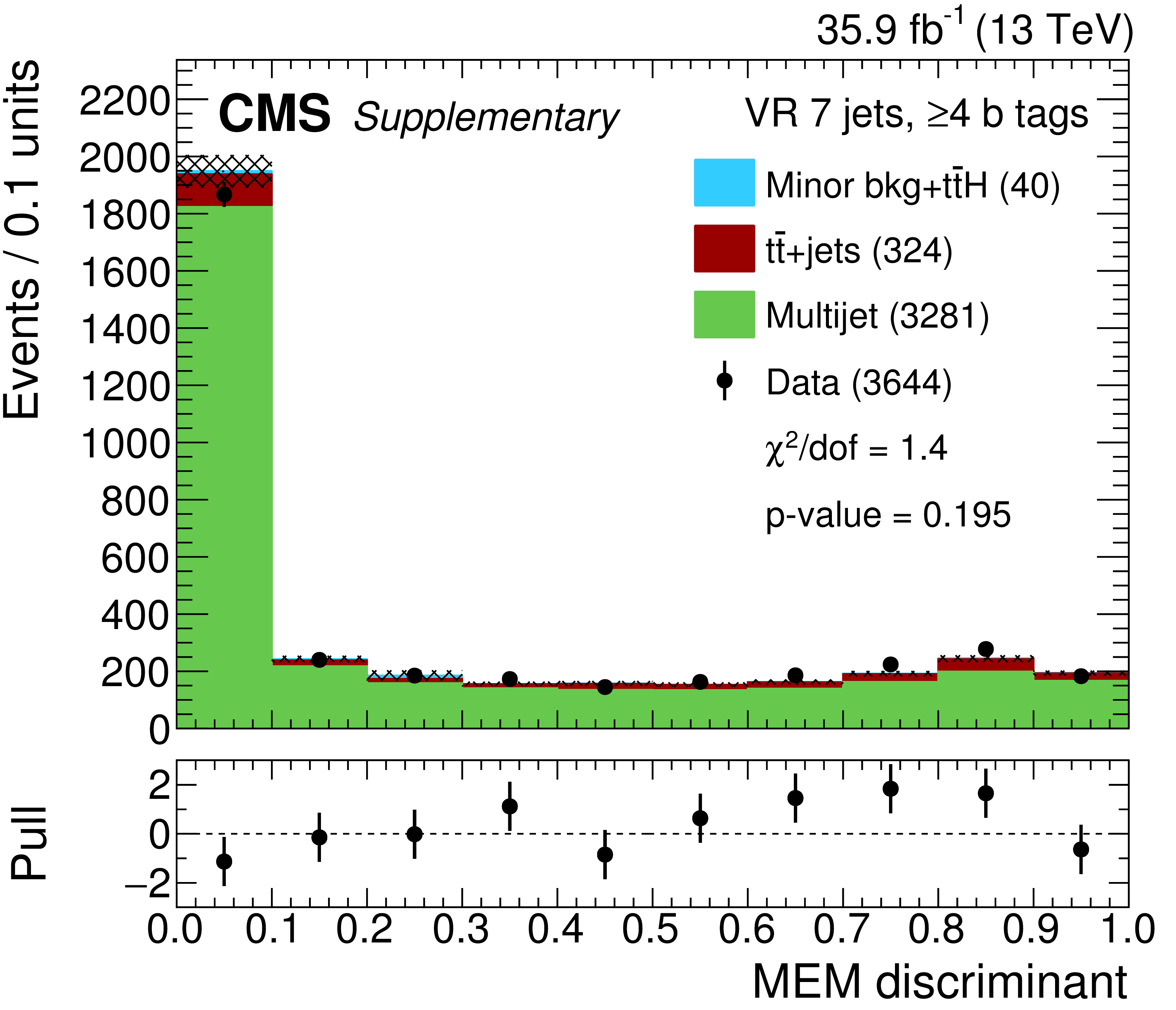
Additional Figure 14:
Distributions in the MEM discriminant in data, simulated backgrounds, and the estimated multijet background in the validation region of each category. The level of agreement between data and estimation is expressed in terms of a $\chi ^2$ divided by the number of degrees of freedom (dof), and the corresponding p-values are also shown. The differences between data and the total estimates divided by the total statistical and systematic uncertainties in the data and estimates added in quadrature (pulls) are given below the main panels. The numbers in parenthesis in the legend represent the total yields for the corresponding entries. |
png pdf |
Additional Figure 14-a:
Distributions in the MEM discriminant in data, simulated backgrounds, and the estimated multijet background in the validation region of each category. The level of agreement between data and estimation is expressed in terms of a $\chi ^2$ divided by the number of degrees of freedom (dof), and the corresponding p-values are also shown. The differences between data and the total estimates divided by the total statistical and systematic uncertainties in the data and estimates added in quadrature (pulls) are given below the main panels. The numbers in parenthesis in the legend represent the total yields for the corresponding entries. |
png pdf |
Additional Figure 14-b:
Distributions in the MEM discriminant in data, simulated backgrounds, and the estimated multijet background in the validation region of each category. The level of agreement between data and estimation is expressed in terms of a $\chi ^2$ divided by the number of degrees of freedom (dof), and the corresponding p-values are also shown. The differences between data and the total estimates divided by the total statistical and systematic uncertainties in the data and estimates added in quadrature (pulls) are given below the main panels. The numbers in parenthesis in the legend represent the total yields for the corresponding entries. |
png pdf |
Additional Figure 14-c:
Distributions in the MEM discriminant in data, simulated backgrounds, and the estimated multijet background in the validation region of each category. The level of agreement between data and estimation is expressed in terms of a $\chi ^2$ divided by the number of degrees of freedom (dof), and the corresponding p-values are also shown. The differences between data and the total estimates divided by the total statistical and systematic uncertainties in the data and estimates added in quadrature (pulls) are given below the main panels. The numbers in parenthesis in the legend represent the total yields for the corresponding entries. |

png pdf |
Additional Figure 14-d:
Distributions in the MEM discriminant in data, simulated backgrounds, and the estimated multijet background in the validation region of each category. The level of agreement between data and estimation is expressed in terms of a $\chi ^2$ divided by the number of degrees of freedom (dof), and the corresponding p-values are also shown. The differences between data and the total estimates divided by the total statistical and systematic uncertainties in the data and estimates added in quadrature (pulls) are given below the main panels. The numbers in parenthesis in the legend represent the total yields for the corresponding entries. |
png pdf |
Additional Figure 14-e:
Distributions in the MEM discriminant in data, simulated backgrounds, and the estimated multijet background in the validation region of each category. The level of agreement between data and estimation is expressed in terms of a $\chi ^2$ divided by the number of degrees of freedom (dof), and the corresponding p-values are also shown. The differences between data and the total estimates divided by the total statistical and systematic uncertainties in the data and estimates added in quadrature (pulls) are given below the main panels. The numbers in parenthesis in the legend represent the total yields for the corresponding entries. |

png pdf |
Additional Figure 14-f:
Distributions in the MEM discriminant in data, simulated backgrounds, and the estimated multijet background in the validation region of each category. The level of agreement between data and estimation is expressed in terms of a $\chi ^2$ divided by the number of degrees of freedom (dof), and the corresponding p-values are also shown. The differences between data and the total estimates divided by the total statistical and systematic uncertainties in the data and estimates added in quadrature (pulls) are given below the main panels. The numbers in parenthesis in the legend represent the total yields for the corresponding entries. |
| References | ||||
| 1 | ATLAS Collaboration | Observation of a new particle in the search for the standard model Higgs boson with the ATLAS detector at the LHC | PLB 716 (2012) 1 | 1207.7214 |
| 2 | CMS Collaboration | Observation of a new boson at a mass of 125 GeV with the CMS experiment at the LHC | PLB 716 (2012) 30 | CMS-HIG-12-028 1207.7235 |
| 3 | CMS Collaboration | Observation of a new boson with mass near 125 GeV in pp collisions at $ \sqrt{s} = $ 7 and 8 TeV | JHEP 06 (2013) 081 | CMS-HIG-12-036 1303.4571 |
| 4 | ATLAS Collaboration | Measurement of Higgs boson production in the diphoton decay channel in pp collisions at center-of-mass energies of 7 and 8 TeV with the ATLAS detector | PRD 90 (2014) 112015 | 1408.7084 |
| 5 | CMS Collaboration | Observation of the diphoton decay of the Higgs boson and measurement of its properties | EPJC 74 (2014) 3076 | CMS-HIG-13-001 1407.0558 |
| 6 | ATLAS Collaboration | Measurements of Higgs boson production and couplings in the four-lepton channel in pp collisions at center-of-mass energies of 7 and 8 TeV with the ATLAS detector | PRD 91 (2015) 012006 | 1408.5191 |
| 7 | CMS Collaboration | Measurement of the properties of a Higgs boson in the four-lepton final state | PRD 89 (2014) 092007 | CMS-HIG-13-002 1312.5353 |
| 8 | ATLAS Collaboration | Study of (W/Z)H production and Higgs boson couplings using $ \mathrm{H} \rightarrow \mathrm{WW}^{\ast} $ decays with the ATLAS detector | JHEP 08 (2015) 137 | 1506.06641 |
| 9 | CMS Collaboration | Measurement of Higgs boson production and properties in the WW decay channel with leptonic final states | JHEP 01 (2014) 096 | CMS-HIG-13-023 1312.1129 |
| 10 | CMS Collaboration | Observation of the Higgs boson decay to a pair of tau leptons | Submitted to \it PLB | CMS-HIG-16-043 1708.00373 |
| 11 | ATLAS Collaboration | Evidence for the $ \mathrm{H} \to \mathrm{b}\bar{\mathrm{b}} $ decay with the ATLAS detector | Submitted to \it JHEP | 1708.03299 |
| 12 | CMS Collaboration | Evidence for the Higgs boson decay to a bottom quark-antiquark pair | Accepted by \it PLB | CMS-HIG-16-044 1709.07497 |
| 13 | ATLAS Collaboration | Measurements of the Higgs boson production and decay rates and coupling strengths using pp collision data at $ \sqrt{s}= $ 7 and 8 TeV in the ATLAS experiment | EPJC 76 (2016) 6 | 1507.04548 |
| 14 | CMS Collaboration | Precise determination of the mass of the Higgs boson and tests of compatibility of its couplings with the standard model predictions using proton collisions at 7 and 8 TeV | EPJC 75 (2015) 212 | CMS-HIG-14-009 1412.8662 |
| 15 | CMS Collaboration | Study of the mass and spin-parity of the Higgs boson candidate via its decays to Z boson pairs | PRL 110 (2013) 081803 | CMS-HIG-12-041 1212.6639 |
| 16 | ATLAS Collaboration | Evidence for the spin-0 nature of the Higgs boson using ATLAS data | PLB 726 (2013) 120 | 1307.1432 |
| 17 | ATLAS and CMS Collaborations | Measurements of the Higgs boson production and decay rates and constraints on its couplings from a combined ATLAS and CMS analysis of the LHC pp collision data at $ \sqrt{s}= $ 7 and 8 TeV | JHEP 08 (2016) 045 | 1606.02266 |
| 18 | CMS Collaboration | Measurements of properties of the Higgs boson decaying into the four-lepton final state in pp collisions at $ \sqrt{s}= $ 13 TeV | JHEP 11 (2017) 047 | CMS-HIG-16-041 1706.09936 |
| 19 | CMS Collaboration | Measurement of the top quark mass using proton-proton data at $ \sqrt{s} = $ 7 and 8 TeV | PRD 93 (2016) 072004 | CMS-TOP-14-022 1509.04044 |
| 20 | ATLAS Collaboration | Evidence for the associated production of the Higgs boson and a top quark pair with the ATLAS detector | Submitted to PRD | 1712.08891 |
| 21 | CMS Collaboration | Search for the associated production of the Higgs boson with a top-quark pair | JHEP 09 (2014) 087 | CMS-HIG-13-029 1408.1682 |
| 22 | CMS Collaboration | Evidence for associated production of a Higgs boson with a top quark pair in final states with electrons, muons, and hadronically decaying $ \tau $ leptons at $ \sqrt{s} = $ 13 TeV | Submitted to JHEP | CMS-HIG-17-018 1803.05485 |
| 23 | CMS Collaboration | Search for a standard model Higgs boson produced in association with a top-quark pair and decaying to bottom quarks using a matrix element method | EPJC 75 (2015) 251 | CMS-HIG-14-010 1502.02485 |
| 24 | ATLAS Collaboration | Search for the standard model Higgs boson produced in association with top quarks and decaying into a $ \mathrm{b}\bar{\mathrm{b}} $ pair in pp collisions at $ \sqrt{s} = $ 13 TeV with the ATLAS detector | Submitted to PRD | 1712.08895 |
| 25 | ATLAS Collaboration | Search for the standard model Higgs boson decaying into $ \mathrm{b}\overline{\mathrm{b}} $ produced in association with top quarks decaying hadronically in pp collisions at $ \sqrt{s}= $ 8 TeV with the ATLAS detector | JHEP 05 (2016) 160 | 1604.03812 |
| 26 | D0 Collaboration | A precision measurement of the mass of the top quark | Nature 429 (2004) 638 | hep-ex/0406031 |
| 27 | D0 Collaboration | Helicity of the W boson in lepton+jets $ \mathrm{t}\bar{\mathrm{t}} $ events | PLB 617 (2005) 1 | hep-ex/0404040 |
| 28 | CDF Collaboration | Search for a Higgs boson in $ \mathrm{W} \mathrm{H} \to \ell \nu \mathrm{b} \bar{\mathrm{b}} $ in $ \mathrm{p}\bar{\mathrm{p}} $ collisions at $ \sqrt{s} = $ 1.96 TeV | PRL 103 (2009) 101802 | 0906.5613 |
| 29 | CMS Collaboration | The CMS trigger system | JINST 12 (2017) P01020 | CMS-TRG-12-001 1609.02366 |
| 30 | CMS Collaboration | The CMS experiment at the CERN LHC | JINST 3 (2008) S08004 | CMS-00-001 |
| 31 | GEANT4 Collaboration | GEANT4---a simulation toolkit | NIMA 506 (2003) 250 | |
| 32 | P. Nason | A new method for combining NLO QCD with shower Monte Carlo algorithms | JHEP 11 (2004) 040 | hep-ph/0409146 |
| 33 | S. Frixione, P. Nason, and C. Oleari | Matching NLO QCD computations with parton shower simulations: the POWHEG method | JHEP 11 (2007) 070 | 0709.2092 |
| 34 | S. Alioli, P. Nason, C. Oleari, and E. Re | A general framework for implementing NLO calculations in shower Monte Carlo programs: the POWHEG BOX | JHEP 06 (2010) 043 | 1002.2581 |
| 35 | H. B. Hartanto, B. Jager, L. Reina, and D. Wackeroth | Higgs boson production in association with top quarks in the POWHEG BOX | PRD 91 (2015) 094003 | 1501.04498 |
| 36 | NNPDF Collaboration | Parton distributions for the LHC Run II | JHEP 04 (2015) 040 | 1410.8849 |
| 37 | T. Sjostrand et al. | An introduction to PYTHIA 8.2 | CPC 191 (2015) 159 | 1410.3012 |
| 38 | J. M. Campbell, R. K. Ellis, P. Nason, and E. Re | Top-pair production and decay at NLO matched with parton showers | JHEP 04 (2015) 114 | 1412.1828 |
| 39 | S. Alioli, P. Nason, C. Oleari, and E. Re | NLO single-top production matched with shower in POWHEG: $ s $- and $ t $-channel contributions | JHEP 09 (2009) 111 | 0907.4076 |
| 40 | E. Re | Single-top Wt-channel production matched with parton showers using the POWHEG method | EPJC 71 (2011) 1547 | 1009.2450 |
| 41 | J. Alwall et al. | The automated computation of tree-level and next-to-leading order differential cross sections, and their matching to parton shower simulations | JHEP 07 (2014) 079 | 1405.0301 |
| 42 | R. Frederix and S. Frixione | Merging meets matching in MC@NLO | JHEP 12 (2012) 061 | 1209.6215 |
| 43 | J. Alwall et al. | Comparative study of various algorithms for the merging of parton showers and matrix elements in hadronic collisions | EPJC 53 (2008) 473 | 0706.2569 |
| 44 | CMS Collaboration | Event generator tunes obtained from underlying event and multiparton scattering measurements | EPJC 76 (2016) 155 | CMS-GEN-14-001 1512.00815 |
| 45 | P. Skands, S. Carrazza, and J. Rojo | Tuning PYTHIA 8.1: the Monash 2013 tune | EPJC 74 (2014) 3024 | 1404.5630 |
| 46 | N. Kidonakis | Top quark production | in Proceedings, Helmholtz International Summer School on Physics of Heavy Quarks and Hadrons (HQ 2013): JINR, Dubna, Russia, p. 139 2014 | 1311.0283 |
| 47 | J. M. Campbell, R. K. Ellis, and C. Williams | Vector boson pair production at the LHC | JHEP 07 (2011) 018 | 1105.0020 |
| 48 | F. Maltoni, D. Pagani, and I. Tsinikos | Associated production of a top-quark pair with vector bosons at NLO in QCD: impact on $ \mathrm{t}\overline{\mathrm{t}}\mathrm{H} $ searches at the LHC | JHEP 02 (2016) 113 | 1507.05640 |
| 49 | LHC Higgs Cross Section Working Group | Handbook of LHC Higgs cross sections: 4. deciphering the nature of the Higgs sector | CERN (2016) | 1610.07922 |
| 50 | M. Czakon and A. Mitov | Top++: A program for the calculation of the top-pair cross-section at hadron colliders | CPC 185 (2014) 2930 | 1112.5675 |
| 51 | CMS Collaboration | Measurement of the differential cross sections for top quark pair production as a function of kinematic event variables in pp collisions at $ \sqrt s = $ 7 and 8 TeV | PRD 94 (2016) 052006 | CMS-TOP-12-042 1607.00837 |
| 52 | CMS Collaboration | Particle-flow reconstruction and global event description with the CMS detector | JINST 12 (2017) P10003 | CMS-PRF-14-001 1706.04965 |
| 53 | M. Cacciari, G. P. Salam, and G. Soyez | The anti-$ {k_{\mathrm{T}}} $ jet clustering algorithm | JHEP 04 (2008) 063 | 0802.1189 |
| 54 | M. Cacciari, G. P. Salam, and G. Soyez | FastJet user manual | EPJC 72 (2012) 1896 | 1111.6097 |
| 55 | CMS Collaboration | Determination of jet energy calibration and transverse momentum resolution in CMS | JINST 6 (2011) P11002 | CMS-JME-10-011 1107.4277 |
| 56 | CMS Collaboration | Jet energy scale and resolution in the CMS experiment in pp collisions at 8 TeV | JINST 12 (2017) P02014 | CMS-JME-13-004 1607.03663 |
| 57 | CMS Collaboration | Identification of b-quark jets with the CMS experiment | JINST 8 (2013) P04013 | CMS-BTV-12-001 1211.4462 |
| 58 | CMS Collaboration | Identification of heavy-flavour jets with the CMS detector in pp collisions at 13 TeV | Submitted to \it JINST | CMS-BTV-16-002 1712.07158 |
| 59 | CMS Collaboration | Measurements of inclusive W and Z cross sections in pp collisions at $ \sqrt{s}= $ 7 TeV | JHEP 01 (2011) 080 | CMS-EWK-10-002 1012.2466 |
| 60 | CMS Collaboration | Performance of quark/gluon discrimination in 8 TeV pp data | CMS-PAS-JME-13-002 | CMS-PAS-JME-13-002 |
| 61 | CMS Collaboration | Performance of quark/gluon discrimination in 13 TeV data | CDS | |
| 62 | S. Dawson et al. | Associated Higgs boson production with top quarks at the CERN large hadron collider: NLO QCD corrections | PRD 68 (2003) 034022 | hep-ph/0305087 |
| 63 | G. P. Lepage | A new algorithm for adaptive multidimensional integration | J. Comput. Phys. 27 (1978) 192 | |
| 64 | A. Buckley et al. | LHAPDF6: parton density access in the LHC precision era | EPJC 75 (2015) 132 | 1412.7420 |
| 65 | P. M. Nadolsky et al. | Implications of CTEQ global analysis for collider observables | PRD 78 (2008) 013004 | 0802.0007 |
| 66 | F. Cascioli, P. Maierhofer, and S. Pozzorini | Scattering amplitudes with Open Loops | PRL 108 (2012) 111601 | 1111.5206 |
| 67 | N. Kauer | Narrow-width approximation limitations | PLB 649 (2007) 413 | hep-ph/0703077 |
| 68 | CMS Collaboration | CMS luminosity measurements for the 2016 data taking period | CMS-PAS-LUM-17-001 | CMS-PAS-LUM-17-001 |
| 69 | CMS Collaboration | Measurements of $ \mathrm{t}\bar{\mathrm{t}} $ cross sections in association with b jets and inclusive jets and their ratio using dilepton final states in pp collisions at $ \sqrt{s} = $ 13 TeV | PLB 776 (2018) 355 | CMS-TOP-16-010 1705.10141 |
| 70 | J. Butterworth et al. | PDF4LHC recommendations for LHC Run II | JPG 43 (2016) 023001 | 1510.03865 |
| 71 | R. J. Barlow and C. Beeston | Fitting using finite Monte Carlo samples | CPC 77 (1993) 219 | |
| 72 | J. S. Conway | Incorporating nuisance parameters in likelihoods for multisource spectra | 1103.0354 | |
| 73 | ATLAS and CMS Collaborations | Procedure for the LHC Higgs boson search combination in summer 2011 | CMS-NOTE-2011-005 | |
| 74 | G. Cowan, K. Cranmer, E. Gross, and O. Vitells | Asymptotic formulae for likelihood-based tests of new physics | EPJC 71 (2011) 1554 | 1007.1727 |
| 75 | T. Junk | Confidence level computation for combining searches with small statistics | NIMA 434 (1999) 435 | hep-ex/9902006 |
| 76 | A. L. Read | Presentation of search results: The CL$ _\text{s} $ technique | JPG 28 (2002) 2693 | |
|
|
Compact Muon Solenoid LHC, CERN |
|

|

|

|

|

|