

Compact Muon Solenoid
LHC, CERN
| CMS-HIG-22-009 ; CERN-EP-2023-110 | ||
| Measurement of the Higgs boson production via vector boson fusion and its decay into bottom quarks in proton-proton collisions at $ \sqrt{s}= $ 13 TeV | ||
| CMS Collaboration | ||
| 2 August 2023 | ||
| JHEP 01 (2024) 173 | ||
| Abstract: A measurement of the Higgs boson (H) production via vector boson fusion (VBF) and its decay into a bottom quark-antiquark pair ($ \mathrm{b} \overline{\mathrm{b}} $) is presented using proton-proton collision data recorded by the CMS experiment at $ \sqrt{s}= $ 13 TeV and corresponding to an integrated luminosity of 90.8 fb$ ^{-1} $. Treating the gluon-gluon fusion process as a background and constraining its rate to the value expected in the standard model (SM) within uncertainties, the signal strength of the VBF process, defined as the ratio of the observed signal rate to that predicted by the SM, is measured to be $ {\mu^{\mathrm{q}\mathrm{q}\mathrm{H}}_{\mathrm{H}\mathrm{b}\overline{\mathrm{b}}}}= $ 1.01$ ^{+0.55}_{-0.46} $. The VBF signal is observed with a significance of 2.4 standard deviations relative to the background prediction, while the expected significance is 2.7 standard deviations. Considering inclusive Higgs boson production and decay into bottom quarks, the signal strength is measured to be $ {\mu^\text{incl.}_{\mathrm{H}\mathrm{b}\overline{\mathrm{b}}}}= $ 0.99$ ^{+0.48}_{-0.41} $, corresponding to an observed (expected) significance of 2.6 (2.9) standard deviations. | ||
| Links: e-print arXiv:2308.01253 [hep-ex] (PDF) ; CDS record ; inSPIRE record ; HepData record ; CADI line (restricted) ; | ||
| Figures | |
png pdf |
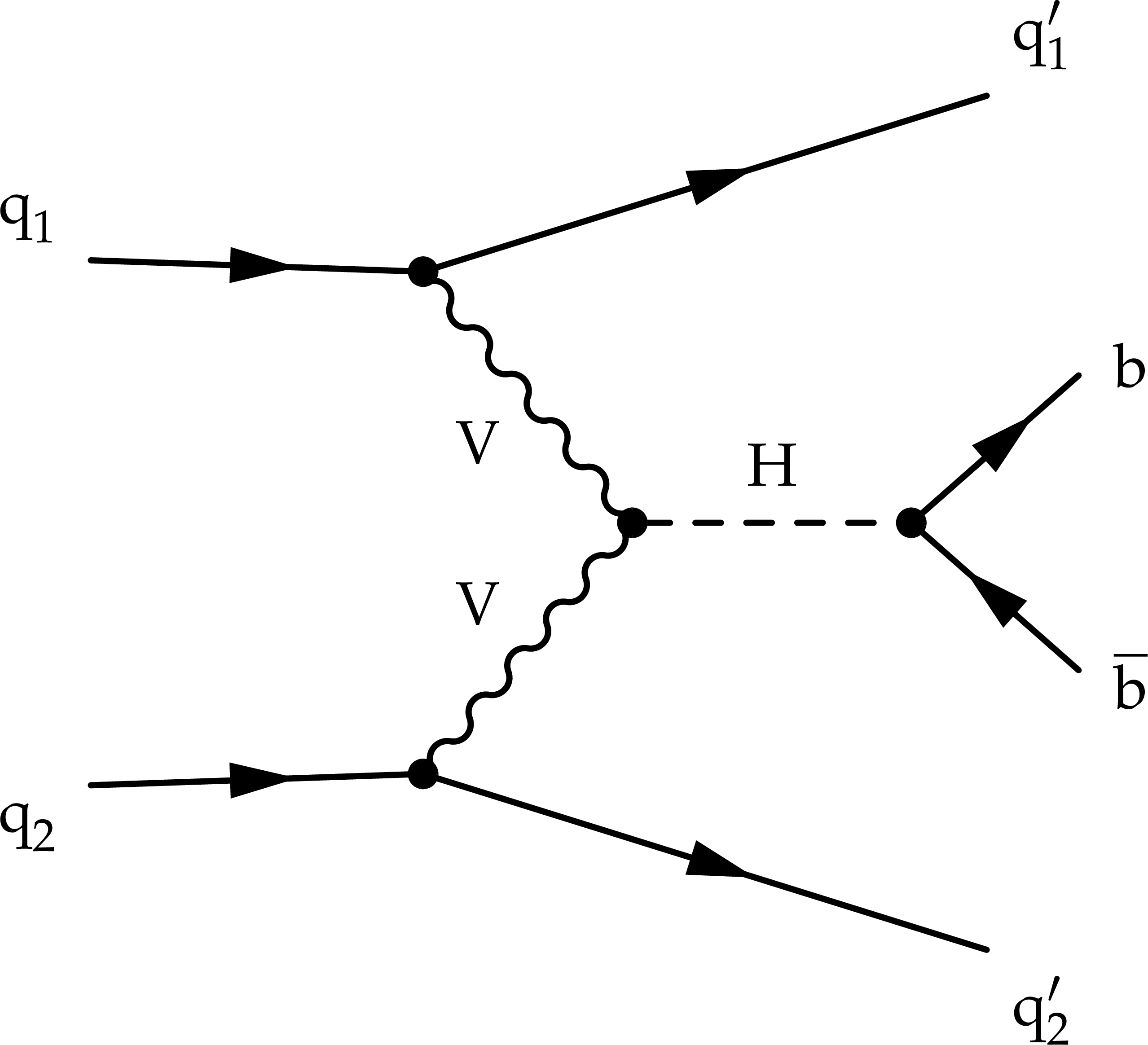
Figure 1:
Representative Feynman diagram of the LO VBF production of a Higgs boson, followed by its decay to a pair of b quarks. |
png pdf |
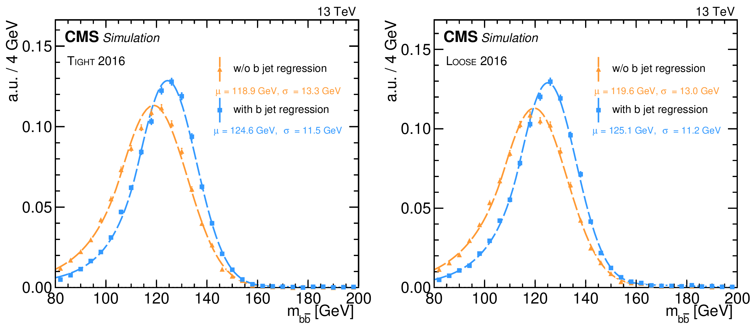
Figure 2:
The invariant mass $ m_{\mathrm{b}\overline{\mathrm{b}}} $ of the b jet pair in simulated $ \mathrm{q}\mathrm{q}\mathrm{H}\to\mathrm{q}\mathrm{q}\mathrm{b}\overline{\mathrm{b}} $ events before (orange dashed line) and after (blue dashed line) the application of the b jet energy regression in the Tight 2016 (left) and Loose 2016 (right) samples. A one-sided Crystal Ball function [50] is used to fit the distributions. |
png pdf |
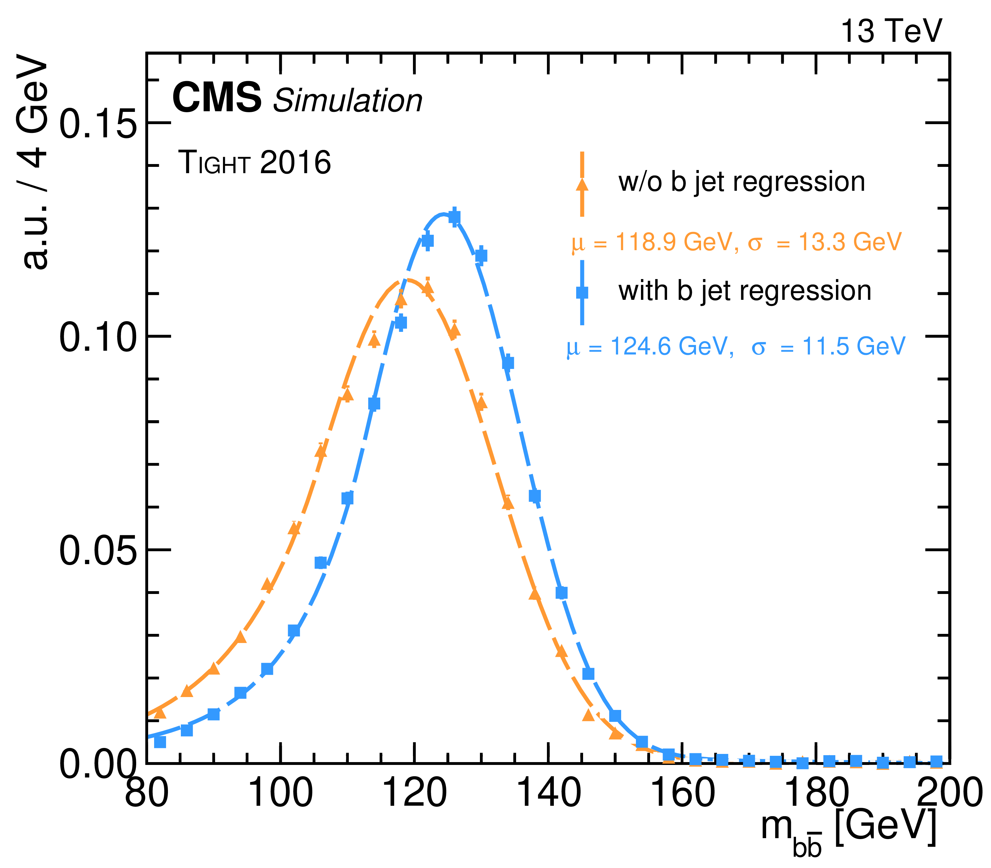
Figure 2-a:
The invariant mass $ m_{\mathrm{b}\overline{\mathrm{b}}} $ of the b jet pair in simulated $ \mathrm{q}\mathrm{q}\mathrm{H}\to\mathrm{q}\mathrm{q}\mathrm{b}\overline{\mathrm{b}} $ events before (orange dashed line) and after (blue dashed line) the application of the b jet energy regression in the Tight 2016 sample. A one-sided Crystal Ball function [50] is used to fit the distributions. |

png pdf |
Figure 2-b:
The invariant mass $ m_{\mathrm{b}\overline{\mathrm{b}}} $ of the b jet pair in simulated $ \mathrm{q}\mathrm{q}\mathrm{H}\to\mathrm{q}\mathrm{q}\mathrm{b}\overline{\mathrm{b}} $ events before (orange dashed line) and after (blue dashed line) the application of the b jet energy regression in the Loose 2016 sample. A one-sided Crystal Ball function [50] is used to fit the distributions. |
png pdf |
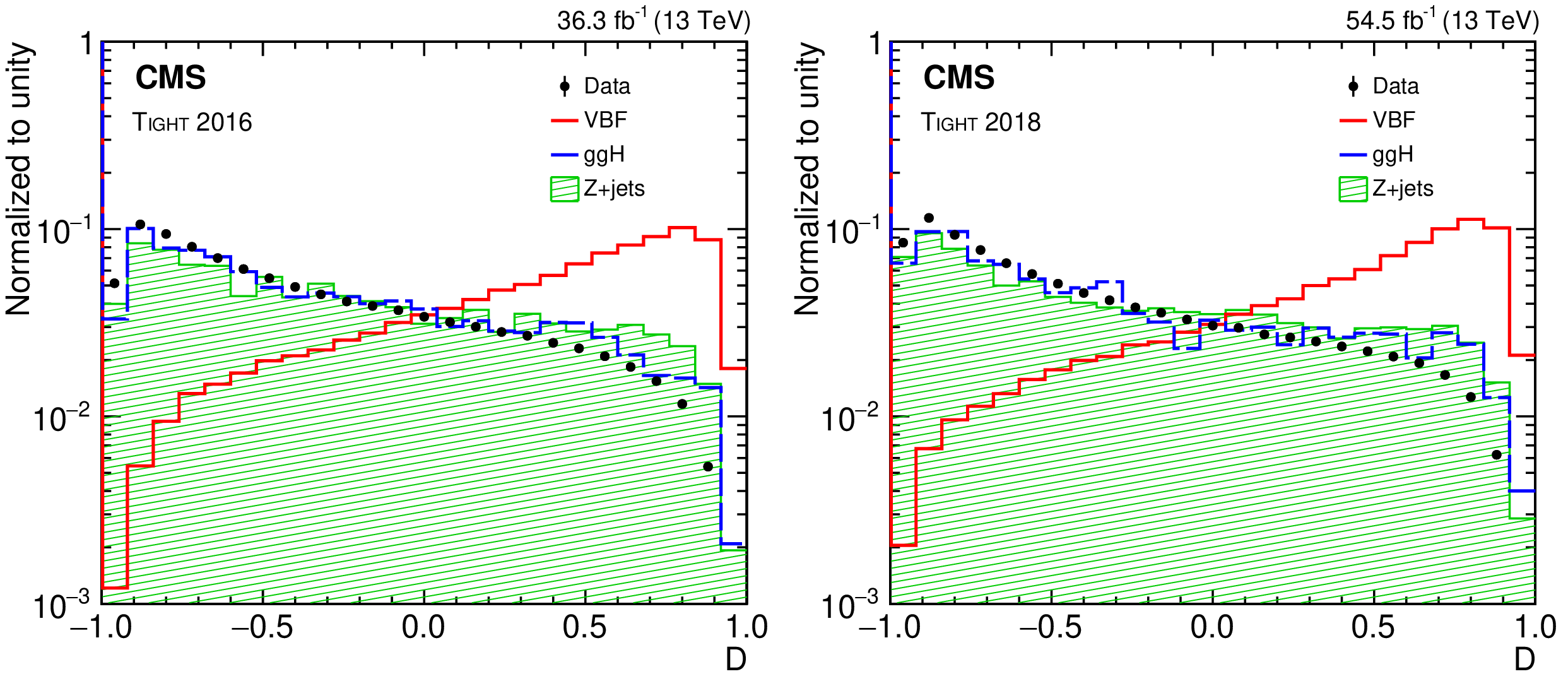
Figure 3:
The unit normalized distributions of the VBF BDT outputs in data and simulated samples in the Tight 2016 (left) and Tight 2018 (right) analysis samples. Data events (points), dominated by the QCD multijet background, are compared to the VBF (red solid line), ggH (blue dashed line), and Z+jets (green hatched area) processes. |

png pdf |
Figure 3-a:
The unit normalized distributions of the VBF BDT outputs in data and simulated samples in the Tight 2016 analysis sample. Data events (points), dominated by the QCD multijet background, are compared to the VBF (red solid line), ggH (blue dashed line), and Z+jets (green hatched area) processes. |
png pdf |
Figure 3-b:
The unit normalized distributions of the VBF BDT outputs in data and simulated samples in the Tight 2018 analysis sample. Data events (points), dominated by the QCD multijet background, are compared to the VBF (red solid line), ggH (blue dashed line), and Z+jets (green hatched area) processes. |
png pdf |
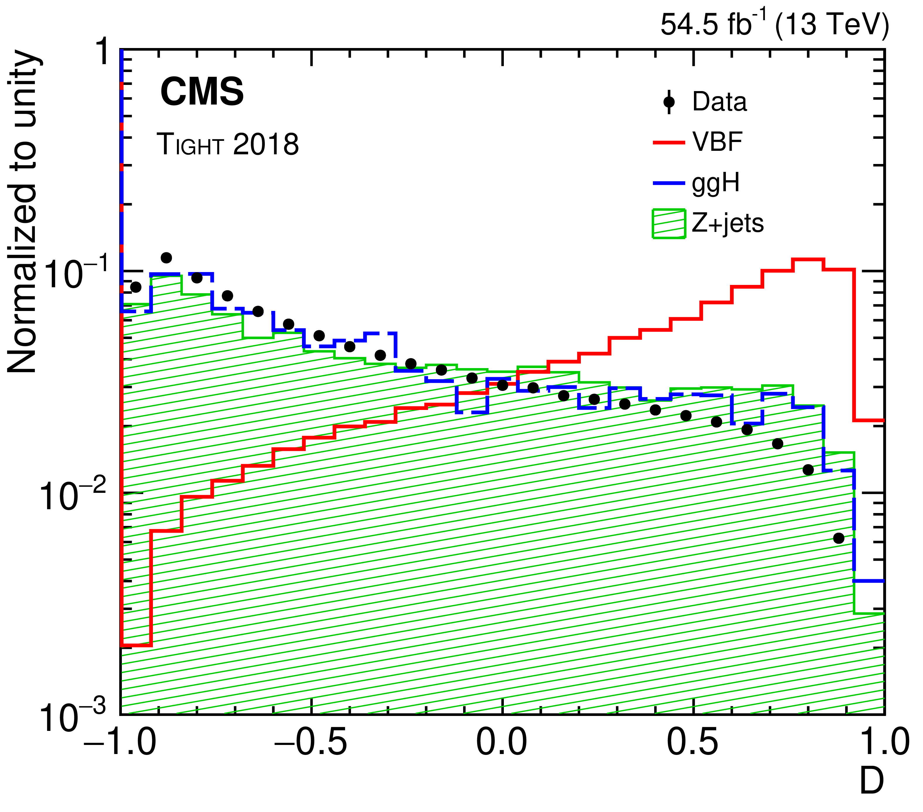
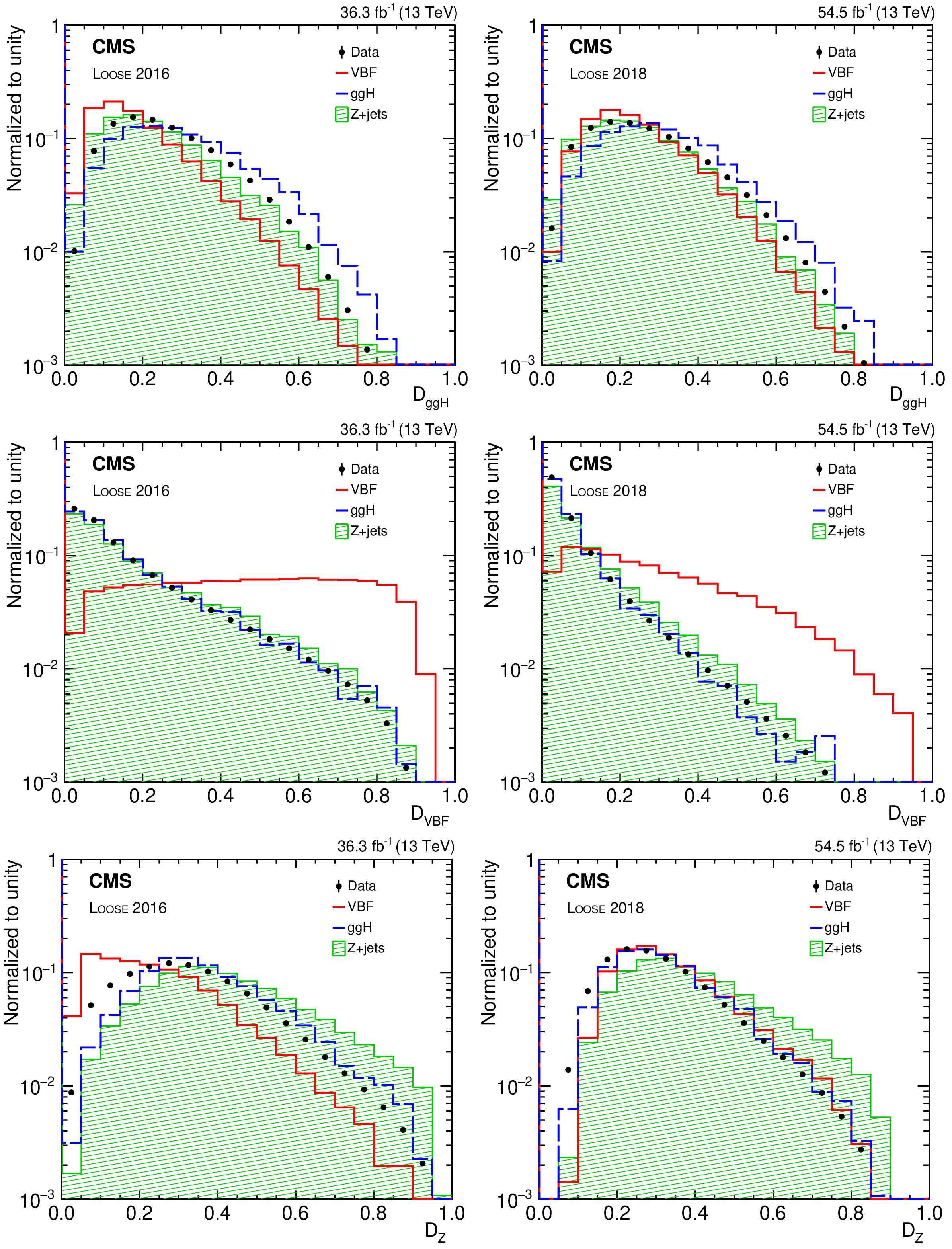
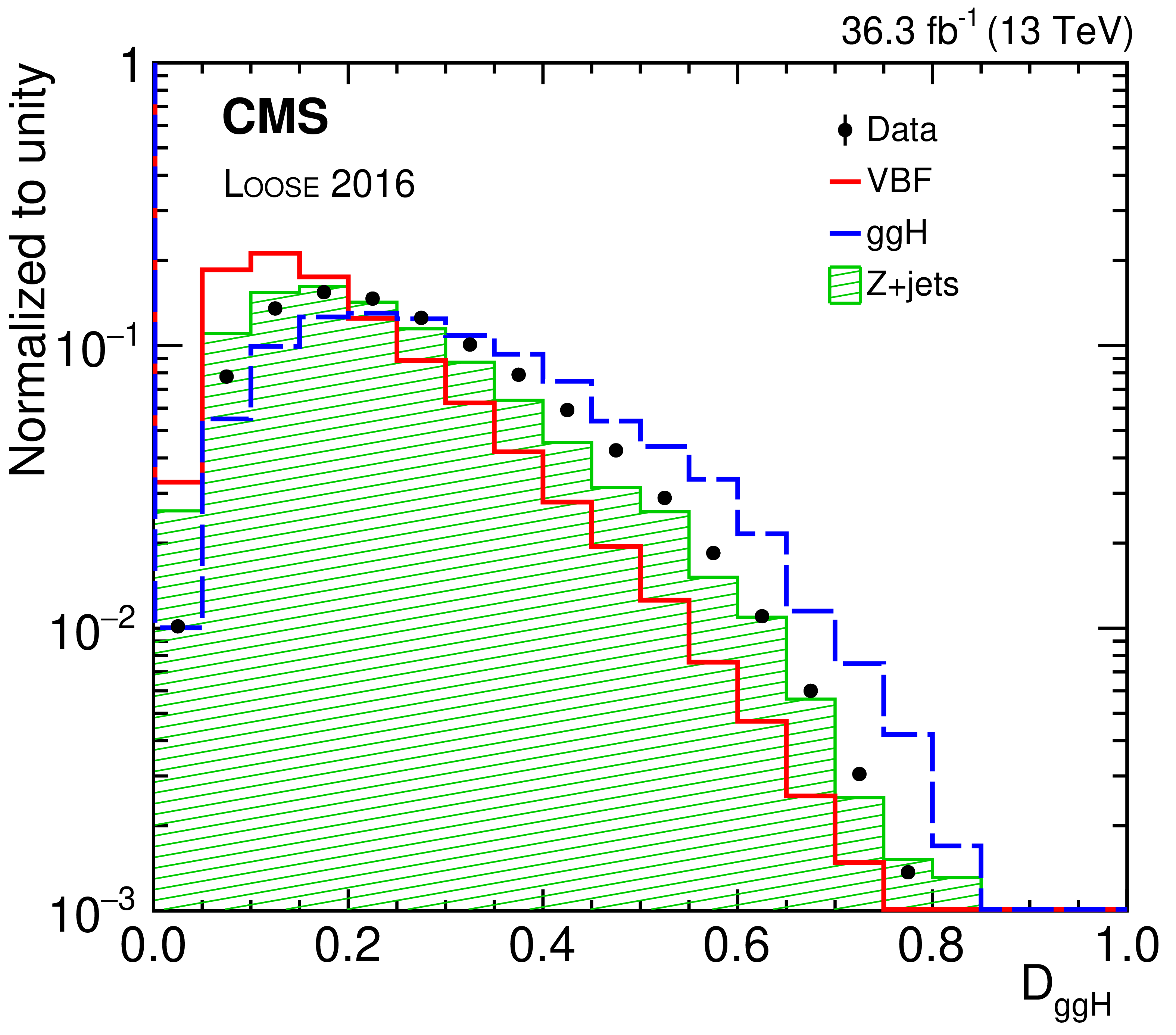
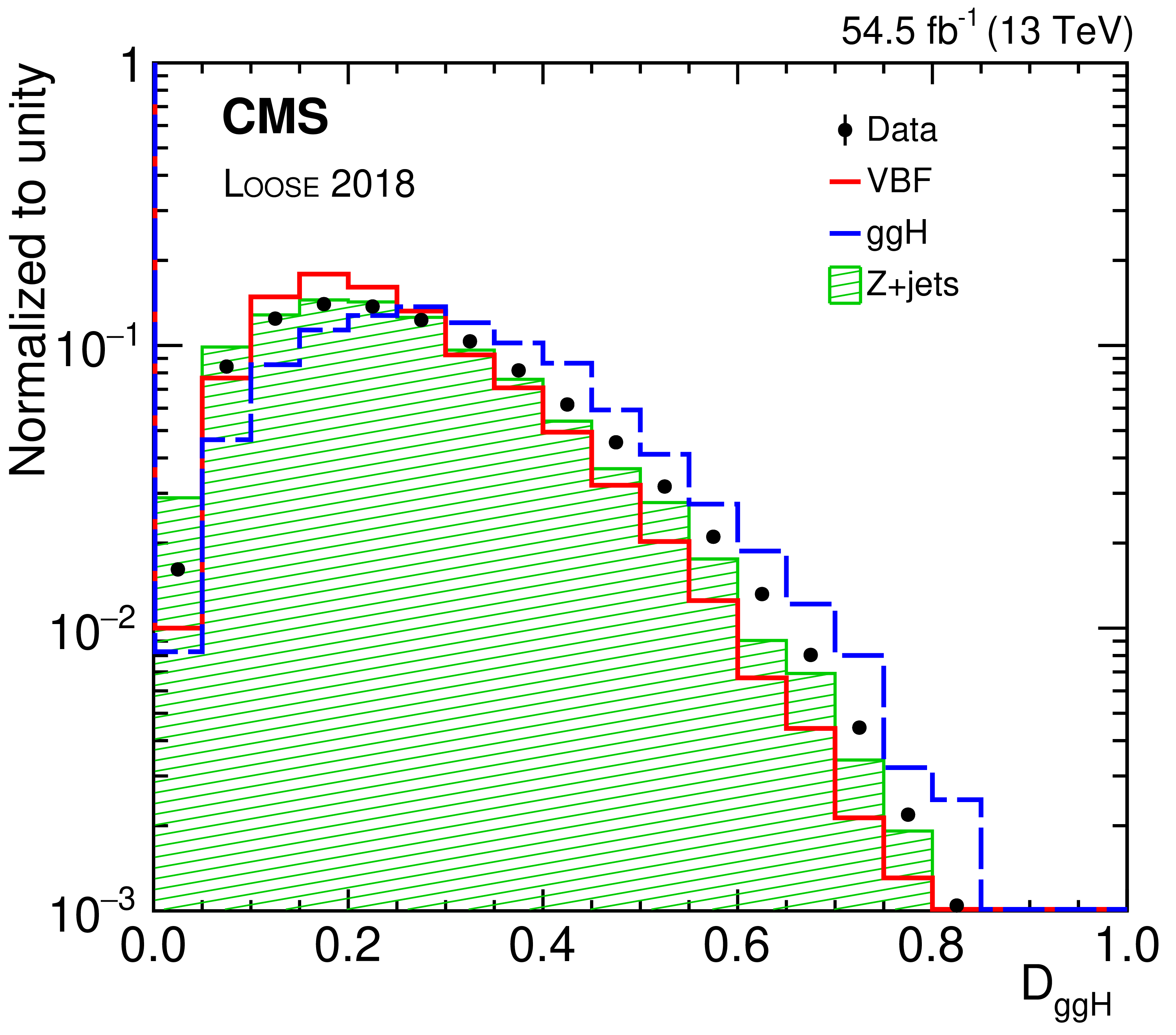
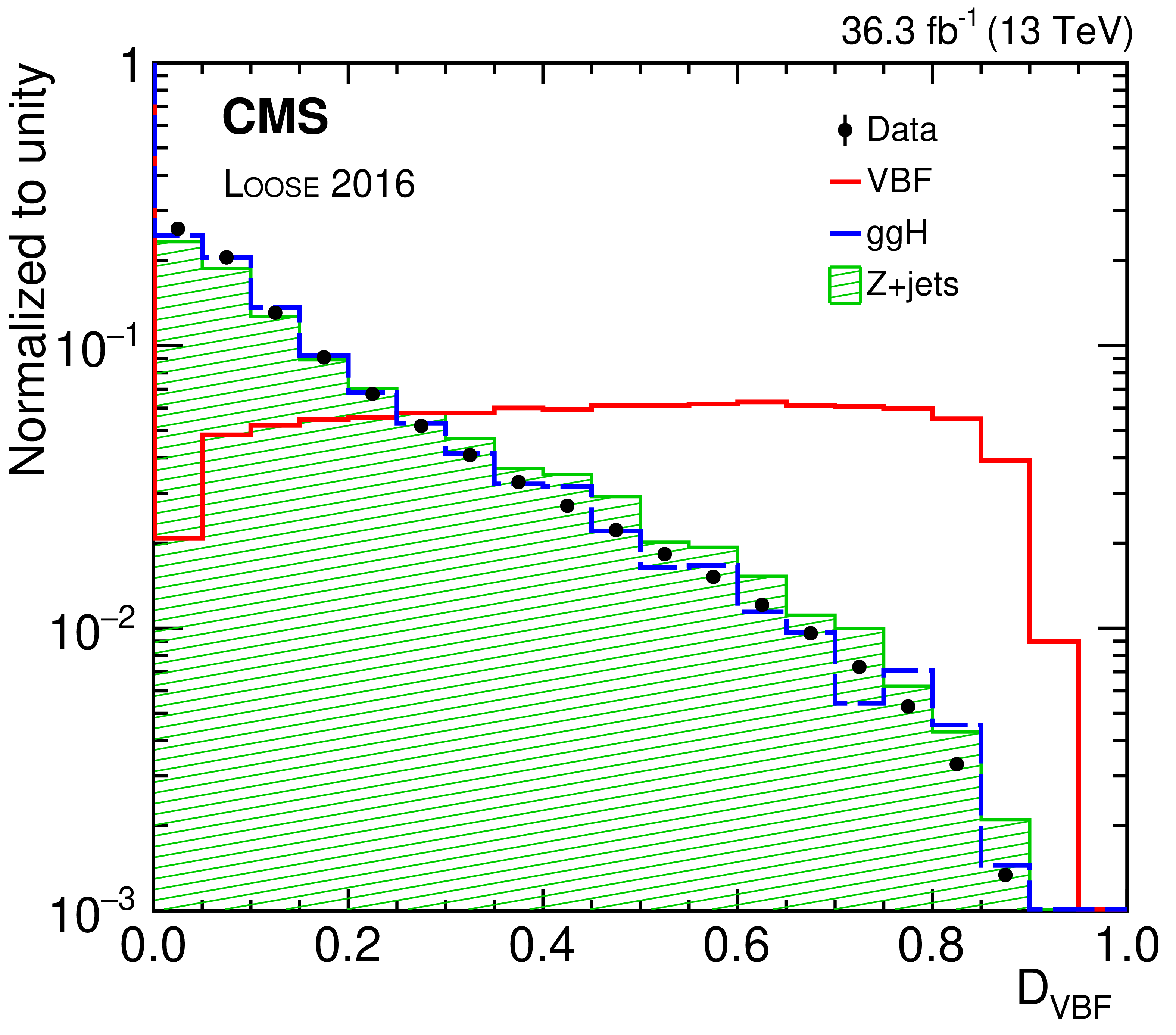
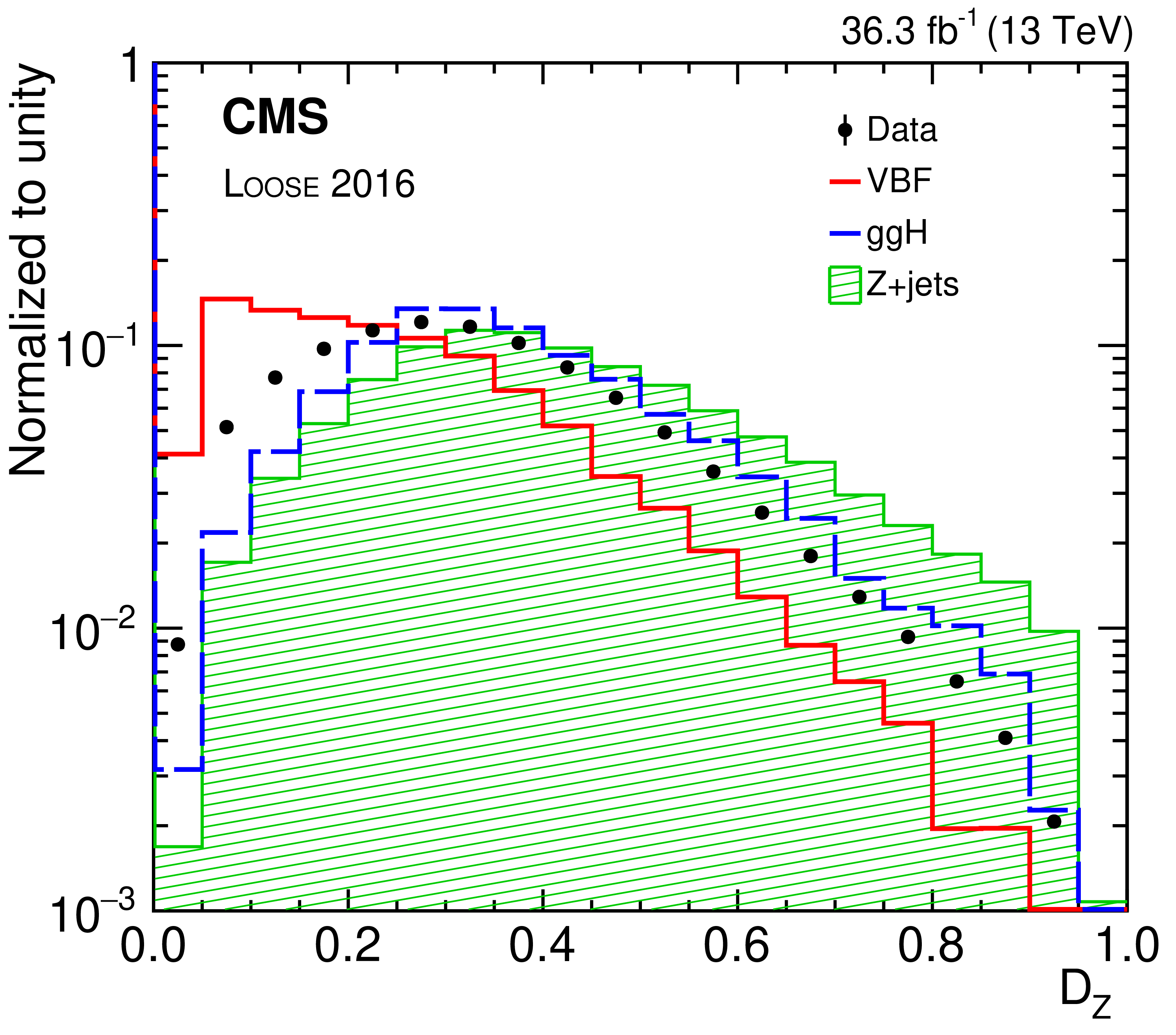
Figure 4:
The unit normalized distributions of the BDT outputs: $ D_{\mathrm{g}\mathrm{g}\mathrm{H}} $ (upper), $ D_{\text{VBF}} $ (middle), and $ D_{\mathrm{Z}} $ (lower) in data and simulated samples in the Loose 2016 (left) and Loose 2018 (right) analysis samples. Data events (points), dominated by the QCD multijet background, are compared to the VBF (red solid line), ggH (blue dashed line), and Z+jets (green hatched area) processes. |
png pdf |
Figure 4-a:
The unit normalized distribution of the $ D_{\mathrm{g}\mathrm{g}\mathrm{H}} $ BDT output in data and simulated samples in the Loose 2016 analysis sample. Data events (points), dominated by the QCD multijet background, are compared to the VBF (red solid line), ggH (blue dashed line), and Z+jets (green hatched area) processes. |
png pdf |
Figure 4-b:
The unit normalized distribution of the $ D_{\mathrm{g}\mathrm{g}\mathrm{H}} $ BDT output in data and simulated samples in the Loose 2018 analysis sample. Data events (points), dominated by the QCD multijet background, are compared to the VBF (red solid line), ggH (blue dashed line), and Z+jets (green hatched area) processes. |
png pdf |
Figure 4-c:
The unit normalized distribution of the $ D_{\text{VBF}} $ BDT output in data and simulated samples in the Loose 2016 analysis sample. Data events (points), dominated by the QCD multijet background, are compared to the VBF (red solid line), ggH (blue dashed line), and Z+jets (green hatched area) processes. |

png pdf |
Figure 4-d:
The unit normalized distribution of the $ D_{\text{VBF}} $ BDT output in data and simulated samples in the Loose 2018 analysis sample. Data events (points), dominated by the QCD multijet background, are compared to the VBF (red solid line), ggH (blue dashed line), and Z+jets (green hatched area) processes. |
png pdf |
Figure 4-e:
The unit normalized distribution of the $ D_{\mathrm{Z}} $ BDT output in data and simulated samples in the Loose 2016 analysis sample. Data events (points), dominated by the QCD multijet background, are compared to the VBF (red solid line), ggH (blue dashed line), and Z+jets (green hatched area) processes. |
png pdf |
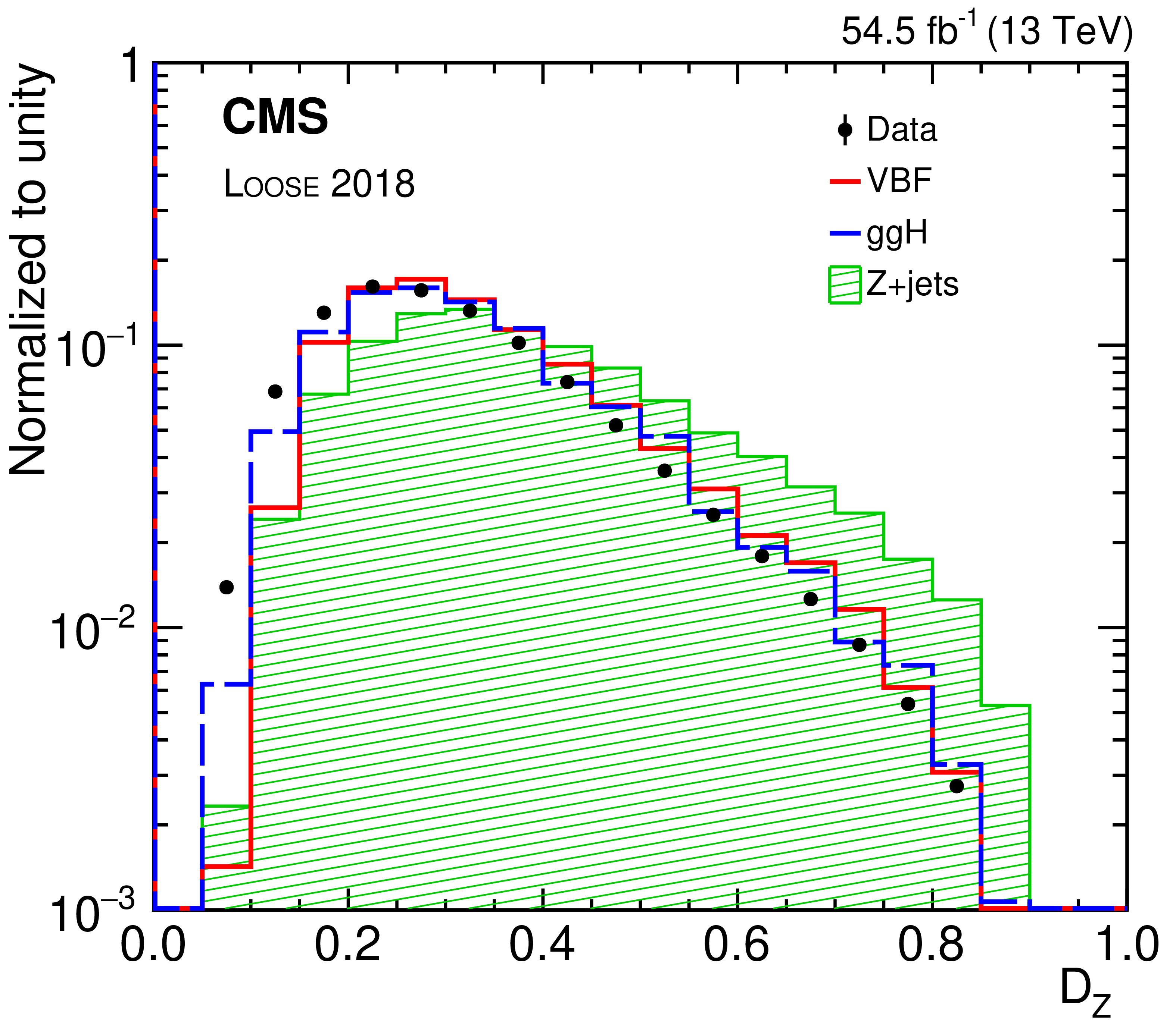
Figure 4-f:
The unit normalized distribution of the $ D_{\mathrm{Z}} $ BDT output in data and simulated samples in the Loose 2018 analysis sample. Data events (points), dominated by the QCD multijet background, are compared to the VBF (red solid line), ggH (blue dashed line), and Z+jets (green hatched area) processes. |
png pdf |
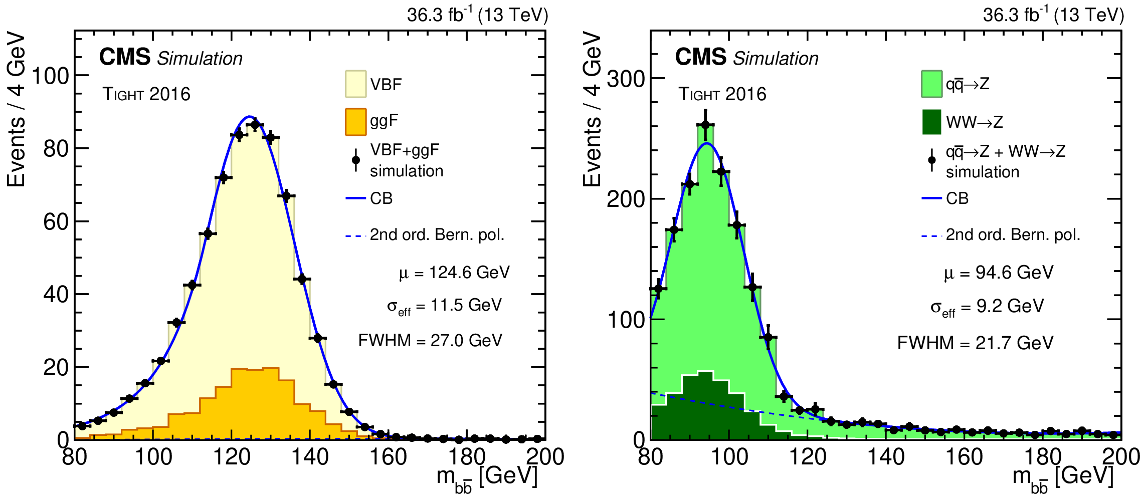
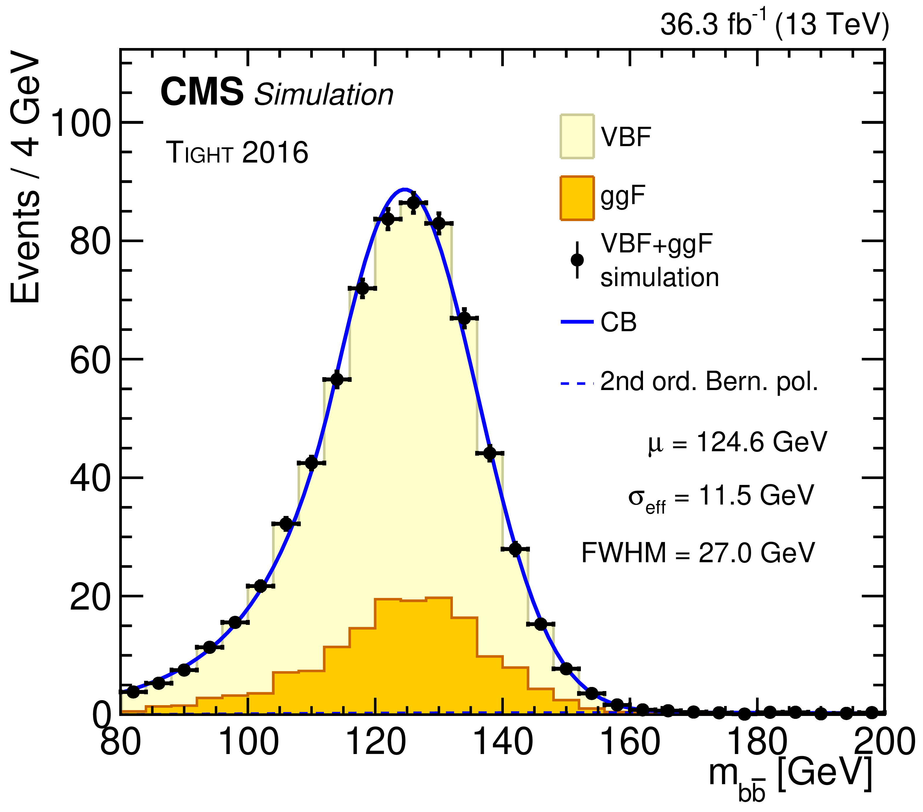
Figure 5:
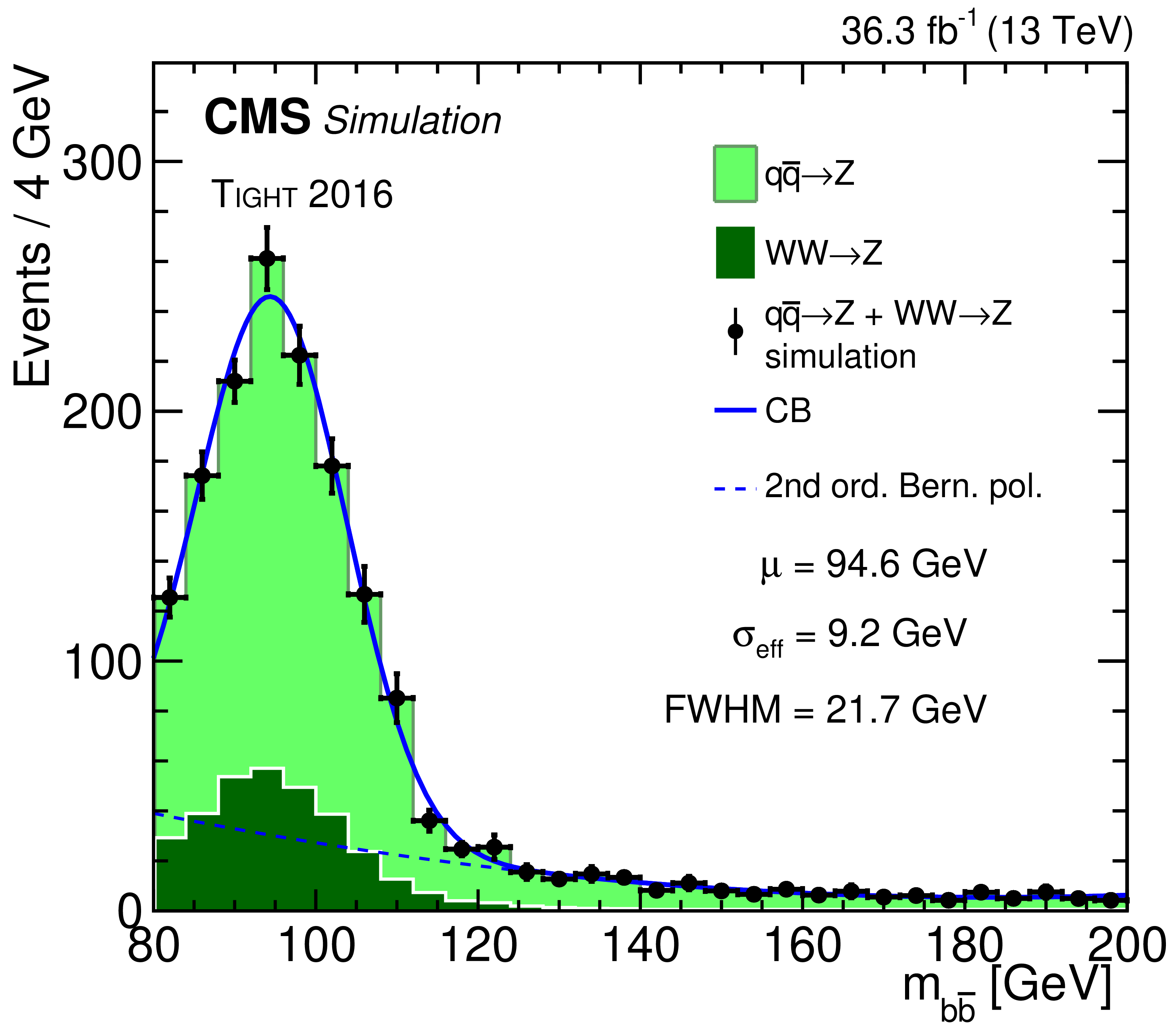
The $ m_{\mathrm{b}\overline{\mathrm{b}}} $ distributions from simulation with overlaid parametric fits (solid blue lines) for the Tight 2016 analysis sample. Left: The fitted $ m_{\mathrm{b}\overline{\mathrm{b}}} $ distribution in the signal combining the VBF (yellow histogram) and ggH (orange) contributions. The black points refer to the total Higgs bosom contribution from VBF and ggH production modes. Right: The fitted $ m_{\mathrm{b}\overline{\mathrm{b}}} $ distribution in simulated Z+jets background (black points) combining the $ \mathrm{W}\mathrm{W}\to\mathrm{Z} $ (dark green histogram) and $ \mathrm{q}\overline{\mathrm{q}}\to\mathrm{Z} $ (light green histogram) production modes. The black points refer to the total Z+jets contribution from $ \mathrm{q}\overline{\mathrm{q}}\to\mathrm{Z} $ and $ \mathrm{W}\mathrm{W}\to\mathrm{Z} $ modes. The dotted lines represent the second-order Bernstein polynomial components used to approximate the contributions from the wrong jet pairing. |
png pdf |
Figure 5-a:
The $ m_{\mathrm{b}\overline{\mathrm{b}}} $ distributions from simulation with overlaid parametric fits (solid blue lines) for the Tight 2016 analysis sample. The fitted $ m_{\mathrm{b}\overline{\mathrm{b}}} $ distribution in the signal combining the VBF (yellow histogram) and ggH (orange) contributions. The black points refer to the total Higgs bosom contribution from VBF and ggH production modes. |
png pdf |
Figure 5-b:
The $ m_{\mathrm{b}\overline{\mathrm{b}}} $ distributions from simulation with overlaid parametric fits (solid blue lines) for the Tight 2016 analysis sample. The fitted $ m_{\mathrm{b}\overline{\mathrm{b}}} $ distribution in simulated Z+jets background (black points) combining the $ \mathrm{W}\mathrm{W}\to\mathrm{Z} $ (dark green histogram) and $ \mathrm{q}\overline{\mathrm{q}}\to\mathrm{Z} $ (light green histogram) production modes. The black points refer to the total Z+jets contribution from $ \mathrm{q}\overline{\mathrm{q}}\to\mathrm{Z} $ and $ \mathrm{W}\mathrm{W}\to\mathrm{Z} $ modes. The dotted lines represent the second-order Bernstein polynomial components used to approximate the contributions from the wrong jet pairing. |

png pdf |
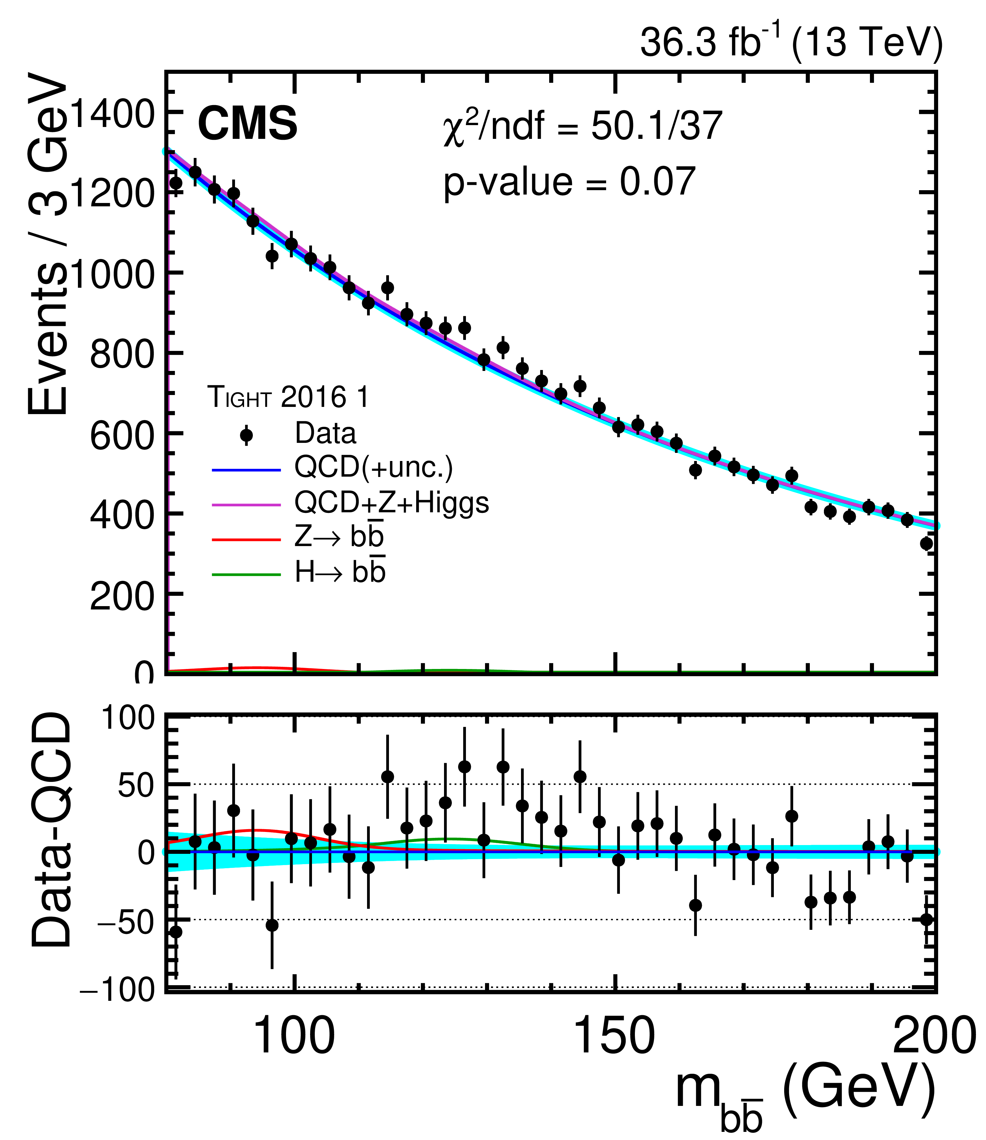
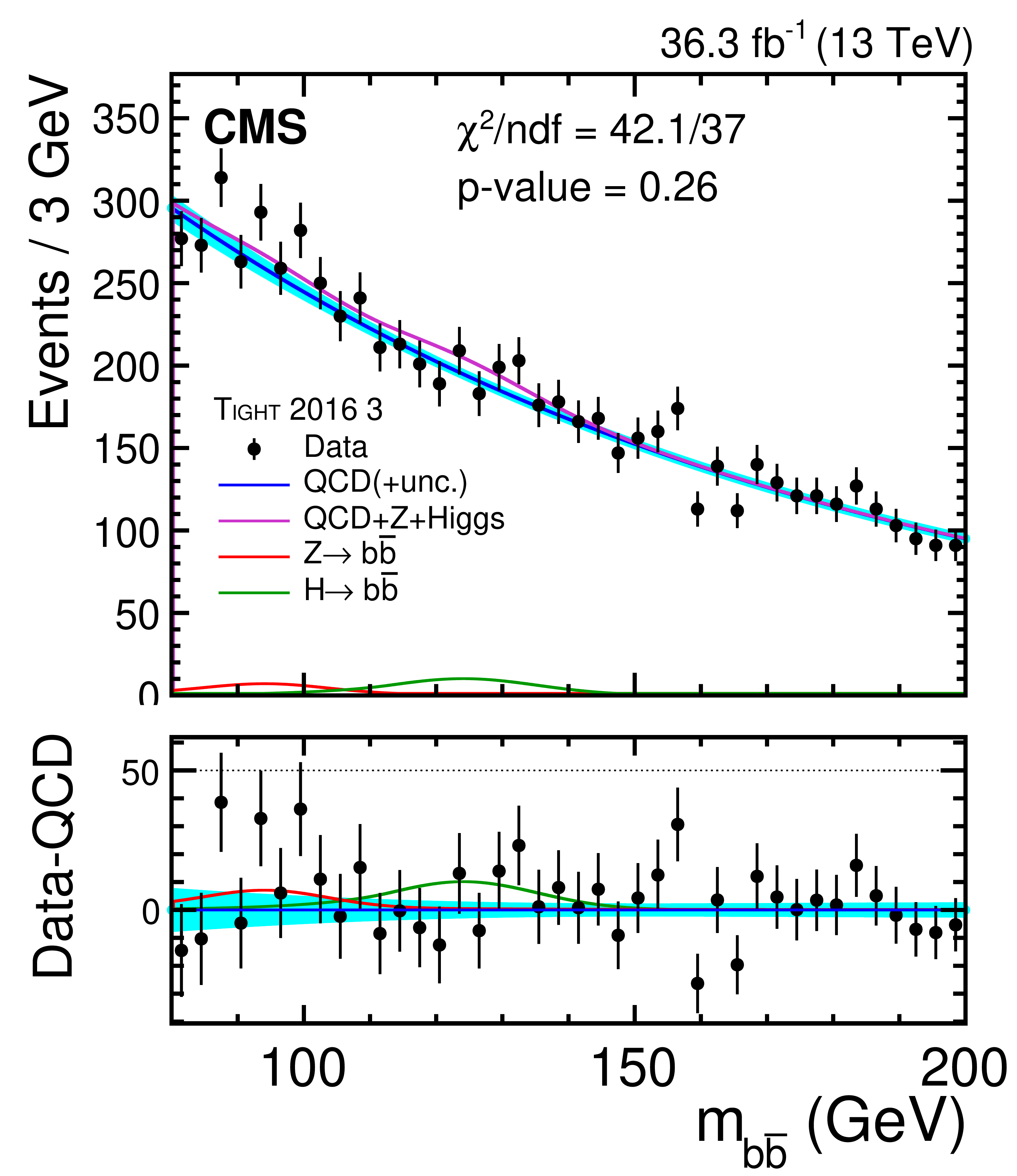
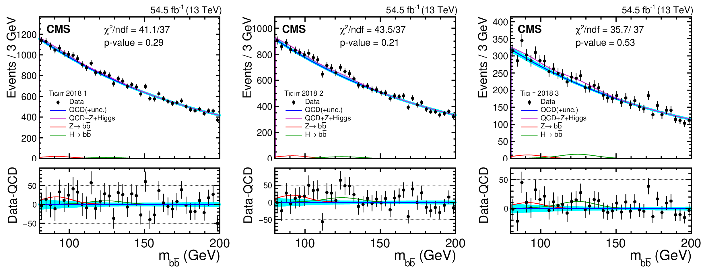
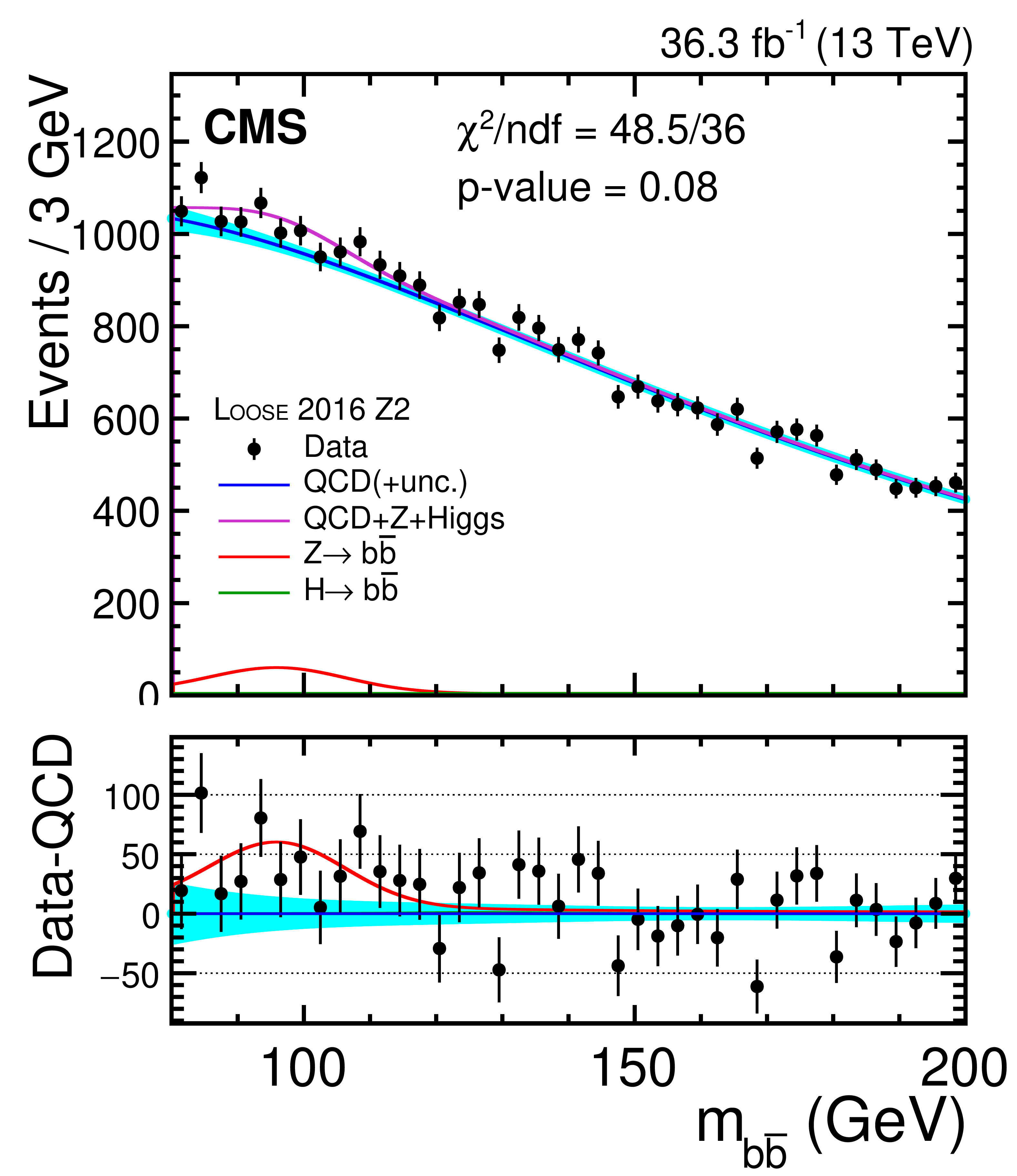
Figure 6:
The $ m_{\mathrm{b}\overline{\mathrm{b}}} $ distributions in three event categories: Tight 2016 1 (left), Tight 2016 2 (center), and Tight 2016 3 (right). The points indicate data, the blue solid curve corresponds to the fitted nonresonant component of the background, dominated by QCD multijet events; the shaded (cyan) band represents the $ \pm $1$ \sigma $ uncertainty band. The total signal-plus-background model includes contributions from $ \mathrm{Z}\to\mathrm{b}\overline{\mathrm{b}} $, $ \mathrm{H}\to\mathrm{b}\overline{\mathrm{b}} $, and the nonresonant component; it is represented by the magenta curve. The lower panel compares the distribution of the data after subtracting the nonresonant component with the resonant contributions of the $ \mathrm{Z}\to\mathrm{b}\overline{\mathrm{b}} $ background (red curve) and $ \mathrm{H}\to\mathrm{b}\overline{\mathrm{b}} $ signal (green curve). |
png pdf |
Figure 6-a:
The $ m_{\mathrm{b}\overline{\mathrm{b}}} $ distributions in the Tight 2016 1 category. The points indicate data, the blue solid curve corresponds to the fitted nonresonant component of the background, dominated by QCD multijet events; the shaded (cyan) band represents the $ \pm $1$ \sigma $ uncertainty band. The total signal-plus-background model includes contributions from $ \mathrm{Z}\to\mathrm{b}\overline{\mathrm{b}} $, $ \mathrm{H}\to\mathrm{b}\overline{\mathrm{b}} $, and the nonresonant component; it is represented by the magenta curve. The lower panel compares the distribution of the data after subtracting the nonresonant component with the resonant contributions of the $ \mathrm{Z}\to\mathrm{b}\overline{\mathrm{b}} $ background (red curve) and $ \mathrm{H}\to\mathrm{b}\overline{\mathrm{b}} $ signal (green curve). |

png pdf |
Figure 6-b:
The $ m_{\mathrm{b}\overline{\mathrm{b}}} $ distributions in the Tight 2016 2 category. The points indicate data, the blue solid curve corresponds to the fitted nonresonant component of the background, dominated by QCD multijet events; the shaded (cyan) band represents the $ \pm $1$ \sigma $ uncertainty band. The total signal-plus-background model includes contributions from $ \mathrm{Z}\to\mathrm{b}\overline{\mathrm{b}} $, $ \mathrm{H}\to\mathrm{b}\overline{\mathrm{b}} $, and the nonresonant component; it is represented by the magenta curve. The lower panel compares the distribution of the data after subtracting the nonresonant component with the resonant contributions of the $ \mathrm{Z}\to\mathrm{b}\overline{\mathrm{b}} $ background (red curve) and $ \mathrm{H}\to\mathrm{b}\overline{\mathrm{b}} $ signal (green curve). |
png pdf |
Figure 6-c:
The $ m_{\mathrm{b}\overline{\mathrm{b}}} $ distributions in the Tight 2016 3 category. The points indicate data, the blue solid curve corresponds to the fitted nonresonant component of the background, dominated by QCD multijet events; the shaded (cyan) band represents the $ \pm $1$ \sigma $ uncertainty band. The total signal-plus-background model includes contributions from $ \mathrm{Z}\to\mathrm{b}\overline{\mathrm{b}} $, $ \mathrm{H}\to\mathrm{b}\overline{\mathrm{b}} $, and the nonresonant component; it is represented by the magenta curve. The lower panel compares the distribution of the data after subtracting the nonresonant component with the resonant contributions of the $ \mathrm{Z}\to\mathrm{b}\overline{\mathrm{b}} $ background (red curve) and $ \mathrm{H}\to\mathrm{b}\overline{\mathrm{b}} $ signal (green curve). |
png pdf |
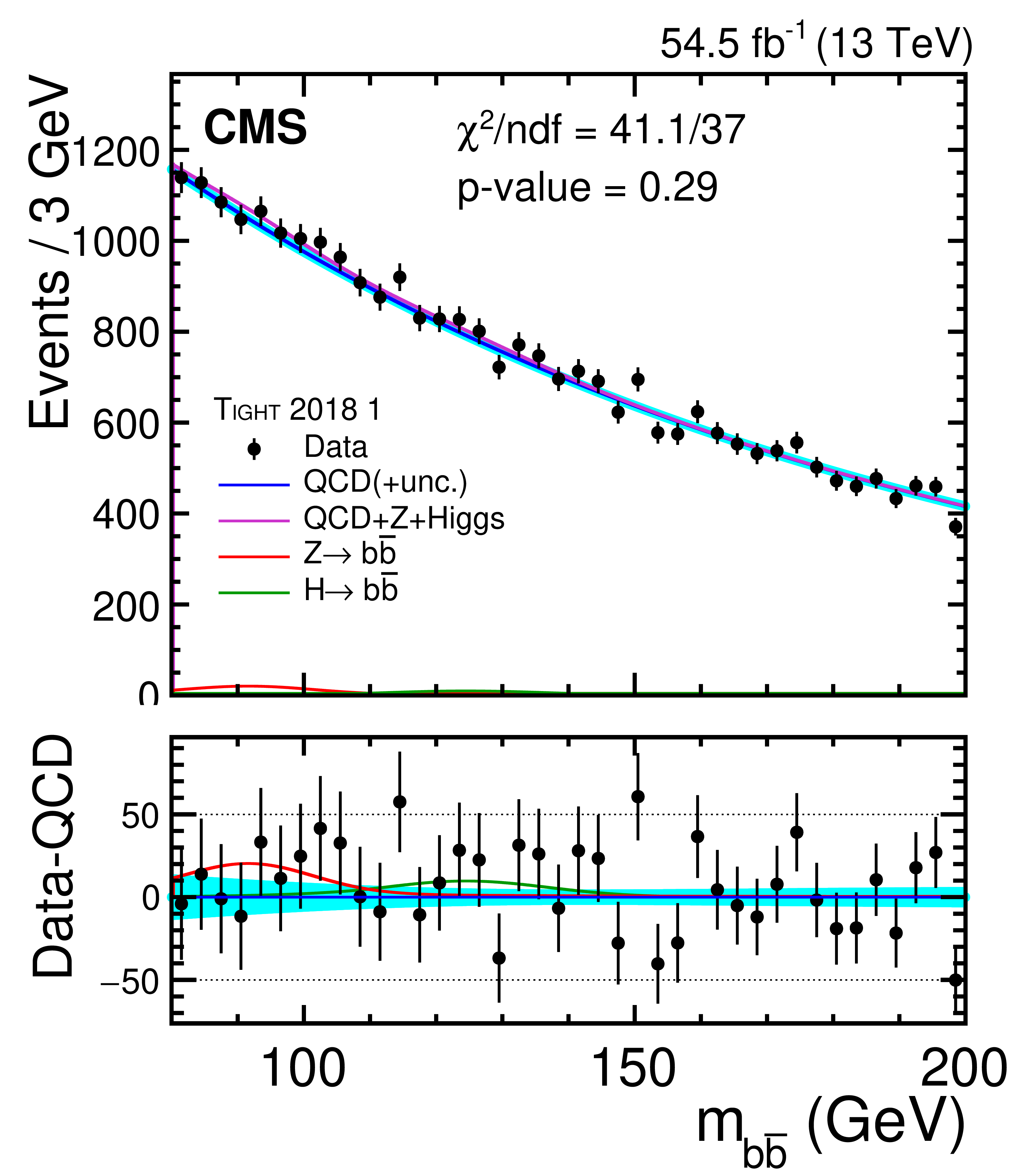
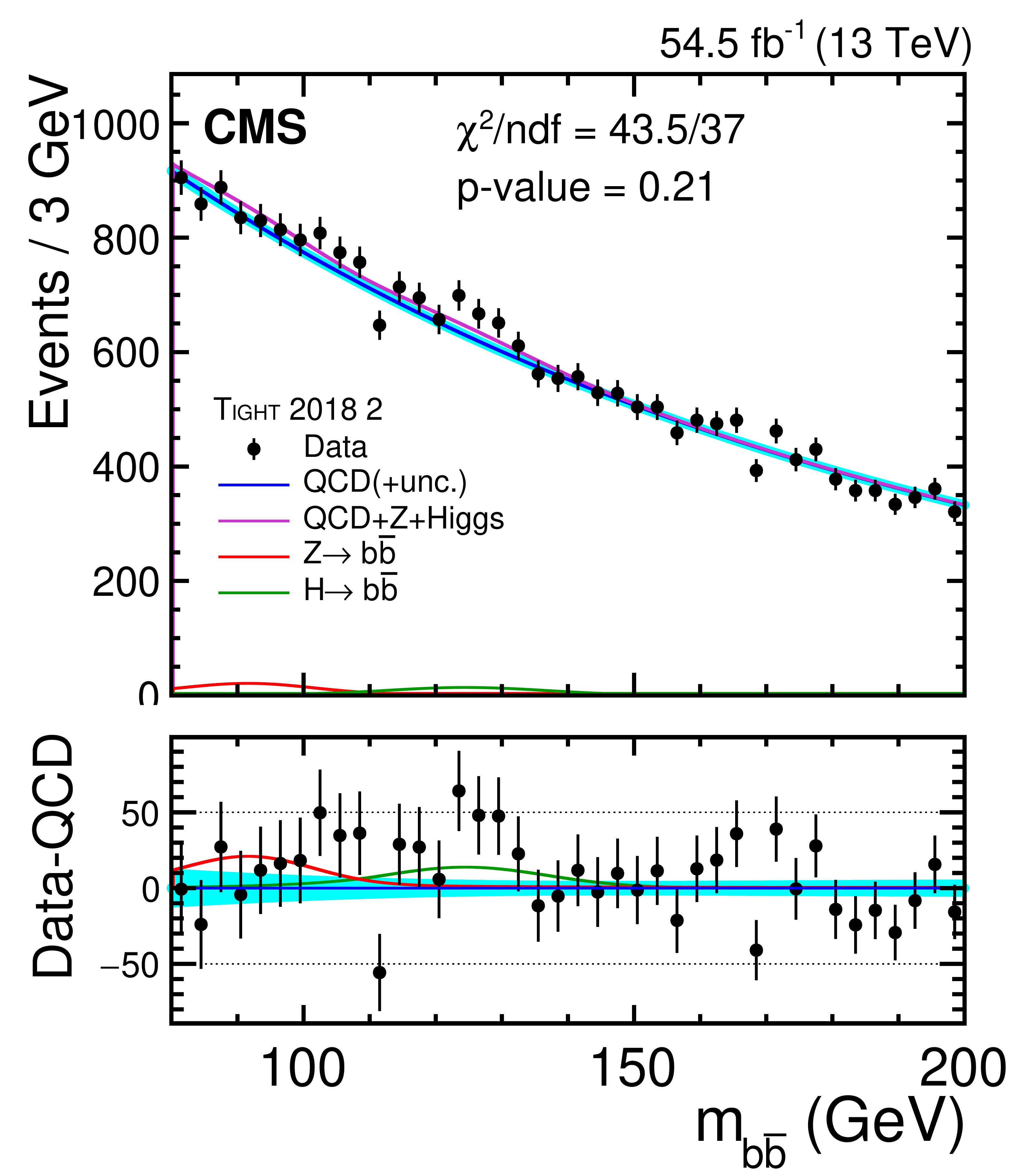
Figure 7:
The $ m_{\mathrm{b}\overline{\mathrm{b}}} $ distributions in three event categories: Tight 2018 1 (left), Tight 2018 2 (center), and Tight 2018 3 (right). A complete description is given in Fig. 6. |
png pdf |
Figure 7-a:
The $ m_{\mathrm{b}\overline{\mathrm{b}}} $ distributions in three event categories: Tight 2018 1. A complete description is given in Fig. 6. |
png pdf |
Figure 7-b:
The $ m_{\mathrm{b}\overline{\mathrm{b}}} $ distributions in three event categories: Tight 2018 2. A complete description is given in Fig. 6. |

png pdf |
Figure 7-c:
The $ m_{\mathrm{b}\overline{\mathrm{b}}} $ distributions in three event categories: Tight 2018 3. A complete description is given in Fig. 6. |
png pdf |
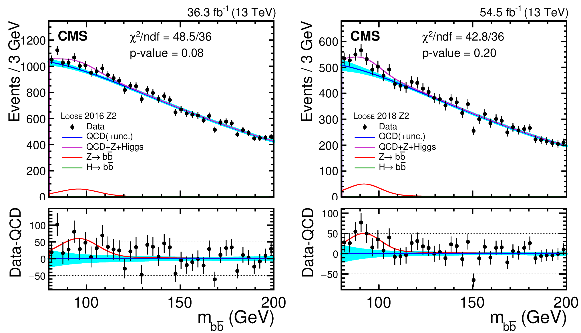
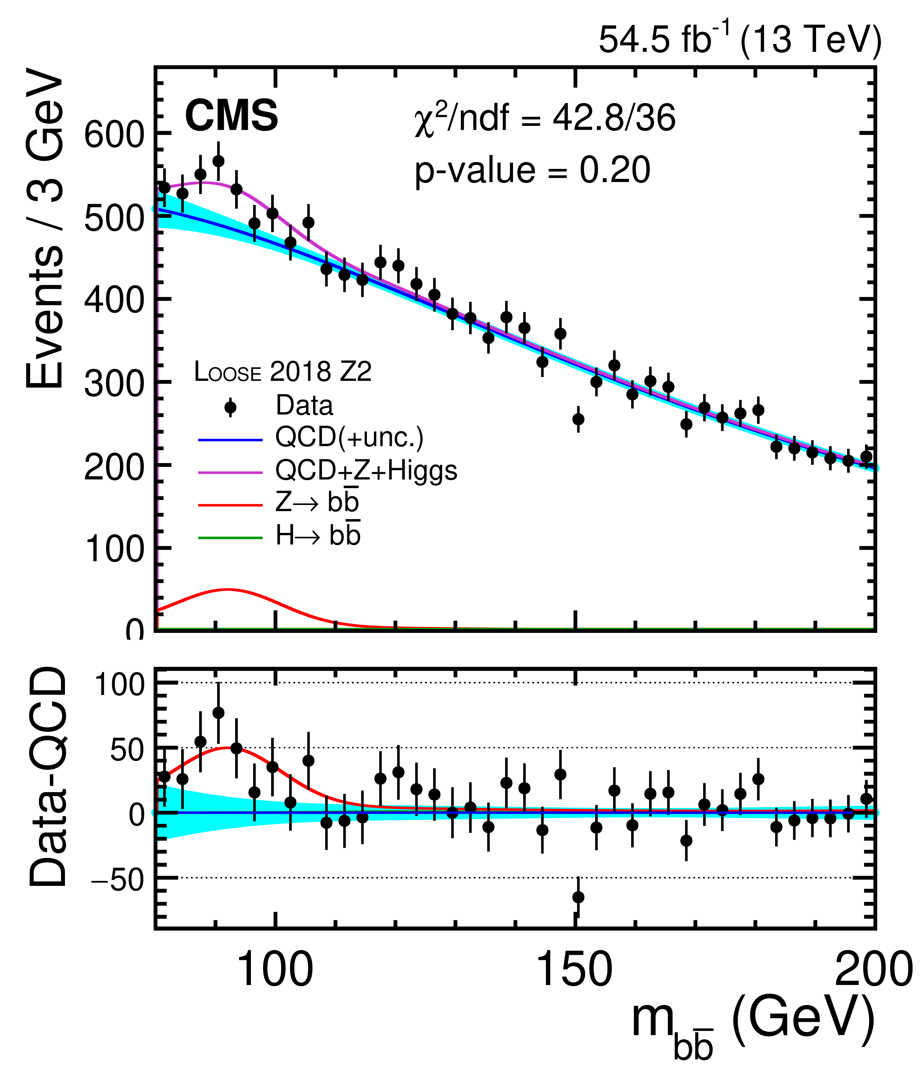
Figure 8:
The $ m_{\mathrm{b}\overline{\mathrm{b}}} $ distributions in two event categories: Loose 2016 Z2 (left) and Loose 2018 Z2 (right). A complete description is given in Fig. 6. |
png pdf |
Figure 8-a:
The $ m_{\mathrm{b}\overline{\mathrm{b}}} $ distributions in two event categories: Loose 2016 Z2. A complete description is given in Fig. 6. |
png pdf |
Figure 8-b:
The $ m_{\mathrm{b}\overline{\mathrm{b}}} $ distributions in two event categories: Loose 2018 Z2. A complete description is given in Fig. 6. |
png pdf |
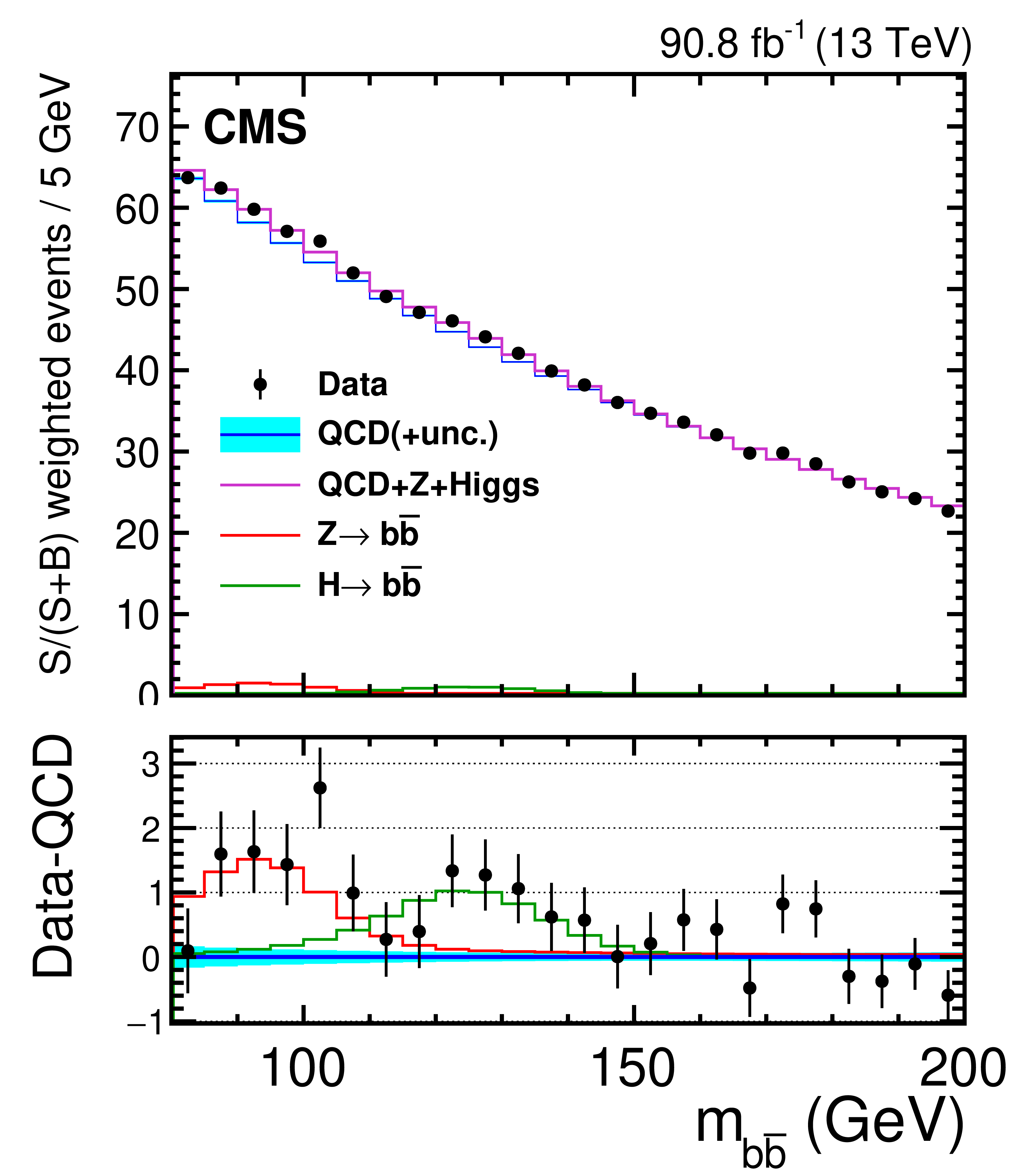
Figure 9:
The $ m_{\mathrm{b}\overline{\mathrm{b}}} $ distribution after weighted combination of all categories in the analysis weighted with $ S/(S+B) $. A complete description is given in Fig. 6. |
png pdf |
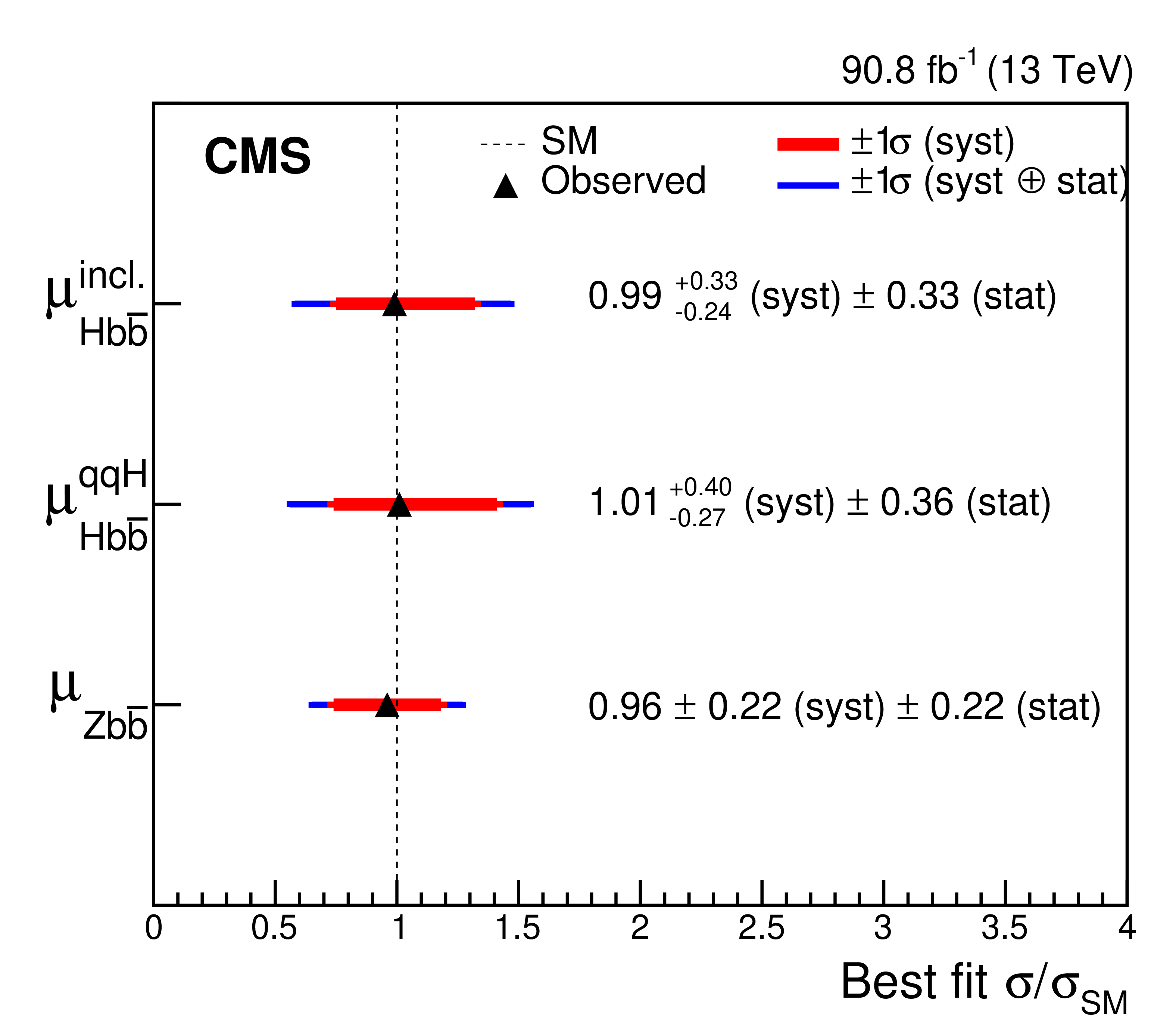
Figure 10:
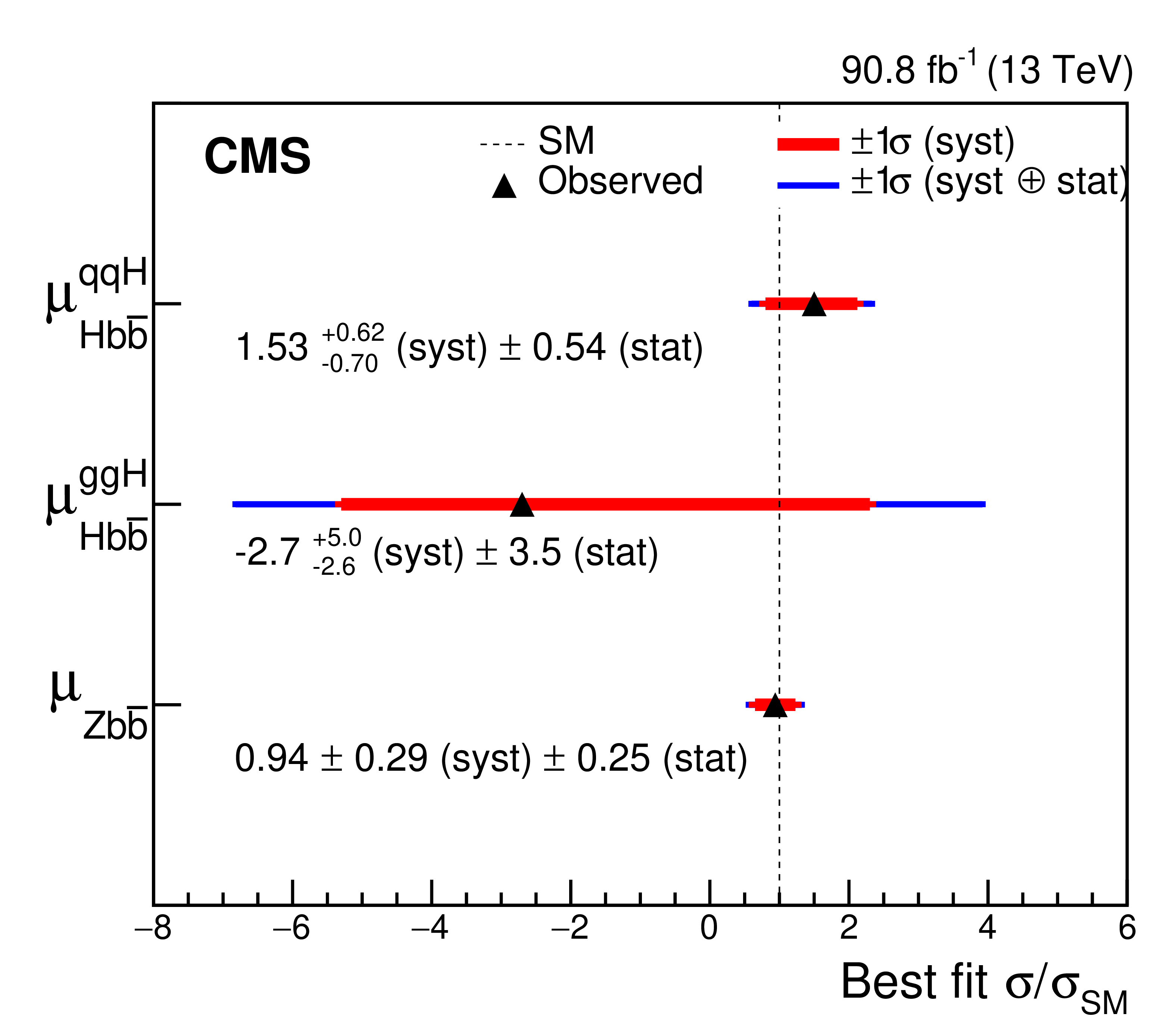
The best fit values of the signal strength modifier for the different processes. The horizontal bars in blue and red colors represent the $ \pm$1$\sigma $ total uncertainty and its systematic component. The vertical dashed line shows the standard model prediction. |
png pdf |
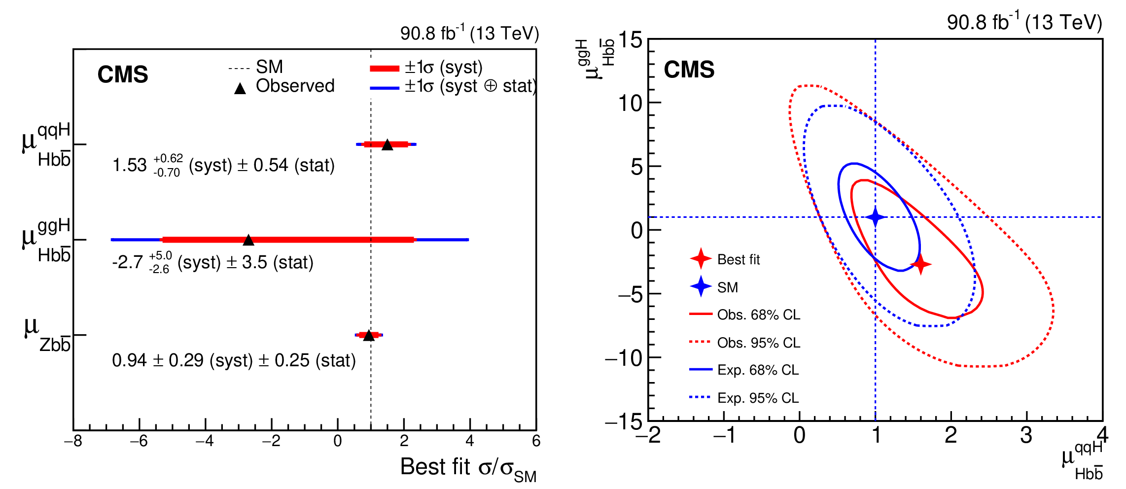
Figure 11:
The best fit values of the signal strength modifier for the different processes, the horizontal bars in blue and red colors represent the $ \pm1\,\sigma $ total uncertainty and its systematic component and the vertical dashed line shows the SM prediction (left). The two-dimensional likelihood scan of $ \mu^{\mathrm{q}\mathrm{q}\mathrm{H}}_{\mathrm{H}\mathrm{b}\overline{\mathrm{b}}} $ and $ \mu^{\mathrm{g}\mathrm{g}\mathrm{H}}_{\mathrm{H}\mathrm{b}\overline{\mathrm{b}}} $, the red (blue) solid and dashed lines correspond to the observed (expected) 68 and 95% CL contours in the $ (\mu^{\mathrm{q}\mathrm{q}\mathrm{H}}_{\mathrm{H}\mathrm{b}\overline{\mathrm{b}}}, \mu^{\mathrm{g}\mathrm{g}\mathrm{H}}_{\mathrm{H}\mathrm{b}\overline{\mathrm{b}}}) $ plane (right). The SM predicted and observed best fit values are indicated by the blue and red crosses. |
png pdf |
Figure 11-a:
The best fit values of the signal strength modifier for the different processes, the horizontal bars in blue and red colors represent the $ \pm1\,\sigma $ total uncertainty and its systematic component and the vertical dashed line shows the SM prediction. |

png pdf |
Figure 11-b:
The two-dimensional likelihood scan of $ \mu^{\mathrm{q}\mathrm{q}\mathrm{H}}_{\mathrm{H}\mathrm{b}\overline{\mathrm{b}}} $ and $ \mu^{\mathrm{g}\mathrm{g}\mathrm{H}}_{\mathrm{H}\mathrm{b}\overline{\mathrm{b}}} $, the red (blue) solid and dashed lines correspond to the observed (expected) 68 and 95% CL contours in the $ (\mu^{\mathrm{q}\mathrm{q}\mathrm{H}}_{\mathrm{H}\mathrm{b}\overline{\mathrm{b}}}, \mu^{\mathrm{g}\mathrm{g}\mathrm{H}}_{\mathrm{H}\mathrm{b}\overline{\mathrm{b}}}) $ plane (right). The SM predicted and observed best fit values are indicated by the blue and red crosses. |
| Tables | |
png pdf |
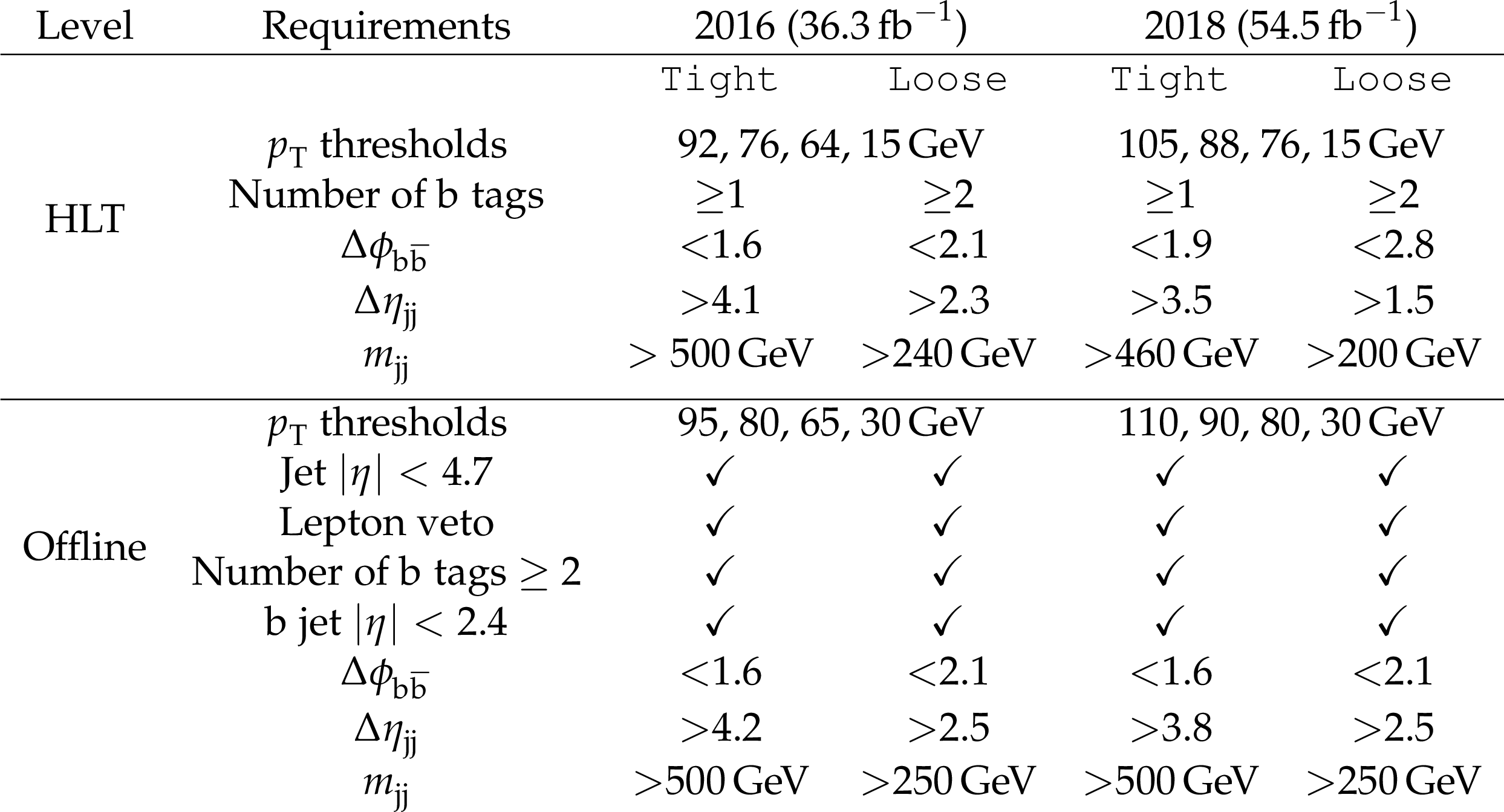
Table 1:
The HLT and offline selection requirements in the four analyzed samples. |
png pdf |
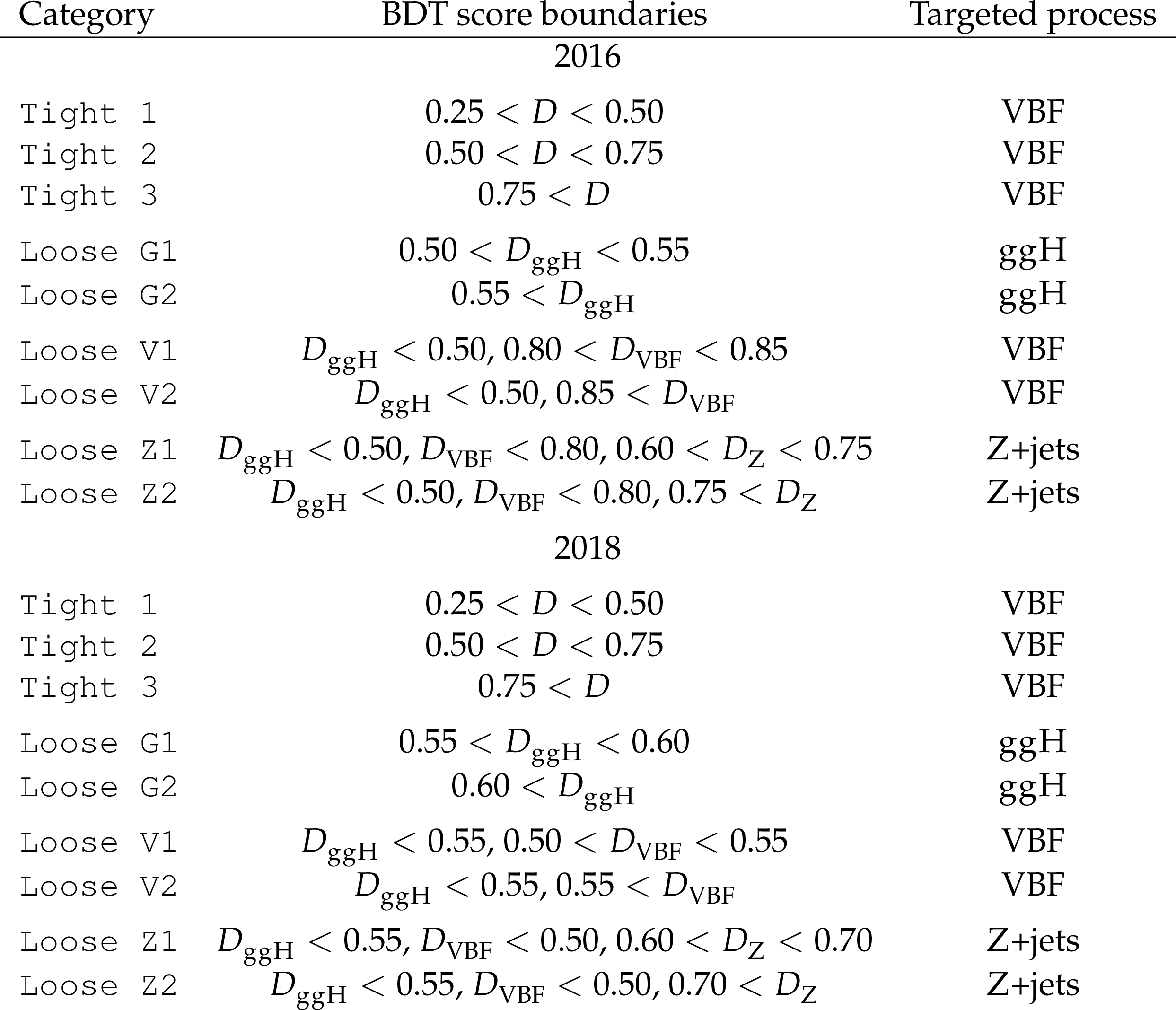
Table 2:
Event categorization used in the analysis for a total of 18 categories. The names of the categories are given in the first column. The BDT score boundaries defining each category are given in the second column and the targeted process is indicated in the third column. |
png pdf |
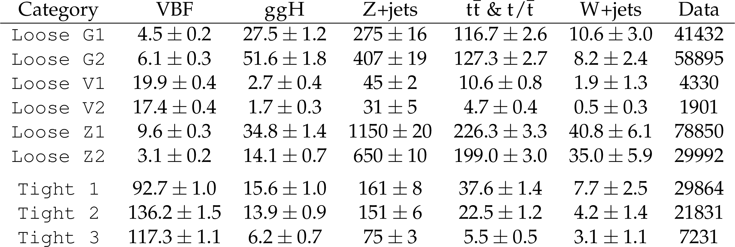
Table 3:
Event yields for various categories of the analyzed 2016 data corresponding to 36.3 fb$ ^{-1} $, compared to the expected number of events from the simulated samples of signal and background other than the QCD multijet process. The quoted uncertainties are statistical only. |
png pdf |
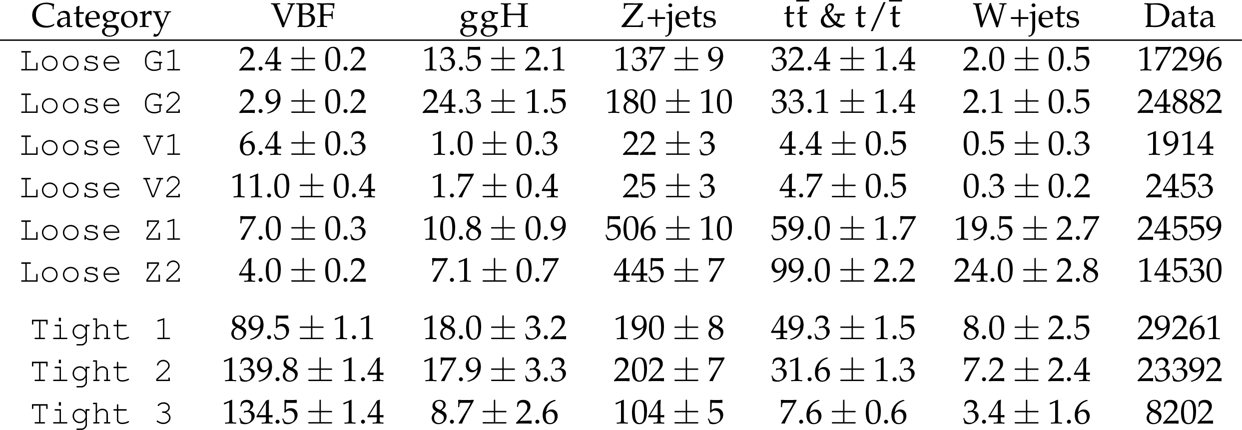
Table 4:
Event yields for various categories of the analyzed 2018 data corresponding to 54.5 fb$ ^{-1} $, compared to the expected number of events from the simulated samples of signal and background other than the QCD multijet process. The quoted uncertainties are statistical only. |
png pdf |
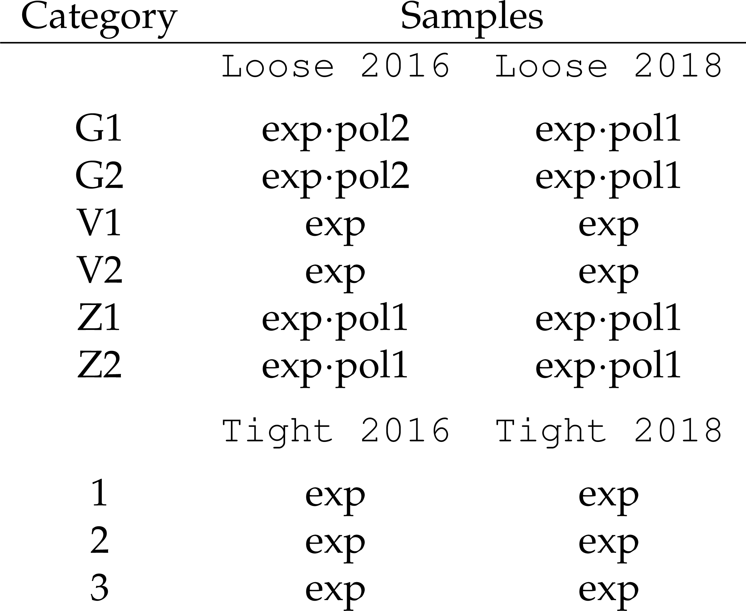
Table 5:
The functional forms used to fit the continuum component of the background in various analysis categories. The notation ``exp'' stands for the exponential function, ``exp$ \cdot $pol1 (pol2)" denotes the product of an exponential function and a first-order (second-order) polynomial. |
png pdf |
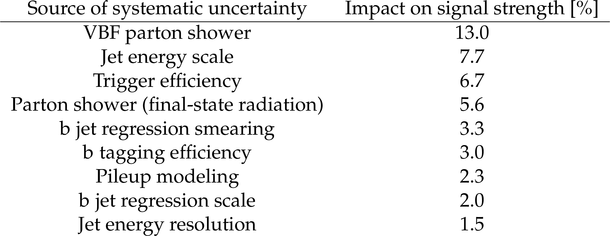
Table 6:
The impact of the dominant systematic uncertainties on the observed signal strength for inclusive Higgs boson production followed by decay to bottom quarks. |
| Summary |
| A measurement of the Higgs boson (H) production via vector boson fusion (VBF) process and its decay to a bottom quark-antiquark pair ($ \mathrm{b} \overline{\mathrm{b}} $) was performed on proton-proton collision data sets collected by the CMS experiment at $ \sqrt{s}= $ 13 TeV corresponding to a total integrated luminosity of 90.8 fb$ ^{-1} $. The analysis employs boosted decision trees (BDTs) to discriminate the signal against major background processes-QCD-induced multijet production and Z+jets events. The BDTs exploit kinematic properties of the VBF jets, information of the b-tagged jets assigned to the $ \mathrm{H}\to\mathrm{b}\overline{\mathrm{b}} $ decay, and global event shape variables. Based on the BDT response, multiple event categories are introduced, targeting the VBF, gluon-gluon fusion (ggH), and Z+jets processes to achieve a maximum sensitivity for the signal. While the VBF categories have the highest signal-to-background ratio, the Z+jets categories constrain the largest resonant background. The ggH categories enhance the sensitivity to the inclusive production of the Higgs boson in association with two jets. The VBF Higgs boson production rate has been measured in its decay to bottom quark-antiquark pairs with the ggH contribution constrained within the theoretical and experimental uncertainties to the standard model prediction. The signal strength of the VBF Higgs production, followed by the $ \mathrm{H}\to\mathrm{b}\overline{\mathrm{b}} $ decay, defined as the rate of the signal process relative to the value predicted in the standard model, is measured to be, $ {\mu^{\mathrm{q}\mathrm{q}\mathrm{H}}_{\mathrm{H}\mathrm{b}\overline{\mathrm{b}}}}= $ 1.01$ ^{+0.55}_{-0.46} $. The signal was observed with a significance of 2.4 standard deviations, compared to the expected significance of 2.7 standard deviations. In addition, inclusive Higgs boson production in association with two jets, followed by $ \mathrm{H}\to\mathrm{b}\overline{\mathrm{b}} $ decay, was measured by treating the ggH contribution as part of the signal. The inclusive signal strength was measured to be $ {\mu^\text{incl.}_{\mathrm{H}\mathrm{b}\overline{\mathrm{b}}}}= $ 0.99$ ^{+0.48}_{-0.41} $, corresponding to an observed (expected) significance of 2.6 (2.9) standard deviations. The measurements are consistent within uncertainties with the prediction from the standard model. |
| References | ||||
| 1 | ATLAS Collaboration | Observation of a new particle in the search for the standard model Higgs boson with the ATLAS detector at the LHC | PLB 716 (2012) 1 | 1207.7214 |
| 2 | CMS Collaboration | Observation of a new boson at a mass of 125 GeV with the CMS experiment at the LHC | PLB 716 (2012) 30 | CMS-HIG-12-028 1207.7235 |
| 3 | CMS Collaboration | Observation of a new boson with mass near 125 GeV in pp collisions at $ \sqrt{s} = $ 7 and 8 TeV | JHEP 06 (2013) 081 | CMS-HIG-12-036 1303.4571 |
| 4 | F. Englert and R. Brout | Broken symmetry and the mass of gauge vector mesons | PRL 13 (1964) 321 | |
| 5 | P. W. Higgs | Broken symmetries, massless particles and gauge fields | PL 12 (1964) 132 | |
| 6 | P. W. Higgs | Broken symmetries and the masses of gauge bosons | PRL 13 (1964) 508 | |
| 7 | G. S. Guralnik, C. R. Hagen, and T. W. B. Kibble | Global conservation laws and massless particles | PRL 13 (1964) 585 | |
| 8 | P. W. Higgs | Spontaneous symmetry breakdown without massless bosons | PR 145 (1966) 1156 | |
| 9 | T. W. B. Kibble | Symmetry breaking in non-abelian gauge theories | PR 155 (1967) 1554 | |
| 10 | A. Djouadi, J. Kalinowski, and M. Spira | HDECAY: A Program for Higgs boson decays in the standard model and its supersymmetric extension | Comput. Phys. Commun. 108 (1998) 56 | hep-ph/9704448 |
| 11 | LHC Higgs Cross Section Working Group | Handbook of LHC Higgs Cross Sections: 4. Deciphering the nature of the Higgs sector | CERN Yellow Rep. Monogr. 2 (2017) | 1610.07922 |
| 12 | CMS Collaboration | Inclusive search for highly boosted Higgs bosons decaying to bottom quark-antiquark pairs in proton-proton collisions at $ \sqrt{s} = $ 13 TeV | JHEP 12 (2020) 085 | CMS-HIG-19-003 2006.13251 |
| 13 | ATLAS Collaboration | Measurements of WH and ZH production in the $ \mathrm{H}\to\mathrm{b}\overline{\mathrm{b}} $ decay channel in pp collisions at 13 TeV with the ATLAS detector | EPJC 81 (2021) 178 | 2007.02873 |
| 14 | CMS Collaboration | Observation of Higgs boson decay to bottom quarks | PRL 121 (2018) 121801 | CMS-HIG-18-016 1808.08242 |
| 15 | F. Maltoni, K. Mawatari, and M. Zaro | Higgs characterisation via vector-boson fusion and associated production: NLO and parton-shower effects | EPJC 74 (2014) 2710 | 1311.1829 |
| 16 | CMS Collaboration | Search for the standard model Higgs boson produced through vector boson fusion and decaying to $ \mathrm{b}\overline{\mathrm{b}} $ | PRD 92 (2015) 032008 | CMS-HIG-14-004 1506.01010 |
| 17 | ATLAS Collaboration | Measurements of Higgs bosons decaying to bottom quarks from vector boson fusion production with the ATLAS experiment at $ \sqrt{s}= $ 13 TeV | EPJC 81 (2021) 537 | 2011.08280 |
| 18 | CMS Collaboration | HEPData record for this analysis | link | |
| 19 | CMS Collaboration | The CMS trigger system | JINST 12 (2017) P01020 | CMS-TRG-12-001 1609.02366 |
| 20 | CMS Collaboration | The CMS high level trigger | EPJC 46 (2006) 605 | hep-ex/0512077 |
| 21 | CMS Collaboration | The CMS experiment at the CERN LHC | JINST 3 (2008) S08004 | |
| 22 | CMS Collaboration | Particle-flow reconstruction and global event description with the CMS detector | JINST 12 (2017) P10003 | CMS-PRF-14-001 1706.04965 |
| 23 | M. Cacciari, G. P. Salam, and G. Soyez | The anti-$ k_{\mathrm{T}} $ jet clustering algorithm | JHEP 04 (2008) 063 | 0802.1189 |
| 24 | M. Cacciari, G. P. Salam, and G. Soyez | FastJet user manual | EPJC 72 (2012) 1896 | 1111.6097 |
| 25 | CMS Collaboration | Jet energy scale and resolution in the CMS experiment in pp collisions at 8 TeV | JINST 12 (2017) P02014 | CMS-JME-13-004 1607.03663 |
| 26 | CMS Collaboration | Identification of b-quark jets with the CMS experiment | JINST 8 (2013) P04013 | CMS-BTV-12-001 1211.4462 |
| 27 | CMS Collaboration | Identification of heavy-flavour jets with the CMS detector in pp collisions at 13 TeV | JINST 13 (2018) P05011 | CMS-BTV-16-002 1712.07158 |
| 28 | E. Bols et al. | Jet flavour classification using DEEPJET | JINST 15 (2020) P12012 | 2008.10519 |
| 29 | CMS Collaboration | Performance of the DeepJet b tagging algorithm using 41.9 fb$^{-1}$ of data from proton-proton collisions at 13 TeV with Phase 1 CMS detector | CMS Detector Performance Note CMS-DP-2018-058, 2018 CDS |
|
| 30 | P. Nason | A new method for combining NLO QCD with shower Monte Carlo algorithms | JHEP 11 (2004) 040 | hep-ph/0409146 |
| 31 | S. Frixione, P. Nason, and C. Oleari | Matching NLO QCD computations with parton shower simulations: the POWHEG method | JHEP 11 (2007) 070 | 0709.2092 |
| 32 | S. Alioli, P. Nason, C. Oleari, and E. Re | A general framework for implementing NLO calculations in shower Monte Carlo programs: the POWHEG box | JHEP 06 (2010) 043 | 1002.2581 |
| 33 | P. Nason and C. Oleari | NLO Higgs boson production via vector-boson fusion matched with shower in POWHEG | JHEP 02 (2010) 037 | 0911.5299 |
| 34 | B. Cabouat and T. Sjöstrand | Some dipole shower studies | EPJC 78 (2018) 226 | 1710.00391 |
| 35 | J. Bellm et al. | HERWIG 7.0/ HERWIG ++3.0 release note | EPJC 76 (2016) 196 | 1512.01178 |
| 36 | G. Luisoni, P. Nason, C. Oleari, and F. Tramontano | HW$^{\pm} $/HZ+0 and 1 jet at NLO with the POWHEG box interfaced to GoSam and their merging within MINLO | JHEP 10 (2013) 083 | 1306.2542 |
| 37 | K. Hamilton, P. Nason, C. Oleari, and G. Zanderighi | Merging H/W/Z+0 and 1 jet at NLO with no merging scale: A path to parton shower + NNLO matching | JHEP 05 (2013) 082 | 1212.4504 |
| 38 | E. Bagnaschi, G. Degrassi, P. Slavich, and A. Vicini | Higgs production via gluon fusion in the POWHEG approach in the SM and in the MSSM | JHEP 02 (2012) 088 | 1111.2854 |
| 39 | R. Frederix and S. Frixione | Merging meets matching in MC@NLO | JHEP 12 (2012) 061 | 1209.6215 |
| 40 | J. Alwall et al. | The automated computation of tree-level and next-to-leading order differential cross sections, and their matching to parton shower simulations | JHEP 07 (2014) 079 | 1405.0301 |
| 41 | M. L. Mangano, M. Moretti, F. Piccinini, and M. Treccani | Matching matrix elements and shower evolution for top-quark production in hadronic collisions | JHEP 01 (2007) 013 | hep-ph/0611129 |
| 42 | J. M. Lindert et al. | Precise predictions for V+jets dark matter backgrounds | EPJC 77 (2017) 829 | 1705.04664 |
| 43 | T. Sjöstrand et al. | An introduction to PYTHIA8.2 | Comput. Phys. Commun. 191 (2015) 159 | 1410.3012 |
| 44 | CMS Collaboration | Extraction and validation of a new set of CMS PYTHIA8 tunes from underlying-event measurements | EPJC 80 (2020) 4 | CMS-GEN-17-001 1903.12179 |
| 45 | NNPDF Collaboration | Parton distributions for the LHC Run II | JHEP 04 (2015) 040 | 1410.8849 |
| 46 | NNPDF Collaboration | Parton distributions from high-precision collider data | EPJC 77 (2017) 663 | 1706.00428 |
| 47 | GEANT4 Collaboration | GEANT4---a simulation toolkit | NIM A 506 (2003) 250 | |
| 48 | CMS Collaboration | Pileup mitigation at CMS in 13 TeV data | JINST 15 (2020) P09018 | CMS-JME-18-001 2003.00503 |
| 49 | CMS Collaboration | A deep neural network for simultaneous estimation of b jet energy and resolution | Comput. Softw. Big Sci. 4 (2020) 10 | CMS-HIG-18-027 1912.06046 |
| 50 | M. J. Oreglia | A study of the reactions $ \psi^\prime \to \gamma \gamma \psi $ | PhD thesis, Stanford University, SLAC Report SLAC-R-236, 1980 link |
|
| 51 | P. Speckmayer, A. Hocker, J. Stelzer, and H. Voss | The toolkit for multivariate data analysis, TMVA 4 | J. Phys. Conf. Ser. 219 (2010) 032057 | |
| 52 | CMS Collaboration | Performance of quark/gluon discrimination in 8 TeV pp data | CMS Physics Analysis Summary, 2013 CMS-PAS-JME-13-002 |
CMS-PAS-JME-13-002 |
| 53 | CMS Collaboration | Jet algorithms performance in 13 TeV data | CMS Physics Analysis Summary , CERN, 2017 CMS-PAS-JME-16-003 |
CMS-PAS-JME-16-003 |
| 54 | ATLAS and CMS Collaborations, and LHC Higgs Combination Group | Procedure for the LHC Higgs boson search combination in Summer 2011 | Technical Report CMS-NOTE-2011-005, ATL-PHYS-PUB-2011-11, 2011 | |
| 55 | R. A. Fisher | On the interpretation of $ \chi^{2} $ from contingency tables, and the calculation of P | J. R. Stat. Soc. 85 (1922) 87 | |
| 56 | CMS Collaboration | Measurement of the inclusive W and Z production cross sections in pp collisions at $ \sqrt{s}= $ 7 TeV | JHEP 10 (2011) 132 | CMS-EWK-10-005 1107.4789 |
| 57 | CMS Collaboration | Precision luminosity measurement in proton-proton collisions at $ \sqrt{s} = $ 13 TeV in 2015 and 2016 at CMS | EPJC 81 (2021) 800 | CMS-LUM-17-003 2104.01927 |
| 58 | CMS Collaboration | CMS luminosity measurement for the 2018 data-taking period at $ \sqrt{s} = $ 13 TeV | CMS Physics Analysis Summary, 2019 link |
CMS-PAS-LUM-18-002 |
| 59 | CMS Collaboration | Measurement of the inelastic proton-proton cross section at $ \sqrt{s}= $ 13 tev | JHEP 07 (2018) 161 | CMS-FSQ-15-005 1802.02613 |
| 60 | CMS Collaboration | Precise determination of the mass of the Higgs boson and tests of compatibility of its couplings with the standard model predictions using proton collisions at 7 and 8 TeV | EPJC 75 (2015) 212 | CMS-HIG-14-009 1412.8662 |
| 61 | E. Gross and O. Vitells | Trial factors for the look elsewhere effect in high energy physics | EPJC 70 (2010) 525 | 1005.1891 |
|
|
Compact Muon Solenoid LHC, CERN |
|

|

|

|

|

|