

Compact Muon Solenoid
LHC, CERN
| CMS-SMP-20-005 ; CERN-EP-2021-219 | ||
| Measurement of ${\mathrm{W^{\pm}}\gamma}$ differential cross sections in proton-proton collisions at $\sqrt{s} = $ 13 TeV and effective field theory constraints | ||
| CMS Collaboration | ||
| 27 November 2021 | ||
| Phys. Rev. D 105 (2022) 052003 | ||
| Abstract: Differential cross section measurements of ${\mathrm{W^{\pm}}\gamma}$ production in proton-proton collisions at $\sqrt{s} = $ 13 TeV are presented. The data set used in this study was collected with the CMS detector at the CERN LHC in 2016-2018 with an integrated luminosity of 138 fb$^{-1}$. Candidate events containing an electron or muon, a photon, and missing transverse momentum are selected. The measurements are compared with standard model predictions computed at next-to-leading and next-to-next-to-leading orders in perturbative quantum chromodynamics. Constraints on the presence of TeV-scale new physics affecting the WW$\gamma$ vertex are determined within an effective field theory framework, focusing on the ${\mathcal{O}_{3W}}$ operator. A simultaneous measurement of the photon transverse momentum and the azimuthal angle of the charged lepton in a special reference frame is performed. This two-dimensional approach provides up to a factor of ten more sensitivity to the interference between the standard model and the ${\mathcal{O}_{3W}}$ contribution than using the transverse momentum alone. | ||
| Links: e-print arXiv:2111.13948 [hep-ex] (PDF) ; CDS record ; inSPIRE record ; HepData record ; CADI line (restricted) ; | ||
| Figures & Tables | Summary | Additional Figures | References | CMS Publications |
|---|
| Figures | |
png pdf |
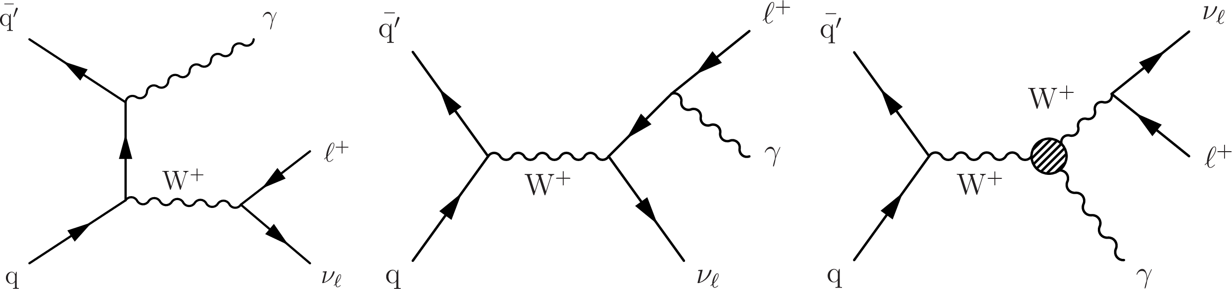
Figure 1:
LO Feynman diagrams for ${\mathrm{W^{+}} \gamma}$ production showing initial-state (left) and final-state (center) radiation of the photon, and the WW$ \gamma$ TGC process (right). |
png pdf |
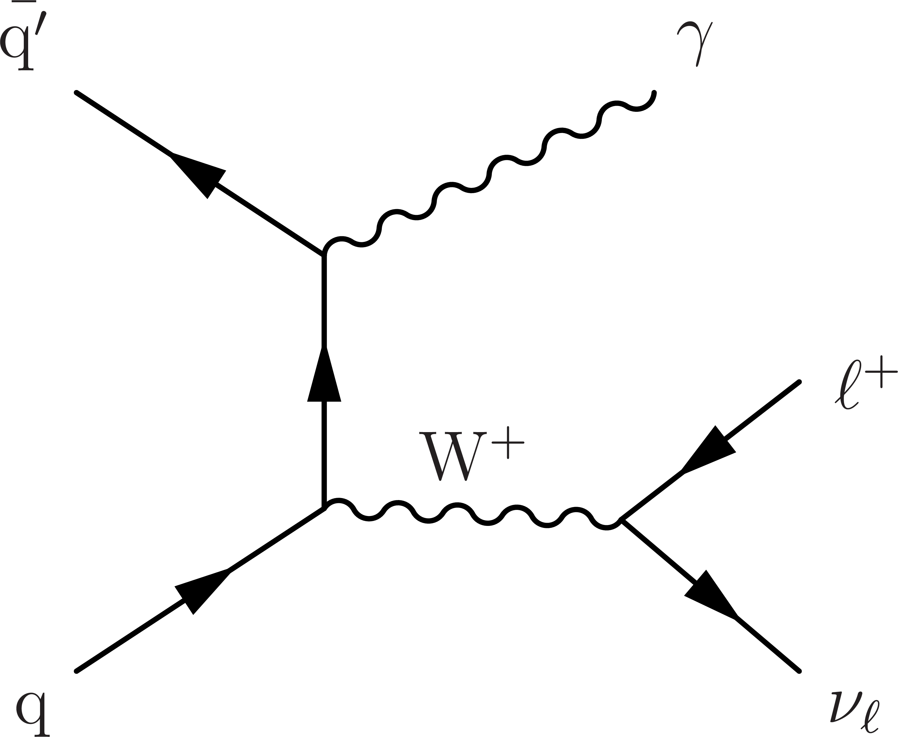
Figure 1-a:
LO Feynman diagrams for ${\mathrm{W^{+}} \gamma}$ production showing initial-state (left) and final-state (center) radiation of the photon, and the WW$ \gamma$ TGC process (right). |
png pdf |
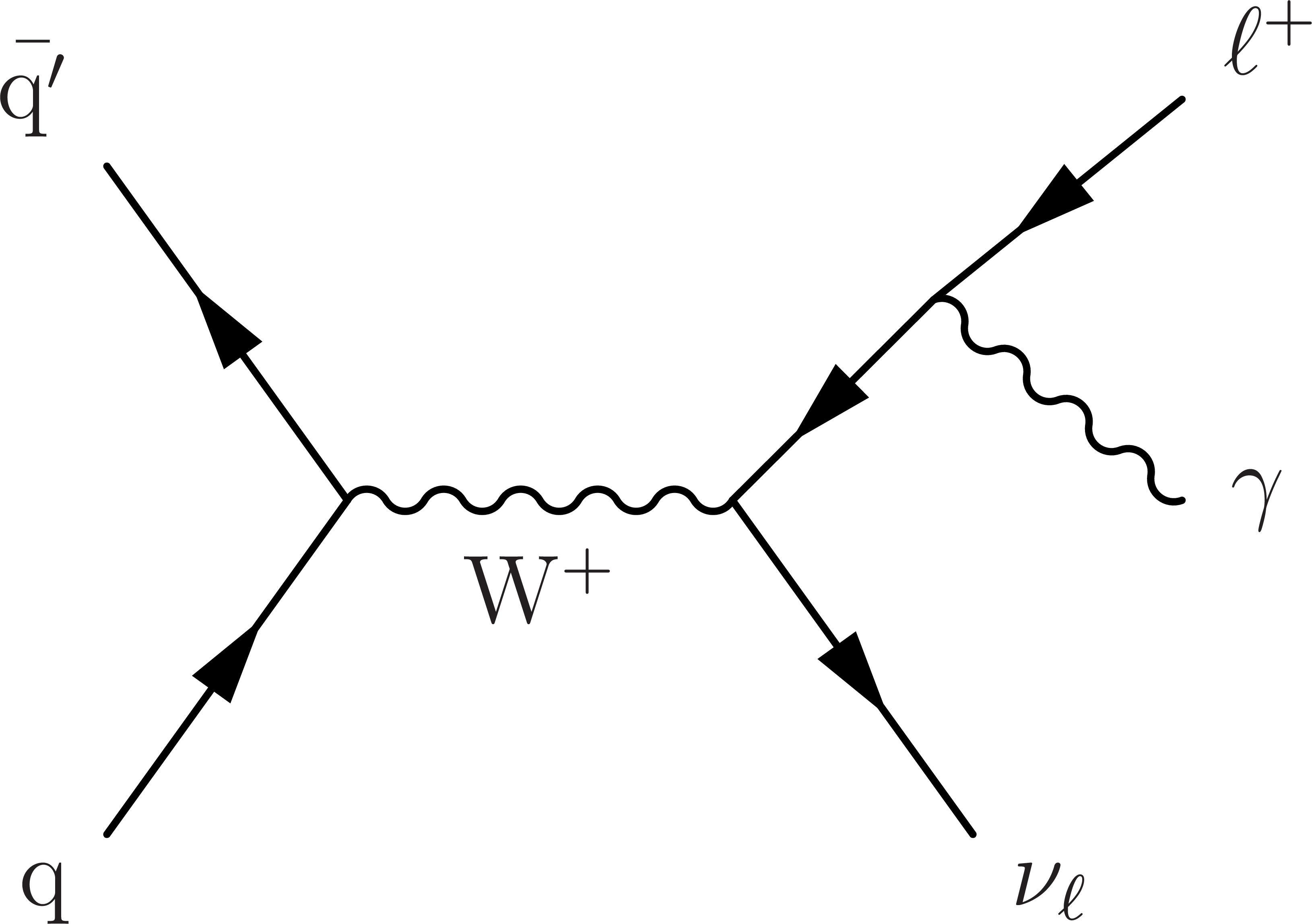
Figure 1-b:
LO Feynman diagrams for ${\mathrm{W^{+}} \gamma}$ production showing initial-state (left) and final-state (center) radiation of the photon, and the WW$ \gamma$ TGC process (right). |
png pdf |
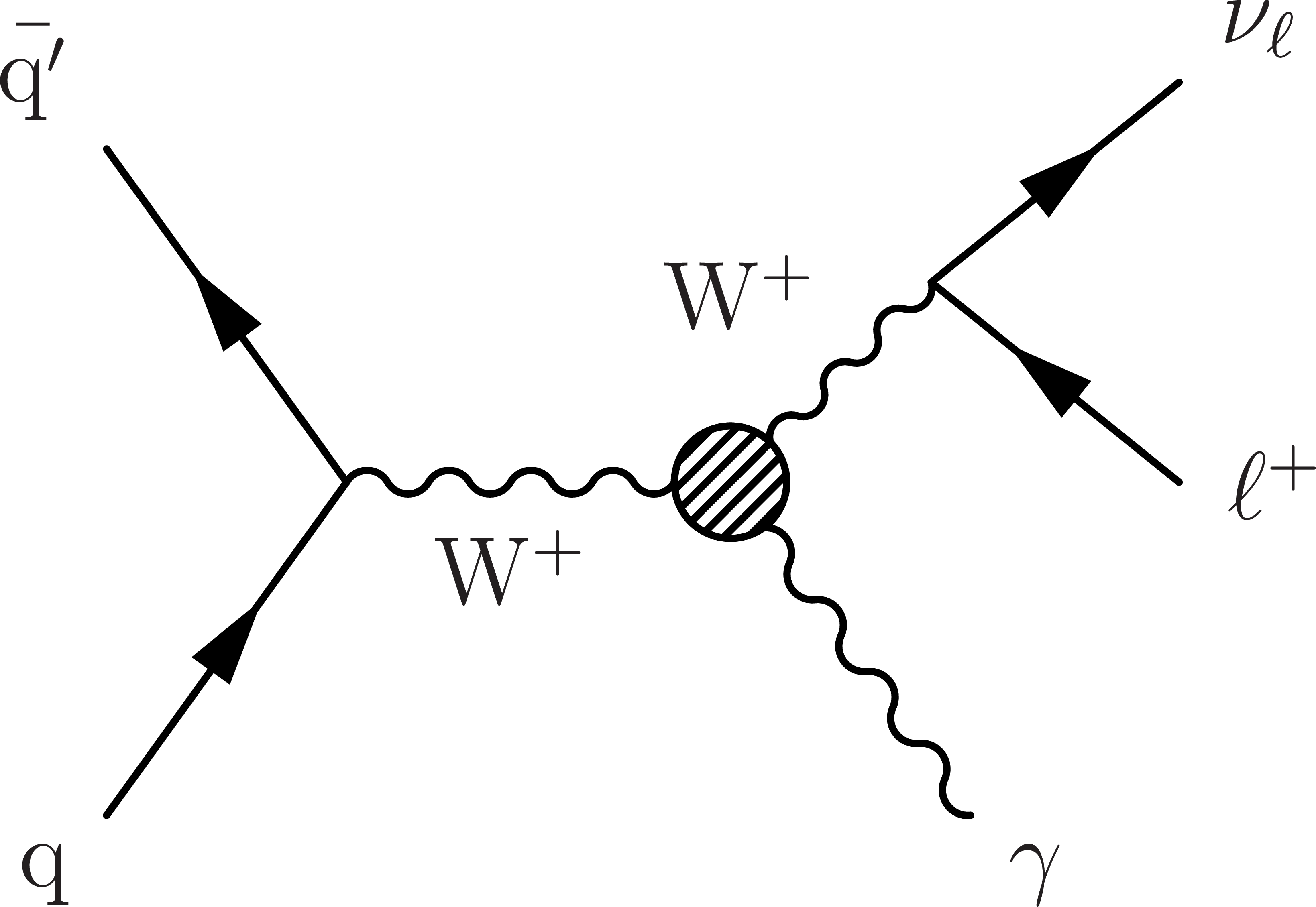
Figure 1-c:
LO Feynman diagrams for ${\mathrm{W^{+}} \gamma}$ production showing initial-state (left) and final-state (center) radiation of the photon, and the WW$ \gamma$ TGC process (right). |
png pdf |
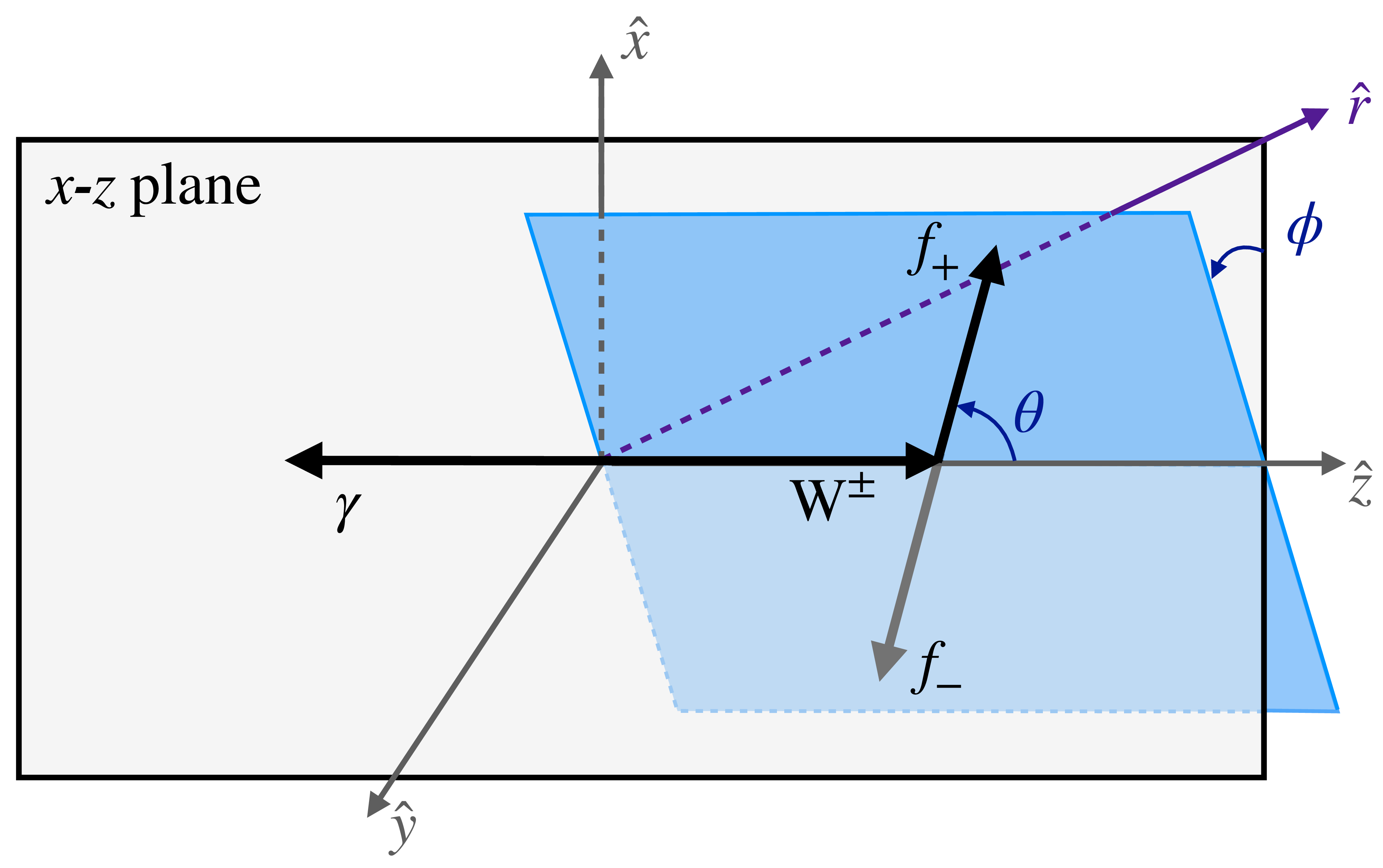
Figure 2:
Scheme of the special coordinate system for ${\mathrm{W^{\pm}} \gamma}$ production, defined by a Lorentz boost to the center-of-mass frame along the direction $\hat{r}$. The $z$ axis is chosen as the $\mathrm{W^{\pm}}$ boson direction in this frame, and $y$ is given by $\hat{z} \times \hat{r}$. The $\mathrm{W^{\pm}}$ boson decay plane is indicated in blue, where the labels ${f_{+}}$ and ${f_{-}}$ refer to positive and negative helicity final-state fermions. The angles $\phi $ and $\theta $ are the azimuthal and polar angles of ${f_{+}}$. |
png pdf |
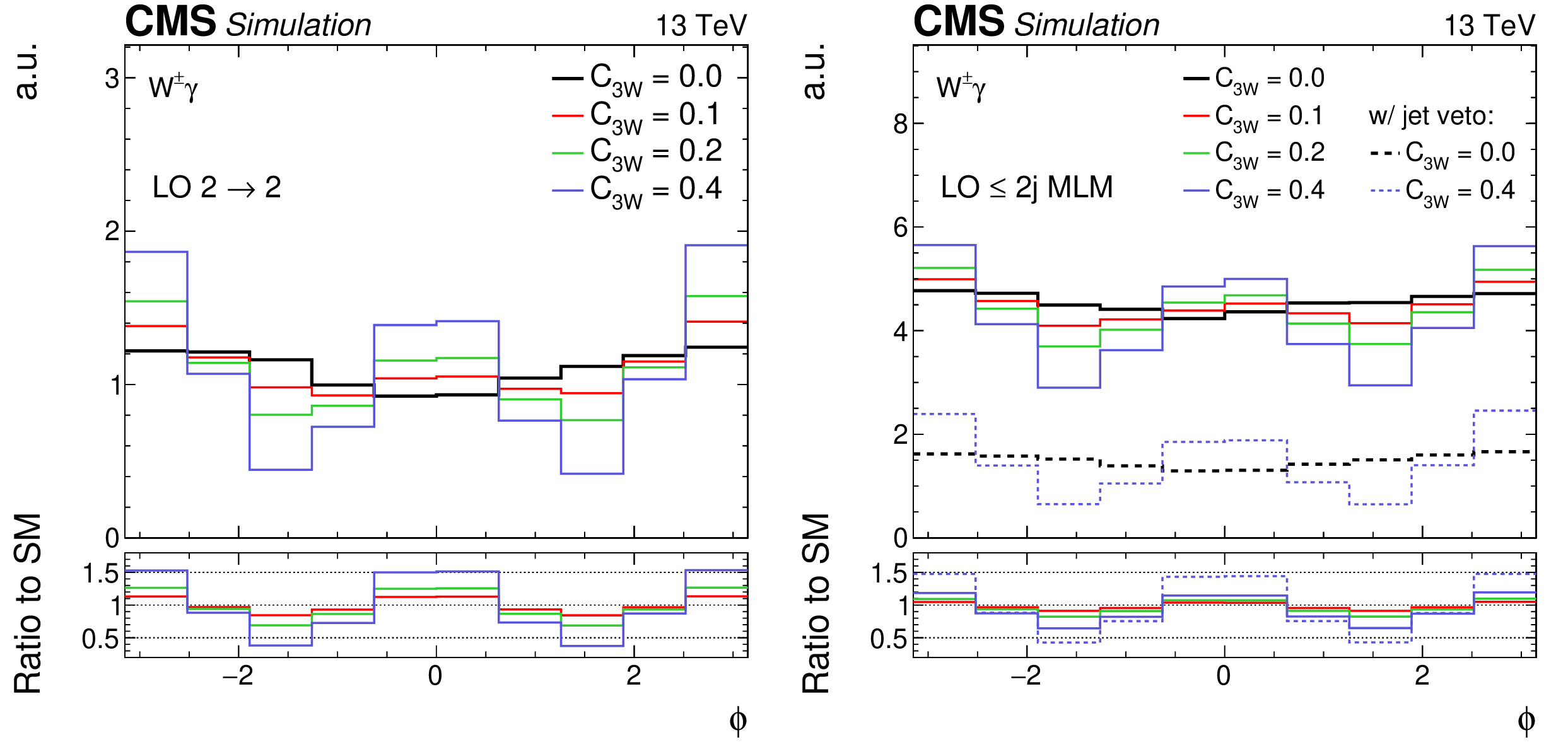
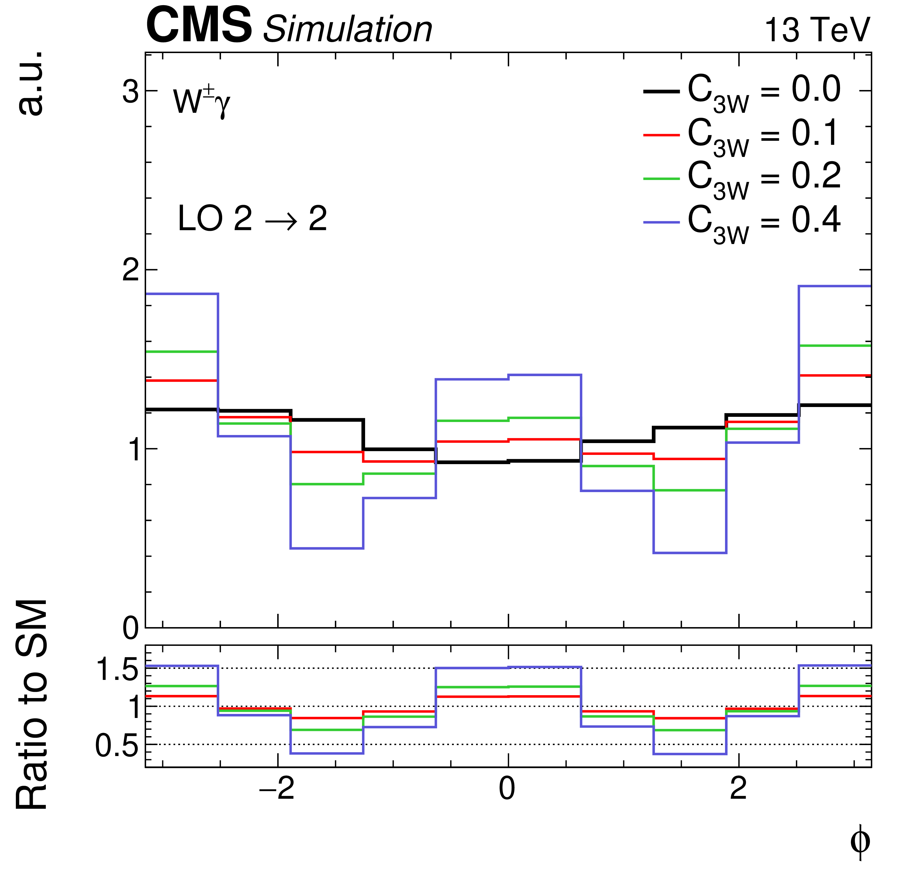
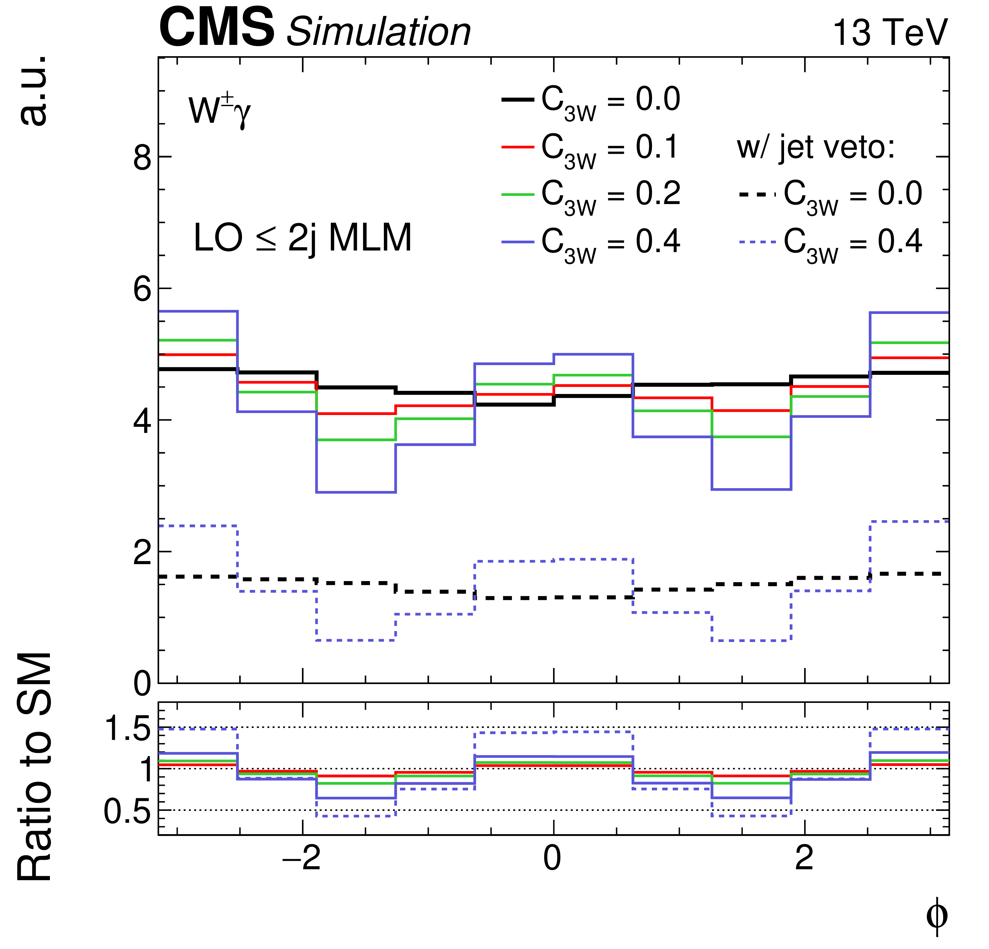
Figure 3:
Particle-level distributions (in arbitrary units) of the decay angle $\phi $, comparing the LO 2 $\to$ 2 process (left) to the LO MLM-merged prediction with up to two additional jets in the matrix element calculations (right). The black line gives the SM prediction ($ {C_{3W}} = $ 0) and the red, green, and blue lines correspond to different nonzero values of ${C_{3W}}$, for which only the interference contribution is shown. The black and blue dashed lines in the right figure give the distributions in the presence of a jet veto, as described in the text. |
png pdf |
Figure 3-a:
Particle-level distributions (in arbitrary units) of the decay angle $\phi $, comparing the LO 2 $\to$ 2 process (left) to the LO MLM-merged prediction with up to two additional jets in the matrix element calculations (right). The black line gives the SM prediction ($ {C_{3W}} = $ 0) and the red, green, and blue lines correspond to different nonzero values of ${C_{3W}}$, for which only the interference contribution is shown. The black and blue dashed lines in the right figure give the distributions in the presence of a jet veto, as described in the text. |
png pdf |
Figure 3-b:
Particle-level distributions (in arbitrary units) of the decay angle $\phi $, comparing the LO 2 $\to$ 2 process (left) to the LO MLM-merged prediction with up to two additional jets in the matrix element calculations (right). The black line gives the SM prediction ($ {C_{3W}} = $ 0) and the red, green, and blue lines correspond to different nonzero values of ${C_{3W}}$, for which only the interference contribution is shown. The black and blue dashed lines in the right figure give the distributions in the presence of a jet veto, as described in the text. |
png pdf |
Figure 4:
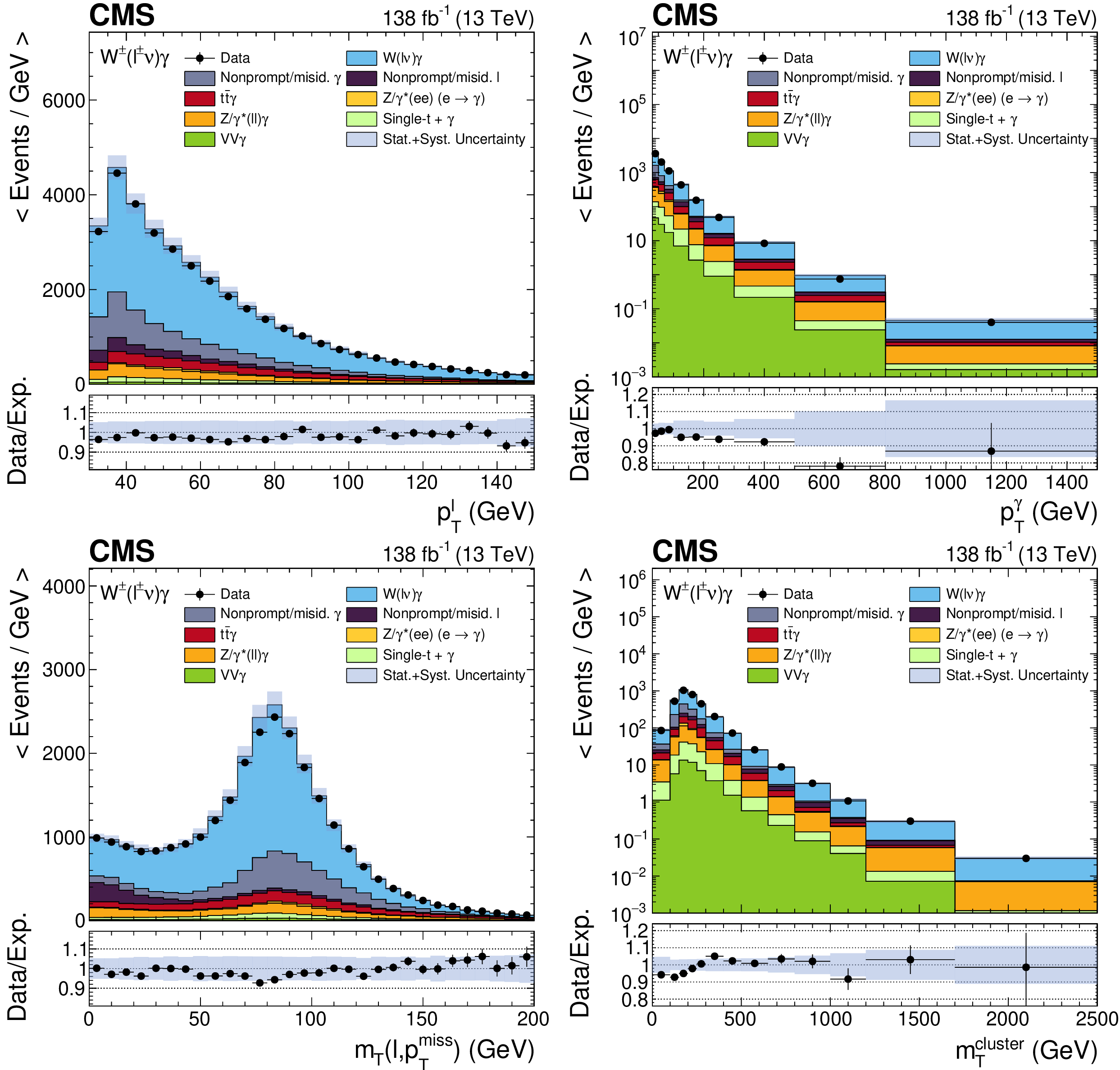
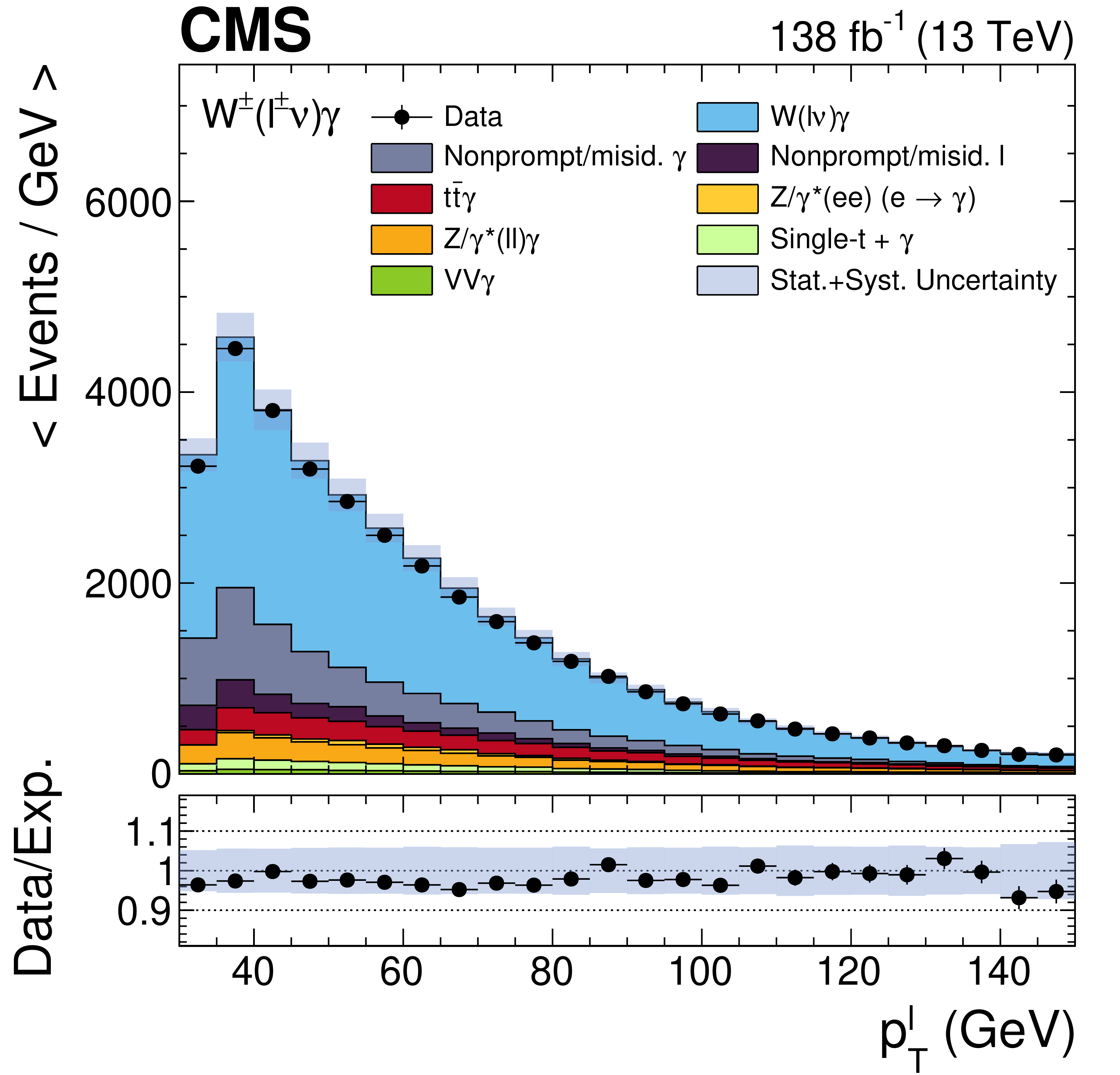
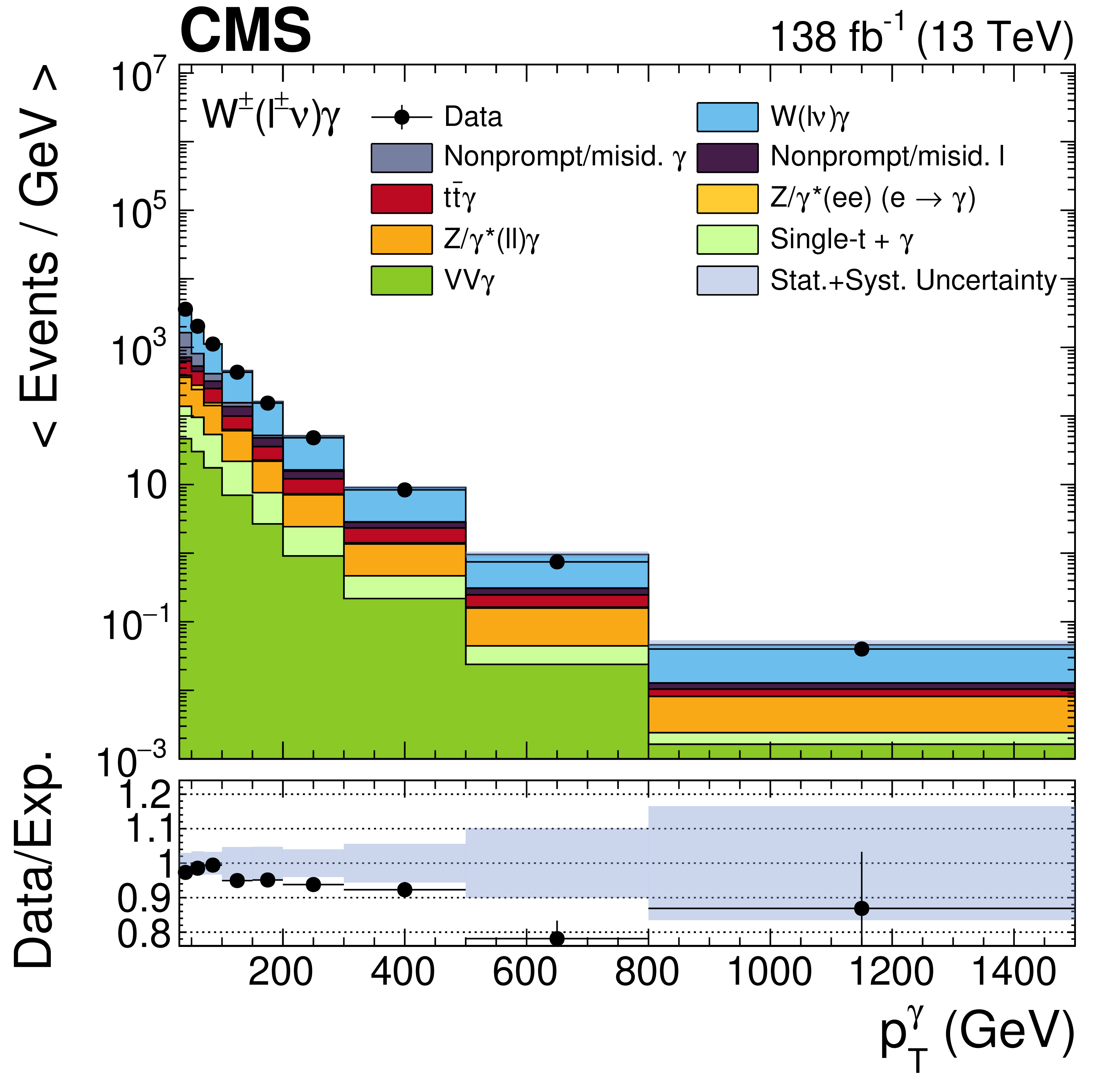
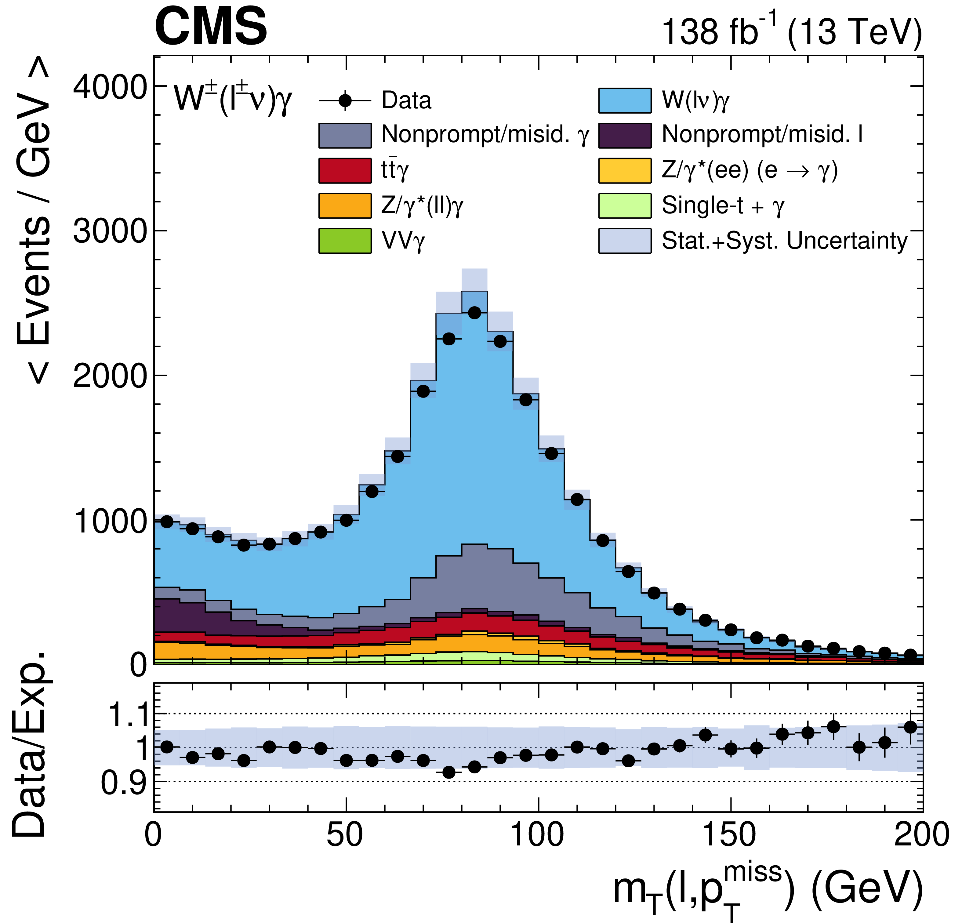
Distributions of the lepton ${p_{\mathrm {T}}}$ (upper left), the photon ${p_{\mathrm {T}}}$ (upper right), ${{m_{\mathrm {T}}} (\ell, {{p_{\mathrm {T}}} ^\text {miss}})}$ (lower left), and ${m_{\mathrm {T}}^{\text {cluster}}}$ (lower right), combining the electron and muon channels. The horizontal and vertical bars associated to the data points correspond to the bin widths and statistical uncertainties, respectively. The shaded band represents the total statistical and systematic uncertainty in the signal plus background expectation. |
png pdf |
Figure 4-a:
Distributions of the lepton ${p_{\mathrm {T}}}$ (upper left), the photon ${p_{\mathrm {T}}}$ (upper right), ${{m_{\mathrm {T}}} (\ell, {{p_{\mathrm {T}}} ^\text {miss}})}$ (lower left), and ${m_{\mathrm {T}}^{\text {cluster}}}$ (lower right), combining the electron and muon channels. The horizontal and vertical bars associated to the data points correspond to the bin widths and statistical uncertainties, respectively. The shaded band represents the total statistical and systematic uncertainty in the signal plus background expectation. |
png pdf |
Figure 4-b:
Distributions of the lepton ${p_{\mathrm {T}}}$ (upper left), the photon ${p_{\mathrm {T}}}$ (upper right), ${{m_{\mathrm {T}}} (\ell, {{p_{\mathrm {T}}} ^\text {miss}})}$ (lower left), and ${m_{\mathrm {T}}^{\text {cluster}}}$ (lower right), combining the electron and muon channels. The horizontal and vertical bars associated to the data points correspond to the bin widths and statistical uncertainties, respectively. The shaded band represents the total statistical and systematic uncertainty in the signal plus background expectation. |
png pdf |
Figure 4-c:
Distributions of the lepton ${p_{\mathrm {T}}}$ (upper left), the photon ${p_{\mathrm {T}}}$ (upper right), ${{m_{\mathrm {T}}} (\ell, {{p_{\mathrm {T}}} ^\text {miss}})}$ (lower left), and ${m_{\mathrm {T}}^{\text {cluster}}}$ (lower right), combining the electron and muon channels. The horizontal and vertical bars associated to the data points correspond to the bin widths and statistical uncertainties, respectively. The shaded band represents the total statistical and systematic uncertainty in the signal plus background expectation. |
png pdf |
Figure 4-d:
Distributions of the lepton ${p_{\mathrm {T}}}$ (upper left), the photon ${p_{\mathrm {T}}}$ (upper right), ${{m_{\mathrm {T}}} (\ell, {{p_{\mathrm {T}}} ^\text {miss}})}$ (lower left), and ${m_{\mathrm {T}}^{\text {cluster}}}$ (lower right), combining the electron and muon channels. The horizontal and vertical bars associated to the data points correspond to the bin widths and statistical uncertainties, respectively. The shaded band represents the total statistical and systematic uncertainty in the signal plus background expectation. |

png pdf |
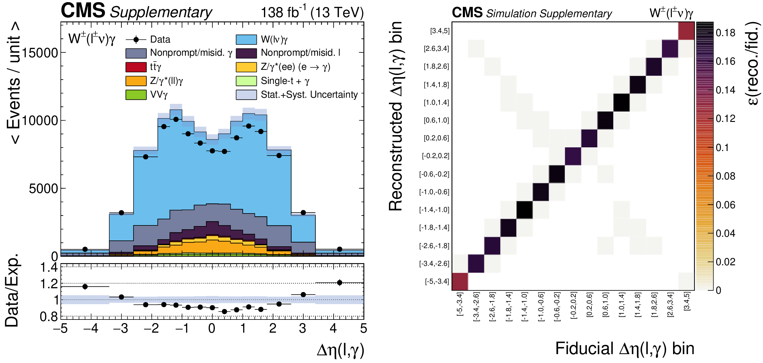
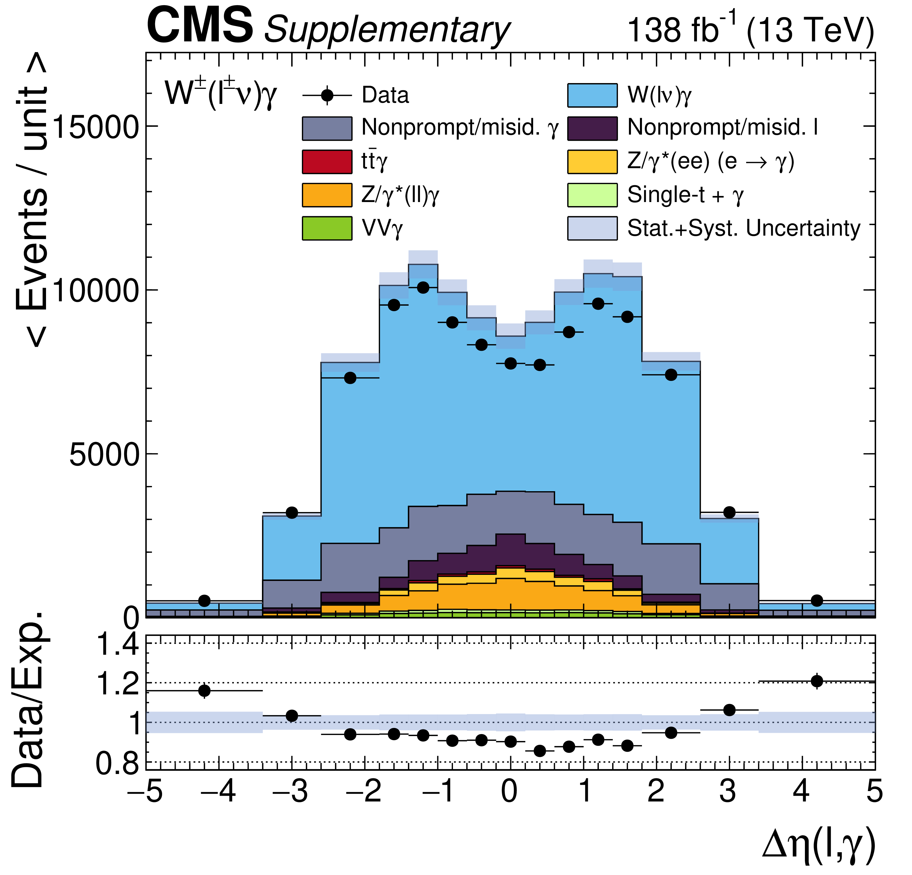
Figure 5:
The two-dimensional distribution of ${\phi ^{\text {gen}}}$ versus ${\phi ^{\text {true}}}$, where the former is reconstructed using the particle-level lepton and photon momenta and ${{\vec{p}}_{\mathrm {T}}^{\, \text {miss}}}$. The off-diagonal components correspond to events where the incorrect solution for ${\eta ^{\nu}}$ is chosen, as described in the text. |
png pdf |
Figure 6:
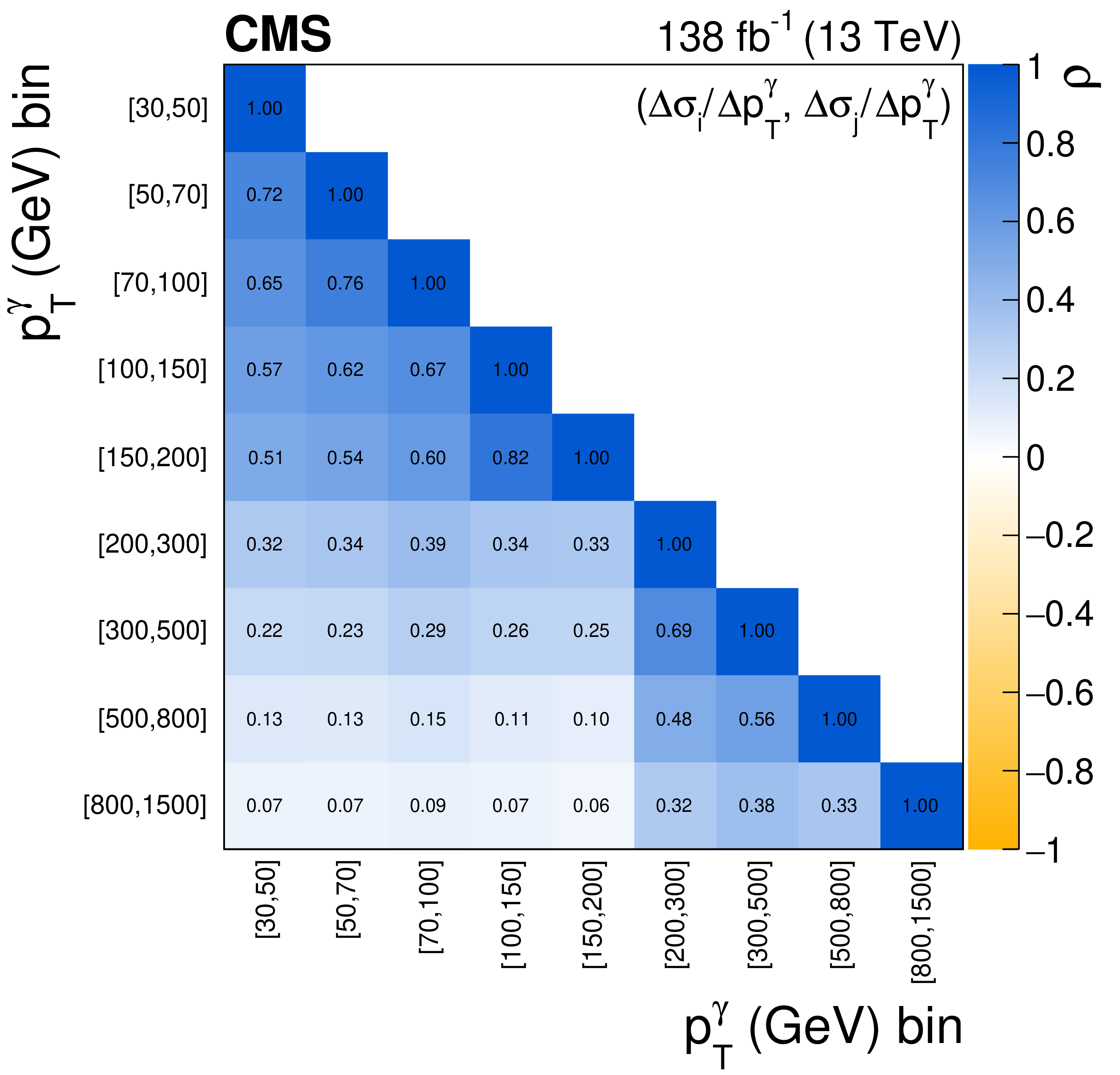
The measured ${{p_{\mathrm {T}}} ^{\gamma}}$ absolute (left) and fractional (right) differential cross sections (upper), compared with the MG5\_aMC+PY8, GENEVA, MATRIX and MCFM predictions, and corresponding uncertainty decomposition (center) and correlation matrices (lower). In the upper figures, the black vertical bars give the total uncertainty on each measurement. The predictions are offset horizontally in each bin to improve visibility, and the corresponding vertical bars show the missing higher order correction uncertainties. |

png pdf |
Figure 6-a:
The measured ${{p_{\mathrm {T}}} ^{\gamma}}$ absolute (left) and fractional (right) differential cross sections (upper), compared with the MG5\_aMC+PY8, GENEVA, MATRIX and MCFM predictions, and corresponding uncertainty decomposition (center) and correlation matrices (lower). In the upper figures, the black vertical bars give the total uncertainty on each measurement. The predictions are offset horizontally in each bin to improve visibility, and the corresponding vertical bars show the missing higher order correction uncertainties. |

png pdf |
Figure 6-b:
The measured ${{p_{\mathrm {T}}} ^{\gamma}}$ absolute (left) and fractional (right) differential cross sections (upper), compared with the MG5\_aMC+PY8, GENEVA, MATRIX and MCFM predictions, and corresponding uncertainty decomposition (center) and correlation matrices (lower). In the upper figures, the black vertical bars give the total uncertainty on each measurement. The predictions are offset horizontally in each bin to improve visibility, and the corresponding vertical bars show the missing higher order correction uncertainties. |
png pdf |
Figure 6-c:
The measured ${{p_{\mathrm {T}}} ^{\gamma}}$ absolute (left) and fractional (right) differential cross sections (upper), compared with the MG5\_aMC+PY8, GENEVA, MATRIX and MCFM predictions, and corresponding uncertainty decomposition (center) and correlation matrices (lower). In the upper figures, the black vertical bars give the total uncertainty on each measurement. The predictions are offset horizontally in each bin to improve visibility, and the corresponding vertical bars show the missing higher order correction uncertainties. |
png pdf |
Figure 6-d:
The measured ${{p_{\mathrm {T}}} ^{\gamma}}$ absolute (left) and fractional (right) differential cross sections (upper), compared with the MG5\_aMC+PY8, GENEVA, MATRIX and MCFM predictions, and corresponding uncertainty decomposition (center) and correlation matrices (lower). In the upper figures, the black vertical bars give the total uncertainty on each measurement. The predictions are offset horizontally in each bin to improve visibility, and the corresponding vertical bars show the missing higher order correction uncertainties. |
png pdf |
Figure 6-e:
The measured ${{p_{\mathrm {T}}} ^{\gamma}}$ absolute (left) and fractional (right) differential cross sections (upper), compared with the MG5\_aMC+PY8, GENEVA, MATRIX and MCFM predictions, and corresponding uncertainty decomposition (center) and correlation matrices (lower). In the upper figures, the black vertical bars give the total uncertainty on each measurement. The predictions are offset horizontally in each bin to improve visibility, and the corresponding vertical bars show the missing higher order correction uncertainties. |

png pdf |
Figure 6-f:
The measured ${{p_{\mathrm {T}}} ^{\gamma}}$ absolute (left) and fractional (right) differential cross sections (upper), compared with the MG5\_aMC+PY8, GENEVA, MATRIX and MCFM predictions, and corresponding uncertainty decomposition (center) and correlation matrices (lower). In the upper figures, the black vertical bars give the total uncertainty on each measurement. The predictions are offset horizontally in each bin to improve visibility, and the corresponding vertical bars show the missing higher order correction uncertainties. |
png pdf |
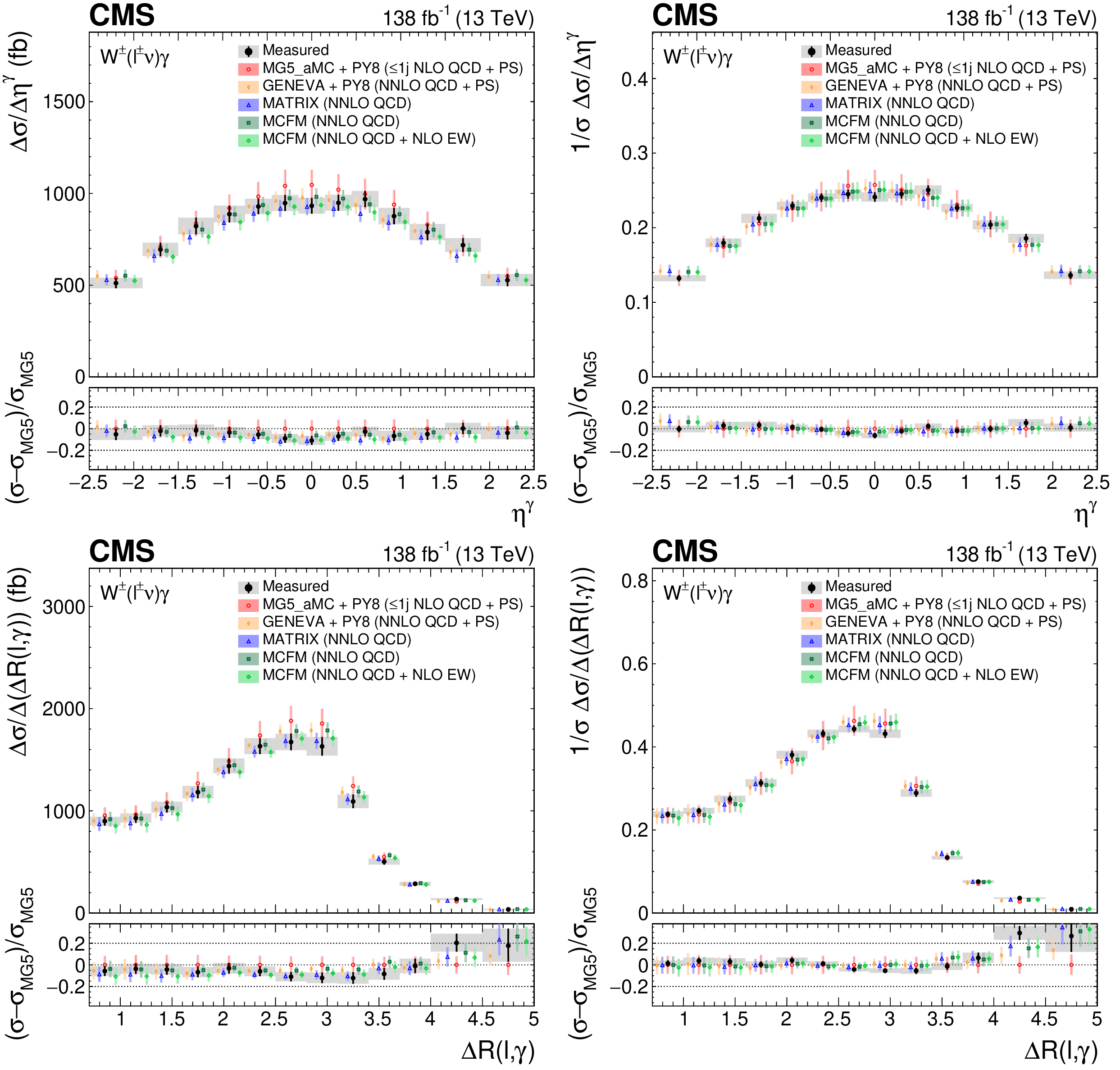
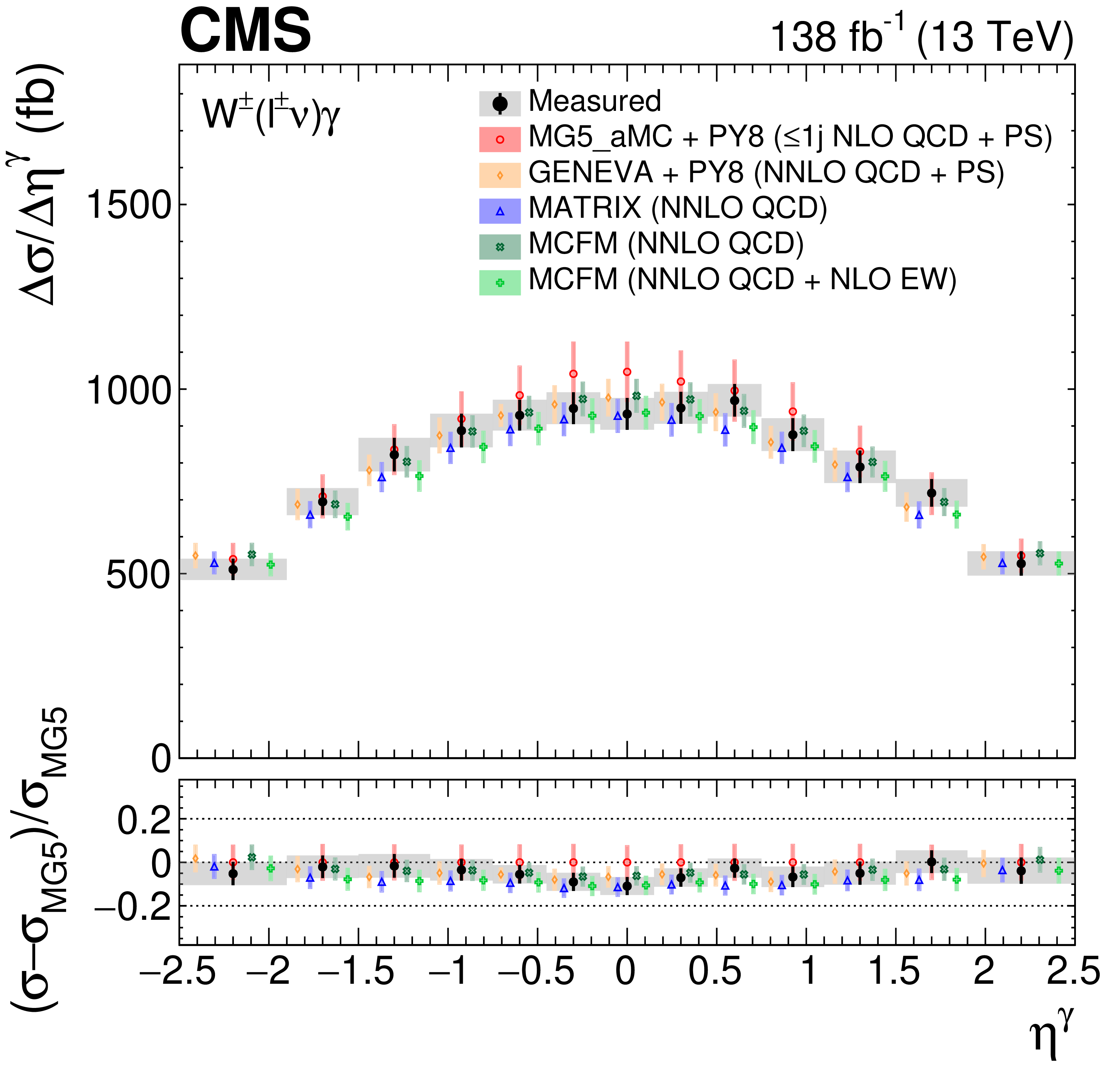
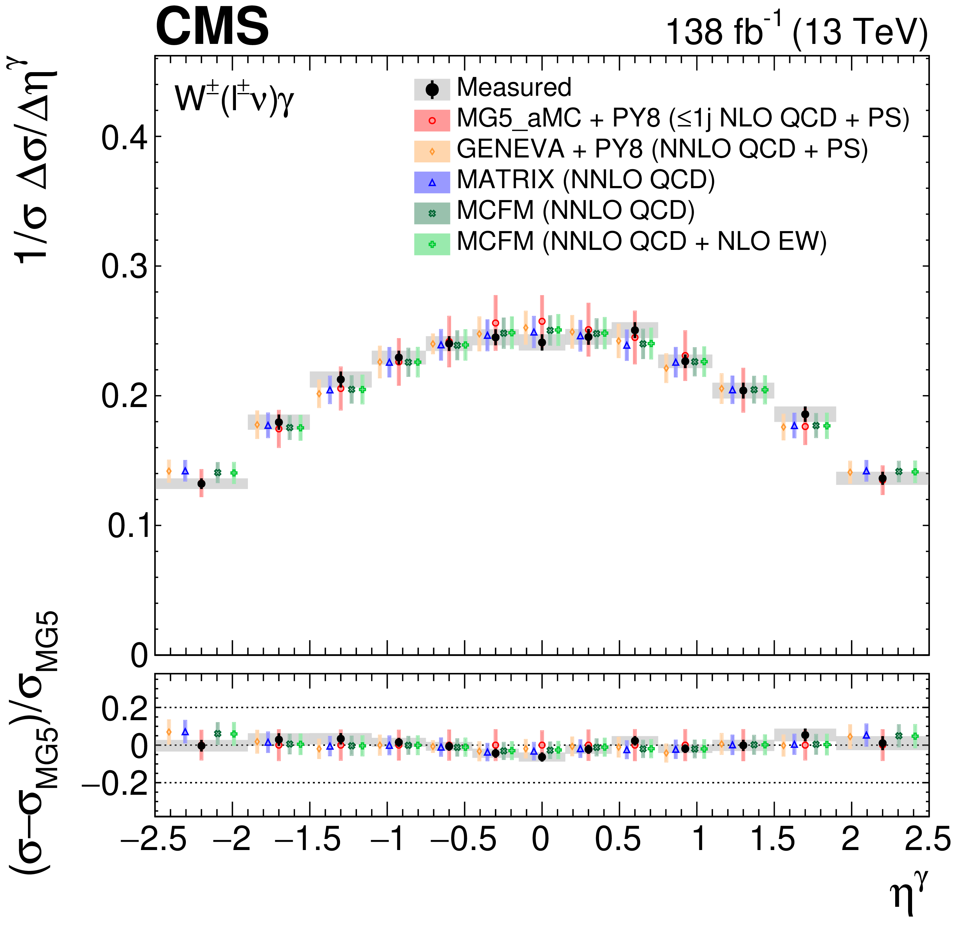
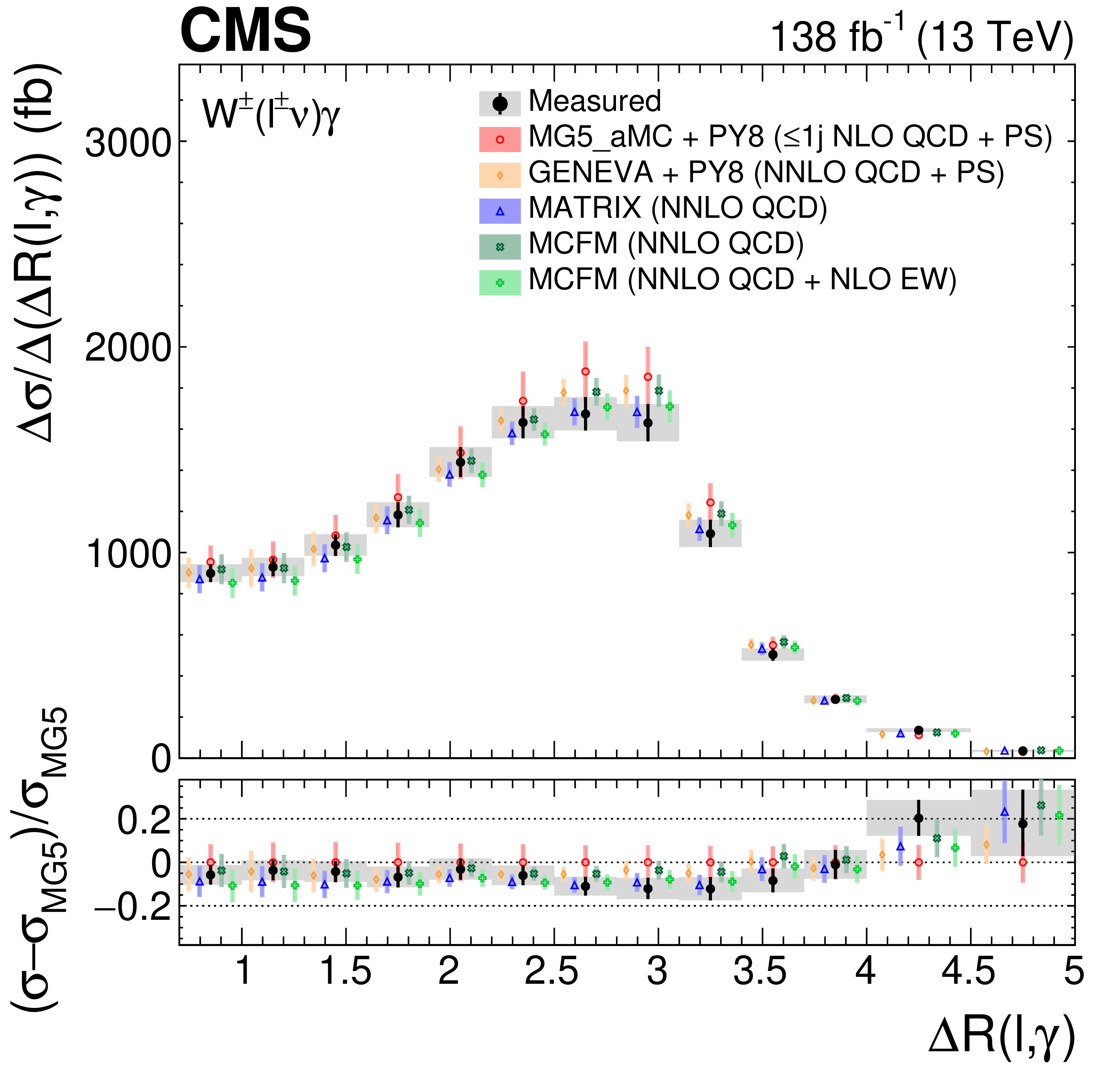
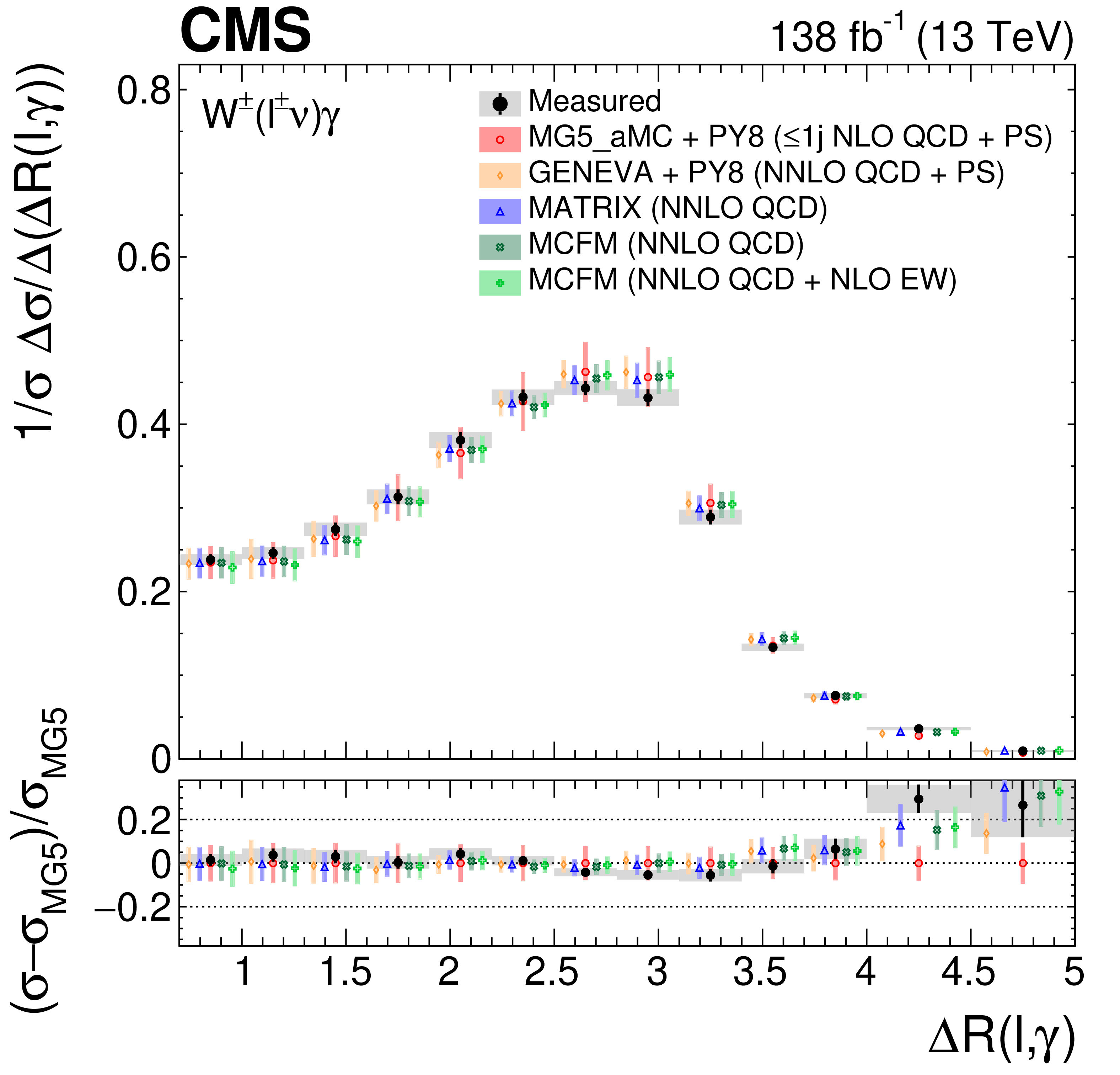
Figure 7:
The measured absolute (left) and fractional (right) differential cross sections for ${\eta ^{\gamma}}$ (upper) and ${{\Delta R}(\ell,\gamma)}$ (lower), compared with the MG5\_aMC+PY8, GENEVA, MATRIX and MCFM predictions. The shaded bands give the corresponding missing higher order correction uncertainties. The black vertical bars give the total uncertainty on each measurement. The predictions are offset horizontally in each bin to improve visibility, and the corresponding vertical bars show the missing higher order correction uncertainties. |
png pdf |
Figure 7-a:
The measured absolute (left) and fractional (right) differential cross sections for ${\eta ^{\gamma}}$ (upper) and ${{\Delta R}(\ell,\gamma)}$ (lower), compared with the MG5\_aMC+PY8, GENEVA, MATRIX and MCFM predictions. The shaded bands give the corresponding missing higher order correction uncertainties. The black vertical bars give the total uncertainty on each measurement. The predictions are offset horizontally in each bin to improve visibility, and the corresponding vertical bars show the missing higher order correction uncertainties. |
png pdf |
Figure 7-b:
The measured absolute (left) and fractional (right) differential cross sections for ${\eta ^{\gamma}}$ (upper) and ${{\Delta R}(\ell,\gamma)}$ (lower), compared with the MG5\_aMC+PY8, GENEVA, MATRIX and MCFM predictions. The shaded bands give the corresponding missing higher order correction uncertainties. The black vertical bars give the total uncertainty on each measurement. The predictions are offset horizontally in each bin to improve visibility, and the corresponding vertical bars show the missing higher order correction uncertainties. |
png pdf |
Figure 7-c:
The measured absolute (left) and fractional (right) differential cross sections for ${\eta ^{\gamma}}$ (upper) and ${{\Delta R}(\ell,\gamma)}$ (lower), compared with the MG5\_aMC+PY8, GENEVA, MATRIX and MCFM predictions. The shaded bands give the corresponding missing higher order correction uncertainties. The black vertical bars give the total uncertainty on each measurement. The predictions are offset horizontally in each bin to improve visibility, and the corresponding vertical bars show the missing higher order correction uncertainties. |
png pdf |
Figure 7-d:
The measured absolute (left) and fractional (right) differential cross sections for ${\eta ^{\gamma}}$ (upper) and ${{\Delta R}(\ell,\gamma)}$ (lower), compared with the MG5\_aMC+PY8, GENEVA, MATRIX and MCFM predictions. The shaded bands give the corresponding missing higher order correction uncertainties. The black vertical bars give the total uncertainty on each measurement. The predictions are offset horizontally in each bin to improve visibility, and the corresponding vertical bars show the missing higher order correction uncertainties. |
png pdf |
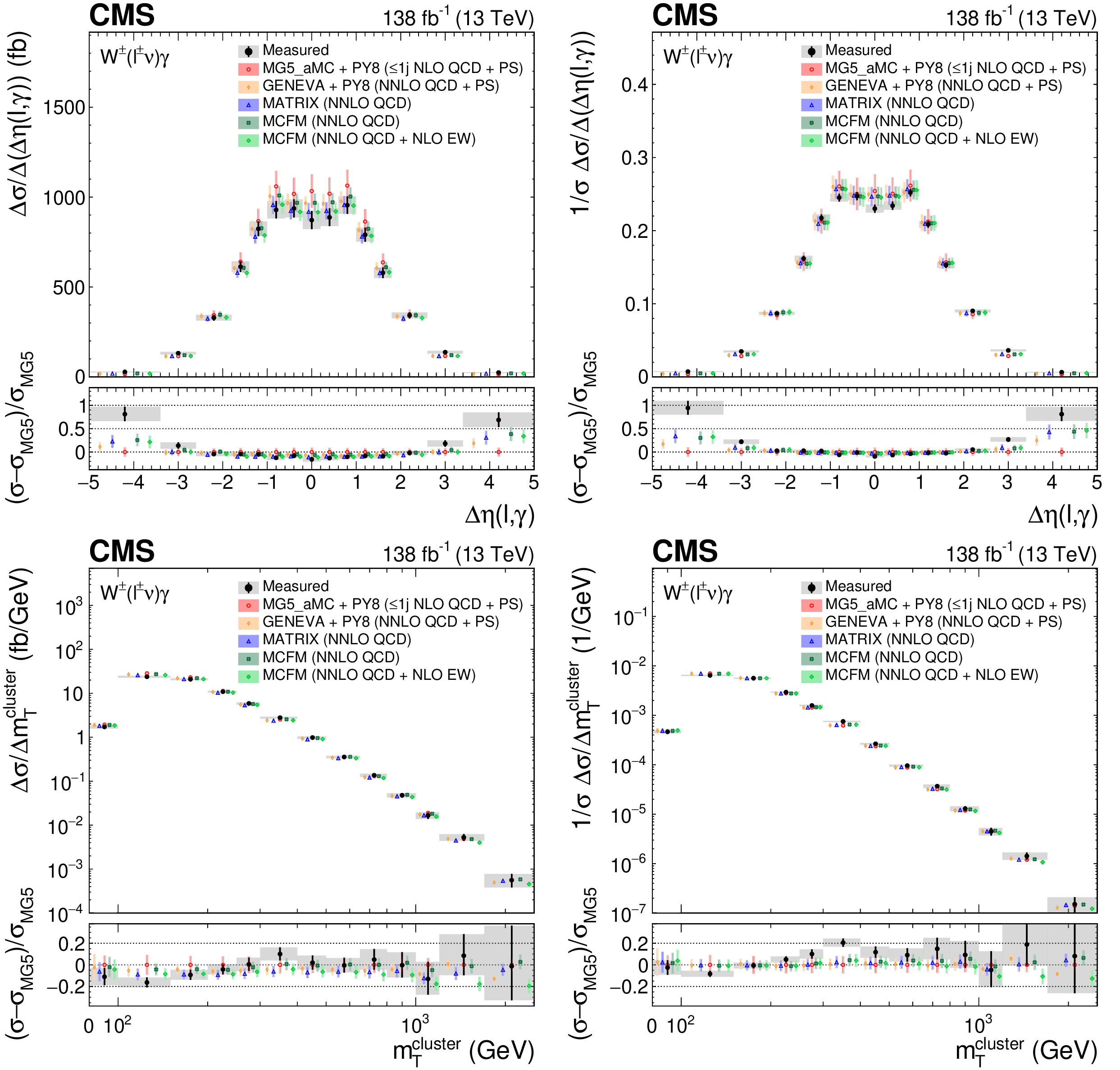
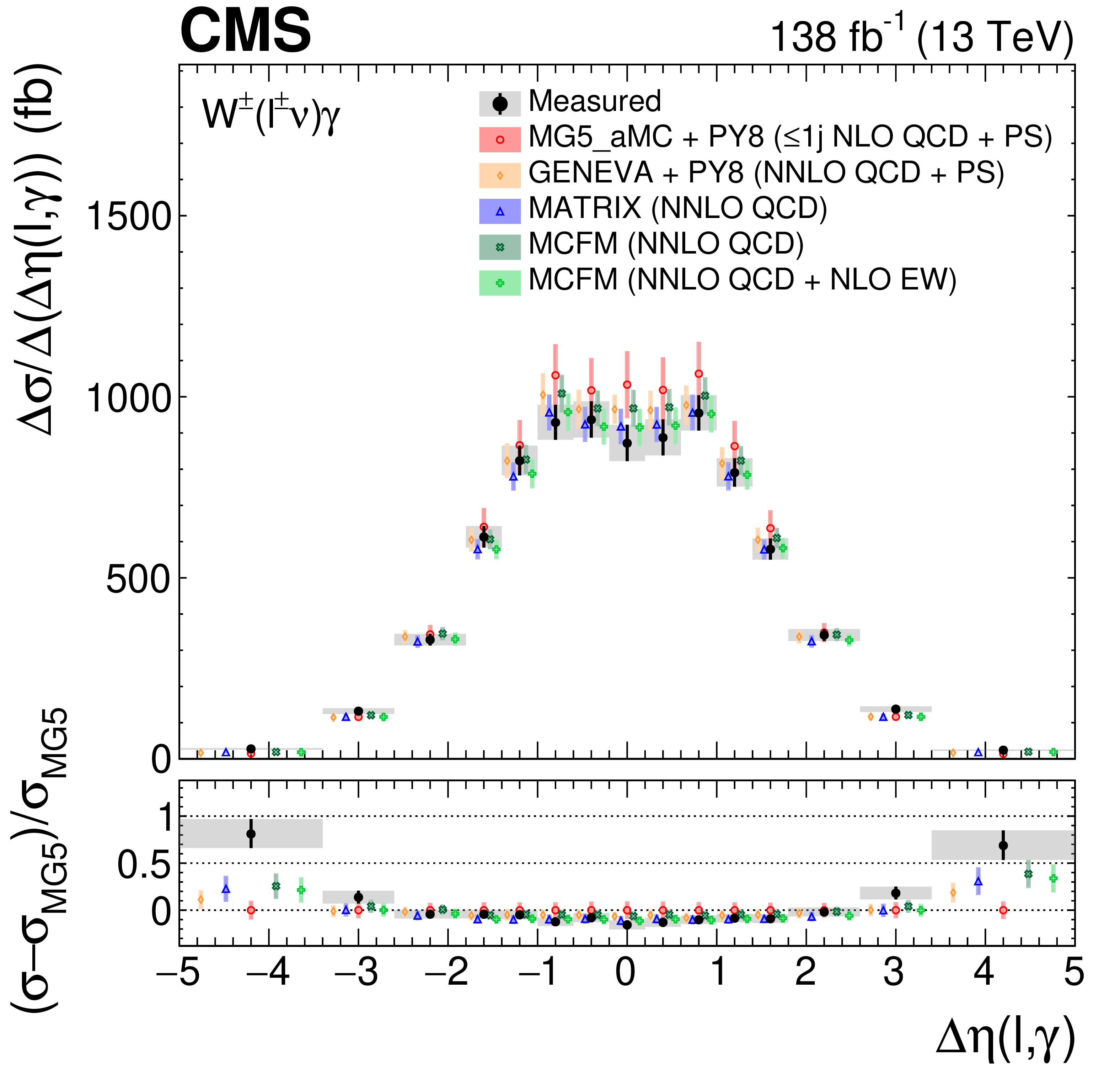
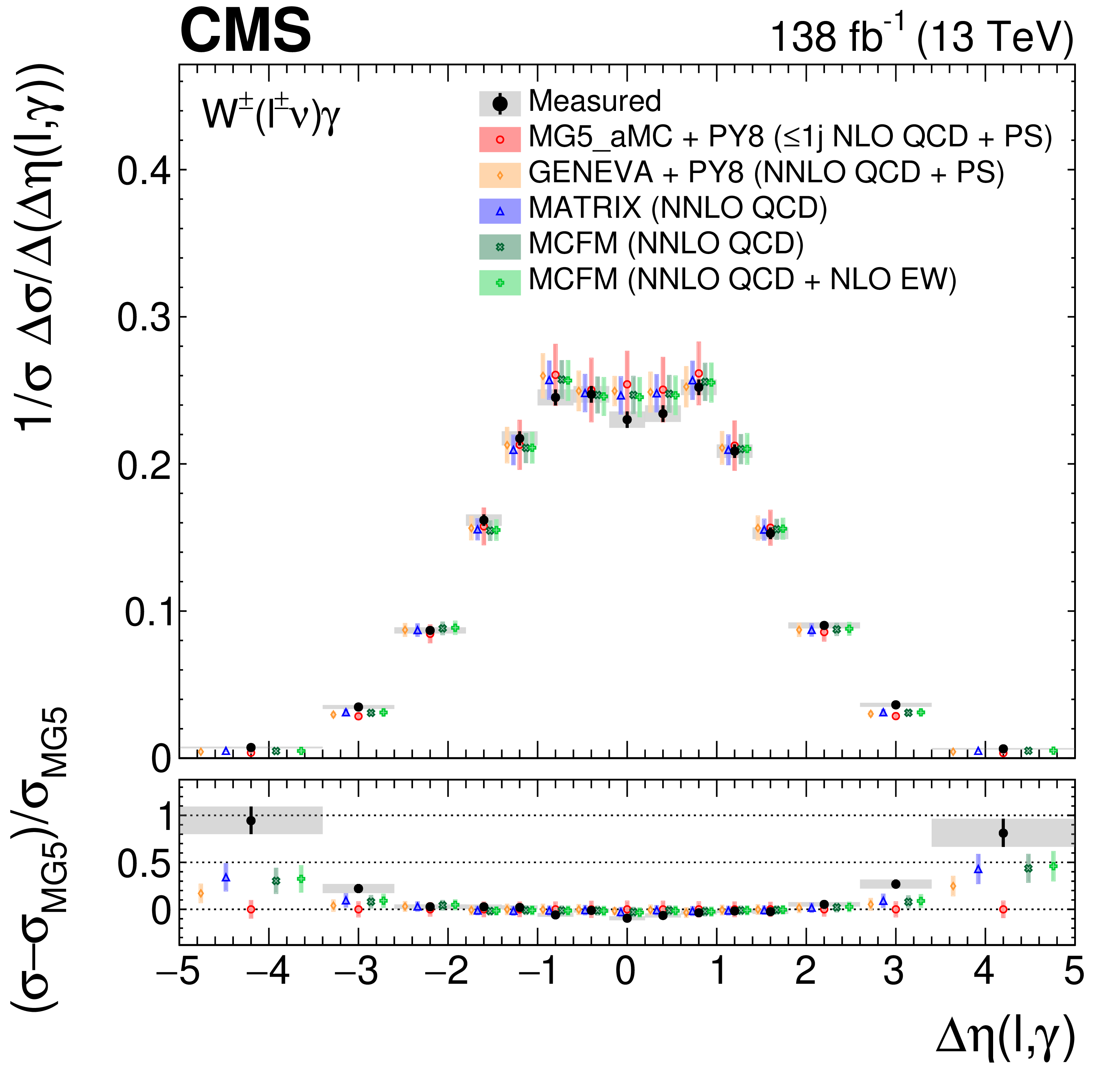
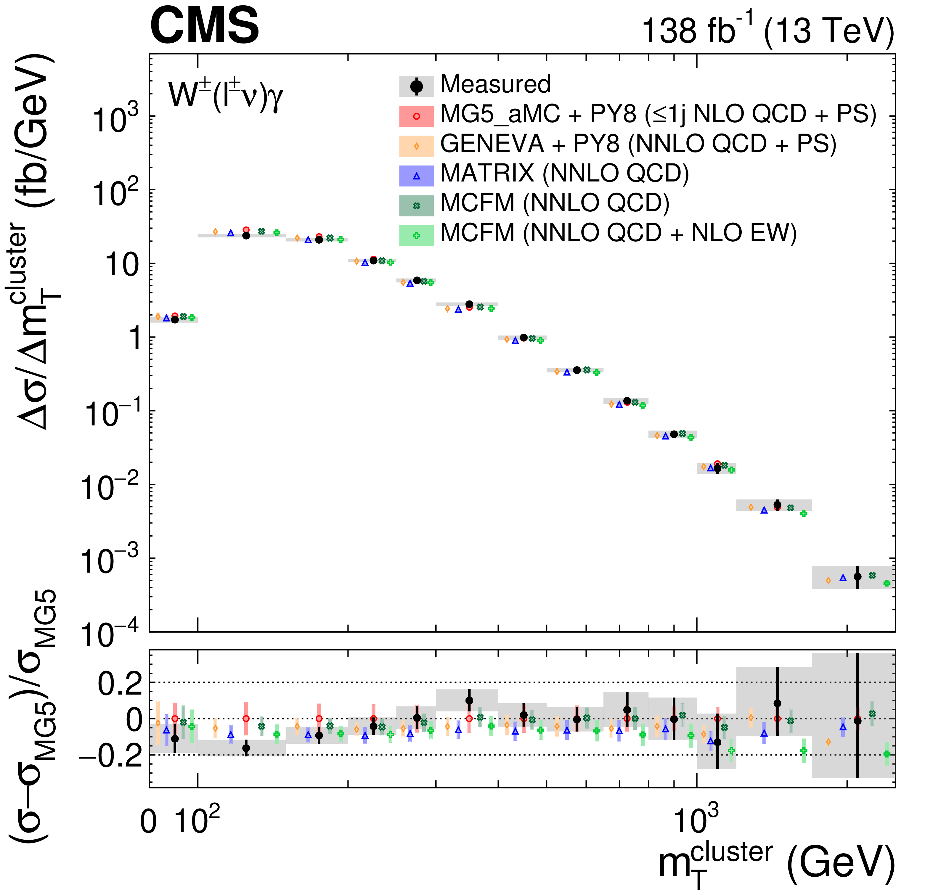
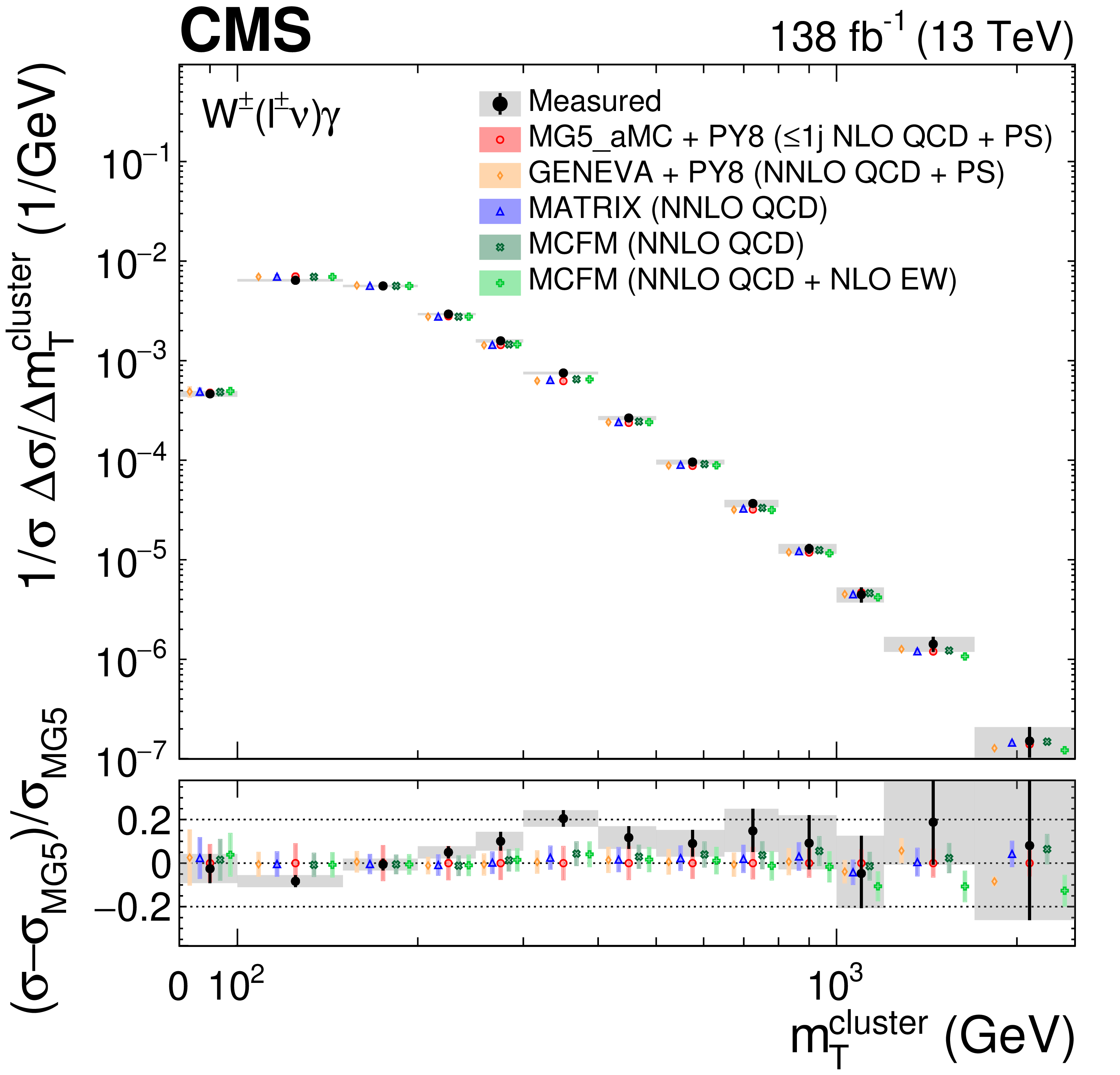
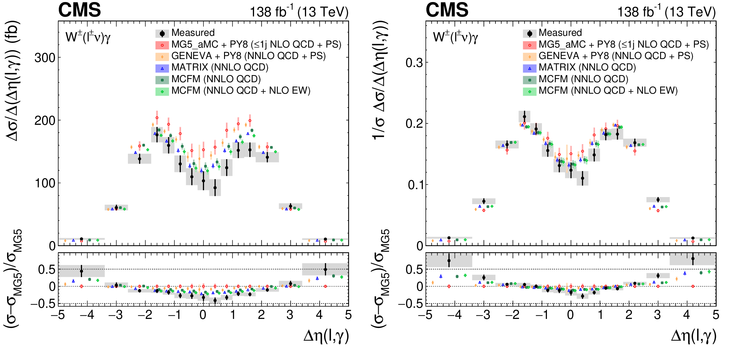
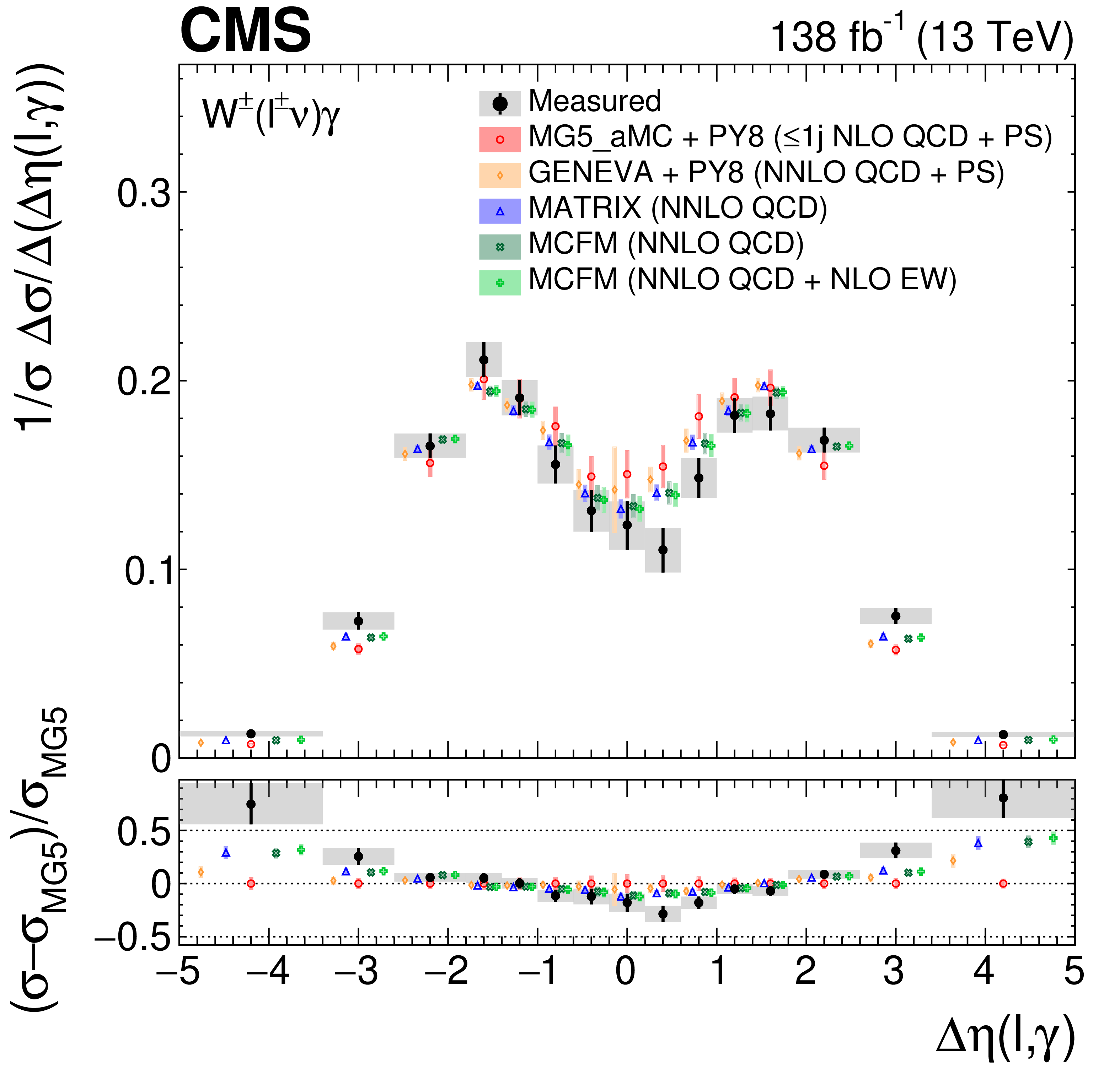
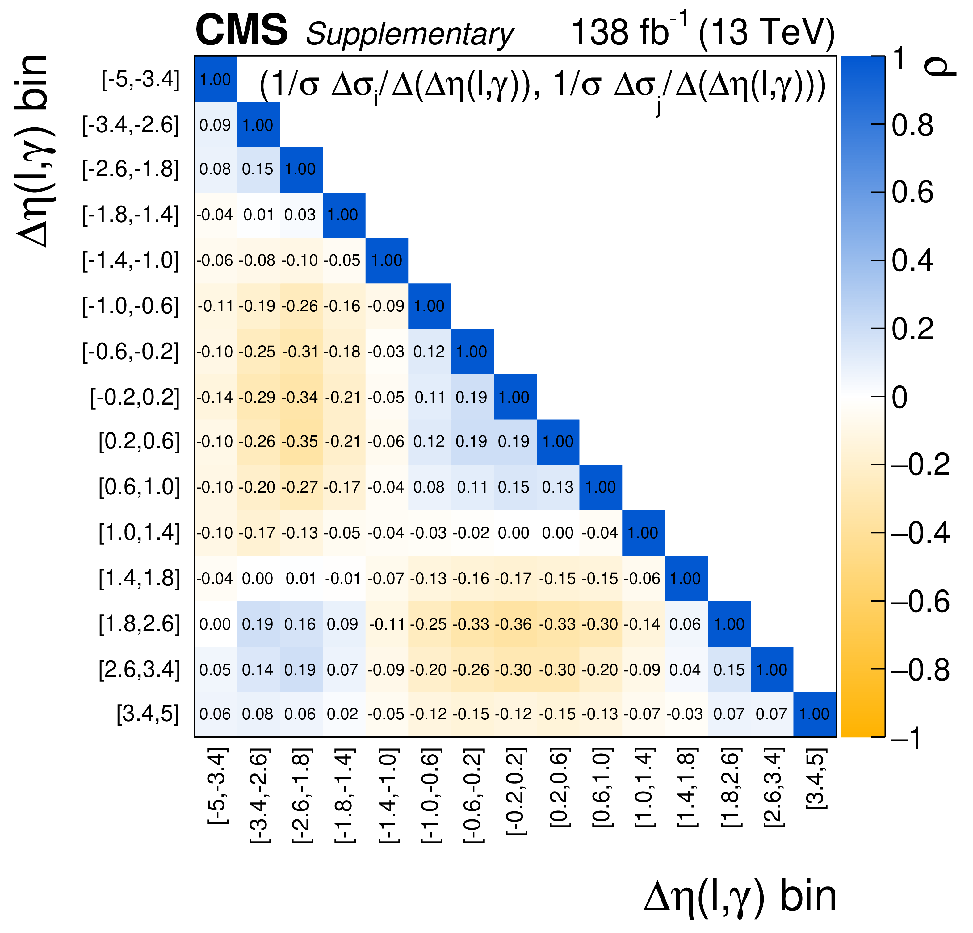
Figure 8:
The measured absolute (left) and fractional (right) differential cross sections for ${{\Delta \eta} (\ell,\gamma)}$ (upper) and ${m_{\mathrm {T}}^{\text {cluster}}}$ (lower), compared with the MG5\_aMC+PY8, GENEVA, MATRIX and MCFM predictions. The shaded bands give the corresponding missing higher order correction uncertainties. The black vertical bars give the total uncertainty on each measurement. The predictions are offset horizontally in each bin to improve visibility, and the corresponding vertical bars show the missing higher order correction uncertainties. |
png pdf |
Figure 8-a:
The measured absolute (left) and fractional (right) differential cross sections for ${{\Delta \eta} (\ell,\gamma)}$ (upper) and ${m_{\mathrm {T}}^{\text {cluster}}}$ (lower), compared with the MG5\_aMC+PY8, GENEVA, MATRIX and MCFM predictions. The shaded bands give the corresponding missing higher order correction uncertainties. The black vertical bars give the total uncertainty on each measurement. The predictions are offset horizontally in each bin to improve visibility, and the corresponding vertical bars show the missing higher order correction uncertainties. |
png pdf |
Figure 8-b:
The measured absolute (left) and fractional (right) differential cross sections for ${{\Delta \eta} (\ell,\gamma)}$ (upper) and ${m_{\mathrm {T}}^{\text {cluster}}}$ (lower), compared with the MG5\_aMC+PY8, GENEVA, MATRIX and MCFM predictions. The shaded bands give the corresponding missing higher order correction uncertainties. The black vertical bars give the total uncertainty on each measurement. The predictions are offset horizontally in each bin to improve visibility, and the corresponding vertical bars show the missing higher order correction uncertainties. |
png pdf |
Figure 8-c:
The measured absolute (left) and fractional (right) differential cross sections for ${{\Delta \eta} (\ell,\gamma)}$ (upper) and ${m_{\mathrm {T}}^{\text {cluster}}}$ (lower), compared with the MG5\_aMC+PY8, GENEVA, MATRIX and MCFM predictions. The shaded bands give the corresponding missing higher order correction uncertainties. The black vertical bars give the total uncertainty on each measurement. The predictions are offset horizontally in each bin to improve visibility, and the corresponding vertical bars show the missing higher order correction uncertainties. |
png pdf |
Figure 8-d:
The measured absolute (left) and fractional (right) differential cross sections for ${{\Delta \eta} (\ell,\gamma)}$ (upper) and ${m_{\mathrm {T}}^{\text {cluster}}}$ (lower), compared with the MG5\_aMC+PY8, GENEVA, MATRIX and MCFM predictions. The shaded bands give the corresponding missing higher order correction uncertainties. The black vertical bars give the total uncertainty on each measurement. The predictions are offset horizontally in each bin to improve visibility, and the corresponding vertical bars show the missing higher order correction uncertainties. |
png pdf |
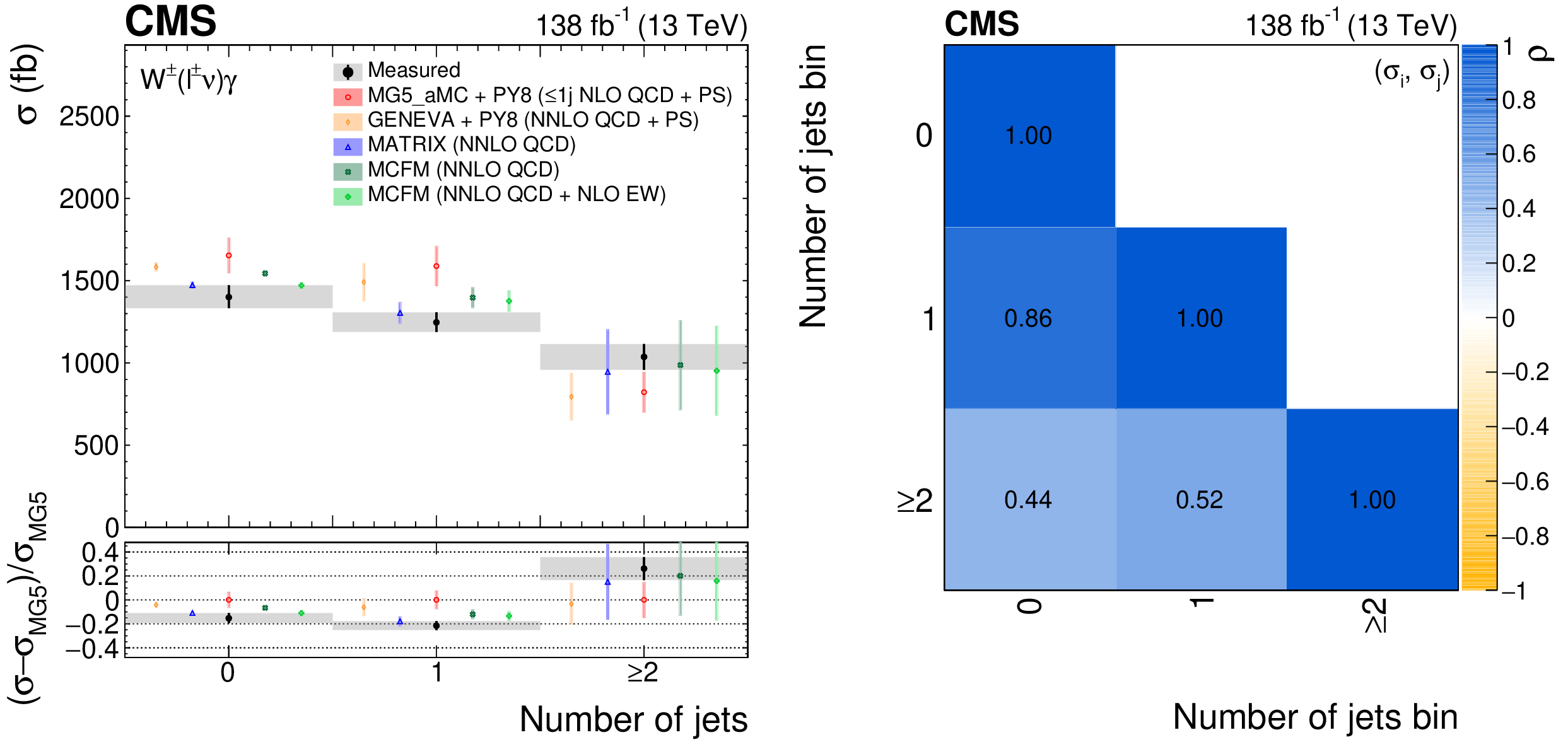
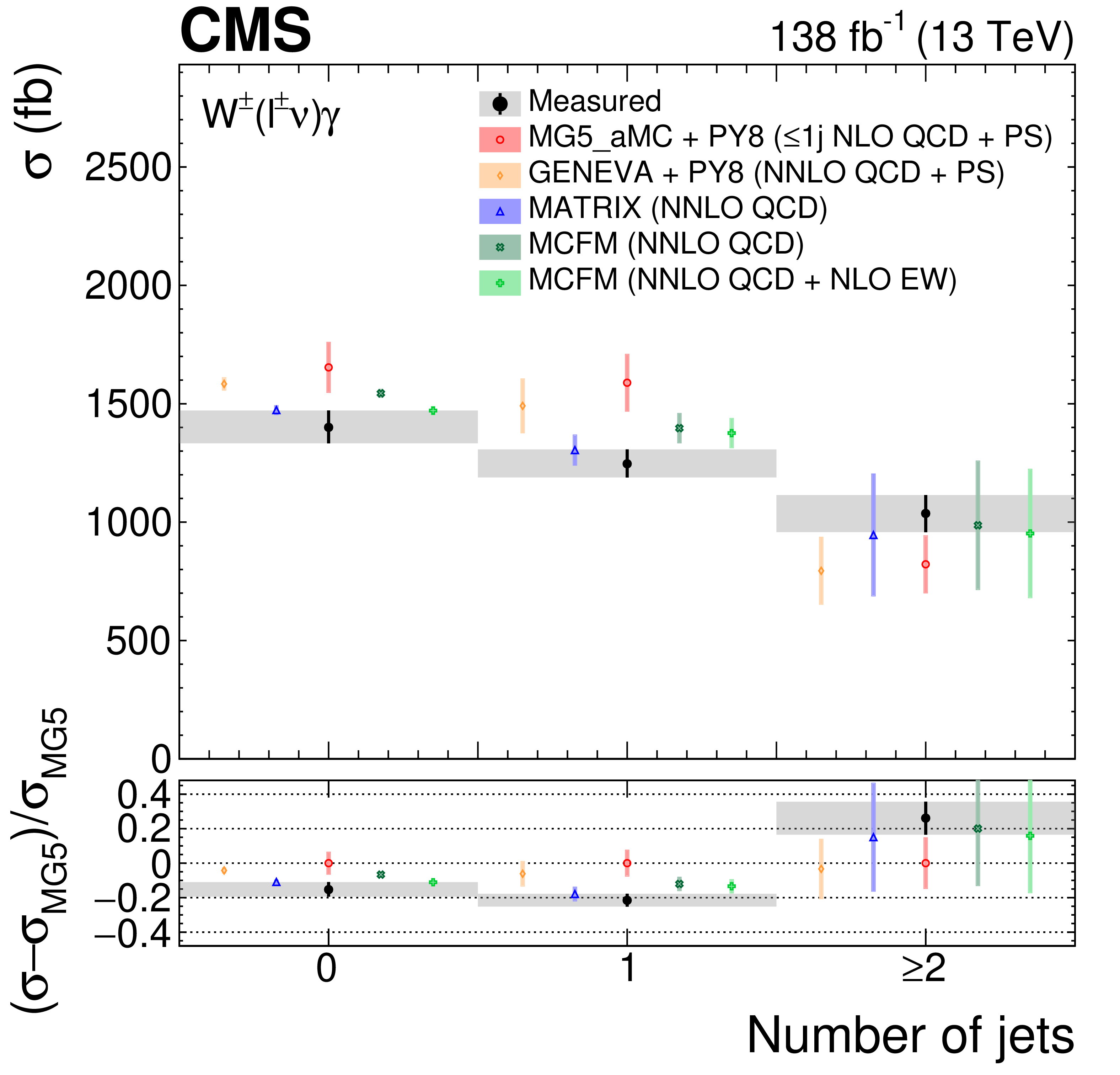
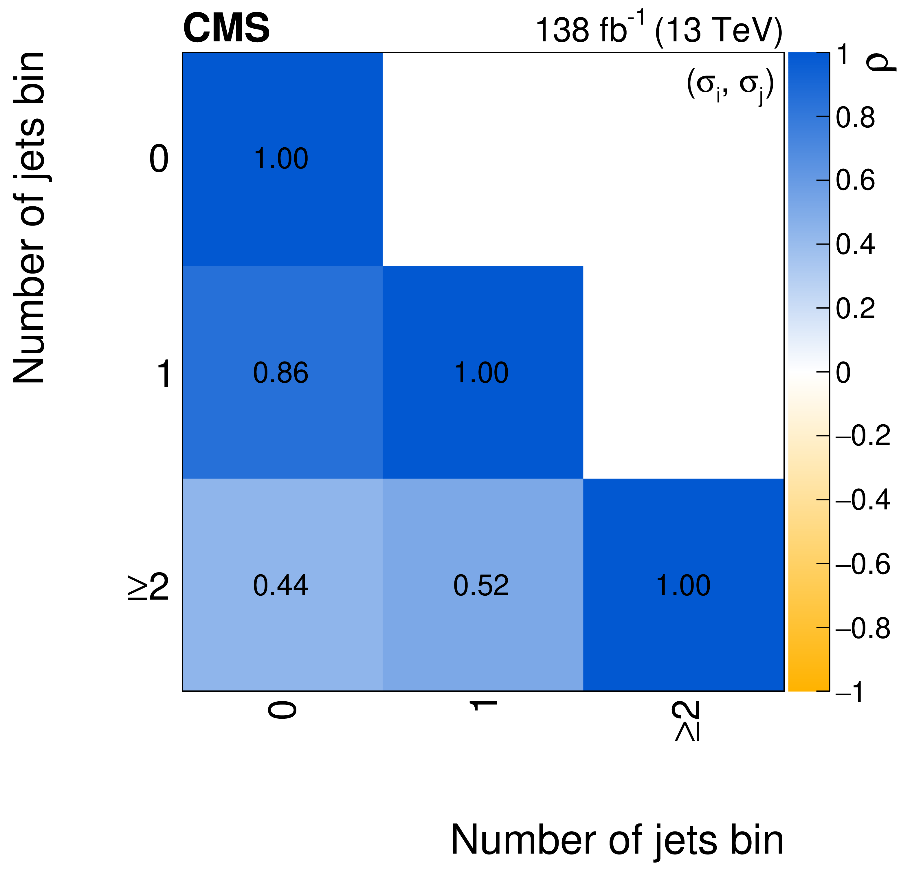
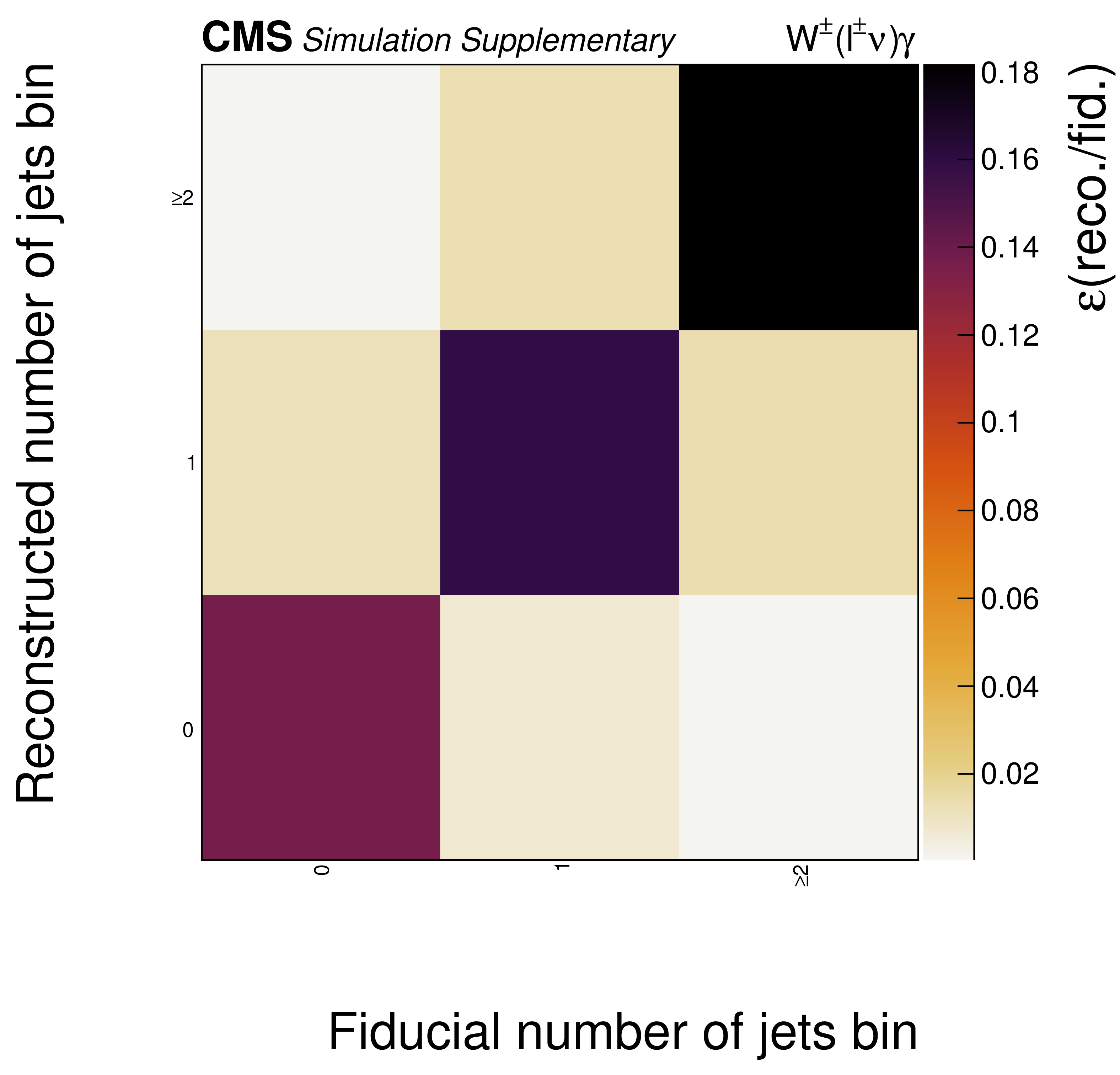
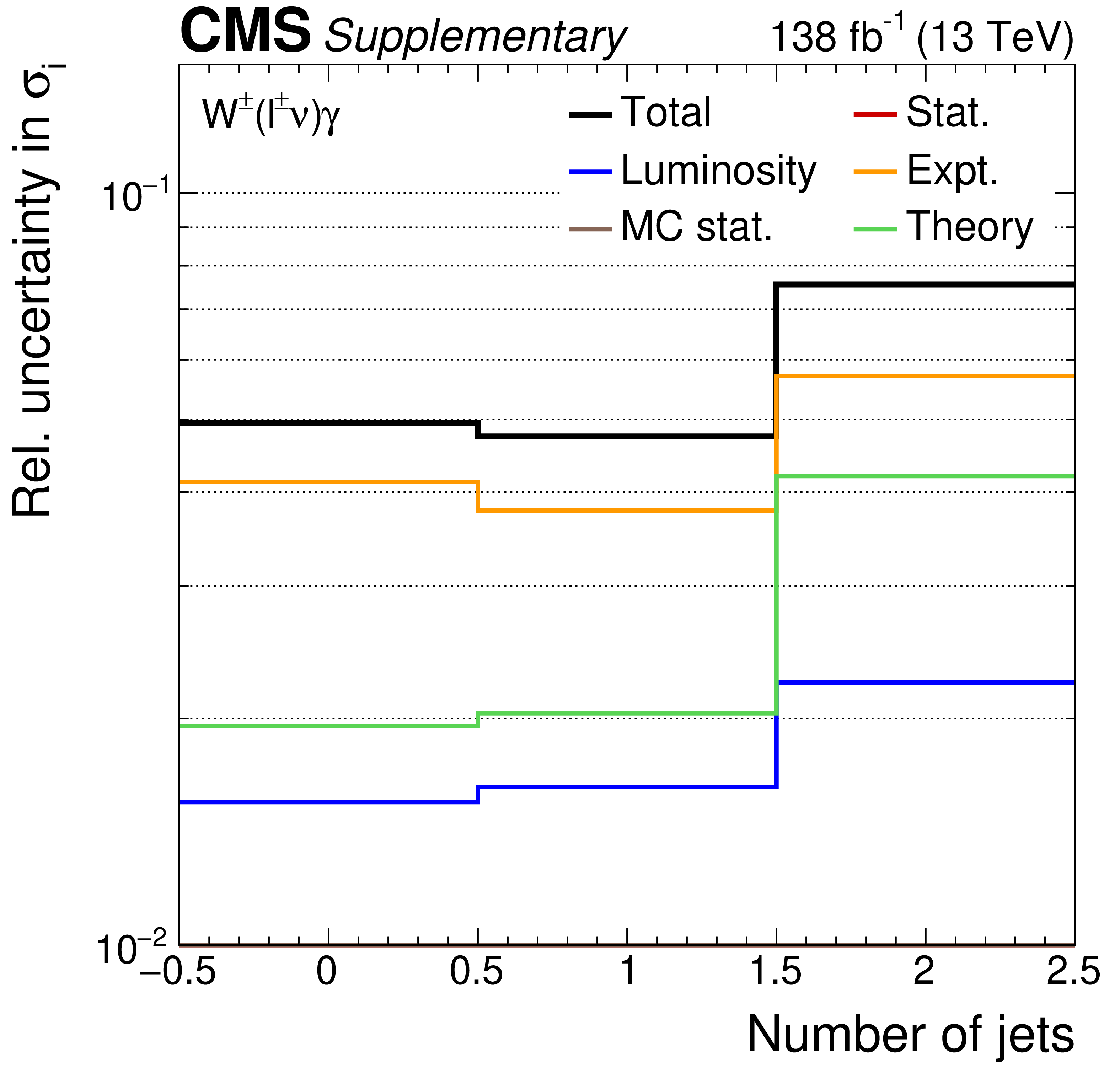
Figure 9:
The measured jet multiplicity cross sections (left) and corresponding correlation matrix (right). In the left figure, the black vertical bars give the total uncertainty on each measurement. The predictions are offset horizontally in each bin to improve visibility, and the corresponding vertical bars show the missing higher order correction uncertainties. |
png pdf |
Figure 9-a:
The measured jet multiplicity cross sections (left) and corresponding correlation matrix (right). In the left figure, the black vertical bars give the total uncertainty on each measurement. The predictions are offset horizontally in each bin to improve visibility, and the corresponding vertical bars show the missing higher order correction uncertainties. |
png pdf |
Figure 9-b:
The measured jet multiplicity cross sections (left) and corresponding correlation matrix (right). In the left figure, the black vertical bars give the total uncertainty on each measurement. The predictions are offset horizontally in each bin to improve visibility, and the corresponding vertical bars show the missing higher order correction uncertainties. |
png pdf |
Figure 10:
The measured ${{\Delta \eta} (\ell,\gamma)}$ absolute (left) and fractional (right) differential cross sections, compared with the MG5\_aMC+PY8, GENEVA, MATRIX and MCFM predictions. The black vertical bars give the total uncertainty on each measurement. The predictions are offset horizontally in each bin to improve visibility, and the corresponding vertical bars show the missing higher order correction uncertainties. |
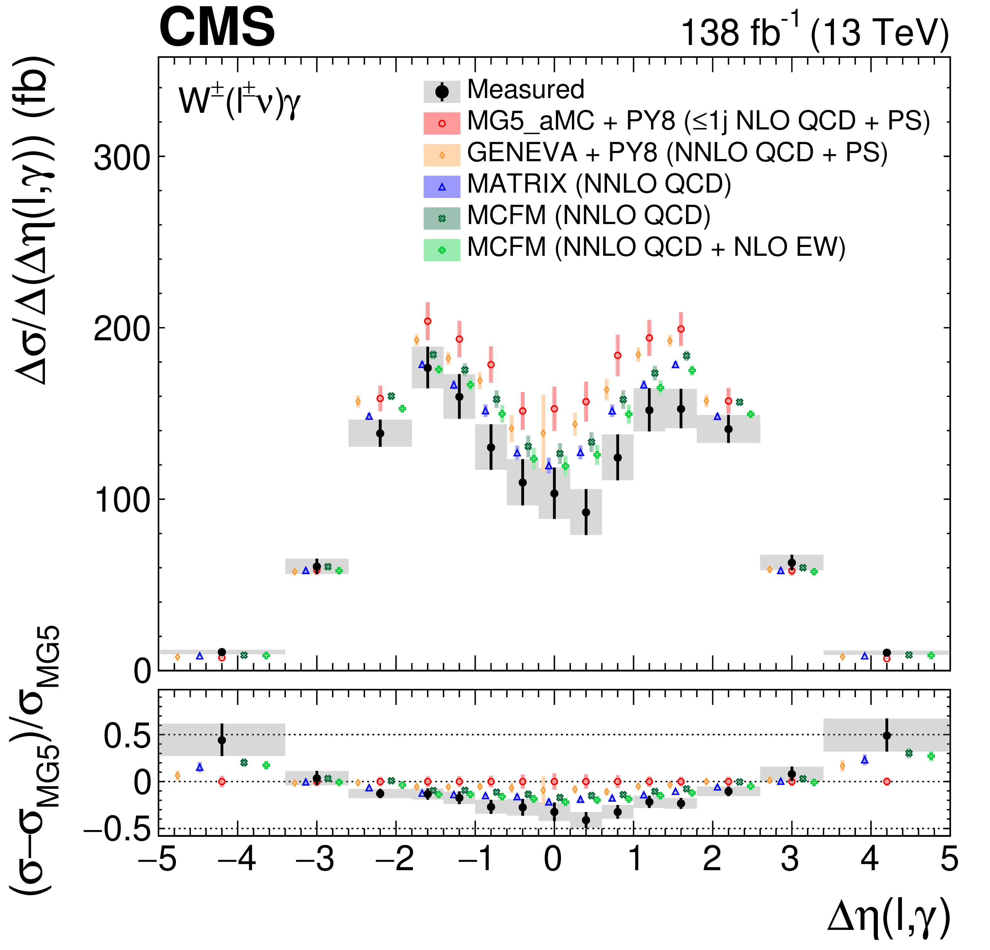
png pdf |
Figure 10-a:
The measured ${{\Delta \eta} (\ell,\gamma)}$ absolute (left) and fractional (right) differential cross sections, compared with the MG5\_aMC+PY8, GENEVA, MATRIX and MCFM predictions. The black vertical bars give the total uncertainty on each measurement. The predictions are offset horizontally in each bin to improve visibility, and the corresponding vertical bars show the missing higher order correction uncertainties. |
png pdf |
Figure 10-b:
The measured ${{\Delta \eta} (\ell,\gamma)}$ absolute (left) and fractional (right) differential cross sections, compared with the MG5\_aMC+PY8, GENEVA, MATRIX and MCFM predictions. The black vertical bars give the total uncertainty on each measurement. The predictions are offset horizontally in each bin to improve visibility, and the corresponding vertical bars show the missing higher order correction uncertainties. |
png pdf |
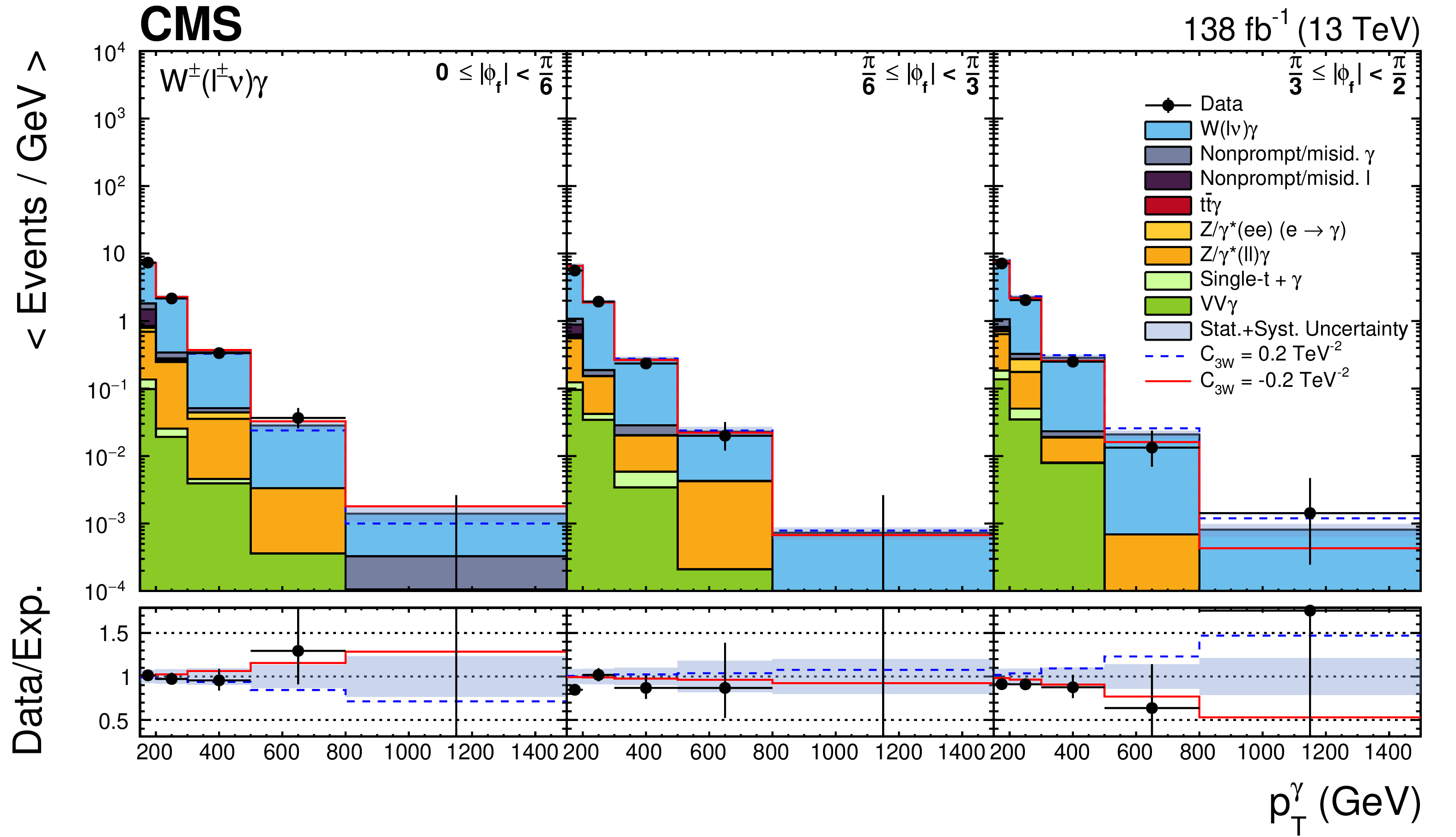
Figure 11:
The expected and observed ${{p_{\mathrm {T}}} ^{\gamma}}$ distribution in each ${| {\phi _{f}} |}$ region before the maximum likelihood fit is performed. The horizontal and vertical bars associated to the data points correspond to the bin widths and statistical uncertainties, respectively. The shaded uncertainty band incorporates all statistical and systematic uncertainties. The red and blue lines show how the total expectation changes when ${C_{3W}}$ is set to $-$0.2 and 0.2 TeV$ ^{-2}$, respectively. Only the SM and interference terms are included in this example. |
png pdf |
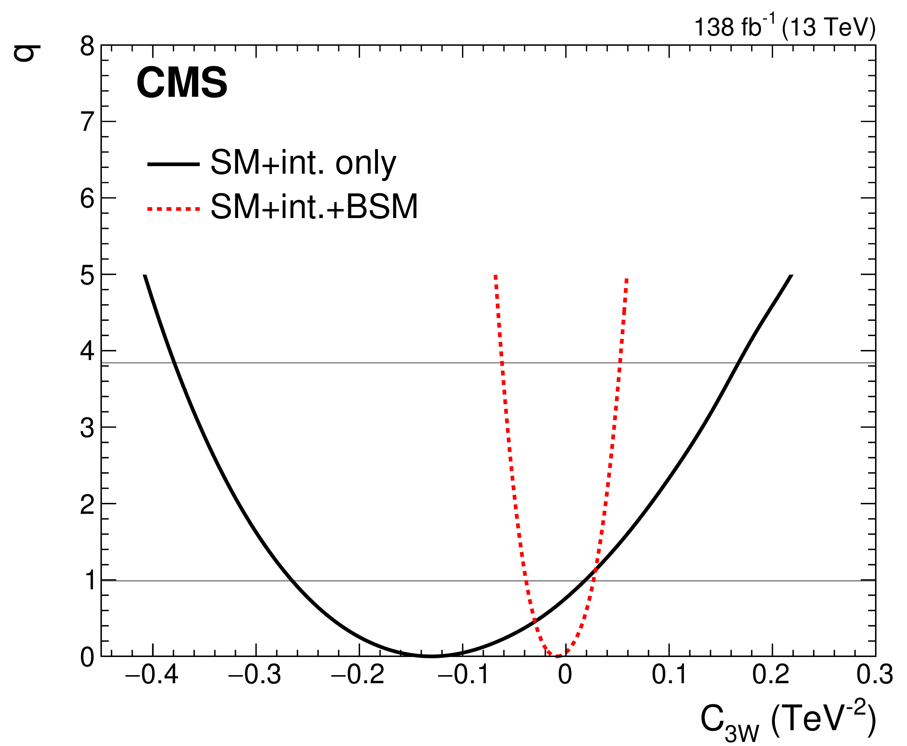
Figure 12:
Scans of the profile likelihood test statistic $q$ as a function of ${C_{3W}}$, given with and without the pure BSM term by the dashed red and solid black lines, respectively. The full set of ${{p_{\mathrm {T}}} ^{\gamma}}$ and ${| {\phi _{f}} |}$ bins, described in the text, are included for these scans. |
png pdf |
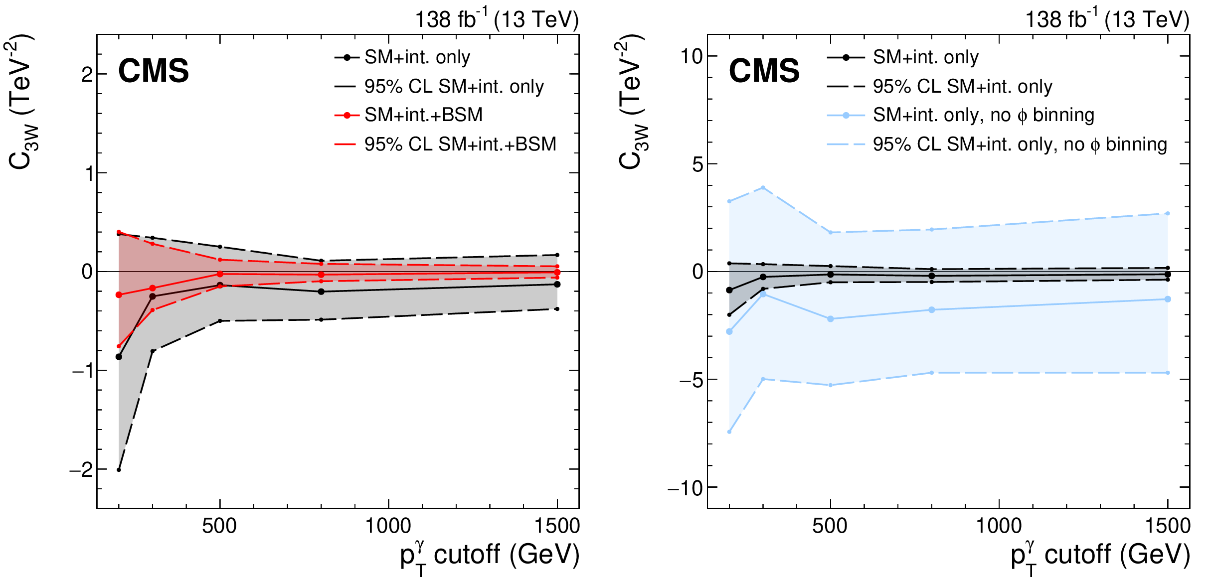
Figure 13:
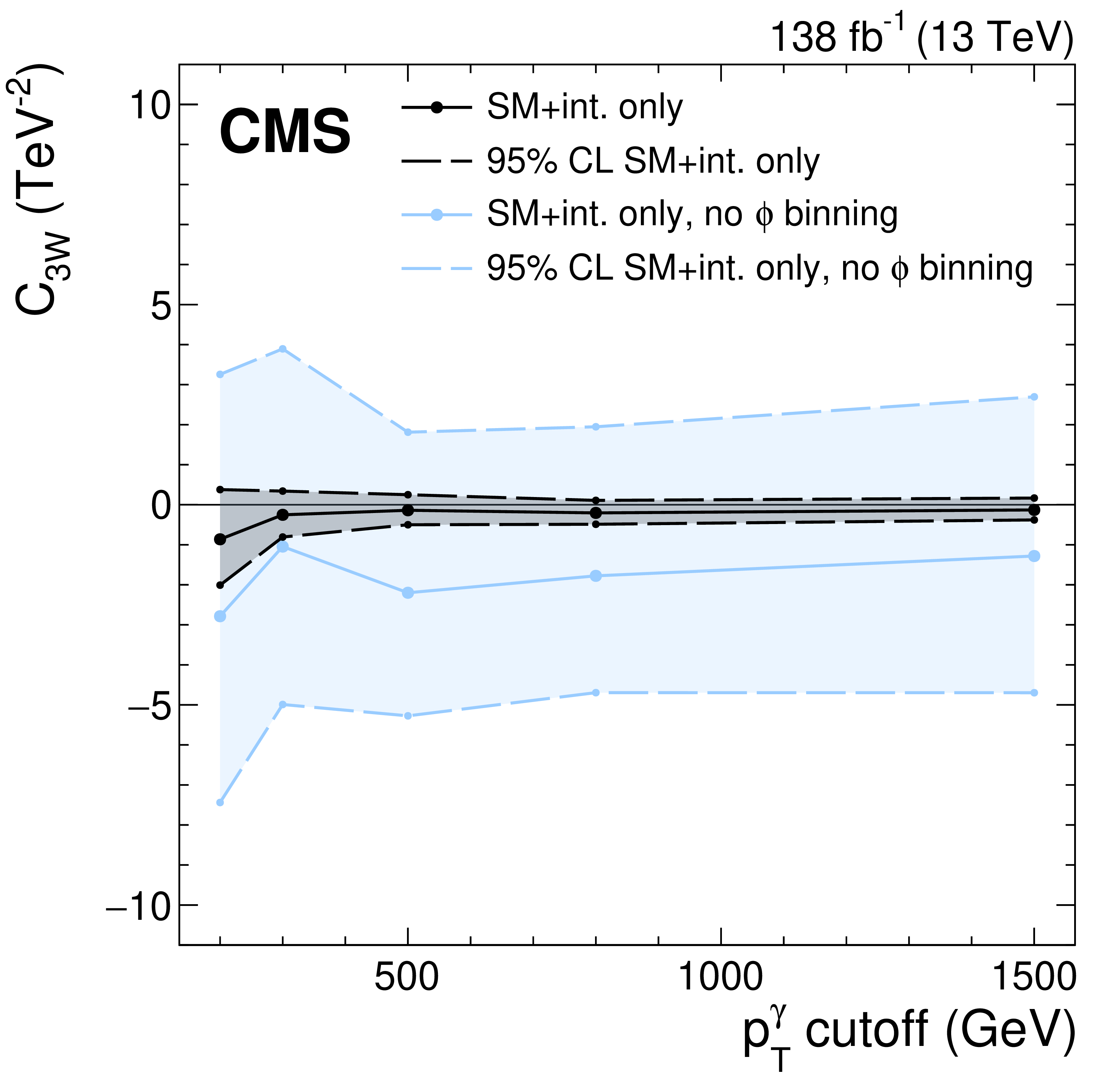
Best-fit values of ${C_{3W}}$ and the corresponding 95% CL confidence intervals as a function of the maximum ${{p_{\mathrm {T}}} ^{\gamma}}$ bin included in the fit (left). Measurements with and without the pure BSM term are given by the black and red lines, respectively. The limits without the pure BSM term given with and without the binning in ${| {\phi _{f}} |}$ are also shown (right), with black and blue lines, respectively. Please note the different vertical scales; the black lines in both figures correspond to the same limits. |

png pdf |
Figure 13-a:
Best-fit values of ${C_{3W}}$ and the corresponding 95% CL confidence intervals as a function of the maximum ${{p_{\mathrm {T}}} ^{\gamma}}$ bin included in the fit (left). Measurements with and without the pure BSM term are given by the black and red lines, respectively. The limits without the pure BSM term given with and without the binning in ${| {\phi _{f}} |}$ are also shown (right), with black and blue lines, respectively. Please note the different vertical scales; the black lines in both figures correspond to the same limits. |
png pdf |
Figure 13-b:
Best-fit values of ${C_{3W}}$ and the corresponding 95% CL confidence intervals as a function of the maximum ${{p_{\mathrm {T}}} ^{\gamma}}$ bin included in the fit (left). Measurements with and without the pure BSM term are given by the black and red lines, respectively. The limits without the pure BSM term given with and without the binning in ${| {\phi _{f}} |}$ are also shown (right), with black and blue lines, respectively. Please note the different vertical scales; the black lines in both figures correspond to the same limits. |
png pdf |
Figure 14:
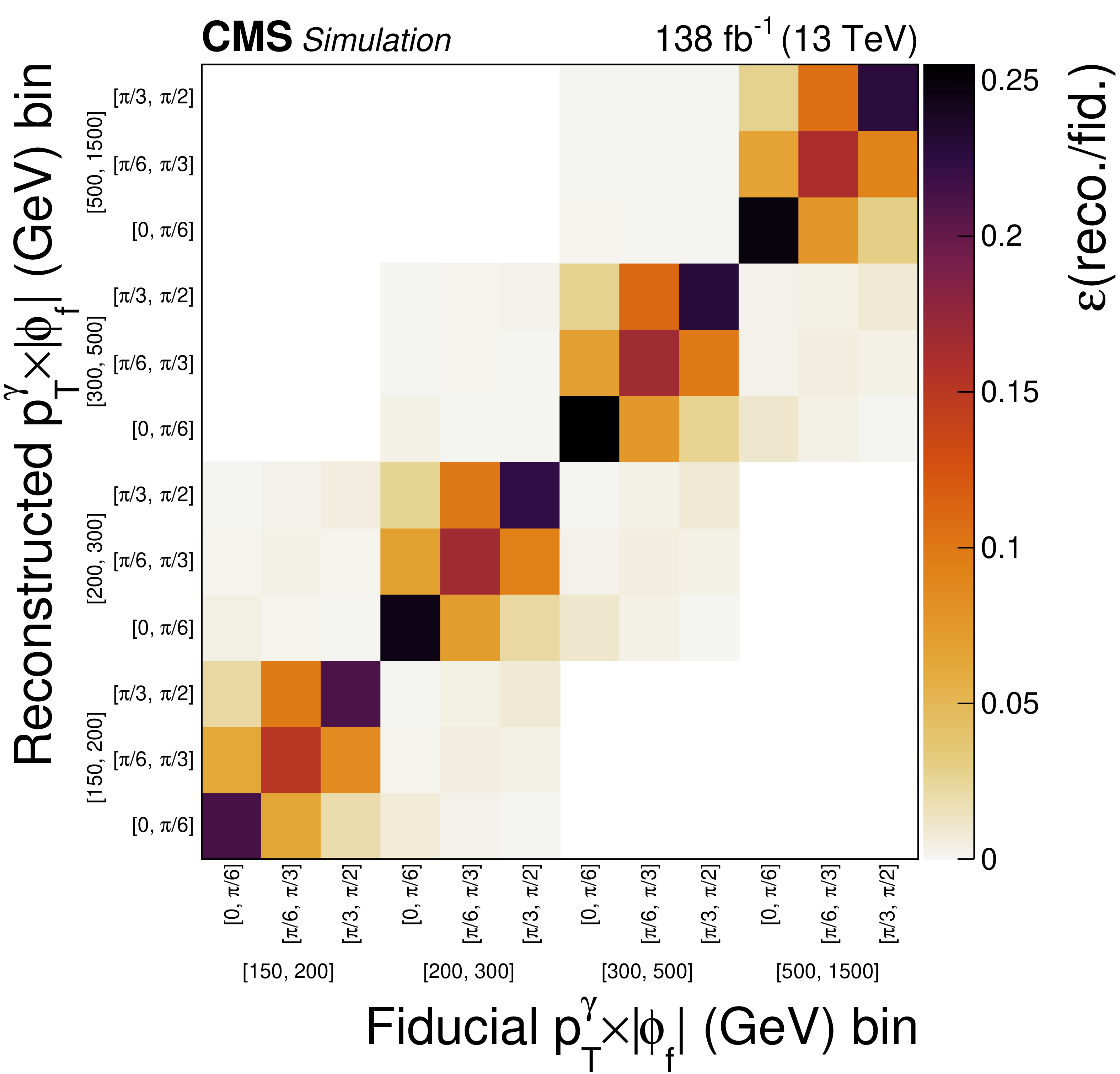
Response matrix for the differential $ {{p_{\mathrm {T}}} ^{\gamma}} {\times} {{| {\phi _{f}} |}} $ cross section measurement. The entry in each bin gives the probability for an event of a given particle-level fiducial bin to be reconstructed in one of the corresponding reconstruction-level bins. The inner labels give the ${| {\phi _{f}} |}$ bin and the outer labels indicate the ${{p_{\mathrm {T}}} ^{\gamma}}$ bin. |
png pdf |
Figure 15:
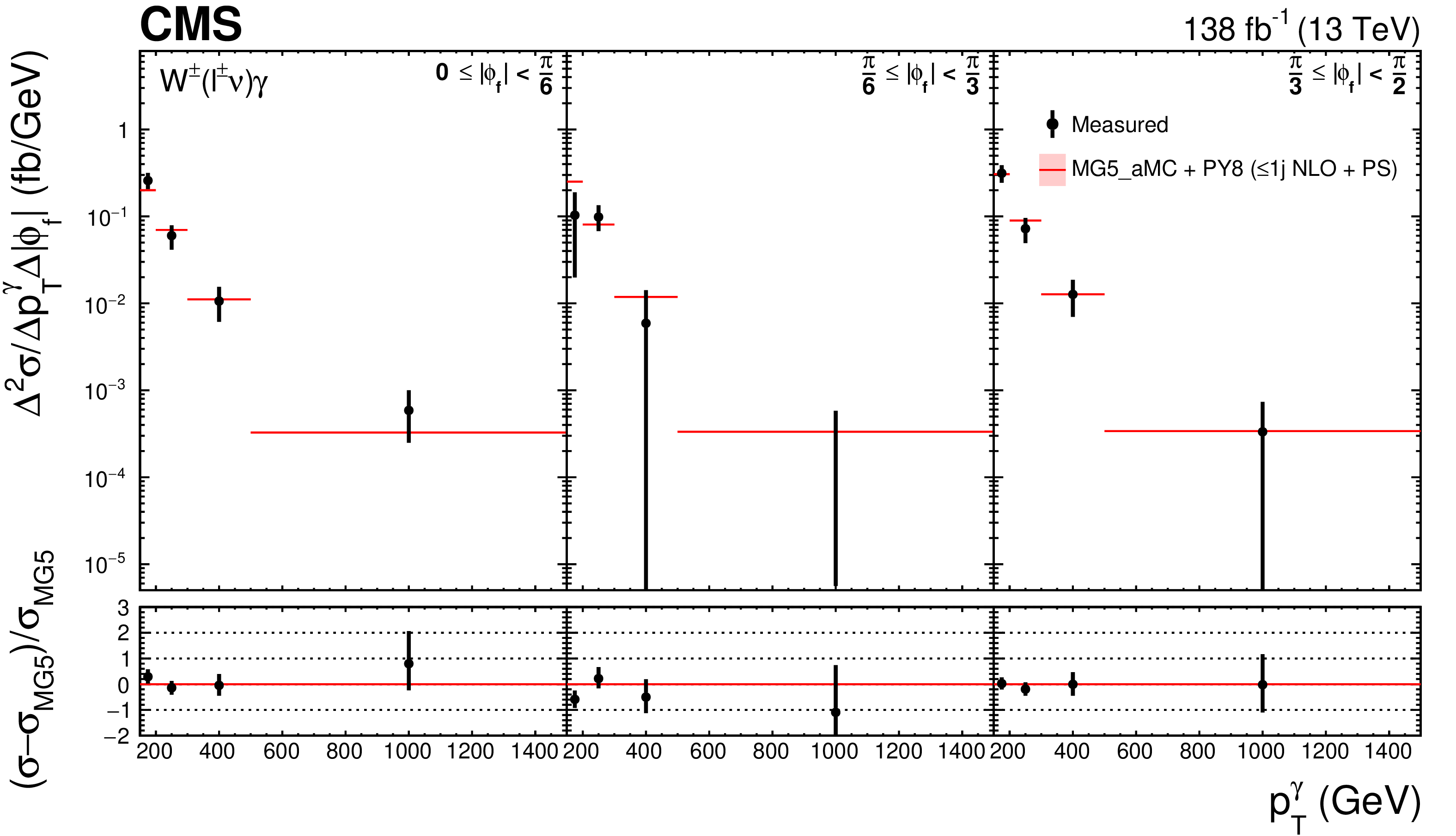
Measured double-differential $ {{p_{\mathrm {T}}} ^{\gamma}} {\times} {{| {\phi _{f}} |}} $ cross section and comparison to the MG5\_aMC+PY8 NLO prediction. The black vertical bars give the total uncertainty on each measurement. The red shaded bands give the missing higher order correction uncertainties in the prediction. |
png pdf |
Figure 16:
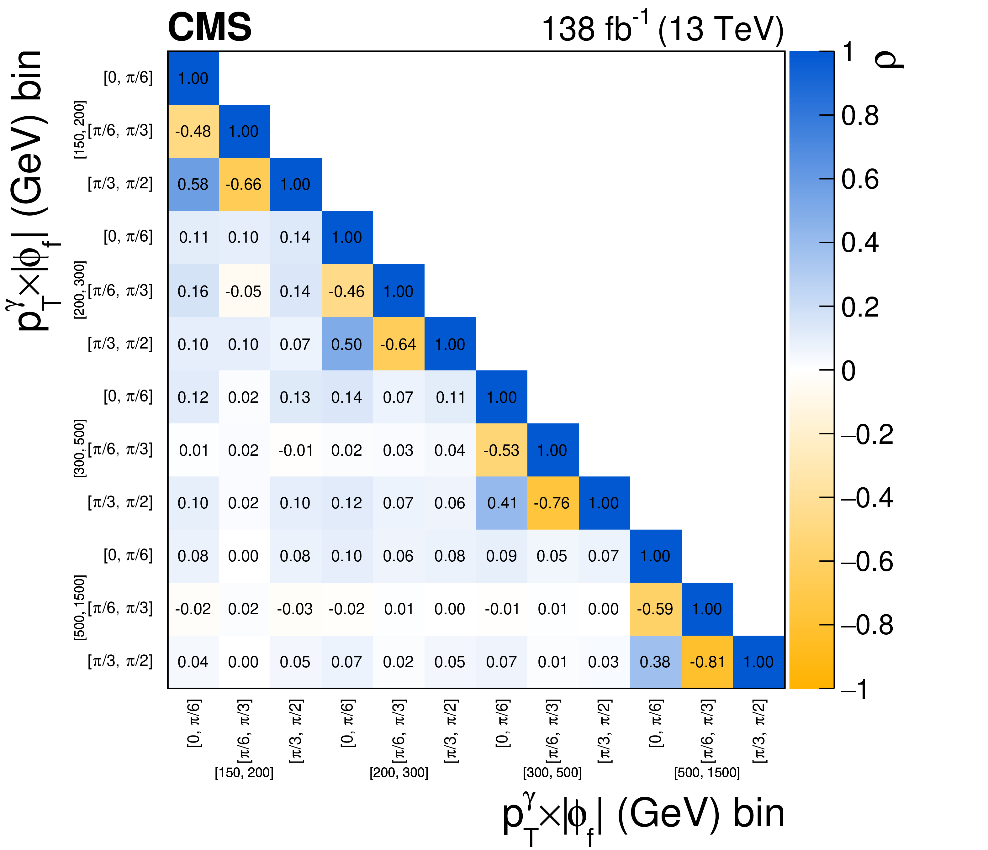
Correlation matrix for the measured $ {{p_{\mathrm {T}}} ^{\gamma}} {\times} {{| {\phi _{f}} |}} $ cross sections. |
| Tables | |
png pdf |
Table 1:
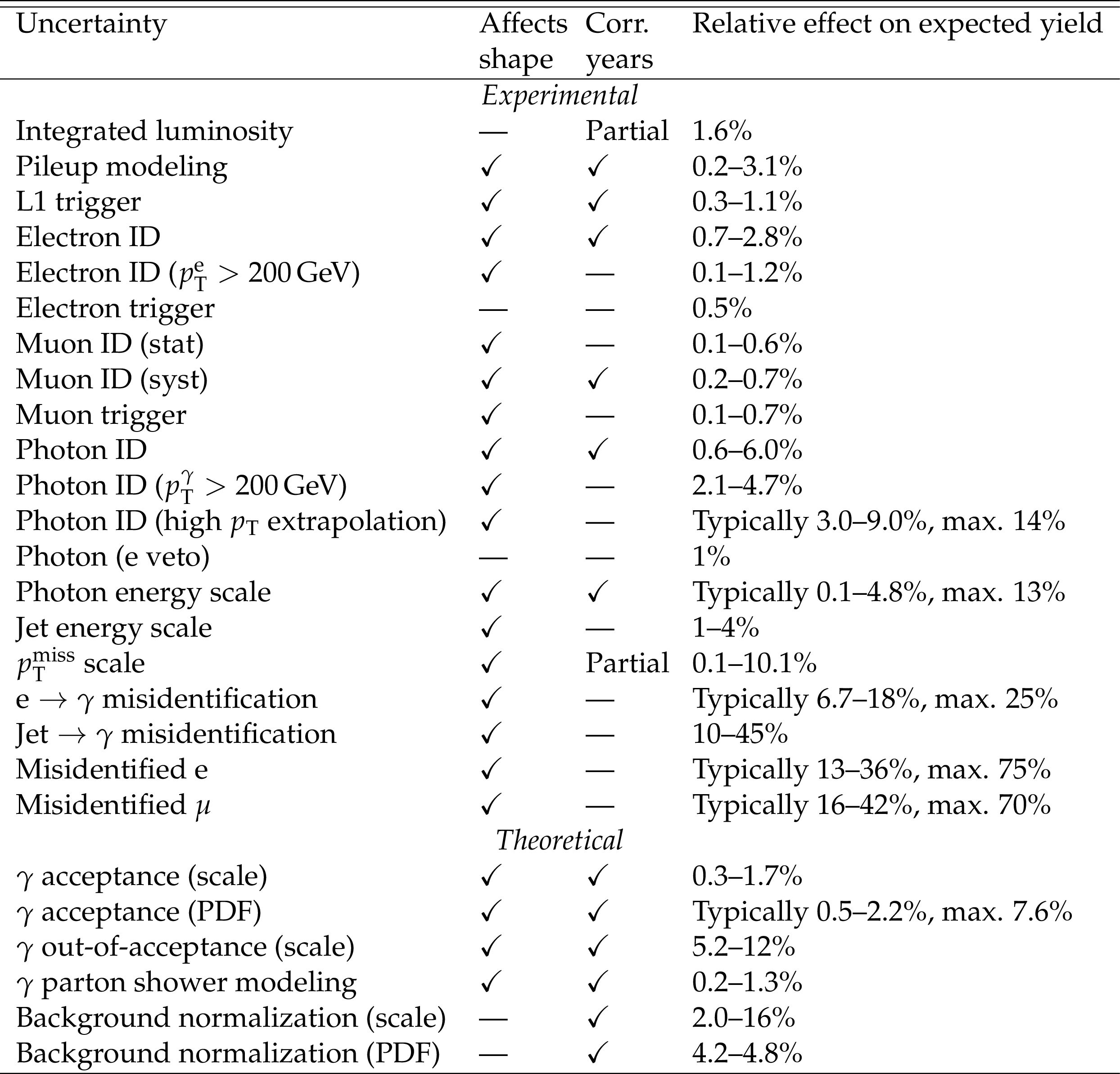
Summary of the systematic uncertainties affecting the signal and background predictions. The table notes whether each uncertainty affects the shape of the measured observable or just the normalization, and whether the effect is correlated between the data-taking years. The normalization effect on the expected yield of the applicable processes is also given. For some shape uncertainties the values vary significantly across the observable distribution. In these cases the typical range and maximum values are given, where the former is the central 68% interval considering all bins. |
png pdf |
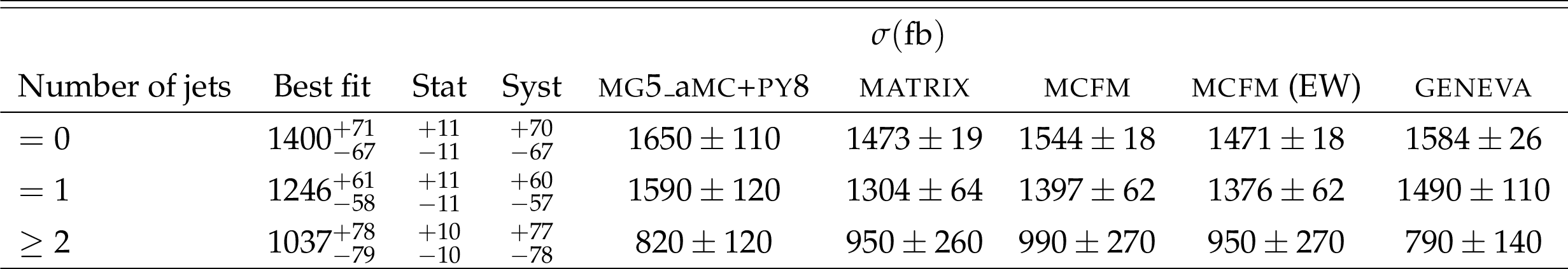
Table 2:
Cross sections measured in bins of jet multiplicity and comparison with the MG5\_aMC+PY8, GENEVA, MATRIX and MCFM predictions. The MCFM column marked (EW) is the NNLO QCD prediction combined with NLO electroweak corrections, as described in the text. |

png pdf |
Table 3:
Fiducial cross section scaling terms as a function of ${C_{3W}}$ in all $ {{p_{\mathrm {T}}} ^{\gamma}} {\times} {{| {\phi _{f}} |}} $ bins. Values are given relative to the SM prediction: $ {\mu ^{\text {int}}} = {\sigma ^{\text {int}}} / {\sigma ^{\text {SM}}} $ and $ {\mu ^{\text {BSM}}} = {\sigma ^{\text {BSM}}} / {\sigma ^{\text {SM}}} $. |
png pdf |
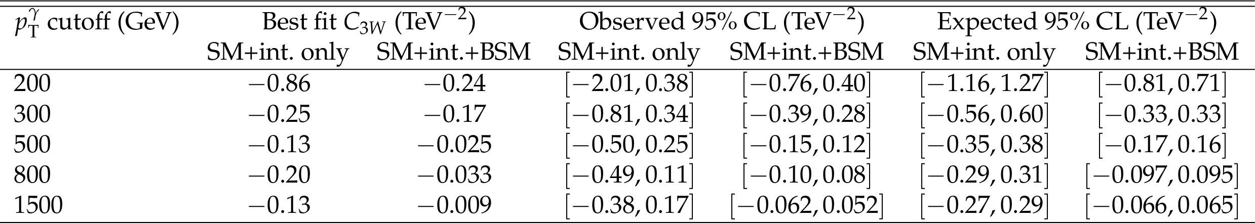
Table 4:
Best fit values of ${C_{3W}}$ and corresponding 95% CL confidence intervals as a function of the maximum ${{p_{\mathrm {T}}} ^{\gamma}}$ bin included in the fit. |
| Summary |
|
This paper has presented an analysis of ${\mathrm{W^{\pm}}\gamma}$ production in $\sqrt{s} = $ 13 TeV proton-proton collisions using data recorded with the CMS detector at the LHC, corresponding to an integrated luminosity of 138 fb$^{-1}$. Differential cross sections have been measured for several observables and compared with standard model (SM) predictions computed at next-to-leading and next-to-next-to-leading orders in perturbative quantum chromodynamics. The radiation amplitude zero effect, caused by interference between ${\mathrm{W^{\pm}}\gamma}$ production diagrams, has been studied via a measurement of the pseudorapidity difference between the lepton and the photon. Constraints on the presence of TeVns-scale new physics affecting the WW$\gamma$ vertex have been determined using an effective field theory framework. Confidence intervals on the Wilson coefficient ${C_{3W}} $, determined at the 95% confidence level, are [$-$0.062, 0.052] TeV$^{-2}$ with the inclusion of the interference and pure beyond the SM contributions, and [$-$0.38, 0.17] TeV$^{-2}$ when only the interference is considered. A novel two-dimensional approach is used with the simultaneous measurement of the photon transverse momentum and the azimuthal angle of the charged lepton in a special reference frame. With this method, the sensitivity to the interference between the SM and the ${\mathcal{O}_{3W}}$ operator is enhanced by up to a factor of ten compared to a measurement using the transverse momentum alone. This improves the validity of the result, as the dependence on the missing higher-order contributions in the EFT expansion is reduced. The technique will also be valuable in the future when sufficiently small values of ${C_{3W}}$ are probed such that the interference contribution will be dominant. |
| Additional Figures | |
png pdf |
Additional Figure 1:
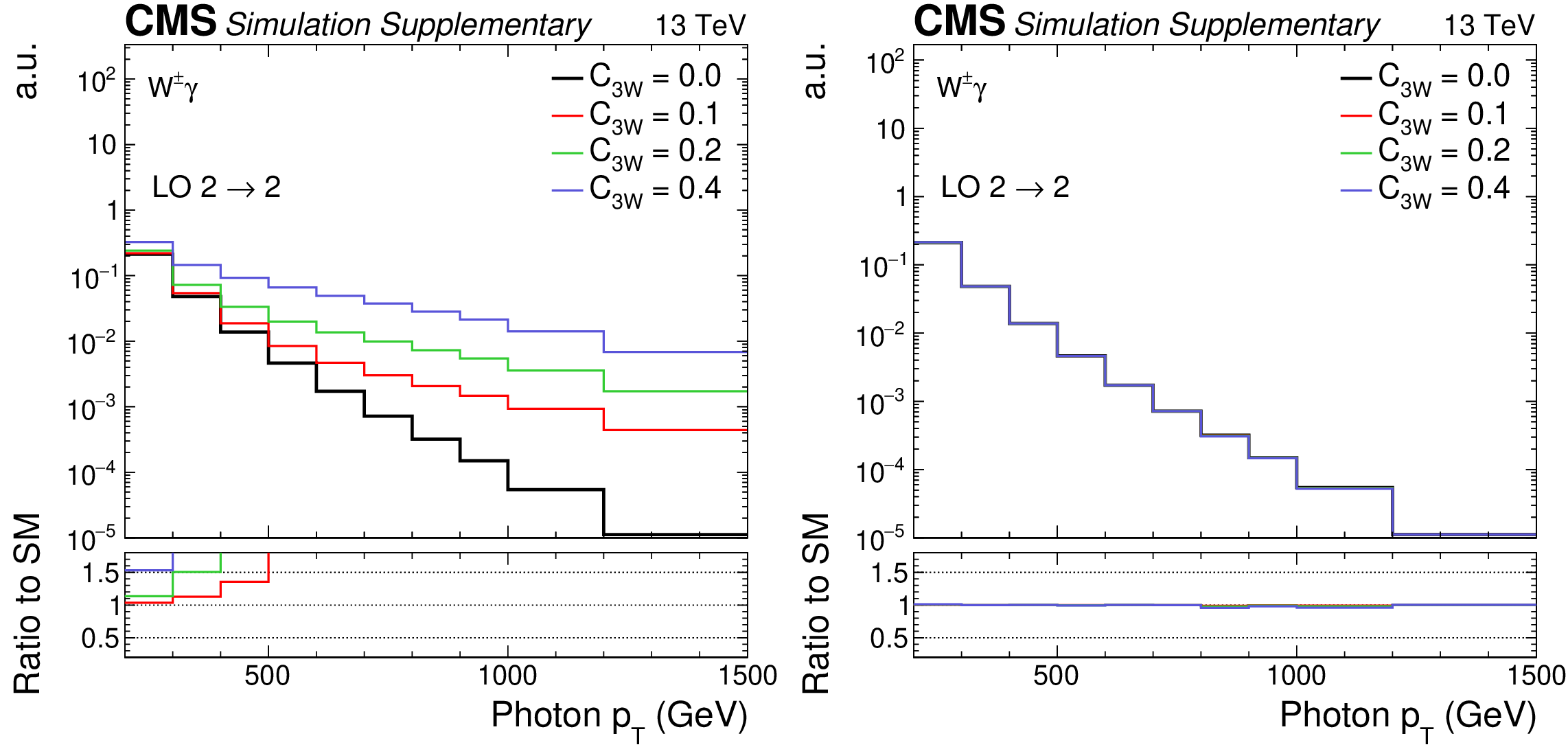
Particle-level distributions of the photon $ {p_{\mathrm {T}}} $, considering only the LO 2 $\rightarrow $ 2 process, comparing the inclusion of the interference and BSM components (left) to the inclusion of only the interference (right). The markers give the SM prediction ($C_{3W} = $ 0) and lines correspond to different values of $C_{3W}$. |
png pdf |
Additional Figure 1-a:
Particle-level distributions of the photon $ {p_{\mathrm {T}}} $, considering only the LO 2 $\rightarrow $ 2 process, with the inclusion of the interference and BSM components. The markers give the SM prediction ($C_{3W} = $ 0) and lines correspond to different values of $C_{3W}$. |
png pdf |
Additional Figure 1-b:
Particle-level distributions of the photon $ {p_{\mathrm {T}}} $, considering only the LO 2 $\rightarrow $ 2 process, with the inclusion of only the interference. The markers give the SM prediction ($C_{3W} = $ 0) and lines correspond to different values of $C_{3W}$. |
png pdf |
Additional Figure 2:
Response matrices for the $ {p_{\mathrm {T}}^{{\gamma}}} $, $\eta ^{{\gamma}}$, $ {\Delta R}(\ell,\gamma)$, $\Delta \eta (\ell,\gamma)$, and $ {m_{\mathrm {T}}^{\text {cluster}}} $ differential cross section measurements under the baseline selection. |
png pdf |
Additional Figure 2-a:
Response matrice for the $ {p_{\mathrm {T}}^{{\gamma}}} $ differential cross section measurement under the baseline selection. |
png pdf |
Additional Figure 2-b:
Response matrice for the $\eta ^{{\gamma}}$ differential cross section measurement under the baseline selection. |

png pdf |
Additional Figure 2-c:
Response matrice for the $ {\Delta R}(\ell,\gamma)$ differential cross section measurement under the baseline selection. |

png pdf |
Additional Figure 2-d:
Response matrice for the $\Delta \eta (\ell,\gamma)$ differential cross section measurement under the baseline selection. |
png pdf |
Additional Figure 2-e:
Response matrice for the $ {m_{\mathrm {T}}^{\text {cluster}}} $ differential cross section measurement under the baseline selection. |

png pdf |
Additional Figure 3:
Expected and observed distributions of $\eta ^{{\gamma}}$, $ {\Delta R}(\ell,\gamma)$ and $\Delta \eta (\ell,\gamma)$ under the baseline selection before the maximum likelihood is performed. |
png pdf |
Additional Figure 3-a:
Expected and observed distributions of $\eta ^{{\gamma}}$ under the baseline selection before the maximum likelihood is performed. |

png pdf |
Additional Figure 3-b:
Expected and observed distributions of $ {\Delta R}(\ell,\gamma)$ under the baseline selection before the maximum likelihood is performed. |
png pdf |
Additional Figure 3-c:
Expected and observed distributions of $\Delta \eta (\ell,\gamma)$ under the baseline selection before the maximum likelihood is performed. |
png pdf |
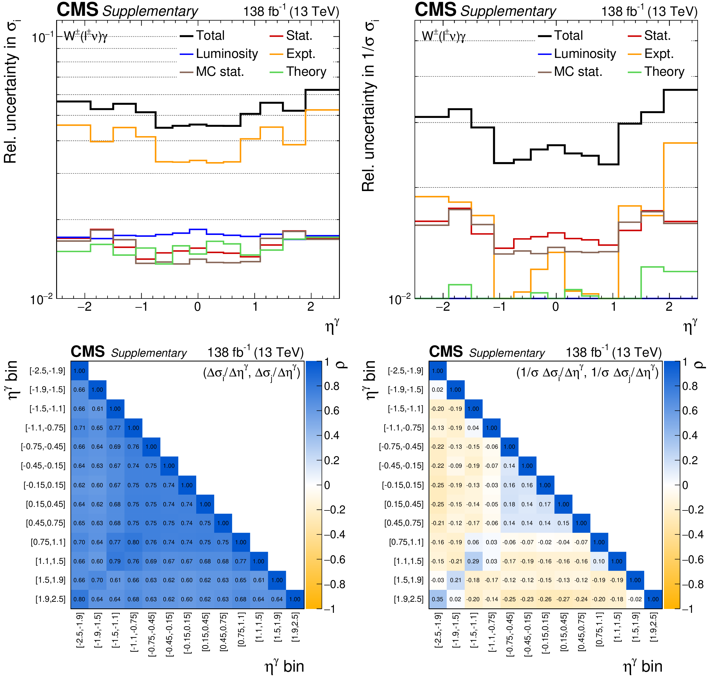
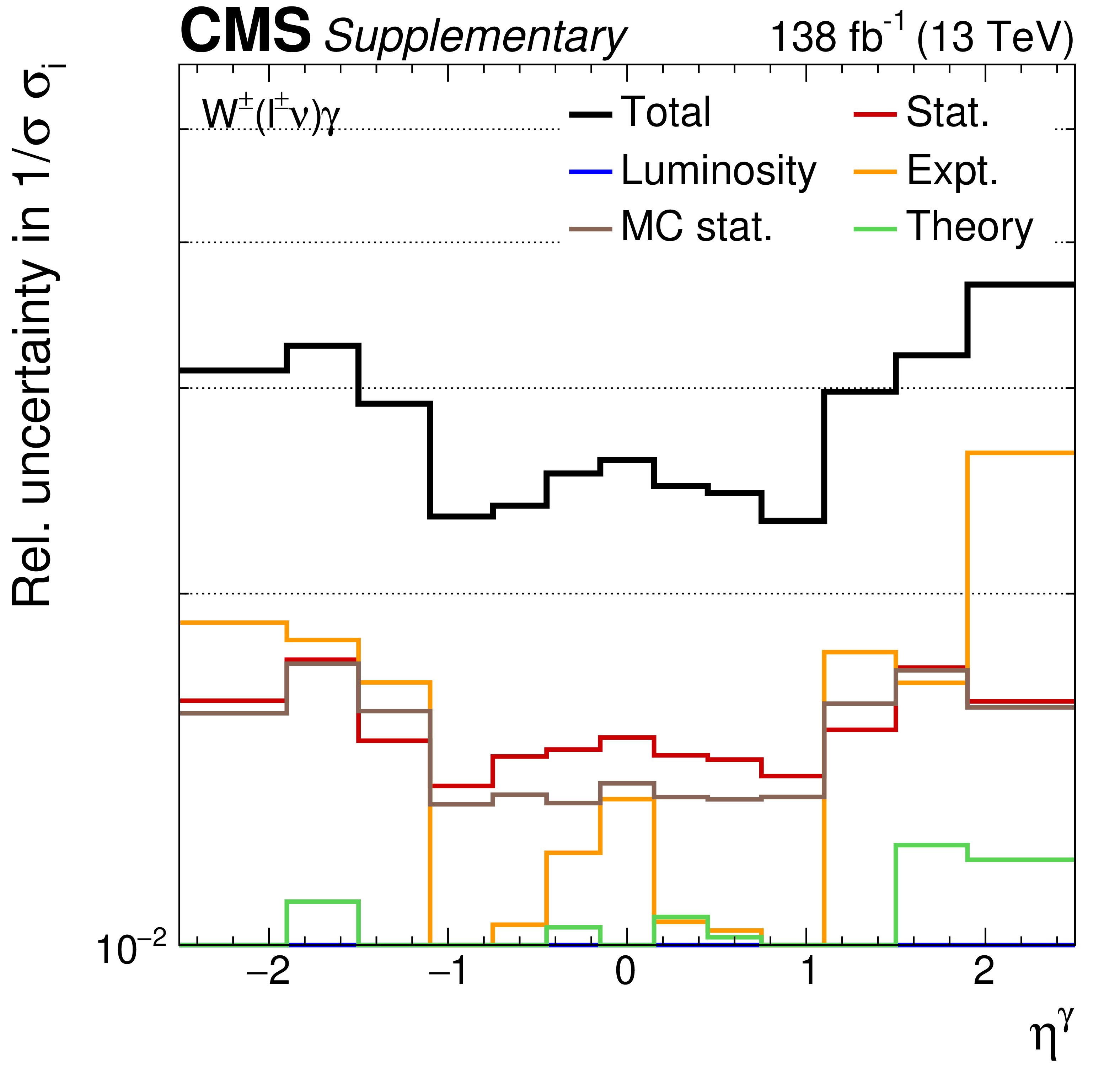
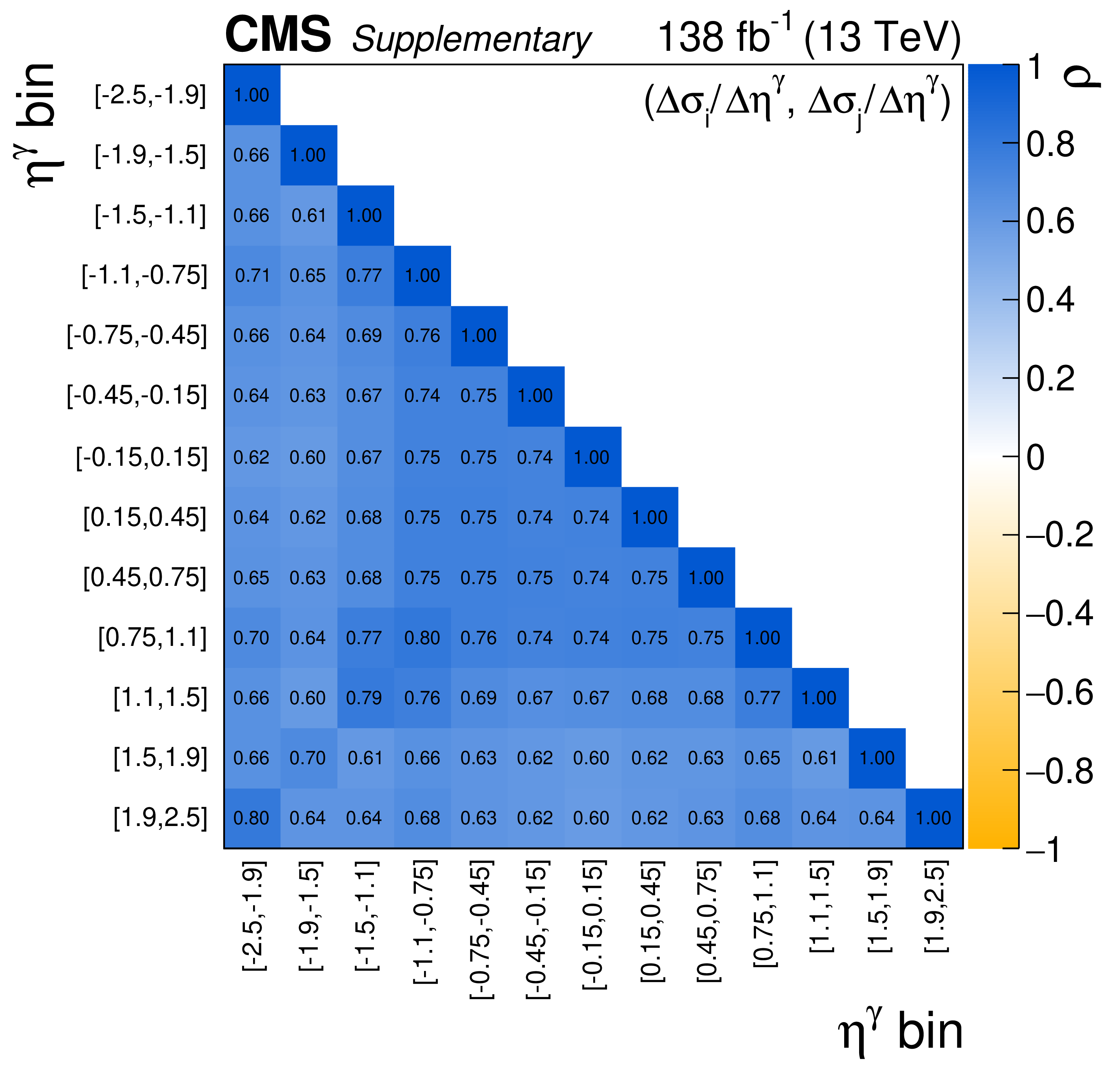
Additional Figure 4:
The uncertainty compositions and correlation matrices for the $\eta ^{\gamma}$ absolute (left) and fractional (right) differential cross sections. |

png pdf |
Additional Figure 4-a:
The uncertainty composition for the $\eta ^{\gamma}$ absolute differential cross section. |
png pdf |
Additional Figure 4-b:
The uncertainty composition for the $\eta ^{\gamma}$ fractional differential cross section. |
png pdf |
Additional Figure 4-c:
The correlation matrice for the $\eta ^{\gamma}$ absolute differential cross section. |

png pdf |
Additional Figure 4-d:
The correlation matrice for the $\eta ^{\gamma}$ fractional differential cross section. |
png pdf |
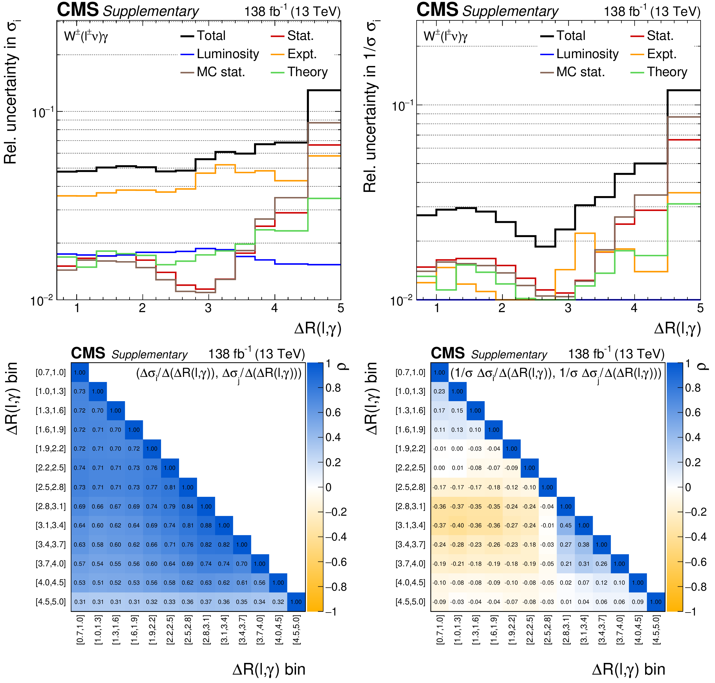
Additional Figure 5:
The uncertainty compositions and correlation matrices for the $\Delta R(\ell,\gamma)$ absolute (left) and fractional (right) differential cross sections. |
png pdf |
Additional Figure 5-a:
The uncertainty composition for the $\Delta R(\ell,\gamma)$ absolute differential cross section. |
png pdf |
Additional Figure 5-b:
The uncertainty composition for the $\Delta R(\ell,\gamma)$ fractional differential cross section. |

png pdf |
Additional Figure 5-c:
The correlation matrice for the $\Delta R(\ell,\gamma)$ absolute differential cross section. |
png pdf |
Additional Figure 5-d:
The correlation matrice for the $\Delta R(\ell,\gamma)$ fractional differential cross section. |

png pdf |
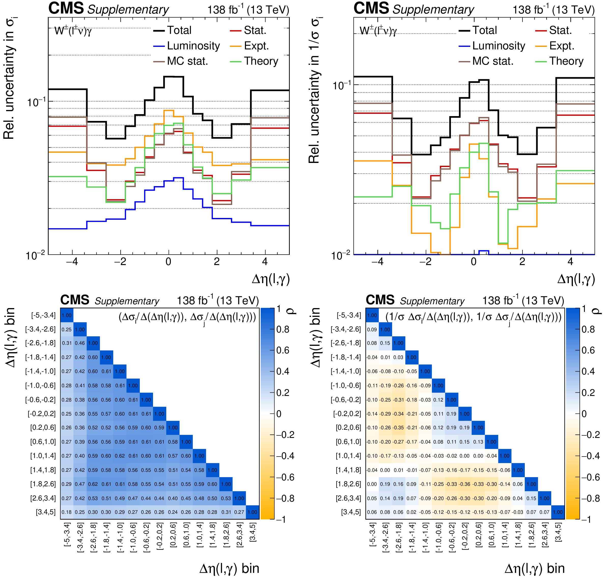
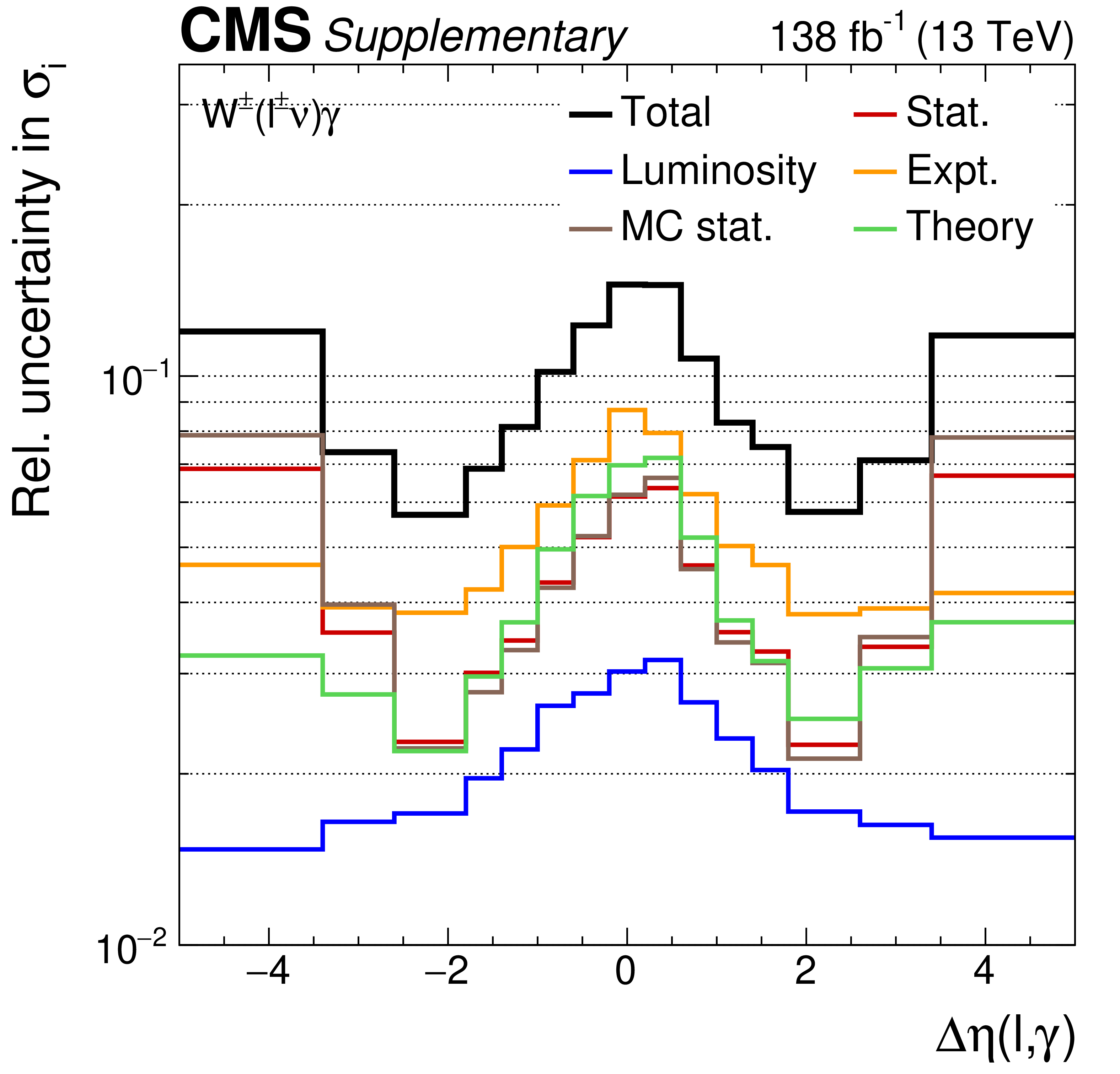
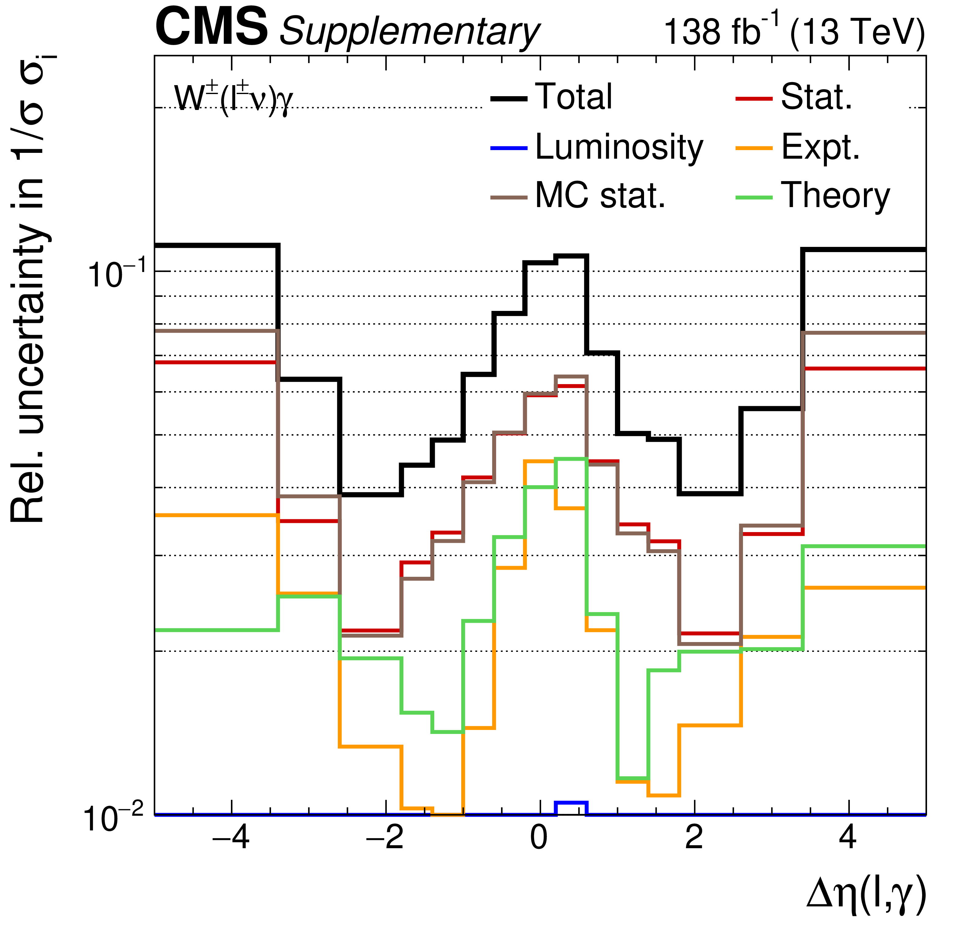
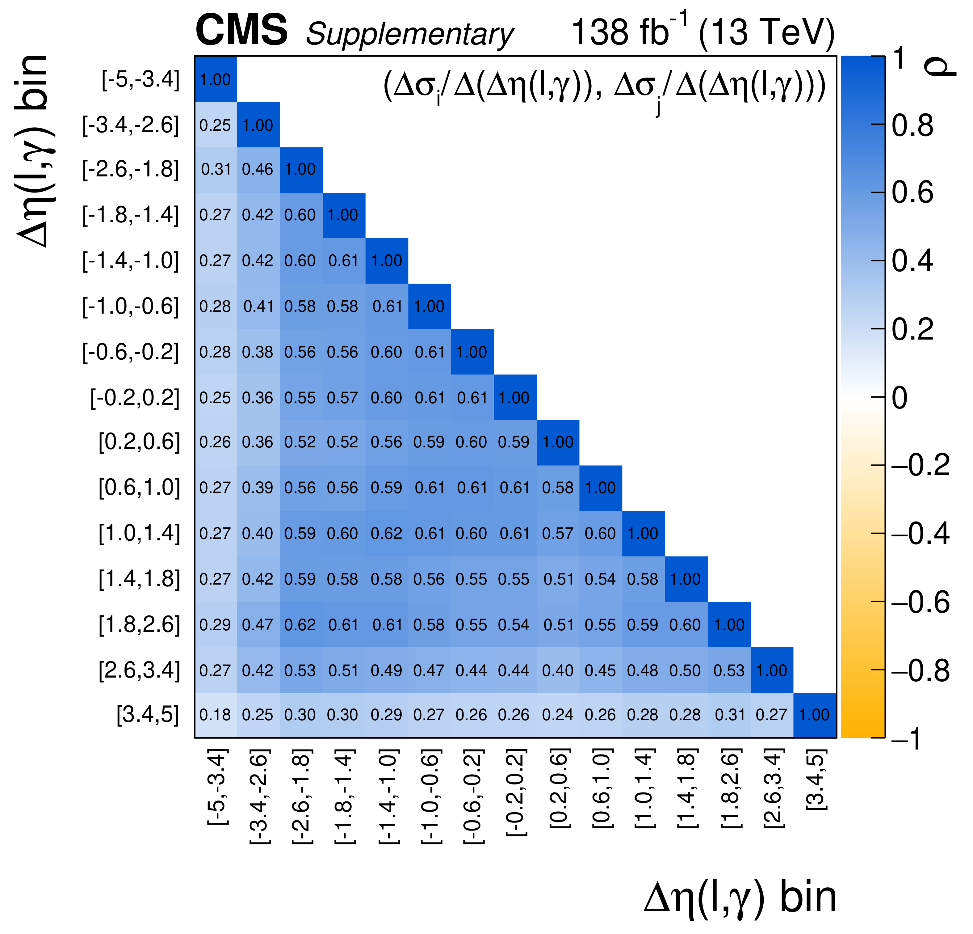
Additional Figure 6:
The uncertainty compositions and correlation matrices for the $\Delta \eta (\ell,\gamma)$ absolute (left) and fractional (right) differential cross sections. |

png pdf |
Additional Figure 6-a:
The uncertainty composition for the $\Delta \eta (\ell,\gamma)$ absolute differential cross section. |
png pdf |
Additional Figure 6-b:
The uncertainty composition for the $\Delta \eta (\ell,\gamma)$ fractional differential cross section. |

png pdf |
Additional Figure 6-c:
The correlation matrice for the $\Delta \eta (\ell,\gamma)$ absolute differential cross section. |

png pdf |
Additional Figure 6-d:
The correlation matrice for the $\Delta \eta (\ell,\gamma)$ fractional differential cross section. |
png pdf |
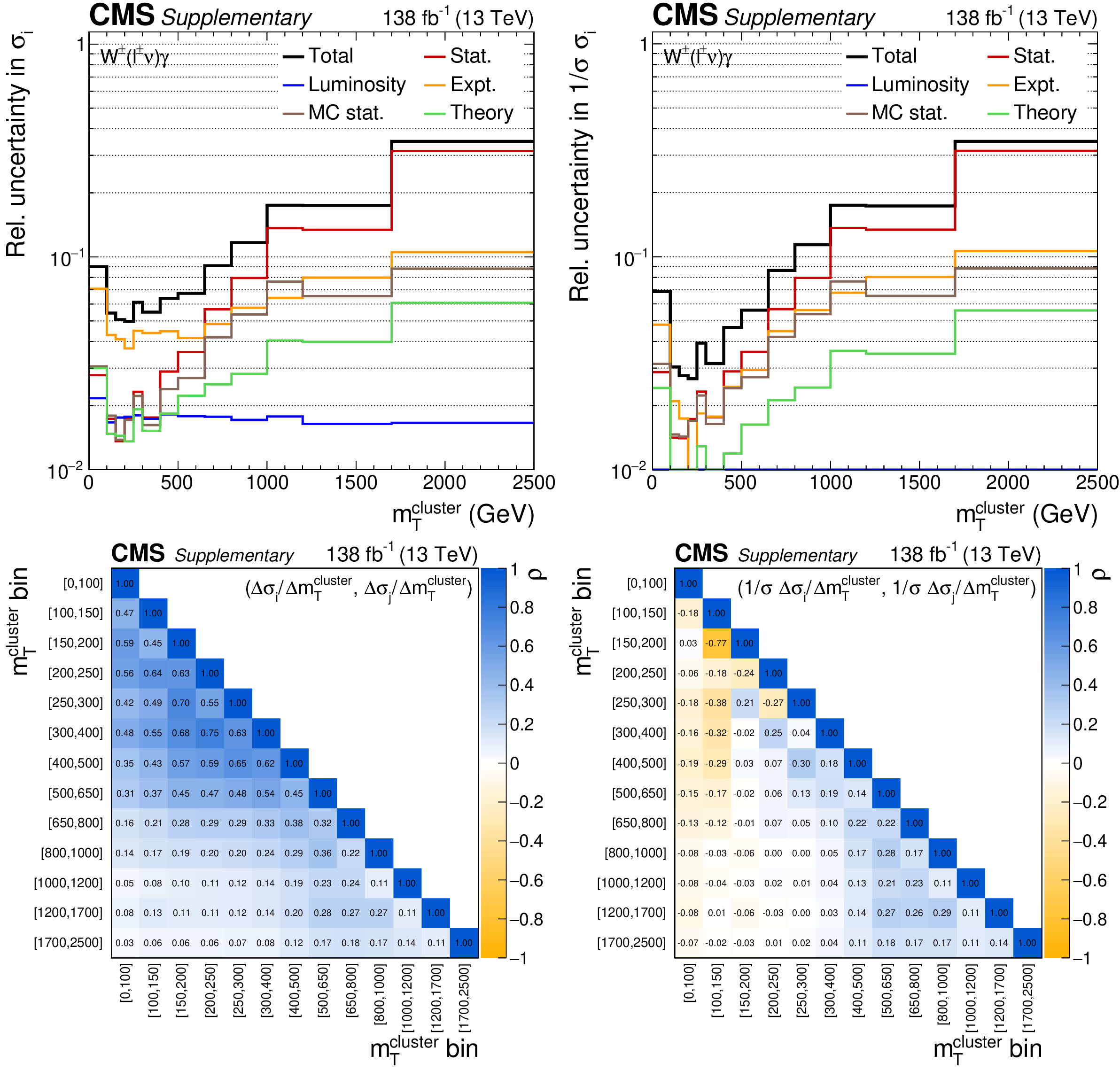
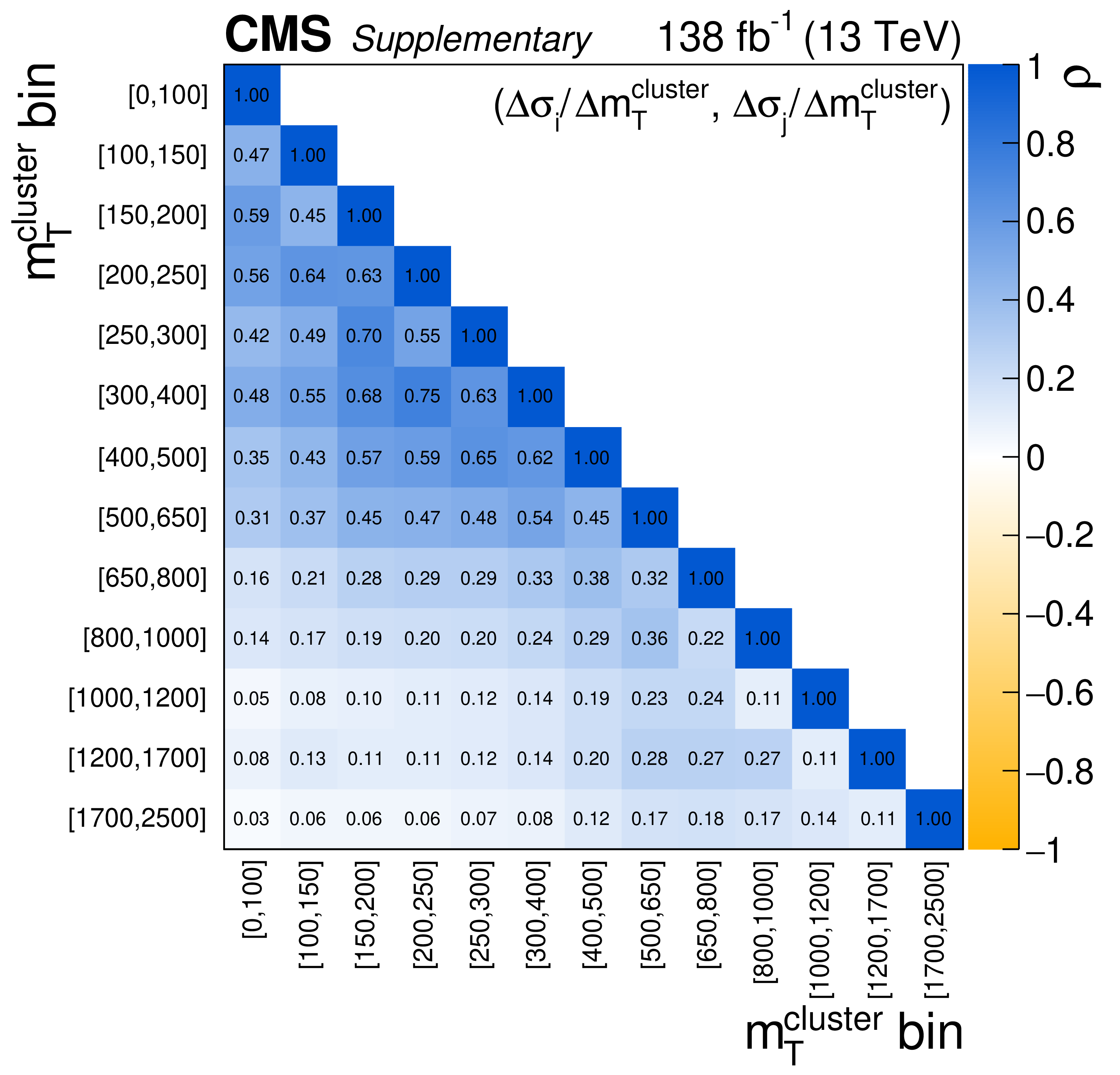
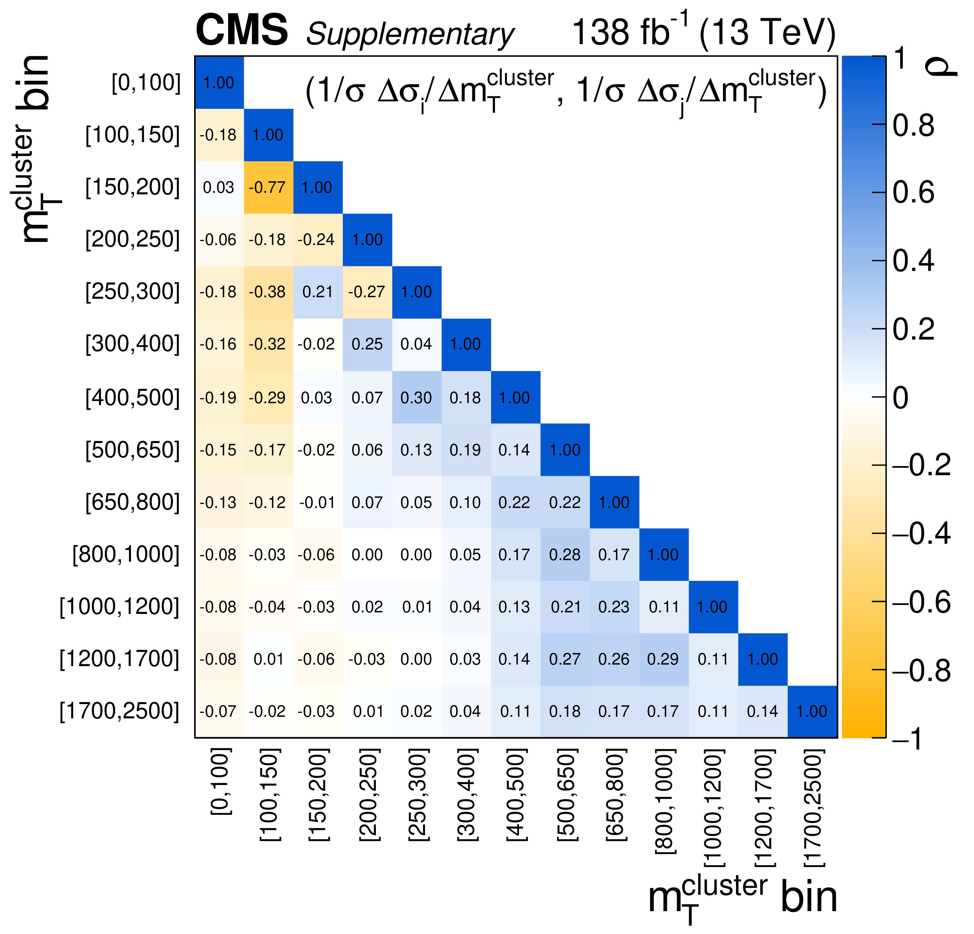
Additional Figure 7:
The uncertainty compositions and correlation matrices for the $ {m_{\mathrm {T}}^{\text {cluster}}} $ absolute (left) and fractional (right) differential cross sections. |

png pdf |
Additional Figure 7-a:
The uncertainty composition for the $ {m_{\mathrm {T}}^{\text {cluster}}} $ absolute differential cross sections. |

png pdf |
Additional Figure 7-b:
The uncertainty composition for the $ {m_{\mathrm {T}}^{\text {cluster}}} $ fractional differential cross sections. |
png pdf |
Additional Figure 7-c:
The correlation matrice for the $ {m_{\mathrm {T}}^{\text {cluster}}} $ absolute differential cross sections. |
png pdf |
Additional Figure 7-d:
The correlation matrice for the $ {m_{\mathrm {T}}^{\text {cluster}}} $ fractional differential cross sections. |
png pdf |
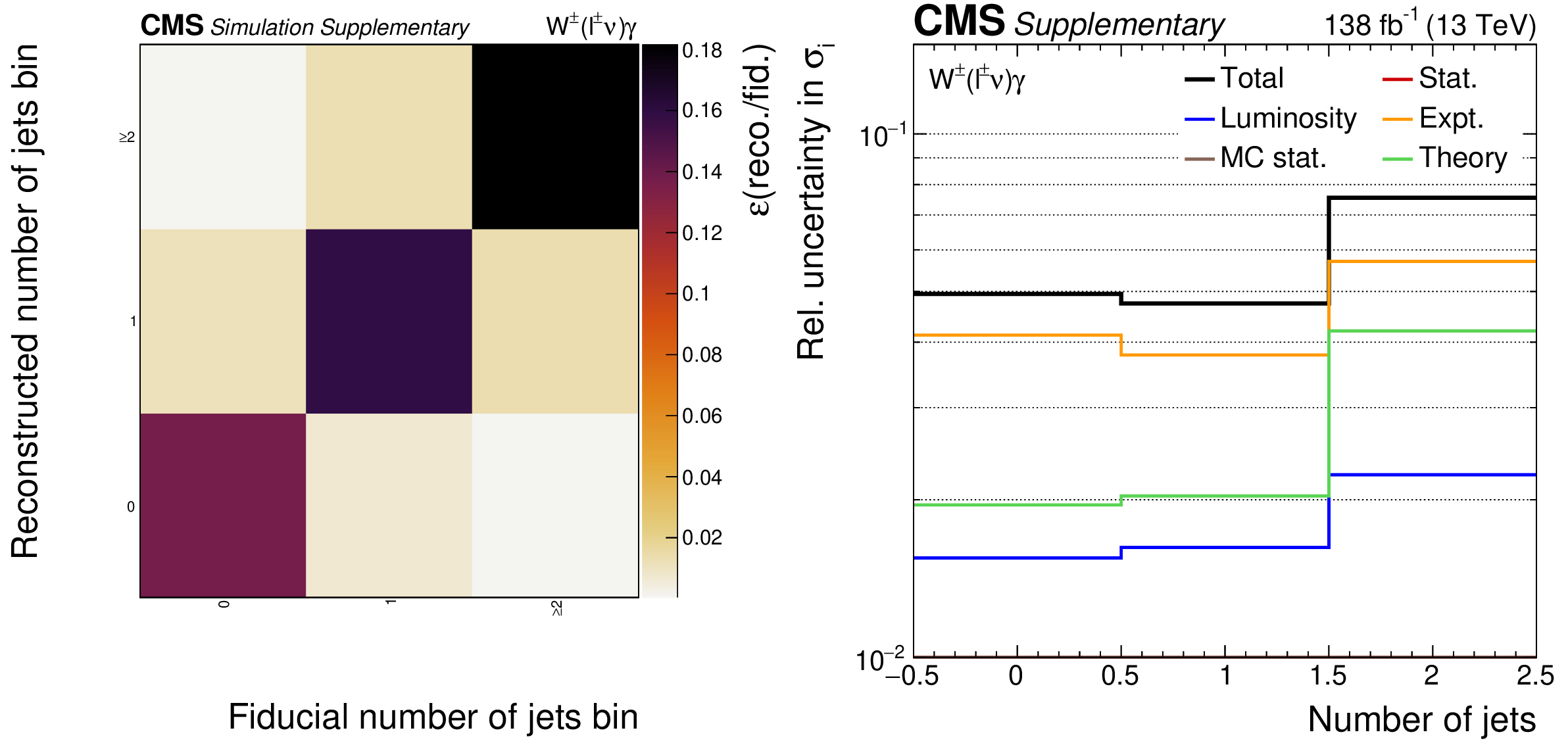
Additional Figure 8:
The response matrix and uncertainty composition for the jet multiplicity cross section measurement. |
png pdf |
Additional Figure 8-a:
The response matrix for the jet multiplicity cross section measurement. |
png pdf |
Additional Figure 8-b:
The uncertainty composition for the jet multiplicity cross section measurement. |
png pdf |
Additional Figure 9:
Expected and observed $\Delta \eta (\ell, \gamma)$ distributions before the maximum likelihood is performed (left). Requirements of $ {m_{\mathrm {T}}^{\text {cluster}}} > $ 150 GeV and a jet veto are applied in addition to the baseline selection to enhance the radiation amplitude zero supression at $\Delta \eta (\ell, \gamma)= $ 0. The shaded uncertainty band incorporates all systematic uncertainties. The corresponding response matrix is also given (right). |
png pdf |
Additional Figure 9-a:
Expected and observed $\Delta \eta (\ell, \gamma)$ distributions before the maximum likelihood is performed. Requirements of $ {m_{\mathrm {T}}^{\text {cluster}}} > $ 150 GeV and a jet veto are applied in addition to the baseline selection to enhance the radiation amplitude zero supression at $\Delta \eta (\ell, \gamma)= $ 0. The shaded uncertainty band incorporates all systematic uncertainties. |

png pdf |
Additional Figure 9-b:
The corresponding response matrix. |
png pdf |
Additional Figure 10:
The uncertainty compositions and correlation matrices for the $\Delta \eta (\ell,\gamma)$ absolute (left) and fractional (right) differential cross sections. Requirements of $ {m_{\mathrm {T}}^{\text {cluster}}} > $ 150 GeV and a jet veto are applied in addition to the baseline selection to enhance the radiation amplitude zero supression at $\Delta \eta (\ell, \gamma)= $ 0. |
png pdf |
Additional Figure 10-a:
The uncertainty composition for the $\Delta \eta (\ell,\gamma)$ absolute differential cross sections. Requirements of $ {m_{\mathrm {T}}^{\text {cluster}}} > $ 150 GeV and a jet veto are applied in addition to the baseline selection to enhance the radiation amplitude zero supression at $\Delta \eta (\ell, \gamma)= $ 0. |
png pdf |
Additional Figure 10-b:
The uncertainty composition for the $\Delta \eta (\ell,\gamma)$ fractional differential cross sections. Requirements of $ {m_{\mathrm {T}}^{\text {cluster}}} > $ 150 GeV and a jet veto are applied in addition to the baseline selection to enhance the radiation amplitude zero supression at $\Delta \eta (\ell, \gamma)= $ 0. |
png pdf |
Additional Figure 10-c:
The correlation matrice for the $\Delta \eta (\ell,\gamma)$ absolute differential cross sections. Requirements of $ {m_{\mathrm {T}}^{\text {cluster}}} > $ 150 GeV and a jet veto are applied in addition to the baseline selection to enhance the radiation amplitude zero supression at $\Delta \eta (\ell, \gamma)= $ 0. |
png pdf |
Additional Figure 10-d:
The correlation matrice for the $\Delta \eta (\ell,\gamma)$ fractional differential cross sections. Requirements of $ {m_{\mathrm {T}}^{\text {cluster}}} > $ 150 GeV and a jet veto are applied in addition to the baseline selection to enhance the radiation amplitude zero supression at $\Delta \eta (\ell, \gamma)= $ 0. |
| References | ||||
| 1 | CDF Collaboration | Measurement of W$ \gamma $ and Z$ \gamma $ production in $ {\mathrm{p}}\mathrm{\bar{p}} $ collisions at $ \sqrt{s} = $ 1.96 TeV | PRL 94 (2005) 041803 | hep-ex/0410008 |
| 2 | D0 Collaboration | Measurement of the $ {\mathrm{p}}\mathrm{\bar{p}} \to \mathrm{W} \gamma $ + $ X $ cross section at $ \sqrt{s} = $ 1.96 TeV and $ \mathrm{W} \mathrm{W} \gamma $ anomalous coupling limits | PRD 71 (2005) 091108 | hep-ex/0503048 |
| 3 | D0 Collaboration | First study of the radiation-amplitude zero in W$ \gamma $ production and limits on anomalous $ \mathrm{W} \mathrm{W} \gamma $ couplings at $ \sqrt{s} = $ 1.96 TeV | PRL 100 (2008) 241805 | 0803.0030 |
| 4 | CMS Collaboration | Measurement of the W$ \gamma $ and Z$ \gamma $ inclusive cross sections in pp collisions at $ \sqrt s= $ 7 TeV and limits on anomalous triple gauge boson couplings | PRD 89 (2014) 092005 | CMS-EWK-11-009 1308.6832 |
| 5 | ATLAS Collaboration | Measurements of W$ \gamma $ and Z$ \gamma $ production in pp collisions at $ \sqrt{s}=$ 7 TeV with the ATLAS detector at the LHC | PRD 87 (2013) 112003 | 1302.1283 |
| 6 | CMS Collaboration | Measurement of the W$ \gamma $ production cross section in proton-proton collisions at $ \sqrt{s} = $ 13 TeV and constraints on effective field theory coefficients | PRL 126 (2021) 252002 | CMS-SMP-19-002 2102.02283 |
| 7 | K. O. Mikaelian, M. A. Samuel, and D. Sahdev | Magnetic moment of weak bosons produced in pp and $ {\mathrm{p}}\mathrm{\bar{p}} $ collisions | PRL 43 (1979) 746 | |
| 8 | C. J. Goebel, F. Halzen, and J. P. Leveille | Angular zeros of Brown, Mikaelian, Sahdev, and Samuel and the factorization of tree amplitudes in gauge theories | PRD 23 (1981) 2682 | |
| 9 | S. J. Brodsky and R. W. Brown | Zeros in amplitudes: Gauge theory and radiation interference | PRL 49 (1982) 966 | |
| 10 | R. W. Brown, K. L. Kowalski, and S. J. Brodsky | Classical radiation zeros in gauge theory amplitudes | PRD 28 (1983) 624 | |
| 11 | U. Baur, S. Errede, and G. L. Landsberg | Rapidity correlations in W$ \gamma $ production at hadron colliders | PRD 50 (1994) 1917 | hep-ph/9402282 |
| 12 | G. Panico, F. Riva, and A. Wulzer | Diboson interference resurrection | PLB 776 (2018) 473 | 1708.07823 |
| 13 | A. Azatov, J. Elias-Miró, Y. Reyimuaji, and E. Venturini | Novel measurements of anomalous triple gauge couplings for the LHC | JHEP 10 (2017) 027 | 1707.08060 |
| 14 | S. Weinberg | Baryon- and lepton-nonconserving processes | PRL 43 (1979) 1566 | |
| 15 | D. Liu, A. Pomarol, R. Rattazzi, and F. Riva | Patterns of strong coupling for LHC searches | JHEP 11 (2016) 141 | 1603.03064 |
| 16 | D. Marzocca et al. | BSM benchmarks for effective field theories in Higgs and electroweak physics | 2020 | 2009.01249 |
| 17 | B. Grzadkowski, M. Iskrzyński, M. Misiak, and J. Rosiek | Dimension-six terms in the standard model Lagrangian | JHEP 10 (2010) 085 | 1008.4884 |
| 18 | A. Azatov, R. Contino, C. S. Machado, and F. Riva | Helicity selection rules and noninterference for BSM amplitudes | PRD 95 (2017) 065014 | 1607.05236 |
| 19 | A. Azatov, D. Barducci, and E. Venturini | Precision diboson measurements at hadron colliders | JHEP 04 (2019) 075 | 1901.04821 |
| 20 | J. Alwall et al. | Comparative study of various algorithms for the merging of parton showers and matrix elements in hadronic collisions | EPJC 53 (2008) 473 | 0706.2569 |
| 21 | CMS Collaboration | Performance of photon reconstruction and identification with the CMS detector in proton-proton collisions at $ \sqrt{s} = $ 8 TeV | JINST 10 (2015) P08010 | CMS-EGM-14-001 1502.02702 |
| 22 | CMS Collaboration | Performance of electron reconstruction and selection with the CMS detector in proton-proton collisions at $ \sqrt{s} = $ 8 TeV | JINST 10 (2015) P06005 | CMS-EGM-13-001 1502.02701 |
| 23 | CMS Collaboration | Performance of the CMS muon detector and muon reconstruction with proton-proton collisions at $ \sqrt{s}= $ 13 TeV | JINST 13 (2018) P06015 | CMS-MUO-16-001 1804.04528 |
| 24 | CMS Collaboration | Performance of the CMS Level-1 trigger in proton-proton collisions at $ \sqrt{s} = $ 13 TeV | JINST 15 (2020) P10017 | CMS-TRG-17-001 2006.10165 |
| 25 | CMS Collaboration | The CMS trigger system | JINST 12 (2017) P01020 | CMS-TRG-12-001 1609.02366 |
| 26 | CMS Collaboration | The CMS experiment at the CERN LHC | JINST 3 (2008) S08004 | CMS-00-001 |
| 27 | J. Alwall et al. | The automated computation of tree-level and next-to-leading order differential cross sections, and their matching to parton shower simulations | JHEP 07 (2014) 079 | 1405.0301 |
| 28 | P. Nason | A new method for combining NLO QCD with shower Monte Carlo algorithms | JHEP 11 (2004) 040 | hep-ph/0409146 |
| 29 | S. Frixione, P. Nason, and C. Oleari | Matching NLO QCD computations with parton shower simulations: the POWHEG method | JHEP 11 (2007) 070 | 0709.2092 |
| 30 | S. Alioli, P. Nason, C. Oleari, and E. Re | A general framework for implementing NLO calculations in shower Monte Carlo programs: the POWHEG BOX | JHEP 06 (2010) 043 | 1002.2581 |
| 31 | S. Frixione, P. Nason, and G. Ridolfi | A positive-weight next-to-leading-order Monte Carlo for heavy flavour hadroproduction | JHEP 09 (2007) 126 | 0707.3088 |
| 32 | R. Frederix, E. Re, and P. Torrielli | Single-top t-channel hadroproduction in the four-flavour scheme with POWHEG and aMC@NLO | JHEP 09 (2012) 130 | 1207.5391 |
| 33 | E. Re | Single-top Wt-channel production matched with parton showers using the POWHEG method | EPJC 71 (2011) 1547 | 1009.2450 |
| 34 | O. Mattelaer | On the maximal use of Monte Carlo samples: re-weighting events at NLO accuracy | EPJC 76 (2016) 674 | 1607.00763 |
| 35 | I. Brivio, Y. Jiang, and M. Trott | The SMEFTsim package, theory and tools | JHEP 12 (2017) 070 | 1709.06492 |
| 36 | I. Brivio | SMEFTsim 3.0 -- a practical guide | JHEP 04 (2021) 073 | 2012.11343 |
| 37 | NNPDF Collaboration | Parton distributions from high-precision collider data | EPJC 77 (2017) 663 | 1706.00428 |
| 38 | NNPDF Collaboration | Parton distributions for the LHC Run II | JHEP 04 (2015) 040 | 1410.8849 |
| 39 | T. Sjostrand et al. | An introduction to PYTHIA 8.2 | CPC 191 (2015) 159 | 1410.3012 |
| 40 | CMS Collaboration | Event generator tunes obtained from underlying event and multiparton scattering measurements | EPJC 76 (2016) 155 | CMS-GEN-14-001 1512.00815 |
| 41 | CMS Collaboration | Investigations of the impact of the parton shower tuning in Pythia 8 in the modelling of $ \mathrm{t\bar{t}} $ at $ \sqrt{s}= $ 8 and 13 TeV | CMS-PAS-TOP-16-021 | CMS-PAS-TOP-16-021 |
| 42 | CMS Collaboration | Extraction and validation of a new set of CMS PYTHIA8 tunes from underlying-event measurements | EPJC 80 (2020) 4 | CMS-GEN-17-001 1903.12179 |
| 43 | GEANT4 Collaboration | GEANT4--a simulation toolkit | NIMA 506 (2003) 250 | |
| 44 | M. Cacciari, G. P. Salam, and G. Soyez | The anti-$ {k_{\mathrm{T}}} $ jet clustering algorithm | JHEP 04 (2008) 063 | 0802.1189 |
| 45 | M. Cacciari, G. P. Salam, and G. Soyez | FastJet user manual | EPJC 72 (2012) 1896 | 1111.6097 |
| 46 | CMS Collaboration | Particle-flow reconstruction and global event description with the CMS detector | JINST 12 (2017) P10003 | CMS-PRF-14-001 1706.04965 |
| 47 | CMS Collaboration | Jet energy scale and resolution in the CMS experiment in pp collisions at 8 TeV | JINST 12 (2017) P02014 | CMS-JME-13-004 1607.03663 |
| 48 | CMS Collaboration | Electron and photon reconstruction and identification with the CMS experiment at the CERN LHC | JINST 16 (2021) P05014 | CMS-EGM-17-001 2012.06888 |
| 49 | CMS Collaboration | Measurements of inclusive W and Z cross sections in pp collisions at $ \sqrt{s}= $ 7 TeV | JHEP 01 (2011) 080 | CMS-EWK-10-002 1012.2466 |
| 50 | A. Bodek et al. | Extracting muon momentum scale corrections for hadron collider experiments | EPJC 72 (2012) 2194 | 1208.3710 |
| 51 | CMS Collaboration | Performance of missing transverse momentum reconstruction in proton-proton collisions at $ \sqrt{s} = $ 13 TeV using the CMS detector | JINST 14 (2019) P07004 | CMS-JME-17-001 1903.06078 |
| 52 | D. Bertolini, P. Harris, M. Low, and N. Tran | Pileup per particle identification | JHEP 10 (2014) 059 | 1407.6013 |
| 53 | CMS Collaboration | Precision luminosity measurement in proton-proton collisions at $ \sqrt{s} = $ 13 TeV in 2015 and 2016 at CMS | EPJC 81 (2021) 800 | CMS-LUM-17-003 2104.01927 |
| 54 | CMS Collaboration | CMS luminosity measurement for the 2017 data-taking period at $ \sqrt{s} = $ 13 TeV | CMS-PAS-LUM-17-004 | CMS-PAS-LUM-17-004 |
| 55 | CMS Collaboration | CMS luminosity measurement for the 2018 data-taking period at $ \sqrt{s} = $ 13 TeV | CMS-PAS-LUM-18-002 | CMS-PAS-LUM-18-002 |
| 56 | CMS Collaboration | Measurement of the inelastic proton-proton cross section at $ \sqrt{s}= $ 13 TeV | JHEP 07 (2018) 161 | CMS-FSQ-15-005 1802.02613 |
| 57 | R. J. Barlow and C. Beeston | Fitting using finite Monte Carlo samples | CPC 77 (1993) 219 | |
| 58 | J. Butterworth et al. | PDF4LHC recommendations for LHC Run II | JPG 43 (2016) 023001 | 1510.03865 |
| 59 | I. W. Stewart and F. J. Tackmann | Theory uncertainties for Higgs mass and other searches using jet bins | PRD 85 (2012) 034011 | 1107.2117 |
| 60 | The ATLAS Collaboration, The CMS Collaboration, The LHC Higgs Combination Group | Procedure for the LHC Higgs boson search combination in Summer 2011 | CMS-NOTE-2011-005 | |
| 61 | ATLAS and CMS Collaborations | Measurements of the Higgs boson production and decay rates and constraints on its couplings from a combined ATLAS and CMS analysis of the LHC pp collision data at $ \sqrt{s} = $ 7 and 8 TeV | JHEP 08 (2016) 45 | 1606.02266 |
| 62 | W. Verkerke and D. P. Kirkby | The RooFit toolkit for data modeling | in Proceedings of the 13th International Conference for Computing in High-Energy and Nuclear Physics (CHEP03) 2003 [eConf C0303241, MOLT007] | physics/0306116 |
| 63 | L. Moneta et al. | The RooStats project | in 13th International Workshop on Advanced Computing and Analysis Techniques in Physics Research (ACAT2010) 2010 | 1009.1003 |
| 64 | G. Cowan, K. Cranmer, E. Gross, and O. Vitells | Asymptotic formulae for likelihood-based tests of new physics | EPJC 71 (2011) 1554 | 1007.1727 |
| 65 | CMS Collaboration | HEPData record for this analysis | link | |
| 66 | S. Frixione | Isolated photons in perturbative QCD | PLB 429 (1998) 369 | hep-ph/9801442 |
| 67 | M. Grazzini, S. Kallweit, and M. Wiesemann | Fully differential NNLO computations with MATRIX | EPJC 78 (2018) 537 | 1711.06631 |
| 68 | M. Grazzini, S. Kallweit, and D. Rathlev | W$ \gamma $ and Z$ \gamma $ production at the LHC in NNLO QCD | JHEP 07 (2015) 085 | 1504.01330 |
| 69 | J. M. Campbell, G. De Laurentis, R. K. Ellis, and S. Seth | The $ {\mathrm{p}}{\mathrm{p}} \to \mathrm{W}(\to \ell\nu) + \gamma $ process at next-to-next-to-leading order | JHEP 07 (2021) 079 | 2105.00954 |
| 70 | J. M. Campbell, R. K. Ellis, and C. Williams | Vector boson pair production at the LHC | JHEP 07 (2011) 018 | 1105.0020 |
| 71 | T. Cridge, M. A. Lim, and R. Nagar | W$ \gamma $ production at NNLO+PS accuracy in GENEVA | 2021 | 2105.13214 |
| 72 | S. Alioli et al. | Combining higher-order resummation with multiple NLO calculations and parton showers in GENEVA | JHEP 09 (2013) 120 | 1211.7049 |
| 73 | S. Alioli et al. | Drell-Yan production at NNLL'+NNLO matched to parton showers | PRD 92 (2015) 094020 | 1508.01475 |
| 74 | S. Alioli et al. | Matching NNLO to parton shower using N$ ^3 $LL colour-singlet transverse momentum resummation in GENEVA | 2021 | 2102.08390 |
| 75 | S. Catani et al. | Vector boson production at hadron colliders: hard-collinear coefficients at the NNLO | EPJC 72 (2012) 2195 | 1209.0158 |
| 76 | S. Catani and M. Grazzini | Next-to-next-to-leading-order subtraction formalism in hadron collisions and its application to Higgs-boson production at the Large Hadron Collider | PRL 98 (2007) 222002 | hep-ph/0703012 |
| 77 | F. Cascioli, P. Maierhofer, and S. Pozzorini | Scattering amplitudes with Open Loops | PRL 108 (2012) 111601 | 1111.5206 |
| 78 | A. Denner, S. Dittmaier, and L. Hofer | Collier: a fortran-based complex one-loop library in extended regularizations | CPC 212 (2017) 220 | 1604.06792 |
| 79 | T. Gehrmann and L. Tancredi | Two-loop QCD helicity amplitudes for $ \mathrm{q}\mathrm{\bar{q}} \to \mathrm{W^{\pm}} \gamma $ and $ \mathrm{q}\mathrm{\bar{q}} \to {\mathrm{Z^0}} \gamma $ | JHEP 02 (2012) 004 | 1112.1531 |
| 80 | A. Denner, S. Dittmaier, M. Hecht, and C. Pasold | NLO QCD and electroweak corrections to W$ \gamma $ production with leptonic W-boson decays | JHEP 04 (2015) 018 | 1412.7421 |
| 81 | R. M. Capdevilla, R. Harnik, and A. Martin | The radiation valley and exotic resonances in W$ \gamma $ production at the LHC | JHEP 03 (2020) 117 | 1912.08234 |
| 82 | R. Contino et al. | On the validity of the effective field theory approach to SM precision tests | JHEP 07 (2016) 144 | 1604.06444 |
| 83 | ATLAS Collaboration | Measurements of $ \mathrm{W}^+\mathrm{W}^-+\ge 1 $jet production cross-sections in pp collisions at $ \sqrt{s}= $ 13 TeV with the ATLAS detector | JHEP 06 (2021) 003 | 2103.10319 |
| 84 | ATLAS Collaboration | Differential cross-section measurements for the electroweak production of dijets in association with a Z boson in proton-proton collisions at ATLAS | EPJC 81 (2021) 163 | 2006.15458 |
|
|
Compact Muon Solenoid LHC, CERN |
|

|

|

|

|

|