

Compact Muon Solenoid
LHC, CERN
| CMS-TOP-17-004 ; CERN-EP-2019-119 | ||
| Measurement of the top quark Yukawa coupling from $\mathrm{t\bar{t}}$ kinematic distributions in the lepton+jets final state in proton-proton collisions at $\sqrt{s} = $ 13 TeV | ||
| CMS Collaboration | ||
| 2 July 2019 | ||
| Phys. Rev. D 100 (2019) 072007 | ||
| Abstract: Results are presented for an extraction of the top quark Yukawa coupling from top quark-antiquark ($\mathrm{t\bar{t}}$) kinematic distributions in the lepton plus jets final state in proton-proton collisions, based on data collected by the CMS experiment at the LHC at $\sqrt{s} = $ 13 TeV, corresponding to an integrated luminosity of 35.8 fb$^{-1}$. Corrections from weak boson exchange, including Higgs bosons, between the top quarks can produce large distortions of differential distributions near the energy threshold of $\mathrm{t\bar{t}}$ production. Therefore, precise measurements of these distributions are sensitive to the Yukawa coupling. Top quark events are reconstructed with at least three jets in the final state, and a novel technique is introduced to reconstruct the $\mathrm{t\bar{t}}$ system for events with one missing jet. This technique enhances the experimental sensitivity in the low invariant mass region, ${M_{\mathrm{t\bar{t}}}} $. The data yields in ${M_{\mathrm{t\bar{t}}}} $, the rapidity difference $|{y_{\mathrm{t}}-y_{\mathrm{\bar{t}}}}|$, and the number of reconstructed jets are compared with distributions representing different Yukawa couplings. These comparisons are used to measure the ratio of the top quark Yukawa coupling to its standard model predicted value to be 1.07$^{+0.34}_{-0.43}$ with an upper limit of 1.67 at the 95% confidence level. | ||
| Links: e-print arXiv:1907.01590 [hep-ex] (PDF) ; CDS record ; inSPIRE record ; CADI line (restricted) ; | ||
| Figures | |
png pdf |
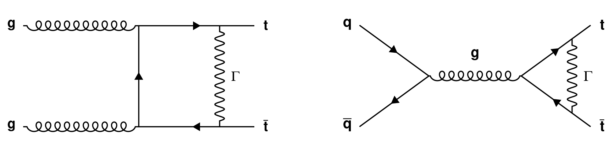
Figure 1:
Example of Feynman diagrams for gluon- and ${\mathrm{q} \mathrm{\bar{q}}}$-induced processes of ${\mathrm{t} {}\mathrm{\bar{t}}}$ production and the virtual corrections. The symbol $\Gamma $ stands for all contributions from gauge and Higgs boson exchanges. |

png pdf |
Figure 1-a:
Example of Feynman diagram for gluon-induced processes of ${\mathrm{t} {}\mathrm{\bar{t}}}$ production and the virtual corrections. The symbol $\Gamma $ stands for all contributions from gauge and Higgs boson exchanges. |
png pdf |
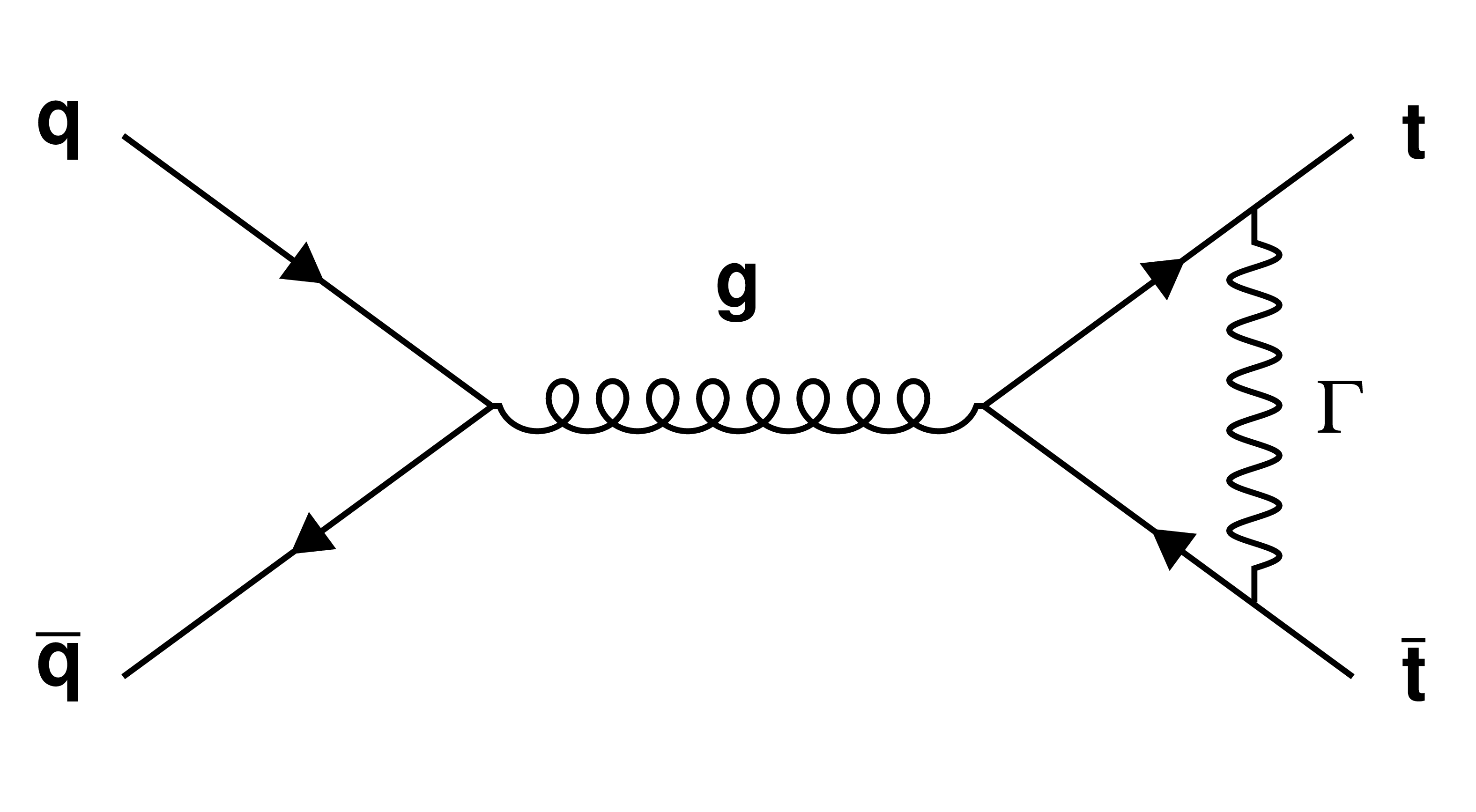
Figure 1-b:
Example of Feynman diagram for ${\mathrm{q} \mathrm{\bar{q}}}$-induced processes of ${\mathrm{t} {}\mathrm{\bar{t}}}$ production and the virtual corrections. The symbol $\Gamma $ stands for all contributions from gauge and Higgs boson exchanges. |
png pdf |
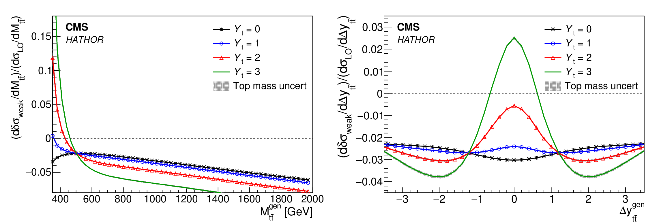
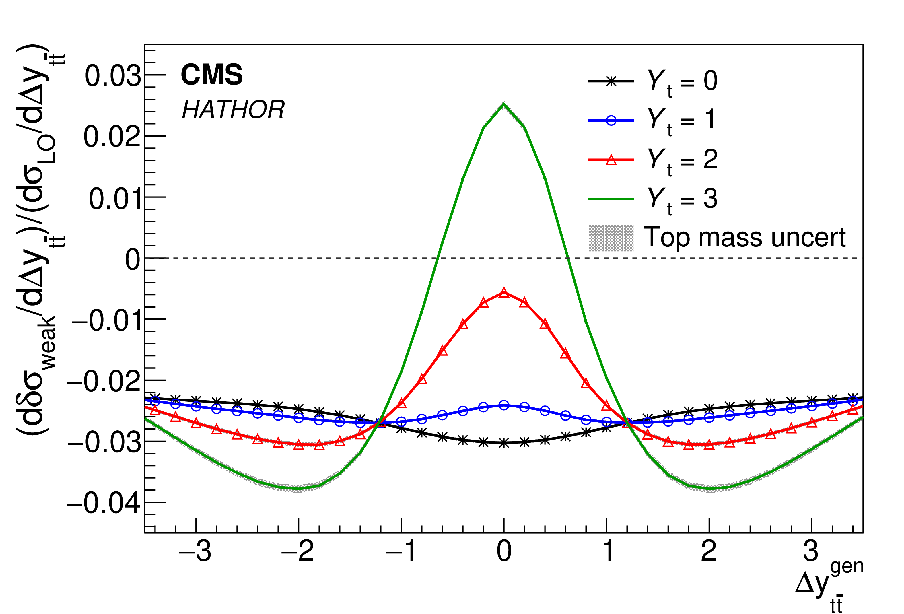
Figure 2:
The dependence of the ratio of weak force corrections over the LO QCD production cross section as calculated by Hathor on the sensitive kinematic variables ${M_{{\mathrm{t} {}\mathrm{\bar{t}}}}}$ and ${\Delta y_{{\mathrm{t} {}\mathrm{\bar{t}}}}}$ at the generator level for different values of ${Y_{\mathrm{t}}} $. The lines contain an uncertainty band (generally not visible) derived from the dependence of the weak correction on the top quark mass varied by $\pm $1 GeV. |
png pdf |
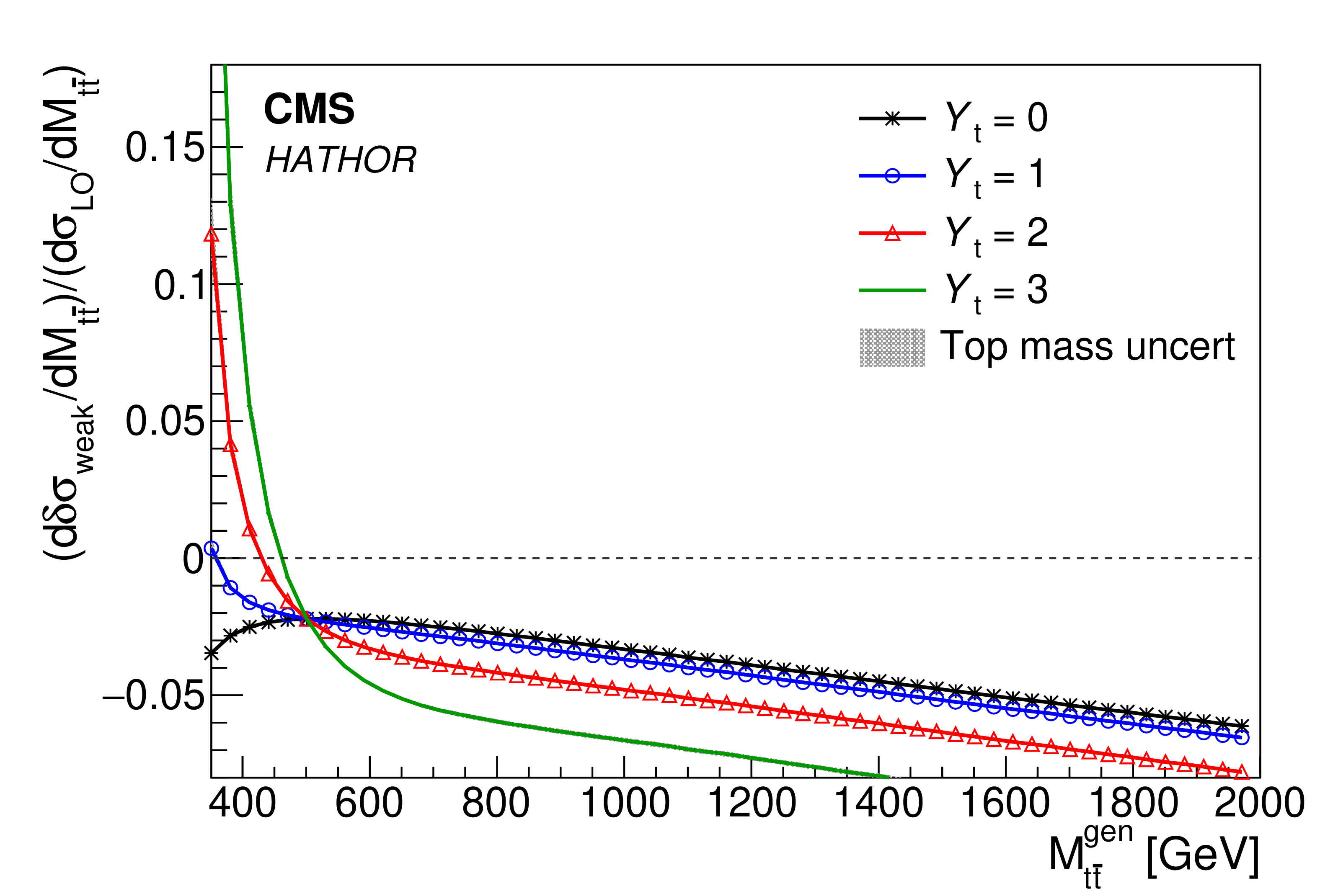
Figure 2-a:
The dependence of the ratio of weak force corrections over the LO QCD production cross section as calculated by Hathor on the sensitive kinematic variable ${M_{{\mathrm{t} {}\mathrm{\bar{t}}}}}$ at the generator level for different values of ${Y_{\mathrm{t}}} $. The lines contain an uncertainty band (generally not visible) derived from the dependence of the weak correction on the top quark mass varied by $\pm $1 GeV. |
png pdf |
Figure 2-b:
The dependence of the ratio of weak force corrections over the LO QCD production cross section as calculated by Hathor on the sensitive kinematic variable ${\Delta y_{{\mathrm{t} {}\mathrm{\bar{t}}}}}$ at the generator level for different values of ${Y_{\mathrm{t}}} $. The lines contain an uncertainty band (generally not visible) derived from the dependence of the weak correction on the top quark mass varied by $\pm $1 GeV. |
png pdf |
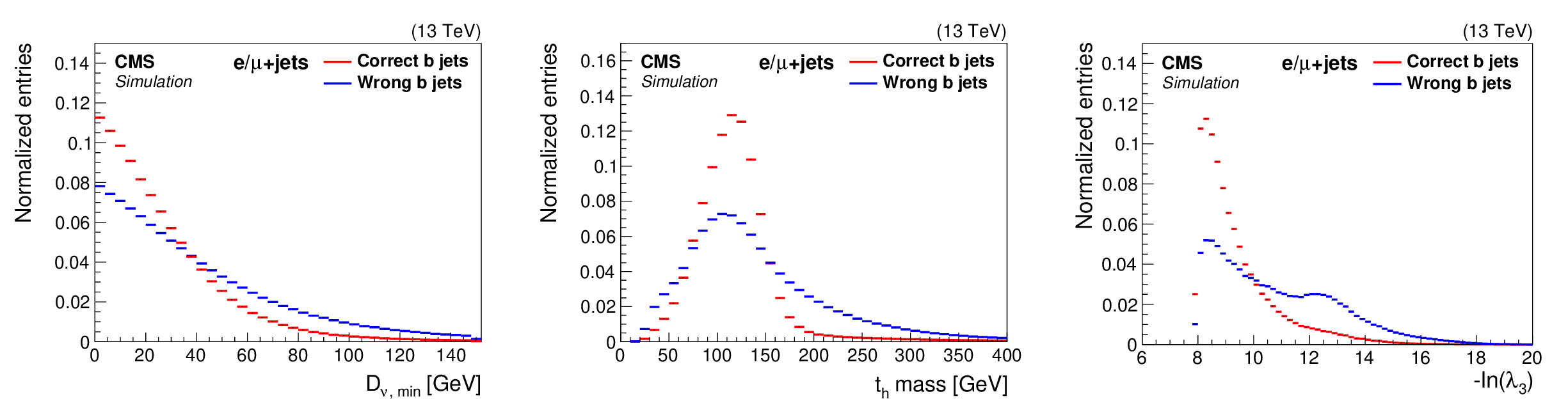
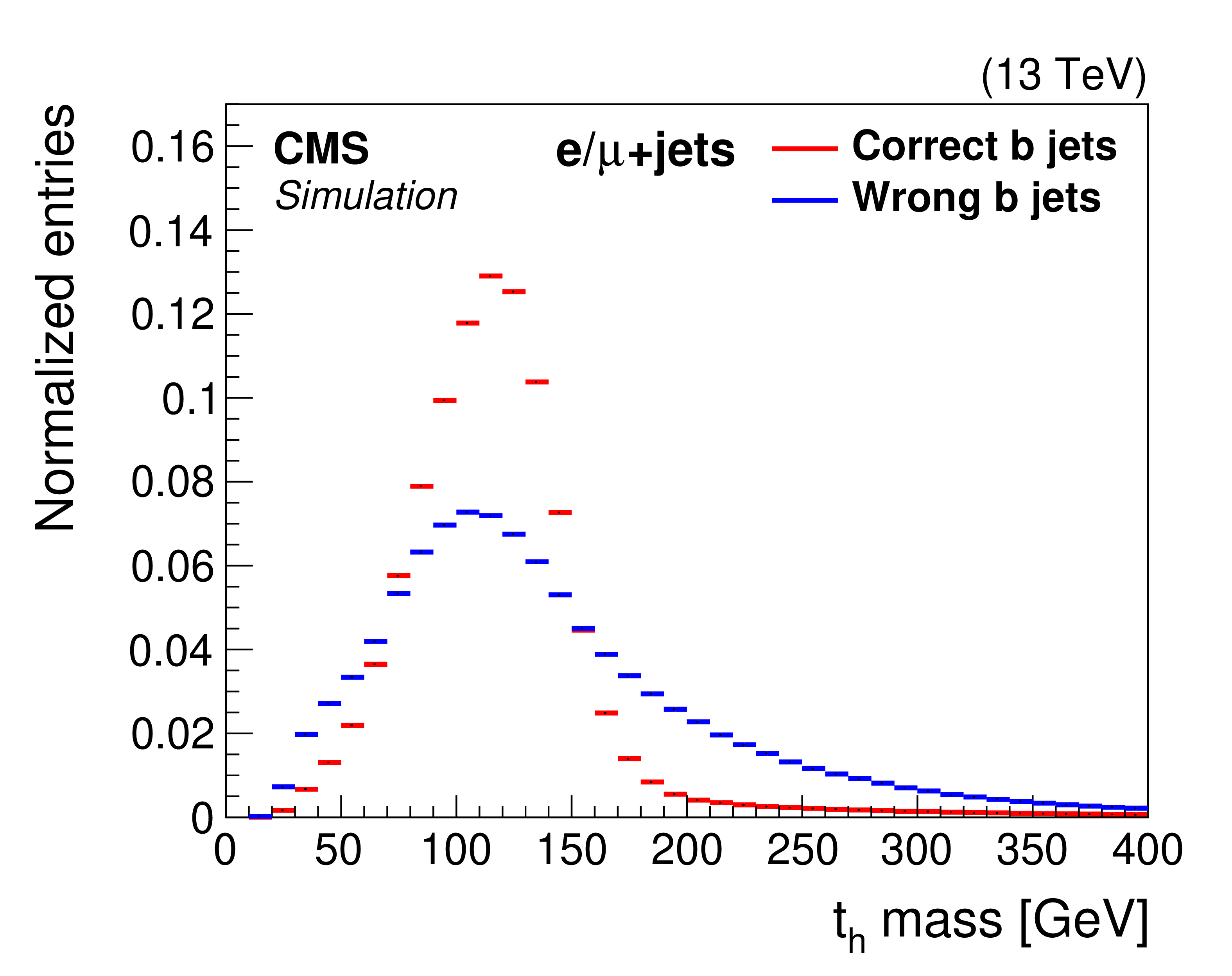
Figure 3:
Three-jet reconstruction. Distributions of the distance ${D_{\nu,\mathrm {min}}}$ for correctly and wrongly selected ${\mathrm{b} _\ell}$ candidates (left). Mass distribution of the correctly and wrongly selected ${\mathrm{b} _\mathrm {h}}$ and the jet from the W boson (middle). Distribution of the negative combined log-likelihood (right). All distributions are normalized to have unit area. |

png pdf |
Figure 3-a:
Three-jet reconstruction. Distributions of the distance ${D_{\nu,\mathrm {min}}}$ for correctly and wrongly selected. All distributions are normalized to have unit area. |
png pdf |
Figure 3-b:
Three-jet reconstruction. Distributions of the distance ${D_{\nu,\mathrm {min}}}$ for correctly and wrongly selected ${\mathrm{b} _\ell}$ candidates. All distributions are normalized to have unit area. |

png pdf |
Figure 3-c:
Three-jet reconstruction. Distribution of the negative combined log-likelihood. All distributions are normalized to have unit area. |
png pdf |
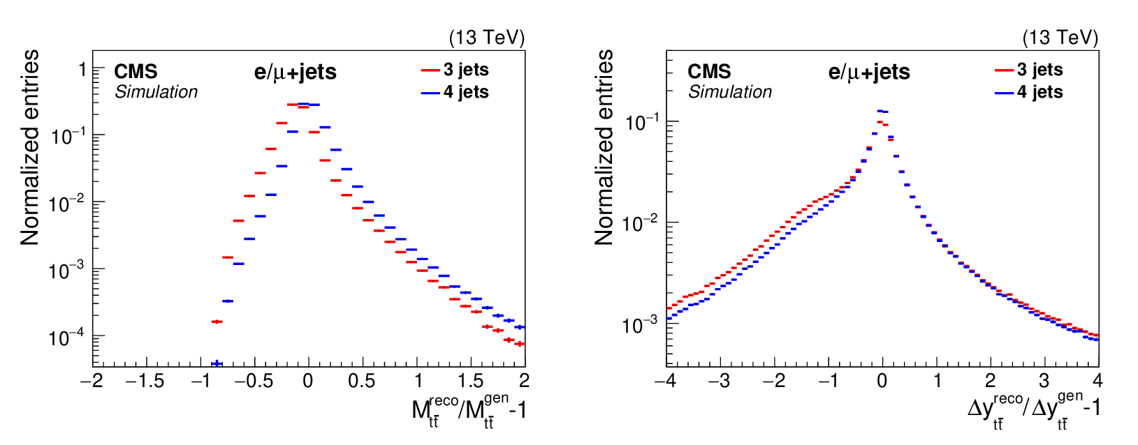
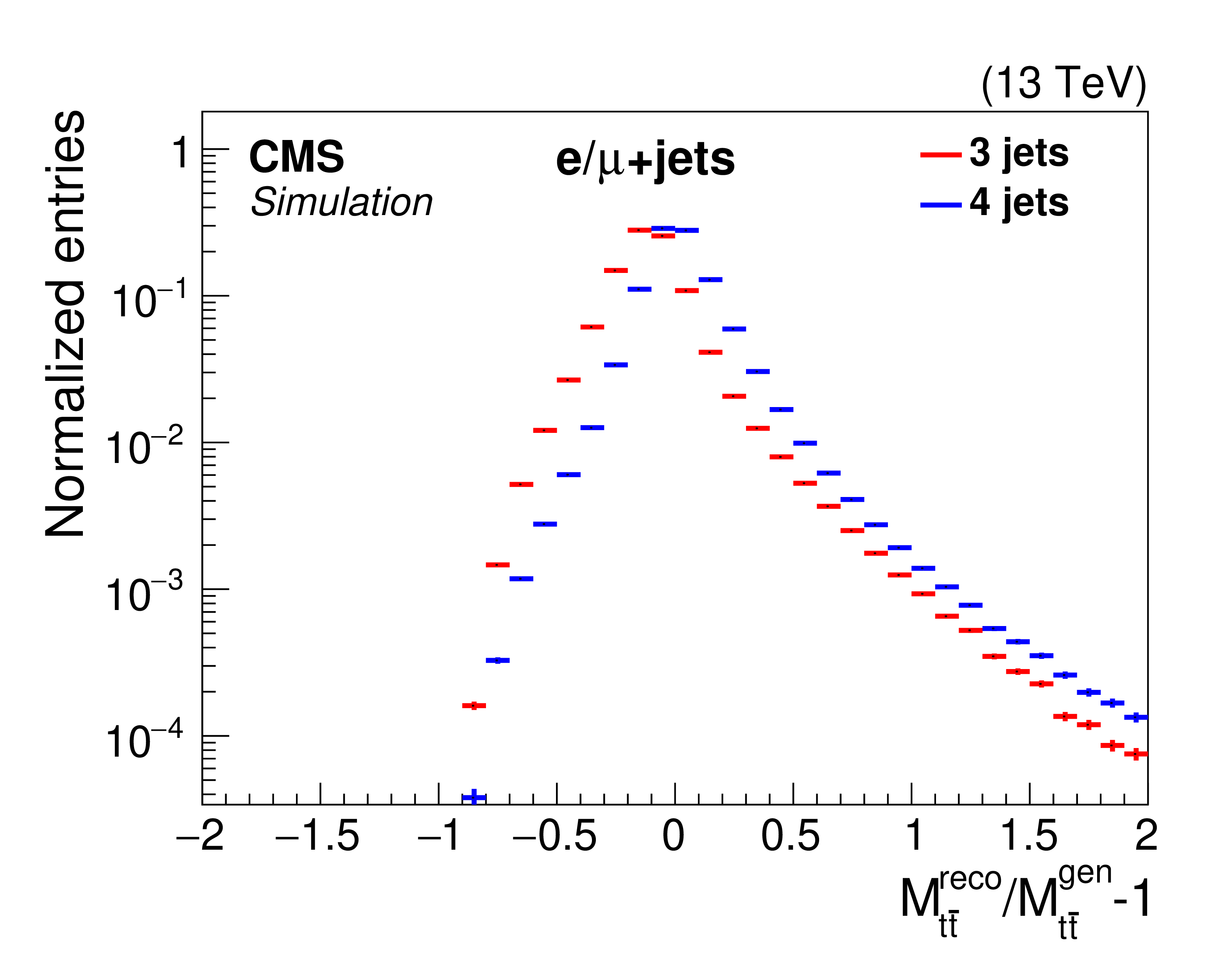
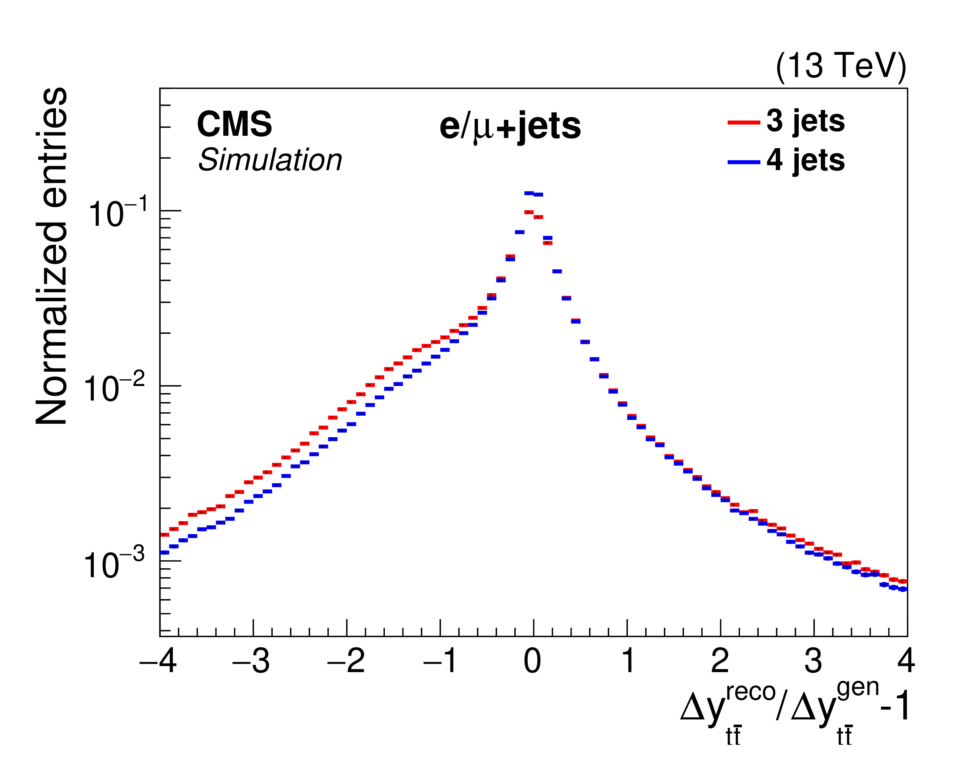
Figure 4:
Relative difference between the reconstructed and generated ${M_{{\mathrm{t} {}\mathrm{\bar{t}}}}}$ (left) and ${\Delta y_{{\mathrm{t} {}\mathrm{\bar{t}}}}}$ (right) for three-jet and four-jet event categories. |
png pdf |
Figure 4-a:
Relative difference between the reconstructed and generated ${M_{{\mathrm{t} {}\mathrm{\bar{t}}}}}$ for three-jet and four-jet event categories. |
png pdf |
Figure 4-b:
Relative difference between the reconstructed and generated ${\Delta y_{{\mathrm{t} {}\mathrm{\bar{t}}}}}$ for three-jet and four-jet event categories. |
png pdf |
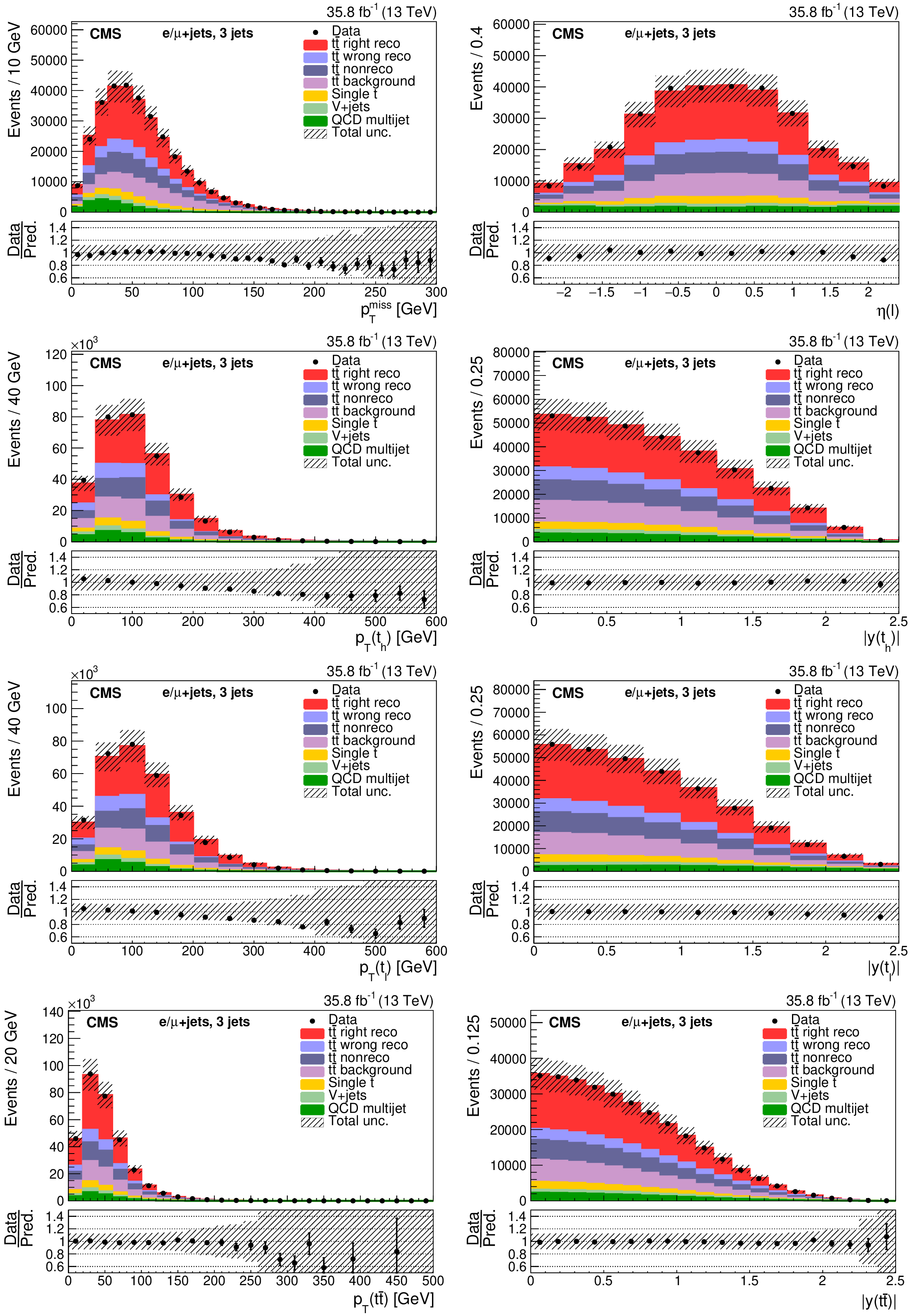
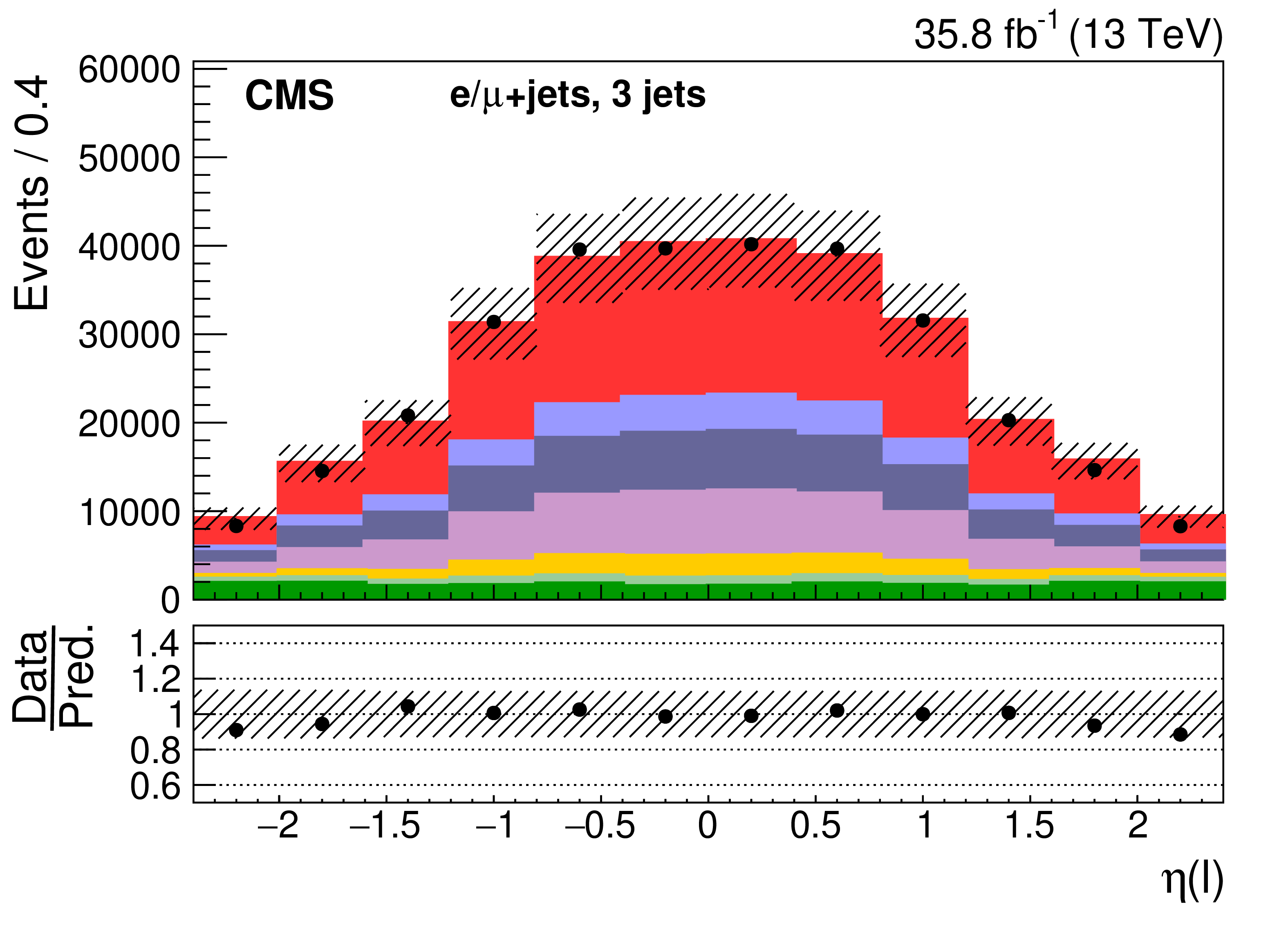
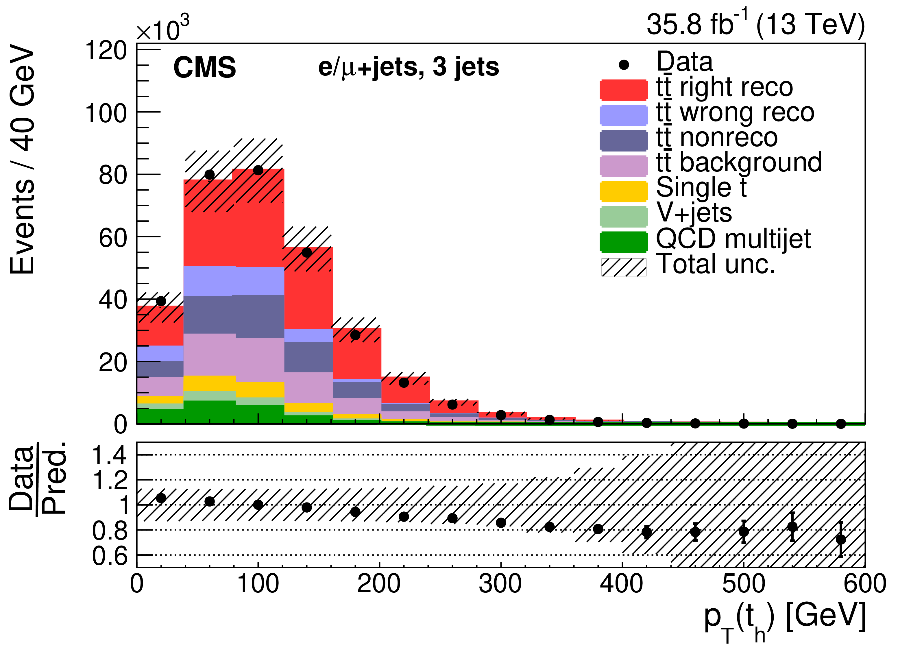
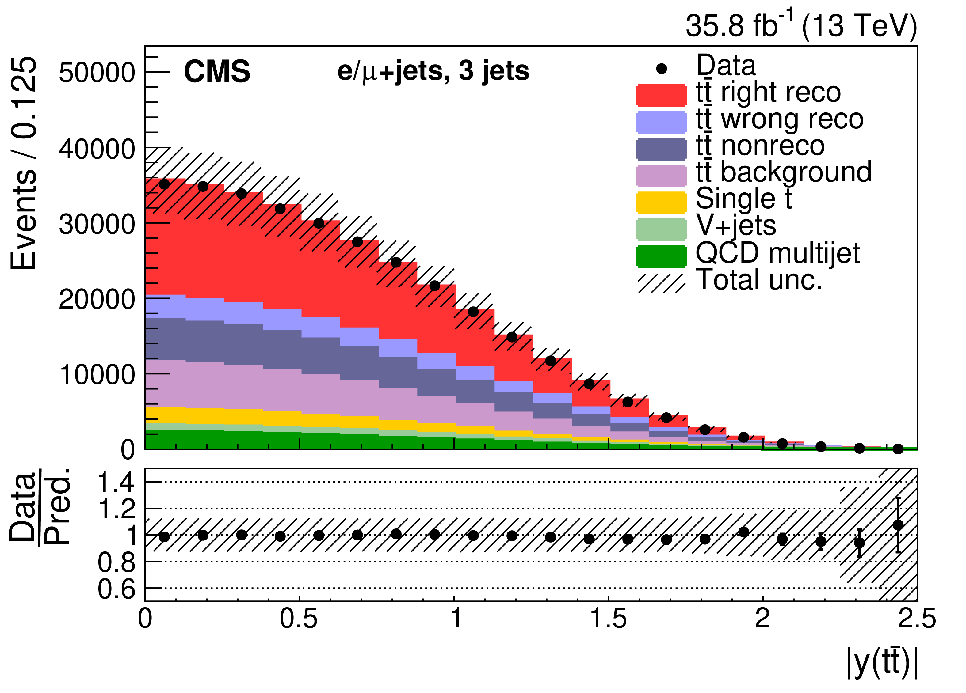
Figure 5:
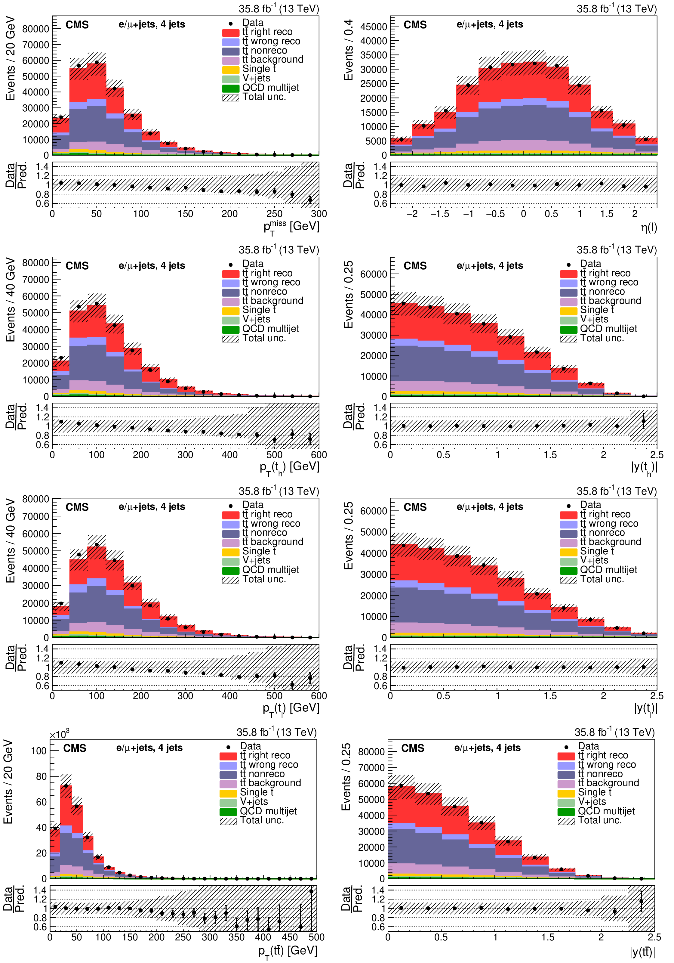
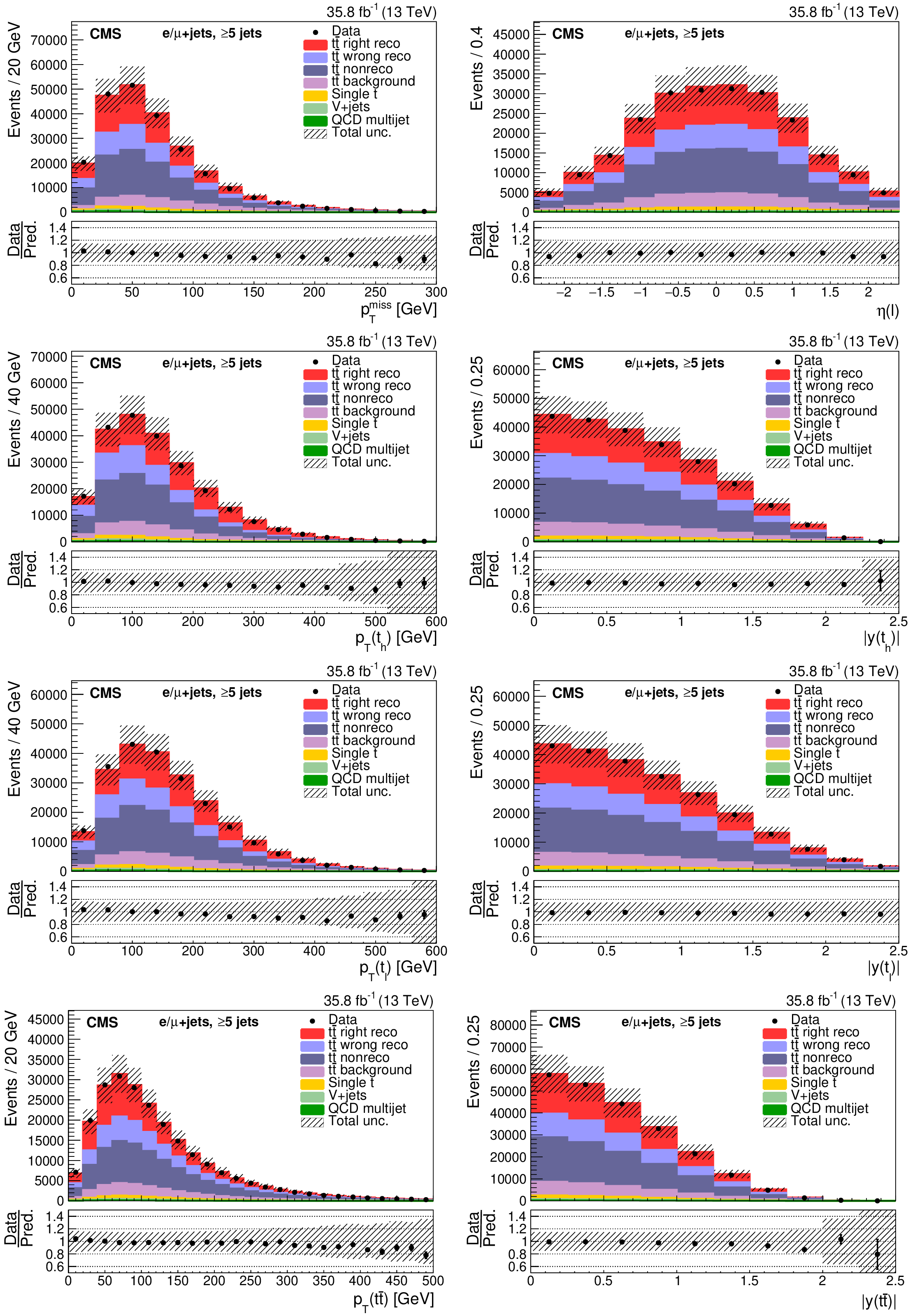
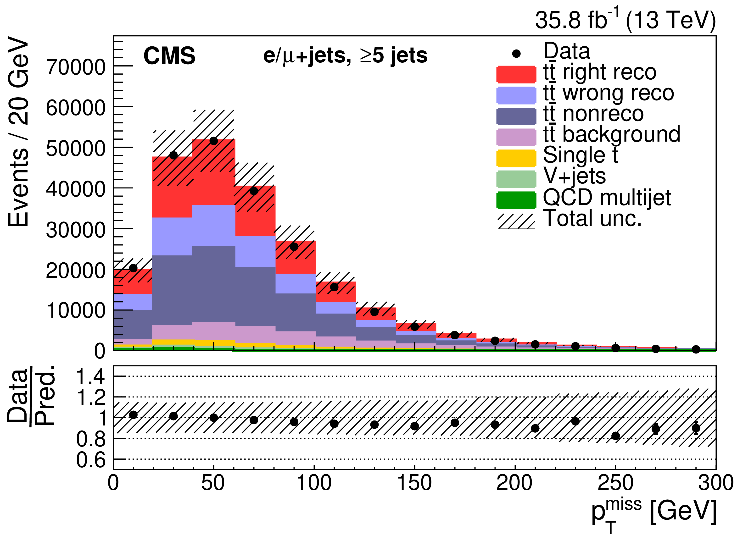
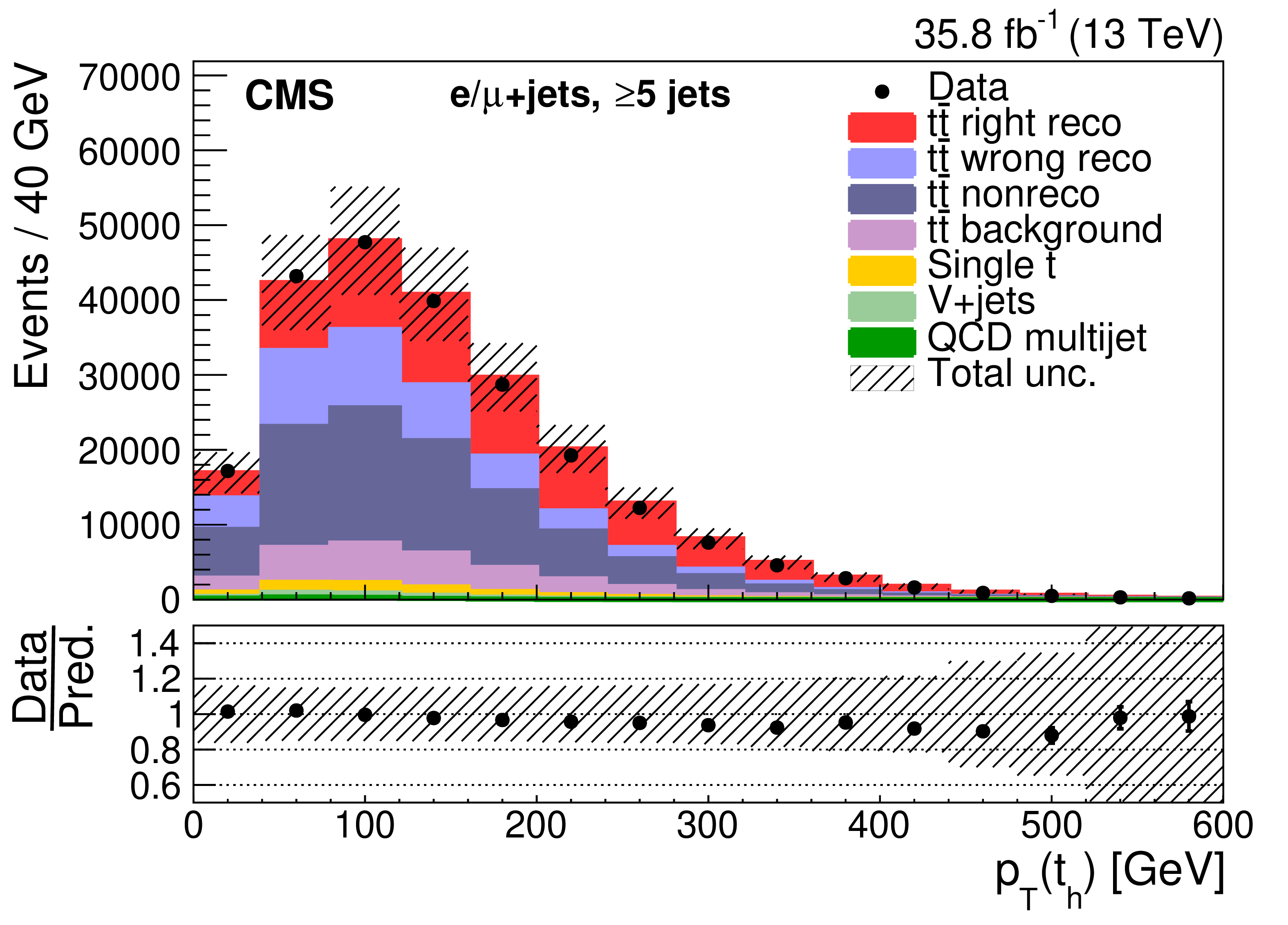
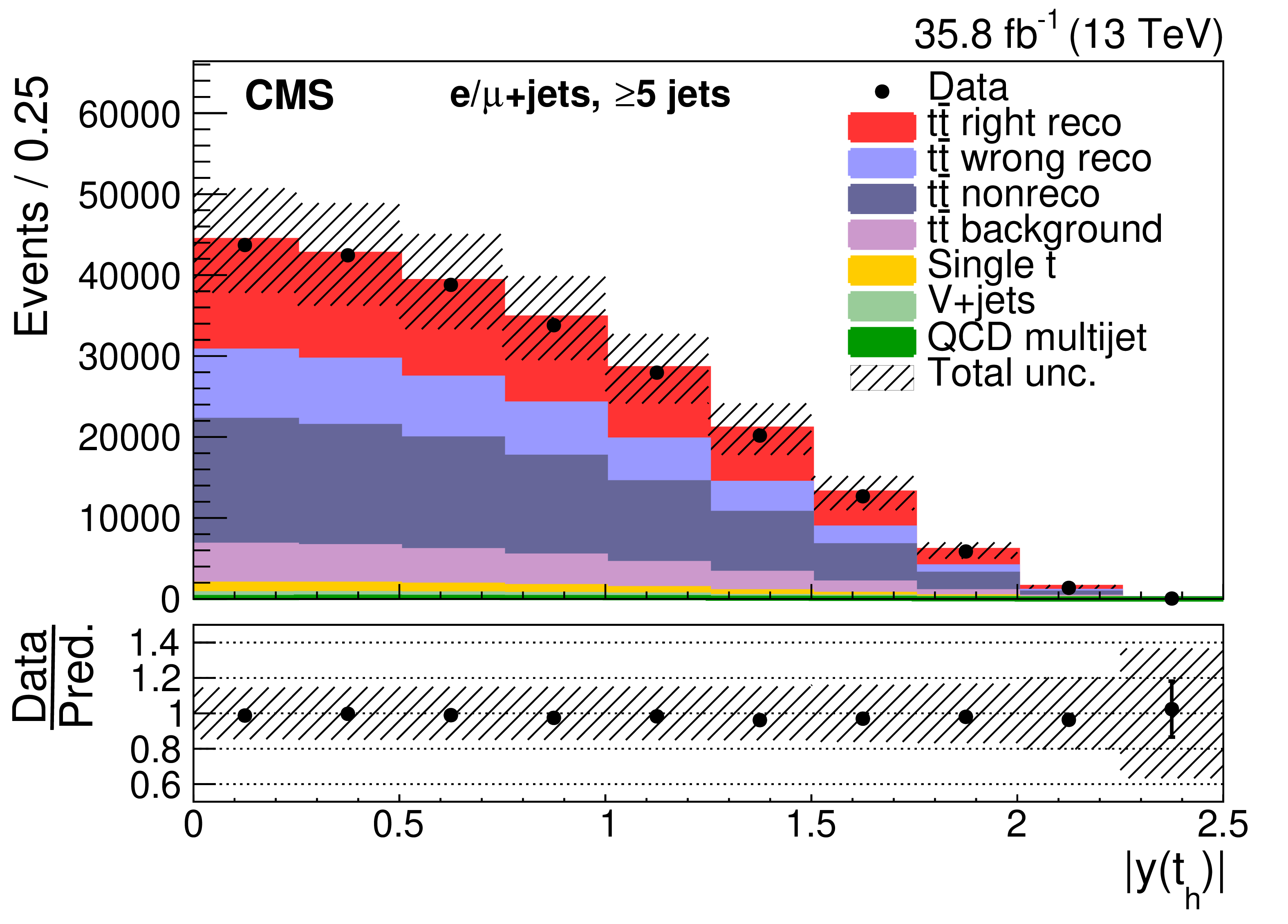
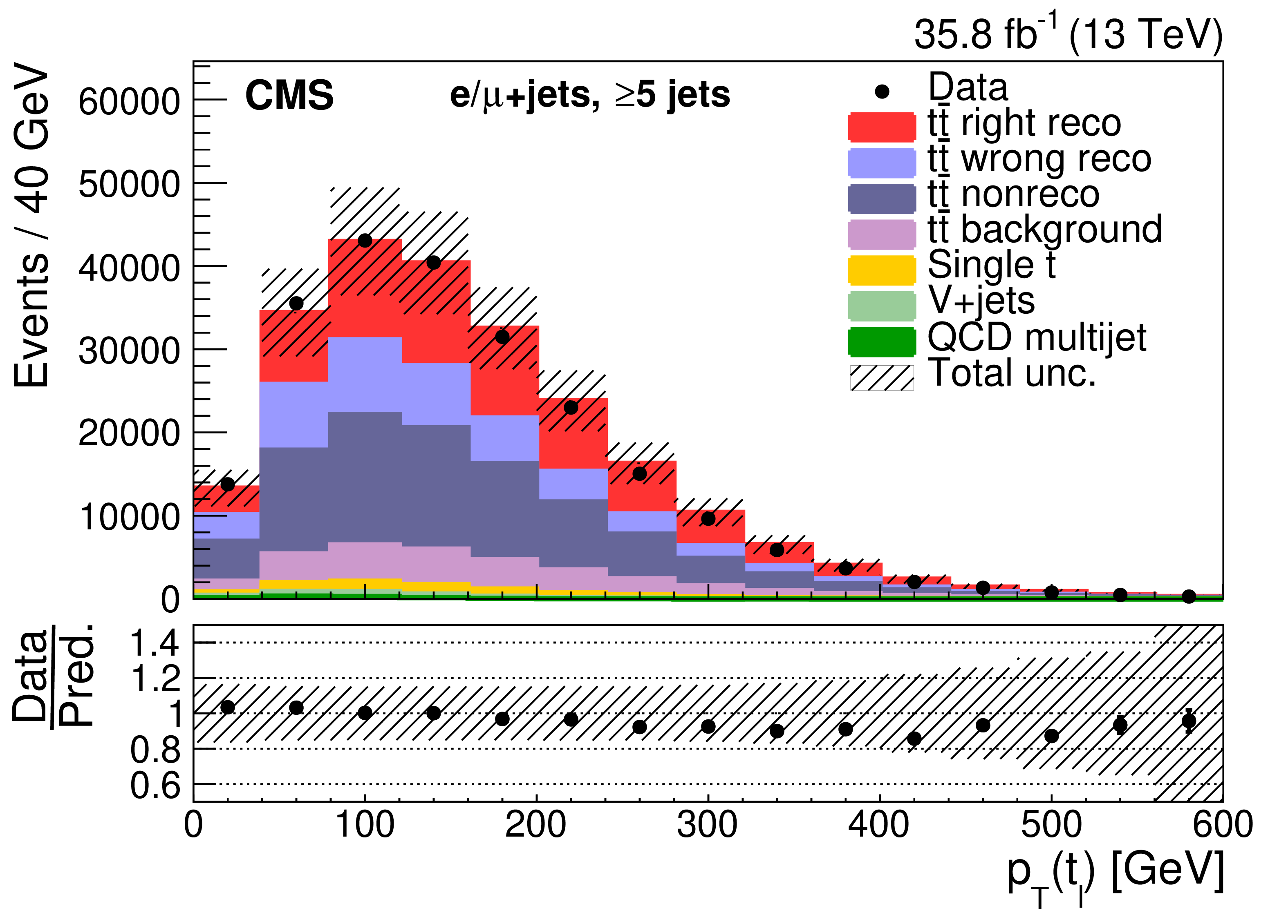
Three-jet events after selection and ${\mathrm{t} {}\mathrm{\bar{t}}}$ reconstruction. The plots show (left to right, upper to lower) the missing transverse momentum (${{p_{\mathrm {T}}} ^\text {miss}}$), the lepton pseudorapidity, and $ {p_{\mathrm {T}}} $ and the absolute rapidity of the top quark decaying hadronically, semileptonically, and of the ${\mathrm{t} {}\mathrm{\bar{t}}}$ system. The hatched band shows the total uncertainty associated with the signal and background predictions with the individual sources of uncertainty assumed to be uncorrelated. The ratios of data to the sum of the predicted yields are provided at the bottom of each panel. |

png pdf |
Figure 5-a:
Three-jet events after selection and ${\mathrm{t} {}\mathrm{\bar{t}}}$ reconstruction. The plot shows the missing transverse momentum (${{p_{\mathrm {T}}} ^\text {miss}}$). The hatched band shows the total uncertainty associated with the signal and background predictions with the individual sources of uncertainty assumed to be uncorrelated. The ratios of data to the sum of the predicted yields are provided at the bottom of the panel. |
png pdf |
Figure 5-b:
Three-jet events after selection and ${\mathrm{t} {}\mathrm{\bar{t}}}$ reconstruction. The plot shows the lepton pseudorapidity. The hatched band shows the total uncertainty associated with the signal and background predictions with the individual sources of uncertainty assumed to be uncorrelated. The ratios of data to the sum of the predicted yields are provided at the bottom of the panel. |
png pdf |
Figure 5-c:
Three-jet events after selection and ${\mathrm{t} {}\mathrm{\bar{t}}}$ reconstruction. The plot shows the $ {p_{\mathrm {T}}} $ of the top quark decaying hadronically. The hatched band shows the total uncertainty associated with the signal and background predictions with the individual sources of uncertainty assumed to be uncorrelated. The ratios of data to the sum of the predicted yields are provided at the bottom of the panel. |
png pdf |
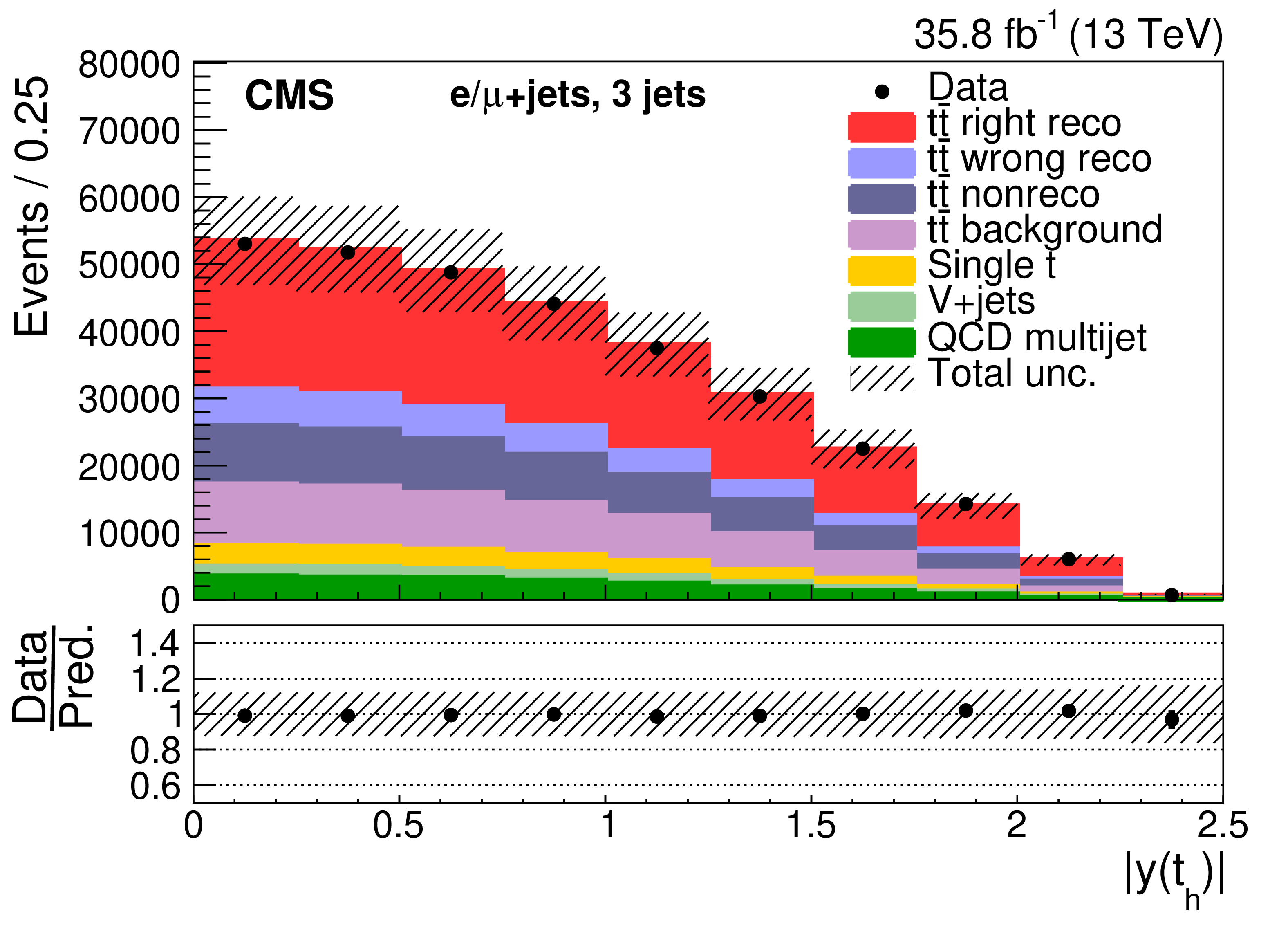
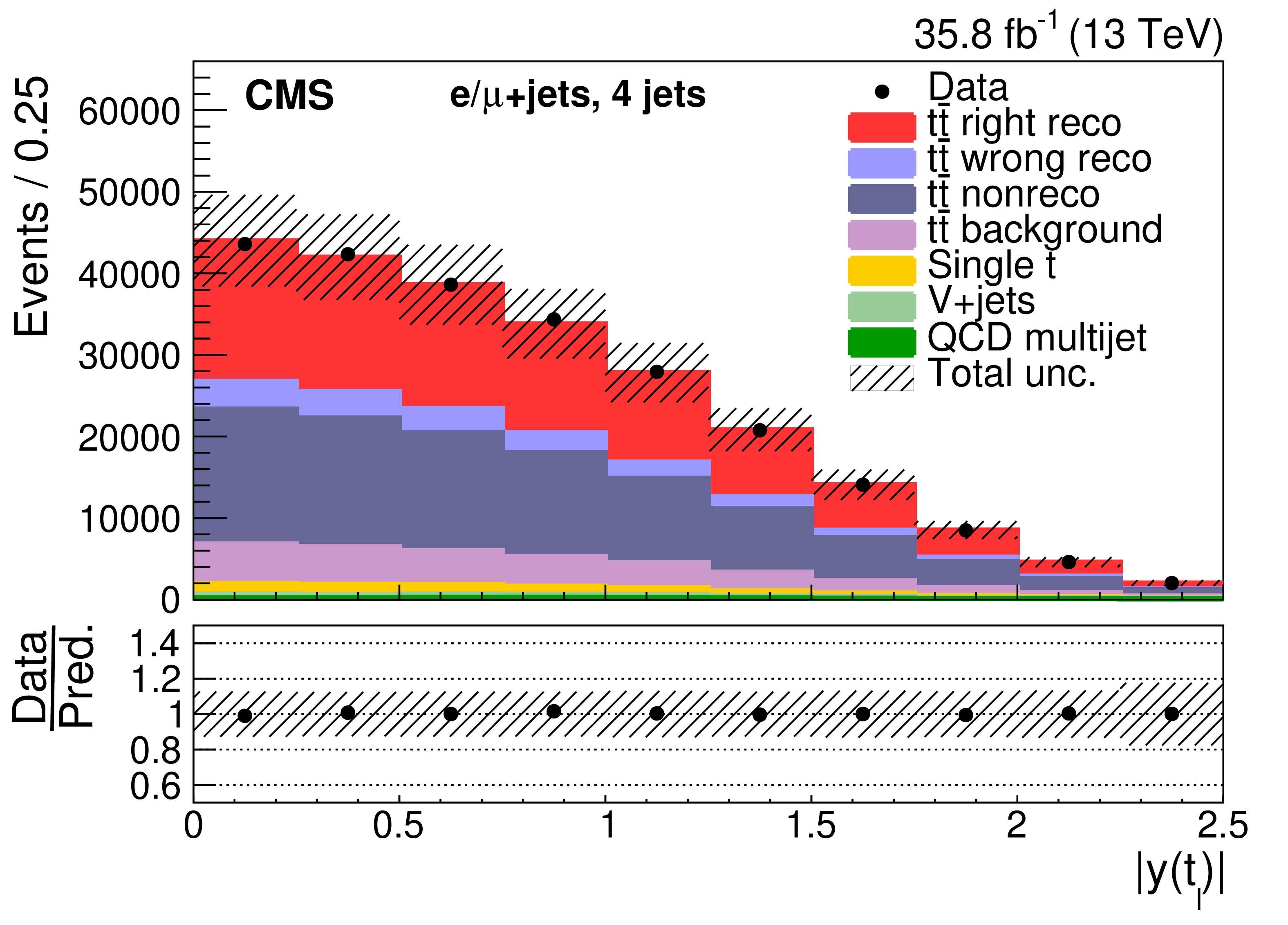
Figure 5-d:
Three-jet events after selection and ${\mathrm{t} {}\mathrm{\bar{t}}}$ reconstruction. The plot shows the absolute rapidity of the top quark decaying hadronically. The hatched band shows the total uncertainty associated with the signal and background predictions with the individual sources of uncertainty assumed to be uncorrelated. The ratios of data to the sum of the predicted yields are provided at the bottom of the panel. |
png pdf |
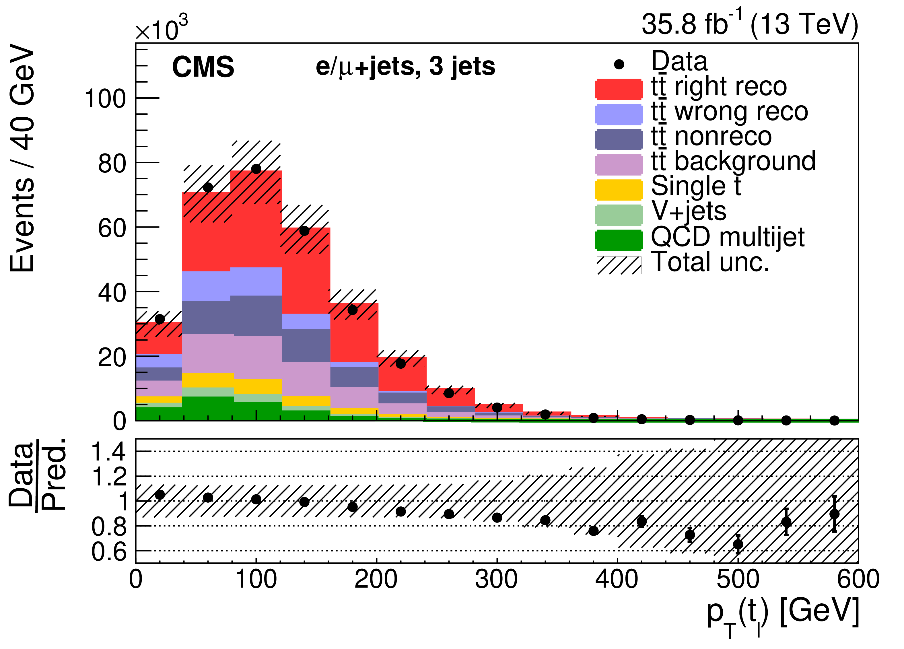
Figure 5-e:
Three-jet events after selection and ${\mathrm{t} {}\mathrm{\bar{t}}}$ reconstruction. The plot shows the $ {p_{\mathrm {T}}} $ of the top quark decaying semileptonically. The hatched band shows the total uncertainty associated with the signal and background predictions with the individual sources of uncertainty assumed to be uncorrelated. The ratios of data to the sum of the predicted yields are provided at the bottom of the panel. |

png pdf |
Figure 5-f:
Three-jet events after selection and ${\mathrm{t} {}\mathrm{\bar{t}}}$ reconstruction. The plot shows the absolute rapidity of the top quark decaying semileptonically. The hatched band shows the total uncertainty associated with the signal and background predictions with the individual sources of uncertainty assumed to be uncorrelated. The ratios of data to the sum of the predicted yields are provided at the bottom of the panel. |
png pdf |
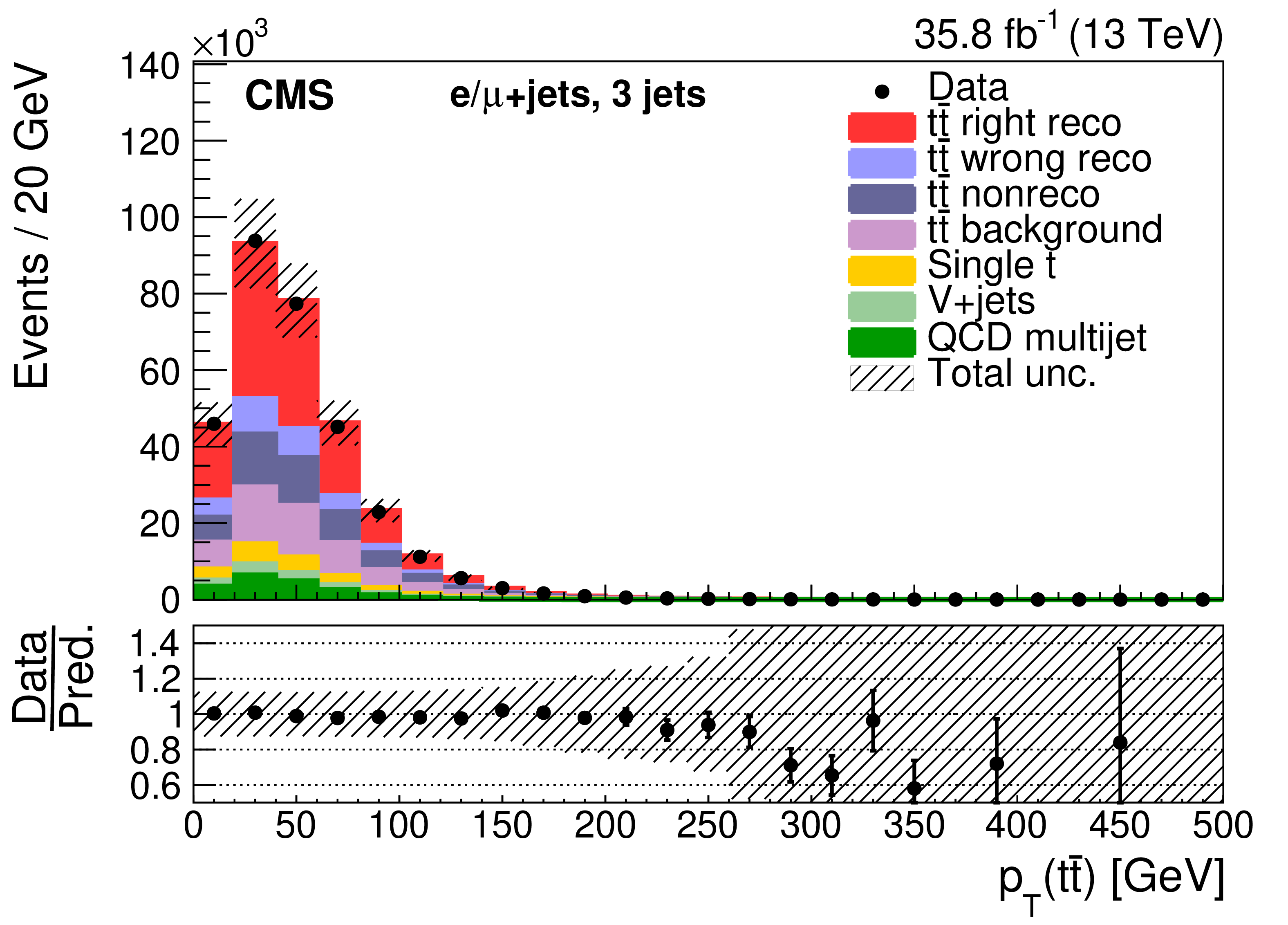
Figure 5-g:
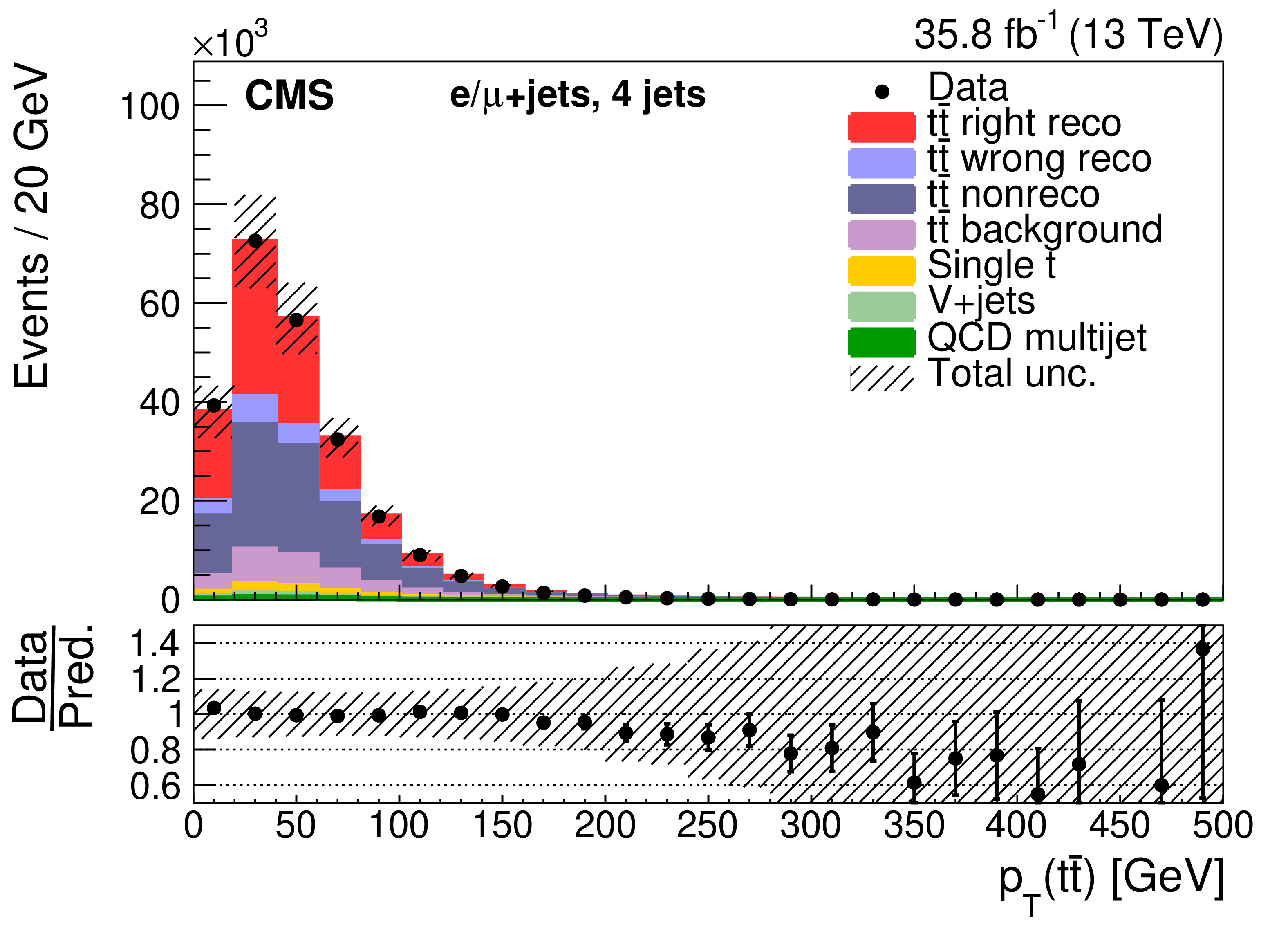
Three-jet events after selection and ${\mathrm{t} {}\mathrm{\bar{t}}}$ reconstruction. The plot shows the $ {p_{\mathrm {T}}} $ of the ${\mathrm{t} {}\mathrm{\bar{t}}}$ system. The hatched band shows the total uncertainty associated with the signal and background predictions with the individual sources of uncertainty assumed to be uncorrelated. The ratios of data to the sum of the predicted yields are provided at the bottom of the panel. |
png pdf |
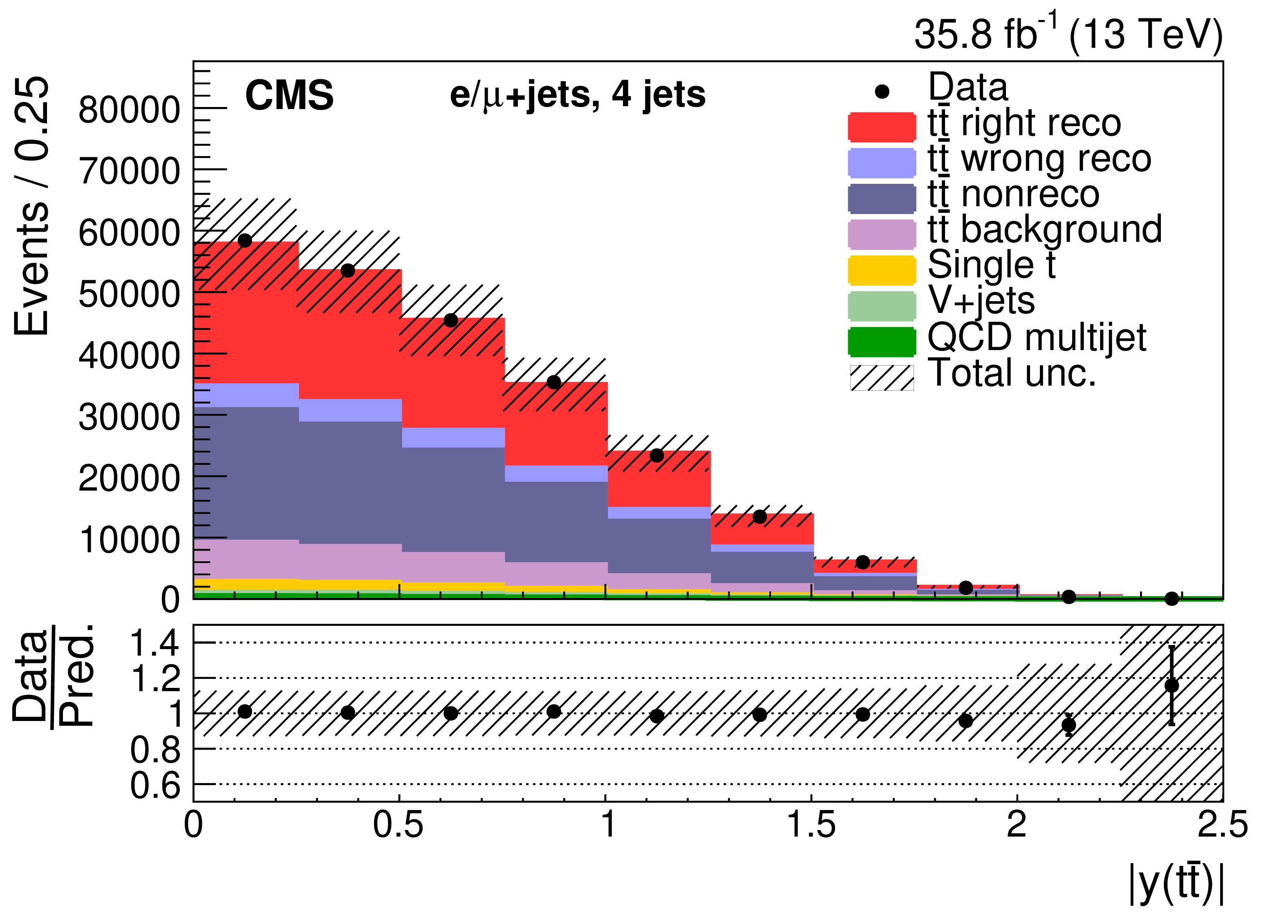
Figure 5-h:
Three-jet events after selection and ${\mathrm{t} {}\mathrm{\bar{t}}}$ reconstruction. The plot shows the absolute rapidity of the ${\mathrm{t} {}\mathrm{\bar{t}}}$ system. The hatched band shows the total uncertainty associated with the signal and background predictions with the individual sources of uncertainty assumed to be uncorrelated. The ratios of data to the sum of the predicted yields are provided at the bottom of the panel. |
png pdf |
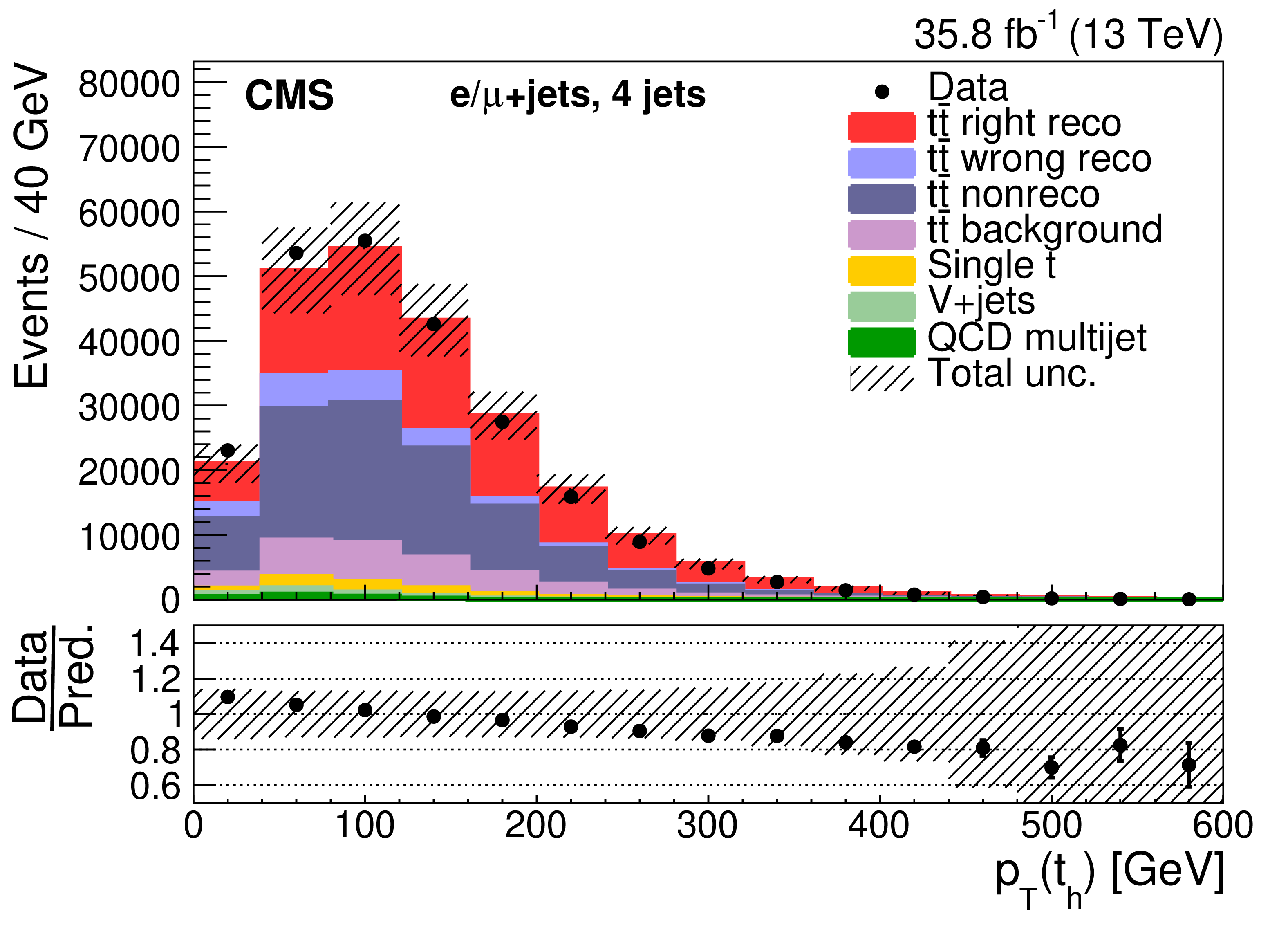
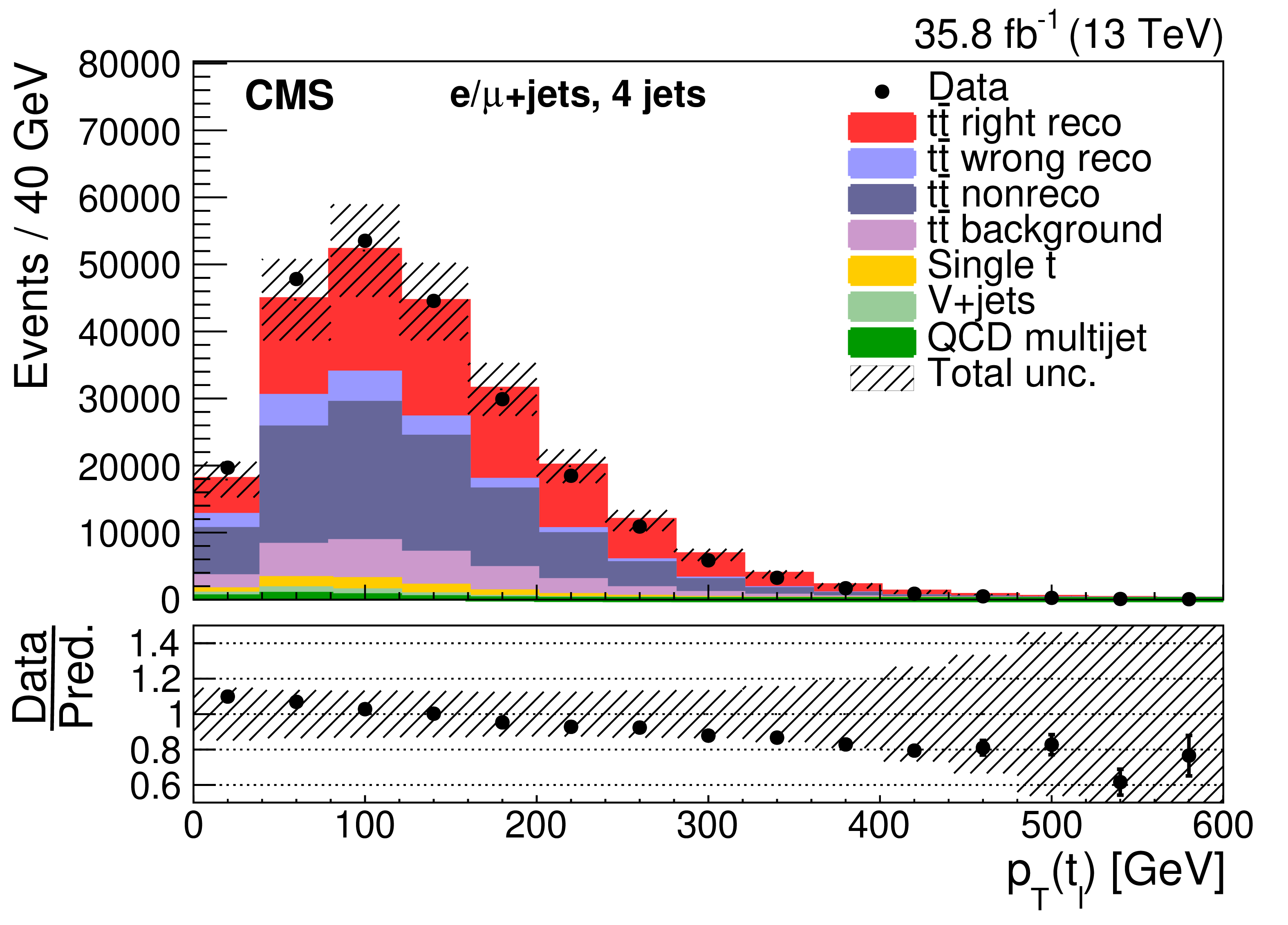
Figure 6:
Four-jet events after selection and ${\mathrm{t} {}\mathrm{\bar{t}}}$ reconstruction. Same distributions as described in Fig. 5. |

png pdf |
Figure 6-a:
Four-jet events after selection and ${\mathrm{t} {}\mathrm{\bar{t}}}$ reconstruction. Same distributions as described in Fig. 5. |

png pdf |
Figure 6-b:
Four-jet events after selection and ${\mathrm{t} {}\mathrm{\bar{t}}}$ reconstruction. Same distributions as described in Fig. 5. |
png pdf |
Figure 6-c:
Four-jet events after selection and ${\mathrm{t} {}\mathrm{\bar{t}}}$ reconstruction. Same distributions as described in Fig. 5. |

png pdf |
Figure 6-d:
Four-jet events after selection and ${\mathrm{t} {}\mathrm{\bar{t}}}$ reconstruction. Same distributions as described in Fig. 5. |
png pdf |
Figure 6-e:
Four-jet events after selection and ${\mathrm{t} {}\mathrm{\bar{t}}}$ reconstruction. Same distributions as described in Fig. 5. |
png pdf |
Figure 6-f:
Four-jet events after selection and ${\mathrm{t} {}\mathrm{\bar{t}}}$ reconstruction. Same distributions as described in Fig. 5. |
png pdf |
Figure 6-g:
Four-jet events after selection and ${\mathrm{t} {}\mathrm{\bar{t}}}$ reconstruction. Same distributions as described in Fig. 5. |
png pdf |
Figure 6-h:
Four-jet events after selection and ${\mathrm{t} {}\mathrm{\bar{t}}}$ reconstruction. Same distributions as described in Fig. 5. |
png pdf |
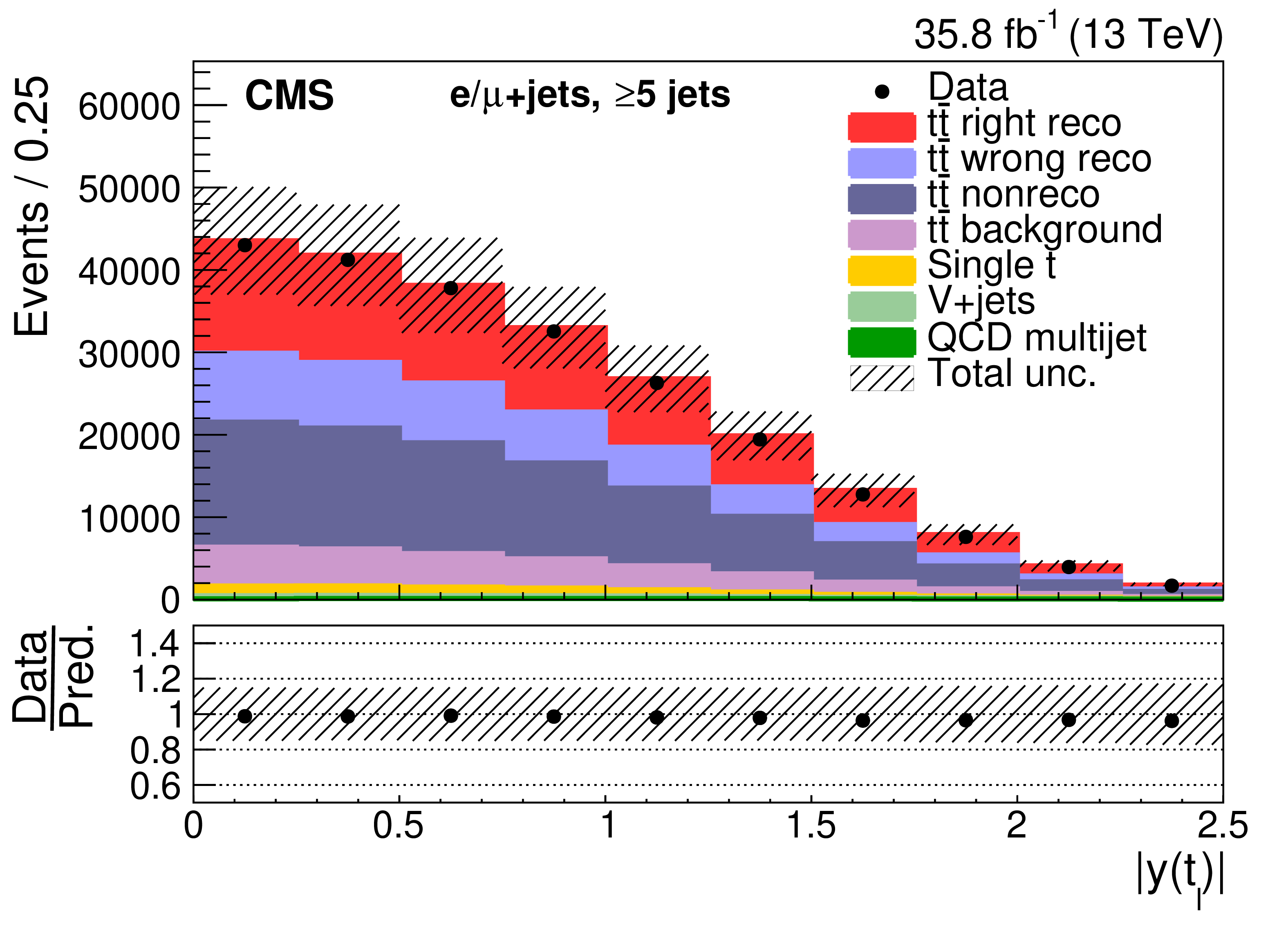
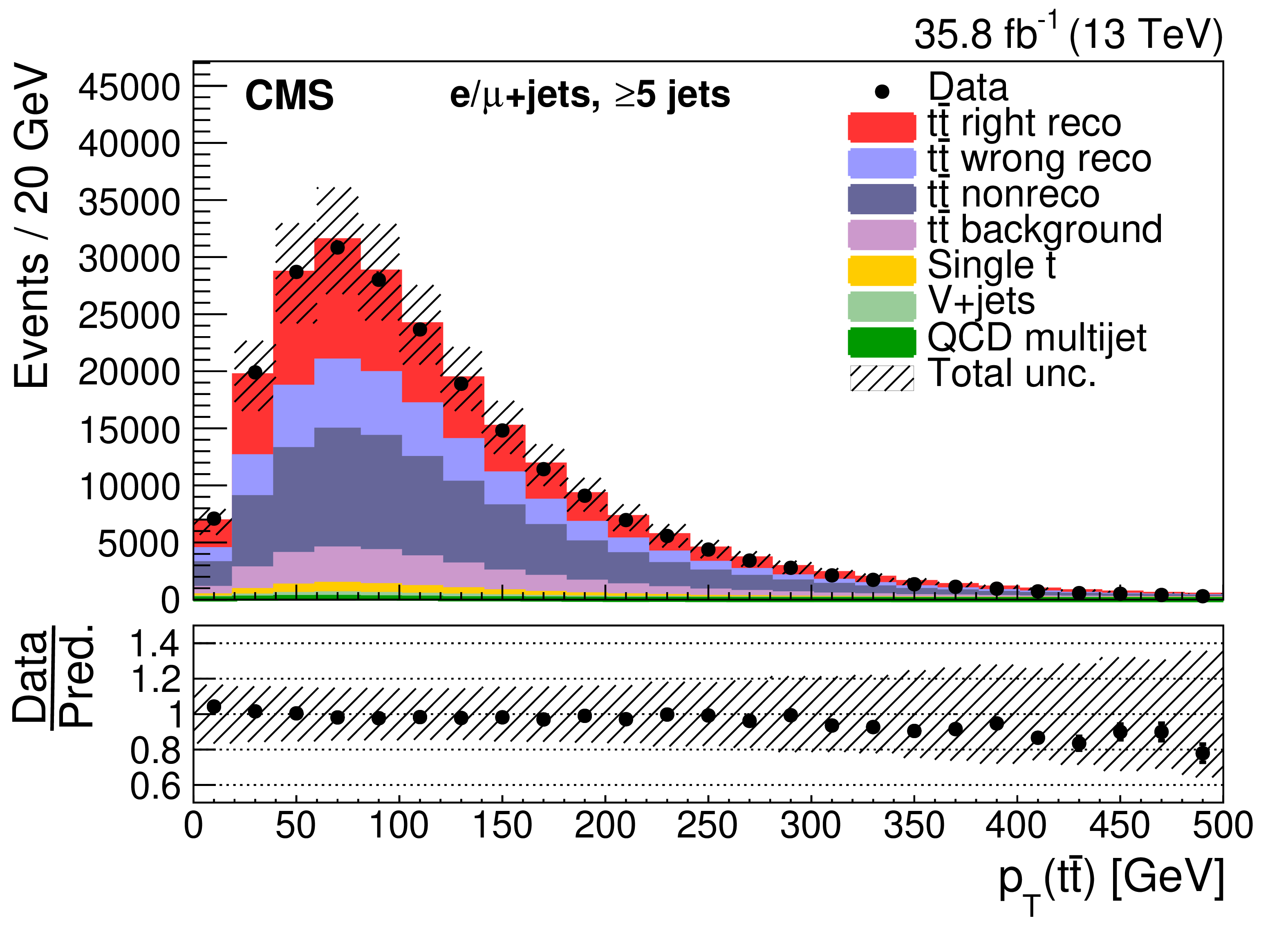
Figure 7:
Events with five or more jets after selection and ${\mathrm{t} {}\mathrm{\bar{t}}}$ reconstruction. Same distributions as described in Fig. 5. |
png pdf |
Figure 7-a:
Events with five or more jets after selection and ${\mathrm{t} {}\mathrm{\bar{t}}}$ reconstruction. Same distributions as described in Fig. 5. |

png pdf |
Figure 7-b:
Events with five or more jets after selection and ${\mathrm{t} {}\mathrm{\bar{t}}}$ reconstruction. Same distributions as described in Fig. 5. |
png pdf |
Figure 7-c:
Events with five or more jets after selection and ${\mathrm{t} {}\mathrm{\bar{t}}}$ reconstruction. Same distributions as described in Fig. 5. |
png pdf |
Figure 7-d:
Events with five or more jets after selection and ${\mathrm{t} {}\mathrm{\bar{t}}}$ reconstruction. Same distributions as described in Fig. 5. |
png pdf |
Figure 7-e:
Events with five or more jets after selection and ${\mathrm{t} {}\mathrm{\bar{t}}}$ reconstruction. Same distributions as described in Fig. 5. |
png pdf |
Figure 7-f:
Events with five or more jets after selection and ${\mathrm{t} {}\mathrm{\bar{t}}}$ reconstruction. Same distributions as described in Fig. 5. |
png pdf |
Figure 7-g:
Events with five or more jets after selection and ${\mathrm{t} {}\mathrm{\bar{t}}}$ reconstruction. Same distributions as described in Fig. 5. |

png pdf |
Figure 7-h:
Events with five or more jets after selection and ${\mathrm{t} {}\mathrm{\bar{t}}}$ reconstruction. Same distributions as described in Fig. 5. |
png pdf |
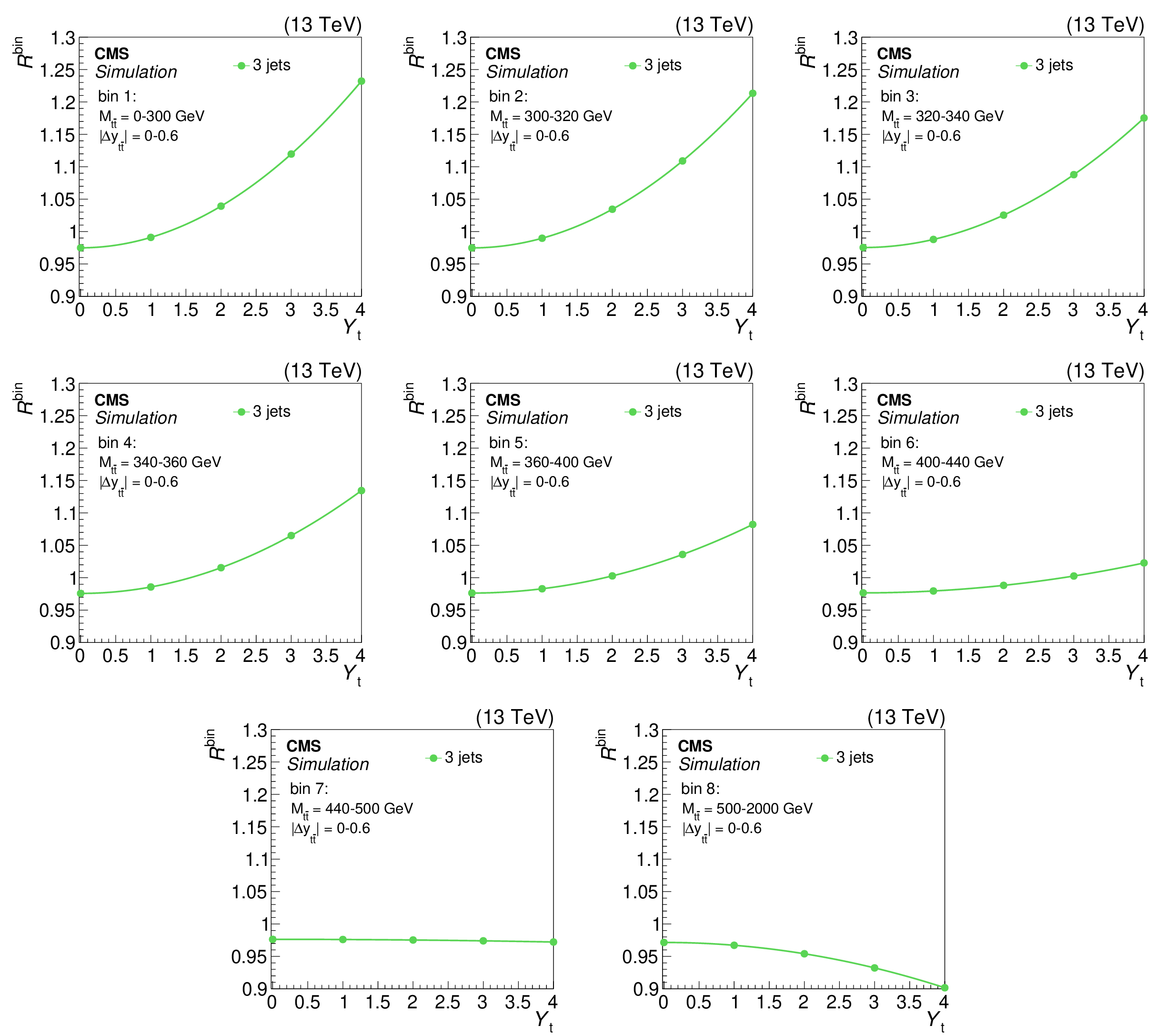
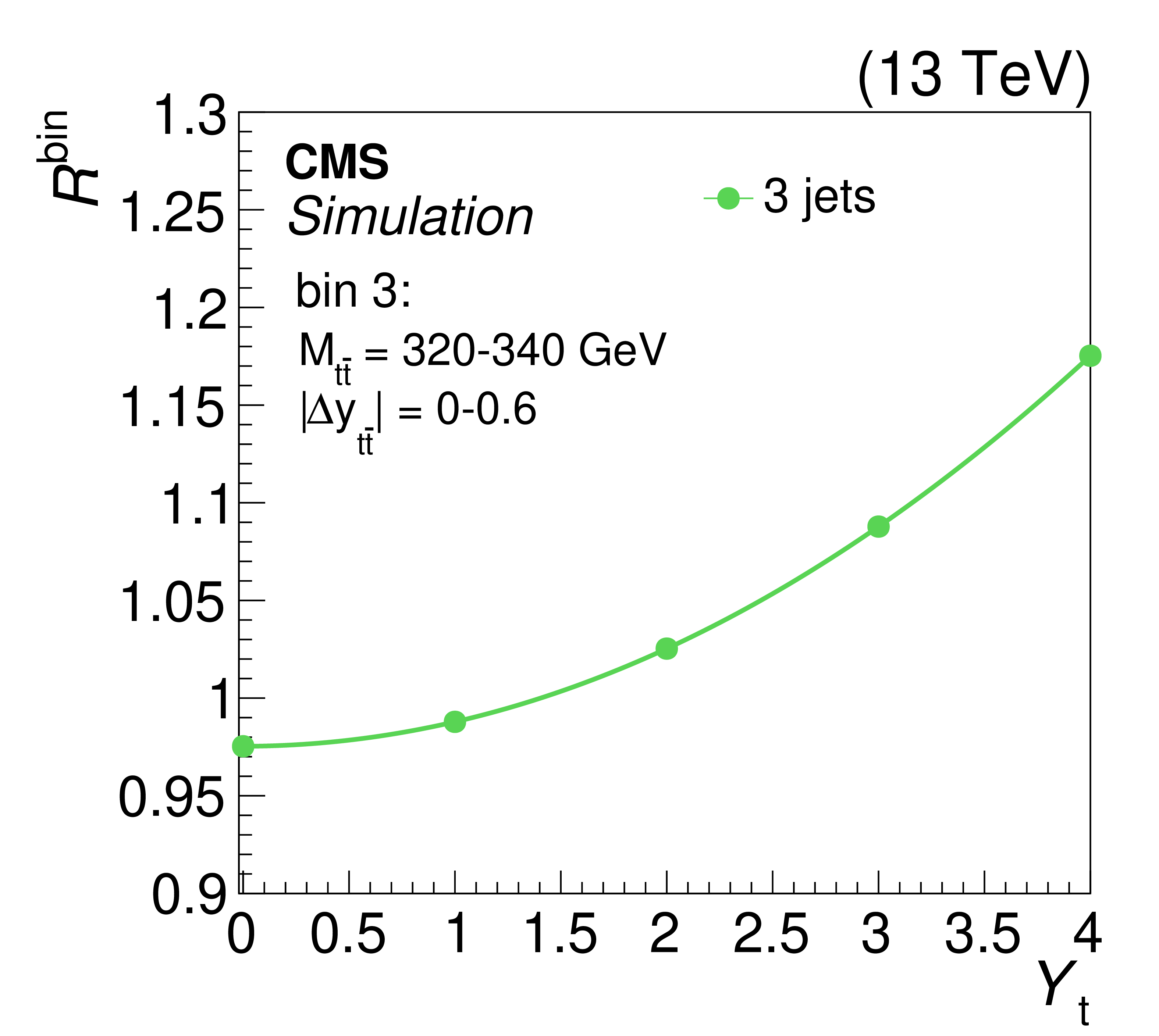
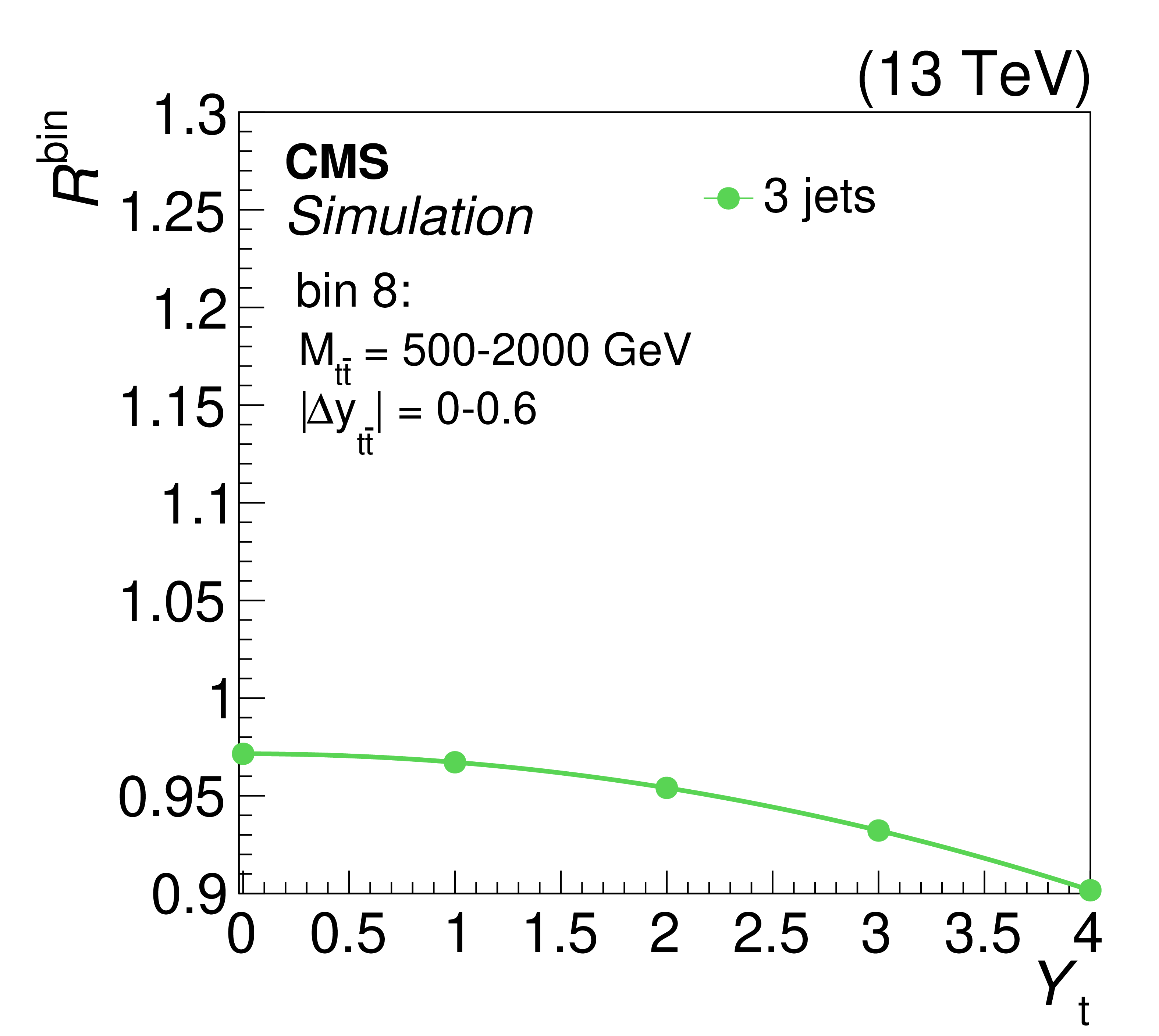
Figure 8:
The strength of the weak interaction correction, relative to the predicted POWHEG signal, $R^\mathrm {bin}$, as a function of ${Y_{\mathrm{t}}} $ in the three-jet category. The plots correspond to the first eight ${M_{{\mathrm{t} {}\mathrm{\bar{t}}}}}$ bins for $ {| {\Delta y_{{\mathrm{t} {}\mathrm{\bar{t}}}}} |} < $ 0.6 (as shown in Fig. 10). A quadratic fit is performed in each bin. |
png pdf |
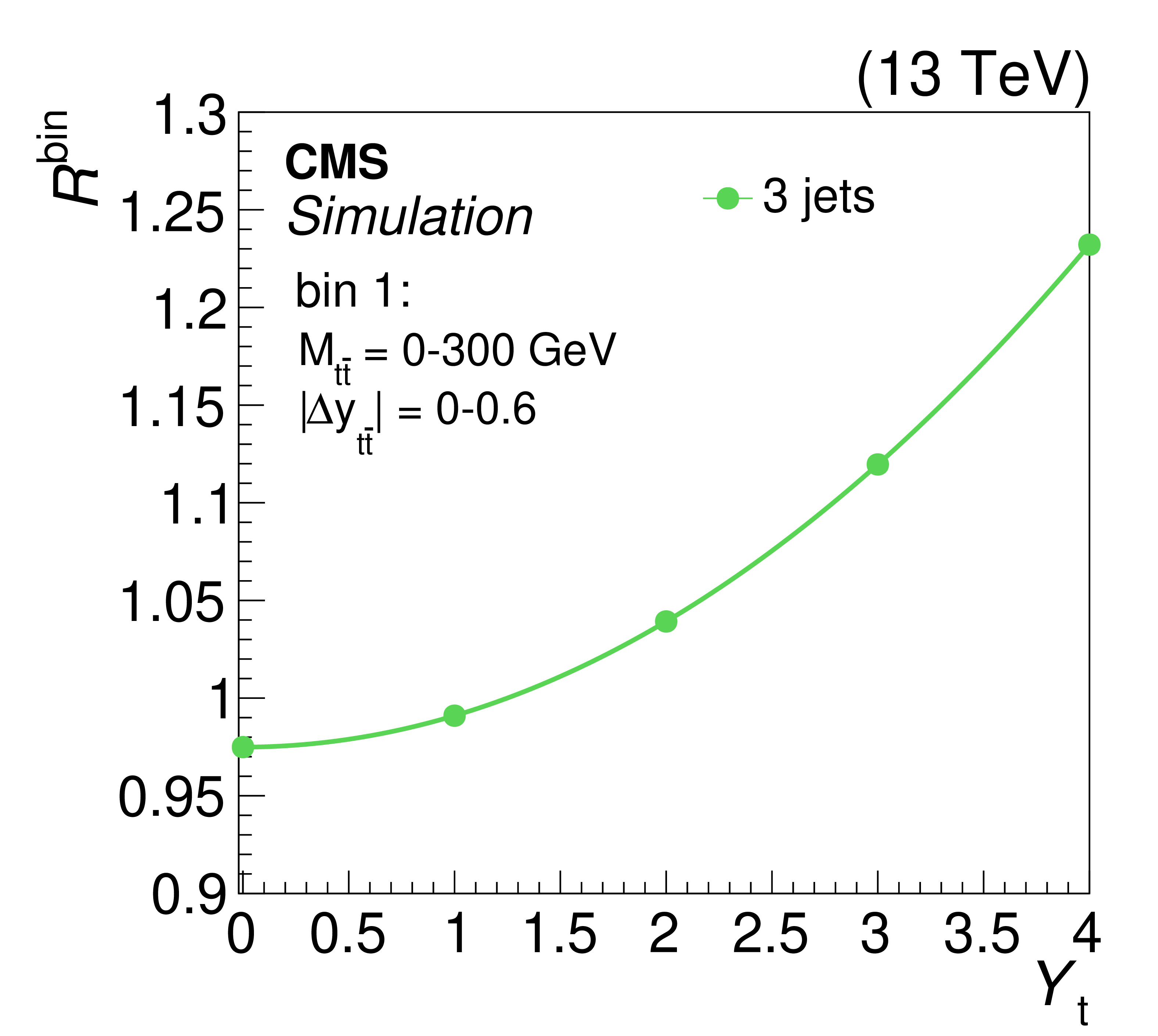
Figure 8-a:
The strength of the weak interaction correction, relative to the predicted POWHEG signal, $R^\mathrm {bin}$, as a function of ${Y_{\mathrm{t}}} $ in the three-jet category. The plot corresponds to ${M_{{\mathrm{t} {}\mathrm{\bar{t}}}}}$ bin 1 for $ {| {\Delta y_{{\mathrm{t} {}\mathrm{\bar{t}}}}} |} < $ 0.6 (as shown in Fig. 10). A quadratic fit is performed in the bin. |

png pdf |
Figure 8-b:
The strength of the weak interaction correction, relative to the predicted POWHEG signal, $R^\mathrm {bin}$, as a function of ${Y_{\mathrm{t}}} $ in the three-jet category. The plot corresponds to ${M_{{\mathrm{t} {}\mathrm{\bar{t}}}}}$ bin 2 for $ {| {\Delta y_{{\mathrm{t} {}\mathrm{\bar{t}}}}} |} < $ 0.6 (as shown in Fig. 10). A quadratic fit is performed in the bin. |
png pdf |
Figure 8-c:
The strength of the weak interaction correction, relative to the predicted POWHEG signal, $R^\mathrm {bin}$, as a function of ${Y_{\mathrm{t}}} $ in the three-jet category. The plot corresponds to ${M_{{\mathrm{t} {}\mathrm{\bar{t}}}}}$ bin 3 for $ {| {\Delta y_{{\mathrm{t} {}\mathrm{\bar{t}}}}} |} < $ 0.6 (as shown in Fig. 10). A quadratic fit is performed in the bin. |
png pdf |
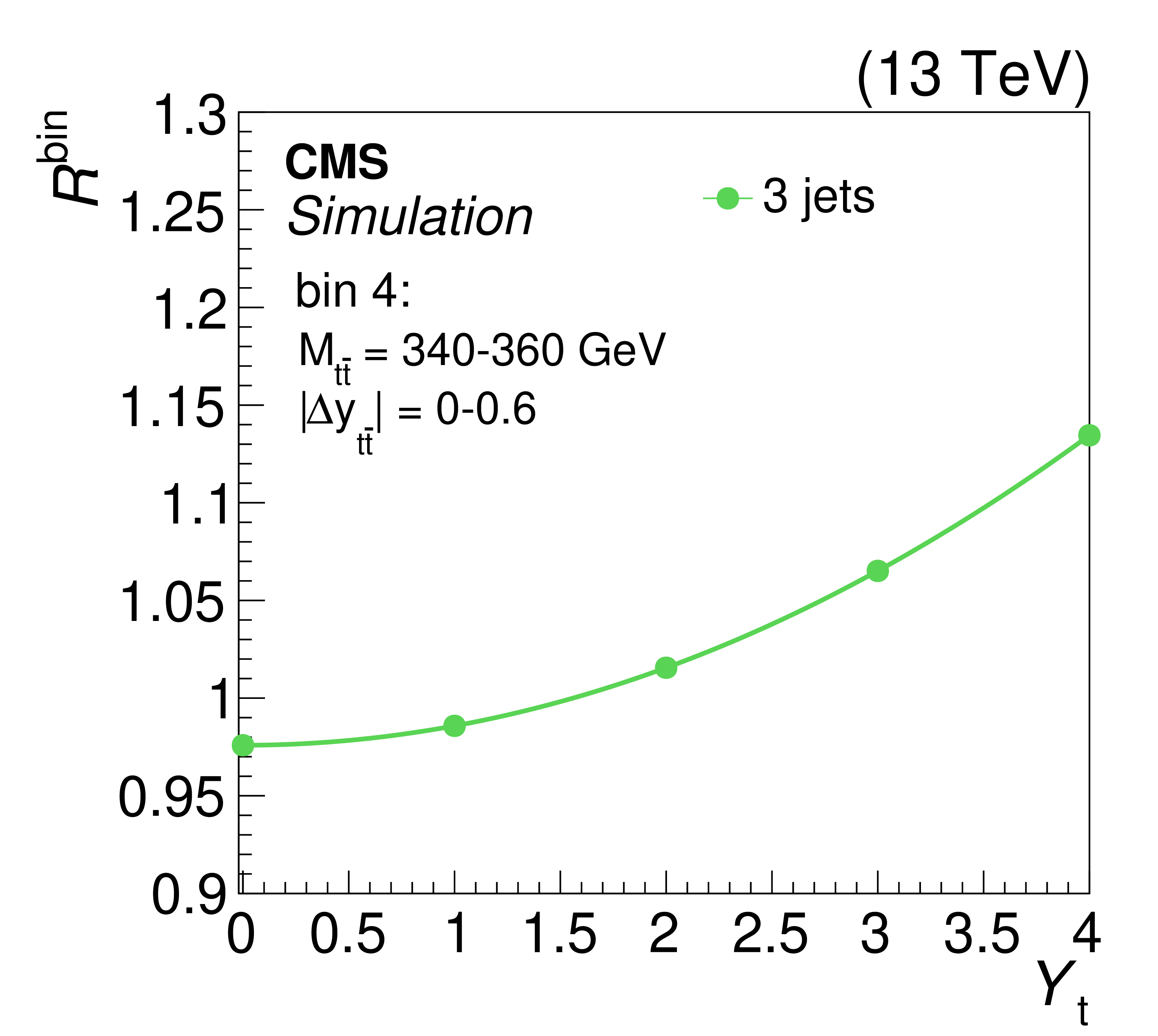
Figure 8-d:
The strength of the weak interaction correction, relative to the predicted POWHEG signal, $R^\mathrm {bin}$, as a function of ${Y_{\mathrm{t}}} $ in the three-jet category. The plot corresponds to ${M_{{\mathrm{t} {}\mathrm{\bar{t}}}}}$ bin 4 for $ {| {\Delta y_{{\mathrm{t} {}\mathrm{\bar{t}}}}} |} < $ 0.6 (as shown in Fig. 10). A quadratic fit is performed in the bin. |
png pdf |
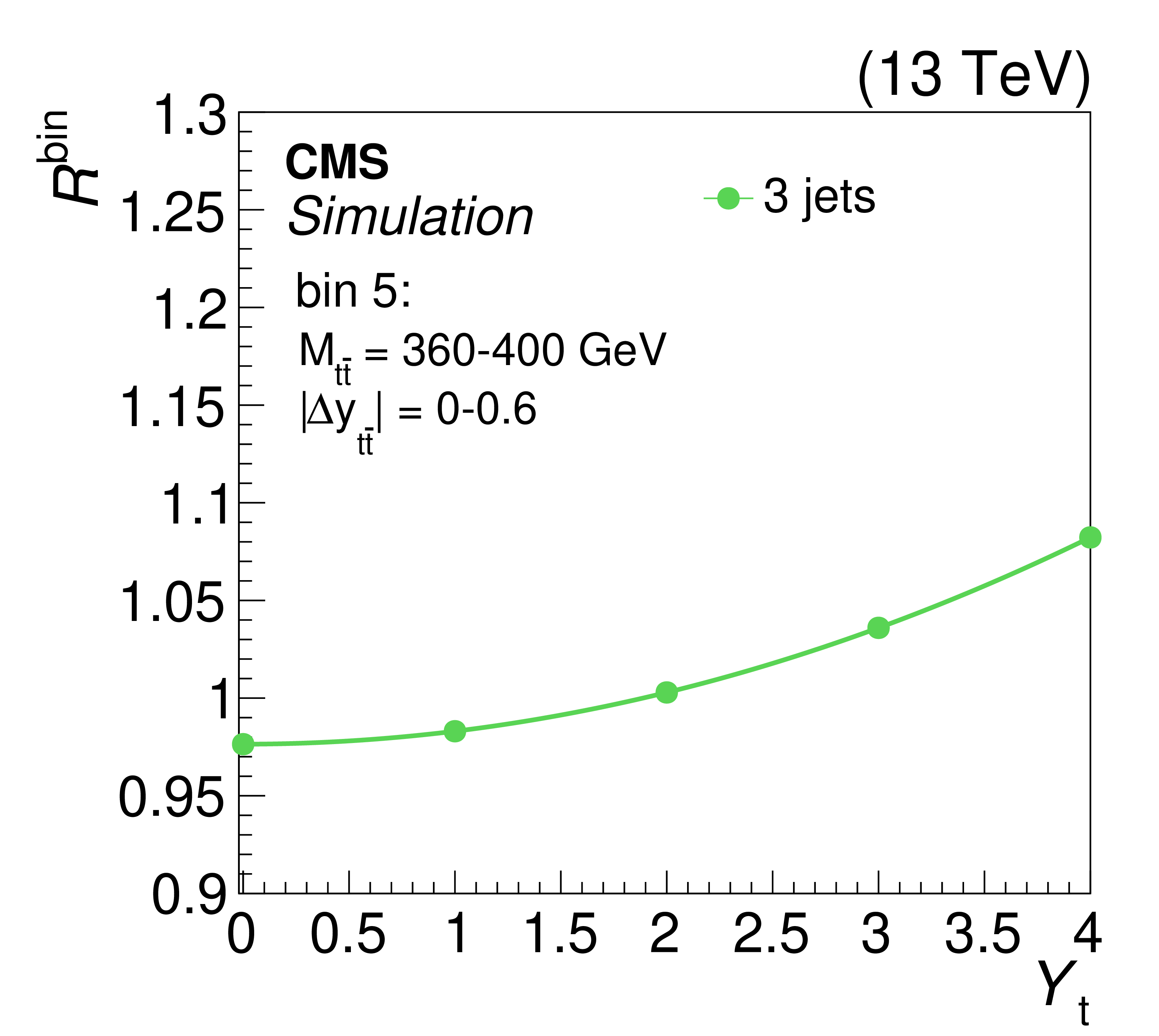
Figure 8-e:
The strength of the weak interaction correction, relative to the predicted POWHEG signal, $R^\mathrm {bin}$, as a function of ${Y_{\mathrm{t}}} $ in the three-jet category. The plot corresponds to ${M_{{\mathrm{t} {}\mathrm{\bar{t}}}}}$ bin 5 for $ {| {\Delta y_{{\mathrm{t} {}\mathrm{\bar{t}}}}} |} < $ 0.6 (as shown in Fig. 10). A quadratic fit is performed in the bin. |

png pdf |
Figure 8-f:
The strength of the weak interaction correction, relative to the predicted POWHEG signal, $R^\mathrm {bin}$, as a function of ${Y_{\mathrm{t}}} $ in the three-jet category. The plot corresponds to ${M_{{\mathrm{t} {}\mathrm{\bar{t}}}}}$ bin 6 for $ {| {\Delta y_{{\mathrm{t} {}\mathrm{\bar{t}}}}} |} < $ 0.6 (as shown in Fig. 10). A quadratic fit is performed in the bin. |
png pdf |
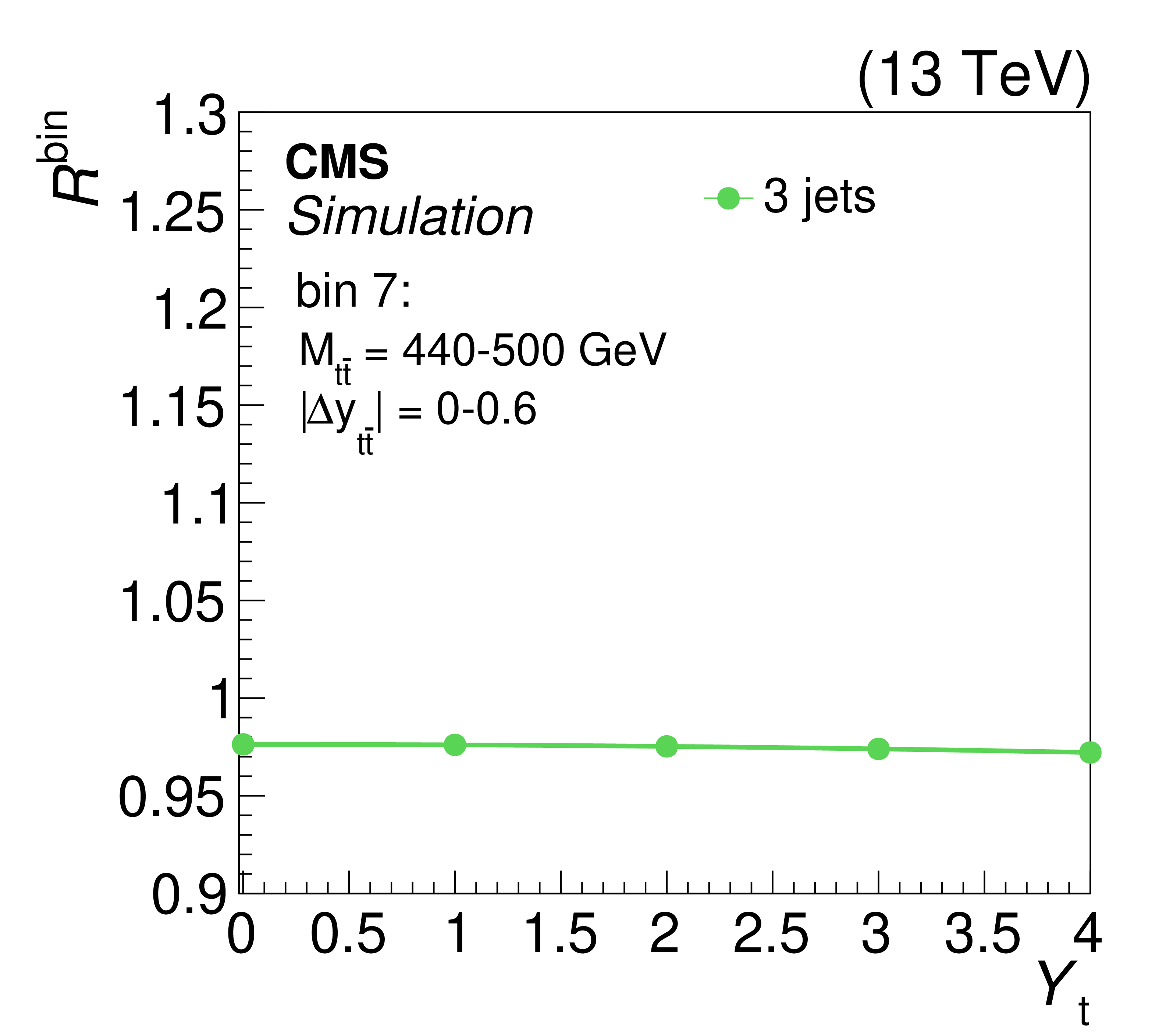
Figure 8-g:
The strength of the weak interaction correction, relative to the predicted POWHEG signal, $R^\mathrm {bin}$, as a function of ${Y_{\mathrm{t}}} $ in the three-jet category. The plot corresponds to ${M_{{\mathrm{t} {}\mathrm{\bar{t}}}}}$ bin 7 for $ {| {\Delta y_{{\mathrm{t} {}\mathrm{\bar{t}}}}} |} < $ 0.6 (as shown in Fig. 10). A quadratic fit is performed in the bin. |
png pdf |
Figure 8-h:
The strength of the weak interaction correction, relative to the predicted POWHEG signal, $R^\mathrm {bin}$, as a function of ${Y_{\mathrm{t}}} $ in the three-jet category. The plot corresponds to ${M_{{\mathrm{t} {}\mathrm{\bar{t}}}}}$ bin 8 for $ {| {\Delta y_{{\mathrm{t} {}\mathrm{\bar{t}}}}} |} < $ 0.6 (as shown in Fig. 10). A quadratic fit is performed in the bin. |
png pdf |
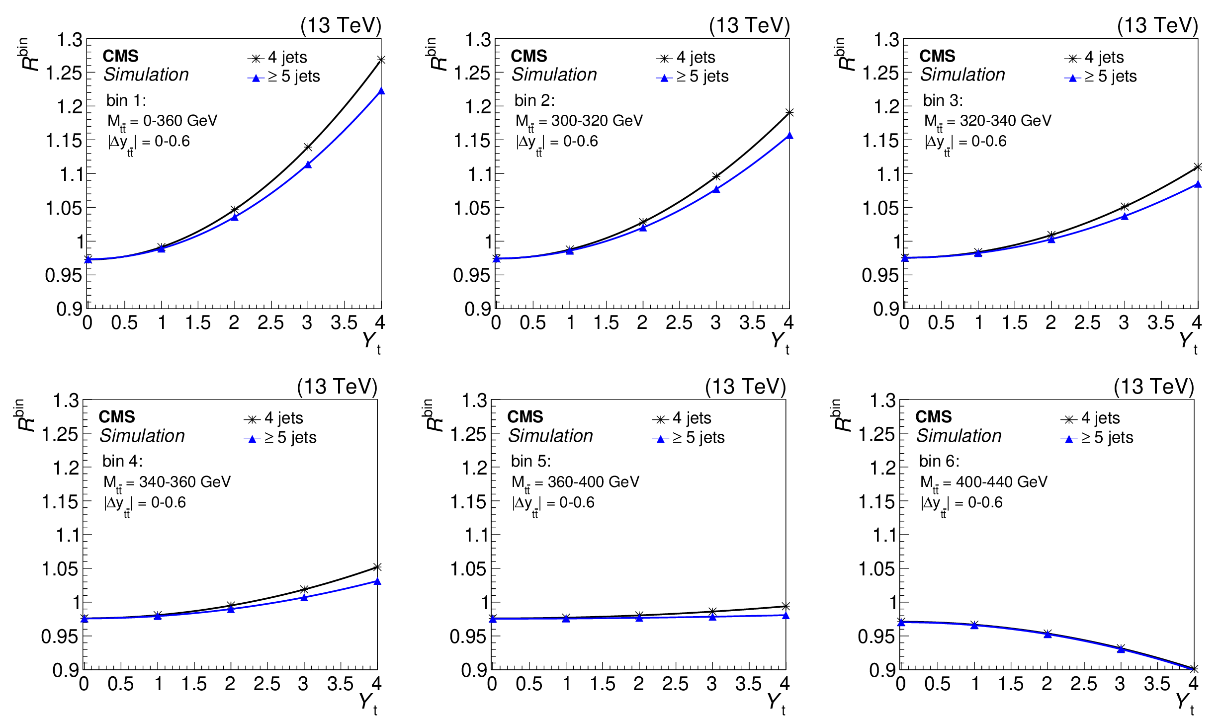
Figure 9:
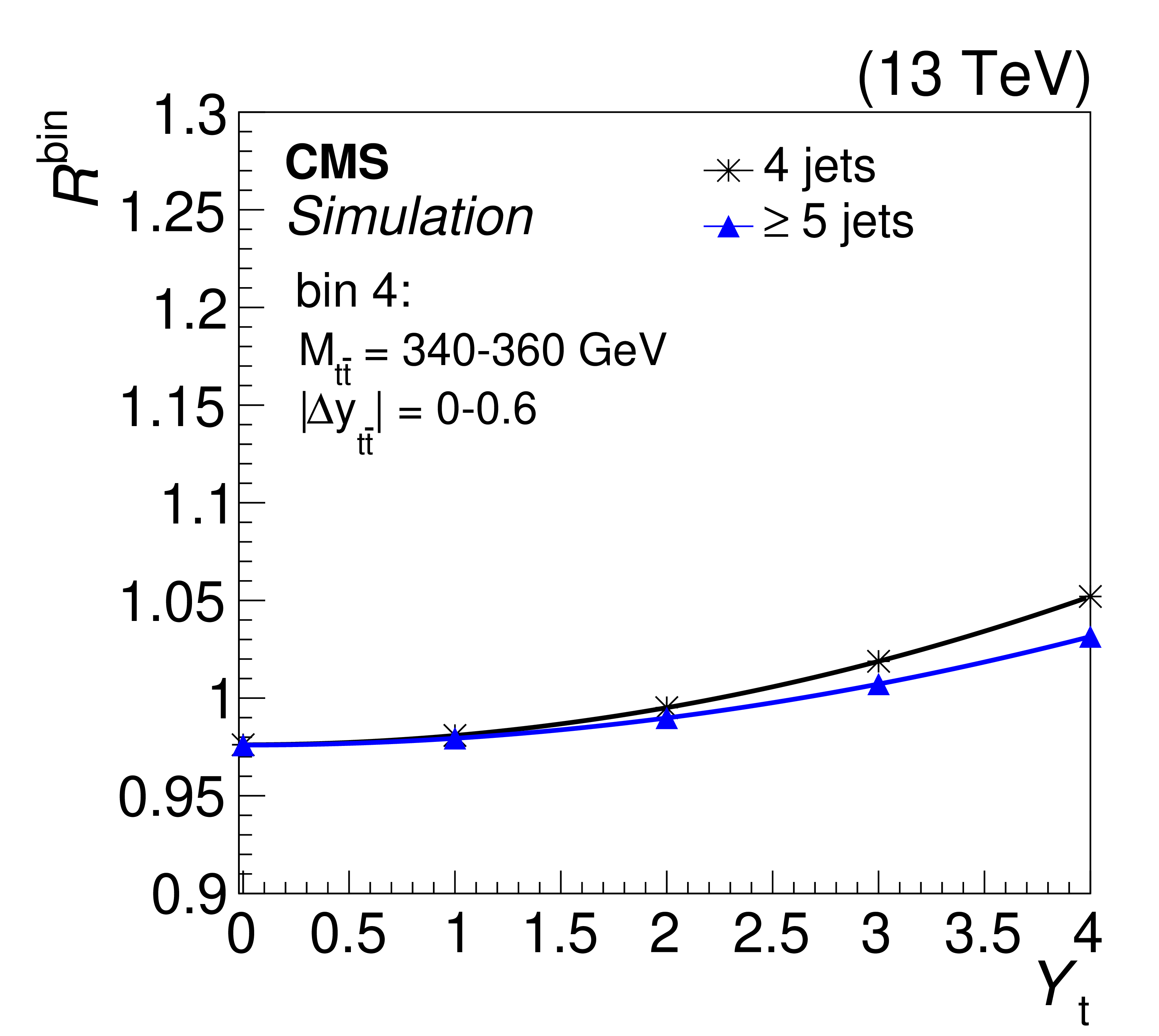
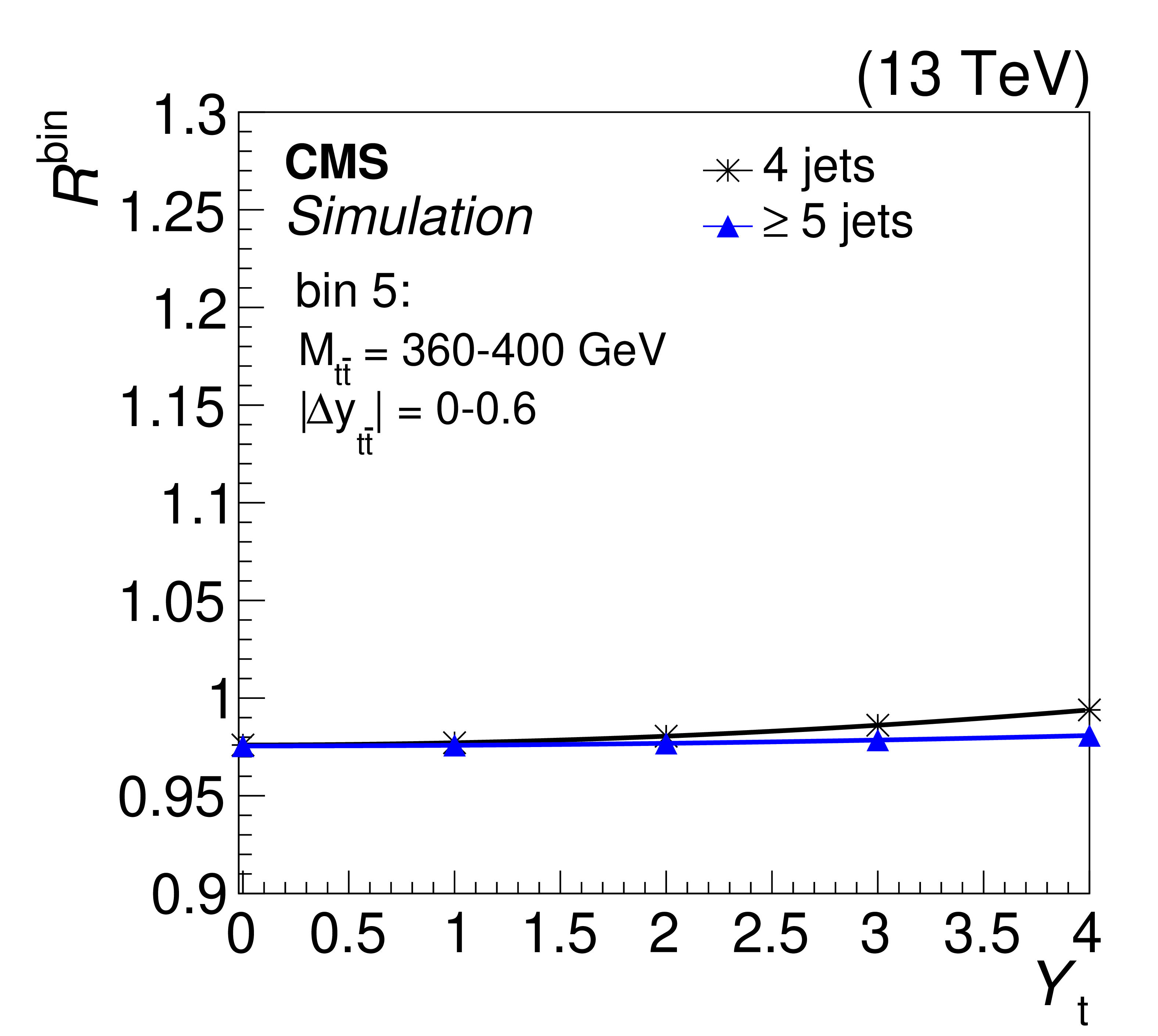
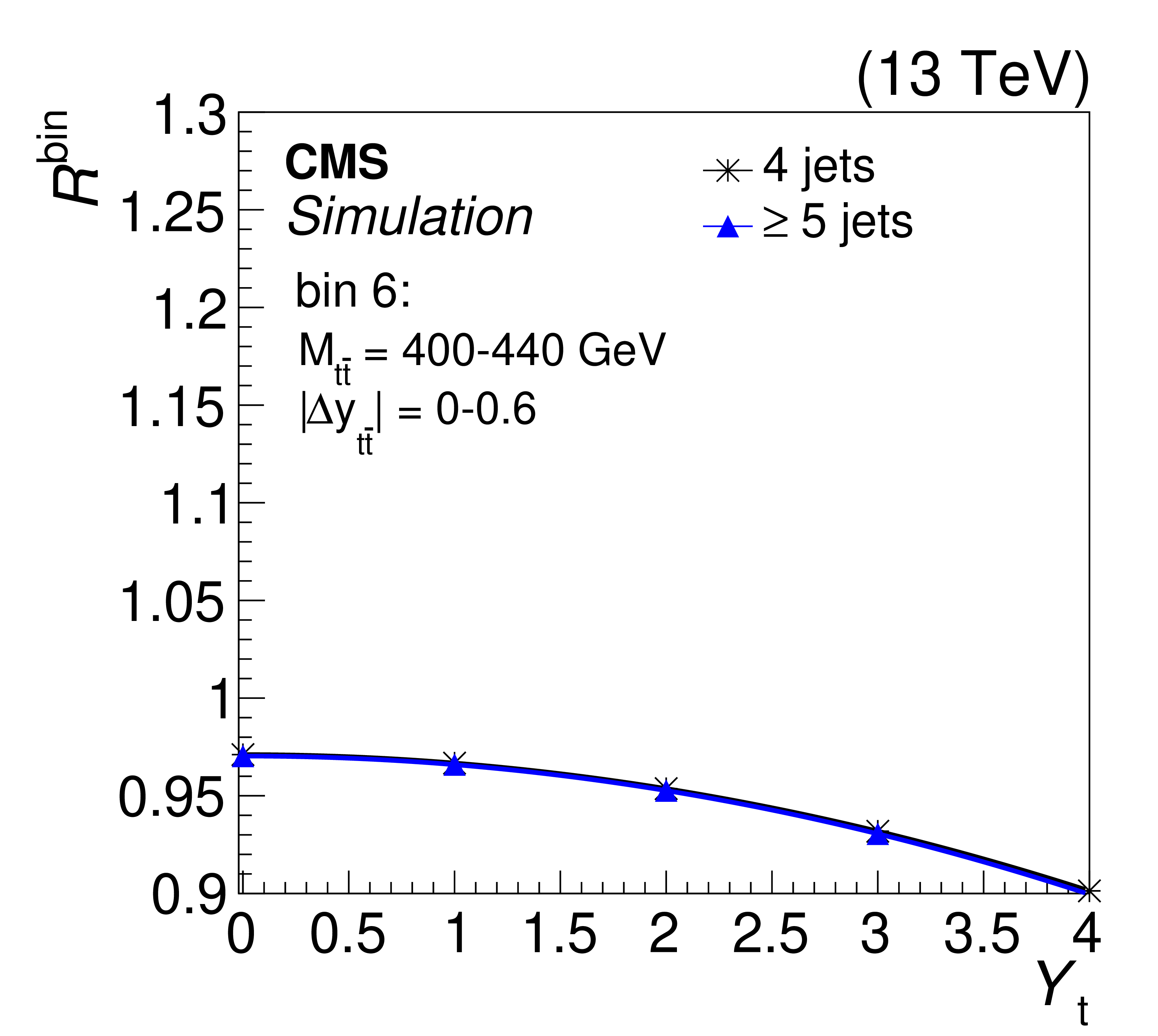
The strength of the weak interaction correction, relative to the predicted POWHEG signal, $R^\mathrm {bin}$, as a function of ${Y_{\mathrm{t}}} $ in the categories with four and five or more jets. The plots correspond to the first six ${M_{{\mathrm{t} {}\mathrm{\bar{t}}}}}$ bins for $ {| {\Delta y_{{\mathrm{t} {}\mathrm{\bar{t}}}}} |} < $ 0.6 (as shown in Fig. 8). A quadratic fit is performed in each bin. |
png pdf |
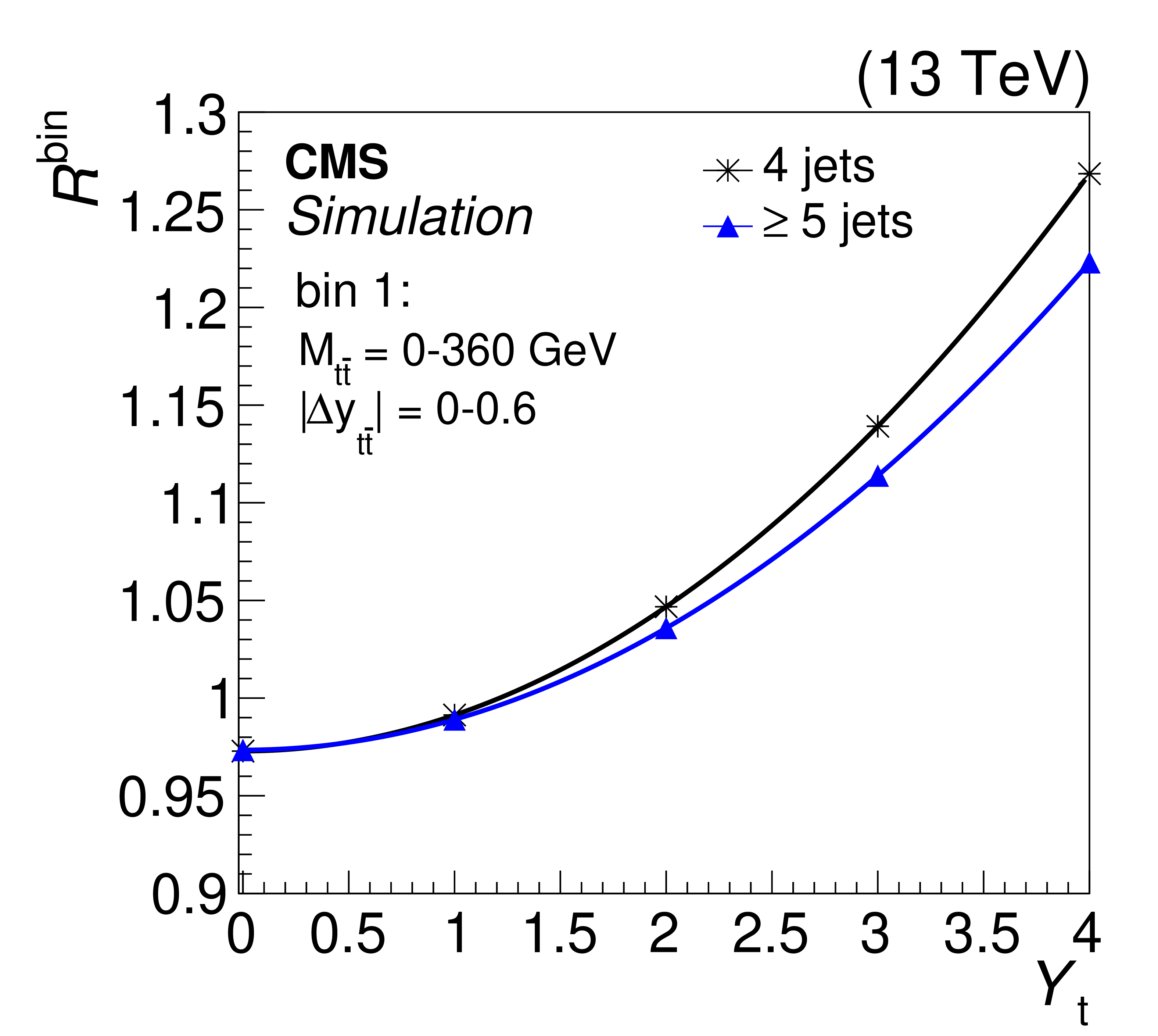
Figure 9-a:
The strength of the weak interaction correction, relative to the predicted POWHEG signal, $R^\mathrm {bin}$, as a function of ${Y_{\mathrm{t}}} $ in the categories with four and five or more jets. The plot corresponds to ${M_{{\mathrm{t} {}\mathrm{\bar{t}}}}}$ bin 1 for $ {| {\Delta y_{{\mathrm{t} {}\mathrm{\bar{t}}}}} |} < $ 0.6 (as shown in Fig. 8). A quadratic fit is performed in the bin. |
png pdf |
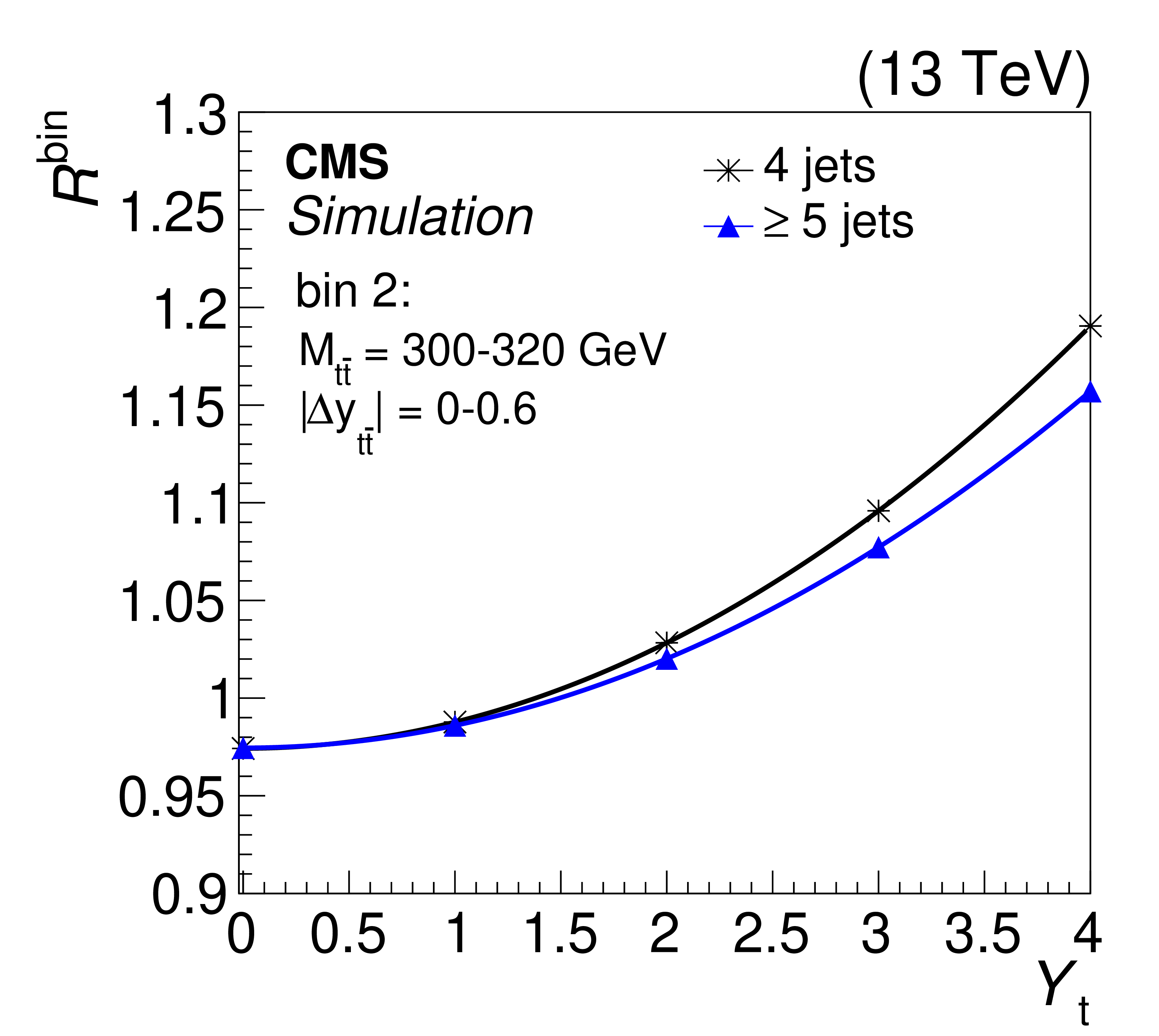
Figure 9-b:
The strength of the weak interaction correction, relative to the predicted POWHEG signal, $R^\mathrm {bin}$, as a function of ${Y_{\mathrm{t}}} $ in the categories with four and five or more jets. The plot corresponds to ${M_{{\mathrm{t} {}\mathrm{\bar{t}}}}}$ bin 2 for $ {| {\Delta y_{{\mathrm{t} {}\mathrm{\bar{t}}}}} |} < $ 0.6 (as shown in Fig. 8). A quadratic fit is performed in the bin. |

png pdf |
Figure 9-c:
The strength of the weak interaction correction, relative to the predicted POWHEG signal, $R^\mathrm {bin}$, as a function of ${Y_{\mathrm{t}}} $ in the categories with four and five or more jets. The plot corresponds to ${M_{{\mathrm{t} {}\mathrm{\bar{t}}}}}$ bin 3 for $ {| {\Delta y_{{\mathrm{t} {}\mathrm{\bar{t}}}}} |} < $ 0.6 (as shown in Fig. 8). A quadratic fit is performed in the bin. |
png pdf |
Figure 9-d:
The strength of the weak interaction correction, relative to the predicted POWHEG signal, $R^\mathrm {bin}$, as a function of ${Y_{\mathrm{t}}} $ in the categories with four and five or more jets. The plot corresponds to ${M_{{\mathrm{t} {}\mathrm{\bar{t}}}}}$ bin 4 for $ {| {\Delta y_{{\mathrm{t} {}\mathrm{\bar{t}}}}} |} < $ 0.6 (as shown in Fig. 8). A quadratic fit is performed in the bin. |
png pdf |
Figure 9-e:
The strength of the weak interaction correction, relative to the predicted POWHEG signal, $R^\mathrm {bin}$, as a function of ${Y_{\mathrm{t}}} $ in the categories with four and five or more jets. The plot corresponds to ${M_{{\mathrm{t} {}\mathrm{\bar{t}}}}}$ bin 5 for $ {| {\Delta y_{{\mathrm{t} {}\mathrm{\bar{t}}}}} |} < $ 0.6 (as shown in Fig. 8). A quadratic fit is performed in the bin. |
png pdf |
Figure 9-f:
The strength of the weak interaction correction, relative to the predicted POWHEG signal, $R^\mathrm {bin}$, as a function of ${Y_{\mathrm{t}}} $ in the categories with four and five or more jets. The plot corresponds to ${M_{{\mathrm{t} {}\mathrm{\bar{t}}}}}$ bin 6 for $ {| {\Delta y_{{\mathrm{t} {}\mathrm{\bar{t}}}}} |} < $ 0.6 (as shown in Fig. 8). A quadratic fit is performed in the bin. |

png pdf |
Figure 10:
The $ {M_{{\mathrm{t} {}\mathrm{\bar{t}}}}} $ distribution in $ {| {\Delta y_{{\mathrm{t} {}\mathrm{\bar{t}}}}} |}$ bins for all events combined, after the simultaneous likelihood fit in all jet channels. The hatched bands show the total post-fit uncertainty. The ratios of data to the sum of the predicted yields are provided in the lower panel. To show the sensitivity of the data to ${Y_{\mathrm{t}}} = $ 1 and ${Y_{\mathrm{t}}} = $ 2, the pre-fit yields are shown in the upper panel, and the yield ratio $R^{\mathrm {bin}}({Y_{\mathrm{t}}} =2)/R^{\mathrm {bin}}({Y_{\mathrm{t}}} =1)$ in the lower panel. |
png pdf |
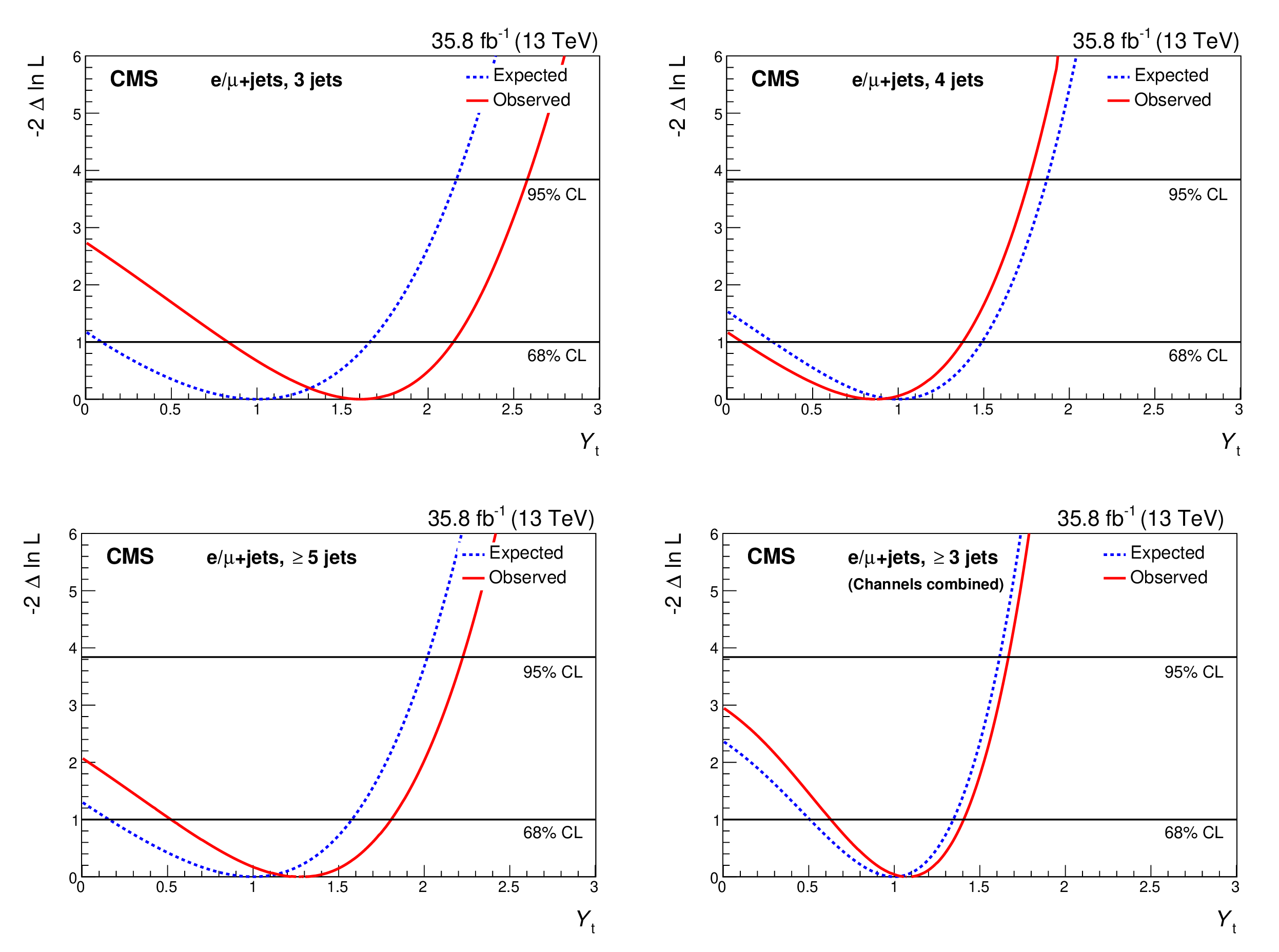
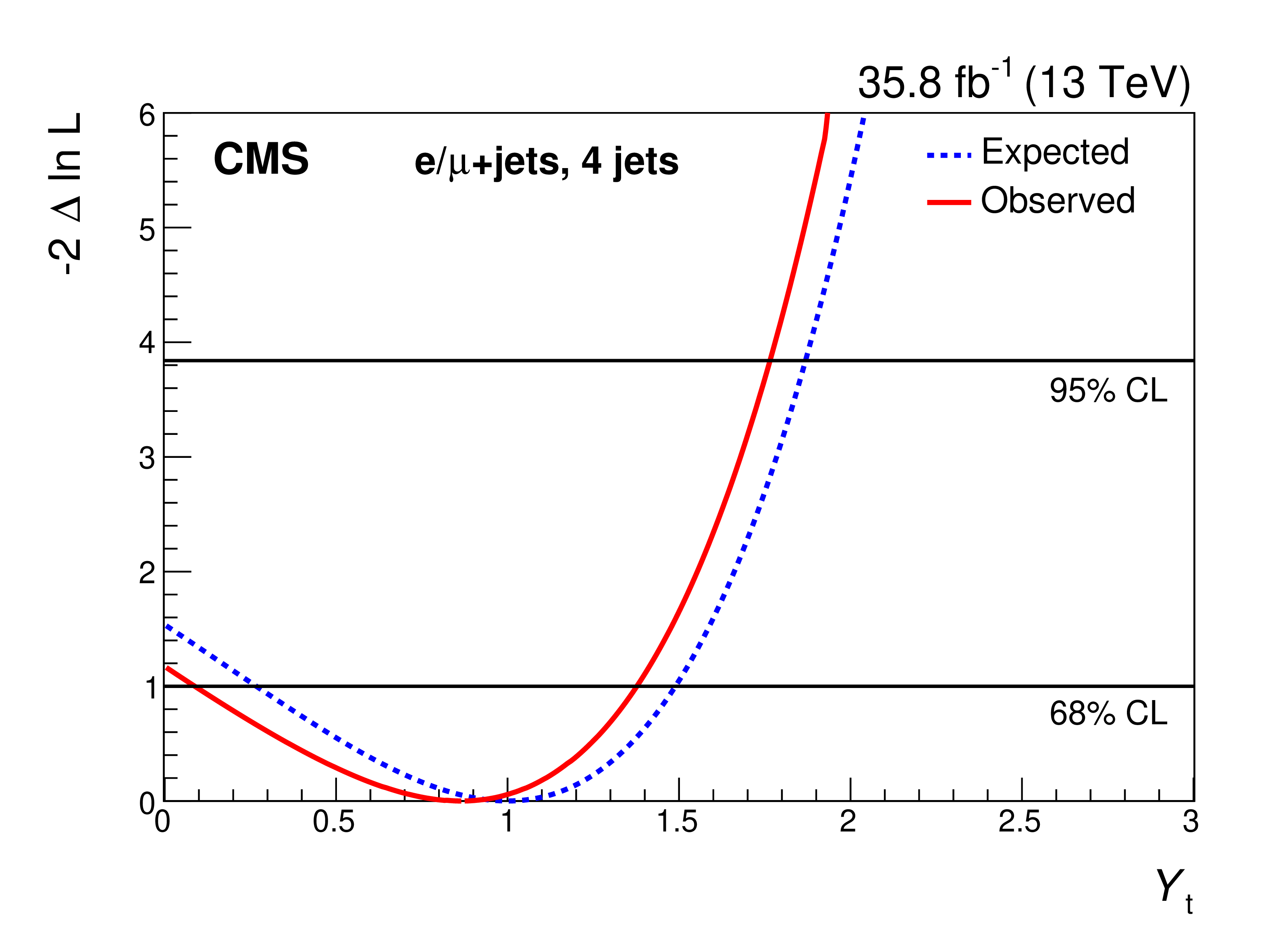
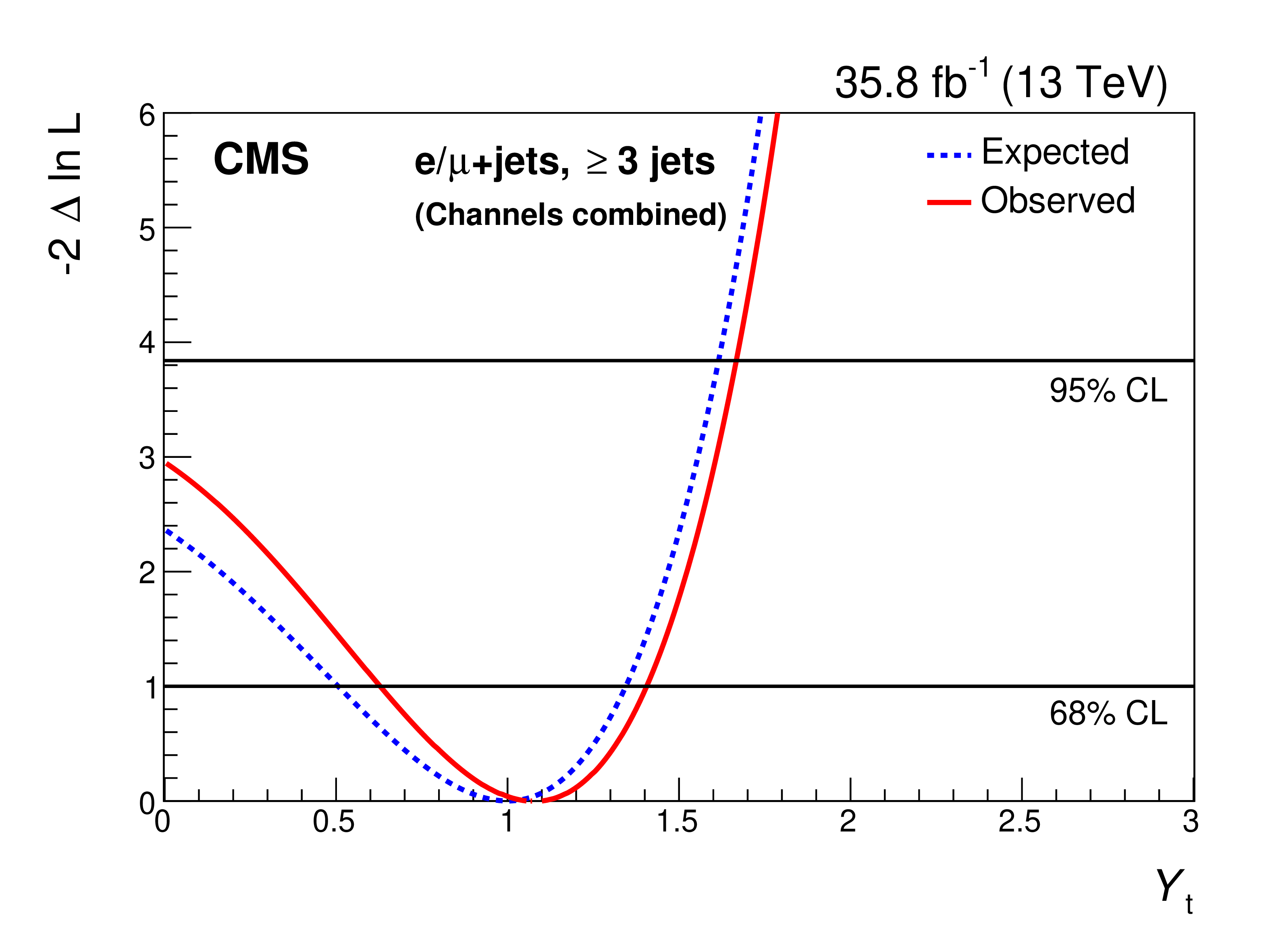
Figure 11:
The test statistic scan versus ${Y_{\mathrm{t}}} $ for each channel (three, four, and five or more jets), and all channels combined. The test statistic minimum indicates the best fit of ${Y_{\mathrm{t}}} $. The horizontal lines indicate 68 and 95% CL intervals. |

png pdf |
Figure 11-a:
The test statistic scan versus ${Y_{\mathrm{t}}} $ for the channel with three jets. The test statistic minimum indicates the best fit of ${Y_{\mathrm{t}}} $. The horizontal lines indicate 68 and 95% CL intervals. |
png pdf |
Figure 11-b:
The test statistic scan versus ${Y_{\mathrm{t}}} $ for the channel with four jets. The test statistic minimum indicates the best fit of ${Y_{\mathrm{t}}} $. The horizontal lines indicate 68 and 95% CL intervals. |

png pdf |
Figure 11-c:
The test statistic scan versus ${Y_{\mathrm{t}}} $ for the channel with five or more jets. The test statistic minimum indicates the best fit of ${Y_{\mathrm{t}}} $. The horizontal lines indicate 68 and 95% CL intervals. |
png pdf |
Figure 11-d:
The test statistic scan versus ${Y_{\mathrm{t}}} $ for all channels combined. The test statistic minimum indicates the best fit of ${Y_{\mathrm{t}}} $. The horizontal lines indicate 68 and 95% CL intervals. |
| Tables | |
png pdf |
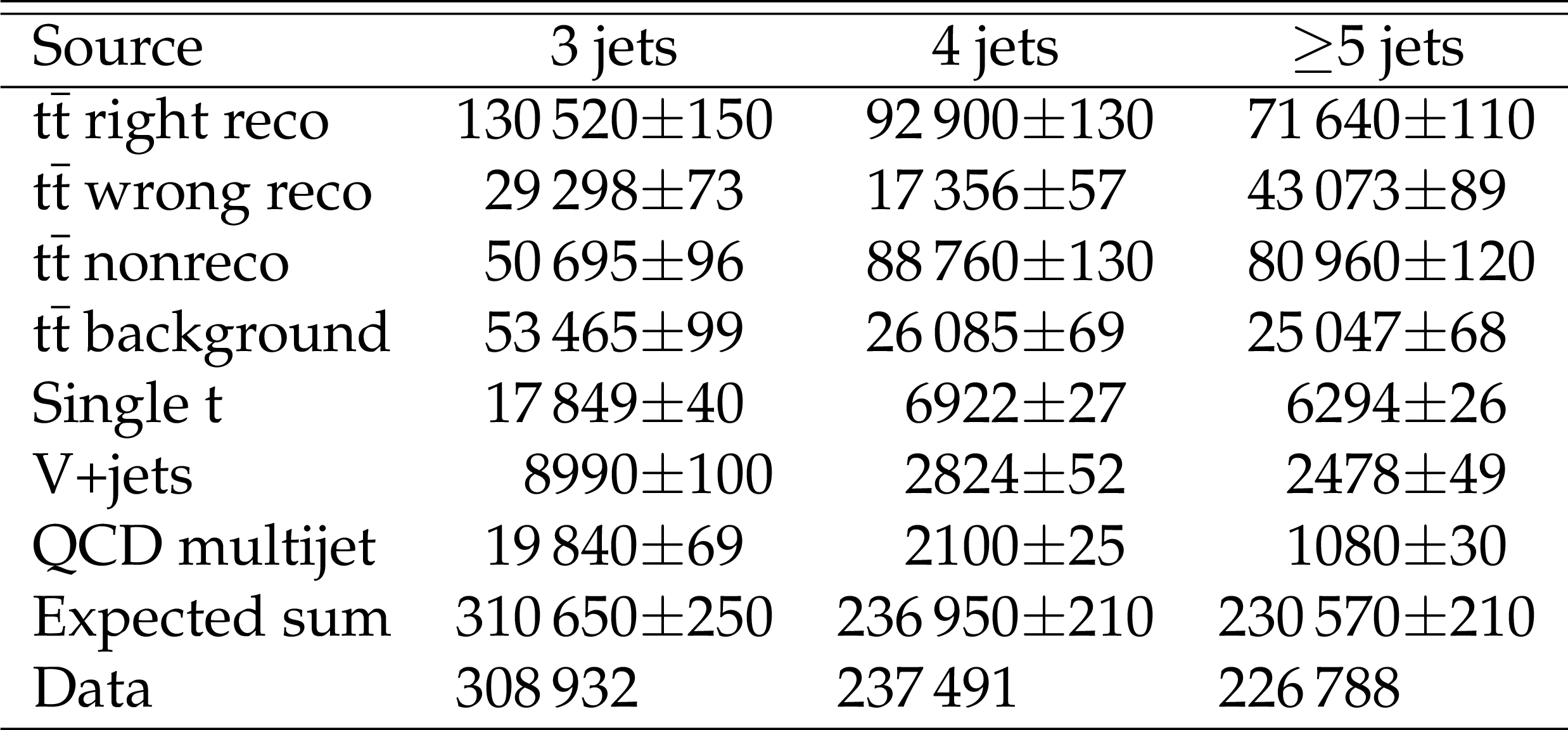
Table 1:
Expected and observed yields after event selection and ${\mathrm{t} {}\mathrm{\bar{t}}}$ reconstruction, with statistical uncertainties in the expected yields. The QCD multijet yield is derived from Eq. (3) and its uncertainty is the statistical uncertainty in the control region from the data-based QCD multijet determination described in Section 7. |
png pdf |
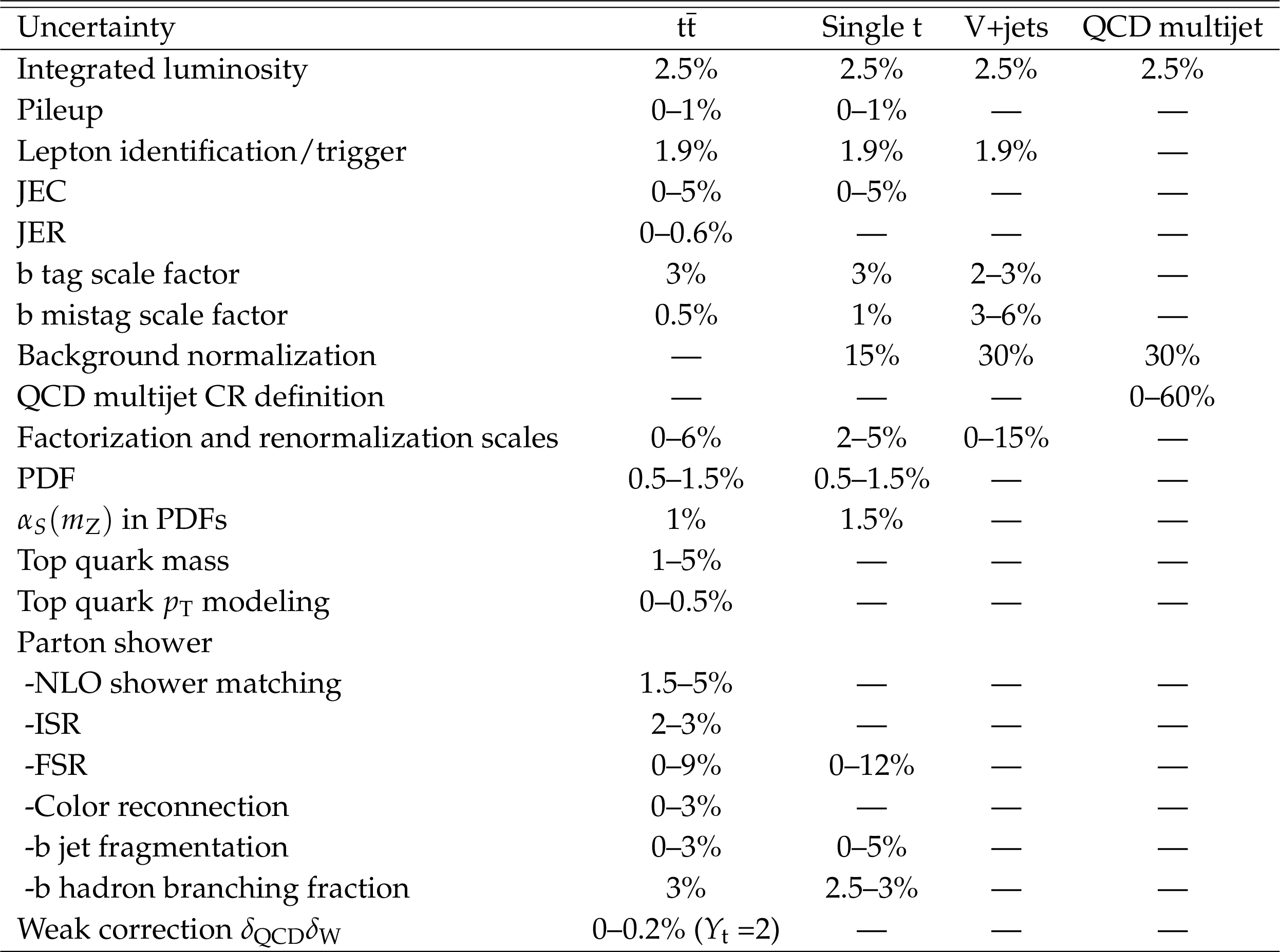
Table 2:
Summary of the sources of systematic uncertainty, their effects and magnitudes on signal and backgrounds. If the uncertainty shows a shape dependence in the ${M_{{\mathrm{t} {}\mathrm{\bar{t}}}}}$ and ${\Delta y_{{\mathrm{t} {}\mathrm{\bar{t}}}}}$ distributions, it is treated as such in the likelihood. Only the luminosity, background normalization, and ISR uncertainties are not considered as shape uncertainties. |
png pdf |
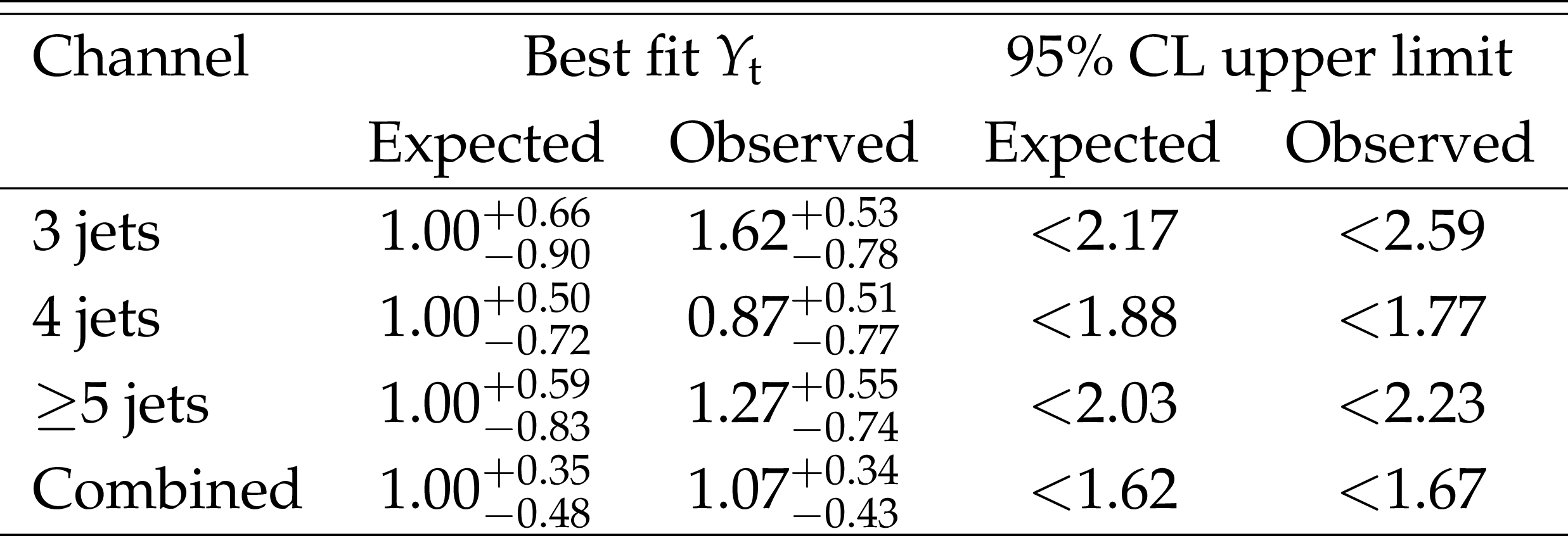
Table 3:
The expected and observed best fit values and 95% CL upper limits on ${Y_{\mathrm{t}}} $. |
| Summary |
|
A measurement of the top quark Yukawa coupling is presented, extracted by investigating $\mathrm{t\bar{t}}$ pair production in final states with an electron or muon and several jets, using proton-proton data collected by the CMS experiment at $\sqrt{s} = $ 13 TeV, corresponding to an integrated luminosity of 35.8 fb$^{-1}$. The $\mathrm{t\bar{t}}$ production cross section is sensitive to the top quark Yukawa coupling through weak force corrections that can modify the distributions of the mass of top quark-antiquark pairs, ${M_{\mathrm{t\bar{t}}}} $, and the rapidity difference between top quark and antiquark, $\delta Y$. The kinematic properties of these final states are reconstructed in events with at least three jets, two of which are identified as originating from bottom quarks. The inclusion of events with only three reconstructed jets using a dedicated algorithm improves the sensitivity of the analysis by increasing the signal from events in the low-${M_{\mathrm{t\bar{t}}}}$ region, which is most sensitive to the Yukawa coupling. The ratio of the top quark Yukawa coupling to its expected SM value, ${Y_{\mathrm{t}}} $, is extracted by comparing the data with the expected $\mathrm{t\bar{t}}$ signal for different values of ${Y_{\mathrm{t}}} $ in a total of 55 bins in ${M_{\mathrm{t\bar{t}}}} $, $|{\delta Y}|$, and the number of reconstructed jets. The measured value of ${Y_{\mathrm{t}}} $ is 1.07$^{+0.34}_{-0.43}$, compared to an expected value of 1.00$^{+0.35}_{-0.48}$. The observed upper limit on ${Y_{\mathrm{t}}} $ is 1.67 at 95% confidence level (CL), with an expected value of 1.62. Although the method presented in this paper is not as sensitive as the combined CMS measurement of ${Y_{\mathrm{t}}} $ performed using Higgs boson production and decays in multiple channels [61], it has the advantage that it does not depend on any assumptions about the couplings of the Higgs boson to particles other than the top quark. The result presented here is more sensitive than the only other result from CMS exclusively dependent on ${Y_{\mathrm{t}}} $, namely the limit on the ${\mathrm{t\bar{t}}}{\mathrm{t\bar{t}}}$ cross section, which constrains ${Y_{\mathrm{t}}} $ to be less than 2.1 at 95% CL [8]. |
| References | ||||
| 1 | S. Weinberg | A model of leptons | PRL 19 (1967) 1264 | |
| 2 | MuLan Collaboration | Measurement of the positive muon lifetime and determination of the Fermi constant to part-per-million precision | PRL 106 (2011) 041803 | 1010.0991 |
| 3 | CMS Collaboration | Measurement of the top quark mass using proton-proton data at $ \sqrt{s} = $ 7 and 8 TeV | PRD 93 (2016) 072004 | CMS-TOP-14-022 1509.04044 |
| 4 | LHC Higgs Cross Section Working Group Collaboration | Handbook of LHC Higgs cross sections: 3. Higgs properties | 1307.1347 | |
| 5 | CMS Collaboration | Measurements of properties of the Higgs boson decaying into the four-lepton final state in pp collisions at $ \sqrt{s}= $ 13 TeV | JHEP 11 (2017) 047 | CMS-HIG-16-041 1706.09936 |
| 6 | CMS Collaboration | Measurements of Higgs boson properties in the diphoton decay channel in proton-proton collisions at $ \sqrt{s} = $ 13 TeV | JHEP 11 (2018) 185 | CMS-HIG-16-040 1804.02716 |
| 7 | CMS Collaboration | Observation of $ \mathrm{t\overline{t}} $H production | PRL 120 (2018) 231801 | CMS-HIG-17-035 1804.02610 |
| 8 | CMS Collaboration | Search for standard model production of four top quarks with same-sign and multilepton final states in proton-proton collisions at $ \sqrt{s} = $ 13 TeV | EPJC 78 (2018) 140 | CMS-TOP-17-009 1710.10614 |
| 9 | J. H. Kuhn, A. Scharf, and P. Uwer | Weak interactions in top-quark pair production at hadron colliders: an update | PRD 91 (2015) 014020 | 1305.5773 |
| 10 | CMS Collaboration | Measurement of differential cross sections for top quark pair production using the lepton+jets final state in proton-proton collisions at 13 TeV | PRD 95 (2017) 092001 | CMS-TOP-16-008 1610.04191 |
| 11 | M. J. Strassler and M. E. Peskin | The heavy top quark threshold: QCD and the Higgs | PRD 43 (1991) 1500 | |
| 12 | M. Beneke, A. Maier, J. Piclum, and T. Rauh | Higgs effects in top anti-top production near threshold in e$ ^+ $e$ ^- $ annihilation | NPB 899 (2015) 180 | 1506.06865 |
| 13 | M. Aliev et al. | Hathor: HAdronic Top and Heavy quarks crOss section calculatoR | CPC 182 (2011) 1034 | 1007.1327 |
| 14 | CMS Collaboration | Measurement of differential cross sections for the production of top quark pairs and of additional jets in lepton+jets events from pp collisions at $ \sqrt{s} = $ 13 TeV | PRD 97 (2018) 112003 | CMS-TOP-17-002 1803.08856 |
| 15 | M. Czakon et al. | Top-pair production at the LHC through NNLO QCD and NLO EW | JHEP 10 (2017) 186 | 1705.04105 |
| 16 | M. L. Czakon et al. | Top quark pair production at NNLO+NNLL$ ' $ in QCD combined with electroweak corrections | in 11th International Workshop on Top Quark Physics (TOP2018) Bad Neuenahr, Germany 2019 | 1901.08281 |
| 17 | W. Hollik and M. Kollar | NLO QED contributions to top-pair production at hadron collider | PRD 77 (2008) 014008 | 0708.1697 |
| 18 | W. Beenakker et al. | Electroweak one loop contributions to top pair production in hadron colliders | NPB 411 (1994) 343 | |
| 19 | P. Nason | A new method for combining NLO QCD with shower Monte Carlo algorithms | JHEP 11 (2004) 040 | hep-ph/0409146 |
| 20 | S. Frixione, P. Nason, and C. Oleari | Matching NLO QCD computations with parton shower simulations: the POWHEG method | JHEP 11 (2007) 070 | 0709.2092 |
| 21 | S. Alioli, P. Nason, C. Oleari, and E. Re | A general framework for implementing NLO calculations in shower Monte Carlo programs: the POWHEG BOX | JHEP 06 (2010) 043 | 1002.2581 |
| 22 | J. M. Campbell, R. K. Ellis, P. Nason, and E. Re | Top-pair production and decay at NLO matched with parton showers | JHEP 04 (2015) 114 | 1412.1828 |
| 23 | CMS Collaboration | The CMS experiment at the CERN LHC | JINST 3 (2008) S08004 | CMS-00-001 |
| 24 | CMS Collaboration | Particle-flow reconstruction and global event description with the CMS detector | JINST 12 (2017) P10003 | CMS-PRF-14-001 1706.04965 |
| 25 | CMS Collaboration | The CMS trigger system | JINST 12 (2017) P01020 | CMS-TRG-12-001 1609.02366 |
| 26 | T. Sjostrand et al. | An introduction to PYTHIA 8.2 | CPC 191 (2015) 159 | 1410.3012 |
| 27 | P. Skands, S. Carrazza, and J. Rojo | Tuning PYTHIA 8.1: the Monash 2013 tune | EPJC 74 (2014) 3024 | 1404.5630 |
| 28 | NNPDF Collaboration | Parton distributions for the LHC Run II | JHEP 04 (2015) 040 | 1410.8849 |
| 29 | M. Czakon and A. Mitov | Top++: A program for the calculation of the top-pair cross-section at hadron colliders | CPC 185 (2014) 2930 | 1112.5675 |
| 30 | J. Alwall et al. | The automated computation of tree-level and next-to-leading order differential cross sections, and their matching to parton shower simulations | JHEP 07 (2014) 079 | 1405.0301 |
| 31 | Y. Li and F. Petriello | Combining QCD and electroweak corrections to dilepton production in FEWZ | PRD 86 (2012) 094034 | 1208.5967 |
| 32 | P. Kant et al. | Hathor for single top-quark production: Updated predictions and uncertainty estimates for single top-quark production in hadronic collisions | CPC 191 (2015) 74 | 1406.4403 |
| 33 | N. Kidonakis | NNLL threshold resummation for top-pair and single-top production | Phys. Part. Nucl. 45 (2014) 714 | 1210.7813 |
| 34 | GEANT4 Collaboration | GEANT4--a simulation toolkit | NIMA 506 (2003) 250 | |
| 35 | M. Cacciari, G. P. Salam, and G. Soyez | The anti-$ {k_{\mathrm{T}}} $ jet clustering algorithm | JHEP 04 (2008) 063 | 0802.1189 |
| 36 | M. Cacciari, G. P. Salam, and G. Soyez | FastJet user manual | EPJC 72 (2012) 1896 | 1111.6097 |
| 37 | CMS Collaboration | Determination of jet energy calibration and transverse momentum resolution in CMS | JINST 6 (2011) P11002 | CMS-JME-10-011 1107.4277 |
| 38 | CMS Collaboration | Jet energy scale and resolution in the CMS experiment in pp collisions at 8 TeV | JINST 12 (2017) P02014 | CMS-JME-13-004 1607.03663 |
| 39 | CMS Collaboration | Jet performance in pp collisions at $ \sqrt{s} = $ 7 TeV | CMS-PAS-JME-10-003 | |
| 40 | CMS Collaboration | Identification of heavy-flavour jets with the CMS detector in pp collisions at 13 TeV | JINST 13 (2018) P05011 | CMS-BTV-16-002 1712.07158 |
| 41 | CMS Collaboration | Measurement of inclusive W and Z boson production cross sections in pp collisions at $ \sqrt{s} = $ 8 TeV | PRL 112 (2014) 191802 | CMS-SMP-12-011 1402.0923 |
| 42 | CMS Collaboration | Performance of CMS muon reconstruction in pp collision events at $ \sqrt{s} = $ 7 TeV | JINST 7 (2012) P10002 | CMS-MUO-10-004 1206.4071 |
| 43 | CMS Collaboration | Performance of electron reconstruction and selection with the CMS detector in proton-proton collisions at $ \sqrt{s} = $ 8 TeV | JINST 10 (2015) P06005 | CMS-EGM-13-001 1502.02701 |
| 44 | B. A. Betchart, R. Demina, and A. Harel | Analytic solutions for neutrino momenta in decay of top quarks | NIMA 736 (2014) 169 | 1305.1878 |
| 45 | R. Demina, A. Harel, and D. Orbaker | Reconstructing $ t\bar{t} $ events with one lost jet | NIMA 788 (2015) 128 | 1310.3263 |
| 46 | The ATLAS Collaboration, The CMS Collaboration, The LHC Higgs Combination Group | Procedure for the LHC Higgs boson search combination in Summer 2011 | CMS-NOTE-2011-005 | |
| 47 | CMS Collaboration | CMS luminosity measurement for the 2016 data taking period | CMS-PAS-LUM-17-001 | CMS-PAS-LUM-17-001 |
| 48 | CMS Collaboration | Measurement of the inelastic proton-proton cross section at $ \sqrt{s}= $ 13 TeV | JHEP 07 (2018) 161 | CMS-FSQ-15-005 1802.02613 |
| 49 | CMS Collaboration | Performance of the CMS muon detector and muon reconstruction with proton-proton collisions at $ \sqrt{s}= $ 13 TeV | JINST 13 (2018) P06015 | CMS-MUO-16-001 1804.04528 |
| 50 | CMS Collaboration | Measurement of the single top quark and antiquark production cross sections in the $ t $ channel and their ratio in proton-proton collisions at $ \sqrt{s}= $ 13 TeV | CMS-TOP-17-011 1812.10514 |
|
| 51 | CMS Collaboration | Evidence for the associated production of a single top quark and a photon in proton-proton collisions at $ \sqrt{s}= $ 13 TeV | PRL 121 (2018) 221802 | CMS-TOP-17-016 1808.02913 |
| 52 | CMS Collaboration | Measurement of the production cross section of a W boson in association with two b jets in pp collisions at $ \sqrt{s} = $ 8 TeV | EPJC 77 (2017) 92 | CMS-SMP-14-020 1608.07561 |
| 53 | ATLAS Collaboration | Measurement of the top quark mass in the $ t\bar{t}\rightarrow $ lepton+jets channel from $ \sqrt{s} = $ 8 TeV ATLAS data and combination with previous results | EPJC 79 (2019) 290 | 1810.01772 |
| 54 | M. Czakon, D. Heymes, and A. Mitov | fastNLO tables for NNLO top-quark pair differential distributions | 1704.08551 | |
| 55 | CMS Collaboration | Investigations of the impact of the parton shower tuning in Pythia 8 in the modelling of $ t\bar{t} $ at $ \sqrt{s} = $ 8 and 13 TeV | CMS-PAS-TOP-16-021 | CMS-PAS-TOP-16-021 |
| 56 | Particle Data Group, M. Tanabashi et al. | Review of particle physics | PRD 98 (2018) 030001 | |
| 57 | J. S. Conway | Incorporating nuisance parameters in likelihoods for multisource spectra | in Proceedings, PHYSTAT 2011 Workshop on statistical issues related to discovery claims in search experiments and unfolding, CERN 2011 | 1103.0354 |
| 58 | T. Junk | Confidence level computation for combining searches with small statistics | NIMA 434 (1999) 435 | hep-ex/9902006 |
| 59 | A. L. Read | Presentation of search results: the CL$ _\mathrm{s} $ technique | in Durham IPPP Workshop: Advanced Statistical Techniques in Particle Physics, Durham 2002 | |
| 60 | G. Cowan, K. Cranmer, E. Gross, and O. Vitells | Asymptotic formulae for likelihood-based tests of new physics | EPJC 71 (2011) 1554 | 1007.1727 |
| 61 | CMS Collaboration | Combined measurements of Higgs boson couplings in proton-proton collisions at $ \sqrt{s}= $ 13 TeV | EPJC 79 (2019) 421 | CMS-HIG-17-031 1809.10733 |
|
|
Compact Muon Solenoid LHC, CERN |
|

|

|

|

|

|