

Compact Muon Solenoid
LHC, CERN
| CMS-B2G-20-008 ; CERN-EP-2021-158 | ||
| Search for heavy resonances decaying to Z($ \nu\bar{\nu} $)V($ \mathrm{q}\mathrm{\bar{q}}' $) in proton-proton collisions at $\sqrt{s} = $ 13 TeV | ||
| CMS Collaboration | ||
| 17 September 2021 | ||
| Phys. Rev. D 106 (2022) 012004 | ||
| Abstract: A search is presented for heavy bosons decaying to Z($ \nu\bar{\nu} $)V($ \mathrm{q}\mathrm{\bar{q}}' $), where V can be a W or a Z boson. A sample of proton-proton collision data at $\sqrt{s} = $ 13 TeV was collected by the CMS experiment during 2016-2018. The data correspond to an integrated luminosity of 137 fb$^{-1}$. The event categorization is based on the presence of high-momentum jets in the forward region to identify production through weak vector boson fusion. Additional categorization uses jet substructure techniques and the presence of large missing transverse momentum to identify W and Z bosons decaying to quarks and neutrinos, respectively. The dominant standard model backgrounds are estimated using data taken from control regions. The results are interpreted in terms of radion, W' boson, and graviton models, under the assumption that these bosons are produced via gluon-gluon fusion, Drell-Yan, or weak vector boson fusion processes. No evidence is found for physics beyond the standard model. Upper limits are set at 95% confidence level on various types of hypothetical new bosons. Observed (expected) exclusion limits on the masses of these bosons range from 1.2 to 4.0 (1.1 to 3.7) TeV. | ||
| Links: e-print arXiv:2109.08268 [hep-ex] (PDF) ; CDS record ; inSPIRE record ; HepData record ; CADI line (restricted) ; | ||
| Figures | |
png pdf |
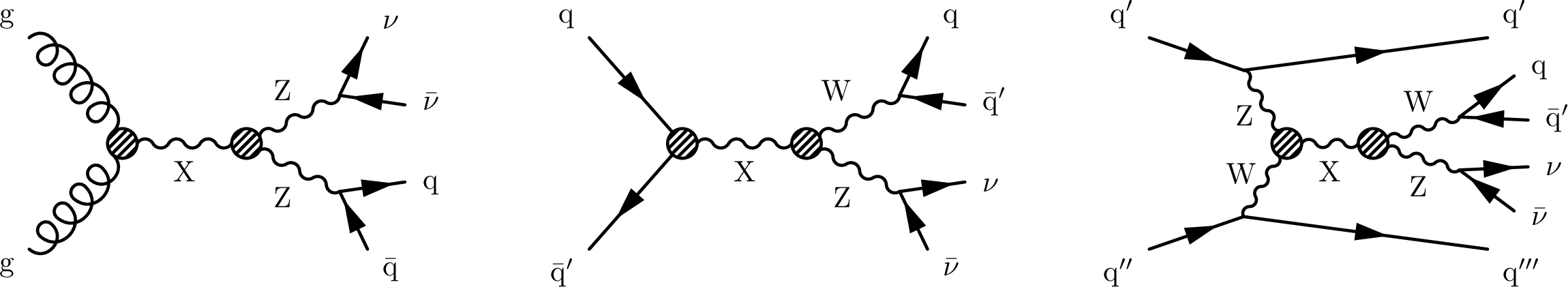
Figure 1:
Representative Feynman diagrams for various production modes of a heavy resonance X. These modes are: a ggF-produced spin-0 or spin-2 resonance decaying to ${{\mathrm{Z Z} \to {\mathrm{q} \mathrm{\bar{q}}} \nu \bar{\nu}}}$ (left), a DY-produced spin-1 resonance decaying to ${\mathrm{W Z} \to {\mathrm{q} \mathrm{\bar{q}}} '\nu \bar{\nu}}$ (center), and a VBF-produced spin-1 resonance decaying to ${\mathrm{W Z} \to {\mathrm{q} \mathrm{\bar{q}}} '\nu \bar{\nu}}$ (right). |

png pdf |
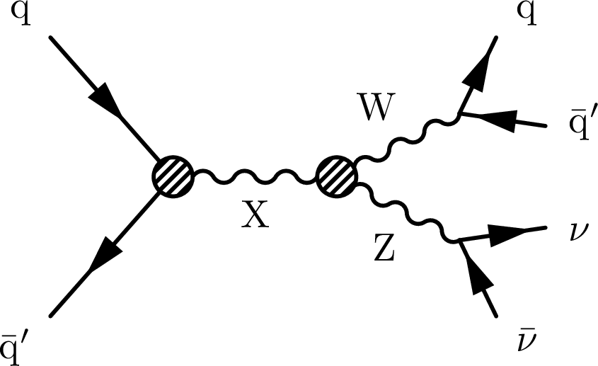
Figure 1-a:
Representative Feynman diagrams for various production modes of a heavy resonance X. These modes are: a ggF-produced spin-0 or spin-2 resonance decaying to ${{\mathrm{Z Z} \to {\mathrm{q} \mathrm{\bar{q}}} \nu \bar{\nu}}}$ (left), a DY-produced spin-1 resonance decaying to ${\mathrm{W Z} \to {\mathrm{q} \mathrm{\bar{q}}} '\nu \bar{\nu}}$ (center), and a VBF-produced spin-1 resonance decaying to ${\mathrm{W Z} \to {\mathrm{q} \mathrm{\bar{q}}} '\nu \bar{\nu}}$ (right). |
png pdf |
Figure 1-b:
Representative Feynman diagrams for various production modes of a heavy resonance X. These modes are: a ggF-produced spin-0 or spin-2 resonance decaying to ${{\mathrm{Z Z} \to {\mathrm{q} \mathrm{\bar{q}}} \nu \bar{\nu}}}$ (left), a DY-produced spin-1 resonance decaying to ${\mathrm{W Z} \to {\mathrm{q} \mathrm{\bar{q}}} '\nu \bar{\nu}}$ (center), and a VBF-produced spin-1 resonance decaying to ${\mathrm{W Z} \to {\mathrm{q} \mathrm{\bar{q}}} '\nu \bar{\nu}}$ (right). |
png pdf |
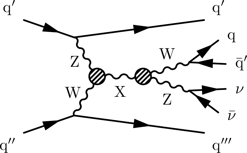
Figure 1-c:
Representative Feynman diagrams for various production modes of a heavy resonance X. These modes are: a ggF-produced spin-0 or spin-2 resonance decaying to ${{\mathrm{Z Z} \to {\mathrm{q} \mathrm{\bar{q}}} \nu \bar{\nu}}}$ (left), a DY-produced spin-1 resonance decaying to ${\mathrm{W Z} \to {\mathrm{q} \mathrm{\bar{q}}} '\nu \bar{\nu}}$ (center), and a VBF-produced spin-1 resonance decaying to ${\mathrm{W Z} \to {\mathrm{q} \mathrm{\bar{q}}} '\nu \bar{\nu}}$ (right). |
png pdf |
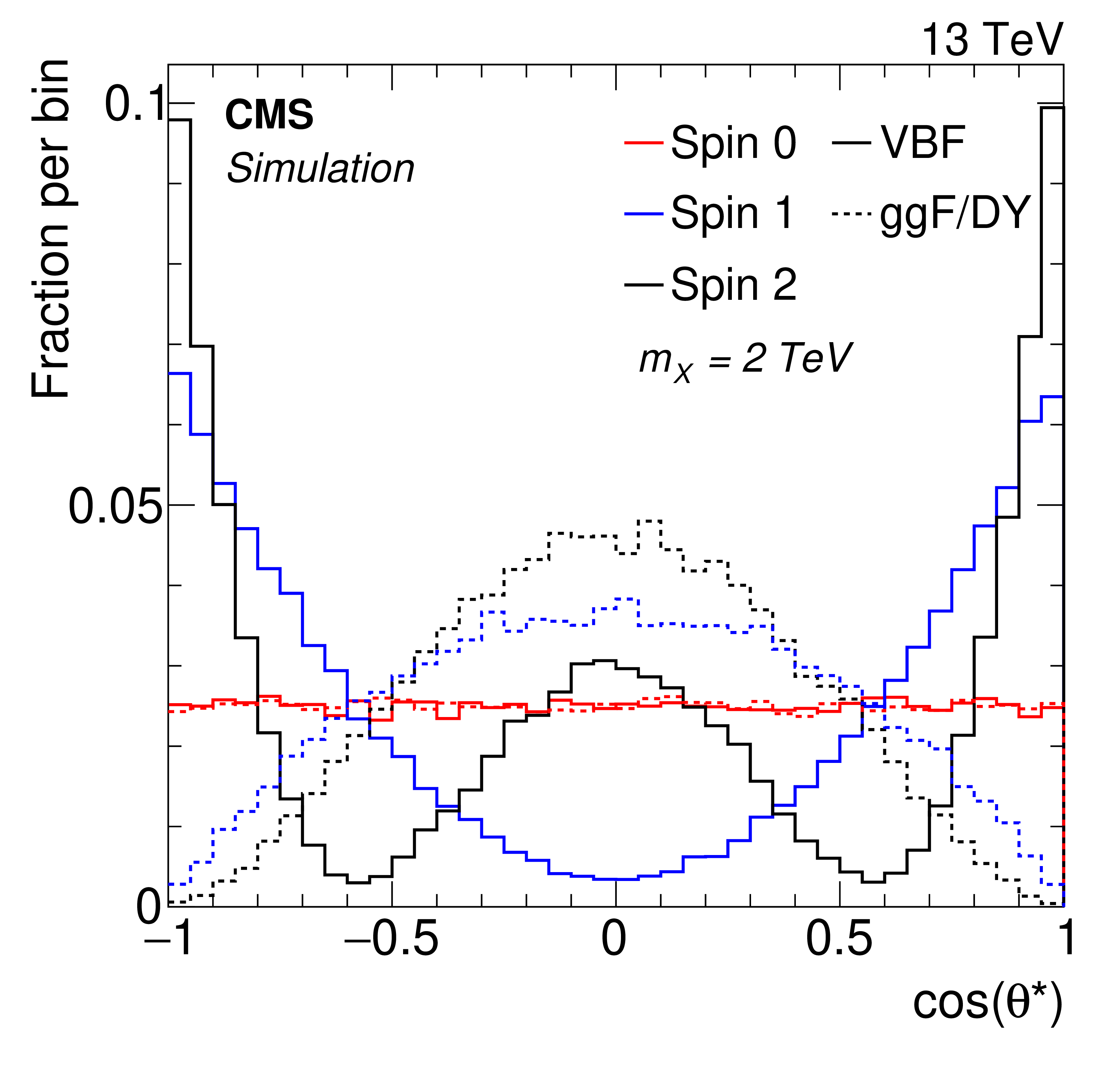
Figure 2:
Simulated distributions are shown for the cosine of the decay angle of SM vector bosons in the rest frame of a parent particle with a mass ($m_\mathrm{X} $) of 2 TeV. Solid lines represent VBF scenarios. Dashed lines represent ggF/DY scenarios. |
png pdf |
Figure 3:
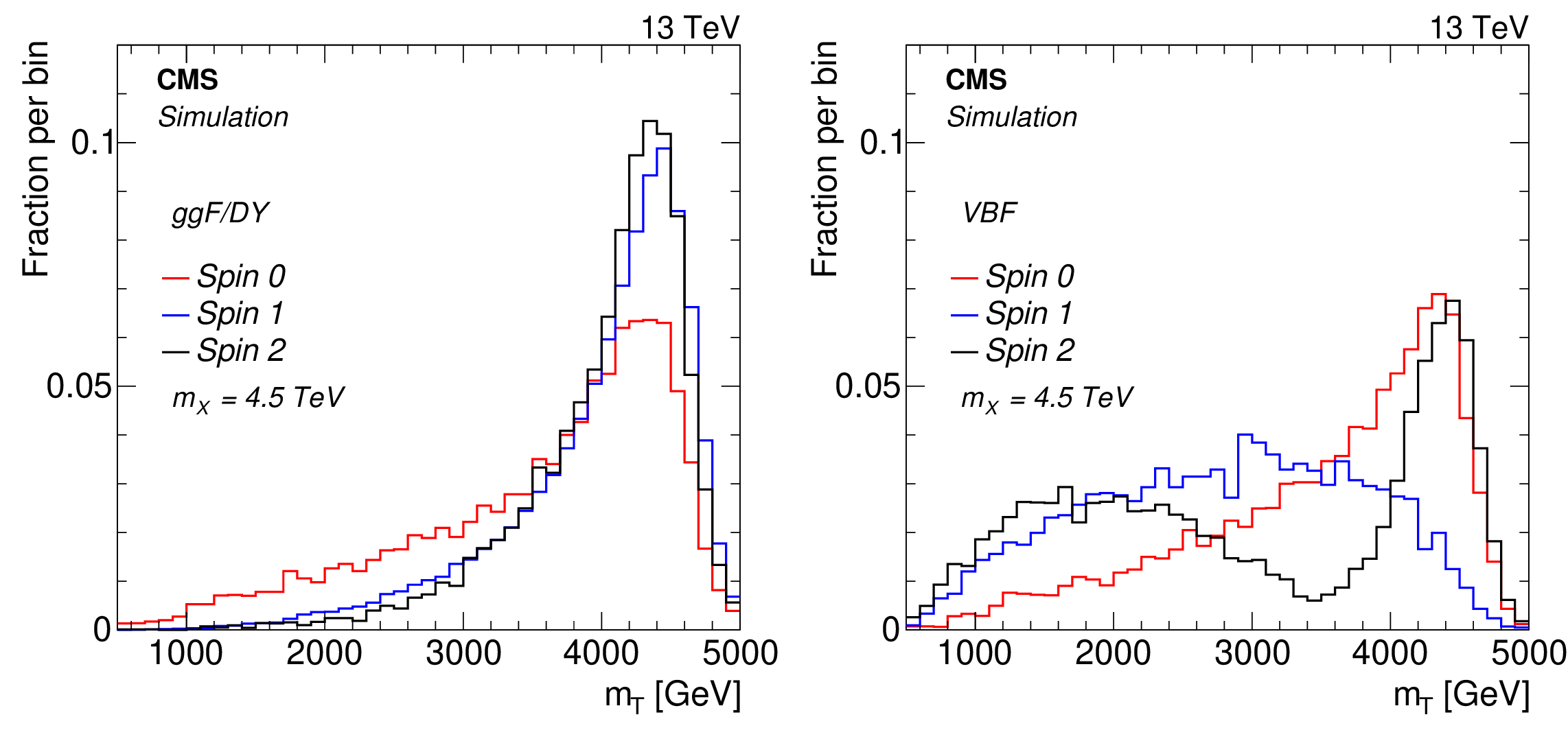
Distributions of ${m_{\mathrm {T}}}$ for ggF/DY- (left) and VBF-produced (right) resonances X of mass 4.5 TeV. Events used are from all SR and CR combined. |
png pdf |
Figure 3-a:
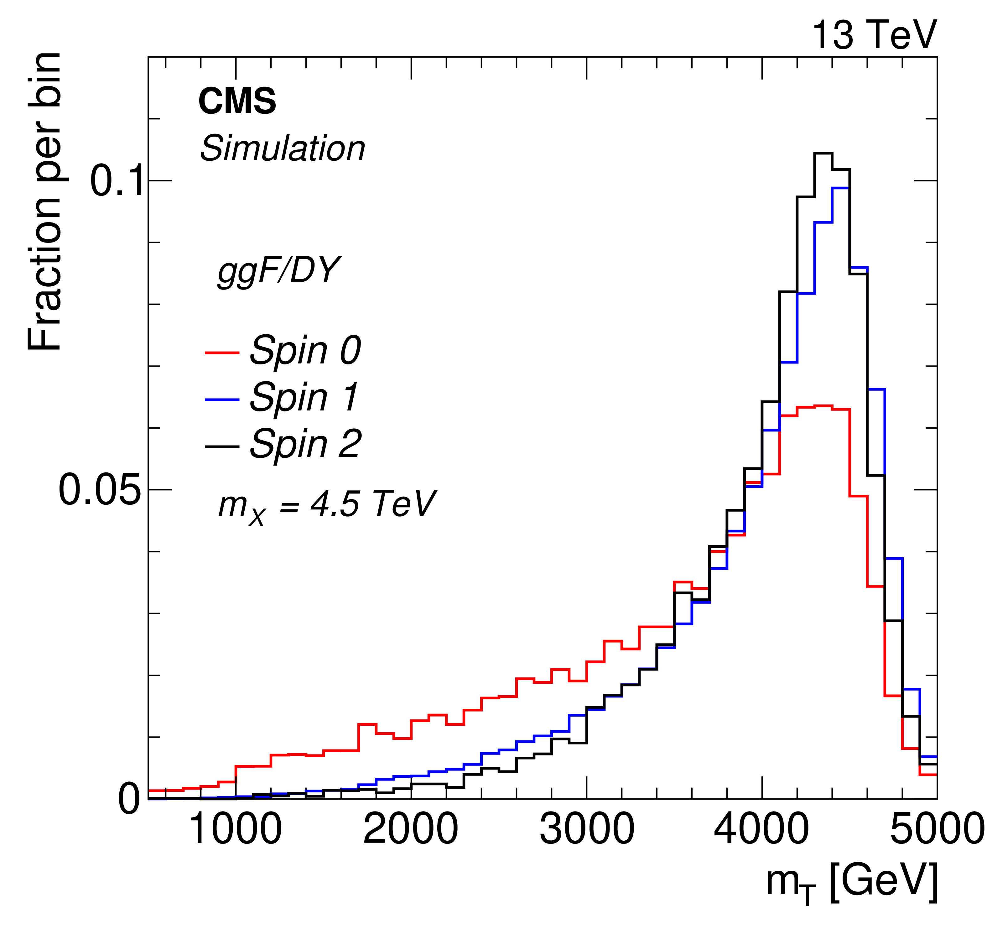
Distribution of ${m_{\mathrm {T}}}$ for ggF/DY-produced resonance X of mass 4.5 TeV. Events used are from all SR and CR combined. |
png pdf |
Figure 3-b:
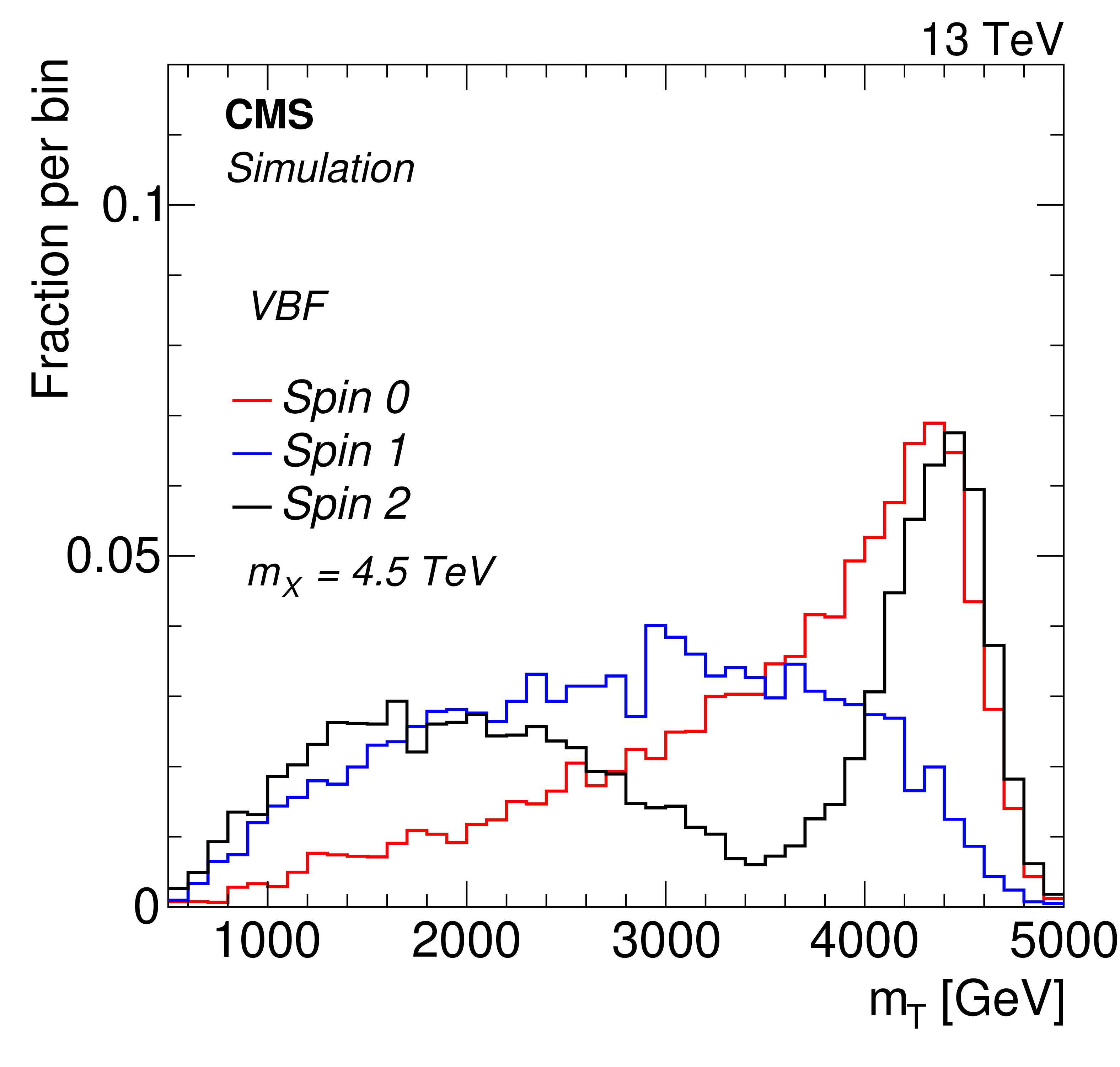
Distribution of ${m_{\mathrm {T}}}$ for VBF-produced resonance X of mass 4.5 TeV. Events used are from all SR and CR combined. |
png pdf |
Figure 4:
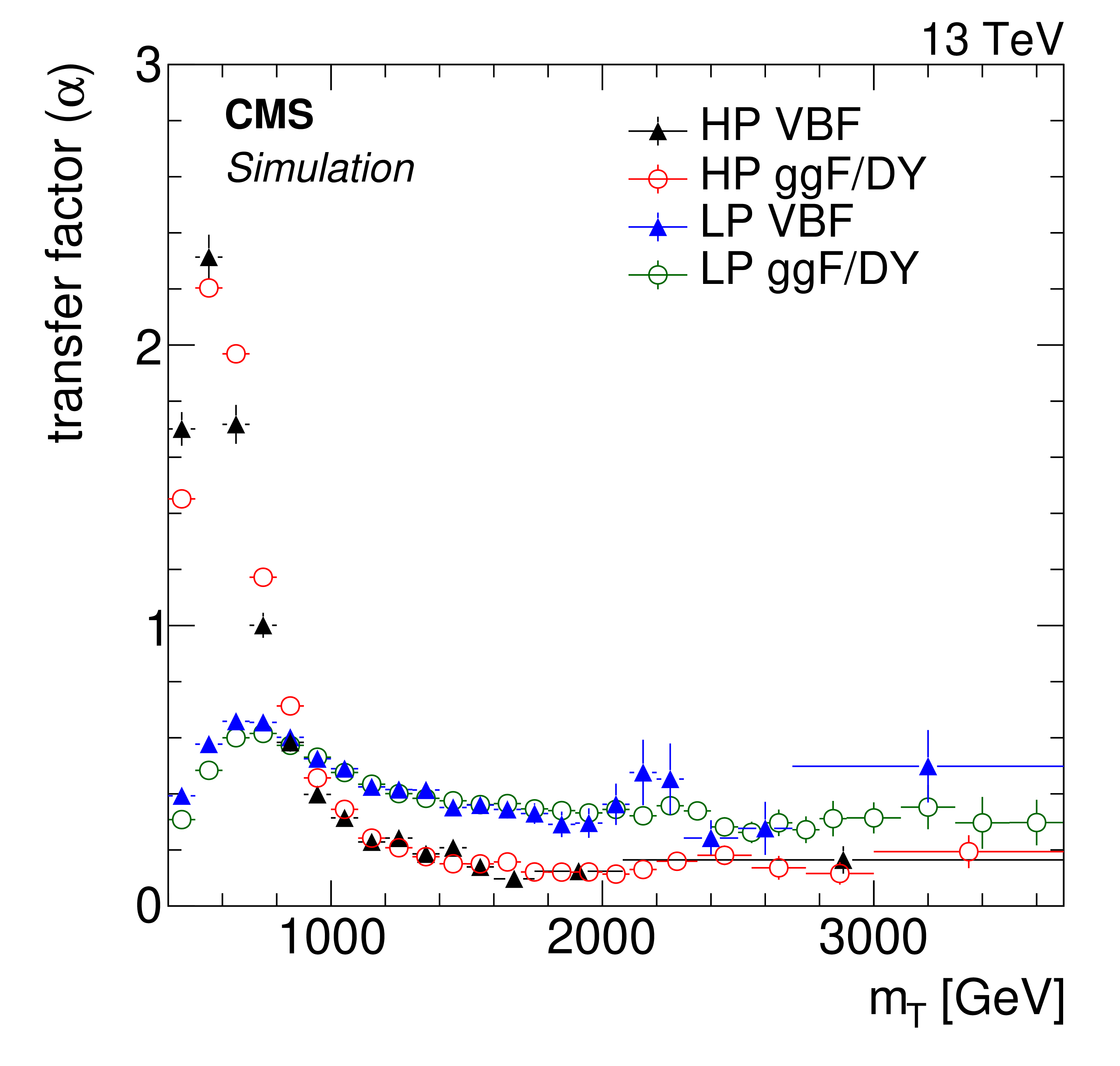
The distributions of the transfer factors ($\alpha $) versus ${m_{\mathrm {T}}}$ in the various event categories are shown. The last bin corresponds to the value obtained by integrating events above the penultimate bin. |

png pdf |
Figure 5:
Comparison of background estimations and observations in the high-purity ggF/DY (upper left), high-purity VBF (upper right), low-purity ggF/DY (lower left), and low-purity VBF (lower right) validation signal regions. The lower panel shows the ratio of the estimated and the observed event yields. The hashed band in the ratio represents the total uncertainty in the corresponding SR. The red line (lower left) is a fit to the ratio of prediction to the data in the LP ggF/DY vSR. |
png pdf |
Figure 5-a:
Comparison of background estimations and observations in the high-purity ggF/DY validation signal region. The lower panel shows the ratio of the estimated and the observed event yields. The hashed band in the ratio represents the total uncertainty in the corresponding SR. |
png pdf |
Figure 5-b:
Comparison of background estimations and observations in the high-purity VBF validation signal region. The lower panel shows the ratio of the estimated and the observed event yields. The hashed band in the ratio represents the total uncertainty in the corresponding SR. |
png pdf |
Figure 5-c:
Comparison of background estimations and observations in the low-purity ggF/DY validation signal region. The lower panel shows the ratio of the estimated and the observed event yields. The hashed band in the ratio represents the total uncertainty in the corresponding SR. |
png pdf |
Figure 5-d:
Comparison of background estimations and observations in the low-purity VBF validation signal region. The lower panel shows the ratio of the estimated and the observed event yields. The hashed band in the ratio represents the total uncertainty in the corresponding SR. |
png pdf |
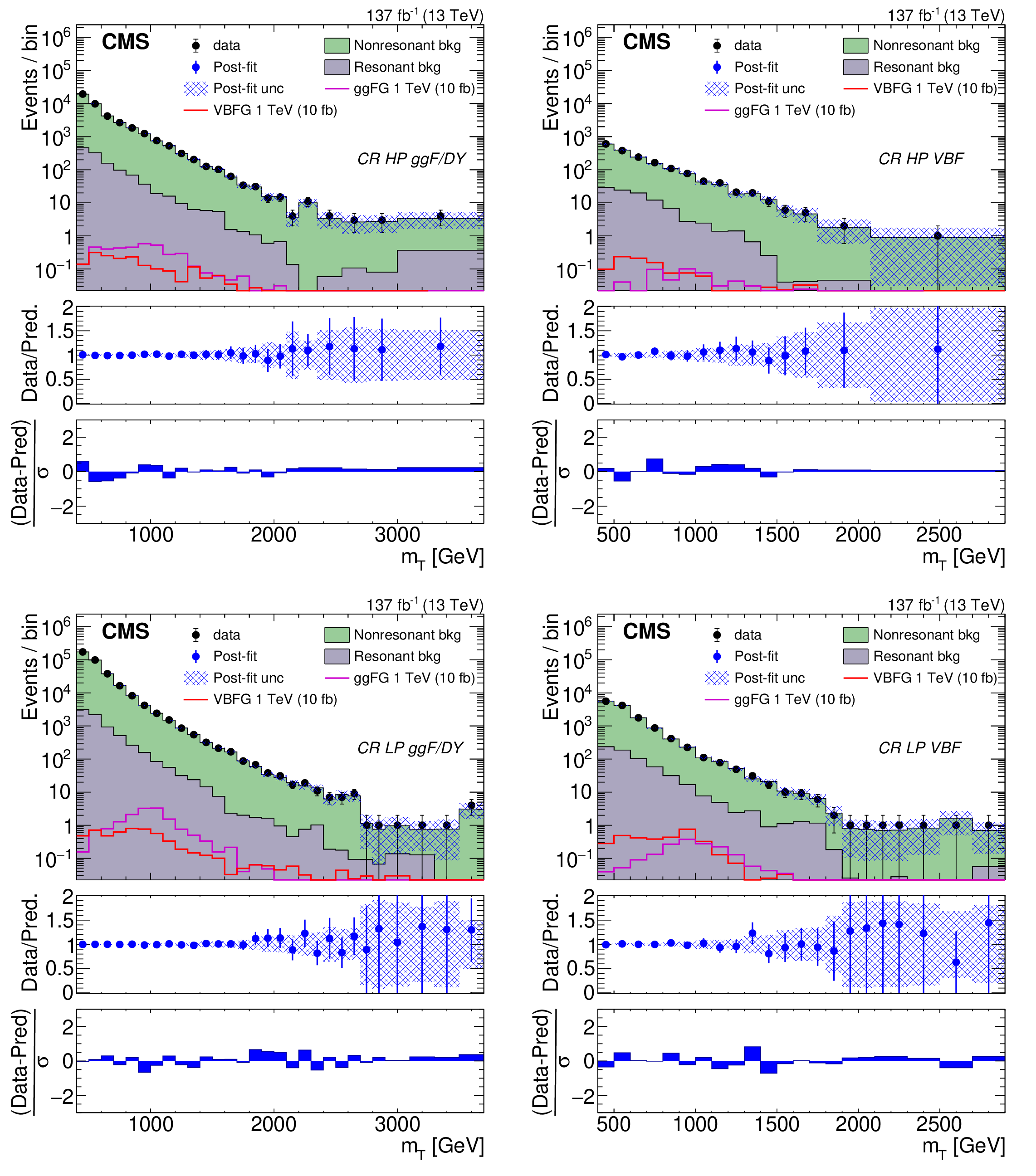
Figure 6:
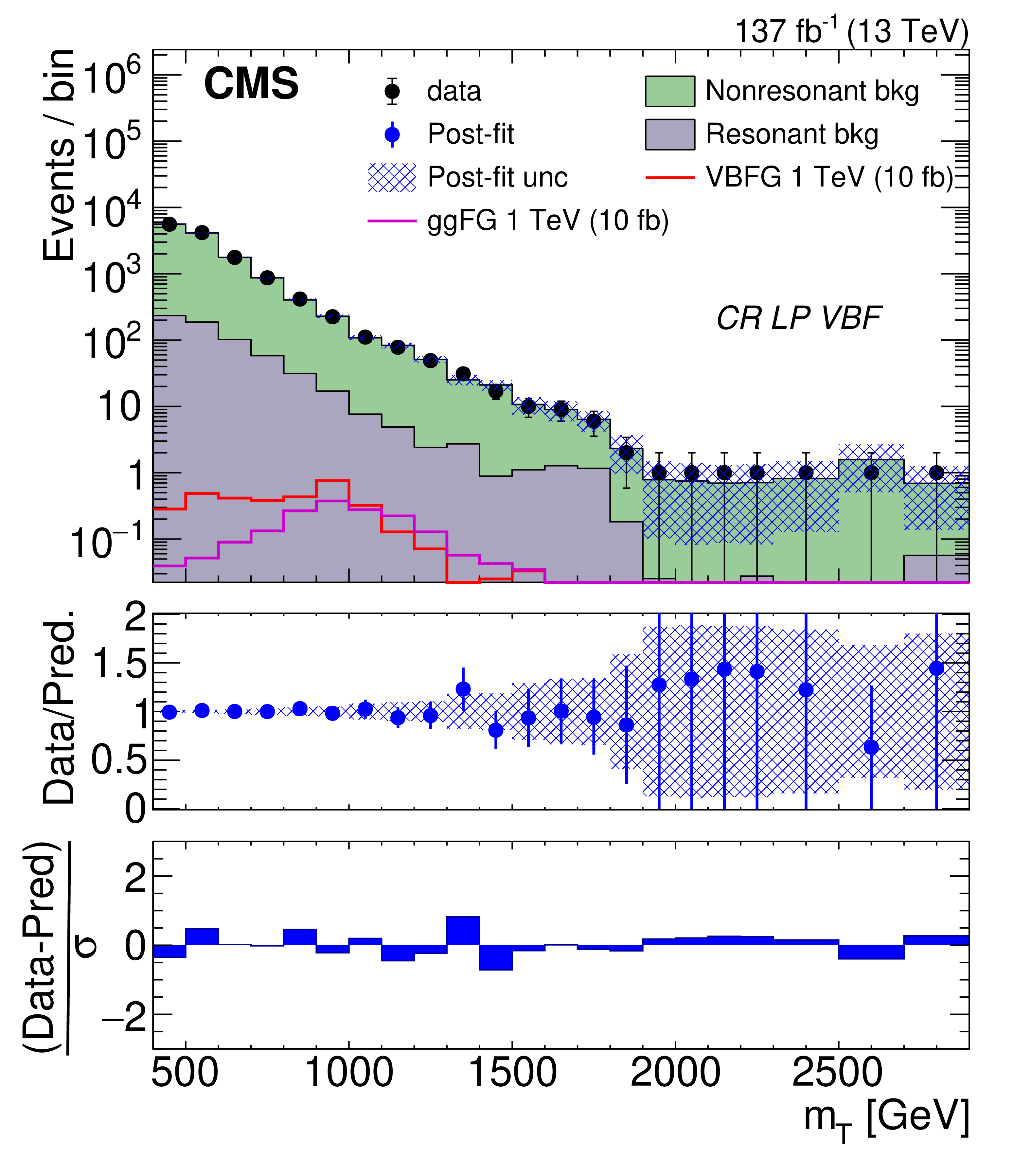
Distributions of ${m_{\mathrm {T}}}$ for high-purity ggF/DY (upper left) and VBF (upper right), and low-purity ggF/DY (lower left) and VBF (lower right) CR events after performing background-only fits. The last bin in the upper left, upper right, lower left, and lower right plot corresponds to the yields integrated above 3, 2.3, 3.5, and 2.7 TeV, respectively. The top panel of each plot shows the post-fit prediction, represented by filled histograms, compared to observed yields, represented by black points. Both the ggF and VBF-produced 1 TeV graviton signals are shown in each plot, represented by the open purple and red histograms, respectively. The signal is normalized to 10 fb. The blue hashed area represents the total uncertainty from the post-fit predicted event yield as a function of ${m_{\mathrm {T}}}$. The middle panel of each plot shows the ratio of data and post-fit predictions in blue. The bottom panel of each plot shows the difference between the observed event yields and the post-fit predictions normalized by the quadratic sum of the statistical uncertainty of the observed yield and the total uncertainty from the post-fit prediction in each ${m_{\mathrm {T}}}$ bin. |
png pdf |
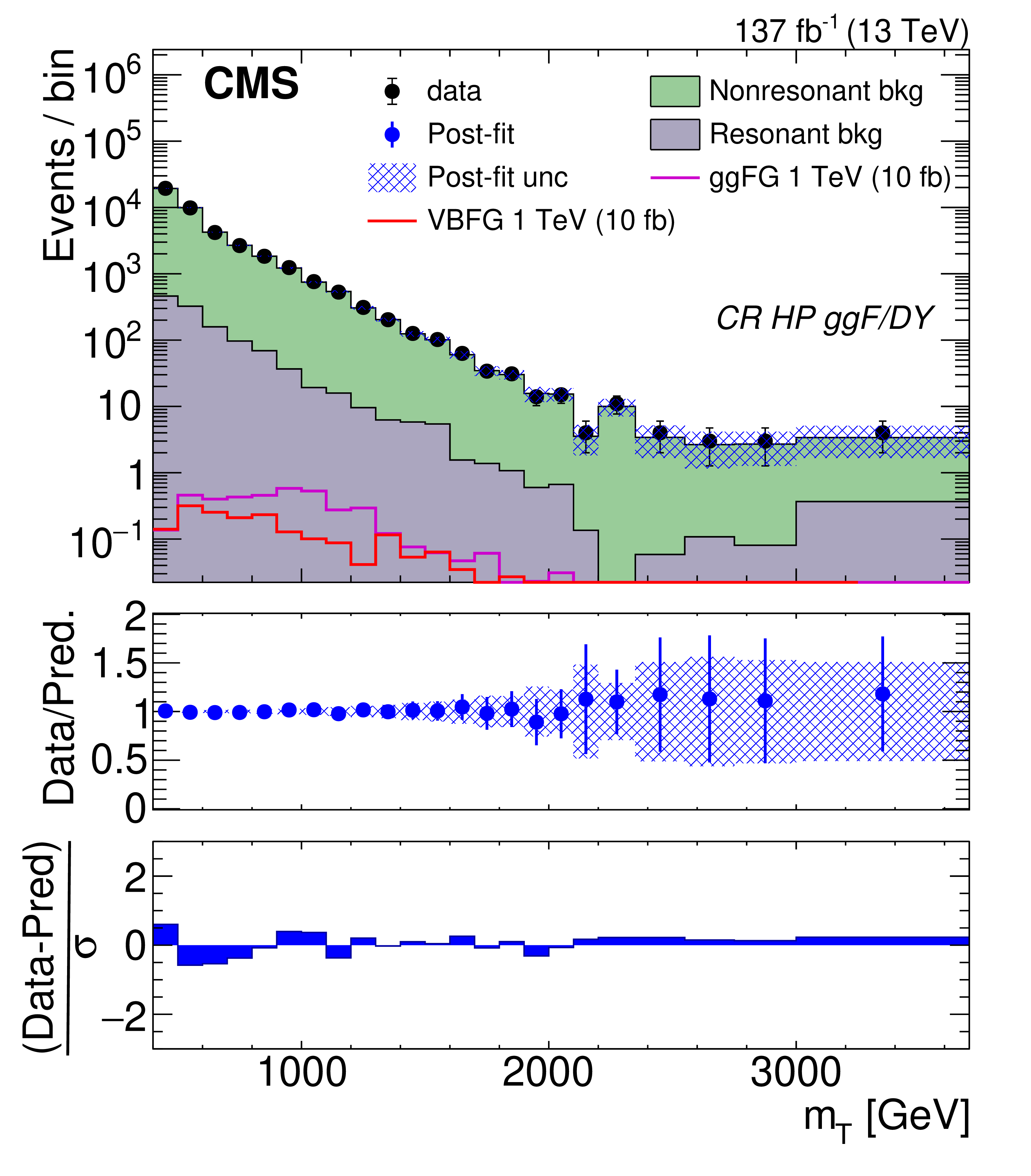
Figure 6-a:
Distribution of ${m_{\mathrm {T}}}$ for high-purity ggF/DY CR events after performing background-only fits. The last bin corresponds to the yields integrated above 3 TeV. The top panel shows the post-fit prediction, represented by filled histograms, compared to observed yields, represented by black points. Both the ggF and VBF-produced 1 TeV graviton signals are shown, represented by the open purple and red histograms, respectively. The signal is normalized to 10 fb. The blue hashed area represents the total uncertainty from the post-fit predicted event yield as a function of ${m_{\mathrm {T}}}$. The middle panel shows the ratio of data and post-fit predictions in blue. The bottom panel shows the difference between the observed event yields and the post-fit predictions normalized by the quadratic sum of the statistical uncertainty of the observed yield and the total uncertainty from the post-fit prediction in each ${m_{\mathrm {T}}}$ bin. |
png pdf |
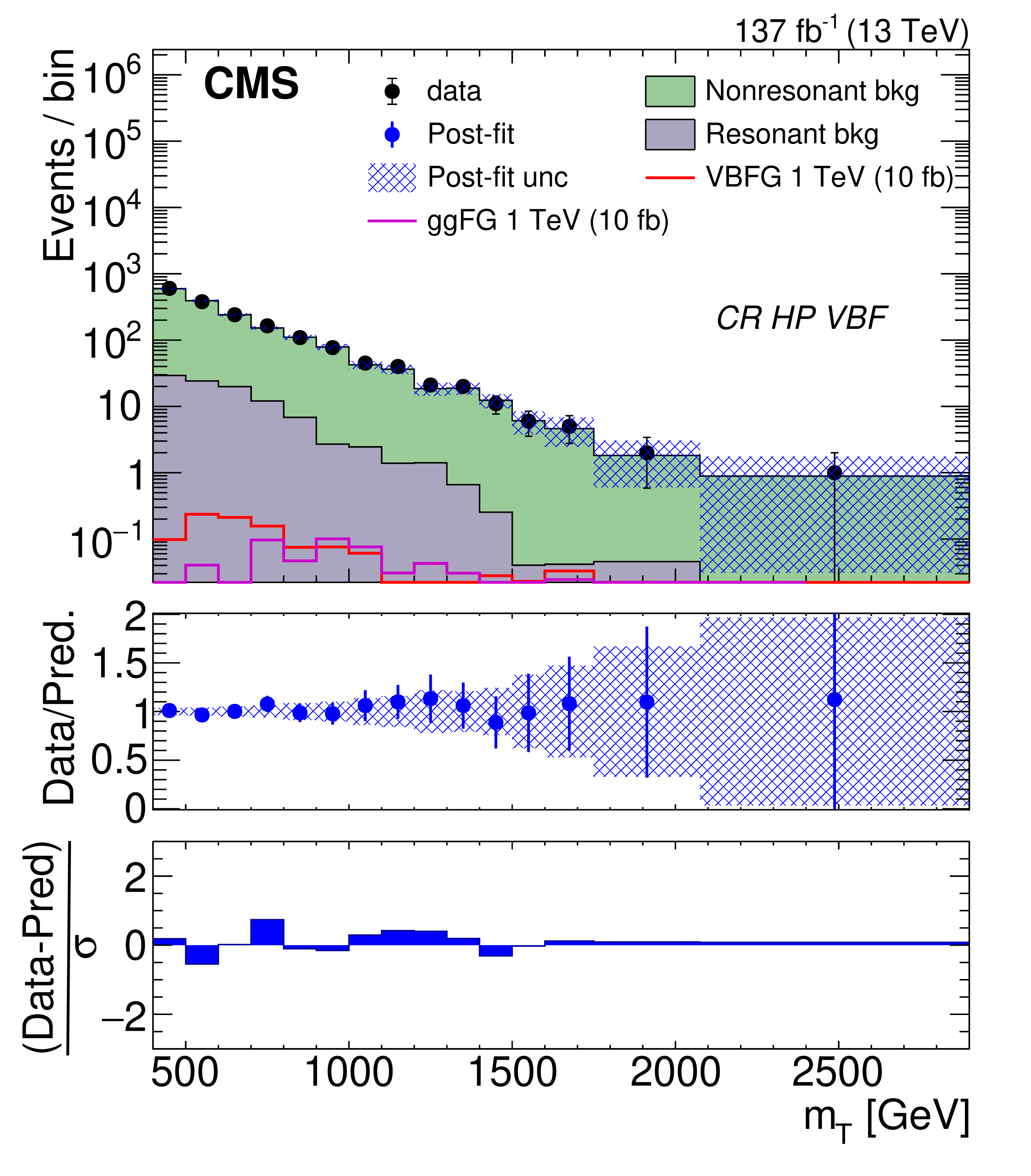
Figure 6-b:
Distribution of ${m_{\mathrm {T}}}$ for high-purity VBF CR events after performing background-only fits. The last bin corresponds to the yields integrated above 2.3 TeV. The top panel shows the post-fit prediction, represented by filled histograms, compared to observed yields, represented by black points. Both the ggF and VBF-produced 1 TeV graviton signals are shown, represented by the open purple and red histograms, respectively. The signal is normalized to 10 fb. The blue hashed area represents the total uncertainty from the post-fit predicted event yield as a function of ${m_{\mathrm {T}}}$. The middle panel shows the ratio of data and post-fit predictions in blue. The bottom panel shows the difference between the observed event yields and the post-fit predictions normalized by the quadratic sum of the statistical uncertainty of the observed yield and the total uncertainty from the post-fit prediction in each ${m_{\mathrm {T}}}$ bin. |
png pdf |
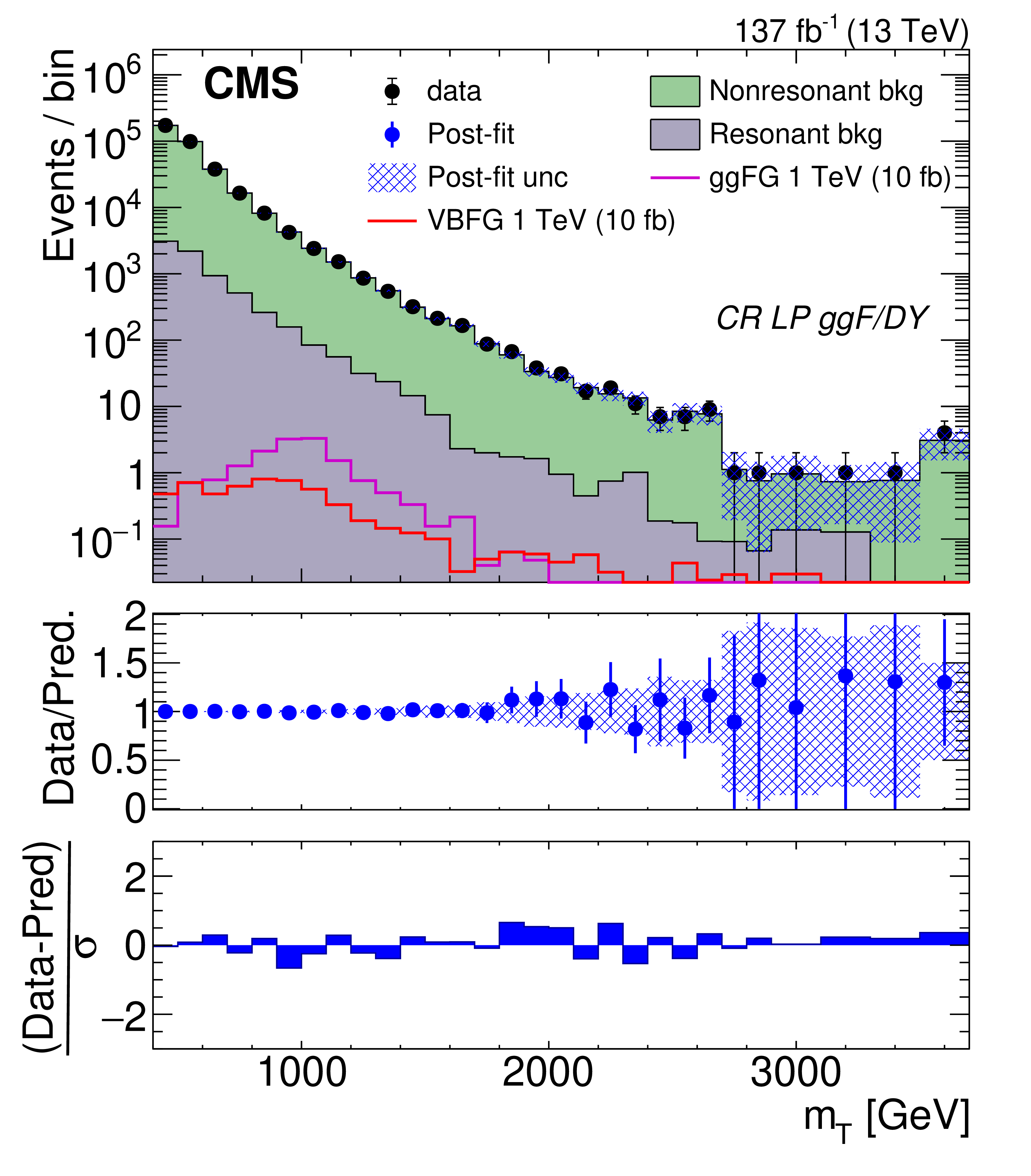
Figure 6-c:
Distribution of ${m_{\mathrm {T}}}$ for low-purity ggF/DY CR events after performing background-only fits. The last bin corresponds to the yields integrated above 3.5 TeV. The top panel shows the post-fit prediction, represented by filled histograms, compared to observed yields, represented by black points. Both the ggF and VBF-produced 1 TeV graviton signals are shown, represented by the open purple and red histograms, respectively. The signal is normalized to 10 fb. The blue hashed area represents the total uncertainty from the post-fit predicted event yield as a function of ${m_{\mathrm {T}}}$. The middle panel shows the ratio of data and post-fit predictions in blue. The bottom panel shows the difference between the observed event yields and the post-fit predictions normalized by the quadratic sum of the statistical uncertainty of the observed yield and the total uncertainty from the post-fit prediction in each ${m_{\mathrm {T}}}$ bin. |
png pdf |
Figure 6-d:
Distribution of ${m_{\mathrm {T}}}$ for low-purity VBF CR events after performing background-only fits. The last bin corresponds to the yields integrated above 2.7 TeV. The top panel shows the post-fit prediction, represented by filled histograms, compared to observed yields, represented by black points. Both the ggF and VBF-produced 1 TeV graviton signals are shown, represented by the open purple and red histograms, respectively. The signal is normalized to 10 fb. The blue hashed area represents the total uncertainty from the post-fit predicted event yield as a function of ${m_{\mathrm {T}}}$. The middle panel shows the ratio of data and post-fit predictions in blue. The bottom panel shows the difference between the observed event yields and the post-fit predictions normalized by the quadratic sum of the statistical uncertainty of the observed yield and the total uncertainty from the post-fit prediction in each ${m_{\mathrm {T}}}$ bin. |
png pdf |
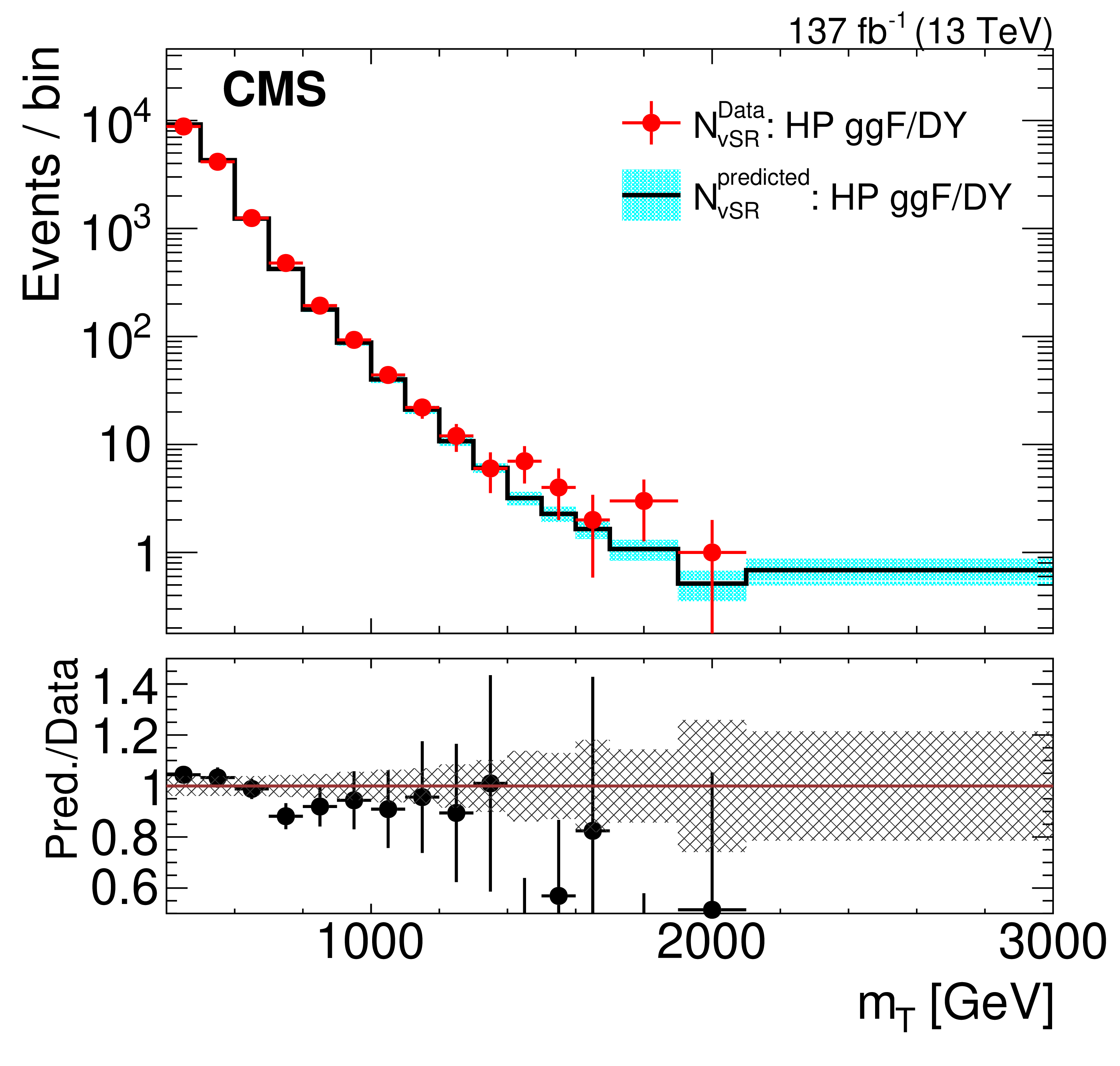
Figure 7:
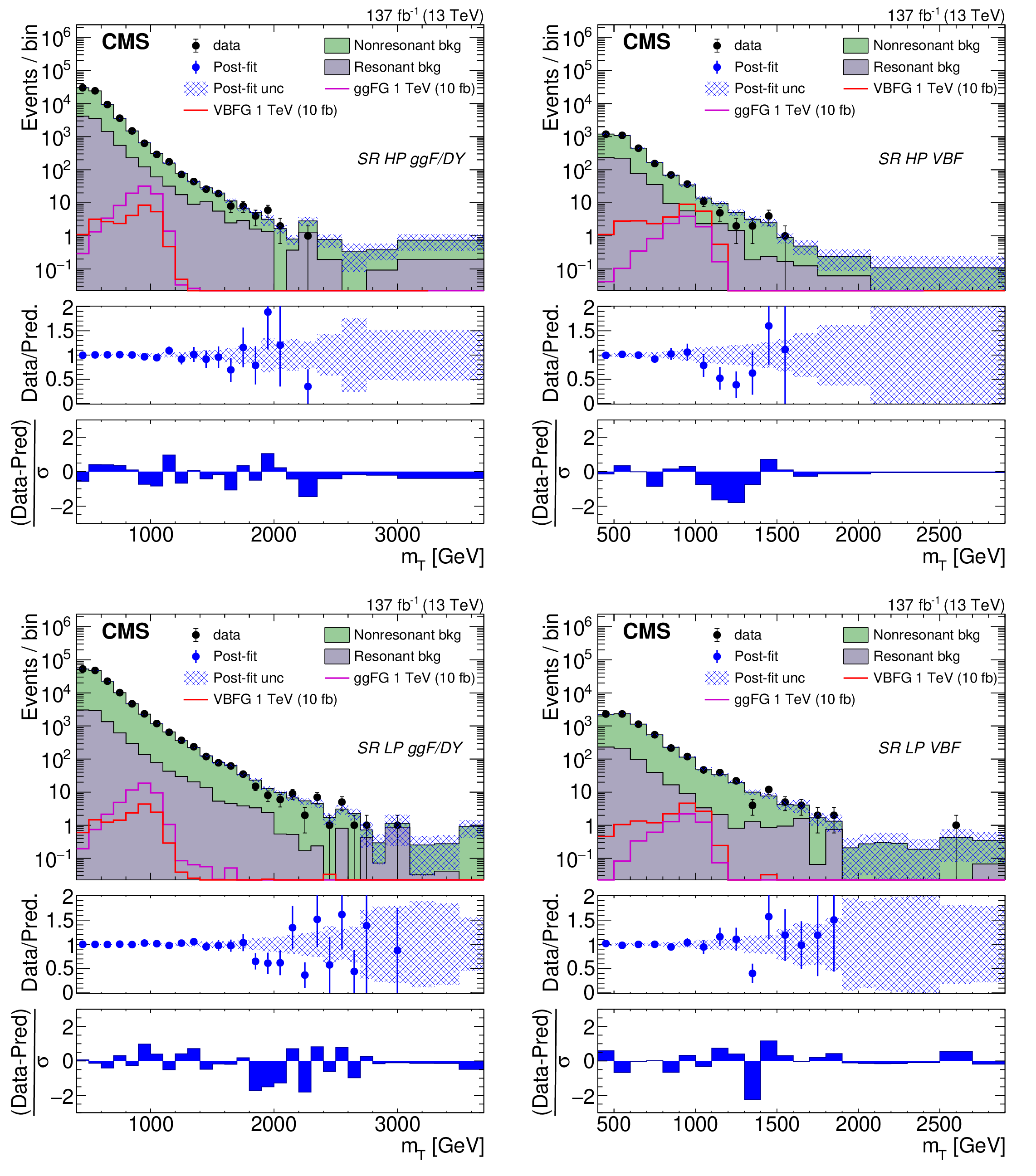
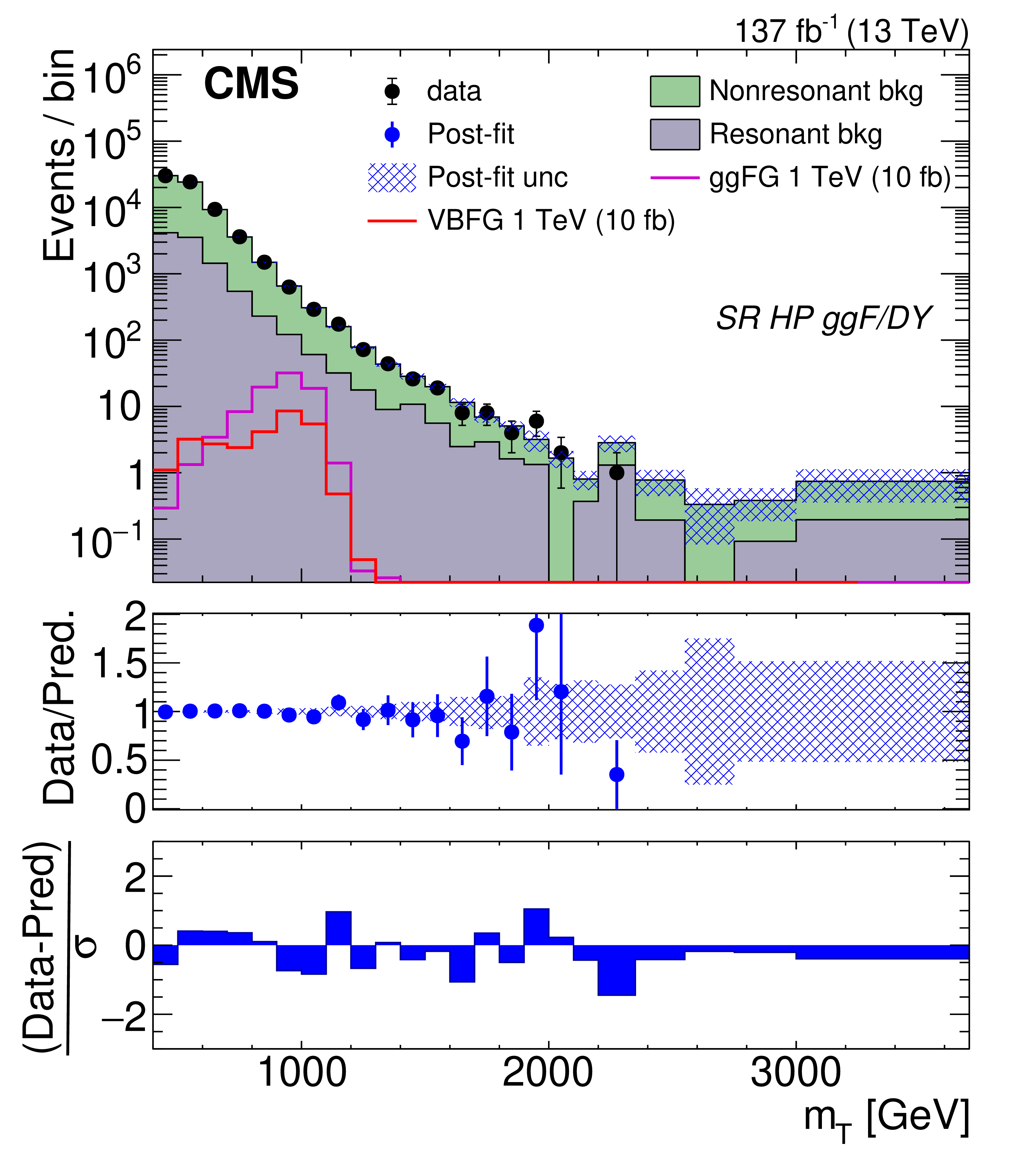
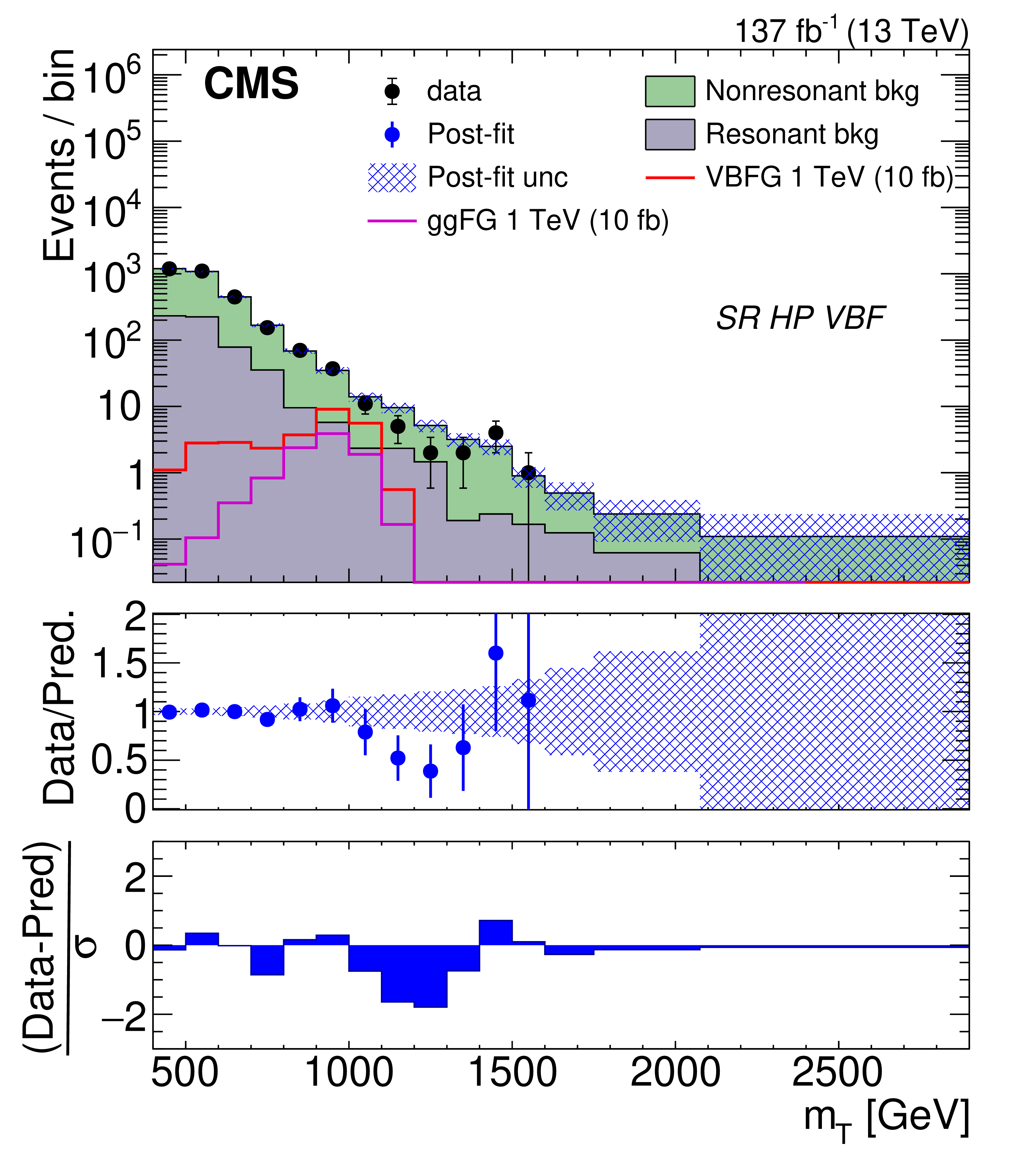
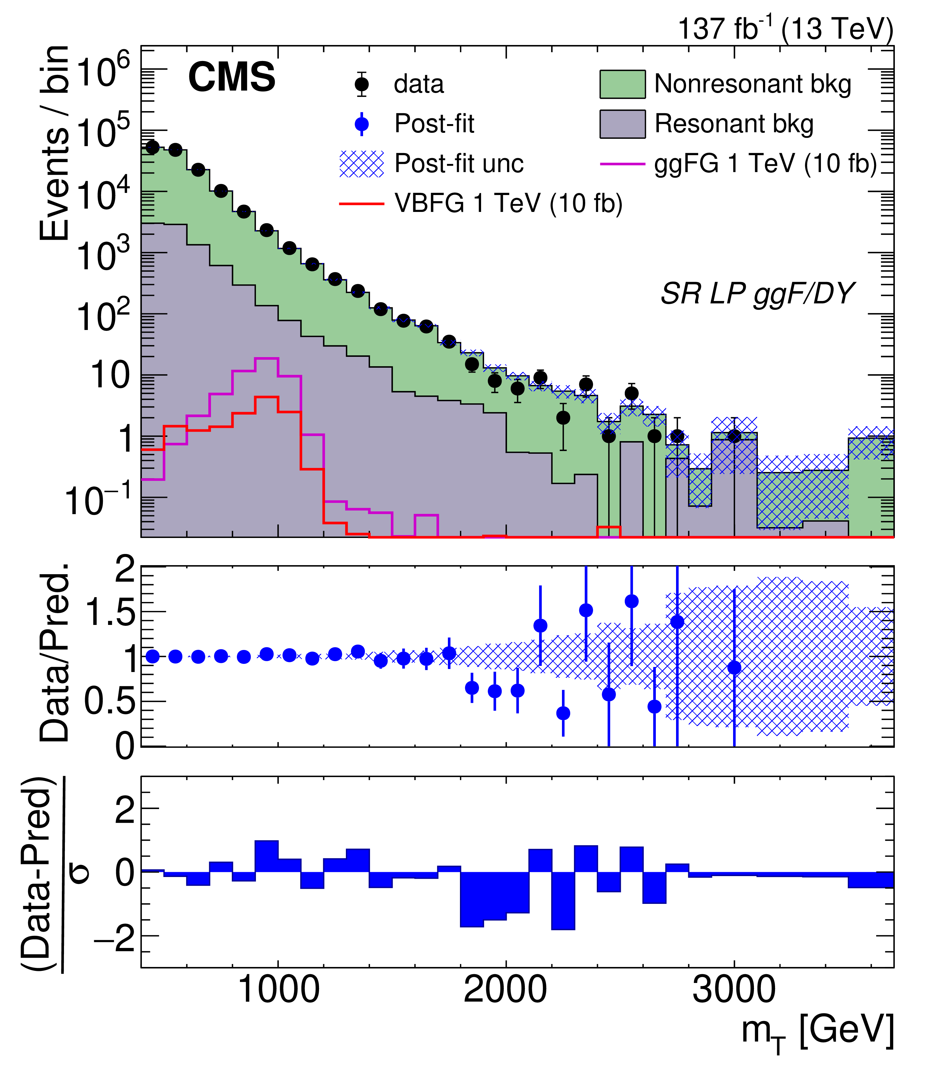
Distribution of the predicted and observed event yields versus ${m_{\mathrm {T}}}$ for high-purity ggF/DY (upper left) and VBF (upper right), and low-purity ggF/DY (lower left) and VBF (lower right) SR events. The last bin in each plot corresponds to the yields integrated above the penultimate bin. The top panel of each plot shows the prediction based on a background-only fit to data, represented by filled histograms, compared to observed yields, represented by black points. Both the ggF and VBF-produced 1 TeV graviton signals are shown in each plot, represented by the open purple and red histograms, respectively. The signal is normalized to 10 fb. The middle panel of each plot shows the ratio of data and post-fit predictions in blue. The blue hashed area represents the total uncertainty from the post-fit predicted event yield as a function of ${m_{\mathrm {T}}}$. The bottom panel of each plot shows the difference between the observed event yields and the post-fit predictions normalized by the quadratic sum of the statistical uncertainty of the observed yield and the total uncertainty from the post-fit prediction in each ${m_{\mathrm {T}}}$ bin. |
png pdf |
Figure 7-a:
Distribution of the predicted and observed event yields versus ${m_{\mathrm {T}}}$ for high-purity ggF/DY SR events. The last bin corresponds to the yields integrated above the penultimate bin. The top panel shows the prediction based on a background-only fit to data, represented by filled histograms, compared to observed yields, represented by black points. Both the ggF and VBF-produced 1 TeV graviton signals are shown in each plot, represented by the open purple and red histograms, respectively. The signal is normalized to 10 fb. The middle panel shows the ratio of data and post-fit predictions in blue. The blue hashed area represents the total uncertainty from the post-fit predicted event yield as a function of ${m_{\mathrm {T}}}$. The bottom panel shows the difference between the observed event yields and the post-fit predictions normalized by the quadratic sum of the statistical uncertainty of the observed yield and the total uncertainty from the post-fit prediction in each ${m_{\mathrm {T}}}$ bin. |
png pdf |
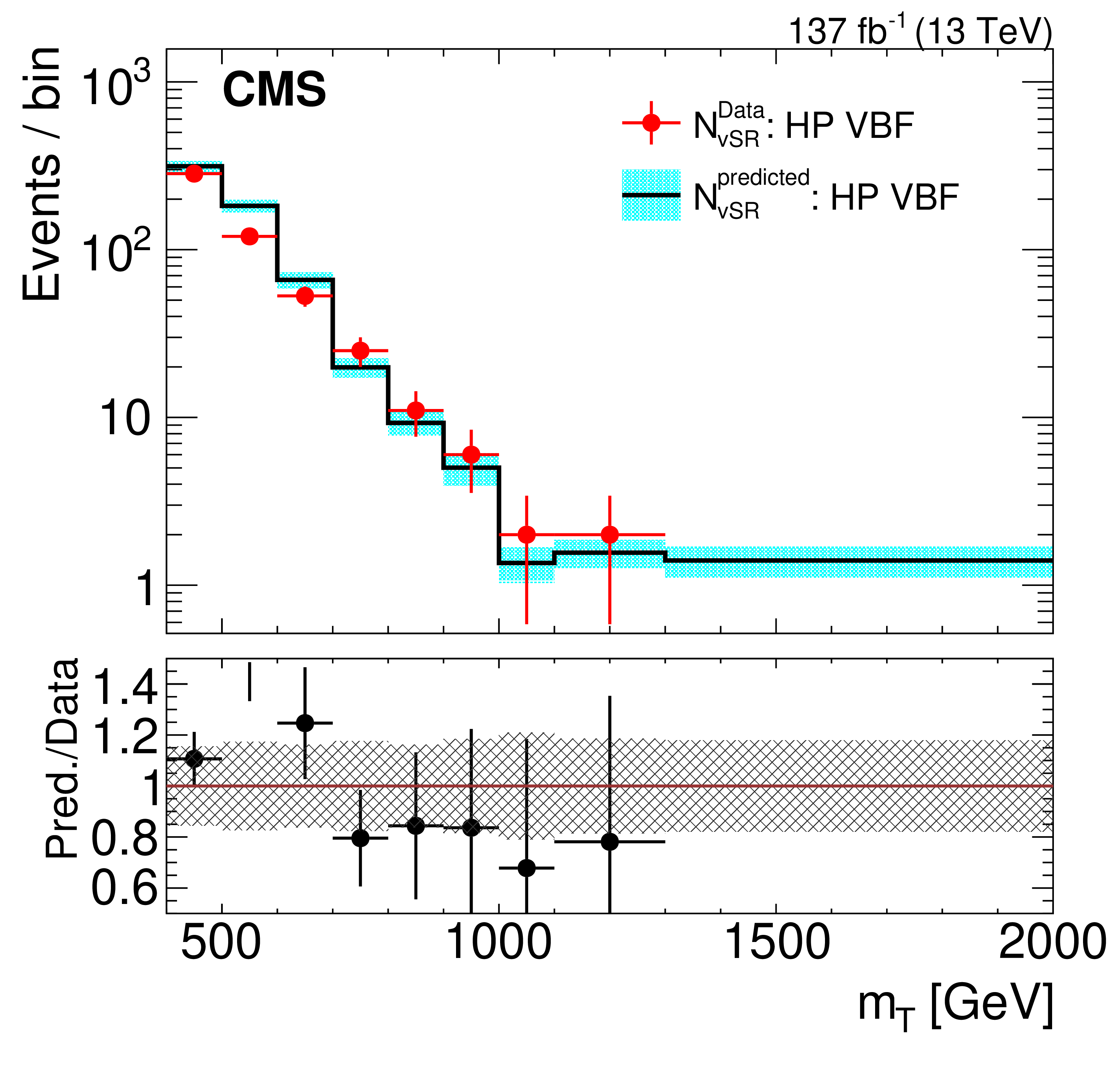
Figure 7-b:
Distribution of the predicted and observed event yields versus ${m_{\mathrm {T}}}$ for high-purity ggF/DY SR events. The last bin corresponds to the yields integrated above the penultimate bin. The top panel shows the prediction based on a background-only fit to data, represented by filled histograms, compared to observed yields, represented by black points. Both the ggF and VBF-produced 1 TeV graviton signals are shown in each plot, represented by the open purple and red histograms, respectively. The signal is normalized to 10 fb. The middle panel shows the ratio of data and post-fit predictions in blue. The blue hashed area represents the total uncertainty from the post-fit predicted event yield as a function of ${m_{\mathrm {T}}}$. The bottom panel shows the difference between the observed event yields and the post-fit predictions normalized by the quadratic sum of the statistical uncertainty of the observed yield and the total uncertainty from the post-fit prediction in each ${m_{\mathrm {T}}}$ bin. |
png pdf |
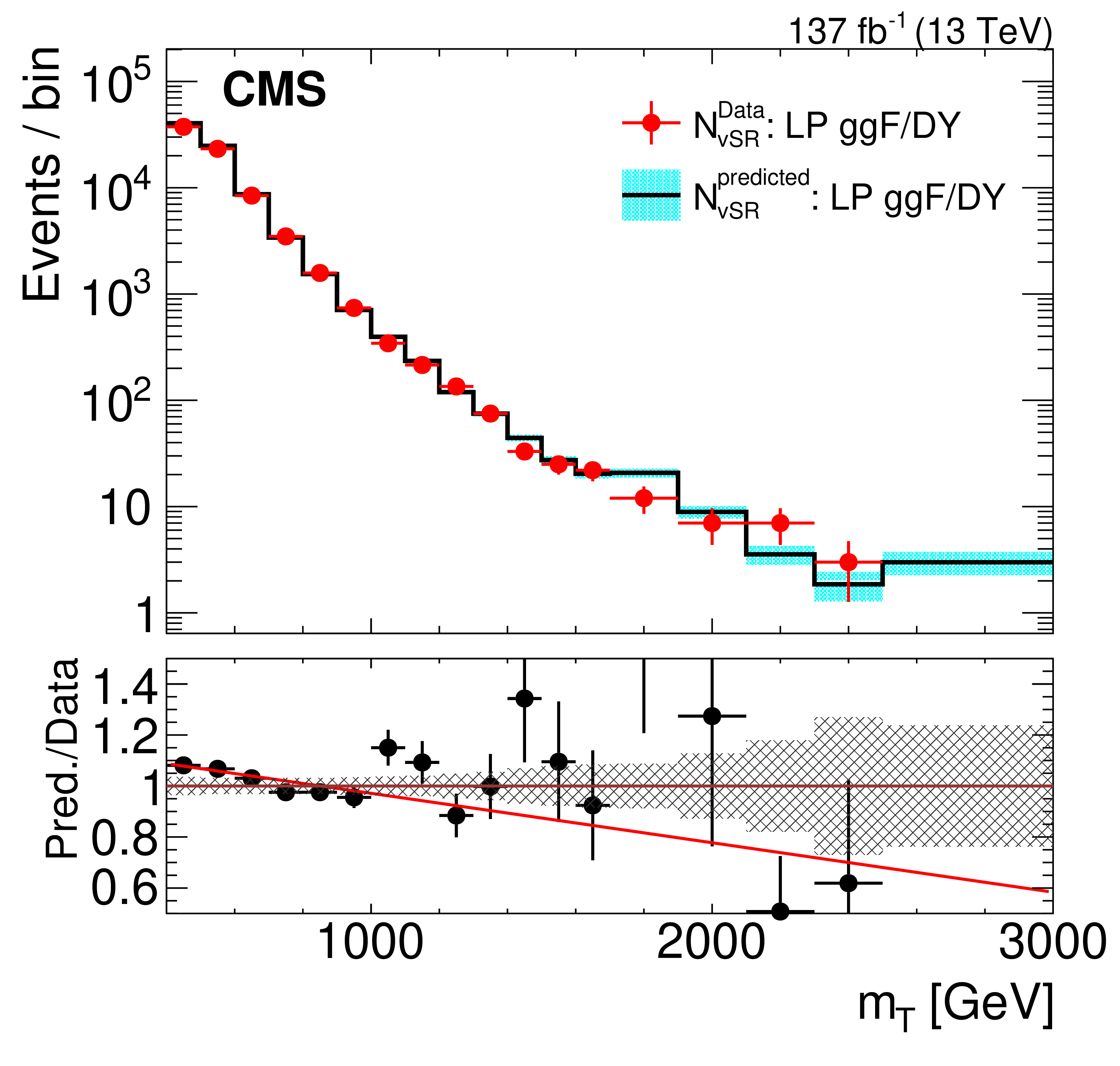
Figure 7-c:
Distribution of the predicted and observed event yields versus ${m_{\mathrm {T}}}$ for low-purity ggF/DY SR events. The last bin corresponds to the yields integrated above the penultimate bin. The top panel shows the prediction based on a background-only fit to data, represented by filled histograms, compared to observed yields, represented by black points. Both the ggF and VBF-produced 1 TeV graviton signals are shown in each plot, represented by the open purple and red histograms, respectively. The signal is normalized to 10 fb. The middle panel shows the ratio of data and post-fit predictions in blue. The blue hashed area represents the total uncertainty from the post-fit predicted event yield as a function of ${m_{\mathrm {T}}}$. The bottom panel shows the difference between the observed event yields and the post-fit predictions normalized by the quadratic sum of the statistical uncertainty of the observed yield and the total uncertainty from the post-fit prediction in each ${m_{\mathrm {T}}}$ bin. |
png pdf |
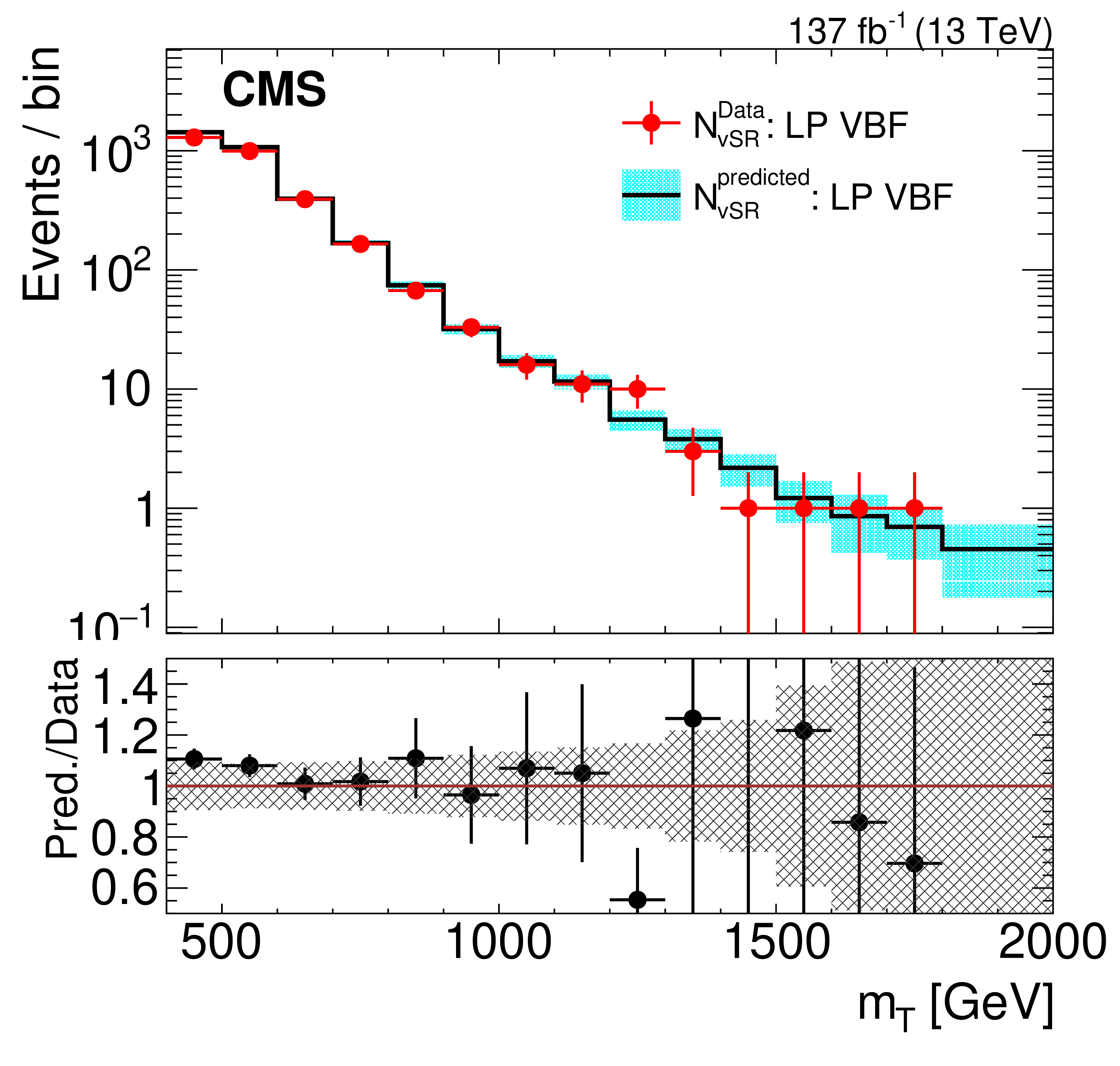
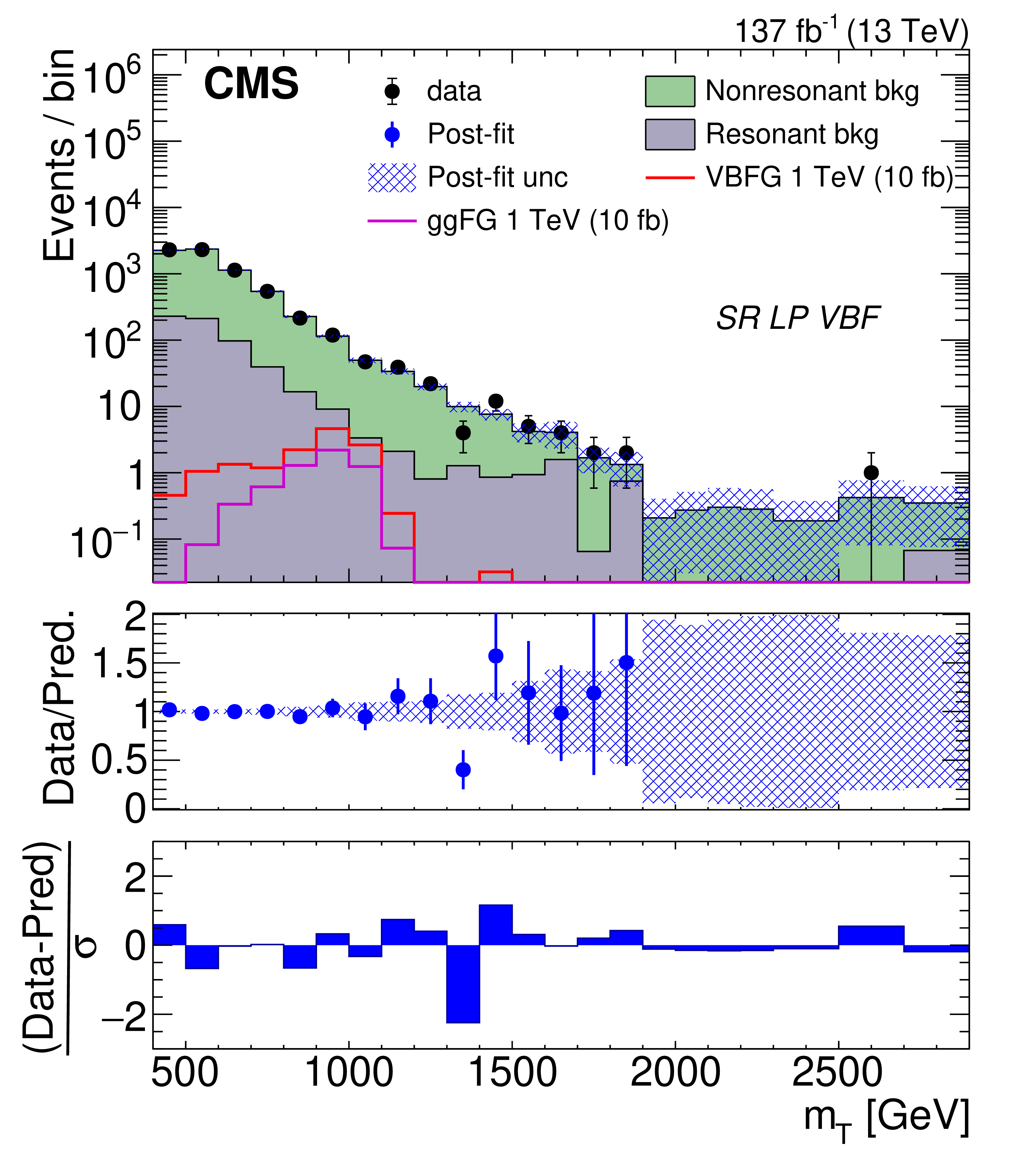
Figure 7-d:
Distribution of the predicted and observed event yields versus ${m_{\mathrm {T}}}$ for low-purity VBF SR events. The last bin corresponds to the yields integrated above the penultimate bin. The top panel shows the prediction based on a background-only fit to data, represented by filled histograms, compared to observed yields, represented by black points. Both the ggF and VBF-produced 1 TeV graviton signals are shown in each plot, represented by the open purple and red histograms, respectively. The signal is normalized to 10 fb. The middle panel shows the ratio of data and post-fit predictions in blue. The blue hashed area represents the total uncertainty from the post-fit predicted event yield as a function of ${m_{\mathrm {T}}}$. The bottom panel shows the difference between the observed event yields and the post-fit predictions normalized by the quadratic sum of the statistical uncertainty of the observed yield and the total uncertainty from the post-fit prediction in each ${m_{\mathrm {T}}}$ bin. |
png pdf |
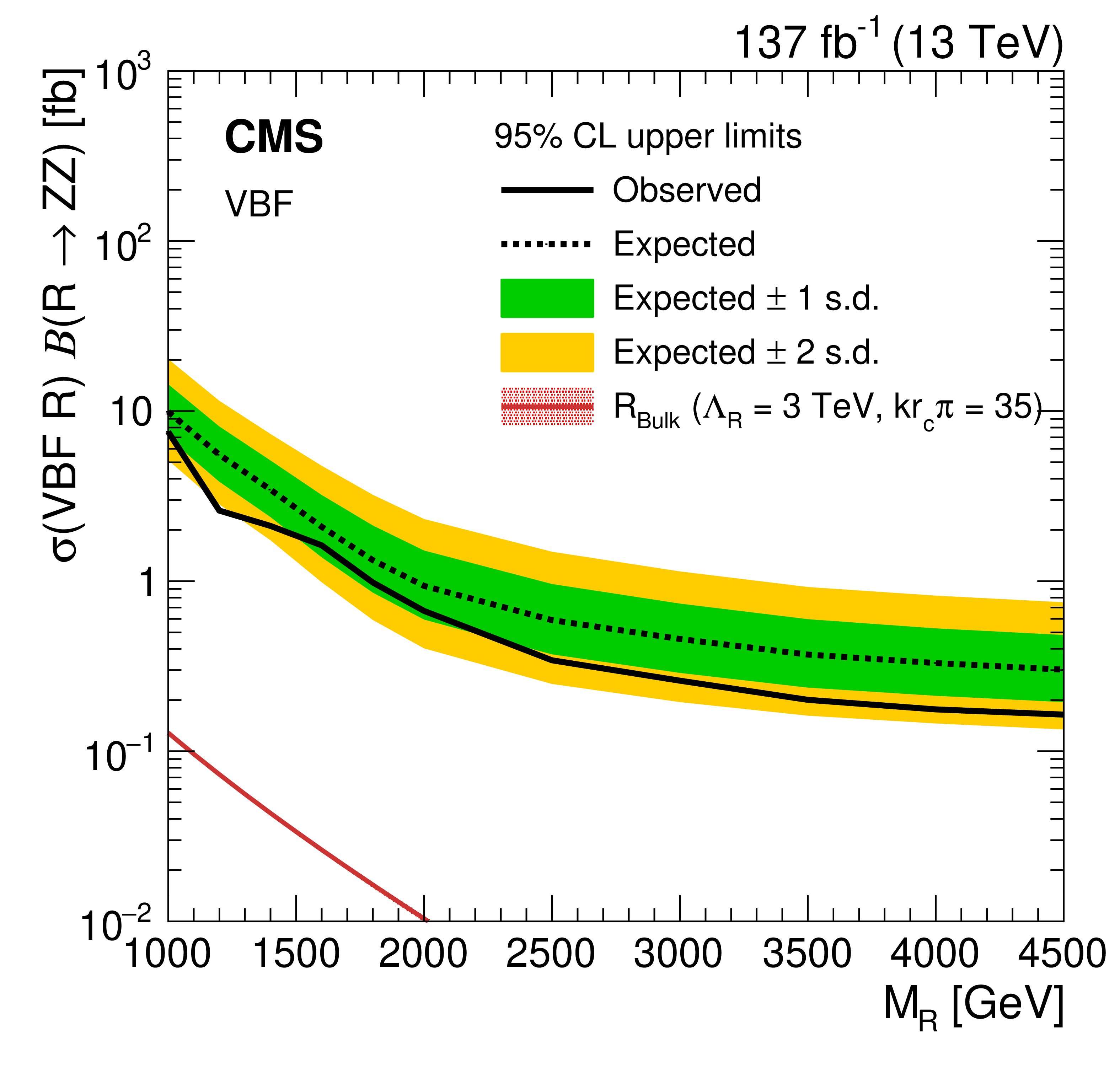
Figure 8:
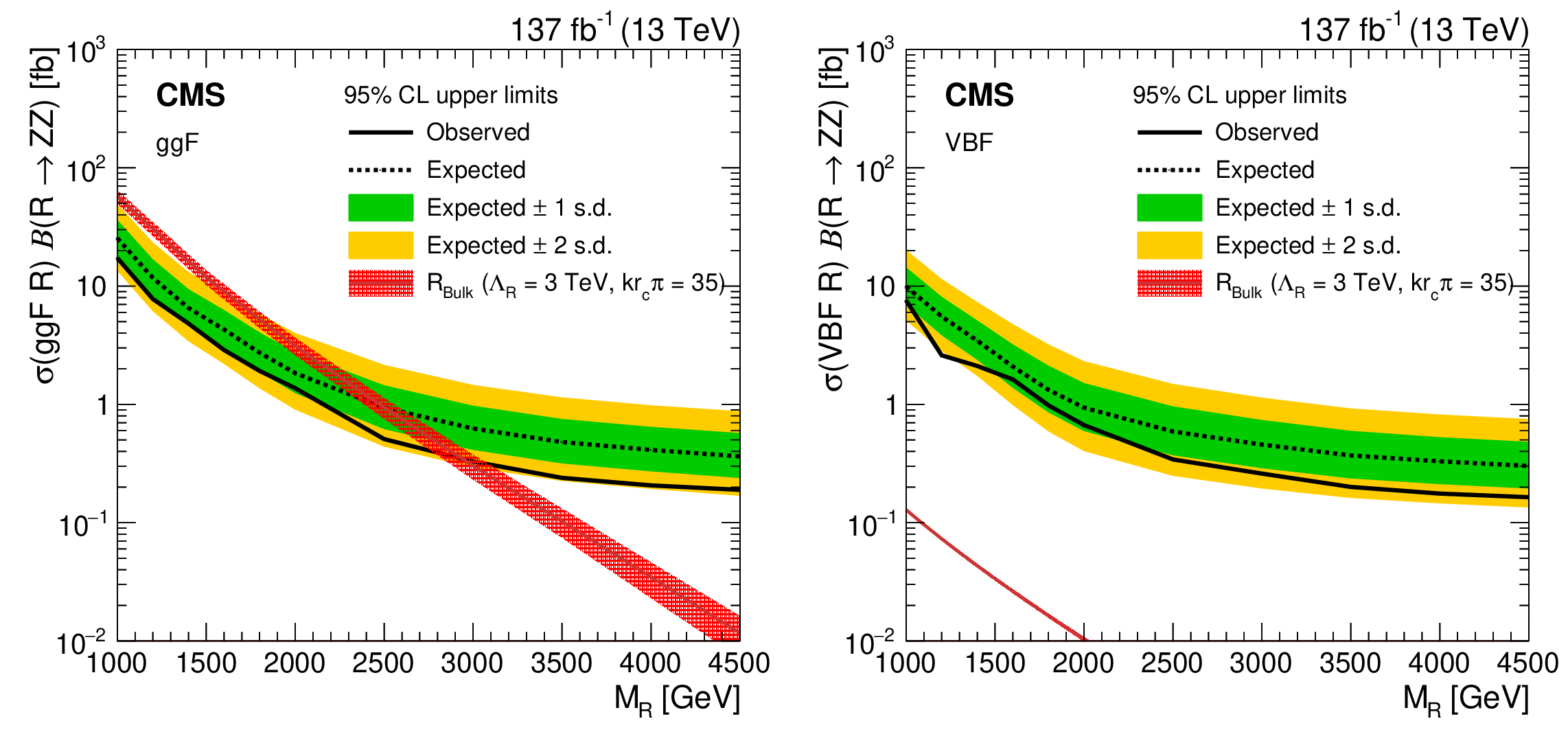
Expected and observed 95% CL upper limits on the product of the radion (R) production cross section and the $\mathrm{R} \to \mathrm{ZZ} $ branching fraction versus the radion mass are shown as dashed and solid black lines, respectively. Green and yellow bands, respectively, represent the 68% and 95% confidence intervals of the expected limit. The red curves show the product of the theoretical radion production cross sections and their branching fractions to ZZ. The hashed red areas represent the theoretical cross section uncertainty due to limited knowledge of PDFs and scale choices. Limits and theory cross sections for ggF-produced radions are shown in the left figure, while the right figure shows the same for VBF-produced radions. |
png pdf |
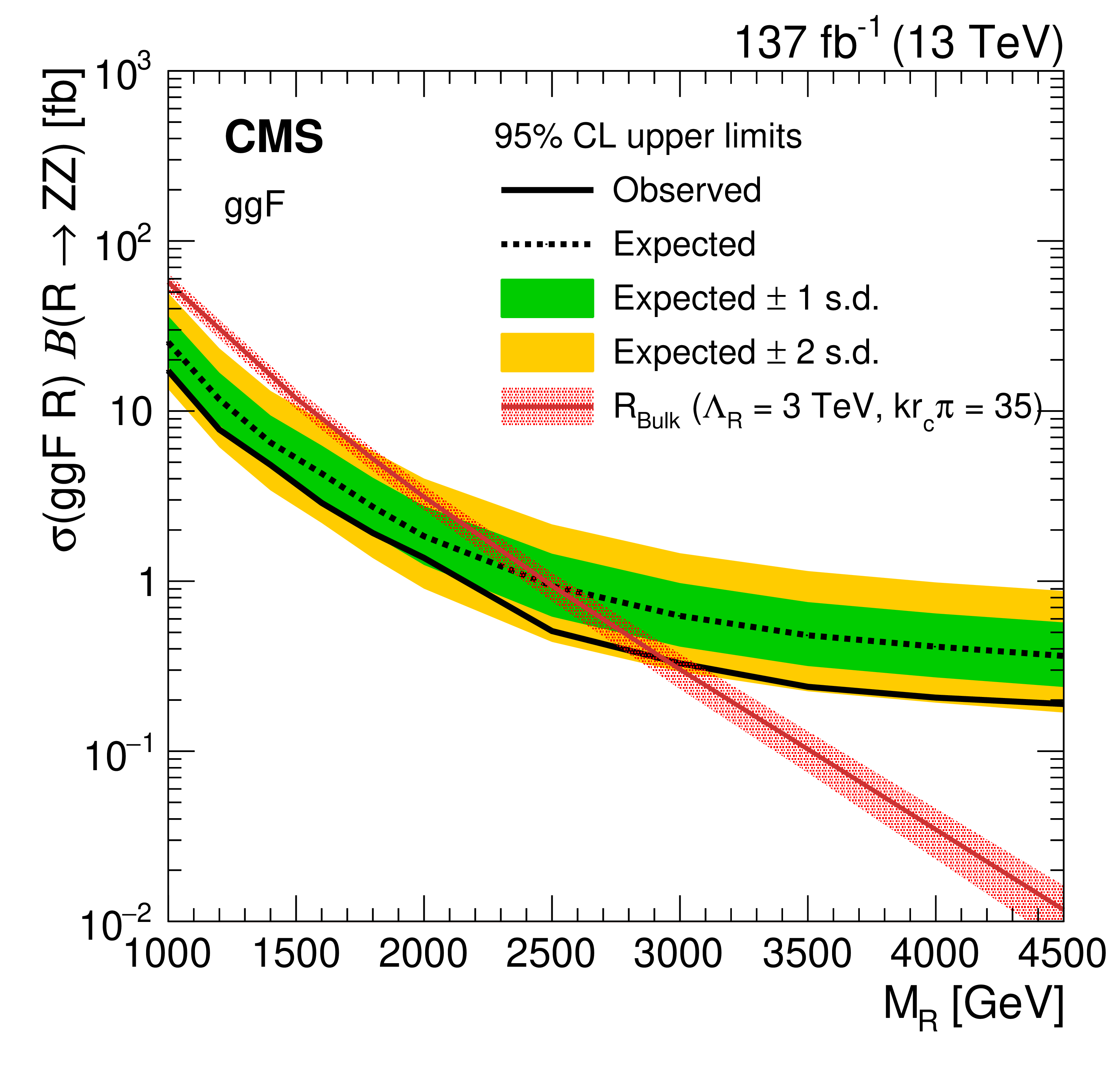
Figure 8-a:
Limits and theory cross sections for ggF-produced radions are shown. Expected and observed 95% CL upper limits on the product of the radion (R) production cross section and the $\mathrm{R} \to \mathrm{ZZ} $ branching fraction versus the radion mass are shown as dashed and solid black lines, respectively. Green and yellow bands, respectively, represent the 68% and 95% confidence intervals of the expected limit. The red curves show the product of the theoretical radion production cross sections and their branching fractions to ZZ. The hashed red areas represent the theoretical cross section uncertainty due to limited knowledge of PDFs and scale choices. |
png pdf |
Figure 8-b:
Limits and theory cross sections for VBF-produced radions are shown. Expected and observed 95% CL upper limits on the product of the radion (R) production cross section and the $\mathrm{R} \to \mathrm{ZZ} $ branching fraction versus the radion mass are shown as dashed and solid black lines, respectively. Green and yellow bands, respectively, represent the 68% and 95% confidence intervals of the expected limit. The red curves show the product of the theoretical radion production cross sections and their branching fractions to ZZ. The hashed red areas represent the theoretical cross section uncertainty due to limited knowledge of PDFs and scale choices. |
png pdf |
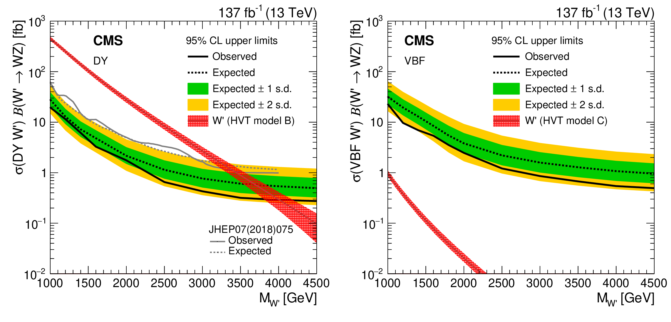
Figure 9:
Expected and observed 95% CL upper limits on the product of the W' production cross section and the $\mathrm{W'} \to W Z $ branching fraction versus the W' mass are shown as dashed and solid black lines, respectively. Green and yellow bands, respectively, represent the 68% and 95% confidence intervals of the expected limit. The red curves show the product of the theoretical W' boson production cross sections and their branching fractions to WZ. The hashed red areas represent the theoretical cross section uncertainty due to limited knowledge of PDFs and scale choices. Limits and theory cross sections for DY-produced W' bosons are shown in the left figure, while the right figure shows the same for VBF-produced W' bosons. The grey curves in the left plot show the previous CMS results with 36 fb$^{-1}$ of data. |
png pdf |
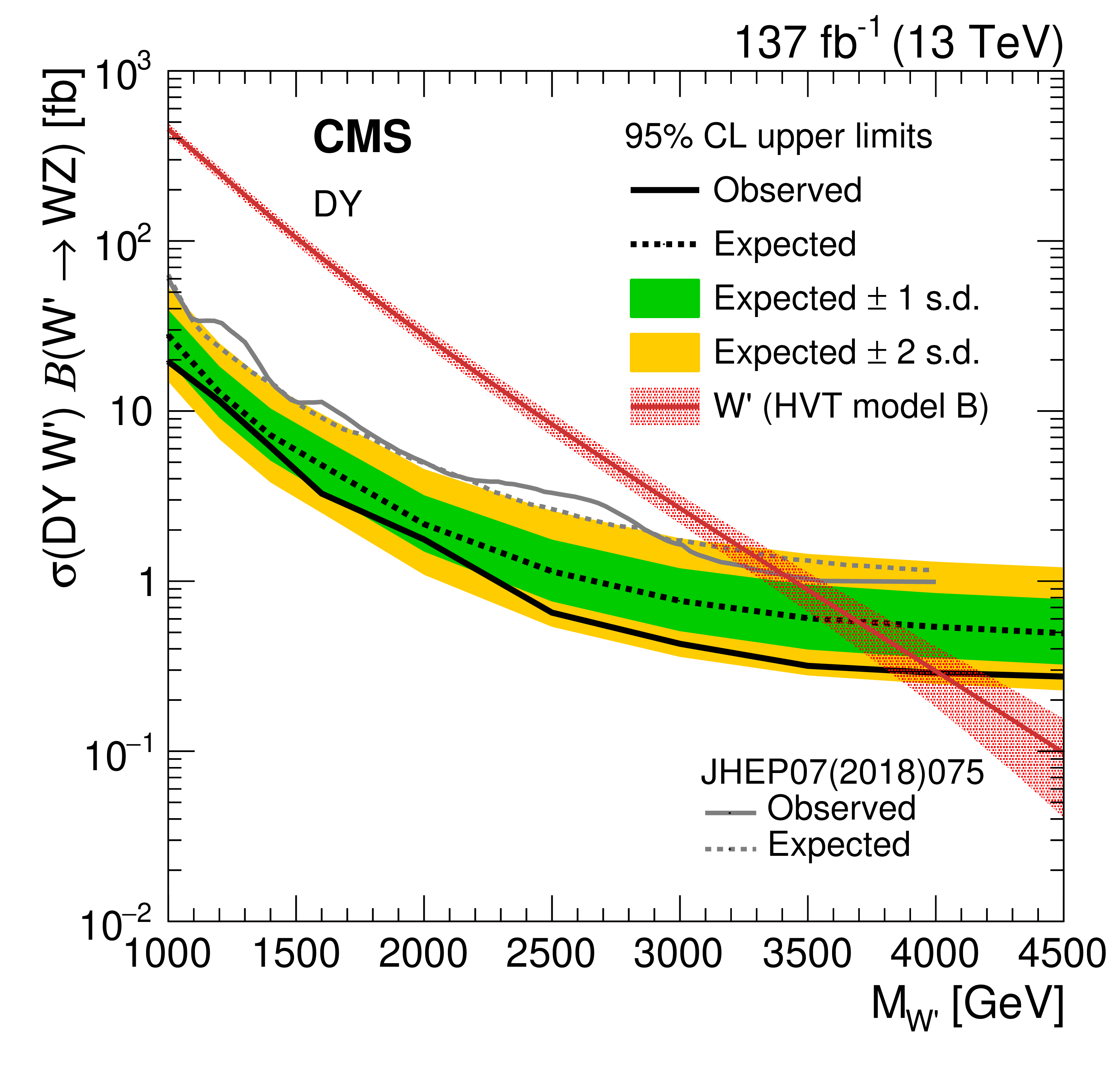
Figure 9-a:
Expected and observed 95% CL upper limits on the product of the W' production cross section and the $\mathrm{W'} \to W Z $ branching fraction versus the W' mass are shown as dashed and solid black lines, respectively. Green and yellow bands, respectively, represent the 68% and 95% confidence intervals of the expected limit. The red curves show the product of the theoretical W' boson production cross sections and their branching fractions to WZ. The hashed red areas represent the theoretical cross section uncertainty due to limited knowledge of PDFs and scale choices. Limits and theory cross sections for DY-produced W' bosons are shown. The grey curves in the left plot show the previous CMS results with 36 fb$^{-1}$ of data. |
png pdf |
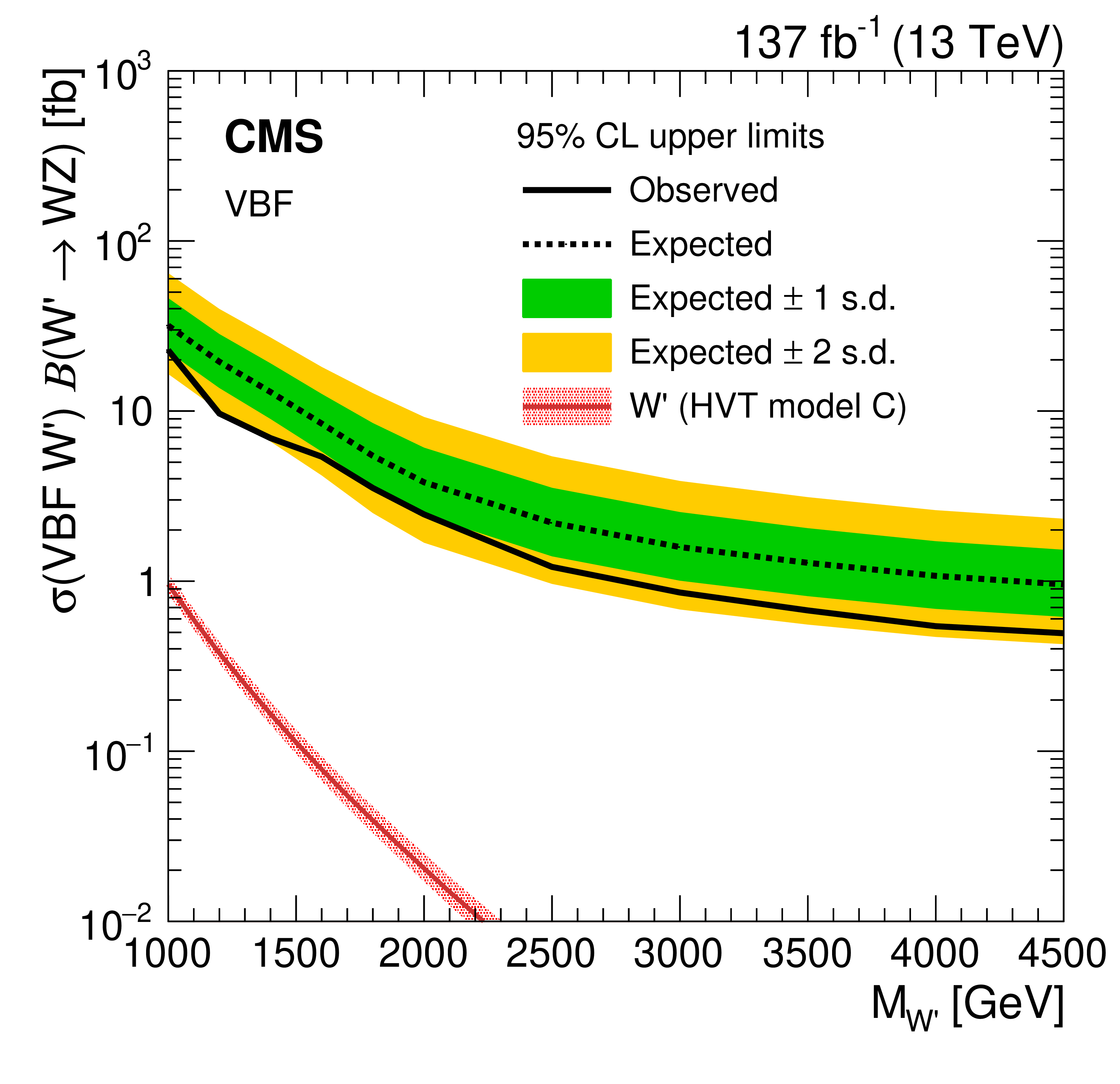
Figure 9-b:
Expected and observed 95% CL upper limits on the product of the W' production cross section and the $\mathrm{W'} \to W Z $ branching fraction versus the W' mass are shown as dashed and solid black lines, respectively. Green and yellow bands, respectively, represent the 68% and 95% confidence intervals of the expected limit. The red curves show the product of the theoretical W' boson production cross sections and their branching fractions to WZ. The hashed red areas represent the theoretical cross section uncertainty due to limited knowledge of PDFs and scale choices. Limits and theory cross sections for VBF-produced W' bosons are shown. The grey curves in the left plot show the previous CMS results with 36 fb$^{-1}$ of data. |
png pdf |
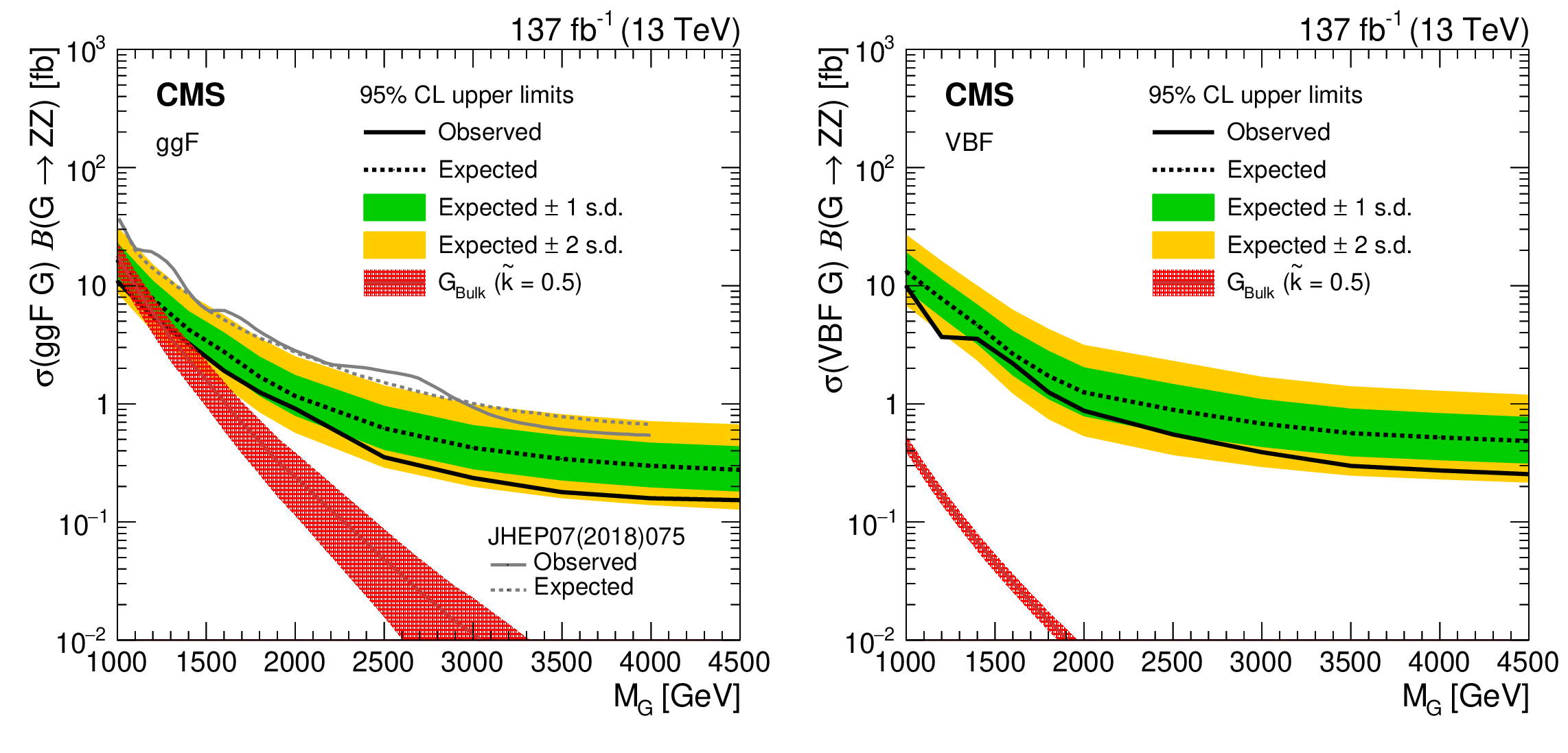
Figure 10:
Expected and observed 95% CL upper limits on the product of the graviton (G) production cross section and the $\mathrm{G} \to \mathrm{ZZ} $ branching fraction versus the graviton mass are shown as dashed and solid black lines, respectively. Green and yellow bands, respectively, represent 68% and 95% confidence intervals of the expected limit. The red curves show the product of the theoretical graviton production cross sections and their branching fractions to ZZ. The hashed red areas represent the theoretical cross section uncertainty due to limited knowledge of PDFs and scale choices. Limits and theory cross sections for ggF-produced gravitons are shown in the left figure, while the right figure shows the same for VBF-produced gravitons. The grey curves in the left plot show the previous CMS results with 36 fb$^{-1}$ of data. |
png pdf |
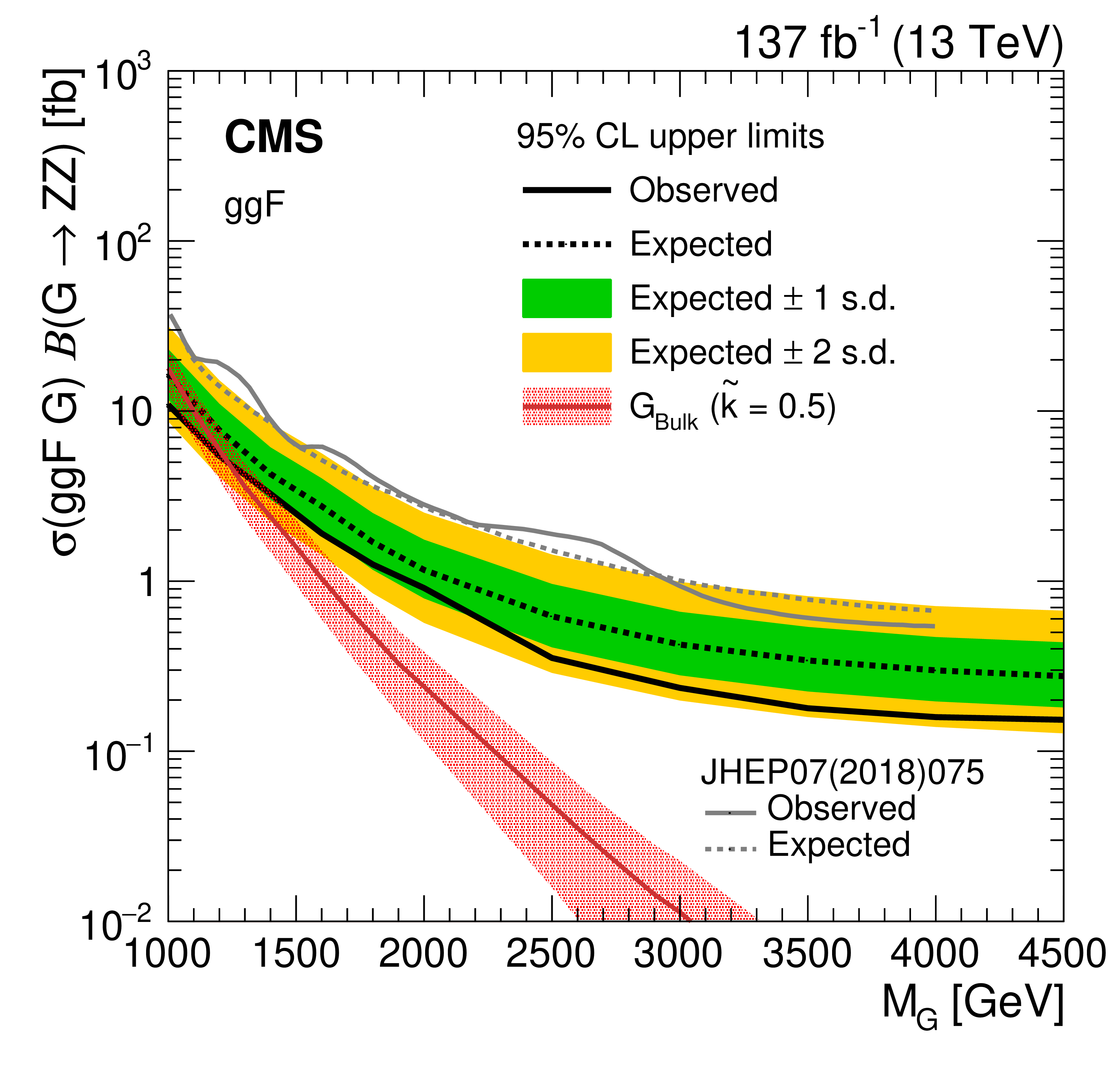
Figure 10-a:
Expected and observed 95% CL upper limits on the product of the graviton (G) production cross section and the $\mathrm{G} \to \mathrm{ZZ} $ branching fraction versus the graviton mass are shown as dashed and solid black lines, respectively. Green and yellow bands, respectively, represent 68% and 95% confidence intervals of the expected limit. The red curves show the product of the theoretical graviton production cross sections and their branching fractions to ZZ. The hashed red areas represent the theoretical cross section uncertainty due to limited knowledge of PDFs and scale choices. |
png pdf |
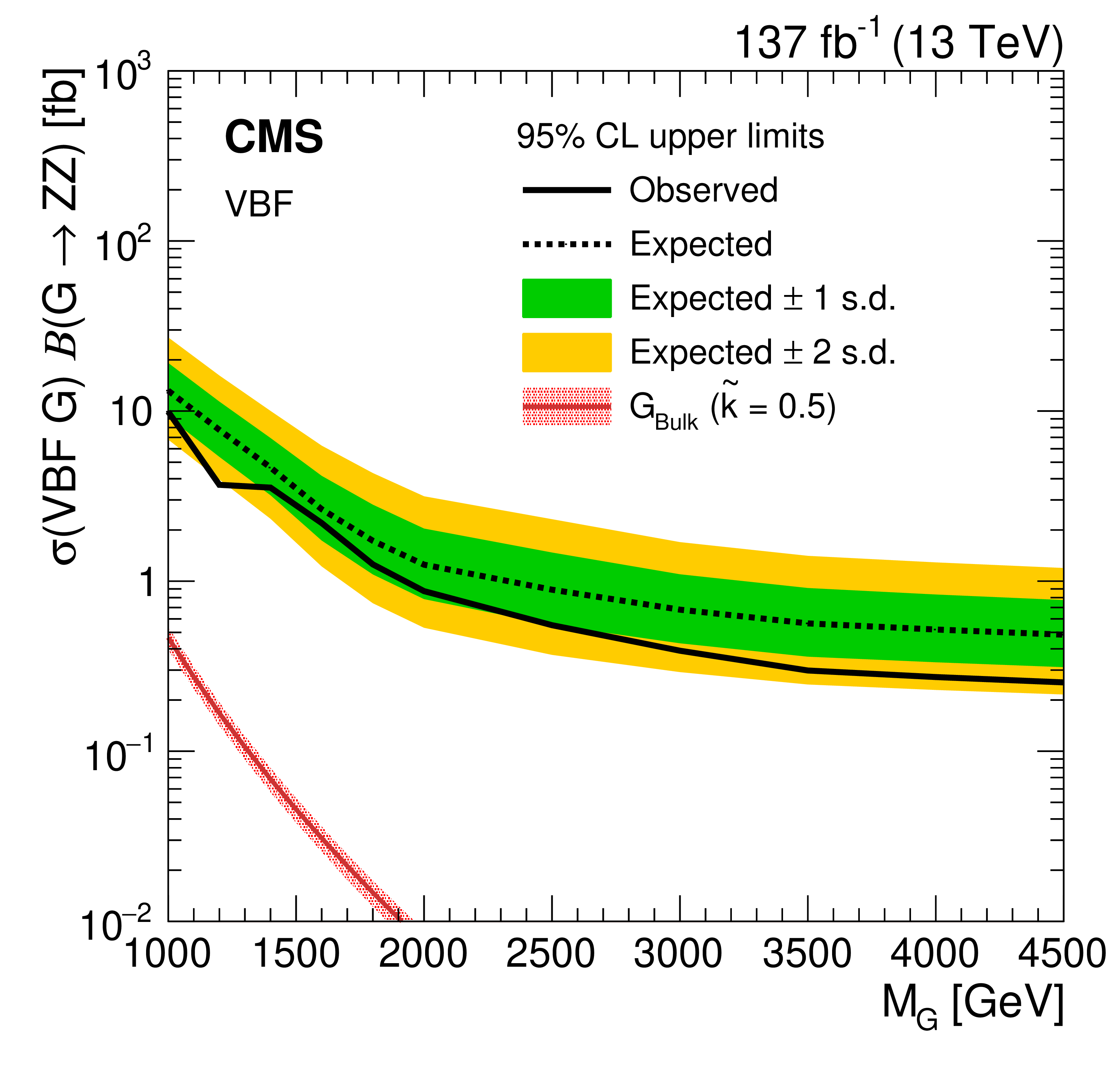
Figure 10-b:
Expected and observed 95% CL upper limits on the product of the graviton (G) production cross section and the $\mathrm{G} \to \mathrm{ZZ} $ branching fraction versus the graviton mass are shown as dashed and solid black lines, respectively. Green and yellow bands, respectively, represent 68% and 95% confidence intervals of the expected limit. The red curves show the product of the theoretical graviton production cross sections and their branching fractions to ZZ. The hashed red areas represent the theoretical cross section uncertainty due to limited knowledge of PDFs and scale choices. |
| Tables | |
png pdf |
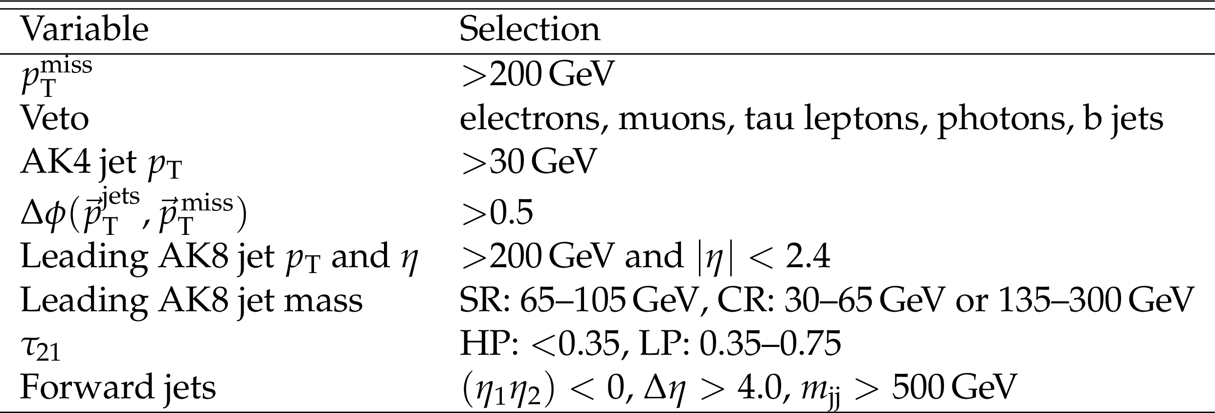
Table 1:
Summary of the event selections. |
png pdf |
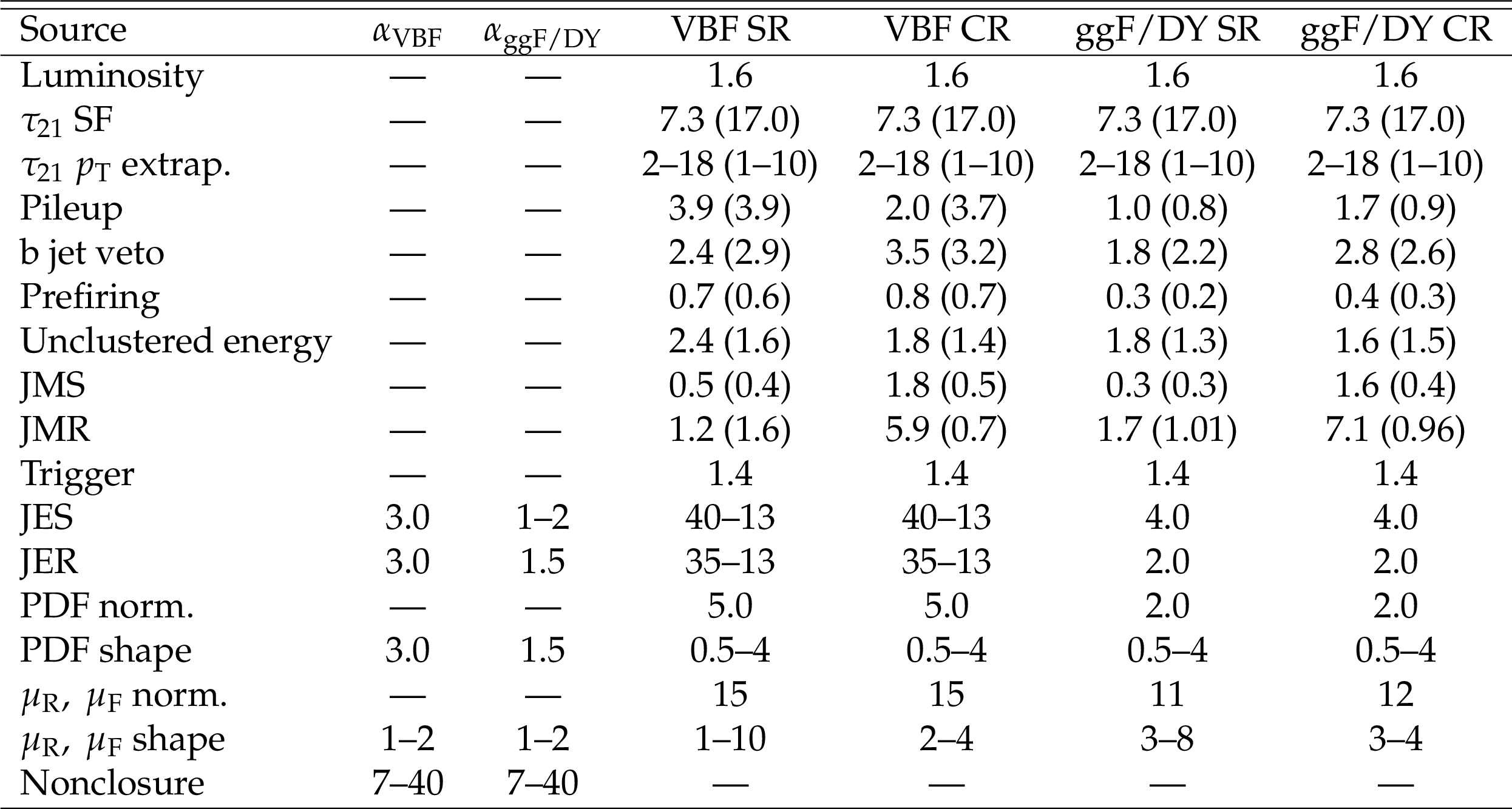
Table 2:
Summary of systematic uncertainties (in %) related to the SM background predictions in various regions. Columns two and three tabulate the representative size of effects on $\alpha $ in the VBF and ggF/DY events categories, respectively. Columns four through seven tabulate the typical size of effects on the prediction of resonant background yields in the VBF SR, VBF CR, ggF/DY SR, and ggF/DY CR, respectively. All of these numbers are the pre-fit values. For some systematic uncertainties, the variation in different ${m_{\mathrm {T}}}$ bins are shown as a range. Values of LP that are different from those of HP are shown in parentheses. |
png pdf |
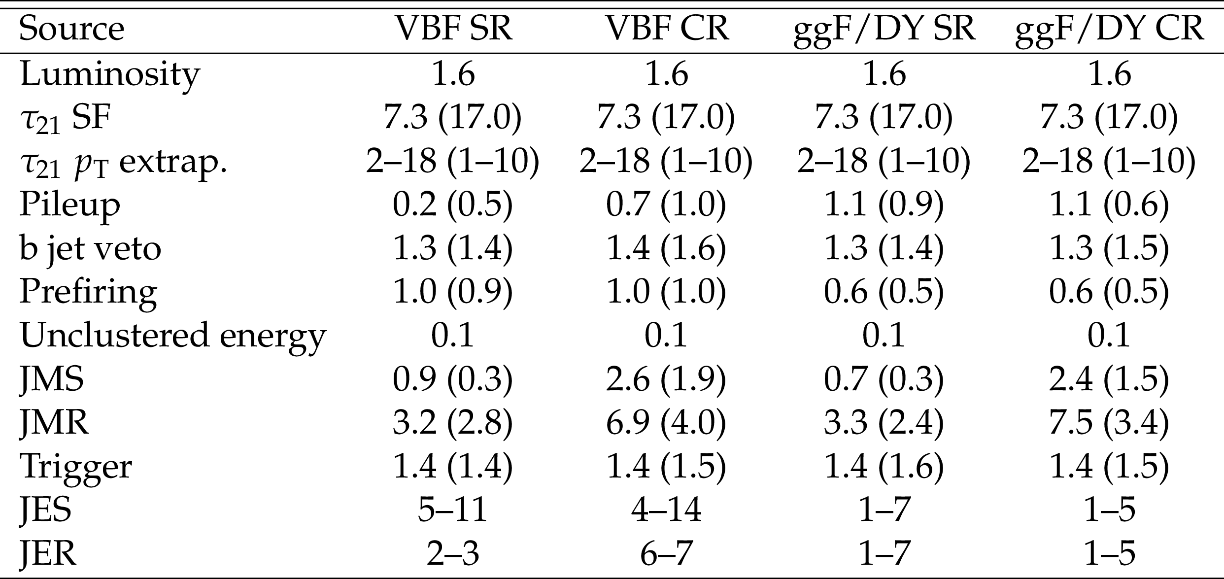
Table 3:
Summary of the typical size of systematic uncertainties (in %) in the predicted signal yields in various regions. All of these numbers are the pre-fit values. A range is given for the shape systematic uncertainties. Values of LP that are different from those of HP are shown in parentheses. |
| Summary |
| A search has been presented for new bosonic states decaying either to a pair of Z bosons or to a W boson and a Z boson. The analyzed final states require large missing transverse momentum and one high-momentum, large-radius jet. Large-radius jets are required to have a mass consistent with either a W or Z boson. Events are categorized based on the presence of large-radius jets passing high-purity and low-purity substructure requirements. Events are also categorized based on the presence or absence of high-momentum jets in the forward region of the detector. Forward jets distinguish weak vector boson fusion (VBF) from other production mechanisms. Contributions from the dominant SM backgrounds are estimated from data control regions using an extrapolation method. No deviation between SM expectation and data is found, and 95% confidence level upper limits are set on the product of the production cross section and branching fraction for several signal models. A lower observed (expected) limit of 3.0 (2.5) TeV is set on the mass of gluon-gluon fusion produced radions. The observed (expected) mass exclusion limit for Drell-Yan produced W' bosons is found to be 4.0 (3.7) TeV. The observed (expected) mass exclusion limit for gluon-gluon fusion produced gravitons is found to be 1.2 (1.1) TeV. At 95% confidence level, upper observed (expected) limits on the product of the VBF production cross section and $\mathrm{X}\to \mathrm{Z}+\mathrm{W}/\mathrm{Z}$ branching fraction range between 0.2 and 20 (0.3 and 30) fb. |
| References | ||||
| 1 | L. Randall and R. Sundrum | Large mass hierarchy from a small extra dimension | PRL 83 (1999) 3370 | hep-ph/9905221 |
| 2 | L. Randall and R. Sundrum | An alternative to compactification | PRL 83 (1999) 4690 | hep-th/9906064 |
| 3 | K. Agashe et al. | LHC signals for warped electroweak charged gauge bosons | PRD 80 (2009) 075007 | 0810.1497 |
| 4 | K. Agashe et al. | LHC signals for coset electroweak gauge bosons in warped/composite pseudo-Goldstone boson Higgs models | PRD 81 (2010) 096002 | 0911.0059 |
| 5 | K. Agashe et al. | CERN LHC signals for warped electroweak neutral gauge bosons | PRD 76 (2007) 115015 | 0709.0007 |
| 6 | D. Pappadopulo, A. Thamm, R. Torre, and A. Wulzer | Heavy vector triplets: Bridging theory and data | JHEP 09 (2014) 060 | 1402.4431 |
| 7 | N. Arkani-Hamed et al. | The minimal moose for a little Higgs | JHEP 08 (2002) 021 | hep-ph/0206020 |
| 8 | N. Arkani-Hamed, A. G. Cohen, E. Katz, and A. E. Nelson | The littlest Higgs | JHEP 07 (2002) 034 | hep-ph/0206021 |
| 9 | G. Burdman, M. Perelstein, and A. Pierce | Large Hadron Collider tests of the little Higgs model | PRL 90 (2003) 241802 | hep-ph/0212228 |
| 10 | K. Agashe, H. Davoudiasl, G. Perez, and A. Soni | Warped gravitons at the CERN LHC and beyond | PRD 76 (2007) 036006 | hep-ph/0701186 |
| 11 | A. L. Fitzpatrick, J. Kaplan, L. Randall, and L.-T. Wang | Searching for the Kaluza-Klein graviton in bulk RS models | JHEP 09 (2007) 013 | hep-ph/0701150 |
| 12 | ATLAS Collaboration | Searches for heavy ZZ and ZW resonances in the $ \ell\ell $qq and $ \nu\nu $qq final states in pp collisions at $ \sqrt{s}= $ 13 TeV with the ATLAS detector | JHEP 03 (2018) 009 | 1708.09638 |
| 13 | CMS Collaboration | Search for a heavy resonance decaying into a Z boson and a vector boson in the $ \nu \overline{\nu}\mathrm{q}\overline{\mathrm{q}} $ final state | JHEP 07 (2018) 075 | CMS-B2G-17-005 1803.03838 |
| 14 | ATLAS Collaboration | Search for heavy diboson resonances in semileptonic final states in pp collisions at $ \sqrt{s}= $ 13 TeV with the ATLAS detector | EPJC 80 (2020) 1165 | 2004.14636 |
| 15 | CMS Collaboration | HEPData record for this analysis | link | |
| 16 | CMS Collaboration | Performance of the CMS Level-1 trigger in proton-proton collisions at $ \sqrt{s} = $ 13 TeV | JINST 15 (2020) P10017 | CMS-TRG-17-001 2006.10165 |
| 17 | CMS Collaboration | The CMS trigger system | JINST 12 (2017) P01020 | CMS-TRG-12-001 1609.02366 |
| 18 | CMS Collaboration | The CMS experiment at the CERN LHC | JINST 3 (2008) S08004 | CMS-00-001 |
| 19 | J. Alwall et al. | The automated computation of tree-level and next-to-leading order differential cross sections, and their matching to parton shower simulations | JHEP 07 (2014) 079 | 1405.0301 |
| 20 | R. Frederix and S. Frixione | Merging meets matching in MC@NLO | JHEP 12 (2012) 061 | 1209.6215 |
| 21 | J. Alwall et al. | Comparative study of various algorithms for the merging of parton showers and matrix elements in hadronic collisions | EPJC 53 (2008) 473 | 0706.2569 |
| 22 | P. Artoisenet, R. Frederix, O. Mattelaer, and R. Rietkerk | Automatic spin-entangled decays of heavy resonances in Monte Carlo simulations | JHEP 03 (2013) 015 | 1212.3460 |
| 23 | P. Nason | A new method for combining NLO QCD with shower Monte Carlo algorithms | JHEP 11 (2004) 040 | hep-ph/0409146 |
| 24 | S. Frixione, P. Nason, and C. Oleari | Matching NLO QCD computations with parton shower simulations: the POWHEG method | JHEP 11 (2007) 070 | 0709.2092 |
| 25 | S. Alioli, P. Nason, C. Oleari, and E. Re | A general framework for implementing NLO calculations in shower Monte Carlo programs: the POWHEG BOX | JHEP 06 (2010) 043 | 1002.2581 |
| 26 | S. Alioli, P. Nason, C. Oleari, and E. Re | NLO single-top production matched with shower in POWHEG: $ s $- and $ t $-channel contributions | JHEP 09 (2009) 111 | 0907.4076 |
| 27 | E. Re | Single-top Wt-channel production matched with parton showers using the POWHEG method | EPJC 71 (2011) 1547 | 1009.2450 |
| 28 | T. Sjostrand et al. | An introduction to PYTHIA 8.2 | CPC 191 (2015) 159 | 1410.3012 |
| 29 | CMS Collaboration | Event generator tunes obtained from underlying event and multiparton scattering measurements | EPJC 76 (2016) 155 | CMS-GEN-14-001 1512.00815 |
| 30 | CMS Collaboration | Extraction and validation of a new set of CMS PYTHIA 8 tunes from underlying-event measurements | EPJC 80 (2020) 4 | CMS-GEN-17-001 1903.12179 |
| 31 | NNPDF Collaboration | Parton distributions for the LHC Run II | JHEP 04 (2015) 040 | 1410.8849 |
| 32 | NNPDF Collaboration | Parton distributions from high-precision collider data | EPJC 77 (2017) 663 | 1706.00428 |
| 33 | GEANT4 Collaboration | GEANT4--a simulation toolkit | NIMA 506 (2003) 250 | |
| 34 | T. Melia, P. Nason, R. Rontsch, and G. Zanderighi | W$ ^+ $W$ ^- $, WZ and ZZ production in the POWHEG BOX | JHEP 11 (2011) 078 | 1107.5051 |
| 35 | M. Beneke, P. Falgari, S. Klein, and C. Schwinn | Hadronic top-quark pair production with NNLL threshold resummation | NPB 855 (2012) 695 | 1109.1536 |
| 36 | M. Cacciari et al. | Top-pair production at hadron colliders with next-to-next-to-leading logarithmic soft-gluon resummation | PLB 710 (2012) 612 | 1111.5869 |
| 37 | P. Barnreuther, M. Czakon, and A. Mitov | Percent-level-precision physics at the Tevatron: Next-to-next-to-leading order QCD corrections to $ \mathrm{q\bar{q}}\to\mathrm{t\bar{t}} $+X | PRL 109 (2012) 132001 | 1204.5201 |
| 38 | M. Czakon and A. Mitov | NNLO corrections to top-pair production at hadron colliders: the all-fermionic scattering channels | JHEP 12 (2012) 054 | 1207.0236 |
| 39 | M. Czakon and A. Mitov | NNLO corrections to top pair production at hadron colliders: the quark-gluon reaction | JHEP 01 (2013) 080 | 1210.6832 |
| 40 | M. Czakon, P. Fiedler, and A. Mitov | Total top-quark pair-production cross section at hadron colliders through $ O({\alpha_S}^4) $ | PRL 110 (2013) 252004 | 1303.6254 |
| 41 | R. Gavin, Y. Li, F. Petriello, and S. Quackenbush | W physics at the LHC with FEWZ 2.1 | CPC 184 (2013) 208 | 1201.5896 |
| 42 | R. Gavin, Y. Li, F. Petriello, and S. Quackenbush | FEWZ 2.0: A code for hadronic Z production at next-to-next-to-leading order | CPC 182 (2011) 2388 | 1011.3540 |
| 43 | J. M. Lindert et al. | Precise predictions for V+jets dark matter backgrounds | EPJC 77 (2017) 829 | 1705.04664 |
| 44 | S. Bolognesi et al. | Spin and parity of a single-produced resonance at the LHC | PRD 86 (2012) 095031 | 1208.4018 |
| 45 | A. Oliveira | Gravity particles from warped extra dimensions, predictions for LHC | 2014 | 1404.0102 |
| 46 | CMS Collaboration | Particle-flow reconstruction and global event description with the CMS detector | JINST 12 (2017) P10003 | CMS-PRF-14-001 1706.04965 |
| 47 | M. Cacciari, G. P. Salam, and G. Soyez | The anti-$ {k_{\mathrm{T}}} $ jet clustering algorithm | JHEP 04 (2008) 063 | 0802.1189 |
| 48 | M. Cacciari, G. P. Salam, and G. Soyez | FastJet user manual | EPJC 72 (2012) 1896 | 1111.6097 |
| 49 | CMS Collaboration | Performance of electron reconstruction and selection with the CMS detector in proton-proton collisions at $ \$ \sqrt{s} = $ $ 8 TeV | JINST 10 (2015) P06005 | CMS-EGM-13-001 1502.02701 |
| 50 | CMS Collaboration | Performance of the CMS muon detector and muon reconstruction with proton-proton collisions at $ \sqrt{s} = $ 13 TeV | JINST 13 (2018) P06015 | CMS-MUO-16-001 1804.04528 |
| 51 | K. Rehermann and B. Tweedie | Efficient identification of boosted semileptonic top quarks at the LHC | JHEP 03 (2011) 059 | 1007.2221 |
| 52 | CMS Collaboration | Performance of photon reconstruction and identification with the CMS detector in proton-proton collisions at $ \sqrt{s} = $ 8 TeV | JINST 10 (2015) P08010 | CMS-EGM-14-001 1502.02702 |
| 53 | CMS Collaboration | Jet energy scale and resolution in the CMS experiment in pp collisions at 8 TeV | JINST 12 (2017) P02014 | CMS-JME-13-004 1607.03663 |
| 54 | D. Bertolini, P. Harris, M. Low, and N. Tran | Pileup per particle identification | JHEP 10 (2014) 059 | 1407.6013 |
| 55 | CMS Collaboration | Pileup mitigation at CMS in 13 TeV data | JINST 15 (2020) P09018 | CMS-JME-18-001 2003.00503 |
| 56 | CMS Collaboration | Jet performance in pp collisions at $ \sqrt{s}= $ 7 TeV | CDS | |
| 57 | CMS Collaboration | Jet algorithms performance in 13 TeV data | CMS-PAS-JME-16-003 | CMS-PAS-JME-16-003 |
| 58 | M. Dasgupta, A. Fregoso, S. Marzani, and G. P. Salam | Towards an understanding of jet substructure | JHEP 09 (2013) 029 | 1307.0007 |
| 59 | A. J. Larkoski, S. Marzani, G. Soyez, and J. Thaler | Soft drop | JHEP 05 (2014) 146 | 1402.2657 |
| 60 | CMS Collaboration | Identification of heavy, energetic, hadronically decaying particles using machine-learning techniques | JINST 15 (Jun, 2020) P06005 | CMS-JME-18-002 2004.08262 |
| 61 | J. Thaler and K. Van Tilburg | Identifying boosted objects with N-subjettiness | JHEP 03 (2011) 015 | 1011.2268 |
| 62 | CMS Collaboration | Identification of heavy-flavour jets with the CMS detector in pp collisions at 13~TeV | JINST 13 (2018) P05011 | CMS-BTV-16-002 1712.07158 |
| 63 | CMS Collaboration | Performance of missing transverse momentum reconstruction in proton-proton collisions at $ \sqrt{s} = $ 13 TeV using the CMS detector | JINST 14 (2019) P07004 | CMS-JME-17-001 1903.06078 |
| 64 | CMS Collaboration | Precision luminosity measurement in proton-proton collisions at $ \sqrt{s} = $ 13 TeV in 2015 and 2016 at CMS | 2021. Accepted by EPJC | CMS-LUM-17-003 2104.01927 |
| 65 | CMS Collaboration | CMS luminosity measurement for the 2017 data-taking period at $ \sqrt{s} = $ 13 TeV | CMS-PAS-LUM-17-004 | CMS-PAS-LUM-17-004 |
| 66 | CMS Collaboration | CMS luminosity measurement for the 2018 data-taking period at $ \sqrt{s} = $ 13 TeV | CMS-PAS-LUM-18-002 | CMS-PAS-LUM-18-002 |
| 67 | P. Vischia | Reporting results in high energy physics publications: A manifesto | Rev. Phys. 5 (2020) 100046 | 1904.11718 |
| 68 | A. L. Read | Presentation of search results: the CLs technique | JPG 28 (2002) 2693 | |
| 69 | G. Cowan, K. Cranmer, E. Gross, and O. Vitells | Asymptotic formulae for likelihood-based tests of new physics | EPJC 71 (2011) 1554 | 1007.1727 |
|
|
Compact Muon Solenoid LHC, CERN |
|

|

|

|

|

|