

Compact Muon Solenoid
LHC, CERN
| CMS-B2G-20-014 ; CERN-EP-2024-016 | ||
| A search for bottom-type vector-like quark pair production in dileptonic and fully hadronic final states in proton-proton collisions at $ \sqrt{s} = $ 13 TeV | ||
| CMS Collaboration | ||
| 21 February 2024 | ||
| Submitted to Phys. Rev. D | ||
| Abstract: A search is described for the production of a pair of bottom-type vector-like quarks (B VLQs) with mass greater than 1000 GeV. Each B VLQ decays into a b quark and a Higgs boson, a b quark and a Z boson, or a t quark and a W boson. This analysis considers both fully hadronic final states and those containing a charged lepton pair from a Z boson decay. The products of the $ \mathrm{H} \to \mathrm{b}\mathrm{b} $ boson decay and of the hadronic Z or W boson decays can be resolved as two distinct jets or merged into a single jet, so the final states are classified by the number of reconstructed jets. The analysis uses data corresponding to an integrated luminosity of 138 fb$ ^{-1} $ collected in proton-proton collisions at $ \sqrt{s} = $ 13 TeV with the CMS detector at the LHC from 2016 to 2018. No excess over the expected background is observed. Lower limits are set on the B VLQ mass at 95% confidence level. These depend on the B VLQ branching fractions and are 1570 and 1540 GeV for 100% $ {\mathrm{B}} \to \mathrm{b}\mathrm{H} $ and 100% $ {\mathrm{B}} \to \mathrm{b}\mathrm{Z} $, respectively. In most cases, the mass limits obtained exceed previous limits by at least 100 GeV. | ||
| Links: e-print arXiv:2402.13808 [hep-ex] (PDF) ; CDS record ; inSPIRE record ; HepData record ; CADI line (restricted) ; | ||
| Figures | |

png pdf |
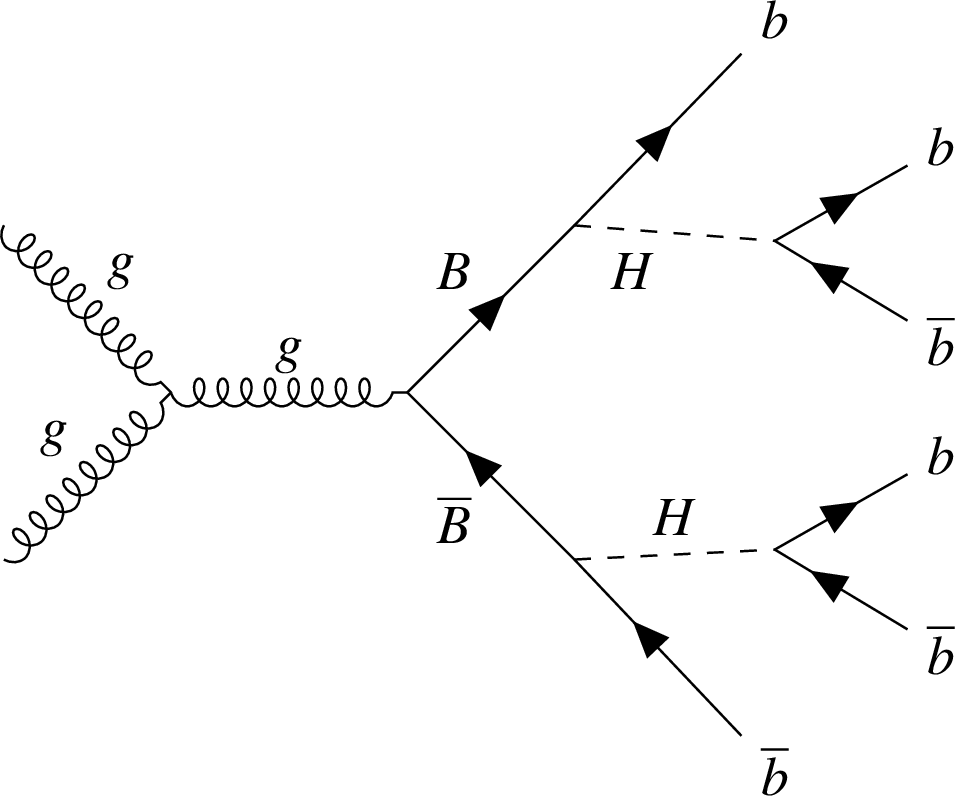
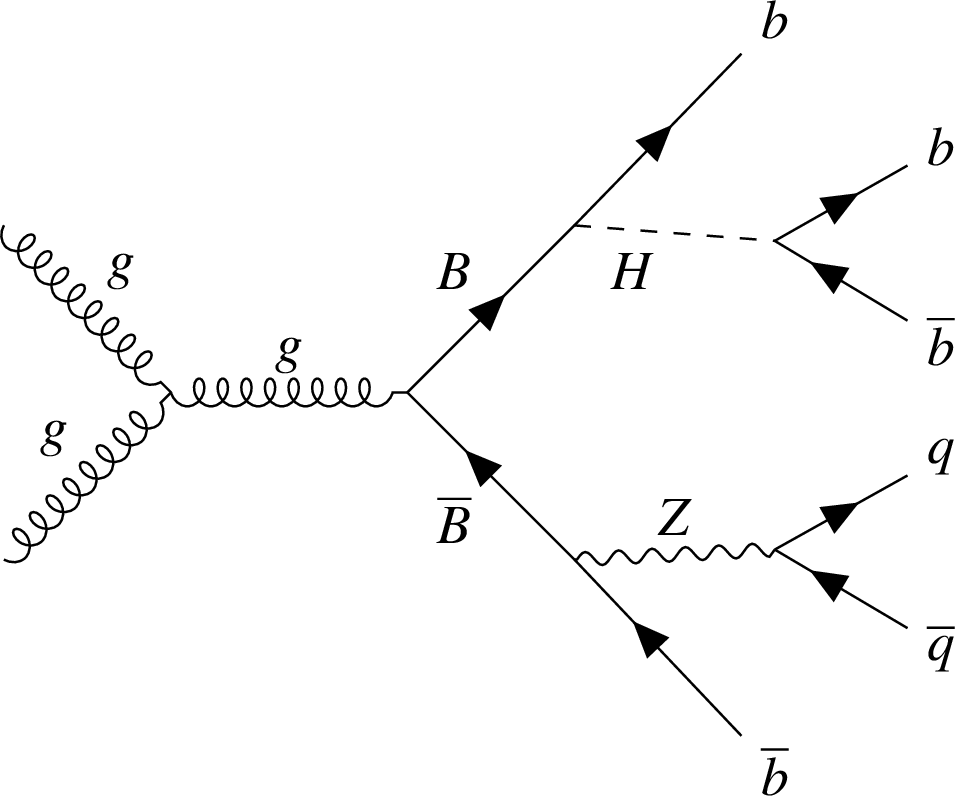
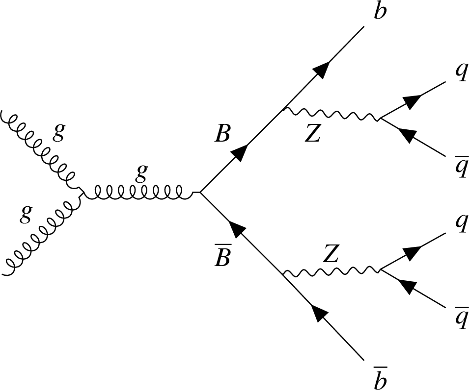
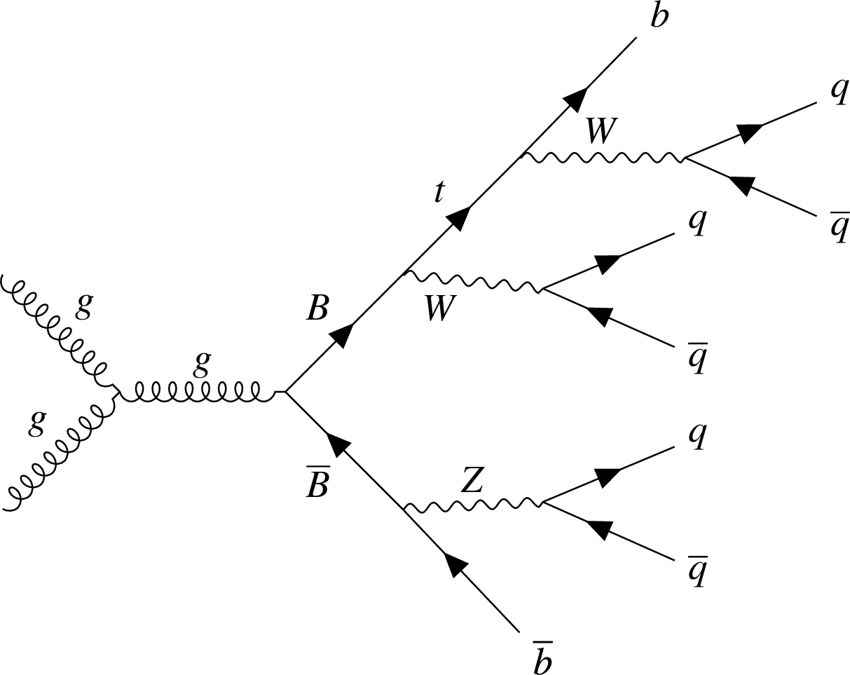
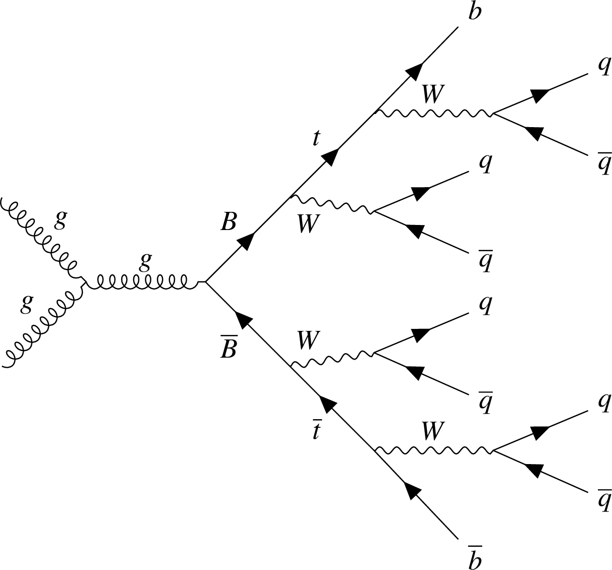
Figure 1:
Feynman diagrams for the pair production of bottom-type VLQs that decay into a b or t quark or antiquark and either a Higgs, Z, or W boson with fully hadronic final states. Upper row: $ \mathrm{b}\mathrm{H}\mathrm{b}\mathrm{H} $ and $ \mathrm{b}\mathrm{H}\mathrm{b}\mathrm{Z} $; middle row: $ \mathrm{b}\mathrm{Z}\mathrm{b}\mathrm{Z} $ and $ \mathrm{b}\mathrm{H}\mathrm{t}\mathrm{W} $; lower row: $ \mathrm{b}\mathrm{Z}\mathrm{t}\mathrm{W} $ and $ \mathrm{t}\mathrm{W}\mathrm{t}\mathrm{W} $. The B and $ \overline{\mathrm{B}} $ can be exchanged in the decays. |
png pdf |
Figure 1-a:
Feynman diagrams for the pair production of bottom-type VLQs that decay into a b or t quark or antiquark and either a Higgs, Z, or W boson with fully hadronic final states. Upper row: $ \mathrm{b}\mathrm{H}\mathrm{b}\mathrm{H} $ and $ \mathrm{b}\mathrm{H}\mathrm{b}\mathrm{Z} $; middle row: $ \mathrm{b}\mathrm{Z}\mathrm{b}\mathrm{Z} $ and $ \mathrm{b}\mathrm{H}\mathrm{t}\mathrm{W} $; lower row: $ \mathrm{b}\mathrm{Z}\mathrm{t}\mathrm{W} $ and $ \mathrm{t}\mathrm{W}\mathrm{t}\mathrm{W} $. The B and $ \overline{\mathrm{B}} $ can be exchanged in the decays. |
png pdf |
Figure 1-b:
Feynman diagrams for the pair production of bottom-type VLQs that decay into a b or t quark or antiquark and either a Higgs, Z, or W boson with fully hadronic final states. Upper row: $ \mathrm{b}\mathrm{H}\mathrm{b}\mathrm{H} $ and $ \mathrm{b}\mathrm{H}\mathrm{b}\mathrm{Z} $; middle row: $ \mathrm{b}\mathrm{Z}\mathrm{b}\mathrm{Z} $ and $ \mathrm{b}\mathrm{H}\mathrm{t}\mathrm{W} $; lower row: $ \mathrm{b}\mathrm{Z}\mathrm{t}\mathrm{W} $ and $ \mathrm{t}\mathrm{W}\mathrm{t}\mathrm{W} $. The B and $ \overline{\mathrm{B}} $ can be exchanged in the decays. |
png pdf |
Figure 1-c:
Feynman diagrams for the pair production of bottom-type VLQs that decay into a b or t quark or antiquark and either a Higgs, Z, or W boson with fully hadronic final states. Upper row: $ \mathrm{b}\mathrm{H}\mathrm{b}\mathrm{H} $ and $ \mathrm{b}\mathrm{H}\mathrm{b}\mathrm{Z} $; middle row: $ \mathrm{b}\mathrm{Z}\mathrm{b}\mathrm{Z} $ and $ \mathrm{b}\mathrm{H}\mathrm{t}\mathrm{W} $; lower row: $ \mathrm{b}\mathrm{Z}\mathrm{t}\mathrm{W} $ and $ \mathrm{t}\mathrm{W}\mathrm{t}\mathrm{W} $. The B and $ \overline{\mathrm{B}} $ can be exchanged in the decays. |

png pdf |
Figure 1-d:
Feynman diagrams for the pair production of bottom-type VLQs that decay into a b or t quark or antiquark and either a Higgs, Z, or W boson with fully hadronic final states. Upper row: $ \mathrm{b}\mathrm{H}\mathrm{b}\mathrm{H} $ and $ \mathrm{b}\mathrm{H}\mathrm{b}\mathrm{Z} $; middle row: $ \mathrm{b}\mathrm{Z}\mathrm{b}\mathrm{Z} $ and $ \mathrm{b}\mathrm{H}\mathrm{t}\mathrm{W} $; lower row: $ \mathrm{b}\mathrm{Z}\mathrm{t}\mathrm{W} $ and $ \mathrm{t}\mathrm{W}\mathrm{t}\mathrm{W} $. The B and $ \overline{\mathrm{B}} $ can be exchanged in the decays. |
png pdf |
Figure 1-e:
Feynman diagrams for the pair production of bottom-type VLQs that decay into a b or t quark or antiquark and either a Higgs, Z, or W boson with fully hadronic final states. Upper row: $ \mathrm{b}\mathrm{H}\mathrm{b}\mathrm{H} $ and $ \mathrm{b}\mathrm{H}\mathrm{b}\mathrm{Z} $; middle row: $ \mathrm{b}\mathrm{Z}\mathrm{b}\mathrm{Z} $ and $ \mathrm{b}\mathrm{H}\mathrm{t}\mathrm{W} $; lower row: $ \mathrm{b}\mathrm{Z}\mathrm{t}\mathrm{W} $ and $ \mathrm{t}\mathrm{W}\mathrm{t}\mathrm{W} $. The B and $ \overline{\mathrm{B}} $ can be exchanged in the decays. |
png pdf |
Figure 1-f:
Feynman diagrams for the pair production of bottom-type VLQs that decay into a b or t quark or antiquark and either a Higgs, Z, or W boson with fully hadronic final states. Upper row: $ \mathrm{b}\mathrm{H}\mathrm{b}\mathrm{H} $ and $ \mathrm{b}\mathrm{H}\mathrm{b}\mathrm{Z} $; middle row: $ \mathrm{b}\mathrm{Z}\mathrm{b}\mathrm{Z} $ and $ \mathrm{b}\mathrm{H}\mathrm{t}\mathrm{W} $; lower row: $ \mathrm{b}\mathrm{Z}\mathrm{t}\mathrm{W} $ and $ \mathrm{t}\mathrm{W}\mathrm{t}\mathrm{W} $. The B and $ \overline{\mathrm{B}} $ can be exchanged in the decays. |
png pdf |
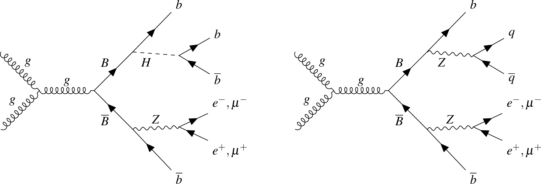
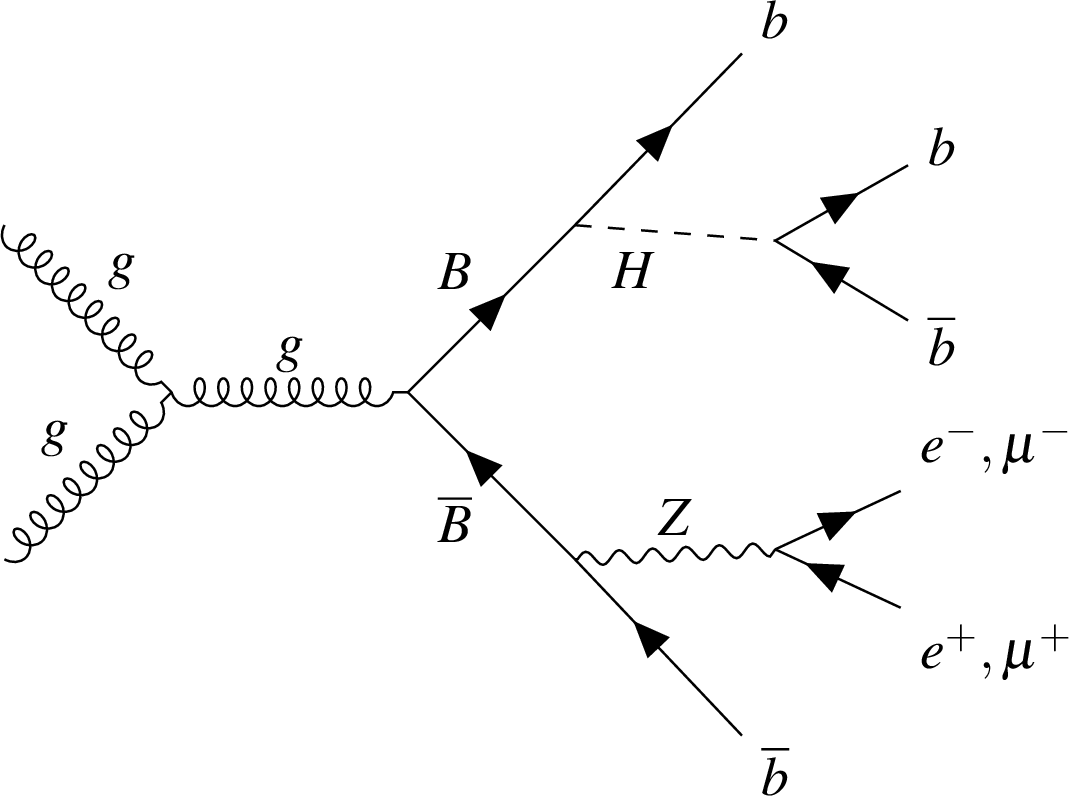
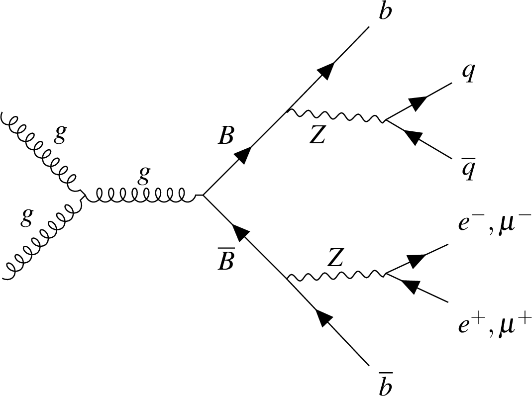
Figure 2:
Feynman diagrams of the pair production of bottom-type VLQ quarks that decay into a b quark or antiquark and either a Higgs or Z boson with a dilepton final state: $ \mathrm{b}\mathrm{H}\mathrm{b}\mathrm{Z} $ mode (left) and $ \mathrm{b}\mathrm{Z}\mathrm{b}\mathrm{Z} $ mode (right). The B and $ \overline{\mathrm{B}} $ can be exchanged in the decays. |
png pdf |
Figure 2-a:
Feynman diagrams of the pair production of bottom-type VLQ quarks that decay into a b quark or antiquark and either a Higgs or Z boson with a dilepton final state: $ \mathrm{b}\mathrm{H}\mathrm{b}\mathrm{Z} $ mode (left) and $ \mathrm{b}\mathrm{Z}\mathrm{b}\mathrm{Z} $ mode (right). The B and $ \overline{\mathrm{B}} $ can be exchanged in the decays. |
png pdf |
Figure 2-b:
Feynman diagrams of the pair production of bottom-type VLQ quarks that decay into a b quark or antiquark and either a Higgs or Z boson with a dilepton final state: $ \mathrm{b}\mathrm{H}\mathrm{b}\mathrm{Z} $ mode (left) and $ \mathrm{b}\mathrm{Z}\mathrm{b}\mathrm{Z} $ mode (right). The B and $ \overline{\mathrm{B}} $ can be exchanged in the decays. |
png pdf |
Figure 3:
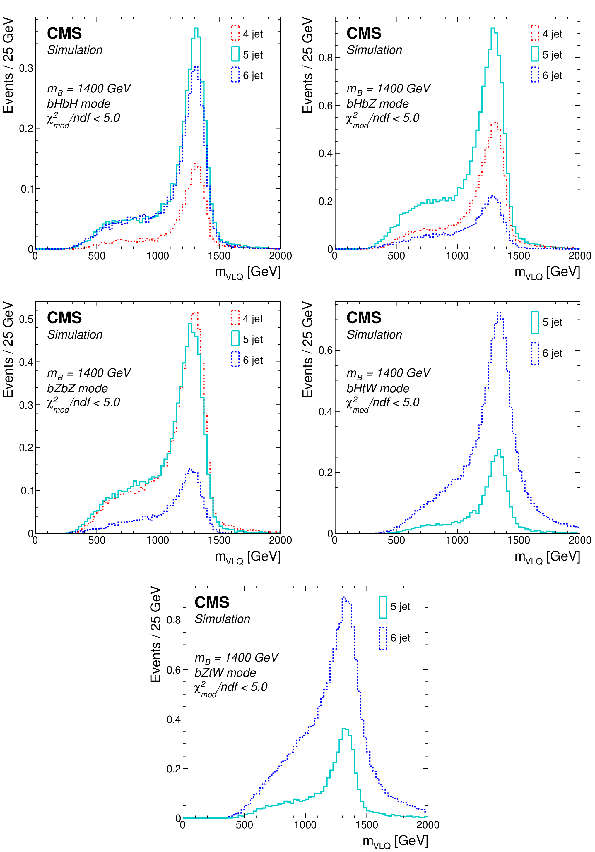
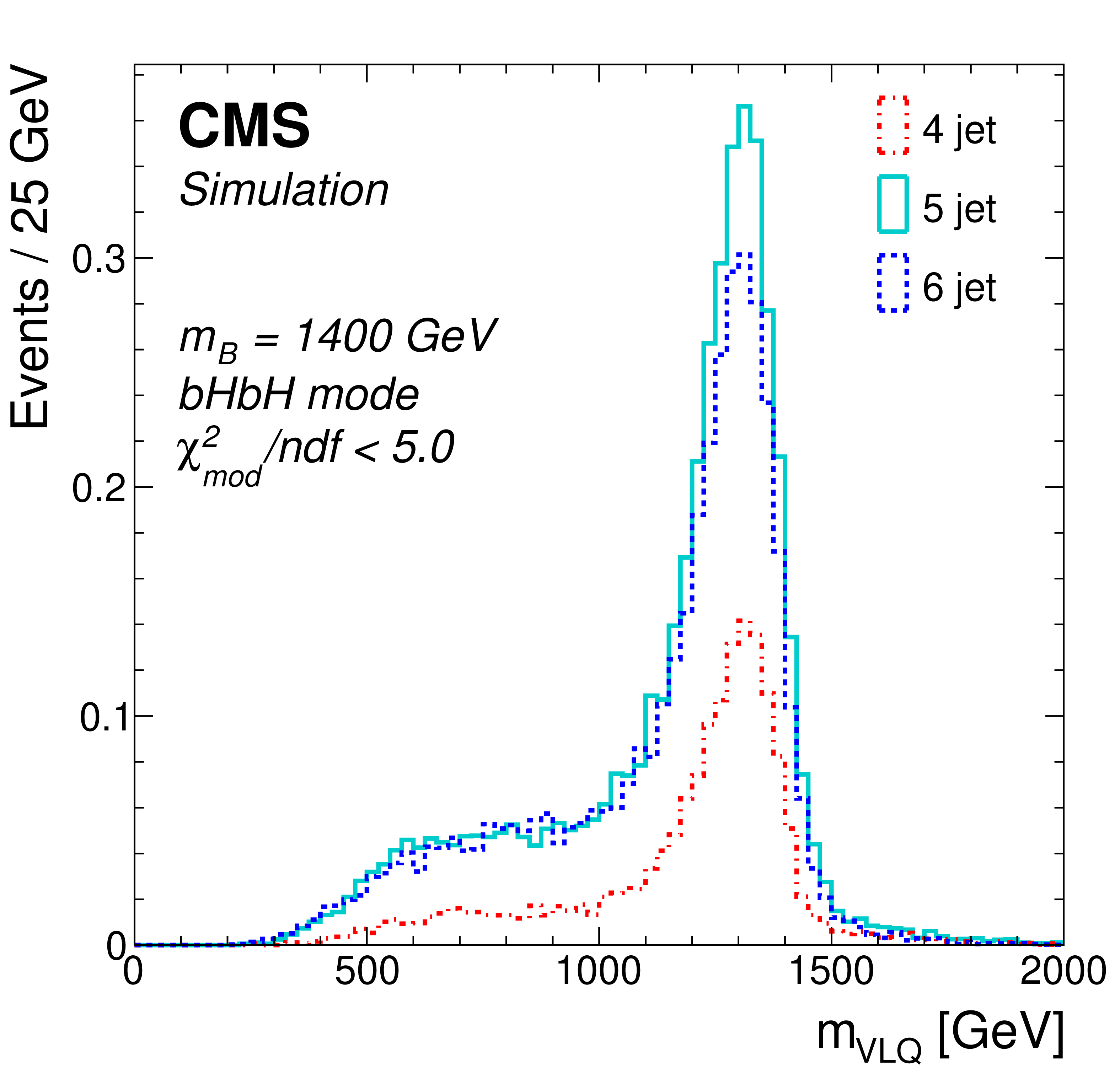
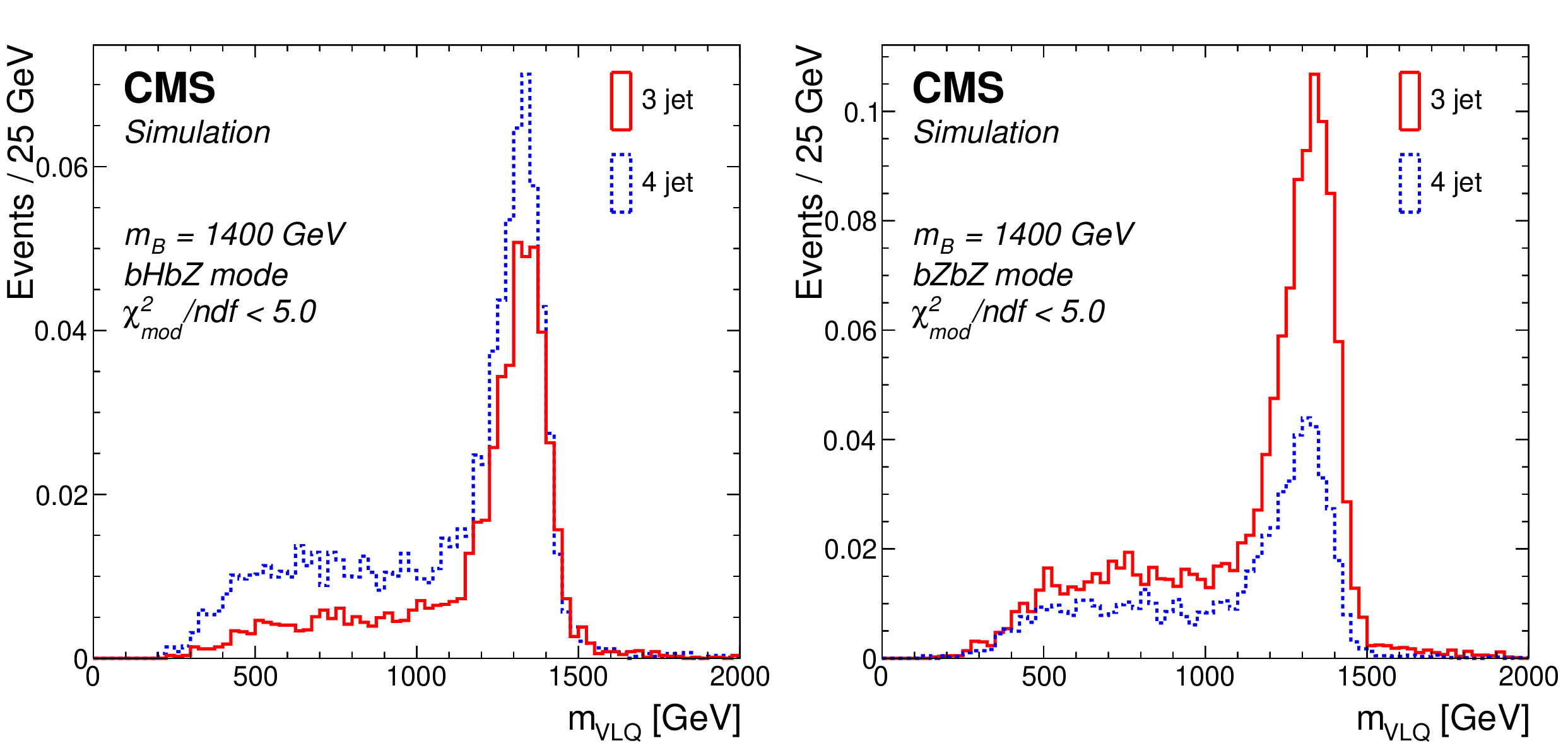
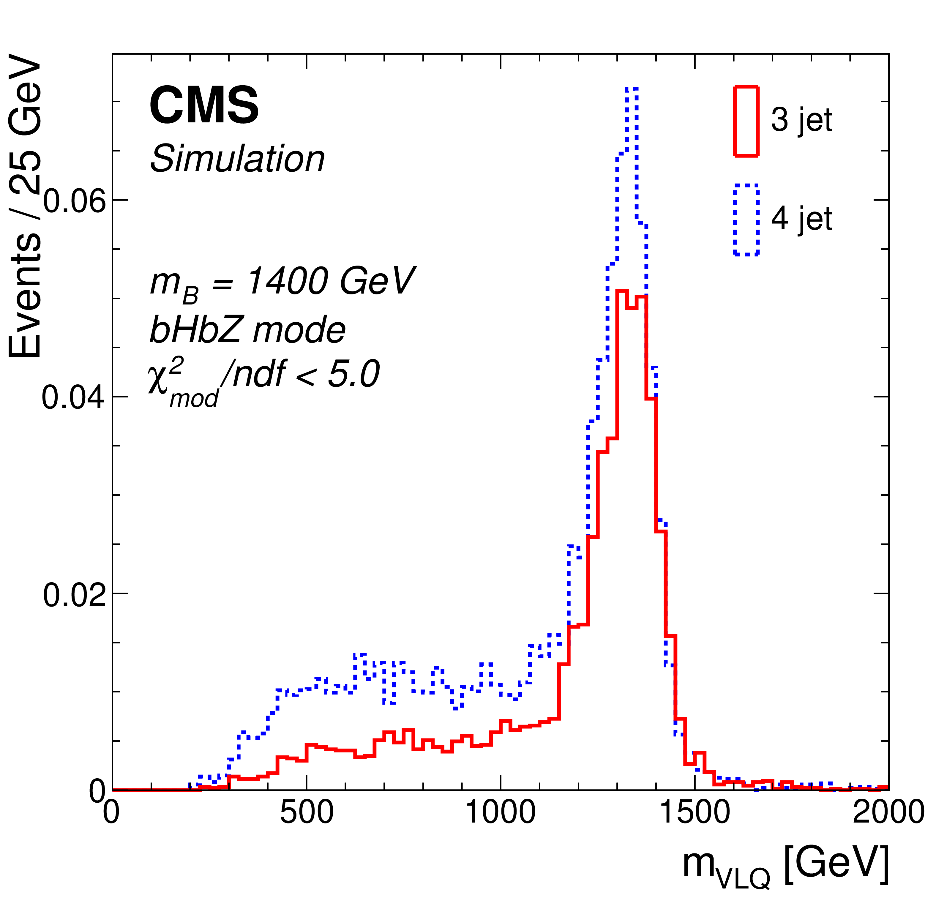
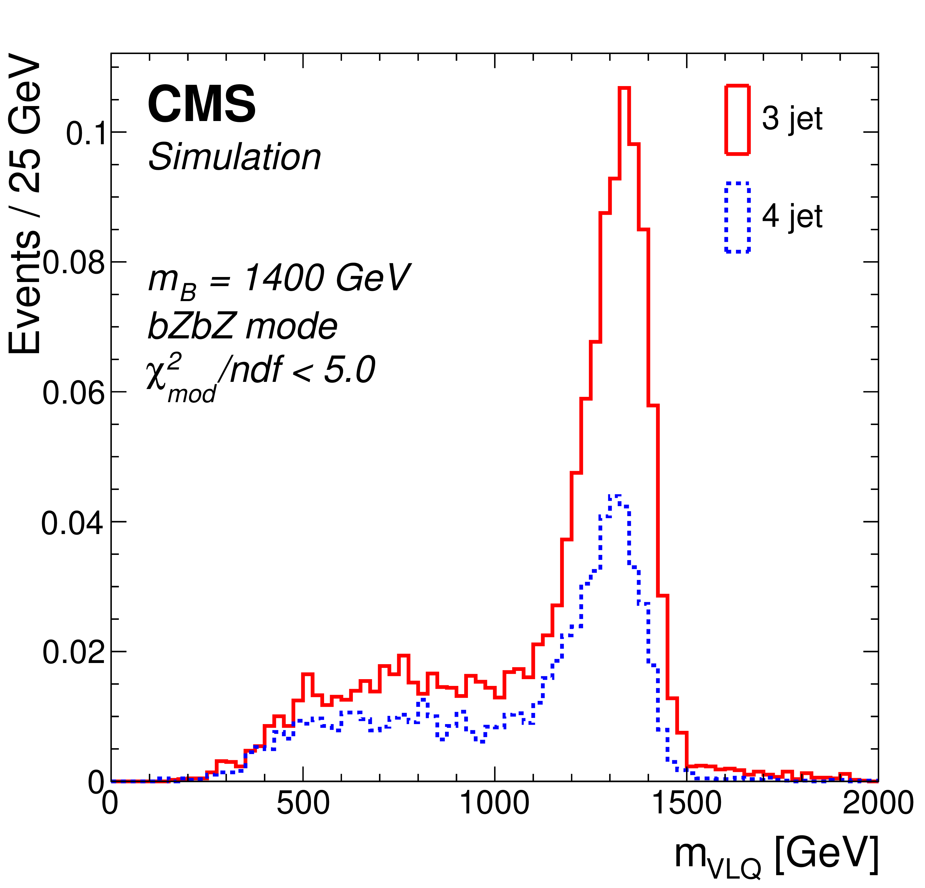
Reconstructed VLQ mass distributions for simulated events for the channels in the fully hadronic category with $ m_{{\mathrm{B}}} = $ 1400 GeV. Upper row: Channels in the $ \mathrm{b}\mathrm{H}\mathrm{b}\mathrm{H} $ (left) and $ \mathrm{b}\mathrm{H}\mathrm{b}\mathrm{Z} $ (right) decay mode. Middle row: Channels in the $ \mathrm{b}\mathrm{Z}\mathrm{b}\mathrm{Z} $ (left) and $ \mathrm{b}\mathrm{H}\mathrm{t}\mathrm{W} $ (right) decay mode. Lower row: Channels in the $ \mathrm{b}\mathrm{Z}\mathrm{t}\mathrm{W} $ decay mode. The different colors indicate the different jet multiplicities. A selection of $ \chi^2_\text{mod}/\text{ndf} < $ 5 has been applied. The values represent the expected number of events over the background in the 2016--2018 data sample. |
png pdf |
Figure 3-a:
Reconstructed VLQ mass distributions for simulated events for the channels in the fully hadronic category with $ m_{{\mathrm{B}}} = $ 1400 GeV. Upper row: Channels in the $ \mathrm{b}\mathrm{H}\mathrm{b}\mathrm{H} $ (left) and $ \mathrm{b}\mathrm{H}\mathrm{b}\mathrm{Z} $ (right) decay mode. Middle row: Channels in the $ \mathrm{b}\mathrm{Z}\mathrm{b}\mathrm{Z} $ (left) and $ \mathrm{b}\mathrm{H}\mathrm{t}\mathrm{W} $ (right) decay mode. Lower row: Channels in the $ \mathrm{b}\mathrm{Z}\mathrm{t}\mathrm{W} $ decay mode. The different colors indicate the different jet multiplicities. A selection of $ \chi^2_\text{mod}/\text{ndf} < $ 5 has been applied. The values represent the expected number of events over the background in the 2016--2018 data sample. |

png pdf |
Figure 3-b:
Reconstructed VLQ mass distributions for simulated events for the channels in the fully hadronic category with $ m_{{\mathrm{B}}} = $ 1400 GeV. Upper row: Channels in the $ \mathrm{b}\mathrm{H}\mathrm{b}\mathrm{H} $ (left) and $ \mathrm{b}\mathrm{H}\mathrm{b}\mathrm{Z} $ (right) decay mode. Middle row: Channels in the $ \mathrm{b}\mathrm{Z}\mathrm{b}\mathrm{Z} $ (left) and $ \mathrm{b}\mathrm{H}\mathrm{t}\mathrm{W} $ (right) decay mode. Lower row: Channels in the $ \mathrm{b}\mathrm{Z}\mathrm{t}\mathrm{W} $ decay mode. The different colors indicate the different jet multiplicities. A selection of $ \chi^2_\text{mod}/\text{ndf} < $ 5 has been applied. The values represent the expected number of events over the background in the 2016--2018 data sample. |
png pdf |
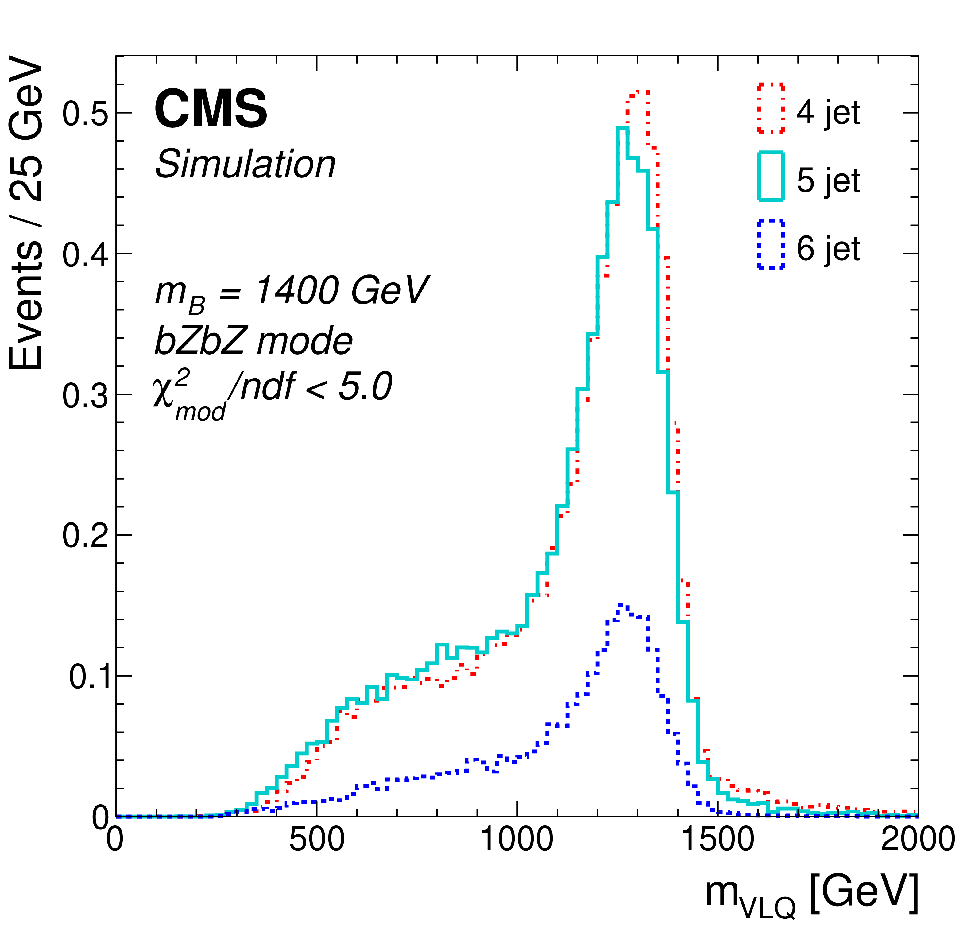
Figure 3-c:
Reconstructed VLQ mass distributions for simulated events for the channels in the fully hadronic category with $ m_{{\mathrm{B}}} = $ 1400 GeV. Upper row: Channels in the $ \mathrm{b}\mathrm{H}\mathrm{b}\mathrm{H} $ (left) and $ \mathrm{b}\mathrm{H}\mathrm{b}\mathrm{Z} $ (right) decay mode. Middle row: Channels in the $ \mathrm{b}\mathrm{Z}\mathrm{b}\mathrm{Z} $ (left) and $ \mathrm{b}\mathrm{H}\mathrm{t}\mathrm{W} $ (right) decay mode. Lower row: Channels in the $ \mathrm{b}\mathrm{Z}\mathrm{t}\mathrm{W} $ decay mode. The different colors indicate the different jet multiplicities. A selection of $ \chi^2_\text{mod}/\text{ndf} < $ 5 has been applied. The values represent the expected number of events over the background in the 2016--2018 data sample. |

png pdf |
Figure 3-d:
Reconstructed VLQ mass distributions for simulated events for the channels in the fully hadronic category with $ m_{{\mathrm{B}}} = $ 1400 GeV. Upper row: Channels in the $ \mathrm{b}\mathrm{H}\mathrm{b}\mathrm{H} $ (left) and $ \mathrm{b}\mathrm{H}\mathrm{b}\mathrm{Z} $ (right) decay mode. Middle row: Channels in the $ \mathrm{b}\mathrm{Z}\mathrm{b}\mathrm{Z} $ (left) and $ \mathrm{b}\mathrm{H}\mathrm{t}\mathrm{W} $ (right) decay mode. Lower row: Channels in the $ \mathrm{b}\mathrm{Z}\mathrm{t}\mathrm{W} $ decay mode. The different colors indicate the different jet multiplicities. A selection of $ \chi^2_\text{mod}/\text{ndf} < $ 5 has been applied. The values represent the expected number of events over the background in the 2016--2018 data sample. |
png pdf |
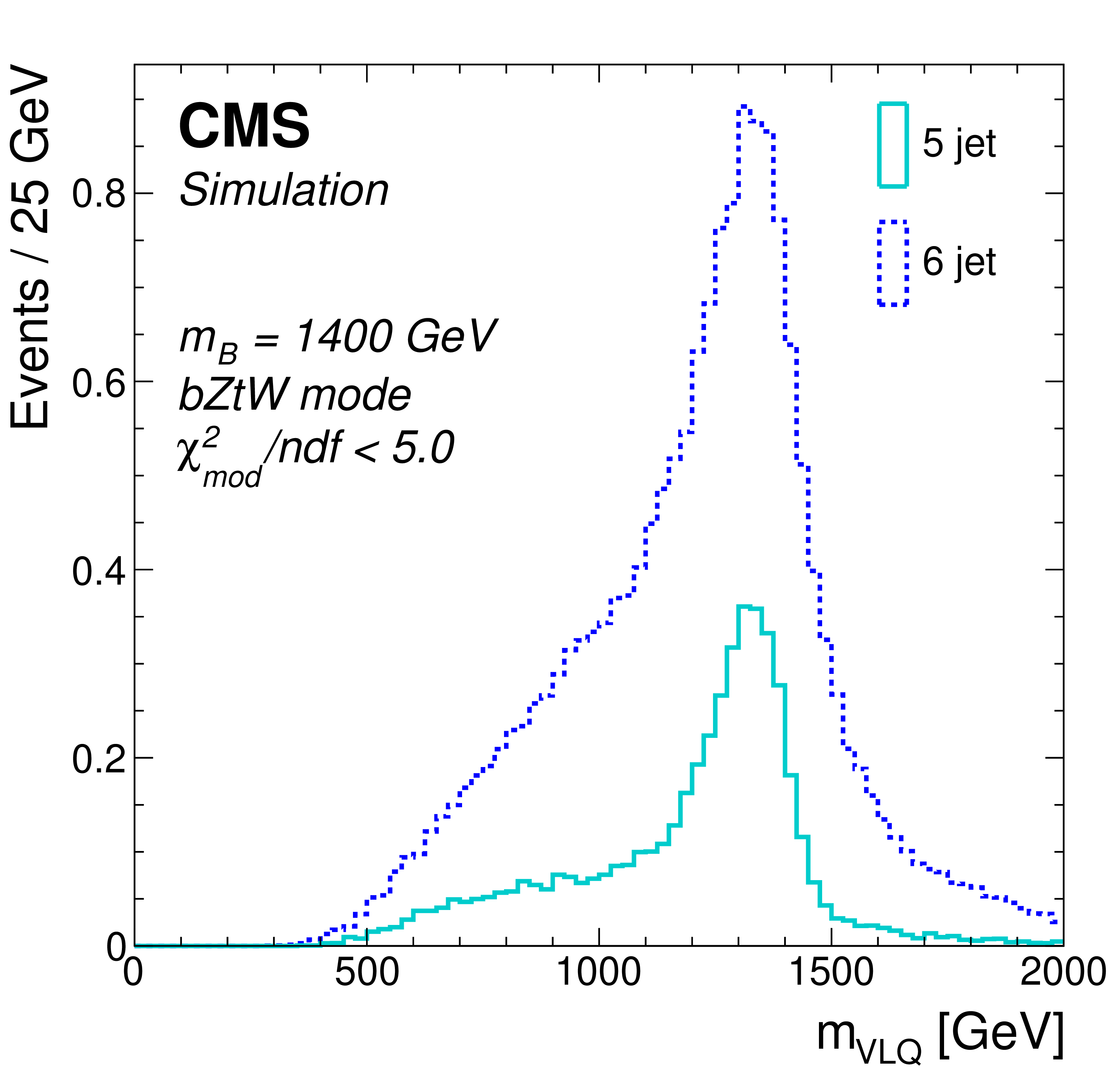
Figure 3-e:
Reconstructed VLQ mass distributions for simulated events for the channels in the fully hadronic category with $ m_{{\mathrm{B}}} = $ 1400 GeV. Upper row: Channels in the $ \mathrm{b}\mathrm{H}\mathrm{b}\mathrm{H} $ (left) and $ \mathrm{b}\mathrm{H}\mathrm{b}\mathrm{Z} $ (right) decay mode. Middle row: Channels in the $ \mathrm{b}\mathrm{Z}\mathrm{b}\mathrm{Z} $ (left) and $ \mathrm{b}\mathrm{H}\mathrm{t}\mathrm{W} $ (right) decay mode. Lower row: Channels in the $ \mathrm{b}\mathrm{Z}\mathrm{t}\mathrm{W} $ decay mode. The different colors indicate the different jet multiplicities. A selection of $ \chi^2_\text{mod}/\text{ndf} < $ 5 has been applied. The values represent the expected number of events over the background in the 2016--2018 data sample. |
png pdf |
Figure 4:
Reconstructed VLQ mass distributions for simulated events passing the b tag requirement for the channels in the dileptonic category with $ m_{{\mathrm{B}}} = $ 1400 GeV in the $ \mathrm{b}\mathrm{H}\mathrm{b}\mathrm{Z} $ (left) and $ \mathrm{b}\mathrm{Z}\mathrm{b}\mathrm{Z} $ (right) event modes. A selection of $ \chi^2_\text{mod}/\text{ndf} < $ 5 has been applied. The values represent the expected number of events over the background in the 2016--2018 data sample. |
png pdf |
Figure 4-a:
Reconstructed VLQ mass distributions for simulated events passing the b tag requirement for the channels in the dileptonic category with $ m_{{\mathrm{B}}} = $ 1400 GeV in the $ \mathrm{b}\mathrm{H}\mathrm{b}\mathrm{Z} $ (left) and $ \mathrm{b}\mathrm{Z}\mathrm{b}\mathrm{Z} $ (right) event modes. A selection of $ \chi^2_\text{mod}/\text{ndf} < $ 5 has been applied. The values represent the expected number of events over the background in the 2016--2018 data sample. |
png pdf |
Figure 4-b:
Reconstructed VLQ mass distributions for simulated events passing the b tag requirement for the channels in the dileptonic category with $ m_{{\mathrm{B}}} = $ 1400 GeV in the $ \mathrm{b}\mathrm{H}\mathrm{b}\mathrm{Z} $ (left) and $ \mathrm{b}\mathrm{Z}\mathrm{b}\mathrm{Z} $ (right) event modes. A selection of $ \chi^2_\text{mod}/\text{ndf} < $ 5 has been applied. The values represent the expected number of events over the background in the 2016--2018 data sample. |
png pdf |
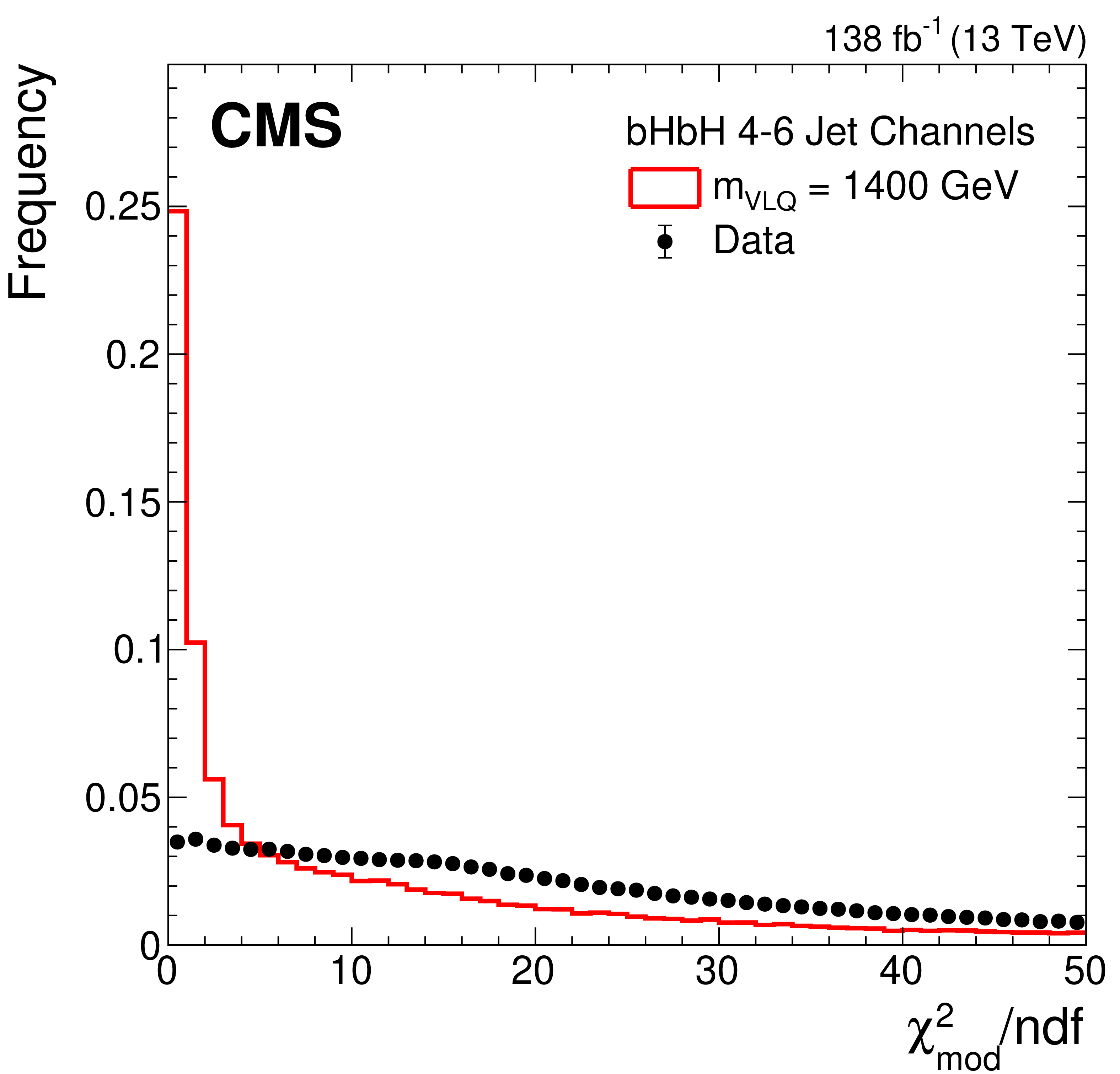
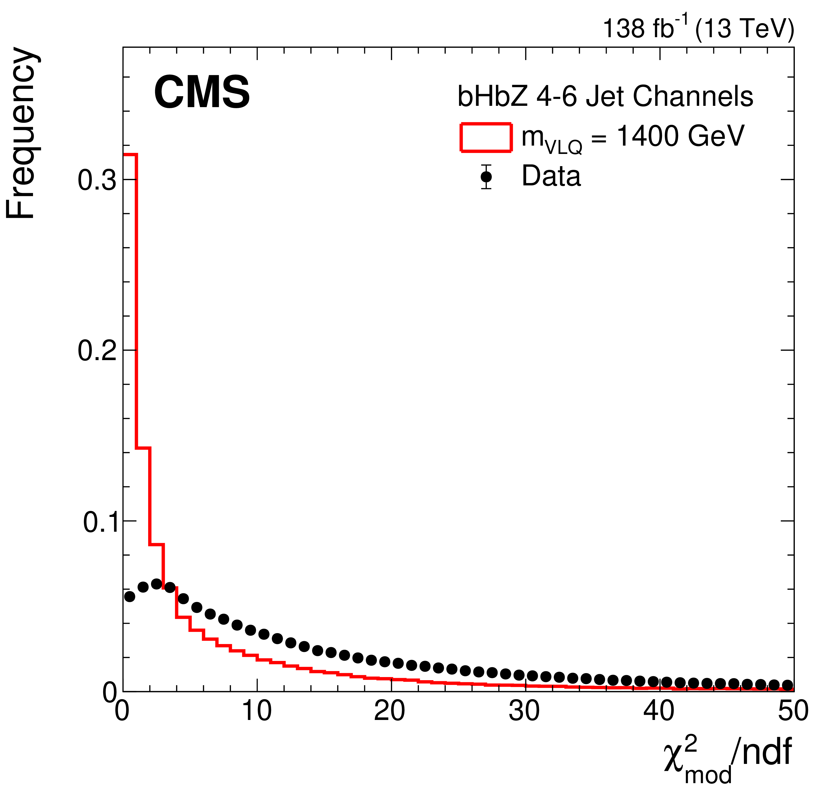
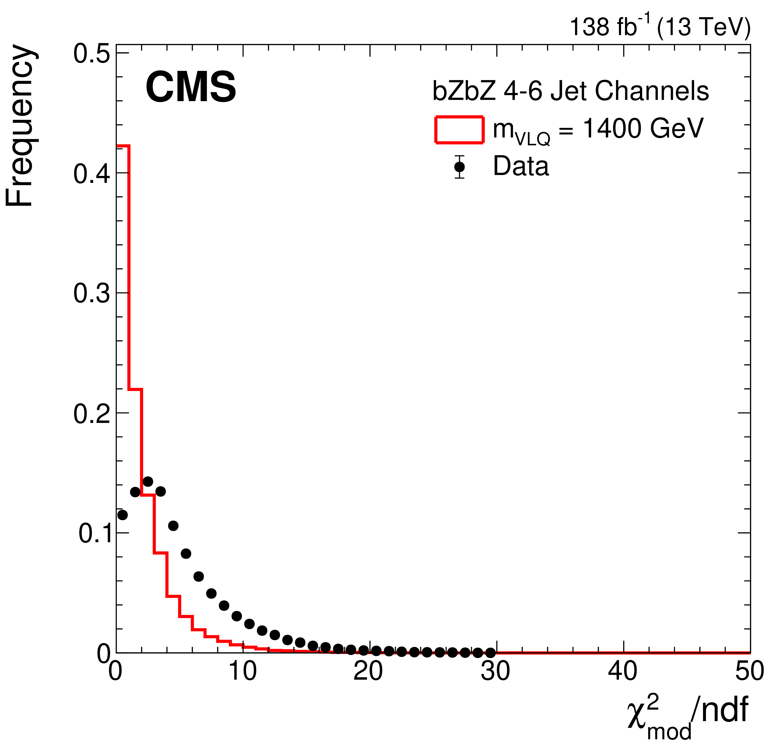
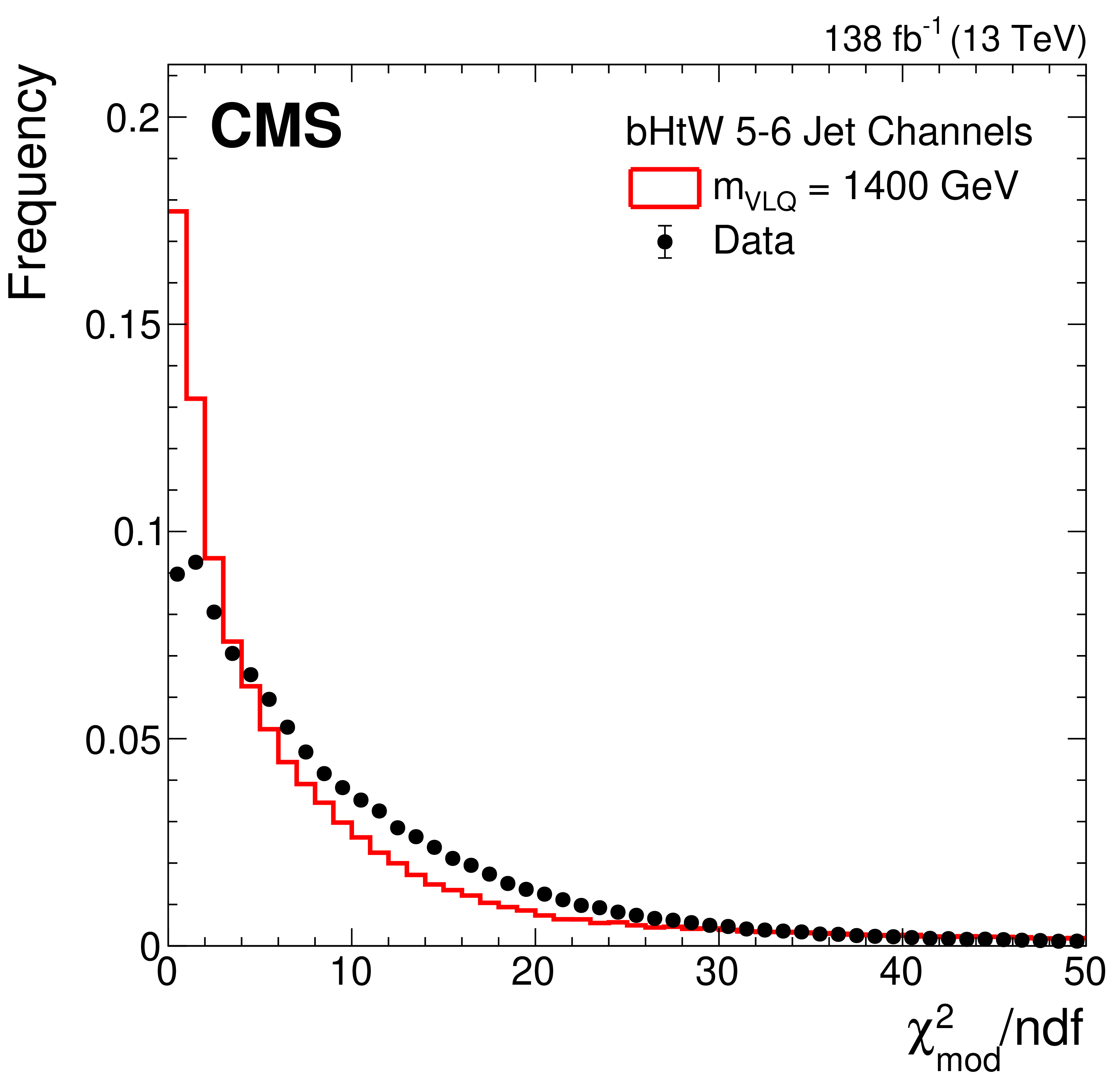
Figure 5:
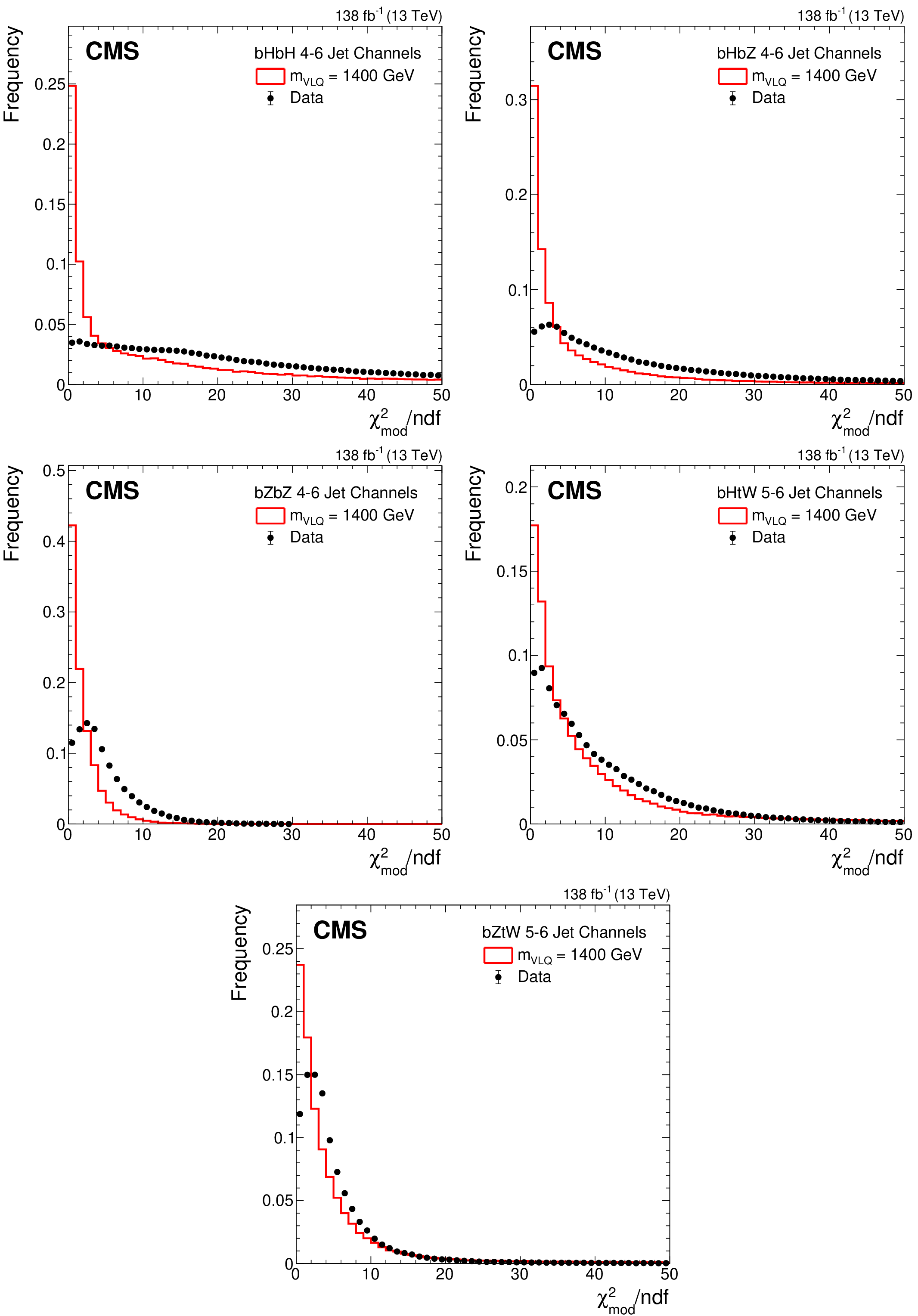
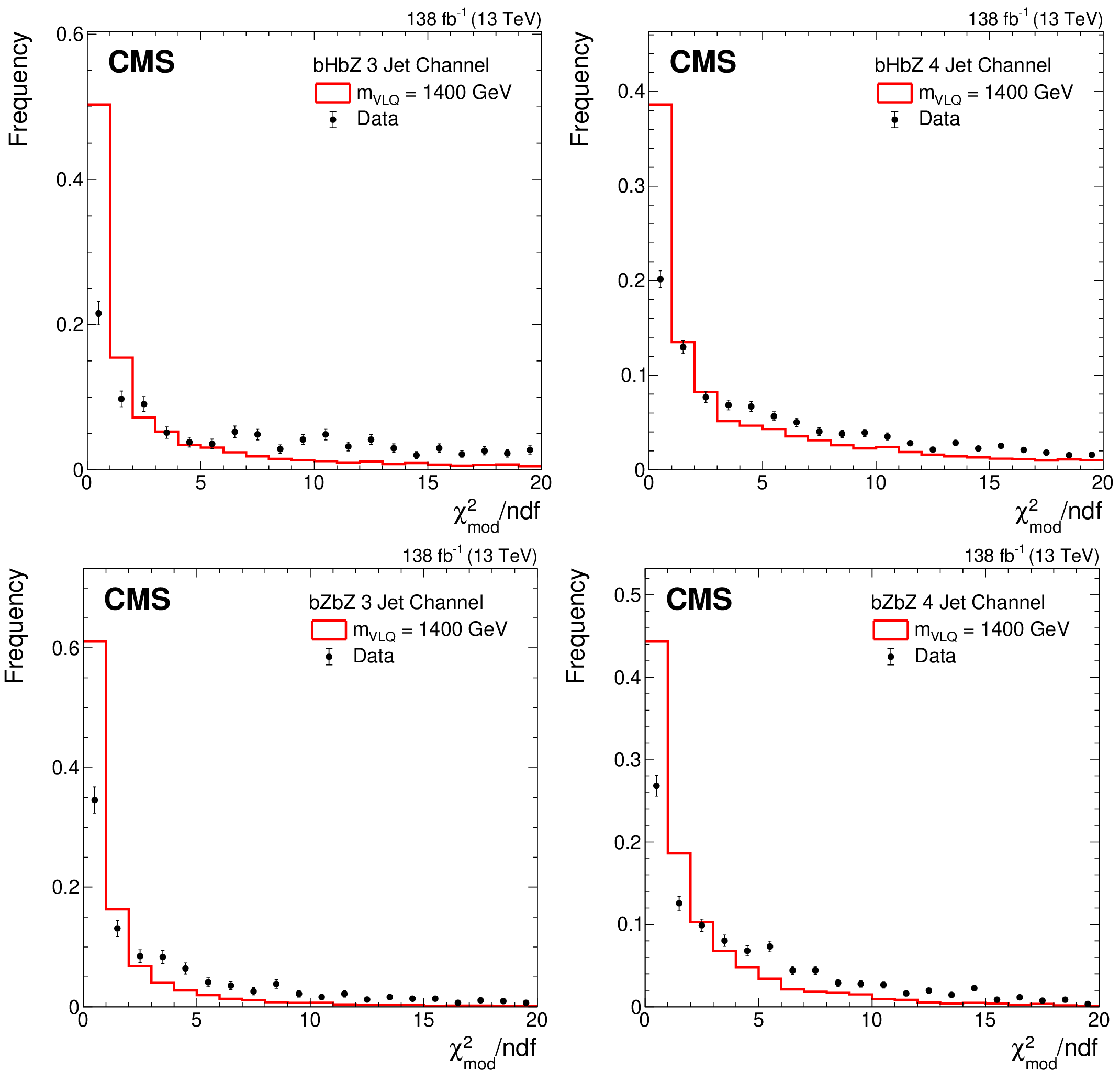
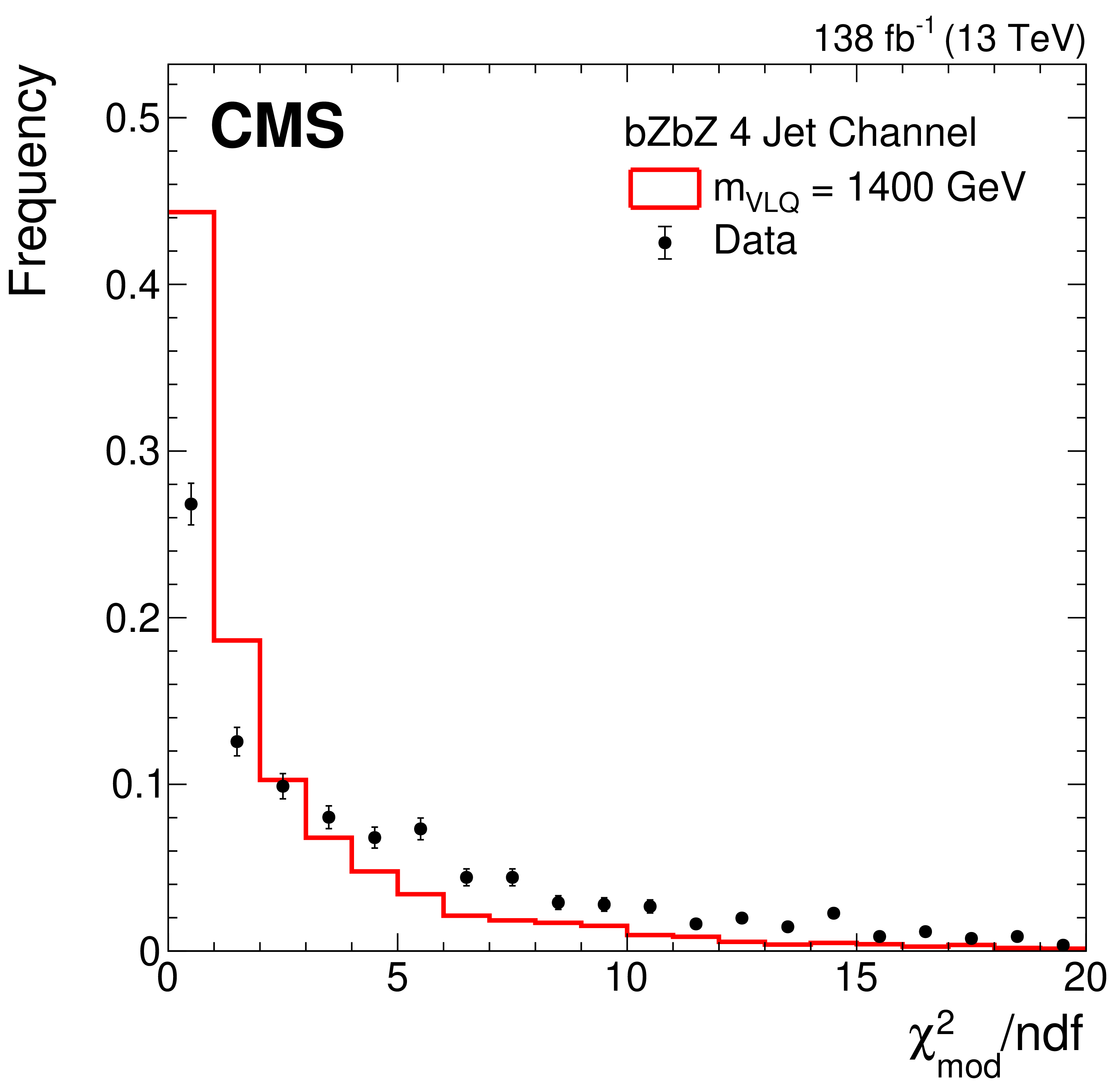
Normalized distributions of the value of the least $ \chi^2_\text{mod}/\text{ndf} $ for simulated signal events and data events in the fully hadronic category before any b tagging requirements are applied in the fully hadronic category. Upper row: $ \mathrm{b}\mathrm{H}\mathrm{b}\mathrm{H} $ (left), $ \mathrm{b}\mathrm{H}\mathrm{b}\mathrm{Z} $ (center), and $ \mathrm{b}\mathrm{Z}\mathrm{b}\mathrm{Z} $ (right) decay modes. Lower row: $ \mathrm{b}\mathrm{H}\mathrm{t}\mathrm{W} $ (left), and $ \mathrm{b}\mathrm{Z}\mathrm{t}\mathrm{W} $ (right) decay modes. A signal mass of $ m_{{\mathrm{B}}} = $ 1400 GeV is used and compared against all three years of data. All jet multiplicities have been combined together. |
png pdf |
Figure 5-a:
Normalized distributions of the value of the least $ \chi^2_\text{mod}/\text{ndf} $ for simulated signal events and data events in the fully hadronic category before any b tagging requirements are applied in the fully hadronic category. Upper row: $ \mathrm{b}\mathrm{H}\mathrm{b}\mathrm{H} $ (left), $ \mathrm{b}\mathrm{H}\mathrm{b}\mathrm{Z} $ (center), and $ \mathrm{b}\mathrm{Z}\mathrm{b}\mathrm{Z} $ (right) decay modes. Lower row: $ \mathrm{b}\mathrm{H}\mathrm{t}\mathrm{W} $ (left), and $ \mathrm{b}\mathrm{Z}\mathrm{t}\mathrm{W} $ (right) decay modes. A signal mass of $ m_{{\mathrm{B}}} = $ 1400 GeV is used and compared against all three years of data. All jet multiplicities have been combined together. |
png pdf |
Figure 5-b:
Normalized distributions of the value of the least $ \chi^2_\text{mod}/\text{ndf} $ for simulated signal events and data events in the fully hadronic category before any b tagging requirements are applied in the fully hadronic category. Upper row: $ \mathrm{b}\mathrm{H}\mathrm{b}\mathrm{H} $ (left), $ \mathrm{b}\mathrm{H}\mathrm{b}\mathrm{Z} $ (center), and $ \mathrm{b}\mathrm{Z}\mathrm{b}\mathrm{Z} $ (right) decay modes. Lower row: $ \mathrm{b}\mathrm{H}\mathrm{t}\mathrm{W} $ (left), and $ \mathrm{b}\mathrm{Z}\mathrm{t}\mathrm{W} $ (right) decay modes. A signal mass of $ m_{{\mathrm{B}}} = $ 1400 GeV is used and compared against all three years of data. All jet multiplicities have been combined together. |
png pdf |
Figure 5-c:
Normalized distributions of the value of the least $ \chi^2_\text{mod}/\text{ndf} $ for simulated signal events and data events in the fully hadronic category before any b tagging requirements are applied in the fully hadronic category. Upper row: $ \mathrm{b}\mathrm{H}\mathrm{b}\mathrm{H} $ (left), $ \mathrm{b}\mathrm{H}\mathrm{b}\mathrm{Z} $ (center), and $ \mathrm{b}\mathrm{Z}\mathrm{b}\mathrm{Z} $ (right) decay modes. Lower row: $ \mathrm{b}\mathrm{H}\mathrm{t}\mathrm{W} $ (left), and $ \mathrm{b}\mathrm{Z}\mathrm{t}\mathrm{W} $ (right) decay modes. A signal mass of $ m_{{\mathrm{B}}} = $ 1400 GeV is used and compared against all three years of data. All jet multiplicities have been combined together. |
png pdf |
Figure 5-d:
Normalized distributions of the value of the least $ \chi^2_\text{mod}/\text{ndf} $ for simulated signal events and data events in the fully hadronic category before any b tagging requirements are applied in the fully hadronic category. Upper row: $ \mathrm{b}\mathrm{H}\mathrm{b}\mathrm{H} $ (left), $ \mathrm{b}\mathrm{H}\mathrm{b}\mathrm{Z} $ (center), and $ \mathrm{b}\mathrm{Z}\mathrm{b}\mathrm{Z} $ (right) decay modes. Lower row: $ \mathrm{b}\mathrm{H}\mathrm{t}\mathrm{W} $ (left), and $ \mathrm{b}\mathrm{Z}\mathrm{t}\mathrm{W} $ (right) decay modes. A signal mass of $ m_{{\mathrm{B}}} = $ 1400 GeV is used and compared against all three years of data. All jet multiplicities have been combined together. |

png pdf |
Figure 5-e:
Normalized distributions of the value of the least $ \chi^2_\text{mod}/\text{ndf} $ for simulated signal events and data events in the fully hadronic category before any b tagging requirements are applied in the fully hadronic category. Upper row: $ \mathrm{b}\mathrm{H}\mathrm{b}\mathrm{H} $ (left), $ \mathrm{b}\mathrm{H}\mathrm{b}\mathrm{Z} $ (center), and $ \mathrm{b}\mathrm{Z}\mathrm{b}\mathrm{Z} $ (right) decay modes. Lower row: $ \mathrm{b}\mathrm{H}\mathrm{t}\mathrm{W} $ (left), and $ \mathrm{b}\mathrm{Z}\mathrm{t}\mathrm{W} $ (right) decay modes. A signal mass of $ m_{{\mathrm{B}}} = $ 1400 GeV is used and compared against all three years of data. All jet multiplicities have been combined together. |
png pdf |
Figure 6:
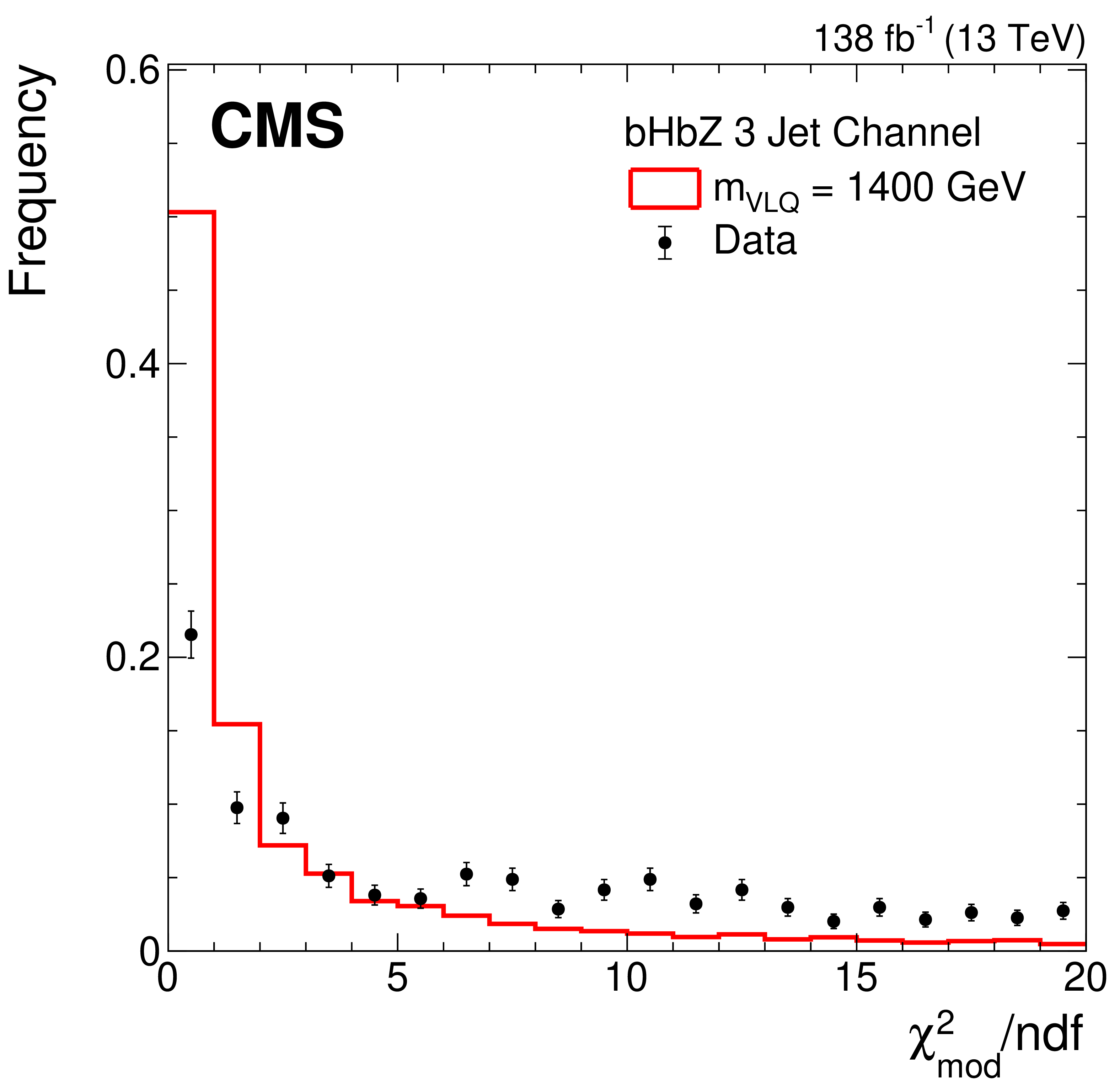
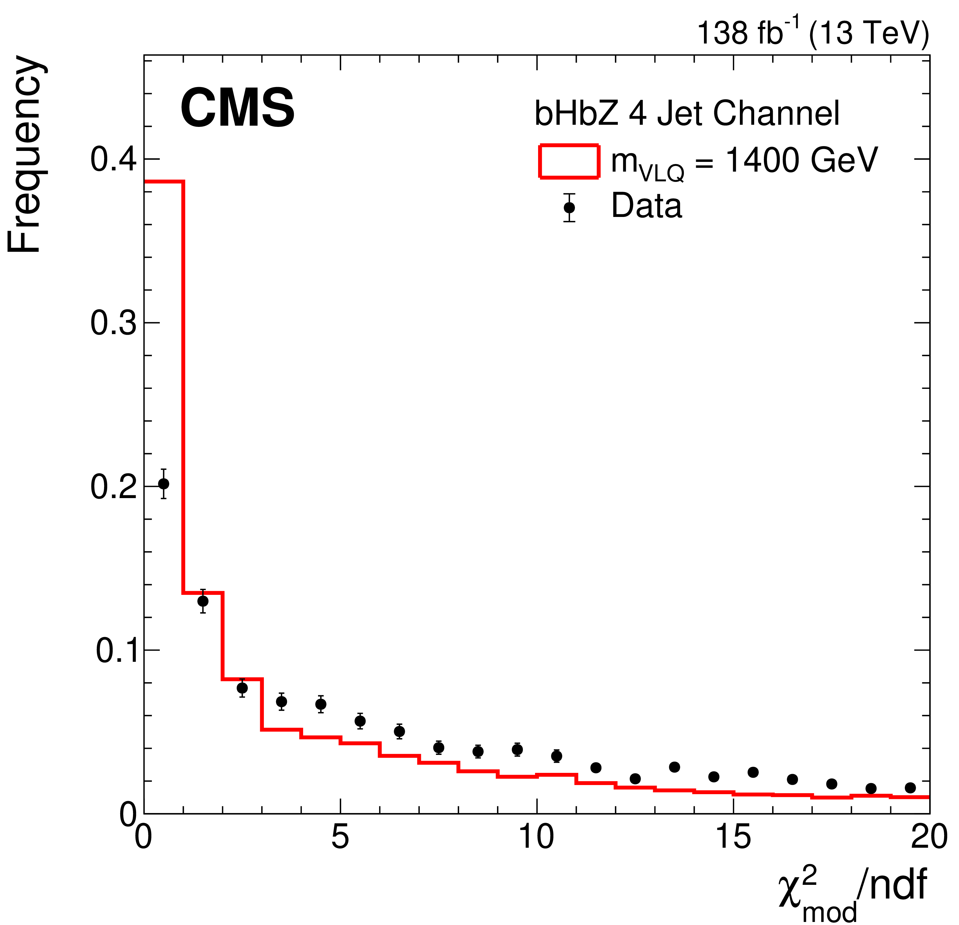
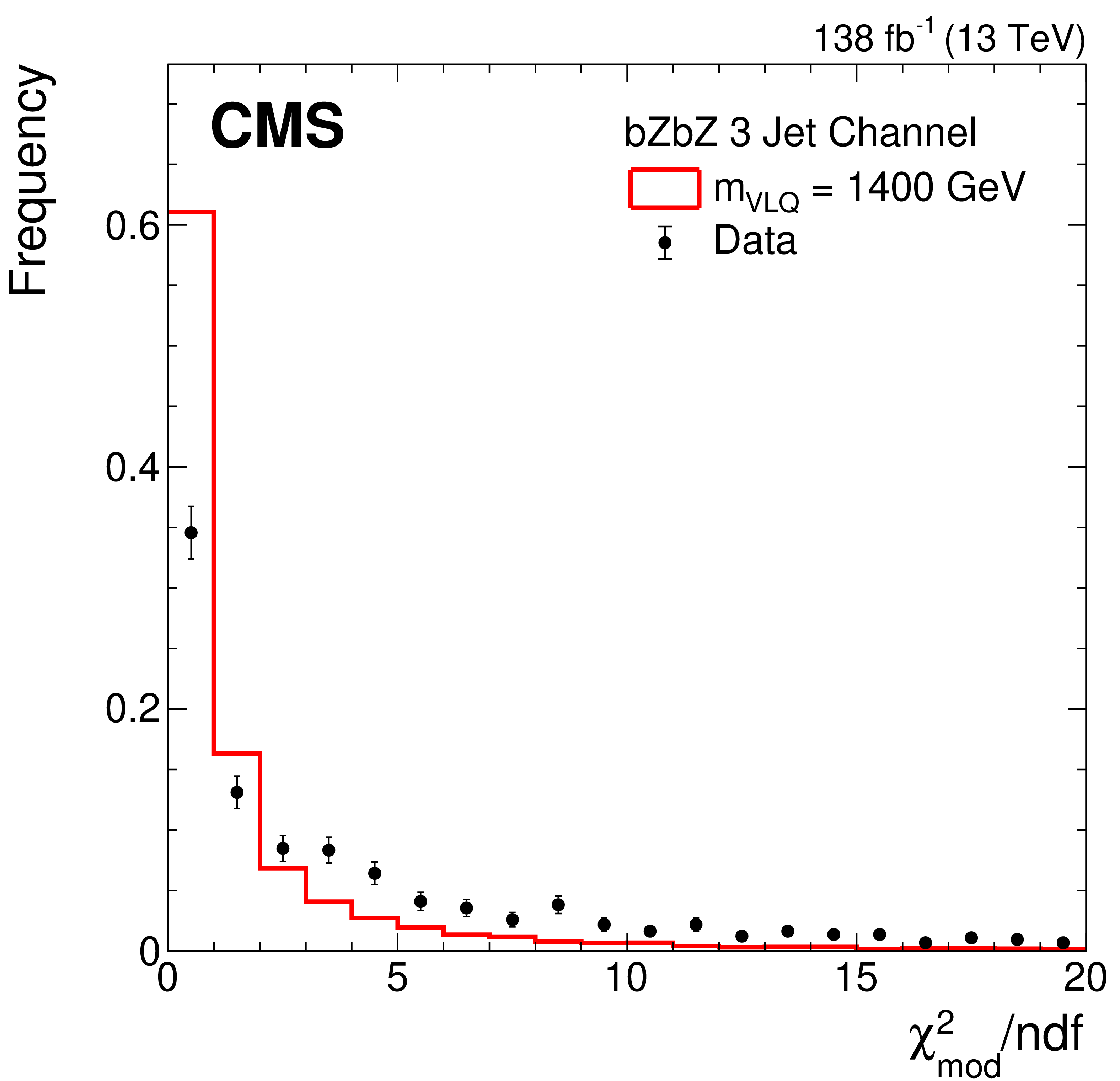
Normalized distributions of the value of the least $ \chi^2_\text{mod}/\text{ndf} $ for simulated signal events and data events in the leptonic category before any b tagging requirements are applied. Upper row: $ \mathrm{b}\mathrm{H}\mathrm{b}\mathrm{Z} $ decay mode, 3-jet (left) and 4-jet (right) events. Lower row: $ \mathrm{b}\mathrm{Z}\mathrm{b}\mathrm{Z} $ decay mode, 3-jet (left) and 4-jet (right) events. A signal mass of $ m_{{\mathrm{B}}} = $ 1400 GeV is used and compared against all three years of data. |
png pdf |
Figure 6-a:
Normalized distributions of the value of the least $ \chi^2_\text{mod}/\text{ndf} $ for simulated signal events and data events in the leptonic category before any b tagging requirements are applied. Upper row: $ \mathrm{b}\mathrm{H}\mathrm{b}\mathrm{Z} $ decay mode, 3-jet (left) and 4-jet (right) events. Lower row: $ \mathrm{b}\mathrm{Z}\mathrm{b}\mathrm{Z} $ decay mode, 3-jet (left) and 4-jet (right) events. A signal mass of $ m_{{\mathrm{B}}} = $ 1400 GeV is used and compared against all three years of data. |
png pdf |
Figure 6-b:
Normalized distributions of the value of the least $ \chi^2_\text{mod}/\text{ndf} $ for simulated signal events and data events in the leptonic category before any b tagging requirements are applied. Upper row: $ \mathrm{b}\mathrm{H}\mathrm{b}\mathrm{Z} $ decay mode, 3-jet (left) and 4-jet (right) events. Lower row: $ \mathrm{b}\mathrm{Z}\mathrm{b}\mathrm{Z} $ decay mode, 3-jet (left) and 4-jet (right) events. A signal mass of $ m_{{\mathrm{B}}} = $ 1400 GeV is used and compared against all three years of data. |
png pdf |
Figure 6-c:
Normalized distributions of the value of the least $ \chi^2_\text{mod}/\text{ndf} $ for simulated signal events and data events in the leptonic category before any b tagging requirements are applied. Upper row: $ \mathrm{b}\mathrm{H}\mathrm{b}\mathrm{Z} $ decay mode, 3-jet (left) and 4-jet (right) events. Lower row: $ \mathrm{b}\mathrm{Z}\mathrm{b}\mathrm{Z} $ decay mode, 3-jet (left) and 4-jet (right) events. A signal mass of $ m_{{\mathrm{B}}} = $ 1400 GeV is used and compared against all three years of data. |
png pdf |
Figure 6-d:
Normalized distributions of the value of the least $ \chi^2_\text{mod}/\text{ndf} $ for simulated signal events and data events in the leptonic category before any b tagging requirements are applied. Upper row: $ \mathrm{b}\mathrm{H}\mathrm{b}\mathrm{Z} $ decay mode, 3-jet (left) and 4-jet (right) events. Lower row: $ \mathrm{b}\mathrm{Z}\mathrm{b}\mathrm{Z} $ decay mode, 3-jet (left) and 4-jet (right) events. A signal mass of $ m_{{\mathrm{B}}} = $ 1400 GeV is used and compared against all three years of data. |
png pdf |
Figure 7:
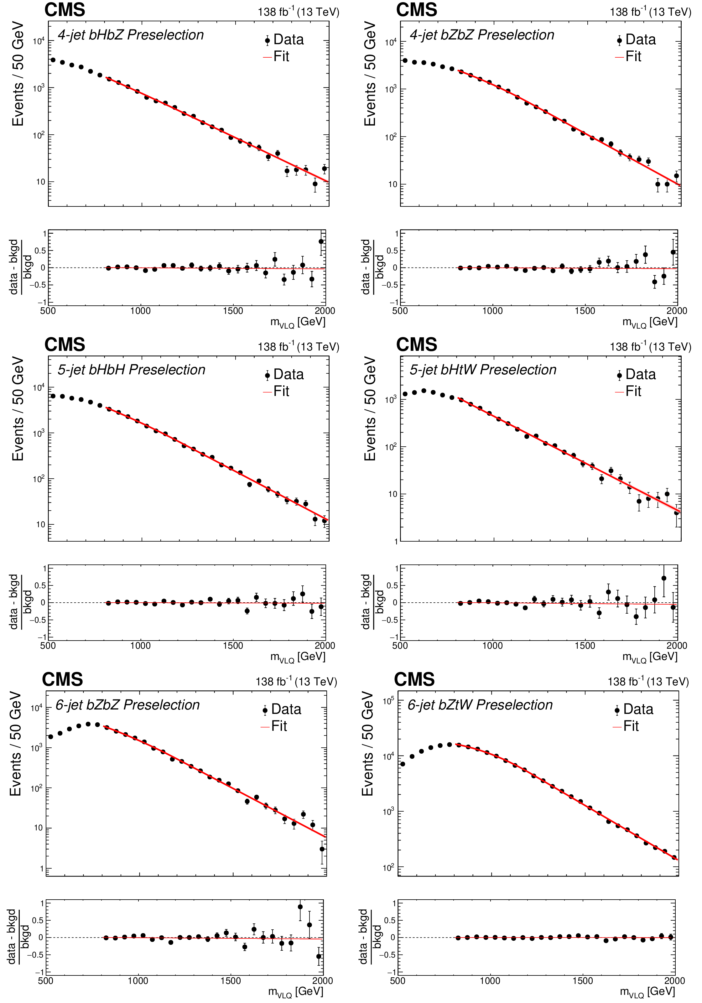
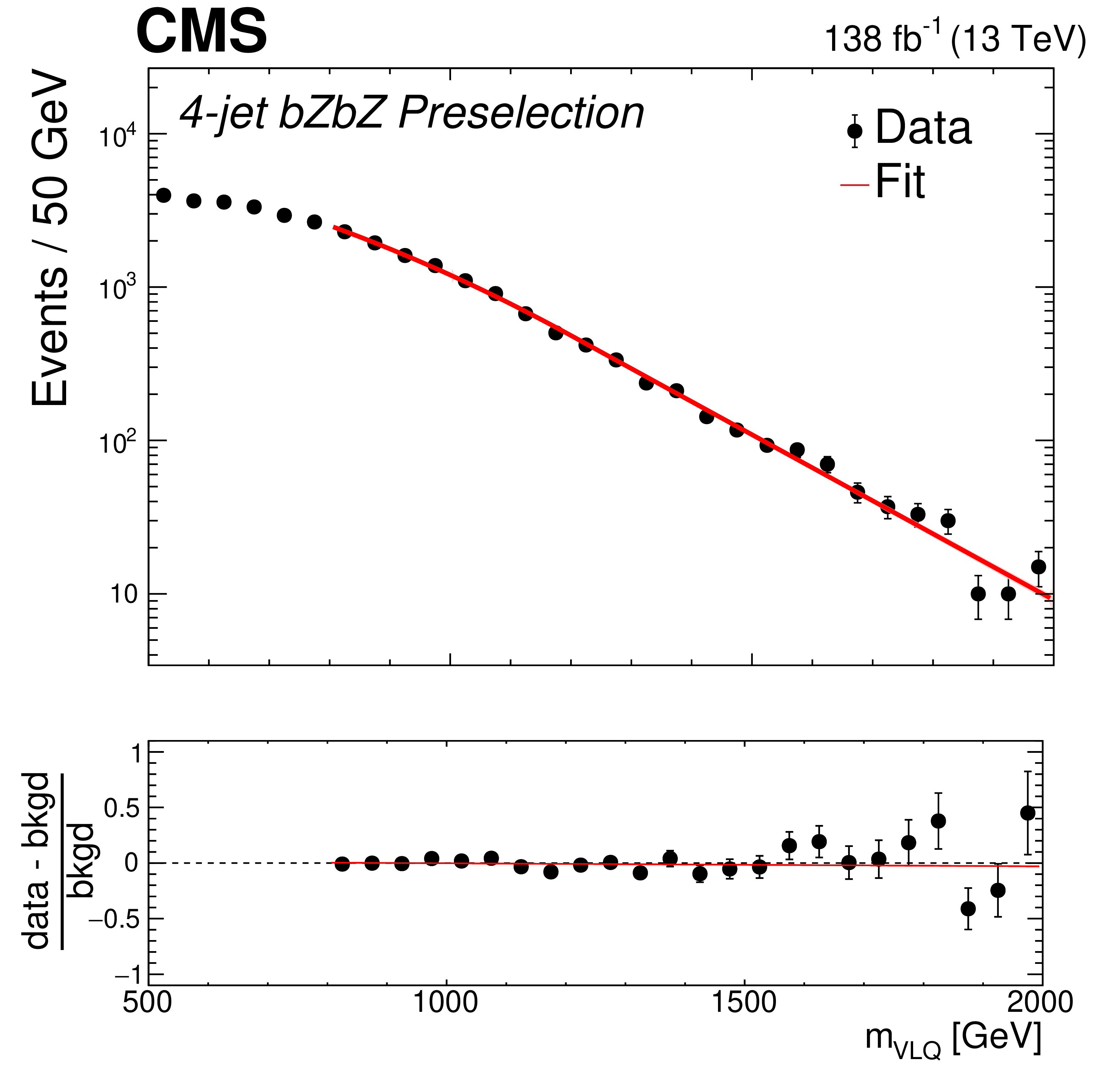
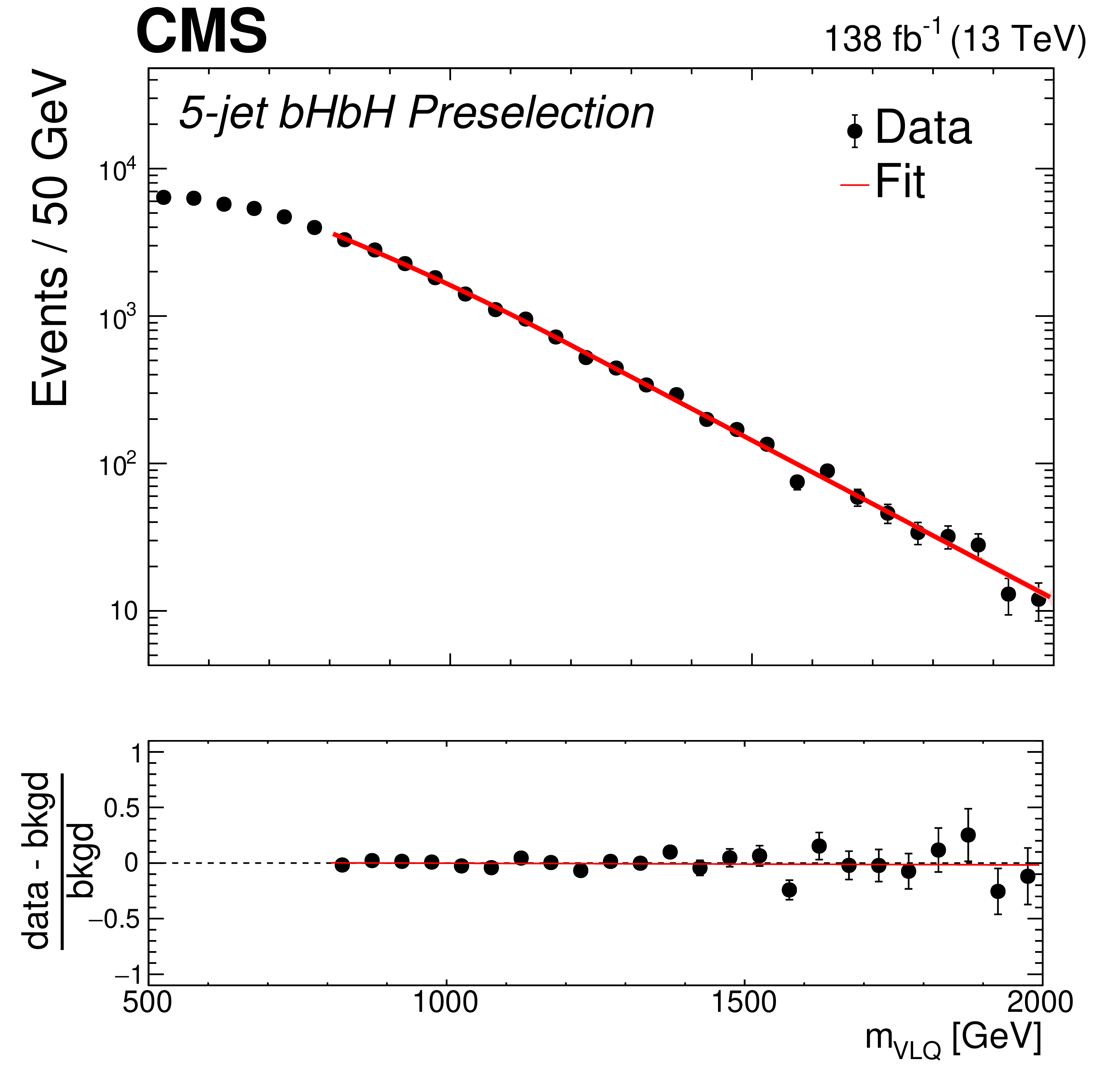
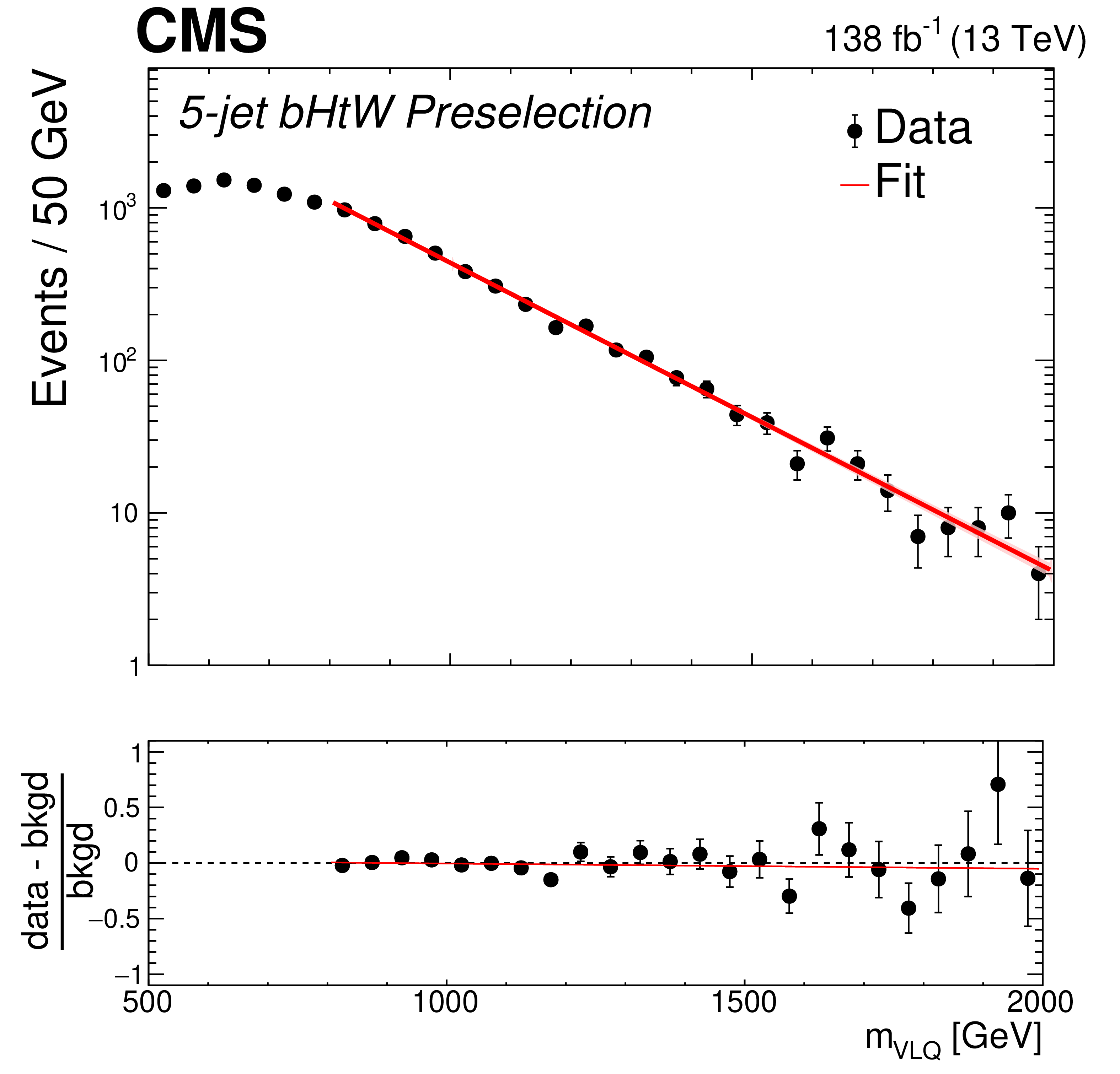
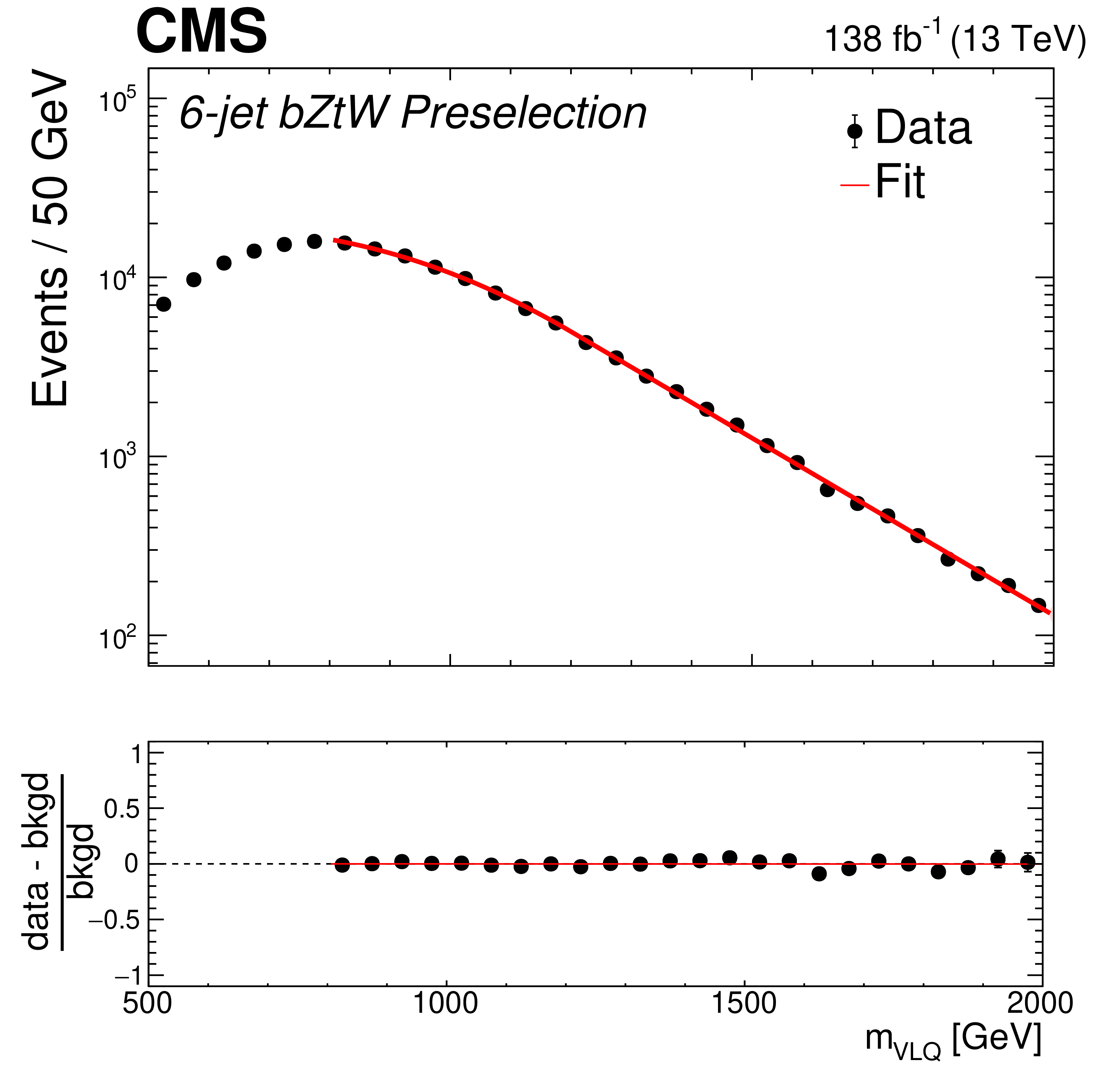
Distributions of $ m_{\text{VLQ}} $ for the preselected data sample in the fully hadronic category for some selected channels. Upper row: 4-jet $ \mathrm{b}\mathrm{H}\mathrm{b}\mathrm{Z} $ (left) and 4-jet $ \mathrm{b}\mathrm{Z}\mathrm{b}\mathrm{Z} $ (right) modes. Middle row: 5-jet $ \mathrm{b}\mathrm{H}\mathrm{b}\mathrm{H} $ (left) and 5-jet $ \mathrm{b}\mathrm{H}\mathrm{t}\mathrm{W} $ (right) modes. Lower row: 6-jet $ \mathrm{b}\mathrm{Z}\mathrm{b}\mathrm{Z} $ (left) and 6-jet $ \mathrm{b}\mathrm{Z}\mathrm{t}\mathrm{W} $ (right) modes. The fit to the data (shown by the black points) is given by the red line, and the bottom panel displays the fractional difference between the data and fit, (data-fit)/fit. |

png pdf |
Figure 7-a:
Distributions of $ m_{\text{VLQ}} $ for the preselected data sample in the fully hadronic category for some selected channels. Upper row: 4-jet $ \mathrm{b}\mathrm{H}\mathrm{b}\mathrm{Z} $ (left) and 4-jet $ \mathrm{b}\mathrm{Z}\mathrm{b}\mathrm{Z} $ (right) modes. Middle row: 5-jet $ \mathrm{b}\mathrm{H}\mathrm{b}\mathrm{H} $ (left) and 5-jet $ \mathrm{b}\mathrm{H}\mathrm{t}\mathrm{W} $ (right) modes. Lower row: 6-jet $ \mathrm{b}\mathrm{Z}\mathrm{b}\mathrm{Z} $ (left) and 6-jet $ \mathrm{b}\mathrm{Z}\mathrm{t}\mathrm{W} $ (right) modes. The fit to the data (shown by the black points) is given by the red line, and the bottom panel displays the fractional difference between the data and fit, (data-fit)/fit. |
png pdf |
Figure 7-b:
Distributions of $ m_{\text{VLQ}} $ for the preselected data sample in the fully hadronic category for some selected channels. Upper row: 4-jet $ \mathrm{b}\mathrm{H}\mathrm{b}\mathrm{Z} $ (left) and 4-jet $ \mathrm{b}\mathrm{Z}\mathrm{b}\mathrm{Z} $ (right) modes. Middle row: 5-jet $ \mathrm{b}\mathrm{H}\mathrm{b}\mathrm{H} $ (left) and 5-jet $ \mathrm{b}\mathrm{H}\mathrm{t}\mathrm{W} $ (right) modes. Lower row: 6-jet $ \mathrm{b}\mathrm{Z}\mathrm{b}\mathrm{Z} $ (left) and 6-jet $ \mathrm{b}\mathrm{Z}\mathrm{t}\mathrm{W} $ (right) modes. The fit to the data (shown by the black points) is given by the red line, and the bottom panel displays the fractional difference between the data and fit, (data-fit)/fit. |
png pdf |
Figure 7-c:
Distributions of $ m_{\text{VLQ}} $ for the preselected data sample in the fully hadronic category for some selected channels. Upper row: 4-jet $ \mathrm{b}\mathrm{H}\mathrm{b}\mathrm{Z} $ (left) and 4-jet $ \mathrm{b}\mathrm{Z}\mathrm{b}\mathrm{Z} $ (right) modes. Middle row: 5-jet $ \mathrm{b}\mathrm{H}\mathrm{b}\mathrm{H} $ (left) and 5-jet $ \mathrm{b}\mathrm{H}\mathrm{t}\mathrm{W} $ (right) modes. Lower row: 6-jet $ \mathrm{b}\mathrm{Z}\mathrm{b}\mathrm{Z} $ (left) and 6-jet $ \mathrm{b}\mathrm{Z}\mathrm{t}\mathrm{W} $ (right) modes. The fit to the data (shown by the black points) is given by the red line, and the bottom panel displays the fractional difference between the data and fit, (data-fit)/fit. |
png pdf |
Figure 7-d:
Distributions of $ m_{\text{VLQ}} $ for the preselected data sample in the fully hadronic category for some selected channels. Upper row: 4-jet $ \mathrm{b}\mathrm{H}\mathrm{b}\mathrm{Z} $ (left) and 4-jet $ \mathrm{b}\mathrm{Z}\mathrm{b}\mathrm{Z} $ (right) modes. Middle row: 5-jet $ \mathrm{b}\mathrm{H}\mathrm{b}\mathrm{H} $ (left) and 5-jet $ \mathrm{b}\mathrm{H}\mathrm{t}\mathrm{W} $ (right) modes. Lower row: 6-jet $ \mathrm{b}\mathrm{Z}\mathrm{b}\mathrm{Z} $ (left) and 6-jet $ \mathrm{b}\mathrm{Z}\mathrm{t}\mathrm{W} $ (right) modes. The fit to the data (shown by the black points) is given by the red line, and the bottom panel displays the fractional difference between the data and fit, (data-fit)/fit. |
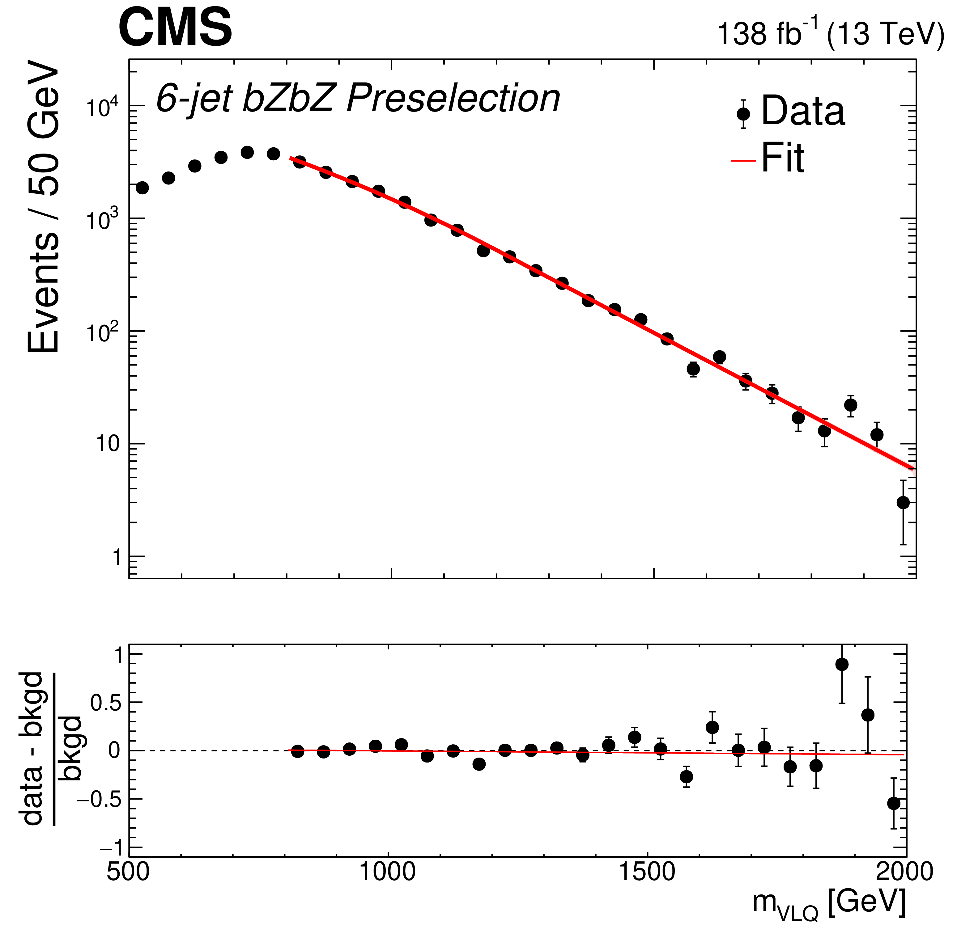
png pdf |
Figure 7-e:
Distributions of $ m_{\text{VLQ}} $ for the preselected data sample in the fully hadronic category for some selected channels. Upper row: 4-jet $ \mathrm{b}\mathrm{H}\mathrm{b}\mathrm{Z} $ (left) and 4-jet $ \mathrm{b}\mathrm{Z}\mathrm{b}\mathrm{Z} $ (right) modes. Middle row: 5-jet $ \mathrm{b}\mathrm{H}\mathrm{b}\mathrm{H} $ (left) and 5-jet $ \mathrm{b}\mathrm{H}\mathrm{t}\mathrm{W} $ (right) modes. Lower row: 6-jet $ \mathrm{b}\mathrm{Z}\mathrm{b}\mathrm{Z} $ (left) and 6-jet $ \mathrm{b}\mathrm{Z}\mathrm{t}\mathrm{W} $ (right) modes. The fit to the data (shown by the black points) is given by the red line, and the bottom panel displays the fractional difference between the data and fit, (data-fit)/fit. |
png pdf |
Figure 7-f:
Distributions of $ m_{\text{VLQ}} $ for the preselected data sample in the fully hadronic category for some selected channels. Upper row: 4-jet $ \mathrm{b}\mathrm{H}\mathrm{b}\mathrm{Z} $ (left) and 4-jet $ \mathrm{b}\mathrm{Z}\mathrm{b}\mathrm{Z} $ (right) modes. Middle row: 5-jet $ \mathrm{b}\mathrm{H}\mathrm{b}\mathrm{H} $ (left) and 5-jet $ \mathrm{b}\mathrm{H}\mathrm{t}\mathrm{W} $ (right) modes. Lower row: 6-jet $ \mathrm{b}\mathrm{Z}\mathrm{b}\mathrm{Z} $ (left) and 6-jet $ \mathrm{b}\mathrm{Z}\mathrm{t}\mathrm{W} $ (right) modes. The fit to the data (shown by the black points) is given by the red line, and the bottom panel displays the fractional difference between the data and fit, (data-fit)/fit. |
png pdf |
Figure 8:
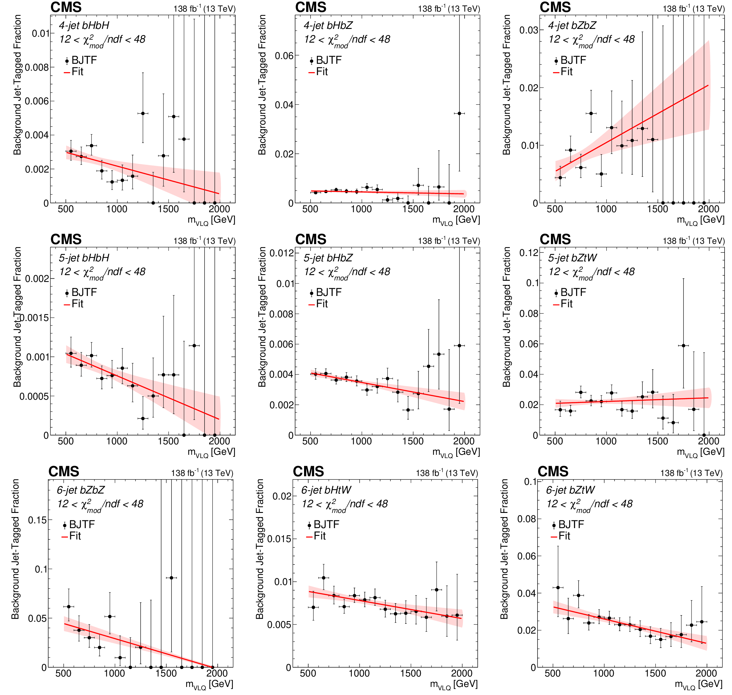
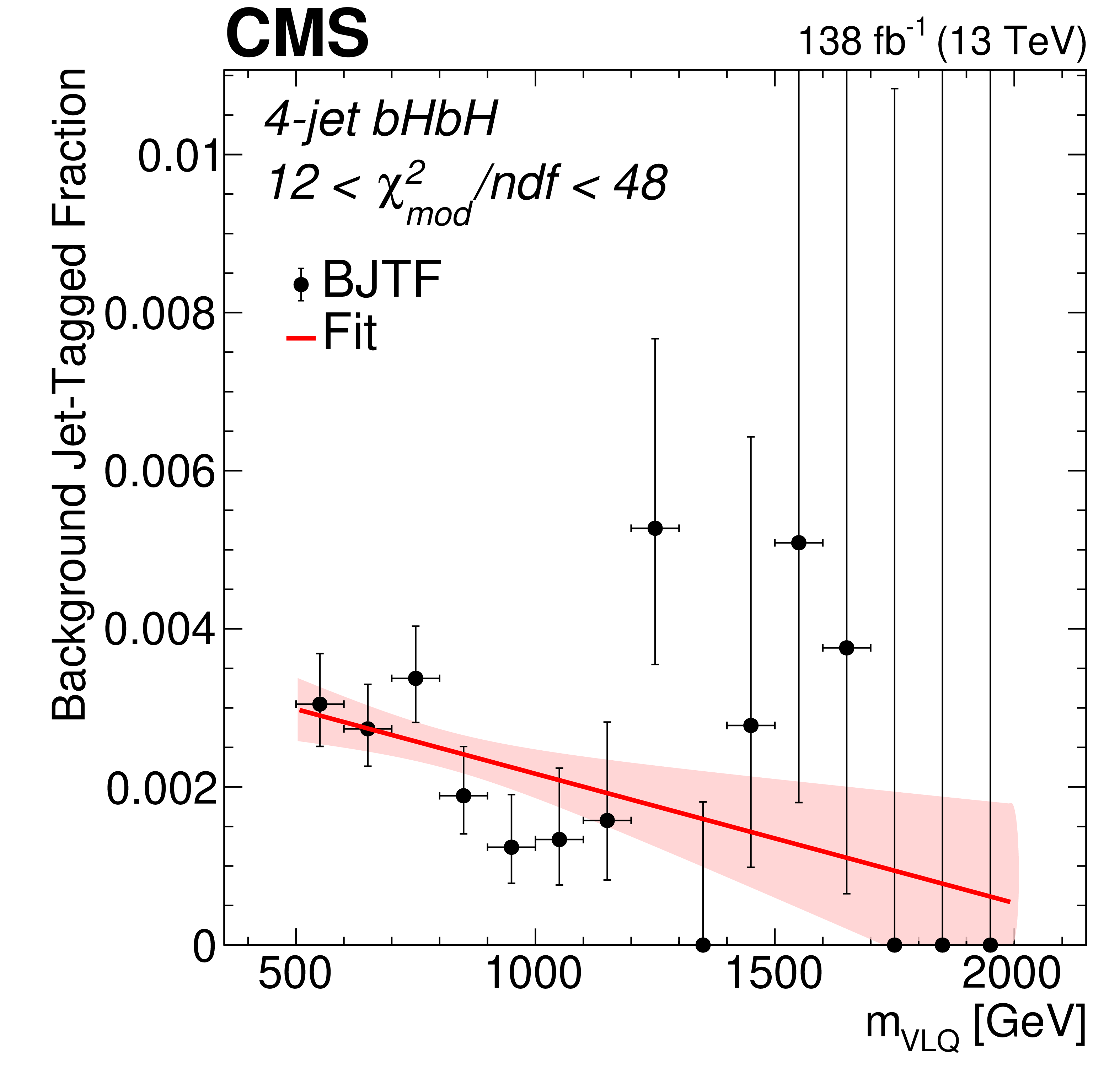
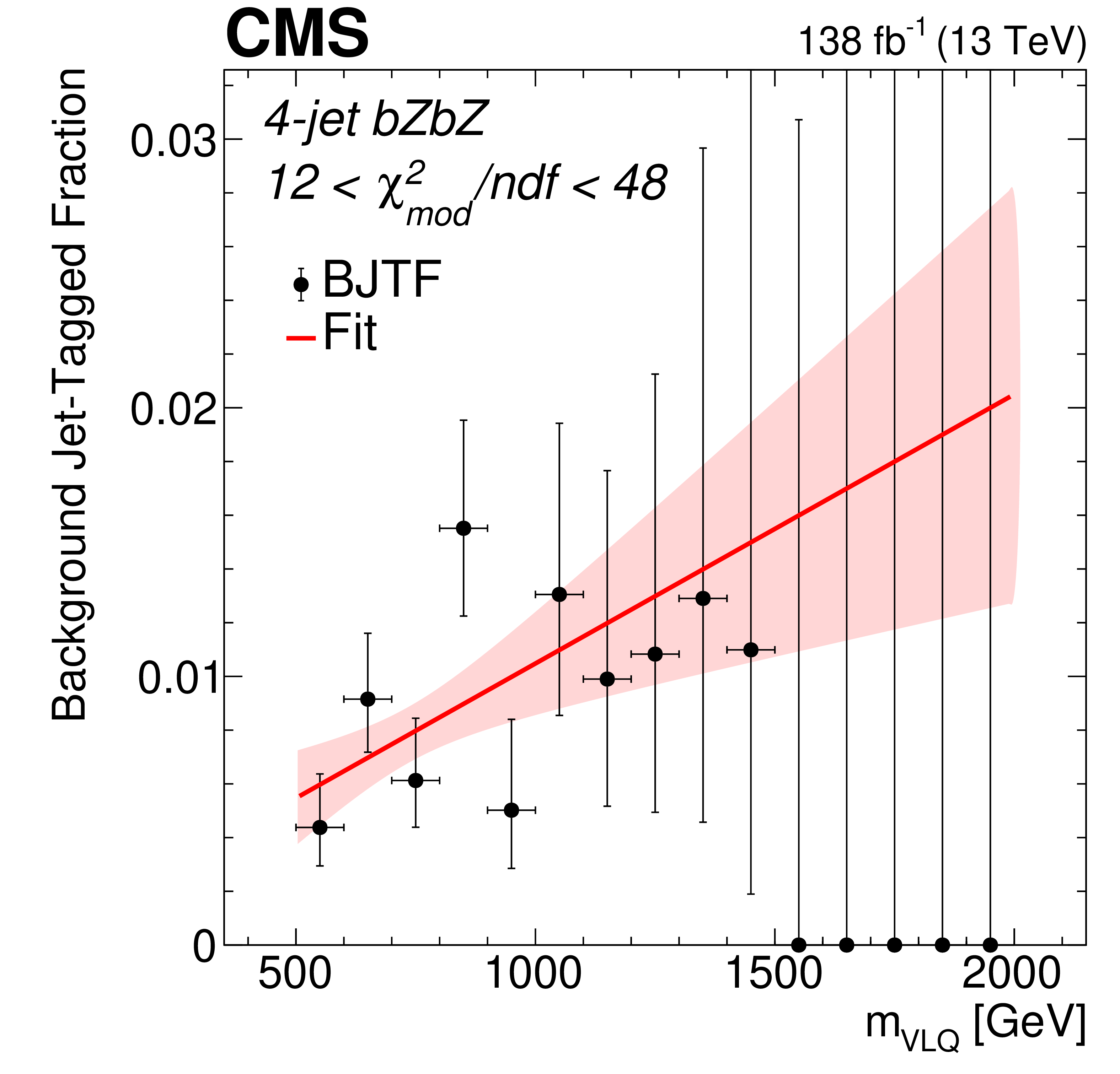
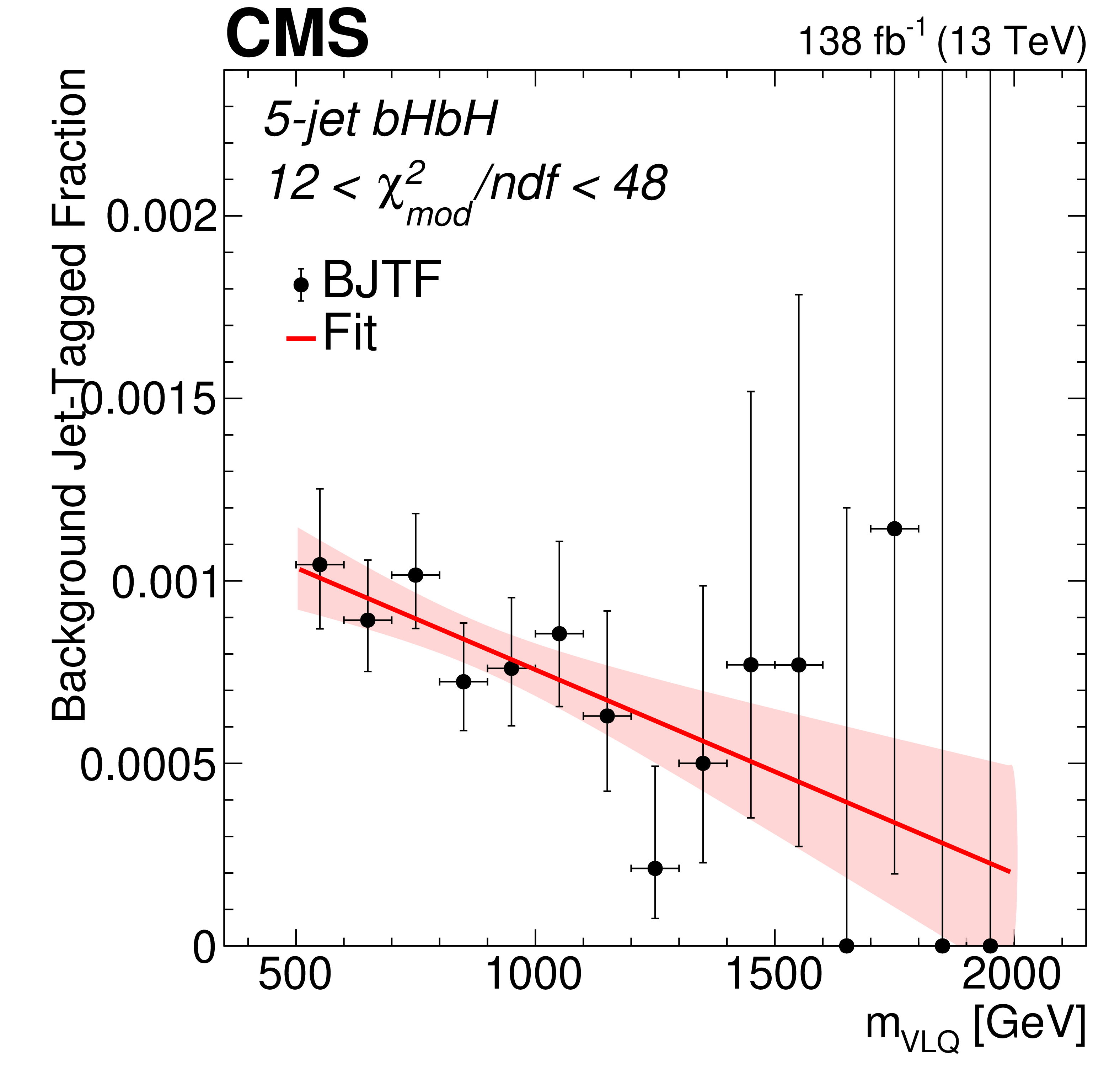
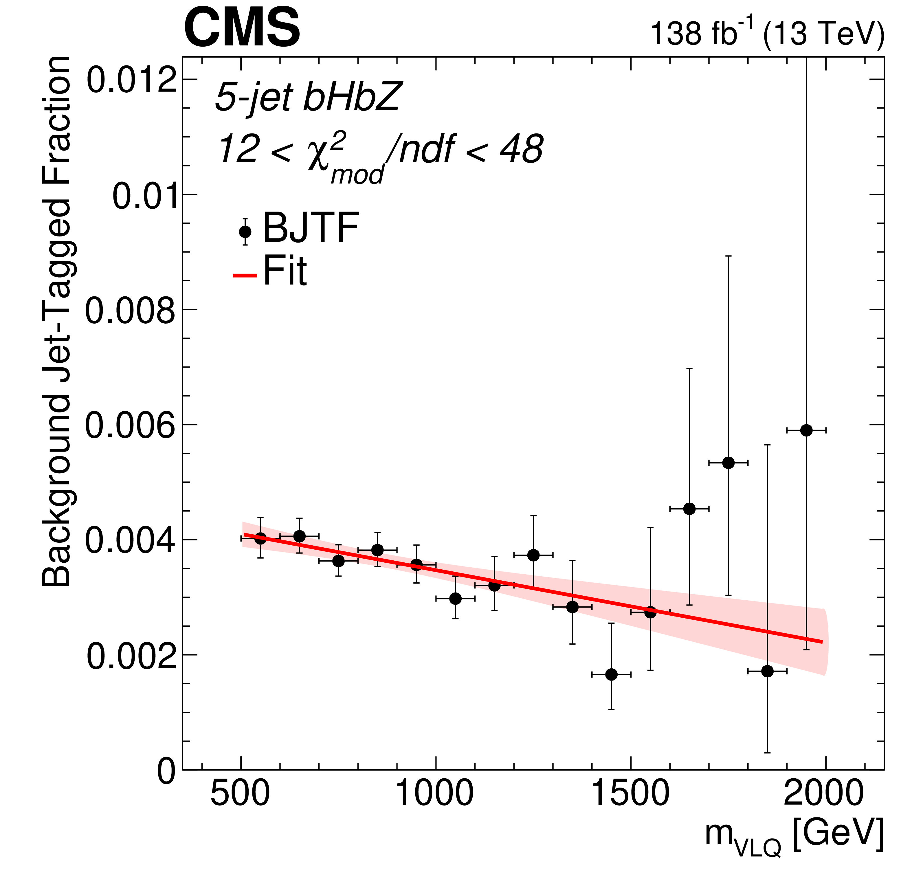
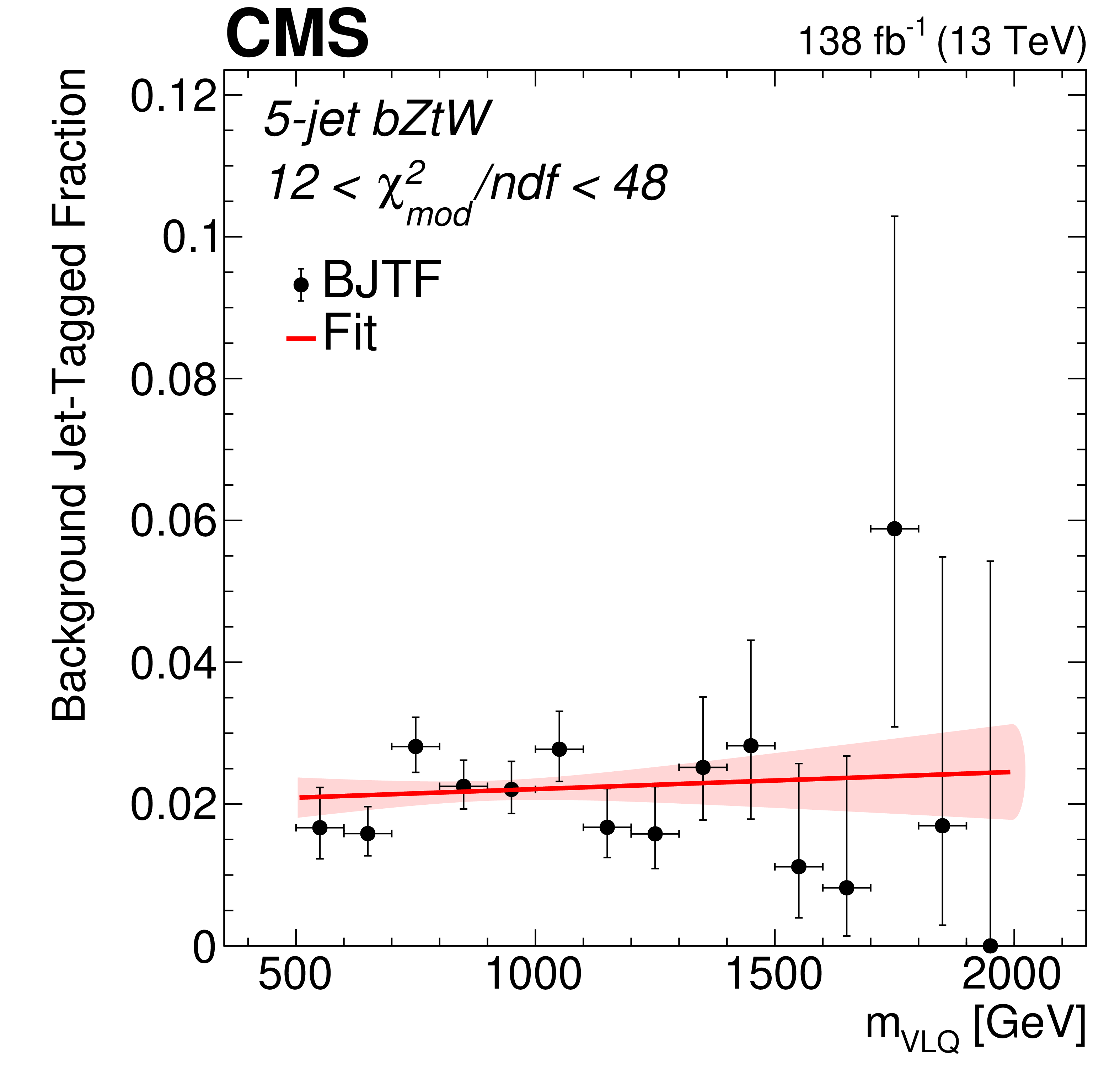
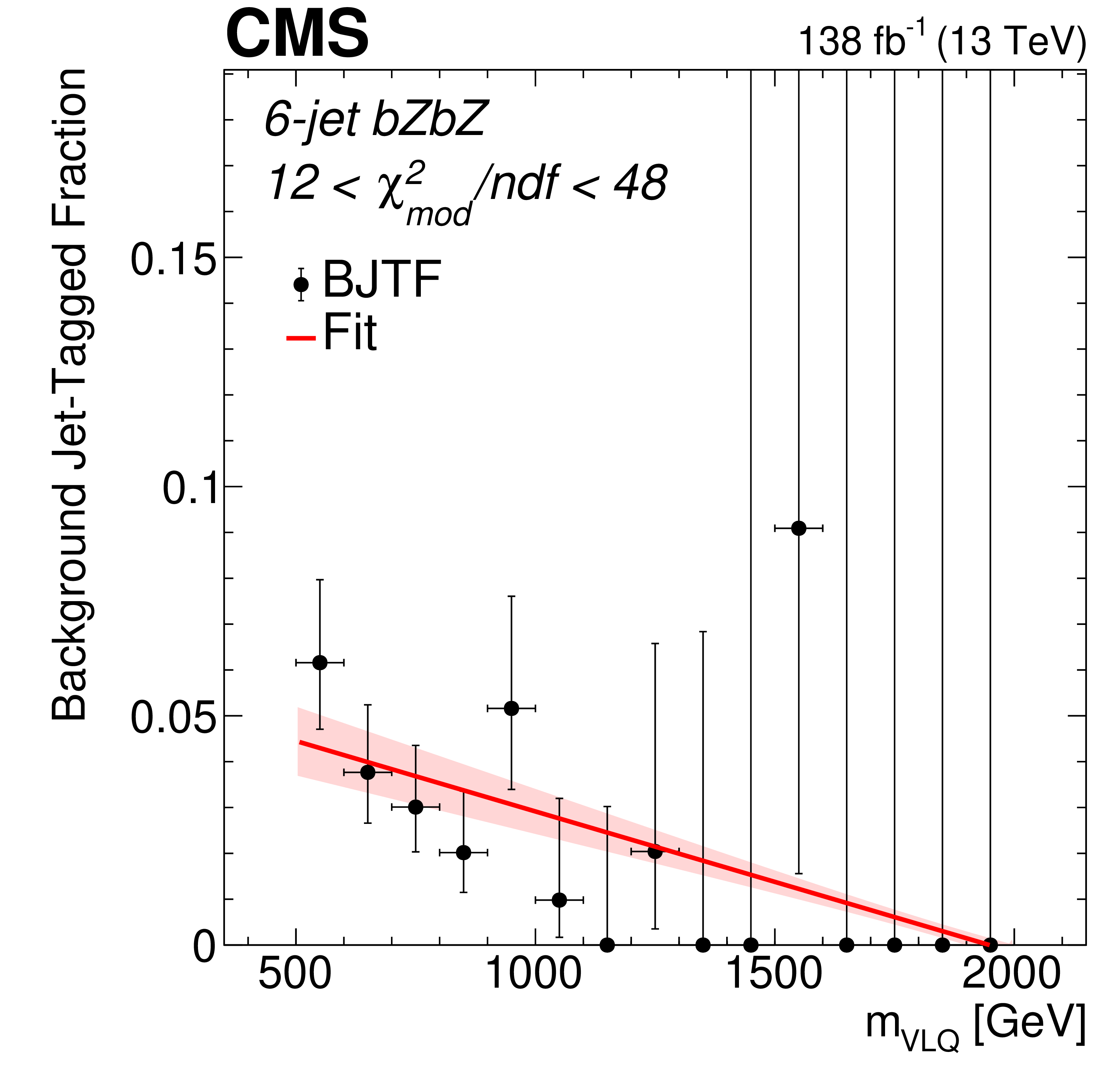
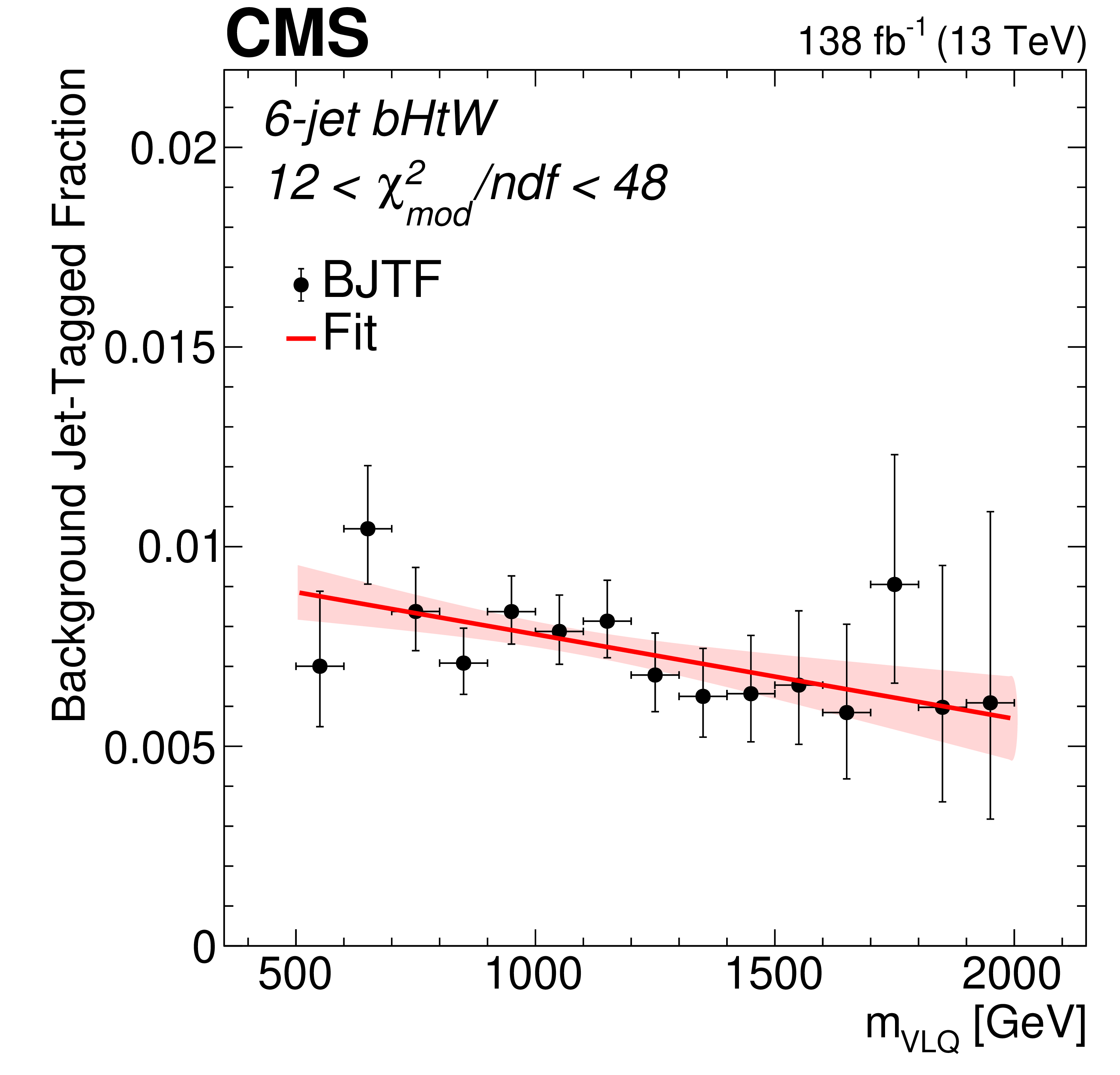
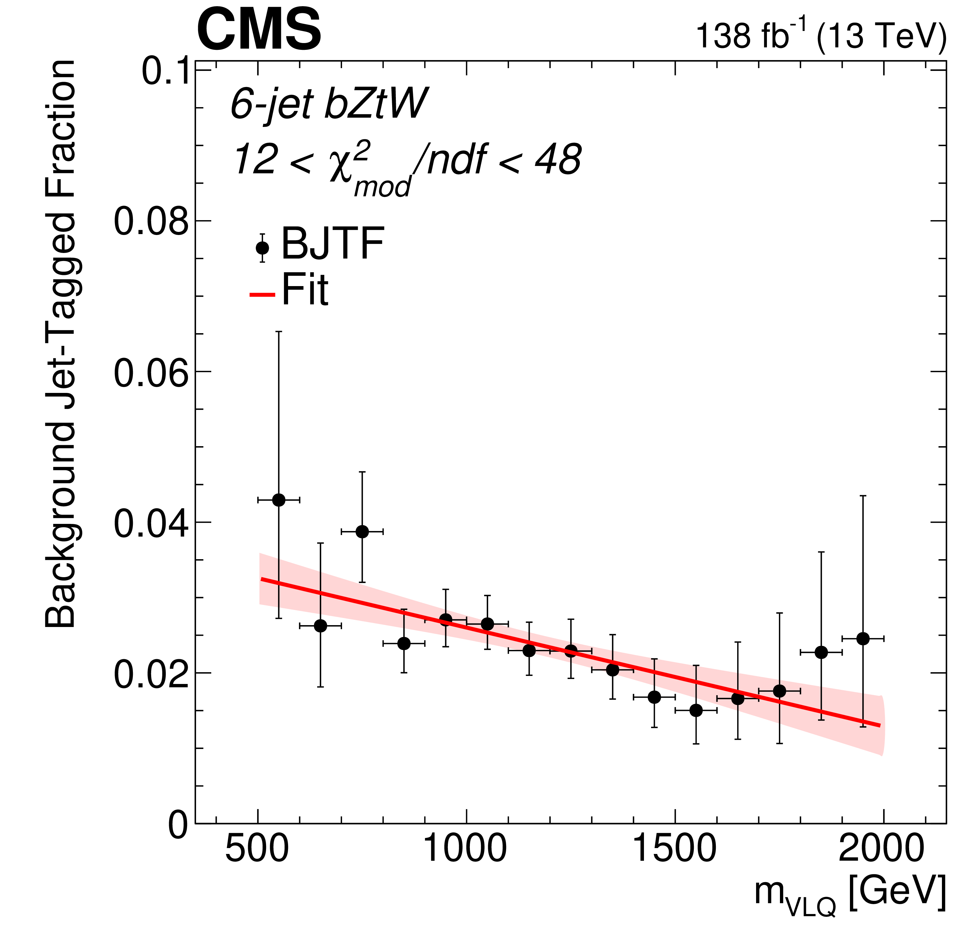
Value of BJTF as a function of $ m_{\text{VLQ}} $ in the control region with 12 $ < \chi^2_\text{mod}/\text{ndf} < $ 48 for some selected fully hadronic channels. Upper row: 4-jet events in the $ \mathrm{b}\mathrm{H}\mathrm{b}\mathrm{H} $ (left), $ \mathrm{b}\mathrm{H}\mathrm{b}\mathrm{Z} $ (center), and $ \mathrm{b}\mathrm{Z}\mathrm{b}\mathrm{Z} $ (right) modes. Middle row: 5-jet events in the $ \mathrm{b}\mathrm{H}\mathrm{b}\mathrm{H} $ (left), $ \mathrm{b}\mathrm{H}\mathrm{b}\mathrm{Z} $ (center), and $ \mathrm{b}\mathrm{Z}\mathrm{t}\mathrm{W} $ (right) modes. Lower row: 6-jet events in the $ \mathrm{b}\mathrm{Z}\mathrm{b}\mathrm{Z} $ (left), $ \mathrm{b}\mathrm{H}\mathrm{t}\mathrm{W} $ (center), and $ \mathrm{b}\mathrm{Z}\mathrm{t}\mathrm{W} $ (right) modes. The linear fit is shown by the red line, and the associated uncertainty in the fit is shown by the shaded band. |
png pdf |
Figure 8-a:
Value of BJTF as a function of $ m_{\text{VLQ}} $ in the control region with 12 $ < \chi^2_\text{mod}/\text{ndf} < $ 48 for some selected fully hadronic channels. Upper row: 4-jet events in the $ \mathrm{b}\mathrm{H}\mathrm{b}\mathrm{H} $ (left), $ \mathrm{b}\mathrm{H}\mathrm{b}\mathrm{Z} $ (center), and $ \mathrm{b}\mathrm{Z}\mathrm{b}\mathrm{Z} $ (right) modes. Middle row: 5-jet events in the $ \mathrm{b}\mathrm{H}\mathrm{b}\mathrm{H} $ (left), $ \mathrm{b}\mathrm{H}\mathrm{b}\mathrm{Z} $ (center), and $ \mathrm{b}\mathrm{Z}\mathrm{t}\mathrm{W} $ (right) modes. Lower row: 6-jet events in the $ \mathrm{b}\mathrm{Z}\mathrm{b}\mathrm{Z} $ (left), $ \mathrm{b}\mathrm{H}\mathrm{t}\mathrm{W} $ (center), and $ \mathrm{b}\mathrm{Z}\mathrm{t}\mathrm{W} $ (right) modes. The linear fit is shown by the red line, and the associated uncertainty in the fit is shown by the shaded band. |

png pdf |
Figure 8-b:
Value of BJTF as a function of $ m_{\text{VLQ}} $ in the control region with 12 $ < \chi^2_\text{mod}/\text{ndf} < $ 48 for some selected fully hadronic channels. Upper row: 4-jet events in the $ \mathrm{b}\mathrm{H}\mathrm{b}\mathrm{H} $ (left), $ \mathrm{b}\mathrm{H}\mathrm{b}\mathrm{Z} $ (center), and $ \mathrm{b}\mathrm{Z}\mathrm{b}\mathrm{Z} $ (right) modes. Middle row: 5-jet events in the $ \mathrm{b}\mathrm{H}\mathrm{b}\mathrm{H} $ (left), $ \mathrm{b}\mathrm{H}\mathrm{b}\mathrm{Z} $ (center), and $ \mathrm{b}\mathrm{Z}\mathrm{t}\mathrm{W} $ (right) modes. Lower row: 6-jet events in the $ \mathrm{b}\mathrm{Z}\mathrm{b}\mathrm{Z} $ (left), $ \mathrm{b}\mathrm{H}\mathrm{t}\mathrm{W} $ (center), and $ \mathrm{b}\mathrm{Z}\mathrm{t}\mathrm{W} $ (right) modes. The linear fit is shown by the red line, and the associated uncertainty in the fit is shown by the shaded band. |
png pdf |
Figure 8-c:
Value of BJTF as a function of $ m_{\text{VLQ}} $ in the control region with 12 $ < \chi^2_\text{mod}/\text{ndf} < $ 48 for some selected fully hadronic channels. Upper row: 4-jet events in the $ \mathrm{b}\mathrm{H}\mathrm{b}\mathrm{H} $ (left), $ \mathrm{b}\mathrm{H}\mathrm{b}\mathrm{Z} $ (center), and $ \mathrm{b}\mathrm{Z}\mathrm{b}\mathrm{Z} $ (right) modes. Middle row: 5-jet events in the $ \mathrm{b}\mathrm{H}\mathrm{b}\mathrm{H} $ (left), $ \mathrm{b}\mathrm{H}\mathrm{b}\mathrm{Z} $ (center), and $ \mathrm{b}\mathrm{Z}\mathrm{t}\mathrm{W} $ (right) modes. Lower row: 6-jet events in the $ \mathrm{b}\mathrm{Z}\mathrm{b}\mathrm{Z} $ (left), $ \mathrm{b}\mathrm{H}\mathrm{t}\mathrm{W} $ (center), and $ \mathrm{b}\mathrm{Z}\mathrm{t}\mathrm{W} $ (right) modes. The linear fit is shown by the red line, and the associated uncertainty in the fit is shown by the shaded band. |
png pdf |
Figure 8-d:
Value of BJTF as a function of $ m_{\text{VLQ}} $ in the control region with 12 $ < \chi^2_\text{mod}/\text{ndf} < $ 48 for some selected fully hadronic channels. Upper row: 4-jet events in the $ \mathrm{b}\mathrm{H}\mathrm{b}\mathrm{H} $ (left), $ \mathrm{b}\mathrm{H}\mathrm{b}\mathrm{Z} $ (center), and $ \mathrm{b}\mathrm{Z}\mathrm{b}\mathrm{Z} $ (right) modes. Middle row: 5-jet events in the $ \mathrm{b}\mathrm{H}\mathrm{b}\mathrm{H} $ (left), $ \mathrm{b}\mathrm{H}\mathrm{b}\mathrm{Z} $ (center), and $ \mathrm{b}\mathrm{Z}\mathrm{t}\mathrm{W} $ (right) modes. Lower row: 6-jet events in the $ \mathrm{b}\mathrm{Z}\mathrm{b}\mathrm{Z} $ (left), $ \mathrm{b}\mathrm{H}\mathrm{t}\mathrm{W} $ (center), and $ \mathrm{b}\mathrm{Z}\mathrm{t}\mathrm{W} $ (right) modes. The linear fit is shown by the red line, and the associated uncertainty in the fit is shown by the shaded band. |
png pdf |
Figure 8-e:
Value of BJTF as a function of $ m_{\text{VLQ}} $ in the control region with 12 $ < \chi^2_\text{mod}/\text{ndf} < $ 48 for some selected fully hadronic channels. Upper row: 4-jet events in the $ \mathrm{b}\mathrm{H}\mathrm{b}\mathrm{H} $ (left), $ \mathrm{b}\mathrm{H}\mathrm{b}\mathrm{Z} $ (center), and $ \mathrm{b}\mathrm{Z}\mathrm{b}\mathrm{Z} $ (right) modes. Middle row: 5-jet events in the $ \mathrm{b}\mathrm{H}\mathrm{b}\mathrm{H} $ (left), $ \mathrm{b}\mathrm{H}\mathrm{b}\mathrm{Z} $ (center), and $ \mathrm{b}\mathrm{Z}\mathrm{t}\mathrm{W} $ (right) modes. Lower row: 6-jet events in the $ \mathrm{b}\mathrm{Z}\mathrm{b}\mathrm{Z} $ (left), $ \mathrm{b}\mathrm{H}\mathrm{t}\mathrm{W} $ (center), and $ \mathrm{b}\mathrm{Z}\mathrm{t}\mathrm{W} $ (right) modes. The linear fit is shown by the red line, and the associated uncertainty in the fit is shown by the shaded band. |
png pdf |
Figure 8-f:
Value of BJTF as a function of $ m_{\text{VLQ}} $ in the control region with 12 $ < \chi^2_\text{mod}/\text{ndf} < $ 48 for some selected fully hadronic channels. Upper row: 4-jet events in the $ \mathrm{b}\mathrm{H}\mathrm{b}\mathrm{H} $ (left), $ \mathrm{b}\mathrm{H}\mathrm{b}\mathrm{Z} $ (center), and $ \mathrm{b}\mathrm{Z}\mathrm{b}\mathrm{Z} $ (right) modes. Middle row: 5-jet events in the $ \mathrm{b}\mathrm{H}\mathrm{b}\mathrm{H} $ (left), $ \mathrm{b}\mathrm{H}\mathrm{b}\mathrm{Z} $ (center), and $ \mathrm{b}\mathrm{Z}\mathrm{t}\mathrm{W} $ (right) modes. Lower row: 6-jet events in the $ \mathrm{b}\mathrm{Z}\mathrm{b}\mathrm{Z} $ (left), $ \mathrm{b}\mathrm{H}\mathrm{t}\mathrm{W} $ (center), and $ \mathrm{b}\mathrm{Z}\mathrm{t}\mathrm{W} $ (right) modes. The linear fit is shown by the red line, and the associated uncertainty in the fit is shown by the shaded band. |
png pdf |
Figure 8-g:
Value of BJTF as a function of $ m_{\text{VLQ}} $ in the control region with 12 $ < \chi^2_\text{mod}/\text{ndf} < $ 48 for some selected fully hadronic channels. Upper row: 4-jet events in the $ \mathrm{b}\mathrm{H}\mathrm{b}\mathrm{H} $ (left), $ \mathrm{b}\mathrm{H}\mathrm{b}\mathrm{Z} $ (center), and $ \mathrm{b}\mathrm{Z}\mathrm{b}\mathrm{Z} $ (right) modes. Middle row: 5-jet events in the $ \mathrm{b}\mathrm{H}\mathrm{b}\mathrm{H} $ (left), $ \mathrm{b}\mathrm{H}\mathrm{b}\mathrm{Z} $ (center), and $ \mathrm{b}\mathrm{Z}\mathrm{t}\mathrm{W} $ (right) modes. Lower row: 6-jet events in the $ \mathrm{b}\mathrm{Z}\mathrm{b}\mathrm{Z} $ (left), $ \mathrm{b}\mathrm{H}\mathrm{t}\mathrm{W} $ (center), and $ \mathrm{b}\mathrm{Z}\mathrm{t}\mathrm{W} $ (right) modes. The linear fit is shown by the red line, and the associated uncertainty in the fit is shown by the shaded band. |
png pdf |
Figure 8-h:
Value of BJTF as a function of $ m_{\text{VLQ}} $ in the control region with 12 $ < \chi^2_\text{mod}/\text{ndf} < $ 48 for some selected fully hadronic channels. Upper row: 4-jet events in the $ \mathrm{b}\mathrm{H}\mathrm{b}\mathrm{H} $ (left), $ \mathrm{b}\mathrm{H}\mathrm{b}\mathrm{Z} $ (center), and $ \mathrm{b}\mathrm{Z}\mathrm{b}\mathrm{Z} $ (right) modes. Middle row: 5-jet events in the $ \mathrm{b}\mathrm{H}\mathrm{b}\mathrm{H} $ (left), $ \mathrm{b}\mathrm{H}\mathrm{b}\mathrm{Z} $ (center), and $ \mathrm{b}\mathrm{Z}\mathrm{t}\mathrm{W} $ (right) modes. Lower row: 6-jet events in the $ \mathrm{b}\mathrm{Z}\mathrm{b}\mathrm{Z} $ (left), $ \mathrm{b}\mathrm{H}\mathrm{t}\mathrm{W} $ (center), and $ \mathrm{b}\mathrm{Z}\mathrm{t}\mathrm{W} $ (right) modes. The linear fit is shown by the red line, and the associated uncertainty in the fit is shown by the shaded band. |
png pdf |
Figure 8-i:
Value of BJTF as a function of $ m_{\text{VLQ}} $ in the control region with 12 $ < \chi^2_\text{mod}/\text{ndf} < $ 48 for some selected fully hadronic channels. Upper row: 4-jet events in the $ \mathrm{b}\mathrm{H}\mathrm{b}\mathrm{H} $ (left), $ \mathrm{b}\mathrm{H}\mathrm{b}\mathrm{Z} $ (center), and $ \mathrm{b}\mathrm{Z}\mathrm{b}\mathrm{Z} $ (right) modes. Middle row: 5-jet events in the $ \mathrm{b}\mathrm{H}\mathrm{b}\mathrm{H} $ (left), $ \mathrm{b}\mathrm{H}\mathrm{b}\mathrm{Z} $ (center), and $ \mathrm{b}\mathrm{Z}\mathrm{t}\mathrm{W} $ (right) modes. Lower row: 6-jet events in the $ \mathrm{b}\mathrm{Z}\mathrm{b}\mathrm{Z} $ (left), $ \mathrm{b}\mathrm{H}\mathrm{t}\mathrm{W} $ (center), and $ \mathrm{b}\mathrm{Z}\mathrm{t}\mathrm{W} $ (right) modes. The linear fit is shown by the red line, and the associated uncertainty in the fit is shown by the shaded band. |
png pdf |
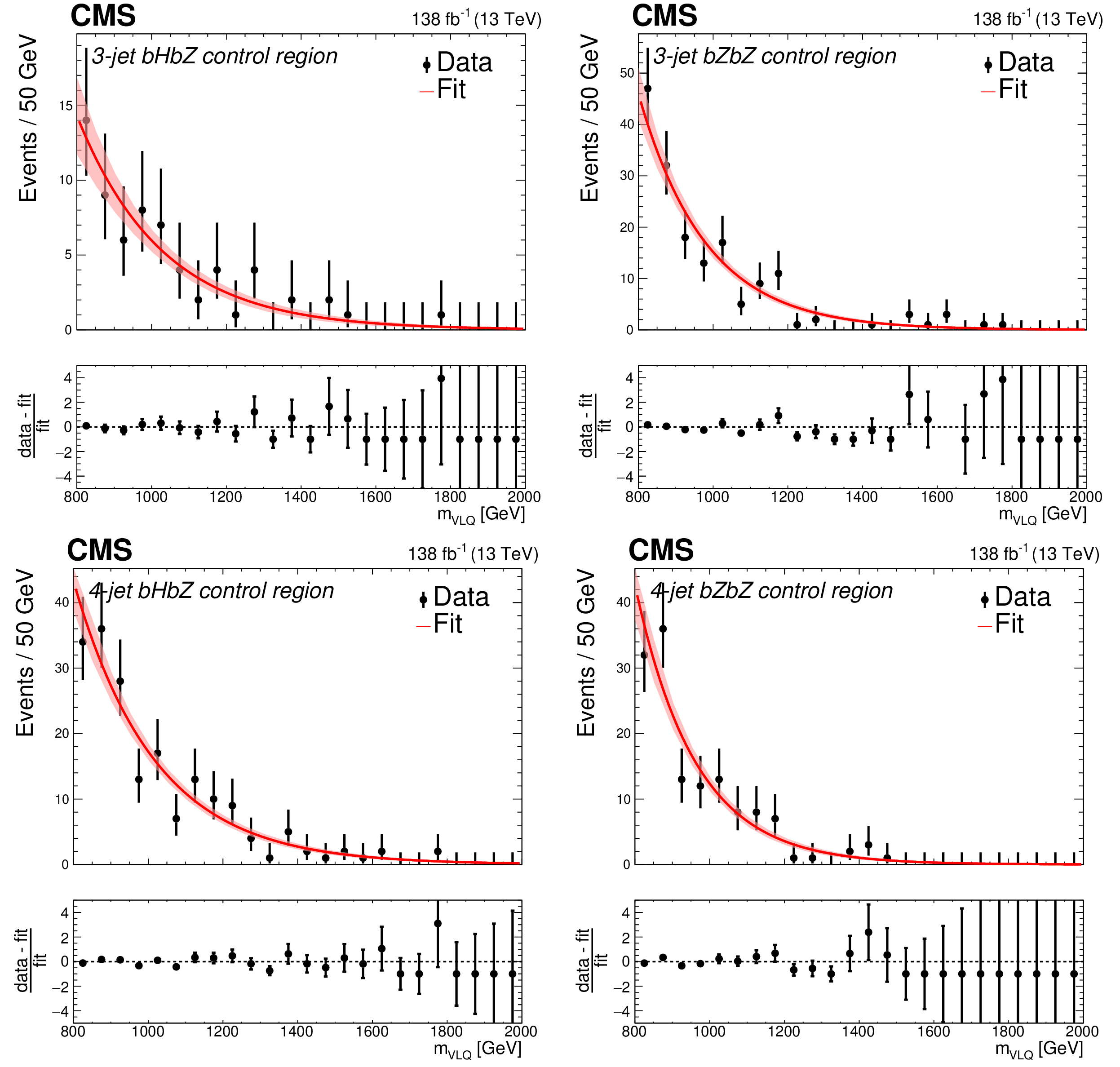
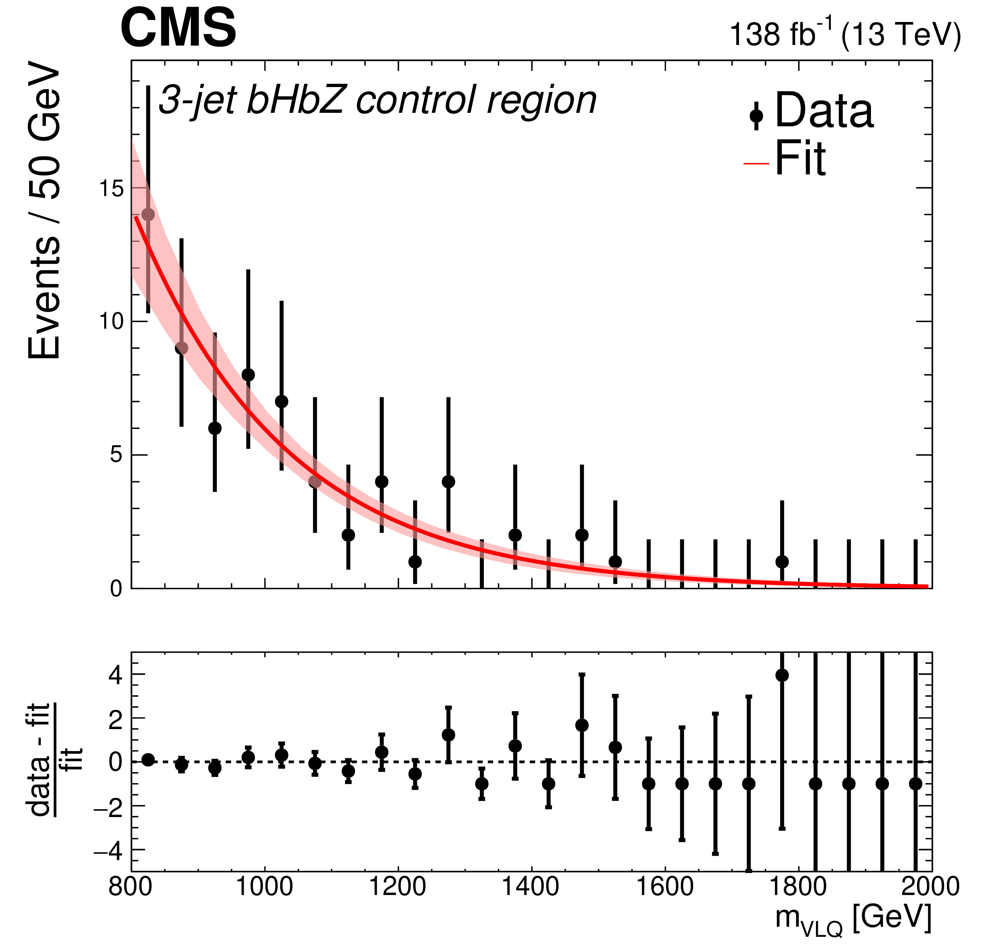
Figure 9:
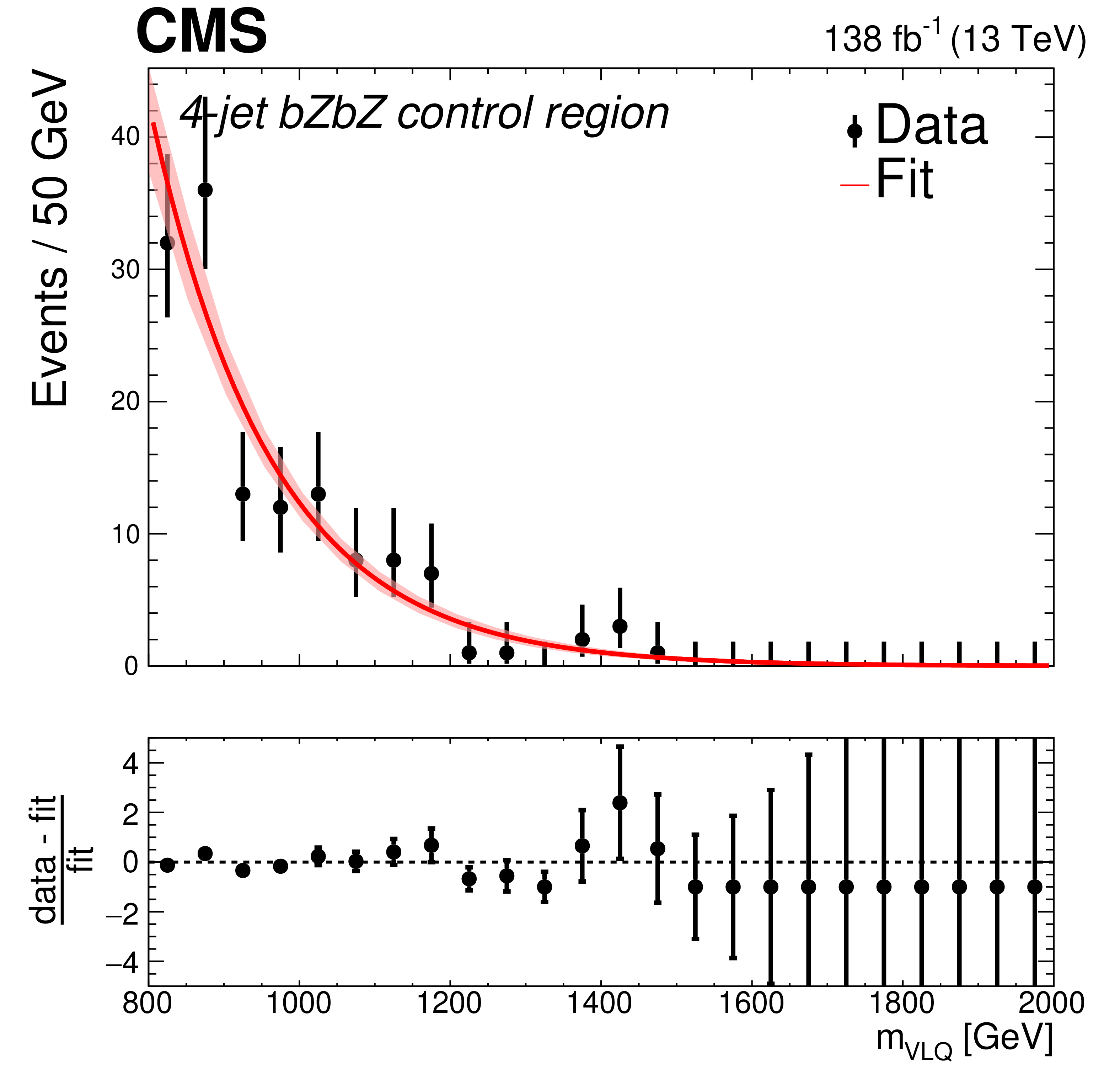
Distributions of $ m_{\text{VLQ}} $ for events in the control region for the channels in the leptonic category. Upper row: 3-jet events in the $ \mathrm{b}\mathrm{H}\mathrm{b}\mathrm{Z} $ (left) and $ \mathrm{b}\mathrm{Z}\mathrm{b}\mathrm{Z} $ (right) modes. Lower row: 4-jet events in the $ \mathrm{b}\mathrm{H}\mathrm{b}\mathrm{Z} $ (left) and $ \mathrm{b}\mathrm{Z}\mathrm{b}\mathrm{Z} $ (right) modes. The exponential fit and its uncertainty are shown by the red line and the light red shaded band, respectively. The bottom panel shows the fractional difference between the data and fit, (data-fit)/fit. |
png pdf |
Figure 9-a:
Distributions of $ m_{\text{VLQ}} $ for events in the control region for the channels in the leptonic category. Upper row: 3-jet events in the $ \mathrm{b}\mathrm{H}\mathrm{b}\mathrm{Z} $ (left) and $ \mathrm{b}\mathrm{Z}\mathrm{b}\mathrm{Z} $ (right) modes. Lower row: 4-jet events in the $ \mathrm{b}\mathrm{H}\mathrm{b}\mathrm{Z} $ (left) and $ \mathrm{b}\mathrm{Z}\mathrm{b}\mathrm{Z} $ (right) modes. The exponential fit and its uncertainty are shown by the red line and the light red shaded band, respectively. The bottom panel shows the fractional difference between the data and fit, (data-fit)/fit. |
png pdf |
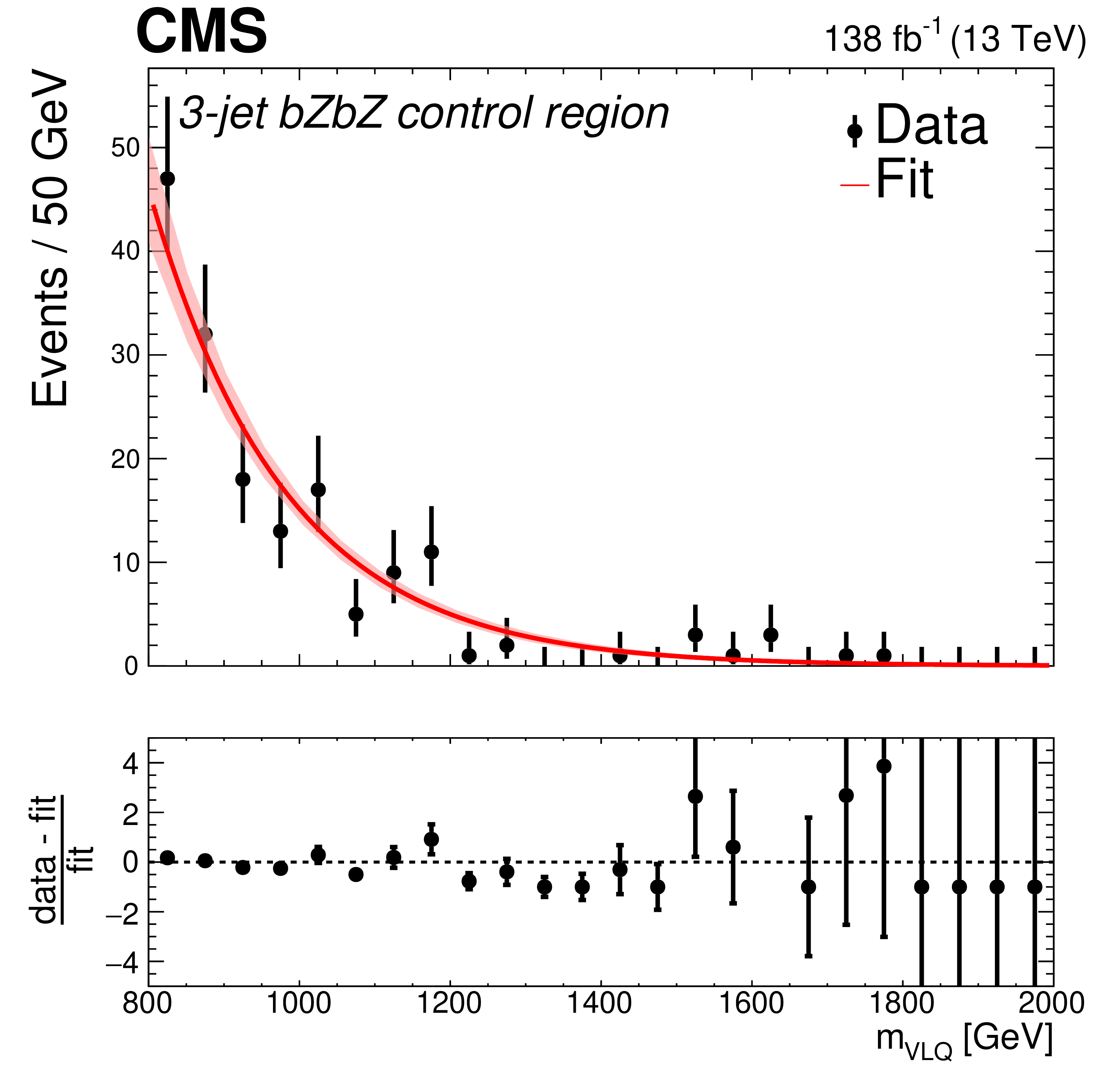
Figure 9-b:
Distributions of $ m_{\text{VLQ}} $ for events in the control region for the channels in the leptonic category. Upper row: 3-jet events in the $ \mathrm{b}\mathrm{H}\mathrm{b}\mathrm{Z} $ (left) and $ \mathrm{b}\mathrm{Z}\mathrm{b}\mathrm{Z} $ (right) modes. Lower row: 4-jet events in the $ \mathrm{b}\mathrm{H}\mathrm{b}\mathrm{Z} $ (left) and $ \mathrm{b}\mathrm{Z}\mathrm{b}\mathrm{Z} $ (right) modes. The exponential fit and its uncertainty are shown by the red line and the light red shaded band, respectively. The bottom panel shows the fractional difference between the data and fit, (data-fit)/fit. |
png pdf |
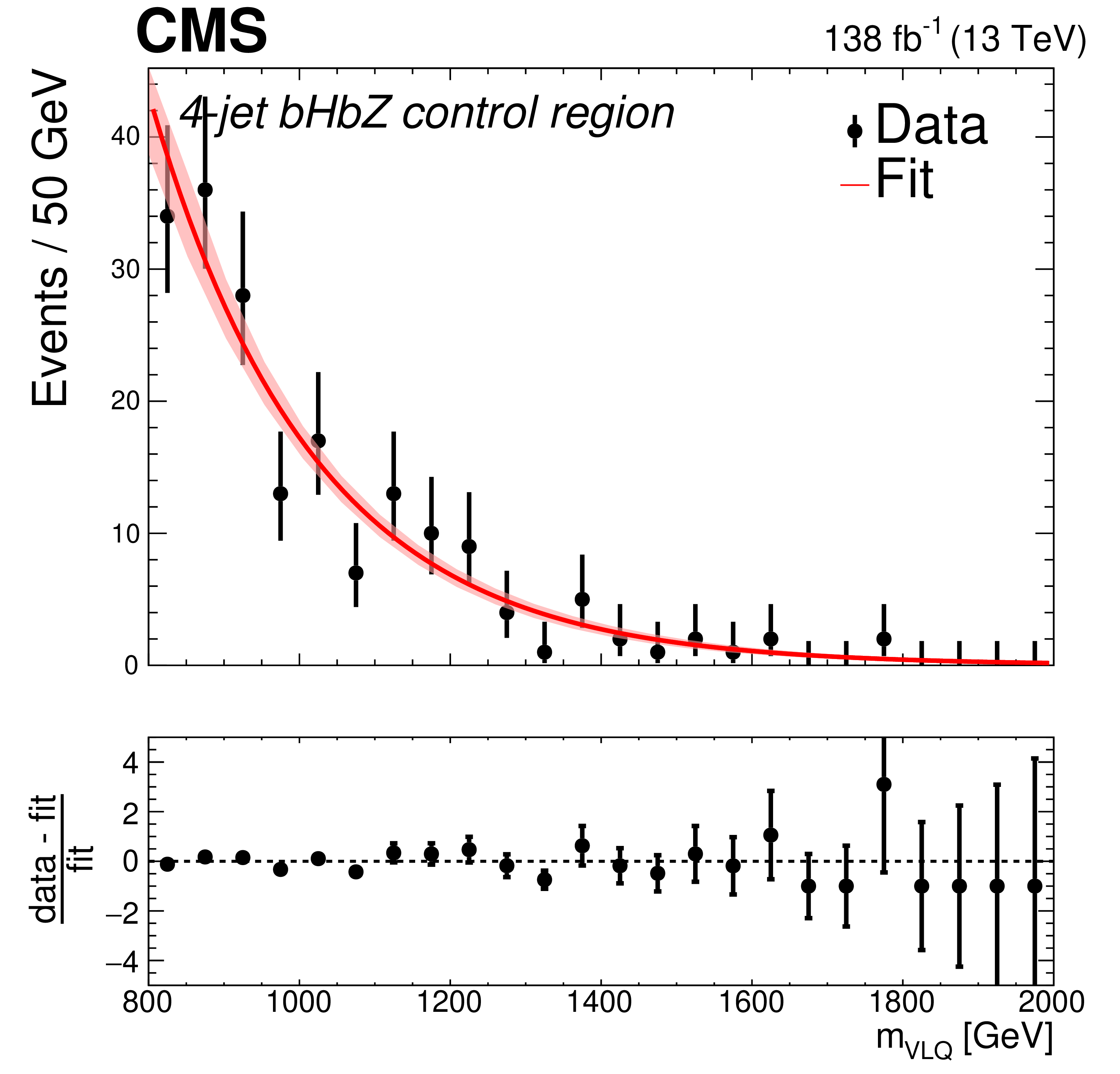
Figure 9-c:
Distributions of $ m_{\text{VLQ}} $ for events in the control region for the channels in the leptonic category. Upper row: 3-jet events in the $ \mathrm{b}\mathrm{H}\mathrm{b}\mathrm{Z} $ (left) and $ \mathrm{b}\mathrm{Z}\mathrm{b}\mathrm{Z} $ (right) modes. Lower row: 4-jet events in the $ \mathrm{b}\mathrm{H}\mathrm{b}\mathrm{Z} $ (left) and $ \mathrm{b}\mathrm{Z}\mathrm{b}\mathrm{Z} $ (right) modes. The exponential fit and its uncertainty are shown by the red line and the light red shaded band, respectively. The bottom panel shows the fractional difference between the data and fit, (data-fit)/fit. |
png pdf |
Figure 9-d:
Distributions of $ m_{\text{VLQ}} $ for events in the control region for the channels in the leptonic category. Upper row: 3-jet events in the $ \mathrm{b}\mathrm{H}\mathrm{b}\mathrm{Z} $ (left) and $ \mathrm{b}\mathrm{Z}\mathrm{b}\mathrm{Z} $ (right) modes. Lower row: 4-jet events in the $ \mathrm{b}\mathrm{H}\mathrm{b}\mathrm{Z} $ (left) and $ \mathrm{b}\mathrm{Z}\mathrm{b}\mathrm{Z} $ (right) modes. The exponential fit and its uncertainty are shown by the red line and the light red shaded band, respectively. The bottom panel shows the fractional difference between the data and fit, (data-fit)/fit. |

png pdf |
Figure 10:
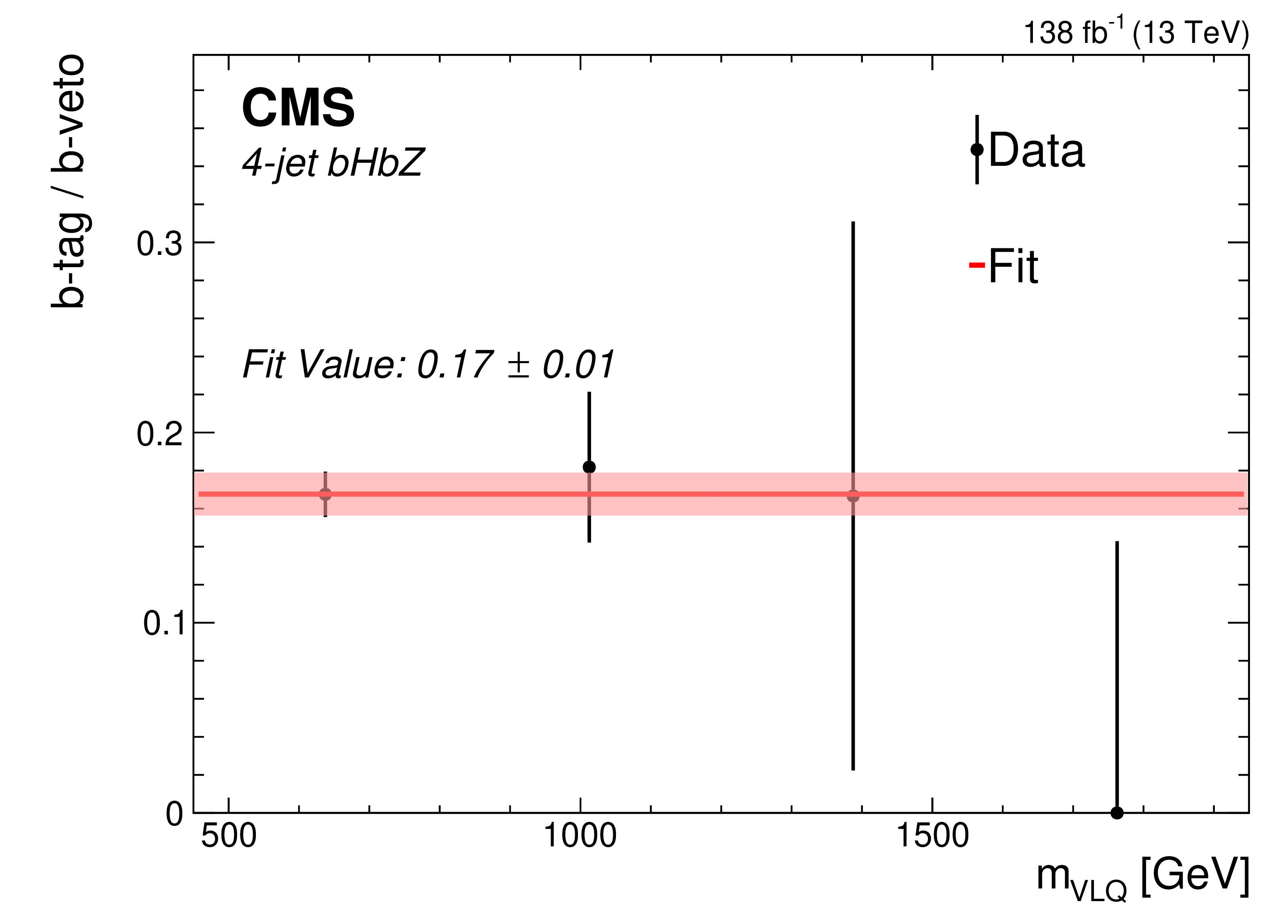
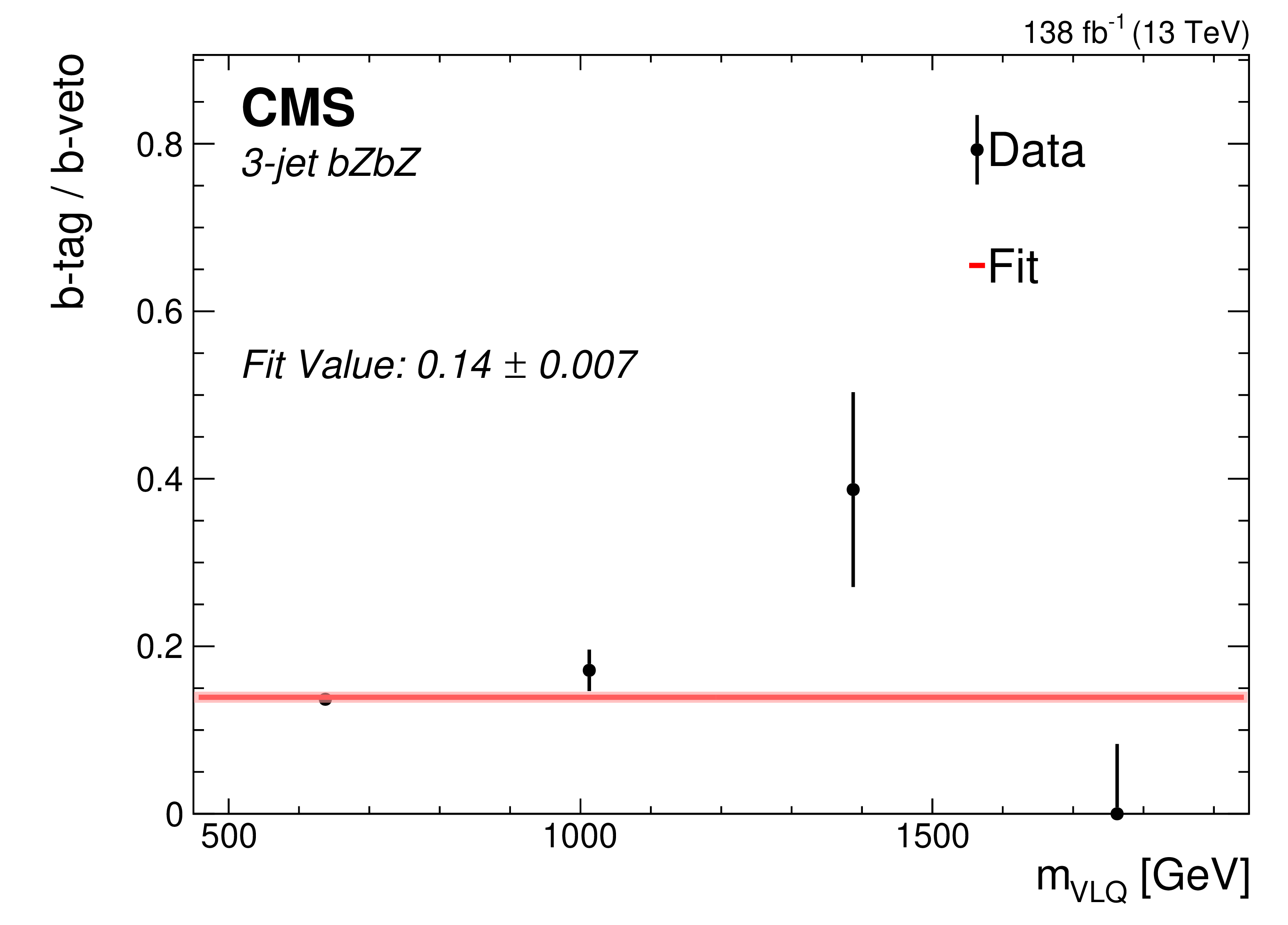
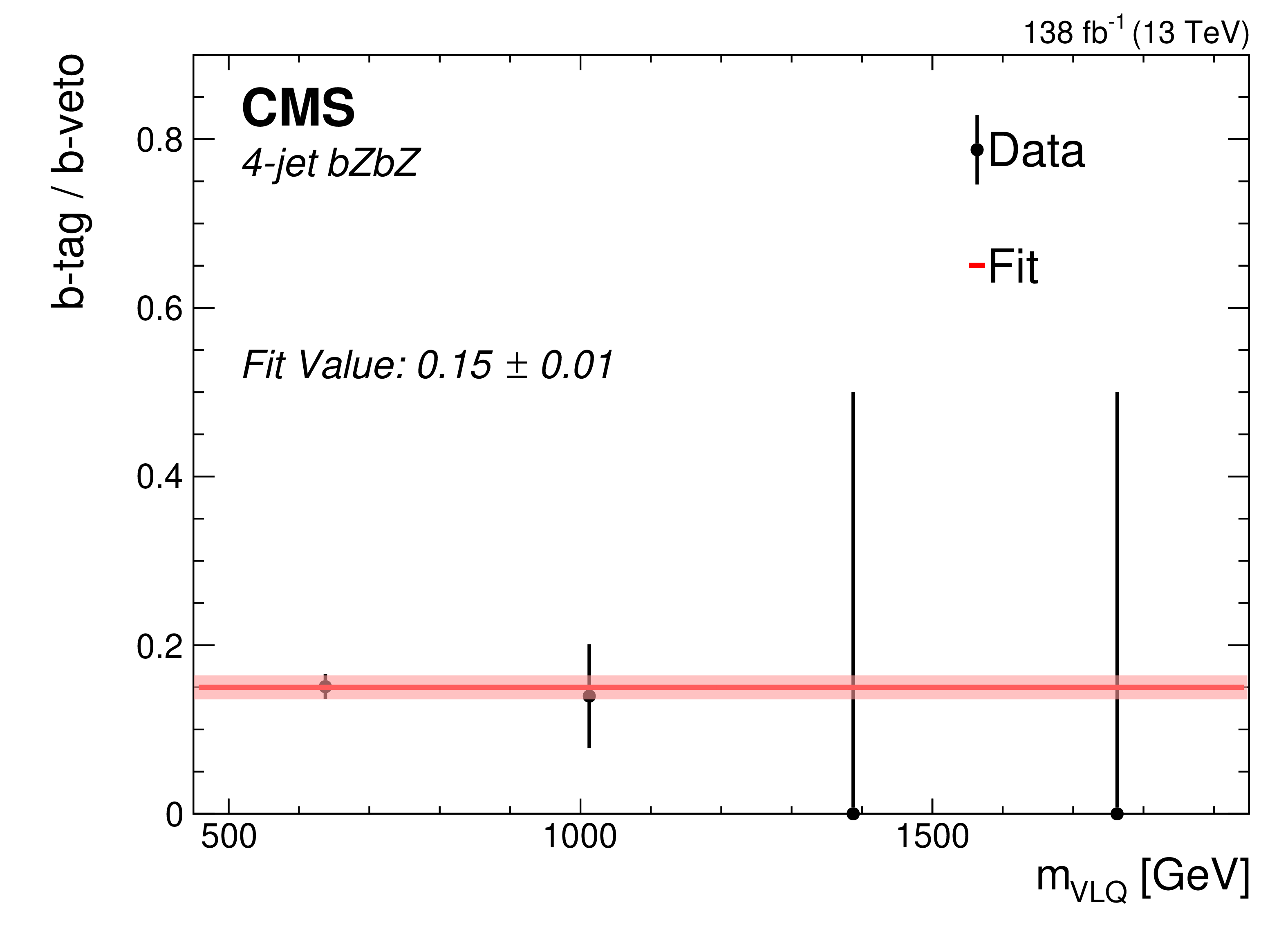
Normalization factor as a function of $ m_{\text{VLQ}} $ for leptonic events in the 5 $ < \chi^2_\text{mod}/\text{ndf} < $ 20 region. Upper row: $ \mathrm{b}\mathrm{H}\mathrm{b}\mathrm{Z} $ events in the 3-jet (left) and 4-jet (right) channels. Lower row: $ \mathrm{b}\mathrm{Z}\mathrm{b}\mathrm{Z} $ events in the 3-jet (left) and 4-jet (right) channels. The fit to a constant value and its uncertainty are shown by the red line and the light red shaded band, respectively. |

png pdf |
Figure 10-a:
Normalization factor as a function of $ m_{\text{VLQ}} $ for leptonic events in the 5 $ < \chi^2_\text{mod}/\text{ndf} < $ 20 region. Upper row: $ \mathrm{b}\mathrm{H}\mathrm{b}\mathrm{Z} $ events in the 3-jet (left) and 4-jet (right) channels. Lower row: $ \mathrm{b}\mathrm{Z}\mathrm{b}\mathrm{Z} $ events in the 3-jet (left) and 4-jet (right) channels. The fit to a constant value and its uncertainty are shown by the red line and the light red shaded band, respectively. |
png pdf |
Figure 10-b:
Normalization factor as a function of $ m_{\text{VLQ}} $ for leptonic events in the 5 $ < \chi^2_\text{mod}/\text{ndf} < $ 20 region. Upper row: $ \mathrm{b}\mathrm{H}\mathrm{b}\mathrm{Z} $ events in the 3-jet (left) and 4-jet (right) channels. Lower row: $ \mathrm{b}\mathrm{Z}\mathrm{b}\mathrm{Z} $ events in the 3-jet (left) and 4-jet (right) channels. The fit to a constant value and its uncertainty are shown by the red line and the light red shaded band, respectively. |
png pdf |
Figure 10-c:
Normalization factor as a function of $ m_{\text{VLQ}} $ for leptonic events in the 5 $ < \chi^2_\text{mod}/\text{ndf} < $ 20 region. Upper row: $ \mathrm{b}\mathrm{H}\mathrm{b}\mathrm{Z} $ events in the 3-jet (left) and 4-jet (right) channels. Lower row: $ \mathrm{b}\mathrm{Z}\mathrm{b}\mathrm{Z} $ events in the 3-jet (left) and 4-jet (right) channels. The fit to a constant value and its uncertainty are shown by the red line and the light red shaded band, respectively. |
png pdf |
Figure 10-d:
Normalization factor as a function of $ m_{\text{VLQ}} $ for leptonic events in the 5 $ < \chi^2_\text{mod}/\text{ndf} < $ 20 region. Upper row: $ \mathrm{b}\mathrm{H}\mathrm{b}\mathrm{Z} $ events in the 3-jet (left) and 4-jet (right) channels. Lower row: $ \mathrm{b}\mathrm{Z}\mathrm{b}\mathrm{Z} $ events in the 3-jet (left) and 4-jet (right) channels. The fit to a constant value and its uncertainty are shown by the red line and the light red shaded band, respectively. |
png pdf |
Figure 11:
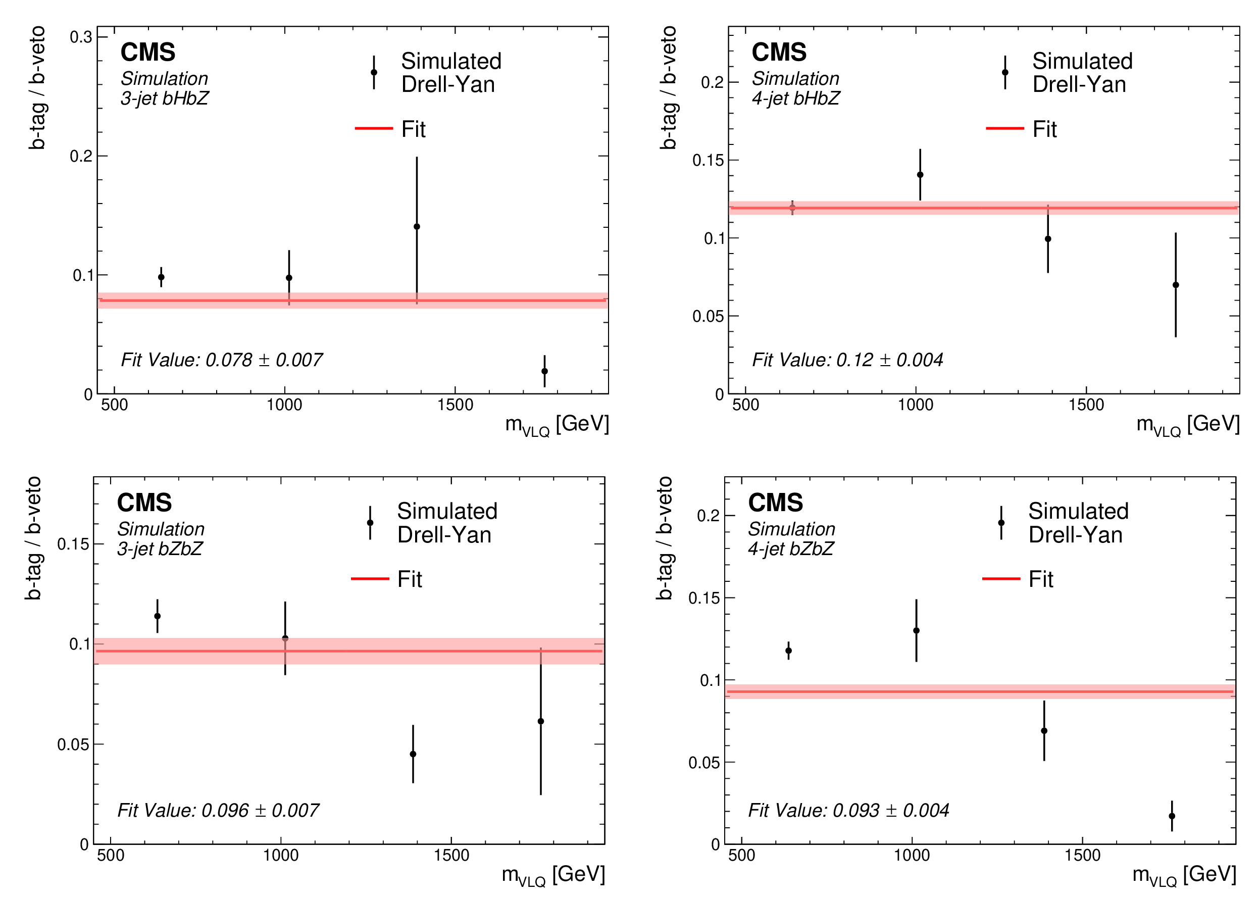
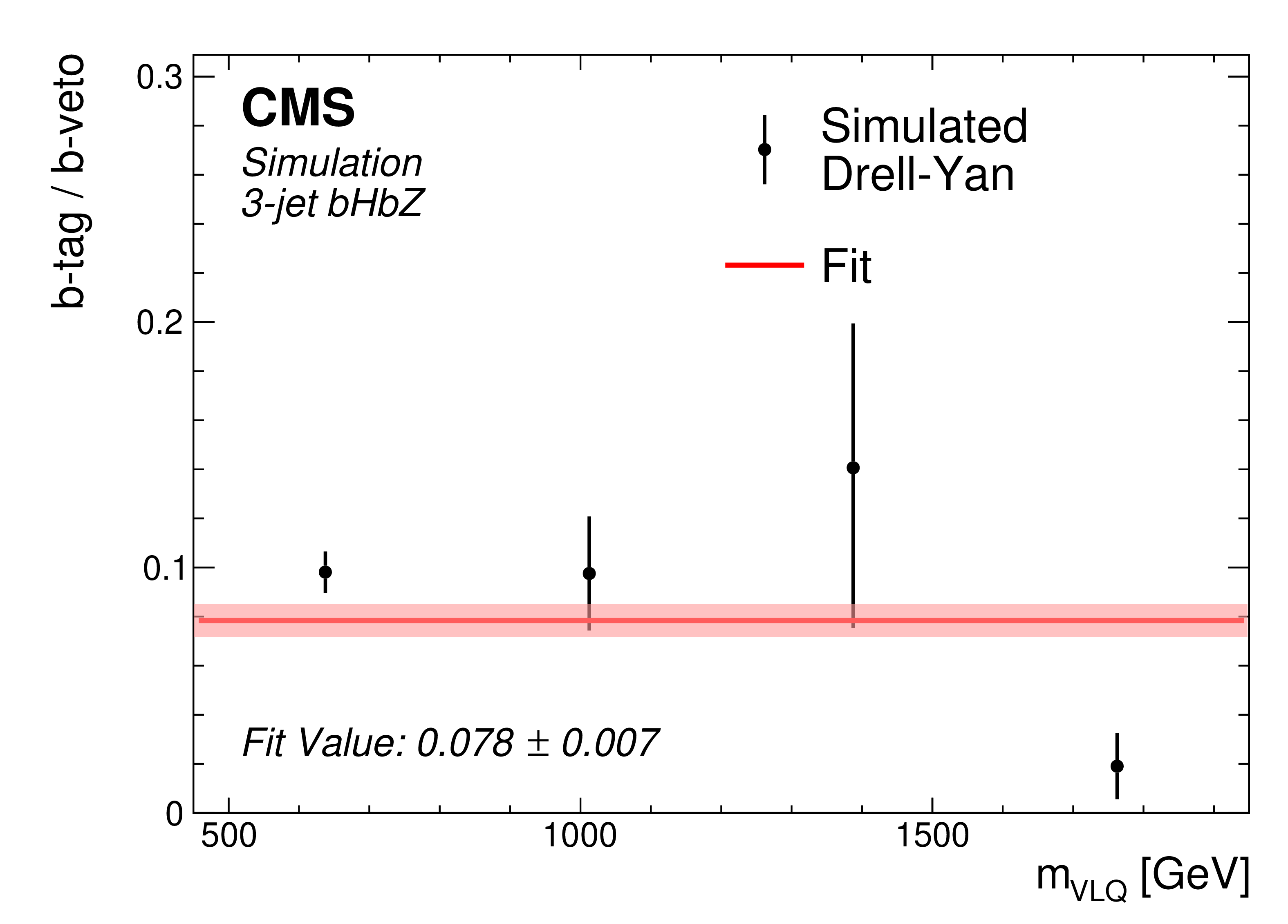
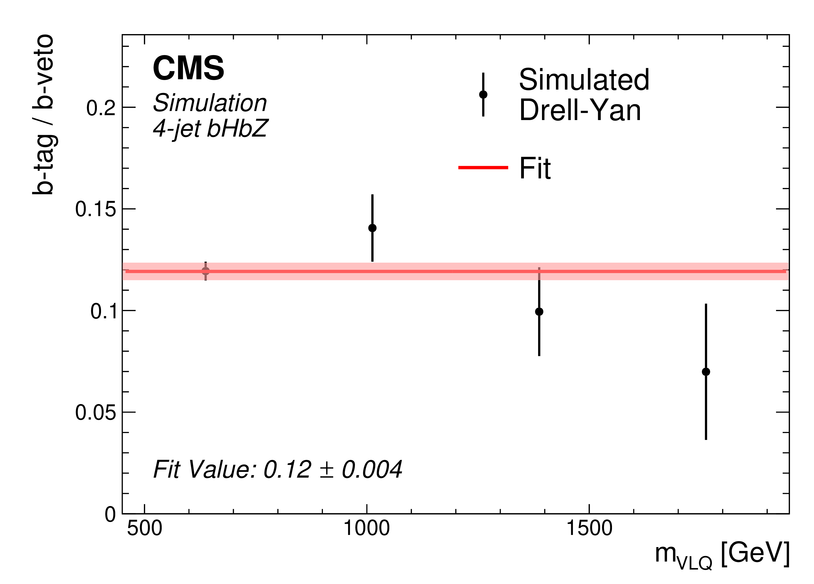
Normalization factor in the leptonic category as a function of $ m_{\text{VLQ}} $ for simulated Drell--Yan events with $ \chi^2_\text{mod}/\text{ndf} < $ 5. Upper row: $ \mathrm{b}\mathrm{H}\mathrm{b}\mathrm{Z} $ events in the 3-jet (left) and 4-jet (right) channels. Lower row: $ \mathrm{b}\mathrm{Z}\mathrm{b}\mathrm{Z} $ events in the 3-jet (left) and 4-jet (right) channels. The fit to a constant value and its uncertainty are shown by the red line and the light red shaded band, respectively. |
png pdf |
Figure 11-a:
Normalization factor in the leptonic category as a function of $ m_{\text{VLQ}} $ for simulated Drell--Yan events with $ \chi^2_\text{mod}/\text{ndf} < $ 5. Upper row: $ \mathrm{b}\mathrm{H}\mathrm{b}\mathrm{Z} $ events in the 3-jet (left) and 4-jet (right) channels. Lower row: $ \mathrm{b}\mathrm{Z}\mathrm{b}\mathrm{Z} $ events in the 3-jet (left) and 4-jet (right) channels. The fit to a constant value and its uncertainty are shown by the red line and the light red shaded band, respectively. |
png pdf |
Figure 11-b:
Normalization factor in the leptonic category as a function of $ m_{\text{VLQ}} $ for simulated Drell--Yan events with $ \chi^2_\text{mod}/\text{ndf} < $ 5. Upper row: $ \mathrm{b}\mathrm{H}\mathrm{b}\mathrm{Z} $ events in the 3-jet (left) and 4-jet (right) channels. Lower row: $ \mathrm{b}\mathrm{Z}\mathrm{b}\mathrm{Z} $ events in the 3-jet (left) and 4-jet (right) channels. The fit to a constant value and its uncertainty are shown by the red line and the light red shaded band, respectively. |

png pdf |
Figure 11-c:
Normalization factor in the leptonic category as a function of $ m_{\text{VLQ}} $ for simulated Drell--Yan events with $ \chi^2_\text{mod}/\text{ndf} < $ 5. Upper row: $ \mathrm{b}\mathrm{H}\mathrm{b}\mathrm{Z} $ events in the 3-jet (left) and 4-jet (right) channels. Lower row: $ \mathrm{b}\mathrm{Z}\mathrm{b}\mathrm{Z} $ events in the 3-jet (left) and 4-jet (right) channels. The fit to a constant value and its uncertainty are shown by the red line and the light red shaded band, respectively. |

png pdf |
Figure 11-d:
Normalization factor in the leptonic category as a function of $ m_{\text{VLQ}} $ for simulated Drell--Yan events with $ \chi^2_\text{mod}/\text{ndf} < $ 5. Upper row: $ \mathrm{b}\mathrm{H}\mathrm{b}\mathrm{Z} $ events in the 3-jet (left) and 4-jet (right) channels. Lower row: $ \mathrm{b}\mathrm{Z}\mathrm{b}\mathrm{Z} $ events in the 3-jet (left) and 4-jet (right) channels. The fit to a constant value and its uncertainty are shown by the red line and the light red shaded band, respectively. |
png pdf |
Figure 12:
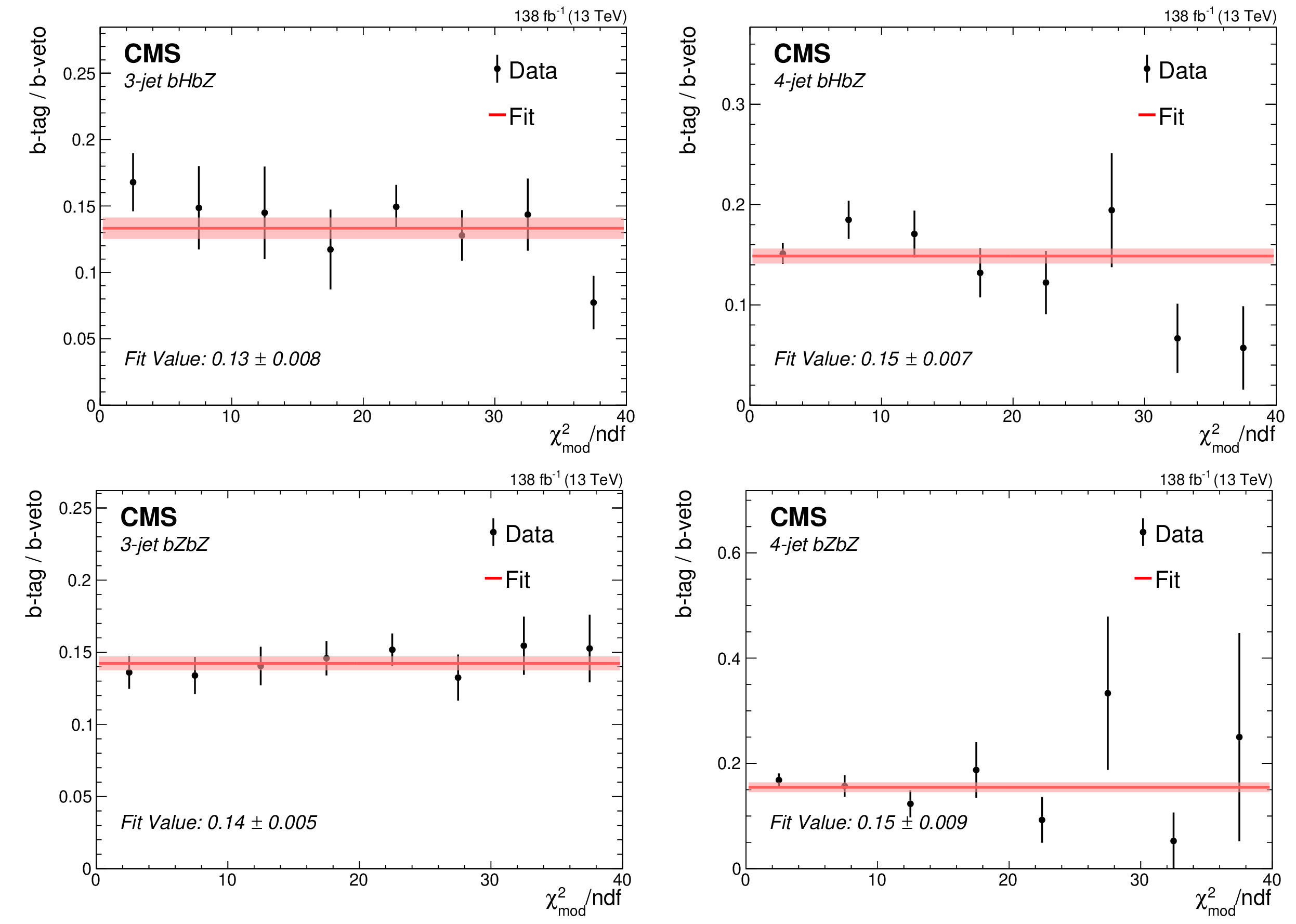
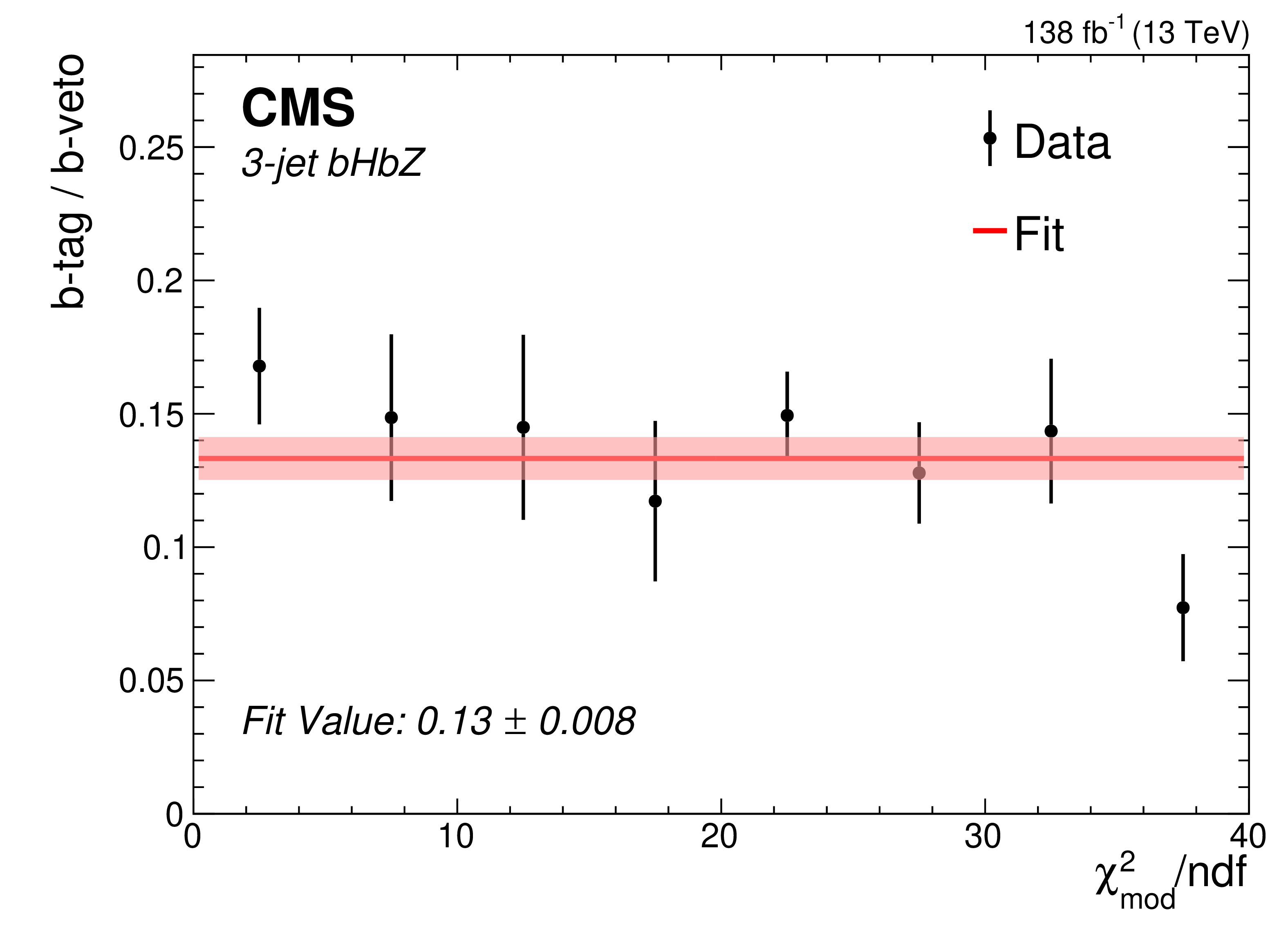
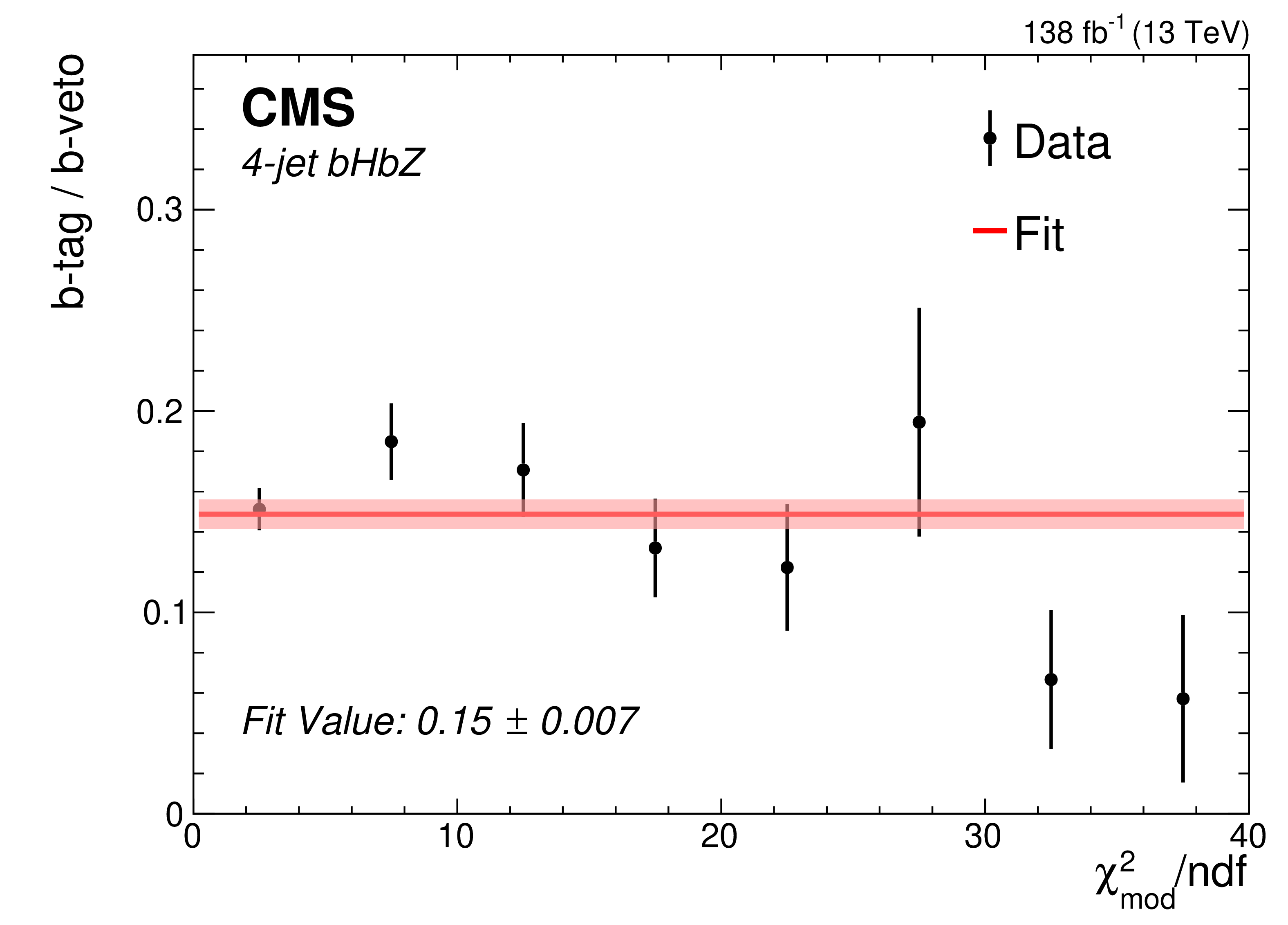
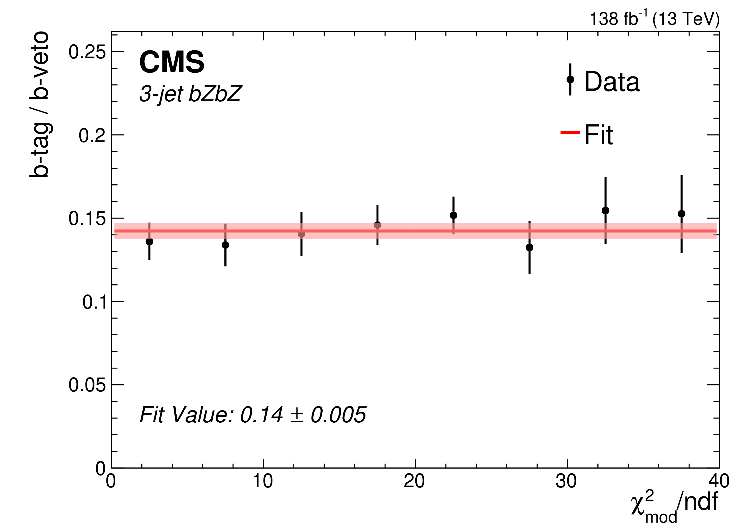
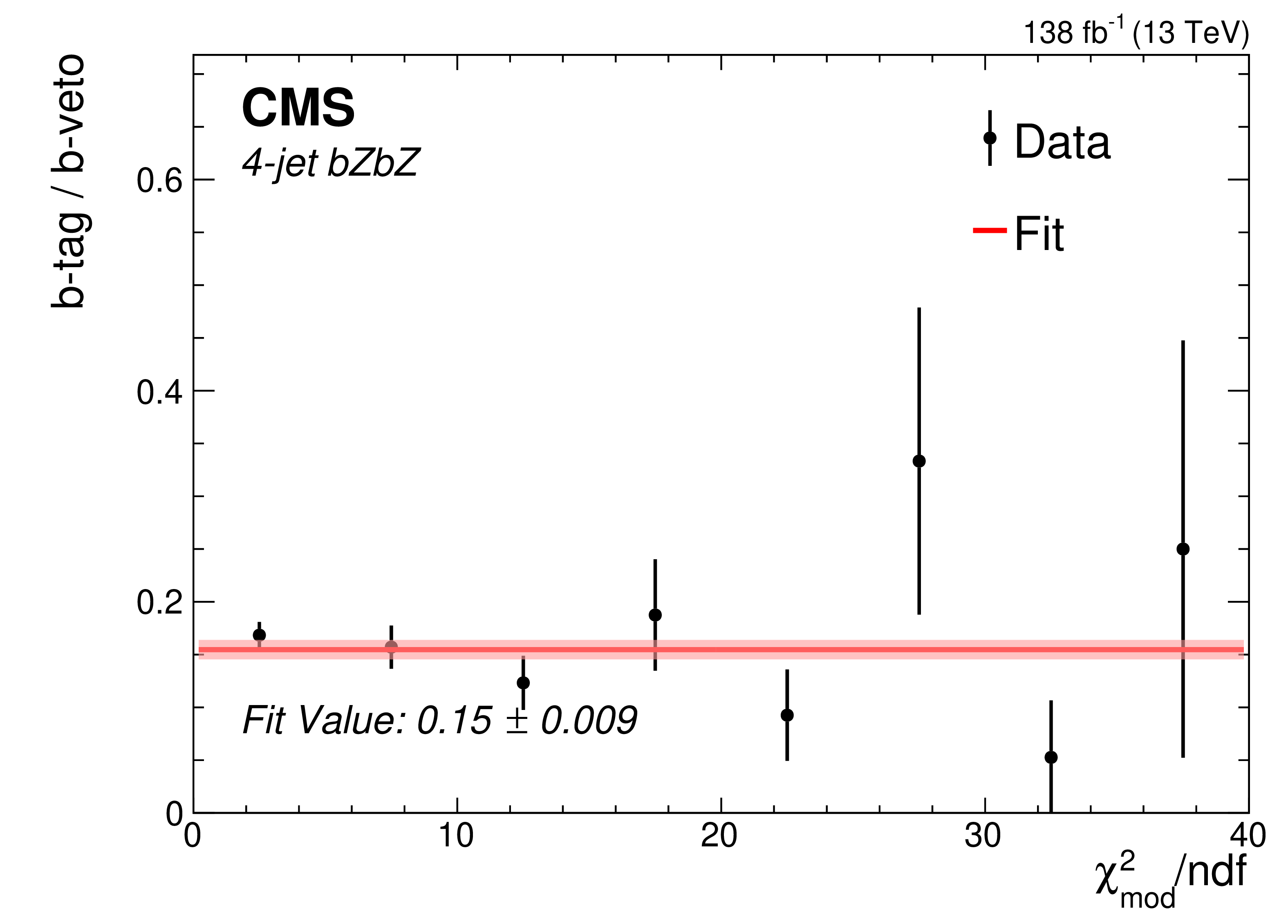
Normalization factor in the leptonic category as a function of $ \chi^2_\text{mod}/\text{ndf} $. Upper row: 3-jet events in the $ \mathrm{b}\mathrm{H}\mathrm{b}\mathrm{Z} $ (left) and $ \mathrm{b}\mathrm{Z}\mathrm{b}\mathrm{Z} $ (right) decay modes. Lower row: 4-jet events in the $ \mathrm{b}\mathrm{H}\mathrm{b}\mathrm{Z} $ (left) and $ \mathrm{b}\mathrm{Z}\mathrm{b}\mathrm{Z} $ (right) decay modes. The fit to a constant value and its uncertainty are shown by the red line and the light red shaded band, respectively. |
png pdf |
Figure 12-a:
Normalization factor in the leptonic category as a function of $ \chi^2_\text{mod}/\text{ndf} $. Upper row: 3-jet events in the $ \mathrm{b}\mathrm{H}\mathrm{b}\mathrm{Z} $ (left) and $ \mathrm{b}\mathrm{Z}\mathrm{b}\mathrm{Z} $ (right) decay modes. Lower row: 4-jet events in the $ \mathrm{b}\mathrm{H}\mathrm{b}\mathrm{Z} $ (left) and $ \mathrm{b}\mathrm{Z}\mathrm{b}\mathrm{Z} $ (right) decay modes. The fit to a constant value and its uncertainty are shown by the red line and the light red shaded band, respectively. |
png pdf |
Figure 12-b:
Normalization factor in the leptonic category as a function of $ \chi^2_\text{mod}/\text{ndf} $. Upper row: 3-jet events in the $ \mathrm{b}\mathrm{H}\mathrm{b}\mathrm{Z} $ (left) and $ \mathrm{b}\mathrm{Z}\mathrm{b}\mathrm{Z} $ (right) decay modes. Lower row: 4-jet events in the $ \mathrm{b}\mathrm{H}\mathrm{b}\mathrm{Z} $ (left) and $ \mathrm{b}\mathrm{Z}\mathrm{b}\mathrm{Z} $ (right) decay modes. The fit to a constant value and its uncertainty are shown by the red line and the light red shaded band, respectively. |
png pdf |
Figure 12-c:
Normalization factor in the leptonic category as a function of $ \chi^2_\text{mod}/\text{ndf} $. Upper row: 3-jet events in the $ \mathrm{b}\mathrm{H}\mathrm{b}\mathrm{Z} $ (left) and $ \mathrm{b}\mathrm{Z}\mathrm{b}\mathrm{Z} $ (right) decay modes. Lower row: 4-jet events in the $ \mathrm{b}\mathrm{H}\mathrm{b}\mathrm{Z} $ (left) and $ \mathrm{b}\mathrm{Z}\mathrm{b}\mathrm{Z} $ (right) decay modes. The fit to a constant value and its uncertainty are shown by the red line and the light red shaded band, respectively. |
png pdf |
Figure 12-d:
Normalization factor in the leptonic category as a function of $ \chi^2_\text{mod}/\text{ndf} $. Upper row: 3-jet events in the $ \mathrm{b}\mathrm{H}\mathrm{b}\mathrm{Z} $ (left) and $ \mathrm{b}\mathrm{Z}\mathrm{b}\mathrm{Z} $ (right) decay modes. Lower row: 4-jet events in the $ \mathrm{b}\mathrm{H}\mathrm{b}\mathrm{Z} $ (left) and $ \mathrm{b}\mathrm{Z}\mathrm{b}\mathrm{Z} $ (right) decay modes. The fit to a constant value and its uncertainty are shown by the red line and the light red shaded band, respectively. |
png pdf |
Figure 13:
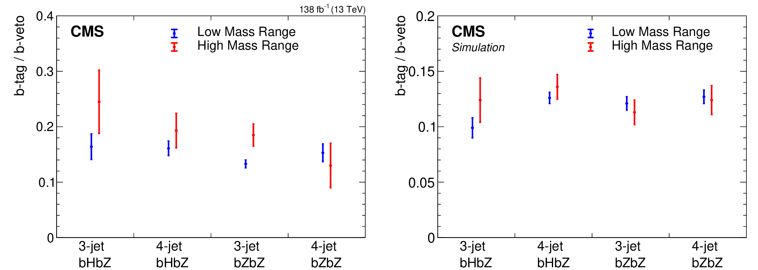
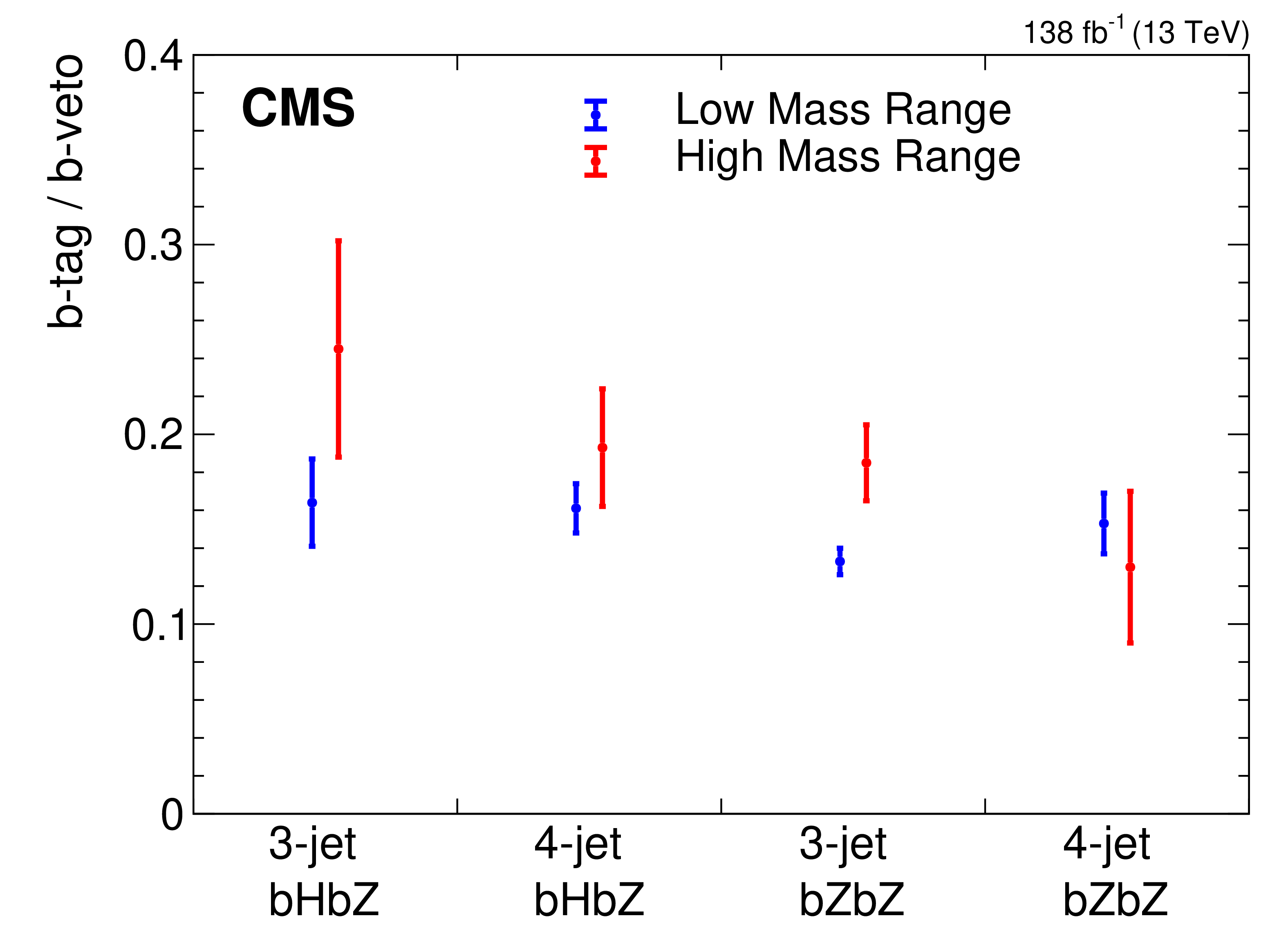
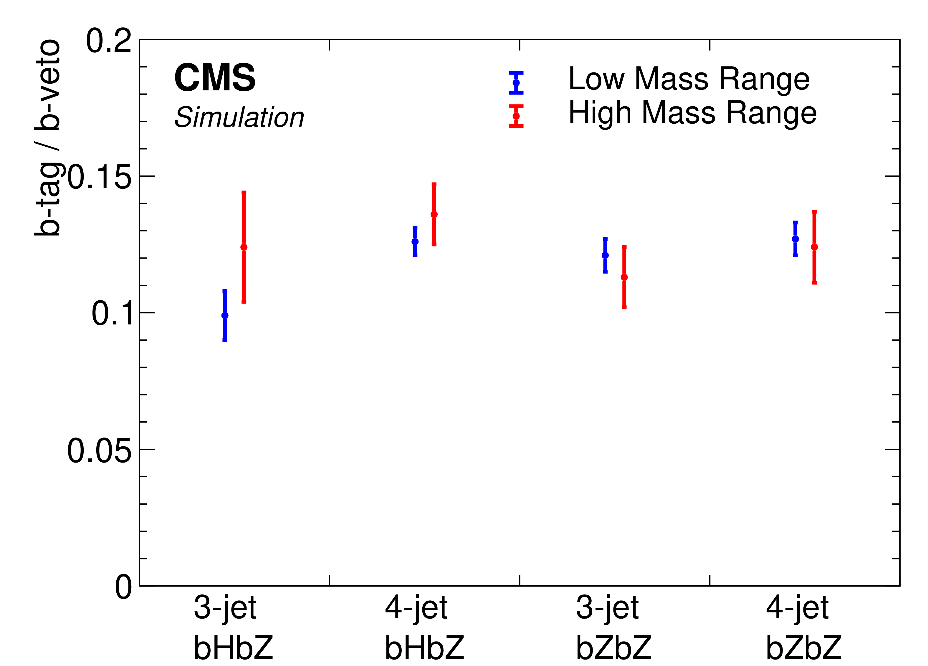
Normalization factor in the low-mass region (450 to 900 GeV) and the high-mass region (800 to 2000 GeV) for events with 5 $ < \chi^2_\text{mod}/\text{ndf} < $ 20 in data (left) and simulated Drell--Yan events with $ \chi^2_\text{mod}/\text{ndf} < $ 5 (right). |
png pdf |
Figure 13-a:
Normalization factor in the low-mass region (450 to 900 GeV) and the high-mass region (800 to 2000 GeV) for events with 5 $ < \chi^2_\text{mod}/\text{ndf} < $ 20 in data (left) and simulated Drell--Yan events with $ \chi^2_\text{mod}/\text{ndf} < $ 5 (right). |
png pdf |
Figure 13-b:
Normalization factor in the low-mass region (450 to 900 GeV) and the high-mass region (800 to 2000 GeV) for events with 5 $ < \chi^2_\text{mod}/\text{ndf} < $ 20 in data (left) and simulated Drell--Yan events with $ \chi^2_\text{mod}/\text{ndf} < $ 5 (right). |
png pdf |
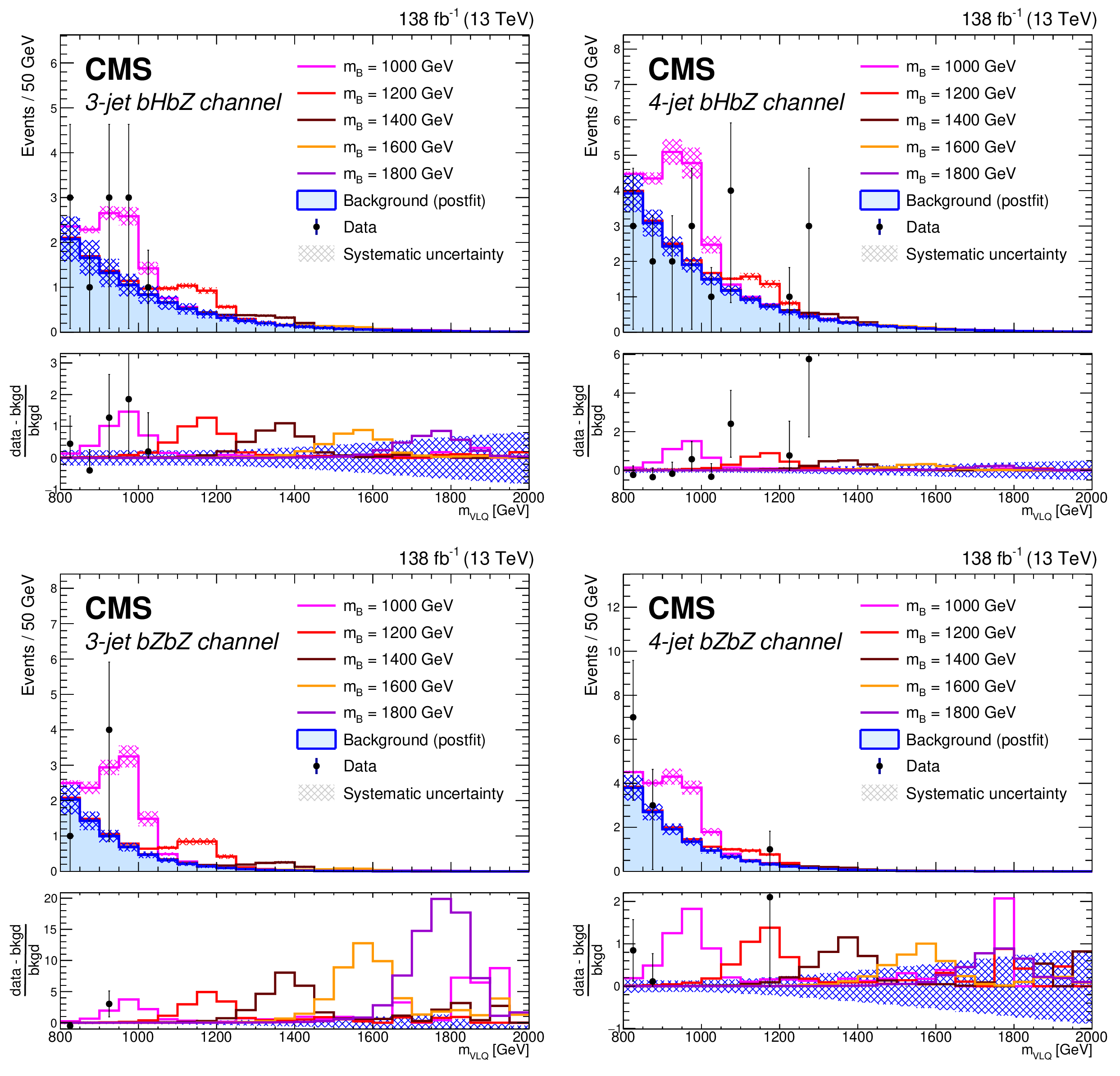
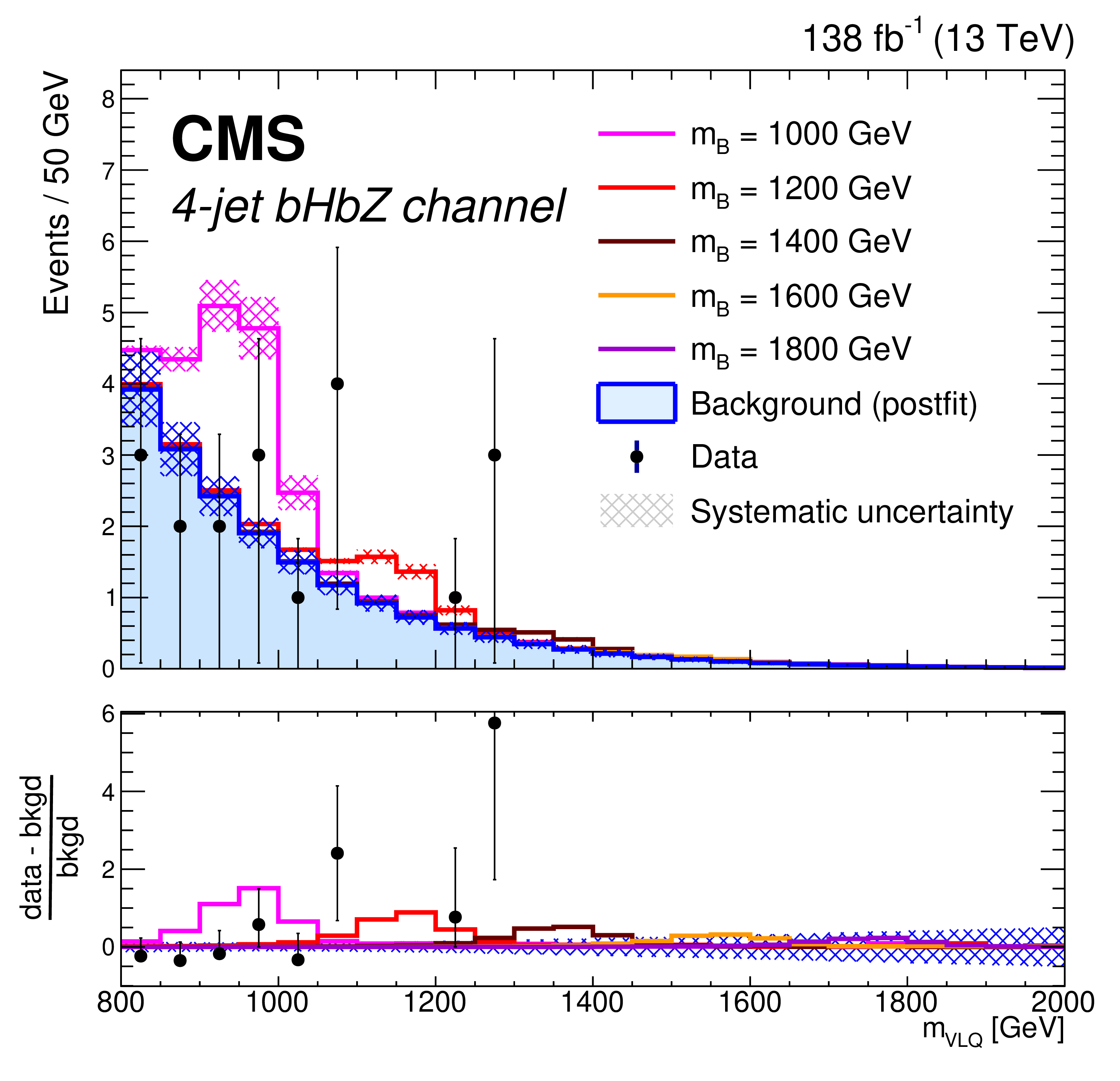
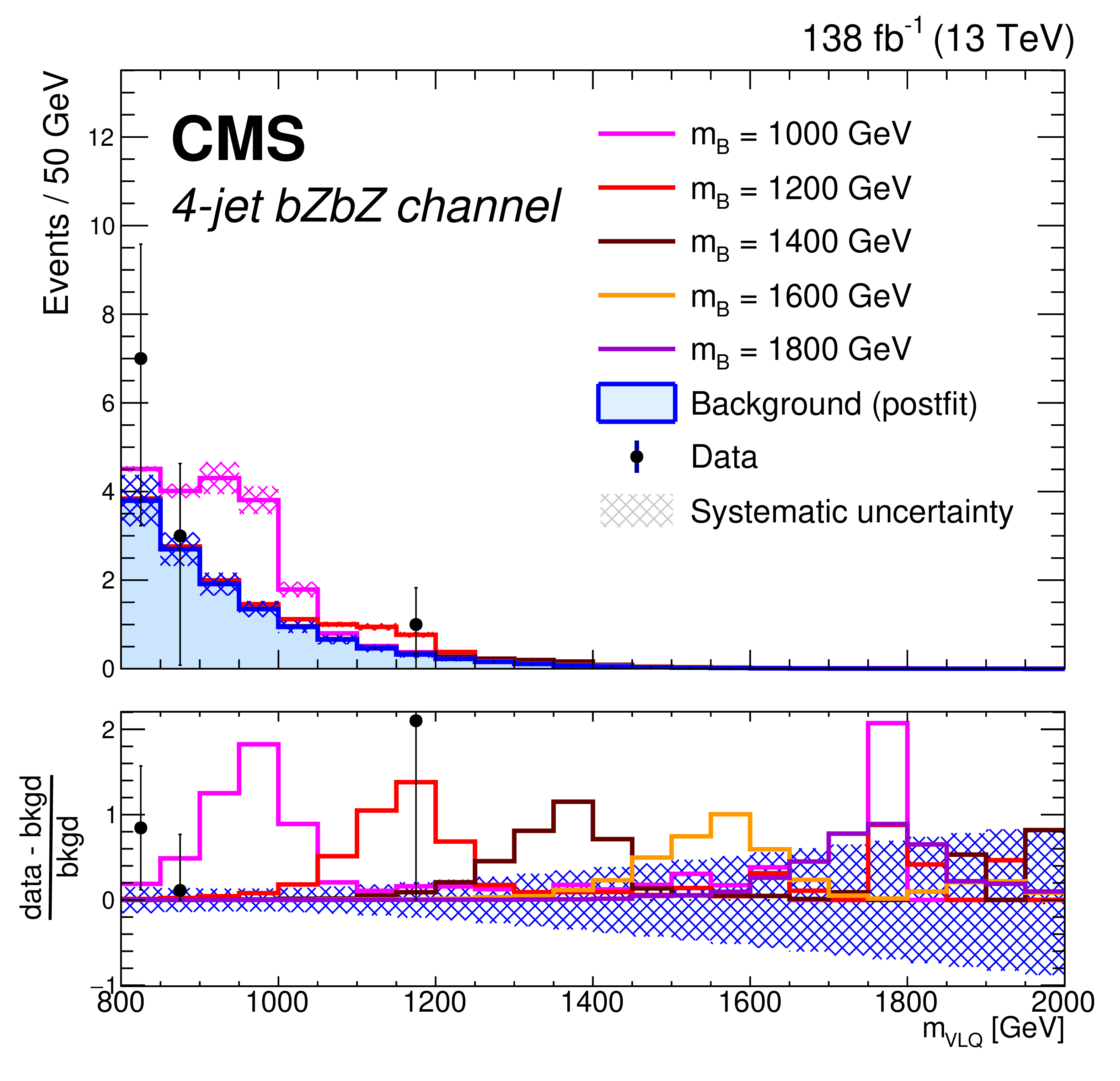
Figure 14:
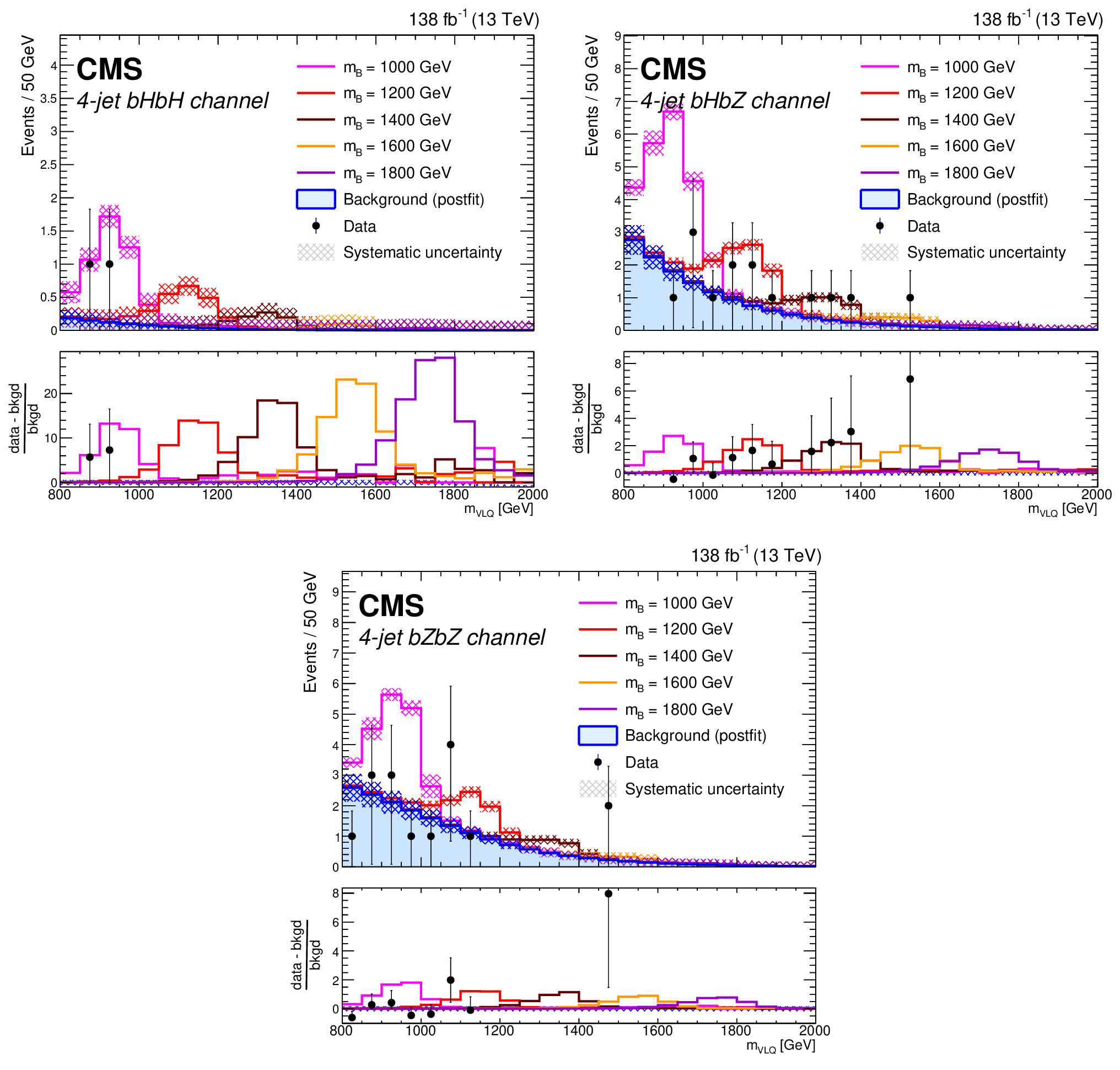
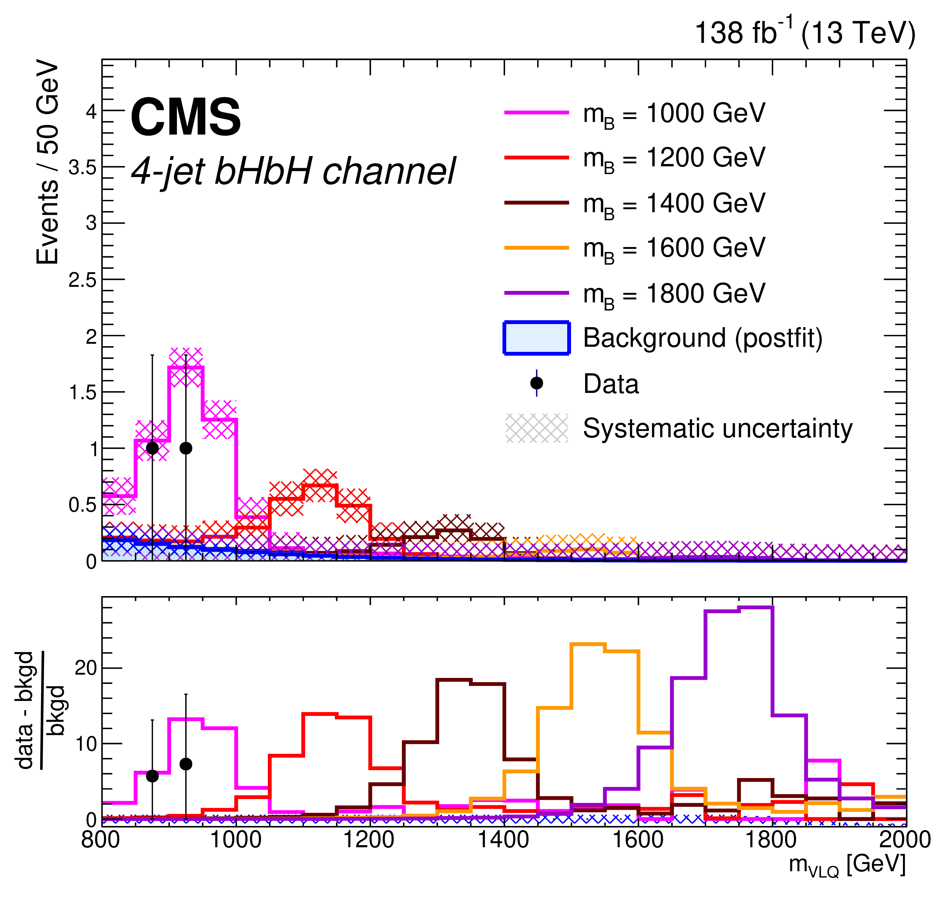
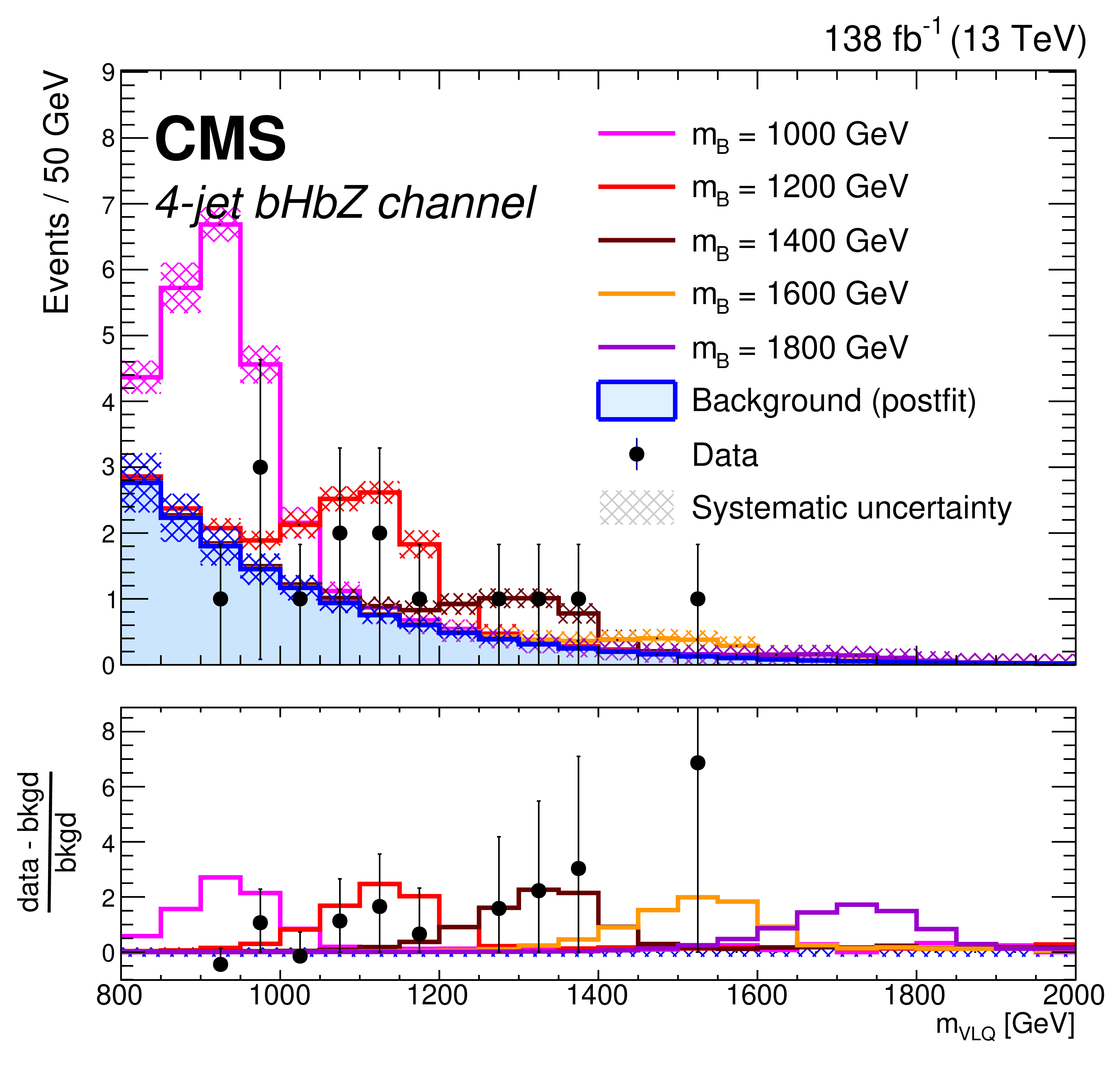
Distributions of reconstructed VLQ mass for expected postfit background (blue histogram), signal plus background (colored lines), and observed data (black points) for events in the hadronic category. The channels shown are 4-jet $ \mathrm{b}\mathrm{H}\mathrm{b}\mathrm{H} $ (upper left), 4-jet $ \mathrm{b}\mathrm{H}\mathrm{b}\mathrm{Z} $ (upper right), 4-jet $ \mathrm{b}\mathrm{Z}\mathrm{b}\mathrm{Z} $ (lower center). Five signal masses are shown: 1000 (magenta), 1200 (red), 1400 (maroon), 1600 (orange), and 1800 GeV (purple). The signal distributions are normalized to the number of events estimated from the expected VLQ production cross section. The assumed branching fractions are $ \mathcal{B}({\mathrm{B}} \to \mathrm{b}\mathrm{H}) = \mathcal{B}({\mathrm{B}} \to \mathrm{b}\mathrm{Z}) = $ 50%, $ \mathcal{B}({\mathrm{B}} \to \mathrm{t}\mathrm{W}) = $ 0%. The background distribution is independent of the signal branching fractions. The hatched regions indicate the total systematic uncertainties in the background estimate. |
png pdf |
Figure 14-a:
Distributions of reconstructed VLQ mass for expected postfit background (blue histogram), signal plus background (colored lines), and observed data (black points) for events in the hadronic category. The channels shown are 4-jet $ \mathrm{b}\mathrm{H}\mathrm{b}\mathrm{H} $ (upper left), 4-jet $ \mathrm{b}\mathrm{H}\mathrm{b}\mathrm{Z} $ (upper right), 4-jet $ \mathrm{b}\mathrm{Z}\mathrm{b}\mathrm{Z} $ (lower center). Five signal masses are shown: 1000 (magenta), 1200 (red), 1400 (maroon), 1600 (orange), and 1800 GeV (purple). The signal distributions are normalized to the number of events estimated from the expected VLQ production cross section. The assumed branching fractions are $ \mathcal{B}({\mathrm{B}} \to \mathrm{b}\mathrm{H}) = \mathcal{B}({\mathrm{B}} \to \mathrm{b}\mathrm{Z}) = $ 50%, $ \mathcal{B}({\mathrm{B}} \to \mathrm{t}\mathrm{W}) = $ 0%. The background distribution is independent of the signal branching fractions. The hatched regions indicate the total systematic uncertainties in the background estimate. |
png pdf |
Figure 14-b:
Distributions of reconstructed VLQ mass for expected postfit background (blue histogram), signal plus background (colored lines), and observed data (black points) for events in the hadronic category. The channels shown are 4-jet $ \mathrm{b}\mathrm{H}\mathrm{b}\mathrm{H} $ (upper left), 4-jet $ \mathrm{b}\mathrm{H}\mathrm{b}\mathrm{Z} $ (upper right), 4-jet $ \mathrm{b}\mathrm{Z}\mathrm{b}\mathrm{Z} $ (lower center). Five signal masses are shown: 1000 (magenta), 1200 (red), 1400 (maroon), 1600 (orange), and 1800 GeV (purple). The signal distributions are normalized to the number of events estimated from the expected VLQ production cross section. The assumed branching fractions are $ \mathcal{B}({\mathrm{B}} \to \mathrm{b}\mathrm{H}) = \mathcal{B}({\mathrm{B}} \to \mathrm{b}\mathrm{Z}) = $ 50%, $ \mathcal{B}({\mathrm{B}} \to \mathrm{t}\mathrm{W}) = $ 0%. The background distribution is independent of the signal branching fractions. The hatched regions indicate the total systematic uncertainties in the background estimate. |

png pdf |
Figure 14-c:
Distributions of reconstructed VLQ mass for expected postfit background (blue histogram), signal plus background (colored lines), and observed data (black points) for events in the hadronic category. The channels shown are 4-jet $ \mathrm{b}\mathrm{H}\mathrm{b}\mathrm{H} $ (upper left), 4-jet $ \mathrm{b}\mathrm{H}\mathrm{b}\mathrm{Z} $ (upper right), 4-jet $ \mathrm{b}\mathrm{Z}\mathrm{b}\mathrm{Z} $ (lower center). Five signal masses are shown: 1000 (magenta), 1200 (red), 1400 (maroon), 1600 (orange), and 1800 GeV (purple). The signal distributions are normalized to the number of events estimated from the expected VLQ production cross section. The assumed branching fractions are $ \mathcal{B}({\mathrm{B}} \to \mathrm{b}\mathrm{H}) = \mathcal{B}({\mathrm{B}} \to \mathrm{b}\mathrm{Z}) = $ 50%, $ \mathcal{B}({\mathrm{B}} \to \mathrm{t}\mathrm{W}) = $ 0%. The background distribution is independent of the signal branching fractions. The hatched regions indicate the total systematic uncertainties in the background estimate. |
png pdf |
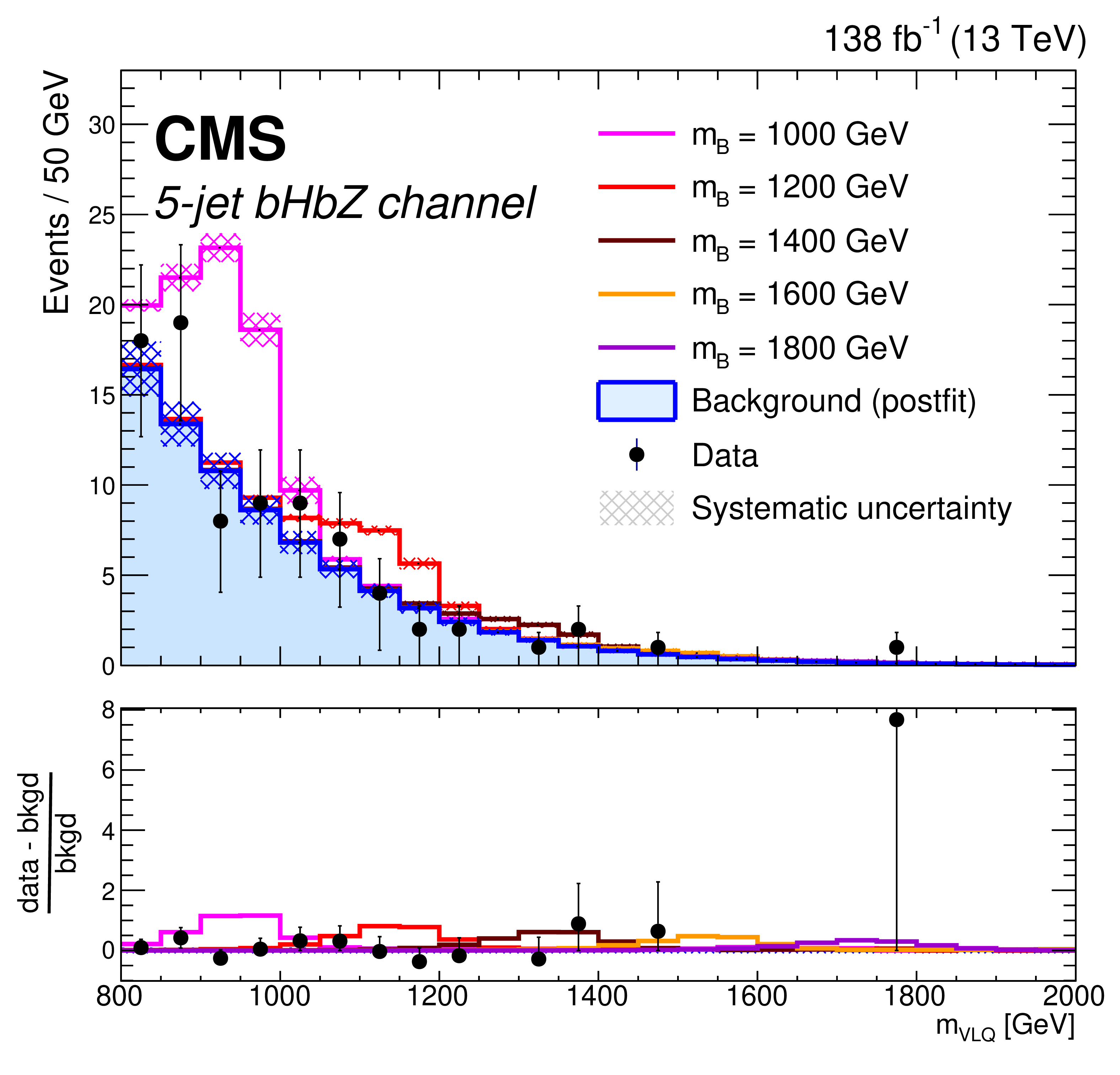
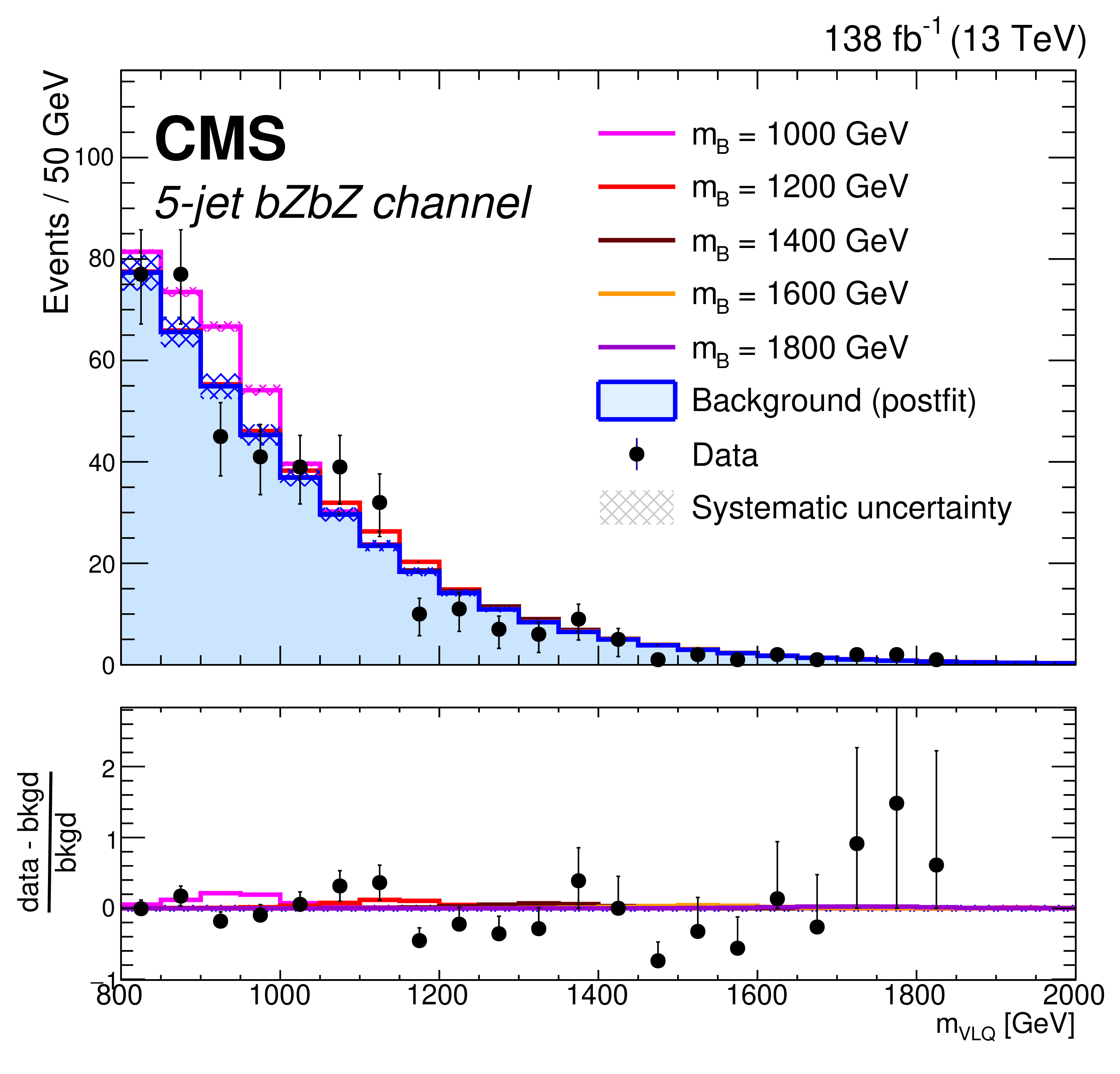
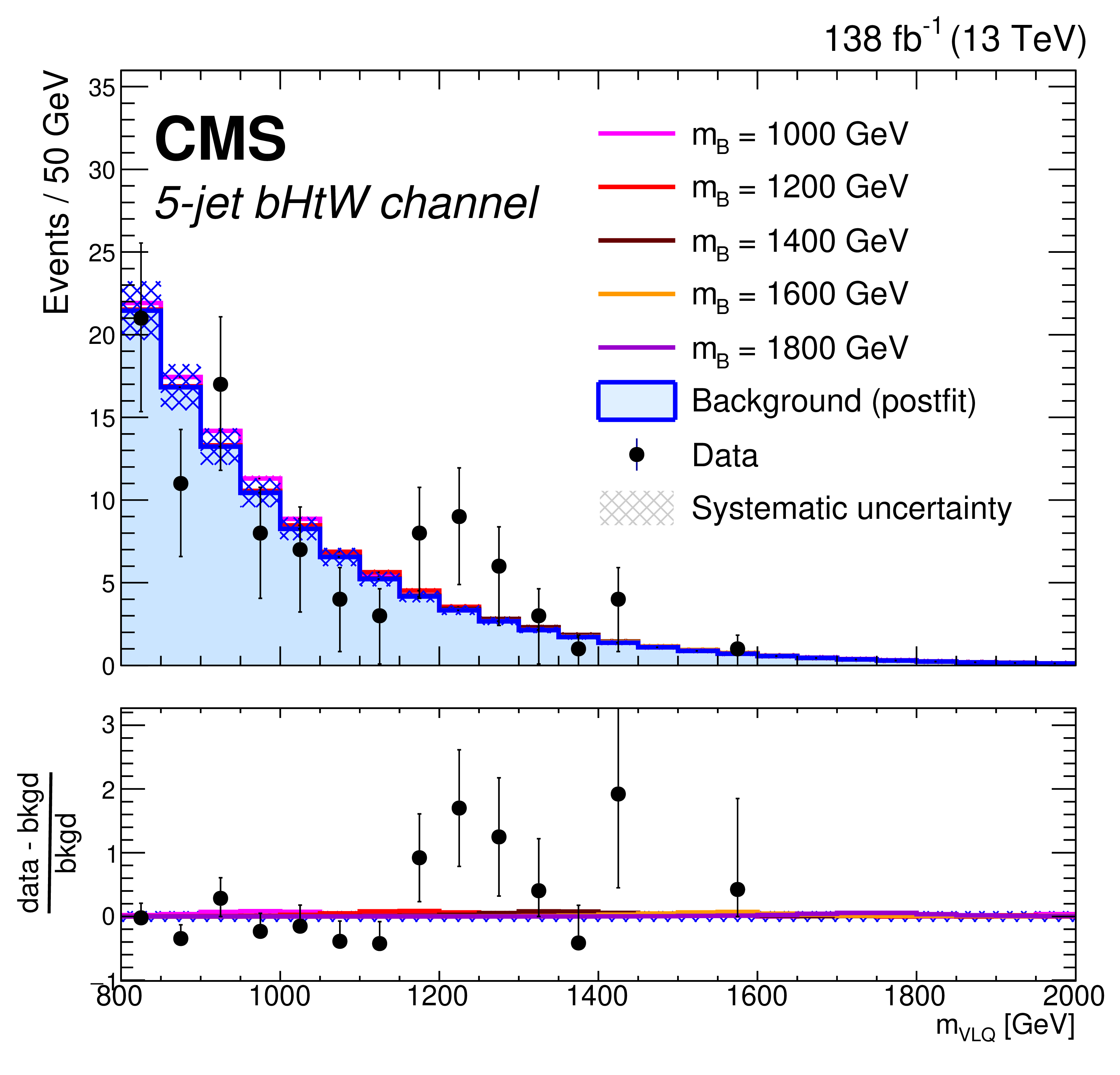
Figure 15:
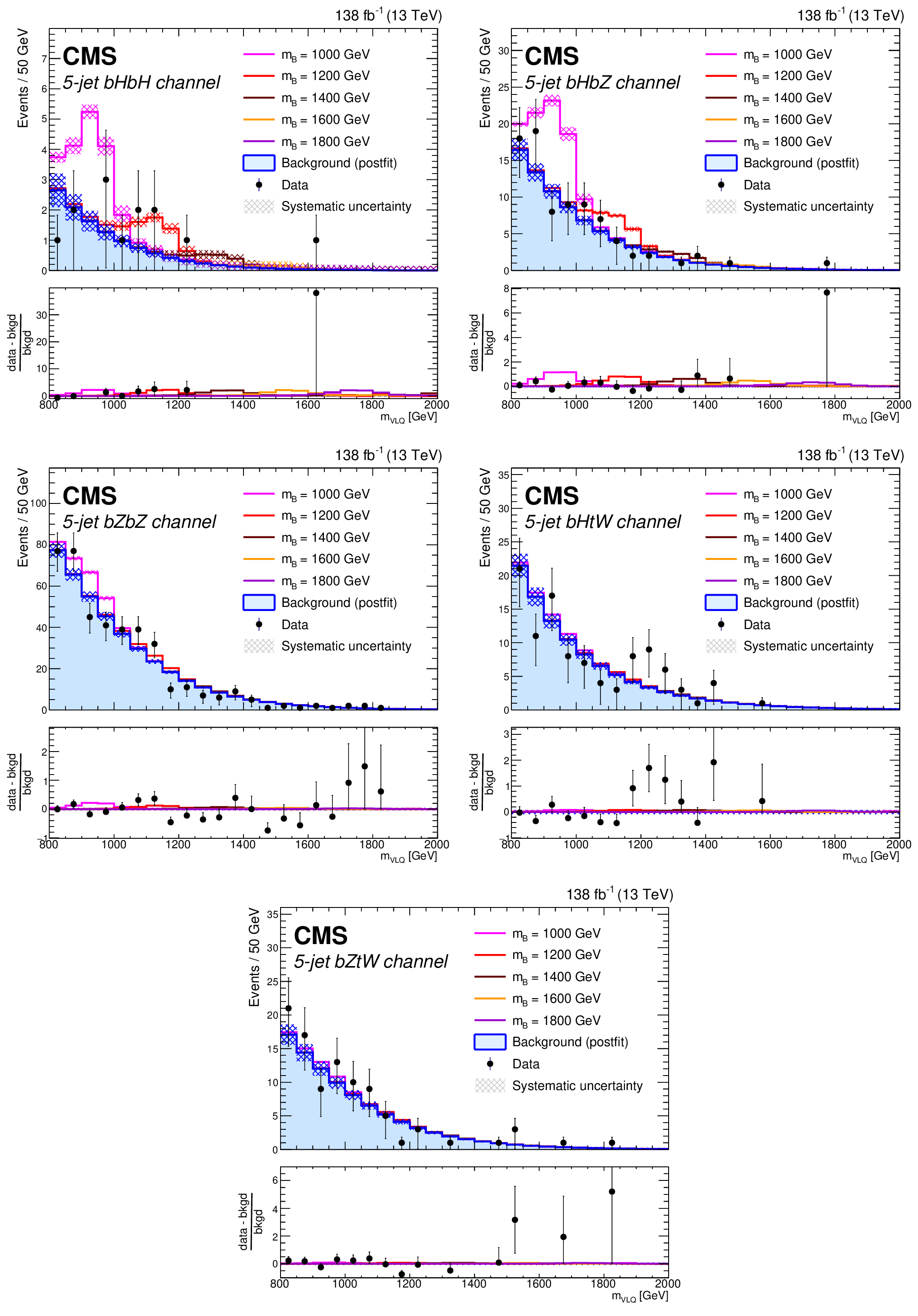
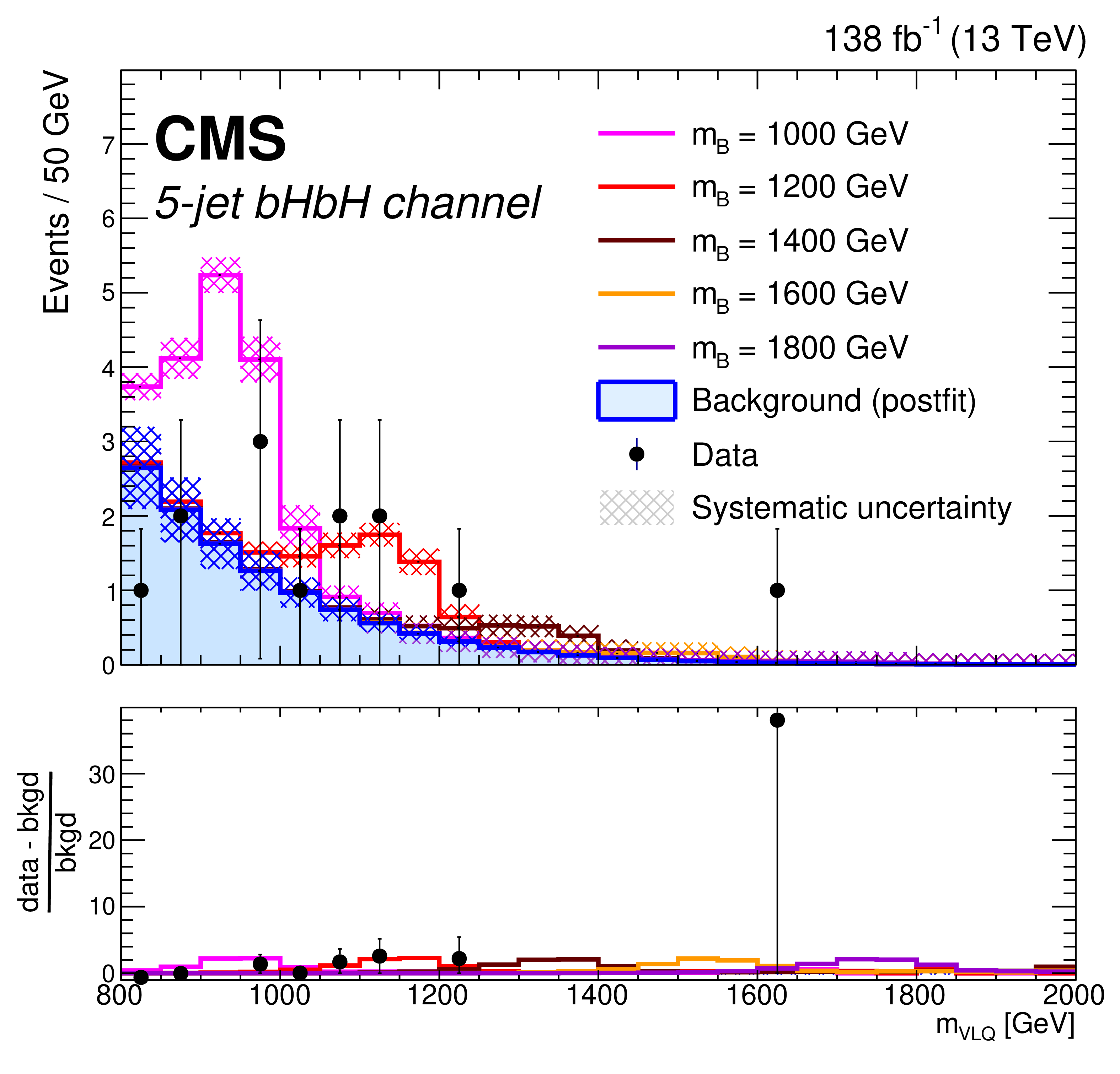
Distributions of reconstructed VLQ mass for expected postfit background (blue histogram), signal plus background (colored lines), and observed data (black points) for events in the hadronic category. The channels shown are 5-jet $ \mathrm{b}\mathrm{H}\mathrm{b}\mathrm{H} $ (upper left), 5-jet $ \mathrm{b}\mathrm{H}\mathrm{b}\mathrm{Z} $ (upper right), 5-jet $ \mathrm{b}\mathrm{Z}\mathrm{b}\mathrm{Z} $ (middle left), 5-jet $ \mathrm{b}\mathrm{H}\mathrm{t}\mathrm{W} $ (middle right), and 5-jet $ \mathrm{b}\mathrm{Z}\mathrm{t}\mathrm{W} $ (lower center). Five signal masses are shown: 1000 (magenta), 1200 (red), 1400 (maroon), 1600 (orange), and 1800 GeV (purple). The signal distributions are normalized to the number of events estimated from the expected VLQ production cross section. The assumed branching fractions are $ \mathcal{B}({\mathrm{B}} \to \mathrm{b}\mathrm{H}) = \mathcal{B}({\mathrm{B}} \to \mathrm{b}\mathrm{Z}) = $ 50%, $ \mathcal{B}({\mathrm{B}} \to \mathrm{t}\mathrm{W}) = $ 0%. The background distribution is independent of the signal branching fractions. The hatched regions indicate the total systematic uncertainties in the background estimate. |
png pdf |
Figure 15-a:
Distributions of reconstructed VLQ mass for expected postfit background (blue histogram), signal plus background (colored lines), and observed data (black points) for events in the hadronic category. The channels shown are 5-jet $ \mathrm{b}\mathrm{H}\mathrm{b}\mathrm{H} $ (upper left), 5-jet $ \mathrm{b}\mathrm{H}\mathrm{b}\mathrm{Z} $ (upper right), 5-jet $ \mathrm{b}\mathrm{Z}\mathrm{b}\mathrm{Z} $ (middle left), 5-jet $ \mathrm{b}\mathrm{H}\mathrm{t}\mathrm{W} $ (middle right), and 5-jet $ \mathrm{b}\mathrm{Z}\mathrm{t}\mathrm{W} $ (lower center). Five signal masses are shown: 1000 (magenta), 1200 (red), 1400 (maroon), 1600 (orange), and 1800 GeV (purple). The signal distributions are normalized to the number of events estimated from the expected VLQ production cross section. The assumed branching fractions are $ \mathcal{B}({\mathrm{B}} \to \mathrm{b}\mathrm{H}) = \mathcal{B}({\mathrm{B}} \to \mathrm{b}\mathrm{Z}) = $ 50%, $ \mathcal{B}({\mathrm{B}} \to \mathrm{t}\mathrm{W}) = $ 0%. The background distribution is independent of the signal branching fractions. The hatched regions indicate the total systematic uncertainties in the background estimate. |
png pdf |
Figure 15-b:
Distributions of reconstructed VLQ mass for expected postfit background (blue histogram), signal plus background (colored lines), and observed data (black points) for events in the hadronic category. The channels shown are 5-jet $ \mathrm{b}\mathrm{H}\mathrm{b}\mathrm{H} $ (upper left), 5-jet $ \mathrm{b}\mathrm{H}\mathrm{b}\mathrm{Z} $ (upper right), 5-jet $ \mathrm{b}\mathrm{Z}\mathrm{b}\mathrm{Z} $ (middle left), 5-jet $ \mathrm{b}\mathrm{H}\mathrm{t}\mathrm{W} $ (middle right), and 5-jet $ \mathrm{b}\mathrm{Z}\mathrm{t}\mathrm{W} $ (lower center). Five signal masses are shown: 1000 (magenta), 1200 (red), 1400 (maroon), 1600 (orange), and 1800 GeV (purple). The signal distributions are normalized to the number of events estimated from the expected VLQ production cross section. The assumed branching fractions are $ \mathcal{B}({\mathrm{B}} \to \mathrm{b}\mathrm{H}) = \mathcal{B}({\mathrm{B}} \to \mathrm{b}\mathrm{Z}) = $ 50%, $ \mathcal{B}({\mathrm{B}} \to \mathrm{t}\mathrm{W}) = $ 0%. The background distribution is independent of the signal branching fractions. The hatched regions indicate the total systematic uncertainties in the background estimate. |
png pdf |
Figure 15-c:
Distributions of reconstructed VLQ mass for expected postfit background (blue histogram), signal plus background (colored lines), and observed data (black points) for events in the hadronic category. The channels shown are 5-jet $ \mathrm{b}\mathrm{H}\mathrm{b}\mathrm{H} $ (upper left), 5-jet $ \mathrm{b}\mathrm{H}\mathrm{b}\mathrm{Z} $ (upper right), 5-jet $ \mathrm{b}\mathrm{Z}\mathrm{b}\mathrm{Z} $ (middle left), 5-jet $ \mathrm{b}\mathrm{H}\mathrm{t}\mathrm{W} $ (middle right), and 5-jet $ \mathrm{b}\mathrm{Z}\mathrm{t}\mathrm{W} $ (lower center). Five signal masses are shown: 1000 (magenta), 1200 (red), 1400 (maroon), 1600 (orange), and 1800 GeV (purple). The signal distributions are normalized to the number of events estimated from the expected VLQ production cross section. The assumed branching fractions are $ \mathcal{B}({\mathrm{B}} \to \mathrm{b}\mathrm{H}) = \mathcal{B}({\mathrm{B}} \to \mathrm{b}\mathrm{Z}) = $ 50%, $ \mathcal{B}({\mathrm{B}} \to \mathrm{t}\mathrm{W}) = $ 0%. The background distribution is independent of the signal branching fractions. The hatched regions indicate the total systematic uncertainties in the background estimate. |
png pdf |
Figure 15-d:
Distributions of reconstructed VLQ mass for expected postfit background (blue histogram), signal plus background (colored lines), and observed data (black points) for events in the hadronic category. The channels shown are 5-jet $ \mathrm{b}\mathrm{H}\mathrm{b}\mathrm{H} $ (upper left), 5-jet $ \mathrm{b}\mathrm{H}\mathrm{b}\mathrm{Z} $ (upper right), 5-jet $ \mathrm{b}\mathrm{Z}\mathrm{b}\mathrm{Z} $ (middle left), 5-jet $ \mathrm{b}\mathrm{H}\mathrm{t}\mathrm{W} $ (middle right), and 5-jet $ \mathrm{b}\mathrm{Z}\mathrm{t}\mathrm{W} $ (lower center). Five signal masses are shown: 1000 (magenta), 1200 (red), 1400 (maroon), 1600 (orange), and 1800 GeV (purple). The signal distributions are normalized to the number of events estimated from the expected VLQ production cross section. The assumed branching fractions are $ \mathcal{B}({\mathrm{B}} \to \mathrm{b}\mathrm{H}) = \mathcal{B}({\mathrm{B}} \to \mathrm{b}\mathrm{Z}) = $ 50%, $ \mathcal{B}({\mathrm{B}} \to \mathrm{t}\mathrm{W}) = $ 0%. The background distribution is independent of the signal branching fractions. The hatched regions indicate the total systematic uncertainties in the background estimate. |

png pdf |
Figure 15-e:
Distributions of reconstructed VLQ mass for expected postfit background (blue histogram), signal plus background (colored lines), and observed data (black points) for events in the hadronic category. The channels shown are 5-jet $ \mathrm{b}\mathrm{H}\mathrm{b}\mathrm{H} $ (upper left), 5-jet $ \mathrm{b}\mathrm{H}\mathrm{b}\mathrm{Z} $ (upper right), 5-jet $ \mathrm{b}\mathrm{Z}\mathrm{b}\mathrm{Z} $ (middle left), 5-jet $ \mathrm{b}\mathrm{H}\mathrm{t}\mathrm{W} $ (middle right), and 5-jet $ \mathrm{b}\mathrm{Z}\mathrm{t}\mathrm{W} $ (lower center). Five signal masses are shown: 1000 (magenta), 1200 (red), 1400 (maroon), 1600 (orange), and 1800 GeV (purple). The signal distributions are normalized to the number of events estimated from the expected VLQ production cross section. The assumed branching fractions are $ \mathcal{B}({\mathrm{B}} \to \mathrm{b}\mathrm{H}) = \mathcal{B}({\mathrm{B}} \to \mathrm{b}\mathrm{Z}) = $ 50%, $ \mathcal{B}({\mathrm{B}} \to \mathrm{t}\mathrm{W}) = $ 0%. The background distribution is independent of the signal branching fractions. The hatched regions indicate the total systematic uncertainties in the background estimate. |
png pdf |
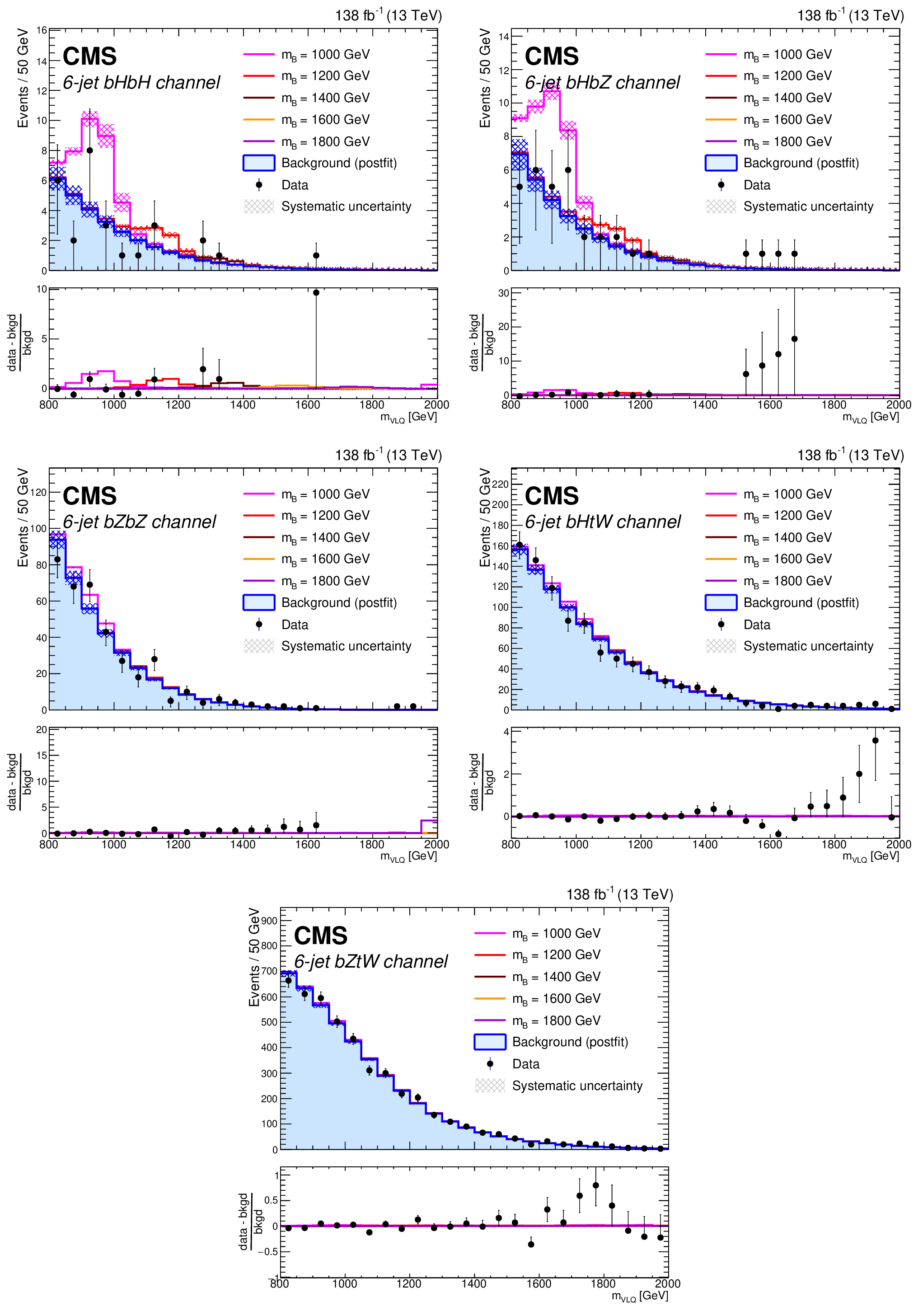
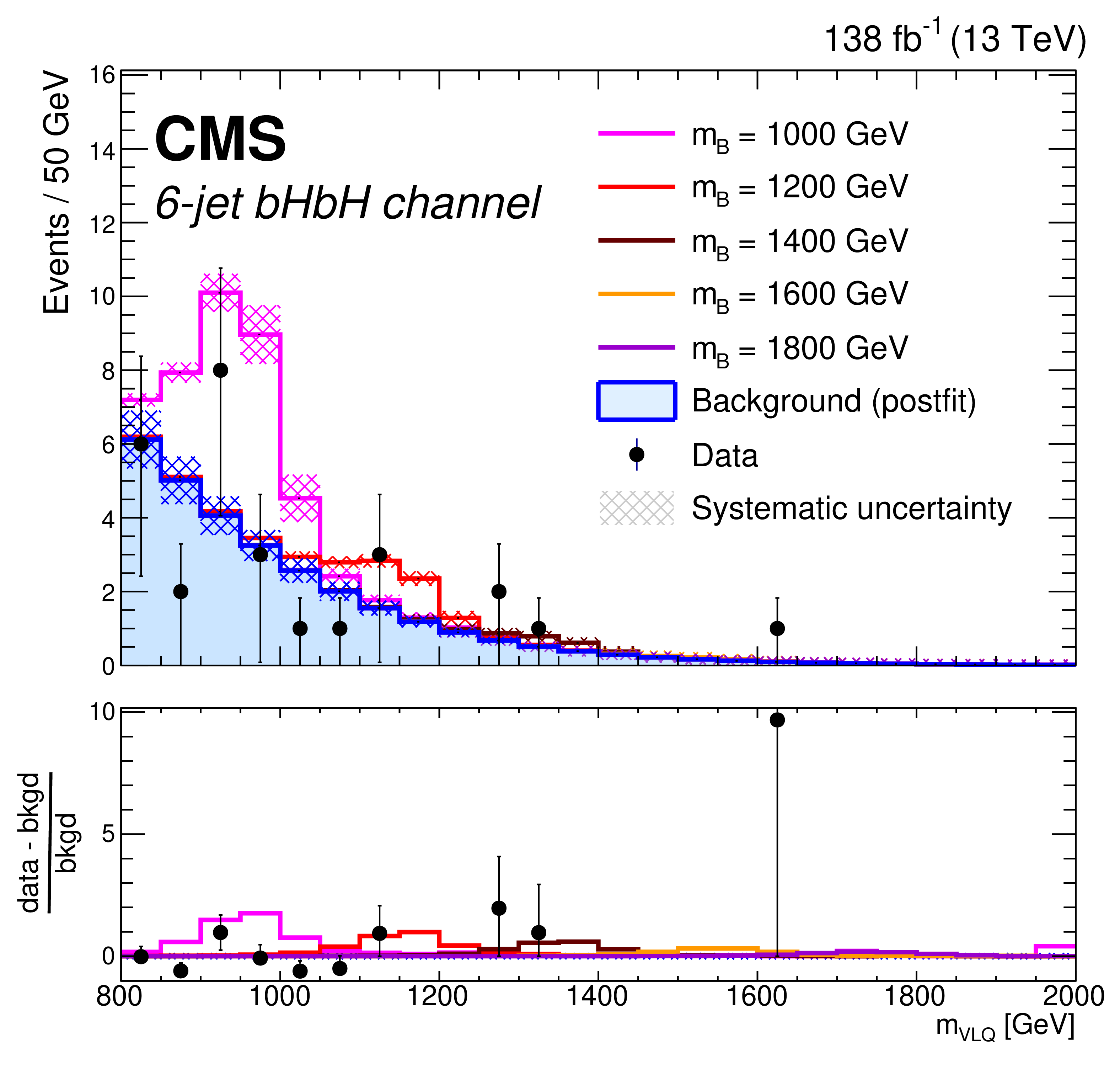
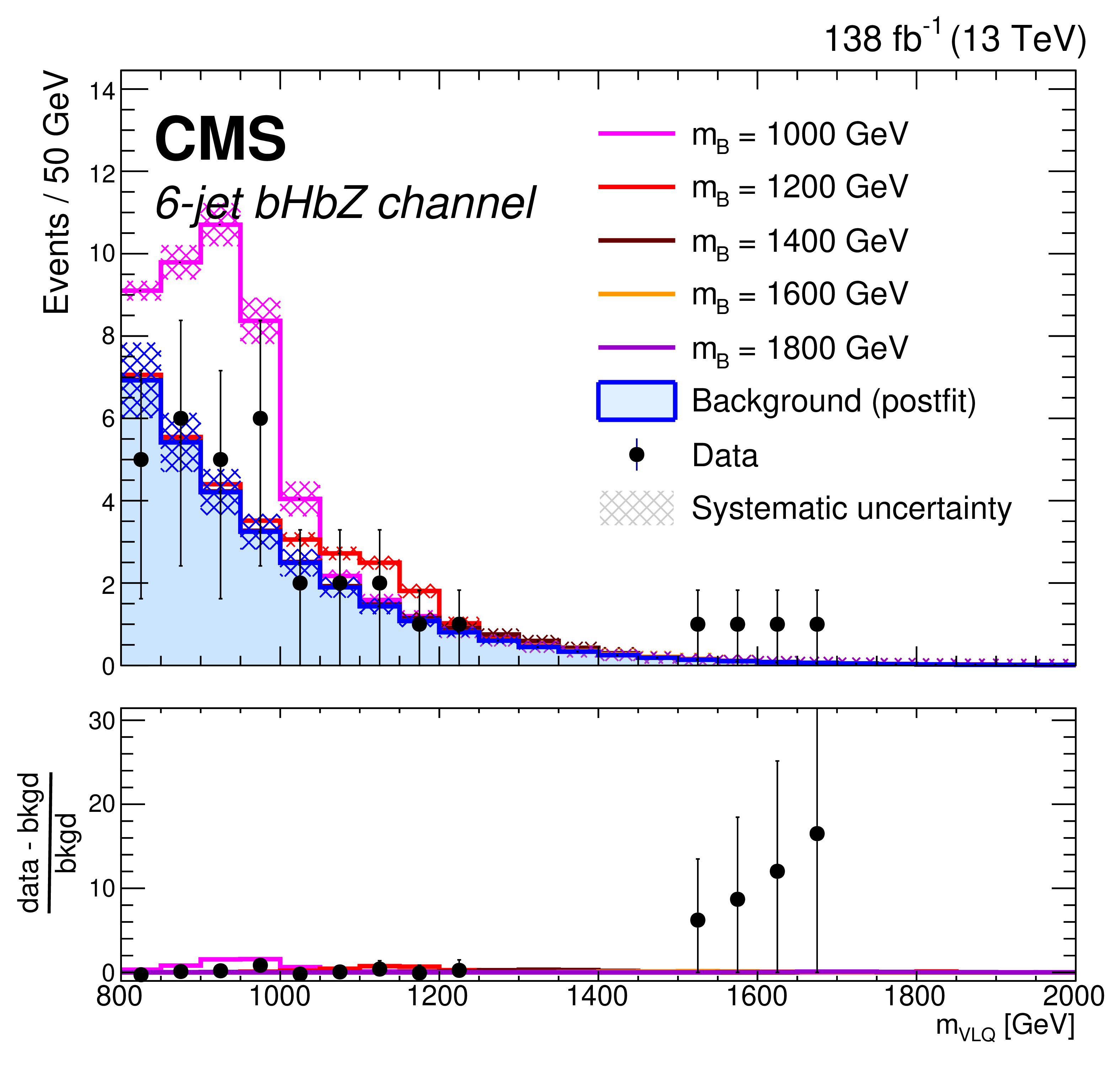
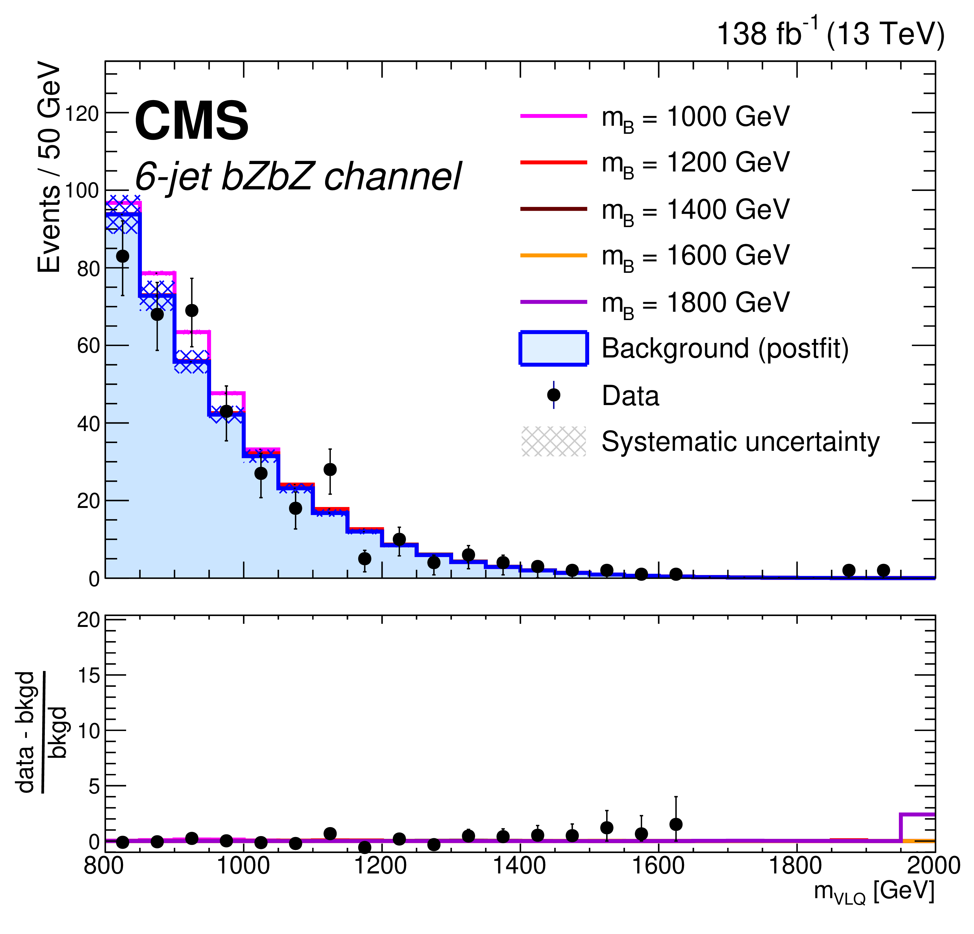
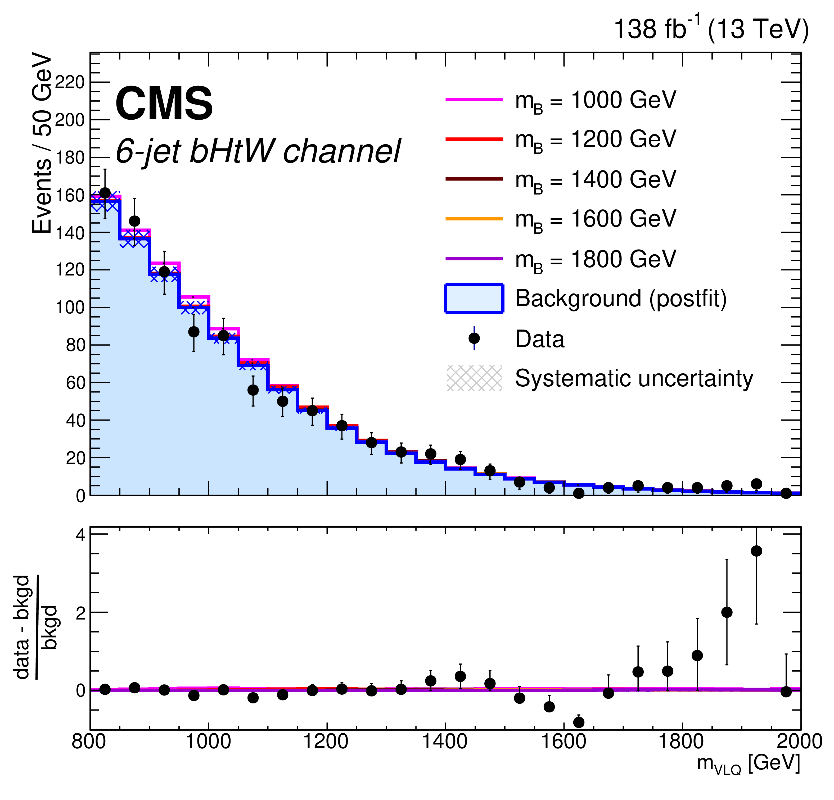
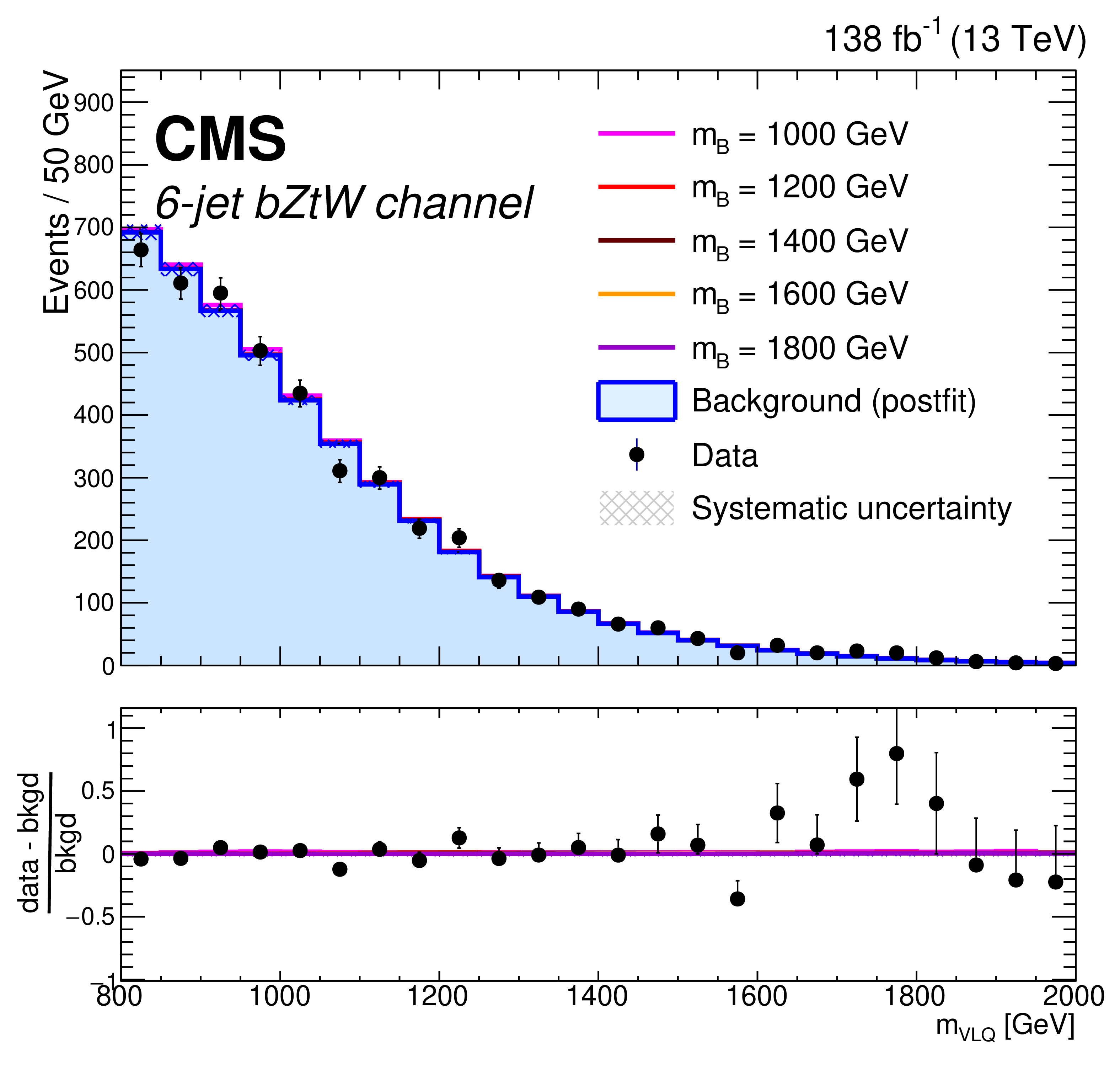
Figure 16:
Distributions of reconstructed VLQ mass for expected postfit background (blue histogram), signal plus background (colored lines), and observed data (black points) for events in the hadronic category. The channels shown are 6-jet $ \mathrm{b}\mathrm{H}\mathrm{b}\mathrm{H} $ (upper left), 6-jet $ \mathrm{b}\mathrm{H}\mathrm{b}\mathrm{Z} $ (upper right), 6-jet $ \mathrm{b}\mathrm{Z}\mathrm{b}\mathrm{Z} $ (middle left), 6-jet $ \mathrm{b}\mathrm{H}\mathrm{t}\mathrm{W} $ (middle right), and 6-jet $ \mathrm{b}\mathrm{Z}\mathrm{t}\mathrm{W} $ (lower center). Five signal masses are shown: 1000 (magenta), 1200 (red), 1400 (maroon), 1600 (orange), and 1800 GeV (purple). The signal distributions are normalized to the number of events estimated from the expected VLQ production cross section. The assumed branching fractions are $ \mathcal{B}({\mathrm{B}} \to \mathrm{b}\mathrm{H}) = \mathcal{B}({\mathrm{B}} \to \mathrm{b}\mathrm{Z}) = $ 50%, $ \mathcal{B}({\mathrm{B}} \to \mathrm{t}\mathrm{W}) = $ 0%. The background distribution is independent of the signal branching fractions. The hatched regions indicate the total systematic uncertainties in the background estimate. |
png pdf |
Figure 16-a:
Distributions of reconstructed VLQ mass for expected postfit background (blue histogram), signal plus background (colored lines), and observed data (black points) for events in the hadronic category. The channels shown are 6-jet $ \mathrm{b}\mathrm{H}\mathrm{b}\mathrm{H} $ (upper left), 6-jet $ \mathrm{b}\mathrm{H}\mathrm{b}\mathrm{Z} $ (upper right), 6-jet $ \mathrm{b}\mathrm{Z}\mathrm{b}\mathrm{Z} $ (middle left), 6-jet $ \mathrm{b}\mathrm{H}\mathrm{t}\mathrm{W} $ (middle right), and 6-jet $ \mathrm{b}\mathrm{Z}\mathrm{t}\mathrm{W} $ (lower center). Five signal masses are shown: 1000 (magenta), 1200 (red), 1400 (maroon), 1600 (orange), and 1800 GeV (purple). The signal distributions are normalized to the number of events estimated from the expected VLQ production cross section. The assumed branching fractions are $ \mathcal{B}({\mathrm{B}} \to \mathrm{b}\mathrm{H}) = \mathcal{B}({\mathrm{B}} \to \mathrm{b}\mathrm{Z}) = $ 50%, $ \mathcal{B}({\mathrm{B}} \to \mathrm{t}\mathrm{W}) = $ 0%. The background distribution is independent of the signal branching fractions. The hatched regions indicate the total systematic uncertainties in the background estimate. |
png pdf |
Figure 16-b:
Distributions of reconstructed VLQ mass for expected postfit background (blue histogram), signal plus background (colored lines), and observed data (black points) for events in the hadronic category. The channels shown are 6-jet $ \mathrm{b}\mathrm{H}\mathrm{b}\mathrm{H} $ (upper left), 6-jet $ \mathrm{b}\mathrm{H}\mathrm{b}\mathrm{Z} $ (upper right), 6-jet $ \mathrm{b}\mathrm{Z}\mathrm{b}\mathrm{Z} $ (middle left), 6-jet $ \mathrm{b}\mathrm{H}\mathrm{t}\mathrm{W} $ (middle right), and 6-jet $ \mathrm{b}\mathrm{Z}\mathrm{t}\mathrm{W} $ (lower center). Five signal masses are shown: 1000 (magenta), 1200 (red), 1400 (maroon), 1600 (orange), and 1800 GeV (purple). The signal distributions are normalized to the number of events estimated from the expected VLQ production cross section. The assumed branching fractions are $ \mathcal{B}({\mathrm{B}} \to \mathrm{b}\mathrm{H}) = \mathcal{B}({\mathrm{B}} \to \mathrm{b}\mathrm{Z}) = $ 50%, $ \mathcal{B}({\mathrm{B}} \to \mathrm{t}\mathrm{W}) = $ 0%. The background distribution is independent of the signal branching fractions. The hatched regions indicate the total systematic uncertainties in the background estimate. |
png pdf |
Figure 16-c:
Distributions of reconstructed VLQ mass for expected postfit background (blue histogram), signal plus background (colored lines), and observed data (black points) for events in the hadronic category. The channels shown are 6-jet $ \mathrm{b}\mathrm{H}\mathrm{b}\mathrm{H} $ (upper left), 6-jet $ \mathrm{b}\mathrm{H}\mathrm{b}\mathrm{Z} $ (upper right), 6-jet $ \mathrm{b}\mathrm{Z}\mathrm{b}\mathrm{Z} $ (middle left), 6-jet $ \mathrm{b}\mathrm{H}\mathrm{t}\mathrm{W} $ (middle right), and 6-jet $ \mathrm{b}\mathrm{Z}\mathrm{t}\mathrm{W} $ (lower center). Five signal masses are shown: 1000 (magenta), 1200 (red), 1400 (maroon), 1600 (orange), and 1800 GeV (purple). The signal distributions are normalized to the number of events estimated from the expected VLQ production cross section. The assumed branching fractions are $ \mathcal{B}({\mathrm{B}} \to \mathrm{b}\mathrm{H}) = \mathcal{B}({\mathrm{B}} \to \mathrm{b}\mathrm{Z}) = $ 50%, $ \mathcal{B}({\mathrm{B}} \to \mathrm{t}\mathrm{W}) = $ 0%. The background distribution is independent of the signal branching fractions. The hatched regions indicate the total systematic uncertainties in the background estimate. |
png pdf |
Figure 16-d:
Distributions of reconstructed VLQ mass for expected postfit background (blue histogram), signal plus background (colored lines), and observed data (black points) for events in the hadronic category. The channels shown are 6-jet $ \mathrm{b}\mathrm{H}\mathrm{b}\mathrm{H} $ (upper left), 6-jet $ \mathrm{b}\mathrm{H}\mathrm{b}\mathrm{Z} $ (upper right), 6-jet $ \mathrm{b}\mathrm{Z}\mathrm{b}\mathrm{Z} $ (middle left), 6-jet $ \mathrm{b}\mathrm{H}\mathrm{t}\mathrm{W} $ (middle right), and 6-jet $ \mathrm{b}\mathrm{Z}\mathrm{t}\mathrm{W} $ (lower center). Five signal masses are shown: 1000 (magenta), 1200 (red), 1400 (maroon), 1600 (orange), and 1800 GeV (purple). The signal distributions are normalized to the number of events estimated from the expected VLQ production cross section. The assumed branching fractions are $ \mathcal{B}({\mathrm{B}} \to \mathrm{b}\mathrm{H}) = \mathcal{B}({\mathrm{B}} \to \mathrm{b}\mathrm{Z}) = $ 50%, $ \mathcal{B}({\mathrm{B}} \to \mathrm{t}\mathrm{W}) = $ 0%. The background distribution is independent of the signal branching fractions. The hatched regions indicate the total systematic uncertainties in the background estimate. |
png pdf |
Figure 16-e:
Distributions of reconstructed VLQ mass for expected postfit background (blue histogram), signal plus background (colored lines), and observed data (black points) for events in the hadronic category. The channels shown are 6-jet $ \mathrm{b}\mathrm{H}\mathrm{b}\mathrm{H} $ (upper left), 6-jet $ \mathrm{b}\mathrm{H}\mathrm{b}\mathrm{Z} $ (upper right), 6-jet $ \mathrm{b}\mathrm{Z}\mathrm{b}\mathrm{Z} $ (middle left), 6-jet $ \mathrm{b}\mathrm{H}\mathrm{t}\mathrm{W} $ (middle right), and 6-jet $ \mathrm{b}\mathrm{Z}\mathrm{t}\mathrm{W} $ (lower center). Five signal masses are shown: 1000 (magenta), 1200 (red), 1400 (maroon), 1600 (orange), and 1800 GeV (purple). The signal distributions are normalized to the number of events estimated from the expected VLQ production cross section. The assumed branching fractions are $ \mathcal{B}({\mathrm{B}} \to \mathrm{b}\mathrm{H}) = \mathcal{B}({\mathrm{B}} \to \mathrm{b}\mathrm{Z}) = $ 50%, $ \mathcal{B}({\mathrm{B}} \to \mathrm{t}\mathrm{W}) = $ 0%. The background distribution is independent of the signal branching fractions. The hatched regions indicate the total systematic uncertainties in the background estimate. |
png pdf |
Figure 17:
Distributions of reconstructed VLQ mass for expected postfit background (blue histogram), signal plus background (colored lines), and observed data (black points) for events in the leptonic category. The channels shown are 3-jet $ \mathrm{b}\mathrm{H}\mathrm{b}\mathrm{Z} $ (upper left), 4-jet $ \mathrm{b}\mathrm{H}\mathrm{b}\mathrm{Z} $ (upper right), 3-jet $ \mathrm{b}\mathrm{Z}\mathrm{b}\mathrm{Z} $ (lower left), and 4-jet $ \mathrm{b}\mathrm{Z}\mathrm{b}\mathrm{Z} $ (lower right). Five signal masses are shown: 1000 (magenta), 1200 (red), 1400 (maroon), 1600 (orange), and 1800 GeV (purple). The signal distributions are normalized to the number of events estimated from the expected VLQ production cross section. The assumed branching fractions are $ \mathcal{B}({\mathrm{B}} \to \mathrm{b}\mathrm{H}) = \mathcal{B}({\mathrm{B}} \to \mathrm{b}\mathrm{Z}) = $ 50%, $ \mathcal{B}({\mathrm{B}} \to \mathrm{t}\mathrm{W}) = $ 0%. The background distribution is independent of the signal branching fractions. The hatched regions indicate the total systematic uncertainties in the background estimate. |

png pdf |
Figure 17-a:
Distributions of reconstructed VLQ mass for expected postfit background (blue histogram), signal plus background (colored lines), and observed data (black points) for events in the leptonic category. The channels shown are 3-jet $ \mathrm{b}\mathrm{H}\mathrm{b}\mathrm{Z} $ (upper left), 4-jet $ \mathrm{b}\mathrm{H}\mathrm{b}\mathrm{Z} $ (upper right), 3-jet $ \mathrm{b}\mathrm{Z}\mathrm{b}\mathrm{Z} $ (lower left), and 4-jet $ \mathrm{b}\mathrm{Z}\mathrm{b}\mathrm{Z} $ (lower right). Five signal masses are shown: 1000 (magenta), 1200 (red), 1400 (maroon), 1600 (orange), and 1800 GeV (purple). The signal distributions are normalized to the number of events estimated from the expected VLQ production cross section. The assumed branching fractions are $ \mathcal{B}({\mathrm{B}} \to \mathrm{b}\mathrm{H}) = \mathcal{B}({\mathrm{B}} \to \mathrm{b}\mathrm{Z}) = $ 50%, $ \mathcal{B}({\mathrm{B}} \to \mathrm{t}\mathrm{W}) = $ 0%. The background distribution is independent of the signal branching fractions. The hatched regions indicate the total systematic uncertainties in the background estimate. |
png pdf |
Figure 17-b:
Distributions of reconstructed VLQ mass for expected postfit background (blue histogram), signal plus background (colored lines), and observed data (black points) for events in the leptonic category. The channels shown are 3-jet $ \mathrm{b}\mathrm{H}\mathrm{b}\mathrm{Z} $ (upper left), 4-jet $ \mathrm{b}\mathrm{H}\mathrm{b}\mathrm{Z} $ (upper right), 3-jet $ \mathrm{b}\mathrm{Z}\mathrm{b}\mathrm{Z} $ (lower left), and 4-jet $ \mathrm{b}\mathrm{Z}\mathrm{b}\mathrm{Z} $ (lower right). Five signal masses are shown: 1000 (magenta), 1200 (red), 1400 (maroon), 1600 (orange), and 1800 GeV (purple). The signal distributions are normalized to the number of events estimated from the expected VLQ production cross section. The assumed branching fractions are $ \mathcal{B}({\mathrm{B}} \to \mathrm{b}\mathrm{H}) = \mathcal{B}({\mathrm{B}} \to \mathrm{b}\mathrm{Z}) = $ 50%, $ \mathcal{B}({\mathrm{B}} \to \mathrm{t}\mathrm{W}) = $ 0%. The background distribution is independent of the signal branching fractions. The hatched regions indicate the total systematic uncertainties in the background estimate. |

png pdf |
Figure 17-c:
Distributions of reconstructed VLQ mass for expected postfit background (blue histogram), signal plus background (colored lines), and observed data (black points) for events in the leptonic category. The channels shown are 3-jet $ \mathrm{b}\mathrm{H}\mathrm{b}\mathrm{Z} $ (upper left), 4-jet $ \mathrm{b}\mathrm{H}\mathrm{b}\mathrm{Z} $ (upper right), 3-jet $ \mathrm{b}\mathrm{Z}\mathrm{b}\mathrm{Z} $ (lower left), and 4-jet $ \mathrm{b}\mathrm{Z}\mathrm{b}\mathrm{Z} $ (lower right). Five signal masses are shown: 1000 (magenta), 1200 (red), 1400 (maroon), 1600 (orange), and 1800 GeV (purple). The signal distributions are normalized to the number of events estimated from the expected VLQ production cross section. The assumed branching fractions are $ \mathcal{B}({\mathrm{B}} \to \mathrm{b}\mathrm{H}) = \mathcal{B}({\mathrm{B}} \to \mathrm{b}\mathrm{Z}) = $ 50%, $ \mathcal{B}({\mathrm{B}} \to \mathrm{t}\mathrm{W}) = $ 0%. The background distribution is independent of the signal branching fractions. The hatched regions indicate the total systematic uncertainties in the background estimate. |
png pdf |
Figure 17-d:
Distributions of reconstructed VLQ mass for expected postfit background (blue histogram), signal plus background (colored lines), and observed data (black points) for events in the leptonic category. The channels shown are 3-jet $ \mathrm{b}\mathrm{H}\mathrm{b}\mathrm{Z} $ (upper left), 4-jet $ \mathrm{b}\mathrm{H}\mathrm{b}\mathrm{Z} $ (upper right), 3-jet $ \mathrm{b}\mathrm{Z}\mathrm{b}\mathrm{Z} $ (lower left), and 4-jet $ \mathrm{b}\mathrm{Z}\mathrm{b}\mathrm{Z} $ (lower right). Five signal masses are shown: 1000 (magenta), 1200 (red), 1400 (maroon), 1600 (orange), and 1800 GeV (purple). The signal distributions are normalized to the number of events estimated from the expected VLQ production cross section. The assumed branching fractions are $ \mathcal{B}({\mathrm{B}} \to \mathrm{b}\mathrm{H}) = \mathcal{B}({\mathrm{B}} \to \mathrm{b}\mathrm{Z}) = $ 50%, $ \mathcal{B}({\mathrm{B}} \to \mathrm{t}\mathrm{W}) = $ 0%. The background distribution is independent of the signal branching fractions. The hatched regions indicate the total systematic uncertainties in the background estimate. |
png pdf |
Figure 18:
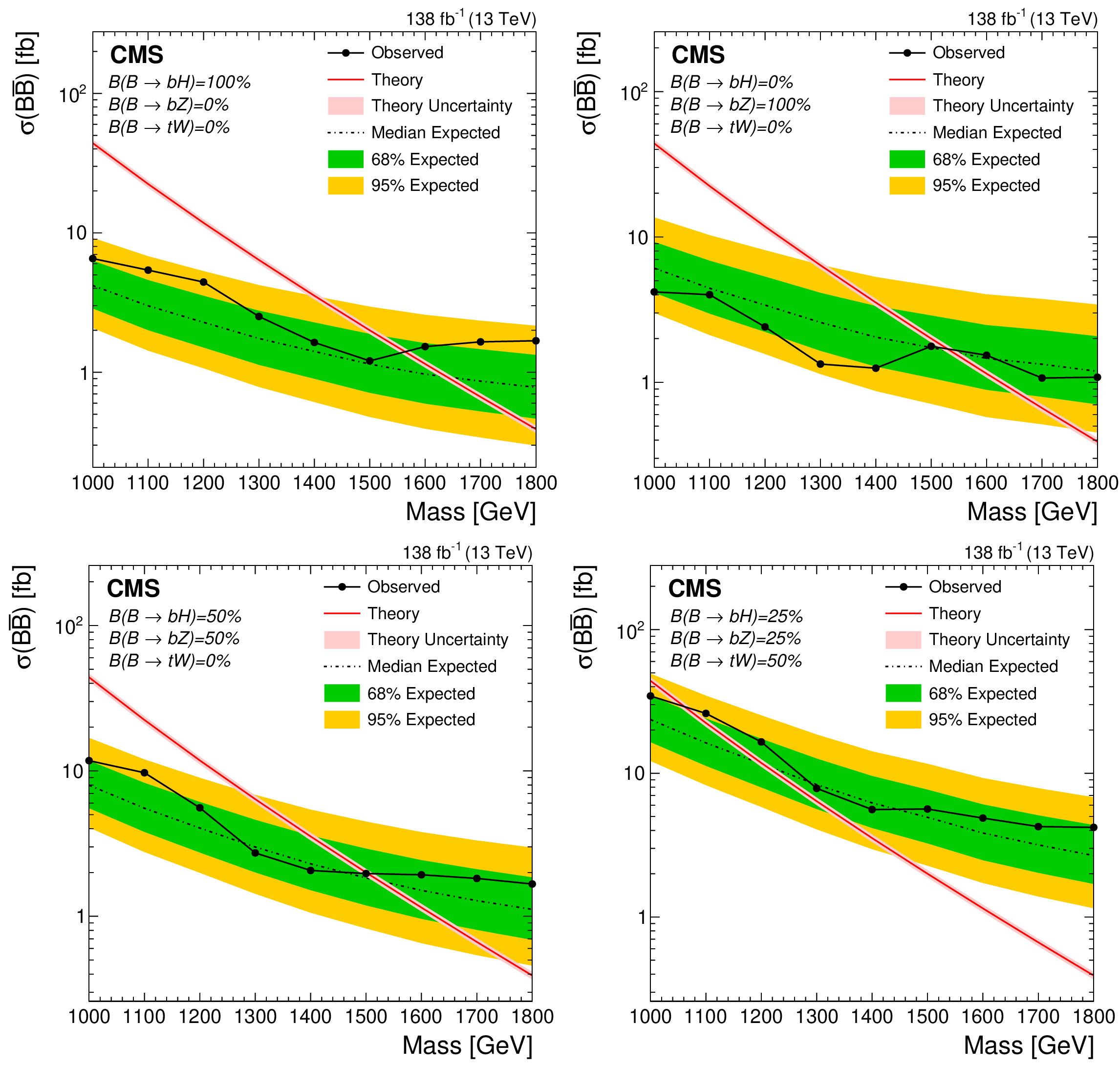
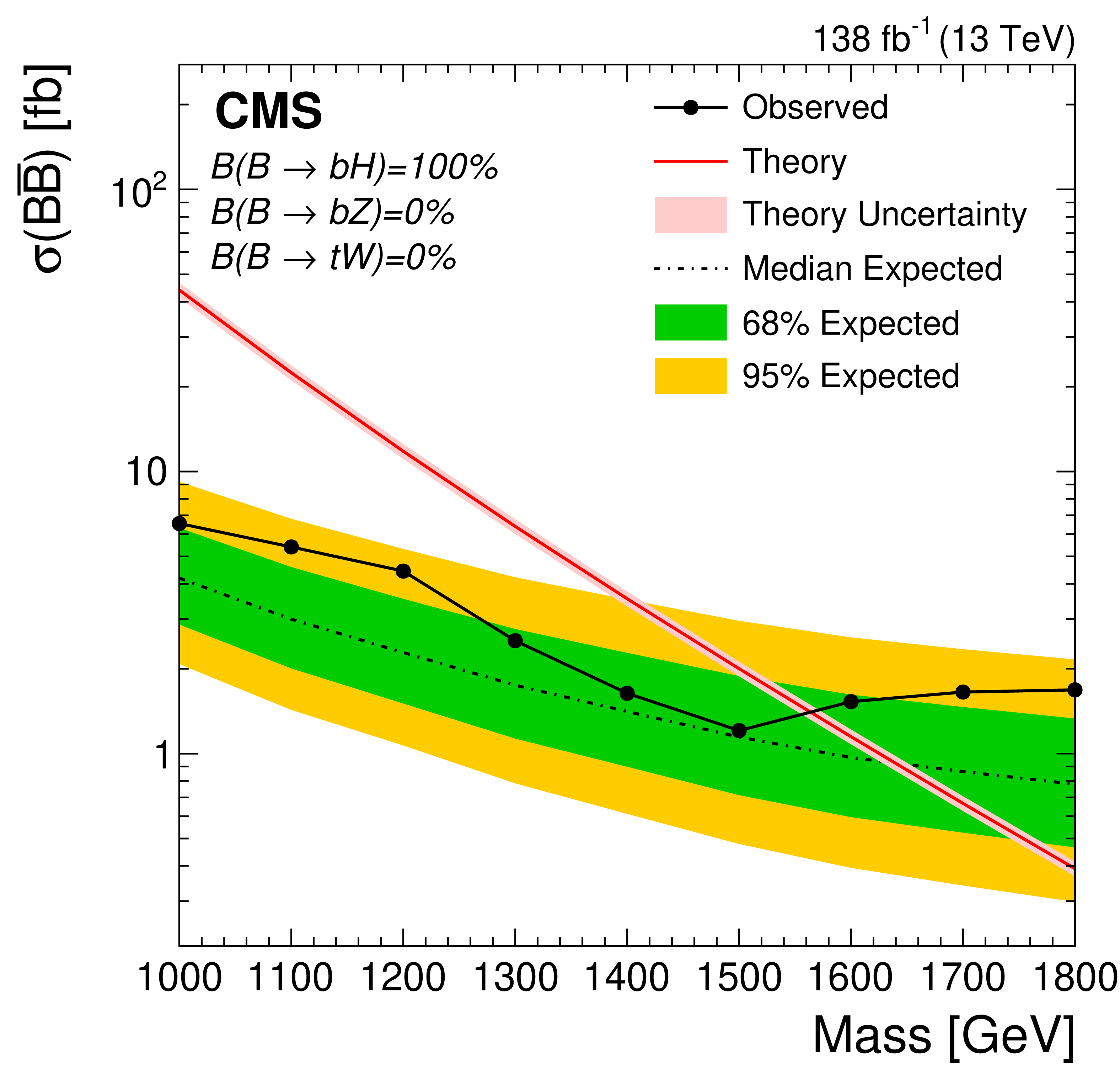
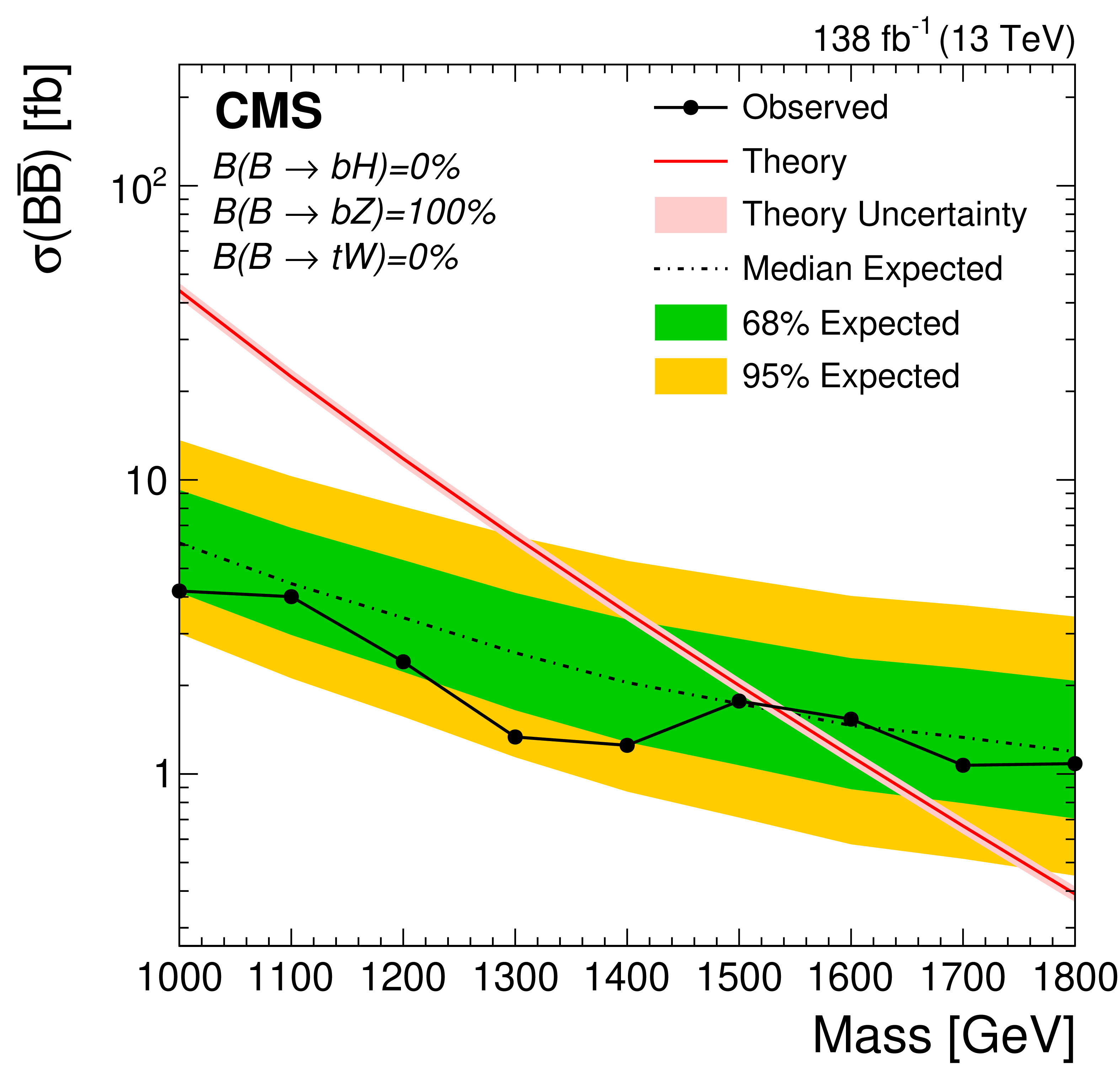
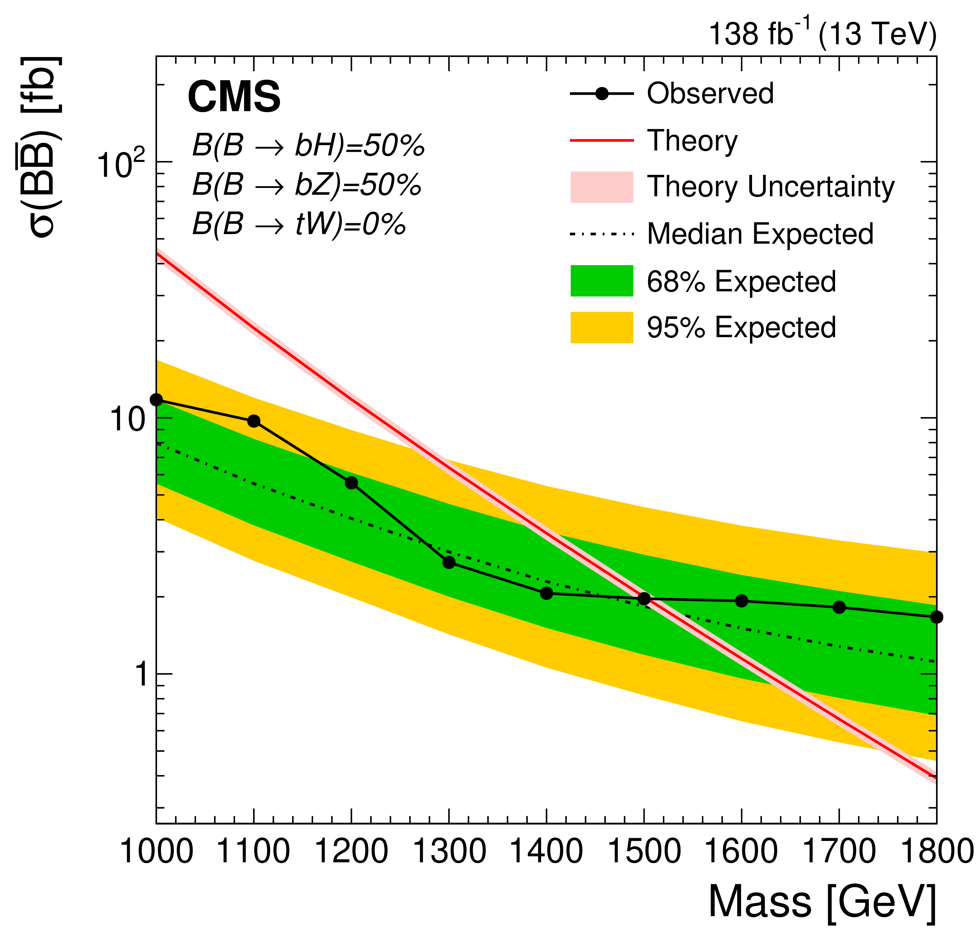
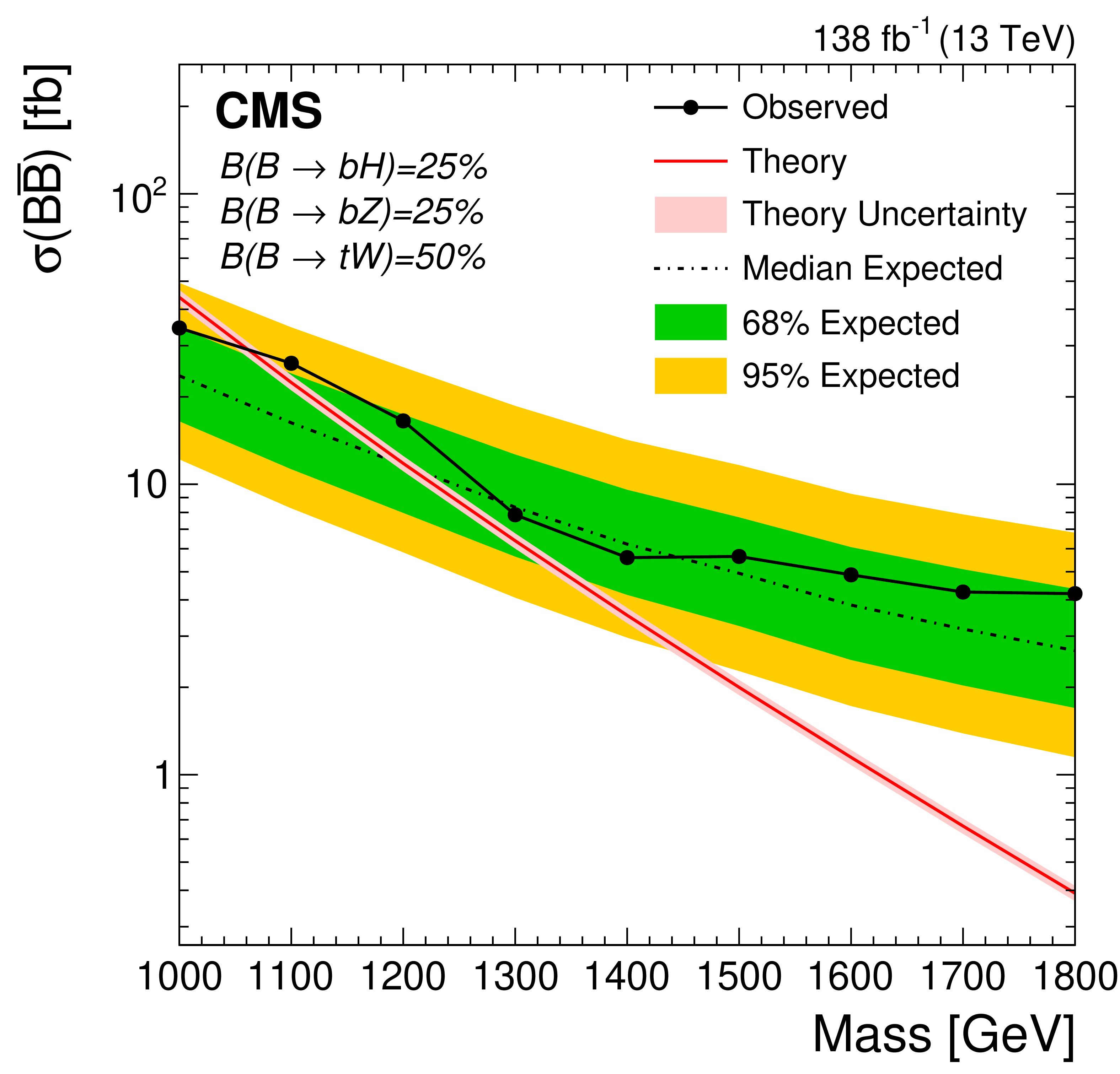
The limit at 95% CL on the cross section for VLQ pair production for four different branching fraction hypothesis: $ \mathcal{B}({\mathrm{B}} \to \mathrm{b}\mathrm{H}) = $ 100% (upper left), $ \mathcal{B}({\mathrm{B}} \to \mathrm{b}\mathrm{Z}) = $ 100% (upper right), $ \mathcal{B}({\mathrm{B}} \to \mathrm{b}\mathrm{H}) = \mathcal{B}({\mathrm{B}} \to \mathrm{b}\mathrm{Z}) = $ 50%, corresponding to the $ \VLQT{\mathrm{B}} $ doublet model with no $ \VLQT\mathrm{t} $ mixing and also to the large VLQ mass $ \mathrm{X}\VLQT{\mathrm{B}} $ triplet model (lower left), and $ \mathcal{B}({\mathrm{B}} \to \mathrm{b}\mathrm{H}) = \mathcal{B}({\mathrm{B}} \to \mathrm{b}\mathrm{Z}) = 25% $, $ \mathcal{B}({\mathrm{B}} \to \mathrm{t}\mathrm{W}) = $ 50%, corresponding to the large VLQ mass $ \VLQT{\mathrm{B}}\VLQY $ triplet model (lower right). The expected limit is shown as the dashed line, with the 68 and 95% uncertainties shown by the green (inner) and yellow (outer) bands, respectively. The theoretical cross section and its uncertainty are shown by the red line and light-red band. |
png pdf |
Figure 18-a:
The limit at 95% CL on the cross section for VLQ pair production for four different branching fraction hypothesis: $ \mathcal{B}({\mathrm{B}} \to \mathrm{b}\mathrm{H}) = $ 100% (upper left), $ \mathcal{B}({\mathrm{B}} \to \mathrm{b}\mathrm{Z}) = $ 100% (upper right), $ \mathcal{B}({\mathrm{B}} \to \mathrm{b}\mathrm{H}) = \mathcal{B}({\mathrm{B}} \to \mathrm{b}\mathrm{Z}) = $ 50%, corresponding to the $ \VLQT{\mathrm{B}} $ doublet model with no $ \VLQT\mathrm{t} $ mixing and also to the large VLQ mass $ \mathrm{X}\VLQT{\mathrm{B}} $ triplet model (lower left), and $ \mathcal{B}({\mathrm{B}} \to \mathrm{b}\mathrm{H}) = \mathcal{B}({\mathrm{B}} \to \mathrm{b}\mathrm{Z}) = 25% $, $ \mathcal{B}({\mathrm{B}} \to \mathrm{t}\mathrm{W}) = $ 50%, corresponding to the large VLQ mass $ \VLQT{\mathrm{B}}\VLQY $ triplet model (lower right). The expected limit is shown as the dashed line, with the 68 and 95% uncertainties shown by the green (inner) and yellow (outer) bands, respectively. The theoretical cross section and its uncertainty are shown by the red line and light-red band. |
png pdf |
Figure 18-b:
The limit at 95% CL on the cross section for VLQ pair production for four different branching fraction hypothesis: $ \mathcal{B}({\mathrm{B}} \to \mathrm{b}\mathrm{H}) = $ 100% (upper left), $ \mathcal{B}({\mathrm{B}} \to \mathrm{b}\mathrm{Z}) = $ 100% (upper right), $ \mathcal{B}({\mathrm{B}} \to \mathrm{b}\mathrm{H}) = \mathcal{B}({\mathrm{B}} \to \mathrm{b}\mathrm{Z}) = $ 50%, corresponding to the $ \VLQT{\mathrm{B}} $ doublet model with no $ \VLQT\mathrm{t} $ mixing and also to the large VLQ mass $ \mathrm{X}\VLQT{\mathrm{B}} $ triplet model (lower left), and $ \mathcal{B}({\mathrm{B}} \to \mathrm{b}\mathrm{H}) = \mathcal{B}({\mathrm{B}} \to \mathrm{b}\mathrm{Z}) = 25% $, $ \mathcal{B}({\mathrm{B}} \to \mathrm{t}\mathrm{W}) = $ 50%, corresponding to the large VLQ mass $ \VLQT{\mathrm{B}}\VLQY $ triplet model (lower right). The expected limit is shown as the dashed line, with the 68 and 95% uncertainties shown by the green (inner) and yellow (outer) bands, respectively. The theoretical cross section and its uncertainty are shown by the red line and light-red band. |
png pdf |
Figure 18-c:
The limit at 95% CL on the cross section for VLQ pair production for four different branching fraction hypothesis: $ \mathcal{B}({\mathrm{B}} \to \mathrm{b}\mathrm{H}) = $ 100% (upper left), $ \mathcal{B}({\mathrm{B}} \to \mathrm{b}\mathrm{Z}) = $ 100% (upper right), $ \mathcal{B}({\mathrm{B}} \to \mathrm{b}\mathrm{H}) = \mathcal{B}({\mathrm{B}} \to \mathrm{b}\mathrm{Z}) = $ 50%, corresponding to the $ \VLQT{\mathrm{B}} $ doublet model with no $ \VLQT\mathrm{t} $ mixing and also to the large VLQ mass $ \mathrm{X}\VLQT{\mathrm{B}} $ triplet model (lower left), and $ \mathcal{B}({\mathrm{B}} \to \mathrm{b}\mathrm{H}) = \mathcal{B}({\mathrm{B}} \to \mathrm{b}\mathrm{Z}) = 25% $, $ \mathcal{B}({\mathrm{B}} \to \mathrm{t}\mathrm{W}) = $ 50%, corresponding to the large VLQ mass $ \VLQT{\mathrm{B}}\VLQY $ triplet model (lower right). The expected limit is shown as the dashed line, with the 68 and 95% uncertainties shown by the green (inner) and yellow (outer) bands, respectively. The theoretical cross section and its uncertainty are shown by the red line and light-red band. |
png pdf |
Figure 18-d:
The limit at 95% CL on the cross section for VLQ pair production for four different branching fraction hypothesis: $ \mathcal{B}({\mathrm{B}} \to \mathrm{b}\mathrm{H}) = $ 100% (upper left), $ \mathcal{B}({\mathrm{B}} \to \mathrm{b}\mathrm{Z}) = $ 100% (upper right), $ \mathcal{B}({\mathrm{B}} \to \mathrm{b}\mathrm{H}) = \mathcal{B}({\mathrm{B}} \to \mathrm{b}\mathrm{Z}) = $ 50%, corresponding to the $ \VLQT{\mathrm{B}} $ doublet model with no $ \VLQT\mathrm{t} $ mixing and also to the large VLQ mass $ \mathrm{X}\VLQT{\mathrm{B}} $ triplet model (lower left), and $ \mathcal{B}({\mathrm{B}} \to \mathrm{b}\mathrm{H}) = \mathcal{B}({\mathrm{B}} \to \mathrm{b}\mathrm{Z}) = 25% $, $ \mathcal{B}({\mathrm{B}} \to \mathrm{t}\mathrm{W}) = $ 50%, corresponding to the large VLQ mass $ \VLQT{\mathrm{B}}\VLQY $ triplet model (lower right). The expected limit is shown as the dashed line, with the 68 and 95% uncertainties shown by the green (inner) and yellow (outer) bands, respectively. The theoretical cross section and its uncertainty are shown by the red line and light-red band. |
png pdf |
Figure 19:
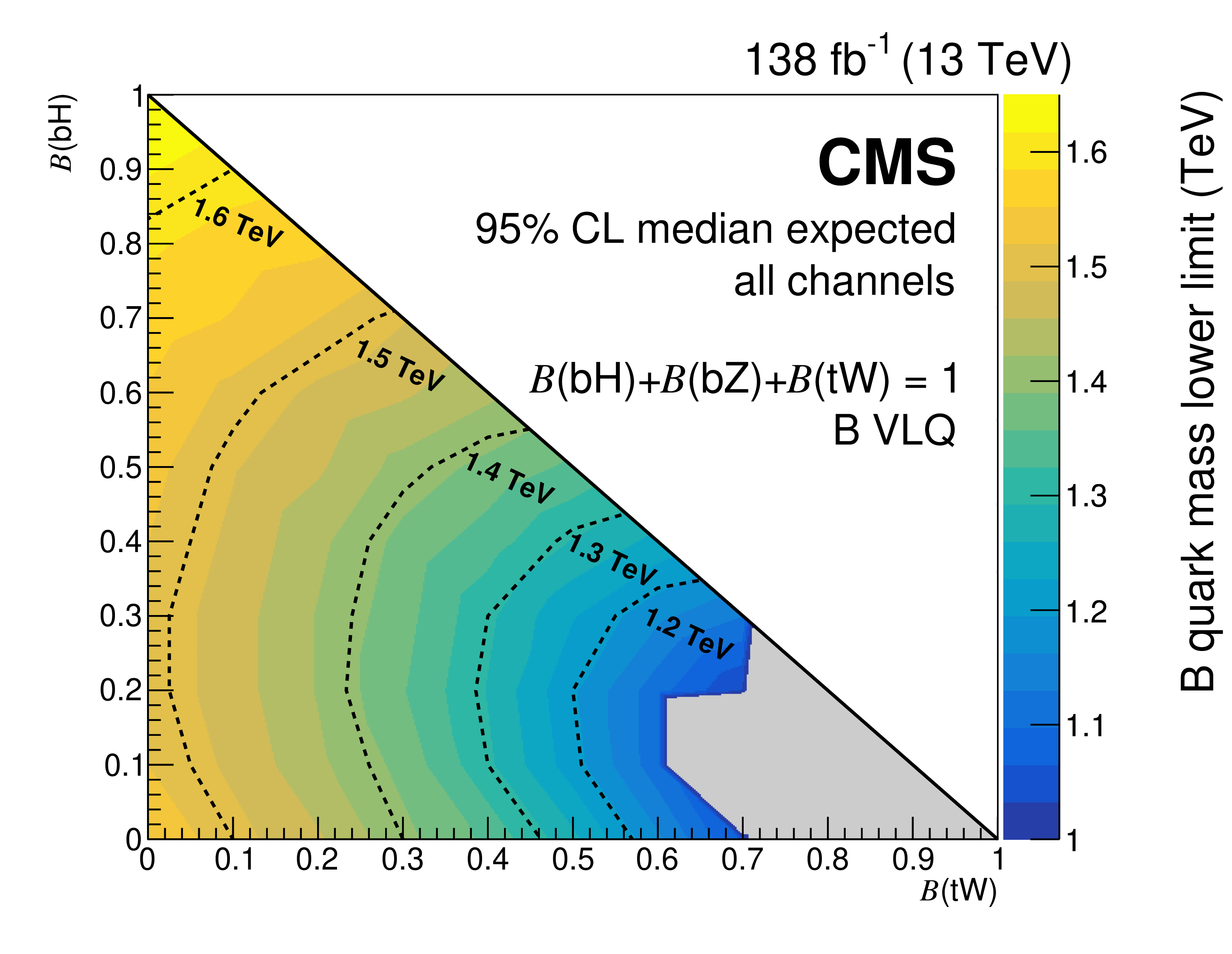
Median expected exclusion limits on the VLQ mass at 95% CL as a function of the branching fractions $ \mathcal{B}({\mathrm{B}} \to \mathrm{b}\mathrm{H}) $ and $ \mathcal{B}({\mathrm{B}} \to \mathrm{t}\mathrm{W}) $, with $ \mathcal{B}({\mathrm{B}} \to \mathrm{t}\mathrm{W}) = 1 - \mathcal{B}({\mathrm{B}} \to \mathrm{b}\mathrm{H}) - \mathcal{B}({\mathrm{B}} \to \mathrm{b}\mathrm{Z}) $. The gray area corresponds to the region where the exclusion limit is less than 1000 GeV. |
png pdf |
Figure 20:
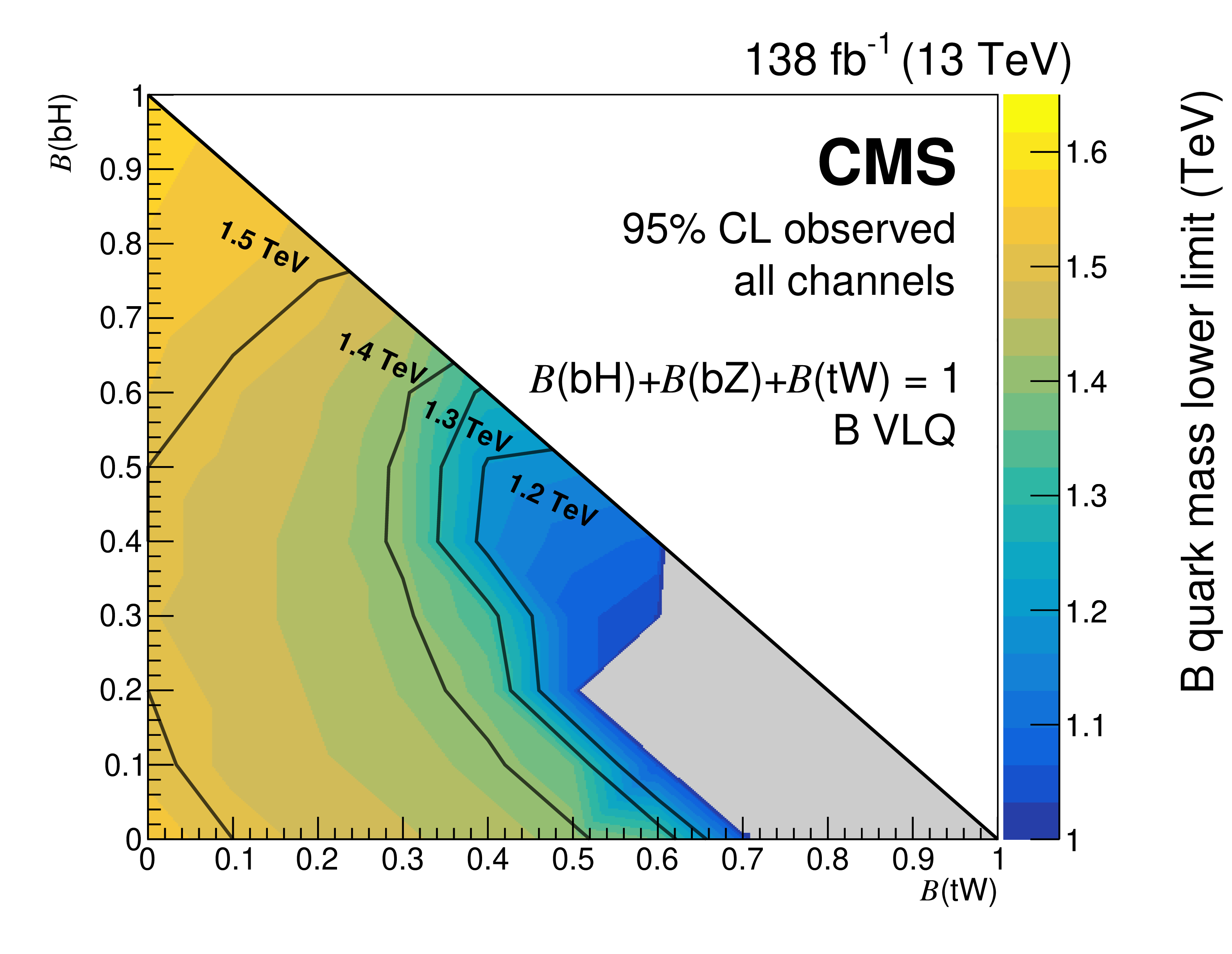
Observed exclusion limits on the VLQ mass at 95% CL as a function of the branching fractions $ \mathcal{B}({\mathrm{B}} \to \mathrm{b}\mathrm{H}) $ and $ \mathcal{B}({\mathrm{B}} \to \mathrm{t}\mathrm{W}) $, with $ \mathcal{B}({\mathrm{B}} \to \mathrm{t}\mathrm{W}) = 1 - \mathcal{B}({\mathrm{B}} \to \mathrm{b}\mathrm{H}) - \mathcal{B}({\mathrm{B}} \to \mathrm{b}\mathrm{Z}) $. The gray area corresponds to the region where the exclusion limit is less than 1000 GeV. |
| Tables | |
png pdf |
Table 1:
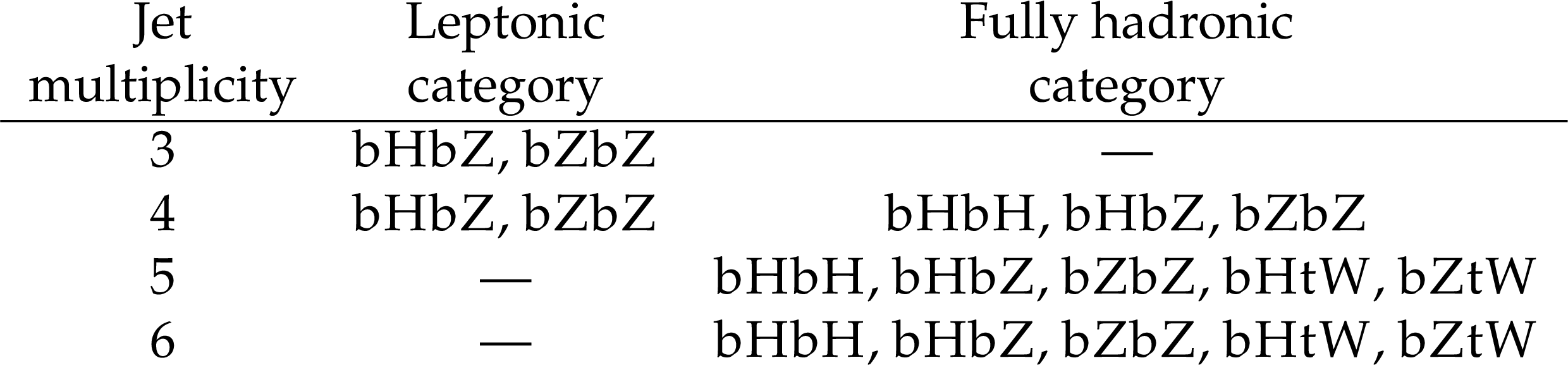
Summary of channels considered for each category and jet multiplicity. Although events with a jet from ISR or FSR are included in the leptonic category, for these events the extra jet is not included in the categorization of the jet multiplicity of the event. |
png pdf |
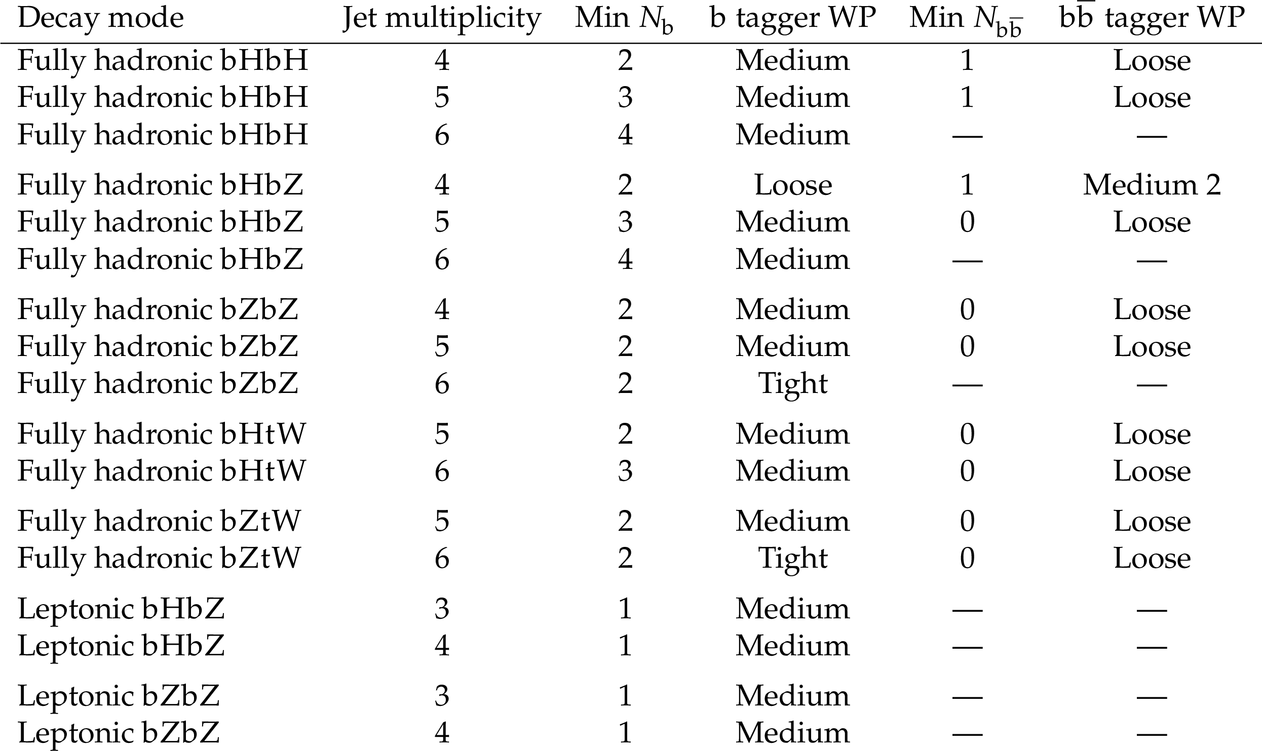
Table 2:
Required minimum number of single ($ N_{\mathrm{b}} $) and double ($ N_{\mathrm{b}\overline{\mathrm{b}}} $) b tags, and working points (WPs) used for each category, decay mode, and jet multiplicity. The working points are described in the text. For a given event mode, there can be several jet multiplicities depending on the number of merged jets. |

png pdf |
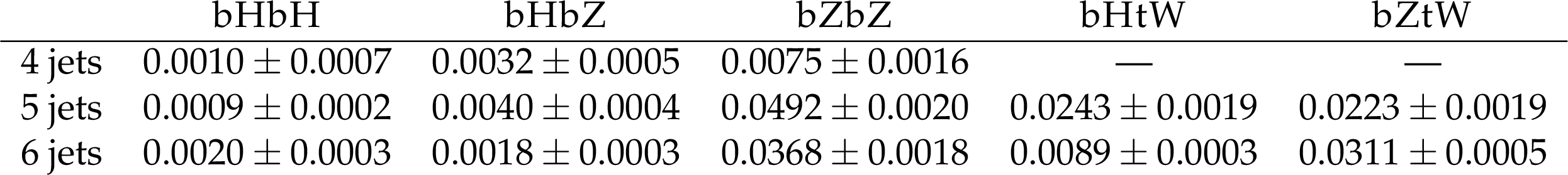
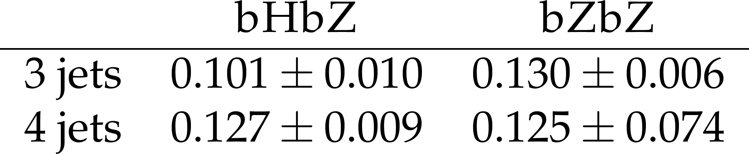
Table 3:
Optimized upper limit values of the $ \chi^2_\text{mod}/\text{ndf} $ selection as a function of jet multiplicity and decay mode. |
png pdf |
Table 4:
Values of the BJTF for data events in the control region with 500 $ < m_{\text{VLQ}} < $ 800 GeV for each of the fully hadronic channels considered. The uncertainties shown are statistical. |
png pdf |
Table 5:
Values of the b-tag to b-veto ratio for events in the mass range 450 $ < m_{\text{VLQ}} < $ 900 GeV with $ \chi^2_\text{mod}/\text{ndf} < $ 5, for each of the dileptonic channels. The uncertainties shown are statistical only. |
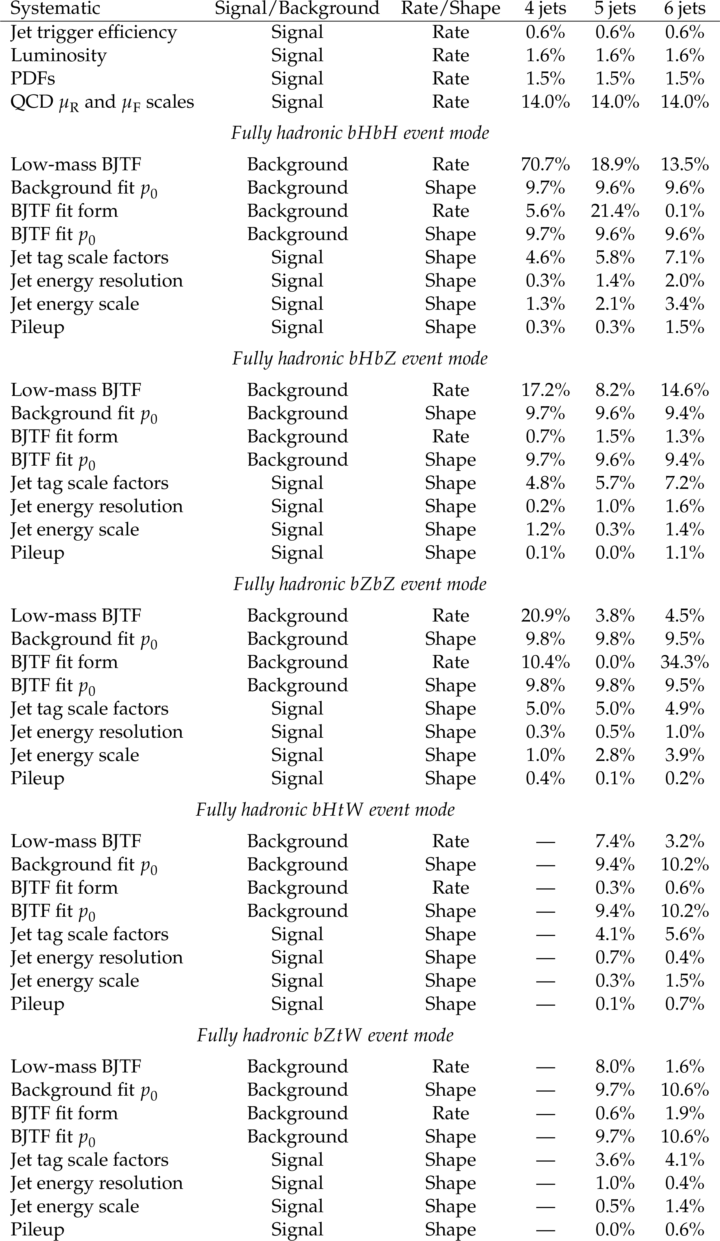
png pdf |
Table 6:
Systematic uncertainties for the fully hadronic channels for a simulated signal mass of 1400 GeV and branching fractions of $ \mathcal{B}({\mathrm{B}} \to \mathrm{b}\mathrm{H}) = 40% $, $ \mathcal{B}({\mathrm{B}} \to \mathrm{b}\mathrm{Z}) = 40% $, and $ \mathcal{B}({\mathrm{B}} \to \mathrm{t}\mathrm{W}) = 20% $. The only parameters in the fits that have significant uncertainties ($ > $0.01%) are the scaling parameters (denoted by $ p_0 $). |
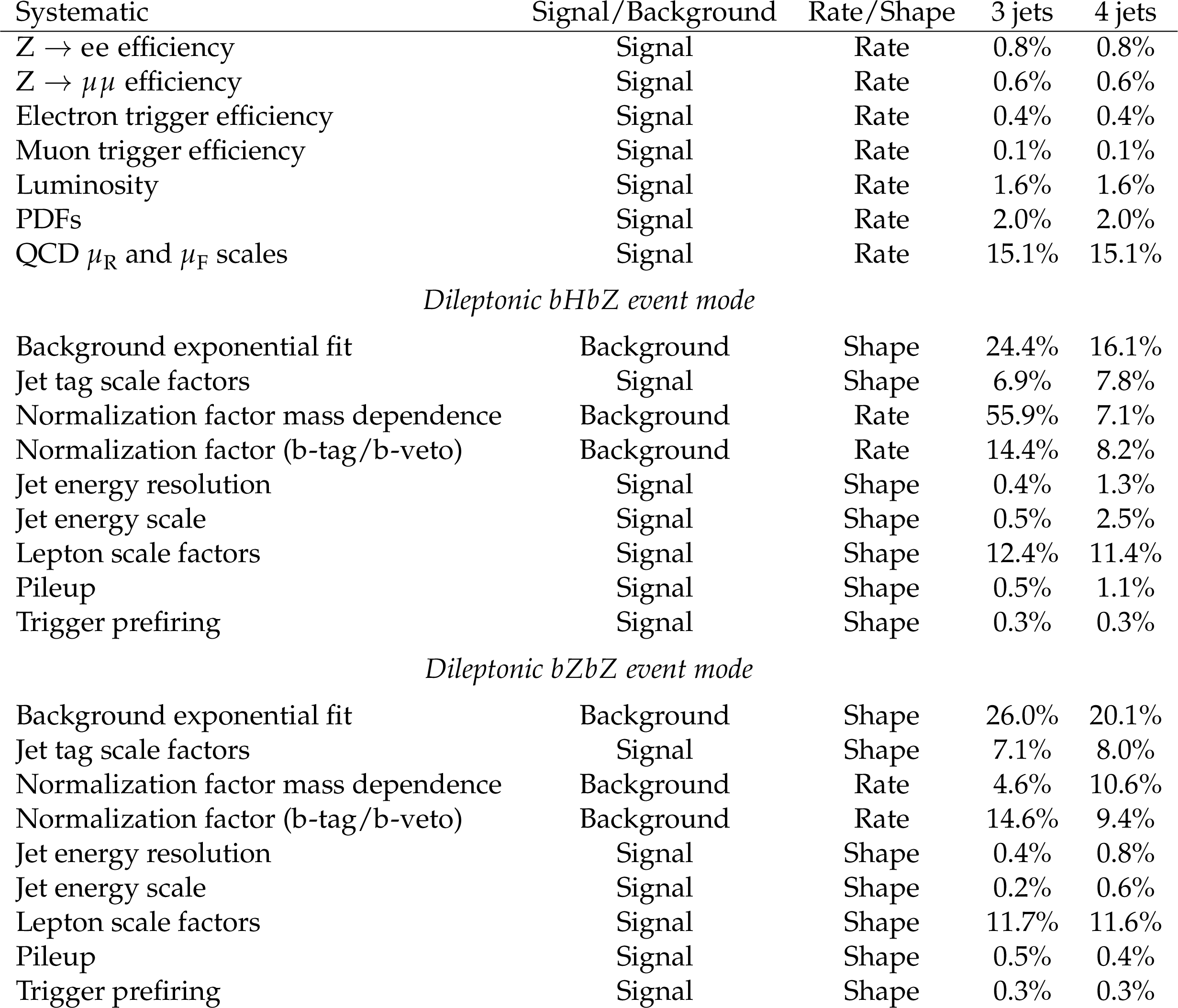
png pdf |
Table 7:
Systematic uncertainties for the dileptonic $ \mathrm{b}\mathrm{H}\mathrm{b}\mathrm{Z} $ and $ \mathrm{b}\mathrm{Z}\mathrm{b}\mathrm{Z} $ channels for a simulated signal mass of 1400 GeV and branching fractions of $ \mathcal{B}({\mathrm{B}} \to \mathrm{b}\mathrm{H}) = 40% $, $ \mathcal{B}({\mathrm{B}} \to \mathrm{b}\mathrm{Z}) = 40% $, and $ \mathcal{B}({\mathrm{B}} \to \mathrm{t}\mathrm{W}) = 20% $. |
| Summary |
| A search for bottom-type vector-like quarks (B VLQs) has been presented, using data from proton-proton collisions collected by the CMS detector in 2016--2018 at $ \sqrt{s} = $ 13 TeV. Results are combined from the fully hadronic category, where each B VLQ decays into either a b quark and a Higgs boson (H), a b quark and a Z boson, or a t quark and a W boson, and the leptonic category, where each B VLQ decays into a b quark and either an H or a Z boson, and at least one decay includes a Z boson that decays into a pair of charged leptons. To account for the fact that the two jets from an H, Z, or W boson decay may be reconstructed separately, or may be merged into a single reconstructed jet due to a high Lorentz boost, events are separated into different jet multiplicity categories and reconstructed appropriately. Backgrounds are estimated from data and limits are set on the VLQ mass at 95% confidence level as a function of the branching fractions $ \mathcal{B}({\mathrm{B}} \to \mathrm{b}\mathrm{H}) $, $ \mathcal{B}({\mathrm{B}} \to \mathrm{b}\mathrm{Z}) $, and $ \mathcal{B}({\mathrm{B}} \to \mathrm{t}\mathrm{W}) $. The most significant improvement over previous results is an increased sensitivity for scenarios with large $ \mathcal{B}({\mathrm{B}} \to \mathrm{b}\mathrm{Z}) $ due to the inclusion of events with leptonic Z boson decays. The current results represent the most stringent limits on B VLQs to date. |
| References | ||||
| 1 | G. 't Hooft | Naturalness, chiral symmetry, and spontaneous chiral symmetry breaking | NATO Sci. Ser. B 59 (1980) 135 | |
| 2 | ATLAS Collaboration | Observation of a new particle in the search for the standard model Higgs boson with the ATLAS detector at the LHC | PLB 716 (2012) 1 | 1207.7214 |
| 3 | CMS Collaboration | Observation of a new boson at a mass of 125GeV with the CMS experiment at the LHC | PLB 716 (2012) 30 | CMS-HIG-12-028 1207.7235 |
| 4 | CMS Collaboration | Observation of a new boson with mass near 125GeV in pp collisions at $ \sqrt{s} = $ 7 and 8 TeV | JHEP 06 (2013) 081 | CMS-HIG-12-036 1303.4571 |
| 5 | CMS Collaboration | A measurement of the Higgs boson mass in the diphoton decay channel | PLB 805 (2020) 135425 | CMS-HIG-19-004 2002.06398 |
| 6 | H. Georgi and A. Pais | Calculability and naturalness in gauge theories | PRD 10 (1974) 539 | |
| 7 | J. Wess and B. Zumino | A Lagrangian model invariant under supergauge transformations | PLB 49 (1974) 52 | |
| 8 | P. Fayet and S. Ferrara | Supersymmetry | Phys. Rept. 32 (1977) 249 | |
| 9 | D. B. Kaplan, H. Georgi, and S. Dimopoulos | Composite Higgs scalars | PLB 136 (1984) 187 | |
| 10 | K. Agashe, R. Contino, and A. Pomarol | The minimal composite Higgs model | NPB 719 (2005) 165 | hep-ph/0412089 |
| 11 | N. Arkani-Hamed, A. G. Cohen, and H. Georgi | Electroweak symmetry breaking from dimensional deconstruction | PLB 513 (2001) 232 | hep-ph/0105239 |
| 12 | N. Arkani-Hamed, A. G. Cohen, E. Katz, and A. E. Nelson | The littlest Higgs | JHEP 07 (2002) 034 | hep-ph/0206021 |
| 13 | M. Schmaltz | Physics beyond the standard model (theory): Introducing the little Higgs | Nucl. Phys. B Proc. Suppl. 117 (2003) 40 | hep-ph/0210415 |
| 14 | F. del Aguila and M. J. Bowick | The possibility of new fermions with $ \Delta I = $ 0 mass | NPB 224 (1983) 107 | |
| 15 | ATLAS Collaboration | Combined measurements of Higgs boson production and decay using up to 80 fb$ ^{-1} $ of proton-proton collision data at $ \sqrt{s}= $ 13 TeV collected with the ATLAS experiment | PRD 101 (2020) 012002 | 1909.02845 |
| 16 | CMS Collaboration | Measurement and interpretation of differential cross sections for Higgs boson production at $ \sqrt{s} = $ 13 TeV | PLB 792 (2019) 369 | CMS-HIG-17-028 1812.06504 |
| 17 | J. A. Aguilar-Saavedra, R. Benbrik, S. Heinemeyer, and M. P é rez-Victoria | Handbook of vectorlike quarks: Mixing and single production | PRD 88 (2013) 094010 | 1306.0572 |
| 18 | A. Atre, M. Carena, T. Han, and J. Santiago | Heavy quarks above the top at the Tevatron | PRD 79 (2009) 054018 | 0806.3966 |
| 19 | A. Atre et al. | Model-independent searches for new quarks at the LHC | JHEP 08 (2011) 080 | 1102.1987 |
| 20 | F. del Aguila, M. P é rez-Victoria, and J. Santiago | Observable contributions of new exotic quarks to quark mixing | JHEP 09 (2000) 011 | hep-ph/0007316 |
| 21 | J. A. Aguilar-Saavedra | Mixing with vector-like quarks: constraints and expectations | EPJ Web Conf. 60 (2013) 16012 | 1306.4432 |
| 22 | CMS Collaboration | A search for bottom-type, vector-like quark pair production in a fully hadronic final state in proton-proton collisions at $ \sqrt{s} = $ 13 TeV | PRD 102 (2020) 112004 | 2008.09835 |
| 23 | ATLAS Collaboration | Combination of the searches for pair-produced vector-like partners of the third-generation quarks at $ \sqrt{s} = $ 13 TeV with the ATLAS detector | PRL 121 (2018) 211801 | 1808.02343 |
| 24 | ATLAS Collaboration | Search for pair-production of vector-like quarks in pp collision events at $ \sqrt{s}= $ 13 TeV with at least one leptonically decaying Z boson and a third-generation quark with the ATLAS detector | PLB 843 (2023) 138019 | 2210.15413 |
| 25 | CMS Collaboration | Precision luminosity measurement in proton-proton collisions at $ \sqrt{s} = $ 13 TeV in 2015 and 2016 at CMS | EPJC 81 (2021) 800 | CMS-LUM-17-003 2104.01927 |
| 26 | CMS Collaboration | CMS luminosity measurement for the 2017 data-taking period at $ \sqrt{s} $ = 13 TeV | CMS Physics Analysis Summary, 2018 CMS-PAS-LUM-17-004 |
CMS-PAS-LUM-17-004 |
| 27 | CMS Collaboration | CMS luminosity measurement for the 2018 data-taking period at $ \sqrt{s} = $ 13 TeV | CMS Physics Analysis Summary, 2019 CMS-PAS-LUM-18-002 |
CMS-PAS-LUM-18-002 |
| 28 | CMS Collaboration | HEPData record for this analysis | link | |
| 29 | CMS Collaboration | Electron and photon reconstruction and identification with the CMS experiment at the CERN LHC | JINST 16 (2021) P05014 | CMS-EGM-17-001 2012.06888 |
| 30 | CMS Collaboration | ECAL 2016 refined calibration and Run2 summary plots | CMS Detector Performance Summary CMS-DP-2020-021, 2020 CDS |
|
| 31 | CMS Collaboration | Performance of the CMS muon detector and muon reconstruction with proton-proton collisions at $ \sqrt{s} = $ 13 TeV | JINST 13 (2018) P06015 | CMS-MUO-16-001 1804.04528 |
| 32 | CMS Collaboration | Performance of the CMS Level-1 trigger in proton-proton collisions at $ \sqrt{s} = $ 13\,TeV | JINST 15 (2020) P10017 | CMS-TRG-17-001 2006.10165 |
| 33 | CMS Collaboration | The CMS trigger system | JINST 12 (2017) P01020 | CMS-TRG-12-001 1609.02366 |
| 34 | CMS Collaboration | The CMS experiment at the CERN LHC | JINST 3 (2008) S08004 | |
| 35 | J. Alwall et al. | The automated computation of tree-level and next-to-leading order differential cross sections, and their matching to parton shower simulations | JHEP 07 (2014) 079 | 1405.0301 |
| 36 | NNPDF Collaboration | Parton distributions for the LHC Run II | JHEP 04 (2015) 040 | 1410.8849 |
| 37 | NNPDF Collaboration | Parton distributions from high-precision collider data | EPJC 77 (2017) 663 | 1706.00428 |
| 38 | T. Sjöstrand et al. | An introduction to PYTHIA 8.2 | Comput. Phys. Commun. 191 (2015) 159 | 1410.3012 |
| 39 | CMS Collaboration | Event generator tunes obtained from underlying event and multiparton scattering measurements | EPJC 76 (2016) 155 | CMS-GEN-14-001 1512.00815 |
| 40 | CMS Collaboration | Extraction and validation of a new set of CMS PYTHIA8 tunes from underlying-event measurements | EPJC 80 (2020) 4 | CMS-GEN-17-001 1903.12179 |
| 41 | M. Czakon, P. Fiedler, and A. Mitov | Total top-quark pair-production cross section at hadron colliders through $ O(\alpha^4_S) $ | PRL 110 (2013) 252004 | 1303.6254 |
| 42 | M. Czakon and A. Mitov | Top++: A program for the calculation of the top-pair cross-section at hadron colliders | Comput. Phys. Commun. 185 (2014) 2930 | 1112.5675 |
| 43 | M. Cacciari et al. | Top-pair production at hadron colliders with next-to-next-to-leading logarithmic soft-gluon resummation | PLB 710 (2012) 612 | 1111.5869 |
| 44 | M. R. Whalley, D. Bourilkov, and R. C. Group | The Les Houches accord PDFs (LHAPDF) and LHAGLUE | in HERA and the LHC: A workshop on the implications of HERA for LHC physics. Proceedings, Part B, 2005 | hep-ph/0508110 |
| 45 | D. Bourilkov, R. C. Group, and M. R. Whalley | LHAPDF: PDF use from the Tevatron to the LHC | in TeV4LHC Workshop - 4th meeting Batavia, Illinois, -22,, 2005 October 2 (2005) 0 |
hep-ph/0605240 |
| 46 | CMS Collaboration | Search for vector-like T and B quark pairs in final states with leptons at $ \sqrt{s} = $ 13 TeV | JHEP 08 (2018) 177 | 1805.04758 |
| 47 | R. Frederix and S. Frixione | Merging meets matching in MC@NLO | JHEP 12 (2012) 061 | 1209.6215 |
| 48 | J. Alwall et al. | Comparative study of various algorithms for the merging of parton showers and matrix elements in hadronic collisions | EPJC 53 (2008) 473 | 0706.2569 |
| 49 | CMS Collaboration | Measurement of the inelastic proton-proton cross section at $ \sqrt{s}= $ 13 TeV | JHEP 07 (2018) 161 | CMS-FSQ-15-005 1802.02613 |
| 50 | GEANT4 Collaboration | GEANT 4---a simulation toolkit | NIM A 506 (2003) 250 | |
| 51 | J. Allison et al. | Geant4 developments and applications | IEEE Trans. Nucl. Sci. 53 (2006) 270 | |
| 52 | CMS Collaboration | Jet energy scale and resolution in the CMS experiment in pp collisions at 8 TeV | JINST 12 (2017) P02014 | CMS-JME-13-004 1607.03663 |
| 53 | CMS Collaboration | Performance of the DeepJet b tagging algorithm using 41.9/fb of data from proton-proton collisions at 13 TeV with phase 1 CMS detector | CMS Detector Performance Summary CMS-DP-2018-058, 2018 CDS |
|
| 54 | CMS Collaboration | Identification of heavy-flavour jets with the CMS detector in pp collisions at 13 TeV | JINST 13 (2018) P05011 | CMS-BTV-16-002 1712.07158 |
| 55 | CMS Collaboration | Particle-flow reconstruction and global event description with the CMS detector | JINST 12 (2017) P10003 | CMS-PRF-14-001 1706.04965 |
| 56 | CMS Collaboration | Technical proposal for the Phase-II upgrade of the Compact Muon Solenoid | CMS Technical Proposal CERN-LHCC-2015-010, CMS-TDR-15-02, 2015 CDS |
|
| 57 | M. Cacciari, G. P. Salam, and G. Soyez | The anti-$ k_{\mathrm{T}} $ jet clustering algorithm | JHEP 04 (2008) 063 | 0802.1189 |
| 58 | M. Cacciari, G. P. Salam, and G. Soyez | FastJet user manual | EPJC 72 (2012) 1896 | 1111.6097 |
| 59 | CMS Collaboration | Pileup mitigation at CMS in 13 TeV data | JINST 15 (2020) P09018 | CMS-JME-18-001 2003.00503 |
| 60 | D. Bertolini, P. Harris, M. Low, and N. Tran | Pileup per particle identification | JHEP 10 (2014) 059 | 1407.6013 |
| 61 | Y. L. Dokshitzer, G. D. Leder, S. Moretti, and B. R. Webber | Better jet clustering algorithms | JHEP 08 (1997) 001 | hep-ph/9707323 |
| 62 | M. Wobisch and T. Wengler | Hadronization corrections to jet cross-sections in deep inelastic scattering | in Proceedings of the Workshop on Monte Carlo Generators for HERA Physics, Hamburg, Germany, 1998 link |
hep-ph/9907280 |
| 63 | M. Dasgupta, A. Fregoso, S. Marzani, and G. P. Salam | Towards an understanding of jet substructure | JHEP 09 (2013) 029 | 1307.0007 |
| 64 | J. M. Butterworth, A. R. Davison, M. Rubin, and G. P. Salam | Jet substructure as a new Higgs search channel at the LHC | PRL 100 (2008) 242001 | 0802.2470 |
| 65 | A. J. Larkoski, S. Marzani, G. Soyez, and J. Thaler | Soft drop | JHEP 05 (2014) 146 | 1402.2657 |
| 66 | E. Bols et al. | Jet flavour classification using DeepJet | JINST 15 (2020) P12012 | 2008.10519 |
| 67 | CMS Collaboration | Search for pair production of vectorlike quarks in the fully hadronic final state | PRD 100 (2019) 072001 | 1906.11903 |
| 68 | ATLAS Collaboration | Search for pair production of heavy vector-like quarks decaying into hadronic final states in $ pp $ collisions at $ \sqrt{s} = $ 13 TeV with the ATLAS detector | PRD 98 (2018) 092005 | 1808.01771 |
| 69 | J. Butterworth et al. | PDF4LHC recommendations for LHC Run II | JPG 43 (2016) 023001 | 1510.03865 |
| 70 | S. Catani, D. de Florian, M. Grazzini, and P. Nason | Soft gluon resummation for Higgs boson production at hadron colliders | JHEP 07 (2003) 028 | hep-ph/0306211 |
| 71 | T. Junk | Confidence level computation for combining searches with small statistics | NIM A 434 (1999) 435 | hep-ex/9902006 |
| 72 | A. L. Read | Presentation of search results: The CL$ _{\text{s}} $ technique | JPG 28 (2002) 2693 | |
| 73 | G. Cowan, K. Cranmer, E. Gross, and O. Vitells | Asymptotic formulae for likelihood-based tests of new physics | EPJC 71 (2011) 1554 | 1007.1727 |
|
|
Compact Muon Solenoid LHC, CERN |
|

|

|

|

|

|