

Compact Muon Solenoid
LHC, CERN
| CMS-EXO-21-006 ; CERN-EP-2022-080 | ||
| Search for long-lived particles decaying to a pair of muons in proton-proton collisions at $\sqrt{s} = $ 13 TeV | ||
| CMS Collaboration | ||
| 17 May 2022 | ||
| JHEP 05 (2023) 228 | ||
| Abstract: An inclusive search for long-lived exotic particles decaying to a pair of muons is presented. The search uses data collected by the CMS experiment at the CERN LHC in proton-proton collisions at $\sqrt{s} = $ 13 TeV in 2016 and 2018 and corresponding to an integrated luminosity of 97.6 fb$^{-1}$. The experimental signature is a pair of oppositely charged muons originating from a common secondary vertex spatially separated from the pp interaction point by distances ranging from several hundred $\mu$m to several meters. The results are interpreted in the frameworks of the hidden Abelian Higgs model, in which the Higgs boson decays to a pair of long-lived dark photons Z$_{\mathrm{D}}$, and of a simplified model, in which long-lived particles are produced in decays of an exotic heavy neutral scalar boson. For the hidden Abelian Higgs model with ${m(\mathrm{Z_D})} $ greater than 20 GeV and less than half the mass of the Higgs boson, they provide the best limits to date on the branching fraction of the Higgs boson to dark photons for ${c\tau} (\mathrm{Z_D})$ (varying with ${m(\mathrm{Z_D})} $) between 0.03 and ${\approx}$0.5 mm, and above ${\approx}$0.5 m. Our results also yield the best constraints on long-lived particles with masses larger than 10 GeV produced in decays of an exotic scalar boson heavier than the Higgs boson and decaying to a pair of muons. | ||
| Links: e-print arXiv:2205.08582 [hep-ex] (PDF) ; CDS record ; inSPIRE record ; HepData record ; Physics Briefing ; CADI line (restricted) ; | ||
| Figures & Tables | Summary | Additional Figures & Tables & Material | References | CMS Publications |
|---|
| Instructions for reinterpretation can be found here |
| Figures | |
png pdf |
Figure 1:
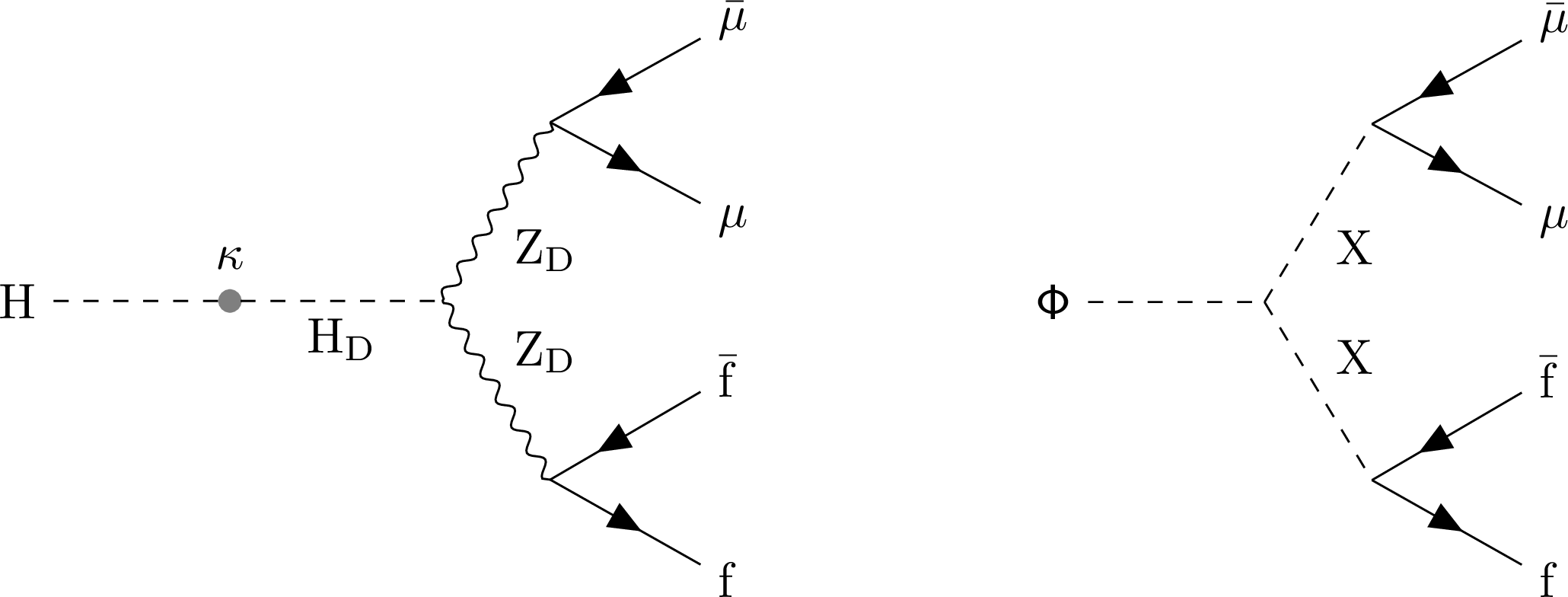
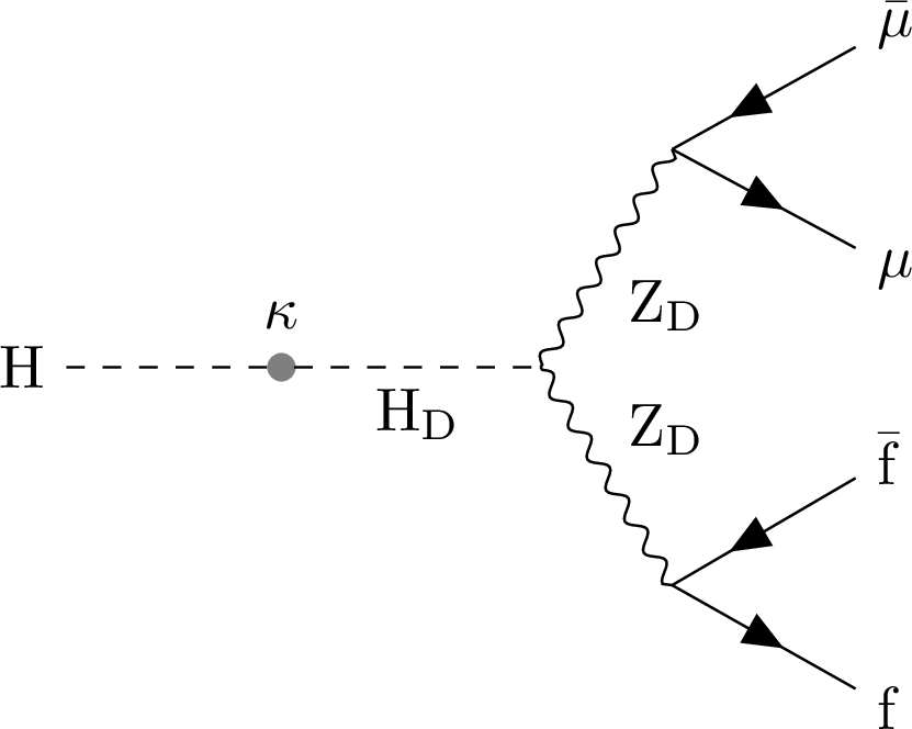
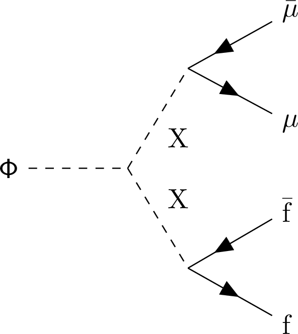
Feynman diagrams for (left) the HAHM model, showing the production of long-lived dark photons Z$_{\mathrm{D}}$ via the Higgs portal, through H-H$_{\mathrm{D}}$ mixing with the parameter $\kappa $, with subsequent decays via the vector portal; and (right) the heavy-scalar model with $ \phi$ boson decaying to a pair of long-lived bosons X. The symbols $f$ and $\overline{f}$ represent, respectively, fermions and antifermions lighter than half the LLP mass. |
png pdf |
Figure 1-a:
Feynman diagram for the HAHM model, showing the production of long-lived dark photons Z$_{\mathrm{D}}$ via the Higgs portal, through H-H$_{\mathrm{D}}$ mixing with the parameter $\kappa $, with subsequent decays via the vector portal. The symbols $f$ and $\overline{f}$ represent, respectively, fermions and antifermions lighter than half the LLP mass. |
png pdf |
Figure 1-b:
Feynman diagram for the heavy-scalar model with $ \phi$ boson decaying to a pair of long-lived bosons X. The symbols $f$ and $\overline{f}$ represent, respectively, fermions and antifermions lighter than half the LLP mass. |
png pdf |
Figure 2:
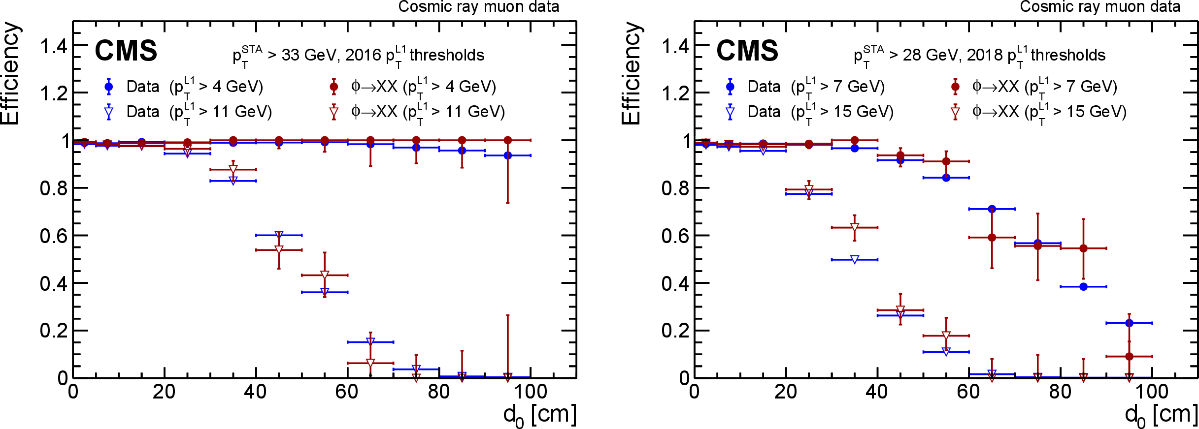
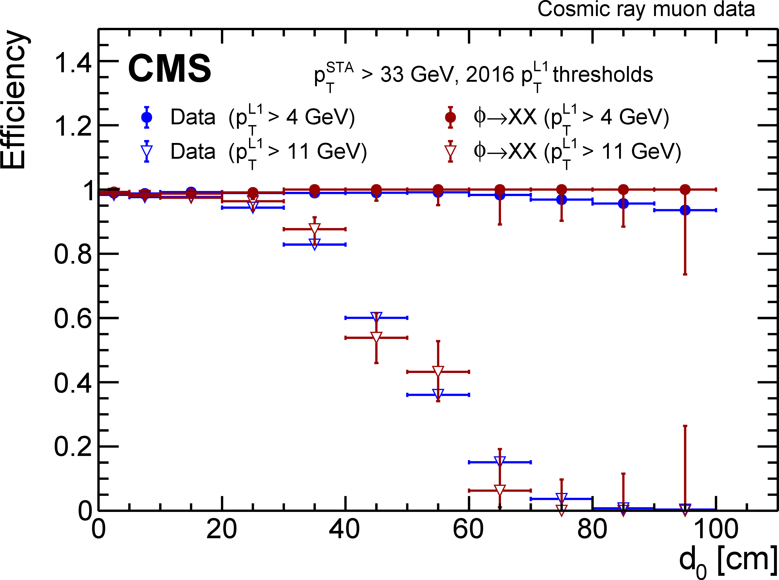
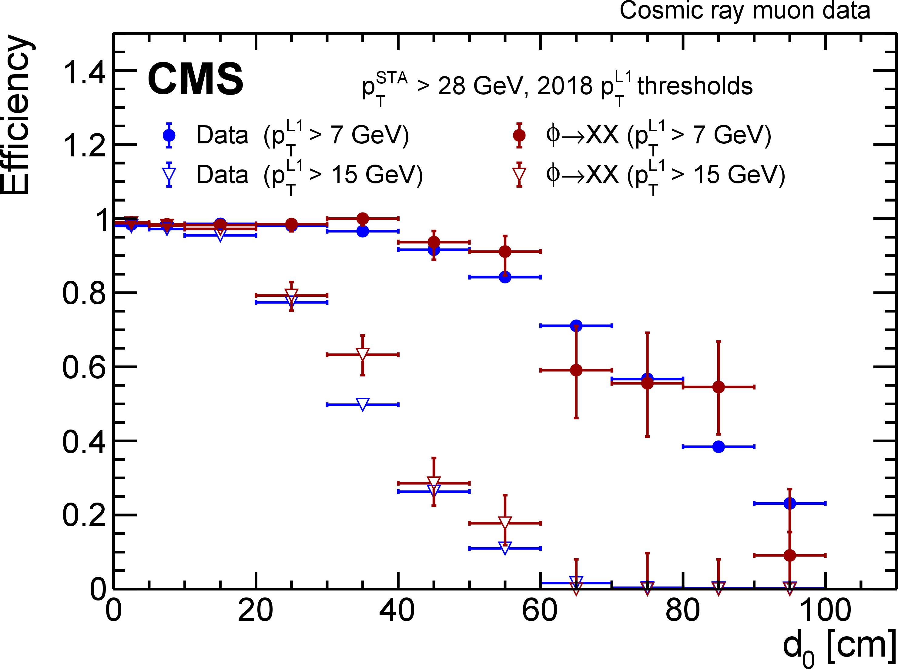
L1 muon trigger efficiency in cosmic ray muon data (blue) and signal simulation (red) as a function of $ {d_{\mathrm {0}}} $, for the L1 trigger ${p_{\mathrm {T}}}$ thresholds used in (left) 2016 and (right) 2018. The denominator in the efficiency calculations is the number of STA muons with $ {| \eta |} < $ 1.2 and $ {p_{\mathrm {T}}} > $ 33 (28) GeV in 2016 (2018). |
png pdf |
Figure 2-a:
L1 muon trigger efficiency in cosmic ray muon data (blue) and signal simulation (red) as a function of $ {d_{\mathrm {0}}} $, for the L1 trigger ${p_{\mathrm {T}}}$ thresholds used in 2016. The denominator in the efficiency calculations is the number of STA muons with $ {| \eta |} < $ 1.2 and $ {p_{\mathrm {T}}} > $ 33 GeV. |
png pdf |
Figure 2-b:
L1 muon trigger efficiency in cosmic ray muon data (blue) and signal simulation (red) as a function of $ {d_{\mathrm {0}}} $, for the L1 trigger ${p_{\mathrm {T}}}$ thresholds used in 2018. The denominator in the efficiency calculations is the number of STA muons with $ {| \eta |} < $ 1.2 and $ {p_{\mathrm {T}}} > $ 28 GeV. |
png pdf |
Figure 3:
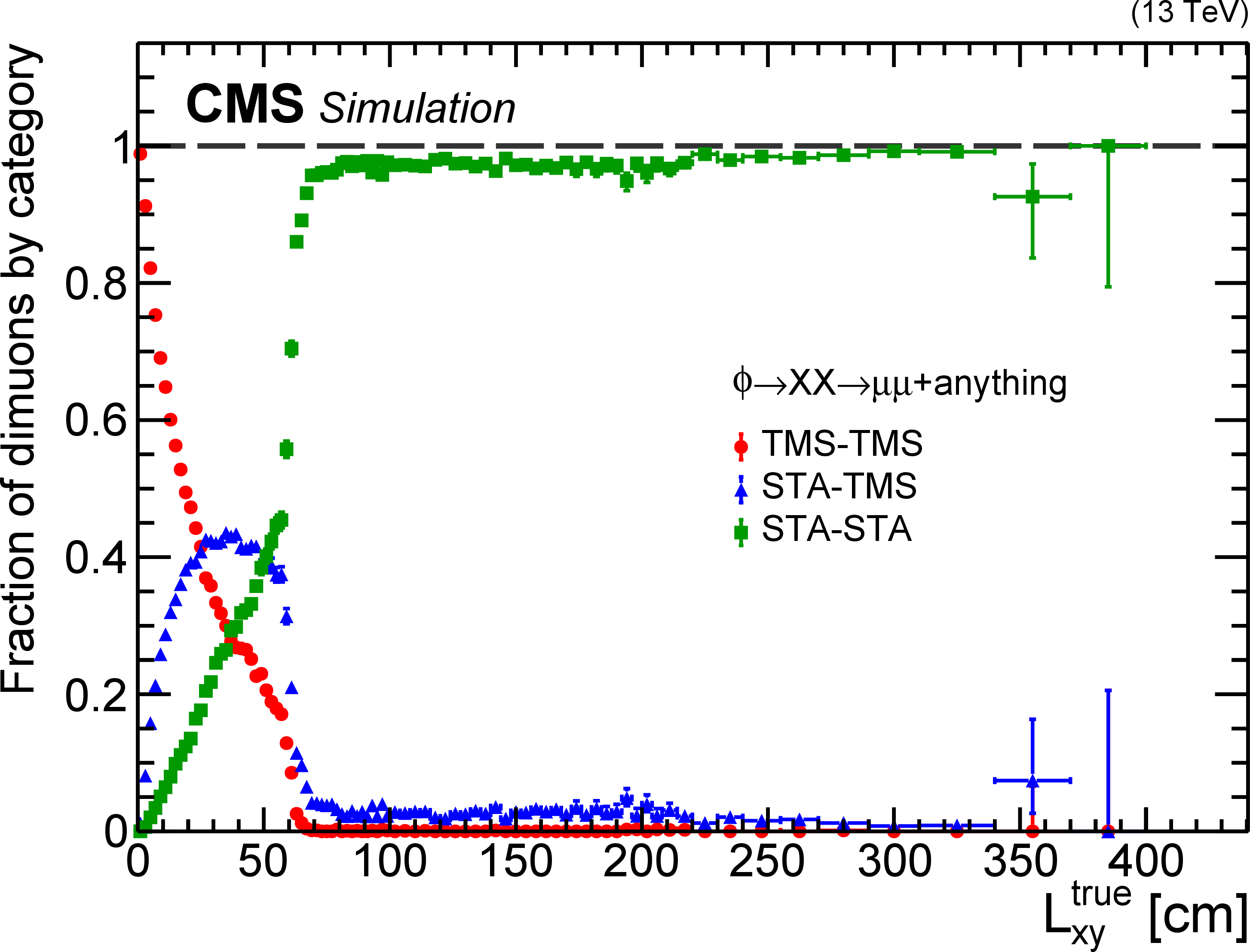
Fractions of signal events with zero (green), one (blue), and two (red) STA muons matched to TMS muons by the STA-to-TMS muon association procedure, as a function of true ${L_{\mathrm {xy}}}$, in all simulated ${\phi\to \mathrm{X} \mathrm{X} \to \mu \mu}$+anything signal samples combined. The fractions are computed relative to the number of signal events passing the trigger and containing two STA muons with more than 12 muon detector hits and $ {p_{\mathrm {T}}} > $ 10 GeV matched to generated muons from $\mathrm{X} \to \mu \mu $ decays. |
png pdf |
Figure 4:
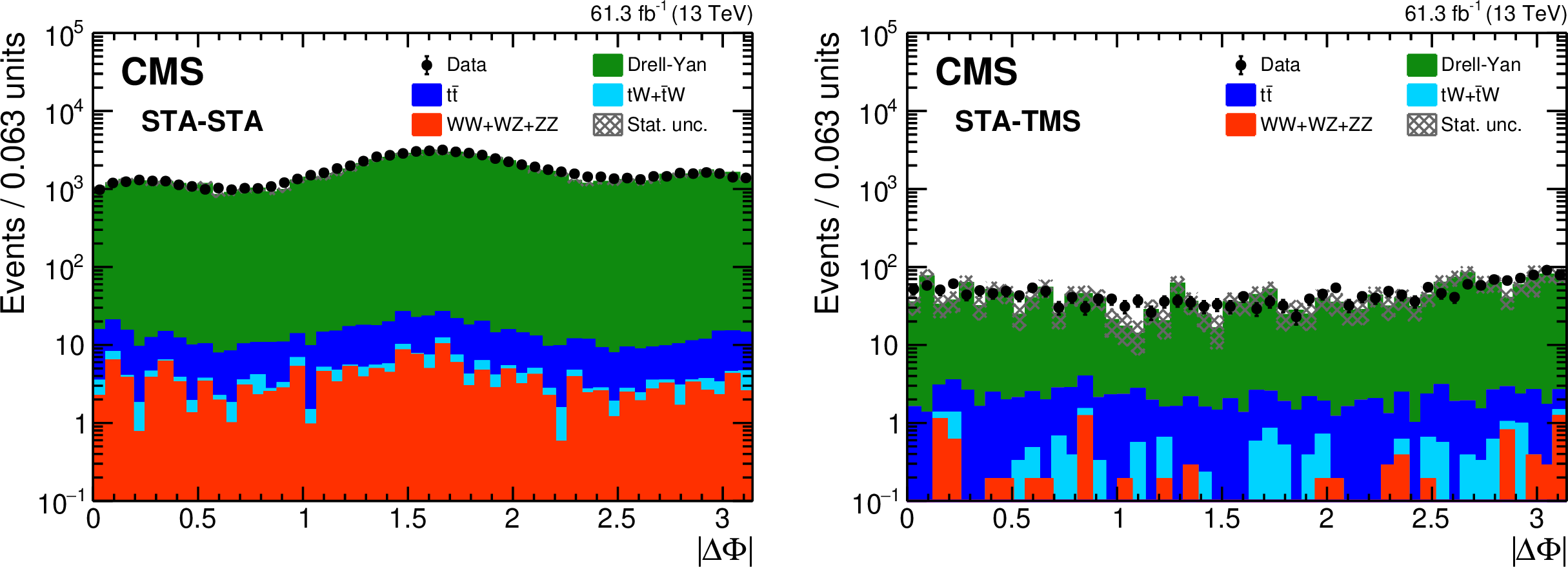
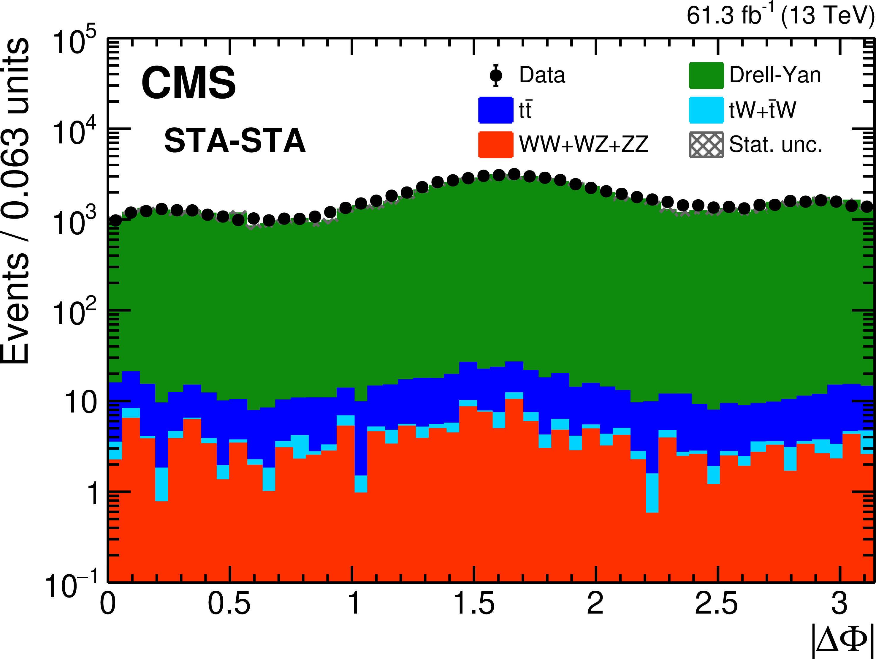
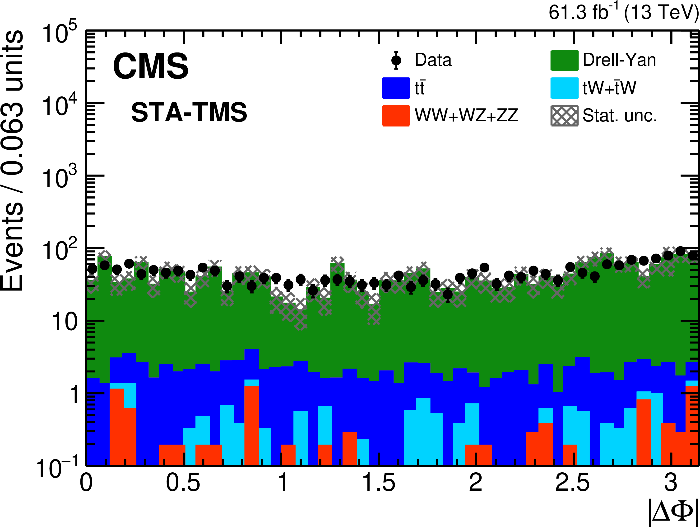
Distributions of $ {{| \Delta \Phi |}} $ for (left) STA-STA and (right) STA-TMS dimuons in 2018 data (black dots) and simulated background processes (stacked histograms), for events in the control regions with the STA-to-TMS association of the STA muons reversed, as described in the text. All nominal selection requirements, including dimuon $ {{L_{\mathrm {xy}}} / {\sigma _{{L_{\mathrm {xy}}}}}} $ and TMS muon $ {{d_{\mathrm {0}}} / {\sigma _{{d_{\mathrm {0}}}}}} $, are applied to the STA-STA and STA-TMS dimuons. The simulated processes are scaled to correspond to the integrated luminosity of the data. The shaded area shows the statistical uncertainty in the simulated background yield. |
png pdf |
Figure 4-a:
Distribution of $ {{| \Delta \Phi |}} $ for STA-STA dimuons in 2018 data (black dots) and simulated background processes (stacked histograms), for events in the control regions with the STA-to-TMS association of the STA muons reversed, as described in the text. All nominal selection requirements, including dimuon $ {{L_{\mathrm {xy}}} / {\sigma _{{L_{\mathrm {xy}}}}}} $, are applied. The simulated processes are scaled to correspond to the integrated luminosity of the data. The shaded area shows the statistical uncertainty in the simulated background yield. |
png pdf |
Figure 4-b:
Distribution of $ {{| \Delta \Phi |}} $ for STA-TMS dimuons in 2018 data (black dots) and simulated background processes (stacked histograms), for events in the control regions with the STA-to-TMS association of the STA muons reversed, as described in the text. All nominal selection requirements, including dimuon $ {{L_{\mathrm {xy}}} / {\sigma _{{L_{\mathrm {xy}}}}}} $ and TMS muon $ {{d_{\mathrm {0}}} / {\sigma _{{d_{\mathrm {0}}}}}} $, are applied. The simulated processes are scaled to correspond to the integrated luminosity of the data. The shaded area shows the statistical uncertainty in the simulated background yield. |

png pdf |
Figure 5:
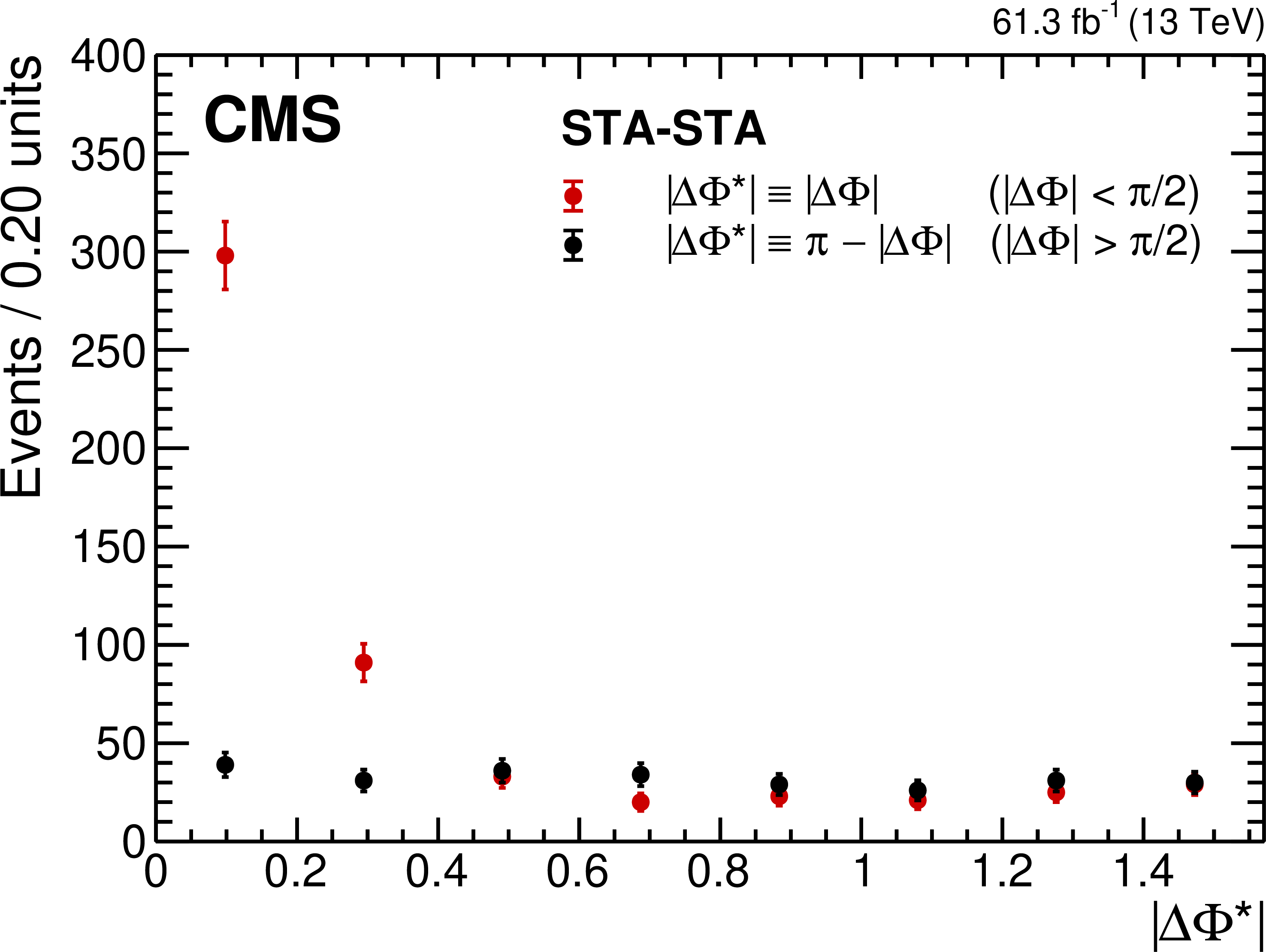
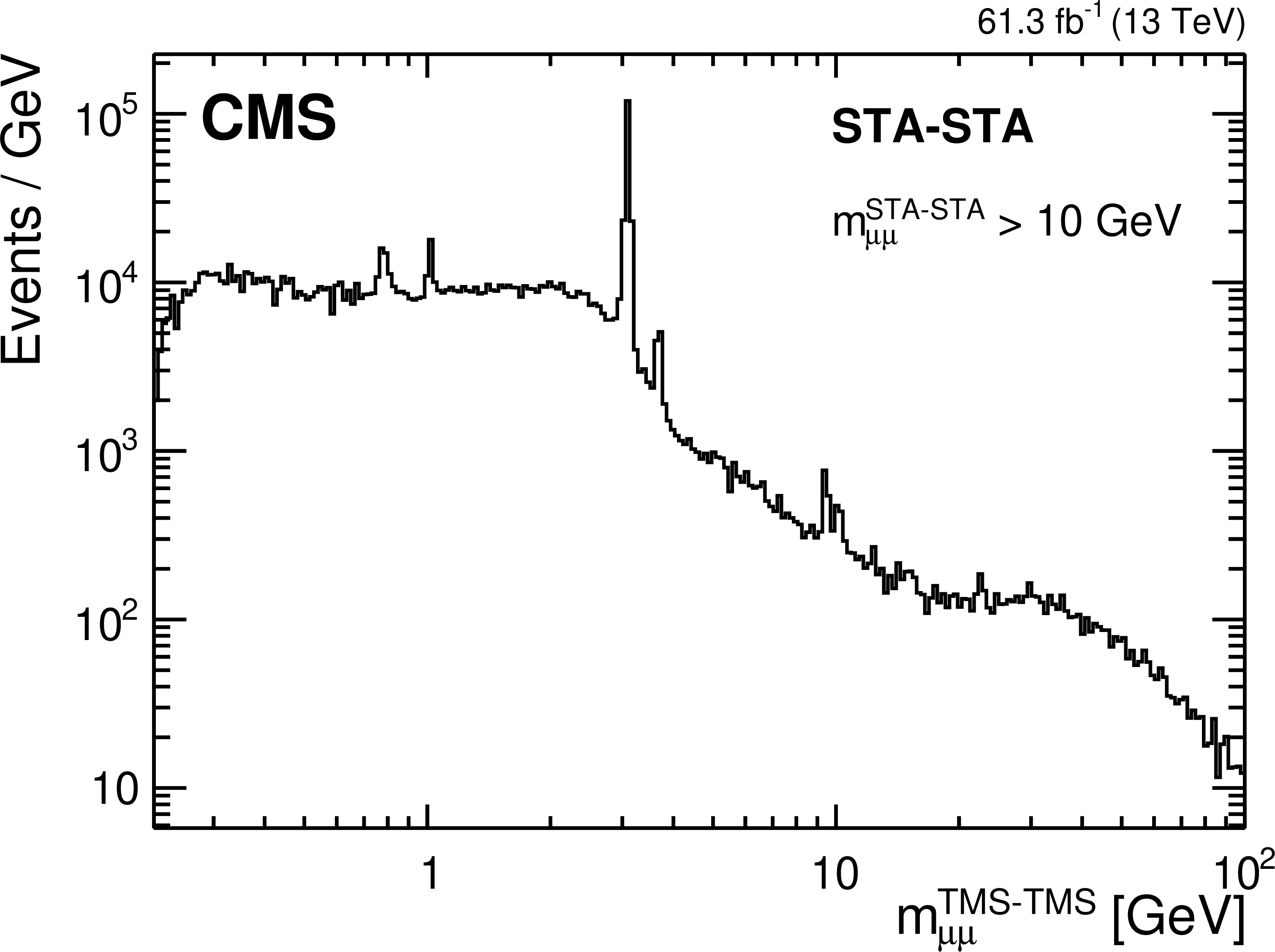
Distributions of (left) $ {{| \Delta \Phi ^{*} |}} $ (defined in the legend) of STA-STA dimuons and (right) ${m_{\mu \mu}}$ of TMS-TMS dimuons associated with STA-STA dimuons. Both distributions show STA-STA dimuons in 2018 data in the control region enriched in QCD events, as described in the text. (The distributions in 2016 data are very similar.) In the left plot, exactly one STA muon is associated with a TMS muon, while in the right plot, both are. All nominal selection requirements, including $ {m_{\mu \mu}} > $ 10 GeV and $ {{L_{\mathrm {xy}}} / {\sigma _{{L_{\mathrm {xy}}}}}} > $ 6, are applied to the STA-STA dimuons. |
png pdf |
Figure 5-a:
Distribution of $ {{| \Delta \Phi ^{*} |}} $ (defined in the legend) of STA-STA dimuons. The distribution shows STA-STA dimuons in 2018 data in the control region enriched in QCD events, as described in the text. (The distribution in 2016 data is very similar.) Exactly one STA muon is associated with a TMS muon. All nominal selection requirements, including $ {m_{\mu \mu}} > $ 10 GeV and $ {{L_{\mathrm {xy}}} / {\sigma _{{L_{\mathrm {xy}}}}}} > $ 6, are applied to the STA-STA dimuons. |
png pdf |
Figure 5-b:
Distribution of ${m_{\mu \mu}}$ of TMS-TMS dimuons associated with STA-STA dimuons. The distribution shows STA-STA dimuons in 2018 data in the control region enriched in QCD events, as described in the text. (The distribution in 2016 data is very similar.) Both STA muons are associated with a TMS muon. All nominal selection requirements, including $ {m_{\mu \mu}} > $ 10 GeV and $ {{L_{\mathrm {xy}}} / {\sigma _{{L_{\mathrm {xy}}}}}} > $ 6, are applied to the STA-STA dimuons. |
png pdf |
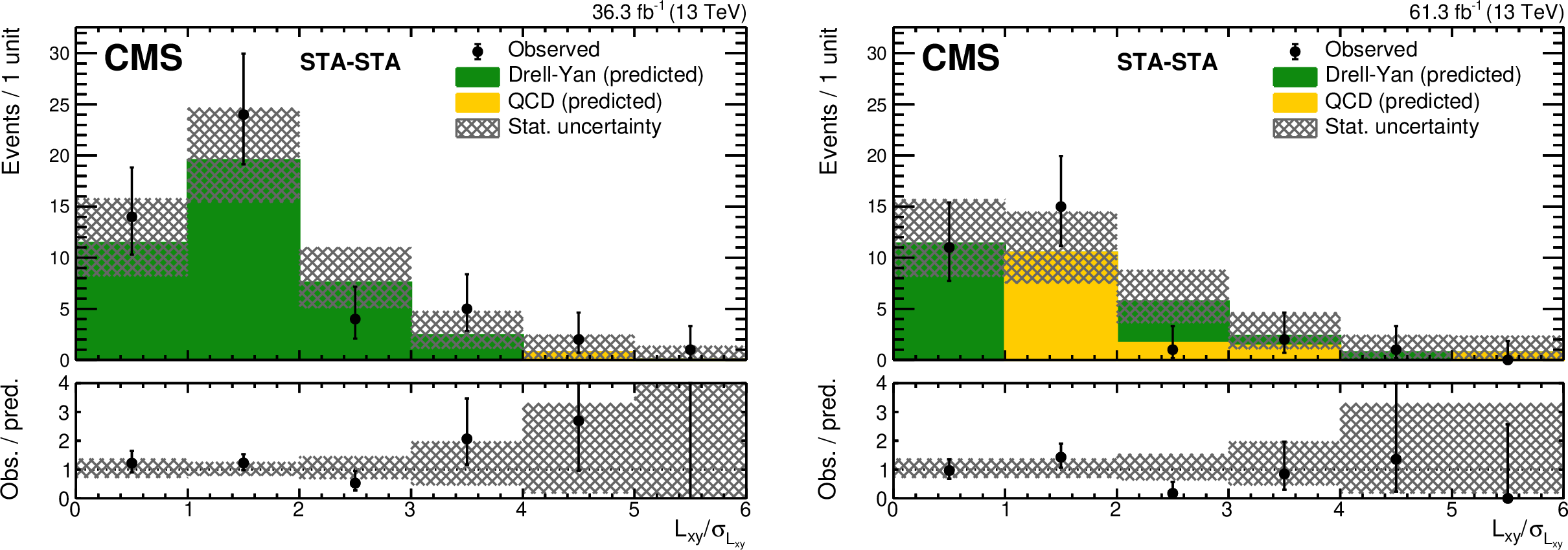
Figure 6:
Distributions of $ {{L_{\mathrm {xy}}} / {\sigma _{{L_{\mathrm {xy}}}}}} $ of STA-STA dimuons in the $ {{L_{\mathrm {xy}}} / {\sigma _{{L_{\mathrm {xy}}}}}} < $ 6 VR, in (left) 2016 and (right) 2018 data, compared to the background predictions. The observed distributions (black points with error bars) are overlayed on stacked histograms containing the expected numbers of DY (green) and QCD (yellow) background events. The lower panels show the ratio of the observed to predicted numbers of events. The shaded area shows the statistical uncertainty in the background prediction. |
png pdf |
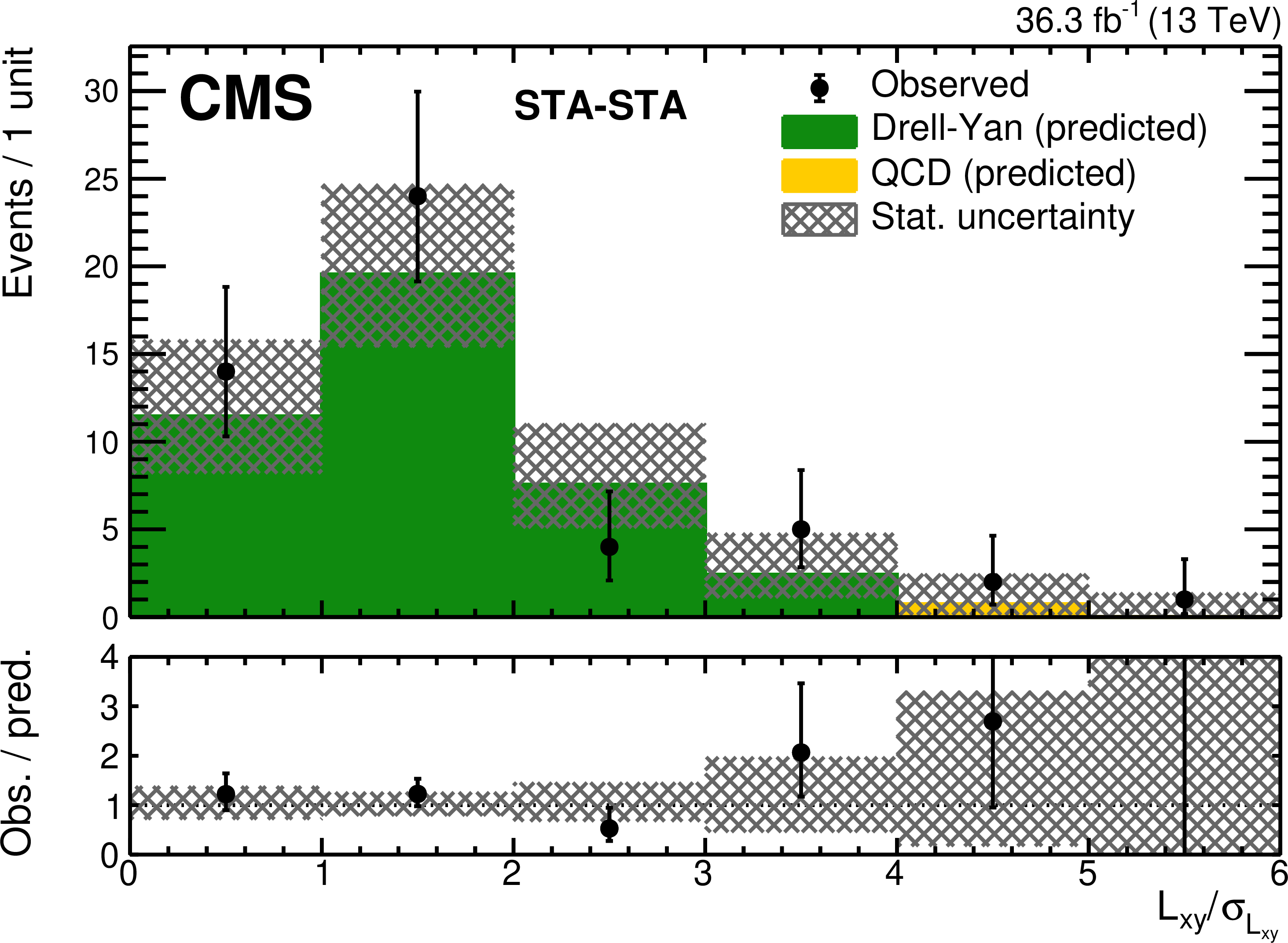
Figure 6-a:
Distributions of $ {{L_{\mathrm {xy}}} / {\sigma _{{L_{\mathrm {xy}}}}}} $ of STA-STA dimuons in the $ {{L_{\mathrm {xy}}} / {\sigma _{{L_{\mathrm {xy}}}}}} < $ 6 VR, in (left) 2016 and (right) 2018 data, compared to the background predictions. The observed distributions (black points with error bars) are overlayed on stacked histograms containing the expected numbers of DY (green) and QCD (yellow) background events. The lower panels show the ratio of the observed to predicted numbers of events. The shaded area shows the statistical uncertainty in the background prediction. |
png pdf |
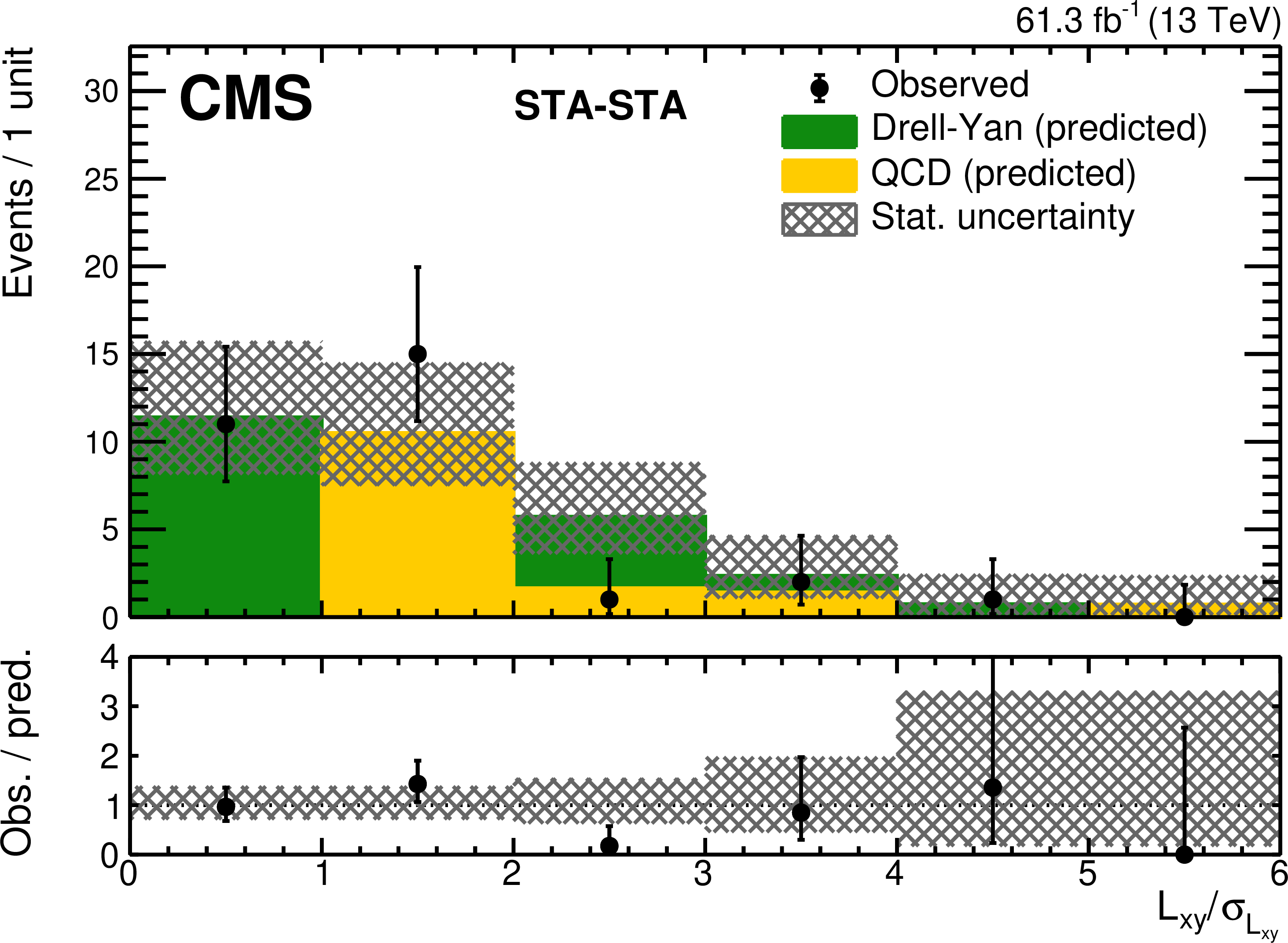
Figure 6-b:
Distributions of $ {{L_{\mathrm {xy}}} / {\sigma _{{L_{\mathrm {xy}}}}}} $ of STA-STA dimuons in the $ {{L_{\mathrm {xy}}} / {\sigma _{{L_{\mathrm {xy}}}}}} < $ 6 VR, in (left) 2016 and (right) 2018 data, compared to the background predictions. The observed distributions (black points with error bars) are overlayed on stacked histograms containing the expected numbers of DY (green) and QCD (yellow) background events. The lower panels show the ratio of the observed to predicted numbers of events. The shaded area shows the statistical uncertainty in the background prediction. |
png pdf |
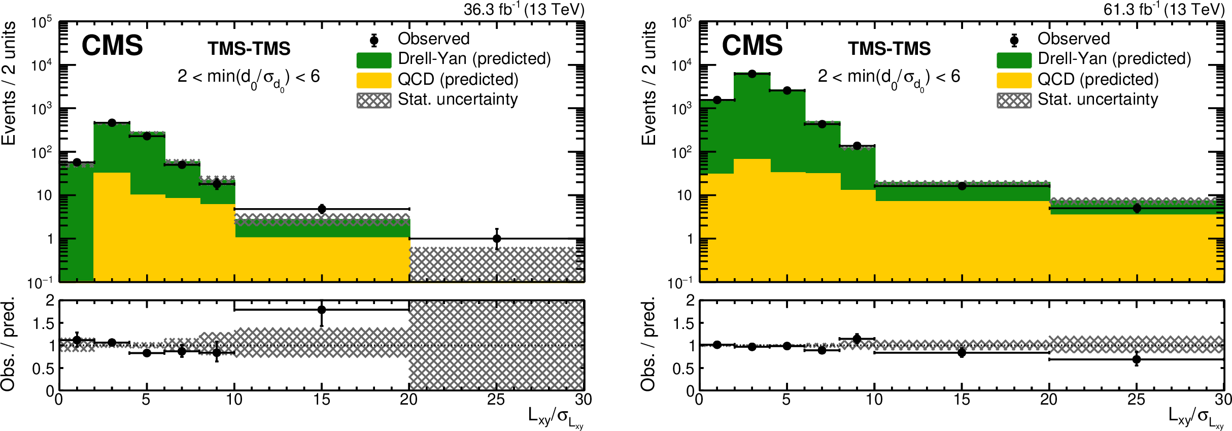
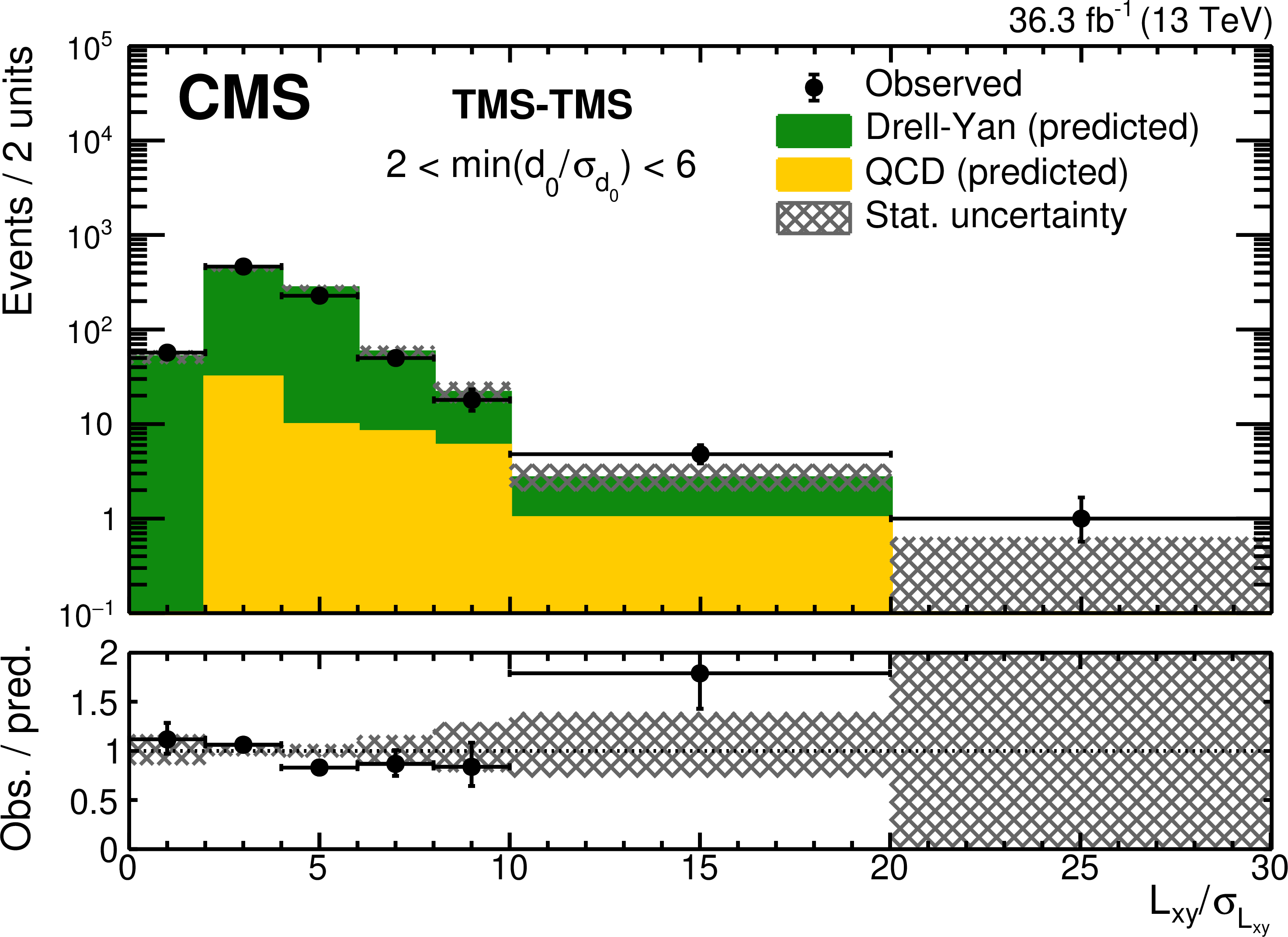
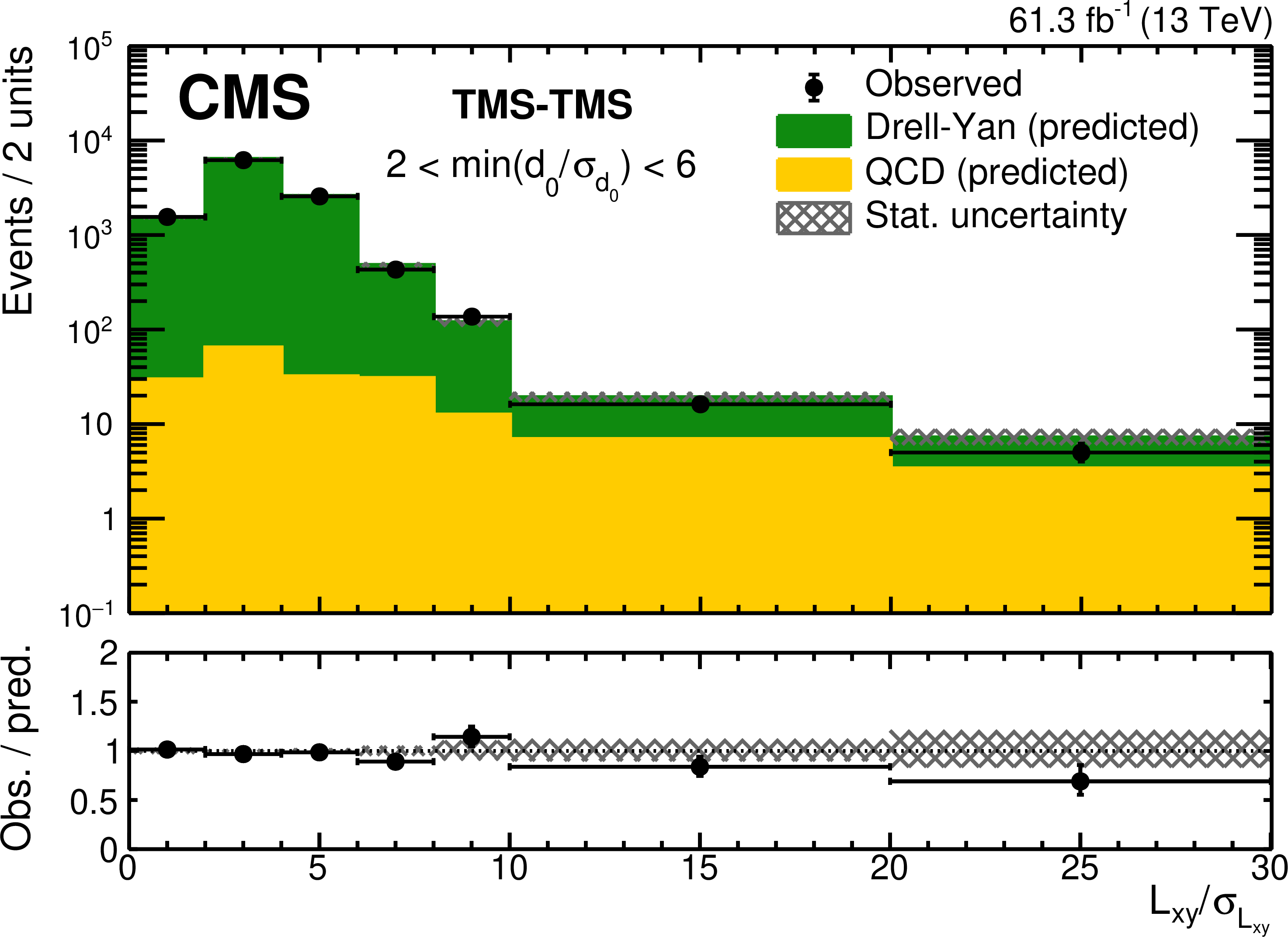
Figure 7:
Distributions of $ {{L_{\mathrm {xy}}} / {\sigma _{{L_{\mathrm {xy}}}}}} $ of TMS-TMS dimuons in the 2 $ < \text {min}({{d_{\mathrm {0}}} / {\sigma _{{d_{\mathrm {0}}}}}}) < $ 6 VR, in (left) 2016 and (right) 2018 data, compared to the background predictions. The observed distributions (black points with error bars) are overlayed on stacked histograms containing the expected numbers of DY (green) and QCD (yellow) background events. The last bin includes events in the overflow. The lower panels show the ratio of the observed to predicted numbers of events. The shaded area shows the statistical uncertainty in the background prediction. |
png pdf |
Figure 7-a:
Distributions of $ {{L_{\mathrm {xy}}} / {\sigma _{{L_{\mathrm {xy}}}}}} $ of TMS-TMS dimuons in the 2 $ < \text {min}({{d_{\mathrm {0}}} / {\sigma _{{d_{\mathrm {0}}}}}}) < $ 6 VR, in (left) 2016 and (right) 2018 data, compared to the background predictions. The observed distributions (black points with error bars) are overlayed on stacked histograms containing the expected numbers of DY (green) and QCD (yellow) background events. The last bin includes events in the overflow. The lower panels show the ratio of the observed to predicted numbers of events. The shaded area shows the statistical uncertainty in the background prediction. |
png pdf |
Figure 7-b:
Distributions of $ {{L_{\mathrm {xy}}} / {\sigma _{{L_{\mathrm {xy}}}}}} $ of TMS-TMS dimuons in the 2 $ < \text {min}({{d_{\mathrm {0}}} / {\sigma _{{d_{\mathrm {0}}}}}}) < $ 6 VR, in (left) 2016 and (right) 2018 data, compared to the background predictions. The observed distributions (black points with error bars) are overlayed on stacked histograms containing the expected numbers of DY (green) and QCD (yellow) background events. The last bin includes events in the overflow. The lower panels show the ratio of the observed to predicted numbers of events. The shaded area shows the statistical uncertainty in the background prediction. |
png pdf |
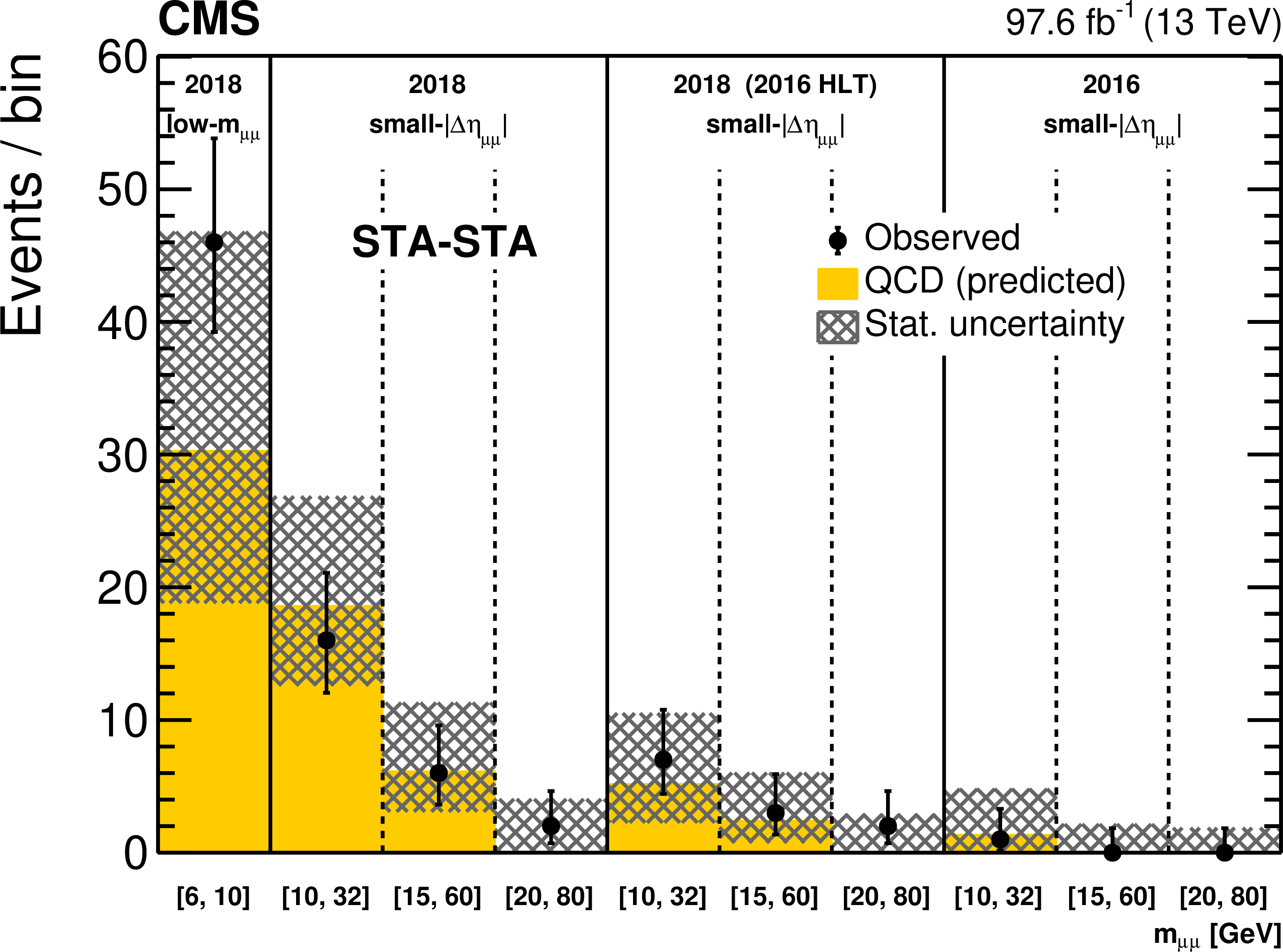
Figure 8:
Comparison of observed (black points with error bars) and predicted (histograms) yields of STA-STA dimuons in the validation regions enriched in QCD background events. The first bin shows the yields in the low-mass VR in 2018 data. The other three groups of bins, separated by solid lines, show the yields in the small-$ {{| \Delta \eta _{\mu \mu} |}}$ VR, in (from left to right) the entire 2018 data set, a subset of 2018 data enriched in events collected in 2016, and the 2016 data set. Each of these three VRs is further subdivided into three ${m_{\mu \mu}}$ intervals, 10-32, 15-60, and 20-80 GeV. The expected number of background events is computed according to Eqs. (3) and (4), separately in each $ {m_{\mu \mu}} $ bin. The shaded area shows the statistical uncertainty in the background prediction. |
png pdf |
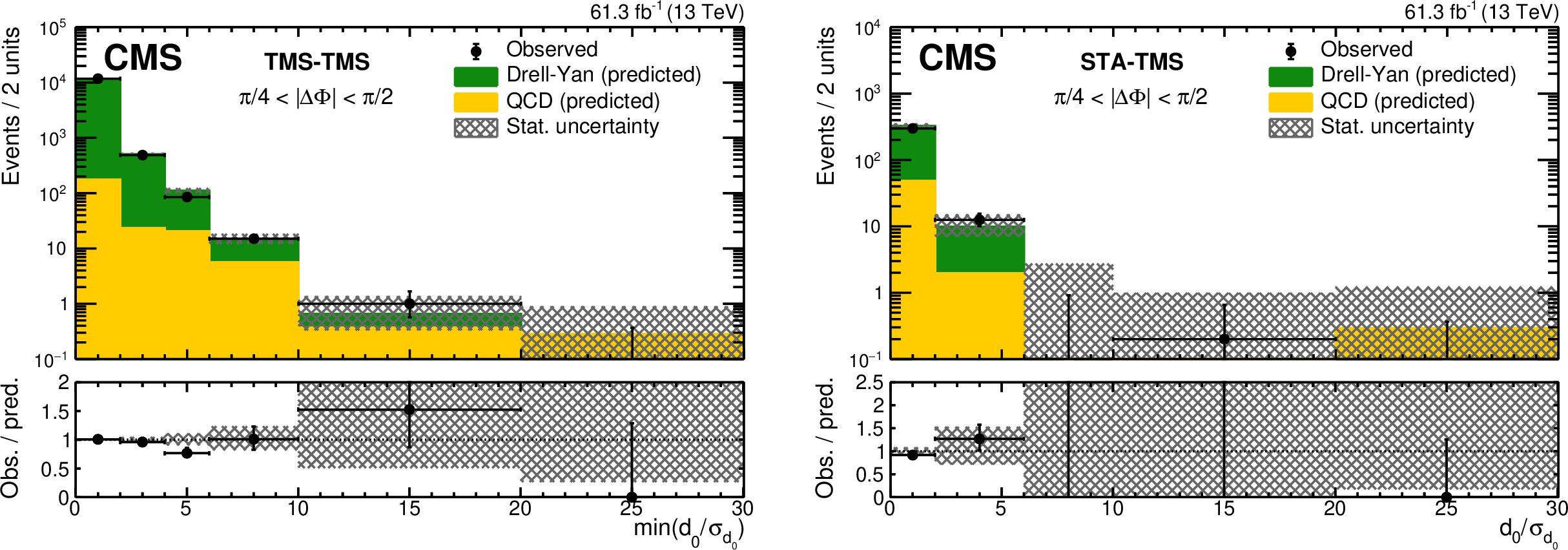
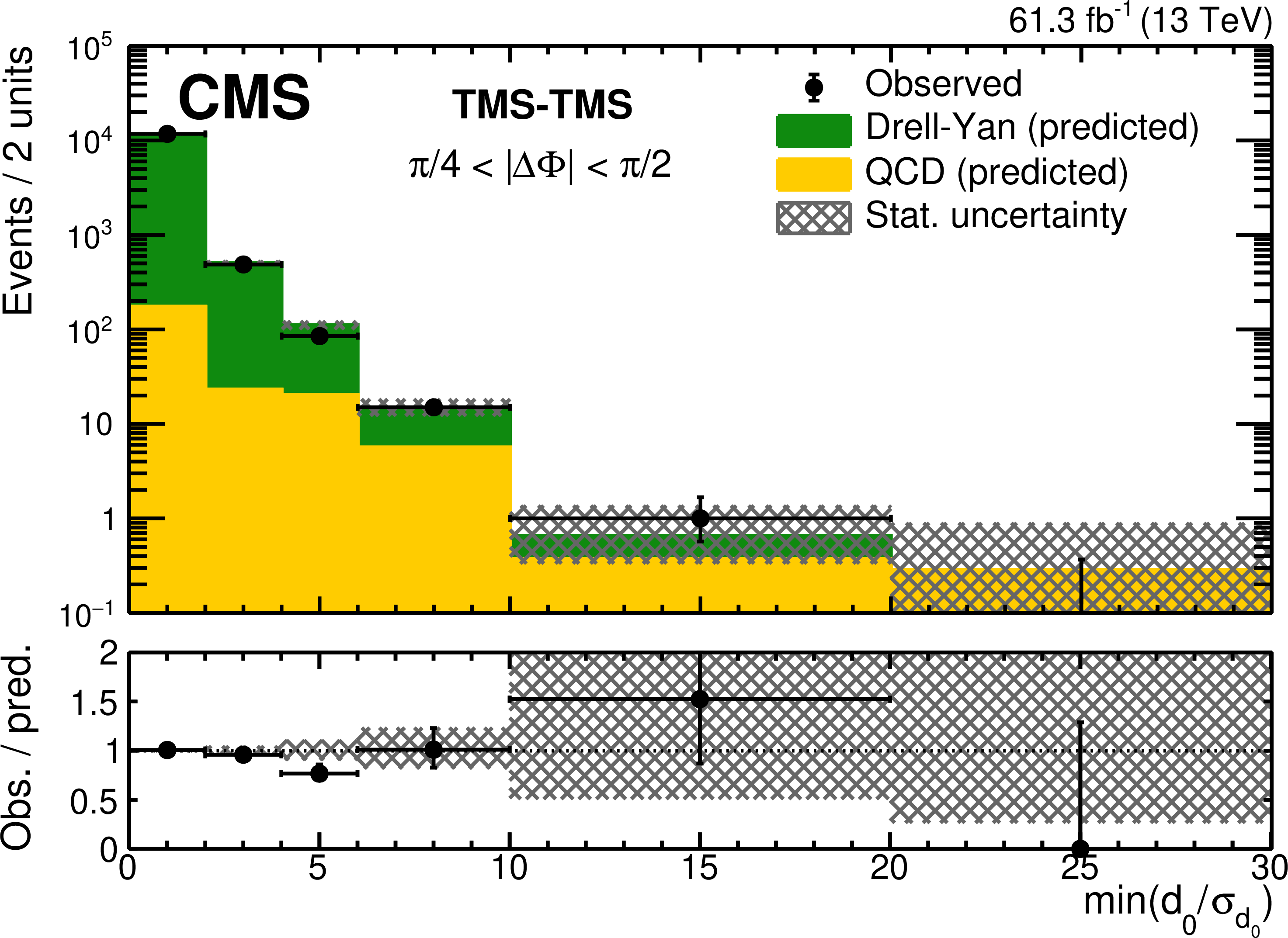
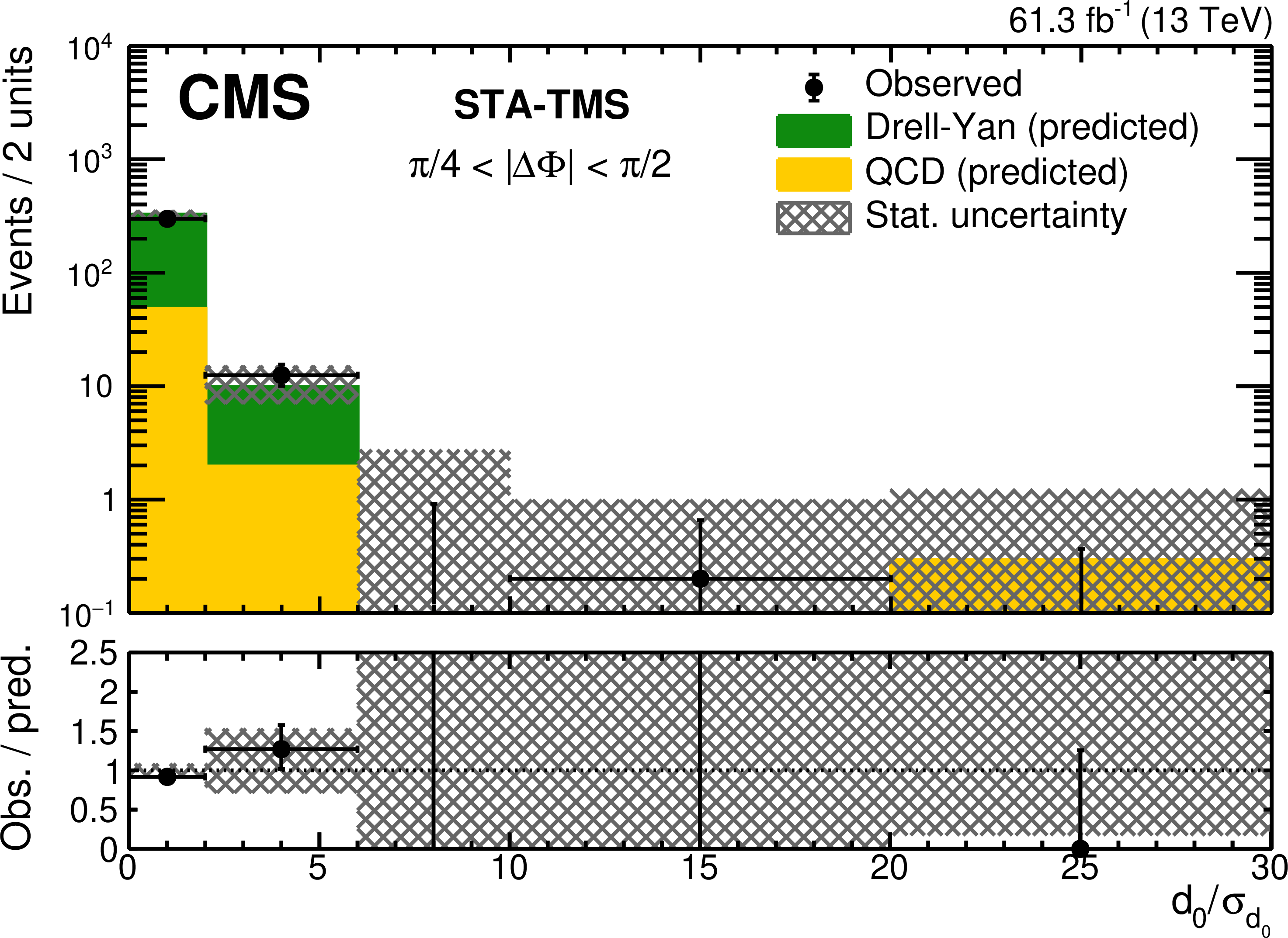
Figure 9:
Distributions in the $\pi /4 < {{| \Delta \Phi |}} < \pi /2$ VR in 2018 data: (left) the smaller of the two $ {{d_{\mathrm {0}}} / {\sigma _{{d_{\mathrm {0}}}}}} $ values for the TMS-TMS dimuon; (right) $ {{d_{\mathrm {0}}} / {\sigma _{{d_{\mathrm {0}}}}}} $ of the TMS muon in the STA-TMS dimuon. The observed distributions (black points with error bars) are compared to the results of the background prediction method applied to events with $\pi /2 < {{| \Delta \Phi |}} < 3\pi /4$. The stacked histograms show the expected numbers of DY (green) and QCD (yellow) background events. The last bin includes events in the overflow. The lower panels show the ratios of the observed to predicted numbers of events. The shaded area shows the statistical uncertainty in the background prediction. |
png pdf |
Figure 9-a:
Distributions in the $\pi /4 < {{| \Delta \Phi |}} < \pi /2$ VR in 2018 data: (left) the smaller of the two $ {{d_{\mathrm {0}}} / {\sigma _{{d_{\mathrm {0}}}}}} $ values for the TMS-TMS dimuon; (right) $ {{d_{\mathrm {0}}} / {\sigma _{{d_{\mathrm {0}}}}}} $ of the TMS muon in the STA-TMS dimuon. The observed distributions (black points with error bars) are compared to the results of the background prediction method applied to events with $\pi /2 < {{| \Delta \Phi |}} < 3\pi /4$. The stacked histograms show the expected numbers of DY (green) and QCD (yellow) background events. The last bin includes events in the overflow. The lower panels show the ratios of the observed to predicted numbers of events. The shaded area shows the statistical uncertainty in the background prediction. |
png pdf |
Figure 9-b:
Distributions in the $\pi /4 < {{| \Delta \Phi |}} < \pi /2$ VR in 2018 data: (left) the smaller of the two $ {{d_{\mathrm {0}}} / {\sigma _{{d_{\mathrm {0}}}}}} $ values for the TMS-TMS dimuon; (right) $ {{d_{\mathrm {0}}} / {\sigma _{{d_{\mathrm {0}}}}}} $ of the TMS muon in the STA-TMS dimuon. The observed distributions (black points with error bars) are compared to the results of the background prediction method applied to events with $\pi /2 < {{| \Delta \Phi |}} < 3\pi /4$. The stacked histograms show the expected numbers of DY (green) and QCD (yellow) background events. The last bin includes events in the overflow. The lower panels show the ratios of the observed to predicted numbers of events. The shaded area shows the statistical uncertainty in the background prediction. |

png pdf |
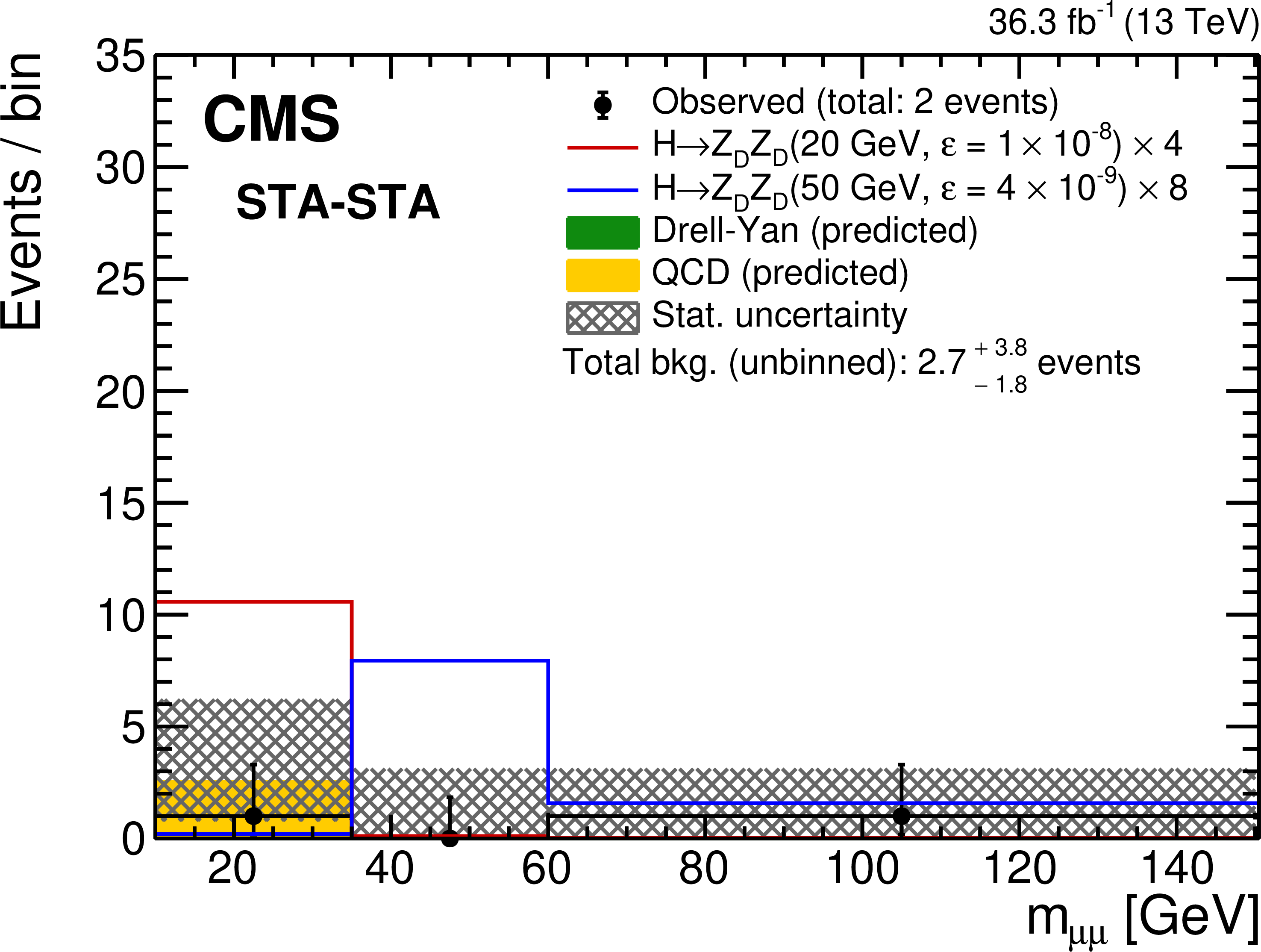
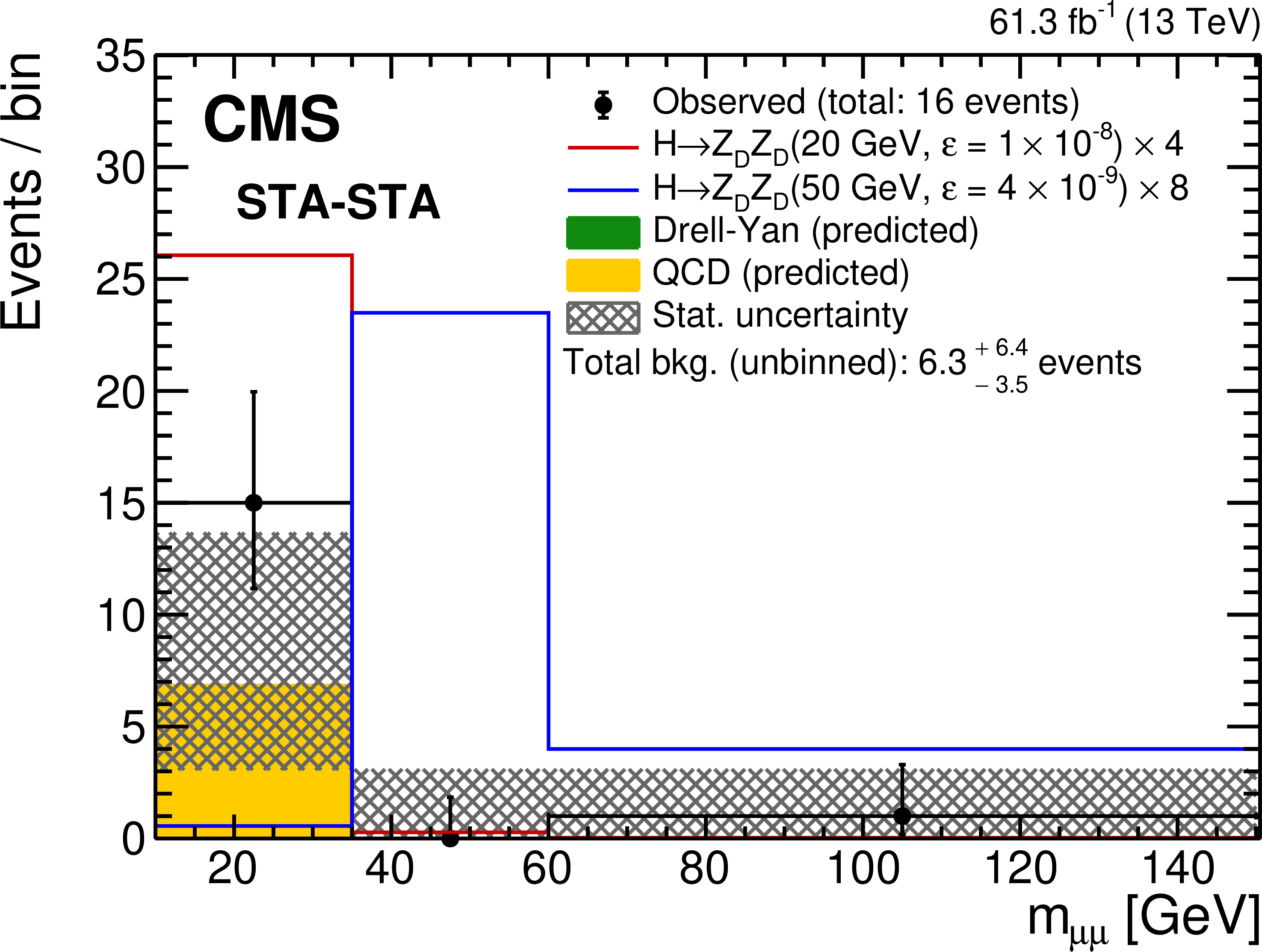
Figure 10:
Comparison of the number of events observed in (left) 2016 and (right) 2018 data in the STA-STA dimuon category with the expected number of background events, in representative ${m_{\mu \mu}}$ intervals. The black points with error bars show the number of observed events; the green and yellow components of the stacked histograms represent the estimated numbers of DY and QCD events, respectively. The last bin includes events in the overflow. The uncertainties in the total expected background (shaded area) are statistical only. Signal contributions expected from simulated $\mathrm{H} \to \mathrm{Z} {\mathrm {_{D}}}\mathrm{Z} {\mathrm {_{D}}}$ with $ {m(\mathrm{Z} {\mathrm {_{D}}})} $ of 20 and 50 GeV are shown in red and blue, respectively. Their yields are set to the corresponding combined median expected exclusion limits at 95% CL, scaled up as indicated in the legend to improve visibility. The legends also include the total number of observed events as well as the number of expected background events obtained inclusively, by applying the background evaluation method to the events in all $ {m_{\mu \mu}} $ intervals combined. |
png pdf |
Figure 10-a:
Comparison of the number of events observed in (left) 2016 and (right) 2018 data in the STA-STA dimuon category with the expected number of background events, in representative ${m_{\mu \mu}}$ intervals. The black points with error bars show the number of observed events; the green and yellow components of the stacked histograms represent the estimated numbers of DY and QCD events, respectively. The last bin includes events in the overflow. The uncertainties in the total expected background (shaded area) are statistical only. Signal contributions expected from simulated $\mathrm{H} \to \mathrm{Z} {\mathrm {_{D}}}\mathrm{Z} {\mathrm {_{D}}}$ with $ {m(\mathrm{Z} {\mathrm {_{D}}})} $ of 20 and 50 GeV are shown in red and blue, respectively. Their yields are set to the corresponding combined median expected exclusion limits at 95% CL, scaled up as indicated in the legend to improve visibility. The legends also include the total number of observed events as well as the number of expected background events obtained inclusively, by applying the background evaluation method to the events in all $ {m_{\mu \mu}} $ intervals combined. |
png pdf |
Figure 10-b:
Comparison of the number of events observed in (left) 2016 and (right) 2018 data in the STA-STA dimuon category with the expected number of background events, in representative ${m_{\mu \mu}}$ intervals. The black points with error bars show the number of observed events; the green and yellow components of the stacked histograms represent the estimated numbers of DY and QCD events, respectively. The last bin includes events in the overflow. The uncertainties in the total expected background (shaded area) are statistical only. Signal contributions expected from simulated $\mathrm{H} \to \mathrm{Z} {\mathrm {_{D}}}\mathrm{Z} {\mathrm {_{D}}}$ with $ {m(\mathrm{Z} {\mathrm {_{D}}})} $ of 20 and 50 GeV are shown in red and blue, respectively. Their yields are set to the corresponding combined median expected exclusion limits at 95% CL, scaled up as indicated in the legend to improve visibility. The legends also include the total number of observed events as well as the number of expected background events obtained inclusively, by applying the background evaluation method to the events in all $ {m_{\mu \mu}} $ intervals combined. |
png pdf |
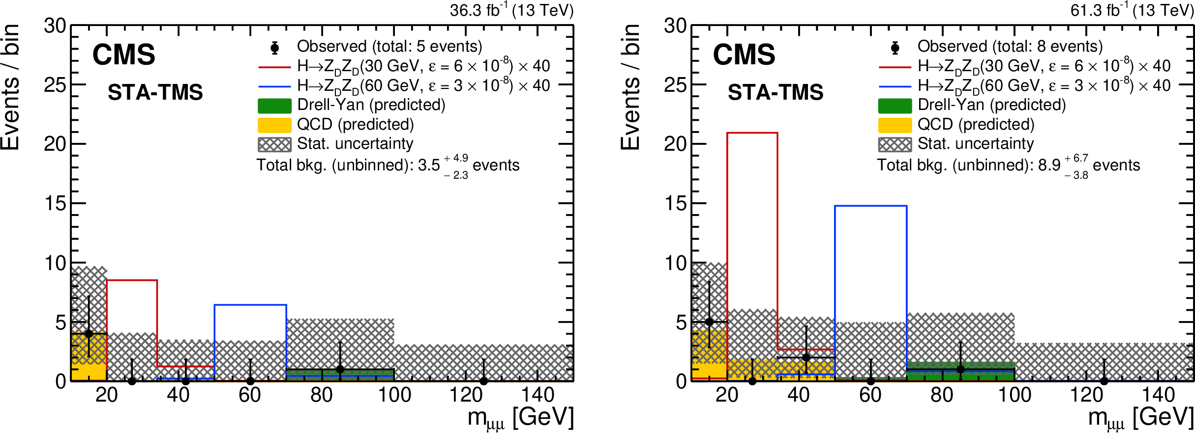
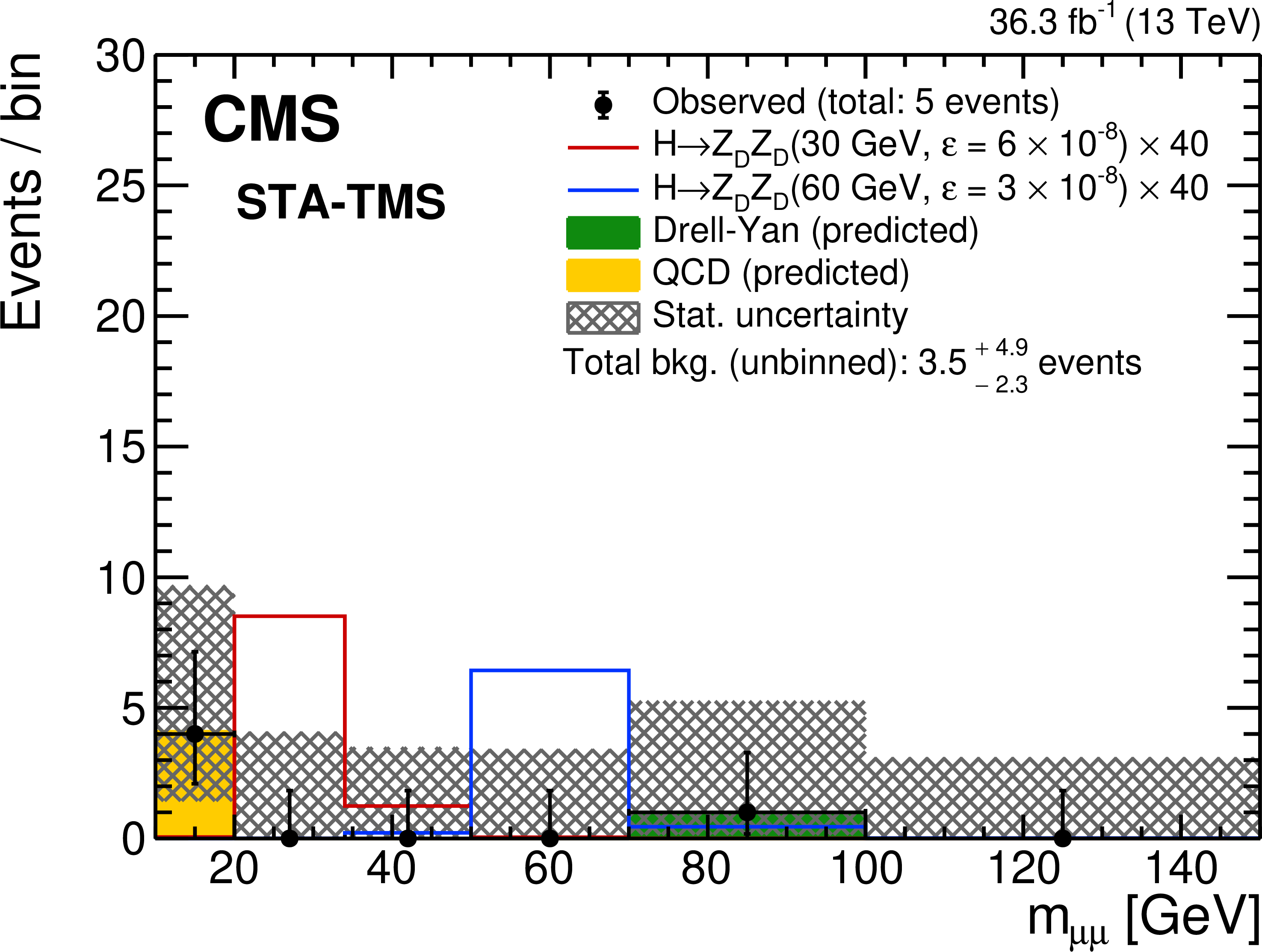
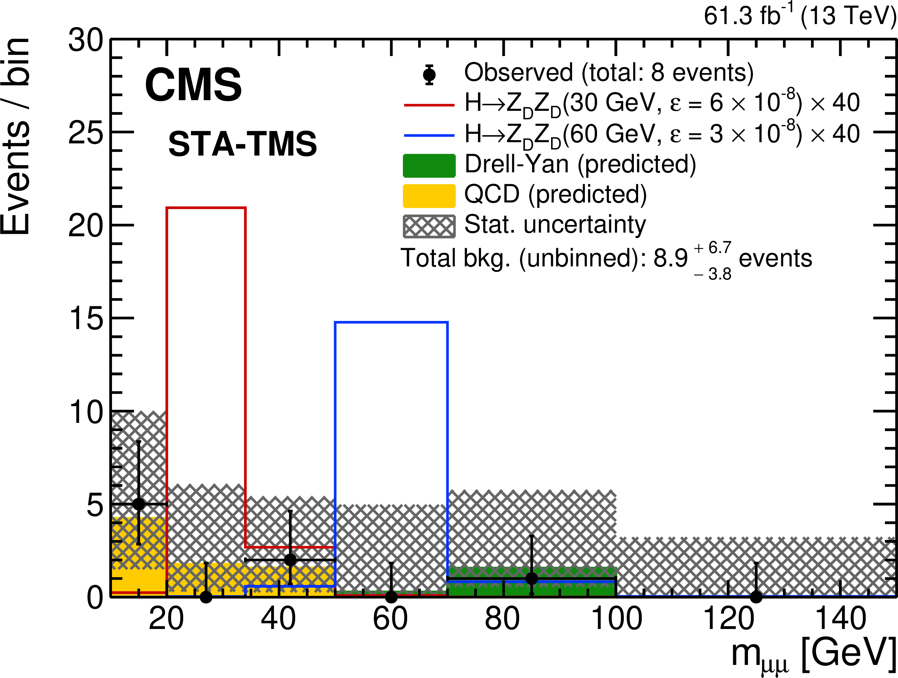
Figure 11:
Comparison of the number of events observed in (left) 2016 and (right) 2018 data in the STA-TMS dimuon category with the expected number of background events, in representative ${m_{\mu \mu}}$ intervals. The black points with error bars show the number of observed events; the green and yellow components of the stacked histograms represent the estimated numbers of DY and QCD events, respectively. The last bin includes events in the overflow. The uncertainties in the total expected background (shaded area) are statistical only. Signal contributions expected from simulated $\mathrm{H} \to \mathrm{Z} {\mathrm {_{D}}}\mathrm{Z} {\mathrm {_{D}}}$ with $ {m(\mathrm{Z} {\mathrm {_{D}}})} $ of 30 and 60 GeV are shown in red and blue, respectively. Their yields are set to the corresponding combined median expected exclusion limits at 95% CL, scaled up as indicated in the legend to improve visibility. The legends also include the total number of observed events as well as the number of expected background events obtained inclusively, by applying the background evaluation method to the events in all $ {m_{\mu \mu}} $ intervals combined. |
png pdf |
Figure 11-a:
Comparison of the number of events observed in (left) 2016 and (right) 2018 data in the STA-TMS dimuon category with the expected number of background events, in representative ${m_{\mu \mu}}$ intervals. The black points with error bars show the number of observed events; the green and yellow components of the stacked histograms represent the estimated numbers of DY and QCD events, respectively. The last bin includes events in the overflow. The uncertainties in the total expected background (shaded area) are statistical only. Signal contributions expected from simulated $\mathrm{H} \to \mathrm{Z} {\mathrm {_{D}}}\mathrm{Z} {\mathrm {_{D}}}$ with $ {m(\mathrm{Z} {\mathrm {_{D}}})} $ of 30 and 60 GeV are shown in red and blue, respectively. Their yields are set to the corresponding combined median expected exclusion limits at 95% CL, scaled up as indicated in the legend to improve visibility. The legends also include the total number of observed events as well as the number of expected background events obtained inclusively, by applying the background evaluation method to the events in all $ {m_{\mu \mu}} $ intervals combined. |
png pdf |
Figure 11-b:
Comparison of the number of events observed in (left) 2016 and (right) 2018 data in the STA-TMS dimuon category with the expected number of background events, in representative ${m_{\mu \mu}}$ intervals. The black points with error bars show the number of observed events; the green and yellow components of the stacked histograms represent the estimated numbers of DY and QCD events, respectively. The last bin includes events in the overflow. The uncertainties in the total expected background (shaded area) are statistical only. Signal contributions expected from simulated $\mathrm{H} \to \mathrm{Z} {\mathrm {_{D}}}\mathrm{Z} {\mathrm {_{D}}}$ with $ {m(\mathrm{Z} {\mathrm {_{D}}})} $ of 30 and 60 GeV are shown in red and blue, respectively. Their yields are set to the corresponding combined median expected exclusion limits at 95% CL, scaled up as indicated in the legend to improve visibility. The legends also include the total number of observed events as well as the number of expected background events obtained inclusively, by applying the background evaluation method to the events in all $ {m_{\mu \mu}} $ intervals combined. |
png pdf |
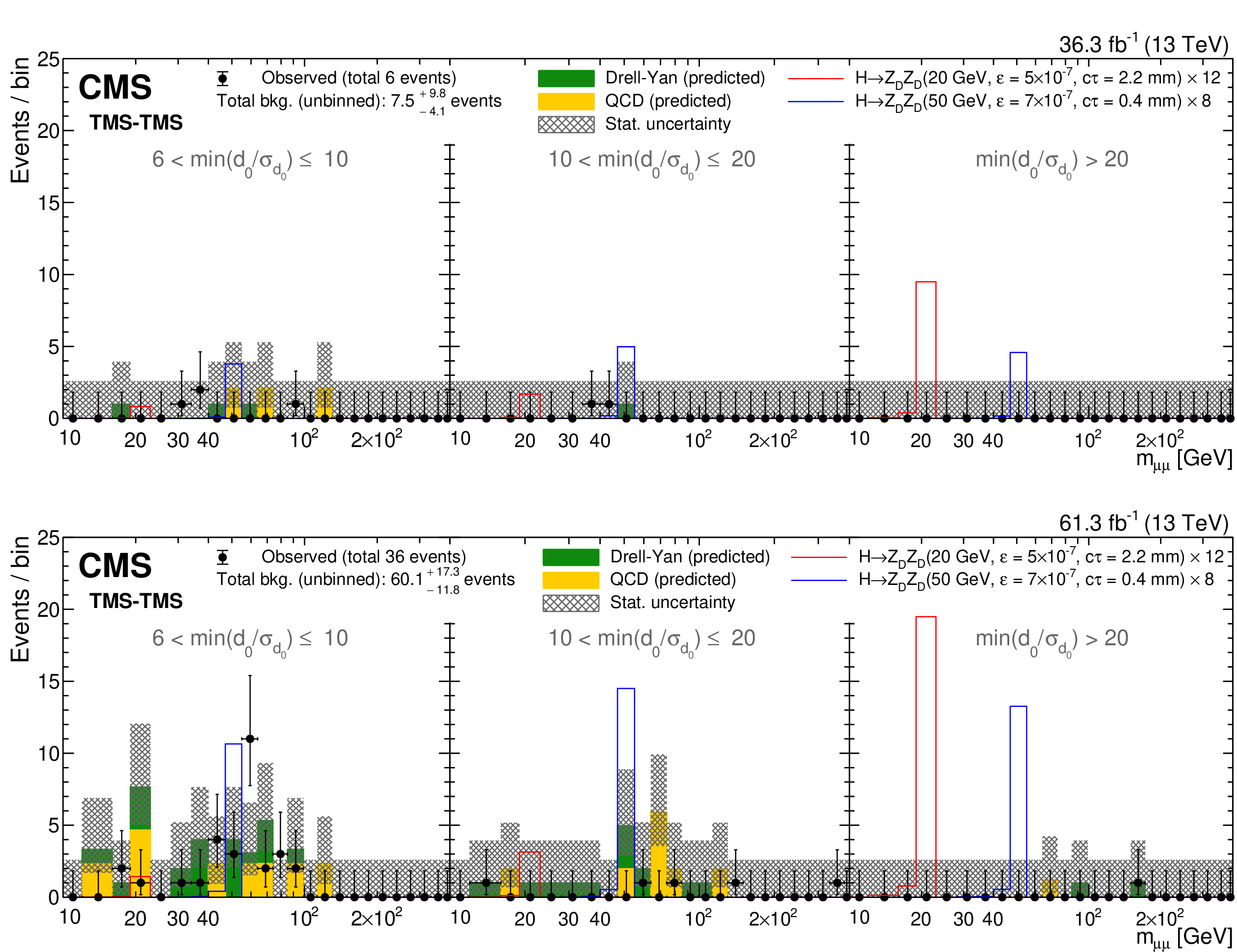
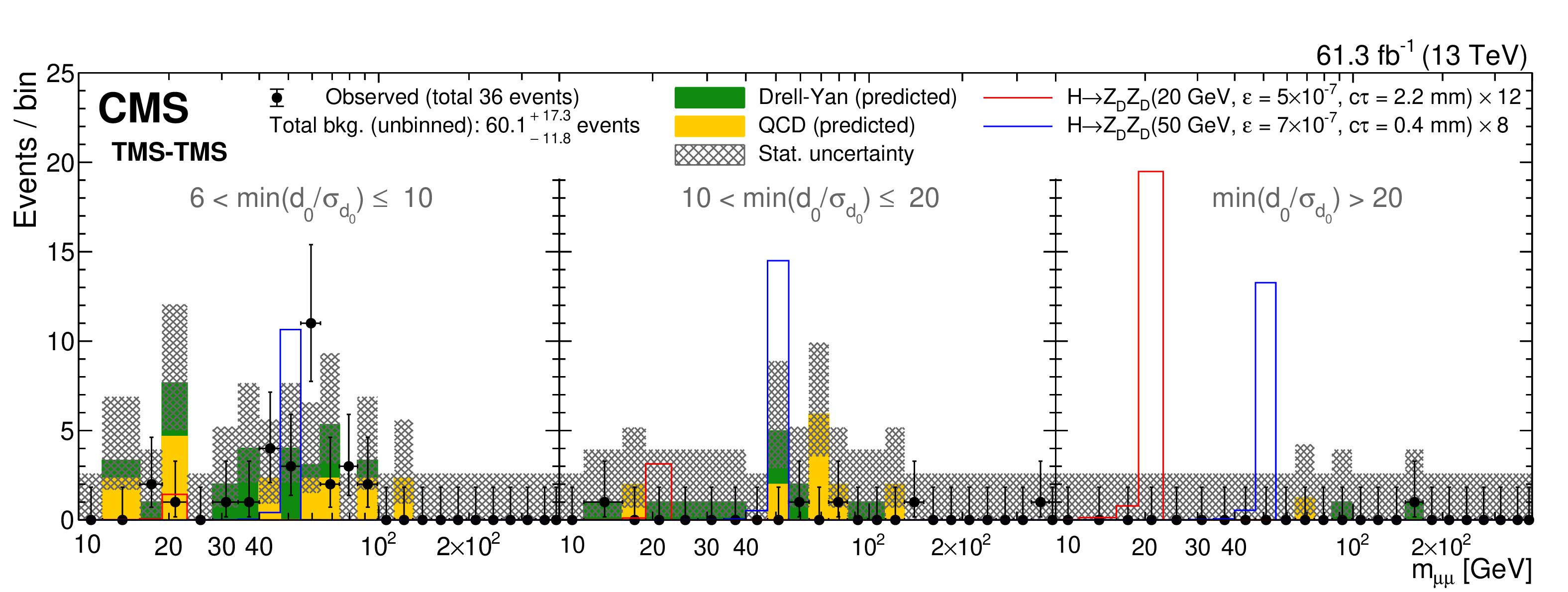
Figure 12:
Comparison of the number of events observed in (upper) 2016 and (lower) 2018 data in the TMS-TMS dimuon category with the expected number of background events, in representative ${m_{\mu \mu}}$ intervals in each of the three min($ {{d_{\mathrm {0}}} / {\sigma _{{d_{\mathrm {0}}}}}} $) bins. The black points with error bars show the number of observed events; the green and yellow components of the stacked histograms represent the estimated numbers of DY and QCD events, respectively. The last bin in each min($ {{d_{\mathrm {0}}} / {\sigma _{{d_{\mathrm {0}}}}}} $) interval includes events in the overflow. The uncertainties in the total expected background (shaded area) are statistical only. Signal contributions expected from simulated $\mathrm{H} \to \mathrm{Z} {\mathrm {_{D}}}\mathrm{Z} {\mathrm {_{D}}}$ with $ {m(\mathrm{Z} {\mathrm {_{D}}})} $ of 20 and 50 GeV are shown in red and blue, respectively. Their yields are set to the corresponding combined median expected exclusion limits at 95% CL, scaled up as indicated in the legend to improve visibility. The legends also include the total number of observed events as well as the number of expected background events obtained inclusively, by applying the background evaluation method to the events in all $ {m_{\mu \mu}} $ and min($ {{d_{\mathrm {0}}} / {\sigma _{{d_{\mathrm {0}}}}}} $) intervals combined. |

png pdf |
Figure 12-a:
Comparison of the number of events observed in (upper) 2016 and (lower) 2018 data in the TMS-TMS dimuon category with the expected number of background events, in representative ${m_{\mu \mu}}$ intervals in each of the three min($ {{d_{\mathrm {0}}} / {\sigma _{{d_{\mathrm {0}}}}}} $) bins. The black points with error bars show the number of observed events; the green and yellow components of the stacked histograms represent the estimated numbers of DY and QCD events, respectively. The last bin in each min($ {{d_{\mathrm {0}}} / {\sigma _{{d_{\mathrm {0}}}}}} $) interval includes events in the overflow. The uncertainties in the total expected background (shaded area) are statistical only. Signal contributions expected from simulated $\mathrm{H} \to \mathrm{Z} {\mathrm {_{D}}}\mathrm{Z} {\mathrm {_{D}}}$ with $ {m(\mathrm{Z} {\mathrm {_{D}}})} $ of 20 and 50 GeV are shown in red and blue, respectively. Their yields are set to the corresponding combined median expected exclusion limits at 95% CL, scaled up as indicated in the legend to improve visibility. The legends also include the total number of observed events as well as the number of expected background events obtained inclusively, by applying the background evaluation method to the events in all $ {m_{\mu \mu}} $ and min($ {{d_{\mathrm {0}}} / {\sigma _{{d_{\mathrm {0}}}}}} $) intervals combined. |
png pdf |
Figure 12-b:
Comparison of the number of events observed in (upper) 2016 and (lower) 2018 data in the TMS-TMS dimuon category with the expected number of background events, in representative ${m_{\mu \mu}}$ intervals in each of the three min($ {{d_{\mathrm {0}}} / {\sigma _{{d_{\mathrm {0}}}}}} $) bins. The black points with error bars show the number of observed events; the green and yellow components of the stacked histograms represent the estimated numbers of DY and QCD events, respectively. The last bin in each min($ {{d_{\mathrm {0}}} / {\sigma _{{d_{\mathrm {0}}}}}} $) interval includes events in the overflow. The uncertainties in the total expected background (shaded area) are statistical only. Signal contributions expected from simulated $\mathrm{H} \to \mathrm{Z} {\mathrm {_{D}}}\mathrm{Z} {\mathrm {_{D}}}$ with $ {m(\mathrm{Z} {\mathrm {_{D}}})} $ of 20 and 50 GeV are shown in red and blue, respectively. Their yields are set to the corresponding combined median expected exclusion limits at 95% CL, scaled up as indicated in the legend to improve visibility. The legends also include the total number of observed events as well as the number of expected background events obtained inclusively, by applying the background evaluation method to the events in all $ {m_{\mu \mu}} $ and min($ {{d_{\mathrm {0}}} / {\sigma _{{d_{\mathrm {0}}}}}} $) intervals combined. |

png pdf |
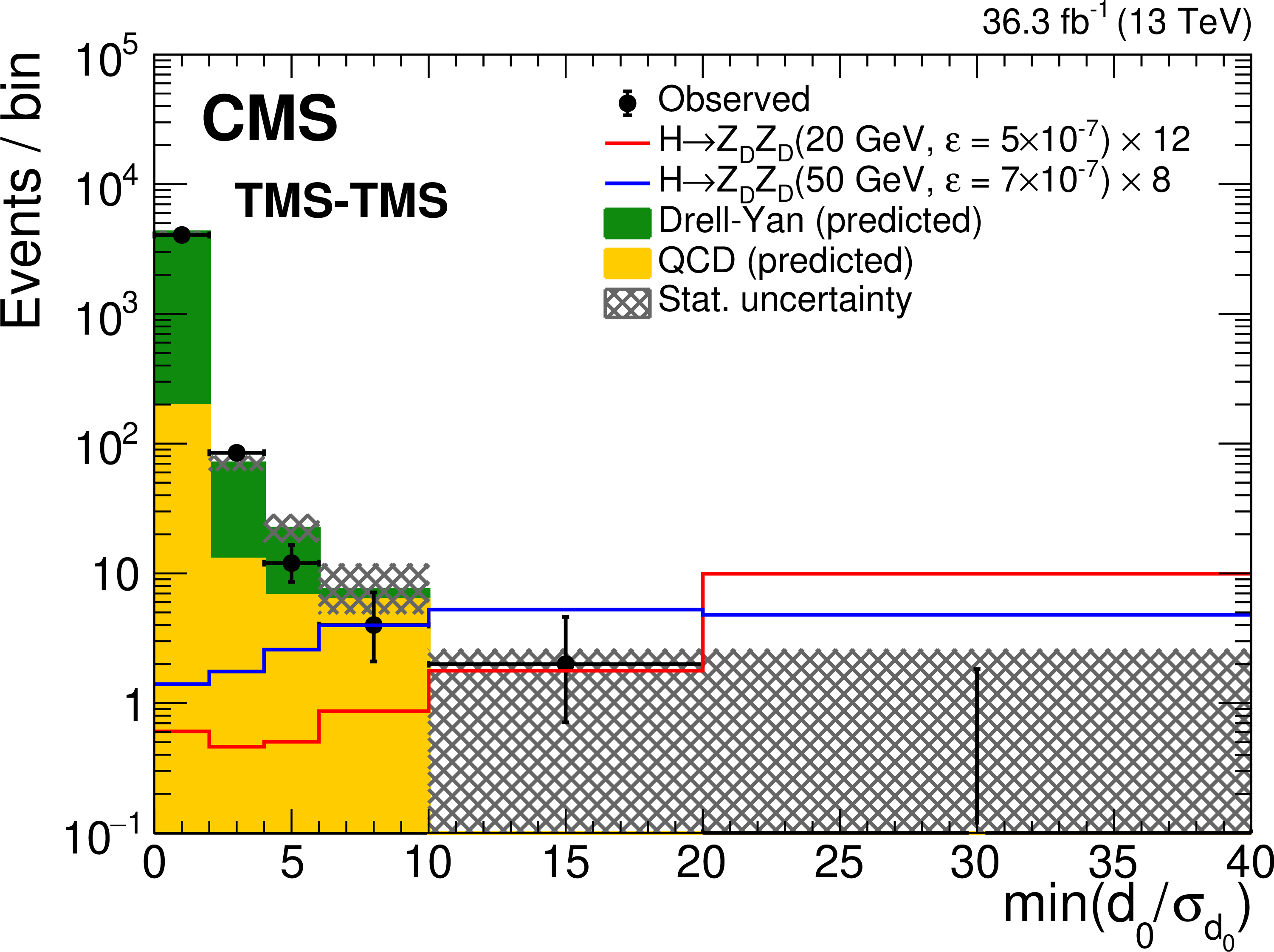
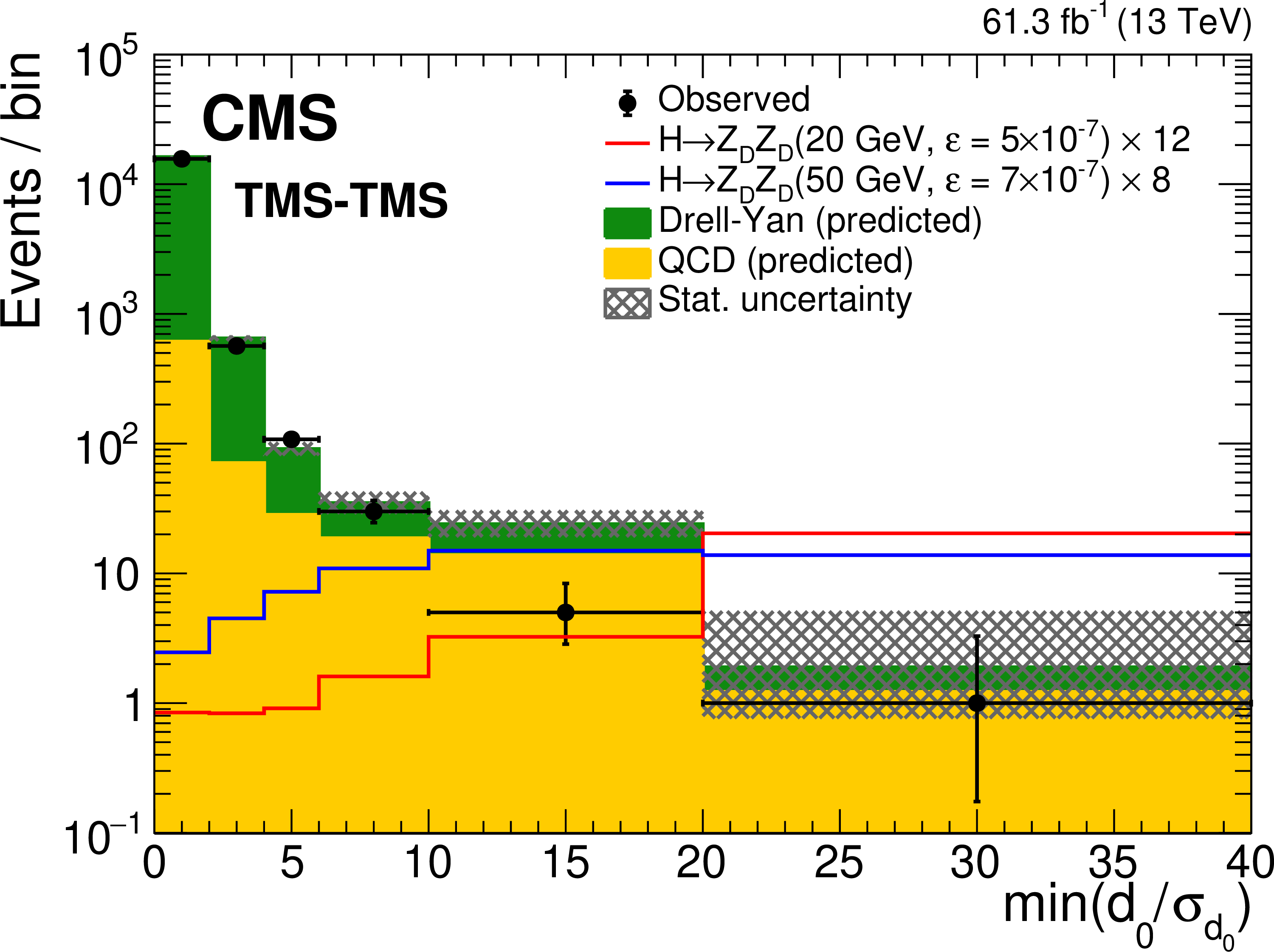
Figure 13:
Comparison of the number of events observed in (left) 2016 and (right) 2018 data in the TMS-TMS dimuon category with the expected number of background events, as a function of the smaller of the two $ {{d_{\mathrm {0}}} / {\sigma _{{d_{\mathrm {0}}}}}} $ values for the TMS-TMS dimuon. The black points with error bars show the number of observed events; the green and yellow components of the stacked histograms represent the estimated numbers of DY and QCD events, respectively. The last bin includes events in the overflow. The uncertainties in the total expected background (shaded area) are statistical only. Signal contributions expected from simulated $\mathrm{H} \to \mathrm{Z} {\mathrm {_{D}}}\mathrm{Z} {\mathrm {_{D}}}$ with $ {m(\mathrm{Z} {\mathrm {_{D}}})} $ of 20 and 50 GeV are shown in red and blue, respectively. Their yields are set to the corresponding combined median expected exclusion limits at 95% CL, scaled up as indicated in the legend to improve visibility. |
png pdf |
Figure 13-a:
Comparison of the number of events observed in (left) 2016 and (right) 2018 data in the TMS-TMS dimuon category with the expected number of background events, as a function of the smaller of the two $ {{d_{\mathrm {0}}} / {\sigma _{{d_{\mathrm {0}}}}}} $ values for the TMS-TMS dimuon. The black points with error bars show the number of observed events; the green and yellow components of the stacked histograms represent the estimated numbers of DY and QCD events, respectively. The last bin includes events in the overflow. The uncertainties in the total expected background (shaded area) are statistical only. Signal contributions expected from simulated $\mathrm{H} \to \mathrm{Z} {\mathrm {_{D}}}\mathrm{Z} {\mathrm {_{D}}}$ with $ {m(\mathrm{Z} {\mathrm {_{D}}})} $ of 20 and 50 GeV are shown in red and blue, respectively. Their yields are set to the corresponding combined median expected exclusion limits at 95% CL, scaled up as indicated in the legend to improve visibility. |
png pdf |
Figure 13-b:
Comparison of the number of events observed in (left) 2016 and (right) 2018 data in the TMS-TMS dimuon category with the expected number of background events, as a function of the smaller of the two $ {{d_{\mathrm {0}}} / {\sigma _{{d_{\mathrm {0}}}}}} $ values for the TMS-TMS dimuon. The black points with error bars show the number of observed events; the green and yellow components of the stacked histograms represent the estimated numbers of DY and QCD events, respectively. The last bin includes events in the overflow. The uncertainties in the total expected background (shaded area) are statistical only. Signal contributions expected from simulated $\mathrm{H} \to \mathrm{Z} {\mathrm {_{D}}}\mathrm{Z} {\mathrm {_{D}}}$ with $ {m(\mathrm{Z} {\mathrm {_{D}}})} $ of 20 and 50 GeV are shown in red and blue, respectively. Their yields are set to the corresponding combined median expected exclusion limits at 95% CL, scaled up as indicated in the legend to improve visibility. |
png pdf |
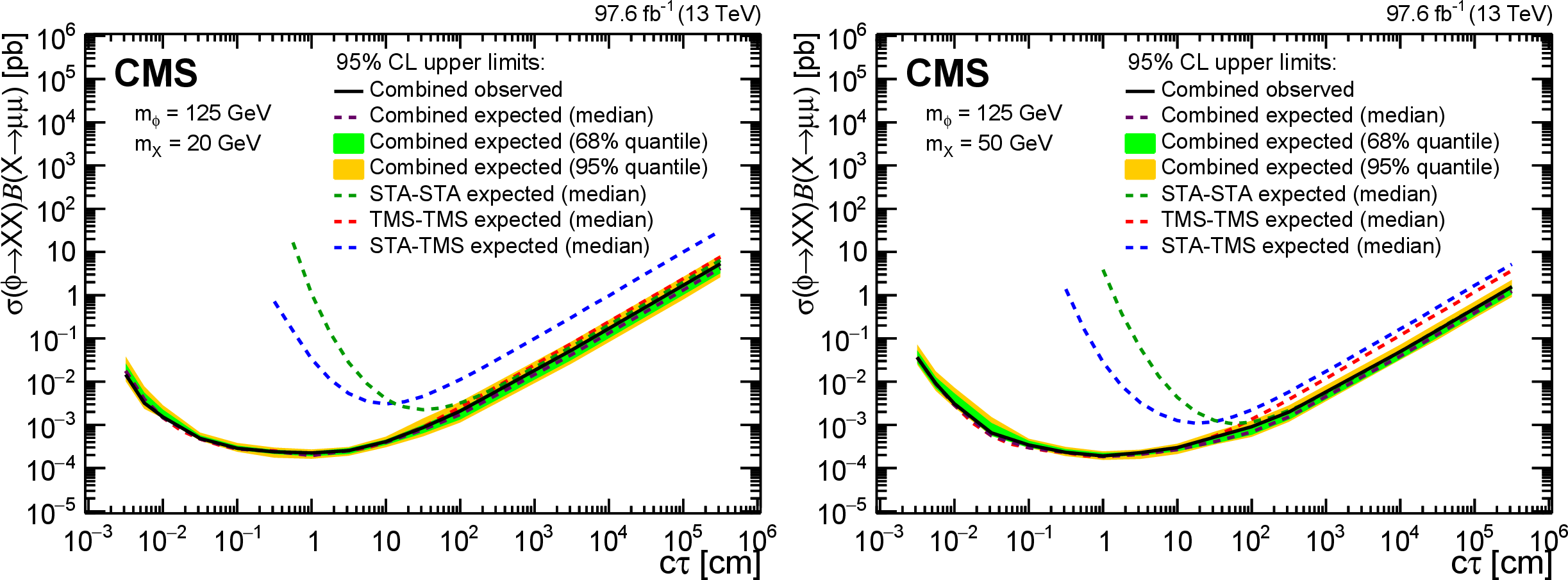
Figure 14:
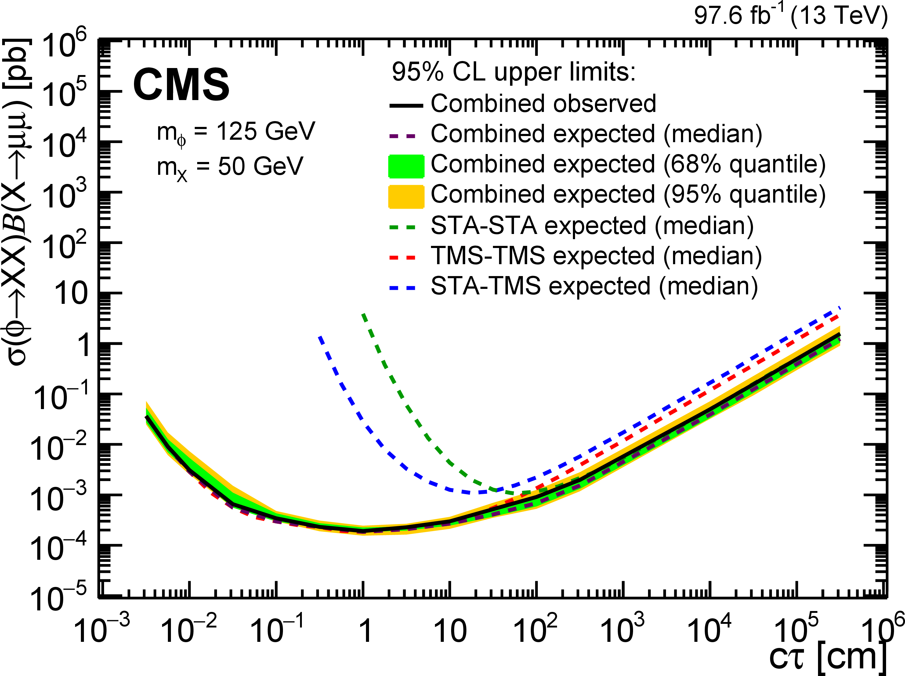
The 95% CL upper limits on $\sigma (\phi\to \mathrm{X} \mathrm{X})\mathcal {B}(\mathrm{X} \to \mu \mu)$ as a function of $ {c\tau} (\mathrm{X})$ in the heavy-scalar model, for $ {m(\phi)} = $ 125 GeV and (left) $ {m(\mathrm{X})} = $ 20 GeV and (right) $ {m(\mathrm{X})} = $ 50 GeV. The median expected limits obtained from the STA-STA, STA-TMS, and TMS-TMS dimuon categories are shown as dashed green, blue, and red curves, respectively; the combined median expected limits are shown as dashed black curves; and the combined observed limits are shown as solid black curves. The green and yellow bands correspond, respectively, to the 68 and 95% quantiles for the combined expected limits. |

png pdf |
Figure 14-a:
The 95% CL upper limits on $\sigma (\phi\to \mathrm{X} \mathrm{X})\mathcal {B}(\mathrm{X} \to \mu \mu)$ as a function of $ {c\tau} (\mathrm{X})$ in the heavy-scalar model, for $ {m(\phi)} = $ 125 GeV and (left) $ {m(\mathrm{X})} = $ 20 GeV and (right) $ {m(\mathrm{X})} = $ 50 GeV. The median expected limits obtained from the STA-STA, STA-TMS, and TMS-TMS dimuon categories are shown as dashed green, blue, and red curves, respectively; the combined median expected limits are shown as dashed black curves; and the combined observed limits are shown as solid black curves. The green and yellow bands correspond, respectively, to the 68 and 95% quantiles for the combined expected limits. |
png pdf |
Figure 14-b:
The 95% CL upper limits on $\sigma (\phi\to \mathrm{X} \mathrm{X})\mathcal {B}(\mathrm{X} \to \mu \mu)$ as a function of $ {c\tau} (\mathrm{X})$ in the heavy-scalar model, for $ {m(\phi)} = $ 125 GeV and (left) $ {m(\mathrm{X})} = $ 20 GeV and (right) $ {m(\mathrm{X})} = $ 50 GeV. The median expected limits obtained from the STA-STA, STA-TMS, and TMS-TMS dimuon categories are shown as dashed green, blue, and red curves, respectively; the combined median expected limits are shown as dashed black curves; and the combined observed limits are shown as solid black curves. The green and yellow bands correspond, respectively, to the 68 and 95% quantiles for the combined expected limits. |
png pdf |
Figure 15:
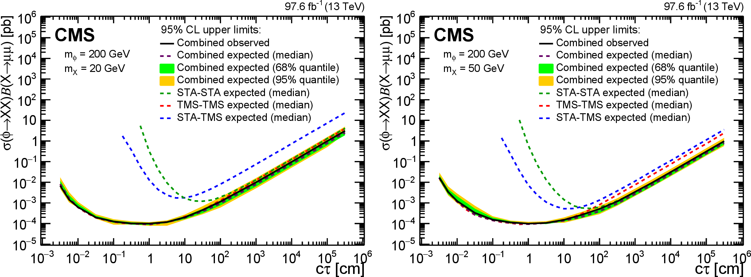
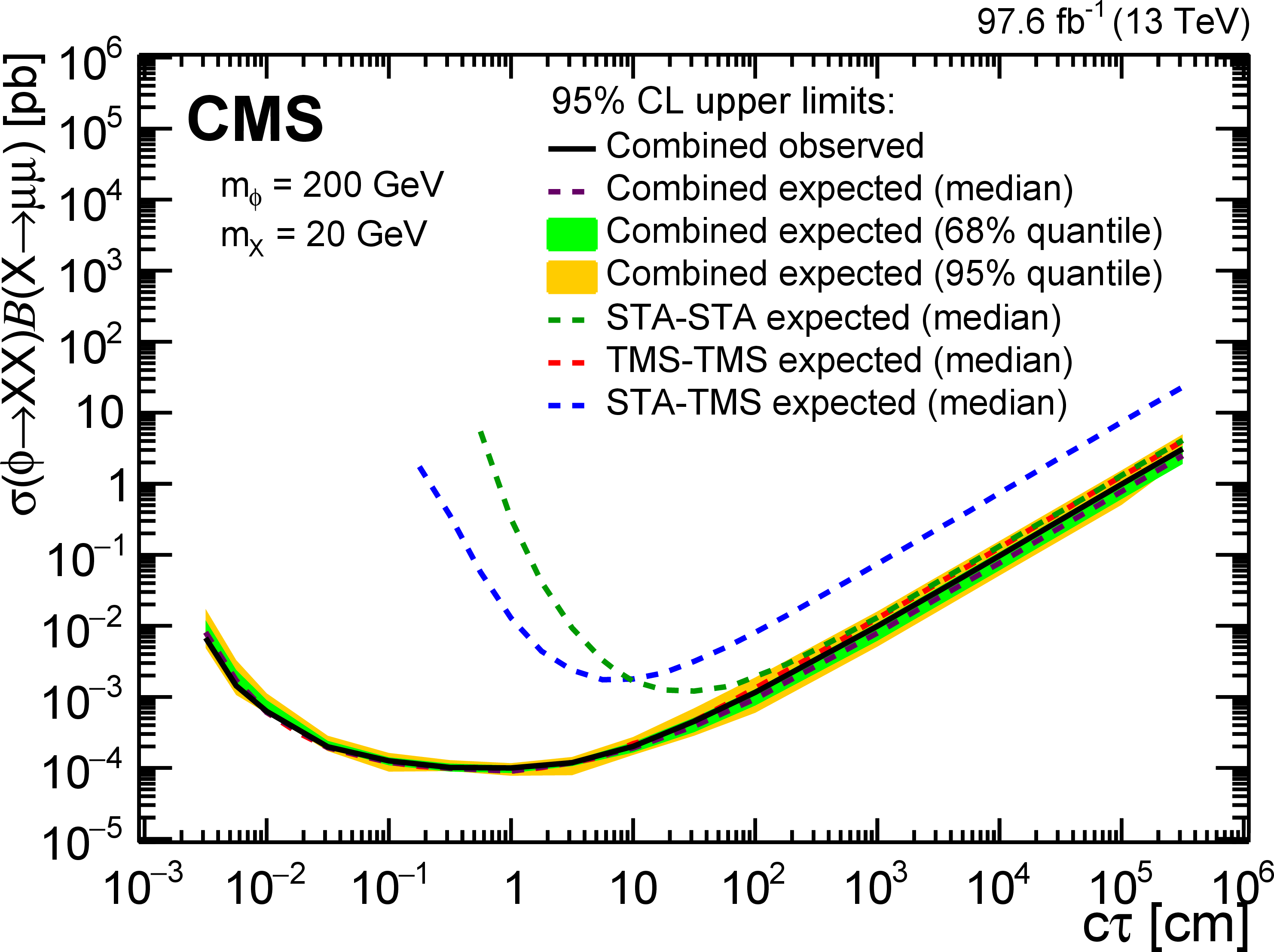
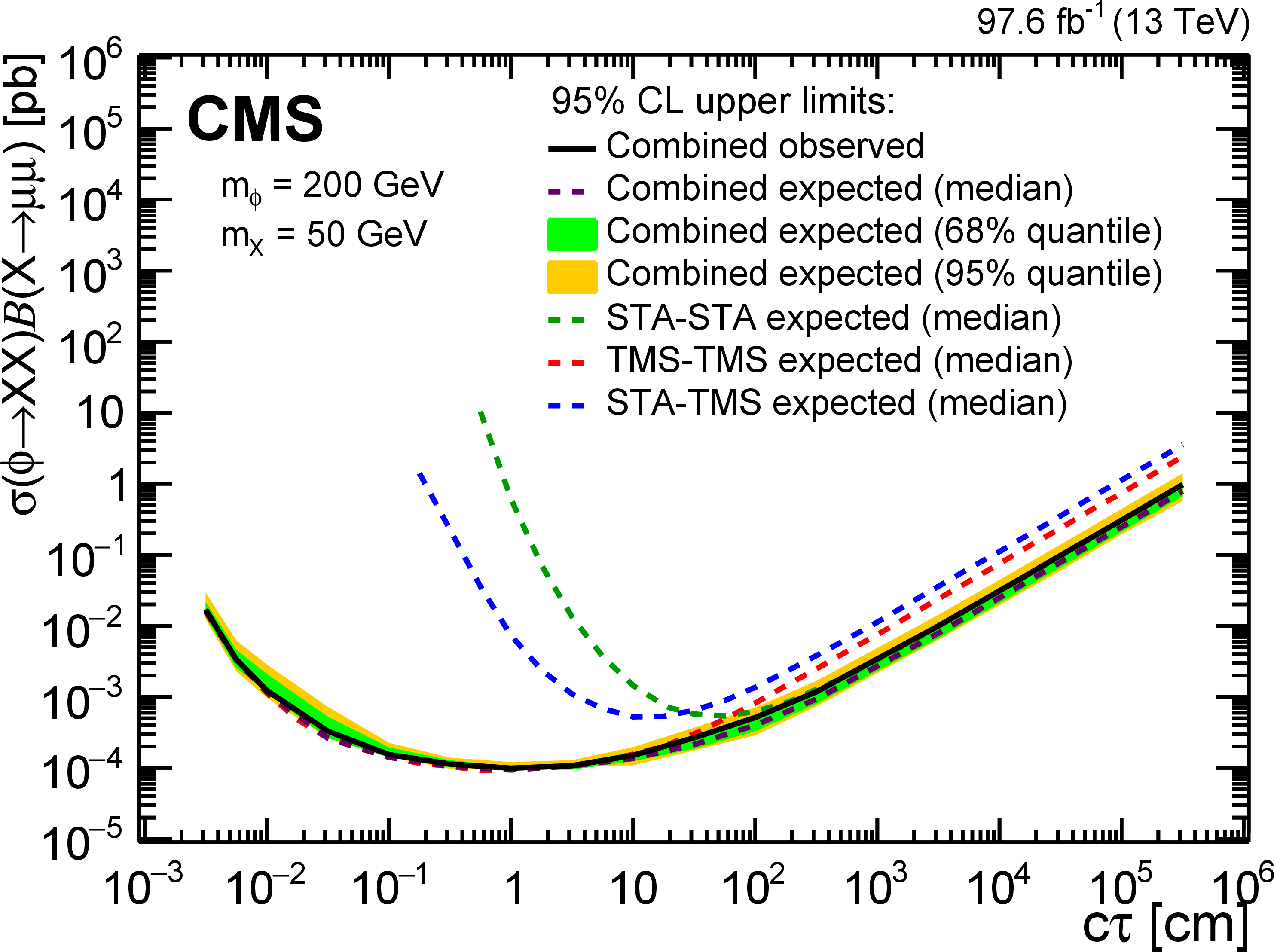
The 95% CL upper limits on $\sigma (\phi\to \mathrm{X} \mathrm{X})\mathcal {B}(\mathrm{X} \to \mu \mu)$ as a function of $ {c\tau} (\mathrm{X})$ in the heavy-scalar model, for $ {m(\phi)} = $ 200 GeV and (left) $ {m(\mathrm{X})} = $ 20 GeV and (right) $ {m(\mathrm{X})} = $ 50 GeV. The median expected limits obtained from the STA-STA, STA-TMS, and TMS-TMS dimuon categories are shown as dashed green, blue, and red curves, respectively; the combined median expected limits are shown as dashed black curves; and the combined observed limits are shown as solid black curves. The green and yellow bands correspond, respectively, to the 68 and 95% quantiles for the combined expected limits. |
png pdf |
Figure 15-a:
The 95% CL upper limits on $\sigma (\phi\to \mathrm{X} \mathrm{X})\mathcal {B}(\mathrm{X} \to \mu \mu)$ as a function of $ {c\tau} (\mathrm{X})$ in the heavy-scalar model, for $ {m(\phi)} = $ 200 GeV and (left) $ {m(\mathrm{X})} = $ 20 GeV and (right) $ {m(\mathrm{X})} = $ 50 GeV. The median expected limits obtained from the STA-STA, STA-TMS, and TMS-TMS dimuon categories are shown as dashed green, blue, and red curves, respectively; the combined median expected limits are shown as dashed black curves; and the combined observed limits are shown as solid black curves. The green and yellow bands correspond, respectively, to the 68 and 95% quantiles for the combined expected limits. |
png pdf |
Figure 15-b:
The 95% CL upper limits on $\sigma (\phi\to \mathrm{X} \mathrm{X})\mathcal {B}(\mathrm{X} \to \mu \mu)$ as a function of $ {c\tau} (\mathrm{X})$ in the heavy-scalar model, for $ {m(\phi)} = $ 200 GeV and (left) $ {m(\mathrm{X})} = $ 20 GeV and (right) $ {m(\mathrm{X})} = $ 50 GeV. The median expected limits obtained from the STA-STA, STA-TMS, and TMS-TMS dimuon categories are shown as dashed green, blue, and red curves, respectively; the combined median expected limits are shown as dashed black curves; and the combined observed limits are shown as solid black curves. The green and yellow bands correspond, respectively, to the 68 and 95% quantiles for the combined expected limits. |

png pdf |
Figure 16:
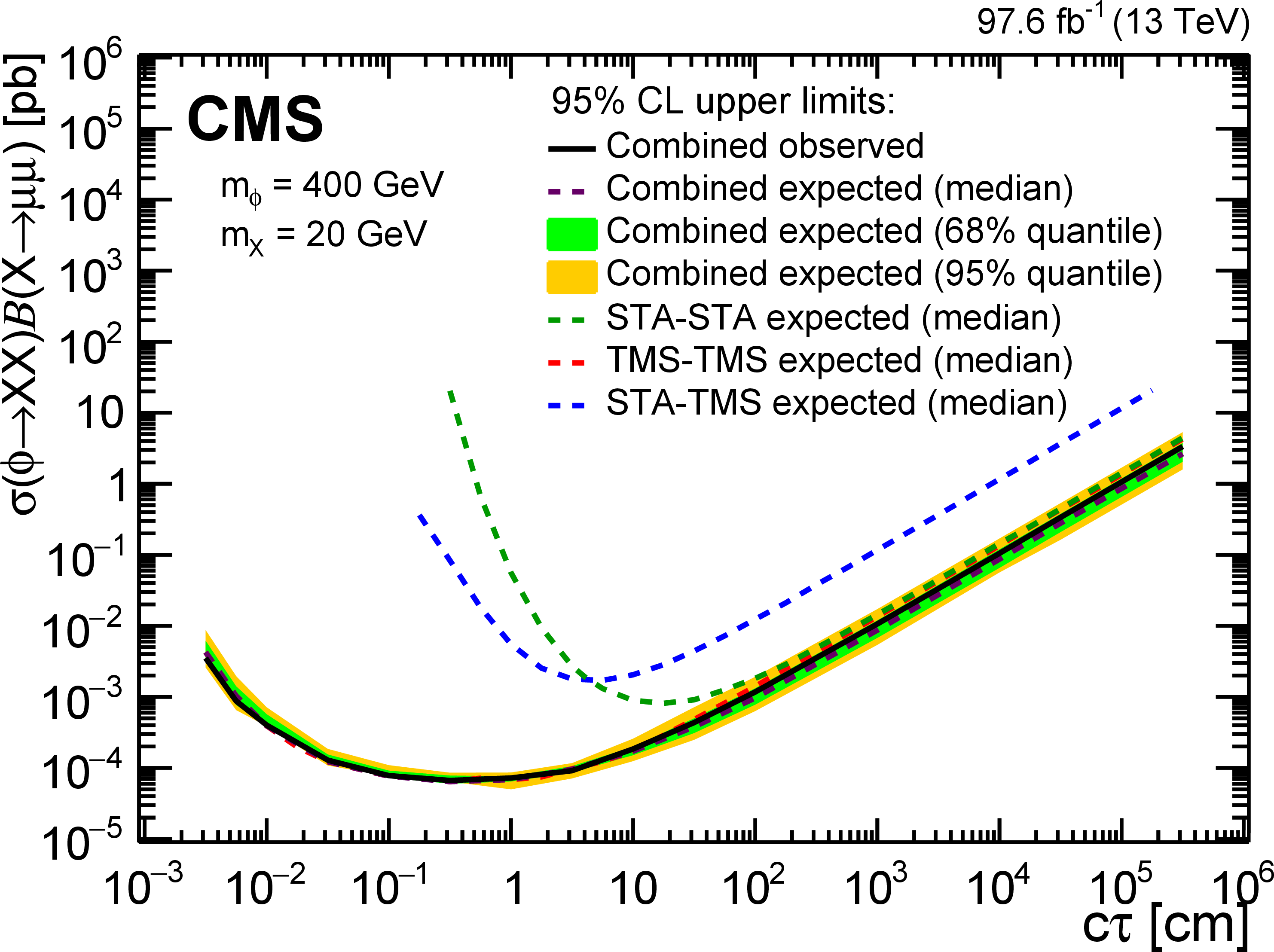
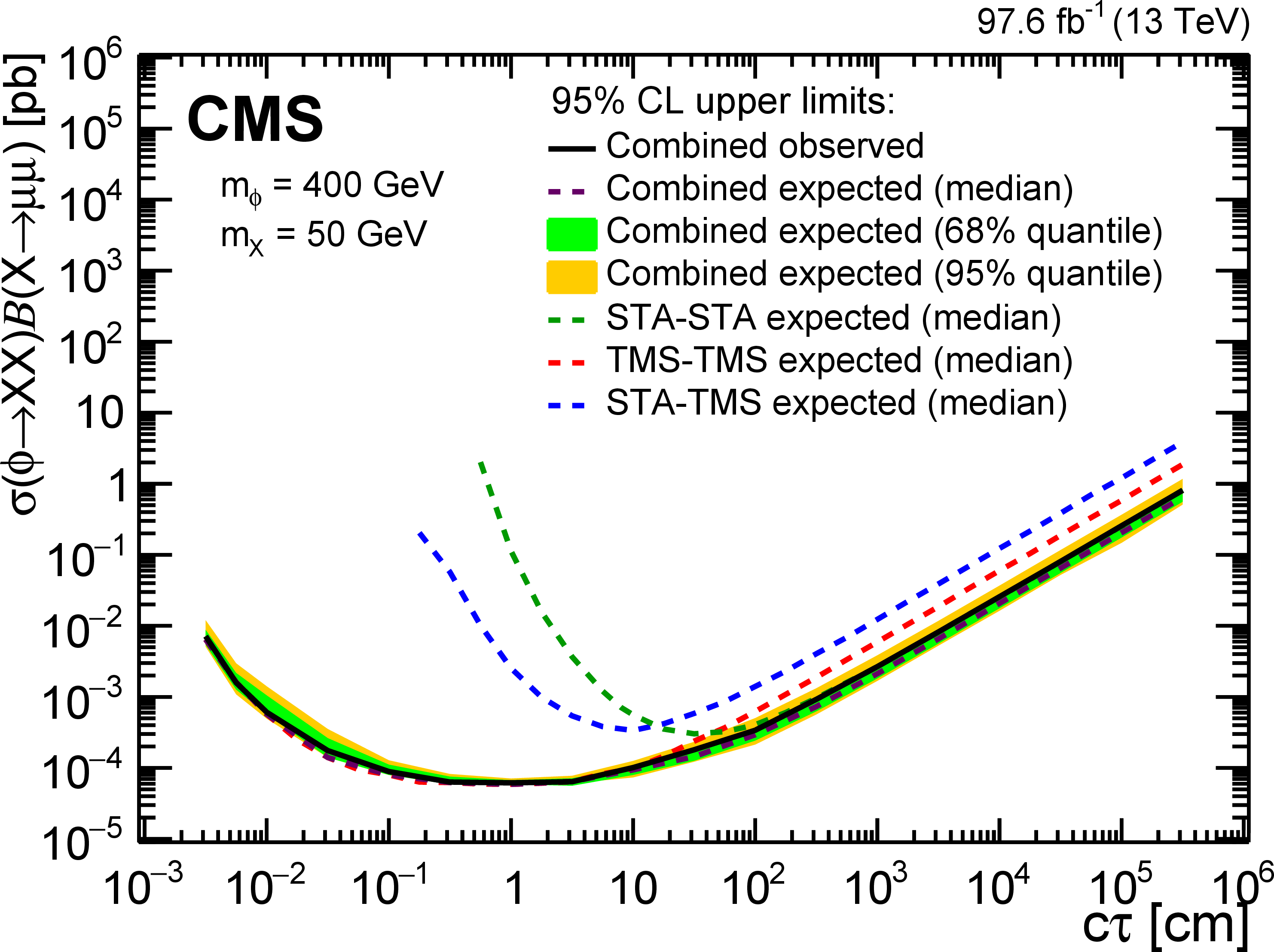
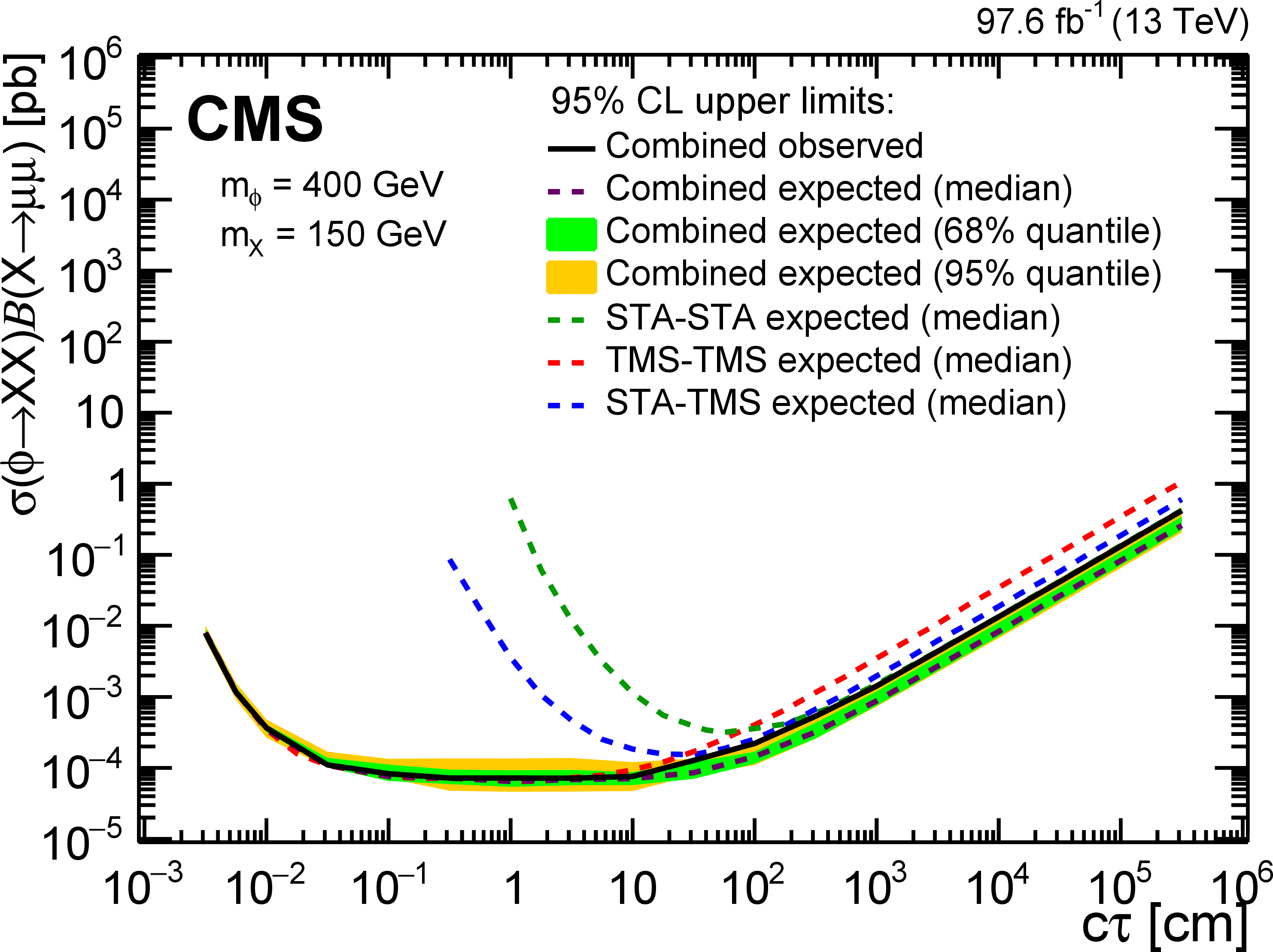
The 95% CL upper limits on $\sigma (\phi\to \mathrm{X} \mathrm{X})\mathcal {B}(\mathrm{X} \to \mu \mu)$ as a function of $ {c\tau} (\mathrm{X})$ in the heavy-scalar model, for $ {m(\phi)} = $ 400 GeV and (upper left) $ {m(\mathrm{X})} = $ 20 GeV, (upper right) $ {m(\mathrm{X})} = $ 50 GeV, and (lower) $ {m(\mathrm{X})} = $ 150 GeV. The median expected limits obtained from the STA-STA, STA-TMS, and TMS-TMS dimuon categories are shown as dashed green, blue, and red curves, respectively; the combined median expected limits are shown as dashed black curves; and the combined observed limits are shown as solid black curves. The green and yellow bands correspond, respectively, to the 68 and 95% quantiles for the combined expected limits. |
png pdf |
Figure 16-a:
The 95% CL upper limits on $\sigma (\phi\to \mathrm{X} \mathrm{X})\mathcal {B}(\mathrm{X} \to \mu \mu)$ as a function of $ {c\tau} (\mathrm{X})$ in the heavy-scalar model, for $ {m(\phi)} = $ 400 GeV and (upper left) $ {m(\mathrm{X})} = $ 20 GeV, (upper right) $ {m(\mathrm{X})} = $ 50 GeV, and (lower) $ {m(\mathrm{X})} = $ 150 GeV. The median expected limits obtained from the STA-STA, STA-TMS, and TMS-TMS dimuon categories are shown as dashed green, blue, and red curves, respectively; the combined median expected limits are shown as dashed black curves; and the combined observed limits are shown as solid black curves. The green and yellow bands correspond, respectively, to the 68 and 95% quantiles for the combined expected limits. |
png pdf |
Figure 16-b:
The 95% CL upper limits on $\sigma (\phi\to \mathrm{X} \mathrm{X})\mathcal {B}(\mathrm{X} \to \mu \mu)$ as a function of $ {c\tau} (\mathrm{X})$ in the heavy-scalar model, for $ {m(\phi)} = $ 400 GeV and (upper left) $ {m(\mathrm{X})} = $ 20 GeV, (upper right) $ {m(\mathrm{X})} = $ 50 GeV, and (lower) $ {m(\mathrm{X})} = $ 150 GeV. The median expected limits obtained from the STA-STA, STA-TMS, and TMS-TMS dimuon categories are shown as dashed green, blue, and red curves, respectively; the combined median expected limits are shown as dashed black curves; and the combined observed limits are shown as solid black curves. The green and yellow bands correspond, respectively, to the 68 and 95% quantiles for the combined expected limits. |
png pdf |
Figure 16-c:
The 95% CL upper limits on $\sigma (\phi\to \mathrm{X} \mathrm{X})\mathcal {B}(\mathrm{X} \to \mu \mu)$ as a function of $ {c\tau} (\mathrm{X})$ in the heavy-scalar model, for $ {m(\phi)} = $ 400 GeV and (upper left) $ {m(\mathrm{X})} = $ 20 GeV, (upper right) $ {m(\mathrm{X})} = $ 50 GeV, and (lower) $ {m(\mathrm{X})} = $ 150 GeV. The median expected limits obtained from the STA-STA, STA-TMS, and TMS-TMS dimuon categories are shown as dashed green, blue, and red curves, respectively; the combined median expected limits are shown as dashed black curves; and the combined observed limits are shown as solid black curves. The green and yellow bands correspond, respectively, to the 68 and 95% quantiles for the combined expected limits. |
png pdf |
Figure 17:
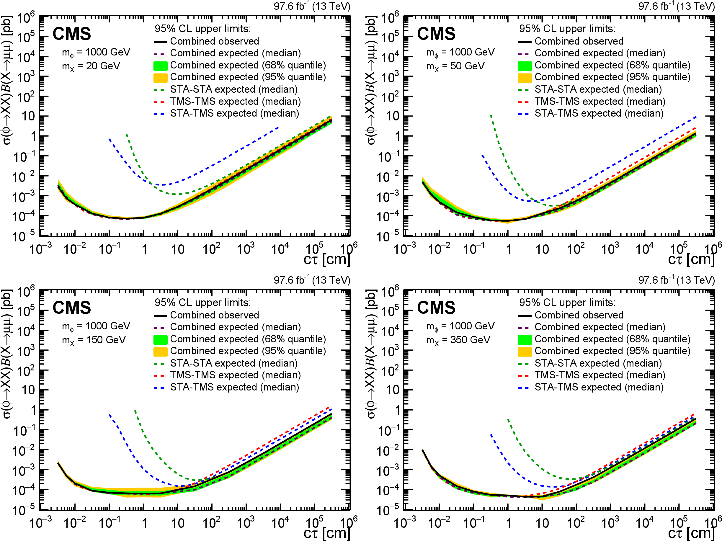
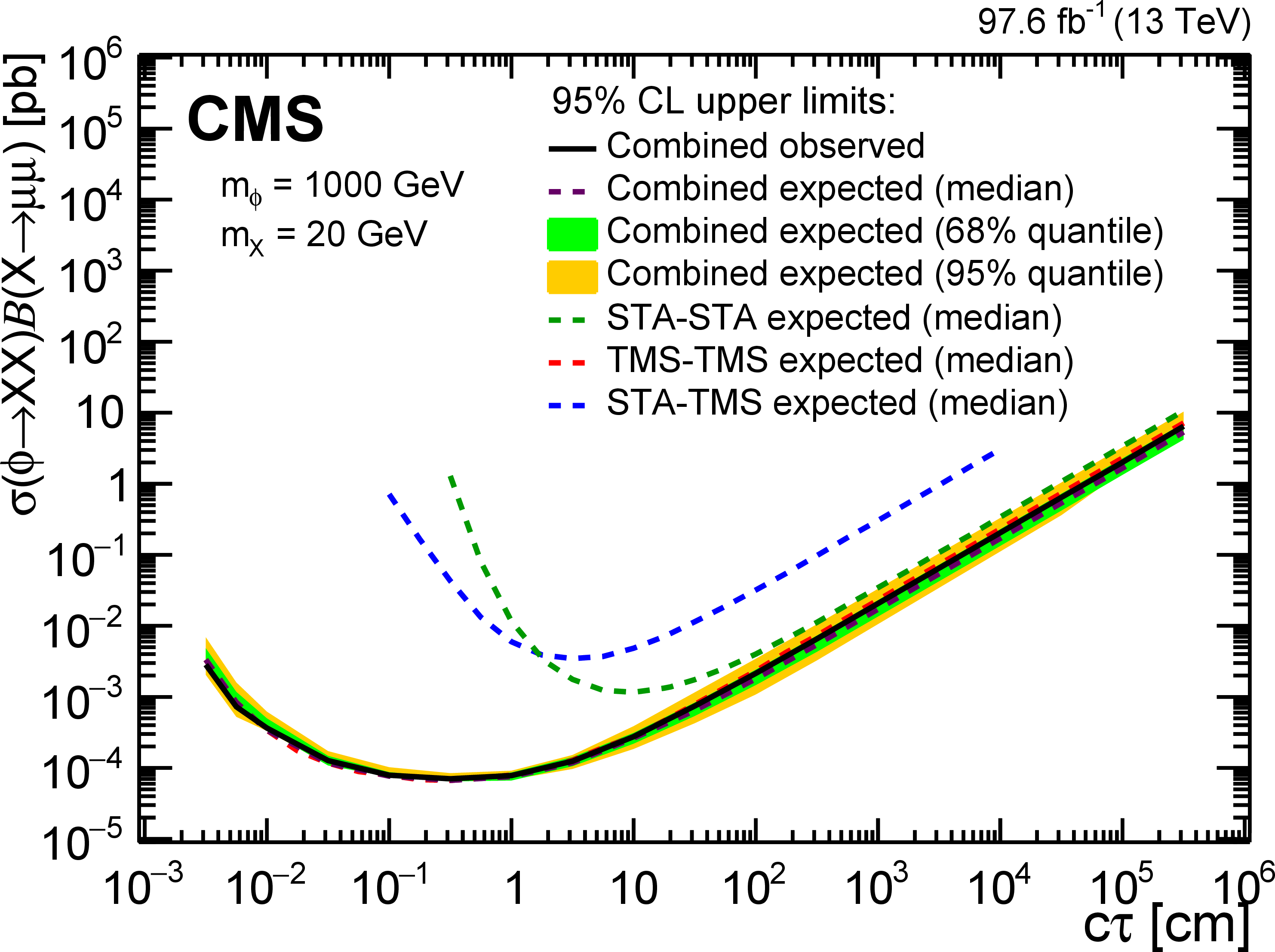
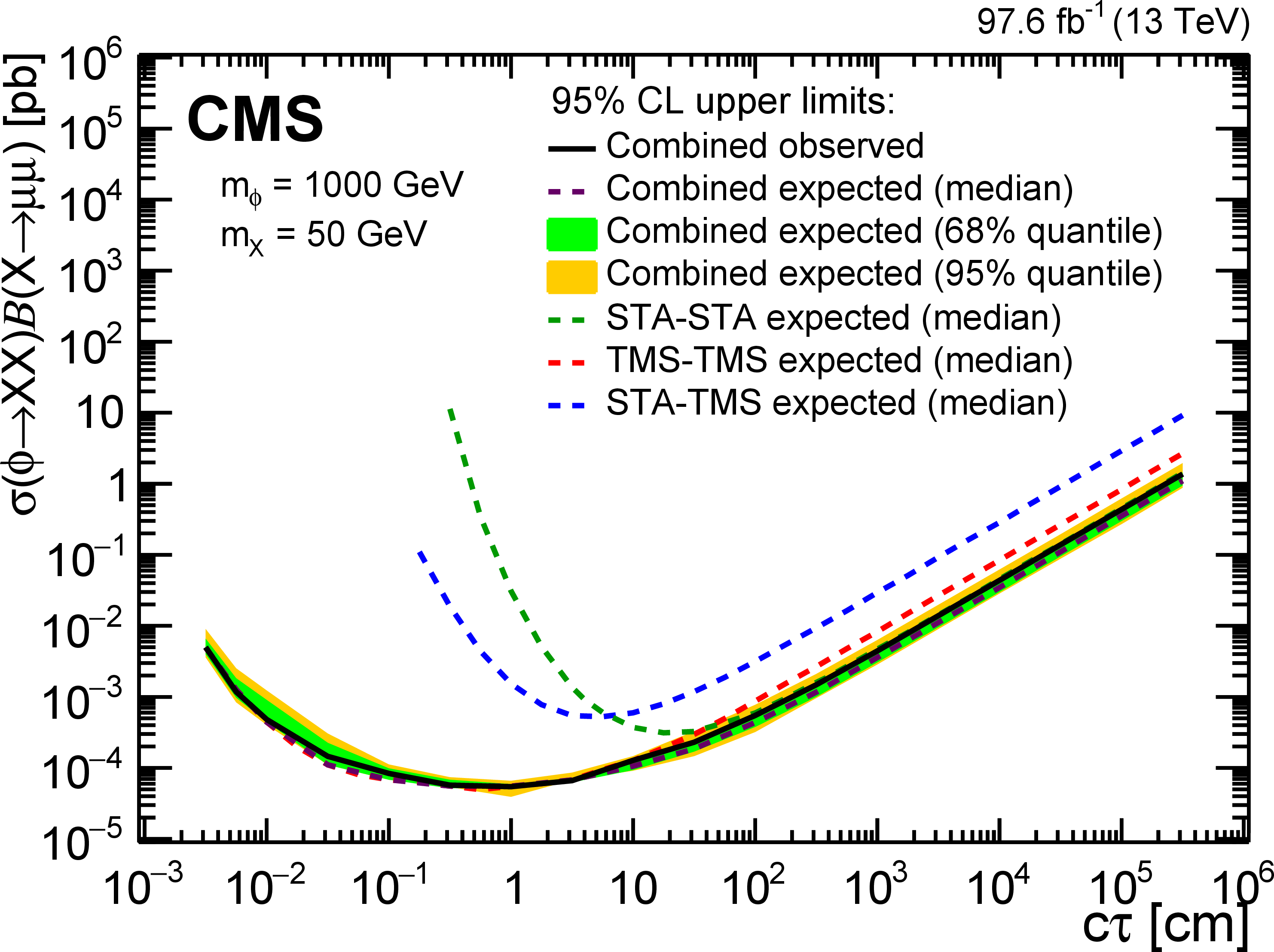
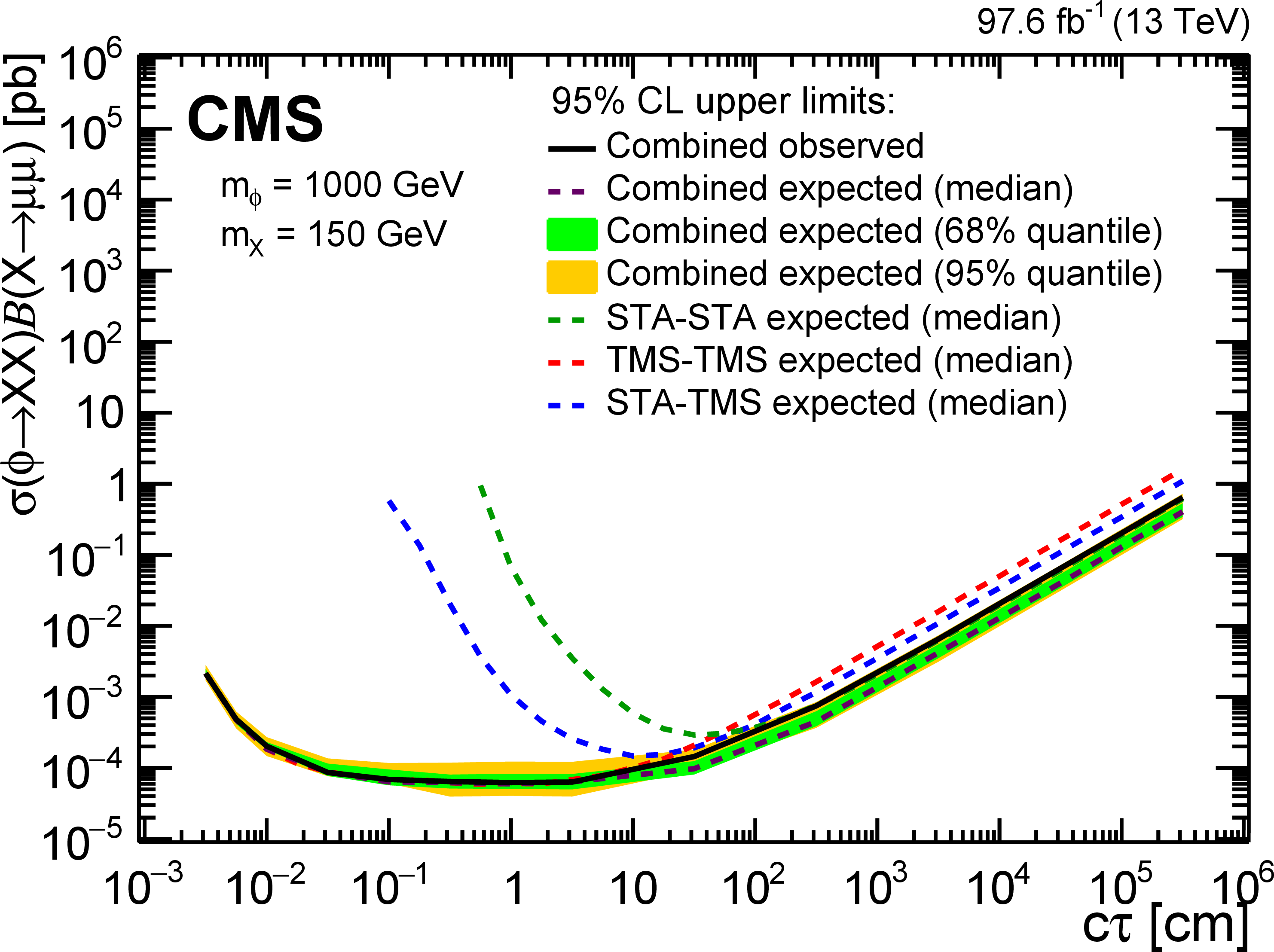
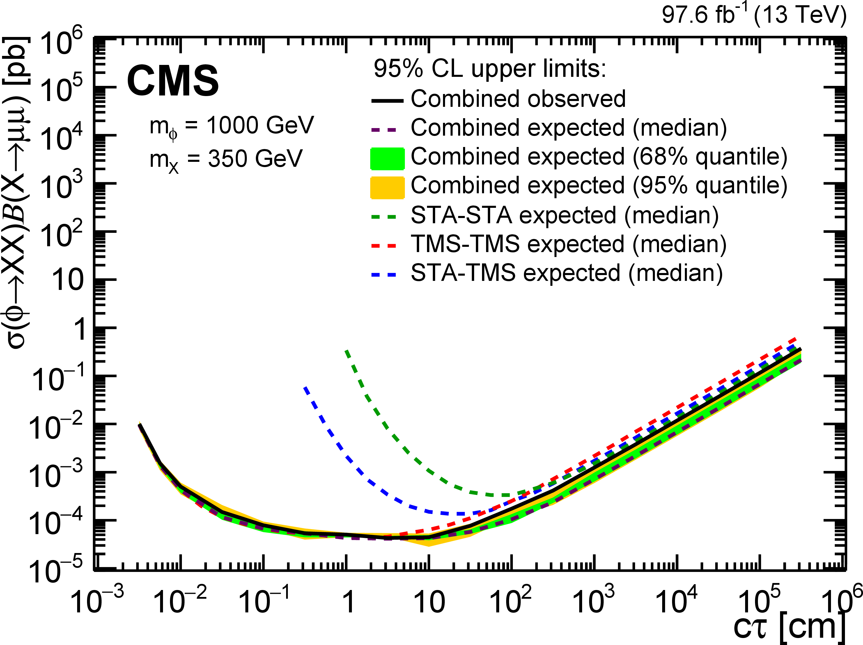
The 95% CL upper limits on $\sigma (\phi\to \mathrm{X} \mathrm{X})\mathcal {B}(\mathrm{X} \to \mu \mu)$ as a function of $ {c\tau} (\mathrm{X})$ in the heavy-scalar model, for $ {m(\phi)} = $ 1 TeV and (upper left) $ {m(\mathrm{X})} = $ 20 GeV, (upper right) $ {m(\mathrm{X})} = $ 50 GeV, (lower left) $ {m(\mathrm{X})} = $ 150 GeV, and (lower right) $ {m(\mathrm{X})} = $ 350 GeV. The median expected limits obtained from the STA-STA, STA-TMS, and TMS-TMS dimuon categories are shown as dashed green, blue, and red curves, respectively; the combined median expected limits are shown as dashed black curves; and the combined observed limits are shown as solid black curves. The green and yellow bands correspond, respectively, to the 68 and 95% quantiles for the combined expected limits. |
png pdf |
Figure 17-a:
The 95% CL upper limits on $\sigma (\phi\to \mathrm{X} \mathrm{X})\mathcal {B}(\mathrm{X} \to \mu \mu)$ as a function of $ {c\tau} (\mathrm{X})$ in the heavy-scalar model, for $ {m(\phi)} = $ 1 TeV and (upper left) $ {m(\mathrm{X})} = $ 20 GeV, (upper right) $ {m(\mathrm{X})} = $ 50 GeV, (lower left) $ {m(\mathrm{X})} = $ 150 GeV, and (lower right) $ {m(\mathrm{X})} = $ 350 GeV. The median expected limits obtained from the STA-STA, STA-TMS, and TMS-TMS dimuon categories are shown as dashed green, blue, and red curves, respectively; the combined median expected limits are shown as dashed black curves; and the combined observed limits are shown as solid black curves. The green and yellow bands correspond, respectively, to the 68 and 95% quantiles for the combined expected limits. |
png pdf |
Figure 17-b:
The 95% CL upper limits on $\sigma (\phi\to \mathrm{X} \mathrm{X})\mathcal {B}(\mathrm{X} \to \mu \mu)$ as a function of $ {c\tau} (\mathrm{X})$ in the heavy-scalar model, for $ {m(\phi)} = $ 1 TeV and (upper left) $ {m(\mathrm{X})} = $ 20 GeV, (upper right) $ {m(\mathrm{X})} = $ 50 GeV, (lower left) $ {m(\mathrm{X})} = $ 150 GeV, and (lower right) $ {m(\mathrm{X})} = $ 350 GeV. The median expected limits obtained from the STA-STA, STA-TMS, and TMS-TMS dimuon categories are shown as dashed green, blue, and red curves, respectively; the combined median expected limits are shown as dashed black curves; and the combined observed limits are shown as solid black curves. The green and yellow bands correspond, respectively, to the 68 and 95% quantiles for the combined expected limits. |
png pdf |
Figure 17-c:
The 95% CL upper limits on $\sigma (\phi\to \mathrm{X} \mathrm{X})\mathcal {B}(\mathrm{X} \to \mu \mu)$ as a function of $ {c\tau} (\mathrm{X})$ in the heavy-scalar model, for $ {m(\phi)} = $ 1 TeV and (upper left) $ {m(\mathrm{X})} = $ 20 GeV, (upper right) $ {m(\mathrm{X})} = $ 50 GeV, (lower left) $ {m(\mathrm{X})} = $ 150 GeV, and (lower right) $ {m(\mathrm{X})} = $ 350 GeV. The median expected limits obtained from the STA-STA, STA-TMS, and TMS-TMS dimuon categories are shown as dashed green, blue, and red curves, respectively; the combined median expected limits are shown as dashed black curves; and the combined observed limits are shown as solid black curves. The green and yellow bands correspond, respectively, to the 68 and 95% quantiles for the combined expected limits. |
png pdf |
Figure 17-d:
The 95% CL upper limits on $\sigma (\phi\to \mathrm{X} \mathrm{X})\mathcal {B}(\mathrm{X} \to \mu \mu)$ as a function of $ {c\tau} (\mathrm{X})$ in the heavy-scalar model, for $ {m(\phi)} = $ 1 TeV and (upper left) $ {m(\mathrm{X})} = $ 20 GeV, (upper right) $ {m(\mathrm{X})} = $ 50 GeV, (lower left) $ {m(\mathrm{X})} = $ 150 GeV, and (lower right) $ {m(\mathrm{X})} = $ 350 GeV. The median expected limits obtained from the STA-STA, STA-TMS, and TMS-TMS dimuon categories are shown as dashed green, blue, and red curves, respectively; the combined median expected limits are shown as dashed black curves; and the combined observed limits are shown as solid black curves. The green and yellow bands correspond, respectively, to the 68 and 95% quantiles for the combined expected limits. |
png pdf |
Figure 18:
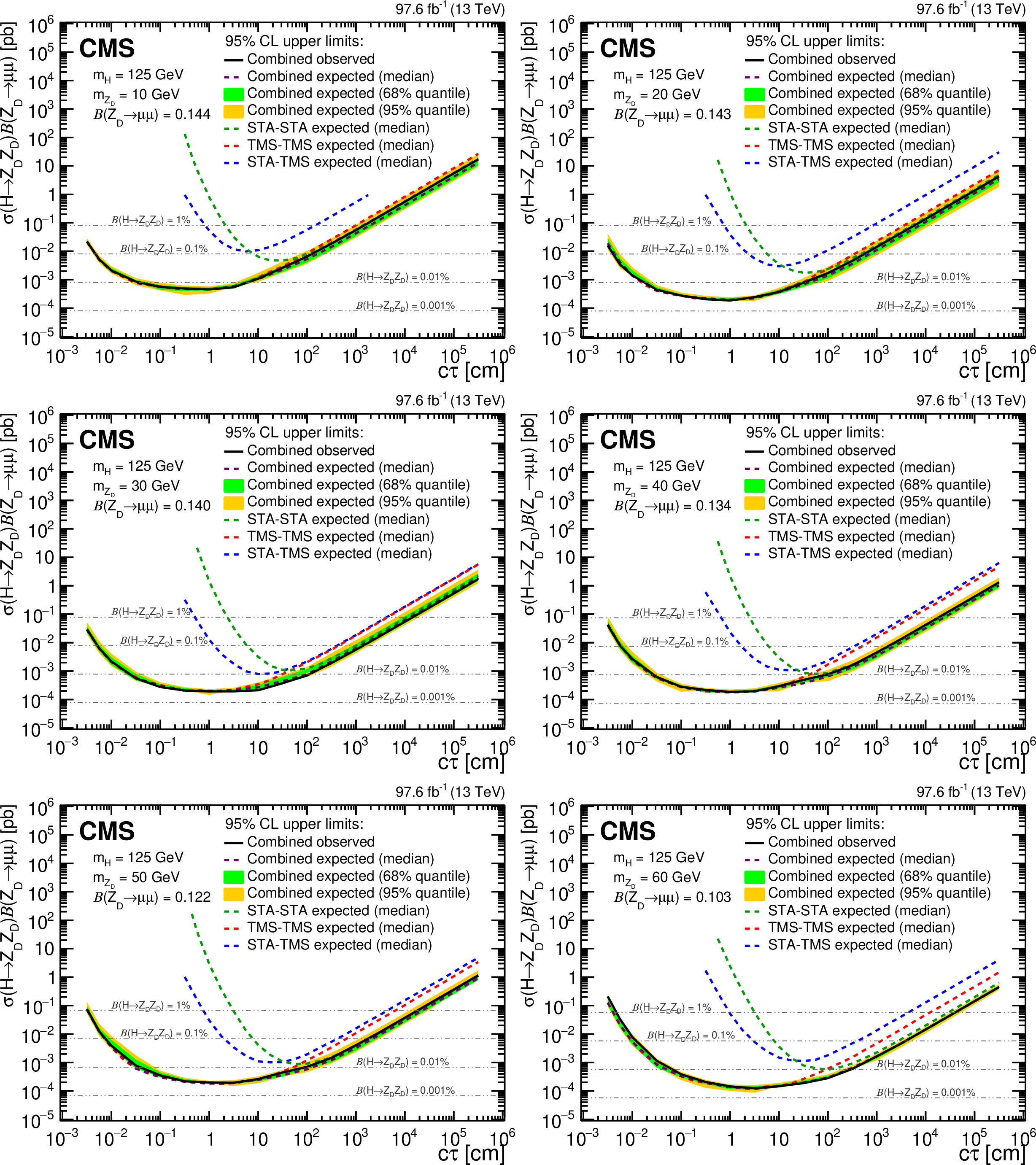
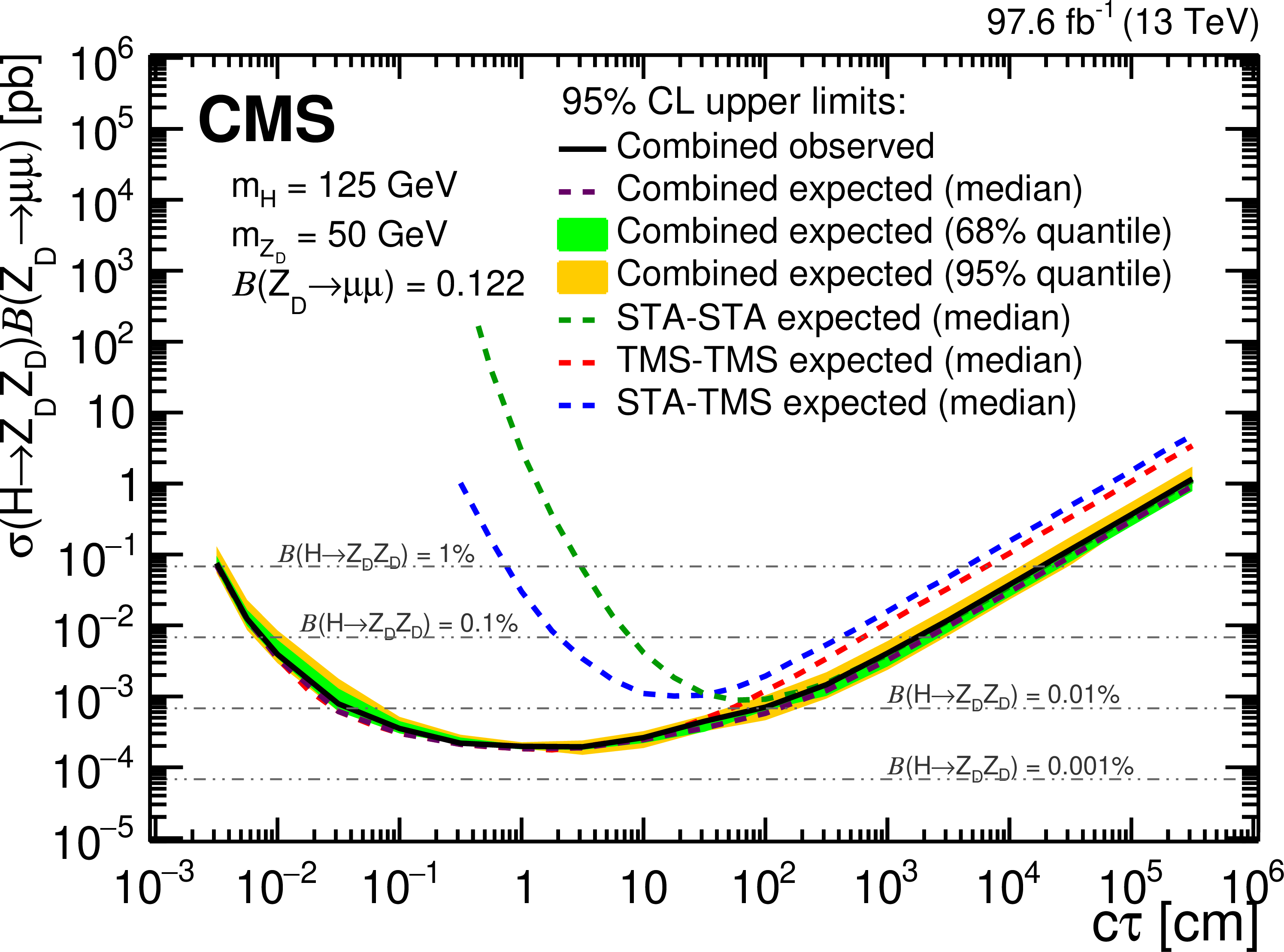
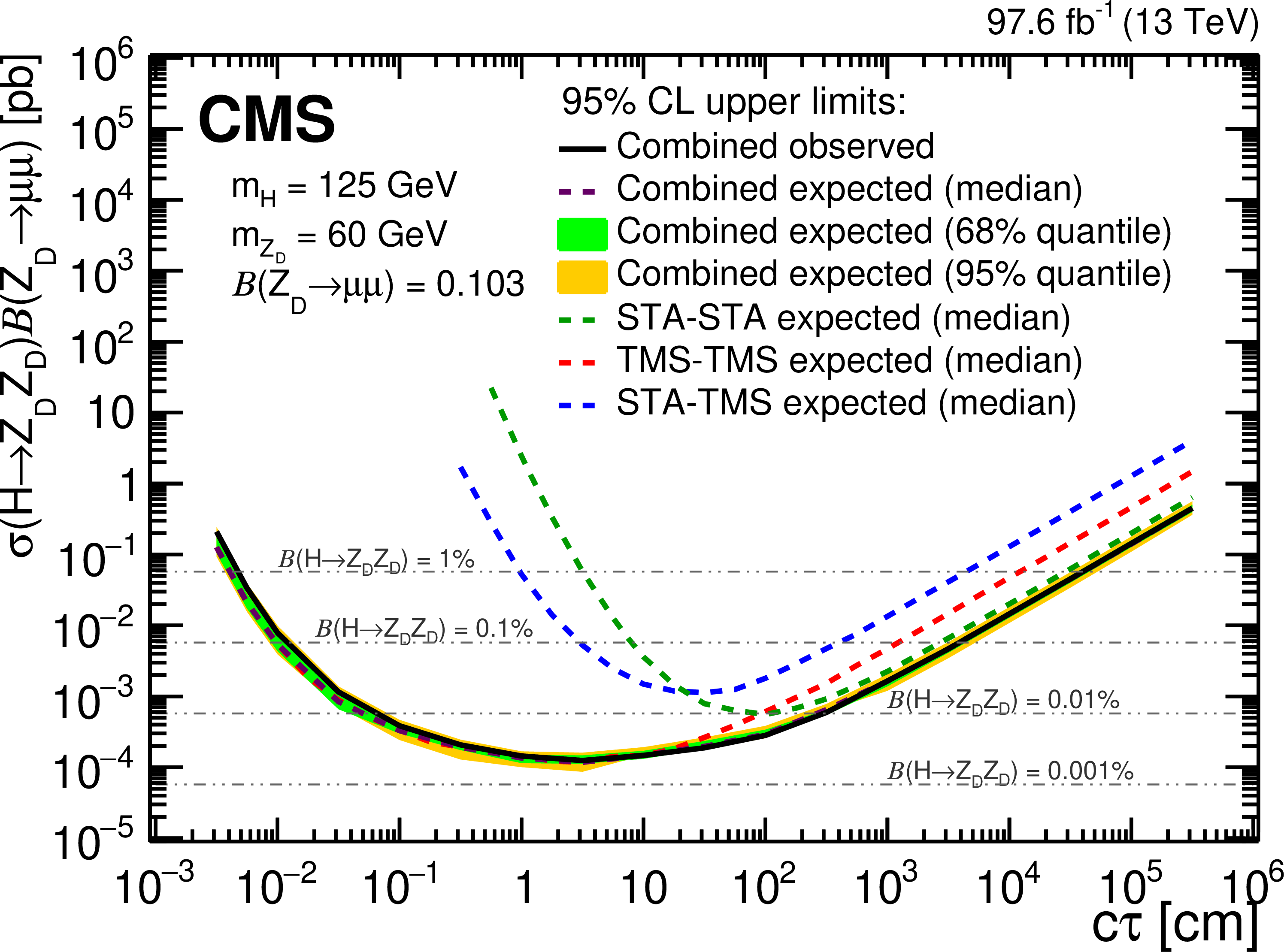
The 95% CL upper limits on $\sigma (\mathrm{H} \to \mathrm{Z} {\mathrm {_{D}}}\mathrm{Z} {\mathrm {_{D}}})\mathcal {B}(\mathrm{Z} {\mathrm {_{D}}}\to \mu \mu)$ as a function of $ {c\tau} (\mathrm{Z} {\mathrm {_{D}}})$ in the HAHM model, for $ {m(\mathrm{Z} {\mathrm {_{D}}})} $ ranging from 10 GeV (upper left) to 60 GeV (lower right). The median expected limits obtained from the STA-STA, STA-TMS, and TMS-TMS dimuon categories are shown as dashed green, blue, and red curves, respectively; the combined median expected limits are shown as dashed black curves; and the combined observed limits are shown as solid black curves. The green and yellow bands correspond, respectively, to the 68 and 95% quantiles for the combined expected limits. The horizontal lines in gray correspond to the theoretical predictions for values of $\mathcal {B}(\mathrm{H} \to \mathrm{Z} {\mathrm {_{D}}}\mathrm{Z} {\mathrm {_{D}}})$ indicated next to the lines. |
png pdf |
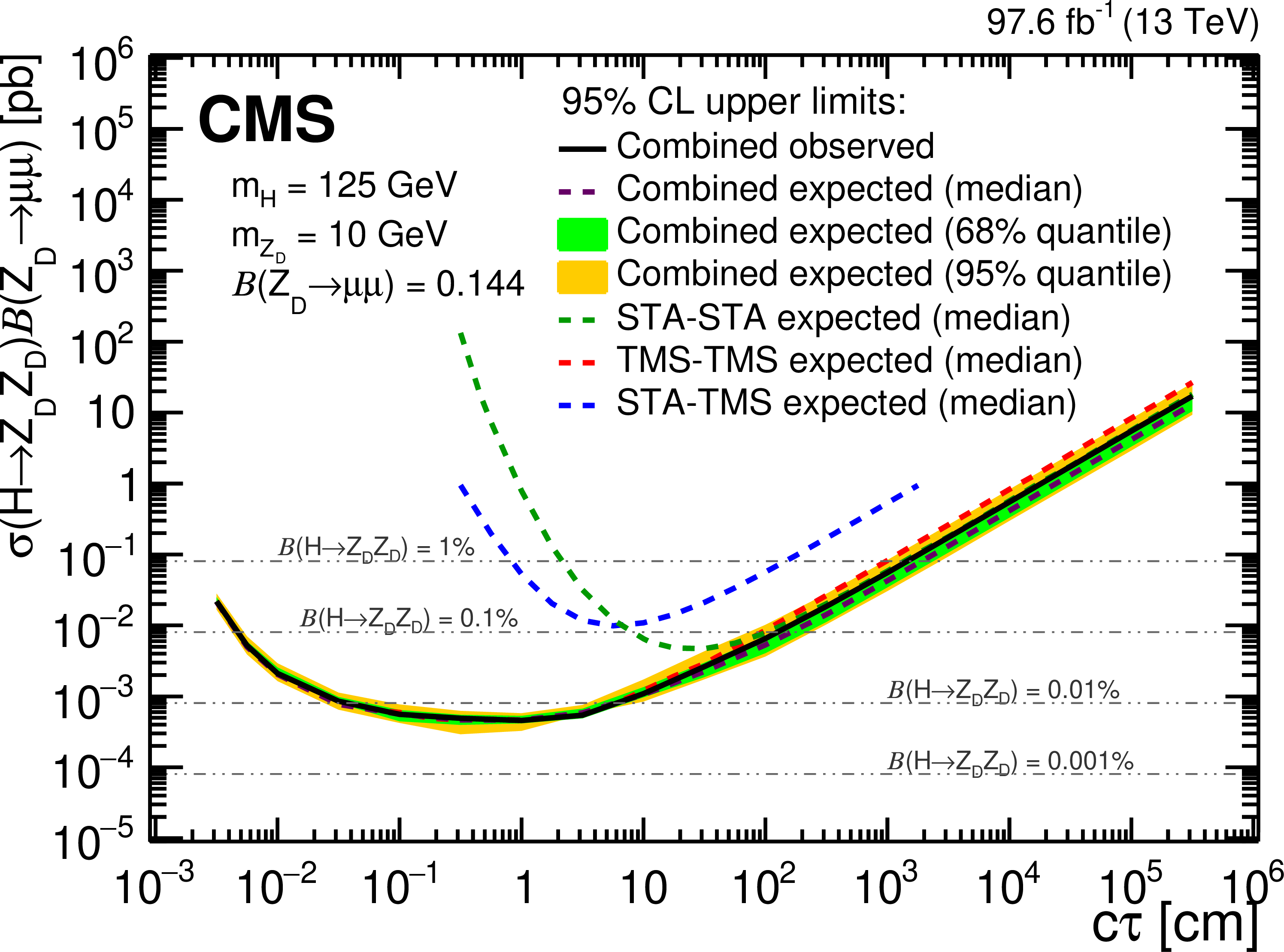
Figure 18-a:
The 95% CL upper limits on $\sigma (\mathrm{H} \to \mathrm{Z} {\mathrm {_{D}}}\mathrm{Z} {\mathrm {_{D}}})\mathcal {B}(\mathrm{Z} {\mathrm {_{D}}}\to \mu \mu)$ as a function of $ {c\tau} (\mathrm{Z} {\mathrm {_{D}}})$ in the HAHM model, for $ {m(\mathrm{Z} {\mathrm {_{D}}})} $ ranging from 10 GeV (upper left) to 60 GeV (lower right). The median expected limits obtained from the STA-STA, STA-TMS, and TMS-TMS dimuon categories are shown as dashed green, blue, and red curves, respectively; the combined median expected limits are shown as dashed black curves; and the combined observed limits are shown as solid black curves. The green and yellow bands correspond, respectively, to the 68 and 95% quantiles for the combined expected limits. The horizontal lines in gray correspond to the theoretical predictions for values of $\mathcal {B}(\mathrm{H} \to \mathrm{Z} {\mathrm {_{D}}}\mathrm{Z} {\mathrm {_{D}}})$ indicated next to the lines. |
png pdf |
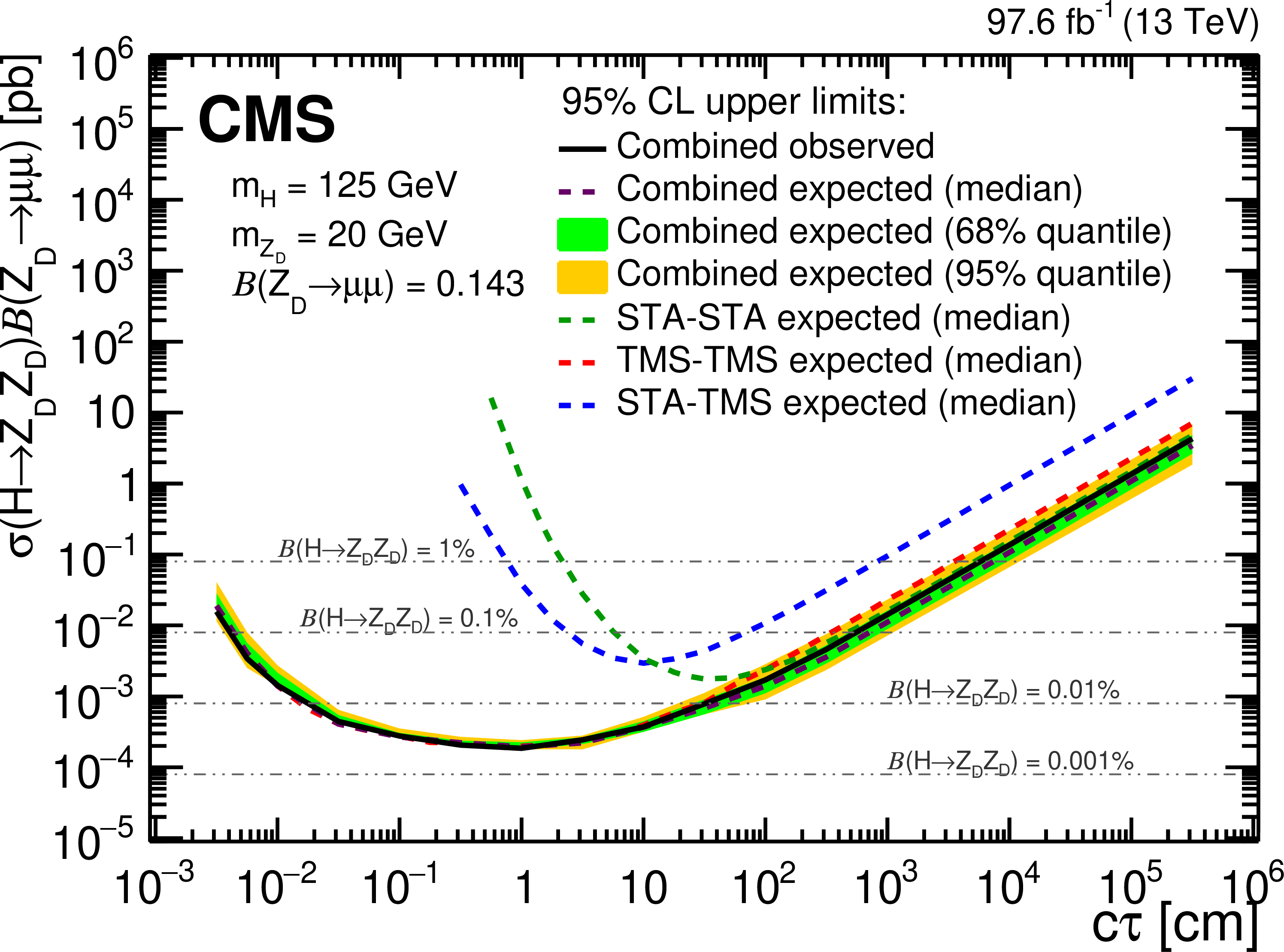
Figure 18-b:
The 95% CL upper limits on $\sigma (\mathrm{H} \to \mathrm{Z} {\mathrm {_{D}}}\mathrm{Z} {\mathrm {_{D}}})\mathcal {B}(\mathrm{Z} {\mathrm {_{D}}}\to \mu \mu)$ as a function of $ {c\tau} (\mathrm{Z} {\mathrm {_{D}}})$ in the HAHM model, for $ {m(\mathrm{Z} {\mathrm {_{D}}})} $ ranging from 10 GeV (upper left) to 60 GeV (lower right). The median expected limits obtained from the STA-STA, STA-TMS, and TMS-TMS dimuon categories are shown as dashed green, blue, and red curves, respectively; the combined median expected limits are shown as dashed black curves; and the combined observed limits are shown as solid black curves. The green and yellow bands correspond, respectively, to the 68 and 95% quantiles for the combined expected limits. The horizontal lines in gray correspond to the theoretical predictions for values of $\mathcal {B}(\mathrm{H} \to \mathrm{Z} {\mathrm {_{D}}}\mathrm{Z} {\mathrm {_{D}}})$ indicated next to the lines. |

png pdf |
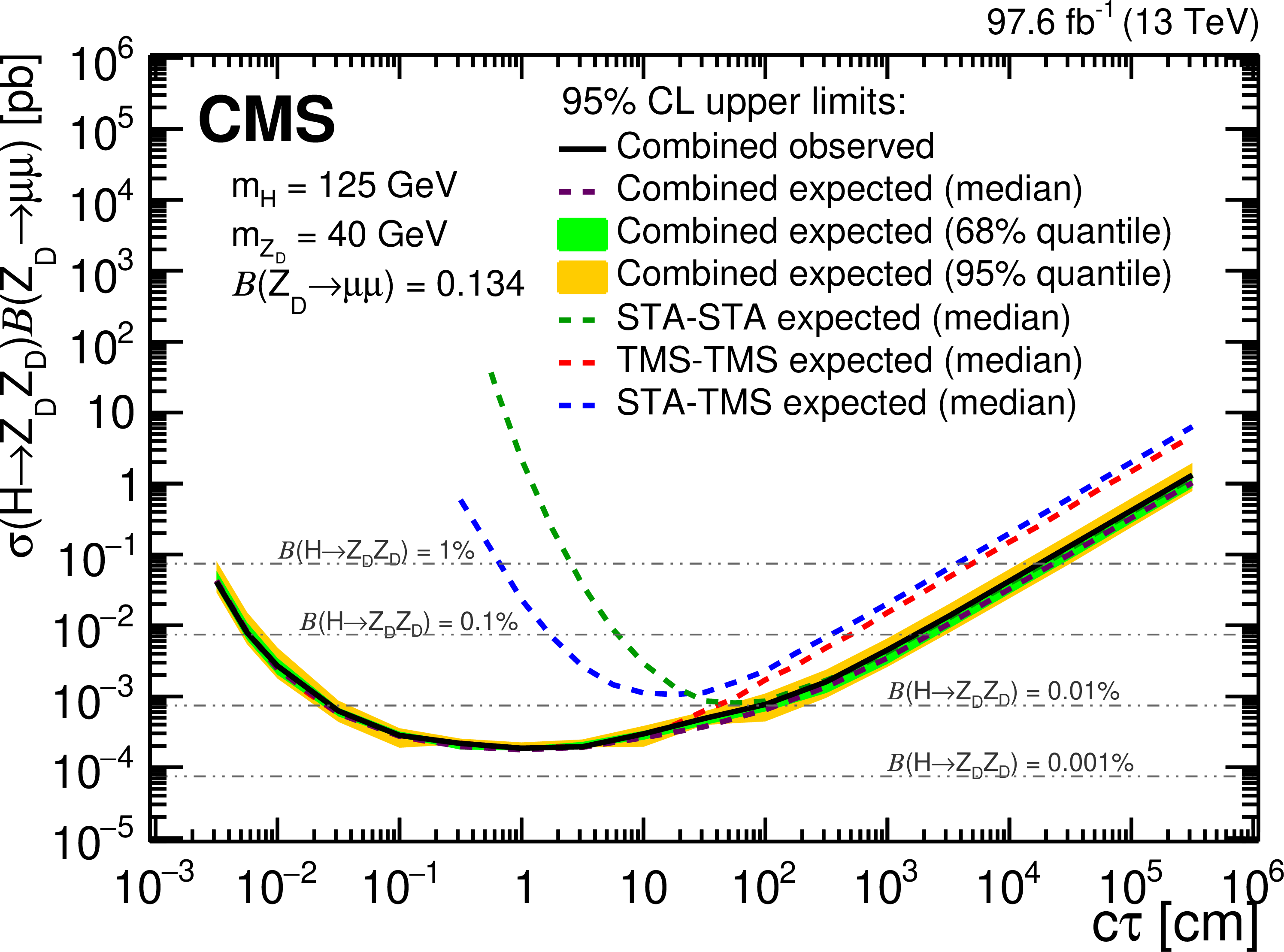
Figure 18-c:
The 95% CL upper limits on $\sigma (\mathrm{H} \to \mathrm{Z} {\mathrm {_{D}}}\mathrm{Z} {\mathrm {_{D}}})\mathcal {B}(\mathrm{Z} {\mathrm {_{D}}}\to \mu \mu)$ as a function of $ {c\tau} (\mathrm{Z} {\mathrm {_{D}}})$ in the HAHM model, for $ {m(\mathrm{Z} {\mathrm {_{D}}})} $ ranging from 10 GeV (upper left) to 60 GeV (lower right). The median expected limits obtained from the STA-STA, STA-TMS, and TMS-TMS dimuon categories are shown as dashed green, blue, and red curves, respectively; the combined median expected limits are shown as dashed black curves; and the combined observed limits are shown as solid black curves. The green and yellow bands correspond, respectively, to the 68 and 95% quantiles for the combined expected limits. The horizontal lines in gray correspond to the theoretical predictions for values of $\mathcal {B}(\mathrm{H} \to \mathrm{Z} {\mathrm {_{D}}}\mathrm{Z} {\mathrm {_{D}}})$ indicated next to the lines. |
png pdf |
Figure 18-d:
The 95% CL upper limits on $\sigma (\mathrm{H} \to \mathrm{Z} {\mathrm {_{D}}}\mathrm{Z} {\mathrm {_{D}}})\mathcal {B}(\mathrm{Z} {\mathrm {_{D}}}\to \mu \mu)$ as a function of $ {c\tau} (\mathrm{Z} {\mathrm {_{D}}})$ in the HAHM model, for $ {m(\mathrm{Z} {\mathrm {_{D}}})} $ ranging from 10 GeV (upper left) to 60 GeV (lower right). The median expected limits obtained from the STA-STA, STA-TMS, and TMS-TMS dimuon categories are shown as dashed green, blue, and red curves, respectively; the combined median expected limits are shown as dashed black curves; and the combined observed limits are shown as solid black curves. The green and yellow bands correspond, respectively, to the 68 and 95% quantiles for the combined expected limits. The horizontal lines in gray correspond to the theoretical predictions for values of $\mathcal {B}(\mathrm{H} \to \mathrm{Z} {\mathrm {_{D}}}\mathrm{Z} {\mathrm {_{D}}})$ indicated next to the lines. |
png pdf |
Figure 18-e:
The 95% CL upper limits on $\sigma (\mathrm{H} \to \mathrm{Z} {\mathrm {_{D}}}\mathrm{Z} {\mathrm {_{D}}})\mathcal {B}(\mathrm{Z} {\mathrm {_{D}}}\to \mu \mu)$ as a function of $ {c\tau} (\mathrm{Z} {\mathrm {_{D}}})$ in the HAHM model, for $ {m(\mathrm{Z} {\mathrm {_{D}}})} $ ranging from 10 GeV (upper left) to 60 GeV (lower right). The median expected limits obtained from the STA-STA, STA-TMS, and TMS-TMS dimuon categories are shown as dashed green, blue, and red curves, respectively; the combined median expected limits are shown as dashed black curves; and the combined observed limits are shown as solid black curves. The green and yellow bands correspond, respectively, to the 68 and 95% quantiles for the combined expected limits. The horizontal lines in gray correspond to the theoretical predictions for values of $\mathcal {B}(\mathrm{H} \to \mathrm{Z} {\mathrm {_{D}}}\mathrm{Z} {\mathrm {_{D}}})$ indicated next to the lines. |
png pdf |
Figure 18-f:
The 95% CL upper limits on $\sigma (\mathrm{H} \to \mathrm{Z} {\mathrm {_{D}}}\mathrm{Z} {\mathrm {_{D}}})\mathcal {B}(\mathrm{Z} {\mathrm {_{D}}}\to \mu \mu)$ as a function of $ {c\tau} (\mathrm{Z} {\mathrm {_{D}}})$ in the HAHM model, for $ {m(\mathrm{Z} {\mathrm {_{D}}})} $ ranging from 10 GeV (upper left) to 60 GeV (lower right). The median expected limits obtained from the STA-STA, STA-TMS, and TMS-TMS dimuon categories are shown as dashed green, blue, and red curves, respectively; the combined median expected limits are shown as dashed black curves; and the combined observed limits are shown as solid black curves. The green and yellow bands correspond, respectively, to the 68 and 95% quantiles for the combined expected limits. The horizontal lines in gray correspond to the theoretical predictions for values of $\mathcal {B}(\mathrm{H} \to \mathrm{Z} {\mathrm {_{D}}}\mathrm{Z} {\mathrm {_{D}}})$ indicated next to the lines. |
png pdf |
Figure 19:
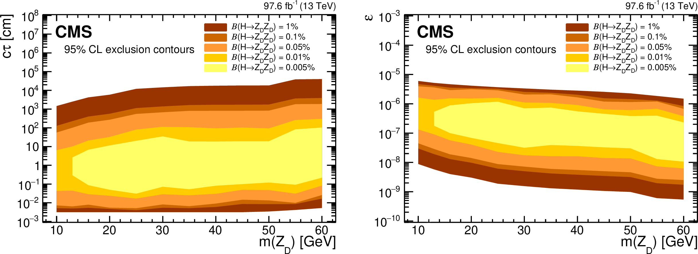
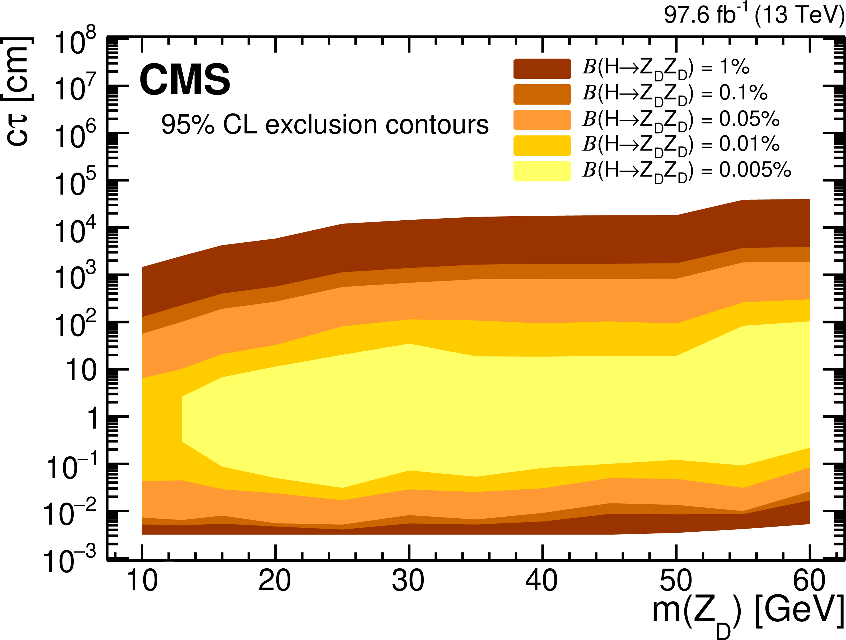
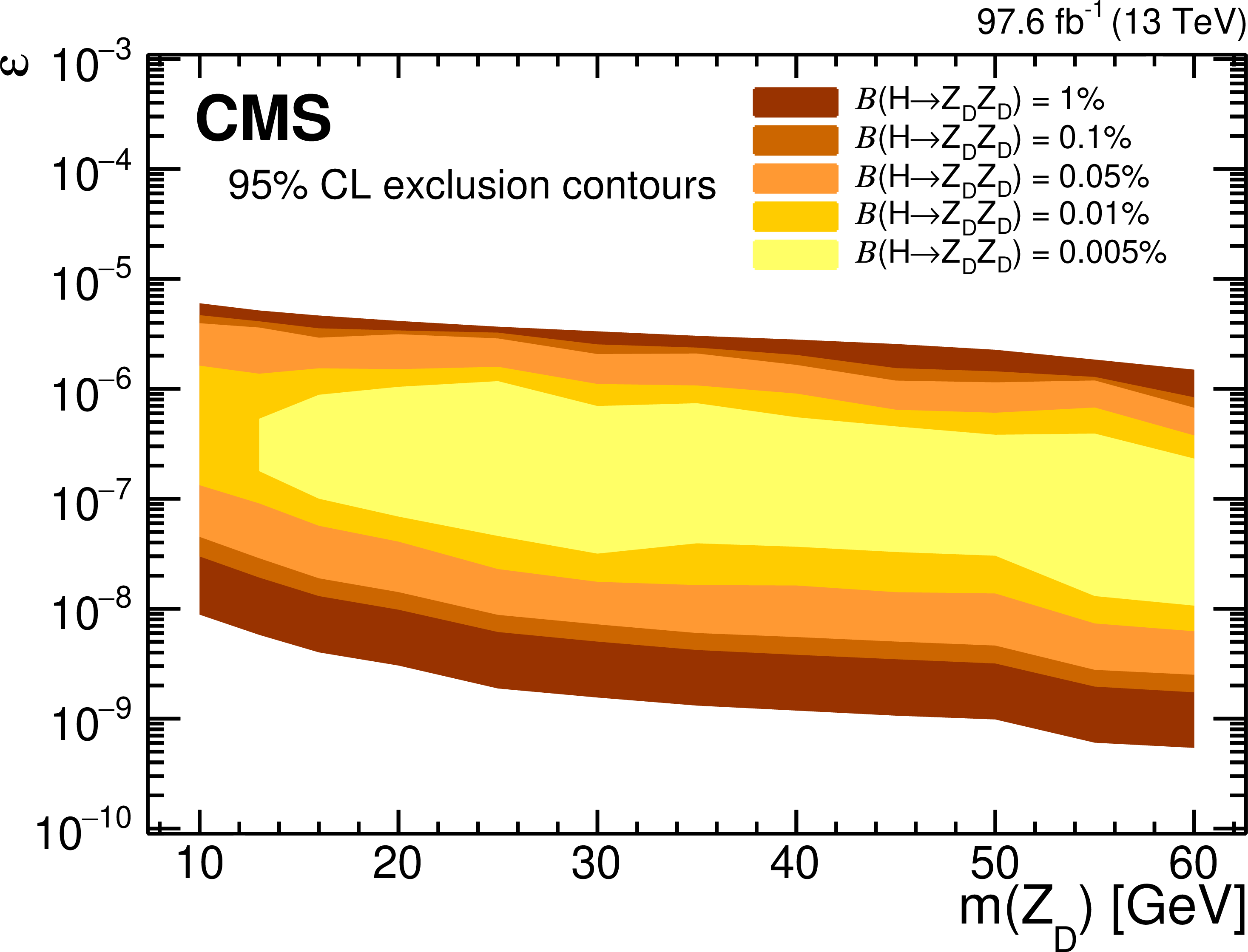
Observed 95% CL exclusion contours in the HAHM model, in the (left) ($ {m(\mathrm{Z} {\mathrm {_{D}}})} $, $ {c\tau} (\mathrm{Z} {\mathrm {_{D}}})$) and (right) ($ {m(\mathrm{Z} {\mathrm {_{D}}})} $, $\epsilon $) planes. The contours correspond to several representative values of $\mathcal {B}(\mathrm{H} \to \mathrm{Z} {\mathrm {_{D}}}\mathrm{Z} {\mathrm {_{D}}})$ ranging from 0.005 to 1%. |
png pdf |
Figure 19-a:
Observed 95% CL exclusion contours in the HAHM model, in the (left) ($ {m(\mathrm{Z} {\mathrm {_{D}}})} $, $ {c\tau} (\mathrm{Z} {\mathrm {_{D}}})$) and (right) ($ {m(\mathrm{Z} {\mathrm {_{D}}})} $, $\epsilon $) planes. The contours correspond to several representative values of $\mathcal {B}(\mathrm{H} \to \mathrm{Z} {\mathrm {_{D}}}\mathrm{Z} {\mathrm {_{D}}})$ ranging from 0.005 to 1%. |
png pdf |
Figure 19-b:
Observed 95% CL exclusion contours in the HAHM model, in the (left) ($ {m(\mathrm{Z} {\mathrm {_{D}}})} $, $ {c\tau} (\mathrm{Z} {\mathrm {_{D}}})$) and (right) ($ {m(\mathrm{Z} {\mathrm {_{D}}})} $, $\epsilon $) planes. The contours correspond to several representative values of $\mathcal {B}(\mathrm{H} \to \mathrm{Z} {\mathrm {_{D}}}\mathrm{Z} {\mathrm {_{D}}})$ ranging from 0.005 to 1%. |
| Tables | |
png pdf |
Table 1:
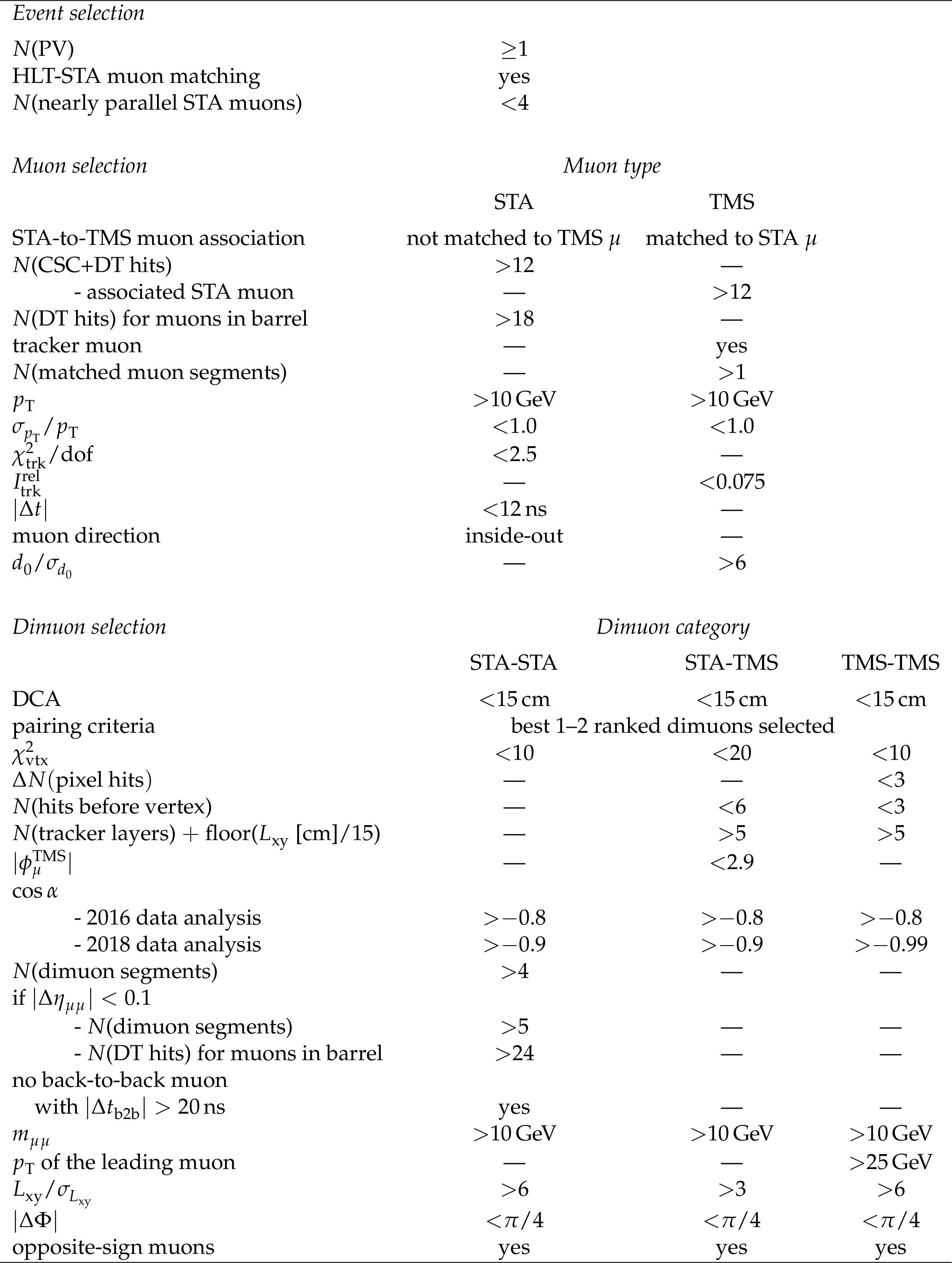
Summary of the selection criteria used in the analysis, grouped into event, muon, and dimuon requirements. |
| Summary |
| Data collected by the CMS experiment in proton-proton collisions at $\sqrt{s} = $ 13 TeV in 2016 and 2018 and corresponding to an integrated luminosity of 97.6 fb$^{-1}$ have been used to conduct an inclusive search for long-lived exotic neutral particles (LLPs) decaying to a pair of oppositely charged muons. The search is largely model-independent and is sensitive to a broad range of LLP lifetimes and masses. No significant excess of events above the standard model background is observed. The results are interpreted as limits on the parameters of the hidden Abelian Higgs model, in which the Higgs boson decays to a pair of long-lived dark photons Z$_{\mathrm{D}}$, and of a simplified model, in which LLPs are produced in decays of an exotic heavy neutral scalar boson. In the mass range 20 $ < {m(\mathrm{Z_D})} < $ 60 GeV, a branching fraction of the Higgs boson to dark photons of 1% is excluded at 95% confidence level in the range of proper decay length ${c\tau} (\mathrm{Z_D})$ from a few tens of $\mu$m to $\approx$100 m. The results of this search significantly extend the previously excluded range of model parameters. For the hidden Abelian Higgs model with ${m(\mathrm{Z_D})} $ greater than 20 GeV and less than half the mass of the Higgs boson, they provide the best limits to date on the branching fraction of the Higgs boson to dark photons for ${c\tau} (\mathrm{Z_D})$ (varying with ${m(\mathrm{Z_D})} $) between 0.03 and ${\approx}$0.5 mm, and above ${\approx}$0.5 m. At exotic scalar boson masses larger than the Higgs boson mass, our results represent the best current constraints for all considered LLP masses and lifetimes. |
| Additional Figures | |
png pdf |
Additional Figure 1:
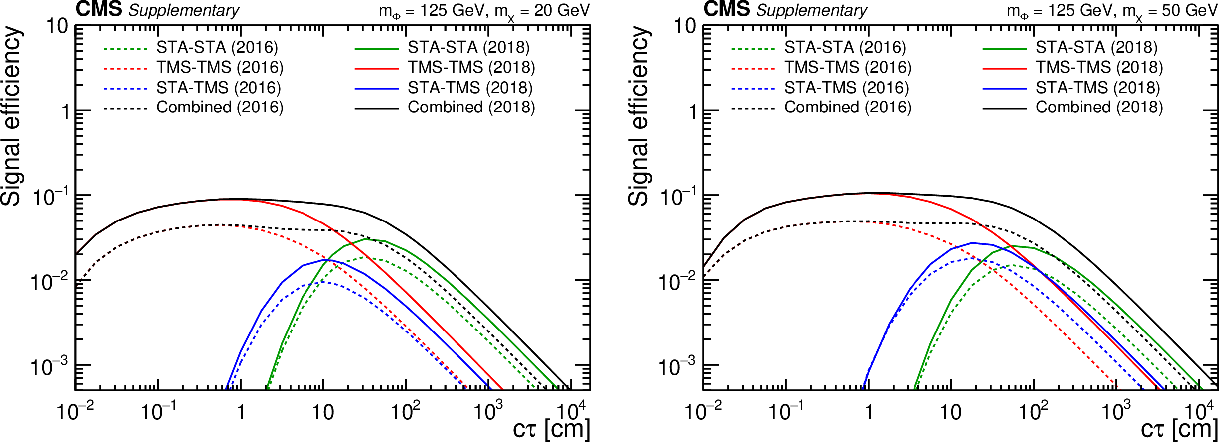
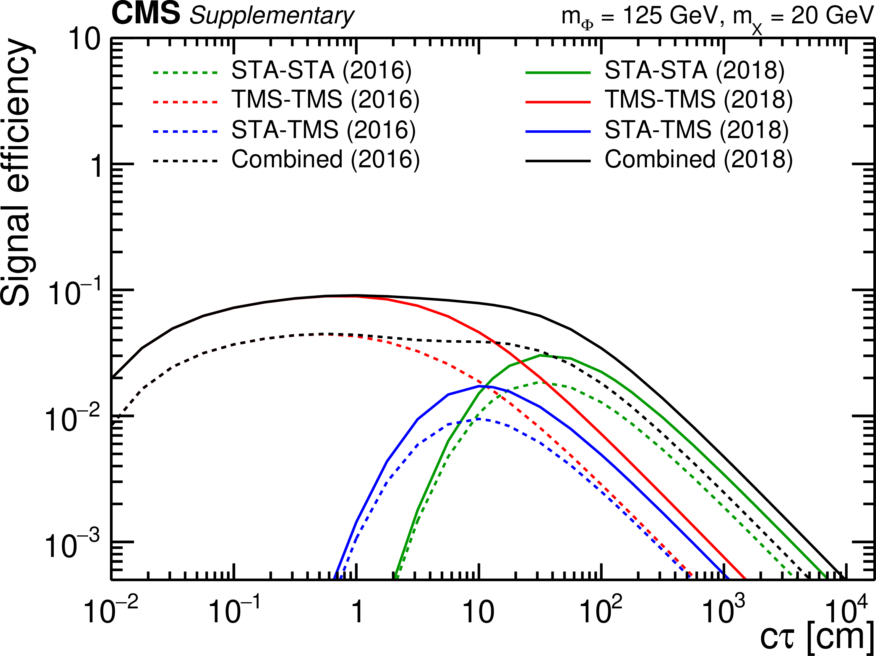
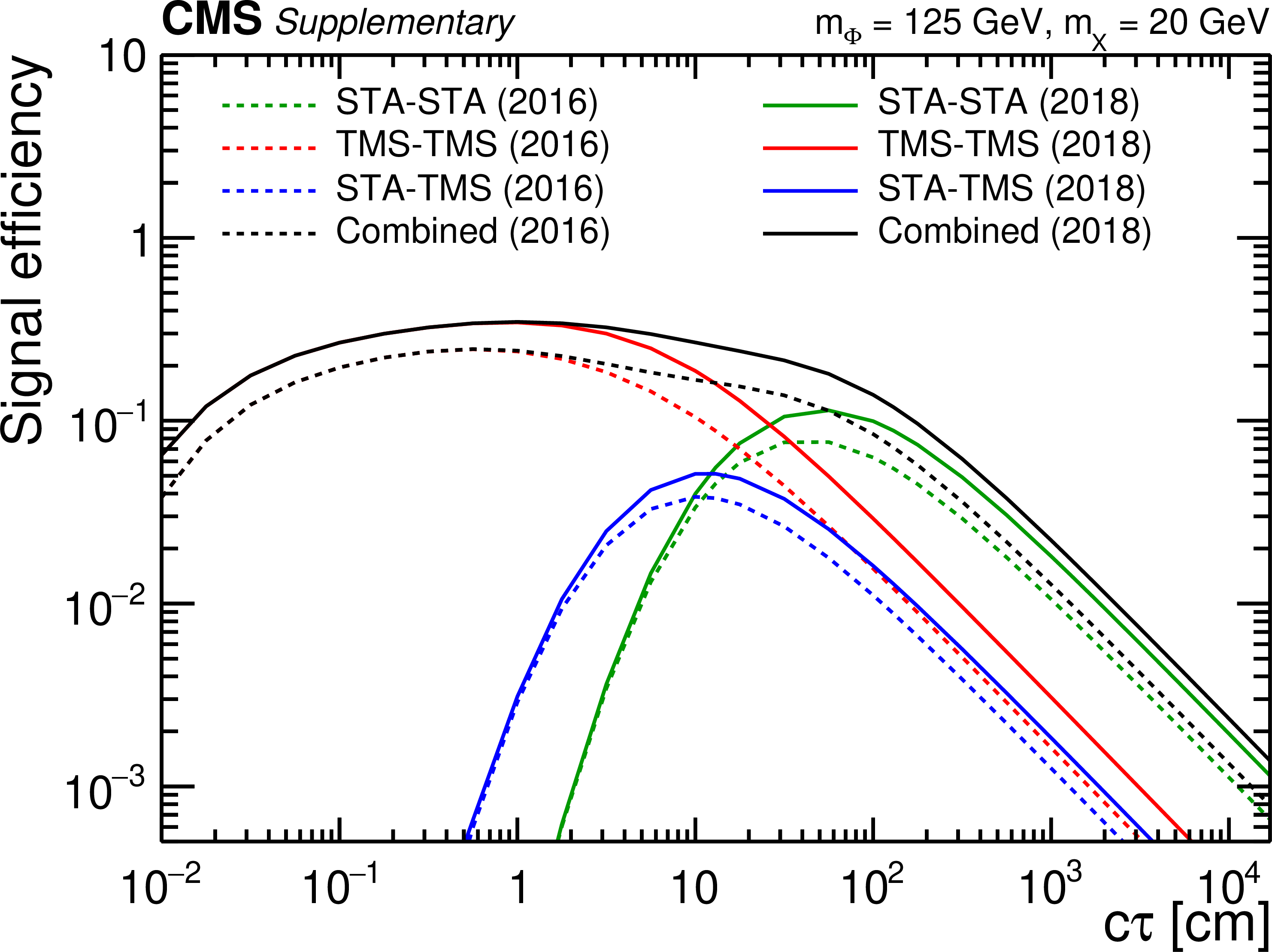
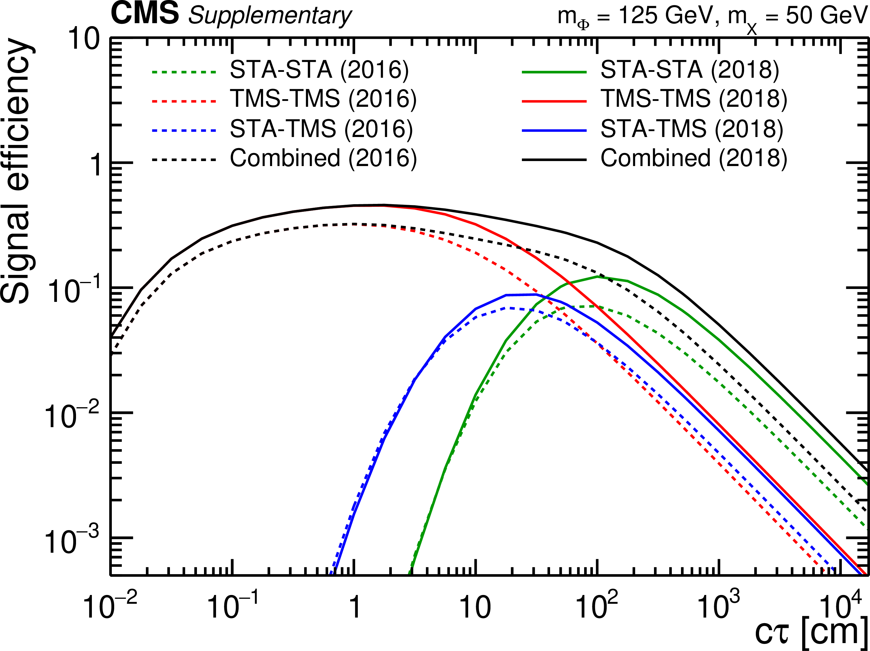
Overall signal efficiencies as a function of $ {c\tau} $ for the $ {\phi\to \mathrm{X} \mathrm{X} \to \mu \mu}+$ anything signal process with $ {m(\phi)} = $ 125 GeV (left: $ {m(\mathrm{X})} = $ 20 GeV, right: $ {m(\mathrm{X})} = $ 50 GeV). Each plot shows efficiencies of the three dimuon categories, STA-STA (green), TMS-TMS (red), and STA-TMS (blue), as well as the combined efficiency (black). Each efficiency is computed as the ratio of the number of simulated signal events in which at least one dimuon candidate of a given type (or any type for the combined efficiency) passes all selection criteria (including the trigger) to the total number of simulated signal events. All efficiencies are corrected by the data-to-simulation scale factors described in the paper. The efficiencies in the 2016 and 2018 data sets are shown as dashed and solid curves, respectively. |
png pdf root |
Additional Figure 1-a:
Overall signal efficiencies as a function of $ {c\tau} $ for the $ {\phi\to \mathrm{X} \mathrm{X} \to \mu \mu}+$ anything signal process with $ {m(\phi)} = $ 125 GeV (left: $ {m(\mathrm{X})} = $ 20 GeV, right: $ {m(\mathrm{X})} = $ 50 GeV). Each plot shows efficiencies of the three dimuon categories, STA-STA (green), TMS-TMS (red), and STA-TMS (blue), as well as the combined efficiency (black). Each efficiency is computed as the ratio of the number of simulated signal events in which at least one dimuon candidate of a given type (or any type for the combined efficiency) passes all selection criteria (including the trigger) to the total number of simulated signal events. All efficiencies are corrected by the data-to-simulation scale factors described in the paper. The efficiencies in the 2016 and 2018 data sets are shown as dashed and solid curves, respectively. |

png pdf root |
Additional Figure 1-b:
Overall signal efficiencies as a function of $ {c\tau} $ for the $ {\phi\to \mathrm{X} \mathrm{X} \to \mu \mu}+$ anything signal process with $ {m(\phi)} = $ 125 GeV (left: $ {m(\mathrm{X})} = $ 20 GeV, right: $ {m(\mathrm{X})} = $ 50 GeV). Each plot shows efficiencies of the three dimuon categories, STA-STA (green), TMS-TMS (red), and STA-TMS (blue), as well as the combined efficiency (black). Each efficiency is computed as the ratio of the number of simulated signal events in which at least one dimuon candidate of a given type (or any type for the combined efficiency) passes all selection criteria (including the trigger) to the total number of simulated signal events. All efficiencies are corrected by the data-to-simulation scale factors described in the paper. The efficiencies in the 2016 and 2018 data sets are shown as dashed and solid curves, respectively. |
png pdf |
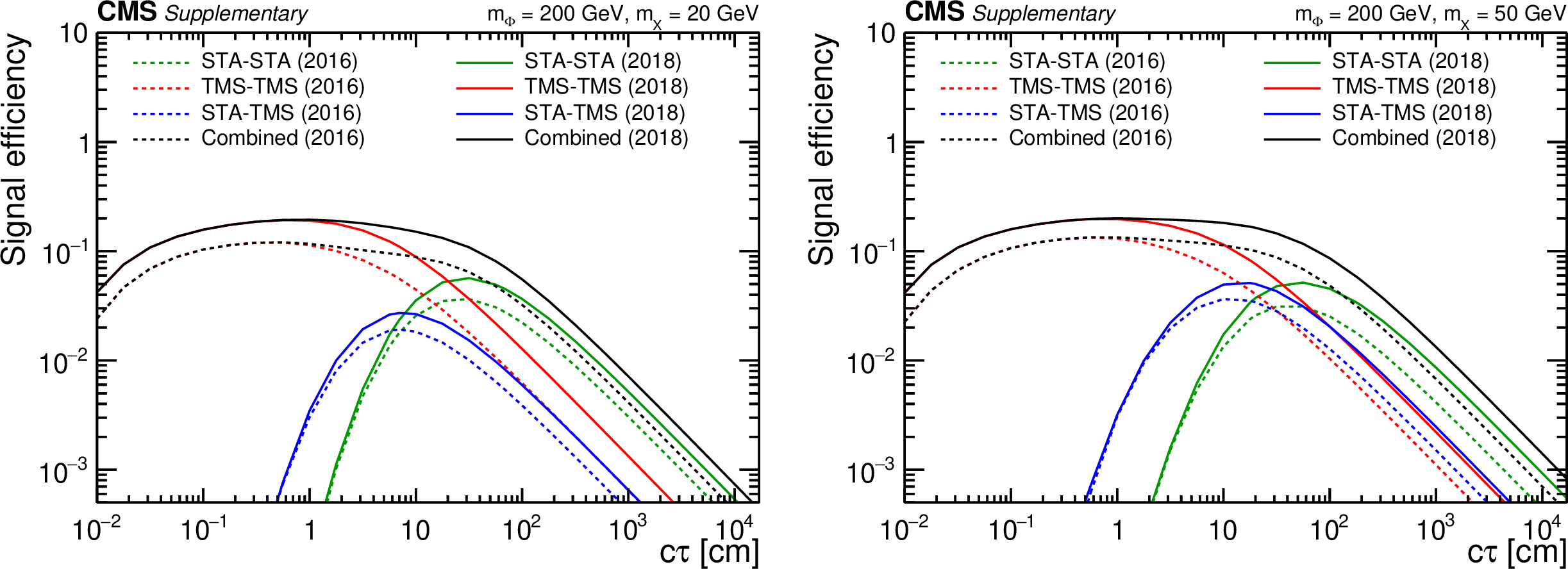
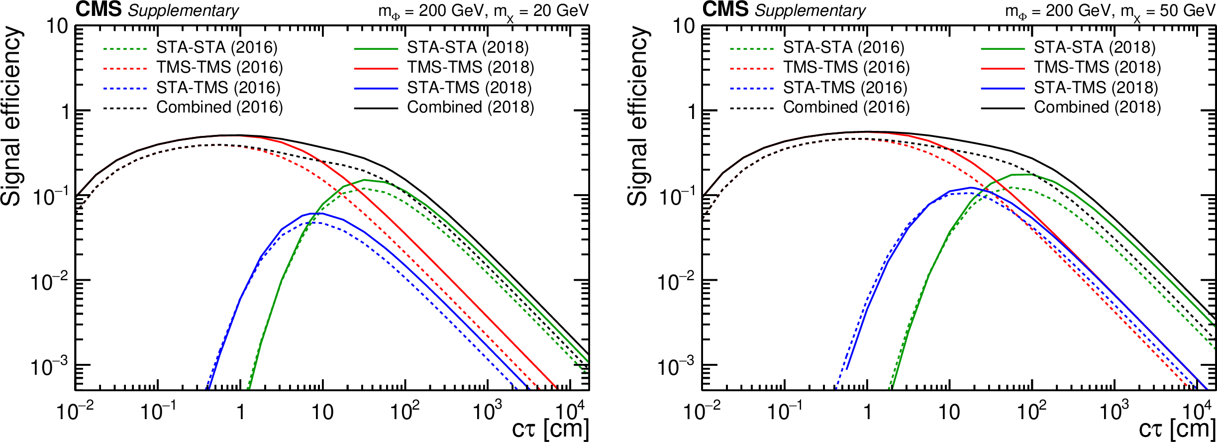
Additional Figure 2:
Overall signal efficiencies as a function of $ {c\tau} $ for the $ {\phi\to \mathrm{X} \mathrm{X} \to \mu \mu}+$ anything signal process with $ {m(\phi)} = $ 200 GeV (left: $ {m(\mathrm{X})} = $ 20 GeV, right: $ {m(\mathrm{X})} = $ 50 GeV). Each plot shows efficiencies of the three dimuon categories, STA-STA (green), TMS-TMS (red), and STA-TMS (blue), as well as the combined efficiency (black). Each efficiency is computed as the ratio of the number of simulated signal events in which at least one dimuon candidate of a given type (or any type for the combined efficiency) passes all selection criteria (including the trigger) to the total number of simulated signal events. All efficiencies are corrected by the data-to-simulation scale factors described in the paper. The efficiencies in the 2016 and 2018 data sets are shown as dashed and solid curves, respectively. |
png pdf root |
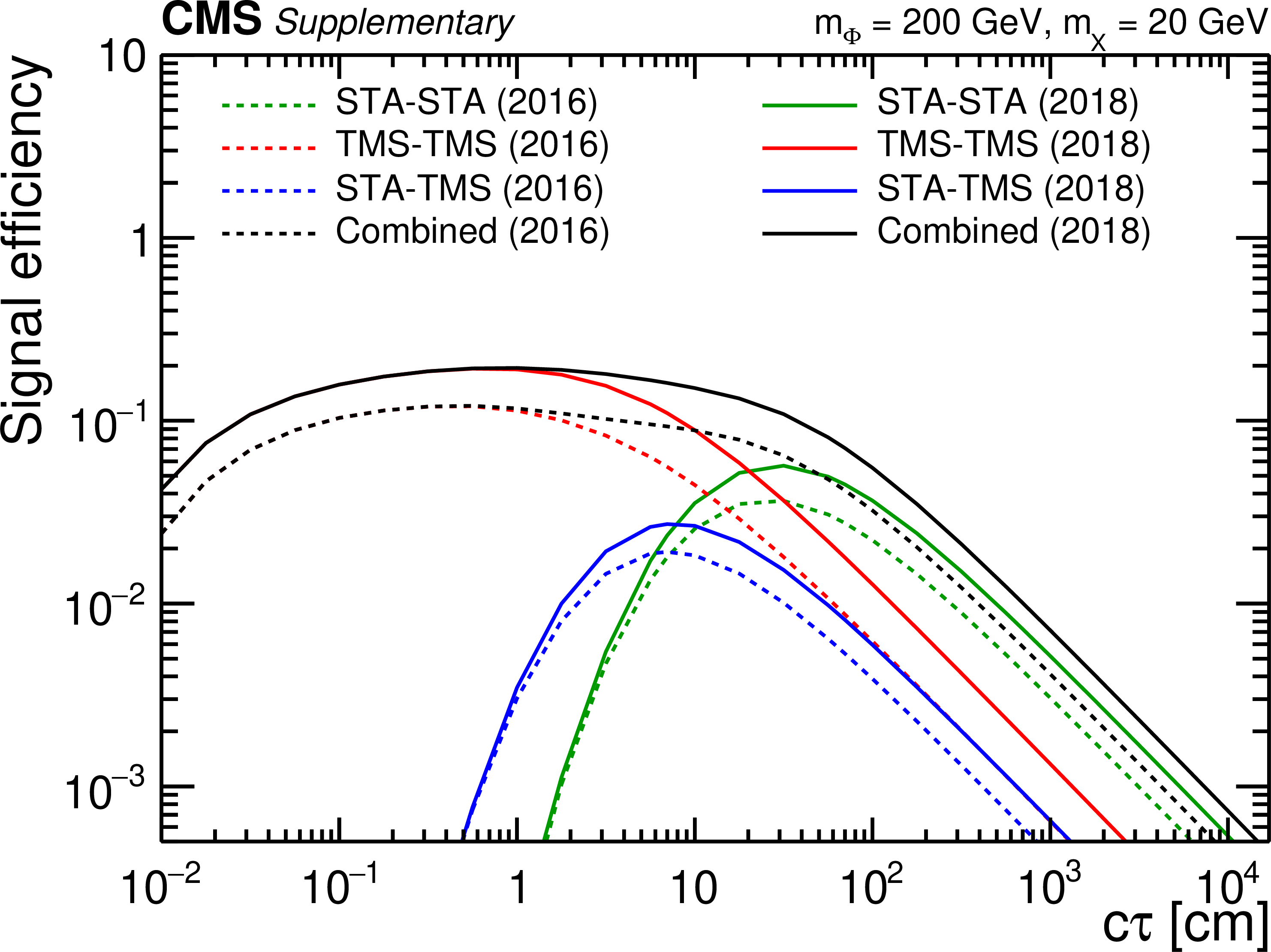
Additional Figure 2-a:
Overall signal efficiencies as a function of $ {c\tau} $ for the $ {\phi\to \mathrm{X} \mathrm{X} \to \mu \mu}+$ anything signal process with $ {m(\phi)} = $ 200 GeV (left: $ {m(\mathrm{X})} = $ 20 GeV, right: $ {m(\mathrm{X})} = $ 50 GeV). Each plot shows efficiencies of the three dimuon categories, STA-STA (green), TMS-TMS (red), and STA-TMS (blue), as well as the combined efficiency (black). Each efficiency is computed as the ratio of the number of simulated signal events in which at least one dimuon candidate of a given type (or any type for the combined efficiency) passes all selection criteria (including the trigger) to the total number of simulated signal events. All efficiencies are corrected by the data-to-simulation scale factors described in the paper. The efficiencies in the 2016 and 2018 data sets are shown as dashed and solid curves, respectively. |
png pdf root |
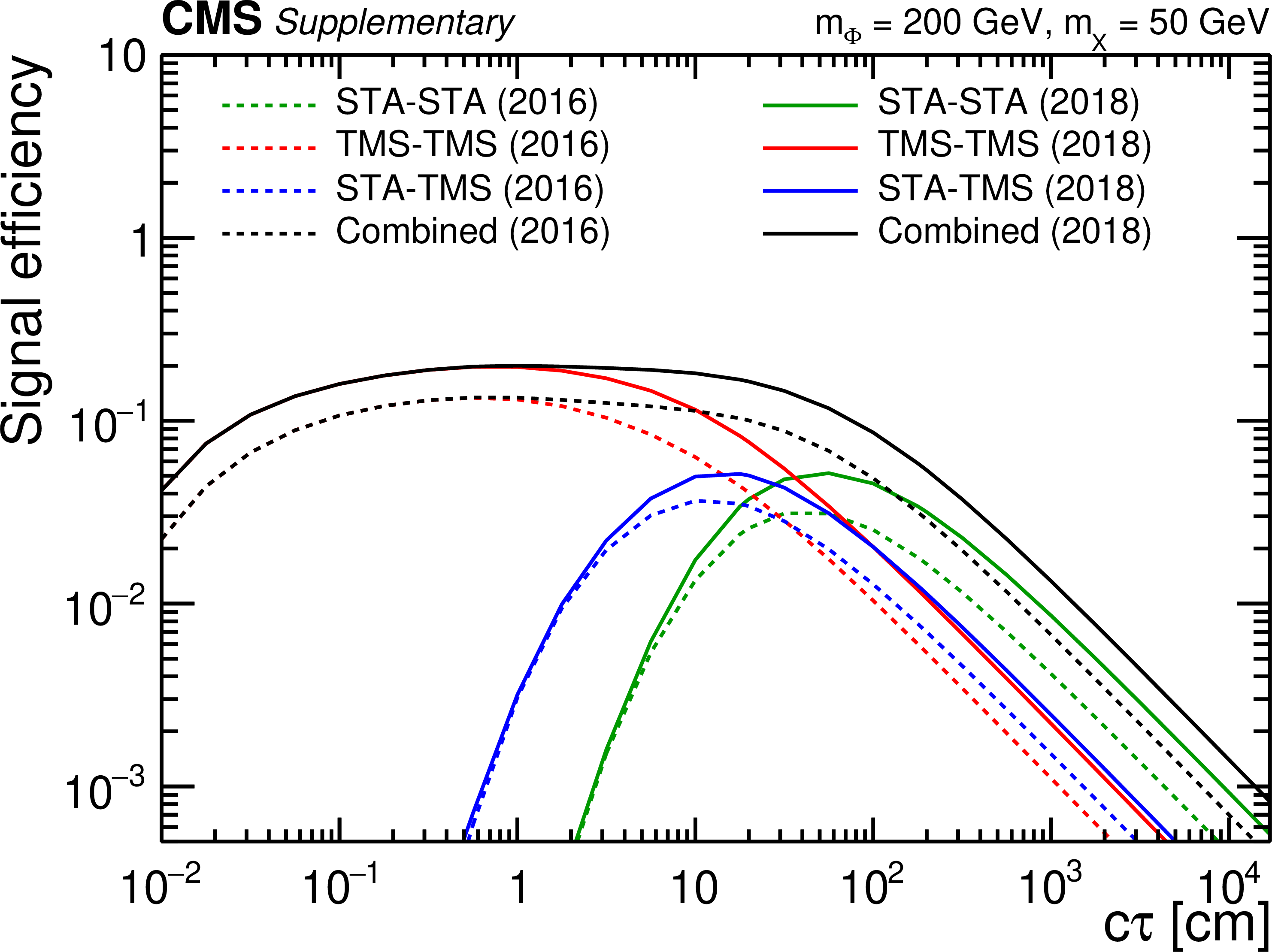
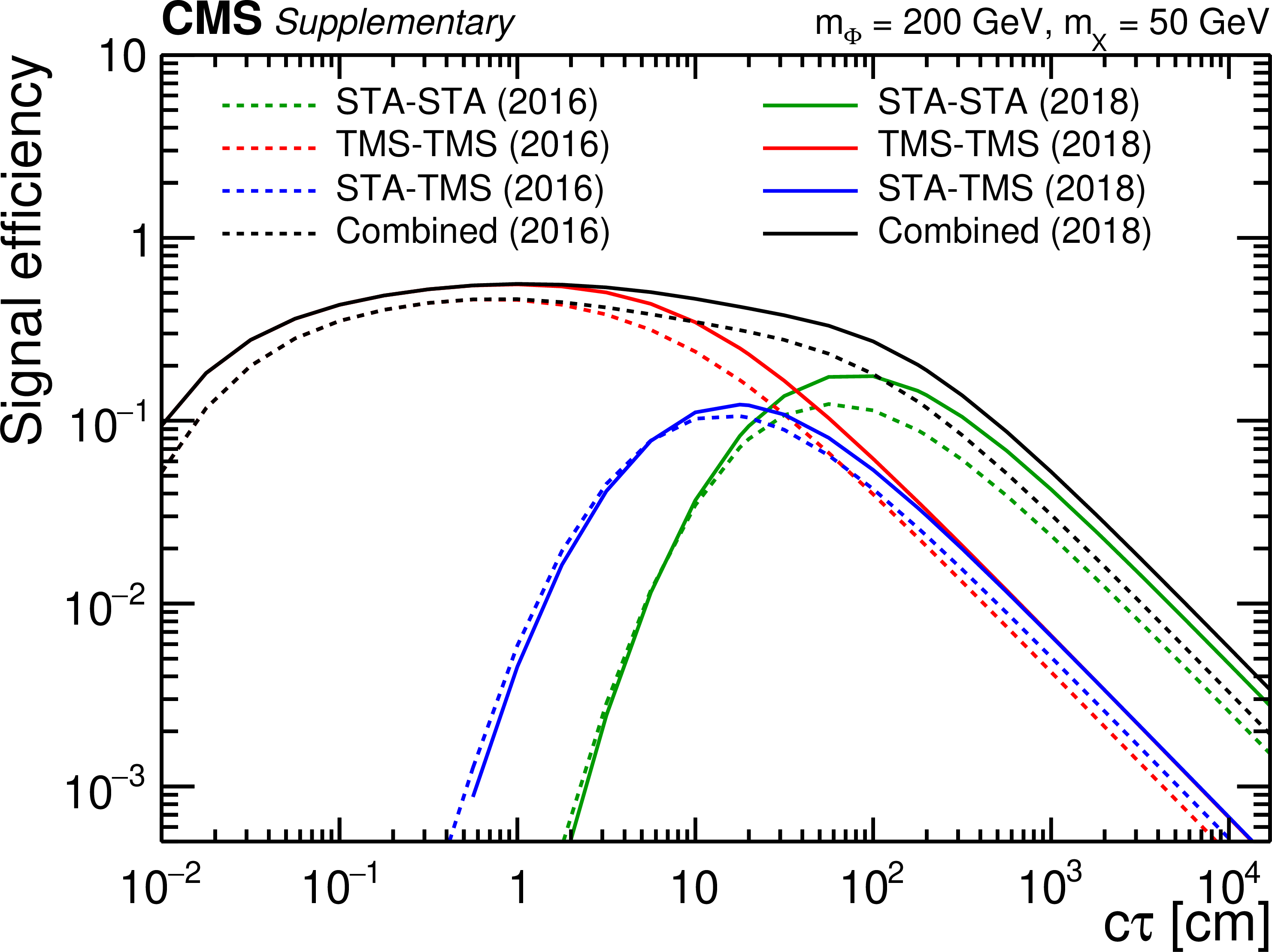
Additional Figure 2-b:
Overall signal efficiencies as a function of $ {c\tau} $ for the $ {\phi\to \mathrm{X} \mathrm{X} \to \mu \mu}+$ anything signal process with $ {m(\phi)} = $ 200 GeV (left: $ {m(\mathrm{X})} = $ 20 GeV, right: $ {m(\mathrm{X})} = $ 50 GeV). Each plot shows efficiencies of the three dimuon categories, STA-STA (green), TMS-TMS (red), and STA-TMS (blue), as well as the combined efficiency (black). Each efficiency is computed as the ratio of the number of simulated signal events in which at least one dimuon candidate of a given type (or any type for the combined efficiency) passes all selection criteria (including the trigger) to the total number of simulated signal events. All efficiencies are corrected by the data-to-simulation scale factors described in the paper. The efficiencies in the 2016 and 2018 data sets are shown as dashed and solid curves, respectively. |
png pdf |
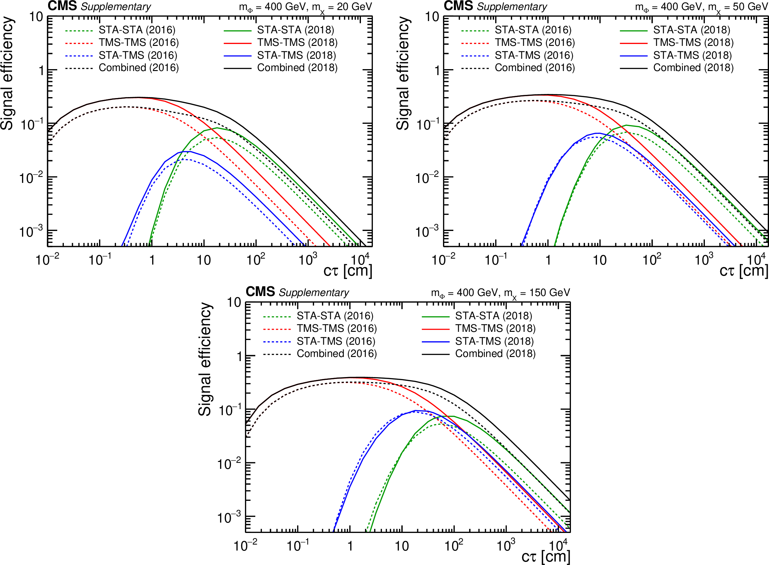
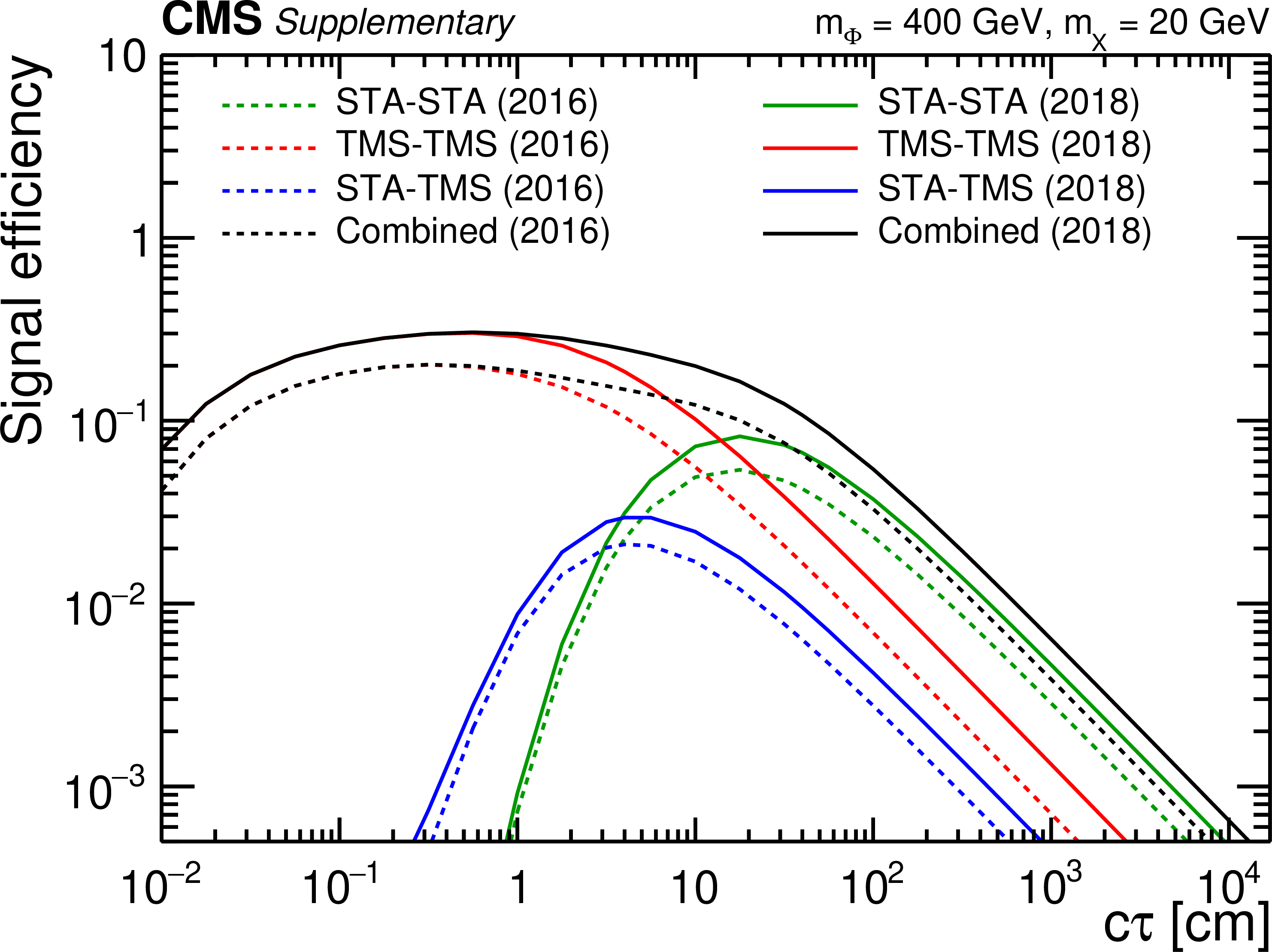
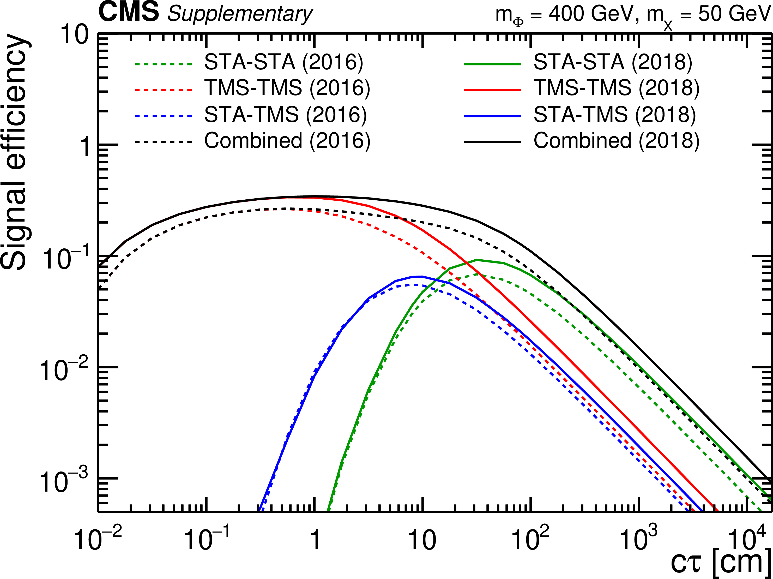
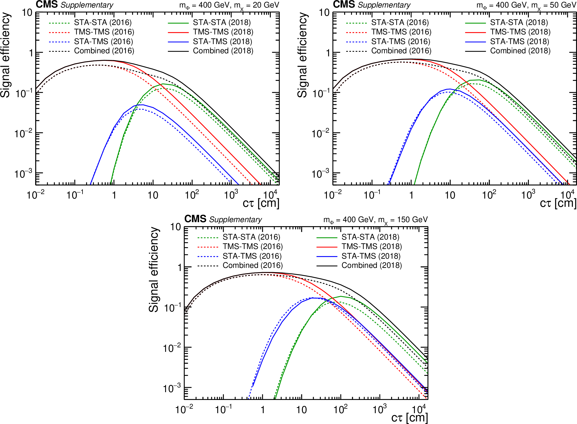
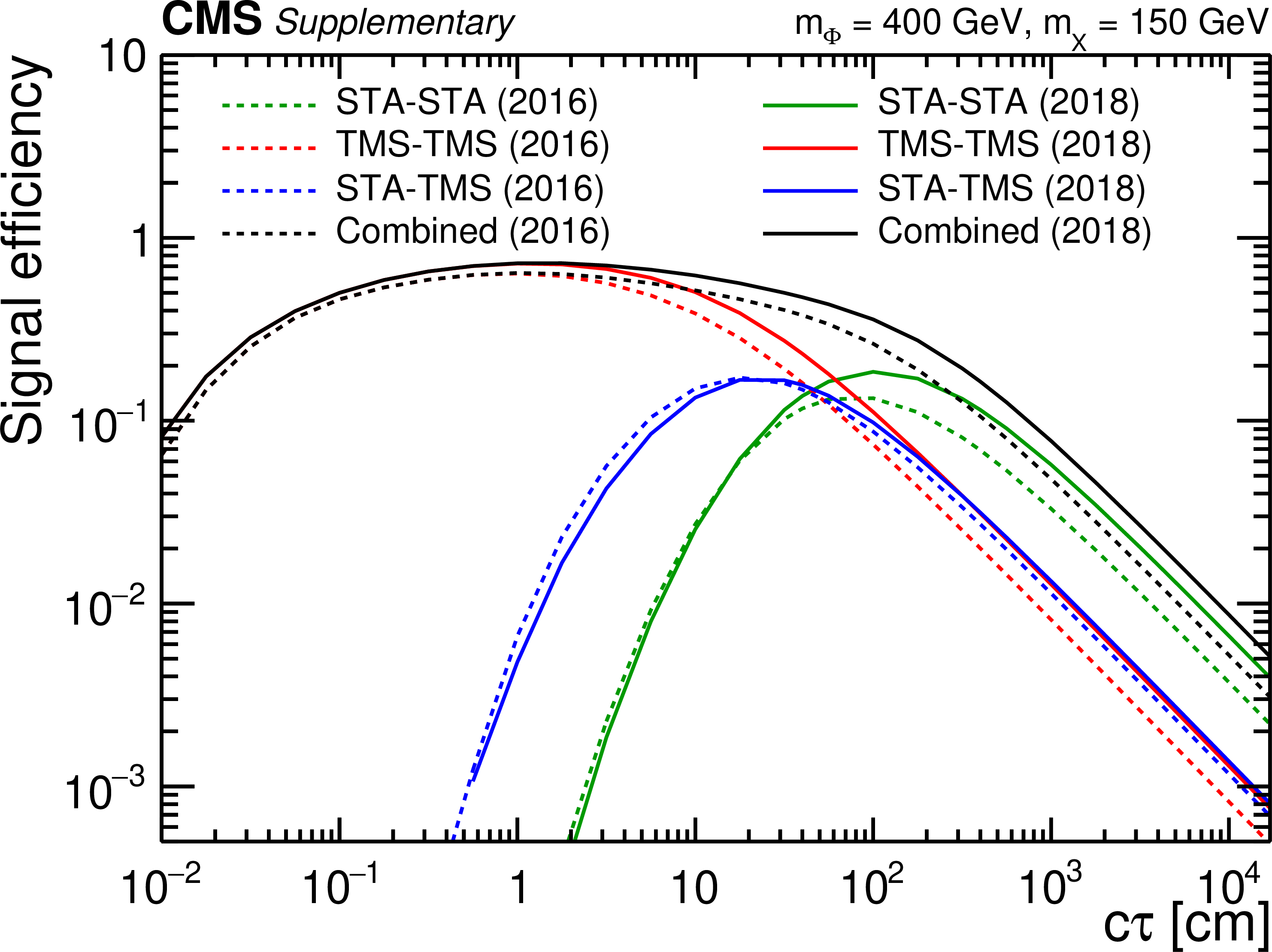
Additional Figure 3:
Overall signal efficiencies as a function of $ {c\tau} $ for the $ {\phi\to \mathrm{X} \mathrm{X} \to \mu \mu}+$ anything signal process with $ {m(\phi)} = $ 400 GeV (upper left: $ {m(\mathrm{X})} = $ 20 GeV, upper right: $ {m(\mathrm{X})} = $ 50 GeV, lower: $ {m(\mathrm{X})} = $ 150 GeV). Each plot shows efficiencies of the three dimuon categories, STA-STA (green), TMS-TMS (red), and STA-TMS (blue), as well as the combined efficiency (black). Each efficiency is computed as the ratio of the number of simulated signal events in which at least one dimuon candidate of a given type (or any type for the combined efficiency) passes all selection criteria (including the trigger) to the total number of simulated signal events. All efficiencies are corrected by the data-to-simulation scale factors described in the paper. The efficiencies in the 2016 and 2018 data sets are shown as dashed and solid curves, respectively. |
png pdf root |
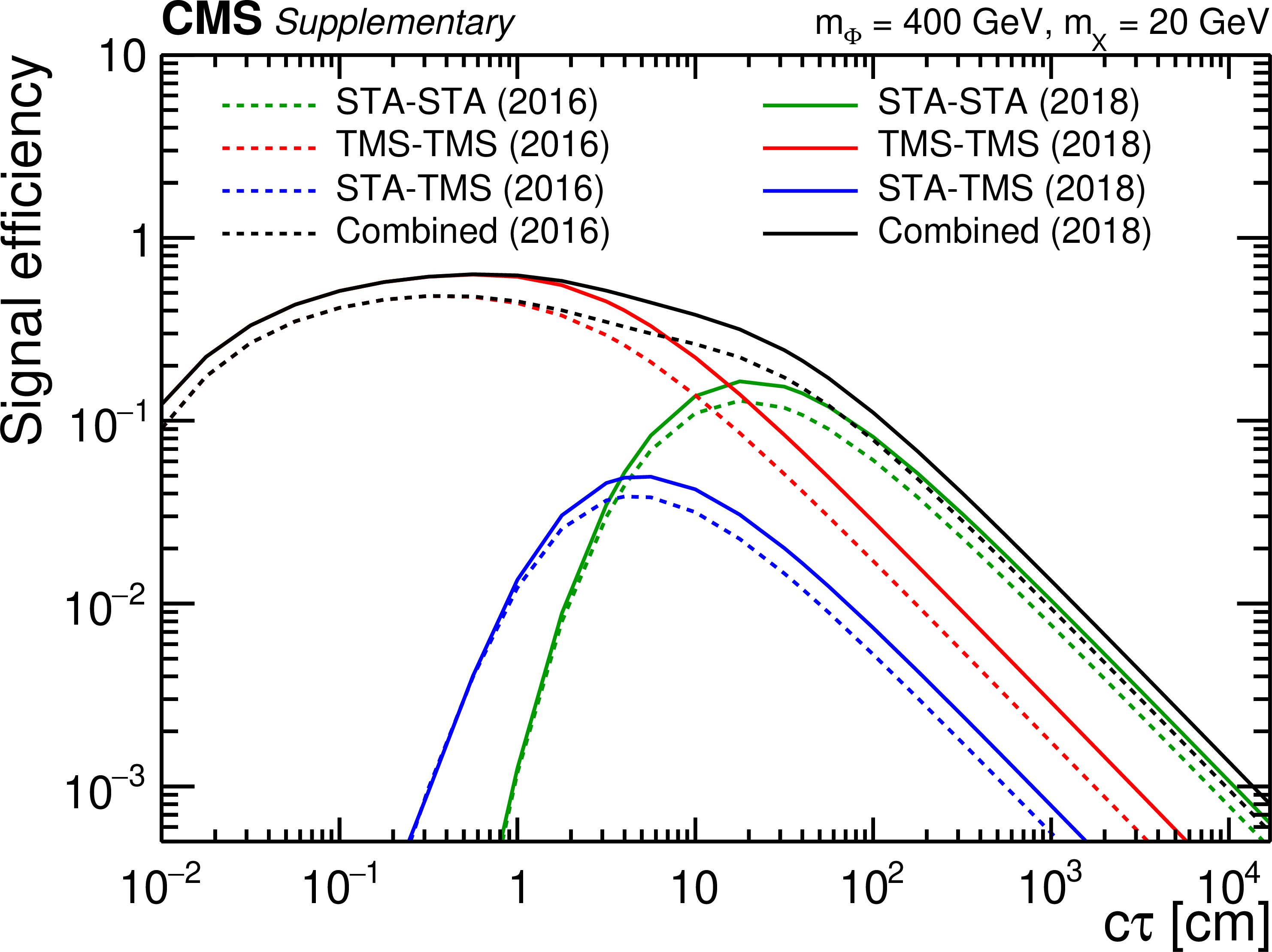
Additional Figure 3-a:
Overall signal efficiencies as a function of $ {c\tau} $ for the $ {\phi\to \mathrm{X} \mathrm{X} \to \mu \mu}+$ anything signal process with $ {m(\phi)} = $ 400 GeV (upper left: $ {m(\mathrm{X})} = $ 20 GeV, upper right: $ {m(\mathrm{X})} = $ 50 GeV, lower: $ {m(\mathrm{X})} = $ 150 GeV). Each plot shows efficiencies of the three dimuon categories, STA-STA (green), TMS-TMS (red), and STA-TMS (blue), as well as the combined efficiency (black). Each efficiency is computed as the ratio of the number of simulated signal events in which at least one dimuon candidate of a given type (or any type for the combined efficiency) passes all selection criteria (including the trigger) to the total number of simulated signal events. All efficiencies are corrected by the data-to-simulation scale factors described in the paper. The efficiencies in the 2016 and 2018 data sets are shown as dashed and solid curves, respectively. |
png pdf root |
Additional Figure 3-b:
Overall signal efficiencies as a function of $ {c\tau} $ for the $ {\phi\to \mathrm{X} \mathrm{X} \to \mu \mu}+$ anything signal process with $ {m(\phi)} = $ 400 GeV (upper left: $ {m(\mathrm{X})} = $ 20 GeV, upper right: $ {m(\mathrm{X})} = $ 50 GeV, lower: $ {m(\mathrm{X})} = $ 150 GeV). Each plot shows efficiencies of the three dimuon categories, STA-STA (green), TMS-TMS (red), and STA-TMS (blue), as well as the combined efficiency (black). Each efficiency is computed as the ratio of the number of simulated signal events in which at least one dimuon candidate of a given type (or any type for the combined efficiency) passes all selection criteria (including the trigger) to the total number of simulated signal events. All efficiencies are corrected by the data-to-simulation scale factors described in the paper. The efficiencies in the 2016 and 2018 data sets are shown as dashed and solid curves, respectively. |

png pdf root |
Additional Figure 3-c:
Overall signal efficiencies as a function of $ {c\tau} $ for the $ {\phi\to \mathrm{X} \mathrm{X} \to \mu \mu}+$ anything signal process with $ {m(\phi)} = $ 400 GeV (upper left: $ {m(\mathrm{X})} = $ 20 GeV, upper right: $ {m(\mathrm{X})} = $ 50 GeV, lower: $ {m(\mathrm{X})} = $ 150 GeV). Each plot shows efficiencies of the three dimuon categories, STA-STA (green), TMS-TMS (red), and STA-TMS (blue), as well as the combined efficiency (black). Each efficiency is computed as the ratio of the number of simulated signal events in which at least one dimuon candidate of a given type (or any type for the combined efficiency) passes all selection criteria (including the trigger) to the total number of simulated signal events. All efficiencies are corrected by the data-to-simulation scale factors described in the paper. The efficiencies in the 2016 and 2018 data sets are shown as dashed and solid curves, respectively. |

png pdf |
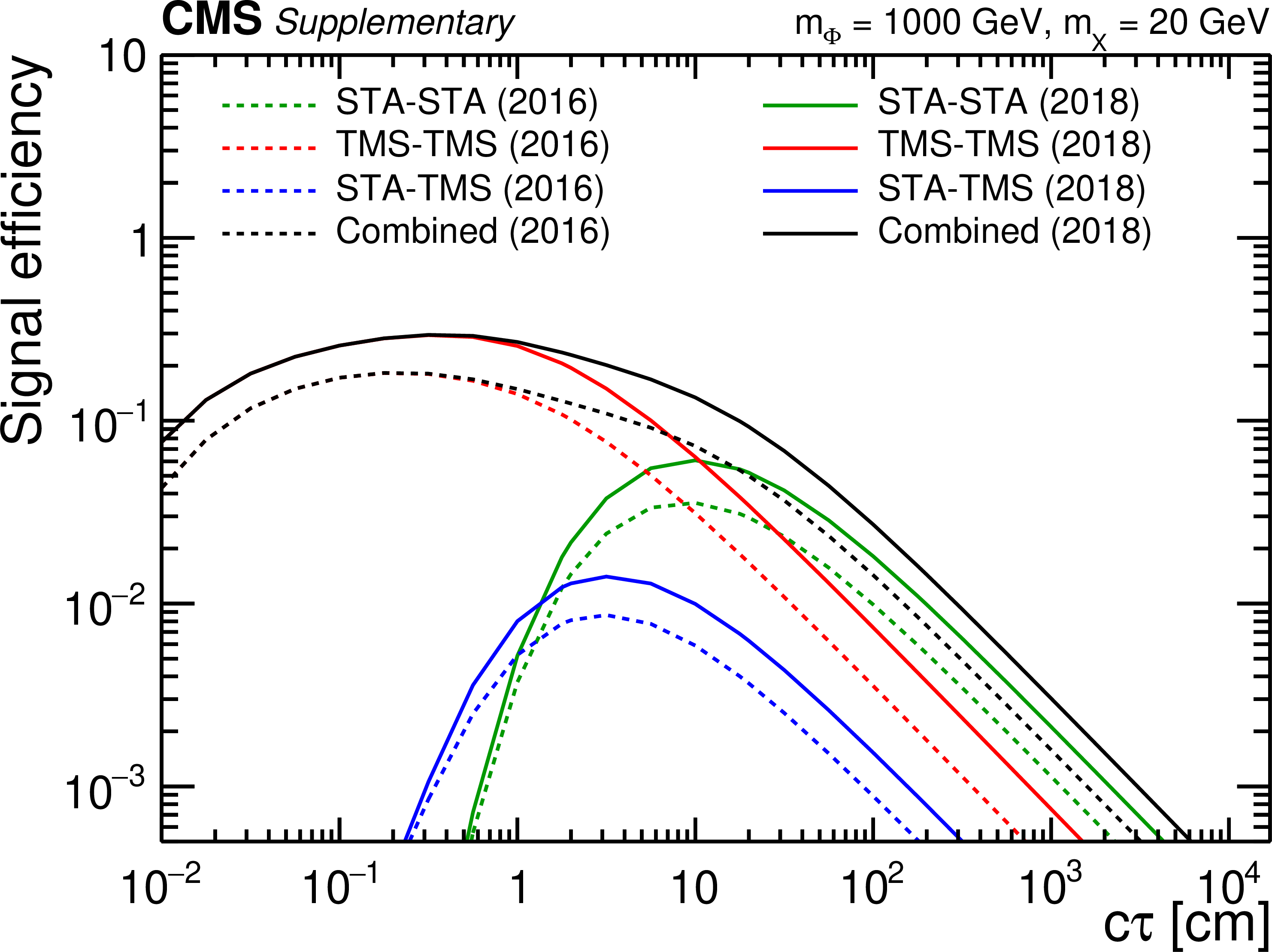
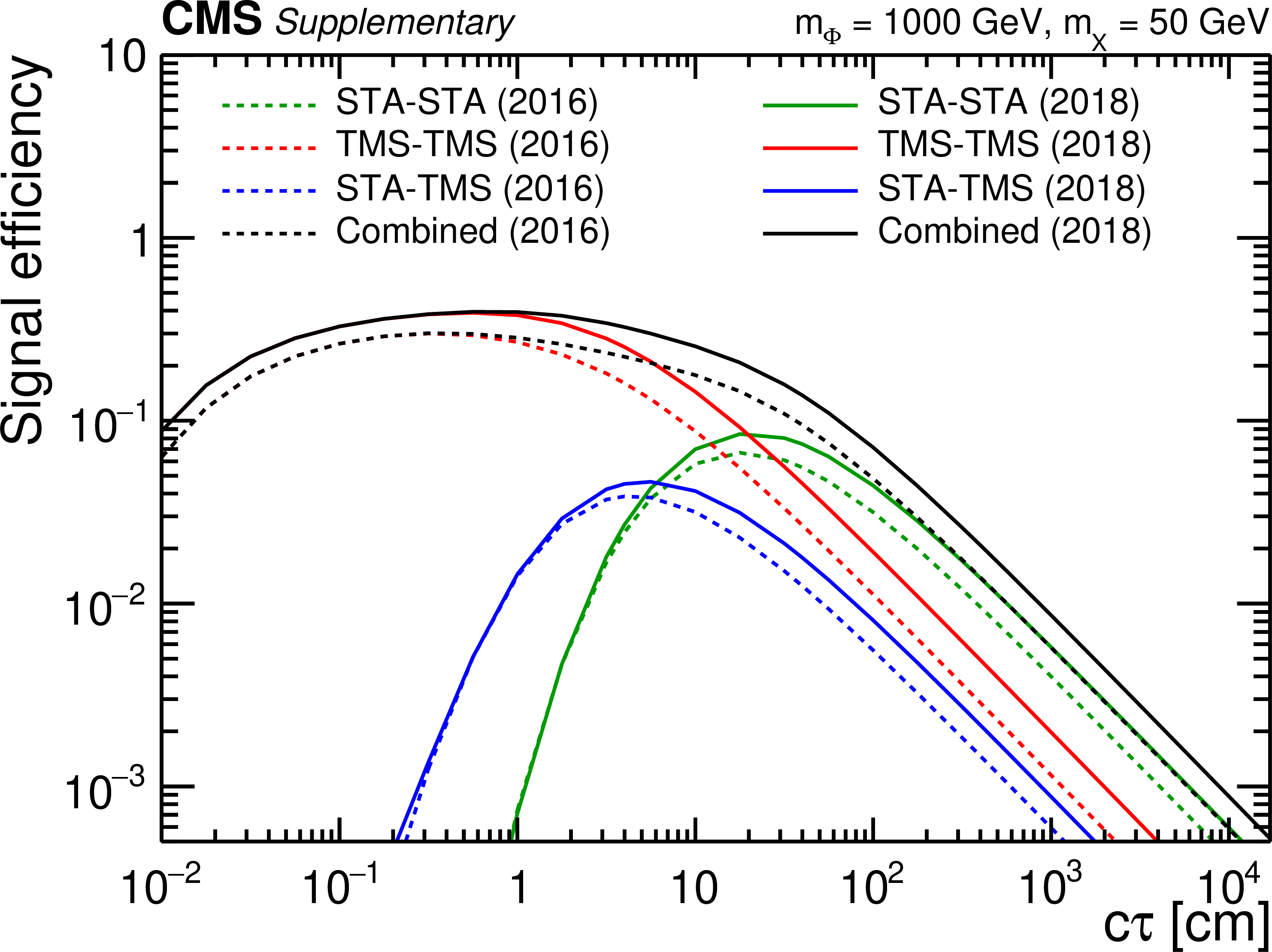
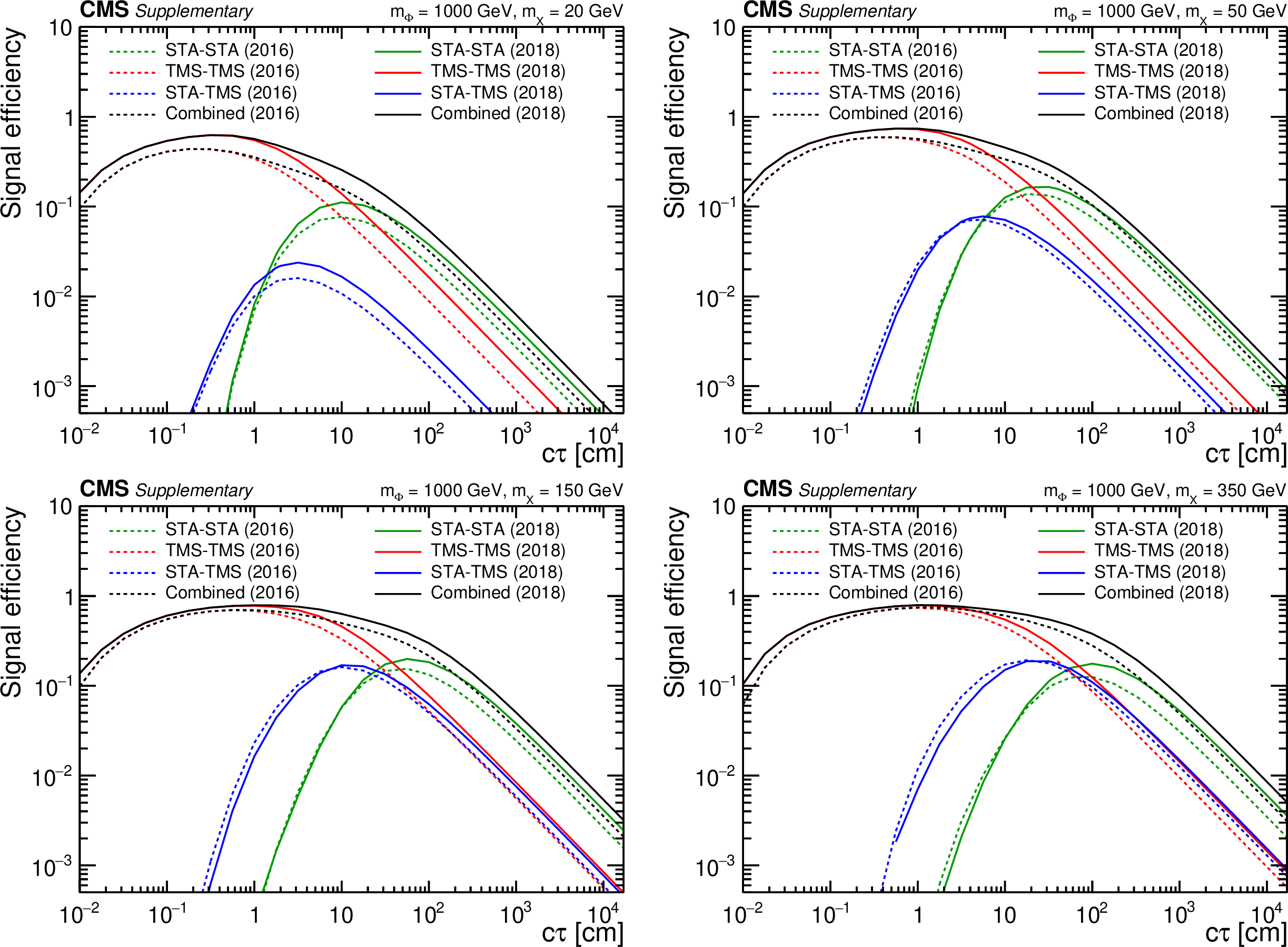
Additional Figure 4:
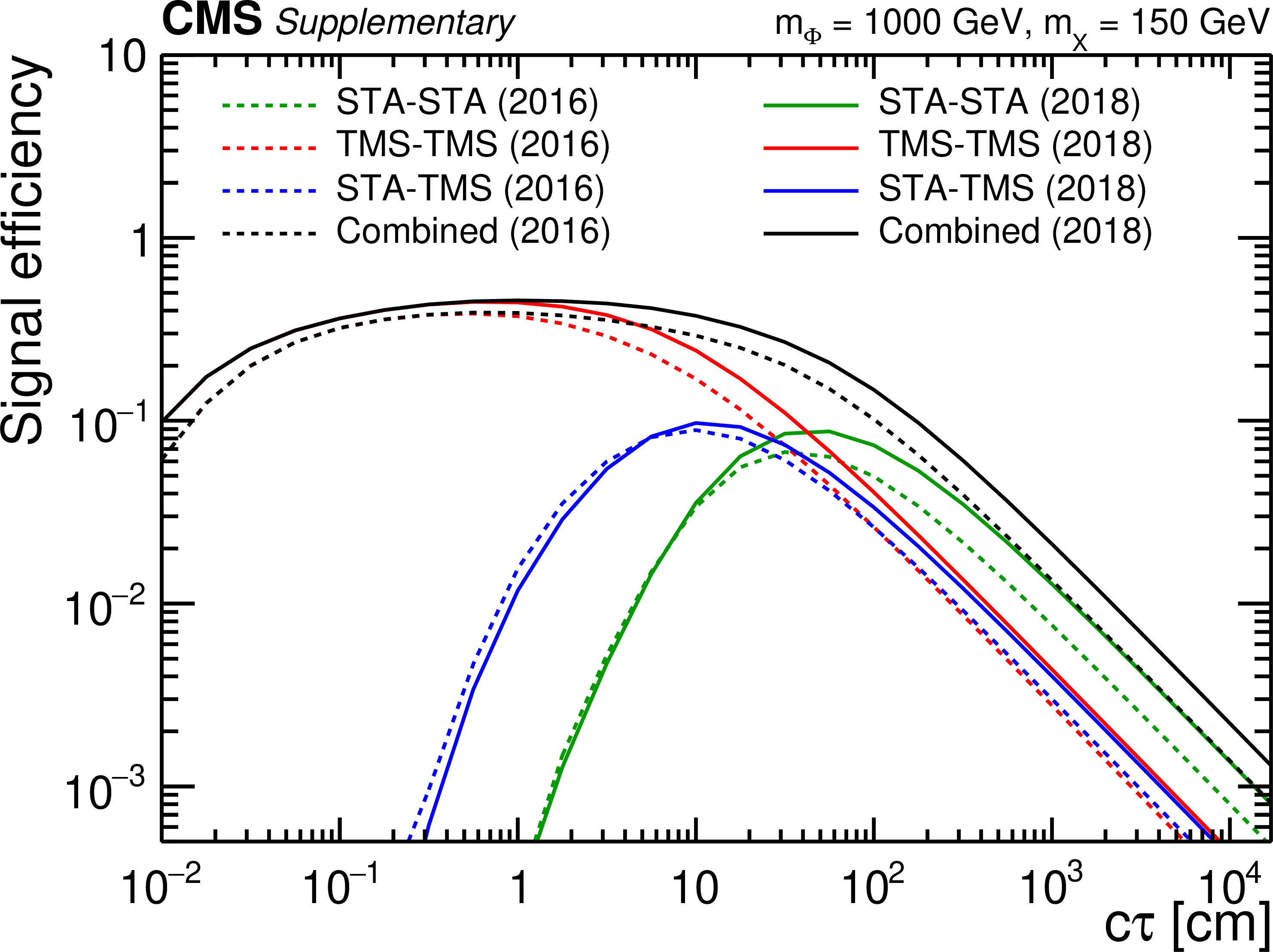
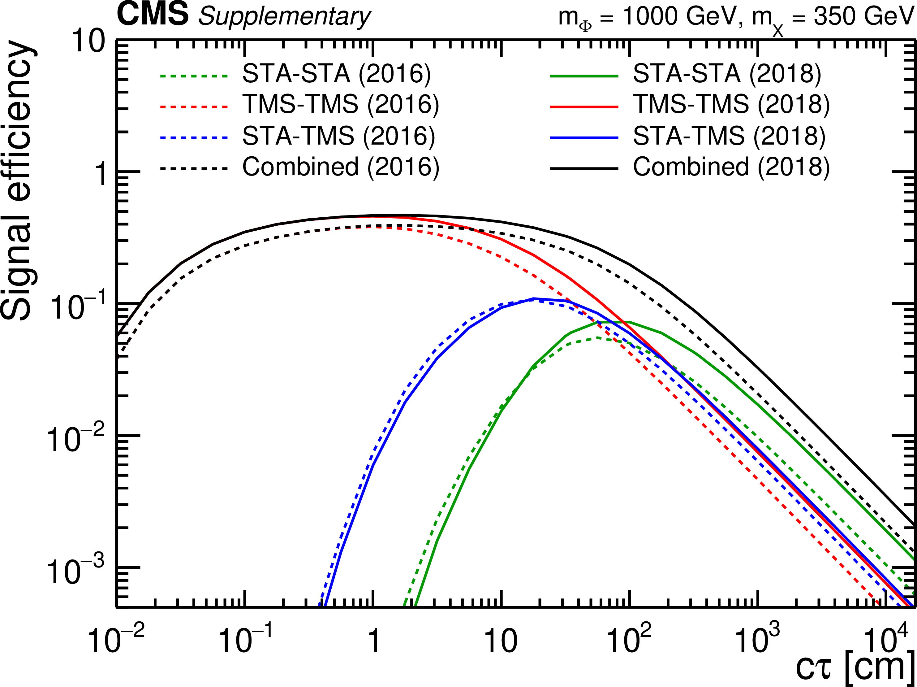
Overall signal efficiencies as a function of $ {c\tau} $ for the $ {\phi\to \mathrm{X} \mathrm{X} \to \mu \mu}+$ anything signal process with $ {m(\phi)} = $ 1 TeV (upper left: $ {m(\mathrm{X})} = $ 20 GeV, upper right: $ {m(\mathrm{X})} = $ 50 GeV, lower left: $ {m(\mathrm{X})} = $ 150 GeV, lower right: $ {m(\mathrm{X})} = $ 350 GeV). Each plot shows efficiencies of the three dimuon categories, STA-STA (green), TMS-TMS (red), and STA-TMS (blue), as well as the combined efficiency (black). Each efficiency is computed as the ratio of the number of simulated signal events in which at least one dimuon candidate of a given type (or any type for the combined efficiency) passes all selection criteria (including the trigger) to the total number of simulated signal events. All efficiencies are corrected by the data-to-simulation scale factors described in the paper. The efficiencies in the 2016 and 2018 data sets are shown as dashed and solid curves, respectively. |
png pdf root |
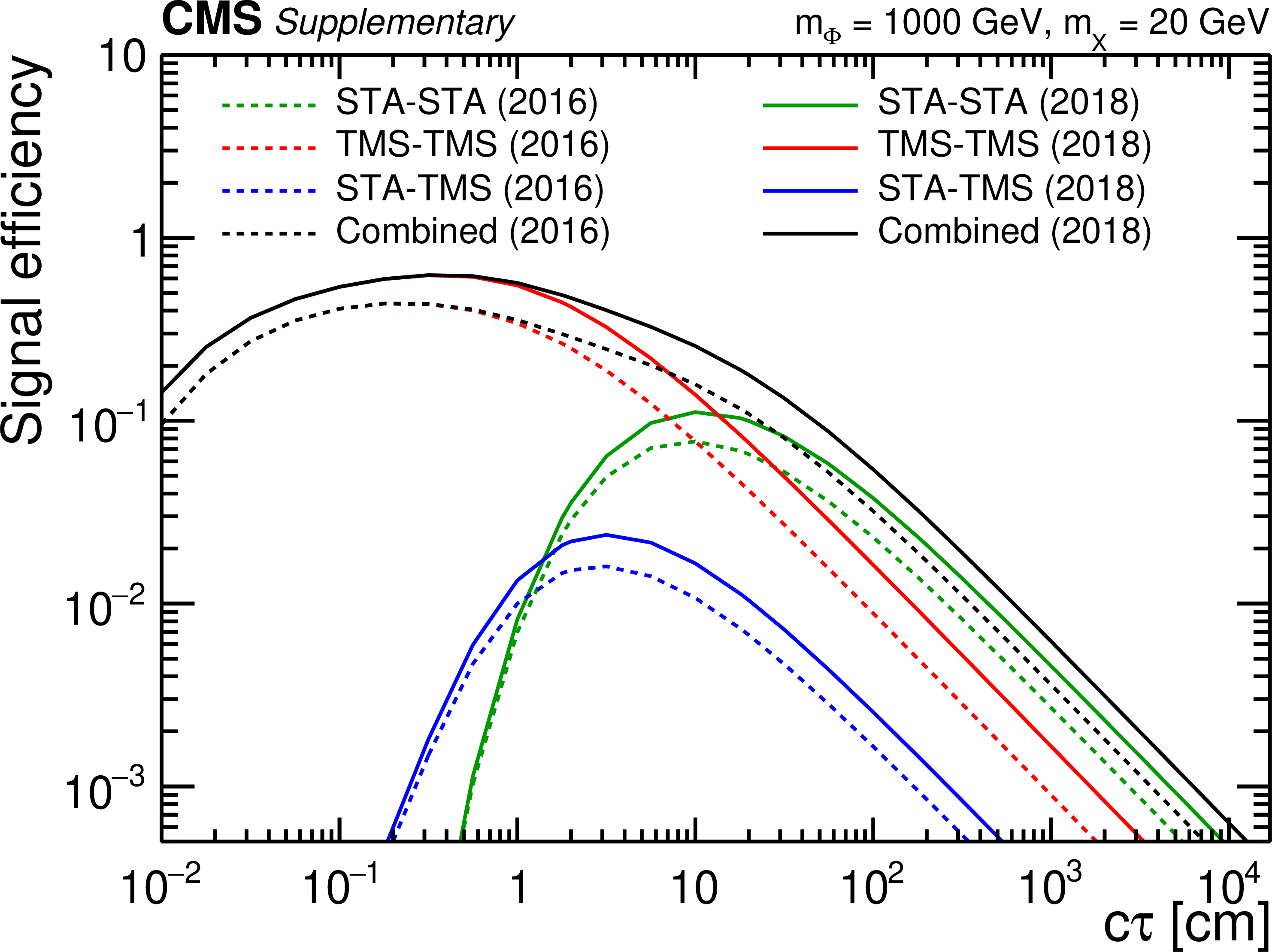
Additional Figure 4-a:
Overall signal efficiencies as a function of $ {c\tau} $ for the $ {\phi\to \mathrm{X} \mathrm{X} \to \mu \mu}+$ anything signal process with $ {m(\phi)} = $ 1 TeV (upper left: $ {m(\mathrm{X})} = $ 20 GeV, upper right: $ {m(\mathrm{X})} = $ 50 GeV, lower left: $ {m(\mathrm{X})} = $ 150 GeV, lower right: $ {m(\mathrm{X})} = $ 350 GeV). Each plot shows efficiencies of the three dimuon categories, STA-STA (green), TMS-TMS (red), and STA-TMS (blue), as well as the combined efficiency (black). Each efficiency is computed as the ratio of the number of simulated signal events in which at least one dimuon candidate of a given type (or any type for the combined efficiency) passes all selection criteria (including the trigger) to the total number of simulated signal events. All efficiencies are corrected by the data-to-simulation scale factors described in the paper. The efficiencies in the 2016 and 2018 data sets are shown as dashed and solid curves, respectively. |
png pdf root |
Additional Figure 4-b:
Overall signal efficiencies as a function of $ {c\tau} $ for the $ {\phi\to \mathrm{X} \mathrm{X} \to \mu \mu}+$ anything signal process with $ {m(\phi)} = $ 1 TeV (upper left: $ {m(\mathrm{X})} = $ 20 GeV, upper right: $ {m(\mathrm{X})} = $ 50 GeV, lower left: $ {m(\mathrm{X})} = $ 150 GeV, lower right: $ {m(\mathrm{X})} = $ 350 GeV). Each plot shows efficiencies of the three dimuon categories, STA-STA (green), TMS-TMS (red), and STA-TMS (blue), as well as the combined efficiency (black). Each efficiency is computed as the ratio of the number of simulated signal events in which at least one dimuon candidate of a given type (or any type for the combined efficiency) passes all selection criteria (including the trigger) to the total number of simulated signal events. All efficiencies are corrected by the data-to-simulation scale factors described in the paper. The efficiencies in the 2016 and 2018 data sets are shown as dashed and solid curves, respectively. |
png pdf root |
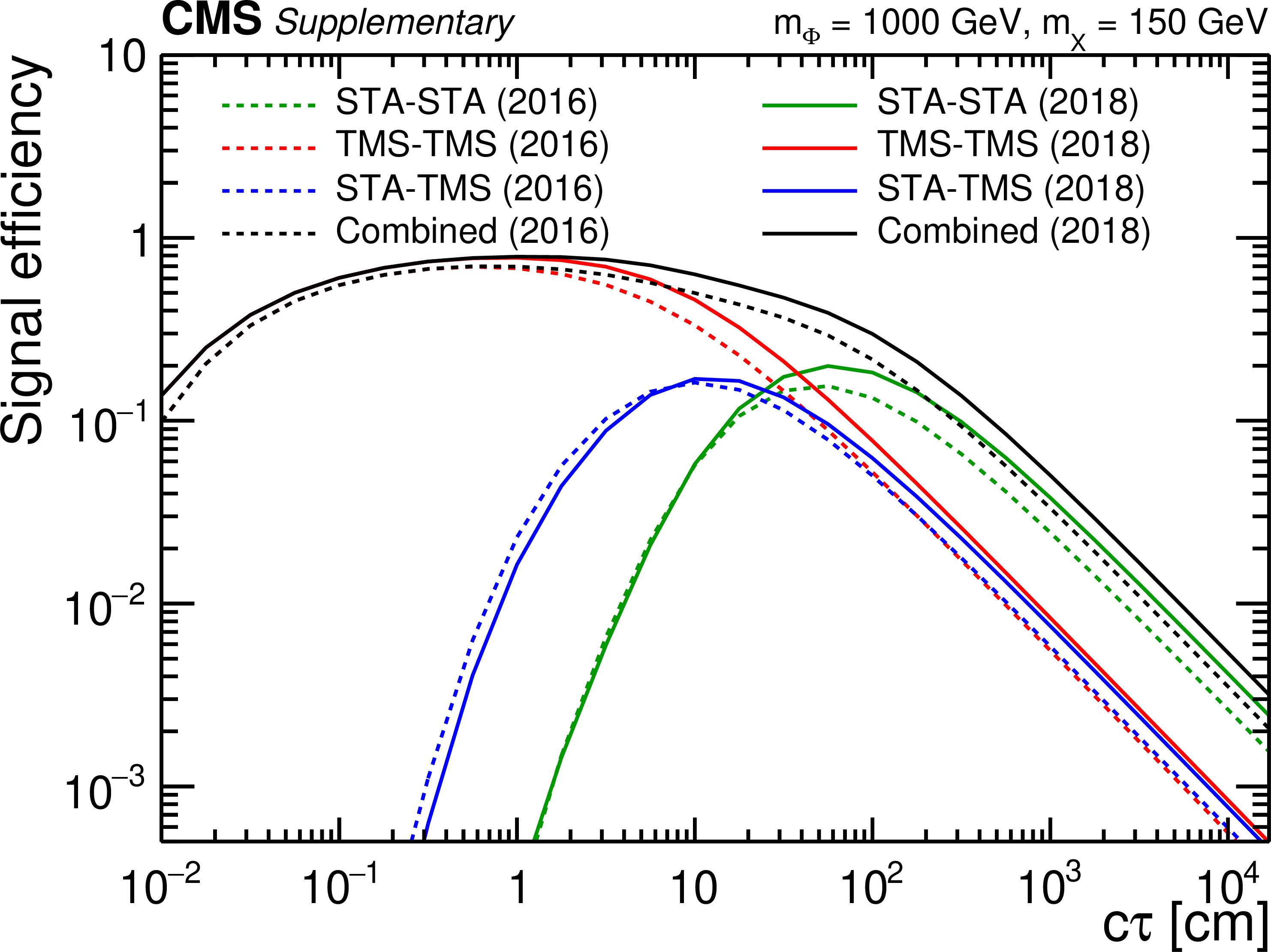
Additional Figure 4-c:
Overall signal efficiencies as a function of $ {c\tau} $ for the $ {\phi\to \mathrm{X} \mathrm{X} \to \mu \mu}+$ anything signal process with $ {m(\phi)} = $ 1 TeV (upper left: $ {m(\mathrm{X})} = $ 20 GeV, upper right: $ {m(\mathrm{X})} = $ 50 GeV, lower left: $ {m(\mathrm{X})} = $ 150 GeV, lower right: $ {m(\mathrm{X})} = $ 350 GeV). Each plot shows efficiencies of the three dimuon categories, STA-STA (green), TMS-TMS (red), and STA-TMS (blue), as well as the combined efficiency (black). Each efficiency is computed as the ratio of the number of simulated signal events in which at least one dimuon candidate of a given type (or any type for the combined efficiency) passes all selection criteria (including the trigger) to the total number of simulated signal events. All efficiencies are corrected by the data-to-simulation scale factors described in the paper. The efficiencies in the 2016 and 2018 data sets are shown as dashed and solid curves, respectively. |
png pdf root |
Additional Figure 4-d:
Overall signal efficiencies as a function of $ {c\tau} $ for the $ {\phi\to \mathrm{X} \mathrm{X} \to \mu \mu}+$ anything signal process with $ {m(\phi)} = $ 1 TeV (upper left: $ {m(\mathrm{X})} = $ 20 GeV, upper right: $ {m(\mathrm{X})} = $ 50 GeV, lower left: $ {m(\mathrm{X})} = $ 150 GeV, lower right: $ {m(\mathrm{X})} = $ 350 GeV). Each plot shows efficiencies of the three dimuon categories, STA-STA (green), TMS-TMS (red), and STA-TMS (blue), as well as the combined efficiency (black). Each efficiency is computed as the ratio of the number of simulated signal events in which at least one dimuon candidate of a given type (or any type for the combined efficiency) passes all selection criteria (including the trigger) to the total number of simulated signal events. All efficiencies are corrected by the data-to-simulation scale factors described in the paper. The efficiencies in the 2016 and 2018 data sets are shown as dashed and solid curves, respectively. |

png pdf |
Additional Figure 5:
Overall signal efficiencies as a function of $ {c\tau} $ for the $ {\phi\to \mathrm{X} \mathrm{X} \to 4\mu} $ signal process with $ {m(\phi)} = $ 125 GeV (left: $ {m(\mathrm{X})} = $ 20 GeV, right: $ {m(\mathrm{X})} = $ 50 GeV). Each plot shows efficiencies of the three dimuon categories, STA-STA (green), TMS-TMS (red), and STA-TMS (blue), as well as the combined efficiency (black). Each efficiency is computed as the ratio of the number of simulated signal events in which at least one dimuon candidate of a given type (or any type for the combined efficiency) passes all selection criteria (including the trigger) to the total number of simulated signal events. All efficiencies are corrected by the data-to-simulation scale factors described in the paper. The efficiencies in the 2016 and 2018 data sets are shown as dashed and solid curves, respectively. |
png pdf root |
Additional Figure 5-a:
Overall signal efficiencies as a function of $ {c\tau} $ for the $ {\phi\to \mathrm{X} \mathrm{X} \to 4\mu} $ signal process with $ {m(\phi)} = $ 125 GeV (left: $ {m(\mathrm{X})} = $ 20 GeV, right: $ {m(\mathrm{X})} = $ 50 GeV). Each plot shows efficiencies of the three dimuon categories, STA-STA (green), TMS-TMS (red), and STA-TMS (blue), as well as the combined efficiency (black). Each efficiency is computed as the ratio of the number of simulated signal events in which at least one dimuon candidate of a given type (or any type for the combined efficiency) passes all selection criteria (including the trigger) to the total number of simulated signal events. All efficiencies are corrected by the data-to-simulation scale factors described in the paper. The efficiencies in the 2016 and 2018 data sets are shown as dashed and solid curves, respectively. |
png pdf root |
Additional Figure 5-b:
Overall signal efficiencies as a function of $ {c\tau} $ for the $ {\phi\to \mathrm{X} \mathrm{X} \to 4\mu} $ signal process with $ {m(\phi)} = $ 125 GeV (left: $ {m(\mathrm{X})} = $ 20 GeV, right: $ {m(\mathrm{X})} = $ 50 GeV). Each plot shows efficiencies of the three dimuon categories, STA-STA (green), TMS-TMS (red), and STA-TMS (blue), as well as the combined efficiency (black). Each efficiency is computed as the ratio of the number of simulated signal events in which at least one dimuon candidate of a given type (or any type for the combined efficiency) passes all selection criteria (including the trigger) to the total number of simulated signal events. All efficiencies are corrected by the data-to-simulation scale factors described in the paper. The efficiencies in the 2016 and 2018 data sets are shown as dashed and solid curves, respectively. |
png pdf |
Additional Figure 6:
Overall signal efficiencies as a function of $ {c\tau} $ for the $ {\phi\to \mathrm{X} \mathrm{X} \to 4\mu} $ signal process with $ {m(\phi)} = $ 200 GeV (left: $ {m(\mathrm{X})} = $ 20 GeV, right: $ {m(\mathrm{X})} = $ 50 GeV). Each plot shows efficiencies of the three dimuon categories, STA-STA (green), TMS-TMS (red), and STA-TMS (blue), as well as the combined efficiency (black). Each efficiency is computed as the ratio of the number of simulated signal events in which at least one dimuon candidate of a given type (or any type for the combined efficiency) passes all selection criteria (including the trigger) to the total number of simulated signal events. All efficiencies are corrected by the data-to-simulation scale factors described in the paper. The efficiencies in the 2016 and 2018 data sets are shown as dashed and solid curves, respectively. |

png pdf root |
Additional Figure 6-a:
Overall signal efficiencies as a function of $ {c\tau} $ for the $ {\phi\to \mathrm{X} \mathrm{X} \to 4\mu} $ signal process with $ {m(\phi)} = $ 200 GeV (left: $ {m(\mathrm{X})} = $ 20 GeV, right: $ {m(\mathrm{X})} = $ 50 GeV). Each plot shows efficiencies of the three dimuon categories, STA-STA (green), TMS-TMS (red), and STA-TMS (blue), as well as the combined efficiency (black). Each efficiency is computed as the ratio of the number of simulated signal events in which at least one dimuon candidate of a given type (or any type for the combined efficiency) passes all selection criteria (including the trigger) to the total number of simulated signal events. All efficiencies are corrected by the data-to-simulation scale factors described in the paper. The efficiencies in the 2016 and 2018 data sets are shown as dashed and solid curves, respectively. |
png pdf root |
Additional Figure 6-b:
Overall signal efficiencies as a function of $ {c\tau} $ for the $ {\phi\to \mathrm{X} \mathrm{X} \to 4\mu} $ signal process with $ {m(\phi)} = $ 200 GeV (left: $ {m(\mathrm{X})} = $ 20 GeV, right: $ {m(\mathrm{X})} = $ 50 GeV). Each plot shows efficiencies of the three dimuon categories, STA-STA (green), TMS-TMS (red), and STA-TMS (blue), as well as the combined efficiency (black). Each efficiency is computed as the ratio of the number of simulated signal events in which at least one dimuon candidate of a given type (or any type for the combined efficiency) passes all selection criteria (including the trigger) to the total number of simulated signal events. All efficiencies are corrected by the data-to-simulation scale factors described in the paper. The efficiencies in the 2016 and 2018 data sets are shown as dashed and solid curves, respectively. |
png pdf |
Additional Figure 7:
Overall signal efficiencies as a function of $ {c\tau} $ for the $ {\phi\to \mathrm{X} \mathrm{X} \to 4\mu} $ signal process with $ {m(\phi)} = $ 400 GeV (upper left: $ {m(\mathrm{X})} = $ 20 GeV, upper right: $ {m(\mathrm{X})} = $ 50 GeV, lower: $ {m(\mathrm{X})} = $ 150 GeV). Each plot shows efficiencies of the three dimuon categories, STA-STA (green), TMS-TMS (red), and STA-TMS (blue), as well as the combined efficiency (black). Each efficiency is computed as the ratio of the number of simulated signal events in which at least one dimuon candidate of a given type (or any type for the combined efficiency) passes all selection criteria (including the trigger) to the total number of simulated signal events. All efficiencies are corrected by the data-to-simulation scale factors described in the paper. The efficiencies in the 2016 and 2018 data sets are shown as dashed and solid curves, respectively. |
png pdf root |
Additional Figure 7-a:
Overall signal efficiencies as a function of $ {c\tau} $ for the $ {\phi\to \mathrm{X} \mathrm{X} \to 4\mu} $ signal process with $ {m(\phi)} = $ 400 GeV (upper left: $ {m(\mathrm{X})} = $ 20 GeV, upper right: $ {m(\mathrm{X})} = $ 50 GeV, lower: $ {m(\mathrm{X})} = $ 150 GeV). Each plot shows efficiencies of the three dimuon categories, STA-STA (green), TMS-TMS (red), and STA-TMS (blue), as well as the combined efficiency (black). Each efficiency is computed as the ratio of the number of simulated signal events in which at least one dimuon candidate of a given type (or any type for the combined efficiency) passes all selection criteria (including the trigger) to the total number of simulated signal events. All efficiencies are corrected by the data-to-simulation scale factors described in the paper. The efficiencies in the 2016 and 2018 data sets are shown as dashed and solid curves, respectively. |

png pdf root |
Additional Figure 7-b:
Overall signal efficiencies as a function of $ {c\tau} $ for the $ {\phi\to \mathrm{X} \mathrm{X} \to 4\mu} $ signal process with $ {m(\phi)} = $ 400 GeV (upper left: $ {m(\mathrm{X})} = $ 20 GeV, upper right: $ {m(\mathrm{X})} = $ 50 GeV, lower: $ {m(\mathrm{X})} = $ 150 GeV). Each plot shows efficiencies of the three dimuon categories, STA-STA (green), TMS-TMS (red), and STA-TMS (blue), as well as the combined efficiency (black). Each efficiency is computed as the ratio of the number of simulated signal events in which at least one dimuon candidate of a given type (or any type for the combined efficiency) passes all selection criteria (including the trigger) to the total number of simulated signal events. All efficiencies are corrected by the data-to-simulation scale factors described in the paper. The efficiencies in the 2016 and 2018 data sets are shown as dashed and solid curves, respectively. |
png pdf root |
Additional Figure 7-c:
Overall signal efficiencies as a function of $ {c\tau} $ for the $ {\phi\to \mathrm{X} \mathrm{X} \to 4\mu} $ signal process with $ {m(\phi)} = $ 400 GeV (upper left: $ {m(\mathrm{X})} = $ 20 GeV, upper right: $ {m(\mathrm{X})} = $ 50 GeV, lower: $ {m(\mathrm{X})} = $ 150 GeV). Each plot shows efficiencies of the three dimuon categories, STA-STA (green), TMS-TMS (red), and STA-TMS (blue), as well as the combined efficiency (black). Each efficiency is computed as the ratio of the number of simulated signal events in which at least one dimuon candidate of a given type (or any type for the combined efficiency) passes all selection criteria (including the trigger) to the total number of simulated signal events. All efficiencies are corrected by the data-to-simulation scale factors described in the paper. The efficiencies in the 2016 and 2018 data sets are shown as dashed and solid curves, respectively. |
png pdf |
Additional Figure 8:
Overall signal efficiencies as a function of $ {c\tau} $ for the $ {\phi\to \mathrm{X} \mathrm{X} \to 4\mu} $ signal process with $ {m(\phi)} = $ 1 TeV (upper left: $ {m(\mathrm{X})} = $ 20 GeV, upper right: $ {m(\mathrm{X})} = $ 50 GeV, lower left: $ {m(\mathrm{X})} = $ 150 GeV, lower right: $ {m(\mathrm{X})} = $ 350 GeV). Each plot shows efficiencies of the three dimuon categories, STA-STA (green), TMS-TMS (red), and STA-TMS (blue), as well as the combined efficiency (black). Each efficiency is computed as the ratio of the number of simulated signal events in which at least one dimuon candidate of a given type (or any type for the combined efficiency) passes all selection criteria (including the trigger) to the total number of simulated signal events. All efficiencies are corrected by the data-to-simulation scale factors described in the paper. The efficiencies in the 2016 and 2018 data sets are shown as dashed and solid curves, respectively. |
png pdf root |
Additional Figure 8-a:
Overall signal efficiencies as a function of $ {c\tau} $ for the $ {\phi\to \mathrm{X} \mathrm{X} \to 4\mu} $ signal process with $ {m(\phi)} = $ 1 TeV (upper left: $ {m(\mathrm{X})} = $ 20 GeV, upper right: $ {m(\mathrm{X})} = $ 50 GeV, lower left: $ {m(\mathrm{X})} = $ 150 GeV, lower right: $ {m(\mathrm{X})} = $ 350 GeV). Each plot shows efficiencies of the three dimuon categories, STA-STA (green), TMS-TMS (red), and STA-TMS (blue), as well as the combined efficiency (black). Each efficiency is computed as the ratio of the number of simulated signal events in which at least one dimuon candidate of a given type (or any type for the combined efficiency) passes all selection criteria (including the trigger) to the total number of simulated signal events. All efficiencies are corrected by the data-to-simulation scale factors described in the paper. The efficiencies in the 2016 and 2018 data sets are shown as dashed and solid curves, respectively. |

png pdf root |
Additional Figure 8-b:
Overall signal efficiencies as a function of $ {c\tau} $ for the $ {\phi\to \mathrm{X} \mathrm{X} \to 4\mu} $ signal process with $ {m(\phi)} = $ 1 TeV (upper left: $ {m(\mathrm{X})} = $ 20 GeV, upper right: $ {m(\mathrm{X})} = $ 50 GeV, lower left: $ {m(\mathrm{X})} = $ 150 GeV, lower right: $ {m(\mathrm{X})} = $ 350 GeV). Each plot shows efficiencies of the three dimuon categories, STA-STA (green), TMS-TMS (red), and STA-TMS (blue), as well as the combined efficiency (black). Each efficiency is computed as the ratio of the number of simulated signal events in which at least one dimuon candidate of a given type (or any type for the combined efficiency) passes all selection criteria (including the trigger) to the total number of simulated signal events. All efficiencies are corrected by the data-to-simulation scale factors described in the paper. The efficiencies in the 2016 and 2018 data sets are shown as dashed and solid curves, respectively. |
png pdf root |
Additional Figure 8-c:
Overall signal efficiencies as a function of $ {c\tau} $ for the $ {\phi\to \mathrm{X} \mathrm{X} \to 4\mu} $ signal process with $ {m(\phi)} = $ 1 TeV (upper left: $ {m(\mathrm{X})} = $ 20 GeV, upper right: $ {m(\mathrm{X})} = $ 50 GeV, lower left: $ {m(\mathrm{X})} = $ 150 GeV, lower right: $ {m(\mathrm{X})} = $ 350 GeV). Each plot shows efficiencies of the three dimuon categories, STA-STA (green), TMS-TMS (red), and STA-TMS (blue), as well as the combined efficiency (black). Each efficiency is computed as the ratio of the number of simulated signal events in which at least one dimuon candidate of a given type (or any type for the combined efficiency) passes all selection criteria (including the trigger) to the total number of simulated signal events. All efficiencies are corrected by the data-to-simulation scale factors described in the paper. The efficiencies in the 2016 and 2018 data sets are shown as dashed and solid curves, respectively. |

png pdf root |
Additional Figure 8-d:
Overall signal efficiencies as a function of $ {c\tau} $ for the $ {\phi\to \mathrm{X} \mathrm{X} \to 4\mu} $ signal process with $ {m(\phi)} = $ 1 TeV (upper left: $ {m(\mathrm{X})} = $ 20 GeV, upper right: $ {m(\mathrm{X})} = $ 50 GeV, lower left: $ {m(\mathrm{X})} = $ 150 GeV, lower right: $ {m(\mathrm{X})} = $ 350 GeV). Each plot shows efficiencies of the three dimuon categories, STA-STA (green), TMS-TMS (red), and STA-TMS (blue), as well as the combined efficiency (black). Each efficiency is computed as the ratio of the number of simulated signal events in which at least one dimuon candidate of a given type (or any type for the combined efficiency) passes all selection criteria (including the trigger) to the total number of simulated signal events. All efficiencies are corrected by the data-to-simulation scale factors described in the paper. The efficiencies in the 2016 and 2018 data sets are shown as dashed and solid curves, respectively. |
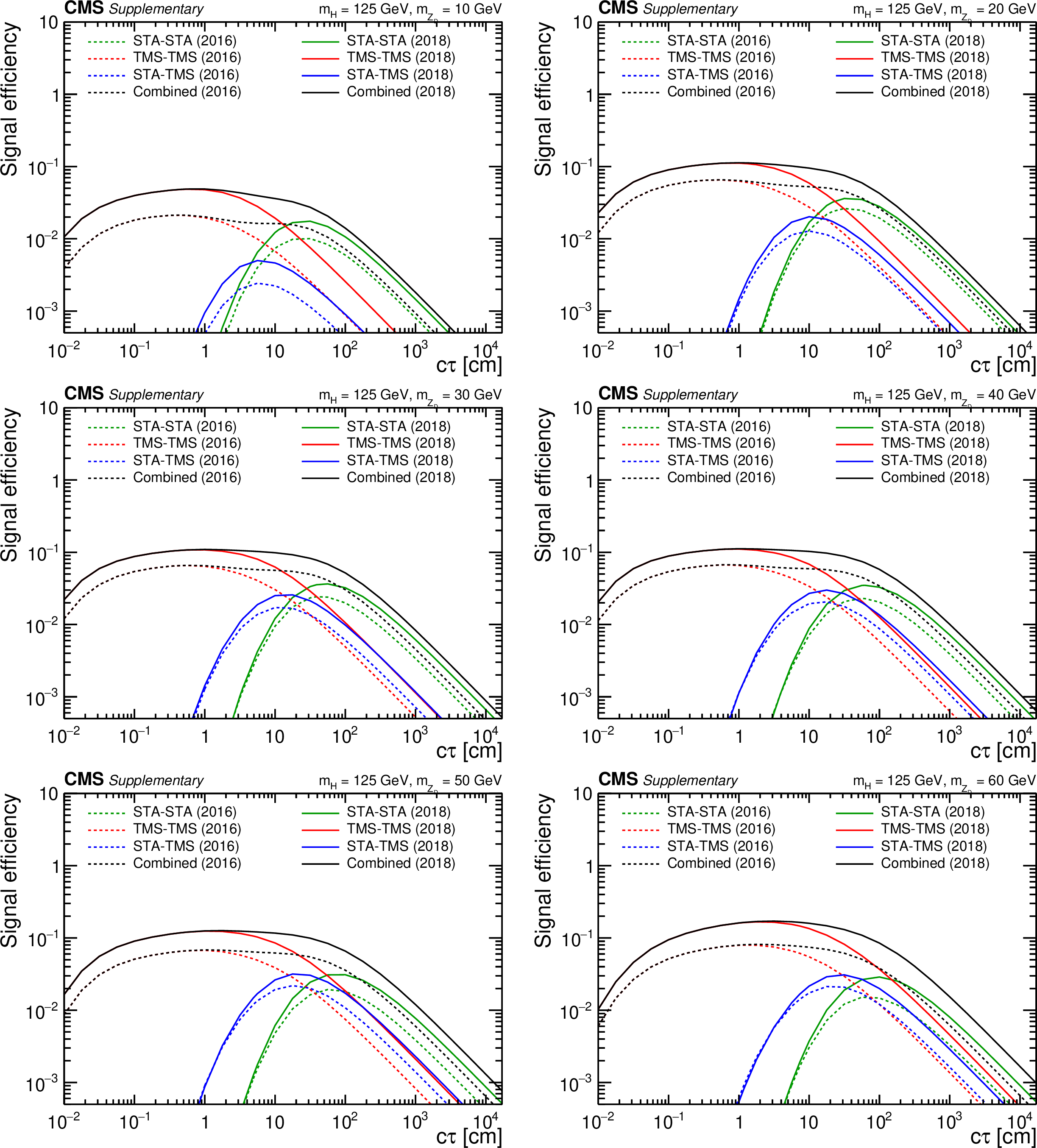
png pdf |
Additional Figure 9:
Overall signal efficiencies as a function of $ {c\tau} $ for the $\mathrm{H} \to \mathrm{Z} {\mathrm {_{D}}}\mathrm{Z} {\mathrm {_{D}}}\to \mu \mu + anything$ signal process with $ {m(\mathrm{H})} = $ 125 GeV, for $ {m(\mathrm{Z} {\mathrm {_{D}}})} $ ranging from 10 GeV (upper left) to 60 GeV (lower right). Each plot shows efficiencies of the three dimuon categories, STA-STA (green), TMS-TMS (red), and STA-TMS (blue), as well the combined efficiency (black). Each efficiency is computed as the ratio of the number of simulated signal events in which at least one dimuon candidate of a given type (or any type for the combined efficiency) passes all selection criteria (including the trigger) to the total number of simulated signal events. All efficiencies are corrected by the data-to-simulation scale factors described in the paper. The efficiencies in the 2016 and 2018 data sets are shown as dashed and solid curves, respectively. |
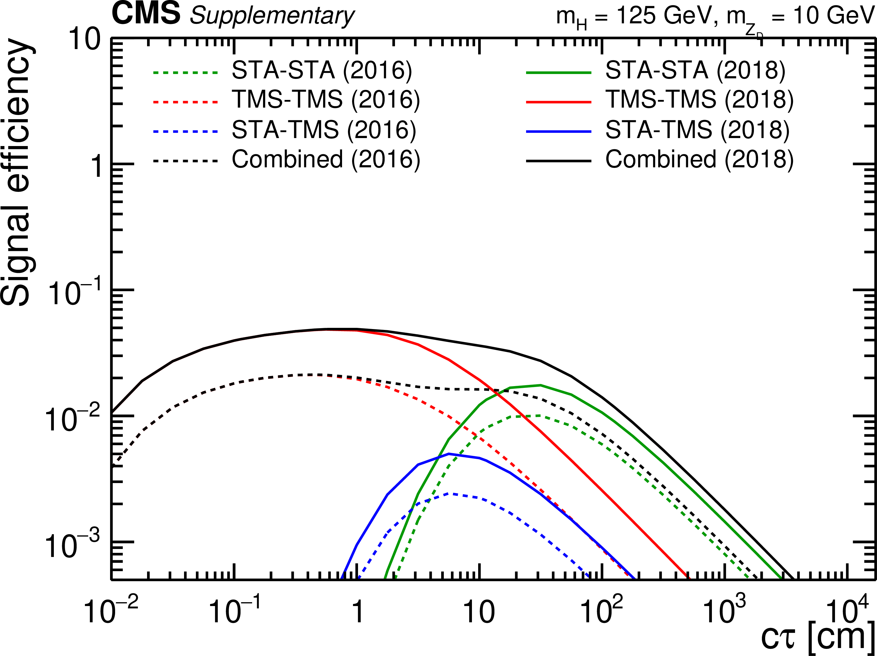
png pdf root |
Additional Figure 9-a:
Overall signal efficiencies as a function of $ {c\tau} $ for the $\mathrm{H} \to \mathrm{Z} {\mathrm {_{D}}}\mathrm{Z} {\mathrm {_{D}}}\to \mu \mu + anything$ signal process with $ {m(\mathrm{H})} = $ 125 GeV, for $ {m(\mathrm{Z} {\mathrm {_{D}}})} $ ranging from 10 GeV (upper left) to 60 GeV (lower right). Each plot shows efficiencies of the three dimuon categories, STA-STA (green), TMS-TMS (red), and STA-TMS (blue), as well the combined efficiency (black). Each efficiency is computed as the ratio of the number of simulated signal events in which at least one dimuon candidate of a given type (or any type for the combined efficiency) passes all selection criteria (including the trigger) to the total number of simulated signal events. All efficiencies are corrected by the data-to-simulation scale factors described in the paper. The efficiencies in the 2016 and 2018 data sets are shown as dashed and solid curves, respectively. |
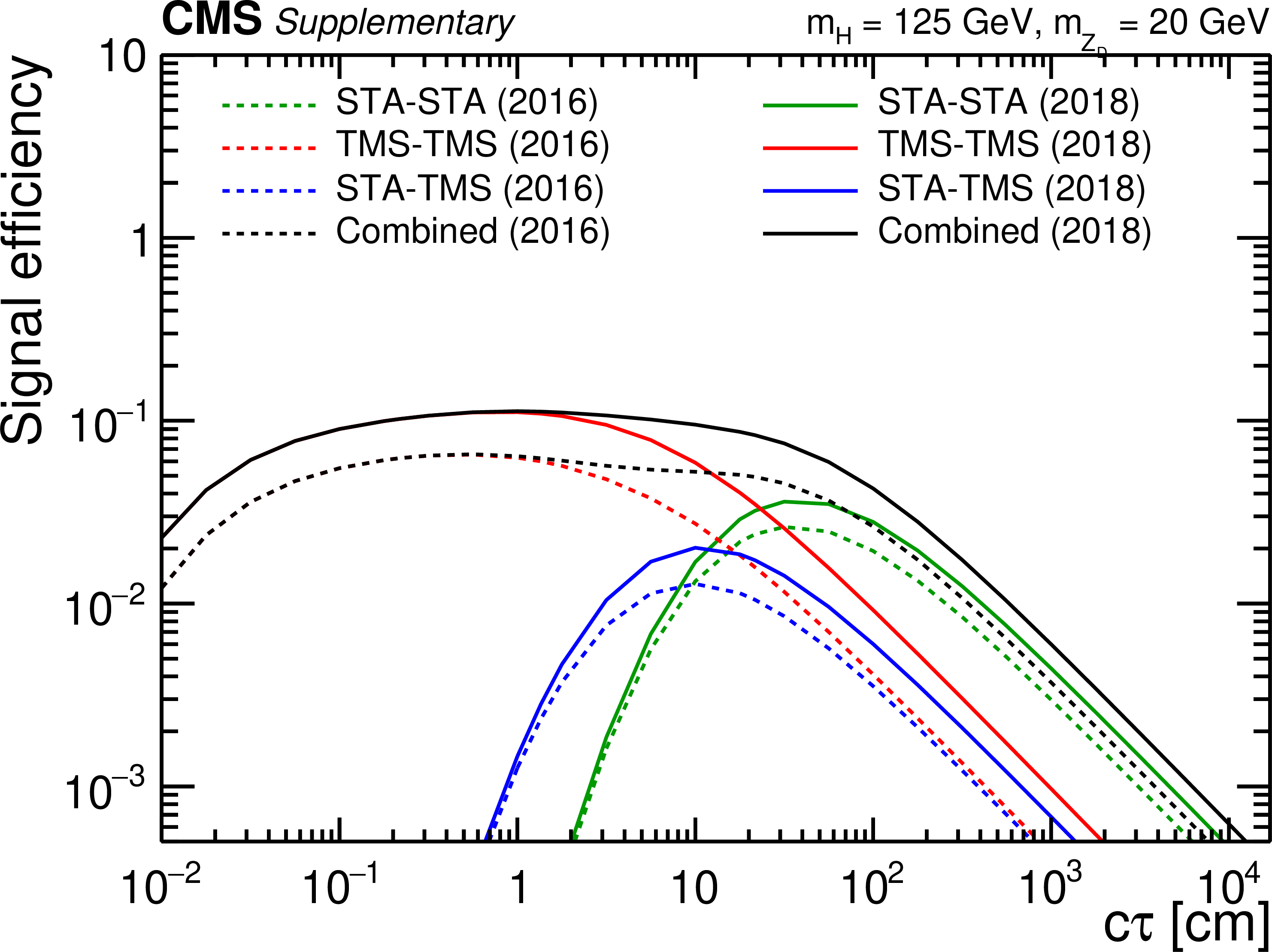
png pdf root |
Additional Figure 9-b:
Overall signal efficiencies as a function of $ {c\tau} $ for the $\mathrm{H} \to \mathrm{Z} {\mathrm {_{D}}}\mathrm{Z} {\mathrm {_{D}}}\to \mu \mu + anything$ signal process with $ {m(\mathrm{H})} = $ 125 GeV, for $ {m(\mathrm{Z} {\mathrm {_{D}}})} $ ranging from 10 GeV (upper left) to 60 GeV (lower right). Each plot shows efficiencies of the three dimuon categories, STA-STA (green), TMS-TMS (red), and STA-TMS (blue), as well the combined efficiency (black). Each efficiency is computed as the ratio of the number of simulated signal events in which at least one dimuon candidate of a given type (or any type for the combined efficiency) passes all selection criteria (including the trigger) to the total number of simulated signal events. All efficiencies are corrected by the data-to-simulation scale factors described in the paper. The efficiencies in the 2016 and 2018 data sets are shown as dashed and solid curves, respectively. |
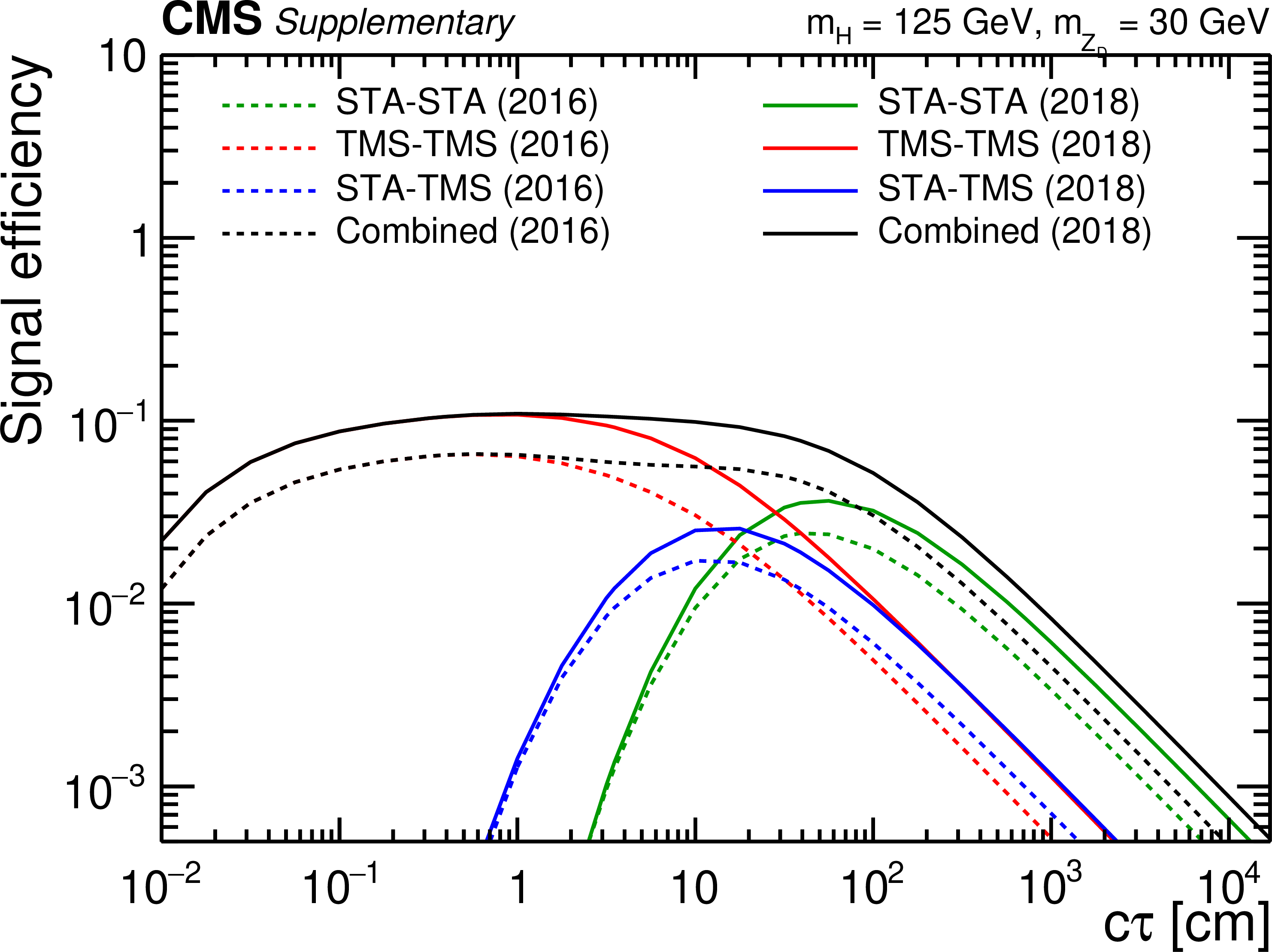
png pdf root |
Additional Figure 9-c:
Overall signal efficiencies as a function of $ {c\tau} $ for the $\mathrm{H} \to \mathrm{Z} {\mathrm {_{D}}}\mathrm{Z} {\mathrm {_{D}}}\to \mu \mu + anything$ signal process with $ {m(\mathrm{H})} = $ 125 GeV, for $ {m(\mathrm{Z} {\mathrm {_{D}}})} $ ranging from 10 GeV (upper left) to 60 GeV (lower right). Each plot shows efficiencies of the three dimuon categories, STA-STA (green), TMS-TMS (red), and STA-TMS (blue), as well the combined efficiency (black). Each efficiency is computed as the ratio of the number of simulated signal events in which at least one dimuon candidate of a given type (or any type for the combined efficiency) passes all selection criteria (including the trigger) to the total number of simulated signal events. All efficiencies are corrected by the data-to-simulation scale factors described in the paper. The efficiencies in the 2016 and 2018 data sets are shown as dashed and solid curves, respectively. |
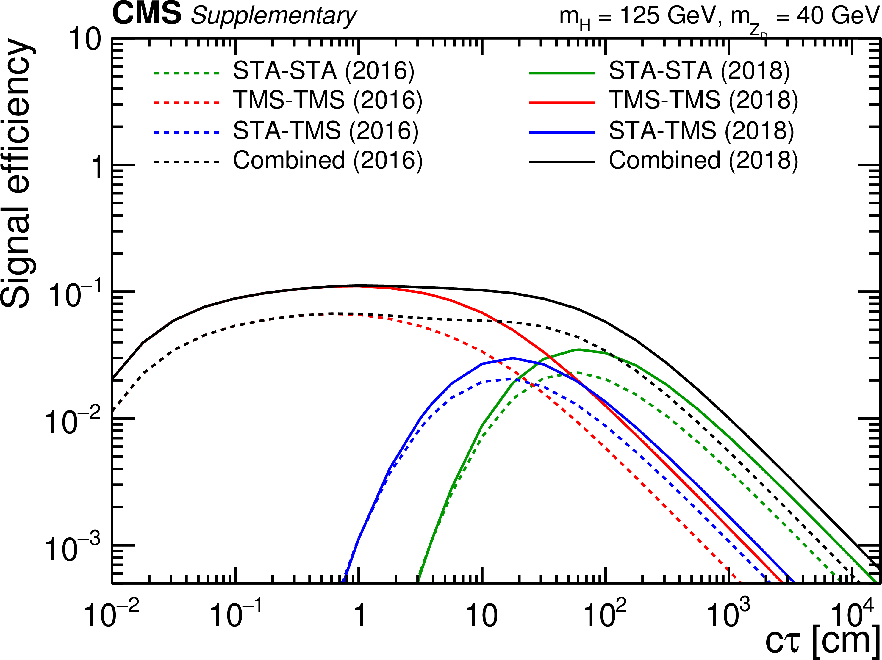
png pdf root |
Additional Figure 9-d:
Overall signal efficiencies as a function of $ {c\tau} $ for the $\mathrm{H} \to \mathrm{Z} {\mathrm {_{D}}}\mathrm{Z} {\mathrm {_{D}}}\to \mu \mu + anything$ signal process with $ {m(\mathrm{H})} = $ 125 GeV, for $ {m(\mathrm{Z} {\mathrm {_{D}}})} $ ranging from 10 GeV (upper left) to 60 GeV (lower right). Each plot shows efficiencies of the three dimuon categories, STA-STA (green), TMS-TMS (red), and STA-TMS (blue), as well the combined efficiency (black). Each efficiency is computed as the ratio of the number of simulated signal events in which at least one dimuon candidate of a given type (or any type for the combined efficiency) passes all selection criteria (including the trigger) to the total number of simulated signal events. All efficiencies are corrected by the data-to-simulation scale factors described in the paper. The efficiencies in the 2016 and 2018 data sets are shown as dashed and solid curves, respectively. |

png pdf root |
Additional Figure 9-e:
Overall signal efficiencies as a function of $ {c\tau} $ for the $\mathrm{H} \to \mathrm{Z} {\mathrm {_{D}}}\mathrm{Z} {\mathrm {_{D}}}\to \mu \mu + anything$ signal process with $ {m(\mathrm{H})} = $ 125 GeV, for $ {m(\mathrm{Z} {\mathrm {_{D}}})} $ ranging from 10 GeV (upper left) to 60 GeV (lower right). Each plot shows efficiencies of the three dimuon categories, STA-STA (green), TMS-TMS (red), and STA-TMS (blue), as well the combined efficiency (black). Each efficiency is computed as the ratio of the number of simulated signal events in which at least one dimuon candidate of a given type (or any type for the combined efficiency) passes all selection criteria (including the trigger) to the total number of simulated signal events. All efficiencies are corrected by the data-to-simulation scale factors described in the paper. The efficiencies in the 2016 and 2018 data sets are shown as dashed and solid curves, respectively. |
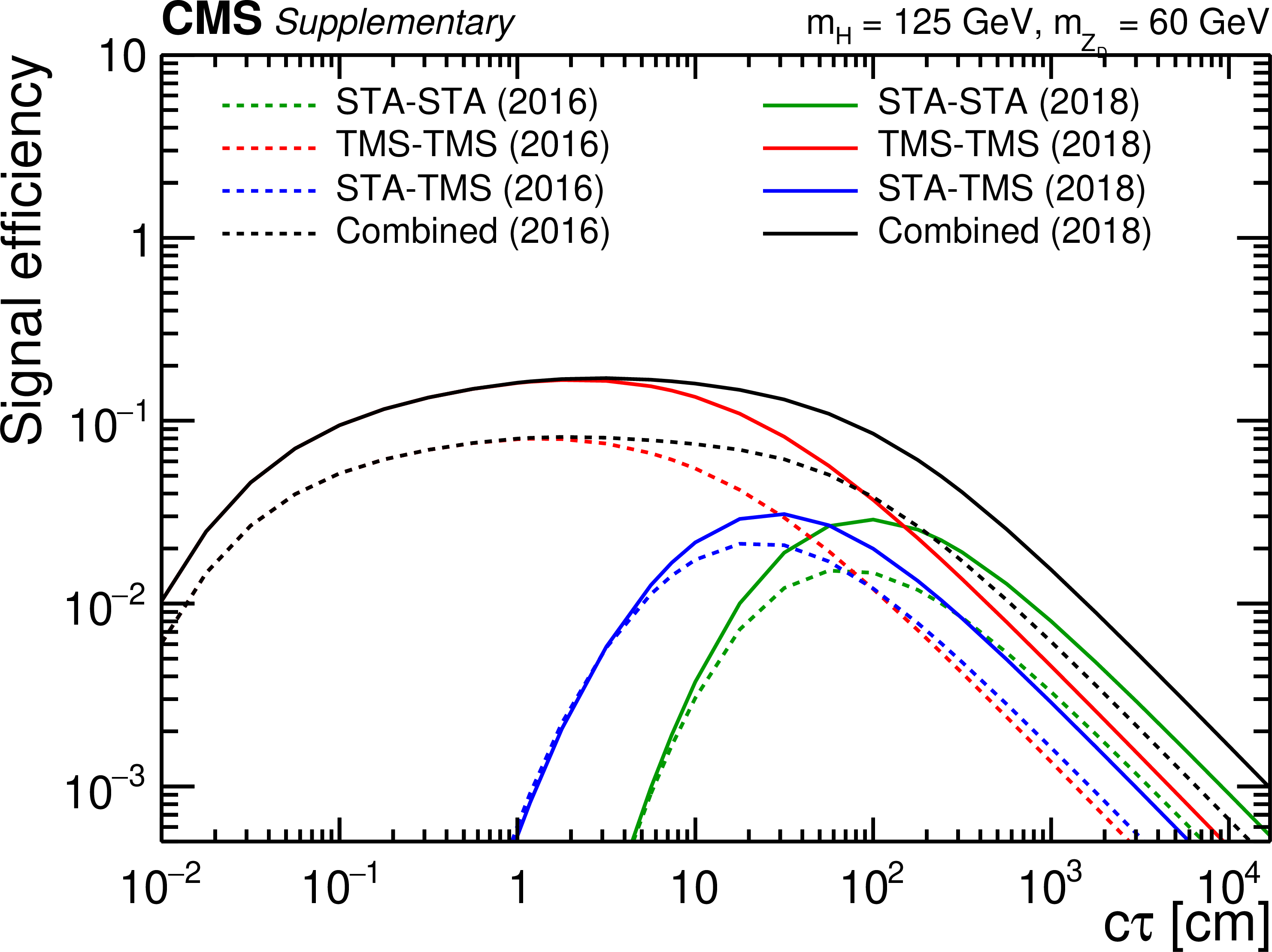
png pdf root |
Additional Figure 9-f:
Overall signal efficiencies as a function of $ {c\tau} $ for the $\mathrm{H} \to \mathrm{Z} {\mathrm {_{D}}}\mathrm{Z} {\mathrm {_{D}}}\to \mu \mu + anything$ signal process with $ {m(\mathrm{H})} = $ 125 GeV, for $ {m(\mathrm{Z} {\mathrm {_{D}}})} $ ranging from 10 GeV (upper left) to 60 GeV (lower right). Each plot shows efficiencies of the three dimuon categories, STA-STA (green), TMS-TMS (red), and STA-TMS (blue), as well the combined efficiency (black). Each efficiency is computed as the ratio of the number of simulated signal events in which at least one dimuon candidate of a given type (or any type for the combined efficiency) passes all selection criteria (including the trigger) to the total number of simulated signal events. All efficiencies are corrected by the data-to-simulation scale factors described in the paper. The efficiencies in the 2016 and 2018 data sets are shown as dashed and solid curves, respectively. |
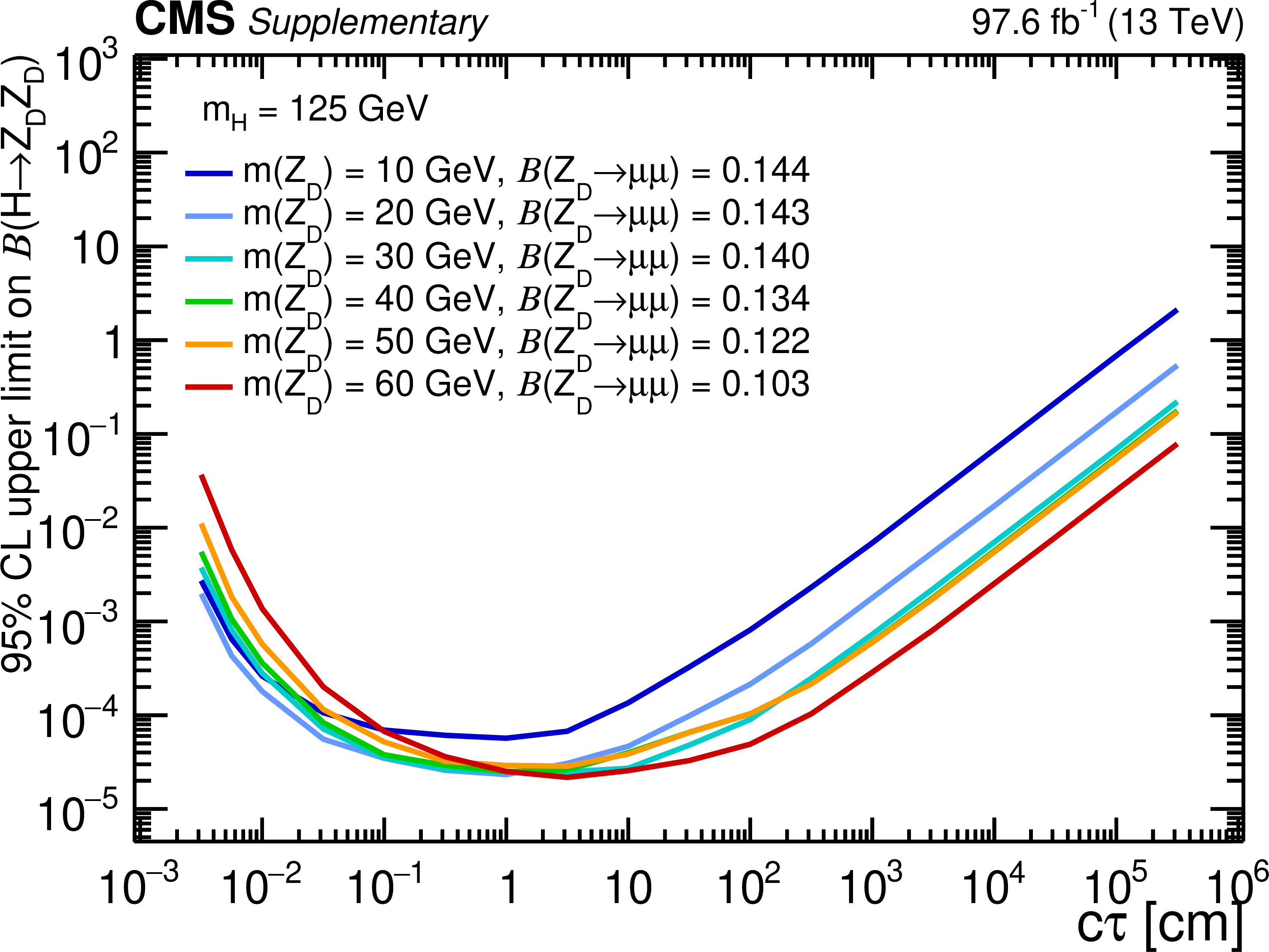
png pdf root |
Additional Figure 10:
The 95% CL combined observed upper limits on $\mathcal {B}(\mathrm{H} \to \mathrm{Z} {\mathrm {_{D}}}\mathrm{Z} {\mathrm {_{D}}})$ as a function of $ {c\tau} (\mathrm{Z} {\mathrm {_{D}}})$ in the HAHM model, for $ {m(\mathrm{Z} {\mathrm {_{D}}})} $ ranging from 10 to 60 GeV. |
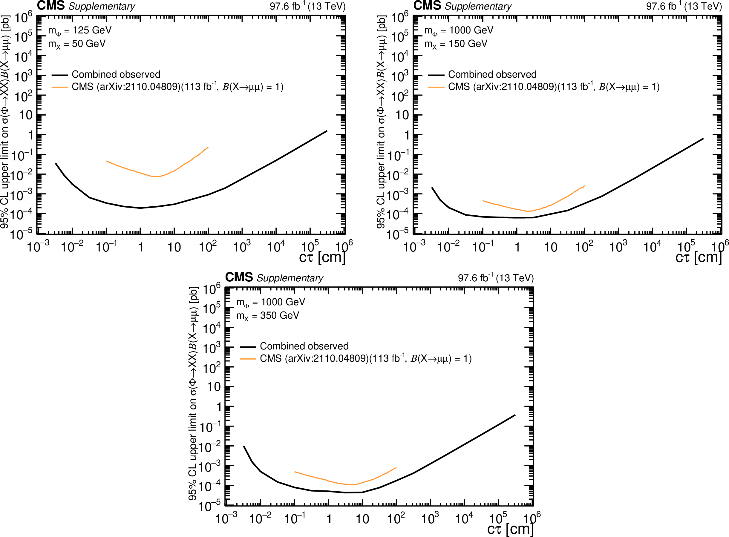
png pdf |
Additional Figure 11:
The 95% CL observed upper limits on $\sigma (\phi\to \mathrm{X} \mathrm{X})\mathcal {B}(\mathrm{X} \to \mu \mu)$ as a function of $ {c\tau} (\mathrm{X})$ in the heavy scalar model, for $ {m(\phi)} = $ 125 GeV and $ {m(\mathrm{X})} = $ 50 GeV (upper left), $ {m(\phi)} = $ 1 TeV and $ {m(\mathrm{X})} = $ 150 GeV (upper right), and $ {m(\phi)} = $ 1 TeV and $ {m(\mathrm{X})} = $ 350 GeV (lower). The limits obtained in this analysis (in black) are compared to the results obtained in the CMS search for LLPs decaying to leptons with large impact parameter (Eur. Phys. J. C 82 (2022) 153, in orange). |
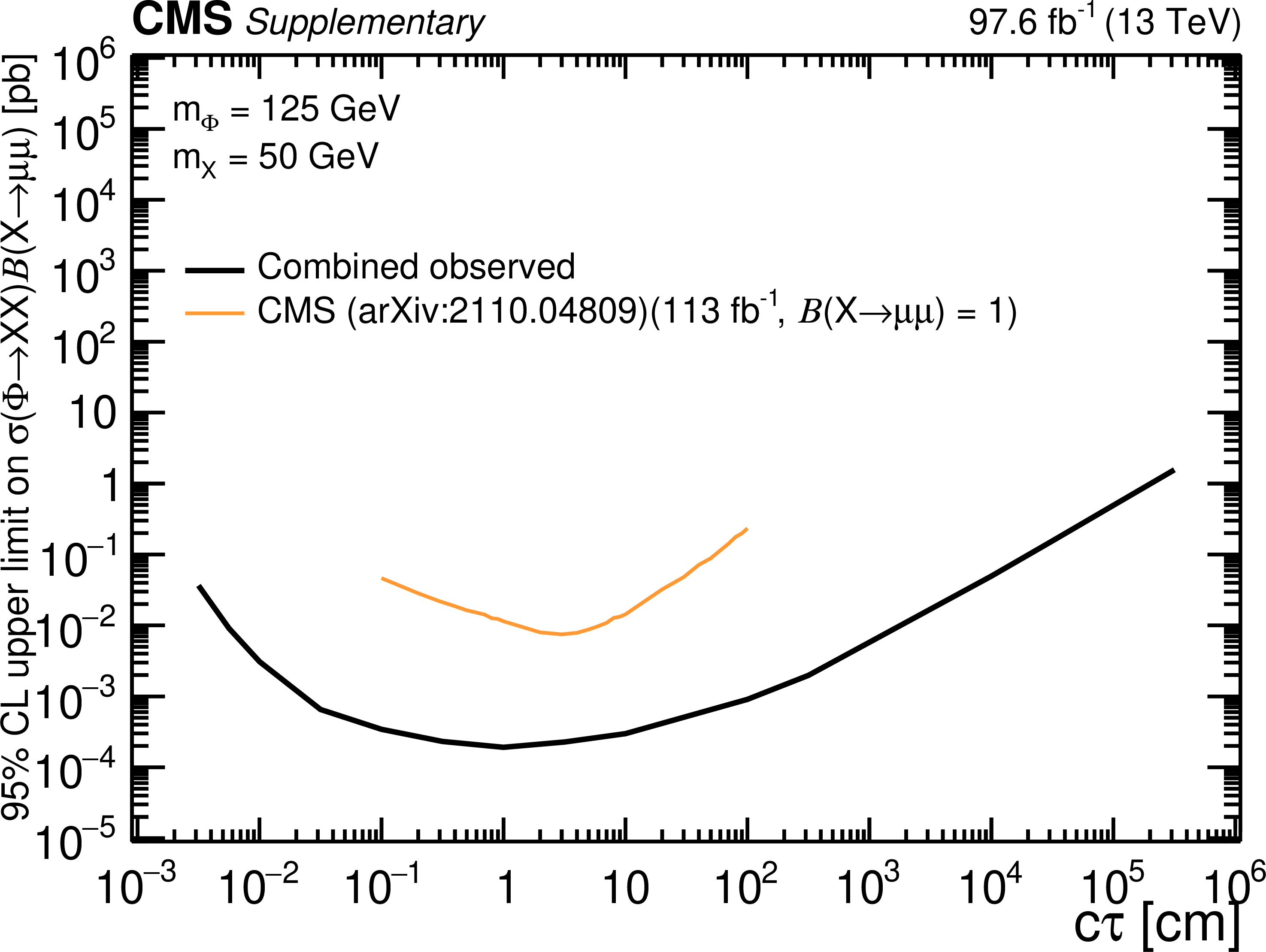
png pdf root |
Additional Figure 11-a:
The 95% CL observed upper limits on $\sigma (\phi\to \mathrm{X} \mathrm{X})\mathcal {B}(\mathrm{X} \to \mu \mu)$ as a function of $ {c\tau} (\mathrm{X})$ in the heavy scalar model, for $ {m(\phi)} = $ 125 GeV and $ {m(\mathrm{X})} = $ 50 GeV (upper left), $ {m(\phi)} = $ 1 TeV and $ {m(\mathrm{X})} = $ 150 GeV (upper right), and $ {m(\phi)} = $ 1 TeV and $ {m(\mathrm{X})} = $ 350 GeV (lower). The limits obtained in this analysis (in black) are compared to the results obtained in the CMS search for LLPs decaying to leptons with large impact parameter (Eur. Phys. J. C 82 (2022) 153, in orange). |
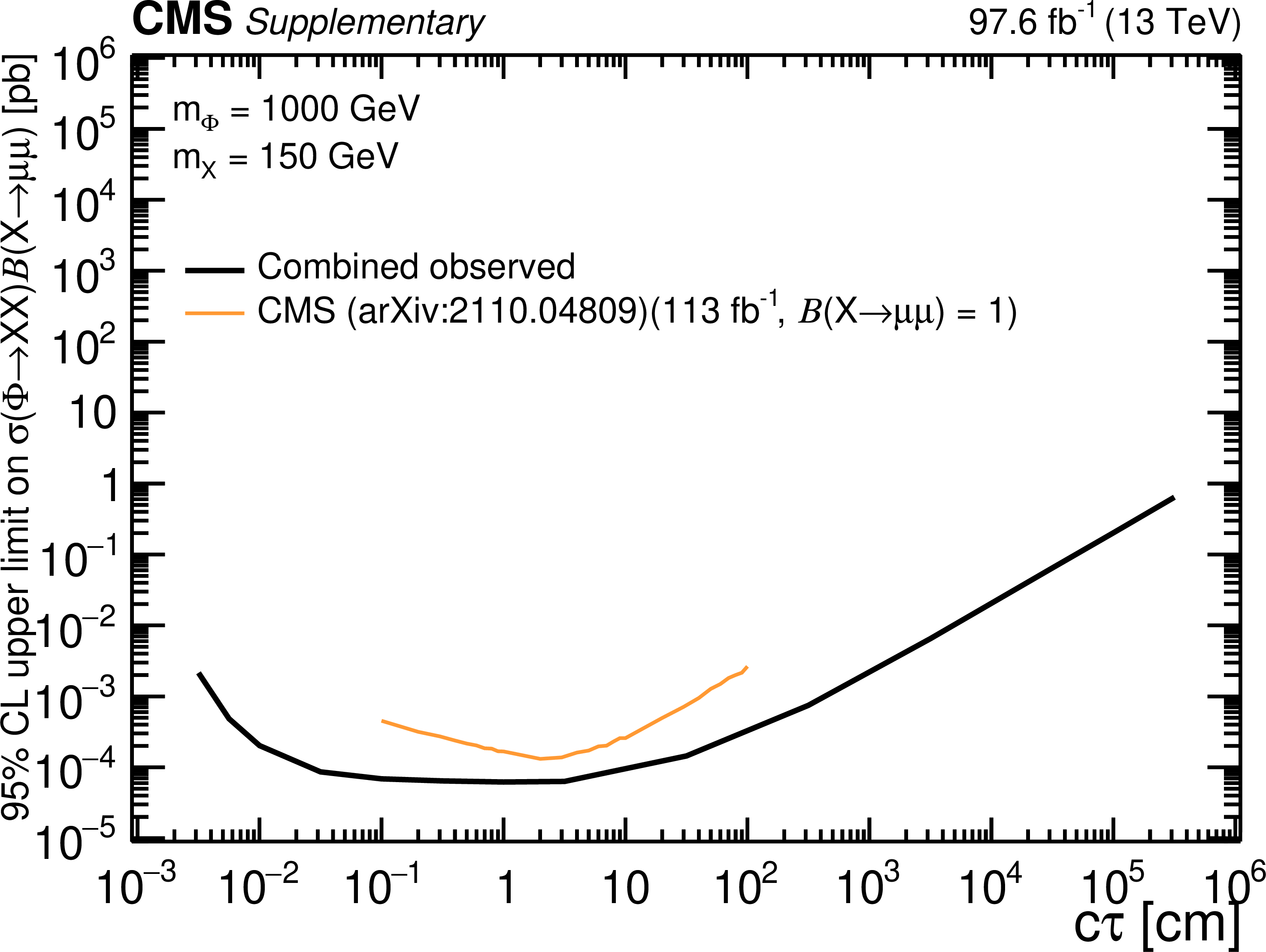
png pdf root |
Additional Figure 11-b:
The 95% CL observed upper limits on $\sigma (\phi\to \mathrm{X} \mathrm{X})\mathcal {B}(\mathrm{X} \to \mu \mu)$ as a function of $ {c\tau} (\mathrm{X})$ in the heavy scalar model, for $ {m(\phi)} = $ 125 GeV and $ {m(\mathrm{X})} = $ 50 GeV (upper left), $ {m(\phi)} = $ 1 TeV and $ {m(\mathrm{X})} = $ 150 GeV (upper right), and $ {m(\phi)} = $ 1 TeV and $ {m(\mathrm{X})} = $ 350 GeV (lower). The limits obtained in this analysis (in black) are compared to the results obtained in the CMS search for LLPs decaying to leptons with large impact parameter (Eur. Phys. J. C 82 (2022) 153, in orange). |
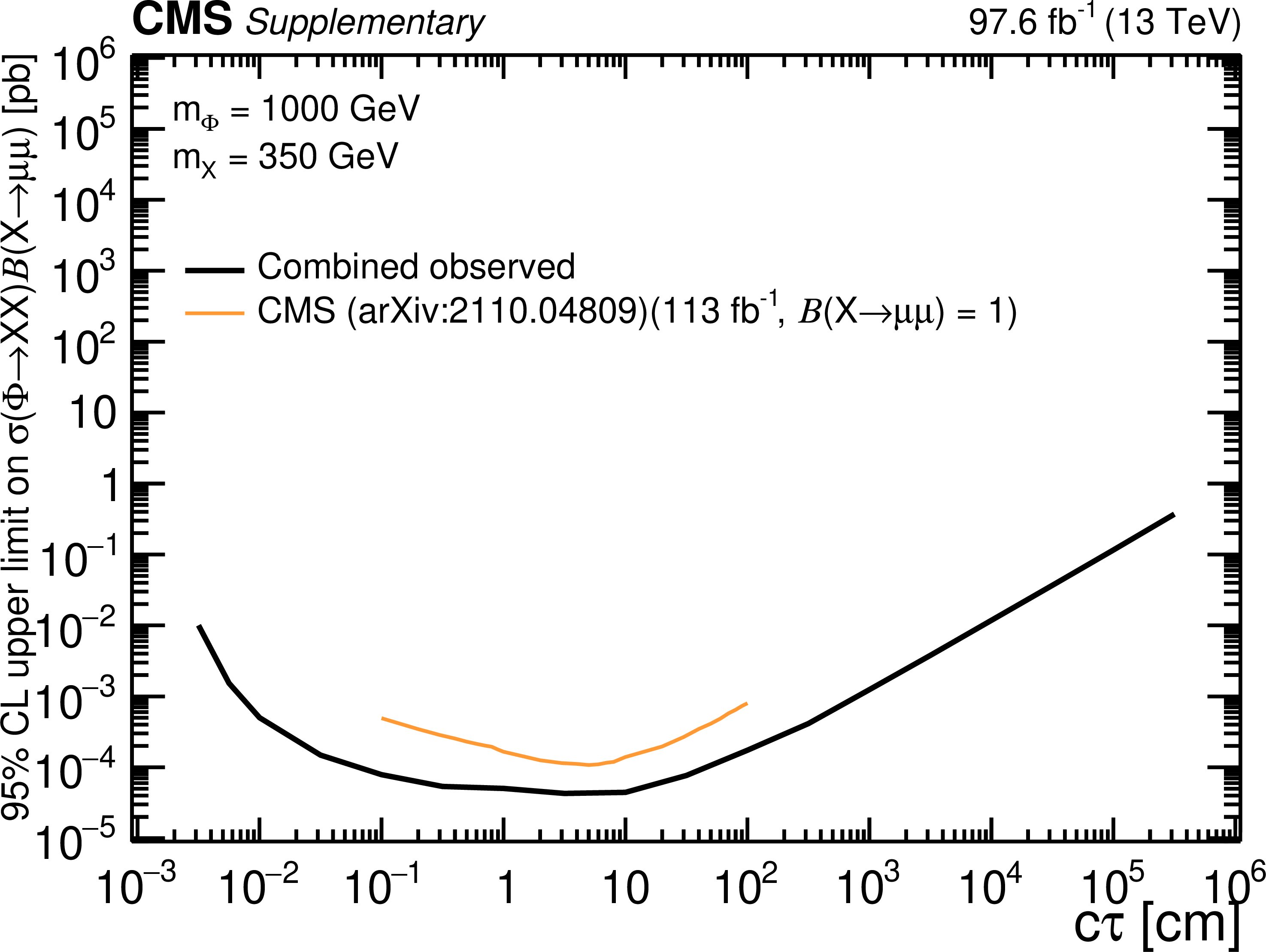
png pdf root |
Additional Figure 11-c:
The 95% CL observed upper limits on $\sigma (\phi\to \mathrm{X} \mathrm{X})\mathcal {B}(\mathrm{X} \to \mu \mu)$ as a function of $ {c\tau} (\mathrm{X})$ in the heavy scalar model, for $ {m(\phi)} = $ 125 GeV and $ {m(\mathrm{X})} = $ 50 GeV (upper left), $ {m(\phi)} = $ 1 TeV and $ {m(\mathrm{X})} = $ 150 GeV (upper right), and $ {m(\phi)} = $ 1 TeV and $ {m(\mathrm{X})} = $ 350 GeV (lower). The limits obtained in this analysis (in black) are compared to the results obtained in the CMS search for LLPs decaying to leptons with large impact parameter (Eur. Phys. J. C 82 (2022) 153, in orange). |
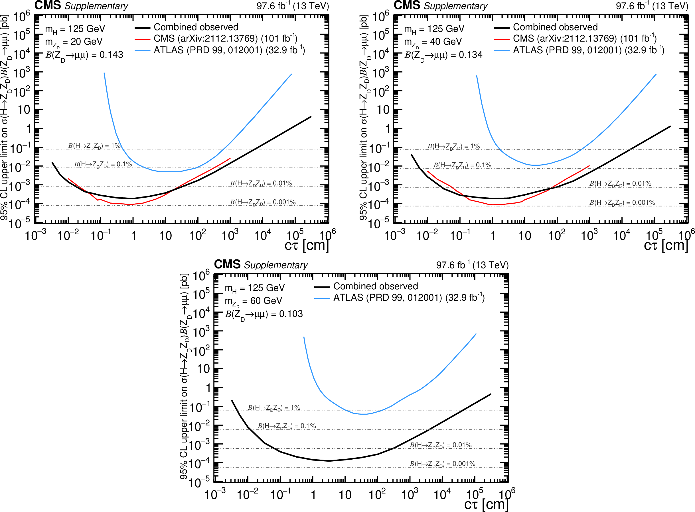
png pdf |
Additional Figure 12:
The 95% CL observed upper limits on $\sigma (\mathrm{H} \to \mathrm{Z} {\mathrm {_{D}}}\mathrm{Z} {\mathrm {_{D}}}) \mathcal {B}(\mathrm{Z} {\mathrm {_{D}}}\to \mu \mu)$ as a function of $ {c\tau} (\mathrm{Z} {\mathrm {_{D}}})$ in the HAHM model, for $ {m(\mathrm{H})} = $ 125 GeV and $ {m(\mathrm{Z} {\mathrm {_{D}}})} = $ 20 GeV (upper left), $ {m(\mathrm{Z} {\mathrm {_{D}}})} = $ 40 GeV (upper right), and $ {m(\mathrm{Z} {\mathrm {_{D}}})} = $ 60 GeV (lower). The limits obtained in this analysis (in black) are compared to the results obtained in the CMS search for LLPs decaying into muon pairs in data collected with a dedicated high-rate data stream (JHEP 04 (2022) 062, in red) and in the ATLAS search for displaced dimuon vertices in the 2016 data set (Phys. Rev. D 99 (2019) 012001, in blue). |
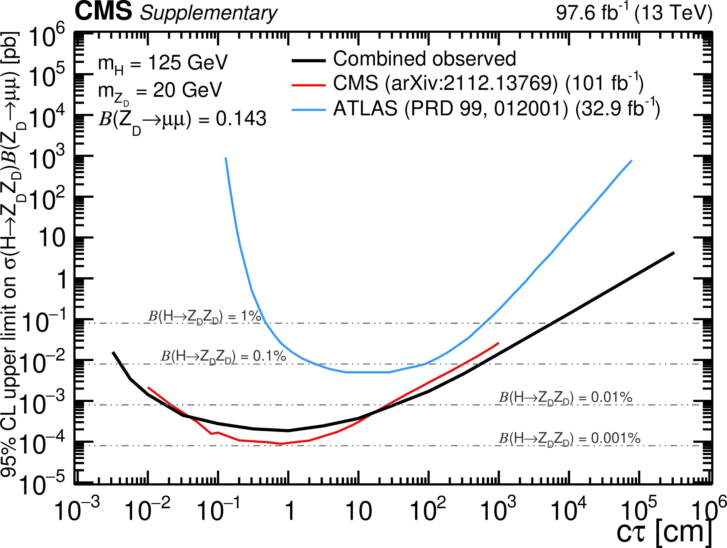
png pdf root |
Additional Figure 12-a:
The 95% CL observed upper limits on $\sigma (\mathrm{H} \to \mathrm{Z} {\mathrm {_{D}}}\mathrm{Z} {\mathrm {_{D}}}) \mathcal {B}(\mathrm{Z} {\mathrm {_{D}}}\to \mu \mu)$ as a function of $ {c\tau} (\mathrm{Z} {\mathrm {_{D}}})$ in the HAHM model, for $ {m(\mathrm{H})} = $ 125 GeV and $ {m(\mathrm{Z} {\mathrm {_{D}}})} = $ 20 GeV (upper left), $ {m(\mathrm{Z} {\mathrm {_{D}}})} = $ 40 GeV (upper right), and $ {m(\mathrm{Z} {\mathrm {_{D}}})} = $ 60 GeV (lower). The limits obtained in this analysis (in black) are compared to the results obtained in the CMS search for LLPs decaying into muon pairs in data collected with a dedicated high-rate data stream (JHEP 04 (2022) 062, in red) and in the ATLAS search for displaced dimuon vertices in the 2016 data set (Phys. Rev. D 99 (2019) 012001, in blue). |
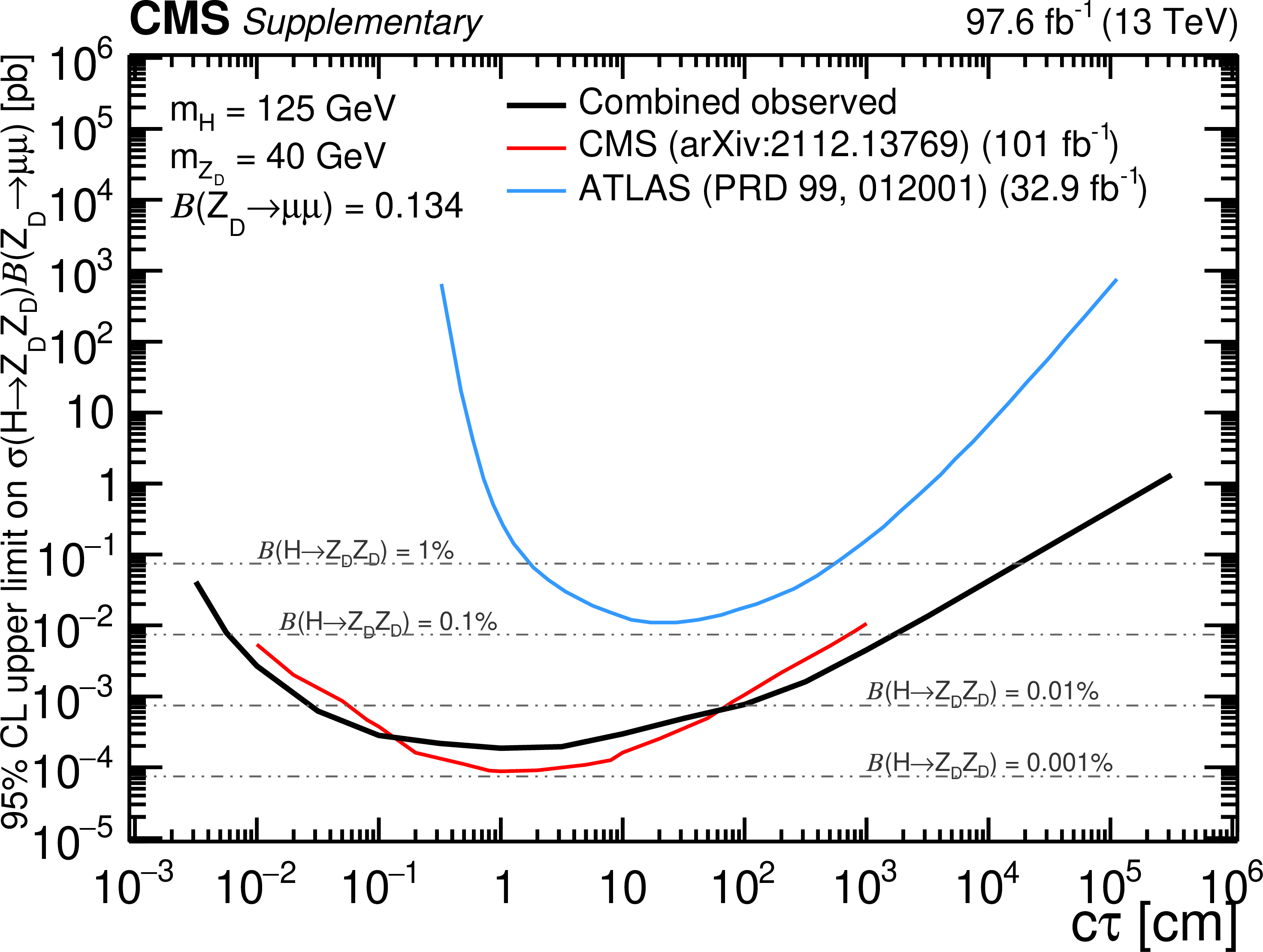
png pdf root |
Additional Figure 12-b:
The 95% CL observed upper limits on $\sigma (\mathrm{H} \to \mathrm{Z} {\mathrm {_{D}}}\mathrm{Z} {\mathrm {_{D}}}) \mathcal {B}(\mathrm{Z} {\mathrm {_{D}}}\to \mu \mu)$ as a function of $ {c\tau} (\mathrm{Z} {\mathrm {_{D}}})$ in the HAHM model, for $ {m(\mathrm{H})} = $ 125 GeV and $ {m(\mathrm{Z} {\mathrm {_{D}}})} = $ 20 GeV (upper left), $ {m(\mathrm{Z} {\mathrm {_{D}}})} = $ 40 GeV (upper right), and $ {m(\mathrm{Z} {\mathrm {_{D}}})} = $ 60 GeV (lower). The limits obtained in this analysis (in black) are compared to the results obtained in the CMS search for LLPs decaying into muon pairs in data collected with a dedicated high-rate data stream (JHEP 04 (2022) 062, in red) and in the ATLAS search for displaced dimuon vertices in the 2016 data set (Phys. Rev. D 99 (2019) 012001, in blue). |
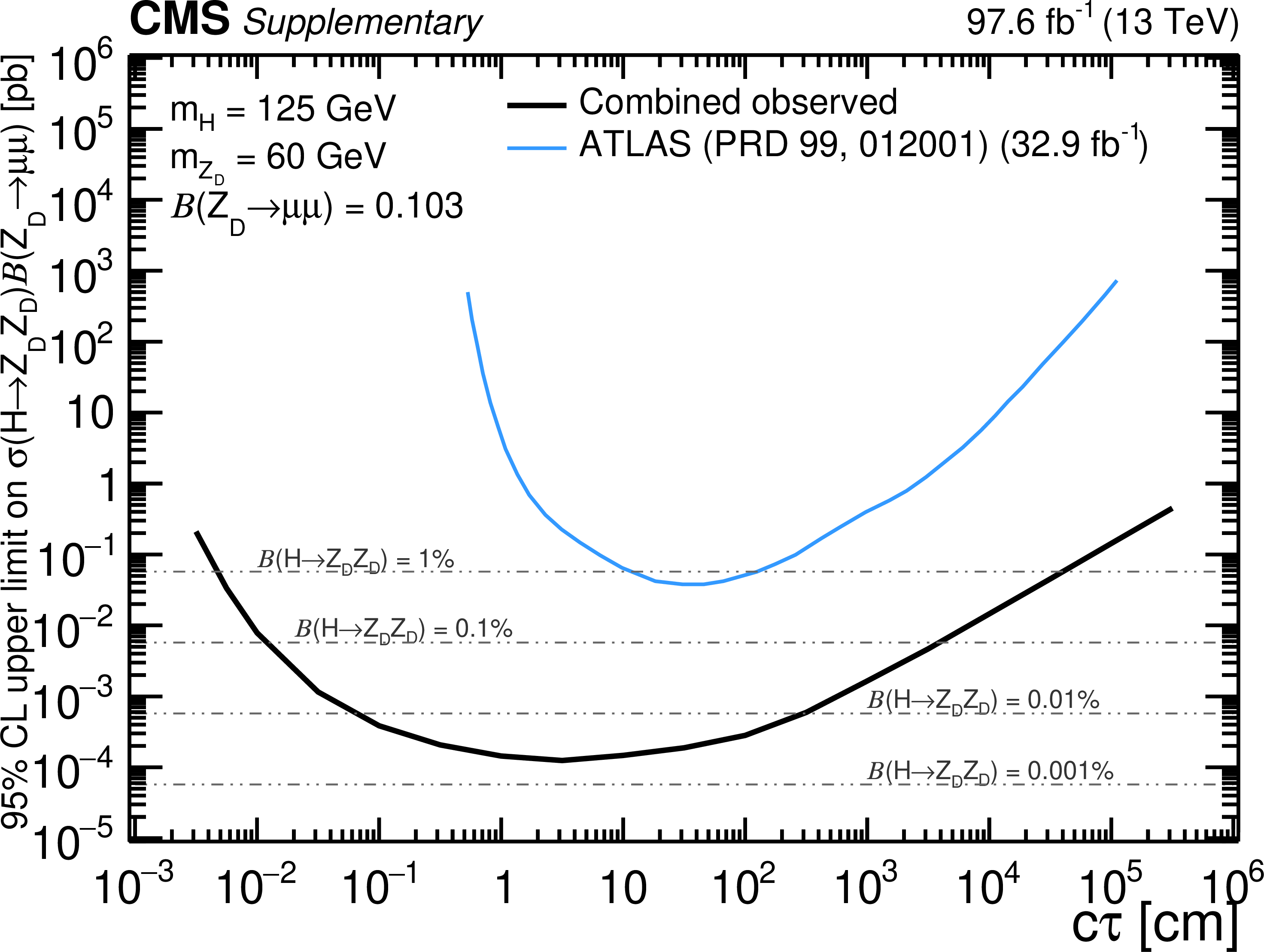
png pdf root |
Additional Figure 12-c:
The 95% CL observed upper limits on $\sigma (\mathrm{H} \to \mathrm{Z} {\mathrm {_{D}}}\mathrm{Z} {\mathrm {_{D}}}) \mathcal {B}(\mathrm{Z} {\mathrm {_{D}}}\to \mu \mu)$ as a function of $ {c\tau} (\mathrm{Z} {\mathrm {_{D}}})$ in the HAHM model, for $ {m(\mathrm{H})} = $ 125 GeV and $ {m(\mathrm{Z} {\mathrm {_{D}}})} = $ 20 GeV (upper left), $ {m(\mathrm{Z} {\mathrm {_{D}}})} = $ 40 GeV (upper right), and $ {m(\mathrm{Z} {\mathrm {_{D}}})} = $ 60 GeV (lower). The limits obtained in this analysis (in black) are compared to the results obtained in the CMS search for LLPs decaying into muon pairs in data collected with a dedicated high-rate data stream (JHEP 04 (2022) 062, in red) and in the ATLAS search for displaced dimuon vertices in the 2016 data set (Phys. Rev. D 99 (2019) 012001, in blue). |
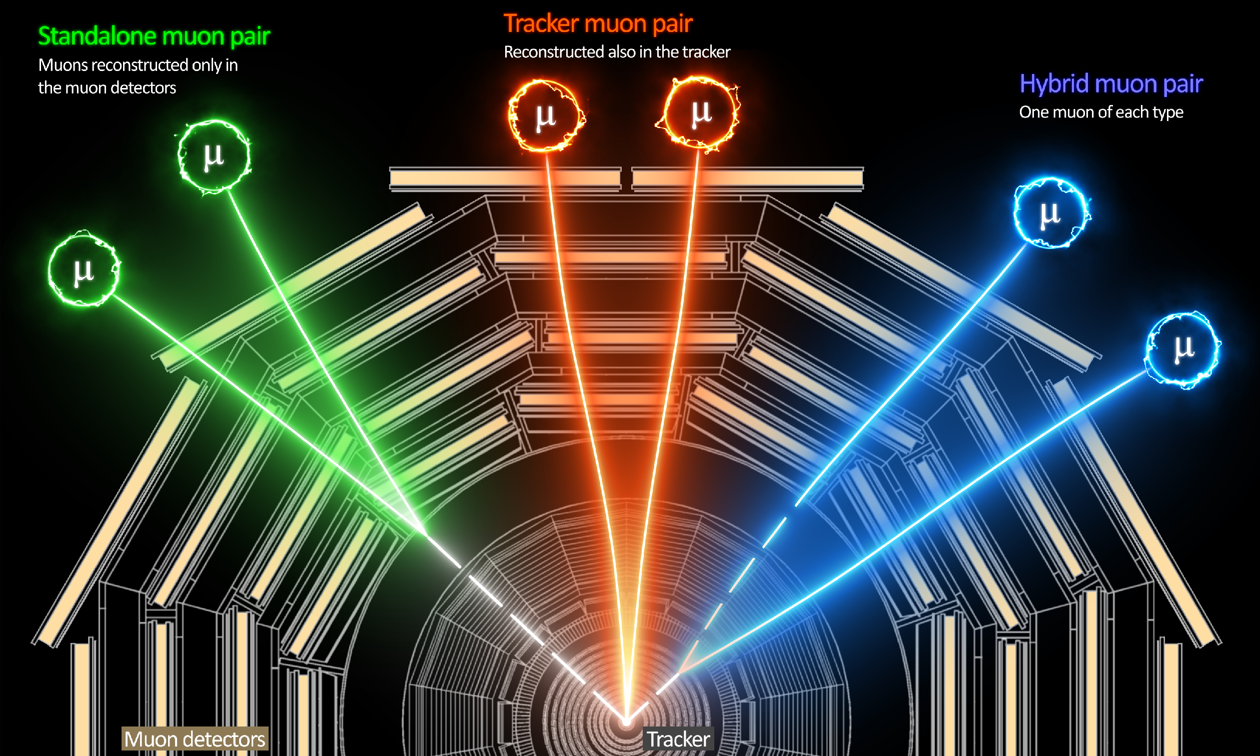
png pdf |
Additional Figure 13:
Cartoon illustrating three dimuon categories used in the analysis: STA-STA (green), TMS-TMS (orange), and STA-TMS (blue). |
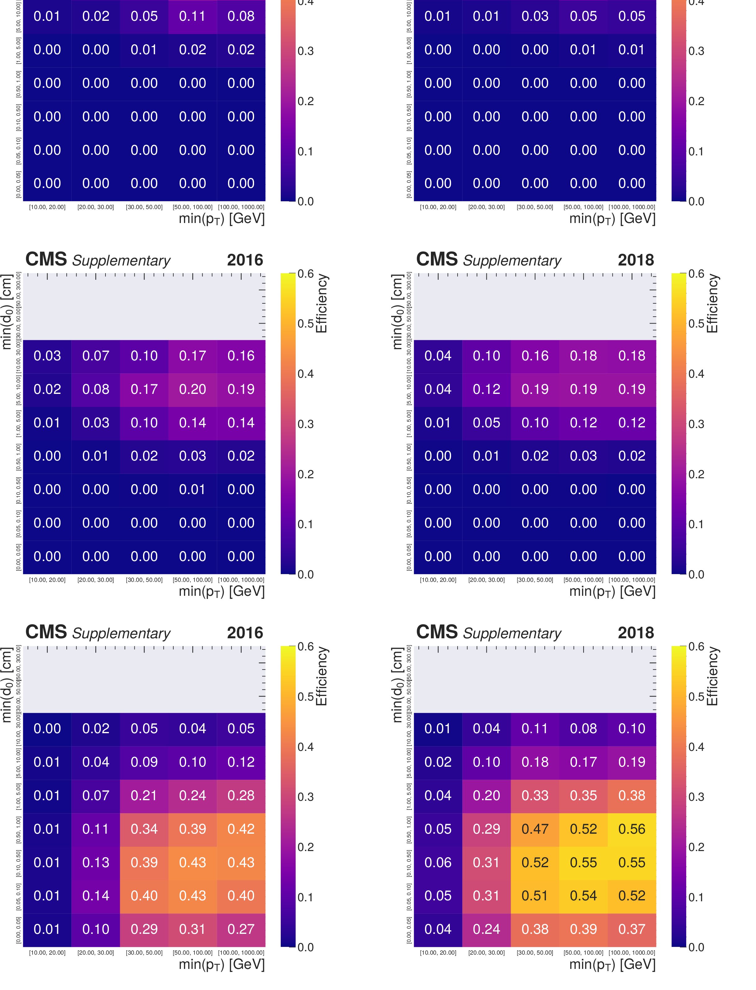
png pdf |
Additional Figure 14:
Signal efficiencies as a function of the smaller of the two values of generated muon ${p_{\mathrm {T}}}$ and ${d_{\mathrm {0}}}$ in dimuons with $ {L_{\mathrm {xy}}} ^\mathrm {true} < $ 20 cm in the $ {\phi\to \mathrm{X} \mathrm{X} \to \mu \mu}+$ anything signal model, in 2016 (left) and 2018 (right) samples. The efficiency in each bin is computed as the ratio of the number of simulated signal dimuons in that bin that pass the trigger requirements and selection criteria applied in the STA-STA (upper), STA-TMS (middle), and TMS-TMS (lower) dimuon category to the total number of simulated signal dimuons in that bin and within the geometric acceptance. The geometric acceptance is defined as the generated longitudinal decay length $ {L_{\mathrm {z}}} ^\mathrm {true}$ smaller than 8 m and $ {| \eta |}$ of both generated muons forming the dimuon smaller than 2.0. The efficiencies obtained from simulation were further corrected by the data-to-simulation scale factors described in the paper. |
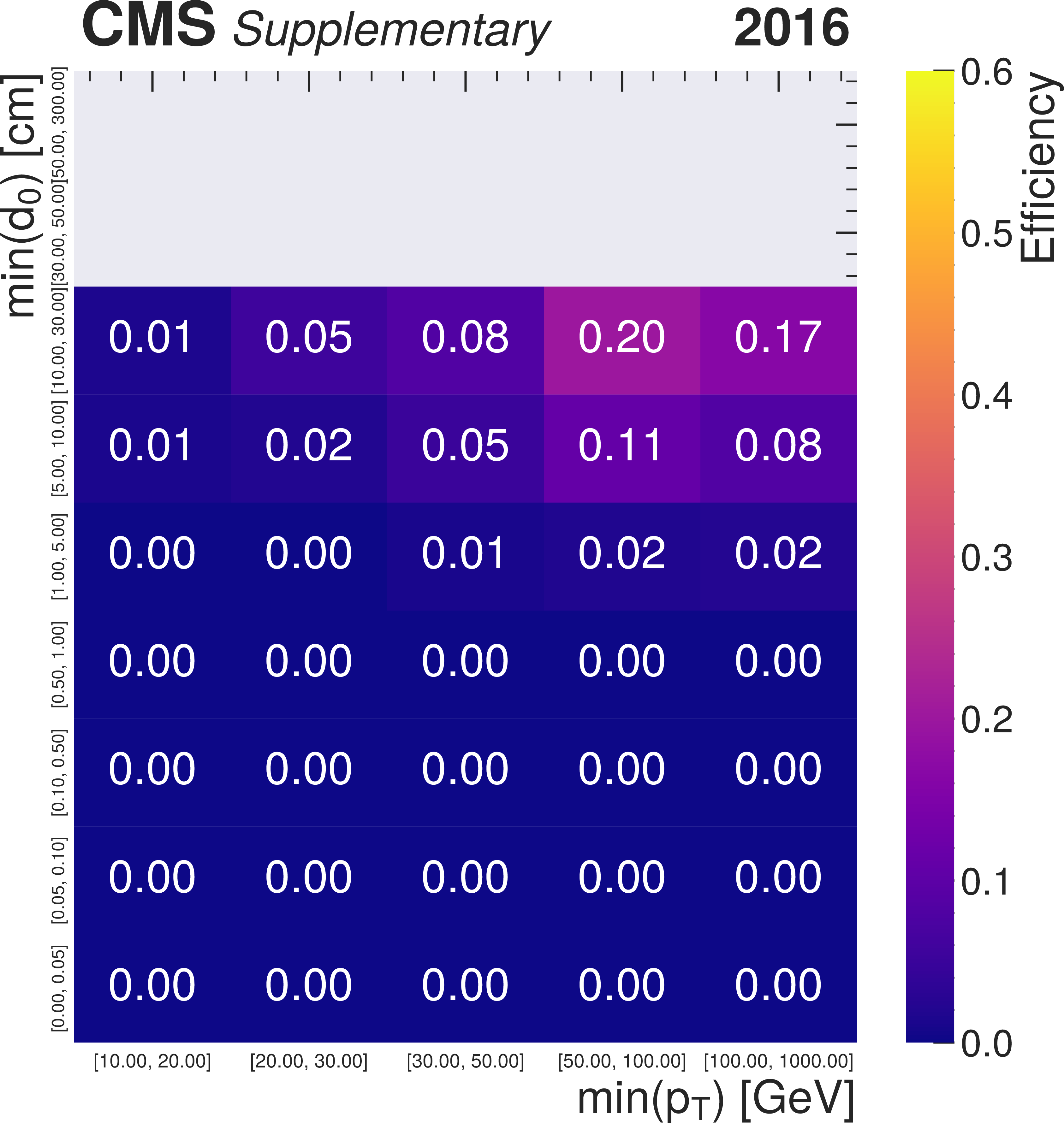
png pdf |
Additional Figure 14-a:
Signal efficiencies as a function of the smaller of the two values of generated muon ${p_{\mathrm {T}}}$ and ${d_{\mathrm {0}}}$ in dimuons with $ {L_{\mathrm {xy}}} ^\mathrm {true} < $ 20 cm in the $ {\phi\to \mathrm{X} \mathrm{X} \to \mu \mu}+$ anything signal model, in 2016 (left) and 2018 (right) samples. The efficiency in each bin is computed as the ratio of the number of simulated signal dimuons in that bin that pass the trigger requirements and selection criteria applied in the STA-STA (upper), STA-TMS (middle), and TMS-TMS (lower) dimuon category to the total number of simulated signal dimuons in that bin and within the geometric acceptance. The geometric acceptance is defined as the generated longitudinal decay length $ {L_{\mathrm {z}}} ^\mathrm {true}$ smaller than 8 m and $ {| \eta |}$ of both generated muons forming the dimuon smaller than 2.0. The efficiencies obtained from simulation were further corrected by the data-to-simulation scale factors described in the paper. |
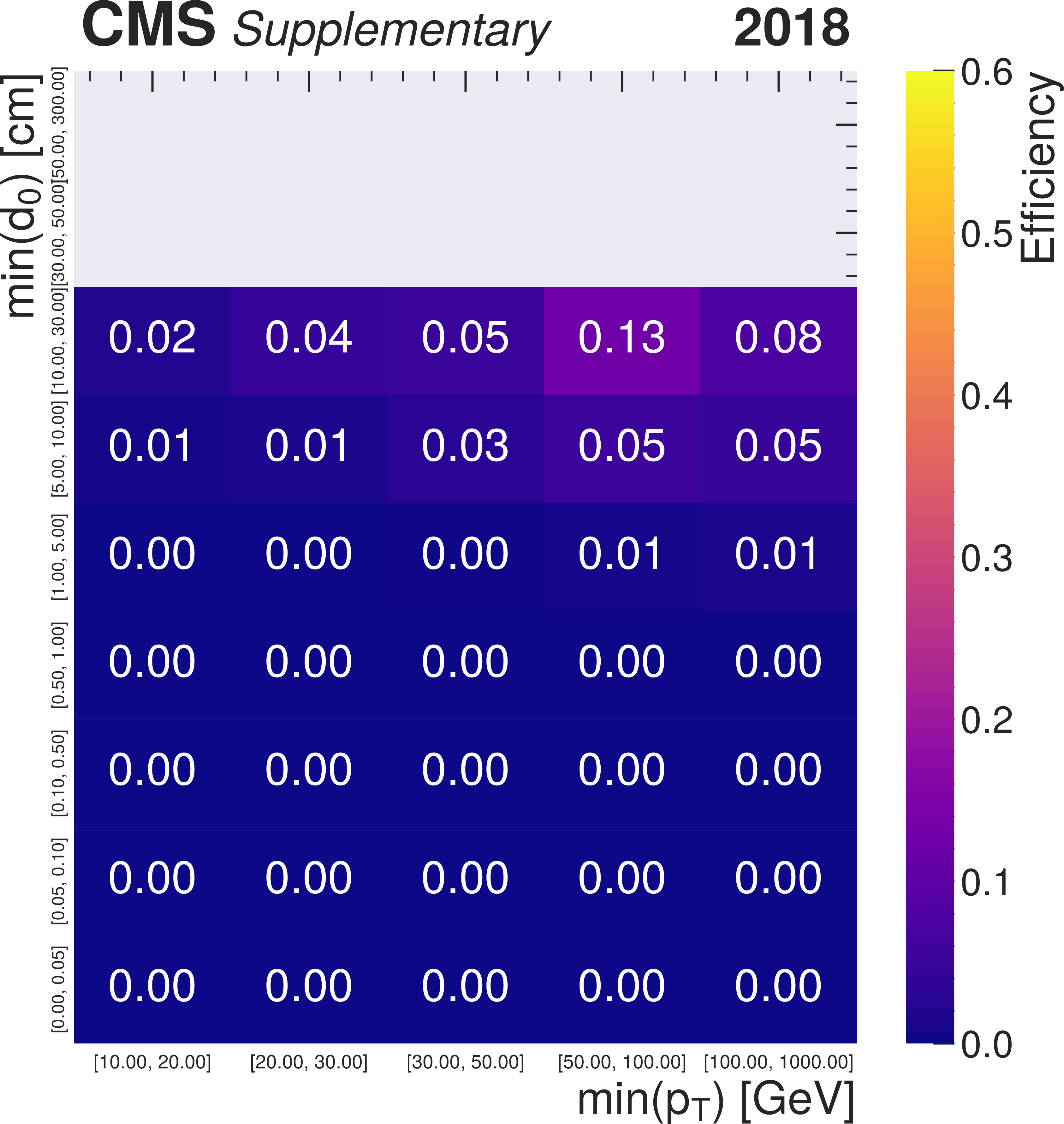
png pdf |
Additional Figure 14-b:
Signal efficiencies as a function of the smaller of the two values of generated muon ${p_{\mathrm {T}}}$ and ${d_{\mathrm {0}}}$ in dimuons with $ {L_{\mathrm {xy}}} ^\mathrm {true} < $ 20 cm in the $ {\phi\to \mathrm{X} \mathrm{X} \to \mu \mu}+$ anything signal model, in 2016 (left) and 2018 (right) samples. The efficiency in each bin is computed as the ratio of the number of simulated signal dimuons in that bin that pass the trigger requirements and selection criteria applied in the STA-STA (upper), STA-TMS (middle), and TMS-TMS (lower) dimuon category to the total number of simulated signal dimuons in that bin and within the geometric acceptance. The geometric acceptance is defined as the generated longitudinal decay length $ {L_{\mathrm {z}}} ^\mathrm {true}$ smaller than 8 m and $ {| \eta |}$ of both generated muons forming the dimuon smaller than 2.0. The efficiencies obtained from simulation were further corrected by the data-to-simulation scale factors described in the paper. |
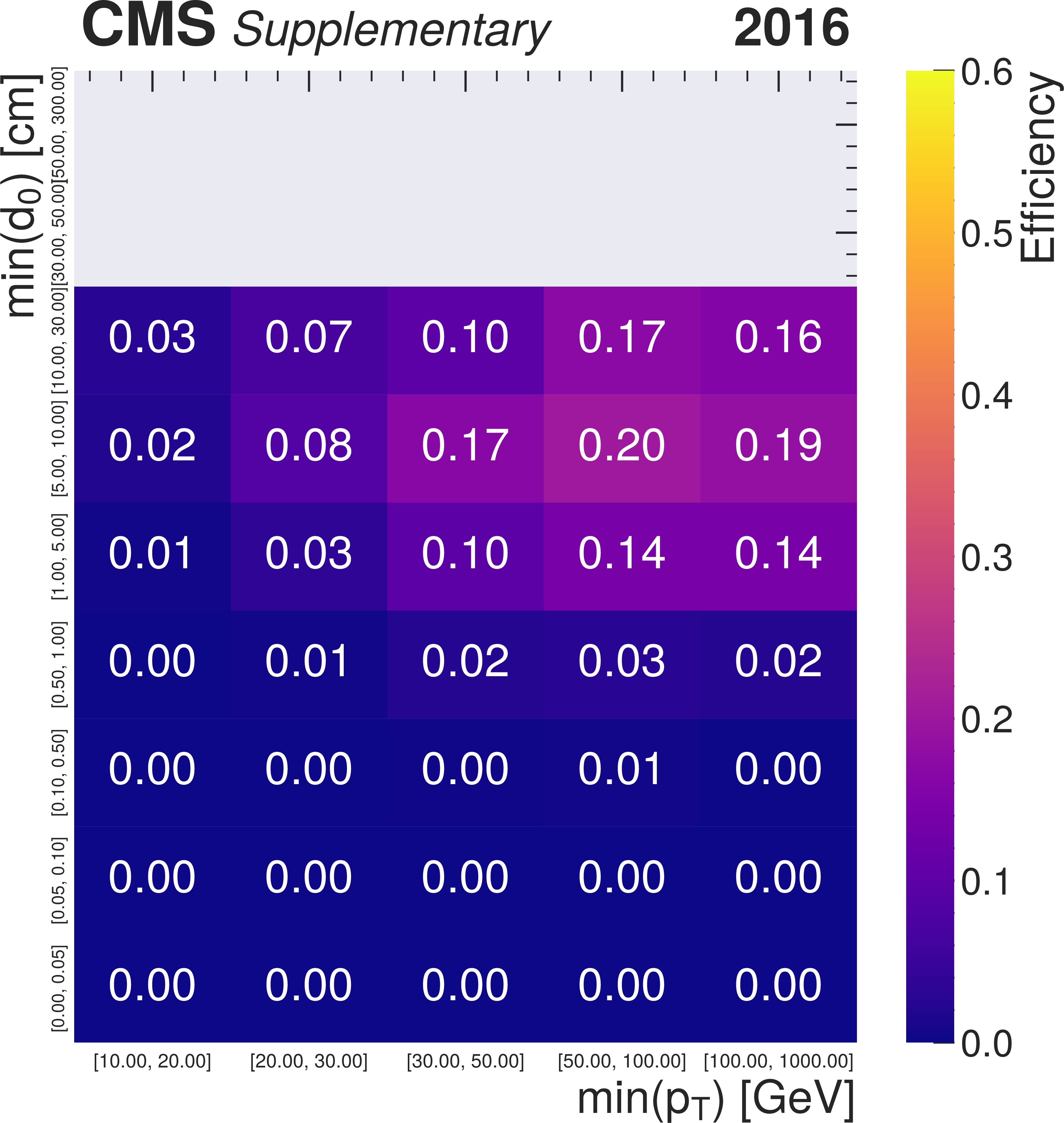
png pdf |
Additional Figure 14-c:
Signal efficiencies as a function of the smaller of the two values of generated muon ${p_{\mathrm {T}}}$ and ${d_{\mathrm {0}}}$ in dimuons with $ {L_{\mathrm {xy}}} ^\mathrm {true} < $ 20 cm in the $ {\phi\to \mathrm{X} \mathrm{X} \to \mu \mu}+$ anything signal model, in 2016 (left) and 2018 (right) samples. The efficiency in each bin is computed as the ratio of the number of simulated signal dimuons in that bin that pass the trigger requirements and selection criteria applied in the STA-STA (upper), STA-TMS (middle), and TMS-TMS (lower) dimuon category to the total number of simulated signal dimuons in that bin and within the geometric acceptance. The geometric acceptance is defined as the generated longitudinal decay length $ {L_{\mathrm {z}}} ^\mathrm {true}$ smaller than 8 m and $ {| \eta |}$ of both generated muons forming the dimuon smaller than 2.0. The efficiencies obtained from simulation were further corrected by the data-to-simulation scale factors described in the paper. |
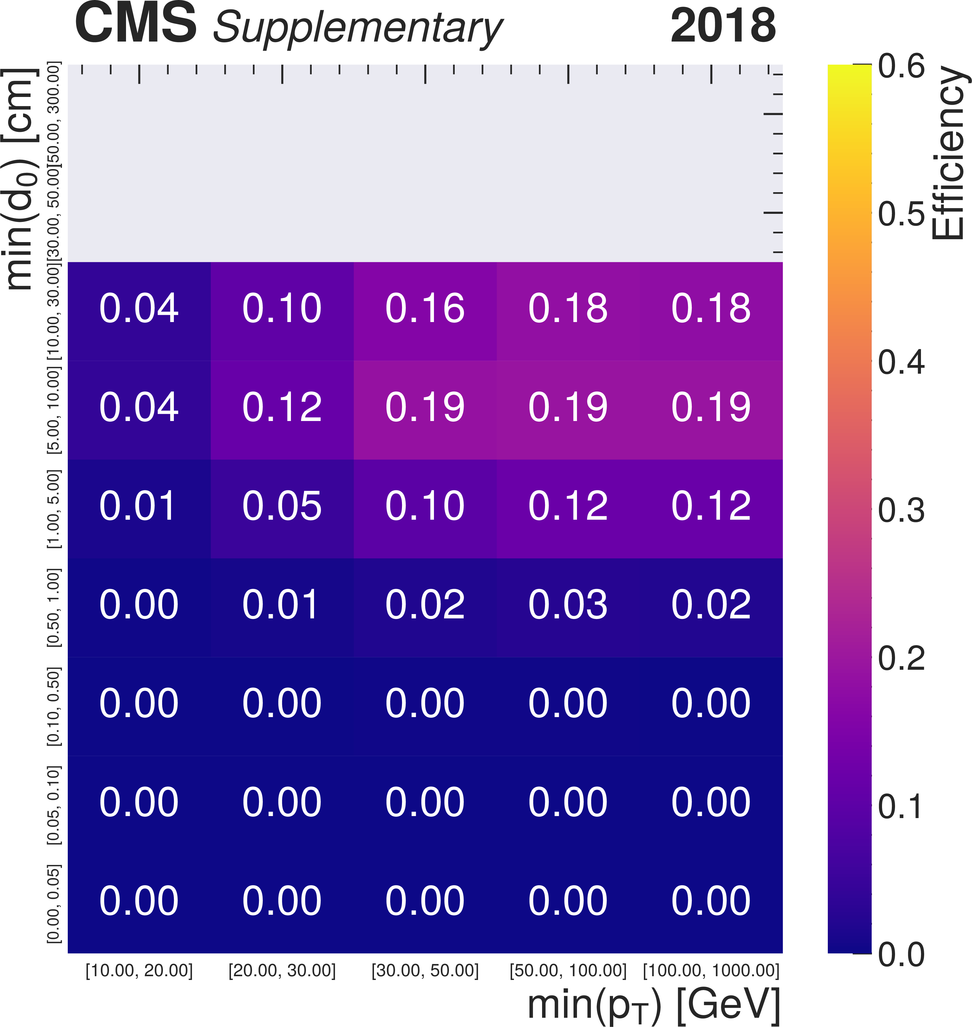
png pdf |
Additional Figure 14-d:
Signal efficiencies as a function of the smaller of the two values of generated muon ${p_{\mathrm {T}}}$ and ${d_{\mathrm {0}}}$ in dimuons with $ {L_{\mathrm {xy}}} ^\mathrm {true} < $ 20 cm in the $ {\phi\to \mathrm{X} \mathrm{X} \to \mu \mu}+$ anything signal model, in 2016 (left) and 2018 (right) samples. The efficiency in each bin is computed as the ratio of the number of simulated signal dimuons in that bin that pass the trigger requirements and selection criteria applied in the STA-STA (upper), STA-TMS (middle), and TMS-TMS (lower) dimuon category to the total number of simulated signal dimuons in that bin and within the geometric acceptance. The geometric acceptance is defined as the generated longitudinal decay length $ {L_{\mathrm {z}}} ^\mathrm {true}$ smaller than 8 m and $ {| \eta |}$ of both generated muons forming the dimuon smaller than 2.0. The efficiencies obtained from simulation were further corrected by the data-to-simulation scale factors described in the paper. |

png pdf |
Additional Figure 14-e:
Signal efficiencies as a function of the smaller of the two values of generated muon ${p_{\mathrm {T}}}$ and ${d_{\mathrm {0}}}$ in dimuons with $ {L_{\mathrm {xy}}} ^\mathrm {true} < $ 20 cm in the $ {\phi\to \mathrm{X} \mathrm{X} \to \mu \mu}+$ anything signal model, in 2016 (left) and 2018 (right) samples. The efficiency in each bin is computed as the ratio of the number of simulated signal dimuons in that bin that pass the trigger requirements and selection criteria applied in the STA-STA (upper), STA-TMS (middle), and TMS-TMS (lower) dimuon category to the total number of simulated signal dimuons in that bin and within the geometric acceptance. The geometric acceptance is defined as the generated longitudinal decay length $ {L_{\mathrm {z}}} ^\mathrm {true}$ smaller than 8 m and $ {| \eta |}$ of both generated muons forming the dimuon smaller than 2.0. The efficiencies obtained from simulation were further corrected by the data-to-simulation scale factors described in the paper. |

png pdf |
Additional Figure 14-f:
Signal efficiencies as a function of the smaller of the two values of generated muon ${p_{\mathrm {T}}}$ and ${d_{\mathrm {0}}}$ in dimuons with $ {L_{\mathrm {xy}}} ^\mathrm {true} < $ 20 cm in the $ {\phi\to \mathrm{X} \mathrm{X} \to \mu \mu}+$ anything signal model, in 2016 (left) and 2018 (right) samples. The efficiency in each bin is computed as the ratio of the number of simulated signal dimuons in that bin that pass the trigger requirements and selection criteria applied in the STA-STA (upper), STA-TMS (middle), and TMS-TMS (lower) dimuon category to the total number of simulated signal dimuons in that bin and within the geometric acceptance. The geometric acceptance is defined as the generated longitudinal decay length $ {L_{\mathrm {z}}} ^\mathrm {true}$ smaller than 8 m and $ {| \eta |}$ of both generated muons forming the dimuon smaller than 2.0. The efficiencies obtained from simulation were further corrected by the data-to-simulation scale factors described in the paper. |

png pdf |
Additional Figure 15:
Signal efficiencies as a function of the smaller of the two values of generated muon ${p_{\mathrm {T}}}$ and ${d_{\mathrm {0}}}$ in dimuons with $20 cm < {L_{\mathrm {xy}}} ^\mathrm {true} < $ 70 cm in the $ {\phi\to \mathrm{X} \mathrm{X} \to \mu \mu}+$ anything signal model, in 2016 (left) and 2018 (right) samples. The efficiency in each bin is computed as the ratio of the number of simulated signal dimuons in that bin that pass the trigger requirements and selection criteria applied in the STA-STA (upper), STA-TMS (middle), and TMS-TMS (lower) dimuon category to the total number of simulated signal dimuons in that bin and within the geometric acceptance. The geometric acceptance is defined as the generated longitudinal decay length $ {L_{\mathrm {z}}} ^\mathrm {true}$ smaller than 8 m and $ {| \eta |}$ of both generated muons forming the dimuon smaller than 2.0. The efficiencies obtained from simulation were further corrected by the data-to-simulation scale factors described in the paper. |
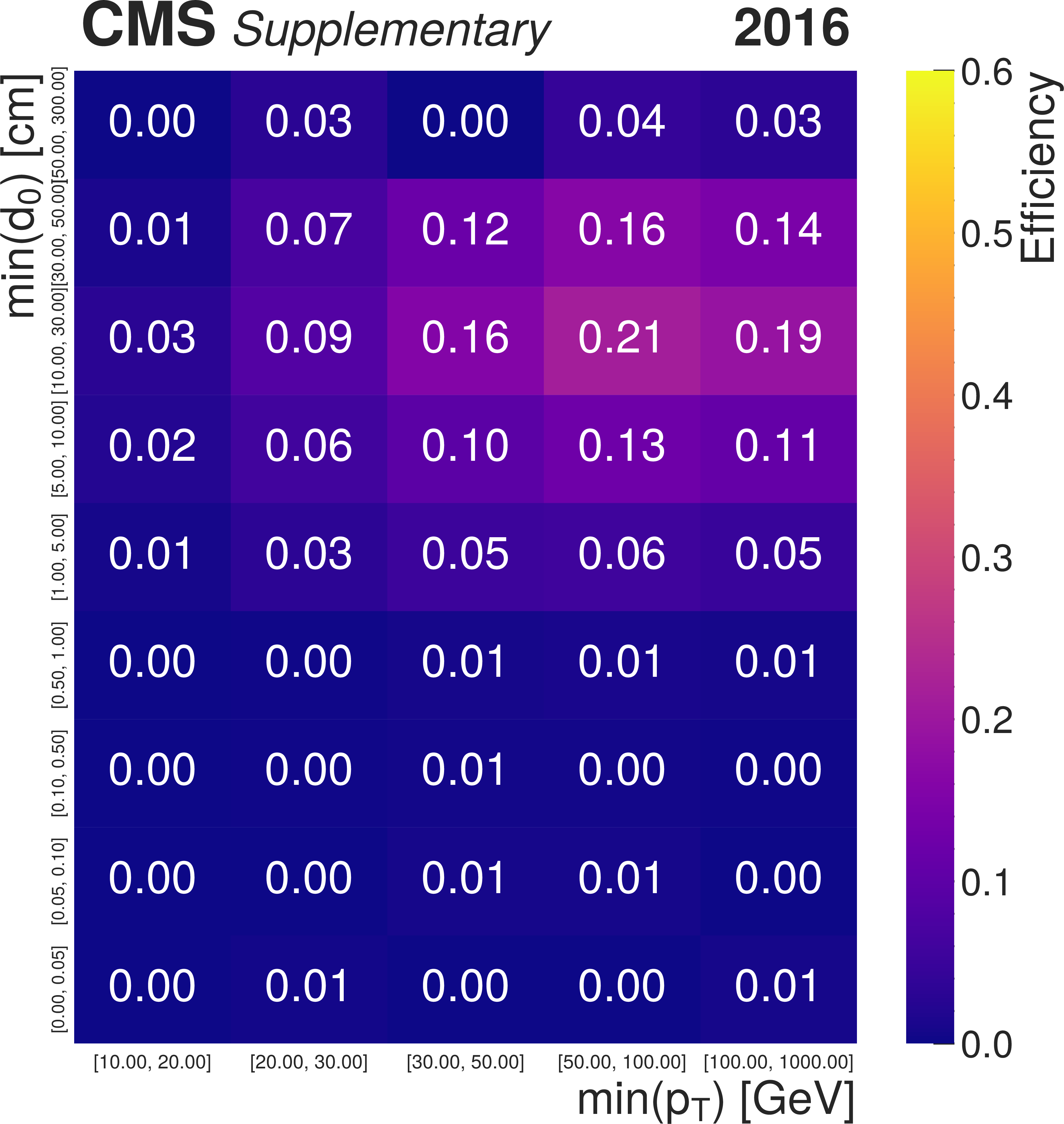
png pdf |
Additional Figure 15-a:
Signal efficiencies as a function of the smaller of the two values of generated muon ${p_{\mathrm {T}}}$ and ${d_{\mathrm {0}}}$ in dimuons with $20 cm < {L_{\mathrm {xy}}} ^\mathrm {true} < $ 70 cm in the $ {\phi\to \mathrm{X} \mathrm{X} \to \mu \mu}+$ anything signal model, in 2016 (left) and 2018 (right) samples. The efficiency in each bin is computed as the ratio of the number of simulated signal dimuons in that bin that pass the trigger requirements and selection criteria applied in the STA-STA (upper), STA-TMS (middle), and TMS-TMS (lower) dimuon category to the total number of simulated signal dimuons in that bin and within the geometric acceptance. The geometric acceptance is defined as the generated longitudinal decay length $ {L_{\mathrm {z}}} ^\mathrm {true}$ smaller than 8 m and $ {| \eta |}$ of both generated muons forming the dimuon smaller than 2.0. The efficiencies obtained from simulation were further corrected by the data-to-simulation scale factors described in the paper. |
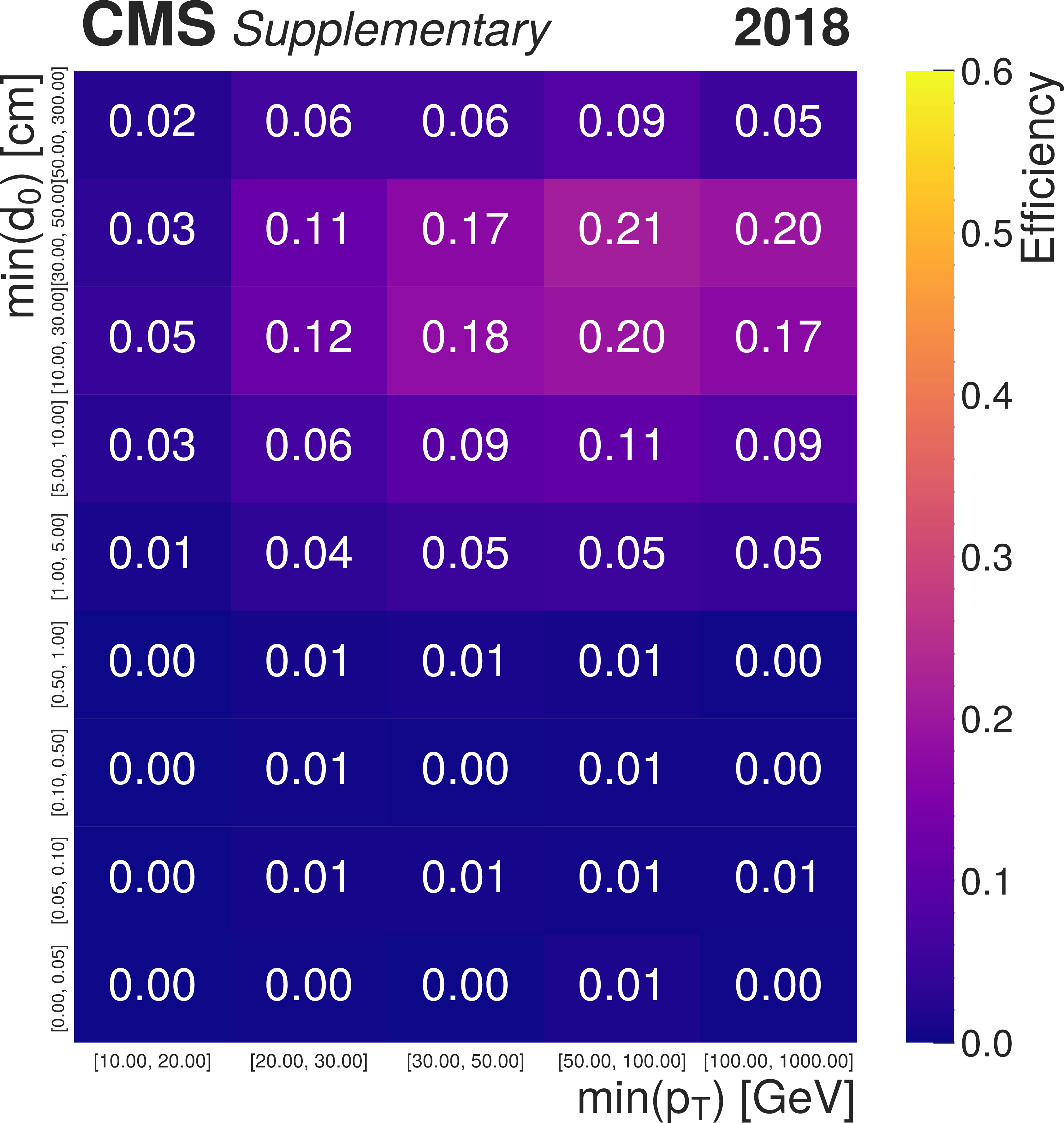
png pdf |
Additional Figure 15-b:
Signal efficiencies as a function of the smaller of the two values of generated muon ${p_{\mathrm {T}}}$ and ${d_{\mathrm {0}}}$ in dimuons with $20 cm < {L_{\mathrm {xy}}} ^\mathrm {true} < $ 70 cm in the $ {\phi\to \mathrm{X} \mathrm{X} \to \mu \mu}+$ anything signal model, in 2016 (left) and 2018 (right) samples. The efficiency in each bin is computed as the ratio of the number of simulated signal dimuons in that bin that pass the trigger requirements and selection criteria applied in the STA-STA (upper), STA-TMS (middle), and TMS-TMS (lower) dimuon category to the total number of simulated signal dimuons in that bin and within the geometric acceptance. The geometric acceptance is defined as the generated longitudinal decay length $ {L_{\mathrm {z}}} ^\mathrm {true}$ smaller than 8 m and $ {| \eta |}$ of both generated muons forming the dimuon smaller than 2.0. The efficiencies obtained from simulation were further corrected by the data-to-simulation scale factors described in the paper. |
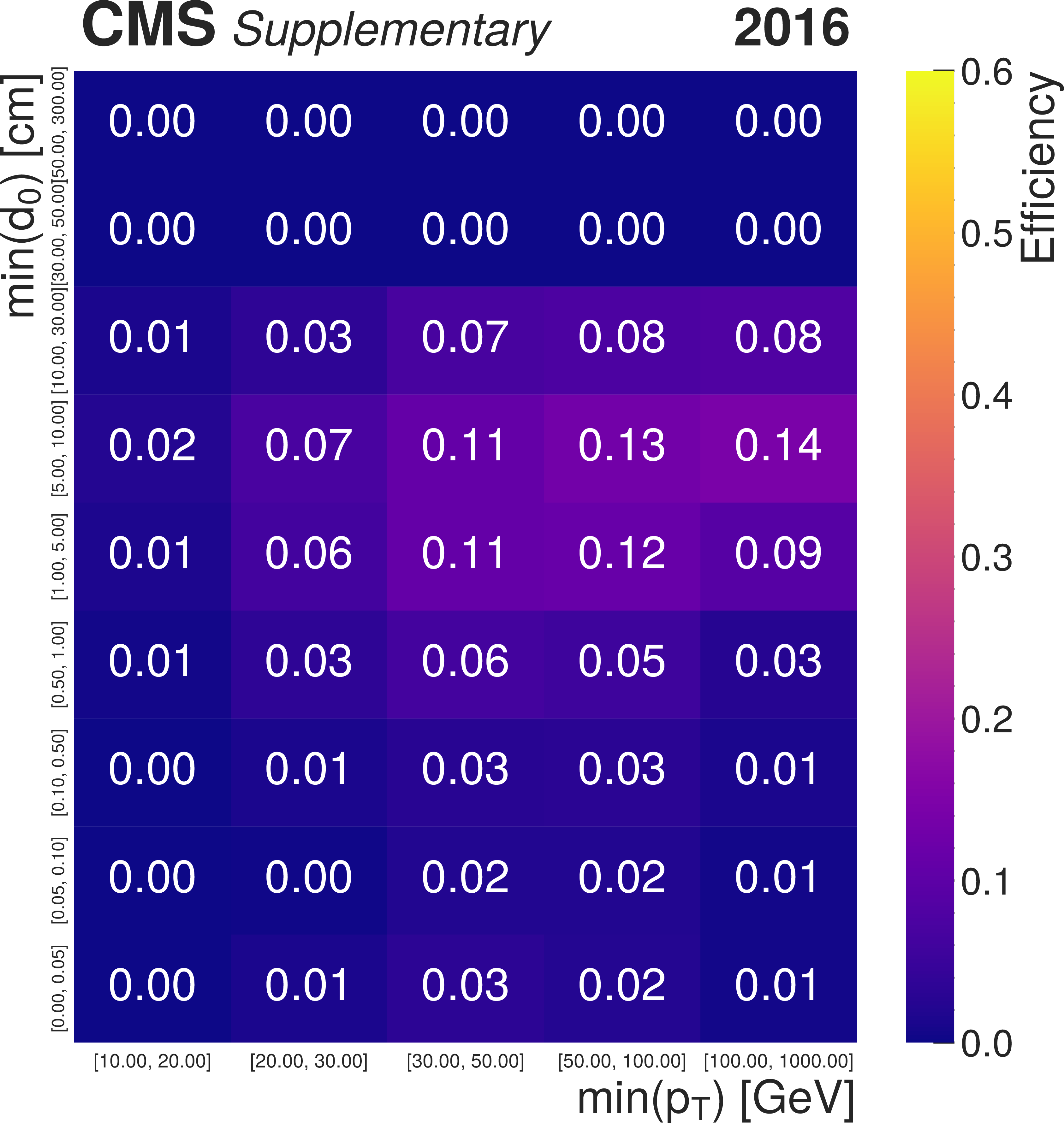
png pdf |
Additional Figure 15-c:
Signal efficiencies as a function of the smaller of the two values of generated muon ${p_{\mathrm {T}}}$ and ${d_{\mathrm {0}}}$ in dimuons with $20 cm < {L_{\mathrm {xy}}} ^\mathrm {true} < $ 70 cm in the $ {\phi\to \mathrm{X} \mathrm{X} \to \mu \mu}+$ anything signal model, in 2016 (left) and 2018 (right) samples. The efficiency in each bin is computed as the ratio of the number of simulated signal dimuons in that bin that pass the trigger requirements and selection criteria applied in the STA-STA (upper), STA-TMS (middle), and TMS-TMS (lower) dimuon category to the total number of simulated signal dimuons in that bin and within the geometric acceptance. The geometric acceptance is defined as the generated longitudinal decay length $ {L_{\mathrm {z}}} ^\mathrm {true}$ smaller than 8 m and $ {| \eta |}$ of both generated muons forming the dimuon smaller than 2.0. The efficiencies obtained from simulation were further corrected by the data-to-simulation scale factors described in the paper. |
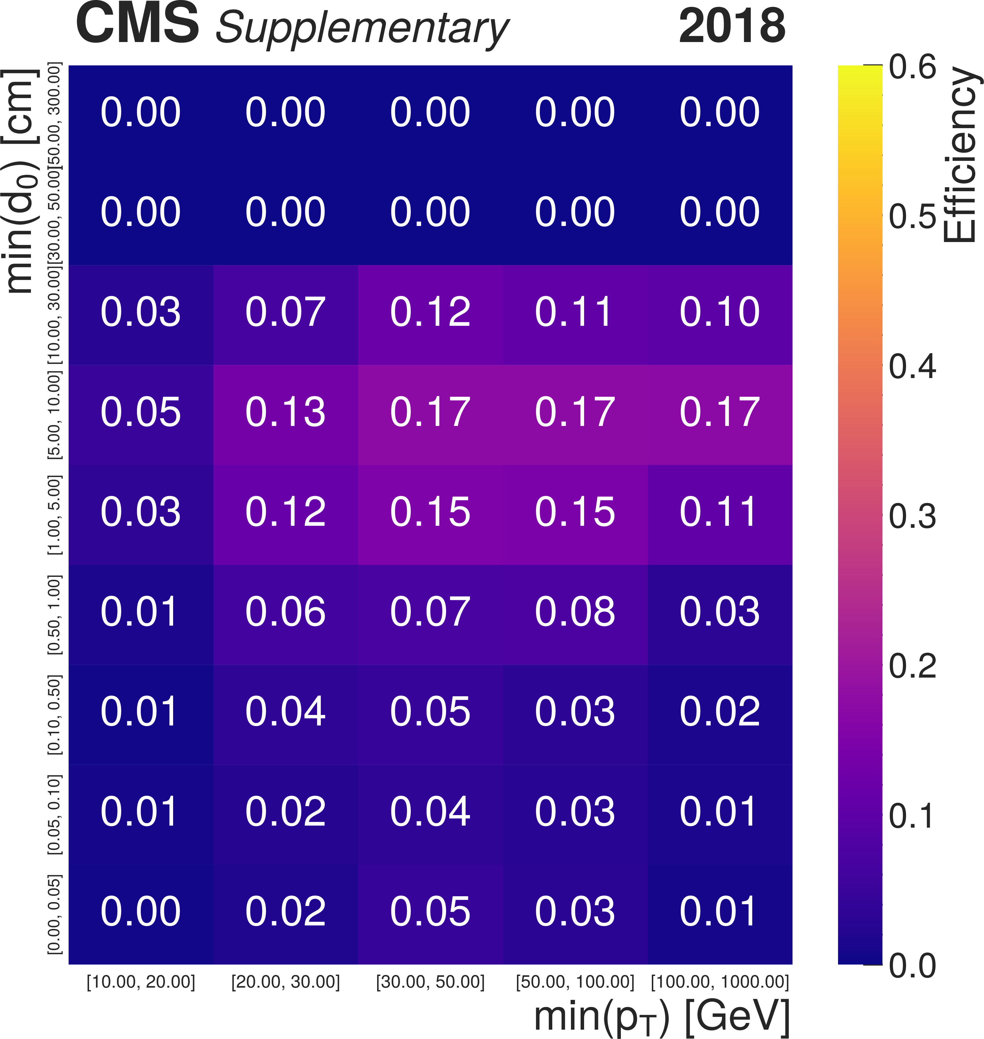
png pdf |
Additional Figure 15-d:
Signal efficiencies as a function of the smaller of the two values of generated muon ${p_{\mathrm {T}}}$ and ${d_{\mathrm {0}}}$ in dimuons with $20 cm < {L_{\mathrm {xy}}} ^\mathrm {true} < $ 70 cm in the $ {\phi\to \mathrm{X} \mathrm{X} \to \mu \mu}+$ anything signal model, in 2016 (left) and 2018 (right) samples. The efficiency in each bin is computed as the ratio of the number of simulated signal dimuons in that bin that pass the trigger requirements and selection criteria applied in the STA-STA (upper), STA-TMS (middle), and TMS-TMS (lower) dimuon category to the total number of simulated signal dimuons in that bin and within the geometric acceptance. The geometric acceptance is defined as the generated longitudinal decay length $ {L_{\mathrm {z}}} ^\mathrm {true}$ smaller than 8 m and $ {| \eta |}$ of both generated muons forming the dimuon smaller than 2.0. The efficiencies obtained from simulation were further corrected by the data-to-simulation scale factors described in the paper. |
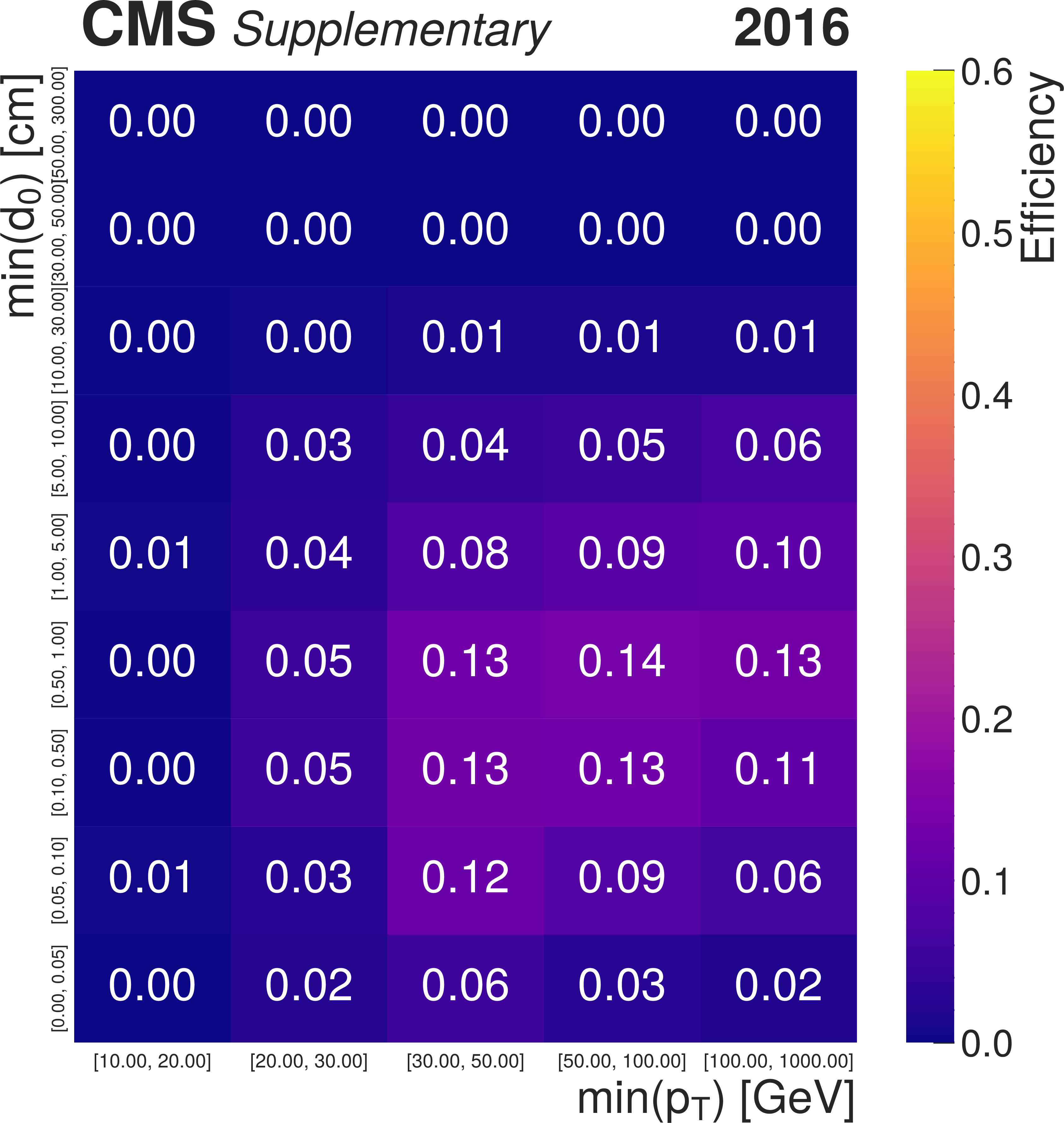
png pdf |
Additional Figure 15-e:
Signal efficiencies as a function of the smaller of the two values of generated muon ${p_{\mathrm {T}}}$ and ${d_{\mathrm {0}}}$ in dimuons with $20 cm < {L_{\mathrm {xy}}} ^\mathrm {true} < $ 70 cm in the $ {\phi\to \mathrm{X} \mathrm{X} \to \mu \mu}+$ anything signal model, in 2016 (left) and 2018 (right) samples. The efficiency in each bin is computed as the ratio of the number of simulated signal dimuons in that bin that pass the trigger requirements and selection criteria applied in the STA-STA (upper), STA-TMS (middle), and TMS-TMS (lower) dimuon category to the total number of simulated signal dimuons in that bin and within the geometric acceptance. The geometric acceptance is defined as the generated longitudinal decay length $ {L_{\mathrm {z}}} ^\mathrm {true}$ smaller than 8 m and $ {| \eta |}$ of both generated muons forming the dimuon smaller than 2.0. The efficiencies obtained from simulation were further corrected by the data-to-simulation scale factors described in the paper. |
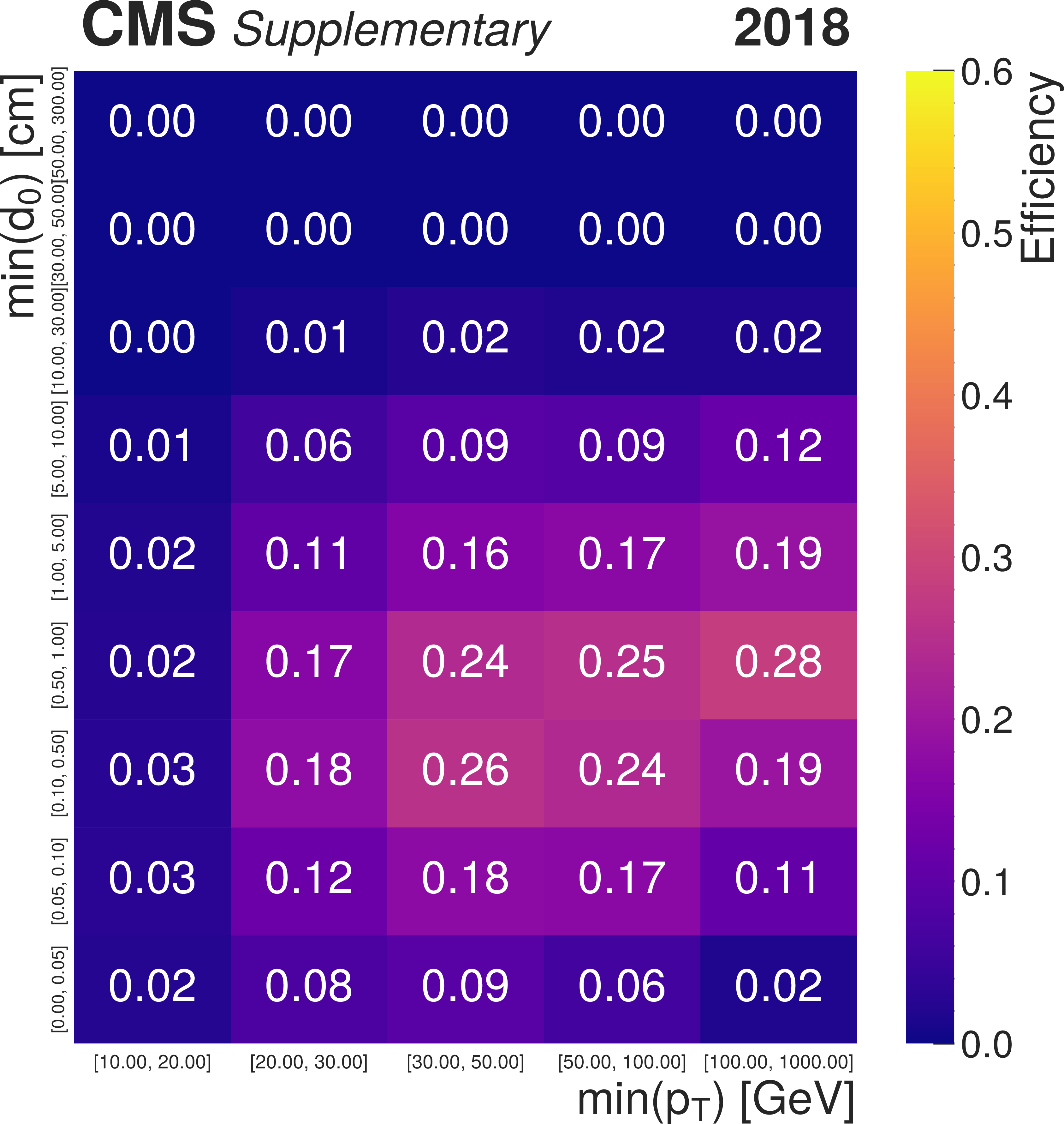
png pdf |
Additional Figure 15-f:
Signal efficiencies as a function of the smaller of the two values of generated muon ${p_{\mathrm {T}}}$ and ${d_{\mathrm {0}}}$ in dimuons with $20 cm < {L_{\mathrm {xy}}} ^\mathrm {true} < $ 70 cm in the $ {\phi\to \mathrm{X} \mathrm{X} \to \mu \mu}+$ anything signal model, in 2016 (left) and 2018 (right) samples. The efficiency in each bin is computed as the ratio of the number of simulated signal dimuons in that bin that pass the trigger requirements and selection criteria applied in the STA-STA (upper), STA-TMS (middle), and TMS-TMS (lower) dimuon category to the total number of simulated signal dimuons in that bin and within the geometric acceptance. The geometric acceptance is defined as the generated longitudinal decay length $ {L_{\mathrm {z}}} ^\mathrm {true}$ smaller than 8 m and $ {| \eta |}$ of both generated muons forming the dimuon smaller than 2.0. The efficiencies obtained from simulation were further corrected by the data-to-simulation scale factors described in the paper. |
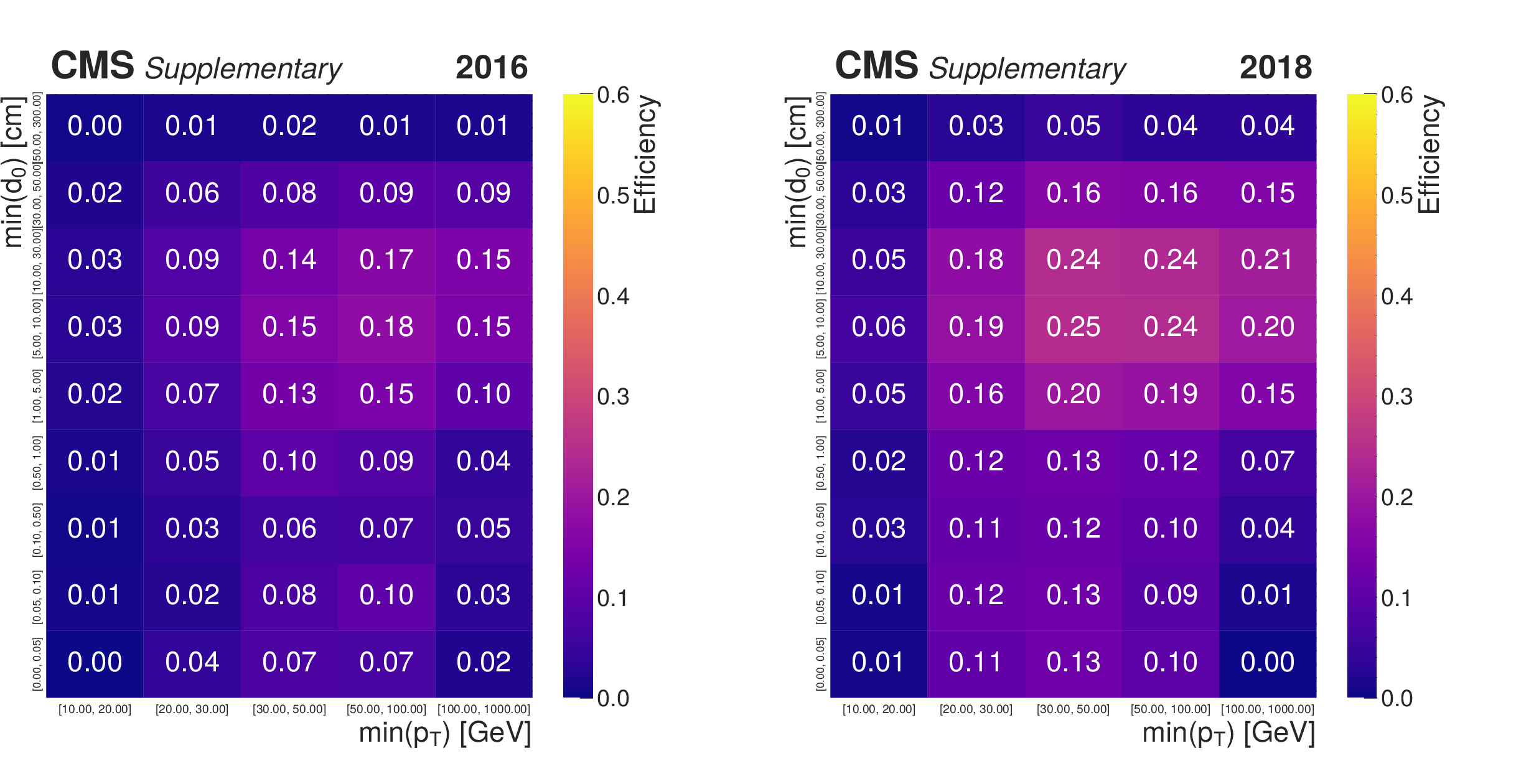
png pdf |
Additional Figure 16:
Signal efficiency as a function of the smaller of the two values of generated muon ${p_{\mathrm {T}}}$ and ${d_{\mathrm {0}}}$ in dimuons with 70 cm $ < {L_{\mathrm {xy}}} ^\mathrm {true} < $ 320 cm in the $ {\phi\to \mathrm{X} \mathrm{X} \to \mu \mu}+$ anything signal model, in 2016 (left) and 2018 (right) samples. The efficiency in each bin is computed as the ratio of the number of simulated signal dimuons in that bin that pass the trigger requirements and selection criteria applied in the STA-STA dimuon category to the total number of simulated signal dimuons in that bin and within the geometric acceptance. The geometric acceptance is defined as the generated longitudinal decay length $ {L_{\mathrm {z}}} ^\mathrm {true}$ smaller than 8 m and $ {| \eta |}$ of both generated muons forming the dimuon smaller than 2.0. The efficiencies obtained from simulation were further corrected by the data-to-simulation scale factors described in the paper. Efficiencies for dimuons with 70 cm $ < {L_{\mathrm {xy}}} ^\mathrm {true} < $ 320 cm in the STA-TMS and TMS-TMS dimuon categories are equal to zero. |
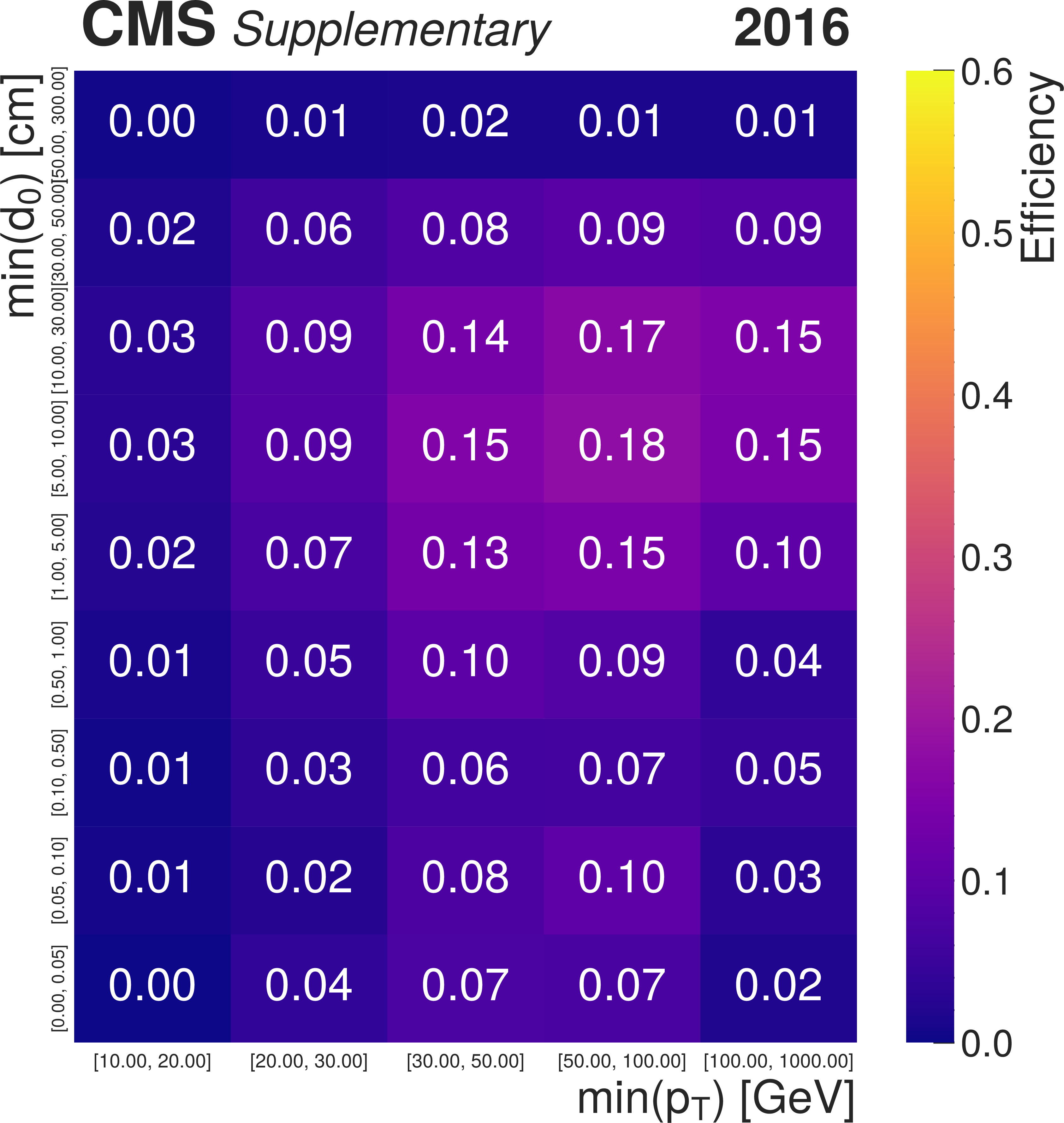
png pdf |
Additional Figure 16-a:
Signal efficiency as a function of the smaller of the two values of generated muon ${p_{\mathrm {T}}}$ and ${d_{\mathrm {0}}}$ in dimuons with 70 cm $ < {L_{\mathrm {xy}}} ^\mathrm {true} < $ 320 cm in the $ {\phi\to \mathrm{X} \mathrm{X} \to \mu \mu}+$ anything signal model, in 2016 (left) and 2018 (right) samples. The efficiency in each bin is computed as the ratio of the number of simulated signal dimuons in that bin that pass the trigger requirements and selection criteria applied in the STA-STA dimuon category to the total number of simulated signal dimuons in that bin and within the geometric acceptance. The geometric acceptance is defined as the generated longitudinal decay length $ {L_{\mathrm {z}}} ^\mathrm {true}$ smaller than 8 m and $ {| \eta |}$ of both generated muons forming the dimuon smaller than 2.0. The efficiencies obtained from simulation were further corrected by the data-to-simulation scale factors described in the paper. Efficiencies for dimuons with 70 cm $ < {L_{\mathrm {xy}}} ^\mathrm {true} < $ 320 cm in the STA-TMS and TMS-TMS dimuon categories are equal to zero. |

png pdf |
Additional Figure 16-b:
Signal efficiency as a function of the smaller of the two values of generated muon ${p_{\mathrm {T}}}$ and ${d_{\mathrm {0}}}$ in dimuons with 70 cm $ < {L_{\mathrm {xy}}} ^\mathrm {true} < $ 320 cm in the $ {\phi\to \mathrm{X} \mathrm{X} \to \mu \mu}+$ anything signal model, in 2016 (left) and 2018 (right) samples. The efficiency in each bin is computed as the ratio of the number of simulated signal dimuons in that bin that pass the trigger requirements and selection criteria applied in the STA-STA dimuon category to the total number of simulated signal dimuons in that bin and within the geometric acceptance. The geometric acceptance is defined as the generated longitudinal decay length $ {L_{\mathrm {z}}} ^\mathrm {true}$ smaller than 8 m and $ {| \eta |}$ of both generated muons forming the dimuon smaller than 2.0. The efficiencies obtained from simulation were further corrected by the data-to-simulation scale factors described in the paper. Efficiencies for dimuons with 70 cm $ < {L_{\mathrm {xy}}} ^\mathrm {true} < $ 320 cm in the STA-TMS and TMS-TMS dimuon categories are equal to zero. |
| Additional Tables | |
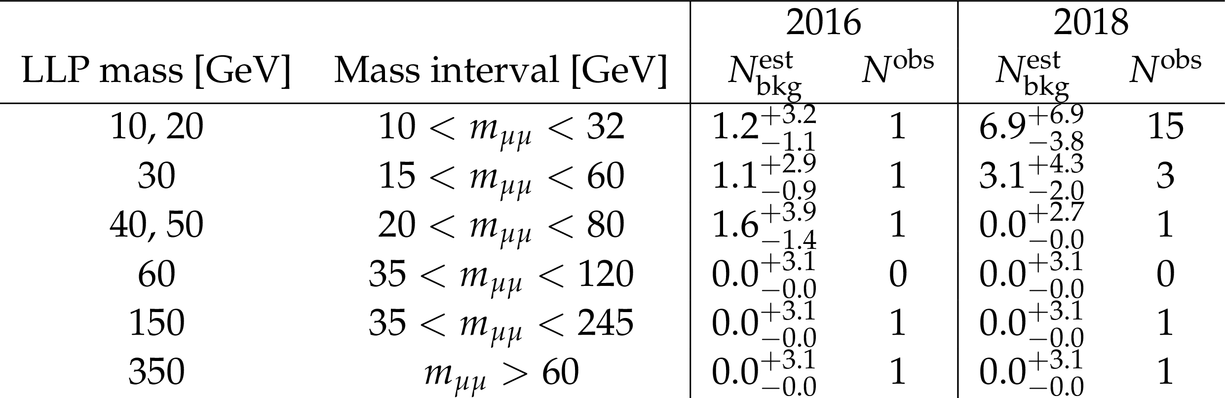
png pdf |
Additional Table 1:
Background estimations and observed numbers of events in the STA-STA dimuon category in 2016 and 2018 data. For each probed LLP mass, the chosen mass interval is shown, followed by the predicted background yield $N^\text {est}_\text {bkg}$ and the observed number of events $N^\text {obs}$ for the given year. The quoted uncertainties are statistical only. |

png pdf |
Additional Table 2:
Background estimations and observed numbers of events in the TMS-TMS dimuon category in 2016 data. For each mass interval, the table shows the predicted background yield $N^\text {est}_\text {bkg}$ and the observed number of events $N^\text {obs}$ in each of the three $\text {min}({{d_{\mathrm {0}}} / {\sigma _{{d_{\mathrm {0}}}}}})$ bins. The quoted uncertainties are statistical only. |
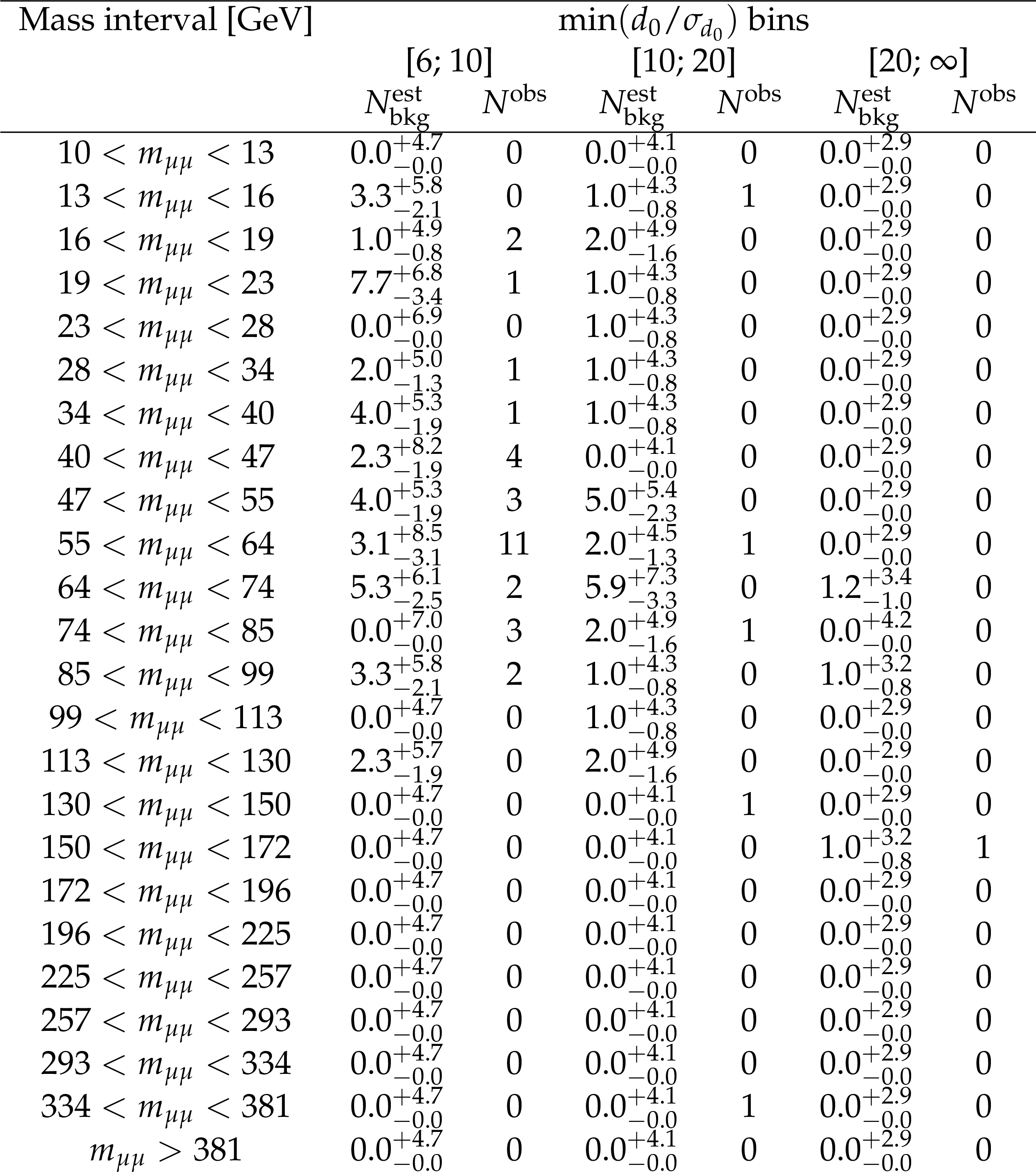
png pdf |
Additional Table 3:
Background estimations and observed numbers of events in the TMS-TMS dimuon category in 2018 data. For each mass interval, the table shows the predicted background yield $N^\text {est}_\text {bkg}$ and the observed number of events $N^\text {obs}$ in each of the three $\text {min}({{d_{\mathrm {0}}} / {\sigma _{{d_{\mathrm {0}}}}}})$ bins. The quoted uncertainties are statistical only. |

png pdf |
Additional Table 4:
Correspondence between the probed LLP masses and the chosen mass intervals in the TMS-TMS category. |
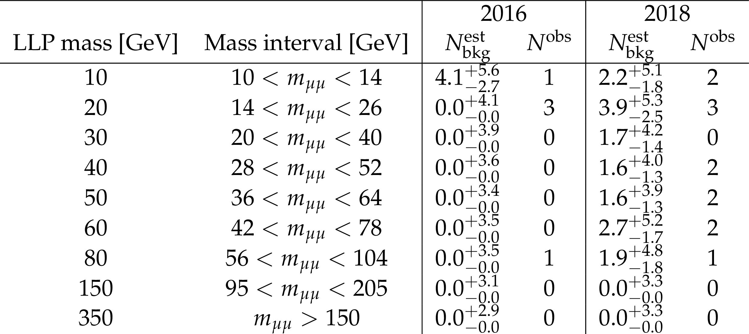
png pdf |
Additional Table 5:
Background estimations and observed numbers of events in the STA-TMS dimuon category in 2016 and 2018 data. For each probed LLP mass, the chosen mass interval is shown, followed by the predicted background yield $N^\text {est}_\text {bkg}$ and the observed number of events $N^\text {obs}$ for the given year. The quoted uncertainties are statistical only. |

png pdf |
Additional Table 6:
Number of events passing consecutive sets of selection criteria, in 2018 data and in a sample of simulated $ {\phi\to \mathrm{X} \mathrm{X} \to \mu \mu}+$ anything signal events with $ {m(\phi)} = $ 125 GeV, $ {m(\mathrm{X})} = $ 20 GeV, and $ {c\tau} = $ 13 cm. Each row introduces a new criterion that is applied in addition to the selection of the previous row. In addition to the total number of events $N(\text {total})$, the event yields in the individual dimuon categories, STA-STA, TMS-TMS, and STA-TMS, are shown in separate columns for each data set. In these columns, events containing selected dimuons of different categories are counted independently for each category. |
| HEPData Instructions for Reinterpretation |
|
While the search presented specifically addresses two benchmark models described in the paper, its results may be applied to other models predicting long-lived particles that decay into a pair of oppositely charged muons. In Figs. A14--A16 we provide a set of generator-level efficiency maps that approximate the reconstruction-level efficiency of this analysis and allow for reinterpretation of the results in the framework of other models. We provide signal efficiencies as a function of the smaller of the two values of generated muon $p_{\mathrm{T}}$, $\mathrm{min}\left(p_{\mathrm{T}}\right)$, and of generated muon $d_{0}$, $\mathrm{min}\left(d_{0}\right)$, in three intervals of the generated transverse decay length $L_{\mathrm{xy}}$ of the signal dimuon, $L_{\mathrm{xy}} < $ 20 cm, 20 $ < L_{\mathrm{xy}} < $ 70 cm, and 70 $ < L_{\mathrm{xy}} < $ 320 cm. These 3D efficiency maps $\epsilon \left( \mathrm{min}\left(p_{\mathrm{T}}\right); \mathrm{min}\left(d_{0}\right); L_{\mathrm{xy}} \right)$ are provided separately for each of the three dimuon categories, STA-STA, STA-TMS, and TMS-TMS, and are shown in Fig. A14, Fig. A15, and Fig. A16 for dimuons with $L_{\mathrm{xy}} < $ 20 cm, 20 $< L_{\mathrm{xy}} < $ 70 cm, and 70 $< L_{\mathrm{xy}} < $ 320 cm, respectively. Each figure contains two sets of maps, for 2016 and 2018 data sets, corresponding to integrated luminosities of 36.3 $ \pm$ 0.4 and 61.3 $\pm$ 1.5 fb$^{-1}$, respectively. The efficiency in each ($\mathrm{min}\left(p_{\mathrm{T}}\right)$; $\mathrm{min}\left(d_{0}\right)$; $L_{\mathrm{xy}}$) bin of the 3D efficiency map is computed as the ratio of the number of simulated signal dimuons in that bin that pass the trigger requirements and selection criteria applied for a given dimuon category (Table A6) to the total number of simulated signal dimuons in that bin and within the geometric acceptance. The computation is performed using an ensemble of all generated $\phi \to \mathrm{XX} \to \mu\mu +$anything signal samples. The geometric acceptance is defined as $\mathrm{min}\left(d_{0}\right) < $ 300 cm, $L_{\mathrm{xy}} < $ 320 cm, generated longitudinal decay length $L_{\mathrm{z}}$ smaller than 800 cm, and $|\eta|$ of both generated muons forming the dimuon smaller than 2.0. The efficiencies obtained from simulation were further corrected by the data-to-simulation scale factors described in the paper. When applied to the previously untested models, the signal efficiency in each dimuon category $j$, $\epsilon_j$, can be obtained from the 3D efficiency maps using the $p_{\mathrm{T}}$, $d_{0}$, and $L_{\mathrm{xy}}$ at generator level: |
| References | ||||
| 1 | R. Barbier et al. | R-parity violating supersymmetry | PR 420 (2005) 1 | hep-ph/0406039 |
| 2 | J. L. Hewett, B. Lillie, M. Masip, and T. G. Rizzo | Signatures of long-lived gluinos in split supersymmetry | JHEP 09 (2004) 070 | hep-ph/0408248 |
| 3 | M. J. Strassler and K. M. Zurek | Echoes of a hidden valley at hadron colliders | PLB 651 (2007) 374 | hep-ph/0604261 |
| 4 | T. Han, Z. Si, K. M. Zurek, and M. J. Strassler | Phenomenology of hidden valleys at hadron colliders | JHEP 07 (2008) 008 | 0712.2041 |
| 5 | D. Curtin, R. Essig, S. Gori, and J. Shelton | Illuminating dark photons with high-energy colliders | JHEP 02 (2015) 157 | 1412.0018 |
| 6 | M. J. Strassler and K. M. Zurek | Discovering the Higgs through highly-displaced vertices | PLB 661 (2008) 263 | hep-ph/0605193 |
| 7 | CMS Collaboration | Search for long-lived particles that decay into final states containing two electrons or two muons in proton-proton collisions at $ \sqrt{s} = $ 8 TeV | PRD 91 (2015) 052012 | CMS-EXO-12-037 1411.6977 |
| 8 | CMS Collaboration | Search for long-lived particles that decay into final states containing two muons, reconstructed using only the CMS muon chambers | CMS-PAS-EXO-14-012 | CMS-PAS-EXO-14-012 |
| 9 | ATLAS Collaboration | Search for long-lived particles in final states with displaced dimuon vertices in pp collisions at $ \sqrt{s}= $ 13 TeV with the ATLAS detector | PRD 99 (2019) 012001 | 1808.03057 |
| 10 | CMS Collaboration | HEPData record for this analysis | link | |
| 11 | CMS Collaboration | Performance of the CMS muon detector and muon reconstruction with proton-proton collisions at $ \sqrt{s} = $ 13 TeV | JINST 13 (2018) P06015 | CMS-MUO-16-001 1804.04528 |
| 12 | CMS Collaboration | The CMS experiment at the CERN LHC | JINST 3 (2008) S08004 | CMS-00-001 |
| 13 | CMS Collaboration | Performance of the CMS Level-1 trigger in proton-proton collisions at $ \sqrt{s} = $ 13 TeV | JINST 15 (2020) P10017 | CMS-TRG-17-001 2006.10165 |
| 14 | CMS Collaboration | The CMS trigger system | JINST 12 (2017) P01020 | CMS-TRG-12-001 1609.02366 |
| 15 | CMS Collaboration | Precision luminosity measurement in proton-proton collisions at $ \sqrt{s} = $ 13 TeV in 2015 and 2016 at CMS | EPJC 81 (2021) 800 | CMS-LUM-17-003 2104.01927 |
| 16 | CMS Collaboration | CMS luminosity measurement for the 2018 data-taking period at $ \sqrt{s} = $ 13 TeV | CMS-PAS-LUM-18-002 | CMS-PAS-LUM-18-002 |
| 17 | J. D. Wells | How to find a hidden world at the Large Hadron Collider | in Perspectives on LHC Physics, G. Kane and A. Pierce, eds., p. 283 World Scientific, Singapore | 0803.1243 |
| 18 | J. Alwall et al. | The automated computation of tree-level and next-to-leading order differential cross sections, and their matching to parton shower simulations | JHEP 07 (2014) 079 | 1405.0301 |
| 19 | M. Cepeda et al. | Report from working group 2: Higgs physics at the HL-LHC and HE-LHC | in Proceedings of the HL/HE-LHC Workshop, A. Dainese et al., eds., volume 7, p. 221 2019 CERN Yellow Rep. Monogr | 1902.00134 |
| 20 | T. Sjostrand et al. | An introduction to PYTHIA 8.2 | CPC 191 (2015) 159 | 1410.3012 |
| 21 | J. Butterworth et al. | PDF4LHC recommendations for LHC Run II | JPG 43 (2016) 023001 | 1510.03865 |
| 22 | CMS Collaboration | Event generator tunes obtained from underlying event and multiparton scattering measurements | EPJC 76 (2016) 155 | CMS-GEN-14-001 1512.00815 |
| 23 | NNPDF Collaboration | Parton distributions from high-precision collider data | EPJC 77 (2017) 663 | 1706.00428 |
| 24 | CMS Collaboration | Extraction and validation of a new set of CMS PYTHIA8 tunes from underlying-event measurements | EPJC 80 (2020) 4 | CMS-GEN-17-001 1903.12179 |
| 25 | \GEANTfour Collaboration | GEANT4--a simulation toolkit | NIMA 506 (2003) 250 | |
| 26 | CMS Collaboration | Technical proposal for the Phase-II upgrade of the Compact Muon Solenoid | CMS-PAS-TDR-15-002 | CMS-PAS-TDR-15-002 |
| 27 | CMS Collaboration | Performance of the CMS muon trigger system in proton-proton collisions at $ \sqrt{s} = $ 13 TeV | JINST 16 (2021) P07001 | CMS-MUO-19-001 2102.04790 |
| 28 | CMS Collaboration | Performance of CMS muon reconstruction in pp collision events at $ \sqrt{s}= $ 7 TeV | JINST 7 (2012) P10002 | CMS-MUO-10-004 1206.4071 |
| 29 | R. Fruhwirth | Application of Kalman filtering to track and vertex fitting | NIMA 262 (1987) 444 | |
| 30 | T. Speer et al. | Vertex fitting in the CMS tracker | CMS-NOTE-2006-032 | |
| 31 | B. C. Allanach et al. | Mass spectrum in R-parity violating mSUGRA and benchmark points | PRD 75 (2007) 035002 | hep-ph/0609263 |
| 32 | F. Deppisch, S. Kulkarni, and W. Liu | Heavy neutrino production via $ Z^\prime $ at the lifetime frontier | PRD 100 (2019) 035005 | 1905.11889 |
| 33 | R. D. Cousins, J. T. Linnemann, and J. Tucker | Evaluation of three methods for calculating statistical significance when incorporating a systematic uncertainty into a test of the background-only hypothesis for a Poisson process | NIMA 595 (2008) 480 | physics/0702156 |
| 34 | CMS Collaboration | Search for new particles decaying to a jet and an emerging jet | JHEP 02 (2019) 179 | CMS-EXO-18-001 1810.10069 |
| 35 | A. L. Read | Presentation of search results: The CL$ _{\text{s}} $ technique | JPG 28 (2002) 2693 | |
| 36 | T. Junk | Confidence level computation for combining searches with small statistics | NIMA 434 (1999) 435 | hep-ex/9902006 |
| 37 | ATLAS and CMS Collaborations, and LHC Higgs Combination Group | Procedure for the LHC Higgs boson search combination in Summer 2011 | CMS-NOTE-2011-005 | |
| 38 | CMS Collaboration | Search for invisible decays of the Higgs boson produced via vector boson fusion in proton--proton collisions at $ \sqrt{s} = $ 13 TeV | Accepted by PRD | CMS-HIG-20-003 2201.11585 |
| 39 | CMS Collaboration | Combined measurements of Higgs boson couplings in proton-proton collisions at $ \sqrt{s} = $ 13 TeV | EPJC 79 (2019) 421 | CMS-HIG-17-031 1809.10733 |
| 40 | CMS Collaboration | Search for long-lived particles decaying into muon pairs in proton-proton collisions at $ \sqrt{s} = $ 13 TeV collected with a dedicated high-rate data stream | JHEP 04 (2022) 062 | CMS-EXO-20-014 2112.13769 |
|
|
Compact Muon Solenoid LHC, CERN |
|

|

|

|

|

|