

Compact Muon Solenoid
LHC, CERN
| CMS-HIG-20-003 ; CERN-EP-2021-273 | ||
| Search for invisible decays of the Higgs boson produced via vector boson fusion in proton-proton collisions at $\sqrt{s} = $ 13 TeV | ||
| CMS Collaboration | ||
| 27 January 2022 | ||
| Phys. Rev. D 105 (2022) 092007 | ||
| Abstract: A search for invisible decays of the Higgs boson produced via vector boson fusion (VBF) has been performed with 101 fb$^{-1}$ of proton-proton collisions delivered by the LHC at $\sqrt{s} = $ 13 TeV and collected by the CMS detector in 2017 and 2018. The sensitivity to the VBF production mechanism is enhanced by constructing two analysis categories, one based on missing transverse momentum, and a second based on the properties of jets. In addition to control regions with Z and W boson candidate events, a highly populated control region, based on the production of a photon in association with jets, is used to constrain the dominant irreducible background from the invisible decay of a Z boson produced in association with jets. The results of this search are combined with all previous measurements in the VBF topology, based on data collected in 2012 (at $\sqrt{s} = $ 8 TeV), 2015, and 2016, corresponding to integrated luminosities of 19.7, 2.3, and 36.3 fb$^{-1}$, respectively. The observed (expected) upper limit on the invisible branching fraction of the Higgs boson is found to be 0.18 (0.10) at the 95% confidence level, assuming the standard model production cross section. The results are also interpreted in the context of Higgs-portal models. | ||
| Links: e-print arXiv:2201.11585 [hep-ex] (PDF) ; CDS record ; inSPIRE record ; HepData record ; Physics Briefing ; CADI line (restricted) ; | ||
| Figures | |

png pdf |
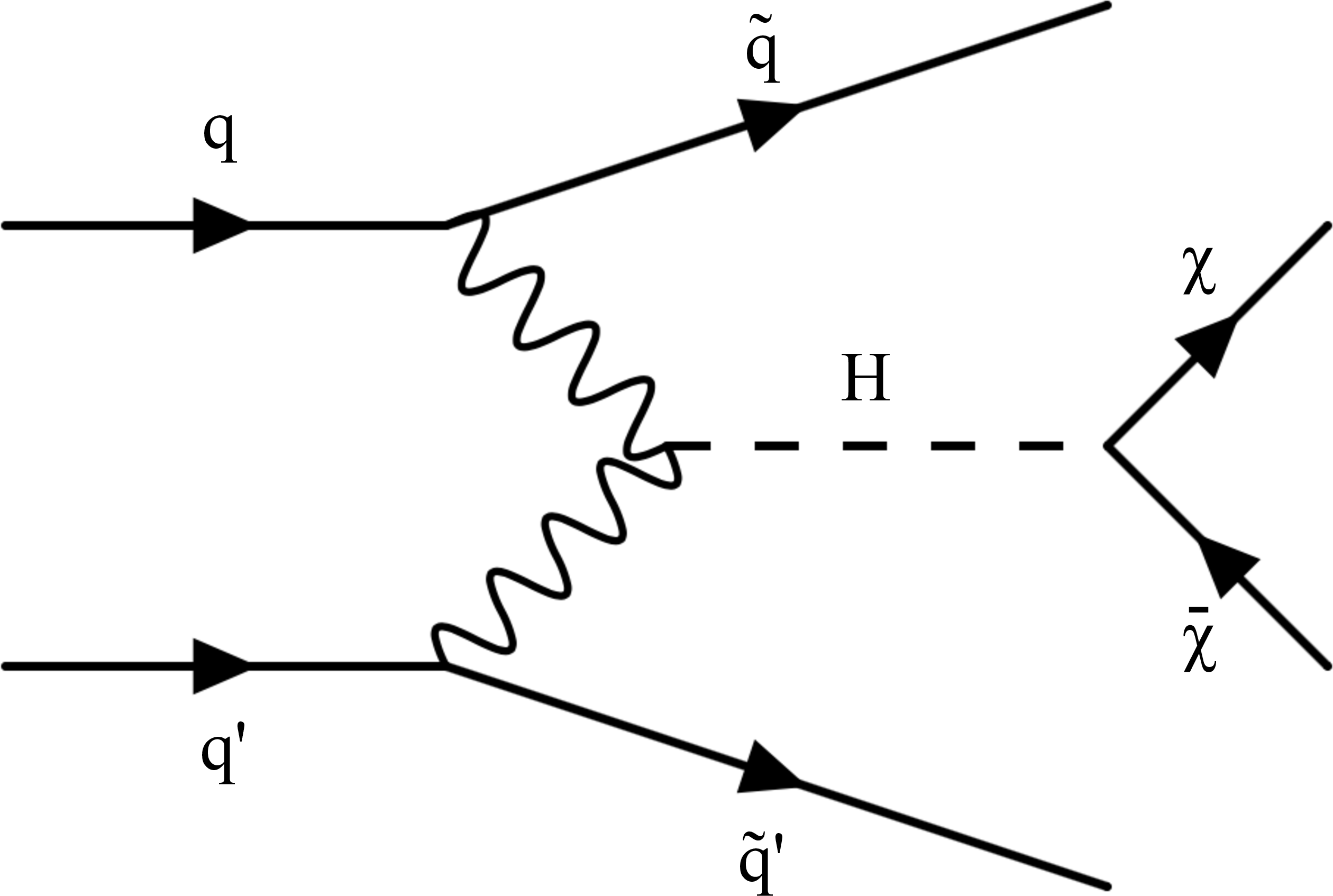
Figure 1:
Leading-order Feynman diagrams for the production of the Higgs boson in association with two jets from VBF (left), and representative leading-order Feynman diagrams for the production of a Z boson in association with two jets either through VBF production (middle) or strong production (right). Diagrams for the production of a W boson in association with two jets are similar. |
png pdf |
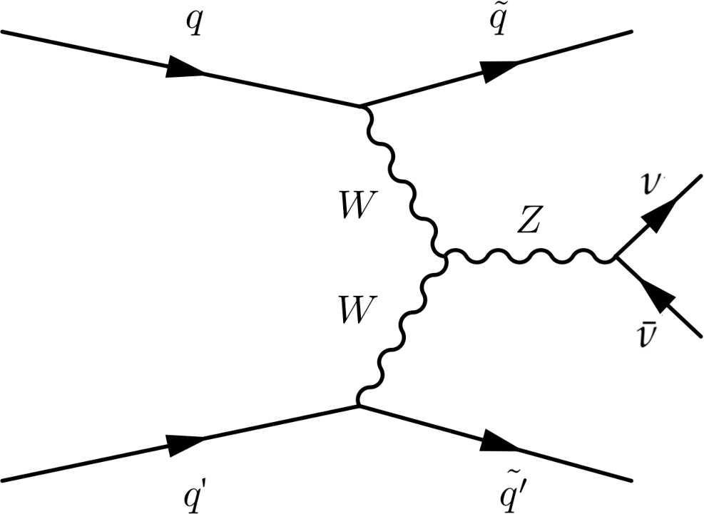
Figure 1-a:
Leading-order Feynman diagrams for the production of the Higgs boson in association with two jets from VBF (left), and representative leading-order Feynman diagrams for the production of a Z boson in association with two jets either through VBF production (middle) or strong production (right). Diagrams for the production of a W boson in association with two jets are similar. |
png pdf |
Figure 1-b:
Leading-order Feynman diagrams for the production of the Higgs boson in association with two jets from VBF (left), and representative leading-order Feynman diagrams for the production of a Z boson in association with two jets either through VBF production (middle) or strong production (right). Diagrams for the production of a W boson in association with two jets are similar. |
png pdf |
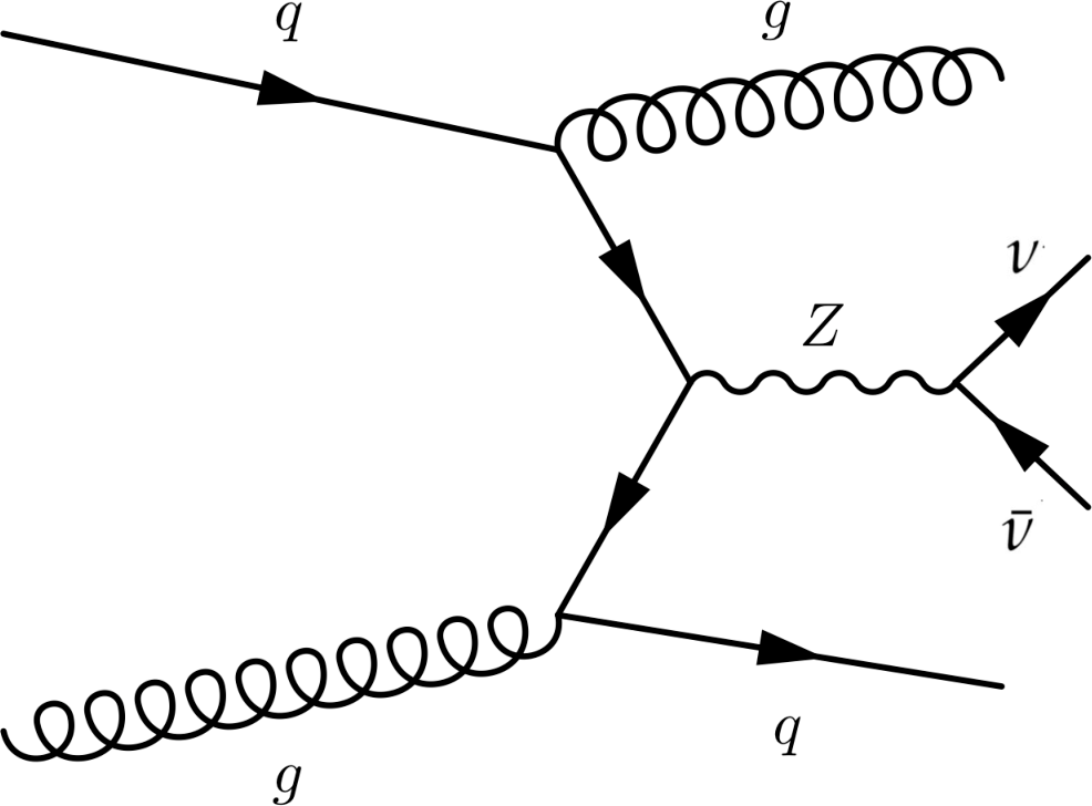
Figure 1-c:
Leading-order Feynman diagrams for the production of the Higgs boson in association with two jets from VBF (left), and representative leading-order Feynman diagrams for the production of a Z boson in association with two jets either through VBF production (middle) or strong production (right). Diagrams for the production of a W boson in association with two jets are similar. |

png pdf |
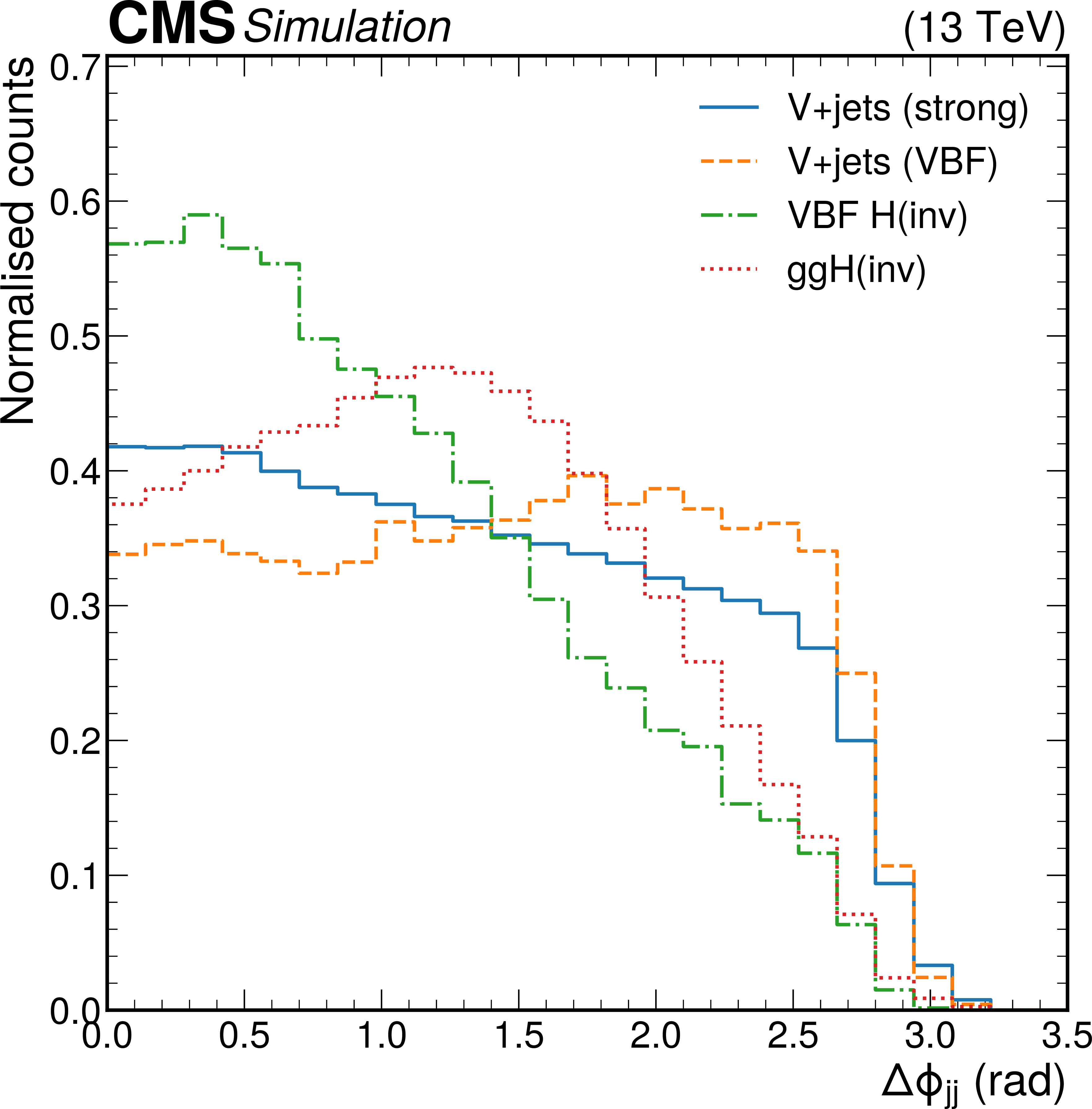
Figure 2:
Comparison of shapes of quantities related to the dijet pair. Shown are ${m_{\mathrm {jj}}}$ (upper), ${\Delta \eta _{\mathrm {jj}}}$ (lower left), and ${\Delta \phi _{\mathrm {jj}}}$ (lower right), as predicted by simulation, separating strong and VBF production for V+jets and signal processes. |

png pdf |
Figure 2-a:
Comparison of shapes of quantities related to the dijet pair. Shown are ${m_{\mathrm {jj}}}$ (upper), ${\Delta \eta _{\mathrm {jj}}}$ (lower left), and ${\Delta \phi _{\mathrm {jj}}}$ (lower right), as predicted by simulation, separating strong and VBF production for V+jets and signal processes. |

png pdf |
Figure 2-b:
Comparison of shapes of quantities related to the dijet pair. Shown are ${m_{\mathrm {jj}}}$ (upper), ${\Delta \eta _{\mathrm {jj}}}$ (lower left), and ${\Delta \phi _{\mathrm {jj}}}$ (lower right), as predicted by simulation, separating strong and VBF production for V+jets and signal processes. |
png pdf |
Figure 2-c:
Comparison of shapes of quantities related to the dijet pair. Shown are ${m_{\mathrm {jj}}}$ (upper), ${\Delta \eta _{\mathrm {jj}}}$ (lower left), and ${\Delta \phi _{\mathrm {jj}}}$ (lower right), as predicted by simulation, separating strong and VBF production for V+jets and signal processes. |
png pdf |
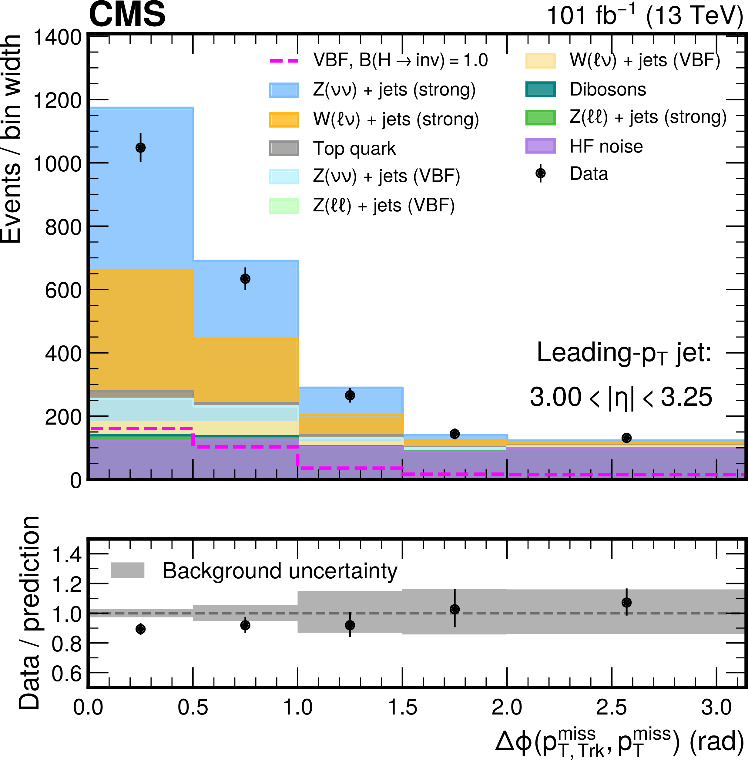
Figure 3:
The $\Delta \phi ({p_{\mathrm {T, trk}}^\text {miss}}, {{p_{\mathrm {T}}} ^\text {miss}})$ distribution in the SR with the additional requirement that the leading-$ {p_{\mathrm {T}}}$ jet passes 3 $ < {| \eta |} < $ 3.25. The 2017 and 2018 data are compared with the sum of the HF noise template and other backgrounds from simulation. The uncertainty band includes only statistical uncertainties in the simulation. |

png pdf |
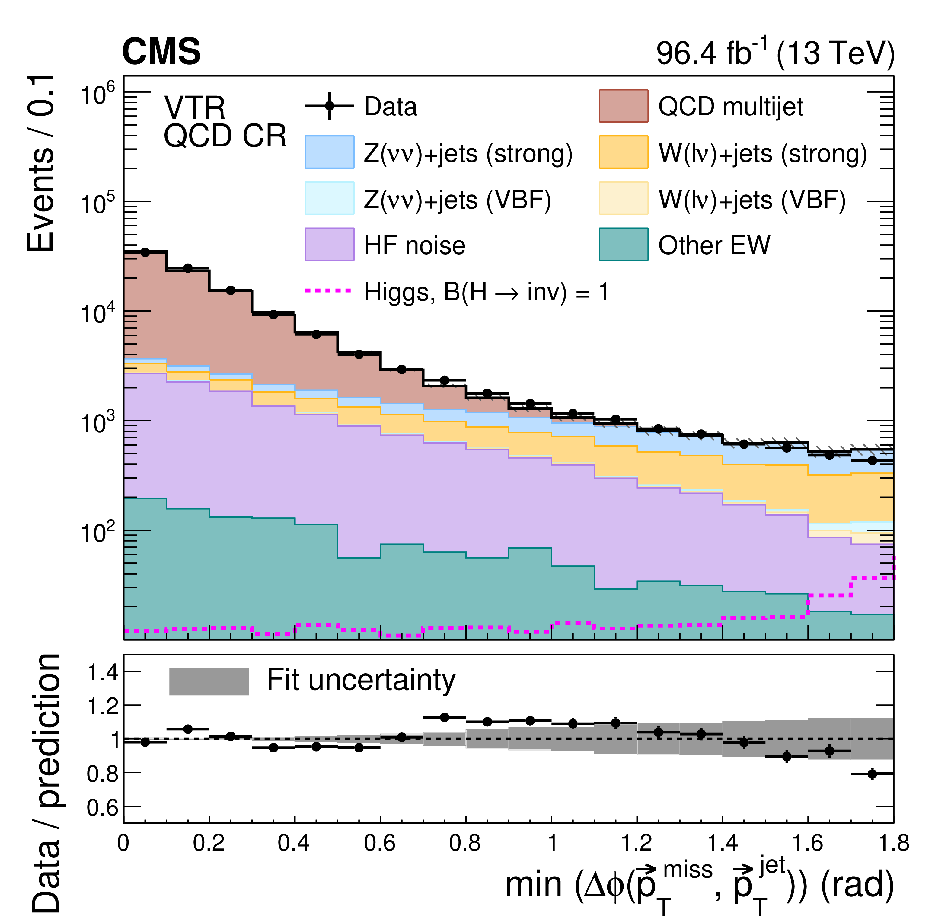
Figure 4:
The $\min({\Delta \phi ({{\vec{p}}_{\mathrm {T}}^{\,\text {miss}}},\vec{p}_{\mathrm {T}}^{\,\text {jet}})})$ distribution in data from 2017 and 2018, and contributions from V+jets, diboson plus top quark processes, HF noise, and QCD multijet events for the MTR (left) and VTR (right) categories. The uncertainty band shows the uncertainty from the fit used to determine the normalization of the QCD multijet template in the corresponding SR. The yields from the 2017 and 2018 samples are summed and the correlations between their uncertainties are neglected. |

png pdf |
Figure 4-a:
The $\min({\Delta \phi ({{\vec{p}}_{\mathrm {T}}^{\,\text {miss}}},\vec{p}_{\mathrm {T}}^{\,\text {jet}})})$ distribution in data from 2017 and 2018, and contributions from V+jets, diboson plus top quark processes, HF noise, and QCD multijet events for the MTR (left) and VTR (right) categories. The uncertainty band shows the uncertainty from the fit used to determine the normalization of the QCD multijet template in the corresponding SR. The yields from the 2017 and 2018 samples are summed and the correlations between their uncertainties are neglected. |
png pdf |
Figure 4-b:
The $\min({\Delta \phi ({{\vec{p}}_{\mathrm {T}}^{\,\text {miss}}},\vec{p}_{\mathrm {T}}^{\,\text {jet}})})$ distribution in data from 2017 and 2018, and contributions from V+jets, diboson plus top quark processes, HF noise, and QCD multijet events for the MTR (left) and VTR (right) categories. The uncertainty band shows the uncertainty from the fit used to determine the normalization of the QCD multijet template in the corresponding SR. The yields from the 2017 and 2018 samples are summed and the correlations between their uncertainties are neglected. |

png pdf |
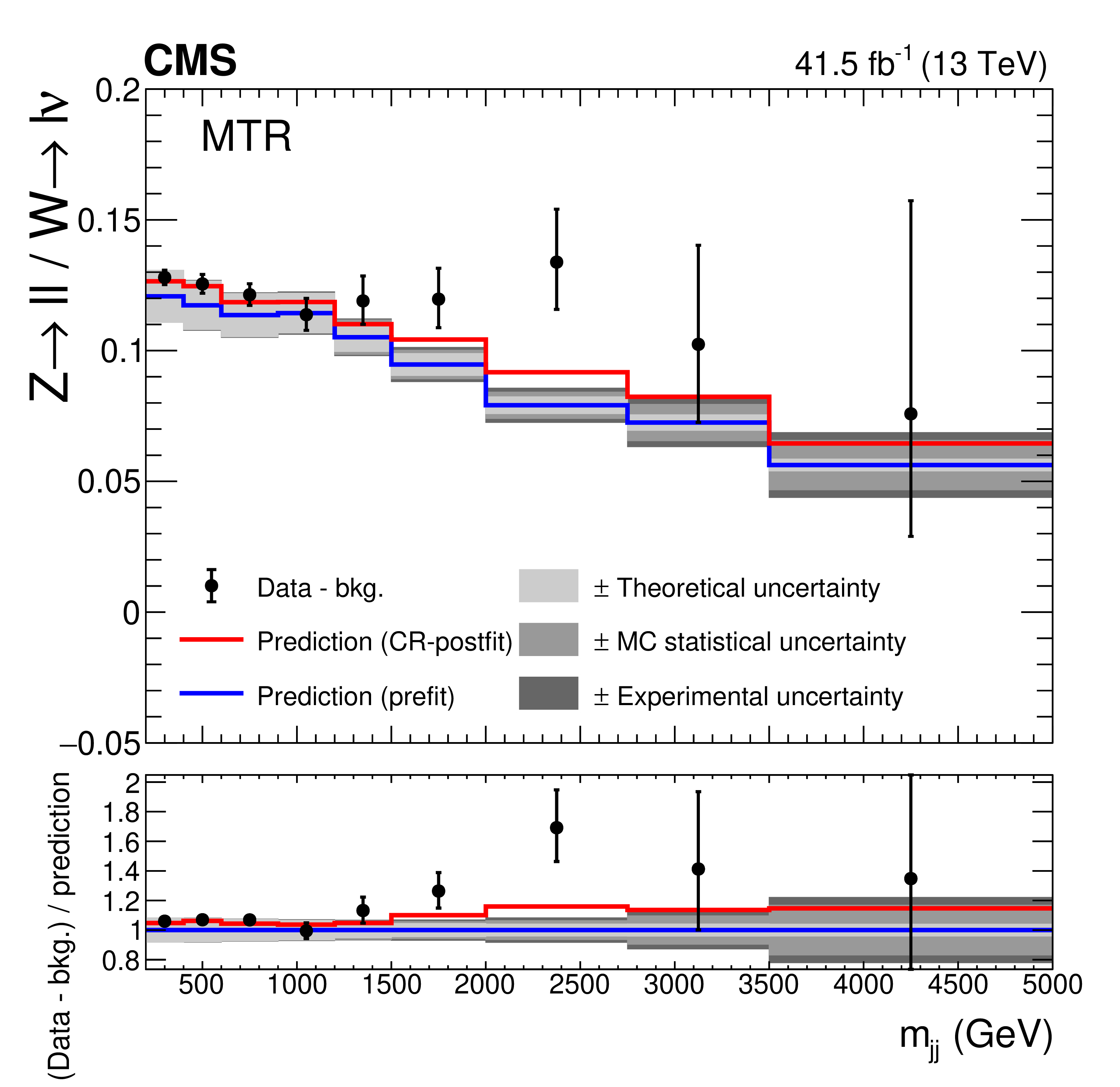
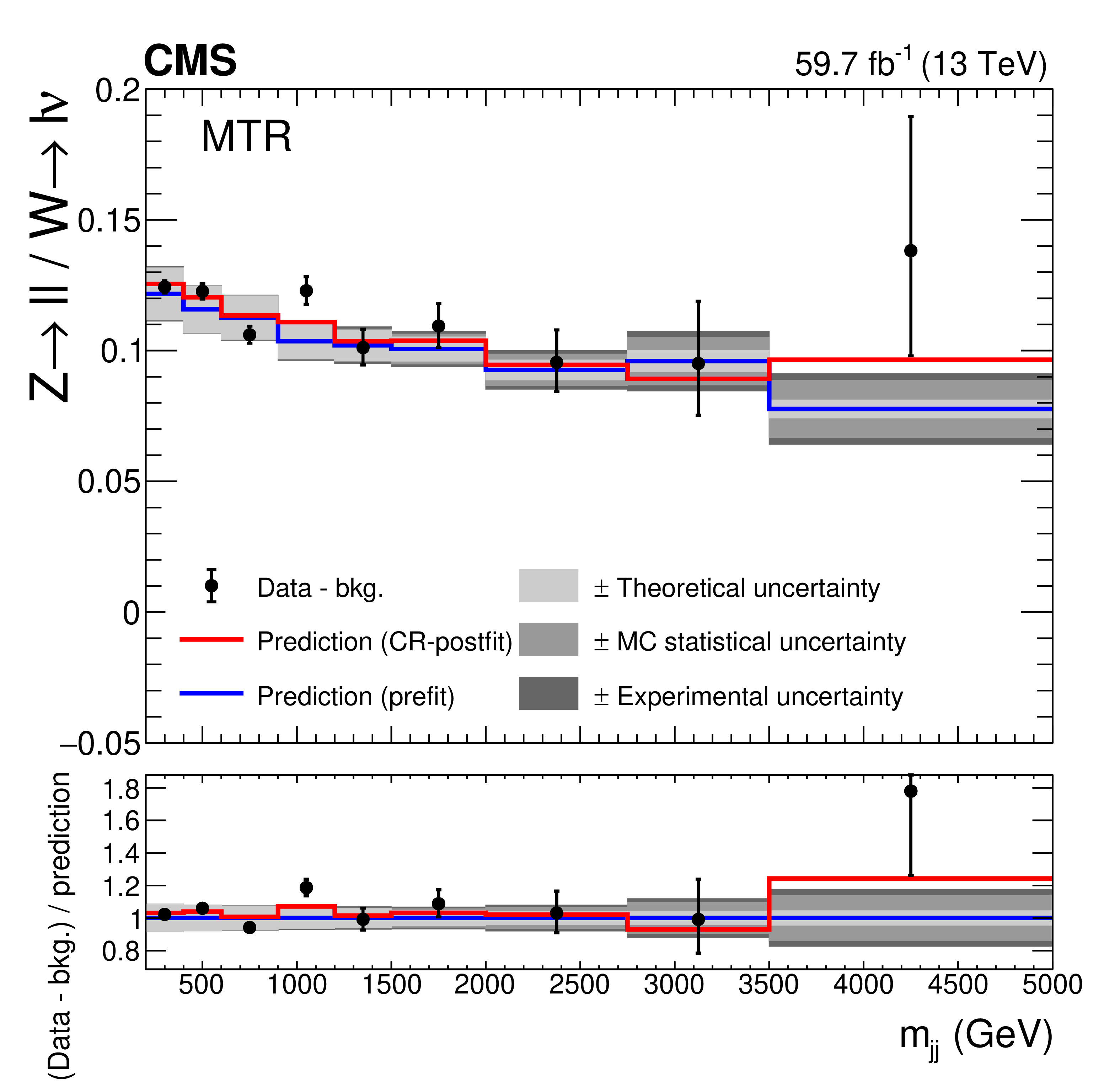
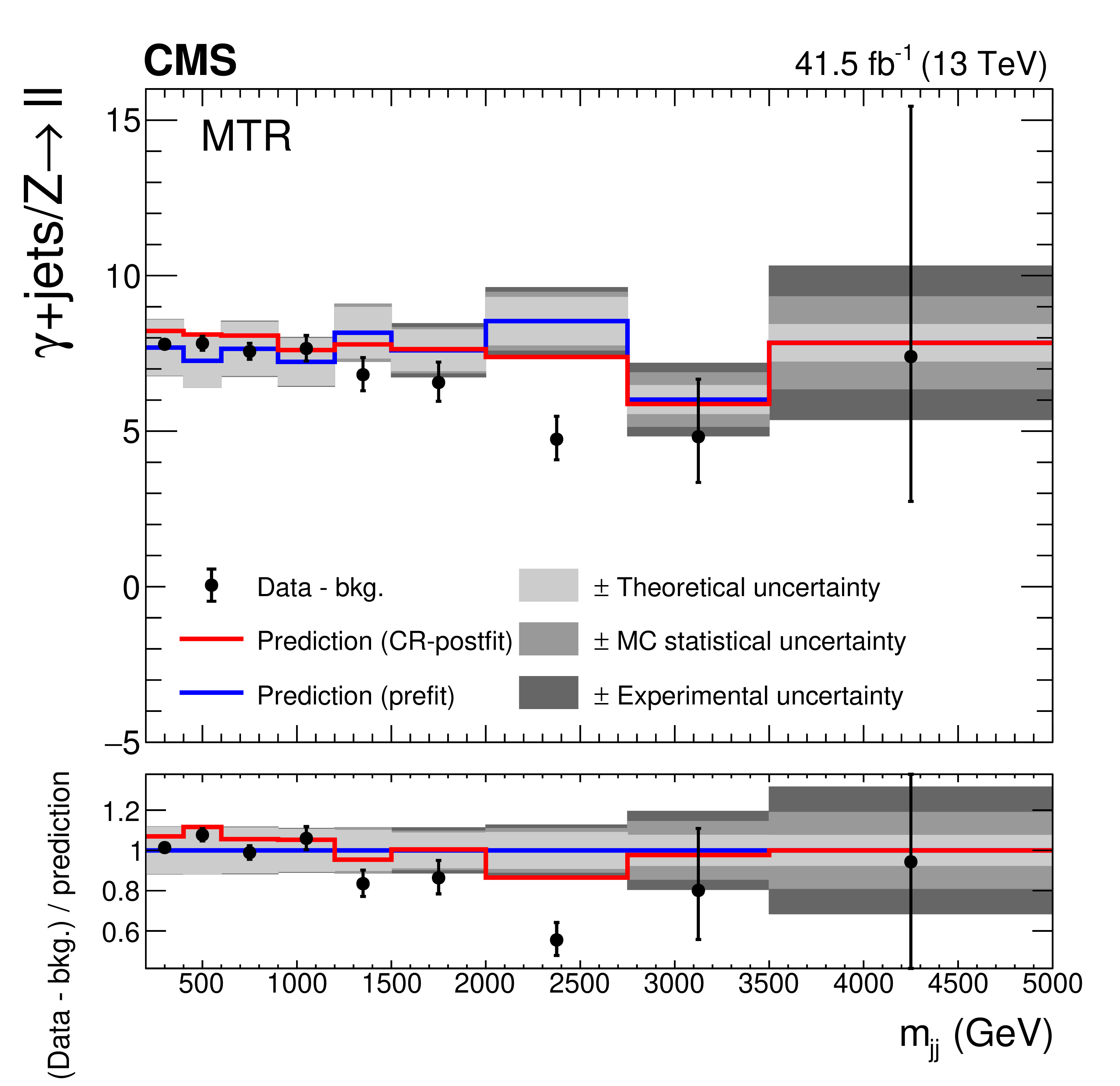
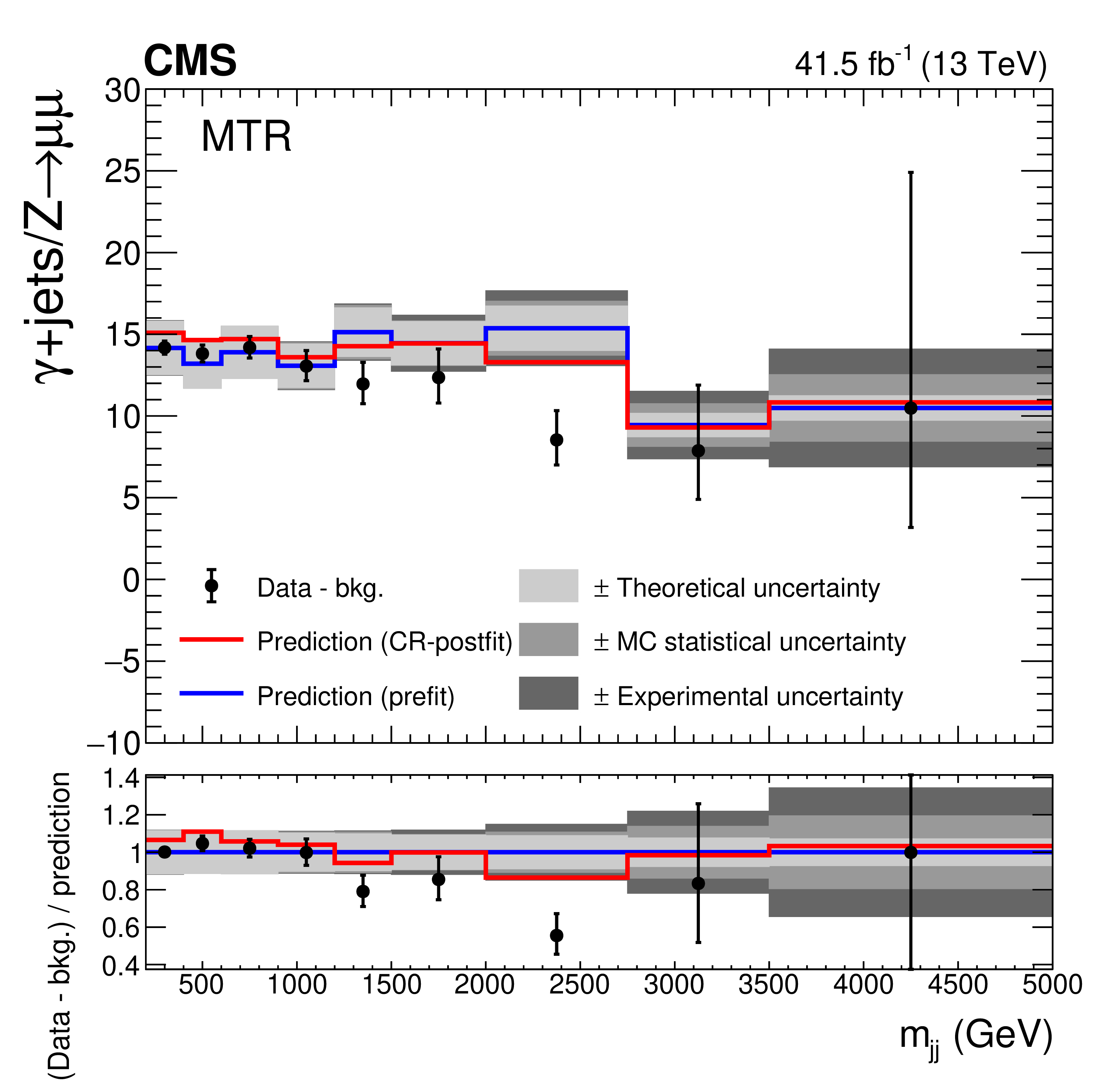
Figure 5:
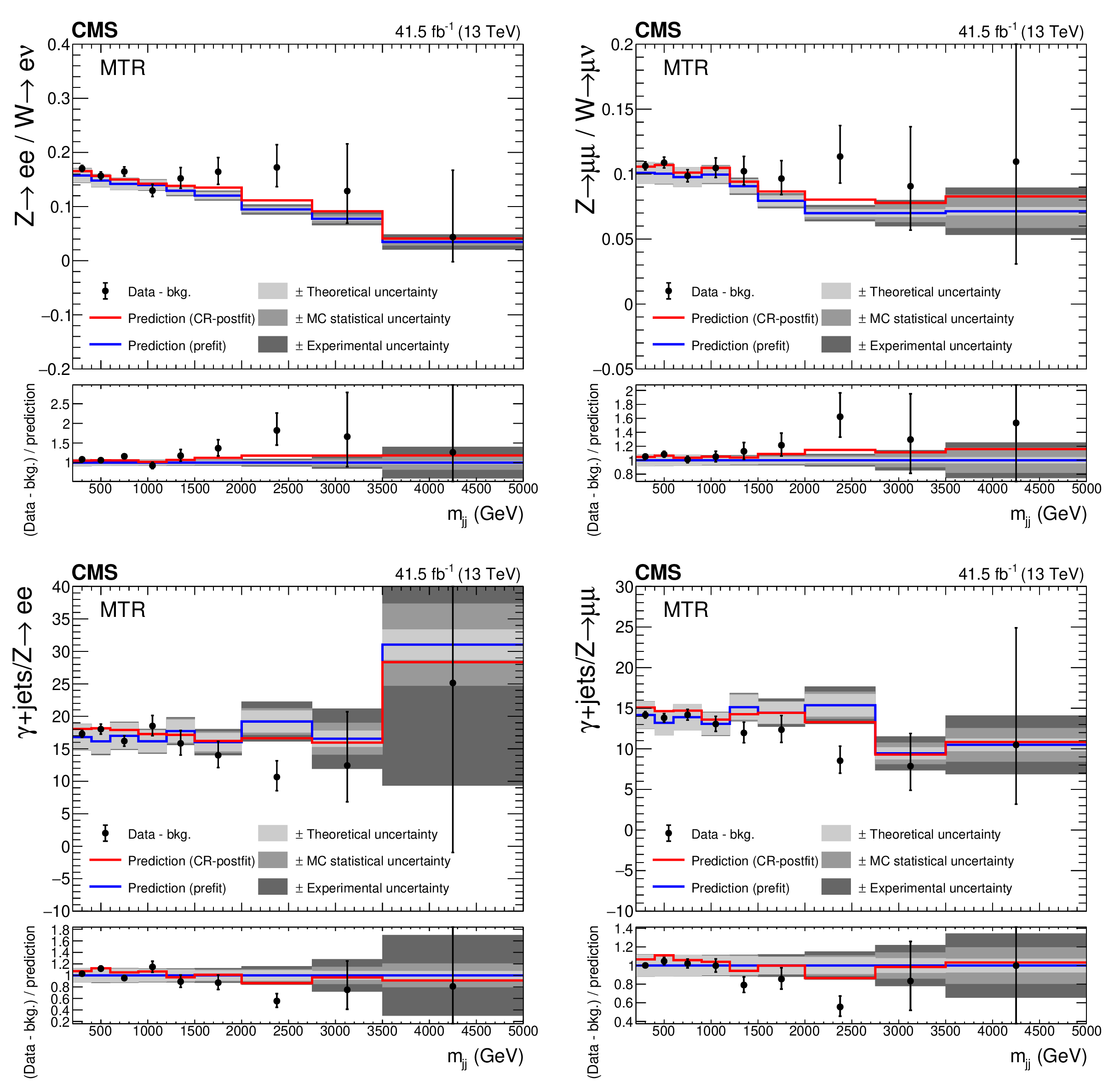
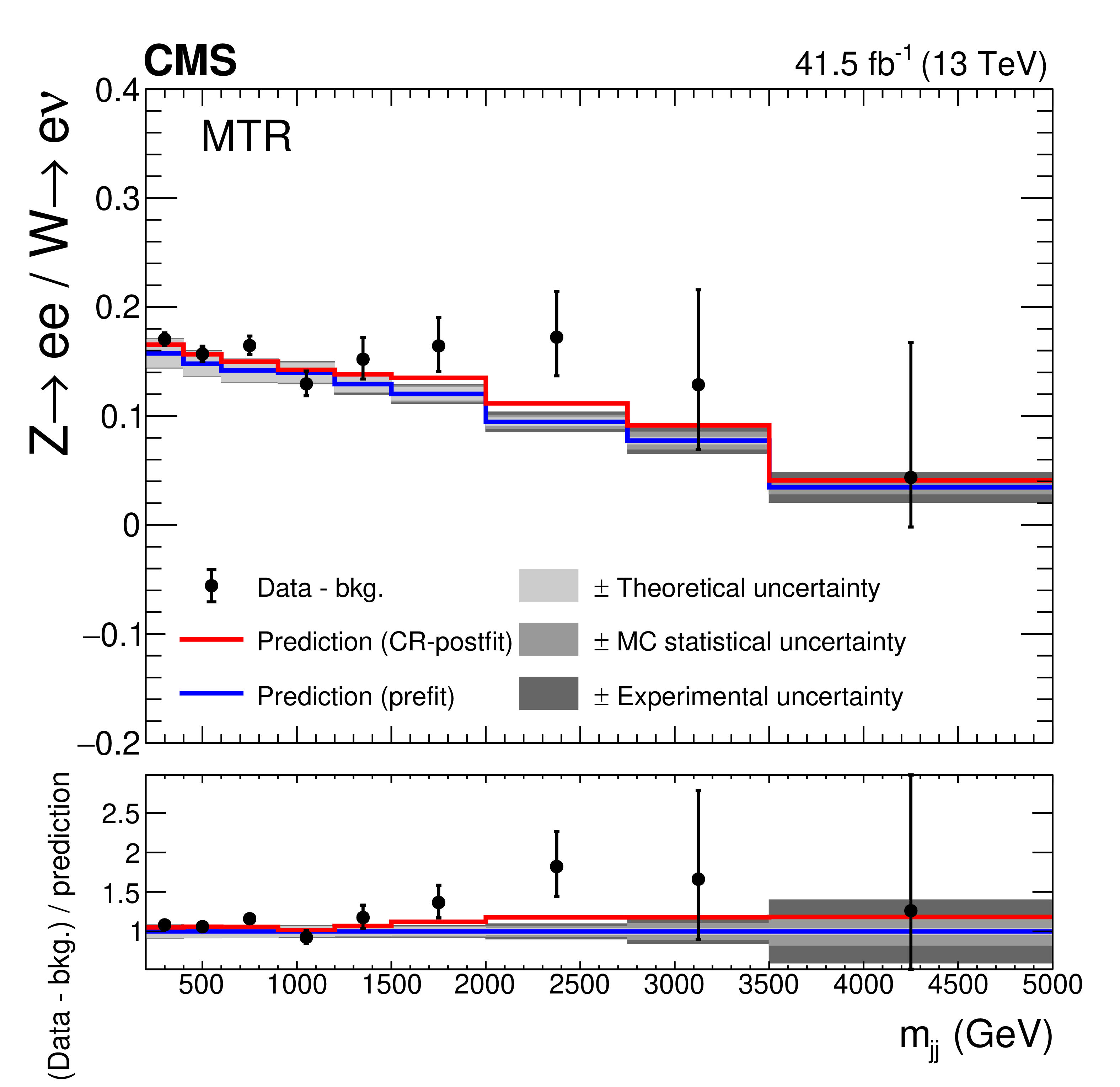
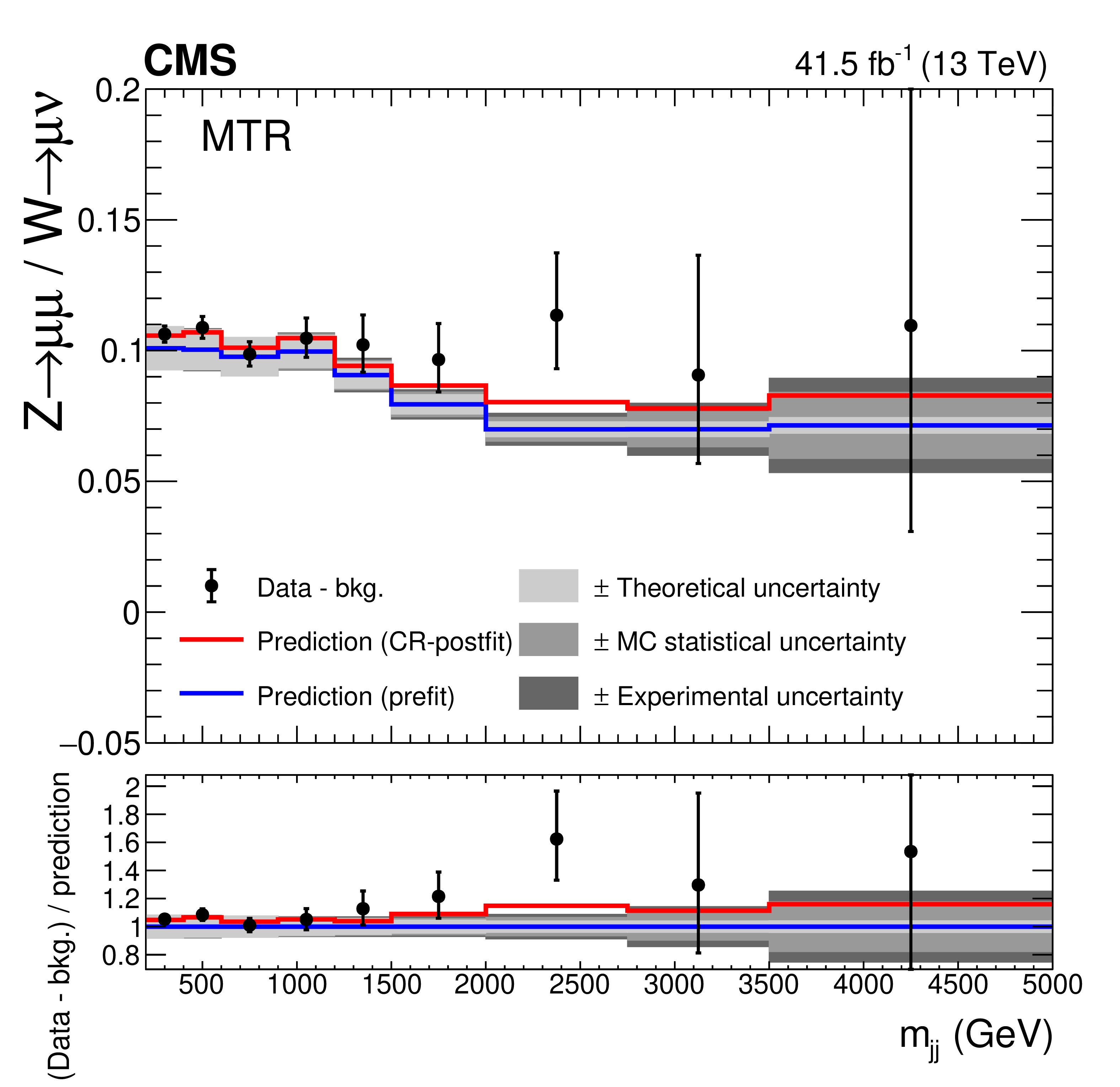
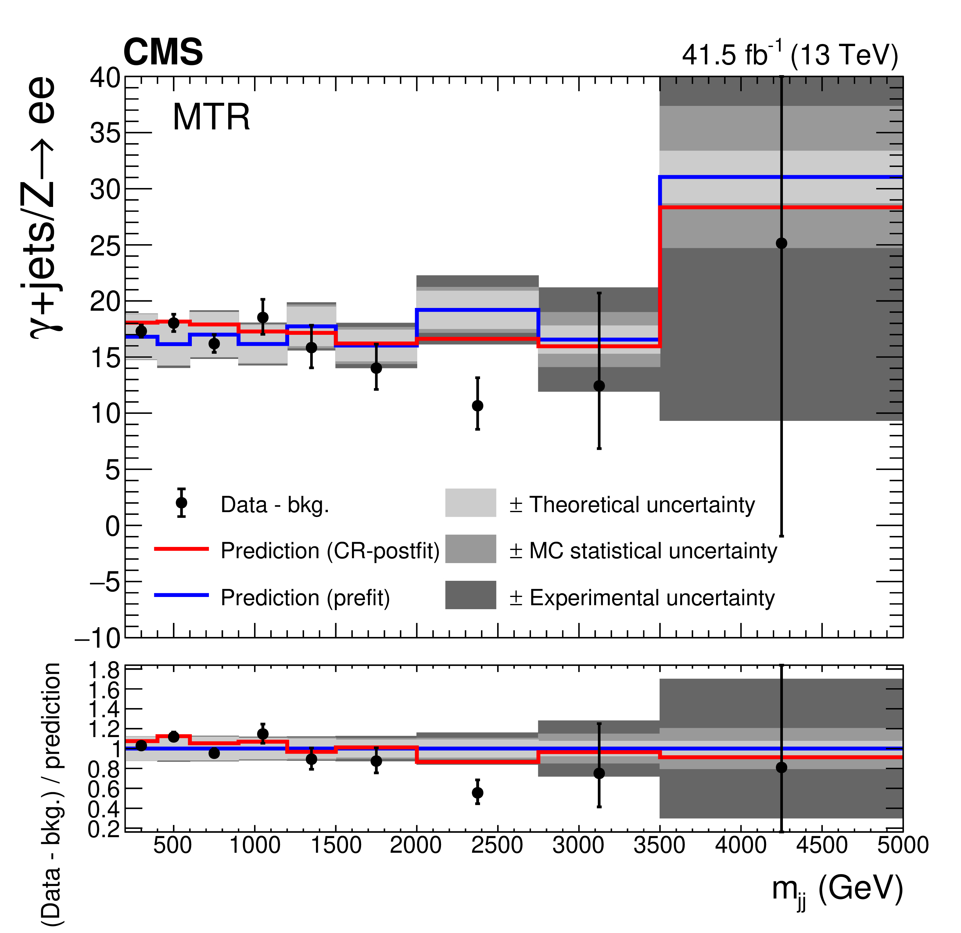
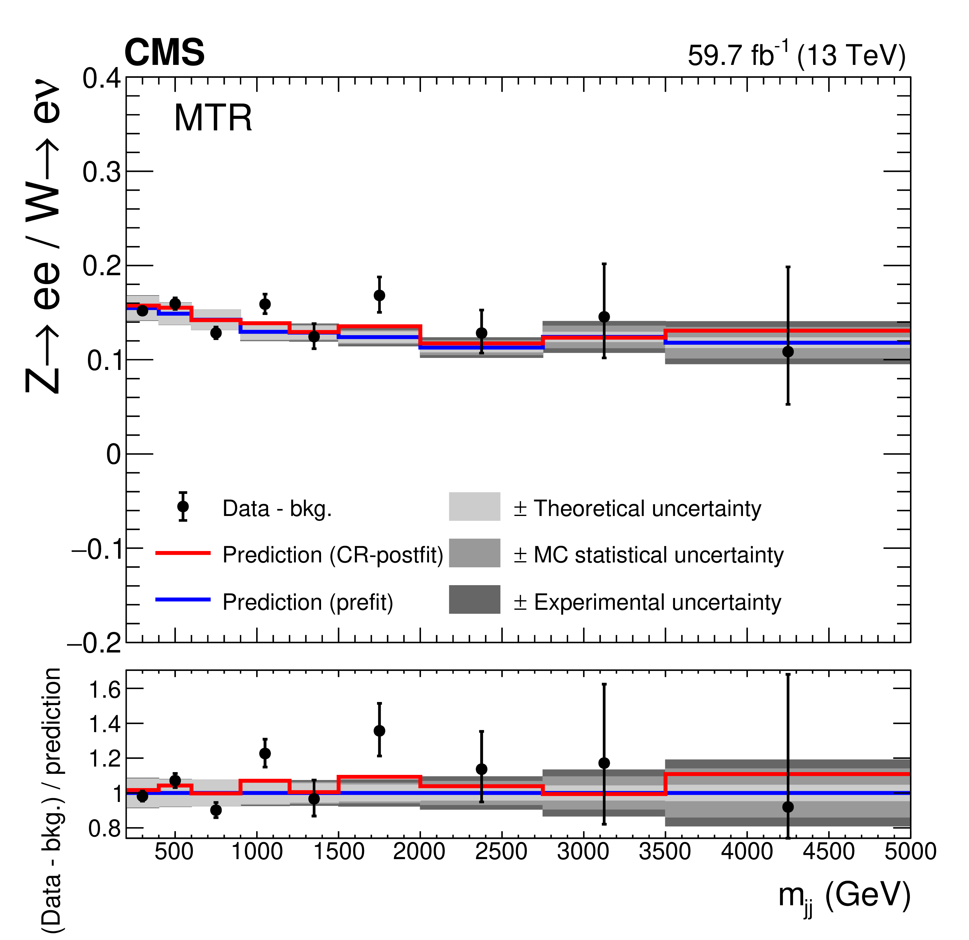
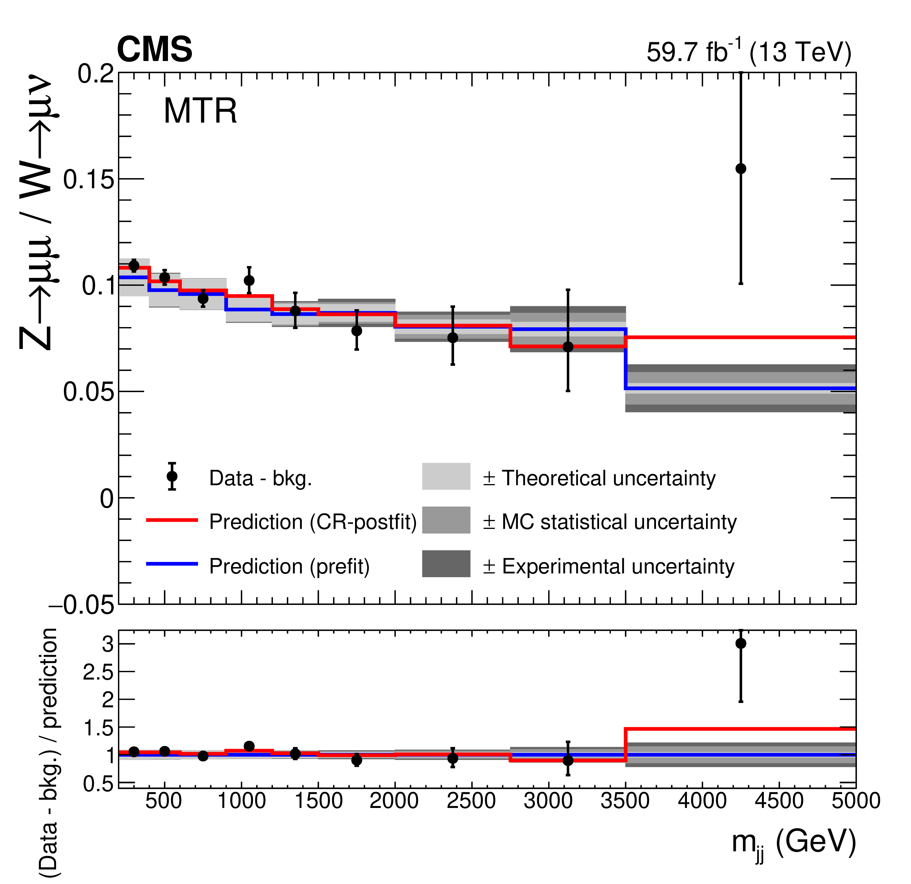
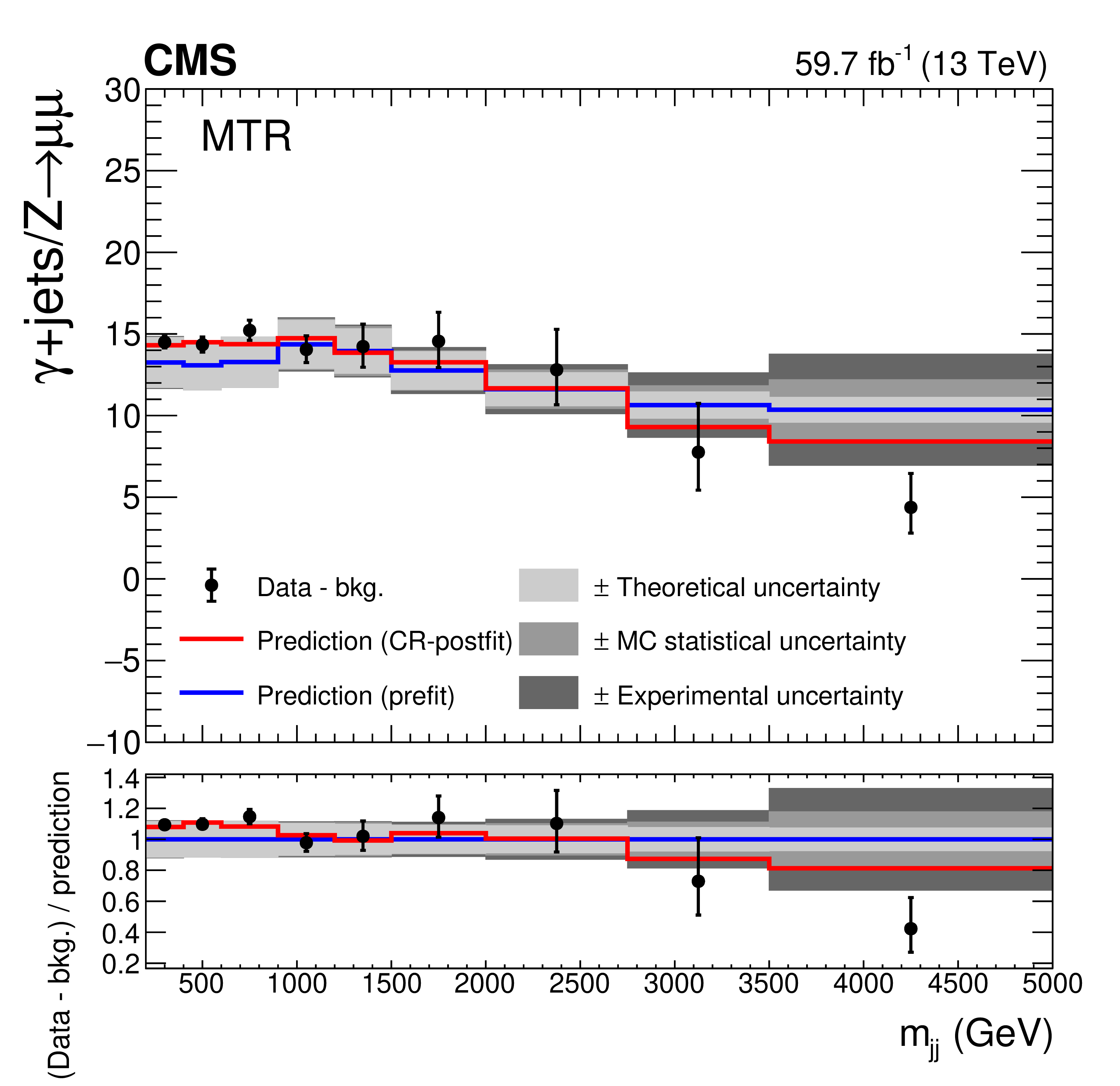
Comparison between data and simulation for the Z($\ell \ell$)+jets / W($\ell \nu$)+jets (upper row) and $\gamma$+jets / Z($\ell \ell$)+jets (lower row) prefit and CR-postfit ratios, as functions of ${m_{\mathrm {jj}}}$, for the MTR category using the 2017 (left) and 2018 (right) event samples. The minor backgrounds in each CR are subtracted from the data using estimates from simulation. The grey bands include the theoretical and experimental systematic uncertainties listed in Table 3, as well as the statistical uncertainty in the simulation. |
png pdf |
Figure 5-a:
Comparison between data and simulation for the Z($\ell \ell$)+jets / W($\ell \nu$)+jets (upper row) and $\gamma$+jets / Z($\ell \ell$)+jets (lower row) prefit and CR-postfit ratios, as functions of ${m_{\mathrm {jj}}}$, for the MTR category using the 2017 (left) and 2018 (right) event samples. The minor backgrounds in each CR are subtracted from the data using estimates from simulation. The grey bands include the theoretical and experimental systematic uncertainties listed in Table 3, as well as the statistical uncertainty in the simulation. |
png pdf |
Figure 5-b:
Comparison between data and simulation for the Z($\ell \ell$)+jets / W($\ell \nu$)+jets (upper row) and $\gamma$+jets / Z($\ell \ell$)+jets (lower row) prefit and CR-postfit ratios, as functions of ${m_{\mathrm {jj}}}$, for the MTR category using the 2017 (left) and 2018 (right) event samples. The minor backgrounds in each CR are subtracted from the data using estimates from simulation. The grey bands include the theoretical and experimental systematic uncertainties listed in Table 3, as well as the statistical uncertainty in the simulation. |
png pdf |
Figure 5-c:
Comparison between data and simulation for the Z($\ell \ell$)+jets / W($\ell \nu$)+jets (upper row) and $\gamma$+jets / Z($\ell \ell$)+jets (lower row) prefit and CR-postfit ratios, as functions of ${m_{\mathrm {jj}}}$, for the MTR category using the 2017 (left) and 2018 (right) event samples. The minor backgrounds in each CR are subtracted from the data using estimates from simulation. The grey bands include the theoretical and experimental systematic uncertainties listed in Table 3, as well as the statistical uncertainty in the simulation. |

png pdf |
Figure 5-d:
Comparison between data and simulation for the Z($\ell \ell$)+jets / W($\ell \nu$)+jets (upper row) and $\gamma$+jets / Z($\ell \ell$)+jets (lower row) prefit and CR-postfit ratios, as functions of ${m_{\mathrm {jj}}}$, for the MTR category using the 2017 (left) and 2018 (right) event samples. The minor backgrounds in each CR are subtracted from the data using estimates from simulation. The grey bands include the theoretical and experimental systematic uncertainties listed in Table 3, as well as the statistical uncertainty in the simulation. |
png pdf |
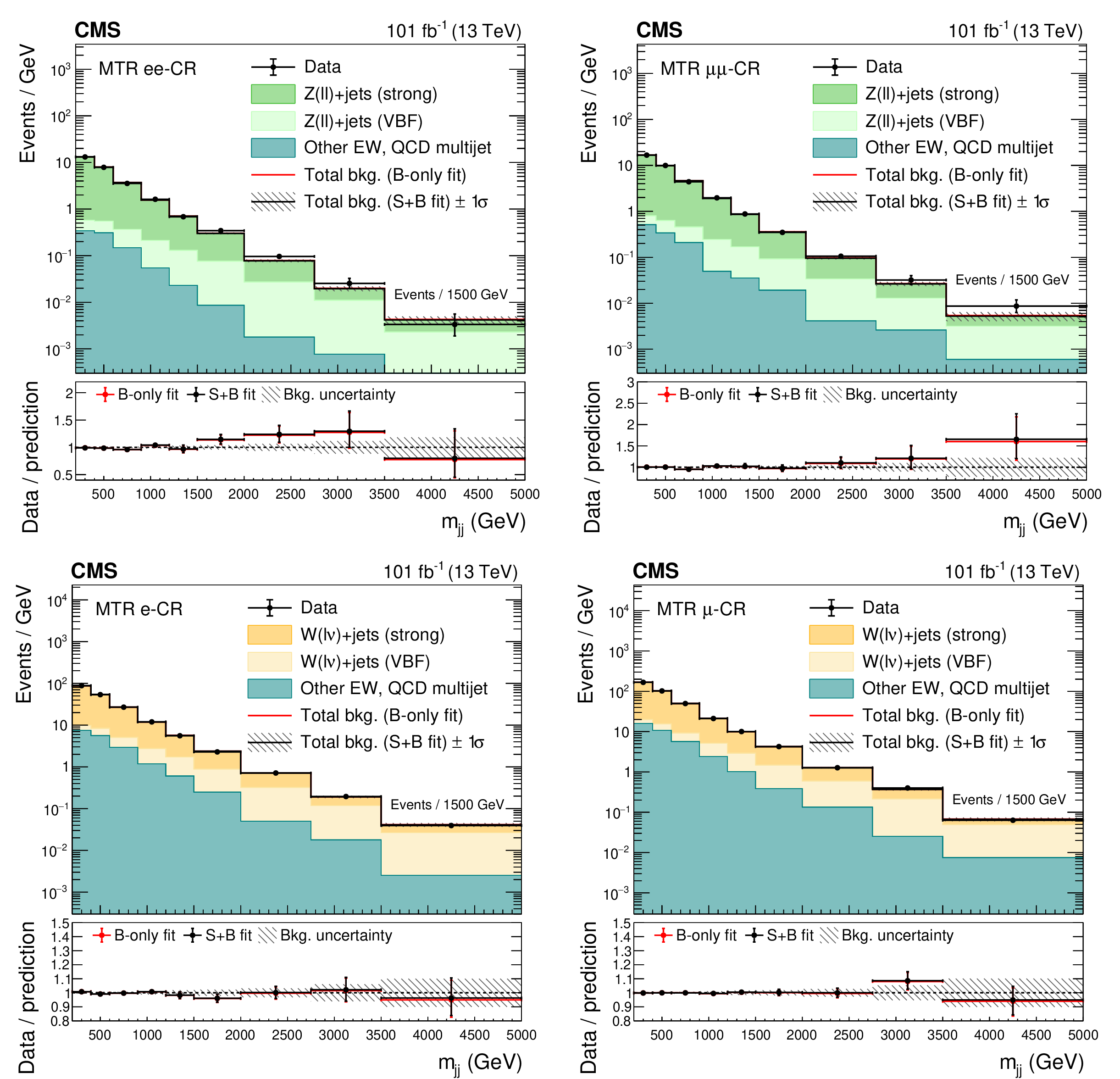
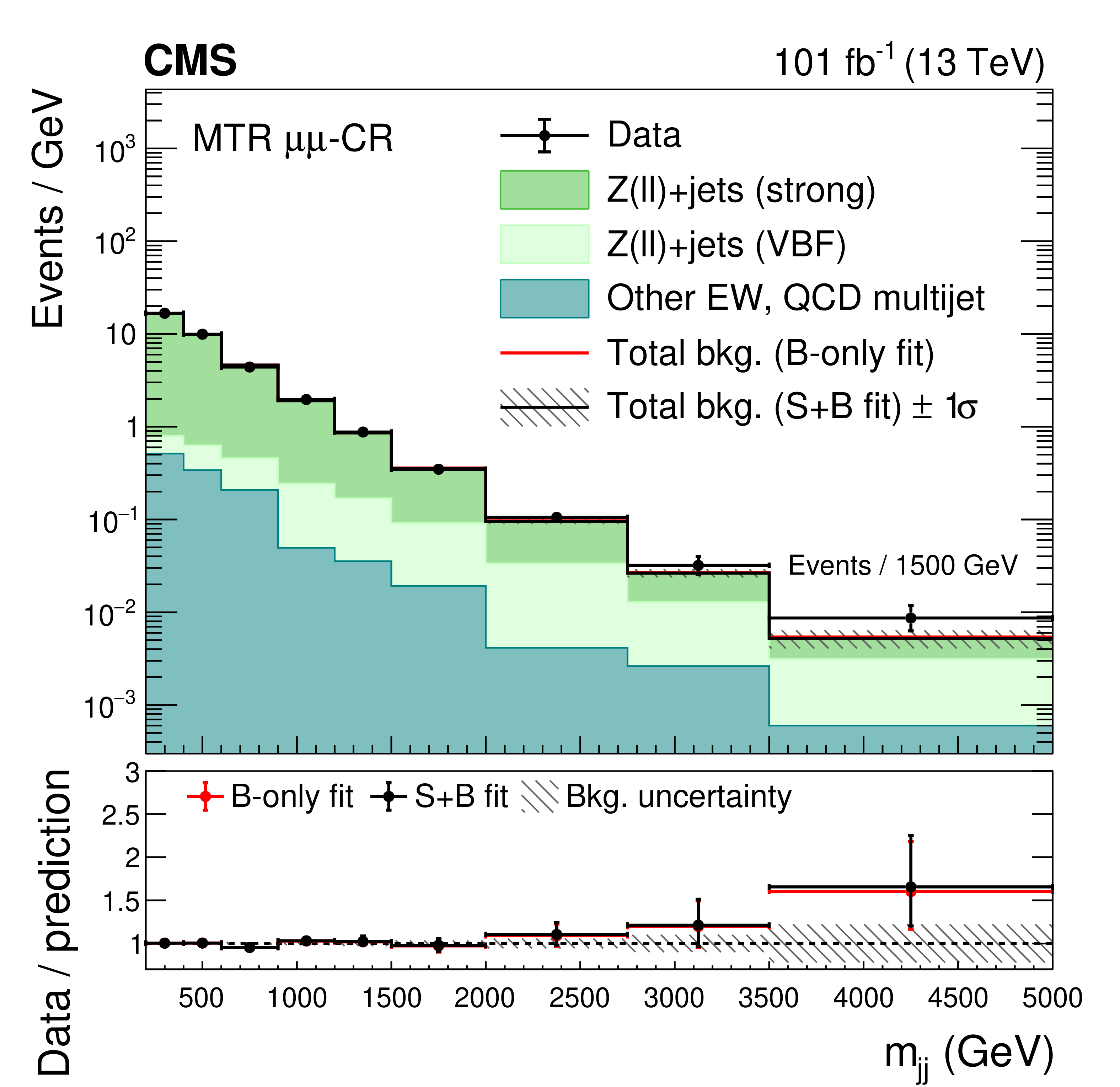
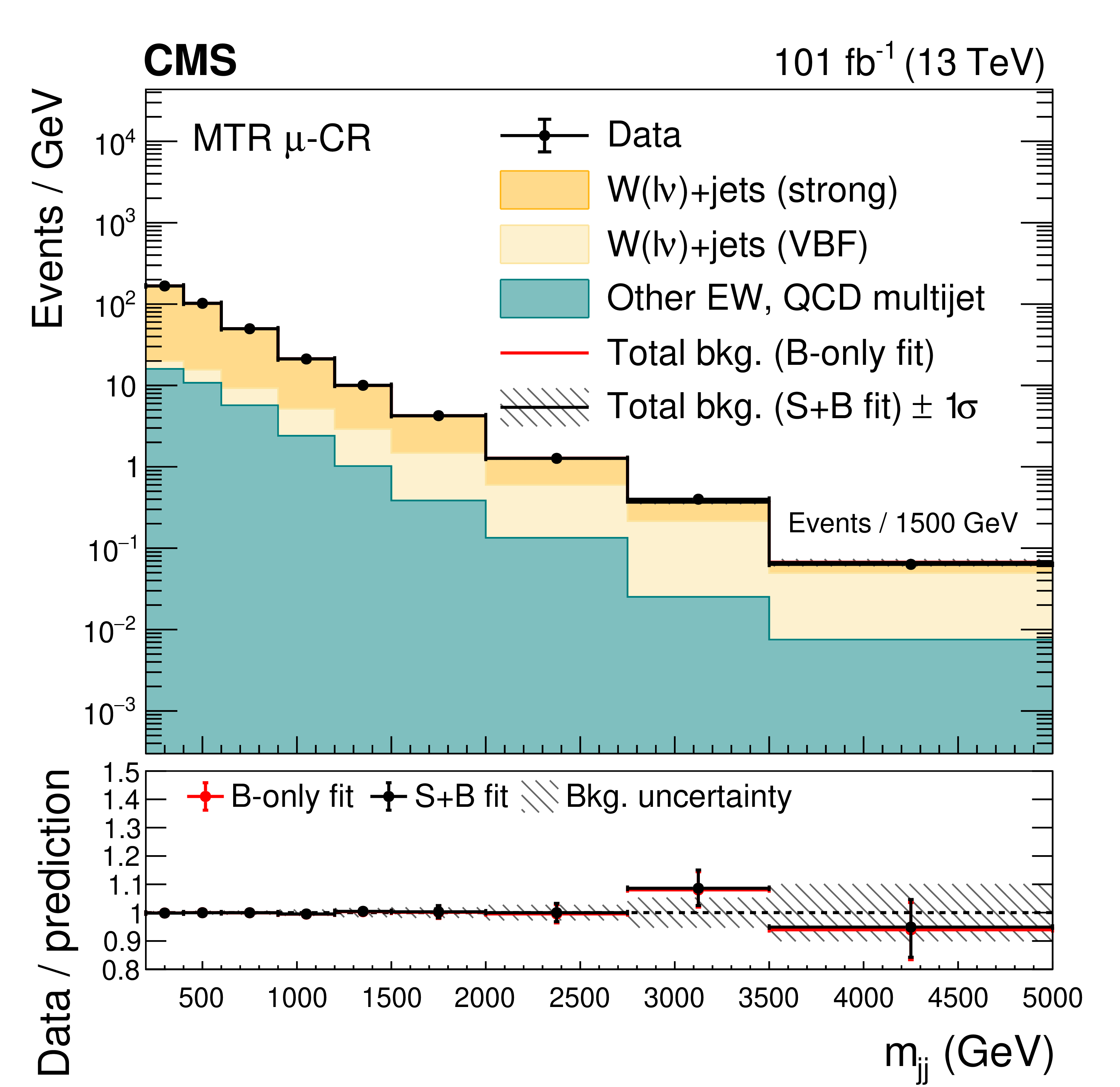
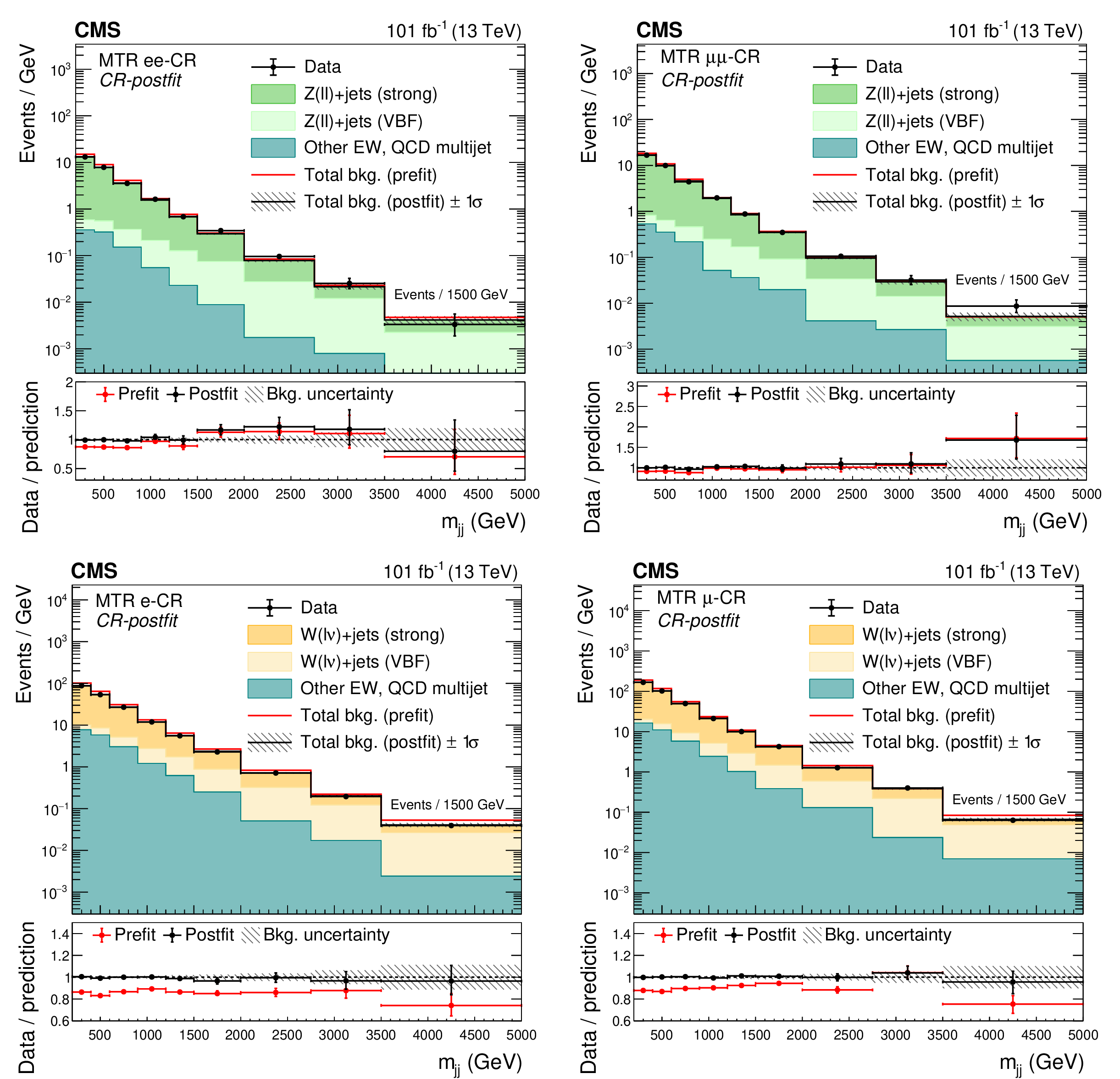
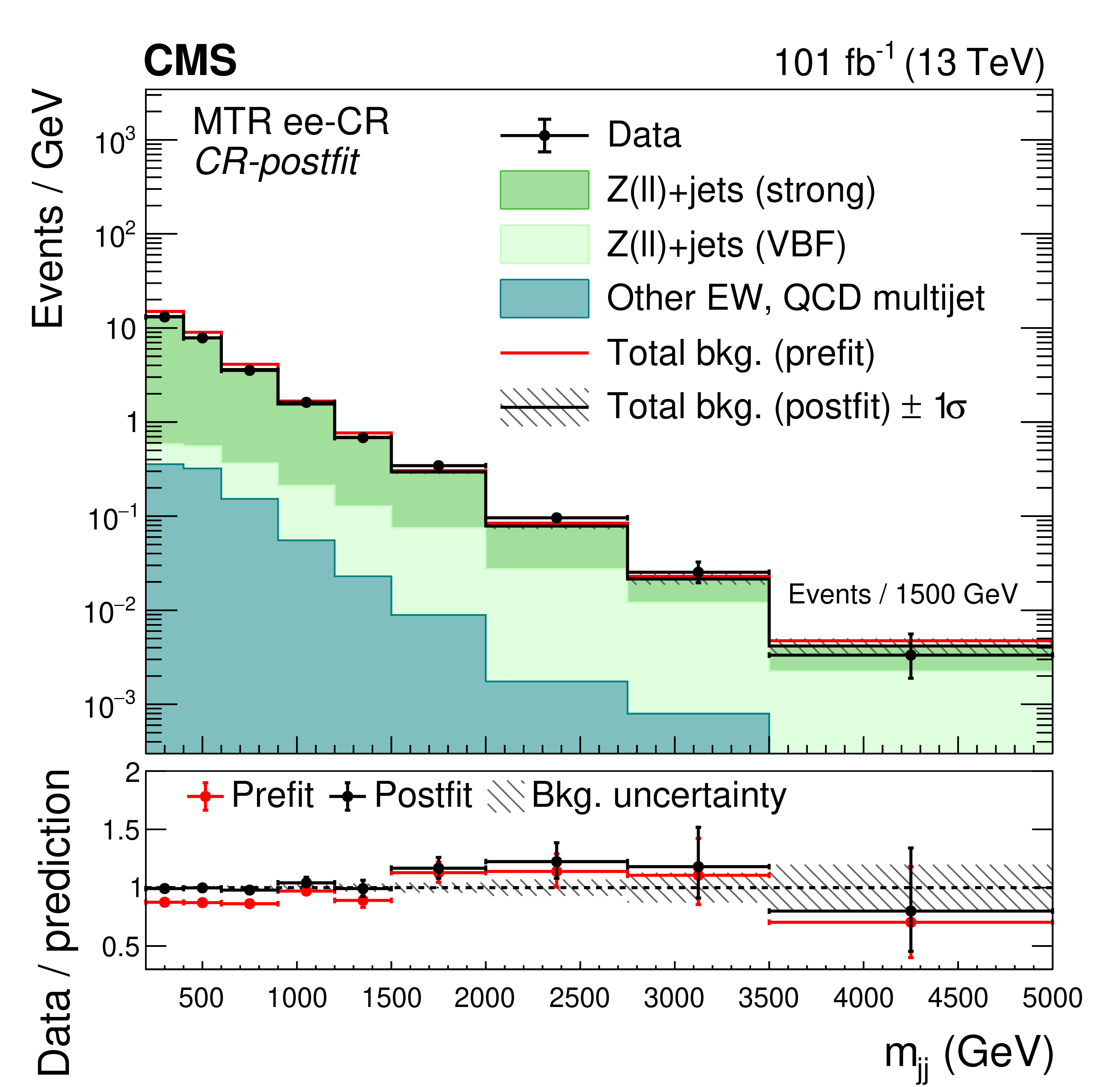
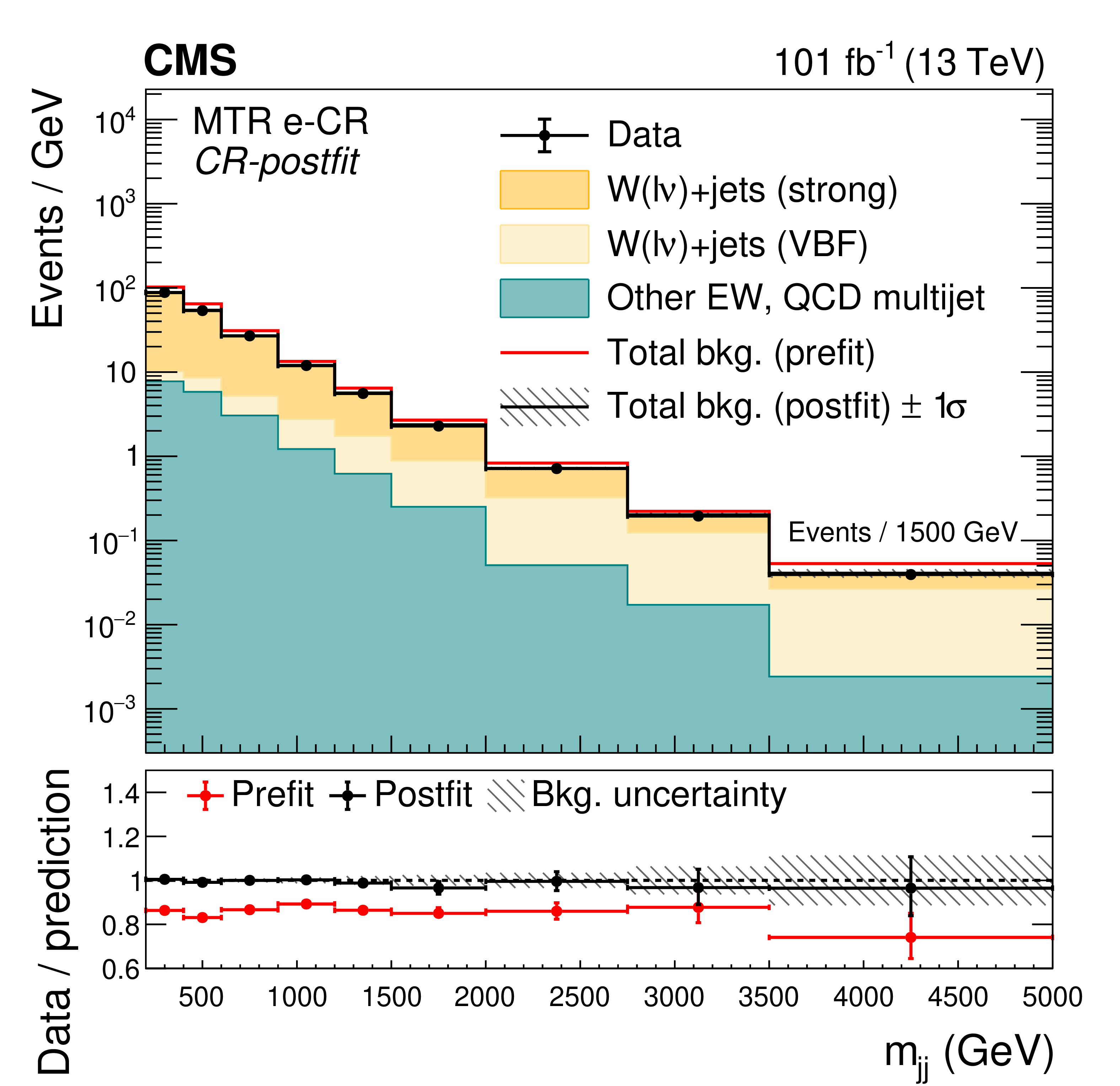
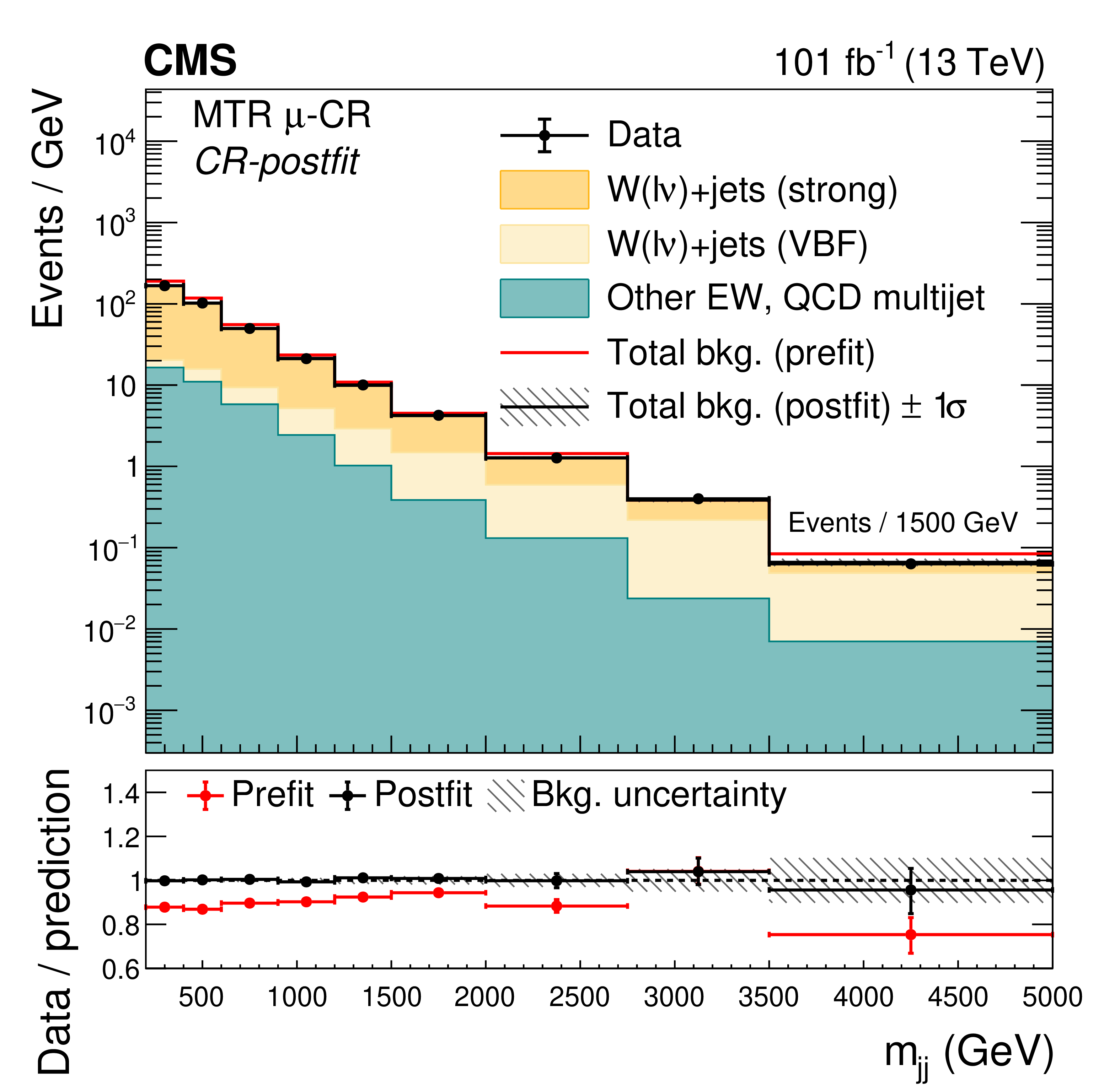
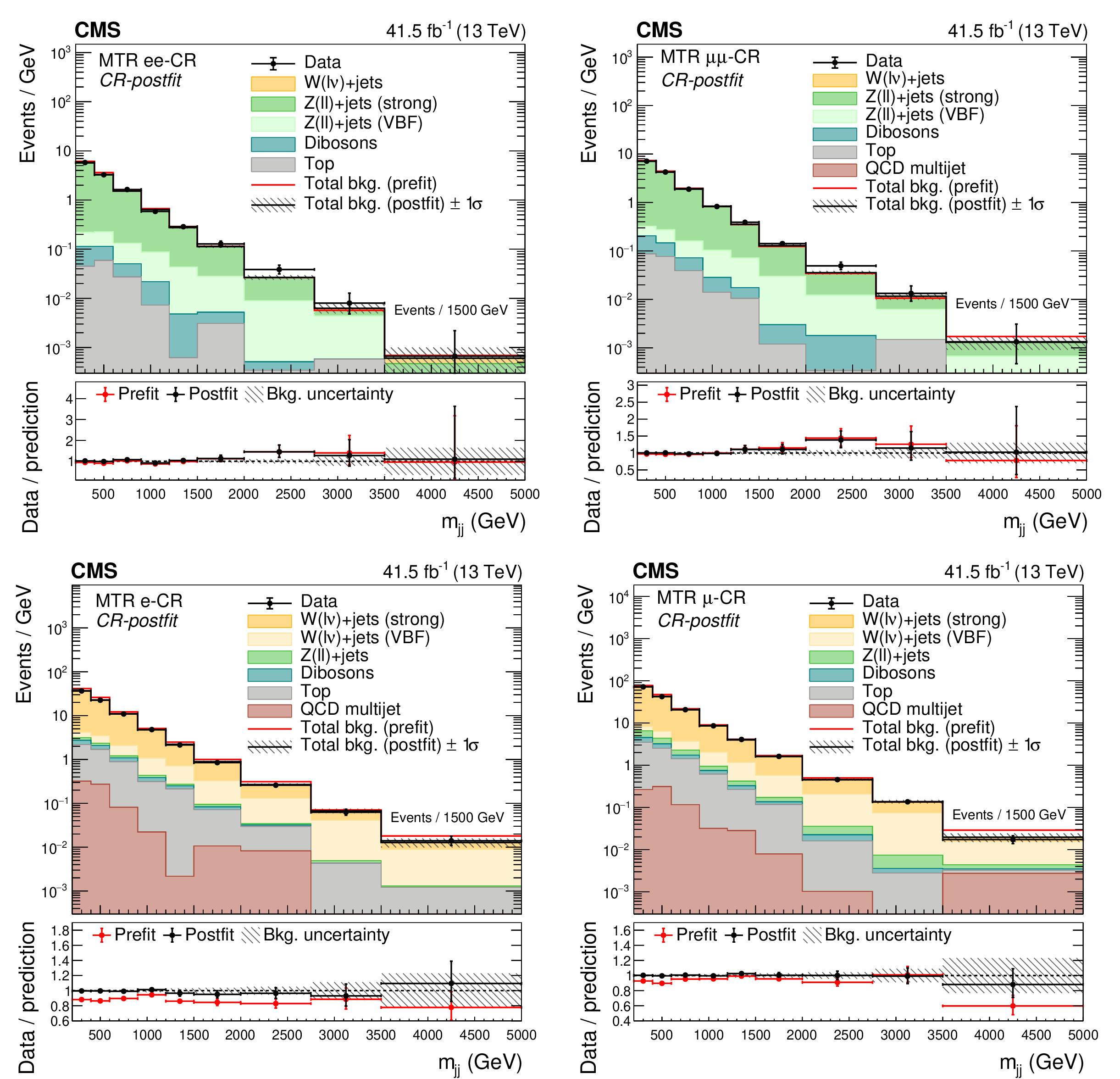
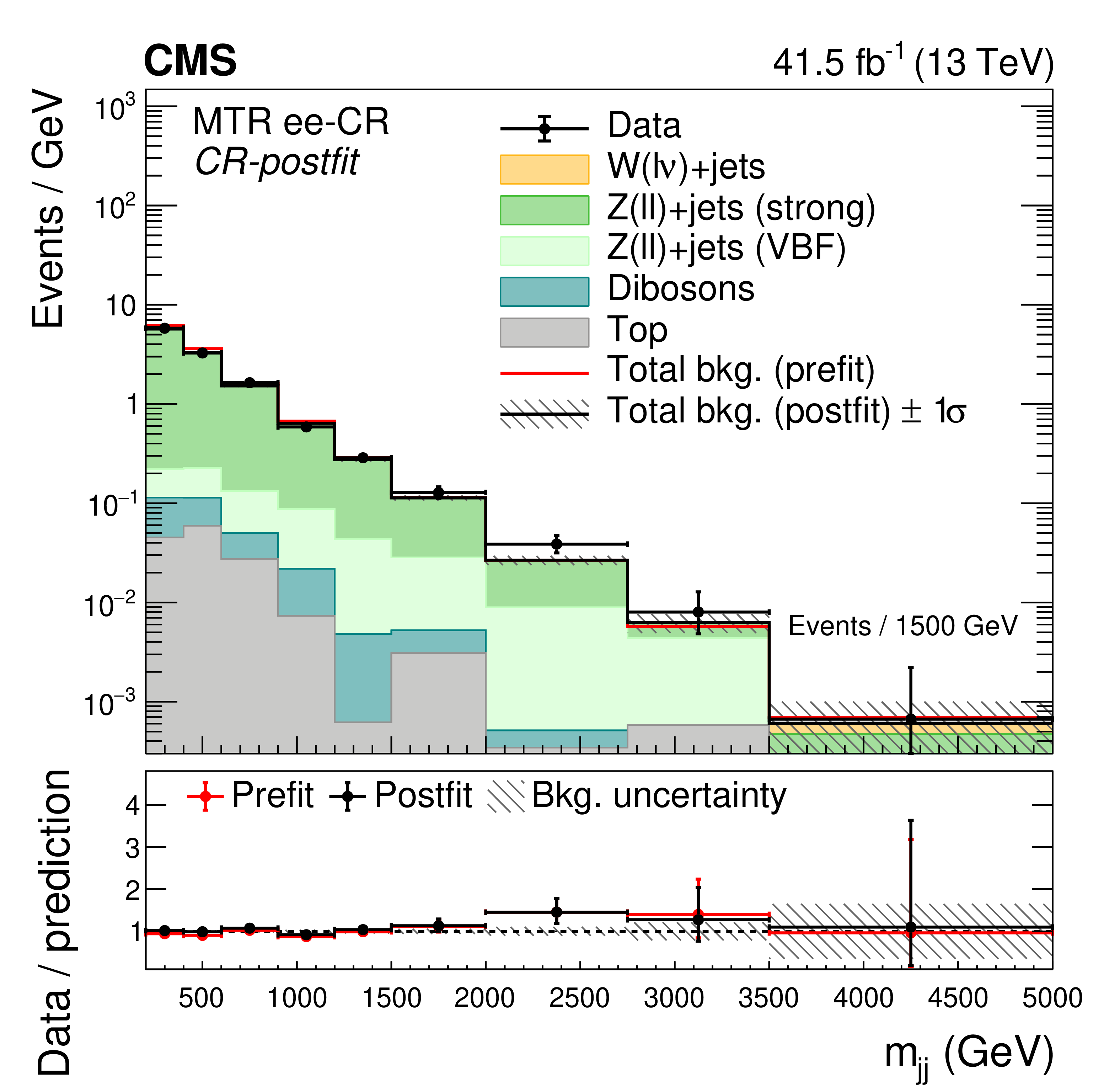
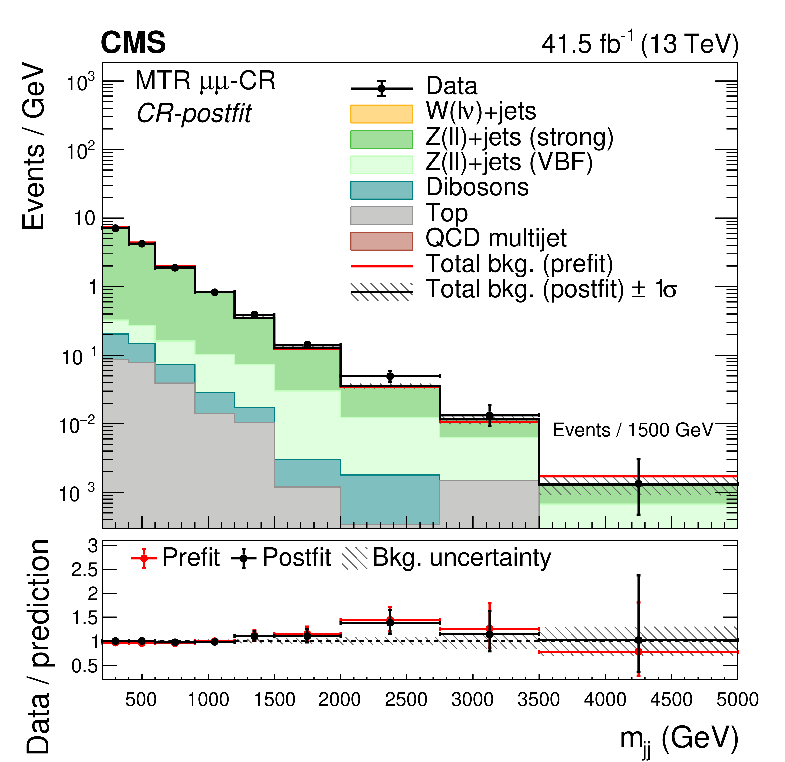
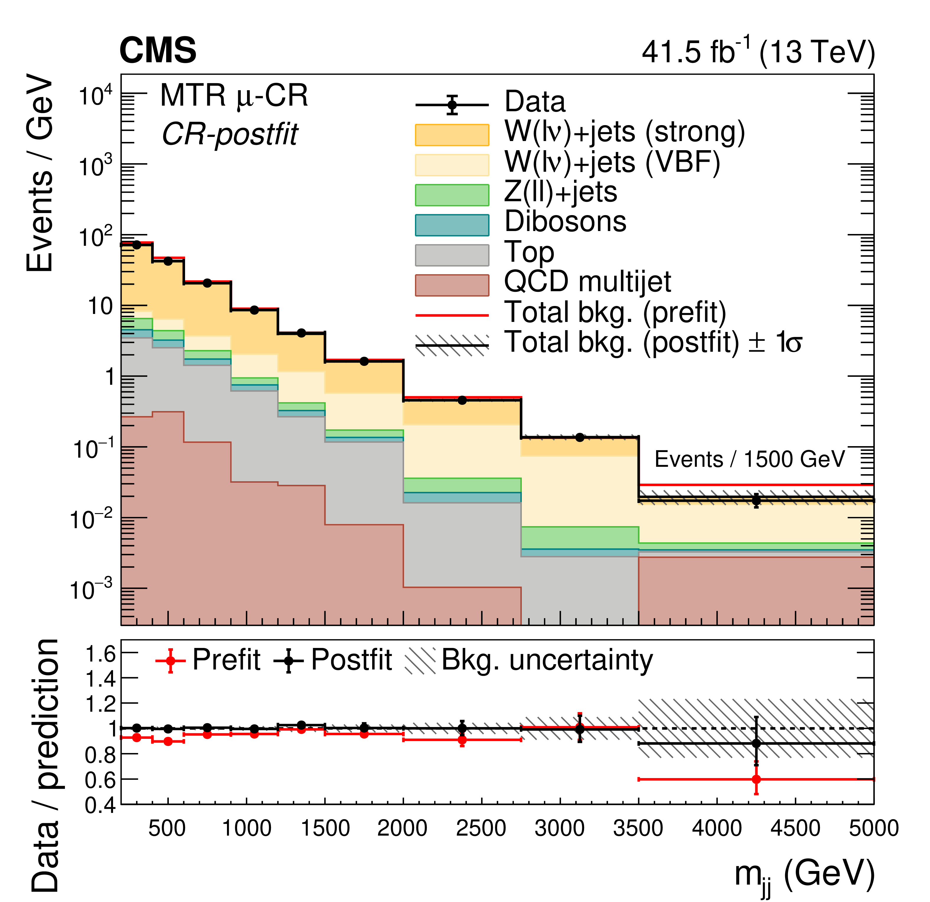
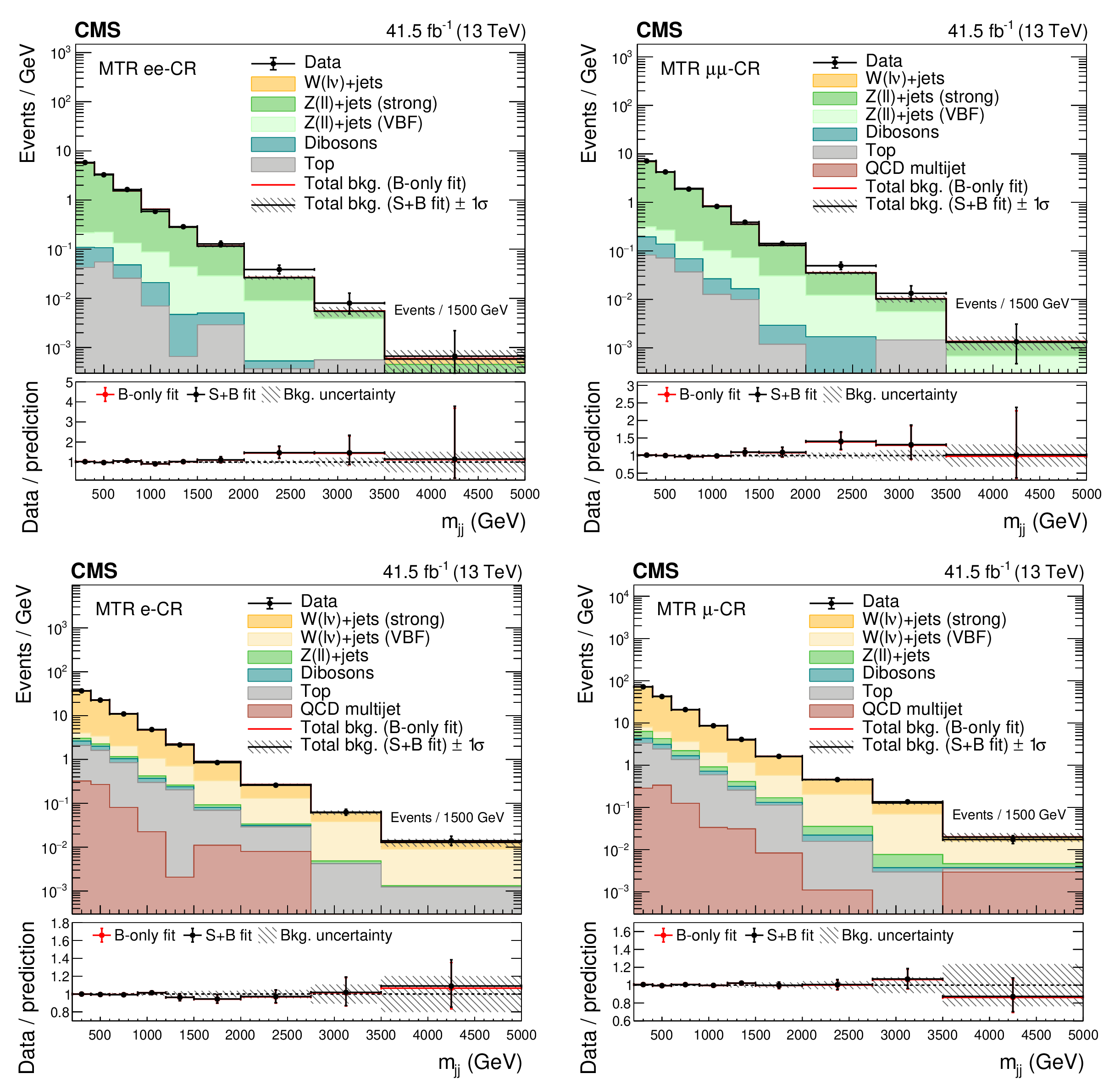
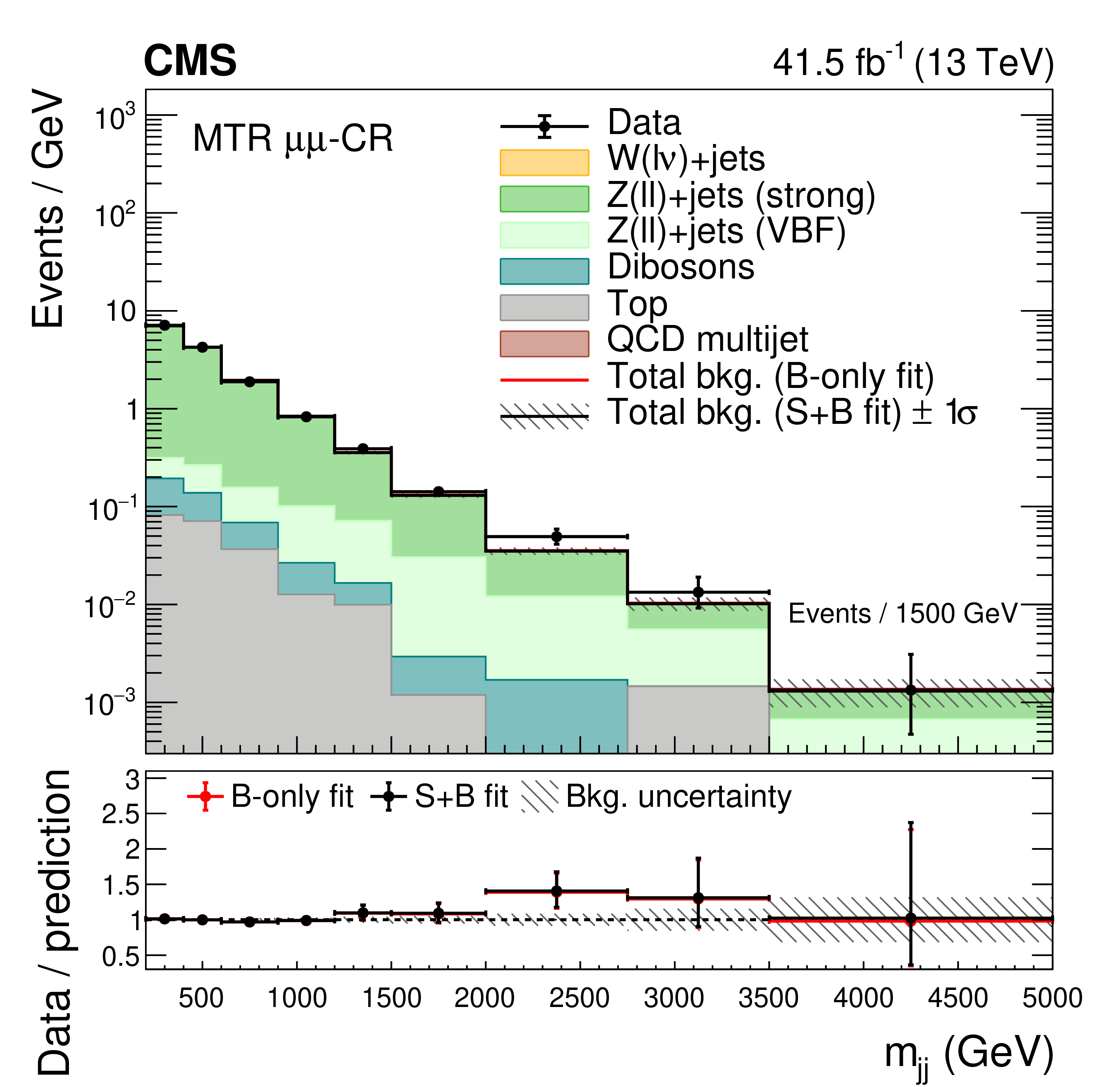
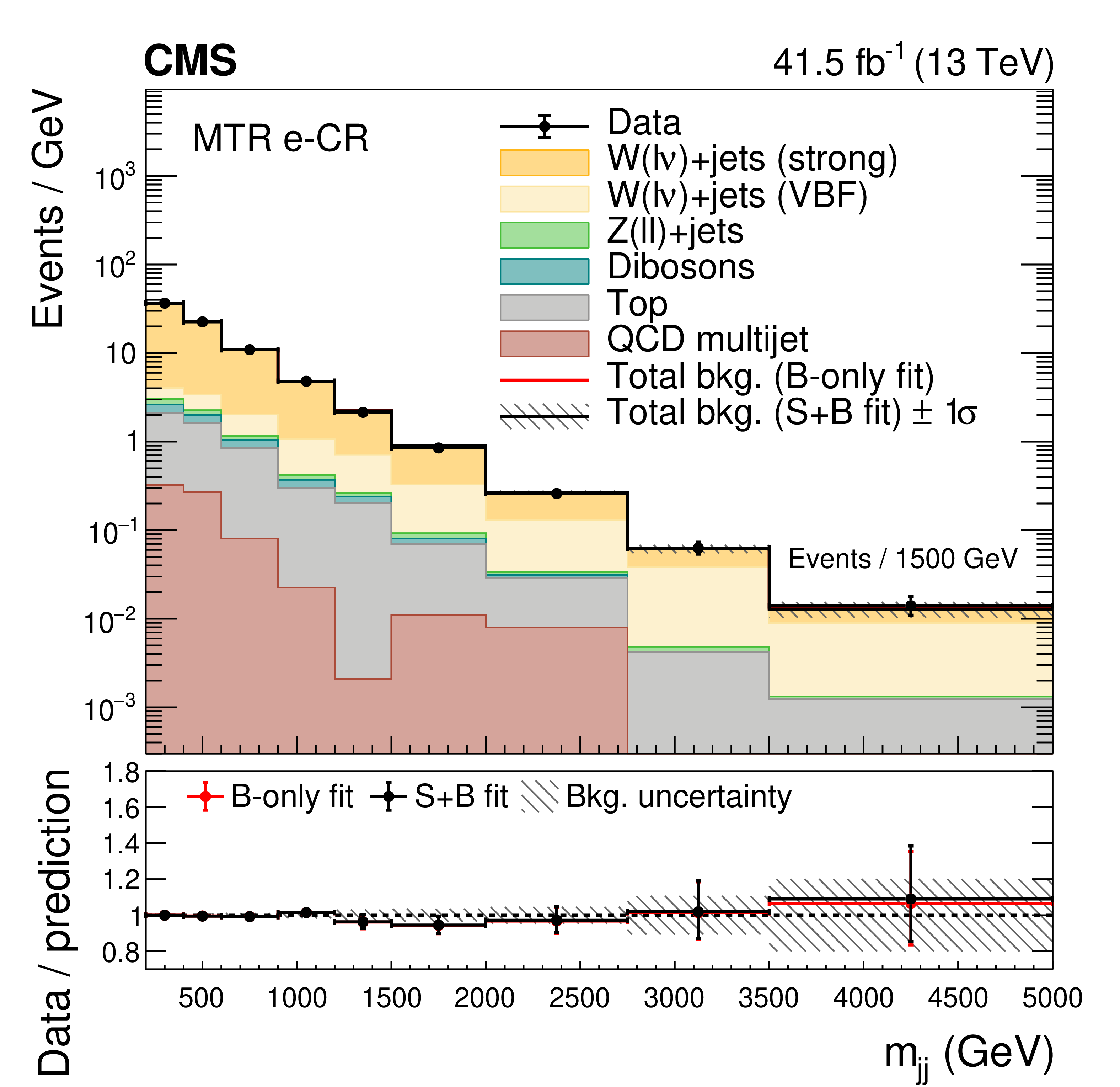
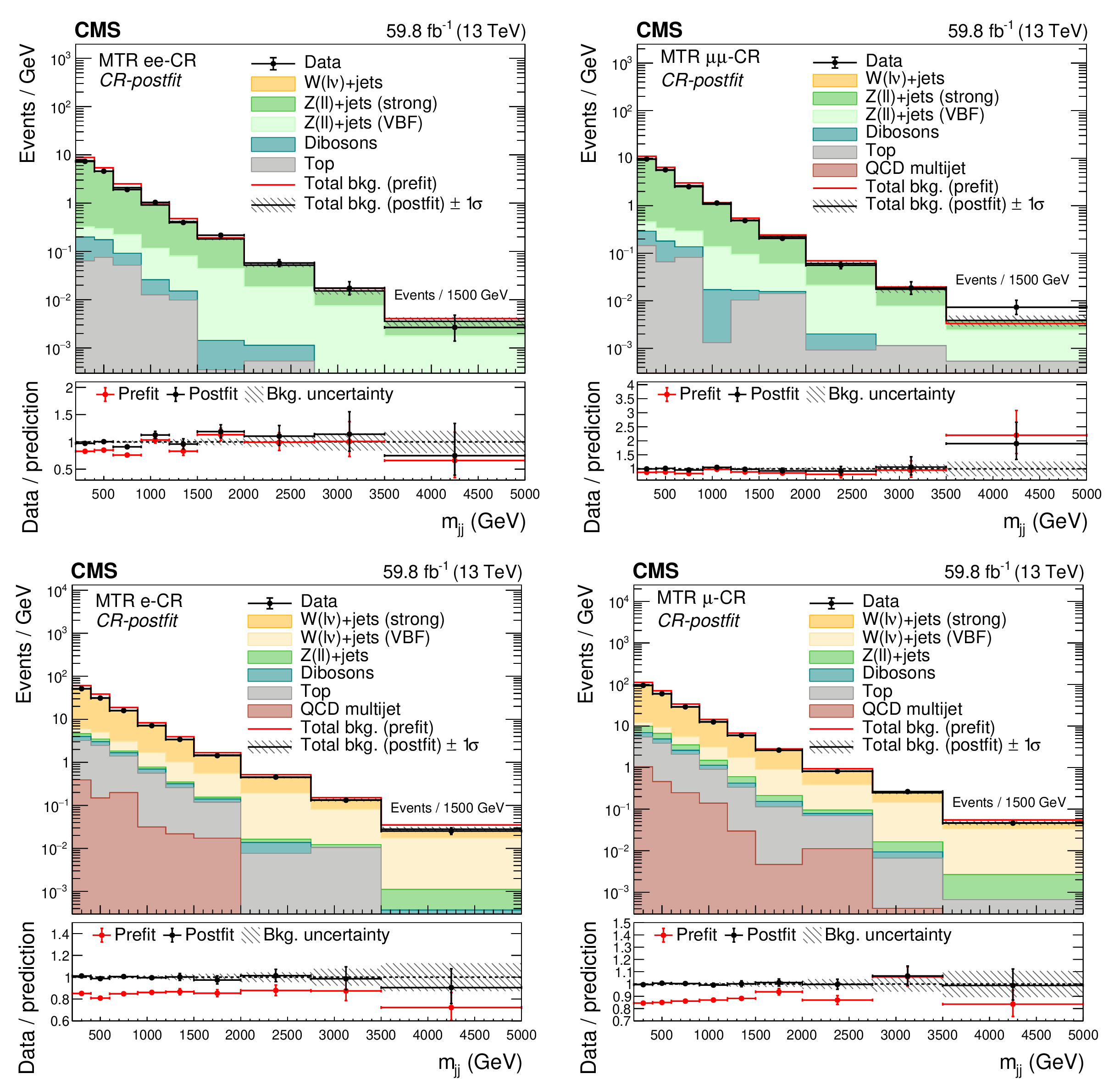
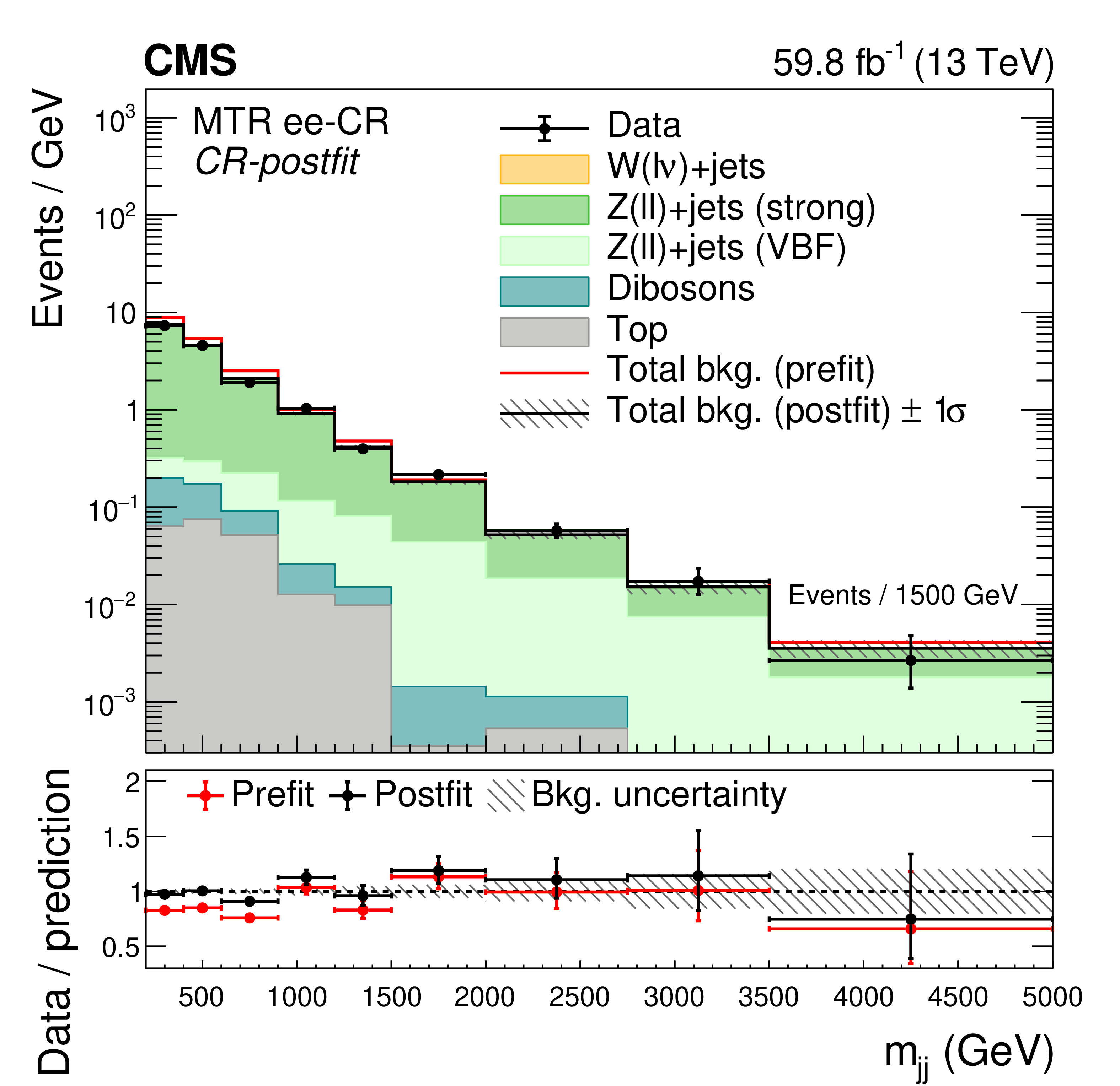
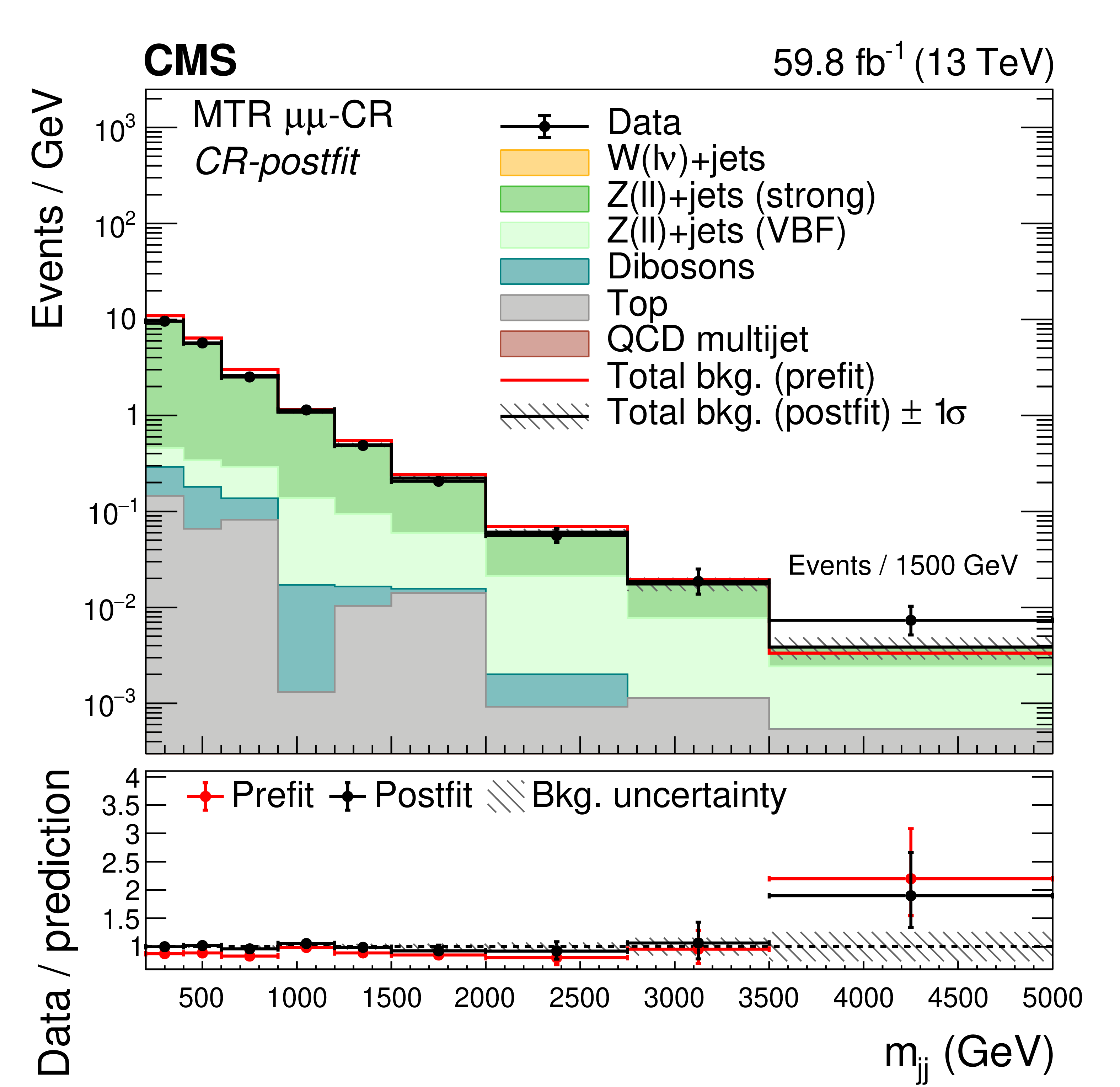
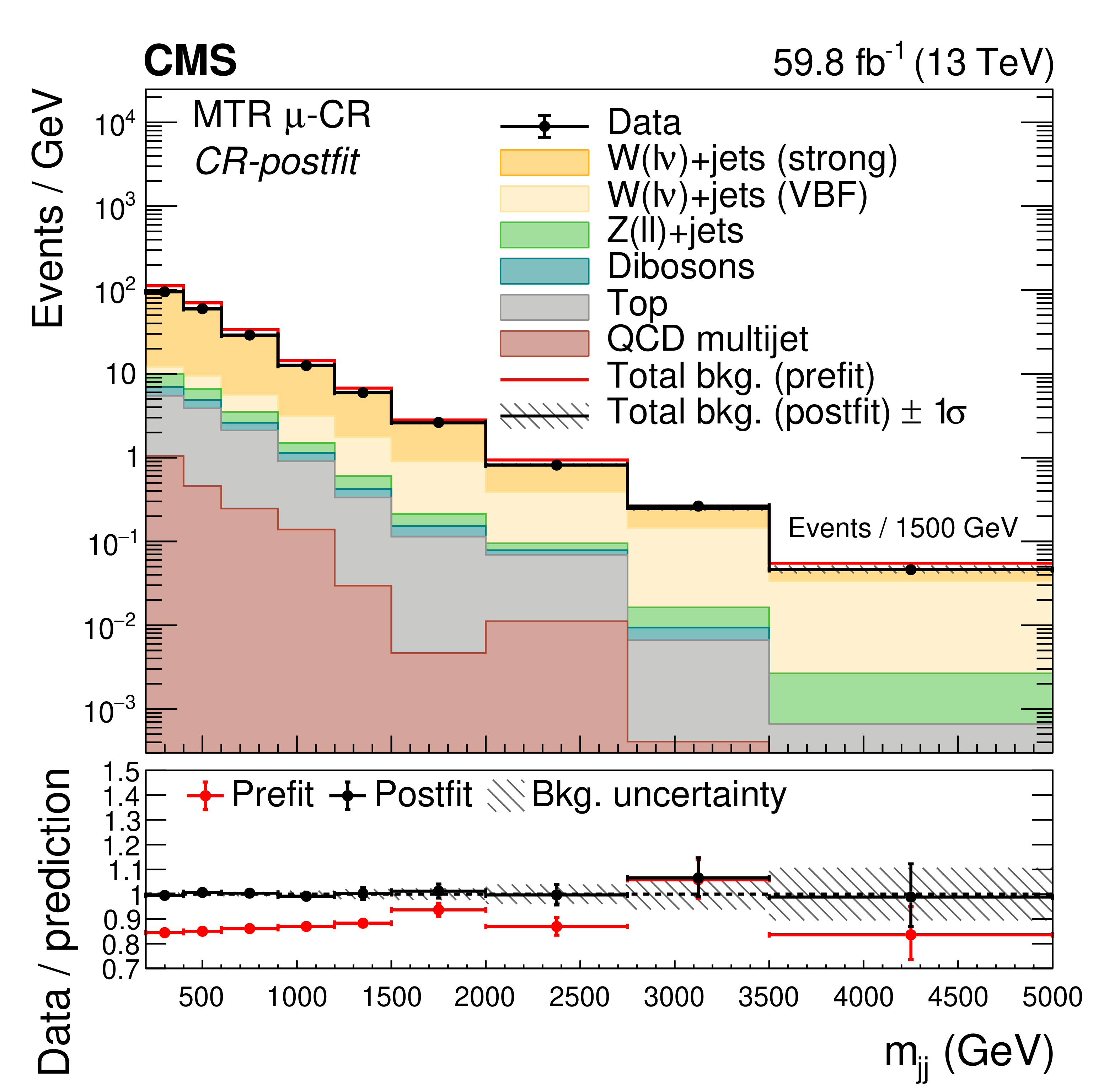
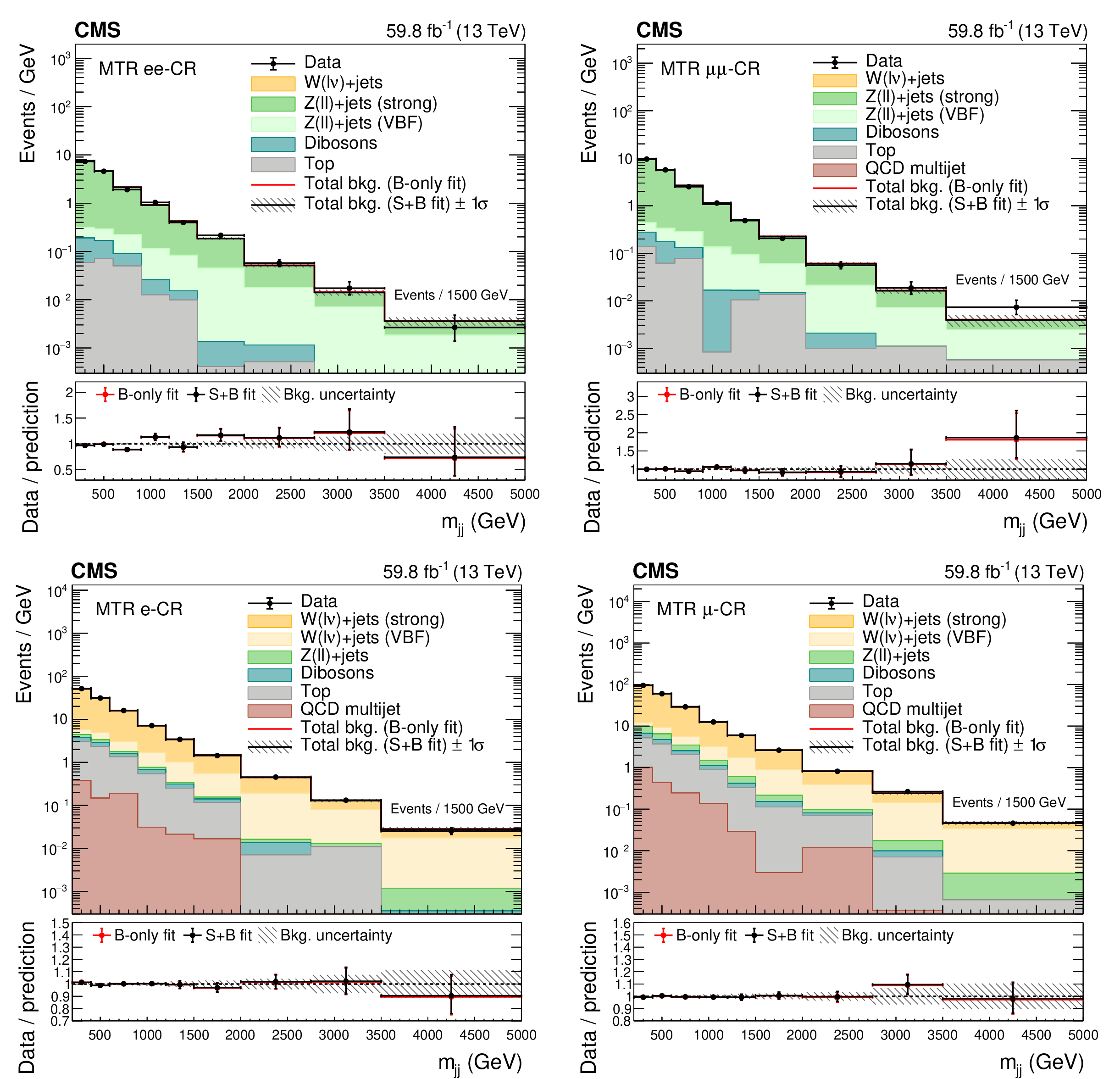
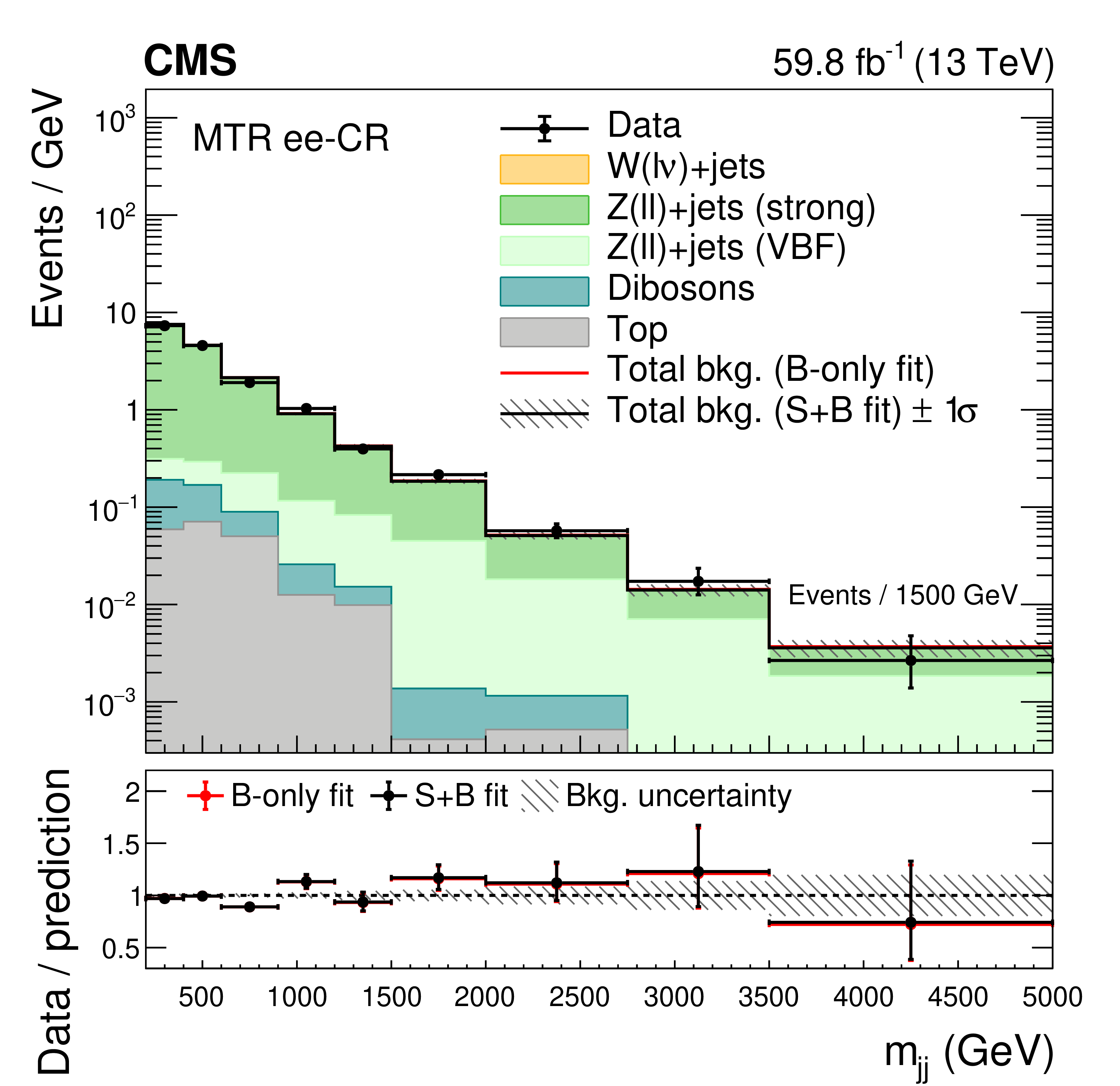
Figure 6:
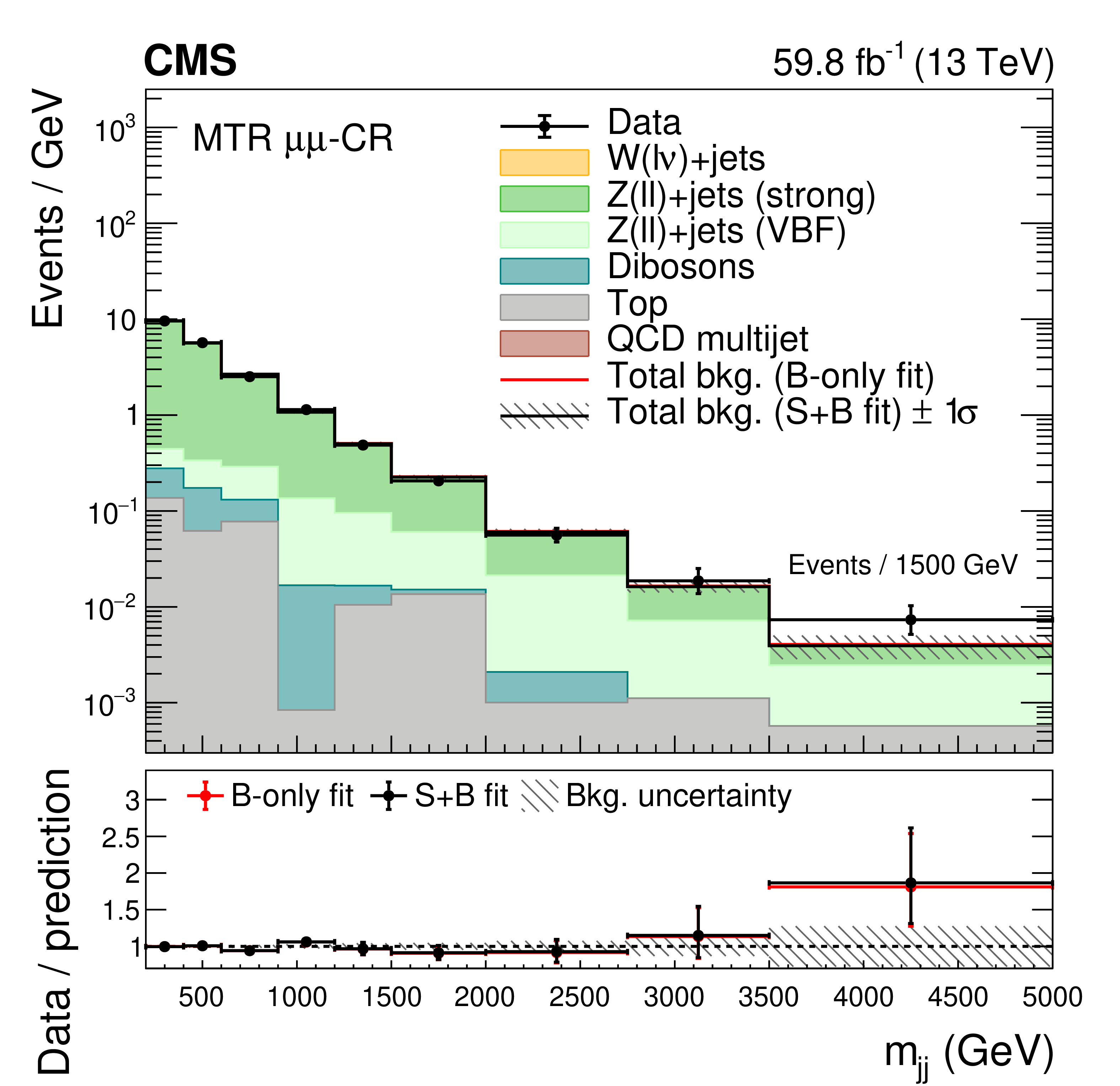
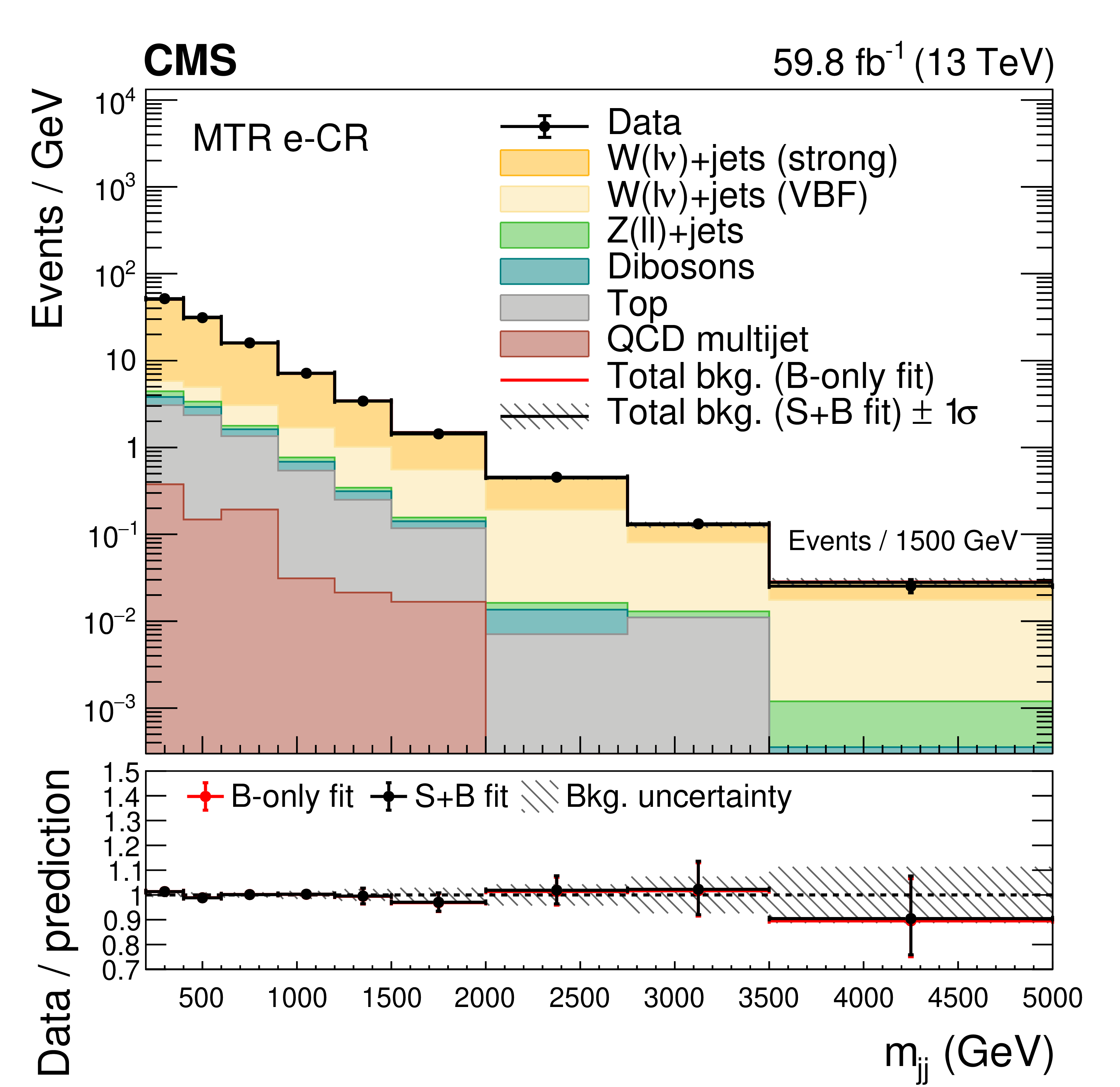
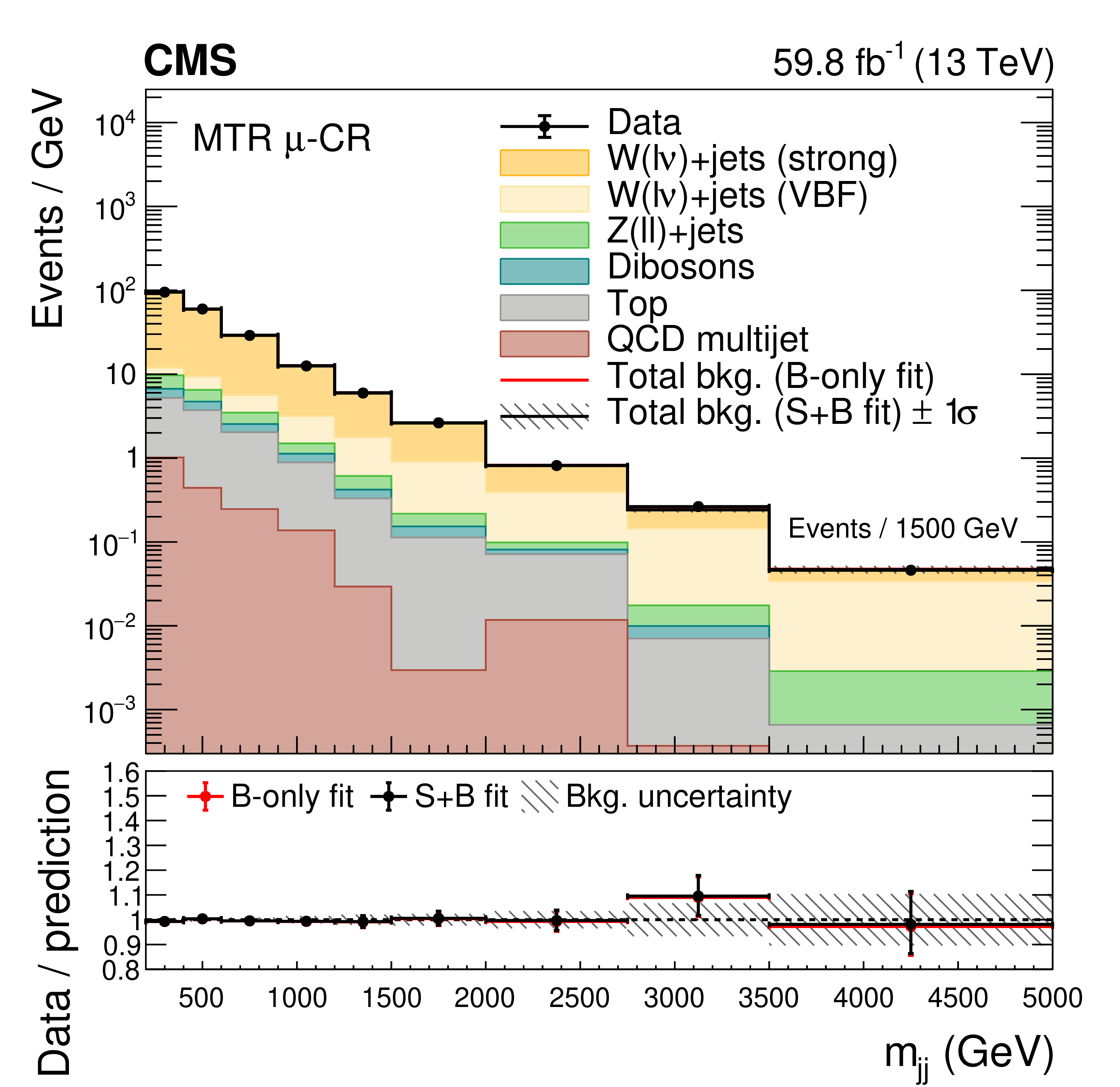
The postfit ${m_{\mathrm {jj}}}$ distributions in the dielectron (upper left), dimuon (upper right), single-electron (lower left), and single-muon (lower right) CR for the MTR category, showing the summed 2017 and 2018 data samples and the background processes. The background contributions are estimated from the fit to the data described in the text (S+B fit). The total background estimated from a fit assuming $ {{\mathcal {B}(\mathrm{H} \to \text {inv})}} =$ 0 (B-only fit) is also shown. The yields from the 2017 and 2018 samples are summed and the correlations between their uncertainties are neglected. The last bin of each distribution integrates events above the bin threshold divided by the bin width. |

png pdf |
Figure 6-a:
The postfit ${m_{\mathrm {jj}}}$ distributions in the dielectron (upper left), dimuon (upper right), single-electron (lower left), and single-muon (lower right) CR for the MTR category, showing the summed 2017 and 2018 data samples and the background processes. The background contributions are estimated from the fit to the data described in the text (S+B fit). The total background estimated from a fit assuming $ {{\mathcal {B}(\mathrm{H} \to \text {inv})}} =$ 0 (B-only fit) is also shown. The yields from the 2017 and 2018 samples are summed and the correlations between their uncertainties are neglected. The last bin of each distribution integrates events above the bin threshold divided by the bin width. |
png pdf |
Figure 6-b:
The postfit ${m_{\mathrm {jj}}}$ distributions in the dielectron (upper left), dimuon (upper right), single-electron (lower left), and single-muon (lower right) CR for the MTR category, showing the summed 2017 and 2018 data samples and the background processes. The background contributions are estimated from the fit to the data described in the text (S+B fit). The total background estimated from a fit assuming $ {{\mathcal {B}(\mathrm{H} \to \text {inv})}} =$ 0 (B-only fit) is also shown. The yields from the 2017 and 2018 samples are summed and the correlations between their uncertainties are neglected. The last bin of each distribution integrates events above the bin threshold divided by the bin width. |

png pdf |
Figure 6-c:
The postfit ${m_{\mathrm {jj}}}$ distributions in the dielectron (upper left), dimuon (upper right), single-electron (lower left), and single-muon (lower right) CR for the MTR category, showing the summed 2017 and 2018 data samples and the background processes. The background contributions are estimated from the fit to the data described in the text (S+B fit). The total background estimated from a fit assuming $ {{\mathcal {B}(\mathrm{H} \to \text {inv})}} =$ 0 (B-only fit) is also shown. The yields from the 2017 and 2018 samples are summed and the correlations between their uncertainties are neglected. The last bin of each distribution integrates events above the bin threshold divided by the bin width. |
png pdf |
Figure 6-d:
The postfit ${m_{\mathrm {jj}}}$ distributions in the dielectron (upper left), dimuon (upper right), single-electron (lower left), and single-muon (lower right) CR for the MTR category, showing the summed 2017 and 2018 data samples and the background processes. The background contributions are estimated from the fit to the data described in the text (S+B fit). The total background estimated from a fit assuming $ {{\mathcal {B}(\mathrm{H} \to \text {inv})}} =$ 0 (B-only fit) is also shown. The yields from the 2017 and 2018 samples are summed and the correlations between their uncertainties are neglected. The last bin of each distribution integrates events above the bin threshold divided by the bin width. |

png pdf |
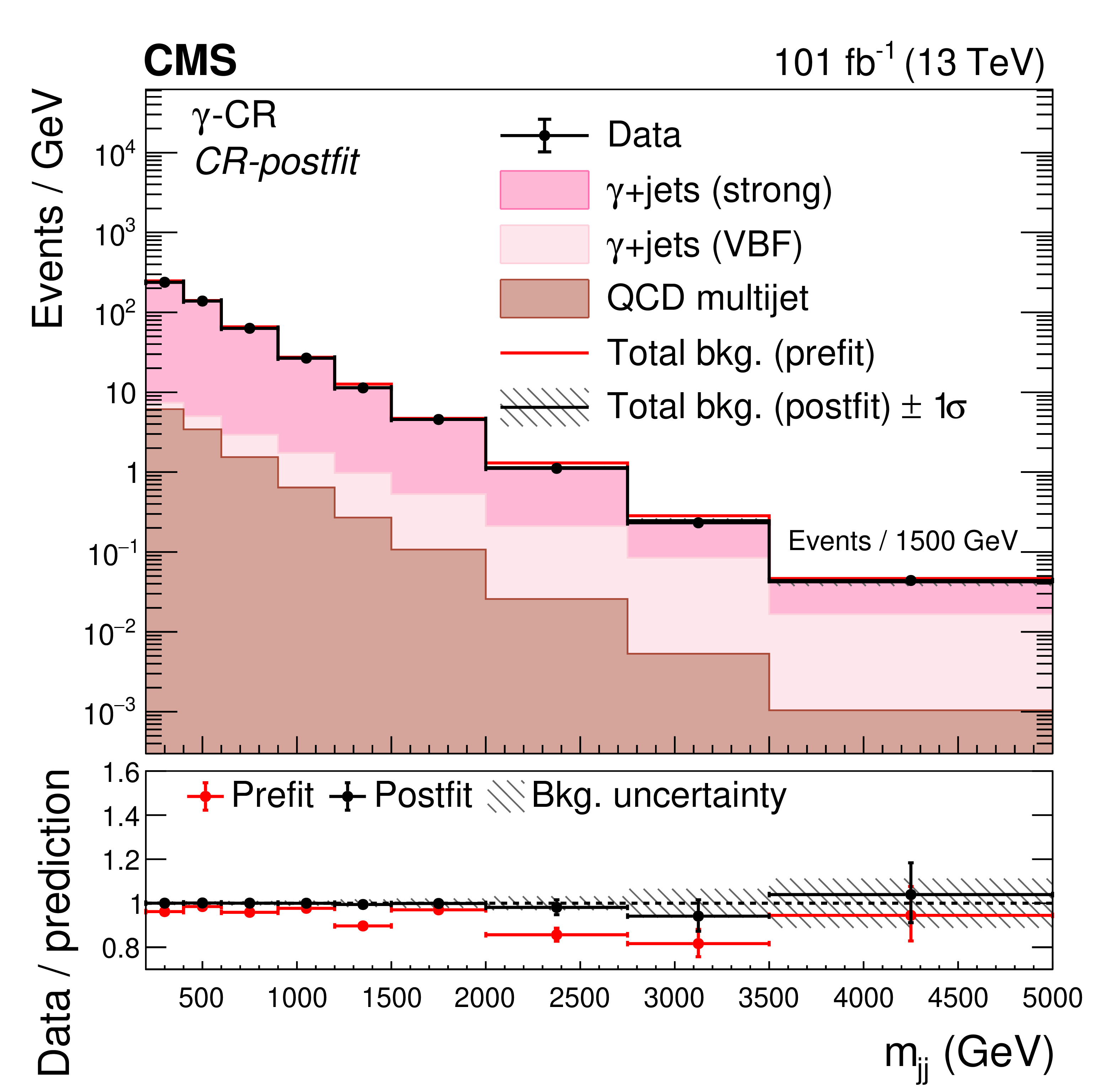
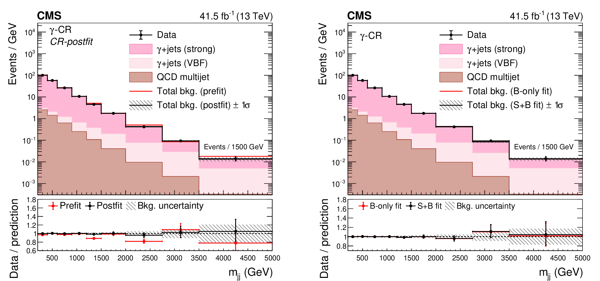
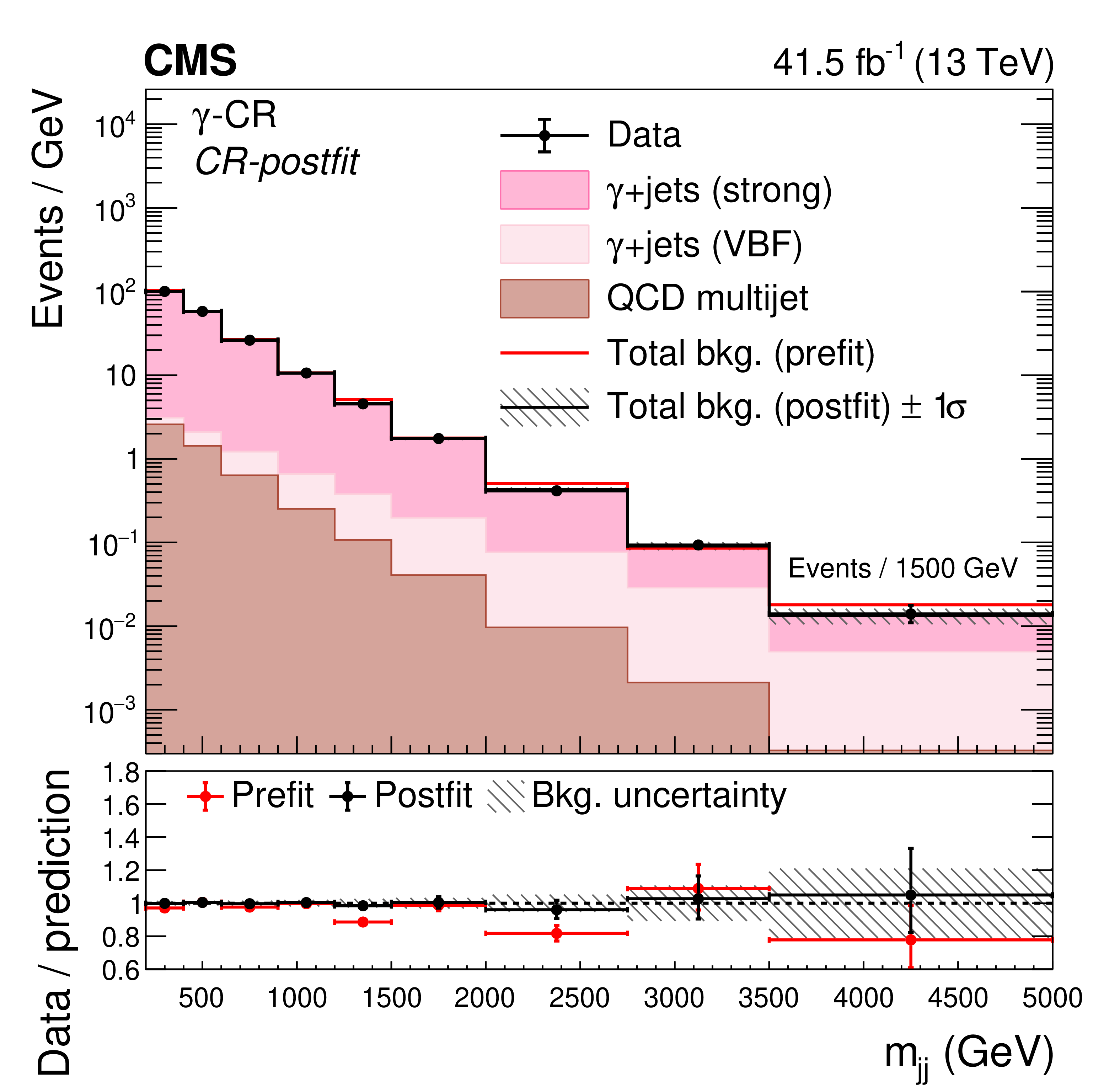
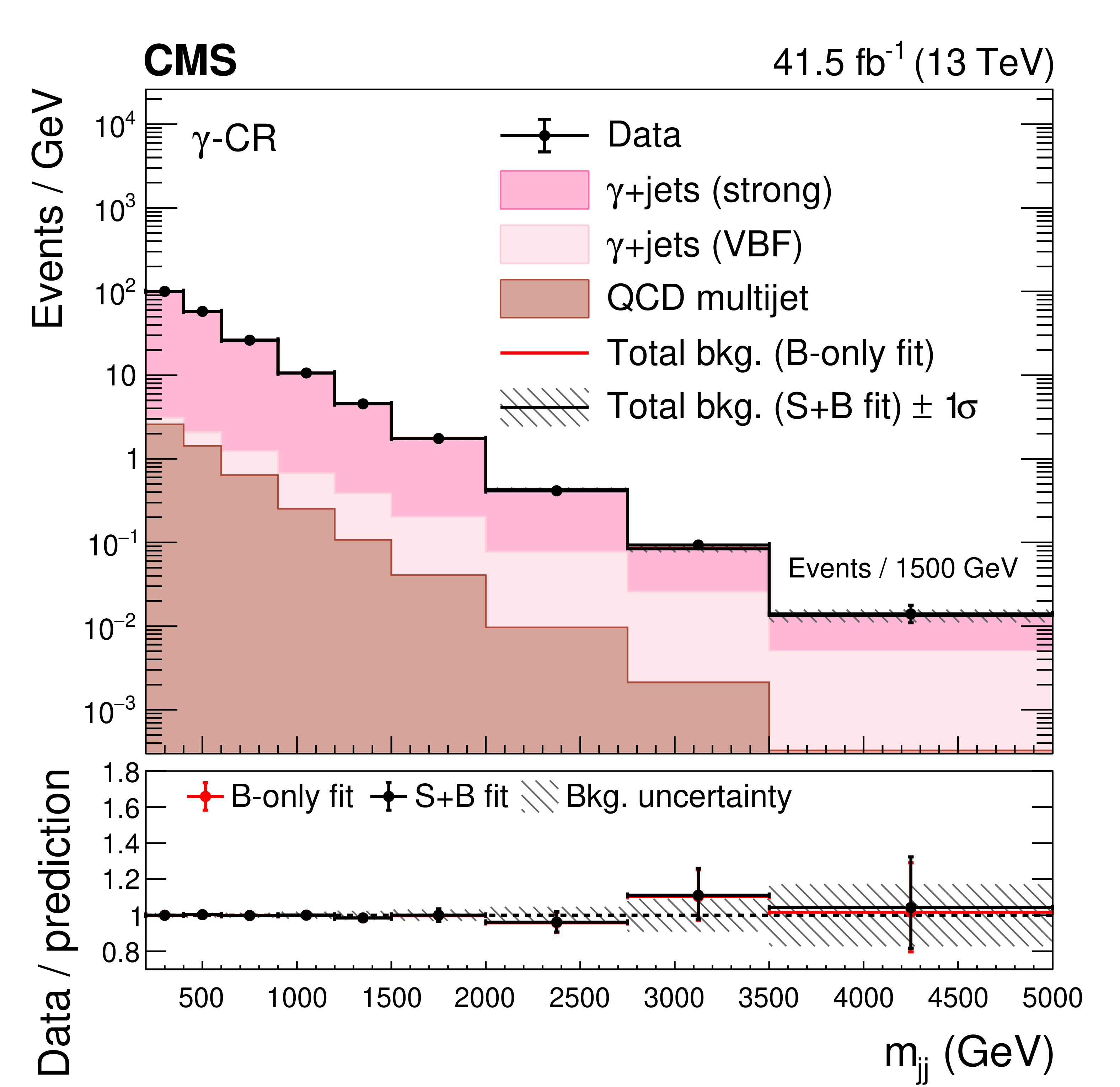
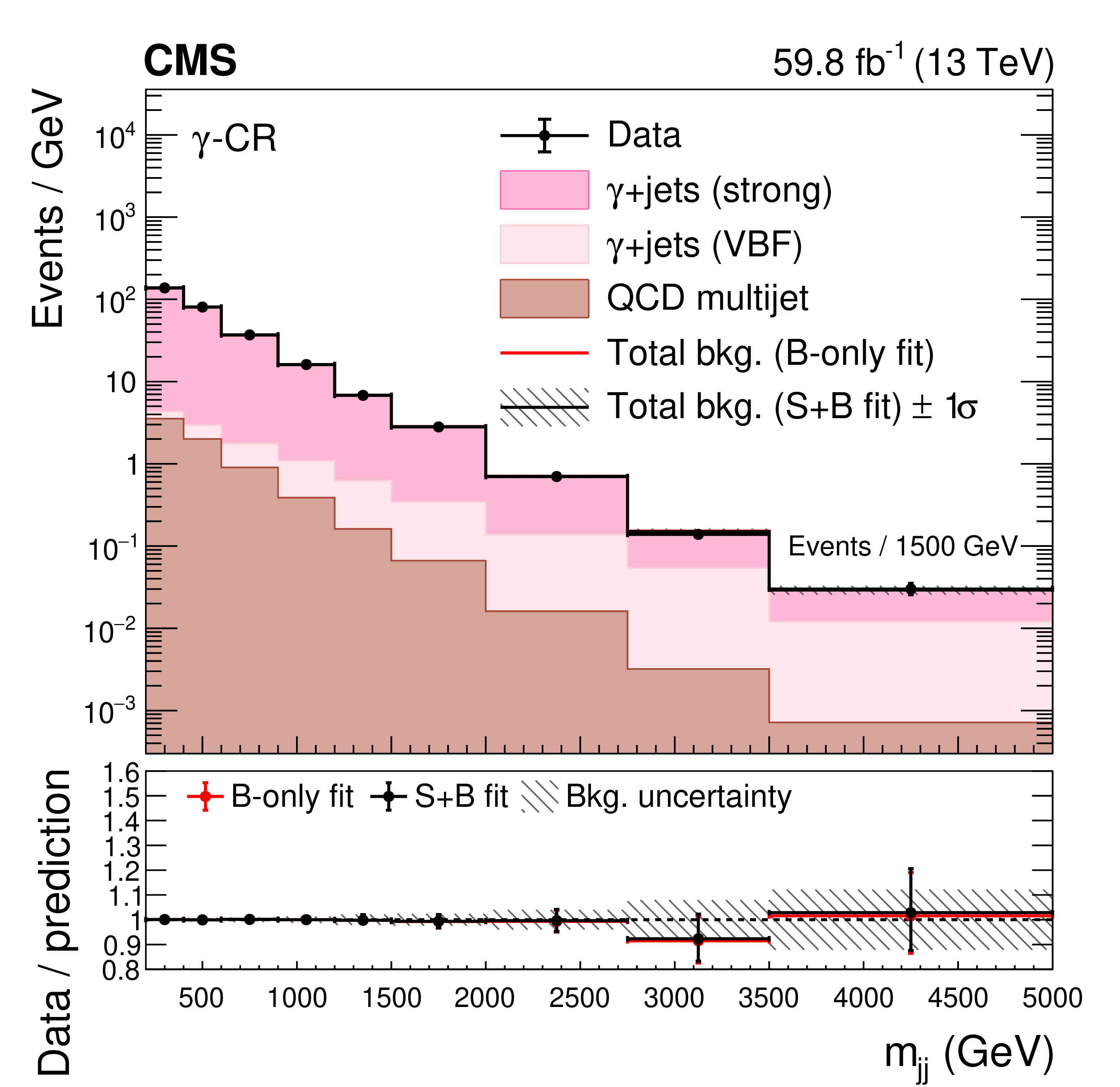
Figure 7:
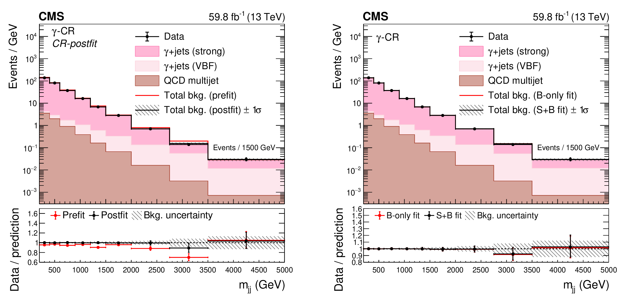
The postfit ${m_{\mathrm {jj}}}$ distribution in the photon CR for the MTR category, showing the summed 2017 and 2018 data samples and the background processes. The background contributions are estimated from the fit to the data described in the text (S+B fit). The total background estimated from a fit assuming $ {{\mathcal {B}(\mathrm{H} \to \text {inv})}} =$ 0 (B-only fit) is also shown. The yields from the 2017 and 2018 samples are summed and the correlations between their uncertainties are neglected. The last bin of each distribution integrates events above the bin threshold divided by the bin width. |
png pdf |
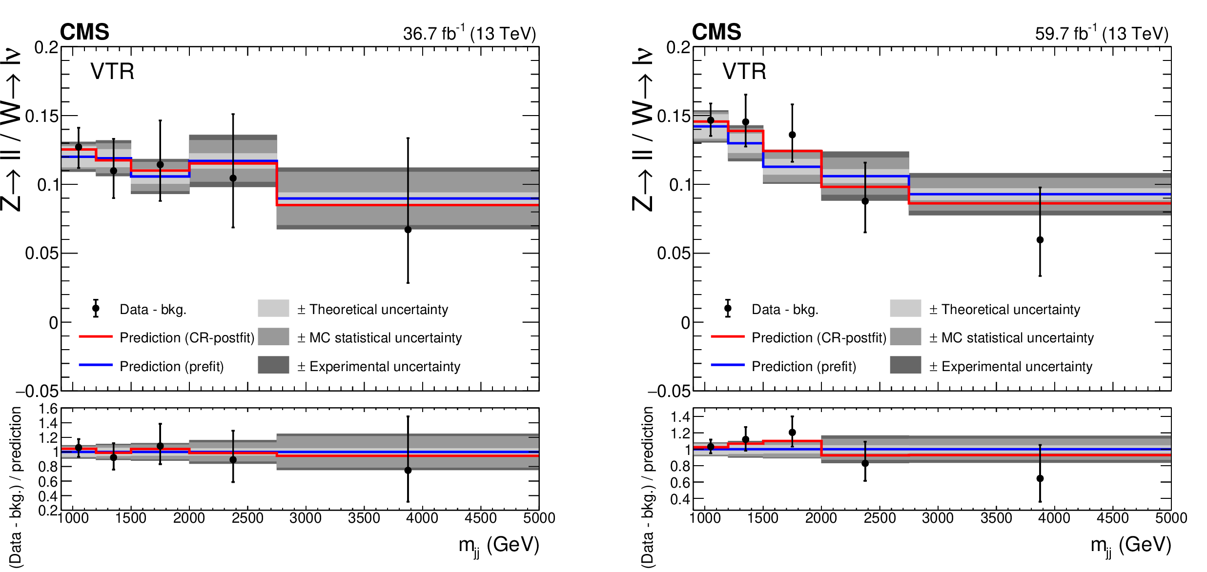
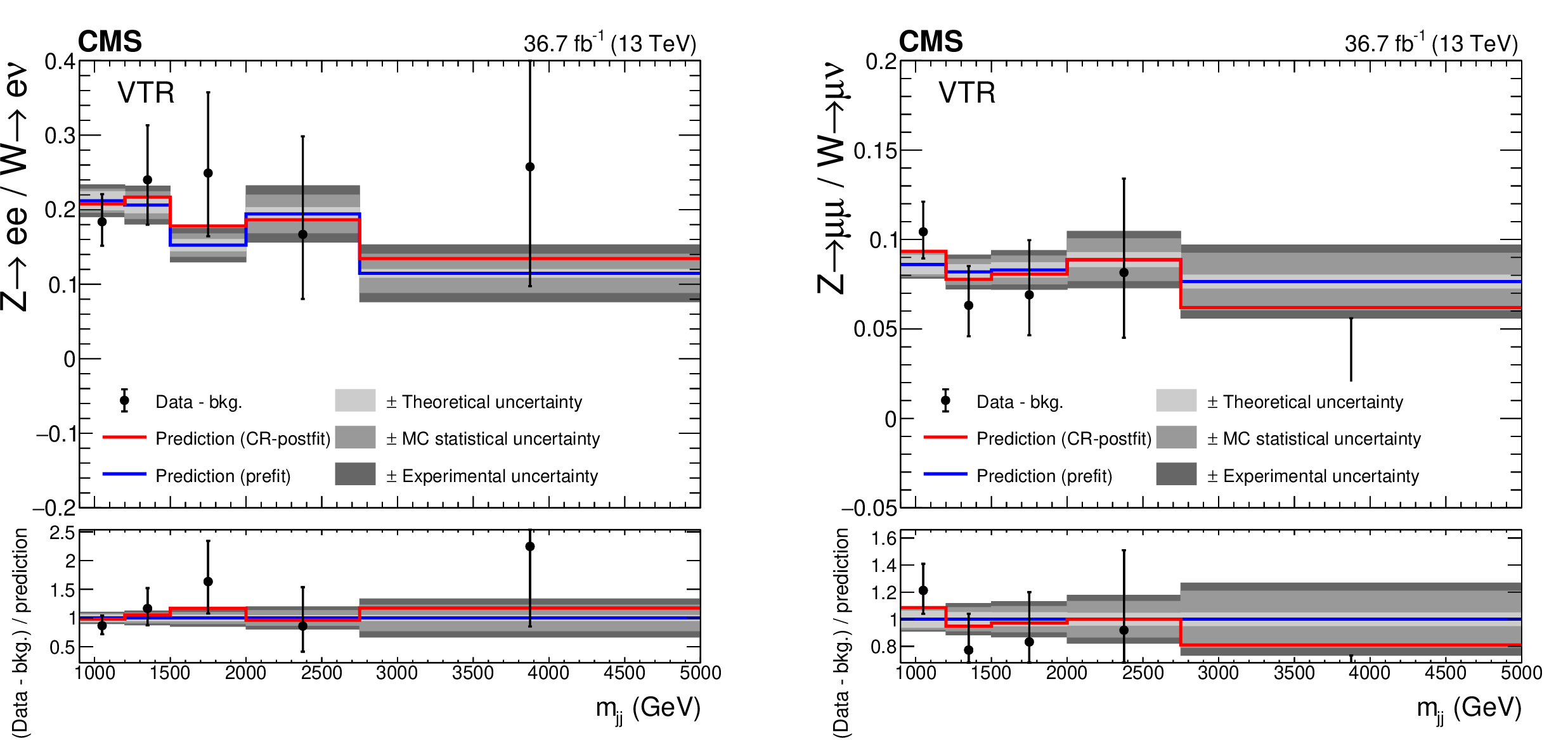
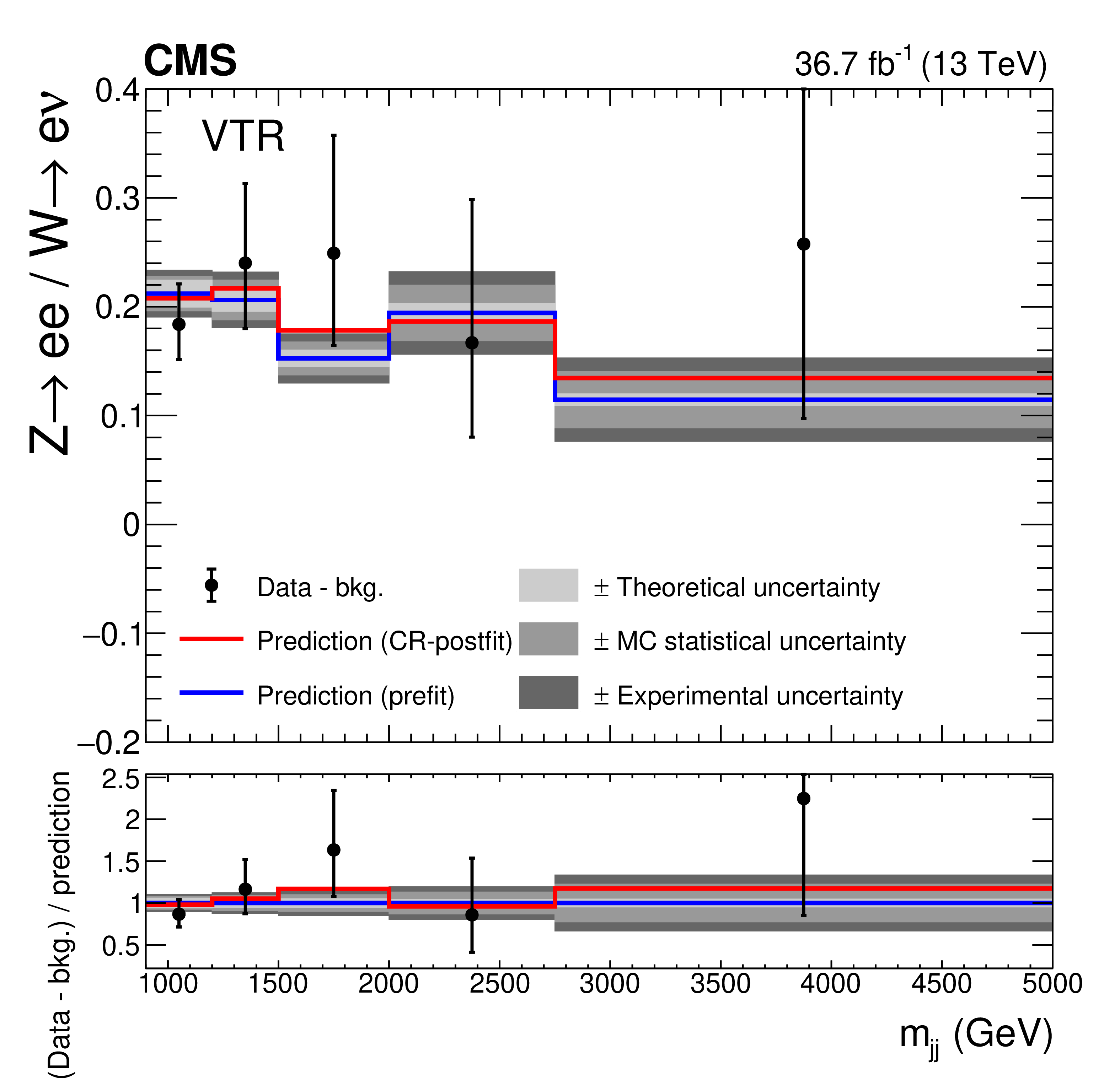
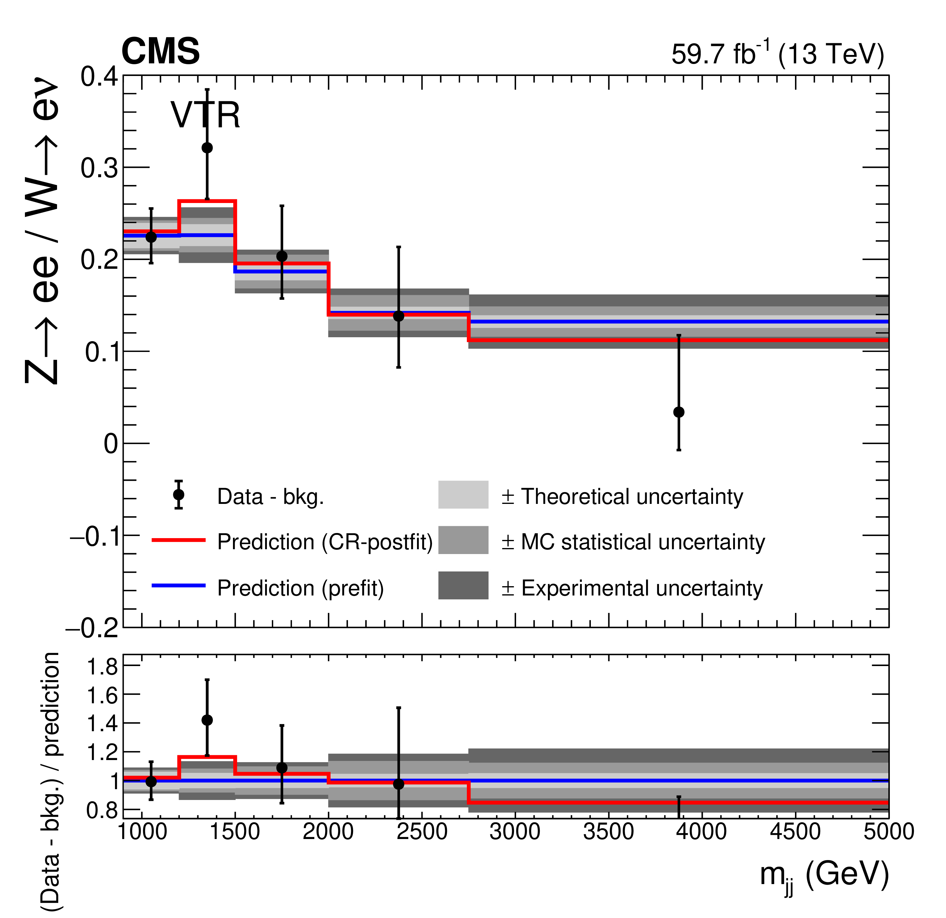
Figure 8:
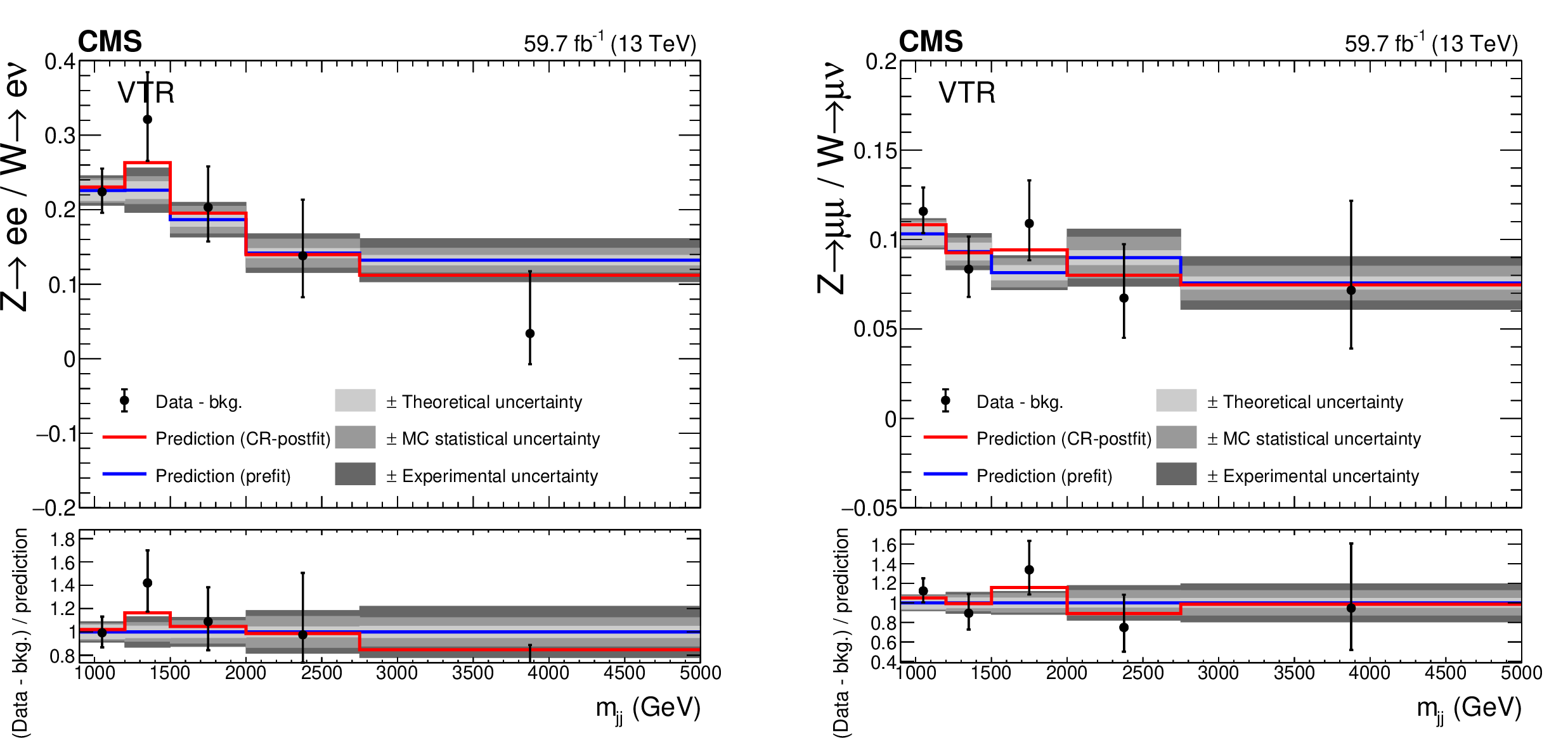
Comparison between data and simulation for the Z($\ell \ell$)+jets / W($\ell \nu$)+jets prefit and CR-postfit ratios, as functions of ${m_{\mathrm {jj}}}$, for the VTR category in the 2017 (left) and 2018 (right) data samples. The minor backgrounds in each CR are subtracted from the data using estimates from simulation. The grey bands include the theoretical and experimental systematic uncertainties listed in Table 3, as well as the statistical uncertainty in the simulation. |
png pdf |
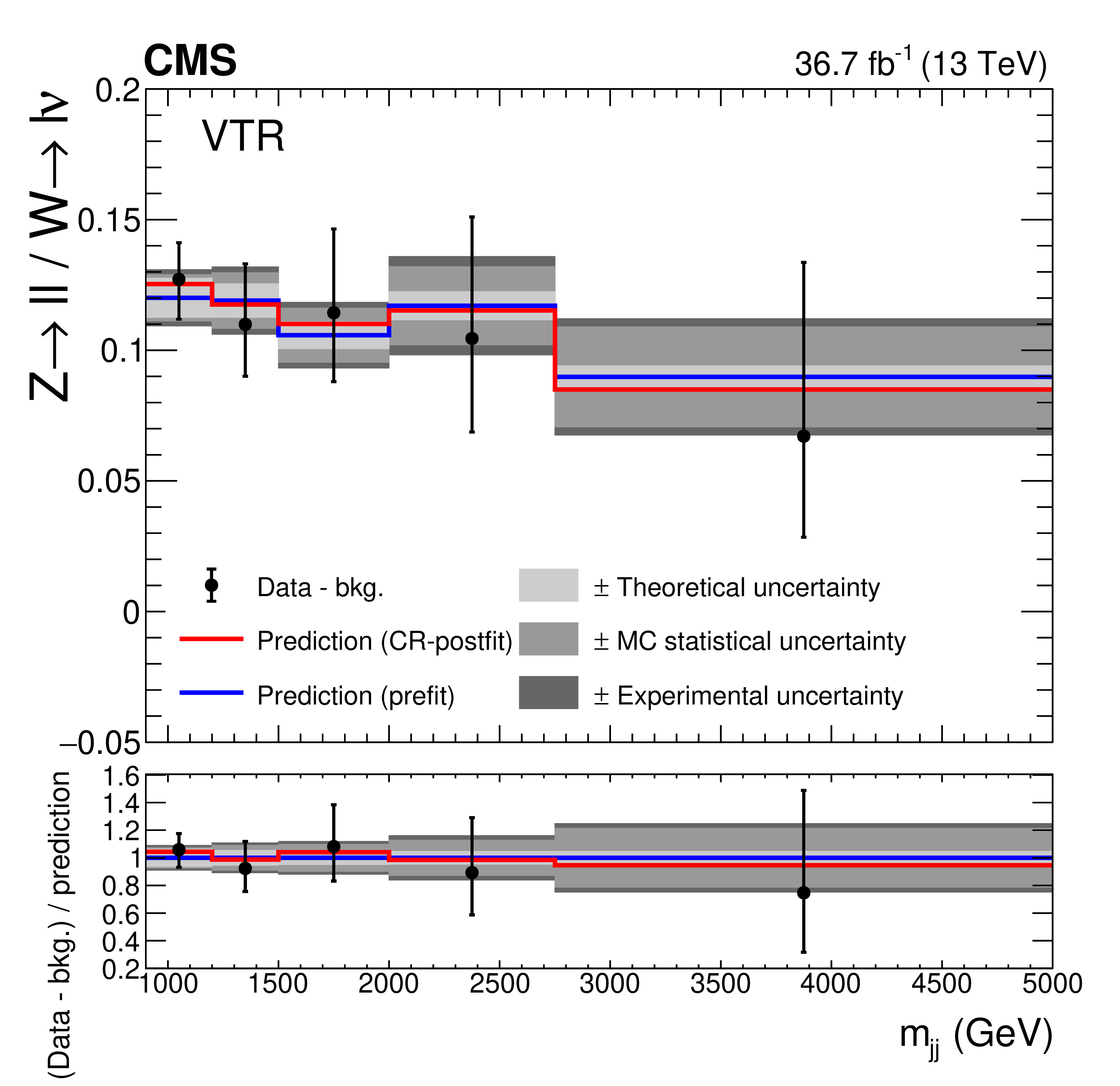
Figure 8-a:
Comparison between data and simulation for the Z($\ell \ell$)+jets / W($\ell \nu$)+jets prefit and CR-postfit ratios, as functions of ${m_{\mathrm {jj}}}$, for the VTR category in the 2017 (left) and 2018 (right) data samples. The minor backgrounds in each CR are subtracted from the data using estimates from simulation. The grey bands include the theoretical and experimental systematic uncertainties listed in Table 3, as well as the statistical uncertainty in the simulation. |
png pdf |
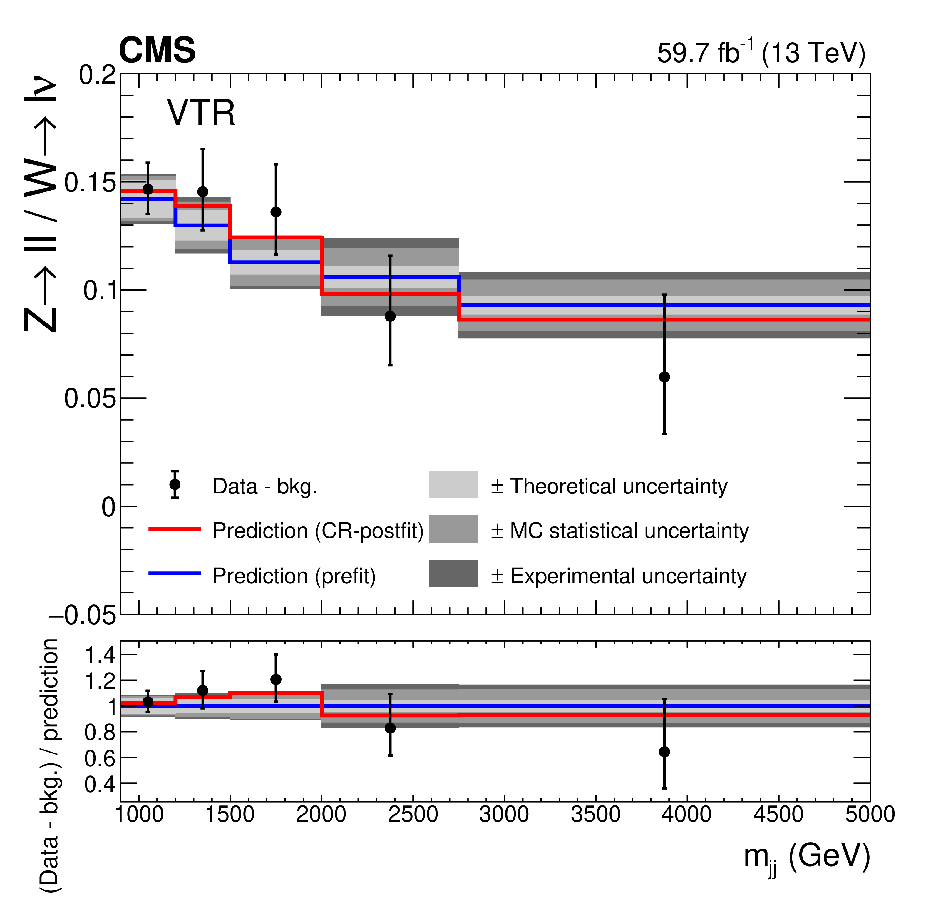
Figure 8-b:
Comparison between data and simulation for the Z($\ell \ell$)+jets / W($\ell \nu$)+jets prefit and CR-postfit ratios, as functions of ${m_{\mathrm {jj}}}$, for the VTR category in the 2017 (left) and 2018 (right) data samples. The minor backgrounds in each CR are subtracted from the data using estimates from simulation. The grey bands include the theoretical and experimental systematic uncertainties listed in Table 3, as well as the statistical uncertainty in the simulation. |

png pdf |
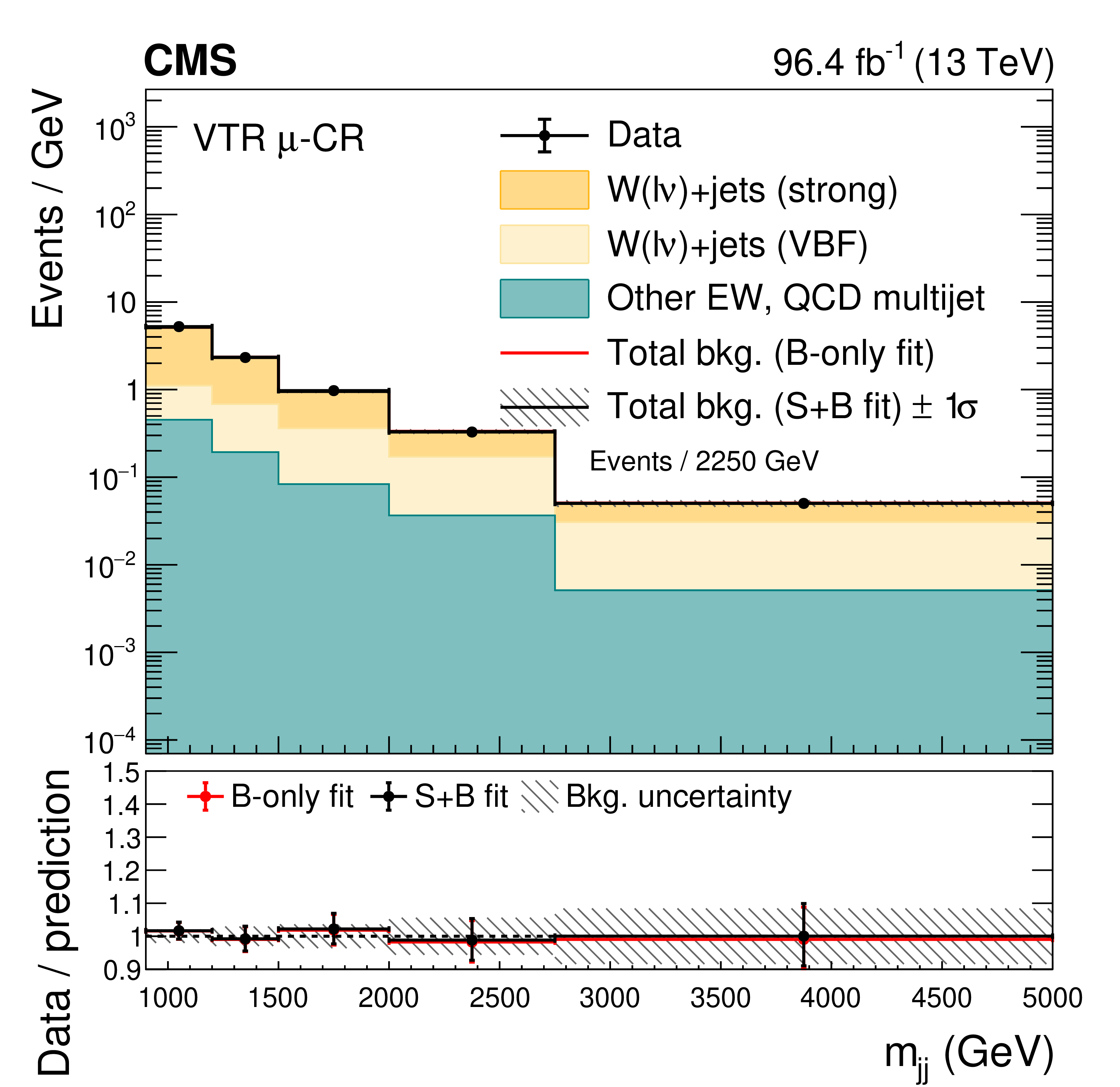
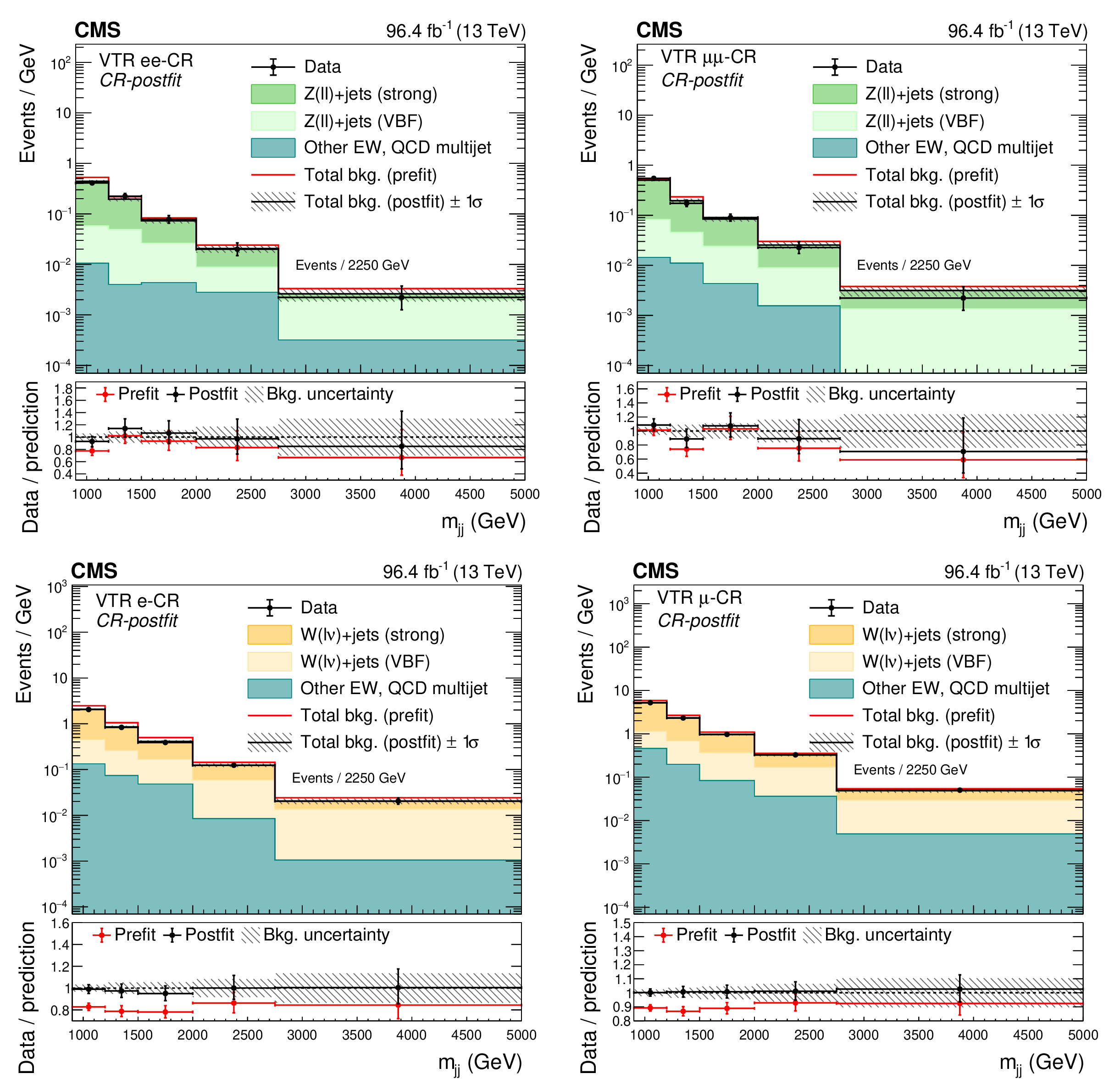
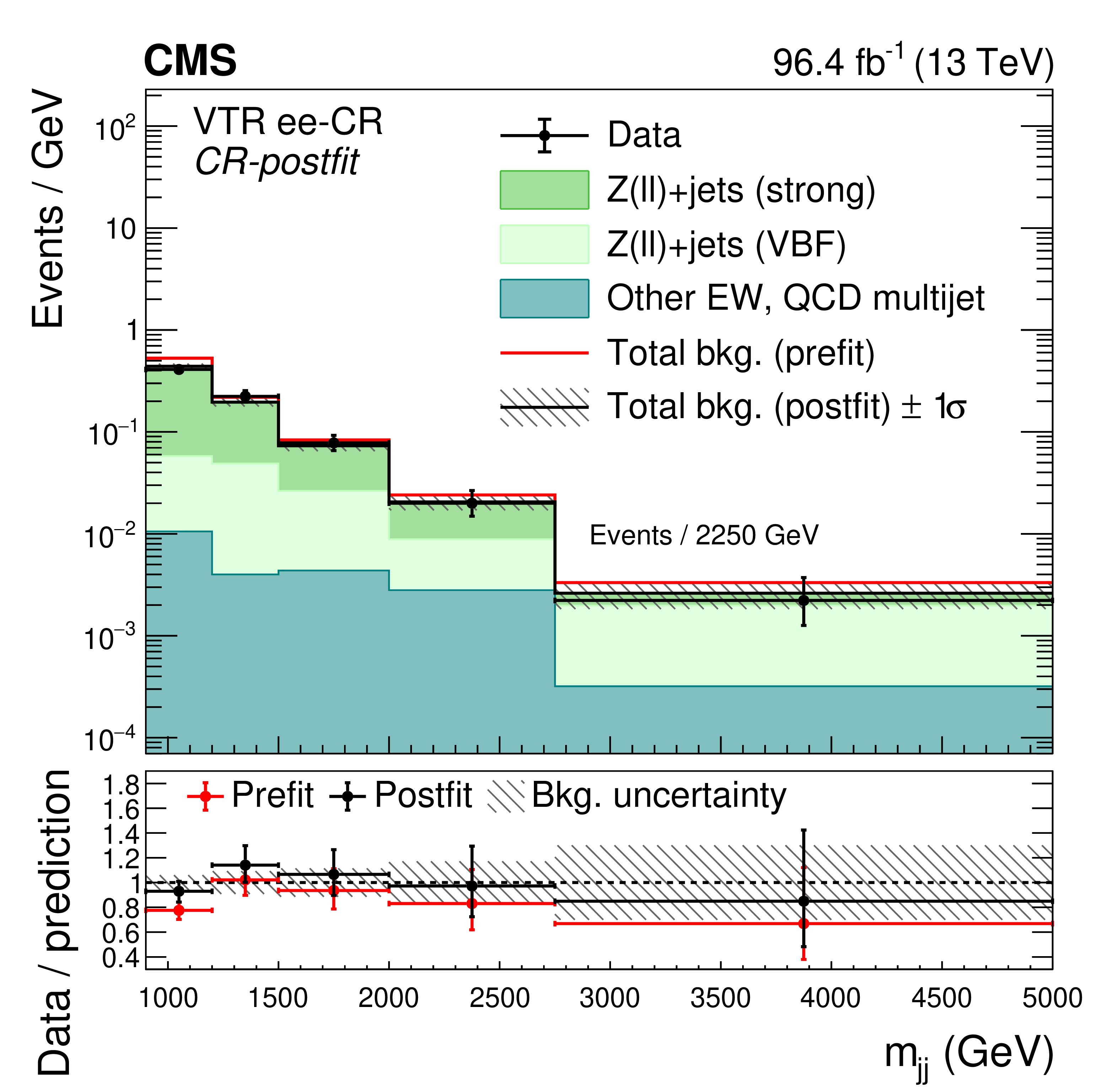
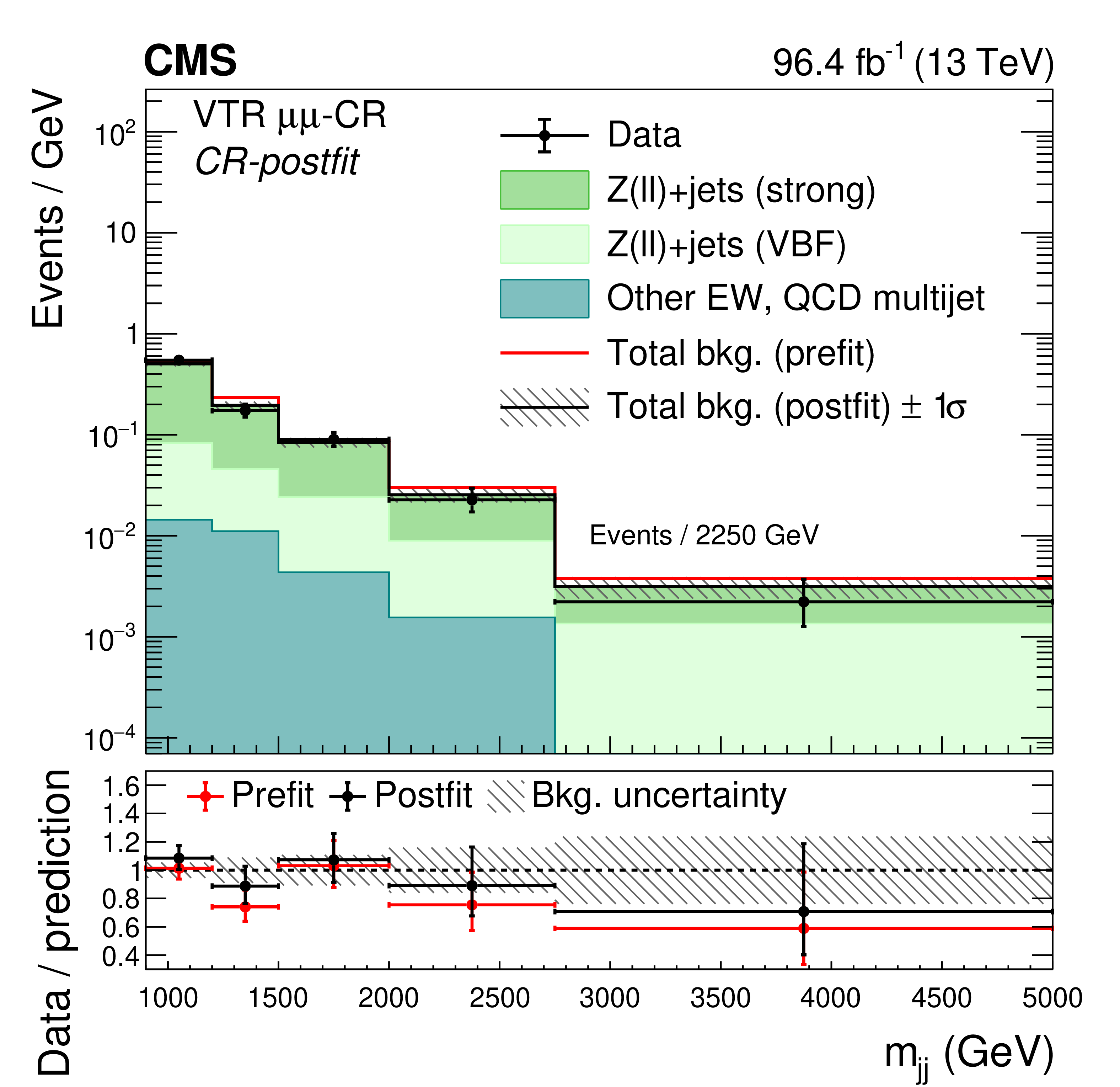
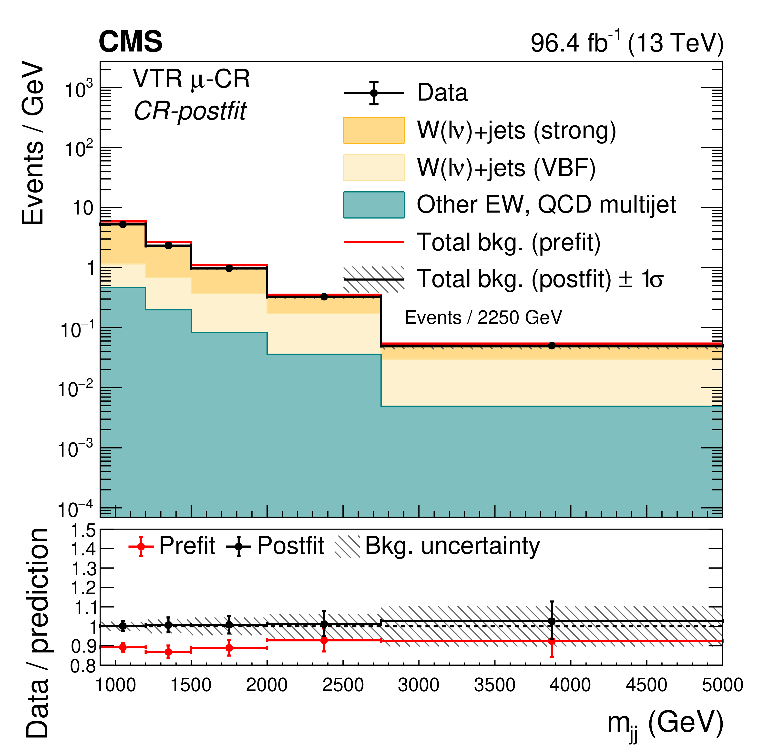
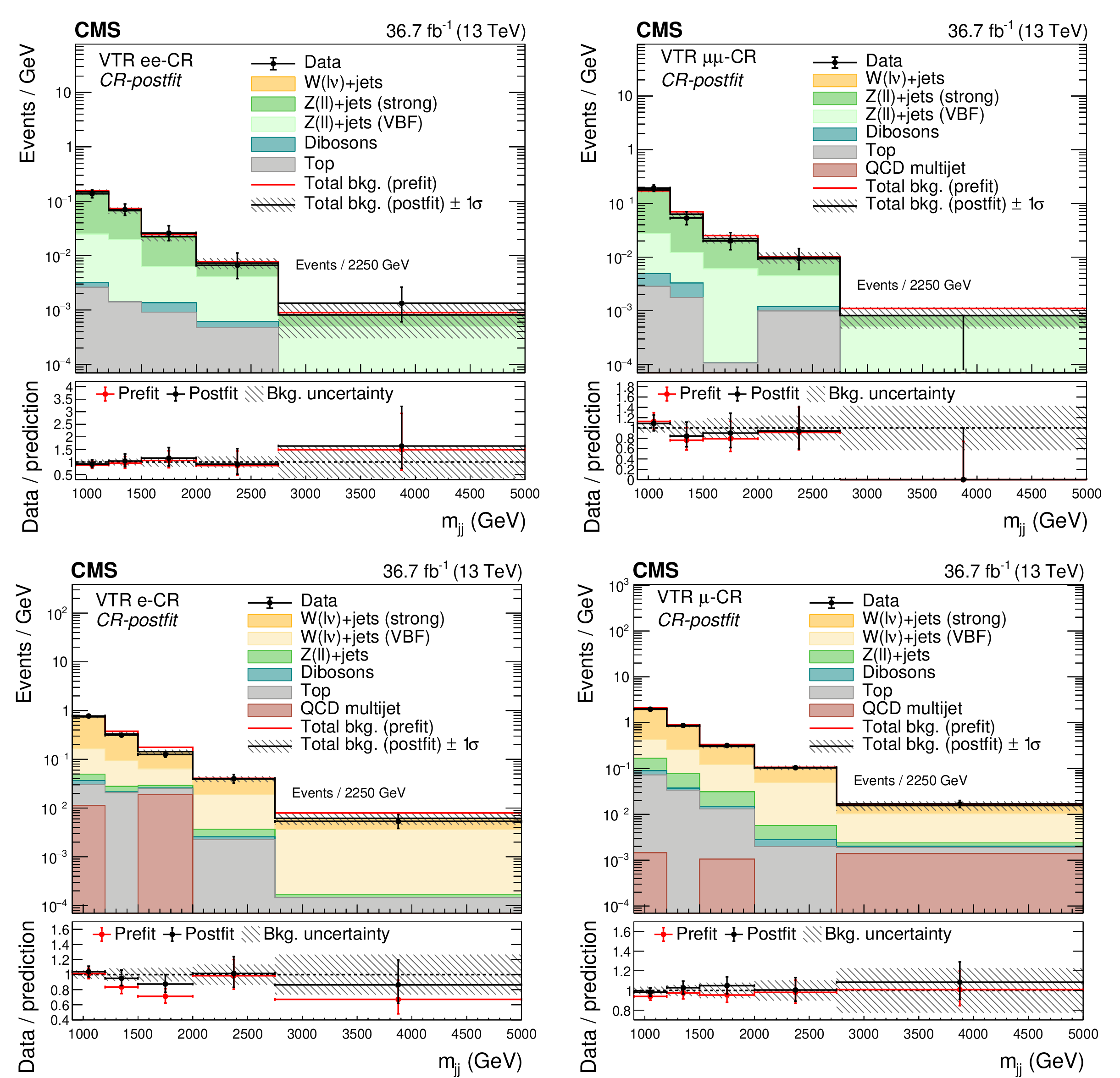
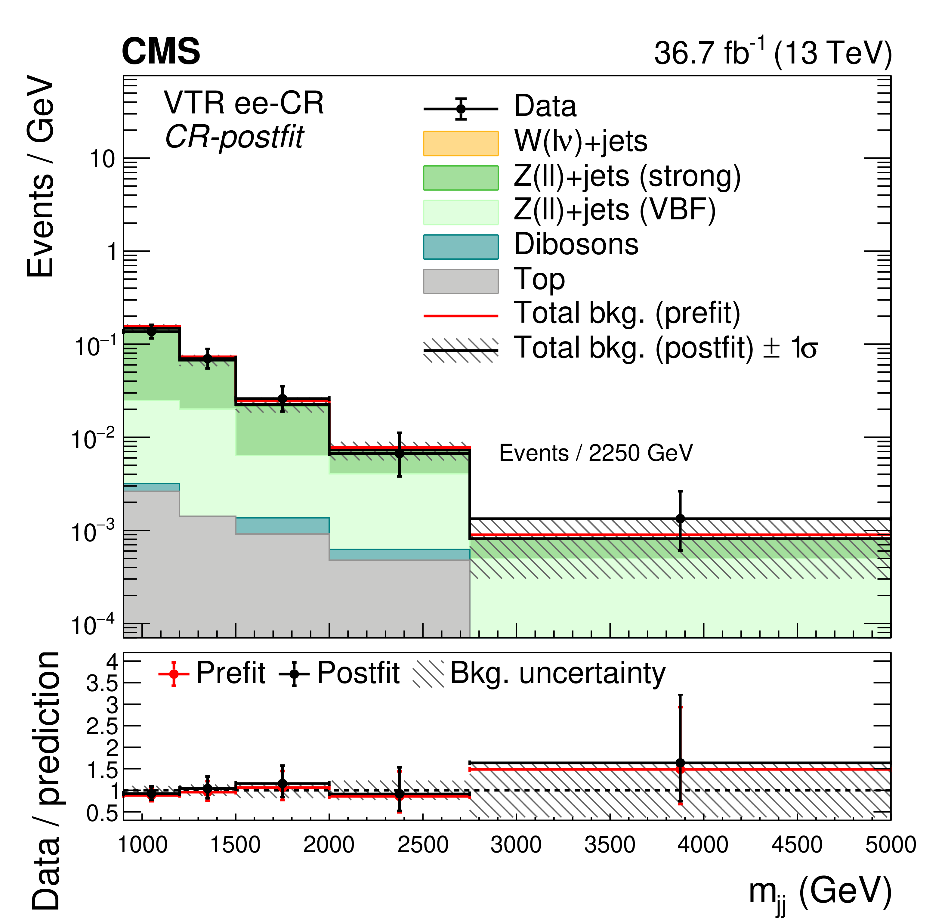
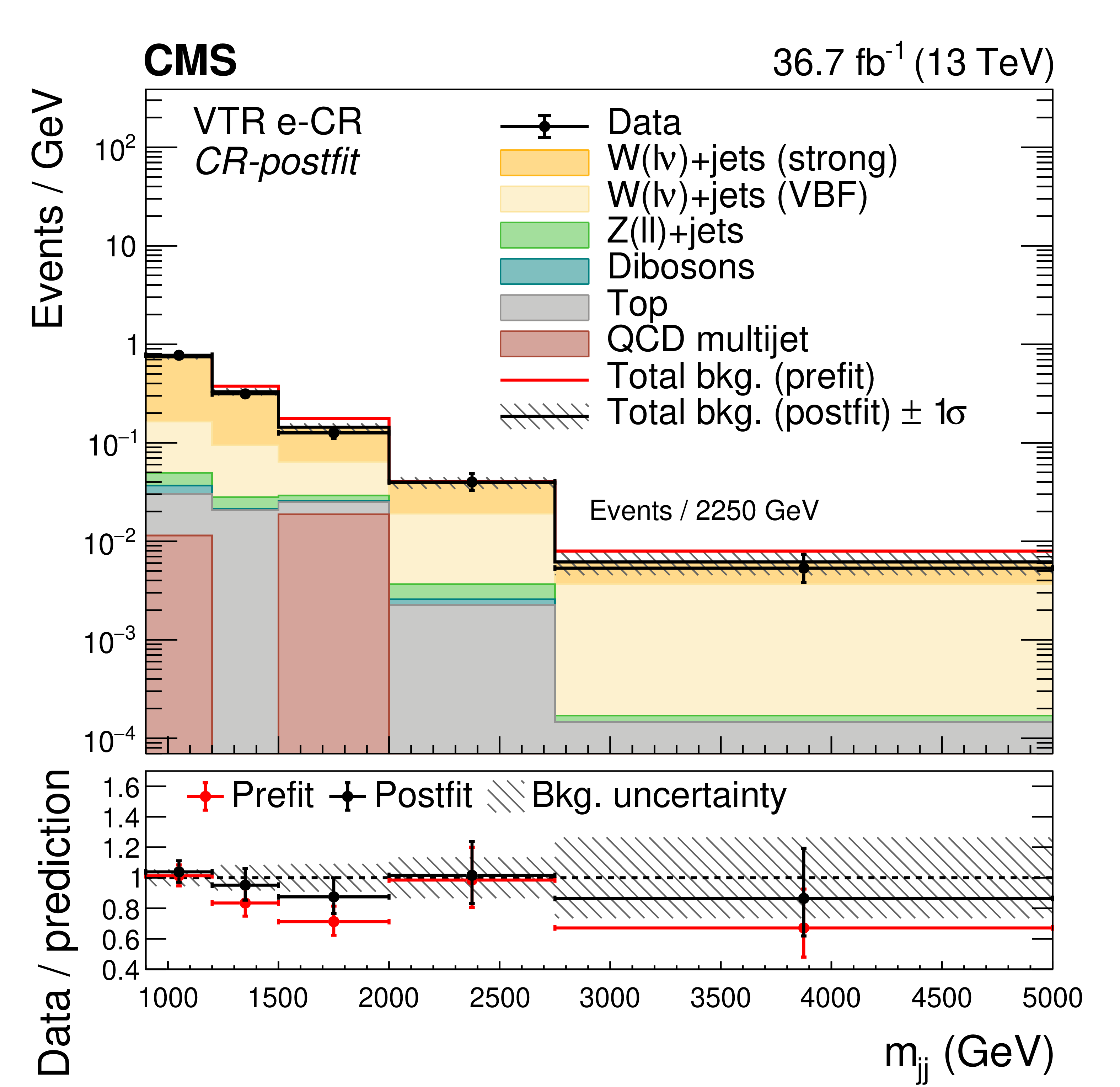
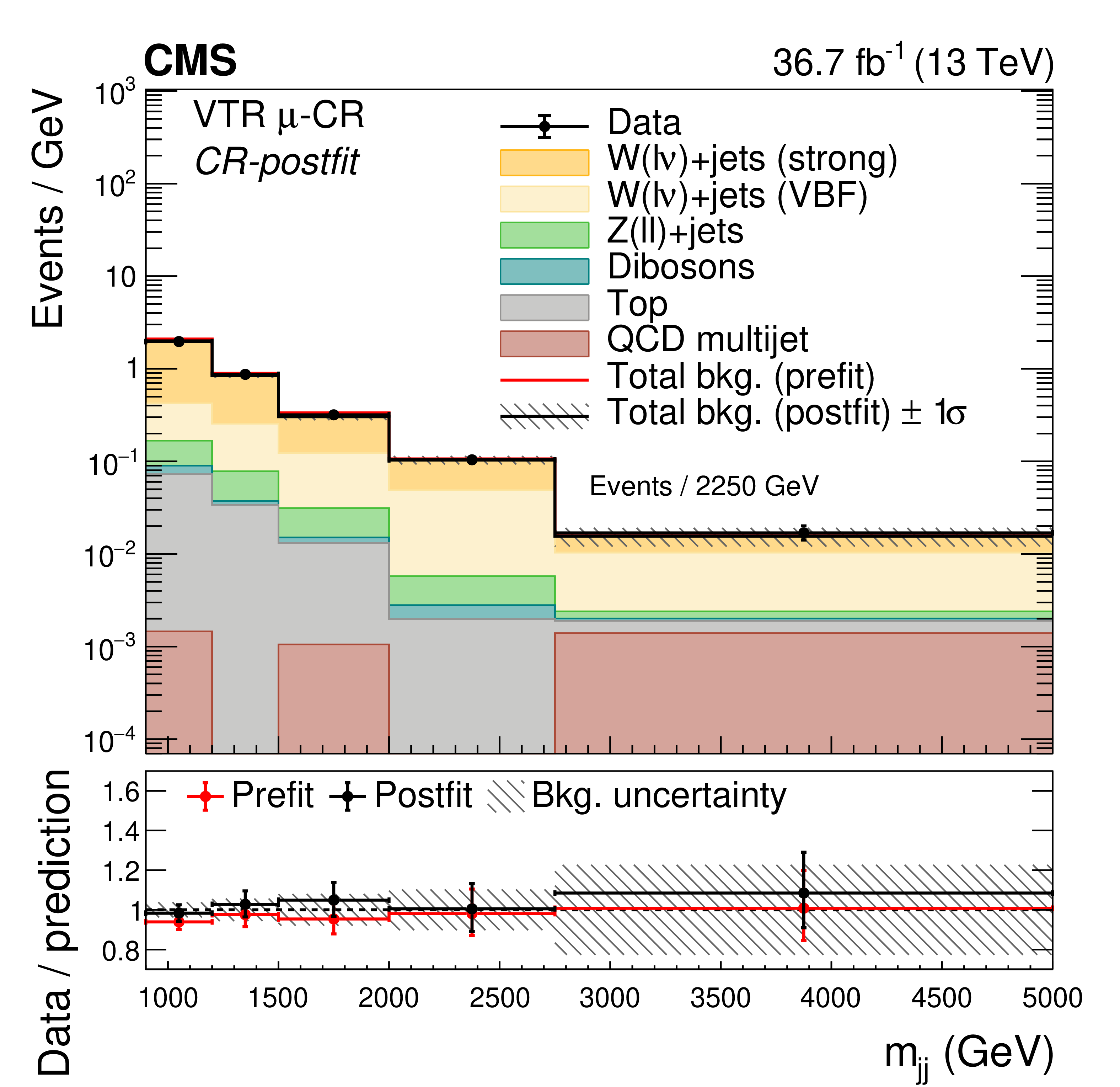
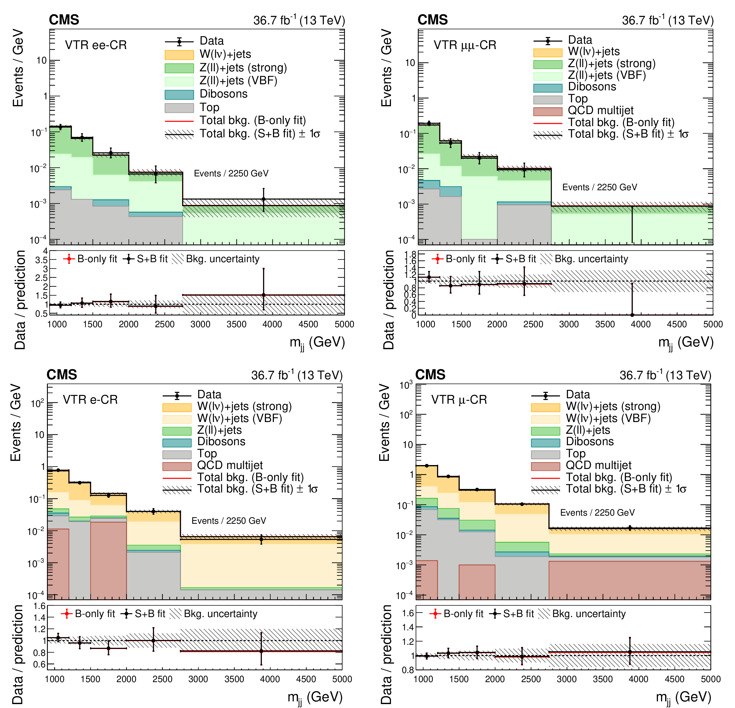
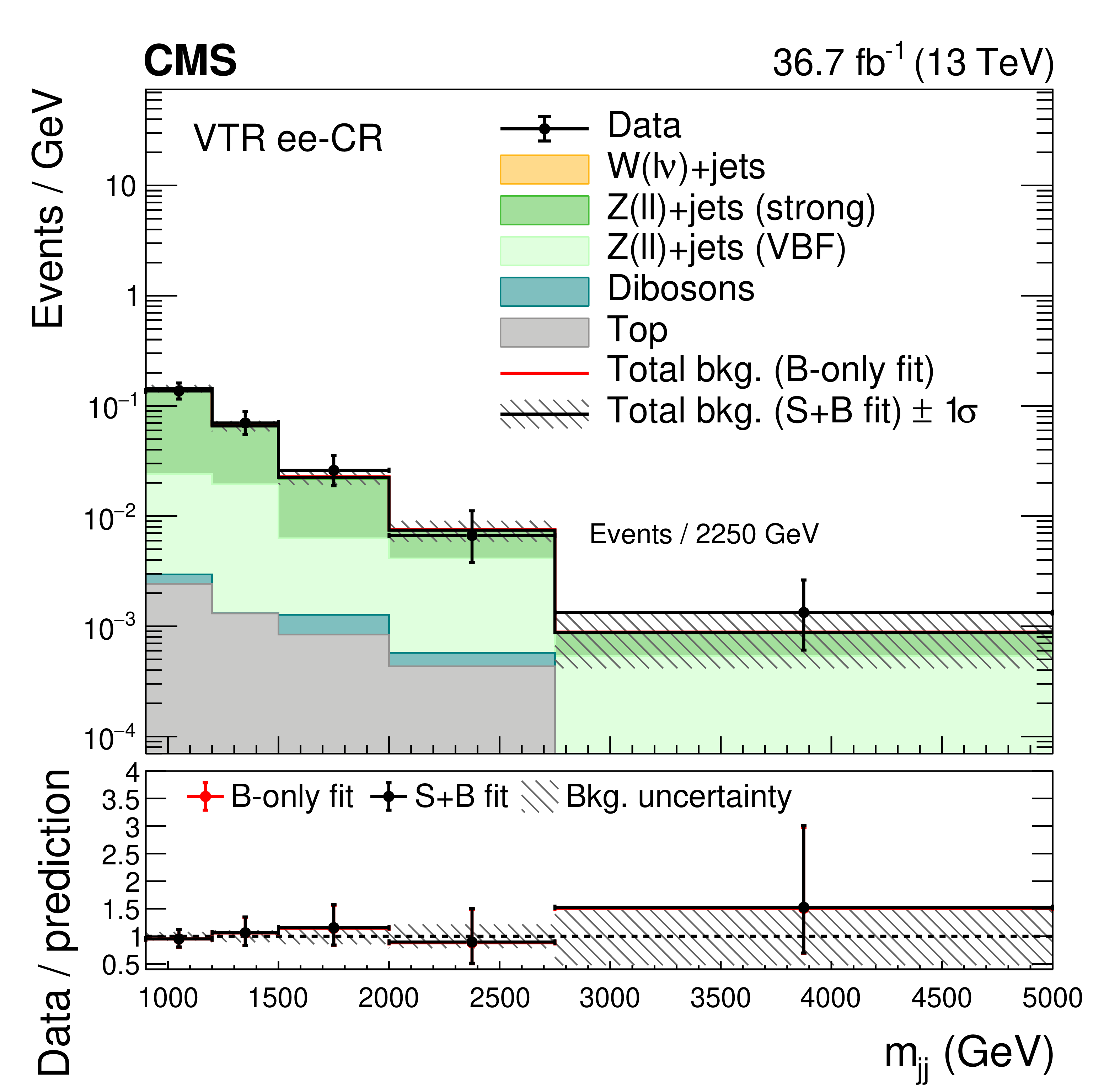
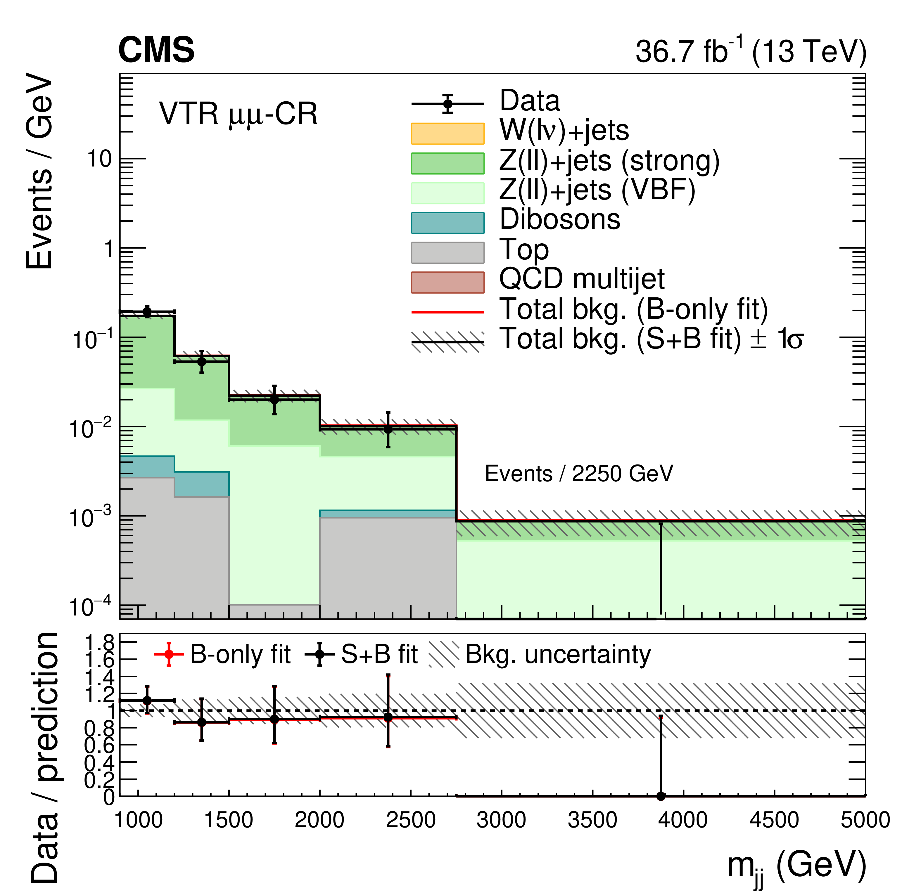
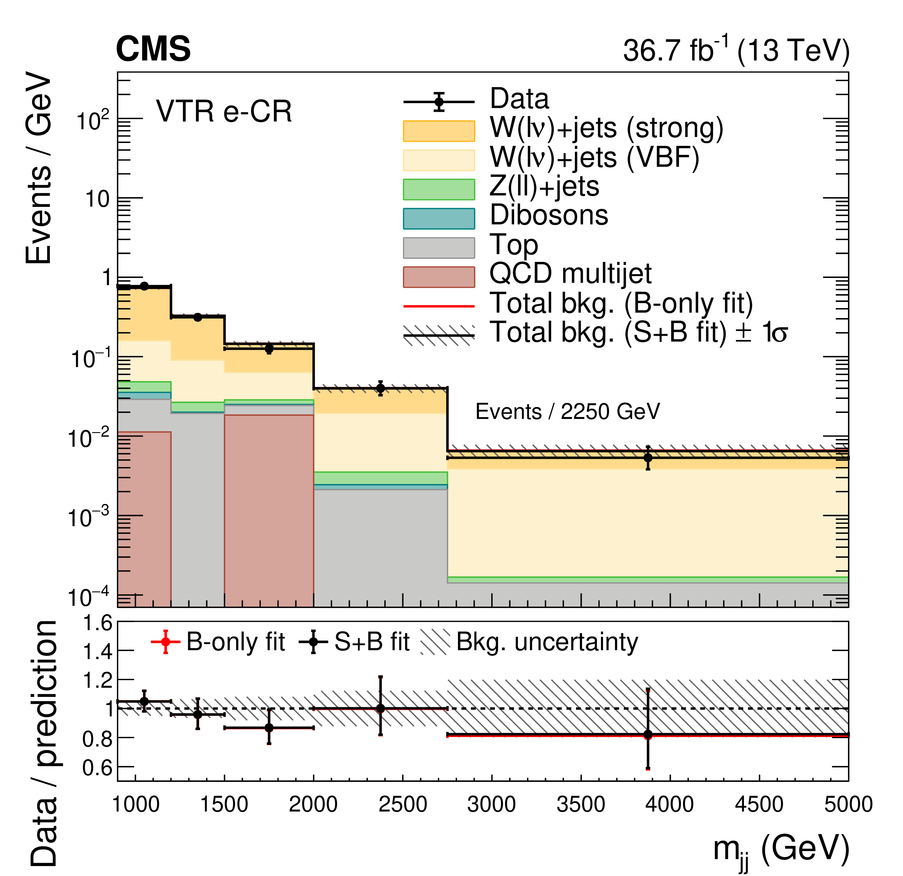
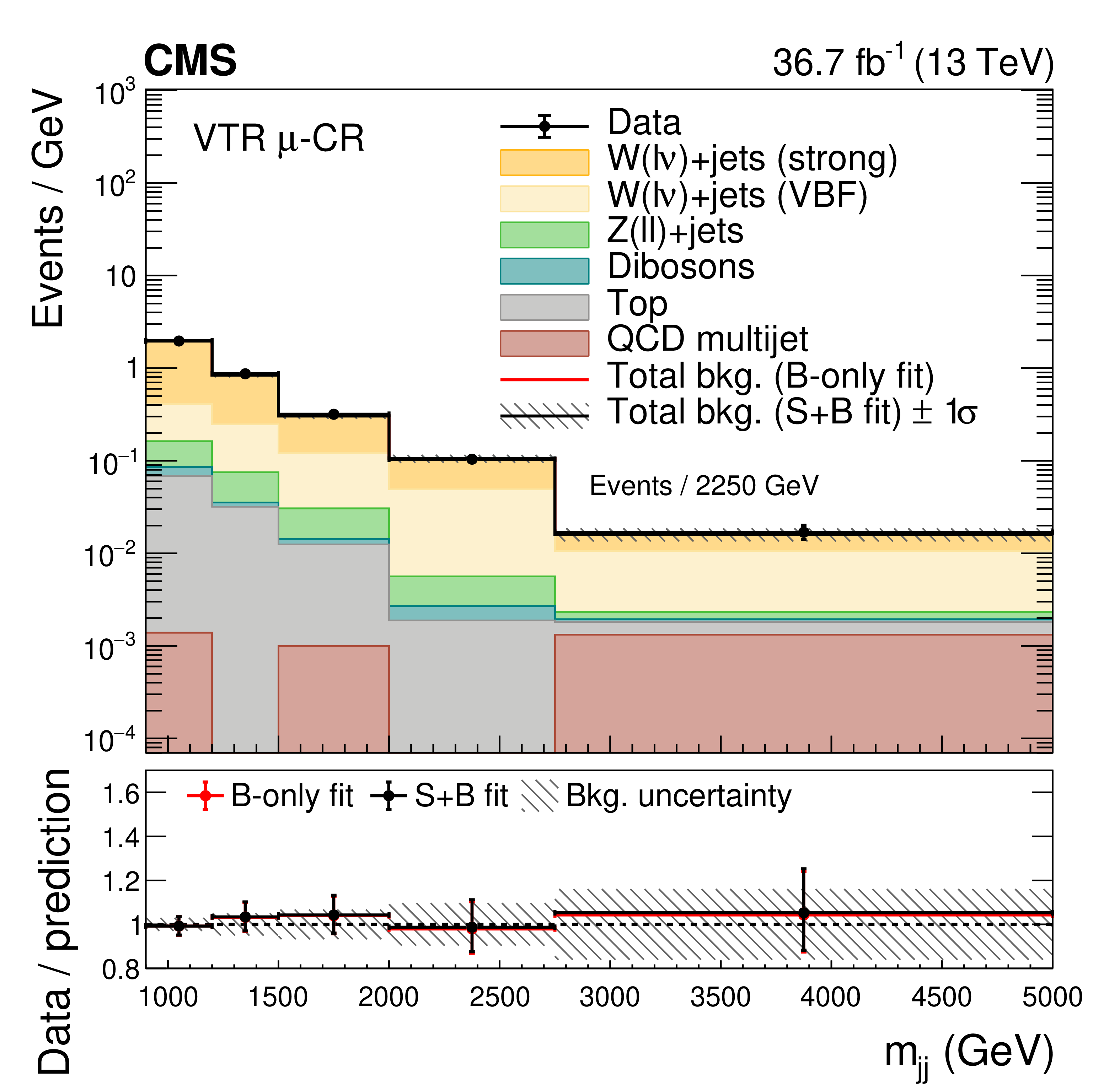
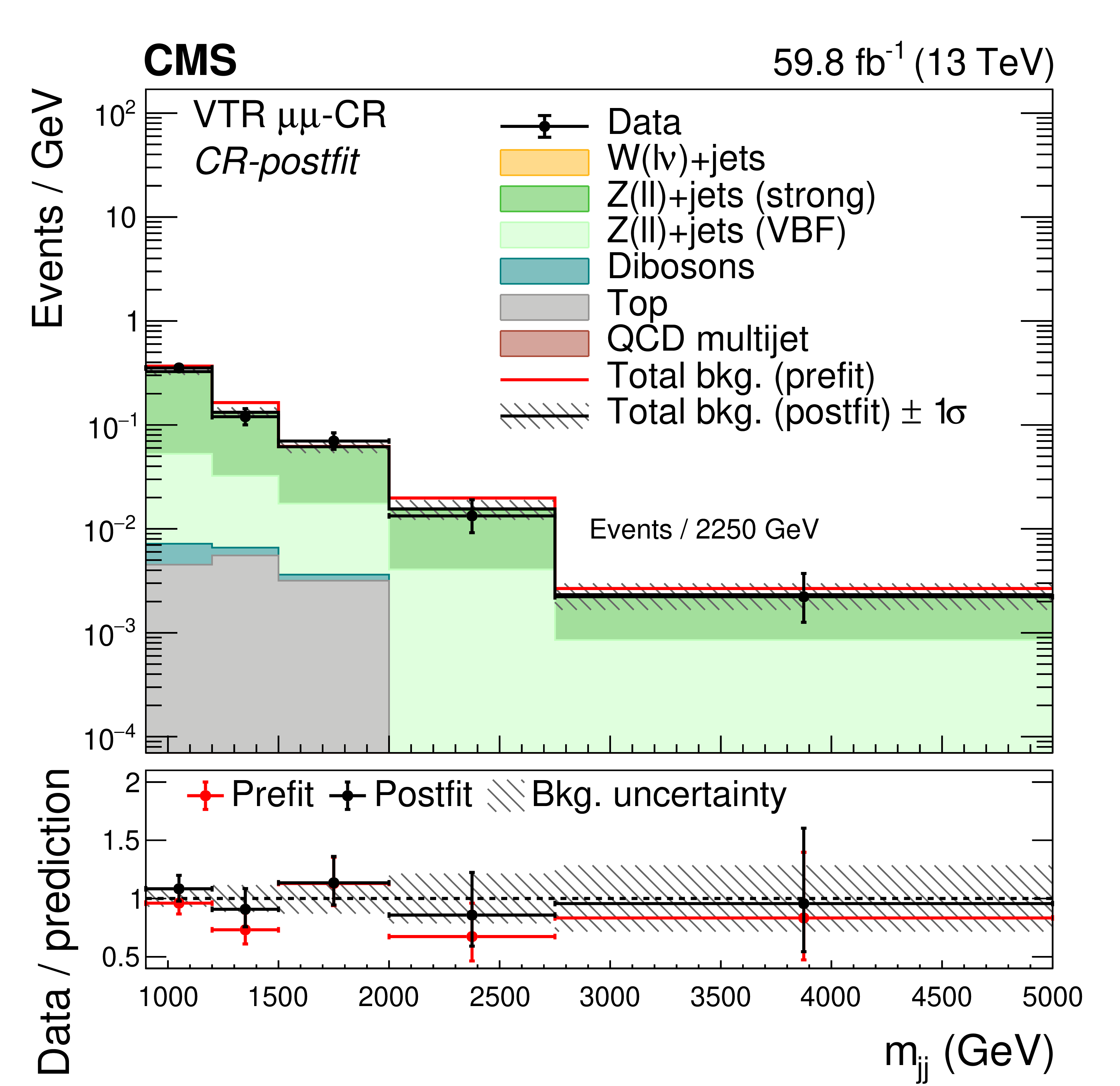
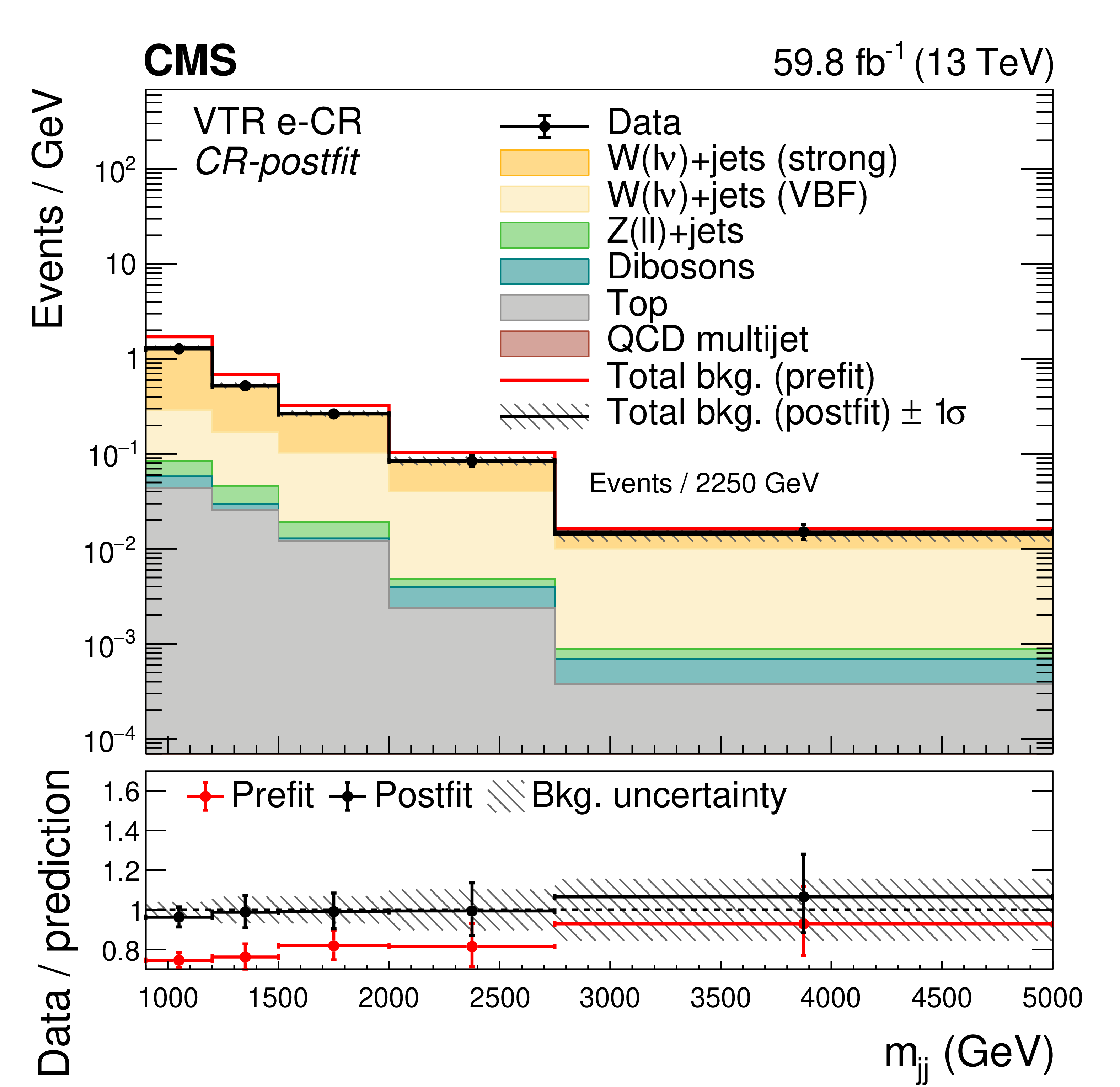
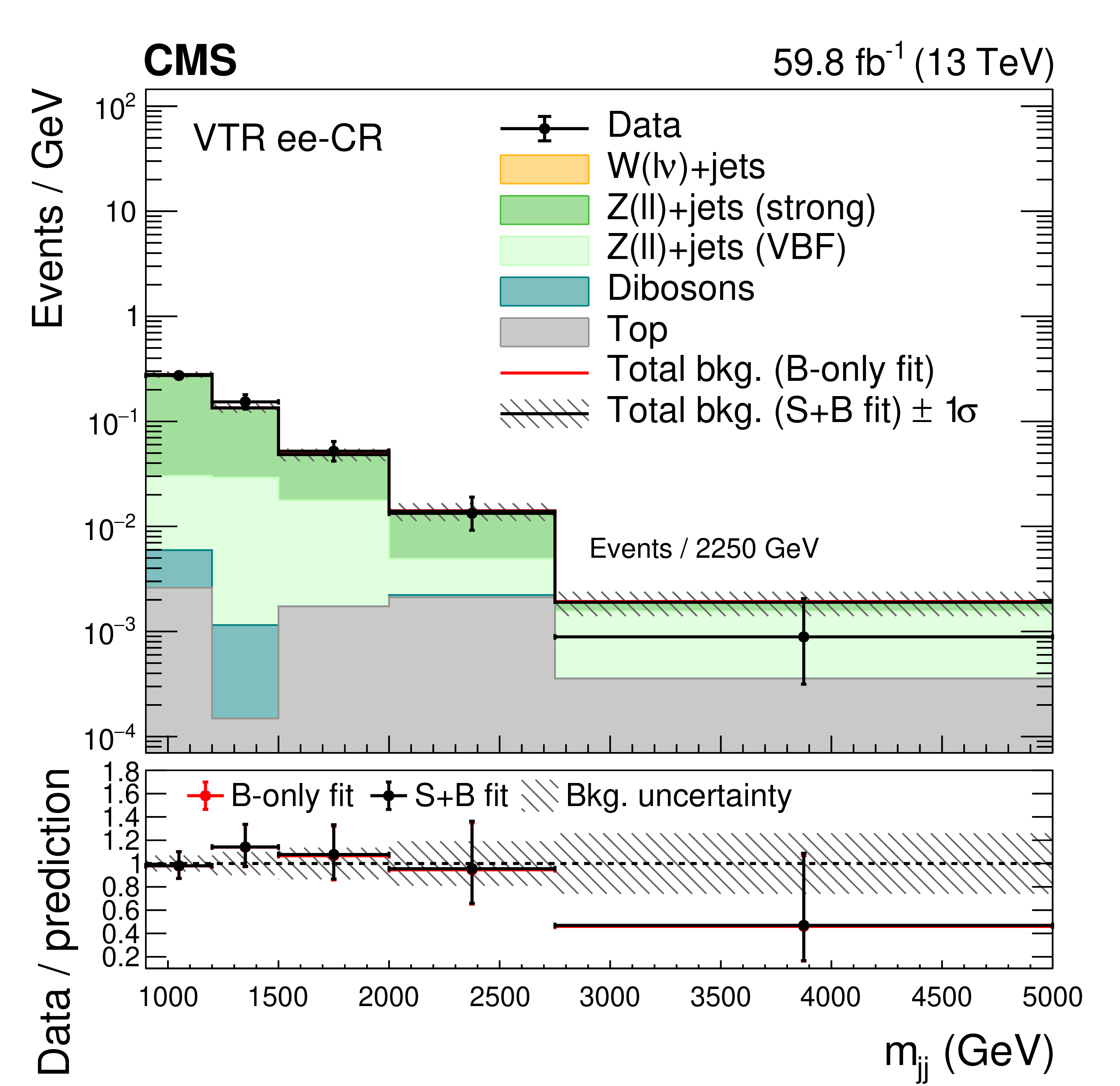
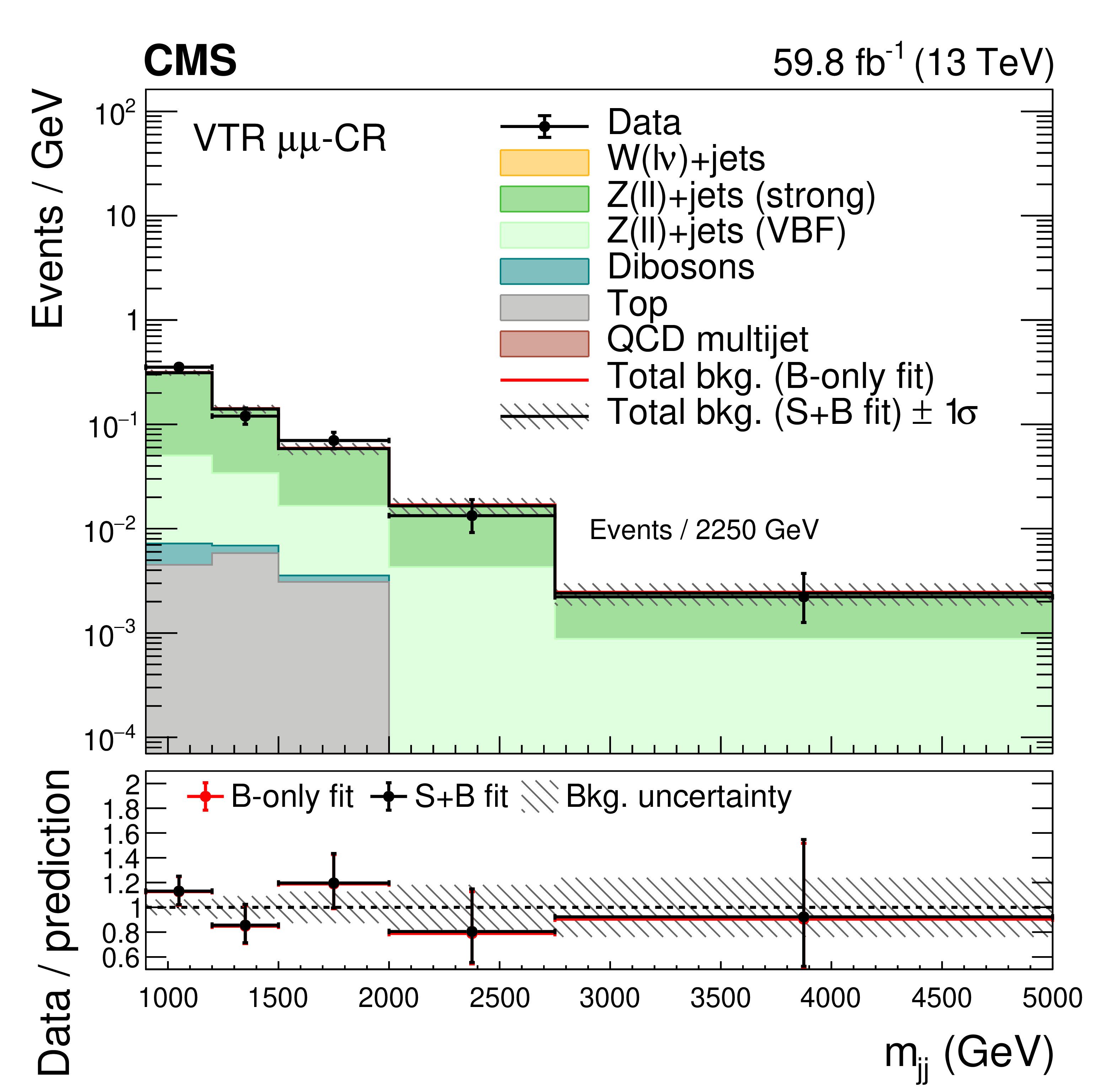
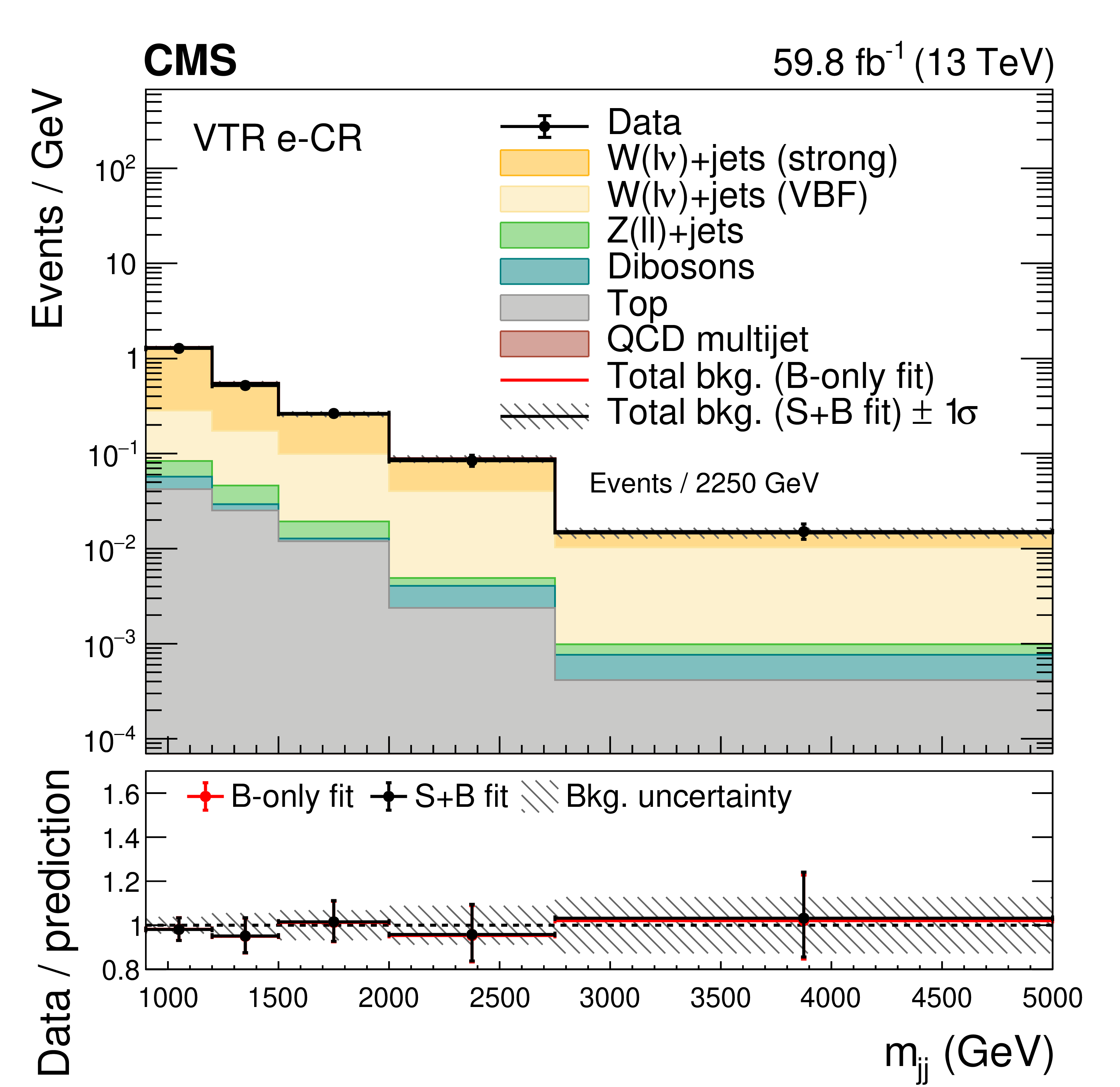
Figure 9:
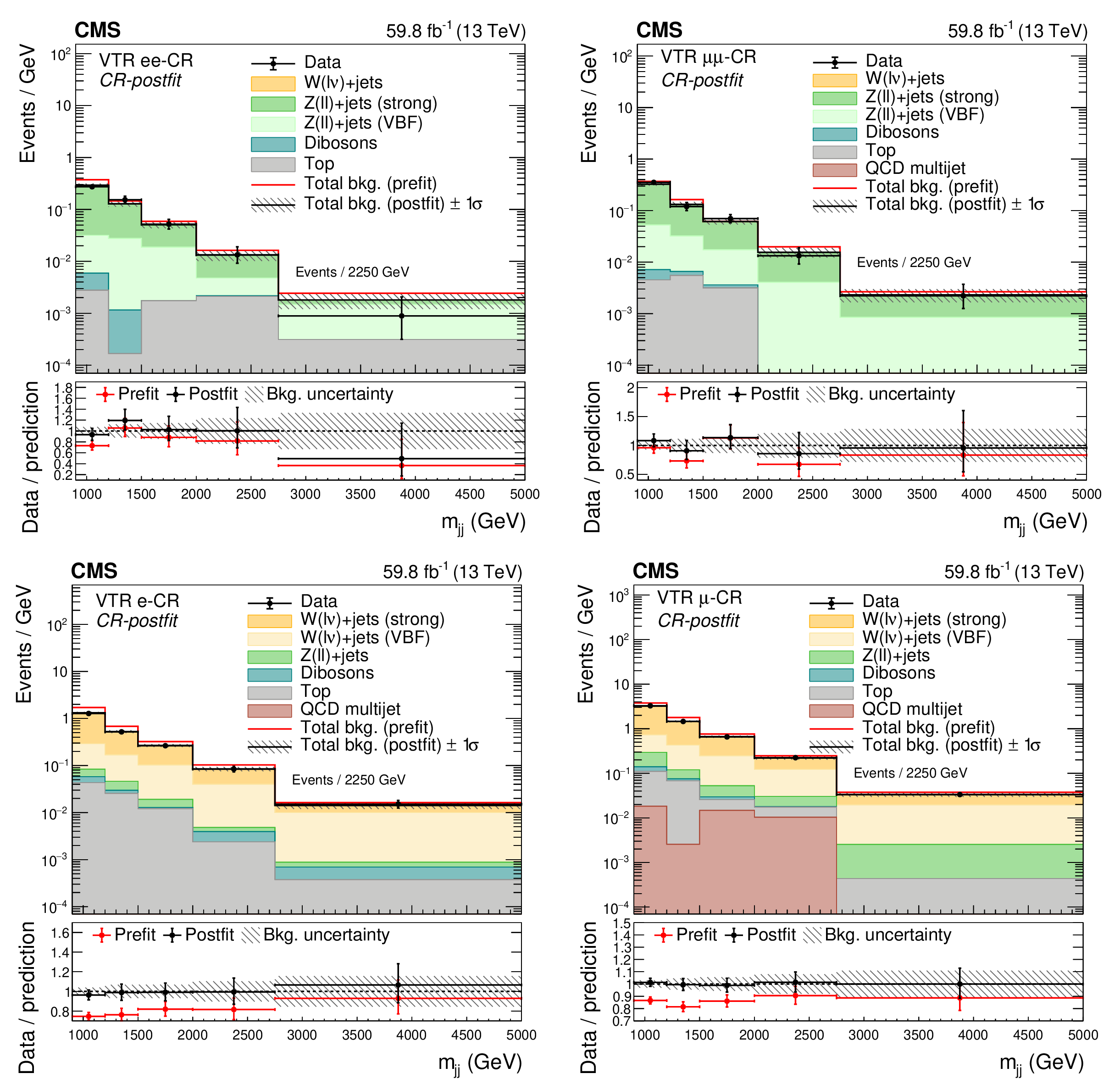
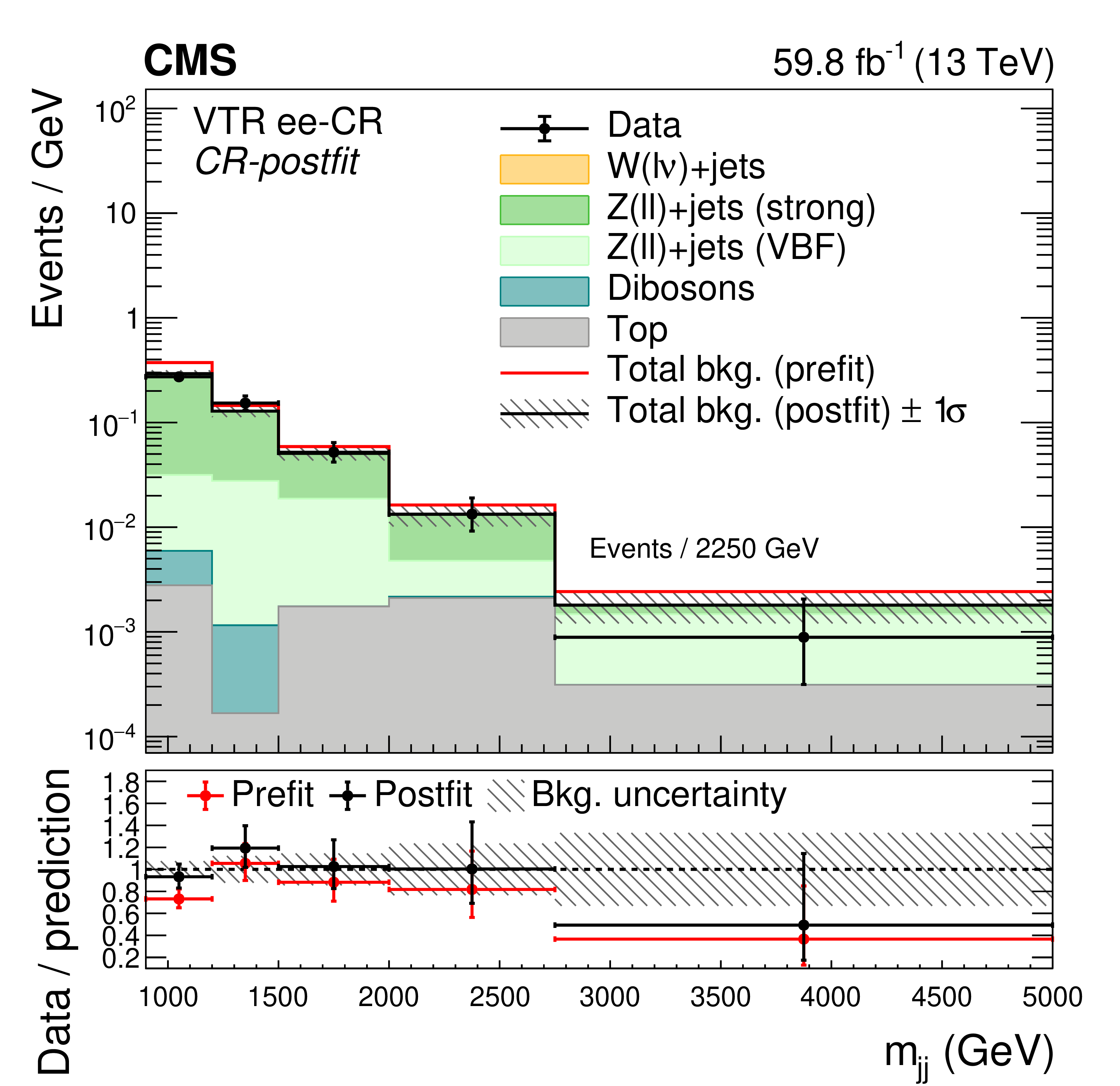
The postfit ${m_{\mathrm {jj}}}$ distributions in the dielectron (upper left), dimuon (upper right), single-electron (lower left), and single-muon (lower right) CRs for the VTR category, showing the summed 2017 and 2018 data samples and the SM background processes. The background contributions are estimated from the fit to the data described in the text (S+B fit). The total background estimated from a fit assuming $ {{\mathcal {B}(\mathrm{H} \to \text {inv})}} =$ 0 (B-only fit) is also shown. The yields from the 2017 and 2018 samples are summed and the correlations between their uncertainties are neglected. The last bin of each distribution integrates events above the bin threshold divided by the bin width. |

png pdf |
Figure 9-a:
The postfit ${m_{\mathrm {jj}}}$ distributions in the dielectron (upper left), dimuon (upper right), single-electron (lower left), and single-muon (lower right) CRs for the VTR category, showing the summed 2017 and 2018 data samples and the SM background processes. The background contributions are estimated from the fit to the data described in the text (S+B fit). The total background estimated from a fit assuming $ {{\mathcal {B}(\mathrm{H} \to \text {inv})}} =$ 0 (B-only fit) is also shown. The yields from the 2017 and 2018 samples are summed and the correlations between their uncertainties are neglected. The last bin of each distribution integrates events above the bin threshold divided by the bin width. |

png pdf |
Figure 9-b:
The postfit ${m_{\mathrm {jj}}}$ distributions in the dielectron (upper left), dimuon (upper right), single-electron (lower left), and single-muon (lower right) CRs for the VTR category, showing the summed 2017 and 2018 data samples and the SM background processes. The background contributions are estimated from the fit to the data described in the text (S+B fit). The total background estimated from a fit assuming $ {{\mathcal {B}(\mathrm{H} \to \text {inv})}} =$ 0 (B-only fit) is also shown. The yields from the 2017 and 2018 samples are summed and the correlations between their uncertainties are neglected. The last bin of each distribution integrates events above the bin threshold divided by the bin width. |

png pdf |
Figure 9-c:
The postfit ${m_{\mathrm {jj}}}$ distributions in the dielectron (upper left), dimuon (upper right), single-electron (lower left), and single-muon (lower right) CRs for the VTR category, showing the summed 2017 and 2018 data samples and the SM background processes. The background contributions are estimated from the fit to the data described in the text (S+B fit). The total background estimated from a fit assuming $ {{\mathcal {B}(\mathrm{H} \to \text {inv})}} =$ 0 (B-only fit) is also shown. The yields from the 2017 and 2018 samples are summed and the correlations between their uncertainties are neglected. The last bin of each distribution integrates events above the bin threshold divided by the bin width. |
png pdf |
Figure 9-d:
The postfit ${m_{\mathrm {jj}}}$ distributions in the dielectron (upper left), dimuon (upper right), single-electron (lower left), and single-muon (lower right) CRs for the VTR category, showing the summed 2017 and 2018 data samples and the SM background processes. The background contributions are estimated from the fit to the data described in the text (S+B fit). The total background estimated from a fit assuming $ {{\mathcal {B}(\mathrm{H} \to \text {inv})}} =$ 0 (B-only fit) is also shown. The yields from the 2017 and 2018 samples are summed and the correlations between their uncertainties are neglected. The last bin of each distribution integrates events above the bin threshold divided by the bin width. |
png pdf |
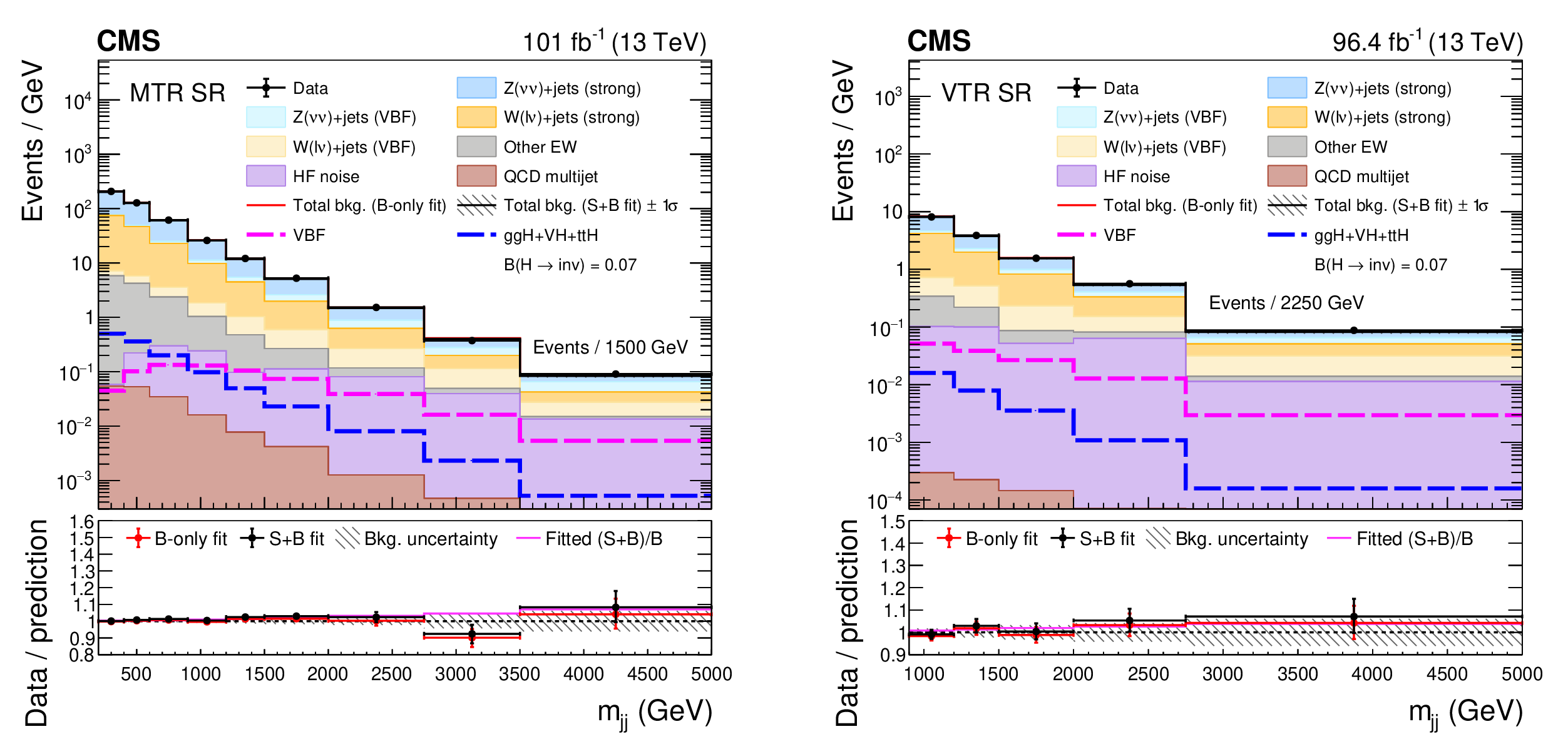
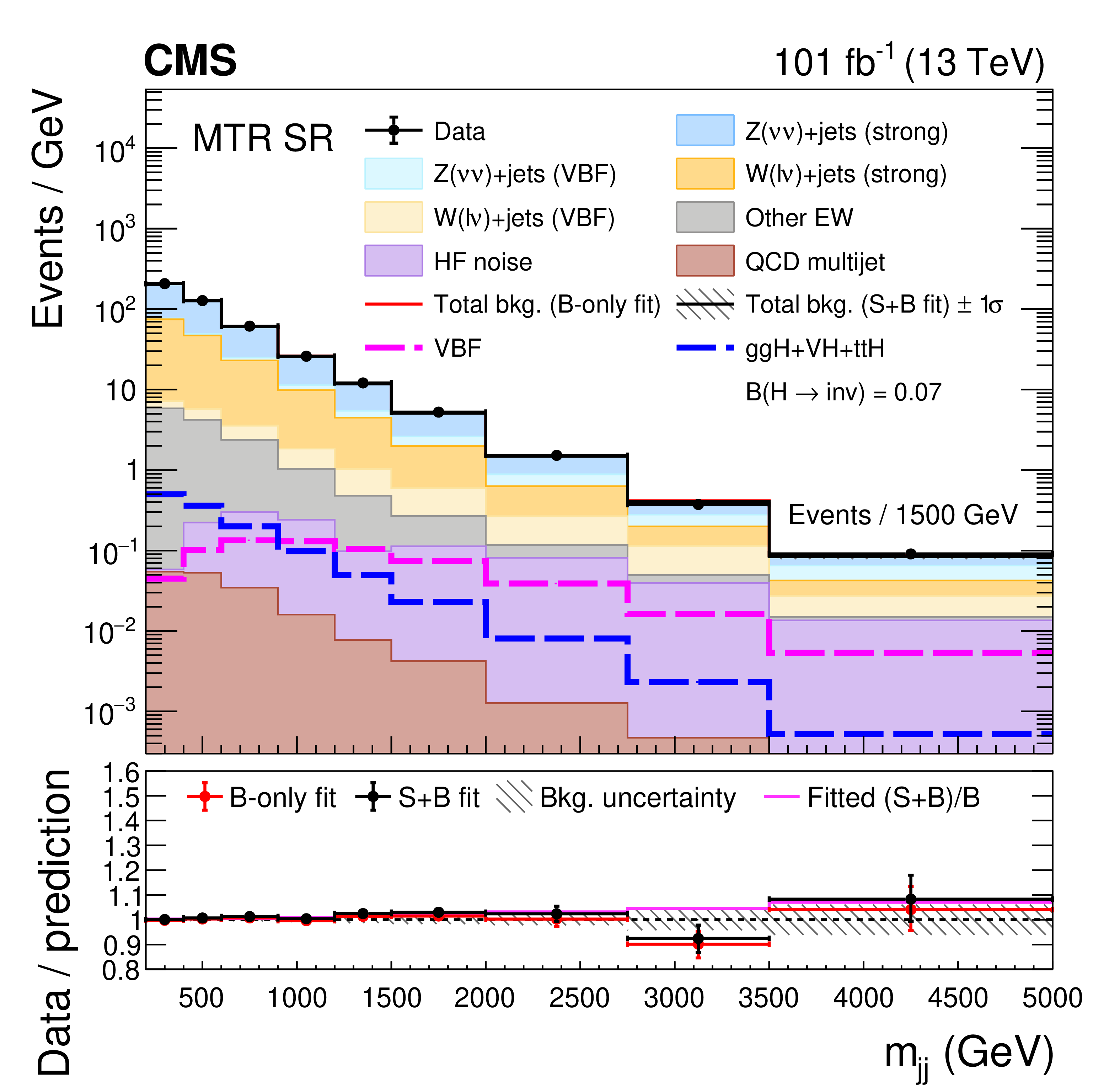
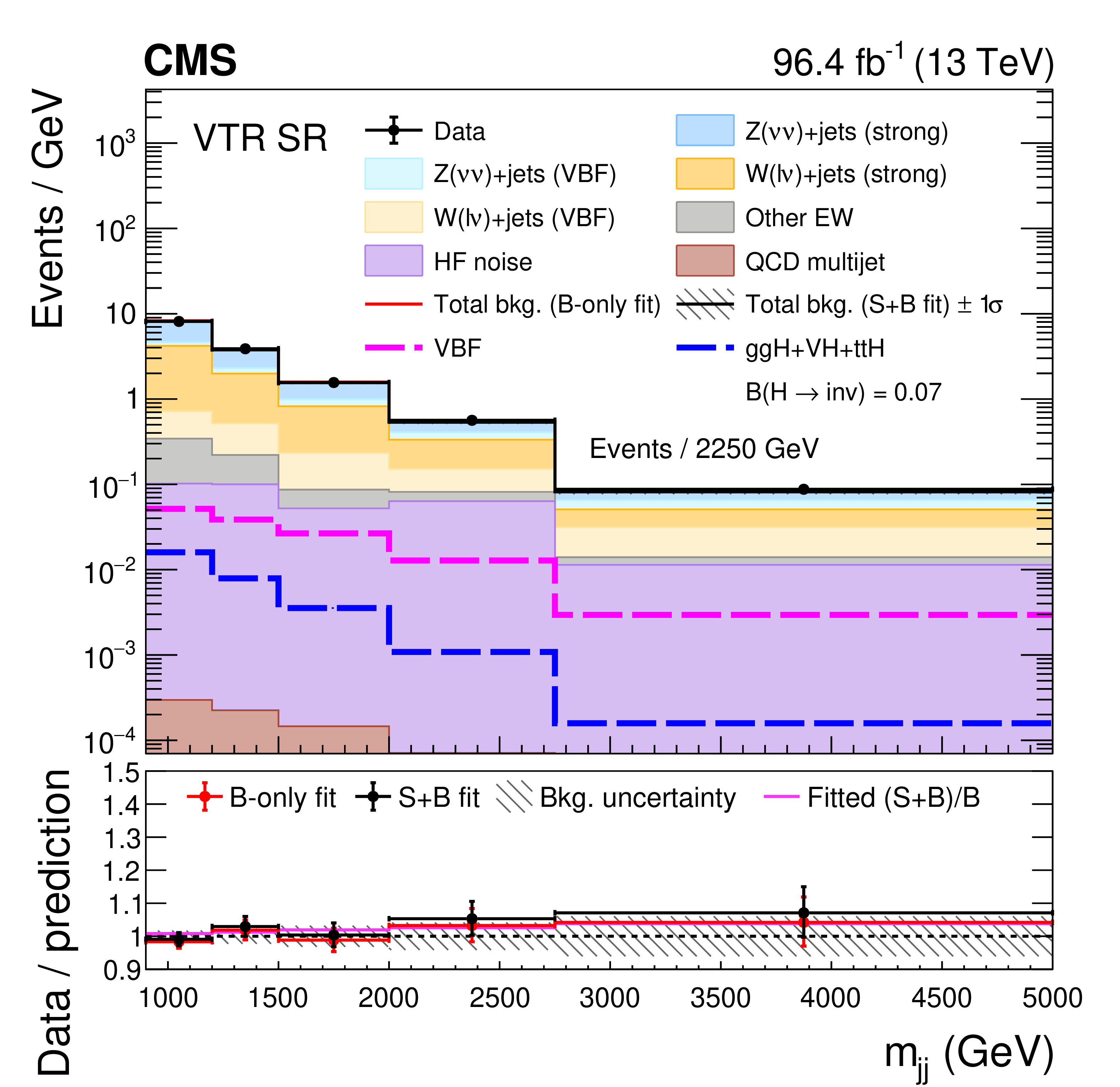
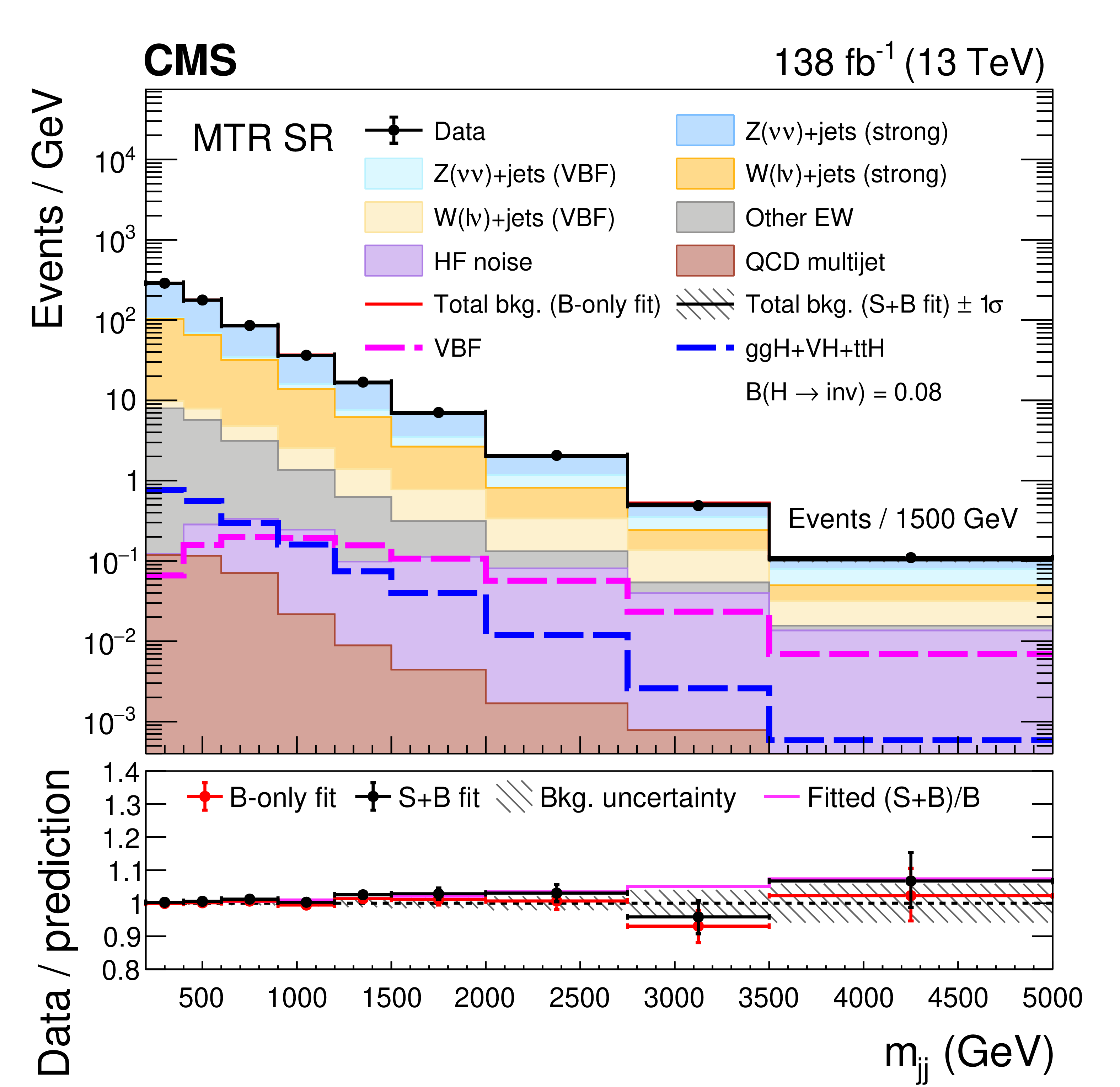
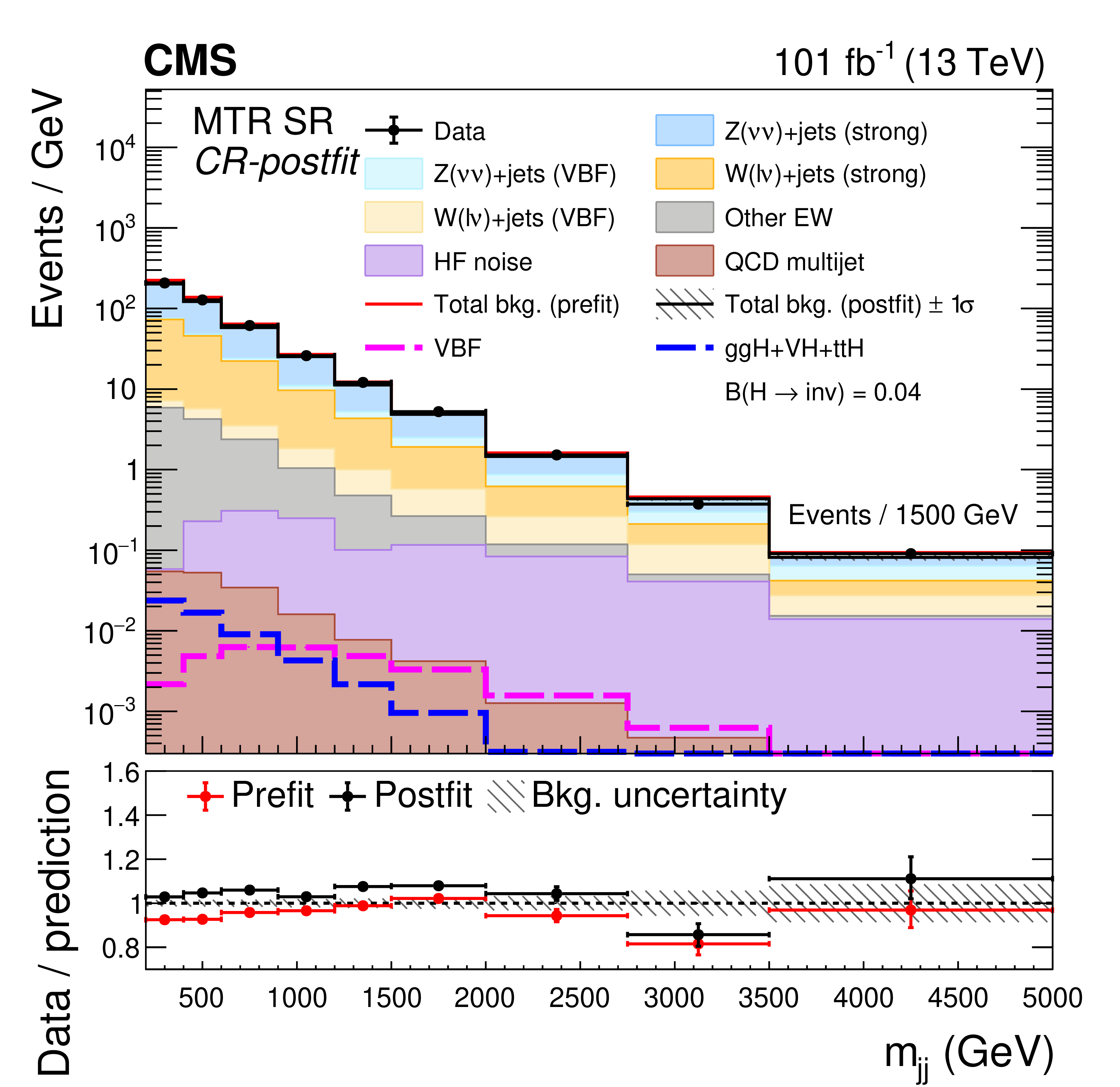
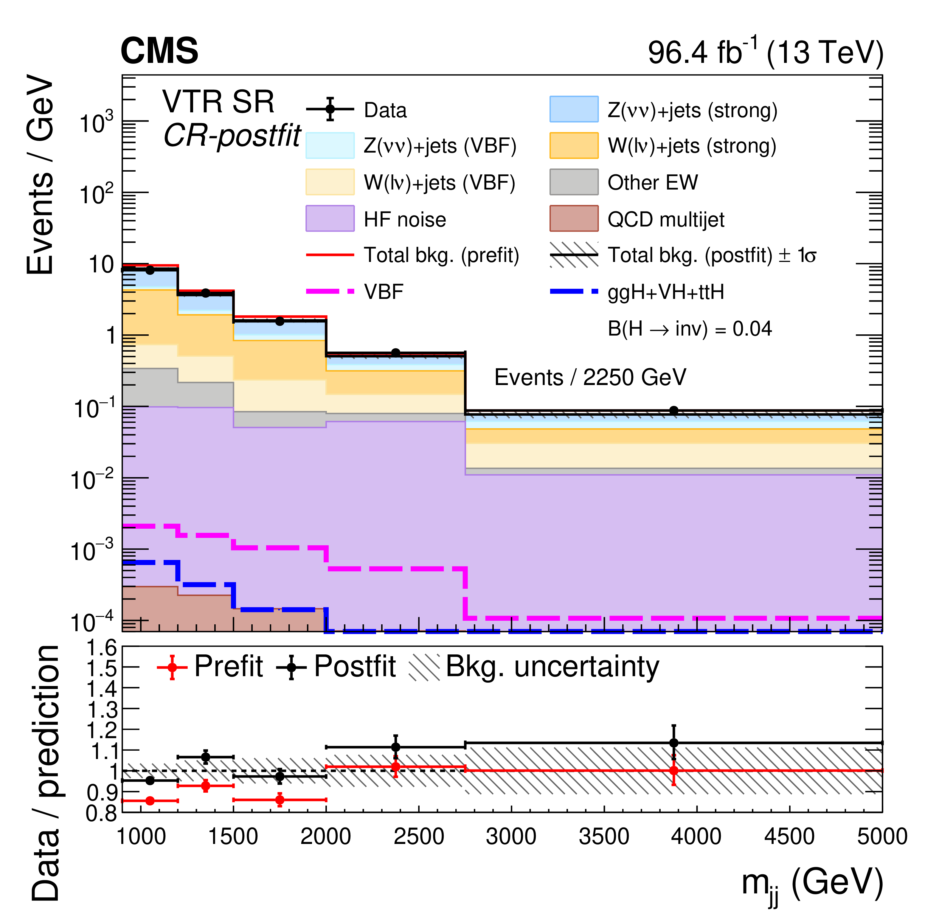
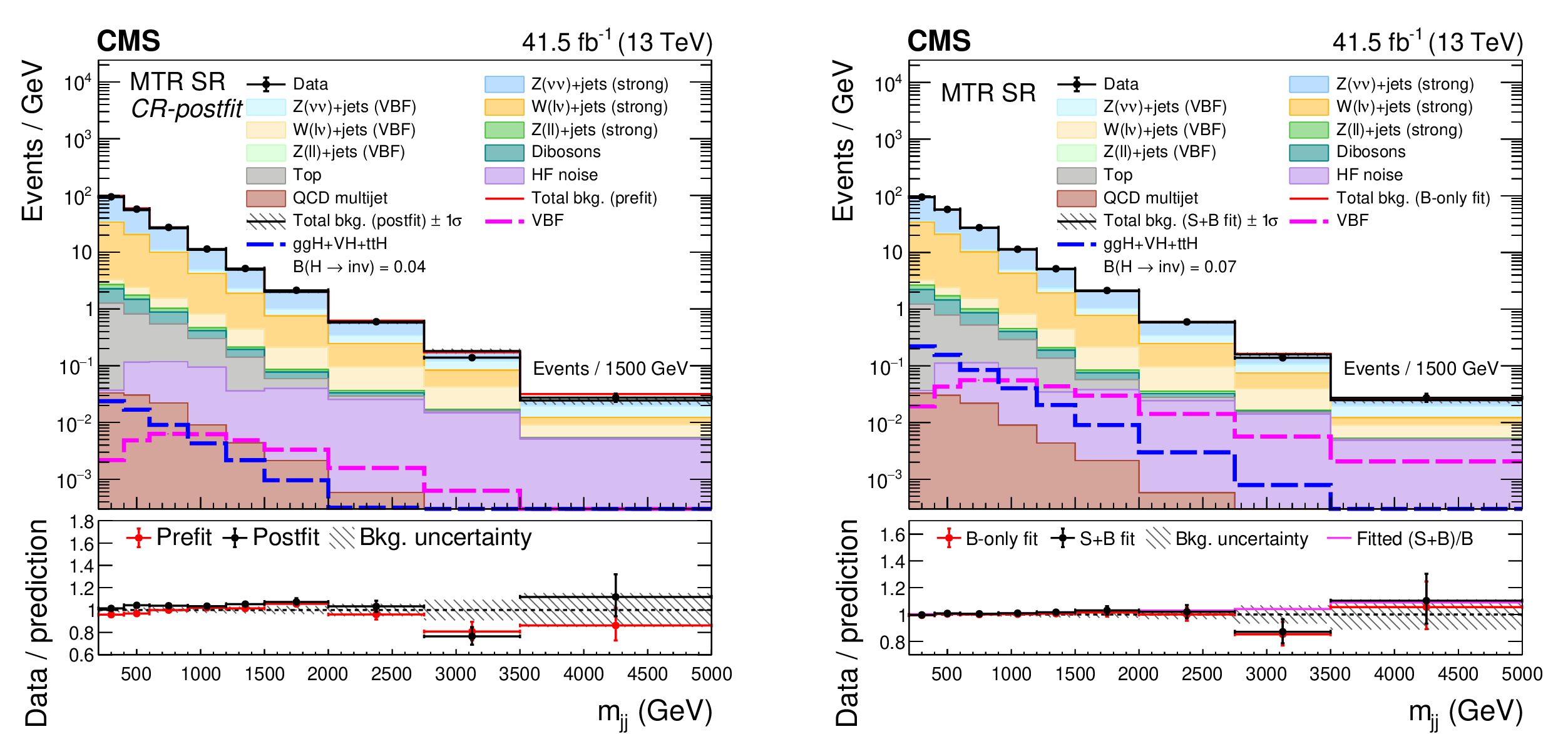
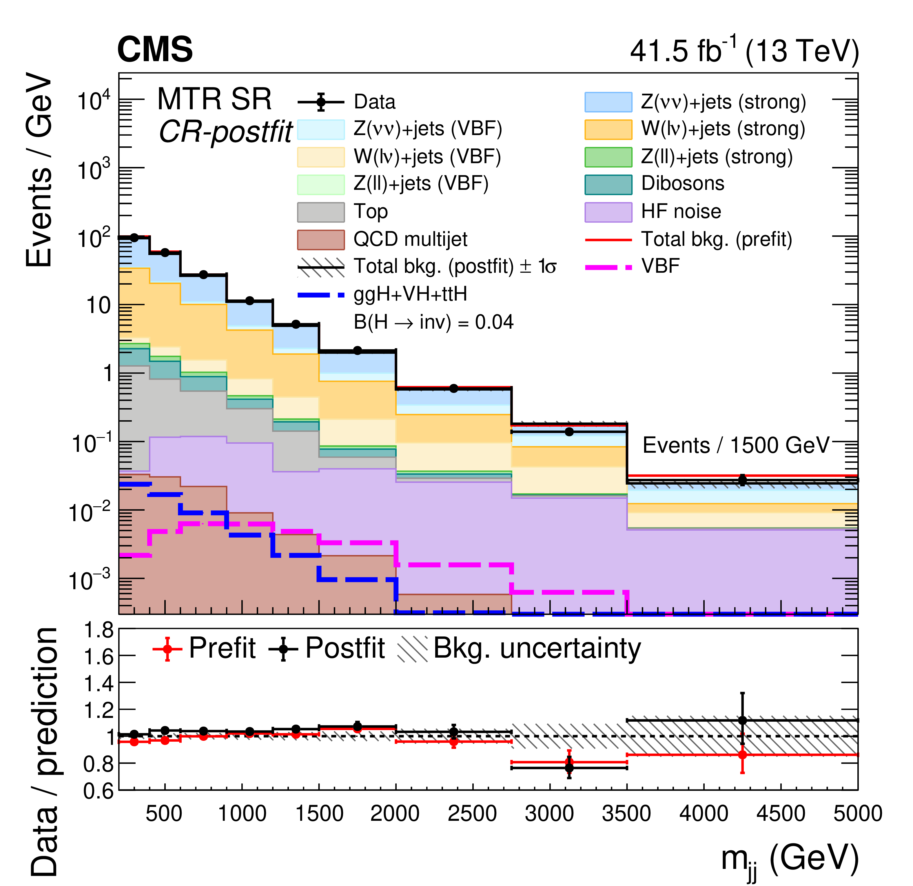
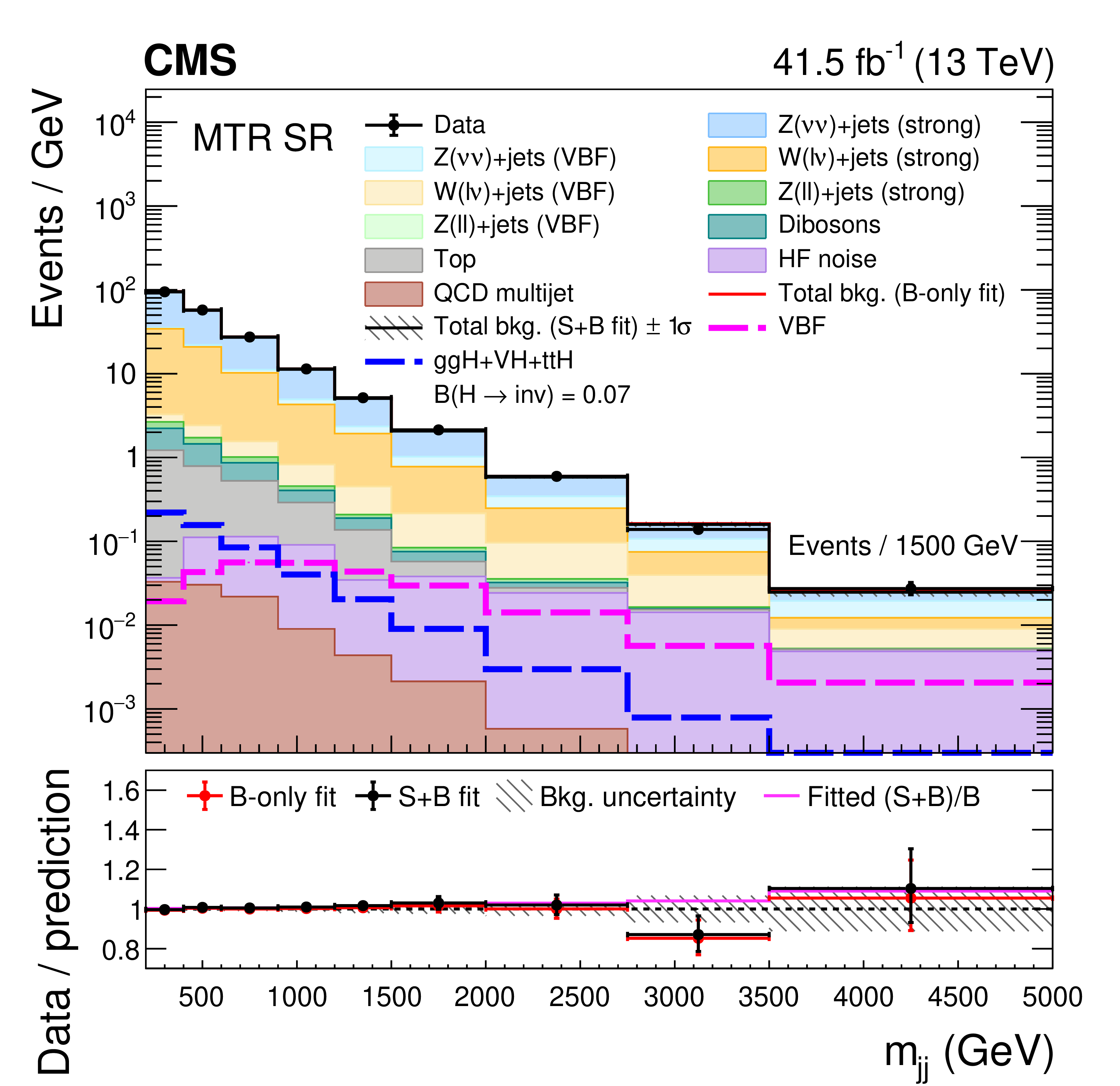
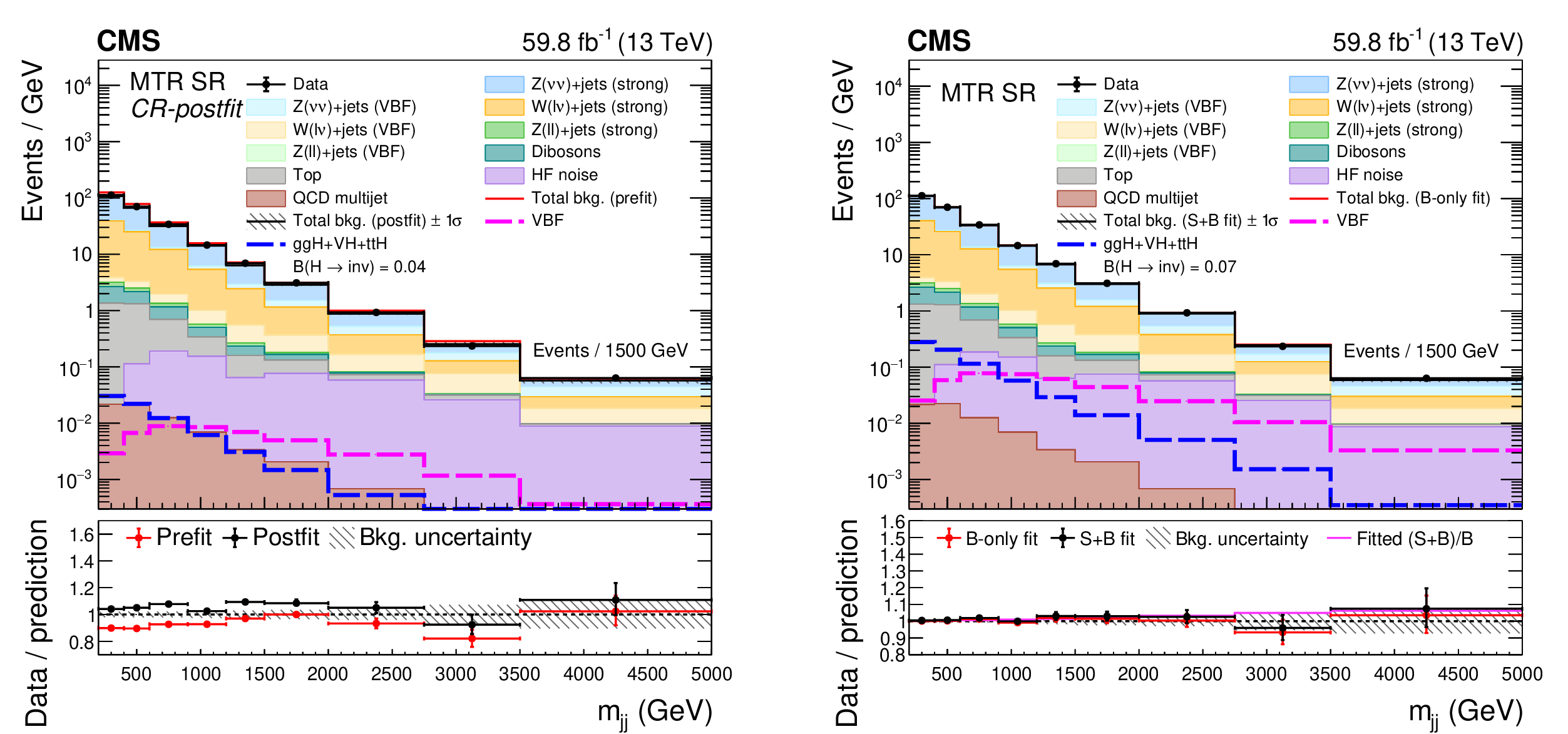
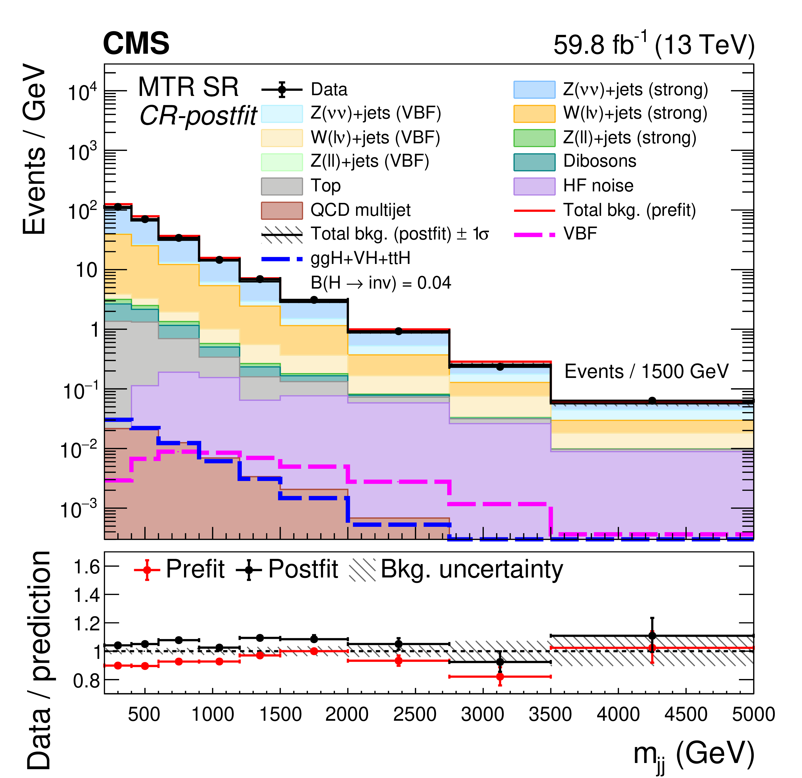
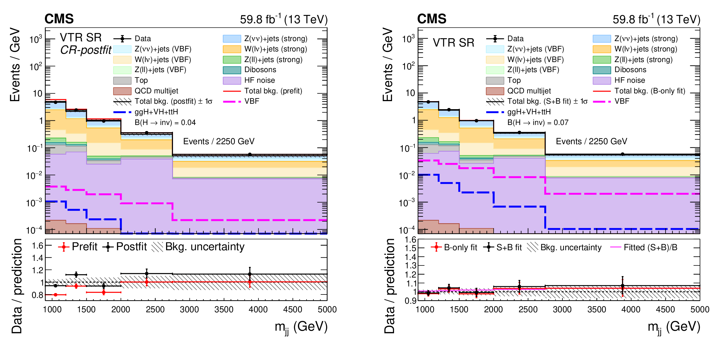
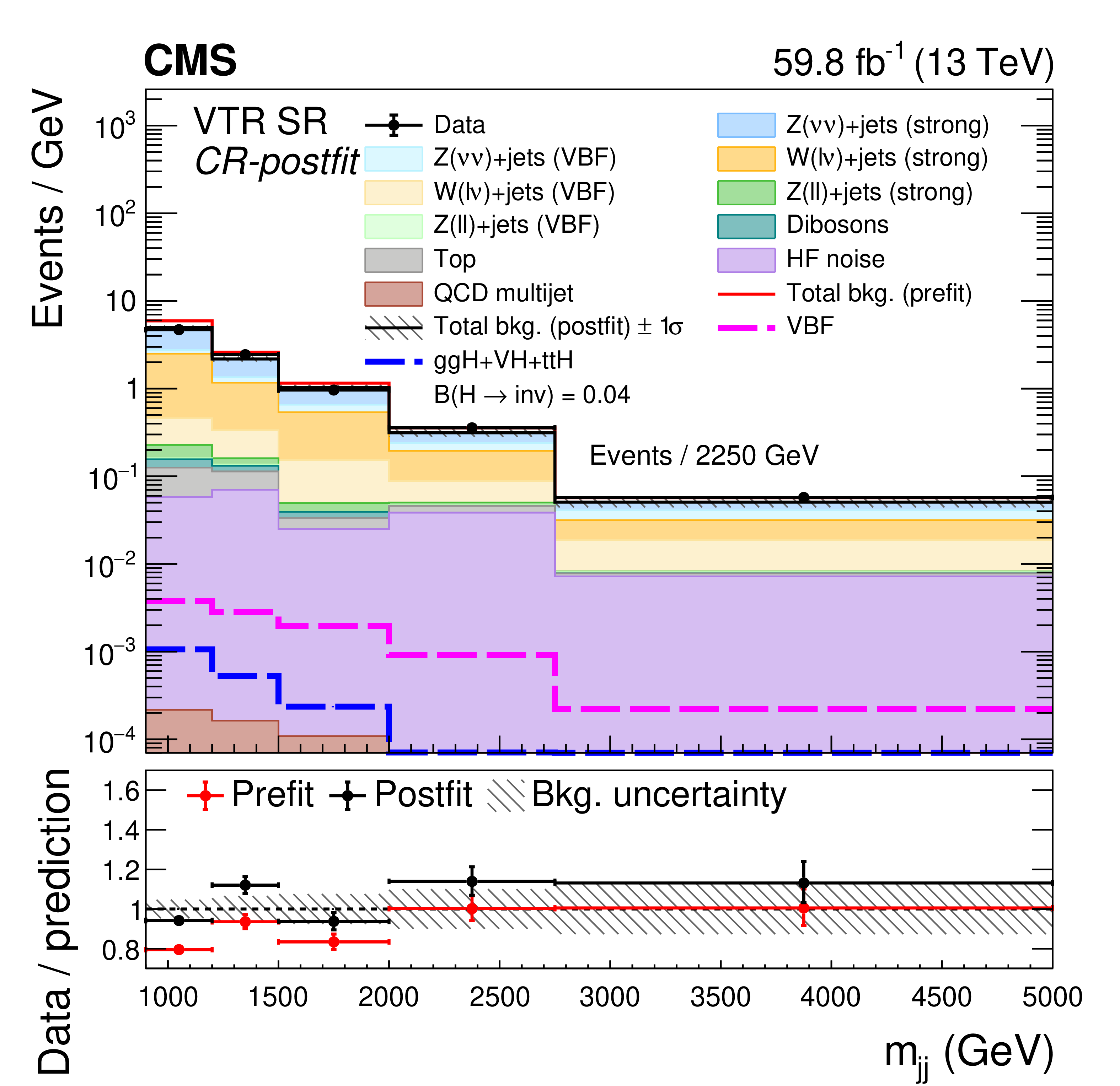
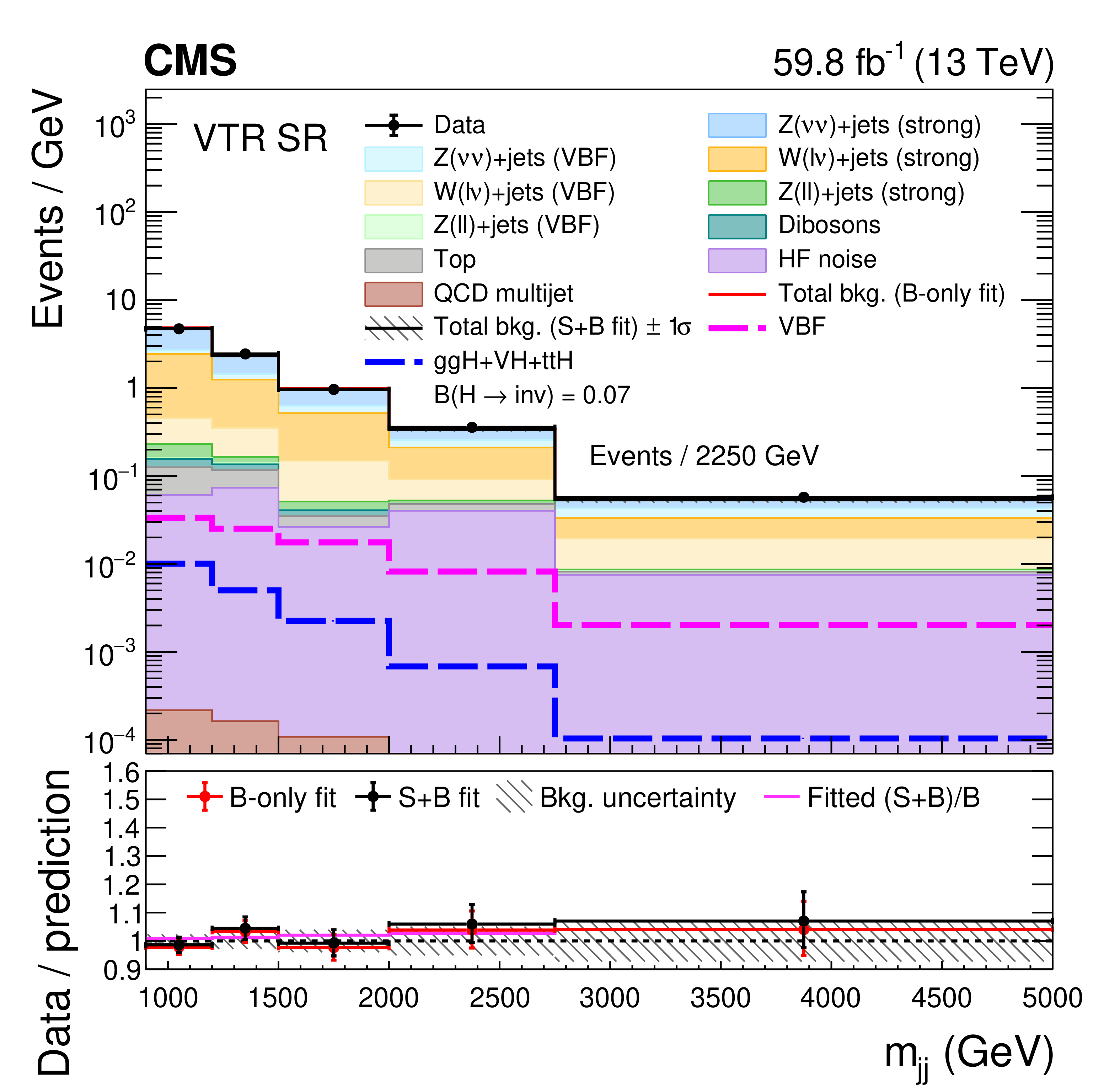
Figure 10:
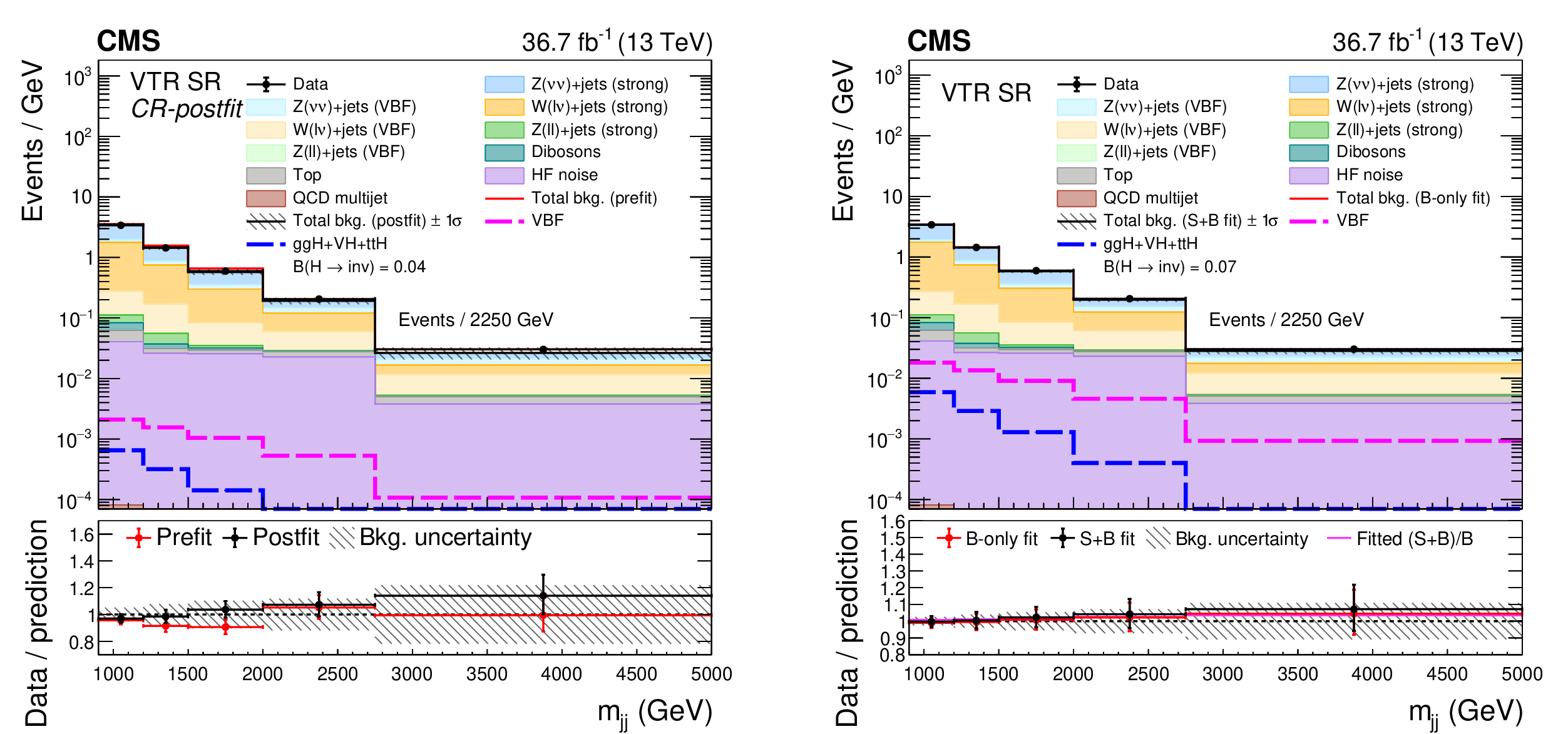
The observed ${m_{\mathrm {jj}}}$ distribution in the MTR (left) and VTR (right) SR compared with the postfit backgrounds, showing the summed 2017 and 2018 samples. The signal processes are scaled by the fitted value of ${{\mathcal {B}(\mathrm{H} \to \text {inv})}}$, shown in the legend. The background contributions are estimated from the fit to the data described in the text (S+B fit). The total background estimated from a fit assuming $ {{\mathcal {B}(\mathrm{H} \to \text {inv})}} =$ 0 (B-only fit) is also shown. The yields from the 2017 and 2018 samples are summed and the correlations between their uncertainties are neglected. The last bin of each distribution integrates events above the bin threshold divided by the bin width. |
png pdf |
Figure 10-a:
The observed ${m_{\mathrm {jj}}}$ distribution in the MTR (left) and VTR (right) SR compared with the postfit backgrounds, showing the summed 2017 and 2018 samples. The signal processes are scaled by the fitted value of ${{\mathcal {B}(\mathrm{H} \to \text {inv})}}$, shown in the legend. The background contributions are estimated from the fit to the data described in the text (S+B fit). The total background estimated from a fit assuming $ {{\mathcal {B}(\mathrm{H} \to \text {inv})}} =$ 0 (B-only fit) is also shown. The yields from the 2017 and 2018 samples are summed and the correlations between their uncertainties are neglected. The last bin of each distribution integrates events above the bin threshold divided by the bin width. |
png pdf |
Figure 10-b:
The observed ${m_{\mathrm {jj}}}$ distribution in the MTR (left) and VTR (right) SR compared with the postfit backgrounds, showing the summed 2017 and 2018 samples. The signal processes are scaled by the fitted value of ${{\mathcal {B}(\mathrm{H} \to \text {inv})}}$, shown in the legend. The background contributions are estimated from the fit to the data described in the text (S+B fit). The total background estimated from a fit assuming $ {{\mathcal {B}(\mathrm{H} \to \text {inv})}} =$ 0 (B-only fit) is also shown. The yields from the 2017 and 2018 samples are summed and the correlations between their uncertainties are neglected. The last bin of each distribution integrates events above the bin threshold divided by the bin width. |

png pdf |
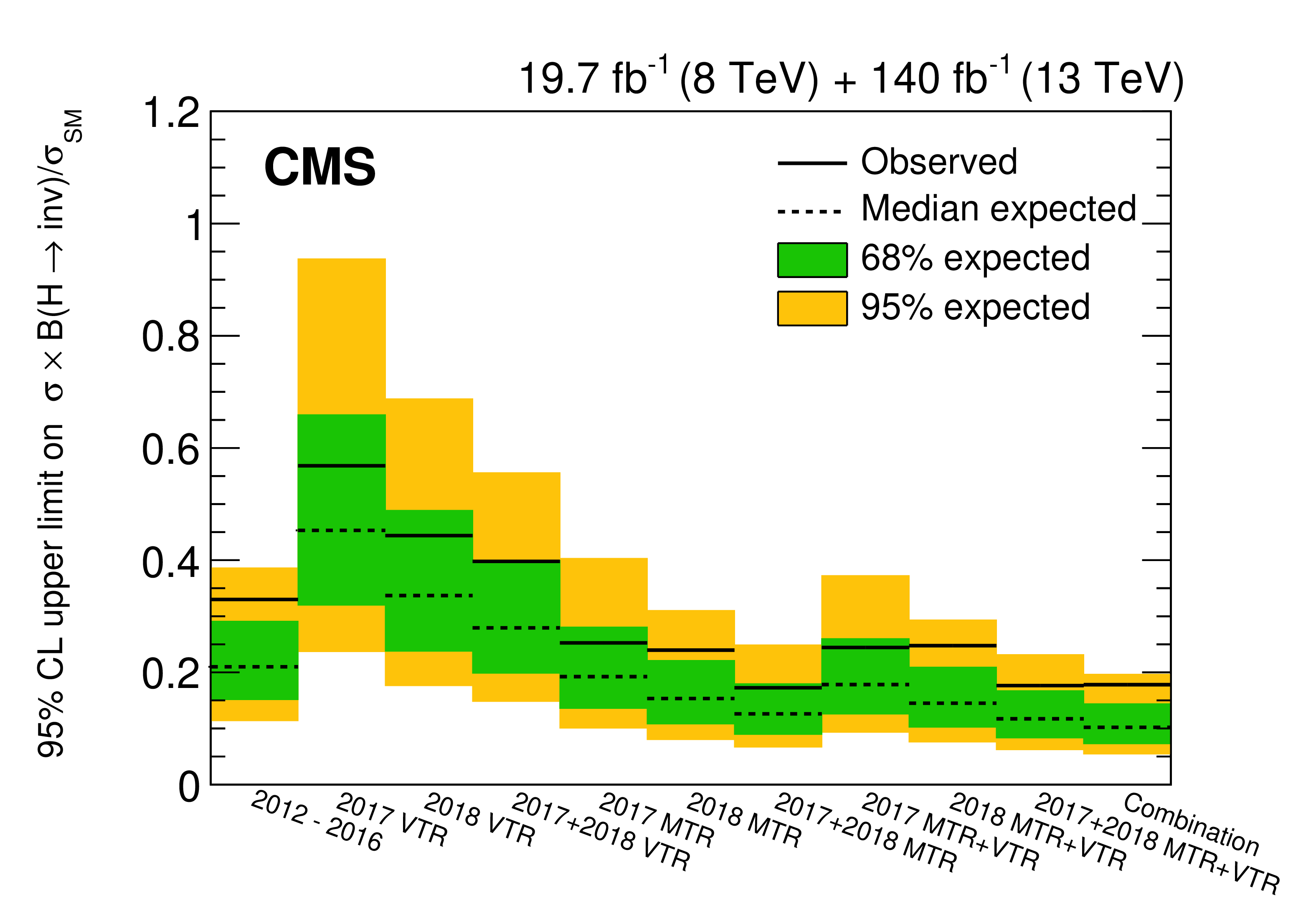
Figure 11:
Observed and expected 95% CL upper limits on ${(\sigma _{\mathrm{H}}/\sigma _{\mathrm{H}}^{\mathrm {SM}}) {{\mathcal {B}(\mathrm{H} \to \text {inv})}}}$ for all data-taking years considered, as well as their combination, assuming an SM Higgs boson with a mass of 125.38 GeV. |
png pdf |
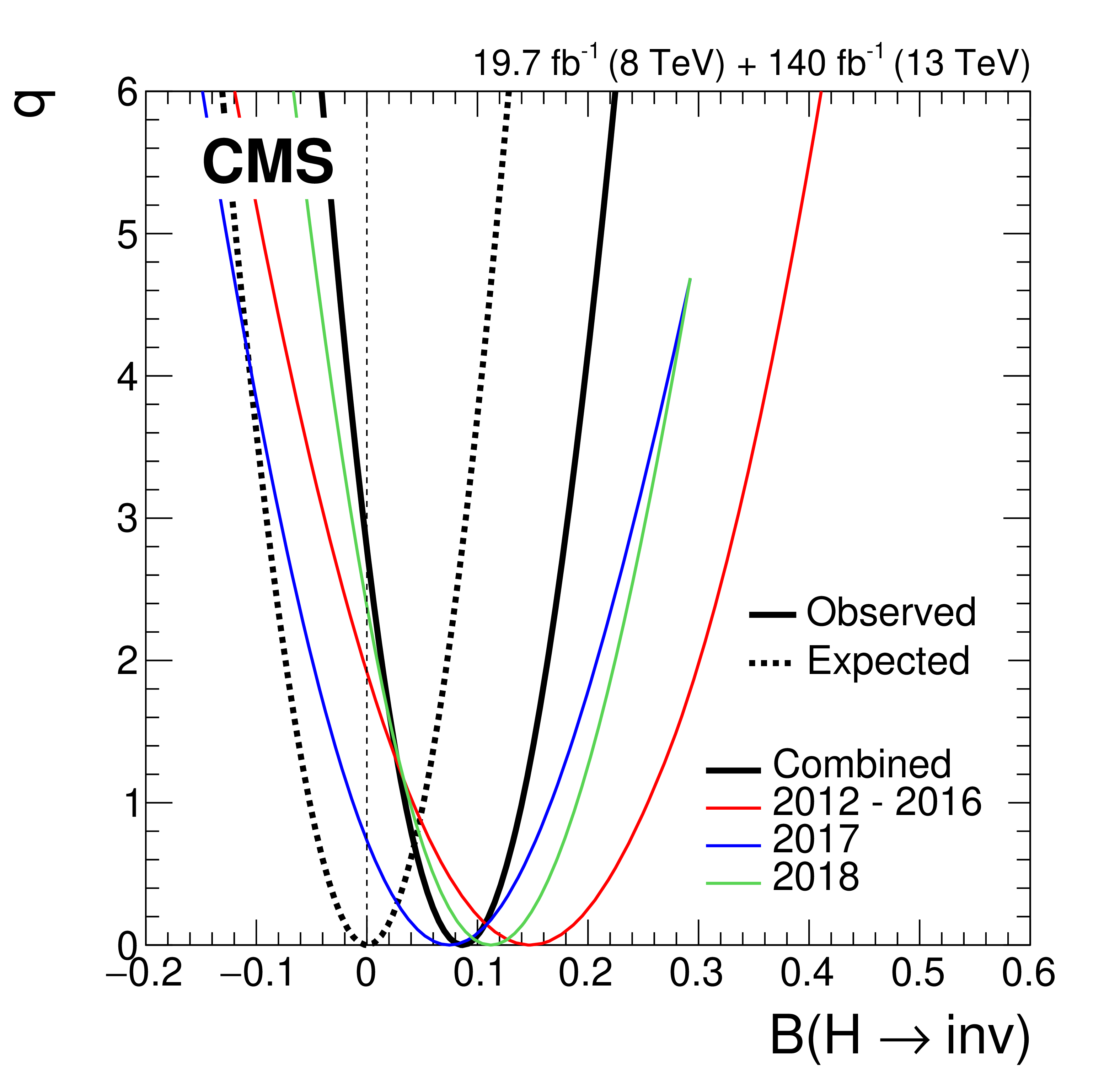
Figure 12:
Profile likelihood ratios, as functions of ${{\mathcal {B}(\mathrm{H} \to \text {inv})}}$. The observed likelihood scans are reported for the full combination of 2012-2018 data, as well as for the individual years. The expected results for the combination are obtained using an Asimov data set [71] with $ {{\mathcal {B}(\mathrm{H} \to \text {inv})}} =$ 0. |
png pdf |
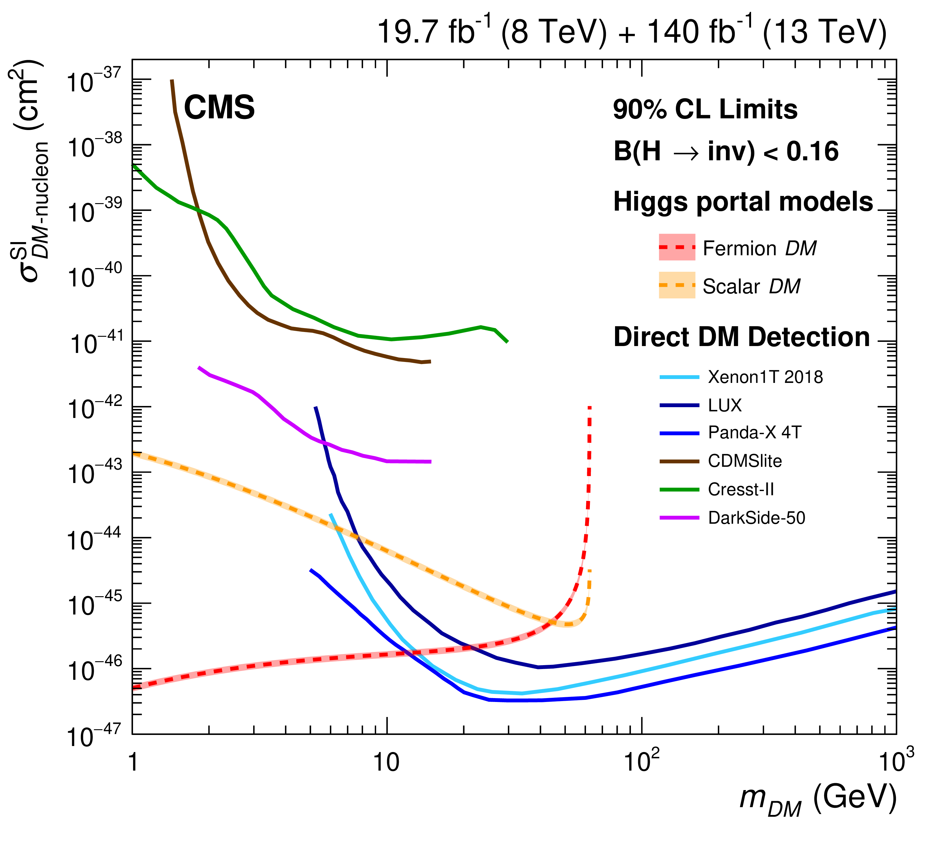
Figure 13:
The 90% CL upper limits on the spin-independent DM-nucleon scattering cross section in Higgs-portal models, assuming a scalar (dashed orange) or fermion (dashed red) DM candidate. Limits are computed as functions of $m_{\mathrm {DM}}$ and are compared to those from the XENON1T [76], CRESST-II [77], CDMSlite [78], LUX [79], Panda-X 4T [80], and DarkSide-50 [81] experiments, which are shown as solid lines. |
png pdf |
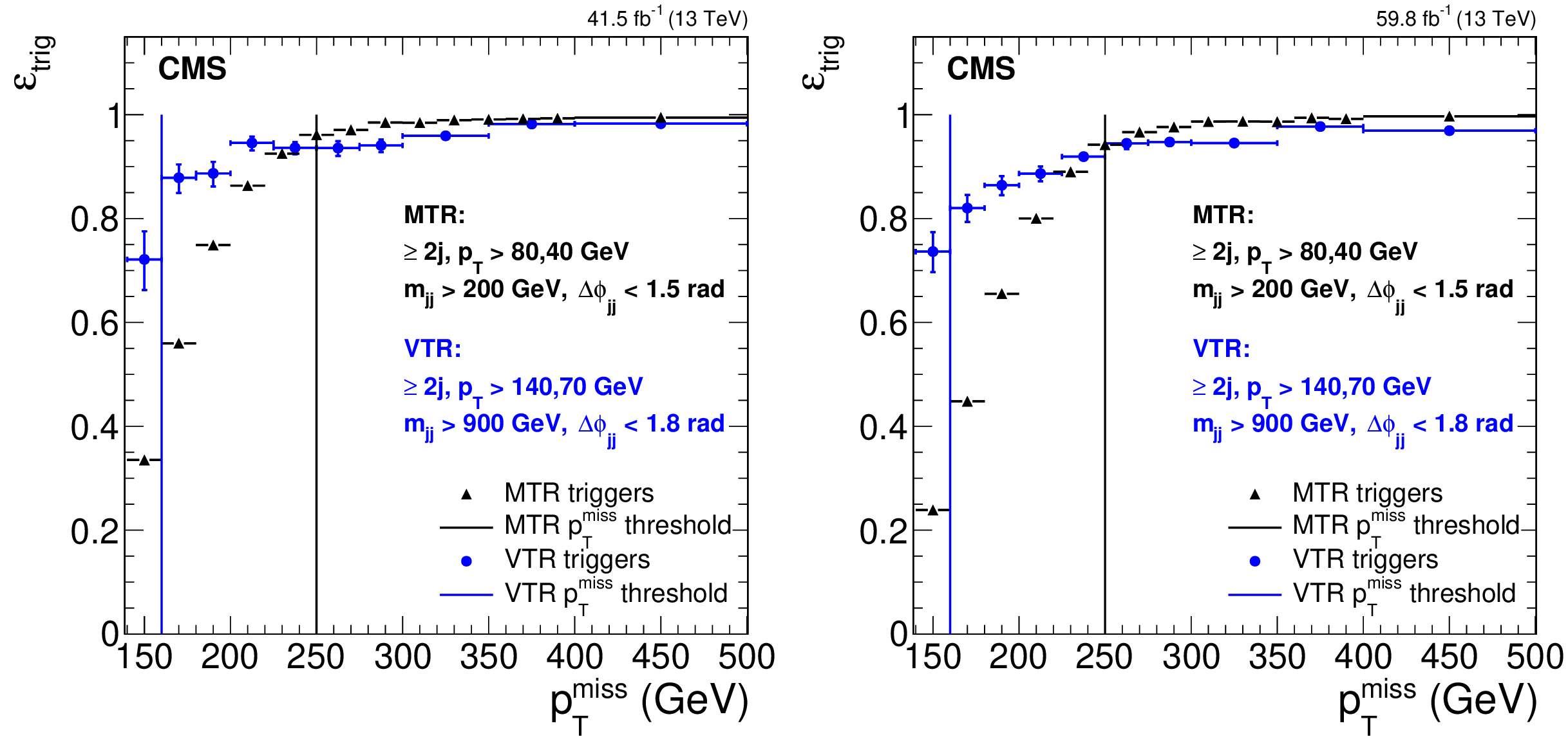
Figure A1:
Trigger efficiency measured in data for the 2017 and 2018 samples, comparing the two sets of triggers used in the analysis (${{p_{\mathrm {T}}} ^\text {miss}} $-based in MTR, VBF jet-based in VTR). The lower thresholds are indicated by the vertical lines. The lower threshold of the MTR category also corresponds to the upper threshold applied in the VTR category. |
png pdf |
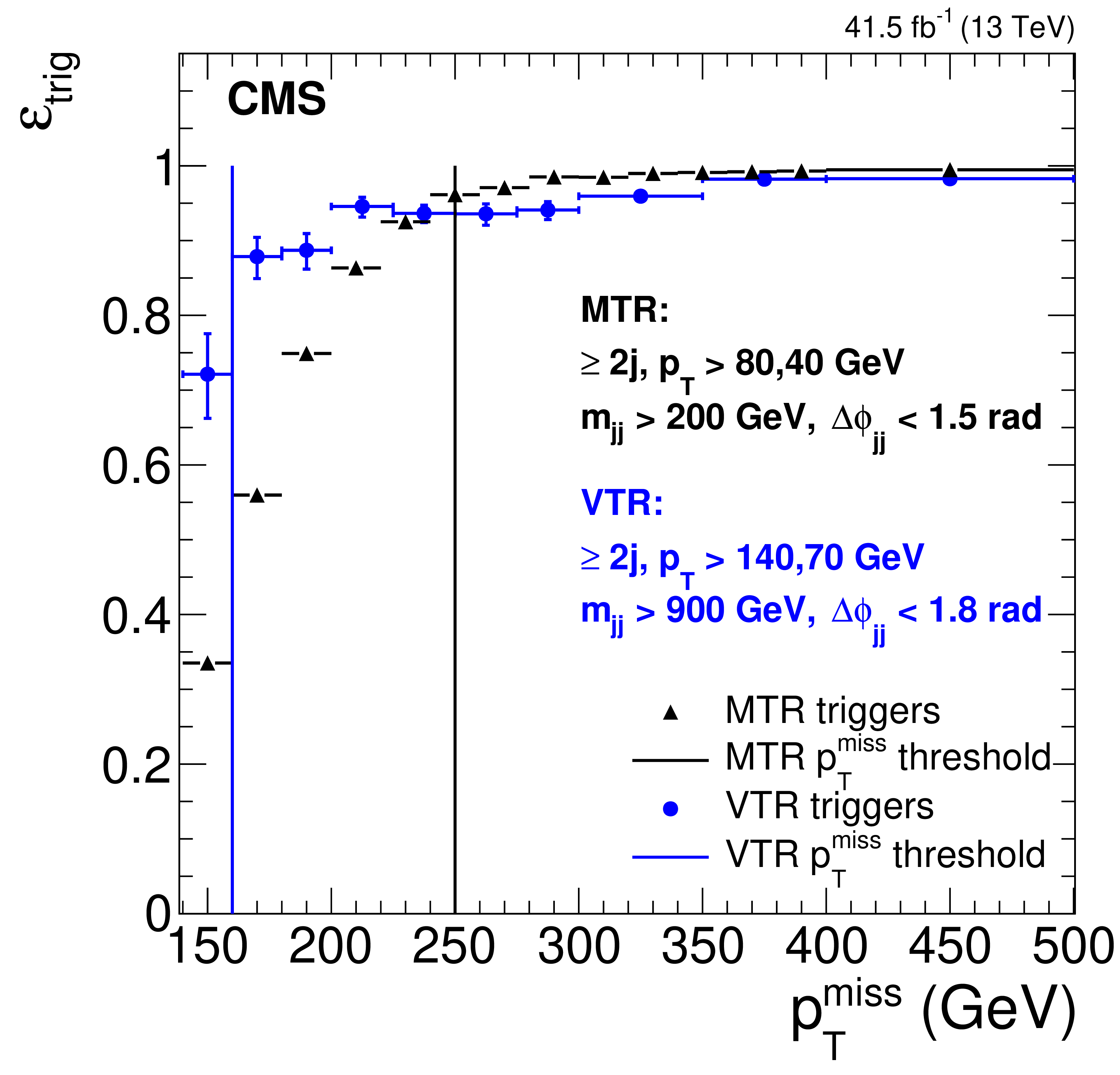
Figure A1-a:
Trigger efficiency measured in data for the 2017 and 2018 samples, comparing the two sets of triggers used in the analysis (${{p_{\mathrm {T}}} ^\text {miss}} $-based in MTR, VBF jet-based in VTR). The lower thresholds are indicated by the vertical lines. The lower threshold of the MTR category also corresponds to the upper threshold applied in the VTR category. |
png pdf |
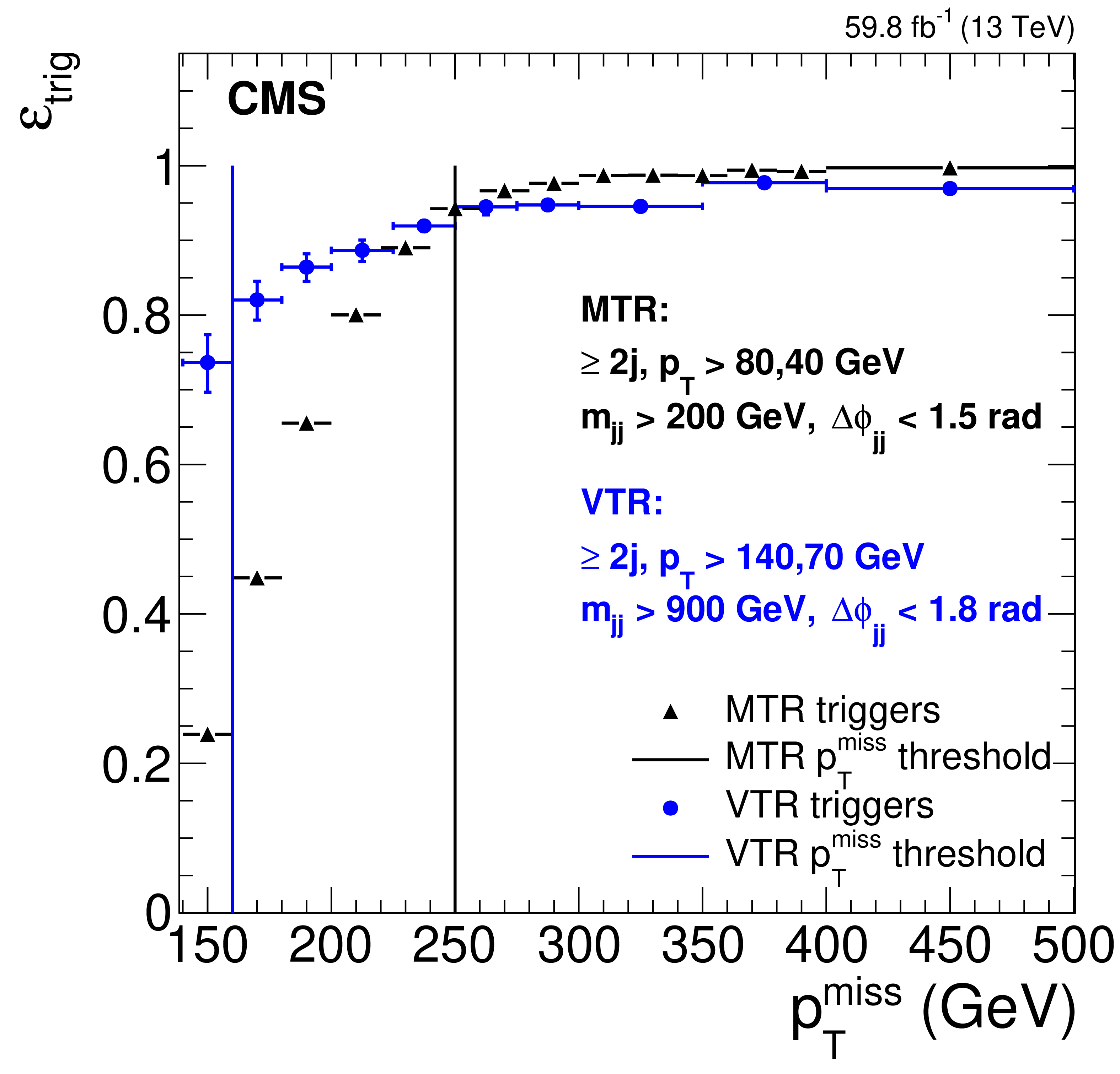
Figure A1-b:
Trigger efficiency measured in data for the 2017 and 2018 samples, comparing the two sets of triggers used in the analysis (${{p_{\mathrm {T}}} ^\text {miss}} $-based in MTR, VBF jet-based in VTR). The lower thresholds are indicated by the vertical lines. The lower threshold of the MTR category also corresponds to the upper threshold applied in the VTR category. |
png pdf |
Figure A2:
Observed and expected 95% CL upper limits on ${(\sigma _{\mathrm{H}}/\sigma _{\mathrm{H}}^{\mathrm {SM}}) {{\mathcal {B}(\mathrm{H} \to \text {inv})}}}$ for both individual categories and all data-taking years, as well as their combination, assuming an SM Higgs boson with a mass of 125.38 GeV. |
png pdf |
Figure A3:
The observed ${m_{\mathrm {jj}}}$ distribution in the MTR SR compared to the postfit backgrounds, with the 2016, 2017, and 2018 samples. The signal processes are scaled by the fitted value of ${{\mathcal {B}(\mathrm{H} \to \text {inv})}}$, shown in the legend. The background contributions are estimated from the fit to the data described in the text (S+B fit) and the total background estimated from a fit assuming $ {{\mathcal {B}(\mathrm{H} \to \text {inv})}} =$ 0 (B-only fit) is also shown. The yields from the 2016, 2017, and 2018 samples are summed and the correlations between their uncertainties are neglected. The last bin of each distribution integrates events above the bin threshold divided by the bin width. |
png pdf |
Figure A4:
The ${m_{\mathrm {jj}}}$ distributions (prefit and CR-postfit) in the dielectron (upper left), dimuon (upper right), single-electron (lower left), and single-muon (lower right) CR for the MTR category, with the 2017 and 2018 samples. The yields from the 2017 and 2018 samples are summed and the correlations between their uncertainties are neglected. |
png pdf |
Figure A4-a:
The ${m_{\mathrm {jj}}}$ distributions (prefit and CR-postfit) in the dielectron (upper left), dimuon (upper right), single-electron (lower left), and single-muon (lower right) CR for the MTR category, with the 2017 and 2018 samples. The yields from the 2017 and 2018 samples are summed and the correlations between their uncertainties are neglected. |

png pdf |
Figure A4-b:
The ${m_{\mathrm {jj}}}$ distributions (prefit and CR-postfit) in the dielectron (upper left), dimuon (upper right), single-electron (lower left), and single-muon (lower right) CR for the MTR category, with the 2017 and 2018 samples. The yields from the 2017 and 2018 samples are summed and the correlations between their uncertainties are neglected. |
png pdf |
Figure A4-c:
The ${m_{\mathrm {jj}}}$ distributions (prefit and CR-postfit) in the dielectron (upper left), dimuon (upper right), single-electron (lower left), and single-muon (lower right) CR for the MTR category, with the 2017 and 2018 samples. The yields from the 2017 and 2018 samples are summed and the correlations between their uncertainties are neglected. |
png pdf |
Figure A4-d:
The ${m_{\mathrm {jj}}}$ distributions (prefit and CR-postfit) in the dielectron (upper left), dimuon (upper right), single-electron (lower left), and single-muon (lower right) CR for the MTR category, with the 2017 and 2018 samples. The yields from the 2017 and 2018 samples are summed and the correlations between their uncertainties are neglected. |
png pdf |
Figure A5:
The ${m_{\mathrm {jj}}}$ distributions (prefit and CR-postfit) in the photon CR for the MTR category, with the 2017 and 2018 samples. The yields from the 2017 and 2018 samples are summed and the correlations between their uncertainties are neglected. |
png pdf |
Figure A6:
The ${m_{\mathrm {jj}}}$ distributions (prefit and CR-postfit) in the dielectron (upper left), dimuon (upper right), single-electron (lower left), and single-muon (lower right) CR for the VTR category, with the 2017 and 2018 samples. The yields from the 2017 and 2018 samples are summed and the correlations between their uncertainties are neglected. |
png pdf |
Figure A6-a:
The ${m_{\mathrm {jj}}}$ distributions (prefit and CR-postfit) in the dielectron (upper left), dimuon (upper right), single-electron (lower left), and single-muon (lower right) CR for the VTR category, with the 2017 and 2018 samples. The yields from the 2017 and 2018 samples are summed and the correlations between their uncertainties are neglected. |
png pdf |
Figure A6-b:
The ${m_{\mathrm {jj}}}$ distributions (prefit and CR-postfit) in the dielectron (upper left), dimuon (upper right), single-electron (lower left), and single-muon (lower right) CR for the VTR category, with the 2017 and 2018 samples. The yields from the 2017 and 2018 samples are summed and the correlations between their uncertainties are neglected. |

png pdf |
Figure A6-c:
The ${m_{\mathrm {jj}}}$ distributions (prefit and CR-postfit) in the dielectron (upper left), dimuon (upper right), single-electron (lower left), and single-muon (lower right) CR for the VTR category, with the 2017 and 2018 samples. The yields from the 2017 and 2018 samples are summed and the correlations between their uncertainties are neglected. |
png pdf |
Figure A6-d:
The ${m_{\mathrm {jj}}}$ distributions (prefit and CR-postfit) in the dielectron (upper left), dimuon (upper right), single-electron (lower left), and single-muon (lower right) CR for the VTR category, with the 2017 and 2018 samples. The yields from the 2017 and 2018 samples are summed and the correlations between their uncertainties are neglected. |

png pdf |
Figure A7:
The observed ${m_{\mathrm {jj}}}$ distribution in the MTR (left) and VTR (right) SRs compared to the CR-postfit backgrounds, with the 2017 and 2018 samples. The yields from the 2017 and 2018 samples are summed and the correlations between their uncertainties are neglected. The signal processes are scaled by the fitted value of ${{\mathcal {B}(\mathrm{H} \to \text {inv})}}$, shown in the legend. |
png pdf |
Figure A7-a:
The observed ${m_{\mathrm {jj}}}$ distribution in the MTR (left) and VTR (right) SRs compared to the CR-postfit backgrounds, with the 2017 and 2018 samples. The yields from the 2017 and 2018 samples are summed and the correlations between their uncertainties are neglected. The signal processes are scaled by the fitted value of ${{\mathcal {B}(\mathrm{H} \to \text {inv})}}$, shown in the legend. |
png pdf |
Figure A7-b:
The observed ${m_{\mathrm {jj}}}$ distribution in the MTR (left) and VTR (right) SRs compared to the CR-postfit backgrounds, with the 2017 and 2018 samples. The yields from the 2017 and 2018 samples are summed and the correlations between their uncertainties are neglected. The signal processes are scaled by the fitted value of ${{\mathcal {B}(\mathrm{H} \to \text {inv})}}$, shown in the legend. |
png pdf |
Figure A8:
The ${m_{\mathrm {jj}}}$ distributions (prefit and CR-postfit) in the dielectron (upper left), dimuon (upper right), single-electron (lower left), and single-muon (lower right) CR for the MTR category, with the 2017 sample. |
png pdf |
Figure A8-a:
The ${m_{\mathrm {jj}}}$ distributions (prefit and CR-postfit) in the dielectron (upper left), dimuon (upper right), single-electron (lower left), and single-muon (lower right) CR for the MTR category, with the 2017 sample. |
png pdf |
Figure A8-b:
The ${m_{\mathrm {jj}}}$ distributions (prefit and CR-postfit) in the dielectron (upper left), dimuon (upper right), single-electron (lower left), and single-muon (lower right) CR for the MTR category, with the 2017 sample. |

png pdf |
Figure A8-c:
The ${m_{\mathrm {jj}}}$ distributions (prefit and CR-postfit) in the dielectron (upper left), dimuon (upper right), single-electron (lower left), and single-muon (lower right) CR for the MTR category, with the 2017 sample. |
png pdf |
Figure A8-d:
The ${m_{\mathrm {jj}}}$ distributions (prefit and CR-postfit) in the dielectron (upper left), dimuon (upper right), single-electron (lower left), and single-muon (lower right) CR for the MTR category, with the 2017 sample. |
png pdf |
Figure A9:
The ${m_{\mathrm {jj}}}$ postfit distributions in the dielectron (upper left), dimuon (upper right), single-electron (lower left), and single-muon (lower right) CR for the MTR category, with the 2017 sample. The background contributions are estimated from a fit to data in the SR and CRs allowing for the signal contribution to vary (S+B fit) and the total background estimated from a fit assuming $ {{\mathcal {B}(\mathrm{H} \to \text {inv})}} =$ 0 (B-only fit) is also shown. |

png pdf |
Figure A9-a:
The ${m_{\mathrm {jj}}}$ postfit distributions in the dielectron (upper left), dimuon (upper right), single-electron (lower left), and single-muon (lower right) CR for the MTR category, with the 2017 sample. The background contributions are estimated from a fit to data in the SR and CRs allowing for the signal contribution to vary (S+B fit) and the total background estimated from a fit assuming $ {{\mathcal {B}(\mathrm{H} \to \text {inv})}} =$ 0 (B-only fit) is also shown. |
png pdf |
Figure A9-b:
The ${m_{\mathrm {jj}}}$ postfit distributions in the dielectron (upper left), dimuon (upper right), single-electron (lower left), and single-muon (lower right) CR for the MTR category, with the 2017 sample. The background contributions are estimated from a fit to data in the SR and CRs allowing for the signal contribution to vary (S+B fit) and the total background estimated from a fit assuming $ {{\mathcal {B}(\mathrm{H} \to \text {inv})}} =$ 0 (B-only fit) is also shown. |
png pdf |
Figure A9-c:
The ${m_{\mathrm {jj}}}$ postfit distributions in the dielectron (upper left), dimuon (upper right), single-electron (lower left), and single-muon (lower right) CR for the MTR category, with the 2017 sample. The background contributions are estimated from a fit to data in the SR and CRs allowing for the signal contribution to vary (S+B fit) and the total background estimated from a fit assuming $ {{\mathcal {B}(\mathrm{H} \to \text {inv})}} =$ 0 (B-only fit) is also shown. |

png pdf |
Figure A9-d:
The ${m_{\mathrm {jj}}}$ postfit distributions in the dielectron (upper left), dimuon (upper right), single-electron (lower left), and single-muon (lower right) CR for the MTR category, with the 2017 sample. The background contributions are estimated from a fit to data in the SR and CRs allowing for the signal contribution to vary (S+B fit) and the total background estimated from a fit assuming $ {{\mathcal {B}(\mathrm{H} \to \text {inv})}} =$ 0 (B-only fit) is also shown. |
png pdf |
Figure A10:
The ${m_{\mathrm {jj}}}$ CR-postfit (left) and postfit (right) distributions in the photon CR for the MTR category, with the 2017 sample. In the right figure, the total background estimated from a fit assuming $ {{\mathcal {B}(\mathrm{H} \to \text {inv})}} =$ 0 (B-only fit) is also shown. |
png pdf |
Figure A10-a:
The ${m_{\mathrm {jj}}}$ CR-postfit (left) and postfit (right) distributions in the photon CR for the MTR category, with the 2017 sample. In the right figure, the total background estimated from a fit assuming $ {{\mathcal {B}(\mathrm{H} \to \text {inv})}} =$ 0 (B-only fit) is also shown. |
png pdf |
Figure A10-b:
The ${m_{\mathrm {jj}}}$ CR-postfit (left) and postfit (right) distributions in the photon CR for the MTR category, with the 2017 sample. In the right figure, the total background estimated from a fit assuming $ {{\mathcal {B}(\mathrm{H} \to \text {inv})}} =$ 0 (B-only fit) is also shown. |
png pdf |
Figure A11:
The observed ${m_{\mathrm {jj}}}$ distribution in the MTR prefit (left) and postfit (right) SR compared to the postfit backgrounds, with the 2017 samples. The signal processes are scaled by the fitted value of ${{\mathcal {B}(\mathrm{H} \to \text {inv})}}$, shown in the legend. |
png pdf |
Figure A11-a:
The observed ${m_{\mathrm {jj}}}$ distribution in the MTR prefit (left) and postfit (right) SR compared to the postfit backgrounds, with the 2017 samples. The signal processes are scaled by the fitted value of ${{\mathcal {B}(\mathrm{H} \to \text {inv})}}$, shown in the legend. |
png pdf |
Figure A11-b:
The observed ${m_{\mathrm {jj}}}$ distribution in the MTR prefit (left) and postfit (right) SR compared to the postfit backgrounds, with the 2017 samples. The signal processes are scaled by the fitted value of ${{\mathcal {B}(\mathrm{H} \to \text {inv})}}$, shown in the legend. |
png pdf |
Figure A12:
The ${m_{\mathrm {jj}}}$ distributions (prefit and CR-postfit) in the dielectron (upper left), dimuon (upper right), single-electron (lower left), and single-muon (lower right) CR for the MTR category, with the 2018 sample. |
png pdf |
Figure A12-a:
The ${m_{\mathrm {jj}}}$ distributions (prefit and CR-postfit) in the dielectron (upper left), dimuon (upper right), single-electron (lower left), and single-muon (lower right) CR for the MTR category, with the 2018 sample. |
png pdf |
Figure A12-b:
The ${m_{\mathrm {jj}}}$ distributions (prefit and CR-postfit) in the dielectron (upper left), dimuon (upper right), single-electron (lower left), and single-muon (lower right) CR for the MTR category, with the 2018 sample. |

png pdf |
Figure A12-c:
The ${m_{\mathrm {jj}}}$ distributions (prefit and CR-postfit) in the dielectron (upper left), dimuon (upper right), single-electron (lower left), and single-muon (lower right) CR for the MTR category, with the 2018 sample. |
png pdf |
Figure A12-d:
The ${m_{\mathrm {jj}}}$ distributions (prefit and CR-postfit) in the dielectron (upper left), dimuon (upper right), single-electron (lower left), and single-muon (lower right) CR for the MTR category, with the 2018 sample. |
png pdf |
Figure A13:
The ${m_{\mathrm {jj}}}$ postfit distributions in the dielectron (upper left), dimuon (upper right), single-electron (lower left), and single-muon (lower right) CR for the MTR category, with the 2018 sample. The background contributions are estimated from a fit to data in the SR and CRs allowing for the signal contribution to vary (S+B fit) and the total background estimated from a fit assuming $ {{\mathcal {B}(\mathrm{H} \to \text {inv})}} =$ 0 (B-only fit) is also shown. |
png pdf |
Figure A13-a:
The ${m_{\mathrm {jj}}}$ postfit distributions in the dielectron (upper left), dimuon (upper right), single-electron (lower left), and single-muon (lower right) CR for the MTR category, with the 2018 sample. The background contributions are estimated from a fit to data in the SR and CRs allowing for the signal contribution to vary (S+B fit) and the total background estimated from a fit assuming $ {{\mathcal {B}(\mathrm{H} \to \text {inv})}} =$ 0 (B-only fit) is also shown. |
png pdf |
Figure A13-b:
The ${m_{\mathrm {jj}}}$ postfit distributions in the dielectron (upper left), dimuon (upper right), single-electron (lower left), and single-muon (lower right) CR for the MTR category, with the 2018 sample. The background contributions are estimated from a fit to data in the SR and CRs allowing for the signal contribution to vary (S+B fit) and the total background estimated from a fit assuming $ {{\mathcal {B}(\mathrm{H} \to \text {inv})}} =$ 0 (B-only fit) is also shown. |
png pdf |
Figure A13-c:
The ${m_{\mathrm {jj}}}$ postfit distributions in the dielectron (upper left), dimuon (upper right), single-electron (lower left), and single-muon (lower right) CR for the MTR category, with the 2018 sample. The background contributions are estimated from a fit to data in the SR and CRs allowing for the signal contribution to vary (S+B fit) and the total background estimated from a fit assuming $ {{\mathcal {B}(\mathrm{H} \to \text {inv})}} =$ 0 (B-only fit) is also shown. |
png pdf |
Figure A13-d:
The ${m_{\mathrm {jj}}}$ postfit distributions in the dielectron (upper left), dimuon (upper right), single-electron (lower left), and single-muon (lower right) CR for the MTR category, with the 2018 sample. The background contributions are estimated from a fit to data in the SR and CRs allowing for the signal contribution to vary (S+B fit) and the total background estimated from a fit assuming $ {{\mathcal {B}(\mathrm{H} \to \text {inv})}} =$ 0 (B-only fit) is also shown. |
png pdf |
Figure A14:
The ${m_{\mathrm {jj}}}$ CR-postfit (left) and postfit (right) distributions in the photon CR for the MTR category, with the 2018 sample. In the right figure, the total background estimated from a fit assuming $ {{\mathcal {B}(\mathrm{H} \to \text {inv})}} =$ 0 (B-only fit) is also shown. |

png pdf |
Figure A14-a:
The ${m_{\mathrm {jj}}}$ CR-postfit (left) and postfit (right) distributions in the photon CR for the MTR category, with the 2018 sample. In the right figure, the total background estimated from a fit assuming $ {{\mathcal {B}(\mathrm{H} \to \text {inv})}} =$ 0 (B-only fit) is also shown. |
png pdf |
Figure A14-b:
The ${m_{\mathrm {jj}}}$ CR-postfit (left) and postfit (right) distributions in the photon CR for the MTR category, with the 2018 sample. In the right figure, the total background estimated from a fit assuming $ {{\mathcal {B}(\mathrm{H} \to \text {inv})}} =$ 0 (B-only fit) is also shown. |
png pdf |
Figure A15:
The observed ${m_{\mathrm {jj}}}$ distribution in the MTR prefit (left) and postfit (right) SR compared to the postfit backgrounds, with the 2018 samples. The signal processes are scaled by the fitted value of ${{\mathcal {B}(\mathrm{H} \to \text {inv})}}$, shown in the legend. |
png pdf |
Figure A15-a:
The observed ${m_{\mathrm {jj}}}$ distribution in the MTR prefit (left) and postfit (right) SR compared to the postfit backgrounds, with the 2018 samples. The signal processes are scaled by the fitted value of ${{\mathcal {B}(\mathrm{H} \to \text {inv})}}$, shown in the legend. |

png pdf |
Figure A15-b:
The observed ${m_{\mathrm {jj}}}$ distribution in the MTR prefit (left) and postfit (right) SR compared to the postfit backgrounds, with the 2018 samples. The signal processes are scaled by the fitted value of ${{\mathcal {B}(\mathrm{H} \to \text {inv})}}$, shown in the legend. |
png pdf |
Figure A16:
The ${m_{\mathrm {jj}}}$ distributions (prefit and CR-postfit) in the dielectron (upper left), dimuon (upper right), single-electron (lower left), and single-muon (lower right) CR for the VTR category, with the 2017 sample. |
png pdf |
Figure A16-a:
The ${m_{\mathrm {jj}}}$ distributions (prefit and CR-postfit) in the dielectron (upper left), dimuon (upper right), single-electron (lower left), and single-muon (lower right) CR for the VTR category, with the 2017 sample. |

png pdf |
Figure A16-b:
The ${m_{\mathrm {jj}}}$ distributions (prefit and CR-postfit) in the dielectron (upper left), dimuon (upper right), single-electron (lower left), and single-muon (lower right) CR for the VTR category, with the 2017 sample. |
png pdf |
Figure A16-c:
The ${m_{\mathrm {jj}}}$ distributions (prefit and CR-postfit) in the dielectron (upper left), dimuon (upper right), single-electron (lower left), and single-muon (lower right) CR for the VTR category, with the 2017 sample. |
png pdf |
Figure A16-d:
The ${m_{\mathrm {jj}}}$ distributions (prefit and CR-postfit) in the dielectron (upper left), dimuon (upper right), single-electron (lower left), and single-muon (lower right) CR for the VTR category, with the 2017 sample. |
png pdf |
Figure A17:
The ${m_{\mathrm {jj}}}$ postfit distributions in the dielectron (upper left), dimuon (upper right), single-electron (lower left), and single-muon (lower right) CR for the VTR category, with the 2017 sample. The background contributions are estimated from a fit to data in the SR and CRs allowing for the signal contribution to vary (S+B fit) and the total background estimated from a fit assuming $ {{\mathcal {B}(\mathrm{H} \to \text {inv})}} =$ 0 (B-only fit) is also shown. |
png pdf |
Figure A17-a:
The ${m_{\mathrm {jj}}}$ postfit distributions in the dielectron (upper left), dimuon (upper right), single-electron (lower left), and single-muon (lower right) CR for the VTR category, with the 2017 sample. The background contributions are estimated from a fit to data in the SR and CRs allowing for the signal contribution to vary (S+B fit) and the total background estimated from a fit assuming $ {{\mathcal {B}(\mathrm{H} \to \text {inv})}} =$ 0 (B-only fit) is also shown. |
png pdf |
Figure A17-b:
The ${m_{\mathrm {jj}}}$ postfit distributions in the dielectron (upper left), dimuon (upper right), single-electron (lower left), and single-muon (lower right) CR for the VTR category, with the 2017 sample. The background contributions are estimated from a fit to data in the SR and CRs allowing for the signal contribution to vary (S+B fit) and the total background estimated from a fit assuming $ {{\mathcal {B}(\mathrm{H} \to \text {inv})}} =$ 0 (B-only fit) is also shown. |
png pdf |
Figure A17-c:
The ${m_{\mathrm {jj}}}$ postfit distributions in the dielectron (upper left), dimuon (upper right), single-electron (lower left), and single-muon (lower right) CR for the VTR category, with the 2017 sample. The background contributions are estimated from a fit to data in the SR and CRs allowing for the signal contribution to vary (S+B fit) and the total background estimated from a fit assuming $ {{\mathcal {B}(\mathrm{H} \to \text {inv})}} =$ 0 (B-only fit) is also shown. |
png pdf |
Figure A17-d:
The ${m_{\mathrm {jj}}}$ postfit distributions in the dielectron (upper left), dimuon (upper right), single-electron (lower left), and single-muon (lower right) CR for the VTR category, with the 2017 sample. The background contributions are estimated from a fit to data in the SR and CRs allowing for the signal contribution to vary (S+B fit) and the total background estimated from a fit assuming $ {{\mathcal {B}(\mathrm{H} \to \text {inv})}} =$ 0 (B-only fit) is also shown. |
png pdf |
Figure A18:
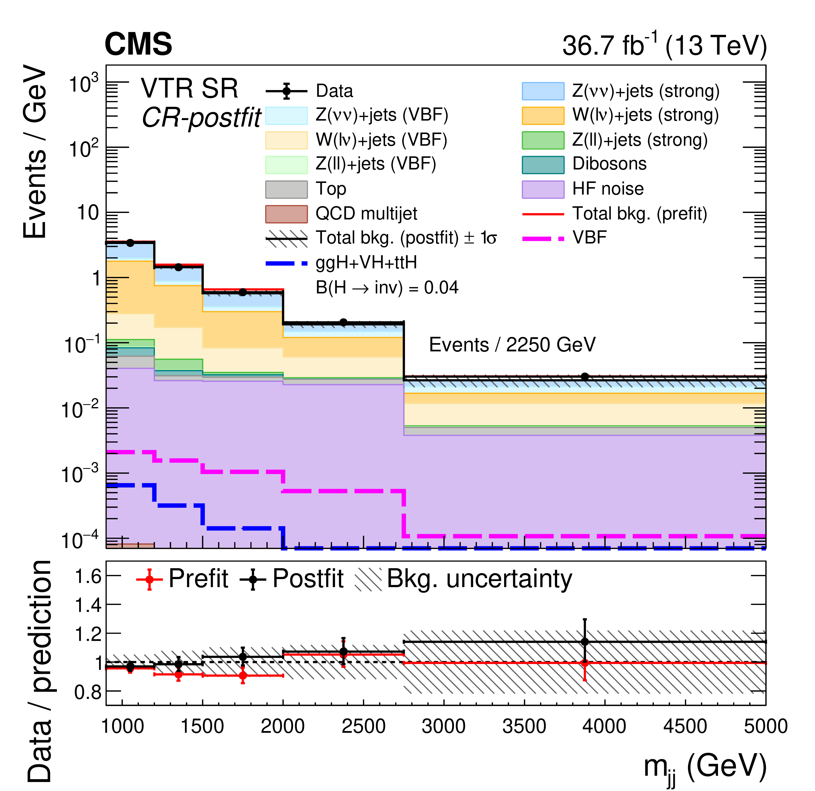
The observed ${m_{\mathrm {jj}}}$ distribution in the VTR prefit (left) and postfit (right) SR compared to the postfit backgrounds, with the 2017 samples. The signal processes are scaled by the fitted value of ${{\mathcal {B}(\mathrm{H} \to \text {inv})}}$, shown in the legend. |
png pdf |
Figure A18-a:
The observed ${m_{\mathrm {jj}}}$ distribution in the VTR prefit (left) and postfit (right) SR compared to the postfit backgrounds, with the 2017 samples. The signal processes are scaled by the fitted value of ${{\mathcal {B}(\mathrm{H} \to \text {inv})}}$, shown in the legend. |

png pdf |
Figure A18-b:
The observed ${m_{\mathrm {jj}}}$ distribution in the VTR prefit (left) and postfit (right) SR compared to the postfit backgrounds, with the 2017 samples. The signal processes are scaled by the fitted value of ${{\mathcal {B}(\mathrm{H} \to \text {inv})}}$, shown in the legend. |
png pdf |
Figure A19:
The ${m_{\mathrm {jj}}}$ distributions (prefit and CR-postfit) in the dielectron (upper left), dimuon (upper right), single-electron (lower left), and single-muon (lower right) CR for the VTR category, with the 2018 sample. |
png pdf |
Figure A19-a:
The ${m_{\mathrm {jj}}}$ distributions (prefit and CR-postfit) in the dielectron (upper left), dimuon (upper right), single-electron (lower left), and single-muon (lower right) CR for the VTR category, with the 2018 sample. |
png pdf |
Figure A19-b:
The ${m_{\mathrm {jj}}}$ distributions (prefit and CR-postfit) in the dielectron (upper left), dimuon (upper right), single-electron (lower left), and single-muon (lower right) CR for the VTR category, with the 2018 sample. |
png pdf |
Figure A19-c:
The ${m_{\mathrm {jj}}}$ distributions (prefit and CR-postfit) in the dielectron (upper left), dimuon (upper right), single-electron (lower left), and single-muon (lower right) CR for the VTR category, with the 2018 sample. |

png pdf |
Figure A19-d:
The ${m_{\mathrm {jj}}}$ distributions (prefit and CR-postfit) in the dielectron (upper left), dimuon (upper right), single-electron (lower left), and single-muon (lower right) CR for the VTR category, with the 2018 sample. |

png pdf |
Figure A20:
The ${m_{\mathrm {jj}}}$ postfit distributions in the dielectron (upper left), dimuon (upper right), single-electron (lower left), and single-muon (lower right) CR for the VTR category, with the 2018 sample. The background contributions are estimated from a fit to data in the SR and CRs allowing for the signal contribution to vary (S+B fit) and the total background estimated from a fit assuming $ {{\mathcal {B}(\mathrm{H} \to \text {inv})}} =$ 0 (B-only fit) is also shown. |
png pdf |
Figure A20-a:
The ${m_{\mathrm {jj}}}$ postfit distributions in the dielectron (upper left), dimuon (upper right), single-electron (lower left), and single-muon (lower right) CR for the VTR category, with the 2018 sample. The background contributions are estimated from a fit to data in the SR and CRs allowing for the signal contribution to vary (S+B fit) and the total background estimated from a fit assuming $ {{\mathcal {B}(\mathrm{H} \to \text {inv})}} =$ 0 (B-only fit) is also shown. |
png pdf |
Figure A20-b:
The ${m_{\mathrm {jj}}}$ postfit distributions in the dielectron (upper left), dimuon (upper right), single-electron (lower left), and single-muon (lower right) CR for the VTR category, with the 2018 sample. The background contributions are estimated from a fit to data in the SR and CRs allowing for the signal contribution to vary (S+B fit) and the total background estimated from a fit assuming $ {{\mathcal {B}(\mathrm{H} \to \text {inv})}} =$ 0 (B-only fit) is also shown. |
png pdf |
Figure A20-c:
The ${m_{\mathrm {jj}}}$ postfit distributions in the dielectron (upper left), dimuon (upper right), single-electron (lower left), and single-muon (lower right) CR for the VTR category, with the 2018 sample. The background contributions are estimated from a fit to data in the SR and CRs allowing for the signal contribution to vary (S+B fit) and the total background estimated from a fit assuming $ {{\mathcal {B}(\mathrm{H} \to \text {inv})}} =$ 0 (B-only fit) is also shown. |

png pdf |
Figure A20-d:
The ${m_{\mathrm {jj}}}$ postfit distributions in the dielectron (upper left), dimuon (upper right), single-electron (lower left), and single-muon (lower right) CR for the VTR category, with the 2018 sample. The background contributions are estimated from a fit to data in the SR and CRs allowing for the signal contribution to vary (S+B fit) and the total background estimated from a fit assuming $ {{\mathcal {B}(\mathrm{H} \to \text {inv})}} =$ 0 (B-only fit) is also shown. |
png pdf |
Figure A21:
The observed ${m_{\mathrm {jj}}}$ distribution in the VTR prefit (left) and postfit (right) SR compared to the postfit backgrounds, with the 2018 samples. The signal processes are scaled by the fitted value of ${{\mathcal {B}(\mathrm{H} \to \text {inv})}}$, shown in the legend. |
png pdf |
Figure A21-a:
The observed ${m_{\mathrm {jj}}}$ distribution in the VTR prefit (left) and postfit (right) SR compared to the postfit backgrounds, with the 2018 samples. The signal processes are scaled by the fitted value of ${{\mathcal {B}(\mathrm{H} \to \text {inv})}}$, shown in the legend. |
png pdf |
Figure A21-b:
The observed ${m_{\mathrm {jj}}}$ distribution in the VTR prefit (left) and postfit (right) SR compared to the postfit backgrounds, with the 2018 samples. The signal processes are scaled by the fitted value of ${{\mathcal {B}(\mathrm{H} \to \text {inv})}}$, shown in the legend. |
png pdf |
Figure A22:
Comparison between data and simulation for the Z(ee)+jets / W(e$\nu$)+jets (upper left), Z($\mu \mu$)+jets / W($\mu \nu$)+jets (upper right), $\gamma$+jets / Z(ee)+jets (lower left), and $\gamma$+jets / Z($\mu \mu$)+jets (lower right) prefit and CR-postfit ratios, as functions of ${m_{\mathrm {jj}}}$, for the MTR category 2017 samples. The minor backgrounds in each CR are subtracted from the data using estimates from simulation. The grey bands include the theoretical and experimental systematic uncertainties listed in Table 3, as well as the statistical uncertainty in the simulation. |
png pdf |
Figure A22-a:
Comparison between data and simulation for the Z(ee)+jets / W(e$\nu$)+jets (upper left), Z($\mu \mu$)+jets / W($\mu \nu$)+jets (upper right), $\gamma$+jets / Z(ee)+jets (lower left), and $\gamma$+jets / Z($\mu \mu$)+jets (lower right) prefit and CR-postfit ratios, as functions of ${m_{\mathrm {jj}}}$, for the MTR category 2017 samples. The minor backgrounds in each CR are subtracted from the data using estimates from simulation. The grey bands include the theoretical and experimental systematic uncertainties listed in Table 3, as well as the statistical uncertainty in the simulation. |
png pdf |
Figure A22-b:
Comparison between data and simulation for the Z(ee)+jets / W(e$\nu$)+jets (upper left), Z($\mu \mu$)+jets / W($\mu \nu$)+jets (upper right), $\gamma$+jets / Z(ee)+jets (lower left), and $\gamma$+jets / Z($\mu \mu$)+jets (lower right) prefit and CR-postfit ratios, as functions of ${m_{\mathrm {jj}}}$, for the MTR category 2017 samples. The minor backgrounds in each CR are subtracted from the data using estimates from simulation. The grey bands include the theoretical and experimental systematic uncertainties listed in Table 3, as well as the statistical uncertainty in the simulation. |
png pdf |
Figure A22-c:
Comparison between data and simulation for the Z(ee)+jets / W(e$\nu$)+jets (upper left), Z($\mu \mu$)+jets / W($\mu \nu$)+jets (upper right), $\gamma$+jets / Z(ee)+jets (lower left), and $\gamma$+jets / Z($\mu \mu$)+jets (lower right) prefit and CR-postfit ratios, as functions of ${m_{\mathrm {jj}}}$, for the MTR category 2017 samples. The minor backgrounds in each CR are subtracted from the data using estimates from simulation. The grey bands include the theoretical and experimental systematic uncertainties listed in Table 3, as well as the statistical uncertainty in the simulation. |
png pdf |
Figure A22-d:
Comparison between data and simulation for the Z(ee)+jets / W(e$\nu$)+jets (upper left), Z($\mu \mu$)+jets / W($\mu \nu$)+jets (upper right), $\gamma$+jets / Z(ee)+jets (lower left), and $\gamma$+jets / Z($\mu \mu$)+jets (lower right) prefit and CR-postfit ratios, as functions of ${m_{\mathrm {jj}}}$, for the MTR category 2017 samples. The minor backgrounds in each CR are subtracted from the data using estimates from simulation. The grey bands include the theoretical and experimental systematic uncertainties listed in Table 3, as well as the statistical uncertainty in the simulation. |
png pdf |
Figure A23:
Comparison between data and simulation for the Z(ee)+jets / W(e$\nu$)+jets (left) and Z($\mu \mu$)+jets / W($\mu \nu$)+jets (right) prefit and CR-postfit ratios, as functions of ${m_{\mathrm {jj}}}$, for the VTR category 2017 samples. The minor backgrounds in each CR are subtracted from the data using estimates from simulation. The grey bands include the theoretical and experimental systematic uncertainties listed in Table 3, as well as the statistical uncertainty in the simulation. |
png pdf |
Figure A23-a:
Comparison between data and simulation for the Z(ee)+jets / W(e$\nu$)+jets (left) and Z($\mu \mu$)+jets / W($\mu \nu$)+jets (right) prefit and CR-postfit ratios, as functions of ${m_{\mathrm {jj}}}$, for the VTR category 2017 samples. The minor backgrounds in each CR are subtracted from the data using estimates from simulation. The grey bands include the theoretical and experimental systematic uncertainties listed in Table 3, as well as the statistical uncertainty in the simulation. |

png pdf |
Figure A23-b:
Comparison between data and simulation for the Z(ee)+jets / W(e$\nu$)+jets (left) and Z($\mu \mu$)+jets / W($\mu \nu$)+jets (right) prefit and CR-postfit ratios, as functions of ${m_{\mathrm {jj}}}$, for the VTR category 2017 samples. The minor backgrounds in each CR are subtracted from the data using estimates from simulation. The grey bands include the theoretical and experimental systematic uncertainties listed in Table 3, as well as the statistical uncertainty in the simulation. |
png pdf |
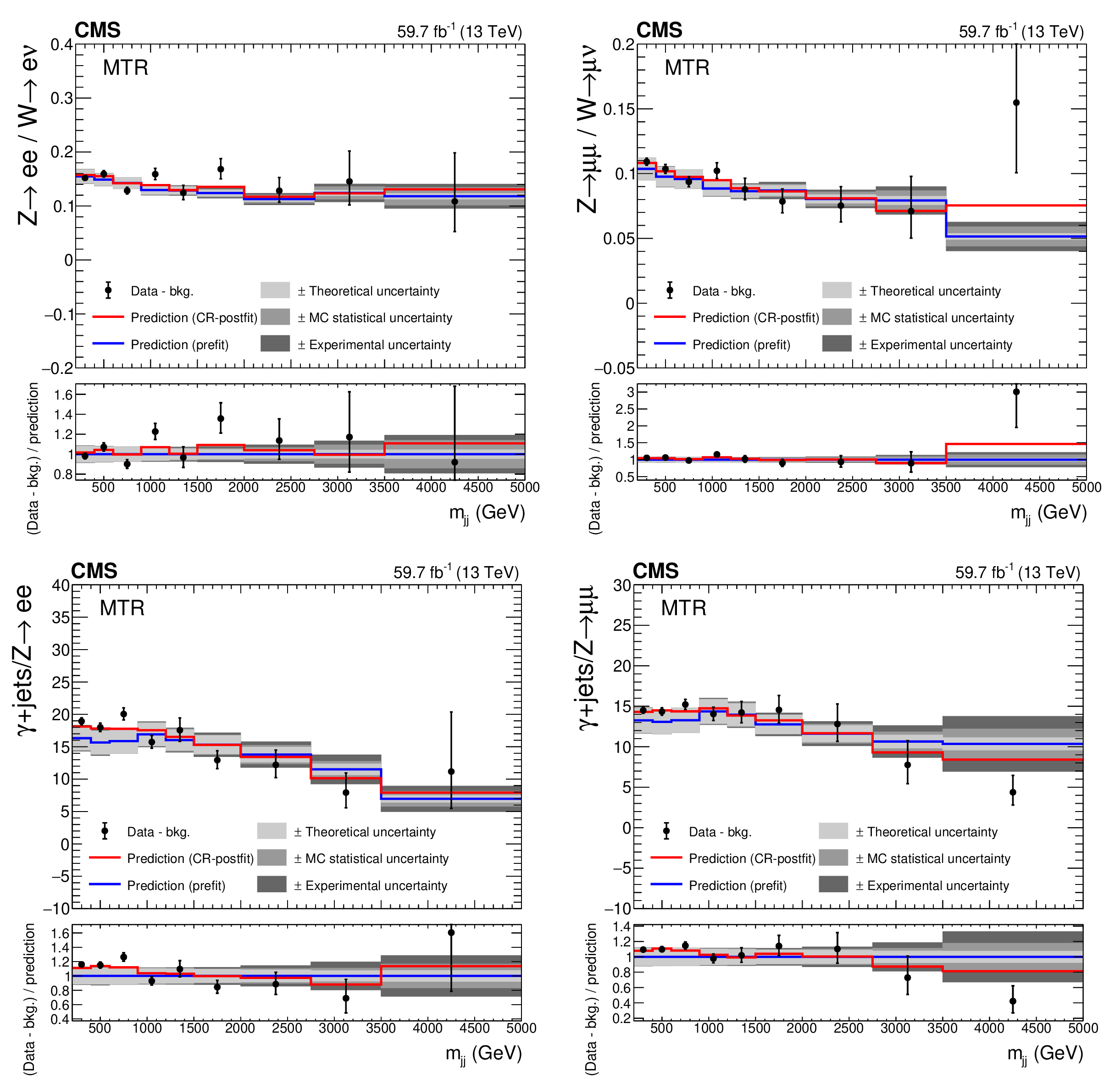
Figure A24:
Comparison between data and simulation for the Z(ee)+jets / W(e$\nu$)+jets (upper left), Z($\mu \mu$)+jets / W($\mu \nu$)+jets (upper right), $\gamma$+jets / Z(ee)+jets (lower left), and $\gamma$+jets / Z($\mu \mu$)+jets (lower right) prefit and CR-postfit ratios, as functions of ${m_{\mathrm {jj}}}$, for the MTR category 2018 samples. The minor backgrounds in each CR are subtracted from the data using estimates from simulation. The grey bands include the theoretical and experimental systematic uncertainties listed in Table 3, as well as the statistical uncertainty in the simulation. |
png pdf |
Figure A24-a:
Comparison between data and simulation for the Z(ee)+jets / W(e$\nu$)+jets (upper left), Z($\mu \mu$)+jets / W($\mu \nu$)+jets (upper right), $\gamma$+jets / Z(ee)+jets (lower left), and $\gamma$+jets / Z($\mu \mu$)+jets (lower right) prefit and CR-postfit ratios, as functions of ${m_{\mathrm {jj}}}$, for the MTR category 2018 samples. The minor backgrounds in each CR are subtracted from the data using estimates from simulation. The grey bands include the theoretical and experimental systematic uncertainties listed in Table 3, as well as the statistical uncertainty in the simulation. |
png pdf |
Figure A24-b:
Comparison between data and simulation for the Z(ee)+jets / W(e$\nu$)+jets (upper left), Z($\mu \mu$)+jets / W($\mu \nu$)+jets (upper right), $\gamma$+jets / Z(ee)+jets (lower left), and $\gamma$+jets / Z($\mu \mu$)+jets (lower right) prefit and CR-postfit ratios, as functions of ${m_{\mathrm {jj}}}$, for the MTR category 2018 samples. The minor backgrounds in each CR are subtracted from the data using estimates from simulation. The grey bands include the theoretical and experimental systematic uncertainties listed in Table 3, as well as the statistical uncertainty in the simulation. |

png pdf |
Figure A24-c:
Comparison between data and simulation for the Z(ee)+jets / W(e$\nu$)+jets (upper left), Z($\mu \mu$)+jets / W($\mu \nu$)+jets (upper right), $\gamma$+jets / Z(ee)+jets (lower left), and $\gamma$+jets / Z($\mu \mu$)+jets (lower right) prefit and CR-postfit ratios, as functions of ${m_{\mathrm {jj}}}$, for the MTR category 2018 samples. The minor backgrounds in each CR are subtracted from the data using estimates from simulation. The grey bands include the theoretical and experimental systematic uncertainties listed in Table 3, as well as the statistical uncertainty in the simulation. |
png pdf |
Figure A24-d:
Comparison between data and simulation for the Z(ee)+jets / W(e$\nu$)+jets (upper left), Z($\mu \mu$)+jets / W($\mu \nu$)+jets (upper right), $\gamma$+jets / Z(ee)+jets (lower left), and $\gamma$+jets / Z($\mu \mu$)+jets (lower right) prefit and CR-postfit ratios, as functions of ${m_{\mathrm {jj}}}$, for the MTR category 2018 samples. The minor backgrounds in each CR are subtracted from the data using estimates from simulation. The grey bands include the theoretical and experimental systematic uncertainties listed in Table 3, as well as the statistical uncertainty in the simulation. |
png pdf |
Figure A25:
Comparison between data and simulation for the Z(ee)+jets / W(e$\nu$)+jets (left) and Z($\mu \mu$)+jets / W($\mu \nu$)+jets (right) prefit and CR-postfit ratios, as functions of ${m_{\mathrm {jj}}}$, for the VTR category 2018 samples. The minor backgrounds in each CR are subtracted from the data using estimates from simulation. The grey bands include the theoretical and experimental systematic uncertainties listed in Table 3, as well as the statistical uncertainty in the simulation. |
png pdf |
Figure A25-a:
Comparison between data and simulation for the Z(ee)+jets / W(e$\nu$)+jets (left) and Z($\mu \mu$)+jets / W($\mu \nu$)+jets (right) prefit and CR-postfit ratios, as functions of ${m_{\mathrm {jj}}}$, for the VTR category 2018 samples. The minor backgrounds in each CR are subtracted from the data using estimates from simulation. The grey bands include the theoretical and experimental systematic uncertainties listed in Table 3, as well as the statistical uncertainty in the simulation. |

png pdf |
Figure A25-b:
Comparison between data and simulation for the Z(ee)+jets / W(e$\nu$)+jets (left) and Z($\mu \mu$)+jets / W($\mu \nu$)+jets (right) prefit and CR-postfit ratios, as functions of ${m_{\mathrm {jj}}}$, for the VTR category 2018 samples. The minor backgrounds in each CR are subtracted from the data using estimates from simulation. The grey bands include the theoretical and experimental systematic uncertainties listed in Table 3, as well as the statistical uncertainty in the simulation. |
| Tables | |
png pdf |
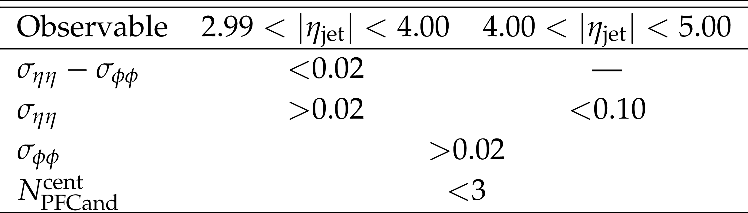
Table 1:
Selection applied in the 2017 and 2018 data sets to remove HF jets stemming from calorimeter noise. |

png pdf |
Table 2:
Summary of the kinematic selections used to define the SR for both the MTR and the VTR categories. |

png pdf |
Table 3:
Experimental and theoretical sources of systematic uncertainty in the V+jets transfer factors. The second column indicates which ratio a given source of uncertainty is applied to. The impact on ${m_{\mathrm {jj}}}$ is given in the 3rd column, as a single value if no dependence on ${m_{\mathrm {jj}}}$ is observed, or as a range. When a range is shown, the uncertainty increases with the value of ${m_{\mathrm {jj}}}$. The quoted uncertainty values represent the absolute value of the relative change in the transfer factor corresponding to a variation of ${\pm}$1 standard deviation in the systematic uncertainty, or equivalently to a variation of ${\pm}$1 in the corresponding nuisance parameter $\theta $ in Eq. (4). |
png pdf |
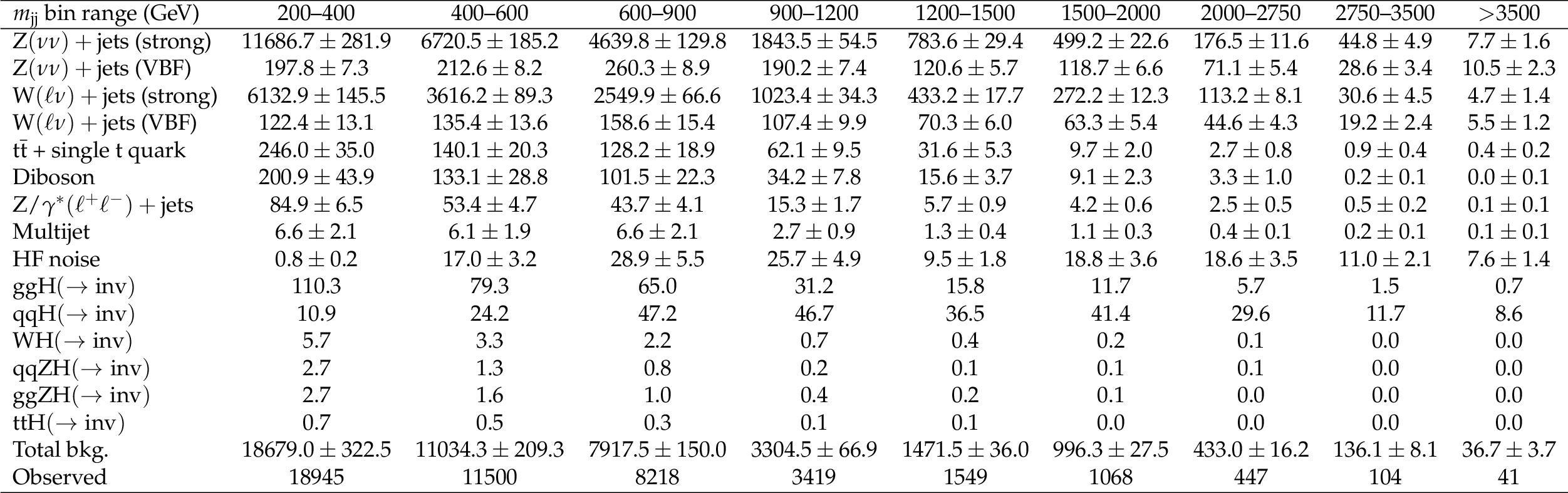
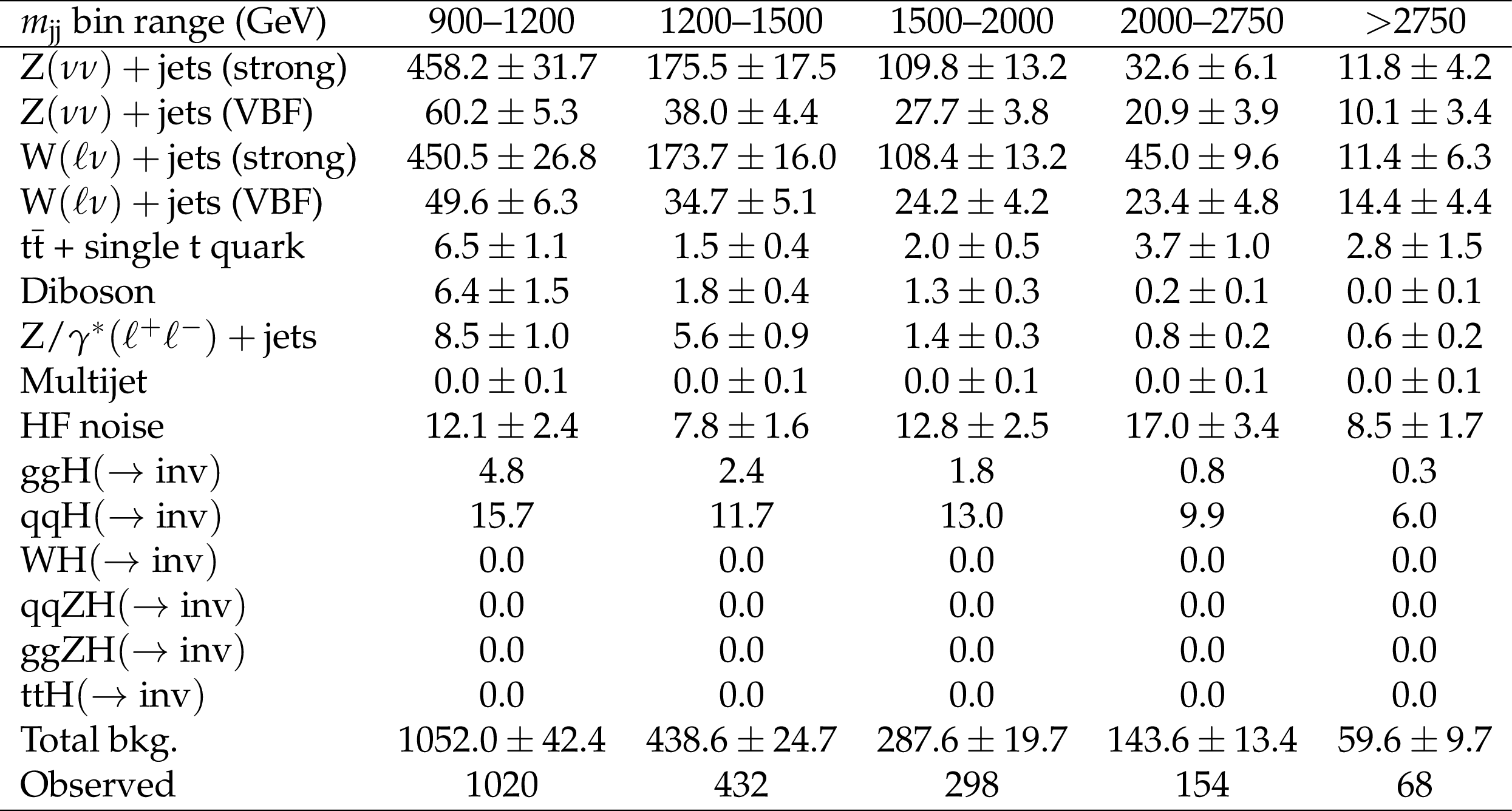
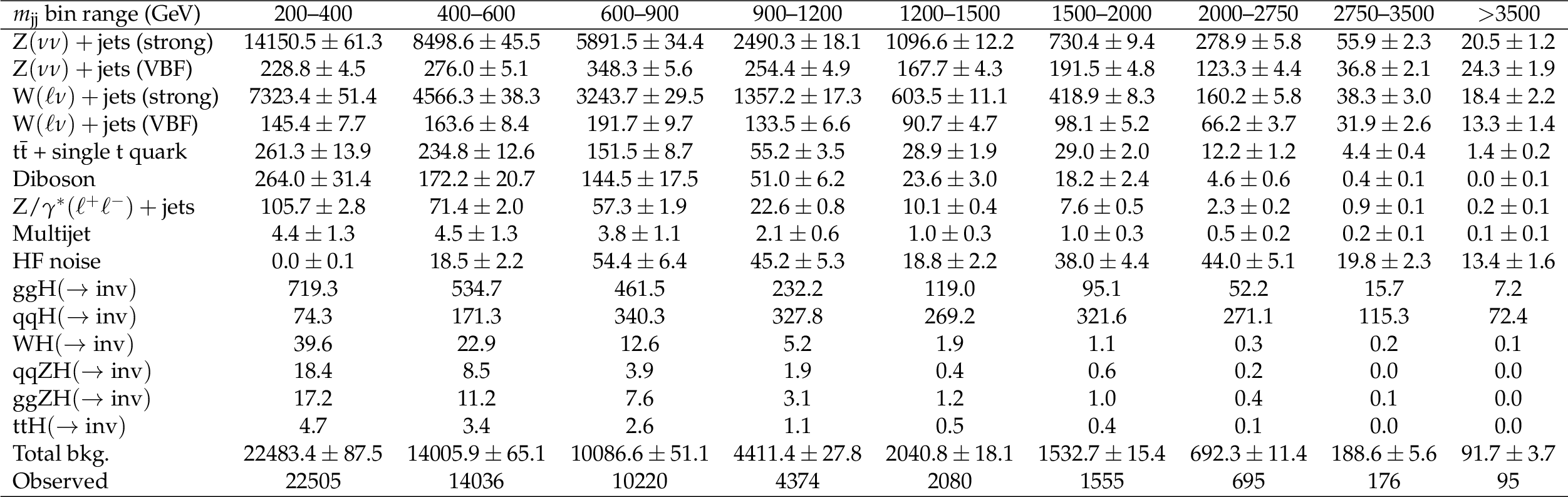
Table 4:
Expected event yields in each ${m_{\mathrm {jj}}}$ bin for the different background processes in the SR of the MTR category, summing the 2017 and 2018 samples. The background yields and the corresponding uncertainties are obtained after performing a combined fit across all of the CRs and the SR. The expected signal contributions for the Higgs boson, produced in the non-VBF and VBF modes, decaying to invisible particles with a branching fraction of $ {{\mathcal {B}(\mathrm{H} \to \text {inv})}} = $ 1, and the observed event yields are also reported. The yields from the 2017 and 2018 samples are summed and the correlations between their uncertainties are neglected. |

png pdf |
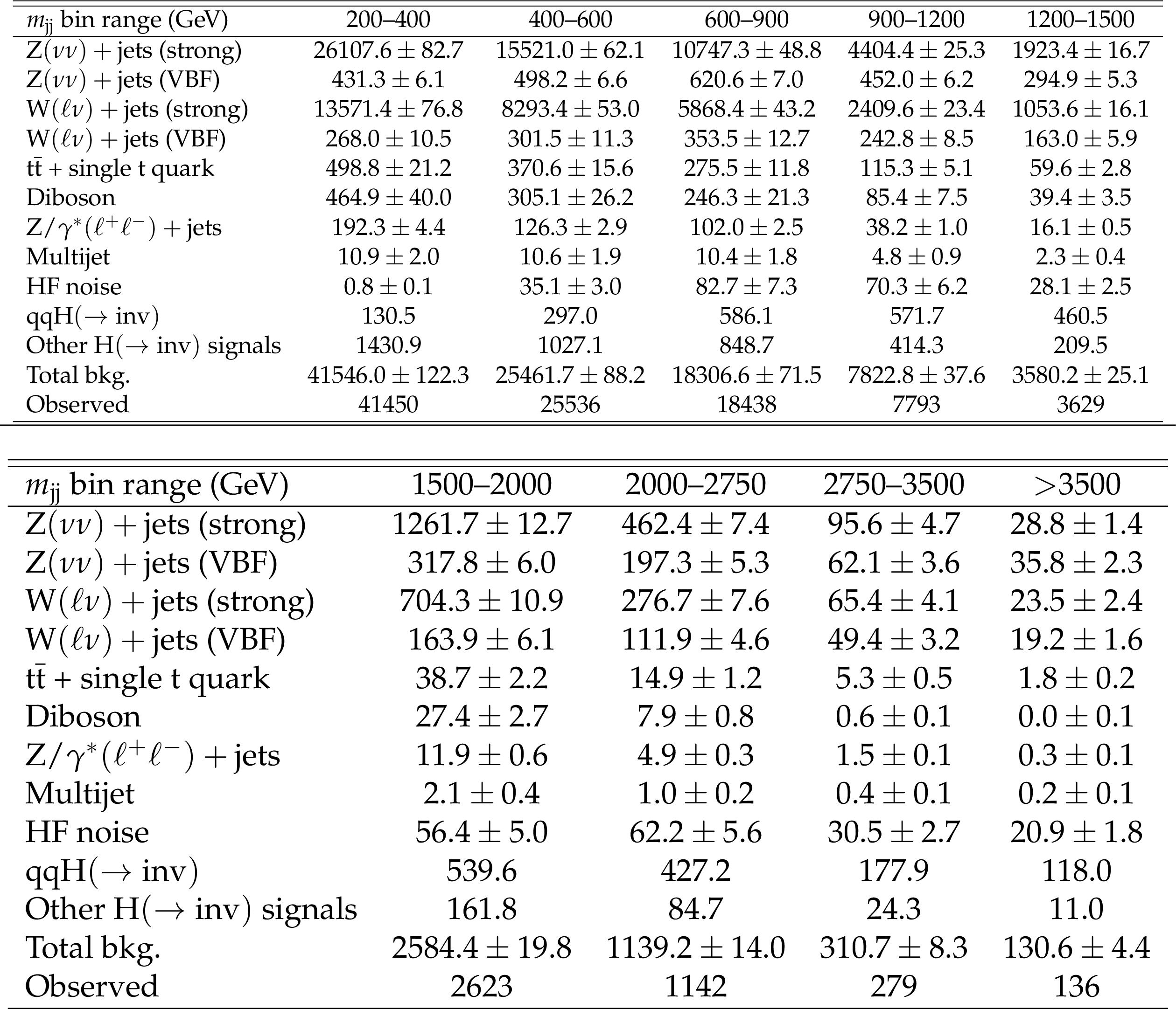
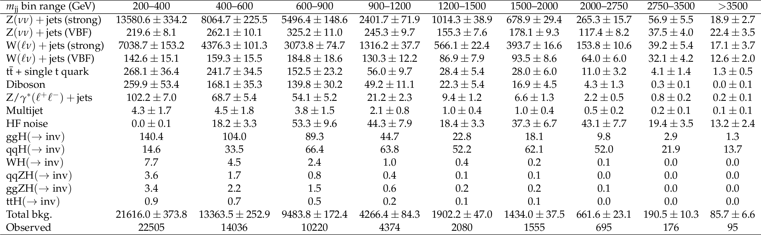
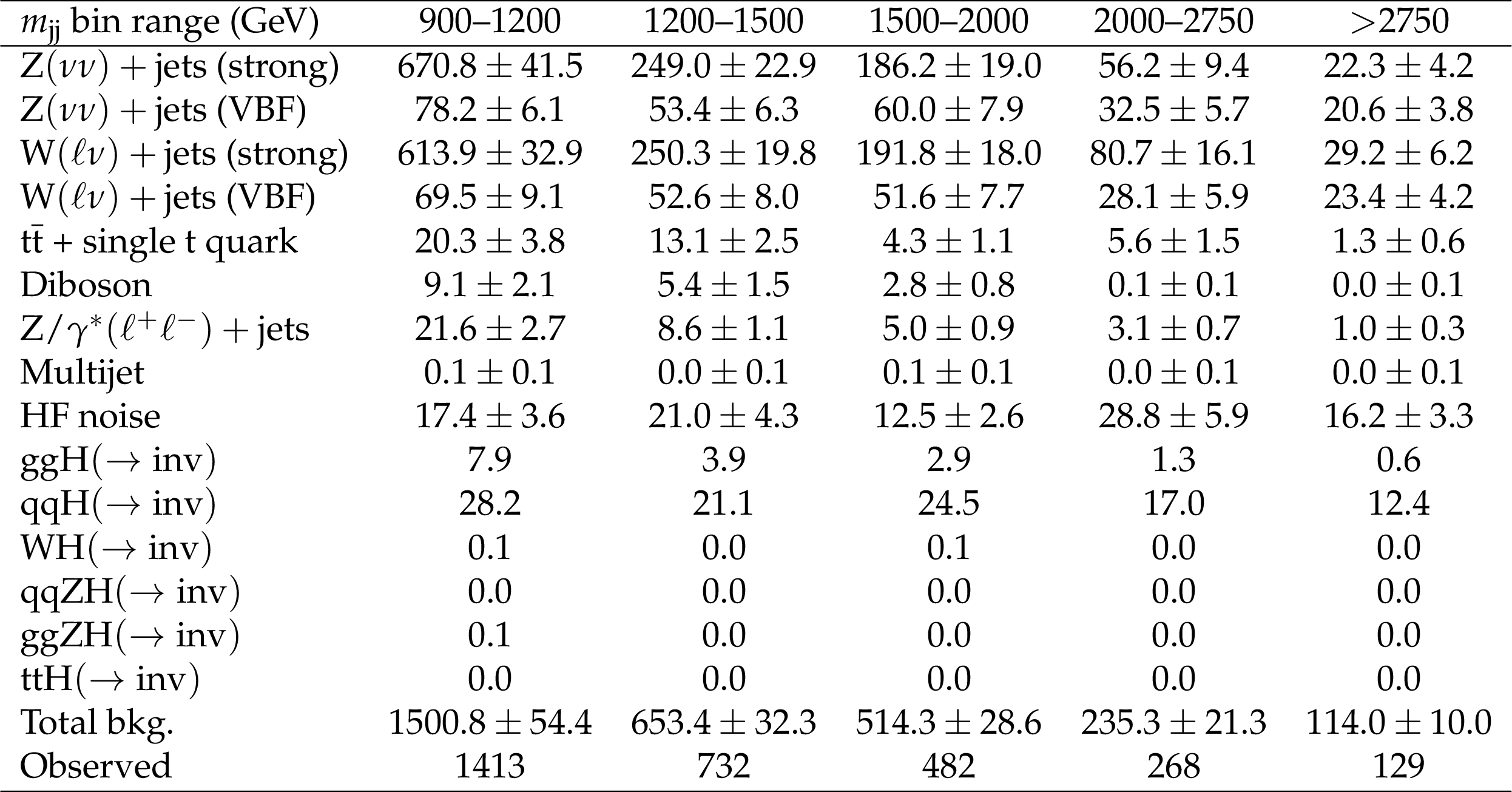
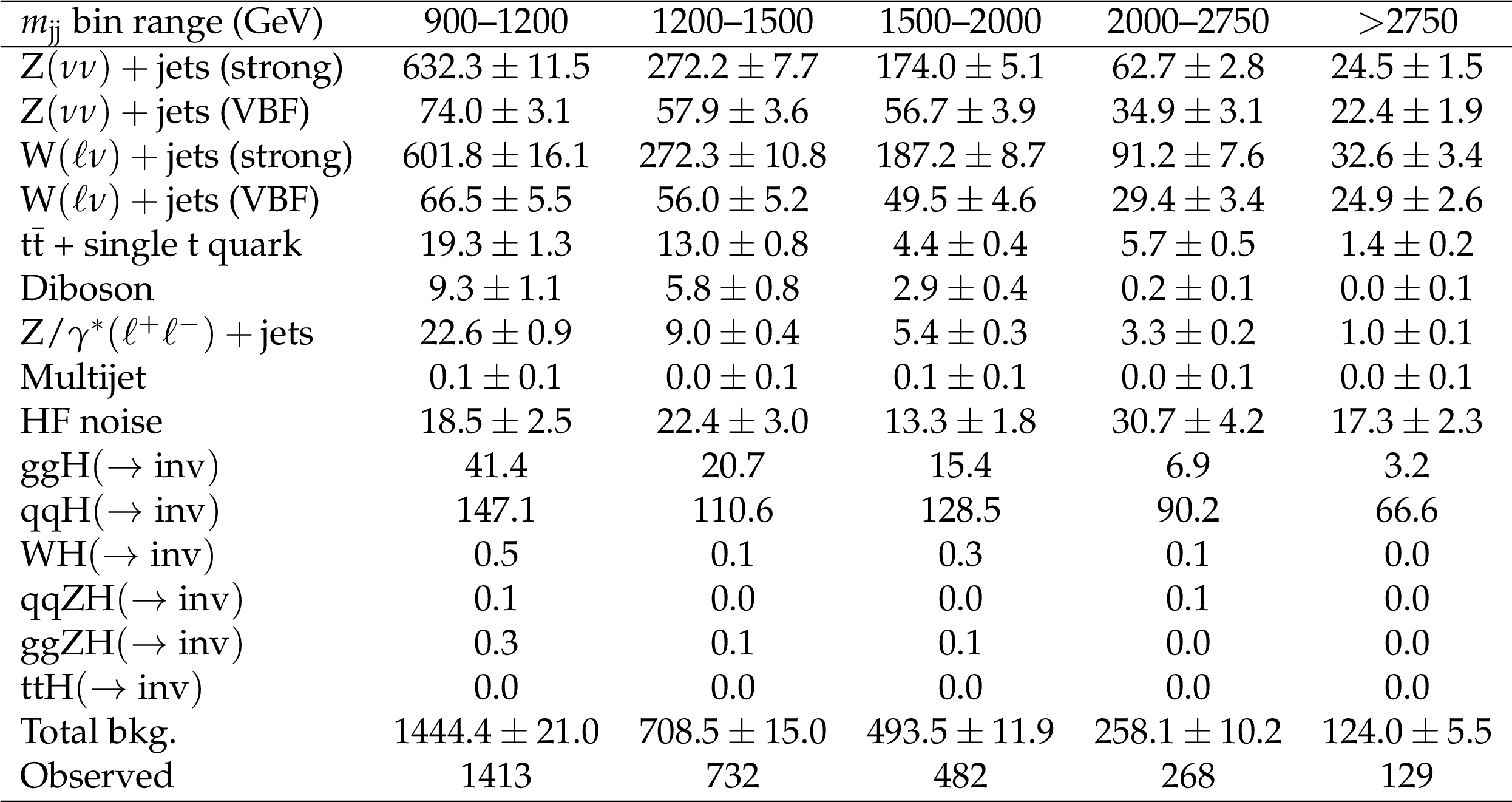
Table 5:
Expected event yields in each ${m_{\mathrm {jj}}}$ bin for the different background processes in the SR of the VTR category, summing the 2017 and 2018 samples. The background yields and the corresponding uncertainties are obtained after performing a combined fit across all of the CRs and the SR. The expected signal contributions for the Higgs boson, produced in the non-VBF and VBF modes, decaying to invisible particles with a branching fraction of $ {{\mathcal {B}(\mathrm{H} \to \text {inv})}} = $ 1, and the observed event yields are also reported. The yields from the 2017 and 2018 samples are summed and the correlations between their uncertainties are neglected. |
png pdf |
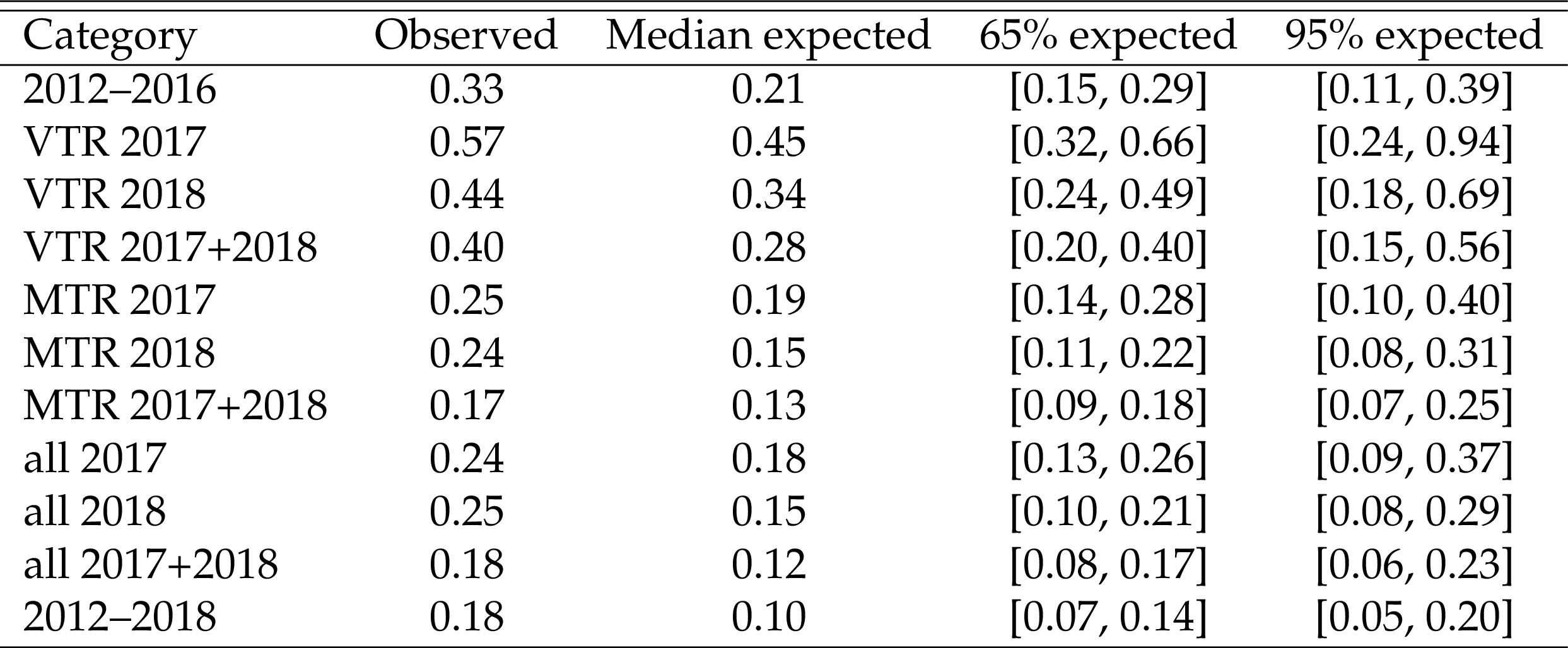
Table 6:
The 95% CL upper limits on ${(\sigma _{\mathrm{H}}/\sigma _{\mathrm{H}}^{\mathrm {SM}}) {{\mathcal {B}(\mathrm{H} \to \text {inv})}}}$, assuming an SM Higgs boson with a mass of 125.38 GeV. The observed and median expected results are shown, along with the 68% and 95% interquartile ranges for each category and for the combinations. |
png pdf |
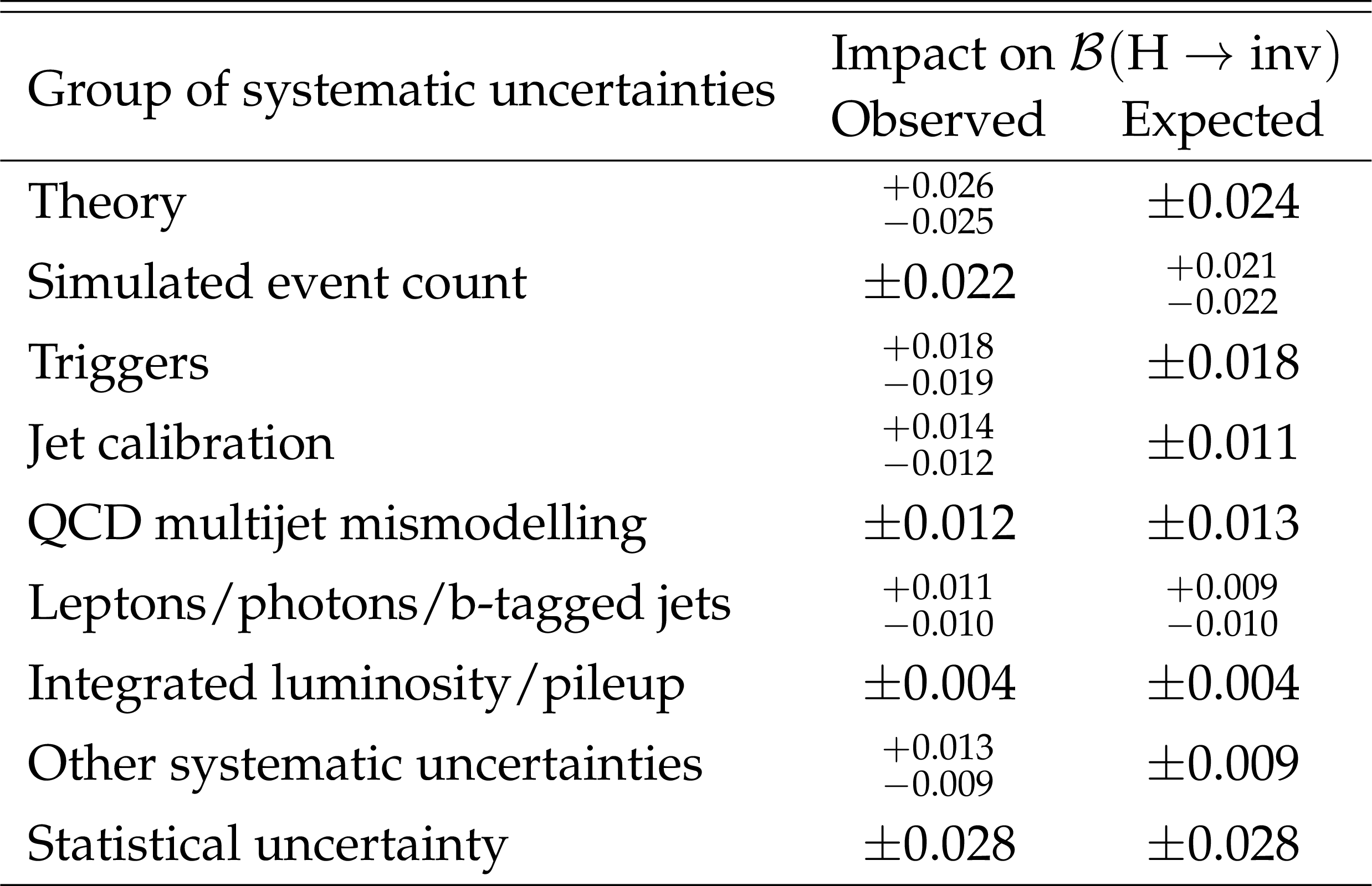
Table 7:
Uncertainty breakdown in ${{\mathcal {B}(\mathrm{H} \to \text {inv})}}$. The sources of uncertainty are separated into different groups. Observed and expected results are quoted for the full combination of 2012-2018 data. The expected results are obtained using an Asimov data set [71] with $ {{\mathcal {B}(\mathrm{H} \to \text {inv})}} =$ 0. |
png pdf |
Table A1:
Expected event yields in each ${m_{\mathrm {jj}}}$ bin for the different background processes in the SR of the MTR category, in the 2017 samples. The background yields and the corresponding uncertainties are obtained after performing a combined fit across all of the CRs and SR. The expected signal contributions for the Higgs boson, produced in the non-VBF and VBF modes, decaying to invisible particles with a branching fraction of $ {{\mathcal {B}(\mathrm{H} \to \text {inv})}} = $ 1, and the observed event yields are also reported. |
png pdf |
Table A2:
Expected event yields in each ${m_{\mathrm {jj}}}$ bin for the different background processes in the SR of the MTR category, in the 2018 samples. The background yields and the corresponding uncertainties are obtained after performing a combined fit across all of the CRs and SR. The expected signal contributions for the Higgs boson, produced in the non-VBF and VBF modes, decaying to invisible particles with a branching fraction of $ {{\mathcal {B}(\mathrm{H} \to \text {inv})}} = $ 1, and the observed event yields are also reported. |
png pdf |
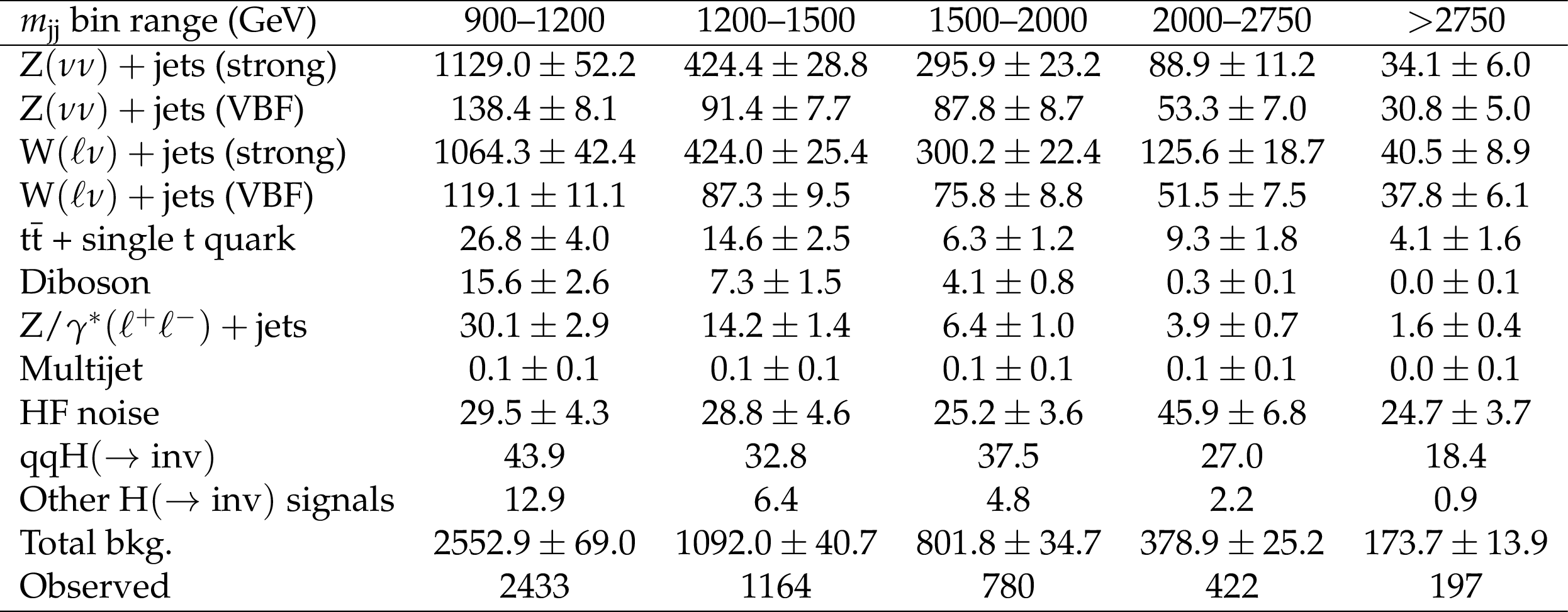
Table A3:
Expected event yields in each ${m_{\mathrm {jj}}}$ bin for the different background processes in the SR of the MTR category, in the 2017 and 2018 samples. The background yields and the corresponding uncertainties are obtained after performing a combined fit across all of the CRs and SR. The expected signal contributions for the Higgs boson, produced in the non-VBF and VBF modes, decaying to invisible particles with a branching fraction of $ {{\mathcal {B}(\mathrm{H} \to \text {inv})}} = $ 1, and the observed event yields are also reported. The yields from the 2017 and 2018 samples are summed and the correlations between their uncertainties are neglected. |
png pdf |
Table A4:
Expected event yields in each ${m_{\mathrm {jj}}}$ bin for the different background processes in the SR of the VTR category, in the 2017 samples. The background yields and the corresponding uncertainties are obtained after performing a combined fit across all of the CRs and SR. The expected signal contributions for the Higgs boson, produced in the non-VBF and VBF modes, decaying to invisible particles with a branching fraction of $ {{\mathcal {B}(\mathrm{H} \to \text {inv})}} = $ 1, and the observed event yields are also reported. |
png pdf |
Table A5:
Expected event yields in each ${m_{\mathrm {jj}}}$ bin for the different background processes in the SR of the VTR category, in the 2018 samples. The background yields and the corresponding uncertainties are obtained after performing a combined fit across all of the CRs and SR. The expected signal contributions for the Higgs boson, produced in the non-VBF and VBF modes, decaying to invisible particles with a branching fraction of $ {{\mathcal {B}(\mathrm{H} \to \text {inv})}} = $ 1, and the observed event yields are also reported. |
png pdf |
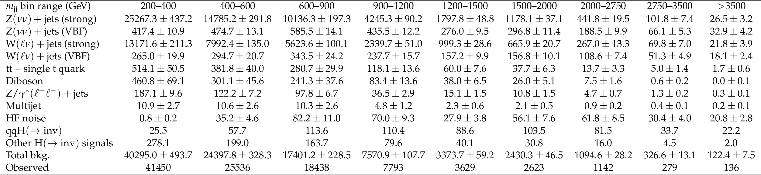
Table A6:
Expected event yields in each ${m_{\mathrm {jj}}}$ bin for the different background processes in the SR of the VTR category, in the 2017 and 2018 samples. The background yields and the corresponding uncertainties are obtained after performing a combined fit across all of the CRs and SR. The expected signal contributions for the Higgs boson, produced in the non-VBF and VBF modes, decaying to invisible particles with a branching fraction of $ {{\mathcal {B}(\mathrm{H} \to \text {inv})}} = $ 1, and the observed event yields are also reported. The yields from the 2017 and 2018 samples are summed and the correlations between their uncertainties are neglected. |
png pdf |
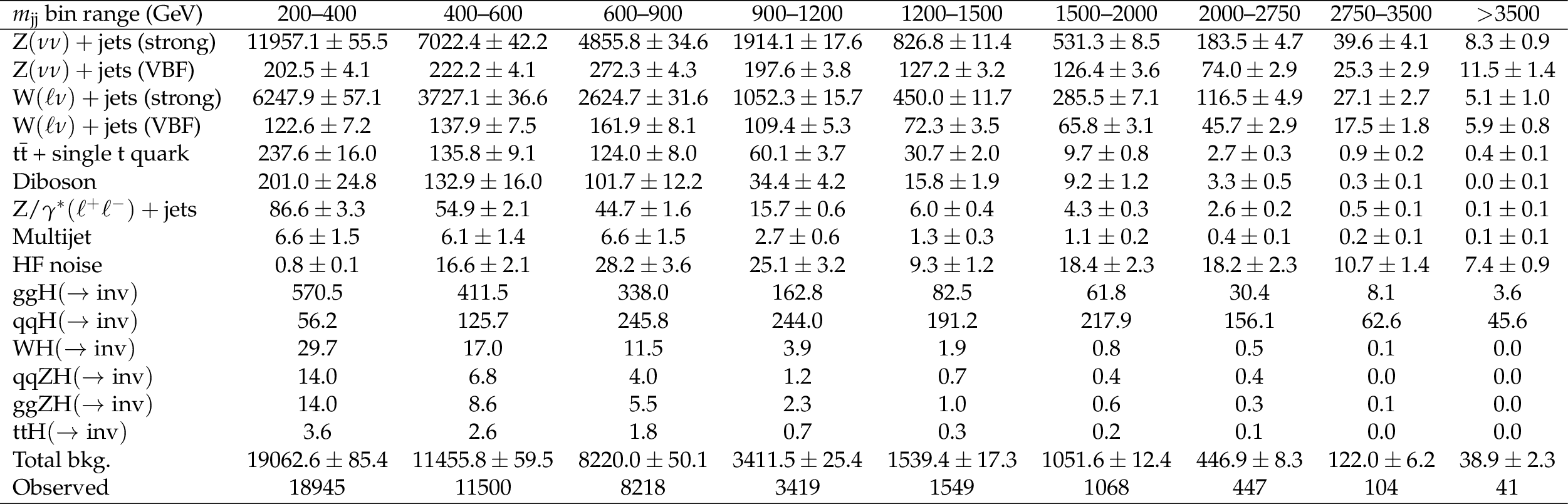
Table A7:
Expected event yields in each ${m_{\mathrm {jj}}}$ bin for the different background processes in the SR of the MTR category, in the 2017 samples. The background yields and the corresponding uncertainties are obtained after performing a combined fit across all of the CRs and SR. The expected signal contributions for the Higgs boson, produced in the non-VBF and VBF modes, decaying to invisible particles with a branching fraction of $ {{\mathcal {B}(\mathrm{H} \to \text {inv})}} = $ 1, and the observed event yields are also reported. |
png pdf |
Table A8:
Expected event yields in each ${m_{\mathrm {jj}}}$ bin for the different background processes in the SR of the MTR category, in the 2018 samples. The background yields and the corresponding uncertainties are obtained after performing a combined fit across all of the CRs and SR. The expected signal contributions for the Higgs boson, produced in the non-VBF and VBF modes, decaying to invisible particles with a branching fraction of $ {{\mathcal {B}(\mathrm{H} \to \text {inv})}} = $ 1, and the observed event yields are also reported. |

png pdf |
Table A9:
Expected event yields in each ${m_{\mathrm {jj}}}$ bin for the different background processes in the SR of the VTR category, in the 2017 samples. The background yields and the corresponding uncertainties are obtained after performing a combined fit across all of the CRs and SR. The expected signal contributions for the Higgs boson, produced in the non-VBF and VBF modes, decaying to invisible particles with a branching fraction of $ {{\mathcal {B}(\mathrm{H} \to \text {inv})}} = $ 1, and the observed event yields are also reported. |
png pdf |
Table A10:
Expected event yields in each ${m_{\mathrm {jj}}}$ bin for the different background processes in the SR of the VTR category, in the 2018 samples. The background yields and the corresponding uncertainties are obtained after performing a combined fit across all of the CRs and SR. The expected signal contributions for the Higgs boson, produced in the non-VBF and VBF modes, decaying to invisible particles with a branching fraction of $ {{\mathcal {B}(\mathrm{H} \to \text {inv})}} = $ 1, and the observed event yields are also reported. |
| Summary |
| A search for the Higgs boson (H) decaying invisibly, produced in the vector boson fusion mode, is performed with 101 fb$^{-1}$ of proton-proton collisions delivered by the LHC at $\sqrt{s} = $ 13 TeV and collected by the CMS detector during 2017-2018. Building upon the previously published results, an additional category targeting events at lower Higgs boson transverse momentum is added. An additional highly populated control region, based on production of a photon associated with jets, is used to constrain the dominant irreducible background from invisible decays of a Z boson produced in association with jets. Compared with the strategy of the previously published analysis, these additions improve the expected limits by approximately 17%. The observed (expected) upper limit on the invisible branching fraction of the Higgs boson, ${{\mathcal{B}(\mathrm{H} \to \text{inv})}} $, is found to be 0.18 (0.12) at the 95% confidence level (CL), assuming the standard model production cross section. The results are combined with previous measurements in the vector boson fusion topology, for total integrated luminosities of 19.7 fb$^{-1}$ at $\sqrt{s} = $ 8 TeV and 140 fb$^{-1}$ at $\sqrt{s} = $ 13 TeV, yielding an observed (expected) upper limit of 0.18 (0.10) at the 95% CL. This is currently the most stringent limit on ${{\mathcal{B}(\mathrm{H} \to \text{inv})}} $. Finally, the results are interpreted in the context of Higgs-portal models. The 90% CL upper limits on the spin-independent dark-matter-nucleon scattering cross section obtained from the observed LHC data collected during 2012-2018 complement the direct detection experiments in the range of dark matter particle masses smaller than 12 (6) GeV, assuming a fermion (scalar) dark matter candidate. |
| References | ||||
| 1 | F. Englert and R. Brout | Broken symmetry and the mass of gauge vector mesons | PRL 13 (1964) 321 | |
| 2 | P. W. Higgs | Broken symmetries, massless particles and gauge fields | PL12 (1964) 132 | |
| 3 | P. W. Higgs | Broken symmetries and the masses of gauge bosons | PRL 13 (1964) 508 | |
| 4 | G. S. Guralnik, C. R. Hagen, and T. W. B. Kibble | Global conservation laws and massless particles | PRL 13 (1964) 585 | |
| 5 | P. W. Higgs | Spontaneous symmetry breakdown without massless bosons | PR145 (1966) 1156 | |
| 6 | T. W. B. Kibble | Symmetry breaking in non-abelian gauge theories | PR155 (1967) 1554 | |
| 7 | ATLAS Collaboration | Observation of a new particle in the search for the standard model Higgs boson with the ATLAS detector at the LHC | PLB 716 (2012) 1 | 1207.7214 |
| 8 | CMS Collaboration | Observation of a new boson at a mass of 125 GeV with the CMS experiment at the LHC | PLB 716 (2012) 30 | CMS-HIG-12-028 1207.7235 |
| 9 | CMS Collaboration | Observation of a new boson with mass near 125 GeV in pp collisions at $ \sqrt{s} = $ 7 and 8 TeV | JHEP 06 (2013) 081 | CMS-HIG-12-036 1303.4571 |
| 10 | LHC Higgs Cross Section Working Group, S. Dittmaier et al. | Handbook of LHC Higgs cross sections: 1. Inclusive observables | CERN-2011-002 | 1101.0593 |
| 11 | G. B\'elanger et al. | The MSSM invisible Higgs in the light of dark matter and g$-$2 | PLB 519 (2001) 93 | hep-ph/0106275 |
| 12 | A. Datta, K. Huitu, J. Laamanen, and B. Mukhopadhyaya | Linear collider signals of an invisible Higgs boson in theories of large extra dimensions | PRD 70 (2004) 075003 | hep-ph/0404056 |
| 13 | D. Dominici and J. F. Gunion | Invisible Higgs decays from Higgs-graviscalar mixing | PRD 80 (2009) 115006 | 0902.1512 |
| 14 | R. E. Shrock and M. Suzuki | Invisible decays of Higgs bosons | PLB 110 (1982) 250 | |
| 15 | S. Argyropoulos, O. Brandt, and U. Haisch | Collider searches for dark matter through the Higgs lens | Symmetry 2021 (2021) 13 | 2109.13597 |
| 16 | A. Djouadi, O. Lebedev, Y. Mambrini, and J. Quevillon | Implications of LHC searches for Higgs--portal dark matter | PLB 709 (2012) 65 | 1112.3299 |
| 17 | S. Baek, P. Ko, W.-I. Park, and E. Senaha | Higgs portal vector dark matter: revisited | JHEP 05 (2013) 036 | 1212.2131 |
| 18 | A. Djouadi, A. Falkowski, Y. Mambrini, and J. Quevillon | Direct detection of Higgs--portal dark matter at the LHC | EPJC 73 (2013) 2455 | 1205.3169 |
| 19 | A. Beniwal et al. | Combined analysis of effective Higgs--portal dark matter models | PRD 93 (2016) 115016 | 1512.06458 |
| 20 | ATLAS Collaboration | Combination of searches for invisible Higgs boson decays with the ATLAS experiment | PRL 122 (2019) 231801 | 1904.05105 |
| 21 | ATLAS Collaboration | Search for associated production of a Z boson with an invisibly decaying Higgs boson or dark matter candidates at $ \sqrt{s}= $ 13 TeV with the ATLAS detector | 2021. Submitted to PLB | 2111.08372 |
| 22 | CMS Collaboration | Search for invisible decays of a Higgs boson produced through vector boson fusion in proton-proton collisions at $ \sqrt{s} = $ 13 TeV | PLB 793 (2019) 520 | CMS-HIG-17-023 1809.05937 |
| 23 | CMS Collaboration | Search for new particles in events with energetic jets and large missing transverse momentum in proton-proton collisions at $ \sqrt{s} = $ 13 TeV | JHEP 11 (2021) 153 | CMS-EXO-20-004 2107.13021 |
| 24 | CMS Collaboration | Search for dark matter produced in association with a leptonically decaying Z boson in proton-proton collisions at $ \sqrt{s} = $ 13 TeV | EPJC 81 (2021) 13 | CMS-EXO-19-003 2008.04735 |
| 25 | CMS Collaboration | Combined measurements of Higgs boson couplings in proton-proton collisions at $ \sqrt{s}=$ 13 TeV | EPJC 79 (2019) 421 | CMS-HIG-17-031 1809.10733 |
| 26 | LHC Higgs Cross Section Working Group | Handbook of LHC Higgs cross sections: 4. Deciphering the nature of the Higgs sector | CERN-2017-002-M | 1610.07922 |
| 27 | CMS Collaboration | Searches for invisible decays of the Higgs boson in pp collisions at $ \sqrt{s} = $ 7 , 8, and 13 TeV | JHEP 02 (2017) 135 | CMS-HIG-16-016 1610.09218 |
| 28 | CMS Collaboration | HEPData record for this analysis | link | |
| 29 | CMS Collaboration | The CMS experiment at the CERN LHC | JINST 3 (2008) S08004 | CMS-00-001 |
| 30 | CMS Collaboration | The CMS trigger system | JINST 12 (2017) P01020 | CMS-TRG-12-001 1609.02366 |
| 31 | CMS Collaboration | Performance of the CMS Level-1 trigger in proton-proton collisions at $ \sqrt{s} = $ 13 TeV | JINST 15 (2020) P10017 | CMS-TRG-17-001 2006.10165 |
| 32 | P. Nason | A new method for combining NLO QCD with shower Monte Carlo algorithms | JHEP 11 (2004) 040 | hep-ph/0409146 |
| 33 | S. Frixione, P. Nason, and C. Oleari | Matching NLO QCD computations with parton shower simulations: the POWHEG method | JHEP 11 (2007) 070 | 0709.2092 |
| 34 | S. Alioli, P. Nason, C. Oleari, and E. Re | A general framework for implementing NLO calculations in shower monte carlo programs: the POWHEG BOX | JHEP 06 (2010) 043 | 1002.2581 |
| 35 | E. Bagnaschi, G. Degrassi, P. Slavich, and A. Vicini | Higgs production via gluon fusion in the POWHEG approach in the SM and in the MSSM | JHEP 02 (2012) 088 | 1111.2854 |
| 36 | P. Nason and C. Oleari | NLO Higgs boson production via vector-boson fusion matched with shower in POWHEG | JHEP 02 (2010) 037 | 0911.5299 |
| 37 | A. Denner, S. Dittmaier, S. Kallweit, and A. Muck | HAWK 2.0: A Monte Carlo program for Higgs production in vector-boson fusion and Higgs strahlung at hadron colliders | CPC 195 (2015) 161 | 1412.5390 |
| 38 | J. Alwall et al. | The automated computation of tree-level and next-to-leading order differential cross sections, and their matching to parton shower simulations | JHEP 07 (2014) 079 | 1405.0301 |
| 39 | R. Frederix and S. Frixione | Merging meets matching in MC@NLO | JHEP 12 (2012) 061 | 1209.6215 |
| 40 | J. Alwall et al. | Comparative study of various algorithms for the merging of parton showers and matrix elements in hadronic collisions | EPJC 53 (2008) 473 | 0706.2569 |
| 41 | J. M. Lindert et al. | Precise predictions for V+jets dark matter backgrounds | EPJC 77 (2017) 829 | 1705.04664 |
| 42 | K. Arnold et al. | VBFNLO: a parton level Monte Carlo for processes with electroweak bosons | CPC 180 (2009) 1661 | 0811.4559 |
| 43 | J. Baglio et al. | Release note --- VBFNLO 2.7.0 | 2014 | 1404.3940 |
| 44 | J. M. Campbell, R. K. Ellis, P. Nason, and E. Re | Top-pair production and decay at NLO matched with parton showers | JHEP 04 (2015) 114 | 1412.1828 |
| 45 | S. Alioli, P. Nason, C. Oleari, and E. Re | NLO single-top production matched with shower in POWHEG: $s$- and $t$-channel contributions | JHEP 09 (2009) 111 | 0907.4076 |
| 46 | E. Re | Single-top Wt-channel production matched with parton showers using the POWHEG method | EPJC 71 (2011) 1547 | 1009.2450 |
| 47 | T. Sjostrand et al. | An introduction to PYTHIA 8.2 | CPC 191 (2015) 159 | 1410.3012 |
| 48 | T. Melia, P. Nason, R. Rontsch, and G. Zanderighi | $ {\mathrm{W}^{+}\mathrm{W}^{-}} $, $ {\mathrm{W}\mathrm{Z}} $ and $ {\mathrm{Z}\mathrm{Z}} $ production in the POWHEG BOX | JHEP 11 (2011) 078 | 1107.5051 |
| 49 | NNPDF Collaboration | Parton distributions for the LHC Run II | JHEP 04 (2015) 040 | 1410.8849 |
| 50 | CMS Collaboration | Extraction and validation of a new set of CMS PYTHIA8 tunes from underlying-event measurements | EPJC 80 (2020) 4 | CMS-GEN-17-001 1903.12179 |
| 51 | GEANT4 Collaboration | GEANT4 --- a simulation toolkit | NIMA 506 (2003) 250 | |
| 52 | CMS Collaboration | Particle-flow reconstruction and global event description with the CMS detector | JINST 12 (2017) P10003 | CMS-PRF-14-001 1706.04965 |
| 53 | CMS Collaboration | Electron and photon reconstruction and identification with the CMS experiment at the CERN LHC | JINST 16 (2021) P05014 | CMS-EGM-17-001 2012.06888 |
| 54 | CMS Collaboration | Performance of the CMS muon detector and muon reconstruction with proton-proton collisions at $ \sqrt{s}= $ 13 TeV | JINST 13 (2018) P06015 | CMS-MUO-16-001 1804.04528 |
| 55 | M. Cacciari, G. P. Salam, and G. Soyez | The anti-$ {k_{\mathrm{T}}} $ jet clustering algorithm | JHEP 04 (2008) 063 | 0802.1189 |
| 56 | M. Cacciari, G. P. Salam, and G. Soyez | FastJet user manual | EPJC 72 (2012) 1896 | 1111.6097 |
| 57 | M. Cacciari and G. P. Salam | Pileup subtraction using jet areas | PLB 659 (2008) 119 | 0707.1378 |
| 58 | CMS Collaboration | Jet energy scale and resolution in the CMS experiment in pp collisions at 8 TeV | JINST 12 (2017) P02014 | CMS-JME-13-004 1607.03663 |
| 59 | CMS Collaboration | Pileup mitigation at CMS in 13 TeV data | JINST 15 (2020) P09018 | CMS-JME-18-001 2003.00503 |
| 60 | CMS Collaboration | Performance of missing transverse momentum reconstruction in proton-proton collisions at $ \sqrt{s} = $ 13 TeV using the CMS detector | JINST 14 (2019) P07004 | CMS-JME-17-001 1903.06078 |
| 61 | R. Bruce et al. | Sources of machine-induced background in the ATLAS and CMS detectors at the CERN Large Hadron Collider | NIMA 729 (2013) 825 | |
| 62 | CMS Collaboration | Performance of the DeepTau algorithm for the discrimination of taus against jets, electron, and muons | CDS | |
| 63 | CMS Collaboration | Identification of heavy-flavour jets with the CMS detector in pp collisions at 13 TeV | JINST 13 (2018) P05011 | CMS-BTV-16-002 1712.07158 |
| 64 | V. Hankele, G. Klamke, D. Zeppenfeld, and T. Figy | Anomalous Higgs boson couplings in vector boson fusion at the CERN LHC | PRD 74 (2006) 095001 | hep-ph/0609075 |
| 65 | CMS Collaboration | CMS technical design report for the Level-1 trigger upgrade | CDS | |
| 66 | CMS Collaboration | Supplemental material: Additional figures and tables | [URL will be inserted by publisher at publication] | |
| 67 | CMS Collaboration | Performance of reconstruction and identification of $ \tau $ leptons decaying to hadrons and $ \nu_\tau $ in pp collisions at $ \sqrt{s}= $ 13 TeV | JINST 13 (2018) P10005 | CMS-TAU-16-003 1809.02816 |
| 68 | CMS Collaboration | Measurement of the inelastic proton-proton cross section at $ \sqrt{s}= $ 13 TeV | JHEP 07 (2018) 161 | CMS-FSQ-15-005 1802.02613 |
| 69 | CMS Collaboration | CMS luminosity measurement for the 2017 data-taking period at $ \sqrt{s} = $ 13 TeV | CMS-PAS-LUM-17-004 | CMS-PAS-LUM-17-004 |
| 70 | CMS Collaboration | CMS luminosity measurement for the 2018 data-taking period at $ \sqrt{s} = $ 13 TeV | CMS-PAS-LUM-18-002 | CMS-PAS-LUM-18-002 |
| 71 | CMS Collaboration | Precision luminosity measurement in proton-proton collisions at $ \sqrt{s} = $ 13 TeV in 2015 and 2016 at CMS | EPJC 81 (2021) 800 | CMS-LUM-17-003 2104.01927 |
| 72 | L. Demortier | P-values and nuisance parameters | in Statistical issues for LHC physics. Proceedings, Workshop, PHYSTAT-LHC, Geneva, 2007 | |
| 73 | T. Junk | Confidence level computation for combining searches with small statistics | NIMA 434 (1999) 435 | hep-ex/9902006 |
| 74 | A. L. Read | Presentation of search results: the CL$_{s}$ technique | JPG 28 (2002) 2693 | |
| 75 | G. Cowan, K. Cranmer, E. Gross, and O. Vitells | Asymptotic formulae for likelihood-based tests of new physics | EPJC 71 (2011) 1554 | 1007.1727 |
| 76 | ATLAS and CMS Collaborations, and LHC Higgs Combination Group | Procedure for the LHC Higgs boson search combination in Summer 2011 | CMS-NOTE-2011-005 | |
| 77 | CMS Collaboration | A measurement of the Higgs boson mass in the diphoton decay channel | PLB 805 (2020) 135425 | CMS-HIG-19-004 2002.06398 |
| 78 | M. Hoferichter, P. Klos, J. Menéndez, and A. Schwenk | Improved limits for Higgs-portal dark matter from LHC searches | PRL 119 (2017) 181803 | 1708.02245 |
| 79 | S. Heinemeyer et al. | Handbook of LHC Higgs cross sections: 3. Higgs properties | CERN-2013-004 | 1307.1347 |
| 80 | XENON Collaboration | Dark matter search results from a one ton-year exposure of XENON1T | PRL 121 (2018) 111302 | 1805.12562 |
| 81 | CRESST Collaboration | Results on light dark matter particles with a low-threshold CRESST-II detector | EPJC 76 (2016) 25 | 1509.01515 |
| 82 | SuperCDMS Collaboration | New results from the search for low-mass weakly interacting massive particles with the CDMS low ionization threshold experiment | PRL 116 (2016) 071301 | 1509.02448 |
| 83 | LUX Collaboration | Results from a search for dark matter in the complete LUX exposure | PRL 118 (2017) 021303 | 1608.07648 |
| 84 | PandaX-4T Collaboration | Dark matter search results from the PandaX-4T commissioning run | PRL 127 (2021) 261802 | 2107.13438 |
| 85 | DarkSide Collaboration | Low-mass dark matter search with the DarkSide-50 experiment | PRL 121 (2018) 081307 | 1802.06994 |
|
|
Compact Muon Solenoid LHC, CERN |
|

|

|

|

|

|