Compact Muon Solenoid
LHC, CERN

Visit us: CMS Public Website, CMS Physics ; Contact us: CMS Publications Committee

CMS-EXO-22-019 ; CERN-EP-2024-053

Search for long-lived heavy neutrinos in the decays of B mesons produced in proton-proton collisions at $ \sqrt{s} = $ 13 TeV

CMS Collaboration

7 March 2024

Submitted to J. High Energy Phys.

Abstract: A search for long-lived heavy neutrinos (N) in the decays of B mesons produced in proton-proton collisions at $ \sqrt{s} = $ 13 TeV is presented. The data sample corresponds to an integrated luminosity of 41.6 fb$ ^{-1} $ collected in 2018 by the CMS experiment at the CERN LHC, using a dedicated data stream that enhances the number of recorded events containing B mesons. The search probes heavy neutrinos with masses in the range 1 $ < m_\mathrm{N} < $ 3 GeV and decay lengths in the range 10$^{-2}$ $ < c\tau_{\mathrm{N}} < $ 10$^{4} $ mm, where $ \tau_\mathrm{N} $ is the N proper mean lifetime. Signal events are defined by the signature B $\to \ell_{\mathrm{B}} $NX; N $ \to \ell^{\pm} \pi^{\mp} $, where the leptons $ \ell_{\mathrm{B}} $ and $ \ell $ can be either a muon or an electron, provided that at least one of them is a muon. The hadronic recoil system, X, is treated inclusively and is not reconstructed. No significant excess of events over the standard model background is observed in any of the $ \ell^{\pm}\pi^{\mp} $ invariant mass distributions. Limits at 95% confidence level on the sum of the squares of the mixing amplitudes between heavy and light neutrinos, $ |V_\mathrm{N}|^2 $, and on $ c\tau_{\mathrm{N}} $ are obtained in different mixing scenarios for both Majorana and Dirac-like N particles. The most stringent upper limit $ |V_\mathrm{N}|^2 < $ 2.0 $\times$ 10$^{-5} $ is obtained at $ m_\mathrm{N}= $ 1.95 GeV for the Majorana case where N mixes exclusively with muon neutrinos. The limits on $ |V_\mathrm{N}|^2 $ for masses 1 $ < m_\mathrm{N} < $ 1.7 GeV are the most stringent from a collider experiment to date.

Links: e-print arXiv:2403.04584 [hep-ex] (PDF) ; CDS record ; inSPIRE record ; HepData record ; CADI line (restricted) ;

Figures
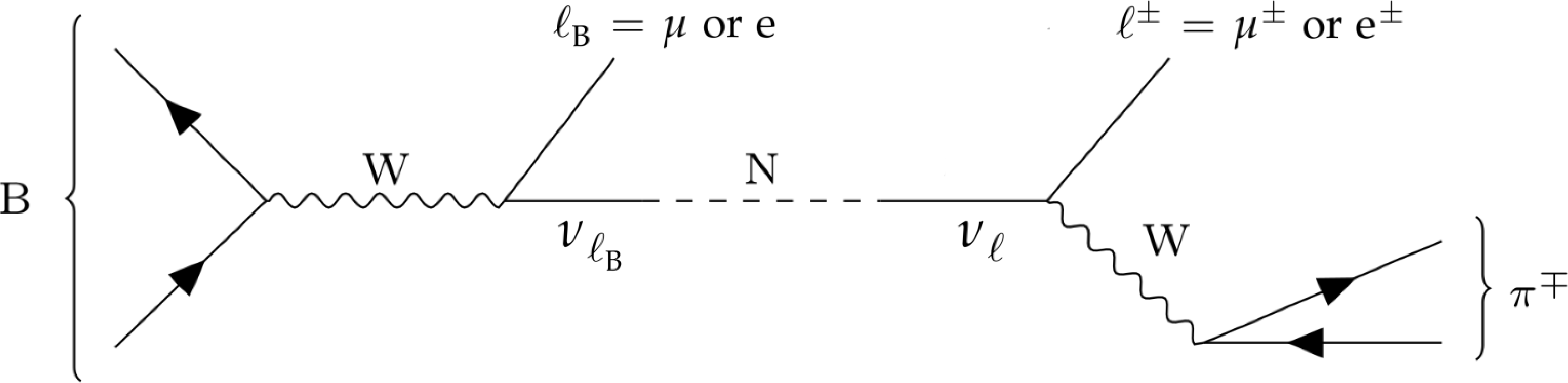
png pdf	Figure 1: Feynman diagrams showing the semileptonic (upper row) and leptonic (lower row) decay of a B meson into a lepton ($ \ell_{\mathrm{B}} $), a hadronic system (X) in case of the semileptonic decay, and a neutrino ($ \nu_{\ell_{\mathrm{B}}} $), which contains a small admixture of a heavy neutrino (N). The N mass eigenstate propagates and, according to its admixture of the neutrino flavour eigenstate ($ \nu_{\ell} $), decays weakly into a lepton $ \ell^{\pm} $ and a charged pion $ \pi^{\mp} $.
png pdf	Figure 1-a: Feynman diagrams showing the semileptonic (upper row) and leptonic (lower row) decay of a B meson into a lepton ($ \ell_{\mathrm{B}} $), a hadronic system (X) in case of the semileptonic decay, and a neutrino ($ \nu_{\ell_{\mathrm{B}}} $), which contains a small admixture of a heavy neutrino (N). The N mass eigenstate propagates and, according to its admixture of the neutrino flavour eigenstate ($ \nu_{\ell} $), decays weakly into a lepton $ \ell^{\pm} $ and a charged pion $ \pi^{\mp} $.
png pdf	Figure 1-b: Feynman diagrams showing the semileptonic (upper row) and leptonic (lower row) decay of a B meson into a lepton ($ \ell_{\mathrm{B}} $), a hadronic system (X) in case of the semileptonic decay, and a neutrino ($ \nu_{\ell_{\mathrm{B}}} $), which contains a small admixture of a heavy neutrino (N). The N mass eigenstate propagates and, according to its admixture of the neutrino flavour eigenstate ($ \nu_{\ell} $), decays weakly into a lepton $ \ell^{\pm} $ and a charged pion $ \pi^{\mp} $.
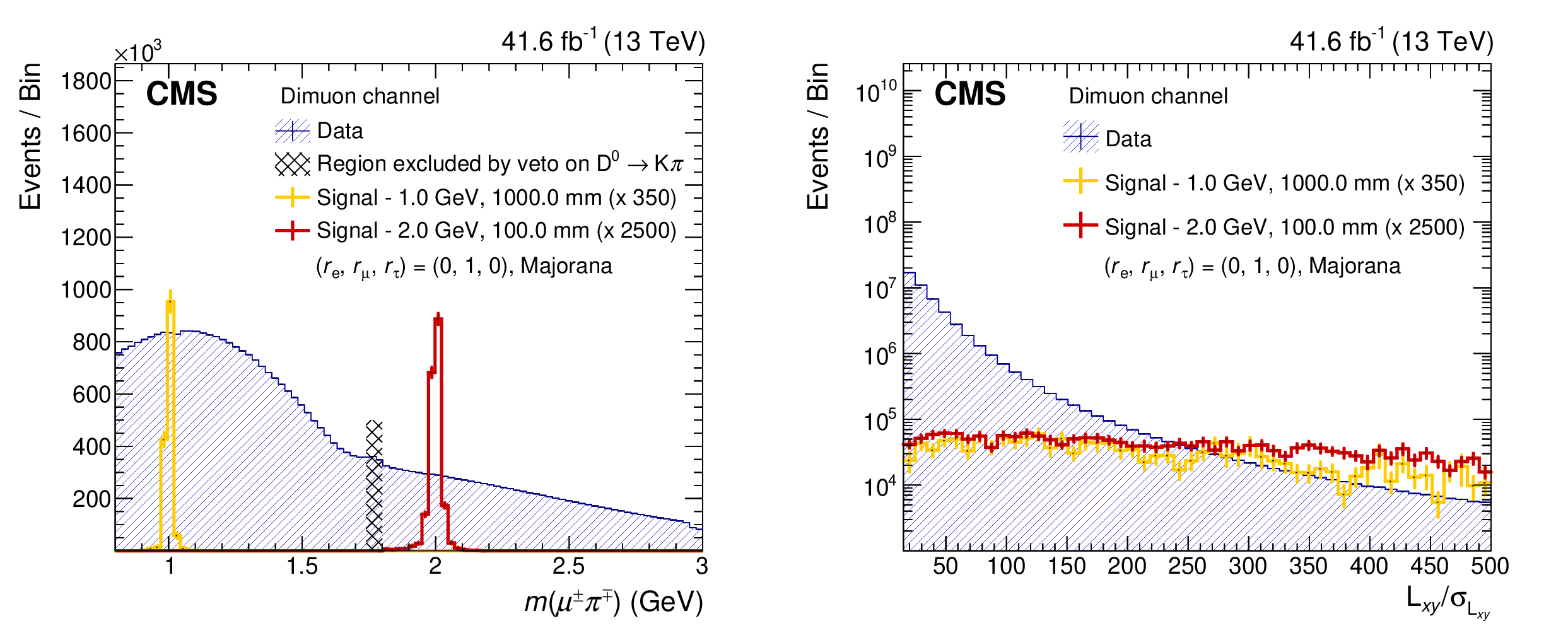
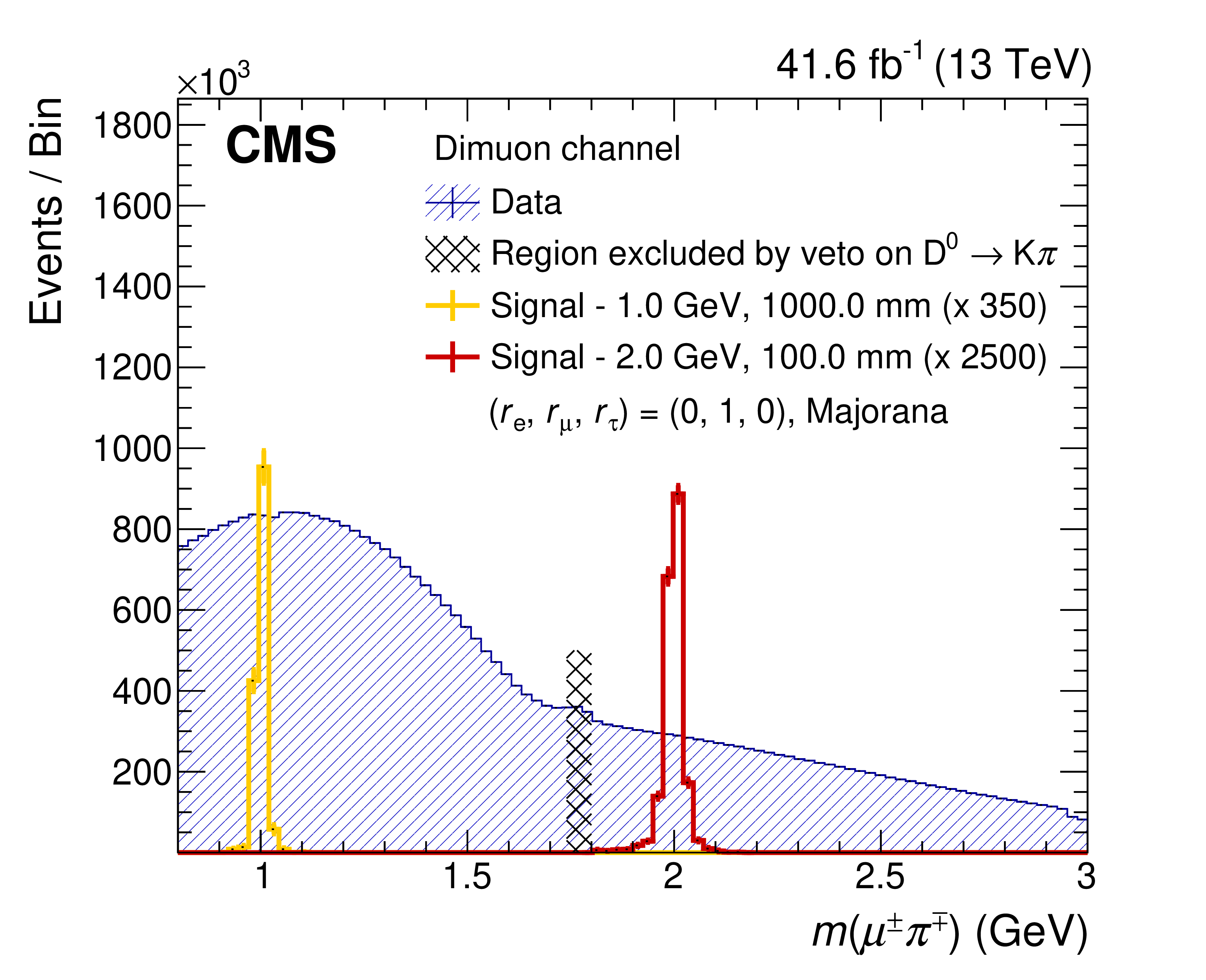
png pdf	Figure 2: Distribution of the displaced $ \mu^{\pm}\pi^{\mp} $ invariant mass (left) and $ L_{xy}/\sigma_{L_{xy}} $ (right) in data and in simulated event samples corresponding to two different signal hypotheses, in the Majorana scenario, and with the N mixing exclusively with the muon sector: $ m_\mathrm{N} = $ 1 GeV, $ c\tau_{\mathrm{N}} =$ 1000 mm, $ |V_\mathrm{N}|^2= |V_{\mu\mathrm{N}}|^2 = $ 5.4 $\times$ 10$^{-4} $; and $ m_\mathrm{N} = $ 2 GeV, $ c\tau_{\mathrm{N}} = $ 100 mm, $ |V_\mathrm{N}|^2=|V_{\mu\mathrm{N}}|^2=$ 1.7 $\times$ 10$^{-4} $. The signal distributions are scaled with factors given in the legend. The vertical lines show the statistical uncertainty in each bin.
png pdf	Figure 2-a: Distribution of the displaced $ \mu^{\pm}\pi^{\mp} $ invariant mass (left) and $ L_{xy}/\sigma_{L_{xy}} $ (right) in data and in simulated event samples corresponding to two different signal hypotheses, in the Majorana scenario, and with the N mixing exclusively with the muon sector: $ m_\mathrm{N} = $ 1 GeV, $ c\tau_{\mathrm{N}} =$ 1000 mm, $ |V_\mathrm{N}|^2= |V_{\mu\mathrm{N}}|^2 = $ 5.4 $\times$ 10$^{-4} $; and $ m_\mathrm{N} = $ 2 GeV, $ c\tau_{\mathrm{N}} = $ 100 mm, $ |V_\mathrm{N}|^2=|V_{\mu\mathrm{N}}|^2=$ 1.7 $\times$ 10$^{-4} $. The signal distributions are scaled with factors given in the legend. The vertical lines show the statistical uncertainty in each bin.
png pdf	Figure 2-b: Distribution of the displaced $ \mu^{\pm}\pi^{\mp} $ invariant mass (left) and $ L_{xy}/\sigma_{L_{xy}} $ (right) in data and in simulated event samples corresponding to two different signal hypotheses, in the Majorana scenario, and with the N mixing exclusively with the muon sector: $ m_\mathrm{N} = $ 1 GeV, $ c\tau_{\mathrm{N}} =$ 1000 mm, $ |V_\mathrm{N}|^2= |V_{\mu\mathrm{N}}|^2 = $ 5.4 $\times$ 10$^{-4} $; and $ m_\mathrm{N} = $ 2 GeV, $ c\tau_{\mathrm{N}} = $ 100 mm, $ |V_\mathrm{N}|^2=|V_{\mu\mathrm{N}}|^2=$ 1.7 $\times$ 10$^{-4} $. The signal distributions are scaled with factors given in the legend. The vertical lines show the statistical uncertainty in each bin.
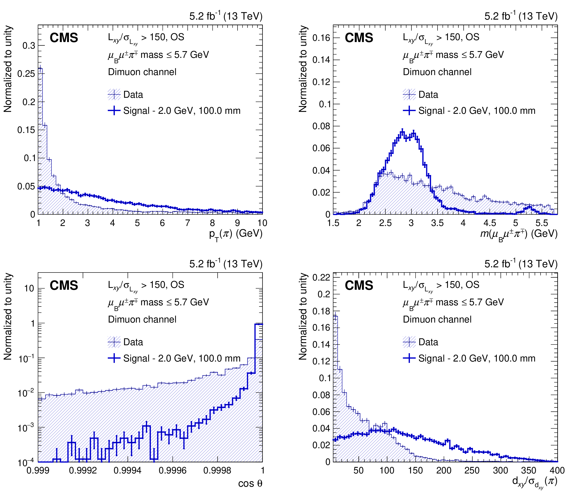
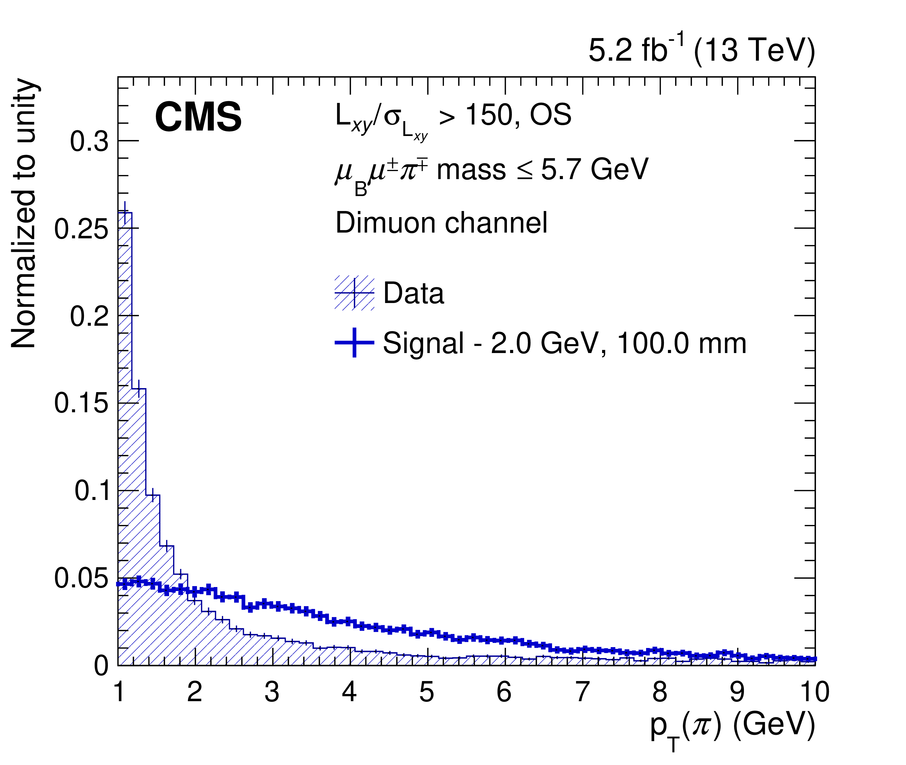
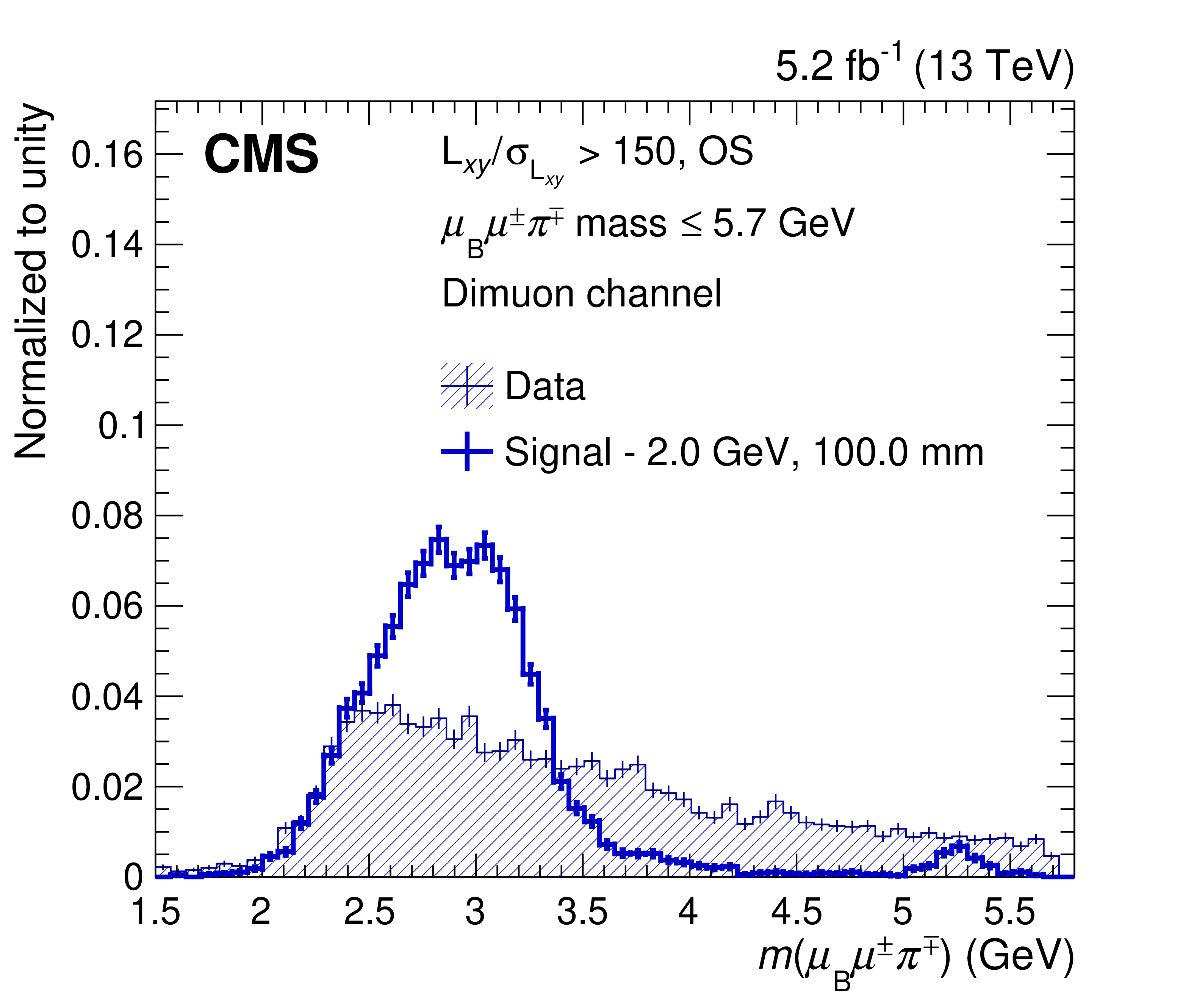
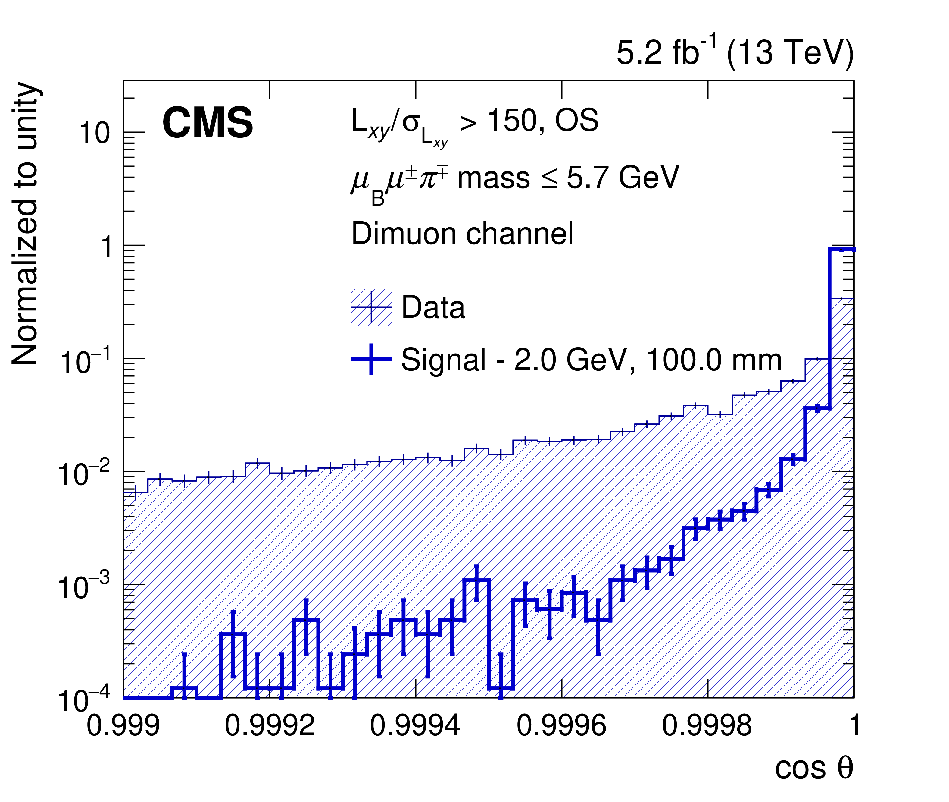
png pdf	Figure 3: The distributions of the pion $ p_{\mathrm{T}} $ (upper left), $ m(\mu_{\mathrm{B}}\mu^\pm\pi^\mp) $ (upper right), $ \cos\theta $ (lower left), and pion $ d_{xy}/\sigma_{d_{xy}} $ (lower right) are shown for data, as well as for a signal hypothesis of $ m_\mathrm{N}= $ 2 GeV and $ c\tau_{\mathrm{N}}=$ 100 mm. The data correspond to an integrated luminosity of 5.2 fb$ ^{-1} $ and are selected in the mass window of size 10 $ \sigma $ around $ m_\mathrm{N}= $ 2 GeV. The distributions, which are normalized to unit area, are shown for the dimuon channel in category with high $ L_{xy}/\sigma_{L_{xy}} $, OS, and low $ \ell_{\mathrm{B}}\ell^\pm\pi^\mp\mathrm{ mass} $. The vertical lines show the statistical uncertainty in each bin.
png pdf	Figure 3-a: The distributions of the pion $ p_{\mathrm{T}} $ (upper left), $ m(\mu_{\mathrm{B}}\mu^\pm\pi^\mp) $ (upper right), $ \cos\theta $ (lower left), and pion $ d_{xy}/\sigma_{d_{xy}} $ (lower right) are shown for data, as well as for a signal hypothesis of $ m_\mathrm{N}= $ 2 GeV and $ c\tau_{\mathrm{N}}=$ 100 mm. The data correspond to an integrated luminosity of 5.2 fb$ ^{-1} $ and are selected in the mass window of size 10 $ \sigma $ around $ m_\mathrm{N}= $ 2 GeV. The distributions, which are normalized to unit area, are shown for the dimuon channel in category with high $ L_{xy}/\sigma_{L_{xy}} $, OS, and low $ \ell_{\mathrm{B}}\ell^\pm\pi^\mp\mathrm{ mass} $. The vertical lines show the statistical uncertainty in each bin.
png pdf	Figure 3-b: The distributions of the pion $ p_{\mathrm{T}} $ (upper left), $ m(\mu_{\mathrm{B}}\mu^\pm\pi^\mp) $ (upper right), $ \cos\theta $ (lower left), and pion $ d_{xy}/\sigma_{d_{xy}} $ (lower right) are shown for data, as well as for a signal hypothesis of $ m_\mathrm{N}= $ 2 GeV and $ c\tau_{\mathrm{N}}=$ 100 mm. The data correspond to an integrated luminosity of 5.2 fb$ ^{-1} $ and are selected in the mass window of size 10 $ \sigma $ around $ m_\mathrm{N}= $ 2 GeV. The distributions, which are normalized to unit area, are shown for the dimuon channel in category with high $ L_{xy}/\sigma_{L_{xy}} $, OS, and low $ \ell_{\mathrm{B}}\ell^\pm\pi^\mp\mathrm{ mass} $. The vertical lines show the statistical uncertainty in each bin.
png pdf	Figure 3-c: The distributions of the pion $ p_{\mathrm{T}} $ (upper left), $ m(\mu_{\mathrm{B}}\mu^\pm\pi^\mp) $ (upper right), $ \cos\theta $ (lower left), and pion $ d_{xy}/\sigma_{d_{xy}} $ (lower right) are shown for data, as well as for a signal hypothesis of $ m_\mathrm{N}= $ 2 GeV and $ c\tau_{\mathrm{N}}=$ 100 mm. The data correspond to an integrated luminosity of 5.2 fb$ ^{-1} $ and are selected in the mass window of size 10 $ \sigma $ around $ m_\mathrm{N}= $ 2 GeV. The distributions, which are normalized to unit area, are shown for the dimuon channel in category with high $ L_{xy}/\sigma_{L_{xy}} $, OS, and low $ \ell_{\mathrm{B}}\ell^\pm\pi^\mp\mathrm{ mass} $. The vertical lines show the statistical uncertainty in each bin.
png pdf	Figure 3-d: The distributions of the pion $ p_{\mathrm{T}} $ (upper left), $ m(\mu_{\mathrm{B}}\mu^\pm\pi^\mp) $ (upper right), $ \cos\theta $ (lower left), and pion $ d_{xy}/\sigma_{d_{xy}} $ (lower right) are shown for data, as well as for a signal hypothesis of $ m_\mathrm{N}= $ 2 GeV and $ c\tau_{\mathrm{N}}=$ 100 mm. The data correspond to an integrated luminosity of 5.2 fb$ ^{-1} $ and are selected in the mass window of size 10 $ \sigma $ around $ m_\mathrm{N}= $ 2 GeV. The distributions, which are normalized to unit area, are shown for the dimuon channel in category with high $ L_{xy}/\sigma_{L_{xy}} $, OS, and low $ \ell_{\mathrm{B}}\ell^\pm\pi^\mp\mathrm{ mass} $. The vertical lines show the statistical uncertainty in each bin.
png pdf	Figure 4: (Left) Performance of the pNN as a function of signal mass for events in the 50 $ < L_{xy}/\sigma_{L_{xy}} < $ 150, OS, and low $ \ell_{\mathrm{B}}\ell^\pm\pi^\mp\mathrm{ mass} $ category in the dimuon channel. The performance is shown by the AUC curve, where a value at unity corresponds to a perfect separation between signal and background. The different coloured curves correspond to different $ c\tau_{\mathrm{N}} $ hypotheses. (Right) Validation of the use of a pNN for intermediate $ m_\mathrm{N} $ mass points, for events in the 50 $ < L_{xy}/\sigma_{L_{xy}} < $ 150, OS and low $ \ell_{\mathrm{B}}\ell^\pm\pi^\mp\mathrm{ mass} $ category in the dimuon channel: a pNN trained on masses $ m_\mathrm{N} = $ 1.0, 1.5, 2.0, and 3.0 GeV (blue) and a NN trained on mass $ m_\mathrm{N}= $ 2 GeV (red). All the points have $ c\tau_{\mathrm{N}}=$ 10 mm. The full circles correspond to mass points on which the pNN and NN were trained on, while the open circles show mass points that have not been trained on.
png pdf	Figure 4-a: (Left) Performance of the pNN as a function of signal mass for events in the 50 $ < L_{xy}/\sigma_{L_{xy}} < $ 150, OS, and low $ \ell_{\mathrm{B}}\ell^\pm\pi^\mp\mathrm{ mass} $ category in the dimuon channel. The performance is shown by the AUC curve, where a value at unity corresponds to a perfect separation between signal and background. The different coloured curves correspond to different $ c\tau_{\mathrm{N}} $ hypotheses. (Right) Validation of the use of a pNN for intermediate $ m_\mathrm{N} $ mass points, for events in the 50 $ < L_{xy}/\sigma_{L_{xy}} < $ 150, OS and low $ \ell_{\mathrm{B}}\ell^\pm\pi^\mp\mathrm{ mass} $ category in the dimuon channel: a pNN trained on masses $ m_\mathrm{N} = $ 1.0, 1.5, 2.0, and 3.0 GeV (blue) and a NN trained on mass $ m_\mathrm{N}= $ 2 GeV (red). All the points have $ c\tau_{\mathrm{N}}=$ 10 mm. The full circles correspond to mass points on which the pNN and NN were trained on, while the open circles show mass points that have not been trained on.
png pdf	Figure 4-b: (Left) Performance of the pNN as a function of signal mass for events in the 50 $ < L_{xy}/\sigma_{L_{xy}} < $ 150, OS, and low $ \ell_{\mathrm{B}}\ell^\pm\pi^\mp\mathrm{ mass} $ category in the dimuon channel. The performance is shown by the AUC curve, where a value at unity corresponds to a perfect separation between signal and background. The different coloured curves correspond to different $ c\tau_{\mathrm{N}} $ hypotheses. (Right) Validation of the use of a pNN for intermediate $ m_\mathrm{N} $ mass points, for events in the 50 $ < L_{xy}/\sigma_{L_{xy}} < $ 150, OS and low $ \ell_{\mathrm{B}}\ell^\pm\pi^\mp\mathrm{ mass} $ category in the dimuon channel: a pNN trained on masses $ m_\mathrm{N} = $ 1.0, 1.5, 2.0, and 3.0 GeV (blue) and a NN trained on mass $ m_\mathrm{N}= $ 2 GeV (red). All the points have $ c\tau_{\mathrm{N}}=$ 10 mm. The full circles correspond to mass points on which the pNN and NN were trained on, while the open circles show mass points that have not been trained on.
png pdf	Figure 5: Branching fractions as functions of $ m_\mathrm{N} $ for $ {\mathrm{B}}_\mathrm{q}\to\mu\mathrm{N}\mathrm{X} $ decays, $ \mathrm{q} = (\mathrm{u}, \mathrm{d}, \mathrm{s}, \mathrm{c}) $, multiplied by the corresponding fragmentation fraction, $ f_{\mathrm{q}} $. Both leptonic and semileptonic decays are considered. The results are shown for the mixing scenario $ |V_\mathrm{N}|^2=|V_{\mu\mathrm{N}}|^2= $ 1. The branching fractions are computed based on the method described in Ref. [9].
png pdf	Figure 6: Distribution of the $ \mathrm{K}^\pm\mu^+\mu^- $ invariant mass for a luminosity of 0.77 fb$ ^{-1} $. A large signal is observed at the $ {\mathrm{B}}_{\mathrm{u}} $ mass. The blue curve shows the fit to signal plus background, while the orange, green, and red curves show the contributions from the signal, composite background, and combinatorial background, respectively.
png pdf	Figure 7: Distribution of the $ \mu^\pm\pi^\mp $ invariant mass in the mass window around 1.5 GeV in the high $ L_{xy}/\sigma_{L_{xy}} $, OS, and low $ \ell_{\mathrm{B}}\ell^\pm\pi^\mp\mathrm{ mass} $ category in the dimuon channel. The result of the background-only fit to the data (red) is shown together with the mass distribution expected from a Majorana signal with $ m_\mathrm{N}= $ 1.5 GeV and $ c\tau_{\mathrm{N}}=$ 500 mm, for the case in which the N mixes with the muon sector only (green).
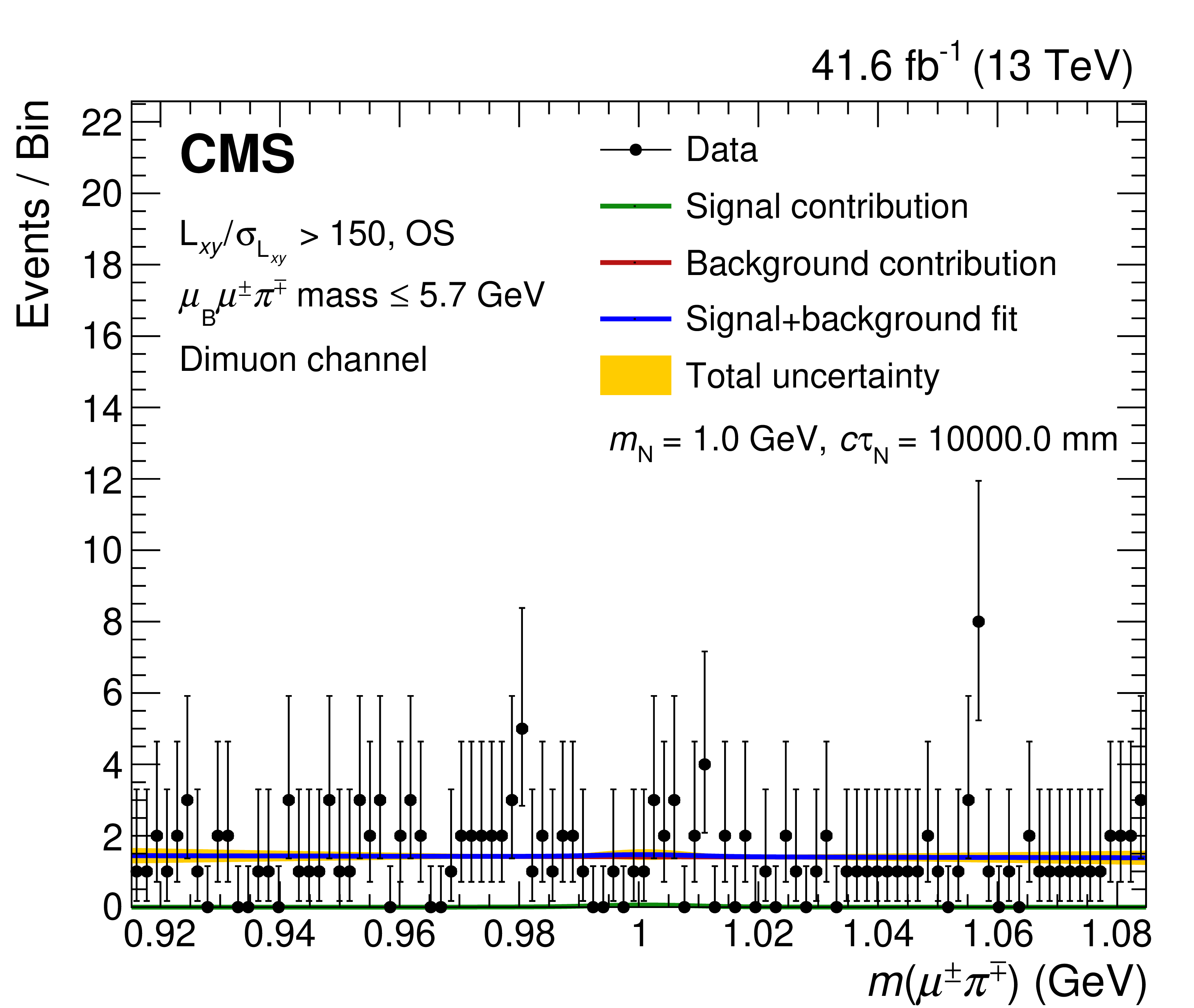
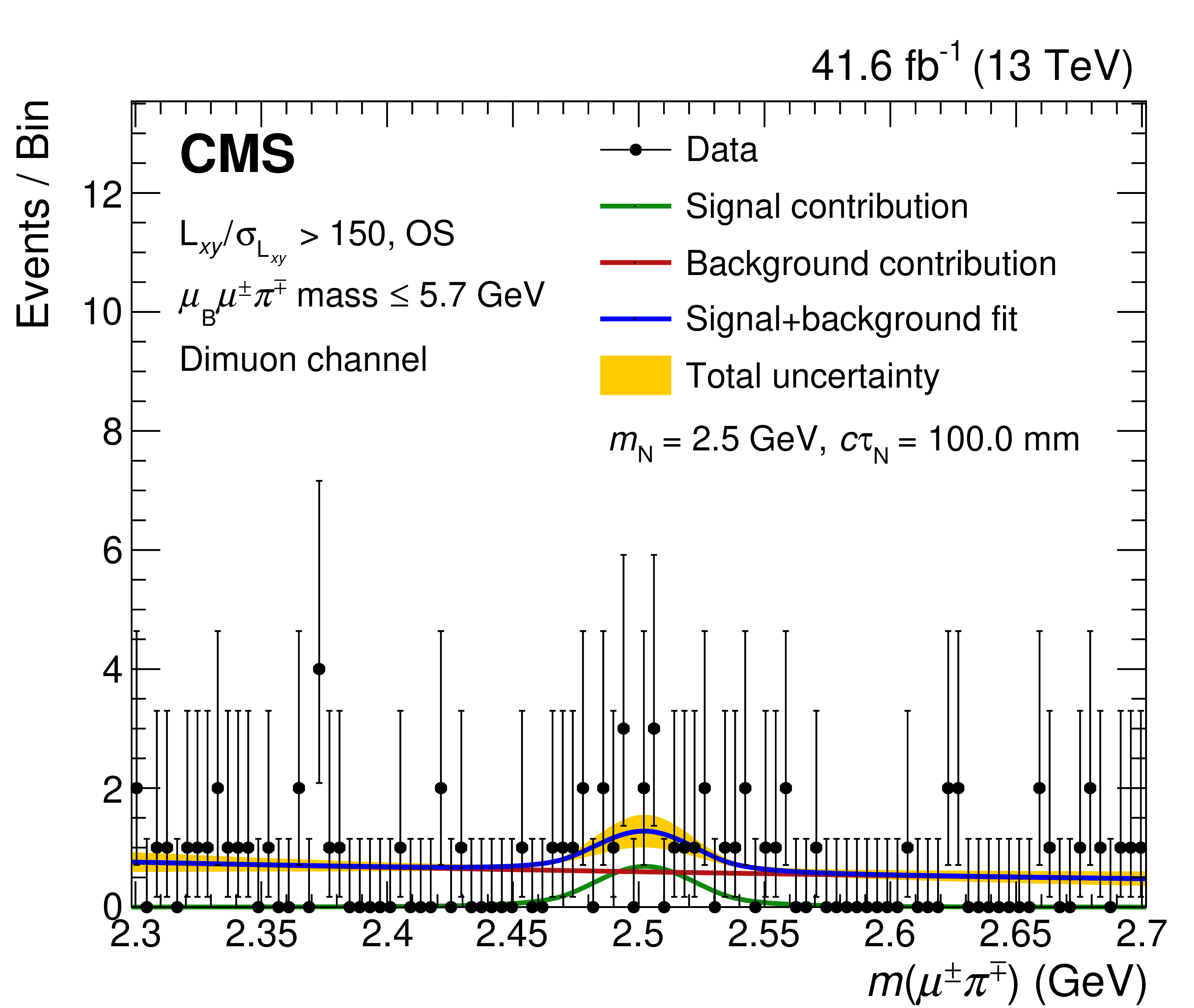
png pdf	Figure 8: Fits of the mass distribution for a signal of mass $ m_\mathrm{N}= $ 1.0 GeV (upper left), 1.5 GeV (upper right), 2.0 GeV (lower left), and 2.5 GeV (lower right), in the high $ L_{xy}/\sigma_{L_{xy}} $, OS, and low $ \ell_{\mathrm{B}}\ell^\pm\pi^\mp\mathrm{ mass} $ category of the dimuon channel. The blue curve corresponds to signal-plus-background fit, while the green and red curves indicate its individual signal and background components, respectively. The yellow band shows the total post-fit systematic plus statistical uncertainty.
png pdf	Figure 8-a: Fits of the mass distribution for a signal of mass $ m_\mathrm{N}= $ 1.0 GeV (upper left), 1.5 GeV (upper right), 2.0 GeV (lower left), and 2.5 GeV (lower right), in the high $ L_{xy}/\sigma_{L_{xy}} $, OS, and low $ \ell_{\mathrm{B}}\ell^\pm\pi^\mp\mathrm{ mass} $ category of the dimuon channel. The blue curve corresponds to signal-plus-background fit, while the green and red curves indicate its individual signal and background components, respectively. The yellow band shows the total post-fit systematic plus statistical uncertainty.
png pdf	Figure 8-b: Fits of the mass distribution for a signal of mass $ m_\mathrm{N}= $ 1.0 GeV (upper left), 1.5 GeV (upper right), 2.0 GeV (lower left), and 2.5 GeV (lower right), in the high $ L_{xy}/\sigma_{L_{xy}} $, OS, and low $ \ell_{\mathrm{B}}\ell^\pm\pi^\mp\mathrm{ mass} $ category of the dimuon channel. The blue curve corresponds to signal-plus-background fit, while the green and red curves indicate its individual signal and background components, respectively. The yellow band shows the total post-fit systematic plus statistical uncertainty.
png pdf	Figure 8-c: Fits of the mass distribution for a signal of mass $ m_\mathrm{N}= $ 1.0 GeV (upper left), 1.5 GeV (upper right), 2.0 GeV (lower left), and 2.5 GeV (lower right), in the high $ L_{xy}/\sigma_{L_{xy}} $, OS, and low $ \ell_{\mathrm{B}}\ell^\pm\pi^\mp\mathrm{ mass} $ category of the dimuon channel. The blue curve corresponds to signal-plus-background fit, while the green and red curves indicate its individual signal and background components, respectively. The yellow band shows the total post-fit systematic plus statistical uncertainty.
png pdf	Figure 8-d: Fits of the mass distribution for a signal of mass $ m_\mathrm{N}= $ 1.0 GeV (upper left), 1.5 GeV (upper right), 2.0 GeV (lower left), and 2.5 GeV (lower right), in the high $ L_{xy}/\sigma_{L_{xy}} $, OS, and low $ \ell_{\mathrm{B}}\ell^\pm\pi^\mp\mathrm{ mass} $ category of the dimuon channel. The blue curve corresponds to signal-plus-background fit, while the green and red curves indicate its individual signal and background components, respectively. The yellow band shows the total post-fit systematic plus statistical uncertainty.
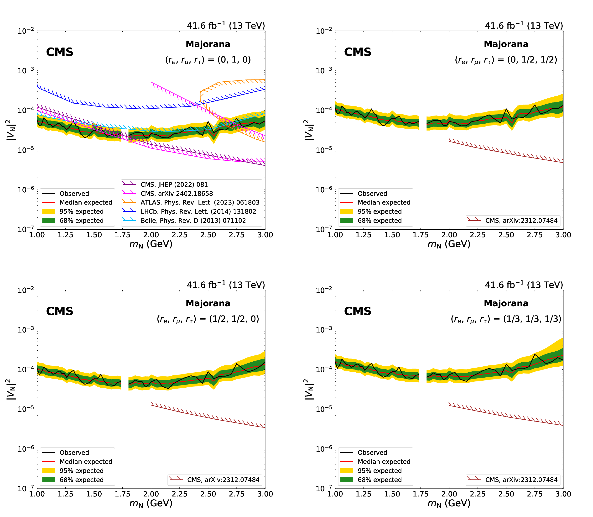
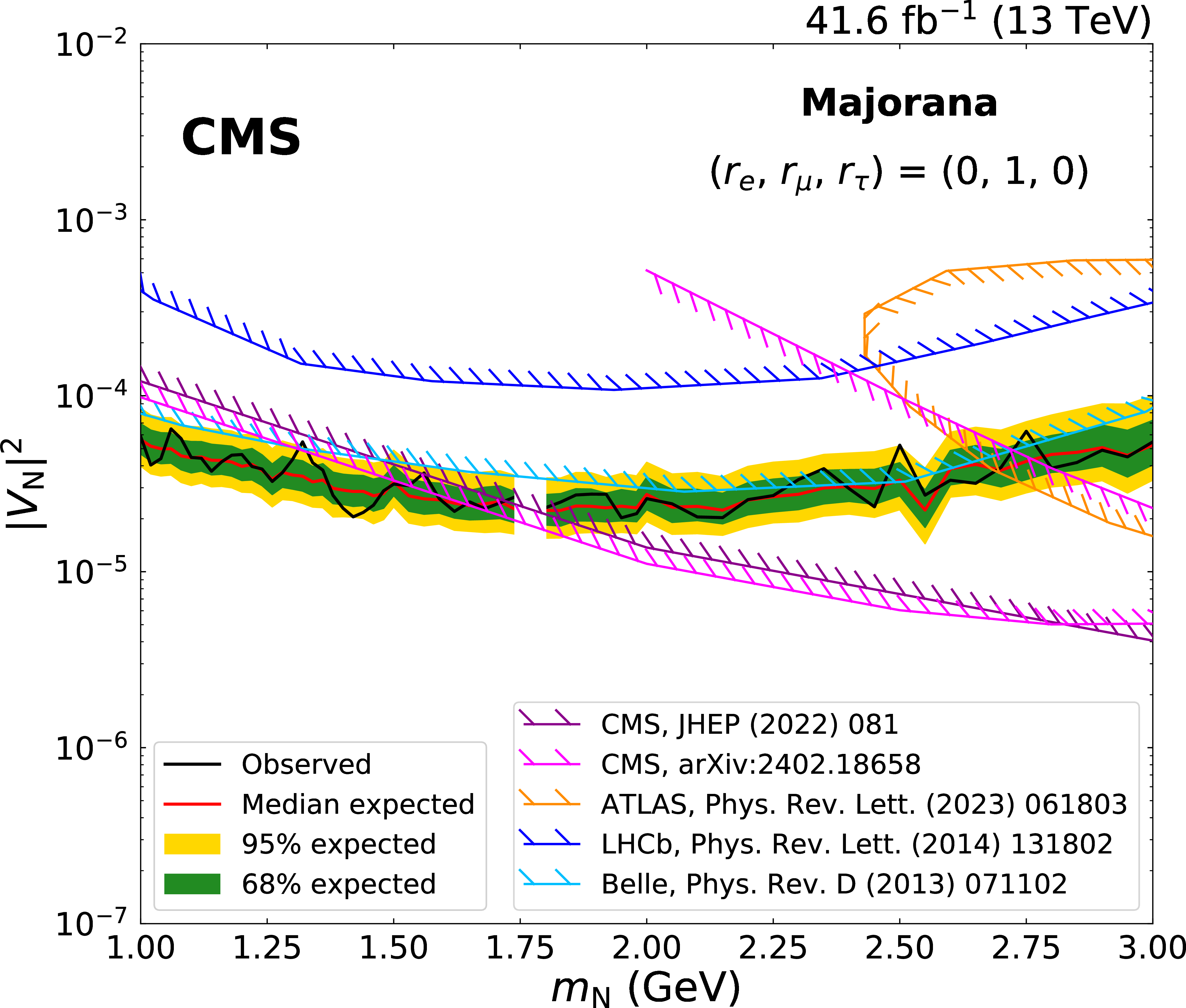
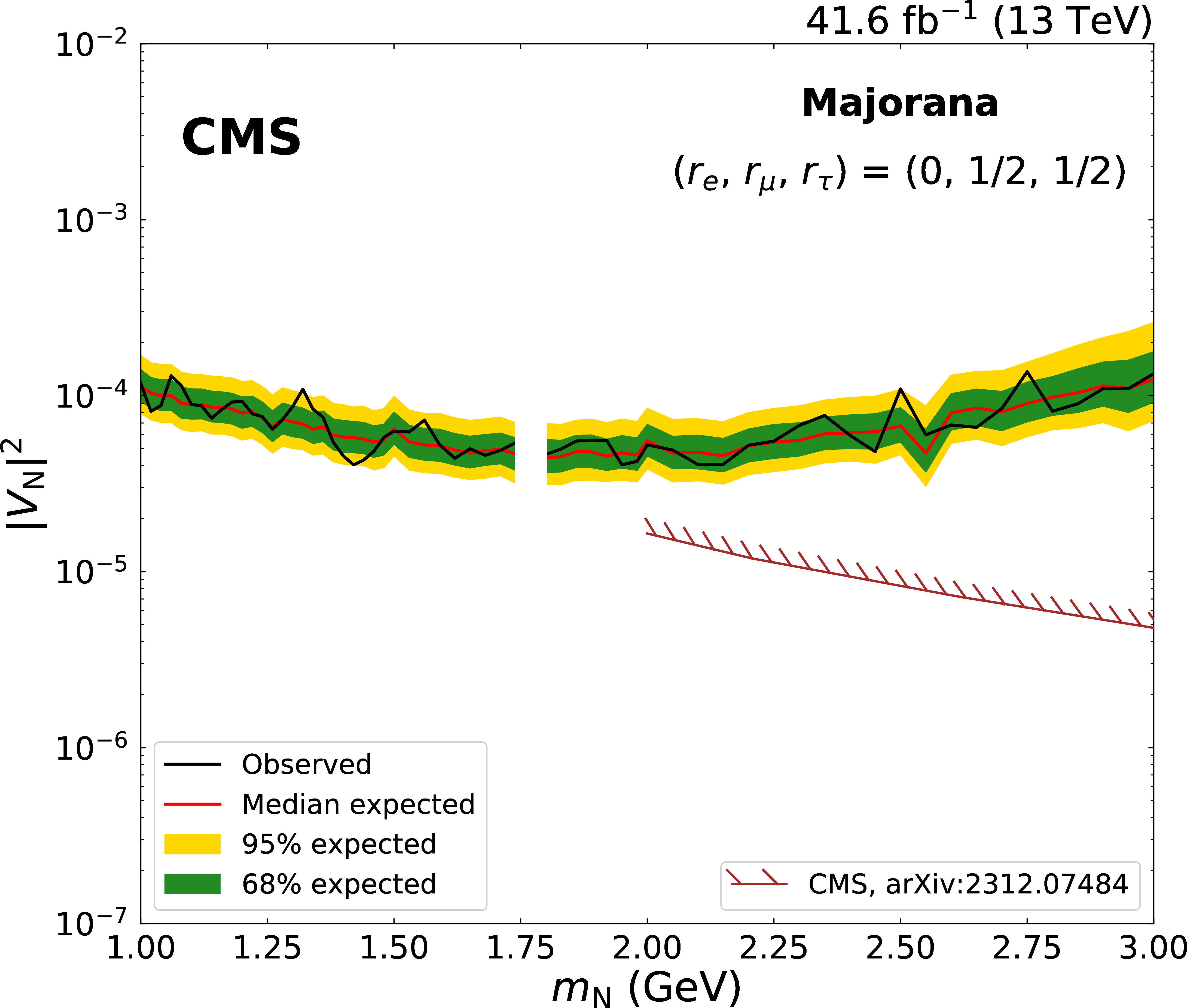
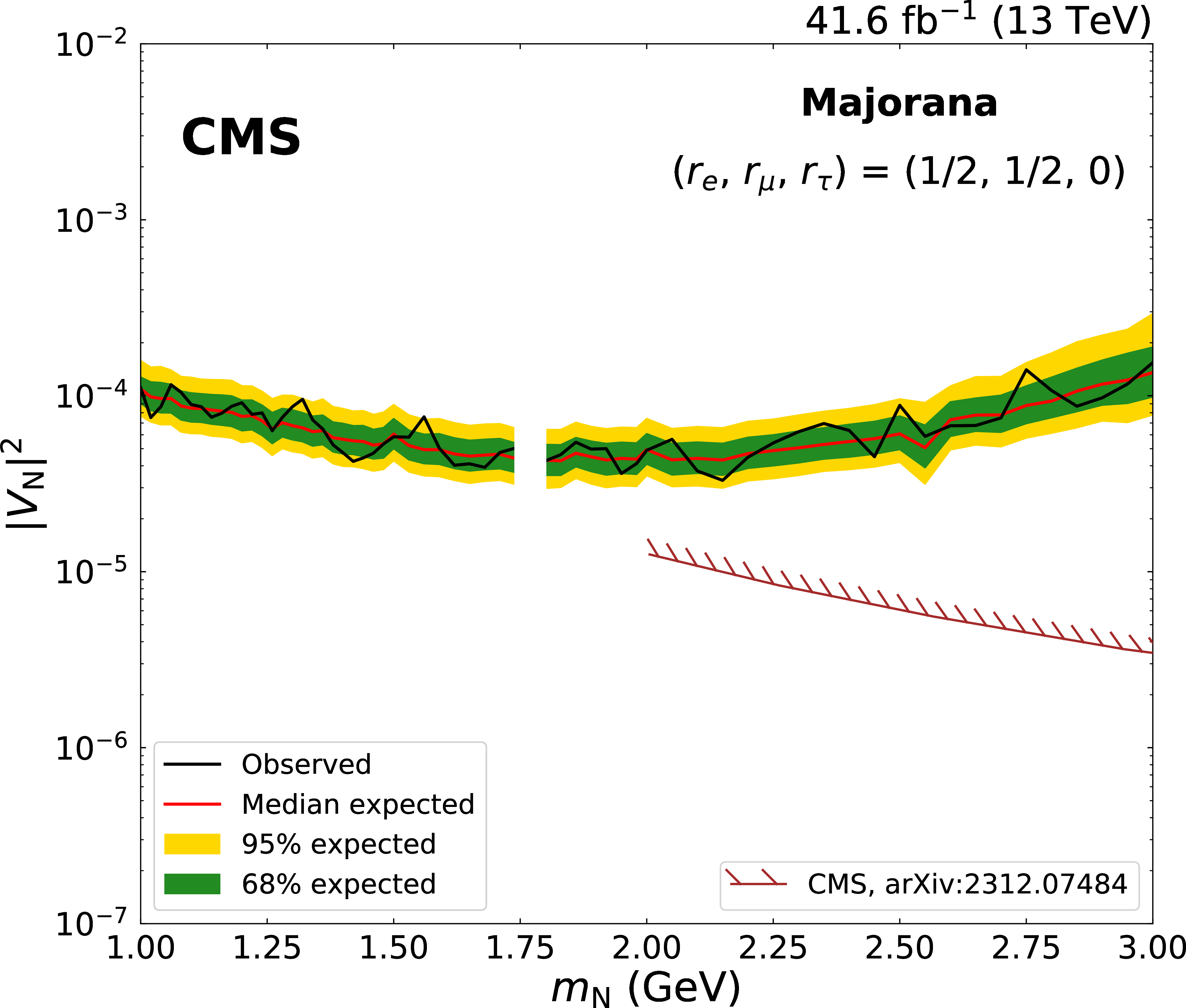
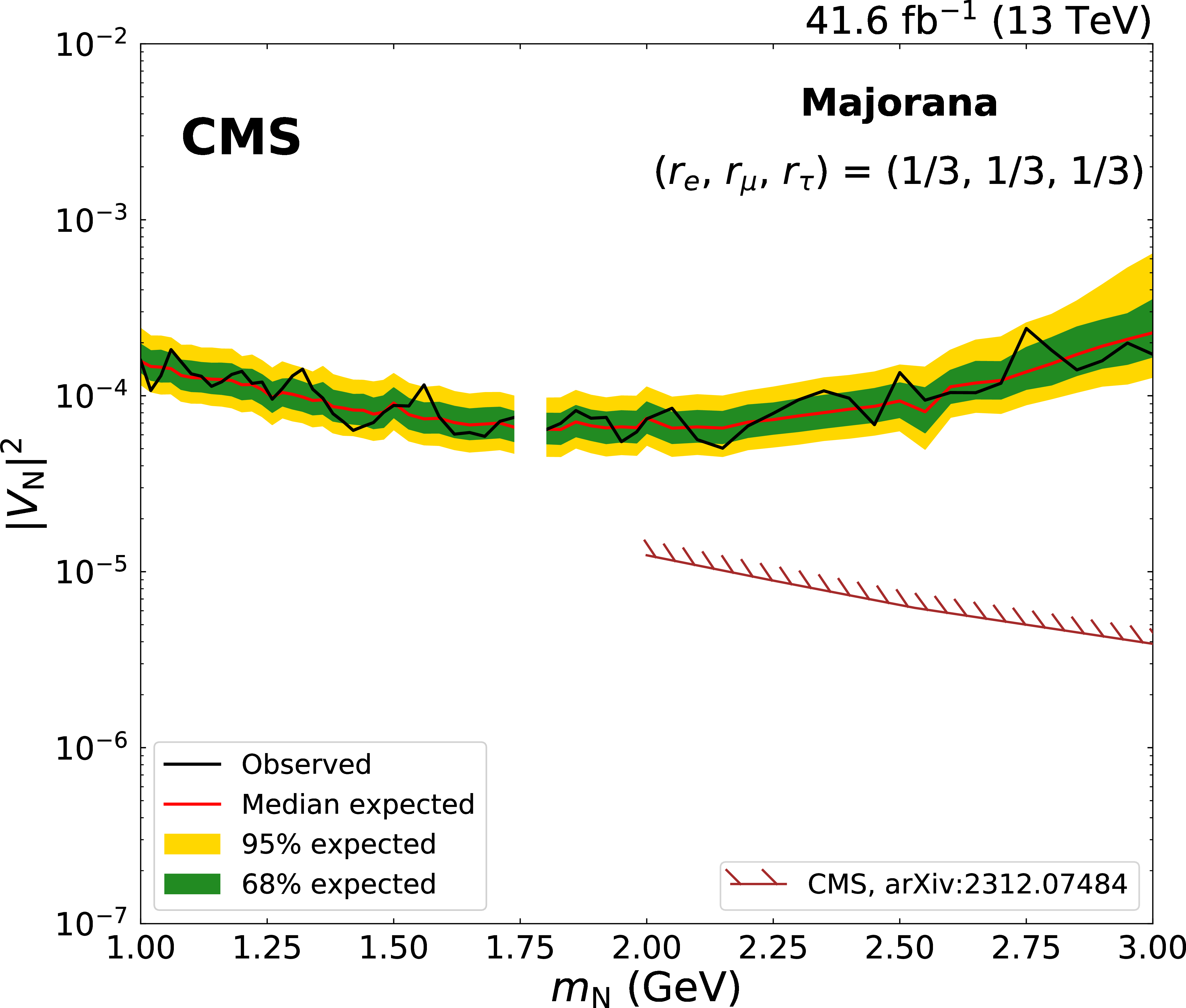
png pdf	Figure 9: Expected and observed 95% CL limits on $ |V_\mathrm{N}|^2 $ as a function of $ m_\mathrm{N} $, in the Majorana scenario. On the upper row, the limits are derived uniquely with the dimuon channel, and are shown for the mixing scenarios ($ r_\mathrm{e} $, $ r_\mu $, $ r_\tau $) $= $(0, 1, 0) on the left and for ($ r_\mathrm{e} $, $ r_\mu $, $ r_\tau $) $=$ (0, 1/2, 1/2) on the right; on the lower row, the limits are obtained with the dimuon and mixed-flavour channel combined, for the mixing scenarios ($ r_\mathrm{e} $, $ r_\mu $, $ r_\tau $) $=$ (1/2, 1/2, 0) on the left and for ($ r_\mathrm{e} $, $ r_\mu $, $ r_\tau $) $=$ (1/3, 1/3, 1/3) on the right. In the upper left figure, results from the CMS [21,23], ATLAS [17], LHCb [24], and Belle [14] Collaborations are shown as a comparison; in the other figures, results from the CMS Collaboration [22] are reported. The mass range with no results shown corresponds to the $ \mathrm{D^0} $ meson veto listed in the lower part of Table 1.
png pdf	Figure 9-a: Expected and observed 95% CL limits on $ |V_\mathrm{N}|^2 $ as a function of $ m_\mathrm{N} $, in the Majorana scenario. On the upper row, the limits are derived uniquely with the dimuon channel, and are shown for the mixing scenarios ($ r_\mathrm{e} $, $ r_\mu $, $ r_\tau $) $= $(0, 1, 0) on the left and for ($ r_\mathrm{e} $, $ r_\mu $, $ r_\tau $) $=$ (0, 1/2, 1/2) on the right; on the lower row, the limits are obtained with the dimuon and mixed-flavour channel combined, for the mixing scenarios ($ r_\mathrm{e} $, $ r_\mu $, $ r_\tau $) $=$ (1/2, 1/2, 0) on the left and for ($ r_\mathrm{e} $, $ r_\mu $, $ r_\tau $) $=$ (1/3, 1/3, 1/3) on the right. In the upper left figure, results from the CMS [21,23], ATLAS [17], LHCb [24], and Belle [14] Collaborations are shown as a comparison; in the other figures, results from the CMS Collaboration [22] are reported. The mass range with no results shown corresponds to the $ \mathrm{D^0} $ meson veto listed in the lower part of Table 1.
png pdf	Figure 9-b: Expected and observed 95% CL limits on $ |V_\mathrm{N}|^2 $ as a function of $ m_\mathrm{N} $, in the Majorana scenario. On the upper row, the limits are derived uniquely with the dimuon channel, and are shown for the mixing scenarios ($ r_\mathrm{e} $, $ r_\mu $, $ r_\tau $) $= $(0, 1, 0) on the left and for ($ r_\mathrm{e} $, $ r_\mu $, $ r_\tau $) $=$ (0, 1/2, 1/2) on the right; on the lower row, the limits are obtained with the dimuon and mixed-flavour channel combined, for the mixing scenarios ($ r_\mathrm{e} $, $ r_\mu $, $ r_\tau $) $=$ (1/2, 1/2, 0) on the left and for ($ r_\mathrm{e} $, $ r_\mu $, $ r_\tau $) $=$ (1/3, 1/3, 1/3) on the right. In the upper left figure, results from the CMS [21,23], ATLAS [17], LHCb [24], and Belle [14] Collaborations are shown as a comparison; in the other figures, results from the CMS Collaboration [22] are reported. The mass range with no results shown corresponds to the $ \mathrm{D^0} $ meson veto listed in the lower part of Table 1.
png pdf	Figure 9-c: Expected and observed 95% CL limits on $ |V_\mathrm{N}|^2 $ as a function of $ m_\mathrm{N} $, in the Majorana scenario. On the upper row, the limits are derived uniquely with the dimuon channel, and are shown for the mixing scenarios ($ r_\mathrm{e} $, $ r_\mu $, $ r_\tau $) $= $(0, 1, 0) on the left and for ($ r_\mathrm{e} $, $ r_\mu $, $ r_\tau $) $=$ (0, 1/2, 1/2) on the right; on the lower row, the limits are obtained with the dimuon and mixed-flavour channel combined, for the mixing scenarios ($ r_\mathrm{e} $, $ r_\mu $, $ r_\tau $) $=$ (1/2, 1/2, 0) on the left and for ($ r_\mathrm{e} $, $ r_\mu $, $ r_\tau $) $=$ (1/3, 1/3, 1/3) on the right. In the upper left figure, results from the CMS [21,23], ATLAS [17], LHCb [24], and Belle [14] Collaborations are shown as a comparison; in the other figures, results from the CMS Collaboration [22] are reported. The mass range with no results shown corresponds to the $ \mathrm{D^0} $ meson veto listed in the lower part of Table 1.
png pdf	Figure 9-d: Expected and observed 95% CL limits on $ |V_\mathrm{N}|^2 $ as a function of $ m_\mathrm{N} $, in the Majorana scenario. On the upper row, the limits are derived uniquely with the dimuon channel, and are shown for the mixing scenarios ($ r_\mathrm{e} $, $ r_\mu $, $ r_\tau $) $= $(0, 1, 0) on the left and for ($ r_\mathrm{e} $, $ r_\mu $, $ r_\tau $) $=$ (0, 1/2, 1/2) on the right; on the lower row, the limits are obtained with the dimuon and mixed-flavour channel combined, for the mixing scenarios ($ r_\mathrm{e} $, $ r_\mu $, $ r_\tau $) $=$ (1/2, 1/2, 0) on the left and for ($ r_\mathrm{e} $, $ r_\mu $, $ r_\tau $) $=$ (1/3, 1/3, 1/3) on the right. In the upper left figure, results from the CMS [21,23], ATLAS [17], LHCb [24], and Belle [14] Collaborations are shown as a comparison; in the other figures, results from the CMS Collaboration [22] are reported. The mass range with no results shown corresponds to the $ \mathrm{D^0} $ meson veto listed in the lower part of Table 1.
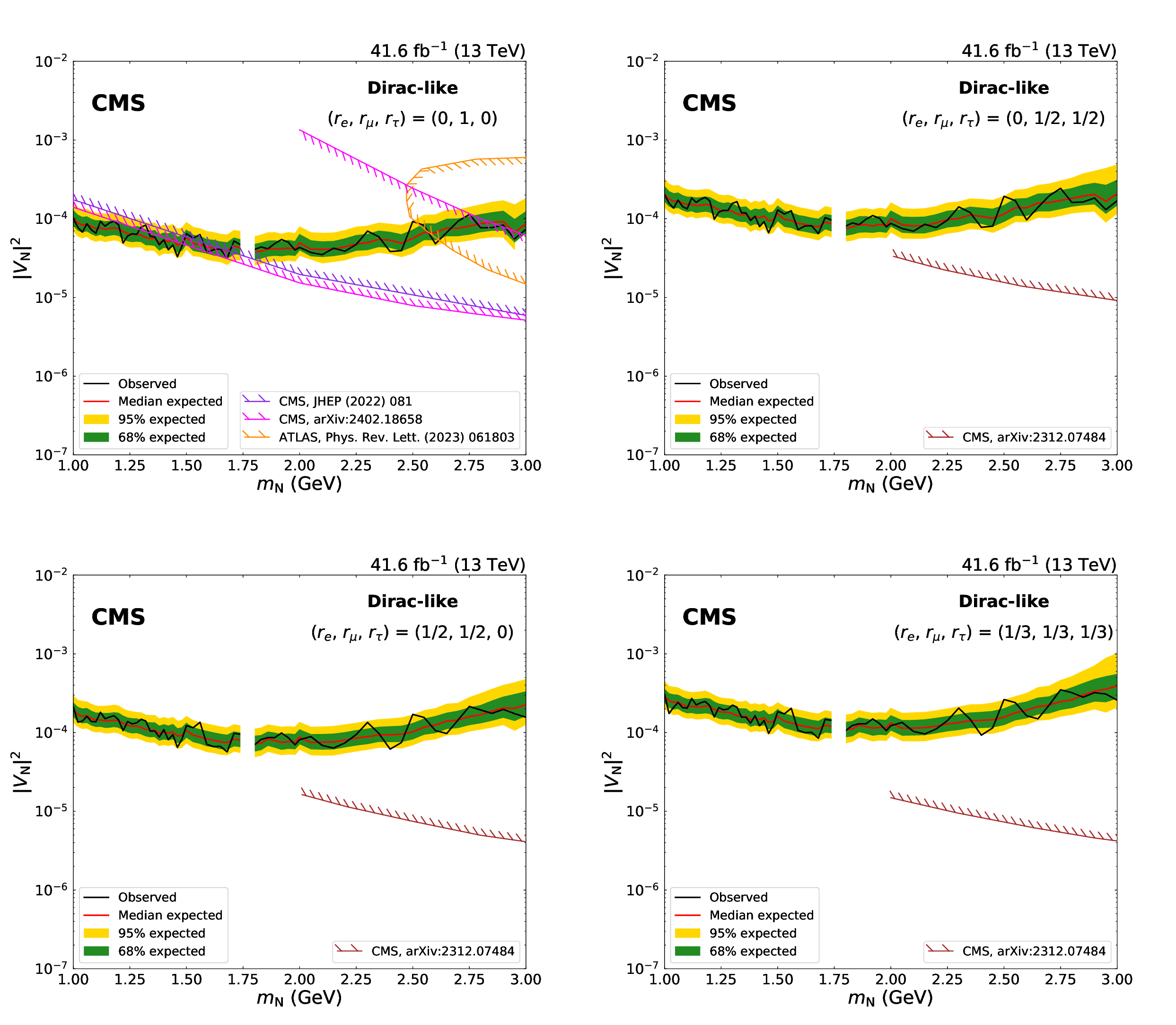
png pdf	Figure 10: Expected and observed 95% CL limits on $ |V_\mathrm{N}|^2 $ as a function of $ m_\mathrm{N} $, in the Dirac-like scenario. On the upper row, the limits are derived uniquely with the dimuon channel, and are shown for the mixing scenarios ($ r_\mathrm{e} $, $ r_\mu $, $ r_\tau $) $=$ (0, 1, 0) on the left and for ($ r_\mathrm{e} $, $ r_\mu $, $ r_\tau $) = (0, 1/2, 1/2) on the right; on the lower row, the limits are obtained with the dimuon and mixed-flavour channel combined, for the mixing scenarios ($ r_\mathrm{e} $, $ r_\mu $, $ r_\tau $) $=$ (1/2, 1/2, 0) on the left and for ($ r_\mathrm{e} $, $ r_\mu $, $ r_\tau $) $=$ (1/3, 1/3, 1/3) on the right. In the upper left figure, results from the CMS [21,23] and ATLAS [17] Collaborations are shown as a comparison; in the other figures, results from the CMS Collaboration [22] are reported. The mass range with no results shown corresponds to the $ \mathrm{D^0} $ meson veto listed in the lower part of Table 1.
png pdf	Figure 10-a: Expected and observed 95% CL limits on $ |V_\mathrm{N}|^2 $ as a function of $ m_\mathrm{N} $, in the Dirac-like scenario. On the upper row, the limits are derived uniquely with the dimuon channel, and are shown for the mixing scenarios ($ r_\mathrm{e} $, $ r_\mu $, $ r_\tau $) $=$ (0, 1, 0) on the left and for ($ r_\mathrm{e} $, $ r_\mu $, $ r_\tau $) = (0, 1/2, 1/2) on the right; on the lower row, the limits are obtained with the dimuon and mixed-flavour channel combined, for the mixing scenarios ($ r_\mathrm{e} $, $ r_\mu $, $ r_\tau $) $=$ (1/2, 1/2, 0) on the left and for ($ r_\mathrm{e} $, $ r_\mu $, $ r_\tau $) $=$ (1/3, 1/3, 1/3) on the right. In the upper left figure, results from the CMS [21,23] and ATLAS [17] Collaborations are shown as a comparison; in the other figures, results from the CMS Collaboration [22] are reported. The mass range with no results shown corresponds to the $ \mathrm{D^0} $ meson veto listed in the lower part of Table 1.
png pdf	Figure 10-b: Expected and observed 95% CL limits on $ |V_\mathrm{N}|^2 $ as a function of $ m_\mathrm{N} $, in the Dirac-like scenario. On the upper row, the limits are derived uniquely with the dimuon channel, and are shown for the mixing scenarios ($ r_\mathrm{e} $, $ r_\mu $, $ r_\tau $) $=$ (0, 1, 0) on the left and for ($ r_\mathrm{e} $, $ r_\mu $, $ r_\tau $) = (0, 1/2, 1/2) on the right; on the lower row, the limits are obtained with the dimuon and mixed-flavour channel combined, for the mixing scenarios ($ r_\mathrm{e} $, $ r_\mu $, $ r_\tau $) $=$ (1/2, 1/2, 0) on the left and for ($ r_\mathrm{e} $, $ r_\mu $, $ r_\tau $) $=$ (1/3, 1/3, 1/3) on the right. In the upper left figure, results from the CMS [21,23] and ATLAS [17] Collaborations are shown as a comparison; in the other figures, results from the CMS Collaboration [22] are reported. The mass range with no results shown corresponds to the $ \mathrm{D^0} $ meson veto listed in the lower part of Table 1.
png pdf	Figure 10-c: Expected and observed 95% CL limits on $ |V_\mathrm{N}|^2 $ as a function of $ m_\mathrm{N} $, in the Dirac-like scenario. On the upper row, the limits are derived uniquely with the dimuon channel, and are shown for the mixing scenarios ($ r_\mathrm{e} $, $ r_\mu $, $ r_\tau $) $=$ (0, 1, 0) on the left and for ($ r_\mathrm{e} $, $ r_\mu $, $ r_\tau $) = (0, 1/2, 1/2) on the right; on the lower row, the limits are obtained with the dimuon and mixed-flavour channel combined, for the mixing scenarios ($ r_\mathrm{e} $, $ r_\mu $, $ r_\tau $) $=$ (1/2, 1/2, 0) on the left and for ($ r_\mathrm{e} $, $ r_\mu $, $ r_\tau $) $=$ (1/3, 1/3, 1/3) on the right. In the upper left figure, results from the CMS [21,23] and ATLAS [17] Collaborations are shown as a comparison; in the other figures, results from the CMS Collaboration [22] are reported. The mass range with no results shown corresponds to the $ \mathrm{D^0} $ meson veto listed in the lower part of Table 1.
png pdf	Figure 10-d: Expected and observed 95% CL limits on $ |V_\mathrm{N}|^2 $ as a function of $ m_\mathrm{N} $, in the Dirac-like scenario. On the upper row, the limits are derived uniquely with the dimuon channel, and are shown for the mixing scenarios ($ r_\mathrm{e} $, $ r_\mu $, $ r_\tau $) $=$ (0, 1, 0) on the left and for ($ r_\mathrm{e} $, $ r_\mu $, $ r_\tau $) = (0, 1/2, 1/2) on the right; on the lower row, the limits are obtained with the dimuon and mixed-flavour channel combined, for the mixing scenarios ($ r_\mathrm{e} $, $ r_\mu $, $ r_\tau $) $=$ (1/2, 1/2, 0) on the left and for ($ r_\mathrm{e} $, $ r_\mu $, $ r_\tau $) $=$ (1/3, 1/3, 1/3) on the right. In the upper left figure, results from the CMS [21,23] and ATLAS [17] Collaborations are shown as a comparison; in the other figures, results from the CMS Collaboration [22] are reported. The mass range with no results shown corresponds to the $ \mathrm{D^0} $ meson veto listed in the lower part of Table 1.
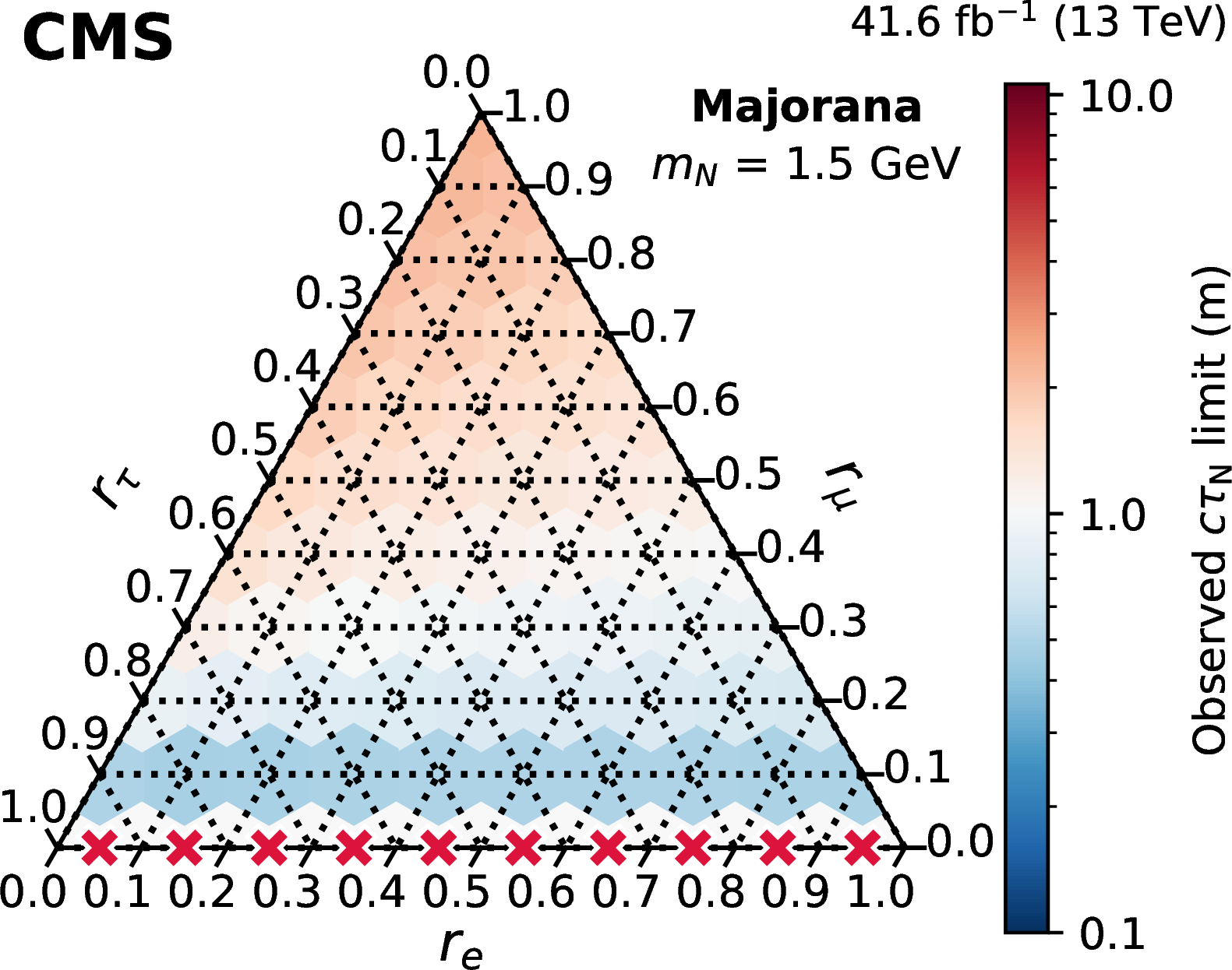
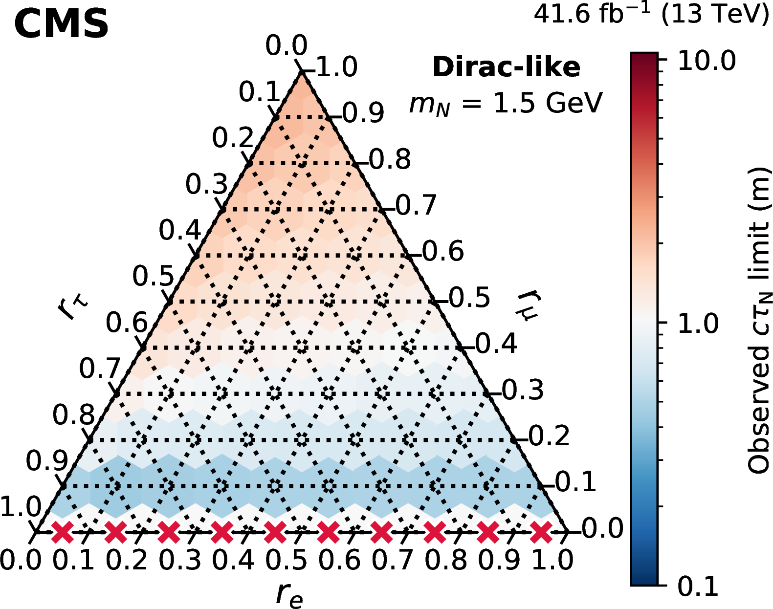
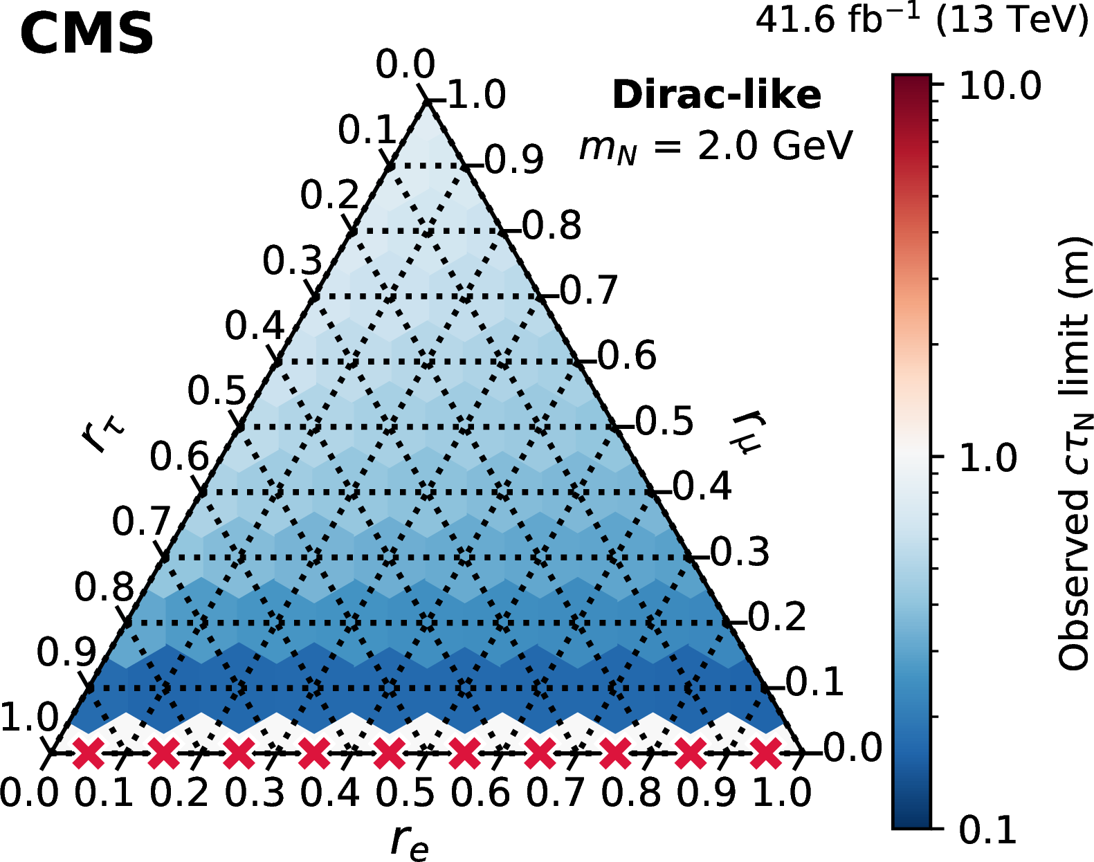
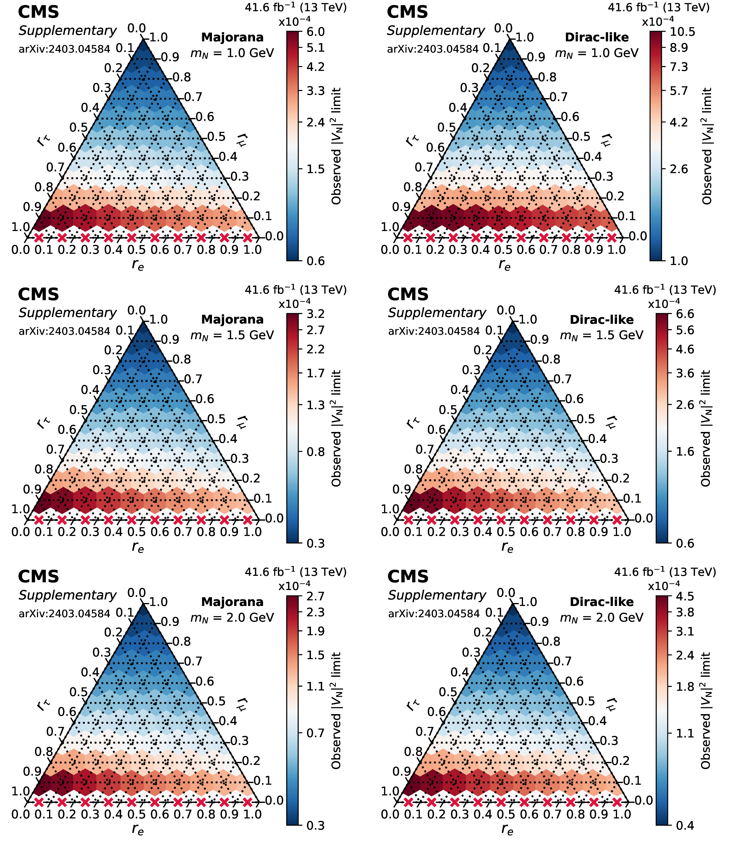
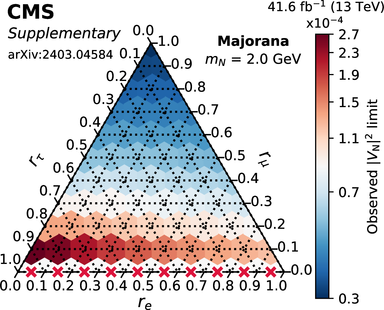
png pdf	Figure 11: Observed 95% CL lower limits on $ c\tau_{\mathrm{N}} $ as functions of the mixing ratios ($ r_\mathrm{e} $, $ r_\mu $, $ r_\tau $) for fixed N masses of 1 GeV (upper row), 1.5 GeV (middle row), and 2 GeV (lower row), in the Majorana (left column) and Dirac-like (right column) scenarios. The red crosses indicate that there is no exclusion found for that point. The orientation of the value markers on each axis identifies the associated internal lines on the plot.
png pdf	Figure 11-a: Observed 95% CL lower limits on $ c\tau_{\mathrm{N}} $ as functions of the mixing ratios ($ r_\mathrm{e} $, $ r_\mu $, $ r_\tau $) for fixed N masses of 1 GeV (upper row), 1.5 GeV (middle row), and 2 GeV (lower row), in the Majorana (left column) and Dirac-like (right column) scenarios. The red crosses indicate that there is no exclusion found for that point. The orientation of the value markers on each axis identifies the associated internal lines on the plot.
png pdf	Figure 11-b: Observed 95% CL lower limits on $ c\tau_{\mathrm{N}} $ as functions of the mixing ratios ($ r_\mathrm{e} $, $ r_\mu $, $ r_\tau $) for fixed N masses of 1 GeV (upper row), 1.5 GeV (middle row), and 2 GeV (lower row), in the Majorana (left column) and Dirac-like (right column) scenarios. The red crosses indicate that there is no exclusion found for that point. The orientation of the value markers on each axis identifies the associated internal lines on the plot.
png pdf	Figure 11-c: Observed 95% CL lower limits on $ c\tau_{\mathrm{N}} $ as functions of the mixing ratios ($ r_\mathrm{e} $, $ r_\mu $, $ r_\tau $) for fixed N masses of 1 GeV (upper row), 1.5 GeV (middle row), and 2 GeV (lower row), in the Majorana (left column) and Dirac-like (right column) scenarios. The red crosses indicate that there is no exclusion found for that point. The orientation of the value markers on each axis identifies the associated internal lines on the plot.
png pdf	Figure 11-d: Observed 95% CL lower limits on $ c\tau_{\mathrm{N}} $ as functions of the mixing ratios ($ r_\mathrm{e} $, $ r_\mu $, $ r_\tau $) for fixed N masses of 1 GeV (upper row), 1.5 GeV (middle row), and 2 GeV (lower row), in the Majorana (left column) and Dirac-like (right column) scenarios. The red crosses indicate that there is no exclusion found for that point. The orientation of the value markers on each axis identifies the associated internal lines on the plot.
png pdf	Figure 11-e: Observed 95% CL lower limits on $ c\tau_{\mathrm{N}} $ as functions of the mixing ratios ($ r_\mathrm{e} $, $ r_\mu $, $ r_\tau $) for fixed N masses of 1 GeV (upper row), 1.5 GeV (middle row), and 2 GeV (lower row), in the Majorana (left column) and Dirac-like (right column) scenarios. The red crosses indicate that there is no exclusion found for that point. The orientation of the value markers on each axis identifies the associated internal lines on the plot.
png pdf	Figure 11-f: Observed 95% CL lower limits on $ c\tau_{\mathrm{N}} $ as functions of the mixing ratios ($ r_\mathrm{e} $, $ r_\mu $, $ r_\tau $) for fixed N masses of 1 GeV (upper row), 1.5 GeV (middle row), and 2 GeV (lower row), in the Majorana (left column) and Dirac-like (right column) scenarios. The red crosses indicate that there is no exclusion found for that point. The orientation of the value markers on each axis identifies the associated internal lines on the plot.

Tables
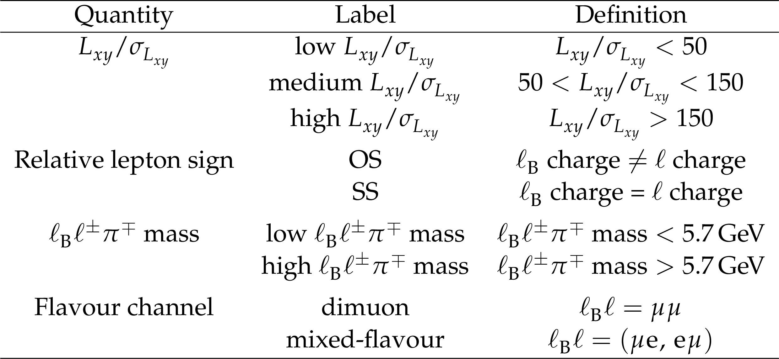
png pdf	Table 1: List of considered SM resonances and the corresponding vetoes in the various two-particle invariant mass spectra. The first seven lines consider any possible opposite-sign pair comprising the lepton originating from the B decay and either of the displaced $ \ell^{\pm} $ and $ \pi^{\mp} $. Events that fail the veto conditions are removed from the analysis. The last two lines pertain to the displaced $ \ell^{\pm}\pi^{\mp} $ candidate and indicate that the signal extraction is not performed and exclusion limits are not provided for $ m_\mathrm{N} $ in the vetoed regions. The presence of misidentified particles is also indicated. For the $ \mathrm{D^0} $ meson vetoes, the mass range is adjusted to account for the incorrect mass hypothesis assigned to the misidentified particle.
png pdf	Table 2: Summary of the event categorisation. The events are classified into 24 mutually exclusive categories.
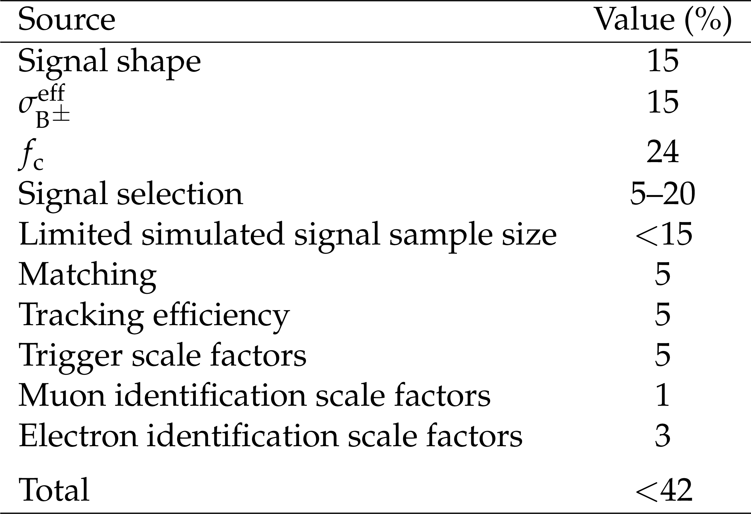
png pdf	Table 3: Sources of systematic uncertainty affecting the expected signal event yield. The ranges given correspond to the uncertainties across the different event categories. The uncertainty in the integrated luminosity is not reported as it is incorporated in the uncertainty in the cross section measurement used to normalize the signal.
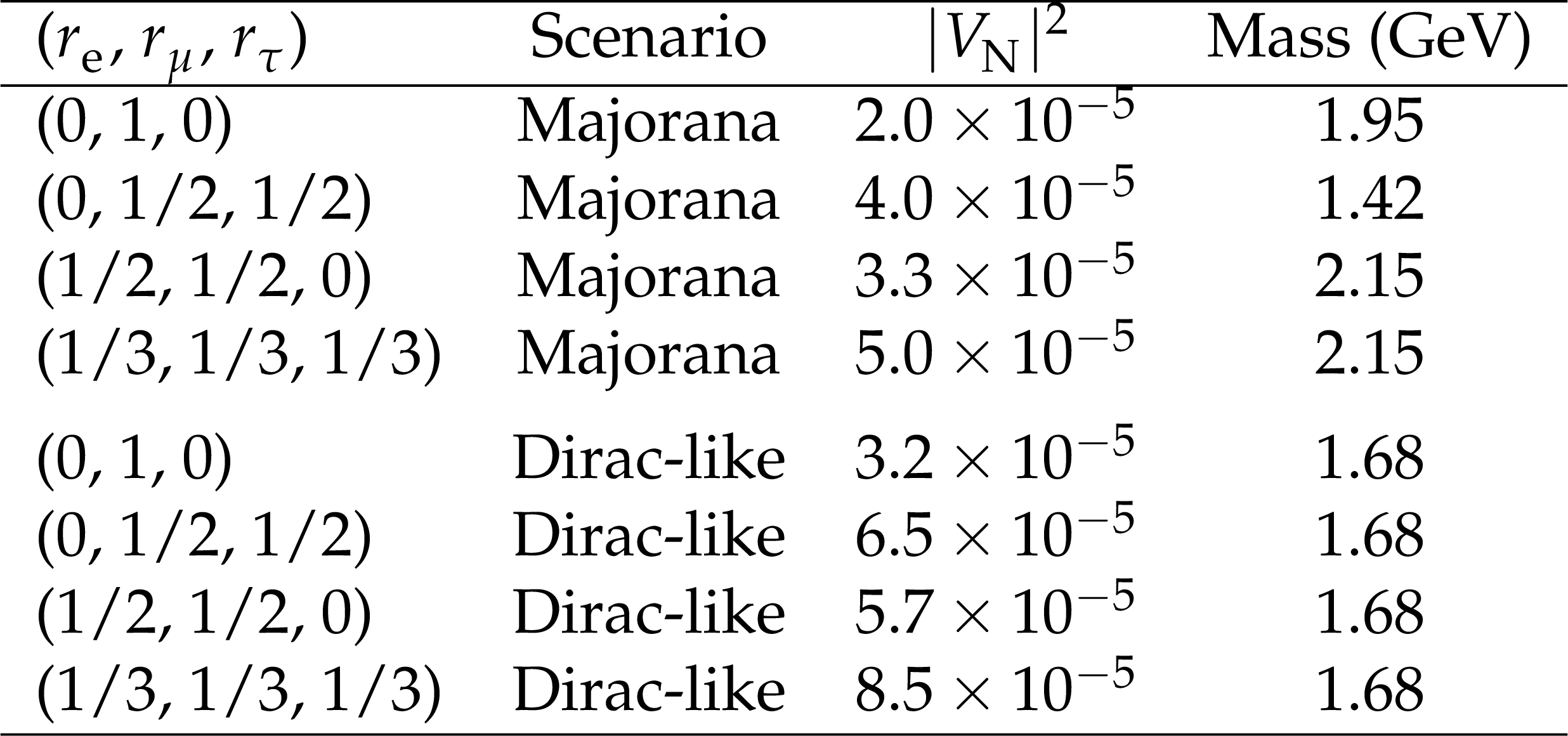
png pdf	Table 4: Summary of the most stringent upper limits on $ |V_\mathrm{N}|^2 $ at 95% CL. For each scenario, the minimum excluded value of $ |V_\mathrm{N}|^2 $ is reported together with the mass at which it occurs.
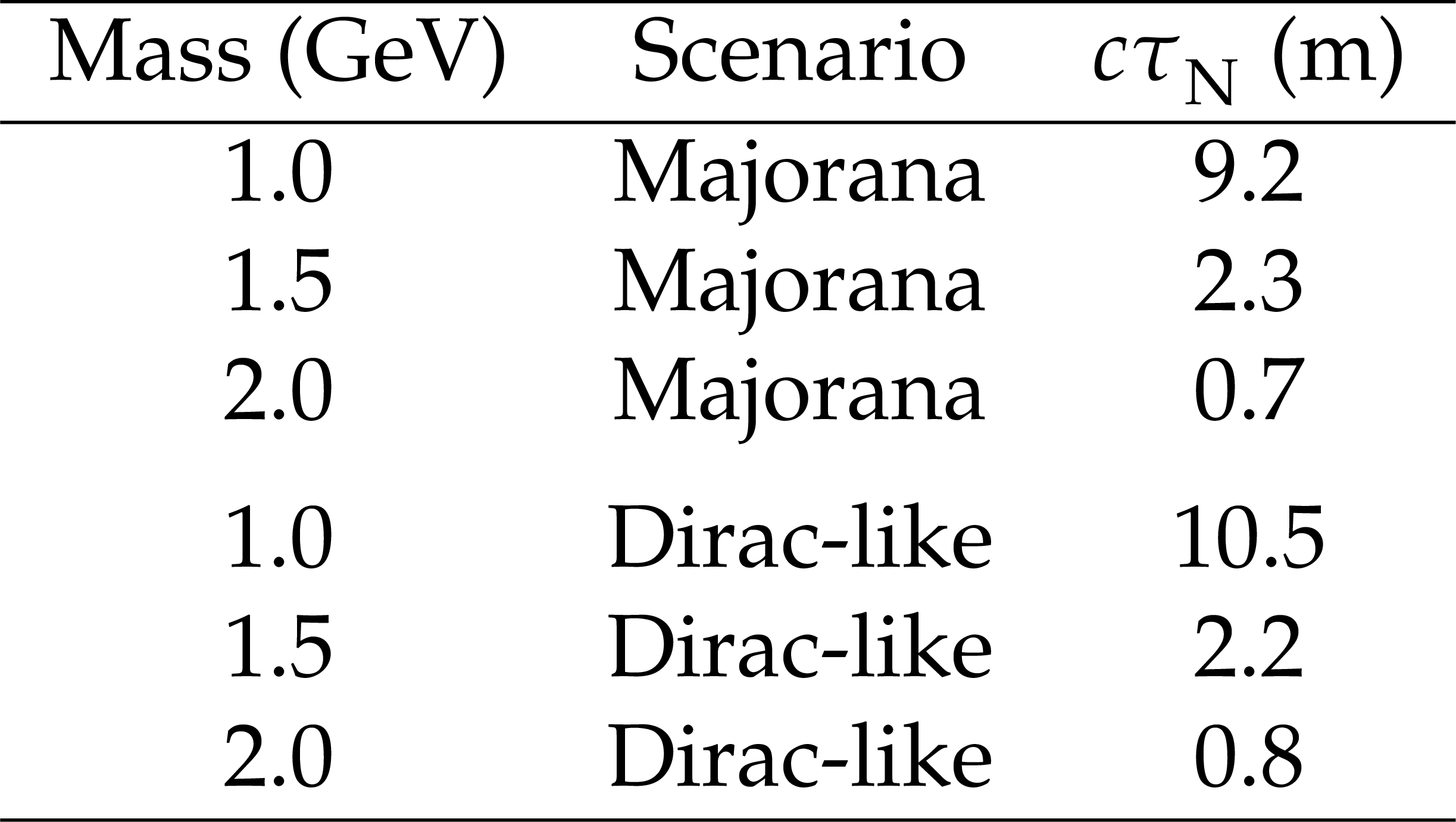
png pdf	Table 5: Summary of the most stringent lower limits on $ c\tau_{\mathrm{N}} $ at 95% CL, obtained for the mixing scenario ($r_\mathrm{e}$, $\,r_\mu$, $\,r_\tau$) $=$ (0, 1, 0). The maximum excluded value of $ c\tau_{\mathrm{N}} $ is reported for masses $ m_\mathrm{N} = $ 1.0, 1.5 and 2.0, and for the Majorana and Dirac-like scenarios.

Summary

A search for long-lived heavy neutrinos, N, in the leptonic and semileptonic decays of B mesons produced in proton-proton collisions at $ \sqrt{s}= $ 13 TeV has been performed. The search uses a special data sample, referred to as the B-parking data sample, accumulated by the CMS experiment during 2018. The sample corresponds to an integrated luminosity of 41.6 fb$ ^{-1} $ and contains of order 10^${10}$ $ \mathrm{b} \overline{\mathrm{b}} $ events. The search is based on the process $ {\mathrm{B}}\to\ell_{\mathrm{B}}\mathrm{N} \mathrm{X} $, $ \mathrm{N}\to \ell^{\pm}\pi^{\mp} $, where the charged leptons $ \ell_{\mathrm{B}} $ and $ \ell $ are required to be $ \ell_{\mathrm{B}}\ell=\mu\mu,\,\mu\mathrm{e},\,\mathrm{or }\mathrm{e}\mu $; the hadronic recoil system, X, is treated inclusively and is not reconstructed and the $ {\mathrm{B}} =({\mathrm{B}}_{{\mathrm{u}}} $, $ {\mathrm{B}}_{{\mathrm{d}}} $, $ {\mathrm{B}}_{{\mathrm{s}}} $, $ {\mathrm{B}}_{{\mathrm{c}}}) $ decays are summed. Results are reported for the N mass range 1 $ < m_{\mathrm{N}} < $ 3 GeV. The main elements of the search signature are (i) two charged leptons, at least one of which must be a muon that satisfies the B-parking trigger requirements, (ii) a displaced vertex associated with the $ \mathrm{N}\to\ell^{\pm}\pi^{\mp} $ decay, and (iii) a peak in the invariant mass distribution of the $ \ell^{\pm}\pi^{\mp} $ system consistent with the expected signal shape. Backgrounds, which arise primarily from strong-interaction processes, are suppressed using a parametric neural network that considers a broad range of event properties. A search for N states is performed using simultaneous maximum likelihood fits to the $ \ell^{\pm}\pi^{\mp} $ invariant mass distributions in 24 mutually exclusive event categories. No significant excess of events over the SM background is observed in any of the fit regions. The results are interpreted for the separate hypotheses of a Majorana or Dirac-like particle as (i) upper limits at 95% CL on $ |V_{\mathrm{N}}|^2 $ as functions of $ m_{\mathrm{N}} $, for representative scenarios specified by different values of the mixing ratios $ r_\mathrm{e} $, $ r_\mu $, and $ r_\tau $; and as (ii) lower limits at 95% CL on $ c\tau_{\mathrm{N}} $ for 66 combinations of $ r_\mathrm{e} $, $ r_\mu $, and $ r_\tau $ for signal masses $ m_\mathrm{N} = $ 1.0, 1.5, and 2.0 GeV. The most stringent limits are $ |V_{\mathrm{N}}|^2 < $ 2.0 $\times$ 10$^{-5} $ and $ c\tau_{\mathrm{N}} > $ 10.5 m, obtained for the Majorana and Dirac-like cases, respectively, and for the scenario in which the N mixes exclusively with the muon sector. This search provides the most stringent exclusion limits on $ |V_\mathrm{N}|^2 $ for masses 1 $ < m_\mathrm{N} < $ 1.7 GeV from a collider experiment to date. Assuming the benchmark scenario $ (r_\mathrm{e},\,r_\mu,\,r_\tau) = $ (0, 1, 0) and the Majorana hypothesis, the exclusion is improved by almost one order of magnitude compared to LHCb [24], and by up to a factor of about 2 compared to Belle [14] and the most stringent previous hadron collider result [23]. Furthermore, the first upper limits on $ |V_\mathrm{N}|^2 $ are set for the mass range 1 $ < m_\mathrm{N} < $ 2 GeV for the mixing scenarios $ (r_\mathrm{e},\,r_\mu,\,r_\tau) = $ (0, 1/2, 1/2), (1/2, 1/2, 0), and (1/3, 1/3, 1/3). Finally, lower limits on $ c\tau_{\mathrm{N}} $ in the form of ternary plots for masses $ m_\mathrm{N} \leq $ 2.0 GeV are presented for the first time.

Additional Figures
png pdf	Additional Figure 1: Observed limits on $ |V_\mathrm{N}|^2 $ as a function of the mixing ratios ($ r_\mathrm{e} $, $ r_\mu $, $ r_\tau $) for fixed N masses of 1 GeV (top row), 1.5 GeV (middle row), and 2 GeV (bottom row), in the Majorana (left column) and Dirac-like (right column) scenarios. The red crosses indicate that there is no exclusion found for that point. The orientation of the value markers on each axis identifies the associated internal lines on the plot.
png pdf	Additional Figure 1-a: Observed limits on $ |V_\mathrm{N}|^2 $ as a function of the mixing ratios ($ r_\mathrm{e} $, $ r_\mu $, $ r_\tau $) for fixed N masses of 1 GeV (top row), 1.5 GeV (middle row), and 2 GeV (bottom row), in the Majorana (left column) and Dirac-like (right column) scenarios. The red crosses indicate that there is no exclusion found for that point. The orientation of the value markers on each axis identifies the associated internal lines on the plot.
png pdf	Additional Figure 1-b: Observed limits on $ |V_\mathrm{N}|^2 $ as a function of the mixing ratios ($ r_\mathrm{e} $, $ r_\mu $, $ r_\tau $) for fixed N masses of 1 GeV (top row), 1.5 GeV (middle row), and 2 GeV (bottom row), in the Majorana (left column) and Dirac-like (right column) scenarios. The red crosses indicate that there is no exclusion found for that point. The orientation of the value markers on each axis identifies the associated internal lines on the plot.
png pdf	Additional Figure 1-c: Observed limits on $ |V_\mathrm{N}|^2 $ as a function of the mixing ratios ($ r_\mathrm{e} $, $ r_\mu $, $ r_\tau $) for fixed N masses of 1 GeV (top row), 1.5 GeV (middle row), and 2 GeV (bottom row), in the Majorana (left column) and Dirac-like (right column) scenarios. The red crosses indicate that there is no exclusion found for that point. The orientation of the value markers on each axis identifies the associated internal lines on the plot.
png pdf	Additional Figure 1-d: Observed limits on $ |V_\mathrm{N}|^2 $ as a function of the mixing ratios ($ r_\mathrm{e} $, $ r_\mu $, $ r_\tau $) for fixed N masses of 1 GeV (top row), 1.5 GeV (middle row), and 2 GeV (bottom row), in the Majorana (left column) and Dirac-like (right column) scenarios. The red crosses indicate that there is no exclusion found for that point. The orientation of the value markers on each axis identifies the associated internal lines on the plot.
png pdf	Additional Figure 1-e: Observed limits on $ |V_\mathrm{N}|^2 $ as a function of the mixing ratios ($ r_\mathrm{e} $, $ r_\mu $, $ r_\tau $) for fixed N masses of 1 GeV (top row), 1.5 GeV (middle row), and 2 GeV (bottom row), in the Majorana (left column) and Dirac-like (right column) scenarios. The red crosses indicate that there is no exclusion found for that point. The orientation of the value markers on each axis identifies the associated internal lines on the plot.
png pdf	Additional Figure 1-f: Observed limits on $ |V_\mathrm{N}|^2 $ as a function of the mixing ratios ($ r_\mathrm{e} $, $ r_\mu $, $ r_\tau $) for fixed N masses of 1 GeV (top row), 1.5 GeV (middle row), and 2 GeV (bottom row), in the Majorana (left column) and Dirac-like (right column) scenarios. The red crosses indicate that there is no exclusion found for that point. The orientation of the value markers on each axis identifies the associated internal lines on the plot.

References
1	S. Bilenky	Neutrino oscillations: From a historical perspective to the present status	NPB 908 (2016) 2	1602.00170
2	J. Silk et al	Particle dark matter: observations, models and searches	Cambridge Univ. Press, Cambridge, ISBN~978-1-107-65392-4, 2010 link
3	G. R. Farrar and M. E. Shaposhnikov	Baryon asymmetry of the universe in the standard electroweak theory	PRD 50 (1994) 774	hep-ph/9305275
4	T. Asaka, S. Blanchet, and M. Shaposhnikov	The nuMSM, dark matter and neutrino masses	PLB 631 (2005) 151	hep-ph/0503065
5	T. Asaka and M. Shaposhnikov	The $ \nu $MSM, dark matter and baryon asymmetry of the universe	PLB 620 (2005) 17	hep-ph/0505013
6	S. Dodelson and L. M. Widrow	Sterile-neutrinos as dark matter	PRL 72 (1994) 17	hep-ph/9303287
7	M. Fukugita and T. Yanagida	Baryogenesis without grand unification	PLB 174 (1986) 45
8	P. Minkowski	$ \mu \to e\gamma $ at a rate of one out of $ 10^{9} $ muon decays?	PLB 67 (1977) 421
9	K. Bondarenko, A. Boyarsky, D. Gorbunov, and O. Ruchayskiy	Phenomenology of GeV-scale heavy neutral leptons	JHEP 11 (2018) 032	1805.08567
10	CHARM Collaboration	A search for decays of heavy neutrinos in the mass range 0.5 - 2.8 GeV	PLB 166 (1986) 473
11	NuTeV-E815 Collaboration	Search for neutral heavy leptons in a high-energy neutrino beam	PRL 83 (1999) 4943	hep-ex/9908011
12	R. Barouki, G. Marocco, and S. Sarkar	Blast from the past II: Constraints on heavy neutral leptons from the BEBC WA66 beam dump experiment	SciPost Phys. 13 (2022) 118	2208.00416
13	WA66 Collaboration	Search for heavy neutrino decays in the BEBC beam dump experiment	PLB 160 (1985) 207
14	Belle Collaboration	Search for heavy neutrinos at Belle	PRD 87 (2013) 071102	1301.1105
15	BABAR Collaboration	Search for heavy neutral leptons using tau lepton decays at BABAR	PRD 107 (2023) 052009	2207.09575
16	ATLAS Collaboration	Search for heavy neutral leptons in decays of $ W $ bosons produced in 13 TeV $ pp $ collisions using prompt and displaced signatures with the ATLAS detector	JHEP 10 (2019) 265	1905.09787
17	ATLAS Collaboration	Search for heavy neutral leptons in decays of W bosons using a dilepton displaced vertex in $ \sqrt{s}= $ 13 TeV pp collisions with the ATLAS detector	PRL 131 (2023) 061803	2204.11988
18	CMS Collaboration	Search for heavy neutral leptons in events with three charged leptons in proton-proton collisions at $ \sqrt{s} = $ 13 TeV	PRL 120 (2018) 221801	CMS-EXO-17-012 1802.02965
19	CMS Collaboration	Search for heavy Majorana neutrinos in same-sign dilepton channels in proton-proton collisions at $ \sqrt{s}= $ 13 TeV	JHEP 01 (2019) 122	CMS-EXO-17-028 1806.10905
20	CMS Collaboration	Search for heavy neutrinos and third-generation leptoquarks in hadronic states of two $ \tau $ leptons and two jets in proton-proton collisions at $ \sqrt{s} = $ 13 TeV	JHEP 03 (2019) 170	CMS-EXO-17-016 1811.00806
21	CMS Collaboration	Search for long-lived heavy neutral leptons with displaced vertices in proton-proton collisions at $ \sqrt{\mathrm{s}} $ =13 TeV	JHEP 07 (2022) 081	CMS-EXO-20-009 2201.05578
22	CMS Collaboration	Search for long-lived heavy neutral leptons with lepton flavour conserving or violating decays to a jet and a charged lepton	link	CMS-EXO-21-013 2312.07484
23	CMS Collaboration	Search for long-lived heavy neutral leptons decaying in the CMS muon detectors in proton-proton collisions at $ \sqrt{s} $ = 13 TeV	2, 2024	CMS-EXO-22-017 2402.18658
24	LHCb Collaboration	Search for Majorana neutrinos in $ B^- \to \pi^+\mu^-\mu^- $ decays	PRL 112 (2014) 131802	1401.5361
25	LHCb Collaboration	Search for heavy neutral leptons in $ W^+\to\mu^{+}\mu^{\pm}\text{jet} $ decays	EPJC 81 (2021) 248	2011.05263
26	CMS Collaboration	Test of lepton flavor universality in B$ ^{\pm} \to $ K$ ^{\pm}\mu^+\mu^- $ and B$ ^{\pm} \to $ K$ ^{\pm} $e$ ^+ $e$ ^- $ decays in proton-proton collisions at $ \sqrt{s} $ = 13 TeV	link	CMS-BPH-22-005 2401.07090
27	F. F. Deppisch, P. S. Bhupal Dev, and A. Pilaftsis	Neutrinos and Collider Physics	New J. Phys. 17 (2015) 075019	1502.06541
28	Particle Data Group	Review of particle physics	PTEP 2022 (2022) 083C01
29	M. Drewes	The phenomenology of right handed neutrinos	Int. J. Mod. Phys. E 22 (2013) 1330019	1303.6912
30	P. Hernández, J. Jones-Pérez, and O. Suarez-Navarro	Majorana vs pseudo-Dirac neutrinos at the ILC	EPJC 79 (2019) 220	1810.07210
31	CMS Collaboration	HEPData record for this analysis	link
32	CMS Collaboration	Performance of the CMS Level-1 trigger in proton-proton collisions at $ \sqrt{s} = $ 13 TeV	JINST 15 (2020) P10017	CMS-TRG-17-001 2006.10165
33	CMS Collaboration	The CMS trigger system	JINST 12 (2017) P01020	CMS-TRG-12-001 1609.02366
34	CMS Collaboration	The CMS experiment at the CERN LHC	JINST 3 (2008) S08004
35	CMS Collaboration	CMS luminosity measurement for the 2018 data-taking period at $ \sqrt{s} = $ 13 TeV	CMS Physics Analysis Summary, 2019 link	CMS-PAS-LUM-18-002
36	LHCb Collaboration	Measurement of the $ B_c^- $ meson production fraction and asymmetry in 7 and 13 TeV $ pp $ collisions	PRD 100 (2019) 112006	1910.13404
37	T. Sjöstrand et al.	An introduction to PYTHIA 8.2	Comput. Phys. Commun. 191 (2015) 159	1410.3012
38	CMS Collaboration	Extraction and validation of a new set of CMS PYTHIA8 tunes from underlying-event measurements	EPJC 80 (2020) 4	CMS-GEN-17-001 1903.12179
39	NNPDF Collaboration	Parton distributions from high-precision collider data	EPJC 77 (2017) 663	1706.00428
40	D. J. Lange	The EvtGen particle decay simulation package	NIM A 462 (2001) 152
41	C.-H. Chang, J.-X. Wang, and X.-G. Wu	BCVEGPY2.0: A Upgrade version of the generator BCVEGPY with an addendum about hadroproduction of the P-wave B(c) states	Comput. Phys. Commun. 174 (2006) 241	hep-ph/0504017
42	GEANT4 Collaboration	GEANT 4---a simulation toolkit	NIM A 506 (2003) 250
43	CMS Collaboration	Performance of the CMS muon detector and muon reconstruction with proton-proton collisions at $ \sqrt{s}= $ 13 TeV	JINST 13 (2018) P06015	CMS-MUO-16-001 1804.04528
44	CMS Collaboration	Particle-flow reconstruction and global event description with the CMS detector	JINST 12 (2017) P10003	CMS-PRF-14-001 1706.04965
45	CMS Collaboration	CMS tracking performance results from early LHC operation	EPJC 70 (2010) 1165	CMS-TRK-10-001 1007.1988
46	CMS Collaboration	Electron and photon reconstruction and identification with the CMS experiment at the CERN LHC	JINST 16 (2021) P05014	CMS-EGM-17-001 2012.06888
47	K. Prokofiev and T. Speer	A kinematic and a decay chain reconstruction library	in 14th International Conference on Computing in High-Energy and Nuclear Physics, 2005
48	P. Baldi et al.	Parameterized neural networks for high-energy physics	EPJC 76 (2016) 235	1601.07913
49	K. Fukushima	Visual feature extraction by a multilayered network of analog threshold elements	IEEE Transactions on Systems Science and Cybernetics 5 (1969) 322
50	F. Chollet et al.	Keras	\hrefF.~Chollet et~al., . \urlhttps://keras.io, 2015
51	M. Abadi et al.	TensorFlow: A system for large-scale machine learning	in Proceedings of the 12th USENIX Conference on Operating Systems Design and Implementation, OSDI'16, USENIX Association, 2016	1605.08695
52	D. P. Kingma and J. Ba	Adam: A method for stochastic optimization		1412.6980
53	F. Pedregosa et al.	Scikit-learn: Machine learning in Python	J. Mach. Learn. Res. 12 (2011) 2825	1201.0490
54	CMS Collaboration	Measurement of the total and differential inclusive $ B^+ $ hadron cross sections in pp collisions at $ \sqrt{s} $ = 13 TeV	PLB 771 (2017) 435	CMS-BPH-15-004 1609.00873
55	M. J. Oreglia	A study of the reactions $ \psi^\prime \to \gamma \gamma \psi $	PhD thesis, Stanford University, . SLAC Report SLAC-R-236, 1980 link
56	J. E. Gaiser	Charmonium spectroscopy from radiative decays of the J/$ \psi $ and $ \psi^\prime $	PhD thesis, Stanford University, SLAC Report SLAC-R-255, 1982
57	P. D. Dauncey, M. Kenzie, N. Wardle, and G. J. Davies	Handling uncertainties in background shapes: the discrete profiling method	JINST 10 (2015) P04015	1408.6865
58	R. A. Fisher	On the mathematical foundations of theoretical statistics	Phil. Trans. Roy. Soc. Lond. A 222 (1922) 309
59	S. S. Wilks	The large-sample distribution of the likelihood ratio for testing composite hypotheses	Annals Math. Statist. 9 (1938) 60
60	A. L. Read	Presentation of search results: The $ CL_s $ technique	JPG 28 (2002) 2693
61	G. Cowan, K. Cranmer, E. Gross, and O. Vitells	Asymptotic formulae for likelihood-based tests of new physics	EPJC 71 (2011) 1554	1007.1727
62	M. Drewes, J. Klarić, and J. López-Pavón	New benchmark models for heavy neutral lepton searches	EPJC 82 (2022) 1176	2207.02742
63	B. Shuve and M. E. Peskin	Revision of the LHCb limit on Majorana neutrinos	PRD 94 (2016) 113007	1607.04258

Compact Muon Solenoid LHC, CERN

© Copyright CERN 2024 for the benefit of the CMS Collaboration