Compact Muon Solenoid
LHC, CERN

Visit us: CMS Public Website, CMS Physics ; Contact us: CMS Publications Committee

CMS-EXO-20-009 ; CERN-EP-2021-264

Search for long-lived heavy neutral leptons with displaced vertices in proton-proton collisions at $\sqrt{s} = $ 13 TeV

CMS Collaboration

14 January 2022

JHEP 07 (2022) 081

Abstract: A search for heavy neutral leptons (HNLs), the right-handed Dirac or Majorana neutrinos, is performed in final states with three charged leptons (electrons or muons) using proton-proton collision data collected by the CMS experiment at $\sqrt{s} = $ 13 TeV at the CERN LHC. The data correspond to an integrated luminosity of 138 fb$^{-1}$. The HNLs could be produced through mixing with standard model neutrinos $\nu$. For small values of the HNL mass ($ < $ 20 GeV) and the square of the HNL-$\nu$ mixing parameter (10$^{-7}$-10$^{-2}$), the decay length of these particles can be large enough so that the secondary vertex of the HNL decay can be resolved with the CMS silicon tracker. The selected final state consists of one lepton emerging from the primary proton-proton collision vertex, and two leptons forming a displaced, secondary vertex. No significant deviations from the standard model expectations are observed, and constraints are obtained on the HNL mass and coupling strength parameters, excluding previously unexplored regions of parameter space in the mass range 1-20 GeV and squared mixing parameter values as low as 10$^{-7}$.

Links: e-print arXiv:2201.05578 [hep-ex] (PDF) ; CDS record ; inSPIRE record ; HepData record ; CADI line (restricted) ;

Figures
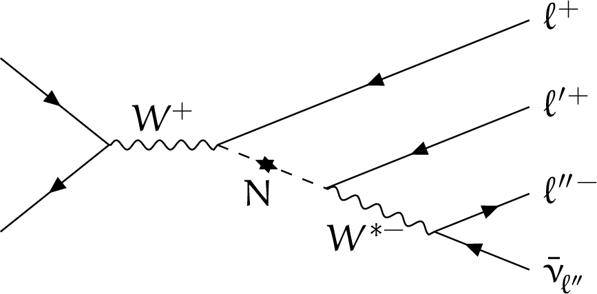
png pdf	Figure 1: Typical diagrams for the production and decay of an HNL through its mixing with an SM neutrino, leading to final states with three charged leptons and a neutrino. The HNL decay is mediated by either a W* (upper row) or a Z* (lower row) boson. In the diagrams on the left, the HNL is assumed to be a Majorana neutrino, thus $\ell$ and $\ell'$ in the W*-mediated diagram can have the same electric charge, and lepton number can be violated. In the diagrams on the right, the HNL decay conserves lepton number and can be either a Majorana or a Dirac particle, and, therefore, $\ell$ and $\ell'$ in the W*-mediated diagram have always opposite charge. The present study only considers the LNC case, thus $\ell$ and $\ell'$ (or $\nu_{\ell'}$) are always of the same flavor. In the case of the HNL decay mediated by a Z* boson, only the case where $\ell$ and $\ell''$ are of the same flavor is considered.
png pdf	Figure 1-a: Typical diagram for the production and decay of an HNL through its mixing with an SM neutrino, leading to final states with three charged leptons and a neutrino. Here, the HNL decay is mediated by a W* boson. The HNL is assumed to be a Majorana neutrino, thus $\ell$ and $\ell'$ can have the same electric charge, and lepton number can be violated. The present study only considers the LNC case, thus $\ell$ and $\ell'$ are always of the same flavor.
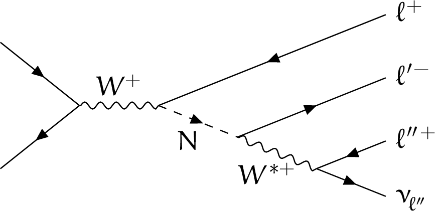
png pdf	Figure 1-b: Typical diagram for the production and decay of an HNL through its mixing with an SM neutrino, leading to final states with three charged leptons and a neutrino. Here, the HNL decay is mediated by a W* boson. The HNL decay conserves lepton number and can be either a Majorana or a Dirac particle, and, therefore, $\ell$ and $\ell'$ have always opposite charge. The present study only considers the LNC case, thus $\ell$ and $\ell'$ are always of the same flavor.
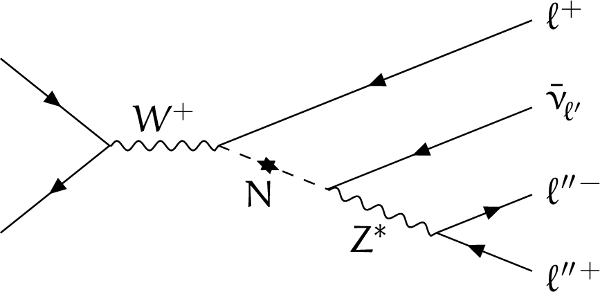
png pdf	Figure 1-c: Typical diagram for the production and decay of an HNL through its mixing with an SM neutrino, leading to final states with three charged leptons and a neutrino. Here, the HNL decay is mediated by a Z* boson. The HNL is assumed to be a Majorana neutrino. The present study only considers the LNC case, thus $\ell$ and $\nu_{\ell'}$ are always of the same flavor. In the case of the HNL decay mediated by a Z* boson, only the case where $\ell$ and $\ell''$ are of the same flavor is considered.
png pdf	Figure 1-d: Typical diagram for the production and decay of an HNL through its mixing with an SM neutrino, leading to final states with three charged leptons and a neutrino. Here, the HNL decay is mediated by a Z* boson. The HNL decay conserves lepton number and can be either a Majorana or a Dirac particle. The present study only considers the LNC case, thus $\ell$ and $\nu_{\ell'}$ are always of the same flavor. In the case of the HNL decay mediated by a Z* boson, only the case where $\ell$ and $\ell''$ are of the same flavor is considered.
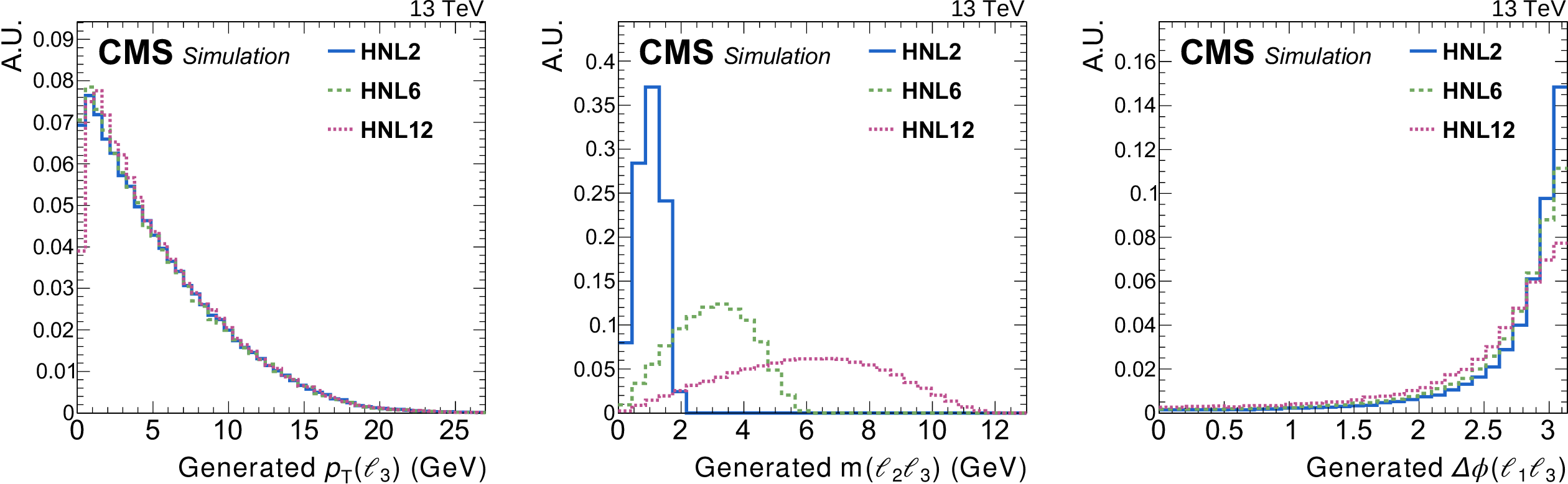
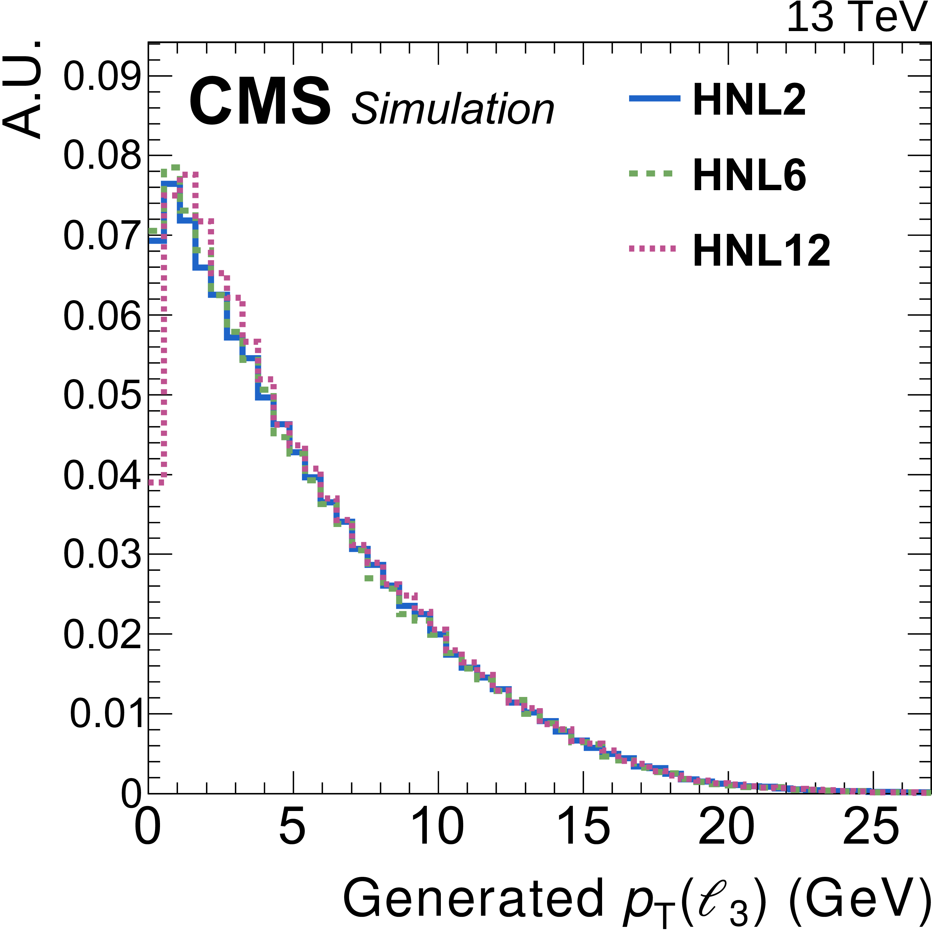
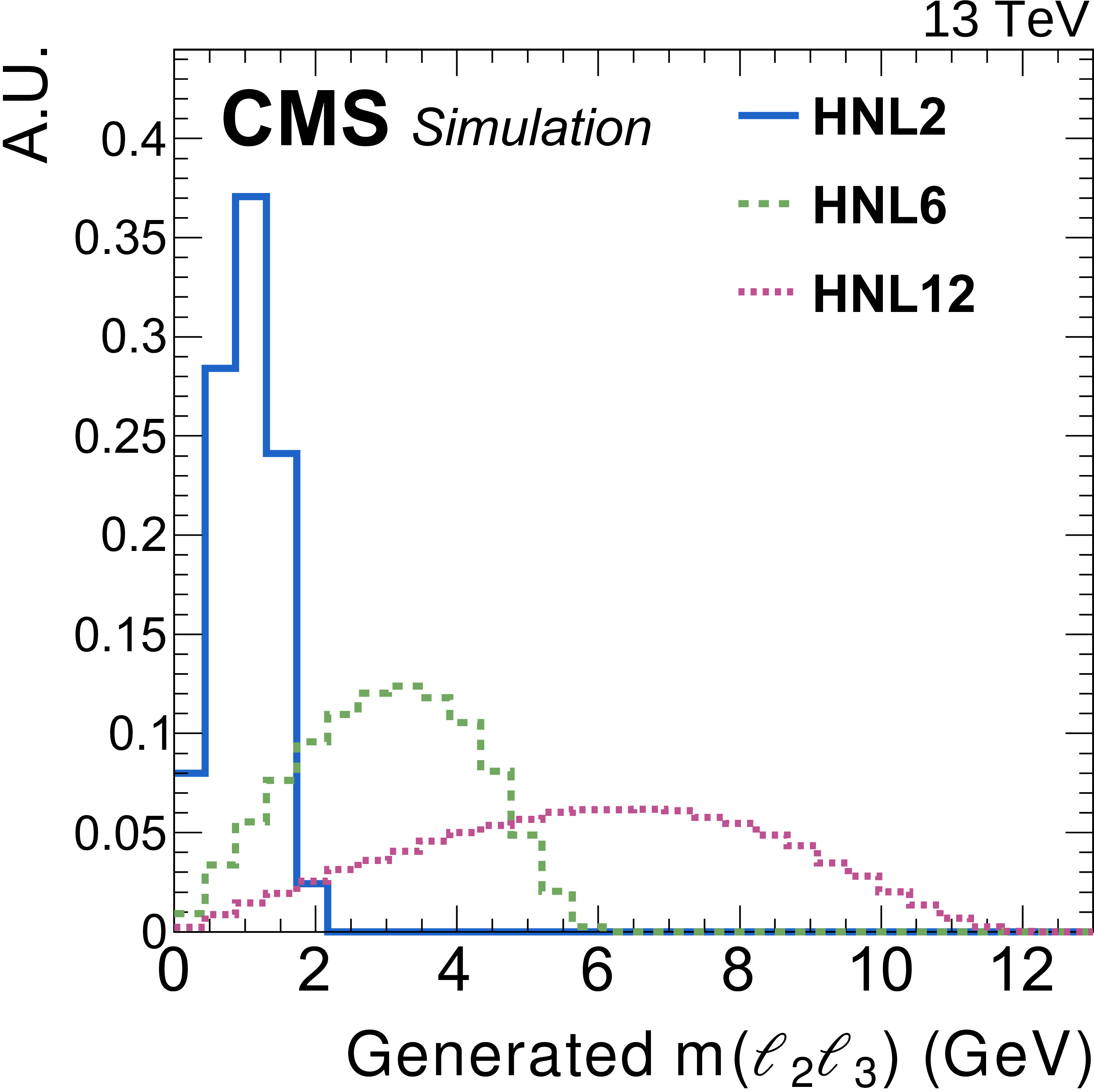
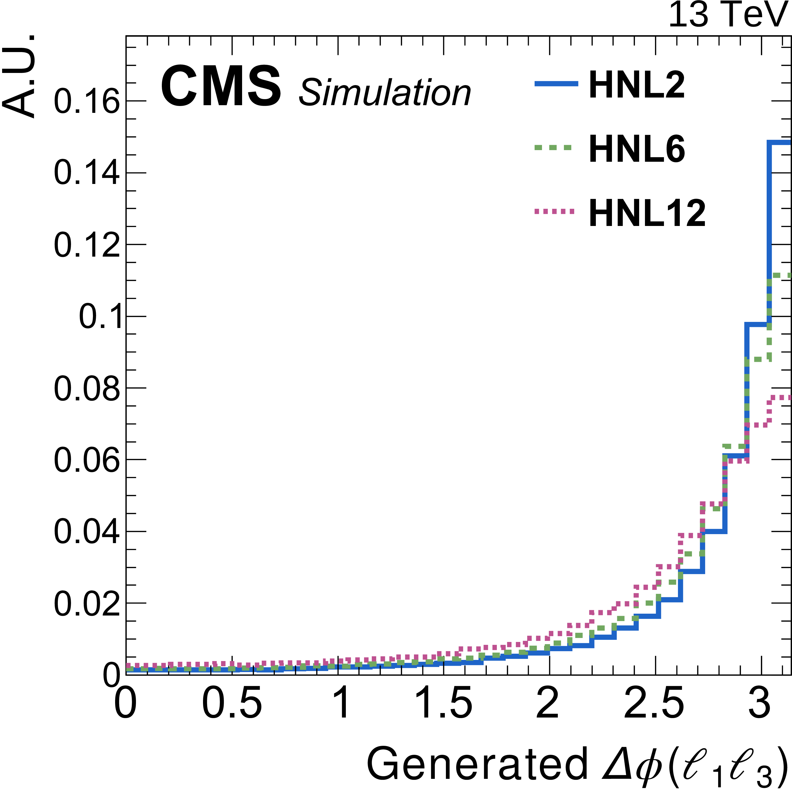
png pdf	Figure 2: Distribution of kinematic properties of the generated leptons for simulated HNL signal events: the ${p_{\mathrm {T}}}$ of ${\ell _3}$ (left), the $m({\ell _2} {\ell _3})$ variable (center), and the angular separation between ${\ell _1}$ and ${\ell _3}$ (right). Predictions are shown for several benchmark hypotheses for Majorana HNL production: ${m_\mathrm{N}} =$ 2 GeV and $ {{| {V_{\mathrm{N} \ell}} |}^2} = $ 1.2$\times$10$^{-4}$ (HNL2), ${m_\mathrm{N}} =$ 6 GeV and $ {{| {V_{\mathrm{N} \ell}} |}^2} = $ 4.1$\times$10$^{-6}$ (HNL6), ${m_\mathrm{N}} =$ 12 GeV and $ {{| {V_{\mathrm{N} \ell}} |}^2} = $ 1.0$\times$10$^{-5}$ (HNL12).
png pdf	Figure 2-a: Distribution of the ${p_{\mathrm {T}}}$ of ${\ell _3}$ for simulated HNL signal events. Predictions are shown for several benchmark hypotheses for Majorana HNL production: ${m_\mathrm{N}} =$ 2 GeV and $ {{| {V_{\mathrm{N} \ell}} |}^2} = $ 1.2$\times$10$^{-4}$ (HNL2), ${m_\mathrm{N}} =$ 6 GeV and $ {{| {V_{\mathrm{N} \ell}} |}^2} = $ 4.1$\times$10$^{-6}$ (HNL6), ${m_\mathrm{N}} =$ 12 GeV and $ {{| {V_{\mathrm{N} \ell}} |}^2} = $ 1.0$\times$10$^{-5}$ (HNL12).
png pdf	Figure 2-b: Distribution of the $m({\ell _2} {\ell _3})$ variable for simulated HNL signal events. Predictions are shown for several benchmark hypotheses for Majorana HNL production: ${m_\mathrm{N}} =$ 2 GeV and $ {{| {V_{\mathrm{N} \ell}} |}^2} = $ 1.2$\times$10$^{-4}$ (HNL2), ${m_\mathrm{N}} =$ 6 GeV and $ {{| {V_{\mathrm{N} \ell}} |}^2} = $ 4.1$\times$10$^{-6}$ (HNL6), ${m_\mathrm{N}} =$ 12 GeV and $ {{| {V_{\mathrm{N} \ell}} |}^2} = $ 1.0$\times$10$^{-5}$ (HNL12).
png pdf	Figure 2-c: Distribution of the angular separation between ${\ell _1}$ and ${\ell _3}$ for simulated HNL signal events. Predictions are shown for several benchmark hypotheses for Majorana HNL production: ${m_\mathrm{N}} =$ 2 GeV and $ {{| {V_{\mathrm{N} \ell}} |}^2} = $ 1.2$\times$10$^{-4}$ (HNL2), ${m_\mathrm{N}} =$ 6 GeV and $ {{| {V_{\mathrm{N} \ell}} |}^2} = $ 4.1$\times$10$^{-6}$ (HNL6), ${m_\mathrm{N}} =$ 12 GeV and $ {{| {V_{\mathrm{N} \ell}} |}^2} = $ 1.0$\times$10$^{-5}$ (HNL12).
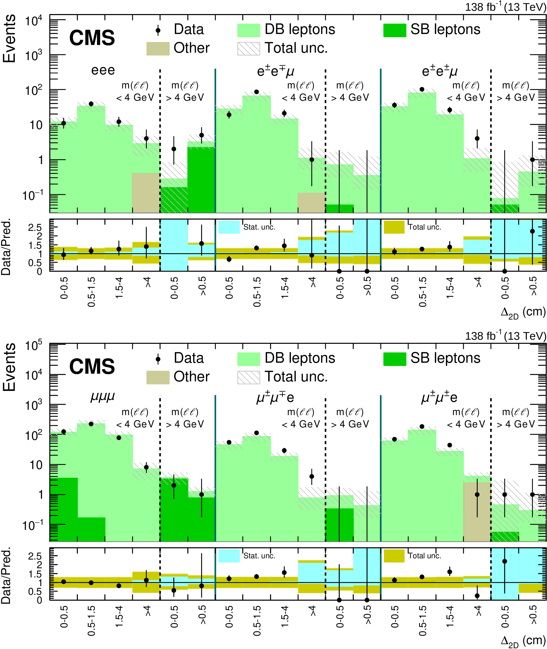
png pdf	Figure 3: Comparison between the number of observed events in data and the background predictions (shaded histograms, stacked) in the control regions for eeX (upper) and $ \mu \mu $X (lower) final states. The hashed band indicates the total systematic and statistical uncertainty in the background prediction. The lower panels indicate the ratio between data and prediction, and missing points indicate that the ratio lies outside the axis range. The uncertainty band assigned to the background prediction includes statistical and systematic contributions. Small contributions from background processes that are estimated from simulation are collectively referred to as "Other''.
png pdf	Figure 3-a: Comparison between the number of observed events in data and the background predictions (shaded histograms, stacked) in the control regions for the eeX final state. The hashed band indicates the total systematic and statistical uncertainty in the background prediction. The lower panel indicates the ratio between data and prediction, and missing points indicate that the ratio lies outside the axis range. The uncertainty band assigned to the background prediction includes statistical and systematic contributions. Small contributions from background processes that are estimated from simulation are collectively referred to as "Other''.
png pdf	Figure 3-b: Comparison between the number of observed events in data and the background predictions (shaded histograms, stacked) in the control regions for the $ \mu \mu $X final state. The hashed band indicates the total systematic and statistical uncertainty in the background prediction. The lower panel indicates the ratio between data and prediction, and missing points indicate that the ratio lies outside the axis range. The uncertainty band assigned to the background prediction includes statistical and systematic contributions. Small contributions from background processes that are estimated from simulation are collectively referred to as "Other''.
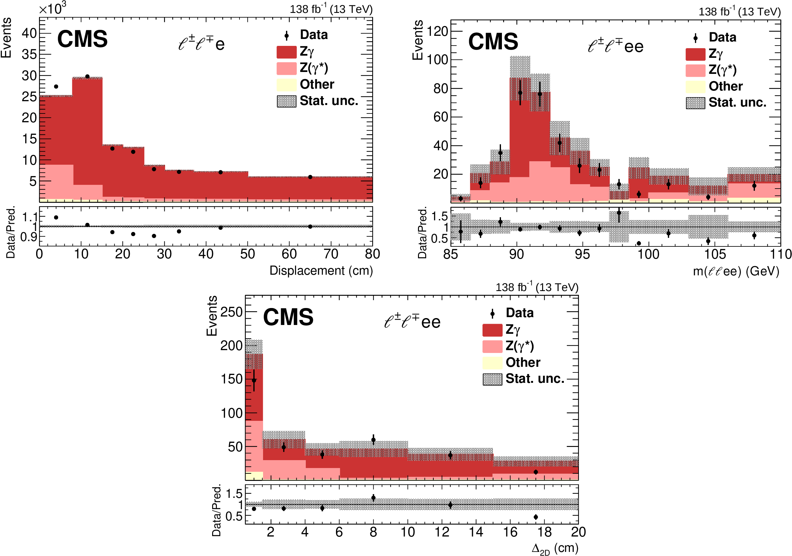
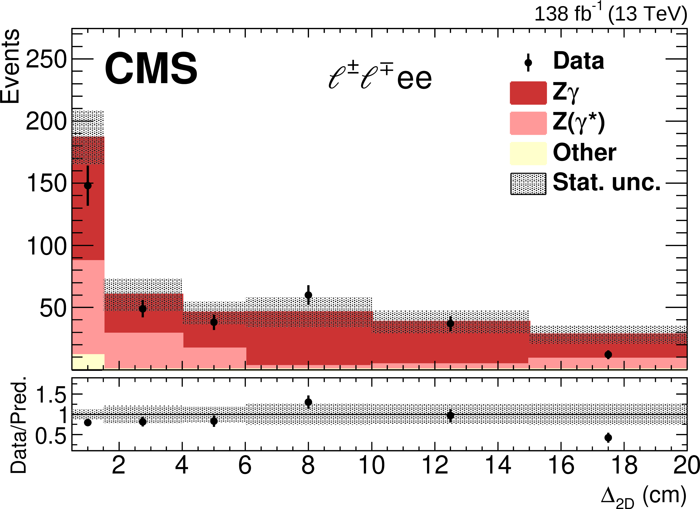
png pdf	Figure 4: Comparison between the observed number of events in data and simulation for converted photons. Events are selected in the final states with three (upper left) or four (upper right, lower) leptons, with one (or two) of the leptons identified as displaced electron(s). The distributions are shown for the displaced electron displacement $d$ (upper left) and reconstructed invariant mass of four leptons (upper right). Additionally, the ${\Delta _{\text {2D}}}$ variable is presented (lower). The simulated events correspond to the processes with external conversions, ${\mathrm{Z} \gamma ^{(*)}}$; internally converted photons, $\mathrm{Z} (\gamma ^{*})$; and other processes with the production of vector bosons and top quarks. The hashed band represents the statistical uncertainty in the simulation. The lower panels indicate the ratio between data and prediction.
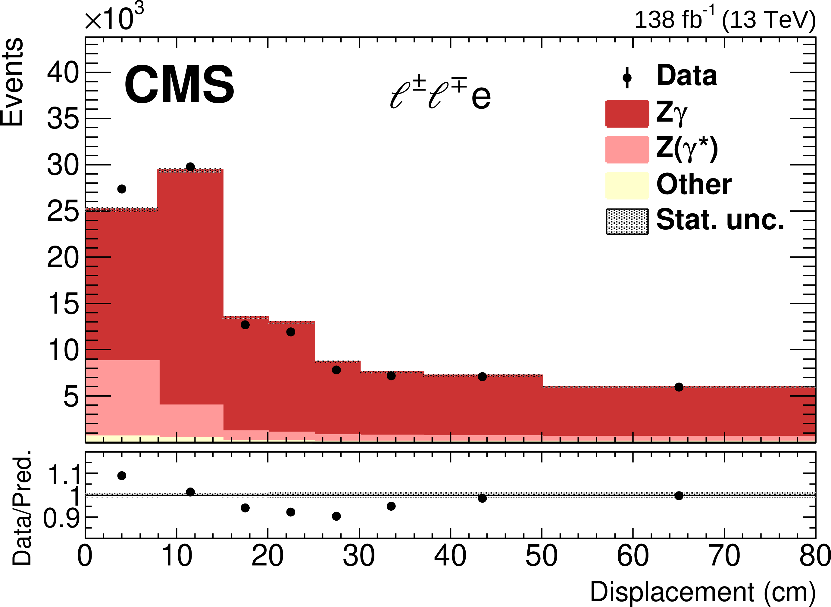
png pdf	Figure 4-a: Comparison between the observed number of events in data and simulation for converted photons. Events are selected in the final states with three leptons, with one (or two) of the leptons identified as displaced electron(s). The distribution of the displaced electron displacement $d$ is presented. The simulated events correspond to the processes with external conversions, ${\mathrm{Z} \gamma ^{(*)}}$; internally converted photons, $\mathrm{Z} (\gamma ^{*})$; and other processes with the production of vector bosons and top quarks. The hashed band represents the statistical uncertainty in the simulation. The lower panel indicates the ratio between data and prediction.
png pdf	Figure 4-b: Comparison between the observed number of events in data and simulation for converted photons. Events are selected in the final states with four leptons, with one (or two) of the leptons identified as displaced electron(s). The distribution of the reconstructed invariant mass of four leptons is presented. The simulated events correspond to the processes with external conversions, ${\mathrm{Z} \gamma ^{(*)}}$; internally converted photons, $\mathrm{Z} (\gamma ^{*})$; and other processes with the production of vector bosons and top quarks. The hashed band represents the statistical uncertainty in the simulation. The lower panel indicates the ratio between data and prediction.
png pdf	Figure 4-c: Comparison between the observed number of events in data and simulation for converted photons. Events are selected in the final states with four leptons, with one (or two) of the leptons identified as displaced electron(s). The distribution of the ${\Delta _{\text {2D}}}$ variable is presented. The simulated events correspond to the processes with external conversions, ${\mathrm{Z} \gamma ^{(*)}}$; internally converted photons, $\mathrm{Z} (\gamma ^{*})$; and other processes with the production of vector bosons and top quarks. The hashed band represents the statistical uncertainty in the simulation. The lower panel indicates the ratio between data and prediction.
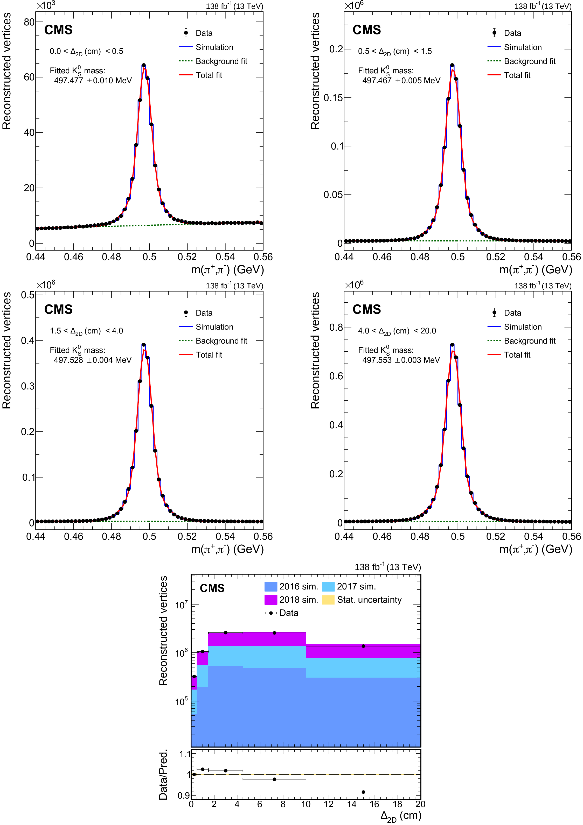
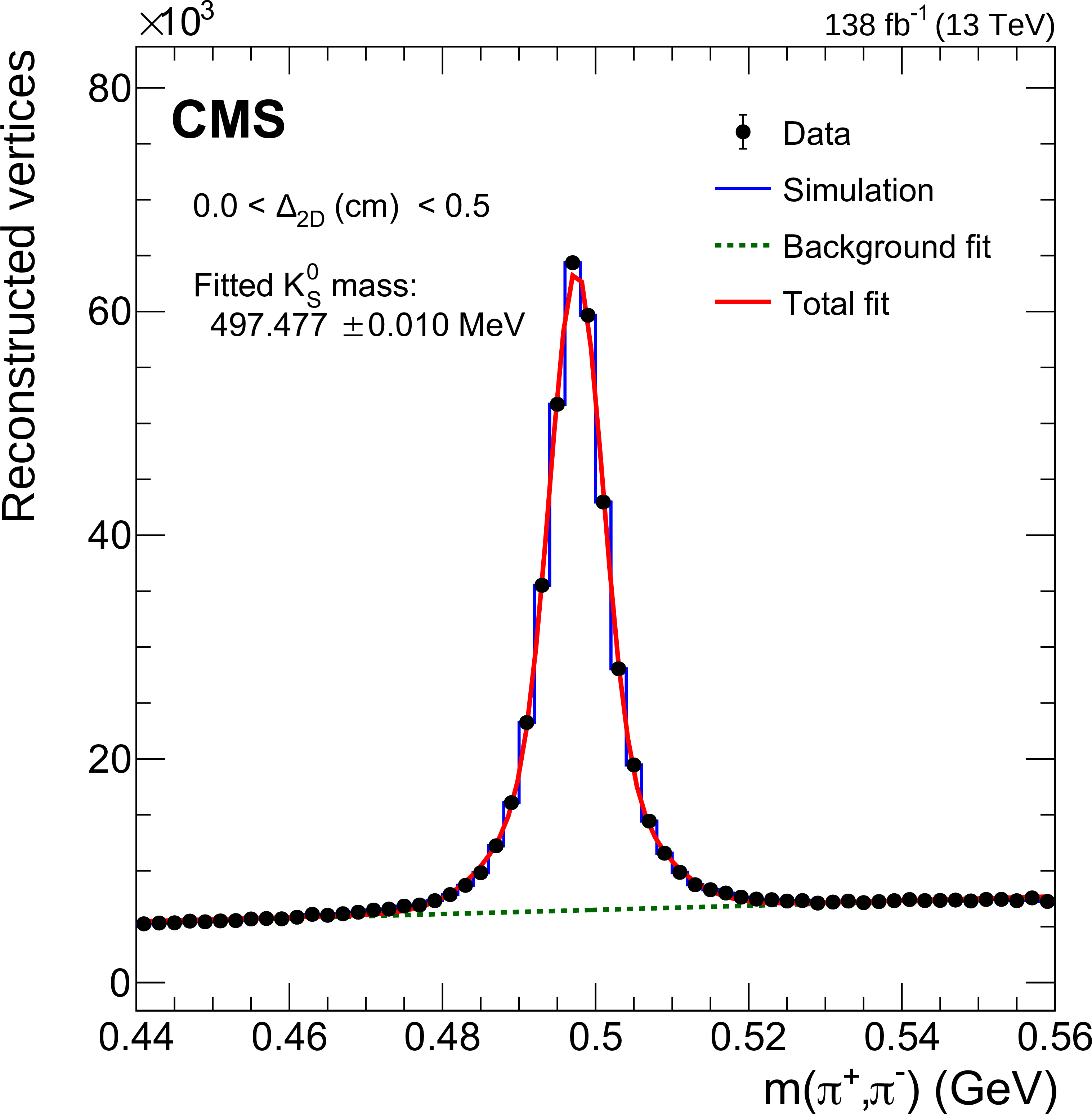
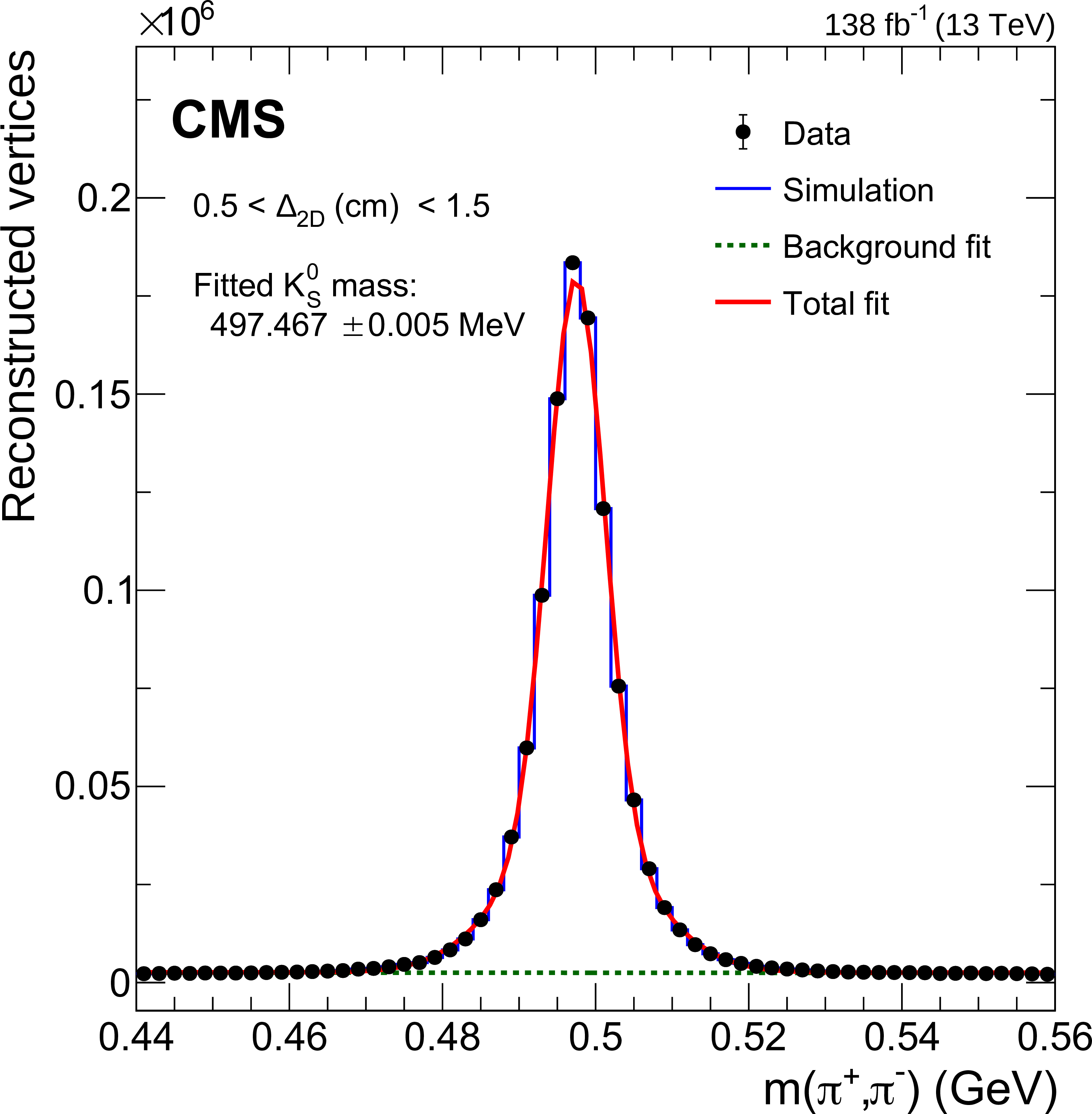
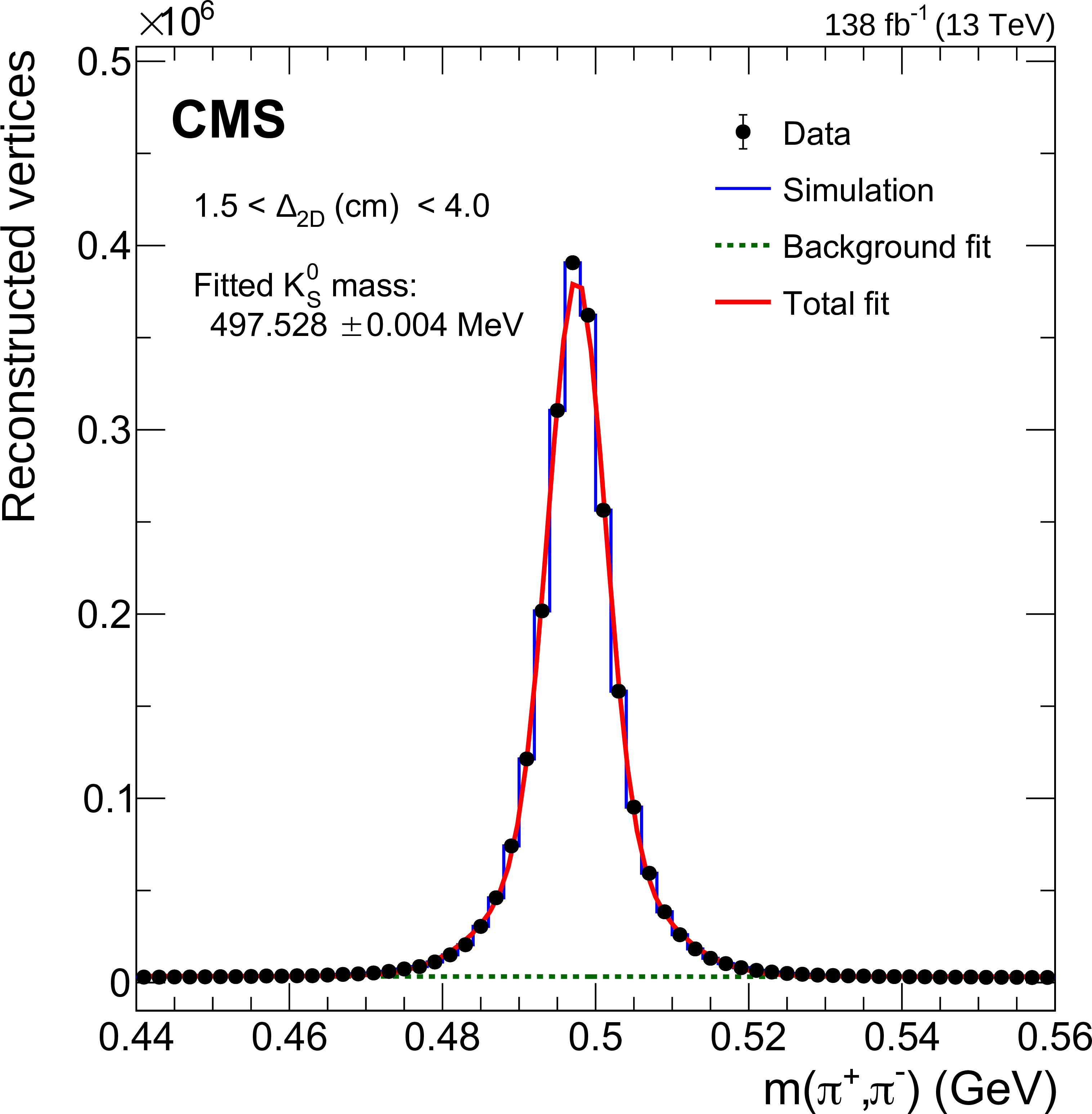
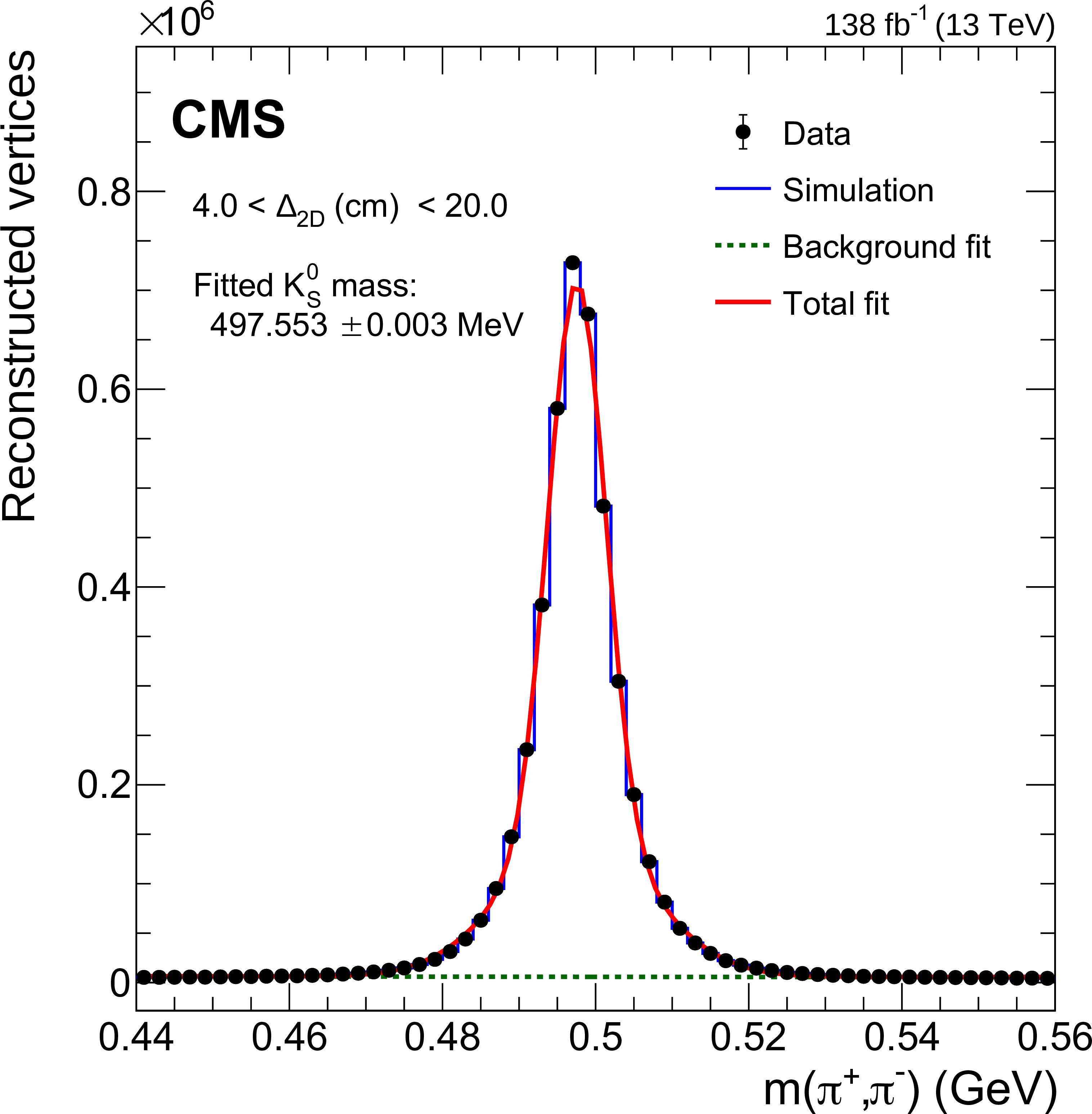
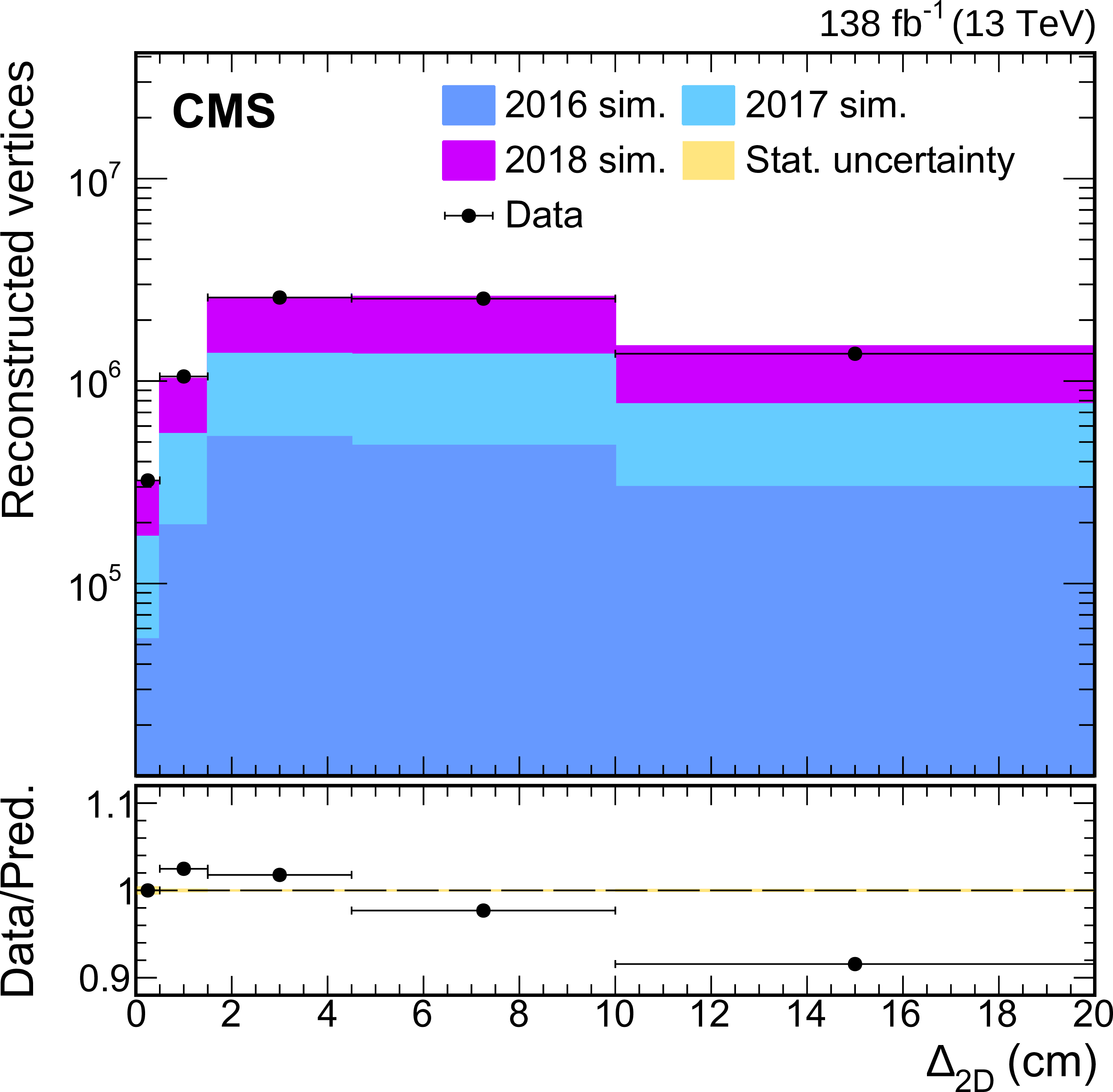
png pdf	Figure 5: The invariant mass distribution of the $\mathrm{K^0_S}$ candidates reconstructed using the $\pi^{\pm} \pi^{\mp}$ tracks for various displacement regions. The fitted $\mathrm{K^0_S}$ candidate mass in data in each region is also shown. The lowermost plot shows the $\mathrm{K^0_S}$ candidate yield after subtracting the background in data and in simulation, as well as their ratio, as a function of radial distance of the $\mathrm{K^0_S}$ vertex to the PV. The simulated yields are scaled to match the data in the lowest displacement bin.
png pdf	Figure 5-a: The invariant mass distribution of the $\mathrm{K^0_S}$ candidates reconstructed using the $\pi^{\pm} \pi^{\mp}$ tracks for 0 $< {\Delta _{\text {2D}}} <$ 0.5. The fitted $\mathrm{K^0_S}$ candidate mass in data in each region is also shown.
png pdf	Figure 5-b: The invariant mass distribution of the $\mathrm{K^0_S}$ candidates reconstructed using the $\pi^{\pm} \pi^{\mp}$ tracks for 0.5 $< {\Delta _{\text {2D}}} <$ 1.5. The fitted $\mathrm{K^0_S}$ candidate mass in data in each region is also shown.
png pdf	Figure 5-c: The invariant mass distribution of the $\mathrm{K^0_S}$ candidates reconstructed using the $\pi^{\pm} \pi^{\mp}$ tracks for 1.5 $< {\Delta _{\text {2D}}} <$ 4.0. The fitted $\mathrm{K^0_S}$ candidate mass in data in each region is also shown.
png pdf	Figure 5-d: The invariant mass distribution of the $\mathrm{K^0_S}$ candidates reconstructed using the $\pi^{\pm} \pi^{\mp}$ tracks for 4.0 $< {\Delta _{\text {2D}}} <$ 20.0. The fitted $\mathrm{K^0_S}$ candidate mass in data in each region is also shown.
png pdf	Figure 5-e: The plot shows the $\mathrm{K^0_S}$ candidate yield after subtracting the background in data and in simulation, as well as their ratio, as a function of radial distance of the $\mathrm{K^0_S}$ vertex to the PV. The simulated yields are scaled to match the data in the lowest displacement bin.
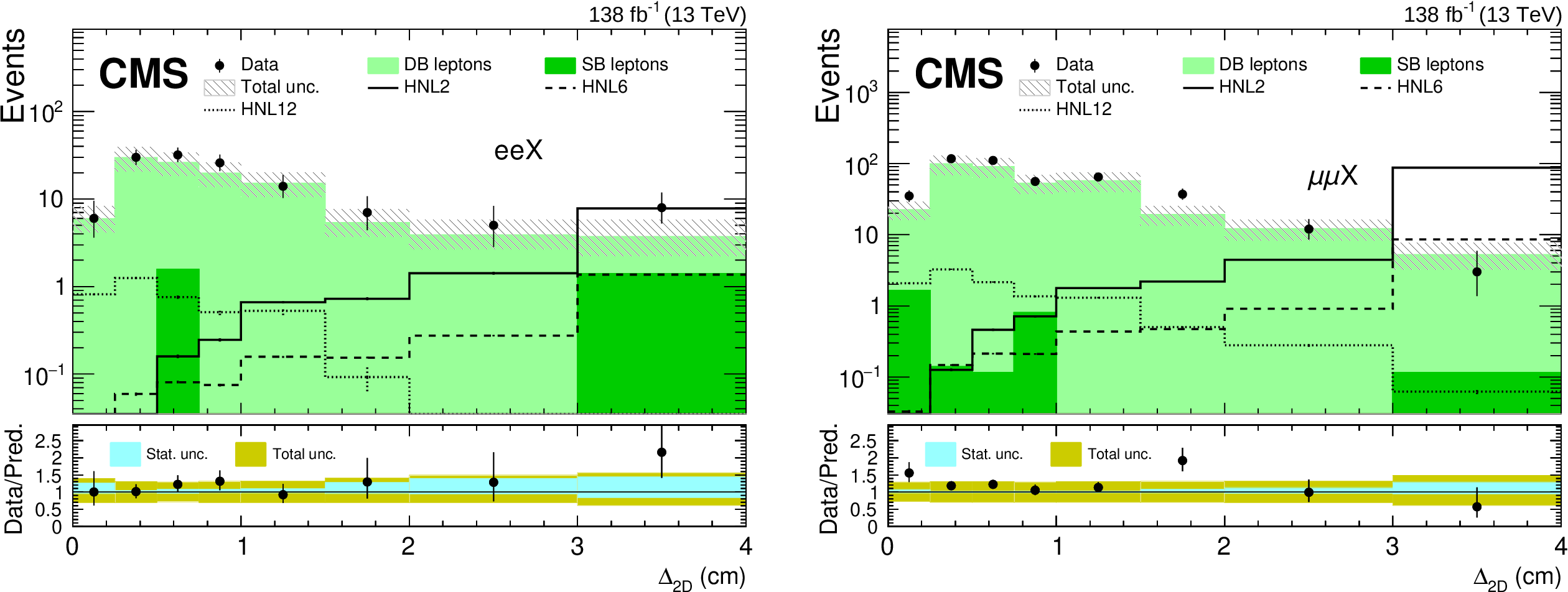
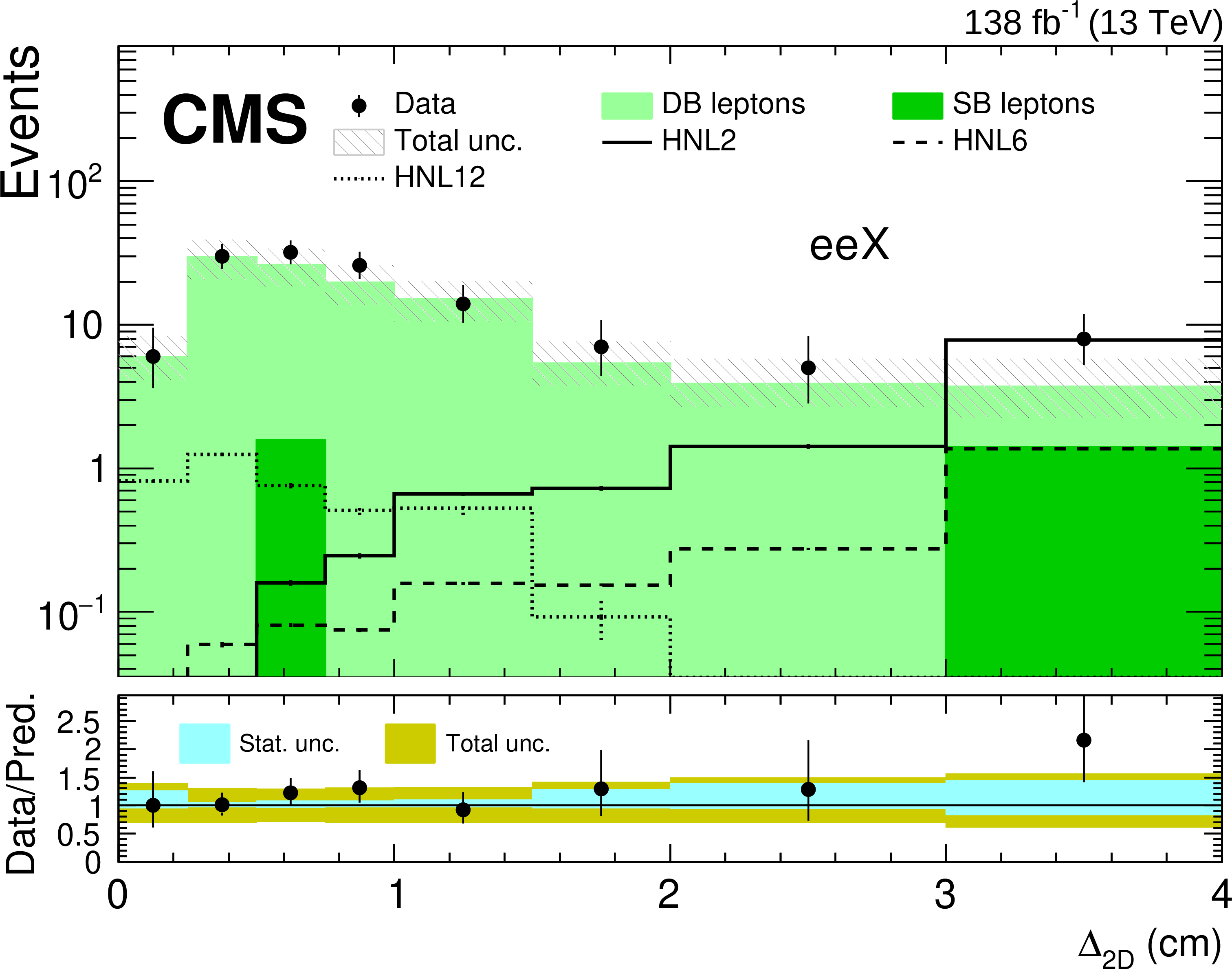
png pdf	Figure 6: Comparison between the number of observed events in data and the background predictions (shaded histograms, stacked) for the ${\Delta _{\text {2D}}}$ variable in eeX (left) and $ \mu \mu $X (right) final states. Events in the overflow bin are included in the last bin. The hashed band indicates the total systematic and statistical uncertainty in the background prediction. The lower panels indicate the ratio between data and prediction. Predictions for signal events are shown for several benchmark hypotheses for Majorana HNL production: ${m_\mathrm{N}} =$ 2 GeV and ${{| {V_{\mathrm{N} \ell}} |}^2} = $ 0.8$\times$10$^{-4}$ (HNL2), ${m_\mathrm{N}} =$ 6 GeV and ${{| {V_{\mathrm{N} \ell}} |}^2} = $ 1.3$\times$10$^{-6}$ (HNL6), ${m_\mathrm{N}} =$ 12 GeV and ${{| {V_{\mathrm{N} \ell}} |}^2} = $ 1.0$\times$10$^{-6}$ (HNL12).
png pdf	Figure 6-a: Comparison between the number of observed events in data and the background predictions (shaded histograms, stacked) for the ${\Delta _{\text {2D}}}$ variable in the eeX final state. Events in the overflow bin are included in the last bin. The hashed band indicates the total systematic and statistical uncertainty in the background prediction. The lower panels indicate the ratio between data and prediction. Predictions for signal events are shown for several benchmark hypotheses for Majorana HNL production: ${m_\mathrm{N}} =$ 2 GeV and ${{| {V_{\mathrm{N} \ell}} |}^2} = $ 0.8$\times$10$^{-4}$ (HNL2), ${m_\mathrm{N}} =$ 6 GeV and ${{| {V_{\mathrm{N} \ell}} |}^2} = $ 1.3$\times$10$^{-6}$ (HNL6), ${m_\mathrm{N}} =$ 12 GeV and ${{| {V_{\mathrm{N} \ell}} |}^2} = $ 1.0$\times$10$^{-6}$ (HNL12).
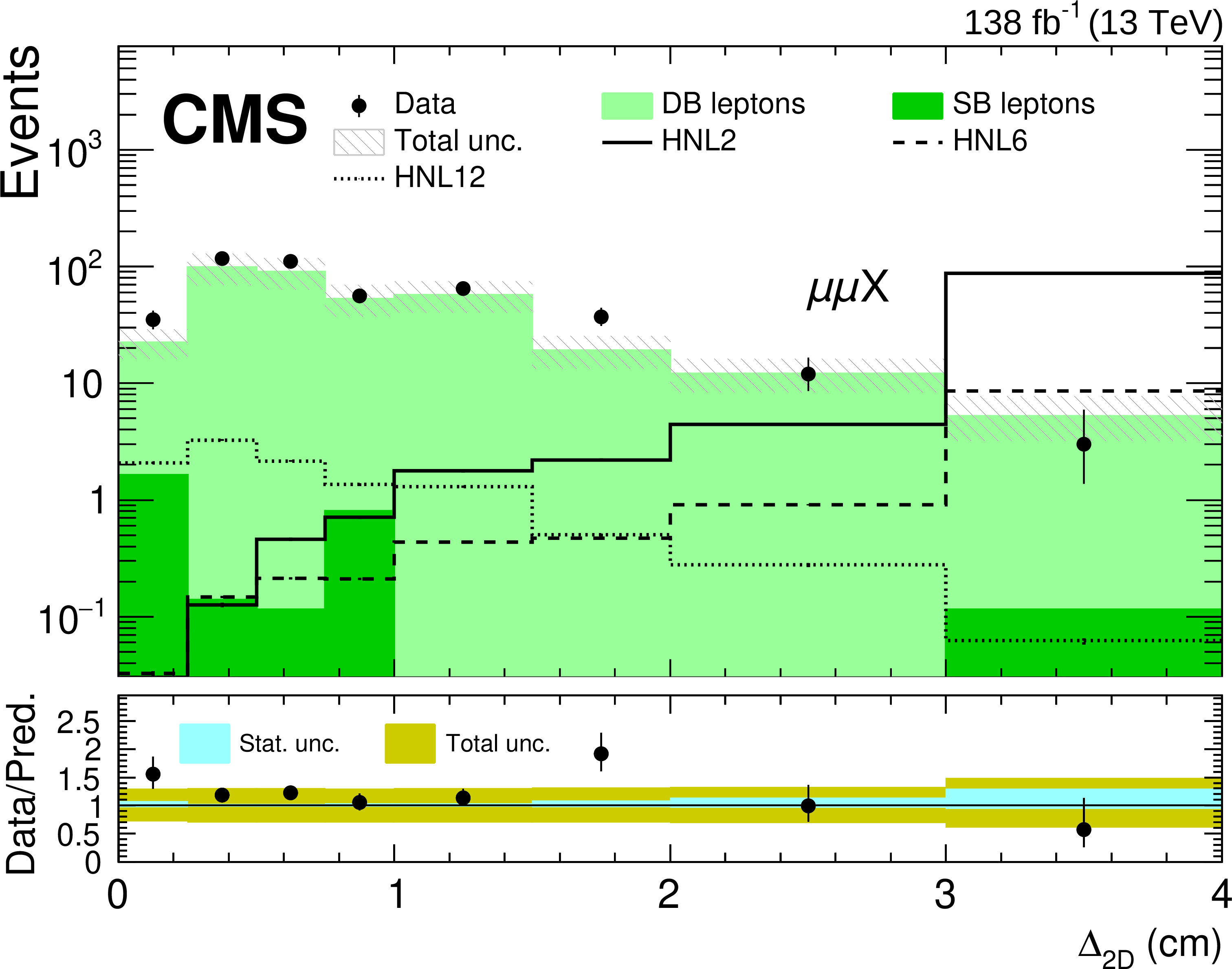
png pdf	Figure 6-b: Comparison between the number of observed events in data and the background predictions (shaded histograms, stacked) for the ${\Delta _{\text {2D}}}$ variable in the $ \mu \mu $X final state. Events in the overflow bin are included in the last bin. The hashed band indicates the total systematic and statistical uncertainty in the background prediction. The lower panels indicate the ratio between data and prediction. Predictions for signal events are shown for several benchmark hypotheses for Majorana HNL production: ${m_\mathrm{N}} =$ 2 GeV and ${{| {V_{\mathrm{N} \ell}} |}^2} = $ 0.8$\times$10$^{-4}$ (HNL2), ${m_\mathrm{N}} =$ 6 GeV and ${{| {V_{\mathrm{N} \ell}} |}^2} = $ 1.3$\times$10$^{-6}$ (HNL6), ${m_\mathrm{N}} =$ 12 GeV and ${{| {V_{\mathrm{N} \ell}} |}^2} = $ 1.0$\times$10$^{-6}$ (HNL12).
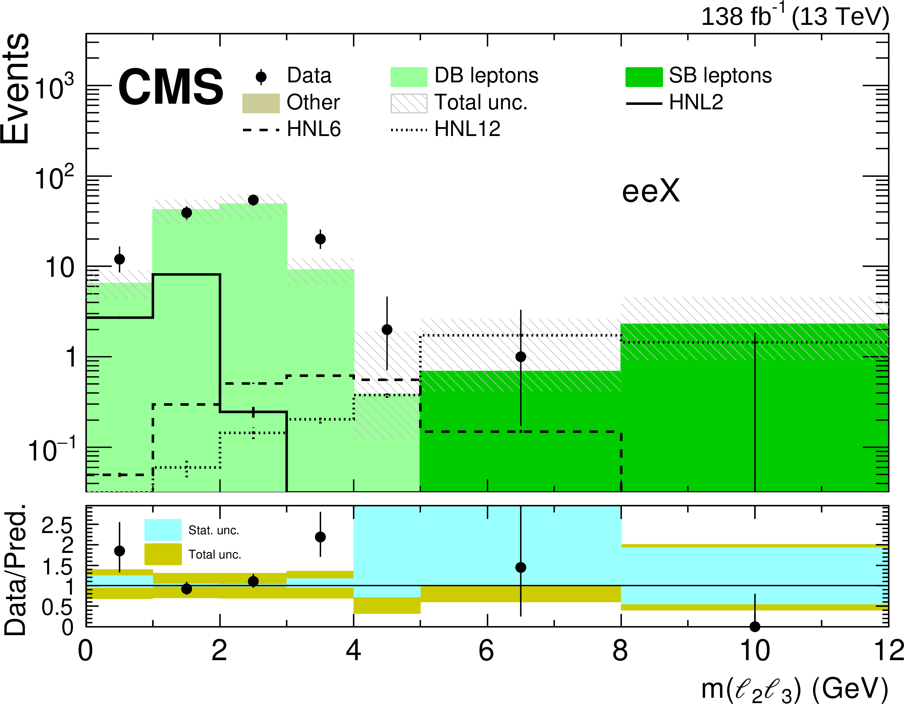
png pdf	Figure 7: Comparison between the number of observed events in data and the background predictions (shaded histograms, stacked) for the $m({\ell _2} {\ell _3})$ variable in eeX (left) and $ \mu \mu $X (right) final states. Events in the overflow bin are included in the last bin. The hashed band indicates the total systematic and statistical uncertainty in the background prediction. The lower panels indicate the ratio between data and prediction, and missing points indicate that the ratio lies outside the axis range. Predictions for signal events are shown for several benchmark hypotheses for Majorana HNL production: ${m_\mathrm{N}} =$ 2 GeV and ${{| {V_{\mathrm{N} \ell}} |}^2} = $ 0.8$\times$10$^{-4}$ (HNL2), ${m_\mathrm{N}} =$ 6 GeV and ${{| {V_{\mathrm{N} \ell}} |}^2} = $ 1.3$\times$10$^{-6}$ (HNL6), ${m_\mathrm{N}} =$ 12 GeV and ${{| {V_{\mathrm{N} \ell}} |}^2} = $ 1.0$\times$10$^{-6}$ (HNL12). Small contributions from background processes that are estimated from simulation are collectively referred to as "Other''.
png pdf	Figure 7-a: Comparison between the number of observed events in data and the background predictions (shaded histograms, stacked) for the $m({\ell _2} {\ell _3})$ variable in the eeX final state. Events in the overflow bin are included in the last bin. The hashed band indicates the total systematic and statistical uncertainty in the background prediction. The lower panels indicate the ratio between data and prediction, and missing points indicate that the ratio lies outside the axis range. Predictions for signal events are shown for several benchmark hypotheses for Majorana HNL production: ${m_\mathrm{N}} =$ 2 GeV and ${{| {V_{\mathrm{N} \ell}} |}^2} = $ 0.8$\times$10$^{-4}$ (HNL2), ${m_\mathrm{N}} =$ 6 GeV and ${{| {V_{\mathrm{N} \ell}} |}^2} = $ 1.3$\times$10$^{-6}$ (HNL6), ${m_\mathrm{N}} =$ 12 GeV and ${{| {V_{\mathrm{N} \ell}} |}^2} = $ 1.0$\times$10$^{-6}$ (HNL12). Small contributions from background processes that are estimated from simulation are collectively referred to as "Other''.
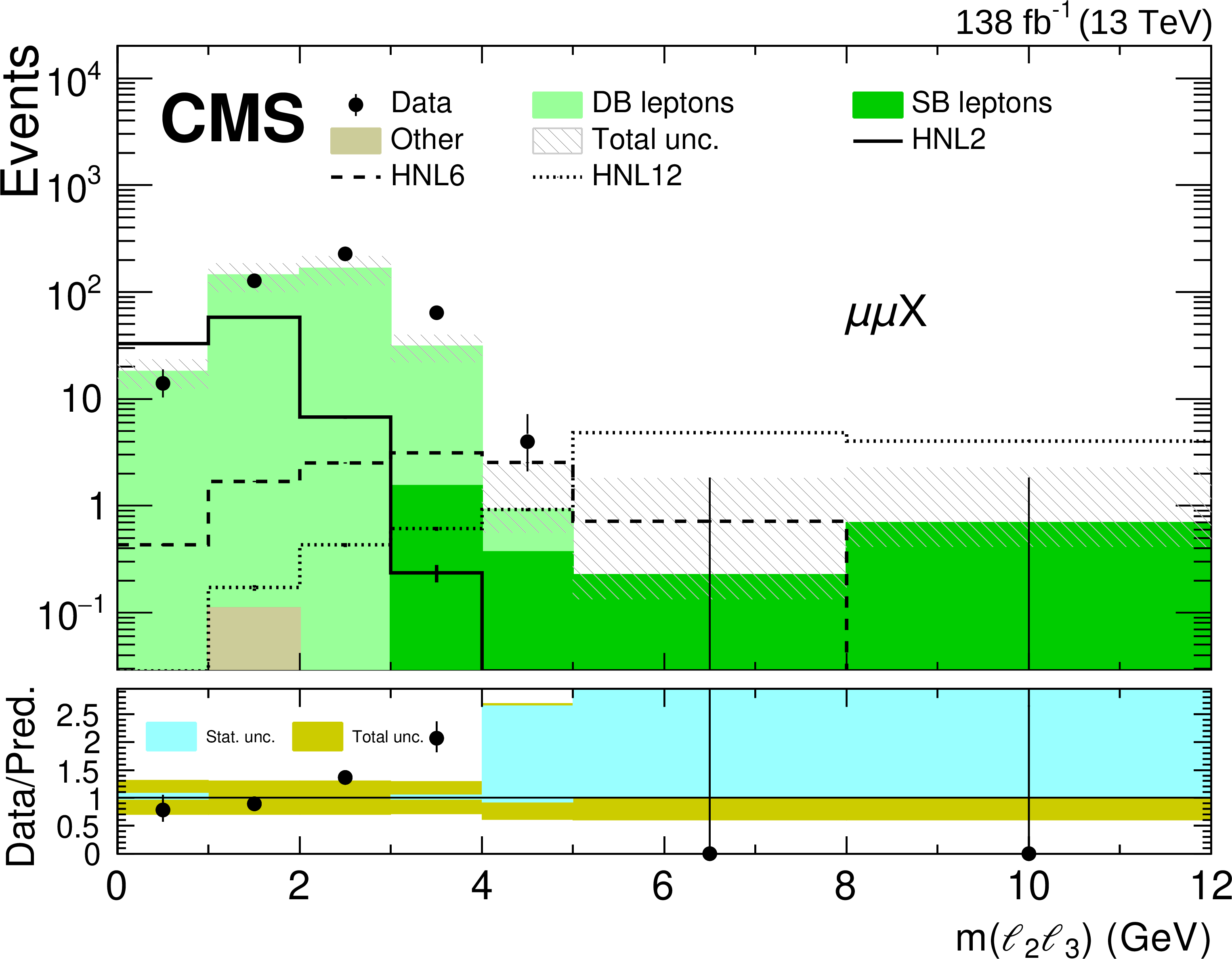
png pdf	Figure 7-b: Comparison between the number of observed events in data and the background predictions (shaded histograms, stacked) for the $m({\ell _2} {\ell _3})$ variable in the $ \mu \mu $X final state. Events in the overflow bin are included in the last bin. The hashed band indicates the total systematic and statistical uncertainty in the background prediction. The lower panels indicate the ratio between data and prediction, and missing points indicate that the ratio lies outside the axis range. Predictions for signal events are shown for several benchmark hypotheses for Majorana HNL production: ${m_\mathrm{N}} =$ 2 GeV and ${{| {V_{\mathrm{N} \ell}} |}^2} = $ 0.8$\times$10$^{-4}$ (HNL2), ${m_\mathrm{N}} =$ 6 GeV and ${{| {V_{\mathrm{N} \ell}} |}^2} = $ 1.3$\times$10$^{-6}$ (HNL6), ${m_\mathrm{N}} =$ 12 GeV and ${{| {V_{\mathrm{N} \ell}} |}^2} = $ 1.0$\times$10$^{-6}$ (HNL12). Small contributions from background processes that are estimated from simulation are collectively referred to as "Other''.
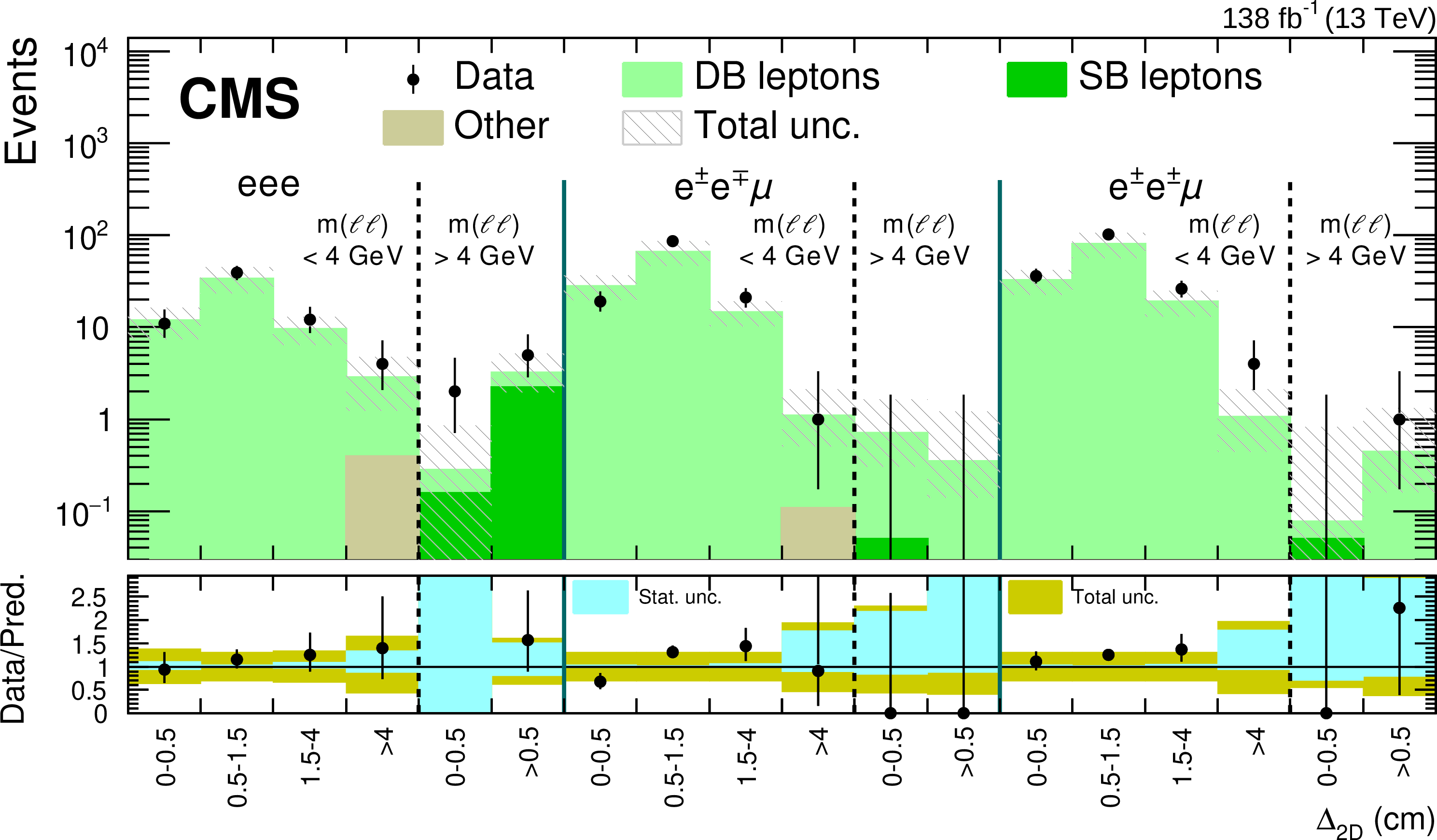
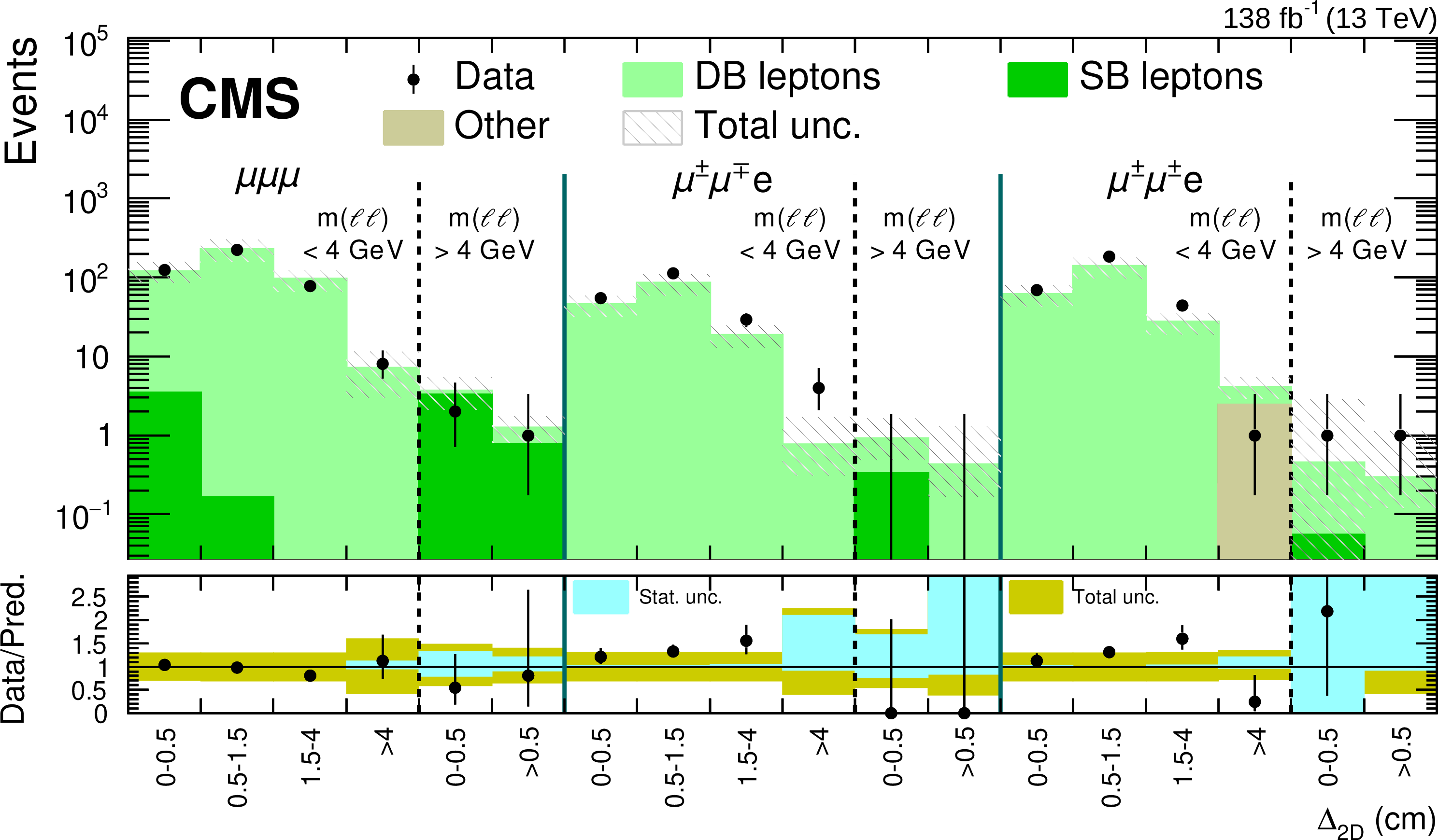
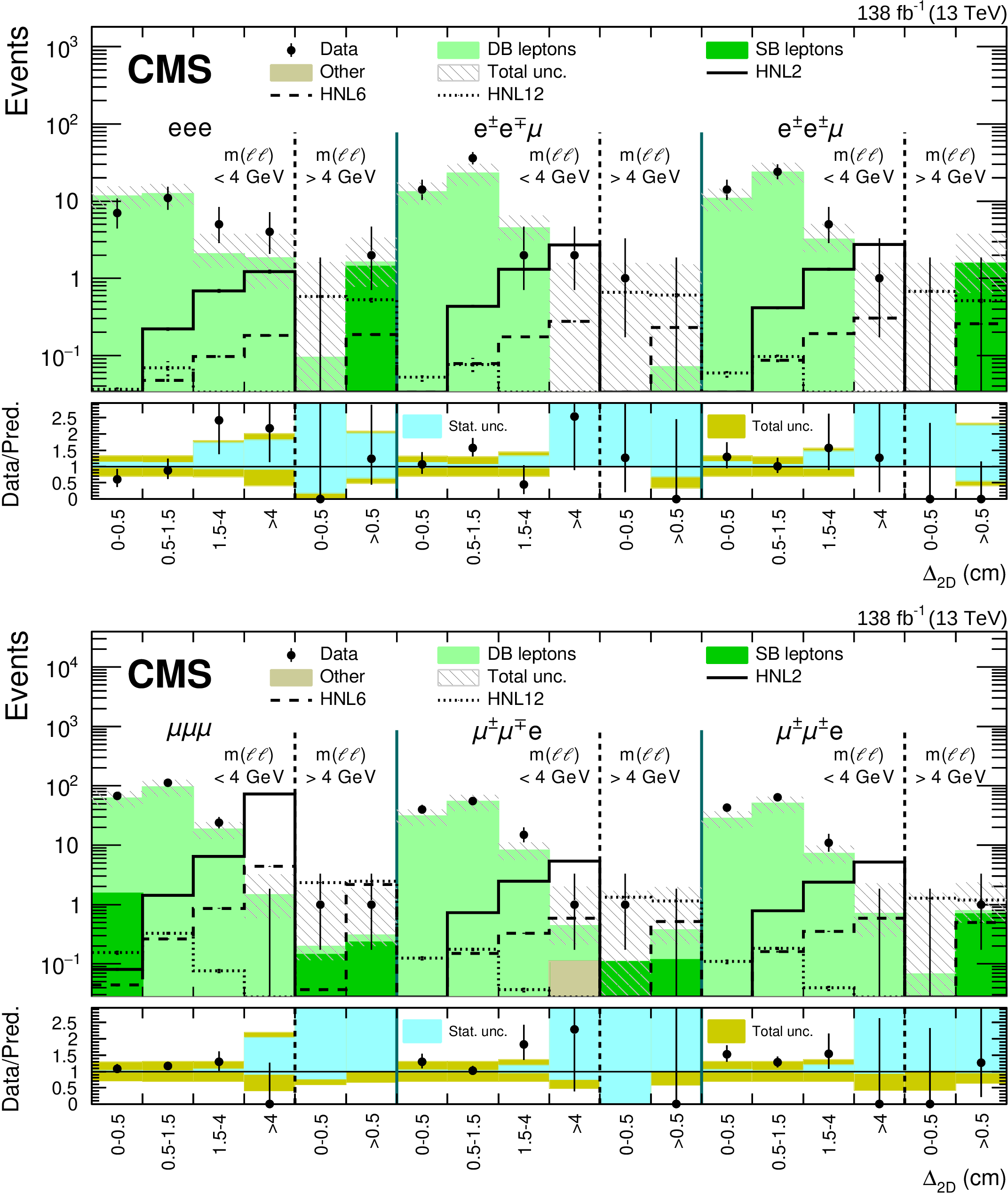
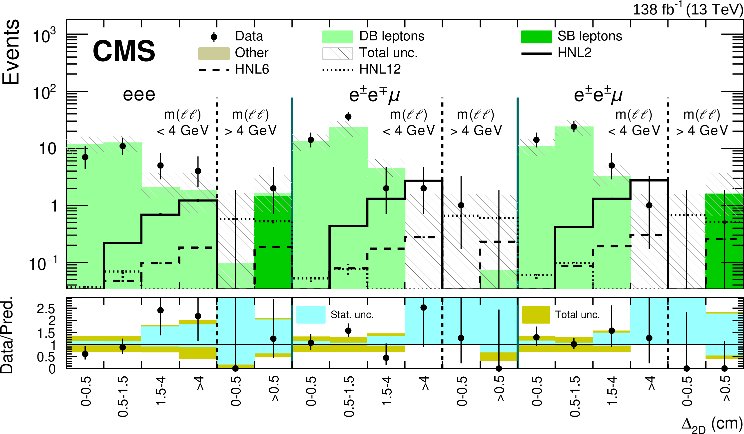
png pdf	Figure 8: Comparison between the number of observed events in data and the background predictions (shaded histograms, stacked) in the search regions for eeX (upper) and $ \mu \mu $X (lower) final states. The hashed band indicates the total systematic and statistical uncertainty in the background prediction. The lower panels indicate the ratio between data and prediction, and missing points indicate that the ratio lies outside the axis range. Predictions for signal events are shown for several benchmark hypotheses for Majorana HNL production: ${m_\mathrm{N}} =$ 2 GeV and ${{| {V_{\mathrm{N} \ell}} |}^2} = $ 0.8$\times$10$^{-4}$ (HNL2), ${m_\mathrm{N}} =$ 6 GeV and ${{| {V_{\mathrm{N} \ell}} |}^2} = $ 1.3$\times$10$^{-6}$ (HNL6), ${m_\mathrm{N}} =$ 12 GeV and ${{| {V_{\mathrm{N} \ell}} |}^2} = $ 1.0$\times$10$^{-6}$ (HNL12). The uncertainty band assigned to the background prediction includes statistical and systematic contributions. Small contributions from background processes that are estimated from simulation are collectively referred to as "Other''.
png pdf	Figure 8-a: Comparison between the number of observed events in data and the background predictions (shaded histograms, stacked) in the search regions for the eeX final states. The hashed band indicates the total systematic and statistical uncertainty in the background prediction. The lower panels indicate the ratio between data and prediction, and missing points indicate that the ratio lies outside the axis range. Predictions for signal events are shown for several benchmark hypotheses for Majorana HNL production: ${m_\mathrm{N}} =$ 2 GeV and ${{| {V_{\mathrm{N} \ell}} |}^2} = $ 0.8$\times$10$^{-4}$ (HNL2), ${m_\mathrm{N}} =$ 6 GeV and ${{| {V_{\mathrm{N} \ell}} |}^2} = $ 1.3$\times$10$^{-6}$ (HNL6), ${m_\mathrm{N}} =$ 12 GeV and ${{| {V_{\mathrm{N} \ell}} |}^2} = $ 1.0$\times$10$^{-6}$ (HNL12). The uncertainty band assigned to the background prediction includes statistical and systematic contributions. Small contributions from background processes that are estimated from simulation are collectively referred to as "Other''.
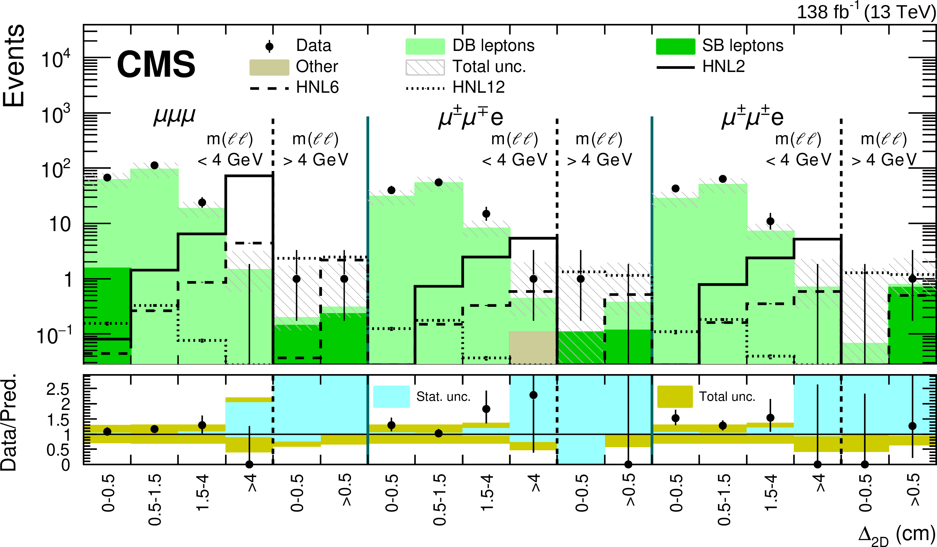
png pdf	Figure 8-b: Comparison between the number of observed events in data and the background predictions (shaded histograms, stacked) in the search regions for the $ \mu \mu $X final states. The hashed band indicates the total systematic and statistical uncertainty in the background prediction. The lower panels indicate the ratio between data and prediction, and missing points indicate that the ratio lies outside the axis range. Predictions for signal events are shown for several benchmark hypotheses for Majorana HNL production: ${m_\mathrm{N}} =$ 2 GeV and ${{| {V_{\mathrm{N} \ell}} |}^2} = $ 0.8$\times$10$^{-4}$ (HNL2), ${m_\mathrm{N}} =$ 6 GeV and ${{| {V_{\mathrm{N} \ell}} |}^2} = $ 1.3$\times$10$^{-6}$ (HNL6), ${m_\mathrm{N}} =$ 12 GeV and ${{| {V_{\mathrm{N} \ell}} |}^2} = $ 1.0$\times$10$^{-6}$ (HNL12). The uncertainty band assigned to the background prediction includes statistical and systematic contributions. Small contributions from background processes that are estimated from simulation are collectively referred to as "Other''.
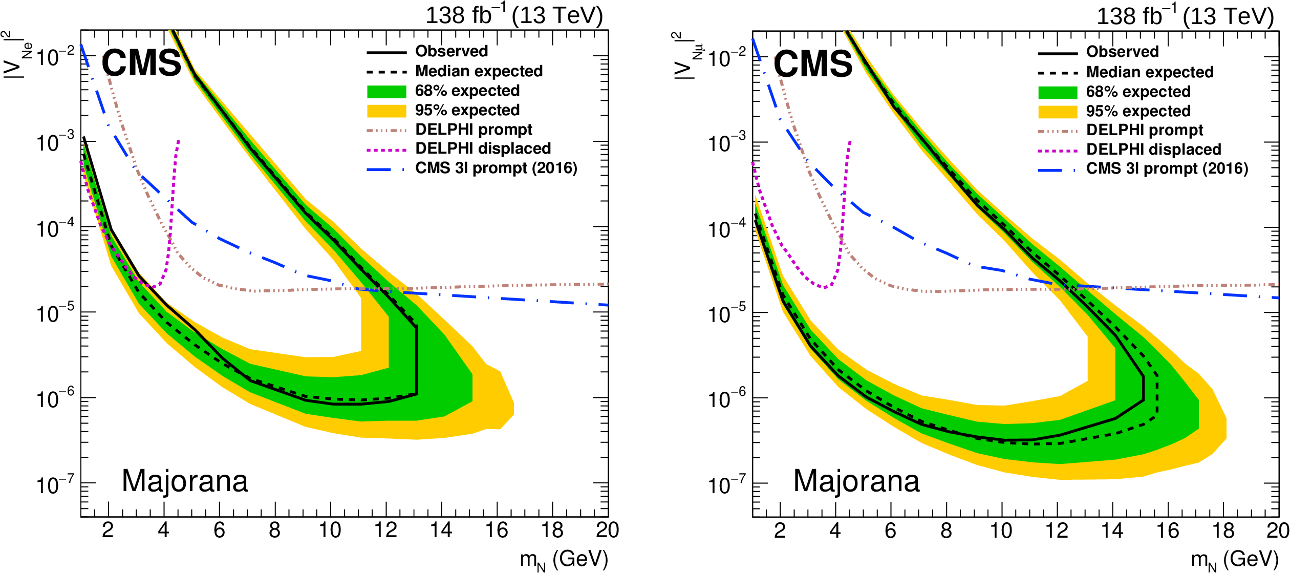
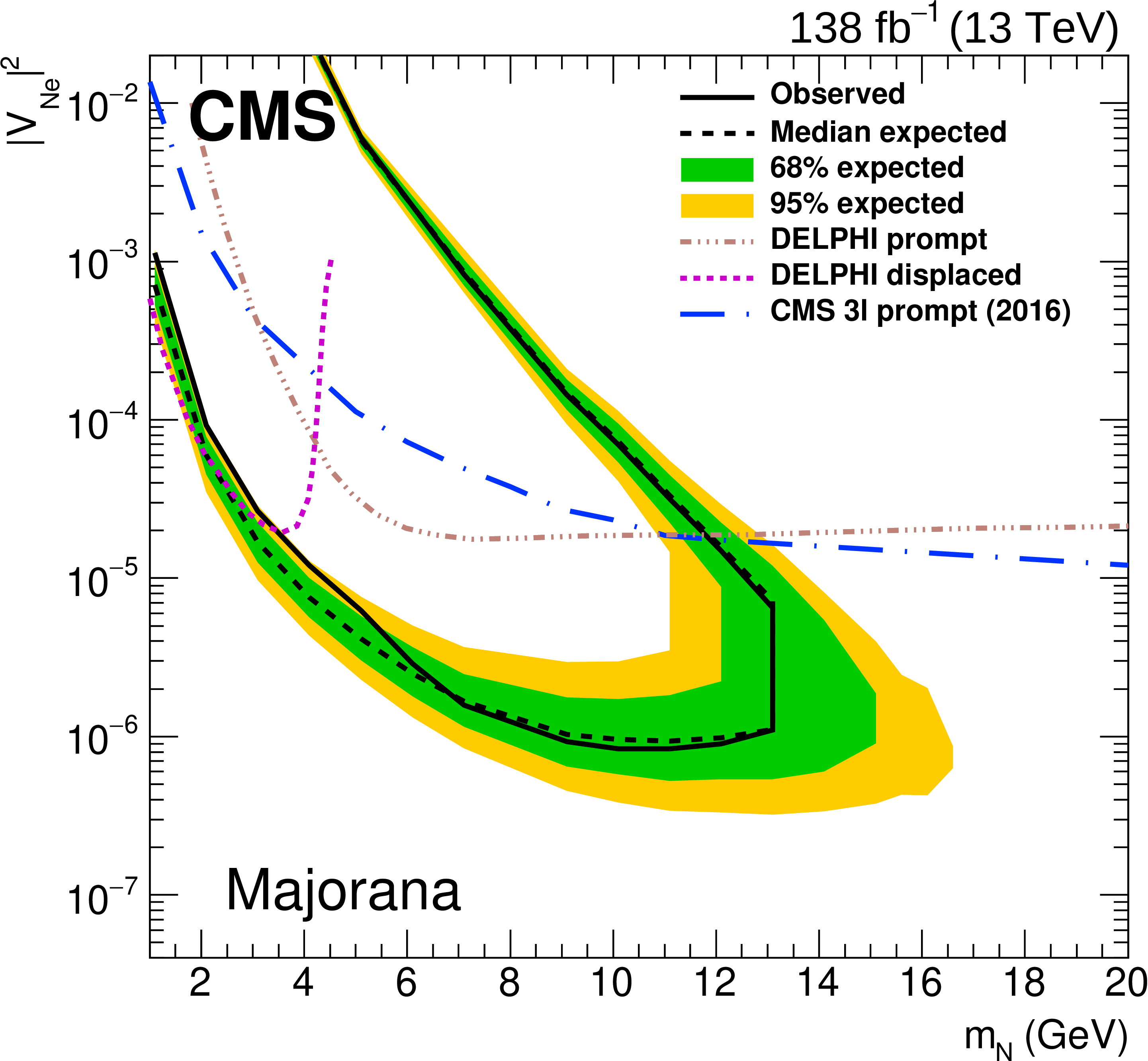
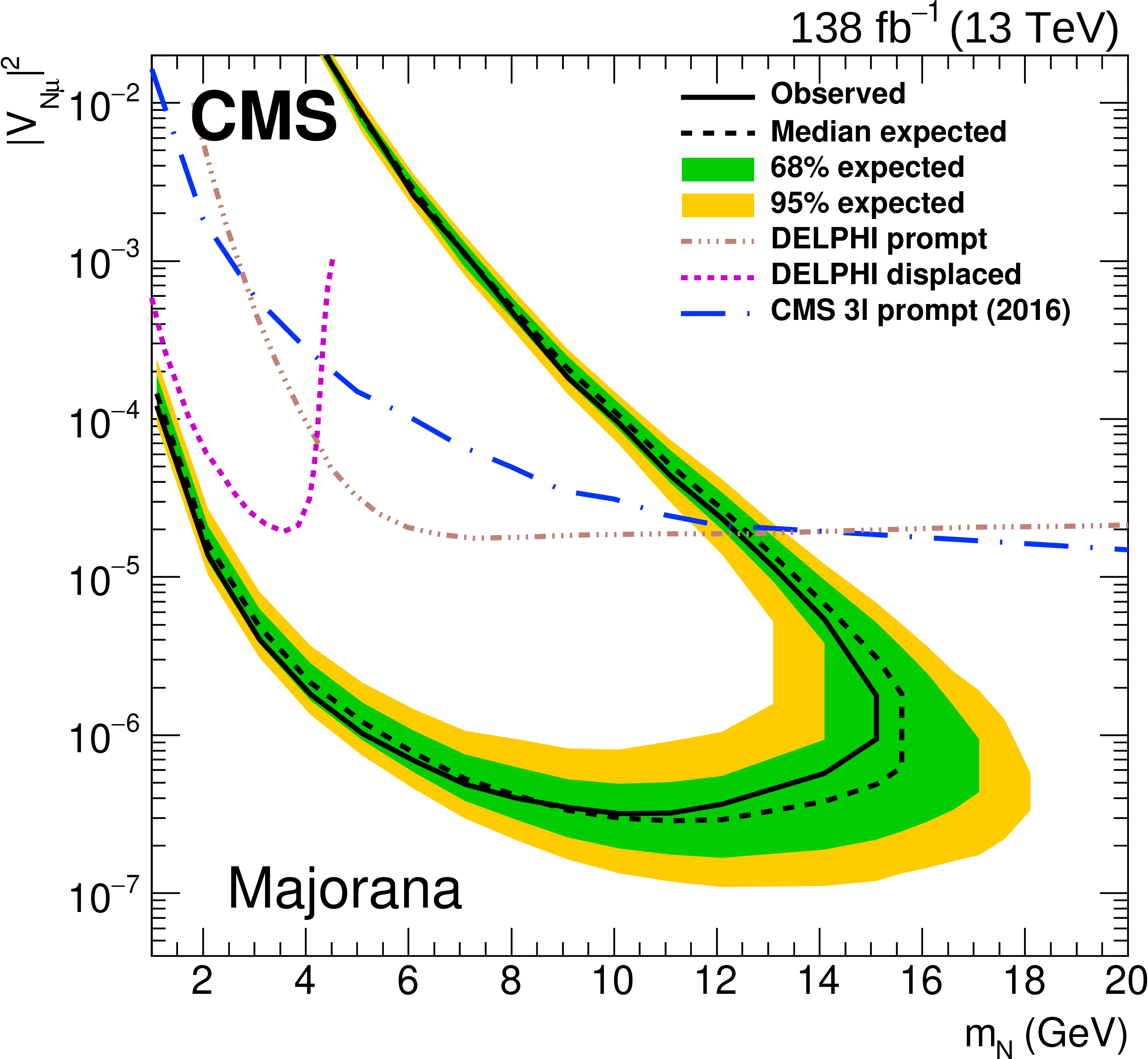
png pdf	Figure 9: The 95% CL limits on ${{| {V_{\mathrm{N} \mathrm{e}}} |}^2}$ (left) and ${{| {V_{\mathrm{N} \mu}} |}^2}$ (right) as functions of ${m_\mathrm{N}}$ for a Majorana HNL. The area inside the solid (dashed) black curve indicates the observed (expected) exclusion region. Results from the DELPHI [18] and the CMS [20,19] Collaborations are shown for reference.
png pdf	Figure 9-a: The 95% CL limits on ${{| {V_{\mathrm{N} \mathrm{e}}} |}^2}$ as functions of ${m_\mathrm{N}}$ for a Majorana HNL. The area inside the solid (dashed) black curve indicates the observed (expected) exclusion region. Results from the DELPHI [18] and the CMS [20,19] Collaborations are shown for reference.
png pdf	Figure 9-b: The 95% CL limits on ${{| {V_{\mathrm{N} \mu}} |}^2}$ as functions of ${m_\mathrm{N}}$ for a Majorana HNL. The area inside the solid (dashed) black curve indicates the observed (expected) exclusion region. Results from the DELPHI [18] and the CMS [20,19] Collaborations are shown for reference.
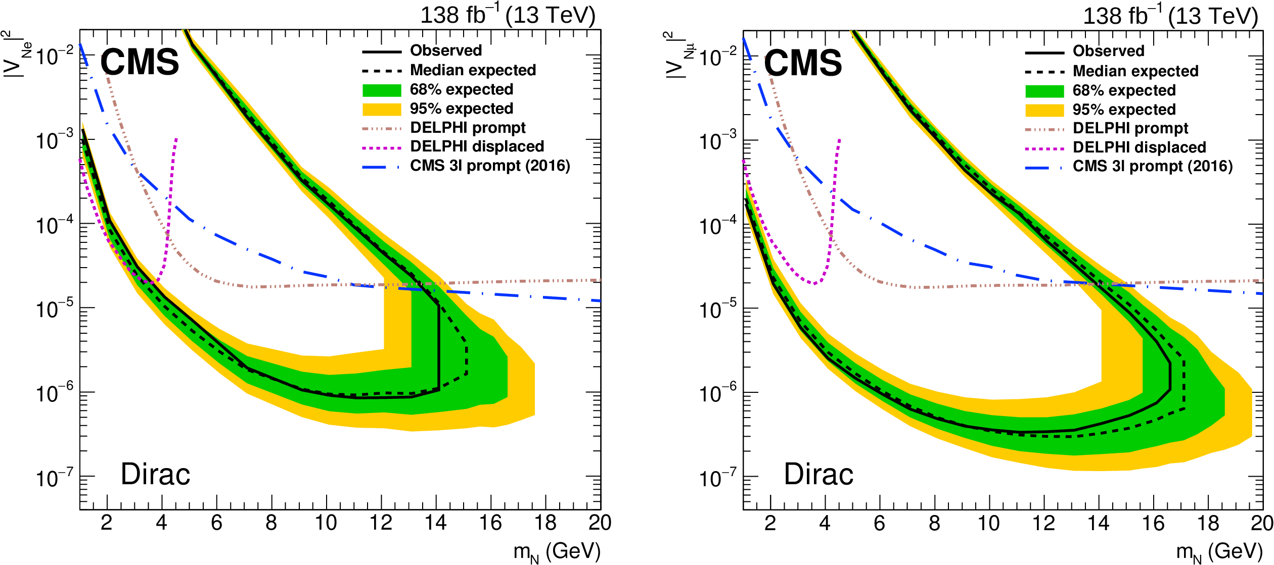
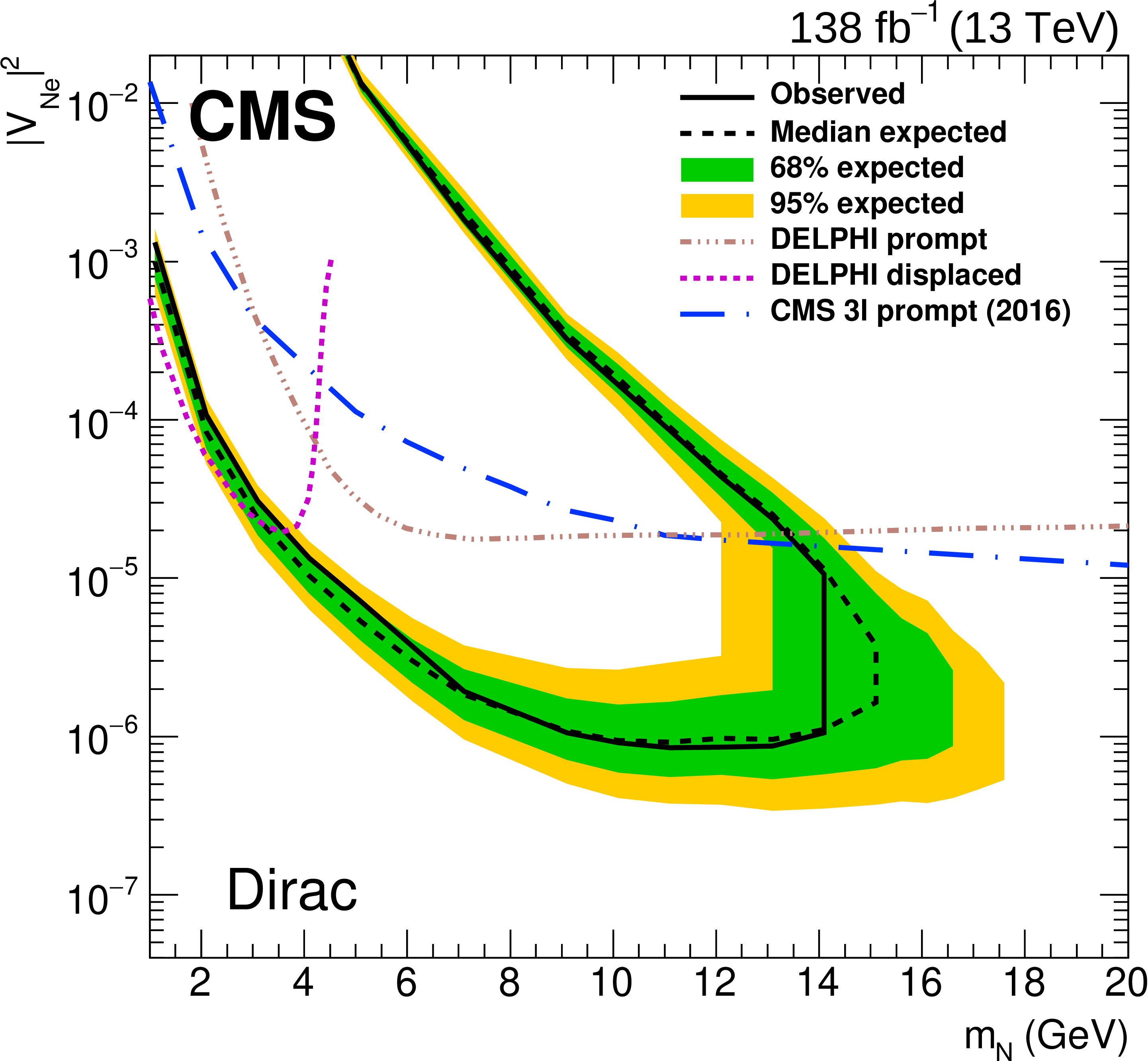
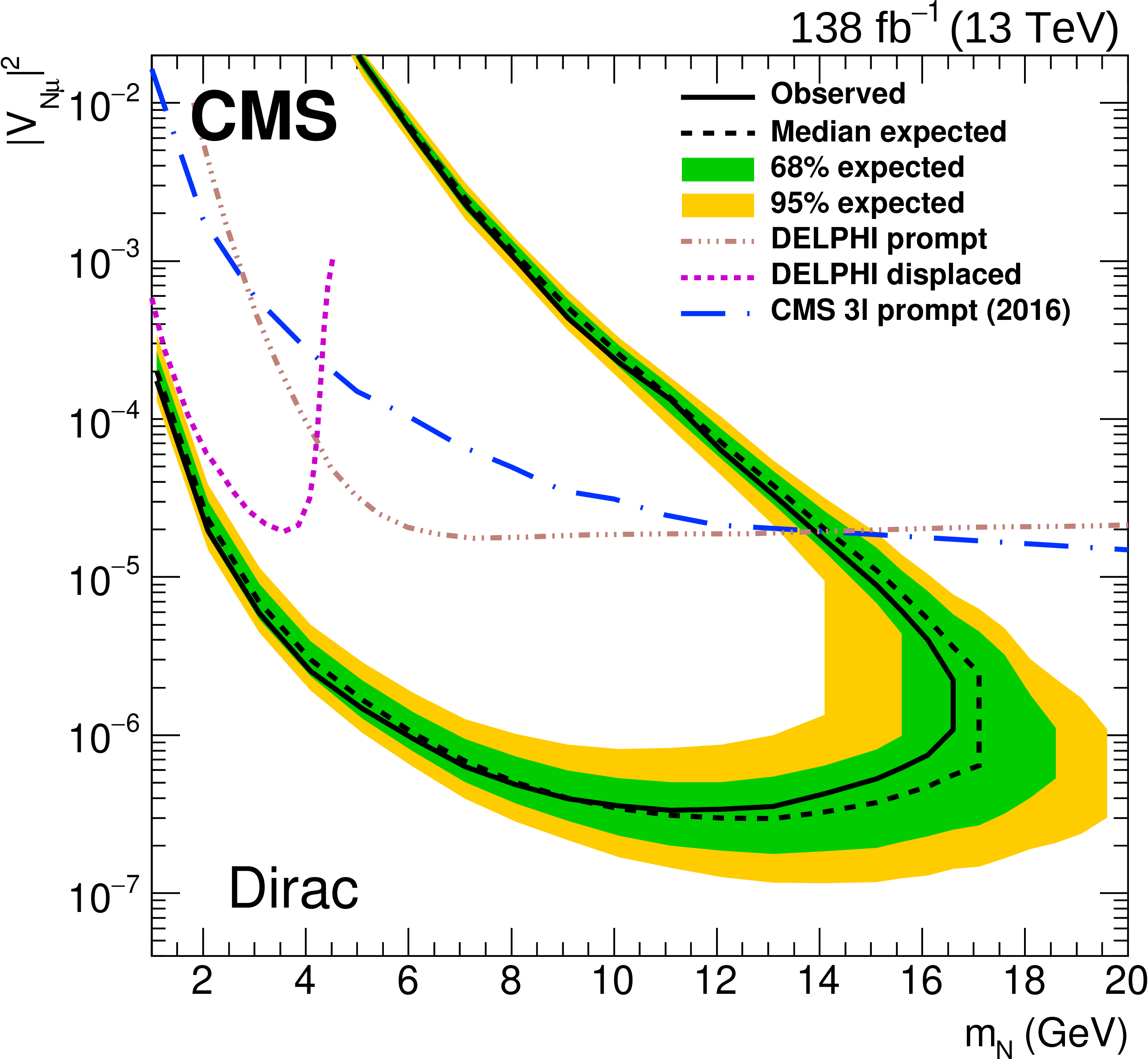
png pdf	Figure 10: The 95% CL limits on ${{| {V_{\mathrm{N} \mathrm{e}}} |}^2}$ (left) and ${{| {V_{\mathrm{N} \mu}} |}^2}$ (right) as functions of ${m_\mathrm{N}}$ for a Dirac HNL. The area inside the solid (dashed) black curve indicates the observed (expected) exclusion region. Results from the DELPHI [18] and the CMS [20,19] Collaborations are shown for reference.
png pdf	Figure 10-a: The 95% CL limits on ${{| {V_{\mathrm{N} \mathrm{e}}} |}^2}$ as functions of ${m_\mathrm{N}}$ for a Dirac HNL. The area inside the solid (dashed) black curve indicates the observed (expected) exclusion region. Results from the DELPHI [18] and the CMS [20,19] Collaborations are shown for reference.
png pdf	Figure 10-b: The 95% CL limits on ${{| {V_{\mathrm{N} \mu}} |}^2}$ as functions of ${m_\mathrm{N}}$ for a Dirac HNL. The area inside the solid (dashed) black curve indicates the observed (expected) exclusion region. Results from the DELPHI [18] and the CMS [20,19] Collaborations are shown for reference.

Tables
png pdf	Table 1: Baseline selection criteria (left) and dilepton invariant mass vetoes (right) applied in the analysis. The width of the vetoed range for the meson resonances reflects the experimental resolution of the dilepton invariant mass reconstruction.
png pdf	Table 2: Definition of kinematic regions in terms of dilepton invariant mass $m({\ell _2} {\ell _3})$ and SV displacement ${\Delta _{\text {2D}}}$.
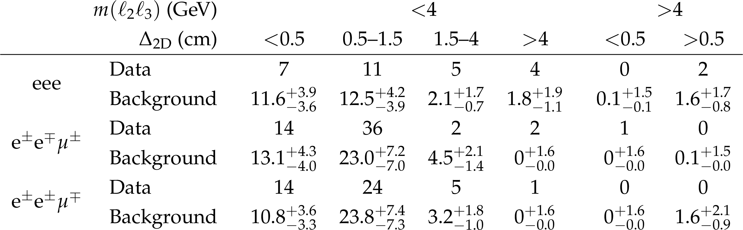
png pdf	Table 3: Number of predicted and observed events in the eeX final states. The quoted uncertainties include statistical and systematic components.
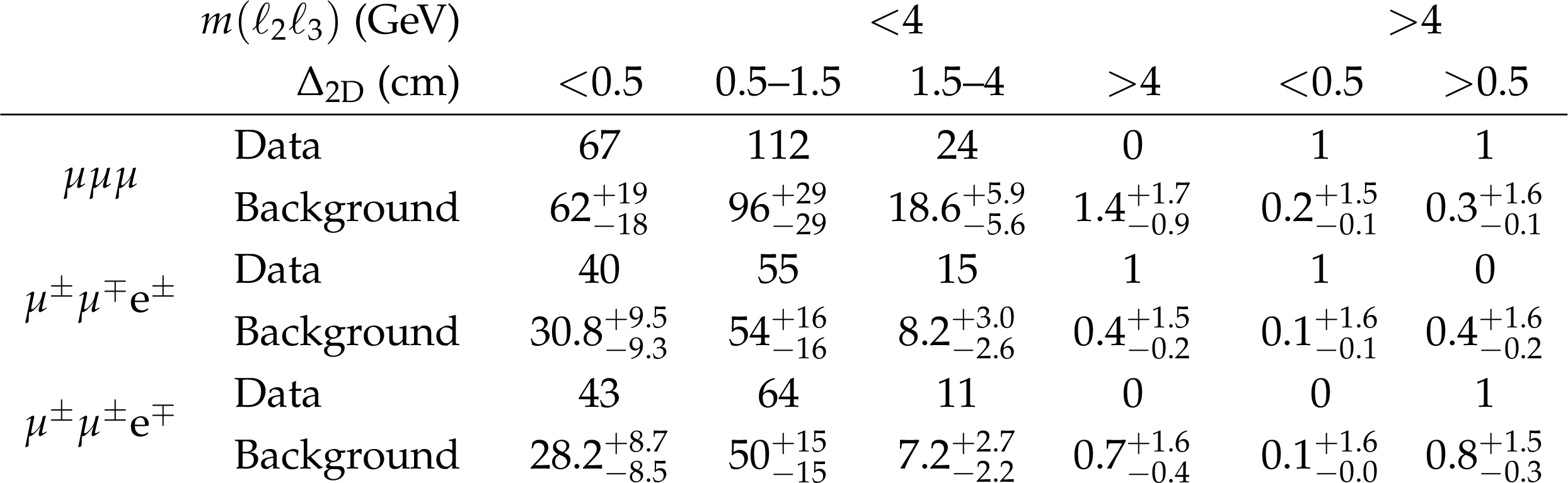
png pdf	Table 4: Number of predicted and observed events in the $ \mu \mu $X final states. The quoted uncertainties include statistical and systematic components.
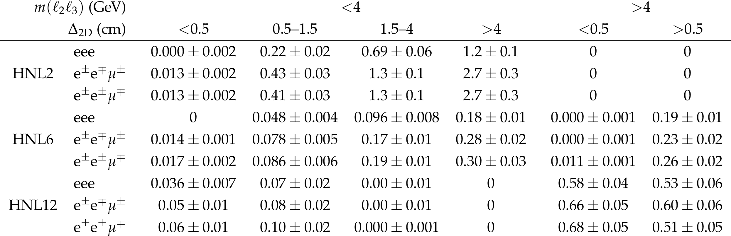
png pdf	Table 5: Number of predicted signal events in the eeX final states. The results are presented for several benchmark signal hypotheses for Majorana HNL production: ${m_\mathrm{N}} =$ 2 GeV and ${{| {V_{\mathrm{N} \ell}} |}^2} = $ 0.8$\times$10$^{-4}$ (HNL2), ${m_\mathrm{N}} =$ 6 GeV and ${{| {V_{\mathrm{N} \ell}} |}^2} = $ 1.3$\times$10$^{-6}$ (HNL6), ${m_\mathrm{N}} =$ 12 GeV and ${{| {V_{\mathrm{N} \ell}} |}^2} = $ 1.0$\times$10$^{-6}$ (HNL12). The quoted uncertainties include statistical and systematic components.
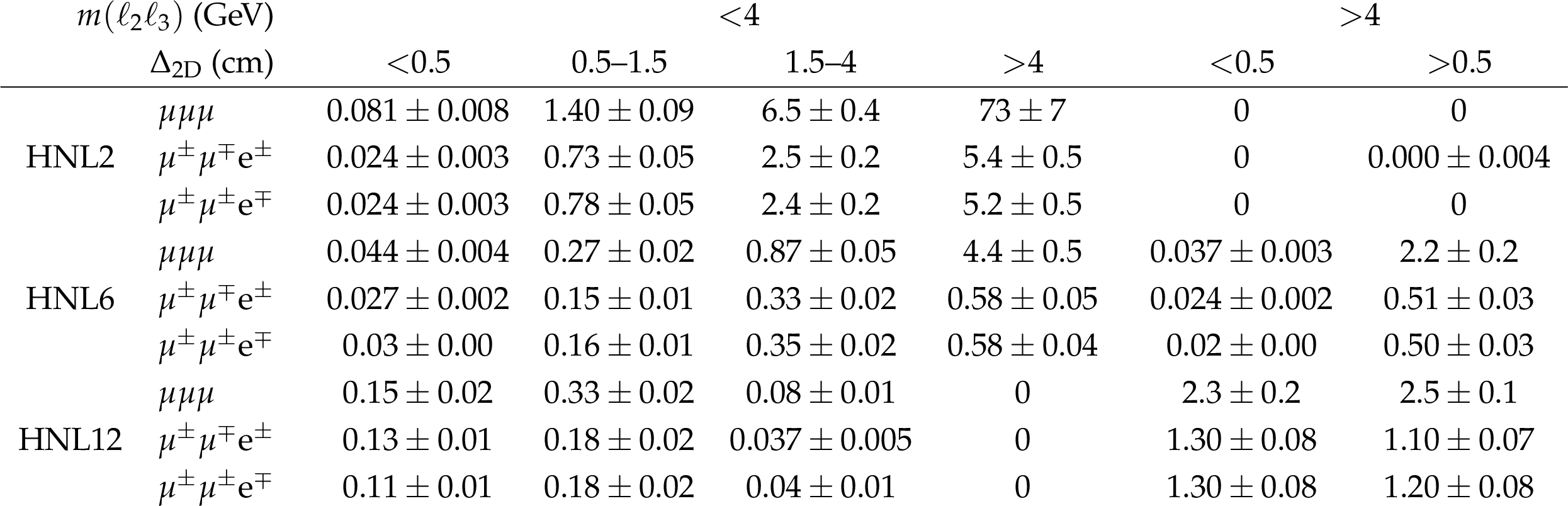
png pdf	Table 6: Number of predicted signal events in the $ \mu \mu $X final states. The results are presented for several benchmark signal hypotheses for Majorana HNL production: ${m_\mathrm{N}} =$ 2 GeV and ${{| {V_{\mathrm{N} \ell}} |}^2} = $ 0.8$\times$10$^{-4}$ (HNL2), ${m_\mathrm{N}} =$ 6 GeV and ${{| {V_{\mathrm{N} \ell}} |}^2} = $ 1.3$\times$10$^{-6}$ (HNL6), ${m_\mathrm{N}} =$ 12 GeV and ${{| {V_{\mathrm{N} \ell}} |}^2} = $ 1.0$\times$10$^{-6}$ (HNL12). The quoted uncertainties include statistical and systematic components.

Summary

A search for heavy neutral leptons (HNLs) has been performed in the decays of W bosons produced in proton-proton collisions at $\sqrt{s} = $ 13 TeV and collected by the CMS experiment at the LHC. The analysis uses a data set corresponding to an integrated luminosity of 138 fb$^{-1}$. Events with three charged leptons are selected, and dedicated methods are applied to identify two displaced leptons consistent with the decay of a long-lived HNL in the mass range 1-20 GeV. Novel methods have been developed to estimate relevant background contributions from control samples in data, addressing one of the important challenges in this type of search at the LHC. No significant deviation from the standard model predictions is observed. Exclusion limits are evaluated at 95% confidence level on the coupling strengths of HNLs to standard model neutrinos as functions of the HNL mass, covering HNL masses from 1 up to 16.5 GeV and squared mixing parameters as low as 3.2$\times$10$^{-7}$, depending on the scenario. These results exceed previous experimental constraints in the mass range 3-14 (1-16.5) GeV for HNLs coupling to electrons (muons) and provide the most stringent limits to date.

Additional Figures
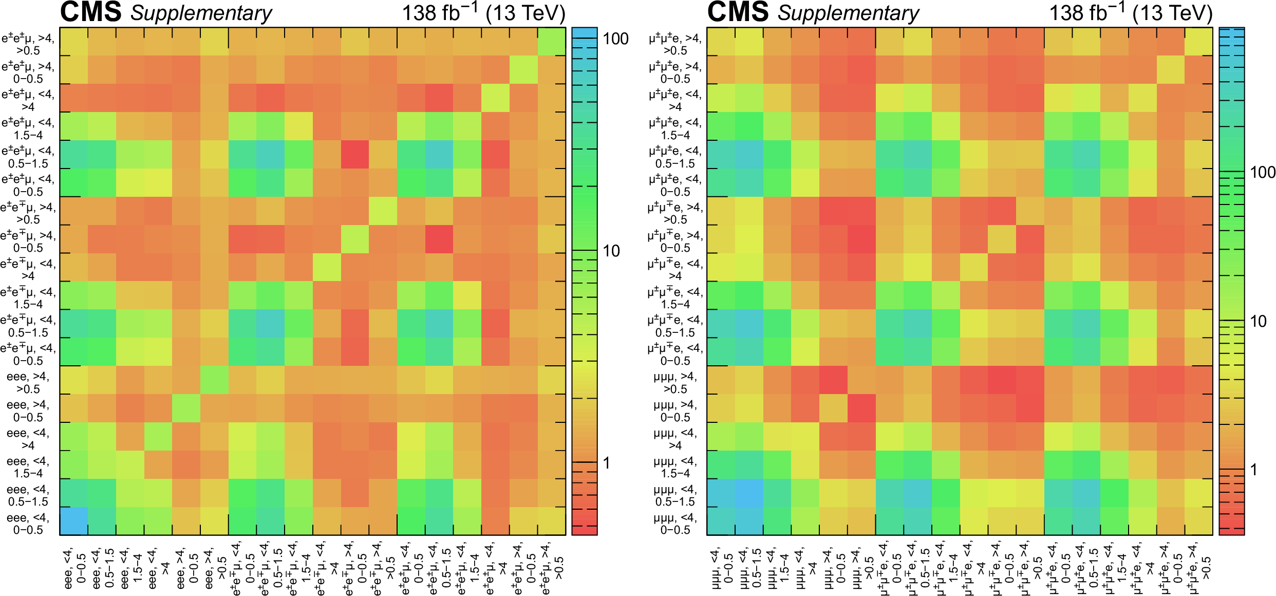
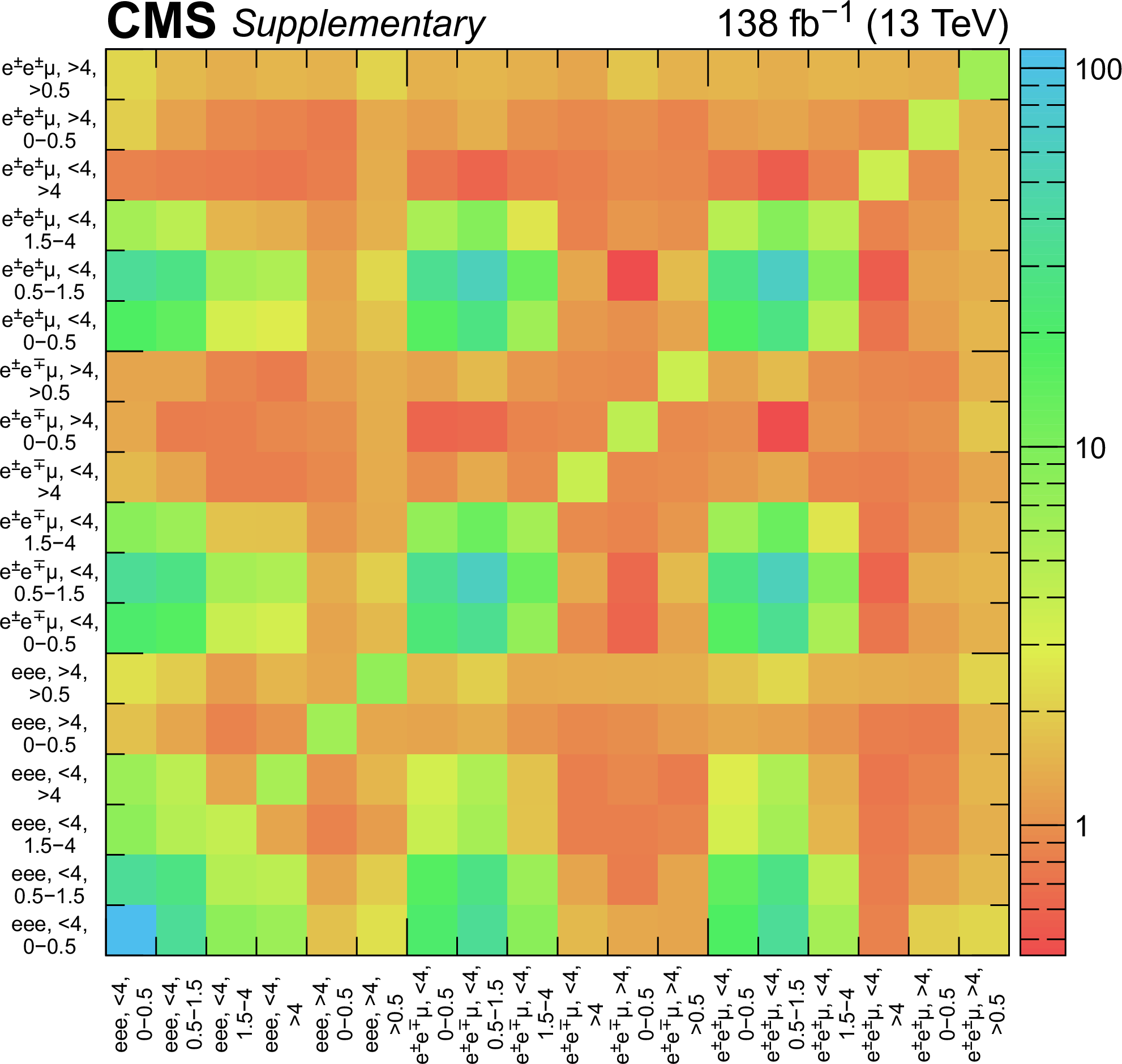
png pdf	Additional Figure 1: Covariance matrix for the background prediction in the signal region bins for the eeX (a) and $ {\mu} {\mu} $X (b) final states. The bin labels specify the channel, the $m(\ell_2,\ell_3)$ bin in GeV, and the $\Delta _{\text {2D}}$ bin in cm.
png pdf	Additional Figure 1-a: Covariance matrix for the background prediction in the signal region bins for the eeX final state. The bin labels specify the channel, the $m(\ell_2,\ell_3)$ bin in GeV, and the $\Delta _{\text {2D}}$ bin in cm.
png pdf	Additional Figure 1-b: Covariance matrix for the background prediction in the signal region bins for the $ {\mu} {\mu} $X final state. The bin labels specify the channel, the $m(\ell_2,\ell_3)$ bin in GeV, and the $\Delta _{\text {2D}}$ bin in cm.
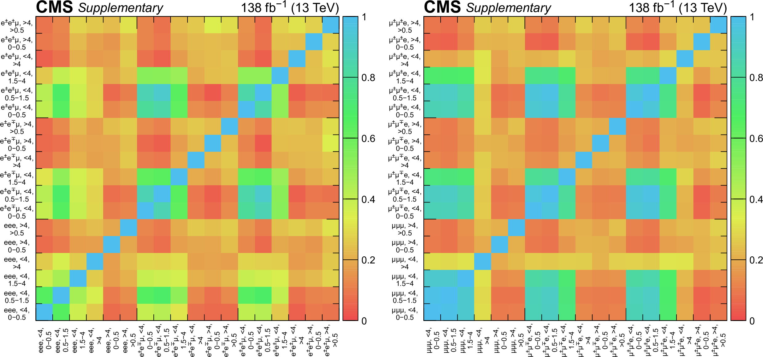
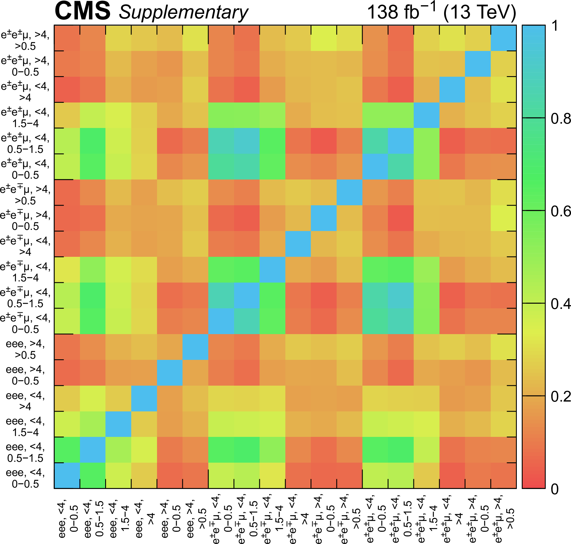
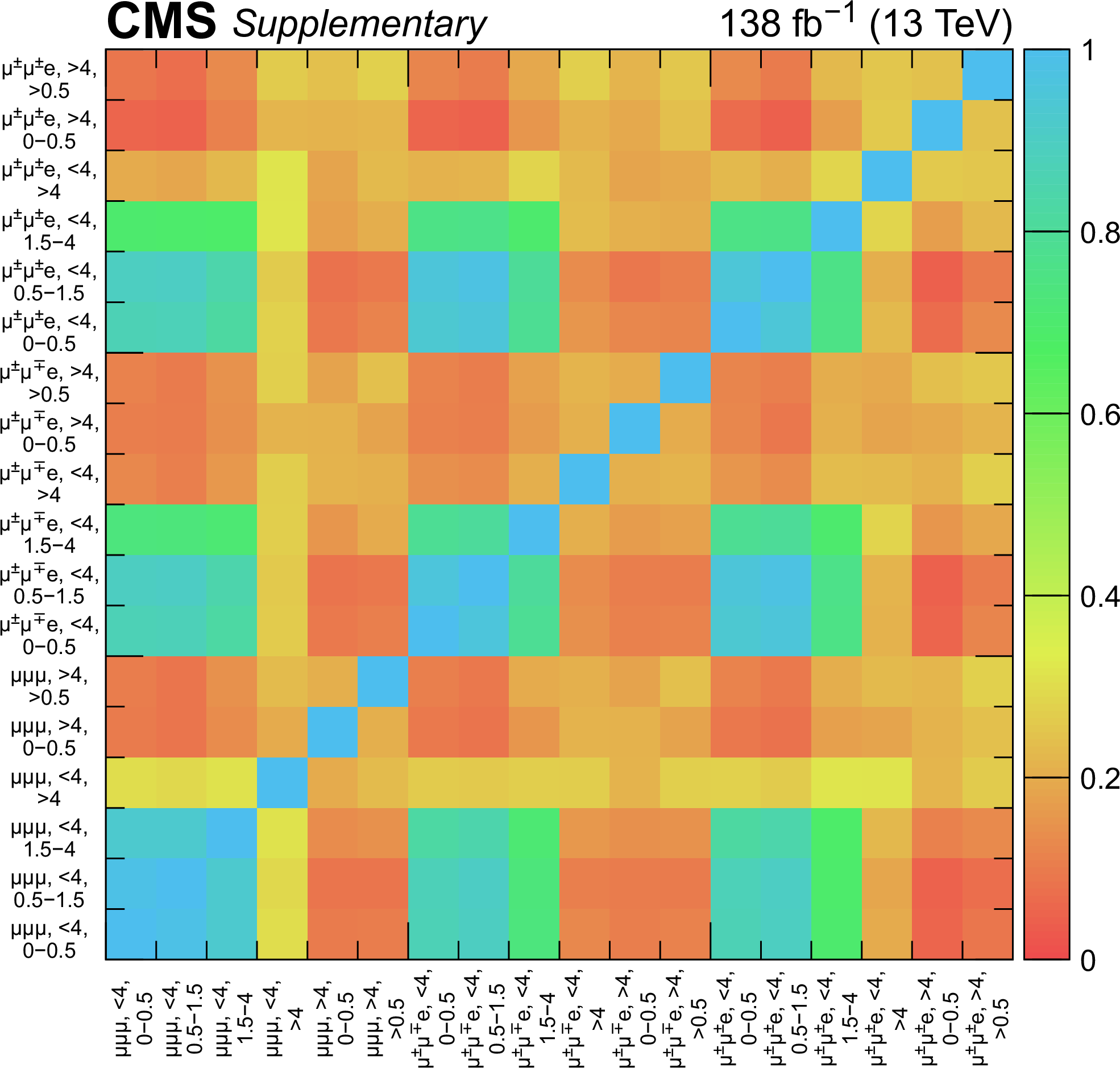
png pdf	Additional Figure 2: Correlation matrix obtained from the covariance matrix for the background prediction in the signal region bins for the eeX (a) and $ {\mu} {\mu} $X (b) final states. The coefficients are obtained from the background-only fit. The bin labels specify the channel, the $m(\ell_2,\ell_3)$ bin in GeV, and the $\Delta _{\text {2D}}$ bin in cm.
png pdf	Additional Figure 2-a: Correlation matrix obtained from the covariance matrix for the background prediction in the signal region bins for the eeX final state. The coefficients are obtained from the background-only fit. The bin labels specify the channel, the $m(\ell_2,\ell_3)$ bin in GeV, and the $\Delta _{\text {2D}}$ bin in cm.
png pdf	Additional Figure 2-b: Correlation matrix obtained from the covariance matrix for the background prediction in the signal region bins for the $ {\mu} {\mu} $X final state. The coefficients are obtained from the background-only fit. The bin labels specify the channel, the $m(\ell_2,\ell_3)$ bin in GeV, and the $\Delta _{\text {2D}}$ bin in cm.

Additional Tables
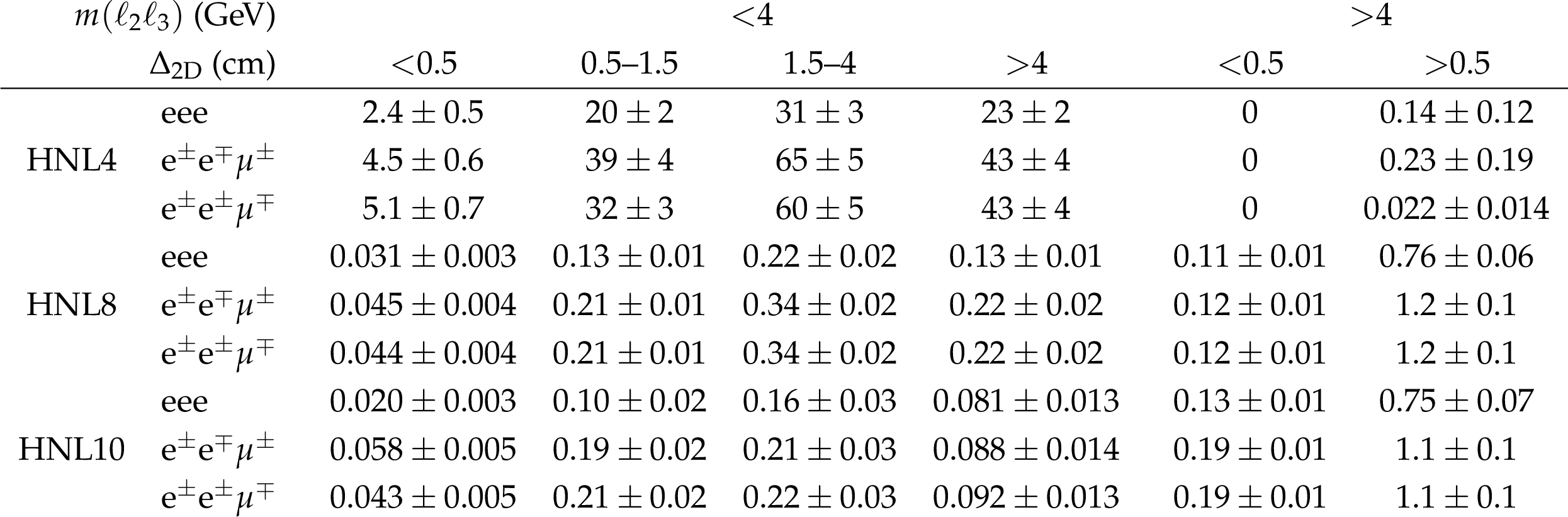
png pdf	Additional Table 1: Number of predicted signal events in the eeX final states. The results are presented for several benchmark signal hypotheses for Majorana HNL production: $m_{\mathrm {N}} = $ 4 GeV and $ {| V_{\mathrm {N}} |}^2=$ 0.8$\times$10$^{-4}$ (HNL4), $m_{\mathrm {N}} = $ 8 GeV and $ {| V_{\mathrm {N}} |}^2=$ 1.3$\times$10$^{-6}$ (HNL8), $m_{\mathrm {N}} = $ 10 GeV and $ {| V_{\mathrm {N}} |}^2=$ 1.0$\times$10$^{-6}$ (HNL10). The quoted uncertainties include statistical and systematic components.
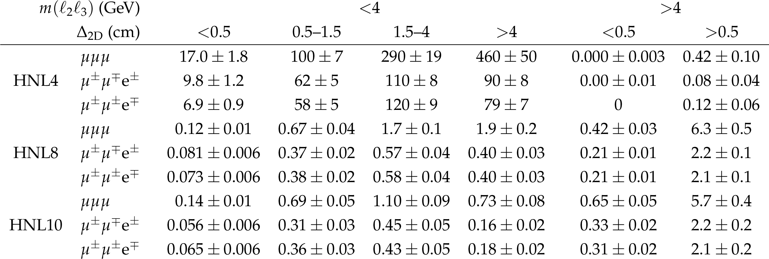
png pdf	Additional Table 2: Number of predicted signal events in the $ {\mu} {\mu} $X final states. The results are presented for several benchmark signal hypotheses for Majorana HNL production: $m_{\mathrm {N}} = $ 4 GeV and $ {| V_{\mathrm {N}} |}^2=$ 0.8$\times$10$^{-4}$ (HNL4), $m_{\mathrm {N}} = $ 8 GeV and $ {| V_{\mathrm {N}} |}^2=$ 1.3$\times$10$^{-6}$ (HNL8), $m_{\mathrm {N}} = $ 10 GeV and $ {| V_{\mathrm {N}} |}^2=$ 1.0$\times$10$^{-6}$ (HNL10). The quoted uncertainties include statistical and systematic components.
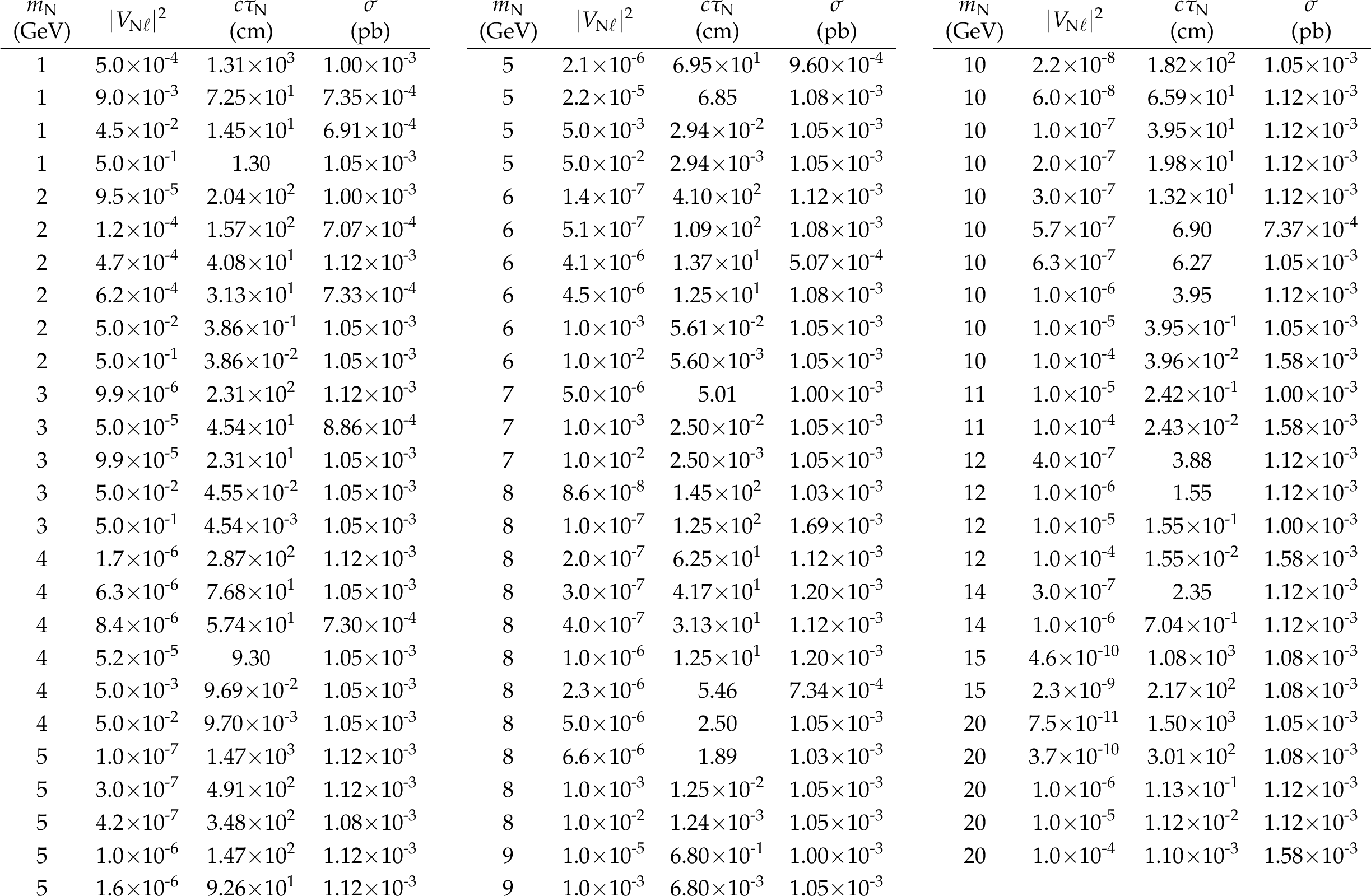
png pdf	Additional Table 3: Mean lifetime and production cross section for HNLs of Majorana nature, for different masses and coupling strengths, assuming the decay to three charged leptons and coupling to only electrons or muons, as evaluated from simulated event samples.

References
1	Super-Kamiokande Collaboration	Evidence for oscillation of atmospheric neutrinos	PRL 81 (1998) 1562	hep-ex/9807003
2	SNO Collaboration	Direct evidence for neutrino flavor transformation from neutral-current interactions in the Sudbury Neutrino Observatory	PRL 89 (2002) 011301	nucl-ex/0204008
3	KamLAND Collaboration	First results from KamLAND: Evidence for reactor antineutrino disappearance	PRL 90 (2003) 021802	hep-ex/0212021
4	S. Bilenky	Neutrino oscillations: From a historical perspective to the present status	NPB 908 (2016) 2	1602.00170
5	S. Roy Choudhury and S. Hannestad	Updated results on neutrino mass and mass hierarchy from cosmology with Planck 2018 likelihoods	JCAP 07 (2020) 037	1907.12598
6	M. Ivanov, M. Simonović, and M. Zaldarriaga	Cosmological parameters and neutrino masses from the final Planck and full-shape BOSS data	PRD 101 (2020) 083504	1912.08208
7	J. Formaggio, A. de Gouvêa, and R. Robertson	Direct measurements of neutrino mass	PR 914 (2021) 1	2102.00594
8	P. Minkowski	$ {\mu\to\mathrm{e}\gamma} $ at a rate of one out of 10$^{9}$ muon decays?	PLB 67 (1977) 421
9	T. Yanagida	Horizontal gauge symmetry and masses of neutrinos	in Proc. Workshop on the Unified Theories and the Baryon Number in the Universe: Tsukuba, Japan, 1979
10	M. Gell-Mann, P. Ramond, and R. Slansky	Complex spinors and unified theories	in Supergravity, North Holland Publishing	1306.4669
11	S. Glashow	The future of elementary particle physics	NATO Sci. Ser. B 61 (1980) 687
12	R. Mohapatra and G. Senjanović	Neutrino mass and spontaneous parity nonconservation	PRL 44 (1980) 912
13	J. Schechter and J. Valle	Neutrino masses in SU(2)$\otimes$U(1) theories	PRD 22 (1980) 2227
14	R. Shrock	General theory of weak leptonic and semileptonic decays. I. leptonic pseudoscalar meson decays, with associated tests for, and bounds on, neutrino masses and lepton mixing	PRD 24 (1981) 1232
15	Y. Cai, T. Han, T. Li, and R. Ruiz	Lepton number violation: Seesaw models and their collider tests	Front. in Phys. 6 (2018) 40	1711.02180
16	Z. Maki, M. Nakagawa, and S. Sakata	Remarks on the unified model of elementary particles	Prog. Theor. Phys. 28 (1962) 870
17	B. Pontecorvo	Neutrino experiments and the problem of conservation of leptonic charge	Zh. Eksp. Teor. Fiz. 53 (1967) 1717
18	Particle Data Group, P. A. Zyla et al.	Review of particle physics	Prog. Theor. Exp. Phys. 2020 (2020) 083C01
19	S. Dodelson and L. Widrow	Sterile neutrinos as dark matter	PRL 72 (1994) 17	hep-ph/9303287
20	A. Boyarsky et al.	Sterile neutrino dark matter	Prog. Part. NP 104 (2019) 1	1807.07938
21	M. Fukugita and T. Yanagida	Baryogenesis without grand unification	PLB 174 (1986) 45
22	E. Chun et al.	Probing leptogenesis	Int. J. Mod. Phys. A 33 (2018) 1842005	1711.02865
23	F. Deppisch, P. Bhupal Dev, and A. Pilaftsis	Neutrinos and collider physics	New J. Phys. 17 (2015) 075019	1502.06541
24	DELPHI Collaboration	Search for neutral heavy leptons produced in Z decays	Z. Phys. C 74 (1997) 57
25	CMS Collaboration	Search for heavy Majorana neutrinos in $ {\mu^{\pm}\mu^{\pm}} $+jets and $ {\mathrm{e^{\pm}}\mathrm{e^{\pm}}} $+jets events in pp collisions at $ \sqrt{s} = $ 7 TeV	PLB 717 (2012) 109	CMS-EXO-11-076 1207.6079
26	CMS Collaboration	Search for heavy Majorana neutrinos in $ {\mu^{\pm}\mu^{\pm}} $+jets events in proton-proton collisions at $ \sqrt{s} = $ 8 TeV	PLB 748 (2015) 144	CMS-EXO-12-057 1501.05566
27	ATLAS Collaboration	Search for heavy Majorana neutrinos with the ATLAS detector in pp collisions at $ \sqrt{s} = $ 8 TeV	JHEP 07 (2015) 162	1506.06020
28	CMS Collaboration	Search for heavy Majorana neutrinos in $ {\mathrm{e^{\pm}}\mathrm{e^{\pm}}} $+jets and $ {\mathrm{e^{\pm}}\mu^{\pm}} $+jets events in proton-proton collisions at $ \sqrt{s} = $ 8 TeV	JHEP 04 (2016) 169	CMS-EXO-14-014 1603.02248
29	CMS Collaboration	Search for heavy neutral leptons in events with three charged leptons in proton-proton collisions at $ \sqrt{s} = $ 13 TeV	PRL 120 (2018) 221801	CMS-EXO-17-012 1802.02965
30	CMS Collaboration	Search for heavy Majorana neutrinos in same-sign dilepton channels in proton-proton collisions at $ \sqrt{s} = $ 13 TeV	JHEP 01 (2019) 122	CMS-EXO-17-028 1806.10905
31	ATLAS Collaboration	Search for heavy neutral leptons in decays of $ \mathrm{W} bosons $ produced in 13 $ TeV pp $ collisions using prompt and displaced signatures with the ATLAS detector	JHEP 10 (2019) 265	1905.09787
32	LHCb Collaboration	Search for heavy neutral leptons in $ {\mathrm{W^{+}}\to\mu^{+}\mu^{\pm} \text{jet}} $ decays	EPJC 81 (2021) 248	2011.05263
33	T. Asaka, S. Blanchet, and M. Shaposhnikov	The $\nu$MSM, dark matter and neutrino masses	PLB 631 (2005) 151	hep-ph/0503065
34	M. Drewes, Y. Georis, and J. Klarić	Mapping the viable parameter space for testable leptogenesis	PRL 128 (2022) 051801	2106.16226
35	A. Abada, N. Bernal, M. Losada, and X. Marcano	Inclusive displaced vertex searches for heavy neutral leptons at the LHC	JHEP 01 (2019) 093	1807.10024
36	J.-L. Tastet, O. Ruchayskiy, and I. Timiryasov	Reinterpreting the ATLAS bounds on heavy neutral leptons in a realistic neutrino oscillation model	JHEP 12 (2021) 182	2107.12980
37	I. Boiarska, A. Boyarsky, O. Mikulenko, and M. Ovchynnikov	Constraints from the CHARM experiment on heavy neutral leptons with tau mixing	PRD 104 (2021) 095019	2107.14685
38	C. Degrande, O. Mattelaer, R. Ruiz, and J. Turner	Fully automated precision predictions for heavy neutrino production mechanisms at hadron colliders	PRD 94 (2016) 053002	1602.06957
39	A. Das, P. Konar, and S. Majhi	Production of heavy neutrino in next-to-leading order QCD at the LHC and beyond	JHEP 06 (2016) 019	1604.00608
40	CMS Collaboration	HEPData record for this analysis	link
41	CMS Collaboration	The CMS experiment at the CERN LHC	JINST 3 (2008) S08004	CMS-00-001
42	CMS Collaboration	Performance of the CMS Level-1 trigger in proton-proton collisions at $ \sqrt{s} = $ 13 TeV	JINST 15 (2020) P10017	CMS-TRG-17-001 2006.10165
43	CMS Collaboration	The CMS trigger system	JINST 12 (2017) P01020	CMS-TRG-12-001 1609.02366
44	CMS Collaboration	Description and performance of track and primary-vertex reconstruction with the CMS tracker	JINST 9 (2014) P10009	CMS-TRK-11-001 1405.6569
45	CMS Collaboration	2017 tracking performance plots	CDS
46	CMS Tracker Group, W. Adam et al.	The CMS Phase-1 pixel detector upgrade	JINST 16 (2021) P02027	2012.14304
47	CMS Collaboration	Track impact parameter resolution for the full pseudo rapidity coverage in the 2017 dataset with the CMS Phase-1 pixel detector	CDS
48	M. Cacciari, G. Salam, and G. Soyez	The anti-$ {k_{\mathrm{T}}} $ jet clustering algorithm	JHEP 04 (2008) 063	0802.1189
49	M. Cacciari, G. Salam, and G. Soyez	FastJet user manual	EPJC 72 (2012) 1896	1111.6097
50	CMS Collaboration	Particle-flow reconstruction and global event description with the CMS detector	JINST 12 (2017) P10003	CMS-PRF-14-001 1706.04965
51	CMS Collaboration	Electron and photon reconstruction and identification with the CMS experiment at the CERN LHC	JINST 16 (2021) P05014	CMS-EGM-17-001 2012.06888
52	CMS Collaboration	Performance of the CMS muon detector and muon reconstruction with proton-proton collisions at $ \sqrt{s} = $ 13 TeV	JINST 13 (2018) P06015	CMS-MUO-16-001 1804.04528
53	CMS Collaboration	Performance of missing transverse momentum reconstruction in proton-proton collisions at $ \sqrt{s} = $ 13 TeV using the CMS detector	JINST 14 (2019) P07004	CMS-JME-17-001 1903.06078
54	CMS Collaboration	Measurement of the inelastic proton-proton cross section at $ \sqrt{s} = $ 13 TeV	JHEP 07 (2018) 161	CMS-FSQ-15-005 1802.02613
55	GEANT4 Collaboration	GEANT4--a simulation toolkit	NIMA 506 (2003) 250
56	J. Alwall et al.	The automated computation of tree-level and next-to-leading order differential cross sections, and their matching to parton shower simulations	JHEP 07 (2014) 079	1405.0301
57	P. Artoisenet, R. Frederix, O. Mattelaer, and R. Rietkerk	Automatic spin-entangled decays of heavy resonances in Monte Carlo simulations	JHEP 03 (2013) 015	1212.3460
58	A. Atre, T. Han, S. Pascoli, and B. Zhang	The search for heavy Majorana neutrinos	JHEP 05 (2009) 030	0901.3589
59	D. Alva, T. Han, and R. Ruiz	Heavy Majorana neutrinos from W$ \gamma $ fusion at hadron colliders	JHEP 02 (2015) 072	1411.7305
60	S. Pascoli, R. Ruiz, and C. Weiland	Heavy neutrinos with dynamic jet vetoes: multilepton searches at $ \sqrt{s}= $ 14 , 27, and 100 TeV	JHEP 06 (2019) 049	1812.08750
61	K. Melnikov and F. Petriello	Electroweak gauge boson production at hadron colliders through $ \mathcal{O}({{\alpha_S}^2}) $	PRD 74 (2006) 114017	hep-ph/0609070
62	R. Gavin, Y. Li, F. Petriello, and S. Quackenbush	FEWZ2.0: A code for hadronic Z production at next-to-next-to-leading order	CPC 182 (2011) 2388	1011.3540
63	R. Gavin, Y. Li, F. Petriello, and S. Quackenbush	W physics at the LHC with FEWZ2.1	CPC 184 (2013) 208	1201.5896
64	Y. Li and F. Petriello	Combining QCD and electroweak corrections to dilepton production in FEWZ	PRD 86 (2012) 094034	1208.5967
65	R. Frederix and S. Frixione	Merging meets matching in MCatNLO	JHEP 12 (2012) 061	1209.6215
66	J. Alwall et al.	Comparative study of various algorithms for the merging of parton showers and matrix elements in hadronic collisions	EPJC 53 (2008) 473	0706.2569
67	P. Nason	A new method for combining NLO QCD with shower Monte Carlo algorithms	JHEP 11 (2004) 040	hep-ph/0409146
68	S. Frixione, P. Nason, and G. Ridolfi	A positive-weight next-to-leading-order Monte Carlo for heavy flavour hadroproduction	JHEP 09 (2007) 126	0707.3088
69	S. Frixione, P. Nason, and C. Oleari	Matching NLO QCD computations with parton shower simulations: the POWHEG method	JHEP 11 (2007) 070	0709.2092
70	S. Alioli, P. Nason, C. Oleari, and E. Re	NLO single-top production matched with shower in POWHEG: $ s $- and $ t $-channel contributions	JHEP 09 (2009) 111	0907.4076
71	S. Alioli, P. Nason, C. Oleari, and E. Re	A general framework for implementing NLO calculations in shower Monte Carlo programs: the POWHEG box	JHEP 06 (2010) 043	1002.2581
72	E. Re	Single-top Wt-channel production matched with parton showers using the POWHEG method	EPJC 71 (2011) 1547	1009.2450
73	T. Melia, P. Nason, R. Rontsch, and G. Zanderighi	W$^{+}$W${-}$, WZ and ZZ production in the POWHEG box	JHEP 11 (2011) 078	1107.5051
74	P. Nason and G. Zanderighi	W$^{+}$W${-}$, WZ and ZZ production in the POWHEG box-v2	EPJC 74 (2014) 2702	1311.1365
75	NNPDF Collaboration	Parton distributions for the LHC Run II	JHEP 04 (2015) 040	1410.8849
76	NNPDF Collaboration	Parton distributions from high-precision collider data	EPJC 77 (2017) 663	1706.00428
77	T. Sjostrand et al.	An introduction to PYTHIA 8.2	CPC 191 (2015) 159	1410.3012
78	CMS Collaboration	Investigations of the impact of the parton shower tuning in PYTHIA-8 in the modelling of $ \mathrm{t\bar{t}} $ at $ \sqrt{s}= $ 8 and 13 TeV	CMS-PAS-TOP-16-021	CMS-PAS-TOP-16-021
79	CMS Collaboration	Extraction and validation of a new set of CMS PYTHIA-8 tunes from underlying-event measurements	EPJC 80 (2020) 4	CMS-GEN-17-001 1903.12179
80	M. Cacciari and G. Salam	Pileup subtraction using jet areas	PLB 659 (2008) 119	0707.1378
81	CMS Collaboration	Jet energy scale and resolution in the CMS experiment in pp collisions at 8 TeV	JINST 12 (2017) P02014	CMS-JME-13-004 1607.03663
82	CMS Collaboration	Identification of heavy-flavour jets with the CMS detector in pp collisions at 13 TeV	JINST 13 (2018) P05011	CMS-BTV-16-002 1712.07158
83	R. Fruhwirth	Application of Kalman filtering to track and vertex fitting	NIMA 262 (1987) 444
84	CMS Collaboration	Muon tracking performance in the CMS Run-2 Legacy data using the tag-and-probe technique	CDS
85	CMS Collaboration	Precision luminosity measurement in proton-proton collisions at $ \sqrt{s} = $ 13 TeV in 2015 and 2016 at CMS	EPJC 81 (2021) 800	CMS-LUM-17-003 2104.01927
86	CMS Collaboration	CMS luminosity measurement for the 2017 data-taking period at $ \sqrt{s} = $ 13 TeV	CMS-PAS-LUM-17-004	CMS-PAS-LUM-17-004
87	CMS Collaboration	CMS luminosity measurement for the 2018 data-taking period at $ \sqrt{s} = $ 13 TeV	CMS-PAS-LUM-18-002	CMS-PAS-LUM-18-002
88	J. Linnemann	Measures of significance in HEP and astrophysics	in Proc. Statistical Problems in Particle Physics, Astrophysics, and Cosmology (PHYSTAT2003), Menlo Park, 2003	physics/0312059
89	R. Cousins, J. Linnemann, and J. Tucker	Evaluation of three methods for calculating statistical significance when incorporating a systematic uncertainty into a test of the background-only hypothesis for a poisson process	NIMA 595 (2008) 480	physics/0702156
90	T. Junk	Confidence level computation for combining searches with small statistics	NIMA 434 (1999) 435	hep-ex/9902006
91	A. Read	Presentation of search results: The CLs technique	JPG 28 (2002) 2693
92	ATLAS and CMS Collaborations, and LHC Higgs Combination Group	Procedure for the LHC Higgs boson search combination in Summer 2011	CMS-NOTE-2011-005
93	G. Cowan, K. Cranmer, E. Gross, and O. Vitells	Asymptotic formulae for likelihood-based tests of new physics	EPJC 71 (2011) 1554	1007.1727

Compact Muon Solenoid LHC, CERN

© Copyright CERN 2018 for the benefit of the CMS Collaboration