

Compact Muon Solenoid
LHC, CERN
| CMS-EXO-23-014 ; CERN-EP-2024-025 | ||
| Search for long-lived particles decaying to final states with a pair of muons in proton-proton collisions at $ \sqrt{s} = $ 13.6 TeV | ||
| CMS Collaboration | ||
| 22 February 2024 | ||
| Accepted for publication in J. High Energy Phys. | ||
| Abstract: An inclusive search for long-lived exotic particles (LLPs) decaying to final states with a pair of muons is presented. The search uses data corresponding to an integrated luminosity of 36.6 fb$ ^{-1} $ collected by the CMS experiment from the proton-proton collisions at $ \sqrt{s} = $ 13.6 TeV in 2022, the first year of Run 3 of the CERN LHC. The experimental signature is a pair of oppositely charged muons originating from a common vertex spatially separated from the proton-proton interaction point by distances ranging from several hundred $ \mu $m to several meters. The sensitivity of the search benefits from new triggers for displaced dimuons developed for Run 3. The results are interpreted in the framework of the hidden Abelian Higgs model, in which the Higgs boson decays to a pair of long-lived dark photons, and of an $ R $-parity violating supersymmetry model, in which long-lived neutralinos decay to a pair of muons and a neutrino. The limits set on these models are the most stringent to date in wide regions of lifetimes for LLPs with masses larger than 10 GeV. | ||
| Links: e-print arXiv:2402.14491 [hep-ex] (PDF) ; CDS record ; inSPIRE record ; HepData record ; Physics Briefing ; CADI line (restricted) ; | ||
| Figures | Summary | Additional Figures & Material | References | CMS Publications |
|---|
| Instructions for reinterpretation can be found here |
| Figures | |
png pdf |
Figure 1:
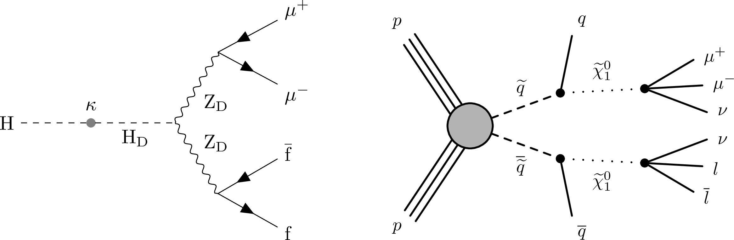
Feynman diagrams for (left) the HAHM model, showing the production of long-lived dark photons $ \mathrm{Z}_\text{D} $ via the Higgs portal, through $ \mathrm{H} $-$ \mathrm{H}_\text{D} $ mixing with the parameter $ \kappa $, with subsequent decays to pairs of muons or other fermions via the vector portal; and (right) pair production of squarks followed by $ \tilde{\mathrm{q}} \to \mathrm{q} \tilde{\chi}_{1}^{0} $ decays, where the RPV neutralino is assumed to be a long-lived particle that decays into a neutrino and two charged leptons. |
png pdf |
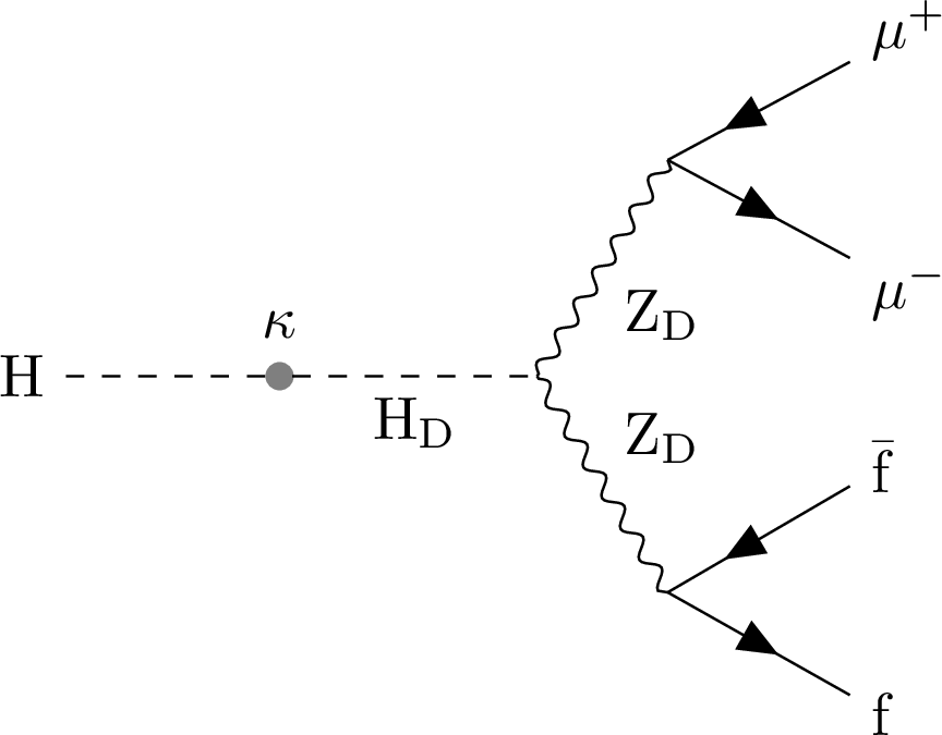
Figure 1-a:
Feynman diagrams for (left) the HAHM model, showing the production of long-lived dark photons $ \mathrm{Z}_\text{D} $ via the Higgs portal, through $ \mathrm{H} $-$ \mathrm{H}_\text{D} $ mixing with the parameter $ \kappa $, with subsequent decays to pairs of muons or other fermions via the vector portal; and (right) pair production of squarks followed by $ \tilde{\mathrm{q}} \to \mathrm{q} \tilde{\chi}_{1}^{0} $ decays, where the RPV neutralino is assumed to be a long-lived particle that decays into a neutrino and two charged leptons. |

png pdf |
Figure 1-b:
Feynman diagrams for (left) the HAHM model, showing the production of long-lived dark photons $ \mathrm{Z}_\text{D} $ via the Higgs portal, through $ \mathrm{H} $-$ \mathrm{H}_\text{D} $ mixing with the parameter $ \kappa $, with subsequent decays to pairs of muons or other fermions via the vector portal; and (right) pair production of squarks followed by $ \tilde{\mathrm{q}} \to \mathrm{q} \tilde{\chi}_{1}^{0} $ decays, where the RPV neutralino is assumed to be a long-lived particle that decays into a neutrino and two charged leptons. |
png pdf |
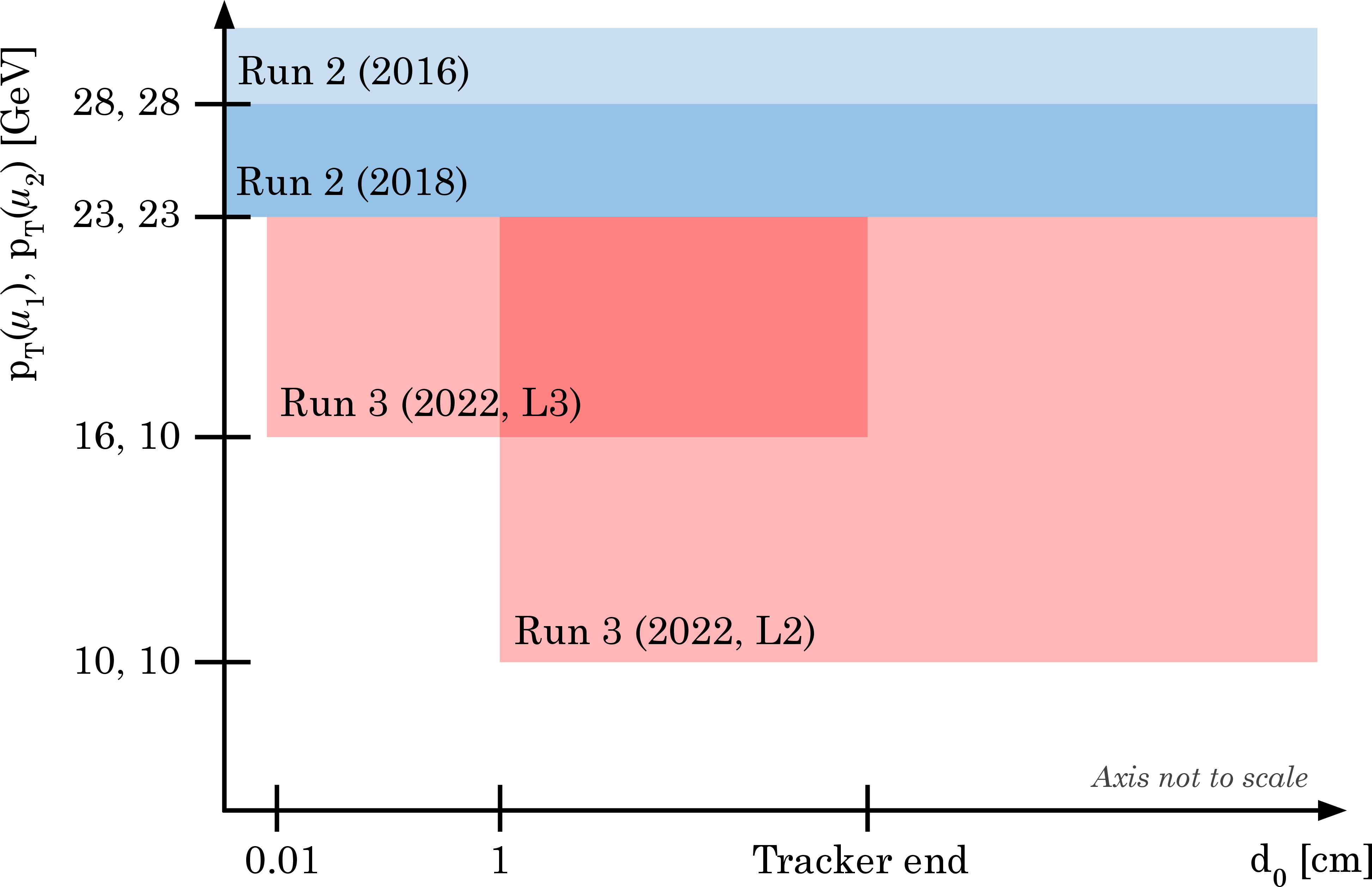
Figure 2:
The $ p_{\mathrm{T}} $ and $ d_{\text{0}} $ coverage of the 2016 Run 2 triggers (light blue), 2018 Run 2 triggers (blue), and newly designed 2022 Run 3 triggers described in the text (red). The two values of the $ p_{\mathrm{T}} $ refer to the trigger thresholds for the muons. |
png pdf |
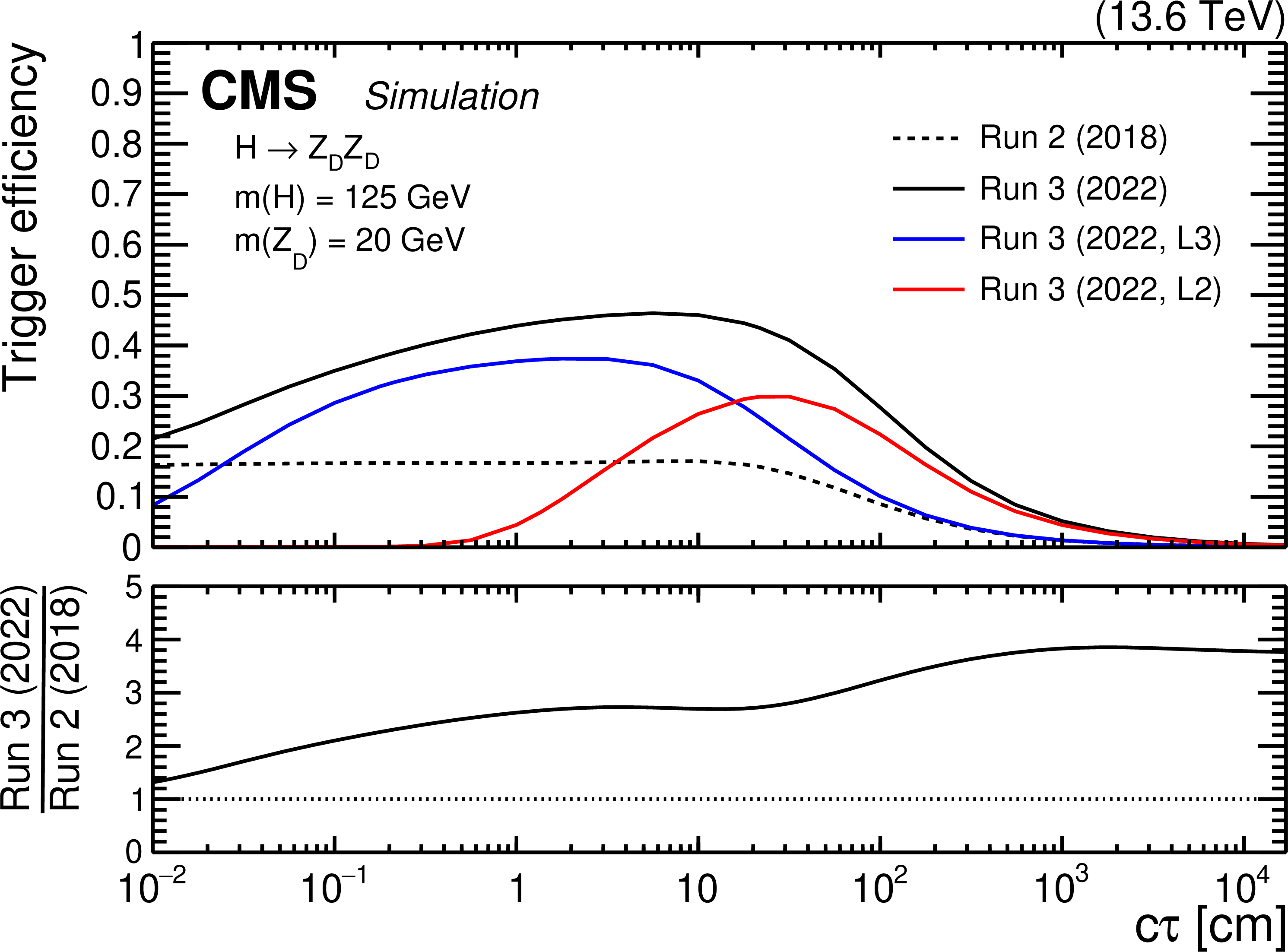
Figure 3:
Efficiencies of the Run 2 and Run 3 displaced dimuon triggers as a function of $ c\tau $ for the HAHM signal events with $ m(\mathrm{Z}_\text{D}) = $ 20 GeV. The efficiency is defined as the fraction of simulated events that satisfy the detector acceptance and the requirements of the following sets of trigger paths: the Run 2 (2018) triggers (dashed black); the Run 3 (2022, L3) triggers (blue); the Run 3 (2022, L2) triggers (red); and the OR of all these triggers (Run 3 (2022), black). The lower panel shows the ratio of the overall Run 3 (2022) efficiency to the Run 2 (2018) efficiency. |
png pdf |
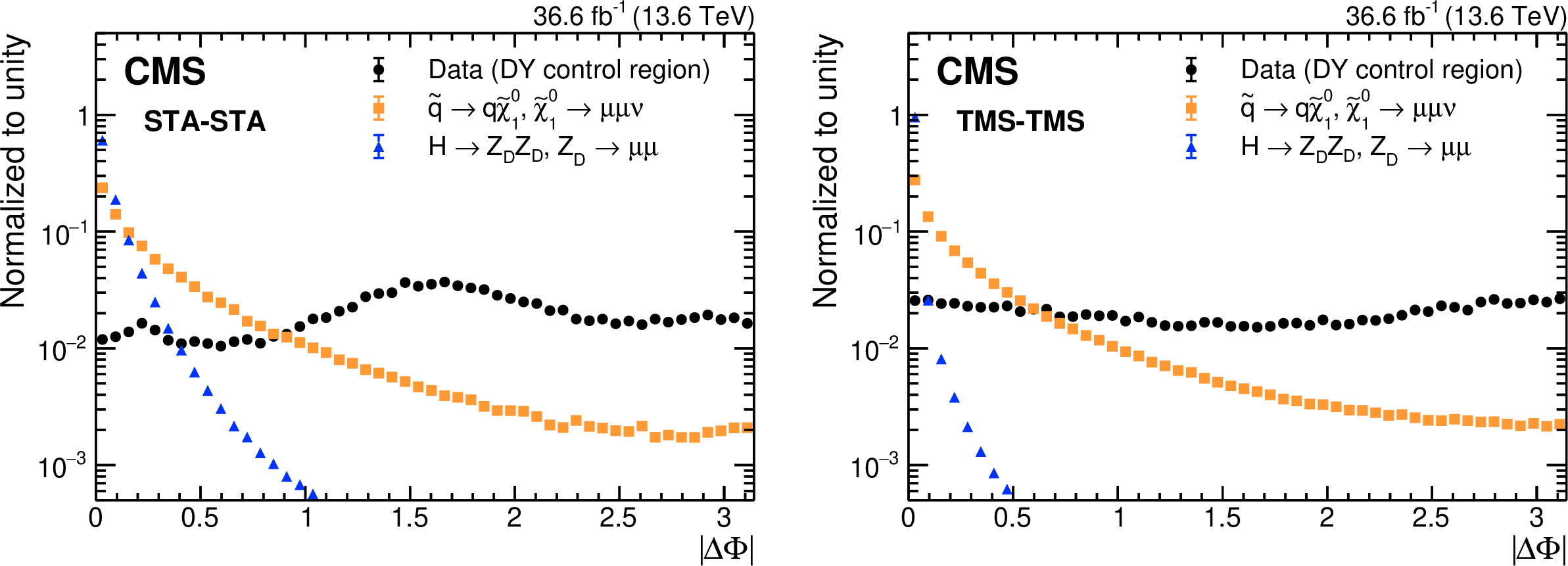
Figure 4:
Distributions of $ |\Delta\Phi| $ for (left) STA-STA and (right) TMS-TMS dimuons in data samples obtained by inverting some of the selection criteria and enriched in DY events (black circles) and for events passing all selection criteria except for a requirement on $ |\Delta\Phi| $ in all HAHM (blue triangles) and RPV SUSY (orange squares) generated signal samples combined. All distributions are normalized to unit area. |
png pdf |
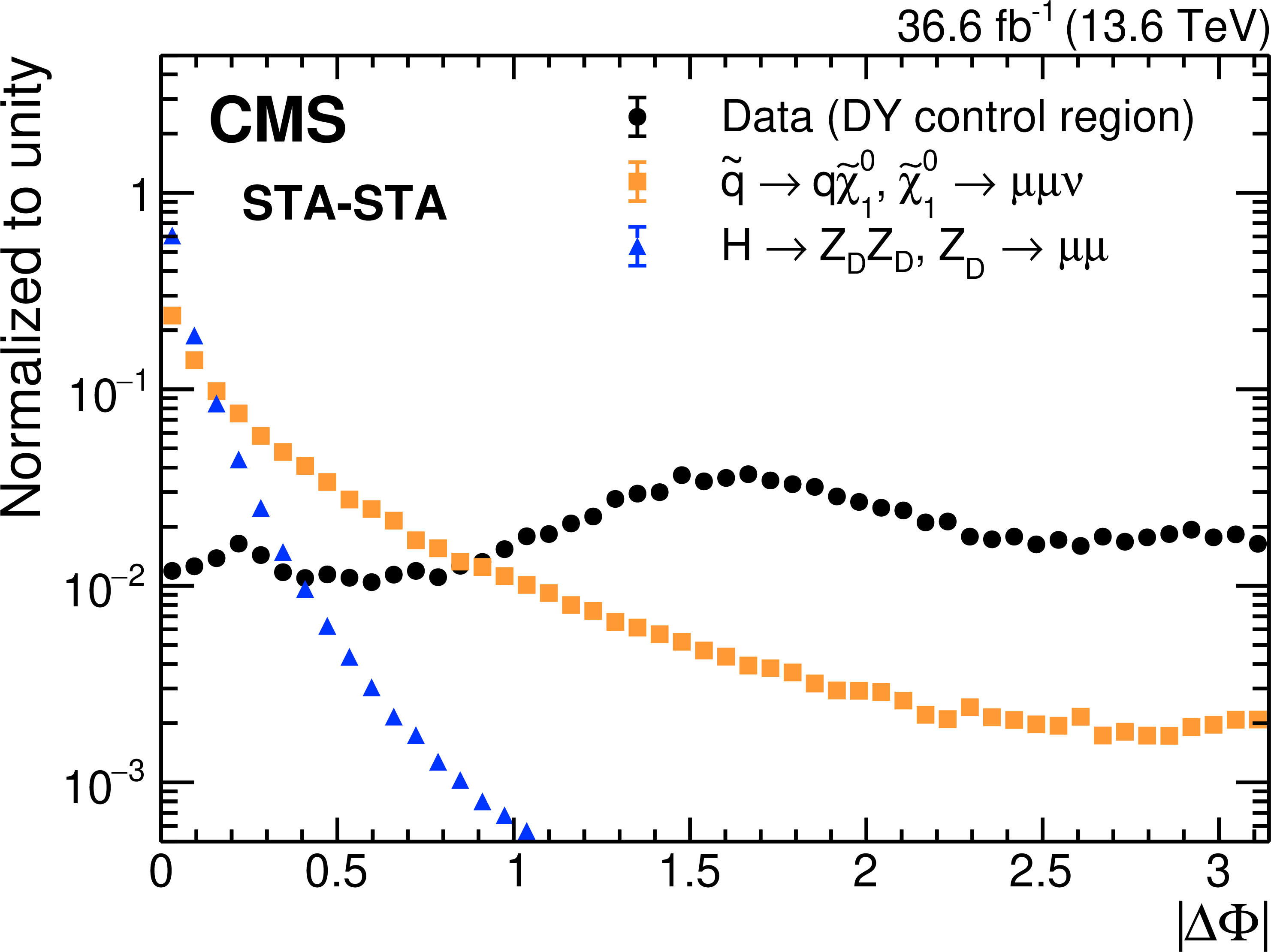
Figure 4-a:
Distributions of $ |\Delta\Phi| $ for (left) STA-STA and (right) TMS-TMS dimuons in data samples obtained by inverting some of the selection criteria and enriched in DY events (black circles) and for events passing all selection criteria except for a requirement on $ |\Delta\Phi| $ in all HAHM (blue triangles) and RPV SUSY (orange squares) generated signal samples combined. All distributions are normalized to unit area. |
png pdf |
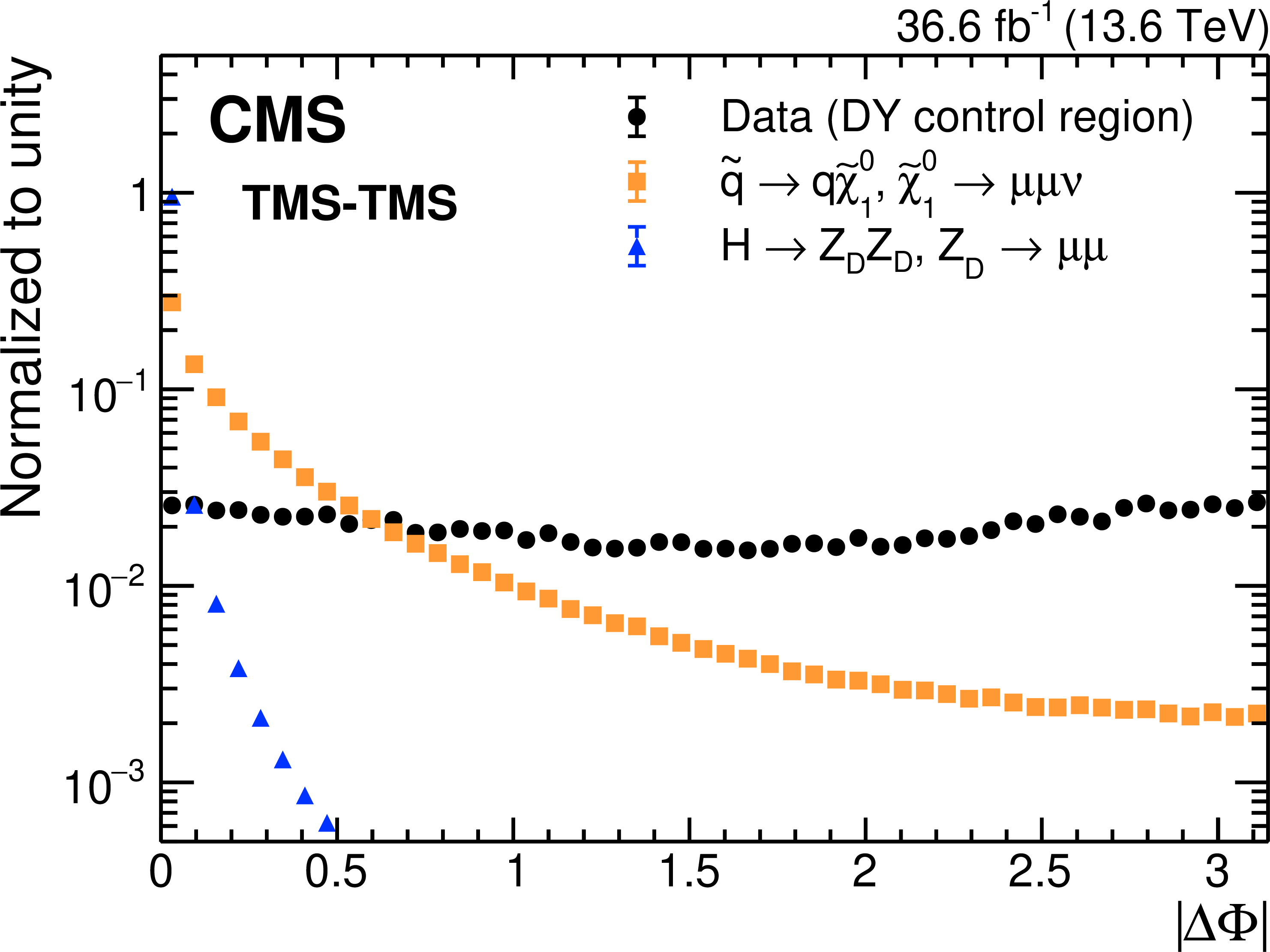
Figure 4-b:
Distributions of $ |\Delta\Phi| $ for (left) STA-STA and (right) TMS-TMS dimuons in data samples obtained by inverting some of the selection criteria and enriched in DY events (black circles) and for events passing all selection criteria except for a requirement on $ |\Delta\Phi| $ in all HAHM (blue triangles) and RPV SUSY (orange squares) generated signal samples combined. All distributions are normalized to unit area. |
png pdf |
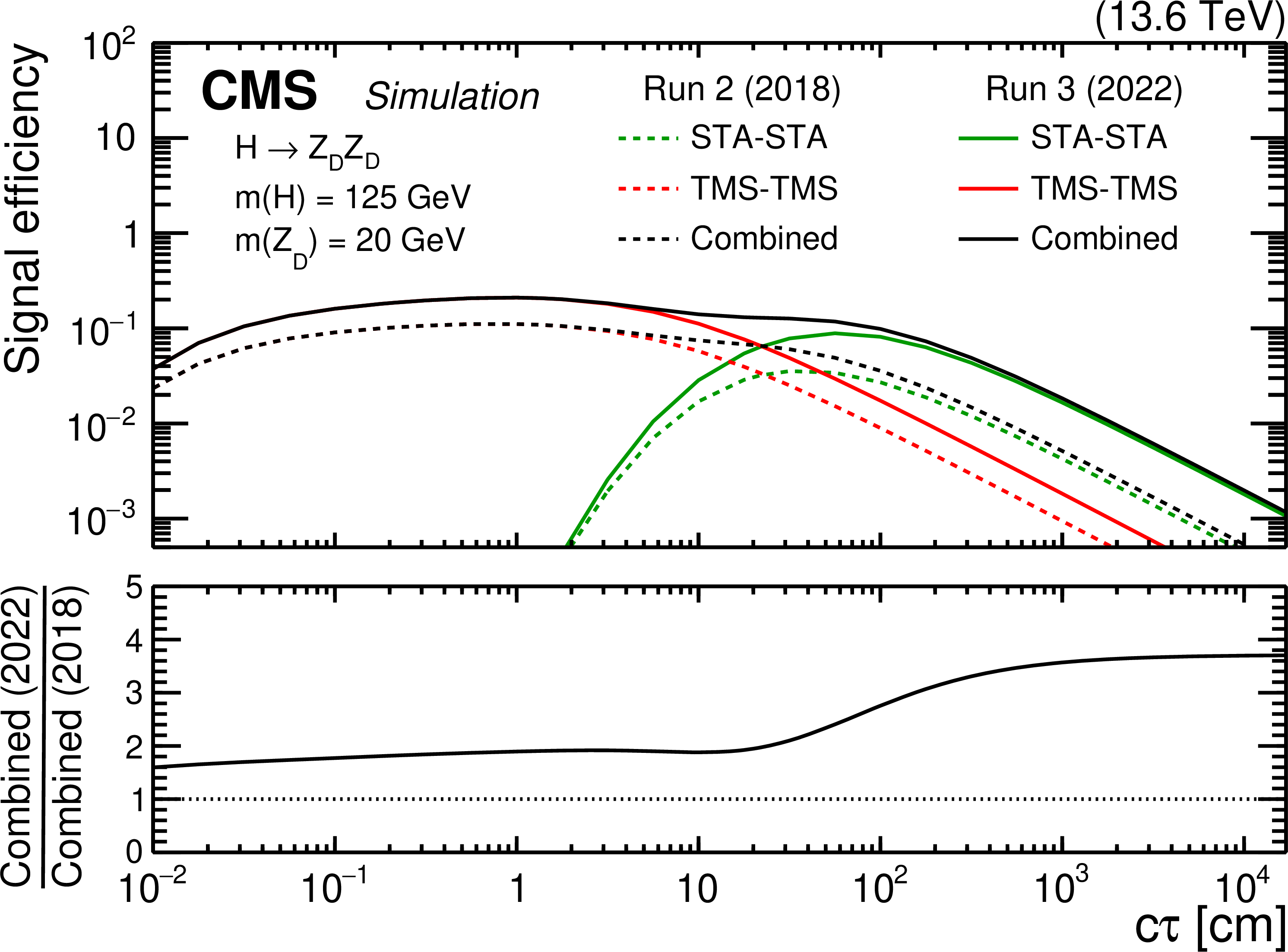
Figure 5:
Overall efficiencies in the STA-STA (green) and TMS-TMS (red) dimuon categories, as well as their combination (black) as a function of $ c\tau $ for the HAHM signal events with $ m(\mathrm{Z}_\text{D})= $ 20 GeV. The solid curves show efficiencies achieved with the 2022 Run 3 triggers, whereas dashed curves show efficiencies for the subset of events selected by the triggers used in the 2018 Run 2 analysis. The efficiency is defined as the fraction of signal events that satisfy the criteria of the indicated trigger as well as the full set of offline selection criteria. The lower panel shows the relative improvement of the overall signal efficiency brought in by improvements in the trigger. |
png pdf |
Figure 6:
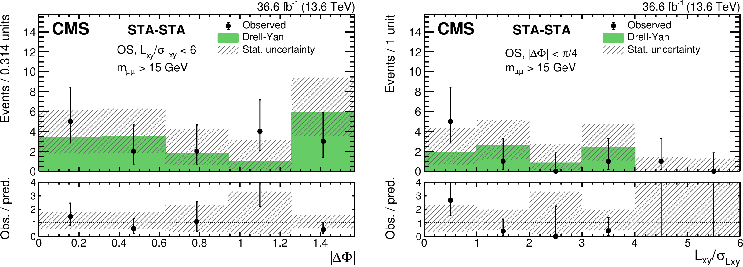
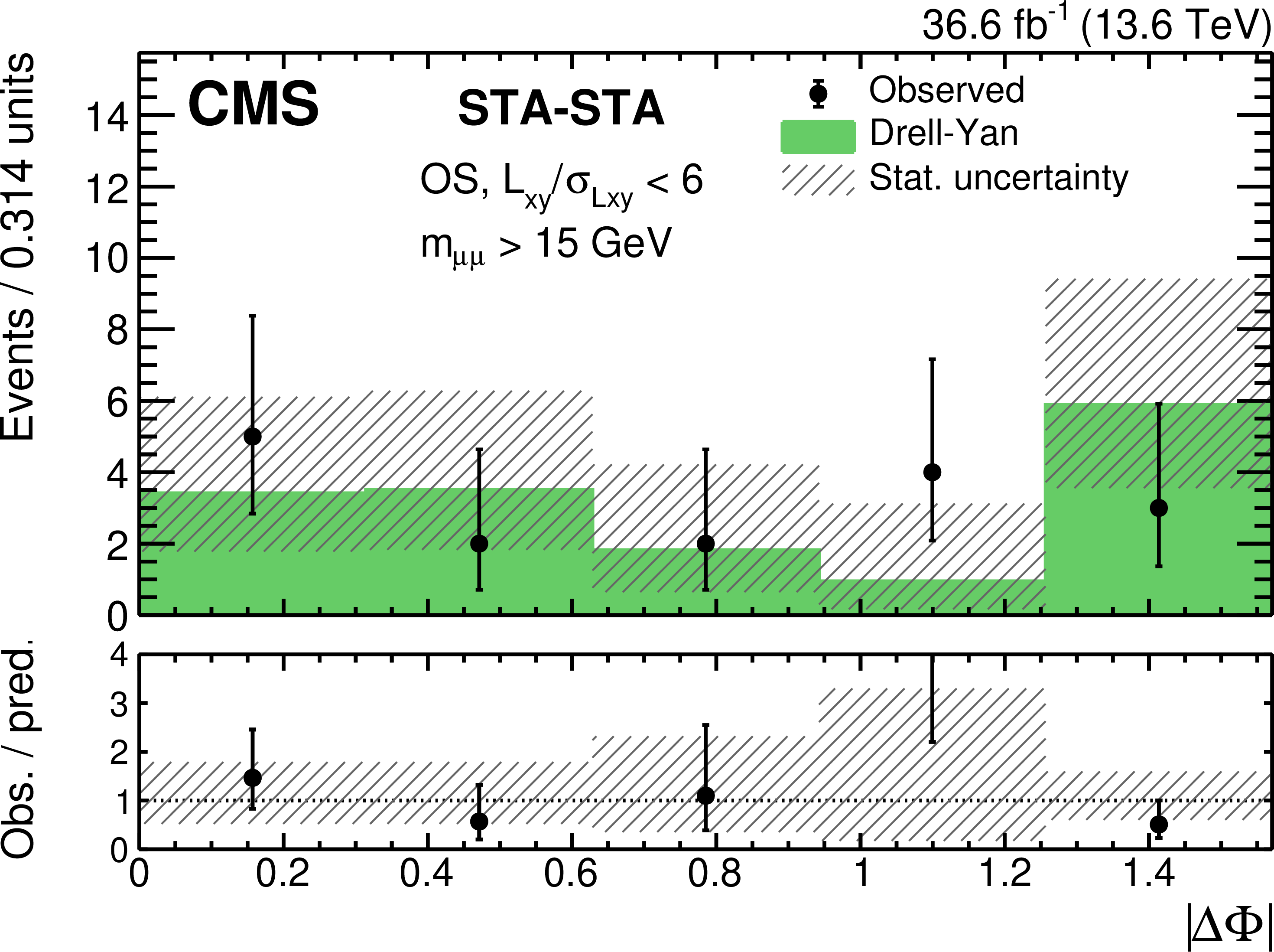
Example of background prediction checks in the STA-STA category: distributions of (left) $ |\Delta\Phi| $ and (right) $ L_{\text{xy}}/\sigma_{L_{\text{xy}}} $ for events with $ m_{\mu\mu} > $ 15 GeV in the $ L_{\text{xy}}/\sigma_{L_{\text{xy}}} < $ 6 validation region in data (black circles) compared to the background predictions (histograms). The lower panels show the ratio of the observed to predicted number of events. Hatched histograms show the statistical uncertainty in the background prediction. |
png pdf |
Figure 6-a:
Example of background prediction checks in the STA-STA category: distributions of (left) $ |\Delta\Phi| $ and (right) $ L_{\text{xy}}/\sigma_{L_{\text{xy}}} $ for events with $ m_{\mu\mu} > $ 15 GeV in the $ L_{\text{xy}}/\sigma_{L_{\text{xy}}} < $ 6 validation region in data (black circles) compared to the background predictions (histograms). The lower panels show the ratio of the observed to predicted number of events. Hatched histograms show the statistical uncertainty in the background prediction. |

png pdf |
Figure 6-b:
Example of background prediction checks in the STA-STA category: distributions of (left) $ |\Delta\Phi| $ and (right) $ L_{\text{xy}}/\sigma_{L_{\text{xy}}} $ for events with $ m_{\mu\mu} > $ 15 GeV in the $ L_{\text{xy}}/\sigma_{L_{\text{xy}}} < $ 6 validation region in data (black circles) compared to the background predictions (histograms). The lower panels show the ratio of the observed to predicted number of events. Hatched histograms show the statistical uncertainty in the background prediction. |
png pdf |
Figure 7:
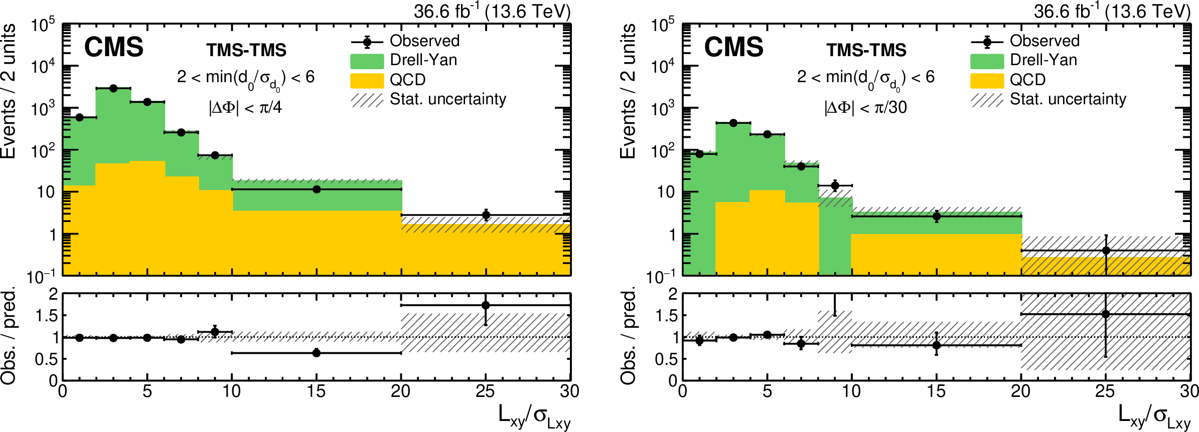
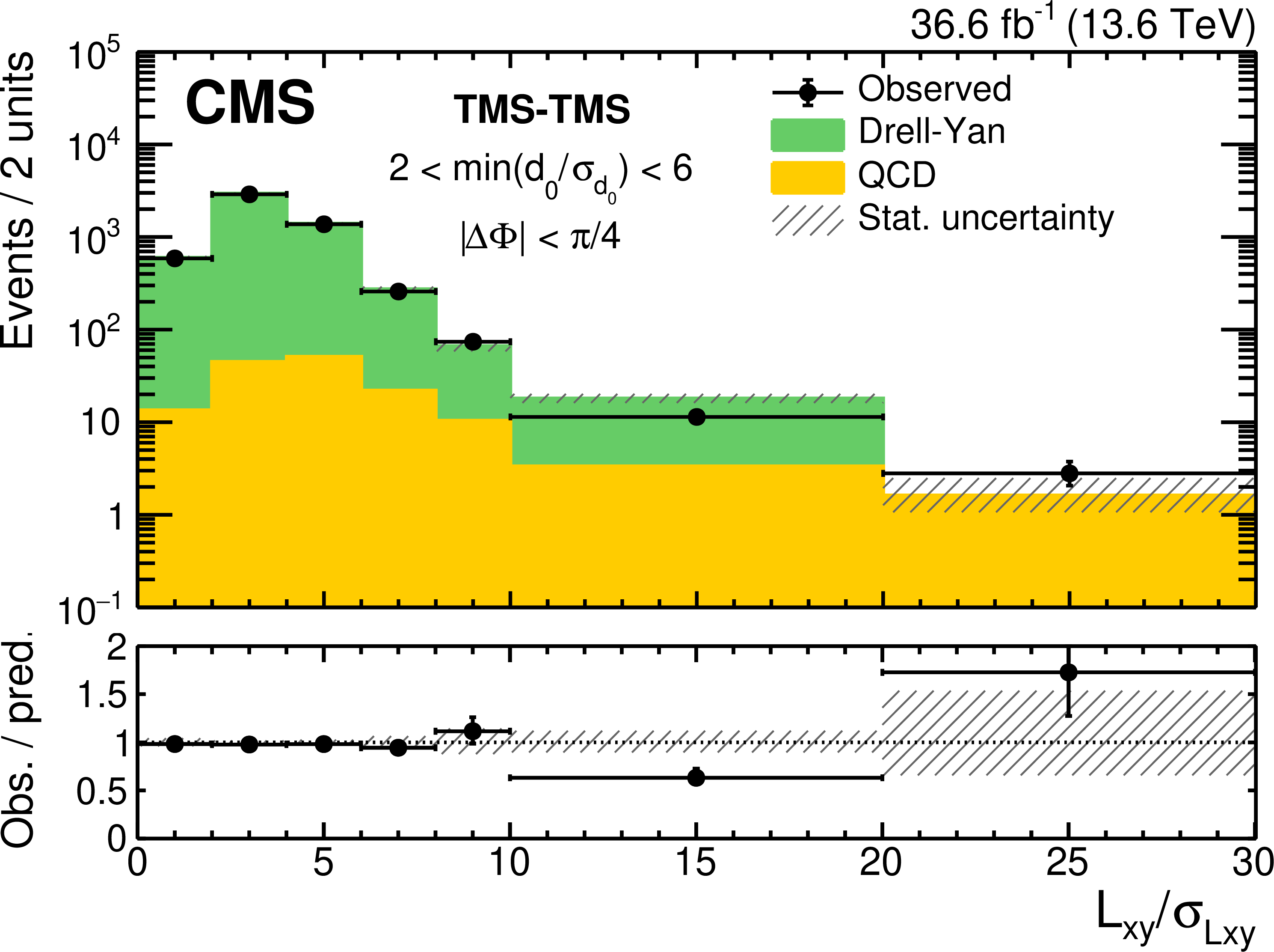
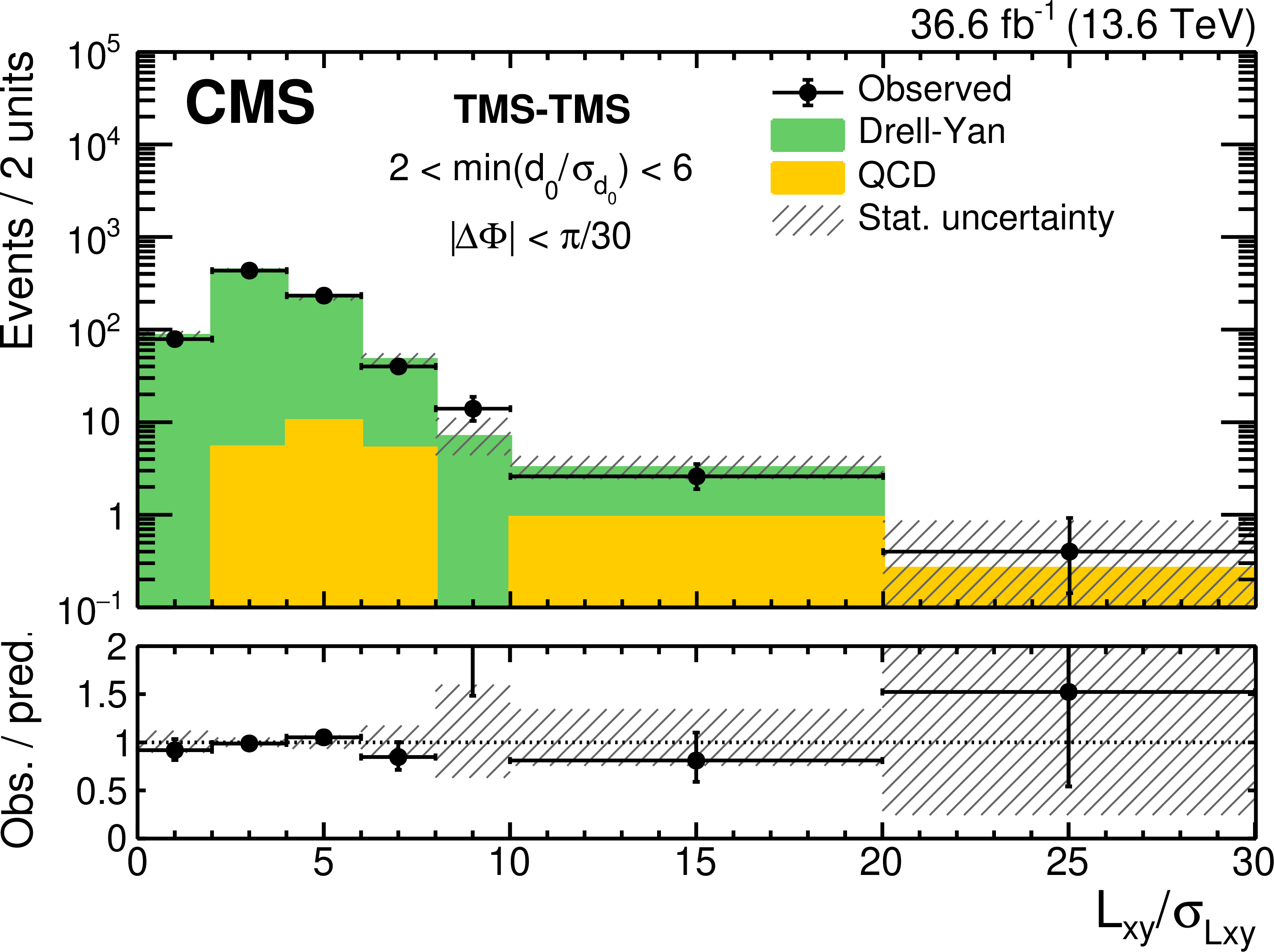
Example of background prediction checks in the TMS-TMS category: $ L_{\text{xy}}/\sigma_{L_{\text{xy}}} $ distributions for events with (left) $ |\Delta\Phi| < \pi/ $4 and (right) $ |\Delta\Phi| < \pi/ $ 30 in the 2 $ < \text{min}(d_{\text{0}}/\sigma_{d_{\text{0}}}) < $ 6 validation regions compared to the background predictions. The number of observed events (black circles) is overlaid with stacked histograms showing the expected numbers of QCD (yellow) and DY (green) background events. The last bin includes events in the histogram overflow. The lower panels show the ratio of the observed to predicted number of events. Hatched histograms show the statistical uncertainty in the background prediction. |
png pdf |
Figure 7-a:
Example of background prediction checks in the TMS-TMS category: $ L_{\text{xy}}/\sigma_{L_{\text{xy}}} $ distributions for events with (left) $ |\Delta\Phi| < \pi/ $4 and (right) $ |\Delta\Phi| < \pi/ $ 30 in the 2 $ < \text{min}(d_{\text{0}}/\sigma_{d_{\text{0}}}) < $ 6 validation regions compared to the background predictions. The number of observed events (black circles) is overlaid with stacked histograms showing the expected numbers of QCD (yellow) and DY (green) background events. The last bin includes events in the histogram overflow. The lower panels show the ratio of the observed to predicted number of events. Hatched histograms show the statistical uncertainty in the background prediction. |
png pdf |
Figure 7-b:
Example of background prediction checks in the TMS-TMS category: $ L_{\text{xy}}/\sigma_{L_{\text{xy}}} $ distributions for events with (left) $ |\Delta\Phi| < \pi/ $4 and (right) $ |\Delta\Phi| < \pi/ $ 30 in the 2 $ < \text{min}(d_{\text{0}}/\sigma_{d_{\text{0}}}) < $ 6 validation regions compared to the background predictions. The number of observed events (black circles) is overlaid with stacked histograms showing the expected numbers of QCD (yellow) and DY (green) background events. The last bin includes events in the histogram overflow. The lower panels show the ratio of the observed to predicted number of events. Hatched histograms show the statistical uncertainty in the background prediction. |

png pdf |
Figure 8:
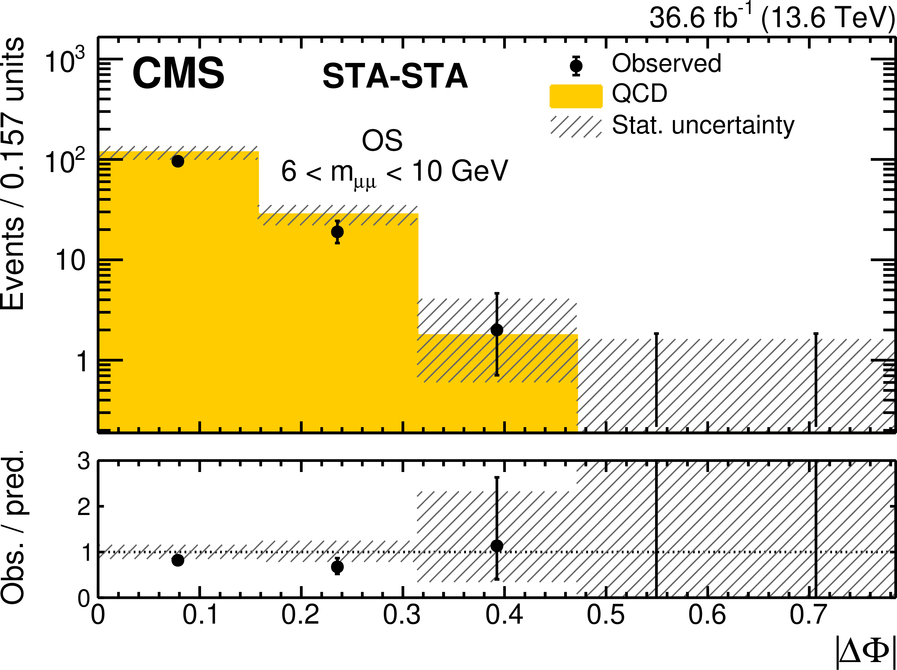
Example of background prediction checks in the STA-STA category: distributions of (left) $ |\Delta\Phi| $ and (right) $ m_{\mu\mu} $ for dimuons in the low-mass (6 $ < m_{\mu\mu} < $ 10 GeV) validation region in data (black circles) compared to the background predictions (histograms). The lower panels show the ratio of the observed to predicted number of events. Hatched histograms show the statistical uncertainty in the background prediction. |
png pdf |
Figure 8-a:
Example of background prediction checks in the STA-STA category: distributions of (left) $ |\Delta\Phi| $ and (right) $ m_{\mu\mu} $ for dimuons in the low-mass (6 $ < m_{\mu\mu} < $ 10 GeV) validation region in data (black circles) compared to the background predictions (histograms). The lower panels show the ratio of the observed to predicted number of events. Hatched histograms show the statistical uncertainty in the background prediction. |

png pdf |
Figure 8-b:
Example of background prediction checks in the STA-STA category: distributions of (left) $ |\Delta\Phi| $ and (right) $ m_{\mu\mu} $ for dimuons in the low-mass (6 $ < m_{\mu\mu} < $ 10 GeV) validation region in data (black circles) compared to the background predictions (histograms). The lower panels show the ratio of the observed to predicted number of events. Hatched histograms show the statistical uncertainty in the background prediction. |
png pdf |
Figure 9:
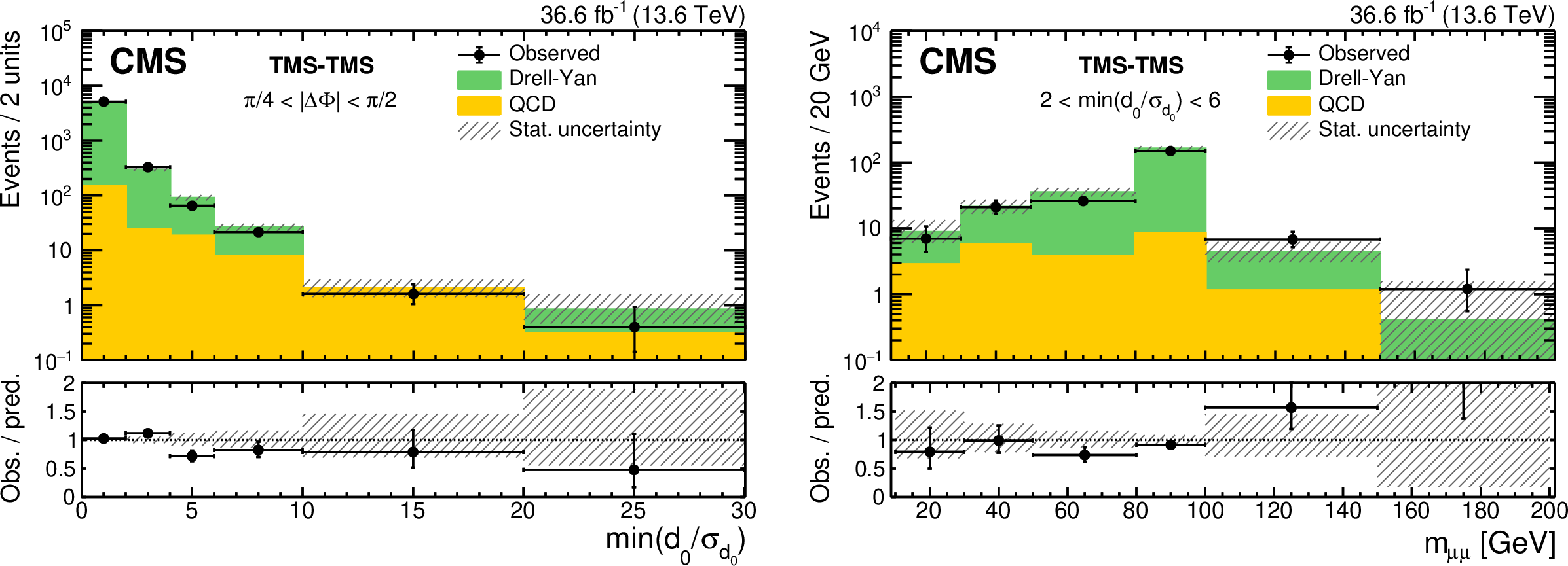
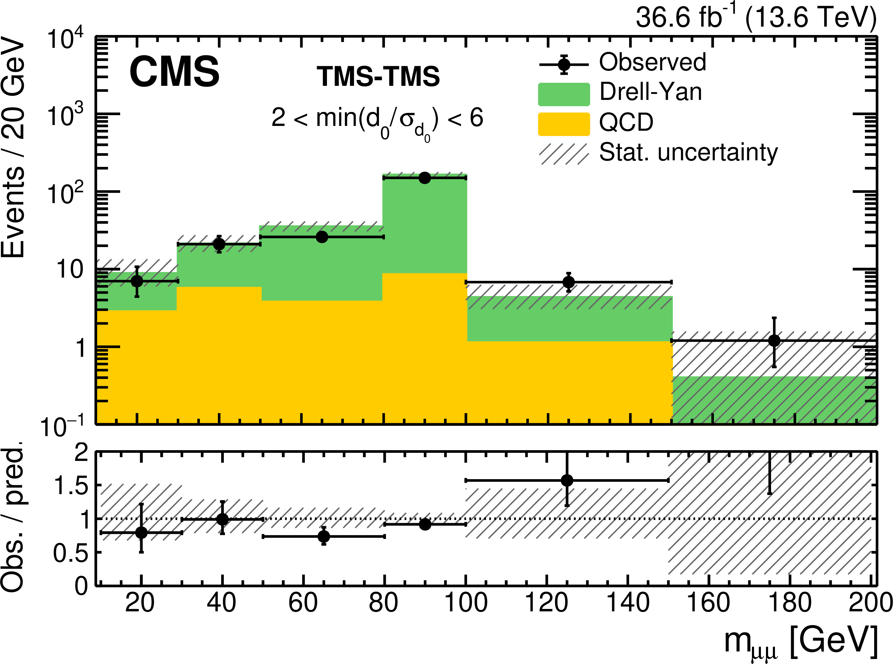
Example of background prediction checks in the TMS-TMS category: (left) distribution of min($ d_{\text{0}}/\sigma_{d_{\text{0}}} $) for events in the $ \pi/4 < |\Delta\Phi| < \pi/ $2 validation region; (right) distribution of $ m_{\mu\mu} $ for events in the 2 $ < \text{min}(d_{\text{0}}/\sigma_{d_{\text{0}}}) < $ 6 validation region. The number of observed events (black circles) is overlaid with stacked histograms showing the expected numbers of QCD (yellow) and DY (green) background events. The last bin includes events in the histogram overflow. The lower panels show the ratios of the observed to predicted number of events. Hatched histograms show the statistical uncertainty in the background prediction. |

png pdf |
Figure 9-a:
Example of background prediction checks in the TMS-TMS category: (left) distribution of min($ d_{\text{0}}/\sigma_{d_{\text{0}}} $) for events in the $ \pi/4 < |\Delta\Phi| < \pi/ $2 validation region; (right) distribution of $ m_{\mu\mu} $ for events in the 2 $ < \text{min}(d_{\text{0}}/\sigma_{d_{\text{0}}}) < $ 6 validation region. The number of observed events (black circles) is overlaid with stacked histograms showing the expected numbers of QCD (yellow) and DY (green) background events. The last bin includes events in the histogram overflow. The lower panels show the ratios of the observed to predicted number of events. Hatched histograms show the statistical uncertainty in the background prediction. |
png pdf |
Figure 9-b:
Example of background prediction checks in the TMS-TMS category: (left) distribution of min($ d_{\text{0}}/\sigma_{d_{\text{0}}} $) for events in the $ \pi/4 < |\Delta\Phi| < \pi/ $2 validation region; (right) distribution of $ m_{\mu\mu} $ for events in the 2 $ < \text{min}(d_{\text{0}}/\sigma_{d_{\text{0}}}) < $ 6 validation region. The number of observed events (black circles) is overlaid with stacked histograms showing the expected numbers of QCD (yellow) and DY (green) background events. The last bin includes events in the histogram overflow. The lower panels show the ratios of the observed to predicted number of events. Hatched histograms show the statistical uncertainty in the background prediction. |
png pdf |
Figure 10:
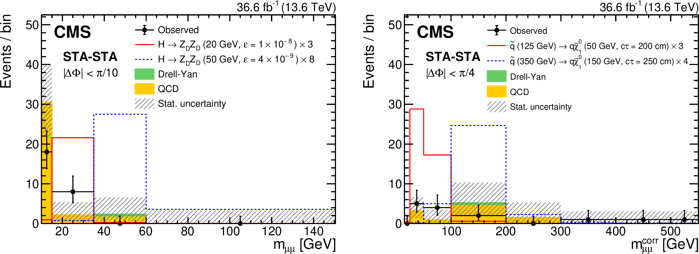
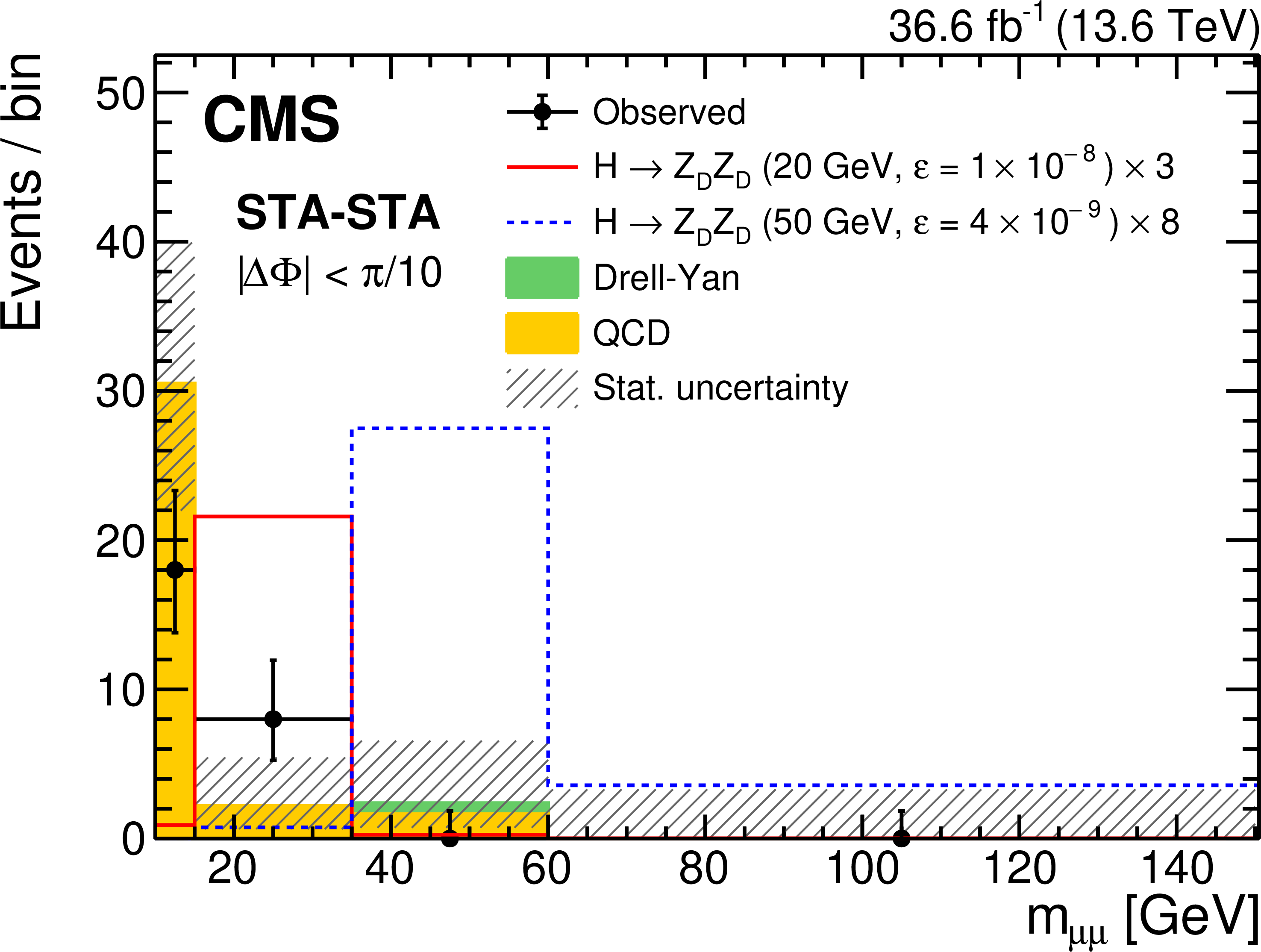
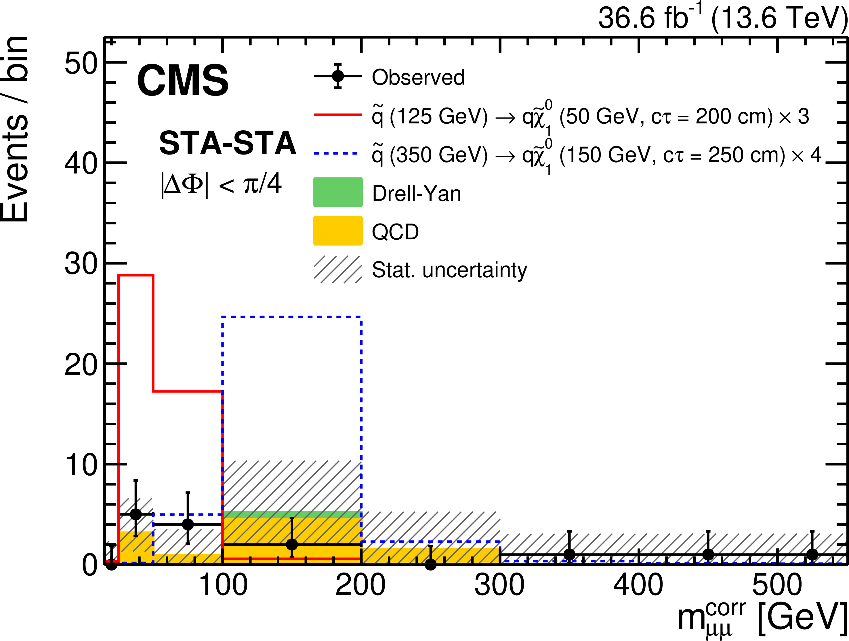
Comparison of the observed (black points) and expected (histograms) numbers of events in nonoverlapping (left) $ m_{\mu\mu} $ and (right) $ m^\text{corr}_{\mu\mu} $ intervals in the STA-STA dimuon category, in the signal regions optimized for the (left) HAHM and (right) RPV SUSY model. Yellow and green stacked filled histograms represent mean expected background contributions from QCD and DY, respectively, while statistical uncertainties in the total expected background are shown as hatched histograms. Signal contributions expected from simulated signals indicated in the legends are shown in red and blue. Their yields are set to the corresponding median expected 95% CL exclusion limits obtained from the ensemble of both dimuon categories, scaled up as indicated in the legend to improve visibility. The last bin includes events in the histogram overflow. |
png pdf |
Figure 10-a:
Comparison of the observed (black points) and expected (histograms) numbers of events in nonoverlapping (left) $ m_{\mu\mu} $ and (right) $ m^\text{corr}_{\mu\mu} $ intervals in the STA-STA dimuon category, in the signal regions optimized for the (left) HAHM and (right) RPV SUSY model. Yellow and green stacked filled histograms represent mean expected background contributions from QCD and DY, respectively, while statistical uncertainties in the total expected background are shown as hatched histograms. Signal contributions expected from simulated signals indicated in the legends are shown in red and blue. Their yields are set to the corresponding median expected 95% CL exclusion limits obtained from the ensemble of both dimuon categories, scaled up as indicated in the legend to improve visibility. The last bin includes events in the histogram overflow. |
png pdf |
Figure 10-b:
Comparison of the observed (black points) and expected (histograms) numbers of events in nonoverlapping (left) $ m_{\mu\mu} $ and (right) $ m^\text{corr}_{\mu\mu} $ intervals in the STA-STA dimuon category, in the signal regions optimized for the (left) HAHM and (right) RPV SUSY model. Yellow and green stacked filled histograms represent mean expected background contributions from QCD and DY, respectively, while statistical uncertainties in the total expected background are shown as hatched histograms. Signal contributions expected from simulated signals indicated in the legends are shown in red and blue. Their yields are set to the corresponding median expected 95% CL exclusion limits obtained from the ensemble of both dimuon categories, scaled up as indicated in the legend to improve visibility. The last bin includes events in the histogram overflow. |
png pdf |
Figure 11:
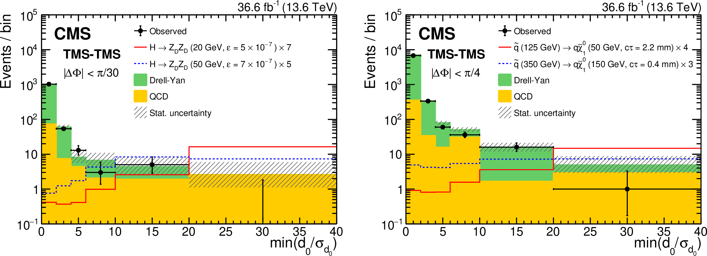
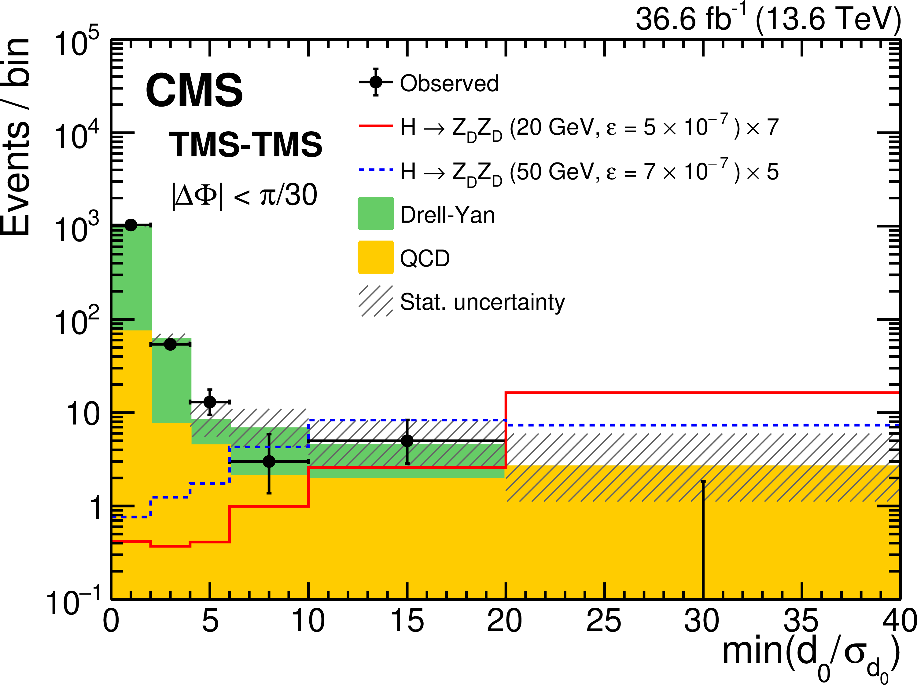
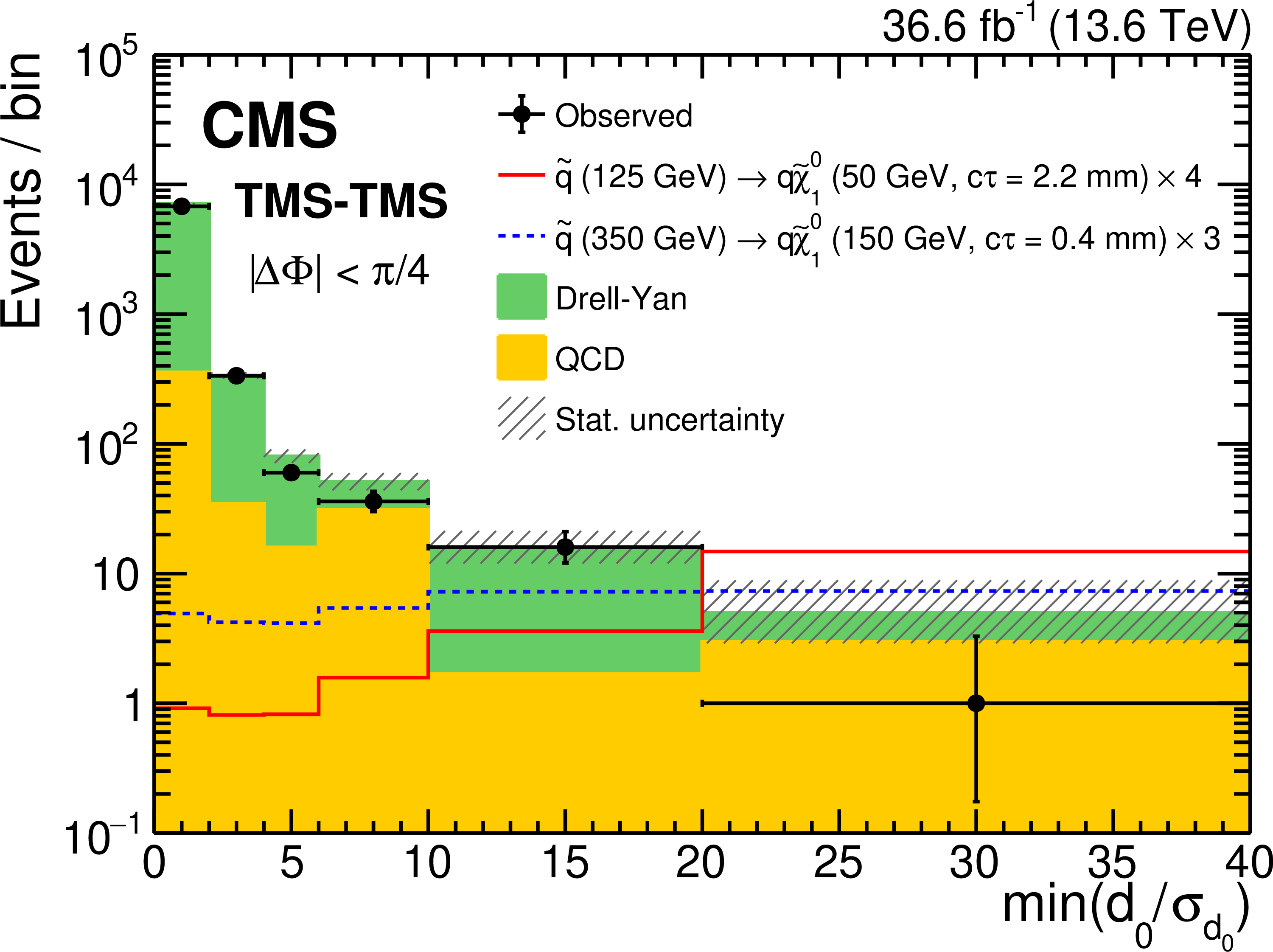
Distributions of $ \text{min}(d_{\text{0}}/\sigma_{d_{\text{0}}}) $ for TMS-TMS dimuons with (left) $ |\Delta\Phi| < \pi/ $ 30 and (right) $ |\Delta\Phi| < \pi/ $ 4, for events in all mass intervals combined. The number of observed events (black circles) is overlaid with the stacked histograms showing the expected numbers of QCD (yellow) and DY (green) background events. Statistical uncertainties in the total expected background are shown as hatched histograms. Signal contributions expected from simulated signals indicated in the legends are shown in red and blue. Their yields are set to the corresponding median expected 95% CL exclusion limits obtained from the ensemble of both dimuon categories, scaled up as indicated in the legend to improve visibility. Events are required to satisfy all nominal selection criteria with the exception of the $ d_{\text{0}}/\sigma_{d_{\text{0}}} $ requirement. The last bin includes events in the histogram overflow. |
png pdf |
Figure 11-a:
Distributions of $ \text{min}(d_{\text{0}}/\sigma_{d_{\text{0}}}) $ for TMS-TMS dimuons with (left) $ |\Delta\Phi| < \pi/ $ 30 and (right) $ |\Delta\Phi| < \pi/ $ 4, for events in all mass intervals combined. The number of observed events (black circles) is overlaid with the stacked histograms showing the expected numbers of QCD (yellow) and DY (green) background events. Statistical uncertainties in the total expected background are shown as hatched histograms. Signal contributions expected from simulated signals indicated in the legends are shown in red and blue. Their yields are set to the corresponding median expected 95% CL exclusion limits obtained from the ensemble of both dimuon categories, scaled up as indicated in the legend to improve visibility. Events are required to satisfy all nominal selection criteria with the exception of the $ d_{\text{0}}/\sigma_{d_{\text{0}}} $ requirement. The last bin includes events in the histogram overflow. |
png pdf |
Figure 11-b:
Distributions of $ \text{min}(d_{\text{0}}/\sigma_{d_{\text{0}}}) $ for TMS-TMS dimuons with (left) $ |\Delta\Phi| < \pi/ $ 30 and (right) $ |\Delta\Phi| < \pi/ $ 4, for events in all mass intervals combined. The number of observed events (black circles) is overlaid with the stacked histograms showing the expected numbers of QCD (yellow) and DY (green) background events. Statistical uncertainties in the total expected background are shown as hatched histograms. Signal contributions expected from simulated signals indicated in the legends are shown in red and blue. Their yields are set to the corresponding median expected 95% CL exclusion limits obtained from the ensemble of both dimuon categories, scaled up as indicated in the legend to improve visibility. Events are required to satisfy all nominal selection criteria with the exception of the $ d_{\text{0}}/\sigma_{d_{\text{0}}} $ requirement. The last bin includes events in the histogram overflow. |
png pdf |
Figure 12:
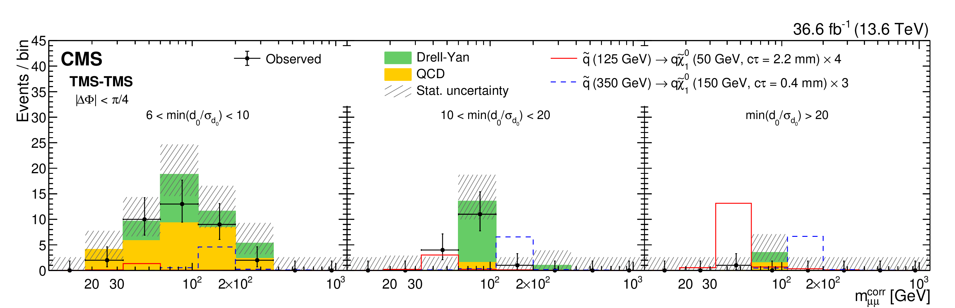
Comparison of observed and expected numbers of events in the TMS-TMS dimuon category, in the RPV SUSY study that requires $ |\Delta\Phi| < \pi/ $ 4, in bins of $ m^\text{corr}_{\mu\mu} $. The number of observed events (black circles) is overlaid with the stacked filled histograms showing the expected numbers of QCD (yellow) and DY (green) background events in bins of $ m^\text{corr}_{\mu\mu} $ in three min($ d_{\text{0}}/\sigma_{d_{\text{0}}} $) bins: (left) 6--10, (center) 10--20, and (right) $ {>} $ 20. Hatched histograms show statistical uncertainties in the total expected background. Contributions expected from signal events predicted by the RPV SUSY model with the parameters indicated in the legends are shown as red and blue histograms. Their yields are set to the corresponding median expected 95% CL exclusion limits obtained from the ensemble of both dimuon categories, scaled up as indicated in the legend to improve visibility. The last bin includes events in the histogram overflow. |
png pdf |
Figure 13:
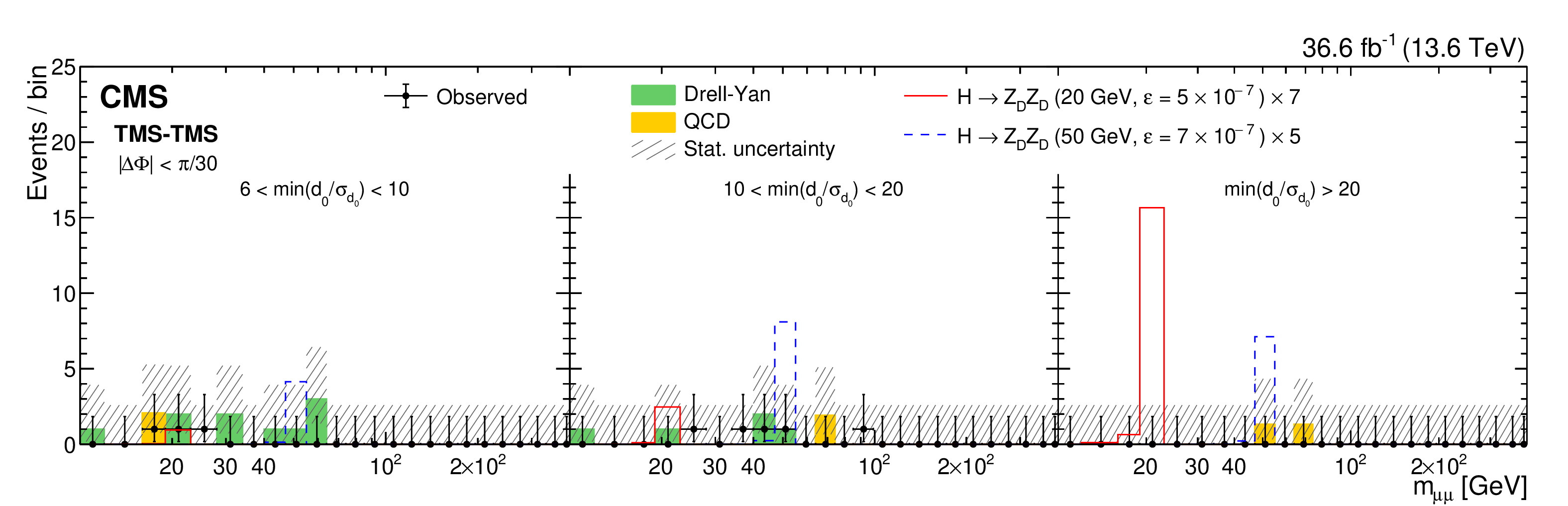
Comparison of observed and expected numbers of events in the TMS-TMS dimuon category, in the HAHM study that requires $ |\Delta\Phi| < \pi/ $30, in bins of $ m_{\mu\mu} $. The number of observed events (black circles) is overlaid with the stacked histograms showing the expected numbers of QCD (yellow) and DY (green) background events in bins of $ m_{\mu\mu} $ in three min($ d_{\text{0}}/\sigma_{d_{\text{0}}} $) bins: (left) 6--10, (center) 10--20, and (right) $ {>} $ 20. Hatched histograms show statistical uncertainties in the total expected background. Signal contributions expected from simulated $ \mathrm{H} \to \mathrm{Z}_\text{D} \mathrm{Z}_\text{D} $ events with the parameters indicated in the legends are shown as red and blue histograms. Their yields are set to the corresponding median expected 95% CL exclusion limits obtained from the ensemble of both dimuon categories, scaled up as indicated in the legend to improve visibility. The last bin includes events in the histogram overflow. |
png pdf |
Figure 14:
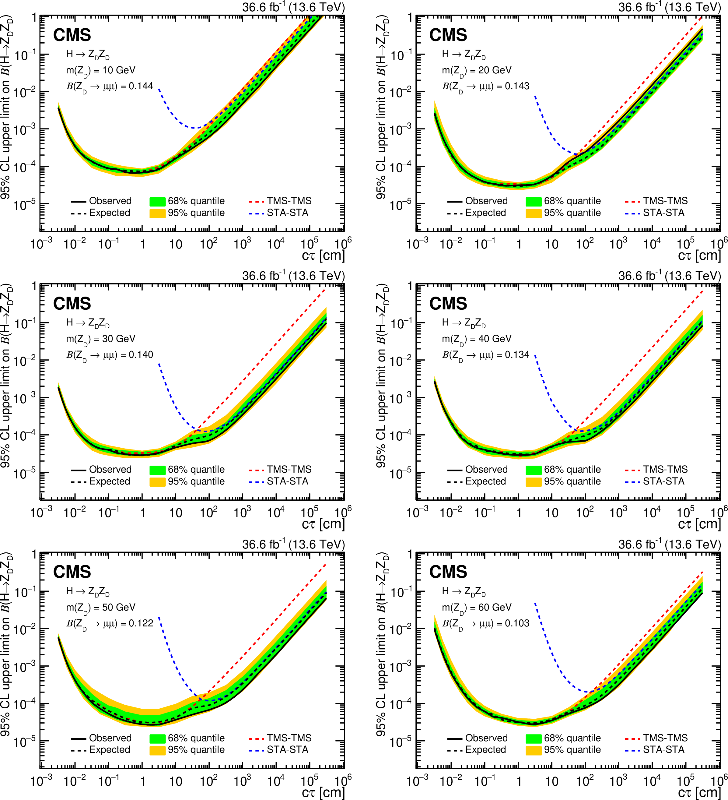
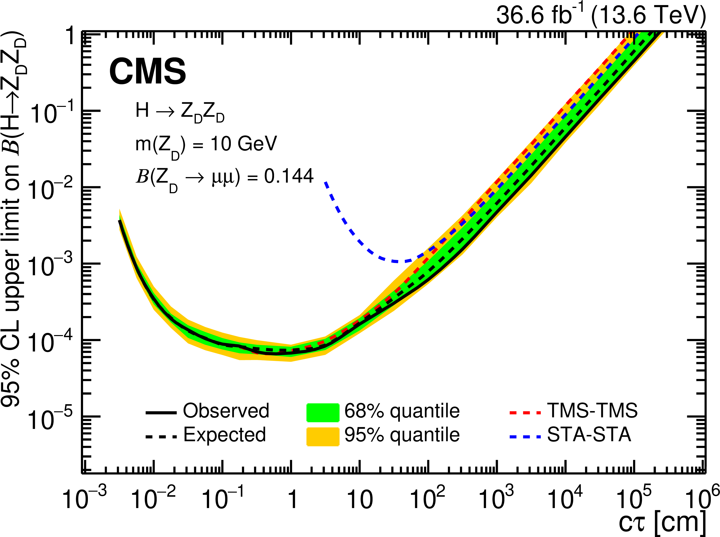
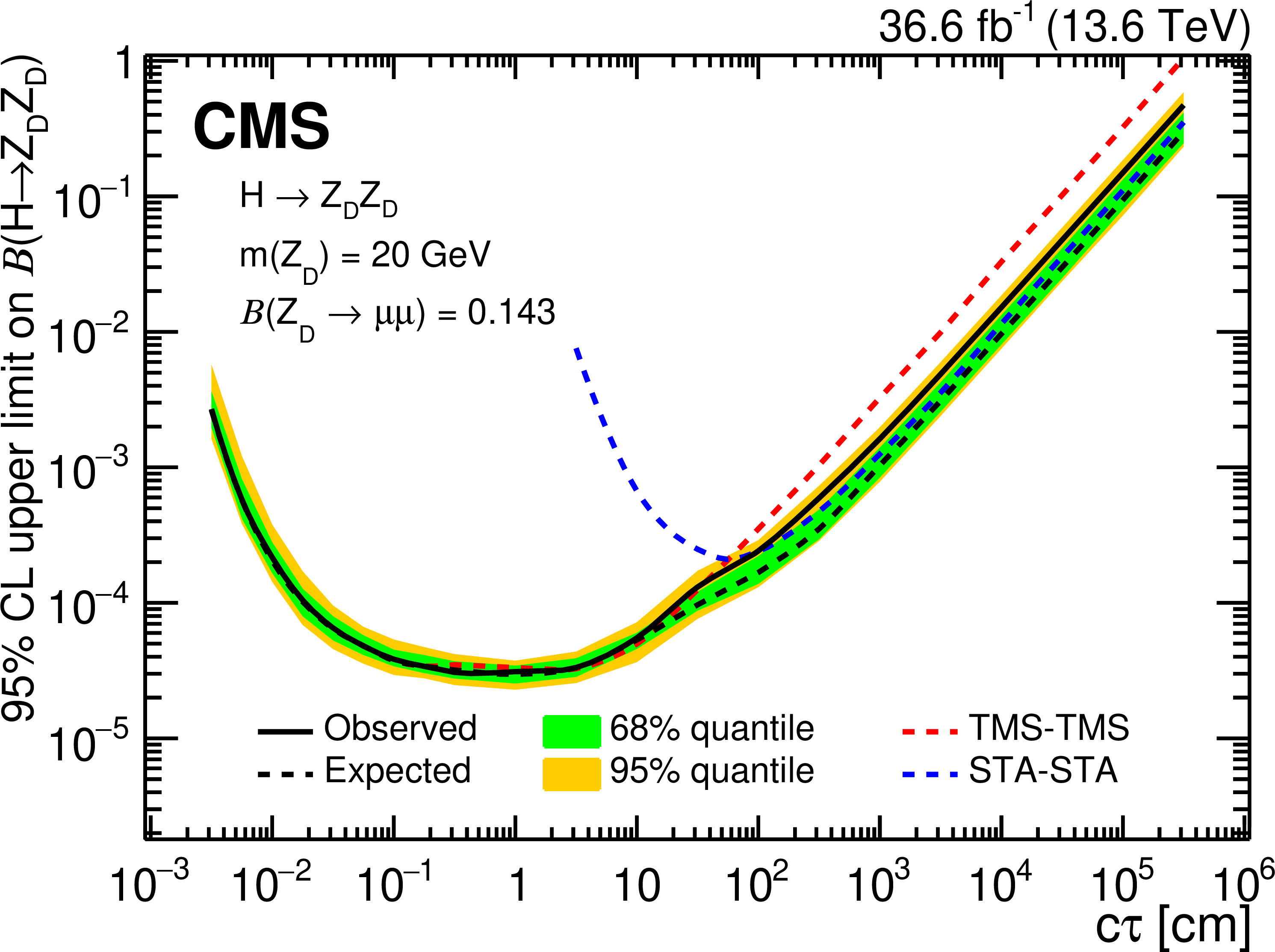
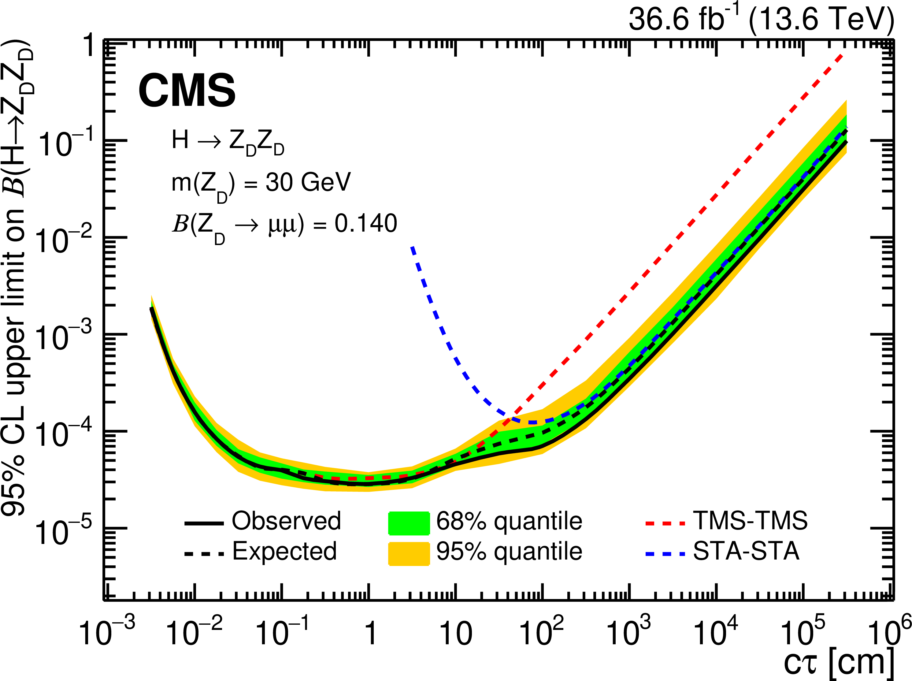
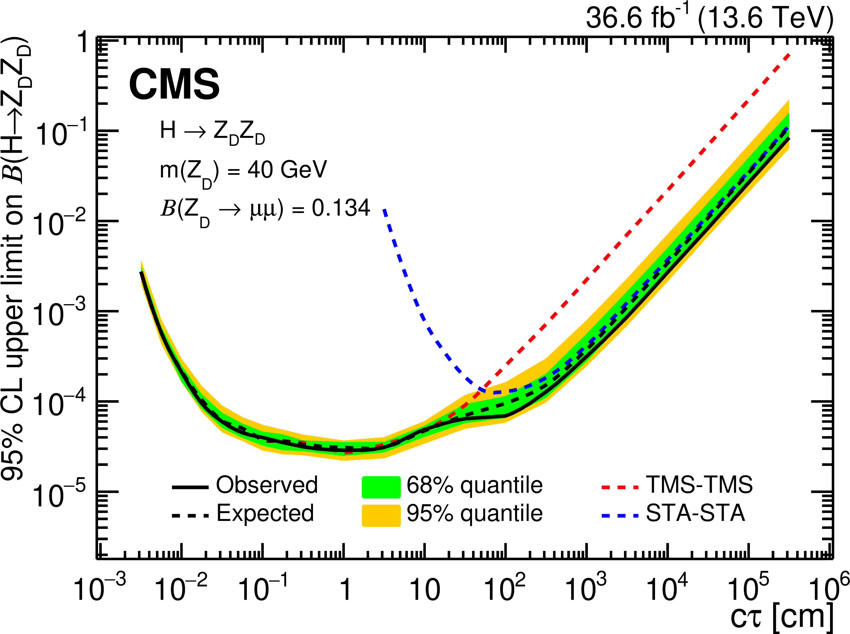
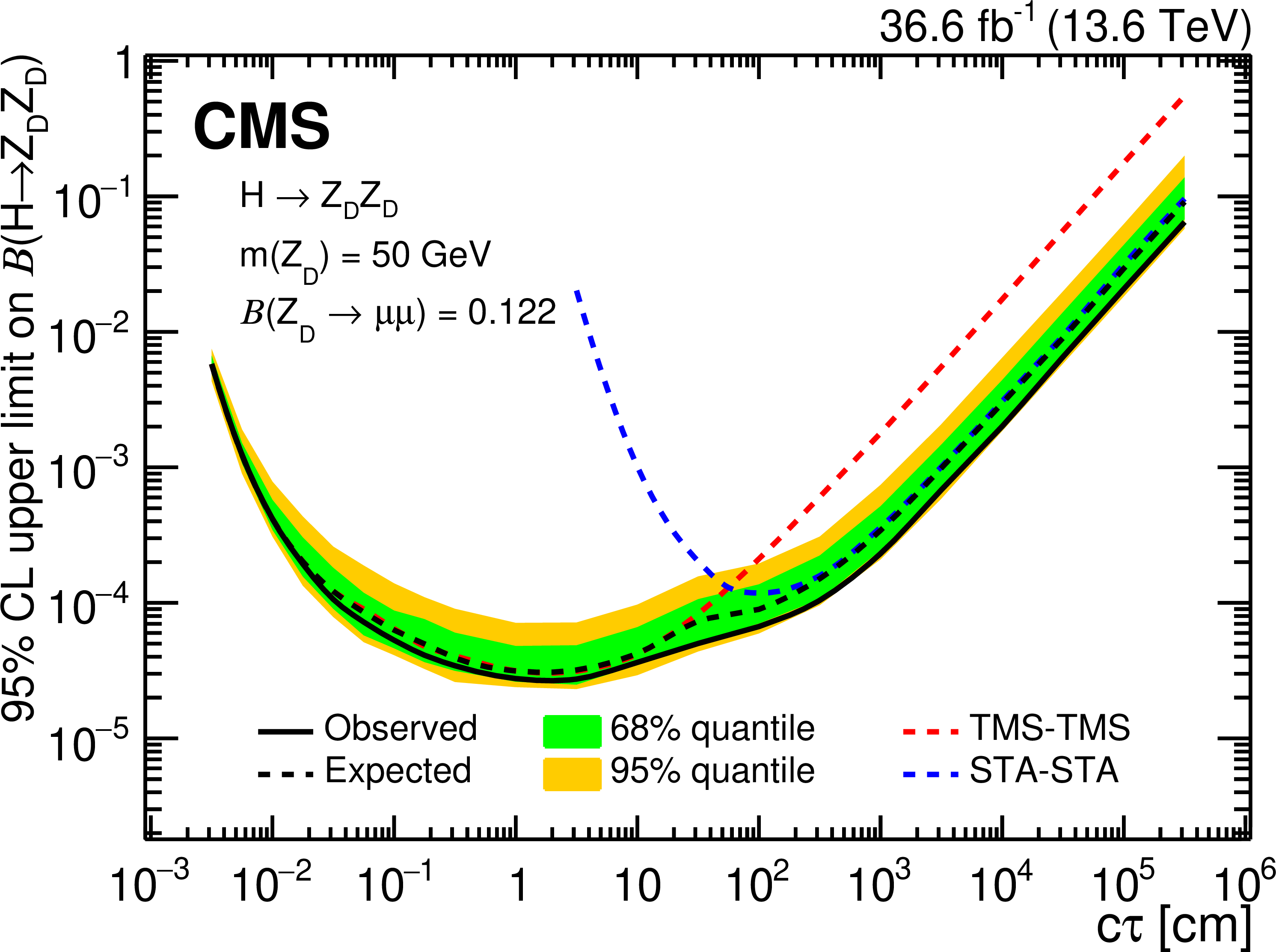
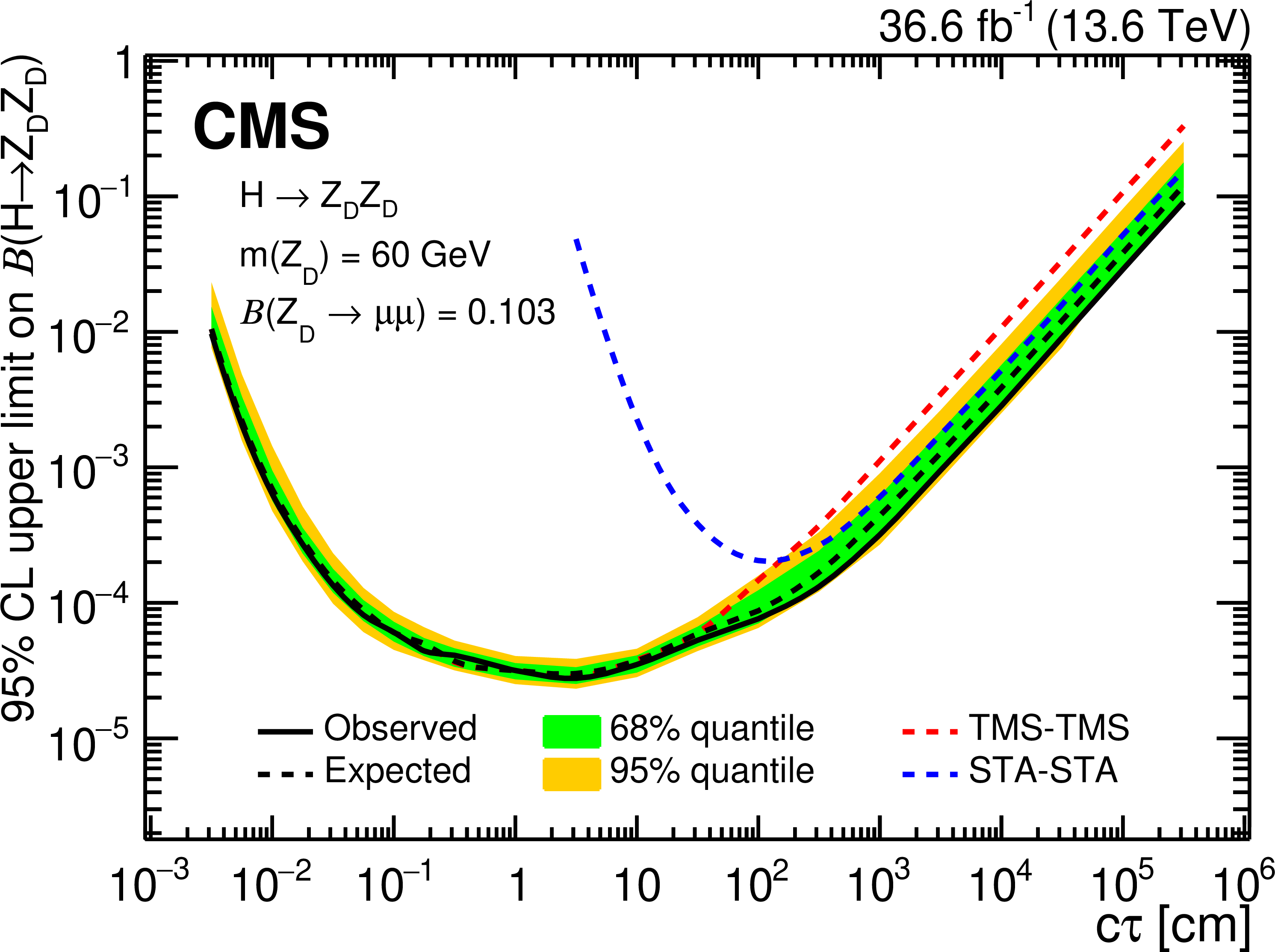
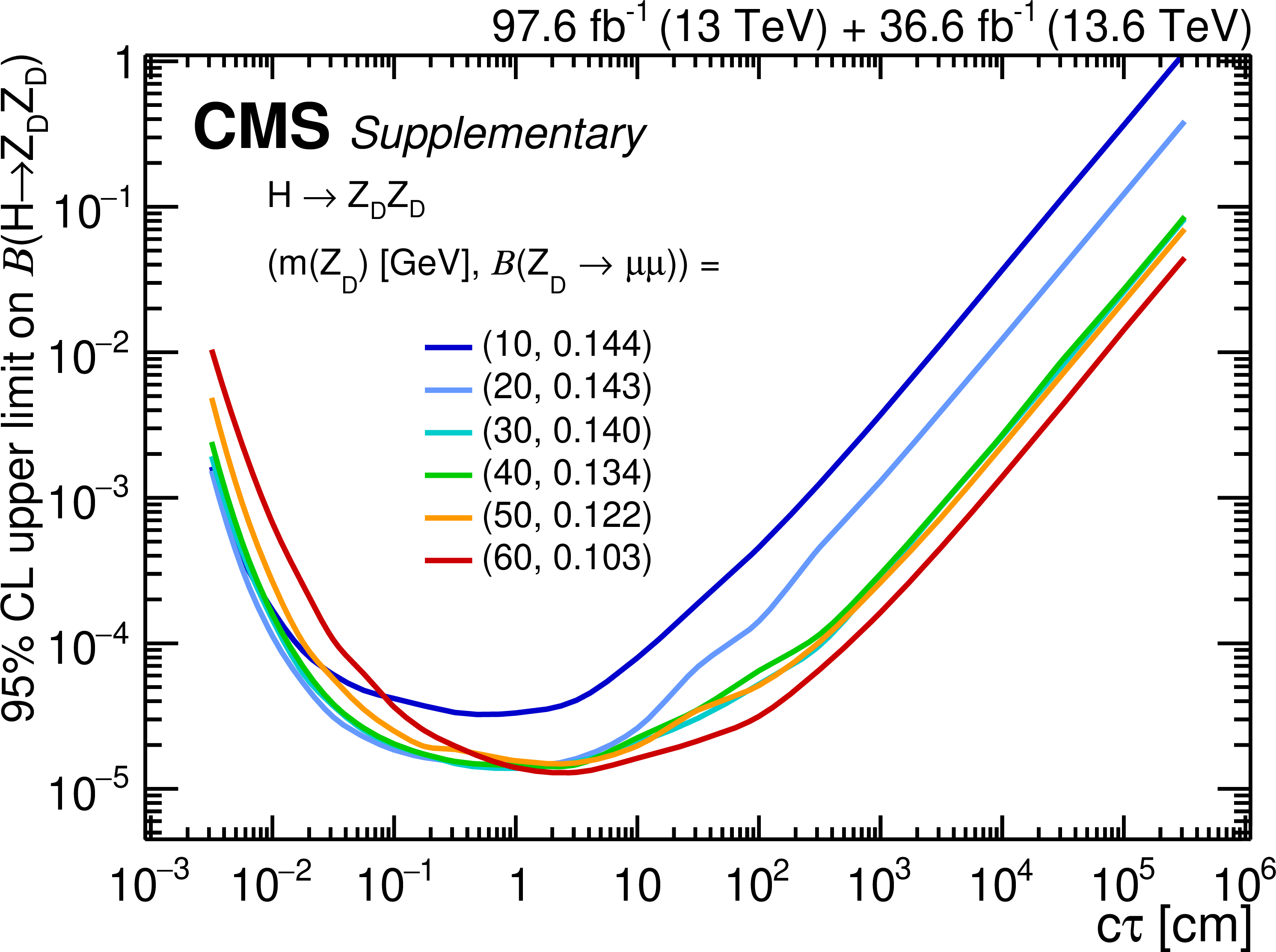
The 95% CL upper limits on $ \mathcal{B}(\mathrm{H} \to \mathrm{Z}_\text{D} \mathrm{Z}_\text{D}) $ as a function of $ c\tau(\mathrm{Z}_\text{D}) $ in the HAHM model, for $ m(\mathrm{Z}_\text{D}) $ ranging from (upper left) 10 GeV to (lower right) 60 GeV, in the STA-STA and TMS-TMS dimuon categories in 2022 data and their combination. The median expected limits obtained from the STA-STA and TMS-TMS dimuon categories are shown as dashed blue and red curves, respectively; the combined median expected limits are shown as dashed black curves; and the combined observed limits are shown as solid black curves. The green and yellow bands correspond, respectively, to the 68 and 95% quantiles for the combined expected limits. |
png pdf |
Figure 14-a:
The 95% CL upper limits on $ \mathcal{B}(\mathrm{H} \to \mathrm{Z}_\text{D} \mathrm{Z}_\text{D}) $ as a function of $ c\tau(\mathrm{Z}_\text{D}) $ in the HAHM model, for $ m(\mathrm{Z}_\text{D}) $ ranging from (upper left) 10 GeV to (lower right) 60 GeV, in the STA-STA and TMS-TMS dimuon categories in 2022 data and their combination. The median expected limits obtained from the STA-STA and TMS-TMS dimuon categories are shown as dashed blue and red curves, respectively; the combined median expected limits are shown as dashed black curves; and the combined observed limits are shown as solid black curves. The green and yellow bands correspond, respectively, to the 68 and 95% quantiles for the combined expected limits. |
png pdf |
Figure 14-b:
The 95% CL upper limits on $ \mathcal{B}(\mathrm{H} \to \mathrm{Z}_\text{D} \mathrm{Z}_\text{D}) $ as a function of $ c\tau(\mathrm{Z}_\text{D}) $ in the HAHM model, for $ m(\mathrm{Z}_\text{D}) $ ranging from (upper left) 10 GeV to (lower right) 60 GeV, in the STA-STA and TMS-TMS dimuon categories in 2022 data and their combination. The median expected limits obtained from the STA-STA and TMS-TMS dimuon categories are shown as dashed blue and red curves, respectively; the combined median expected limits are shown as dashed black curves; and the combined observed limits are shown as solid black curves. The green and yellow bands correspond, respectively, to the 68 and 95% quantiles for the combined expected limits. |
png pdf |
Figure 14-c:
The 95% CL upper limits on $ \mathcal{B}(\mathrm{H} \to \mathrm{Z}_\text{D} \mathrm{Z}_\text{D}) $ as a function of $ c\tau(\mathrm{Z}_\text{D}) $ in the HAHM model, for $ m(\mathrm{Z}_\text{D}) $ ranging from (upper left) 10 GeV to (lower right) 60 GeV, in the STA-STA and TMS-TMS dimuon categories in 2022 data and their combination. The median expected limits obtained from the STA-STA and TMS-TMS dimuon categories are shown as dashed blue and red curves, respectively; the combined median expected limits are shown as dashed black curves; and the combined observed limits are shown as solid black curves. The green and yellow bands correspond, respectively, to the 68 and 95% quantiles for the combined expected limits. |
png pdf |
Figure 14-d:
The 95% CL upper limits on $ \mathcal{B}(\mathrm{H} \to \mathrm{Z}_\text{D} \mathrm{Z}_\text{D}) $ as a function of $ c\tau(\mathrm{Z}_\text{D}) $ in the HAHM model, for $ m(\mathrm{Z}_\text{D}) $ ranging from (upper left) 10 GeV to (lower right) 60 GeV, in the STA-STA and TMS-TMS dimuon categories in 2022 data and their combination. The median expected limits obtained from the STA-STA and TMS-TMS dimuon categories are shown as dashed blue and red curves, respectively; the combined median expected limits are shown as dashed black curves; and the combined observed limits are shown as solid black curves. The green and yellow bands correspond, respectively, to the 68 and 95% quantiles for the combined expected limits. |
png pdf |
Figure 14-e:
The 95% CL upper limits on $ \mathcal{B}(\mathrm{H} \to \mathrm{Z}_\text{D} \mathrm{Z}_\text{D}) $ as a function of $ c\tau(\mathrm{Z}_\text{D}) $ in the HAHM model, for $ m(\mathrm{Z}_\text{D}) $ ranging from (upper left) 10 GeV to (lower right) 60 GeV, in the STA-STA and TMS-TMS dimuon categories in 2022 data and their combination. The median expected limits obtained from the STA-STA and TMS-TMS dimuon categories are shown as dashed blue and red curves, respectively; the combined median expected limits are shown as dashed black curves; and the combined observed limits are shown as solid black curves. The green and yellow bands correspond, respectively, to the 68 and 95% quantiles for the combined expected limits. |
png pdf |
Figure 14-f:
The 95% CL upper limits on $ \mathcal{B}(\mathrm{H} \to \mathrm{Z}_\text{D} \mathrm{Z}_\text{D}) $ as a function of $ c\tau(\mathrm{Z}_\text{D}) $ in the HAHM model, for $ m(\mathrm{Z}_\text{D}) $ ranging from (upper left) 10 GeV to (lower right) 60 GeV, in the STA-STA and TMS-TMS dimuon categories in 2022 data and their combination. The median expected limits obtained from the STA-STA and TMS-TMS dimuon categories are shown as dashed blue and red curves, respectively; the combined median expected limits are shown as dashed black curves; and the combined observed limits are shown as solid black curves. The green and yellow bands correspond, respectively, to the 68 and 95% quantiles for the combined expected limits. |
png pdf |
Figure 15:
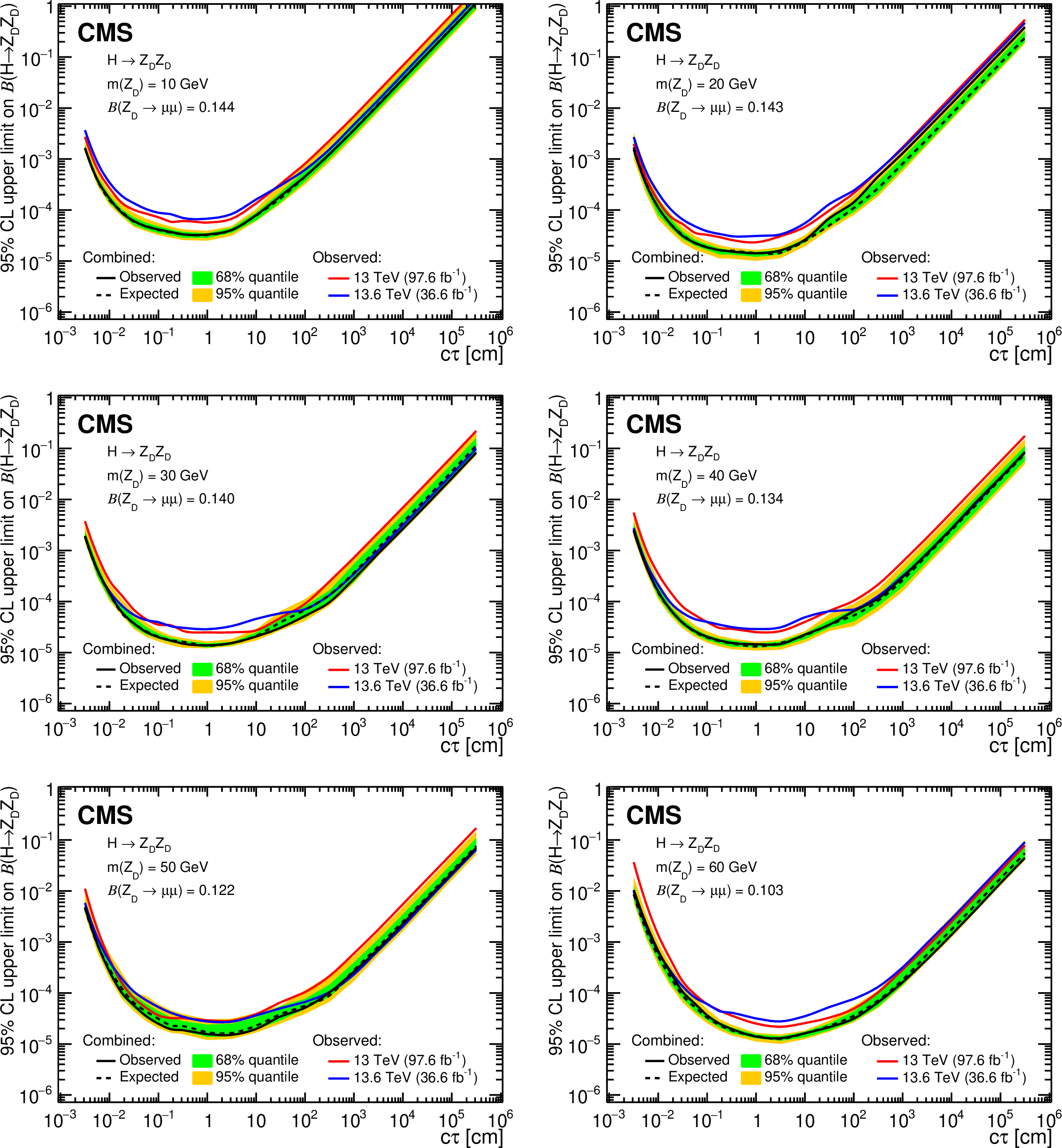
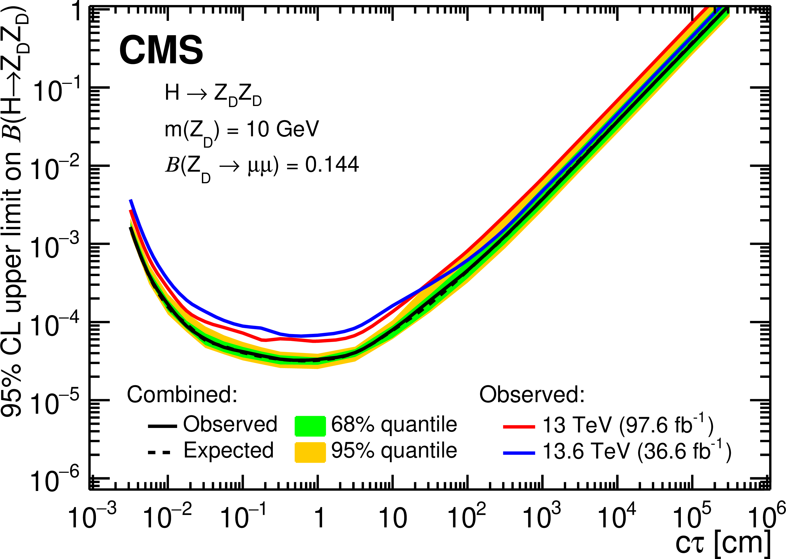
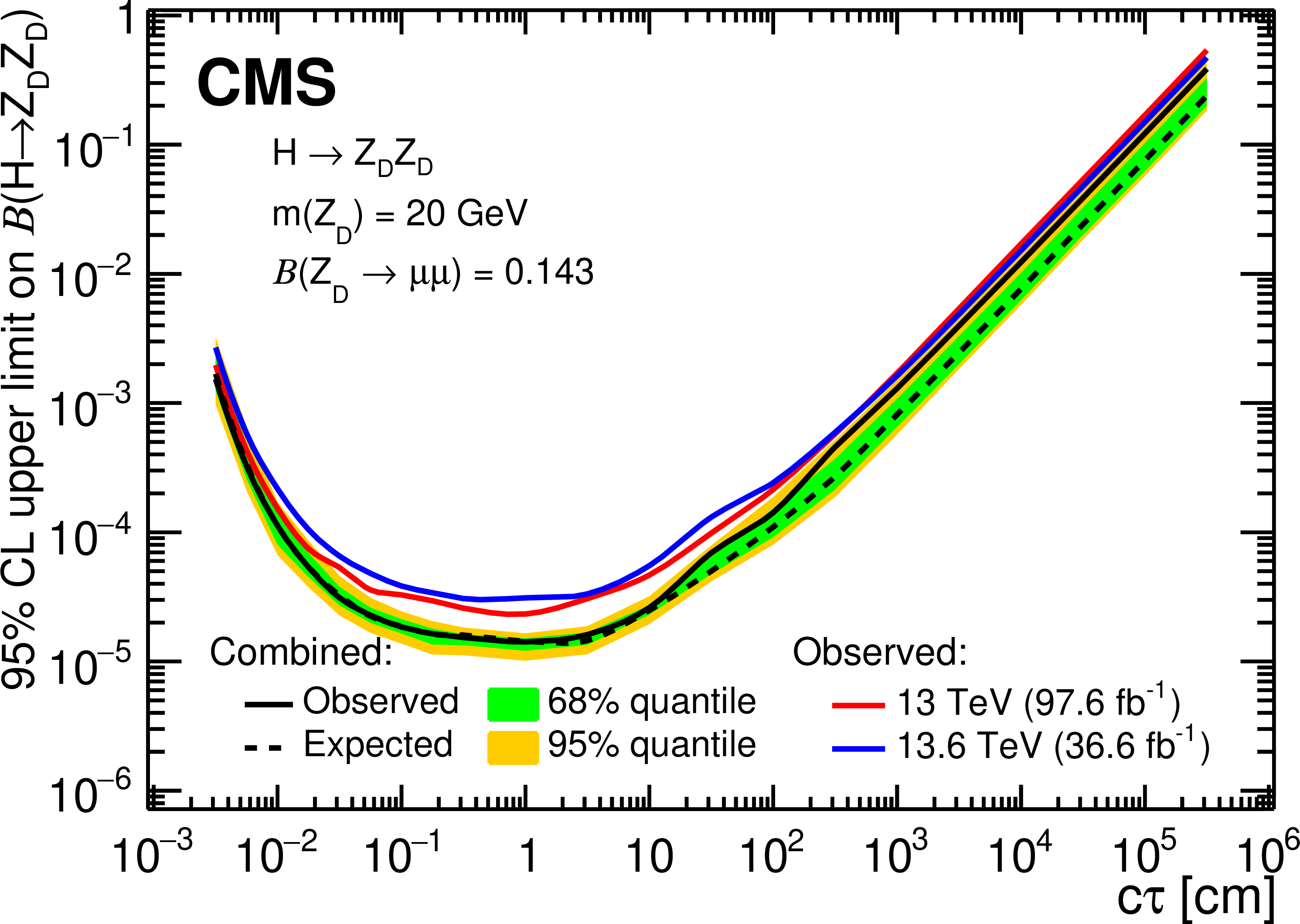
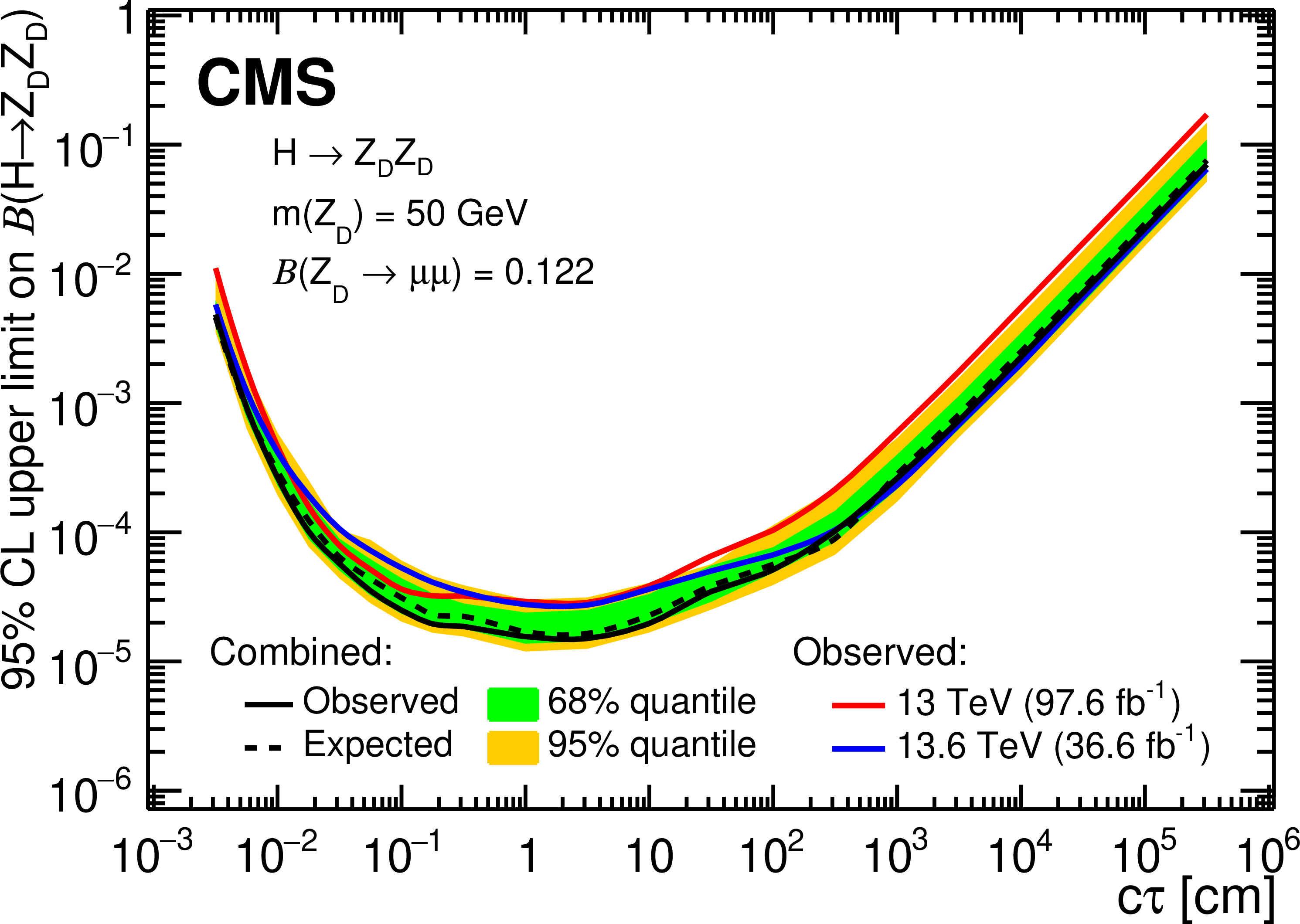
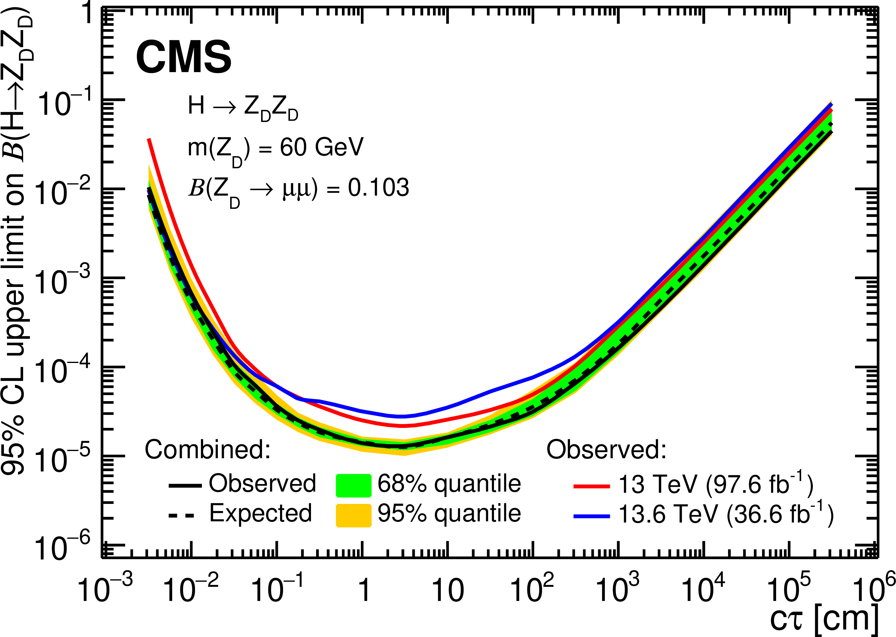
The 95% CL upper limits on $ \mathcal{B}(\mathrm{H} \to \mathrm{Z}_\text{D} \mathrm{Z}_\text{D}) $ as a function of $ c\tau(\mathrm{Z}_\text{D}) $ in the HAHM model, for $ m(\mathrm{Z}_\text{D}) $ ranging from (upper left) 10 GeV to (lower right) 60 GeV, obtained in this analysis, the Run 2 analysis [5], and their combination. The observed limits in this analysis and in the Run 2 analysis [5] are shown as blue and red curves, respectively; the median combined expected limits are shown as dashed black curves; and the combined observed limits are shown as solid black curves. The green and yellow bands correspond, respectively, to the 68 and 95% quantiles for the combined expected limits. |
png pdf |
Figure 15-a:
The 95% CL upper limits on $ \mathcal{B}(\mathrm{H} \to \mathrm{Z}_\text{D} \mathrm{Z}_\text{D}) $ as a function of $ c\tau(\mathrm{Z}_\text{D}) $ in the HAHM model, for $ m(\mathrm{Z}_\text{D}) $ ranging from (upper left) 10 GeV to (lower right) 60 GeV, obtained in this analysis, the Run 2 analysis [5], and their combination. The observed limits in this analysis and in the Run 2 analysis [5] are shown as blue and red curves, respectively; the median combined expected limits are shown as dashed black curves; and the combined observed limits are shown as solid black curves. The green and yellow bands correspond, respectively, to the 68 and 95% quantiles for the combined expected limits. |
png pdf |
Figure 15-b:
The 95% CL upper limits on $ \mathcal{B}(\mathrm{H} \to \mathrm{Z}_\text{D} \mathrm{Z}_\text{D}) $ as a function of $ c\tau(\mathrm{Z}_\text{D}) $ in the HAHM model, for $ m(\mathrm{Z}_\text{D}) $ ranging from (upper left) 10 GeV to (lower right) 60 GeV, obtained in this analysis, the Run 2 analysis [5], and their combination. The observed limits in this analysis and in the Run 2 analysis [5] are shown as blue and red curves, respectively; the median combined expected limits are shown as dashed black curves; and the combined observed limits are shown as solid black curves. The green and yellow bands correspond, respectively, to the 68 and 95% quantiles for the combined expected limits. |

png pdf |
Figure 15-c:
The 95% CL upper limits on $ \mathcal{B}(\mathrm{H} \to \mathrm{Z}_\text{D} \mathrm{Z}_\text{D}) $ as a function of $ c\tau(\mathrm{Z}_\text{D}) $ in the HAHM model, for $ m(\mathrm{Z}_\text{D}) $ ranging from (upper left) 10 GeV to (lower right) 60 GeV, obtained in this analysis, the Run 2 analysis [5], and their combination. The observed limits in this analysis and in the Run 2 analysis [5] are shown as blue and red curves, respectively; the median combined expected limits are shown as dashed black curves; and the combined observed limits are shown as solid black curves. The green and yellow bands correspond, respectively, to the 68 and 95% quantiles for the combined expected limits. |

png pdf |
Figure 15-d:
The 95% CL upper limits on $ \mathcal{B}(\mathrm{H} \to \mathrm{Z}_\text{D} \mathrm{Z}_\text{D}) $ as a function of $ c\tau(\mathrm{Z}_\text{D}) $ in the HAHM model, for $ m(\mathrm{Z}_\text{D}) $ ranging from (upper left) 10 GeV to (lower right) 60 GeV, obtained in this analysis, the Run 2 analysis [5], and their combination. The observed limits in this analysis and in the Run 2 analysis [5] are shown as blue and red curves, respectively; the median combined expected limits are shown as dashed black curves; and the combined observed limits are shown as solid black curves. The green and yellow bands correspond, respectively, to the 68 and 95% quantiles for the combined expected limits. |
png pdf |
Figure 15-e:
The 95% CL upper limits on $ \mathcal{B}(\mathrm{H} \to \mathrm{Z}_\text{D} \mathrm{Z}_\text{D}) $ as a function of $ c\tau(\mathrm{Z}_\text{D}) $ in the HAHM model, for $ m(\mathrm{Z}_\text{D}) $ ranging from (upper left) 10 GeV to (lower right) 60 GeV, obtained in this analysis, the Run 2 analysis [5], and their combination. The observed limits in this analysis and in the Run 2 analysis [5] are shown as blue and red curves, respectively; the median combined expected limits are shown as dashed black curves; and the combined observed limits are shown as solid black curves. The green and yellow bands correspond, respectively, to the 68 and 95% quantiles for the combined expected limits. |
png pdf |
Figure 15-f:
The 95% CL upper limits on $ \mathcal{B}(\mathrm{H} \to \mathrm{Z}_\text{D} \mathrm{Z}_\text{D}) $ as a function of $ c\tau(\mathrm{Z}_\text{D}) $ in the HAHM model, for $ m(\mathrm{Z}_\text{D}) $ ranging from (upper left) 10 GeV to (lower right) 60 GeV, obtained in this analysis, the Run 2 analysis [5], and their combination. The observed limits in this analysis and in the Run 2 analysis [5] are shown as blue and red curves, respectively; the median combined expected limits are shown as dashed black curves; and the combined observed limits are shown as solid black curves. The green and yellow bands correspond, respectively, to the 68 and 95% quantiles for the combined expected limits. |
png pdf |
Figure 16:
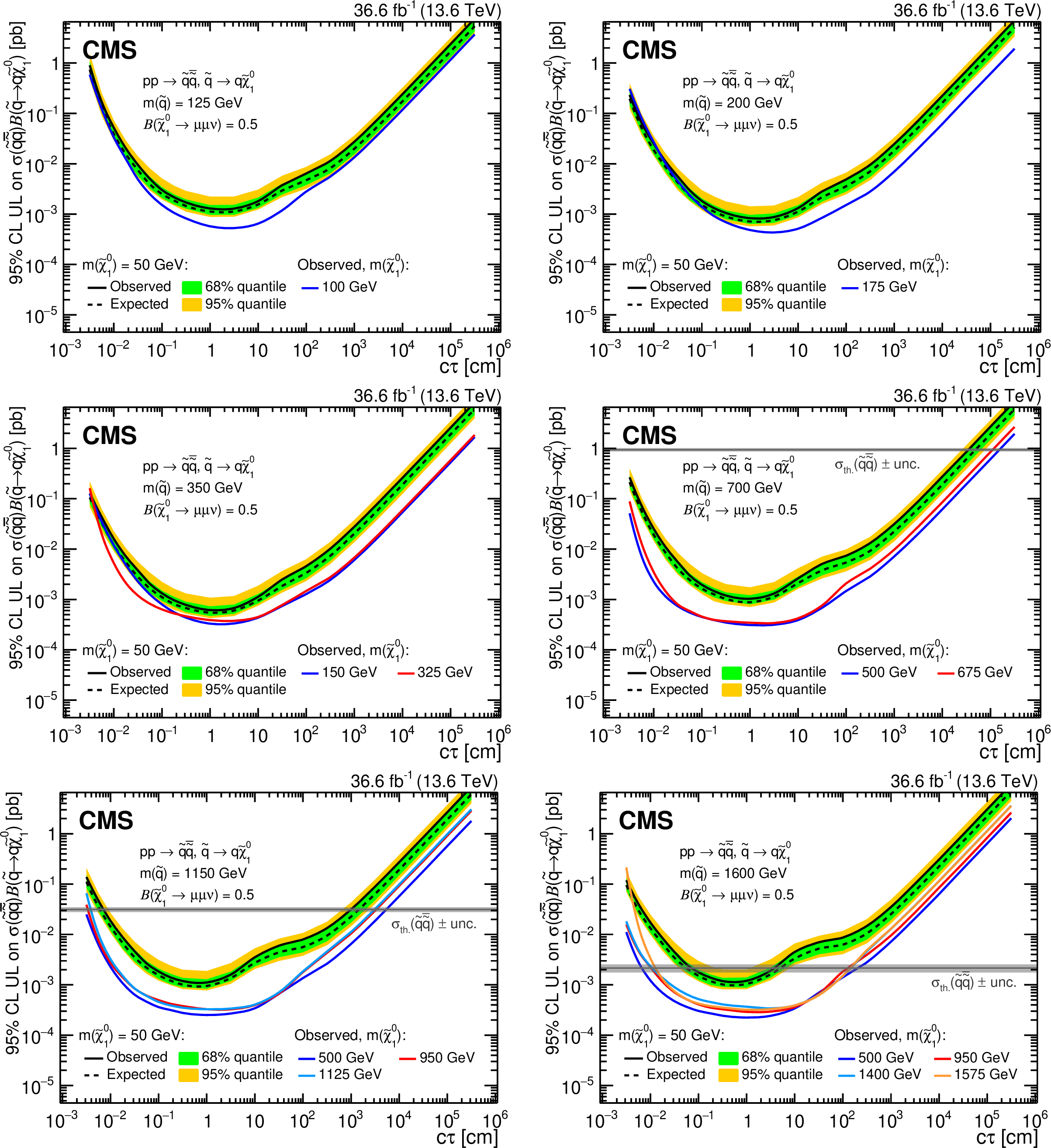
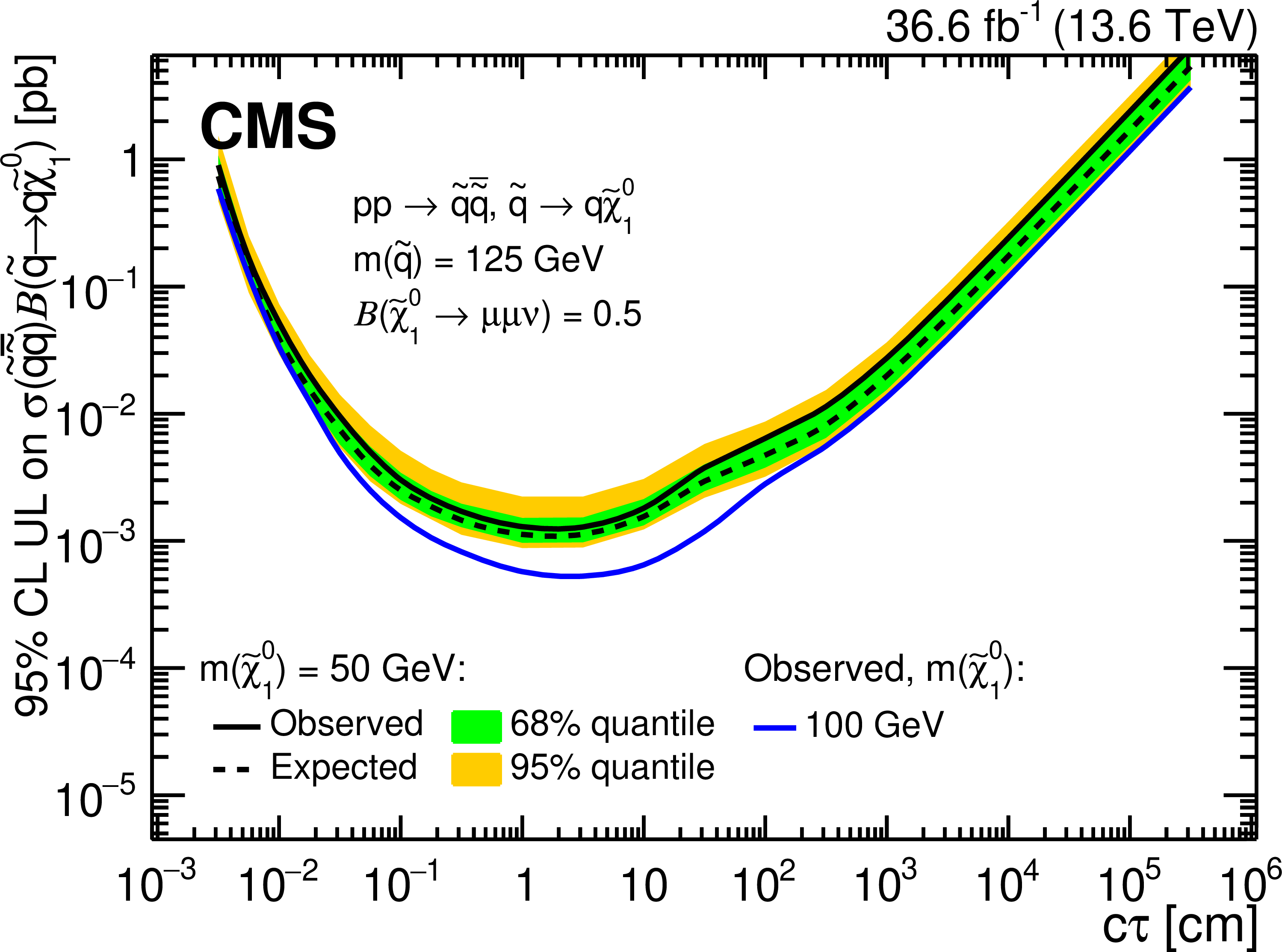
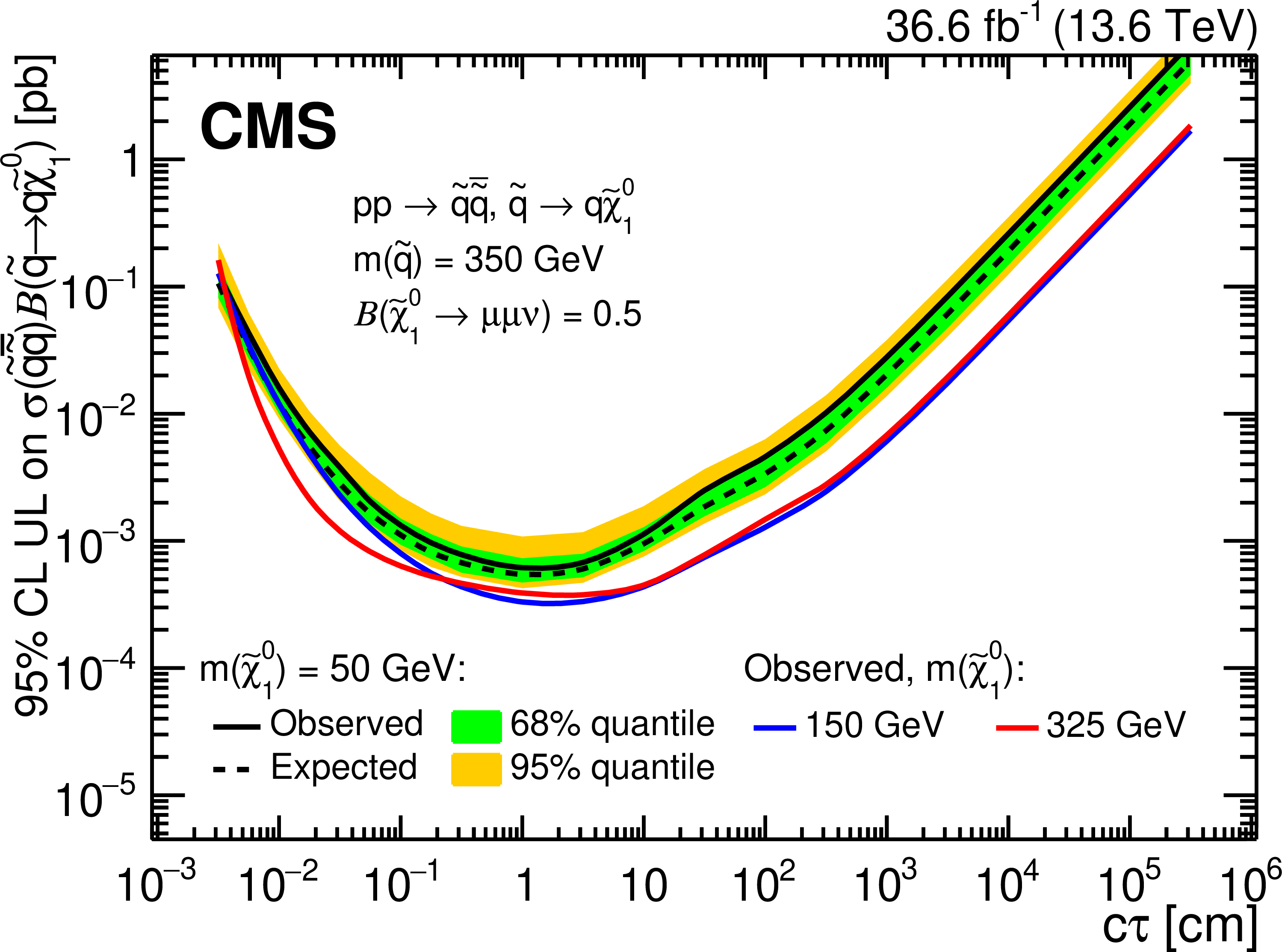
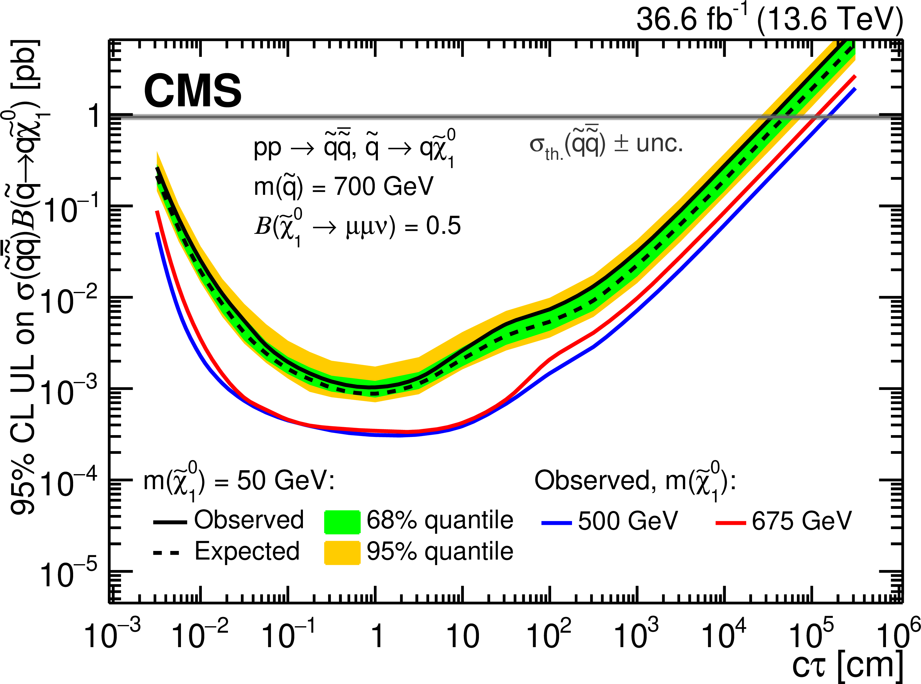
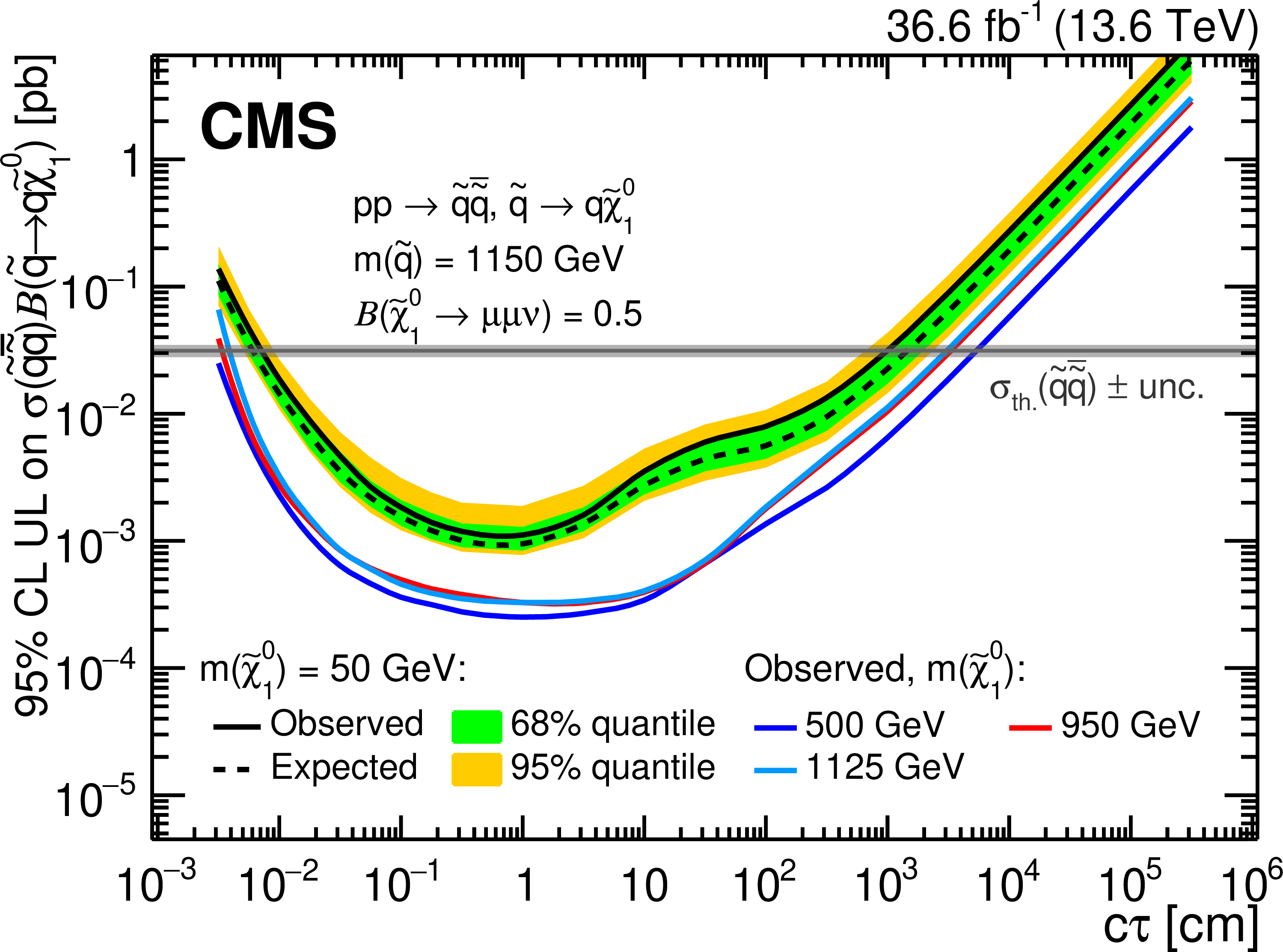
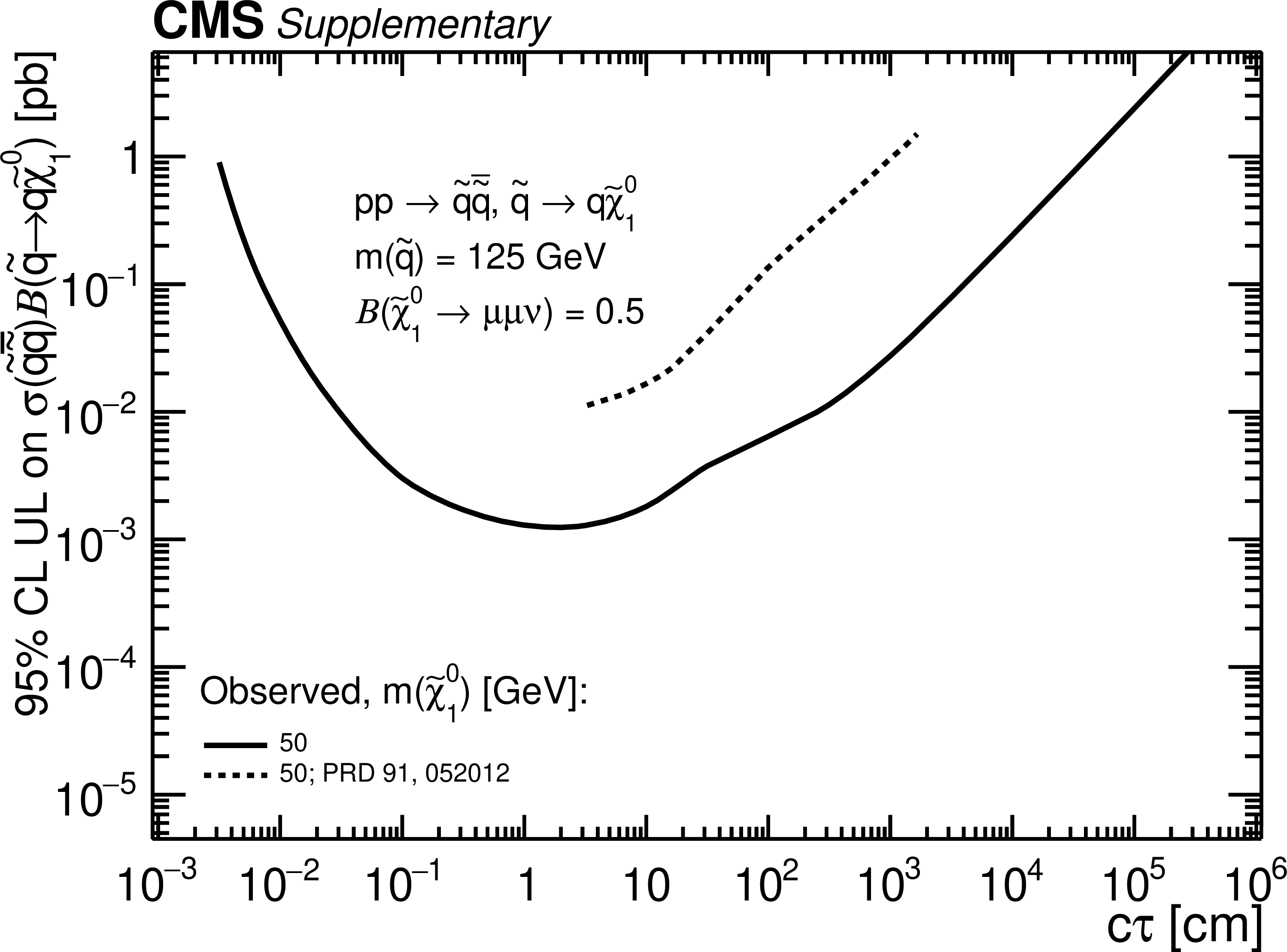
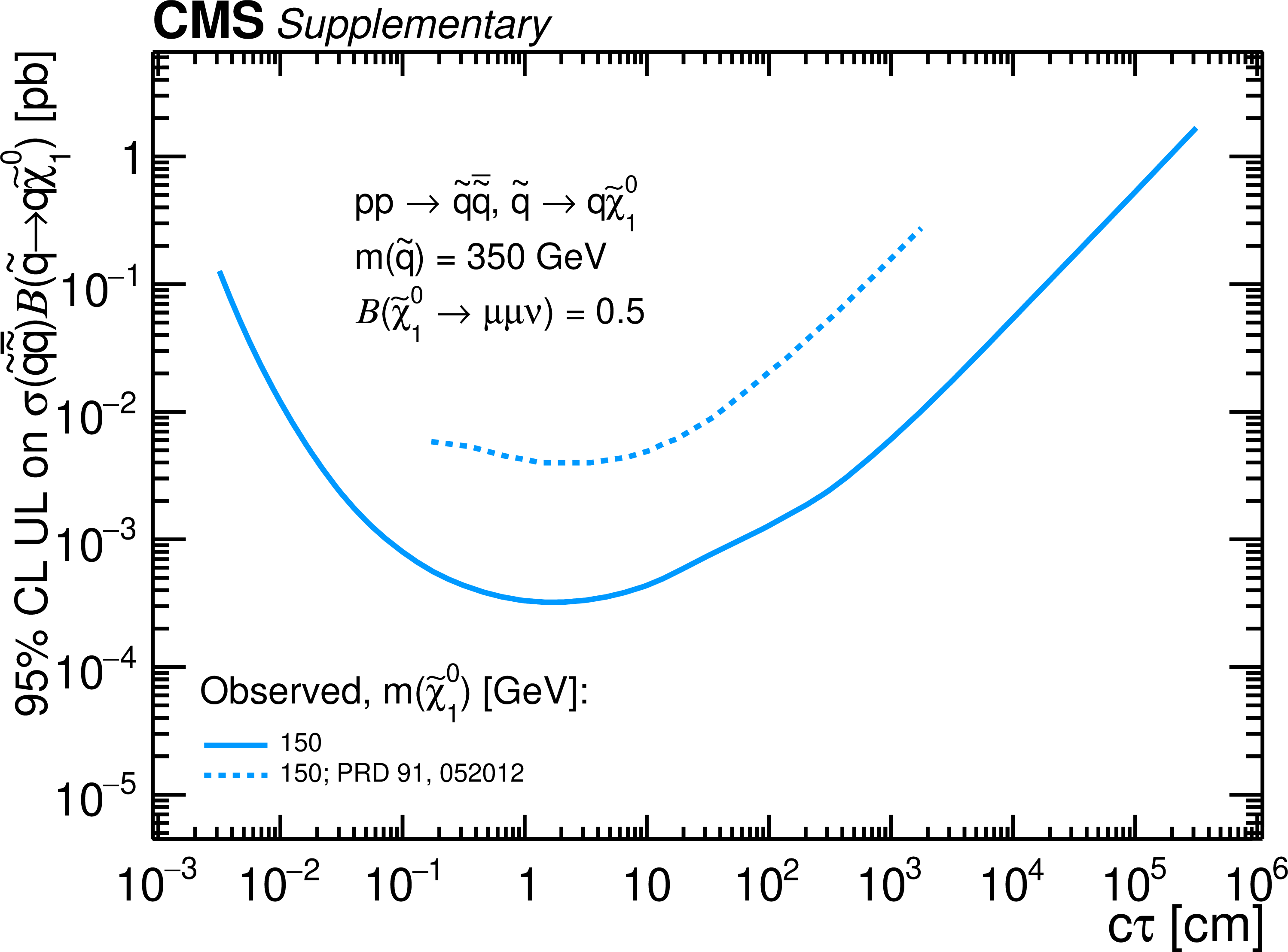
The 95% CL upper limits on $ \sigma(\mathrm{p}\mathrm{p}\to{\tilde{\mathrm{q}}} \overline{\tilde{\mathrm{q}}})\mathcal{B}( \tilde{\mathrm{q}} \to \mathrm{q} \tilde{\chi}_{1}^{0} ) $ as a function of $ c\tau(\tilde{\chi}_{1}^{0}) $ in the RPV SUSY model, for $ \mathcal{B}(\tilde{\chi}_{1}^{0}\to\mu^{+}\mu^{-}\nu) = $ 0.5 and $ m({\tilde{\mathrm{q}}} ) $ ranging from (upper left) 125 GeV to (lower right) 1.6 TeV. The observed limits for various combinations of $ m({\tilde{\mathrm{q}}} ) $ and $ m(\tilde{\chi}_{1}^{0}) $ indicated in the legends are shown as solid curves. The median expected limits and their 68 and 95% quantiles are shown, respectively, as dashed black curves and green and yellow bands for the case of $ m(\tilde{\chi}_{1}^{0}) = $ 50 GeV and omitted for other neutralino masses for clarity. The gray horizontal lines indicate the theoretical values of the squark-antisquark production cross sections with the uncertainties shown as gray shaded bands. The predicted cross sections for $ m({\tilde{\mathrm{q}}} ) = $ 125, 200, and 350 GeV are, respectively, 7200, 840, and 50 pb, and fall outside the $ y $-axis range. |
png pdf |
Figure 16-a:
The 95% CL upper limits on $ \sigma(\mathrm{p}\mathrm{p}\to{\tilde{\mathrm{q}}} \overline{\tilde{\mathrm{q}}})\mathcal{B}( \tilde{\mathrm{q}} \to \mathrm{q} \tilde{\chi}_{1}^{0} ) $ as a function of $ c\tau(\tilde{\chi}_{1}^{0}) $ in the RPV SUSY model, for $ \mathcal{B}(\tilde{\chi}_{1}^{0}\to\mu^{+}\mu^{-}\nu) = $ 0.5 and $ m({\tilde{\mathrm{q}}} ) $ ranging from (upper left) 125 GeV to (lower right) 1.6 TeV. The observed limits for various combinations of $ m({\tilde{\mathrm{q}}} ) $ and $ m(\tilde{\chi}_{1}^{0}) $ indicated in the legends are shown as solid curves. The median expected limits and their 68 and 95% quantiles are shown, respectively, as dashed black curves and green and yellow bands for the case of $ m(\tilde{\chi}_{1}^{0}) = $ 50 GeV and omitted for other neutralino masses for clarity. The gray horizontal lines indicate the theoretical values of the squark-antisquark production cross sections with the uncertainties shown as gray shaded bands. The predicted cross sections for $ m({\tilde{\mathrm{q}}} ) = $ 125, 200, and 350 GeV are, respectively, 7200, 840, and 50 pb, and fall outside the $ y $-axis range. |

png pdf |
Figure 16-b:
The 95% CL upper limits on $ \sigma(\mathrm{p}\mathrm{p}\to{\tilde{\mathrm{q}}} \overline{\tilde{\mathrm{q}}})\mathcal{B}( \tilde{\mathrm{q}} \to \mathrm{q} \tilde{\chi}_{1}^{0} ) $ as a function of $ c\tau(\tilde{\chi}_{1}^{0}) $ in the RPV SUSY model, for $ \mathcal{B}(\tilde{\chi}_{1}^{0}\to\mu^{+}\mu^{-}\nu) = $ 0.5 and $ m({\tilde{\mathrm{q}}} ) $ ranging from (upper left) 125 GeV to (lower right) 1.6 TeV. The observed limits for various combinations of $ m({\tilde{\mathrm{q}}} ) $ and $ m(\tilde{\chi}_{1}^{0}) $ indicated in the legends are shown as solid curves. The median expected limits and their 68 and 95% quantiles are shown, respectively, as dashed black curves and green and yellow bands for the case of $ m(\tilde{\chi}_{1}^{0}) = $ 50 GeV and omitted for other neutralino masses for clarity. The gray horizontal lines indicate the theoretical values of the squark-antisquark production cross sections with the uncertainties shown as gray shaded bands. The predicted cross sections for $ m({\tilde{\mathrm{q}}} ) = $ 125, 200, and 350 GeV are, respectively, 7200, 840, and 50 pb, and fall outside the $ y $-axis range. |
png pdf |
Figure 16-c:
The 95% CL upper limits on $ \sigma(\mathrm{p}\mathrm{p}\to{\tilde{\mathrm{q}}} \overline{\tilde{\mathrm{q}}})\mathcal{B}( \tilde{\mathrm{q}} \to \mathrm{q} \tilde{\chi}_{1}^{0} ) $ as a function of $ c\tau(\tilde{\chi}_{1}^{0}) $ in the RPV SUSY model, for $ \mathcal{B}(\tilde{\chi}_{1}^{0}\to\mu^{+}\mu^{-}\nu) = $ 0.5 and $ m({\tilde{\mathrm{q}}} ) $ ranging from (upper left) 125 GeV to (lower right) 1.6 TeV. The observed limits for various combinations of $ m({\tilde{\mathrm{q}}} ) $ and $ m(\tilde{\chi}_{1}^{0}) $ indicated in the legends are shown as solid curves. The median expected limits and their 68 and 95% quantiles are shown, respectively, as dashed black curves and green and yellow bands for the case of $ m(\tilde{\chi}_{1}^{0}) = $ 50 GeV and omitted for other neutralino masses for clarity. The gray horizontal lines indicate the theoretical values of the squark-antisquark production cross sections with the uncertainties shown as gray shaded bands. The predicted cross sections for $ m({\tilde{\mathrm{q}}} ) = $ 125, 200, and 350 GeV are, respectively, 7200, 840, and 50 pb, and fall outside the $ y $-axis range. |
png pdf |
Figure 16-d:
The 95% CL upper limits on $ \sigma(\mathrm{p}\mathrm{p}\to{\tilde{\mathrm{q}}} \overline{\tilde{\mathrm{q}}})\mathcal{B}( \tilde{\mathrm{q}} \to \mathrm{q} \tilde{\chi}_{1}^{0} ) $ as a function of $ c\tau(\tilde{\chi}_{1}^{0}) $ in the RPV SUSY model, for $ \mathcal{B}(\tilde{\chi}_{1}^{0}\to\mu^{+}\mu^{-}\nu) = $ 0.5 and $ m({\tilde{\mathrm{q}}} ) $ ranging from (upper left) 125 GeV to (lower right) 1.6 TeV. The observed limits for various combinations of $ m({\tilde{\mathrm{q}}} ) $ and $ m(\tilde{\chi}_{1}^{0}) $ indicated in the legends are shown as solid curves. The median expected limits and their 68 and 95% quantiles are shown, respectively, as dashed black curves and green and yellow bands for the case of $ m(\tilde{\chi}_{1}^{0}) = $ 50 GeV and omitted for other neutralino masses for clarity. The gray horizontal lines indicate the theoretical values of the squark-antisquark production cross sections with the uncertainties shown as gray shaded bands. The predicted cross sections for $ m({\tilde{\mathrm{q}}} ) = $ 125, 200, and 350 GeV are, respectively, 7200, 840, and 50 pb, and fall outside the $ y $-axis range. |
png pdf |
Figure 16-e:
The 95% CL upper limits on $ \sigma(\mathrm{p}\mathrm{p}\to{\tilde{\mathrm{q}}} \overline{\tilde{\mathrm{q}}})\mathcal{B}( \tilde{\mathrm{q}} \to \mathrm{q} \tilde{\chi}_{1}^{0} ) $ as a function of $ c\tau(\tilde{\chi}_{1}^{0}) $ in the RPV SUSY model, for $ \mathcal{B}(\tilde{\chi}_{1}^{0}\to\mu^{+}\mu^{-}\nu) = $ 0.5 and $ m({\tilde{\mathrm{q}}} ) $ ranging from (upper left) 125 GeV to (lower right) 1.6 TeV. The observed limits for various combinations of $ m({\tilde{\mathrm{q}}} ) $ and $ m(\tilde{\chi}_{1}^{0}) $ indicated in the legends are shown as solid curves. The median expected limits and their 68 and 95% quantiles are shown, respectively, as dashed black curves and green and yellow bands for the case of $ m(\tilde{\chi}_{1}^{0}) = $ 50 GeV and omitted for other neutralino masses for clarity. The gray horizontal lines indicate the theoretical values of the squark-antisquark production cross sections with the uncertainties shown as gray shaded bands. The predicted cross sections for $ m({\tilde{\mathrm{q}}} ) = $ 125, 200, and 350 GeV are, respectively, 7200, 840, and 50 pb, and fall outside the $ y $-axis range. |

png pdf |
Figure 16-f:
The 95% CL upper limits on $ \sigma(\mathrm{p}\mathrm{p}\to{\tilde{\mathrm{q}}} \overline{\tilde{\mathrm{q}}})\mathcal{B}( \tilde{\mathrm{q}} \to \mathrm{q} \tilde{\chi}_{1}^{0} ) $ as a function of $ c\tau(\tilde{\chi}_{1}^{0}) $ in the RPV SUSY model, for $ \mathcal{B}(\tilde{\chi}_{1}^{0}\to\mu^{+}\mu^{-}\nu) = $ 0.5 and $ m({\tilde{\mathrm{q}}} ) $ ranging from (upper left) 125 GeV to (lower right) 1.6 TeV. The observed limits for various combinations of $ m({\tilde{\mathrm{q}}} ) $ and $ m(\tilde{\chi}_{1}^{0}) $ indicated in the legends are shown as solid curves. The median expected limits and their 68 and 95% quantiles are shown, respectively, as dashed black curves and green and yellow bands for the case of $ m(\tilde{\chi}_{1}^{0}) = $ 50 GeV and omitted for other neutralino masses for clarity. The gray horizontal lines indicate the theoretical values of the squark-antisquark production cross sections with the uncertainties shown as gray shaded bands. The predicted cross sections for $ m({\tilde{\mathrm{q}}} ) = $ 125, 200, and 350 GeV are, respectively, 7200, 840, and 50 pb, and fall outside the $ y $-axis range. |
| Summary |
| Data collected by the CMS experiment in proton-proton collisions at $ \sqrt{s} = $ 13.6 TeV in 2022 and corresponding to an integrated luminosity of 36.6 fb$ ^{-1} $ have been used to conduct an inclusive search for long-lived exotic neutral particles decaying to final states with a pair of oppositely charged muons. The search strategy is largely model independent and is sensitive to a broad range of lifetimes and masses. No significant excess of events above the standard model background is observed. The results are interpreted as limits on the parameters of the hidden Abelian Higgs model, in which the Higgs boson H decays to a pair of long-lived dark photons $ \mathrm{Z}_\text{D} $, and of an $ R $-parity violating supersymmetry model, in which long-lived neutralinos decay to a pair of muons and a neutrino. Even though the size of the data sample used by this analysis is about a factor of 2.5 smaller than that used in the previous search for displaced dimuons by the CMS experiment in pp collisions at $ \sqrt{s} = $ 13 TeV, the constraints on the parameters of the hidden Abelian Higgs model are comparable or tighter in a significant fraction of the parameter space, thanks mainly to improvements in the trigger algorithms. The combination of the results of this analysis with the results obtained at $ \sqrt{s} = $ 13 TeV improves the constraints on the branching fraction of the Higgs boson to dark photons, $ \mathcal{B}(\mathrm{H} \to \mathrm{Z}_\text{D} \mathrm{Z}_\text{D}) $, by approximately a factor of 2. In the range 10--60 GeV of the $ \mathrm{Z}_\text{D} $ mass $ m(\mathrm{Z}_\text{D}) $, $ \mathcal{B}(\mathrm{H} \to \mathrm{Z}_\text{D} \mathrm{Z}_\text{D}) = $ 1% is excluded at 95% confidence level in the range of proper decay length $ c\tau(\mathrm{Z}_\text{D}) $ from a few tens of $ \mu $m to 30 m (700 m) for $ m(\mathrm{Z}_\text{D}) $ = 10 GeV (60 GeV). For $ m(\mathrm{Z}_\text{D}) $ greater than 20 GeV and less than $ m(\mathrm{H})/ $ 2, the combined limits provide the most stringent constraints to date on $ \mathcal{B}(\mathrm{H} \to \mathrm{Z}_\text{D} \mathrm{Z}_\text{D}) $ for $ c\tau(\mathrm{Z}_\text{D}) $ between 30 $ \mu $m and $ {\approx}$ 0.1 cm, and above $ {\approx}$ 10 cm. When interpreted in the framework of the $ R $-parity violating supersymmetry model at a squark mass of 1.6 TeV, the results exclude mean proper neutralino decay lengths between 0.07 and 4 cm for a 50 GeV neutralino and between 70 $ \mu $m and 2 m for a 500 GeV neutralino. |
| Additional Figures | |

png pdf |
Additional Figure 1:
Illustration showing two long-lived particles with different lifetimes decaying into a pair of muons, depicting how the signals of the muons can be traced back to the long-lived particle decay point using data from the tracker and muon detectors. |

png pdf |
Additional Figure 2:
Run 3 event containing a candidate for a long-lived particle that decays into a pair of muons away from the interaction point, reconstructed in the CMS detector. The red lines correspond to the two standalone muons, which are detected only in the muon system. The muon tracks are used to calculate a dimuon vertex, indicated by the white circle, where the long-lived particle is hypothesized to have decayed. |
png pdf root |
Additional Figure 3:
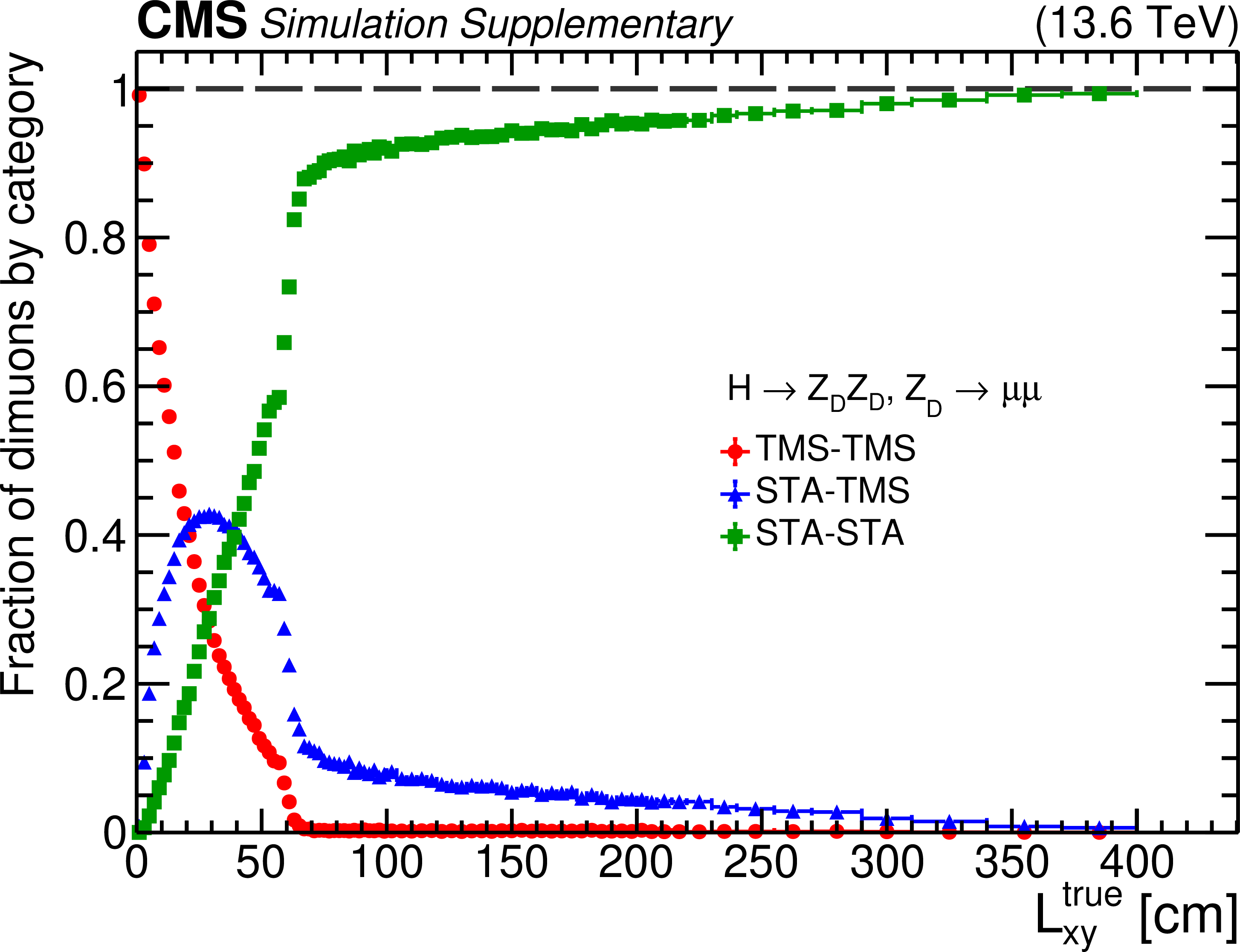
Fractions of signal events with zero (green), one (blue), and two (red) STA muons matched to TMS muons by the STA to TMS association procedure, as a function of generated $ L_{\text{xy}} $, in all HAHM signal samples combined. |
png pdf root |
Additional Figure 4:
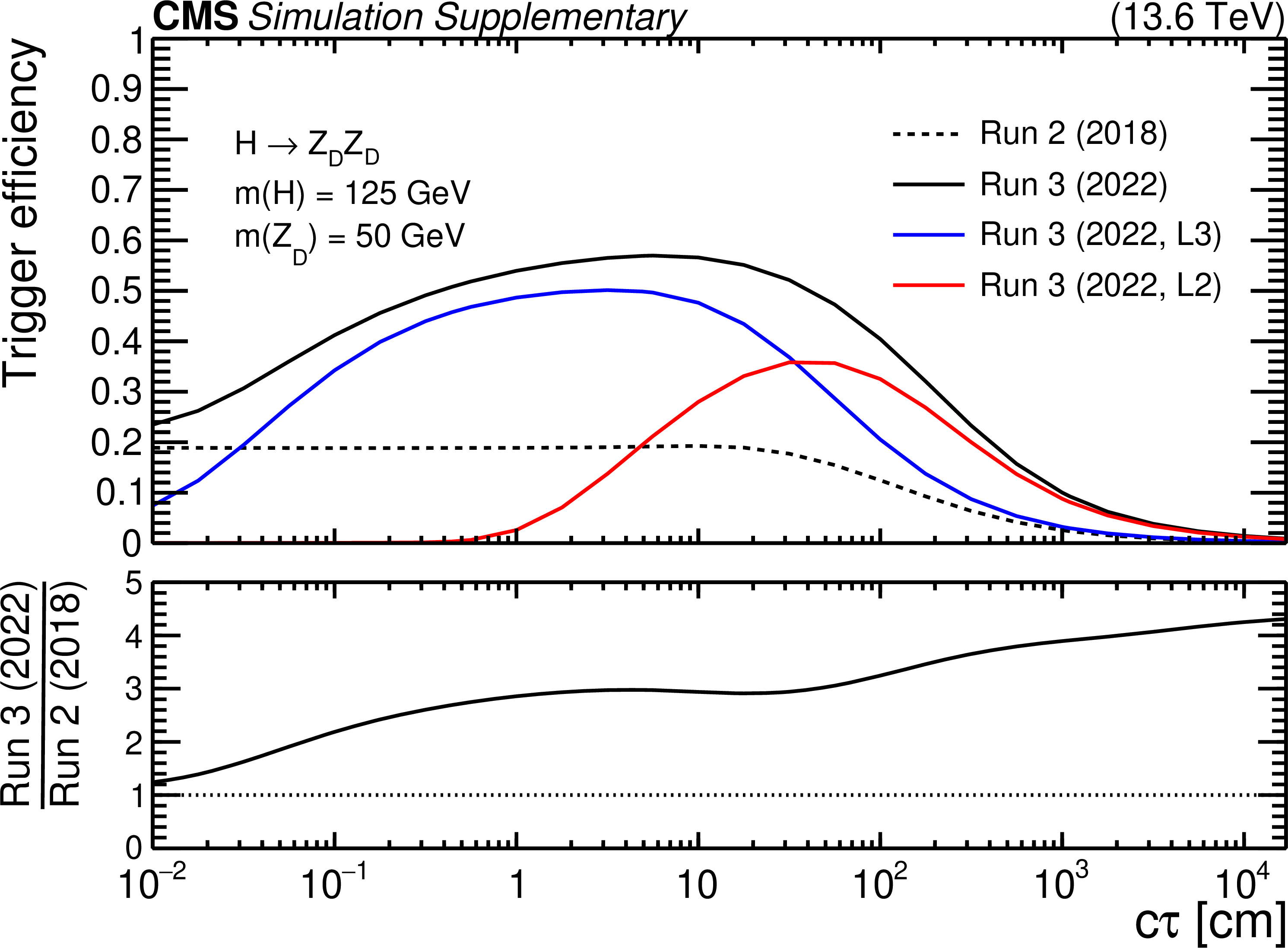
Efficiencies of the Run 2 and Run 3 displaced dimuon triggers as a function of $ c\tau $ for the HAHM signal events with $ m(\mathrm{Z}_\text{D}) = $ 50 GeV. The efficiency is defined as the fraction of simulated events that satisfy the detector acceptance and the requirements of the following sets of trigger paths: the Run 2 (2018) triggers (dashed black); the Run 3 (2022, L3) triggers (blue); the Run 3 (2022, L2) triggers (red); and the OR of all these triggers (Run 3 (2022), black). The lower panel shows the ratio of the overall Run 3 (2022) efficiency to the Run 2 (2018) efficiency. |

png pdf |
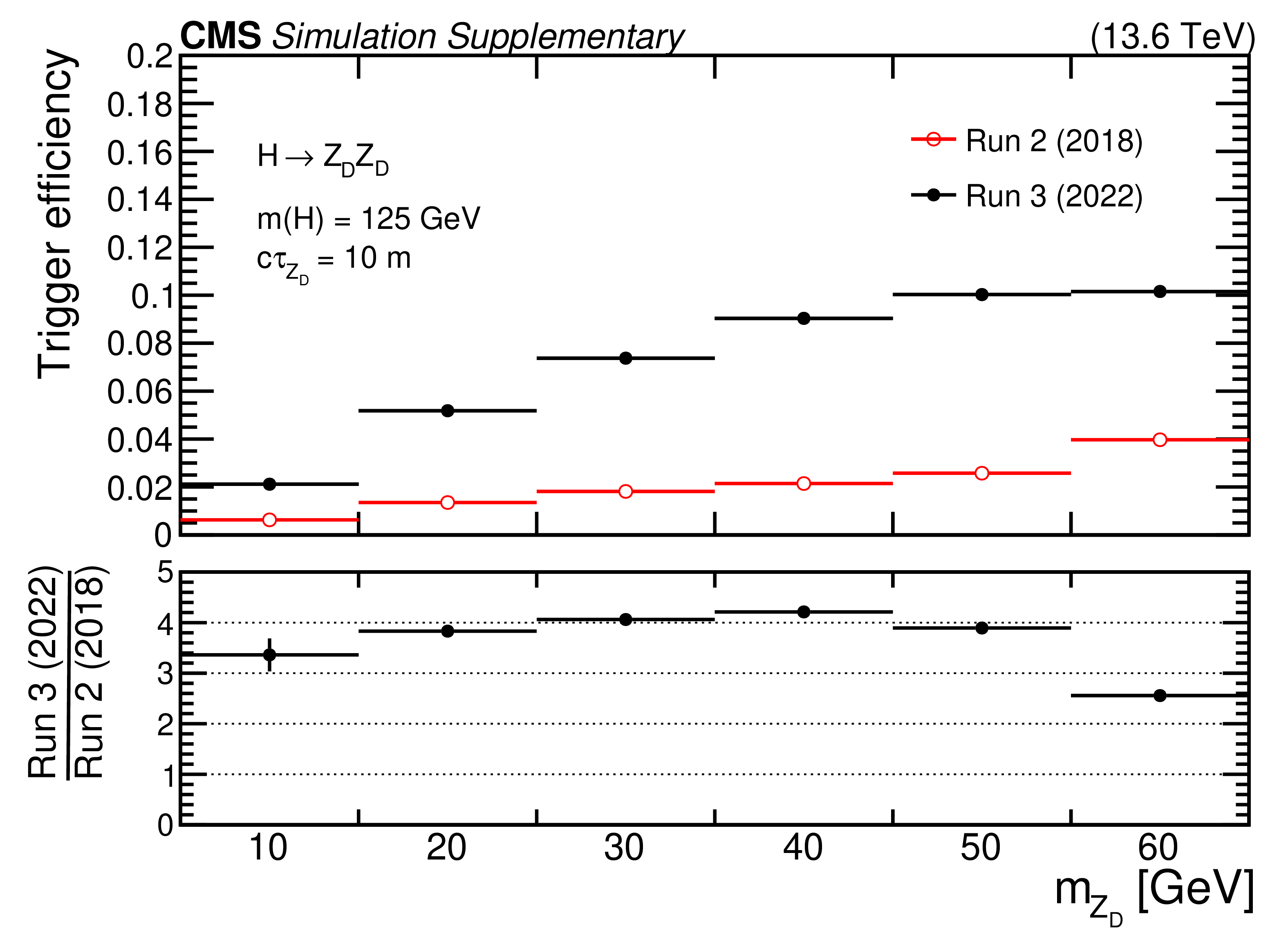
Additional Figure 5:
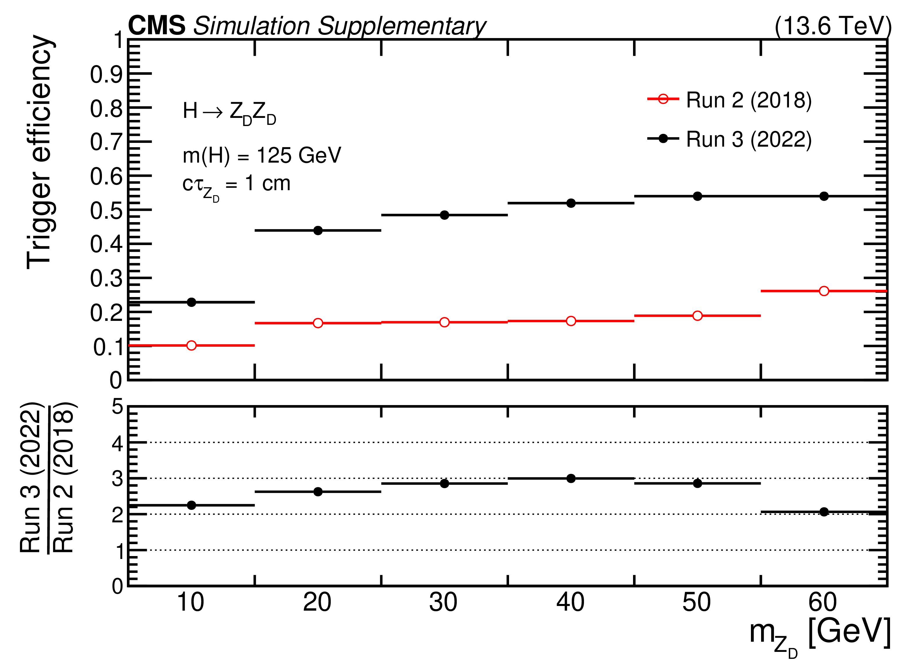
Efficiencies of the Run 2 (2018) (red) and Run 3 (2022) (black) sets of displaced dimuon triggers as a function of $ m(\mathrm{Z}_\text{D}) $ for the HAHM signal events with $ c\tau = $ 1 cm (left) and 10 m (right). The efficiency is defined as the fraction of simulated events that satisfy the detector acceptance and the requirements of the indicated set of trigger paths. The lower panel shows the ratio of the Run 3 (2022) efficiency to the Run 2 (2018) efficiency. |
png pdf root |
Additional Figure 5-a:
Efficiencies of the Run 2 (2018) (red) and Run 3 (2022) (black) sets of displaced dimuon triggers as a function of $ m(\mathrm{Z}_\text{D}) $ for the HAHM signal events with $ c\tau = $ 1 cm (left) and 10 m (right). The efficiency is defined as the fraction of simulated events that satisfy the detector acceptance and the requirements of the indicated set of trigger paths. The lower panel shows the ratio of the Run 3 (2022) efficiency to the Run 2 (2018) efficiency. |
png pdf root |
Additional Figure 5-b:
Efficiencies of the Run 2 (2018) (red) and Run 3 (2022) (black) sets of displaced dimuon triggers as a function of $ m(\mathrm{Z}_\text{D}) $ for the HAHM signal events with $ c\tau = $ 1 cm (left) and 10 m (right). The efficiency is defined as the fraction of simulated events that satisfy the detector acceptance and the requirements of the indicated set of trigger paths. The lower panel shows the ratio of the Run 3 (2022) efficiency to the Run 2 (2018) efficiency. |
png pdf |
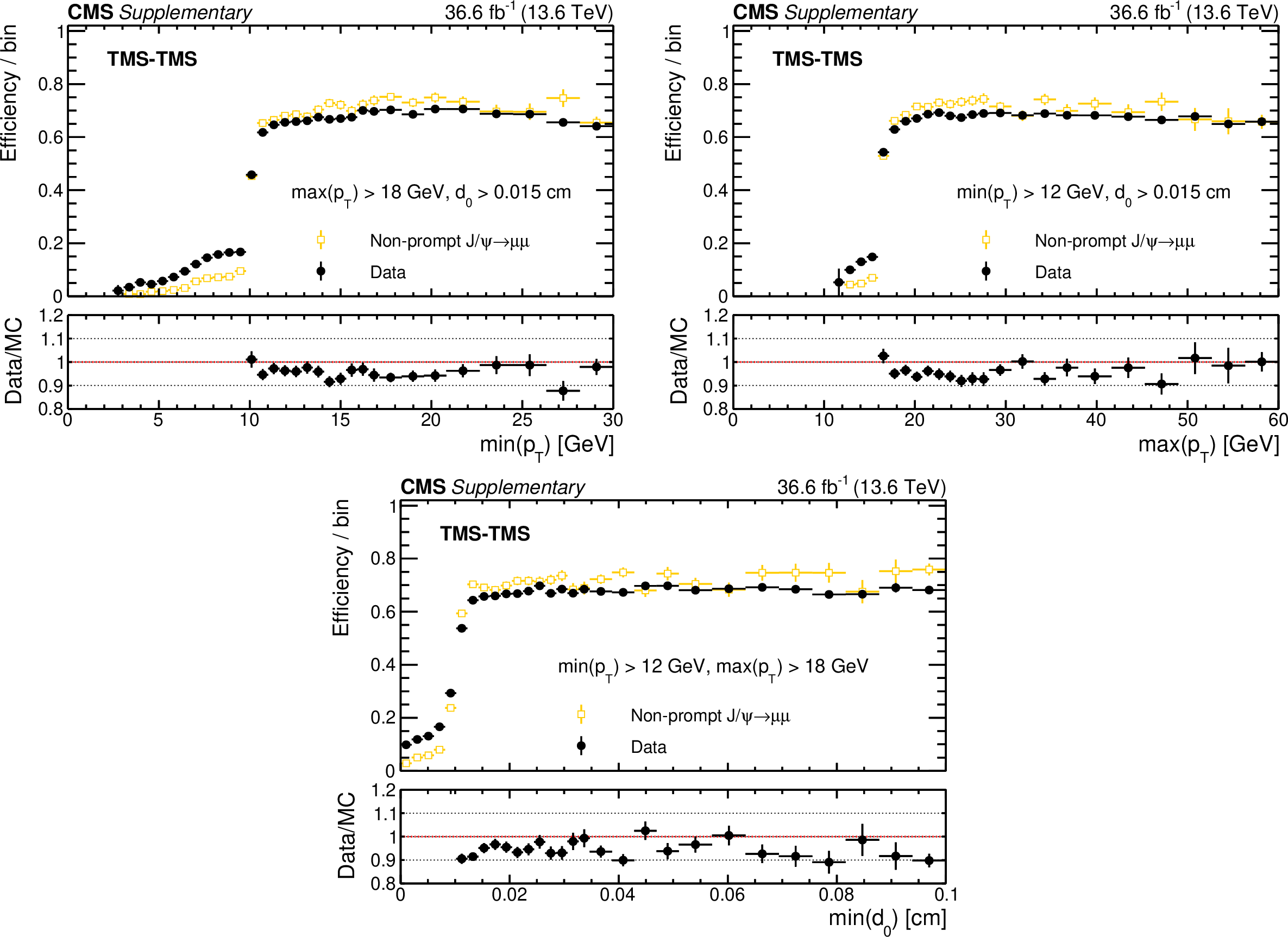
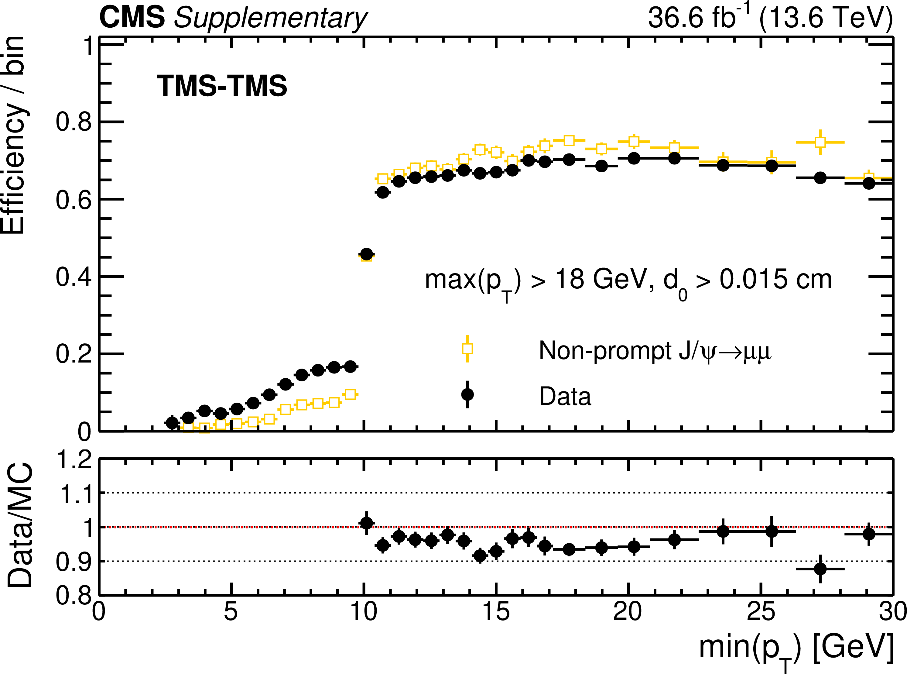
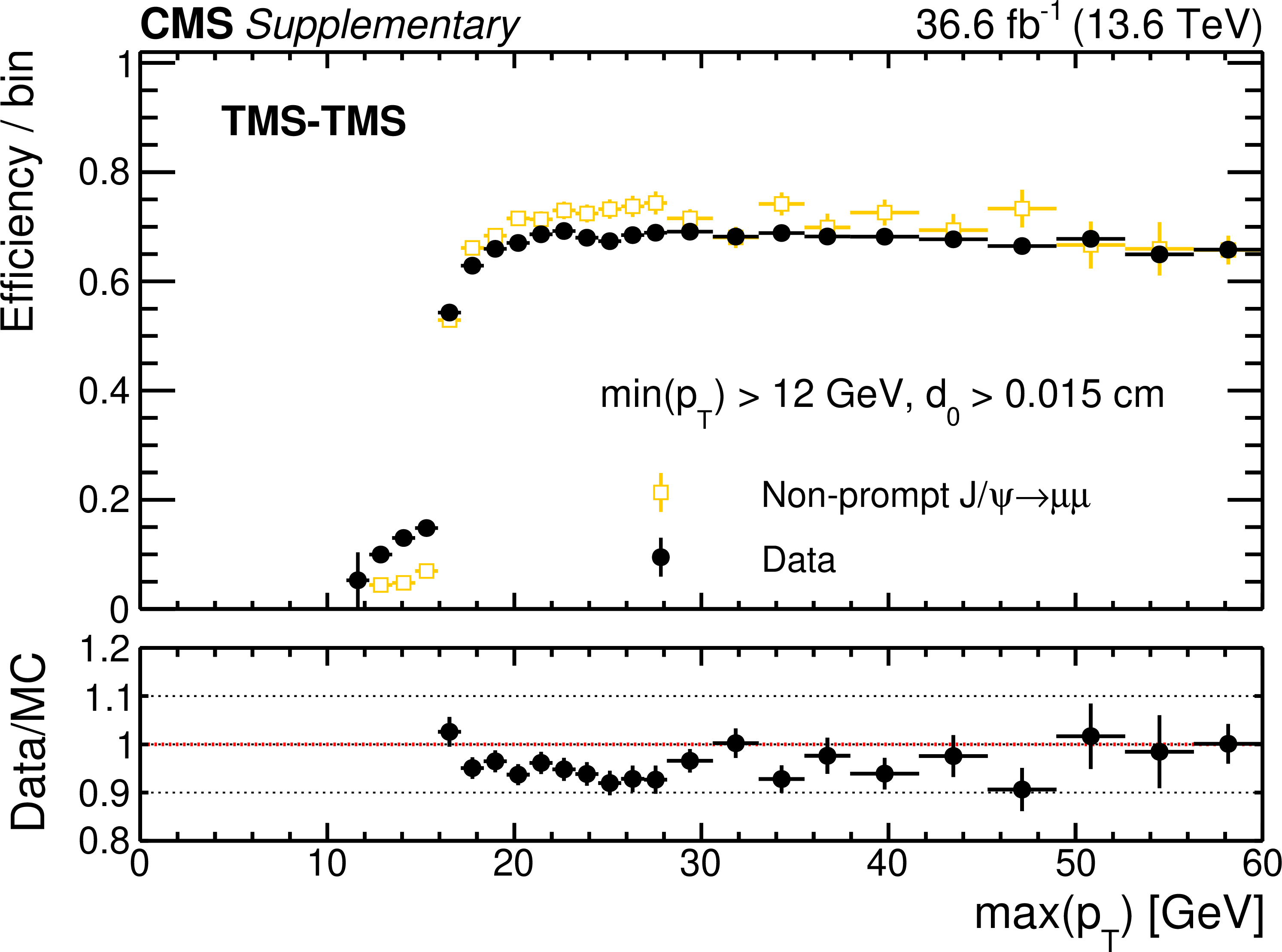
Additional Figure 6:
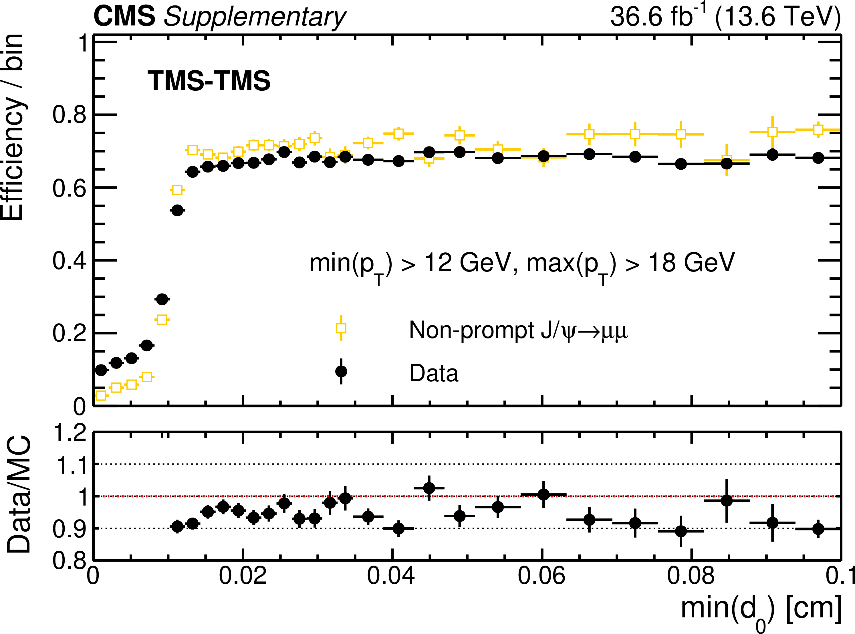
Efficiency of the Run 3 (2022, L3) triggers in data (black) and in simulation (yellow) as a function of min($ p_{\mathrm{T}} $) (upper left), max($ p_{\mathrm{T}} $) (upper right), and min($ d_{\text{0}} $) (lower) of the two muons forming a dimuon in events enriched in $ {\mathrm{J}/\psi} \to\mu\mu $. Efficiency in data is the fraction of $ {\mathrm{J}/\psi} \to\mu\mu $ events recorded by the triggers based on the information from jets and missing transverse energy that also satisfy the requirements of the Run 3 (2022, L3) triggers. It is compared to the efficiency of the Run 3 (2022, L3) triggers in a combination of simulated samples of $ {\mathrm{J}/\psi} \to\mu\mu $ events produced in various B hadron decays. |
png pdf root |
Additional Figure 6-a:
Efficiency of the Run 3 (2022, L3) triggers in data (black) and in simulation (yellow) as a function of min($ p_{\mathrm{T}} $) (upper left), max($ p_{\mathrm{T}} $) (upper right), and min($ d_{\text{0}} $) (lower) of the two muons forming a dimuon in events enriched in $ {\mathrm{J}/\psi} \to\mu\mu $. Efficiency in data is the fraction of $ {\mathrm{J}/\psi} \to\mu\mu $ events recorded by the triggers based on the information from jets and missing transverse energy that also satisfy the requirements of the Run 3 (2022, L3) triggers. It is compared to the efficiency of the Run 3 (2022, L3) triggers in a combination of simulated samples of $ {\mathrm{J}/\psi} \to\mu\mu $ events produced in various B hadron decays. |
png pdf root |
Additional Figure 6-b:
Efficiency of the Run 3 (2022, L3) triggers in data (black) and in simulation (yellow) as a function of min($ p_{\mathrm{T}} $) (upper left), max($ p_{\mathrm{T}} $) (upper right), and min($ d_{\text{0}} $) (lower) of the two muons forming a dimuon in events enriched in $ {\mathrm{J}/\psi} \to\mu\mu $. Efficiency in data is the fraction of $ {\mathrm{J}/\psi} \to\mu\mu $ events recorded by the triggers based on the information from jets and missing transverse energy that also satisfy the requirements of the Run 3 (2022, L3) triggers. It is compared to the efficiency of the Run 3 (2022, L3) triggers in a combination of simulated samples of $ {\mathrm{J}/\psi} \to\mu\mu $ events produced in various B hadron decays. |
png pdf root |
Additional Figure 6-c:
Efficiency of the Run 3 (2022, L3) triggers in data (black) and in simulation (yellow) as a function of min($ p_{\mathrm{T}} $) (upper left), max($ p_{\mathrm{T}} $) (upper right), and min($ d_{\text{0}} $) (lower) of the two muons forming a dimuon in events enriched in $ {\mathrm{J}/\psi} \to\mu\mu $. Efficiency in data is the fraction of $ {\mathrm{J}/\psi} \to\mu\mu $ events recorded by the triggers based on the information from jets and missing transverse energy that also satisfy the requirements of the Run 3 (2022, L3) triggers. It is compared to the efficiency of the Run 3 (2022, L3) triggers in a combination of simulated samples of $ {\mathrm{J}/\psi} \to\mu\mu $ events produced in various B hadron decays. |
png pdf |
Additional Figure 7:
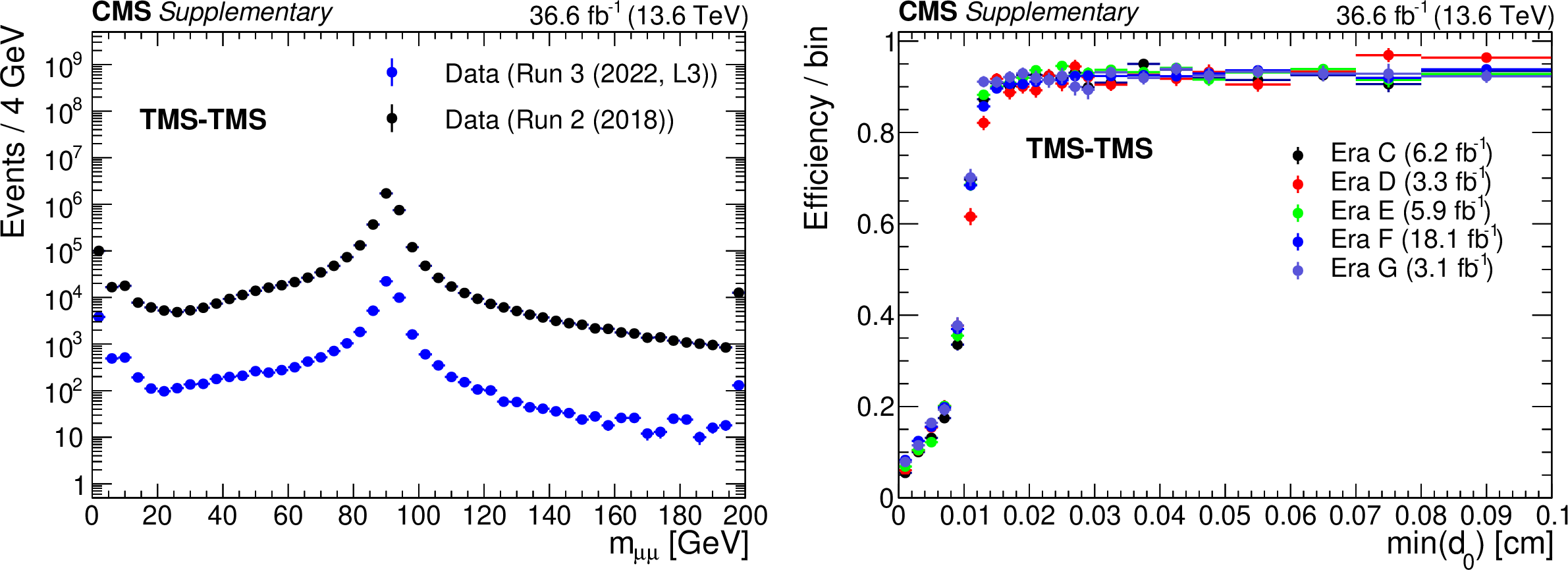
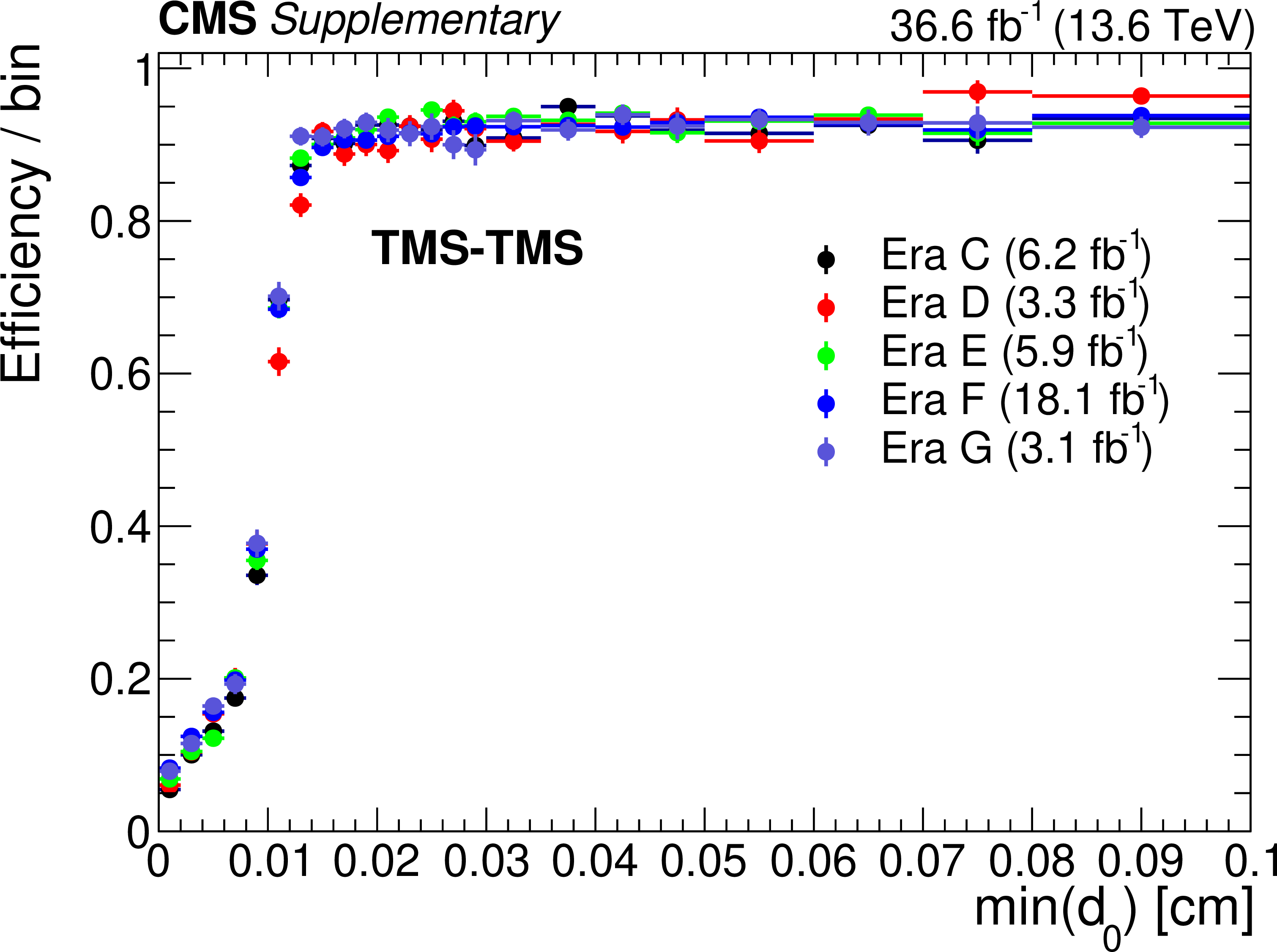
Left: Invariant mass distribution for TMS-TMS dimuons with $ L_{\text{xy}}/\sigma_{L_{\text{xy}}} < $ 1 in events recorded by the Run 2 (2018) triggers in 2022 data (black), and in the subset of events also selected by the Run 3 (2022, L3) triggers (blue), illustrating the background rejection of the Run 3 (2022, L3) triggers. Right: Trigger efficiency, defined as the fraction of events recorded by the Run 2 (2018) triggers that also satisfied the requirements of the Run 3 (2022, L3) triggers, as a function of offline-reconstructed min($ d_{\text{0}} $) of the two muons forming TMS-TMS dimuons in events enriched in $ {\mathrm{J}/\psi} \to\mu\mu $. Different symbols show efficiencies in different periods of the 2022 data taking corresponding to the integrated luminosities indicated in the legend. For dimuons with offline $ \text{min}(d_{\text{0}}) > $ 0.012 cm, the combined efficiency of the L3 muon reconstruction and the online min($ d_{\text{0}} $) requirement is larger than 90% in all data taking periods. |

png pdf root |
Additional Figure 7-a:
Left: Invariant mass distribution for TMS-TMS dimuons with $ L_{\text{xy}}/\sigma_{L_{\text{xy}}} < $ 1 in events recorded by the Run 2 (2018) triggers in 2022 data (black), and in the subset of events also selected by the Run 3 (2022, L3) triggers (blue), illustrating the background rejection of the Run 3 (2022, L3) triggers. Right: Trigger efficiency, defined as the fraction of events recorded by the Run 2 (2018) triggers that also satisfied the requirements of the Run 3 (2022, L3) triggers, as a function of offline-reconstructed min($ d_{\text{0}} $) of the two muons forming TMS-TMS dimuons in events enriched in $ {\mathrm{J}/\psi} \to\mu\mu $. Different symbols show efficiencies in different periods of the 2022 data taking corresponding to the integrated luminosities indicated in the legend. For dimuons with offline $ \text{min}(d_{\text{0}}) > $ 0.012 cm, the combined efficiency of the L3 muon reconstruction and the online min($ d_{\text{0}} $) requirement is larger than 90% in all data taking periods. |
png pdf root |
Additional Figure 7-b:
Left: Invariant mass distribution for TMS-TMS dimuons with $ L_{\text{xy}}/\sigma_{L_{\text{xy}}} < $ 1 in events recorded by the Run 2 (2018) triggers in 2022 data (black), and in the subset of events also selected by the Run 3 (2022, L3) triggers (blue), illustrating the background rejection of the Run 3 (2022, L3) triggers. Right: Trigger efficiency, defined as the fraction of events recorded by the Run 2 (2018) triggers that also satisfied the requirements of the Run 3 (2022, L3) triggers, as a function of offline-reconstructed min($ d_{\text{0}} $) of the two muons forming TMS-TMS dimuons in events enriched in $ {\mathrm{J}/\psi} \to\mu\mu $. Different symbols show efficiencies in different periods of the 2022 data taking corresponding to the integrated luminosities indicated in the legend. For dimuons with offline $ \text{min}(d_{\text{0}}) > $ 0.012 cm, the combined efficiency of the L3 muon reconstruction and the online min($ d_{\text{0}} $) requirement is larger than 90% in all data taking periods. |
png pdf |
Additional Figure 8:
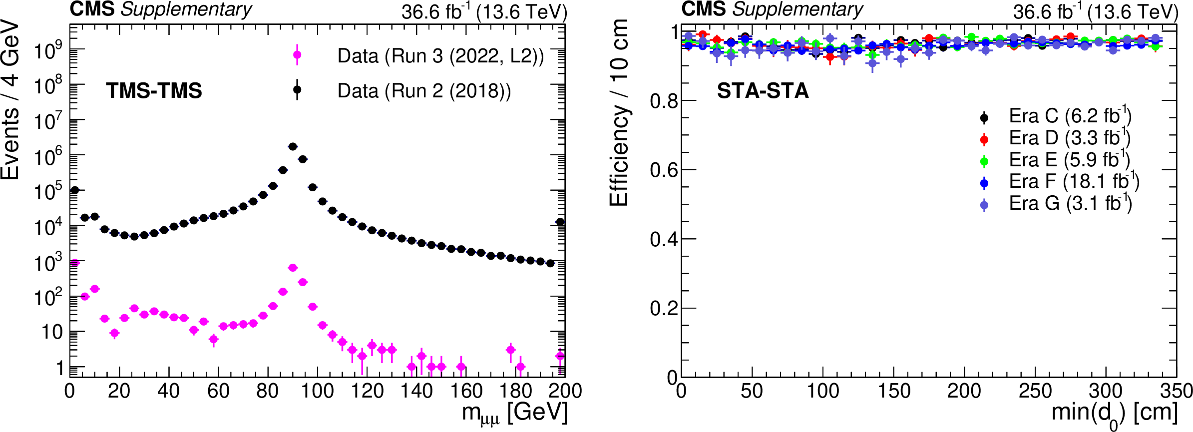
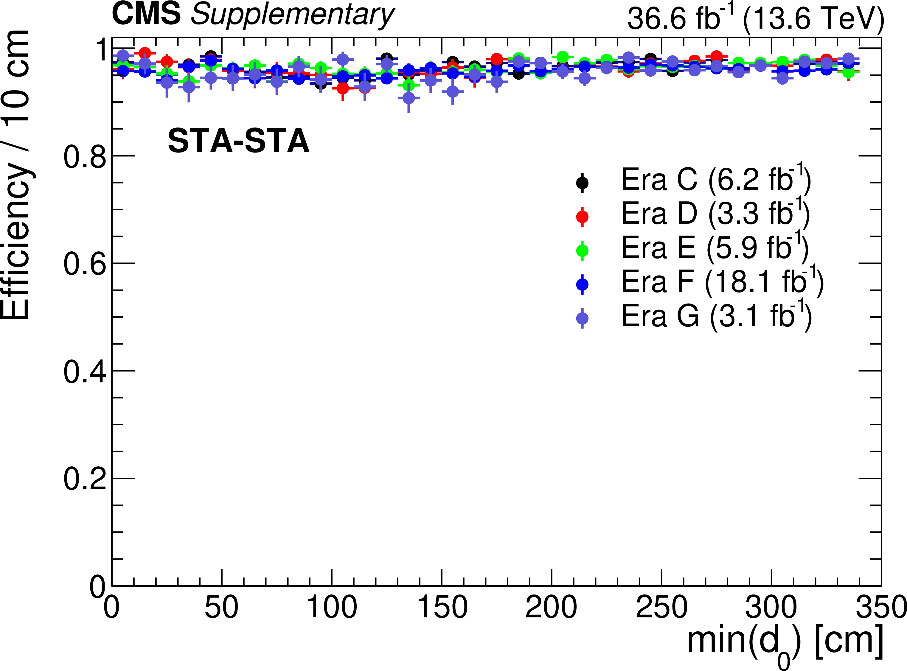
Left: Invariant mass distribution for TMS-TMS dimuons with $ L_{\text{xy}}/\sigma_{L_{\text{xy}}} < $ 1 in events recorded by the Run 2 (2018) triggers in 2022 data (black), and in the subset of events also selected by the Run 3 (2022, L2) triggers (pink), illustrating the background rejection of the Run 3 (2022, L2) triggers. Right: Trigger efficiency, defined as the fraction of events recorded by the Run 2 (2018) triggers that also satisfied the requirements of the Run 3 (2022, L2) triggers, as a function of offline-reconstructed min($ d_{\text{0}} $) of the two muons forming STA-STA dimuons in events enriched in cosmic ray muons. Different symbols show efficiencies in different periods of the 2022 data taking corresponding to the integrated luminosities indicated in the legend. For displaced muons, the efficiency of the online min($ d_{\text{0}} $) requirement is larger than 95% in all data taking periods. |
png pdf root |
Additional Figure 8-a:
Left: Invariant mass distribution for TMS-TMS dimuons with $ L_{\text{xy}}/\sigma_{L_{\text{xy}}} < $ 1 in events recorded by the Run 2 (2018) triggers in 2022 data (black), and in the subset of events also selected by the Run 3 (2022, L2) triggers (pink), illustrating the background rejection of the Run 3 (2022, L2) triggers. Right: Trigger efficiency, defined as the fraction of events recorded by the Run 2 (2018) triggers that also satisfied the requirements of the Run 3 (2022, L2) triggers, as a function of offline-reconstructed min($ d_{\text{0}} $) of the two muons forming STA-STA dimuons in events enriched in cosmic ray muons. Different symbols show efficiencies in different periods of the 2022 data taking corresponding to the integrated luminosities indicated in the legend. For displaced muons, the efficiency of the online min($ d_{\text{0}} $) requirement is larger than 95% in all data taking periods. |
png pdf root |
Additional Figure 8-b:
Left: Invariant mass distribution for TMS-TMS dimuons with $ L_{\text{xy}}/\sigma_{L_{\text{xy}}} < $ 1 in events recorded by the Run 2 (2018) triggers in 2022 data (black), and in the subset of events also selected by the Run 3 (2022, L2) triggers (pink), illustrating the background rejection of the Run 3 (2022, L2) triggers. Right: Trigger efficiency, defined as the fraction of events recorded by the Run 2 (2018) triggers that also satisfied the requirements of the Run 3 (2022, L2) triggers, as a function of offline-reconstructed min($ d_{\text{0}} $) of the two muons forming STA-STA dimuons in events enriched in cosmic ray muons. Different symbols show efficiencies in different periods of the 2022 data taking corresponding to the integrated luminosities indicated in the legend. For displaced muons, the efficiency of the online min($ d_{\text{0}} $) requirement is larger than 95% in all data taking periods. |
png pdf |
Additional Figure 9:
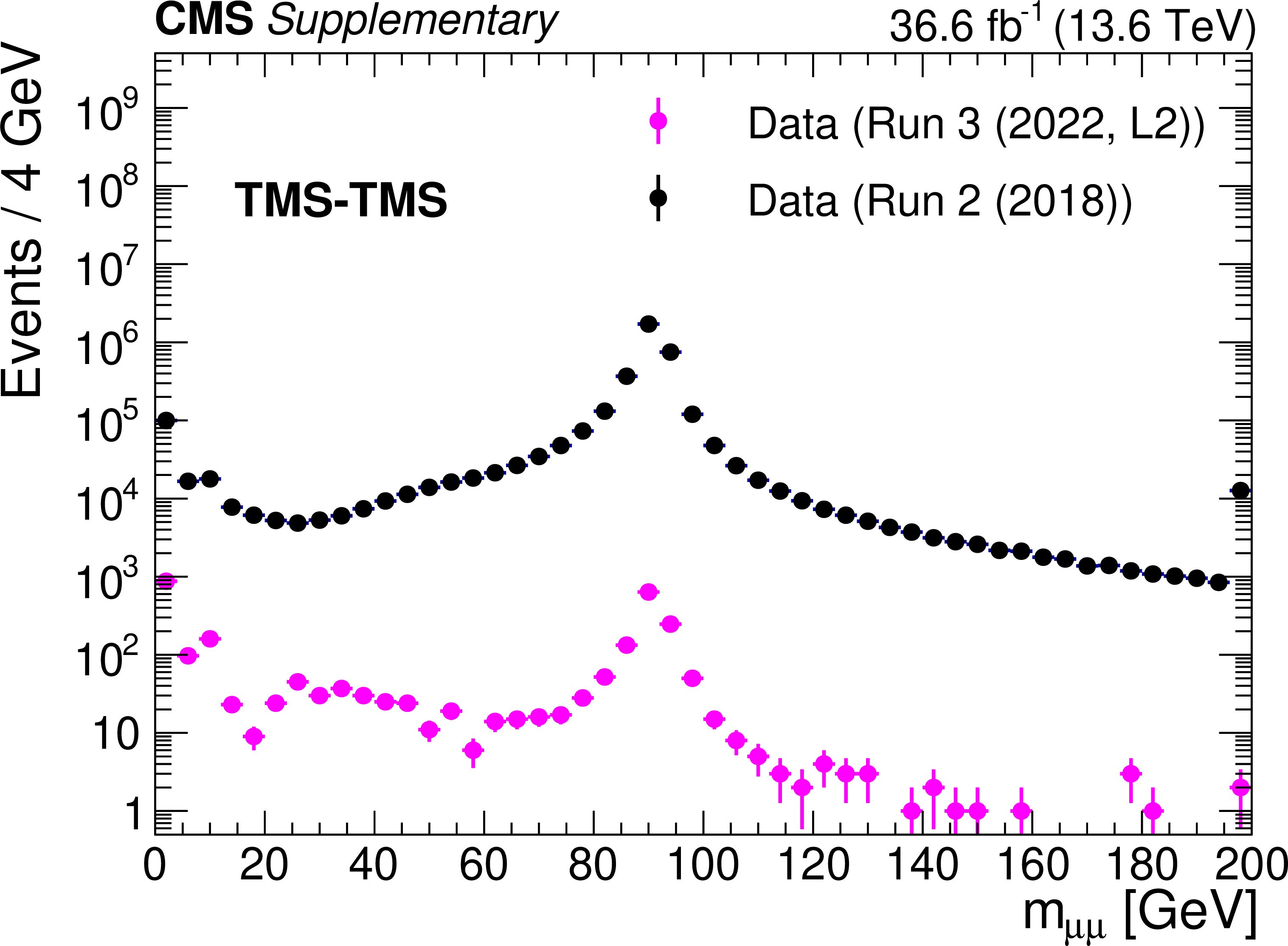
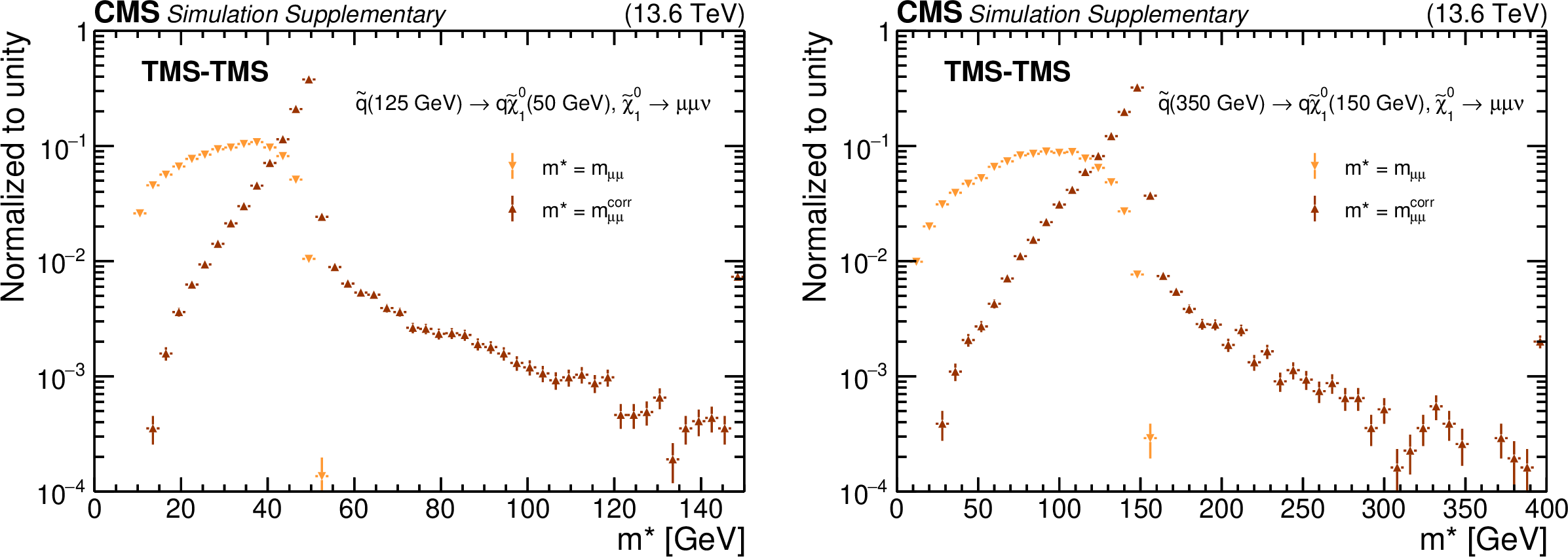
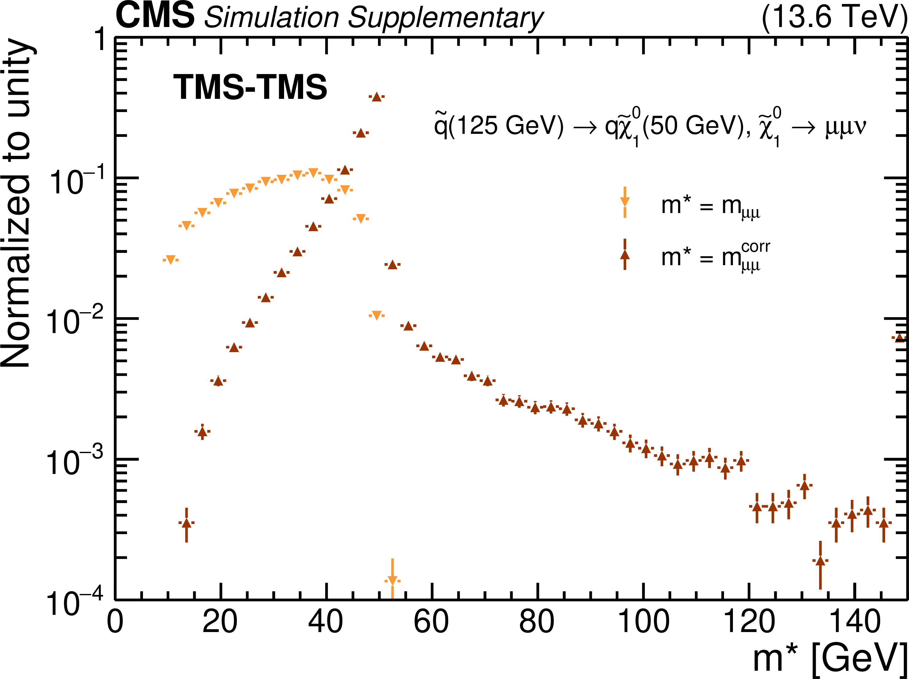
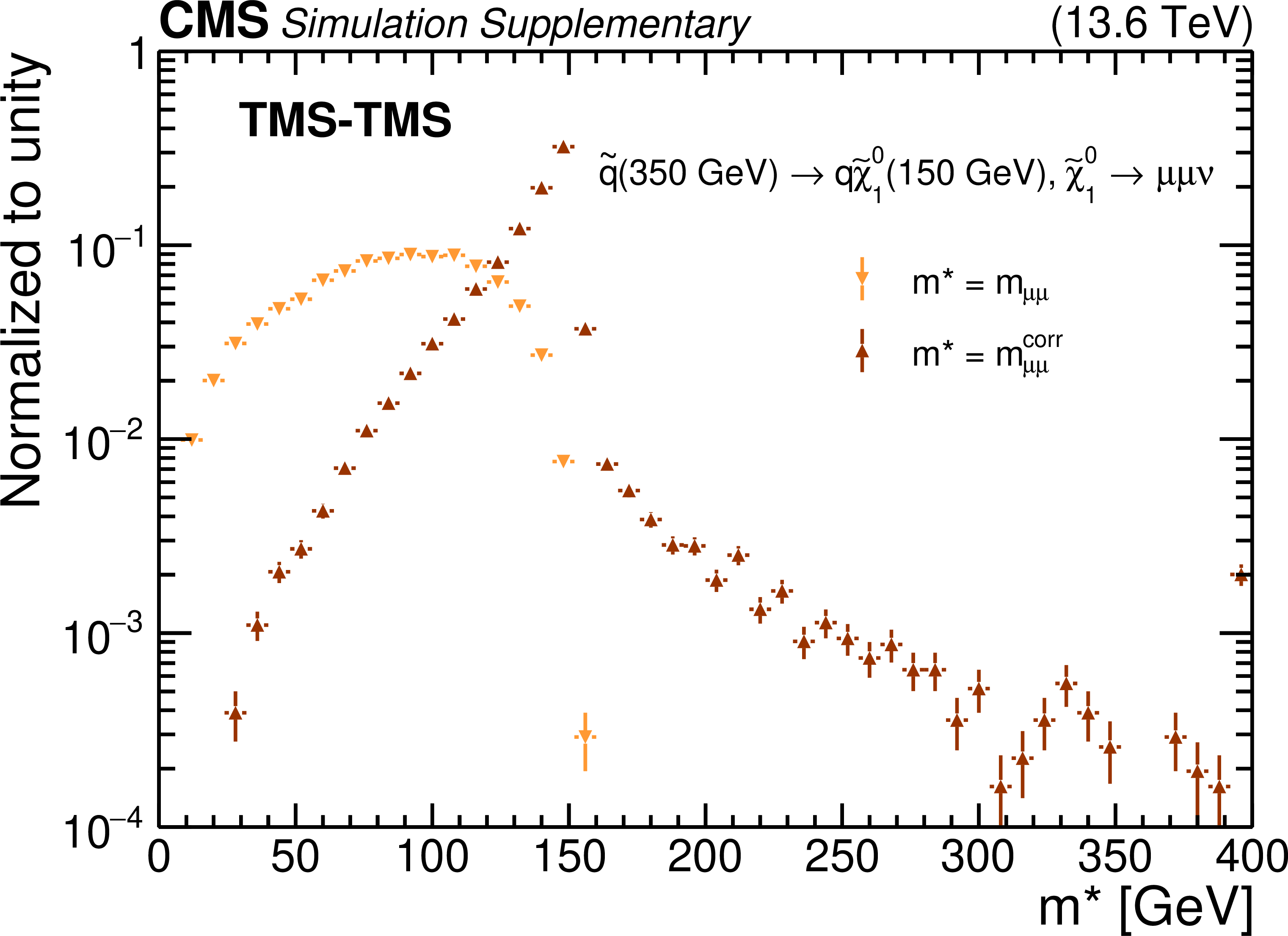
Distributions of $ m_{\mu\mu} $ (red) and $ m^\text{corr}_{\mu\mu} $ (orange) in the TMS-TMS dimuon category, for simulated signal events with $ m({\tilde{\mathrm{q}}} ) = $ 125 GeV and $ m(\tilde{\chi}_{1}^{0}) = $ 50 GeV (left), and $ m({\tilde{\mathrm{q}}} ) = $ 350 GeV and $ m(\tilde{\chi}_{1}^{0}) = $ 150 GeV (right) in the RPV SUSY model. The last bin includes events in the histogram overflow. |
png pdf root |
Additional Figure 9-a:
Distributions of $ m_{\mu\mu} $ (red) and $ m^\text{corr}_{\mu\mu} $ (orange) in the TMS-TMS dimuon category, for simulated signal events with $ m({\tilde{\mathrm{q}}} ) = $ 125 GeV and $ m(\tilde{\chi}_{1}^{0}) = $ 50 GeV (left), and $ m({\tilde{\mathrm{q}}} ) = $ 350 GeV and $ m(\tilde{\chi}_{1}^{0}) = $ 150 GeV (right) in the RPV SUSY model. The last bin includes events in the histogram overflow. |
png pdf root |
Additional Figure 9-b:
Distributions of $ m_{\mu\mu} $ (red) and $ m^\text{corr}_{\mu\mu} $ (orange) in the TMS-TMS dimuon category, for simulated signal events with $ m({\tilde{\mathrm{q}}} ) = $ 125 GeV and $ m(\tilde{\chi}_{1}^{0}) = $ 50 GeV (left), and $ m({\tilde{\mathrm{q}}} ) = $ 350 GeV and $ m(\tilde{\chi}_{1}^{0}) = $ 150 GeV (right) in the RPV SUSY model. The last bin includes events in the histogram overflow. |
png pdf root |
Additional Figure 10:
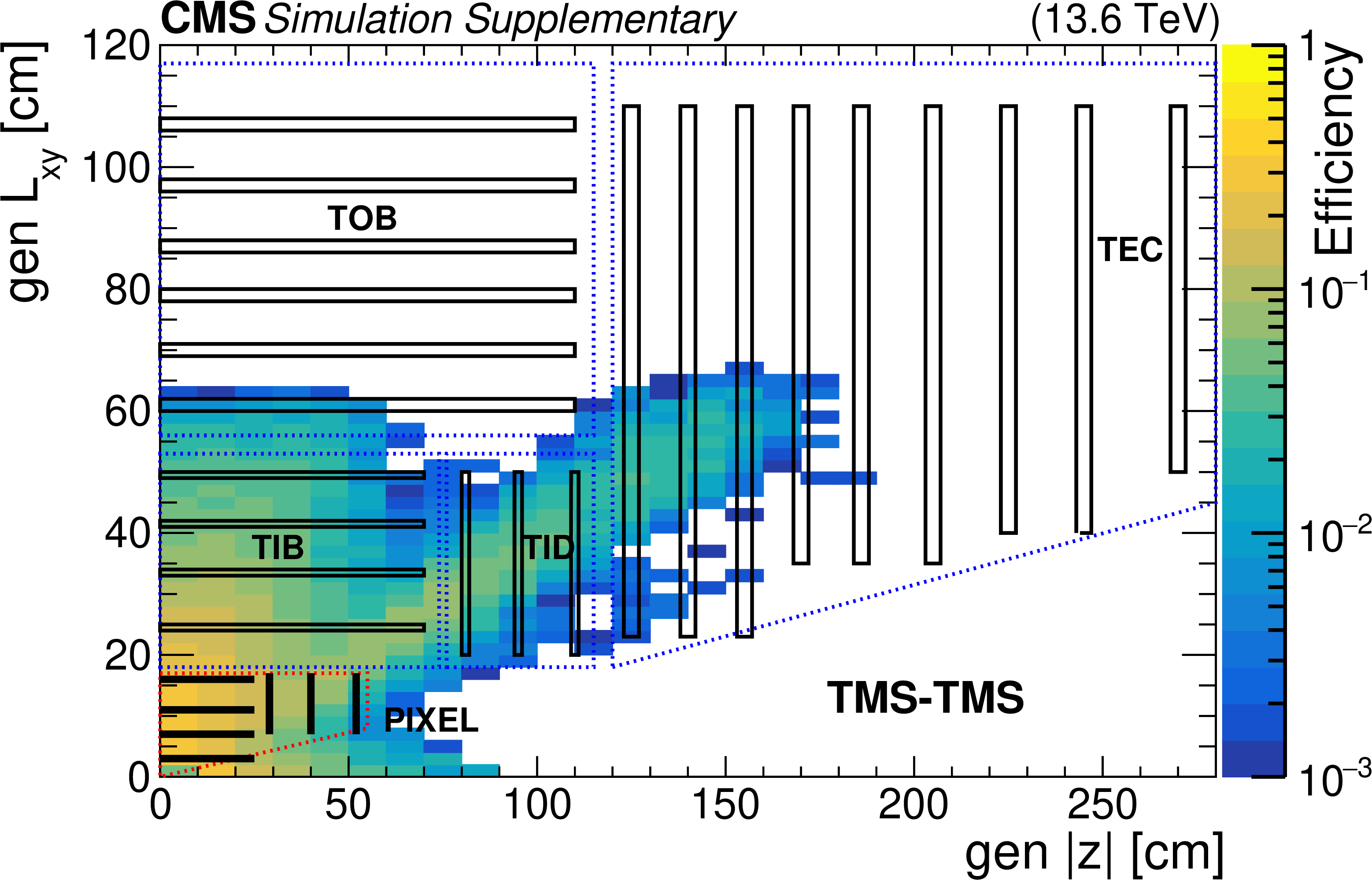
Offline selection efficiency of TMS-TMS dimuons as a function of simulated $ L_{\text{xy}} $ and $ |z| $ decay positions of $ \mathrm{Z}_\text{D} $, in all generated HAHM signal samples combined. Approximate locations of silicon pixel and strip tracker modules -- tracker inner barrel (TIB) and disks (TID), tracker outer barrel (TOB), and tracker endcap (TEC) -- are drawn superimposed as black boxes. |

png pdf root |
Additional Figure 11:
Offline selection efficiency of STA-STA dimuons as a function of simulated $ L_{\text{xy}} $ and $ |z| $ decay positions of $ \mathrm{Z}_\text{D} $, in all generated HAHM signal samples combined. Approximate locations of various CMS subdetectors are drawn superimposed as black boxes. MB1-MB4 denote four DT stations in the barrel, while ME followed by two indices denote CSC stations (the first index) and rings (the second index) in the endcap. |
png pdf |
Additional Figure 12:
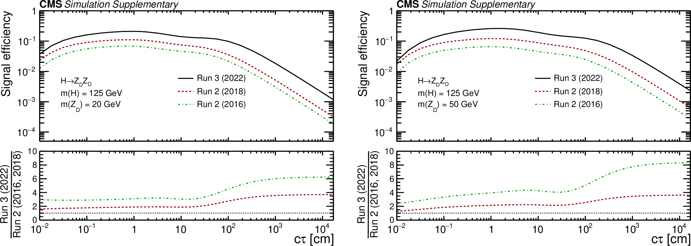
Overall selection efficiencies as a function of $ c\tau(\mathrm{Z}_\text{D}) $ for the HAHM signal with $ m(\mathrm{Z}_\text{D}) = $ 20 GeV (left) and 50 GeV (right) in different years of data taking. Efficiencies are computed as the ratios of the number of simulated signal events in which at least one dimuon candidate passes all 2016 (dashed green), 2018 (dashed red), and 2022 (solid black) trigger and offline selection criteria to the total number of simulated signal events. The lower panel shows the ratio of the 2022 efficiency to the 2018 efficiency (dashed red) and to the 2016 efficiency (dashed green). |

png pdf root |
Additional Figure 12-a:
Overall selection efficiencies as a function of $ c\tau(\mathrm{Z}_\text{D}) $ for the HAHM signal with $ m(\mathrm{Z}_\text{D}) = $ 20 GeV (left) and 50 GeV (right) in different years of data taking. Efficiencies are computed as the ratios of the number of simulated signal events in which at least one dimuon candidate passes all 2016 (dashed green), 2018 (dashed red), and 2022 (solid black) trigger and offline selection criteria to the total number of simulated signal events. The lower panel shows the ratio of the 2022 efficiency to the 2018 efficiency (dashed red) and to the 2016 efficiency (dashed green). |

png pdf root |
Additional Figure 12-b:
Overall selection efficiencies as a function of $ c\tau(\mathrm{Z}_\text{D}) $ for the HAHM signal with $ m(\mathrm{Z}_\text{D}) = $ 20 GeV (left) and 50 GeV (right) in different years of data taking. Efficiencies are computed as the ratios of the number of simulated signal events in which at least one dimuon candidate passes all 2016 (dashed green), 2018 (dashed red), and 2022 (solid black) trigger and offline selection criteria to the total number of simulated signal events. The lower panel shows the ratio of the 2022 efficiency to the 2018 efficiency (dashed red) and to the 2016 efficiency (dashed green). |
png pdf |
Additional Figure 13:
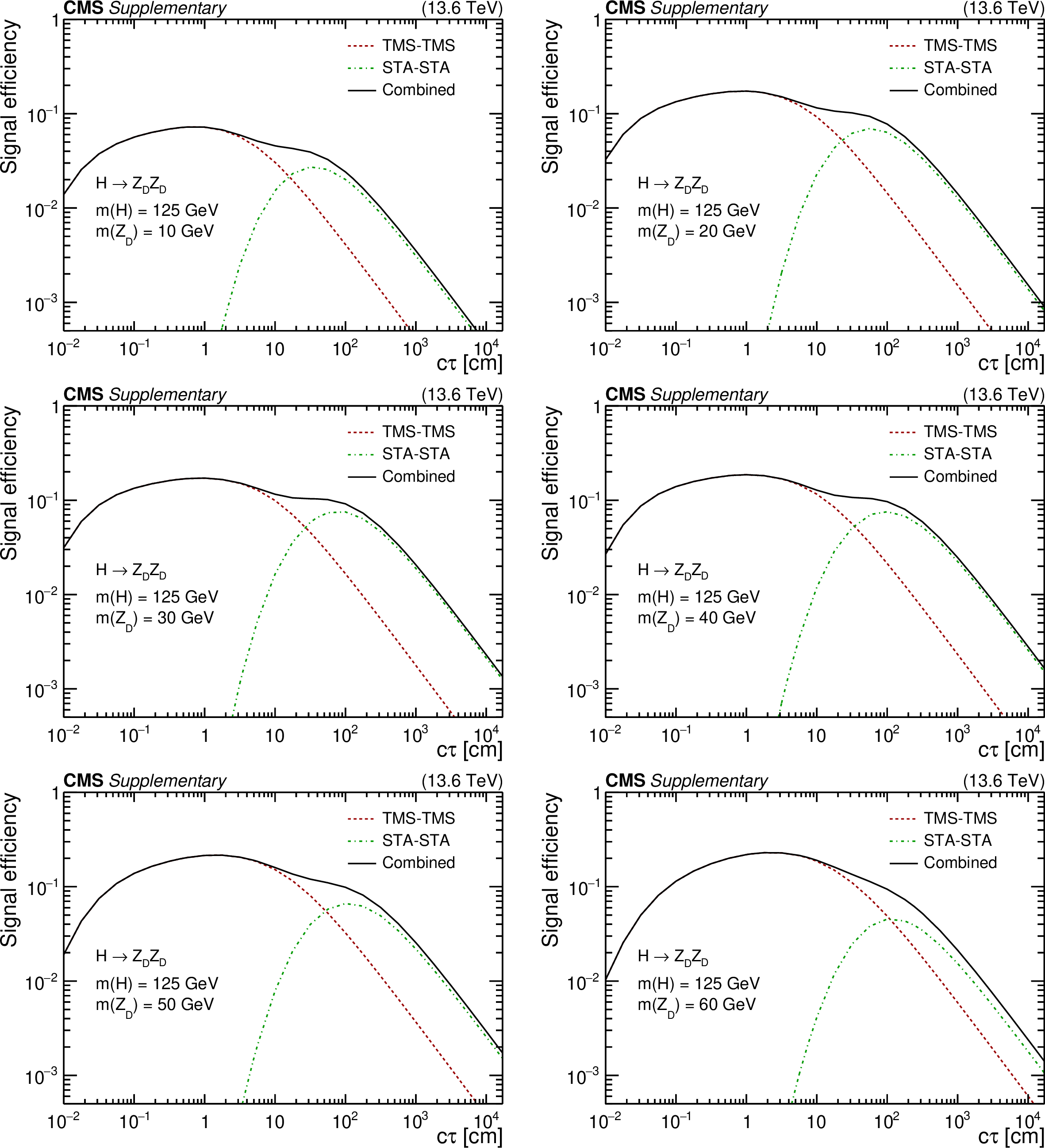
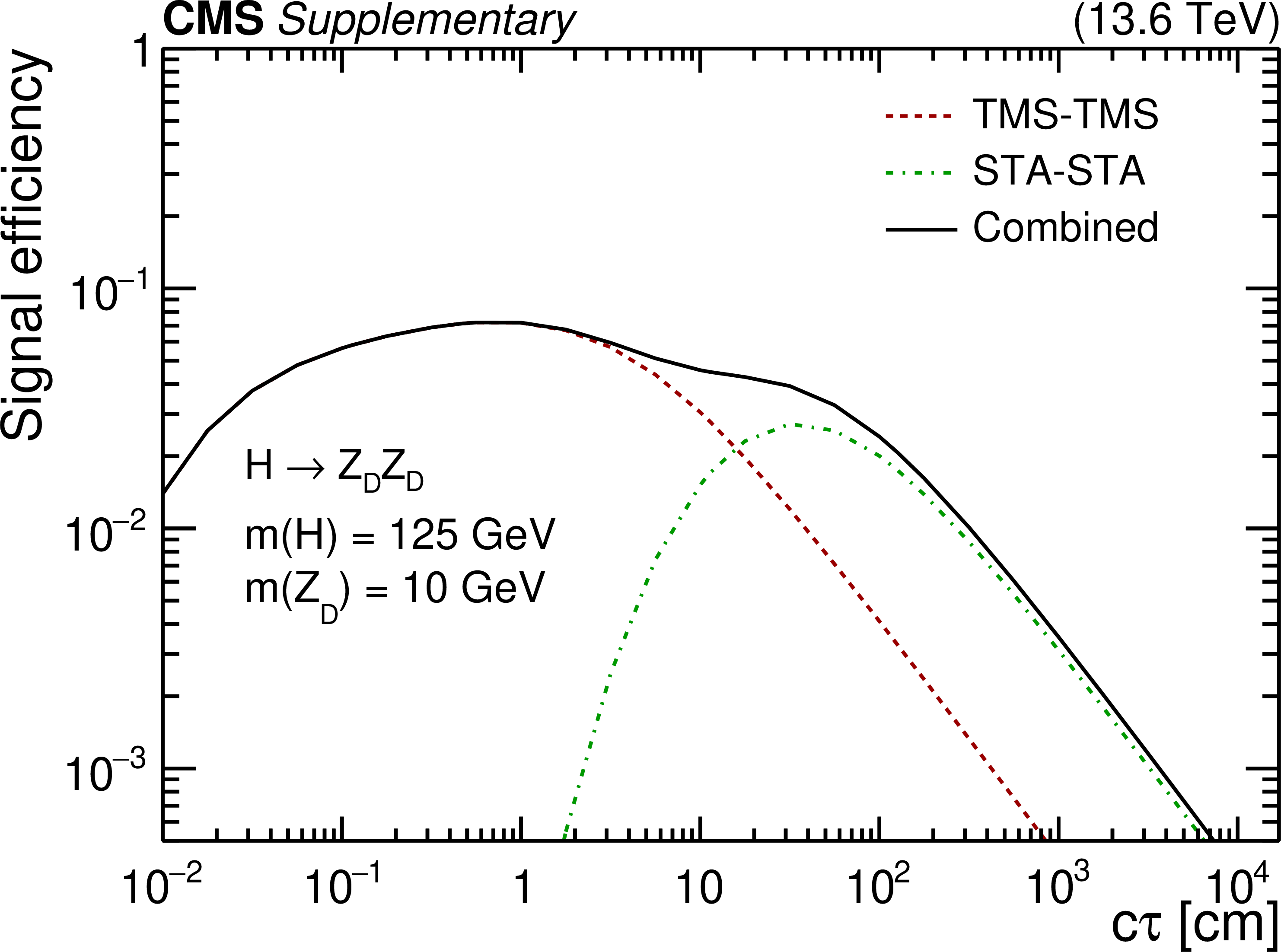
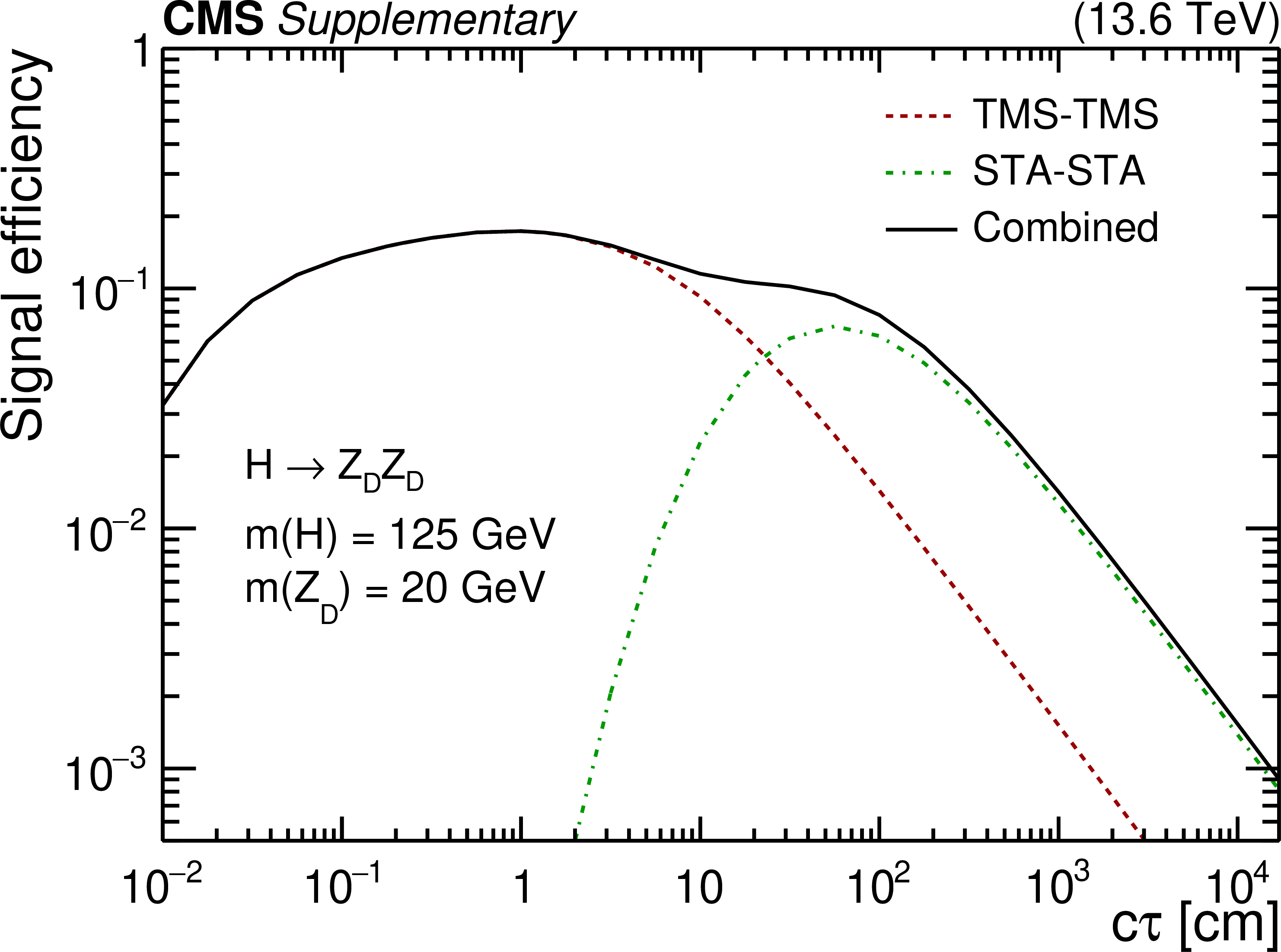
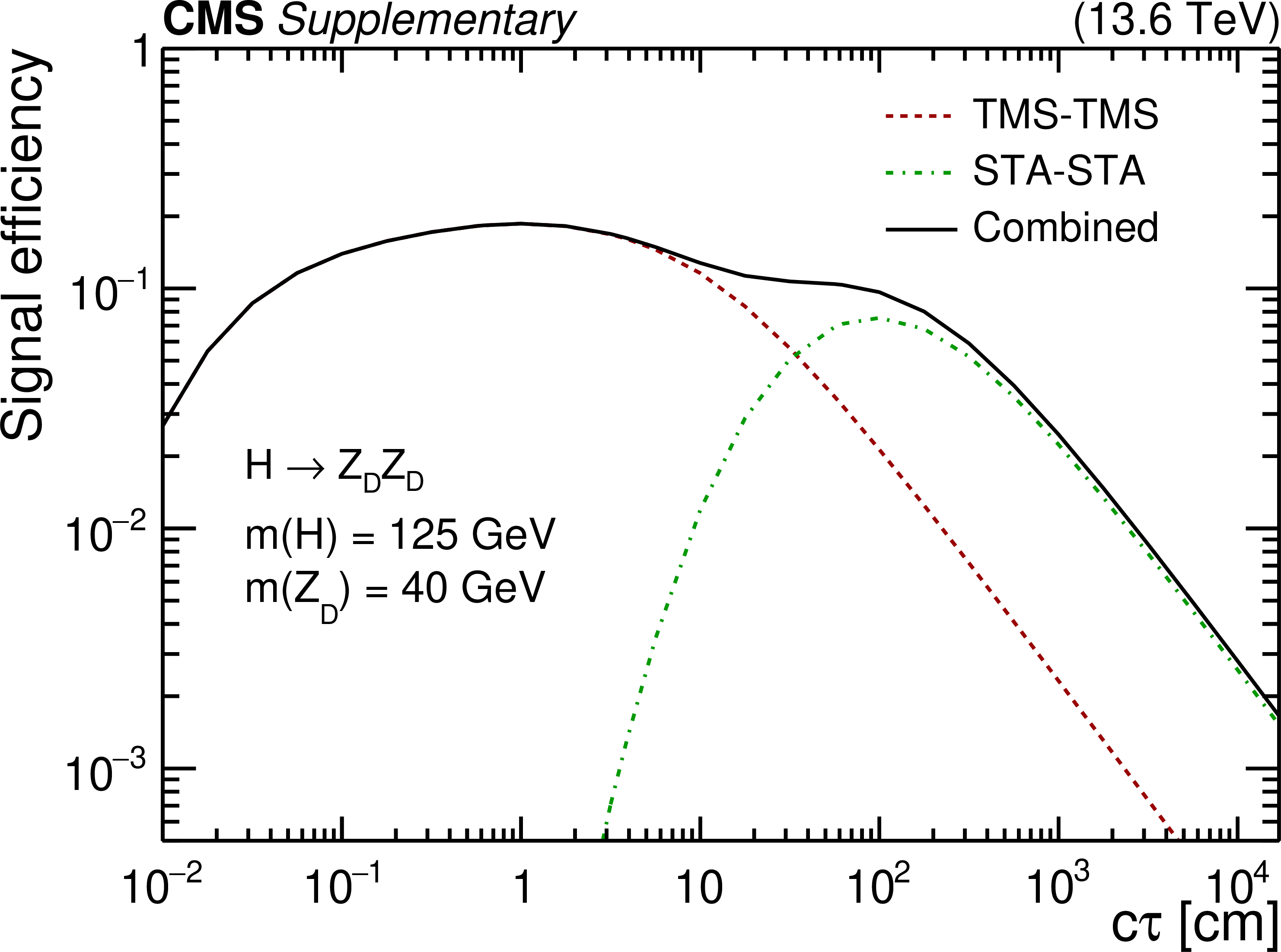
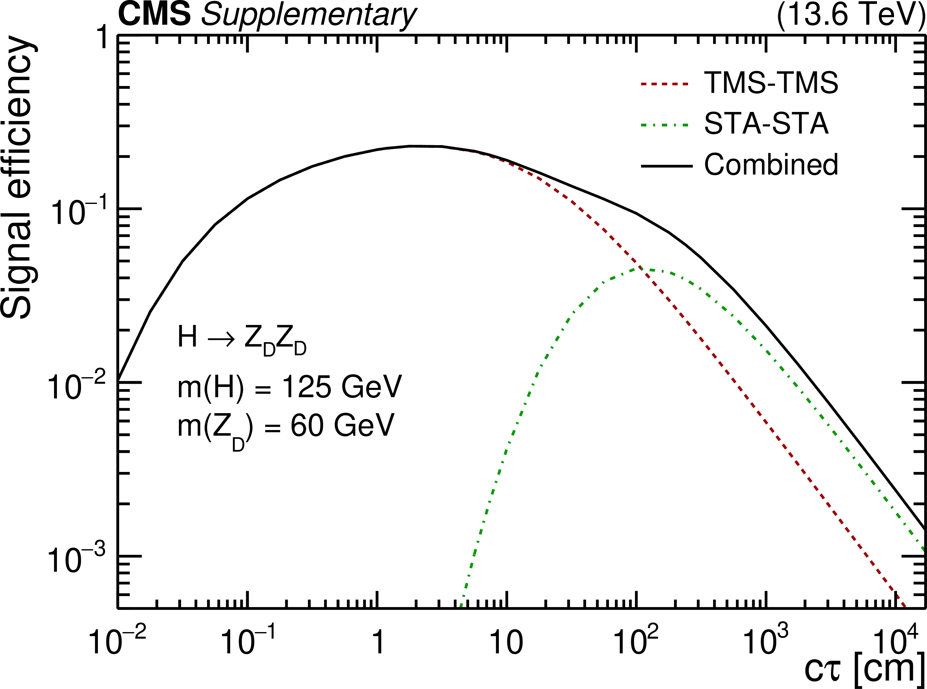
Overall selection efficiencies as a function of $ c\tau(\mathrm{Z}_\text{D}) $ for the HAHM model with $ m(\mathrm{Z}_\text{D}) $ ranging from 10 GeV (upper left) to 60 GeV (lower right). Each plot shows efficiencies of the two dimuon categories, TMS-TMS (dashed red) and STA-STA (dashed green), as well as their combination (solid black). Each efficiency is computed as the ratio of the number of simulated signal events in which at least one dimuon candidate of a given type (or any type for the combined efficiency) passes all selection criteria (including the trigger) to the total number of simulated signal events. All efficiencies are corrected by the data-to-simulation scale factors described in the paper. |
png pdf root |
Additional Figure 13-a:
Overall selection efficiencies as a function of $ c\tau(\mathrm{Z}_\text{D}) $ for the HAHM model with $ m(\mathrm{Z}_\text{D}) $ ranging from 10 GeV (upper left) to 60 GeV (lower right). Each plot shows efficiencies of the two dimuon categories, TMS-TMS (dashed red) and STA-STA (dashed green), as well as their combination (solid black). Each efficiency is computed as the ratio of the number of simulated signal events in which at least one dimuon candidate of a given type (or any type for the combined efficiency) passes all selection criteria (including the trigger) to the total number of simulated signal events. All efficiencies are corrected by the data-to-simulation scale factors described in the paper. |
png pdf root |
Additional Figure 13-b:
Overall selection efficiencies as a function of $ c\tau(\mathrm{Z}_\text{D}) $ for the HAHM model with $ m(\mathrm{Z}_\text{D}) $ ranging from 10 GeV (upper left) to 60 GeV (lower right). Each plot shows efficiencies of the two dimuon categories, TMS-TMS (dashed red) and STA-STA (dashed green), as well as their combination (solid black). Each efficiency is computed as the ratio of the number of simulated signal events in which at least one dimuon candidate of a given type (or any type for the combined efficiency) passes all selection criteria (including the trigger) to the total number of simulated signal events. All efficiencies are corrected by the data-to-simulation scale factors described in the paper. |

png pdf root |
Additional Figure 13-c:
Overall selection efficiencies as a function of $ c\tau(\mathrm{Z}_\text{D}) $ for the HAHM model with $ m(\mathrm{Z}_\text{D}) $ ranging from 10 GeV (upper left) to 60 GeV (lower right). Each plot shows efficiencies of the two dimuon categories, TMS-TMS (dashed red) and STA-STA (dashed green), as well as their combination (solid black). Each efficiency is computed as the ratio of the number of simulated signal events in which at least one dimuon candidate of a given type (or any type for the combined efficiency) passes all selection criteria (including the trigger) to the total number of simulated signal events. All efficiencies are corrected by the data-to-simulation scale factors described in the paper. |
png pdf root |
Additional Figure 13-d:
Overall selection efficiencies as a function of $ c\tau(\mathrm{Z}_\text{D}) $ for the HAHM model with $ m(\mathrm{Z}_\text{D}) $ ranging from 10 GeV (upper left) to 60 GeV (lower right). Each plot shows efficiencies of the two dimuon categories, TMS-TMS (dashed red) and STA-STA (dashed green), as well as their combination (solid black). Each efficiency is computed as the ratio of the number of simulated signal events in which at least one dimuon candidate of a given type (or any type for the combined efficiency) passes all selection criteria (including the trigger) to the total number of simulated signal events. All efficiencies are corrected by the data-to-simulation scale factors described in the paper. |

png pdf root |
Additional Figure 13-e:
Overall selection efficiencies as a function of $ c\tau(\mathrm{Z}_\text{D}) $ for the HAHM model with $ m(\mathrm{Z}_\text{D}) $ ranging from 10 GeV (upper left) to 60 GeV (lower right). Each plot shows efficiencies of the two dimuon categories, TMS-TMS (dashed red) and STA-STA (dashed green), as well as their combination (solid black). Each efficiency is computed as the ratio of the number of simulated signal events in which at least one dimuon candidate of a given type (or any type for the combined efficiency) passes all selection criteria (including the trigger) to the total number of simulated signal events. All efficiencies are corrected by the data-to-simulation scale factors described in the paper. |
png pdf root |
Additional Figure 13-f:
Overall selection efficiencies as a function of $ c\tau(\mathrm{Z}_\text{D}) $ for the HAHM model with $ m(\mathrm{Z}_\text{D}) $ ranging from 10 GeV (upper left) to 60 GeV (lower right). Each plot shows efficiencies of the two dimuon categories, TMS-TMS (dashed red) and STA-STA (dashed green), as well as their combination (solid black). Each efficiency is computed as the ratio of the number of simulated signal events in which at least one dimuon candidate of a given type (or any type for the combined efficiency) passes all selection criteria (including the trigger) to the total number of simulated signal events. All efficiencies are corrected by the data-to-simulation scale factors described in the paper. |
png pdf |
Additional Figure 14:
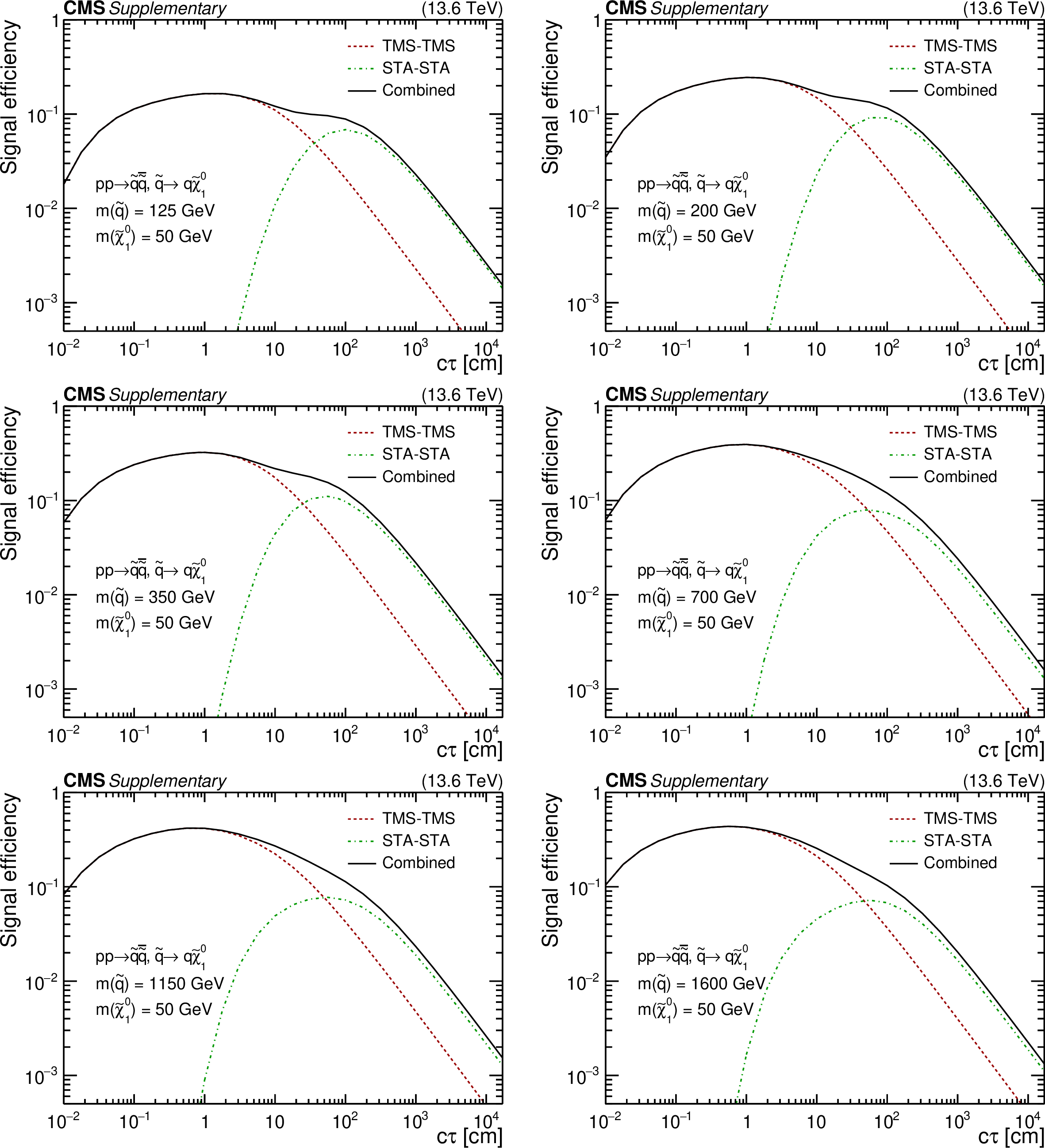
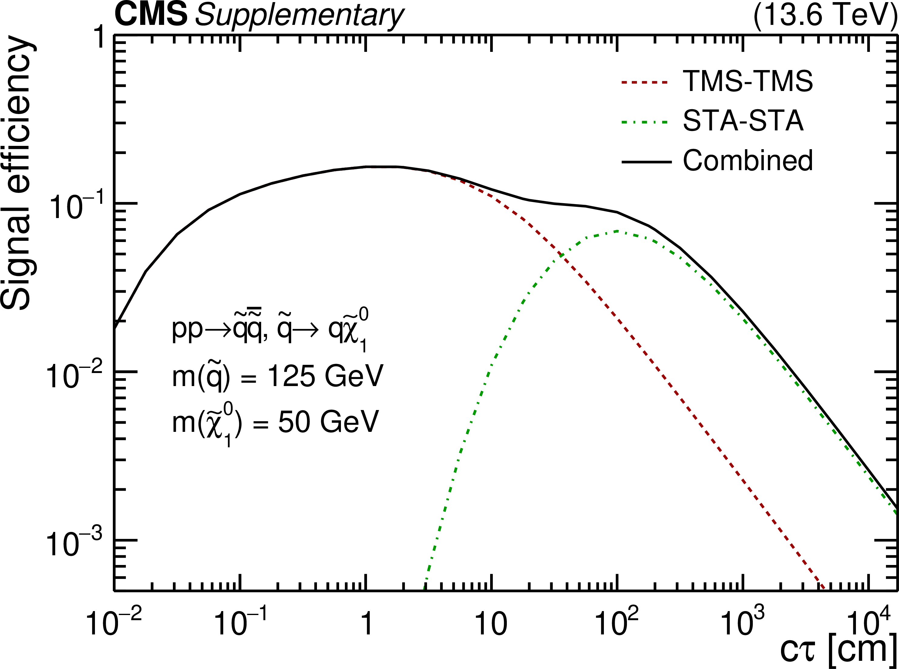
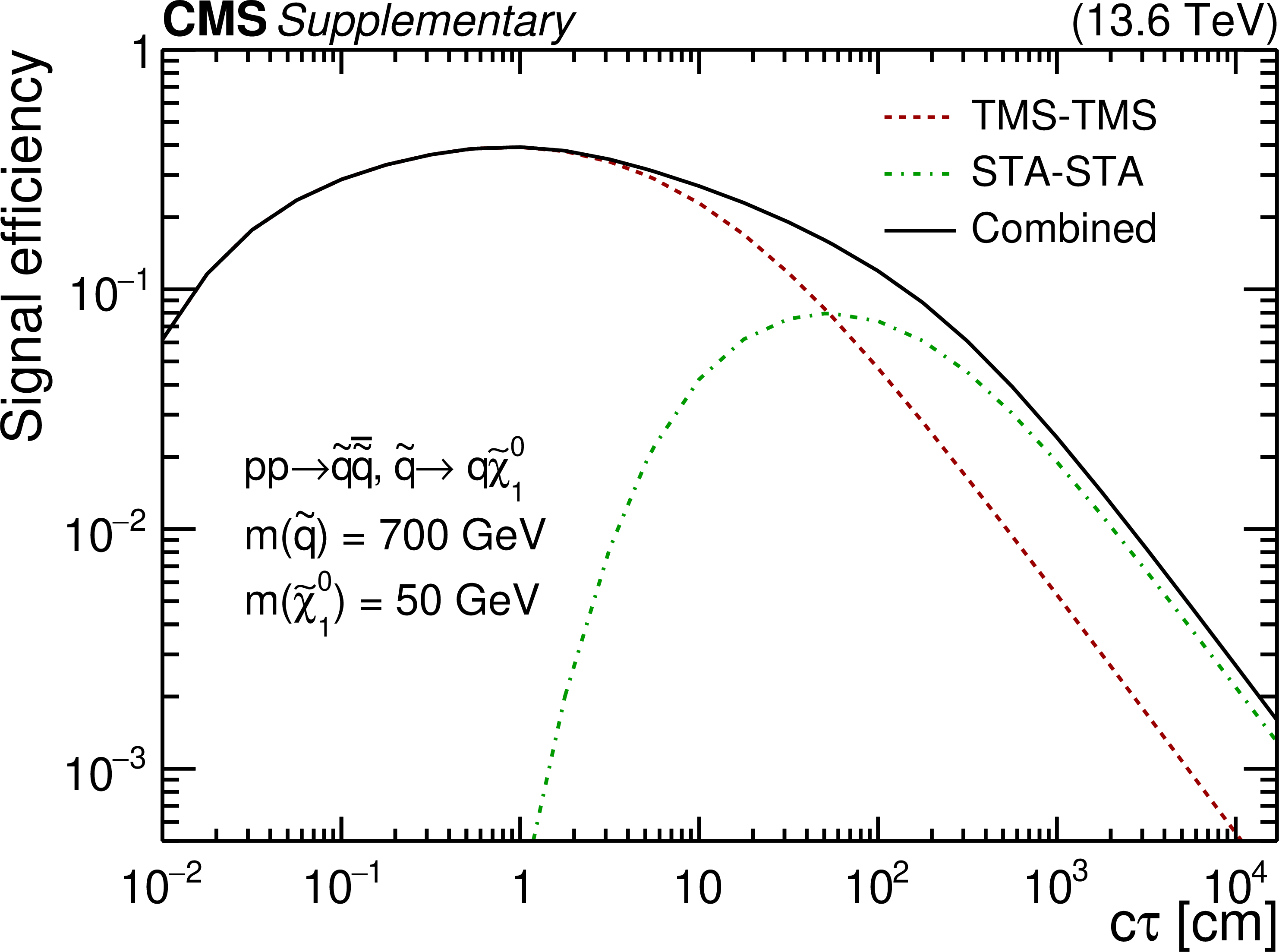
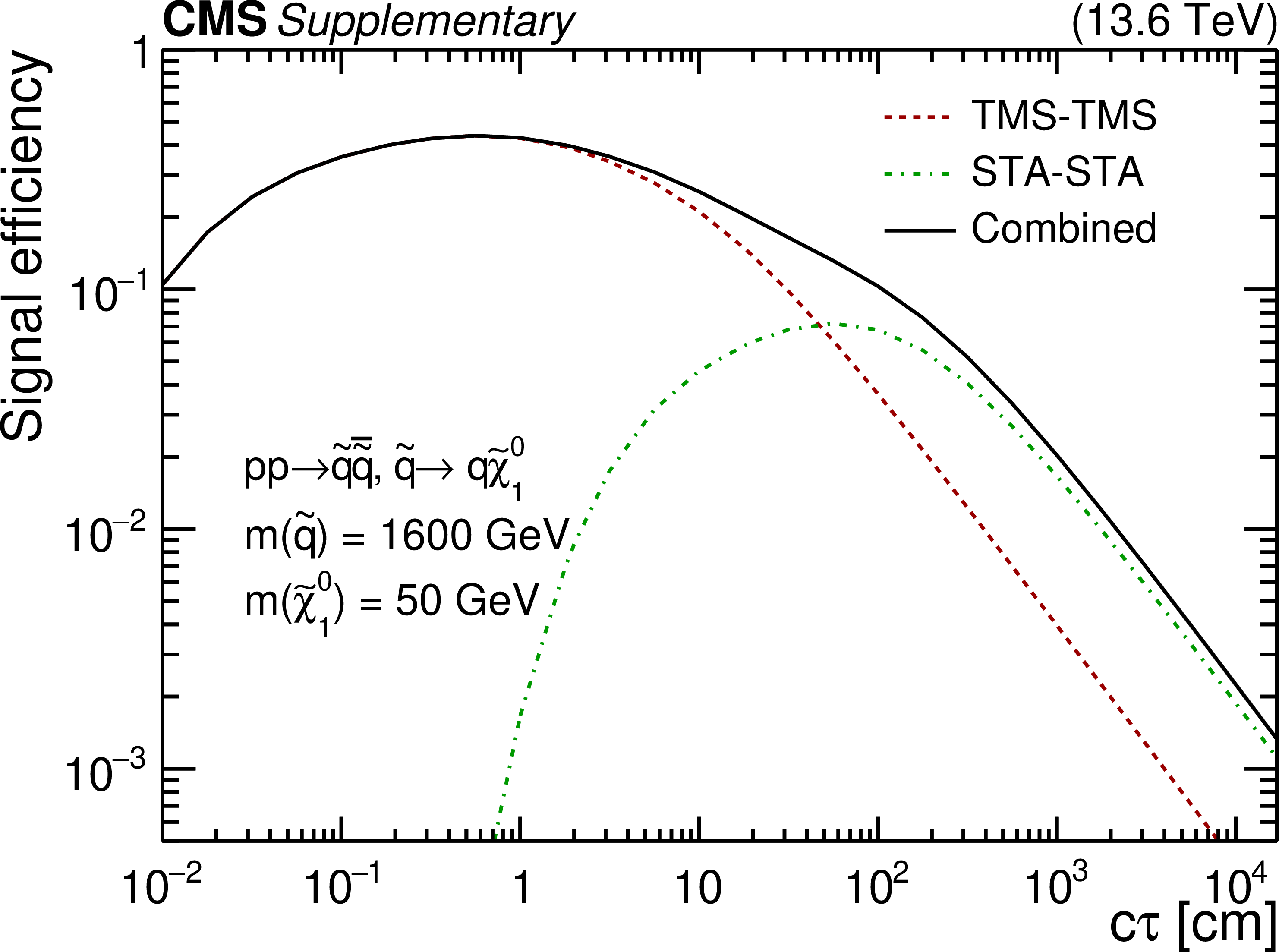
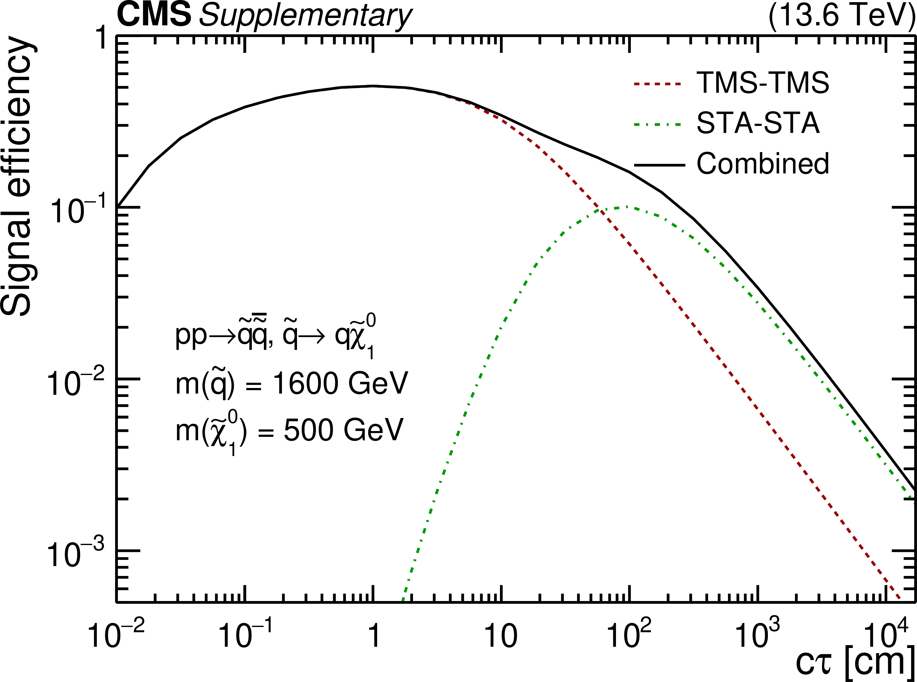
Overall selection efficiencies as a function of $ c\tau(\tilde{\chi}_{1}^{0}) $ for the RPV SUSY model, for events with $ m({\tilde{\mathrm{q}}} ) $ ranging from 125 GeV (upper left) to 1600 GeV (lower right) and $ m(\tilde{\chi}_{1}^{0}) = $ 50 GeV. Each plot shows efficiencies of the two dimuon categories, TMS-TMS (dashed red) and STA-STA (dashed green), as well as their combination (solid black). Each efficiency is computed as the ratio of the number of simulated signal events in which at least one dimuon candidate of a given type (or any type for the combined efficiency) passes all selection criteria (including the trigger) to the total number of simulated signal events. All efficiencies are corrected by the data-to-simulation scale factors described in the paper. |
png pdf root |
Additional Figure 14-a:
Overall selection efficiencies as a function of $ c\tau(\tilde{\chi}_{1}^{0}) $ for the RPV SUSY model, for events with $ m({\tilde{\mathrm{q}}} ) $ ranging from 125 GeV (upper left) to 1600 GeV (lower right) and $ m(\tilde{\chi}_{1}^{0}) = $ 50 GeV. Each plot shows efficiencies of the two dimuon categories, TMS-TMS (dashed red) and STA-STA (dashed green), as well as their combination (solid black). Each efficiency is computed as the ratio of the number of simulated signal events in which at least one dimuon candidate of a given type (or any type for the combined efficiency) passes all selection criteria (including the trigger) to the total number of simulated signal events. All efficiencies are corrected by the data-to-simulation scale factors described in the paper. |
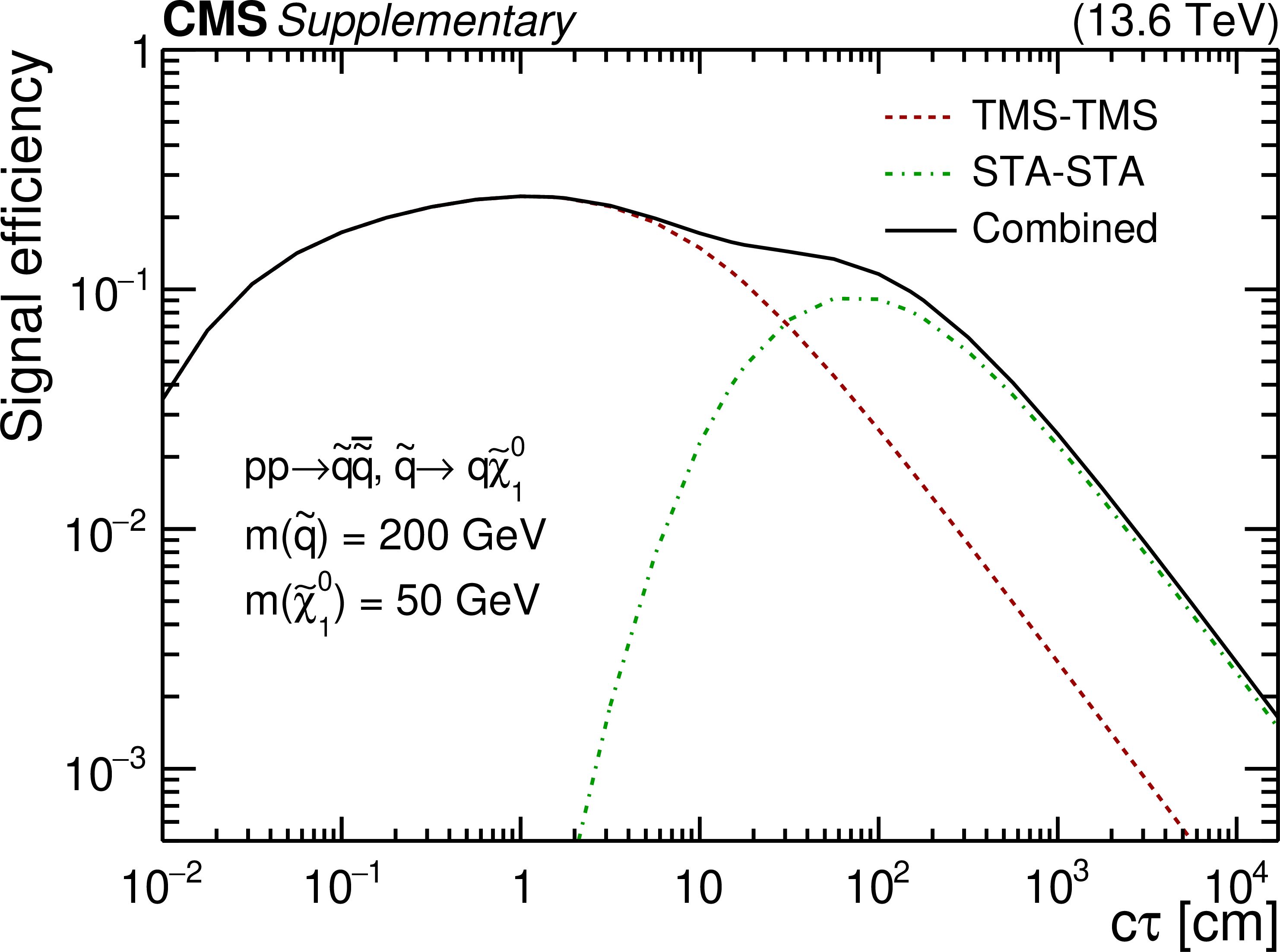
png pdf root |
Additional Figure 14-b:
Overall selection efficiencies as a function of $ c\tau(\tilde{\chi}_{1}^{0}) $ for the RPV SUSY model, for events with $ m({\tilde{\mathrm{q}}} ) $ ranging from 125 GeV (upper left) to 1600 GeV (lower right) and $ m(\tilde{\chi}_{1}^{0}) = $ 50 GeV. Each plot shows efficiencies of the two dimuon categories, TMS-TMS (dashed red) and STA-STA (dashed green), as well as their combination (solid black). Each efficiency is computed as the ratio of the number of simulated signal events in which at least one dimuon candidate of a given type (or any type for the combined efficiency) passes all selection criteria (including the trigger) to the total number of simulated signal events. All efficiencies are corrected by the data-to-simulation scale factors described in the paper. |

png pdf root |
Additional Figure 14-c:
Overall selection efficiencies as a function of $ c\tau(\tilde{\chi}_{1}^{0}) $ for the RPV SUSY model, for events with $ m({\tilde{\mathrm{q}}} ) $ ranging from 125 GeV (upper left) to 1600 GeV (lower right) and $ m(\tilde{\chi}_{1}^{0}) = $ 50 GeV. Each plot shows efficiencies of the two dimuon categories, TMS-TMS (dashed red) and STA-STA (dashed green), as well as their combination (solid black). Each efficiency is computed as the ratio of the number of simulated signal events in which at least one dimuon candidate of a given type (or any type for the combined efficiency) passes all selection criteria (including the trigger) to the total number of simulated signal events. All efficiencies are corrected by the data-to-simulation scale factors described in the paper. |
png pdf root |
Additional Figure 14-d:
Overall selection efficiencies as a function of $ c\tau(\tilde{\chi}_{1}^{0}) $ for the RPV SUSY model, for events with $ m({\tilde{\mathrm{q}}} ) $ ranging from 125 GeV (upper left) to 1600 GeV (lower right) and $ m(\tilde{\chi}_{1}^{0}) = $ 50 GeV. Each plot shows efficiencies of the two dimuon categories, TMS-TMS (dashed red) and STA-STA (dashed green), as well as their combination (solid black). Each efficiency is computed as the ratio of the number of simulated signal events in which at least one dimuon candidate of a given type (or any type for the combined efficiency) passes all selection criteria (including the trigger) to the total number of simulated signal events. All efficiencies are corrected by the data-to-simulation scale factors described in the paper. |

png pdf root |
Additional Figure 14-e:
Overall selection efficiencies as a function of $ c\tau(\tilde{\chi}_{1}^{0}) $ for the RPV SUSY model, for events with $ m({\tilde{\mathrm{q}}} ) $ ranging from 125 GeV (upper left) to 1600 GeV (lower right) and $ m(\tilde{\chi}_{1}^{0}) = $ 50 GeV. Each plot shows efficiencies of the two dimuon categories, TMS-TMS (dashed red) and STA-STA (dashed green), as well as their combination (solid black). Each efficiency is computed as the ratio of the number of simulated signal events in which at least one dimuon candidate of a given type (or any type for the combined efficiency) passes all selection criteria (including the trigger) to the total number of simulated signal events. All efficiencies are corrected by the data-to-simulation scale factors described in the paper. |
png pdf root |
Additional Figure 14-f:
Overall selection efficiencies as a function of $ c\tau(\tilde{\chi}_{1}^{0}) $ for the RPV SUSY model, for events with $ m({\tilde{\mathrm{q}}} ) $ ranging from 125 GeV (upper left) to 1600 GeV (lower right) and $ m(\tilde{\chi}_{1}^{0}) = $ 50 GeV. Each plot shows efficiencies of the two dimuon categories, TMS-TMS (dashed red) and STA-STA (dashed green), as well as their combination (solid black). Each efficiency is computed as the ratio of the number of simulated signal events in which at least one dimuon candidate of a given type (or any type for the combined efficiency) passes all selection criteria (including the trigger) to the total number of simulated signal events. All efficiencies are corrected by the data-to-simulation scale factors described in the paper. |
png pdf |
Additional Figure 15:
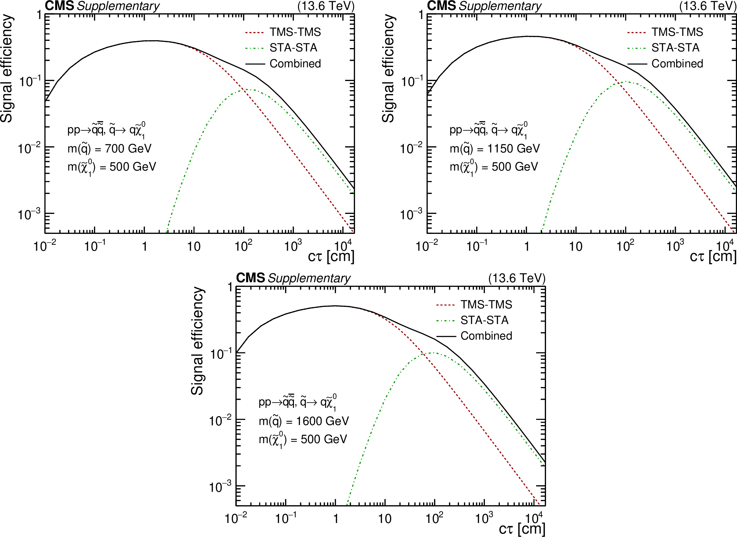
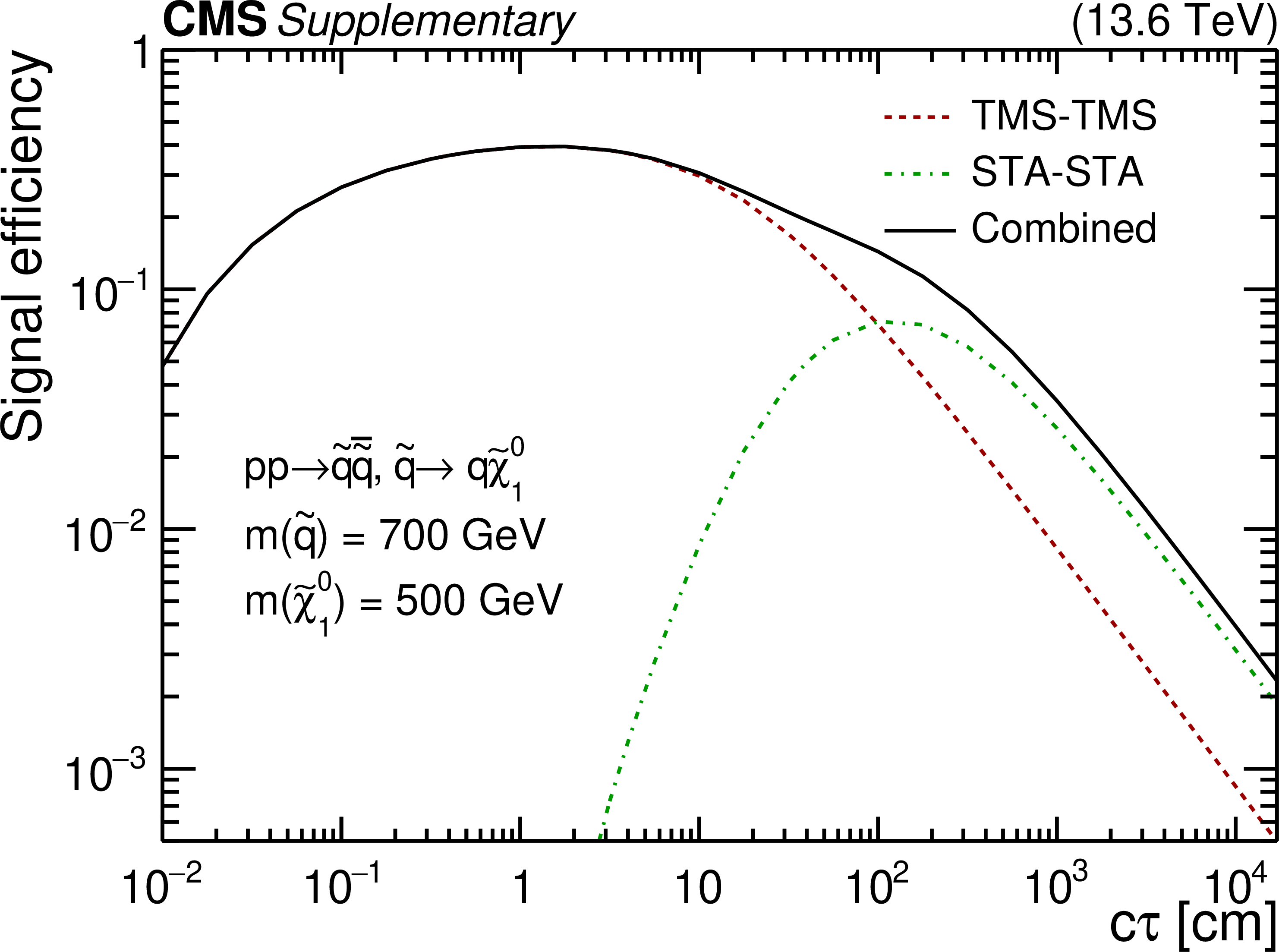
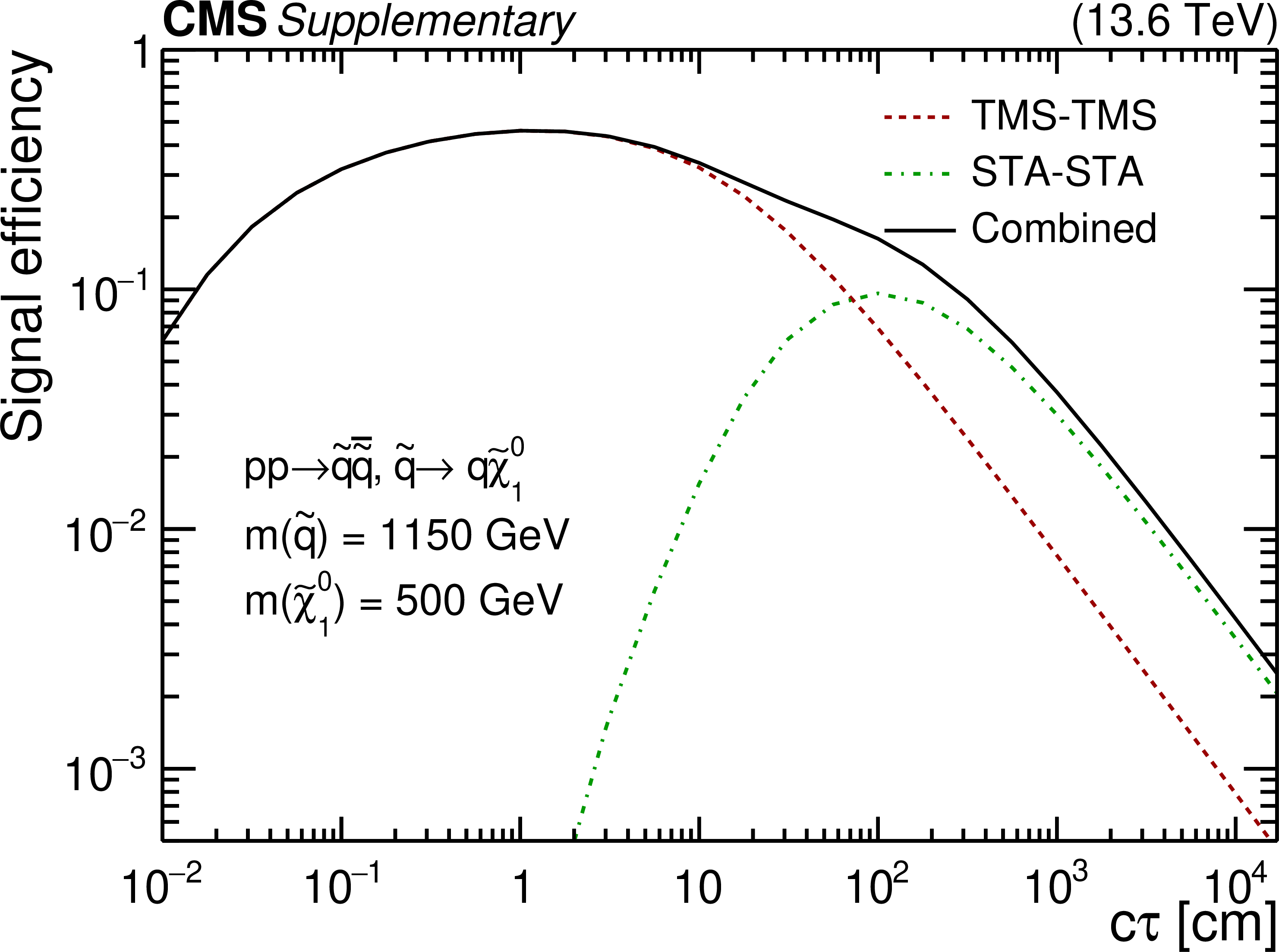
Overall selection efficiencies as a function of $ c\tau(\tilde{\chi}_{1}^{0}) $ for the RPV SUSY model, for events with $ m({\tilde{\mathrm{q}}} ) $ ranging from 700 GeV (upper left) to 1600 GeV (lower) and $ m(\tilde{\chi}_{1}^{0}) = $ 500 GeV. Each plot shows efficiencies of the two dimuon categories, TMS-TMS (dashed red) and STA-STA (dashed green), as well as their combination (solid black). Each efficiency is computed as the ratio of the number of simulated signal events in which at least one dimuon candidate of a given type (or any type for the combined efficiency) passes all selection criteria (including the trigger) to the total number of simulated signal events. All efficiencies are corrected by the data-to-simulation scale factors described in the paper. |
png pdf root |
Additional Figure 15-a:
Overall selection efficiencies as a function of $ c\tau(\tilde{\chi}_{1}^{0}) $ for the RPV SUSY model, for events with $ m({\tilde{\mathrm{q}}} ) $ ranging from 700 GeV (upper left) to 1600 GeV (lower) and $ m(\tilde{\chi}_{1}^{0}) = $ 500 GeV. Each plot shows efficiencies of the two dimuon categories, TMS-TMS (dashed red) and STA-STA (dashed green), as well as their combination (solid black). Each efficiency is computed as the ratio of the number of simulated signal events in which at least one dimuon candidate of a given type (or any type for the combined efficiency) passes all selection criteria (including the trigger) to the total number of simulated signal events. All efficiencies are corrected by the data-to-simulation scale factors described in the paper. |
png pdf root |
Additional Figure 15-b:
Overall selection efficiencies as a function of $ c\tau(\tilde{\chi}_{1}^{0}) $ for the RPV SUSY model, for events with $ m({\tilde{\mathrm{q}}} ) $ ranging from 700 GeV (upper left) to 1600 GeV (lower) and $ m(\tilde{\chi}_{1}^{0}) = $ 500 GeV. Each plot shows efficiencies of the two dimuon categories, TMS-TMS (dashed red) and STA-STA (dashed green), as well as their combination (solid black). Each efficiency is computed as the ratio of the number of simulated signal events in which at least one dimuon candidate of a given type (or any type for the combined efficiency) passes all selection criteria (including the trigger) to the total number of simulated signal events. All efficiencies are corrected by the data-to-simulation scale factors described in the paper. |
png pdf root |
Additional Figure 15-c:
Overall selection efficiencies as a function of $ c\tau(\tilde{\chi}_{1}^{0}) $ for the RPV SUSY model, for events with $ m({\tilde{\mathrm{q}}} ) $ ranging from 700 GeV (upper left) to 1600 GeV (lower) and $ m(\tilde{\chi}_{1}^{0}) = $ 500 GeV. Each plot shows efficiencies of the two dimuon categories, TMS-TMS (dashed red) and STA-STA (dashed green), as well as their combination (solid black). Each efficiency is computed as the ratio of the number of simulated signal events in which at least one dimuon candidate of a given type (or any type for the combined efficiency) passes all selection criteria (including the trigger) to the total number of simulated signal events. All efficiencies are corrected by the data-to-simulation scale factors described in the paper. |
png pdf root |
Additional Figure 16:
The 95% CL observed upper limits on $ \mathcal{B}(\mathrm{H} \to \mathrm{Z}_\text{D}\mathrm{Z}_\text{D}) $ as a function of $ c\tau(\mathrm{Z}_\text{D}) $ for the HAHM model with $ m(\mathrm{Z}_\text{D}) $ ranging from 10 to 60 GeV, obtained by combining the results of this analysis with those of the Run 2 analysis (JHEP 05 (2023) 228). |

png pdf |
Additional Figure 17:
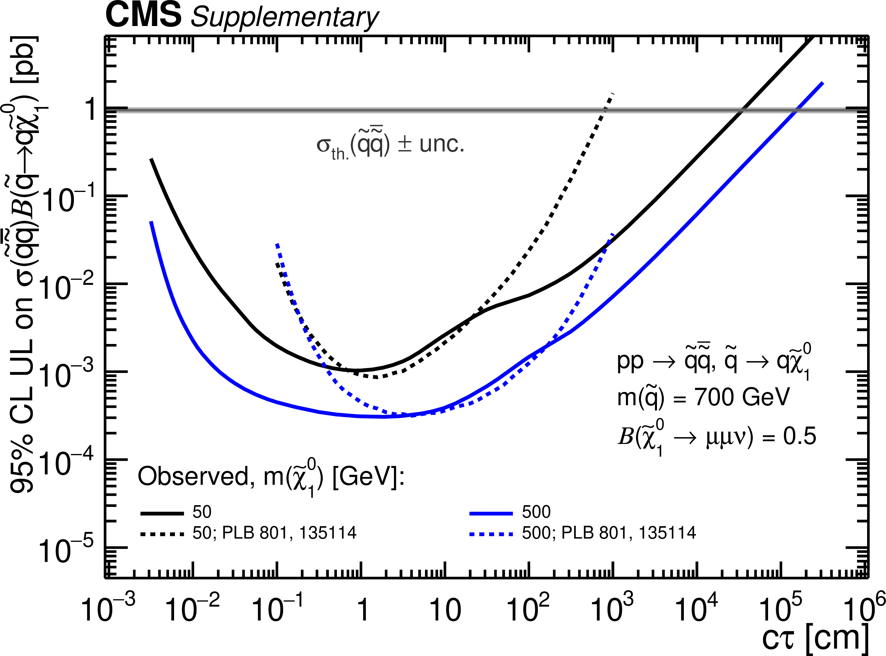
Observed 95% CL upper limits on $ \sigma(\mathrm{p}\mathrm{p}\to{\tilde{\mathrm{q}}} \overline{\tilde{\mathrm{q}}})\mathcal{B}( \tilde{\mathrm{q}} \to \mathrm{q} \tilde{\chi}_{1}^{0} ) $ as a function of $ c\tau(\tilde{\chi}_{1}^{0}) $ in the RPV SUSY model, for $ \mathcal{B}(\tilde{\chi}_{1}^{0}\to\mu^{+}\mu^{-}\nu) = $ 0.5 and various combinations of $ m({\tilde{\mathrm{q}}} ) $ and $ m(\tilde{\chi}_{1}^{0}) $ indicated in the legends. The limits obtained in this analysis (solid) are compared with the corresponding limits (dashed) from the analysis of CMS Run 1 data (PRD 91, 052012) rescaled by the ratio of $ \sigma(\mathrm{p}\mathrm{p}\to{\tilde{\mathrm{q}}} \overline{\tilde{\mathrm{q}}}) $ at 13.6 TeV and 8 TeV, and from the ATLAS search for displaced vertices of oppositely charged leptons in the 2016 data set (PLB 801, 135114) rescaled by the ratio of $ \sigma(\mathrm{p}\mathrm{p}\to{\tilde{\mathrm{q}}} \overline{\tilde{\mathrm{q}}}) $ at 13.6 TeV and 13 TeV. The gray horizontal lines indicate the theoretical values of the squark-antisquark production cross sections with the uncertainties shown as gray shaded bands. The predicted cross sections for $ m({\tilde{\mathrm{q}}} ) $ = 125 and 350 GeV are, respectively, 7200 and 50 pb, and fall outside the $ y $-axis range. |
png pdf root |
Additional Figure 17-a:
Observed 95% CL upper limits on $ \sigma(\mathrm{p}\mathrm{p}\to{\tilde{\mathrm{q}}} \overline{\tilde{\mathrm{q}}})\mathcal{B}( \tilde{\mathrm{q}} \to \mathrm{q} \tilde{\chi}_{1}^{0} ) $ as a function of $ c\tau(\tilde{\chi}_{1}^{0}) $ in the RPV SUSY model, for $ \mathcal{B}(\tilde{\chi}_{1}^{0}\to\mu^{+}\mu^{-}\nu) = $ 0.5 and various combinations of $ m({\tilde{\mathrm{q}}} ) $ and $ m(\tilde{\chi}_{1}^{0}) $ indicated in the legends. The limits obtained in this analysis (solid) are compared with the corresponding limits (dashed) from the analysis of CMS Run 1 data (PRD 91, 052012) rescaled by the ratio of $ \sigma(\mathrm{p}\mathrm{p}\to{\tilde{\mathrm{q}}} \overline{\tilde{\mathrm{q}}}) $ at 13.6 TeV and 8 TeV, and from the ATLAS search for displaced vertices of oppositely charged leptons in the 2016 data set (PLB 801, 135114) rescaled by the ratio of $ \sigma(\mathrm{p}\mathrm{p}\to{\tilde{\mathrm{q}}} \overline{\tilde{\mathrm{q}}}) $ at 13.6 TeV and 13 TeV. The gray horizontal lines indicate the theoretical values of the squark-antisquark production cross sections with the uncertainties shown as gray shaded bands. The predicted cross sections for $ m({\tilde{\mathrm{q}}} ) $ = 125 and 350 GeV are, respectively, 7200 and 50 pb, and fall outside the $ y $-axis range. |
png pdf root |
Additional Figure 17-b:
Observed 95% CL upper limits on $ \sigma(\mathrm{p}\mathrm{p}\to{\tilde{\mathrm{q}}} \overline{\tilde{\mathrm{q}}})\mathcal{B}( \tilde{\mathrm{q}} \to \mathrm{q} \tilde{\chi}_{1}^{0} ) $ as a function of $ c\tau(\tilde{\chi}_{1}^{0}) $ in the RPV SUSY model, for $ \mathcal{B}(\tilde{\chi}_{1}^{0}\to\mu^{+}\mu^{-}\nu) = $ 0.5 and various combinations of $ m({\tilde{\mathrm{q}}} ) $ and $ m(\tilde{\chi}_{1}^{0}) $ indicated in the legends. The limits obtained in this analysis (solid) are compared with the corresponding limits (dashed) from the analysis of CMS Run 1 data (PRD 91, 052012) rescaled by the ratio of $ \sigma(\mathrm{p}\mathrm{p}\to{\tilde{\mathrm{q}}} \overline{\tilde{\mathrm{q}}}) $ at 13.6 TeV and 8 TeV, and from the ATLAS search for displaced vertices of oppositely charged leptons in the 2016 data set (PLB 801, 135114) rescaled by the ratio of $ \sigma(\mathrm{p}\mathrm{p}\to{\tilde{\mathrm{q}}} \overline{\tilde{\mathrm{q}}}) $ at 13.6 TeV and 13 TeV. The gray horizontal lines indicate the theoretical values of the squark-antisquark production cross sections with the uncertainties shown as gray shaded bands. The predicted cross sections for $ m({\tilde{\mathrm{q}}} ) $ = 125 and 350 GeV are, respectively, 7200 and 50 pb, and fall outside the $ y $-axis range. |
png pdf root |
Additional Figure 17-c:
Observed 95% CL upper limits on $ \sigma(\mathrm{p}\mathrm{p}\to{\tilde{\mathrm{q}}} \overline{\tilde{\mathrm{q}}})\mathcal{B}( \tilde{\mathrm{q}} \to \mathrm{q} \tilde{\chi}_{1}^{0} ) $ as a function of $ c\tau(\tilde{\chi}_{1}^{0}) $ in the RPV SUSY model, for $ \mathcal{B}(\tilde{\chi}_{1}^{0}\to\mu^{+}\mu^{-}\nu) = $ 0.5 and various combinations of $ m({\tilde{\mathrm{q}}} ) $ and $ m(\tilde{\chi}_{1}^{0}) $ indicated in the legends. The limits obtained in this analysis (solid) are compared with the corresponding limits (dashed) from the analysis of CMS Run 1 data (PRD 91, 052012) rescaled by the ratio of $ \sigma(\mathrm{p}\mathrm{p}\to{\tilde{\mathrm{q}}} \overline{\tilde{\mathrm{q}}}) $ at 13.6 TeV and 8 TeV, and from the ATLAS search for displaced vertices of oppositely charged leptons in the 2016 data set (PLB 801, 135114) rescaled by the ratio of $ \sigma(\mathrm{p}\mathrm{p}\to{\tilde{\mathrm{q}}} \overline{\tilde{\mathrm{q}}}) $ at 13.6 TeV and 13 TeV. The gray horizontal lines indicate the theoretical values of the squark-antisquark production cross sections with the uncertainties shown as gray shaded bands. The predicted cross sections for $ m({\tilde{\mathrm{q}}} ) $ = 125 and 350 GeV are, respectively, 7200 and 50 pb, and fall outside the $ y $-axis range. |
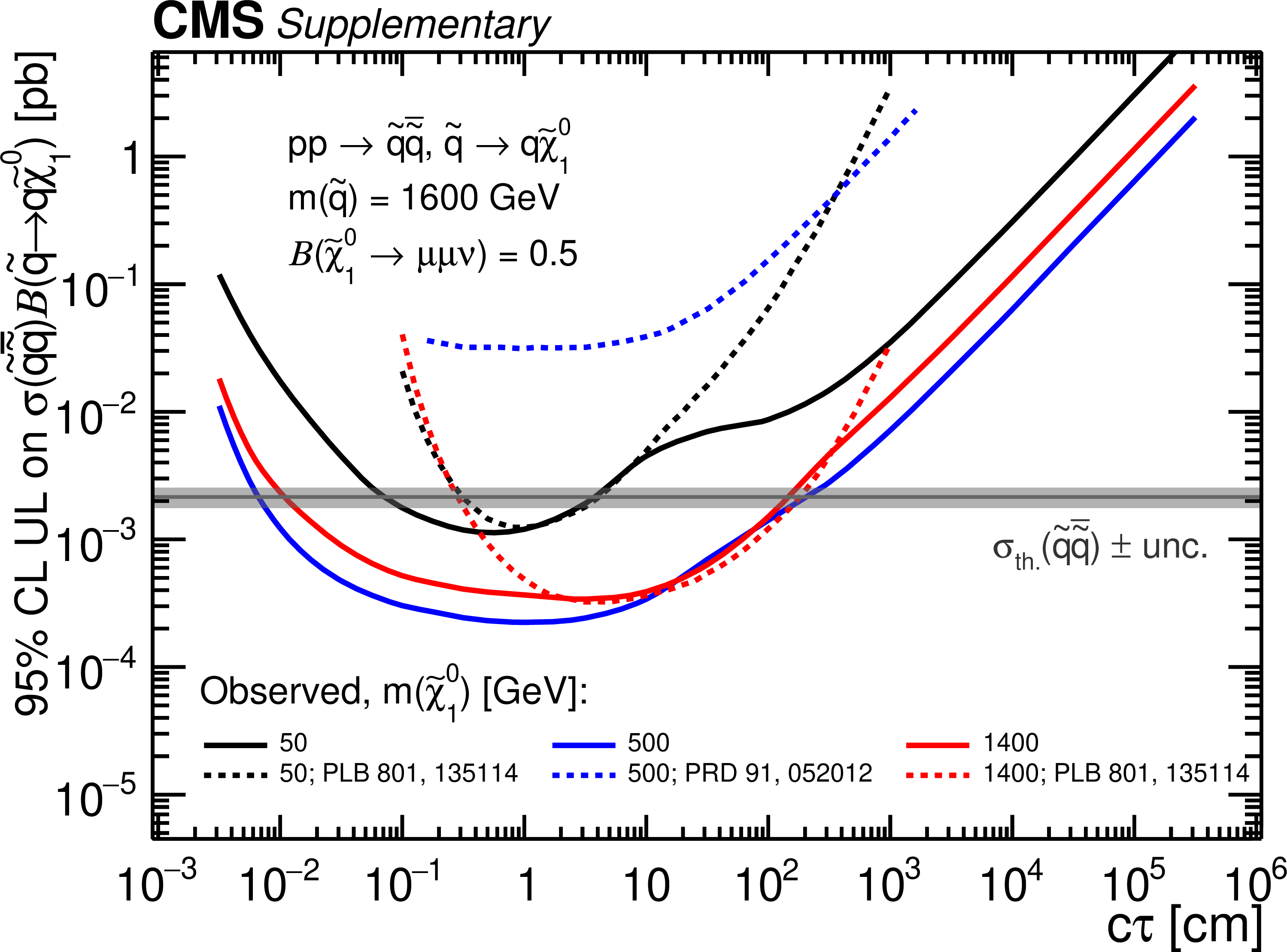
png pdf root |
Additional Figure 17-d:
Observed 95% CL upper limits on $ \sigma(\mathrm{p}\mathrm{p}\to{\tilde{\mathrm{q}}} \overline{\tilde{\mathrm{q}}})\mathcal{B}( \tilde{\mathrm{q}} \to \mathrm{q} \tilde{\chi}_{1}^{0} ) $ as a function of $ c\tau(\tilde{\chi}_{1}^{0}) $ in the RPV SUSY model, for $ \mathcal{B}(\tilde{\chi}_{1}^{0}\to\mu^{+}\mu^{-}\nu) = $ 0.5 and various combinations of $ m({\tilde{\mathrm{q}}} ) $ and $ m(\tilde{\chi}_{1}^{0}) $ indicated in the legends. The limits obtained in this analysis (solid) are compared with the corresponding limits (dashed) from the analysis of CMS Run 1 data (PRD 91, 052012) rescaled by the ratio of $ \sigma(\mathrm{p}\mathrm{p}\to{\tilde{\mathrm{q}}} \overline{\tilde{\mathrm{q}}}) $ at 13.6 TeV and 8 TeV, and from the ATLAS search for displaced vertices of oppositely charged leptons in the 2016 data set (PLB 801, 135114) rescaled by the ratio of $ \sigma(\mathrm{p}\mathrm{p}\to{\tilde{\mathrm{q}}} \overline{\tilde{\mathrm{q}}}) $ at 13.6 TeV and 13 TeV. The gray horizontal lines indicate the theoretical values of the squark-antisquark production cross sections with the uncertainties shown as gray shaded bands. The predicted cross sections for $ m({\tilde{\mathrm{q}}} ) $ = 125 and 350 GeV are, respectively, 7200 and 50 pb, and fall outside the $ y $-axis range. |

png pdf |
Additional Figure 18:
Signal efficiencies in the TMS-TMS (left) and STA-STA (right) dimuon category as a function of the smaller of the two values of generated muon $ p_{\mathrm{T}} $ and $ d_{\text{0}} $ in dimuons with $ L_{\text{xy}}^\mathrm{true} $ smaller than 20 cm (upper), 20--70 cm (middle), and 70-500 cm (lower) in the HAHM signal model. The efficiency in each bin is computed as the ratio of the number of simulated signal dimuons in that bin that pass the trigger requirements and selection criteria to the total number of simulated signal dimuons in that bin and within the geometric acceptance. The geometric acceptance is defined as the generated longitudinal decay length $ L_{\text{z}}^\mathrm{true} $ smaller than 8 m and $ |\eta| $ of both generated muons forming the dimuon smaller than 2.0. The efficiencies obtained from simulation are corrected by the data-to-simulation scale factors described in the paper. Efficiency in the TMS-TMS dimuon category for dimuons with $ L_{\text{xy}}^\mathrm{true} > $ 70 cm is zero and is not shown. |
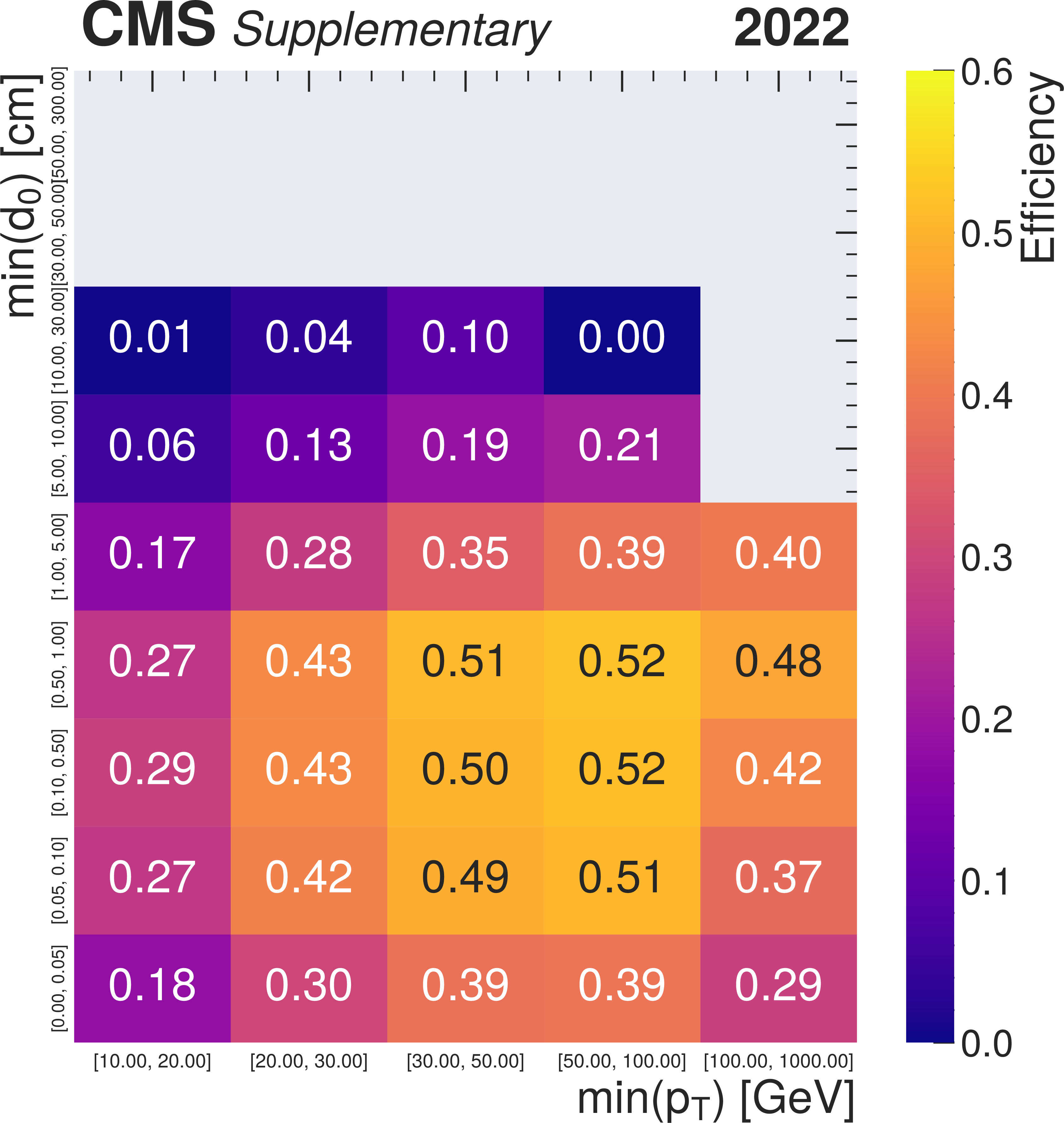
png pdf |
Additional Figure 18-a:
Signal efficiencies in the TMS-TMS (left) and STA-STA (right) dimuon category as a function of the smaller of the two values of generated muon $ p_{\mathrm{T}} $ and $ d_{\text{0}} $ in dimuons with $ L_{\text{xy}}^\mathrm{true} $ smaller than 20 cm (upper), 20--70 cm (middle), and 70-500 cm (lower) in the HAHM signal model. The efficiency in each bin is computed as the ratio of the number of simulated signal dimuons in that bin that pass the trigger requirements and selection criteria to the total number of simulated signal dimuons in that bin and within the geometric acceptance. The geometric acceptance is defined as the generated longitudinal decay length $ L_{\text{z}}^\mathrm{true} $ smaller than 8 m and $ |\eta| $ of both generated muons forming the dimuon smaller than 2.0. The efficiencies obtained from simulation are corrected by the data-to-simulation scale factors described in the paper. Efficiency in the TMS-TMS dimuon category for dimuons with $ L_{\text{xy}}^\mathrm{true} > $ 70 cm is zero and is not shown. |
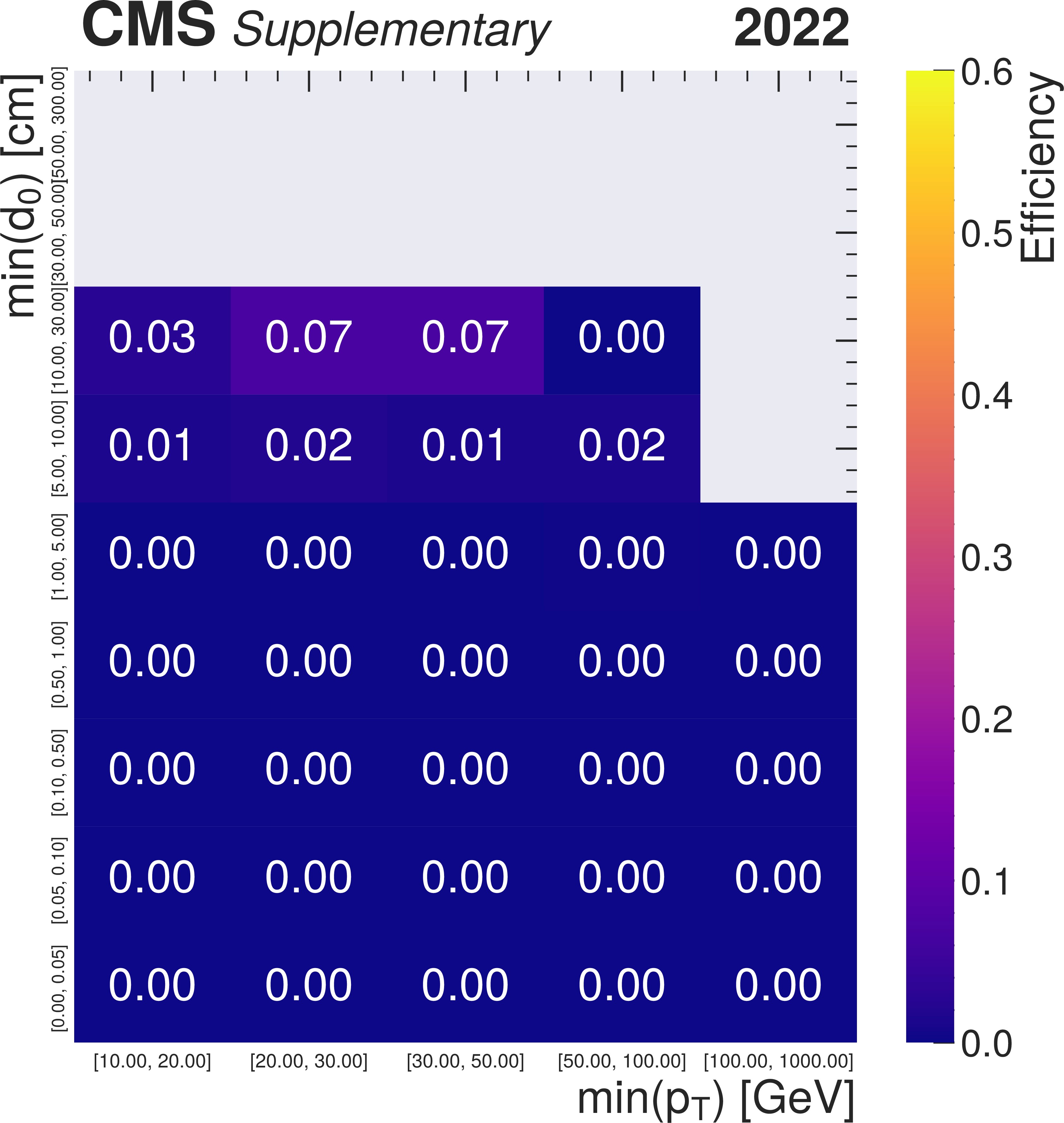
png pdf |
Additional Figure 18-b:
Signal efficiencies in the TMS-TMS (left) and STA-STA (right) dimuon category as a function of the smaller of the two values of generated muon $ p_{\mathrm{T}} $ and $ d_{\text{0}} $ in dimuons with $ L_{\text{xy}}^\mathrm{true} $ smaller than 20 cm (upper), 20--70 cm (middle), and 70-500 cm (lower) in the HAHM signal model. The efficiency in each bin is computed as the ratio of the number of simulated signal dimuons in that bin that pass the trigger requirements and selection criteria to the total number of simulated signal dimuons in that bin and within the geometric acceptance. The geometric acceptance is defined as the generated longitudinal decay length $ L_{\text{z}}^\mathrm{true} $ smaller than 8 m and $ |\eta| $ of both generated muons forming the dimuon smaller than 2.0. The efficiencies obtained from simulation are corrected by the data-to-simulation scale factors described in the paper. Efficiency in the TMS-TMS dimuon category for dimuons with $ L_{\text{xy}}^\mathrm{true} > $ 70 cm is zero and is not shown. |
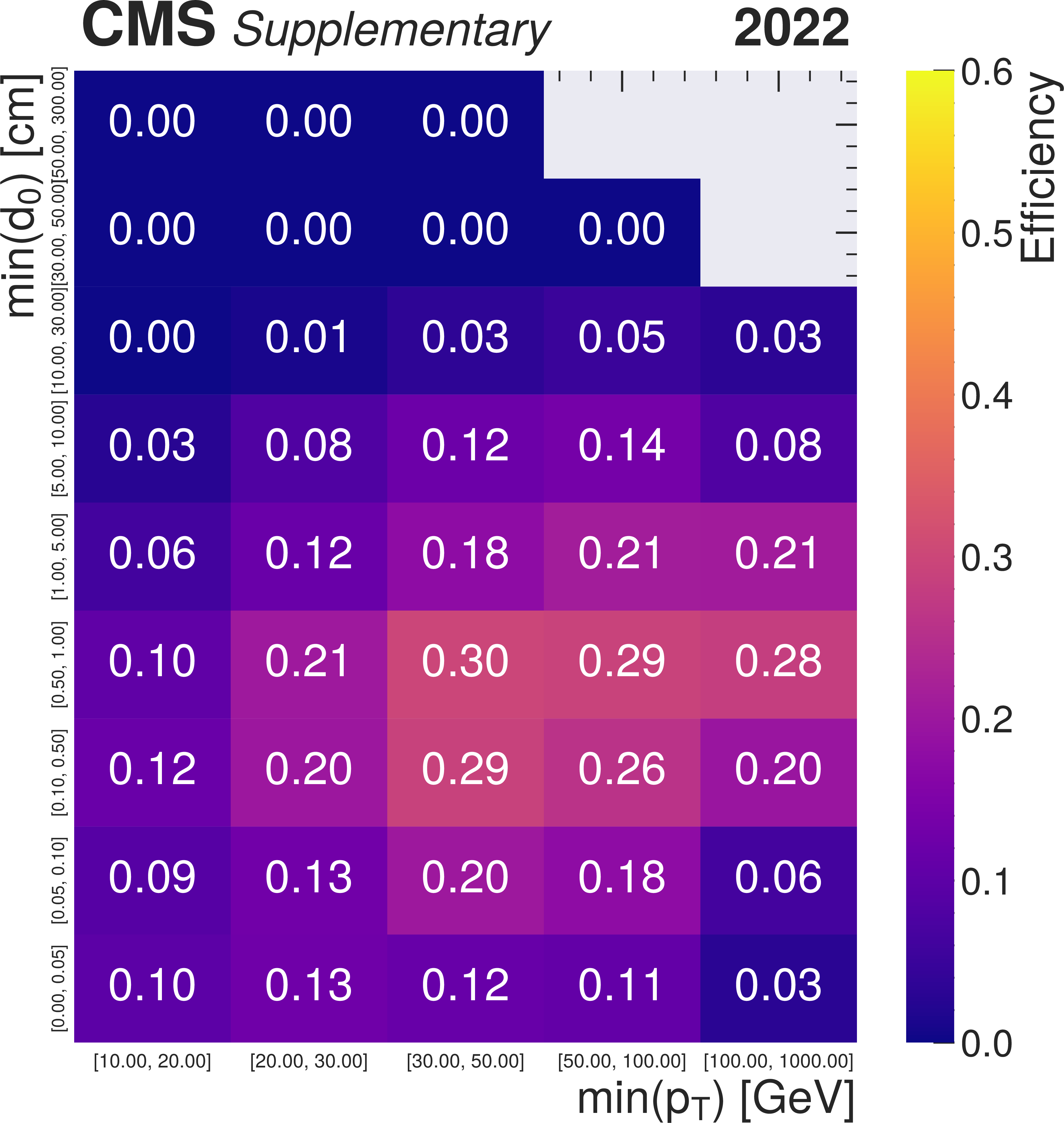
png pdf |
Additional Figure 18-c:
Signal efficiencies in the TMS-TMS (left) and STA-STA (right) dimuon category as a function of the smaller of the two values of generated muon $ p_{\mathrm{T}} $ and $ d_{\text{0}} $ in dimuons with $ L_{\text{xy}}^\mathrm{true} $ smaller than 20 cm (upper), 20--70 cm (middle), and 70-500 cm (lower) in the HAHM signal model. The efficiency in each bin is computed as the ratio of the number of simulated signal dimuons in that bin that pass the trigger requirements and selection criteria to the total number of simulated signal dimuons in that bin and within the geometric acceptance. The geometric acceptance is defined as the generated longitudinal decay length $ L_{\text{z}}^\mathrm{true} $ smaller than 8 m and $ |\eta| $ of both generated muons forming the dimuon smaller than 2.0. The efficiencies obtained from simulation are corrected by the data-to-simulation scale factors described in the paper. Efficiency in the TMS-TMS dimuon category for dimuons with $ L_{\text{xy}}^\mathrm{true} > $ 70 cm is zero and is not shown. |

png pdf |
Additional Figure 18-d:
Signal efficiencies in the TMS-TMS (left) and STA-STA (right) dimuon category as a function of the smaller of the two values of generated muon $ p_{\mathrm{T}} $ and $ d_{\text{0}} $ in dimuons with $ L_{\text{xy}}^\mathrm{true} $ smaller than 20 cm (upper), 20--70 cm (middle), and 70-500 cm (lower) in the HAHM signal model. The efficiency in each bin is computed as the ratio of the number of simulated signal dimuons in that bin that pass the trigger requirements and selection criteria to the total number of simulated signal dimuons in that bin and within the geometric acceptance. The geometric acceptance is defined as the generated longitudinal decay length $ L_{\text{z}}^\mathrm{true} $ smaller than 8 m and $ |\eta| $ of both generated muons forming the dimuon smaller than 2.0. The efficiencies obtained from simulation are corrected by the data-to-simulation scale factors described in the paper. Efficiency in the TMS-TMS dimuon category for dimuons with $ L_{\text{xy}}^\mathrm{true} > $ 70 cm is zero and is not shown. |
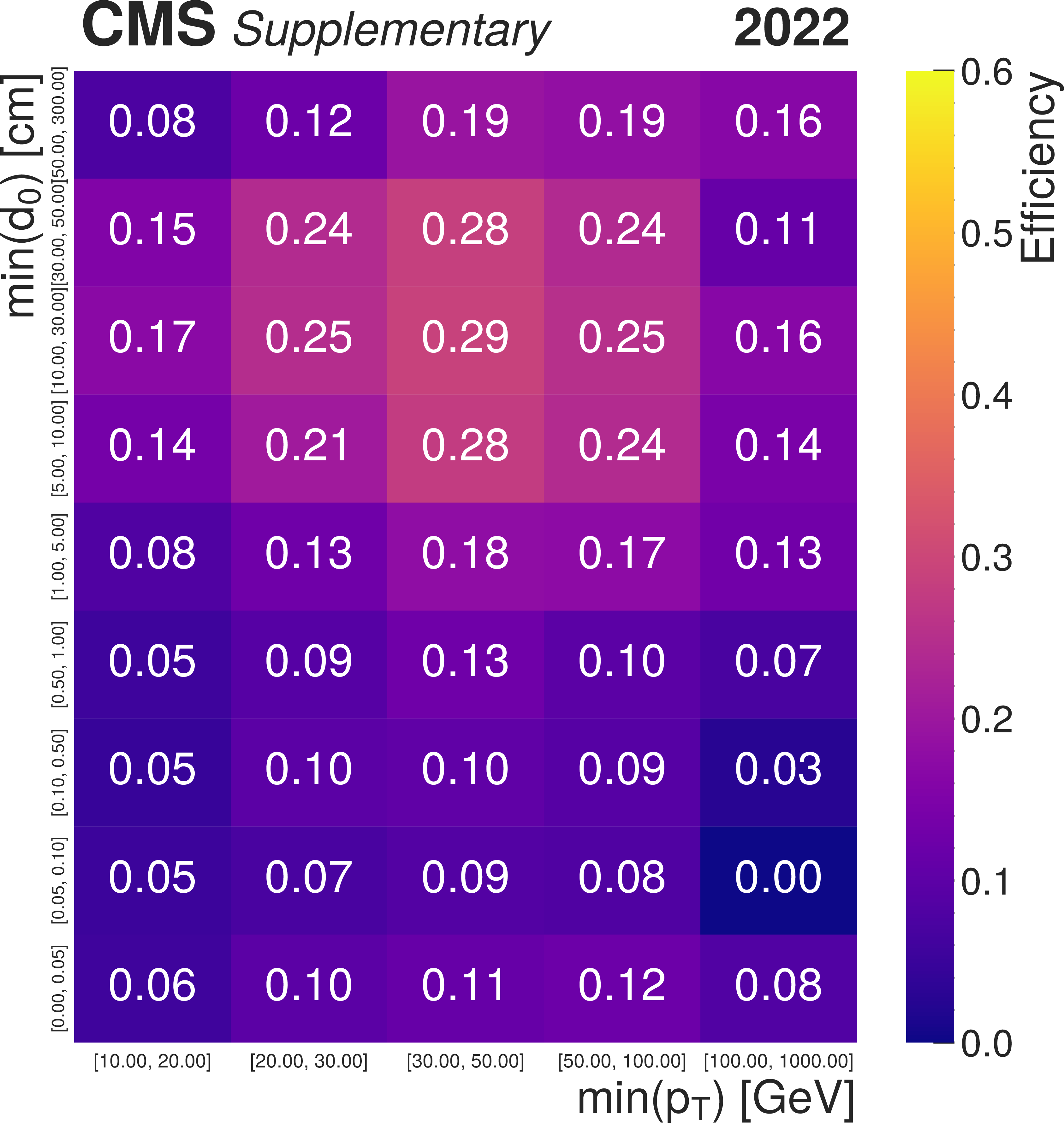
png pdf |
Additional Figure 18-e:
Signal efficiencies in the TMS-TMS (left) and STA-STA (right) dimuon category as a function of the smaller of the two values of generated muon $ p_{\mathrm{T}} $ and $ d_{\text{0}} $ in dimuons with $ L_{\text{xy}}^\mathrm{true} $ smaller than 20 cm (upper), 20--70 cm (middle), and 70-500 cm (lower) in the HAHM signal model. The efficiency in each bin is computed as the ratio of the number of simulated signal dimuons in that bin that pass the trigger requirements and selection criteria to the total number of simulated signal dimuons in that bin and within the geometric acceptance. The geometric acceptance is defined as the generated longitudinal decay length $ L_{\text{z}}^\mathrm{true} $ smaller than 8 m and $ |\eta| $ of both generated muons forming the dimuon smaller than 2.0. The efficiencies obtained from simulation are corrected by the data-to-simulation scale factors described in the paper. Efficiency in the TMS-TMS dimuon category for dimuons with $ L_{\text{xy}}^\mathrm{true} > $ 70 cm is zero and is not shown. |

png pdf |
Additional Figure 19:
Signal efficiencies in the TMS-TMS (left) and STA-STA (right) dimuon category as a function of the smaller of the two values of generated muon $ p_{\mathrm{T}} $ and $ d_{\text{0}} $ in dimuons with $ L_{\text{xy}}^\mathrm{true} $ smaller than 20 cm (upper), 20--70 cm (middle), and 70-500 cm (lower) in the RPV SUSY signal model. The efficiency in each bin is computed as the ratio of the number of simulated signal dimuons in that bin that pass the trigger requirements and selection criteria to the total number of simulated signal dimuons in that bin and within the geometric acceptance. The geometric acceptance is defined as the generated longitudinal decay length $ L_{\text{z}}^\mathrm{true} $ smaller than 8 m and $ |\eta| $ of both generated muons forming the dimuon smaller than 2.0. The efficiencies obtained from simulation are corrected by the data-to-simulation scale factors described in the paper. Efficiency in the TMS-TMS dimuon category for dimuons with $ L_{\text{xy}}^\mathrm{true} > $ 70 cm is zero and is not shown. |

png pdf |
Additional Figure 19-a:
Signal efficiencies in the TMS-TMS (left) and STA-STA (right) dimuon category as a function of the smaller of the two values of generated muon $ p_{\mathrm{T}} $ and $ d_{\text{0}} $ in dimuons with $ L_{\text{xy}}^\mathrm{true} $ smaller than 20 cm (upper), 20--70 cm (middle), and 70-500 cm (lower) in the RPV SUSY signal model. The efficiency in each bin is computed as the ratio of the number of simulated signal dimuons in that bin that pass the trigger requirements and selection criteria to the total number of simulated signal dimuons in that bin and within the geometric acceptance. The geometric acceptance is defined as the generated longitudinal decay length $ L_{\text{z}}^\mathrm{true} $ smaller than 8 m and $ |\eta| $ of both generated muons forming the dimuon smaller than 2.0. The efficiencies obtained from simulation are corrected by the data-to-simulation scale factors described in the paper. Efficiency in the TMS-TMS dimuon category for dimuons with $ L_{\text{xy}}^\mathrm{true} > $ 70 cm is zero and is not shown. |
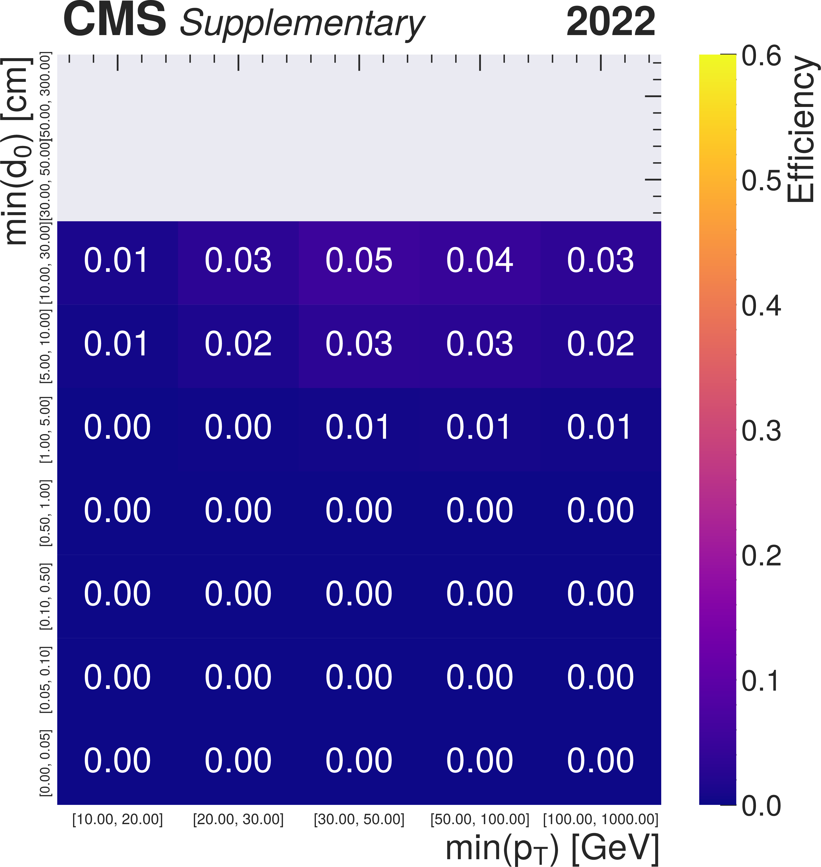
png pdf |
Additional Figure 19-b:
Signal efficiencies in the TMS-TMS (left) and STA-STA (right) dimuon category as a function of the smaller of the two values of generated muon $ p_{\mathrm{T}} $ and $ d_{\text{0}} $ in dimuons with $ L_{\text{xy}}^\mathrm{true} $ smaller than 20 cm (upper), 20--70 cm (middle), and 70-500 cm (lower) in the RPV SUSY signal model. The efficiency in each bin is computed as the ratio of the number of simulated signal dimuons in that bin that pass the trigger requirements and selection criteria to the total number of simulated signal dimuons in that bin and within the geometric acceptance. The geometric acceptance is defined as the generated longitudinal decay length $ L_{\text{z}}^\mathrm{true} $ smaller than 8 m and $ |\eta| $ of both generated muons forming the dimuon smaller than 2.0. The efficiencies obtained from simulation are corrected by the data-to-simulation scale factors described in the paper. Efficiency in the TMS-TMS dimuon category for dimuons with $ L_{\text{xy}}^\mathrm{true} > $ 70 cm is zero and is not shown. |
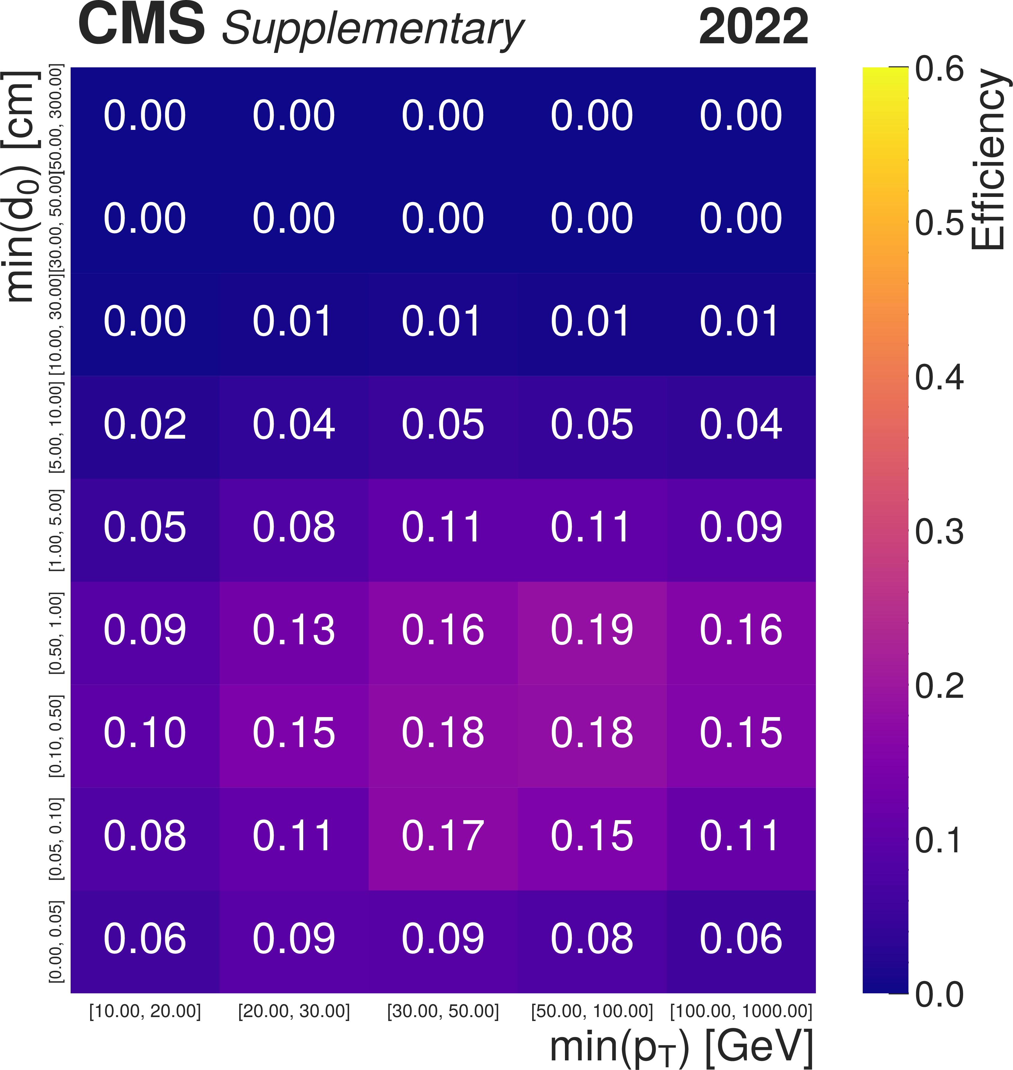
png pdf |
Additional Figure 19-c:
Signal efficiencies in the TMS-TMS (left) and STA-STA (right) dimuon category as a function of the smaller of the two values of generated muon $ p_{\mathrm{T}} $ and $ d_{\text{0}} $ in dimuons with $ L_{\text{xy}}^\mathrm{true} $ smaller than 20 cm (upper), 20--70 cm (middle), and 70-500 cm (lower) in the RPV SUSY signal model. The efficiency in each bin is computed as the ratio of the number of simulated signal dimuons in that bin that pass the trigger requirements and selection criteria to the total number of simulated signal dimuons in that bin and within the geometric acceptance. The geometric acceptance is defined as the generated longitudinal decay length $ L_{\text{z}}^\mathrm{true} $ smaller than 8 m and $ |\eta| $ of both generated muons forming the dimuon smaller than 2.0. The efficiencies obtained from simulation are corrected by the data-to-simulation scale factors described in the paper. Efficiency in the TMS-TMS dimuon category for dimuons with $ L_{\text{xy}}^\mathrm{true} > $ 70 cm is zero and is not shown. |

png pdf |
Additional Figure 19-d:
Signal efficiencies in the TMS-TMS (left) and STA-STA (right) dimuon category as a function of the smaller of the two values of generated muon $ p_{\mathrm{T}} $ and $ d_{\text{0}} $ in dimuons with $ L_{\text{xy}}^\mathrm{true} $ smaller than 20 cm (upper), 20--70 cm (middle), and 70-500 cm (lower) in the RPV SUSY signal model. The efficiency in each bin is computed as the ratio of the number of simulated signal dimuons in that bin that pass the trigger requirements and selection criteria to the total number of simulated signal dimuons in that bin and within the geometric acceptance. The geometric acceptance is defined as the generated longitudinal decay length $ L_{\text{z}}^\mathrm{true} $ smaller than 8 m and $ |\eta| $ of both generated muons forming the dimuon smaller than 2.0. The efficiencies obtained from simulation are corrected by the data-to-simulation scale factors described in the paper. Efficiency in the TMS-TMS dimuon category for dimuons with $ L_{\text{xy}}^\mathrm{true} > $ 70 cm is zero and is not shown. |
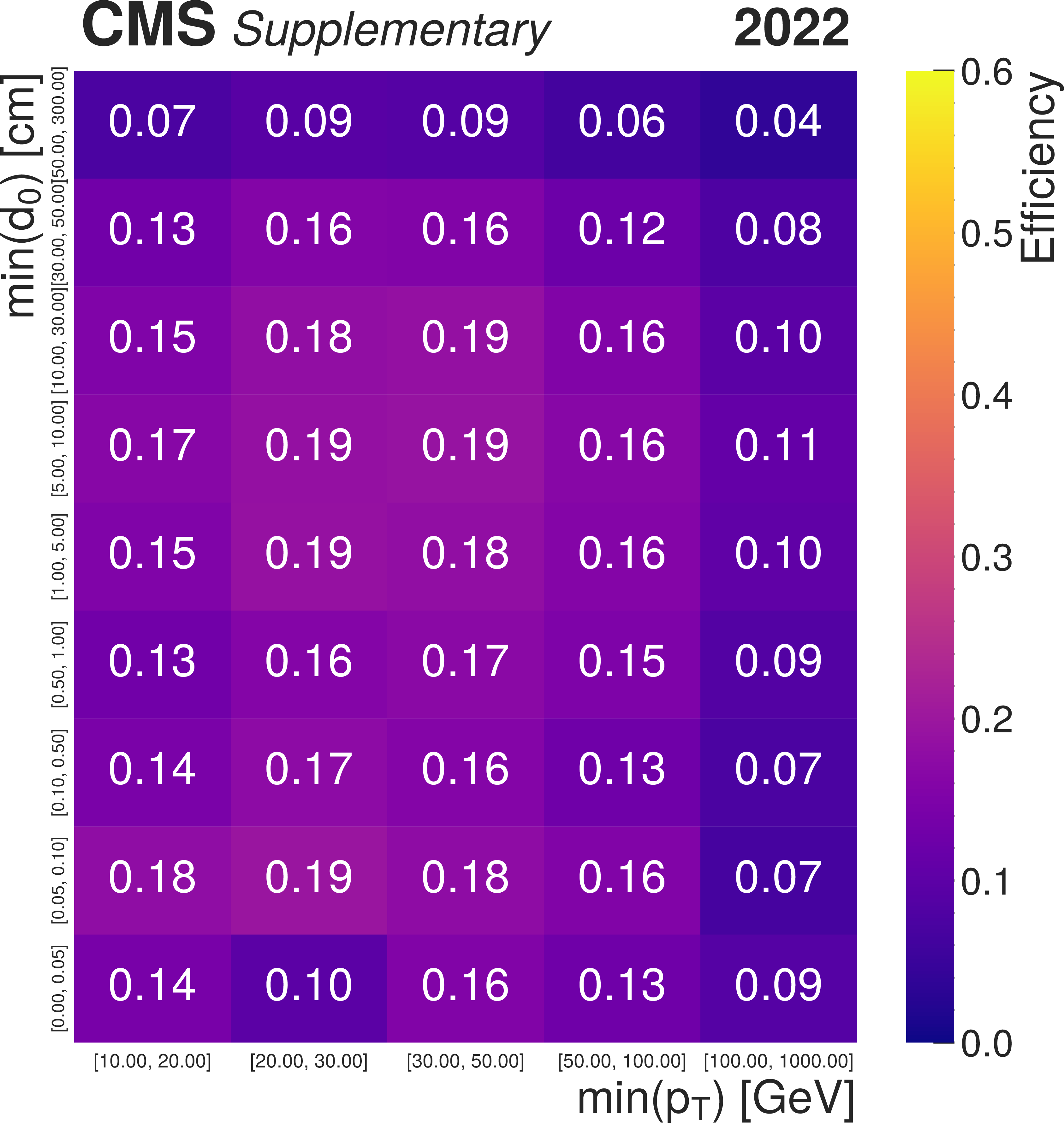
png pdf |
Additional Figure 19-e:
Signal efficiencies in the TMS-TMS (left) and STA-STA (right) dimuon category as a function of the smaller of the two values of generated muon $ p_{\mathrm{T}} $ and $ d_{\text{0}} $ in dimuons with $ L_{\text{xy}}^\mathrm{true} $ smaller than 20 cm (upper), 20--70 cm (middle), and 70-500 cm (lower) in the RPV SUSY signal model. The efficiency in each bin is computed as the ratio of the number of simulated signal dimuons in that bin that pass the trigger requirements and selection criteria to the total number of simulated signal dimuons in that bin and within the geometric acceptance. The geometric acceptance is defined as the generated longitudinal decay length $ L_{\text{z}}^\mathrm{true} $ smaller than 8 m and $ |\eta| $ of both generated muons forming the dimuon smaller than 2.0. The efficiencies obtained from simulation are corrected by the data-to-simulation scale factors described in the paper. Efficiency in the TMS-TMS dimuon category for dimuons with $ L_{\text{xy}}^\mathrm{true} > $ 70 cm is zero and is not shown. |
| HEPData Instructions for Reinterpretation |
|
While the search presented specifically addresses two benchmark models described in the paper, its results may be applied to other models predicting long-lived particles that decay to final states with a pair of oppositely charged muons. In Figs. A18-A19, we provide a set of generator-level efficiency maps that approximate the reconstruction-level efficiencies of this analysis and allow for reinterpretation of the results in the framework of other models. Signal efficiencies are provided as a function of the smaller of the two values of generated muon $ p_{\mathrm{T}} $, $ \mathrm{min}( p_{\mathrm{T}} ) $, and of generated muon $ d_{\text{0}} $, $ \mathrm{min}( d_{0} ) $, in three intervals of the generated transverse decay length $ L_{\text{xy}} $ of the signal dimuon, $ L_{\text{xy}} < $ 20 cm, 20 $ < L_{\text{xy}} < $ 70 cm, and 70 $ < L_{\text{xy}} < $ 500 cm. The efficiencies are given separately for the HAHM and RPV SUSY signal models used in the paper. Efficiency maps obtained from HAHM samples are recommended for models featuring $ \mu\mu $ decay vertices and collinear signatures, while maps obtained from RPV SUSY samples are recommended for models featuring $ \mu\mu\nu $ decay vertices and non-collinear signatures. The 3D efficiency maps $ \epsilon \left( \mathrm{min}( p_{\mathrm{T}} ); \mathrm{min}( d_{0} ); L_{\text{xy}} \right) $ are provided separately for the two dimuon categories, TMS-TMS and STA-STA, and are shown in Fig. A18 for the HAHM signal model and Fig. A19 for the RPV SUSY signal model. They are valid to approximate the efficiencies in the analysis of the 2022 data set. The efficiency in each ($ \mathrm{min}( p_{\mathrm{T}} ) $; $ \mathrm{min}( d_{0} ) $; $ L_{\text{xy}} $) bin of the 3D efficiency map is computed as the ratio of the number of simulated signal dimuons in that bin that pass the trigger requirements and selection criteria applied for a given dimuon category to the total number of simulated signal dimuons in that bin and within the geometric acceptance. The computation is performed separately using the ensemble of all generated HAHM and RPV SUSY signal samples listed in the paper. The geometric acceptance is defined as $ \mathrm{min}( d_{0} ) < $ 300 cm, $ L_{\text{xy}} < $ 500 cm, generated longitudinal decay length $ L_{\text{z}} $ smaller than 800 cm, and $ |\eta| $ of both generated muons forming the dimuon smaller than 2.0. The efficiencies obtained from simulation are further corrected by the data-to-simulation scale factors described in the paper. When applied to the previously untested models, the signal efficiency in each dimuon category $ j $, $ \epsilon_j $, can be obtained from the 3D efficiency maps using the $ p_{\mathrm{T}} $, $ d_{\text{0}} $, and $ L_{\text{xy}} $ at generator level: |
| References | ||||
| 1 | J. L. Hewett, B. Lillie, M. Masip, and T. G. Rizzo | Signatures of long-lived gluinos in split supersymmetry | JHEP 09 (2004) 070 | hep-ph/0408248 |
| 2 | R. Barbier et al. | $ R $-parity-violating supersymmetry | Phys. Rept. 420 (2005) 1 | hep-ph/0406039 |
| 3 | M. J. Strassler and K. M. Zurek | Echoes of a hidden valley at hadron colliders | PLB 651 (2007) 374 | hep-ph/0604261 |
| 4 | T. Han, Z. Si, K. M. Zurek, and M. J. Strassler | Phenomenology of hidden valleys at hadron colliders | JHEP 07 (2008) 008 | 0712.2041 |
| 5 | CMS Collaboration | Search for long-lived particles decaying to a pair of muons in proton-proton collisions at $ \sqrt{s} = $ 13 TeV | JHEP 05 (2023) 228 | CMS-EXO-21-006 2205.08582 |
| 6 | D. Curtin, R. Essig, S. Gori, and J. Shelton | Illuminating dark photons with high-energy colliders | JHEP 02 (2015) 157 | 1412.0018 |
| 7 | CMS Collaboration | Search for long-lived particles decaying into muon pairs in proton-proton collisions at $ \sqrt{s} = $ 13 TeV collected with a dedicated high-rate data stream | JHEP 04 (2022) 062 | CMS-EXO-20-014 2112.13769 |
| 8 | CMS Collaboration | Search for long-lived particles that decay into final states containing two electrons or two muons in proton-proton collisions at $ \sqrt{s} = $ 8 TeV | PRD 91 (2015) 052012 | CMS-EXO-12-037 1411.6977 |
| 9 | CMS Collaboration | Search for long-lived particles that decay into final states containing two muons, reconstructed using only the CMS muon chambers | CMS Physics Analysis Summary, 2015 CMS-PAS-EXO-14-012 |
CMS-PAS-EXO-14-012 |
| 10 | ATLAS Collaboration | Search for long-lived particles in final states with displaced dimuon vertices in pp collisions at $ \sqrt{s} = $ 13 TeV with the ATLAS detector | PRD 99 (2019) 012001 | 1808.03057 |
| 11 | ATLAS Collaboration | Search for displaced vertices of oppositely charged leptons from decays of long-lived particles in pp collisions at $ \sqrt{s} = $ 13 TeV with the ATLAS detector | PLB 801 (2020) 135114 | 1907.10037 |
| 12 | CMS Collaboration | HEPData record for this analysis | link | |
| 13 | CMS Collaboration | Performance of the CMS muon detector and muon reconstruction with proton-proton collisions at $ \sqrt{s} = $ 13 TeV | JINST 13 (2018) P06015 | CMS-MUO-16-001 1804.04528 |
| 14 | CMS Collaboration | The CMS experiment at the CERN LHC | JINST 3 (2008) S08004 | |
| 15 | CMS Collaboration | Development of the CMS detector for the CERN LHC Run 3 | Accepted by JINST, 2023 | CMS-PRF-21-001 2309.05466 |
| 16 | CMS Collaboration | Performance of the CMS Level-1 trigger in proton-proton collisions at $ \sqrt{s} = $ 13 TeV | JINST 15 (2020) P10017 | CMS-TRG-17-001 2006.10165 |
| 17 | CMS Collaboration | The CMS trigger system | JINST 12 (2017) P01020 | CMS-TRG-12-001 1609.02366 |
| 18 | J. D. Wells | How to find a hidden world at the Large Hadron Collider | in Perspectives on LHC Physics, G. Kane and A. Pierce, eds., World Scientific, Singapore, 2008 link |
0803.1243 |
| 19 | J. Alwall et al. | The automated computation of tree-level and next-to-leading order differential cross sections, and their matching to parton shower simulations | JHEP 07 (2014) 079 | 1405.0301 |
| 20 | M. Cepeda et al. | Report from working group 2: Higgs physics at the HL-LHC and HE-LHC | in Proceedings of the HL/HE-LHC Workshop, A. Dainese et al., eds., vol 7, CERN Yellow Rep. Monogr., 2019 link |
1902.00134 |
| 21 | LHC Higgs Cross Section Working Group | Ad interim 13.6 TeV cross sections | link | |
| 22 | T. Sjöstrand et al. | An introduction to PYTHIA 8.2 | Comp. Phys. Com. 191 (2015) 159 | 1410.3012 |
| 23 | H. K. Dreiner | An introduction to explicit $ R $-parity violation | Adv. Ser. Direct. HEP 21 (2010) 565 | hep-ph/9707435 |
| 24 | D. Dercks et al. | $ R $-parity violation at the LHC | EPJC 77 (2017) 856 | 1706.09418 |
| 25 | W. Beenakker et al. | NNLL-fast: predictions for coloured supersymmetric particle production at the LHC with threshold and Coulomb resummation | JHEP 12 (2016) 133 | 1607.07741 |
| 26 | PDF4LHC Working Group , R. D. Ball et al. | The PDF4LHC21 combination of global PDF fits for the LHC Run III | JPG 49 (2022) 080501 | 2203.05506 |
| 27 | NNPDF Collaboration | Parton distributions from high-precision collider data | EPJC 77 (2017) 663 | 1706.00428 |
| 28 | CMS Collaboration | Extraction and validation of a new set of CMS PYTHIA8 tunes from underlying-event measurements | EPJC 80 (2020) 4 | CMS-GEN-17-001 1903.12179 |
| 29 | \GEANTfour Collaboration | GEANT 4---a simulation toolkit | NIM A 506 (2003) 250 | |
| 30 | W. A. Nash | Search for long-lived particles that decay to muon pairs at 13 TeV and an algorithm to improve resolution in the muon system of the Compact Muon Solenoid | PhD thesis, UCLA, 2022 link |
|
| 31 | CMS Collaboration | Technical proposal for the Phase-II upgrade of the Compact Muon Solenoid | CMS Technical Proposal CERN-LHCC-2015-010, CMS-TDR-15-02, 2015 CDS |
|
| 32 | CMS Collaboration | Performance of the CMS muon trigger system in proton-proton collisions at $ \sqrt{s} = $ 13 TeV | JINST 16 (2021) P07001 | CMS-MUO-19-001 2102.04790 |
| 33 | CMS Collaboration | Performance of CMS muon reconstruction in pp collision events at $ \sqrt{s} = $ 7 TeV | JINST 7 (2012) P10002 | CMS-MUO-10-004 1206.4071 |
| 34 | LHCb Collaboration | Identification of beauty and charm quark jets at LHCb | JINST 10 (2015) P06013 | 1504.07670 |
| 35 | CMS Collaboration | Identification of heavy-flavour jets with the CMS detector in pp collisions at 13 TeV | JINST 13 (2018) P05011 | CMS-BTV-16-002 1712.07158 |
| 36 | CMS Collaboration | First measurement of the top quark pair production cross section in proton-proton collisions at $ \sqrt{s} = $ 13.6 TeV | JHEP 08 (2023) 204 | CMS-TOP-22-012 2303.10680 |
| 37 | A. L. Read | Presentation of search results: The CL$ _{\text{s}} $ technique | JPG 28 (2002) 2693 | |
| 38 | T. Junk | Confidence level computation for combining searches with small statistics | NIM A 434 (1999) 435 | hep-ex/9902006 |
| 39 | ATLAS and CMS Collaborations, and LHC Higgs Combination Group | Procedure for the LHC Higgs boson search combination in summer 2011 | Technical Report CMS-NOTE-2011-005. ATL-PHYS-PUB-2011-11, 2011 | |
| 40 | CMS Collaboration | A search for decays of the Higgs boson to invisible particles in events with a top-antitop quark pair or a vector boson in proton-proton collisions at $ \sqrt{s}= $ 13 TeV | EPJC 83 (2023) 933 | CMS-HIG-21-007 2303.01214 |
| 41 | CMS Collaboration | Search for invisible decays of a Higgs boson produced through vector boson fusion in proton--proton collisions at $ \sqrt{s} = $ 13 TeV | PRD 105 (2022) 092007 | CMS-HIG-20-003 2201.11585 |
| 42 | CMS Collaboration | Combined measurements of Higgs boson couplings in proton-proton collisions at $ \sqrt{s}= $ 13 TeV | EPJC 79 (2019) 421 | CMS-HIG-17-031 1809.10733 |
|
|
Compact Muon Solenoid LHC, CERN |
|

|

|

|

|

|