

Compact Muon Solenoid
LHC, CERN
| CMS-HIG-17-001 ; CERN-EP-2017-292 | ||
| Search for lepton flavour violating decays of the Higgs boson to $\mu\tau$ and $\mathrm{e}\tau$ in proton-proton collisions at $\sqrt{s} = $ 13 TeV | ||
| CMS Collaboration | ||
| 20 December 2017 | ||
| JHEP 06 (2018) 001 | ||
| Abstract: A search for lepton flavour violating decays of the Higgs boson in the $\mu\tau$ and $\mathrm{e}\tau$ decay modes is presented. The search is based on a data set corresponding to an integrated luminosity of 35.9 fb$^{-1}$ of proton-proton collisions collected with the CMS detector in 2016, at a centre-of-mass energy of 13 TeV. No significant excess over the standard model expectation is observed. The observed (expected) upper limits on the lepton flavour violating branching fractions of the Higgs boson are $\mathcal{B}(\mathrm{H}\to\mu\tau) < $ 0.25% (0.25%) and $\mathcal{B}(\mathrm{H}\to\mathrm{e}\tau) < $ 0.61% (0.37%), at 95% confidence level. These results are used to derive upper limits on the off-diagonal $\mu\tau$ and $\mathrm{e}\tau$ Yukawa couplings $\sqrt{|{Y_{\mu\tau}}|^{2}+|{Y_{\tau\mu}}|^{2}} < 1.43\times 10^{-3}$ and $\sqrt{|{Y_{\mathrm{e}\tau}}|^{2}+|{Y_{\tau\mathrm{e}}}|^{2}} < 2.26\times 10^{-3}$ at 95% confidence level. The limits on the lepton flavour violating branching fractions of the Higgs boson and on the associated Yukawa couplings are the most stringent to date. | ||
| Links: e-print arXiv:1712.07173 [hep-ex] (PDF) ; CDS record ; inSPIRE record ; HepData record ; CADI line (restricted) ; | ||
| Figures | |
png pdf |
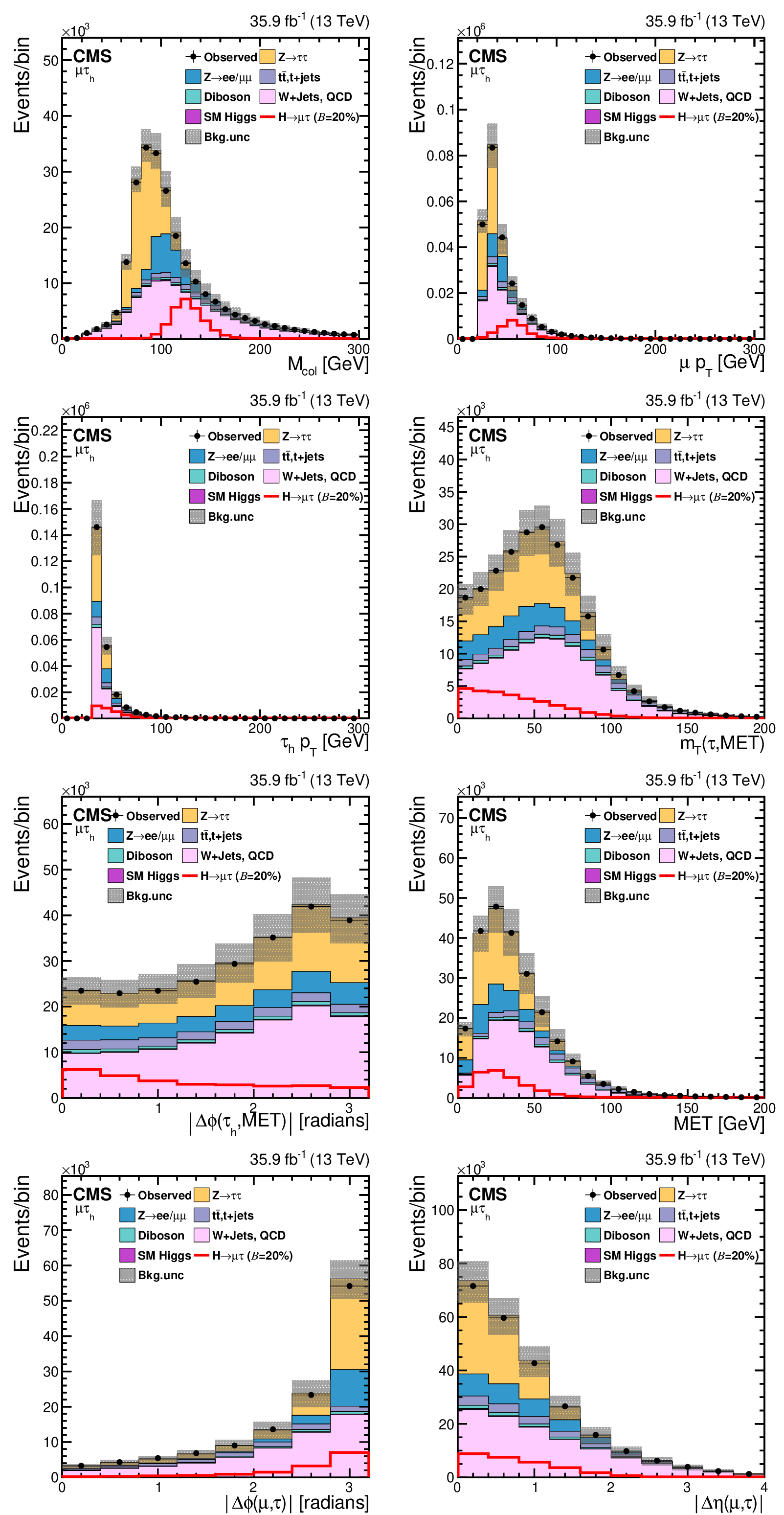
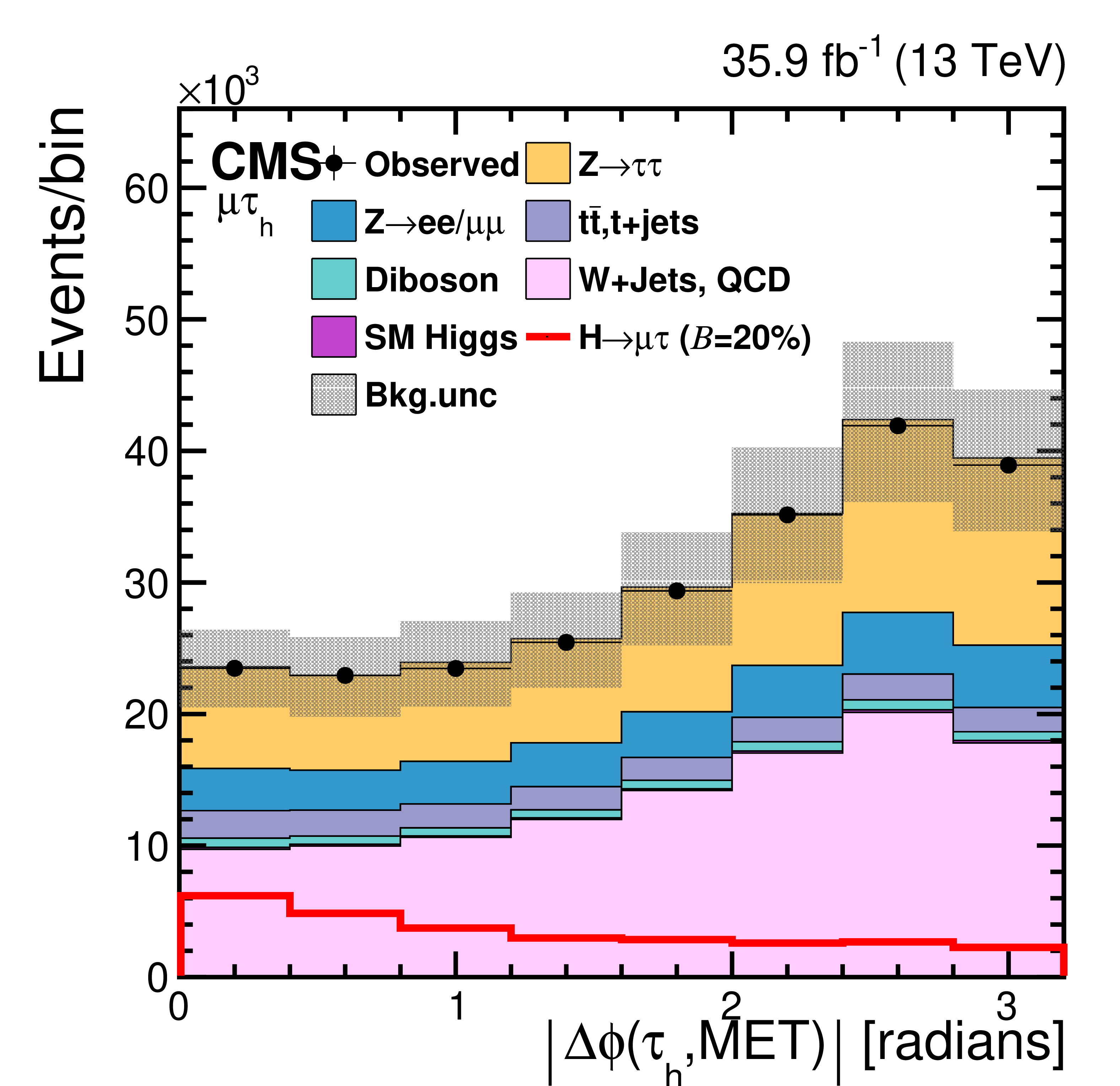
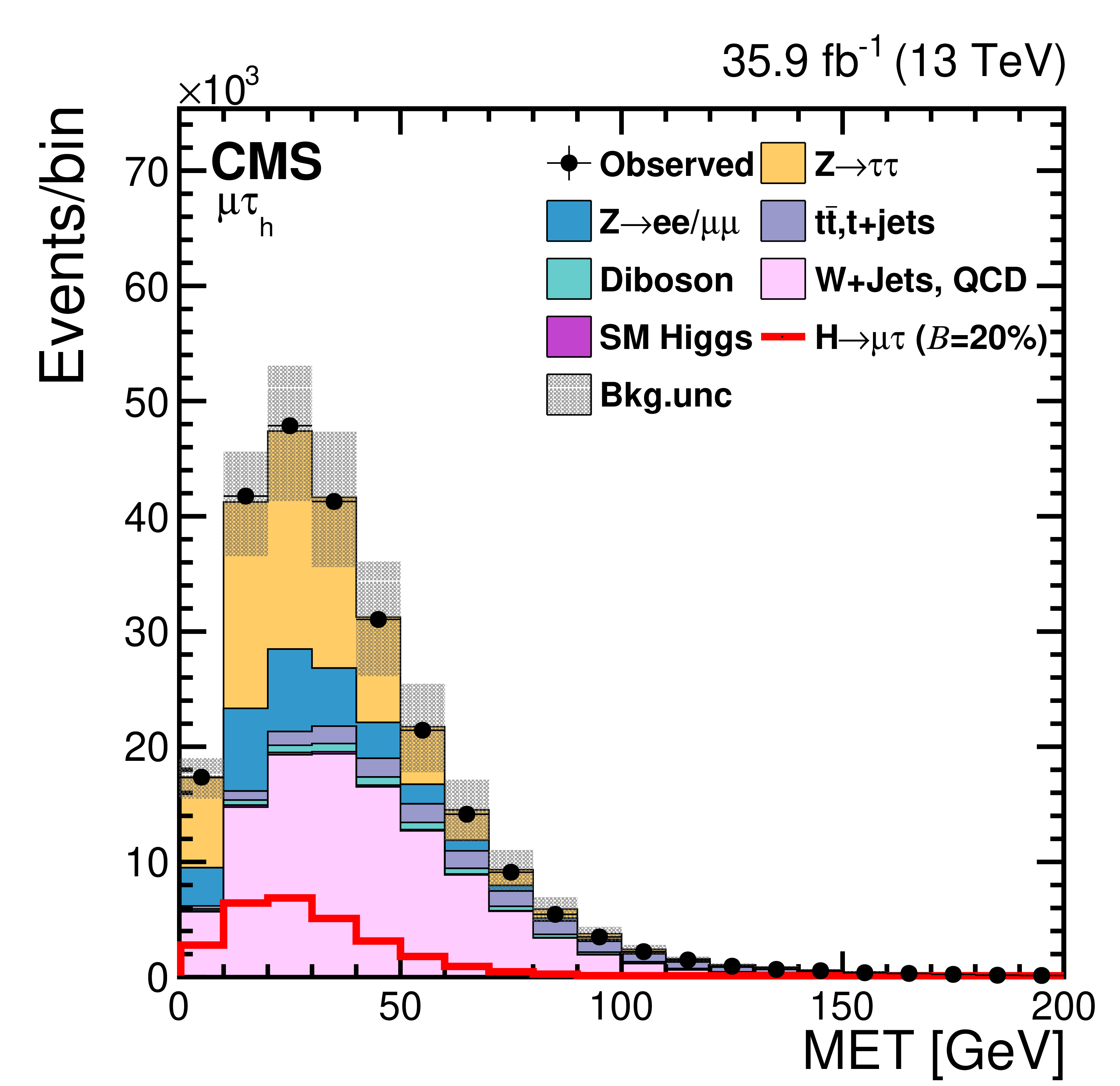
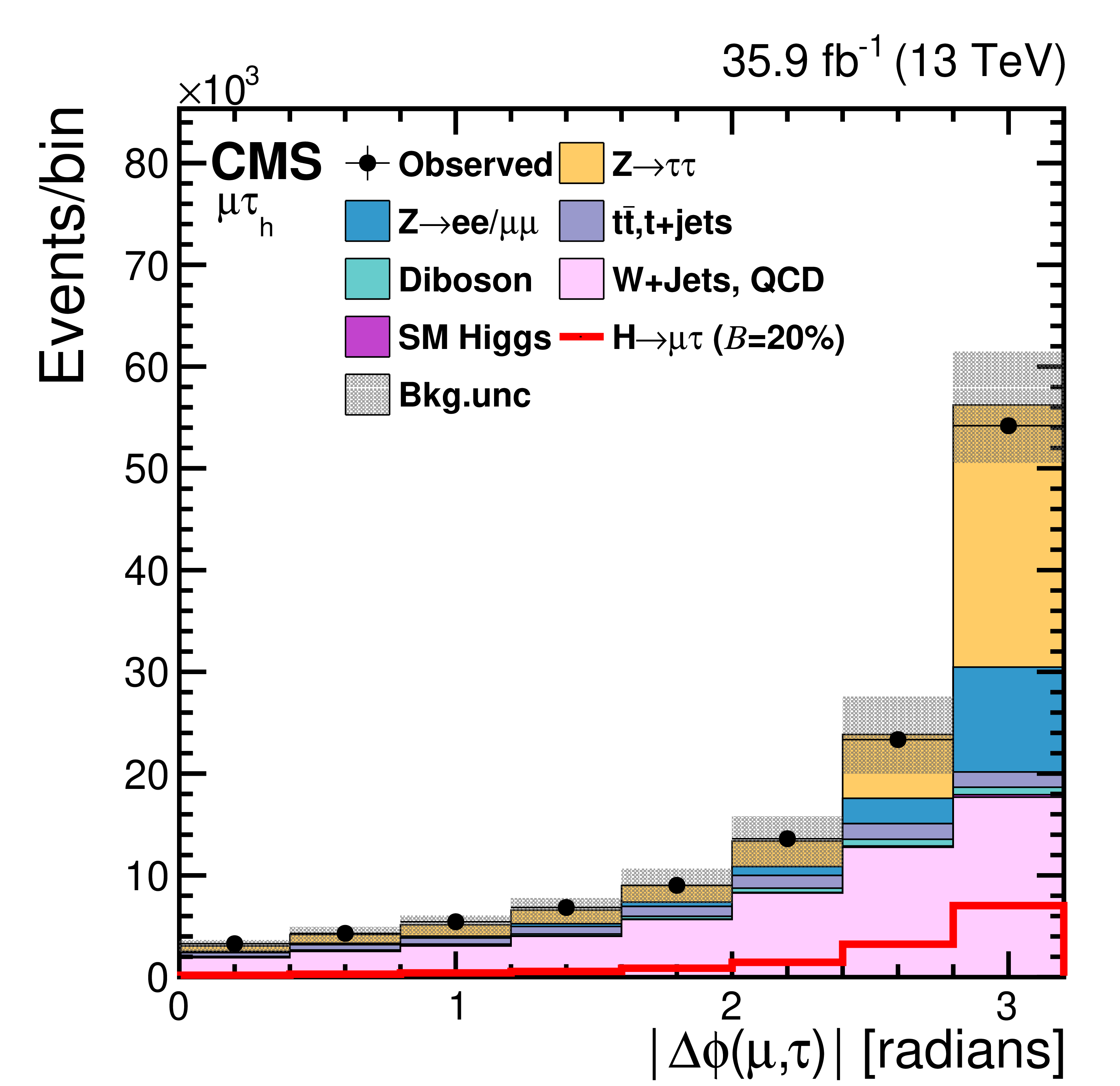
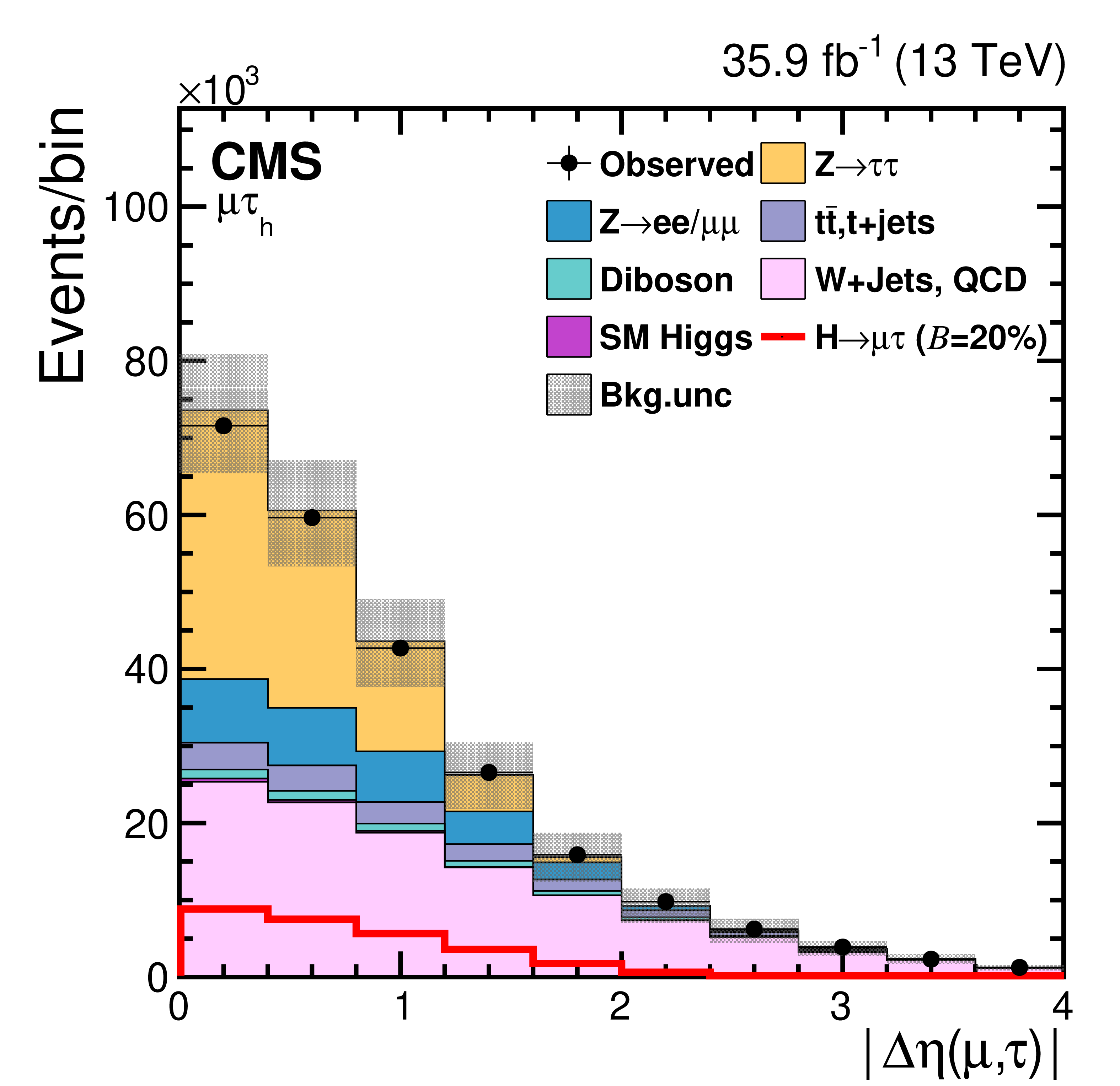
Figure 1:
Distributions of the input variables to the BDT for the $ {{\mathrm {H}} \to {{\mu}} {\tau}_{\text {h}}} $ channel. The background from SM Higgs boson production is small and not visible in the plots. |
png pdf |
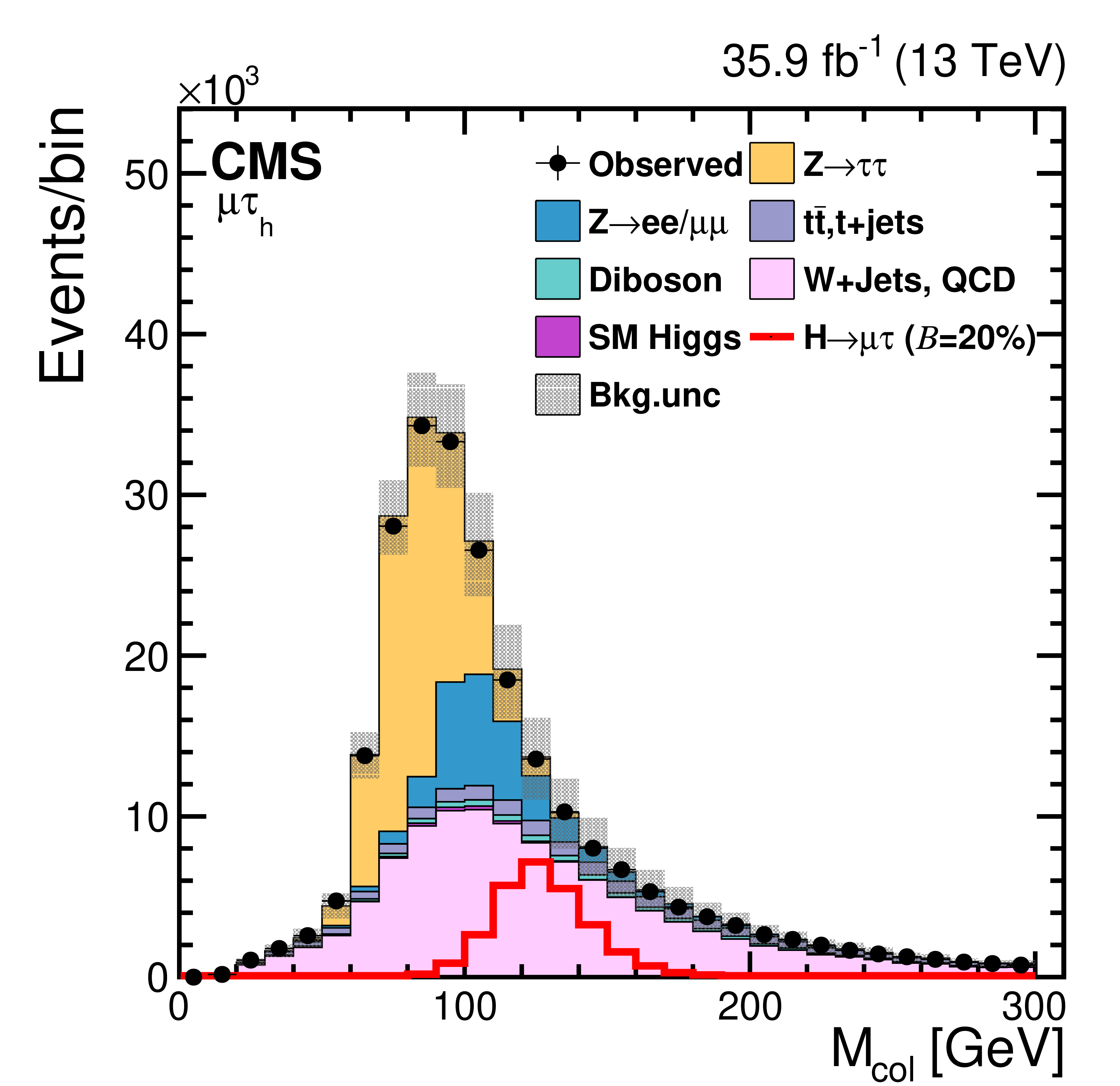
Figure 1-a:
Distribution of one of the input variables to the BDT for the $ {{\mathrm {H}} \to {{\mu}} {\tau}_{\text {h}}} $ channel. The background from SM Higgs boson production is small and not visible. |
png pdf |
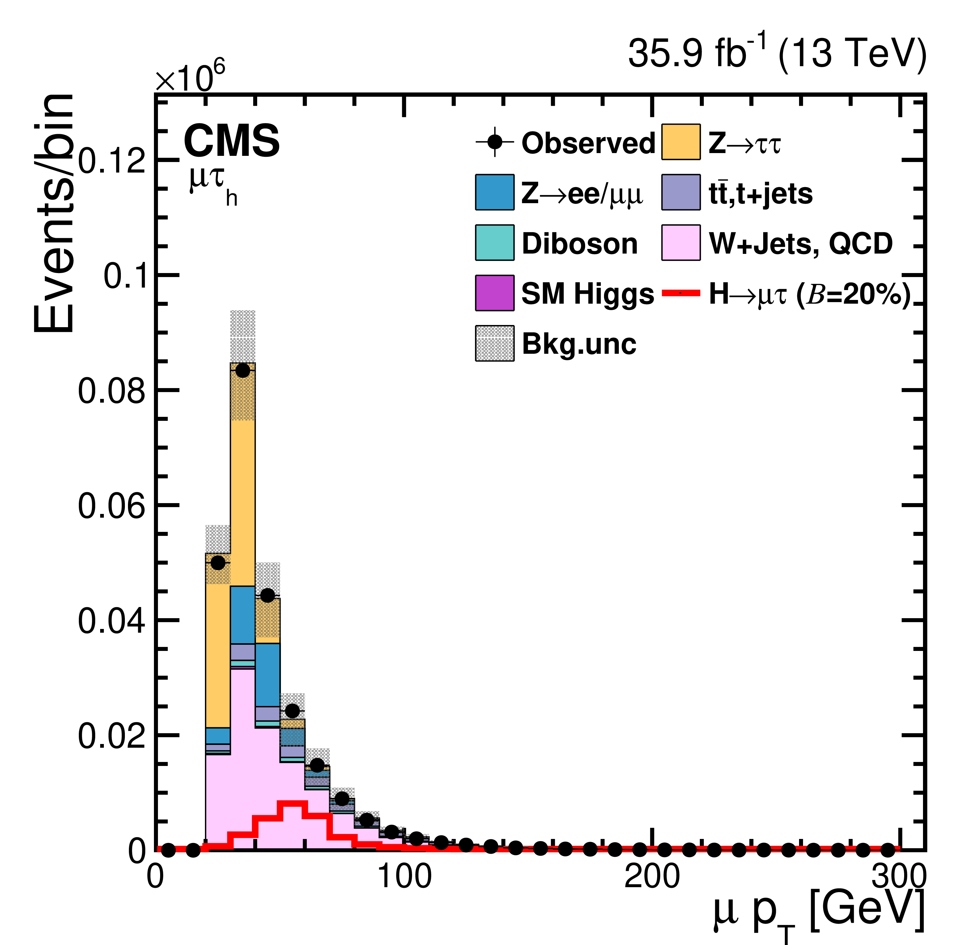
Figure 1-b:
Distribution of one of the input variables to the BDT for the $ {{\mathrm {H}} \to {{\mu}} {\tau}_{\text {h}}} $ channel. The background from SM Higgs boson production is small and not visible. |

png pdf |
Figure 1-c:
Distribution of one of the input variables to the BDT for the $ {{\mathrm {H}} \to {{\mu}} {\tau}_{\text {h}}} $ channel. The background from SM Higgs boson production is small and not visible. |
png pdf |
Figure 1-d:
Distribution of one of the input variables to the BDT for the $ {{\mathrm {H}} \to {{\mu}} {\tau}_{\text {h}}} $ channel. The background from SM Higgs boson production is small and not visible. |
png pdf |
Figure 1-e:
Distribution of one of the input variables to the BDT for the $ {{\mathrm {H}} \to {{\mu}} {\tau}_{\text {h}}} $ channel. The background from SM Higgs boson production is small and not visible. |
png pdf |
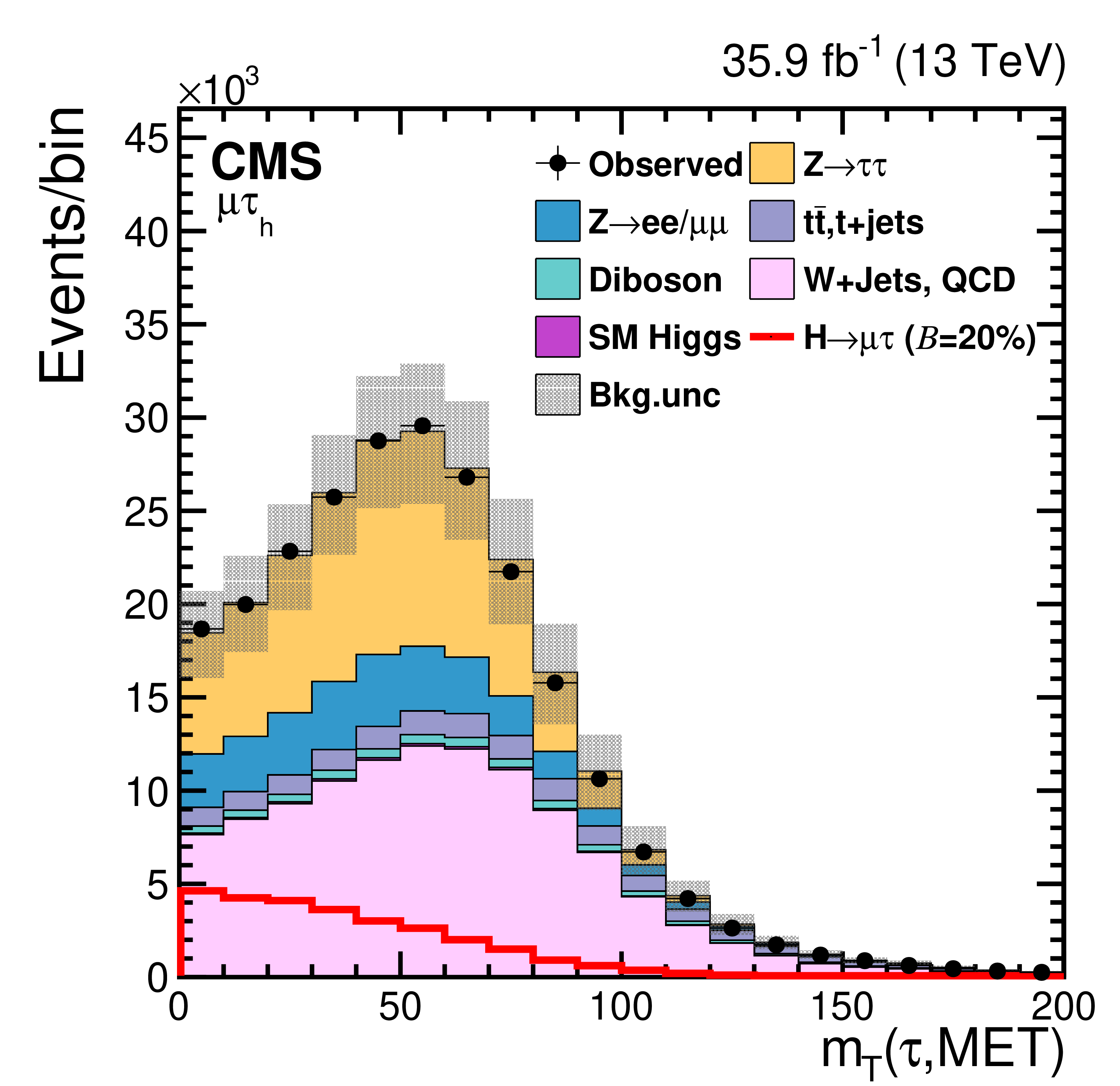
Figure 1-f:
Distribution of one of the input variables to the BDT for the $ {{\mathrm {H}} \to {{\mu}} {\tau}_{\text {h}}} $ channel. The background from SM Higgs boson production is small and not visible. |
png pdf |
Figure 1-g:
Distribution of one of the input variables to the BDT for the $ {{\mathrm {H}} \to {{\mu}} {\tau}_{\text {h}}} $ channel. The background from SM Higgs boson production is small and not visible. |
png pdf |
Figure 1-h:
Distribution of one of the input variables to the BDT for the $ {{\mathrm {H}} \to {{\mu}} {\tau}_{\text {h}}} $ channel. The background from SM Higgs boson production is small and not visible. |
png pdf |
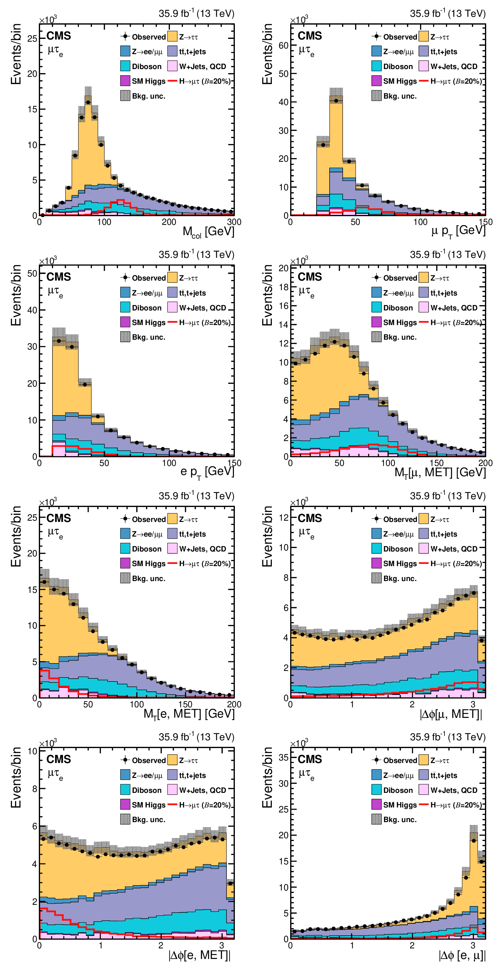
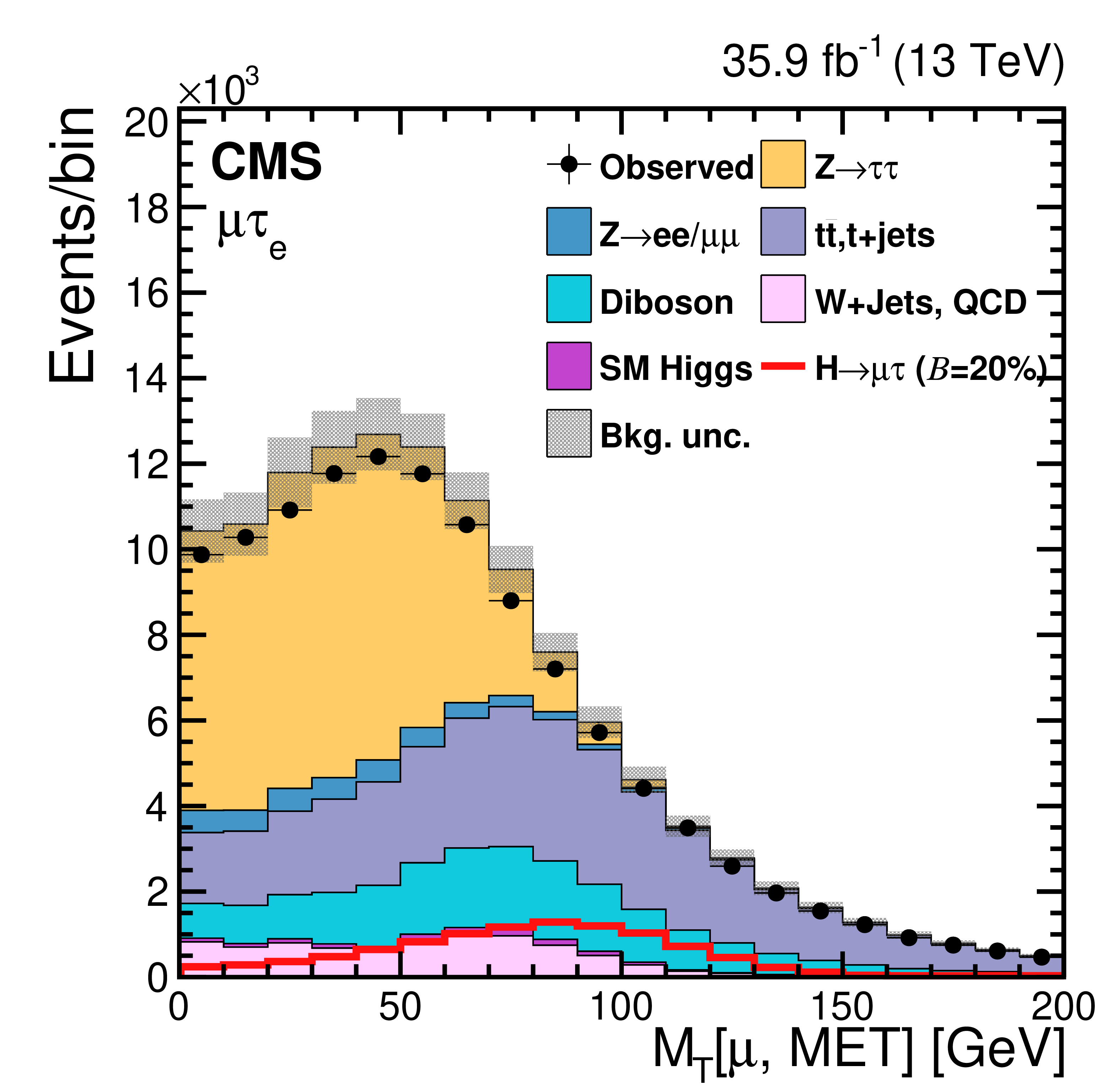
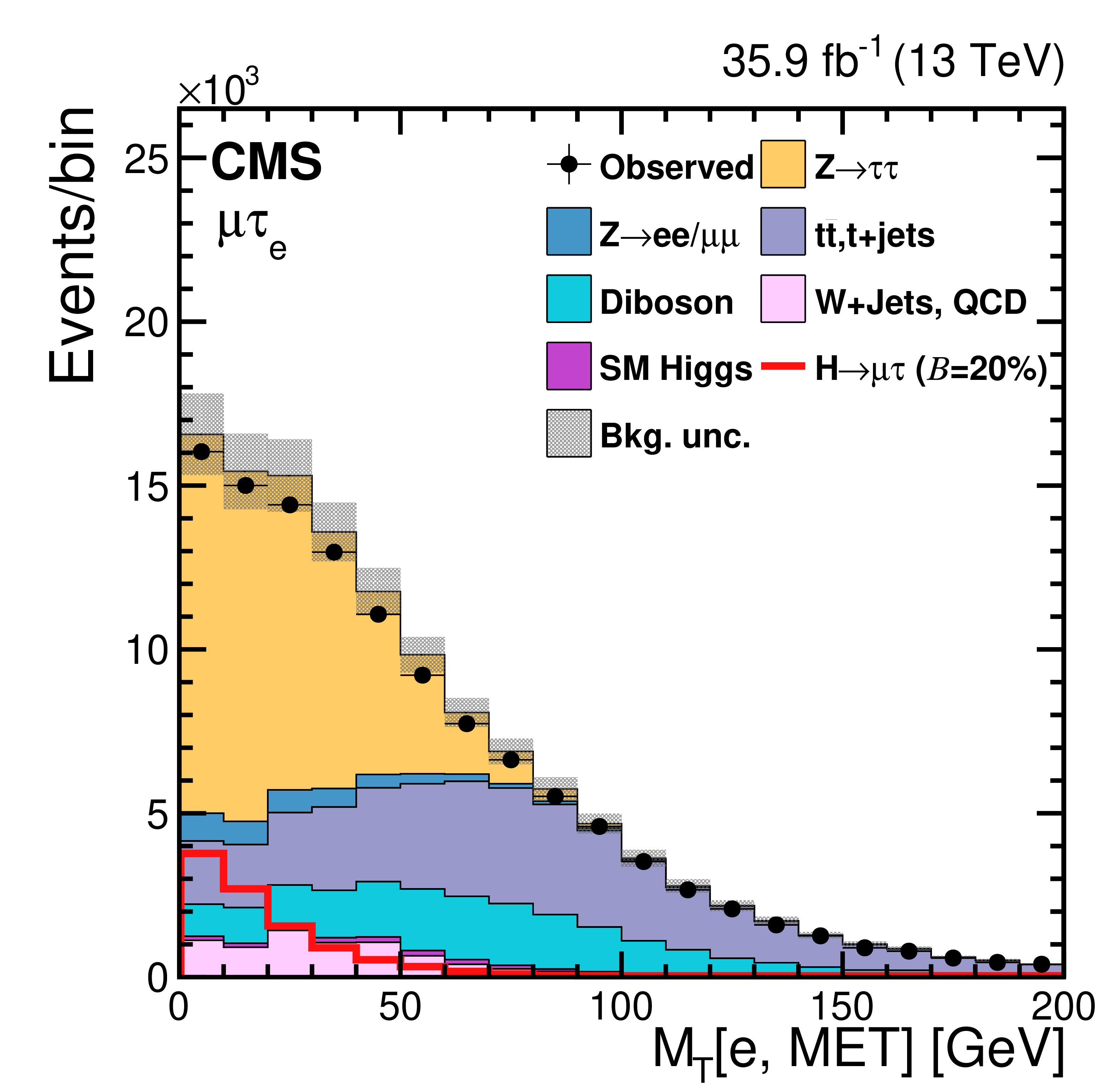
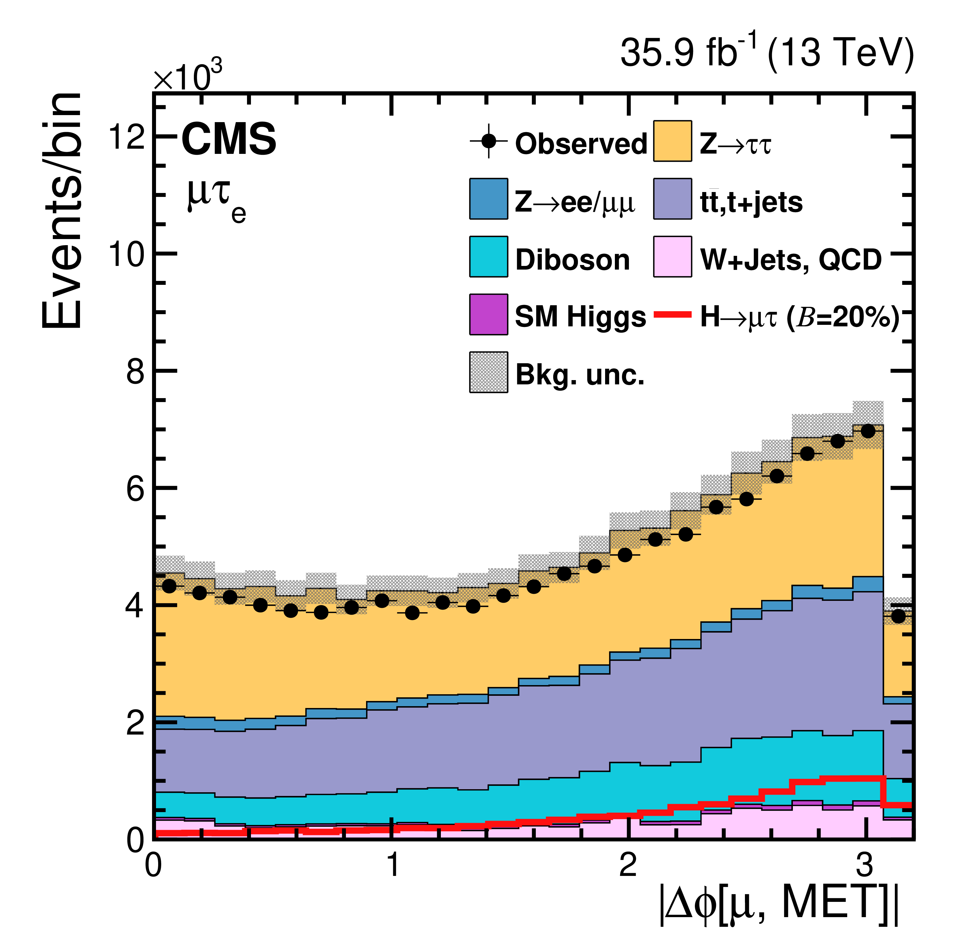
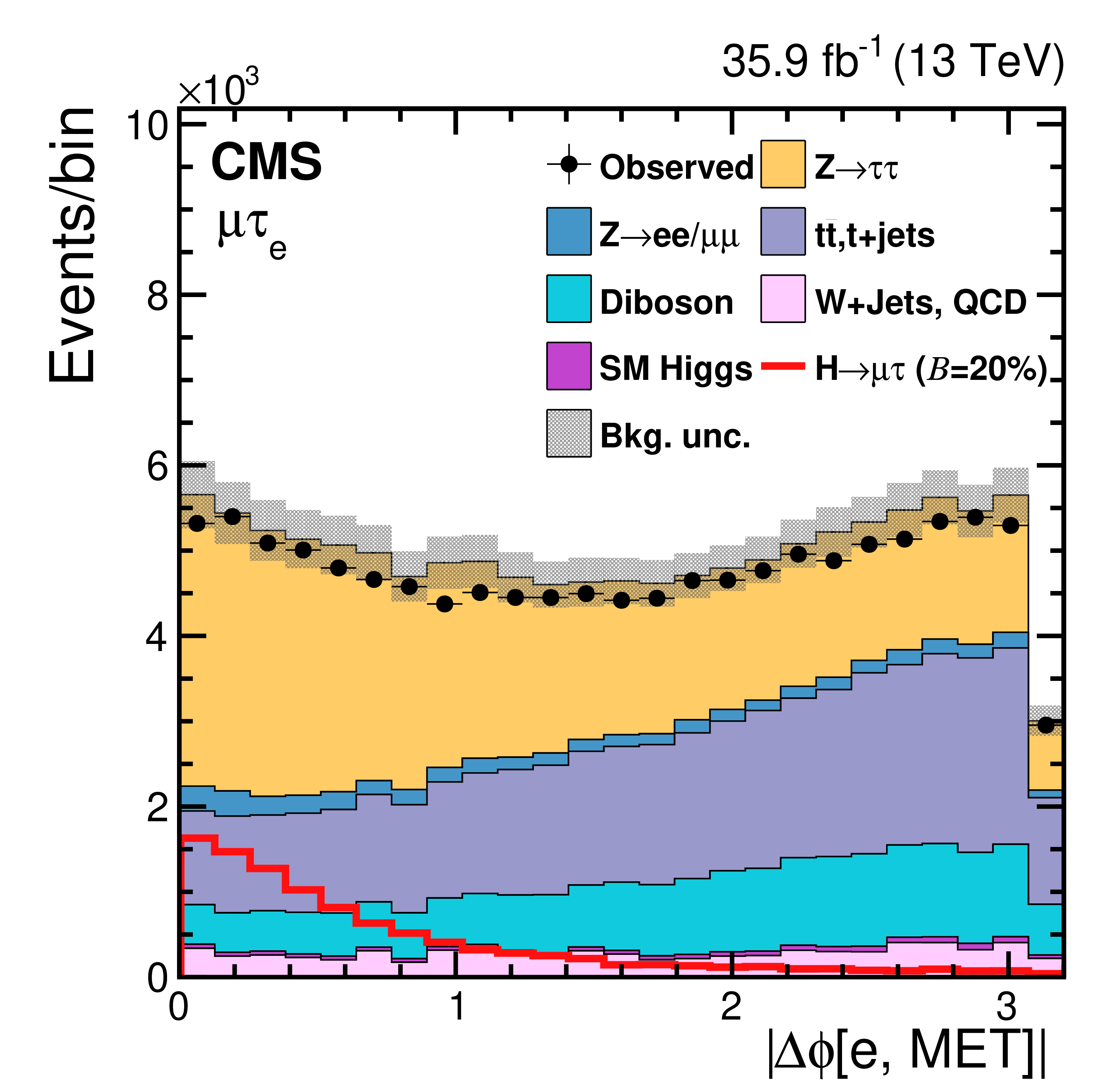
Figure 2:
Distributions of the input variables to the BDT for the $ {{\mathrm {H}} \to {{\mu}} {\tau}_{{\mathrm {e}}}} $ channel. |
png pdf |
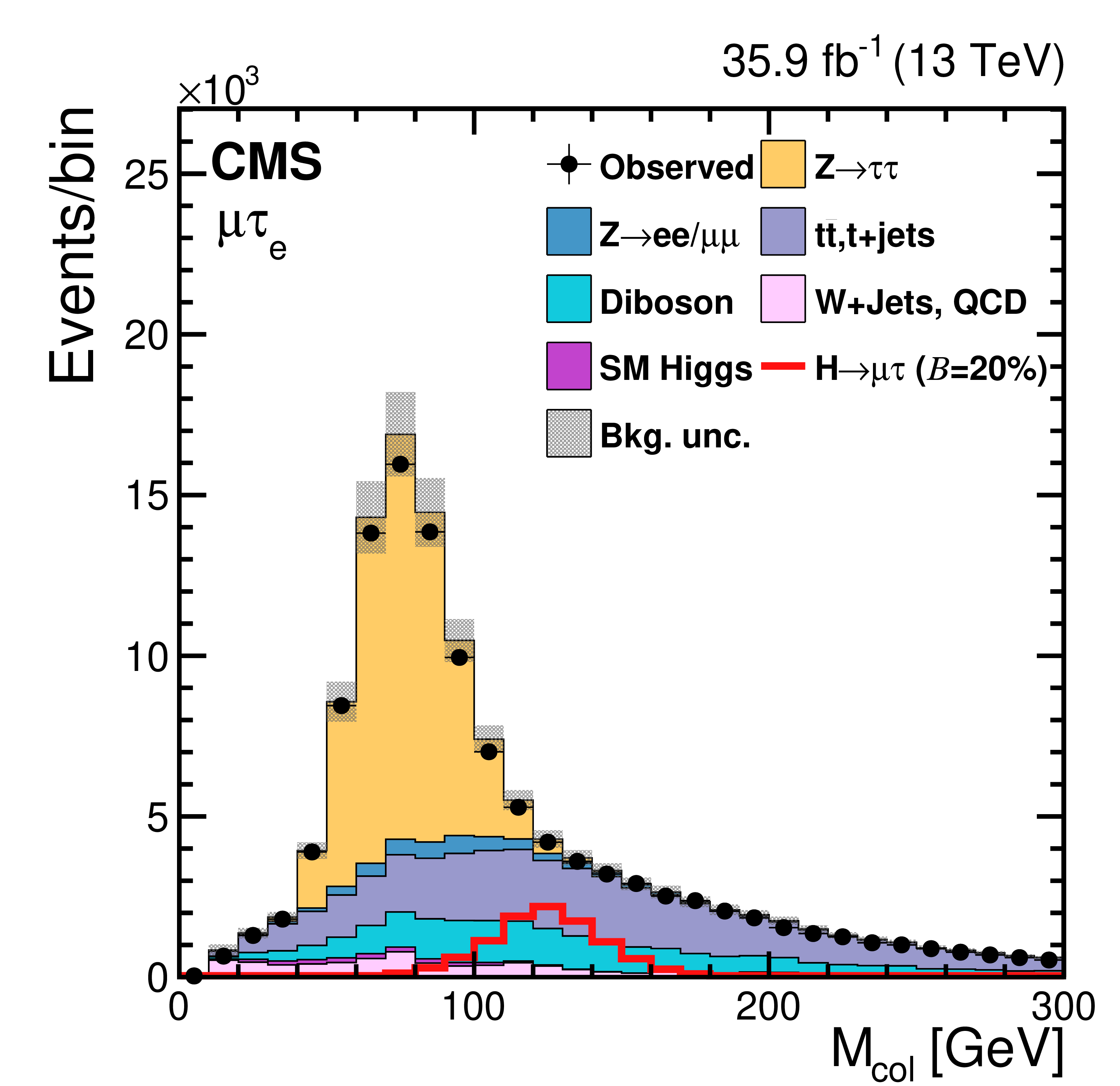
Figure 2-a:
Distribution of one of the input variables to the BDT for the $ {{\mathrm {H}} \to {{\mu}} {\tau}_{{\mathrm {e}}}} $ channel. |
png pdf |
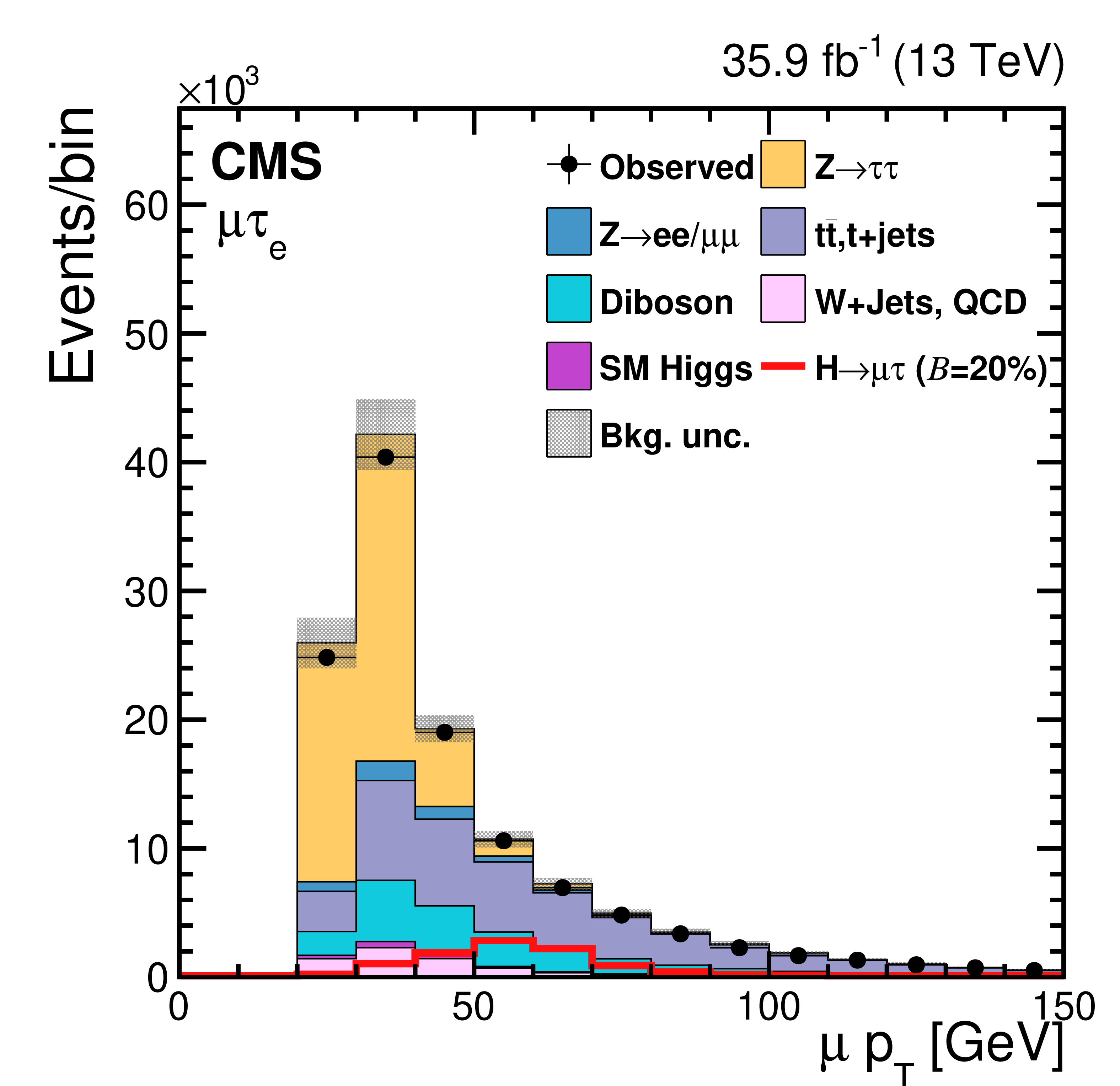
Figure 2-b:
Distribution of one of the input variables to the BDT for the $ {{\mathrm {H}} \to {{\mu}} {\tau}_{{\mathrm {e}}}} $ channel. |
png pdf |
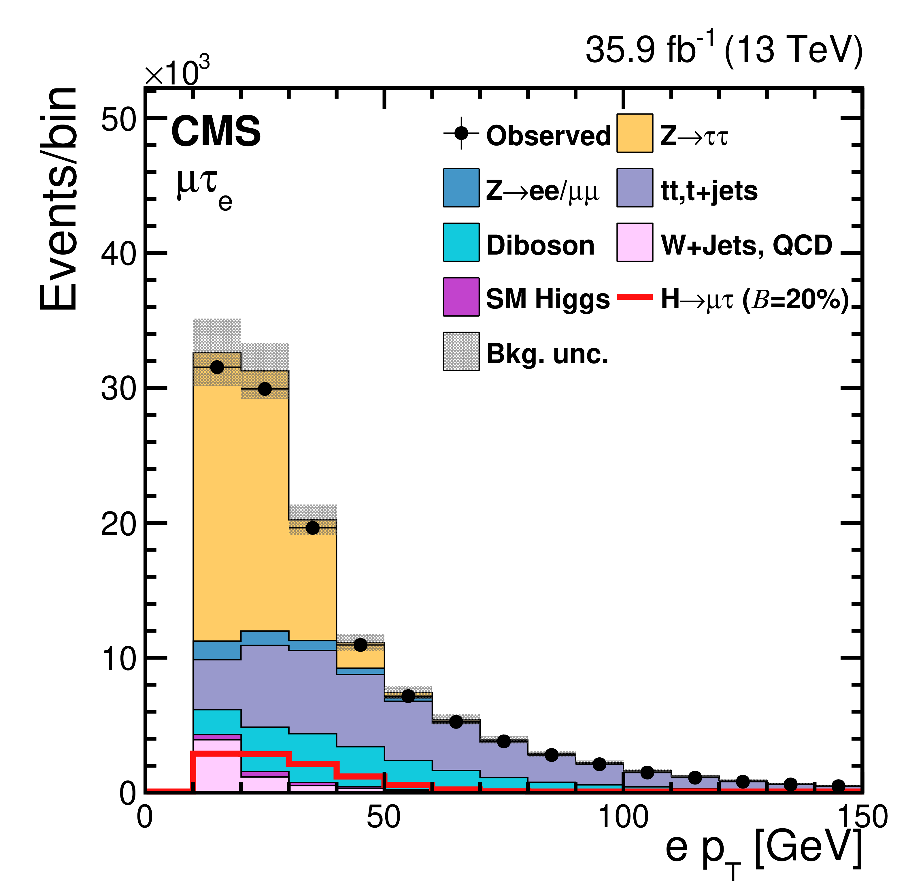
Figure 2-c:
Distribution of one of the input variables to the BDT for the $ {{\mathrm {H}} \to {{\mu}} {\tau}_{{\mathrm {e}}}} $ channel. |
png pdf |
Figure 2-d:
Distribution of one of the input variables to the BDT for the $ {{\mathrm {H}} \to {{\mu}} {\tau}_{{\mathrm {e}}}} $ channel. |
png pdf |
Figure 2-e:
Distribution of one of the input variables to the BDT for the $ {{\mathrm {H}} \to {{\mu}} {\tau}_{{\mathrm {e}}}} $ channel. |
png pdf |
Figure 2-f:
Distribution of one of the input variables to the BDT for the $ {{\mathrm {H}} \to {{\mu}} {\tau}_{{\mathrm {e}}}} $ channel. |
png pdf |
Figure 2-g:
Distribution of one of the input variables to the BDT for the $ {{\mathrm {H}} \to {{\mu}} {\tau}_{{\mathrm {e}}}} $ channel. |

png pdf |
Figure 2-h:
Distribution of one of the input variables to the BDT for the $ {{\mathrm {H}} \to {{\mu}} {\tau}_{{\mathrm {e}}}} $ channel. |
png pdf |
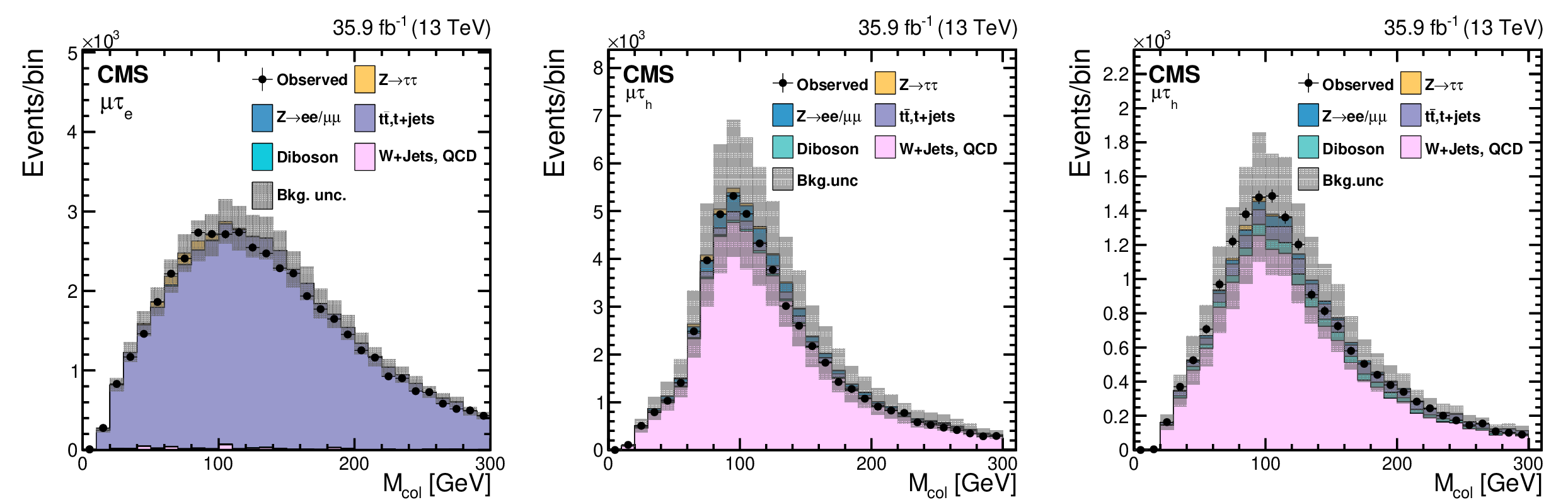
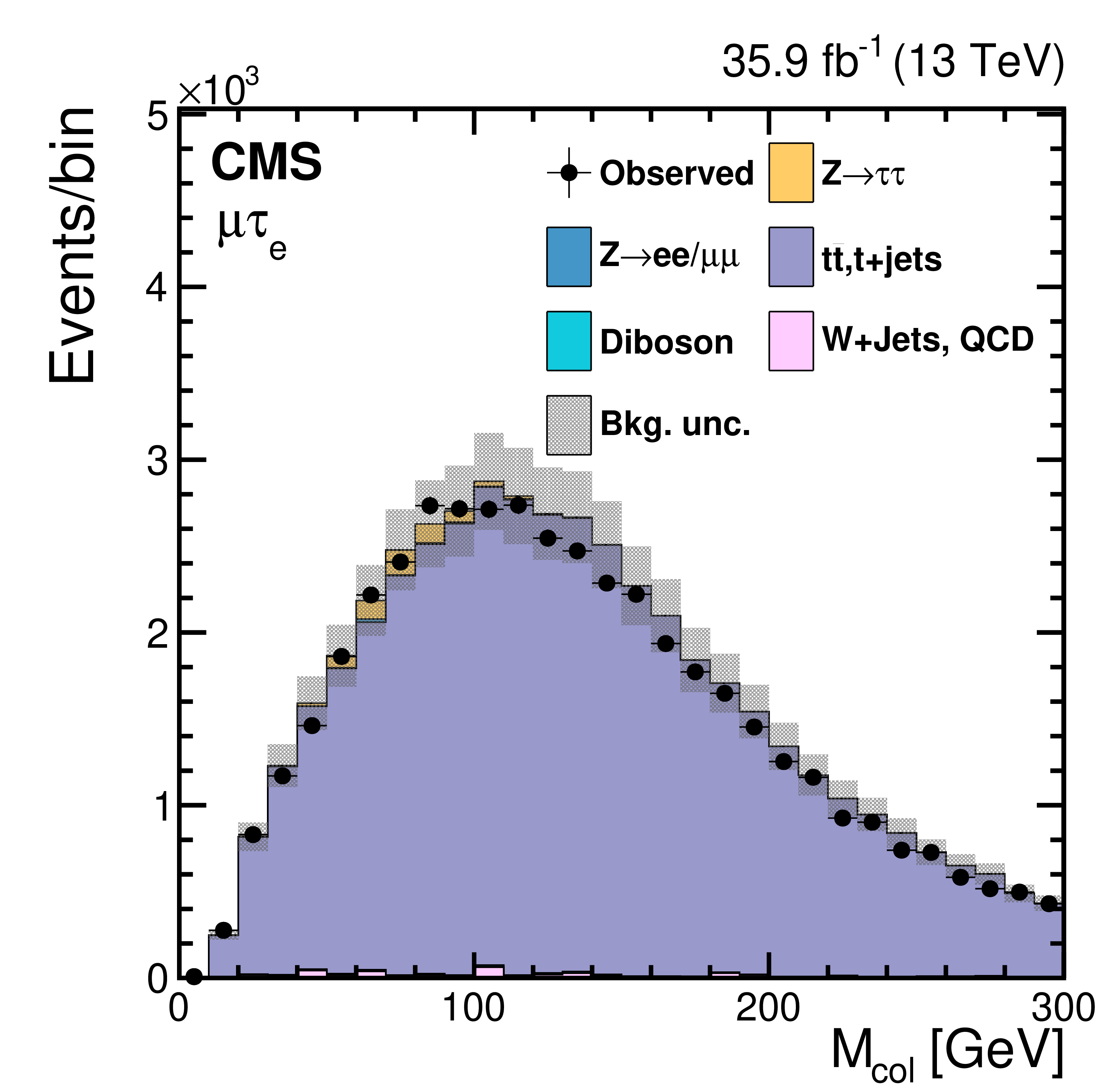
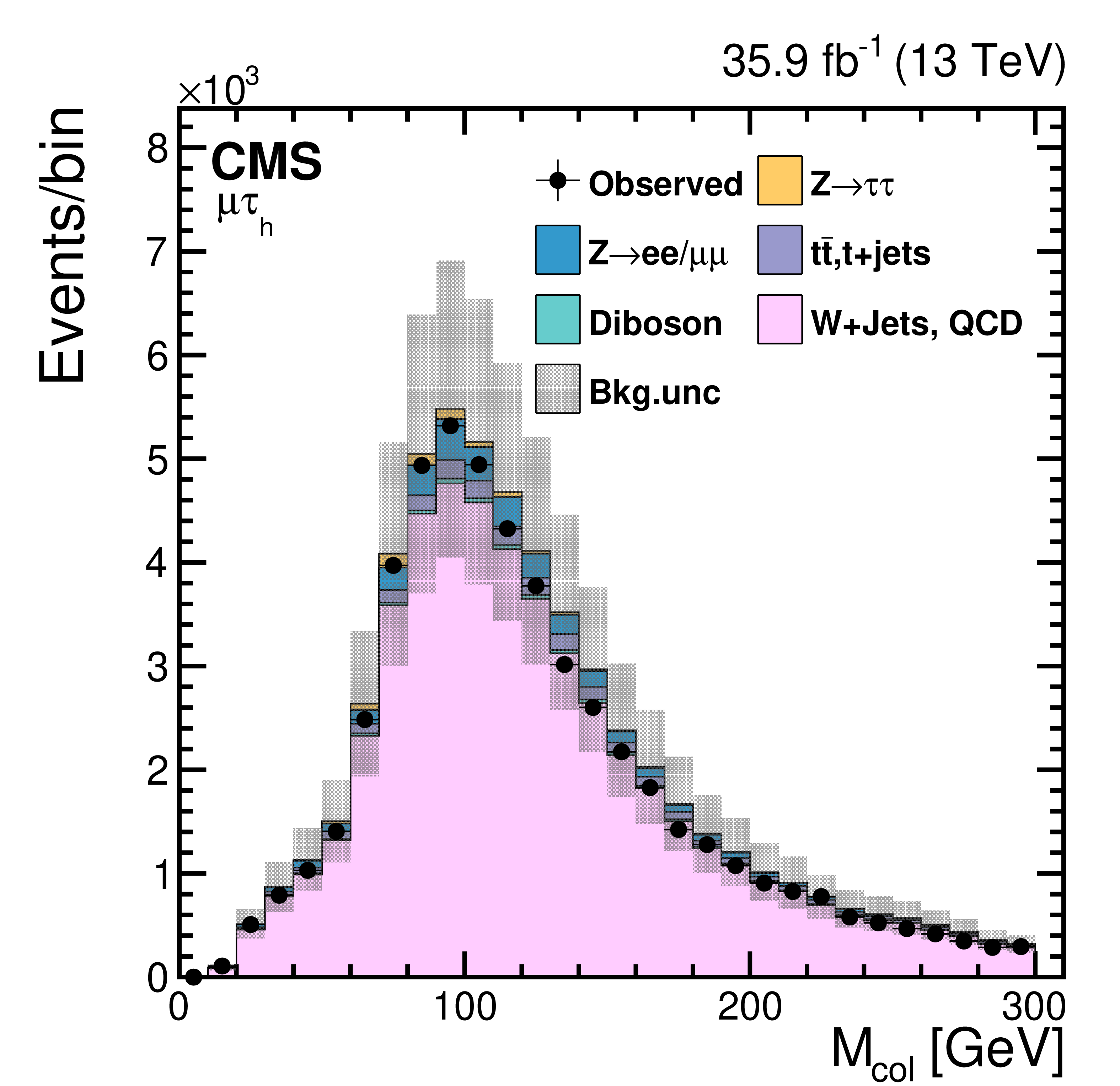
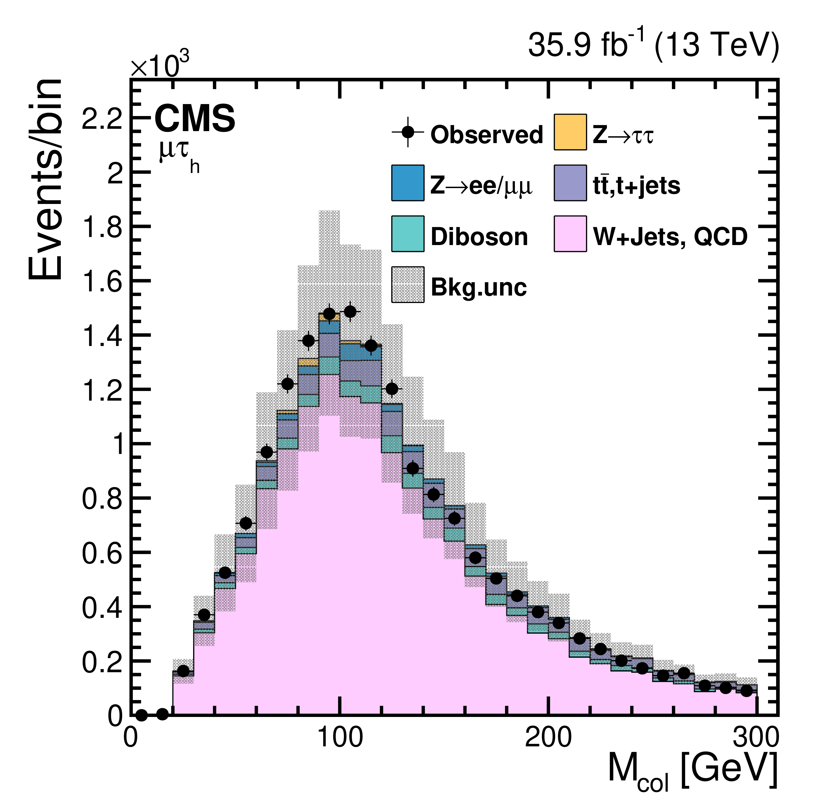
Figure 3:
$ {M_{\text {col}}} $ distribution in $ {\mathrm {t}\overline {\mathrm {t}}} $ enriched (left), like-sign lepton (central), and W+jets enriched (right) control samples defined in the text. The distributions include both statistical and systematic uncertainties. |
png pdf |
Figure 3-a:
$ {M_{\text {col}}} $ distribution in the $ {\mathrm {t}\overline {\mathrm {t}}} $ enriched control sample defined in the text. The distributions include both statistical and systematic uncertainties. |
png pdf |
Figure 3-b:
$ {M_{\text {col}}} $ distribution in the like-sign lepton control sample defined in the text. The distributions include both statistical and systematic uncertainties. |
png pdf |
Figure 3-c:
$ {M_{\text {col}}} $ distribution in the W+jets enriched control sample defined in the text. The distributions include both statistical and systematic uncertainties. |

png pdf |
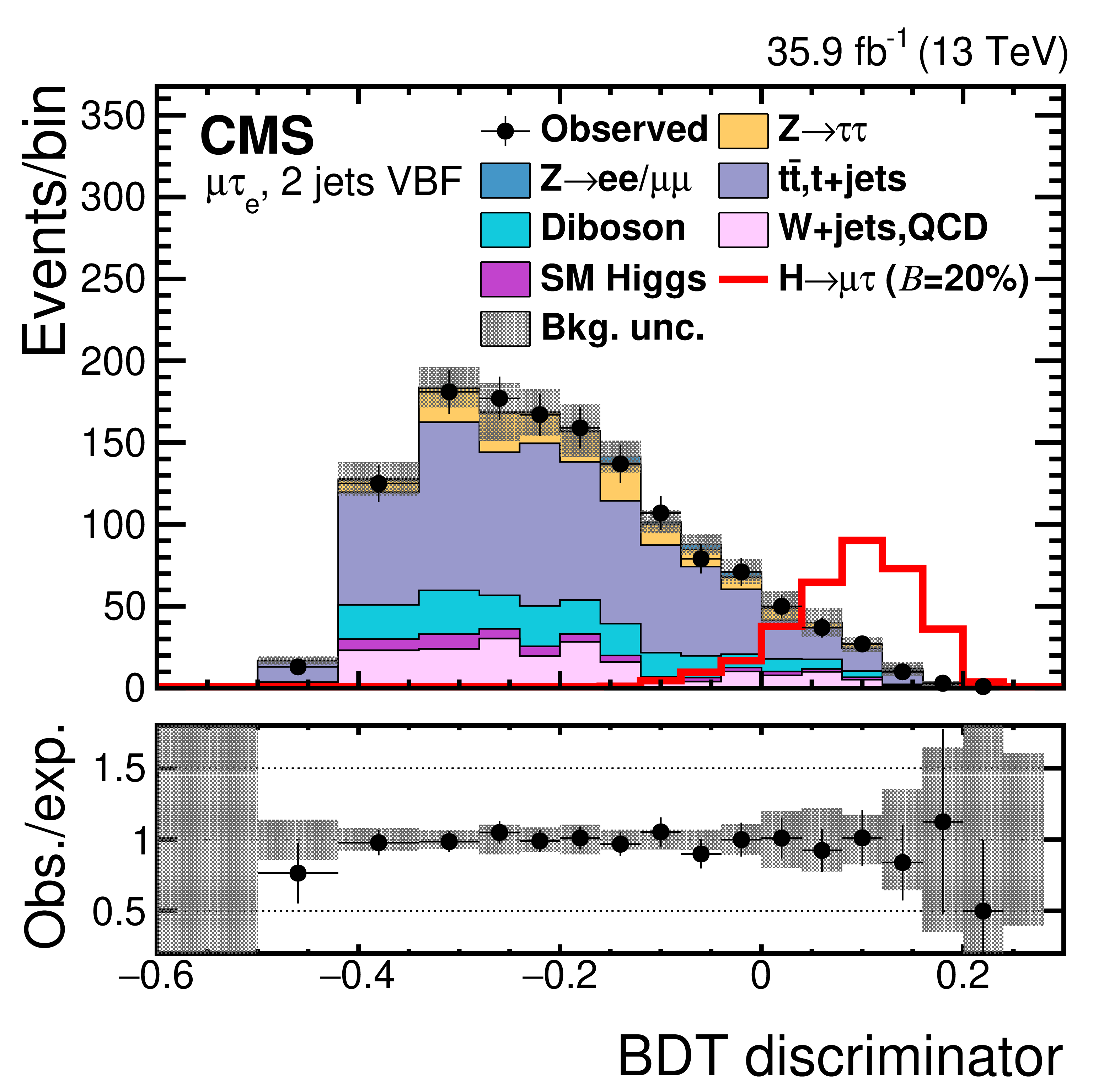
Figure 4:
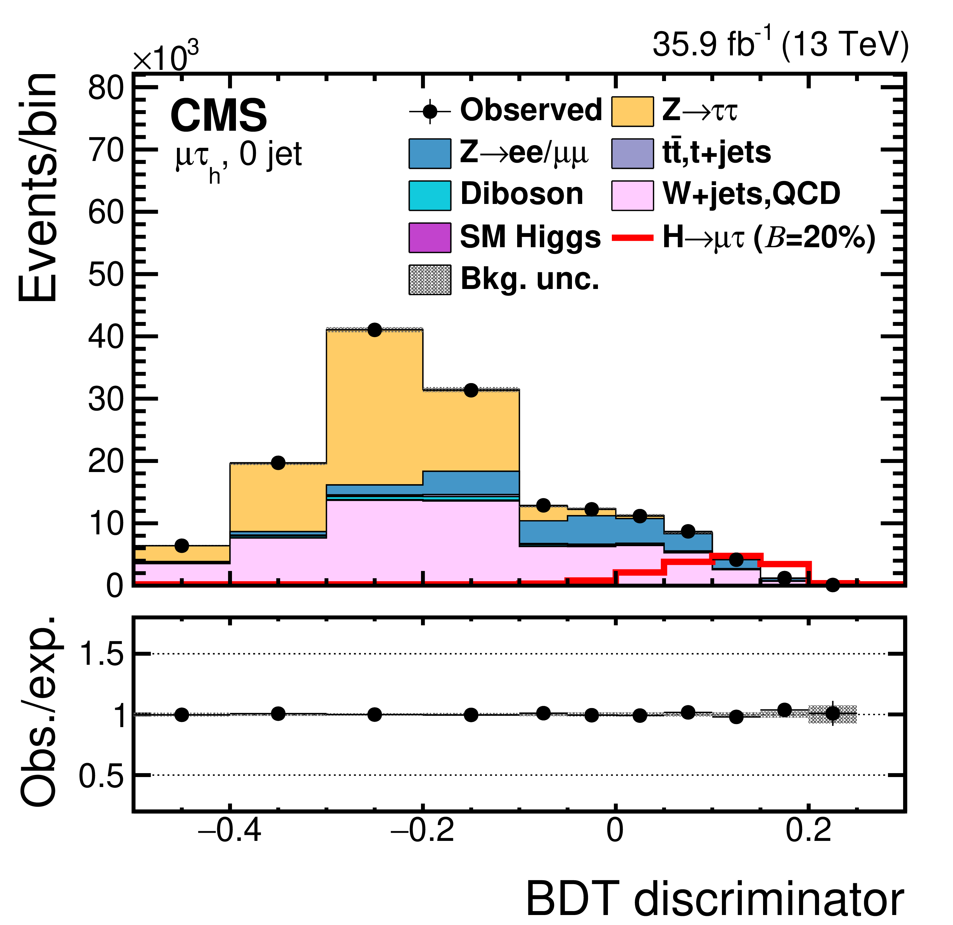
Distribution of the BDT discriminator for the $ {\mathrm {H}} \to {{\mu}} {\tau}$ process in the BDT fit analysis, in the individual channels and categories compared to the signal and background estimation. The background is normalized to the best fit values from the signal plus background fit while the simulated signal corresponds to $\mathcal {B}({\mathrm {H}} \to {{\mu}} {\tau})=$ 5%. The bottom panel in each plot shows the fractional difference between the observed data and the fitted background. The left column of plots corresponds to the $ {\mathrm {H}} \to {{\mu}} {{\tau} _\mathrm {h}} $ categories, from 0-jets (first row) to 2-jets VBF (fourth row). The right one to their $ {\mathrm {H}} \to {{\mu}} {\tau}_{{\mathrm {e}}}$ counterparts. |
png pdf |
Figure 4-a:
Distribution of the BDT discriminator for the $ {\mathrm {H}} \to {{\mu}} {\tau}$ process in the BDT fit analysis, in the $ {\mathrm {H}} \to {{\mu}} {{\tau}_{\mathrm {h}}} $ channel, 0-jet category, compared to the signal and background estimation. The background is normalized to the best fit values from the signal plus background fit while the simulated signal corresponds to $\mathcal {B}({\mathrm {H}} \to {{\mu}} {\tau})=$ 5%. The bottom panel shows the fractional difference between the observed data and the fitted background. |

png pdf |
Figure 4-b:
Distribution of the BDT discriminator for the $ {\mathrm {H}} \to {{\mu}} {\tau}$ process in the BDT fit analysis, in the $ {\mathrm {H}} \to {{\mu}} {{\tau}_{\mathrm { e}}} $ channel, 0-jet category, compared to the signal and background estimation. The background is normalized to the best fit values from the signal plus background fit while the simulated signal corresponds to $\mathcal {B}({\mathrm {H}} \to {{\mu}} {\tau})=$ 5%. The bottom panel shows the fractional difference between the observed data and the fitted background. |
png pdf |
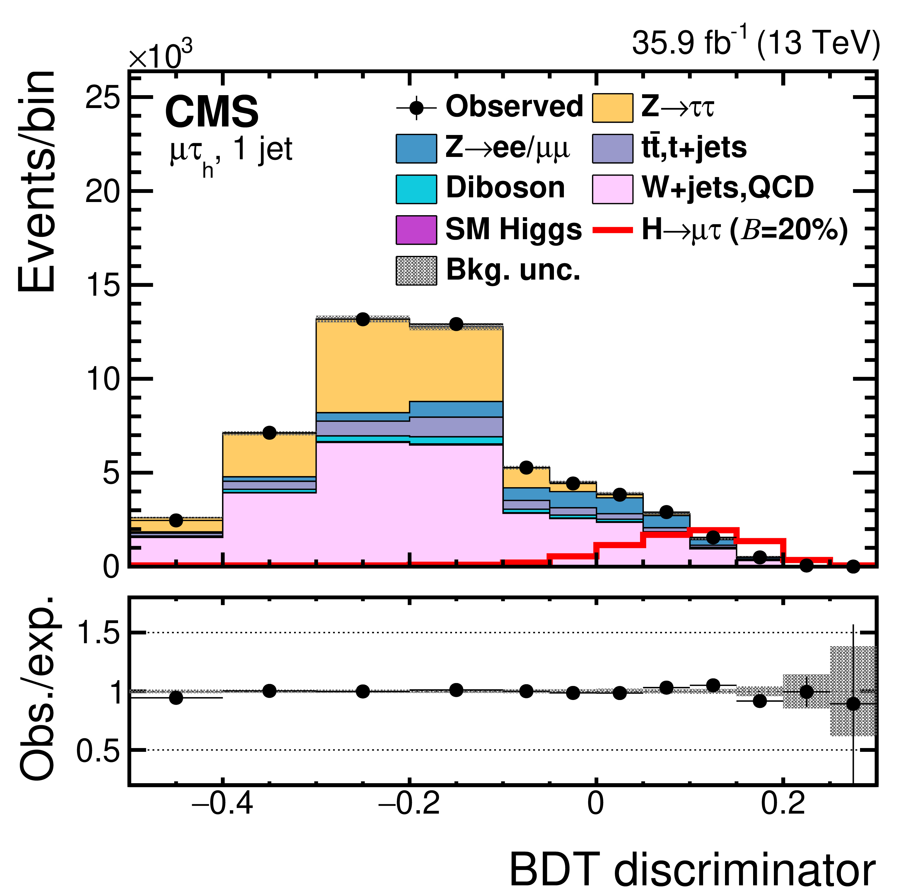
Figure 4-c:
Distribution of the BDT discriminator for the $ {\mathrm {H}} \to {{\mu}} {\tau}$ process in the BDT fit analysis, in the $ {\mathrm {H}} \to {{\mu}} {{\tau}_{\mathrm {h }}} $ channel, 1-jet category, compared to the signal and background estimation. The background is normalized to the best fit values from the signal plus background fit while the simulated signal corresponds to $\mathcal {B}({\mathrm {H}} \to {{\mu}} {\tau})=$ 5%. The bottom panel shows the fractional difference between the observed data and the fitted background. |

png pdf |
Figure 4-d:
Distribution of the BDT discriminator for the $ {\mathrm {H}} \to {{\mu}} {\tau}$ process in the BDT fit analysis, in the $ {\mathrm {H}} \to {{\mu}} {{\tau}_{\mathrm { e}}} $ channel, 1-jet category, compared to the signal and background estimation. The background is normalized to the best fit values from the signal plus background fit while the simulated signal corresponds to $\mathcal {B}({\mathrm {H}} \to {{\mu}} {\tau})=$ 5%. The bottom panel shows the fractional difference between the observed data and the fitted background. |
png pdf |
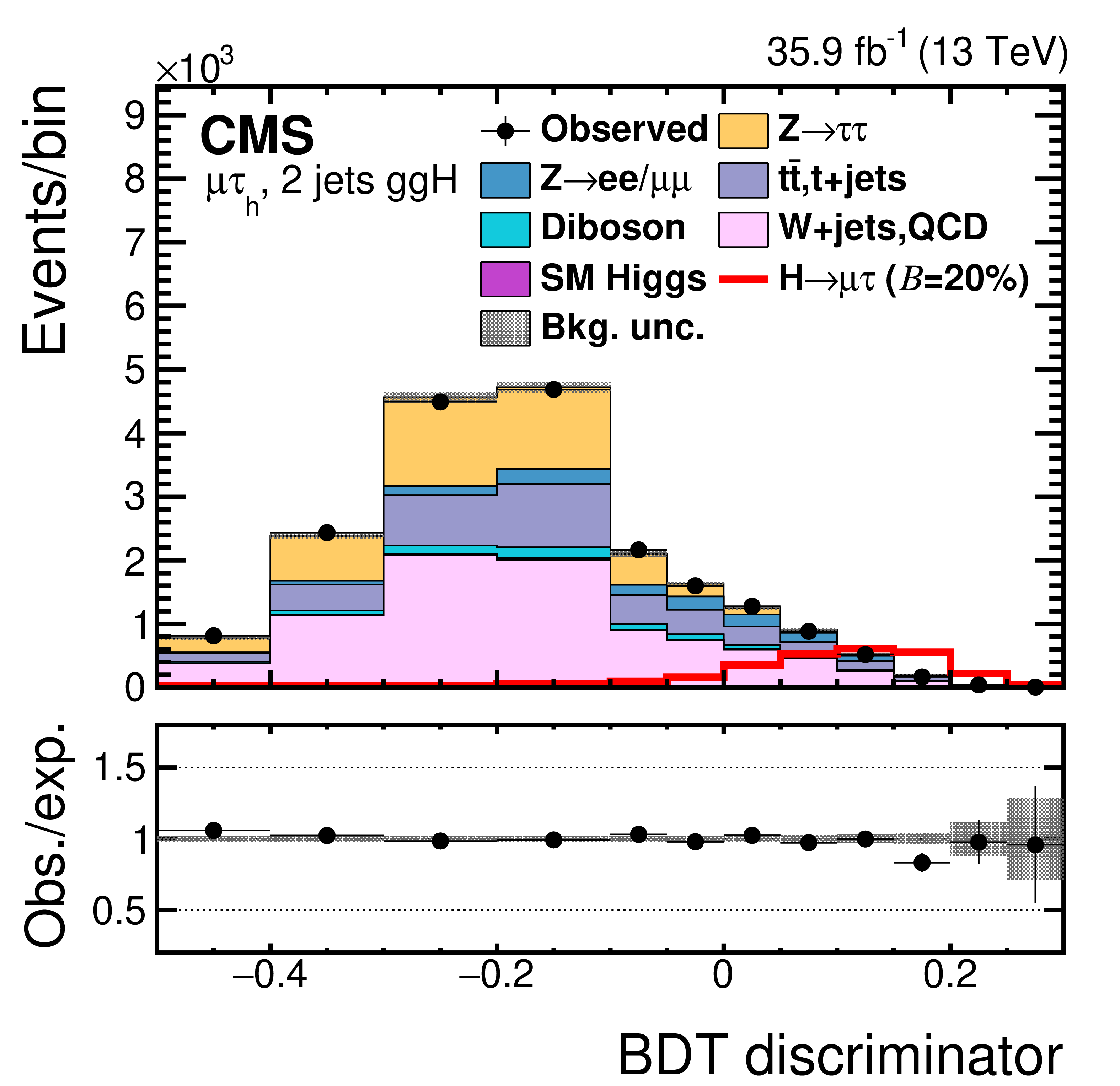
Figure 4-e:
Distribution of the BDT discriminator for the $ {\mathrm {H}} \to {{\mu}} {\tau}$ process in the BDT fit analysis, in the $ {\mathrm {H}} \to {{\mu}} {{\tau}_{\mathrm {h }}} $ channel, 2-jets ggH category, compared to the signal and background estimation. The background is normalized to the best fit values from the signal plus background fit while the simulated signal corresponds to $\mathcal {B}({\mathrm {H}} \to {{\mu}} {\tau})=$ 5%. The bottom panel shows the fractional difference between the observed data and the fitted background. |
png pdf |
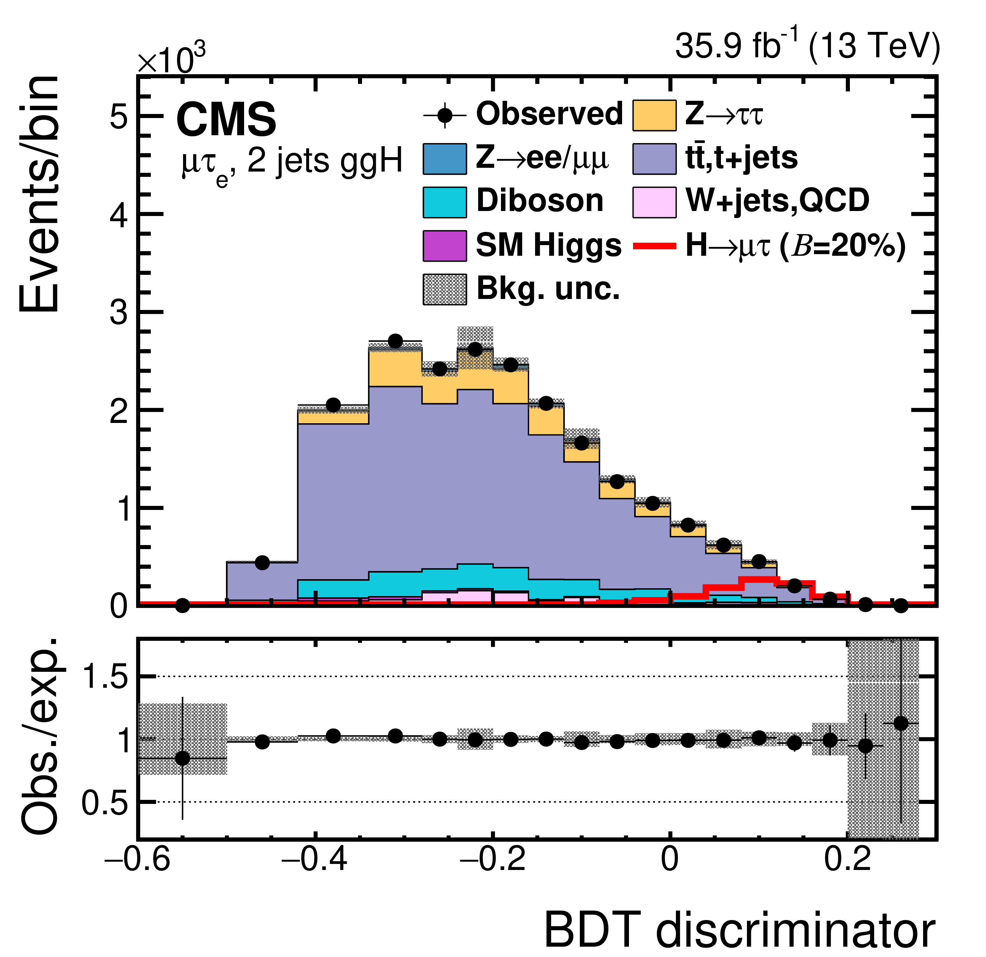
Figure 4-f:
Distribution of the BDT discriminator for the $ {\mathrm {H}} \to {{\mu}} {\tau}$ process in the BDT fit analysis, in the $ {\mathrm {H}} \to {{\mu}} {{\tau}_{\mathrm { e}}} $ channel, 2-jets ggH category, compared to the signal and background estimation. The background is normalized to the best fit values from the signal plus background fit while the simulated signal corresponds to $\mathcal {B}({\mathrm {H}} \to {{\mu}} {\tau})=$ 5%. The bottom panel shows the fractional difference between the observed data and the fitted background. |
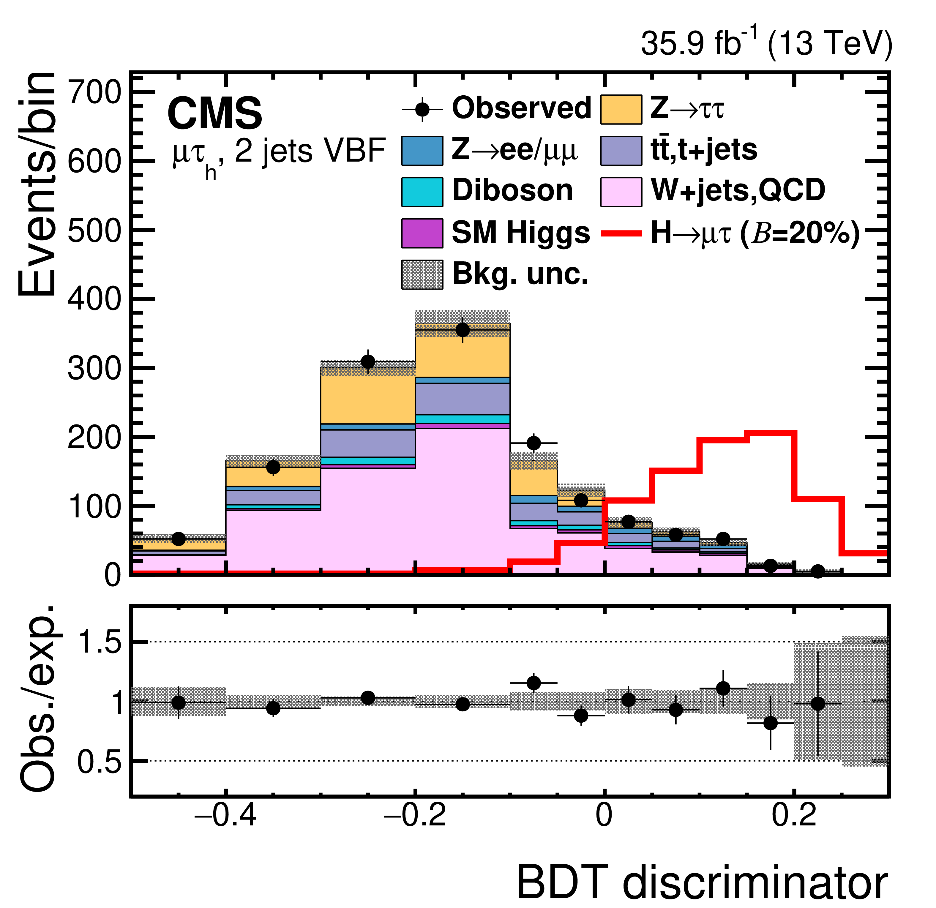
png pdf |
Figure 4-g:
Distribution of the BDT discriminator for the $ {\mathrm {H}} \to {{\mu}} {\tau}$ process in the BDT fit analysis, in the $ {\mathrm {H}} \to {{\mu}} {{\tau}_{\mathrm {h }}} $ channel, 2-jets VBF category, compared to the signal and background estimation. The background is normalized to the best fit values from the signal plus background fit while the simulated signal corresponds to $\mathcal {B}({\mathrm {H}} \to {{\mu}} {\tau})=$ 5%. The bottom panel shows the fractional difference between the observed data and the fitted background. |
png pdf |
Figure 4-h:
Distribution of the BDT discriminator for the $ {\mathrm {H}} \to {{\mu}} {\tau}$ process in the BDT fit analysis, in the $ {\mathrm {H}} \to {{\mu}} {{\tau}_{\mathrm { e}}} $ channel, 2-jets VBF category, compared to the signal and background estimation. The background is normalized to the best fit values from the signal plus background fit while the simulated signal corresponds to $\mathcal {B}({\mathrm {H}} \to {{\mu}} {\tau})=$ 5%. The bottom panel shows the fractional difference between the observed data and the fitted background. |

png pdf |
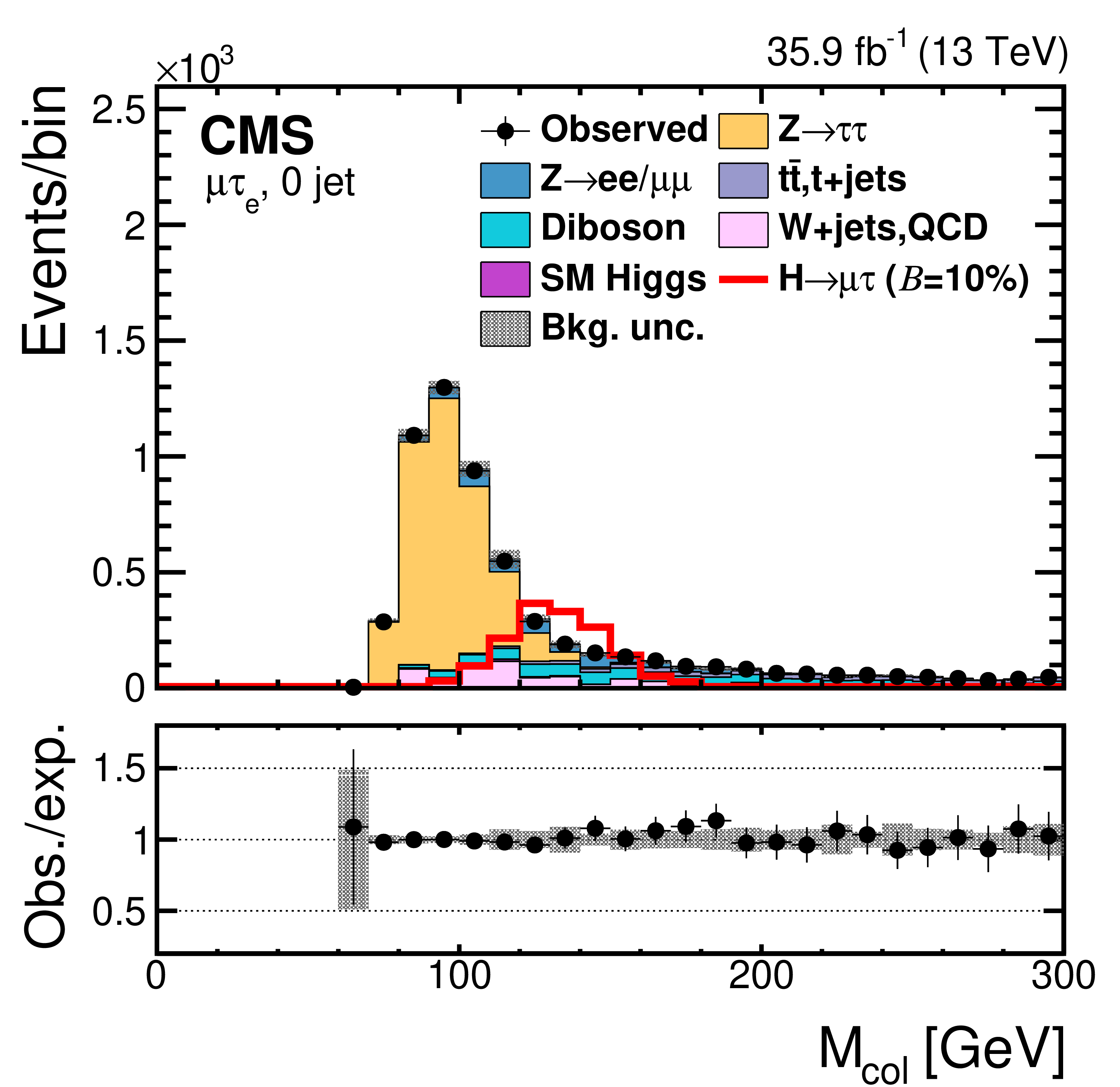
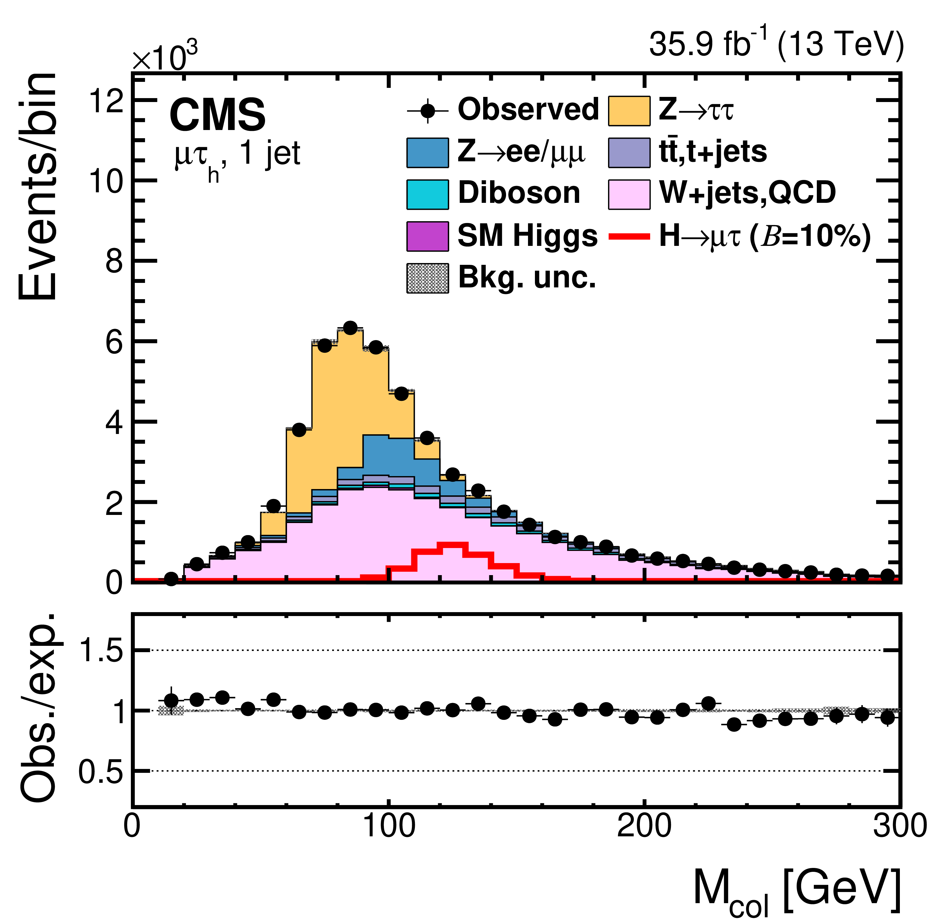
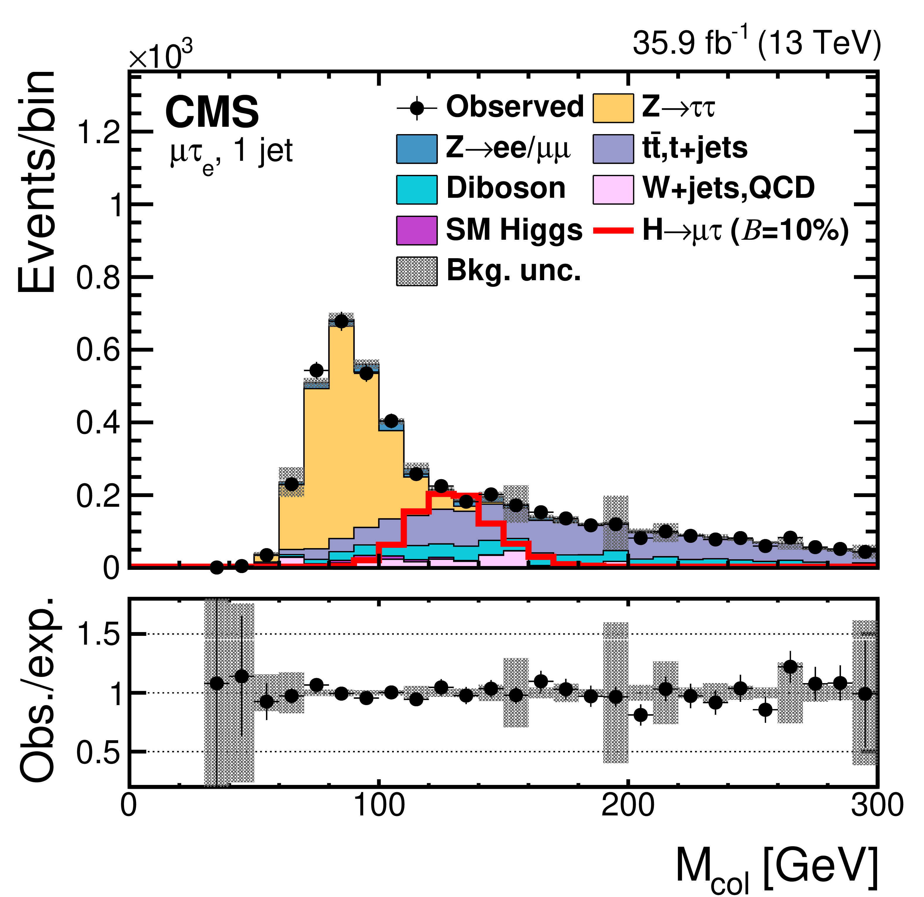
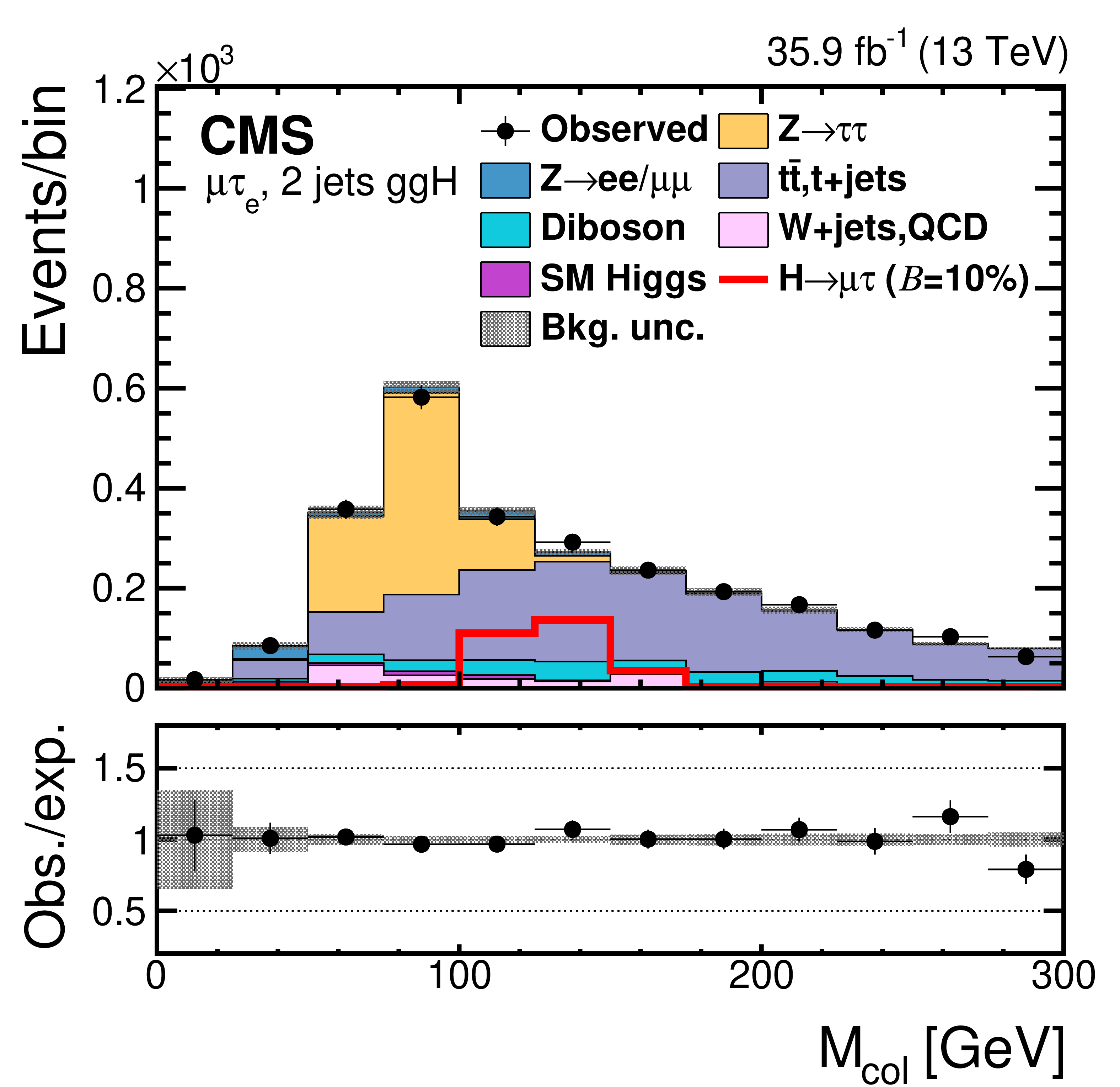
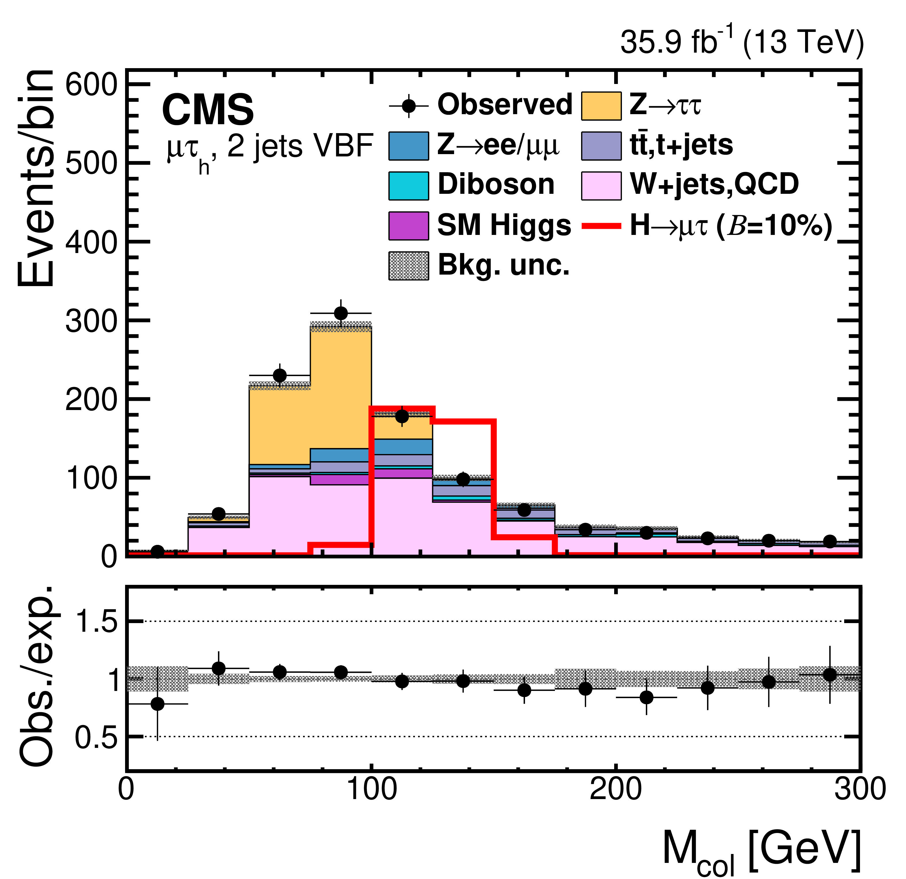
Figure 5:
Distribution of the collinear mass $ {M_{\text {col}}} $ for the $ {\mathrm {H}} \to {{\mu}} {\tau}$ process in $ {M_{\text {col}}} $ fit analysis, in different channels and categories compared to the signal and background estimation. The background is normalized to the best fit values from the signal plus background fit while the overlaid simulated signal corresponds to $\mathcal {B}({\mathrm {H}} \to {{\mu}} {\tau})= $ 5%. The bottom panel in each plot shows the ratio between the observed data and the fitted background. The left column of plots corresponds to the $ {\mathrm {H}} \to {{\mu}} {{\tau} _\mathrm {h}} $ categories, from 0-jets (first row) to 2-jets VBF (fourth row). The right one to their $ {\mathrm {H}} \to {{\mu}} {\tau}_{{\mathrm {e}}}$ counterparts. |

png pdf |
Figure 5-a:
Distribution of the collinear mass $ {M_{\text {col}}} $ for the $ {\mathrm {H}} \to {{\mu}} {\tau}$ process in $ {M_{\text {col}}} $ fit analysis, in the $ {\mathrm {H}} \to {{\mu}} {{\tau} _{\mathrm {h} {\mathrm {e}} } $ channel, category, compared to the signal and background estimation. The background is normalized to the best fit values from the signal plus background fit while the overlaid simulated signal corresponds to $\mathcal {B}({\mathrm {H}} \to {{\mu}} {\tau})=5%$. The bottom panel in each plot shows the ratio between the observed data and the fitted background. The left column of plots corresponds to the $ {\mathrm {H}} \to {{\mu}} {{\tau} _\mathrm {h}} $ categories, from 0-jets (first row) to 2-jets VBF (fourth row). The right one to their $ {\mathrm {H}} \to {{\mu}} {\tau}_{{\mathrm {e}}}$ counterparts. |
png pdf |
Figure 5-b:
Distribution of the collinear mass $ {M_{\text {col}}} $ for the $ {\mathrm {H}} \to {{\mu}} {\tau}$ process in $ {M_{\text {col}}} $ fit analysis, in different channels and categories compared to the signal and background estimation. The background is normalized to the best fit values from the signal plus background fit while the overlaid simulated signal corresponds to $\mathcal {B}({\mathrm {H}} \to {{\mu}} {\tau})= $ 5%. The bottom panel in each plot shows the ratio between the observed data and the fitted background. The left column of plots corresponds to the $ {\mathrm {H}} \to {{\mu}} {{\tau} _\mathrm {h}} $ categories, from 0-jets (first row) to 2-jets VBF (fourth row). The right one to their $ {\mathrm {H}} \to {{\mu}} {\tau}_{{\mathrm {e}}}$ counterparts. |
png pdf |
Figure 5-c:
Distribution of the collinear mass $ {M_{\text {col}}} $ for the $ {\mathrm {H}} \to {{\mu}} {\tau}$ process in $ {M_{\text {col}}} $ fit analysis, in different channels and categories compared to the signal and background estimation. The background is normalized to the best fit values from the signal plus background fit while the overlaid simulated signal corresponds to $\mathcal {B}({\mathrm {H}} \to {{\mu}} {\tau})= $ 5%. The bottom panel in each plot shows the ratio between the observed data and the fitted background. The left column of plots corresponds to the $ {\mathrm {H}} \to {{\mu}} {{\tau} _\mathrm {h}} $ categories, from 0-jets (first row) to 2-jets VBF (fourth row). The right one to their $ {\mathrm {H}} \to {{\mu}} {\tau}_{{\mathrm {e}}}$ counterparts. |
png pdf |
Figure 5-d:
Distribution of the collinear mass $ {M_{\text {col}}} $ for the $ {\mathrm {H}} \to {{\mu}} {\tau}$ process in $ {M_{\text {col}}} $ fit analysis, in different channels and categories compared to the signal and background estimation. The background is normalized to the best fit values from the signal plus background fit while the overlaid simulated signal corresponds to $\mathcal {B}({\mathrm {H}} \to {{\mu}} {\tau})= $ 5%. The bottom panel in each plot shows the ratio between the observed data and the fitted background. The left column of plots corresponds to the $ {\mathrm {H}} \to {{\mu}} {{\tau} _\mathrm {h}} $ categories, from 0-jets (first row) to 2-jets VBF (fourth row). The right one to their $ {\mathrm {H}} \to {{\mu}} {\tau}_{{\mathrm {e}}}$ counterparts. |

png pdf |
Figure 5-e:
Distribution of the collinear mass $ {M_{\text {col}}} $ for the $ {\mathrm {H}} \to {{\mu}} {\tau}$ process in $ {M_{\text {col}}} $ fit analysis, in different channels and categories compared to the signal and background estimation. The background is normalized to the best fit values from the signal plus background fit while the overlaid simulated signal corresponds to $\mathcal {B}({\mathrm {H}} \to {{\mu}} {\tau})= $ 5%. The bottom panel in each plot shows the ratio between the observed data and the fitted background. The left column of plots corresponds to the $ {\mathrm {H}} \to {{\mu}} {{\tau} _\mathrm {h}} $ categories, from 0-jets (first row) to 2-jets VBF (fourth row). The right one to their $ {\mathrm {H}} \to {{\mu}} {\tau}_{{\mathrm {e}}}$ counterparts. |
png pdf |
Figure 5-f:
Distribution of the collinear mass $ {M_{\text {col}}} $ for the $ {\mathrm {H}} \to {{\mu}} {\tau}$ process in $ {M_{\text {col}}} $ fit analysis, in different channels and categories compared to the signal and background estimation. The background is normalized to the best fit values from the signal plus background fit while the overlaid simulated signal corresponds to $\mathcal {B}({\mathrm {H}} \to {{\mu}} {\tau})= $ 5%. The bottom panel in each plot shows the ratio between the observed data and the fitted background. The left column of plots corresponds to the $ {\mathrm {H}} \to {{\mu}} {{\tau} _\mathrm {h}} $ categories, from 0-jets (first row) to 2-jets VBF (fourth row). The right one to their $ {\mathrm {H}} \to {{\mu}} {\tau}_{{\mathrm {e}}}$ counterparts. |
png pdf |
Figure 5-g:
Distribution of the collinear mass $ {M_{\text {col}}} $ for the $ {\mathrm {H}} \to {{\mu}} {\tau}$ process in $ {M_{\text {col}}} $ fit analysis, in different channels and categories compared to the signal and background estimation. The background is normalized to the best fit values from the signal plus background fit while the overlaid simulated signal corresponds to $\mathcal {B}({\mathrm {H}} \to {{\mu}} {\tau})= $ 5%. The bottom panel in each plot shows the ratio between the observed data and the fitted background. The left column of plots corresponds to the $ {\mathrm {H}} \to {{\mu}} {{\tau} _\mathrm {h}} $ categories, from 0-jets (first row) to 2-jets VBF (fourth row). The right one to their $ {\mathrm {H}} \to {{\mu}} {\tau}_{{\mathrm {e}}}$ counterparts. |

png pdf |
Figure 5-h:
Distribution of the collinear mass $ {M_{\text {col}}} $ for the $ {\mathrm {H}} \to {{\mu}} {\tau}$ process in $ {M_{\text {col}}} $ fit analysis, in different channels and categories compared to the signal and background estimation. The background is normalized to the best fit values from the signal plus background fit while the overlaid simulated signal corresponds to $\mathcal {B}({\mathrm {H}} \to {{\mu}} {\tau})= $ 5%. The bottom panel in each plot shows the ratio between the observed data and the fitted background. The left column of plots corresponds to the $ {\mathrm {H}} \to {{\mu}} {{\tau} _\mathrm {h}} $ categories, from 0-jets (first row) to 2-jets VBF (fourth row). The right one to their $ {\mathrm {H}} \to {{\mu}} {\tau}_{{\mathrm {e}}}$ counterparts. |
png pdf |
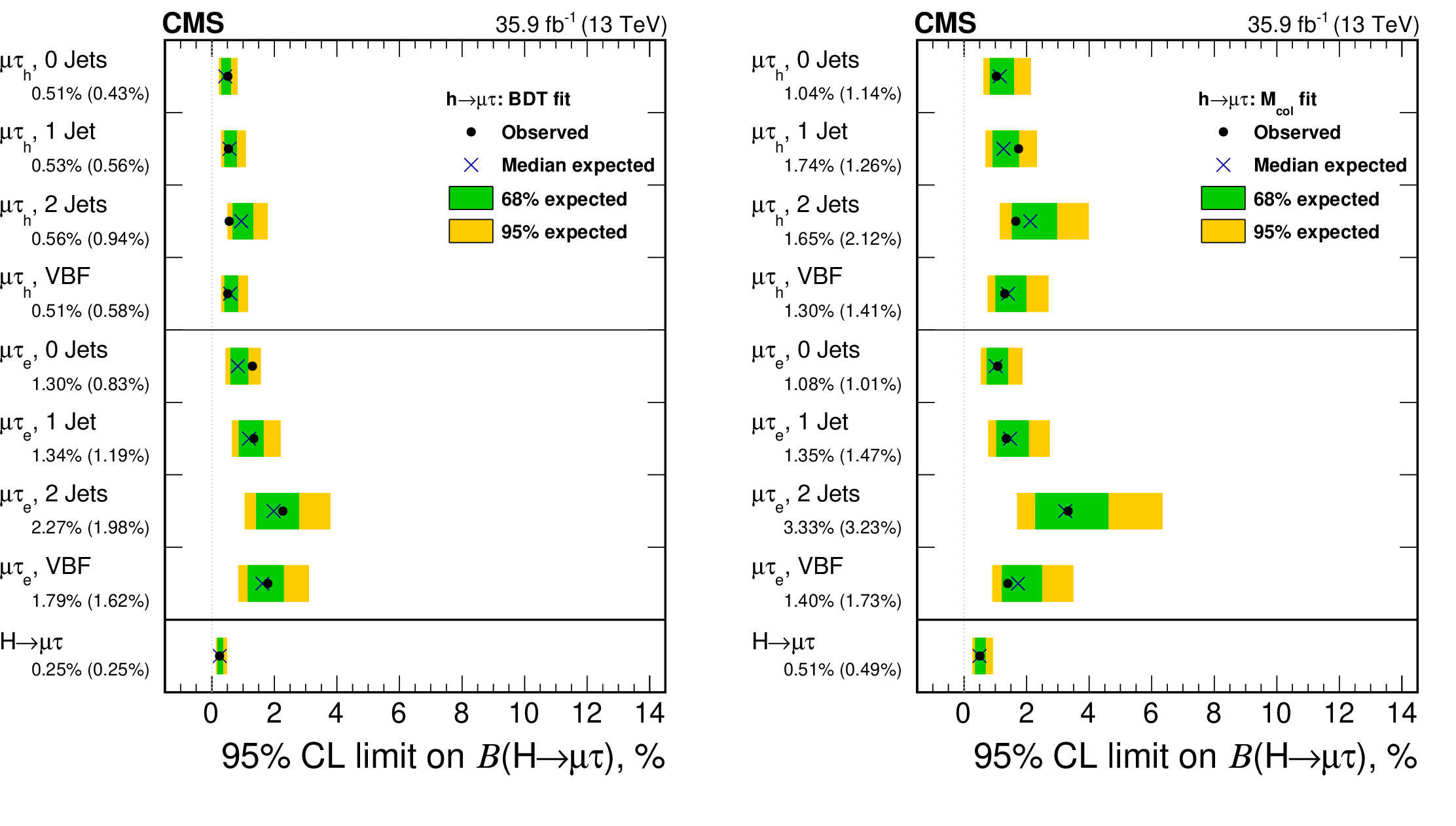
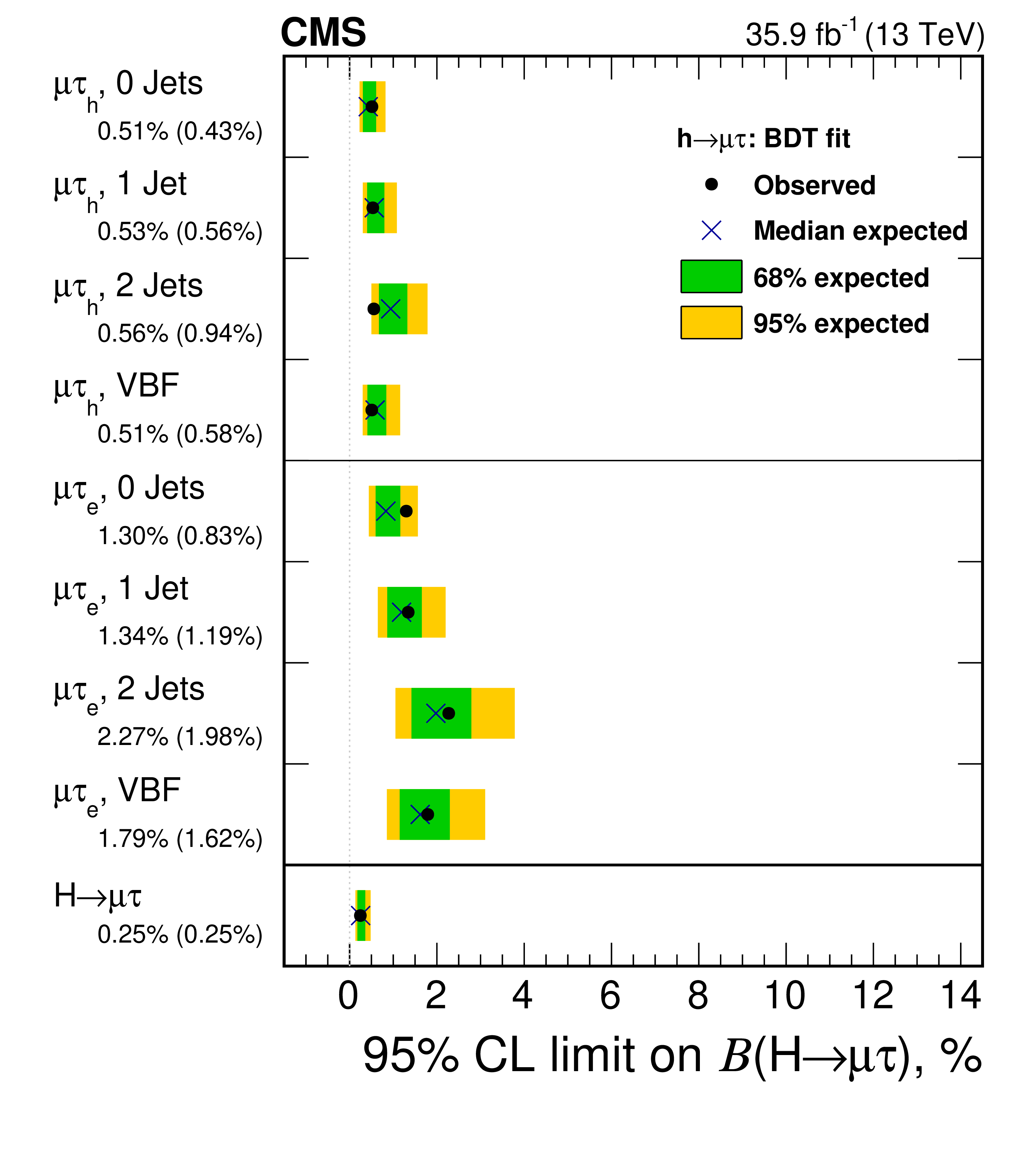
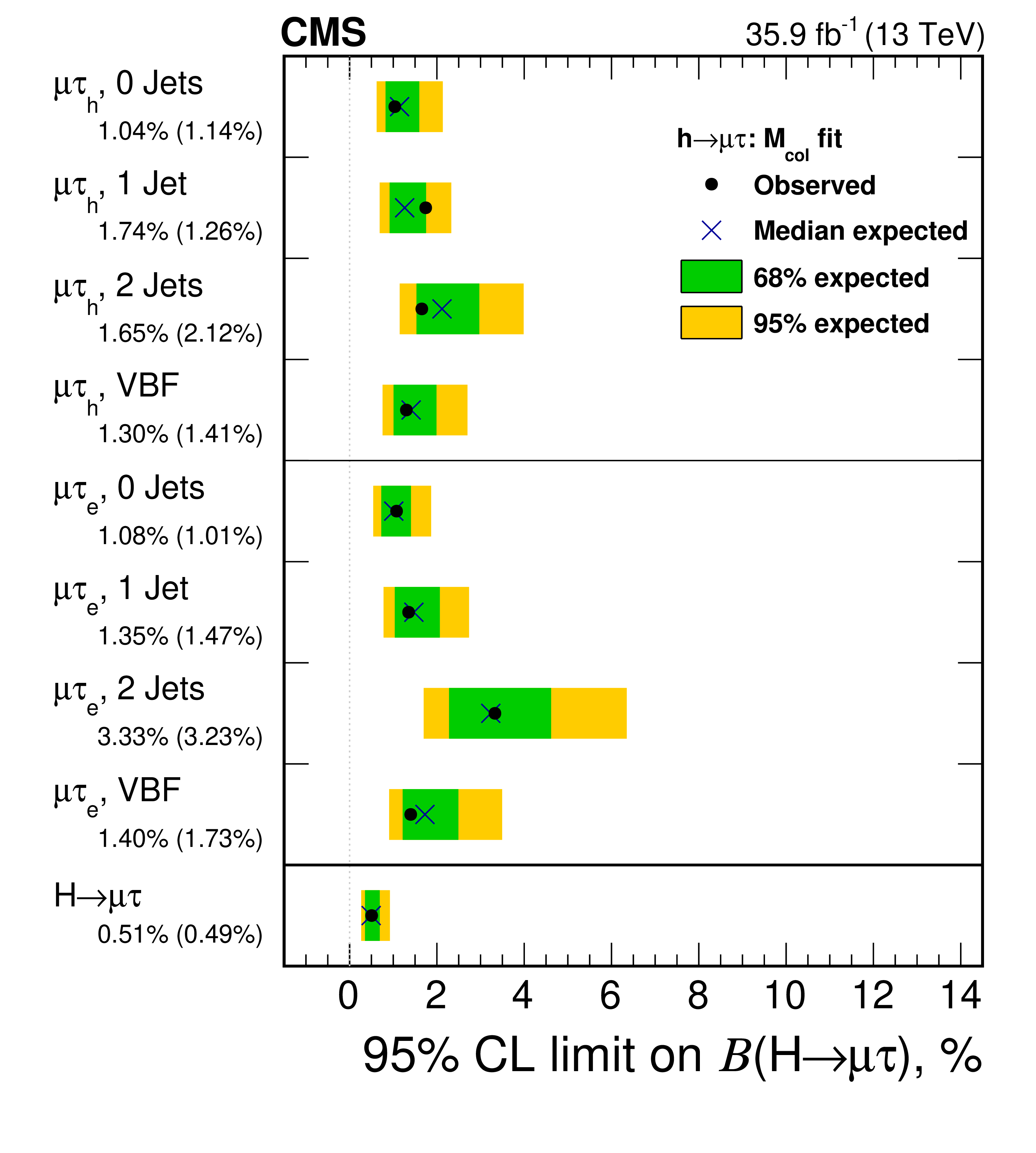
Figure 6:
Observed and expected 95% CL upper limits on the $\mathcal {B}({\mathrm {H}} \to {{\mu}} {\tau})$ for each individual category and combined. Left: BDT fit analysis. Right: $ {M_{\text {col}}} $ fit analysis. |
png pdf |
Figure 6-a:
Observed and expected 95% CL upper limits on the $\mathcal {B}({\mathrm {H}} \to {{\mu}} {\tau})$ for each individual category and combined. Left: BDT fit analysis. Right: $ {M_{\text {col}}} $ fit analysis. |
png pdf |
Figure 6-b:
Observed and expected 95% CL upper limits on the $\mathcal {B}({\mathrm {H}} \to {{\mu}} {\tau})$ for each individual category and combined. Left: BDT fit analysis. Right: $ {M_{\text {col}}} $ fit analysis. |
png pdf |
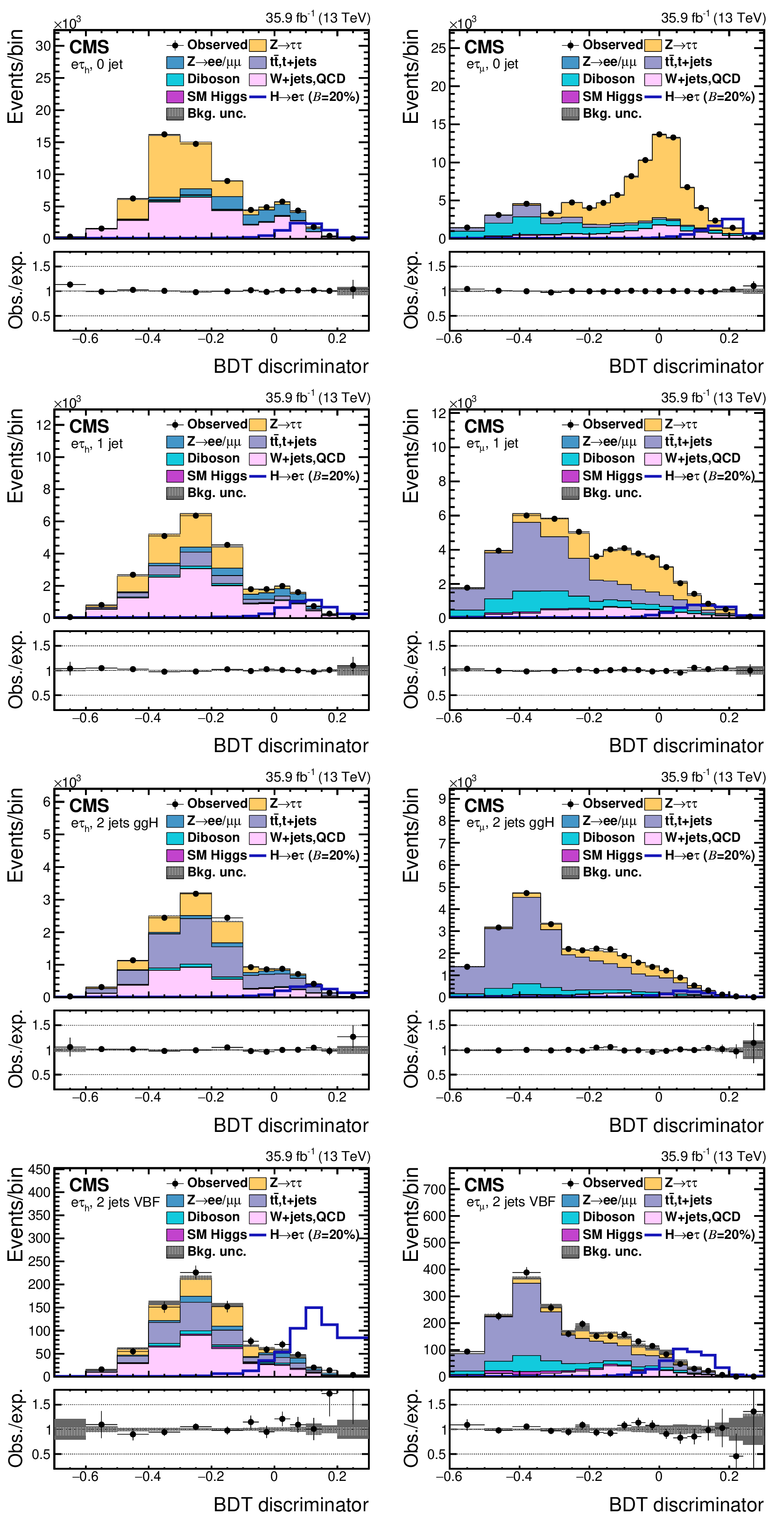
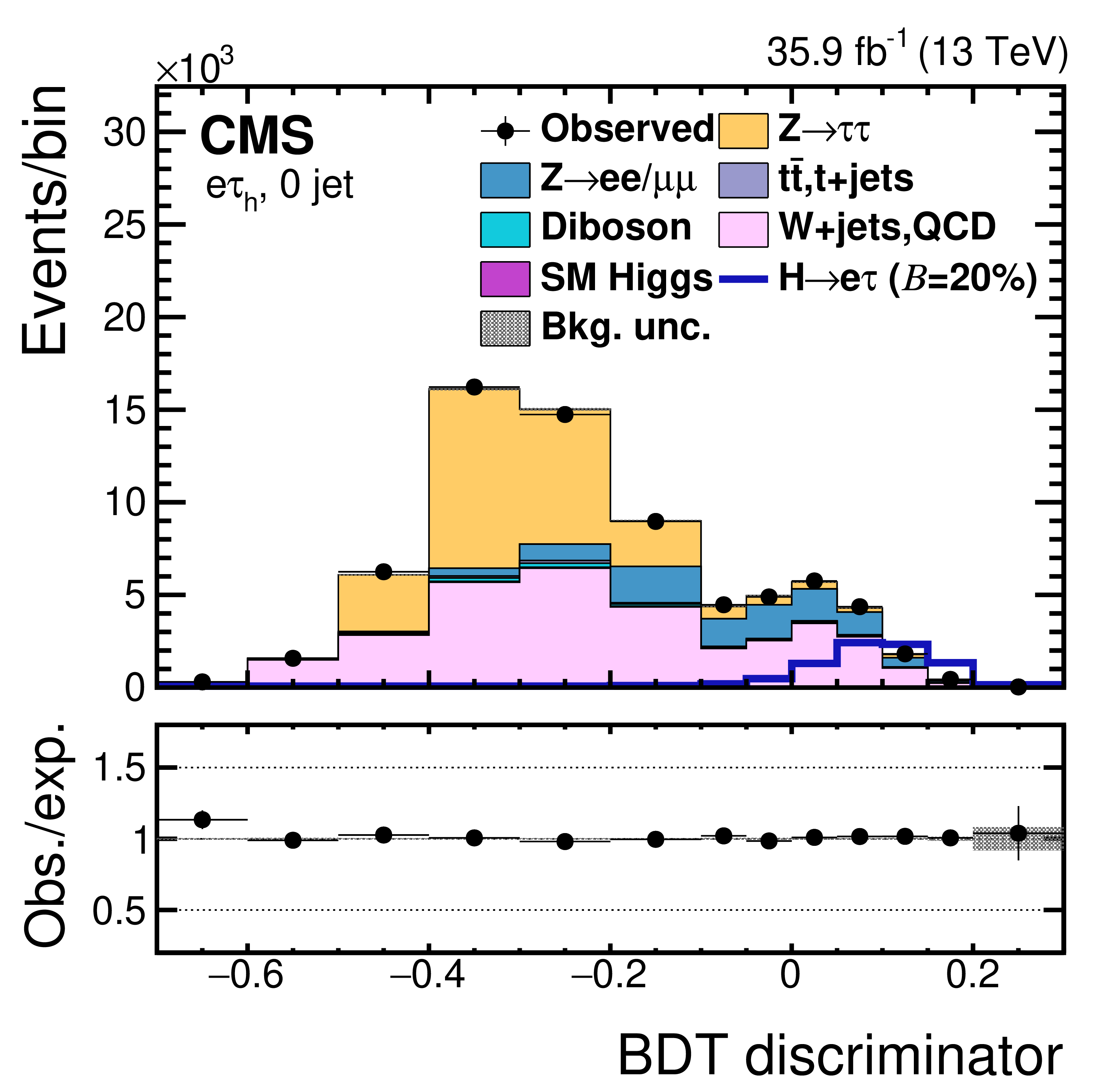
Figure 7:
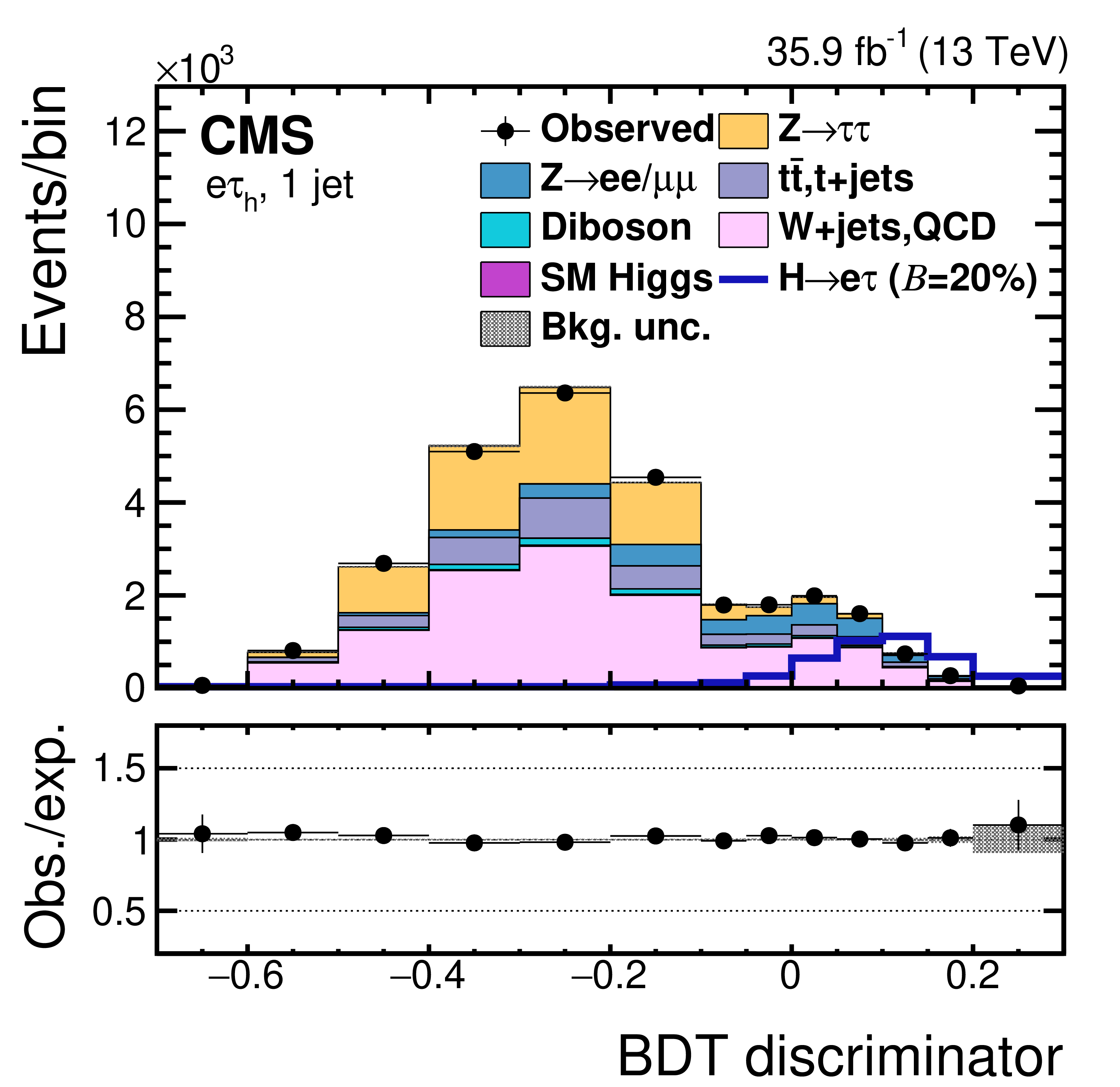
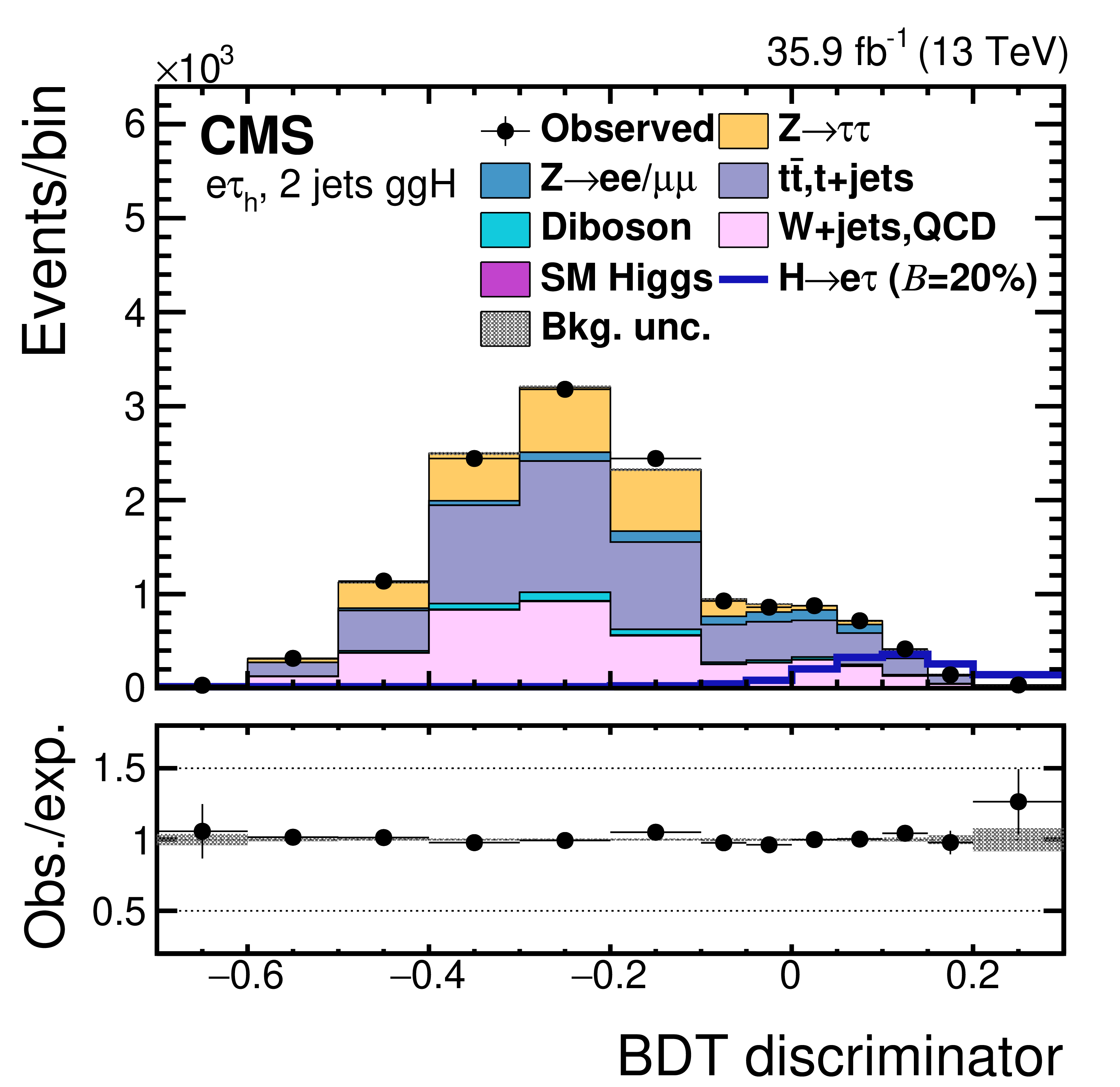
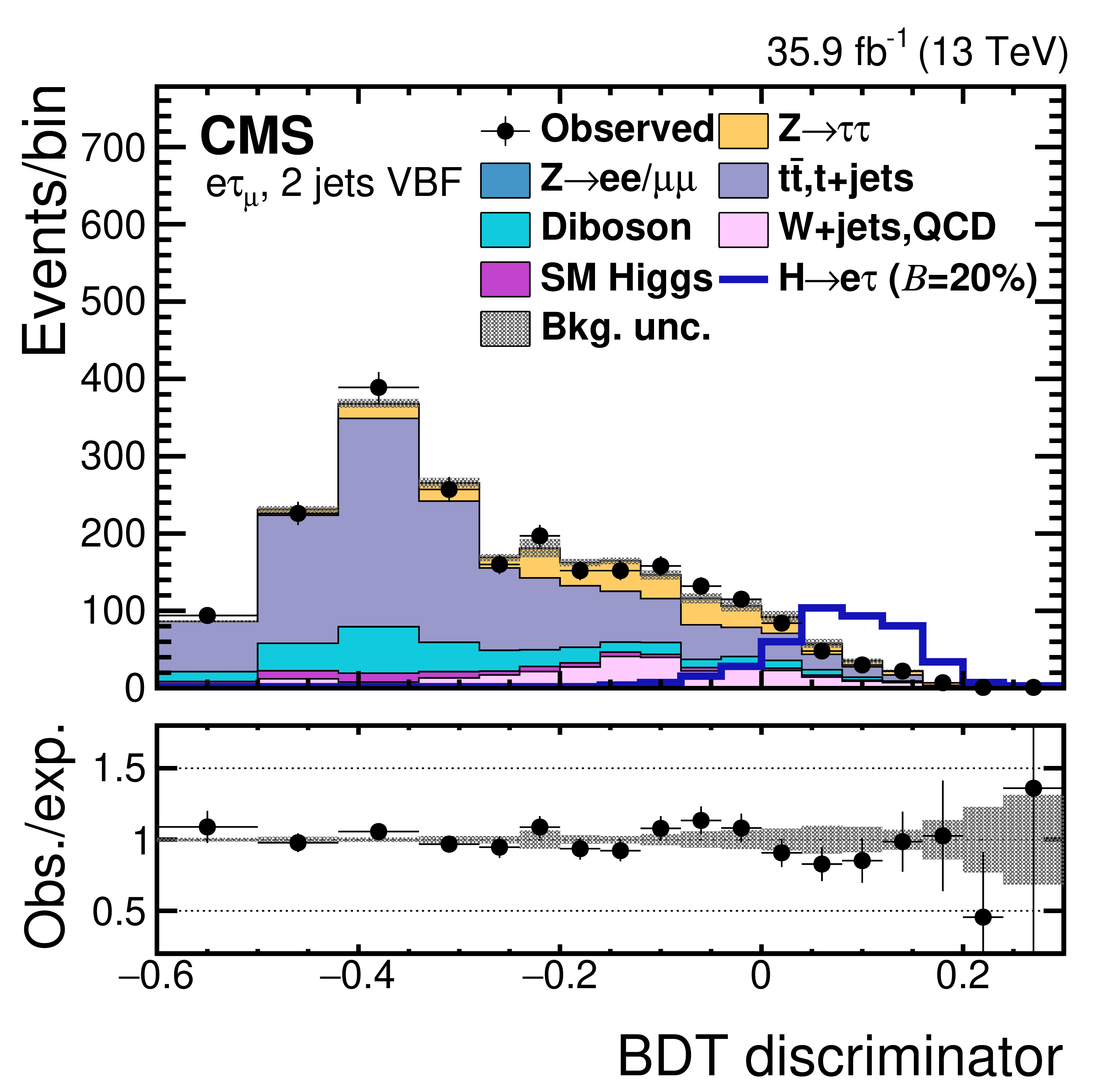
Distribution of the BDT discriminator for the $ {\mathrm {H}} \to {\mathrm {e}} {\tau}$ process for the BDT fit analysis, in different channels and categories compared to the signal and background estimation. The background is normalized to the best fit values from the signal plus background fit while the simulated signal corresponds to $\mathcal {B}({\mathrm {H}} \to {\mathrm {e}} {\tau})= $ 5%. The bottom panel in each plot shows the ratio between the observed data and the fitted background. The left column of plots corresponds to the $ {\mathrm {H}} \to {\mathrm {e}} {{\tau} _\mathrm {h}} $ categories, from 0-jets (first row) to 2-jets VBF (fourth row). The right one to their $ {\mathrm {H}} \to {\mathrm {e}} {\tau}_{{{\mu}}}$ counterparts. |
png pdf |
Figure 7-a:
Distribution of the BDT discriminator for the $ {\mathrm {H}} \to {\mathrm {e}} {\tau}$ process for the BDT fit analysis, in different channels and categories compared to the signal and background estimation. The background is normalized to the best fit values from the signal plus background fit while the simulated signal corresponds to $\mathcal {B}({\mathrm {H}} \to {\mathrm {e}} {\tau})= $ 5%. The bottom panel in each plot shows the ratio between the observed data and the fitted background. The left column of plots corresponds to the $ {\mathrm {H}} \to {\mathrm {e}} {{\tau} _\mathrm {h}} $ categories, from 0-jets (first row) to 2-jets VBF (fourth row). The right one to their $ {\mathrm {H}} \to {\mathrm {e}} {\tau}_{{{\mu}}}$ counterparts. |

png pdf |
Figure 7-b:
Distribution of the BDT discriminator for the $ {\mathrm {H}} \to {\mathrm {e}} {\tau}$ process for the BDT fit analysis, in different channels and categories compared to the signal and background estimation. The background is normalized to the best fit values from the signal plus background fit while the simulated signal corresponds to $\mathcal {B}({\mathrm {H}} \to {\mathrm {e}} {\tau})= $ 5%. The bottom panel in each plot shows the ratio between the observed data and the fitted background. The left column of plots corresponds to the $ {\mathrm {H}} \to {\mathrm {e}} {{\tau} _\mathrm {h}} $ categories, from 0-jets (first row) to 2-jets VBF (fourth row). The right one to their $ {\mathrm {H}} \to {\mathrm {e}} {\tau}_{{{\mu}}}$ counterparts. |
png pdf |
Figure 7-c:
Distribution of the BDT discriminator for the $ {\mathrm {H}} \to {\mathrm {e}} {\tau}$ process for the BDT fit analysis, in different channels and categories compared to the signal and background estimation. The background is normalized to the best fit values from the signal plus background fit while the simulated signal corresponds to $\mathcal {B}({\mathrm {H}} \to {\mathrm {e}} {\tau})= $ 5%. The bottom panel in each plot shows the ratio between the observed data and the fitted background. The left column of plots corresponds to the $ {\mathrm {H}} \to {\mathrm {e}} {{\tau} _\mathrm {h}} $ categories, from 0-jets (first row) to 2-jets VBF (fourth row). The right one to their $ {\mathrm {H}} \to {\mathrm {e}} {\tau}_{{{\mu}}}$ counterparts. |

png pdf |
Figure 7-d:
Distribution of the BDT discriminator for the $ {\mathrm {H}} \to {\mathrm {e}} {\tau}$ process for the BDT fit analysis, in different channels and categories compared to the signal and background estimation. The background is normalized to the best fit values from the signal plus background fit while the simulated signal corresponds to $\mathcal {B}({\mathrm {H}} \to {\mathrm {e}} {\tau})= $ 5%. The bottom panel in each plot shows the ratio between the observed data and the fitted background. The left column of plots corresponds to the $ {\mathrm {H}} \to {\mathrm {e}} {{\tau} _\mathrm {h}} $ categories, from 0-jets (first row) to 2-jets VBF (fourth row). The right one to their $ {\mathrm {H}} \to {\mathrm {e}} {\tau}_{{{\mu}}}$ counterparts. |
png pdf |
Figure 7-e:
Distribution of the BDT discriminator for the $ {\mathrm {H}} \to {\mathrm {e}} {\tau}$ process for the BDT fit analysis, in different channels and categories compared to the signal and background estimation. The background is normalized to the best fit values from the signal plus background fit while the simulated signal corresponds to $\mathcal {B}({\mathrm {H}} \to {\mathrm {e}} {\tau})= $ 5%. The bottom panel in each plot shows the ratio between the observed data and the fitted background. The left column of plots corresponds to the $ {\mathrm {H}} \to {\mathrm {e}} {{\tau} _\mathrm {h}} $ categories, from 0-jets (first row) to 2-jets VBF (fourth row). The right one to their $ {\mathrm {H}} \to {\mathrm {e}} {\tau}_{{{\mu}}}$ counterparts. |
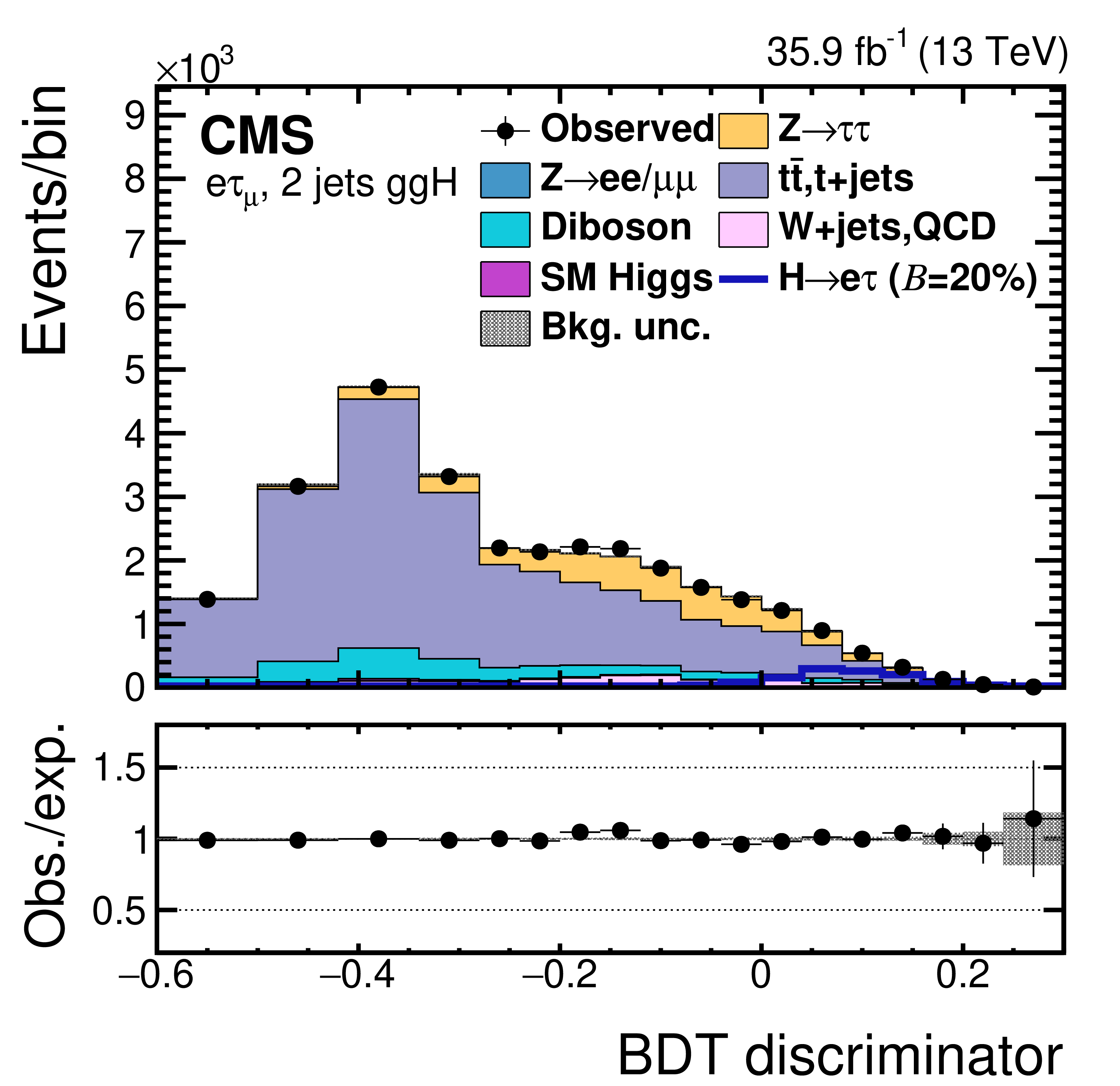
png pdf |
Figure 7-f:
Distribution of the BDT discriminator for the $ {\mathrm {H}} \to {\mathrm {e}} {\tau}$ process for the BDT fit analysis, in different channels and categories compared to the signal and background estimation. The background is normalized to the best fit values from the signal plus background fit while the simulated signal corresponds to $\mathcal {B}({\mathrm {H}} \to {\mathrm {e}} {\tau})= $ 5%. The bottom panel in each plot shows the ratio between the observed data and the fitted background. The left column of plots corresponds to the $ {\mathrm {H}} \to {\mathrm {e}} {{\tau} _\mathrm {h}} $ categories, from 0-jets (first row) to 2-jets VBF (fourth row). The right one to their $ {\mathrm {H}} \to {\mathrm {e}} {\tau}_{{{\mu}}}$ counterparts. |

png pdf |
Figure 7-g:
Distribution of the BDT discriminator for the $ {\mathrm {H}} \to {\mathrm {e}} {\tau}$ process for the BDT fit analysis, in different channels and categories compared to the signal and background estimation. The background is normalized to the best fit values from the signal plus background fit while the simulated signal corresponds to $\mathcal {B}({\mathrm {H}} \to {\mathrm {e}} {\tau})= $ 5%. The bottom panel in each plot shows the ratio between the observed data and the fitted background. The left column of plots corresponds to the $ {\mathrm {H}} \to {\mathrm {e}} {{\tau} _\mathrm {h}} $ categories, from 0-jets (first row) to 2-jets VBF (fourth row). The right one to their $ {\mathrm {H}} \to {\mathrm {e}} {\tau}_{{{\mu}}}$ counterparts. |
png pdf |
Figure 7-h:
Distribution of the BDT discriminator for the $ {\mathrm {H}} \to {\mathrm {e}} {\tau}$ process for the BDT fit analysis, in different channels and categories compared to the signal and background estimation. The background is normalized to the best fit values from the signal plus background fit while the simulated signal corresponds to $\mathcal {B}({\mathrm {H}} \to {\mathrm {e}} {\tau})= $ 5%. The bottom panel in each plot shows the ratio between the observed data and the fitted background. The left column of plots corresponds to the $ {\mathrm {H}} \to {\mathrm {e}} {{\tau} _\mathrm {h}} $ categories, from 0-jets (first row) to 2-jets VBF (fourth row). The right one to their $ {\mathrm {H}} \to {\mathrm {e}} {\tau}_{{{\mu}}}$ counterparts. |

png pdf |
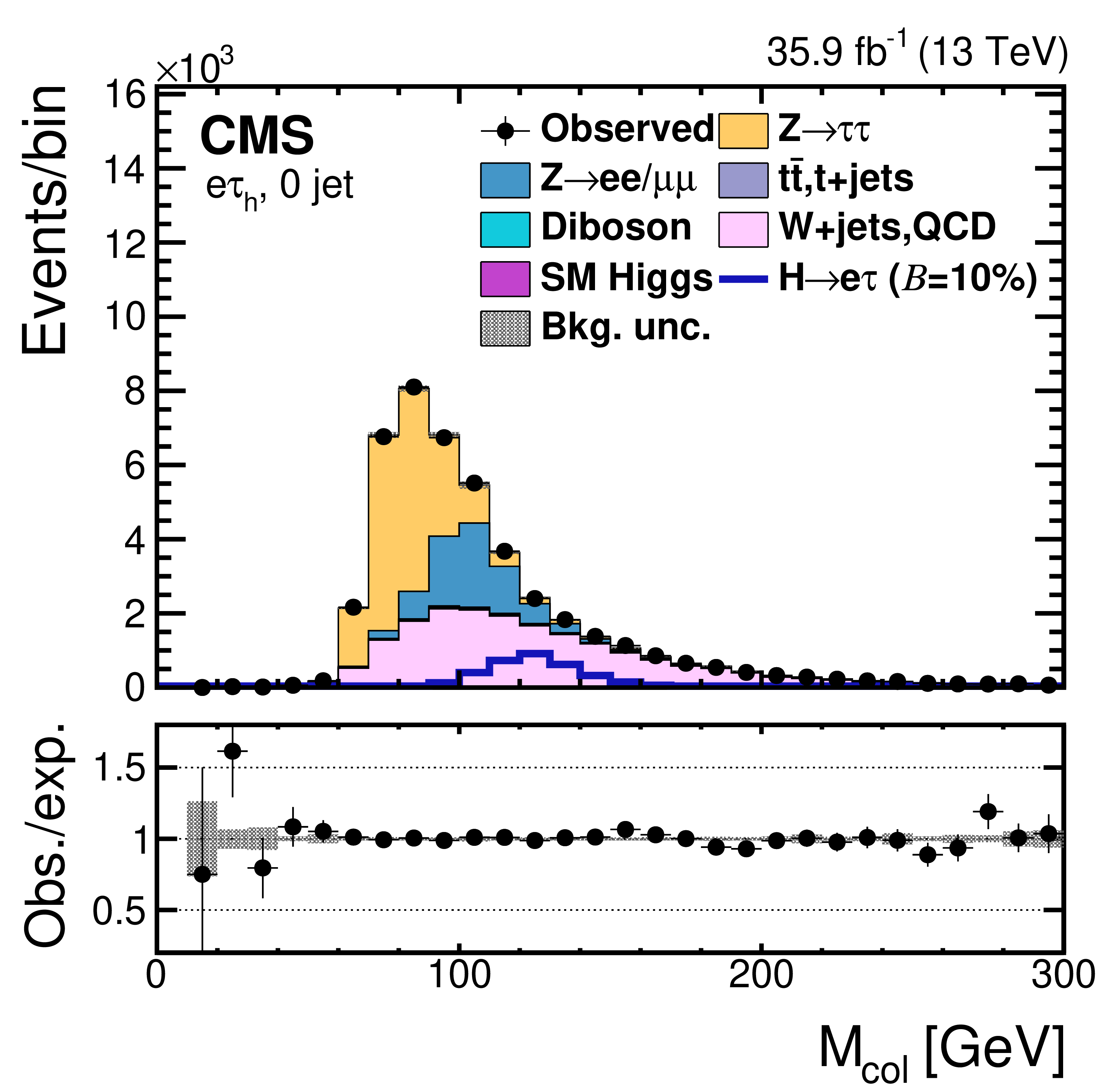
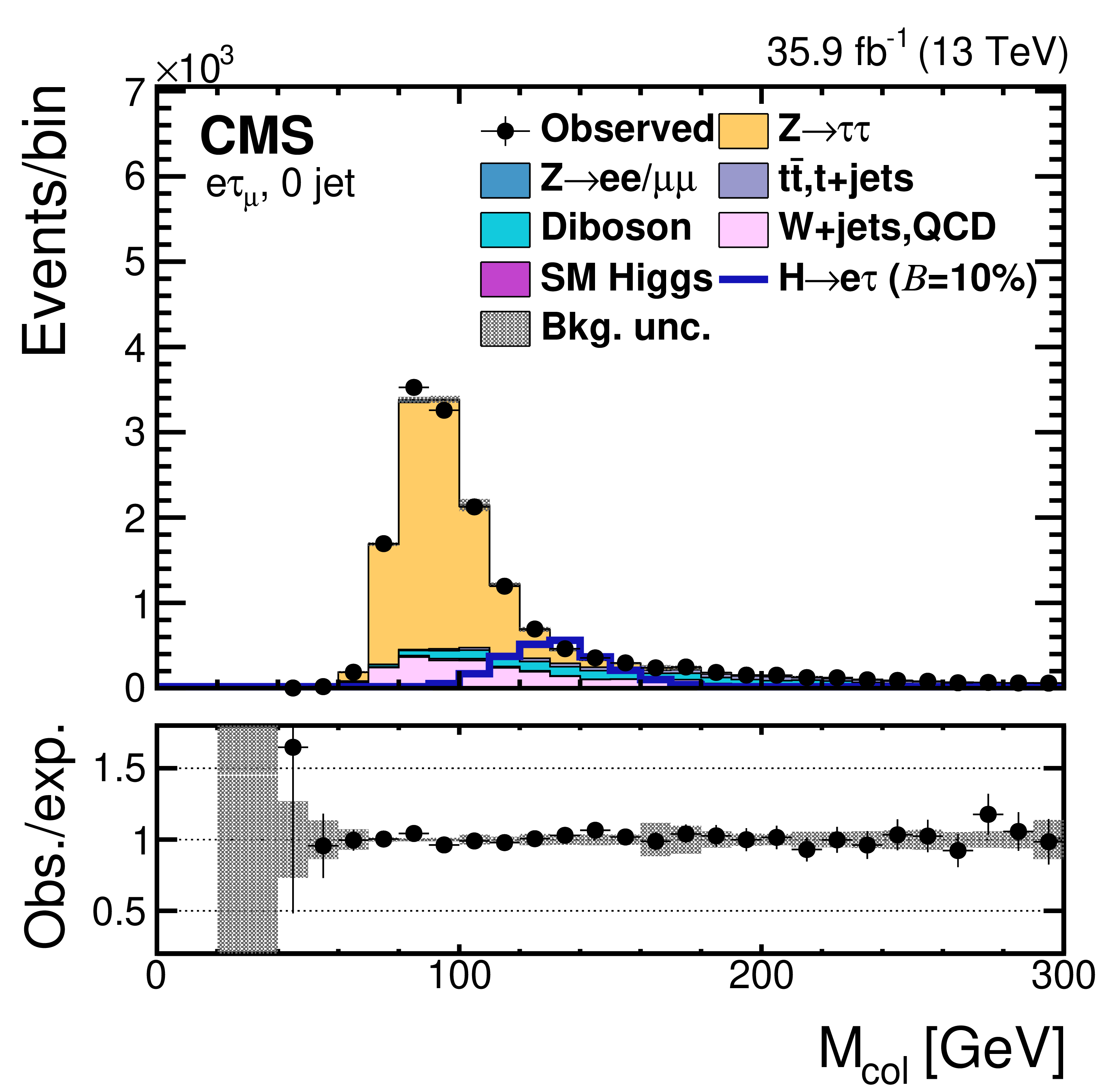
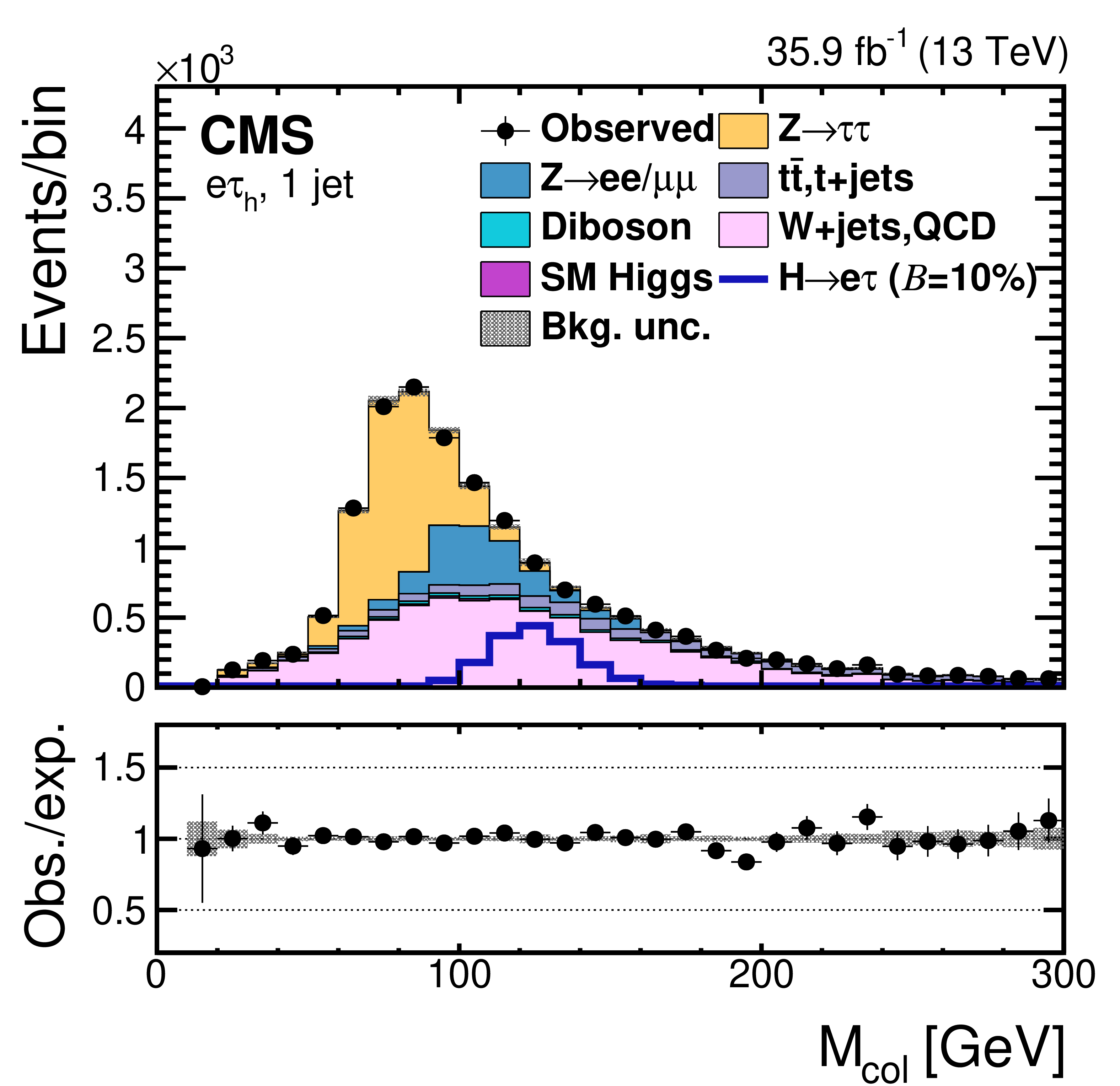
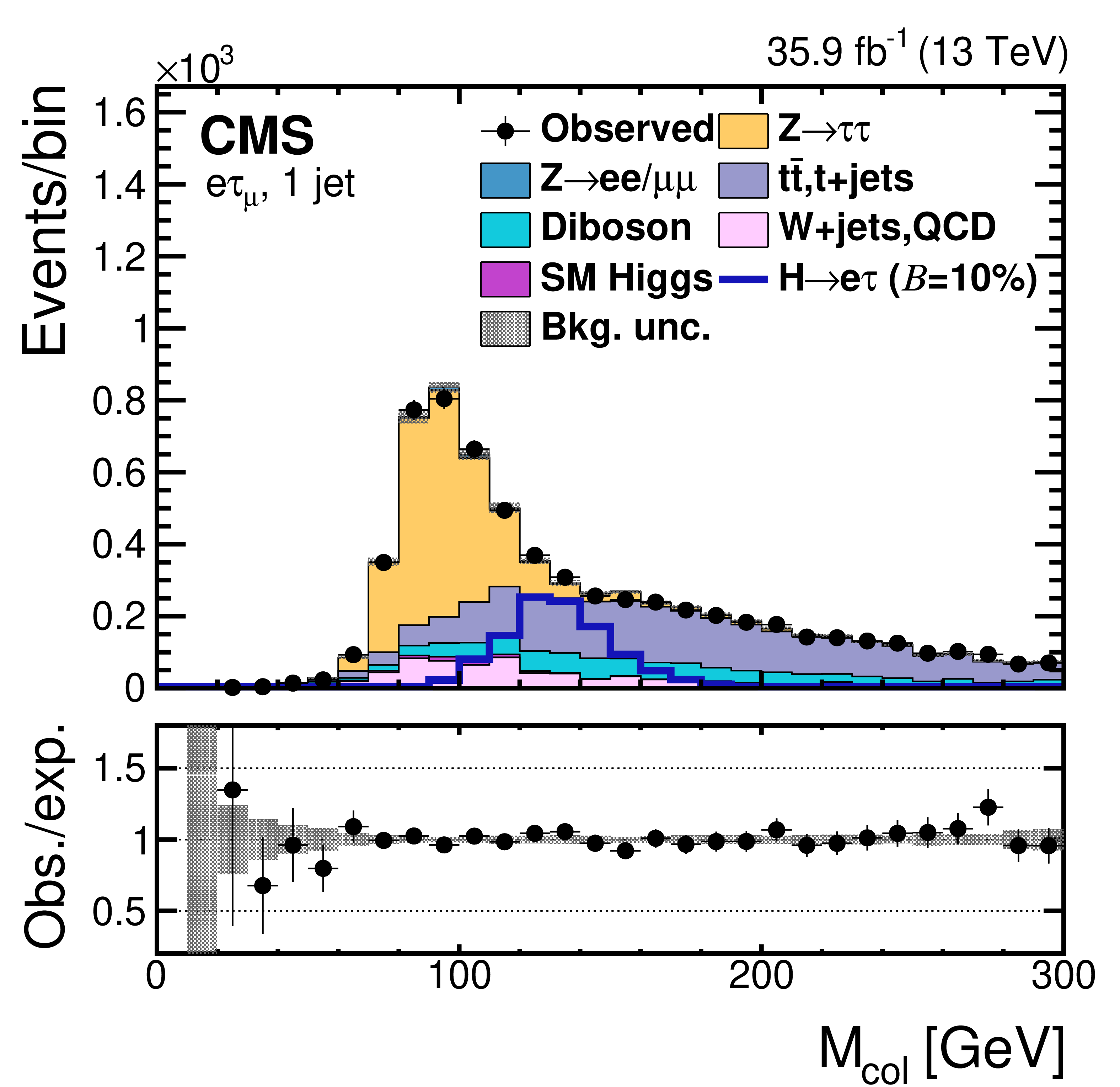
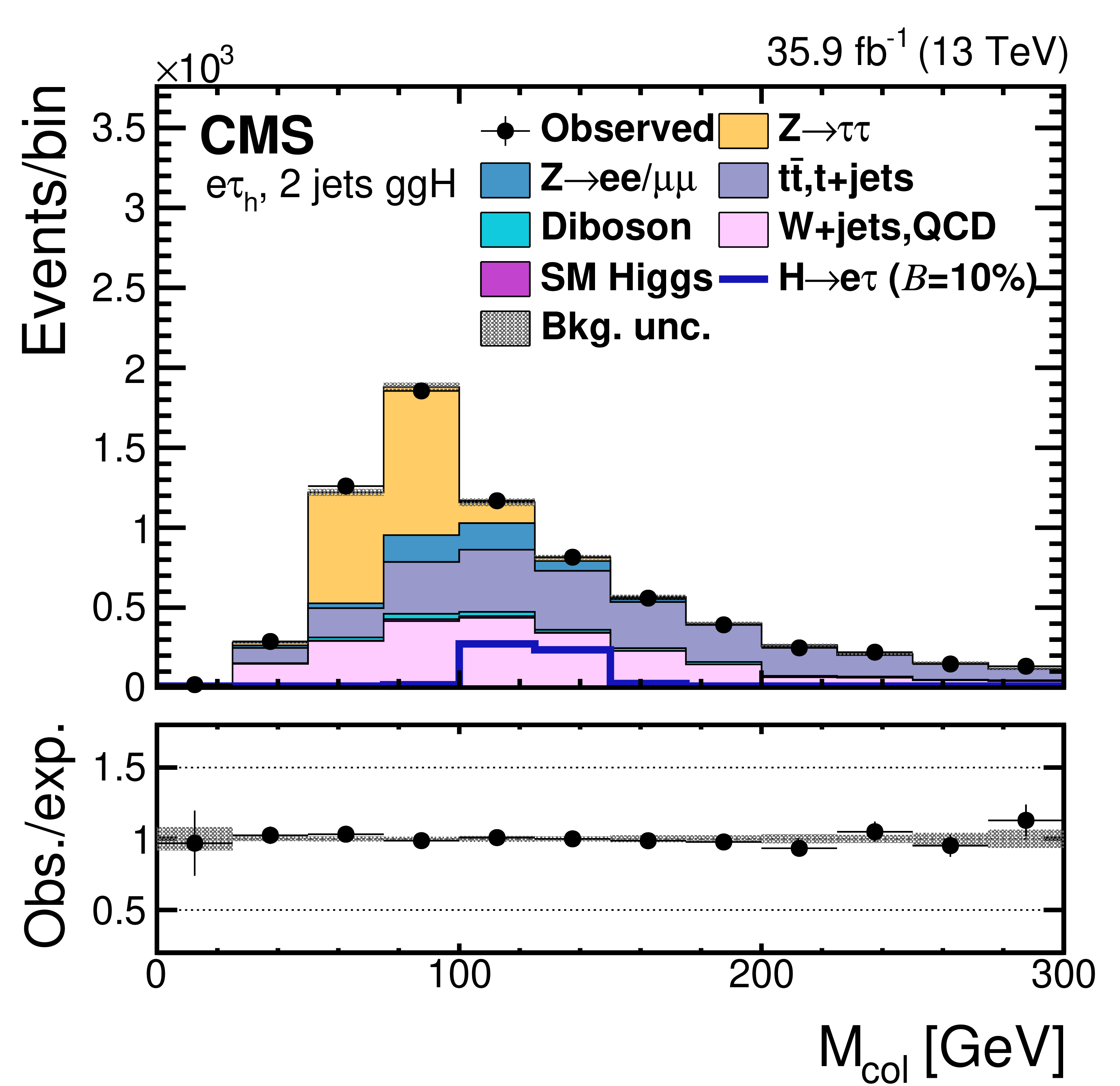
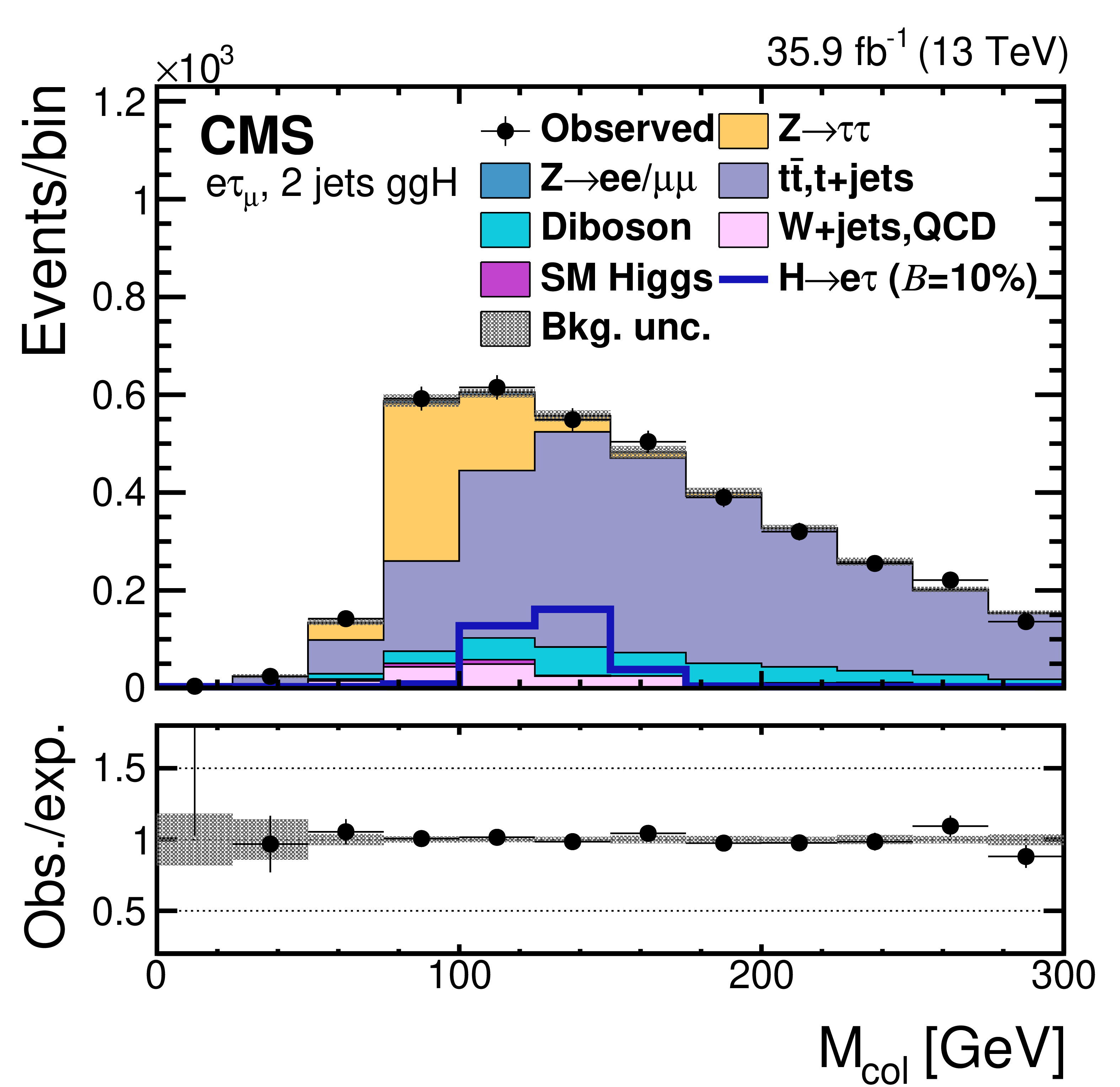
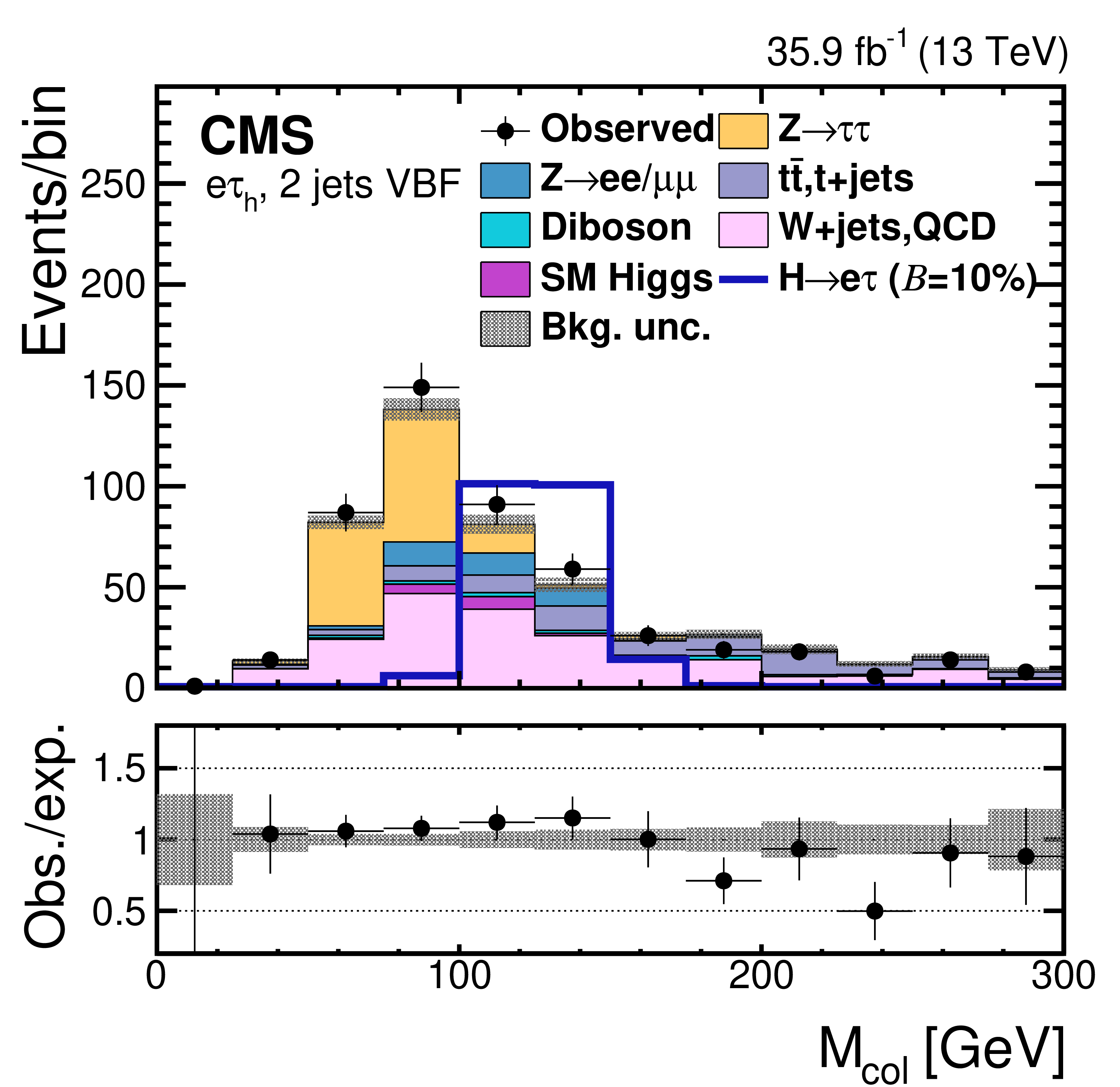
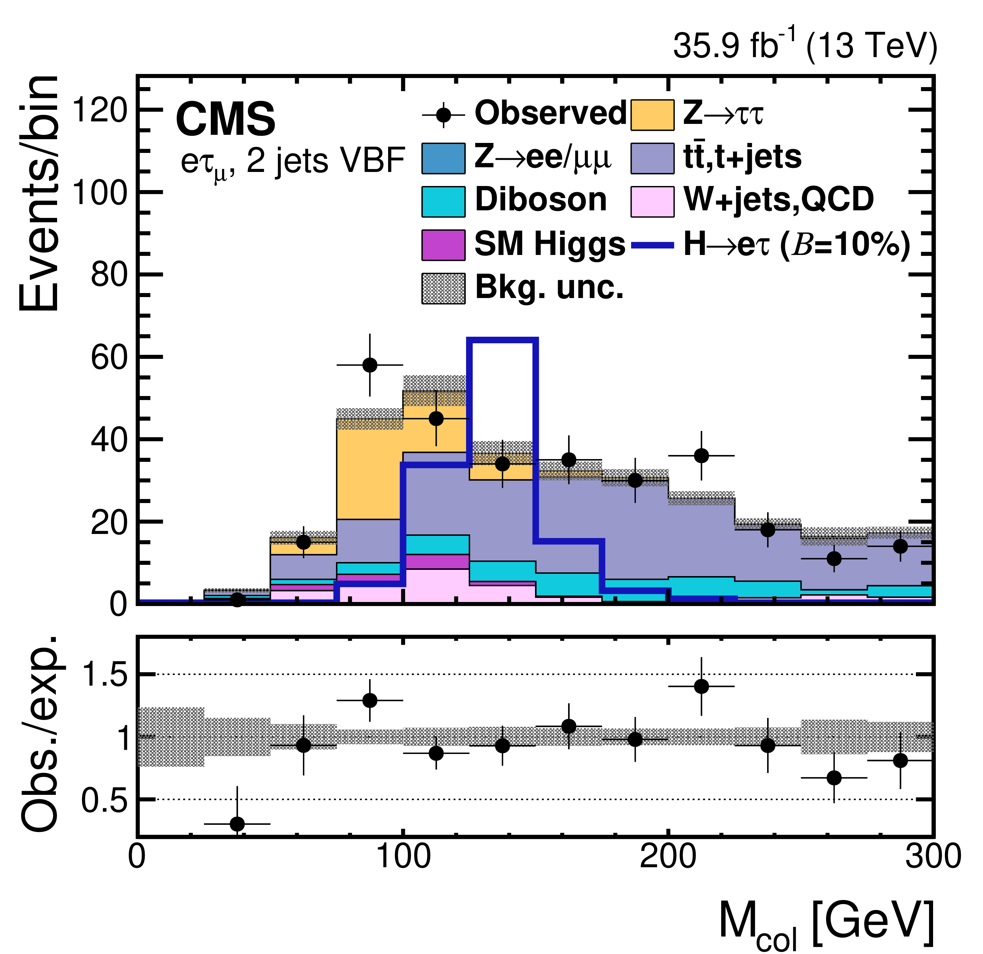
Figure 8:
Distribution of the collinear mass $M_\text {col}$ for the $ {\mathrm {H}} \to {\mathrm {e}} {\tau}$ process in the $ {M_{\text {col}}} $ fit analysis, in different channels and categories compared to the signal and background estimation. The background is normalized to the best fit values from the signal plus background fit while the simulated signal corresponds to $\mathcal {B}({\mathrm {H}} \to {\mathrm {e}} {\tau})=5%$. The lower panel in each plot shows the ratio between the observed data and the fitted background. The left column of plots correspond to the $ {\mathrm {H}} \to {\mathrm {e}} {{\tau} _\mathrm {h}} $ categories, from 0-jets (first row) to 2 jets VBF (fourth row). The right one to their $ {\mathrm {H}} \to {\mathrm {e}} {\tau}_{{{\mu}}}$ counterparts. |
png pdf |
Figure 8-a:
Distribution of the collinear mass $M_\text {col}$ for the $ {\mathrm {H}} \to {\mathrm {e}} {\tau}$ process in the $ {M_{\text {col}}} $ fit analysis, in different channels and categories compared to the signal and background estimation. The background is normalized to the best fit values from the signal plus background fit while the simulated signal corresponds to $\mathcal {B}({\mathrm {H}} \to {\mathrm {e}} {\tau})=5%$. The lower panel in each plot shows the ratio between the observed data and the fitted background. The left column of plots correspond to the $ {\mathrm {H}} \to {\mathrm {e}} {{\tau} _\mathrm {h}} $ categories, from 0-jets (first row) to 2 jets VBF (fourth row). The right one to their $ {\mathrm {H}} \to {\mathrm {e}} {\tau}_{{{\mu}}}$ counterparts. |
png pdf |
Figure 8-b:
Distribution of the collinear mass $M_\text {col}$ for the $ {\mathrm {H}} \to {\mathrm {e}} {\tau}$ process in the $ {M_{\text {col}}} $ fit analysis, in different channels and categories compared to the signal and background estimation. The background is normalized to the best fit values from the signal plus background fit while the simulated signal corresponds to $\mathcal {B}({\mathrm {H}} \to {\mathrm {e}} {\tau})=5%$. The lower panel in each plot shows the ratio between the observed data and the fitted background. The left column of plots correspond to the $ {\mathrm {H}} \to {\mathrm {e}} {{\tau} _\mathrm {h}} $ categories, from 0-jets (first row) to 2 jets VBF (fourth row). The right one to their $ {\mathrm {H}} \to {\mathrm {e}} {\tau}_{{{\mu}}}$ counterparts. |
png pdf |
Figure 8-c:
Distribution of the collinear mass $M_\text {col}$ for the $ {\mathrm {H}} \to {\mathrm {e}} {\tau}$ process in the $ {M_{\text {col}}} $ fit analysis, in different channels and categories compared to the signal and background estimation. The background is normalized to the best fit values from the signal plus background fit while the simulated signal corresponds to $\mathcal {B}({\mathrm {H}} \to {\mathrm {e}} {\tau})=5%$. The lower panel in each plot shows the ratio between the observed data and the fitted background. The left column of plots correspond to the $ {\mathrm {H}} \to {\mathrm {e}} {{\tau} _\mathrm {h}} $ categories, from 0-jets (first row) to 2 jets VBF (fourth row). The right one to their $ {\mathrm {H}} \to {\mathrm {e}} {\tau}_{{{\mu}}}$ counterparts. |
png pdf |
Figure 8-d:
Distribution of the collinear mass $M_\text {col}$ for the $ {\mathrm {H}} \to {\mathrm {e}} {\tau}$ process in the $ {M_{\text {col}}} $ fit analysis, in different channels and categories compared to the signal and background estimation. The background is normalized to the best fit values from the signal plus background fit while the simulated signal corresponds to $\mathcal {B}({\mathrm {H}} \to {\mathrm {e}} {\tau})=5%$. The lower panel in each plot shows the ratio between the observed data and the fitted background. The left column of plots correspond to the $ {\mathrm {H}} \to {\mathrm {e}} {{\tau} _\mathrm {h}} $ categories, from 0-jets (first row) to 2 jets VBF (fourth row). The right one to their $ {\mathrm {H}} \to {\mathrm {e}} {\tau}_{{{\mu}}}$ counterparts. |
png pdf |
Figure 8-e:
Distribution of the collinear mass $M_\text {col}$ for the $ {\mathrm {H}} \to {\mathrm {e}} {\tau}$ process in the $ {M_{\text {col}}} $ fit analysis, in different channels and categories compared to the signal and background estimation. The background is normalized to the best fit values from the signal plus background fit while the simulated signal corresponds to $\mathcal {B}({\mathrm {H}} \to {\mathrm {e}} {\tau})=5%$. The lower panel in each plot shows the ratio between the observed data and the fitted background. The left column of plots correspond to the $ {\mathrm {H}} \to {\mathrm {e}} {{\tau} _\mathrm {h}} $ categories, from 0-jets (first row) to 2 jets VBF (fourth row). The right one to their $ {\mathrm {H}} \to {\mathrm {e}} {\tau}_{{{\mu}}}$ counterparts. |
png pdf |
Figure 8-f:
Distribution of the collinear mass $M_\text {col}$ for the $ {\mathrm {H}} \to {\mathrm {e}} {\tau}$ process in the $ {M_{\text {col}}} $ fit analysis, in different channels and categories compared to the signal and background estimation. The background is normalized to the best fit values from the signal plus background fit while the simulated signal corresponds to $\mathcal {B}({\mathrm {H}} \to {\mathrm {e}} {\tau})=5%$. The lower panel in each plot shows the ratio between the observed data and the fitted background. The left column of plots correspond to the $ {\mathrm {H}} \to {\mathrm {e}} {{\tau} _\mathrm {h}} $ categories, from 0-jets (first row) to 2 jets VBF (fourth row). The right one to their $ {\mathrm {H}} \to {\mathrm {e}} {\tau}_{{{\mu}}}$ counterparts. |
png pdf |
Figure 8-g:
Distribution of the collinear mass $M_\text {col}$ for the $ {\mathrm {H}} \to {\mathrm {e}} {\tau}$ process in the $ {M_{\text {col}}} $ fit analysis, in different channels and categories compared to the signal and background estimation. The background is normalized to the best fit values from the signal plus background fit while the simulated signal corresponds to $\mathcal {B}({\mathrm {H}} \to {\mathrm {e}} {\tau})=5%$. The lower panel in each plot shows the ratio between the observed data and the fitted background. The left column of plots correspond to the $ {\mathrm {H}} \to {\mathrm {e}} {{\tau} _\mathrm {h}} $ categories, from 0-jets (first row) to 2 jets VBF (fourth row). The right one to their $ {\mathrm {H}} \to {\mathrm {e}} {\tau}_{{{\mu}}}$ counterparts. |
png pdf |
Figure 8-h:
Distribution of the collinear mass $M_\text {col}$ for the $ {\mathrm {H}} \to {\mathrm {e}} {\tau}$ process in the $ {M_{\text {col}}} $ fit analysis, in different channels and categories compared to the signal and background estimation. The background is normalized to the best fit values from the signal plus background fit while the simulated signal corresponds to $\mathcal {B}({\mathrm {H}} \to {\mathrm {e}} {\tau})=5%$. The lower panel in each plot shows the ratio between the observed data and the fitted background. The left column of plots correspond to the $ {\mathrm {H}} \to {\mathrm {e}} {{\tau} _\mathrm {h}} $ categories, from 0-jets (first row) to 2 jets VBF (fourth row). The right one to their $ {\mathrm {H}} \to {\mathrm {e}} {\tau}_{{{\mu}}}$ counterparts. |
png pdf |
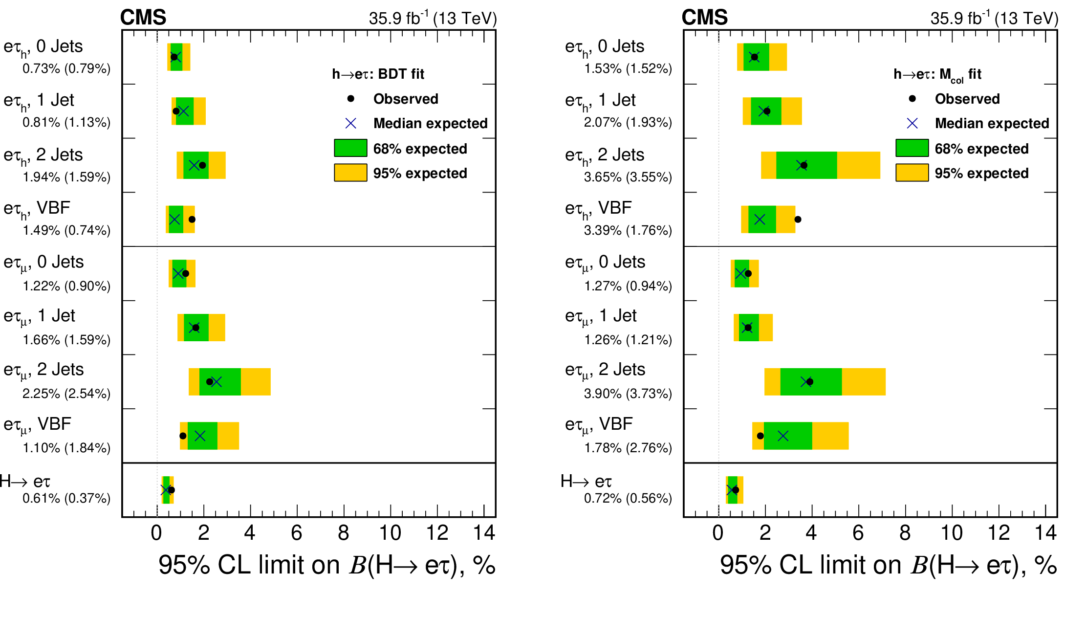
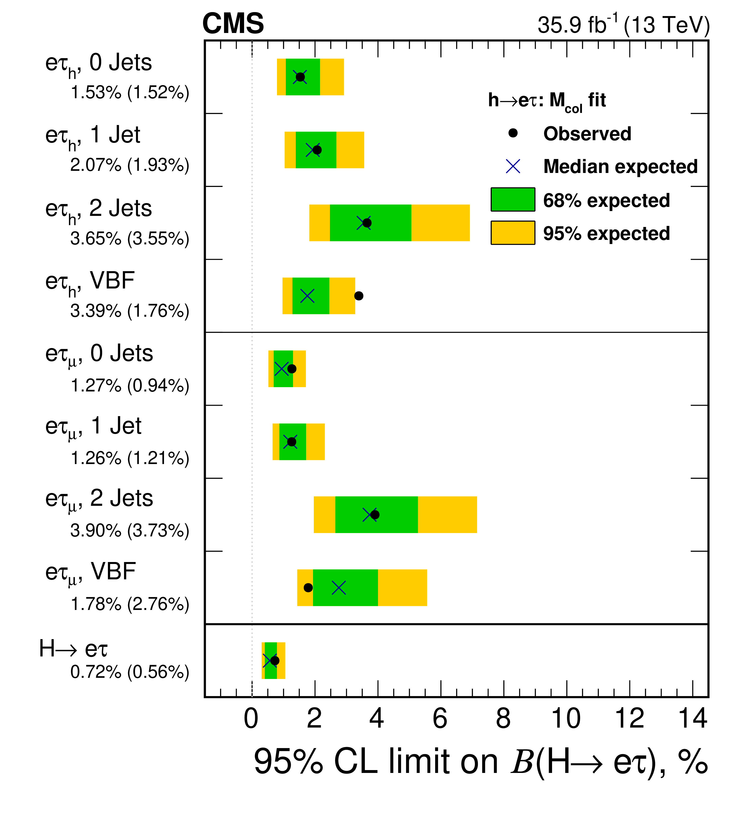
Figure 9:
Observed and expected 95% CL upper limits on the $\mathcal {B}({\mathrm {H}} \to {\mathrm {e}} {\tau})$ for each individual category and combined. Left: BDT fit analysis. Right: $ {M_{\text {col}}} $ fit analysis. |

png pdf |
Figure 9-a:
Observed and expected 95% CL upper limits on the $\mathcal {B}({\mathrm {H}} \to {\mathrm {e}} {\tau})$ for each individual category and combined. Left: BDT fit analysis. Right: $ {M_{\text {col}}} $ fit analysis. |
png pdf |
Figure 9-b:
Observed and expected 95% CL upper limits on the $\mathcal {B}({\mathrm {H}} \to {\mathrm {e}} {\tau})$ for each individual category and combined. Left: BDT fit analysis. Right: $ {M_{\text {col}}} $ fit analysis. |
png pdf |
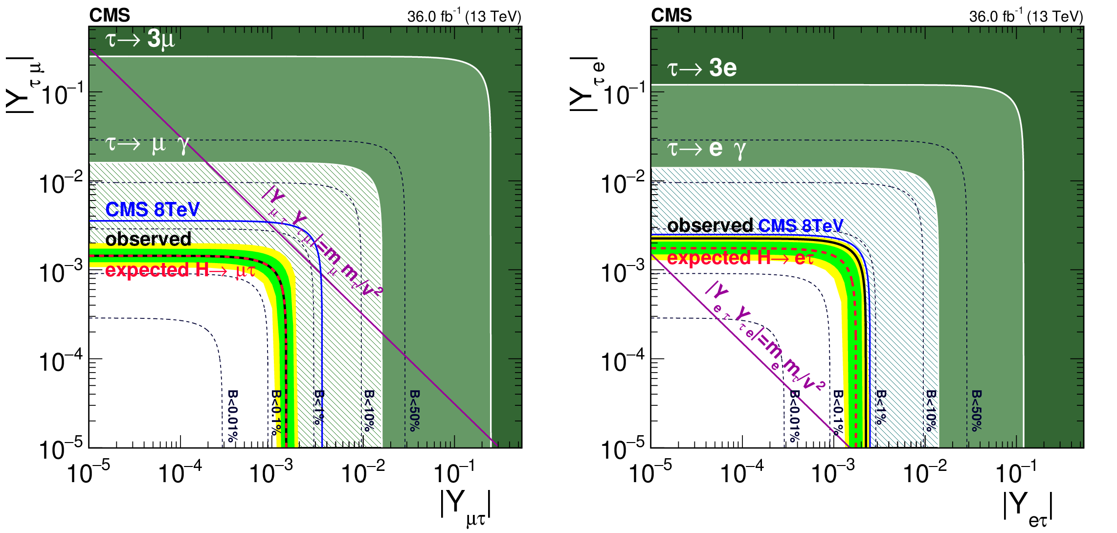
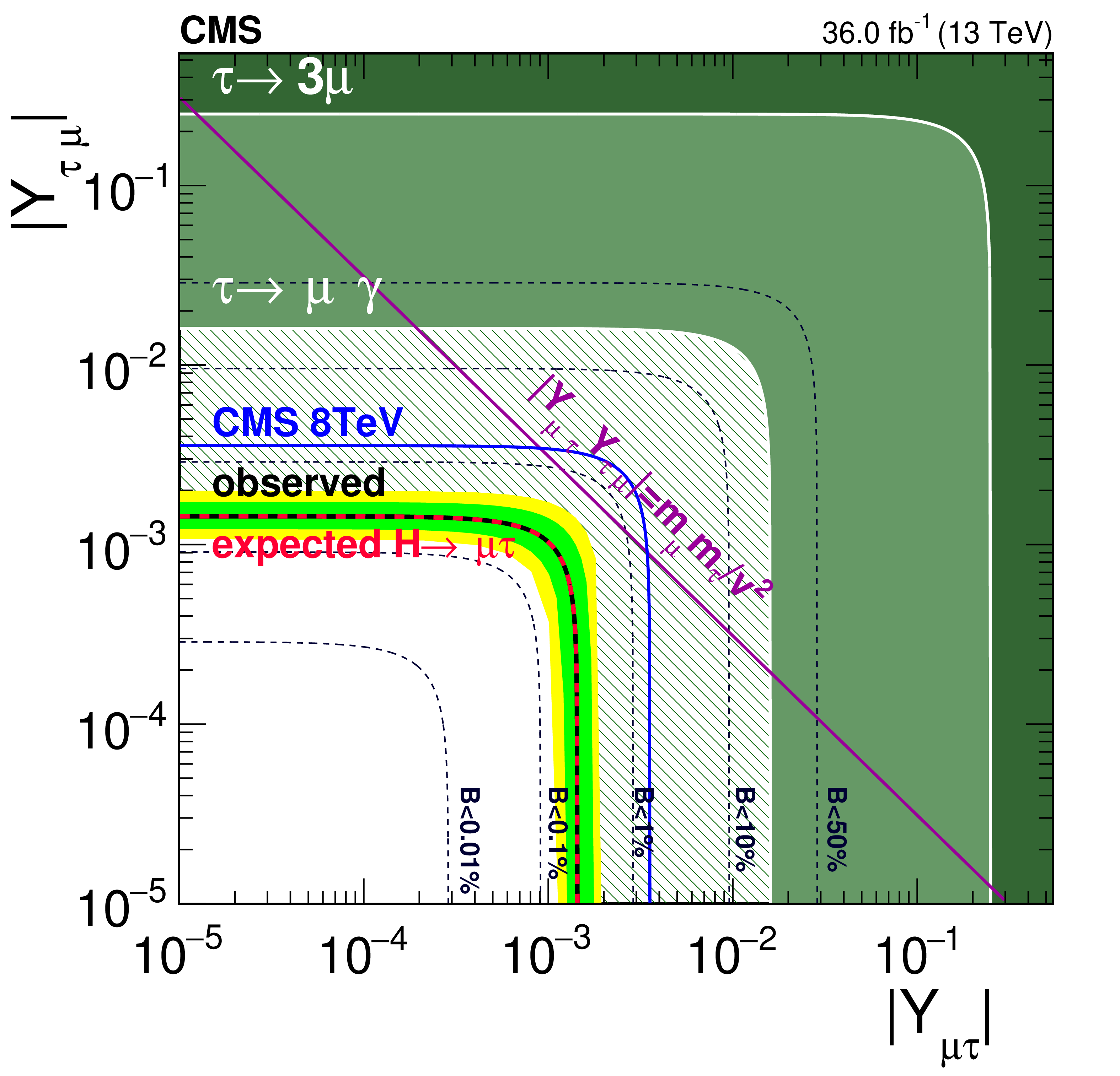
Figure 10:
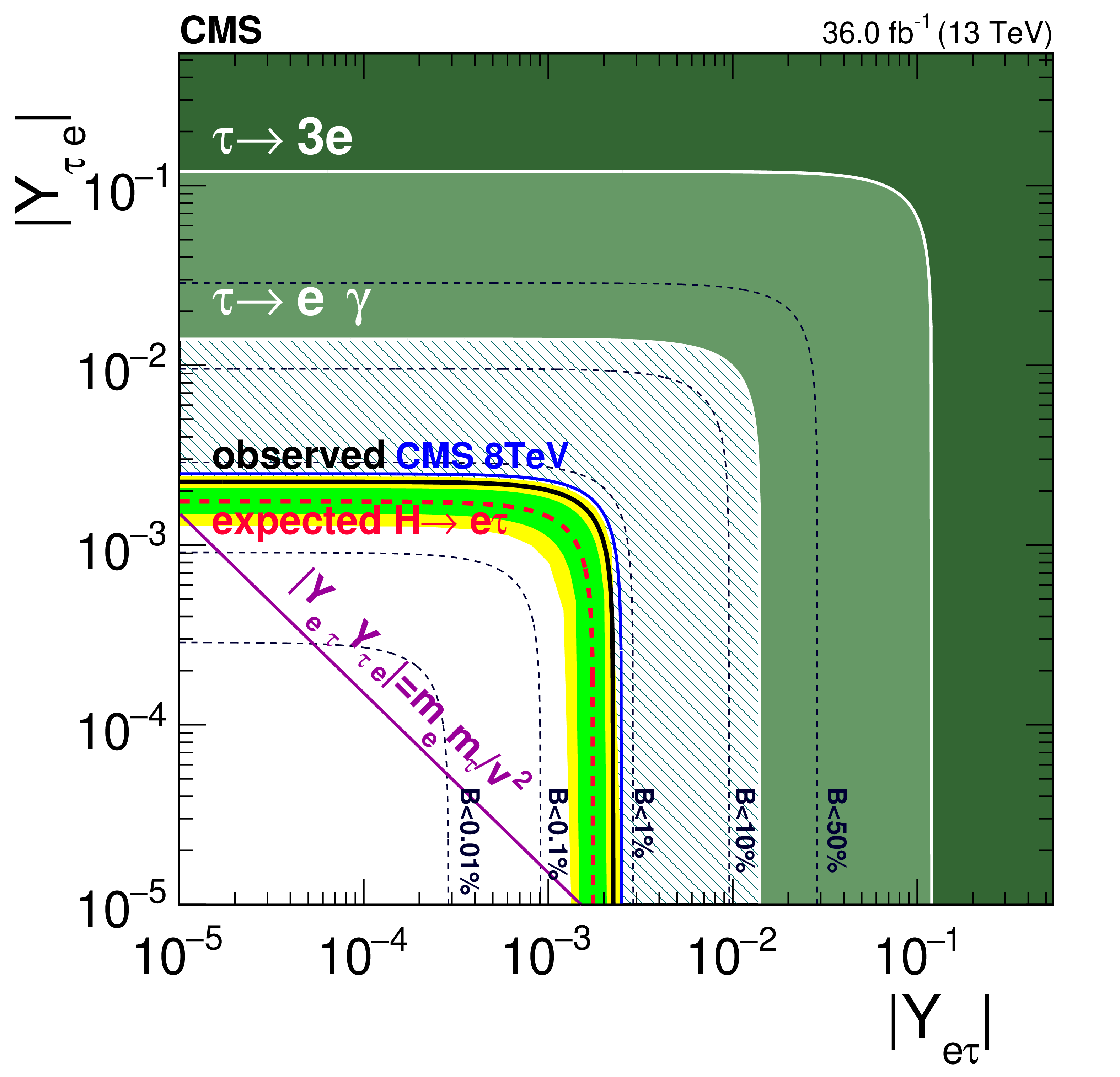
Constraints on the flavour violating Yukawa couplings, $|Y_{{{\mu}} {\tau}}|, |Y_{{\tau} {{\mu}}}|$ (left) and $|Y_{{\mathrm {e}} {\tau}}|, |Y_{{\tau} {\mathrm {e}}}|$ (right), from the BDT result. The expected (red dashed line) and observed (black solid line) limits are derived from the limit on $\mathcal {B}({\mathrm {H}} \to {{\mu}} {\tau})$ and $\mathcal {B}({\mathrm {H}} \to {\mathrm {e}} {\tau})$ from the present analysis. The flavour-diagonal Yukawa couplings are approximated by their SM values. The green (yellow) band indicates the range that is expected to contain 68% (95%) of all observed limit excursions from the expected limit. The shaded regions are derived constraints from null searches for $ {\tau}\to 3 {{\mu}}$ or $ {\tau}\to 3 {\mathrm {e}}$ (dark green) [91,92,41] and $ {\tau}\to {{\mu}}\gamma $ or $ {\tau}\to {\mathrm {e}}\gamma $ (lighter green) [92,41]. The green hashed region is derived by the CMS direct search presented in this paper. The blue solid lines are the CMS limits from [44] (left) and [45](right). The purple diagonal line is the theoretical naturalness limit $|Y_{ij}Y_{ji}| \leq m_im_j/v^2$ [41]. |
png pdf |
Figure 10-a:
Constraints on the flavour violating Yukawa couplings, $|Y_{{{\mu}} {\tau}}|, |Y_{{\tau} {{\mu}}}|$ (left) and $|Y_{{\mathrm {e}} {\tau}}|, |Y_{{\tau} {\mathrm {e}}}|$ (right), from the BDT result. The expected (red dashed line) and observed (black solid line) limits are derived from the limit on $\mathcal {B}({\mathrm {H}} \to {{\mu}} {\tau})$ and $\mathcal {B}({\mathrm {H}} \to {\mathrm {e}} {\tau})$ from the present analysis. The flavour-diagonal Yukawa couplings are approximated by their SM values. The green (yellow) band indicates the range that is expected to contain 68% (95%) of all observed limit excursions from the expected limit. The shaded regions are derived constraints from null searches for $ {\tau}\to 3 {{\mu}}$ or $ {\tau}\to 3 {\mathrm {e}}$ (dark green) [91,92,41] and $ {\tau}\to {{\mu}}\gamma $ or $ {\tau}\to {\mathrm {e}}\gamma $ (lighter green) [92,41]. The green hashed region is derived by the CMS direct search presented in this paper. The blue solid lines are the CMS limits from [44] (left) and [45](right). The purple diagonal line is the theoretical naturalness limit $|Y_{ij}Y_{ji}| \leq m_im_j/v^2$ [41]. |
png pdf |
Figure 10-b:
Constraints on the flavour violating Yukawa couplings, $|Y_{{{\mu}} {\tau}}|, |Y_{{\tau} {{\mu}}}|$ (left) and $|Y_{{\mathrm {e}} {\tau}}|, |Y_{{\tau} {\mathrm {e}}}|$ (right), from the BDT result. The expected (red dashed line) and observed (black solid line) limits are derived from the limit on $\mathcal {B}({\mathrm {H}} \to {{\mu}} {\tau})$ and $\mathcal {B}({\mathrm {H}} \to {\mathrm {e}} {\tau})$ from the present analysis. The flavour-diagonal Yukawa couplings are approximated by their SM values. The green (yellow) band indicates the range that is expected to contain 68% (95%) of all observed limit excursions from the expected limit. The shaded regions are derived constraints from null searches for $ {\tau}\to 3 {{\mu}}$ or $ {\tau}\to 3 {\mathrm {e}}$ (dark green) [91,92,41] and $ {\tau}\to {{\mu}}\gamma $ or $ {\tau}\to {\mathrm {e}}\gamma $ (lighter green) [92,41]. The green hashed region is derived by the CMS direct search presented in this paper. The blue solid lines are the CMS limits from [44] (left) and [45](right). The purple diagonal line is the theoretical naturalness limit $|Y_{ij}Y_{ji}| \leq m_im_j/v^2$ [41]. |
| Tables | |
png pdf |
Table 1:
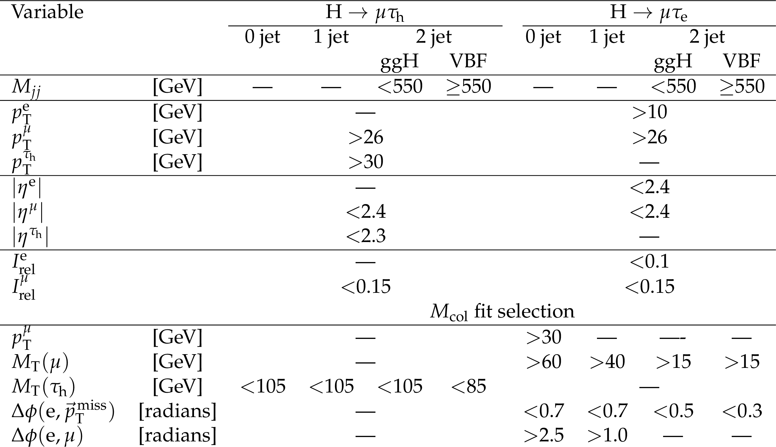
Event selection criteria for the kinematic variables for the $ {\mathrm {H}} \to {{\mu}} {\tau}$ channels. |
png pdf |
Table 2:
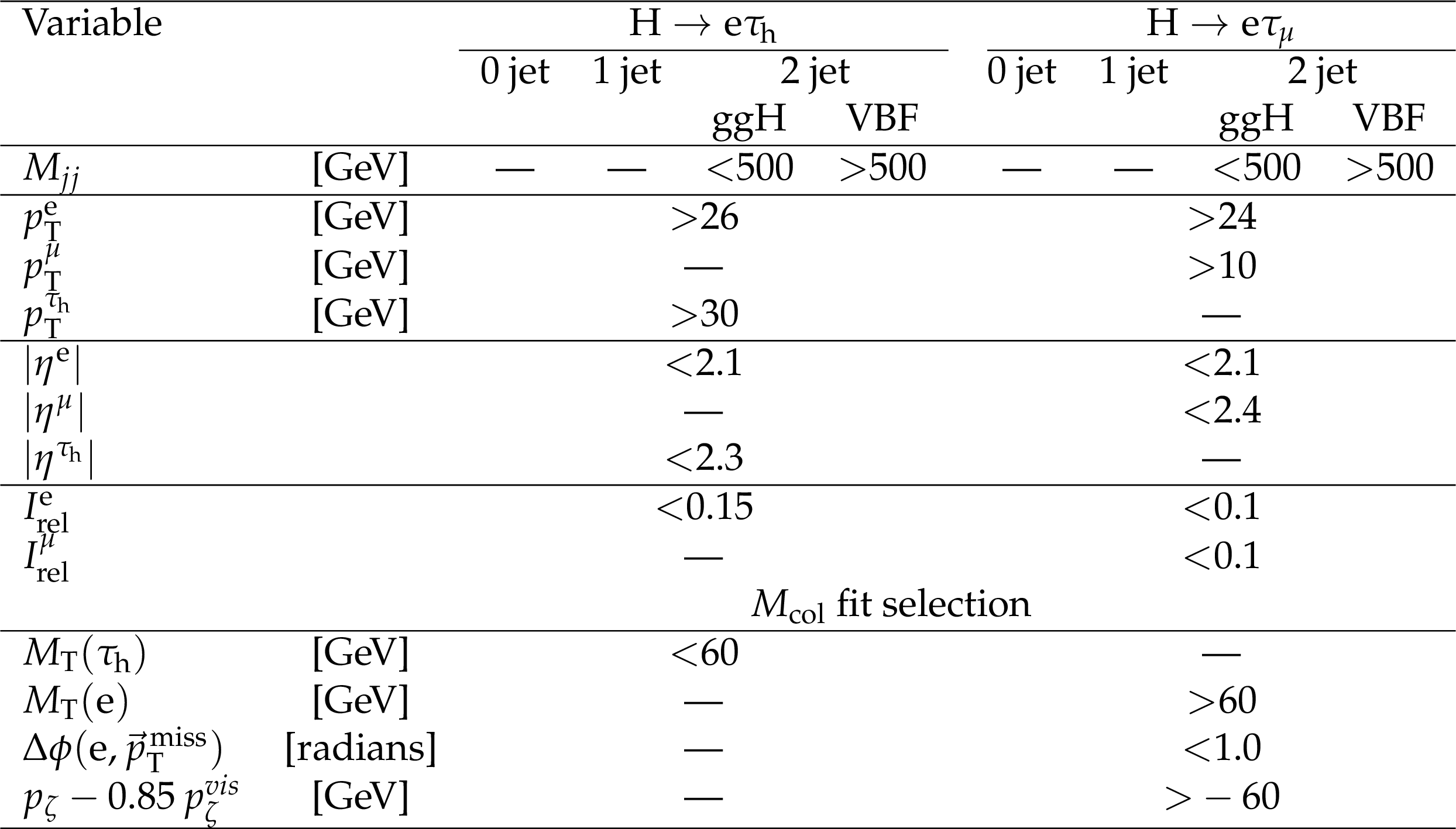
Event selection criteria for the kinematic variables for the $ {\mathrm {H}} \to {\mathrm {e}} {\tau}$ channels. |
png pdf |
Table 3:
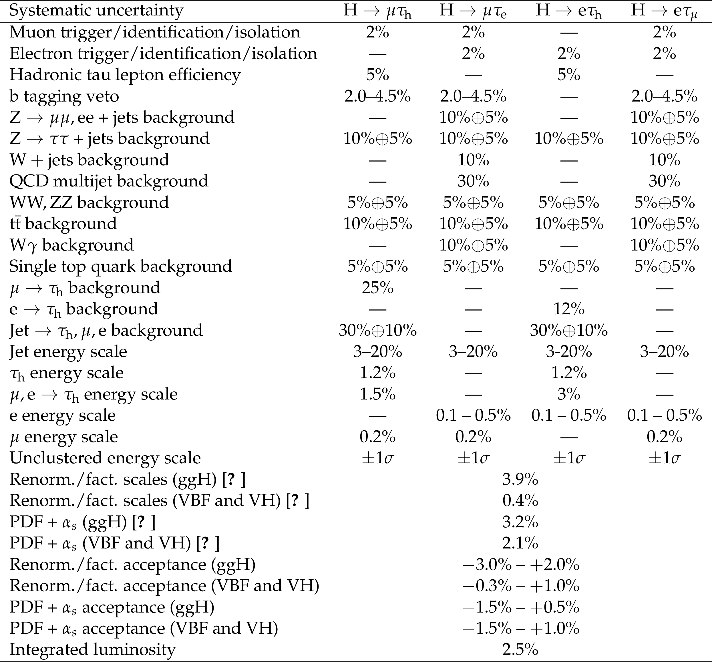
Systematic uncertainties in the expected event yields. All uncertainties are treated as correlated between the categories, except those that have two values separated by the $+$ sign. In this case, the first value is the correlated uncertainty and the second value is the uncorrelated uncertainty for each individual category. Theoretical uncertainties on VBF Higgs boson production [84] are also applied to VH production. Uncertainties on acceptance lead to migration of events between the categories, and can be correlated or anticorrelated between categories. Ranges of uncertainties for the Higgs boson production indicate the variation in size, from negative (anticorrelated) to positive (correlated). |

png pdf |
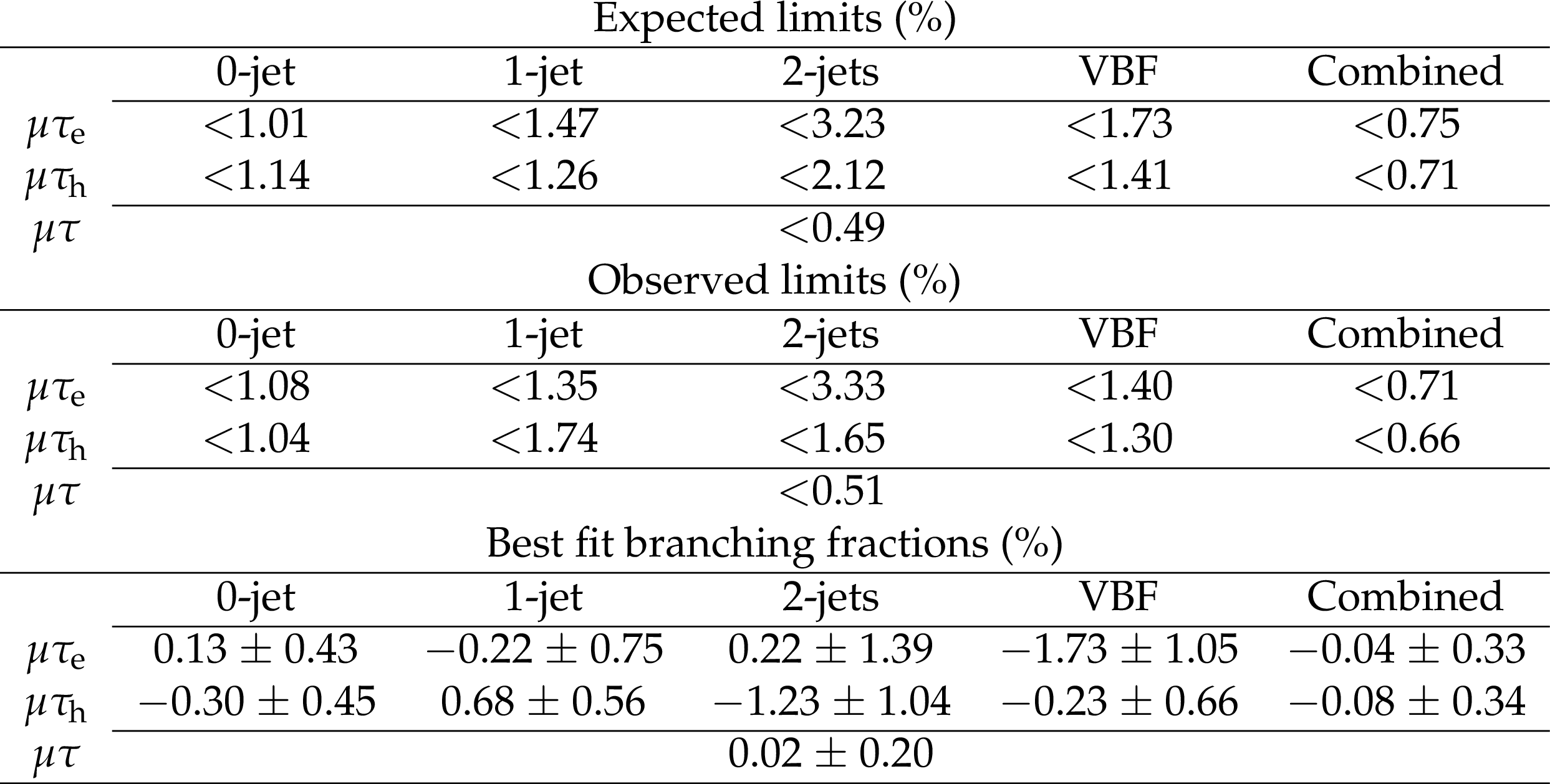
Table 4:
Expected and observed upper limits at 95% CL, and best fit branching fractions in percent for each individual jet category, and combined, in the $ {\mathrm {H}} \to {{\mu}} {\tau}$ process obtained with the BDT fit analysis. |
png pdf |
Table 5:
Expected and observed upper limits at 95% CL, and best fit branching fractions in percent for each individual jet category, and combined, in the $ {\mathrm {H}} \to {{\mu}} {\tau}$ process obtained with the $ {M_{\text {col}}} $ fit analysis. |

png pdf |
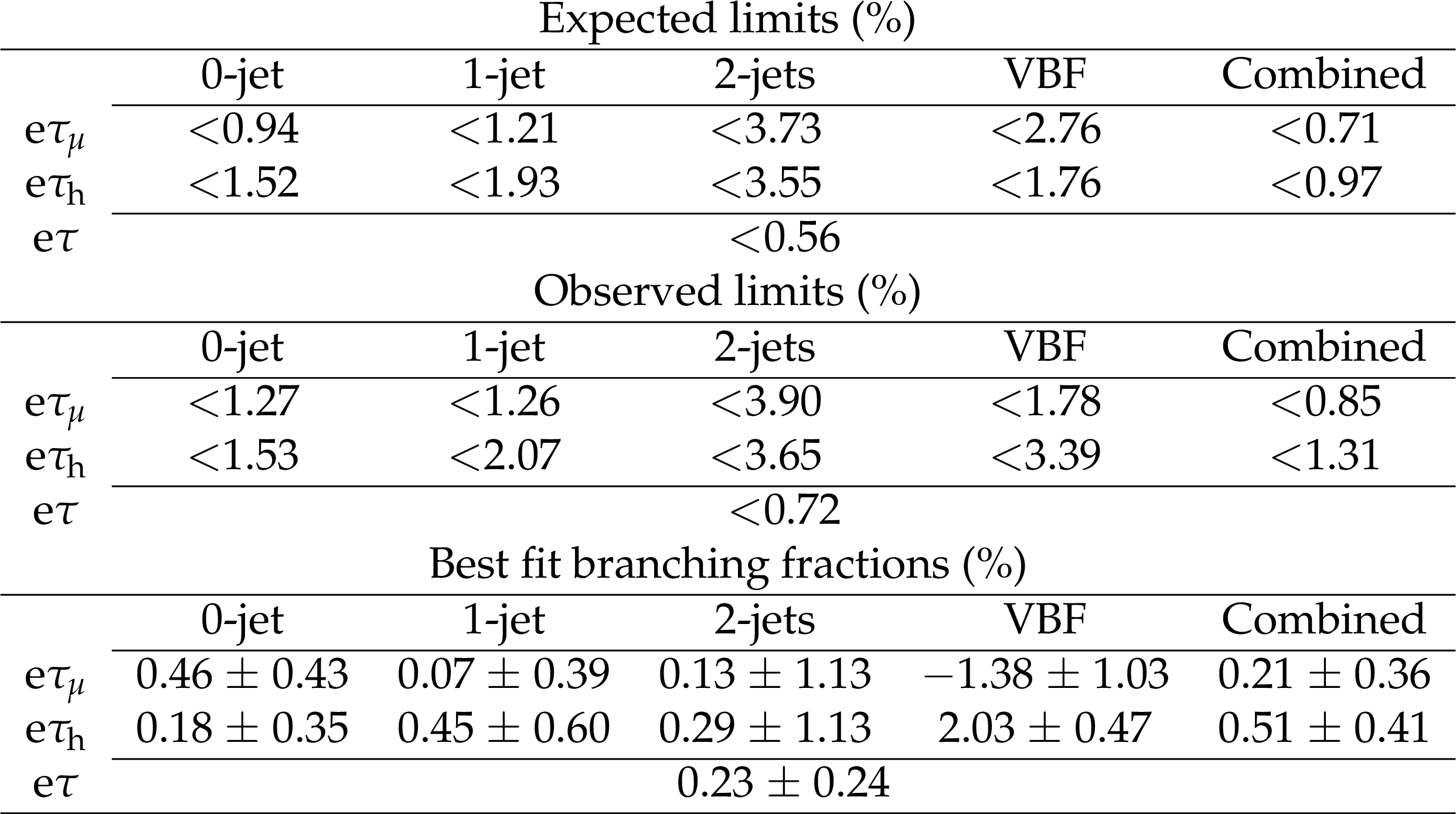
Table 6:
Expected and observed upper limits at 95% CL and best fit branching fractions in percent for each individual jet category, and combined, in the $ {\mathrm {H}} \to {\mathrm {e}} {\tau}$ process obtained with the BDT fit analysis. |
png pdf |
Table 7:
Expected and observed upper limits at 95% CL and best fit branching fractions in percent for each individual jet category, and combined, in the $ {\mathrm {H}} \to {\mathrm {e}} {\tau}$ process obtained with the $ {M_{\text {col}}} $ fit analysis. |
png pdf |
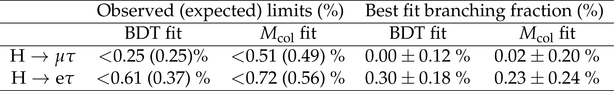
Table 8:
Summary of the observed and expected upper limits at the 95% CL and the best fit branching fractions in percent for the $ {\mathrm {H}} \to {{\mu}} {\tau}$ and $ {\mathrm {H}} \to {\mathrm {e}} {\tau}$ processes, for the main analysis (BDT fit) and the cross check ($ {M_{\text {col}}} $ fit) method. |

png pdf |
Table 9:
95% CL observed upper limit on the Yukawa couplings, for the main analysis (BDT fit) and the cross check ($ {M_{\text {col}}} $ fit) method. |
| Summary |
| The search for lepton flavour violating decays of the Higgs boson in the $\mu\tau$ and $\mathrm{e}\tau$ channels, with the 2016 data collected by the CMS detector, is presented in this paper. The data set analysed corresponds to an integrated luminosity of 35.9 fb$^{-1}$ of proton-proton collision data recorded at $\sqrt{s}= $ 13 TeV. The results are extracted by a fit to the output of a boosted decision trees discriminator trained to distinguish the signal from backgrounds. The results are cross-checked with an alternate analysis that fits the collinear mass distribution after applying selection criteria on kinematic variables. No evidence is found for lepton flavour violating Higgs boson decays. The observed (expected) limits on the branching fraction of the Higgs boson to $\mu\tau$ and to $\mathrm{e}\tau$ are less than 0.25% (0.25%) and 0.61% (0.37%), respectively, at 95% confidence level. These limits constitute a significant improvement over the previously obtained limits by CMS and ATLAS using 8 TeV proton-proton collision data corresponding to an integrated luminosity of about 20 fb$^{-1}$. Upper limits on the off-diagonal $\mu\tau$ and $\mathrm{e}\tau$ Yukawa couplings are derived from these constraints, $\sqrt{\smash[b]{|{Y_{\mu\tau}}|^{2}+|{Y_{\tau\mu}}}|^{2}} < 1.43 \times 10^{-3}$ and $\sqrt{|{Y_{\mathrm{e}\tau}}|^{2}+|{Y_{\tau\mathrm{e}}}|^{2}} < 2.26\times 10^{-3}$ at 95% confidence level. |
| References | ||||
| 1 | ATLAS Collaboration | Observation of a new particle in the search for the Standard Model Higgs boson with the ATLAS detector at the LHC | PLB 716 (2012) 1 | 1207.7214 |
| 2 | CMS Collaboration | Observation of a new boson at a mass of 125 GeV with the CMS experiment at the LHC | PLB 716 (2012) 30 | CMS-HIG-12-028 1207.7235 |
| 3 | CMS Collaboration | Observation of a new boson with mass near 125 GeV in pp collisions at $ \sqrt{s} = $ 7 and 8 TeV | JHEP 06 (2013) 081 | CMS-HIG-12-036 1303.4571 |
| 4 | ATLAS, CMS Collaboration | Measurements of the Higgs boson production and decay rates and constraints on its couplings from a combined ATLAS and CMS analysis of the LHC pp collision data at $ \sqrt{s} = $ 7 and 8 TeV | JHEP 08 (2016) 045 | 1606.02266 |
| 5 | J. L. Diaz-Cruz and J. J. Toscano | Lepton flavor violating decays of Higgs bosons beyond the standard model | PRD 62 (2000) 116005 | hep-ph/9910233 |
| 6 | T. Han and D. Marfatia | $ h \to \mu \tau $ at hadron colliders | PRL 86 (2001) 1442 | hep-ph/0008141 |
| 7 | E. Arganda, A. M. Curiel, M. J. Herrero, and D. Temes | Lepton flavor violating Higgs boson decays from massive seesaw neutrinos | PRD 71 (2005) 035011 | hep-ph/0407302 |
| 8 | A. Arhrib, Y. Cheng, and O. C. W. Kong | Comprehensive analysis on lepton flavor violating Higgs boson to $ \mu\bar{\tau} + \tau \bar{\mu} $ decay in supersymmetry without R parity | PRD 87 (2013) 015025 | 1210.8241 |
| 9 | M. Arana-Catania, E. Arganda, and M. J. Herrero | Non-decoupling SUSY in LFV Higgs decays: a window to new physics at the LHC | JHEP 09 (2013) 160 | 1304.3371 |
| 10 | E. Arganda, M. J. Herrero, R. Morales, and A. Szynkman | Analysis of the $ h, H, A \to\tau\mu $ decays induced from SUSY loops within the Mass Insertion Approximation | JHEP 03 (2016) 055 | 1510.04685 |
| 11 | E. Arganda, M. J. Herrero, X. Marcano, and C. Weiland | Enhancement of the lepton flavor violating Higgs boson decay rates from SUSY loops in the inverse seesaw model | PRD 93 (2016) 055010 | 1508.04623 |
| 12 | M. E. Gomez, S. Heinemeyer, and M. Rehman | Lepton flavor violating higgs boson decays in supersymmetric high scale seesaw models | 1703.02229 | |
| 13 | H.-B. Zhang et al. | 125 GeV Higgs decay with lepton flavor violation in the $ \mu\nu $SSM | CPC 41 (2017) 043106 | 1511.08979 |
| 14 | K. Agashe and R. Contino | Composite Higgs-mediated flavor-changing neutral current | PRD 80 (2009) 075016 | 0906.1542 |
| 15 | A. Azatov, M. Toharia, and L. Zhu | Higgs mediated flavor changing neutral currents in warped extra dimensions | PRD 80 (2009) 035016 | 0906.1990 |
| 16 | G. Perez and L. Randall | Natural neutrino masses and mixings from warped geometry | JHEP 01 (2009) 077 | 0805.4652 |
| 17 | S. Casagrande et al. | Flavor physics in the Randall-Sundrum model I. Theoretical setup and electroweak precision tests | JHEP 10 (2008) 094 | 0807.4937 |
| 18 | A. J. Buras, B. Duling, and S. Gori | The impact of Kaluza-Klein fermions on Standard Model fermion couplings in a RS model with custodial protection | JHEP 09 (2009) 076 | 0905.2318 |
| 19 | J. D. Bjorken and S. Weinberg | Mechanism for nonconservation of muon number | PRL 38 (1977) 622 | |
| 20 | J.-P. Lee and K. Y. Lee | $ B_s \to \mu \tau $ and $ h \to \mu \tau $ decays in the general two Higgs doublet model | 1612.04057 | |
| 21 | H. Ishimori et al. | Non-Abelian Discrete Symmetries in Particle Physics | Prog. Theor. Phys. Suppl. 183 (2010) 1 | 1003.3552 |
| 22 | M. Blanke et al. | $ \Delta F= $ 2 observables and fine-tuning in a warped extra dimension with custodial protection | JHEP 03 (2009) 001 | 0809.1073 |
| 23 | G. F. Giudice and O. Lebedev | Higgs-dependent Yukawa couplings | PLB 665 (2008) 79 | 0804.1753 |
| 24 | J. A. Aguilar-Saavedra | A minimal set of top-Higgs anomalous couplings | NPB 821 (2009) 215 | 0904.2387 |
| 25 | M. E. Albrecht et al. | Electroweak and flavour structure of a warped extra dimension with custodial protection | JHEP 09 (2009) 064 | 0903.2415 |
| 26 | A. Goudelis, O. Lebedev, and J. H. Park | Higgs-induced lepton flavor violation | PLB 707 (2012) 369 | 1111.1715 |
| 27 | D. McKeen, M. Pospelov, and A. Ritz | Modified Higgs branching ratios versus CP and lepton flavor violation | PRD 86 (2012) 113004 | 1208.4597 |
| 28 | A. Pilaftsis | Lepton flavour nonconservation in $ \mathrm{H}^0 $ decays | PLB 285 (1992) 68 | |
| 29 | J. G. Korner, A. Pilaftsis, and K. Schilcher | Leptonic $ \mathrm{CP} $ asymmetries in flavor-changing $ \mathrm{H}^{0} $ decays | PRD 47 (1993) 1080 | |
| 30 | E. Arganda, M. J. Herrero, X. Marcano, and C. Weiland | Imprints of massive inverse seesaw model neutrinos in lepton flavor violating Higgs boson decays | PRD 91 (2015) 015001 | 1405.4300 |
| 31 | J. Herrero-Garcia, N. Rius, and A. Santamaria | Higgs lepton flavour violation: UV completions and connection to neutrino masses | JHEP 11 (2016) 084 | 1605.06091 |
| 32 | F. del Aguila et al. | Lepton flavor changing higgs decays in the littlest Higgs model with T-parity | JHEP 08 (2017) 028 | 1705.08827 |
| 33 | N. H. Thao, L. T. Hue, H. T. Hung, and N. T. Xuan | Lepton flavor violating Higgs boson decays in seesaw models: New discussions | NPB 921 (2017) 159 | 1703.00896 |
| 34 | I. Galon and J. Zupan | Dark sectors and enhanced $ h\to \tau \mu $ transitions | JHEP 05 (2017) 083 | 1701.08767 |
| 35 | E. Arganda et al. | Effective lepton flavor violating $ H\ell_i\ell_j $ vertex from right-handed neutrinos within the mass insertion approximation | PRD 95 (2017) 095029 | 1612.09290 |
| 36 | D. Choudhury, A. Kundu, S. Nandi, and S. K. Patra | Unified resolution of the $ R(D) $ and $ R(D^*) $ anomalies and the lepton flavor violating decay $ h\to\mu\tau $ | PRD 95 (2017) 035021 | 1612.03517 |
| 37 | B. McWilliams and L.-F. Li | Virtual effects of Higgs particles | NPB 179 (1981) 62 | |
| 38 | O. U. Shanker | Flavour violation, scalar particles and leptoquarks | NPB 206 (1982) 253 | |
| 39 | A. Celis, V. Cirigliano, and E. Passemar | Lepton flavor violation in the Higgs sector and the role of hadronic tau-lepton decays | PRD 89 (2014) 013008 | 1309.3564 |
| 40 | G. Blankenburg, J. Ellis, and G. Isidori | Flavour-changing decays of a 125 GeV Higgs-like particle | PLB 712 (2012) 386 | 1202.5704 |
| 41 | R. Harnik, J. Kopp, and J. Zupan | Flavor violating higgs decays | JHEP 03 (2013) 26 | 1209.1397 |
| 42 | S. M. Barr and A. Zee | Electric dipole moment of the electron and of the neutron | PRL 65 (1990) 21 | |
| 43 | MEG Collaboration | Search for the lepton flavour violating decay $ \mu ^+ \rightarrow \mathrm {e}^+ \gamma $ with the full dataset of the MEG experiment | EPJC 76 (2016) 434 | 1605.05081 |
| 44 | CMS Collaboration | Search for lepton-flavour-violating decays of the Higgs boson | PLB 749 (2015) 337 | CMS-HIG-14-005 1502.07400 |
| 45 | CMS Collaboration | Search for lepton flavour violating decays of the higgs boson to $ \mathrm{e}\tau $ and $ \mathrm{e}\mu $ in proton-proton collisions at $ \sqrt{s}= $ 8 TeV | PLB 763 (2016) 472 | CMS-HIG-14-040 1607.03561 |
| 46 | ATLAS Collaboration | Search for lepton-flavour-violating decays of the Higgs and $ Z $ bosons with the ATLAS detector | EPJC 77 (2017) 70 | 1604.07730 |
| 47 | ATLAS Collaboration | Search for lepton-flavour-violating $ \mathrm{H}\to\mu\tau $ decays of the Higgs boson with the ATLAS detector | JHEP 11 (2015) 211 | 1508.03372 |
| 48 | CMS Collaboration | Evidence for the direct decay of the 125 GeV Higgs boson to fermions | NP 10 (2014) 557 | CMS-HIG-13-033 1401.6527 |
| 49 | CMS Collaboration | Evidence for the 125 GeV Higgs boson decaying to a pair of $ \tau $ leptons | JHEP 05 (2014) 104 | CMS-HIG-13-004 1401.5041 |
| 50 | CMS Collaboration | Observation of the Higgs boson decay to a pair of $ \tau $ leptons | Submitted to PLB | CMS-HIG-16-043 1708.00373 |
| 51 | ATLAS Collaboration | Evidence for the Higgs-boson Yukawa coupling to tau leptons with the ATLAS detector | JHEP 04 (2015) 117 | 1501.04943 |
| 52 | CMS Collaboration | The CMS trigger system | JINST 12 (2017) P01020 | CMS-TRG-12-001 1609.02366 |
| 53 | CMS Collaboration | The CMS experiment at the CERN LHC | JINST 3 (2008) S08004 | CMS-00-001 |
| 54 | H. M. Georgi, S. L. Glashow, M. E. Machacek, and D. V. Nanopoulos | Higgs bosons from two gluon annihilation in proton proton collisions | PRL 40 (1978) 692 | |
| 55 | R. N. Cahn, S. D. Ellis, R. Kleiss, and W. J. Stirling | Transverse-momentum signatures for heavy Higgs bosons | PRD 35 (1987) 1626 | |
| 56 | S. L. Glashow, D. V. Nanopoulos, and A. Yildiz | Associated production of Higgs bosons and Z particles | PRD 18 (1978) 1724 | |
| 57 | P. Nason | A new method for combining NLO QCD with shower Monte Carlo algorithms | JHEP 11 (2004) 040 | hep-ph/0409146 |
| 58 | S. Frixione, P. Nason, and C. Oleari | Matching NLO QCD computations with parton shower simulations: the POWHEG method | JHEP 11 (2007) 070 | 0709.2092 |
| 59 | S. Alioli, P. Nason, C. Oleari, and E. Re | A general framework for implementing NLO calculations in shower Monte Carlo programs: the POWHEG BOX | JHEP 06 (2010) 043 | 1002.2581 |
| 60 | S. Alioli et al. | Jet pair production in POWHEG | JHEP 04 (2011) 081 | 1012.3380 |
| 61 | S. Alioli, P. Nason, C. Oleari, and E. Re | NLO Higgs boson production via gluon fusion matched with shower in POWHEG | JHEP 04 (2009) 002 | 0812.0578 |
| 62 | G. Luisoni, P. Nason, C. Oleari, and F. Tramontano | HW$ ^{\pm} $/HZ $ + $ 0 and 1 jet at NLO with the POWHEG BOX interfaced to GoSam and their merging within MiNLO | JHEP 10 (2013) 083 | 1306.2542 |
| 63 | J. Alwall et al. | The automated computation of tree-level and next-to-leading order differential cross sections, and their matching to parton shower simulations | JHEP 07 (2014) 079 | 1405.0301 |
| 64 | J. Alwall et al. | Comparative study of various algorithms for the merging of parton showers and matrix elements in hadronic collisions | EPJC 53 (2008) 473 | 0706.2569 |
| 65 | R. Frederix and S. Frixione | Merging meets matching in MC@NLO | JHEP 12 (2012) 061 | 1209.6215 |
| 66 | T. Sjostrand et al. | An introduction to PYTHIA 8.2 | CPC 191 (2015) 159 | 1410.3012 |
| 67 | CMS Collaboration | Event generator tunes obtained from underlying event and multiparton scattering measurements | EPJC 76 (2016) 155 | CMS-GEN-14-001 1512.00815 |
| 68 | GEANT4 Collaboration | GEANT4 --- a simulation toolkit | NIMA 506 (2003) 250 | |
| 69 | CMS Collaboration | Particle-flow reconstruction and global event description with the CMS detector | JINST 12 (2017) P10003 | CMS-PRF-14-001 1706.04965 |
| 70 | M. Cacciari, G. P. Salam, and G. Soyez | The anti-$ k_t $ jet clustering algorithm | JHEP 04 (2008) 063 | 0802.1189 |
| 71 | M. Cacciari, G. P. Salam, and G. Soyez | FastJet user manual | EPJC 72 (2012) 1896 | 1111.6097 |
| 72 | CMS Collaboration | Performance of CMS muon reconstruction in pp collision events at $ \sqrt{s} = $ 7 TeV | JINST 7 (2012) P10002 | CMS-MUO-10-004 1206.4071 |
| 73 | CMS Collaboration | Performance of electron reconstruction and selection with the CMS detector in proton-proton collisions at $ \sqrt{s} = $ 8 TeV | JINST 10 (2015) P06005 | CMS-EGM-13-001 1502.02701 |
| 74 | CMS Collaboration | Reconstruction and identification of tau lepton decays to hadrons and $ \nu_\tau $ at CMS | JINST 11 (2016) P01019 | CMS-TAU-14-001 1510.07488 |
| 75 | CMS Collaboration | Performance of reconstruction and identification of tau leptons in their decays to hadrons and tau neutrino in LHC Run-2 | CMS-PAS-TAU-16-002 | CMS-PAS-TAU-16-002 |
| 76 | M. Cacciari, G. P. Salam | Dispelling the $ N^{3} $ myth for the $ k_t $ jet-finder | PLB 641 (2006) 57 | hep-ph/0512210 |
| 77 | CMS Collaboration | Determination of jet energy calibration and transverse momentum resolution in CMS | JINST 6 (2011) 11002 | CMS-JME-10-011 1107.4277 |
| 78 | CMS Collaboration | Jet energy scale and resolution in the CMS experiment in pp collisions at 8 TeV | JINST 12 (2017) P02014 | CMS-JME-13-004 1607.03663 |
| 79 | M. Cacciari, G. P. Salam, and G. Soyez | The catchment area of jets | JHEP 04 (2008) 005 | 0802.1188 |
| 80 | M. Cacciari and G. P. Salam | Pileup subtraction using jet areas | PLB 659 (2008) 119 | 0707.1378 |
| 81 | CMS Collaboration | Performance of the CMS missing transverse momentum reconstruction in pp data at $ \sqrt{s} = $ 8 TeV | JINST 10 (2015) P02006 | CMS-JME-13-003 1411.0511 |
| 82 | R. K. Ellis, I. Hinchliffe, M. Soldate, and J. J. van der Bij | Higgs decay to $ \tau^+\tau^- $: A possible signature of intermediate mass Higgs bosons at high energy hadron colliders | NPB 297 (1988) 221 | |
| 83 | CMS Collaboration | Identification of b quark jets at the CMS Experiment in the LHC Run 2 | CMS-PAS-BTV-15-001 | CMS-PAS-BTV-15-001 |
| 84 | D. de Florian et al. | Handbook of LHC Higgs cross sections: 4. deciphering the nature of the Higgs sector | CERN-2017-002-M | 1610.07922 |
| 85 | CMS Collaboration | Measurements of inclusive W and Z cross sections in pp collisions at $ \sqrt{s} = $ 7 TeV | JHEP 01 (2011) 080 | CMS-EWK-10-002 1012.2466 |
| 86 | CMS Collaboration | CMS luminosity measurements for the 2016 data taking period | CMS-PAS-LUM-17-001 | CMS-PAS-LUM-17-001 |
| 87 | T. Junk | Confidence level computation for combining searches with small statistics | NIMA 434 (1999) 435 | hep-ex/9902006 |
| 88 | A. L. Read | Presentation of search results: the $ CL_s $ technique | in Durham IPPP Workshop: Advanced Statistical Techniques in Particle Physics, p. 2693 Durham, UK, March, 2002 [JPG 28 (2002) 2693] | |
| 89 | G. Cowan, K. Cranmer, E. Gross, and O. Vitells | Asymptotic formulae for likelihood-based tests of new physics | EPJC 71 (2011) 1554 | 1007.1727 |
| 90 | A. Denner et al. | Standard model Higgs-boson branching ratios with uncertainties | EPJC 71 (2011) 1753 | 1107.5909 |
| 91 | Belle Collaboration | Search for lepton flavor violating $ \tau $ decays into three leptons with 719 million produced $ \tau^+\tau^- $ pairs | PLB 687 (2010) 139 | 1001.3221 |
| 92 | Particle Data Group, C. Patrignani et al. | Review of Particle Physics | CPC 40 (2016) 100001 | |
|
|
Compact Muon Solenoid LHC, CERN |
|

|

|

|

|

|